arX

iv:1

111.

2264

v1 [

mat

h.Q

A]

9 N

ov 2

011 Free Bosonic Vertex Operator Algebras on

Genus Two Riemann Surfaces II

Geoffrey Mason∗

Department of Mathematics,

University of California Santa Cruz,CA 95064, U.S.A.

Michael P. Tuite

School of Mathematics, Statistics and Applied Mathematics,National University of Ireland Galway

University Road, Galway, Ireland.

Abstract

We continue our program to define and study n-point correlationfunctions for a vertex operator algebra V on a higher genus compactRiemann surface obtained by sewing surfaces of lower genus. Here weconsider Riemann surfaces of genus 2 obtained by attaching a handleto a torus. We obtain closed formulas for the genus two partitionfunction for free bosonic theories and lattice vertex operator alge-bras VL. We prove that the partition function is holomorphic in thesewing parameters on a given suitable domain and describe its mod-ular properties. We also compute the genus two Heisenberg vectorn-point function and show that the Virasoro vector one point func-tion satisfies a genus two Ward identity. We compare our results withthose obtained in the companion paper, when a pair of tori are sewntogether, and show that the partition functions are not compatible inthe neighborhood of a two-tori degeneration point. The normalized

partition functions of a lattice theory VL are compatible, each beingidentified with the genus two theta function of L.

∗Supported by the NSF and NSA

1

Contents

1 Introduction 2

2 Genus Two Riemann Surface from Self-Sewing a Torus 62.1 Some elliptic function theory . . . . . . . . . . . . . . . . . . . 72.2 The ρ-formalism for self-sewing a torus . . . . . . . . . . . . . 82.3 Graphical expansions . . . . . . . . . . . . . . . . . . . . . . . 13

3 Vertex Operator Algebras and the Li-Zamolodchikov metric 163.1 Vertex operator algebras . . . . . . . . . . . . . . . . . . . . . 163.2 The Li-Zamolodchikov metric . . . . . . . . . . . . . . . . . . 18

4 Partition and n-Point Functions for Vertex Operator Alge-bras on a Genus Two Riemann Surface 204.1 Genus one . . . . . . . . . . . . . . . . . . . . . . . . . . . . . 204.2 Genus two . . . . . . . . . . . . . . . . . . . . . . . . . . . . . 24

5 The Heisenberg VOA 265.1 The genus two partition function Z

(2)M (τ, w, ρ) . . . . . . . . . 26

5.2 Holomorphic and modular-invariance properties . . . . . . . . 305.3 Some genus two n-point functions . . . . . . . . . . . . . . . . 33

6 Lattice VOAs 356.1 The genus two partition function Z

(2)VL

(τ, w, ρ) . . . . . . . . . 356.2 Some genus two n-point functions . . . . . . . . . . . . . . . . 40

7 Comparison between the ǫ and ρ-Formalisms 42

8 Final Remarks 46

9 Appendix 47

1 Introduction

In previous work ([MT1]-[MT4]) we developed the general theory of n-pointfunctions for a Vertex Operator Algebra (VOA) on a compact Riemann sur-face S obtained by sewing together two surfaces of lower genus, and appliedthis theory to obtain detailed results in the case that S is obtained by sewing

2

a pair of complex tori - the so-called ǫ-formalism discussed in the companionpaper [MT4]. In the present paper we consider in detail the situation whenS results from self-sewing a complex torus, i.e., attaching a handle, whichwe refer to as the ρ-formalism. We describe the nature of the resulting n-point functions, paying particular attention to the 0-point function, i.e., thegenus 2 partition function, in the ρ-formalism. We find the explicit form ofthe partition function for the Heisenberg free bosonic string and for latticevertex operator algebras, and show that these functions are holomorphic onthe parameter domain defined by the sewing. We study the generating func-tion for genus two Heisenberg n-point functions and show that the Virasorovector 1-point function satisfies a genus two Ward identity. Many of these re-sults are analogous to those found in the ǫ-formalism discussed in [MT4] butwith significant technical differences. Finally, we compare the results in thetwo formalisms, and show that the partition functions (and hence all n-pointfunctions) are incompatible. We introduce normalized partition functions,and in the case of VL show that they are compatible; in both formalisms thenormalized partition function is the genus two Siegel theta function θ

(2)L .

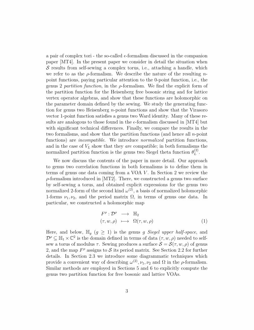
We now discuss the contents of the paper in more detail. Our approachto genus two correlation functions in both formalisms is to define them interms of genus one data coming from a VOA V . In Section 2 we review theρ-formalism introduced in [MT2]. There, we constructed a genus two surfaceby self-sewing a torus, and obtained explicit expressions for the genus twonormalized 2-form of the second kind ω(2), a basis of normalized holomorphic1-forms ν1, ν2, and the period matrix Ω, in terms of genus one data. Inparticular, we constructed a holomorphic map

F ρ : Dρ −→ H2

(τ, w, ρ) 7−→ Ω(τ, w, ρ) (1)

Here, and below, Hg (g ≥ 1) is the genus g Siegel upper half-space, andDρ ⊆ H1×C

2 is the domain defined in terms of data (τ, w, ρ) needed to self-sew a torus of modulus τ . Sewing produces a surface S = S(τ, w, ρ) of genus2, and the map F ρ assigns to S its period matrix. See Section 2.2 for furtherdetails. In Section 2.3 we introduce some diagrammatic techniques whichprovide a convenient way of describing ω(2), ν1, ν2 and Ω in the ρ-formalism.Similar methods are employed in Sections 5 and 6 to explicitly compute thegenus two partition function for free bosonic and lattice VOAs.

3

Section 3 consists of a brief review of relevant background material onVOA theory, with particular attention paid to the Li-Zamolodchikov or LiZmetric. In Section 4, motivated by ideas in conformal field theory ([FS], [So1],[So2], [P]), we introduce n-point functions (at genus one and two) in the ρ-formalism for a general VOA with nondegenerate LiZ metric. In particular,the genus two partition function Z

(2)V : Dρ → C is formally defined as

Z(2)V (τ, w, ρ) =

∑

n≥0

ρn∑

u∈V[n]

Z(1)V (u, u, w, τ), (2)

where Z(1)V (u, u, w, τ) is a genus one 2-point function and u is the LiZ metric

dual of u. In Section 4.1 we consider an example of self-sewing a sphere(Theorem 4.2), while in Section 4.2 we show (Theorem 4.4) that a particulardegeneration of the genus 2 partition function of a VOA V can be describedin terms of genus 1 data. Of particular interest here is the unexpected roleplayed by the Catalan series.

In Sections 5 and 6 we consider in detail the case of the Heisenbergfree bosonic theory M l corresponding to l free bosons, and lattice VOAsVL associated with a positive-definite even lattice L. Although (2) is a prioria formal power series in ρ, w and q = e2πiτ , we will see that for these twotheories it is a holomorphic function on Dρ. We expect that this result holdsin much wider generality. Although our calculations in these two Sectionsgenerally parallel those for the ǫ-formalism ([MT4]), the ρ-formalism is notmerely a simple translation. Several issues require additional attention, sothat the ρ-formalism is rather more complicated than its ǫ- counterpart. Thiscircumstance was already evident in [MT2], and stems in part from the factthat F ρ involves a logarithmic term that is absent in the ǫ-formalism. Themoment matrices are also more unwieldy, as they must be considered ashaving entries which themselves are 2× 2 block-matrices with entries whichare elliptic-type functions.

We establish (Theorem 5.1) a fundamental formula describing Z(2)M (τ, w, ρ)

as a quotient of the genus one partition function for M by a certain infinitedeterminant. This determinant already appeared in [MT2], and its holomor-

phy and nonvanishing in Dρ (loc. cit.) implies the holomorphy of Z(2)M . We

also obtain a product formula for the infinite determinant (Theorem 5.5),

and establish the automorphic properties of Z(2)M2 with respect to the action

of a group Γ1∼= SL(Z) (Theorem 5.7) that naturally acts on Dρ. In partic-

ular, we find that Z(2)

M24 is a form of weight −12 with respect to the action of

4

Γ1. These are the analogs in the ρ-formalism of results obtained in Section6 of [MT4] for the genus two partition function of M in the ǫ-formalism.

In Section 5.3 we calculate some genus two n-point functions for the rankone Heisenberg VOA M , specifically the n-point function for the weight 1Heisenberg vector and the 1-point function for the Virasoro vector ω. Weshow that, up to an overall factor of the genus two partition function, the for-mal differential forms associated with these n-point functions are describedin terms of the global symmetric 2-form ω(2) ([TUY]) and the genus twoprojective connection ([Gu]) respectively. Once again, these results are anal-ogous to results obtained in [MT4] in the ǫ-formalism. Parallel calculations,including a genus two Ward identity involving the Virasoro 1-point function(Proposition 6.5), are carried out for lattice theories in Section 6.2.

In Section 6.1 we establish (Theorem 6.1) a basic formula for the genustwo partition function for lattice theories in the ρ-formalism. The result is

Z(2)VL

(τ, w, ρ) = Z(2)

M l(τ, w, ρ)θ(2)L (Ω), (3)

where θ(2)L (Ω) is the genus two Siegel theta function attached to L ([Fr])

and Ω = F ρ(τ, w, ρ); indeed, (3) is an identity of formal power series. The

holomorphy and automorphic properties of Z(2)VL,ρ

follow from (3) and those

of Z(2)

M l and Θ(2)L .

Section 7 is devoted to a comparison of genus two n-point functions, andespecially partition functions, in the ǫ- and ρ-formalisms. After all, at genustwo we have at our disposal not one but two partition functions. In view ofthe strong formal similarities between Z

(2)

M l,ǫ(τ1, τ2, ǫ) and Z

(2)

M l,ρ(τ, w, ρ), for

example, it is natural to ask if they are equal in some sense 1. One may ask thesame question for lattice and other rational theories. In the very special casethat V is holomorphic (i.e., it has a unique irreducible module), one knows(e.g., [TUY]) that the genus 2 conformal block is 1-dimensional, in which casean identification of the two partition functions might seem inevitable. On theother hand, the partition functions are defined on quite different domains,so there is no question of them being literally equal. Indeed, we argue inSection 7 that Z

(2)

M l,ǫ(τ1, τ2, ǫ) and Z

(2)

M l,ρ(τ, w, ρ) are incompatible, i.e., there

is no sensible way in which they can be identified.

1Here we include an additional subscript of either ǫ or ρ to distinguish between the twoformalisms.

5

It is useful to introduce normalized partition functions, defined as

Z(2)V,ρ(τ, w, ρ) :=

Z(2)V,ρ(τ, w, ρ)

Z(2)

M l,ρ(τ, w, ρ)

, Z(2)V,ǫ(τ1, τ2, ǫ) :=

Z(2)V,ǫ(τ1, τ2, ǫ)

Z(2)

M l,ǫ(τ1, τ2, ǫ)

,

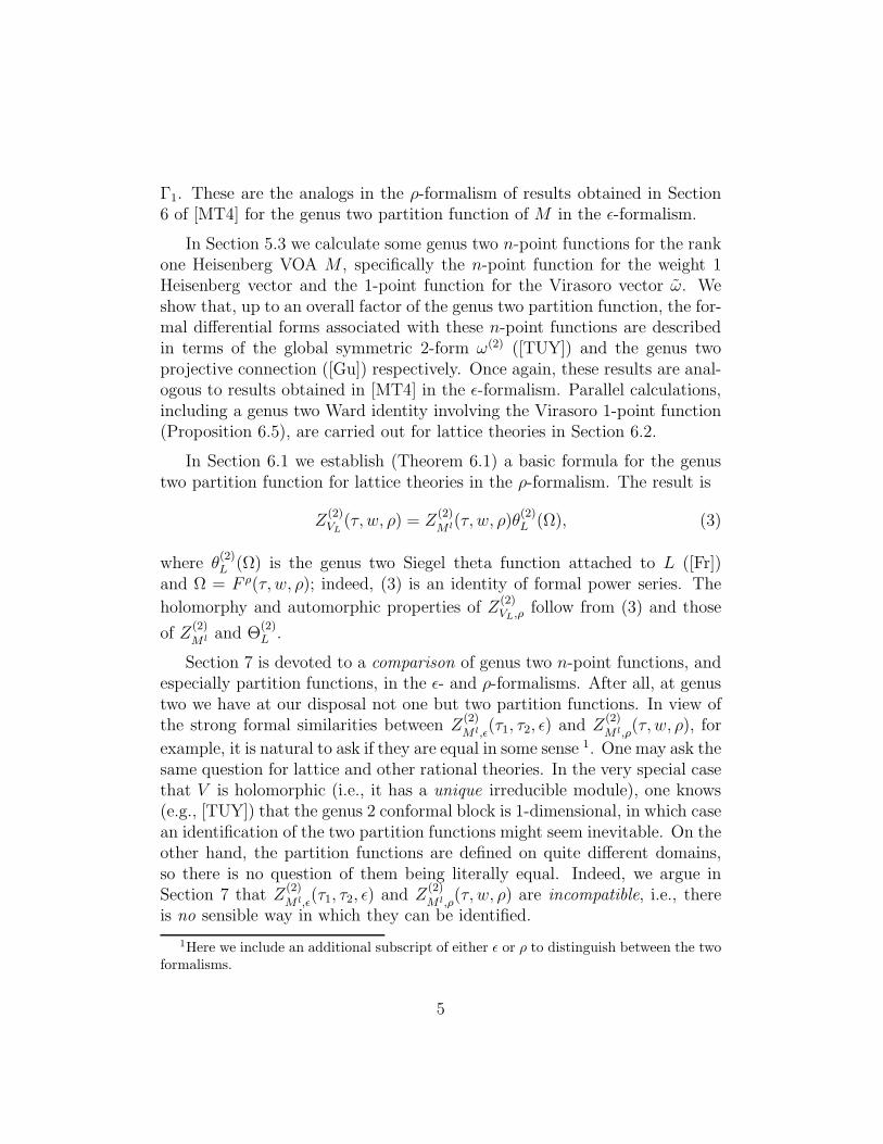
associated to a VOA V of central charge l. For M l, the normalized partitionfunctions are equal to 1. The relation between the normalized partitionfunctions for lattice theories VL (rkL = l) in the two formalisms can bedisplayed in the diagram

Dǫ F ǫ

−→ H2F ρ

←− Dρ

Z(2)V,ǫ

ց ↓ θ(2)LZ

(2)V,ρ

ւ

C

(4)

That this is a commuting diagram combines formula (3) in the ρ-formalism,and Theorem 14 of [MT4] for the analogous result in the ǫ-formalism. Thus,the normalized partition functions for VL are independent of the sewingscheme. They can be identified, via the sewing maps F •, with a genus twoSiegel modular form of weight l/2, the Siegel theta function. It is thereforethe normalized partition function(s) which can be identified with an elementof the conformal block, and with each other.

The fact that (4) commutes is, from our current perspective, somethingof a miracle; it is achieved by two quite separate and lengthy calculations,one for each of the formalisms. It would obviously be useful to have availablea result that provides an a priori guarantee of this fact. Section 8 containsa brief further discussion of these issues in the light of related ideas in stringtheory and algebraic geometry.

2 Genus Two Riemann Surface from Self-Sewing

a Torus

In this section we review some relevant results of [MT2] based on a generalsewing formalism due to Yamada [Y]. In particular, we review the construc-tion of a genus two Riemann surface formed by self-sewing a twice-puncturedtorus. We refer to this sewing scheme as the ρ-formalism. We discuss the

6

explicit form of various genus two structures such as the period matrix Ω.We also review the convergence and holomorphy of an infinite determinantthat naturally arises later on. An alternative genus two surface formed bysewing together two tori, which we refer to as the ǫ-formalism, is utilised inthe companion paper [MT4].

2.1 Some elliptic function theory

We begin with the definition of various modular and elliptic functions [MT1],[MT2]. We define

P2(τ, z) = ℘(τ, z) + E2(τ)

=1

z2+

∞∑

k=2

(k − 1)Ek(τ)zk−2, (5)

where τ ∈ H1, the complex upper half-plane and where ℘(τ, z) is the Weier-strass function (with periods 2πi and 2πiτ) and Ek(τ) = 0 for k odd, andfor k even is the Eisenstein series

Ek(τ) = Ek(q) = −Bk

k!+

2

(k − 1)!

∑

n≥1

σk−1(n)qn. (6)

Here and below, we take q = exp(2πiτ); σk−1(n) =∑

d|n dk−1, and Bk is a

kth Bernoulli number e.g. [Se]. If k ≥ 4 then Ek(τ) is a holomorphic modularform of weight k on SL(2,Z) whereas E2(τ) is a quasi-modular form [KZ],[MT2]. We define P0(τ, z), up to a choice of the logarithmic branch, andP1(τ, z) by

P0(τ, z) = − log(z) +∑

k≥2

1

kEk(τ)z

k, (7)

P1(τ, z) =1

z−∑

k≥2

Ek(τ)zk−1, (8)

where P2 = − ddzP1 and P1 = − d

dzP0. P0 is related to the elliptic prime form

K(τ, z), by [Mu1]K(τ, z) = exp(−P0(τ, z)). (9)

Define elliptic functions Pk(τ, z) for k ≥ 3

Pk(τ, z) =(−1)k−1

(k − 1)!

dk−1

dzk−1P1(τ, z). (10)

7

Define for k, l ≥ 1

C(k, l) = C(k, l, τ) = (−1)k+1 (k + l − 1)!

(k − 1)!(l − 1)!Ek+l(τ), (11)

D(k, l, z) = D(k, l, τ, z) = (−1)k+1 (k + l − 1)!

(k − 1)!(l − 1)!Pk+l(τ, z). (12)

Note that C(k, l) = C(l, k) and D(k, l, z) = (−1)k+lD(l, k, z). We also definefor k ≥ 1,

C(k, 0) = C(k, 0, τ) = (−1)k+1Ek(τ), (13)

D(k, 0, z, τ) = (−1)k+1Pk(z, τ). (14)

The Dedekind eta-function is defined by

η(τ) = q1/24∞∏

n=1

(1− qn). (15)

2.2 The ρ-formalism for self-sewing a torus

Consider a compact Riemann surface S of genus 2 with standard homologybasis a1, a2, b1, b2. There exists two holomorphic 1-forms νi, i = 1, 2 whichwe may normalize by [FK]

∮

ai

νj = 2πiδij . (16)

These forms can also be defined via the unique singular bilinear 2-form ω(2),known as the normalized differential of the second kind. It is defined by thefollowing properties [FK], [Y]:

ω(2)(x, y) = (1

(x− y)2 + regular terms)dxdy (17)

for local coordinates x, y, with normalization

∮

ai

ω(2)(x, ·) = 0 (1 ≤ i ≤ 2). (18)

8

Using the Riemann bilinear relations, one finds that

νi(x) =

∮

bi

ω(2)(x, ·) (1 ≤ i ≤ 2). (19)

The period matrix Ω is defined by

Ωij =1

2πi

∮

bi

νj (1 ≤ i, j ≤ 2). (20)

It is well-known that Ω ∈ H2, the Siegel upper half plane.We now review a general method due to Yamada [Y], and discussed at

length in [MT2], for calculating ω(2)(x, y), νi(x) and Ωij on the Riemannsurface formed by sewing a handle to an oriented torus S = C/Λ with latticeΛ = 2πi(Zτ ⊕Z) (τ ∈ H1). Consider discs centered at z = 0 and z = w withlocal coordinates z1 = z and z2 = z−w, and positive radius ra <

12D(q) with

1 ≤ a ≤ 2. Here, we have introduced the minimal lattice distance

D(q) = min(m,n)6=(0,0)

2π|m+ nτ | > 0. (21)

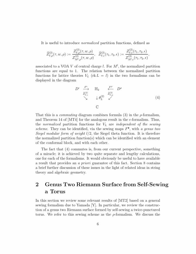
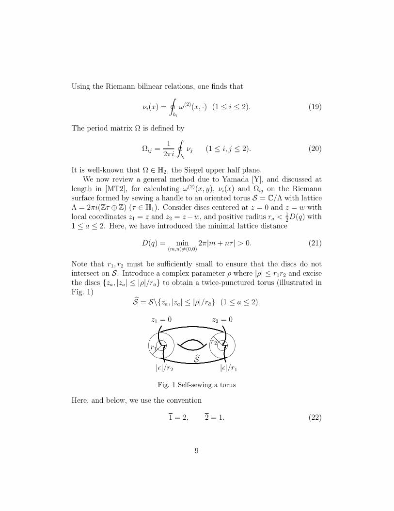
Note that r1, r2 must be sufficiently small to ensure that the discs do notintersect on S. Introduce a complex parameter ρ where |ρ| ≤ r1r2 and excisethe discs za, |za| ≤ |ρ|/ra to obtain a twice-punctured torus (illustrated inFig. 1)

S = S\za, |za| ≤ |ρ|/ra (1 ≤ a ≤ 2).

z2 = 0

r2

|ǫ|/r1S

❯

z1 = 0

r1

|ǫ|/r2

Fig. 1 Self-sewing a torus

Here, and below, we use the convention

1 = 2, 2 = 1. (22)

9

Define annular regions Aa = za, |ρ|r−1a ≤ |za| ≤ ra ∈ S (1 ≤ a ≤ 2), and

identify A1 with A2 as a single region via the sewing relation

z1z2 = ρ. (23)

The resulting genus two Riemann surface (excluding the degeneration pointρ = 0) is parameterized by the domain

Dρ = (τ, w, ρ) ∈ H1 × C× C : |w − λ| > 2|ρ|1/2 > 0 for all λ ∈ Λ, (24)

where the first inequality follows from the requirement that the annuli donot intersect. The Riemann surface inherits the genus one homology basisa1, b1. The cycle a2 is defined to be the anti-clockwise contour surroundingthe puncture at w, and b2 is a path between identified points z1 = z0 toz2 = ρ/z0 for some z0 ∈ A1.

ω(2), νi and (Ωij), are expressed as a functions of (τ, w, ρ) ∈ Dρ in termsof an infinite matrix of 2 × 2 blocks R(τ, w, ρ) = (R(k, l, τ, w, ρ)) (k, l ≥ 1)where [MT2]

R(k, l, τ, w, ρ) = −ρ(k+l)/2

√kl

(D(k, l, τ, w) C(k, l, τ)C(k, l, τ) D(l, k, τ, w)

), (25)

for C,D of (11) and (12). Note that Rab(k, l) = Rab(l, k) (1 ≤ a, b ≤ 2).I − R and det(I − R) play a central role in our discussion, where I denotesthe doubly-indexed identity matrix and det(I − R) is defined by

log det(I − R) = Tr log(I − R) = −∑

n≥1

1

nTrRn. (26)

In particular (op. cit. , Proposition 6 and Theorem 7)

Theorem 2.1 We have(a)

(I −R)−1 =∑

n≥0

Rn (27)

is convergent in Dρ.(b) det(I −R) is nonvanishing and holomorphic in Dρ.

10

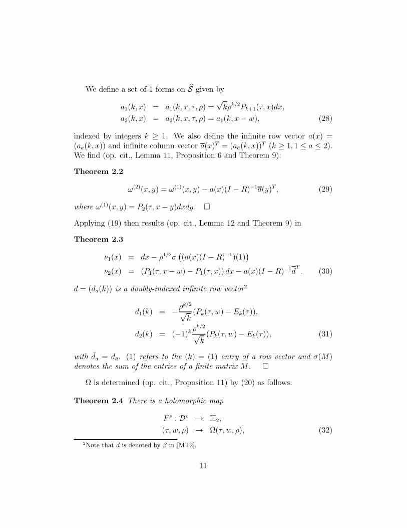
We define a set of 1-forms on S given by

a1(k, x) = a1(k, x, τ, ρ) =√kρk/2Pk+1(τ, x)dx,

a2(k, x) = a2(k, x, τ, ρ) = a1(k, x− w), (28)

indexed by integers k ≥ 1. We also define the infinite row vector a(x) =(aa(k, x)) and infinite column vector a(x)T = (aa(k, x))

T (k ≥ 1, 1 ≤ a ≤ 2).We find (op. cit., Lemma 11, Proposition 6 and Theorem 9):

Theorem 2.2

ω(2)(x, y) = ω(1)(x, y)− a(x)(I − R)−1a(y)T , (29)

where ω(1)(x, y) = P2(τ, x− y)dxdy.

Applying (19) then results (op. cit., Lemma 12 and Theorem 9) in

Theorem 2.3

ν1(x) = dx− ρ1/2σ((a(x)(I −R)−1)(1)

)

ν2(x) = (P1(τ, x− w)− P1(τ, x)) dx− a(x)(I −R)−1dT. (30)

d = (da(k)) is a doubly-indexed infinite row vector2

d1(k) = −ρk/2

√k(Pk(τ, w)− Ek(τ)),

d2(k) = (−1)k ρk/2

√k(Pk(τ, w)− Ek(τ)), (31)

with da = da. (1) refers to the (k) = (1) entry of a row vector and σ(M)denotes the sum of the entries of a finite matrix M .

Ω is determined (op. cit., Proposition 11) by (20) as follows:

Theorem 2.4 There is a holomorphic map

F ρ : Dρ → H2,

(τ, w, ρ) 7→ Ω(τ, w, ρ), (32)

2Note that d is denoted by β in [MT2].

11

where Ω = Ω(τ, w, ρ) is given by

2πiΩ11 = 2πiτ − ρσ((I − R)−1(1, 1)), (33)

2πiΩ12 = w − ρ1/2σ((d(I − R)−1(1)), (34)

2πiΩ22 = log

(− ρ

K(τ, w)2

)− d(I −R)−1dT . (35)

K is the elliptic prime form (9), (1, 1) and (1) refer to the (k, l) = (1, 1), re-spectively, (k) = (1) entries of an infinite matrix and row vector respectively.σ(M) denotes the sum over the finite indices for a given 2×2 or 1×2 matrixM .

Dρ admits an action of the Jacobi group J = SL(2,Z)⋉ Z2 as follows:

(a, b).(τ, w, ρ) = (τ, w + 2πiaτ + 2πib, ρ) ((a, b) ∈ Z2), (36)

γ1.(τ, w, ρ) = (a1τ + b1c1τ + d1

,w

c1τ + d1,

ρ

(c1τ + d1)2) (γ1 ∈ Γ1), (37)

with Γ1 =

(a1 b1c1 d1

)= SL(2,Z). Due to the branch structure of the

logarithmic term in (35), F ρ is not equivariant with respect to J . (Insteadone must pass to a simply-connected covering space Dρ on which L = HΓ1,a split extension of SL(2,Z) by an integer Heisenberg group H, acts. SeeSection 6.3 of [MT2] for details).

There is an injection Γ1 → Sp(4,Z) defined by

(a1 b1c1 d1

)7→

a1 0 b1 00 1 0 0c1 0 d1 00 0 0 1

, (38)

through which Γ1 acts on H2 by the standard action

γ.Ω= (AΩ+B)(CΩ +D)−1

(γ =

(A BC D

)∈ Sp(4,Z)

). (39)

We then have (op. cit., Theorem 11, Corollary 2)

12

Theorem 2.5 F ρ is equivariant with respect to the action of Γ1, i.e. thereis a commutative diagram for γ1 ∈ Γ1,

Dρ F ρ

→ H2

γ1 ↓ ↓ γ1Dρ F ρ

→ H2

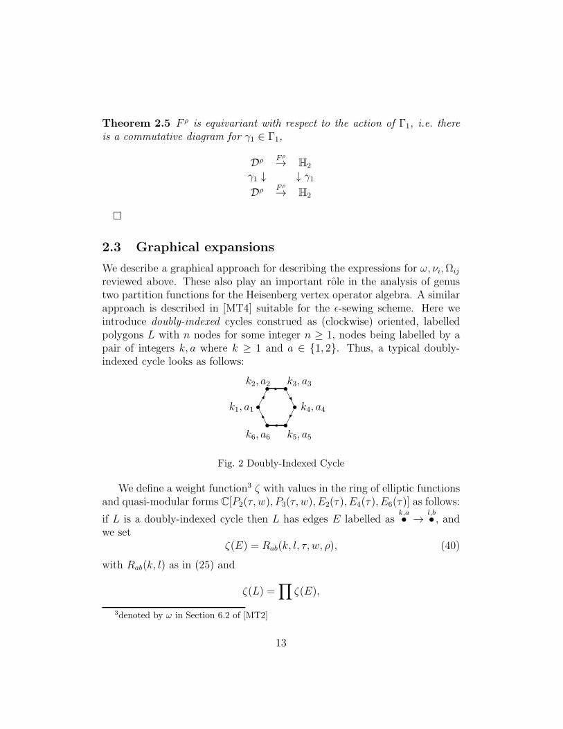
2.3 Graphical expansions

We describe a graphical approach for describing the expressions for ω, νi,Ωijreviewed above. These also play an important role in the analysis of genustwo partition functions for the Heisenberg vertex operator algebra. A similarapproach is described in [MT4] suitable for the ǫ-sewing scheme. Here weintroduce doubly-indexed cycles construed as (clockwise) oriented, labelledpolygons L with n nodes for some integer n ≥ 1, nodes being labelled by apair of integers k, a where k ≥ 1 and a ∈ 1, 2. Thus, a typical doubly-indexed cycle looks as follows:

k1, a1 sk2, a2s

k3, a3s❯

k4, a4s

k5, a5s

k6, a6s

Fig. 2 Doubly-Indexed Cycle

We define a weight function3 ζ with values in the ring of elliptic functionsand quasi-modular forms C[P2(τ, w), P3(τ, w), E2(τ), E4(τ), E6(τ)] as follows:

if L is a doubly-indexed cycle then L has edges E labelled ask,a• → l,b• , and

we setζ(E) = Rab(k, l, τ, w, ρ), (40)

with Rab(k, l) as in (25) and

ζ(L) =∏

ζ(E),

3denoted by ω in Section 6.2 of [MT2]

13

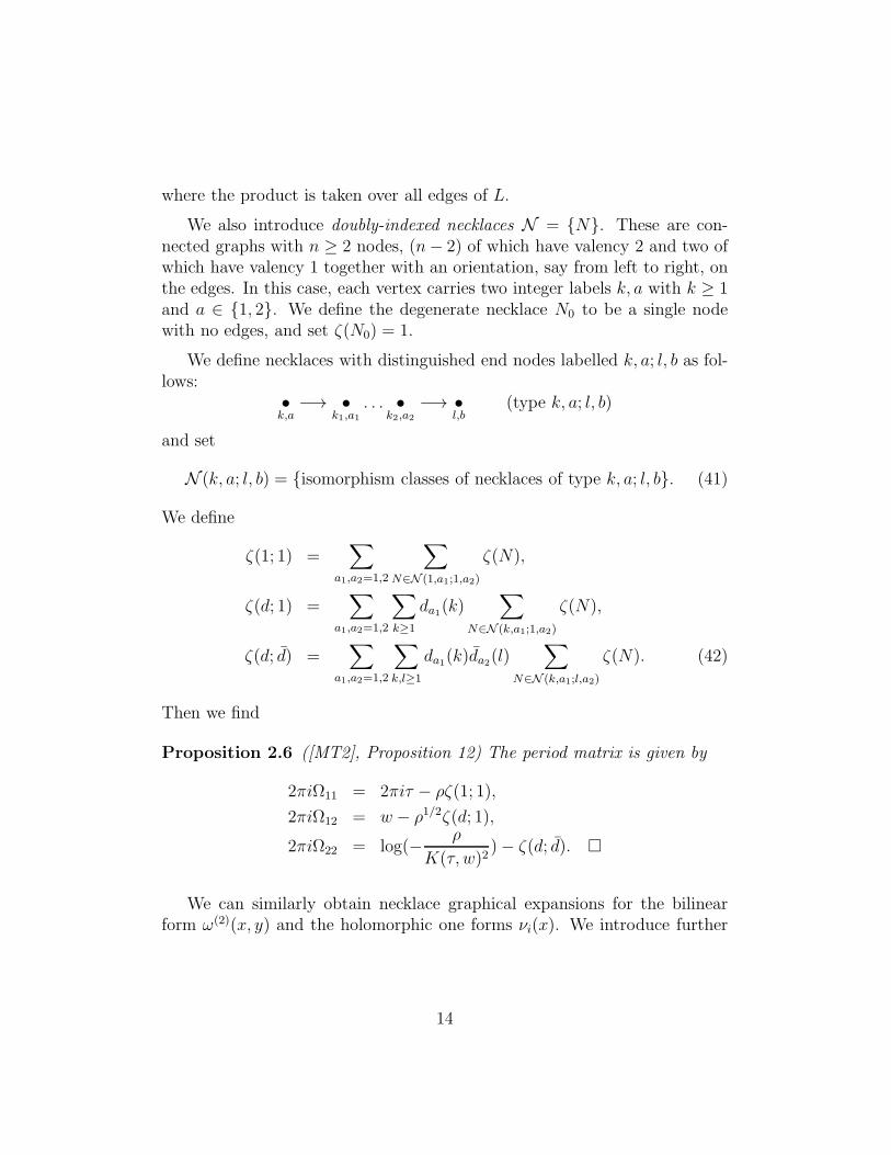
where the product is taken over all edges of L.

We also introduce doubly-indexed necklaces N = N. These are con-nected graphs with n ≥ 2 nodes, (n− 2) of which have valency 2 and two ofwhich have valency 1 together with an orientation, say from left to right, onthe edges. In this case, each vertex carries two integer labels k, a with k ≥ 1and a ∈ 1, 2. We define the degenerate necklace N0 to be a single nodewith no edges, and set ζ(N0) = 1.

We define necklaces with distinguished end nodes labelled k, a; l, b as fol-lows:

•k,a−→ •

k1,a1. . . •

k2,a2−→ •

l,b(type k, a; l, b)

and set

N (k, a; l, b) = isomorphism classes of necklaces of type k, a; l, b. (41)

We define

ζ(1; 1) =∑

a1,a2=1,2

∑

N∈N (1,a1;1,a2)

ζ(N),

ζ(d; 1) =∑

a1,a2=1,2

∑

k≥1

da1(k)∑

N∈N (k,a1;1,a2)

ζ(N),

ζ(d; d) =∑

a1,a2=1,2

∑

k,l≥1

da1(k)da2(l)∑

N∈N (k,a1;l,a2)

ζ(N). (42)

Then we find

Proposition 2.6 ([MT2], Proposition 12) The period matrix is given by

2πiΩ11 = 2πiτ − ρζ(1; 1),2πiΩ12 = w − ρ1/2ζ(d; 1),2πiΩ22 = log(− ρ

K(τ, w)2)− ζ(d; d).

We can similarly obtain necklace graphical expansions for the bilinearform ω(2)(x, y) and the holomorphic one forms νi(x). We introduce further

14

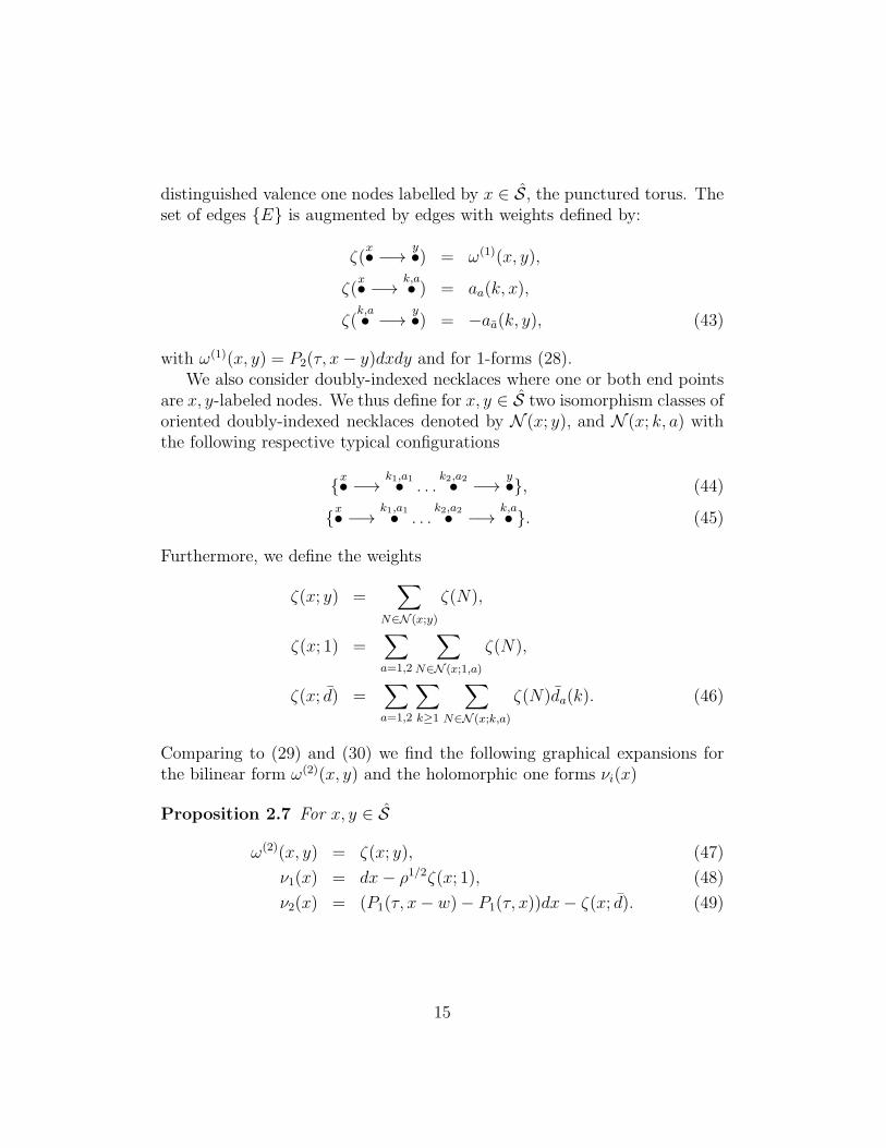
distinguished valence one nodes labelled by x ∈ S, the punctured torus. Theset of edges E is augmented by edges with weights defined by:

ζ(x• −→ y•) = ω(1)(x, y),

ζ(x• −→ k,a• ) = aa(k, x),

ζ(k,a• −→ y•) = −aa(k, y), (43)

with ω(1)(x, y) = P2(τ, x− y)dxdy and for 1-forms (28).We also consider doubly-indexed necklaces where one or both end points

are x, y-labeled nodes. We thus define for x, y ∈ S two isomorphism classes oforiented doubly-indexed necklaces denoted by N (x; y), and N (x; k, a) withthe following respective typical configurations

x• −→ k1,a1• . . .k2,a2• −→ y•, (44)

x• −→ k1,a1• . . .k2,a2• −→ k,a• . (45)

Furthermore, we define the weights

ζ(x; y) =∑

N∈N (x;y)

ζ(N),

ζ(x; 1) =∑

a=1,2

∑

N∈N (x;1,a)

ζ(N),

ζ(x; d) =∑

a=1,2

∑

k≥1

∑

N∈N (x;k,a)

ζ(N)da(k). (46)

Comparing to (29) and (30) we find the following graphical expansions forthe bilinear form ω(2)(x, y) and the holomorphic one forms νi(x)

Proposition 2.7 For x, y ∈ S

ω(2)(x, y) = ζ(x; y), (47)

ν1(x) = dx− ρ1/2ζ(x; 1), (48)

ν2(x) = (P1(τ, x− w)− P1(τ, x))dx− ζ(x; d). (49)

15

3 Vertex Operator Algebras and the Li-Zamolodchikov

metric

3.1 Vertex operator algebras

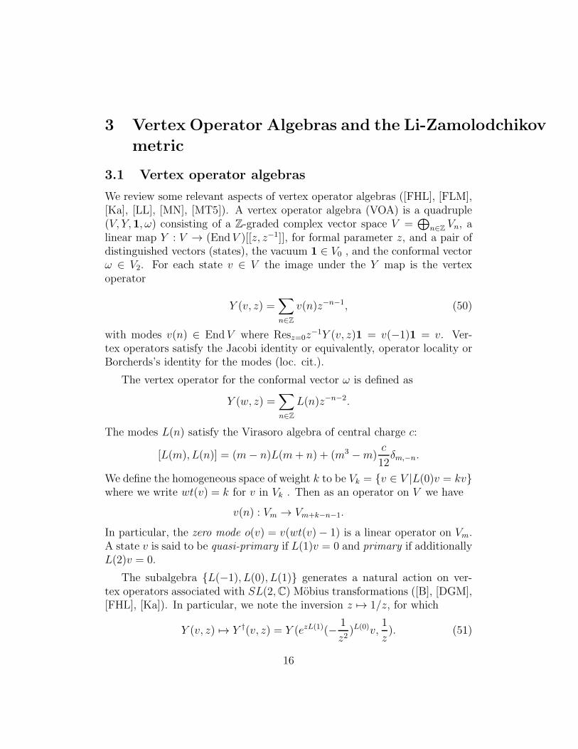
We review some relevant aspects of vertex operator algebras ([FHL], [FLM],[Ka], [LL], [MN], [MT5]). A vertex operator algebra (VOA) is a quadruple(V, Y, 1, ω) consisting of a Z-graded complex vector space V =

⊕n∈Z Vn, a

linear map Y : V → (EndV )[[z, z−1]], for formal parameter z, and a pair ofdistinguished vectors (states), the vacuum 1 ∈ V0 , and the conformal vectorω ∈ V2. For each state v ∈ V the image under the Y map is the vertexoperator

Y (v, z) =∑

n∈Zv(n)z−n−1, (50)

with modes v(n) ∈ End V where Resz=0z−1Y (v, z)1 = v(−1)1 = v. Ver-

tex operators satisfy the Jacobi identity or equivalently, operator locality orBorcherds’s identity for the modes (loc. cit.).

The vertex operator for the conformal vector ω is defined as

Y (w, z) =∑

n∈ZL(n)z−n−2.

The modes L(n) satisfy the Virasoro algebra of central charge c:

[L(m), L(n)] = (m− n)L(m+ n) + (m3 −m)c

12δm,−n.

We define the homogeneous space of weight k to be Vk = v ∈ V |L(0)v = kvwhere we write wt(v) = k for v in Vk . Then as an operator on V we have

v(n) : Vm → Vm+k−n−1.

In particular, the zero mode o(v) = v(wt(v)− 1) is a linear operator on Vm.A state v is said to be quasi-primary if L(1)v = 0 and primary if additionallyL(2)v = 0.

The subalgebra L(−1), L(0), L(1) generates a natural action on ver-tex operators associated with SL(2,C) Mobius transformations ([B], [DGM],[FHL], [Ka]). In particular, we note the inversion z 7→ 1/z, for which

Y (v, z) 7→ Y †(v, z) = Y (ezL(1)(− 1

z2)L(0)v,

1

z). (51)

16

Y †(v, z) is the adjoint vertex operator [FHL].

We consider in particular the Heisenberg free boson VOA and latticeVOAs. Consider an l-dimensional complex vector space (i.e., abelian Liealgebra) H equipped with a non-degenerate, symmetric, bilinear form ( , )and a distinguished orthonormal basis a1, a2, . . . al. The corresponding affineLie algebra is the Heisenberg Lie algebra H = H⊗C[t, t−1]⊕Ck with brackets[k, H] = 0 and

[ai ⊗ tm, aj ⊗ tn] = mδi,jδm,−nk. (52)

Corresponding to an element λ in the dual space H∗ we consider the Fockspace defined by the induced (Verma) module

M (λ) = U(H)⊗U(H⊗C[t]⊕Ck) C,

where C is the 1-dimensional space annihilated by H⊗ tC[t] and on which kacts as the identity and H ⊗ t0 via the character λ; U denotes the universalenveloping algebra. There is a canonical identification of linear spaces

M (λ) = S(H⊗ t−1C[t−1]),

where S denotes the (graded) symmetric algebra. The Heisenberg free bosonVOA M l corresponds to the case λ = 0. The Fock states

v = a1(−1)e1.a1(−2)e2 . . . .a1(−n)en . . . .al(−1)f1 .al(−2)f2 . . . al(−p)fp.1,(53)

for non-negative integers ei, . . . , fj form a basis of M l. The vacuum 1 iscanonically identified with the identity of M0 = C, while the weight 1 sub-space M1 may be naturally identified with H. M l is a simple VOA of centralcharge l.

Next we consider the case of a lattice vertex operator algebra VL associ-ated to a positive-definite even lattice L (cf. [B], [FLM]). Thus L is a freeabelian group of rank l equipped with a positive definite, integral bilinearform ( , ) : L⊗L→ Z such that (α, α) is even for α ∈ L. Let H be the spaceC ⊗Z L equipped with the C-linear extension of ( , ) to H ⊗ H and let M l

be the corresponding Heisenberg VOA. The Fock space of the lattice theorymay be described by the linear space

VL =M l ⊗ C[L] =∑

α∈LM l ⊗ eα, (54)

17

where C[L] denotes the group algebra of L with canonical basis eα, α ∈ L.M l may be identified with the subspace M l ⊗ e0 of VL, in which case M l

is a subVOA of VL and the rightmost equation of (54) then displays thedecomposition of VL into irreducible M l-modules. VL is a simple VOA ofcentral charge l. Each 1⊗ eα ∈ VL is a primary state of weight 1

2(α, α) with

vertex operator (loc. cit.)

Y (1⊗ eα, z) = Y−(α, z)Y+(α, z)eαzα,

Y±(α, z) = exp(∓∑

n>0

α(±n)n

z∓n). (55)

The operators eα ∈ C[L] obey

eαeβ = ǫ(α, β)eα+β (56)

for a bilinear 2-cocycle ǫ(α, β) satisfying ǫ(α, β)ǫ(β, α) = (−1)(α,β).

3.2 The Li-Zamolodchikov metric

A bilinear form 〈 , 〉 : V × V−→C is called invariant in case the followingidentity holds for all a, b, c ∈ V ([FHL]):

〈Y (a, z)b, c〉 = 〈b, Y †(a, z)c〉, (57)

with Y †(a, z) the adjoint operator (51). If V0 = C1 and V is self-dual (i.e.V is isomorphic to the contragredient module V ′ as a V -module) then V hasa unique non-zero invariant bilinear form up to scalar [Li]. Note that 〈 , 〉 isnecessarily symmetric by a theorem of [FHL]. Furthermore, if V is simplethen such a form is necessarily non-degenerate. All of the VOAs that occurin this paper satisfy these conditions, so that normalizing 〈1, 1〉 = 1 impliesthat 〈 , 〉 is unique. We refer to such a bilinear form as the Li-Zamolodchikovmetric on V , or LiZ-metric for short [MT4]. We also note that the LiZ-metric is multiplicative over tensor products in the sense that LiZ metric ofthe tensor product V1 ⊗ V2 of a pair of simple VOAs satisfying the aboveconditions is by uniqueness, the tensor product of the LiZ metrics on V1 andV2.

For a quasi-primary vector a of weight wt(a), the component form of (57)becomes

〈a(n)b, c〉 = (−1)wt(a)〈b, a(2wt(a)− n− 2)c〉. (58)

18

In particular, for the conformal vector ω we obtain

〈L(n)b, c〉 = 〈b, L(−n)c〉. (59)

Taking n = 0, it follows that the homogeneous spaces Vn and Vm are orthog-onal if n 6= m.

Consider the rank one Heisenberg VOA M = M1 generated by a weightone state a with (a, a) = 1. Then 〈a, a〉 = −〈1, a(1)a(−1)1〉 = −1. Using(52), it is straightforward to verify that the Fock basis (53) is orthogonalwith respect to the LiZ-metric and

〈v, v〉 =∏

1≤i≤p(−i)eiei!. (60)

This result generalizes in an obvious way to the rank l free boson VOA M l

because the LiZ metric is multiplicative over tensor products.

We consider next the lattice vertex operator algebra VL for a positive-definite even lattice L. We take as our Fock basis the states v ⊗ eα wherev is as in (53) and α ranges over the elements of L.

Lemma 3.1 If u, v ∈M l and α, β ∈ L, then

〈u⊗ eα, v ⊗ eβ〉 = 〈u, v〉〈1⊗ eα, 1⊗ eβ〉= (−1) 1

2(α,α)ǫ(α,−α)〈u, v〉δα,−β.

Proof. It follows by successive applications of (58) that the first equality inthe Lemma is true, and that it is therefore enough to prove it in the case thatu = v = 1. We identify the primary vector 1 ⊗ eα with eα in the following.Then 〈eα, eβ〉 = 〈eα(−1)1, eβ〉 is given by

(−1) 12(α,α)〈1, eα((α, α)− 1)eβ〉

= (−1) 12(α,α) Resz=0z

(α,α)−1〈1, Y (eα, z)eβ〉= (−1) 1

2(α,α)ǫ(α, β) Resz=0z

(α,β)+(α,α)−1〈1, Y−(α, z).eα+β〉.

Unless α+β = 0, all states to the left inside the bracket 〈 , 〉 on the previousline have positive weight, hence are orthogonal to 1. So 〈eα, eβ〉 = 0 ifα + β 6= 0. In the contrary case, the exponential operator acting on thevacuum yields just the vacuum itself among weight zero states, and we get〈eα, e−α〉 = (−1) 1

2(α,α)ǫ(α,−α) in this case.

19

Corollary 3.2 We may choose the cocycle so that ǫ(α,−α) = (−1) 12(α,α) (cf.

(138) in the Appendix). In this case, we have

〈u⊗ eα, v ⊗ eβ〉 = 〈u, v〉δα,−β. (61)

4 Partition and n-Point Functions for Vertex

Operator Algebras on a Genus Two Rie-

mann Surface

In this section we consider the partition and n-point functions for a VOAon Riemann surface of genus one or two, formed by attaching a handle to asurface of lower genus. We assume that V has a non-degenerate LiZ metric〈 , 〉. Then for any V basis u(a), we may define the dual basis u(a) withrespect to the LiZ metric where

〈u(a), u(b)〉 = δab. (62)

4.1 Genus one

It is instructive to first consider an alternative approach to defining the genusone partition function. In order to define n-point correlation functions ona torus, Zhu introduced ([Z]) a second VOA (V, Y [ , ], 1, ω) isomorphic to(V, Y ( , ), 1, ω) with vertex operators

Y [v, z] =∑

n∈Zv[n]z−n−1 = Y (qL(0)z v, qz − 1), (63)

and conformal vector ω = ω − c241. Let

Y [ω, z] =∑

n∈ZL[n]z−n−2, (64)

and write wt[v] = k if L[0]v = kv, V[k] = v ∈ V |wt[v] = k. Similarly, wedefine the square bracket LiZ metric 〈 , 〉sq which is invariant with respect tothe square bracket adjoint.

The (genus one) 1-point function is now defined as

Z(1)V (v, τ) = Tr V

(o(v)qL(0)−c/24

). (65)

20

An n-point function can be expressed in terms of 1-point functions ([MT1],Lemma 3.1) as follows:

Z(1)V (v1, z1; . . . vn, zn; τ)

= Z(1)V (Y [v1, z1] . . . Y [vn−1, zn−1]Y [vn, zn]1, τ) (66)

= Z(1)V (Y [v1, z1n] . . . Y [vn−1, zn−1n]vn, τ), (67)

where zin = zi − zn (1 ≤ i ≤ n − 1). In particular, Z(1)V (v1, z1; v2, z2; τ)

depends only one z12, and we denote this 2-point function by

Z(1)V (v1, v2, z12, τ) = Z

(1)V (v1, z1; v2, z2; τ)

= Tr V(o(Y [v1, z12]v2)q

L(0)). (68)

Now consider a torus obtained by self-sewing a Riemann sphere withpunctures located at the origin and an arbitrary point w on the complex plane(cf. [MT2], Section 5.2.2.). Choose local coordinates z1 in the neighborhoodof the origin and z2 = z − w for z in the neighborhood of w. For a complexsewing parameter ρ, identify the annuli |ρ|r−1

a ≤ |za| ≤ ra for 1 ≤ a ≤ 2 and|ρ| ≤ r1r2 via the sewing relation

z1z2 = ρ. (69)

Define

χ = − ρ

w2. (70)

Then the annuli do not intersect provided |χ| < 14, and the torus modular

parameter isq = f(χ), (71)

where f(χ) the Catalan series

f(χ) =1−√1− 4χ

2χ− 1 =

∑

n≥1

1

n

(2n

n + 1

)χn. (72)

f = f(χ) satisfies f = χ(1 + f)2 and the following identity, which can beproved by induction on m:

21

Lemma 4.1 f(χ) satisfies

f(χ)m =∑

n≥m

m

n

(2n

n+m

)χn (m ≥ 1).

We now define the genus one partition function in the sewing scheme (69)by

Z(1)V,ρ(ρ, w) =

∑

n≥0

ρn∑

u∈VnResz2=0z

−12 Resz1=0z

−11 〈1, Y (u, w + z2)Y (u, z1)1〉.(73)

This partition function is directly related to Z(1)V (q) = Tr V (q

L(0)−c/24) asfollows:

Theorem 4.2 In the sewing scheme (69), we have

Z(1)V,ρ(ρ, w) = qc/24Z

(1)V (q), (74)

where q = f(χ) is given by (71).

Proof. The summand in (73) is

〈1,Y (u, w)u〉 = 〈Y †(u, w)1, u〉= (−w−2)n〈Y (ewL(1)u, w−1)1, u〉= (−w−2)n〈ew−1L(−1)ewL(1)u, u〉,

where we have used (51) and also Y (v, z)1 = exp(zL(−1))v. (See [Ka] or[MN] for the latter equality.) Hence we find that

Z(1)V,ρ(ρ, w) =

∑

n≥0

(− ρ

w2)n∑

u∈Vn〈ew−1L(−1)ewL(1)u, u〉

=∑

n≥0

χnTr Vn(ew−1L(−1)ewL(1)).

Expanding the exponentials yields

Z(1)V,ρ(ρ, w) = Tr V (

∑

r≥0

L(−1)rL(1)r(r!)2

χL(0)), (75)

an expression which depends only on χ.

22

In order to compute (75) we consider the quasi-primary decomposition ofV . Let Qm = v ∈ Vm|L(1)v = 0 denote the space of quasiprimary statesof weight m ≥ 1. Then dimQm = pm − pm−1 with pm = dimVm. Considerthe decomposition of V into L(−1)-descendents of quasi-primaries

Vn =

n⊕

m=1

L(−1)n−mQm. (76)

Lemma 4.3 Let v ∈ Qm for m ≥ 1. For an integer n ≥ m,

∑

r≥0

L(−1)rL(1)r(r!)2

L(−1)n−mv =(2n− 1

n−m

)L(−1)n−mv.

Proof. First use induction on t ≥ 0 to show that

L(1)L(−1)tv = t(2m+ t− 1)L(−1)t−1v.

Then by induction in r it follows that

L(−1)rL(1)r(r!)2

L(−1)n−mv =(n−mr

)(n +m− 1

r

)L(−1)n−mv.

Hence

∑

r≥0

L(−1)rL(1)r(r!)2

L(−1)n−mv =

n−m∑

r≥0

(n−mr

)(n+m− 1

r

)L(−1)n−mv,

=

(2n− 1

n−m

)L(−1)n−mv,

where the last equality follows from a comparison of the coefficient of xn−m

in the identity (1 + x)n−m(1 + x)n+m−1 = (1 + x)2n−1.

Lemma 4.3 and (76) imply that for n ≥ 1,

Tr Vn(∑

r≥0

L(−1)rL(1)r(r!)2

) =n∑

m=1

TrQm(∑

r≥0

L(−1)rL(1)r(r!)2

L(−1)n−m)

=n∑

m=1

(pm − pm−1)

(2n− 1

n−m

).

23

The coefficient of pm is

(2n− 1

n−m

)−(

2n− 1

n−m− 1

)=m

n

(2n

m+ n

),

and hence

Tr Vn(∑

r≥0

L(−1)rL(1)r(r!)2

) =

n∑

m=1

m

n

(2n

m+ n

)pm.

Using Lemma 4.1, we find that

Z(1)V,ρ(ρ, w) = 1 +

∑

n≥1

χnn∑

m=1

m

n

(2n

m+ n

)pm,

= 1 +∑

m≥1

pm∑

n≥m

m

n

(2n

m+ n

)χn

= 1 +∑

m≥1

pm(f(χ))m

= Tr V (f(χ)L(0)),

and Theorem 4.2 follows.

4.2 Genus two

We now turn to the case of genus two. Following Section 2.2, we employ the ρ-sewing scheme to self-sew a torus S with modular parameter τ via the sewingrelation (23). For x1, . . . , xn ∈ S with |xi| ≥ |ǫ|/r2 and |xi − w| ≥ |ǫ|/r1, wedefine the genus two n-point function in the ρ-formalism by

Z(2)V (v1, x1; . . . vn, xn; τ, w, ρ) =∑

r≥0

ρr∑

u∈V[r]

Resz1=0z−11 Resz2=0z

−12 Z

(1)V (u, w + z2; v1, x1; . . . vn, xn; u, z1; τ).

(77)

In particular, with the notation (68), the genus two partition function is

Z(2)V (τ, w, ρ) =

∑

n≥0

ρn∑

u∈V[n]

Z(1)V (u, u, w, τ). (78)

24

Next we consider Z(2)V (τ, w, ρ) in the two-tori degeneration limit. Define,

much as in (70),

χ = − ρ

w2, (79)

where w denotes a point on the torus and ρ is the genus two sewing parameter.Then one finds that two tori degeneration limit is given by ρ, w → 0 for fixedχ, where

Ω→(τ 00 1

2πilog(f(χ))

)(80)

and f(χ) is the Catalan series (72) (cf. [MT2], Section 6.4).

Theorem 4.4 For fixed |χ| < 14, we have

limw,ρ→0

Z(2)V (τ, w, ρ) = f(χ)c/24Z

(1)V (q)Z

(1)V (f(χ)).

Proof. By (68) we have

Z(1)V (u, u, w, τ) = Tr V (o(Y [u, w]u)q

L(0)).

Using the non-degeneracy of the LiZ metric 〈 , 〉sq in the square bracketformalism we obtain

Y [u, w]u =∑

m≥0

∑

v∈V[m]

〈v, Y [u, w]u〉sqv.

Arguing much as in the first part of the proof of Theorem 4.2, we also find

〈v, Y [u, w]u〉sq = (−w−2)n〈Y [ewL[1]u, w−1]v, u〉sq= (−w−2)n〈ew−1L[−1]Y [v,−w−1]ewL[1]u, u〉sq= (−w−2)n〈E[v, w]u, u〉sq,

whereE[v, w] = exp(w−1L[−1])Y [v,−w−1] exp(wL[1]).

Hence

Z(2)V (τ, w, ρ) =

∑

m≥0

∑

v∈V[m]

∑

n≥0

χn∑

u∈V [n]

〈E[v, w]u, u〉Z(1)V (v, q)

=∑

m≥0

∑

v∈V[m]

Tr V (E[v, w]χL[0])Z

(1)V (v, q).

25

Now consider

Tr V (E[v, w]χL[0]) =

wm∑

r,s≥0

(−1)r+m 1

r!s!Tr V (L[−1]r v[r − s−m− 1]L[1]sχL[0]).

The leading term in w is w0 (arising from v = 1) and is given by

Tr V (E[1, w]χL[0]) = f(χ)c/24Z

(1)V (f(χ)).

This follows from (75) and the isomorphism between the original and squarebracket formalisms. Taking w → 0 for fixed χ the result follows.

5 The Heisenberg VOA

In this Section we compute the genus two partition function in the ρ-formalismfor the rank 1 Heisenberg VOA M . We also compute the genus two n-pointfunction for n copies of Heisenberg vector a and the genus two one pointfunction for the Virasoro vector ω. The main results mirror those obtainedin the ǫ-formalism in Section 6 of [MT4].

5.1 The genus two partition function Z(2)M (τ, w, ρ)

We begin by establishing a formula for Z(2)M (τ, w, ρ) in terms of the infinite

matrix R (25).

Theorem 5.1 We have

Z(2)M (τ, w, ρ) =

Z(1)M (τ)

det(1−R)1/2 , (81)

where Z(1)M (τ) = 1/η(τ).

Remark 5.2 From Remark 2 of [MT4] it follows that the genus two partitionfunction for l free bosons M l is just the lth power of (81).

26

Proof. The proof is similar in structure to that of Theorem 5 of [MT4].From (78) we have

Z(2)M (τ, w, ρ) =

∑

n≥0

∑

u∈M[n]

Z(1)M (u, u, w, τ)ρn, (82)

where u ranges over a basis ofM[n] and u is the dual state with respect to the

square-bracket LiZ metric. Z(1)M (u, v, w, τ) is a genus one Heisenberg 2-point

function (68). We choose the square bracket Fock basis:

v = a[−1]e1 . . . a[−p]ep1. (83)

The Fock state v naturally corresponds to an unrestricted partition λ =1e1 . . . pep of n =

∑1≤i≤p iei. We write v = v(λ) to indicate this correspon-

dence. The Fock vectors form an orthogonal set from (60) with

v(λ) =1∏

1≤i≤p(−i)eiei!v(λ).

The 2-point function Z(1)M (v(λ), v(λ), w, τ) is given in Corollary 1 of [MT1]

where it is denoted by FM(v, w1, v, w2; τ). In order to describe this explicitlywe introduce the set Φλ,2 which is the disjoint union of two isomorphic label

sets Φ(1)λ , Φ

(2)λ each with ei elements labelled i determined by λ. Let ι : Φ

(1)λ ↔

Φ(2)λ denote the canonical label identification. Then we have (loc. cit.)

Z(1)M (v(λ), v(λ), w, τ) = Z

(1)M (τ)

∑

φ∈F (Φλ,2)

Γ(φ), (84)

whereΓ(φ, w, τ) = Γ(φ) =

∏

r,sξ(r, s, w, τ), (85)

and φ ranges over the elements of F (Φλ,2), the fixed-point-free involutions inΣ(Φλ,2) and where r, s ranges over the orbits of φ on Φλ,2. Finally

ξ(r, s) = ξ(r, s, w, τ) =

C(r, s, τ), if r, s ⊆ Φ

(a)λ , a = 1 or 2,

D(r, s, wab, τ) if r ∈ Φ(a)λ , s ∈ Φ

(b)λ , a 6= b.

,

where w12 = w1 − w2 = w and w21 = w2 − w1 = −w.

27

Remark 5.3 Note that ξ is well-defined sinceD(r, s, wab, τ) = D(s, r, wba, τ).

Using the expression (84), it follows that the genus two partition function(82) can be expressed as

Z(2)M (τ, w, ρ) = Z

(1)M (τ)

∑

λ=iei

E(λ)∏i(−i)eiei!

ρ∑iei, (86)

where λ runs over all unrestricted partitions and

E(λ) =∑

φ∈F (Φλ,2)

Γ(φ). (87)

We employ the doubly-indexed diagrams of Section 2.3. Consider the‘canonical’ matching defined by ι as a fixed-point-free involution. We maythen compose ι with each fixed-point-free involution φ ∈ F (Φλ,2) to define a1-1 mapping ιφ on the underlying labelled set Φλ,2. For each φ we define adoubly-indexed diagram D whose nodes are labelled by k, a for an elementk ∈ Φ

(a)λ for a = 1, 2 and with cycles corresponding to the orbits of the cyclic

group 〈ιφ〉. Thus, if l = φ(k) for k ∈ Φ(a)λ and l ∈ Φ

(b)λ and ι : b 7→ b with

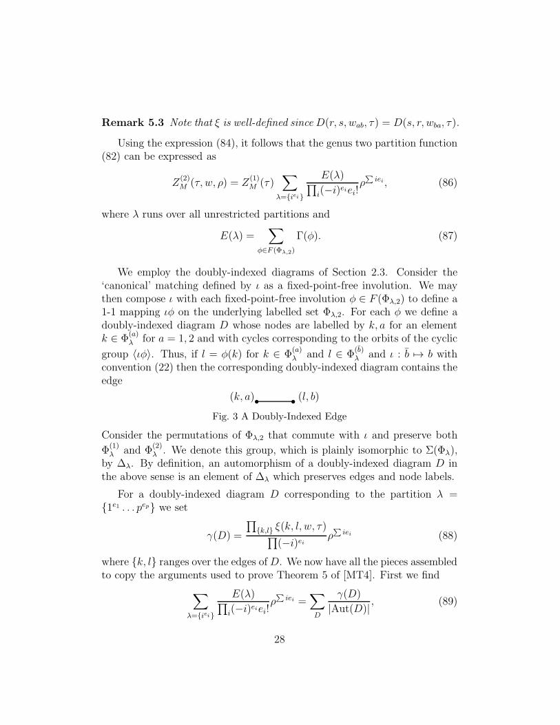
convention (22) then the corresponding doubly-indexed diagram contains theedge

(k, a) s (l, b)sFig. 3 A Doubly-Indexed Edge

Consider the permutations of Φλ,2 that commute with ι and preserve both

Φ(1)λ and Φ

(2)λ . We denote this group, which is plainly isomorphic to Σ(Φλ),

by ∆λ. By definition, an automorphism of a doubly-indexed diagram D inthe above sense is an element of ∆λ which preserves edges and node labels.

For a doubly-indexed diagram D corresponding to the partition λ =1e1 . . . pep we set

γ(D) =

∏k,l ξ(k, l, w, τ)∏

(−i)ei ρ∑iei (88)

where k, l ranges over the edges ofD. We now have all the pieces assembledto copy the arguments used to prove Theorem 5 of [MT4]. First we find

∑

λ=iei

E(λ)∏i(−i)eiei!

ρ∑iei =

∑

D

γ(D)

|Aut(D)| , (89)

28

the sum ranging over all doubly-indexed diagrams.

We next introduce a weight function ζ as follows: for a doubly-indexeddiagram D we set ζ(D) =

∏ζ(E), the product running over all edges. More-

over for an edge E with nodes labelled (k, a) and (l, b) as in Fig. 3, we set

ζ(E) = Rab(k, l),

for R of (25). We then find

Lemma 5.4 ζ(D) = γ(D).

Proof. From (88) it follows that for a doubly-indexed diagram D we have

γ(D) =∏

k,l−ξ(k, l, w, τ)ρ

(k+l)/2

√kl

, (90)

the product ranging over the edges k, l of D. So to prove the Lemma it

suffices to show that if k, l lie in Φ(a)λ ,Φ

(b)λ respectively then the (a, b)-entry

of R(k, l) coincides with the corresponding factor of (90). This follows fromour previous discussion together with Remark 5.3.

From Lemma 5.4 and following similar arguments to the proof of Theo-rem 5 of [MT4] we find

∑

D

γ(D)

|Aut(D)| =∑

D

ζ(D)

|Aut(D)|

= exp

(∑

L

ζ(L)

|Aut(L)|

),

where L denotes the set of non-isomorphic unoriented doubly indexed cycles.Orient these cycles, say in a clockwise direction. Let M denote the set ofnon-isomorphic oriented doubly indexed cycles and Mn the oriented cycleswith n nodes. Then we find (cf. [MT4], Lemma 2) that

1

nTrRn =

∑

Mn

ζ(Mn)

|Aut(Mn)|.

29

It follows that

∑

L

ζ(L)

|Aut(L)| =1

2

∑

M

ζ(M)

|Aut(M)|

=1

2Tr

(∑

n≥1

1

nRn

)

= −12Tr log(I −R)

= −12log det(I − R).

This completes the proof of Theorem 5.1.

We may also find a product formula analogous to Theorem 6 of [MT4].Let R denote the rotationless doubly-indexed oriented cycles i.e. cycles withtrivial automorphism group. Then we find

Theorem 5.5

Z(2)M (τ, w, ρ) =

Z(1)M (τ)∏

R(1− ζ(N))1/2(91)

5.2 Holomorphic and modular-invariance properties

In Section 2.2 we reviewed the genus two ρ-sewing formalism and introducedthe domain Dρ which parametrizes the genus two surface. An immediateconsequence of Theorem 2.1 is the following.

Theorem 5.6 Z(2)M (τ, w, ρ) is holomorphic in Dρ.

We next consider the invariance properties of the genus two partitionfunction with respect to the action of the Dρ-preserving group Γ1 reviewedin Section 2.2. Let χ be the character of SL(2,Z) defined by its action onη(τ)−2, i.e.

η(γτ)−2 = χ(γ)η(τ)−2(cτ + d)−1, (92)

30

where γ =

(a bc d

)∈ SL(2,Z). Recall (e.g. [Se]) that χ(γ) is a twelfth

root of unity. For a function f(τ) on H1, k ∈ Z and γ ∈ SL(2,Z), we define

f(τ)|kγ = f(γτ) (cτ + d)−k, (93)

so thatZ

(1)M2(τ)|−1γ = χ(γ)Z

(1)M2(τ). (94)

At genus two, analogously to (93), we define

f(τ, w, ρ)|kγ = f(γ(τ, w, ρ)) det(CΩ +D)−k. (95)

Here, the action of γ on the right-hand-side is as in (24). We have abusednotation by adopting the following conventions in (95), which we continue touse below:

Ω = F ρ(τ, w, ρ), γ =

(A BC D

)∈ Sp(4,Z) (96)

where F ρ is as in Theorem 2.4, and γ is identified with an element of Sp(4,Z)via (38) and (39). Note that (95) defines a right action of G on functionsf(τ, w, ρ). We then have a natural analog of Theorem 8 of [MT4]

Theorem 5.7 If γ ∈ Γ1 then

Z(2)M2(τ, w, ρ)|−1γ = χ(γ)Z

(2)M2(τ, w, ρ).

Corollary 5.8 If γ ∈ Γ1 with Z(2)M24 = (Z

(2)M2)

12 then

Z(2)M24(τ, w, ρ)|−12γ = Z

(2)M24(τ, w, ρ).

Proof. The proof is similar to that of Theorem 8 of [MT4]. We have toshow that

Z(2)M2(γ.(τ, w, ρ)) det(CΩ+D) = χ(γ)Z

(2)M2(τ, w, ρ) (97)

for γ ∈ Γ1 where det(CΩ11 + D) = c1Ω11 + d1. Consider the determinantformula (81). For γ ∈ Γ1 define

R ′ab(k, l, τ, w, ρ) = Rab(k, l,

a1τ + b1c1τ + d1

,w

c1τ + d1,

ρ

(c1τ + d1)2)

31

following (37). We find from Section 6.3 of [MT2] that

1− R ′ = 1− R− κ∆= (1− κS).(1− R),

where

∆ab(k, l) = δk1δl1,

κ =ρ

2πi

c1c1τ + d1

,

Sab(k, l) = δk1∑

c∈1,2((1− R)−1)cb(1, l).

Since det(1−R) and det(1− R ′) are convergent on Dρ we find

det(1−R ′) = det(1− κS). det(1− R).

Indexing the columns and rows by (a, k) = (1, 1), (2, 1), . . . (1, k), (2, k) . . .and noting that S1b(k, l) = S2b(k, l) we find that

det(1− κS) =

∣∣∣∣∣∣∣∣∣

1− κS11(1, 1) −κS12(1, 1) −κS11(1, 2) · · ·−κS11(1, 1) 1− κS12(1, 1) −κS11(1, 2) · · ·

0 0 1 · · ·...

......

. . .

∣∣∣∣∣∣∣∣∣= 1− κS11(1, 1)− κS12(1, 1),

= 1− κσ((1− R)−1)(1, 1)),

where σ(M) denotes the sum of the entries of a (finite) matrix M . Applying(33), it is clear that

det(1− κS) = c1Ω11 + d1c1τ + d1

.

The Theorem then follows from (94).

Remark 5.9 Z(2)

M2(τ, w, ρ) can be trivially considered as function on the cov-

ering space Dρ discussed in [MT2], Section 6.3. Then Z(2)M2(τ, w, ρ) is mod-

ular with respect to L = HΓ1 with trivial invariance under the action of theHeisenberg group H (loc. cit.).

32

5.3 Some genus two n-point functions

In this section we calculate some examples of genus two n-point functionsfor the rank one Heisenberg VOA M . We consider here the examples of then-point function for the Heisenberg vector a and the 1-point function for theVirasoro vector ω. We find that, up to an overall factor of the partitionfunction, the formal differential form associated with the Heisenberg n-pointfunction is described in terms of the global symmetric two form ω(2) [TUY]whereas the Virasoro 1-point function is described by the genus two projectiveconnection [Gu]. These results agree with those found in [MT4] in the ǫ-formalism up to an overall ǫ-formalism partition function factor.

The genus two Heisenberg vector 1-point function with the Heisenbergvector a inserted at x is Z

(2)M (a, x; τ, w, ρ) = 0 since Z

(1)M (Y [a, x]Y [v, w]v, τ) =

0 from [MT1]. The 2-point function for two Heisenberg vectors inserted atx1, x2 is

Z(2)M (a, x1; a, x2; τ, w, ρ) =

∑

r≥0

ρr∑

v∈M[r]

Z(1)M (a, x1; a, x2; v, w1, v, w2; τ). (98)

We consider the associated formal differential form

F (2)M (a, a; τ, w, ρ) = Z

(2)M (a, x1; a, x2; τ, w, ρ)dx1dx2, (99)

and find that it is determined by the bilinear form ω(2) (17):

Theorem 5.10 The genus two Heisenberg vector 2-point function is givenby

F (2)M (a, a; τ, w, ρ) = ω(2)(x1, x2)Z

(2)M (τ, w, ρ). (100)

Proof. The proof proceeds along the same lines as Theorem 5.1. As be-fore, we let v(λ) denote a Heisenberg Fock vector (83) determined by anunrestricted partition λ = 1e1 . . . pep with label set Φλ. Define a label set

for the four vectors a, a, v(λ), v(λ) given by Φ = Φ1 ∪ Φ2 ∪ Φ(1)λ ∪ Φ

(2)λ for

Φ1,Φ2 = 1 and let F (Φ) denote the set of fixed point free involutions onΦ. For φ = . . . (rs) . . . ∈ F (Φ) let Γ(x1, x2, φ) =

∏(r,s) ξ(r, s) as defined in

(86) for r, s ∈ Φ(2)λ = Φ

(1)λ ∪ Φ

(2)λ and

ξ(r, s) =

D(1, 1, xi − xj , τ) = P2(τ, xi − xj), r, s ∈ Φi, i 6= j,

D(1, s, xi − wa, τ) = sPs+1(τ, xi − wa), r ∈ Φi, s ∈ Φ(a)λ ,(101)

33

for i, j, a ∈ 1, 2 with D of (12). Then following Corollary 1 of [MT1] wehave

Z(1)M (a, x1; a, x2; v(λ), w1; v(λ), w2; τ) = Z

(1)M (τ)

∑

φ∈F (Φ)

Γ(x1, x2, φ).

We then obtain the following analog of (86)

F (2)(a, a; τ, w, ρ) = Z(1)M (τ)

∑

λ=iei

E(x1, x2, λ)∏i(−i)eiei!

ρ∑ieidx1dx2, (102)

whereE(x1, x2, λ) =

∑

φ∈F (Φ)

Γ(x1, x2, φ).

The sum in (102) can be re-expressed as the sum of weights ζ(D) for iso-morphism classes of doubly-indexed configurations D where here D includestwo distinguished valency one nodes labelled xi (see Section 2.3) correspond-ing to the label sets Φ1,Φ2 = 1. As before, ζ(D) =

∏E ζ(E) for standard

doubly-indexed edges E augmented by the contributions from edges con-nected to the two valency one nodes with weights as in (43). Thus we find

F (2)(a, a; τ, w, ρ) = Z(1)M (τ)

∑

D

ζ(D)∏i ei!

dx1dx2,

Each D can be decomposed into exactly one necklace configuration N oftype N (x; y) of (44) connecting the two distinguished nodes and a standardconfiguration D of the type appearing in the proof of Theorem 5.1 withζ(D) = ζ(N)ζ(D). Since |Aut(N)| = 1 we obtain

F (2)(a, a; τ, w, ρ) = Z(1)M (τ)

∑

D

ζ(D)

|Aut(D)|∑

N∈N (x;y)

ζ(N)

= Z(2)M (τ, w, ρ)ζ(x1; x2)

= Z(2)M (τ, w, ρ)ω(2)(x1, x2),

using (47) of Proposition 2.7.

Theorem 5.10 result can be generalized to compute the n-point functioncorresponding to the insertion of n Heisenberg vectors. We find that it van-ishes for n odd, and for n even is determined by the symmetric tensor

Symnω(2) =

∑

ψ

∏

(r,s)

ω(2)(xr, xs), (103)

34

where the sum is taken over the set of fixed point free involutions ψ =. . . (rs) . . . of the labels 1, . . . , n. We then have

Theorem 5.11 The genus two Heisenberg vector n-point function vanishesfor odd n even; for even n it is given by the global symmetric meromorphicn-form:

F (2)M (a, . . . , a; τ, w, ρ)

Z(2)M (τ, w, ρ)

= Symnω(2). (104)

This agrees with the corresponding ratio in Theorem 10 of [MT4] in theǫ-formalism and earlier results in [TUY] based on an assumed analytic struc-ture for the n-point function.

Using this result and the associativity of vertex operators, we can computeall n-point functions. In particular, the 1-point function for the Virasorovector ω = 1

2a[−1]a is as follows (cf. [MT4], Proposition 8):

Proposition 5.12 The genus two 1-point function for the Virasoro vectorω inserted at x is given by

F (2)M (ω; τ, w, ρ)

Z(2)M (τ, w, ρ)

=1

12s(2)(x), (105)

where s(2)(x) = 6 limx→y

(ω(2)(x, y)− dxdy

(x−y)2)is the genus two projective con-

nection ([Gu]).

6 Lattice VOAs

6.1 The genus two partition function Z(2)VL(τ, w, ρ)

Let L be an even lattice with VL the corresponding lattice theory vertexoperator algebra. The underlying Fock space is

VL =M l ⊗ C[L] = ⊕β∈LM l ⊗ eβ, (106)

where M l is the corresponding Heisenberg free boson theory of rank l =dim L based on H = C ⊗Z L. We follow Section 3.1 and [MT1] concerningfurther notation for lattice theories. We utilize the Fock space u⊗eβ where

35

β ranges over L and u ranges over the usual orthogonal basis for M l. FromLemma 3.1 and Corollary 3.2 we see that

Z(2)VL

(τ, w, ρ) =∑

α,β∈LZ

(2)α,β(τ, w, ρ), (107)

Z(2)α,β(τ, w, ρ) =

∑

n≥0

∑

u∈M l[n]

Z(1)

M l⊗eα(u⊗ eβ, u⊗ e−β, w, τ)ρn+(β,β)/2.(108)

The general shape of the 2-point function occurring in (108) is discussedextensively in [MT1]. By Proposition 1 (loc. cit.) it splits as a product

Z(1)

M l⊗eα(u⊗ eβ, u⊗ e−β, w, τ) =QβM l⊗eα(u, u, w, τ)Z

(1)

M l⊗eα(eβ, e−β, w, τ), (109)

where we have identified eβ with 1 ⊗ eβ, and where QβM l⊗eα is a function4

that we will shortly discuss in greater detail. In [MT1], Corollary 5 (cf. theAppendix to the present paper) we established also that

Z(1)

M l⊗eα(eβ , e−β, w, τ) = ǫ(β,−β)q(α,α)/2 exp((α, β)w)

K(w, τ)(β,β)Z

(1)

M l(τ), (110)

where, as usual, we are taking w in place of z12 = z1 − z2. With cocyclechoice ǫ(β,−β) = (−1)(β,β)/2 (cf. Appendix) we may then rewrite (108) as

Z(2)α,β(τ, w, ρ) = Z

(1)

M l(τ) exp

πi((α, α)τ + 2(α, β)

w

2πi+

(β, β)

2πilog

( −ρK(w, τ)2

))

·∑

n≥0

∑

u∈M l[n]

QβM l⊗eα(u, u, w, τ)ρ

n. (111)

We note that this expression is, as it should be, independent of the choiceof branch for the logarithm function. We are going to establish the preciseanalog of Theorem 14 of [MT4] as follows:

Theorem 6.1 We have

Z(2)VL

(τ, w, ρ) = Z(2)

M l(τ, w, ρ)θ(2)L (Ω), (112)

where θ(2)L (Ω) is the genus two theta function of L ([Fr]).

4Note: in [MT1] the functional dependence on β, here denoted by a superscript, wasomitted.

36

Proof. We note that

θ(2)L (Ω) =

∑

α,β∈Lexp(πi((α, α)Ω11 + 2(α, β)Ω12 + (β, β)Ω22)). (113)

We first handle the case of rank 1 lattices and then consider the generalcase. The inner double sum in (111) is the object which requires attention,and we can begin to deal with it along the lines of previous Sections. Namely,arguments that we have already used several times show that the double summay be written in the form

∑

D

γ(D)

|Aut(D)| = exp

(1

2

∑

N∈Nγ(N)

).

Here, D ranges over the oriented doubly indexed cycles of Section 5, whileN ranges over oriented doubly-indexed necklaces N = N (k, a; l, b) of (41).Leaving aside the definition of γ(N) for now, we recognize as before thatthe piece involving only connected diagrams with no end nodes splits off asa factor. Apart from a Z

(1)M (τ) term this factor is, of course, precisely the

expression (89) for M . With these observations, we see from (111) that thefollowing holds:

Z(2)α,β(τ, w, ρ)

Z(2)M (τ, w, ρ)

= exp

iπ

((α, α)τ + 2(α, β)

w

2πi+

(β, β)

2πilog

( −ρK(w, τ)2

)

+1

2πi

∑

N∈Nγ(N)

). (114)

To prove Theorem 6.1, we see from (113) and (114) that it is sufficient toestablish that for each pair of lattice elements α, β ∈ L, we have

Z(2)α,β(τ, w, ρ)

Z(2)M (τ, w, ρ)

= exp (πi ((α, α)Ω11 + 2(α, β)Ω12 + (β, β)Ω22)) . (115)

Recall the formula for Ω in Proposition 2.6. In order to reconcile (115)with the formula for Ω, we must carefully consider the expression

∑N∈N γ(N).

The function γ is essentially (88), except that we also get contributions fromthe end nodes which are now present. Suppose that an end node has label

37

k ∈ Φ(a), a ∈ 1, 2. Then according to Proposition 1 and display (45) of[MT1] (cf. (139) of the Appendix to the present paper), the contribution ofthe end node is equal to

ξα,β(k, a) = ξα,β(k, a, τ, w, ρ) =ρk/2√k(a, δk1α + C(k, 0, τ)β +D(k, 0, w, τ)(−β)) , a = 1

ρk/2√k(a, δk1α + C(k, 0, τ)(−β) +D(k, 0,−w, τ)β) , a = 2

(116)

together with a contribution arising from the −1 in the denominator of (88)(we will come back to this point later). Using (cf. [MT1], displays (6), (11)and (12))

D(k, 0,−w, τ) = (−1)k+1Pk(−w, τ) = −Pk(w, τ),C(k, 0, τ) = (−1)k+1Ek(τ),

we can combine the two possibilities in (116) as follows (recalling that Ek = 0for odd k):

ξα,β(k, a) = (a, α)ρ1/2δk1 + (a, β)da(k), (117)

where da(k) is given by (31). We may then compute the weight for an orienteddoubly-indexed necklace N ∈ N (k, a; l, b) (41). Let N ′ denote the orientednecklace from which the two end nodes and edges have been removed (werefer to these as shortened necklaces). From (117) we see that the totalcontribution to γ(N) is

− ξα,β(k, a)ξα,β(l, b)γ(N ′) = − [(α, α)ρδk1δl1 + (β, β)da(k)db(l)

+(α, β)ρ1/2 (da(k)δl,1 + db(l)δk,1)]γ(N ′),

(118)

where we note that a sign −1 arises from each pair of nodes, as follows from(88).

We next consider the terms in (118) corresponding to (α, α), (α, β) and(β, β) separately, and show that they are precisely the corresponding termson each side of (115). This will complete the proof of Theorem 6.1 in thecase of rank 1 lattices. From (118), an (α, α) term arises only if the endnode weights k, l are both equal to 1. Hence

∑γ(N ′) = ζ(1; 1) (cf. (42)),

where the sum ranges over shortened necklaces with end nodes of weight

38

1 ∈ Φ(a) and 1 ∈ Φ(b). Thus using Proposition 2.6, the total contribution tothe right-hand-side of (115) is equal to

2πiτ − ρζ(1; 1) = 2πiΩ11. (119)

Next, from (118) we see that an (α, β)-contribution arises whenever atleast one of the end nodes has label 1. If the labels of the end nodes areunequal then the shortened necklace with the opposite orientation makes anequal contribution. The upshot is that we may assume that the end nodeto the right of the shortened necklace has label l = 1 ∈ Φ(b), as long aswe count accordingly. We thus find

∑γ(N ′) = ζ(d; 1) (cf. (42)), where the

sum ranges over shortened necklaces with end nodes of weight k ∈ Φ(a) and1 ∈ Φ(b). Then Proposition 2.6 implies that the total contribution to the(α, β) term on the right-hand-side of (115) is

2w − 2ρ1/2ζ(d; 1) = 2Ω12,

as required.

It remains to deal with the (β, β) term, the details of which are verymuch along the lines as the case (α, β) just handled. A similar argumentshows that the contribution to the (β, β)-term from (118) is equal to theexpression −ζ(d; d) of (42). Thus the total contribution to the (β, β) termon the right-hand-side of (115) is

log

( −ρK(w, τ)2

)− ζ(d; d) = Ω22,

as in (35). This completes the proof of Theorem 6.1 in the rank 1 case.

As for the general case - we adopt the mercy rule and omit details! Thereader who has progressed this far will have no difficulty in dealing with thegeneral case, which follows by generalizing the calculations in the rank 1 casejust considered.

The analytic and automorphic properties of Z(2)VL

(τ, w, ρ) can be deduced

from Theorem 6.1 using the known behaviour of θ(2)L (Ω) and the analagous

results for Z(2)

M l(τ, w, ρ) established in Section 5. We simply record

Theorem 6.2 Z(2)VL

(τ, w, ρ) is holomorphic on the domain Dρ.

39

6.2 Some genus two n-point functions

In this section we consider the genus two n-point functions for n Heisenbergvectors and the 1-point function for the Virasoro vector ω for a rank l latticeVOA. The results are similar to those of Section 5.3 so that detailed proofswill not be given.

Consider the 1-point function for a Heisenberg vector ai inserted at x.We define the differential 1-form

F (2)α,β(ai; τ, w, ρ) =

∑

n≥0

∑

u∈M l[n]

Z(1)

M l⊗eα(ai, x; u⊗ eβ, w; u⊗ e−β , 0, τ)ρn+(β,β)/2dx.

(120)This can be expressed in terms of the genus two holomorphic 1-forms ν1, ν2of (30) in a similar way to Theorem 12 of [MT4]. Defining

νi,α,β(x) = (ai, α)ν1(x) + (ai, β)ν2(x),

we find

Theorem 6.3

F (2)α,β(ai; τ, w, ρ) = νi,α,β(x)Z

(2)α,β(τ, w, ρ). (121)

Proof. The proof proceeds along the same lines as Theorems 5.10 and 6.1and Theorem 12 of (op. cit.). We find that

F (2)α,β(ai; τ, w, ρ) = Z

(1)M (τ)

∑

D

γ(D)

|Aut(D)|dx,

where the sum is taken over isomorphism classes of doubly-indexed configu-rations D where, in this case, each configuration includes one distinguishedvalence one node labelled by x as in (43). Each D can be decomposed intoexactly one necklace configuration of type N (x; k, a) of (45), standard config-urations of the type appearing in Theorem 5.10 and necklace contributions asin Theorem 112. The result then follows on applying (117) and the graphicalexpansion for ν1(x), ν2(x) of (48) and (49).

Summing over all lattice vectors, we find that the Heisenberg 1-point func-tion vanishes for VL. Similarly, one can generalize Theorem 5.11 concerning

40

the n-point function for n Heisenberg vectors ai1 , . . . , ain . Defining

F (2)α,β(ai1 , . . . , ain ; τ, w, ρ) =

n∏

t=1

dxt∑

n≥0

∑

u∈M l[n]

ρn+(β,β)/2 ·

Z(1)

M l⊗eα(ai1 , x1; . . . ; ain, xn; u⊗ eβ , w; u⊗ e−β, 0, τ),we obtain the analogue of Theorem 13 of (op. cit.):

Theorem 6.4

F (2)α,β(ai1 , . . . , ain; τ, w, ρ) = Symn

(ω(2), νit,α,β

)Z

(2)α,β(τ, w, ρ), (122)

the symmetric product of ω(2)(xr, xs) and νit,α,β(xt) defined by

Symn

(ω(2), νit,α,β

)=∑

ψ

∏

(r,s)

ω(2)(xs, xs)∏

(t)

νit,α,β(xt), (123)

where the sum is taken over the set of involutions ψ = . . . (ij) . . . (k) . . . ofthe labels 1, . . . , n.

We may also compute the genus two 1-point function for the Virasoro vec-tor ω = 1

2

∑li=1 ai[−1]ai using associativity of vertex operators as in Propo-

sition 5.12. We find that for a rank l lattice,

F (2)α,β(ω; τ, w, ρ) ≡

∑

n≥0

∑

u∈M l[n]

Z(1)

M l⊗eα(ω, x; u⊗ eβ, w; u⊗ e−β, 0, τ)ρn+(β,β)/2dx2

=

(1

2

∑

i

νi,α,β(x)2 +

l

2s(2)(x)

)Z

(2)α,β(τ, w, ρ)

= Z(2)

M l(τ, w, ρ)

(D +

l

12s(2))eiπ((α,α)Ω11+2(α,β)Ω12+(β,β)Ω22).

Here, we used (115) and the differential operator ([Fa], [U], [MT4])

D =1

2πi

∑

1≤a≤b≤2

νaνb∂

∂Ωab. (124)

Defining the normalized Virasoro 1-point form

F (2)VL

(ω; τ, w, ρ) =F (2)VL

(ω; τ, w, ρ)

Z(2)

M l(τ, w, ρ), (125)

we obtain

41

Proposition 6.5 The normalized Virasoro 1-point function for the latticetheory VL satisfies

F (2)VL

(ω; τ, w, ρ) =

(D +

l

12s(2))θ(2)L (Ω). (126)

(The Ward identity (126) is similar to Proposition 11 in [MT4] in the ǫ-sewingformalism.)

Finally, we can obtain the analogue of Proposition 12 (op. cit.), where we

find that F (2)VL

enjoys the same modular properties as Z(2)VL

= θ(2)L (Ω(τ, w, ρ)).

That is,

Proposition 6.6 The normalized Virasoro 1-point function for a lattice VOAobeys

F (2)VL

(ω; τ, w, ρ)|l/2γ =(D +

l

12s(2))(Z

(2)VL

(τ, w, ρ)|l/2γ), (127)

for γ ∈ Γ1.

7 Comparison between the ǫ and ρ-Formalisms

In this section we consider the relationship between the genus two boson andlattice partition functions computed in the ǫ-formalism of [MT4] (based ona sewing construction with two separate tori with modular parameters τ1, τ2and a sewing parameter ǫ) and the ρ-formalism developed in this paper. Wewrite

Z(2)V,ǫ = Z

(2)V,ǫ(τ1, τ2, ǫ) =

∑

n≥0

ǫn∑

u∈V[n]

Z(1)V (u, τ1)Z

(1)V (u, τ2),

Z(2)V,ρ = Z

(2)V,ρ(τ, w, ρ) =

∑

n≥0

ρn∑

u∈V[n]

Z(1)V (u, u, w, τ).

Although, for a given VOA V , the partition functions enjoy many similarproperties, we show below that the partition functions are not equal in thetwo formalisms. This result follows from an explicit computation of thepartition functions for two free bosons in the neighborhood of a two toridegeneration points where Ω12 = 0. It then follows that there is likewise

42

no equality between the partition functions in the ǫ- and ρ-formalisms for alattice VOA.

As shown in Theorem 12 of [MT2], we may relate the ǫ- and ρ-formalismsin certain open neighborhoods of the two tori degeneration point, whereΩ12 = 0. In the ǫ-formalism, the genus two Riemann surface is parameterizedby the domain

Dǫ = (τ1, τ2, ǫ) ∈ H1×H1×C | |ǫ| <1

4D(q1)D(q2), (128)

with qa = exp(2πiτa) and D(q) as in (21). In this case the two torus degen-eration is, by definition, given by ǫ → 0. In the ρ-formalism, the two torusdegeneration is described by the limit (80). In order to understand this moreprecisely we introduce the domain ([MT2])

Dχ = (τ, w, χ) ∈ H1 × C× C | (τ, w,−w2χ) ∈ Dρ, 0 < |χ| < 1

4, (129)

for Dρ of (24) and χ = − ρw2 of (79). The period matrix is determined by a

Γ1-equivariant holomorphic map

F χ : Dχ → H2,

(τ, w, χ) 7→ Ω(2)(τ, w,−w2χ). (130)

Then

Dχ0 = (τ, 0, χ) ∈ H1 × C× C | 0 < |χ| < 1

4, (131)

is the space of two-tori degeneration limit points of the domain Dχ. We maycompare the two parameterizations on certain Γ1-invariant neighborhoods ofa two tori degeneration point in both parameterizations to obtain:

Theorem 7.1 (op. cit., Theorem 12) There exists a 1-1 holomorphic map-ping between Γ1-invariant open domains Iχ ⊂ (Dχ ∪Dχ0 ) and Iǫ ⊂ Dǫ whereIχ and Iǫ are open neighborhoods of a two tori degeneration point.

We next describe the explicit relationship between (τ1, τ2, ǫ) and (τ, w, χ)in more detail. Firstly, from Theorem 4 of [MT2] we obtain

2πiΩ11 = 2πiτ1 + E2 (τ2) ǫ2 + E2 (τ1)E2 (τ2)

2 ǫ4 +O(ǫ6),

2πiΩ12 = −ǫ− E2 (τ1)E2 (τ2) ǫ3 +O(ǫ5),

2πiΩ22 = 2πiτ2 + E2 (τ1) ǫ2 + E2 (τ1)

2E2 (τ2) ǫ4 +O(ǫ6).

43

Making use of the identity

1

2πi

d

dτE2(τ) = 5E4(τ)−E2(τ)

2, (132)

it is straightforward to invert Ωij(τ1, τ2, ǫ) to find

Lemma 7.2 In the neighborhood of the two tori degeneration point r =2πiΩ12 = 0 of Ω ∈ H2 we have

2πiτ1 = 2πiΩ11 − E2(Ω22)r2 + 5E2(Ω11)E4(Ω22)r

4 +O(r6),

ǫ = −r + E2(Ω11)E2(Ω22)r3 +O(r5),

2πiτ2 = 2πiΩ22 − E2(Ω11)r2 + 5E2(Ω22)E4(Ω11)r

4 +O(r6).

From Theorem 2.4 we may also determine Ωij(τ, w, χ) to O(w4) in aneighborhood of a two tori degeneration point to find

Proposition 7.3 For (τ, w, χ) ∈ Dχ ∪ Dχ0 we have

2πiΩ11 = 2πiτ +G(χ)σ2 +G(χ)2E2(τ)σ4 +O(w6),

2πiΩ22 = log f(χ) + E2(τ)σ2 +

(G(χ)E2(τ)

2 +1

2E4(τ)

)σ4 +O(w6)

2πiΩ12 = σ +G(χ)E2(τ)σ3 +O(w5),

where σ = w√1− 4χ, G(χ) = 1

12+ E2(q = f(χ)) = O(χ) and f(χ) is the

Catalan series (72).

This result is an extension of [MT2], Proposition 13 and the general proofproceeds along the same lines. For our purposes, it is sufficient to expandthe non-logarithmic terms to O(w4, χ0). Since R(k, l) = O(χ) and da(k) =O(χ1/2) then Theorem 2.4 implies

2πiΩ11 = 2πiτ +O(χ), (133)

2πiΩ22 = logχ+ 2∑

k≥2

1

kEk(τ)w

k +O(χ), (134)

2πiΩ12 = w +O(χ), (135)

to all orders in w. In particular, we can readily confirm Proposition 7.3 toO(w4, χ0). Substituting (133)–(135) into Lemma 7.2 and using (132) and(142) we obtain

44

Proposition 7.4 For (τ, w, χ) ∈ Dχ ∪ Dχ0 we have

2πiτ1 = 2πiτ +1

12w2 +

1

144E2(τ)w

4 +O(w6, χ),

2πiτ2 = log(χ) +1

12E4(τ)w

4 +O(w6, χ),

ǫ = −w − 1

12E2(τ)w

3 +O(w5, χ).

Define the ratio

Tǫ,ρ(τ, w, χ) =Z

(2)M2,ǫ(τ1, τ2, ǫ)

Z(2)M2,ρ(τ, w,−w2χ)

, (136)

for τ1, τ2, ǫ as given in Proposition 7.4. From Theorems 8 of [MT4] andTheorems 5.7 and 7.1 above we see that Tǫ,ρ is Γ1-invariant. From Theorem4.4 for V =M2, we find in the two tori degeneration limit that

limw→0

Tǫ,ρ(τ, w, χ) = f(χ)−1/12,

i.e., the two partition functions do not even agree in this limit! The origin ofthis discrepancy may be thought to arise from the central charge dependentfactors of q−c/24 and q−c/241 q

−c/242 present in the definitions of Z

(2)V,ρ and Z

(2)V,ǫ re-

spectively (which, of course, are necessary for any modular invariance). Onemodification of the definition of the genus two partition functions compatiblewith the two tori degeneration limit might be:

Znew(2)V,ǫ (τ1, τ2, ǫ) = ǫ−c/12Z(2)

V,ǫ(τ1, τ2, ǫ), Znew(2)V,ρ (τ, w, ρ) = ρ−c/24Z(2)

V,ρ(τ, w, ρ).

However, for V =M2, we immediately observe that the ratio cannot be unitydue to the incompatible Γ1 actions arising from

ǫ→ ǫ

c1τ1 + d1, ρ→ ρ

(c1τ + d1)2,

as given in Lemmas 8 and 15 of [MT2] (cf. (37)).

Consider instead a further Γ1-invariant factor of f(χ)−c/24 in the definition

of the genus two partition function in the ρ-formalism. Once again, we findthat the partition functions do not agree in the neighborhood of a two-toridegeneration point:

45

Proposition 7.5

f(χ)1/12Tǫ,ρ(τ, w, χ) = 1− 1

288E4(τ)w

4 + O(w6, χ).

Proof. As noted earlier, R(k, l) = O(χ) so that we immediately obtain

f(χ)−1/12Z(2)

M2,ρ(τ, w,−w2χ) =1

η(τ)2η(f(χ))2+O(χ),

to all orders in w. On the other hand, Z(2)M2,ǫ(τ1, τ2, ǫ) of Theorem 5 of [MT4]

to O(ǫ4) is given by

1

η(τ1)2η(τ2)2[1 + E2(τ1)E2(τ2)ǫ

2 +(E2(τ1)

2E2(τ2)2 + 15E4(τ1)E4(τ2)

)ǫ4]+O(ǫ6).

(137)We expand this to O(w4, χ) using Proposition 7.4, (132) and

1

2πi

d

dτη(τ) = −1

2E2(τ)η(τ),

to eventually find that

Z(2)

M2,ǫ(τ1, τ2, ǫ) =1

η(q)2η(f(χ))2

(1− 1

288E4(τ)w

4

)+O(w6, χ).

8 Final Remarks

Let us briefly and heuristically sketch how our results compare to some re-lated ideas in the physics and mathematics literature. There is a wealth ofliterature concerning the bosonic string e.g. [GSW], [P]. In particular, theconformal anomaly implies that the physically defined path integral partitionfunction Zstring cannot be reduced to an integral over the moduli spaceMg

of a Riemann surface of genus g except for the 26 dimensional critical stringwhere the anomaly vanishes. Furthermore, for the critical string, Belavinand Knizhnik argue that

Zstring =

∫

Mg

|F |2 dµ,

46

where dµ denotes a natural volume form onMg and F is holomorphic andnon-vanishing onMg [BK], [Kn]. They also claim that for g ≥ 2, F is a globalsection for the line bundle K ⊗ λ−13 (where K is the canonical bundle andλ the Hodge bundle) on Mg which is trivial by Mumford’s theorem [Mu2].In this identification, the λ−13 section is associated with 26 bosons, the Ksection with a c = −26 ghost system and the vanishing conformal anomalyto the vanishing first Chern class for K ⊗ λ−13 [N]. More recently, some ofthese ideas have also been rigorously proved for a zeta function regularizeddeterminant of an appropriate Laplacian operator ∆n [McIT]. The genus two

partition functions Z(2)

M2,ǫ(τ1, τ2, ǫ) and Z(2)

M2,ρ(τ, w, ρ) constructed in [MT4]and the present paper for a rank 2 Heisenberg VOA should correspond in

these approaches to a local description of the holomorphic part of(

det′ ∆1

detN1

)−1

of refs. [Kn], [McIT], giving a local section of the line bundle λ−1. Given

these assumptions, it follows that Tǫ,ρ = Z(2)

M2,ǫ/Z(2)

M2,ρ 6= 1 in the neighborhoodof a two-tori degeneration point where the ratio of the two sections is a non-trivial transition function Tǫ,ρ.

In the case of a general rational conformal field theory, the conformalanomaly continues to obstruct the existence of a global partition functionon moduli space for g ≥ 2. However, all CFTs of a given central chargec are believed to share the same conformal anomaly e.g. [FS]. Thus, theidentification of the normalized lattice partition and n-point functions ofSection 6 reflect the equality of the first Chern class of some bundle associatedto a rank c lattice VOA to that for λ−c with transition function T

c/2ǫ,ρ . It is

interesting to note that even in the case of a unimodular lattice VOA with aunique conformal block ([MS], [TUY]) the genus two partition function cantherefore only be described locally. It would obviously be extremely valuableto find a rigorous description of the relationship between the VOA approachdescribed here and these related ideas in conformal field theory and algebraicgeometry.

9 Appendix

We list here some corrections to [MT1] and [MT2] that we needed above.

(a) Display (27) of [MT1] should read

ǫ(α,−α) = ǫ(α, α) = (−1)(α,α)/2. (138)

47

(b) Display (45) of [MT1] should read

γ(Ξ) = (a, δr,1β + C(r, 0, τ)αk +∑

l 6=kD(r, 0, zkl, τ)αl). (139)

(c) As a result of (a), displays (79) and (80) of [MT1] are modified and nowread

FN (eα, z1; e

−α, z2; q) = ǫ(α,−α)q(β,β)/2

ηl(τ)

exp((β, α)z12)

K(z12, τ)(α,α), (140)

FVL(eα, z1; e

−α, z2; q) = ǫ(α,−α) 1

ηl(τ)

Θα,L(τ, z12/2πi)

K(z12, τ)(α,α). (141)

(d) The expression for ǫ(τ, w, χ) of display (172) of [MT2] should read

ǫ(τ, w, χ) = −w√

1− 4χ(1 +1

24w2E2(τ)(1− 4χ) +O(w4)) (142)

48

References

[B] Borcherds, R.E.: Vertex algebras, Kac-Moody algebras and the Mon-ster. Proc.Nat.Acad.Sc. 83 (1986) 3068–3071.

[BK] Belavin, A.A. and Knizhnik, V.G.: Alegbaic geometry and the ge-ometry of quantum strings. Phys.Lett 168B (1986) 202–206.

[DGM] Dolan, L., Goddard, P. and Montague, P.: Conformal field theories,representations and lattice constructions. Commun.Math.Phys.179(1996) 61–120.

[Fa] Fay, J.: Theta functions on Riemann surfaces, Lecture Notes inMathematics 352, Springer-Verlag, (Berlin and New York, 1973).

[FHL] Frenkel, I., Huang, Y. and Lepowsky, J.: On axiomatic approachesto vertex operator algebras and modules. Mem.Amer.Math.Soc. 104,(1993).

[FK] Farkas, H.M. and Kra, I.: Riemann surfaces, Springer-Verlag (NewYork, 1980).

[FLM] Frenkel, I., Lepowsky, J. and Meurman, A.: Vertex Operator Algebrasand the Monster, (Academic Press, New York, 1988).

[Fr] Freitag, E.: Siegelische Modulfunktionen, Springer-Verlag, (Berlinand New York,1983).

[FS] Freidan, D. and Shenker, S.: The analytic geometry of two dimen-sional conformal field theory. Nucl.Phys. B281 (1987) 509–545.

[GSW] Green, M., Schwartz, J. and Witten, E.: Superstring Theory Vol. 1,Cambridge University Press, (Cambridge, 1987).

[Gu] Gunning, R.C.: Lectures on Riemann surfaces , Princeton Univ.Press, (Princeton, 1966).

[Ka] Kac, V.: Vertex Operator Algebras for Beginners, University LectureSeries, Vol. 10, (AMS 1998).

49

[KZ] Kaneko, M. and Zagier, D.: A generalized Jacobi theta functionand quasimodular forms. The Moduli Space of Curves (Texel Island,1994), Progr. in Math. 129, Birkhauser, (Boston, 1995).

[Kn] Knizhnik, V.G., Multiloop amplitudes in the theory of quantumstrings and complex geometry. Sov.Sci.Rev.A.Phys. 10 (1989) 1–76.

[Li] Li, H.: Symmetric invariant bilinear forms on vertex operator alge-bras. J.Pure.Appl.Alg. 96 (1994) 279–297.

[LL] Lepowsky, J and Li, H.: Introduction to Vertex Operator Algebrasand Their Representations, Birkhauser, (Boston, 2004).

[McIT] McIntyre, A. and Takhtajan, L.A.: Holomorphic factorizationof determinants of Laplacians on Riemann surfaces and highergenus generalization of Kronecker’s first limit formula. GAFA,Geom.funct.anal. 16 (2006) 1291–1323.

[MN] Matsuo, A. and Nagatomo, K,: Axioms for a vertex algebra and thelocality of quantum fields. Math.Soc.Jap.Mem. 4 (1999).

[MS] Moore, G. and Seiberg, N.: Classical and quantum conformal fieldtheory. Commun.Math.Phys. 123 (1989) 177–254.

[MT1] Mason, G. and Tuite, M.P.: Torus chiral n-point functions for freeboson and lattice vertex operator algebras. Commun.Math.Phys. 235(2003) 47–68.

[MT2] Mason, G. and Tuite, M.P.: On genus two Riemann surfaces formedfrom sewn tori. Commun.Math.Phys. 270 (2007) 587–634.

[MT3] Mason, G. and Tuite, M.P.: Partition functions and chiral algebras,in Lie Algebras, Vertex Operator Algebras and their Applications (inhonor of Jim Lepowsky and Robert Robert L. Wilson), Contempo-rary Mathematics 442 (2007).

[MT4] Mason, G. and Tuite, M.P.: Free bosonic vertex operator algebrason genus two Riemann surfaces I, Commun.Math.Phys. 300 (2010)673–713.

50

[MT5] Mason, G. and Tuite, M.P.: Vertex operators and modular forms,A Window into Zeta and Modular Physics eds. K. Kirsten andF. Williams, MSRI Publications 57 183–278, Cambridge UniversityPress, (Cambridge, 2010).

[Mu1] Mumford, D.: Tata lectures on Theta I and II, Birkhauser, (Boston,1983).

[Mu2] Mumford, D.: Stability of Projective Varieties. L.Ens.Math. 23(1977) 39–110.

[N] Nelson, P., Lectures on strings and moduli space. Phys.Reports 149(1987) 337–375.

[P] Polchinski, J.: String Theory, Volume I, Cambridge University Press,(Cambridge, 1998).

[Se] Serre, J-P.: A Course in Arithmetic, Springer-Verlag, (Berlin 1978).

[So1] Sonoda, H.: Sewing conformal field theories I. Nucl.Phys. B311(1988) 401–416.

[So2] Sonoda, H.: Sewing conformal field theories II. Nucl.Phys. B311(1988) 417–432.

[T] Tuite, M.P: Genus Two Meromorphic Conformal Field Theory, CRMProceedings and Lecture Notes 30 (2001), 231–251.

[TUY] Tsuchiya, A, Ueno, K. and Yamada, Y.: Conformal field the-ory on universal family of stable curves with gauge symmetries.Adv.Stud.Pure.Math. 19 (1989) 459–566.

[U] Ueno, K.: Introduction to conformal field theory with gauge sym-metries. in Geometry and Physics - Proceedings of the conference atAarhus Univeristy, Aaarhus, Denmark, Marcel Dekker, (New York1997).

[Y] Yamada, A.: Precise variational formulas for abelian differentials.Kodai Math.J. 3 (1980) 114–143.

[Z] Zhu, Y.: Modular invariance of characters of vertex operator alge-bras. J.Amer.Math.Soc. 9 (1996) 237–302.

51