Embed Size (px)
Citation preview
Ginzburg-Landau Theory
for Bosonic Gases in Optical Lattices
im Fachbereich Physik der
Freien Universität Berlin
eingereichte Dissertation
von
Francisco Ednilson Alves dos Santos
October 2011
Die in vorliegender Dissertation dargestellte Arbeit wurde in der Zeit zwischen April 2007 und
August 2011 im Fachbereich Physik an der Freien Universität Berlin unter Betreuung von Priv.- Doz.
Dr. Axel Pelster durchgeführt.
Erstgutachter: Priv.-Doz. Dr. Axel Pelster
Zweitgutachter: Prof. Dr. Jürgen Bosse
2
Abstract
In this thesis the quantum phase transition of spinless bosons in optical lattices is described within a
Ginzburg-Landau theory. To this end the underlying eective action is derived from the microscopic
Bose-Hubbard Hamiltonian by developing diagrammatic techniques for a resummed hopping expansion.
Thus, this Ginzburg-Landau theory inaugurates a new approach for determining the properties of
bosonic atoms in lattice systems. Already in second hopping order it exhibits a relative error of less
than 3 % for the boundary between the superuid and the Mott insulator phase of a three-dimensional
cubic optical lattice when compared with the most recent results of Quantum Monte Carlo simulations.
In addition, the Ginzburg-Landau theory also allows to calculate near-equilibrium as well as non-
equilibrium quantities. Thus, this thesis shows that, although comparable with numerical methods
in terms of accuracy, the analytical Ginzburg-Landau theory presented here oers a much better
qualitative understanding of the respective system properties.
The thesis starts in Chapter 1 with a brief introduction of the experimental achievements and
the theoretical description of Bose-Einstein condensation in general and lattice physics in particular.
Afterwards, Chapter 2 discusses in more detail the theory of laser-generated optical lattices. Second-
order phase transitions are then covered in Chapter 3 with special emphasis on the physics of the
quantum phase transition between a Mott insulator and a superuid.
The Ginzburg-Landau theory itself is developed systematically in Chapter 4. It contains the dia-
grammatic techniques, which are used to calculate the eective action of the lattice system in a power
series of the hopping parameter. To this end symmetry-breaking currents are coupled to the bosonic
operators and, by applying a Legendre transformation to the free energy, the resulting eective action
is obtained. This procedure leads to an eective resummation of the free energy which makes it possible
to analytically describe the properties of the dierent phases of the lattice system.
Various applications of the Ginzburg-Landau theory are presented in Chapters 5 and 6. In Chapter 5,
the eective action is used to calculate various static and dynamical properties of cubic bosonic lattices
at both zero and nite temperature. It shows an impressive accordance with the numerically calculated
quantum phase diagrams for two and three dimensions already at second hopping order. In addition,
the equivalence between condensate and superuid density is demonstrated at rst hopping order.
Furthermore, the spectra of the various collective excitations appearing in both the Mott insulator and
the superuid phase are analyzed in detail. In Chapter 6, the Ginzburg-Landau theory is then adapted
to deal with the collapse and revival dynamics of matter waves in an optical lattice loaded with 87Rb
atoms according to the experiment performed in Ref. [1]. Our method is used to reproduce at least
qualitatively the observed damped oscillations of the coherence.
3

4
Kurzzusammenfassung
In der vorliegenden Arbeit wird der Quantenphasenübergang spinloser Bosonen in optischen Gittern
im Rahmen einer Ginzburg-Landau-Theorie beschrieben. Hierzu wird die zugrunde liegende eektive
Wirkung ausgehend vom mikroskopischen Bose-Hubbard-Hamiltonian abgeleitet, indem eine diagram-
matische Technik zur Resummation einer Tunnel-Entwicklung ausgearbeitet wird. Die so erhaltene
Ginzburg-Landau-Theorie erönet einen neuen Zugang, um die Eigenschaften bosonischer Atome in
einem Gittersystem zu bestimmen. Schon in zweiter Hopping-Ordnung ergibt sich ein Fehler von
nur 3 % für die Grenze zwischen der superuiden und der Mott-Isolator-Phase eines dreidimen-
sionalen kubischen optischen Gitters im Vergleich zu neuesten Quanten Monte-Carlo-Simulationen.
Auÿerdem erlaubt die Ginzburg-Landau-Theorie, physikalische Gröÿen nahe des Gleichgewichtes und
im Nichtgleichgewicht zu berechnen. Die Arbeit zeigt daher, dass die hier vorgestellte analytische
Ginzburg-Landau-Theorie ein viel besseres qualitatives Verständnis der jeweiligen Systemeigenschaften
ermöglicht, auch wenn die Genauigkeit der Ergebnisse mit denen durch numerische Methoden erzielten
Ergebnisse vergleichbar ist.
Die Arbeit beginnt in Kapitel 1 mit einer kurzen Einführung in die experimentelle Errungenschaften
und die theoretische Beschreibung der Bose-Einstein-Kondensation im allgemeinen und der Gitter-
physik im besonderen. Anschlieÿend diskutiert Kapitel 2 detaillierter die Theorie der durch Laser
erzeugten optischen Gitter. Phasenübergänge zweiter Ordnung werden dann im Kapitel 3 behandelt,
wobei besonders die Physik des Quantenphasenübergangs vom Mott-Isolator zum Superuid betont
wird.
Die eigentliche Ginzburg-Landau-Theorie wird systematisch in Kapitel 4 entwickelt. Sie beinhal-
tet die diagrammatischen Techniken, die zur Berechnung der eektiven Wirkung eines Gittersys-
tems als Potenzreihe des Tunnelparameters verwendet werden. Hierzu werden Symmetrie brechende
Ströme an die bosonischen Operatoren gekoppelt und die eektive Wirkung folgt durch eine Legendre-
Transformation der freien Energie. Dieses Verfahren führt zu einer eektiven Resummation der freien
Energie, die eine analytische Beschreibung der Eigenschaften in den verschiedenen Phasen des Gitter-
systems ermöglicht.
Verschiedene Anwendungen der Ginzburg-Landau-Theorie werden in den Kapiteln 5 und 6 vorgestellt.
In Kapitel 5 wird die eektive Wirkung verwendet, um die verschiedenen statischen und dynamischen
Eigenschaften von kubischen bosonischen Gittern sowohl bei verschwindender als auch bei endlicher
Temperatur zu berechnen. Es zeigt sich, dass die Quantenphasendiagramme für zwei und drei Dimen-
sionen schon in zweiter Tunnelordnung beeindruckend mit numerisch erzielten Ergebnissen überein-
stimmen. Ferner wird gezeigt, dass Kondensatdichte und superuide Dichte in erster Tunnelordnung
äquivalent sind. Auÿerdem werden die Spektren der verschiedenen kollektiven Anregungen genauer
analysiert, die sowohl in der Mott-Isolator als auch in der superuiden Phase auftreten. In Kapitel
6 wird die Ginzburg-Landau-Theorie angewandt, um die Kollaps-und-Wiederkehr-Dynamik von Ma-
5
teriewellen in einem mit 87Rb Atome beladenen optischen Gitter zu behandeln, die im Experiment der
Ref. [1] beobachtet wurde. Unsere Methode ist in der Lage, die beobachteten gedämpften Oszillationen
der Kohährenz zumindest qualitativ zu reproduzieren.
Wir halten zusammenfassend fest, dass unsere Ginzburg-Landau-Theorie für Bosonen in optis-
chen Gittern verschiedene Überprüfungen beim Vergleich mit numerischen Simulationen und experi-
mentellen Resultaten erfolgreich bestanden hat. Daher erwarten wir, dass sie zur Planung und Analyse
künftiger Gitterexperimente nützlich sein wird.
6
Contents
1. Introduction 9
1.1. Bose-Einstein Condensation . . . . . . . . . . . . . . . . . . . . . . . . . . . . . . . . . 9
1.2. Bosons in optical lattices . . . . . . . . . . . . . . . . . . . . . . . . . . . . . . . . . . . 10
1.3. Overview . . . . . . . . . . . . . . . . . . . . . . . . . . . . . . . . . . . . . . . . . . . 14
2. Optical Lattice Potentials 17
2.1. Laser forces . . . . . . . . . . . . . . . . . . . . . . . . . . . . . . . . . . . . . . . . . . 17
2.2. Band structure . . . . . . . . . . . . . . . . . . . . . . . . . . . . . . . . . . . . . . . . 20
2.3. Bose-Hubbard Hamiltonian . . . . . . . . . . . . . . . . . . . . . . . . . . . . . . . . . 23
2.3.1. Hamiltonian Parameters . . . . . . . . . . . . . . . . . . . . . . . . . . . . . . . 25
2.3.2. Corrections due to Laser Inhomogeneity . . . . . . . . . . . . . . . . . . . . . . 28
3. Quantum Phase Transitions 33
3.1. Second-Order Quantum Phase Transitions . . . . . . . . . . . . . . . . . . . . . . . . . 33
3.2. Quantum Phase Transitions in Bosonic Lattices . . . . . . . . . . . . . . . . . . . . . . 35
3.3. Mean-Field Theory . . . . . . . . . . . . . . . . . . . . . . . . . . . . . . . . . . . . . . 40
4. Bosonic Lattices at Finite Temperature 47
4.1. Perturbation Theory . . . . . . . . . . . . . . . . . . . . . . . . . . . . . . . . . . . . . 49
4.2. Lattice Diagrammatics . . . . . . . . . . . . . . . . . . . . . . . . . . . . . . . . . . . . 50
4.3. Diagrammatic Representation . . . . . . . . . . . . . . . . . . . . . . . . . . . . . . . . 51
4.4. Eective Action and 1-Particle Irreducible Diagrams . . . . . . . . . . . . . . . . . . . 53
4.5. Matsubara Representation . . . . . . . . . . . . . . . . . . . . . . . . . . . . . . . . . . 55
4.6. Zeroth-Hopping Order Eective Action . . . . . . . . . . . . . . . . . . . . . . . . . . . 57
4.7. First-hopping order eective action . . . . . . . . . . . . . . . . . . . . . . . . . . . . . 63
4.8. Second-hopping order eective action . . . . . . . . . . . . . . . . . . . . . . . . . . . . 64
5. Homogeneous Lattices 69
5.1. Quasi-Momentum Representation . . . . . . . . . . . . . . . . . . . . . . . . . . . . . . 69
5.2. Static Properties . . . . . . . . . . . . . . . . . . . . . . . . . . . . . . . . . . . . . . . 71
5.2.1. First Hopping Order . . . . . . . . . . . . . . . . . . . . . . . . . . . . . . . . . 71
5.2.2. Second Hopping Order . . . . . . . . . . . . . . . . . . . . . . . . . . . . . . . . 73
5.3. Dynamical Properties . . . . . . . . . . . . . . . . . . . . . . . . . . . . . . . . . . . . 76
5.3.1. Superuid Density . . . . . . . . . . . . . . . . . . . . . . . . . . . . . . . . . . 76
5.3.2. Excitation Spectra . . . . . . . . . . . . . . . . . . . . . . . . . . . . . . . . . . 78
7
Contents
5.3.3. Critical Exponents . . . . . . . . . . . . . . . . . . . . . . . . . . . . . . . . . . 89
6. Collapse and Revival of Matter Waves 95
6.1. Equations of motion for J = 0 . . . . . . . . . . . . . . . . . . . . . . . . . . . . . . . . 95
6.2. Exact solution for J = 0 . . . . . . . . . . . . . . . . . . . . . . . . . . . . . . . . . . . 96
6.3. Initial conditions . . . . . . . . . . . . . . . . . . . . . . . . . . . . . . . . . . . . . . . 97
6.4. Momentum distributions . . . . . . . . . . . . . . . . . . . . . . . . . . . . . . . . . . . 97
6.5. Comparison with Experiments . . . . . . . . . . . . . . . . . . . . . . . . . . . . . . . . 100
7. Summary and Conclusion 103
A. Appendix 1 109
B. Appendix 2 113
Bibliography 115
8
1. Introduction
1.1. Bose-Einstein Condensation
By applying the new quantum statistics developed by Satyendra N. Bose [2], Albert Einstein predicted
the possibility of a new state of matter emerging in extremely cold bosonic gases: the Bose-Einstein
Condensate (BEC) [3,4]. According to his theory, when a non-interacting bosonic gas is cooled until it
reaches a certain critical temperature, a phase transition occurs. Below such temperature, the number
of particles occupying the ground state of the system becomes macroscopic. Following these ideas, in
1938 [5], F. London was the rst to suggest the formation of a BEC as the explanation for superuidity
in 4He. Although Einstein's theory concerns only with ideal Bose gases, the prediction of London was
later experimentally conrmed by using neutron scattering techniques [6].
Despite all the theoretical predictions, it took more 70 years before the extremely low temperatures
necessary for the realization of the rst BEC became available. It was only in the early 1980s that
laser cooling techniques turned temperatures of the order of micro-Kelvin accessible to experiments.
For this achievement, Chu, Cohen-Tannoudji, and Phillips received the physics Nobel prize in 1997.
The basic idea of laser cooling is to use the Doppler eect due to the thermal motion of the atoms
in such a way that they absorb more photons when moving towards the light source than in other
directions. This eect is obtained by tuning the laser to a frequency a little smaller than an electronic
transition of the atom. This way, when an atom moves in the direction of the laser source, its transition
frequency matches the laser frequency due to the Doppler eect. By using two laser beams pointing
in opposite directions, the atom will absorb more photons whenever it moves towards a light source,
thus reducing its momentum. Later, when the excited atom spontaneously emits the absorbed photon,
it will receive the photon momentum in an arbitrary direction. The net eect of such a cycle of an
absorption and an emission process is an overall decrease in the speed of atom and, therefore, the
cooling of the gas.
Alkali atoms are particularly accessible to laser-based methods due to their peculiar electronic struc-
ture and because their transitions are reachable by available lasers. Such methods provided the basis
for the next step in achieving even lower temperatures by using a procedure called evaporative cooling
[7]. This technique consists in successively lowering the trapping potential so that the most energetic
atoms y from the sample leaving behind a cooler gas. This nally made possible the temperatures of
only a few nano-Kelvin which are necessary to produce a BEC.
Finally in 1995, the rst BECs were experimentally produced using rubidium atoms by Wiemann
and Cornell [8], and using sodium atoms by Ketterle [9]. In these experiments the ultracold gas is
released from its magnetic trap so that the atomic cloud can freely expand for a few milliseconds before
a picture of the expanded cloud is taken by shining resonant laser light on it and capturing its shadow
using a CCD-camera. As the density distribution of the expanded cloud reproduces almost exactly the
9
1. Introduction
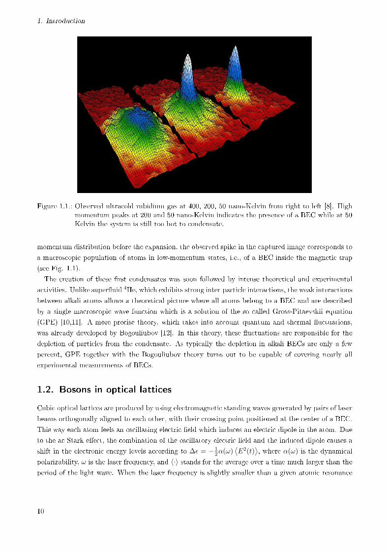
Figure 1.1.: Observed ultracold rubidium gas at 400, 200, 50 nano-Kelvin from right to left [8]. Highmomentum peaks at 200 and 50 nano-Kelvin indicates the presence of a BEC while at 50Kelvin the system is still too hot to condensate.
momentum distribution before the expansion, the observed spike in the captured image corresponds to
a macroscopic population of atoms in low-momentum states, i.e., of a BEC inside the magnetic trap
(see Fig. 1.1).
The creation of these rst condensates was soon followed by intense theoretical and experimental
activities. Unlike superuid 4He, which exhibits strong inter-particle interactions, the weak interactions
between alkali atoms allows a theoretical picture where all atoms belong to a BEC and are described
by a single macroscopic wave function which is a solution of the so called Gross-Pitaevskii equation
(GPE) [10,11]. A more precise theory, which takes into account quantum and thermal uctuations,
was already developed by Bogouliubov [12]. In this theory, these uctuations are responsible for the
depletion of particles from the condensate. As typically the depletion in alkali BECs are only a few
percent, GPE together with the Bogouliubov theory turns out to be capable of covering nearly all
experimental measurements of BECs.
1.2. Bosons in optical lattices
Cubic optical lattices are produced by using electromagnetic standing waves generated by pairs of laser
beams orthogonally aligned to each other, with their crossing point positioned at the center of a BEC.
This way each atom feels an oscillating electric eld which induces an electric dipole in the atom. Due
to the ac Stark eect, the combination of the oscillatory electric eld and the induced dipole causes a
shift in the electronic energy levels according to ∆ε = −12α(ω)
⟨E2(t)
⟩, where α(ω) is the dynamical
polarizability, ω is the laser frequency, and 〈·〉 stands for the average over a time much larger than the
period of the light wave. When the laser frequency is slightly smaller than a given atomic resonance
10
1.2. Bosons in optical lattices
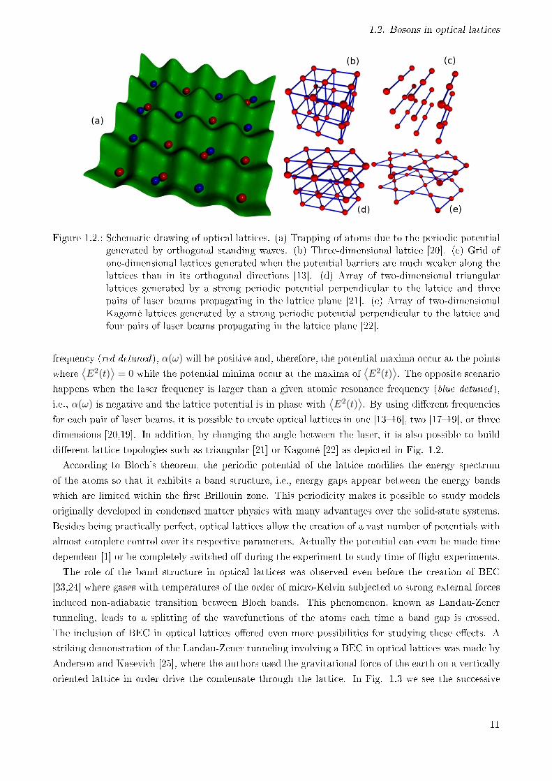
Figure 1.2.: Schematic drawing of optical lattices. (a) Trapping of atoms due to the periodic potentialgenerated by orthogonal standing waves. (b) Three-dimensional lattice [20]. (c) Grid ofone-dimensional lattices generated when the potential barriers are much weaker along thelattices than in its orthogonal directions [13]. (d) Array of two-dimensional triangularlattices generated by a strong periodic potential perpendicular to the lattice and threepairs of laser beams propagating in the lattice plane [21]. (e) Array of two-dimensionalKagomé lattices generated by a strong periodic potential perpendicular to the lattice andfour pairs of laser beams propagating in the lattice plane [22].
frequency (red detuned), α(ω) will be positive and, therefore, the potential maxima occur at the points
where⟨E2(t)
⟩= 0 while the potential minima occur at the maxima of
⟨E2(t)
⟩. The opposite scenario
happens when the laser frequency is larger than a given atomic resonance frequency (blue detuned),
i.e., α(ω) is negative and the lattice potential is in phase with⟨E2(t)
⟩. By using dierent frequencies
for each pair of laser beams, it is possible to create optical lattices in one [1316], two [1719], or three
dimensions [20,19]. In addition, by changing the angle between the laser, it is also possible to build
dierent lattice topologies such as triangular [21] or Kagomé [22] as depicted in Fig. 1.2.
According to Bloch's theorem, the periodic potential of the lattice modies the energy spectrum
of the atoms so that it exhibits a band structure, i.e., energy gaps appear between the energy bands
which are limited within the rst Brillouin zone. This periodicity makes it possible to study models
originally developed in condensed matter physics with many advantages over the solid-state systems.
Besides being practically perfect, optical lattices allow the creation of a vast number of potentials with
almost complete control over its respective parameters. Actually the potential can even be made time
dependent [1] or be completely switched o during the experiment to study time-of-ight experiments.
The role of the band structure in optical lattices was observed even before the creation of BEC
[23,24] where gases with temperatures of the order of micro-Kelvin subjected to strong external forces
induced non-adiabatic transition between Bloch bands. This phenomenon, known as Landau-Zener
tunneling, leads to a splitting of the wavefunctions of the atoms each time a band gap is crossed.
The inclusion of BEC in optical lattices oered even more possibilities for studying these eects. A
striking demonstration of the Landau-Zener tunneling involving a BEC in optical lattices was made by
Anderson and Kasevich [25], where the authors used the gravitational force of the earth on a vertically
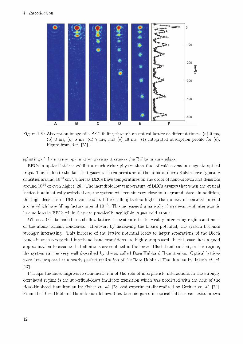
oriented lattice in order drive the condensate through the lattice. In Fig. 1.3 we see the successive
11
1. Introduction
Figure 1.3.: Absorption image of a BEC falling through an optical lattice at dierent times. (a) 0 ms,(b) 3 ms, (c) 5 ms, (d) 7 ms, and (e) 10 ms. (f) Integrated absorption prole for (e).Figure from Ref. [25].
splinting of the macroscopic matter wave as it crosses the Brillouin zone edges.
BECs in optical lattices exhibit a much richer physics than that of cold atoms in magneto-optical
traps. This is due to the fact that gases with temperatures of the order of micro-Kelvin have typically
densities around 1010 cm3, whereas BECs have temperatures on the order of nano-Kelvin and densities
around 1014 or even higher [26]. The incredible low temperature of BECs assures that when the optical
lattice is adiabatically switched on, the system will remain very close to its ground state. In addition,
the high densities of BECs can lead to lattice lling factors higher than unity, in contrast to cold
atoms which have lling factors around 10−3. This increases dramatically the relevance of inter-atomic
interactions in BECs while they are practically negligible in just cold atoms.
When a BEC is loaded in a shallow lattice the system is in the weakly interacting regime and most
of the atoms remain condensed. However, by increasing the lattice potential, the system becomes
strongly interacting. This increase of the lattice potential leads to larger separations of the Bloch
bands in such a way that interband band transitions are highly suppressed. In this case, it is a good
approximation to assume that all atoms are conned in the lowest Bloch band so that, in this regime,
the system can be very well described by the so called Bose-Hubbard Hamiltonian. Optical lattices
were rst proposed as a nearly perfect realization of the Bose-Hubbard Hamiltonian by Jaksch et. al.
[27].
Perhaps the most impressive demonstration of the role of interparticle interactions in the strongly
correlated regime is the superuid-Mott insulator transition which was predicted with the help of the
Bose-Hubbard Hamiltonian by Fisher et. al. [28] and experimentally realized by Greiner et. al. [29].
From the Bose-Hubbard Hamiltonian follows that bosonic gases in optical lattices can exist in two
12
1.2. Bosons in optical lattices
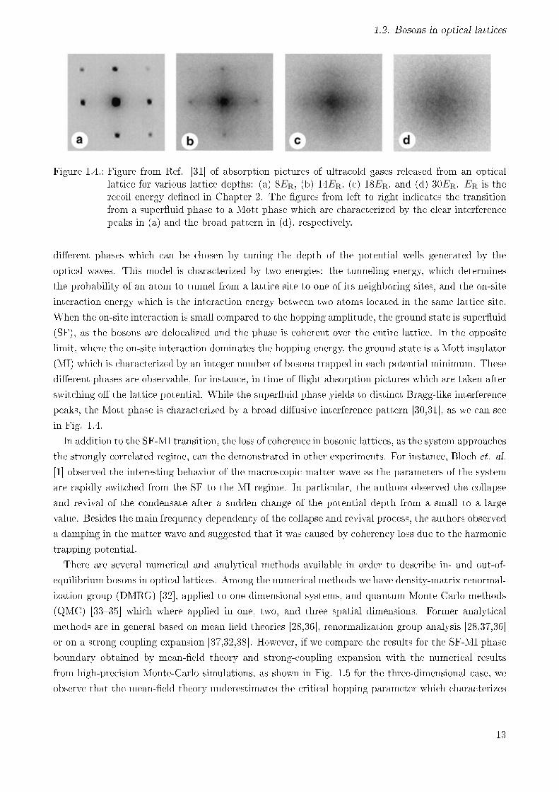
Figure 1.4.: Figure from Ref. [31] of absorption pictures of ultracold gases released from an opticallattice for various lattice depths: (a) 8ER, (b) 14ER, (c) 18ER, and (d) 30ER. ER is therecoil energy dened in Chapter 2. The gures from left to right indicates the transitionfrom a superuid phase to a Mott phase which are characterized by the clear interferencepeaks in (a) and the broad pattern in (d), respectively.
dierent phases which can be chosen by tuning the depth of the potential wells generated by the
optical waves. This model is characterized by two energies: the tunneling energy, which determines
the probability of an atom to tunnel from a lattice site to one of its neighboring sites, and the on-site
interaction energy which is the interaction energy between two atoms located in the same lattice site.
When the on-site interaction is small compared to the hopping amplitude, the ground state is superuid
(SF), as the bosons are delocalized and the phase is coherent over the entire lattice. In the opposite
limit, where the on-site interaction dominates the hopping energy, the ground state is a Mott insulator
(MI) which is characterized by an integer number of bosons trapped in each potential minimum. These
dierent phases are observable, for instance, in time-of-ight absorption pictures which are taken after
switching o the lattice potential. While the superuid phase yields to distinct Bragg-like interference
peaks, the Mott phase is characterized by a broad diusive interference pattern [30,31], as we can see
in Fig. 1.4.
In addition to the SF-MI transition, the loss of coherence in bosonic lattices, as the system approaches
the strongly correlated regime, can the demonstrated in other experiments. For instance, Bloch et. al.
[1] observed the interesting behavior of the macroscopic matter wave as the parameters of the system
are rapidly switched from the SF to the MI regime. In particular, the authors observed the collapse
and revival of the condensate after a sudden change of the potential depth from a small to a large
value. Besides the main frequency dependency of the collapse and revival process, the authors observed
a damping in the matter wave and suggested that it was caused by coherency loss due to the harmonic
trapping potential.
There are several numerical and analytical methods available in order to describe in- and out-of-
equilibrium bosons in optical lattices. Among the numerical methods we have density-matrix renormal-
ization group (DMRG) [32], applied to one-dimensional systems, and quantum Monte Carlo methods
(QMC) [3335] which where applied in one, two, and three spatial dimensions. Former analytical
methods are in general based on mean eld theories [28,36], renormalization group analysis [28,37,36]
or on a strong coupling expansion [37,32,38]. However, if we compare the results for the SF-MI phase
boundary obtained by mean-eld theory and strong-coupling expansion with the numerical results
from high-precision Monte-Carlo simulations, as shown in Fig. 1.5 for the three-dimensional case, we
observe that the mean-eld theory underestimates the critical hopping parameter which characterizes
13
1. Introduction
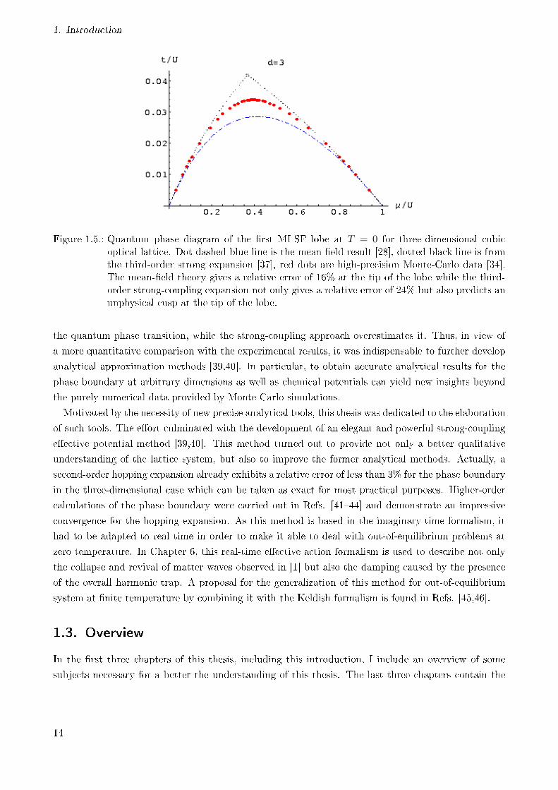
Figure 1.5.: Quantum phase diagram of the rst MI-SF lobe at T = 0 for three-dimensional cubicoptical lattice. Dot-dashed blue line is the mean eld result [28], dotted black line is fromthe third-order strong expansion [37], red dots are high-precision Monte-Carlo data [34].The mean-eld theory gives a relative error of 16% at the tip of the lobe while the third-order strong-coupling expansion not only gives a relative error of 24% but also predicts anunphysical cusp at the tip of the lobe.
the quantum phase transition, while the strong-coupling approach overestimates it. Thus, in view of
a more quantitative comparison with the experimental results, it was indispensable to further develop
analytical approximation methods [39,40]. In particular, to obtain accurate analytical results for the
phase boundary at arbitrary dimensions as well as chemical potentials can yield new insights beyond
the purely numerical data provided by Monte-Carlo simulations.
Motivated by the necessity of new precise analytical tools, this thesis was dedicated to the elaboration
of such tools. The eort culminated with the development of an elegant and powerful strong-coupling
eective potential method [39,40]. This method turned out to provide not only a better qualitative
understanding of the lattice system, but also to improve the former analytical methods. Actually, a
second-order hopping expansion already exhibits a relative error of less than 3% for the phase boundary
in the three-dimensional case which can be taken as exact for most practical purposes. Higher-order
calculations of the phase boundary were carried out in Refs. [4144] and demonstrate an impressive
convergence for the hopping expansion. As this method is based in the imaginary-time formalism, it
had to be adapted to real time in order to make it able to deal with out-of-equilibrium problems at
zero temperature. In Chapter 6, this real-time eective action formalism is used to describe not only
the collapse and revival of matter waves observed in [1] but also the damping caused by the presence
of the overall harmonic trap. A proposal for the generalization of this method for out-of-equilibrium
system at nite temperature by combining it with the Keldish formalism is found in Refs. [45,46].
1.3. Overview
In the rst three chapters of this thesis, including this introduction, I include an overview of some
subjects necessary for a better the understanding of this thesis. The last three chapters contain the
14
1.3. Overview
original contributions of my PhD work.
In Chapter 2, the general theory of optical lattices is discussed. It is described how laser generated
standing waves are used to produce periodic trapping potentials. These potentials are capable of
reproducing many features of solid-state systems with the advantage of a defect-free lattice for which
the tunnel coupling between dierent potential wells can be tuned by both the intensity and the
frequency of the lasers. Due to the ac-Stark eect, the atoms are trapped in the maxima or minima of
the laser eld depending on whether the laser are red or blue detuned, respectively [20].
In Chapter 3, a general introduction to second-order phase transitions according to the modern
classication of phase transitions is made. In particular, I address the symmetry breakdown mechanism
which applies when the system passes from one more ordered to a less ordered phase of system. A
discussion is also made about the role of the order parameter and concept of universality as well as
its relation to the dierent critical exponents characterizing dierent systems. Special attention is
given to quantum phase transitions which are transitions that can happen even in systems at zero
temperature. Most of these discussions are made in the context of bosons in optical lattices so that
the theory of second-order phase transitions is specically applied to the Mott insulator-superuid
transition. Explicit calculation of the quantum phase diagram is performed by using mean-eld theory
and the properties of the two dierent phases are discussed.
In Chapter 4, a perturbation theory is developed by taking advantage of a diagrammatic notation
specially developed to deal with bosons in optical lattices. The calculation of the eective action, which
is dened through a Legendre transformation of the free energy, leads to an automatic resummation of
the hopping expansion. This allows the description of the system properties in both the Mott insulator
and superuid phase. By using a set of diagrammatic rules, the eective action is calculated up to
second hopping order.
In Chapter 5, the eective action is used to calculate various static and dynamical properties of cubic
bosonic lattices at nite and zero temperature. By comparing the compressibility in the superuid
phase with the mean-led result, it is shown some advantages of the eective-action approach over
the mean-eld theory. The second-hopping order calculation of the quantum phase diagram exhibits
an impressive accordance with the numerically calculated phase diagrams for two and three dimen-
sions. This indicates that already at second-hopping order, our theory has enough precision for most
practical applications. In addition, the equivalence between condensed density and superuid density
is demonstrated at rst hopping order. The spectra of the various excitations appearing in the Mott
phase and superuid phase are calculated. In particular, the gaps and masses of the gapped modes
are calculated as well as the sound velocity associated with the Goldstone mode.
In Chapter 6, is discussed the formation and dynamics of matter waves in a optical lattice loaded
with 87Rb atoms which was experimentally observed by Greiner at. al [1]. I use the results from our
eective action theory to reproduce the observed features in Ref. [1] and test our theory against the
experimental results.
In order to facilitate the comprehension of calculations in Matsubara space, some extra computational
details are included in the appendices A and B.
15

16
2. Optical Lattice Potentials
In this chapter the general theory of optical lattices is discussed. It is described how laser generated
standing waves are used in order to produce periodic trapping potentials. These potential are capable
of reproducing many features of solid-state systems with the advantages of a defect-free lattice whose
tunnel coupling between dierent potential wells can be tuned by both the intensity and the frequency
of the lasers. Due to the AC Stark eect, the atoms are trapped in maxima or minima of the laser
eld depending on whether the lasers are red or blue detuned, respectively [20].
2.1. Laser forces
First, consider the Hamiltonian of a freely moving atom
HFree =1
2mp2 +
∑n
En |n〉 〈n| , (2.1)
where m is the mass of the atom, p is the center-of-mass momentum operator, and |n〉 are the internalelectronic states with energy En.
Now, let us consider the laser-generated electric eld
E(t) = E0ε cos(ωt), (2.2)
where ε indicates the direction of polarization of the laser light.
In the dipole approximation [47,48], the eect of the oscillating electric eld on the atom is taken
into account by adding the interaction term
I(t) = −d · E(t) (2.3)
to the Hamiltonian HFree, with the dipole momentum operator dened as
d = −e∑i
ri, (2.4)
where e is the electric charge of the electron and ri is the position operator of the i-th atomic electron
relative to the nucleus.
As we are interested in systems at very low temperatures, the atom is considered to be in its
electronic ground state |0〉. In this case, the rst non-vanishing contribution to the ground-state
energy is of second order and is given by [11,47]
∆E = −1
2α(ω)|E(t)|2, (2.5)
17
2. Optical Lattice Potentials
where f(t) stands for the time average of an arbitrary function f(t) over a period much larger than
2π/ω and the frequency-dependent polarizability α(ω) is given by
α(ω) = <i limη→0
∫ ∞
0dteit(ω+iη) 〈0| 1
~
[ε · d(t), ε · d
]|0〉
≈∑n6=0
∣∣∣〈n| ε · d |0〉∣∣∣2 [ En − E0 − ~ω
(En − Em − ~ω)2 + (~Γn/2)2+ (ω → −ω)
], (2.6)
where in the last line, the nite lifetime of excited atomic states was approximately accounted for by
writing 〈n| ε · d(t) |0〉 ≈ 〈n| ε · d |0〉 eit(En−E0)/~−|t|Γn/2. In practice, the long lifetime of electronic states
implies Γn, Γm |En − Em| /~ for any two atomic states |n〉 and |m〉. Therefore, the frequency-
dependent polarizability in the vicinity of the n-th atomic excitation frequency, i.e, for frequencies
ω = (En−Em)/~+ δn with |δn| = O(Γn) |En −Em| /~, will be dominated by only a single term in
the above sum over excited states:
α(ω) ≈∣∣∣〈n| ε · d |0〉
∣∣∣2 1
~(−δn)
δ2n + Γ2n/4
, δn = ω − (En − E0)/~. (2.7)
Inserting this into Eq. (2.5), one nds for the second-order shift of the atomic ground-state energy
∆E =~Ω2
R
2
δnδ2n + Γ2
n/4, (2.8)
with the Rabi frequency
ΩR =1
~
√∣∣∣〈n| d · E(t) |0〉∣∣∣2. (2.9)
Besides inducing an r-dependent shift ∆E to the atomic ground-state energy which resembles an
external potential experienced by atoms, the laser light will also be absorbed and excite atoms which
will make transitions |0〉 → |n〉 at a rate w0→n ∝ (Γn/δn)∆E which, in view of Eq. (2.8), will be
maximal at resonance (δn = 0). In order to avoid strong absorption which would be associated with
heating up the ultracold gas, the lasers must be detuned with δn as large as possible.
Now we must take into account the fact that the laser generated standing wave possesses not only
a time-dependent electric eld but also has a space dependency. Therefore, instead of Eq. (2.2), we
consider
E(r, t) = E0(r)ε cos(ωt) (2.10)
As the spatial variation of the electric eld E(r, t) is negligible inside the atoms, we may assume
that the laser-induced electric eld produces an eective external potential Vfull felt by each atom, this
spatio-temporal dependent electric eld produces the spatially dependent potential
Vfull(r) = −1
2α(ω)|E(r, t)|2. (2.11)
The intensity prole of a single Gaussian laser beams in cylindrical coordinates is given by [49]
18
2.1. Laser forces
I(r) = |E(0, t)|2 w0
w(z)e− 2
w(z)2r2cos2(kLz), (2.12)
where z is the direction of propagation of the laser beam, w(z) = w0
√1 + (z/zR) is the radius at which
the intensity drops to 1/e2 of its maximum, zR = πw20/λ is the Rayleigh length, λ is the wave length
of the lattice, and w0 is the beam waist size. The laser beams must be aligned so that the location of
their respective waists coincide. In this way, the approximation w(z) ≈ w0 can be made leading to a
potential of the form
Vfull(r) = −V0e−2x2+y2
w20 cos2(kLz)− V0e
−2x2+z2
w20 cos2(kLy)− V0e
−2 y2+z2
w20 cos2(kLx). (2.13)
This can be rearranged to the form
Vfull(r) = Vtrap(r) + VOL(r) (2.14)
with trap and optical-lattice contributions
Vtrap(r) = −V0
(e−2x2+y2
w20 + e
−2 y2+z2
w20 + e
−2x2+z2
w20
)≈ −3V0 +
4V0w20
|r|2 , (2.15)
VOL(r) = Vx(r) sin2(kLx) + Vy(r) sin
2(kLy) + Vz(r) sin2(kLz), (2.16)
and the abbreviations
Vx(r) = V0e−2 y2+z2
w20 ≈ V0 −
2V0w20
(y2 + z2), (2.17)
Vy(r) = V0e−2x2+z2
w20 ≈ V0 −
2V0w20
(x2 + z2), (2.18)
Vz(r) = V0e−2x2+y2
w20 ≈ V0 −
2V0w20
(x2 + y2). (2.19)
Finally the full Hamiltonian which describes the motion of a single atom in a far detuned laser eld
can be written as
Hfull =1
2mp2 + Vfull(r). (2.20)
In most applications, the atoms are concentrated in a region |r| w0 near the center of the trap.
For this reason, deviations from periodicity in the full external potential Vfull(r) may be ignored, i.e.,
Vfull(r) ≈ −3V0 + V (r). Therefore, the only part that will be considered in following is
V (r) = V0[sin2(kLx) + sin2(kLy) + sin2(kLz)
], (2.21)
thus leading to the single atom Hamiltonian
19
2. Optical Lattice Potentials
H ′ =1
2mp2 + V (r). (2.22)
2.2. Band structure
The Bloch theorem states that the eigenfunctions of the Schrödinger equation[− ~2
2m∇2 + V (r)
]Ψ
(n)k (r) = E
(n)k Ψ
(n)k (r) (2.23)
with a periodic potential V (r) has eigenfunctions of the form [50]
Ψ(n)k (r) = eik·rΦ
(n)k (r), (2.24)
where the Bloch functions Φ(n)k (r) have the same periodicity of V (r), n = (nx, ny, nz) is the collective
band index, and k is restricted to rst Brillouin zone, i.e., its components are in the interval −π/a ≤ki < π/a, with the lattice spacing a = π/kL = λ/2.
In many interesting cases the depth of the potential V (r) is large enough to trap the atoms in its wells
so that they move from one well to its neighbor by tunnel eect which is known as the tight-binding
limit. As the Bloch functions are spatially delocalized, it is convenient to dene a new set of wave
functions which are localized around each potential well. These are the so called Wannier functions
and are dened as [51]
U (n)(r− ri) =1√Ns
∑k
e−ik·riΨ(n)k (r), (2.25)
where Ns is the total number of lattice sites, ri is the location of the i-th lattice site, and the sum
in k runs over the rst Brillouin zone. From this denition it is possible to derive the orthonormality
property
∫ ∞
−∞d3rU (n)(r− ri)
∗U (n′)(r− rj) =1
Ns
∑k′,k
eik′·ri−ik·rj
∫ ∞
−∞d3rΨ
(n′)k′ (r)∗Ψ
(n)k (r)
=δn′,n
Ns
∑k
eik·(ri−rj) (2.26)
= δn′,nδi,j ,
as well as the completeness property
∑i,n
U (n)(r′ − ri)∗U (n)(r− ri) =
1
Ns
∑n
∑k′,k
Ψ(n)k′ (r
′)∗Ψ(n)k (r)
∑i
ei(k′−k)·ri
=∑n
∑k
Ψ(n)k (r′)∗Ψ
(n)k (r) (2.27)
= δ(r− r′).
20
2.2. Band structure
These conditions assure that any three-dimensional wavefunction can be expanded in terms of Wannier
functions.
As the equation (2.23) with the periodic potential given by (2.21) can be solved by separation of
variables, we can write its eigenfunctions and eigenvalues, respectively as
Ψ(n)k (r) = ψ
(nx)kx
(x)ψ(ny)ky
(y)ψ(nz)kz
(z), (2.28)
E(n)k = ε
(nx)kx
+ ε(ny)ky
+ ε(nz)kz
. (2.29)
And analogously with the Bloch and Wannier functions
Φ(n)k (r) = φ
(nx)kx
(x)φ(ny)ky
(y)φ(nz)kz
(z), (2.30)
U (n)(r− ri) = u(nx)(x− xi)u(ny)(y − yi)u
(nz)(z − zi), (2.31)
where ψ(n)k (x) are solutions of the one-dimensional Schrödinger equation[
− ~2
2m
∂2
∂x2+ V0 sin
2(kLx)
]ψ(n)k (x) = ε
(n)k ψ
(n)k (x), (2.32)
with the one-dimensional Bloch and Wannier function dened as
ψ(n)k (x) = eikxφ
(n)k (x), (2.33)
u(n)(x− xi) =1
N1/6s
∑k
e−ikxiψ(n)k (x). (2.34)
The one-dimensional Wannier functions also obey the orthonormality and completeness conditions
∫ ∞
−∞dxu(n
′)(x− xi)∗u(n)(x− xj) = δi,jδn,n′ , (2.35)∑
n,i
u(n)(x′ − xi)∗u(n)(x− xi) = δ(x− x′). (2.36)
The Schrödinger equation (2.32) can be simplied by expressing it in terms the dimensionless quantities
x′ =π
ax; k′ =
a
πk; V ′
0 =V0ER
; ε(n) =ε(n)
ER, (2.37)
where the recoil energy is dened as
ER =~2k2L2m
. (2.38)
Thus, the dimensionless Schrödinger equation (2.32) reads
21
2. Optical Lattice Potentials
-1.0-0.5 0.0 0.5 1.0kkL
5
10
15
20
EHkLER
-1.0-0.5 0.0 0.5 1.0kkL
5
10
15
20
EHkLER
-1.0-0.5 0.0 0.5 1.0kkL
5
10
15
20
EHkLER
Figure 2.1.: First four Bloch bands for dierent values of V ′0 . Left: V
′0 = 1. Middle: V ′
0 = 10. Right:V ′0 = 20. Here we see that for high enough lattice potentials, each band energy can be
considered as momentum independent.
[− ∂2
∂x′2+ V ′
0 sin2(x′)
]ψ(n)k′ (x′) = ε
(n)k′ ψ
(n)k′ (x′). (2.39)
For the Bloch's function in dimensionless units we have[k′2 − 2ik′
∂
∂x′− ∂2
∂x′2+ V ′
0 sin2(x′)
]φ(n)k′ (x′) = ε
(n)k′ φ
(n)k′ (x′). (2.40)
Due to its periodicity, the Bloch function can be expanded in a Fourier series according to
φ(n)k′ (x′) =
∞∑l=−∞
c(n)k′,le
2ilx′ . (2.41)
Then Eq. (2.40) can be written in terms of the Fourier components[(k′ + 2l)2 +
V ′0
2
]c(n)k′,l +
V ′0
4(c
(n)k′,l+1 + c
(n)k′,l−1) = ε
(n)k′ c
(n)k′,l. (2.42)
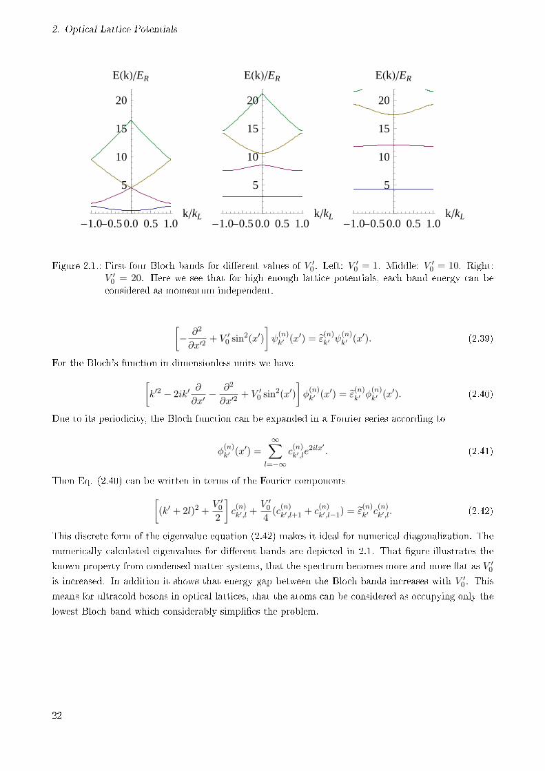
This discrete form of the eigenvalue equation (2.42) makes it ideal for numerical diagonalization. The
numerically calculated eigenvalues for dierent bands are depicted in 2.1. That gure illustrates the
known property from condensed matter systems, that the spectrum becomes more and more at as V ′0
is increased. In addition it shows that energy gap between the Bloch bands increases with V ′0 . This
means for ultracold bosons in optical lattices, that the atoms can be considered as occupying only the
lowest Bloch band which considerably simplies the problem.
22
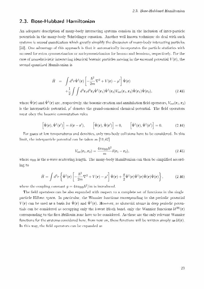
2.3. Bose-Hubbard Hamiltonian
2.3. Bose-Hubbard Hamiltonian
An adequate description of many-body interacting systems consists in the inclusion of inter-particle
potentials in the many-body Schrödinger equation. Another well known technique do deal with such
systems is second quantization which greatly simplify the discussion of many-body interacting particles
[52]. One advantage of this approach is that it automatically incorporates the particle statistics with
no need for extra symmetrization or antisymmetrization for bosons and fermions, respectively. For the
case of nonrelativistic interacting identical bosonic particles moving in the external potential V (r), the
second quantized Hamiltonian is
H =
∫d3rΨ†(r)
[− ~2
2m∇2 + V (r)− µ′
]Ψ(r)
+1
2
∫ ∫d3r1d
3r2Ψ†(r1)Ψ
†(r2)Vint(r1, r2)Ψ(r1)Ψ(r2), (2.43)
where Ψ(r) and Ψ†(r) are , respectively, the bosonic creation and annihilation eld operators, Vint(r1, r2)
is the interparticle potential, µ′ denotes the grand-canonical chemical potential. The eld operators
must obey the bosonic commutation rules
[Ψ(r), Ψ†(r′)
]= δ(r− r′),
[Ψ(r), Ψ(r′)
]= 0,
[Ψ†(r), Ψ†(r′)
]= 0. (2.44)
For gases at low temperatures and densities, only two-body collisions have to be considered. In this
limit, the interparticle potential can be taken as [11,47]
Vint(r1, r2) =4πaBB~2
mδ(r1 − r2), (2.45)
where aBB is the s-wave scattering length. The many-body Hamiltonian can then be simplied accord-
ing to
H =
∫d3r
Ψ†(r)
[− ~2
2m∇2 + V (r)− µ′
]Ψ(r) +
g
2Ψ†(r)Ψ†(r)Ψ(r)Ψ(r)
, (2.46)
where the coupling constant g = 4πaBB~2/m is introduced.
The eld operators can be also expanded with respect to a complete set of functions in the single-
particle Hilbert space. In particular, the Wannier functions corresponding to the periodic potential
V (r) can be used as a basis for Ψ(r) and Ψ†(r). However, as ultracold atoms in deep periodic poten-
tials can be considered as occupying only the lowest Bloch band, only the Wannier functions U (0)(r)
corresponding to the rst Brillouin zone have to be considered. As these are the only relevant Wannier
functions for the systems considered here, from now on, these functions will be written simply as U(r).In this way, the eld operators can be expanded as
23
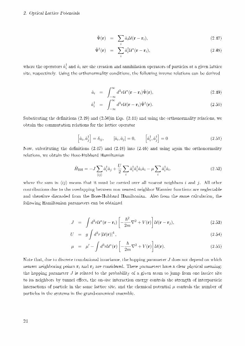
2. Optical Lattice Potentials
Ψ(r) =∑i
aiU(r− ri), (2.47)
Ψ†(r) =∑i
a†iU∗(r− ri), (2.48)
where the operators a†i and ai are the creation and annihilation operators of particles at a given lattice
site, respectively. Using the orthonormality conditions, the following inverse relations can be derived
ai =
∫ ∞
−∞d3rU∗(r− ri)Ψ(r), (2.49)
a†i =
∫ ∞
−∞d3rU(r− ri)Ψ
†(r). (2.50)
Substituting the denitions (2.49) and (2.50)in Eqs. (2.44) and using the orthonormality relations, we
obtain the commutation relations for the lattice operator
[ai, a
†j
]= δij , [ai, aj ] = 0,
[a†i , a
†j
]= 0 (2.51)
Now, substituting the denitions (2.47) and (2.48) into (2.46) and using again the orthonormality
relations, we obtain the Bose-Hubbard Hamiltonian
HBH = −J∑〈ij〉
a†i aj +U
2
∑i
a†i a†i aiai − µ
∑i
a†i ai. (2.52)
where the sum in 〈ij〉 means that it must be carried over all nearest neighbors i and j. All other
contributions due to the overlapping between non-nearest neighbor Wannier functions are neglectable
and therefore discarded from the Bose-Hubbard Hamiltonian. Also from the same calculation, the
following Hamiltonian parameters can be obtained
J =
∫d3rU∗(r− ri)
[− ~2
2m∇2 + V (r)
]U(r− rj), (2.53)
U = g
∫d3r |U(r)|4 , (2.54)
µ = µ′ −∫d3rU∗(r)
[− ~2m
∇2 + V (r)
]U(r). (2.55)
Note that, due to discrete translational invariance, the hopping parameter J does not depend on which
nearest neighboring points ri and rj are considered. These parameters have a clear physical meaning:
the hopping parameter J is related to the probability of a given atom to jump from one lattice site
to its neighbors by tunnel eect, the on-site interaction energy controls the strength of interparticle
interactions of particle in the same lattice site, and the chemical potential µ controls the number of
particles in the systems in the grand-canonical ensemble.
24
2.3. Bose-Hubbard Hamiltonian
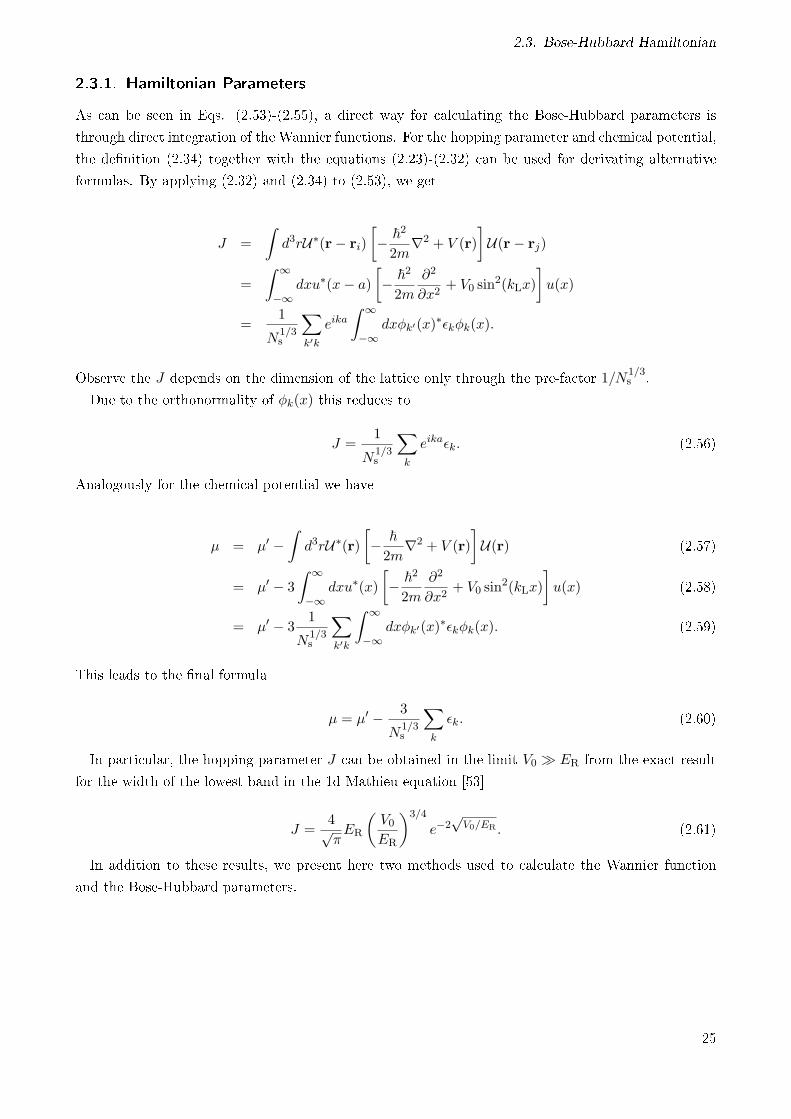
2.3.1. Hamiltonian Parameters
As can be seen in Eqs. (2.53)-(2.55), a direct way for calculating the Bose-Hubbard parameters is
through direct integration of the Wannier functions. For the hopping parameter and chemical potential,
the denition (2.34) together with the equations (2.23)-(2.32) can be used for derivating alternative
formulas. By applying (2.32) and (2.34) to (2.53), we get
J =
∫d3rU∗(r− ri)
[− ~2
2m∇2 + V (r)
]U(r− rj)
=
∫ ∞
−∞dxu∗(x− a)
[− ~2
2m
∂2
∂x2+ V0 sin
2(kLx)
]u(x)
=1
N1/3s
∑k′k
eika∫ ∞
−∞dxφk′(x)
∗εkφk(x).
Observe the J depends on the dimension of the lattice only through the pre-factor 1/N1/3s .
Due to the orthonormality of φk(x) this reduces to
J =1
N1/3s
∑k
eikaεk. (2.56)
Analogously for the chemical potential we have
µ = µ′ −∫d3rU∗(r)
[− ~2m
∇2 + V (r)
]U(r) (2.57)
= µ′ − 3
∫ ∞
−∞dxu∗(x)
[− ~2
2m
∂2
∂x2+ V0 sin
2(kLx)
]u(x) (2.58)
= µ′ − 31
N1/3s
∑k′k
∫ ∞
−∞dxφk′(x)
∗εkφk(x). (2.59)
This leads to the nal formula
µ = µ′ − 3
N1/3s
∑k
εk. (2.60)
In particular, the hopping parameter J can be obtained in the limit V0 ER from the exact result
for the width of the lowest band in the 1d Mathieu-equation [53]
J =4√πER
(V0ER
)3/4
e−2√V0/ER . (2.61)
In addition to these results, we present here two methods used to calculate the Wannier function
and the Bose-Hubbard parameters.
25
2. Optical Lattice Potentials
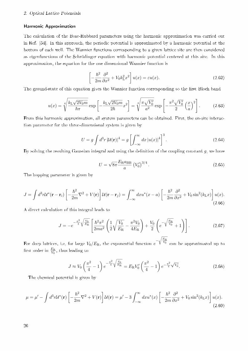
Harmonic Approximation
The calculation of the Bose-Hubbard parameters using the harmonic approximation was carried out
in Ref. [54]. In this approach, the periodic potential is approximated by a harmonic potential at the
bottom of each well. The Wannier functions corresponding to a given lattice site are then considered
as eigenfunctions of the Schrödinger equation with harmonic potential centered at this site. In this
approximation, the equation for the one-dimensional Wannier function is[− ~2
2m
∂2
∂x2+ V0k
2Lx
2
]u(x) = εu(x). (2.62)
The ground-state of this equation gives the Wannier function corresponding to the rst Bloch band
u(x) =4
√kL
√2V0m
~πexp
[−kL
√2V0m
2~x2]=
4
√π√V ′0
a2exp
[−π2√V ′0
2
(xa
)2]. (2.63)
From this harmonic approximation, all system parameters can be obtained. First, the on-site interac-
tion parameter for the three-dimensional system is given by
U = g
∫d3r |U(r)|4 = g
[∫ ∞
−∞dx |u(x)|4
]3. (2.64)
By solving the resulting Gaussian integral and using the denition of the coupling constant g, we have
U =√8πERaBB
a
(V ′0
)3/4. (2.65)
The hopping parameter is given by
J =
∫d3rU∗(r− ri)
[− ~2
2m∇2 + V (r)
]U(r− rj) =
∫ ∞
−∞dxu∗(x− a)
[− ~2
2m
∂2
∂x2+ V0 sin
2(kLx)
]u(x).
(2.66)
A direct calculation of this integral leads to
J = −e−π2
4
√V0ER
[~2π2
2ma2
(1
2
√V0ER
− π2V04ER
)+V02
(e−√
ERV0 + 1
)]. (2.67)
For deep lattices, i.e, for large V0/ER, the exponential function e−√
ERV0 can be approximated up to
rst order in ERV0, thus leading to
J ≈ V0
(π2
4− 1
)e−π2
4
√V0ER = ERV
′0
(π2
4− 1
)e−
π2
4
√V ′0 . (2.68)
The chemical potential is given by
µ = µ′ −∫d3rU∗(r)
[− ~2
2m∇2 + V (r)
]U(r) = µ′ − 3
∫ ∞
−∞dxu∗(x)
[− ~2
2m
∂2
∂x2+ V0 sin
2(kLx)
]u(x).
(2.69)
26
2.3. Bose-Hubbard Hamiltonian
-2 Π-3 Π
2-Π -
Π
2
Π
2Π
3 Π
22 Π
kLx
0.2
0.4
0.6
0.8
1.0wHxL
-2 Π-3 Π
2-Π -
Π
2
Π
2Π
3 Π
22 Π
kLx
0.2
0.4
0.6
0.8
1.0wHxL
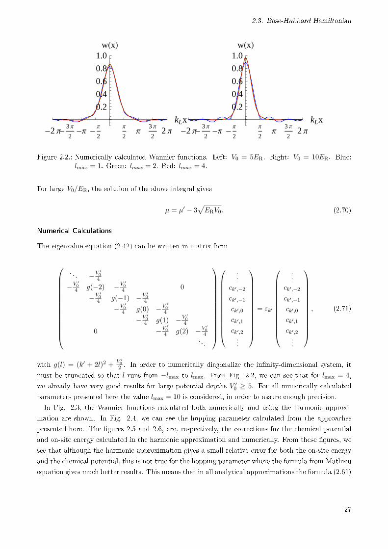
Figure 2.2.: Numerically calculated Wannier functions. Left: V0 = 5ER. Right: V0 = 10ER. Blue:lmax = 1. Green: lmax = 2. Red: lmax = 4.
For large V0/ER, the solution of the above integral gives
µ = µ′ − 3√ERV0. (2.70)
Numerical Calculations
The eigenvalue equation (2.42) can be written in matrix form
. . . −V ′04
−V ′04 g(−2) −V ′
04 0
−V ′04 g(−1) −V ′
04
−V ′04 g(0) −V ′
04
−V ′04 g(1) −V ′
04
0 −V ′04 g(2) −V ′
04
. . .
...
ck′,−2
ck′,−1
ck′,0
ck′,1
ck′,2...
= εk′
...
ck′,−2
ck′,−1
ck′,0
ck′,1
ck′,2...
, (2.71)
with g(l) = (k′ + 2l)2 +V ′02 . In order to numerically diagonalize the innity-dimensional system, it
must be truncated so that l runs from −lmax to lmax. From Fig. 2.2, we can see that for lmax = 4,
we already have very good results for large potential depths V ′0 ≥ 5. For all numerically calculated
parameters presented here the value lmax = 10 is considered, in order to assure enough precision.
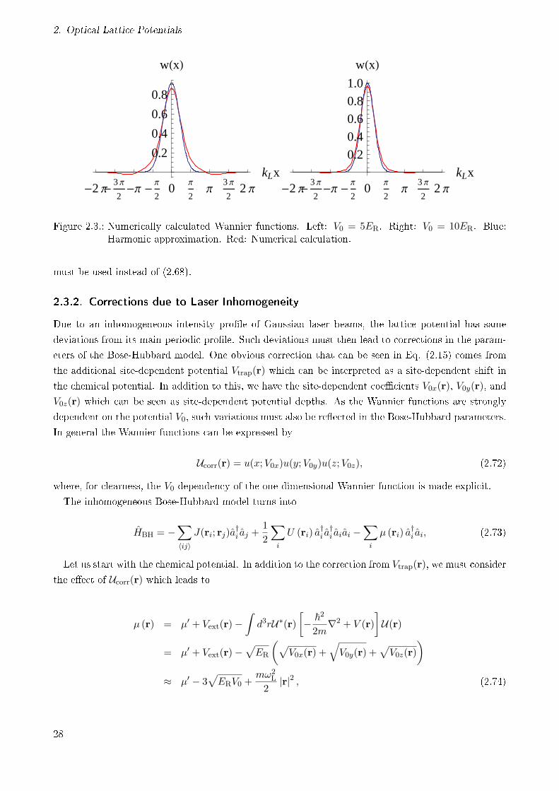
In Fig. 2.3, the Wannier functions calculated both numerically and using the harmonic approxi-
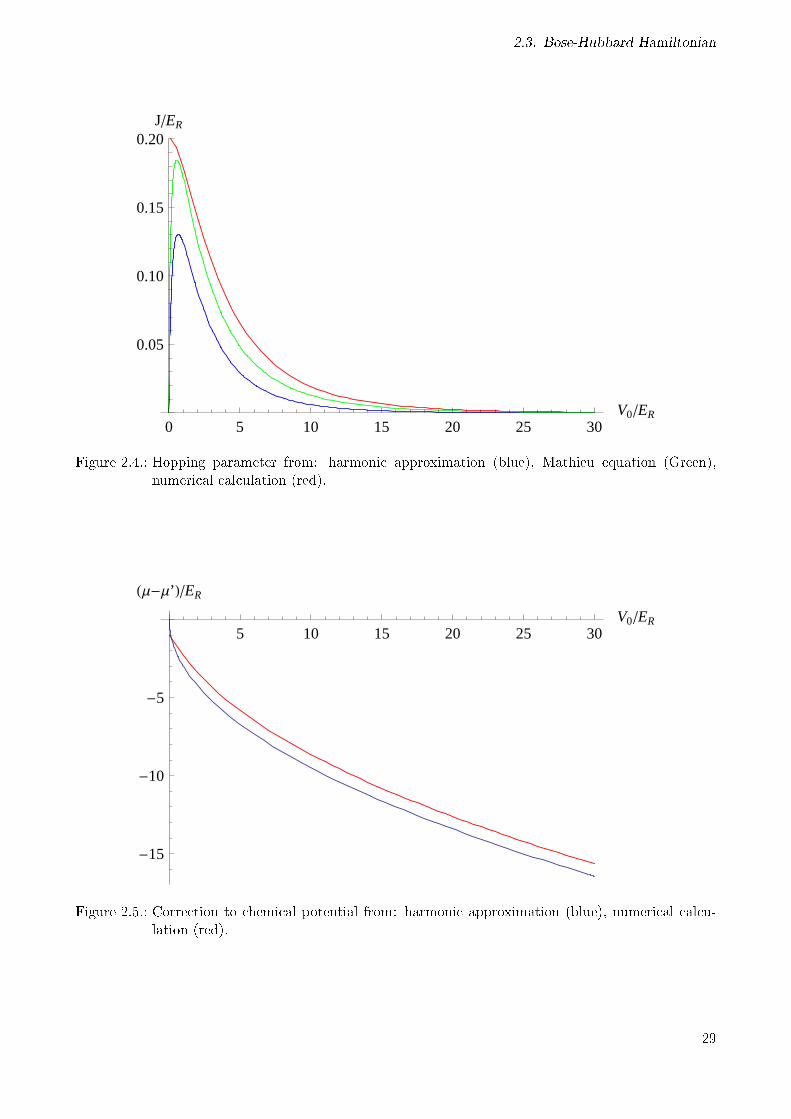
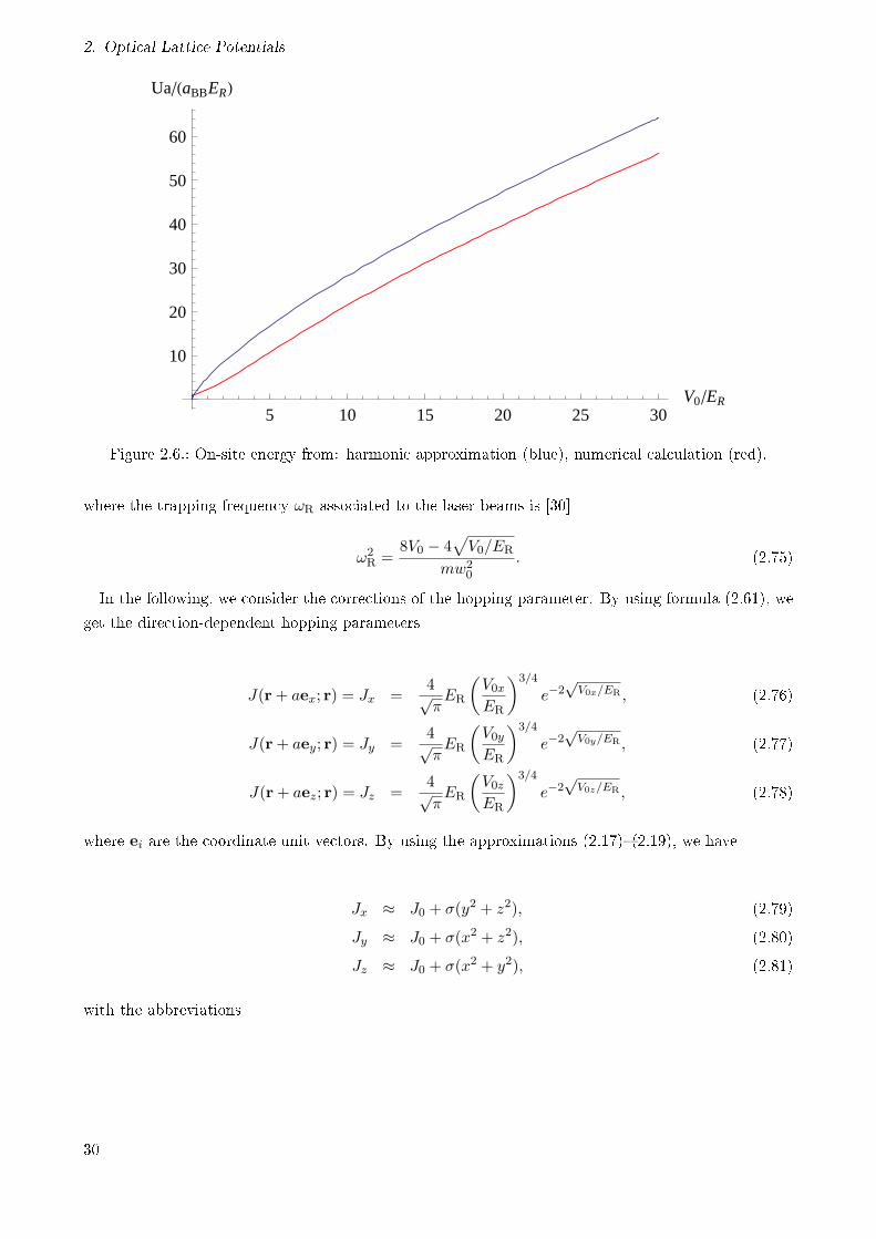
mation are shown. In Fig. 2.4, we can see the hopping parameter calculated from the approaches
presented here. The gures 2.5 and 2.6, are, respectively, the corrections for the chemical potential
and on-site energy calculated in the harmonic approximation and numerically. From these gures, we
see that although the harmonic approximation gives a small relative error for both the on-site energy
and the chemical potential, this is not true for the hopping parameter where the formula from Mathieu
equation gives much better results. This means that in all analytical approximations the formula (2.61)
27
2. Optical Lattice Potentials
-2 Π-3 Π
2-Π -
Π
20
Π
2Π
3 Π
22 Π
kLx
0.2
0.4
0.6
0.8
wHxL
-2 Π-3 Π
2-Π -
Π
20
Π
2Π
3 Π
22 Π
kLx
0.2
0.4
0.6
0.8
1.0
wHxL
Figure 2.3.: Numerically calculated Wannier functions. Left: V0 = 5ER. Right: V0 = 10ER. Blue:Harmonic approximation. Red: Numerical calculation.
must be used instead of (2.68).
2.3.2. Corrections due to Laser Inhomogeneity
Due to an inhomogeneous intensity prole of Gaussian laser beams, the lattice potential has same
deviations from its main periodic prole. Such deviations must then lead to corrections in the param-
eters of the Bose-Hubbard model. One obvious correction that can be seen in Eq. (2.15) comes from
the additional site-dependent potential Vtrap(r) which can be interpreted as a site-dependent shift in
the chemical potential. In addition to this, we have the site-dependent coecients V0x(r), V0y(r), and
V0z(r) which can be seen as site-dependent potential depths. As the Wannier functions are strongly
dependent on the potential V0, such variations must also be reected in the Bose-Hubbard parameters.
In general the Wannier functions can be expressed by
Ucorr(r) = u(x;V0x)u(y;V0y)u(z;V0z), (2.72)
where, for clearness, the V0-dependency of the one-dimensional Wannier function is made explicit.
The inhomogeneous Bose-Hubbard model turns into
HBH = −∑〈ij〉
J(ri; rj)a†i aj +
1
2
∑i
U (ri) a†i a
†i aiai −
∑i
µ (ri) a†i ai, (2.73)
Let us start with the chemical potential. In addition to the correction from Vtrap(r), we must consider
the eect of Ucorr(r) which leads to
µ (r) = µ′ + Vext(r)−∫d3rU∗(r)
[− ~2
2m∇2 + V (r)
]U(r)
= µ′ + Vext(r)−√ER
(√V0x(r) +
√V0y(r) +
√V0z(r)
)≈ µ′ − 3
√ERV0 +
mω2L
2|r|2 , (2.74)
28
2.3. Bose-Hubbard Hamiltonian
0 5 10 15 20 25 30V0ER
0.05
0.10
0.15
0.20JER
Figure 2.4.: Hopping parameter from: harmonic approximation (blue), Mathieu equation (Green),numerical calculation (red).
5 10 15 20 25 30V0ER
-15
-10
-5
HΜ-Μ’LER
Figure 2.5.: Correction to chemical potential from: harmonic approximation (blue), numerical calcu-lation (red).
29
2. Optical Lattice Potentials
5 10 15 20 25 30V0ER
10
20
30
40
50
60
UaHaBBERL
Figure 2.6.: On-site energy from: harmonic approximation (blue), numerical calculation (red).
where the trapping frequency ωR associated to the laser beams is [30]
ω2R =
8V0 − 4√V0/ER
mw20
. (2.75)
In the following, we consider the corrections of the hopping parameter. By using formula (2.61), we
get the direction-dependent hopping parameters
J(r+ aex; r) = Jx =4√πER
(V0xER
)3/4
e−2√V0x/ER , (2.76)
J(r+ aey; r) = Jy =4√πER
(V0yER
)3/4
e−2√V0y/ER , (2.77)
J(r+ aez; r) = Jz =4√πER
(V0zER
)3/4
e−2√V0z/ER , (2.78)
where ei are the coordinate unit vectors. By using the approximations (2.17)(2.19), we have
Jx ≈ J0 + σ(y2 + z2), (2.79)
Jy ≈ J0 + σ(x2 + z2), (2.80)
Jz ≈ J0 + σ(x2 + y2), (2.81)
with the abbreviations
30
2.3. Bose-Hubbard Hamiltonian
J0 =4√πER
(V0ER
)3/4
e−2√V0/ER , (2.82)
σ =2
w2√πER
[4
(V0ER
)5/4
− 3
(V0ER
)3/4]e−2
√V0/ER . (2.83)
Now, for the on-site energy we have
U (r) =√8πE
1/4R aBB
a(V 0xV 0yV 0z)
1/4 . (2.84)
By using the approximations (2.17)(2.19), we have
U ≈ U0
(1− |r|2
w20
). (2.85)
The limit of validity for the Homogeneous Bose-Hubbard Hamiltonian can now be extracted from
Eqs. (2.74),(2.79),(2.80),(2.81), and (2.85). These equations show that as long as the region, at the
center of the trap, is much smaller than the laser beam waist w, all system parameters can be considered
as homogeneous. In Chapter 6, I show how spatially dependent chemical potential contributes to the
observed damping of the condensate wave function in Ref. [1].
31

32
3. Quantum Phase Transitions
In this chapter, a general introduction to second-order phase transitions according to the modern
classication of phase transitions is made. In particular, I address the symmetry breakdown mechanism
which applies when the system passes from one more ordered to a less ordered phase of system. A
discussion is also made about the role of the order parameter and concept of universality as well as
its relation to the dierent critical exponents characterizing dierent systems. Special attention is
given to quantum phase transitions which are transitions that can happen even in systems at zero
temperature. Most of these discussions are made in the context of bosons in optical lattices so that
the theory of second-order phase transitions is specically applied to the Mott insulator-superuid
transition. Explicit calculation of the quantum phase diagram is performed by using mean-eld theory
and the properties of the two dierent phases are discussed.
3.1. Second-Order Quantum Phase Transitions
A common fact observed in nature is that matter in thermodynamical equilibrium exists in dierent
phases. When a medium undergoes a transition from one phase to another, some of its properties
are modied, often abruptly, as a result of the change in external conditions, such as temperature,
pressure, or even external electric and magnetic elds. Some of these external conditions are quantied
in terms of control parameters in the underlying system Hamiltonian. The values of the system
parameters, at which the phase transition happens, dene the phase boundary in the control parameter
space. More precisely, phase transitions are dened as points in the control parameter space where the
thermodynamical potential becomes non-analytic.
Such a non-analytical behavior of a thermodynamical potential seems, at rst sight, to contradict
statistical mechanics, as for any nite system, its partition function is a nite sum of analytical func-
tions, and is therefore always analytic. This is not true, however, if the system's size together with its
total number of particles is considered to be innite, which is known as the thermodynamical limit. As
macroscopic systems typically contain about 1023 particles, the thermodynamic limit is considered to
be a very good approximation.
The modern classication of phase transitions establishes two kinds of transitions depending on
whether a thermodynamical potential varies continuously or not at the transition point. Transitions
which involve latent heat are associated with a discontinuity in the thermodynamical potential and
are called rst-order phase transitions. On the other hand, if a transition does not involve any latent
heat, then this thermodynamical potential is continuous and we have a second-order phase transition.
Non-analytic properties of systems near a second-order phase transition are called critical phenomena
[5557]. The point in the phase diagram, where a second-order phase transition takes place, is called
critical point.
33
3. Quantum Phase Transitions
In second-order phase transitions the symmetry present in one of the phases is reduced when the
phase boundary is crossed and the other phase is reached. Due to this reduction of symmetry, an
extra parameter is needed to describe the system in the less symmetrical phase. This extra parameter
is called order parameter. The choice of the order parameter is often dictated by its utility and is
usually taken in such a way that it vanishes in the symmetric phase and becomes non-zero in the non-
symmetric one. Among many well-known examples of order parameters is the density in solid/liquid or
liquid/gas transitions, and the net magnetization in ferromagnetic systems. Depending on the system
considered, the order parameter may take the form of a complex number, a vector, or even a tensor.
An interesting feature of second-order phase transitions is that the lack of analyticity is also present
in quantities which can be expressed as second derivatives of the free energy, such as the specic heat
or the compressibility, as they usually exhibit a singular power law behavior at the vicinity of the
transition point. In general, all non-analyticities of thermodynamical quantities with respect to one of
the system parameters are described by a set of exponents in terms of a power law associated to these
quantities. They are called critical exponents and are denoted by a list of Greek letters: α, β, γ, δ, η,
ν and for quantum systems we still have the so called dynamical critical exponent z [58].
Usually, the temperature is chosen to be the control parameter used to express the singularities.
Here we consider a general parameter g which has the value gc at the phase boundary. In the limit
g → gc, any thermodynamic quantity can be decomposed into a regular part, which remains nite plus
a singular part which absorbs all singularities of this quantity. This singular part is assumed to be
proportional to some power of g − gc.
The rst four exponents are dened considering the singularities in the free-energy density fs, the
order parameter ψ, and the susceptibility χ with respect to both g and the thermodynamic conjugate
of the order parameter J , as follows [59]
fs ∼ |g − gc|2−α , (3.1)
ψ ∼ |g − gc|β , (3.2)
χ ∼ |g − gc|−γ , (3.3)
ψ ∼J1/δ, (3.4)
where for the rst three relations we must consider J = 0, while the last one clearly refers to the case
where J 6= 0. Observe that the equation (3.2) makes sense only when the phase boundary is approached
from the ordered phase as in the disordered phase the order parameter should vanish identically. The
other three equation are valid in both sides of the phase boundary.
The exponents ν and z describe the singularities of the correlation length ξ and correlation time τξat the vicinity of the phase boundary :
ξ ∼ |g − gc|−ν , (3.5)
τξ ∼ |g − gc|−νz . (3.6)
And, nally, the parameter η relates to the power-law behavior of the correlation function at the phase
34
3.2. Quantum Phase Transitions in Bosonic Lattices
boundary, as follows
G (r) ∼ r−(d+z−2+η). (3.7)
The early measures of critical exponents revealed the rather unexpected fact that many phase tran-
sitions occurring in apparently very dierent systems had actually the same critical exponents. This
characteristic shared among many systems is known as universality . Such a peculiarity emerges in
regimes in which the correlation length and all relevant distances are much larger than the microscopic
scale, in other words, the main properties of the system near the critical point do not dependent on
its short-distance structure.
These critical exponents are actually not independent from one another. Instead, they are con-
strained by scaling laws for the system thermodynamic functions. These laws are usually derived from
the scaling hypothesis [59] which states that, near the critical point, the correlation length ξ is the
only relevant length of the system, in terms of which all other lengths can be measured. In the case of
quantum systems, where time plays a very important role, the scaling hypothesis must be extended by
considering that, together with the characteristic length ξ, we also have a characteristic time τξ which,
is the only relevant time in terms of which all other times must be measured.
Comparing the dimensions of the above quantities and considering the scaling hypothesis we get the
scaling laws [60], as follows
2− α = ν(d+ z) (3.8)
α+ 2β + γ = 2 (3.9)
β + γ = βδ (3.10)
ν(2− η) = γ. (3.11)
Those relations reduce the number of independent critical exponents from seven to only three.
3.2. Quantum Phase Transitions in Bosonic Lattices
Unlike classical phase transitions, where the variation in the temperature induces the transition, quan-
tum phase transitions can occur due to a competition between dierent control parameters in the
system Hamiltonian. In the quantum case, the quantum uctuations play the role of the thermal
uctuations in the classical case. This means that the quantum character of the critical uctuations
makes possible the occurrence of these phase transitions even at zero temperature.
As already discussed in Chapter 1, all low-temperature physics of spinless bosons loaded in optical
lattices can be described by the single-band Bose-Hubbard Hamiltonian
HBH = −∑i,i′
Jii′ a†i ai′ +
U
2
∑i
ni(ni − 1)−∑i
µini. (3.12)
In the case of BEC, the order parameter is the macroscopic wave function of the condensate Ψ(r) =
〈Ψ(r)〉. For the Bose-Hubbard Hamiltonian, the order parameter can be similarly dened as ψi = 〈ai〉
35
3. Quantum Phase Transitions
which is simply ψ for a homogeneous system. In the ordered phase we have ψ = Aeiθ, with a well
dened phase θ while in the disordered phase we have ψ = 0. The phase θ of the condensate wave
function is a priory unknown, however, in order to attain the ordered phase, the system has to undergo
a spontaneous symmetry breaking, i.e., the phase θ has to pick a certain direction. In practice the
resulting direction is decided by an innitesimal external perturbation like a boundary condition.
When the system is not disturbed by an external perturbation, the dierent values of the phase
θ correspond to a global U(1) phase symmetry in the Bose-Hubbard Hamiltonian (3.12), and each
microscopic conguration belongs to a set of congurations with exactly the same energy, where only
the value of the phase θ is modied. Now, according to Boltzmann's ergodic hypothesis, when a system
is in equilibrium all system states with the same energy have exactly the same probability and will be
equally populated, therefore yielding ψ = 0. This means that no ordered phase should ever occur.
The answer to this paradox lies in the fact that we are implicitly considering an innite system,
i.e., that we are working in the thermodynamical limit. The physical picture behind Boltzmann's
ergodic hypothesis is that, as time progresses, the system goes from one state to the next, and will
eventually visit all possible states. For a system with few degrees of freedom the transition rate between
any two states is appreciable, and thus the system does visit all available states in a relatively short
period of time. However, for large systems the situation can be very dierent as the time, which
is necessary for the system to visit all microscopic congurations, may become innitely large as we
increase the system size. As a result, the system cannot explore the entire conguration space as
Boltzmann assumed. Therefore, it is conned in a certain subspace which corresponds to ψ = Aeiθ.
Thus, spontaneous symmetry breaking happens dynamically, i.e., it is a manifestation of ergodicity
breaking.
In spite of these limitations, it doesn't mean that we cannot use the Boltzmann distribution anymore,
actually all we have to do is to impose a constraint limiting the statistical sum to the congurations
that the system can really explore. In 1932, John von Neumann [61] established that, in order to
obtain the density matrix operator ρ corresponding to any statistical ensemble, all we have to do is to
nd the Hermitean operator ρ so that it maximizes the quantum mechanical entropy
S = −kBTrρ ln(ρ), (3.13)
with the trace constraint Trρ = 1 and all additional constraints corresponding to the ensemble in which
we are working, where kB is the Boltzmann constant. In order to obtain the Boltzmann distribution
one has to impose a constraint on the expectation value of the system energy E = 〈HBH〉, thus deningthe canonical ensemble. The grand-canonical ensemble is obtained when we also include a constraint
N =∑
i〈ni〉 on the total number of particles in the system. The Lagrange parameters associated
with these two constraints are the inverse of the absolute temperature 1/T and the chemical potential
µ, respectively. This is equivalent to state that the grand-canonical distribution is a consequence of
minimizing of the thermodynamical potential
Γ = TrρHBH + kBTTrρ ln(ρ), (3.14)
where we redened µi according to µi + µ → µi so that it absorbs the chemical potential µ. This
36
3.2. Quantum Phase Transitions in Bosonic Lattices
variational principle constitutes the starting point for an adequate approach towards second-order
quantum phase transitions.
As already stated, in order to limit the statistical sum to the congurations that the system actually
visits, we must still impose a constraint to the system so that its order parameter has a given xed
value. In the case of bosons in homogeneous optical lattices, we have the order parameters ψ = 〈ai〉and ψ∗ = 〈a†i 〉 which leads to the introduction of Lagrange multipliers j and j∗ in (3.14) and the free
energy
F (j∗, j) = Γ + Trρ∑i
(j∗ai + ja†i
). (3.15)
The ψ-dependent eective thermodynamic potential is then called eective potential. This transfor-
mation is equivalent to modifying the Bose-Hubbard Hamiltonian in the following way
HBH(j∗, j) = HBH +
∑i
(j∗ai + ja†i
). (3.16)
By minimizing (3.15) with the constraint Trρ = 1, we obtain the source-dependent density matrix
ρ(j∗, j) = Z−1e−βHBH(j∗,j), (3.17)
where we dene β = 1/kBT and the partition function Z given by
Z(j∗, j) = Tre−βHBH(j∗,j). (3.18)
Substituting ρ(j∗, j) into (3.15), we nd the explicit form of the source-dependent free energy
F (j∗, j) = − 1
βlnZ(j∗, j). (3.19)
The order parameter ψ as well as its complex conjugate ψ∗ can be found by dierentiating the free
energy F (j∗, j) with respect to j∗ and j
ψ =1
Ns
∂F
∂j∗,
ψ∗ =1
Ns
∂F
∂j, (3.20)
where Ns is the total number of lattice sites.
It is important to keep in mind that, in order to nd the minimum of (3.14), we still have to minimize
Γ with respect to ψ. This means that the value of ψ can be extracted from the equations
∂Γ
∂ψ= 0, (3.21)
∂Γ
∂ψ∗ = 0. (3.22)
A direct consequence of the global phase invariance of HBH is that the eective potential Γ must
also exhibit an invariance with respect to the order parameter phase. The independence on the phase
37
3. Quantum Phase Transitions
-1.0
-0.5
0.0
0.5
1.0
-1.0
-0.5
0.0
0.5
1.0
0.8
0.9
1.0
-1.0
-0.5
0.0
0.5
1.0
-1.0
-0.5
0.0
0.5
1.0
0
2
4
Figure 3.1.: Left: Mexican-hat potential typical of symmetry-broken phase. Right: potential with asingle minimum at the origin which characterizes the symmetric phase.
of ψ implies that Γ has to be a function of |ψ|2. This also implies that there is no unique solution for
(3.21) with ψ 6= 0, as any particular solution of (3.21) can be multiplied by an arbitrary phase factor
and still obeys this equation. As already discussed, this uncertainty in the phase of ψ characterizes a
symmetry-broken phase. However, if we have only the trivial solution ψ = 0, then there is no ambiguity
in dening the order parameter and, therefore, we have a symmetric phase.
Now, in order to know if a given set of control parameters in HHB leads to a symmetric or unsym-
metrical phase, we must nd out whether the minimum of Γ is attained for |ψ| = 0 or |ψ| 6= 0. The
solution to this problem was given by Lev Landau and is based on analyzing the terms in the respective
expansion of Γ in a power series of |ψ|2
Γ = a0 + a2|ψ|2 + a4|ψ|4 + · · · . (3.23)
Landau argued that second-order phase transitions could, in general, be fully explained by only
considering the coecients a2 and a4. In the simplest case, where a4 > 0, the second-order phase
transition is characterized by the change in the sign of a2. This comes from the fact that, if a2 > 0, the
only solution of (3.21) is ψ = 0, thus corresponding to a symmetric phase, while if a2 < 0, the eective
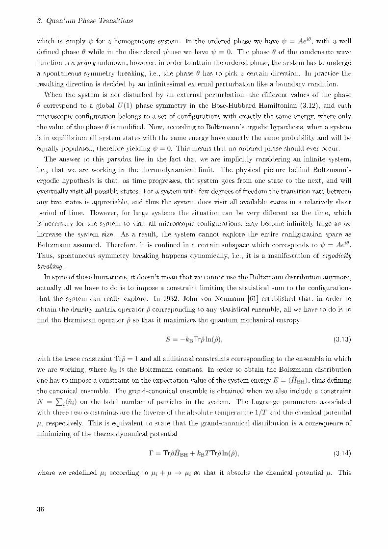
potential Γ has a Mexican hat shape as depicted in Fig. 3.1. In the latter case Γ has innitely many
minima with |ψ| 6= 0 which dier only in phase.
The condition a2 = 0 denes the boundary line which separates the ordered and disordered phases
in the control parameters space. At the vicinity of this boundary, the absolute value of the order
parameter can be calculated by using (3.21) and (3.23), which leads to
|ψ| =√− a22a4
. (3.24)
Up to this point we focused our attention on the second-order phase transitions where the global U(1)
phase symmetry of the system is broken by the emergence of a non-zero homogeneous order parameter.
Although this approach is well suited for dealing with most second-order phase transitions, due to the
38
3.2. Quantum Phase Transitions in Bosonic Lattices
assumption of homogeneity, we cannot apply this eective potential method to systems which may
exhibit spontaneous symmetry breaking with a site-dependent order parameter, i.e, systems where
the translation symmetry is also broken. There are many well known cases of this kind of phase in
the literature, perhaps the most famous of them being the anti-ferromagnetic phase in spin lattice
systems, where the spins of any two neighbor lattice sites are antiparallelly aligned to each other.
An eect similar to antiferromagnetism can also take place in bosonic optical lattices if the hopping
matrix elements in the Bose-Hubbard Hamiltonian could be tuned to become negative, as recently
suggested in Ref. [62]. In such cases we may also have second-order phase transitions, but unlike the
homogeneous case, the order parameter ψi = 〈ai〉 can be also be site dependent. Therefore, in order
to have a method capable of dealing also with site-dependent order parameters, we must introduce in
our method site-dependent sources, which lead to a more general thermodynamic potential Γ(ψ∗i , ψi).
Analogously to the homogeneous case, this is accomplished by using site-dependent sources j∗i and ji,
which serve to impose the constraints 〈a†i 〉 = ψ∗i and 〈ai〉 = ψi, respectively.
An even more general thermodynamical potential can be dened if we explore the similarities between
the quantum-mechanical evolution operator and the quantum-statistical density matrix. Considering
~ = 1, we observe that the operator e−βH has the same form of the evolution operator e−itH . Thus, we
can consider the operator e−βH as a quantum-evolution operator evolving in imaginary time from 0 to
β by making the Wick rotation it→ τ . Now, instead of considering only site-dependent source terms,
we can have time-dependent as well as site-dependent terms by dening the general Hamiltonian
HBH(τ) = HBH +∑i
[j∗i (τ)ai + ji(τ)a
†i
]. (3.25)
The imaginary-time evolution operator therefore obeys a Schrödinger-like equation with τ = it, i.e.,
−∂U(τ, τ0)
∂τ= HBH(τ)U(τ, τ0). (3.26)
The solution of (3.26) can be written as
U(τ, τ0) = T e−
∫ ττ0dτ ′HBH(τ ′)
. (3.27)
The source-dependent partition function is then dened by
Z[j∗i (τ), ji(τ)] = TrU(β, 0), (3.28)
and analogous to the time-independent case we dene the functional
F [j∗i (τ), ji(τ)] = − 1
βlnZ[j∗i (τ), ji(τ)]. (3.29)
The use of this free-energy functional not only allows us to deal with more general phase transitions,
but it also makes possible to represent most of the system quantities by means of functional derivatives
39
3. Quantum Phase Transitions
of F with respect to the sources. In particular, the space-time dependent order parameter is given by
ψi(τ) = βδF
δj∗i (τ). (3.30)
Finally we are able to generalize the eective potential by means of a Legendre transformation. This
gives us the eective action
Γ [ψ∗i (τ), ψi(τ)] = F − 1
β
∑i
∫ β
0dτ [ψ∗
i (τ)ji(τ) + ψi(τ)j∗i (τ)]. (3.31)
The physical value of the order-parameter is then obtained by minimizing Γ [ψ∗i (τ), ψi(τ)] with
respect to ψi(τ) and ψ∗i (τ) leading to the equations of motion
δΓψ∗i (τ), ψi(τ)δψi(τ)
= 0,
δΓψ∗i (τ), ψi(τ)δψ∗
i (τ)= 0. (3.32)
The eective action Γ [ψ∗i (τ), ψi(τ)] is the central element in our analysis as is contains all information
concerning the Bose-Hubbard Hamiltonian regardless of phase in which the system is.
3.3. Mean-Field Theory
In the mean-eld theory, the central idea is to rewrite the eld operator as a sum of its mean value
with its uctuations, i.e.,
ai = 〈ai〉+ δai (3.33)
and then neglect all products of uctuations δai and δa†i , in the perturbation term, which in our case
is the hopping term. Here we treat the homogeneous Bose-Hubbard Hamiltonian at T = 0 with only
nearest-interactions. In this way, we express the hopping term according to
−J∑〈i,j〉
a†i aj = −J∑〈i,j〉
(⟨a†i
⟩+ δa†i
)(〈ai〉+ δai)
= −J∑〈i,j〉
(⟨a†i
⟩ai + 〈ai〉 a†i −
⟨a†i
⟩〈ai〉+ δa†iδai
)(3.34)
The mean-eld approximation is achieved by neglecting products of uctuations, i.e., neglecting the
term δa†iδai in Eq. (3.34), which results in
40
3.3. Mean-Field Theory
−J∑〈i,j〉
a†i aj ≈ −J∑〈i,j〉
(⟨a†i
⟩ai + 〈ai〉 a†i −
⟨a†i
⟩〈ai〉
)= −Jz
∑i
(ψ∗ai + ψa†i − |ψ|2
). (3.35)
In the last step, homogeneity of the system was assumed implying the expectation value⟨a†i
⟩= ψ
to be independent of the lattice site i. Then the hopping term will reduce to a single sum over all
lattice sites with z denoting the number of nearest-neighbor sites. By using the approximation (3.35),
we obtain the mean-eld Hamiltonian
HMF = −Jz∑i
(ψa†i + ψ∗ai − ψ∗ψ
)+U
2
∑i
ni(ni − 1)− µ∑i
ni. (3.36)
Here we can observe that imposing the conditions
ψ∗ =⟨a†i
⟩; ψ = 〈ai〉 (3.37)
to the ground state of HMF is equivalent to minimize the ground-state energy EMF as follows
∂EMF
∂ψ= 0 ;
∂EMF
∂ψ∗ = 0. (3.38)
Our statement that ψ is site independent lies on the assumption that the translational symmetry
is never broken, as the order parameter is the same on every site. This approximation simplies
considerably the calculation of quantities related to our system due to fact that now our problem
is reduced to the analysis of independent identical Hamiltonians dened at each site of our lattice.
Notice also that HMF does not possess the explicit U(1) symmetric present in HBH. In order to recover
this symmetry, we must apply to the order parameter the same phase transformation applied in the
operators. This is necessary in order to allow for the possibility of symmetry-broken phases, while
symmetric phases will appear at the special value ψ = 0.
Due to this phase invariance the energy EMF must be a function of only |ψ|2 which can be calculatedperturbatively producing the Landau series
EMF(|ψ|2)Ns
= a0 + a2 |ψ|2 +1
2!2a4 |ψ|4 + · · · , (3.39)
where Ns is the total number of sites and a0 is the ground state of HBH for case J = 0, while the
coecients a2 and a4 can be calculated using Rayleigh-Schrödinger perturbation theory.
The rst step to calculate the Landau coecients is to nd the ground state of the on-site Hamilto-
nian
H0 =U
2n(n− 1)− µn, (3.40)
here, as all sites are equivalent, we ignored the site indices. As this Hamiltonian involves only the
number operator n, its eigenstates are the states containing integer number of bosons per lattice site,
41
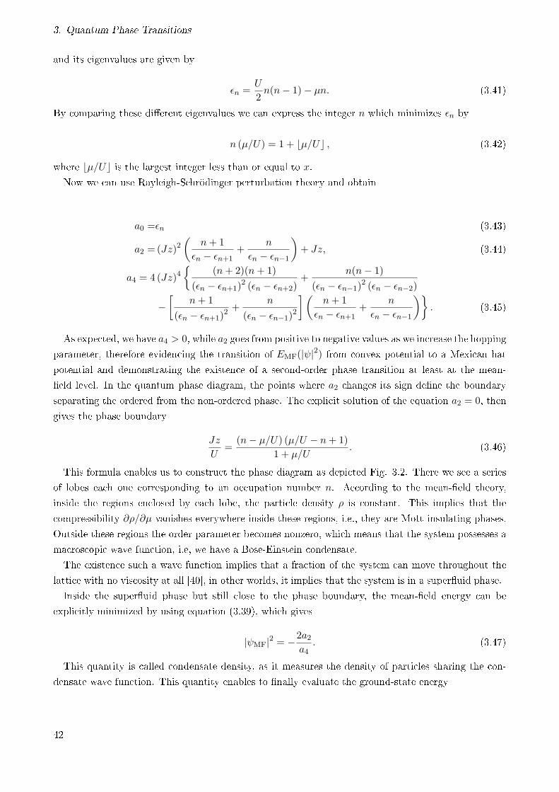
3. Quantum Phase Transitions
and its eigenvalues are given by
εn =U
2n(n− 1)− µn. (3.41)
By comparing these dierent eigenvalues we can express the integer n which minimizes εn by
n (µ/U) = 1 + bµ/Uc , (3.42)
where bµ/Uc is the largest integer less than or equal to x.
Now we can use Rayleigh-Schrödinger perturbation theory and obtain
a0 =εn (3.43)
a2 =(Jz)2(
n+ 1
εn − εn+1+
n
εn − εn−1
)+ Jz, (3.44)
a4 = 4 (Jz)4
(n+ 2)(n+ 1)
(εn − εn+1)2 (εn − εn+2)
+n(n− 1)
(εn − εn−1)2 (εn − εn−2)
−[
n+ 1
(εn − εn+1)2 +
n
(εn − εn−1)2
](n+ 1
εn − εn+1+
n
εn − εn−1
). (3.45)
As expected, we have a4 > 0, while a2 goes from positive to negative values as we increase the hopping
parameter, therefore evidencing the transition of EMF(|ψ|2) from convex potential to a Mexican hat
potential and demonstrating the existence of a second-order phase transition at least at the mean-
eld level. In the quantum phase diagram, the points where a2 changes its sign dene the boundary
separating the ordered from the non-ordered phase. The explicit solution of the equation a2 = 0, then
gives the phase boundary
Jz
U=
(n− µ/U) (µ/U − n+ 1)
1 + µ/U. (3.46)
This formula enables us to construct the phase diagram as depicted Fig. 3.2. There we see a series
of lobes each one corresponding to an occupation number n. According to the mean-eld theory,
inside the regions enclosed by each lobe, the particle density ρ is constant. This implies that the
compressibility ∂ρ/∂µ vanishes everywhere inside these regions, i.e., they are Mott insulating phases.
Outside these regions the order parameter becomes nonzero, which means that the system possesses a
macroscopic wave function, i.e, we have a Bose-Einstein condensate.
The existence such a wave function implies that a fraction of the system can move throughout the
lattice with no viscosity at all [40], in other worlds, it implies that the system is in a superuid phase.
Inside the superuid phase but still close to the phase boundary, the mean-eld energy can be
explicitly minimized by using equation (3.39), which gives
|ψMF|2 = −2a2a4
. (3.47)
This quantity is called condensate density, as it measures the density of particles sharing the con-
densate wave function. This quantity enables to nally evaluate the ground-state energy
42
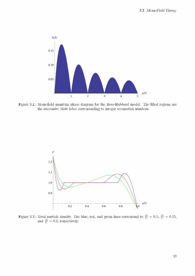
3.3. Mean-Field Theory
1 2 3 4 5ΜU
0.05
0.10
0.15
JzU
Figure 3.2.: Mean-eld quantum phase diagram for the Bose-Hubbard model. The lled regions arethe successive Mott lobes corresponding to integer occupation numbers.
0.2 0.4 0.6 0.8 1.0ΜU
0.9
1.0
1.1
1.2
Ρ
Figure 3.3.: Total particle density. The blue, red, and green lines correspond to JzU = 0.1, JzU = 0.15,
and JzU = 0.2, respectively.
43
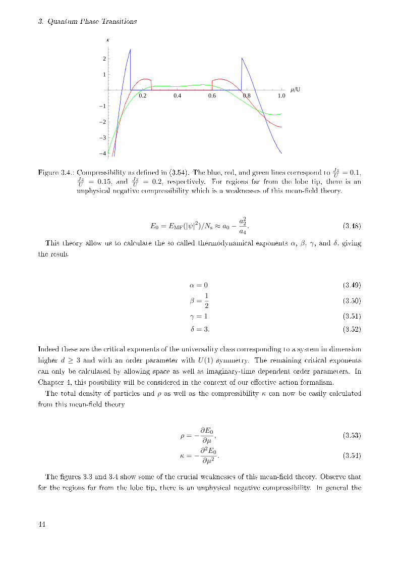
3. Quantum Phase Transitions
0.2 0.4 0.6 0.8 1.0ΜU
-4
-3
-2
-1
1
2
Κ
Figure 3.4.: Compressibility as dened in (3.54). The blue, red, and green lines correspond to JzU = 0.1,
JzU = 0.15, and Jz
U = 0.2, respectively. For regions far from the lobe tip, there is anunphysical negative compressibility which is a weaknesses of this mean-eld theory.
E0 = EMF(|ψ|2)/Ns ≈ a0 −a22a4. (3.48)
This theory allow us to calculate the so called thermodynamical exponents α, β, γ, and δ, giving
the result
α = 0 (3.49)
β =1
2(3.50)
γ = 1 (3.51)
δ = 3. (3.52)
Indeed these are the critical exponents of the universality class corresponding to a system in dimension
higher d ≥ 3 and with an order parameter with U(1) symmetry. The remaining critical exponents
can only be calculated by allowing space as well as imaginary-time dependent order parameters. In
Chapter 4, this possibility will be considered in the context of our eective action formalism.
The total density of particles and ρ as well as the compressibility κ can now be easily calculated
from this mean-eld theory
ρ = −∂E0
∂µ, (3.53)
κ = −∂2E0
∂µ2. (3.54)
The gures 3.3 and 3.4 show some of the crucial weaknesses of this mean-eld theory. Observe that
for the regions far from the lobe tip, there is an unphysical negative compressibility. In general the
44
3.3. Mean-Field Theory
mean-eld theory gives very bad if not contradictory results inside the superuid phase.
In the next chapters we will see how these problems are xed by using the eective potential and
eective action methods.
45

46
4. Bosonic Lattices at Finite Temperature
In this chapter, a perturbation theory is developed by taking advantage of a diagrammatic notation
specially developed to deal with bosons in optical lattices. The calculation of the eective action, which
is dened through a Legendre transformation of the free energy, leads to an automatic resummation of
the hopping expansion. This allows the description of the system properties in both the Mott-insulator
and the superuid phase. By using a set of diagrammatic rules, the eective action is calculated up to
second hopping order.
We treat the Bose-Hubbard model as belonging to a more general class of Hamiltonians which can
be written as a sum of a hopping term and a local term
H = Hh + Hl, (4.1)
with the respective terms being dened by
Hl =∑i
fi(ni), (4.2)
Hh = −∑ii′
Jii′ a†i ai′ . (4.3)
The Bose-Hubbard Hamiltonian is recovered if we choose fi(x) = U(x2 − x)/2− µx and Jij = J if ij
are nearest neighbors lattice sites while Jij = 0 otherwise.
In order to calculate the expectation values of physical quantities, we use the so-called Green's
functions
G(n,m)(τ1, i1; · · · ; τn, in|τ ′1, i′1; · · · ; τ ′m, i′m
)= Z−1Tr
e−βH T
[ai1(τ1) · · · ain(τn)a
†i′1(τ ′1) · · · a
†i′m(τ ′m)
](4.4)
where the partition function is Z = Tre−βH and a time-dependent Heisenberg operator is dened from
the Schrödinger operator OS as O(τ) = eτHOSe−τH .
In order to facilitate the calculation of G(n,m), we dene a new time-dependent Hamiltonian by
adding to it a time-dependent source term, according to
H(τ) = H + Hs(τ), (4.5)
where
Hs(τ) =∑i
[j∗i (τ)ai + ji(τ)a
†i
]. (4.6)
47
4. Bosonic Lattices at Finite Temperature
The partition function for H(τ) is then given by the functional
Z [j∗, j] = TrU(β, 0), (4.7)
where the imaginary-time evolution operator U(τ, τ0) obeys the evolution equation
− ∂
∂τU(τ, τ0) = H(τ)U(τ, τ0) (4.8)
with the initial condition U(τ0; τ0) = 1. In the following, we show that all Green functions can be
obtained from functional derivatives of Z [j∗, j] with respect to j∗ and j. To this end note that equation
(4.8) together with its initial condition can be rewritten in the integral form
U(τ, τ0) = 1−∫ τ
τ0
H(τ ′)U(τ ′, τ0)dτ′, (4.9)
which can be solved iteratively leading to the Born series
U(τ, τ0) = 1−∫ τ
τ0
dτ1H(τ1) +
∫ τ
τ0
dτ1
∫ τ1
τ0
dτ2H(τ2)H(τ1) (4.10)
−∫ τ
τ0
dτ1
∫ τ1
τ0
dτ2
∫ τ2
τ0
dτ3H(τ3)H(τ2)H(τ1) + · · · . (4.11)
Using the time-ordering operator we have
U(τ, τ0) = 1−∫ τ
τ0
dτ1H(τ1) +1
2!
∫ τ
τ0
dτ1
∫ τ
τ0
dτ2T[H(τ2)H(τ1)
]− 1
3!
∫ τ
τ0
dτ1
∫ τ
τ0
dτ2
∫ τ
τ0
dτ3T[H(τ3)H(τ2)H(τ1)
]+ · · · (4.12)
This series can be summarized by the formula
U(τ, τ0) = T e−
∫ ττ0H(τ ′)dτ ′
. (4.13)
It is also useful to observe the semi-group property of the imaginary-time evolution operator
U(τ, τ0) = U(τ, τ ′)U(τ ′, τ0), if τ ≥ τ ′ ≥ τ0. (4.14)
This semi-group property allows us rewrite the evolution operator by isolating a subinterval from τ−∆
to τ +∆, with ∆ > 0, i.e.,
U(β, 0) = U(β, τ +∆)U(τ +∆, τ −∆)U(τ −∆, 0). (4.15)
The functional derivative of U(β, 0) with respect to j∗i (τ) can be expressed as
δ
δj∗i (τ)U(β, 0) = U(β, τ +∆)
δU(τ +∆, τ −∆)
δj∗i (τ)U(τ −∆, 0). (4.16)
48
4.1. Perturbation Theory
Using equation (4.12), we see that
δU(τ +∆, τ −∆)
δj∗i (τ)= −ai +
∫ τ+∆
τ−∆dτ1
[Θ(τ − τ1)aiH(τ1) + Θ(τ1 − τ)H(τ1)ai
]− · · · . (4.17)
By substituting (4.17) into (4.16) and taking the limit ∆ → 0 we obtain
δU(β, 0)
δj∗i (τ)= −U(β, τ)aiU(τ, 0) = −U(β, 0)ai(τ), (4.18)
where ai(τ) = U−1(τ, 0)aiU(τ, 0). Observe that we get back to the denition of Heisenberg operators
in (4.4) by setting j∗i (τ) = ji(τ) = 0.
By taking more functional derivatives of (4.18) with respect to the source elds, we nally obtain
the formula
δ(n+m)U(β, 0)
δj∗i1(τ1) · · · δj∗in(τn)δji′1(τ
′1) · · · δji′m(τ ′m)
= U(β, 0)T[ai1(τ1) · · · ain(τn)a
†i′1(τ ′1) · · · a
†i′m(τ ′m)
]. (4.19)
The trace of this equation nally leads us to the formula for Green's functions as functional derivatives
of the generating functional Z [j∗, j]
G(n,m)(τ1, i1; · · · ; τn, in|τ ′1, i′1; · · · ; τ ′m, i′m
)= Z [j∗, j]−1 δ(n+m)Z [j∗, j]
δj∗i1(τ1) · · · δj∗in(τn)δji′1(τ
′1) · · · δji′m(τ ′m)
∣∣∣∣∣j∗=j=0
.
(4.20)
4.1. Perturbation Theory
In order to calculate U(τ, 0) as a power series of the hopping matrix element Jij , we split the full
imaginary-time dependent Hamiltonian H(τ) into an unperturbed part H0(τ) = Hl + Hs(τ) plus the
hopping-dependent perturbation Hh, i.e,
H(τ) = H0(τ) + Hh. (4.21)
The imaginary-time dependent evolution operator can now be factorized as an unperturbed part
times an interaction part
U(τ ; 0) = U0(τ ; 0)UI(τ ; 0), (4.22)
where the unperturbed evolution operator obeys the following evolution equation:
− ∂
∂τU0(τ ; 0) = H0(τ)U0(τ ; 0), (4.23)
which analogously to Eq. (4.13) has the solution
U0(τ ; τ0) = T e−
∫ ττ0H0(τ ′)dτ ′ . (4.24)
49
4. Bosonic Lattices at Finite Temperature
Using (4.8) and (4.23) we deduce the evolution equation for the interaction part of evolution operator
− ∂
∂τUI(τ ; 0) = HI
h(τ)UI(τ ; 0), (4.25)
where
HIh(τ) = U−1
0 (τ ; 0)HhU0(τ ; 0). (4.26)
Here we can repeat the same iterative procedure as in (4.13) and obtain the solution for (4.25) as
UI(τ ; 0) = T e−∫ τ0 dτ ′HI
h(τ′). (4.27)
The full partition function (4.7) can now, with (4.22) and (4.27), written as
Z [j∗, j] = Tr[U0(β; 0)T e
−∫ β0 dτ ′HI
h(τ′)]
(4.28)
Thus, using the (4.3) and (4.19), we can express Z [j∗, j] in terms of functional derivatives of the
unperturbed partition function Z0 [j∗, j] via
Z [j∗, j] = e∑
ij Jij∫ β0 dτ δ2
δj∗i(τ)δjj(τ)Z0 [j
∗, j] , (4.29)
where we have
Z0 [j∗, j] = Tr
[U0(β, 0)
]. (4.30)
4.2. Lattice Diagrammatics
Let us now consider the unperturbed partition function in more detail. For Jij = 0, the system splits
into independent lattice sites in such a way that the partition function can be factorized as
Z0 [j∗, j] =
∏i
Zi [j∗, j] . (4.31)
In practice, in order to avoid the annoying β−1 prefactor appearing in equations (3.29) and (3.31), we
use instead, in our diagrammatic calculations, the functional
W [j∗, j] = lnZ [j∗, j] = −βF [j∗, j] . (4.32)
For a reason that will become clear later we can also call W [j∗, j] the generating functional of the con-
nected Green's functions Gc, while the partition function Z [j∗, j] can be also be named the generating
functional of the full Green's function G. The functional W can also be represented as a power of the
sources j and j∗ as follows
50
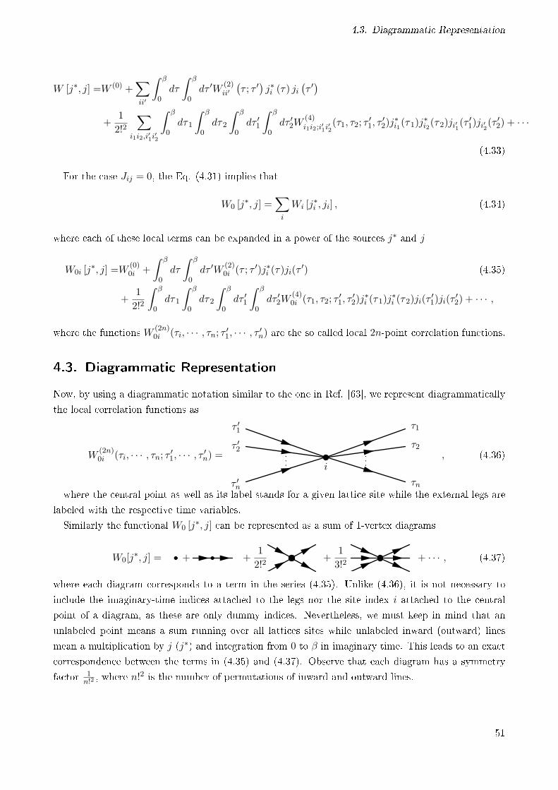
4.3. Diagrammatic Representation
W [j∗, j] =W (0) +∑ii′
∫ β
0dτ
∫ β
0dτ ′W
(2)ii′(τ ; τ ′
)j∗i (τ) ji
(τ ′)
+1
2!2
∑i1i2,i′1i
′2
∫ β
0dτ1
∫ β
0dτ2
∫ β
0dτ ′1
∫ β
0dτ ′2W
(4)i1i2;i′1i
′2(τ1, τ2; τ
′1, τ
′2)j
∗i1(τ1)j
∗i2(τ2)ji′1(τ
′1)ji′2(τ
′2) + · · ·
(4.33)
For the case Jij = 0, the Eq. (4.31) implies that
W0 [j∗, j] =
∑i
Wi [j∗i , ji] , (4.34)
where each of these local terms can be expanded in a power of the sources j∗ and j
W0i [j∗, j] =W
(0)0i +
∫ β
0dτ
∫ β
0dτ ′W
(2)0i (τ ; τ ′)j∗i (τ)ji(τ
′) (4.35)
+1
2!2
∫ β
0dτ1
∫ β
0dτ2
∫ β
0dτ ′1
∫ β
0dτ ′2W
(4)0i (τ1, τ2; τ
′1, τ
′2)j
∗i (τ1)j
∗i (τ2)ji(τ
′1)ji(τ
′2) + · · · ,
where the functions W (2n)0i (τi, · · · , τn; τ ′1, · · · , τ ′n) are the so called local 2n-point correlation functions.
4.3. Diagrammatic Representation
Now, by using a diagrammatic notation similar to the one in Ref. [63], we represent diagrammatically
the local correlation functions as
W(2n)0i (τi, · · · , τn; τ ′1, · · · , τ ′n) =
τ ′n
τ ′2
τ ′1
τn
τ2
τ1
i, (4.36)
where the central point as well as its label stands for a given lattice site while the external legs are
labeled with the respective time variables.
Similarly the functional W0 [j∗, j] can be represented as a sum of 1-vertex diagrams
W0[j∗, j] = + +
1
2!2+
1
3!2+ · · · , (4.37)
where each diagram corresponds to a term in the series (4.35). Unlike (4.36), it is not necessary to
include the imaginary-time indices attached to the legs nor the site index i attached to the central
point of a diagram, as these are only dummy indices. Nevertheless, we must keep in mind that an
unlabeled point means a sum running over all lattices sites while unlabeled inward (outward) lines
mean a multiplication by j (j∗) and integration from 0 to β in imaginary time. This leads to an exact
correspondence between the terms in (4.35) and (4.37). Observe that each diagram has a symmetry
factor 1n!2
, where n!2 is the number of permutations of inward and outward lines.
51
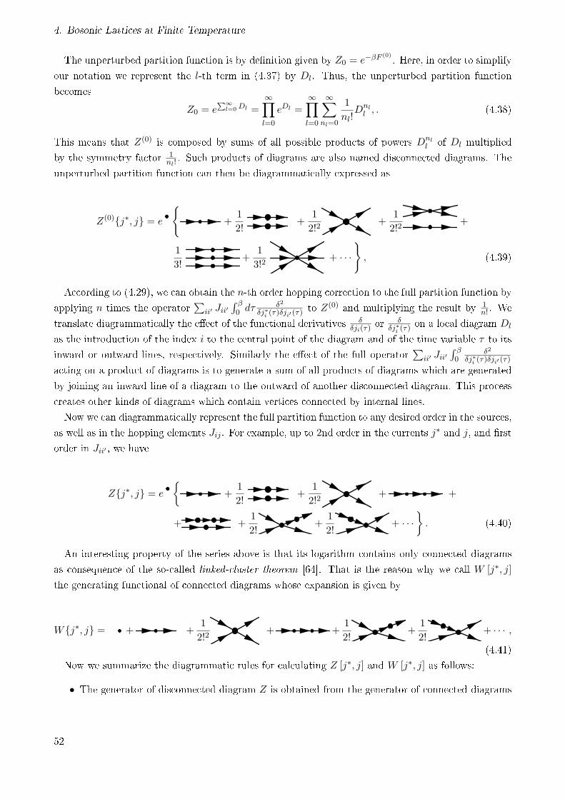
4. Bosonic Lattices at Finite Temperature
The unperturbed partition function is by denition given by Z0 = e−βF(0). Here, in order to simplify
our notation we represent the l-th term in (4.37) by Dl. Thus, the unperturbed partition function
becomes
Z0 = e∑∞
l=0Dl =∞∏l=0
eDl =∞∏l=0
∞∑nl=0
1
nl!Dnll , . (4.38)
This means that Z(0) is composed by sums of all possible products of powers Dnll of Dl multiplied
by the symmetry factor 1nl!. Such products of diagrams are also named disconnected diagrams. The
unperturbed partition function can then be diagrammatically expressed as
Z(0)j∗, j = e
+
1
2!+
1
2!2+
1
2!2+
1
3!+
1
3!2+ · · ·
, (4.39)
According to (4.29), we can obtain the n-th order hopping correction to the full partition function by
applying n times the operator∑
ii′ Jii′∫ β0 dτ
δ2
δj∗i (τ)δji′ (τ)to Z(0) and multiplying the result by 1
n! . We
translate diagrammatically the eect of the functional derivatives δδji(τ)
or δδj∗i (τ)
on a local diagram Dl
as the introduction of the index i to the central point of the diagram and of the time variable τ to its
inward or outward lines, respectively. Similarly the eect of the full operator∑
ii′ Jii′∫ β0
δ2
δj∗i (τ)δji′ (τ)
acting on a product of diagrams is to generate a sum of all products of diagrams which are generated
by joining an inward line of a diagram to the outward of another disconnected diagram. This process
creates other kinds of diagrams which contain vertices connected by internal lines.
Now we can diagrammatically represent the full partition function to any desired order in the sources,
as well as in the hopping elements Jij . For example, up to 2nd order in the currents j∗ and j, and rst
order in Jii′ , we have
Zj∗, j = e
+
1
2!+
1
2!2+ +
+ +1
2!+
1
2!+ · · ·
. (4.40)
An interesting property of the series above is that its logarithm contains only connected diagrams
as consequence of the so-called linked-cluster theorem [64]. That is the reason why we call W [j∗, j]
the generating functional of connected diagrams whose expansion is given by
Wj∗, j = + +1
2!2+ +
1
2!+
1
2!+ · · · ,
(4.41)
Now we summarize the diagrammatic rules for calculating Z [j∗, j] and W [j∗, j] as follows:
• The generator of disconnected diagram Z is obtained from the generator of connected diagrams
52
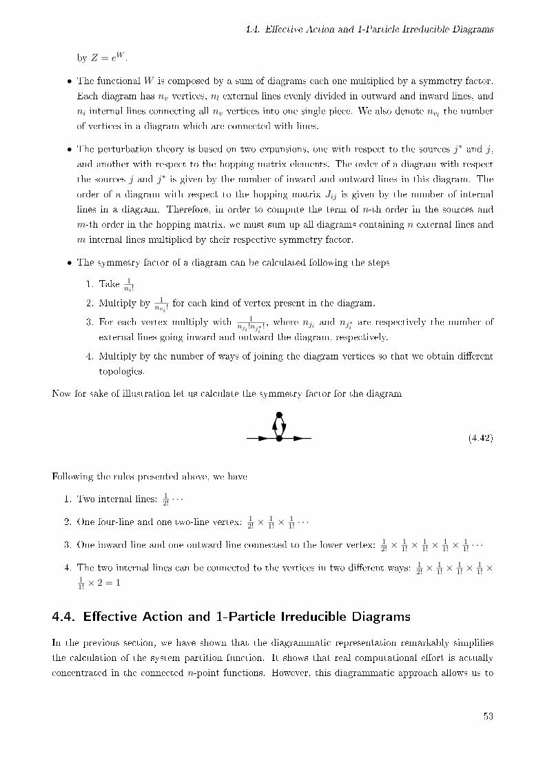
4.4. Eective Action and 1-Particle Irreducible Diagrams
by Z = eW .
• The functional W is composed by a sum of diagrams each one multiplied by a symmetry factor.
Each diagram has nv vertices, nl external lines evenly divided in outward and inward lines, and
ni internal lines connecting all nv vertices into one single piece. We also denote nvl the number
of vertices in a diagram which are connected with lines.
• The perturbation theory is based on two expansions, one with respect to the sources j∗ and j,
and another with respect to the hopping matrix elements. The order of a diagram with respect
the sources j and j∗ is given by the number of inward and outward lines in this diagram. The
order of a diagram with respect to the hopping matrix Jij is given by the number of internal
lines in a diagram. Therefore, in order to compute the term of n-th order in the sources and
m-th order in the hopping matrix, we must sum up all diagrams containing n external lines and
m internal lines multiplied by their respective symmetry factor.
• The symmetry factor of a diagram can be calculated following the steps
1. Take 1ni!
2. Multiply by 1nvi !
for each kind of vertex present in the diagram.
3. For each vertex multiply with 1nji
!nj∗i! , where nji and nj∗i are respectively the number of
external lines going inward and outward the diagram, respectively.
4. Multiply by the number of ways of joining the diagram vertices so that we obtain dierent
topologies.
Now for sake of illustration let us calculate the symmetry factor for the diagram
(4.42)
Following the rules presented above, we have
1. Two internal lines: 12! · · ·
2. One four-line and one two-line vertex: 12! ×
11! ×
11! · · ·
3. One inward line and one outward line connected to the lower vertex: 12! ×
11! ×
11! ×
11! ×
11! · · ·
4. The two internal lines can be connected to the vertices in two dierent ways: 12! ×
11! ×
11! ×
11! ×
11! × 2 = 1
4.4. Eective Action and 1-Particle Irreducible Diagrams
In the previous section, we have shown that the diagrammatic representation remarkably simplies
the calculation of the system partition function. It shows that real computational eort is actually
concentrated in the connected n-point functions. However, this diagrammatic approach allows us to
53
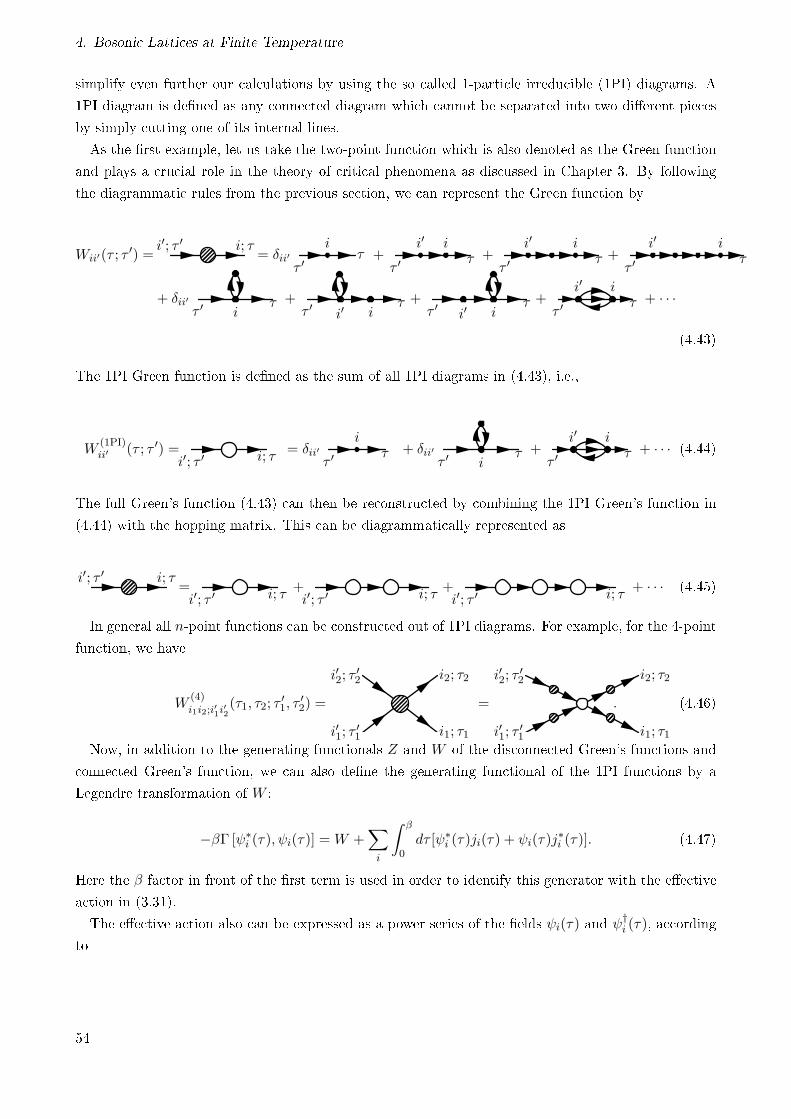
4. Bosonic Lattices at Finite Temperature
simplify even further our calculations by using the so called 1-particle irreducible (1PI) diagrams. A
1PI diagram is dened as any connected diagram which cannot be separated into two dierent pieces
by simply cutting one of its internal lines.
As the rst example, let us take the two-point function which is also denoted as the Green function
and plays a crucial role in the theory of critical phenomena as discussed in Chapter 3. By following
the diagrammatic rules from the previous section, we can represent the Green function by
Wii′(τ ; τ′) =
i′; τ ′ i; τ= δii′
τ ′τ
i+τ ′
τi′ i
+τ ′
τi′ i
+τ ′
τi′ i
+ δii′τ ′
τi
+τ ′
τi′ i
+τ ′
τi′ i
+τ ′
τi′ i
+ · · ·
(4.43)
The 1PI Green function is dened as the sum of all 1PI diagrams in (4.43), i.e.,
W(1PI)ii′ (τ ; τ ′) =
i′; τ ′ i; τ= δii′
τ ′τ
i+ δii′
τ ′τ
i+τ ′
τi′ i
+ · · · (4.44)
The full Green's function (4.43) can then be reconstructed by combining the 1PI Green's function in
(4.44) with the hopping matrix. This can be diagrammatically represented as
i′; τ ′ i; τ=i′; τ ′ i; τ
+i′; τ ′ i; τ
+i′; τ ′ i; τ
+ · · · (4.45)
In general all n-point functions can be constructed out of 1PI diagrams. For example, for the 4-point
function, we have
W(4)i1i2;i′1i
′2(τ1, τ2; τ
′1, τ
′2) =
i′1; τ′1
i′2; τ′2
i1; τ1
i2; τ2
=
i′1; τ′1
i′2; τ′2
i1; τ1
i2; τ2
. (4.46)
Now, in addition to the generating functionals Z and W of the disconnected Green's functions and
connected Green's function, we can also dene the generating functional of the 1PI functions by a
Legendre transformation of W :
−βΓ [ψ∗i (τ), ψi(τ)] =W +
∑i
∫ β
0dτ [ψ∗
i (τ)ji(τ) + ψi(τ)j∗i (τ)]. (4.47)
Here the β factor in front of the rst term is used in order to identify this generator with the eective
action in (3.31).
The eective action also can be expressed as a power series of the elds ψi(τ) and ψ†i (τ), according
to
54
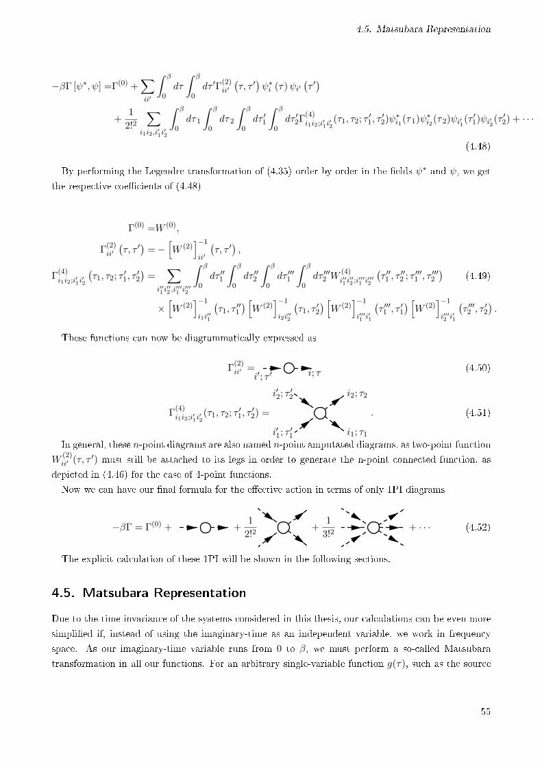
4.5. Matsubara Representation
−βΓ [ψ∗, ψ] =Γ(0) +∑ii′
∫ β
0dτ
∫ β
0dτ ′Γ
(2)ii′(τ, τ ′
)ψ∗i (τ)ψi′
(τ ′)
+1
2!2
∑i1i2,i′1i
′2
∫ β
0dτ1
∫ β
0dτ2
∫ β
0dτ ′1
∫ β
0dτ ′2Γ
(4)i1i2;i′1i
′2(τ1, τ2; τ
′1, τ
′2)ψ
∗i1(τ1)ψ
∗i2(τ2)ψi′1(τ
′1)ψi′2(τ
′2) + · · ·
(4.48)
By performing the Legendre transformation of (4.35) order by order in the elds ψ∗ and ψ, we get
the respective coecients of (4.48)
Γ(0) =W (0),
Γ(2)ii′(τ, τ ′
)=−
[W (2)
]−1
ii′
(τ, τ ′
),
Γ(4)i1i2;i′1i
′2
(τ1, τ2; τ
′1, τ
′2
)=
∑i′′1 i
′′2 ,i
′′′1 i
′′′2
∫ β
0dτ ′′1
∫ β
0dτ ′′2
∫ β
0dτ ′′′1
∫ β
0dτ ′′′2 W
(4)i′′1 i
′′2 ;i
′′′1 i
′′′2
(τ ′′1 , τ
′′2 ; τ
′′′1 , τ
′′′2
)(4.49)
×[W (2)
]−1
i1i′′1
(τ1, τ
′′1
) [W (2)
]−1
i2i′′2
(τ1, τ
′2
) [W (2)
]−1
i′′′1 i′1
(τ ′′′1 , τ
′1
) [W (2)
]−1
i′′′2 i′1
(τ ′′′2 , τ
′2
).
These functions can now be diagrammatically expressed as
Γ(2)ii′ =
i′; τ ′ i; τ(4.50)
Γ(4)i1i2;i′1i
′2(τ1, τ2; τ
′1, τ
′2) =
i′1; τ′1
i′2; τ′2
i1; τ1
i2; τ2
. (4.51)
In general, these n-point diagrams are also named n-point amputated diagrams, as two-point function
W(2)ii′ (τ, τ
′) must still be attached to its legs in order to generate the n-point connected function, as
depicted in (4.46) for the case of 4-point functions.
Now we can have our nal formula for the eective action in terms of only 1PI diagrams
−βΓ = Γ(0) + +1
2!2+
1
3!2+ · · · (4.52)
The explicit calculation of these 1PI will be shown in the following sections.
4.5. Matsubara Representation
Due to the time invariance of the systems considered in this thesis, our calculations can be even more
simplied if, instead of using the imaginary-time as an independent variable, we work in frequency
space. As our imaginary-time variable runs from 0 to β, we must perform a so-called Matsubara
transformation in all our functions. For an arbitrary single-variable function g(τ), such as the source
55
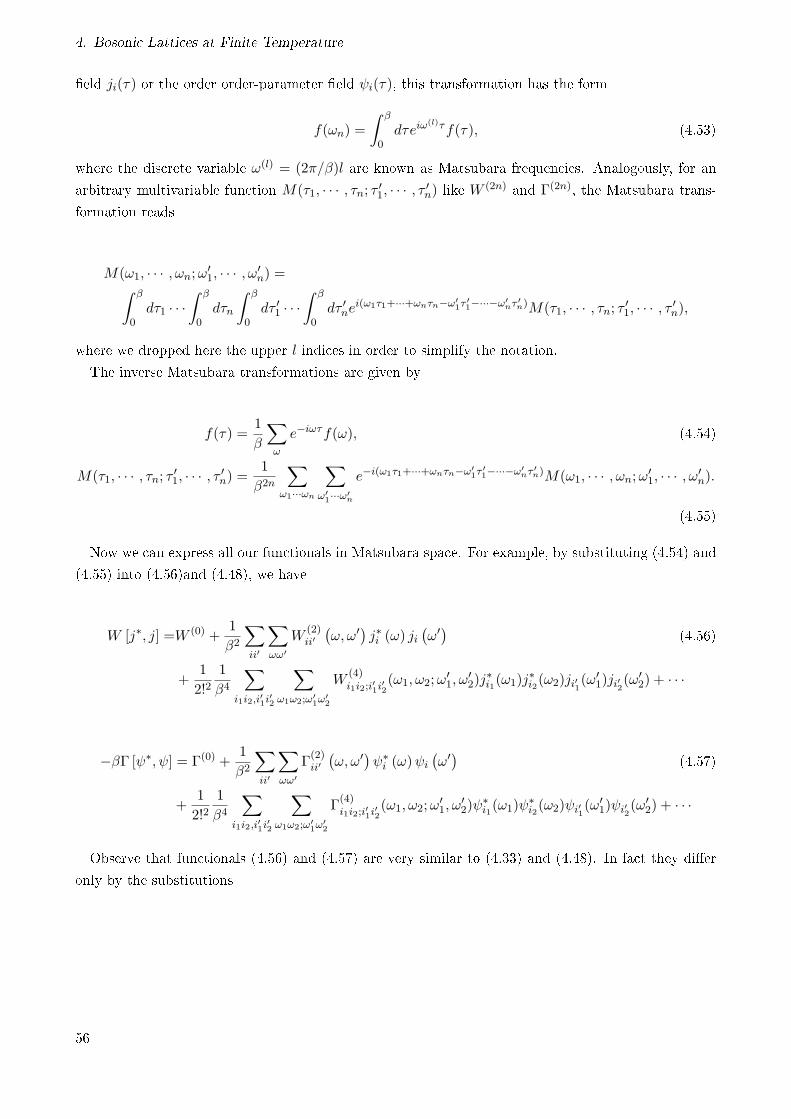
4. Bosonic Lattices at Finite Temperature
eld ji(τ) or the order order-parameter eld ψi(τ), this transformation has the form
f(ωn) =
∫ β
0dτeiω
(l)τf(τ), (4.53)
where the discrete variable ω(l) = (2π/β)l are known as Matsubara frequencies. Analogously, for an
arbitrary multivariable function M(τ1, · · · , τn; τ ′1, · · · , τ ′n) like W (2n) and Γ(2n), the Matsubara trans-
formation reads
M(ω1, · · · , ωn;ω′1, · · · , ω′
n) =∫ β
0dτ1 · · ·
∫ β
0dτn
∫ β
0dτ ′1 · · ·
∫ β
0dτ ′ne
i(ω1τ1+···+ωnτn−ω′1τ
′1−···−ω′
nτ′n)M(τ1, · · · , τn; τ ′1, · · · , τ ′n),
where we dropped here the upper l indices in order to simplify the notation.
The inverse Matsubara transformations are given by
f(τ) =1
β
∑ω
e−iωτf(ω), (4.54)
M(τ1, · · · , τn; τ ′1, · · · , τ ′n) =1
β2n
∑ω1···ωn
∑ω′1···ω′
n
e−i(ω1τ1+···+ωnτn−ω′1τ
′1−···−ω′
nτ′n)M(ω1, · · · , ωn;ω′
1, · · · , ω′n).
(4.55)
Now we can express all our functionals in Matsubara space. For example, by substituting (4.54) and
(4.55) into (4.56)and (4.48), we have
W [j∗, j] =W (0) +1
β2
∑ii′
∑ωω′
W(2)ii′(ω, ω′) j∗i (ω) ji (ω′) (4.56)
+1
2!21
β4
∑i1i2,i′1i
′2
∑ω1ω2;ω′
1ω′2
W(4)i1i2;i′1i
′2(ω1, ω2;ω
′1, ω
′2)j
∗i1(ω1)j
∗i2(ω2)ji′1(ω
′1)ji′2(ω
′2) + · · ·
−βΓ [ψ∗, ψ] = Γ(0) +1
β2
∑ii′
∑ωω′
Γ(2)ii′(ω, ω′)ψ∗
i (ω)ψi(ω′) (4.57)
+1
2!21
β4
∑i1i2,i′1i
′2
∑ω1ω2;ω′
1ω′2
Γ(4)i1i2;i′1i
′2(ω1, ω2;ω
′1, ω
′2)ψ
∗i1(ω1)ψ
∗i2(ω2)ψi′1(ω
′1)ψi′2(ω
′2) + · · ·
Observe that functionals (4.56) and (4.57) are very similar to (4.33) and (4.48). In fact they dier
only by the substitutions
56
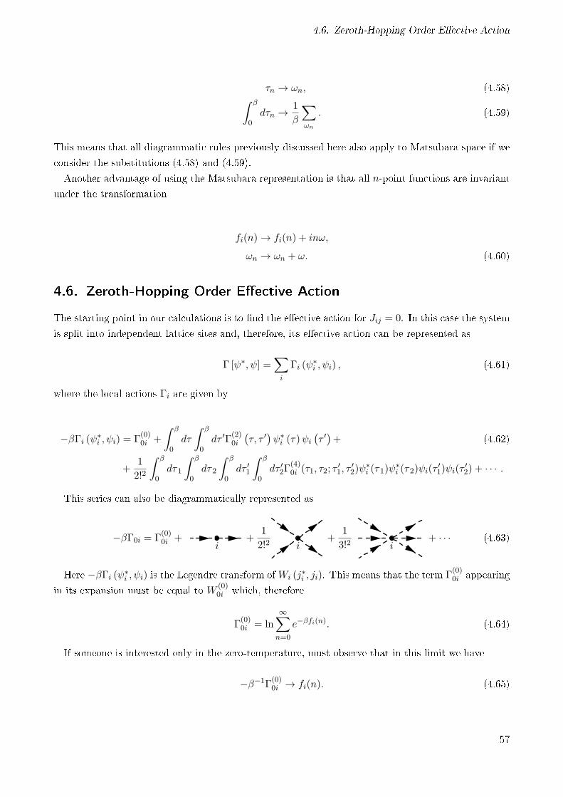
4.6. Zeroth-Hopping Order Eective Action
τn → ωn, (4.58)∫ β
0dτn → 1
β
∑ωn
. (4.59)
This means that all diagrammatic rules previously discussed here also apply to Matsubara space if we
consider the substitutions (4.58) and (4.59).
Another advantage of using the Matsubara representation is that all n-point functions are invariant
under the transformation
fi(n) → fi(n) + inω,
ωn → ωn + ω. (4.60)
4.6. Zeroth-Hopping Order Eective Action
The starting point in our calculations is to nd the eective action for Jij = 0. In this case the system
is split into independent lattice sites and, therefore, its eective action can be represented as
Γ [ψ∗, ψ] =∑i
Γi (ψ∗i , ψi) , (4.61)
where the local actions Γi are given by
−βΓi (ψ∗i , ψi) = Γ
(0)0i +
∫ β
0dτ
∫ β
0dτ ′Γ
(2)0i
(τ, τ ′
)ψ∗i (τ)ψi
(τ ′)+ (4.62)
+1
2!2
∫ β
0dτ1
∫ β
0dτ2
∫ β
0dτ ′1
∫ β
0dτ ′2Γ
(4)0i (τ1, τ2; τ
′1, τ
′2)ψ
∗i (τ1)ψ
∗i (τ2)ψi(τ
′1)ψi(τ
′2) + · · · .
This series can also be diagrammatically represented as
−βΓ0i = Γ(0)0i +
i+
1
2!2 i+
1
3!2 i+ · · · (4.63)
Here −βΓi (ψ∗i , ψi) is the Legendre transform ofWi (j
∗i , ji). This means that the term Γ
(0)0i appearing
in its expansion must be equal to W (0)0i which, therefore
Γ(0)0i = ln
∞∑n=0
e−βfi(n). (4.64)
If someone is interested only in the zero-temperature, must observe that in this limit we have
−β−1Γ(0)0i → fi(n). (4.65)
57
4. Bosonic Lattices at Finite Temperature
The next term to be considered is Γ(2)0i . According to (4.49), it can be obtained by inverting
W(2)0i (τ, τ ′) =
1
Z0Tre−βH0 T
[a†i (τ
′)ai(τ)]
. (4.66)
The direct evaluation yields
W(2)0i (τ, τ ′) =
1
Z0
∞∑n=0
e−βfi(n)θ(τ − τ ′)(n+ 1)e(τ−τ
′)[fi(n)−fi(n+1)] + θ(τ ′ − τ)ne(τ′−τ)[fi(n)−fi(n−1)]
,
(4.67)
which is given, in the Matsubara representation, by
W(2)0i (ω, ω′) = βδω,ω′gi(ω), (4.68)
where δω,ω′ is the Kronecker delta symbol and
gi(ω) =1
Z0i
∞∑n=0
(n+ 1)e−βfi(n+1) − e−βfi(n)
iω + fi(n)− fi(n+ 1). (4.69)
Now the inverse must obey the equation
1
β
∑ω′′
W(2)0i (ω, ω′′)Γ
(2)0i (ω
′′, ω′) =1
β
∑ω′′
Γ(2)0i (ω, ω
′′)W(2)0i (ω′′, ω′) = −βδωω′ . (4.70)
The diagonal form of W (2)0i in the Matsubara representation makes its inversion very simple, thus
giving
Γ(2)0i (ω, ω
′) = −βδω,ω′Z0
[ ∞∑n=0
(n+ 1)e−βfi(n+1) − e−βfi(n)
iω + fi(n)− fi(n+ 1)
]−1
. (4.71)
In order to get the zero-temperature limit of Γ(2)0i (ω, ω
′), we must at rst observe that the Matsubara
sums and Kronecker deltas transform in this limit into frequency integrals and Dirac deltas, respectively,
according to
1
β
∑ω
→ 1
2π
∫dω, (4.72)
βδω,ω′ → 2πδ(ω − ω′). (4.73)
Therefore the zero-temperature limit of Γ(2)0i (ω, ω
′) reads
Γ(2)0i (ω, ω
′) → −2πδ(ω − ω′)
[n
iω + fi(n− 1)− fi(n)− n+ 1
iω + fi(n)− fi(n+ 1)
]−1
. (4.74)
Now we must calculate the term Γ(4)0i , in order to construct our Ginzburg-Landau expansion. Its
diagrammatic representation is
58
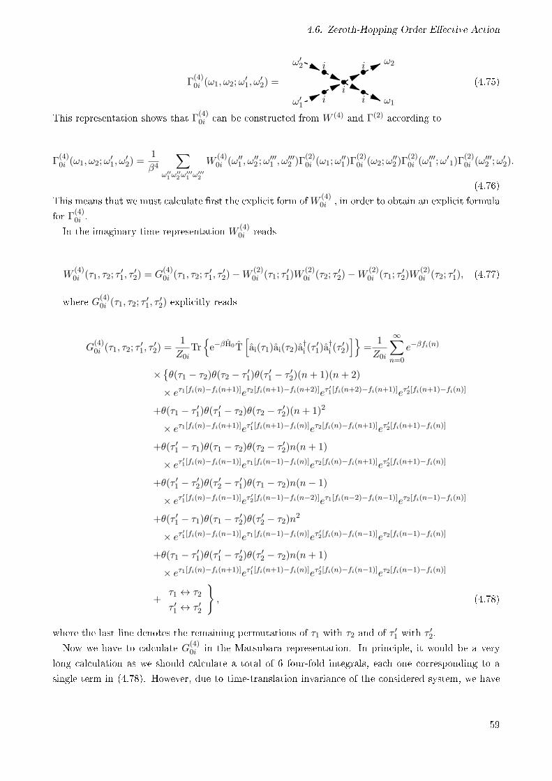
4.6. Zeroth-Hopping Order Eective Action
Γ(4)0i (ω1, ω2;ω
′1, ω
′2) =
ω′1
ω′2
ω1
ω2
ii
i
i i
(4.75)
This representation shows that Γ(4)0i can be constructed from W (4) and Γ(2) according to
Γ(4)0i (ω1, ω2;ω
′1, ω
′2) =
1
β4
∑ω′′1ω
′′2ω
′′′1 ω
′′′2
W(4)0i (ω′′
1 , ω′′2 ;ω
′′′1 , ω
′′′2 )Γ
(2)0i (ω1;ω
′′1)Γ
(2)0i (ω2;ω
′′2)Γ
(2)0i (ω
′′′1 ;ω
′1)Γ
(2)0i (ω
′′′2 ;ω
′2).
(4.76)
This means that we must calculate rst the explicit form ofW (4)0i , in order to obtain an explicit formula
for Γ(4)0i .
In the imaginary-time representation W (4)0i reads
W(4)0i (τ1, τ2; τ
′1, τ
′2) = G
(4)0i (τ1, τ2; τ
′1, τ
′2)−W
(2)0i (τ1; τ
′1)W
(2)0i (τ2; τ
′2)−W
(2)0i (τ1; τ
′2)W
(2)0i (τ2; τ
′1), (4.77)
where G(4)0i (τ1, τ2; τ
′1, τ
′2) explicitly reads
G(4)0i (τ1, τ2; τ
′1, τ
′2) =
1
Z0iTre−βH0T
[ai(τ1)ai(τ2)a
†i (τ
′1)a
†i (τ
′2)]
=1
Z0i
∞∑n=0
e−βfi(n)
×θ(τ1 − τ2)θ(τ2 − τ ′1)θ(τ
′1 − τ ′2)(n+ 1)(n+ 2)
× eτ1[fi(n)−fi(n+1)]eτ2[fi(n+1)−fi(n+2)]eτ′1[fi(n+2)−fi(n+1)]eτ
′2[fi(n+1)−fi(n)]
+θ(τ1 − τ ′1)θ(τ′1 − τ2)θ(τ2 − τ ′2)(n+ 1)2
× eτ1[fi(n)−fi(n+1)]eτ′1[fi(n+1)−fi(n)]eτ2[fi(n)−fi(n+1)]eτ
′2[fi(n+1)−fi(n)]
+θ(τ ′1 − τ1)θ(τ1 − τ2)θ(τ2 − τ ′2)n(n+ 1)
× eτ′1[fi(n)−fi(n−1)]eτ1[fi(n−1)−fi(n)]eτ2[fi(n)−fi(n+1)]eτ
′2[fi(n+1)−fi(n)]
+θ(τ ′1 − τ ′2)θ(τ′2 − τ ′1)θ(τ1 − τ2)n(n− 1)
× eτ′1[fi(n)−fi(n−1)]eτ
′2[fi(n−1)−fi(n−2)]eτ1[fi(n−2)−fi(n−1)]eτ2[fi(n−1)−fi(n)]
+θ(τ ′1 − τ1)θ(τ1 − τ ′2)θ(τ′2 − τ2)n
2
× eτ′1[fi(n)−fi(n−1)]eτ1[fi(n−1)−fi(n)]eτ
′2[fi(n)−fi(n−1)]eτ2[fi(n−1)−fi(n)]
+θ(τ1 − τ ′1)θ(τ′1 − τ ′2)θ(τ
′2 − τ2)n(n+ 1)
× eτ1[fi(n)−fi(n+1)]eτ′1[fi(n+1)−fi(n)]eτ
′2[fi(n)−fi(n−1)]eτ2[fi(n−1)−fi(n)]
+τ1 ↔ τ2
τ ′1 ↔ τ ′2
, (4.78)
where the last line denotes the remaining permutations of τ1 with τ2 and of τ ′1 with τ′2.
Now we have to calculate G(4)0i in the Matsubara representation. In principle, it would be a very
long calculation as we should calculate a total of 6 four-fold integrals, each one corresponding to a
single term in (4.78). However, due to time-translation invariance of the considered system, we have
59
4. Bosonic Lattices at Finite Temperature
to calculate only 3 three-fold integrals. In Appendix A, it is shown that we actually can set one of the
imaginary-time variables equal to zero and integrate the other variables so that G(4)0i is given, in the
Matsubara representation, by
G(4)0i (ω1, ω2;ω
′1, ω
′2) = βδω′
1+ω′2,ω1+ω2
∫ β
0dτ1
∫ β
0dτ2
∫ β
0dτ ′1e
−i(ω1τ1+ω2τ2−ω′1τ
′1)G
(4)0i (τ1, τ2; τ
′1, 0). (4.79)
By inserting the formula (4.78) for G(4)0i , we get
G(4)0i (ω1, ω2;ω
′1, ω
′2) =
β
Z0iδω′
1+ω′2,ω1+ω2
×∞∑n=0
e−βfi(n)(n+ 1)2I
[iω2 + fi(n)− fi(n+ 1),−iω′
1 + fi(n+ 1)− fi(n), iω1 + fi(n)− fi(n+ 1)]
(4.80)
+ (n+ 1)(n+ 2)I[iω2 + fi(n)− fi(n+ 1), iω1 + fi(n+ 1)− fi(n+ 2),−iω′
1 + fi(n+ 2)− fi(n+ 1)]
+ n(n+ 1)I[−iω′
1 + fi(n)− fi(n− 1), iω2 + fi(n− 1)− fi(n), iω1 + fi(n)− fi(n+ 1)]
+ω′1 ↔ ω1
, (4.81)
where the function I(x3, x2, x1) represents the integral
I(x3, x2, x1) =
∫ β
0dτ3
∫ τ3
0dτ2
∫ τ2
0dτ1e
x3τ3+x2τ2+x1τ1 . (4.82)
The direct calculation of this integral gives
60
4.6. Zeroth-Hopping Order Eective Action
I[iω2 + fi(n)− fi(n+ 1),−iω′
1 + fi(n+ 1)− fi(n), iω1 + fi(n)− fi(n+ 1)]
=e−β[fi(n+1)−fi(n)] − 1
[fi(n+ 1)− fi(n+ 2) + iω1] [fi(n)− fi(n+ 1) + iω2] [fi(n+ 2)− fi(n+ 1)− iω′1]
− e−β[fi(n+2)−fi(n)] − 1
[fi(n+ 1)− fi(n+ 2) + iω1] [fi(n)− fi(n+ 2) + iω1 + iω2] [fi(n+ 2)− fi(n+ 1)− iω′1]
(4.83)
+βδω1,ω′
1e−β[fi(n+1)−fi(n)]
[fi(n+ 2)− fi(n+ 1)− iω′1] [fi(n)− fi(n+ 1) + iω2]
− e−β[fi(n+1)−fi(n)] − 1
[fi(n+ 2)− fi(n+ 1)− iω′1] [fi(n)− fi(n+ 1) + iω1 + iω2 − iω′
1] [fi(n)− fi(n+ 1) + iω2],
I[−iω′
1 + fi(n)− fi(n− 1), iω2 + fi(n− 1)− fi(n), iω1 + fi(n)− fi(n+ 1)]
=e−β[fi(n−1)−fi(n)] − 1
[fi(n)− fi(n+ 1) + iω1] [fi(n− 1)− fi(n) + iω2] [fi(n)− fi(n− 1)− iω′1]
− e−β[fi(n−1)−fi(n)] − 1
[fi(n)− fi(n+ 1) + iω1] [fi(n− 1)− fi(n+ 1) + iω1 + iω2] [fi(n)− fi(n− 1)− iω′1]
(4.84)
−βδω2,ω′
1
[fi(n)− fi(n+ 1) + iω1] [fi(n− 1)− fi(n) + iω2]
+e−β[fi(n+1)−fi(n)] − 1
[fi(n)− fi(n+ 1) + iω1] [fi(n− 1)− fi(n+ 1) + iω1 + iω2] [fi(n)− fi(n+ 1) + iω1 + iω2 − iω′1],
I[iω2 + fi(n)− fi(n+ 1),−iω′
1 + fi(n+ 1)− fi(n), iω1 + fi(n)− fi(n+ 1)]
=e−β[fi(n+1)−fi(n)] − 1
[fi(n)− fi(n+ 1) + iω1] [fi(n)− fi(n+ 1) + iω2] [fi(n+ 1)− fi(n)− iω′1]
−βδω2,ω′
1
[fi(n)− fi(n+ 1) + iω1] [fi(n+ 1)− fi(n)− iω′1]
+βδω2,ω′
1e−β[fi(n+1)−fi(n)]
[fi(n)− fi(n+ 1) + iω1] [fi(n)− fi(n+ 1) + iω2]
(4.85)
− e−β[fi(n+1)−fi(n)] − 1
[fi(n)− fi(n+ 1) + iω1] [fi(n)− fi(n+ 1) + iω1 + iω2 − iω′1] [fi(n)− fi(n+ 1) + iω2]
.
By substituting these results into (4.81) and simplifying the terms with the help of the condition
ω′1 + ω′
2 = ω1 + ω2, we get
61
4. Bosonic Lattices at Finite Temperature
G(4)0i (ω1, ω2;ω
′1, ω
′2) =
β2
Z0i
(δω1,ω′
1δω2,ω′
2+ δω1,ω′
2δω2,ω′
1
)×
∞∑n=0
e−βfi(n)[
n+ 1
fi(n+ 1)− fi(n)− iω2+
n
fi(n− 1)− fi(n) + iω2
]×[
n+ 1
fi(n+ 1)− fi(n)− iω1+
n
fi(n− 1)− fi(n) + iω1
](4.86)
+β
Z0iδω′
1+ω′2,ω1+ω2
∞∑n=0
e−βfi(n)
×(
(n+ 2)(n+ 1)
[fi(n+ 1)− fi(n)− iω′2] [fi(n+ 2)− fi(n)− iω′
1 − iω′2] [fi(n+ 1)− fi(n)− iω1]
+n(n− 1)
[fi(n− 1)− fi(n) + iω2] [fi(n− 1)− fi(n) + iω′1] [fi(n− 2)− fi(n) + iω1 + iω2]
−
n+ 1
[fi(n+ 1)− fi(n)− iω1] [fi(n+ 1)− fi(n) + iω′1]
+n
[fi(n− 1)− fi(n) + iω1] [fi(n− 1)− fi(n) + iω′1]
×
n+ 1
fi(n+ 1)− fi(n)− iω′2
+n
fi(n− 1)− fi(n) + iω2
+
ω′1 ↔ ω′
2
ω1 ↔ ω2
).
This leads to the nal expression for W (4)0i
W(4)0i (ω1, ω2;ω
′1, ω
′2) =
β2
Z0i
(δω1,ω′
1δω2,ω′
2+ δω1,ω′
2δω2,ω′
1
)×
∞∑n=0
e−βfi(n)[
n+ 1
fi(n+ 1)− fi(n)− iω2+
n
fi(n− 1)− fi(n) + iω2
]×[
n+ 1
fi(n+ 1)− fi(n)− iω1+
n
fi(n− 1)− fi(n) + iω1
]− 1
Z0i
∞∑m,n=0
e−β[fi(n)+fi(m)]
[n+ 1
fi(n+ 1)− fi(n)− iω2+
n
fi(n− 1)− fi(n) + iω2
](4.87)
×[
m+ 1
fi(m+ 1)− fi(m)− iω1+
m
fi(m− 1)− fi(m) + iω1
]+
β
Z0iδω′
1+ω′2,ω1+ω2
∞∑n=0
e−βfi(n)(
(n+ 2)(n+ 1)
[fi(n+ 1)− fi(n)− iω′2] [fi(n+ 2)− fi(n)− iω′
1 − iω′2] [fi(n+ 1)− fi(n)− iω1]
+n(n− 1)
[fi(n− 1)− fi(n) + iω2] [fi(n− 1)− fi(n) + iω′1] [fi(n− 2)− fi(n) + iω1 + iω2]
−
n+ 1
[fi(n+ 1)− fi(n)− iω1] [fi(n+ 1)− fi(n)− iω′1]
+n
[fi(n− 1)− fi(n) + iω1] [fi(n− 1)− fi(n) + iω′1]
×
n+ 1
fi(n+ 1)− fi(n)− iω′2
+n
fi(n− 1)− fi(n) + iω2
+
ω′1 ↔ ω′
2
ω1 ↔ ω2
).
62
4.7. First-hopping order eective action
Finally we can construct Γ(4)0i in following way
Γ(4)0i (ω1, ω2;ω
′1, ω
′2) =
W(4)0i (ω1, ω2;ω
′1, ω
′2)
g(ω1)g(ω′1)g(ω2)g(ω′
2). (4.88)
The zero-temperature of Γ(4)0i (ω1, ω2;ω
′1, ω
′2) can be obtained by observing that
W(4)0i (ω1, ω2;ω
′1, ω
′2) →
+ 2πδ(ω′1 + ω′
2 − ω1 − ω2)
((n+ 2)(n+ 1)
[fi(n+ 1)− fi(n)− iω′2] [fi(n+ 2)− fi(n)− iω′
1 − iω′2] [fi(n+ 1)− fi(n)− iω1]
+n(n− 1)
[fi(n− 1)− fi(n) + iω2] [fi(n− 1)− fi(n) + iω′1] [fi(n− 2)− fi(n) + iω1 + iω2]
−
n+ 1
[fi(n+ 1)− fi(n)− iω1] [fi(n+ 1)− fi(n)− iω′1]
+n
[fi(n− 1)− fi(n) + iω1] [fi(n− 1)− fi(n) + iω′1]
×
n+ 1
fi(n+ 1)− fi(n)− iω′2
+n
fi(n− 1)− fi(n) + iω2
+
ω′1 ↔ ω′
2
ω1 ↔ ω2
), (4.89)
while for gi(ω) we have
gi(ω) →n
iω + fi(n− 1)− fi(n)− n+ 1
iω + fi(n)− fi(n+ 1). (4.90)
This completes all the terms necessary for our Ginzburg-Landau theory.
4.7. First-hopping order eective action
Now, by observing the diagrammatic expansions, we see that W (1PI)(2)ii′ (τ, τ ′) is the only 1PI function
which has a rst-order hopping contribution. It means that at rst-hopping order only Γ(2) has to be
corrected. From equation (4.49), it can be obtained by inverting W (2)ii′ (τ, τ
′), which up to rst order is
given by
Wii′(τ ; τ′) = δii′
ω′ ω
i+ω′ ω
i′ i+ · · · (4.91)
Order by order inversion of (4.91) leads to
Γ(2)ij (ω;ω′) = δij
ω′ ω
i+ βδω,ω′Jij + · · · (4.92)
Thus, by using the result for Γ(2)0i in (4.71), we can explicitly write (4.92) up to rst-hopping order
in the Matsubara space
Γ(2)ij (ω, ω′) ≈ βδω,ω′Jij − βδω,ω′δijZ0
[ ∞∑n=0
(n+ 1)e−βfi(n+1) − e−βfi(n)
iω + fi(n)− fi(n+ 1)
]−1
. (4.93)
This means that up to rst hopping order, the eective action has a very simple form
63
4. Bosonic Lattices at Finite Temperature
Γ [ψ∗, ψ] ≈ − 1
β2
∑ω
∑ij
Jijψ∗i (ω)ψj(ω) + Γ0 [ψ
∗, ψ] . (4.94)
4.8. Second-hopping order eective action
Now we will calculate the second-order correction to Γ(2). This correction is given by
δijω′ ω
i(4.95)
In order to calculate this diagram, we must rst calculate the second-order correction to W (2) which
can be represented as
δijω′ ω
i(4.96)
Now we can make use of the transformation (4.60) so that we can set ω = ω′ = 0 in W (4)0i and later
make the transformation fi(n) → fi(n)− inω.
According to our diagrammatic rules, this diagram can be constructed fromW(4)0i andW (2)
0i , according
to
ω′ ω
i=
1
β
∑j
J2ij
∑ω′′
W(4)0i (ω′′, ω′;ω′′, ω)gj(ω
′′) (4.97)
where W (4)0i (ω, 0;ω, 0) is obtained from (4.87) and can rewritten as
64
4.8. Second-hopping order eective action
Z(0)
βW
(4)0i (ω, 0;ω, 0) = βδω,0
∞∑n=0
e−βfi(n)[
n+ 1
fi(n+ 1)− fi(n)− iω+
n
fi(n− 1)− fi(n) + iω
]2
− 1
Z(0)
( ∞∑n=0
e−βfi(n)[
n+ 1
fi(n+ 1)− fi(n)− iω+
n
fi(n− 1)− fi(n) + iω
])2
+ β
∞∑n=0
e−βfi(n)[
n+ 1
fi(n+ 1)− fi(n)− iω+
n
fi(n− 1)− fi(n) + iω
](4.98)
×[
n+ 1
fi(n+ 1)− fi(n)+
n
fi(n− 1)− fi(n)
]
− 1
Z(0)
∞∑m,n=0
e−β[fi(n)+fi(n)][
n+ 1
fi(n+ 1)− fi(n)− iω+
n
fi(n− 1)− fi(n) + iω
]
×[
m+ 1
fi(m+ 1)− fi(m)+
m
fi(m− 1)− fi(m)
])+
∞∑n=0
i[e−βfi(n+1) − e−βfi(n)
]ω − i [fi(n)− fi(n+ 1)]
(n+ 2)(n+ 1)
[1
fi(n+ 2)− fi(n+ 1)+
1
fi(n)− fi(n+ 1)
]2+n(n+ 1)
[1
fi(n)− fi(n− 1)+
1
fi(n)− fi(n+ 1)
]2
−∞∑n=0
i[e−βfi(n+2) − e−βfi(n)
]ω − i [fi(n)− fi(n+ 2)]
(n+ 2)(n+ 1)
[1
fi(n+ 1)− fi(n+ 2)+
1
fi(n+ 1)− fi(n)
]2+
∞∑n=0
e−βfi(n+1) − e−βfi(n)
ω − i [fi(n)− fi(n+ 1)]2
[(n+ 2)(n+ 1)
fi(n+ 2)− fi(n+ 1)+
n(n+ 1)
fi(n)− fi(n− 1)+ 2
(n+ 1)2
fi(n)− fi(n+ 1)
].
This form of writing W (4)0i (ω, 0;ω, 0) is particularly useful, as it can be used to obtain (4.97) with the
help of the formulas in Appendix B. For the special case of homogeneous systems, i.e., if fi(n) = f(n),
W(4)0i (ω, 0;ω, 0) =W
(4)0 (ω, 0;ω, 0), and gi(ω) = g(ω), we have
65
4. Bosonic Lattices at Finite Temperature
(Z(0)
)2β
∑ω
W(4)0 (ω, 0;ω, 0)g(ω) = −β
∞∑n=0
e−βf(n)b(n)2 − 1
Z(0)
[ ∞∑n=0
e−βf(n)b(n)
]2∞∑n=0
e−βf(n)b(n)
+ β∑m6=n
(n+ 1)(m+ 1) [a(n) + b(n)]e−β[f(n)+f(m+1)] − e−β[f(m)+f(n+1)]
[f(n)− f(n+ 1)]− [f(m)− f(m+ 1)]2
+ β2∑m6=n
(n+ 1)(m+ 1)
[f(n)− f(n+ 1)]− [f(m)− f(m+ 1)]
e−β[f(m)+f(n+1)]a(n) + e−β[f(n)+f(m+1)]b(n)
+β2
Z(0)
[ ∞∑n=0
e−βf(n)b(n)
] ∞∑m 6=n
(m+ 1)(n+ 1)e−β[f(n)+f(m+1)] − e−β[f(m)+f(n+1)]
[f(m)− f(m+ 1)]− [f(n)− f(n+ 1)]
+ β∑m6=n
(m+ 1)c(n)e−β[f(m)+f(n+1)] − e−β[f(n)+f(m+1)]
[f(m)− f(m+ 1)]− [f(n)− f(n+ 1)](4.99)
+ β
∞∑m,n=0
(m+ 1)d(n)e−β[f(m)+f(n+2)] − e−β[f(n)+f(m+1)]
[f(m)− f(m+ 1)]− [f(n)− f(n+ 2)]
+β3
2
∞∑n=0
e−β[f(n+1)+f(n)](n+ 1)2 [a(n)− b(n)]
+β3
Z(0)
[ ∞∑n=0
e−βf(n)b(n)
][ ∞∑n=0
(n+ 1)2e−β[f(n+1)+f(n)]
]
− β2∞∑n=0
e−β[f(n+1)+f(n)](n+ 1)c(n),
where
a(n) =n+ 2
f(n+ 2)− f(n+ 1)+
n+ 1
f(n)− f(n+ 1)
b(n) =n
f(n)− f(n− 1)+
n+ 1
f(n)− f(n+ 1)
c(n) = (n+ 2)(n+ 1)
[1
f(n+ 2)− f(n+ 1)+
1
f(n)− f(n+ 1)
]2(4.100)
+ n(n+ 1)
[1
f(n)− f(n− 1)+
1
f(n)− f(n+ 1)
]2d(n) = −(n+ 2)(n+ 1)
[1
f(n+ 1)− f(n+ 2)+
1
f(n+ 1)− f(n)
]2.
Now, by applying the transformation fi(n) → fi(n) − inω, we can obtain the nal result for the
second-order correction to Γ(2)
66
4.8. Second-hopping order eective action
ω′ ω
i=
δω,ω′∑
j J2ij
g(ω)2(Z(0)
)2−β
∞∑n=0
e−βf(n)b(n, ω)2 − 1
Z(0)
[ ∞∑n=0
e−βf(n)b(n, ω)
]2∞∑n=0
e−βf(n)b(n, ω)
+ β∑m6=n
(n+ 1)(m+ 1) [a(n, ω) + b(n, ω)]e−β[f(n)+f(m+1)] − e−β[f(m)+f(n+1)]
[f(n)− f(n+ 1)]− [f(m)− f(m+ 1)]2
+ β2∑m6=n
(n+ 1)(m+ 1)
[f(n)− f(n+ 1)]− [f(m)− f(m+ 1)]
e−β[f(m)+f(n+1)]a(n, ω) + e−β[f(n)+f(m+1)]b(n, ω)
+β2
Z(0)
[ ∞∑n=0
e−βf(n)b(n, ω)
] ∞∑m6=n
(m+ 1)(n+ 1)e−β[f(n)+f(m+1)] − e−β[f(m)+f(n+1)]
[f(m)− f(m+ 1)]− [f(n)− f(n+ 1)]
+ β∑m6=n
(m+ 1)c(n, ω)e−β[f(m)+f(n+1)] − e−β[f(n)+f(m+1)]
[f(m)− f(m+ 1)]− [f(n)− f(n+ 1)](4.101)
+ β
∞∑m,n=0
(m+ 1)d(n, ω)e−β[f(m)+f(n+2)] − e−β[f(n)+f(m+1)]
[f(m)− f(m+ 1)]− [f(n)− f(n+ 2)]− iω
+β3
2
∞∑n=0
e−β[f(n+1)+f(n)](n+ 1)2 [a(n, ω)− b(n, ω)]
+β3
Z(0)
[ ∞∑n=0
e−βf(n)b(n, ω)
][ ∞∑n=0
(n+ 1)2e−β[f(n+1)+f(n)]
]
−β2∞∑n=0
e−β[f(n+1)+f(n)](n+ 1)c(n, ω)
],
where
a(n) =n+ 2
f(n+ 2)− f(n+ 1)− iω+
n+ 1
f(n)− f(n+ 1) + iω
b(n) =n
f(n)− f(n− 1)− iω+
n+ 1
f(n)− f(n+ 1) + iω
c(n) = (n+ 2)(n+ 1)
[1
f(n+ 2)− f(n+ 1)− iω+
1
f(n)− f(n+ 1) + iω
]2(4.102)
+ n(n+ 1)
[1
f(n)− f(n− 1)− iω+
1
f(n)− f(n+ 1) + iω
]2d(n) = −(n+ 2)(n+ 1)
[1
f(n+ 1)− f(n+ 2) + iω+
1
f(n+ 1)− f(n)− iω
]2.
In the zero-temperature limit, we have
67
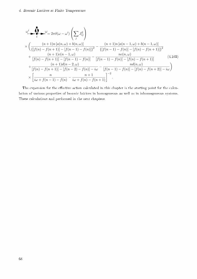
4. Bosonic Lattices at Finite Temperature
ω′ ω
i= 2πδ(ω − ω′)
∑j
J2ij
×(
(n+ 1)n [a(n, ω) + b(n, ω)]
[f(n)− f(n+ 1)]− [f(n− 1)− f(n)]2− (n+ 1)n [a(n− 1, ω) + b(n− 1, ω)]
[f(n− 1)− f(n)]− [f(n)− f(n+ 1)]2
+(n+ 1)c(n− 1, ω)
[f(n)− f(n+ 1)]− [f(n− 1)− f(n)]− nc(n, ω)
[f(n− 1)− f(n)]− [f(n)− f(n+ 1)](4.103)
+(n+ 1)d(n− 2, ω)
[f(n)− f(n+ 1)]− [f(n− 2)− f(n)]− iω− nd(n, ω)
[f(n− 1)− f(n)]− [f(n)− f(n+ 2)]− iω
)×[
n
iω + f(n− 1)− f(n)− n+ 1
iω + f(n)− f(n+ 1)
]−2
.
The expansion for the eective action calculated in this chapter is the starting point for the calcu-
lation of various properties of bosonic lattices in homogeneous as well as in inhomogeneous systems.
These calculations and performed in the next chapters.
68
5. Homogeneous Lattices
Having developed our eld-theoretical approach for the general Hamiltonian in the previous chapter, we
can now apply it to the specic case of the homogeneous Bose-Hubbard Hamiltonian in D-dimensional
cubic optical lattices. To this end, we must make following identications
fi(n) =U
2(n2 − n)− µn, (5.1)
Jij =
J,
0,
if i and j are nearest neighbors
otherwise.(5.2)
5.1. Quasi-Momentum Representation
The discrete translation symmetry in the homogeneous case allows us to further simplify our formalism
by performing a discrete Fourier transformation to our elds, thus leading to the quasi-momentum
representation
ψ(k) =∑i
e−ik·riψi, (5.3)
were ri denotes the location of the i-th lattice site and components kα of quasi-momentum k are re-
stricted to the rst Brillouin zone. Analogously all site-dependent functions are transformed according
to
M(k1, · · · ,kn;k′1, · · · ,k′
n) =∑
i1,··· ,in;i′1,··· ,i′n
e−i(k1·ri1+···+kn·rin−k′
1·ri′1−···−k′
n·ri′n )Mi1,··· ,in;i′1,··· ,i′n . (5.4)
The inverse transformations read
ψi =( a2π
)D ∫dDkeik·riψ(k), (5.5)
Mi1,··· ,in,i′1,··· ,i′n =( a2π
)2Dn ∫dDk1 · · ·
∫dDkn
∫dDk′
1 · · ·∫dDk′
nei(k1·ri1+···+kn·rin−k′
1·ri′1−···−k′
n·ri′n)
×M(k1, · · · ,kn;k′1, · · · ,k′
n). (5.6)
These transformations can be checked by using the formula
69
5. Homogeneous Lattices
∑i
e−ik·ri =
(2π
a
)Dδ(k). (5.7)
This formula enables us to relate δ(k = 0) and the total number of lattice sites NS according to
δ(k = 0) =( a2π
)DNs. (5.8)
By combining this discrete Fourier transformation with the Matsubara transformation, we can
rewrite the eective action in (4.48) and (4.57) according to
−βΓ [ψ∗, ψ] = Γ(0) +1
β2
( a2π
)2D∑ωω′
∫dDk
∫dDk′Γ(2)
(k, ω;k′, ω′)ψ∗ (k, ω)ψ
(k′, ω′)
+1
2!21
β4
( a2π
)4D ∑ω1ω2;ω′
1ω′2
∫dDk1
∫dDk2
∫dDk′
1
∫dDk′
2Γ(4)(k1, ω1,k2, ω2;k
′1, ω
′1,k
′2, ω
′2)
×ψ∗(k1, ω1)ψ∗(k1, ω2)ψ(k
′1, ω
′1)ψ(k
′2, ω
′2) + · · · . (5.9)
From (4.92) and (4.95) we know the 2-point 1PI Green's function up to second hopping order
Γ(2)ij (ω;ω′) = δij
ω′ ω
i+ βδω,ω′Jij + δij
ω′ ω
i+ · · · (5.10)
From (4.71) and (4.101), we see that for homogeneous lattices, both diagrams in (5.10) are site inde-
pendent. Thus, using (5.4) and (5.10), we have
Γ(2)(k, ω;k′, ω′) =
(2π
a
)Dδ(k− k′)
ω′ ω
i+ βδω,ω′J(k) +
ω′ ω
i+ · · ·
(5.11)
with the Fourier transformed hopping
J(k) = 2J∑α
cos(kαa). (5.12)
For the 4-point 1PI function, we know only its zeroth-order contribution
Γ(4)i1i2;i′1i
′2(ω1, ω2;ω
′1, ω
′2) = δi1i2δi′1i2δi1i′1
ω′1
ω′2
ω1
ω2
ii
i
i i
+ · · · (5.13)
From (4.87) and (4.88), we observe that the diagram in (5.13) is also site independent. By using (5.4)
and (5.13), we get
70
5.2. Static Properties
Γ(4)(k1, ω1,k2, ω2;k′1, ω
′1,k
′2, ω
′2) =
( a2π
)Dδ(k1 + k2 − k′
1 − k′2)
ω′1
ω′2
ω1
ω2
ii
i
i i
+ · · · (5.14)
5.2. Static Properties
In the homogeneous optical lattices discussed here, the spatial and temporal translation symmetry of
the Bose-Hubbard Hamiltonian is preserved in its equilibrium state. Therefore, in order to calculate
many of their equilibrium properties it is enough to consider the eective action for an order parameter
which is homogeneous in both space and imaginary time, i.e.
ψi(τ) = ψeq. (5.15)
This can be expressed in the quasi-momentum Matsubara representation according to
ψeq(k, ω) = β
(2π
a
)Dδω,0δ(k)ψeq. (5.16)
For homogeneous order parameters, it is usual to work with the so called eective potential [39,40]
which is dened as the eective action per lattice site: Γpot = Γ/Ns. Considering this denition and
substituting (5.16) into (5.9), we obtain the Landau expansion
Γpot(ψ∗, ψ) = a0 + a2 |ψ|2 +
1
2!2a4 |ψ|4 + · · · , (5.17)
with the coecients given by
a0 = −β−1 ln
∞∑n=0
e−βfi(n), (5.18)
a2 = −Γ(2)(0, 0;0′, 0)
βNs= β−1
0 0
i+ βJ(0) +
0 0
i+ · · ·
, (5.19)
a4 =Γ(4)(0, 0,0, 0;0, 0,0, 0)
βNs2!2=
1
β2!2
0
0
0
0
ii
i
i i
+ · · · . (5.20)
5.2.1. First Hopping Order
According to the discussion in Chapter 4, we must rst check whether the condition a4 > 0 is satised.
It can be directly calculated form Eqs. (4.87), (4.88), and (5.20). The positivity of a4 can be seen
from Fig. 5.1. Once this condition is satised, the phase boundary separating the Mott insulator and
the superuid phases is given by the condition a2 = 0.
In the rst hopping order approximation, the phase boundary is obtained by ignoring second and
higher hopping orderin (5.19) and imposing the condition a2 = 0 on the system parameters, which
71
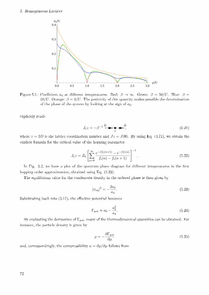
5. Homogeneous Lattices
0.0 0.5 1.0 1.5 2.0 2.5 3.0ΜU
0.1
0.2
0.3
0.4a4U
Figure 5.1.: Coecient a4 at dierent temperatures. Red: β → ∞. Green: β = 50/U . Blue: β =10/U . Orange: β = 3/U . The positivity of this quantity makes possible the determinationof the phase of the system by looking at the sign of a2.
explicitly reads
Jcz = −β−1 0 0
i, (5.21)
where z = 2D is the lattice coordination number and Jz = J(0). By using Eq. (4.71), we obtain the
explicit formula for the critical value of the hopping parameter
Jcz = Z0
[ ∞∑n=0
e−βfi(n+1) − e−βfi(n)
fi(n)− fi(n+ 1)
]−1
. (5.22)
In Fig. 5.2, we have a plot of the quantum-phase diagram for dierent temperatures in the rst
hopping order approximation, obtained using Eq. (5.22).
The equilibrium value for the condensate density in the ordered phase is then given by
|ψeq|2 = −2a2a4
. (5.23)
Substituting back into (5.17), the eective potential becomes
Γpot ≈ a0 −a22a4. (5.24)
By evaluating the derivatives of Γpot, many of the thermodynamical quantities can be obtained. For
instance, the particle density is given by
ρ = −∂Γpot
∂µ(5.25)
and, correspondingly, the compressibility κ = ∂ρ/∂µ follows from
72
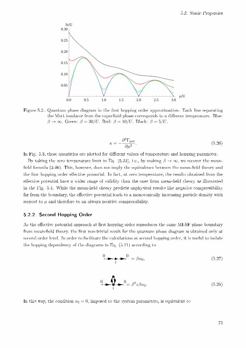
5.2. Static Properties
0.0 0.5 1.0 1.5 2.0 2.5 3.0ΜU
0.05
0.10
0.15
0.20
0.25
0.30JzU
Figure 5.2.: Quantum phase diagram in the rst hopping order approximation. Each line separatingthe Mott insulator from the superuid phase corresponds to a dierent temperature. Blue:β → ∞. Green: β = 30/U . Red: β = 10/U . Black: β = 5/U .
κ = −∂2Γpot
∂µ2. (5.26)
In Fig. 5.3, these quantities are plotted for dierent values of temperature and hopping parameter.
By taking the zero temperature limit in Eq. (5.22), i.e., by making β → ∞, we recover the mean-
eld formula (3.46). This, however, does not imply the equivalence between the mean-eld theory and
the rst hopping order eective potential. In fact, at zero temperature, the results obtained from the
eective potential have a wider range of validity than the ones from mean-eld theory as illustrated
in the Fig. 5.4. While the mean-eld theory predicts unphysical results like negative compressibility
far from the boundary, the eective potential leads to a monotonically increasing particle density with
respect to µ and therefore to an always positive compressibility.
5.2.2. Second Hopping Order
As the eective potential approach at rst hopping order reproduces the same MI-SF phase boundary
from mean-eld theory, the rst non-trivial result for the quantum phase diagram is obtained only at
second order level. In order to facilitate the calculations at second hopping order, it is useful to isolate
the hopping dependency of the diagrams in Eq. (5.11) according to
0 0
i= βα0, (5.27)
0 0
i= J2zβα2. (5.28)
In this way, the condition a2 = 0, imposed to the system parameters, is equivalent to
73
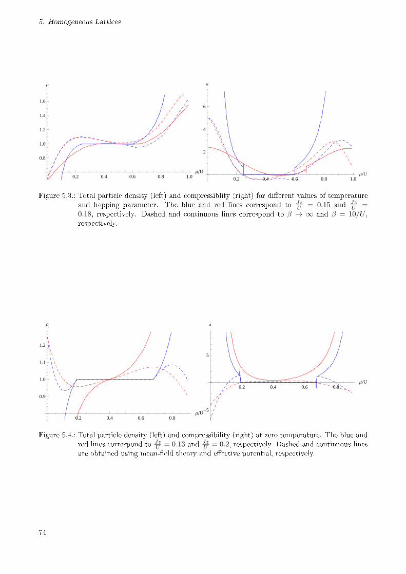
5. Homogeneous Lattices
0.2 0.4 0.6 0.8 1.0ΜU
0.8
1.0
1.2
1.4
1.6
Ρ
0.2 0.4 0.6 0.8 1.0ΜU
2
4
6
Κ
Figure 5.3.: Total particle density (left) and compressiblity (right) for dierent values of temperatureand hopping parameter. The blue and red lines correspond to Jz
U = 0.15 and JzU =
0.18, respectively. Dashed and continuous lines correspond to β → ∞ and β = 10/U ,respectively.
0.2 0.4 0.6 0.8ΜU
0.9
1.0
1.1
1.2
Ρ
0.2 0.4 0.6 0.8ΜU
-5
5
Κ
Figure 5.4.: Total particle density (left) and compressibility (right) at zero temperature. The blue andred lines correspond to Jz
U = 0.13 and JzU = 0.2, respectively. Dashed and continuous lines
are obtained using mean-eld theory and eective potential, respectively.
74
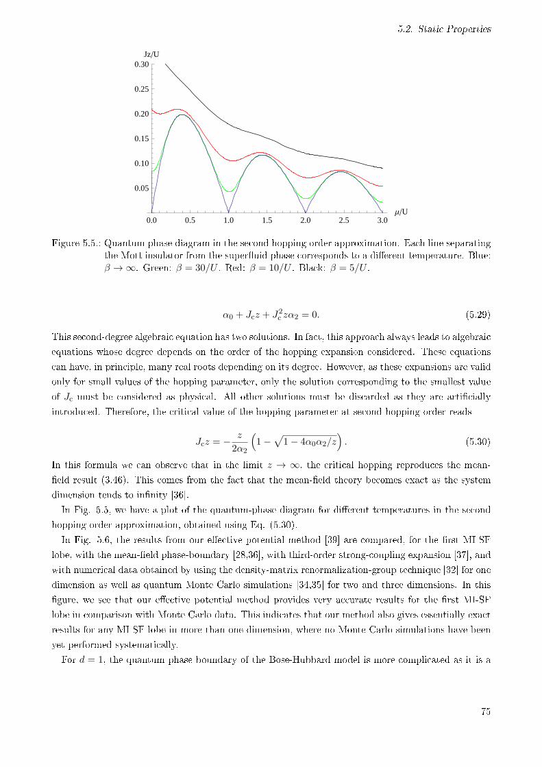
5.2. Static Properties
0.0 0.5 1.0 1.5 2.0 2.5 3.0ΜU
0.05
0.10
0.15
0.20
0.25
0.30JzU
Figure 5.5.: Quantum phase diagram in the second hopping order approximation. Each line separatingthe Mott insulator from the superuid phase corresponds to a dierent temperature. Blue:β → ∞. Green: β = 30/U . Red: β = 10/U . Black: β = 5/U .
α0 + Jcz + J2c zα2 = 0. (5.29)
This second-degree algebraic equation has two solutions. In fact, this approach always leads to algebraic
equations whose degree depends on the order of the hopping expansion considered. These equations
can have, in principle, many real roots depending on its degree. However, as these expansions are valid
only for small values of the hopping parameter, only the solution corresponding to the smallest value
of Jc must be considered as physical. All other solutions must be discarded as they are articially
introduced. Therefore, the critical value of the hopping parameter at second hopping order reads
Jcz = − z
2α2
(1−
√1− 4α0α2/z
). (5.30)
In this formula we can observe that in the limit z → ∞, the critical hopping reproduces the mean-
eld result (3.46). This comes from the fact that the mean-eld theory becomes exact as the system
dimension tends to innity [36].
In Fig. 5.5, we have a plot of the quantum-phase diagram for dierent temperatures in the second
hopping order approximation, obtained using Eq. (5.30).
In Fig. 5.6, the results from our eective potential method [39] are compared, for the rst MI-SF
lobe, with the mean-eld phase-boundary [28,36], with third-order strong-coupling expansion [37], and
with numerical data obtained by using the density-matrix renormalization-group technique [32] for one
dimension as well as quantum Monte Carlo simulations [34,35] for two and three dimensions. In this
gure, we see that our eective potential method provides very accurate results for the rst MI-SF
lobe in comparison with Monte Carlo data. This indicates that our method also gives essentially exact
results for any MI-SF lobe in more than one dimension, where no Monte Carlo simulations have been
yet performed systematically.
For d = 1, the quantum phase boundary of the Bose-Hubbard model is more complicated as it is a
75
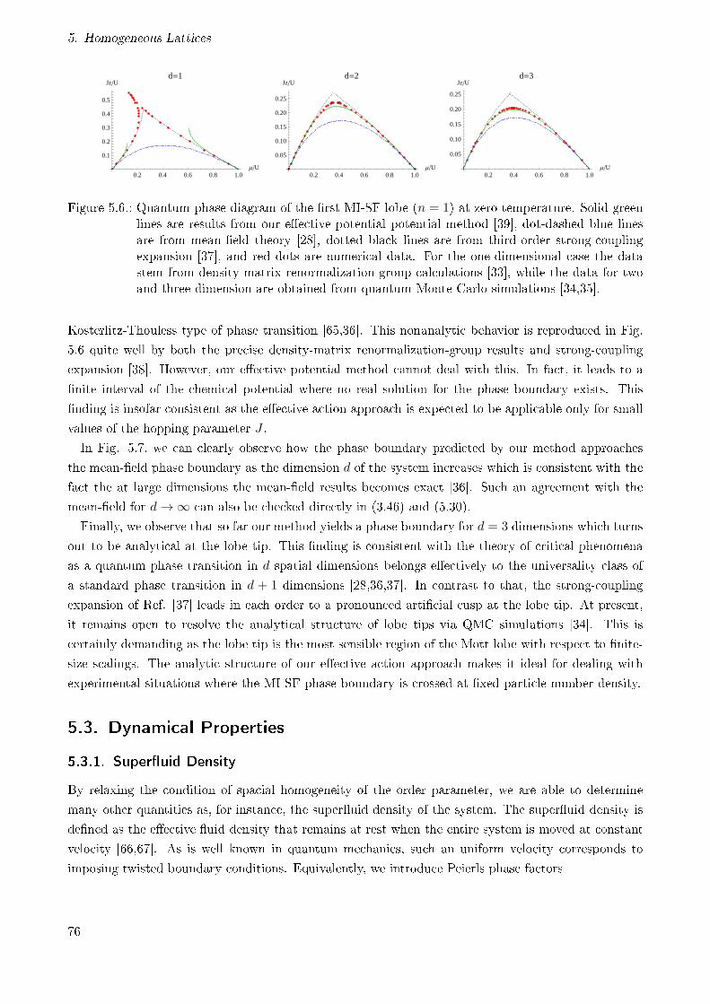
5. Homogeneous Lattices
0.2 0.4 0.6 0.8 1.0ΜU
0.1
0.2
0.3
0.4
0.5
JzUd=1
0.2 0.4 0.6 0.8 1.0ΜU
0.05
0.10
0.15
0.20
0.25
JzUd=2
0.2 0.4 0.6 0.8 1.0ΜU
0.05
0.10
0.15
0.20
0.25
JzUd=3
Figure 5.6.: Quantum phase diagram of the rst MI-SF lobe (n = 1) at zero temperature. Solid greenlines are results from our eective potential potential method [39], dot-dashed blue linesare from mean-eld theory [28], dotted black lines are from third-order strong-couplingexpansion [37], and red dots are numerical data. For the one-dimensional case the datastem from density-matrix renormalization-group calculations [33], while the data for twoand three dimension are obtained from quantum Monte Carlo simulations [34,35].
Kosterlitz-Thouless type of phase transition [65,36]. This nonanalytic behavior is reproduced in Fig.
5.6 quite well by both the precise density-matrix renormalization-group results and strong-coupling
expansion [38]. However, our eective potential method cannot deal with this. In fact, it leads to a
nite interval of the chemical potential where no real solution for the phase boundary exists. This
nding is insofar consistent as the eective action approach is expected to be applicable only for small
values of the hopping parameter J .
In Fig. 5.7, we can clearly observe how the phase boundary predicted by our method approaches
the mean-eld phase boundary as the dimension d of the system increases which is consistent with the
fact the at large dimensions the mean-eld results becomes exact [36]. Such an agreement with the
mean-eld for d→ ∞ can also be checked directly in (3.46) and (5.30).
Finally, we observe that so far our method yields a phase boundary for d = 3 dimensions which turns
out to be analytical at the lobe tip. This nding is consistent with the theory of critical phenomena
as a quantum phase transition in d spatial dimensions belongs eectively to the universality class of
a standard phase transition in d + 1 dimensions [28,36,37]. In contrast to that, the strong-coupling
expansion of Ref. [37] leads in each order to a pronounced articial cusp at the lobe tip. At present,
it remains open to resolve the analytical structure of lobe tips via QMC simulations [34]. This is
certainly demanding as the lobe tip is the most sensible region of the Mott lobe with respect to nite-
size scalings. The analytic structure of our eective action approach makes it ideal for dealing with
experimental situations where the MI-SF phase boundary is crossed at xed particle number density.
5.3. Dynamical Properties
5.3.1. Superuid Density
By relaxing the condition of spacial homogeneity of the order parameter, we are able to determine
many other quantities as, for instance, the superuid density of the system. The superuid density is
dened as the eective uid density that remains at rest when the entire system is moved at constant
velocity [66,67]. As is well known in quantum mechanics, such an uniform velocity corresponds to
imposing twisted boundary conditions. Equivalently, we introduce Peierls phase factors
76
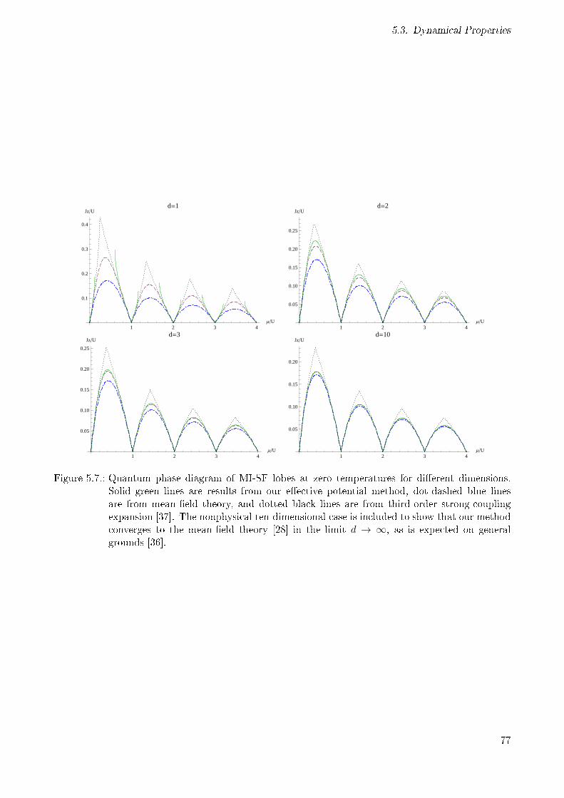
5.3. Dynamical Properties
1 2 3 4ΜU
0.1
0.2
0.3
0.4
JzUd=1
1 2 3 4ΜU
0.05
0.10
0.15
0.20
0.25
JzUd=2
1 2 3 4ΜU
0.05
0.10
0.15
0.20
0.25
JzUd=3
1 2 3 4ΜU
0.05
0.10
0.15
0.20
JzUd=10
Figure 5.7.: Quantum phase diagram of MI-SF lobes at zero temperatures for dierent dimensions.Solid green lines are results from our eective potential method, dot-dashed blue linesare from mean-eld theory, and dotted black lines are from third-order strong-couplingexpansion [37]. The nonphysical ten-dimensional case is included to show that our methodconverges to the mean-eld theory [28] in the limit d → ∞, as is expected on generalgrounds [36].
77
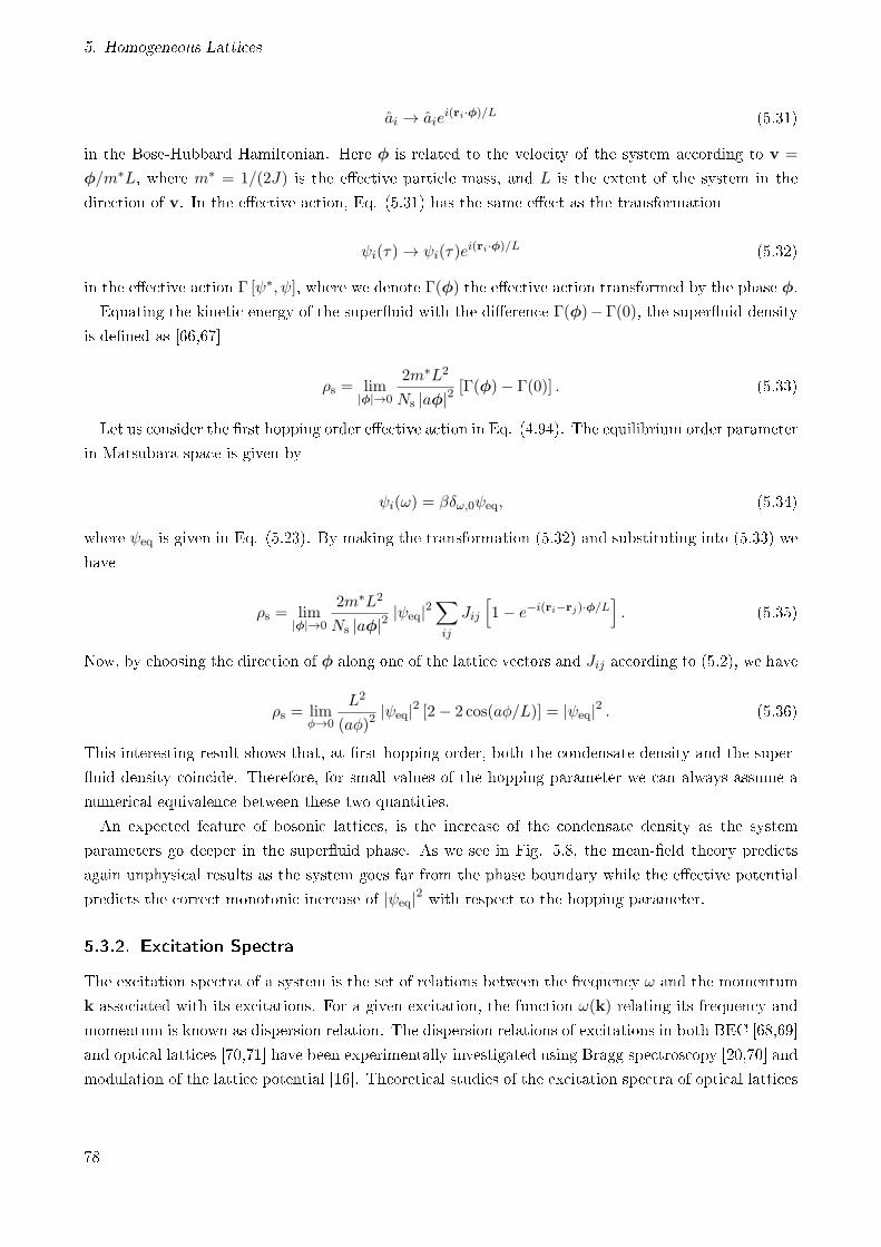
5. Homogeneous Lattices
ai → aiei(ri·φ)/L (5.31)
in the Bose-Hubbard Hamiltonian. Here φ is related to the velocity of the system according to v =
φ/m∗L, where m∗ = 1/(2J) is the eective particle mass, and L is the extent of the system in the
direction of v. In the eective action, Eq. (5.31) has the same eect as the transformation
ψi(τ) → ψi(τ)ei(ri·φ)/L (5.32)
in the eective action Γ [ψ∗, ψ], where we denote Γ(φ) the eective action transformed by the phase φ.
Equating the kinetic energy of the superuid with the dierence Γ(φ)−Γ(0), the superuid density
is dened as [66,67]
ρs = lim|φ|→0
2m∗L2
Ns |aφ|2[Γ(φ)− Γ(0)] . (5.33)
Let us consider the rst hopping order eective action in Eq. (4.94). The equilibrium order parameter
in Matsubara space is given by
ψi(ω) = βδω,0ψeq, (5.34)
where ψeq is given in Eq. (5.23). By making the transformation (5.32) and substituting into (5.33) we
have
ρs = lim|φ|→0
2m∗L2
Ns |aφ|2|ψeq|2
∑ij
Jij
[1− e−i(ri−rj)·φ/L
]. (5.35)
Now, by choosing the direction of φ along one of the lattice vectors and Jij according to (5.2), we have
ρs = limφ→0
L2
(aφ)2|ψeq|2 [2− 2 cos(aφ/L)] = |ψeq|2 . (5.36)
This interesting result shows that, at rst hopping order, both the condensate density and the super-
uid density coincide. Therefore, for small values of the hopping parameter we can always assume a
numerical equivalence between these two quantities.
An expected feature of bosonic lattices, is the increase of the condensate density as the system
parameters go deeper in the superuid phase. As we see in Fig. 5.8, the mean-eld theory predicts
again unphysical results as the system goes far from the phase boundary while the eective potential
predicts the correct monotonic increase of |ψeq|2 with respect to the hopping parameter.
5.3.2. Excitation Spectra
The excitation spectra of a system is the set of relations between the frequency ω and the momentum
k associated with its excitations. For a given excitation, the function ω(k) relating its frequency and
momentum is known as dispersion relation. The dispersion relations of excitations in both BEC [68,69]
and optical lattices [70,71] have been experimentally investigated using Bragg spectroscopy [20,70] and
modulation of the lattice potential [16]. Theoretical studies of the excitation spectra of optical lattices
78
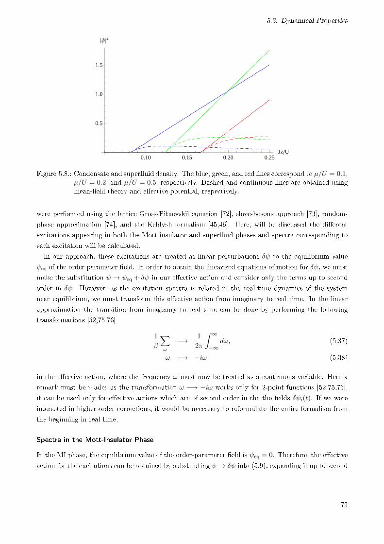
5.3. Dynamical Properties
0.10 0.15 0.20 0.25JzU
0.5
1.0
1.5
ÈΨ 2
Figure 5.8.: Condensate and superuid density. The blue, green, and red lines correspond to µ/U = 0.1,µ/U = 0.2, and µ/U = 0.5, respectively. Dashed and continuous lines are obtained usingmean-eld theory and eective potential, respectively.
were performed using the lattice Gross-Pitaevskii equation [72], slave-bosons approach [73], random-
phase approximation [74], and the Keldysh formalism [45,46]. Here, will be discussed the dierent
excitations appearing in both the Mott-insulator and superuid phases and spectra corresponding to
each excitation will be calculated.
In our approach, these excitations are treated as linear perturbations δψ to the equilibrium value
ψeq of the order parameter eld. In order to obtain the linearized equations of motion for δψ, we must
make the substitution ψ → ψeq + δψ in our eective action and consider only the terms up to second
order in δψ. However, as the excitation spectra is related in the real-time dynamics of the system
near equilibrium, we must transform this eective action from imaginary to real time. In the linear
approximation the transition from imaginary to real time can be done by performing the following
transformations [52,75,76]
1
β
∑ω
−→ 1
2π
∫ ∞
−∞dω, (5.37)
ω −→ −iω (5.38)
in the eective action, where the frequency ω must now be treated as a continuous variable. Here a
remark must be made: as the transformation ω −→ −iω works only for 2-point functions [52,75,76],
it can be used only for eective actions which are of second order in the the elds δψi(t). If we were
interested in higher-order corrections, it would be necessary to reformulate the entire formalism from
the beginning in real time.
Spectra in the Mott-Insulator Phase
In the MI phase, the equilibrium value of the order-parameter eld is ψeq = 0. Therefore, the eective
action for the excitations can be obtained by substituting ψ → δψ into (5.9), expanding it up to second
79
5. Homogeneous Lattices
-3-2-1 1 2 3ka
-0.4
-0.2
0.2
0.4
Ω
-3-2-1 1 2 3ka
-0.4
-0.2
0.2
0.4
Ω
-3-2-1 1 2 3ka
-0.4
-0.2
0.2
0.4
Ω
Figure 5.9.: Excitation spectra of a cubic lattice in the Mott-insulator phase with β = 30/U andµ = 0.4U and dierent values of the hopping parameter. Left: Jz = 0.13U . Middle:Jz = 0.15U . Right: Jz = 0.17U .
order in δψ, and making the transformations (5.37) and (5.38). This nally yields
Γreal [δψ∗, δψ] = −β−1Γ(0) +
1
2π
( a2π
)2D ∫dω
∫dDkξ0 (k, ω) |δψ (k, ω)|2 , (5.39)
where the function ξ0 is given by
ξ0(k, ω) = −β−1Γ(2)(k,−iω;k,−iω)
= −J(k) + Z0
[ ∞∑n=0
(n+ 1)e−βfi(n+1) − e−βfi(n)
ω + fi(n)− fi(n+ 1)
]−1
. (5.40)
By extremalizing (5.39), we obtain the equation of motion
ξ0 (k, ω) δψ (k, ω) = 0, (5.41)
which has nontrivial solutions only if
ξ0 (k, ω) = 0. (5.42)
This is the equation which relates the frequencies and momenta of the excitations in the system and
denes the dispersion relations ω(k) for each of these excitations. The MI phase is characterized by
the existence of gaps in the dispersion relations of all excitations, i.e., for all excitations we must
have |ω(0)| > 0. In fact, since the phase boundary is dened by ξ0 (0, 0) = 0, the gap of at least
one excitation must vanish as the phase boundary is approached from the MI phase. The numerical
solution of (5.42) can be seen in Fig. 5.9 for a cubic lattice at nite temperate in the MI phase. There
we can observe how the gaps become smaller as we approach the MI-SF phase boundary.
Now, by observing that ξ0(k, ω) in Eq. (5.40) is invariant under the transformations
80
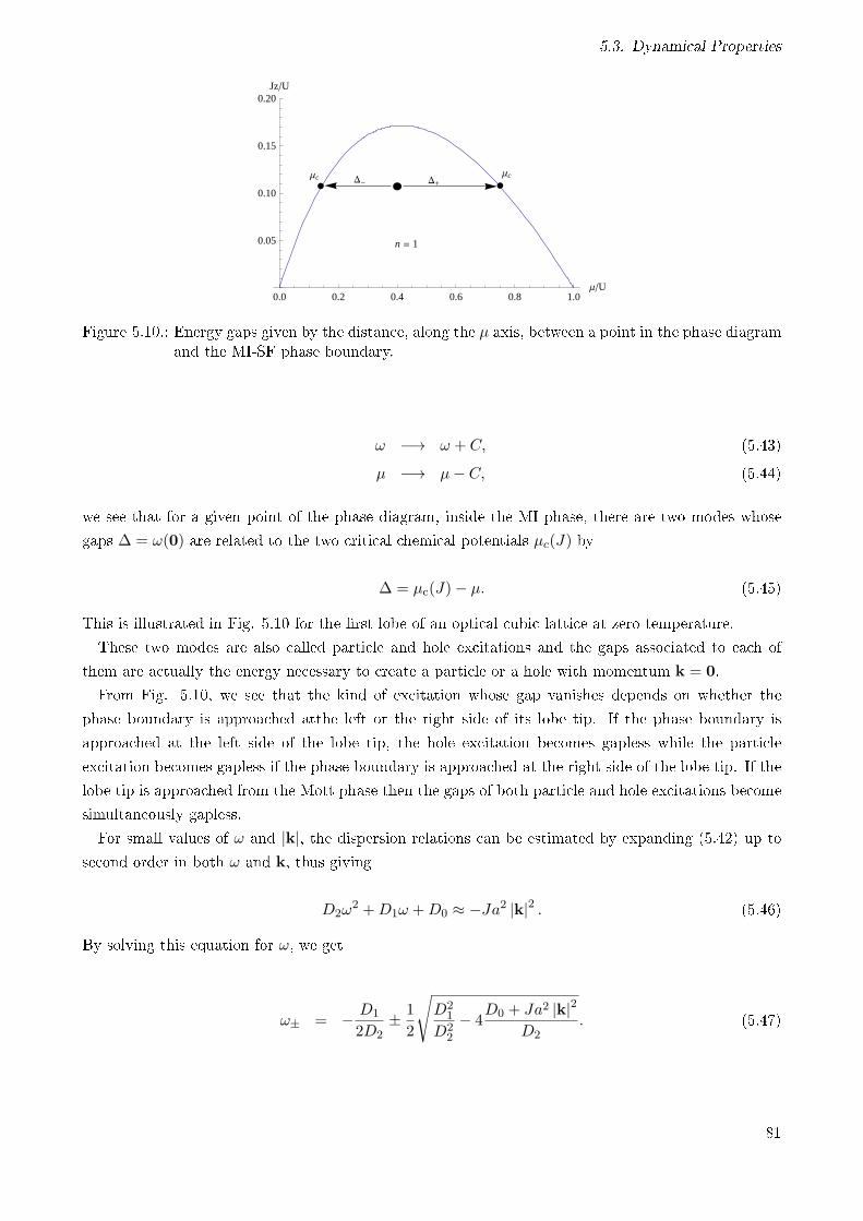
5.3. Dynamical Properties
D- D+
n = 1
ΜcΜc
0.0 0.2 0.4 0.6 0.8 1.0ΜU
0.05
0.10
0.15
0.20JzU
Figure 5.10.: Energy gaps given by the distance, along the µ axis, between a point in the phase diagramand the MI-SF phase boundary.
ω −→ ω + C, (5.43)
µ −→ µ− C, (5.44)
we see that for a given point of the phase diagram, inside the MI phase, there are two modes whose
gaps ∆ = ω(0) are related to the two critical chemical potentials µc(J) by
∆ = µc(J)− µ. (5.45)
This is illustrated in Fig. 5.10 for the rst lobe of an optical cubic lattice at zero temperature.
These two modes are also called particle and hole excitations and the gaps associated to each of
them are actually the energy necessary to create a particle or a hole with momentum k = 0.
From Fig. 5.10, we see that the kind of excitation whose gap vanishes depends on whether the
phase boundary is approached atthe left or the right side of its lobe tip. If the phase boundary is
approached at the left side of the lobe tip, the hole excitation becomes gapless while the particle
excitation becomes gapless if the phase boundary is approached at the right side of the lobe tip. If the
lobe tip is approached from the Mott phase then the gaps of both particle and hole excitations become
simultaneously gapless.
For small values of ω and |k|, the dispersion relations can be estimated by expanding (5.42) up to
second order in both ω and k, thus giving
D2ω2 +D1ω +D0 ≈ −Ja2 |k|2 . (5.46)
By solving this equation for ω, we get
ω± = − D1
2D2± 1
2
√D2
1
D22
− 4D0 + Ja2 |k|2
D2. (5.47)
81
5. Homogeneous Lattices
The expansion of (5.47) up to second order in k gives
ω± ≈ ∆± ± 1
2m′ |k|2 , (5.48)
where the gaps ∆± associated with each excitation in the system and the eective mass m′ of the
excitations are given by
∆± = − D1
2D2± 1
2
√D2
1
D22
− 4D0
D2, (5.49)
m′ =
√D2
1 − 4D0D2
2a2J. (5.50)
For sake of illustration, let us consider the zero-temperature case with n = 1. In this case, the
coecients are given by
D0 = −Jz − (µ− U)µ
µ+ U, (5.51)
D1 = −−U2 + 2µU + µ2
(µ+ U)2, (5.52)
D2 = − 2U2
(U + µ)3. (5.53)
By substituting these coecients into (5.49) and (5.50), we get the gaps ∆± and the mass m′ in
terms of the system parameters. In Fig. 5.11, we present the plots of both the gaps ∆± and mass m′
for β → ∞ and n = 1.
The transformations (5.43) and (5.44) imply that the derivatives of ξ0(k, ω) with respect to ω or µ
are, actually, identical. Therefore the conditions
ξ0(0, 0) = 0, (5.54)
∂ξ0(0, 0)
∂µ
∣∣∣∣µ=0
= 0, (5.55)
which characterizes the phase boundary and the location of the lobe tip, respectively, are equivalent
to
D0 = 0, (5.56)
D1 = 0. (5.57)
Observe that the expansion (5.48) is not valid if both D0 and D1 vanish. In fact, in this case, then
Eq. (5.46) can be solved according to
82
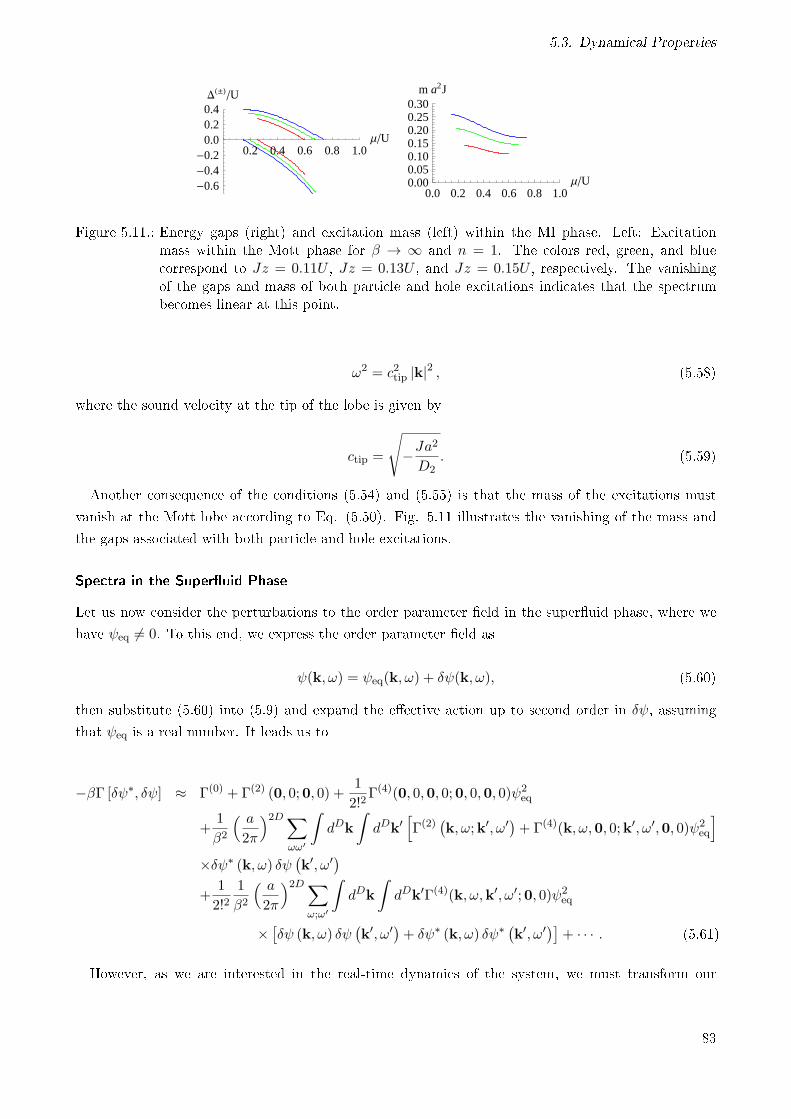
5.3. Dynamical Properties
0.2 0.4 0.6 0.8 1.0ΜU
-0.6-0.4-0.2
0.00.20.4DH±LU
0.0 0.2 0.4 0.6 0.8 1.0ΜU0.00
0.050.100.150.200.250.30
m a2J
Figure 5.11.: Energy gaps (right) and excitation mass (left) within the MI phase. Left: Excitationmass within the Mott phase for β → ∞ and n = 1. The colors red, green, and bluecorrespond to Jz = 0.11U , Jz = 0.13U , and Jz = 0.15U , respectively. The vanishingof the gaps and mass of both particle and hole excitations indicates that the spectrumbecomes linear at this point.
ω2 = c2tip |k|2 , (5.58)
where the sound velocity at the tip of the lobe is given by
ctip =
√−Ja
2
D2. (5.59)
Another consequence of the conditions (5.54) and (5.55) is that the mass of the excitations must
vanish at the Mott lobe according to Eq. (5.50). Fig. 5.11 illustrates the vanishing of the mass and
the gaps associated with both particle and hole excitations.
Spectra in the Superuid Phase
Let us now consider the perturbations to the order parameter eld in the superuid phase, where we
have ψeq 6= 0. To this end, we express the order parameter eld as
ψ(k, ω) = ψeq(k, ω) + δψ(k, ω), (5.60)
then substitute (5.60) into (5.9) and expand the eective action up to second order in δψ, assuming
that ψeq is a real number. It leads us to
−βΓ [δψ∗, δψ] ≈ Γ(0) + Γ(2) (0, 0;0, 0) +1
2!2Γ(4)(0, 0,0, 0;0, 0,0, 0)ψ2
eq
+1
β2
( a2π
)2D∑ωω′
∫dDk
∫dDk′
[Γ(2)
(k, ω;k′, ω′)+ Γ(4)(k, ω,0, 0;k′, ω′,0, 0)ψ2
eq
]×δψ∗ (k, ω) δψ
(k′, ω′)
+1
2!21
β2
( a2π
)2D∑ω;ω′
∫dDk
∫dDk′Γ(4)(k, ω,k′, ω′;0, 0)ψ2
eq
×[δψ (k, ω) δψ
(k′, ω′)+ δψ∗ (k, ω) δψ∗ (k′, ω′)]+ · · · . (5.61)
However, as we are interested in the real-time dynamics of the system, we must transform our
83
5. Homogeneous Lattices
eective action from imaginary to real time. This is done by performing the transformations (5.37)
and (5.38) [52,75,76].
By applying these transformations, the eective action in real-time becomes
Γreal[δψ∗, δψ] ≈ Γpot +
1
2π
( a2π
)2D ∫dω
∫dDkξ1(k, ω) |δψ (k, ω)|2 (5.62)
+1
2
1
2π
( a2π
)2D ∫dω
∫dDkξ2(k, ω) [δψ (k, ω) δψ (−k,−ω) + δψ∗ (k, ω) δψ∗ (−k,−ω)]
where, for simplicity, we suppressed the integration limits and made the following identications
ξ1(k, ω) = −β−1Γ(2)(k,−iω;k,−iω)− β−1Γ(4)(k,−iω,0, 0;k,−iω,0, 0)ψ2eq, (5.63)
ξ2(k, ω) = −1
2β−1Γ(4)(k,−iω,−k, iω;0, 0,0, 0)ψ2
eq, (5.64)
with the equilibrium value of the order-parameter eld
ψ2eq = −2
Γ(2)(0, 0;0, 0)
Γ(4)(0, 0,0, 0;0, 0,0, 0). (5.65)
Substituting this expression for ψeq into (5.63) and (5.64), we get the identity
ξ1(0, 0) = ξ2(0, 0). (5.66)
In addition, due to the permutation symmetries of Γ(4), we see that the ξ2(k, ω) is an even function
with respect to both k and ω. This yields to
∂ξ2(k, ω)
∂ki
∣∣∣∣ki=ω=0
=∂ξ2(k, ω)
∂ω
∣∣∣∣ki=ω=0
= 0. (5.67)
where ki stands for the three components of k.
By extremalizing (5.62), we nally get the equations of motion for δψ in frequency-momentum space
ξ1(k, ω)δψ (k, ω) + ξ2(k, ω)δψ∗ (−k,−ω) = 0, (5.68)
ξ1(k, ω)δψ∗ (k, ω) + ξ2(k, ω)δψ (−k,−ω) = 0. (5.69)
From these equations, we can immediately observe that any function δψ which is both stationary
and purely imaginary, will automatically solve (5.68) and (5.69). This is a result of the global phase
invariance of (5.9) and the non-stationary generalization of these solutions are gapless excitations
known as Goldstone modes.
The solution to the equations (5.68) and (5.69) can be obtained by expressing (5.69) as
δψ∗ (k, ω) = − ξ2(k, ω)
ξ1(k,−ω)δψ (k, ω) (5.70)
84
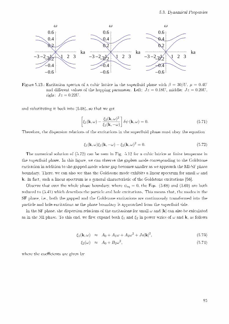
5.3. Dynamical Properties
-3-2-1 1 2 3ka
-0.6-0.4-0.2
0.20.40.6Ω
-3-2-1 1 2 3ka
-0.6-0.4-0.2
0.20.40.6Ω
-3-2-1 1 2 3ka
-0.6-0.4-0.2
0.20.40.6Ω
Figure 5.12.: Excitation spectra of a cubic lattice in the superuid phase with β = 30/U , µ = 0.4Uand dierent values of the hopping parameter. Left: Jz = 0.18U , middle: Jz = 0.20U ,right: Jz = 0.22U .
and substituting it back into (5.68), so that we get[ξ1(k, ω)−
ξ2(k, ω)2
ξ1(k,−ω)
]δψ (k, ω) = 0. (5.71)
Therefore, the dispersion relations of the excitations in the superuid phase must obey the equation
ξ1(k, ω)ξ1(k,−ω)− ξ2(k, ω)2 = 0. (5.72)
The numerical solution of (5.72) can be seen in Fig. 5.12 for a cubic lattice at nite temperate in
the superuid phase. In this gure, we can observe the gapless mode corresponding to the Goldstone
excitation in addition to the gapped mode whose gap becomes smaller as we approach the MI-SF phase
boundary. There, we can also see that the Goldstone mode exhibits a linear spectrum for small ω and
k. In fact, such a linear spectrum is a general characteristic of the Goldstone excitations [56].
Observe that over the whole phase boundary, where ψeq = 0, the Eqs. (5.68) and (5.69) are both
reduced to (5.41) which describes the particle and hole excitations. This means that, the modes in the
SF phase, i.e., both the gapped and the Goldstone excitations are continuously transformed into the
particle and hole excitations as the phase boundary is approached from the superuid side.
In the SF phase, the dispersion relations of the excitations for small ω and |k| can also be calculated
as in the MI phase. To this end, we rst expand both ξ1 and ξ2 in power series of ω and k, as follows
ξ1(k, ω) ≈ A0 +A1ω +A2ω2 + Ja|k|2, (5.73)
ξ2(ω) ≈ A0 +B2ω2, (5.74)
where the coecients are given by
85
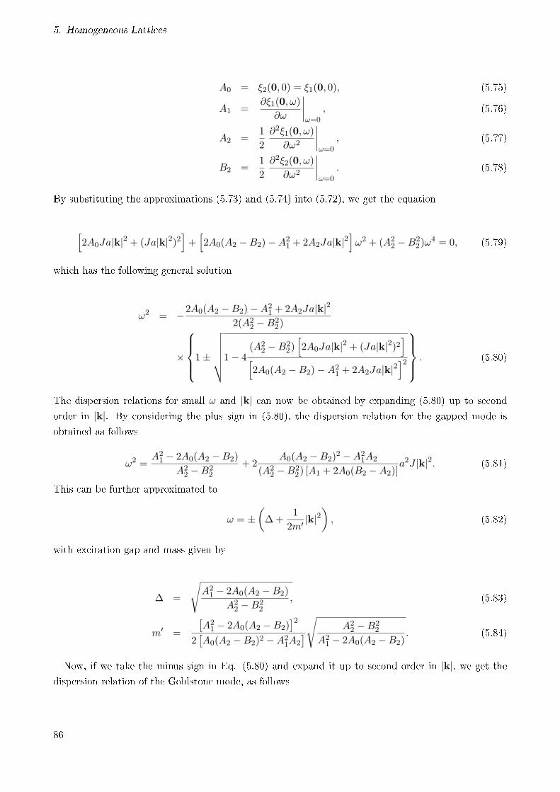
5. Homogeneous Lattices
A0 = ξ2(0, 0) = ξ1(0, 0), (5.75)
A1 =∂ξ1(0, ω)
∂ω
∣∣∣∣ω=0
, (5.76)
A2 =1
2
∂2ξ1(0, ω)
∂ω2
∣∣∣∣ω=0
, (5.77)
B2 =1
2
∂2ξ2(0, ω)
∂ω2
∣∣∣∣ω=0
. (5.78)
By substituting the approximations (5.73) and (5.74) into (5.72), we get the equation
[2A0Ja|k|2 + (Ja|k|2)2
]+[2A0(A2 −B2)−A2
1 + 2A2Ja|k|2]ω2 + (A2
2 −B22)ω
4 = 0, (5.79)
which has the following general solution
ω2 = −2A0(A2 −B2)−A21 + 2A2Ja|k|2
2(A22 −B2
2)
×
1±
√√√√√√1− 4(A2
2 −B22)[2A0Ja|k|2 + (Ja|k|2)2
][2A0(A2 −B2)−A2
1 + 2A2Ja|k|2]2 . (5.80)
The dispersion relations for small ω and |k| can now be obtained by expanding (5.80) up to second
order in |k|. By considering the plus sign in (5.80), the dispersion relation for the gapped mode is
obtained as follows
ω2 =A2
1 − 2A0(A2 −B2)
A22 −B2
2
+ 2A0(A2 −B2)
2 −A21A2
(A22 −B2
2) [A1 + 2A0(B2 −A2)]a2J |k|2. (5.81)
This can be further approximated to
ω = ±(∆+
1
2m′ |k|2
), (5.82)
with excitation gap and mass given by
∆ =
√A2
1 − 2A0(A2 −B2)
A22 −B2
2
, (5.83)
m′ =
[A2
1 − 2A0(A2 −B2)]2
2[A0(A2 −B2)2 −A2
1A2
]√ A22 −B2
2
A21 − 2A0(A2 −B2)
. (5.84)
Now, if we take the minus sign in Eq. (5.80) and expand it up to second order in |k|, we get thedispersion relation of the Goldstone mode, as follows
86
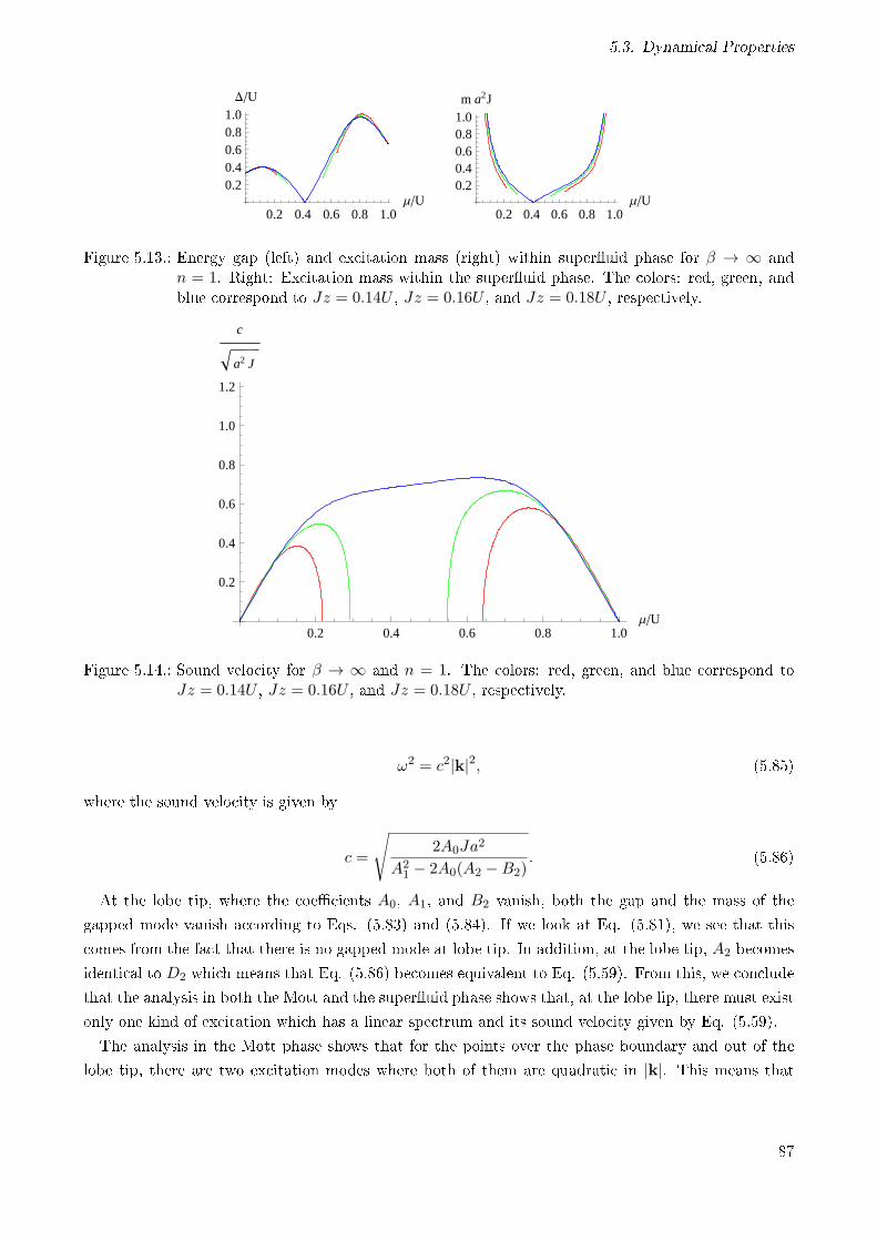
5.3. Dynamical Properties
0.2 0.4 0.6 0.8 1.0ΜU
0.20.40.60.81.0DU
0.2 0.4 0.6 0.8 1.0ΜU
0.20.40.60.81.0m a2J
Figure 5.13.: Energy gap (left) and excitation mass (right) within superuid phase for β → ∞ andn = 1. Right: Excitation mass within the superuid phase. The colors: red, green, andblue correspond to Jz = 0.14U , Jz = 0.16U , and Jz = 0.18U , respectively.
0.2 0.4 0.6 0.8 1.0ΜU
0.2
0.4
0.6
0.8
1.0
1.2
c
a2 J
Figure 5.14.: Sound velocity for β → ∞ and n = 1. The colors: red, green, and blue correspond toJz = 0.14U , Jz = 0.16U , and Jz = 0.18U , respectively.
ω2 = c2|k|2, (5.85)
where the sound velocity is given by
c =
√2A0Ja2
A21 − 2A0(A2 −B2)
. (5.86)
At the lobe tip, where the coecients A0, A1, and B2 vanish, both the gap and the mass of the
gapped mode vanish according to Eqs. (5.83) and (5.84). If we look at Eq. (5.81), we see that this
comes from the fact that there is no gapped mode at lobe tip. In addition, at the lobe tip, A2 becomes
identical to D2 which means that Eq. (5.86) becomes equivalent to Eq. (5.59). From this, we conclude
that the analysis in both the Mott and the superuid phase shows that, at the lobe lip, there must exist
only one kind of excitation which has a linear spectrum and its sound velocity given by Eq. (5.59).
The analysis in the Mott phase shows that for the points over the phase boundary and out of the
lobe tip, there are two excitation modes where both of them are quadratic in |k|. This means that
87
5. Homogeneous Lattices
the sound velocity of of the Goldstone mode must vanish as these points are approached from the SF
phase. This can be checked by considering Eq. (5.86) with A0 = 0 and A1 6= 0.
For simplicity, let us consider the zero-temperature case with n = 1. In this case, the coecients
(5.75)(5.78) can be explicitly calculated, thus yielding
A0 =(−1 + µ′)µ′ + J ′z(1 + µ′)
1 + µ′, (5.87)
A1 =[−2(−1 + µ′)2µ′2
(−18 + 42µ′ − 23µ′2 + 8µ′3 + µ′4
)J ′z(9− 66µ′ + 103µ′2 + 12µ′3 − 117µ′4 + 46µ′5 − 3µ′6
)]/µ′(1 + µ′)2
(9− 30µ′ + 46µ′2 − 32µ′3 + 5µ′4 + 2µ′5
)U, (5.88)
A2 =[3J ′ (27− 135µ′ + 207µ′2 − 23µ′3 − 185µ′4 + 165µ′5 − 41µ′6 + µ′7
)+ µ′
(−27 + 351µ′ − 1197µ′2 + 1907µ′3 − 1639µ′4 + 739µ′5 − 137µ′6 + 3µ′7
)]/(3− 2µ′)2(−1 + µ′)µ′(1 + µ′)3
(3− 5µ′ + 5µ′2 + µ′3
)U2 (5.89)
B2 = − 12µ′ [(−1 + µ′)µ+ J ′z(1 + µ′)]
(1 + µ′)3 (3− 5µ′ + 5µ′2 + µ′3)U2, (5.90)
where µ′ = µ/U and J ′ = J/U .
By substituting these coecients into (5.83) and (5.84), we obtain the gap and mass of the gapped
mode above the rst Mott lobe as depicted in Fig. 5.13. The sound velocity above the rst Mott lobe
is obtained by substituting these coecients into (5.86) and is shown in Fig. 5.14.
By numerically solving Eqs. (5.42) and (5.72), the properties of the excitation spectra in both the
MI and SF phases can be analyzed in an even more precise way. In Fig. 5.15, these properties are
exposed in detail according to the various points considered in the phase diagram. In C1 and C3, we
see the hole excitations becoming gapless as the phase boundary is approached from the MI phase
which indicates that the hole excitation transforms into the Goldstone mode as the phase boundary is
crossed. In C2 and C3, the coincidence between both the mass and the gap of the particle excitation
and the SF gapped excitation indicates that the particle excitation transforms into the SF gapped
mode as the phase boundary is crossed from the MI phase. The roles of particle and hole excitations
are exchanged at the other side of the lobe tip, as we can see in A1-A3. In this case, the particle
excitation is the one which gives rise to the Goldstone mode while the hole excitation becomes the SF
gapped mode, as depicted in A2 and A3. At the Mott lobe, we have a special situation where both
particle and hole excitations are merged into single linear excitations as the lobe tip is approached
form the MI phase as shown in B1. In addition, the vanishing masses and gaps at the lobe tip in B2
and B3 shows the absence of any gapped or massive mode at the lobe tip. In fact, the only possible
mode at this point is the linear mode with nite sound velocity indicated in B3 as opposed to the
other points over the boundary, where the vanishing sound velocity in A3 and C3 indicates that only
massive modes exist.
88
5.3. Dynamical Properties
5.3.3. Critical Exponents
In this chapter, some properties of the excitation spectra such as gaps and masses of the various
modes were calculated by means of expansions of the dispersion relations in powers of ω and |k|,as in Eqs. (5.48) and (5.81). This kind of approximation becomes better and better as the phase
boundary is approached, since in the vicinity of the critical points only excitations with low energy
and momenta play relevant roles. Therefore, these approximations are enough for the discussion of the
critical properties at the MI-SF transition.
At rst, it is important to distinguish the transitions at the lobe tip from the ones occurring across
the other points of the MI-SF border. At the lobe tip, the relativistic dispersion relations implies
that the transitions occurring at this point belong to universality classes which are dierent from the
transitions crossing the other points.
Let us rst concentrate on the transitions occurring away from the lobe tip where the phase boundary
is crossed vertically with µ constant. In the MI phase, the correlation length is related to the coecient
of |ψ|2 in the eective action according to [56,57,60]
ξ−2 ∼ Γ(2)(0, 0;0, 0). (5.91)
From Eq. (5.40), we have
Γ(2)(0, 0;0, 0) ∼ |J − Jc| , (5.92)
where Jc denotes the critical hopping. The critical exponent ν is dened according to
ξ ∼ |J − Jc|ν . (5.93)
The combination of (5.91)(5.93) leads to
ν =1
2. (5.94)
The denition of the susceptibility [36,56,60] is also related to Γ(2)(0, 0;0, 0) according to
χ ∼ Γ(2)(0, 0;0, 0)−1, (5.95)
while the critical exponent χ is dened by
χ ∼ |J − Jc|−γ . (5.96)
By combining (5.95) and (5.96) with (5.92) we get another coecient
γ = 1. (5.97)
The critical exponent z is related to the way in which an excitation vanishes at the critical point [36]
according to
∆ ∼ |J − Jc|νz . (5.98)
89
5. Homogeneous Lattices
From (5.49) and (5.83), we see that
∆ ∼ |J − Jc| . (5.99)
Using the value of ν from (5.94) with (5.98) and (5.99), we have
z = 2. (5.100)
Another possibility is crossing the phase boundary horizontally with J constant. In this case, all
the discussion made above can be repeated by considering |µ− µc| instead of |J − Jc| in such a way
that the critical exponents are the same. For both paths, the remaining coecients can be obtained
by using the scaling relations (3.1)(3.4), thus giving
α = −1
2, (5.101)
β =3
4, (5.102)
δ =7
3, (5.103)
η = 0. (5.104)
Now let us consider the transition where the lobe tip is crossed vertically. Since the equation (5.92)
also holds when the lobe tip is approached, the exponents ν and γ have the same value. However, in
Fig. 5.10, we see that, due to the parabolic shape of the phase boundary near the lobe tip, the gaps
of the excitations must vanish according to
∆ ∼ |J − Jc|2 . (5.105)
From Eq. (5.98), we can then infer for the lobe tip that
z = 1. (5.106)
By using the scaling relations (3.1)(3.4), we get the remaining critical exponents at the lobe tip
α = 0, (5.107)
β =1
2, (5.108)
δ = 3, (5.109)
η = 0. (5.110)
Another possible critical behavior can be observed when the lobe tip is approached horizontally from
the SF phase without penetrating into the MI phase. To this end, we must use the eective action in
the SF phase. In particular, the coecients ν and γ which are related to the correlation length and
the susceptibility, respectively, can be obtained from
90
5.3. Dynamical Properties
ξ−2 ∼ ξ1(0, 0), (5.111)
χ ∼ ξ1(0, 0)−1, (5.112)
where ξ1 is dened in (5.63). Note that, at the Mott lobe, the derivative of ξ1 with respect to µ vanishes
since the derivatives of both Γ(2)and Γ(4) go to zero at this point. Therefore, at the Mott lobe, we
must have
ξ1(0, 0) ∼ (µ− µc)2. (5.113)
This allows us to nd the coecients
ν = 1, (5.114)
γ = 2. (5.115)
From (5.83) and Fig. 5.13 we see that the gap of the SF gapped mode behaves according to
∆ ∼ |µ− µc| (5.116)
along the horizontal path which touches the Mott lobe. This leads us to our next coecient
z = 1. (5.117)
The remaining coecients can now be calculated using (3.1)(3.4), thus giving
α = −2, (5.118)
β = 1, (5.119)
δ = 3, (5.120)
η = 0. (5.121)
These results are summarized in Fig. 5.16 with the various transitions corresponding to the dierent
crossings of the MI-SF border discriminated.
91
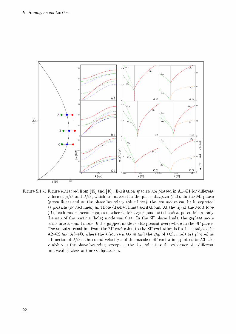
5. Homogeneous Lattices
Figure 5.15.: Figure extracted from [45] and [46]. Excitation spectra are plotted in A1C1 for dierentvalues of µ/U and J/U , which are marked in the phase diagram (left). In the MI phase(green lines) and on the phase boundary (blue lines), the two modes can be interpretedas particle (dotted lines) and hole (dashed lines) excitations. At the tip of the Mott lobe(B), both modes become gapless, whereas for larger (smaller) chemical potentials µ, onlythe gap of the particle (hole) mode vanishes. In the SF phase (red), the gapless modeturns into a sound mode, but a gapped mode is also present everywhere in the SF phase.The smooth transition from the MI excitation to the SF excitation is further analyzed inA2C2 and A3C3, where the eective mass m and the gap of each mode are plotted asa function of J/U . The sound velocity c of the massless SF excitation, plotted in A3C3,vanishes at the phase boundary except at the tip, indicating the existence of a dierentuniversality class in this conguration.
92
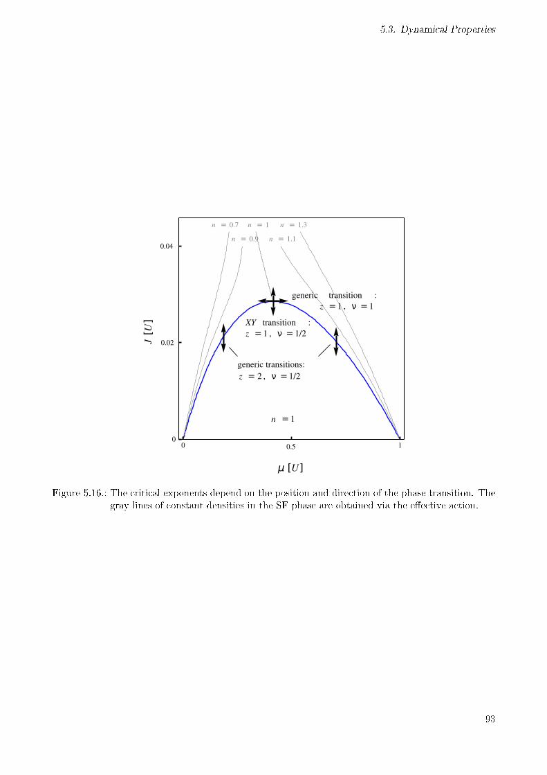
5.3. Dynamical Properties
Figure 5.16.: The critical exponents depend on the position and direction of the phase transition. Thegray lines of constant densities in the SF phase are obtained via the eective action.
93

94
6. Collapse and Revival of Matter Waves
This chapter discusses the formation and dynamics of matter waves in an optical lattice loaded with
2× 10⁵ 87Rb atoms which was experimentally observed by Greiner et al. [1]. In particular, we analyse
the observed collapse and revival of the condensate eld after a sudden change of the potential depth
from a small value VA to a large value VB. Various examples of such eect have been observed not
only with the matter waves in a BEC [1,77,78], but also for the coherent light eld interacting with a
single atom in cavity quantum electrodynamics [79] and for a single ion captured in a trap [80].
Besides the main frequency dependency of the collapse and revival process on the laser potential,
the authors in Ref. [1] detected a clear dierence between the revival and collapse times which also
depend on the external laser potential. Additionally, a damping of those matter waves is perceived
which was possibly caused by a loss of coherence due to the harmonic trapping potential. Here we use
the results from our eective action theory to reproduce the observed features in Ref. [1] and to test
our theory against the experimental results. Therefore, all numeric parameters used here are the same
as in Ref. [1].
For suciently large values of the laser beam intensity V0, the hopping parameter can be neglected,
so that our system is described by the Bose-Hubbard Hamiltonian
HBH =U
2ni (ni − 1) + Vini, (6.1)
with Vi = (1/2)mω2|r|2i and ω2 = ω2m + ω2
l . Here ω2m = 2π × 24 Hz is the magnetic trap frequency
and, due to the Gaussian prole of the laser beams, an additional contribution ω2l must be taken into
account, which reads according to (2.15)
ω2l =
8V0mw2
0
, (6.2)
with m being the mass of the 87Rb atoms. Here we consider the values VA = 8 ER and VB = 22 ER
as in Ref. [1]. This gives for the laser-generated angular frequencies the values ωA = 225 Hz and
ωB = 389 Hz corresponding to the potentials VA and VB, respectively, where, we have used the laser
beam wavelength λ = 838 nm and the beam waists w0 = 125 µm.
6.1. Equations of motion for J = 0
The Hamiltonian (6.1) allows us to treat the system as a set of independent lattice points. Therefore,
in an analogous way to (5.39), the real-time eective action for a small ψi is given by
Γreal [ψ∗i , ψi] = −β−1Γ(0)/NS +
1
2π
∫dωξ (ω) |ψi (ω)|2 , (6.3)
95
6. Collapse and Revival of Matter Waves
where, for β → ∞, the function ξ is given by
ξ(ω) =
[n
ω + fi(n− 1)− fi(n)− (n+ 1)
ω + fi(n)− fi(n+ 1)
]−1
(6.4)
with the following identication
fi(n) =U
2(n2 − n) + Vin. (6.5)
By extremalizing (6.3), we obtain the equation of motion
ξ (ω)ψi (ω) = 0. (6.6)
Therefore, the order parameter ψi(ω) is nonzero only for frequencies obeying
ξ (ω) = 0. (6.7)
By using (6.6) and (6.5), we conclude that these frequencies are
ω1 =UBni~
+mω2
B
2~r2i , (6.8)
ω2 =UB(ni − 1)
~+mω2
B
2~r2i , (6.9)
where we recovered the explicit dependency on the Planck constant ~ by dimensional analysis. This
means that the general evolution of ψi(t) is given by
ψi(t) =[A+i e
−iUBni~ t +A−
i e−iUB(ni−1)
~ t]e−i
mω2B
2~ r2i t, (6.10)
where A+i and A
−i are constants which are determined by the initial conditions.
6.2. Exact solution for J = 0
Here we consider that the initial lattice potential is very small so that we can consider our initial state
as a direct product of on-site coherent states
|Φ〉 =∏i
⊗|φi〉, (6.11)
with the local states
|φi〉 = e−12|ψi|2
∞∑ni=0
ψnii√ni!
|ni〉. (6.12)
96
6.3. Initial conditions
The time evolution of the order eld ψi is then given by
ψi(t) = 〈φi|eit~ Hiaie
−it~ Hi |φi〉. (6.13)
A direct evaluation of (6.13) with (6.1) nally leads to
ψi(t) = ψi exp|ψi|2
[e−
itUB~ − 1
]e−i
mω2B
2~ r2i t. (6.14)
6.3. Initial conditions
Initial equilibrium situations happening deep in the superuid phase can be described by the lattice
version of the Gross-Pitaevskii equation
−JA∑j∈n.n
ψj + UA|ψi|2ψi + Viψi = µψi. (6.15)
Now we use the Thomas-Fermi approximation as solution of (6.15)
ψi =
√zJA + µ− Vi
UA. (6.16)
The constant zJA + µ is determined from the initial total number of condensed atoms which in our
case is Nc = 0.6× 2× 105. Here the factor 0.6 corresponds to the initial coherent fraction observed in
Ref. [1].
Since in Ref. [1], there was around 150,000 populated lattice sites, we can consider the Thomas-
Fermi radius as being much larger than the lattice spacing a, in such a way that ri can be regarded as
a continuous variable. The explicit formulas for the constant zJA + µ and the Thomas-Fermi radius
R are given by
zJA + µ =
(15UAa
3Nc
8π
)2/5 (mω2
A/2)3/5
, (6.17)
R =
√2 (zJA + µ)
mω2A
, (6.18)
where, in our case, we have UA = 4.84× 10⁻³¹J which leads to the Thomas-Fermi radius R = 32.6a.
The solution (6.16) can be directly used as the initial condition of (6.14). However, since Eq. (6.10)
determines only the sum A+i + A−
i , the dierence A+i − A−
i between the amplitude modes has to be
determined from the minimum of the observed oscillations of Nc.
6.4. Momentum distributions
In the limit of validity of the Bose-Hubbard model the condensate wave function in coordinate space
is given by
Ψ(r, t) =∑i
U(r− ri)ψi(t). (6.19)
97
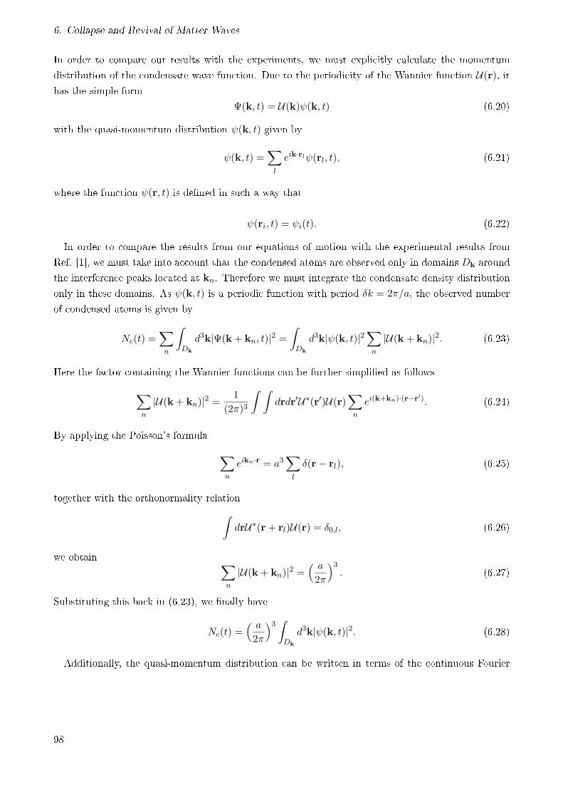
6. Collapse and Revival of Matter Waves
In order to compare our results with the experiments, we must explicitly calculate the momentum
distribution of the condensate wave function. Due to the periodicity of the Wannier function U(r), ithas the simple form
Ψ(k, t) = U(k)ψ(k, t) (6.20)
with the quasi-momentum distribution ψ(k, t) given by
ψ(k, t) =∑l
eik·rlψ(rl, t), (6.21)
where the function ψ(r, t) is dened in such a way that
ψ(ri, t) = ψi(t). (6.22)
In order to compare the results from our equations of motion with the experimental results from
Ref. [1], we must take into account that the condensed atoms are observed only in domains Dk around
the interference peaks located at kn. Therefore we must integrate the condensate density distribution
only in these domains. As ψ(k, t) is a periodic function with period δk = 2π/a, the observed number
of condensed atoms is given by
Nc(t) =∑n
∫Dk
d3k|Ψ(k+ kn, t)|2 =∫Dk
d3k|ψ(k, t)|2∑n
|U(k+ kn)|2. (6.23)
Here the factor containing the Wannier functions can be further simplied as follows
∑n
|U(k+ kn)|2 =1
(2π)3
∫ ∫drdr′U∗(r′)U(r)
∑n
ei(k+kn)·(r−r′). (6.24)
By applying the Poisson's formula ∑n
eikn·r = a3∑l
δ(r− rl), (6.25)
together with the orthonormality relation∫drU∗(r+ rl)U(r) = δ0,l, (6.26)
we obtain ∑n
|U(k+ kn)|2 =( a2π
)3. (6.27)
Substituting this back in (6.23), we nally have
Nc(t) =( a2π
)3 ∫Dk
d3k|ψ(k, t)|2. (6.28)
Additionally, the quasi-momentum distribution can be written in terms of the continuous Fourier
98
6.4. Momentum distributions
0.5 1.0 1.5 2.0 2.5 3.0t HmsL
0.1
0.2
0.3
0.4
0.5
0.6
NcohNtot
0.5 1.0 1.5 2.0 2.5 3.0t HmsL
0.1
0.2
0.3
0.4
0.5
0.6
NcohNtot
Figure 6.1.: Observed coherent fraction. Left: calculated from formula (6.10). Right: calculated fromformula (6.14). The green lines are obtained using approximation (6.36). The red linesstem from a numerical calculation of Eq. (6.21). The blue dots are experimental pointsfrom [1]. The lower lines correspond to the momentum-space window δk = 2.0× 10⁶m−1
whereas the upper lines correspond to δk = 3.0× 10⁶m−1.
transform. In order to see this, we rewrite Eq. (6.21) in the following form
ψ(k, t) =∑l
∫d3rδ(r− rl)e
ik·rψ(r, t). (6.29)
Using the Poisson formula (6.25) once more, we have
ψ(k, t) =(2π)3/2
a3
∑n
ψc(k+ kn, t), (6.30)
where ψc(k, t) is the usual continuous Fourier transform of the order parameter eld
ψc(k, t) =1
(2π)3/2
∫dreik·rψ(r, t). (6.31)
Now observe that Eqs. (6.10) and (6.14) can both be written in the form
ψ(rl, t) = p(rl, t)e−imω2
B2~ r2l t, (6.32)
where p(r, t) is a periodic function in t with period U/h. Substitution of (6.32) into (6.21), reveals an
additional frequency mode with period T = 4π/mω2Ba
2. Eq. (6.32) also enables us to evaluate the
integral (6.31) for large times by using a saddle-point approximation which gives
ψc(k, t) ≈1
(imω2Bt)
3/2exp
(i
k2
2mω2Bt
)p
(k
mω2Bt, t
). (6.33)
Additionally, if the function ψc(k, t) is localized in a region with side smaller than δk, we can ignore
99
6. Collapse and Revival of Matter Waves
all terms with n 6= 0 in Eq. (6.30), which leads to
ψ(k, t) ≈ (2π)3/2
a3ψc(k, t). (6.34)
Now we can substitute (6.33) into (6.28) and obtain
Nc(t) ≈1
a3
∫Dr
d3r|p(r, t)|2, (6.35)
where Dr is the domain Dk contracted by a factor mω2Bt. As the width of the function p(r, t), which
is given by the Thomas-Fermi radius in Eq. (6.18), can be considered as much larger than the lattice
spacing a, we can approximate the above integral as a sum over the lattice points
Nc(t) ≈∑i∈Dr
|p(ri, t)|2. (6.36)
In order to be consistent with the results obtained from the time-of-ight pictures in Ref. [1], the
region Dk must be taken as a rectangular parallelepiped with dimensions δk × δk × 2π/a. This leads
to a loss of the observed condensed fraction to the region outside of Dk as the momentum distribution
|ψ(k, t)|2 becomes less localized. From Eqs. (6.35) and (6.36) we see that the loss process starts exactly
at the moment when the function |p(r, t)|2 stops tting into the domain Dr due to its contraction.
This allows us to calculate the critical time when the loss process starts
tc =δk
2mω2BR
. (6.37)
6.5. Comparison with Experiments
Now we compare the results obtained in Ref. [1] for Nc(t) with the exact numerical evaluation of (6.28)
using Fast-Fourier transform algorithms as well as with the analytical approximation of (6.28) given
by (6.36). In Fig. 6.1, we present the results for Nc calculated both numerically, using Fast-Fourier
transform algorithms, and using formula (6.36).
In Eq. (6.37), we see that the critical time, after which the loss in the observed coherent density
begins, depends linearly on the side δk of the observed momentum domain Dk. In the experiments of
Ref. [1], the observations are restricted to a squares with width δx = 130µm, around the interference
peaks in the pictures obtained after the time-of-ight tflight = 16ms. The corresponding δk is related
to the width δx = 130µm according to
δx =~δkm
tflight. (6.38)
This leads us to a momentum domain with width δk = 1.11× 10⁷m−1. According to our theory, such
a big momentum domain should give no observable loss of the condensate during the time interval
between 0 and tc = 2.4ms. In fact, our theoretical results become comparable with the the experimental
data only if we consider δk to be one order of magnitude smaller, as we can see in Fig. 6.1. A possible
explanation for such a disagreement may come from the fact that, in Ref. [1], part of the atoms
100
6.5. Comparison with Experiments
inside the domain Dk are considered as belonging to the thermal could. This may lead to systematic
underestimations of the coherent fraction and, therefore, to a condensate loss much higher than the
theoretically expected.
101

102
7. Summary and Conclusion
Since 1989, despite many experimental and theoretical advancements, the most accurate analytical
calculation of the MI-SF quantum phase diagram was based on the mean-eld theory in Ref. [28].
In comparison with the high-precision Quantum Monte Carlo data [34], it underestimates by 16% the
location of the rst lobe tip for three-dimensional cubic lattices. An alternative way to obtain the
MI-SF phase boundary at zero temperature is based on a strong-coupling expansion as is worked out
in detail in Ref. [37]. However, the position of the rst MI-SF lobe tip in the third-order hopping
expansion is overestimated by 24% in three-dimensional lattices. For the two-dimensional case, the
situation is in favor of the third-order hopping expansion which overestimate the position of the rst
lobe tip by 13% while the mean-eld theory underestimates it by 28% [35]. The strong-coupling
expansion has a clear advantage when one-dimensional systems are considered as it is even capable of
reproducing the correct Kosterlitz-Thouless behavior in these systems.
This constituted the state-of-the-art treatment of bosons in a optical lattice at the time this thesis
work was started. Precise results could be extracted from numerical simulations while physical un-
derstanding of the system was limited by inadequate analytical theories. Moreover, since numerical
simulations are necessarily restricted to nite regions of the phase diagram, all published numerical
studies concerning the MI-SF phase transition were concentrated in the region around the rst Mott
lobe. This means that there was a total lack of precise results for the regions with densities larger than
one particle per lattice site. In view of a better quantitative comparison with experimental results,
where the harmonic connement is dealt within the local density approximation and, thus, usually
involves more than one Mott lobe, it was indispensable to further develop analytical approximation
methods.
Driven by this necessity of new precise analytical methods to deal with bosons in optical lattices,
this thesis was dedicated to elaborate a set of tools which culminated in the development of an elegant
and powerful Ginzburg-Landau theory [39,40]. This method turned out to provide not only a better
qualitative understanding of the lattice system, but also to improve the former analytical methods.
Actually, the rst-order hopping expansion reproduces the above mentioned mean-eld results and our
second-order hopping expansion already exhibits a relative error of less than 3% for the phase boundary
in the three-dimensional case which can be considered as exact for most practical purposes. In this way,
our accurate analytical results for the phase boundary at arbitrary dimensions, chemical potentials,
and temperatures, yields new insights beyond the purely numerical data provided by Quantum Monte
Carlo simulations.
After the initial application of our new Ginzburg-Landau theory to cubic lattices in two and three
dimensions [39,40], a stream of papers were published both using the quantum phase diagram ob-
tained from our method as reference data [8183] and applying our Ginzburg-Landau theory in various
situations involving bosons in optical lattices [4146,8486].
103
7. Summary and Conclusion
In our rst two papers, where the general techniques were introduced [39,40], the actual computations
were performed only at rst and second hopping order. A systematic study of our theory for higher
orders of the hopping parameter was performed by the group of Martin Holthaus in Oldenburg [4144]
and demonstrated an impressive convergence for the hopping expansion. In fact, their extrapolation of
the 10th hopping order results are indistinguishable from the Quantum Monte Carlo data [34]. After
that, our theory was applied by the authors of Ref. [84] to obtain the phase boundary separating
the Mott insulator phase from the so called pair superuid phase (PSF) which is induced by excited
molecules loaded into the optical lattice. In Ref. [85], the authors used our theory to study the
phase diagram of attractive atoms with three-body constraint in optical lattices. In particular, they
calculated the MI-SF phase boundary as well as the phase boundary separating the MI phase and
a dimer superuid phase (DSF). The application for triangular and hexagonal optical lattices was
made in Ref. [86] where the authors generated the rst reference data for optical lattices with these
geometries. In Refs. [45,46], our eective action approach was combined with the Keldysh formalism
in order to describe cubic optical lattices in out-of-equilibrium conditions.
The rst three chapters of this thesis introduce the physics of optical lattices and serve as an overview
over some subjects which are relevant for a better understanding of the methods developed here. The
last three chapters contain the original contributions of my PhD work.
In Chapter 2, the general theory of optical lattices was discussed. It was described how laser
generated standing waves are used to produce periodic potentials as in Eq. (2.21). These potentials
are capable of reproducing many features of solid-state systems with the advantage of a defect-free
lattice whose tunnel coupling can be tuned by both the intensity and the frequency of the lasers. Due
to the ac-Stark eect, the atoms are trapped in the maxima or minima of the laser eld depending on
whether the lasers are red or blue detuned, respectively. The Bloch theorem states that the spectrum
of free particles moving through the lattice has a band structure as depicted in Fig. 2.1. Since
the separation between Bloch bands increases with the lattice depth, the assumption of deep enough
lattices at temperatures close to zero allows to describe these systems in terms of the so called Bose-
Hubbard Hamiltonian (2.52). By an explicit calculation of the Wannier function (2.25), it was possible
to obtain the Bose-Hubbard parameters dened in Eqs. (2.53)-(2.55). Approximate expressions for the
hopping parameter and the on-site energy are shown in (2.61) and (2.65), which are compared with
the numerically calculated parameters in Figs. 2.4 and 2.6. The eects due to the inhomogeneities
of the generating laser beams are considered in the inhomogeneous Bose-Hubbard Hamiltonian (2.73)
and the corresponding expressions for system parameters are provided in Eqs. (2.74), (2.79)(2.81),
and (2.85).
In Chapter 3, a general introduction to second-order phase transitions was provided according to
the modern classication of critical phenomena. In particular, the symmetry breaking mechanism
was addressed, which applies when the system passes from one more ordered to a less ordered phase.
A discussion was also made on the role of the order parameter and the concept of universality as
well as its relation to the dierent critical exponents characterizing the immediate vicinity of a phase
transition. Special attention was given to quantum phase transitions which are transitions that can
happen even at zero temperature. Most of these discussions are made in the context of bosons in
optical lattices so that the theory of second-order phase transitions was specically applied to the
104
MI-SF transition. It was also described how to apply quantum statistical mechanics to systems with
spontaneous symmetry breaking. This method consists in minimizing the Von Neumann entropy
(3.13) subjected to constraints in the order parameter in addition to the constraints of the considered
ensemble. In the grand-canonical ensemble, this generates the eective potential (3.14) which depends
on the order parameter. The rst step for the actual calculation of the eective potential is to obtain
the free energy according to Eq. (3.15). This free energy depends on the symmetry-breaking sources
which are also the Lagrange multipliers used to enforce the constraints in the order parameter. The
eective potential itself must be obtained from the Legendre transformation of (3.15). By analyzing
the expansion of the eective potential in a power series of the order parameter (3.23), it is possible
to determine the phase of the system depending on the values of its control parameters. The eective
potential was also generalized to the so called eective action by allowing the order parameter to vary
both in space and imaginary time. This generalization was essential for the diagrammatic approach
developed in Chapter 4 and for the calculation of dynamical properties like the excitation spectra in
Chapter 5. The explicit expression for the MI-SF phase boundary calculated using mean-eld theory
is given by Eq. (3.46) and the corresponding phase diagram is displayed in Fig. 3.2. The unphysical
decreasing of the total particle density with the chemical potential shown in Fig. 3.3 and the consequent
negative compressibility in Fig. 3.4 are pointed out as weaknesses of the mean-eld theory.
In Chapter 4, a perturbation theory was developed by taking advantage of a diagrammatic notation
which has been specially developed to deal with bosons in optical lattices. Such a notation follows
the ideas introduced in Ref. [63], where a diagrammatic expansion for the fermionic Hubbard model
is considered. In the bosonic case, the calculation of the eective action, which is dened through a
Legendre transformation of the free energy, leads to an automatic resummation of the hopping expan-
sion. This allows the description of the system properties in both the Mott insulator and superuid
phase. By dening a set of diagrammatic rules, the eective action was calculated up to second hop-
ping order. At rst, by analyzing the expansion of the partition function (4.7) in a power series of
both the order parameter and the hopping parameter, it was possible to nd the general formula
(4.29). This formula not only simplies the computation of the terms in the partition function but
also allows us to construct the set of diagrammatic rules for our calculations. Further simplication of
our calculations was possible by dening the generating functional of connected diagrams (4.32) and
the generating functional of the 1PI diagrams (4.47) which represent the diagrammatic content of the
free energy and the eective action, respectively. The Matsubara representation was introduced and
it was shown that, in this representation, the same rules used for imaginary time can also be applied
if we take into account the transformations (4.58) and (4.59). The most relevant terms in the eective
action are then systematically calculated up to second hopping order and are given by (4.71), (4.88),
(4.92), and (4.101). In order to facilitate the comprehension of calculations in Matsubara space, some
computational details are relegated to the appendices A and B.
In Chapter 5, the eective action was used to calculate various static and dynamical properties
of cubic bosonic lattices at both zero and nite temperature. In Fig. 5.4, the comparison of the
total particle density and the compressibility in the superuid phase with the mean-eld results shows
that the unphysical features of the mean-eld results are not present in our theory. Eq. (5.30) gives
the critical hopping based on our second-order hopping expansion. This result shows an impressive
105
7. Summary and Conclusion
accordance with the numerically calculated phase diagrams for two and three dimensions, as depicted in
Fig. 5.6. This indicates that already at second-hopping order our theory has enough precision for most
practical applications. In addition, the equivalence between condensed density and superuid density
was demonstrated at rst hopping order by using the denition of superuid density (5.33). Here it
should be noted, however, that this property does not necessarily hold for higher orders of the hopping
expansion [87]. By considering the uctuations of the order parameter around its equilibrium value
in (5.9) and using (5.37) and (5.38) to Wick rotate from imaginary time to real time, it was possible
to nd the equations dening the dispersion relations for collective excitations in the MI phase (5.42)
and SF phase (5.68), (5.69). In the MI phase, the solution of Eq. (5.42) shown in Fig. 5.9 indicates
the existence of two excitations which are known as particle and hole excitations with positive and
negative gaps, respectively. In order to evaluate the gaps and masses associated with these excitations
in (5.49) and (5.50), the Eq. (5.42) was solved in the limit of large wavelengths and small frequencies.
In the SF phase, the solution of (5.68) and (5.69) in Fig. 5.12 exhibits a gapless excitation known as
Goldstone mode in addition to the gapped mode. By solving Eqs. (5.68) and (5.69) in the limit of
large wavelengths and small frequencies, the gap and mass of the gapped mode in Eqs. (5.83) and
(5.84) as well as sound velocity in Eq. (5.86) associated with the Goldstone mode are calculated. The
mass and gap of the gapped mode are shown in Fig. 5.13, while the sound velocity was depicted in
Fig. 5.14.
Chapter 6 discusses the formation and dynamics of matter waves in an optical lattice loaded with87Rb atoms which was experimentally observed by Greiner et al. [1]. The results from our theory
are used to reproduce the features observed in Ref. [1] and to test our theory against the respective
experimental results. The real-time eective action for small oscillations of the order parameter was
considered in Eq. (6.3) which makes it possible to construct the general solution (6.10). The exact
solution for the order parameter time evolution was also considered in (6.14). The initial conditions
are taken from the Thomas-Fermi approximation (6.16). In order to reproduce the experimentally
observed decay of the coherent fraction, it was necessary to consider the fact that the experiment is
restricted to a nite region of momentum space according to Eq. (6.28). This allows us to compare
the time evolution of the coherent fraction obtained from the solutions (6.10) and (6.14) with the
experimental results as shown in Fig. 6.1. In addition, the critical time after which the coherent
fraction starts to decay was calculated in Eq. (6.37).
In this thesis, a new eective action approach combined with diagrammatic techniques was developed
and applied to analyze static and dynamic properties of spinless bosons in optical lattices. These
new tools can also be applied to a wide range of atomic systems in optical lattices by adapting the
diagrammatic rules to the Hamiltonian of interest where the Legendre transformation leading to the
eective action must be made according to the order parameters of the considered system. More
precisely, a new source term must be added to the Hamiltonian for each order parameter considered.
By making such modications, our formalism was already applied, for example, in Refs. [84,85]. Among
other possible systems, where this formalism can be applied, we have Bose-Bose [88,89] and Bose-Fermi
mixtures, optical lattices with non-trivial geometries such as triangular [86,90] and Kagomé [22], and
even other realizations of lattice systems as QED lattices [91].
Bose-Bose mixtures can be obtained, for instance, by using heteronuclear mixtures as in Ref. [89],
106
where the authors trapped 87Rb and 41K atoms in a 3D optical lattice, or by conning a mixture
of atoms of the same species but in dierent hyperne states as in Ref. [88], where the hyperne
states |F = 2,mF = −2〉 and |F = 1,mF = −1〉 of 87Rb were used. In these cases a two-species Bose-
Hubbard Hamiltonian has to be considered [9295]. A natural generalization for such systems consists
in considering two order parameter elds corresponding to the macroscopic wave function of each
species.
Bose-Fermi mixtures can be realized for example by using 40K-87Rb or 40K-23Na mixtures as in
Ref. [96]. There, in addition to the usual superuid order parameter, extra order parameters must be
included in order to distinguish between dierent non-superuid phases as the charge density and spin
density waves [96].
Dierent geometries can also be treated with our approach, as was shown in Ref. [86] for triangular
and hexagonal lattices. Another geometry, which could be considered, is the Kagomé geometry [22].
A straightforward application of the methods developed here is in the eld of optical QED lattices
where the so called Jaynes-Cummings-Hubbard model can be used to describe the Bose-Einstein con-
densation of polaritons in a way analogous to the condensation of bosonic atoms in optical lattices.
This problem was treated in the diploma thesis in Ref. [91], where further references to this interesting
topic can be found.
We conclude that our Ginzburg-Landau theory for bosons in optical lattices has successfully passed
various tests against numerical simulations and experimental results. Therefore, we expect it to be
useful for planning and analyzing future lattice experiments.
107

108
A. Appendix 1
This appendix contain the derivation of the general formula used in Chapter 4 to simplify the calculation
of Matsubara transformed Green functions.
The objective is to calculate the general multiple integral
C(ωn, · · · , ω1) =
∫ β
0dτn · · ·
∫ β
0dτ1e
i(ω1τ1+···+ωnτn)Tre−βH T
[On(τn) · · · O1(τ1)
], (A.1)
here Matsubara frequencies are ωn = (2π/β)n, where n are integer numbers. H is an arbitrary
time-independent Hamiltonian and Oi(τi) are arbitrary operators in Heisenberg representation, i.e,
Oi(τi) = eτHOi(0)e−τH .
The rst observation that we have to make is that, due to invariance of the trace under cyclic
permutations, we have
Tre−βH T
[On(τn) · · · O1(τ1)
]= Tr
e−βH T
[On(τn − τ1) · · · O2(τ2 − τ1)O1(0)
]. (A.2)
By making the transformation τi → τi + τ1 in the variables τn, · · · , τ2, we can rewrite (A.1) as
C(ωn, · · · , ω1) =∫ β
0dτ1e
i(ω1+···+ωn)τ1
∫ β−τ1
−τ1dτn · · ·
∫ β−τ1
−τ1dτ2e
i(ω2τ2+···+ωnτn)Tre−βH T
[On(τn) · · · O2(τ2)O1(0)
].
(A.3)
The integration interval (−τ1, β − τ1) of the variables τn, · · · , τ2 can be spited into the two sub-
intervals (−τ1, 0) and (0, β − τ1), i.e,
∫ β−τ1
−τ1dτn · · ·
∫ β−τ1
−τ1dτ2e
i(ω2τ2+···+ωnτn)Tre−βH T
[On(τn) · · · O2(τ2)O1(0)
]=
(∫ β−τ1
0dτn +
∫ 0
−τ1dτn
)· · ·(∫ β−τ1
0dτ2 +
∫ 0
−τ1dτ2
)ei(ω2τ2+···+ωnτn)Tr
e−βH T
[On(τn) · · · O2(τ2)O1(0)
].
(A.4)
It means that Eq. (A.4) is composed by a sum of multiple integrals where, in each of these terms, a
given variable τi is integrated in either the interval (−τ1, 0) or (0, β− τ1). Let us consider an arbitrary
109
A. Appendix 1
term which has l − 1 variables τil , · · · , τi2 integrated in the interval (0, β − τ1) and n − l variablesτin , · · · , τil+1
integrated in the interval (τ1, 0). Such a term can be expressed as
∫ 0
−τ1dτin · · ·
∫ 0
−τ1dτil+1
∫ β−τ1
0dτil · · ·
∫ β−τ1
0dτi2e
i(ωi2τi2+···+ωinτin)Tr
e−βH T
[Oin(τin) · · · Oi2(τi2)O1(0)
](A.5)
=
∫ 0
−τ1dτin · · ·
∫ 0
−τ1dτil+1
∫ β−τ1
0dτil · · ·
∫ β−τ1
0dτi2e
i(ωi2τi2+···+ωinτin)
× Tre−βH T
[Oil(τil) · · · Oi2(τi2)
]O1(0)T
[Oin(τin) · · · Oil+1
(τil+1)]
,
where the right-hand side of this equation is obtained by observing that τ < 0 if τ ∈τin , · · · , τil+1
and τ > 0 if τ ∈ τil , · · · , τi2.Now, by making the transformation τ → τ − β in the variables
τin , · · · , τil+1
we have
∫ 0
−τ1dτin · · ·
∫ 0
−τ1dτil+1
∫ β−τ1
0dτil · · ·
∫ β−τ1
0dτi2e
i(ωi2τi2+···+ωinτin)Tr
e−βH T
[Oin(τin) · · · Oi2(τi2)O1(0)
]=
∫ β
β−τ1dτin · · ·
∫ β
β−τ1dτil+1
∫ β−τ1
0dτil · · ·
∫ β−τ1
0dτi2e
i(ωi2τi2+···+ωinτin )
× Tre−βH T
[Oil(τil) · · · Oi2(τi2)
]O1(0)e
−βH T[Oin(τin) · · · Oil+1
(τil+1)]eβH
=
∫ β
β−τ1dτin · · ·
∫ β
β−τ1dτil+1
∫ β−τ1
0dτil · · ·
∫ β−τ1
0dτi2e
i(ωi2τi2+···+ωinτin )
× Tre−βH T
[Oin(τin) · · · Oil+1
(τil+1)]T[Oil(τil) · · · Oi2(τi2)
]O1(0)
=
∫ β
β−τ1dτin · · ·
∫ β
β−τ1dτil+1
∫ β−τ1
0dτil · · ·
∫ β−τ1
0dτi2e
i(ωi2τi2+···+ωinτin )
×Tre−βH T
[Oin(τin) · · · Oi2(τi2)O1(0)
],
(A.6)
This means that the integration limits (0,−τ1) in Eq. (A.4) can actually be substituted by the new
limits (β, β − τ1), i.e,
(∫ β−τ1
0dτn +
∫ 0
−τ1dτn
)· · ·(∫ β−τ1
0dτ2 +
∫ 0
−τ1dτ2
)ei(ω2τ2+···+ωnτn)Tr
e−βH T
[On(τn) · · · O2(τ2)O1(0)
]=
(∫ β−τ1
0dτn +
∫ β
β−τ1dτn
)· · ·(∫ β−τ1
0dτ2 +
∫ β
β−τ1dτ2
)ei(ω2τ2+···+ωnτn)
×Tre−βH T
[On(τn) · · · O2(τ2)O1(0)
], (A.7)
which is equivalent to
110
∫ β−τ1
−τ1dτn · · ·
∫ β−τ1
−τ1dτ2e
i(ω2τ2+···+ωnτn)Tre−βH T
[On(τn) · · · O2(τ2)O1(0)
]=
∫ β
0dτn · · ·
∫ β
0dτ2e
i(ω2τ2+···+ωnτn)Tre−βH T
[On(τn) · · · O2(τ2)O1(0)
].
Substituting this result back into (A.3), we nally obtain our nal result
C(ωn, · · · , ω1) = βδ0,ωn+···+ω1
∫ β
0dτn · · ·
∫ β
0dτ2e
i(ω2τ2+···+ωnτn)Tre−βH T
[On(τn) · · · O2(τ2)O1(0)
](A.8)
111

112
B. Appendix 2
Consider a function f(x) which decays faster than |x|−1 as |x| → ∞ and whose only divergences are
simple poles located at ω±i = ia±i with a+i > 0 and a−i < 0. Then
∞∑n=−∞
f(2π
βn) =
∫ ∞
−∞dω
∞∑n=−∞
δ
(ω − 2π
βn
)f(ω) =
β
2π
∞∑n=−∞
∫ ∞
−∞dωeiβωnf (ω)
=β
2π
(2πi
∑i+
∞∑n=0
e−βa+i nc+i − 2πi
∑i−
−1∑n=−∞
e−βa−i nc−i
), (B.1)
where we used the Poisson formula. The coecients c±i are the residues associated with the poles ω±i .
The sum over n gives
∞∑n=−∞
f
(2π
βn
)= iβ
(∑i+
c+i
1− e−βa+i
−∑i−
eβa−i c−i
1− eβa−i
)(B.2)
= iβ∑i
ci1− e−βai
. (B.3)
Here the index i labels all poles above and below the real line of the complex plane.
Below we show some very useful application of this formula
∞∑n=−∞
1
ωn − iµ= iβ
1
1− e−βµ(B.4)
∞∑n=−∞
1
(ωn − iµ) (ωn − iν)= iβ
(1
1− e−βµ1
iµ− iν+
1
1− e−βν1
iν − iµ
)= β
e−βµ − e−βν
(1− e−βµ) (1− e−βν) (µ− ν)
(B.5)
113
B. Appendix 2
∞∑n=−∞
1
(ωn − iµ) (ωn − iν) (ωn − iη)= iβ
(1
1− e−βµ1
(iµ− iν) (iµ− iη)
+1
1− e−βν1
(iν − iµ) (iν − iη)+
1
1− e−βη1
(iη − iµ) (iη − iν)
)= iβ
[1
(ν − µ) (ν − η)
(1
1− e−βµ− 1
1− e−βν
)(B.6)
+1
(η − ν) (η − µ)
(1
1− e−βµ− 1
1− e−βη
)]In the cases where we have higher-order divergences, we can calculate the sums by taking derivatives
of functions with only single poles. Here are some examples
∞∑n=−∞
1
(ωn − iµ)2= −i∂µ
∞∑n=−∞
1
ωn − iµ= −β2 e−βµ
(1− e−βµ)2 = β2
[1
1− e−βµ− 1
(1− e−βµ)2
](B.7)
∞∑n=−∞
1
(ωn − iµ)2 (ωn − iν)= −i∂µ
∞∑n=−∞
1
(ωn − iµ) (ωn − iν)
= iβ
[e−βµ − e−βν
(µ− ν)2 (1− e−βµ) (1− e−βν)+
βe−βµ
(µ− ν) (1− e−βµ)2
]
∞∑n=−∞
1
(ωn − iµ)3=
−i2∂µ
∞∑n=−∞
1
(ωn − iµ)2= −iβ3
[e−2βµ
(1− e−βµ)3 +
e−βµ
2 (1− e−βµ)2
](B.8)
114
Bibliography
[1] M. Greiner, O. Mandel, T. W. Hänsch, and I. Bloch. Collapse and revival of the matter wave eld
of a Bose-Einstein condensate. Nature, 419:51, 2002.
[2] S. N. Bose. Plancks Gesetz und Lichtquantenhypothese. Z. Phys., 26:178, 1924.
[3] A. Einstein. Siz. Kgl. Preuss. Akad. Wiss., page 261, 1924.
[4] A. Einstein. Siz. Kgl. Preuss. Akad. Wiss., page 3, 1925.
[5] F. London. The λ -Phenomenon of Liquid Helium and the Bose-Einstein Degeneracy. Nature,
141:643, 1938.
[6] E. C. Svensson and V. F. Sears. Neutron Scattering by 4He and 3He. Prog. Low Temp. Phys.,
11:189, 1987.
[7] W. Ketterle and N. V. Druten. Evaporative cooling of trapped atoms. Adv. Atom. Mol. Opt.
Phys., 37:181, 1996.
[8] M. H. Anderson, J. R. Ensher, M. R. Matthews, C. E. Wieman, and E. A. Cornell. Observation
of Bose-Einstein condensation in a dilute atomic vapor. Science, 269:198, 1995.
[9] K. B. Davis, M. Mewes, M. R. Andrews, N. J. van Druten, D. S. Durfee, D. M. Kurn, and
W. Ketterle. Bose-Einstein condensation in a gas of sodium atoms. Phys. Rev. Lett., 75:3969,
1995.
[10] E. P. Gross. Structure of a quantized vortex in boson systems. Nuovo Cimiento, 20:454, 1961.
[11] L. P. Pitaevskii. Vortex Lines in an Imperfect Bose Gas. JETP, 13:451, 1961.
[12] N. N. Bogoliubov. On the theory of superuidity. J. Phys. (USSR), 11:23, 1947.
[13] H. Moritz, T. Stöferle, M. Köhl, and T. Esslinger. Exciting Collective Oscillations in a Trapped
1D Gas. Phys. Rev. Lett., 91:1, 2003.
[14] B. Paredes, A. Widera, V. Murg, O. Mandel, S. Fölling, I. Cirac, G.V. Shlyapnikov, T.W. Hänsch,
and I. Bloch. Tonks-Girardeau gas of ultracold atoms in an optical lattice. Nature, 429:277, 2004.
[15] T. Kinoshita, T. Wenger, and D. S. Weiss. Observation of a one-dimensional Tonks-Girardeau
gas. Science (New York, N.Y.), 305:1125, 2004.
[16] T. Stöferle, H. Moritz, C. Schori, M. Köhl, and T. Esslinger. Transition from a Strongly Interacting
1D Superuid to a Mott Insulator. Phys. Rev. Lett., 92:1, 2004.
115
Bibliography
[17] G. Grynberg, B. Lounis, P. Verkerk, J. Courtois, and C. Salomon. Quantized motion of cold
cesium atoms in two- and three-dimensional optical potentials. Phys. Rev. Lett., 70:2249, 1993.
[18] A. Hemmerich and T. Hänsch. Two-dimesional atomic crystal bound by light. Phys. Rev. Lett.,
70:410, 1993.
[19] Z. Hadzibabic, P. Krüger, M. Cheneau, B. Battelier, and J. Dalibard. Berezinskii-Kosterlitz-
Thouless crossover in a trapped atomic gas. Nature, 441:1118, 2006.
[20] M. Weidemüller, A. Hemmerich, A. Görlitz, T. Esslinger, and T. W. Hänsch. Bragg diraction in
an atomic lattice bound by light. Phys. Rev. Lett., 75:4583, 1995.
[21] D. Jaksch and P. Zoller. The cold atom Hubbard toolbox. Ann. of Phys., 315:52, 2005.
[22] L. Santos, M. Baranov, J. Cirac, H.-U. Everts, H. Fehrmann, and M. Lewenstein. Atomic Quantum
Gases in Kagomé Lattices. Phys. Rev. Lett., 93:4, 2004.
[23] Q. Niu, X. G. Zhao, G. A. Georgakis, and M. G. Raizen. Atomic Landau-Zener tunneling and
Wannier-Stark ladders in optical potentials. Phys. Rev. Lett., 76:4504, 1996.
[24] B. M. Dahan, E. Peik, J. Reichel, Y. Castin, and C. Salomon. Bloch oscillations of atoms in an
optical potential. Phys. Rev. Lett., 76:4508, 1996.
[25] B. P. Anderson and M. A. Kasevich. Macroscopic Quantum Interference from Atomic Tunnel
Arrays. Science, 282:1686, 1998.
[26] O. Morsch and M. Oberthaler. Dynamics of Bose-Einstein condensates in optical lattices. Rev.
Mod. Phys., 78:179, 2006.
[27] D. Jaksch, C. Bruder, J. Cirac, C. Gardiner, and P. Zoller. Cold Bosonic Atoms in Optical
Lattices. Phys. Rev. Lett., 81:3108, 1998.
[28] M. P. A. Fisher, P. B. Weichman, G. Grinstein, and D. S. Fischer. Boson localization and the
superuid-insulator transition. Phys. Rev. B, 40:546, 1989.
[29] M. Greiner, O. Mandel, T. Esslinger, T. W. Hänsch, and I. Bloch. Quantum phase transition
from a superuid to a Mott insulator in a gas of ultracold atoms. Nature, 415:39, 2002.
[30] F. Gerbier, A. Widera, S. Fölling, O. Mandel, T. Gericke, and I. Bloch. Interference pattern and
visibility of a Mott insulator. Phys. Rev. A, 72:053606, 2005.
[31] F. Gerbier, A. Widera, S. Fölling, O. Mandel, T. Gericke, and I. Bloch. Phase Coherence of an
Atomic Mott Insulator. Phys. Rev. Lett., 95:050404, 2005.
[32] T. D. Kühner and H. Monien. Phases of the one-dimensional Bose-Hubbard model. Phys. Rev.
B, 58:R14741, 1998.
[33] G. G. Batrouni, R. T. Scalettar, and G. T. Zimanyi. Quantum critical phenomena in one-
dimensional Bose systems. Phys. Rev. Lett., 65:1765, 1990.
116
Bibliography
[34] B. Capogrosso-Sansone, N. Prokof'ev, and B. Svistunov. Phase diagram and thermodynamics of
the three-dimensional Bose-Hubbard model. Phys. Rev. B, 75:134302, 2007.
[35] B. Capogrosso-Sansone, S. Söyler, N. Prokof'ev, and B. Svistunov. Monte Carlo study of the
two-dimensional Bose-Hubbard model. Phys. Rev. A, 77:015602, 2008.
[36] S. Sachdev. Quantum Phase Transitions. Cambridge University Press, Cambridge, 1999.
[37] J. K. Freericks and H. Monien. Strong-Coupling expansions for the pure and disordered Bose-
Hubbard model. Phys. Rev. B, 53:2691, 1996.
[38] N. Elstner and H. Monien. Dynamics and thermodynamics of the Bose-Hubbard model. Phys.
Rev. B, 59:12184, 1999.
[39] F. E. A. dos Santos and A. Pelster. Quantum phase diagram of bosons in optical lattices. Phys.
Rev. A, 79:013614, 2009.
[40] B. Bradlyn, F. E. A. dos Santos, and A. Pelster. Eective action approach for quantum phase
transitions in bosonic lattices. Phys. Rev. A, 79:013615, 2009.
[41] A. Eckardt. Process-chain approach to high-order perturbation calculus for quantum lattice mod-
els. Phys. Rev. B, 79:195131, 2009.
[42] N. Teichmann, D. Hinrichs, M. Holthaus, and A. Eckardt. Bose-Hubbard phase diagram with
arbitrary integer lling. Phys. Rev. B, 79:100503, 2009.
[43] N. Teichmann, D. Hinrichs, M. Holthaus, and A. Eckardt. Process-chain approach to the Bose-
Hubbard model: Ground-state properties and phase diagram. Phys. Rev. B, 79:224515, 2009.
[44] N. Teichmann and D. Hinrichs. Scaling property of the critical hopping parameters for the Bose-
Hubbard model. Eur. Phys. J. B, 71:219, 2009.
[45] T. D. Grass, F. E. A. dos Santos, and A. Pelster. Real-Time Ginzburg-Landau Theory for Bosons
in Optical Lattices. Laser Physics, 21:1459, 2011.
[46] T. D. Grass, F. E. A. dos Santos, and A. Pelster. Excitation Spectra of Bosons in Optical Lattices
from Schwinger-Keldysh Calculation. Phys. Rev. A, 84:013613, 2011.
[47] C. J. Pethick and H. Smith. Bose-Einstein Condensates in Dilute Gases. Cambridge University
Press, Cambridge, 2nd edition, 2008.
[48] L. Pitaevskii and S. Stringari. Bose-Einstein Condensation. Oxford University Press, Oxford,
2003.
[49] L. Mandel and E. Wolf. Optical Coherence and Quantum Optics. Cambridge University Press,
Cambridge, 1995.
[50] N. W. Ashcroft and N. D. Mermin. Solid State Physics. Saunders College Publishing, 1976.
117
Bibliography
[51] M. Greiner, I. Bloch, O. Mandel, T. Hänsch, and T. Esslinger. Exploring Phase Coherence in a
2D Lattice of Bose-Einstein Condensates. Phys. Rev. Lett., 87:2, 2001.
[52] A. L. Fetter and J. D. Walecka. Quantum theory of many-particle systems. Dover Publications,
New York, 2003.
[53] W. Zwerger. Mott Hubbard transition of cold atoms in optical lattices. J. of Opt. B: Quantum
and Semiclass. Opt., 5:S9, 2003.
[54] A. Albus, F. Illuminati, and J. Eisert. Mixtures of bosonic and fermionic atoms in optical lattices.
Phys. Rev. A, 68:1, 2003.
[55] K. Huang. Statistical Mechanics. John Wiley & Sons, Singapore, 1987.
[56] H. Kleinert and V. Schulte-Frohlinde. Critical Properties of φ4-Theories. World Scientic, Singa-
pore, 2001.
[57] J. Zinn-Justin. Quantum Field Theory and Critical Phenomena. Claredon Press, Oxford, 2002.
[58] P. Hohenberg and B. Halperin. Theory of dynamic critical phenomena. Rev. Mod. Phys., 49:435,
1977.
[59] H. E. Stanley. Introduction to Phase Transitions and Critical Phenomena. Oxford University
Press, London, 1971.
[60] M. A. Continentino. Quantum Scaling in Many-Body Systems. World Scientic, Singapore, 2001.
[61] J. von Neumann. Mathematische Grundlagen der Quantenmechanik. Springer, Berlin, 1995.
[62] A. Eckardt, P. Hauke, P. Soltan-Panahi, C. Becker, K. Sengstock, and M. Lewenstein. Frustrated
quantum antiferromagnetism with ultracold bosons in a triangular lattice. EPL, 89:10010, 2010.
[63] W. Metzner. Linked-cluster atomic Hubbard. Phys. Rev. B, 43:8549, 1991.
[64] M. P. Gelfand, R. R. P. Singh, and D. A. Huse. Perturbation expansions for quantum many-body
systems. J. Stat. Phys., 59:1093, 1990.
[65] J. M. Kosterlitz and D. J. Thouless. Ordering, metastability and phase transitions in two-
dimensional systems. J. Phys. C, 6:1181, 1973.
[66] M.E. Fisher, M.N. Barber, and D. Jasnow. Helicity modulus, superuidity, and scaling in isotropic
systems. Phys. Rev. A, 8:1111, 1973.
[67] R. Roth and K. Burnett. Superuidity and interference pattern of ultracold bosons in optical
lattices. Phys. Rev. A, 67:1, 2003.
[68] J. Stenger, S. Inouye, A. P. Chikkatur, D. M. Stamper-Kurn, D. E. Pritchard, and W. Ketterle.
Bragg spectroscopy of a Bose-Einstein condensate. Phys. Rev. Lett., 82:4569, 1999.
118
Bibliography
[69] M. Kozuma, L. Deng, E. W. Hagley, J. Wen, R. Lutwak, K. Helmerson, S. L. Rolston, and
W. D. Phillips. Coherent splitting of Bose-Einstein condensed atoms with optically induced Bragg
diraction. Phys. Rev. Lett., 82:871, 1999.
[70] P. T. Ernst, S. Götze, J. S. Krauser, K. Pyka, D.-S. Lühmann, D. Pfannkuche, and K. Sengstock.
Probing superuids in optical lattices by momentum-resolved Bragg spectroscopy. Nature Physics,
6:56, 2009.
[71] D. Clément, N. Fabbri, L. Fallani, C. Fort, and M. Inguscio. Exploring Correlated 1D Bose Gases
from the Superuid to the Mott-Insulator State by Inelastic Light Scattering. Phys. Rev. Lett.,
102:1, 2009.
[72] A. Polkovnikov, S. Sachdev, and S. Girvin. Nonequilibrium Gross-Pitaevskii dynamics of boson
lattice models. Phys. Rev. A, 66:1, 2002.
[73] S. Huber, E. Altman, H. Büchler, and G. Blatter. Dynamical properties of ultracold bosons in an
optical lattice. Phys. Rev. B, 75:085106, 2007.
[74] C. Menotti and N. Trivedi. Spectral weight redistribution in strongly correlated bosons in optical
lattices. Phys. Rev. B, 77:1, 2008.
[75] A. A. Abrikosov, L. P. Gorkov, and I. E. Dzyaloshinski. Quantum eld theoretical methods in
statistical physics. Dover Publications, New York, 1975.
[76] A. J. Leggett. Bose-Einstein condensation in the alkali gases: Some fundamental concepts. Rev.
Mod. Phys., 73:307, 2001.
[77] J. Sebby-Strabley, B. Brown, M. Anderlini, P. Lee, W. Phillips, J. Porto, and P. Johnson. Prepar-
ing and Probing Atomic Number States with an Atom Interferometer. Phys. Rev. Lett., 98:1,
2007.
[78] S. Will, T. Best, U. Schneider, L. Hackermüller, D.-S. Lühmann, and I. Bloch. Time-resolved
observation of coherent multi-body interactions in quantum phase revivals. Nature, 465:197, 2010.
[79] M. Brune, F. Schmidt-Kaler, A. Maali, J. Dreyer, E. Hagley, J. M. Raimond, and S. Haroche.
Quantum Rabi oscillation: A direct test of eld quantization in a cavity. Phys. Rev. Lett., 76:1800,
1996.
[80] D. M. Meekhof, C. Monroe, B. E. King, W. M. Itano, and D. J. Wineland. Generation of
nonclassical motional states of a trapped atom. Phys. Rev. Lett., 76:1796, 1996.
[81] A. Hubener, M. Snoek, and W. Hofstetter. Magnetic phases of two-component ultracold bosons
in an optical lattice. Phys. Rev. B, 80:1, 2009.
[82] M. Snoek, J. L. Song, and F. Zhou. Hyperne spin-two (F=2) atoms in three-dimensional optical
lattices: Phase diagrams and phase transitions. Phys. Rev. A, 80:1, 2009.
[83] A. Mering and M. Fleischhauer. Multiband and nonlinear hopping corrections to the three-
dimensional Bose-Fermi-Hubbard model. Phys. Rev. A, 83:1, 2011.
119
Bibliography
[84] X.-F. Zhou, Y.-S. Zhang, and G.-C. Guo. Pair tunneling of bosonic atoms in an optical lattice.
Phys. Rev. A, 80:1, 2009.
[85] Y.-W. Lee and M.-F. Yang. Superuid-insulator transitions in attractive Bose-Hubbard model
with three-body constraint. Phys. Rev. A, 81, 2010.
[86] N. Teichmann, D. Hinrichs, and M. Holthaus. Reference data for phase diagrams of triangular
and hexagonal bosonic lattices. Europhys. Lett., 91:10004, 2010.
[87] I. Hen and M. Rigol. Analytical and numerical study of trapped strongly correlated bosons in
two- and three-dimensional lattices. Phys. Rev. A, 82:1, 2010.
[88] O. Mandel, M. Greiner, A. Widera, T. Rom, T. W. Hänsch, and I. Bloch. Controlled collisions
for multiparticle entanglement of optically trapped atoms. Nature, 425:937, 2003.
[89] S. Söyler, B. Capogrosso-Sansone, N. Prokof'ev, and B. V. Svistunov. Sign-alternating interaction
mediated by strongly correlated lattice bosons. New J. Phys., 11:073036, 2009.
[90] C. Becker, P. Soltan-Panahi, J. Kronjäger, S. Dörscher, K. Bongs, and K. Sengstock. Ultracold
quantum gases in triangular optical lattices. New J. Phys., 12:065025, 2010.
[91] C. Nietner. Diploma Thesis. Quantum Phase Transition of Light in the Jaynes-Cummings Lattice,
2010.
[92] E. Altman, W. Hofstetter, E. Demler, and M. D. Lukin. Phase diagram of two-component bosons
on an optical lattice. New J. Phys., 5:113, 2003.
[93] L.-M. Duan, E. Demler, and M. Lukin. Controlling Spin Exchange Interactions of Ultracold Atoms
in Optical Lattices. Phys. Rev. Lett., 91:1, 2003.
[94] A. B. Kuklov and B. V. Svistunov. Counterow Superuidity of Two-Species Ultracold Atoms in
a Commensurate Optical Lattice. Phys. Rev. Lett., 90:12, 2003.
[95] A. Kuklov, N. Prokof'ev, and B. Svistunov. Commensurate Two-Component Bosons in an Optical
Lattice: Ground State Phase Diagram. Phys. Rev. Lett., 92:3, 2004.
[96] D.-W. Wang, M. Lukin, and E. Demler. Engineering superuidity in Bose-Fermi mixtures of
ultracold atoms. Phys. Rev. A, 72:051604(R), 2005.
120
List of Publications
1. F. E. A. dos Santos and A. Pelster. Quantum phase diagram of bosons in optical lattices. Phys.
Rev. A, 79:013614, 2009.
2. B. Bradlyn, F. E. A. dos Santos, and A. Pelster. Eective action approach for quantum phase
transitions in bosonic lattices. Phys. Rev. A, 79:013615, 2009.
3. T. D. Grass, F. E. A. dos Santos, and A. Pelster. Real-Time Ginzburg-Landau Theory for Bosons
in Optical Lattices. Laser Physics, 21:1459, 2011.
4. T. D. Grass, F. E. A. dos Santos, and A. Pelster. Excitation Spectra of Bosons in Optical Lattices
from Schwinger-Keldysh Calculation. Phys. Rev. A , 84: 013613, (2011).
5. F. E. A. dos Santos and A. Pelster. Collapse and revival of matter waves in bosonic lattices, (in
preparation).
121

122
Acknowledgements
This thesis is the result of four stimulating years of work at the Physics Department of the Free
University of Berlin. It could not be accomplished without the valuable support of my advisor Priv.-
Doz. Dr. Axel Pelster, to whom I am very grateful for his guidance in the art of scientic research.
His deep mathematical understanding and commitment to his students provided me with exceptional
lessons not only in Physics but also in life, which I will keep as a treasure.
I also want to express my gratitude to Prof. Dr. Dr. h.c. mult. Hagen Kleinert for accepting me in
his group. It was inspiring to observe his urge to transmit knowledge which is so great that his lessons
during the lunch time became known as The universe in a piece of napkin.
It gives me great pleasure in acknowledging my co-advisor Prof. Dr. Jürgen Bosse for his wise words
when I had many doubts about my career as a physicist. I also would like to thank him for all the
support letters for extensions of my DAAD scholarship as well as for his critical suggestions to this
manuscript.
Special thanks goes to the Brazilian guys also known as The Brazilian Maa for their friendship:
Aristeu Lima, Victor Bezerra, Flavio Nogueira and the honorary member Tobias Graÿ. I specially
thank Flavio Nogueira and my another oce colleague Jürgen Dietel for being always available to
discuss various topics in physics.
I am indebted to my many colleagues with whom I had the privilege to work at the Free University
of Berlin: Konstantin Glaum, Walja Korolewski, Christian Nietner, Alexander Homann, Matthias
Ohliger, Mahmoud Ghabour, Hamid Al-Jibbouri, and Mohammad Mobarak.
I cannot nd words to express my gratitude to Prof. Vanderlei Bagnato for his support at the
later stages of this work. Without his help, the accomplishment of this thesis would be seriously
compromised.
Very special thanks go to my wife Lorena for being by my side during these years even with the
personal sacrices that this implied.
I acknowledge the nancial support from the German Academic Exchange Service (DAAD). I am
particularly indebted to Mrs. Maria Salgado for her kind support during all the period of my DAAD-
scholarship.
123


![THREE-DIMENSIONAL GINZBURG-LANDAU SOLITONS: …rrp.infim.ro/2009_61_2/art01Mihalache.pdf3 Three-dimensional Ginzburg-Landau solitons 177 [37]. Unique properties are also featured by](https://img.dokumen.tips/doc/110x75/5e8059e0521fd176f93a139b/three-dimensional-ginzburg-landau-solitons-rrpinfimro2009612-3-three-dimensional.jpg)