Classical-quantum correspondence in bosonic two-mode conversion systems:polynomial algebras and Kummer shapes

Eva-Maria Graefe1, Hans Jurgen Korsch2,∗ and Alexander Rush1

1 Department of Mathematics, Imperial College London, London, SW7 2AZ, United Kingdom2 FB Physik, TU Kaiserslautern, D–67653 Kaiserslautern, Germany

(Dated: February 8, 2016)

Bosonic quantum conversion systems can be modeled by many-particle single-mode Hamiltoniansdescribing a conversion of n molecules of type A into m molecules of type B and vice versa. TheseHamiltonians are analyzed in terms of generators of a polynomially deformed su(2) algebra. In themean-field limit of large particle numbers, these systems become classical and their Hamiltoniandynamics can again be described by polynomial deformations of a Lie algebra, where quantum com-mutators are replaced by Poisson brackets. The Casimir operator restricts the motion to Kummershapes, deformed Bloch spheres with cusp singularities depending on m and n. It is demonstratedthat the many-particle eigenvalues can be recovered from the mean-field dynamics using a WKBtype quantization condition. The many-particle state densities can be semiclassically approximatedby the time-periods of periodic orbits, which show characteristic steps and singularities related tothe fixed points, whose bifurcation properties are analyzed.

PACS numbers: 02.20.Sv, 03.65.Fd, 03.65.Sq, 05.30.Jp

I. INTRODUCTION

In a recent paper [1] some of the authors stud-ied bosonic atom-molecule conversion systems describing(non-interacting) atoms which can undergo a conversionto diatomic molecules, both populating a single mode.This is the simplest possible conversion system mod-eling atom diatomic molecule conversion in cold atomsystems and Bose-Einstein condensates (BECs). Thesesystems have been studied extensively [2–15], quite of-ten in a mean-field approximation [1, 3, 6, 7, 14] wherethe conversion can be described in terms of classical dy-namics. In addition, the influence of particle interaction[6, 7, 10, 12], noise [13] and particle losses [12] has beenstudied as well as extensions to systems coupling twomodes [16].

The mean-field approximation of the many-particlesystem derived in [1] based on a polynomially deformedsu(2) algebra [17–20] showed that the mean-field conver-sion dynamics takes place on a deformed Bloch sphere ofa teardrop shape (see also [12]). Such surfaces also ap-pear in the different context of classical harmonic oscil-lators at a 1 : 2 resonance. In this context these surfaceshave been denoted as Kummer shapes [21, 22], namedafter preceding work by Kummer [23–27].

Here we extend the work in [1] to more general conver-sion systems, where m molecules of type A can form nmolecules of type B and vice versa, conserving the totalnumber of particles. The corresponding Hamiltonian dis-cussed in the subsequent section models, e.g., polyatomichomonuclear molecular BECs [11, 28, 29], however, inaddition to these applications in cold atom physics, italso describes other systems of interest in different areas

∗Electronic address: korsch@physik.uni-kl.de

of physics, as for example higher order harmonic gen-eration, multiphoton processes, frequency conversion or,quite generally, the superposition of two harmonic oscil-lators.

For such systems, nonlinear polynomial algebras [17,18, 30] arise in a natural way [2, 4, 8, 20, 31–34]. How-ever they have been almost exclusively employed in con-text with superintegrability (or supersymmetry) [31–33]allowing an analytic evaluation of the energy spectrum bymeans of an algebraic Bethe ansatz [5, 11, 34]. Here weemploy this algebraic approach to demonstrate an inter-esting connection between these quantum nonlinear alge-bras to corresponding ones in classical mechanics wherequantum commutators are replaced by Poisson bracketsin a mean-field approximation for large N . Here the gen-eral n : m-Kummer shapes [21, 22] replace the familiarBloch sphere of the 1:1 case.

Algebraic methods are employed in most studies ofmany-particle conversion models, as for example thecombined Heisenberg-Weyl and su(1, 1) algebras in [14]for atom-diatom conversion. Here we will employ poly-nomially deformed algebras appearing in a Jordan-Schwinger transformation, which is described in the fol-lowing section. The corresponding mean-field system isderived in the subsequent section, followed by a numer-ical comparison between the many particle energies andthe mean-field energies. We then apply a quantizationmethod to the mean-field system to demonstrate howmany-particle energies can be acccurately recovered fromthe classical system, before finally comparing the mean-field period and the many-particle density of states. Weend with a summary and an outlook.

2

II. QUANTUM MANY-PARTICLECONVERSION SYSTEMS

A. The Hamiltonian

A toy model for studying multi-particle conversion sys-tems is provided by the Hamiltonian

H0 = εaa†a+ εbb

†b+ v

2√Nm+n−2

(a†mbn + amb†n

), (1)

where a†, a and b†, b with [a, a†] = [b, b†] = 1, [a, b] =[a, b†] = 0 are the molecular creation and annihilationoperators of molecules of type A or type B, respectively,and εa,b are the energies of the molecular modes. Theconversion of m molecules A into n molecules B and viceversa conserves the total number N of particles, i.e.,

N = na†a+mb†b (2)

commutes with the Hamiltonian:[H0, N

]= 0. In (1).

The parameter v describes the conversion strength perparticle, and, due to the N -dependent scaling factor ofthe conversion strength, all terms in the Hamiltonianscale linearly with N .

For the special cases where either n = 1 or m = 1the Hamiltonian (1) describes the association and disso-ciation of polyatmic molecules [28, 29]. For n = m, theterm a†mbn and its Hermitian conjugate can describetunneling of groups of atoms between the two states, acommon example is pair tunneling [35, 36]. The trivialcase n = 1 = m reduces to the tunneling of individualbosonic particles in a two-mode system.

As the particle number N is conserved we can dropthe constant N -dependent term (mεa + nεb) N

2mn fromthe Hamiltonian (1) and from now on we consider

H = εna†a−mb†b

2mn+ v

2√Nm+n−2

(a†mbn + amb†n

)(3)

with

ε = mεa − nεb. (4)

In the present paper we focus on the effect of the con-version term in the Hamiltonian, and disregard interac-tions between the particles, which could be included asterms of the form a†a a†a, b†b b†b and a†a b†b [6, 7, 10].Note that while these interactions would make the classi-cal dynamics and the quantum spectra more complicated,the algebraic approach presented here carries through tothe case with interactions. In particular, the Hamilto-nian can still be expressed in terms of deformed SU(2)algebras.

B. Quantum polynomial algebras

The analysis of the system described by the Hamilto-nian (1) is greatly simplified by using techniques recently

developed as deformed Lie algebras, more precisely poly-nomial deformations of the su(2) algebra (see AppendixA). Here we will closely follow the analysis by Lee et al.[20]. We first introduce the generalized Jordan-Schwingermapping to the operators

sx =a†mbn + amb†n

2√Nm+n−2

, sy =a†mbn − amb†n

2i√Nm+n−2

,

sz =na†a−mb†b

2mn, (5)

which commute with the number operator N in (2). Allthese operators scale linearly with the particle numberN .In analogy to the case of a simple two-mode system, theoperator sz encodes the population imbalance betweenmolecules of type A and type B, and the operators s± =sx ± isy describe the conversion from A to B and viceversa.

According to [20], the commutation relations can bewritten as

[sz, sx]=isy, [sy, sz]=isx, [sx, sy]=iF (sz), (6)

where F (sz) is a polynomial of order n + m in sz, andcan be expressed as

F (sz) = − nnmm

2Nm+n−2

(P (sz)− P (sz−1)

), (7)

with (see Appendix A for details)

P (sz)=Πmµ=1

(N

2mn+ sz+ µm

)Πnν=1

(N

2mn−sz−1+ νn

). (8)

The Casimir operator for the algebra is given by

C = s2x + s2y + G(sz), (9)

with

G(sz) = − nnmm

2Nm+n−2

(P (sz) + P (sz−1)

). (10)

Obviously the Casimir operator (9) can be modified byadding terms depending only on the number operator N ,which also commutes with the sj .

If n and m are interchanged, (m,n) ←→ (n,m), thepolynomials F (sz) and G(sz) transform according to

F (sz)←→ −F (−sz) , G(sz)←→ G(−sz), (11)

and thus for m = n they have the symmetries

F (−sz) = −F (sz) and G(−sz) = G(sz) , (12)

i.e. F (sz) and G(sz) are odd or even polynomials.In terms of the operators (5) the Hamiltonian (3) can

be rewritten as

H = εsz + vsx, (13)

which is the Hamiltonian referred to in the following.

3

The Heisenberg equations of motion i ˙A = [A, H] for

the operators (5) read

ddtsx = −εsy,

ddtsy = εsx − vF (sz), (14)

ddtsz = vsy,

which conserve, in addition to the particle number N ,the Casimir operator C(sx, sy, sz), i.e.

s2x + s2y = C − G(sz), (15)

and therefore 〈s2x〉 + 〈s2y〉 = 〈C〉 − 〈G(sz)〉, correspond-ing to a generalized Bloch sphere [13], i.e. a deformationof the Bloch sphere also denoted as a quantum Kum-mer shape [37] in view of the classical Kummer shapesdiscussed in the mean-field approximation in section III.

Let us discuss some cases considered in the followingsection in more detail, where in view of the symmetry(11) it is sufficient to study the cases m ≥ n.

(1) (m,n) = (1, 1) : In this linear case of a simple Nparticle two-mode system we encounter the su(2) alge-bra, with

F (sz) = sz , G(sz) = s2z −(

N2mn

)2

− N2mn (16)

and the Casimir operator

C = s2x + s2y + s2z −(

N2mn

)2

− N2mn . (17)

Up to insignificant N2mn -dependent terms this operator

is known as L2 for the angular momentum algebra. TheCasimir operator then imposes a restriction to the surfaceof the Bloch sphere

s2x + s2y = C +(

N2mn

)2

+ N2mn − s

2z . (18)

(2) (m,n) = (2, 1) : In this case, describing a conversionof two atoms into diatomic molecules, which has beenstudied quite extensively (see [1] and references therein),we have

F (sz)= 6N s

2z + N

N sz −N2

8N −N2N , (19)

G(sz)= 4N s

3z+ N

N s2z+ 8−N2−4N

4N sz− 4N3

N + 4N2

N , (20)

in agreement with [1] up to the sz-independent terms.

(3) (m,n) = (2, 2) : For this case the nonlinear algebracorresponds to the (cubic) Higgs algebra (see [31, 33] andreferences therein) with

F (sz) = 4N2

(−8s3z +

(8(N

2mn

)2

+ 4 N2mn − 1

)sz

)(21)

G(sz) = 4N2

(−4s4z +

(8(N

2mn

)2

+ 4 N2mn − 5

)s2z

−4(N

2mn

)4

−4(N

2mn

)3

+(N

2mn

)2

+ N2mn

). (22)

Note that F (sz) is an odd polynomial in sz and G(sz) iseven, as expected from (12).

In the same way the cases m,n ≥ 3 can be writtenas explicit polynomials, if desired. The coefficients ofthe polynomials F and G can in general be related asdiscussed in Appendix A.

C. Matrix representation for numerical calculations

The dimension of the Hilbert space is[Nmn

]<

+ 1, inwhat follows we shall assume that N is an integer mul-tiple of mn. As a consequence of the superintegrabilitythe eigenvalues of the Hamiltonians can be obtained ana-lytically [11, 20] by means of a Bethe ansatz [34], but forthe following results we simply diagonalize H numericallyusing a Fock basis

|j, k〉 = 1√j! k!

a†j b†k |0, 0〉 , j, k = 0, 1, . . . , (23)

where j and k denote the numbers of molecules of type Aand B respectively. The states |j, k〉 form an orthonormalbasis of the Hilbert space, that is, 〈j′, k′|j, k〉 = δj′,jδk′,k.We have

〈j′, k′|a†a|j, k〉 = j δj′,jδk′,k,

〈j′ k′|a†m|j k〉 =√

(j+m)!j! δj′,j+mδk′,k, (24)

〈j′, k′|am|j, k〉 =√

j!(j−m)! δj′,j−rδk′,k,

and similarly for b with j replaced by k. The(Nmn + 1

)-

dimensional subspaces of eigenstates of N with eigen-value N are spanned by the basis

|µ〉 = |µm, Nm − µn〉 , µ = 0, 1, . . . , Nmn . (25)

Then the operators sx, sy, sz are represented by the ma-trices

〈µ′|sx|µ〉 = 12

(√βµ+1 δµ′,µ+1 +

√βµ δµ′,µ−1

), (26)

〈µ′|sy|µ〉 = 12i

(√βµ+1 δµ′,µ+1 −

√βµ δµ′,µ−1

), (27)

〈µ′|sz|µ〉 =(µ− N

2mn

)δµ′,µ . (28)

with

βµ =1

Nm+n−2

(µm)!(µm−m)!

(Nm − µn+ n)!(Nm − µn)!

. (29)

The matrices representing sx and sy are tridiagonal andthe matrix sz is diagonal with equidistant eigenvaluesranging from − N

2mn for µ = 0 to + N2mn for µ = N

mn .Trivially N is equal to the identity multiplied by N , sothat also F (sz) and G(sz) are diagonal.

4

III. CLASSICAL MEAN-FIELD SYSTEMS

A. The mean-field limit

In the mean-field limit N → ∞, also denoted asthermodynamic limit, the quantum operators A(a, a†)are replaced by c functions A(a, a∗) and the quantumcommutator [A, B] by the Poisson bracket i {A,B} =∂aA∂a∗B − ∂aB∂a∗A + ∂bA∂b∗B − ∂bB∂b∗A. In orderto derive this thermodynamic limit for the systems dis-cussed above, we follow two different routes:

(a) First, as in [1], we consider the limit of large Hilbertspace dimension, similar to a classical limit, with thesmall parameter η = ( N

mn + 1)−1 → 0, where only theleading order terms of the algebra survive. With thereplacement ηA → A and η2[A, B] → i {A,B} the com-mutator relations (6) transform to{

sz, sx}

= sy ,{sy, sz

}= sx ,

{sx, sy

}= f(sz). (30)

Where f(sz) is deduced from the identification η F (sz)→f(sz) in leading order of η as

f(sz) = 12m

2−nn2−m(n(

12 + sz

)m( 12 − sz

)n−1

−m(

12 + sz

)m−1( 12 − sz

)n), (31)

where we have used the identification ηN → mn. TheCasimir operator (9) translates via η2C → C to

C(sx, sy, sz) = s2x + s2y + g(sz), (32)

where with η2 G(sz)→ g(sz) we have

g(sz) = −m2−nn2−m ( 12 + sz

)m( 12 − sz

)n. (33)

For the special case (m,n) = (2, 1) this yields

f(sz) = − 14 + sz + 3s2z (34)

g(sz) = − 14 −

14sz + s2z + 2s3z (35)

in agreement with [1].

(b) Alternatively, one can start from the classicalized ver-sion of the Hamiltonian (1),

H0 = εaa∗a+ εbb

∗b+ v′(a∗mbn + amb∗n

), (36)

where the operators a, a† are replaced by c-numbers a,a∗, i.e. η aa† → a∗a with {a, a∗} = −i. The equations ofmotion A = {A,H0} conserve the function na∗a+mb∗b,whose value is the limit η(na†a+mb†b) = ηN → mn. Inanalogy to (5) we define

sx =a∗mbn + amb∗n

2√

(nm)m+n−2, sy =

a∗mbn − amb∗n

2i√

(nm)m+n−2,

sz =na∗a−mb∗b

2mn. (37)

with

a∗a = m(

12 + sz

)and b∗b = n

(12 − sz

). (38)

The Poisson bracket relations and the Casimir functioncan be easily evaluated using {a, a∗m} = −ima∗m−1 aswell as {

am, a∗m}

= −im2(a∗a)m−1 (39)

in agreement with the leading order term of the quantumcommutator given in the Appendix in equation (A3), andcan be found in Holm’s book Geometric Mechanics [21].The results are again the Poisson brackets (30) with thesame function f(sz) obtained in (31) and finally from(37) and (38)

s2x + s2y = (mn)2−m−n (a∗a)m(b∗b)n (40)

= m2−nn2−m( 12 + sz

)m( 12 − sz

)n = −g(sz),

which defines the functional relation C(sx, sy, sz) = s2x +s2y + g(sz) [21], exactly as obtained above.

B. Classical polynomial algebras

We therefore obtain the Poisson bracket relations{sz, sx

}= sy ,

{sy, sz

}= sx ,

{sx, sy

}= f(sz), (41)

and we define the function

C(sx, sy, sz) = s2x + s2y + g(sz) , (42)

where f(sz) and g(sz) are given in (31) and (33). Onecan easily check that these functions satisfy

dg(sz)dsz

= 2 f(sz) (43)

and therefore, using{sx, h(sz)

}= −syh′(sz) and{

sy, h(sz)}

= sxh′(sz), we find the relations{

C, sx}

={C, sy

}={C, sz

}= 0 . (44)

This is a polynomial deformation of the Lie algebra with aPoisson bracket instead of a commutator and the Casimirfunction C(sx, sy, sz), i.e. it is a constant of motion forHamiltonians H(sx, sy, sz).

C. Dynamics on Kummer shapes

The vector s = (sx, sy, sz) evolves in time according toHamiltonian dynamical equations we shall discuss later,keeping the Casimir function constant, C(s) = C, wherethe value C can be chosen equal to zero. An immediateconsequence is the restriction of the dynamics to the orbitmanifold

s2x + s2y = −g(sz) = r2(sz)

= m2−nn2−m ( 12 + sz

)m( 12 − sz

)n, (45)

5

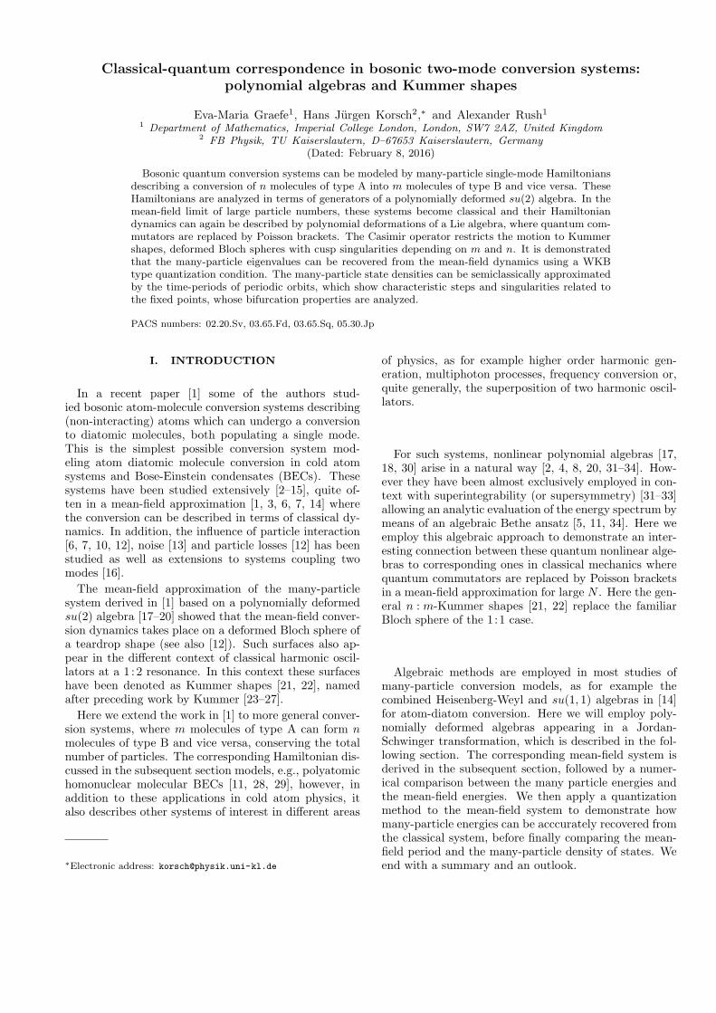
FIG. 1: (Color online) Kummer shapes (45) for selected valuesof m and n.

i.e. a surface of revolution with a sz-dependent radiusr(sz). Following Holm, these surfaces will be denoted asKummer shapes based on previous work by Kummer (see[21, 22, 25–27]), which generalizes the Bloch sphere

s2x + s2y = r2(sz) = 14 − s

2z (46)

for (m,n) = (1, 1) to polynomial algebras. Figure 1shows some examples of these shapes for different val-ues of n and m.

These Kummer shapes are manifolds with the possibleexceptions of the poles s± = (0, 0,± 1

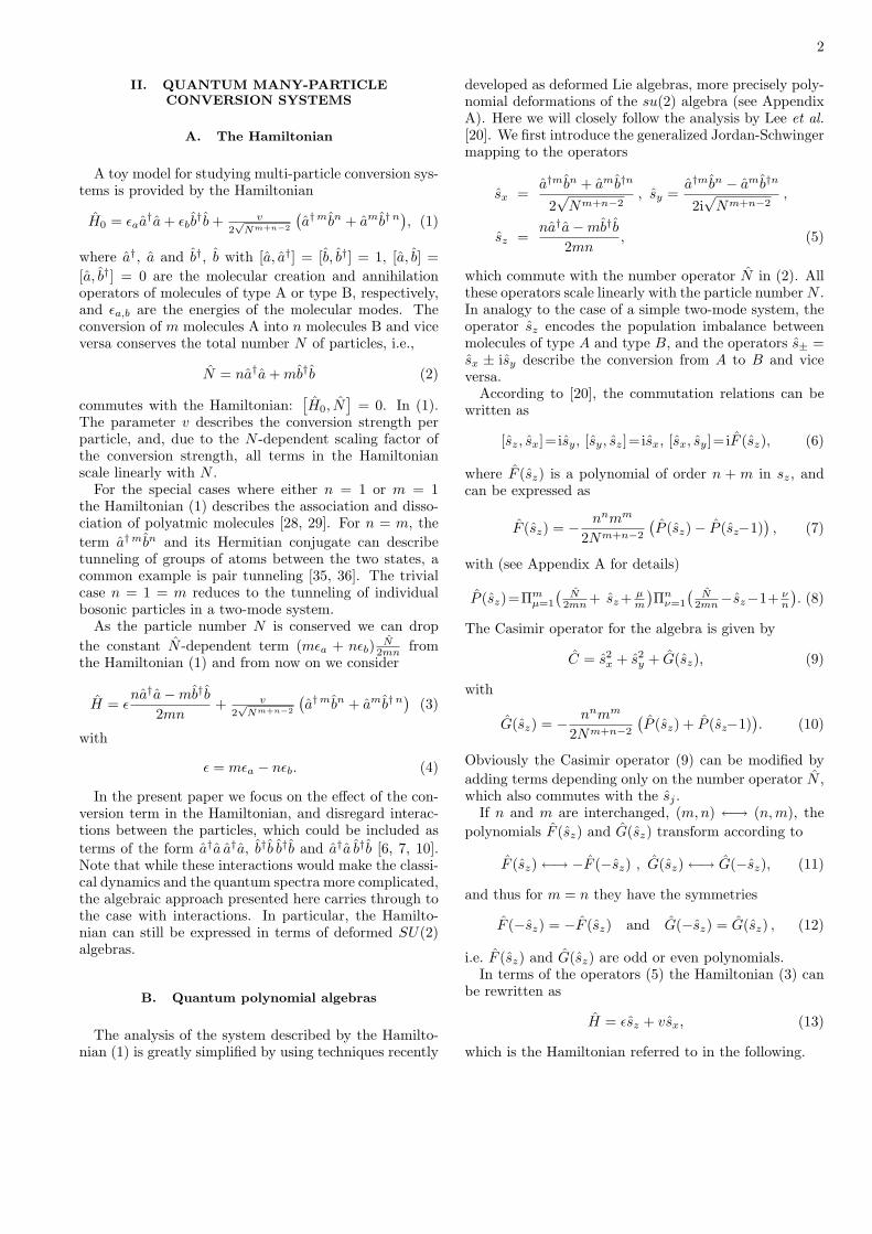
2 ). Here the surfaceis smooth at the north pole s+ for n = 1, and at the southpole s− for m = 1. For n ≥ 2 or m ≥ 2 the surfaces arepinched at these points, where we have a tip for m or nequal to 2 and a cusp for larger values. Figure 2 showsthe radius r(sz) as a function of sz for selected valuesof m and n. The slope of the radius r(sz) at the northpole s+ is infinite for n = 1, and the same holds for thesouth pole for m = 1. For m = 2 the slope at s− is equalto 21−n/2, i.e.

√2 for n = 1, 1 for n = 2 and 1/2 for

n = 4. For n = 2 the slope at s+ is equal to 21−m/2. Form,n > 2 the slope at the poles is zero.

Let us recall that the dynamics generated by theHamiltonian

H = vsx + εsz (47)

follows the equations of motion sj ={sj , H

}, i.e.

sx = −εsy ,sy = εsx − vf(sz) , (48)sz = vsy,

and the conservation of C(sx, sy, sz) restricts the orbitto the Kummer surface (45), and in addition by the con-servation of energy, so that the orbits are geometricallygiven by the intersection of the Kummer shape (45) with

−0.5 0 0.50

0.2

0.4

sz

r(sz)

−0.5 0 0.50

0.2

0.4

sz

r(sz)

FIG. 2: Radius r(sz) of the Kummer surface (45) for (m,n) =(1, 1), (2, 1), (2, 2) (left) and (3, 1), (3, 2), (3, 3) (right).

the surface H(sx, sy, sz) = E, which is a plane for theHamiltonian (36).

As already pointed out in Holm’s book [21] as well as in[37], the Kummer dynamics can be formulated in termsof the Nambu-Poisson bracket, a Lie bracket which alsosatisfies the Leibnitz relation [38]. Using the relation (43)between f(sz) and g(sz), one can rewrite the equationsof motions in terms of the Nambu bracket{

A,B}C

= 12∇C ·

(∇A×∇B

), (49)

where 12∇C = (sx, sy, f(sz)) is the gradient of the

Casimir function given in (42), in the convenient form

A ={A,H

}C, (50)

which immediately reveals the conservation of both theHamiltonian H and the Casimir function C. In addition,the equation of motion for the vector s can be written as

s ={s, H

}C

= 12∇C ×∇H . (51)

Alternatively, one can describe the dynamics in terms ofcanonical variables p and q, where p ∈ [− 1

2 ,12 ] is equal to

sz and q ∈ [0, 2π] is the angle in the sx, sy plane [1]:

sz = p , sx = r(p) cos q , sy = r(p) sin q (52)

with radius (compare (45))

r(p)=r0(

12 +p

)m/2( 12−p

)n/2, r0 =

1√mn−2nm−2

. (53)

Then the dynamics is given by the standard Poissonbracket {A,B} = ∂pA∂qB − ∂qA∂pB and the Hamilto-nian

H(p, q) = εp+ vr(p) cos q . (54)

Note that in this formulation the restriction to the Kum-mer surface (45) is immediately obvious.

Furthermore this canonical description can be conve-niently used as a basis for a semiclassical WKB-typequantization recovering the individual multi-particle en-ergy eigenvalues and eigenstates that we shall perform inSection V.

6

D. Fixed points

Important for the organization of the dynamics bothin classical and quantum mechanics are the fixed pointsof the motion. The fixed points are found at sy = 0and εsx = vf(sz). Squaring this equation, using theconstraint (45) and inserting the expression (31) for f(sz)this can be rewritten as a condition for the sz coordinateof the fixed point

4ε2

v2mn−2nm−2

(12 +sz

)m( 12−sz

)n (55)

=[n(

12 +sz

)m( 12−sz

)n−1 −m(

12 +sz

)m−1( 12−sz

)n]2.

Thus, for n > 1 the north pole is always a fixed point,independently of the parameter values, and for m > 1the same holds for the south pole.

To find the remaining fixed points, we rearrange to findthe condition

16ε2mn−2nm−2 (56)

= v2(

12 +sz

)m−2( 12−sz

)n−2 (2(n+m)sz + n−m)2.

In the special case m = n this simplifies to

ε2m2m−6 = v2(

14 − s

2z

)m−2s2z . (57)

The real roots of the polynomial (56) with − 12 ≤ sz ≤

+ 12 , sx = v

ε f(sz), and sy = 0, yield the fixed points,in addition to those at the poles for m,n > 1. Thatis, the total number of fixed points for a given n and mis bounded by n + m. As we shall see in what follows,however, for n + m ≥ 6 the maximal number of fixedpoints is six.

At a fixed point (apart from those at the poles for nor m larger than one) the energy plane E = vsx + εszis tangential to the Kummer surface, i.e. the slope ofthe straight line sx = (E − εsz)/v must be equal to theslope of r(sz). Thus, we need to determine at how manypoints the slope of r(sz) can have a prescribed value (itis instructive to have a look at figure 2). For this purposeit is useful to divide the Kummer surface in a southernand northern part along the line of maximal radius (the‘equator’). The value of m determines the qualitativebehaviour of the slope on the southern part, the value ofn that on the northern part. Let us consider the southernpart in dependence on m. For m = 1 the slope at thesouth pole is infinite and decreases monotonically to zeroat the equator. That is, there is exactly one value of szcorresponding to each prescribed value of the slope, andthus we have one fixed point on the southern part of theKummer shape. For m = 2 the south pole is a fixed pointfor all parameter values. The slope at the south pole isequal to 21−n/2 and decreases monotonically to zero atthe equator. Thus, there is exactly one point at whichthe energy plane is tangential to the southern part of theKummer shape for ε2/v2 ≤ 22−n and none otherwise.

In total we thus have either one or two fixed points onthe southern part. For m ≥ 3 we always have the samescenario: The south pole is a fixed point for all parametervalues, the slope at the south pole is zero, with increasingsz it increases to a maximum at the point of inflection,after which it decreases to zero at the equator. Thus,for values of |ε/v| smaller than the maximal value of theslope there are two points on the southern part of theKummer shape at which the energy plane is tangentialto the shape, for larger values there is none. In totalthere are thus either one or three fixed points on thesouthern part of the Kummer shape. The same holds forthe northern part in dependence on n. In summary, themaximal number of fixed points for given values of n andm is given by min(n+m, 6).

The character of the fixed points can be determinedfrom the eigenvalues of the Jacobi matrix

λ± = ±√−ε2 − v2f ′(sz) , (58)

which are a complex conjugate pair for a center, in thevicinity of which the motion is a rotation with frequency

ω =√ε2 + v2f ′(sz), (59)

or a pair of real numbers with different signs for a saddlepoint.

At critical parameter values the number of fixed pointschanges. This can happen in two ways at εc:

(i) Two fixed points can coalesce and disappear. Thissaddle-node bifurcation must necessarily occur at the in-flection point sz of r(sz) and the critical value of ε isgiven by the slope at this point: εc = ±vr′(sz).

(ii) Fixed points can enter or leave the system at thepoles in a transcritical bifurcation [1]. Because the slopeof r(sz) at the poles is zero for m,n > 2, this can (forε 6= 0) only happen if m or n is equal to 2, for m = 2at the south pole for εc = v 21−n/2 and for n = 2 at thenorth pole for εc = v 21−m/2. A stability analysis showsthat here a center at the pole changes into a saddle anda new center appears moving away form the pole.

One should note that the sum of the Poincare indices(centers have index +1, saddles index -1, see, e.g., [42])remains constant on the Kummer surface for bifurcationsof type (i), whereas it changes for type (ii).

IV. MEAN-FIELD AND MANY-PARTICLECORRESPONDENCE

Let us now discuss the correspondence between quan-tum many-particle eigenvalues and mean-field dynamicsfor some cases in more detail. We will use the notationp, q introduced at the end of section III C. The allowedmean-field energy interval is bounded by the maximumand minimum of the classical Hamiltonian on the phase

7

space, that is the maximum and minimum of the energies

Ef =v2

εf(pf ) + εpf (60)

at the fixed points pf , that is, the poles or the real solu-tions of the polynomial (56) in the interval [− 1

2 ,+12 ]. For

large values of |ε|, in the supercritical regime, where wehave only two fixed points (at the poles for n,m > 1), themean-field energy interval is E− < E < E+. In the sub-critical regime below the critical value(s) of ε, there areadditional fixed points which correspond to stationaryvalues of the energy, the global extrema are not locatedat the poles in this case. The extrema of the mean-fieldenergy are upper and lower bounds for the many-particleenergies (rescaled by η). The additional stationary valuesdo not correspond to individual many-particle eigenval-ues, but mark lines along which many-particle eigenval-ues accumulate. To demonstrate this correspondence weshow examples of the many-particle spectrum togetherwith the mean-field stationary energies in dependence onthe parameter ε for several values of n and m, corre-sponding to the examples depicted in figure 1, in figures3, 4, and 5.

It is worthwhile to note that in all cases the many-particle eigenvalues are non-degenerate so that all appar-ent crossings are avoided as already observed before foran atom-molecule conversion system [5]. This is simply aconsequence of the fact that the Hamiltonian is tridiago-nal (see section II C) and hence can only have eigenvaluedegeneracies if all off-diagonal elements vanish [44].(1) For (m,n) = (1, 1), i.e. for the dynamics on the Blochsphere, we have f(p) = p and the two fixed points are atp± = ±1/(2

√1 + v2/ε2), q+ = 0, q− = π, which are

both centers with frequency ω =√ε2 + v2 and an energy

E± = H(p±, q±) = ± 12

√ε2 + v2 , (61)

which are upper and lower bounds for the many-particleeigenvalues (rescaled by η).

(2) The case (m,n) = (2, 1), describing the dissociationand association of diatomic molecules, has been analyzedin [1, 14]. Here the Kummer surface

s2x + s2y = r2(p)

= 2(

12 + p

)2( 12 − p

)= 1

4 + 12p− p

2 − 2p3 (62)

has the shape of a teardrop (see figure 1). As discussedbefore, at the north pole it is smooth and there is a tipat the south pole. The slope of r(p) at the south pole isequal to

√2, which is the critical value of±ε/v. Therefore

the supercritical region with only two fixed points is givenby |ε/v| >

√2 (see also [1, 14]). With f(p) = − 1

4 +p+3p2

the equations of motion written in terms of the sj are

sx = −εsy ,sy = εsx − v

(− 1

4 +sz+3s2z), (63)

sz = vsy

−2 0 2−1.5

−1

−0.5

0

0.5

1

1.5

ε

E

−2 0 2−1.5

−1

−0.5

0

0.5

1

1.5

ε

E

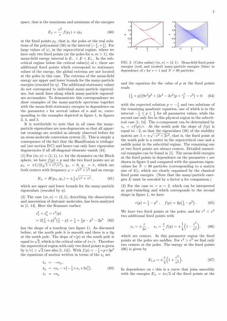
FIG. 3: (Color online) (m,n) = (2, 1) : Mean-field fixed pointenergies (red) and (scaled) many-particle energies (blue) independence of ε for v = 1 and N = 80 particles.

and the equation for the value of p at the fixed pointsreads(

12 + p

)(9v2p2 + (2ε2 − 3v2)p+ v2

4 − ε2)

= 0 (64)

with the expected solution p = − 12 and two solutions of

the remaining quadratic equation, one of which is in theinterval − 1

2 ≤ p ≤ 12 for all parameter values, while the

second one only lies in this physical region in the subcrit-ical case [1, 14]. The x-component can be determined bysx = vf(p)/ε. At the south pole the slope of f(p) isequal to −2, so that the eigenvalues (58) of the stabilitymatrix are λ = ±

√−ε2 + 2v2, that is, the fixed point at

the south pole is a center in the supercritical case and asaddle point in the subcritial regime. The remaining oneor two fixed points are always centers. Detailed numeri-cal examples can be found in [1]. The mean-field energiesat the fixed points in dependence on the parameter ε areshown in figure 3 and compared with the quantum eigen-values for N = 80 particles (corresponding to a matrixsize of 41), which are clearly organized by the classicalfixed point energies. (Note that the many-particle ener-gies E must be rescaled by a factor η for comparison.)

(3) For the case m = n = 2, which can be interpretedas pair-tunneling and which corresponds to the secondshape in figure 1, we have

r(p) = 14 − p

2 , f(p) = 2p(

14 − p

2). (65)

We have two fixed points at the poles, and for ε2 < v2

two additional fixed points with

sz = ± ε

2v, sx =

v

εf(p) = ±1

4

(1− ε2

v2

), (66)

which are centers. In this parameter region the fixedpoints at the poles are saddles. For ε2 > v2 we find onlytwo centers at the poles. The energy at the fixed points(66) is given by

E1,2 = ±v4

(1 +

ε2

v2

). (67)

In dependence on ε this is a curve that joins smoothlywith the energies E± = ±ε/2 of the fixed points at the

8

−1 0 1

−0.5

0

0.5

ε

E

−1 0 1

−0.5

0

0.5

ε

E

FIG. 4: (Color online) (m,n) = (2, 2) : Mean-field fixed pointenergies (red) and (scaled) many-particle energies (blue) independence of ε for v = 1 and N = 160 particles.

poles at the critical values ε = ±v. Figure 4 shows themean-field energies at the fixed points and the quantumeigenvalues for N = 160 particles (corresponding to amatrix size of 41 as in the previous example), which areagain supported by the classical skeleton of fixed pointenergies.

(4) The case (m,n) = (3, 3), corresponding to the thirdshape in figure 1, is more involved. First we have

r(p) = 13

(14 − p

2)3/2

, f(p) = 13p(

14 − p

2)2 (68)

and the fixed points are found from (57), a second orderpolynomial in p2, as

p = ±√

18

(1±

√1− (8ε/v)2

), sx = v

ε f(p) (69)

for (8ε)2 < v2. Note that here we have four fixed pointsin addition to the poles, which is the maximum numberpossible, as discussed above.

Figure 5 shows the energies at the six fixed points in de-pendence of ε. The four non-trivial ones trace out a dou-ble swallow tail curve with four cusps at the critical valuesεc = ±v/8 with energy E = ±v/12

√2 = ±

√2ε/3, which

is slightly smaller than the energy ±ε/2 at the poles. Thefixed points close to the line ±ε are saddle points, thoseon the curved lines passing through E = ±v/24 for ε = 0are centers. At the cusps the character changes, whichcan also be seen from the vanishing of the eigenvalues ofin Jacobi matrix (58). Again, as demonstrated in figure5 for N = 320 particles (Ndim = 41), the classical fixedpoint energies provide a skeleton for the quantum eigen-values.

(5) Finally we will briefly consider the cases (m,n) =(3, 1) and (3, 2) whose energy eigenvalues are shown infigure 6 for N = 120 or 240 particles. Their structureshould be understandable now without presenting theirclassical skeleton.

The figure on the left, for (3, 1), is a combinationof the structures already shown in figures 3 and 5 for(m,n) = (2, 1) and (3, 3), respectively. At the north polethe Kummer surface is smooth and generates no bifurca-tion. At the south pole we find a cusp, leading to a cusp

−0.2 −0.1 0 0.1 0.2−0.1

−0.05

0

0.05

0.1

ε

E

−0.2 −0.1 0 0.1 0.2−0.1

−0.05

0

0.05

0.1

ε

E

FIG. 5: (Color online) (m,n) = (3, 3) : Mean-field fixed pointenergies (red) and (scaled) many-particle energies (blue) independence of ε for v = 1 and N = 360 particles.

−2 −1 0 1 2−1

−0.5

0

0.5

1

ε

E

−0.5 0 0.5

−0.2

0

0.2

ε

E

FIG. 6: (Color online) Many-particle (scaled) energies in de-pendence of ε for v = 1 and (m,n) = (3, 1) (left, N = 120particles) and (m,n) = (3, 2) (right, N = 240 particles).

singularity as in the case (3, 3) showing up in the upperleft and lower right of the (E, ε)-plane.

The figure on the right, for (3, 2), also combines fea-tures discussed before. Again we observe the cusps on theupper left and lower right, but here we also have a tipof the Kummer surface at the north pole, giving rise toa bifurcation and the additional line E = ε/2 as alreadyseen in figures 4 and 5.

V. SEMICLASSICAL QUANTIZATION ANDDENSITY OF STATES

We can recover the many-particle spectrum from themean-field system from a WKB type quantization con-dition as carried out for (m,n) = (1, 1) in [39–41] andfor (m,n) = (2, 1) in [1]. In the case where there is asingle classically allowed region for any given energy thequantization condition is given by

S (ηEν) = 2πη(ν +

12

), (70)

where ν ∈{

0, 1, 2, . . . , Nmn}

, and where S(ηE) denotesthe phase space area enclosed by the orbit correspondingto the mean-field energy H = ηE.

It is useful to introduce the mean-field momentum ‘po-tential functions’ U±(p), which are the maximum andminimum curves of the Hamiltonian with respect to theangle variable q, given by

U±(p) = εp± v r(p). (71)

9

-0.5 0 0.5p

0

0.5

1

E

-0.5 0 0.5p0

2

4

6

q

-0.2

0

0.2

0.4

0.6

-0.5 0 0.5p0

2

4

6

q

-0.5 0 0.5p0

2

4

6

q

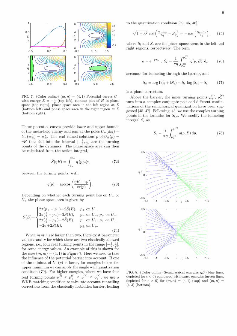
FIG. 7: (Color online) (m,n) = (4, 1) Potential curves U±with energy E = − 1

4(top left), contour plot of H in phase

space (top right), phase space area in the left region at E(bottom left) and phase space area in the right region at E(bottom right).

These potential curves provide lower and upper boundsof the mean-field energy and join at the poles U+(± 1

2 ) =U−(± 1

2 ) = ± ε2 . The real valued solutions p of U±(p) =

ηE that fall into the interval [− 12 ,

12 ] are the turning

points of the dynamics. The phase space area can thenbe calculated from the action integral,

S(ηE) =∫ p+

p−

q (p) dp, (72)

between the turning points, with

q(p) = arccos(ηE − εpvr(p)

). (73)

Depending on whether each turning point lies on U− orU+ the phase space area is given by

S(E)=

2π(p+ − p−)−2S(E), p± on U−,

2π( 12 − p−)−2S(E), p− on U−, p+ on U+,

2π( 12 + p+)−2S(E), p− on U+, p+ on U−,

−2π+2S(E), p± on U+.

(74)Whenm or n are larger than two, there exist parameter

values ε and v for which there are two classically allowedregions, i.e., four real turning points in the range [− 1

2 ,12 ],

for some energy values. An example of this is shown forthe case (m,m) = (4, 1) in Figure 7. Here we need to takethe influence of the potential barrier into account. If oneof the minima of U−(p) is lower, for energies below theupper minimum we can apply the single well quantizationcondition (70). For higher energies, where we have fourreal turning points p(l)

− ≤ p(l)+ ≤ p

(r)− ≤ p

(r)+ , we use a

WKB matching condition to take into account tunnellingcorrections from the classically forbidden barrier, leading

to the quantization condition [39, 45, 46]√1 + κ2 cos

(Sl+Sr

2η − Sφ)

= − cos(Sl−Sr

2η

), (75)

where Sl and Sr are the phase space areas in the left andright regions, respectively. The term

κ = e−πSε , Sε =1πη

∫ p(r)−

p(l)+

|q(p,E)|dp (76)

accounts for tunneling through the barrier, and

Sφ = arg Γ( 12 + iSε)− Sε log |Sε|+ Sε (77)

is a phase correction.Above the barrier, the inner turning points p(l)

+ , p(r)−

turn into a complex conjugate pair and different contin-uations of the semiclassical quantization have been sug-gested [45–47]. Following [45] we use the complex turningpoints in the formulas for Sl,r. We modify the tunnelingintegral Sε as

Sε =iπη

∫ p(r)−

p(l)+

q(p,E) dp, (78)

-1.5 -1 -0.5 0 0.5 1 1.5!-0.5

0

0.5

" E

-1.5 -1 -0.5 0 0.5 1 1.5!

-0.5

0

0.5

" E

FIG. 8: (Color online) Semiclassical energies ηE (blue lines,depicted for ε < 0) compared with exact energies (green lines,depicted for ε > 0) for (m,n) = (4, 1) (top) and (m,n) =(4, 3) (bottom).

10

such that the quantity κ is positive above the barrier. Inequation (75) we take the real parts of the actions Sr,land Sφ.

Analogous quantization rules can be applied when theupper potential curve has two maxima.

The results of the semiclassical quantization in com-parison with the numerically exact many-particle eigen-values for different values of m and n are shown in figure8. We observe an excellent agreement, including very wellreproduced avoided crossings as we vary the parameterε.

Let us finally turn to a discussion of the many-particledensity of states, which can be obtained from the mean-field dynamics on the basis of a semiclassical argument[1]. The many-particle density of states ρ(E) at a scaledenergy E is (approximately) related to the mean-fieldperiod T (E) = dS/dE of the orbit by

ρ(E)≈ 12π T (E)=

1π

∫ p+

p−

dp√(U+(p)−E)(E−U−(p))

, (79)

where U± are the potential functions (71), and p± are theturning points, the real valued solutions of U±(p) = Efalling into the interval [− 1

2 ,+12 ]. The function under the

square root in (79),

(U+(p)− E)(E − U−(p)) = v2r2(p)− (E − εp)2, (80)

is a polynomial of order m + n in p and the integral(79) can be evaluated in closed form for (m,n) = (1, 1)and (m,n) = (2, 1) [1, 39]. The mean-field period T (E)given by the integral (79) can be efficiently evaluatedby means of a Gauss-Mehler quadrature. If the fixedpoint is a center, T (E)/2π is given by the inverse fre-quency ω =

√ε2 + v2f ′(pc) at the center pc (see (59)).

In the subcritical parameter region, the period T di-verges logarithmically at the saddle point energies, as al-ready observed before for dynamics on the Bloch spherem = n = 1 in the presence of interactions [39, 43], and for(m,n) = (2, 1) [1]. Therefore the quantum energy eigen-values accumulate at the all-molecule configurations inthis regime. Such a level bunching at the classical saddlepoint energy in this limit can be related to a quantumphase transition [6, 14, 48]. We shall now demonstratethis behaviour for several examples.

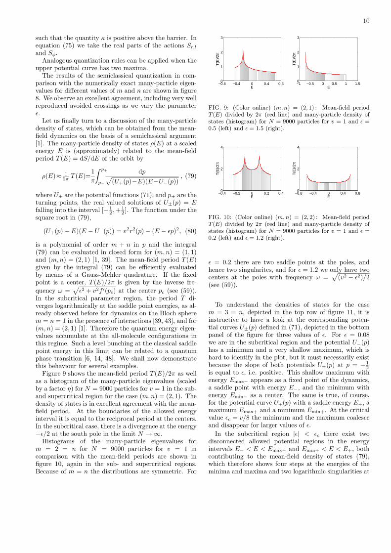
Figure 9 shows the mean-field period T (E)/2π as wellas a histogram of the many-particle eigenvalues (scaledby a factor η) for N = 9000 particles for v = 1 in the sub-and supercritical region for the case (m,n) = (2, 1). Thedensity of states is in excellent agreement with the mean-field period. At the boundaries of the allowed energyinterval it is equal to the reciprocal period at the centers.In the subcritical case, there is a divergence at the energy−ε/2 at the south pole in the limit N →∞.

Histograms of the many-particle eigenvalues form = 2 = n for N = 9000 particles for v = 1 incomparison with the mean-field periods are shown infigure 10, again in the sub- and supercritical regions.Because of m = n the distributions are symmetric. For

−0.8 −0.4 0 0.4 0.80

1

2

3

E

T(E

)/2π

−1 −0.5 0 0.5 1 1.50

1

2

3

E

T(E

)/2π

FIG. 9: (Color online) (m,n) = (2, 1) : Mean-field periodT (E) divided by 2π (red line) and many-particle density ofstates (histogram) for N = 9000 particles for v = 1 and ε =0.5 (left) and ε = 1.5 (right).

−0.4 −0.2 0 0.2 0.40

2

4

E

T(E

)/2π

−0.8 −0.4 0 0.4 0.80

2

4

E

T(E

)/2π

FIG. 10: (Color online) (m,n) = (2, 2) : Mean-field periodT (E) divided by 2π (red line) and many-particle density ofstates (histogram) for N = 9000 particles for v = 1 and ε =0.2 (left) and ε = 1.2 (right).

ε = 0.2 there are two saddle points at the poles, andhence two singularites, and for ε = 1.2 we only have twocenters at the poles with frequency ω =

√(v2 − ε2)/2

(see (59)).

To understand the densities of states for the casem = 3 = n, depicted in the top row of figure 11, it isinstructive to have a look at the corresponding poten-tial curves U±(p) defined in (71), depicted in the bottompanel of the figure for three values of ε. For ε = 0.08we are in the subcritical region and the potential U−(p)has a minimum and a very shallow maximum, which ishard to identify in the plot, but it must necessarily existbecause the slope of both potentials U±(p) at p = − 1

2is equal to ε, i.e. positive. This shallow maximum withenergy Emax− appears as a fixed point of the dynamics,a saddle point with energy E−, and the minimum withenergy Emin− as a center. The same is true, of course,for the potential curve U+(p) with a saddle energy E+, amaximum Emax+ and a minimum Emin+. At the criticalvalue εc = v/8 the minimum and the maximum coalesceand disappear for larger values of ε.

In the subcritical region |ε| < εc there exist twodisconnected allowed potential regions in the energyintervals E− < E < Emax− and Emin+ < E < E+, bothcontributing to the mean-field density of states (79),which therefore shows four steps at the energies of theminima and maxima and two logarithmic singularities at

11

−0.08 −0.04 0 0.04 0.08 0

20

40

E

T(E

)/2π

−0.08 −0.04 0 0.04 0.08 0

20

40

E

T(E

)/2π

−0.08 −0.04 0 0.04 0.08 0

20

40

E

T(E

)/2π

−0.5 0 0.5−0.1

0

0.1

p

U±(p

)

−0.5 0 0.5−0.1

0

0.1

p

U±(p

)

−0.5 0 0.5−0.1

0

0.1

p

U±(p

)

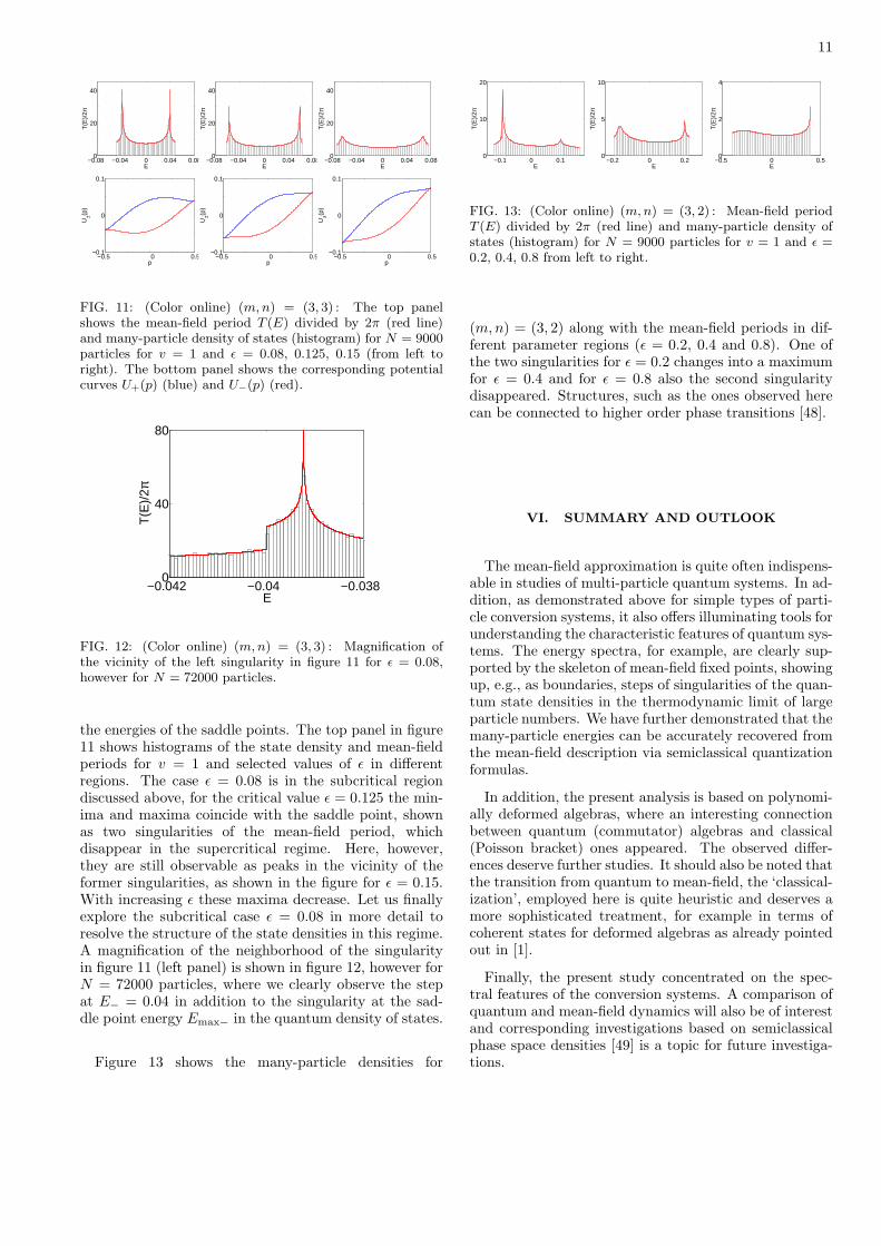
FIG. 11: (Color online) (m,n) = (3, 3) : The top panelshows the mean-field period T (E) divided by 2π (red line)and many-particle density of states (histogram) for N = 9000particles for v = 1 and ε = 0.08, 0.125, 0.15 (from left toright). The bottom panel shows the corresponding potentialcurves U+(p) (blue) and U−(p) (red).

−0.042 −0.04 −0.0380

40

80

E

T(E

)/2π

FIG. 12: (Color online) (m,n) = (3, 3) : Magnification ofthe vicinity of the left singularity in figure 11 for ε = 0.08,however for N = 72000 particles.

the energies of the saddle points. The top panel in figure11 shows histograms of the state density and mean-fieldperiods for v = 1 and selected values of ε in differentregions. The case ε = 0.08 is in the subcritical regiondiscussed above, for the critical value ε = 0.125 the min-ima and maxima coincide with the saddle point, shownas two singularities of the mean-field period, whichdisappear in the supercritical regime. Here, however,they are still observable as peaks in the vicinity of theformer singularities, as shown in the figure for ε = 0.15.With increasing ε these maxima decrease. Let us finallyexplore the subcritical case ε = 0.08 in more detail toresolve the structure of the state densities in this regime.A magnification of the neighborhood of the singularityin figure 11 (left panel) is shown in figure 12, however forN = 72000 particles, where we clearly observe the stepat E− = 0.04 in addition to the singularity at the sad-dle point energy Emax− in the quantum density of states.

Figure 13 shows the many-particle densities for

−0.1 0 0.10

10

20

E

T(E

)/2π

−0.2 0 0.20

5

10

E

T(E

)/2π

−0.5 0 0.50

2

4

E

T(E

)/2π

FIG. 13: (Color online) (m,n) = (3, 2) : Mean-field periodT (E) divided by 2π (red line) and many-particle density ofstates (histogram) for N = 9000 particles for v = 1 and ε =0.2, 0.4, 0.8 from left to right.

(m,n) = (3, 2) along with the mean-field periods in dif-ferent parameter regions (ε = 0.2, 0.4 and 0.8). One ofthe two singularities for ε = 0.2 changes into a maximumfor ε = 0.4 and for ε = 0.8 also the second singularitydisappeared. Structures, such as the ones observed herecan be connected to higher order phase transitions [48].

VI. SUMMARY AND OUTLOOK

The mean-field approximation is quite often indispens-able in studies of multi-particle quantum systems. In ad-dition, as demonstrated above for simple types of parti-cle conversion systems, it also offers illuminating tools forunderstanding the characteristic features of quantum sys-tems. The energy spectra, for example, are clearly sup-ported by the skeleton of mean-field fixed points, showingup, e.g., as boundaries, steps of singularities of the quan-tum state densities in the thermodynamic limit of largeparticle numbers. We have further demonstrated that themany-particle energies can be accurately recovered fromthe mean-field description via semiclassical quantizationformulas.

In addition, the present analysis is based on polynomi-ally deformed algebras, where an interesting connectionbetween quantum (commutator) algebras and classical(Poisson bracket) ones appeared. The observed differ-ences deserve further studies. It should also be noted thatthe transition from quantum to mean-field, the ‘classical-ization’, employed here is quite heuristic and deserves amore sophisticated treatment, for example in terms ofcoherent states for deformed algebras as already pointedout in [1].

Finally, the present study concentrated on the spec-tral features of the conversion systems. A comparison ofquantum and mean-field dynamics will also be of interestand corresponding investigations based on semiclassicalphase space densities [49] is a topic for future investiga-tions.

12

APPENDIX A: POLYNOMIAL DEFORMATIONSOF su(2)

The deformed algebra is generated by the three ele-ments J0 = J†0 , J+ = J†− satisfying

[J0, J±] = ±J± , [J+, J−] = 2F (J0) , (A1)

where [ . , . ] is the commutator, and F (J0) =∑kj=0 αj J

j0

is a polynomial of order k. For F (J0) = J0 we have[J+, J−] = 2J0, i.e. the Lie algebra su(2), so that wehave a polynomial deformation of su(2). Similar to theSchwinger representation of su(2) the deformed su(2) al-gebras can be represented via two-mode bosonic creationand annihilation operators [17, 20] according to equations(5). Using the well known properties of the oscillator al-gebra one obtains the commutator[am, a†m

]= Πm

µ=1(a†a+ µ)−Πmµ=1(a†a+ 1− µ), (A2)

which is a polynomial of the number operator a†a whoseleading order term is[

am, a†m]

= m2(a†a)m−1 + . . . . (A3)

It can be shown that the Casimir operator of the de-formed su(2) algebra is given by

C = J−J+ + φ(J0) (A4)

where φ(J0) is a polynomial in J0 of order k + 1 withφ(0) = 0, which can be expressed in terms of Bernoullipolynomials Bn(z) and Bernoulli numbers Bn = Bn(0)as

φ(J0) = 2k∑j=0

(−1)j+1

j + 1αj(Bj+1(−J0)−Bj+1

), (A5)

related to F (J0) by

F (J0) = 12

(φ(J0)− φ(J0 − 1)

). (A6)

(see, e.g., [30] and references therein). Up to third order,k = 3, (A5) yields

φ(J0) =(

2α0 + α1 + α23

)J0 +

(α1 + α2 + α3

2

)J2

0

+(

2α23 + α3

)J3

0 + α32 J

40 (A7)

(see also [32, 33]). Alternatively, with

Jx = 12

(J+ + J−

), Jy = 1

2i

(J+ − J−

), Jz = J0 , (A8)

and

[Jy, Jz] = iJx , [Jz, Jx] = iJy , [Jx, Jy] = i F (Jz) (A9)

the Casimir (A4) is written as

C = J2x+J2

y−F (Jz)+φ(Jz)

= J2x+J2

y+ 12

(φ(Jz)+φ(Jz−1)

). (A10)

For polynomials up to third order (A7) implies

C = J2x + J2

y − α0 +(

2α0 + α23

)Jz

+(α1 + α3

2

)J2z + 2α2

3 J3z + α3

2 J4z . (A11)

For the linear case F (Jz) = Jz we have φ(Jz) = Jz + J2z

and C = J2x + J2

y + J2z .

The commutator and the Casimir operator can alter-natively be expressed using an auxiliary polynomial oforder m+ n in N

2mn and sz defined as

P (Jz)=m∏µ=1

( N2mn+Jz+ µ

m )n∏ν=1

( N2mn−Jz−1+ ν

n ),(A12)

with

P (Jz)←→ P (−Jz − 1) for (m,n)←→ (n,m).(A13)

We then define the operator functions

F (Jz) = − nnmm

2Nm+n−2

(P (Jz)− P (Jz − 1)

),(A14)

G(Jz) = − nnmm

2Nm+n−2

(P (Jz) + P (Jz − 1)

). (A15)

From (A13) we find

F (Jz)←→ −F (−Jz) , G(Jz)←→ G(−Jz) (A16)

for (m,n) ←→ (n,m) and therefore for m = n the sym-metries

F (−Jz) = −F (Jz) and G(−Jz) = G(Jz) , (A17)

i.e. F (Jz) and G(Jz) are odd or even polynomials. Theleading order term of the polynomials P (Jz) and P (Jz −1) is equal to (−1)n+1J

(m+n)z and hence G(Jz) or F (Jz)

are polynomials in Jz of order m + n or m + n − 1, re-spectively. The function F is the one appearing in thecommutator (A1) and the Casimir operator can be writ-ten as

C = J2x + J2

y + G(Jz). (A18)

It should be noted that the relations above depend on theLie bracket of the algebra. They are derived for the com-mutator bracket and are different for the Poisson bracket(see the footnote in [17]). In both cases we find a relationbetween the polynomial F (Jz) or f(sz) appearing in thepolynomial extension of the Lie brackets and the polyno-mial G(Jz) or g(sz) appearing in the Casimir operator.This relation is simple in the classical algebra, namelyg′(sz) = 2f(sz) (see equation (43), and more elaboratein the quantum algebra.

13

Let us finally evaluate the leading terms in the limitof large N . With the abbreviations A± = N

2mn ± Jz oneobtains from (A12) and (A14), (A15)

P (Jz) = Am+ An− − n−1

2 Am+ An−1−

+m+12 Am−1+ An− + . . . (A19)

P (Jz − 1) = Am+ An− + n+1

2 Am+ An−1−

−m−12 Am−1+ An− + . . . (A20)

and

F (Jz)=nnmm(n Am+ A

n−1− −mAm−1

+ An−+. . .)2Nm+n−2

(A21)

G(Jz)=−nnmm(Am+ A

n− + . . .)

2Nm+n−2. (A22)

ACKNOWLEDGMENTS

The authors thank Kevin Rapedius for valuable com-ments on the manuscript. E.M.G. acknowledges sup-port from the Royal Society via a University ResearchFellowship (Grant. No. UF130339). A.R. acknowl-edges support from the Engineering and Physical Sci-ences Research Council via the Doctoral Research Allo-cation Grant No. EP/K502856/1.

[1] E. M. Graefe, M. Graney, and A. Rush, Phys. Rev. A 92(2015) 012121

[2] V. P. Karassiov and A. B. Klimov, Phys. Lett. A 191(1998) 117

[3] A. Vardi, V. A. Yurovsky, and J. R. Anglin, Phys. Rev.A 64 (2001) 063611

[4] V. P. Karassiov, A. A. Gusev, and S. I. Vinitsky, Phys.Lett. A 295 (2002) 247

[5] H.-Q. Zhou, J. Links, and R. H. McKenzie, Int. J. Mod.Phys. B 17 (2003) 5819

[6] G. Santos, A. Tonel, A. Foerster, and J. Links, Phys.Rev. A 73 (2006) 023609

[7] J. Li, D.-F. Ye, C. Ma, L.-B. Fu, and J. Liu, Phys. Rev.A 79 (2009) 025602

[8] J. Liu and B. Liu, Front. Phys. China 5 (2010) 123[9] C. Khripkov and A. Vardi, Phys. Rev. A 84 (2011)

021606[10] S.-C. Li and L.-B. Fu, Phys. Rev. A 84 (2011) 023605[11] G. Santos, J. Phys. A 44 (2011) 345003[12] B. Cui, L. C. Wang, and X. X. Yi, Phys. Rev. A 85

(2012) 013618[13] H. Z. Shen, X.-M. Xiu, and X. X. Yi, Phys. Rev. A 87

(2013) 063613[14] P. Perez-Fernandez, P. Cejnar, J. M. Arias, J. Dukelsky,

J. E. Garcıa-Ramos, and A. Relano, Phys. Rev. A 83(2011) 033802

[15] E. A. Donley, N. R. Claussen, S. T. Thompson, and C. E.Wieman, Nature 417 (2002) 529

[16] A. Relano, J. Dukelsky, P. Perez-Fernandez, and J. M.Arias, Phys. Rev. E 90 (2014) 042139

[17] M. Rocek, Phys. Lett. B 255 (1991) 554[18] A. P. Polychronakos, Mod. Phys. Lett. A 5 (1990) 2325[19] D. Bonatsos, P. Kolokotronis, C. Daskaloyannis,

A. Ludu, and C. Quesne, Czech. J. Phys. 46 (1996) 1189[20] Y.-H. Lee, W.-L. Yang, and Y.-Z. Zhang, J. Phys. A 43

(2010) 185204[21] D. D. Holm, Geometric Mechanics Part I: Dynamics and

Symmetry, Imperial College Press, London, 2011[22] D. D. Holm and C. Vizman, J. Geom. Mech. 4 (2012)

297

[23] M. Kummer, Comm. Math. Phys. 48 (1976) 53[24] M. Kummer, Comm. Math. Phys. 58 (1978) 85[25] M. Kummer, Indiana Univ. Math. J. 30 (1981) 281[26] M. Kummer, in Local and Global Methods in Nonlinear

Dynamics, Lecture notes in Physics, Vol. 252, edited byA. V. Saenz, page 19. Springer, New York, 1986

[27] M. Kummer, J. Diff. Eq 83 (1990) 220[28] F.-Q. Dou, S.-C. Li, H. Cao, and L.-B. Fu, Phys. Rev. A

85 (2012) 023629[29] F. Q. Dou, L. B. Fu, and J. Liu, Phys. Rev. A 87 (2013)

043631[30] C. Delbecq and C. Quesne, J. Phys. A 26 (1993) L127[31] N. Debergh, J. Phys. A 31 (1998) 4013[32] N. Debergh, J. Phys. A 33 (2000) 7109[33] J. Beckers, Proceedings of Institute of Mathematics of

NAS of Ukraine 30 (2000) 275[34] J. Links, H.-Q. Zhou, R. H. McKenzie, and M. D. Gould,

J. Phys. A 36 (2003) R63[35] G. Mazzarella, S. M. Giampaolo, and F. Illuminati, Phys.

Rev. A 73 (2006) 013625[36] M. Eckholt and J. J. Garcia-Ripoll, Phys. Rev. A 77

(2008) 063603[37] A. Odzijewicz, in Int. Conf: Quantum control, exact per-

turbative, linear or nonlinear, 2014. see http://pluton.

fis.cinvestav.mx/Bogdan50/2014Meksyk_Kummer.pdf

[38] D. D. Holm, Geometric Mechanics Part II: Rotating,Translating and Rolling, Imperial College Press, London,2011

[39] E. M. Graefe and H. J. Korsch, Phys. Rev. A 76 (2007)032116

[40] F. Nissen and J. Keeling, Phys. Rev. A 81 (2010) 063628[41] L. Simon and W. T. Strunz, Phys. Rev. A 86 (2012)

053625[42] V. I. Arnold, Ordinary differential equations, Springer,

Berlin, New York, 2006[43] E.-M. Graefe, H. J. Korsch, and M. P. Strzys, J. Phys. A

47 (2014) 085304[44] J. H. Wilkinson, The Algebraic Eigenvalue Problem, Ox-

ford University Press, Oxford, 1965[45] N. Froman, P. O. Froman, U. Myhrman, and R. Paulsson,

14

Ann. Phys. (N.Y.) 74, 314 (1972).[46] M. S. Child, Semiclassical mechanics with molecular ap-

plications (Oxford University Press, Oxford, 1991).[47] M. S. Child, J. Molec. Spec. 53, 280 (1974).[48] P. Stransky, M. Macek, and P. Cejnar, Ann. Phys. 345

73 (2014)[49] F. Trimborn, D. Witthaut, and H. J. Korsch, Phys. Rev.

A 77 (2008) 043631