Embed Size (px)
Citation preview
Structural Response to
Vapour Cloud Explosions
Anqi Chen
Department of Civil and Environmental Engineering
Imperial College London
A thesis submitted for the degree of
Doctor of Philosophy
2014
Abstract
Over the last few decades, a number of major industrial blast accidents
involving oil and gas installations occurred worldwide. These include
the blast explosion that occurred in an industrial facility at Buncefield
in the United Kingdom in 2005. Extensive damage occurred due to
the blast, both to the industrial plant and surrounding buildings, as
a consequence of much higher overpressures than would normally be
expected from a vapour cloud explosion of this nature. In response
to this event, a great deal of work was carried out on collecting and
analysing available evidence from the incident in order to understand
the explosion mechanism and estimate the overpressure levels within
the gas cloud that formed. Subsequent investigations included the
examination of steel switch boxes on the site located within the area
covered by the vapour cloud. These boxes suffered varying degrees
of damage and could therefore be used as overpressure indicators. A
series of tests were commissioned after the event in order to compare
the damage of the field boxes with detonation tests on similar boxes.
The thesis firstly reports on numerical studies carried out on assess-
ing the damage to steel boxes subjected to both detonation and de-
flagration scenarios in order to aid the investigation of the explo-
sion. Several modelling approaches are adopted in the numerical stud-
ies, including: Pure Lagrangian, Uncoupled Lagrangian-Eulerian and
Coupled Lagrangian-Eulerian techniques. The numerical models are
validated against data collected from gas detonation experiments on
similar steel boxes. It is found that the coupled approach is able to
predict the results accurately, although such an approach cannot be
used in detailed parametric investigations due to its prohibitive com-
putational demand. The pure Lagrangian approach is therefore used
instead, but the overpressure range in the parametric assessments is
limited to 4 bar (side-on) as an adequate level of accuracy from this
modelling technique cannot be ensured beyond this range. The re-
sults are summarised in the form of pressure-impulse diagrams, and
typical residual shapes are selected with the aim of aiding forensic
investigations of future explosion incidents.
The investigation is extended thereafter to the response of a steel-
clad portal frame structures located outside the gas cloud and which
suffered varying degrees of damage. A typical warehouse building is
studied through a pure Lagrangian approach. A non-linear finite el-
ement model of a representative sub-structure of the warehouse wall
is validated against a full scale test carried out at Imperial College
London. A series of pressure-impulse diagrams of the sub-structure
is then constructed based on the results of parametric non-linear dy-
namic assessments using the developed numerical model under various
combinations of overpressures and impulses. A new failure criterion
based on the total failure of the self-tapping screws is proposed in
conjunction with pressure-impulse diagrams. This failure condition
provides a more direct assessment of the damage to the side walls of
the warehouse. The pressure-impulse diagrams can be used to assess
the response of a typical warehouse structure to blast loading, and
to provide some guidance on the safe siting in a hazardous environ-
ment around oil and storage sites. Simplified approaches based on
single degree of freedom representations are also employed, and their
results are compared with those from the detailed non-linear finite el-
ement models. The findings show that the simplified approaches offer
a reasonably reliable and practical tool for predicting the response of
the side rails. However, it is illustrated that such idealisations are
not suited for assessing the ultimate response of cladding panels, as
the side rail-cladding interactions cannot be captured by simplified
approaches and necessitate the deployment of detailed numerical pro-
cedures.

Declaration of Originality
I hereby declare that this thesis and the work reported herein was
composed by and originated entirely from me. Information derived
from the published and unpublished work of others has been
acknowledged in the text and references are given in the list of
sources.
Copyright Declaration
The copyright of this thesis rests with the author and is made
available under a Creative Commons Attribution Non-Commercial
No Derivatives licence. Researchers are free to copy, distribute or
transmit the thesis on the condition that they attribute it, that they
do not use it for commercial purposes and that they do not alter,
transform or build upon it. For any reuse or redistribution,
researchers must make clear to others the licence terms of this work.

I would like to dedicate this thesis to my loving parents Jun and
Zhengming, and my dear wife Lijia for their love and support.

Acknowledgements
I would like to express my deepest gratitude and appreciation to
my supervisors Dr Luke Louca and Prof Ahmed Elghazouli for their
continuous encouragement, involvement, fruitful advice and support
throughout my research steps. I greatly appreciate they provided me
with the opportunity of research and working with them in such an
excellent environment at Civil Engineering Department of Imperial
College London.
I would like to acknowledge the financial and mental support I received
from my parents and my wife without them this work would have
never been completed.
I would like to also acknowledge the technical support from Dr Gra-
ham Atkinson from Health and Safety Laboratory, Dr Bassam Burgan
from Steel Construction Institute and Mr Bob Simpson from Health
and Safety Executive.
Finally, the test data used to validate the model for the analysis of
instrument boxes was generated in a Joint Industry Project entitled
“Dispersion and Explosion Characteristics of Large Vapour Clouds”.
The project was managed by the Steel Construction Institute and
sponsored by:
• BP Exploration Operating Company Limited
• Health and Safety Executive (UK)
• Petrleo Brasileiro S.A. Petrobras
• Shell Research Limited
• Statoil Petroelum AS

• Total Refining and Chemicals
• Le Ministre de Lcologie, du Dveloppement Durable, des Trans-
ports et du Logement (France)
• National Institute for Public Health and The Environment (Nether-
lands)
The author wishes to thank the sponsors for allowing this data to be
used in the present research.
Contents
Contents vii
List of Figures xiii
Nomenclature xxix
1 Introduction 1
1.1 Background . . . . . . . . . . . . . . . . . . . . . . . . . . . . . . 1
1.2 Buncefield incident . . . . . . . . . . . . . . . . . . . . . . . . . . 3
1.3 Motivation and objectives . . . . . . . . . . . . . . . . . . . . . . 4
2 Literature review 8
2.1 Vapour cloud explosion . . . . . . . . . . . . . . . . . . . . . . . . 8
2.1.1 Explosion mechanisms . . . . . . . . . . . . . . . . . . . . 8
2.1.2 Methods for explosion analysis . . . . . . . . . . . . . . . . 11
2.2 Review of past incidents . . . . . . . . . . . . . . . . . . . . . . . 15
2.2.1 Buncefield incident . . . . . . . . . . . . . . . . . . . . . . 15
2.2.2 Other major accidents . . . . . . . . . . . . . . . . . . . . 18
2.3 Blast wave and loading . . . . . . . . . . . . . . . . . . . . . . . . 19
2.3.1 Blast wave characteristics . . . . . . . . . . . . . . . . . . 20
2.3.1.1 Normal shock . . . . . . . . . . . . . . . . . . . . 20
2.3.1.2 Blast wave and scaling law . . . . . . . . . . . . . 26
2.3.2 Dynamic blast loads . . . . . . . . . . . . . . . . . . . . . 29
2.3.2.1 Front surface load . . . . . . . . . . . . . . . . . 30
2.3.2.2 Rear surface load . . . . . . . . . . . . . . . . . . 32
vii
CONTENTS
2.3.2.3 Top and side surface loads . . . . . . . . . . . . . 32
2.3.2.4 Loads on the frame . . . . . . . . . . . . . . . . . 32
2.3.2.5 Non-ideal blast wave . . . . . . . . . . . . . . . . 35
2.4 Structural response . . . . . . . . . . . . . . . . . . . . . . . . . . 36
2.4.1 Analysis methods . . . . . . . . . . . . . . . . . . . . . . . 36
2.4.1.1 Single degree of freedom method . . . . . . . . . 36
2.4.1.2 Pressure - impulse diagram . . . . . . . . . . . . 43
2.4.1.3 Finite element method . . . . . . . . . . . . . . . 45
2.4.2 Material properties at high strain rate . . . . . . . . . . . 46
2.4.3 Modelling structural components . . . . . . . . . . . . . . 47
2.5 Design guidelines . . . . . . . . . . . . . . . . . . . . . . . . . . . 52
3 Numerical tools 54
3.1 Non-linear finite element method . . . . . . . . . . . . . . . . . . 54
3.2 Solution methods for non-linear FE problems . . . . . . . . . . . . 59
3.2.1 Newton - Raphson method . . . . . . . . . . . . . . . . . . 60
3.2.2 Arc length method . . . . . . . . . . . . . . . . . . . . . . 61
3.2.3 Explicit direct integration method . . . . . . . . . . . . . . 63
3.3 Eulerian analysis for blast wave . . . . . . . . . . . . . . . . . . . 64
3.4 Approaches for study of blast responses . . . . . . . . . . . . . . . 66
3.4.1 Lagrangian approach . . . . . . . . . . . . . . . . . . . . . 68
3.4.2 Uncoupled Eulerian - Lagrangian approach . . . . . . . . . 69
3.4.3 Coupled Eulerian - Lagrangian approach . . . . . . . . . . 69
3.5 Numerical model validations . . . . . . . . . . . . . . . . . . . . 69
3.5.1 One dimensional model . . . . . . . . . . . . . . . . . . . . 70
3.5.2 Blast wave propagation . . . . . . . . . . . . . . . . . . . . 72
3.5.3 Reflection of ideal blast wave . . . . . . . . . . . . . . . . 73
3.5.4 Square plate subjected to close HE explosion . . . . . . . . 76
3.6 Finite element analysis packages . . . . . . . . . . . . . . . . . . . 82
4 Blast response of field objects 85
4.1 Experimental observations . . . . . . . . . . . . . . . . . . . . . . 86
4.1.1 Steel switch boxes . . . . . . . . . . . . . . . . . . . . . . . 87
viii
CONTENTS
4.1.1.1 Box150 . . . . . . . . . . . . . . . . . . . . . . . 87
4.1.1.2 Box200 . . . . . . . . . . . . . . . . . . . . . . . 88
4.1.2 TNT detonation tests . . . . . . . . . . . . . . . . . . . . . 89
4.1.3 Gas detonation tests . . . . . . . . . . . . . . . . . . . . . 91
4.2 Numerical methodology . . . . . . . . . . . . . . . . . . . . . . . 98
4.2.1 Numerical model of boxes . . . . . . . . . . . . . . . . . . 98
4.2.1.1 Model of Box150 . . . . . . . . . . . . . . . . . . 98
4.2.1.2 Model of Box200 . . . . . . . . . . . . . . . . . . 101
4.2.2 Lagrangian analysis . . . . . . . . . . . . . . . . . . . . . . 101
4.2.2.1 Consideration of internal pressure . . . . . . . . . 105
4.2.3 Uncoupled Eulerian - Lagrangian analysis . . . . . . . . . 106
4.2.4 Coupled Eulerian - Lagrangian analysis . . . . . . . . . . . 110
4.2.5 Comparison of computational demands . . . . . . . . . . . 111
4.3 Comparative assessment . . . . . . . . . . . . . . . . . . . . . . . 112
4.3.1 Comparison of numerical results . . . . . . . . . . . . . . . 112
4.3.1.1 Blast wave and dynamic loading . . . . . . . . . 113
4.3.1.2 Box response to gas detonations . . . . . . . . . . 119
4.3.2 Model selection for parametric studies . . . . . . . . . . . 126
4.4 Parametric study and discussion . . . . . . . . . . . . . . . . . . . 135
4.4.1 Reflection of deflagration blast waves . . . . . . . . . . . . 135
4.4.2 Pressure - Impulse diagram and residual shapes . . . . . . 138
4.4.3 Comparison with recovered boxes . . . . . . . . . . . . . . 145
4.5 Conclusion . . . . . . . . . . . . . . . . . . . . . . . . . . . . . . . 149
5 Modelling of warehouse structures 150
5.1 Damages to Buncefield warehouses . . . . . . . . . . . . . . . . . 150
5.2 Typical portal frame configuration . . . . . . . . . . . . . . . . . . 153
5.3 Description of warehouse components . . . . . . . . . . . . . . . . 154
5.3.1 Portal frames . . . . . . . . . . . . . . . . . . . . . . . . . 154
5.3.2 Gable wall frames . . . . . . . . . . . . . . . . . . . . . . . 155
5.3.3 Roof bracing . . . . . . . . . . . . . . . . . . . . . . . . . 155
5.3.4 Side wall bracing . . . . . . . . . . . . . . . . . . . . . . . 156
5.3.5 Eaves beam . . . . . . . . . . . . . . . . . . . . . . . . . . 157
ix
CONTENTS
5.3.6 Purlin and side rail . . . . . . . . . . . . . . . . . . . . . . 157
5.3.7 Cladding . . . . . . . . . . . . . . . . . . . . . . . . . . . . 158
5.3.8 Self-tapping screw fasteners . . . . . . . . . . . . . . . . . 158
5.3.9 M12 Bolt-Cleat connections . . . . . . . . . . . . . . . . . 159
5.4 Material properties . . . . . . . . . . . . . . . . . . . . . . . . . . 160
5.4.1 Strength increase factor (SIF) . . . . . . . . . . . . . . . . 160
5.4.2 Dynamic increase factor (DIF) . . . . . . . . . . . . . . . . 161
5.5 Numerical models of warehouse . . . . . . . . . . . . . . . . . . . 162
5.5.1 Double span full model . . . . . . . . . . . . . . . . . . . . 162
5.5.2 Single span full model . . . . . . . . . . . . . . . . . . . . 164
5.5.3 Sub-assemblage model . . . . . . . . . . . . . . . . . . . . 164
5.5.4 Component model . . . . . . . . . . . . . . . . . . . . . . 164
5.5.5 Comparison of displacement histories . . . . . . . . . . . . 165
5.6 Validation of sub-assemblage model . . . . . . . . . . . . . . . . . 166
5.6.1 Tests on cladding-side rail assemblage . . . . . . . . . . . . 166
5.6.2 Numerical simulations . . . . . . . . . . . . . . . . . . . . 169
5.7 Refined sub-assemblage model . . . . . . . . . . . . . . . . . . . . 173
5.7.1 Fastener model and validation . . . . . . . . . . . . . . . . 174
5.7.2 Coupled response of fasteners . . . . . . . . . . . . . . . . 179
5.7.3 M12 Bolt-Cleat Connection model . . . . . . . . . . . . . . 183
5.8 Complete warehouse sub-assemblage model . . . . . . . . . . . . . 187
6 Response of warehouse structures 190
6.1 Response measurement and damage levels . . . . . . . . . . . . . 190
6.2 Modal analysis and loading scenarios . . . . . . . . . . . . . . . . 194
6.3 Side rail deflection . . . . . . . . . . . . . . . . . . . . . . . . . . 196
6.4 Cladding and fasteners . . . . . . . . . . . . . . . . . . . . . . . . 198
6.5 Side rail axial response and connection behaviour . . . . . . . . . 212
6.6 Combined response . . . . . . . . . . . . . . . . . . . . . . . . . . 213
6.7 Pressure - impulse diagrams . . . . . . . . . . . . . . . . . . . . . 217
6.7.1 Side rail transverse displacement . . . . . . . . . . . . . . 218
6.7.2 Side rail axial displacement . . . . . . . . . . . . . . . . . 219
6.7.3 Percentage of total connector failure . . . . . . . . . . . . 219
x
CONTENTS
6.7.4 Iso-curves for TNT explosive charges . . . . . . . . . . . . 221
6.7.5 Combined pressure - impulse diagrams . . . . . . . . . . . 222
6.8 Strain rate hardening of fasteners . . . . . . . . . . . . . . . . . . 224
6.8.1 Estimation of local strain rate hardening . . . . . . . . . . 224
6.8.2 Influence of strengthened fasteners . . . . . . . . . . . . . 231
7 Simplified approaches and design considerations 236
7.1 Single degree of freedom approach . . . . . . . . . . . . . . . . . . 236
7.1.1 Wall cladding . . . . . . . . . . . . . . . . . . . . . . . . . 237
7.1.2 Side rail . . . . . . . . . . . . . . . . . . . . . . . . . . . . 238
7.1.3 Component interaction . . . . . . . . . . . . . . . . . . . . 241
7.1.4 Response of simplified model of side rail . . . . . . . . . . 242
7.1.5 Response of simplified model of cladding . . . . . . . . . . 245
7.1.6 Pressure - impulse diagrams of simplified models . . . . . . 248
7.2 Assessment of blast overpressures . . . . . . . . . . . . . . . . . . 249
7.2.1 Blast wave simulation on rigid warehouse . . . . . . . . . . 249
7.2.2 Discussion of blast loading results . . . . . . . . . . . . . . 254
7.3 Design considerations for steel-clad industrial buildings . . . . . . 263
7.3.1 Pressure - impulse diagrams . . . . . . . . . . . . . . . . . 263
7.3.2 Example of application of P-I diagrams . . . . . . . . . . . 264
7.3.3 SDOF and FE models . . . . . . . . . . . . . . . . . . . . 267
7.3.4 Side-rail connections . . . . . . . . . . . . . . . . . . . . . 268
7.3.5 Cladding connections (fasteners) . . . . . . . . . . . . . . . 268
7.3.6 Other considerations . . . . . . . . . . . . . . . . . . . . . 269
8 Conclusions and further work 270
8.1 Blast response of field objects . . . . . . . . . . . . . . . . . . . . 270
8.2 Blast responses of warehouse structures . . . . . . . . . . . . . . . 271
8.3 Assessment of blast loading . . . . . . . . . . . . . . . . . . . . . 273
8.4 Recommendations for further work . . . . . . . . . . . . . . . . . 274
Appendix A: Results of assessment of blast overpressure 276
xi

CONTENTS
Appendix B: Loading scenarios for parametric study of sub-assemblage
model 284
References 286
xii
List of Figures
1.1 The fire during Buncefield incident (SCI, 2009) . . . . . . . . . . 4
1.2 Damages due to explosion (SCI, 2009) . . . . . . . . . . . . . . . 5
2.1 Blast waves . . . . . . . . . . . . . . . . . . . . . . . . . . . . . . 10
2.2 Blast waves parameters in TNO multi-energy method (Berg, 1985) 13
2.3 Buncefield site with location of buildings (Atkinson, 2011) . . . . 16
2.4 Buncefield Explosion Damages (SCI, 2009) . . . . . . . . . . . . . 17
2.5 Stationary normal shock in a moving stream . . . . . . . . . . . . 20
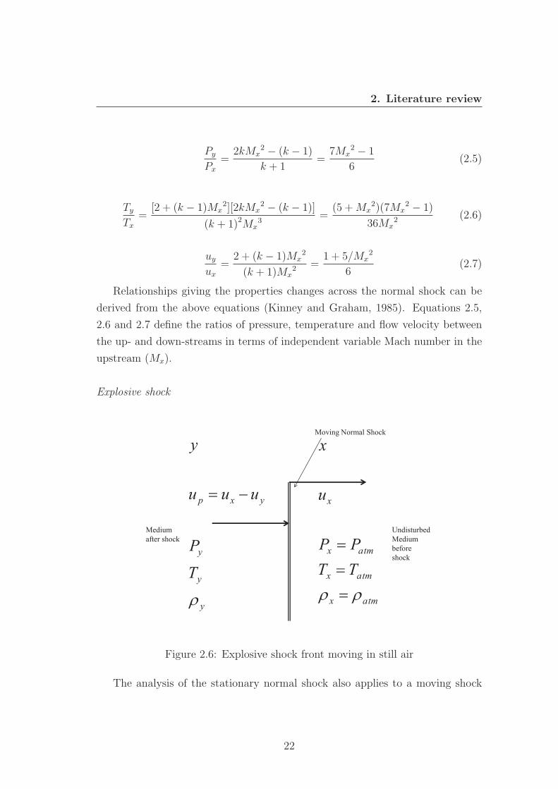
2.6 Explosive shock front moving in still air . . . . . . . . . . . . . . . 22
2.7 Normal reflected shock on a rigid surface . . . . . . . . . . . . . . 24
2.8 Reflected pressure coefficients vs. angle of incidence (β) (USDOD,
2008) . . . . . . . . . . . . . . . . . . . . . . . . . . . . . . . . . . 25
2.9 Shape of blast waves . . . . . . . . . . . . . . . . . . . . . . . . . 27
2.10 Passage of a blast wave over a rigid object . . . . . . . . . . . . . 29
2.11 Blast curves (Kinney and Graham, 1985) . . . . . . . . . . . . . . 30
2.12 Blast load-time history on front surface (Kinney and Graham, 1985) 31
2.13 Blast load-time history other surface (Kinney and Graham, 1985) 33
2.14 Blast load-time history on frame (Kinney and Graham, 1985) . . 34
2.15 Typical equivalent single-degree-of-freedom system . . . . . . . . . 36
2.16 Resistance curve R(δ) for a typical SDOF system . . . . . . . . . 39
2.17 Response for all regimes . . . . . . . . . . . . . . . . . . . . . . . 42
2.18 Pressure - impulse diagrams . . . . . . . . . . . . . . . . . . . . . 44
2.19 Pressure - impulse diagrams comparison . . . . . . . . . . . . . . 45
2.20 Material response at high strain rate (USDOD, 2008) . . . . . . . 46
2.21 Strain rate hardening models . . . . . . . . . . . . . . . . . . . . . 48
xiii
LIST OF FIGURES
3.1 Newton Raphson Method . . . . . . . . . . . . . . . . . . . . . . 61
3.2 Modified Riks method . . . . . . . . . . . . . . . . . . . . . . . . 62
3.3 Lagrangian v.s. Eulerian deformation . . . . . . . . . . . . . . . . 64
3.4 Eulerian time incrementation (Spinelli and Vitali, 2009) . . . . . . 65
3.5 One dimensional Eulerian model . . . . . . . . . . . . . . . . . . . 70
3.6 Mesh study of 1D Eulerian model . . . . . . . . . . . . . . . . . . 71
3.7 Comparison for shock strength decay . . . . . . . . . . . . . . . . 72
3.8 Normal reflection in Eulerian model pin = 34.5kPa . . . . . . . . 74
3.9 Oblique reflection (pin = 34.5kPa) . . . . . . . . . . . . . . . . . . 75
3.10 Comparison for shock strength decay (USDOD, 2008) . . . . . . . 76
3.11 Boyd’s experiment configuration (Boyd, 2000) . . . . . . . . . . . 77
3.12 Numerical model in AUTODYN . . . . . . . . . . . . . . . . . . 78
3.13 Comparison of responses and the modified model . . . . . . . . . 80
4.1 Damaged steel switch box in the vapour cloud (SCI, 2009) . . . . 86
4.2 Photos of steel switch boxes . . . . . . . . . . . . . . . . . . . . . 87
4.3 Box150 (300×300×150mm) . . . . . . . . . . . . . . . . . . . . . 88
4.4 Box200 (300×300×200mm) . . . . . . . . . . . . . . . . . . . . . 89
4.5 Configuration of TNT detonation test (SCI, 2009) . . . . . . . . . 90
4.6 Residual deformations of ”Box150” exposed to TNT detonation,
incident overpressure from left to right: 100kPa, 200kPa, 480kPa
and 750kPa (SCI, 2009) . . . . . . . . . . . . . . . . . . . . . . . 90
4.7 Simplifield layout of gas detonation test . . . . . . . . . . . . . . . 92
4.8 Configuration of box support (Courtesy of Steel Construction In-
stitute) . . . . . . . . . . . . . . . . . . . . . . . . . . . . . . . . . 92
4.9 Test in progress (Allason, 2013) . . . . . . . . . . . . . . . . . . . 93
4.10 Pressure - time histories recorded by transducers . . . . . . . . . . 94
4.11 Before and after photographs of Box200-1,3,5 and 7 (Allason, 2013) 96
4.12 Digital scan of boxes . . . . . . . . . . . . . . . . . . . . . . . . . 97
4.13 Deformation measurement of scanned box . . . . . . . . . . . . . 97
4.14 Box150 numerical model details . . . . . . . . . . . . . . . . . . . 99
4.15 Box150 model boundary conditions with mesh . . . . . . . . . . . 100
4.16 Box numerical mode mesh study . . . . . . . . . . . . . . . . . . . 100
xiv
LIST OF FIGURES
4.17 Box200 numerical model with mesh . . . . . . . . . . . . . . . . . 102
4.18 Box faces subjected to reflected and side-on pressure loading in
pure Lagrangian approach . . . . . . . . . . . . . . . . . . . . . . 103
4.19 Load application in Lagrangian analysis (Box200-7, Transducer B11)103
4.20 Modelling of internal pressure . . . . . . . . . . . . . . . . . . . . 105
4.21 Calibration of blast wave in Eulerian model . . . . . . . . . . . . 107
4.22 3D Eulerian model . . . . . . . . . . . . . . . . . . . . . . . . . . 108
4.23 A quarter of 3D Eulerian model for UEL analysis Step 1 . . . . . 109
4.24 Overpressure loading curves for UEL analysis . . . . . . . . . . . 110
4.25 CEL numerical model . . . . . . . . . . . . . . . . . . . . . . . . . 111
4.26 Numerical blast wave and loading results for Box200-1 (Transducer
B16) . . . . . . . . . . . . . . . . . . . . . . . . . . . . . . . . . . 113
4.27 Numerical blast wave and loading results for Box200-3 (Transducer
B9) . . . . . . . . . . . . . . . . . . . . . . . . . . . . . . . . . . . 114
4.28 Numerical blast wave and loading results for Box200-5 (Transducer
B10) . . . . . . . . . . . . . . . . . . . . . . . . . . . . . . . . . . 115
4.29 Numerical blast wave and loading results for Box200-7 (Transducer
B11) . . . . . . . . . . . . . . . . . . . . . . . . . . . . . . . . . . 116
4.30 Displacement - time histories of box front face centre . . . . . . . 119
4.31 Comparison of residual shapes of Box200-1 . . . . . . . . . . . . 123
4.32 Comparison of residual shapes of Box200-3 . . . . . . . . . . . . 124
4.33 Comparison of residual shapes of Box200-5 . . . . . . . . . . . . 125
4.34 Comparison of residual shapes of Box200-7 . . . . . . . . . . . . 126
4.35 Numerical results of overpressures for TNT explosions . . . . . . 128
4.36 Numerical results of displacements for boxes in TNT explosions . 129
4.37 Numerical displacements error compared with CEL model . . . . 132
4.38 Numerical residual shapes for Box150 in TNT explosions. Peak
side-on pressure: 1 bar, 2 bar and 3 bar . . . . . . . . . . . . . . . 133
4.39 Numerical residual shapes for Box150 in TNT explosions. Peak
side-on pressure: 4 bar, 4.8 bar and 7.5 bar . . . . . . . . . . . . 134
4.40 Numerical Eulerian model for reflection of deflagration . . . . . . 136
4.41 Reflection coefficient for deflagration(non-ideal blast wave) . . . . 137
4.42 Overpressure dynamic loadings for parametric study . . . . . . . . 138
xv
LIST OF FIGURES
4.43 Pressure - Impulse diagrams for Box150 (back support) . . . . . . 143
4.44 Pressure - Impulse diagrams for Box150 (bottom support) . . . . 144
4.45 Numerical residual shapes of Box150 (back support) . . . . . . . . 146
4.46 Numerical residual shapes of Box150 (bottom support) . . . . . . 147
4.47 Comparison of numerical residual shapes to damaged boxes from
Buncefield (SCI, 2009) . . . . . . . . . . . . . . . . . . . . . . . . 148
5.1 Damage to Warehouse 1 (Atkinson, 2011) . . . . . . . . . . . . . 151
5.2 Damage to Warehouse 2 (Atkinson, 2011) . . . . . . . . . . . . . 152
5.3 Typical warehouse configuration (Burgan and Moutaftsis, 2011) . 153
5.4 Portal frame layout (Burgan and Moutaftsis, 2011) . . . . . . . . 155
5.5 Gable wall frames (Burgan and Moutaftsis, 2011) . . . . . . . . . 155
5.6 Roof plan (Burgan and Moutaftsis, 2011) . . . . . . . . . . . . . . 156
5.7 Side wall frames (Burgan and Moutaftsis, 2011) . . . . . . . . . . 156
5.8 Cross-sectional details of eaves beam, purlin and side rail [units:mm]
(Hadley, 2004) . . . . . . . . . . . . . . . . . . . . . . . . . . . . . 157
5.9 Built-up cladding details (Burgan and Moutaftsis, 2011) . . . . . 158
5.10 Self-tapping screw (CA, 2008) . . . . . . . . . . . . . . . . . . . . 159
5.11 M12 Bolt-Cleat connection (Hadley, 2004) . . . . . . . . . . . . . 159
5.12 Numerical modelling levels . . . . . . . . . . . . . . . . . . . . . . 163
5.13 Comparison of displacement histories of side wall models . . . . . 165
5.14 Full scale test configuration of cladding-side rail assembly (Elgha-
zouli et al., 2014) . . . . . . . . . . . . . . . . . . . . . . . . . . . 167
5.15 Profile of cladding TR35/207 (thickness=1 mm) [unit:mm] . . . . 167
5.16 Material models for cladding and side rail . . . . . . . . . . . . . 168
5.17 Numerical model used for validation . . . . . . . . . . . . . . . . . 169
5.18 Mesh of test assembly numerical model . . . . . . . . . . . . . . . 170
5.19 Comparison of numerical results and experimental measurements 171
5.20 Deformed shapes of test assembly (Riks method) . . . . . . . . . 172
5.21 Comparison of pressure - central displacement responses . . . . . 173
5.22 Details of sub-assembly model representing the side wall of warehouse174
5.23 Self-tapping screw connector model . . . . . . . . . . . . . . . . . 175
xvi
LIST OF FIGURES
5.24 Lap joint pulling test using static test components (validation of
detailed fastener model) . . . . . . . . . . . . . . . . . . . . . . . 177
5.25 Shear response estimation of the fastener for connector model . . 178
5.26 Definition of the connector shear response for fasteners . . . . . . 182
5.27 Finite element model of M12 Bolt-Cleat connection . . . . . . . . 184
5.28 Response estimation of M12 Bolt - Cleat connection . . . . . . . . 185
5.29 Connector model for M12 Bolt-cleat connection . . . . . . . . . . 186
5.30 Sub-assemblage model of the wall structure in the warehouse building187
6.1 Details of sub-assemblage model . . . . . . . . . . . . . . . . . . . 191
6.2 Structural component mid-span deflection and end rotation . . . . 192
6.3 Sub-assemblage mode shapes . . . . . . . . . . . . . . . . . . . . . 194
6.4 Loading scenarios: combinations of overpressure and impulse . . . 195
6.5 Displacement history at the mid-span of the central side rail with
loading profiles . . . . . . . . . . . . . . . . . . . . . . . . . . . . 197
6.6 Deformed shapes of the sub-assemblage . . . . . . . . . . . . . . . 198
6.7 Response of central fastener of the sub-assemblage model in Case 98199
6.8 Response of central cladding of the sub-assemblage in Case 98 . . 201
6.9 Relative displacement at the middle of the cladding with failure of
the corresponding fastener . . . . . . . . . . . . . . . . . . . . . . 202
6.10 Response of central fastener of the sub-assemblage model in Case
157 . . . . . . . . . . . . . . . . . . . . . . . . . . . . . . . . . . . 203
6.11 Response of central cladding of the sub-assemblage in Case 157 . 205
6.12 Response of side fastener of the sub-assemblage model in Case 75 206
6.13 Response of side cladding of the sub-assemblage in Case 75 . . . . 207
6.14 Comparison of failure behaviour of central and side cladding with
fasteners for the sub-assemblage model in Case 98 . . . . . . . . . 209
6.15 Cases with identical failure behaviour of cladding and fasteners at
centre and side . . . . . . . . . . . . . . . . . . . . . . . . . . . . 210
6.16 Response of middle fastener of the sub-assemblage model in Case 98211
6.17 Numerical response of the M12 bolt-cleat connection . . . . . . . 212
6.18 Axial and transverse displacement time history of side rail . . . . 214
6.19 Side rail transverse response with failure of fasteners . . . . . . . 216
xvii
LIST OF FIGURES
6.20 Percentage of total fastener failure with side rail displacement . . 217
6.21 Pressure - impulse diagrams: maximum side rail displacement . . 218
6.22 Pressure - impulse diagram: maximum axial displacement . . . . . 219
6.23 Pressure - impulse diagram . . . . . . . . . . . . . . . . . . . . . . 220
6.24 Iso-curves for TNT explosive charges . . . . . . . . . . . . . . . . 221
6.25 Combined pressure - impulse diagrams . . . . . . . . . . . . . . . 222
6.26 Strain rate effect on dynamic increase factor . . . . . . . . . . . . 224
6.27 Estimation of strain rate in the screw connection . . . . . . . . . 225
6.28 Stress, strain and strain rate time histories in the sampling shell
element . . . . . . . . . . . . . . . . . . . . . . . . . . . . . . . . 226
6.29 Simplified model to estimate the strain rate in a screw connection 227
6.30 Applied 0.2 mm displacement over total time step of 0.01 second . 228
6.31 Strain rate analysis around the hole . . . . . . . . . . . . . . . . . 229
6.32 Relationship between nominal and concetrated strain rates . . . . 230
6.33 Connector response with and without the estimated strain rate effect230
6.34 Comparison of response of side rail with and without rate stiffened
fasteners . . . . . . . . . . . . . . . . . . . . . . . . . . . . . . . . 232
6.35 Effect of the rate stiffened fastener on the pressure - impulse dia-
grams of the side rail maximum displacement . . . . . . . . . . . 233
6.36 Effect of the rate stiffened fastener on the percentage failure of
fasteners . . . . . . . . . . . . . . . . . . . . . . . . . . . . . . . . 233
6.37 Influence of the rate effect on the pressure - impulse diagram of
maximum percentage of fastener failure (50% failure) . . . . . . . 234
7.1 Cladding panel and side rail simplified SDOF model . . . . . . . . 237
7.2 Resistance curve of SDOF model for cladding panel . . . . . . . . 239
7.3 Resistance curve of SDOF model for side rail . . . . . . . . . . . . 241
7.4 Response of simplified model of side rail . . . . . . . . . . . . . . 243
7.5 Comparison of pressure - impulse diagrams (maximum dynamic
displacement) . . . . . . . . . . . . . . . . . . . . . . . . . . . . . 244
7.6 Responses of simplified model of cladding . . . . . . . . . . . . . . 246
7.7 Combined pressure - impulse diagram using the simplified approach248
xviii
LIST OF FIGURES
7.8 Numerical modelling of blast wave (semi-spherical 7500kg TNT
charge and 324m stand-off) and the rigid warehouse structure . . 251
7.9 Coupled model of blast wave with rigid warehouse . . . . . . . . . 252
7.10 Location of numerical pressure gauges . . . . . . . . . . . . . . . . 252
7.11 Pre-cut holes on the blastward wall of the rigid warehouse model . 253
7.12 30% venting area with different shapes of holes . . . . . . . . . . . 254
7.13 Simulation of blast loading on rigid warehouse model . . . . . . . 255
7.14 Overpressure loading results for Case 4 (30% venting area) . . . . 256
7.15 Internal pressurisation due to venting area on front wall . . . . . . 257
7.16 Overpressure loadings at the back wall . . . . . . . . . . . . . . . 259
7.17 Overpressure loadings of side wall . . . . . . . . . . . . . . . . . . 260
7.18 Effect of venting area shapes on internal pressurisation . . . . . . 262
7.19 Application of pressure - impulse diagram . . . . . . . . . . . . . 265
1 Overpressure loadings on rigid warehouse (Case 1) . . . . . . . . . 276
2 Overpressure loadings on rigid warehouse (Case 2) . . . . . . . . . 277
3 Overpressure loadings on rigid warehouse (Case 3) . . . . . . . . . 277
4 Overpressure loadings on rigid warehouse (Case 4) . . . . . . . . . 278
5 Overpressure loadings on rigid warehouse (Case 5) . . . . . . . . . 278
6 Overpressure loadings on rigid warehouse (Case 6) . . . . . . . . . 279
7 Overpressure loadings of back wall (Case 1 & 2) . . . . . . . . . . 279
8 Overpressure loadings of back wall (Case 3 & 4) . . . . . . . . . . 280
9 Overpressure loadings of back wall (Case 5 & 6) . . . . . . . . . . 280
10 Overpressure loadings of side wall (Case 1 & 2) . . . . . . . . . . 280
11 Overpressure loadings of side wall (Case 3 & 4) . . . . . . . . . . 281
12 Overpressure loadings of side wall (Case 5 & 6) . . . . . . . . . . 281
13 Overpressure loadings of front roof (Case 1 & 2) . . . . . . . . . . 281
14 Overpressure loadings of front roof (Case 3 & 4) . . . . . . . . . . 282
15 Overpressure loadings of front roof (Case 5 & 6) . . . . . . . . . . 282
16 Overpressure loadings of back roof (Case 1 & 2) . . . . . . . . . . 282
17 Overpressure loadings of back roof (Case 3 & 4) . . . . . . . . . . 283
18 Overpressure loadings of back roof (Case 5 & 6) . . . . . . . . . . 283
xix

LIST OF FIGURES
19 Combination of overpressures and impulses with corresponding
case number and positive duration . . . . . . . . . . . . . . . . . 285
xx
Nomenclature
Roman Symbols
[B] Strain matrix
[c] Constitutive matrix
[D] Assembled nodal displacement matrix
[De] Global nodal displacement matrix
[de] Local nodal displacement matrix
[F ] Assembled consistent nodal force vector
[fb] Body force vector
[Fe] Global consistent nodal force vector
[fe] Local consistent nodal force vector
[fs] Surface force vector
[I] Internal forces of the flexible body
[K] Assembled stiffness matrix
[Ke] Global stiffness matrix
[ke] Local stiffness matrix
[M ] Assembled mass matrix
xxi
LIST OF FIGURES
[T ] Transformation matrix
[U ] Displacement matrix
upl ABAQUS connector equivalent plastic relative motion
ΔPs Blast strength number (1-10)
ΔPs Maximum overpressure
Δt Step time increment
ΔP s Dimensionless maximum overpressure
upl ABAQUS collection of plastic relative motion rate
R Energy scaled distance
t+ Dimensionless positive duration
A Cross sectional area
a, b TNO multi-energy correlation constants
a0 Local speed of sound
ax Local sound of speed (atmosphere)
C Strain rate hardening parameter for Johnson-Cook model
c0 Atmospheric speed of sound
Cd Dilatation wave speed
Cd Discharge coefficient
cp Specific heat at constant pressure
D Average obstacle size
D Diameter of the self-tapping screw shaft
D, p Strain rate hardening parameter for Cowper-Symonds model
xxii
LIST OF FIGURES
E Combustible energy of vapour cloud
E Detonation energy per initial volume
E Young’s modulus
F Axial pre-tension
F Distributed load
F Opening percentage
f ABAQUS collection of active connector forces
F 0 ABAQUS connector equivalent yield force
Fe Equivalent force of SDOF system
fe TNT efficiency factor
FN ABAQUS connector equivalent tensile (normal) force
FS ABAQUS connector equivalent shear force
fu Material ultimate stress
fx, fy, fz ABAQUS connector force
fy Material yield stress
fdu Material dynamic ultimate stress
fdy Material dynamic yield stress
g(t) Time function of the applied distributed load
HTNT Explosive heat of TNT
Hvapour Combustion heat of the fuel in vapour cloud
I Specific impulse
K Stiffness of SDOF model
xxiii

LIST OF FIGURES
K Torque coefficient
k Specific heat ratio (1.4 for ideal gas)
k Stiffness
K, r ABAQUS connector defining parameter
Ke Equivalent stiffness of SDOF system
KLM Load-mass factor
kTM Strain energy
L Characteristic length of the target
L Lagrange
L Length of a simply supported beam
Le Characteristic element length
Lf Flame path
m Mass
Me Equivalent mass of SDOF system
Me Global mass matrix
me Equivalent TNT mass
me Local mass matrix
Mp Ultimate plastic moment
Mx Upstream flow Mach number
mx,my,mz ABAQUS connector moment
My Downstream flow Mach number
mvapour Total mass of the vapour cloud
xxiv

LIST OF FIGURES
N Admissible functions
n nth incremental step
P ABAQUS connector potential
P Total applied load P=FL
p Blast wave overpressure
p(x, t) Applied distributed load
P0 Atmospheric pressure
Pa Atmospheric pressure
pA Atmospheric pressure
pi Incident overpressure
po Peak overpressure value
Pr Reflected pressure
pr Reflected overpressure
Px Upstream flow pressure
Py Downstream flow pressure
Patm Atmospheric pressure
Pincident Incident overpressure
Pstag Stagnation pressure
pstag Stagnation overpressure
Ptransmission Transmitted overpressure through perforated barriers
Qi Generalised force
qi Admissible functions
xxv
LIST OF FIGURES
R Ideal gas constant
R Stand-off distance
r Distance to target
R0 Charge radius
rc Radius of high explosive charge
Rm Maximum plastic load of SDOF resistance curve
RN ABAQUS connector equivalent tensile (normal) capacity
RS ABAQUS connector equivalent shear capacity
S Characteristic width of the reflected surface
Sc TNO multi-energy correlation scale factor
Sl Laminar burning velocity
sx Upstream flow entropy
sy Downstream flow entropy
T Kinetic energy
T Natural period
T Tension membrane force
T Tightening torque
t Time
t+ Positive duration
ta Shock front arrival time
td Shock wave positive duration
TH Temperature dependency parameter for Johnson-Cook material model
xxvi
LIST OF FIGURES
Tn Natural period of structure
tr Deflagration finite rise time
Tx Upstream flow temperature
Ty Downstream flow temperature
Tatm Atmospheric temperature
up Blast wave particle velocity
ux Upstream flow velocity (shock front velocity)
ux, uy, uz ABAQUS connector displacement
uy Downstream flow velocity
urx, ury, urz ABAQUS connector rotation
V Plastic dissipation energy
V Relative volume or the expansion of the explosive product
V Strain energy
W High explosive charge weight
W Work done by external forces
w(x, t) Response solution of a simply supported beam
Z Scaled distance
uplDI ABAQUS connector damage initiation displacement
uplf ABAQUS connector shear failure displacement
epeff Effective plastic strain
f failz ABAQUS connector tensile failure force
Greek Symbols
xxvii

LIST OF FIGURES
[ε] Strain matrix
[σ] Stress matrix
α Blast wave form parameter
β Shock wave incident angle
δ Delta operator
δ(t) Generalised time response of a supported beam
δe Transverse displacement of beam at yieldings
δm Maximum transverse displacement of beam
δy Yielding displacement
δTM Strain energy
ε The base of natural logarithm
εp Plastic strain
εy Material yield strain
Λn Pressure reflected ratio
μ Ductility ratio
ω Undamped natural circular frequency
Φ ABAQUS connector yield function
φ(x) Assumed mode shape function
π Potential energy
Ψm ABAQUS connector mode-mix ratio
ρ Density
ρx Density of the upstream flow
xxviii
LIST OF FIGURES
ρy Density of the downstream flow
ρatm Atmospheric density
σp Plastic stress
σy Material yield stress
Θ Temperature
θ Support rotation of beam
Θz Absolute zero
ε Strain rate
εPeff Effective plastic strain rate
ε0 Reference strain rate
Acronyms
CEL Coupled Eulerian - Lagrangian
DIF Dynamic increase factor
NLFEM Non-linear finite element model
SDOF Single degree of freedom
UEL Uncoupled Eulerian - Lagrangian
V BR Volume blockage ratio
V CE Vapour cloud explosion
xxix
Chapter 1
Introduction
The 2005 Buncefield event was unexpectedly destructive for a vapour cloud ex-
plosion. It showed huge cost associated with blast damages to commercial and
residential buildings surrounding a major explosion incident. The main char-
acteristic of the Buncefield explosion was that its intensity and the severity of
damage caused to structures/buildings had not been anticipated by any major
hazardous design practice. The work presented in this thesis focuses on assessing
structural damage of vapour cloud explosions and aiming to provide insight into
the structure and objects response to blast loadings.
1.1 Background
An explosion is a sudden release of substantial energy, which transfers to its
surrounding in the form of a rapidly moving rise in pressure called a blast wave.
There are three categories of explosion: physical, nuclear and chemical (Smith
and Hetherington, 1994). The most common physical explosion can be found for
example in a failure of a vessel of compressed gas or other pressurized devices.
The violent expansion of the compressed gas is the source of the released energy.
The Nuclear explosion is much more destructive than the other two. The energy
in a nuclear explosion comes from the formation of different atomic nuclei by
redistribution of the neutrons and proton within the reacting nuclei.
Chemical explosions are exothermic reactions. The surrounding temperature
1
1. Introduction
is raised by the heat from oxidation of the fuel element contained within the
explosive compound. Then the volume of the gases becomes much larger than
the compound, generating a high pressure and subsequent blast wave. The energy
released arises from the formation of new molecular bonds in the products of the
reaction. Explosives that fall into this category are such as Trinitrotoluene (TNT,
high explosive), gunpowder (low explosive) and even the wheat flour dust in a
grain elevator. This explosion is known as a detonative process.
There is a special case of chemical explosion called vapour cloud explosion
(VCE) that involves a fuel (e.g. propane or butane) mixed with the atmosphere,
and usually this occurs in an offshore platform or industrial/chemical plant. If
the mixture is ignited, the flame velocity would be fast enough to generate a blast
wave. Although the overpressure in the blast wave might not be as high as in other
explosions, it can be strong enough to damage or even destroy nearby structures.
In a vapour cloud explosion, deflagration is the result that the flame front travels
slower than the speed of sound and if it moves faster than the speed of sound, we
would expect a detonation to occur (deflagration transition to detonation). It is
more destructive as it generates stronger blast waves than deflagration.
The blast wave (high overpressure) from an uncontrolled explosion can be
destructive and even lethal. To prevent its damage to buildings, there is a need
to understand the characteristics of explosions, blast waves and subsequently
the response of building structures. Empirical charts/tools are widely adopted
for analysis of characteristics of an explosion. The blast wave parameters can
be readily determined by using charts or empirical equations based on scaled
explosive charge weight and stand-off distance. Empirical methods are available
for both high explosive and vapour cloud explosions. With the development of
scientific computers, a more complex method known as Computational Fluid
Dynamics (CFD) is now widely available. It is capable of producing results with
better accuracy but involves greater cost of computational resource and operator
manpower.
Several methods are available for analysis of dynamic structural response.
Biggs’ Single Degree of Freedom (SDOF) model has been extensively used to
investigate the response of structural component to dynamic loadings. Results
can be presented in a graphical, analytical or numerical forms. This method is
2
1. Introduction
based on a representation of the actual component configurations by an equiv-
alent spring-mass system which has only one degree of freedom (Biggs, 1964).
An improved SDOF model is presented in the Technical Note 7 (SCI, 2002)
which overcomes some difficulties in Biggs’ model and includes complex support-
ing conditions. By using energy methods to generate equilibrium equations, the
mode approximation method has been extended by Schleyer (Schleyer and Hsu,
2000) and Langdon (Langdon and Schleyer, 2006b) and to incorporate full elas-
tic response and include variable support constraints. This method divides the
dynamic response of a component into different stages/modes and obtain results
by solving a Multi-Degree of Freedom system.
Finite element methods are also widely used to analyse the dynamic response
of structures. Commercial codes such as ?, ANSYS and LS-DYNA are commonly
used in research and industries. Borvik (Borvik et al., 2009) used LS-DYNA to
investigate whether a pure Lagrangian model can be used to determine the struc-
tural response in a specified blast problem or a more complicated fully coupled
Eulerian - Lagrangian model should be adopted. By using non-linear finite ele-
ment package Louca (Louca et al., 1996) studied the response of a typical blast
wall and a stiffened panel subject to hydrocarbon explosion. Langdon (Langdon
and Schleyer, 2006c) used ? to predict the response time histories and permanent
deformations of a stainless steel blast wall and connection systems.
1.2 Buncefield incident
Over the last few decades, there have been a number of major industrial accidents
involving oil and gas installations worldwide. These include the Buncefield event
in the UK in December 2005. The incident was a vapour cloud explosion which
occurred at the Buncefield Oil Storage Depot, Hemel Hempstead, Hertfordshire.
Fortunately there were no casualties but 43 people were injured. The explo-
sion and subsequent fire caused extensive damage to the plant and surrounding
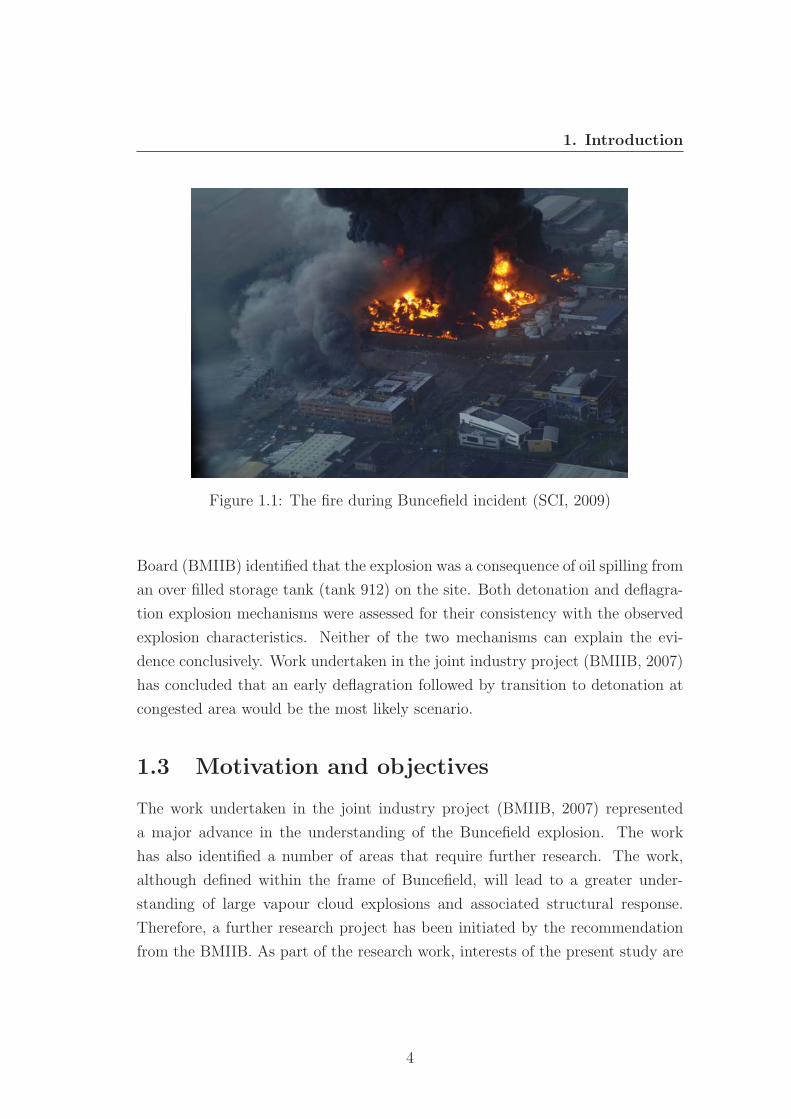
buildings, both commercial and residential properties. An aerial view of the site
during the fire is shown in Figure 1.1. The economic impact of the incident
broadly adds up to £1 billion.
The subsequent investigation by the Buncefield Major Incident Investigation
3
1. Introduction
Figure 1.1: The fire during Buncefield incident (SCI, 2009)
Board (BMIIB) identified that the explosion was a consequence of oil spilling from
an over filled storage tank (tank 912) on the site. Both detonation and deflagra-
tion explosion mechanisms were assessed for their consistency with the observed
explosion characteristics. Neither of the two mechanisms can explain the evi-
dence conclusively. Work undertaken in the joint industry project (BMIIB, 2007)
has concluded that an early deflagration followed by transition to detonation at
congested area would be the most likely scenario.
1.3 Motivation and objectives
The work undertaken in the joint industry project (BMIIB, 2007) represented
a major advance in the understanding of the Buncefield explosion. The work
has also identified a number of areas that require further research. The work,
although defined within the frame of Buncefield, will lead to a greater under-
standing of large vapour cloud explosions and associated structural response.
Therefore, a further research project has been initiated by the recommendation
from the BMIIB. As part of the research work, interests of the present study are
4
1. Introduction
mainly lying in the structural response of various field objects and the steel portal
warehouse building.
The objective of the project is to study damage produced to buildings from
low-lying vapour cloud explosion which occurred in the previous accidents. Data
in the public domain on the damage observed will be used to investigate the
characteristics of the pressure time histories required to produce the damage
processes observed. Much effort will be placed in studying the impact of selected
pressure loads on representative building structures through detailed non-linear
finite element analysis. Analytical methods will be used in simple structures
where applicable. The anticipated outcome of this work would be to propose
guidance for the assessment of loading and the evaluation of structural response.
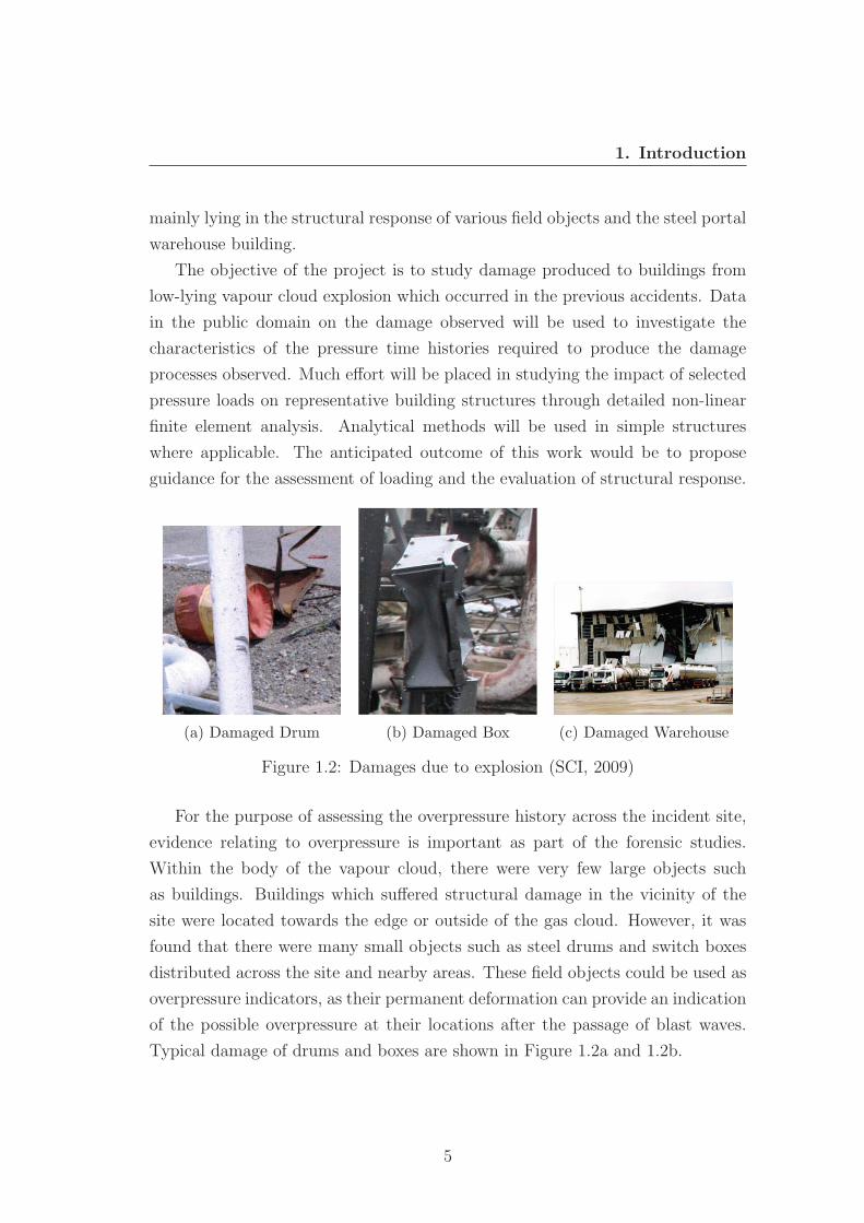
(a) Damaged Drum (b) Damaged Box (c) Damaged Warehouse
Figure 1.2: Damages due to explosion (SCI, 2009)
For the purpose of assessing the overpressure history across the incident site,
evidence relating to overpressure is important as part of the forensic studies.
Within the body of the vapour cloud, there were very few large objects such
as buildings. Buildings which suffered structural damage in the vicinity of the
site were located towards the edge or outside of the gas cloud. However, it was
found that there were many small objects such as steel drums and switch boxes
distributed across the site and nearby areas. These field objects could be used as
overpressure indicators, as their permanent deformation can provide an indication
of the possible overpressure at their locations after the passage of blast waves.
Typical damage of drums and boxes are shown in Figure 1.2a and 1.2b.
5
1. Introduction
During the explosion, both steel frame and masonry buildings were damaged
to different levels. Large steel portal frame warehouse type structures were af-
fected at a quite long distance. Among the damaged structures, steel frame
cladding warehouses are of the most interests. A damaged warehouse is shown
in Figure 1.2c. The high surface area and light-weight construction make the
pressure applied by wind a key structural design aspect. The common design
wind pressure of a steel cladding warehouse is lower than it is of a typical brick
building, and almost all of the surface structural steel and cladding is potentially
at risk (rather than just windows/doors). Therefore it is relatively more vulner-
able to accidental overpressure and the level of damage to a warehouse maybe be
particularly extensive and time consuming to repair, leading to longer periods of
business disruption.
Given the above considerations, field objects such as steel switch boxes were
chosen to perform a forensic study. While the steel frame cladding warehouse is
the subject of the analysis of structural response to vapour cloud explosions. The
main objectives of this project are:
• to model steel switch boxes subject to various blast loading
• to examine the blast response of steel boxes in the form of pressure-impulse
diagrams and permanently deformed shapes
• to provide information for forensic studies to investigate the current and
future explosions
• to model light weight steel portal frame warehouse structures under different
blast loadings
• to generate pressure-impulse diagrams of steel frame cladding warehouses
• to provide design implications for steel portal frame warehouses
In the following chapters, a literature review covering the recent research work
on study and investigation of blast explosion and structural response is presented,
following by a introduction of the numerical tools that adopted in the current
research project. Forensic works carried out on the field objects which can be
6

1. Introduction
used to help the investigation are presented. A detailed finite element analysis
on the response of light weight steel clad warehouse structure is presented and
the results are discussed. Some design implication and improvements to the
structures are included at the end of this thesis.
7
Chapter 2
Literature review
This chapter presents an overview of different types of explosions and their char-
acteristics. The Buncefield and other previous major incidents are reviewed and
their main characteristics are noted. Blast wave, the associated dynamic load-
ing and various tools for structural dynamic analysis are presented. A review
of previous work on studies of responses to blast loading is also included and
discussed.
2.1 Vapour cloud explosion
2.1.1 Explosion mechanisms
A cloud of combustible material (e.g. propane, butane and pentane etc.) in either
confined or unconfined atmosphere can explode under certain conditions. Con-
ditions leading to an unconfined vapour cloud explosion are first, a quick release
of a large quantity of fuel which forms a vapour cloud. Secondly the cloud is
ignited by a spark or flame. There are two mechanisms that a vapour cloud could
explode: deflagration and detonation. If the ignition occurs immediately after
the release of the combustible material before it mixes with the surrounding air,
the explosion is very likely to be a deflagration. When ignition of the combustible
cloud occurs after its formation so that the air has became well mixed with the
combustible vapour, and if the air-fuel mixture is just within the flammability
range, a detonation is most likely to occur.
8
2.Literature review
A vapour cloud explosion involving deflagration is certainly less destructive
than detonation. The overpressure is generated by the flame front travelling at
high speeds but under the local speed of sound. The mixture ahead is ignited by
heat radiation from the flame front. The flame generates pressure because of the
inertia of the unreacted mixture in front of the flame, similar to a object travelling
at high speed through the air generates a pressure wave in front of it. It is well
understood that deflagration of a vapour cloud in a confined or congested area
(such as a section fully packed with pipe works) can generate damaging pressures
due to acceleration of flame front. In some cases, the turbulence induced by
the congested obstacles will promote the reaction rate, producing successively
higher flame speeds and increasing overpressures. Thus it can eventually lead to
deflagration - detonation transition (DDT). It is important to note that the high
speed of flame is dependent on the congested obstacles, once the flame travels from
a confined area to an open area it rapidly decelerates. Hence the overpressures
decreases as the blast wave propagates away from the congested region.
As compared to deflagration, the detonation front has an initial sudden rise in
pressure, which then decays. This abrupt rise of overpressure is known as shock
front and the whole pressure wave as a shock wave. The shock front compresses
the air-fuel mixture in the front and raises the temperature. In detonation the
temperature rise can ignite the fresh mixture ahead as it exceeds the auto-ignition
temperature of the mixture. The magnitude of the shock front is maintained by
the energy released from the combustion process in detonation. The process is
self-sustainable so it is not dependent on any congestion or obstacles.
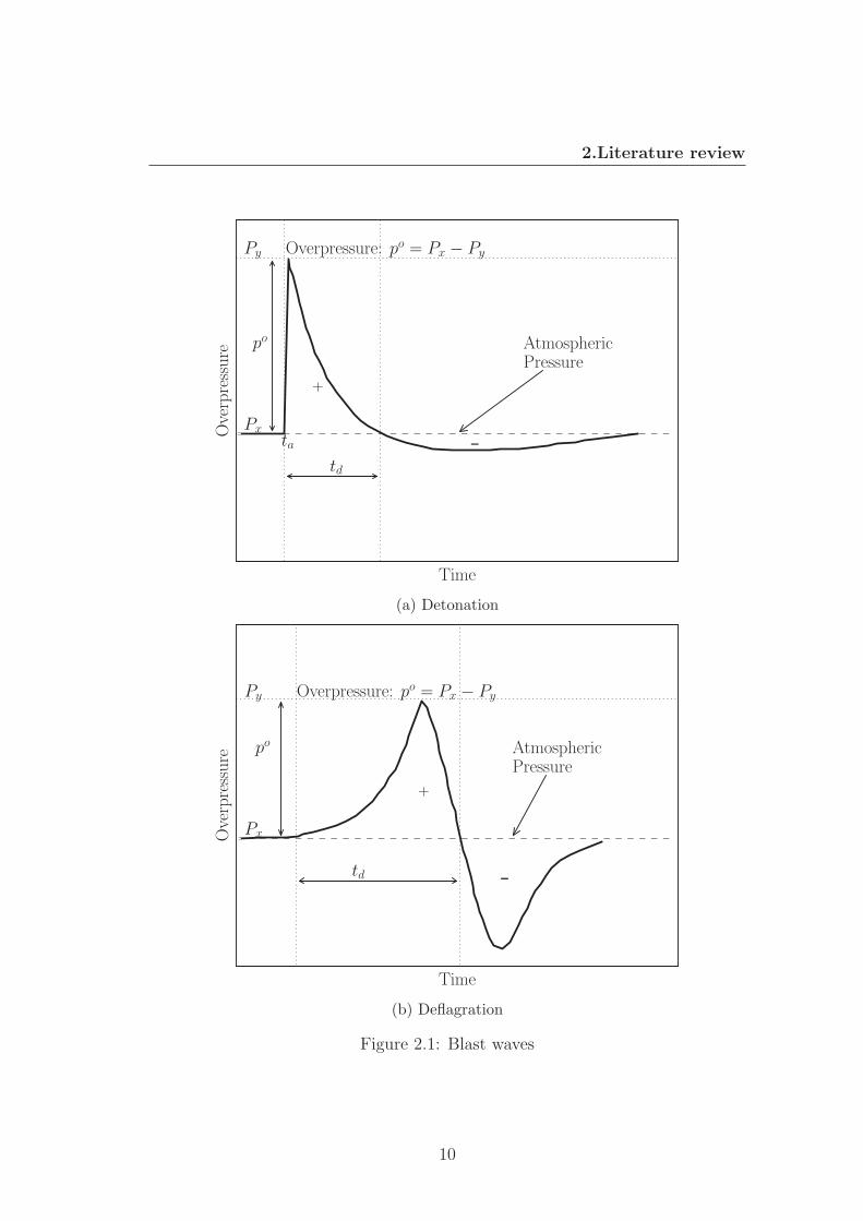
The pressure - time history of a typical blast wave from detonation as recorded
some distance away from the explosion centre is shown in Figure 2.1a. At an
arrival time ta after initiation of the explosion, the pressure at the remote location
suddenly increased to a peak value. The overpressure then immediately starts
to decay to atmospheric pressure over a period known as the duration of the
positive phase td. Due to the inertia of the air in the wave, a negative pressure
phase will occur after passage of the overpressure blast wave. The peak value
of the negative phase is much lower but the duration is much longer than the
positive phase. Generally three independent parameters are used to define a
detonation blast wave: the peak overpressure po, the positive phase duration td
9
2.Literature review
0.0 0.2 0.4 0.6 0.8 1.0
Time
-0.4
-0.2
0.0
0.2
0.4
0.6
0.8
1.0
Overpressure
po
td
ta
+
-
Overpressure: po = Px − Py
Px
Py
AtmosphericPressure
(a) Detonation
0.0 0.1 0.2 0.3 0.4 0.5 0.6 0.7 0.8
Time
-0.4
-0.2
0.0
0.2
0.4
0.6
0.8
1.0
Overpressure
po
td
+
-
Overpressure: po = Px − Py
Px
Py
AtmosphericPressure
(b) Deflagration
Figure 2.1: Blast waves
10
2.Literature review
and the specific impulse which is the area under the positive phase I = 12potd.
The specific impulse is defined as the blast wave impulse per unit area.
In the case of deflagration the volume of the air-combustible mixture is gener-
ally high and the energy release is relatively low. This occurs because the reaction
rate in the deflagration is low compared with detonation. The flame propagation
is also slow so the pressure effects are small. When turbulence is generated, the
combustion speed increases and the pressure wave tends to pick up in magnitude
and become similar to a detonation. The profile of a blast wave from vapour
cloud deflagration is more likely an ”N” curve, as shown in 2.1b. The leading
wave is not a shock front, but a gradually increasing compression wave. Similarly,
peak overpressure po, positive duration td and specific impulse I are still used to
define the pressure profile. Moreover, the negative phase has a maximum of the
same order of the magnitude as that in the peak positive phase. The duration of
the negative phase is also of the same length as the positive phase.
2.1.2 Methods for explosion analysis
Predicting the blast damages to a piece of equipment and structure requires
firstly to calculate the time history of the blast wave produced in air. Nowadays.
computational advancement allow researchers to use sophisticated CFD tools to
examine the vapour cloud explosion and the blast wave characteristics. FLACSv9
and AutoReaGas are two CFD-based codes, developed by Century Dynamics
and Gexcon. Such codes usually comprise two solvers: a ”Gas explosion” solver
(Navier-Stokes) and a ”Blast” solver (Euler). The gas explosion solver is used for
analysis of the explosion process, including flame propagation, turbulence and the
effects of obstacles/congestions in the flow field. The blast solver is responsible for
accurate, efficient modelling of the shock phenomena and blast wave propagations.
The above two codes are not readily available at Imperial College. However,
recent updates of ? offered the Eulerian capabilities, which enables us to model
the blast wave without the explosion process. Modelling the blast wave is useful
in terms of wave propagation and most importantly the interaction with the
objects/structures. The Eulerian solver of ANSYS (AUTODYN) has also been
used in this project.
11
2.Literature review
In order to define a blast wave, in the absence of simulation of the vapour
cloud explosion process, there are two methods available: the TNT-equivalency
method and the TNO multi-energy method.
TNT-equivalency method
One way to predicting the blast wave from a vapour cloud explosion is to
estimate the mass of high explosive TNT that would produce the comparable
blast damage and similar blast wave time history. This is known as the TNT
equivalency method. Due to its simplicity and acceptable accuracy for most of
the vapour cloud explosions, it is still widely used today. However the method
should produce a reasonable prediction of the blast wave in the far-field, where the
blast wave from a vapour cloud explosion is transforming into an ideal blast wave
(detonation type). In the near - field the predicted blast wave can be significantly
different from an actual vapour cloud blast wave (Pritchard, 1989).
To estimate the equivalent TNT mass me from the energy of the vapour
release, a factor called TNT efficiency fe is used. It is the ratio, defined by the
total explosive heat of the equivalent TNT to the total combustion heat released
from the vapour cloud.
fe =HTNTme
Hvapourmvapour
% (2.1)
In Equation 2.1, HTNT is the explosive heat of TNT, me is the equivalent
mass of TNT, Hvapour is the combustion heat of the fuel in the vapour cloud and
mvapour is the total mass of the vapour cloud. It was suggested by Pritchard
(Pritchard, 1989) that to estimate an explosive involving vapour cloud, the value
between 1% and 10% is usually used for TNT efficiency fe. The highest value
for deflagration is 10%, beyond this value it is representative for a detonation.
The major uncertainty of this method comes from value used for TNT efficiency.
Once it is determined, the equivalent mass of TNT me can be readily obtained
and the blast wave parameters at any distance from the explosion centre can be
found by lots published charts/tables or equations by Kinney and Graham (1985).
TNO multi-energy method
12
2.Literature review
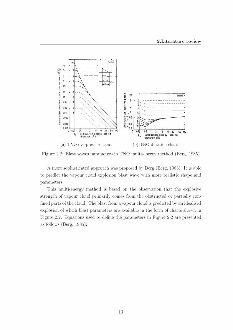
(a) TNO overpressure chart (b) TNO duration chart
Figure 2.2: Blast waves parameters in TNO multi-energy method (Berg, 1985)
A more sophisticated approach was proposed by Berg (Berg, 1985). It is able
to predict the vapour cloud explosion blast wave with more realistic shape and
parameters.
This multi-energy method is based on the observation that the explosive
strength of vapour cloud primarily comes from the obstructed or partially con-
fined parts of the cloud. The blast from a vapour cloud is predicted by an idealised
explosion of which blast parameters are available in the form of charts shown in
Figure 2.2. Equations used to define the parameters in Figure 2.2 are presented
as follows (Berg, 1985):
13
2.Literature review
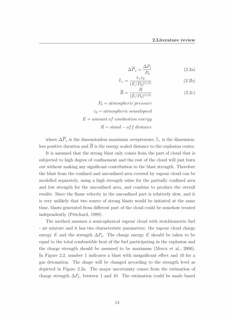
ΔP s =ΔPs
P0
(2.2a)
t+ =t+c0
(E/P0)(1/3)(2.2b)
R =R
(E/P0)(1/3)(2.2c)
P0 = atmospheric pressure
c0 = atmospheric soundspeed
E = amount of combustion energy
R = stand− off distance
where ΔP s is the dimensionless maximum overpressure, t+ is the dimension-
less positive duration and R is the energy scaled distance to the explosion centre.
It is assumed that the strong blast only comes from the part of cloud that is
subjected to high degree of confinement and the rest of the cloud will just burn
out without making any significant contribution to the blast strength. Therefore
the blast from the confined and unconfined area covered by vapour cloud can be
modelled separately, using a high strength value for the partially confined area
and low strength for the unconfined area, and combine to produce the overall
results. Since the flame velocity in the unconfined part is relatively slow, and it
is very unlikely that two source of strong blasts would be initiated at the same
time, blasts generated from different part of the cloud could be somehow treated
independently (Pritchard, 1989).
The method assumes a semi-spherical vapour cloud with stoichiometric fuel
- air mixture and it has two characteristic parameters: the vapour cloud charge
energy E and the strength ΔPs. The charge energy E should be taken to be
equal to the total combustible heat of the fuel participating in the explosion and
the charge strength should be assumed to be maximum (Mercx et al., 2000).
In Figure 2.2, number 1 indicates a blast with insignificant effect and 10 for a
gas detonation. The shape will be changed according to the strength level as
depicted in Figure 2.2a. The major uncertainty comes from the estimation of
charge strength ΔPs, between 1 and 10. The estimation could be made based
14
2. Literature review
on the observed damage or experience. For an more sophisticated and accurate
approach, the correlation with experiments to quantify the charge strength can
be done according to the procedures laid out by Mercx (Mercx et al., 2000). The
correlation equation is:
ΔPs = a
[V BR · Lf
D
]bSl
2.7Sc0.7 (2.3)
In equation 2.3, V BR is the volume blockage ratio, which is the portion of the
volume occupied by the obstacles within the cloud. Lf is the flame path, which
is the longest distance from the point of ignition to an outer edge of the obstacle.
D is the average obstacle size (m). Sl is the laminar burning velocity (m/s). Sc
is a scale factor and a, b are correlation fitting constants. Equation 2.3 takes into
account of the effects from three influence factors: the boundary conditions, the
mixture reactivity and the explosion scale. Once the charge strength is deter-
mined, the selection of curves can be completed. The overpressure and positive
duration can be readily extracted from Figure 2.2 as a function of energy scaled
distance R.
2.2 Review of past incidents
2.2.1 Buncefield incident
On the morning of Sunday 11th December 2005, a vapour cloud explosion oc-
curred at the Buncefield Oil Storage Depot, Hemel Hempstead, Hertfordshire,
UK. The investigation immediately carried out by the Buncefield Major Incident
Investigation Board (BMIIB) identified that the explosion was a consequence of
the overflow of 250,000 litres of petrol from the storage tank 912 in the depot.
The cloud was approximately circular with a radius of 200 metres before the
explosion occurred, with average height of 2 metres (SCI, 2009).
The blast caused tremendous damage to the near and far field buildings. Due
to lack of any significant congestion in the site, the severity of the explosion had
not been anticipated in any major hazard assessment of the oil and gas storage
site before. The red line in Figure 2.3 represents the approximate boundary of
15
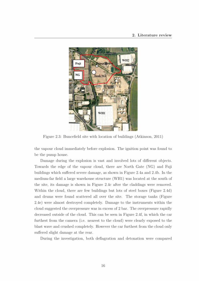
2. Literature review
Figure 2.3: Buncefield site with location of buildings (Atkinson, 2011)
the vapour cloud immediately before explosion. The ignition point was found to
be the pump house.
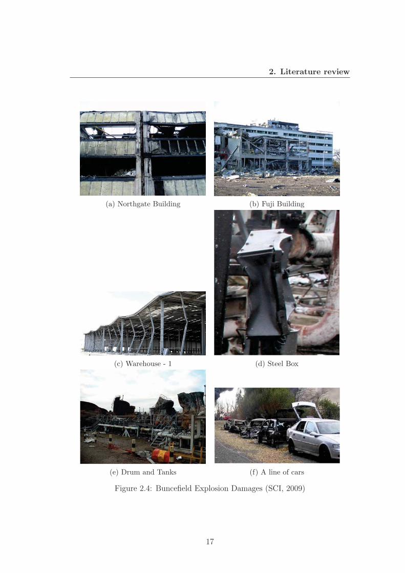
Damage during the explosion is vast and involved lots of different objects.
Towards the edge of the vapour cloud, there are North Gate (NG) and Fuji
buildings which suffered severe damage, as shown in Figure 2.4a and 2.4b. In the
medium-far field a large warehouse structure (WH1) was located at the south of
the site, its damage is shown in Figure 2.4c after the claddings were removed.
Within the cloud, there are few buildings but lots of steel boxes (Figure 2.4d)
and drums were found scattered all over the site. The storage tanks (Figure
2.4e) were almost destroyed completely. Damage to the instruments within the
cloud suggested the overpressure was in excess of 2 bar. The overpressure rapidly
decreased outside of the cloud. This can be seen in Figure 2.4f, in which the car
furthest from the camera (i.e. nearest to the cloud) were clearly exposed to the
blast wave and crushed completely. However the car furthest from the cloud only
suffered slight damage at the rear.
During the investigation, both deflagration and detonation were compared
16
2. Literature review
(a) Northgate Building (b) Fuji Building
(c) Warehouse - 1 (d) Steel Box
(e) Drum and Tanks (f) A line of cars
Figure 2.4: Buncefield Explosion Damages (SCI, 2009)
17

2. Literature review
with the observed damages but neither is able to explain the explosion conclu-
sively. It was concluded in the joint industry project (SCI, 2009) and by Johnson
(Johnson, 2010) that due to the lack of congested pipe works within the vapour
cloud (which is a prerequisite for a strong vapour cloud explosion), the explo-
sion initially started as deflagration at the pump house. And when the flame
approached to the trees and undergrowths along the lanes around the site, the
combustion flame accelerated due to the turbulence generated by the wooden
branches, then developed in to detonation. At least part of the cloud has been
detonated afterwards.
Compared with the past major incidents, the 2005 Buncefield explosion of-
fered lots of evidence and damage for forensic studies and investigations. The
investigation work presented a great advancement in understanding vapour cloud
explosions. It also identified some areas worthy of fundamental researches.
2.2.2 Other major accidents
Buncefield is not the first vapour cloud explosion that occurred in the oil and gas
industries. A few previous incidents involving vapour cloud and gas explosions
are summarised below:
• Flixborough, UK, 1974 (Sadee et al., 1977), in which the failure of a section
of 700 mm diameter temporary pipe released approximately 100 tonnes of
cyclohexane. The explosion caused significant damage to the building struc-
tures on site. The overpressure at the edge of the cloud was approximately
1 bar declining with distance as would be expected from a TNT charge
detonation. Within the cloud the pressure was estimated to be as high as
10 bar.
• Port Hudson, Missouri, US, 1970 (Burgess and Zabetakis, 1973), in which
the pipeline failure released approximately 120,000 litres of propane. The
character and distribution of damage strongly resembled that at Buncefield
(SCI, 2009). Damages to buildings within the cloud are significant and
suggesting overpressure of at least 1 bar over the area covered by the cloud.
18
2. Literature review
• Ufa, Ural Mountains, Russia, 1989 (Makhviladze and Yakush, 2002), in
which the failure of a pipeline of 700 mm diameter released a total 2000-
10,000 tonnes of liquefied petroleum gas (LPG). Trains were damaged as if
they were clamped in a vice. Trees felled over a large area suggesting the
overpressure exceeded 1 bar.
• Naples, 1985 (Maremonti et al., 1999), in which approximately 700 tonnes
petrol escaped from an over-filled tank, and a subsequent vapour cloud ex-
plosion occurred. Maximum pressure was indicated by the damaged objects
to be 0.48 bar. Windows were broken to a range of 1 km.
• Saint Herblain, France, 1991 (Lechaudel and Mouilleau, 1995), in which a
hydrocarbon explosion occurred in a tank farm as a consequence of petrol
leakage. Explosion caused severe damages to the buildings in the surround-
ing area and also to the tanks on site. Overpressure indicators were analysed
and the maximum pressure of 0.25 bar was estimated.
• Texas City, Texas, U.S, 2005 (BP, 2005), in which a total of 28,700 litres
hydrocarbons C5-C7 released into atmosphere and mixed with air. The
damage was focused in congested areas of the site where there was en-
hancement of turbulence promoting the combustion rate. The overpressure
was estimated to be over 1 bar within the congested area.
2.3 Blast wave and loading
Detonation and deflagration of a vapour cloud generate very different forms of
blast waves as shown in Figure 2.1a and 2.1b. The shape of the blast wave from
a deflagration will approach to detonation at the medium to far-field distance.
The blast wave from a detonation led by a shock front (with instantaneous rise
of pressure) is usually referred to as an ideal blast wave. Its parameters can
be defined by the TNT-equivalent method (with stand-off distance and charge
weight).
19
2. Literature review
2.3.1 Blast wave characteristics
A detonation blast wave is usually referred to as an ideal blast wave or shock
wave. It is led by a shock front when travelling through the air and compresses
the fuel mixture or air in the front. The properties of the medium before and
after the shock front can be related by the Rankine-Hugoniot relations. The shock
wave characteristics can be defined by TNT explosion and scaling laws based on
the charge weight and stand-off distance.
2.3.1.1 Normal shock
x
x
x
x
TP
u
x
y
y
y
y
TP
u
y
upstream
Stationary Normal Shock
downstream
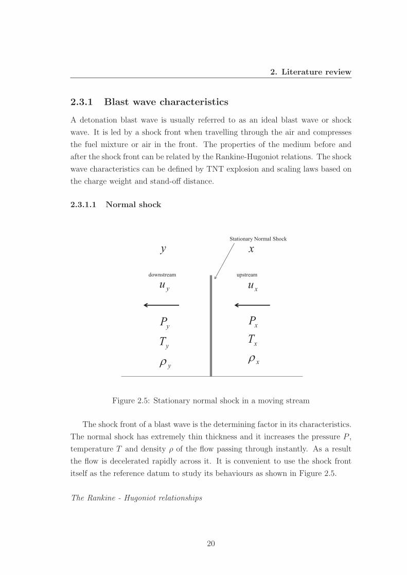
Figure 2.5: Stationary normal shock in a moving stream
The shock front of a blast wave is the determining factor in its characteristics.
The normal shock has extremely thin thickness and it increases the pressure P ,
temperature T and density ρ of the flow passing through instantly. As a result
the flow is decelerated rapidly across it. It is convenient to use the shock front
itself as the reference datum to study its behaviours as shown in Figure 2.5.
The Rankine - Hugoniot relationships
20
2. Literature review
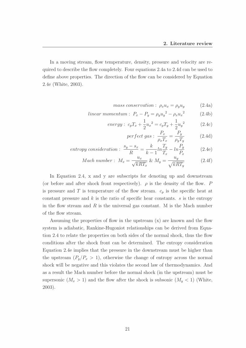
In a moving stream, flow temperature, density, pressure and velocity are re-
quired to describe the flow completely. Four equations 2.4a to 2.4d can be used to
define above properties. The direction of the flow can be considered by Equation
2.4e (White, 2003).
mass conservation : ρxux = ρyuy (2.4a)
linear momentum : Px − Py = ρyuy2 − ρxux
2 (2.4b)
energy : cpTx +1
2ux
2 = cpTy +1
2uy
2 (2.4c)
perfect gas :Px
ρxTx
=Py
ρyTy
(2.4d)
entropy consideration :sy − sx
R=
k
k − 1ln
Ty
Tx
− lnPy
Px
(2.4e)
Mach number : Mx =ux√kRTx
& My =uy√kRTy
(2.4f)
In Equation 2.4, x and y are subscripts for denoting up and downstream
(or before and after shock front respectively). ρ is the density of the flow. P
is pressure and T is temperature of the flow stream. cp is the specific heat at
constant pressure and k is the ratio of specific hear constants. s is the entropy
in the flow stream and R is the universal gas constant. M is the Mach number
of the flow stream.
Assuming the properties of flow in the upstream (x) are known and the flow
system is adiabatic, Rankine-Hugoniot relationships can be derived from Equa-
tion 2.4 to relate the properties on both sides of the normal shock, thus the flow
conditions after the shock front can be determined. The entropy consideration
Equation 2.4e implies that the pressure in the downstream must be higher than
the upstream (Py/Px > 1), otherwise the change of entropy across the normal
shock will be negative and this violates the second law of thermodynamics. And
as a result the Mach number before the normal shock (in the upstream) must be
supersonic (Mx > 1) and the flow after the shock is subsonic (My < 1) (White,
2003).
21
2. Literature review
Py
Px
=2kMx
2 − (k − 1)
k + 1=
7Mx2 − 1
6(2.5)
Ty
Tx
=[2 + (k − 1)Mx
2][2kMx2 − (k − 1)]
(k + 1)2Mx3
=(5 +Mx
2)(7Mx2 − 1)
36Mx2 (2.6)
uy
ux
=2 + (k − 1)Mx
2
(k + 1)Mx2 =
1 + 5/Mx2
6(2.7)
Relationships giving the properties changes across the normal shock can be
derived from the above equations (Kinney and Graham, 1985). Equations 2.5,
2.6 and 2.7 define the ratios of pressure, temperature and flow velocity between
the up- and down-streams in terms of independent variable Mach number in the
upstream (Mx).
Explosive shock
atmx
atmx
atmx
x
TTPP
u
x
y
y
y
yxp
TP
uuu
yMoving Normal Shock
Medium after shock
Undisturbed Medium before shock
Figure 2.6: Explosive shock front moving in still air
The analysis of the stationary normal shock also applies to a moving shock
22
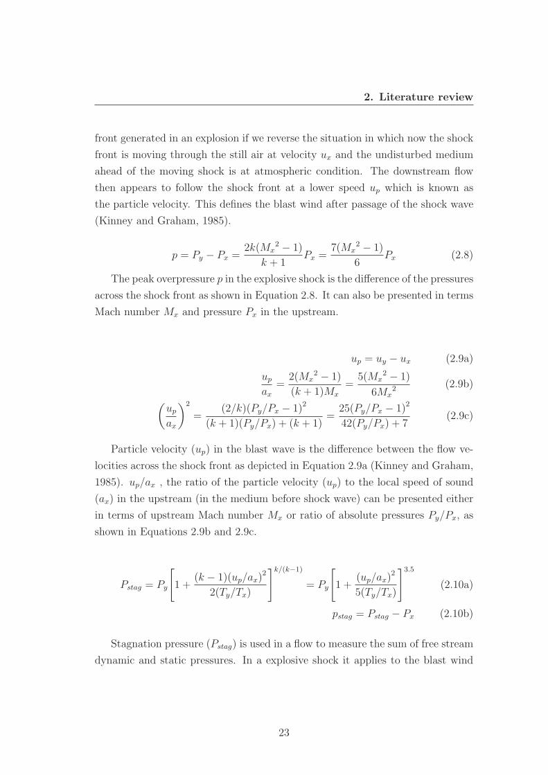
2. Literature review
front generated in an explosion if we reverse the situation in which now the shock
front is moving through the still air at velocity ux and the undisturbed medium
ahead of the moving shock is at atmospheric condition. The downstream flow
then appears to follow the shock front at a lower speed up which is known as
the particle velocity. This defines the blast wind after passage of the shock wave
(Kinney and Graham, 1985).
p = Py − Px =2k(Mx
2 − 1)
k + 1Px =
7(Mx2 − 1)
6Px (2.8)
The peak overpressure p in the explosive shock is the difference of the pressures
across the shock front as shown in Equation 2.8. It can also be presented in terms
Mach number Mx and pressure Px in the upstream.
up = uy − ux (2.9a)
up
ax=
2(Mx2 − 1)
(k + 1)Mx
=5(Mx
2 − 1)
6Mx2 (2.9b)(
up
ax
)2
=(2/k)(Py/Px − 1)2
(k + 1)(Py/Px) + (k + 1)=
25(Py/Px − 1)2
42(Py/Px) + 7(2.9c)
Particle velocity (up) in the blast wave is the difference between the flow ve-
locities across the shock front as depicted in Equation 2.9a (Kinney and Graham,
1985). up/ax , the ratio of the particle velocity (up) to the local speed of sound
(ax) in the upstream (in the medium before shock wave) can be presented either
in terms of upstream Mach number Mx or ratio of absolute pressures Py/Px, as
shown in Equations 2.9b and 2.9c.
Pstag = Py
[1 +
(k − 1)(up/ax)2
2(Ty/Tx)
]k/(k−1)
= Py
[1 +
(up/ax)2
5(Ty/Tx)
]3.5(2.10a)
pstag = Pstag − Px (2.10b)
Stagnation pressure (Pstag) is used in a flow to measure the sum of free stream
dynamic and static pressures. In a explosive shock it applies to the blast wind
23
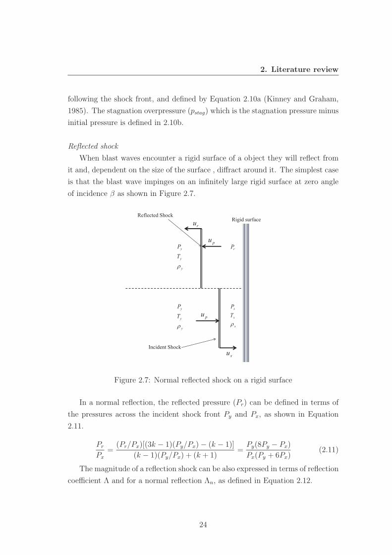
2. Literature review
following the shock front, and defined by Equation 2.10a (Kinney and Graham,
1985). The stagnation overpressure (pstag) which is the stagnation pressure minus
initial pressure is defined in 2.10b.
Reflected shock
When blast waves encounter a rigid surface of a object they will reflect from
it and, dependent on the size of the surface , diffract around it. The simplest case
is that the blast wave impinges on an infinitely large rigid surface at zero angle
of incidence β as shown in Figure 2.7.
x
x
x
TP
y
y
y
TP
Incident Shock
Reflected Shock
pu
xu
Rigid surface
rP
y
y
y
TP
ru
pu
Figure 2.7: Normal reflected shock on a rigid surface
In a normal reflection, the reflected pressure (Pr) can be defined in terms of
the pressures across the incident shock front Py and Px, as shown in Equation
2.11.
Pr
Px
=(Pr/Px)[(3k − 1)(Py/Px)− (k − 1)]
(k − 1)(Py/Px) + (k + 1)=
Py(8Py − Px)
Px(Py + 6Px)(2.11)
The magnitude of a reflection shock can be also expressed in terms of reflection
coefficient Λ and for a normal reflection Λn, as defined in Equation 2.12.
24
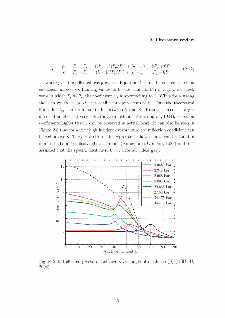
2. Literature review
Λn =prp
=Pr − Px
Py − Px
=(3k − 1)(Py/Px) + (k + 1)
(k − 1)(Py/Px) + (k + 1)=
8Py + 6Px
Py + 6Px
(2.12)
where pr is the reflected overpressure. Equation 2.12 for the normal reflection
coefficient allows two limiting values to be determined. For a very weak shock
wave in which Py ≈ Px, the coefficient Λn is approaching to 2. While for a strong
shock in which Py � Px, the coefficient approaches to 8. Thus the theoretical
limits for Λn can be found to be between 2 and 8. However, because of gas
dissociation effect at very close range (Smith and Hetherington, 1994), reflection
coefficients higher than 8 can be observed in actual blast. It can also be seen in
Figure 2.8 that for a very high incident overpressure the reflection coefficient can
be well above 8. The derivation of the expressions shown above can be found in
more details in “Explosive shocks in air” (Kinney and Graham, 1985) and it is
assumed that the specific heat ratio k = 1.4 for air (ideal gas).
0 10 20 30 40 50 60 70 80 90Angle of incident β
0
2
4
6
8
10
12
Reflection
coeffi
cientΛ
0.0689 bar
0.345 bar
2.068 bar
6.895 bar
20.685 bar
27.58 bar
34.475 bar
344.75 bar
Figure 2.8: Reflected pressure coefficients vs. angle of incidence (β) (USDOD,2008)
25
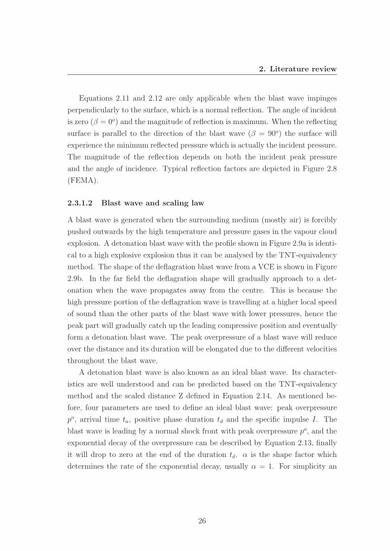
2. Literature review
Equations 2.11 and 2.12 are only applicable when the blast wave impinges
perpendicularly to the surface, which is a normal reflection. The angle of incident
is zero (β = 0o) and the magnitude of reflection is maximum. When the reflecting
surface is parallel to the direction of the blast wave (β = 90o) the surface will
experience the minimum reflected pressure which is actually the incident pressure.
The magnitude of the reflection depends on both the incident peak pressure
and the angle of incidence. Typical reflection factors are depicted in Figure 2.8
(FEMA).
2.3.1.2 Blast wave and scaling law
A blast wave is generated when the surrounding medium (mostly air) is forcibly
pushed outwards by the high temperature and pressure gases in the vapour cloud
explosion. A detonation blast wave with the profile shown in Figure 2.9a is identi-
cal to a high explosive explosion thus it can be analysed by the TNT-equivalency
method. The shape of the deflagration blast wave from a VCE is shown in Figure
2.9b. In the far field the deflagration shape will gradually approach to a det-
onation when the wave propagates away from the centre. This is because the
high pressure portion of the deflagration wave is travelling at a higher local speed
of sound than the other parts of the blast wave with lower pressures, hence the
peak part will gradually catch up the leading compressive position and eventually
form a detonation blast wave. The peak overpressure of a blast wave will reduce
over the distance and its duration will be elongated due to the different velocities
throughout the blast wave.
A detonation blast wave is also known as an ideal blast wave. Its character-
istics are well understood and can be predicted based on the TNT-equivalency
method and the scaled distance Z defined in Equation 2.14. As mentioned be-
fore, four parameters are used to define an ideal blast wave: peak overpressure
po, arrival time ta, positive phase duration td and the specific impulse I. The
blast wave is leading by a normal shock front with peak overpressure po, and the
exponential decay of the overpressure can be described by Equation 2.13, finally
it will drop to zero at the end of the duration td. α is the shape factor which
determines the rate of the exponential decay, usually α = 1. For simplicity an
26
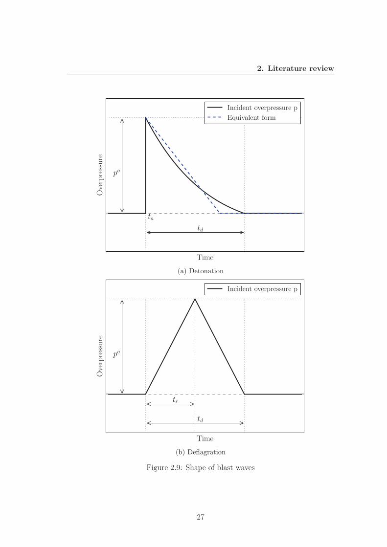
2. Literature review
0.0 0.2 0.4 0.6 0.8 1.0
Time-0.4
-0.2
0.0
0.2
0.4
0.6
0.8
1.0
Overpressure
po
td
ta
Incident overpressure p
Equivalent form
(a) Detonation
0.0 0.2 0.4 0.6 0.8 1.0
Time-0.4
-0.2
0.0
0.2
0.4
0.6
0.8
1.0
Overpressure
po
td
tr
Incident overpressure p
(b) Deflagration
Figure 2.9: Shape of blast waves
27
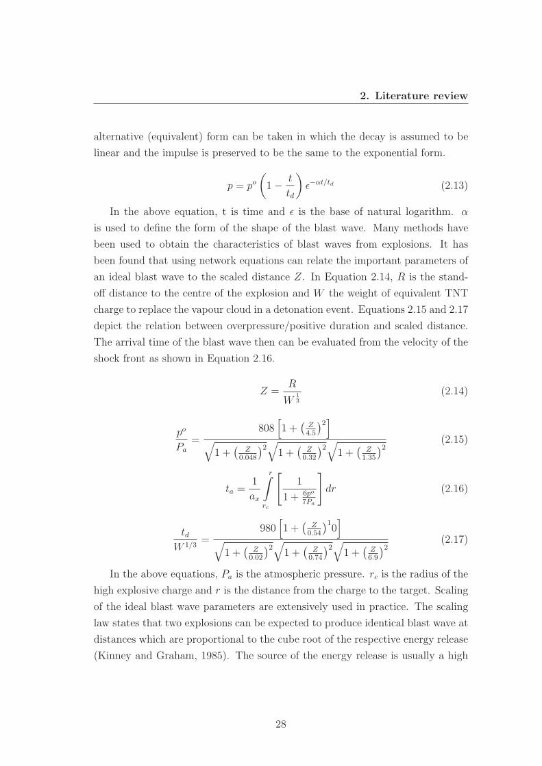
2. Literature review
alternative (equivalent) form can be taken in which the decay is assumed to be
linear and the impulse is preserved to be the same to the exponential form.
p = po(1− t
td
)ε−αt/td (2.13)
In the above equation, t is time and ε is the base of natural logarithm. α
is used to define the form of the shape of the blast wave. Many methods have
been used to obtain the characteristics of blast waves from explosions. It has
been found that using network equations can relate the important parameters of
an ideal blast wave to the scaled distance Z. In Equation 2.14, R is the stand-
off distance to the centre of the explosion and W the weight of equivalent TNT
charge to replace the vapour cloud in a detonation event. Equations 2.15 and 2.17
depict the relation between overpressure/positive duration and scaled distance.
The arrival time of the blast wave then can be evaluated from the velocity of the
shock front as shown in Equation 2.16.
Z =R
W13
(2.14)
po
Pa
=808[1 +(
Z4.5
)2]√1 +(
Z0.048
)2√1 +(
Z0.32
)2√1 +(
Z1.35
)2 (2.15)
ta =1
ax
r∫rc
[1
1 + 6po
7Pa
]dr (2.16)
tdW 1/3
=980[1 +(
Z0.54
)10]
√1 +(
Z0.02
)2√1 +(
Z0.74
)2√1 +(
Z6.9
)2 (2.17)
In the above equations, Pa is the atmospheric pressure. rc is the radius of the
high explosive charge and r is the distance from the charge to the target. Scaling
of the ideal blast wave parameters are extensively used in practice. The scaling
law states that two explosions can be expected to produce identical blast wave at
distances which are proportional to the cube root of the respective energy release
(Kinney and Graham, 1985). The source of the energy release is usually a high
28
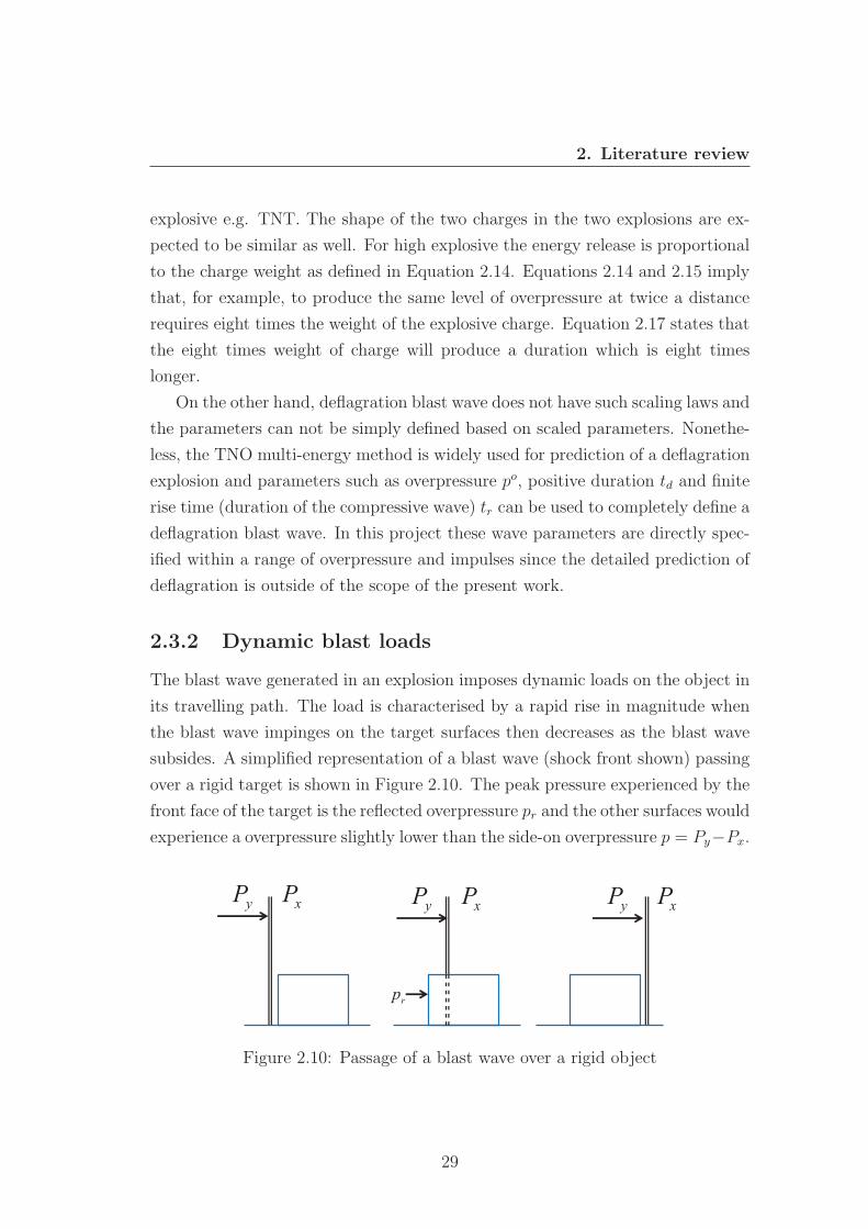
2. Literature review
explosive e.g. TNT. The shape of the two charges in the two explosions are ex-
pected to be similar as well. For high explosive the energy release is proportional
to the charge weight as defined in Equation 2.14. Equations 2.14 and 2.15 imply
that, for example, to produce the same level of overpressure at twice a distance
requires eight times the weight of the explosive charge. Equation 2.17 states that
the eight times weight of charge will produce a duration which is eight times
longer.
On the other hand, deflagration blast wave does not have such scaling laws and
the parameters can not be simply defined based on scaled parameters. Nonethe-
less, the TNO multi-energy method is widely used for prediction of a deflagration
explosion and parameters such as overpressure po, positive duration td and finite
rise time (duration of the compressive wave) tr can be used to completely define a
deflagration blast wave. In this project these wave parameters are directly spec-
ified within a range of overpressure and impulses since the detailed prediction of
deflagration is outside of the scope of the present work.
2.3.2 Dynamic blast loads
The blast wave generated in an explosion imposes dynamic loads on the object in
its travelling path. The load is characterised by a rapid rise in magnitude when
the blast wave impinges on the target surfaces then decreases as the blast wave
subsides. A simplified representation of a blast wave (shock front shown) passing
over a rigid target is shown in Figure 2.10. The peak pressure experienced by the
front face of the target is the reflected overpressure pr and the other surfaces would
experience a overpressure slightly lower than the side-on overpressure p = Py−Px.
yP xP yP xP yP xP
rp
Figure 2.10: Passage of a blast wave over a rigid object
29
2. Literature review
The ideal dynamic pressure loads experienced by the surfaces of a target are
shown in Figure 2.11. The reflected pressure load is produced by the shock front
impinging on the surface perpendicular to the blast wave (normal reflection). The
stagnation pressure is caused by the movement of the particles behind the shock
front, which are brought to halt by the surfaces. Side-on pressure is also known
as the incident pressure and finally the drag pressure is the load exerted by the
blast wind. The difference (stagnation - drag) is the load experienced at the rear
surface of the body. Using the blast curves the actual dynamic loadings on the
different faces of the target can be estimated in the following sections.
0.0 0.2 0.4 0.6 0.8 1.0
Time0.0
0.2
0.4
0.6
0.8
1.0
Overpressure
reflected
stagnation
side-on
stagnation-drag
drag
Figure 2.11: Blast curves (Kinney and Graham, 1985)
2.3.2.1 Front surface load
When the blast wave strikes the front surface, it will immediately experience
a peak reflected pressure pr which follows the reflected curve in Figure 2.11.
The reflected pressure is significantly greater than the surrounding pressure. A
rarefaction wave then forms over the front surface of the object and progresses
30
2. Literature review
inwards from the edge, travelling at the speed of sound in the reflected medium.
With the decaying of the reflected pressure the velocity of the rarefaction wave
will reduce and an arbitrary small panel on the front surface will be subjected
to the reflected pressure until at time d/Ux when the arrival of the rarefaction
wave brings the relief effect so the pressure level drops significantly to stagnation
overpressure, where d is the shortest distance of the small panel to the edge of the
front face. Therefore an average sense is needed to take into account the progress
of the rarefaction wave over the whole front surface, where the earliest panel to see
the pressure relief is at the edge while in the centre the panels will experience the
reflected pressure the longest. To generalise the effects, as shown in Figure 2.12,
the overpressure will start with pr at zero time and reduce to stagnation pressure
at time 3S/ux, where S is the half width or height of the front surface, whichever
is smaller. And after this time the overpressure will follow the stagnation pressure
curve and reduces to ambient. In Figure 2.12, pi is the incident pressure.
0.0 0.2 0.4 0.6 0.8 1.0
Time0.0
0.2
0.4
0.6
0.8
1.0
Overpressure
pi
pr
3Sux td
front
side-on
Figure 2.12: Blast load-time history on front surface (Kinney and Graham, 1985)
31
2. Literature review
2.3.2.2 Rear surface load
The rear surface will not experience any load until the blast wave travels through
the length of the target L at time L/ux, as shown in Figure 2.13a. After this
time the pressure loading will start to build up and reach the instantaneous
value, which is the different between the stagnation and the drag pressure. The
compression wave will take a finite time to travel from the edge to the centre hence
different locations on the rear face will feel the pressure at different times with
different magnitudes. The entire load on the rear face is an average of the loads
on each location. Therefore, the average starts to rise at time L/ux and reaches
the peak value pstag − pdrag after a finite rise time of 3S/us. Then the loadings
vanishes along the stagnation-drag curve to zero at time td+L/ux. It is important
to note that the actual pressure loadings on the rear surface will be offset by a
time L/ux and the peak value is lower than the side-on peak overpressure.
2.3.2.3 Top and side surface loads
Top and side faces are parallel to the direction of the blast wave, ideally they will
be subjected to the side-on (incident or free-field) over pressure.
However, the edges between the front face and the top/side face will induce
diffraction in the flow field and this diffracted wave will slightly reduce the peak
overpressure. Similarly, an arbitrary panel at the front will experience the load-
ings earlier than panels located towards the back, as depicted in Figure 2.13b.
The average will starts at time zero when the blast wave strikes on the front face
and then gradually increase to a peak which is slightly lower than the peak side-
on value at time L/ux. It then decays to atmosphere pressure at time td +L/ux.
The time L/ux and the rise of the loading are used to determine the load on the
whole surface in an average manner.
2.3.2.4 Loads on the frame
Blast loadings on the surfaces of a structure will be transferred to its frames and
eventually to the ground. Once the frame fails then the whole structure is severely
damaged regardless of the condition of the claddings. The net lateral load on the
frame of a structure can be calculated by the difference between the total loads
32
2. Literature review
0.0 0.2 0.4 0.6 0.8 1.0
Time0.0
0.2
0.4
0.6
0.8
1.0
Overpressure
pi
Lux
3Sux td +
Lux
rear
side-on
(a) Rear surface
0.0 0.2 0.4 0.6 0.8 1.0
Time0.0
0.2
0.4
0.6
0.8
1.0
Overpressure
pi
Lux td td +
Lux
close to front
middle
close to rear
average
(b) Top/side surface
Figure 2.13: Blast load-time history other surface (Kinney and Graham, 1985)
33
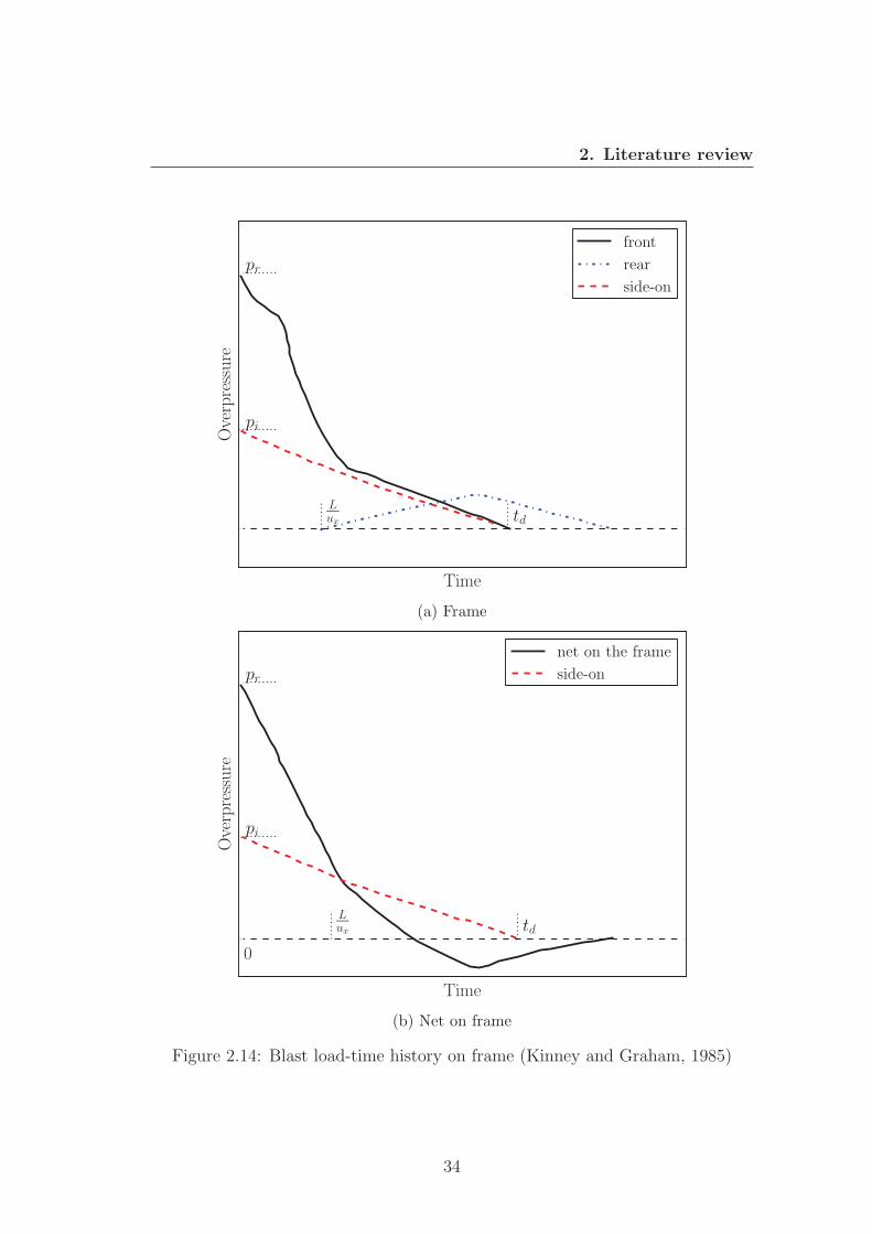
2. Literature review
0.0 0.2 0.4 0.6 0.8 1.0
Time
0.0
0.2
0.4
0.6
0.8
1.0
Overpressure
pi
pr
Lux td
front
rear
side-on
(a) Frame
0.0 0.2 0.4 0.6 0.8 1.0
Time
0.0
0.2
0.4
0.6
0.8
1.0
Overpressure
pi
pr
Lux td
0
net on the frame
side-on
(b) Net on frame
Figure 2.14: Blast load-time history on frame (Kinney and Graham, 1985)
34
2. Literature review
on the front and rear surfaces. This can be readily established as shown in Figure
2.14. Figure 2.14a superimposes the blast loadings on the front and rear faces.
Figure 2.14b shows the net sidewise load on the frame by subtracting the rear
load from the front. It can be noted that there is a negative load acting on the
frame in the opposite direction. The negative phase is caused by the offset of the
rear face load and occurs when the load on the front face decreases to a value
lower than the rear surface load.
2.3.2.5 Non-ideal blast wave
The deflagration blast wave is also known as a non-ideal blast wave. Structural
loads resulting from the non-ideal blast wave can not be readily determined by
simple methods shown above. The non-ideal blast wave has a compressive wave
in the front rather than a normal shock. This means that the Rankine-Hugoniot
relationships are not applicable, thus the reflection curves are not applicable
either. Due to the fact that the rise of the overpressure takes a finite amount
of time, when the blast wave impinges on the surface, the reflected pressure can
start to relieve even before the peak is reached. This finite rise time allows a flow
around the target to be established. The loadings of a structure thus becomes
strongly dependent on the dimension of the target and as well as the blast wave
parameters.
The rate of energy release in the deflagration is slow so it could take up to
several hundreds of milliseconds to reach the peak overpressure. The relief waves
and flow due to rarefaction can be established even over relatively large buildings
in such a long time period. If the deflagration blast wave takes 100 ms to reach
the peak, for a building with dimension of 10 meters the rarefaction wave will
travel across the surface in about 30 ms at ambient speed of sound. The relief
from structure loads occurs on the same time scale as the loadings. Therefore the
blast loads are more closely dependent on the parameters of the incident blast
wave. It has been noted that the loadings, caused the compressive wave in a non-
ideal blast wave, does not have a significant enhancements as normally expected
from a ideal blast shock wave at the same level of peak overpressure (Needham,
2010).
35
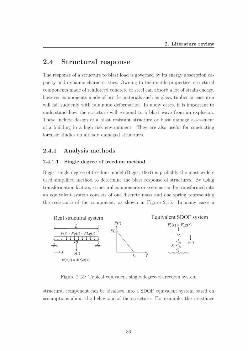
2. Literature review
2.4 Structural response
The response of a structure to blast load is governed by its energy absorption ca-
pacity and dynamic characteristics. Owning to the ductile properties, structural
components made of reinforced concrete or steel can absorb a lot of strain energy,
however components made of brittle materials such as glass, timber or cast iron
will fail suddenly with minimum deformation. In many cases, it is important to
understand how the structure will respond to a blast wave from an explosion.
These include design of a blast resistant structure or blast damage assessment
of a building in a high risk environment. They are also useful for conducting
forensic studies on already damaged structures.
2.4.1 Analysis methods
2.4.1.1 Single degree of freedom method
Biggs’ single degree of freedom model (Biggs, 1964) is probably the most widely
used simplified method to determine the blast response of structures. By using
transformation factors, structural components or systems can be transformed into
an equivalent system consists of one discrete mass and one spring representing
the resistance of the component, as shown in Figure 2.15. In many cases a
m)()()( tFLgtPgtP
)(t
L
x)()(),( xttxw
Real structural system
t
)(tP
FL
dt
Equivalent SDOF system
)(t
)()( tgFtF ee
eM
eK
Figure 2.15: Typical equivalent single-degree-of-freedom system
structural component can be idealised into a SDOF equivalent system based on
assumptions about the behaviour of the structure. For example, the resistance
36
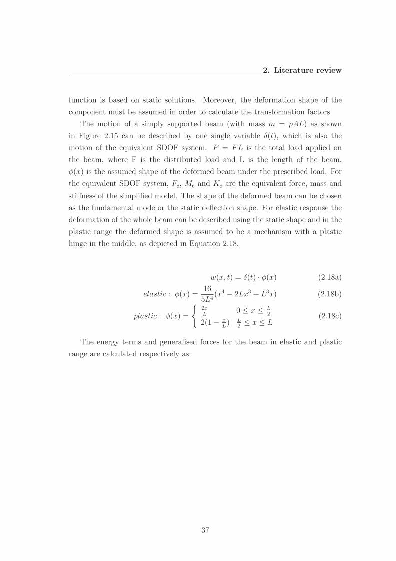
2. Literature review
function is based on static solutions. Moreover, the deformation shape of the
component must be assumed in order to calculate the transformation factors.
The motion of a simply supported beam (with mass m = ρAL) as shown
in Figure 2.15 can be described by one single variable δ(t), which is also the
motion of the equivalent SDOF system. P = FL is the total load applied on
the beam, where F is the distributed load and L is the length of the beam.
φ(x) is the assumed shape of the deformed beam under the prescribed load. For
the equivalent SDOF system, Fe, Me and Ke are the equivalent force, mass and
stiffness of the simplified model. The shape of the deformed beam can be chosen
as the fundamental mode or the static deflection shape. For elastic response the
deformation of the whole beam can be described using the static shape and in the
plastic range the deformed shape is assumed to be a mechanism with a plastic
hinge in the middle, as depicted in Equation 2.18.
w(x, t) = δ(t) · φ(x) (2.18a)
elastic : φ(x) =16
5L4(x4 − 2Lx3 + L3x) (2.18b)
plastic : φ(x) =
{2xL
0 ≤ x ≤ L2
2(1− xL) L
2≤ x ≤ L
(2.18c)
The energy terms and generalised forces for the beam in elastic and plastic
range are calculated respectively as:
37
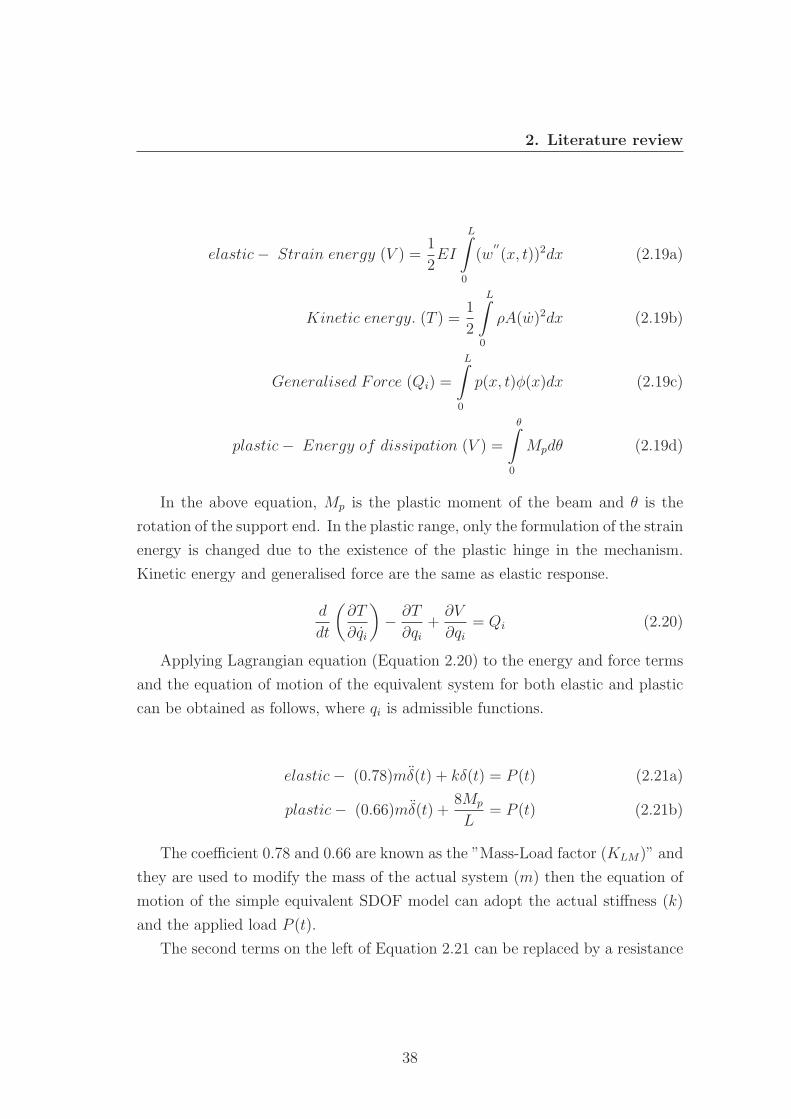
2. Literature review
elastic− Strain energy (V ) =1
2EI
L∫0
(w′′(x, t))2dx (2.19a)
Kinetic energy. (T ) =1
2
L∫0
ρA(w)2dx (2.19b)
Generalised Force (Qi) =
L∫0
p(x, t)φ(x)dx (2.19c)
plastic− Energy of dissipation (V ) =
θ∫0
Mpdθ (2.19d)
In the above equation, Mp is the plastic moment of the beam and θ is the
rotation of the support end. In the plastic range, only the formulation of the strain
energy is changed due to the existence of the plastic hinge in the mechanism.
Kinetic energy and generalised force are the same as elastic response.
d
dt
(∂T
∂qi
)− ∂T
∂qi+
∂V
∂qi= Qi (2.20)
Applying Lagrangian equation (Equation 2.20) to the energy and force terms
and the equation of motion of the equivalent system for both elastic and plastic
can be obtained as follows, where qi is admissible functions.
elastic− (0.78)mδ(t) + kδ(t) = P (t) (2.21a)
plastic− (0.66)mδ(t) +8Mp
L= P (t) (2.21b)
The coefficient 0.78 and 0.66 are known as the ”Mass-Load factor (KLM)” and
they are used to modify the mass of the actual system (m) then the equation of
motion of the simple equivalent SDOF model can adopt the actual stiffness (k)
and the applied load P (t).
The second terms on the left of Equation 2.21 can be replaced by a resistance
38
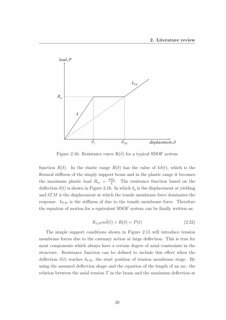
2. Literature review
,ntdisplaceme
Pload ,
mR
k
TMk
y TM
Figure 2.16: Resistance curve R(δ) for a typical SDOF system
function R(δ). In the elastic range R(δ) has the value of kδ(t), which is the
flexural stiffness of the simply support beam and in the plastic range it becomes
the maximum plastic load Rm = 8Mp
L. The resistance function based on the
deflection δ(t) is shown in Figure 2.16. In which δy is the displacement at yielding
and δTM is the displacement at which the tensile membrane force dominates the
response. kTM is the stiffness of due to the tensile membrane force. Therefore
the equation of motion for a equivalent SDOF system can be finally written as:
KLMmδ(t) +R(δ) = P (t) (2.22)
The simple support conditions shown in Figure 2.15 will introduce tension
membrane forces due to the catenary action at large deflection. This is true for
most components which always have a certain degree of axial constraints in the
structure. Resistance function can be defined to include this effect when the
deflection δ(t) reaches δTM , the start position of tension membrane stage. By
using the assumed deflection shape and the equation of the length of an arc, the
relation between the axial tension T in the beam and the maximum deflection at
39
2. Literature review
the middle point δ(t) can be derived as:
δTM = δy +
√4TL2
π2EA(2.23)
Above equation implies that it is assumed to be no axial tension in the beam
until reaching the yielding displacement δy, and the catenary stage will start
only when the axial tension reaches the value of T . EA is the axial rigidity of
the beam. The membrane tension T is usually taken as the minimum of the
plastic capacity of the beam section or the support. Membrane tension in the
beam between δy and δTM is assumed to be small and the support is assumed to
have limited flexibility to allow moderate axial displacement. When the catenary
stage starts, taking equilibrium between the applied uniform load P(t) and the
membrane tension T yields Equation 2.24, which provides the formula to evaluate
the stiffness of the catenary stage and shows the relation between the applied load
F and the maximum deflection δ of the beam in terms of the membrane tension
T .
F =8T
L2δ, where KTM =
8T
L2(2.24)
The formulations presented above are for a simply supported beam with axial
restraints. Without axial constraints the catenary stage can be simply ignored
and the resistance function becomes a bi-linear elastic - perfect plastic curve.
Formulations and Load-Mass factors of beams and plates with other support
conditions were derived by Biggs (Biggs, 1964). SBEDS (USACE, 2008a), a
spreadsheet software for single degree of freedom system published by US. Army
Corps of Engineers, presents the formulations of the membrane stiffness shown
in this section and this software was used in the current work to compare with
the advanced finite element method. The original approach for evaluation of
the transformation factors proposed by Biggs (Biggs, 1964) directly calculate the
transformation factors by equating the energies and work done by the external
forces between the actual and equivalent systems. His approach is nlengthy but
shows more explicitly how the system is transformed.
The equation of motion (Equation 2.22) needs to be solved to determine the
maximum dynamic response or the permanent deformation. A closed-form solu-
40
2. Literature review
tion can be obtained for simple dynamic loading functions. However, in many
cases the loading function will not have an analytical form, therefore the equa-
tion must be solved by time - stepping numerical integration methods (Craig,
1981). It has been shown that the Mass - Load factor KLM has different value for
elastic and plastic responses. The transformation factor and resistance are then
chosen to match the type of behaviour expected. If little yielding is expected,
the values for elastic response are used. Values for plastic behaviour can be used
if severe plasticity is expected. Average values can be used if moderate plasticity
is expected.
A simple analysis can reveal some insight into the response of a system to the
dynamic load. If the load function is a simple triangle shown in Figure 2.15, then
the equation of motion can be written as:
Meδ(t) +R(δ) = P
(1− t
td
)(2.25)
For the initial conditions of no displacement and no velocity at time t = 0,
the transient dynamic solution is (in which ω is the undamped natural circular
frequency):
δ(t)
P/k= (1− cosωt) +
1
td
(sinωt
ω− t
)(2.26)
Maximum deflection δmax = δ(tm) is always of the most interests, it can be
evaluated by differentiating Equation 2.26 and set to equal to zero:
0 = (ωtd) · sin(ωtm) + cos(ωtm)− 1 (2.27)
It can be deduced that there is a relation between (ωtd) and (ωtm) which can
be written as ωtm = f(ωtd), where ω =√
k/m, the natural circular frequency of
the equivalent SDOF system. In the view of this relationship, we can deduced
from Equation 2.26 that δmax/(F/k) at t = tm (the time at which maximum
dynamic deflection occurs) is a function of the ratio of load duration to the
system’s natural period T:
δmax
F/k= φ(ωtd) = φ′(
tdT) (2.28)
41
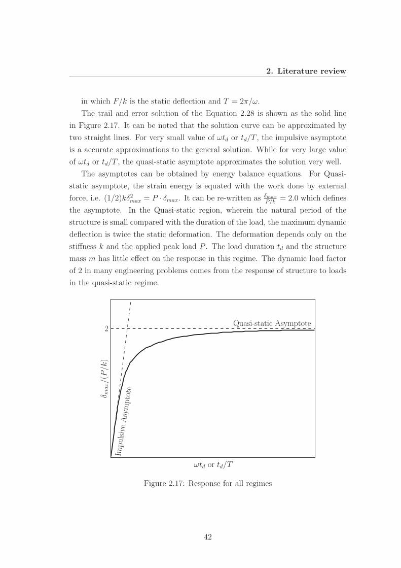
2. Literature review
in which F/k is the static deflection and T = 2π/ω.
The trail and error solution of the Equation 2.28 is shown as the solid line
in Figure 2.17. It can be noted that the solution curve can be approximated by
two straight lines. For very small value of ωtd or td/T , the impulsive asymptote
is a accurate approximations to the general solution. While for very large value
of ωtd or td/T , the quasi-static asymptote approximates the solution very well.
The asymptotes can be obtained by energy balance equations. For Quasi-
static asymptote, the strain energy is equated with the work done by external
force, i.e. (1/2)kδ2max = P · δmax. It can be re-written as δmax
P/k= 2.0 which defines
the asymptote. In the Quasi-static region, wherein the natural period of the
structure is small compared with the duration of the load, the maximum dynamic
deflection is twice the static deformation. The deformation depends only on the
stiffness k and the applied peak load P . The load duration td and the structure
mass m has little effect on the response in this regime. The dynamic load factor
of 2 in many engineering problems comes from the response of structure to loads
in the quasi-static regime.
0.0 0.2 0.4 0.6 0.8 1.0
ωtd or td/T0.0
0.2
0.4
0.6
0.8
1.0
δ max/(P/k
)
2Quasi-static Asymptote
ImpulsiveAsymptote
Figure 2.17: Response for all regimes
42
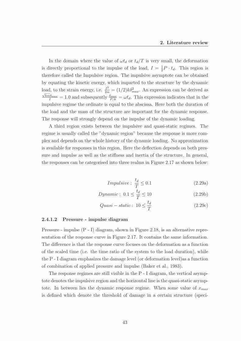
2. Literature review
In the domain where the value of ωtd or td/T is very small, the deformation
is directly proportional to the impulse of the load, I = 12P · td. This region is
therefore called the Impulsive region. The impulsive asymptote can be obtained
by equating the kinetic energy, which imparted to the structure by the dynamic
load, to the strain energy, i.e. I2
2m= (1/2)kδ2max. An expression can be derived as√
kmδmax
I= 1.0 and subsequently δmax
P/k= ωtd. This expression indicates that in the
impulsive regime the ordinate is equal to the abscissa. Here both the duration of
the load and the mass of the structure are important for the dynamic response.
The response will strongly depend on the impulse of the dynamic loading.
A third region exists between the impulsive and quasi-static regimes. The
regime is usually called the ”dynamic region” because the response is more com-
plex and depends on the whole history of the dynamic loading. No approximation
is available for responses in this region. Here the deflection depends on both pres-
sure and impulse as well as the stiffness and inertia of the structure. In general,
the responses can be categorised into three realms in Figure 2.17 as shown below:
Impulsive :tdT
≤ 0.1 (2.29a)
Dynamic : 0.1 ≤ tdT
≤ 10 (2.29b)
Quasi− static : 10 ≤ tdT
(2.29c)
2.4.1.2 Pressure - impulse diagram
Pressure - impulse (P - I) diagram, shown in Figure 2.18, is an alternative repre-
sentation of the response curve in Figure 2.17. It contains the same information.
The difference is that the response curve focuses on the deformation as a function
of the scaled time (i.e. the time ratio of the system to the load duration), while
the P - I diagram emphasizes the damage level (or deformation level)as a function
of combination of applied pressure and impulse (Baker et al., 1983).
The response regimes are still visible in the P - I diagram, the vertical asymp-
tote denotes the impulsive region and the horizontal line is the quasi-static asymp-
tote. In between lies the dynamic response regime. When some value of xmax
is defined which denote the threshold of damage in a certain structure (speci-
43
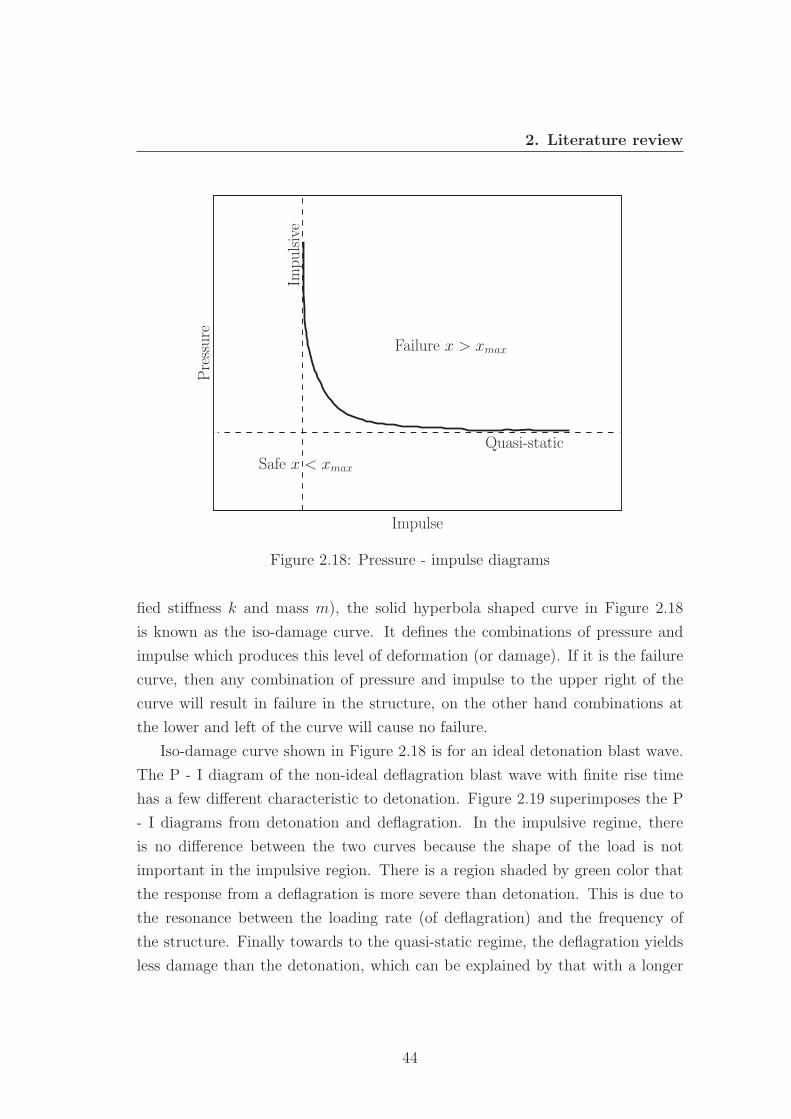
2. Literature review
0.0 0.5 1.0 1.5 2.0 2.5 3.0 3.5 4.0 4.5
Impulse0.0
0.5
1.0
1.5
2.0
2.5
3.0
3.5
4.0
Pressure
Quasi-static
Impulsive
Failure x > xmax
Safe x < xmax
Figure 2.18: Pressure - impulse diagrams
fied stiffness k and mass m), the solid hyperbola shaped curve in Figure 2.18
is known as the iso-damage curve. It defines the combinations of pressure and
impulse which produces this level of deformation (or damage). If it is the failure
curve, then any combination of pressure and impulse to the upper right of the
curve will result in failure in the structure, on the other hand combinations at
the lower and left of the curve will cause no failure.
Iso-damage curve shown in Figure 2.18 is for an ideal detonation blast wave.
The P - I diagram of the non-ideal deflagration blast wave with finite rise time
has a few different characteristic to detonation. Figure 2.19 superimposes the P
- I diagrams from detonation and deflagration. In the impulsive regime, there
is no difference between the two curves because the shape of the load is not
important in the impulsive region. There is a region shaded by green color that
the response from a deflagration is more severe than detonation. This is due to
the resonance between the loading rate (of deflagration) and the frequency of
the structure. Finally towards to the quasi-static regime, the deflagration yields
less damage than the detonation, which can be explained by that with a longer
44
2. Literature review
0.0 0.5 1.0 1.5 2.0 2.5 3.0 3.5 4.0 4.5
Impulse0.0
0.5
1.0
1.5
2.0
2.5
3.0
3.5
4.0
Pressure
Quasi-static
Impulsive
Detonation
Deflagration
Figure 2.19: Pressure - impulse diagrams comparison
duration the deflagration blast wave becomes more similar to a static load, and
less dynamic effect in the response of the structure. While the dynamic load
factor of detonation approaches to 2 in the quasi-static cases the deflagration is
approaching 1, i.e. equivalent to a static load.
2.4.1.3 Finite element method
Finite element modelling is widely used in dynamic/transient problems in re-
search and industry. It has advantages in being able to representing complex
structural geometry and boundary conditions, and components of different mate-
rial. While the simplified SDOF method treats the components individually, the
finite element method can include all components of essential interests and model
them as an assembly so that the interactions between components can be well
captured.Many commercial finite element packages are available and extensively
used, for example: ?, ANSYS and LS-DYNA. As the main analysis tool for the
present project, a more formal introduction of finite element method is presented
45
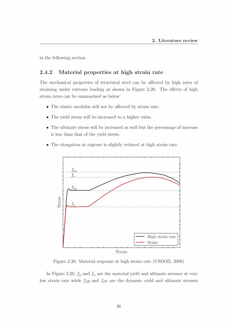
2. Literature review
in the following section.
2.4.2 Material properties at high strain rate
The mechanical properties of structural steel can be affected by high rates of
straining under extreme loading as shown in Figure 2.20. The effects of high
strain rates can be summarised as below:
• The elastic modulus will not be affected by strain rate.
• The yield stress will be increased to a higher value.
• The ultimate stress will be increased as well but the percentage of increase
is less than that of the yield stress.
• The elongation at rupture is slightly reduced at high strain rate.
0.0 0.2 0.4 0.6 0.8 1.0
Strain0.0
0.2
0.4
0.6
0.8
1.0
Stress
fy
fu
fdy
fdu
High strain rate
Static
Figure 2.20: Material response at high strain rate (USDOD, 2008)
In Figure 2.20, fy and fu are the material yield and ultimate stresses at very
low strain rate while fdy and fdu are the dynamic yield and ultimate stresses
46
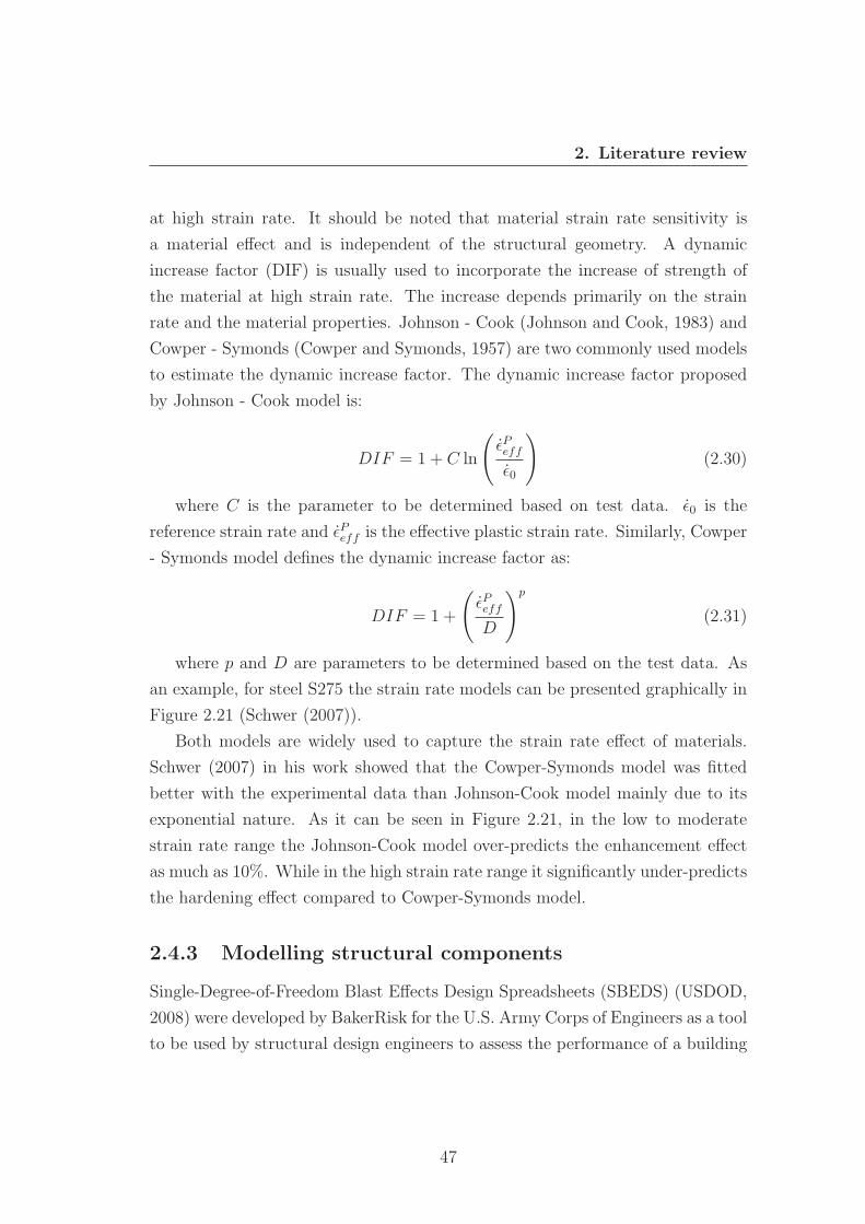
2. Literature review
at high strain rate. It should be noted that material strain rate sensitivity is
a material effect and is independent of the structural geometry. A dynamic
increase factor (DIF) is usually used to incorporate the increase of strength of
the material at high strain rate. The increase depends primarily on the strain
rate and the material properties. Johnson - Cook (Johnson and Cook, 1983) and
Cowper - Symonds (Cowper and Symonds, 1957) are two commonly used models
to estimate the dynamic increase factor. The dynamic increase factor proposed
by Johnson - Cook model is:
DIF = 1 + C ln
(εPeffε0
)(2.30)
where C is the parameter to be determined based on test data. ε0 is the
reference strain rate and εPeff is the effective plastic strain rate. Similarly, Cowper
- Symonds model defines the dynamic increase factor as:
DIF = 1 +
(εPeffD
)p
(2.31)
where p and D are parameters to be determined based on the test data. As
an example, for steel S275 the strain rate models can be presented graphically in
Figure 2.21 (Schwer (2007)).
Both models are widely used to capture the strain rate effect of materials.
Schwer (2007) in his work showed that the Cowper-Symonds model was fitted
better with the experimental data than Johnson-Cook model mainly due to its
exponential nature. As it can be seen in Figure 2.21, in the low to moderate
strain rate range the Johnson-Cook model over-predicts the enhancement effect
as much as 10%. While in the high strain rate range it significantly under-predicts
the hardening effect compared to Cowper-Symonds model.
2.4.3 Modelling structural components
Single-Degree-of-Freedom Blast Effects Design Spreadsheets (SBEDS) (USDOD,
2008) were developed by BakerRisk for the U.S. Army Corps of Engineers as a tool
to be used by structural design engineers to assess the performance of a building
47
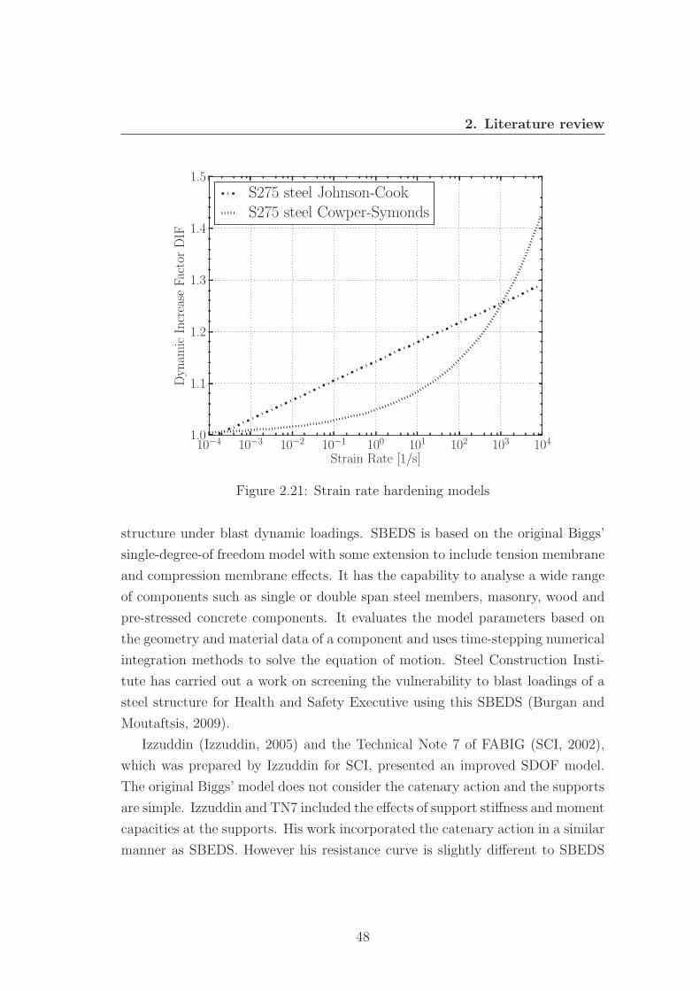
2. Literature review
10−4 10−3 10−2 10−1 100 101 102 103 104
Strain Rate [1/s]
1.0
1.1
1.2
1.3
1.4
1.5Dynam
icIncrease
FactorDIF
S275 steel Johnson-CookS275 steel Cowper-Symonds
Figure 2.21: Strain rate hardening models
structure under blast dynamic loadings. SBEDS is based on the original Biggs’
single-degree-of freedom model with some extension to include tension membrane
and compression membrane effects. It has the capability to analyse a wide range
of components such as single or double span steel members, masonry, wood and
pre-stressed concrete components. It evaluates the model parameters based on
the geometry and material data of a component and uses time-stepping numerical
integration methods to solve the equation of motion. Steel Construction Insti-
tute has carried out a work on screening the vulnerability to blast loadings of a
steel structure for Health and Safety Executive using this SBEDS (Burgan and
Moutaftsis, 2009).
Izzuddin (Izzuddin, 2005) and the Technical Note 7 of FABIG (SCI, 2002),
which was prepared by Izzuddin for SCI, presented an improved SDOF model.
The original Biggs’ model does not consider the catenary action and the supports
are simple. Izzuddin and TN7 included the effects of support stiffness and moment
capacities at the supports. His work incorporated the catenary action in a similar
manner as SBEDS. However his resistance curve is slightly different to SBEDS
48
2. Literature review
due to the order of formation of plastic hinges at the centre and supports of
the beam. There are additional elastic-plastic stages before the plastic bending
stage and one transient catenary stage that introduces a non-linear relationship
between the applied load and deflection before the final catenary stage starts.
Langdon has (Langdon and Schleyer, 2006a),(Langdon and Schleyer, 2006b),
(Langdon and Schleyer, 2006c) studied the response of various blast walls to dy-
namic overpressure loading. The experimental works investigated a small scale
blast wall with connections subject to pulse pressure loading to determine the
failure modes and revealed the importance of contribution of the support con-
nection to blast resistance. The stiffness and capacities of the end connections
are also determined in the experiments, which provided data for the subsequent
analytical work. Mode approximation techniques have been used in the analytical
analysis of the blast wall. The model represents a typical single trough of the
corrugated steel wall and incorporates the stiffness and capacities of the end con-
nections. Instead of deriving a resistance curve, the mode approximation method
breaks the response into three stages: elastic, elastic-plastic and plastic. Each
stage is approximated by two or three assumed mode shapes in order to represent
the possible combination of response modes. Equation of motion for each stage
is formulated based on energies and the Lagrange equation.
Leach (P.Leach, 1993) has extended Biggs’ method to corrugated cladding
panels with different boundary conditions and has provided design charts for the
elasto-plastic response of panels subjected to blast loadings. Louca (Louca et al.,
1996) used a non-linear finite element analysis package to study the response
of a blast wall subject to hydrocarbon explosions. The work showed boundary
restraints have significant influence on both the torsional response of the stiffeners
and the overall deformation of the panel. He also reported that, for a SDOF model
of the blast wall, the static resistance curve provided by Biggs’ table cannot
produce comparable results, however the results can be much improved by using
a non-linear FE analysis to establish the static resistance curves. The SDOF
model in Technical Note 5 (SCI, 1999a) issued by the Fire and Blast Information
Group (FABIG) and Steel Construction Institute (SCI) is widely used for design
of profiled panels. Louca (Louca et al., 2004) reviewed the adequacy of this
design guide by using non-linear finite element analysis. Liang (Liang and Louca,
49
2. Literature review
2007) derived new transformation factors for corrugated panels and the Biggs’
method has been extended to profiled panels with end plates. Fallah (Fallah and
L.A.Louca, 2007) formulated and sovled the SDOF model with elastic-plastic-
hardening and softening properties. Pressure - impulse diagrams are constructed
based on the improved SDOF models.
Plates are one of the basic elements of structures. The steel switch boxes
recovered from the Buncefield site are essentially made up of several thin plates,
although the boundary conditions would be significantly different to the studies
in literatures. Plate subject to uniform blast loading can be analysed by using
Biggs’ method as a two-way spanning member. Studies of plastic responses of
rectangular and circular plates are presented by Jones (Jones, 1997). Langdon
(Langdon and Schleyer, 1999) and Schleyer (Schleyer et al., 1999) studied the
response of metal plates subject to static and dynamic pressure loading through
a series of experiments in newly designed pressure test chamber. The pressure
profiles produced in the pressure chamber were of deflagration. Jacinto (Jacinto
et al., 2001) has carried out detonation tests on unstiffened metal plates and
compared the non-linear dynamic finite element model with the experimental
results. In his numerical studies, the applied external loading is obtained as the
difference between the pressure traces recorded at the front and back of the thin
plate. This way of applying pressure loading significantly improved the accuracy
of the numerical model compared with only applying the pressure loading as
recorded at the front. Another method of applying external loading which proved
to be adequate for thin plates is using the blast load predicted by empirical tools
and introducing a cut-off time at which the pressure loading is suddenly reduced
to zero before it naturally subsides. Either method is designed to capture the
phenomena that when the pressure wave travels to the back of the plate it will
exert a counter force to the pressure loading at the front.
The advancement in numerical simulations allows engineers and researchers to
model the blast wave in Eulerian finite elements and even consider the interaction
of blast wave and structures in the coupled numerical model. Borvik (Borvik
et al., 2009) studied the response of a ISO container to a planar blast wave
by using LS-DYNA. In their work the numerical results were compared with
tests and the numerical model was validated. The work consists of different
50
2. Literature review
approaches to examine the blast problem. The container was analysed in pure
Lagrangian models (subjected to CONWEP load, CONWEP is a collection of
conventional weapons effects calculations from the equations and curves of TM
5-855-1 (USDOA, 1986)) and coupled models which take into account the fluid-
structure interaction. It was found that it is difficult to only base the design
on a structural model alone since the fully coupled model could yield better
results. Zarkrisson (Zarkrisson et al., 2011) performed numerical simulations of
air blast loading in the near-field acting on deformable steel plates. The work
was carried out in LS-DYNA and results were compared with experiments. The
objective was to investigate the accuracy of simulating the blast load using an
Eulerian domain. The results showed that blast loading from simplified empirical
data (CONWEP load) assuming spherical or semi-spherical charges significantly
under-estimated the deformation of the steel plates while the Eulerian approach
only under-predicted the measured plate deformation with 9.4− 11%.
Luccioni (Luccioni et al., 2006), Rememnikov (Rememnikov) and Fairlie (Fair-
lie, 1997) studied the pressure and impulse produced by hydrocodes AUTODYN
in ANSYS. Numerical results are compared with those obtained with analytical
expressions for different scaled distances (i.e. Equations 2.14 - 2.17). Practical
analyse were carried out in a urban congested environment and results obtained
for different locations are compared. Good agreements were observed between
numerical results and small scale experiments.
ABAQUS/Explicit has been widely used for dynamic problems in industry
and academia for many years. The recent addition of Eulerian and therefore
the Coupled Eulerian - Lagrangian (CEL) capability significantly enhanced its
application in blast engineering applications. The blast wave can be modelled in
the Eulerian domain and coupled with Lagrangian parts (structures) if necessary.
Carlucci (Carlucci et al., 2010) carried out a class of problems using ABAQUS
Eulerian model and compared the numerical results with experiments. The vali-
dation work includes Dynamic tensile extrusion of copper, explosive loading val-
idation (using JWL Equation of state) and compressible inviscid flow (validation
using a shock tube). Generally the numerical results are compared favourably
with test and theoretical data. It provided necessary confidence of using the
new Eulerian tool in ABAQUS. Further validation work on ABAQUS Eulerian
51
2. Literature review
capacity was carried out by Mougeotte (Mougeotte et al., 2010). The work was
especially focused on using Eulerian and CEL methods to conducting blast load-
ing analysis. It also showcased a number of techniques to simulate the blast
wave in ABAQUS. Blast wave propagation, reflection and interaction with solid
structures are studied in the work and the results are reasonably accurate which
showed the new capacity can be used as a valuable tool for blast loading analysis.
2.5 Design guidelines
Many guidelines and codes have been published for design of structure to resist
accidental blast loading. Most of the codes are based on Biggs’ single degree of
freedom model and covering both determination of blast loading and structural
response. A few commonly used design guidelines are introduced in this section.
• Structure to resist the effects of accident explosions UFC 3-340-02 ((US-
DOD, 2008))
UFC 3-340-02 is the most widely used publication in both military and
civilian organisations for design of structures to prevent blast damage to
structure or personnel from accidental explosions. It establishes design pro-
cedures and construction techniques whereby propagation of explosion or
destructive detonation can be mitigated. It includes information on blast,
shock loading prediction, principles of dynamic analysis and reinforced con-
crete/steel design for blast.
• FEMA 426 Reference manual to mitigate potential terrorist attacks against
buildings (FEMA)
FEMA 426 is prepared for reducing physical damage to structure and non-
structural components of buildings. It is applicable for commercial office,
retail commercial facilities and light industrial and manufacturing buildings.
Not only has it covered information on explosion blast and building design
for such events, but also site/layout design, assets evaluation and risk/threat
assessment.
52
2. Literature review
• SCI FABIG Technical Note 5 (SCI, 2002), 7 (SCI, 1999a) and 10 (SCI,
1999b)
Technical Note 5 offers guidance on the design of stainless steel blast walls
made from corrugated sheeting, material behaviour, response to blast load-
ing and design for bending including the effect of plasticity. Particular at-
tention has been placed on simple trapezoidal corrugation with or without
stiffeners. This note is based on the European design standard for struc-
tural stainless steel, Eurocode 3: Part 1.4. Technical Note 7 is prepared
for improved Biggs’ SDOF model, by incorporating the effects of support
stiffness, moment capacities at the supports and also catenary action in
beam components. Technical Note 10 improves the advanced SDOF model
in TN 7 by in including the material rate sensitivity.
53
Chapter 3
Numerical tools
The current research work emphasises mainly on using non-linear finite element
analysis to study the impact of selected pressure loads on representative build-
ings structures and also to carry out advanced numerical simulation to provide
information on incident forensic studies. Finite element package ? is the main
numerical tool used in this project. ANSYS (AUTODYN) has been used for a few
problems as well. In this chapter, the numerical tools used in the current work
are introduced and some general validation of numerical models are presented.
3.1 Non-linear finite element method
Finite element method (FEM) as its name suggests involves the discretisation of
the continuum (or domain) of interests as the core step in the process. There
are two typical ways of using FEM: numerical approximation to mathematical
problems and model based simulation of physical systems. When FEM is used
to solve mathematical models, often ordinary or partial differential equations
(ODEs and PDEs), the discretisation step involves generating a discrete finite
element model from a variational or weak form of the mathematical model. It is
a procedure for obtaining the numerical approximations to the solution of initial
and boundary value problems posed over a domain Ω. This domain is replaced
by a group of sub-domains called finite elements Ψ. In general both the solution
and geometry of the domain Ω are approximated by that of Ψ.
54
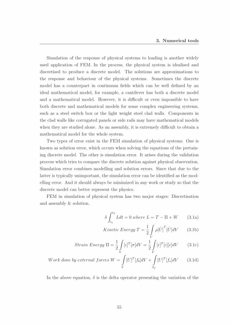
3. Numerical tools
Simulation of the response of physical systems to loading is another widely
used application of FEM. In the process, the physical system is idealised and
discretised to produce a discrete model. The solutions are approximations to
the response and behaviour of the physical systems. Sometimes the discrete
model has a counterpart in continuum fields which can be well defined by an
ideal mathematical model, for example, a cantilever has both a discrete model
and a mathematical model. However, it is difficult or even impossible to have
both discrete and mathematical models for some complex engineering systems,
such as a steel switch box or the light weight steel clad walls. Components in
the clad walls like corrugated panels or side rails may have mathematical models
when they are studied alone. As an assembly, it is extremely difficult to obtain a
mathematical model for the whole system.
Two types of error exist in the FEM simulation of physical systems. One is
known as solution error, which occurs when solving the equations of the pertain-
ing discrete model. The other is simulation error. It arises during the validation
process which tries to compare the discrete solution against physical observation.
Simulation error combines modelling and solution errors. Since that due to the
latter is typically unimportant, the simulation error can be identified as the mod-
elling error. And it should always be minimized in any work or study so that the
discrete model can better represent the physics.
FEM in simulation of physical system has two major stages: Discretisation
and assembly & solution.
δ
∫ t2
t1
Ldt = 0 where L = T − Π+W (3.1a)
Kinetic Energy T =1
2
∫V
ρ ˙[U ]T ˙[U ]dV (3.1b)
Strain Energy Π =1
2
∫V
[ε]T [σ]dV =1
2
∫V
[ε]T [c][ε]dV (3.1c)
Work done by external forces W =
∫V
[U ]T [fb]dV +
∫Sf
[U ]T [fs]dV (3.1d)
In the above equation, δ is the delta operator presenting the variation of the
55
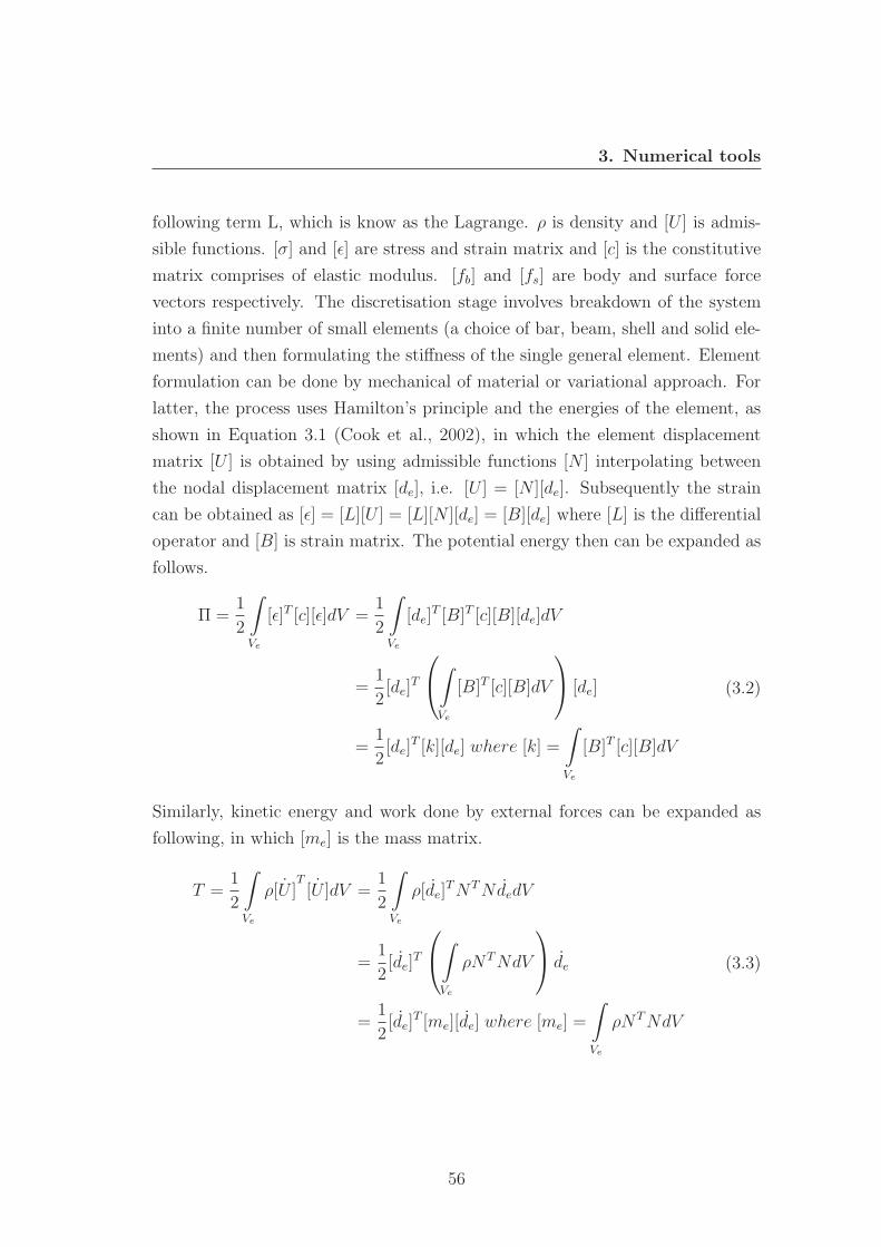
3. Numerical tools
following term L, which is know as the Lagrange. ρ is density and [U ] is admis-
sible functions. [σ] and [ε] are stress and strain matrix and [c] is the constitutive
matrix comprises of elastic modulus. [fb] and [fs] are body and surface force
vectors respectively. The discretisation stage involves breakdown of the system
into a finite number of small elements (a choice of bar, beam, shell and solid ele-
ments) and then formulating the stiffness of the single general element. Element
formulation can be done by mechanical of material or variational approach. For
latter, the process uses Hamilton’s principle and the energies of the element, as
shown in Equation 3.1 (Cook et al., 2002), in which the element displacement
matrix [U ] is obtained by using admissible functions [N ] interpolating between
the nodal displacement matrix [de], i.e. [U ] = [N ][de]. Subsequently the strain
can be obtained as [ε] = [L][U ] = [L][N ][de] = [B][de] where [L] is the differential
operator and [B] is strain matrix. The potential energy then can be expanded as
follows.
Π =1
2
∫Ve
[ε]T [c][ε]dV =1
2
∫Ve
[de]T [B]T [c][B][de]dV
=1
2[de]
T
⎛⎝∫
Ve
[B]T [c][B]dV
⎞⎠ [de]
=1
2[de]
T [k][de] where [k] =
∫Ve
[B]T [c][B]dV
(3.2)
Similarly, kinetic energy and work done by external forces can be expanded as
following, in which [me] is the mass matrix.
T =1
2
∫Ve
ρ ˙[U ]T ˙[U ]dV =
1
2
∫Ve
ρ[de]TNTNdedV
=1
2[de]
T
⎛⎝∫
Ve
ρNTNdV
⎞⎠ de
=1
2[de]
T [me][de] where [me] =
∫Ve
ρNTNdV
(3.3)
56
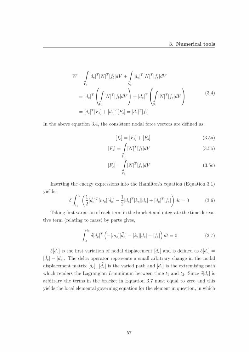
3. Numerical tools
W =
∫Ve
[de]T [N ]T [fb]dV +
∫Se
[de]T [N ]T [fs]dV
= [de]T
⎛⎝∫
Ve
[N ]T [fb]dV
⎞⎠+ [de]
T
⎛⎝∫
Se
[N ]T [fs]dV
⎞⎠
= [de]T [Fb] + [de]
T [Fs] = [de]T [fe]
(3.4)
In the above equation 3.4, the consistent nodal force vectors are defined as:
[fe] = [Fb] + [Fs] (3.5a)
[Fb] =
∫Ve
[N ]T [fb]dV (3.5b)
[Fs] =
∫Ve
[N ]T [fs]dV (3.5c)
Inserting the energy expressions into the Hamilton’s equation (Equation 3.1)
yields:
δ
∫ t2
t1
(1
2[de]
T [me][de]− 1
2[de]
T [ke][de] + [de]T [fe]
)dt = 0 (3.6)
Taking first variation of each term in the bracket and integrate the time deriva-
tive term (relating to mass) by parts gives,
∫ t2
t1
δ[de]T(−[me][de]− [ke][de] + [fe]
)dt = 0 (3.7)
δ[de] is the first variation of nodal displacement [de] and is defined as δ[de] =˜[de] − [de]. The delta operator represents a small arbitrary change in the nodal
displacement matrix [de]. ˜[de] is the varied path and [de] is the extremising path
which renders the Lagrangian L minimum between time t1 and t2. Since δ[de] is
arbitrary the terms in the bracket in Equation 3.7 must equal to zero and this
yields the local elemental governing equation for the element in question, in which
57
3. Numerical tools
[ke] is the local stiffness matrix.
[me][de] + [ke][de] = [fe] (3.8)
The finite element equation in the local coordinates can be transferred into
global coordinates as shown below with the help of a transformation matrix [T]:
[Me][De] + [Ke][De] = [Fe]
where
[Ke] = [T ]T [ke][T ], [Me] = [T ]T [me][T ], [Fe] = [T ]T [fe][T ],
(3.9)
In the above equations, [Me],[De],[Ke] and [Fe] are mass, displacement, stiff-
ness and force matrix for one element in global coordinates. [T ] is the transfor-
mation matrix. Now the discretisation stage is completed and next step is to
assemble all the elements into a master governing equation representing the en-
tire system and finally the discrete solution can be obtain by solving the master
equations accordingly. Equation 3.10 shows the complete general finite element
equations for static and dynamic problems, in which [M ],[D],[K] and [F ] are
assembled mass, displacement, stiffness and force matrix in global coordinates.
dynamic − [M ][D] + [K][D] = [F ] (3.10a)
static − [K][D] = [F ] (3.10b)
Non-linear behaviours in the engineering problems arise from a wide variety of
phenomena. Each source of the non-linearity is perhaps difficult to formulate and
they might interact with each other as well. Linear models might be sufficient
for some applications but unfortunately substantial departure from linearity is
common. There are four common sources of non-linear behaviours in engineering
problems: material, geometric, force and displacement boundary conditions.
Material behaviour depends on the current deformation state and possibly the
past history of the deformation. The structure might undergo non-linear elastic-
ity, plasticity, viscoelasticity, creep or inelastic rate effects. In blast engineering,
the plasticity and strain rate effects are the most important properties. Large
58
3. Numerical tools
strain and deformation are also common in blast engineering problems. Geomet-
ric non-linearity should be considered for slender structures and tensile structures
which have strong axial constraints.
Boundary conditions impose non-linearity as well. The applied force can de-
pend on the deformation, for example, the pressure loads of fluids, this includes
hydrostatic loads on the submerged structures and more importantly the hydro-
dynamic loads caused by wind and blast waves. Similarly, displacement boundary
conditions can depend on the deformation of the structure. The most important
application is the contact problem, in which no-penetration conditions are en-
forced on deformable bodies while the extent of the contact area is unknown.
3.2 Solution methods for non-linear FE prob-
lems
Engineering problems maybe classified according to whether the inertial effects
should be taken into account or not. In static problems the inertia forces are
ignored so Equation 3.10b can be solved to obtain the discrete displacement
solution if the system is linear, the load of duration of the static problems are
usually very long so the dynamic effect is negligible. In dynamic problems, the
durations of load are shorter or comparable to the fundamental period of the
system and the intertia forces of the system cannot be ignored, as discussed
earlier. Equation 3.10a should be used for such problems.
There is a type of problems classified as quasi-static, in which the real time
scale might not be considered and the dynamic effect is small in such a way the
kinetic energy is less than 5% of the strain energy in the system for the most
of the time during the analysis. The advantages of this approach are that static
problems can be solved by Equation 3.10a if the load is applied over a comparably
long period to minimise the kinetic energy. The problems then can be solved
explicitly to overcome convergence difficulties. On the contrary, problems such
as metal forming (a dynamic process) sometimes can be solved as static problem
(i.e. quasi-static) provided by that ignoring the inertial force will not severely
affect the solution. The static analysis will be more efficient than a dynamic one
59
3. Numerical tools
over a long period.
Finite element equations for static and dynamics problems can be re-written
in a more general form,
dynamic − [M ][D] + [I] = [F ] (3.11a)
static − [I] = [F ] (3.11b)
where [I] is the internal forces of the flexible body and [I] = [K][D] for a linear
system, the stiffness [K] does not change. In a non-linear model the stiffness [K]
could be dependent on the displacement [D] then an iterative process is needed
for the solution. The internal force I can be obtained through internal stresses
I =∫V
[B]T [σ]dV .
3.2.1 Newton - Raphson method
One of the most widely used methods for non-linear static or quasi-static problems
is the Newton - Raphson method, as depicted in Figure 3.1. At the start of the
solution tangential stiffnessKT0 is formed at displacement d = 0. By applying the
step load ΔP1 an intermediate displacement dA is obtained and the corresponding
internal force is calculated from the internal stresses as IA. If residual force
ReA = P1 − IA is smaller than some convergence criteria then the point a is
the converged solution, otherwise further iteration is needed from point a. By
using a newly formed tangential stiffness KTa and the residual force ReA a new
intermediate displacement dB = dA + δA can be obtained at point b, where
δA = ReA/KTa. The residual ReB will be checked and if no convergence is found
forwarding to next point c with ReB and KTb. At every iteration point the force
residual will be checked until it is lower than the required criteria, then at point
1 a new converged point is said to be found. Thus an other incremental step load
can be applied which will start a new iterative stage and forward the solution
along the response path.
60
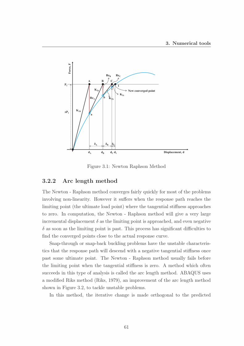
3. Numerical tools
Displacement, d
Forc
e, F
P1
ΔP1 KT0
A B C
New converged point
ReA
KTa
a
b
c 1
dA dB dC d1
ReB ReC
KTb KTc
δA δB δC
Figure 3.1: Newton Raphson Method
3.2.2 Arc length method
The Newton - Raphson method converges fairly quickly for most of the problems
involving non-linearity. However it suffers when the response path reaches the
limiting point (the ultimate load point) where the tangential stiffness approaches
to zero. In computation, the Newton - Raphson method will give a very large
incremental displacement δ as the limiting point is approached, and even negative
δ as soon as the limiting point is past. This process has significant difficulties to
find the converged points close to the actual response curve.
Snap-through or snap-back buckling problems have the unstable characteris-
tics that the response path will descend with a negative tangential stiffness once
past some ultimate point. The Newton - Raphson method usually fails before
the limiting point when the tangential stiffness is zero. A method which often
succeeds in this type of analysis is called the arc length method. ABAQUS uses
a modified Riks method (Riks, 1979), an improvement of the arc length method
shown in Figure 3.2, to tackle unstable problems.
In this method, the iterative change is made orthogonal to the predicted
61
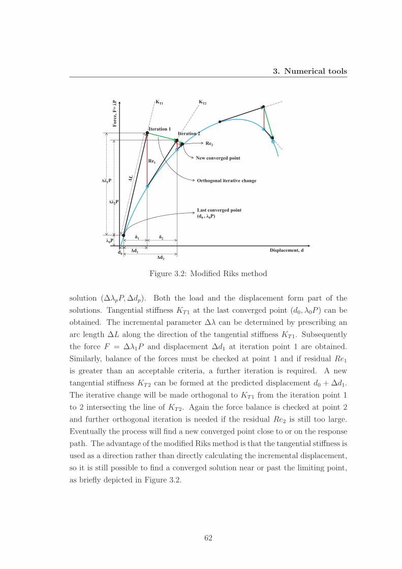
3. Numerical tools
Iteration 1 Iteration 2
New converged point
Last converged point (d0 , λ0P)
Orthogonal iterative change
KT1 KT2
Displacement, d
Forc
e, F
= λP
d0
λ0P
Δd1 Δd2
Δλ2P
Δλ1P
δ2 δ1
Re2
Re1
Figure 3.2: Modified Riks method
solution (ΔλpP,Δdp). Both the load and the displacement form part of the
solutions. Tangential stiffness KT1 at the last converged point (d0, λ0P ) can be
obtained. The incremental parameter Δλ can be determined by prescribing an
arc length ΔL along the direction of the tangential stiffness KT1. Subsequently
the force F = Δλ1P and displacement Δd1 at iteration point 1 are obtained.
Similarly, balance of the forces must be checked at point 1 and if residual Re1
is greater than an acceptable criteria, a further iteration is required. A new
tangential stiffness KT2 can be formed at the predicted displacement d0 + Δd1.
The iterative change will be made orthogonal to KT1 from the iteration point 1
to 2 intersecting the line of KT2. Again the force balance is checked at point 2
and further orthogonal iteration is needed if the residual Re2 is still too large.
Eventually the process will find a new converged point close to or on the response
path. The advantage of the modified Riks method is that the tangential stiffness is
used as a direction rather than directly calculating the incremental displacement,
so it is still possible to find a converged solution near or past the limiting point,
as briefly depicted in Figure 3.2.
62
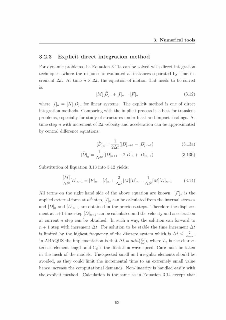
3. Numerical tools
3.2.3 Explicit direct integration method
For dynamic problems the Equation 3.11a can be solved with direct integration
techniques, where the response is evaluated at instances separated by time in-
crement Δt. At time n × Δt, the equation of motion that needs to be solved
is:
[M ][D]n + [I]n = [F ]n (3.12)
where [I]n = [K][D]n for linear systems. The explicit method is one of direct
integration methods. Comparing with the implicit process it is best for transient
problems, especially for study of structures under blast and impact loadings. At
time step n with increment of Δt velocity and acceleration can be approximated
by central difference equations:
˙[D]n =1
2Δt([D]n+1 − [D]n−1) (3.13a)
¨[D]n =1
Δt2([D]n+1 − 2[D]n + [D]n−1) (3.13b)
Substitution of Equation 3.13 into 3.12 yields:
[M ]
Δt2[D]n+1 = [F ]n − [I]n +
2
Δt2[M ][D]n − 1
Δt2[M ][D]n−1 (3.14)
All terms on the right hand side of the above equation are known. [F ]n is the
applied external force at nth step, [I]n can be calculated from the internal stresses
and [D]n and [D]n−1 are obtained in the previous steps. Therefore the displace-
ment at n+1 time step [D]n+1 can be calculated and the velocity and acceleration
at current n step can be obtained. In such a way, the solution can forward to
n + 1 step with increment Δt. For solution to be stable the time increment Δt
is limited by the highest frequency of the discrete system which is Δt ≤ 2ωmax
.
In ABAQUS the implementation is that Δt = min(Le
Cd), where Le is the charac-
teristic element length and Cd is the dilatation wave speed. Care must be taken
in the mesh of the models. Unexpected small and irregular elements should be
avoided, as they could limit the incremental time to an extremely small value
hence increase the computational demands. Non-linearity is handled easily with
the explicit method. Calculation is the same as in Equation 3.14 except that
63
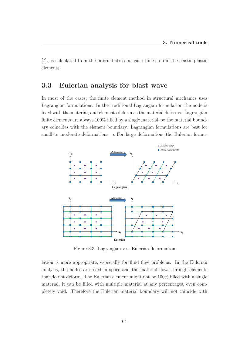
3. Numerical tools
[I]n is calculated from the internal stress at each time step in the elastic-plastic
elements.
3.3 Eulerian analysis for blast wave
In most of the cases, the finite element method in structural mechanics uses
Lagrangian formulations. In the traditional Lagrangian formulation the node is
fixed with the material, and elements deform as the material deforms. Lagrangian
finite elements are always 100% filled by a single material, so the material bound-
ary coincides with the element boundary. Lagrangian formulations are best for
small to moderate deformations. s For large deformation, the Eulerian formu-
x1
x2 x2
x1
deformation
x1
x2
x1
x2 deformation
Lagrangian
Eulerian
Material point
Finite element node
Figure 3.3: Lagrangian v.s. Eulerian deformation
lation is more appropriate, especially for fluid flow problems. In the Eulerian
analysis, the nodes are fixed in space and the material flows through elements
that do not deform. The Eulerian element might not be 100% filled with a single
material, it can be filled with multiple material at any percentages, even com-
pletely void. Therefore the Eulerian material boundary will not coincide with
64
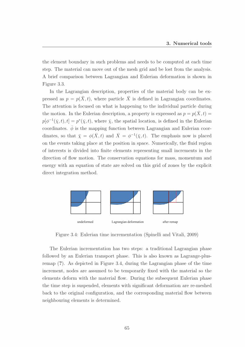
3. Numerical tools
the element boundary in such problems and needs to be computed at each time
step. The material can move out of the mesh grid and be lost from the analysis.
A brief comparison between Lagrangian and Eulerian deformation is shown in
Figure 3.3.
In the Lagrangian description, properties of the material body can be ex-
pressed as p = p(X, t), where particle X is defined in Lagrangian coordinates.
The attention is focused on what is happening to the individual particle during
the motion. In the Eulerian description, a property is expressed as p = p(X, t) =
p[φ−1(χ, t), t] = p∗(χ, t), where χ, the spatial location, is defined in the Eulerian
coordinates. φ is the mapping function between Lagrangian and Eulerian coor-
dinates, so that χ = φ(X, t) and X = φ−1(χ, t). The emphasis now is placed
on the events taking place at the position in space. Numerically, the fluid region
of interests is divided into finite elements representing small increments in the
direction of flow motion. The conservation equations for mass, momentum and
energy with an equation of state are solved on this grid of zones by the explicit
direct integration method.
undeformed Lagrangian deformation after remap
Figure 3.4: Eulerian time incrementation (Spinelli and Vitali, 2009)
The Eulerian incrementation has two steps: a traditional Lagrangian phase
followed by an Eulerian transport phase. This is also known as Lagrange-plus-
remap (?). As depicted in Figure 3.4, during the Lagrangian phase of the time
increment, nodes are assumed to be temporarily fixed with the material so the
elements deform with the material flow. During the subsequent Eulerian phase
the time step is suspended, elements with significant deformation are re-meshed
back to the original configuration, and the corresponding material flow between
neighbouring elements is determined.
65
3. Numerical tools
The shock front of a blast wave is extremely thin, hence it is often approxi-
mated as a discontinuous change in flow properties. A representative thickness
of a shock plane with Mx = 2 is given in “Explosive shocks in air” (Kinney and
Graham, 1985) to be about 0.00025 mm. This is much thinner than a typical
finite element length used in a numerical model for practical use. Special treat-
ment is used in programs to solve the discontinuity and still keep conservation
laws, e.g. the Rankine-Hugoniot relations for shock waves. In order to model
the shock numerically, an artificial viscosity is used (O.C.Zienkiewicz and Taylor,
2000) to damp out the shock front over several elements.
The fluid medium used in the blast analysis is usually air. The ideal gas
equation of state for air can be defined as:
p+ pA = ρR(Θ−Θz) (3.15)
where pA is the atmospheric pressure, R is the gas constant, ρ is the density of
the air, Θ is the atmospheric temperature and Θz is the absolute zero on the
temperature scale being used. The ABAQUS Eulerian capability used in this
research project only involves the blast wave propagation though air. In the next
sub-section, the AUTODYN is used to validate the coupled Lagrangian-Eulerian
method and this Eulerian model consist of air and high explosive, which can be
defined by the Jones-Wilkins-Lee (JWL) equation of state as follow:
p = A
(1− ω
R1Ve−R1V
)+B
(1− ω
R2Ve−R2V
)+
ωE
V(3.16)
where A, B, R1, R2 and ω are empirically derived constants which are different
for each explosive. V is the relative volume or the expansion of the explosive
product, and E is the detonation energy per initial unit volume (ANSYS). The
values of the parameters for air and high explosive (Pentolite) are shown in Table
3.1.
3.4 Approaches for study of blast responses
Most of the blast problems can be divided into four stages (Borvik et al., 2009).
66
3. Numerical tools
Table 3.1: Definition of Eulerian materials
Material Type Property Value Unit
Air
Density Mass density 1.2258 kg/m3
EOSSpecific gas constant 287 J/kgKAmbient pressure 101.325 kPa
Specific heat Specific heat 717.54 kJ/kgViscosity Dynamic viscosity 1 ×10⁻⁵ kg/(m · s)
Initial stateAmbient temperature 288.15 KelvinAmbient pressure 101.325 kPa
Pentolite
Density Mass density 1.63 kg/m3
JWL EOS
Detonation speed 7360 m/sA 531.77 GPaB 8.933 GPaω 0.33 -R1 4.6 -R2 1.05 -
Initial stateSpecific energy 8 kJ/cm3
Ambient pressure 101.325 kPa
• Stage I: the explosion stage where the explosives explode generating high
temperature and pressure gases that propagate violently through the sur-
rounding medium (usually air).
• Stage II: the propagation phase where high intensity blast waves generated
by the expanding gases propagate through the medium at a distance, from
the explosion centre to the target.
• Stage III: the interaction phase between the blast wave and the target struc-
tures where the blast loading is applied on the surfaces.
• Stage IV: the response of structures to the dynamic loading imposed by the
incoming blast waves.
The four stages can be separated to simplify the problem but a strong coupling
exists between each phase and they are all of the same importance to completely
describe the structural response to blast loading problems. Stage I is out of the
scope of this research study. The primary aim of the present work is not studying
the explosion mechanism of explosives but the subsequent events. The main
67
3. Numerical tools
focus will be placed on Stage IV the response of various objects to blast dynamic
loadings, with attention to the blast - structure interaction and the propagation
of blast waves. Throughout the current study the blast waves are defined either
by scaled distance with charge side or directly specifying the wave parameters
(i.e. incident peak overpressure and positive duration).
Separating the four stages can significantly simplify the blast problems. Three
numerical modelling approaches can be developed with different levels of com-
plexity.
3.4.1 Lagrangian approach
In this approach, a pure Lagrangian formulation is used to describe the deforma-
tion of the structures. The blast load is approximated as an idealised pressure
- time curve directly applied on the relevant surface of the structures. During
the simulation the pressure loading is always normal to the surface subjected to
the load, independent of the structural deformation. If the deformation is small
and the geometry is regular, this approach may give reasonable results. Only
stage IV is considered in this approach. Stages I - III are replaced by empirical
or analytical tools of predicting the blast wave.
The blast load can be defined directly with the incident peak overpressure and
the positive duration, with either linear or exponential form. Then following the
procedures presented in Section 2.3.2 the dynamic blast loads on the surfaces of a
structure with simple geometry can be determined. This is referred as analytical
blast load in the following sections.
CONWEP, a collection of conventional weapons effects calculations from the
equations and curves of TM 5-855-1 manual (USDOA, 1986), is incorporated
into the current release of ?. This module provides another way to apply the
detonation blast load. By specifying the weight and stand-off distance of the TNT
high explosive charge, the dynamic pressure loads are automatically applied on
the relevant surfaces of the target according to the incident angle. This is referred
yo as CONWEP load (CONWEP) in the following sections.
68
3. Numerical tools
3.4.2 Uncoupled Eulerian - Lagrangian approach
The second approach consists of two steps: (i) Eulerian simulation to determine
the pressure loads and (ii) the Lagrangian modelling to analyse the structural
response. In the first step the structure is often treated as a rigid body so the
pressure loads on the surfaces can be determined and recorded without consider-
ing deformation. Then the pre-determined surface pressure - time curves can be
applied directly on the relevant surfaces of the structures in the second step. The
method will give reliable results if the iteration between the blast and structure is
small, i.e. moderate structural deformation should be expected. The advantage of
this uncoupled method is that it is considerably less computationally demanding
than a fully coupled simulation.
This approach involves stage II - IV of a blast problem in a decoupled manner.
In step one the Eulerian simulation considers the propagation of the blast wave
and its interaction with a rigid structure (stage II and III). The second step is
equivalent to stage IV in which the response of the structure is determined.
3.4.3 Coupled Eulerian - Lagrangian approach
The Eulerian algorithm can be coupled with the Lagrangian formulation to have
a full coupling between the blast wave and deformation of structure. Stages I-IV
or II-IV are coupled together and the interaction between the blast wave and the
structure can be well described for even large deformations, at the cost of greater
computational demands.
The general explicit contact definition of ? implements the contact between
Eulerian and Lagrangian parts automatically. In AUTODYN (ANSYS) there is
a specific Eulerian - Lagrangian contact definition used to impose the coupling
effect.
3.5 Numerical model validations
The finite element method and various simulation approaches were discussed in
the above sections. In order to build confidence of using numerical models in the
present study, it is necessary to validate the numerical models at the most general
69
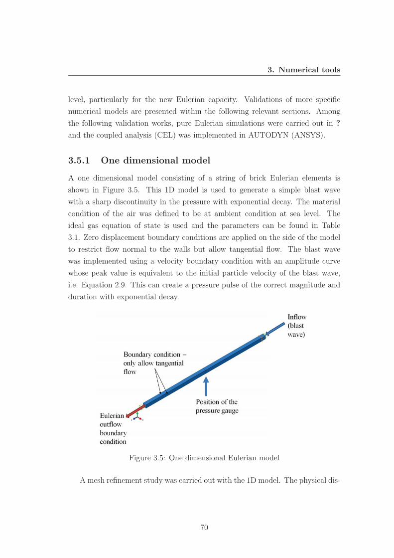
3. Numerical tools
level, particularly for the new Eulerian capacity. Validations of more specific
numerical models are presented within the following relevant sections. Among
the following validation works, pure Eulerian simulations were carried out in ?
and the coupled analysis (CEL) was implemented in AUTODYN (ANSYS).
3.5.1 One dimensional model
A one dimensional model consisting of a string of brick Eulerian elements is
shown in Figure 3.5. This 1D model is used to generate a simple blast wave
with a sharp discontinuity in the pressure with exponential decay. The material
condition of the air was defined to be at ambient condition at sea level. The
ideal gas equation of state is used and the parameters can be found in Table
3.1. Zero displacement boundary conditions are applied on the side of the model
to restrict flow normal to the walls but allow tangential flow. The blast wave
was implemented using a velocity boundary condition with an amplitude curve
whose peak value is equivalent to the initial particle velocity of the blast wave,
i.e. Equation 2.9. This can create a pressure pulse of the correct magnitude and
duration with exponential decay.
Figure 3.5: One dimensional Eulerian model
A mesh refinement study was carried out with the 1D model. The physical dis-
70
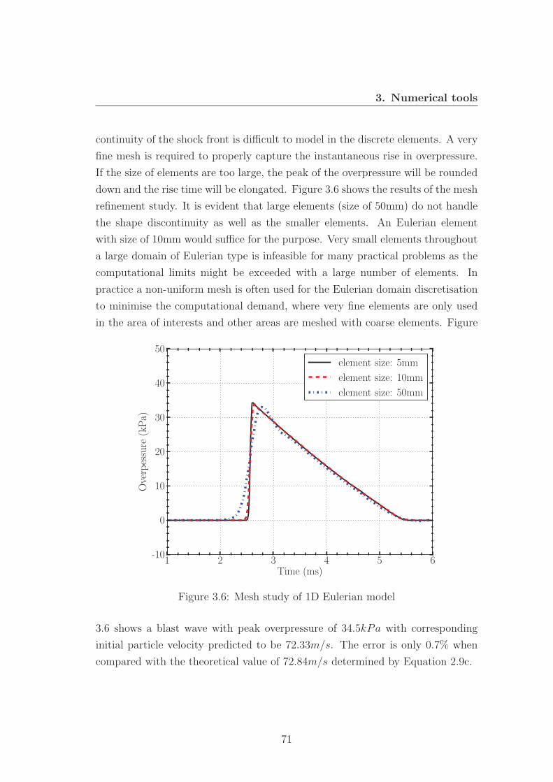
3. Numerical tools
continuity of the shock front is difficult to model in the discrete elements. A very
fine mesh is required to properly capture the instantaneous rise in overpressure.
If the size of elements are too large, the peak of the overpressure will be rounded
down and the rise time will be elongated. Figure 3.6 shows the results of the mesh
refinement study. It is evident that large elements (size of 50mm) do not handle
the shape discontinuity as well as the smaller elements. An Eulerian element
with size of 10mm would suffice for the purpose. Very small elements throughout
a large domain of Eulerian type is infeasible for many practical problems as the
computational limits might be exceeded with a large number of elements. In
practice a non-uniform mesh is often used for the Eulerian domain discretisation
to minimise the computational demand, where very fine elements are only used
in the area of interests and other areas are meshed with coarse elements. Figure
1 2 3 4 5 6Time (ms)
-10
0
10
20
30
40
50
Overpessure
(kPa)
element size: 5mm
element size: 10mm
element size: 50mm
Figure 3.6: Mesh study of 1D Eulerian model
3.6 shows a blast wave with peak overpressure of 34.5kPa with corresponding
initial particle velocity predicted to be 72.33m/s. The error is only 0.7% when
compared with the theoretical value of 72.84m/s determined by Equation 2.9c.
71
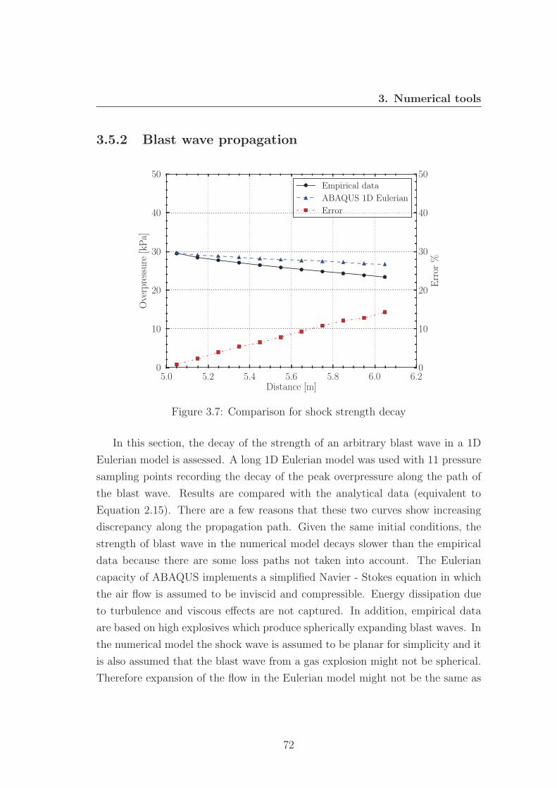
3. Numerical tools
3.5.2 Blast wave propagation
5.0 5.2 5.4 5.6 5.8 6.0 6.2Distance [m]
0
10
20
30
40
50
Overpressure
[kPa]
Empirical data
ABAQUS 1D Eulerian
Error
0
10
20
30
40
50
Error
%
Figure 3.7: Comparison for shock strength decay
In this section, the decay of the strength of an arbitrary blast wave in a 1D
Eulerian model is assessed. A long 1D Eulerian model was used with 11 pressure
sampling points recording the decay of the peak overpressure along the path of
the blast wave. Results are compared with the analytical data (equivalent to
Equation 2.15). There are a few reasons that these two curves show increasing
discrepancy along the propagation path. Given the same initial conditions, the
strength of blast wave in the numerical model decays slower than the empirical
data because there are some loss paths not taken into account. The Eulerian
capacity of ABAQUS implements a simplified Navier - Stokes equation in which
the air flow is assumed to be inviscid and compressible. Energy dissipation due
to turbulence and viscous effects are not captured. In addition, empirical data
are based on high explosives which produce spherically expanding blast waves. In
the numerical model the shock wave is assumed to be planar for simplicity and it
is also assumed that the blast wave from a gas explosion might not be spherical.
Therefore expansion of the flow in the Eulerian model might not be the same as
72
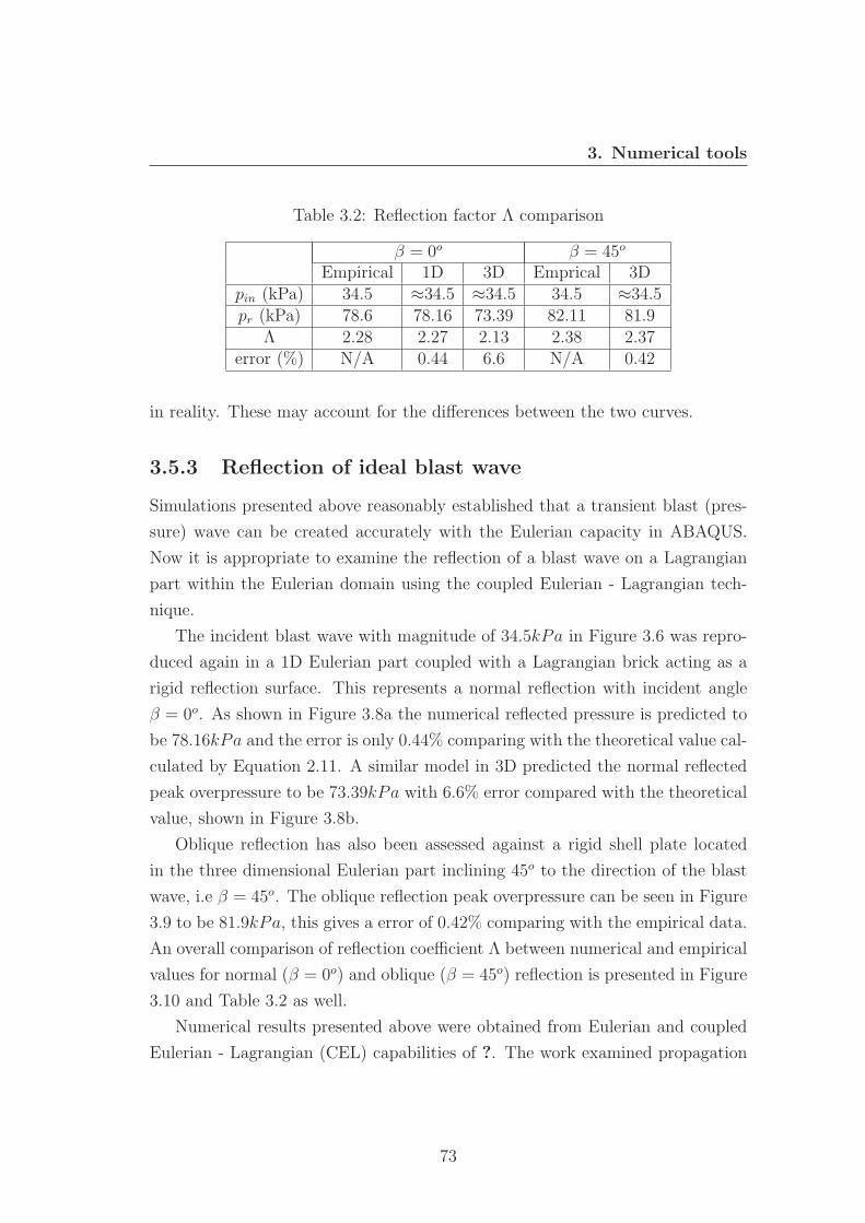
3. Numerical tools
Table 3.2: Reflection factor Λ comparison
β = 0o β = 45o
Empirical 1D 3D Emprical 3Dpin (kPa) 34.5 ≈34.5 ≈34.5 34.5 ≈34.5pr (kPa) 78.6 78.16 73.39 82.11 81.9
Λ 2.28 2.27 2.13 2.38 2.37error (%) N/A 0.44 6.6 N/A 0.42
in reality. These may account for the differences between the two curves.
3.5.3 Reflection of ideal blast wave
Simulations presented above reasonably established that a transient blast (pres-
sure) wave can be created accurately with the Eulerian capacity in ABAQUS.
Now it is appropriate to examine the reflection of a blast wave on a Lagrangian
part within the Eulerian domain using the coupled Eulerian - Lagrangian tech-
nique.
The incident blast wave with magnitude of 34.5kPa in Figure 3.6 was repro-
duced again in a 1D Eulerian part coupled with a Lagrangian brick acting as a
rigid reflection surface. This represents a normal reflection with incident angle
β = 0o. As shown in Figure 3.8a the numerical reflected pressure is predicted to
be 78.16kPa and the error is only 0.44% comparing with the theoretical value cal-
culated by Equation 2.11. A similar model in 3D predicted the normal reflected
peak overpressure to be 73.39kPa with 6.6% error compared with the theoretical
value, shown in Figure 3.8b.
Oblique reflection has also been assessed against a rigid shell plate located
in the three dimensional Eulerian part inclining 45o to the direction of the blast
wave, i.e β = 45o. The oblique reflection peak overpressure can be seen in Figure
3.9 to be 81.9kPa, this gives a error of 0.42% comparing with the empirical data.
An overall comparison of reflection coefficient Λ between numerical and empirical
values for normal (β = 0o) and oblique (β = 45o) reflection is presented in Figure
3.10 and Table 3.2 as well.
Numerical results presented above were obtained from Eulerian and coupled
Eulerian - Lagrangian (CEL) capabilities of ?. The work examined propagation
73
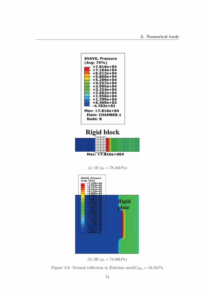
3. Numerical tools
(a) 1D (pr = 78.16kPa)
(b) 3D (pr = 73.39kPa)
Figure 3.8: Normal reflection in Eulerian model pin = 34.5kPa
74
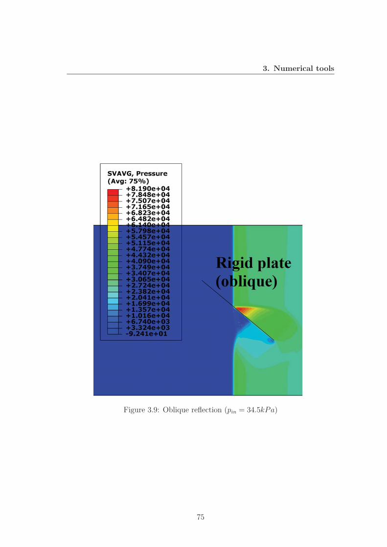
3. Numerical tools
Figure 3.9: Oblique reflection (pin = 34.5kPa)
75
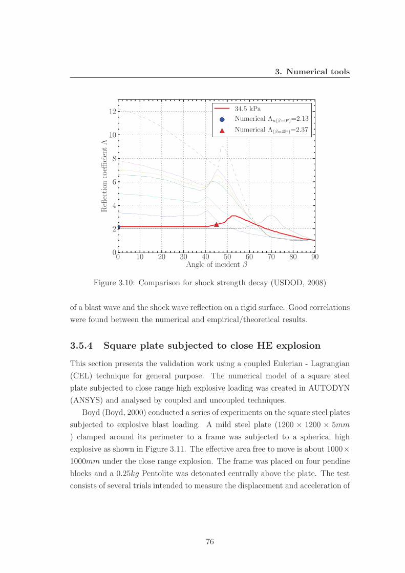
3. Numerical tools
0 10 20 30 40 50 60 70 80 90Angle of incident β
0
2
4
6
8
10
12Reflection
coeffi
cientΛ
34.5 kPa
Numerical Λn(β=0o)=2.13
Numerical Λ(β=45o)=2.37
Figure 3.10: Comparison for shock strength decay (USDOD, 2008)
of a blast wave and the shock wave reflection on a rigid surface. Good correlations
were found between the numerical and empirical/theoretical results.
3.5.4 Square plate subjected to close HE explosion
This section presents the validation work using a coupled Eulerian - Lagrangian
(CEL) technique for general purpose. The numerical model of a square steel
plate subjected to close range high explosive loading was created in AUTODYN
(ANSYS) and analysed by coupled and uncoupled techniques.
Boyd (Boyd, 2000) conducted a series of experiments on the square steel plates
subjected to explosive blast loading. A mild steel plate (1200 × 1200 × 5mm
) clamped around its perimeter to a frame was subjected to a spherical high
explosive as shown in Figure 3.11. The effective area free to move is about 1000×1000mm under the close range explosion. The frame was placed on four pendine
blocks and a 0.25kg Pentolite was detonated centrally above the plate. The test
consists of several trials intended to measure the displacement and acceleration of
76
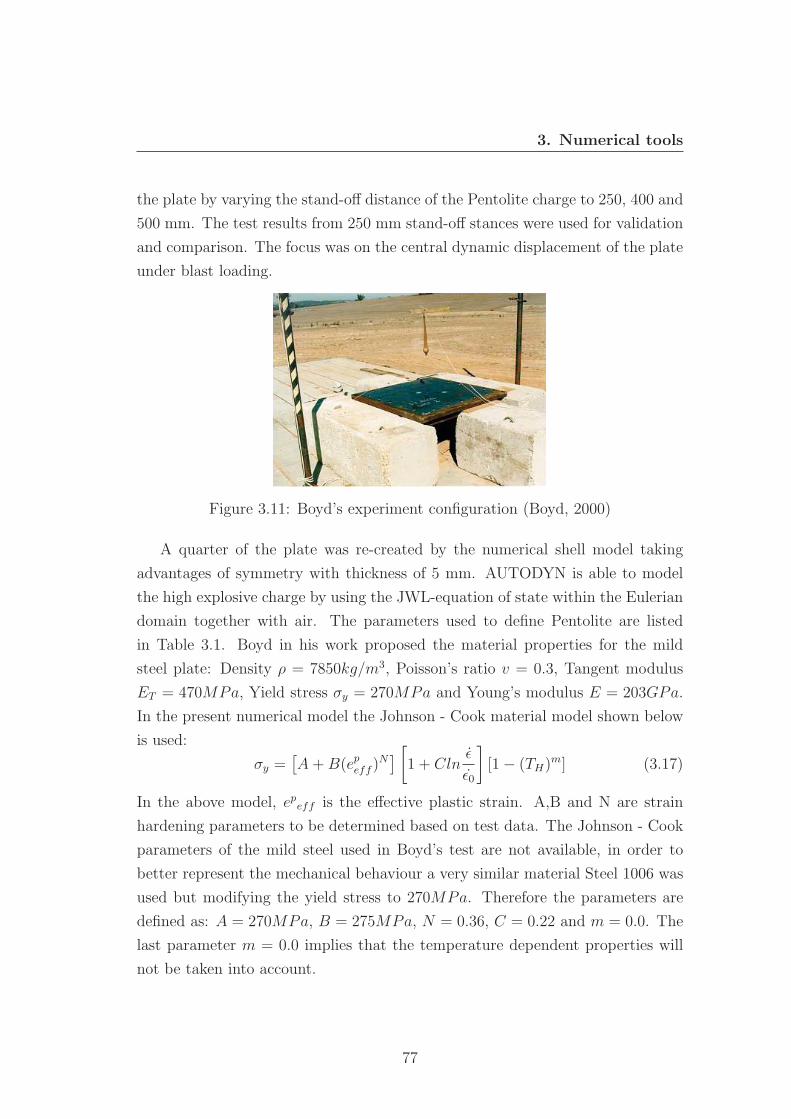
3. Numerical tools
the plate by varying the stand-off distance of the Pentolite charge to 250, 400 and
500 mm. The test results from 250 mm stand-off stances were used for validation
and comparison. The focus was on the central dynamic displacement of the plate
under blast loading.
Figure 3.11: Boyd’s experiment configuration (Boyd, 2000)
A quarter of the plate was re-created by the numerical shell model taking
advantages of symmetry with thickness of 5 mm. AUTODYN is able to model
the high explosive charge by using the JWL-equation of state within the Eulerian
domain together with air. The parameters used to define Pentolite are listed
in Table 3.1. Boyd in his work proposed the material properties for the mild
steel plate: Density ρ = 7850kg/m3, Poisson’s ratio v = 0.3, Tangent modulus
ET = 470MPa, Yield stress σy = 270MPa and Young’s modulus E = 203GPa.
In the present numerical model the Johnson - Cook material model shown below
is used:
σy =[A+B(epeff )
N] [
1 + Clnε
ε0
][1− (TH)
m] (3.17)
In the above model, epeff is the effective plastic strain. A,B and N are strain
hardening parameters to be determined based on test data. The Johnson - Cook
parameters of the mild steel used in Boyd’s test are not available, in order to
better represent the mechanical behaviour a very similar material Steel 1006 was
used but modifying the yield stress to 270MPa. Therefore the parameters are
defined as: A = 270MPa, B = 275MPa, N = 0.36, C = 0.22 and m = 0.0. The
last parameter m = 0.0 implies that the temperature dependent properties will
not be taken into account.
77
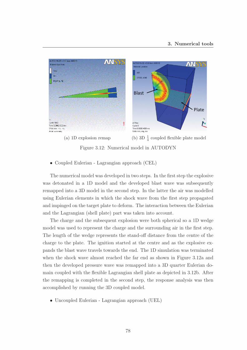
3. Numerical tools
(a) 1D explosion remap (b) 3D 14 coupled flexible plate model
Figure 3.12: Numerical model in AUTODYN
• Coupled Eulerian - Lagrangian approach (CEL)
The numerical model was developed in two steps. In the first step the explosive
was detonated in a 1D model and the developed blast wave was subsequently
remapped into a 3D model in the second step. In the latter the air was modelled
using Eulerian elements in which the shock wave from the first step propagated
and impinged on the target plate to deform. The interaction between the Eulerian
and the Lagrangian (shell plate) part was taken into account.
The charge and the subsequent explosion were both spherical so a 1D wedge
model was used to represent the charge and the surrounding air in the first step.
The length of the wedge represents the stand-off distance from the centre of the
charge to the plate. The ignition started at the centre and as the explosive ex-
pands the blast wave travels towards the end. The 1D simulation was terminated
when the shock wave almost reached the far end as shown in Figure 3.12a and
then the developed pressure wave was remapped into a 3D quarter Eulerian do-
main coupled with the flexible Lagrangian shell plate as depicted in 3.12b. After
the remapping is completed in the second step, the response analysis was then
accomplished by running the 3D coupled model.
• Uncoupled Eulerian - Lagrangian approach (UEL)
78
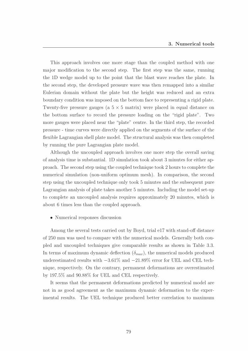
3. Numerical tools
This approach involves one more stage than the coupled method with one
major modification to the second step. The first step was the same, running
the 1D wedge model up to the point that the blast wave reaches the plate. In
the second step, the developed pressure wave was then remapped into a similar
Eulerian domain without the plate but the height was reduced and an extra
boundary condition was imposed on the bottom face to representing a rigid plate.
Twenty-five pressure gauges (a 5 × 5 matrix) were placed in equal distance on
the bottom surface to record the pressure loading on the “rigid plate”. Two
more gauges were placed near the “plate” centre. In the third step, the recorded
pressure - time curves were directly applied on the segments of the surface of the
flexible Lagrangian shell plate model. The structural analysis was then completed
by running the pure Lagrangian plate model.
Although the uncoupled approach involves one more step the overall saving
of analysis time is substantial. 1D simulation took about 3 minutes for either ap-
proach. The second step using the coupled technique took 2 hours to complete the
numerical simulation (non-uniform optimum mesh). In comparison, the second
step using the uncoupled technique only took 5 minutes and the subsequent pure
Lagrangian analysis of plate takes another 5 minutes. Including the model set-up
to complete an uncoupled analysis requires approximately 20 minutes, which is
about 6 times less than the coupled approach.
• Numerical responses discussion
Among the several tests carried out by Boyd, trial e17 with stand-off distance
of 250 mm was used to compare with the numerical models. Generally both cou-
pled and uncoupled techniques give comparable results as shown in Table 3.3.
In terms of maximum dynamic deflection (δmax), the numerical models produced
underestimated results with −3.61% and −21.89% error for UEL and CEL tech-
nique, respectively. On the contrary, permanent deformations are overestimated
by 197.5% and 90.88% for UEL and CEL respectively.
It seems that the permanent deformations predicted by numerical model are
not in as good agreement as the maximum dynamic deformation to the exper-
imental results. The UEL technique produced better correlation to maximum
79
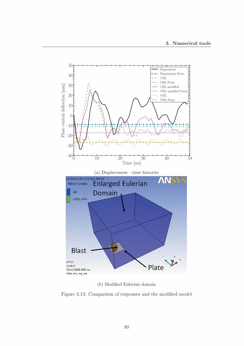
3. Numerical tools
0 10 20 30 40 50Time [ms]
-40
-30
-20
-10
0
10
20
30
40
50Plate
centraldeflection
[mm]
Experiment
Experiment Perm
CEL
CEL Perm
CEL modified
CEL modified Perm
UEL
UEL Perm
(a) Displacement - time histories
(b) Modified Eulerian domain
Figure 3.13: Comparison of responses and the modified model
80
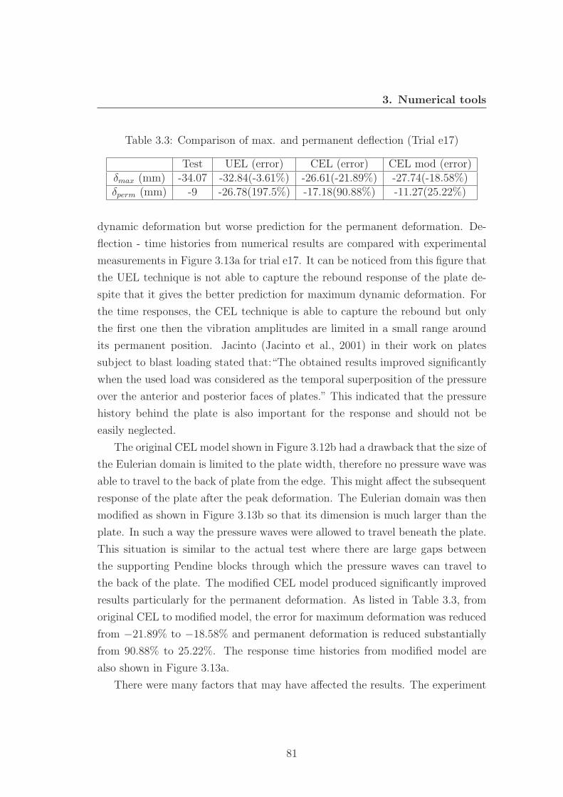
3. Numerical tools
Table 3.3: Comparison of max. and permanent deflection (Trial e17)
Test UEL (error) CEL (error) CEL mod (error)δmax (mm) -34.07 -32.84(-3.61%) -26.61(-21.89%) -27.74(-18.58%)δperm (mm) -9 -26.78(197.5%) -17.18(90.88%) -11.27(25.22%)
dynamic deformation but worse prediction for the permanent deformation. De-
flection - time histories from numerical results are compared with experimental
measurements in Figure 3.13a for trial e17. It can be noticed from this figure that
the UEL technique is not able to capture the rebound response of the plate de-
spite that it gives the better prediction for maximum dynamic deformation. For
the time responses, the CEL technique is able to capture the rebound but only
the first one then the vibration amplitudes are limited in a small range around
its permanent position. Jacinto (Jacinto et al., 2001) in their work on plates
subject to blast loading stated that:“The obtained results improved significantly
when the used load was considered as the temporal superposition of the pressure
over the anterior and posterior faces of plates.” This indicated that the pressure
history behind the plate is also important for the response and should not be
easily neglected.
The original CEL model shown in Figure 3.12b had a drawback that the size of
the Eulerian domain is limited to the plate width, therefore no pressure wave was
able to travel to the back of plate from the edge. This might affect the subsequent
response of the plate after the peak deformation. The Eulerian domain was then
modified as shown in Figure 3.13b so that its dimension is much larger than the
plate. In such a way the pressure waves were allowed to travel beneath the plate.
This situation is similar to the actual test where there are large gaps between
the supporting Pendine blocks through which the pressure waves can travel to
the back of the plate. The modified CEL model produced significantly improved
results particularly for the permanent deformation. As listed in Table 3.3, from
original CEL to modified model, the error for maximum deformation was reduced
from −21.89% to −18.58% and permanent deformation is reduced substantially
from 90.88% to 25.22%. The response time histories from modified model are
also shown in Figure 3.13a.
There were many factors that may have affected the results. The experiment
81
3. Numerical tools
might have some unexpected errors such as the position of the plate and movement
of the clamping frame. In addition, the simulation assumed that the plate is fully
clamped around its edges, which might not be the case in the test. Slip may hence
occurs during the explosion at the perimeter. Thus can have a large impact on the
central deflection of the panel. Despite all the unidentifiable errors, this simple
validation work showed the importance of proper consideration of the coupling
between the blast wave and the movement of the target to the accuracy of the
numerical model.
3.6 Finite element analysis packages
Two FE packages have been used in the present work: AUTODYN/ANSYS and
ABAQUS. As demonstrated in the previous sections, both packages have explicit
solvers and Eulerian capabilities to undertake high-speed blast and impact prob-
lems, either in a coupled or in an uncoupled manner. In this sub-section, brief
comments on lessons learnt from the experience of using these two packages are
provided.
For the validation work of Boyd’s experiment (Boyd, 2000), only results from
AUTODYN/ANSYS were presented due to the nature of the problem. AUTO-
DYN provides a special approach (re-mapping) to simulate the close range high
explosive detonation. This approach makes AUTODYN very efficient for mod-
elling the actual explosion of the charge and the subsequent response of the target.
ABAQUS recently incorporated a new Eulerian capability (starting from Version
6.9) which enables the simulation of this problem but without the re-mapping
technique. ABAQUS has only been used in the UEL analysis (the Lagrangian
step) for the validation work, since the Eulerian capability was not available when
the validation work of Boyd’s test has being undertaken.
Although it was shown that the UEL approach did not compare as well as
the CEL approach with the experimental results, UEL simulation of ABAQUS
produced very similar structural response of the plate to UEL results of AUTO-
DYN/ANSYS. In addition, in collaboration with the Steel Construction Institute,
both AUTODYN/ANSYS and ABAQUS were used to analyse a simple portal
frame structure as well side rail and cladding components. The results between
82
3. Numerical tools
the two numerical packages were also very similar. The new Eulerian capability of
ABAQUS provides an alternative approach for the simulation of blast problems.
In the previous and following sections, it is shown that the Eulerian explicit solver
of ABAQUS can simulate blast waves and their interactions with adequate accu-
racy. During the course of the project, AUTODYN/ANSYS has also been used
to reproduce the blast effects from equivalent TNT charges for the Buncefield
investigation. The results compared reasonably well with empirical data.
The Eulerian capability of ABAQUS has been extensively used in this project
for forensic studies. Although it does not offer the re-mapping technique, it has
a customisable Eulerian inflow boundary condition within the unified CAE envi-
ronment as well as more sophisticated meshing tools. The customisable Eulerian
inflow module can be used to produce a variety of incident blast waves, either
detonation or deflagration. The meshing tools of ABAQUS provide a compara-
tively high quality mesh of the Eulerian model hence increase the computational
efficiency. In AUTODYN/ANSYS, a subroutine must be used in order to pro-
duce a customisable blast wave at the inflow boundary condition. The subroutine
has to be written in C or FORTRAN which entails extra compilation cost and
programming time. Partitioning is not available for the Eulerian model in AU-
TODYN/ANSYS, and the meshing capabilities of the domain are very limited -
often resulting in an excessive number of unnecessary elements.
ABAQUS provides a unified CAE environment in which the Lagrangian (struc-
tural) and Eulerian (air/water) parts are created and assembled within one model.
All the pre- and post-processing work can therefore be accomplished within one
package. AUTODYN is one of the integrated modules within ANSYS, although
it can be used as a stand-alone package. AUTODYN itself does not provide
detailed CAD tools for the creation of complex Lagrangian and Eulerian parts.
Accordingly, most of the pre-processing work has to be carried out in a dedicate
modelling module in the ANSYS/WORKBENCH, and then the parts have to be
transferred into AUTODYN for analysis. Subsequently, the results need to be
transferred into another module for post-processing. Moreover, ABAQUS uses
Python as a scripting interface, and the scripting is integrated with every func-
tion within the package. Scripting in ABAQUS is therefore extremely powerful
in the pre- and post- processing phases of the numerical analysis. Creating, or
83
3. Numerical tools
repeatedly modifying, the model and carrying out extensive parametric studies
are hence relatively straightforward and efficient. While scripting in ANSYS is
possible in the WORKBENCH environment and for creating models, it is not
available for AUTODYN. As a result, the efficiency and practicality of the script-
ing procedures for AUTODYN/ANSYS are not as effective as in ABAQUS.
Advancements in computational facilities now enable the deployment of par-
allel processing techniques for extensive numerical analysis. Both packages are
able to take advantage of multi-core processor or multi-processor technologies. In
AUTODYN/ANSYS, the models have to be decomposed into specified domains
corresponding to the number of available processors before submitting the job
for analysis. In ABAQUS, the models are decomposed automatically after sub-
mission of the job for analysis according to the number of available processors,
which does not require any direct user intervention. AUTODYN has been widely
used in industry and academia and long before the introduction of the Eulerian
capability in ABAQUS. The former has an extensive library of readily available
material models, including not only metal materials such as steel, aluminium and
copper but also fluids such as air and water. In contrast, for ABAQUS, the user
has to input the necessary material parameters.
Based on the experience of using AUTODYN/ANSYS and ABAQUS, both
packages can produce reasonably accurate results for Lagrangian (structural dy-
namics) and Eulerian (Blast wave) simulations. Due to the unified CAE environ-
ment, ABAQUS has comparatively better usability than AUTODYN/ANSYS,
and also relatively more efficient scripting and parallel processing capabilities.
This makes the former more effective in the numerical simulation of blast prob-
lems, particularly for extensive parametric studies (such as those involving de-
tailed pressure-impulse diagrams). The new Eulerian capability in ABAQUS has
only been introduced in recent years and is in the early stages in terms of vali-
dation. Nevertheless, the accuracy and usability demonstrated over the course of
this research project suggest that it offers a powerful alternative to the currently
available AUTODYN/ANSYS procedures.
84
Chapter 4
Blast response of field objects
In the previous chapters, an overview and motivation of the research study has
been presented. The numerical tools were introduced and the validation work
were carried out to provide confidence in the following numerical studies. In this
chapter, focus is placed on a specific type of target to show how advanced finite
element methods can be used in forensic studies to aid both the explosion incident
investigation and future design.
For the purpose of assessing the pressure history across the Buncefield site,
evidence relating to overpressure is important as part of the forensic studies.
Within the body of the Buncefield vapour cloud, there were very few large ob-
jects such as buildings. Building structures that suffered damages in the vicinity
of the site are located towards the edge or outside of the vapour cloud. How-
ever, it was found that there were many small objects such as steel switch boxes
distributed across the site and nearby areas, as shown in Figure 4.1. These field
objects have been used as overpressure indicators, as the residual deformation of
these objects can provide an indication of possible overpressure at their location
after the passage of the blast waves. Preliminary investigation carried out at
the Health and Safety Laboratory (SCI, 2009) indicated that the overpressure
required to cause the damage to switch boxes observed at Buncefield exceeds 200
kPa. This data was however limited to shock waves with relatively short duration
(i.e. detonation blast waves). One of the objectives of the work presented here
is therefore to overcome such limitations by using numerical tools and carry out
analyses covering both detonation and deflagration scenarios within a range of
85
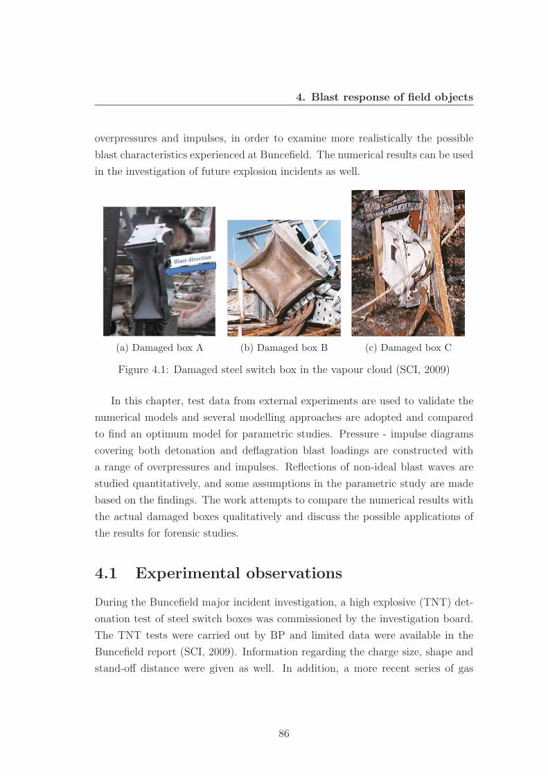
4. Blast response of field objects
overpressures and impulses, in order to examine more realistically the possible
blast characteristics experienced at Buncefield. The numerical results can be used
in the investigation of future explosion incidents as well.
(a) Damaged box A (b) Damaged box B (c) Damaged box C
Figure 4.1: Damaged steel switch box in the vapour cloud (SCI, 2009)
In this chapter, test data from external experiments are used to validate the
numerical models and several modelling approaches are adopted and compared
to find an optimum model for parametric studies. Pressure - impulse diagrams
covering both detonation and deflagration blast loadings are constructed with
a range of overpressures and impulses. Reflections of non-ideal blast waves are
studied quantitatively, and some assumptions in the parametric study are made
based on the findings. The work attempts to compare the numerical results with
the actual damaged boxes qualitatively and discuss the possible applications of
the results for forensic studies.
4.1 Experimental observations
During the Buncefield major incident investigation, a high explosive (TNT) det-
onation test of steel switch boxes was commissioned by the investigation board.
The TNT tests were carried out by BP and limited data were available in the
Buncefield report (SCI, 2009). Information regarding the charge size, shape and
stand-off distance were given as well. In addition, a more recent series of gas
86
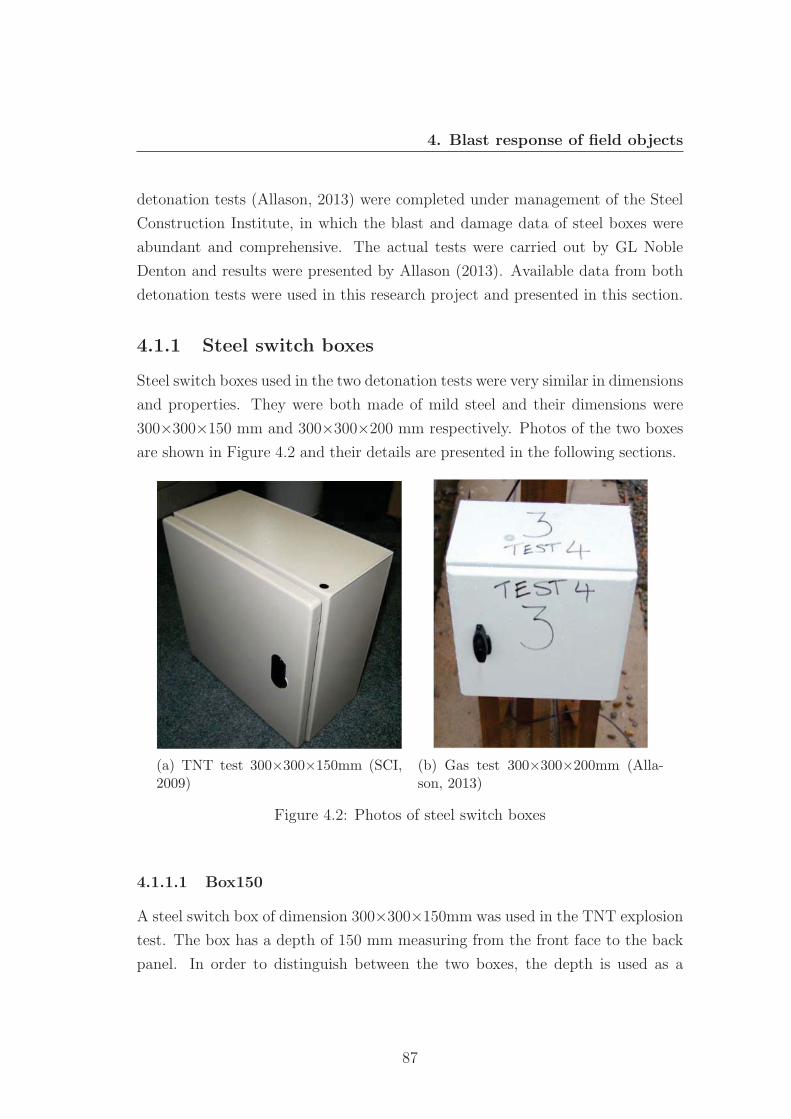
4. Blast response of field objects
detonation tests (Allason, 2013) were completed under management of the Steel
Construction Institute, in which the blast and damage data of steel boxes were
abundant and comprehensive. The actual tests were carried out by GL Noble
Denton and results were presented by Allason (2013). Available data from both
detonation tests were used in this research project and presented in this section.
4.1.1 Steel switch boxes
Steel switch boxes used in the two detonation tests were very similar in dimensions
and properties. They were both made of mild steel and their dimensions were
300×300×150 mm and 300×300×200 mm respectively. Photos of the two boxes
are shown in Figure 4.2 and their details are presented in the following sections.
(a) TNT test 300×300×150mm (SCI,2009)
(b) Gas test 300×300×200mm (Alla-son, 2013)
Figure 4.2: Photos of steel switch boxes
4.1.1.1 Box150
A steel switch box of dimension 300×300×150mm was used in the TNT explosion
test. The box has a depth of 150 mm measuring from the front face to the back
panel. In order to distinguish between the two boxes, the depth is used as a
87
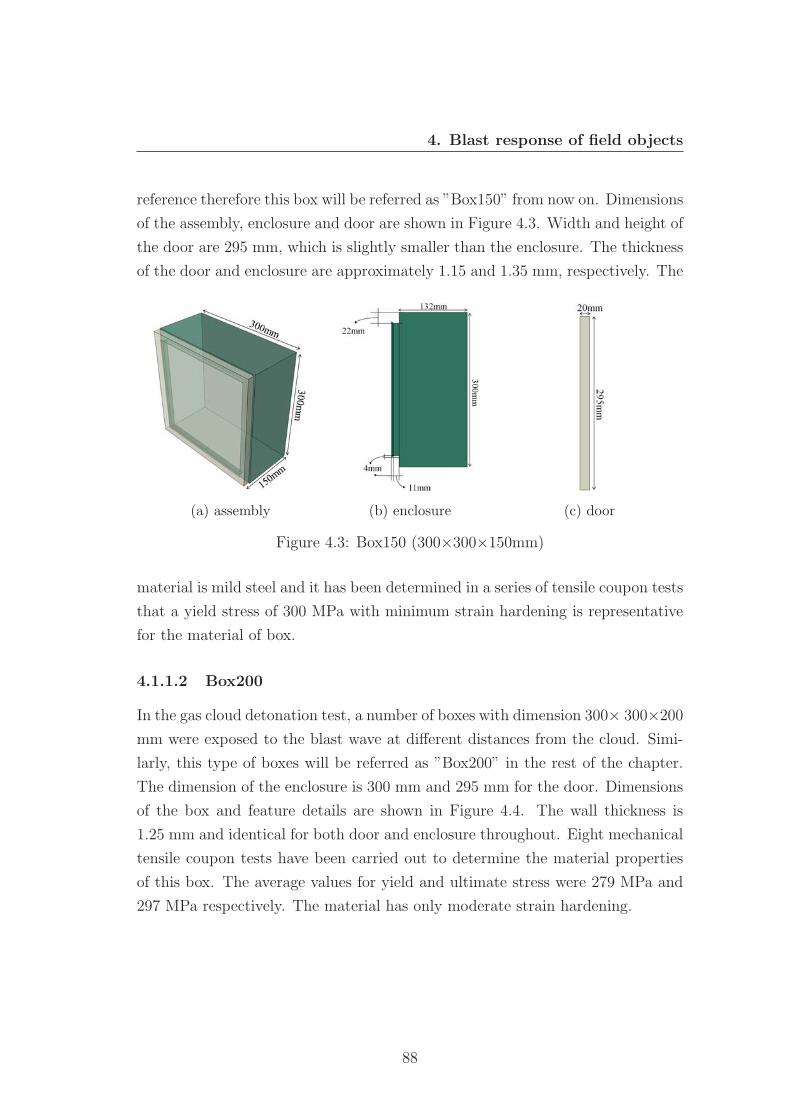
4. Blast response of field objects
reference therefore this box will be referred as ”Box150” from now on. Dimensions
of the assembly, enclosure and door are shown in Figure 4.3. Width and height of
the door are 295 mm, which is slightly smaller than the enclosure. The thickness
of the door and enclosure are approximately 1.15 and 1.35 mm, respectively. The
(a) assembly (b) enclosure (c) door
Figure 4.3: Box150 (300×300×150mm)
material is mild steel and it has been determined in a series of tensile coupon tests
that a yield stress of 300 MPa with minimum strain hardening is representative
for the material of box.
4.1.1.2 Box200
In the gas cloud detonation test, a number of boxes with dimension 300× 300×200
mm were exposed to the blast wave at different distances from the cloud. Simi-
larly, this type of boxes will be referred as ”Box200” in the rest of the chapter.
The dimension of the enclosure is 300 mm and 295 mm for the door. Dimensions
of the box and feature details are shown in Figure 4.4. The wall thickness is
1.25 mm and identical for both door and enclosure throughout. Eight mechanical
tensile coupon tests have been carried out to determine the material properties
of this box. The average values for yield and ultimate stress were 279 MPa and
297 MPa respectively. The material has only moderate strain hardening.
88
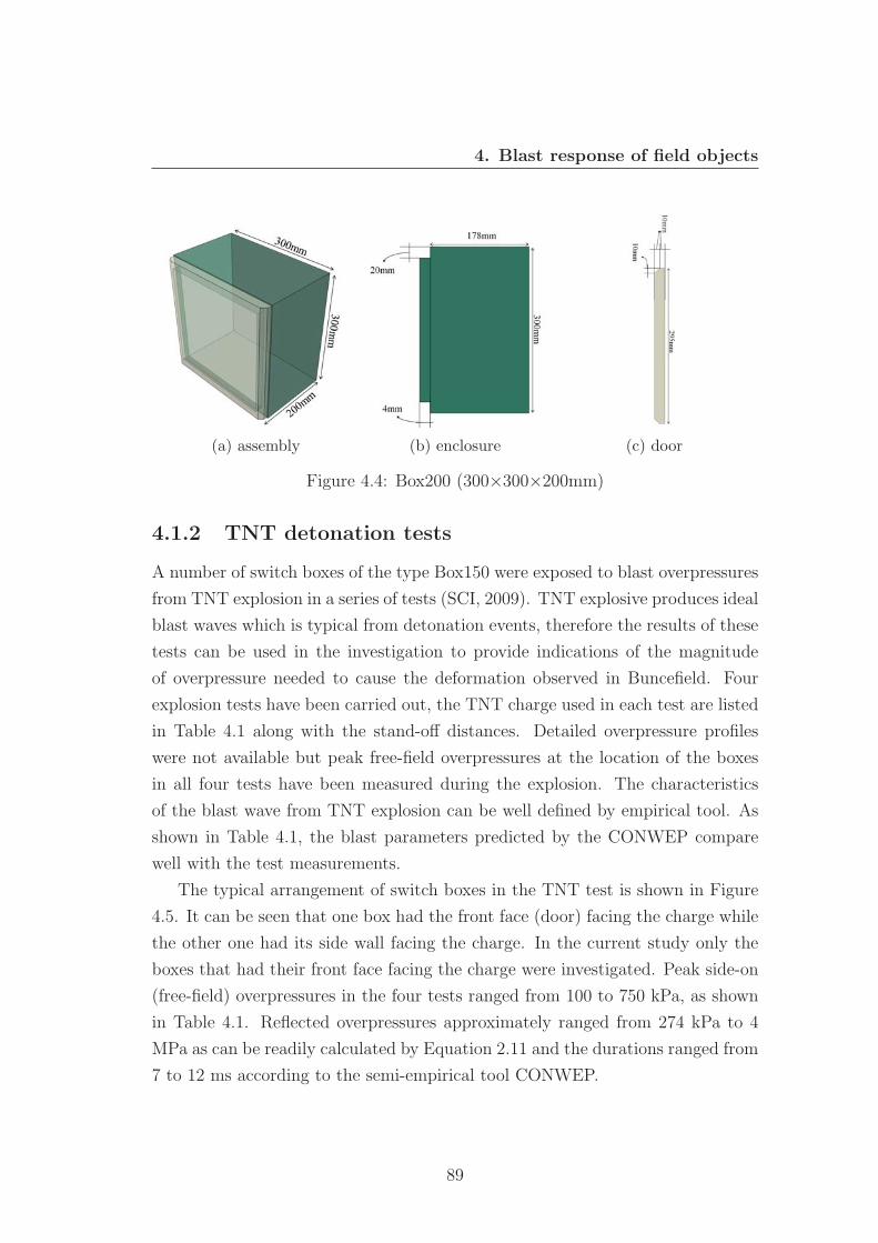
4. Blast response of field objects
(a) assembly (b) enclosure (c) door
Figure 4.4: Box200 (300×300×200mm)
4.1.2 TNT detonation tests
A number of switch boxes of the type Box150 were exposed to blast overpressures
from TNT explosion in a series of tests (SCI, 2009). TNT explosive produces ideal
blast waves which is typical from detonation events, therefore the results of these
tests can be used in the investigation to provide indications of the magnitude
of overpressure needed to cause the deformation observed in Buncefield. Four
explosion tests have been carried out, the TNT charge used in each test are listed
in Table 4.1 along with the stand-off distances. Detailed overpressure profiles
were not available but peak free-field overpressures at the location of the boxes
in all four tests have been measured during the explosion. The characteristics
of the blast wave from TNT explosion can be well defined by empirical tool. As
shown in Table 4.1, the blast parameters predicted by the CONWEP compare
well with the test measurements.
The typical arrangement of switch boxes in the TNT test is shown in Figure
4.5. It can be seen that one box had the front face (door) facing the charge while
the other one had its side wall facing the charge. In the current study only the
boxes that had their front face facing the charge were investigated. Peak side-on
(free-field) overpressures in the four tests ranged from 100 to 750 kPa, as shown
in Table 4.1. Reflected overpressures approximately ranged from 274 kPa to 4
MPa as can be readily calculated by Equation 2.11 and the durations ranged from
7 to 12 ms according to the semi-empirical tool CONWEP.
89
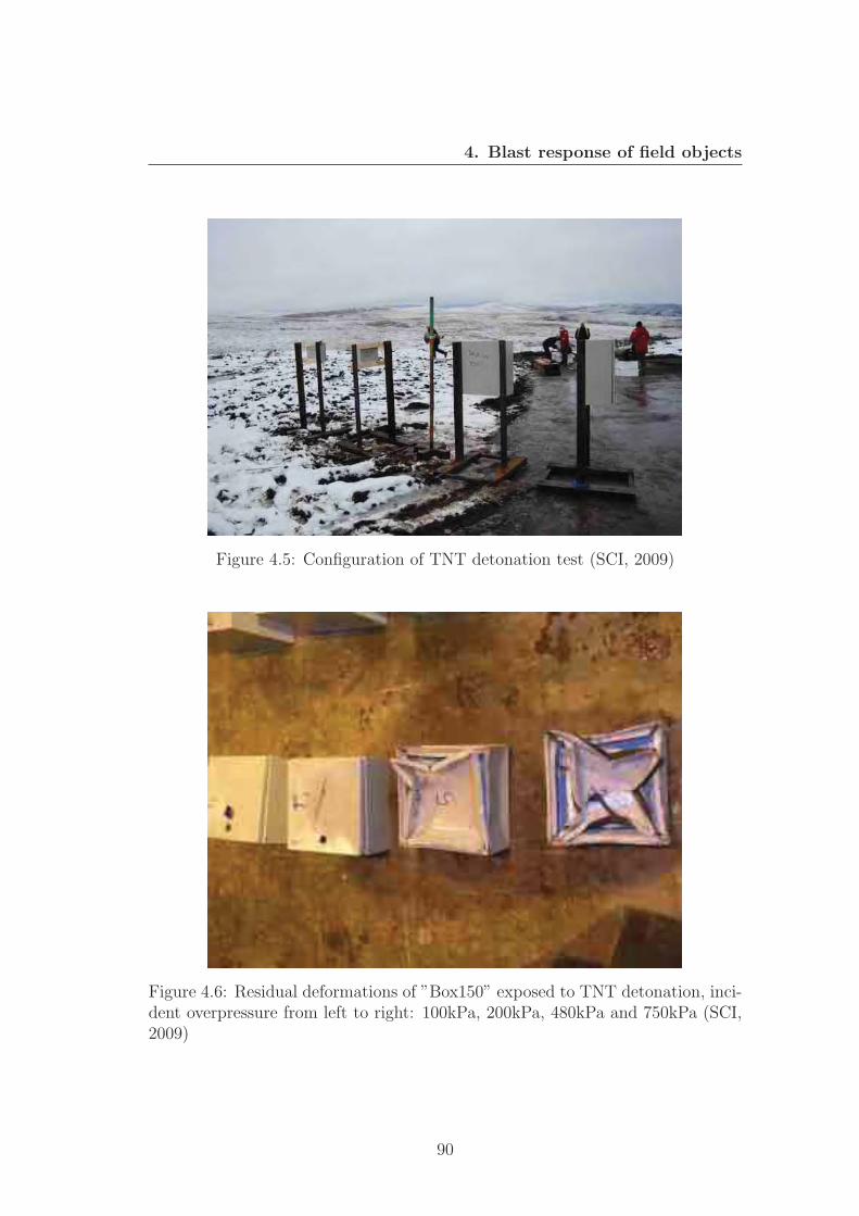
4. Blast response of field objects
Figure 4.5: Configuration of TNT detonation test (SCI, 2009)
Figure 4.6: Residual deformations of ”Box150” exposed to TNT detonation, inci-dent overpressure from left to right: 100kPa, 200kPa, 480kPa and 750kPa (SCI,2009)
90
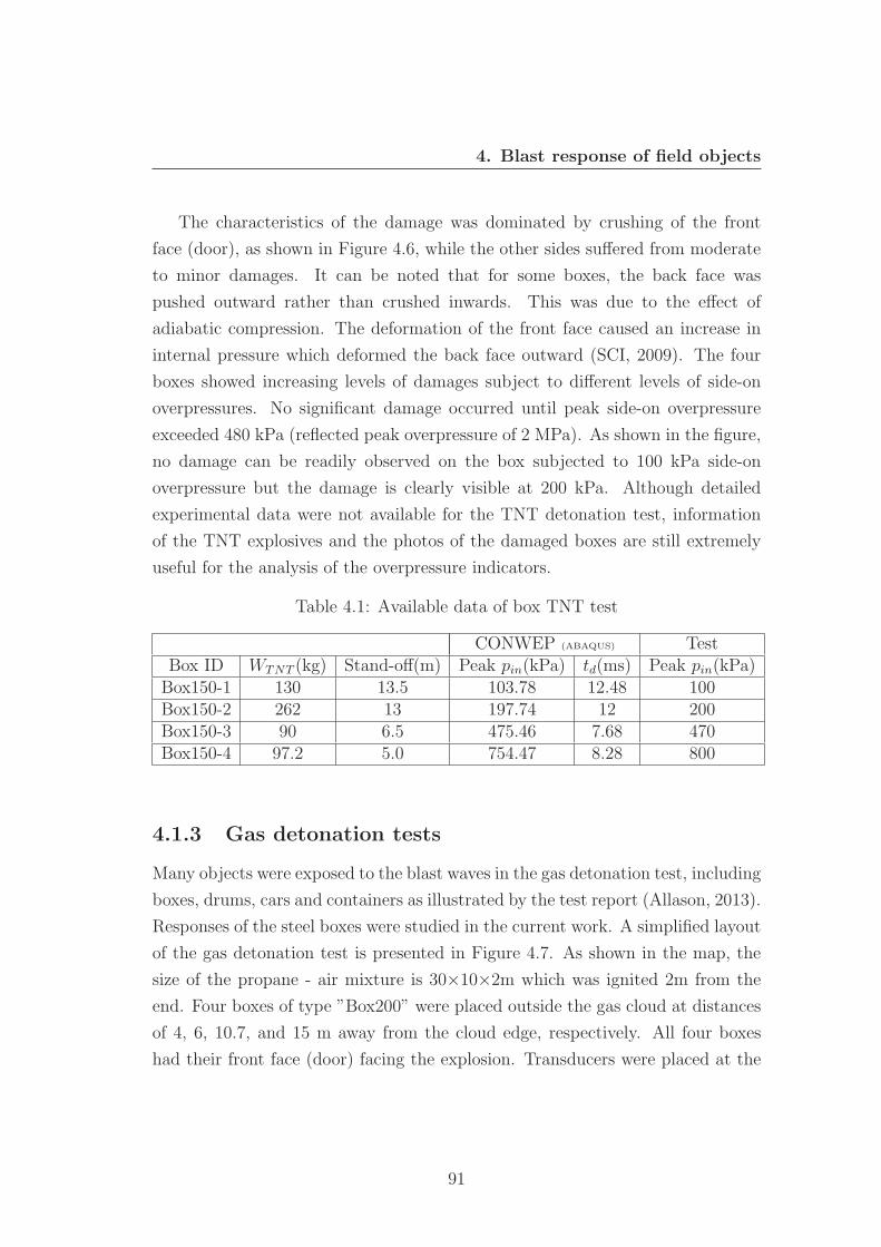
4. Blast response of field objects
The characteristics of the damage was dominated by crushing of the front
face (door), as shown in Figure 4.6, while the other sides suffered from moderate
to minor damages. It can be noted that for some boxes, the back face was
pushed outward rather than crushed inwards. This was due to the effect of
adiabatic compression. The deformation of the front face caused an increase in
internal pressure which deformed the back face outward (SCI, 2009). The four
boxes showed increasing levels of damages subject to different levels of side-on
overpressures. No significant damage occurred until peak side-on overpressure
exceeded 480 kPa (reflected peak overpressure of 2 MPa). As shown in the figure,
no damage can be readily observed on the box subjected to 100 kPa side-on
overpressure but the damage is clearly visible at 200 kPa. Although detailed
experimental data were not available for the TNT detonation test, information
of the TNT explosives and the photos of the damaged boxes are still extremely
useful for the analysis of the overpressure indicators.
Table 4.1: Available data of box TNT test
CONWEP (ABAQUS) TestBox ID WTNT (kg) Stand-off(m) Peak pin(kPa) td(ms) Peak pin(kPa)Box150-1 130 13.5 103.78 12.48 100Box150-2 262 13 197.74 12 200Box150-3 90 6.5 475.46 7.68 470Box150-4 97.2 5.0 754.47 8.28 800
4.1.3 Gas detonation tests
Many objects were exposed to the blast waves in the gas detonation test, including
boxes, drums, cars and containers as illustrated by the test report (Allason, 2013).
Responses of the steel boxes were studied in the current work. A simplified layout
of the gas detonation test is presented in Figure 4.7. As shown in the map, the
size of the propane - air mixture is 30×10×2m which was ignited 2m from the
end. Four boxes of type ”Box200” were placed outside the gas cloud at distances
of 4, 6, 10.7, and 15 m away from the cloud edge, respectively. All four boxes
had their front face (door) facing the explosion. Transducers were placed at the
91
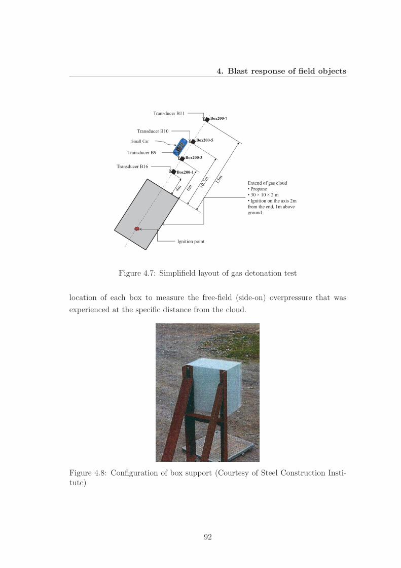
4. Blast response of field objects
Transducer B16
Transducer B9
Transducer B10
Transducer B11
Box200-1
Extend of gas cloud • Propane • 30 × 10 × 2 m • Ignition on the axis 2m from the end, 1m above ground
Box200-3
Box200-5
Box200-7
Small Car
Ignition point
Figure 4.7: Simplifield layout of gas detonation test
location of each box to measure the free-field (side-on) overpressure that was
experienced at the specific distance from the cloud.
Figure 4.8: Configuration of box support (Courtesy of Steel Construction Insti-tute)
92
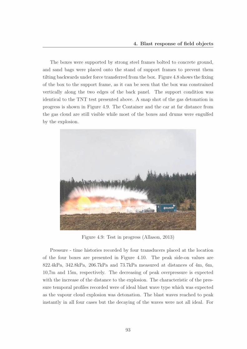
4. Blast response of field objects
The boxes were supported by strong steel frames bolted to concrete ground,
and sand bags were placed onto the stand of support frames to prevent them
tilting backwards under force transferred from the box. Figure 4.8 shows the fixing
of the box to the support frame, as it can be seen that the box was constrained
vertically along the two edges of the back panel. The support condition was
identical to the TNT test presented above. A snap shot of the gas detonation in
progress is shown in Figure 4.9. The Container and the car at far distance from
the gas cloud are still visible while most of the boxes and drums were engulfed
by the explosion.
Figure 4.9: Test in progress (Allason, 2013)
Pressure - time histories recorded by four transducers placed at the location
of the four boxes are presented in Figure 4.10. The peak side-on values are
822.4kPa, 342.8kPa, 206.7kPa and 73.7kPa measured at distances of 4m, 6m,
10,7m and 15m, respectively. The decreasing of peak overpressure is expected
with the increase of the distance to the explosion. The characteristic of the pres-
sure temporal profiles recorded were of ideal blast wave type which was expected
as the vapour cloud explosion was detonation. The blast waves reached to peak
instantly in all four cases but the decaying of the waves were not all ideal. For
93
4. Blast response of field objects
example the pressure - time curve of transducer B10 in Figure 4.10 did not show
a exponential decay. The pressure dropped below ambient immediately after the
peak and then increased gradually to a second peak with lower magnitude within
a finite time. This might due to the turbulent flow caused by the complex envi-
0 20 40 60 80 100Time [ms]
-200
0
200
400
600
800
1000
Overpressure
[kPa]
Transducer B16
Transducer B9
Transducer B10
Transducer B11
Figure 4.10: Pressure - time histories recorded by transducers
ronment around the boxes. As indicated earlier, many objects were exposed to
blast wave in the same test including a car which was placed next to transducer
B9 and B10. Transducer B9 was located at the front of the car, while the latter
was at the rear. The turbulence or reflection generated by the blast wave when
passing through the car would very likely to affect the pressure waves recorded by
the transducers, particularly for B10. This can be examined in detail by looking
at all four pressure curves shown in Figure 4.10. It can been see that there is no
substantial distortions to the pressure profile of transducer B16 and B11, which
were some distances away from the car. Transducer B9 placed near the front of
the car registered a slightly distorted pressure profile which had a lower second
peak. The pressure profile of transducer B10 was clearly significantly affected by
the presence of the car. It is also worthy to note that the pressure waves did not
94
4. Blast response of field objects
completely reduce to ambient and the time history scattered dramatically. These
inaccuracies are attributed to the high sensitivity of the transducers. They might
malfunction after the passage of blast waves with high peak overpressures.
Photos of the four boxes before and after they were exposed to blast waves in
the gas detonation test are presented in Figure 4.11. Similar to the boxes exposed
to pressure waves from TNT explosions, the damages of boxes from the gas cloud
detonation were dominated by crushing of the front face as well. This can be
expected since both explosions generated same types of blast waves. Box200-
1 suffered the most severe damage at its front face (the door) when subjected
to a peak side-on overpressure of 822.4 kPa and the damage is decreasing with
decreased peak overpressures. No damage can be found observed at the front face
of Box200-7 which was subjected to a peak side-on overpressure of 73.7 kPa.
After the gas explosion test, the damaged boxes were collected and scanned in
a laser machine. The damaged boxes prepared for scanning are shown in Figure
4.11 as well. Scan photos of the residual shape of each box are shown in Figure
4.12. The digital files containing information of the residual shape of the boxes
were used to study the response of the boxes to blast waves.
The residual deformation of the boxes have been measured in CAD software
SolidWorks. Figure 4.13 shows the measurement of the deformation at the centre
of the front face of the box (door). The measurement was taken from the middle
of the right edge of the front face to the centre. The original position of the centre
of the front face is unclear in the digital file. Due to the dominating damage at
the front face, permanent deformations at the centre of the front face were used
in the quantitative analysis of the response of the boxes. Permanent deformation
at the centre of the front face of each box measured from the digital files are
listed in Table 4.2, together with the experimental side-on peak overpressure at
the location of each box.
95
4. Blast response of field objects
(a) Box200-1 before (b) Box200-1 after (c) Box200-1 ready
(d) Box200-3 before (e) Box200-3 after (f) Box200-3 ready
(g) Box200-5 before (h) Box200-5 after (i) Box200-5 ready
(j) Box200-7 before (k) Box200-7 after (l) Box200-7 ready
Figure 4.11: Before and after photographs of Box200-1,3,5 and 7 (Allason, 2013)
96
4. Blast response of field objects
(a) box200-1 (b) box200-3 (c) box200-5 (d) box200-7
Figure 4.12: Digital scan of boxes
Figure 4.13: Deformation measurement of scanned box
Table 4.2: Brief information of box gas detonation test
Box ID Transducer Peak pside−on (kPa) δperm@door centre (mm)Box200-1 B16 822.4 50.82Box200-3 B9 342.8 32.63Box200-5 B10 206.7 9.19Box200-7 B11 73.7 1.55
97
4. Blast response of field objects
4.2 Numerical methodology
One of the objectives of the current study is using numerical models of a steel
box to examine the response of boxes to blast loading. This section presents the
details of the ? numerical model and various analysis approaches adopted in the
studies.
4.2.1 Numerical model of boxes
4.2.1.1 Model of Box150
Material of Box150 is carbon steel and the Johnson-Cook plasticity and strain-rate
model (Equation 3.17) was used. The parameters for the material are listed in
Table 4.3, in which m = 0 since the material thermal dependencies are neglected
here.
Table 4.3: Johnson-Cook parameters for material of Box150
A 300 MPaB 200 MPaN 0.228C 0.01622ε0 0.000154
Details of the numerical model of Box150 are shown in Figure 4.14. Each
face was assigned with a name to avoid confusion in the future when referring to
them. In the common design of steel switch boxes, the door and the enclosure are
joined with two hinges at one side of the box and the lock was located at the other
side. Thus, two connectors were used to represent the axially rotating behaviour
of the hinges. As shown in Figure 4.14b, the two segments (shaded area in red)
of the door and the enclosure are rigidly tied to two reference points which were
in turn joined by a hinge connector. These connectors only allow axial rotation
about the longitudinal axis of the hinge. It was difficult to model the failure of
the plastic lock that holds the door in position, both the capacity and failure
mode are unclear and impractical to examine in detail within the scope of the
current study. For simplicity, a rigid weld connector was used to join two single
98
4. Blast response of field objects
nodes on the door and enclosure respectively, as shown in Figure 4.14c. The rigid
connector would not fail and the door will always be kept in the closed position
when the box is exposed to blast loading. Although it has been observed that
the lock failed in all gas detonation tests, such simplification would not affect
the results significantly and made the displacement - time history measurement
easier to be interpreted. Otherwise if the lock was allowed to fail then the door
would open and the displacement of the centre of the door will be affected by the
rigid rotation of the door.
(a) model details (b) Hinge model (c) Lock model
Figure 4.14: Box150 numerical model details
Two types of boundary conditions were applied to the box model. Figure
4.15a approximately represents the support conditions of the boxes used in both
tests. As it can be seen in Figures 4.5 and 4.8 that the boxes were fixed to the
support frame on the back face along the two vertical edges. Figure 4.1 shows
the actual boxes found at Buncefield. The support conditions for box B and C
were not very clear due to the large deformation of the frames. It can be seen
that box A was not supported at the back but instead at the bottom. Although
exact support conditions were not known it would suffice to replicate the support
condition by fully fixing the perimeters of the bottom face as depicted in Figure
4.15b.
ABAQUS shell element S4R was used to mesh the box models. A mesh con-
vergence study was carried out by applying an arbitrary dynamic pressure load to
the surfaces of the numerical model. As shown in Figure 4.16, the differences in
maximum dynamic and permanent displacement are reducing as the total num-
99
4. Blast response of field objects
(a) Box150 support on back face (b) Box150 support on bottom face
Figure 4.15: Box150 model boundary conditions with mesh
ber of elements is increasing. When the total number of elements exceeds 8601
there was no significant improvement to the predicted values, therefore the corre-
sponding element size of 7 mm was used for the majority of the box model, while
finer elements were used for features with relatively small dimensions. Figure
4.15 shows the mesh quality of Box150.
0 2000 4000 6000 8000 10000 12000 14000 16000 18000Mesh density: total number of shell elements
0.000
0.005
0.010
0.015
0.020
0.025
0.030
0.035
Displacementar
centre
offrontface(m
)
Residual displacement
Max displacement
Figure 4.16: Box numerical mode mesh study
100
4. Blast response of field objects
4.2.1.2 Model of Box200
Based on the results from the tensile tests for the material of Box200, a piece-
wise plasticity with isotropic strain hardening model was used to represent the
material behaviour of Box200. The Johnson - Cook strain rate hardening model is
also used, i.e. he middle term of Equation 3.17. Parameters used in the material
model are shown in the table below. Rate dependent data were not available from
tensile tests. The strain rate hardening parameters of S275 steel were adopted,
which has similar properties to the material of the boxes used in the current
study.
Table 4.4: Piece-wise plasticity for material of Box200
σy εy276 MPa 0.0297 MPa 0.367297 MPa 0.5
C 0.01622ε0 0.000154
The configurations of the two boxes are very similar, the door and enclosure
of Box200 were joined by two hinges as well. A plastic lock was used to keep the
door closed. The differences were the hinges of Box200 are slightly larger and
located at the opposite side of Box150, as shown in Figure 4.17a. The hinge and
lock were modelled in the same way as in Box150. Box200 was also meshed by
7 mm S4R shell elements as well, and with finer element at small features. The
mesh quality of Box200 is shown in Figure 4.17b.
4.2.2 Lagrangian analysis
Deformation of the shell structural elements are described by Lagrangian formu-
lations. The Lagrangian analysis model involves only numerical shell elements
(S4R) and the dynamic loads are implemented by applying pressure loading di-
rectly on the segments of the surfaces of the structures. The finite element models
are shown in Figures 4.15 and 4.17.
Dynamic pressure loading from the blast waves was applied directly on the
101
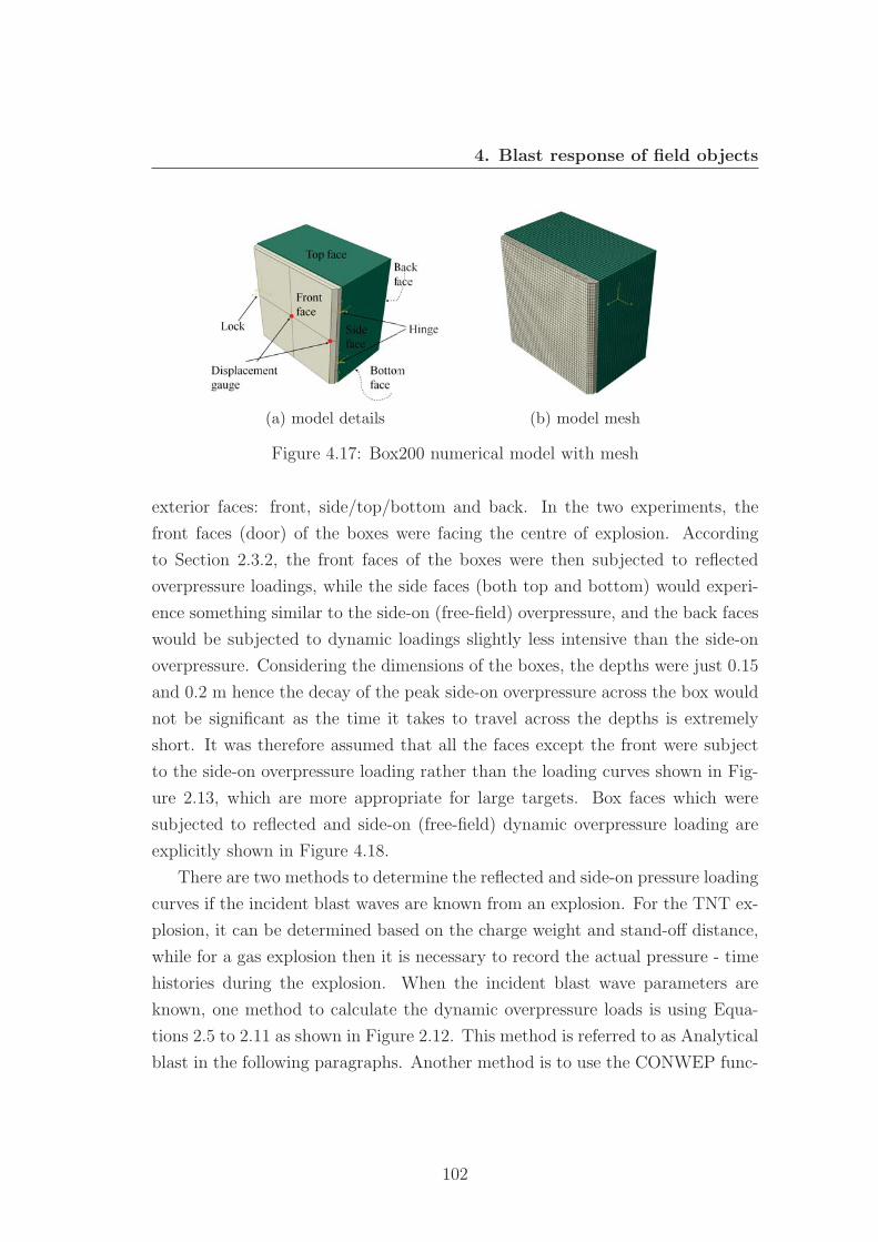
4. Blast response of field objects
(a) model details (b) model mesh
Figure 4.17: Box200 numerical model with mesh
exterior faces: front, side/top/bottom and back. In the two experiments, the
front faces (door) of the boxes were facing the centre of explosion. According
to Section 2.3.2, the front faces of the boxes were then subjected to reflected
overpressure loadings, while the side faces (both top and bottom) would experi-
ence something similar to the side-on (free-field) overpressure, and the back faces
would be subjected to dynamic loadings slightly less intensive than the side-on
overpressure. Considering the dimensions of the boxes, the depths were just 0.15
and 0.2 m hence the decay of the peak side-on overpressure across the box would
not be significant as the time it takes to travel across the depths is extremely
short. It was therefore assumed that all the faces except the front were subject
to the side-on overpressure loading rather than the loading curves shown in Fig-
ure 2.13, which are more appropriate for large targets. Box faces which were
subjected to reflected and side-on (free-field) dynamic overpressure loading are
explicitly shown in Figure 4.18.
There are two methods to determine the reflected and side-on pressure loading
curves if the incident blast waves are known from an explosion. For the TNT ex-
plosion, it can be determined based on the charge weight and stand-off distance,
while for a gas explosion then it is necessary to record the actual pressure - time
histories during the explosion. When the incident blast wave parameters are
known, one method to calculate the dynamic overpressure loads is using Equa-
tions 2.5 to 2.11 as shown in Figure 2.12. This method is referred to as Analytical
blast in the following paragraphs. Another method is to use the CONWEP func-
102
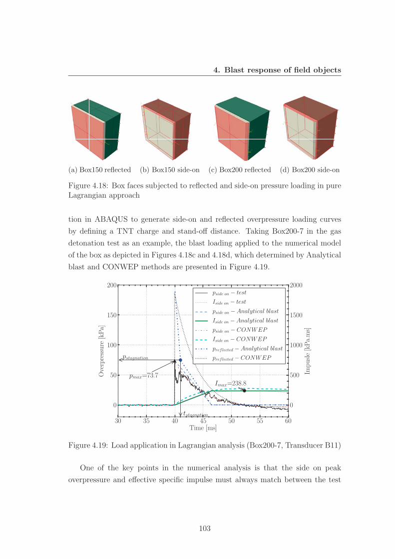
4. Blast response of field objects
(a) Box150 reflected (b) Box150 side-on (c) Box200 reflected (d) Box200 side-on
Figure 4.18: Box faces subjected to reflected and side-on pressure loading in pureLagrangian approach
tion in ABAQUS to generate side-on and reflected overpressure loading curves
by defining a TNT charge and stand-off distance. Taking Box200-7 in the gas
detonation test as an example, the blast loading applied to the numerical model
of the box as depicted in Figures 4.18c and 4.18d, which determined by Analytical
blast and CONWEP methods are presented in Figure 4.19.
30 35 40 45 50 55 60Time [ms]
0
50
100
150
200
Overpressure
[kPa]
pmax=73.7
pstagnation
tstagnation
pside on − test
Iside on − test
pside on − Analytical blast
Iside on − Analytical blast
pside on − CONWEP
Iside on − CONWEP
preflected − Analytical blast
preflected − CONWEP
0
500
1000
1500
2000
Impusle[kPa.ms]
Imax=238.8
Figure 4.19: Load application in Lagrangian analysis (Box200-7, Transducer B11)
One of the key points in the numerical analysis is that the side on peak
overpressure and effective specific impulse must always match between the test
103
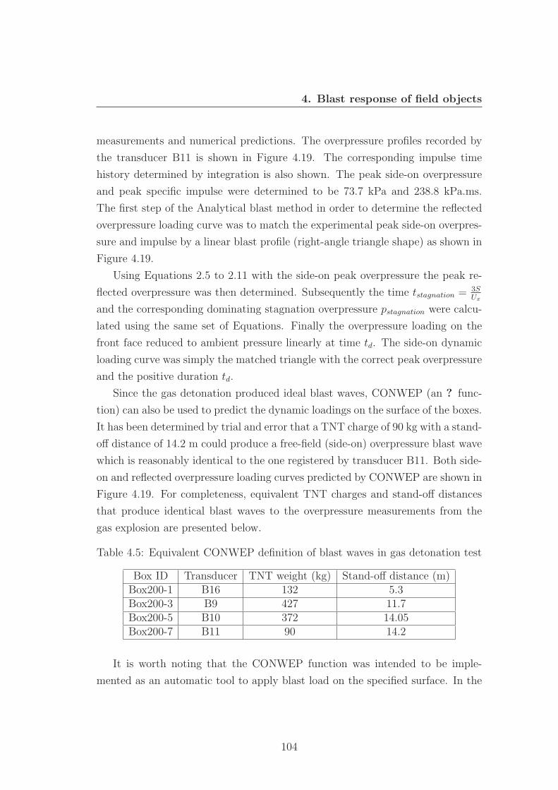
4. Blast response of field objects
measurements and numerical predictions. The overpressure profiles recorded by
the transducer B11 is shown in Figure 4.19. The corresponding impulse time
history determined by integration is also shown. The peak side-on overpressure
and peak specific impulse were determined to be 73.7 kPa and 238.8 kPa.ms.
The first step of the Analytical blast method in order to determine the reflected
overpressure loading curve was to match the experimental peak side-on overpres-
sure and impulse by a linear blast profile (right-angle triangle shape) as shown in
Figure 4.19.
Using Equations 2.5 to 2.11 with the side-on peak overpressure the peak re-
flected overpressure was then determined. Subsequently the time tstagnation = 3SUx
and the corresponding dominating stagnation overpressure pstagnation were calcu-
lated using the same set of Equations. Finally the overpressure loading on the
front face reduced to ambient pressure linearly at time td. The side-on dynamic
loading curve was simply the matched triangle with the correct peak overpressure
and the positive duration td.
Since the gas detonation produced ideal blast waves, CONWEP (an ? func-
tion) can also be used to predict the dynamic loadings on the surface of the boxes.
It has been determined by trial and error that a TNT charge of 90 kg with a stand-
off distance of 14.2 m could produce a free-field (side-on) overpressure blast wave
which is reasonably identical to the one registered by transducer B11. Both side-
on and reflected overpressure loading curves predicted by CONWEP are shown in
Figure 4.19. For completeness, equivalent TNT charges and stand-off distances
that produce identical blast waves to the overpressure measurements from the
gas explosion are presented below.
Table 4.5: Equivalent CONWEP definition of blast waves in gas detonation test
Box ID Transducer TNT weight (kg) Stand-off distance (m)Box200-1 B16 132 5.3Box200-3 B9 427 11.7Box200-5 B10 372 14.05Box200-7 B11 90 14.2
It is worth noting that the CONWEP function was intended to be imple-
mented as an automatic tool to apply blast load on the specified surface. In the
104
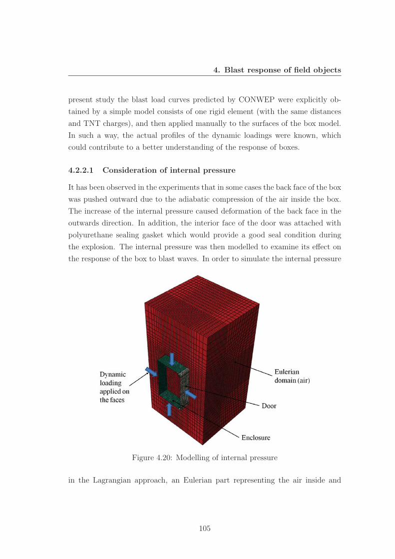
4. Blast response of field objects
present study the blast load curves predicted by CONWEP were explicitly ob-
tained by a simple model consists of one rigid element (with the same distances
and TNT charges), and then applied manually to the surfaces of the box model.
In such a way, the actual profiles of the dynamic loadings were known, which
could contribute to a better understanding of the response of boxes.
4.2.2.1 Consideration of internal pressure
It has been observed in the experiments that in some cases the back face of the box
was pushed outward due to the adiabatic compression of the air inside the box.
The increase of the internal pressure caused deformation of the back face in the
outwards direction. In addition, the interior face of the door was attached with
polyurethane sealing gasket which would provide a good seal condition during
the explosion. The internal pressure was then modelled to examine its effect on
the response of the box to blast waves. In order to simulate the internal pressure
Figure 4.20: Modelling of internal pressure
in the Lagrangian approach, an Eulerian part representing the air inside and
105
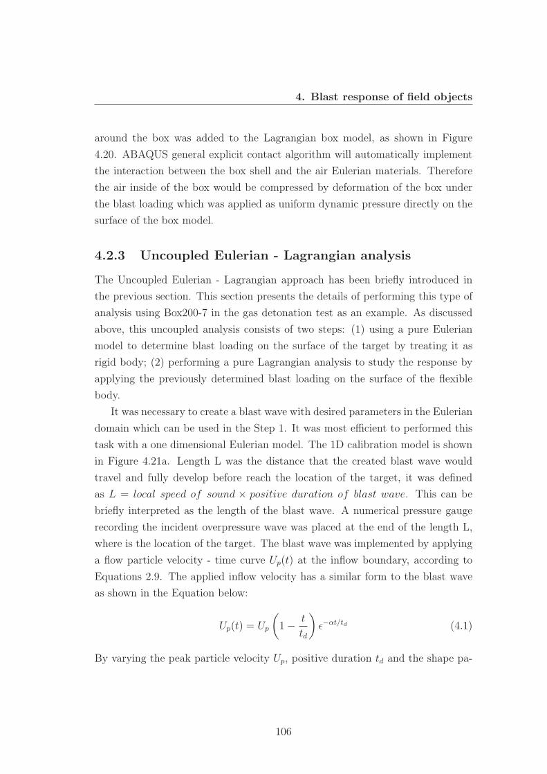
4. Blast response of field objects
around the box was added to the Lagrangian box model, as shown in Figure
4.20. ABAQUS general explicit contact algorithm will automatically implement
the interaction between the box shell and the air Eulerian materials. Therefore
the air inside of the box would be compressed by deformation of the box under
the blast loading which was applied as uniform dynamic pressure directly on the
surface of the box model.
4.2.3 Uncoupled Eulerian - Lagrangian analysis
The Uncoupled Eulerian - Lagrangian approach has been briefly introduced in
the previous section. This section presents the details of performing this type of
analysis using Box200-7 in the gas detonation test as an example. As discussed
above, this uncoupled analysis consists of two steps: (1) using a pure Eulerian
model to determine blast loading on the surface of the target by treating it as
rigid body; (2) performing a pure Lagrangian analysis to study the response by
applying the previously determined blast loading on the surface of the flexible
body.
It was necessary to create a blast wave with desired parameters in the Eulerian
domain which can be used in the Step 1. It was most efficient to performed this
task with a one dimensional Eulerian model. The 1D calibration model is shown
in Figure 4.21a. Length L was the distance that the created blast wave would
travel and fully develop before reach the location of the target, it was defined
as L = local speed of sound × positive duration of blast wave. This can be
briefly interpreted as the length of the blast wave. A numerical pressure gauge
recording the incident overpressure wave was placed at the end of the length L,
where is the location of the target. The blast wave was implemented by applying
a flow particle velocity - time curve Up(t) at the inflow boundary, according to
Equations 2.9. The applied inflow velocity has a similar form to the blast wave
as shown in the Equation below:
Up(t) = Up
(1− t
td
)ε−αt/td (4.1)
By varying the peak particle velocity Up, positive duration td and the shape pa-
106
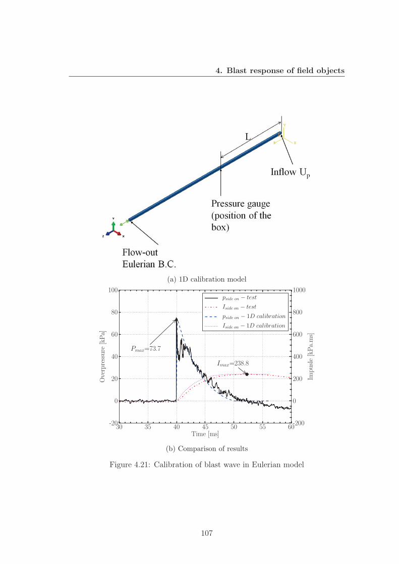
4. Blast response of field objects
(a) 1D calibration model
30 35 40 45 50 55 60Time [ms]
-20
0
20
40
60
80
100
Overpressure
[kPa]
Pmax=73.7
pside on − test
Iside on − test
pside on − 1D calibration
Iside on − 1D calibration
-200
0
200
400
600
800
1000
Impusle[kPa.ms]
Imax=238.8
(b) Comparison of results
Figure 4.21: Calibration of blast wave in Eulerian model
107
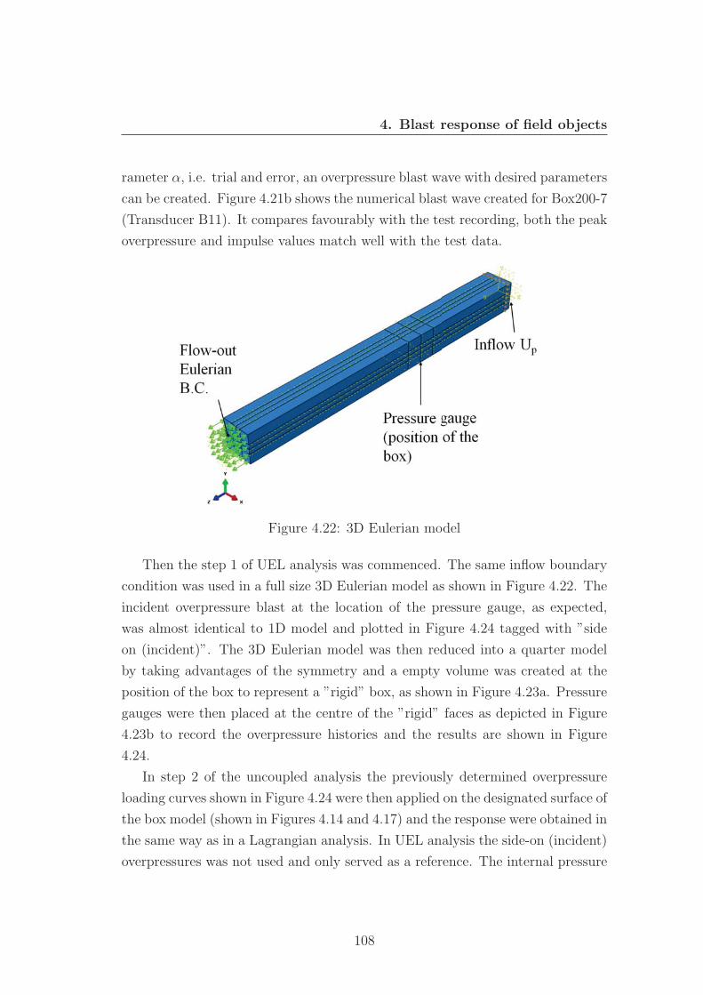
4. Blast response of field objects
rameter α, i.e. trial and error, an overpressure blast wave with desired parameters
can be created. Figure 4.21b shows the numerical blast wave created for Box200-7
(Transducer B11). It compares favourably with the test recording, both the peak
overpressure and impulse values match well with the test data.
Figure 4.22: 3D Eulerian model
Then the step 1 of UEL analysis was commenced. The same inflow boundary
condition was used in a full size 3D Eulerian model as shown in Figure 4.22. The
incident overpressure blast at the location of the pressure gauge, as expected,
was almost identical to 1D model and plotted in Figure 4.24 tagged with ”side
on (incident)”. The 3D Eulerian model was then reduced into a quarter model
by taking advantages of the symmetry and a empty volume was created at the
position of the box to represent a ”rigid” box, as shown in Figure 4.23a. Pressure
gauges were then placed at the centre of the ”rigid” faces as depicted in Figure
4.23b to record the overpressure histories and the results are shown in Figure
4.24.
In step 2 of the uncoupled analysis the previously determined overpressure
loading curves shown in Figure 4.24 were then applied on the designated surface of
the box model (shown in Figures 4.14 and 4.17) and the response were obtained in
the same way as in a Lagrangian analysis. In UEL analysis the side-on (incident)
overpressures was not used and only served as a reference. The internal pressure
108
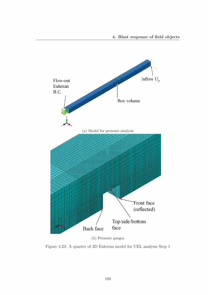
4. Blast response of field objects
(a) Model for pressure analysis
(b) Pressure gauges
Figure 4.23: A quarter of 3D Eulerian model for UEL analysis Step 1
109
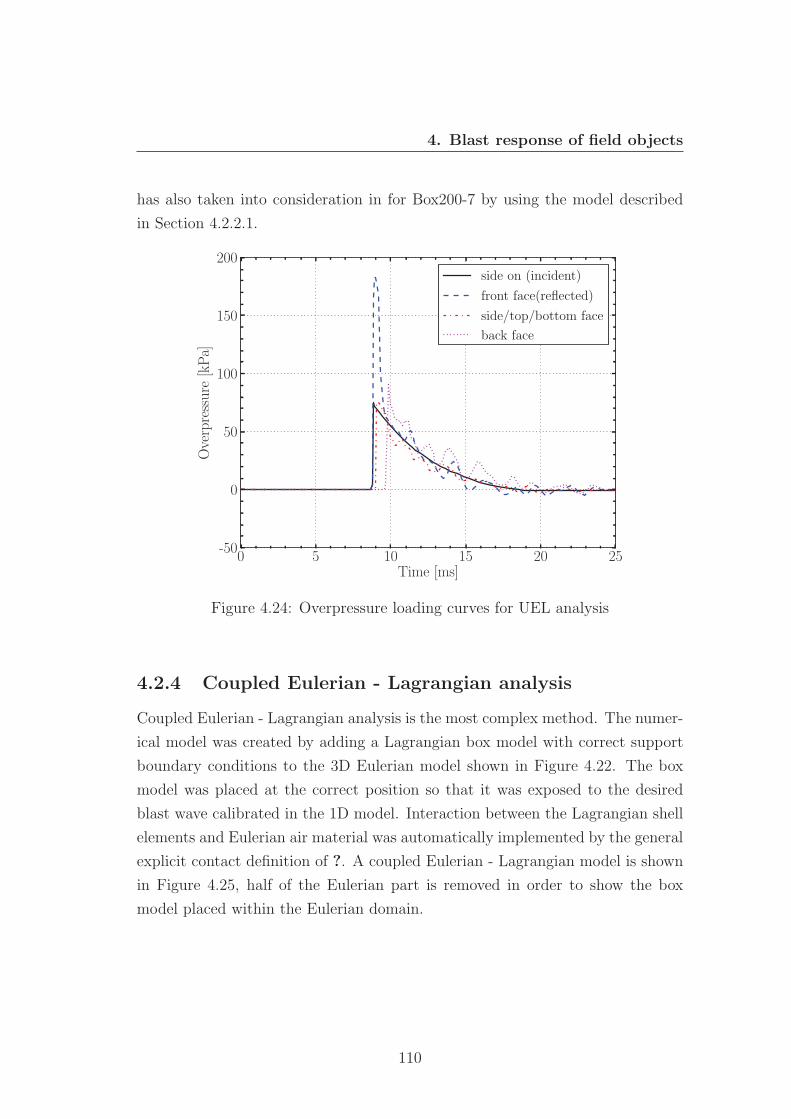
4. Blast response of field objects
has also taken into consideration in for Box200-7 by using the model described
in Section 4.2.2.1.
0 5 10 15 20 25Time [ms]
-50
0
50
100
150
200
Overpressure
[kPa]
side on (incident)
front face(reflected)
side/top/bottom face
back face
Figure 4.24: Overpressure loading curves for UEL analysis
4.2.4 Coupled Eulerian - Lagrangian analysis
Coupled Eulerian - Lagrangian analysis is the most complex method. The numer-
ical model was created by adding a Lagrangian box model with correct support
boundary conditions to the 3D Eulerian model shown in Figure 4.22. The box
model was placed at the correct position so that it was exposed to the desired
blast wave calibrated in the 1D model. Interaction between the Lagrangian shell
elements and Eulerian air material was automatically implemented by the general
explicit contact definition of ?. A coupled Eulerian - Lagrangian model is shown
in Figure 4.25, half of the Eulerian part is removed in order to show the box
model placed within the Eulerian domain.
110
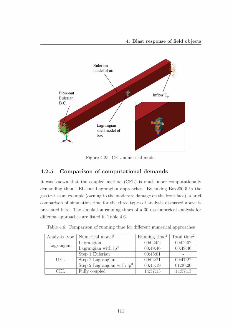
4. Blast response of field objects
Figure 4.25: CEL numerical model
4.2.5 Comparison of computational demands
It was known that the coupled method (CEL) is much more computationally
demanding than UEL and Lagrangian approaches. By taking Box200-5 in the
gas test as an example (owning to the moderate damage on the front face), a brief
comparison of simulation time for the three types of analysis discussed above is
presented here. The simulation running times of a 30 ms numerical analysis for
different approaches are listed in Table 4.6.
Table 4.6: Comparison of running time for different numerical approaches
Analysis type Numerical model1 Running time2 Total time2
LagrangianLagrangian 00:02:02 00:02:02Lagrangian with ip3 00:49:46 00:49:46
UELStep 1 Eulerian 00:45:01 -Step 2 Lagrangian 00:02:21 00:47:22Step 2 Lagrangian with ip3 00:45:19 01:30:20
CEL Fully coupled 14:57:13 14:57:13
111
4. Blast response of field objects
The Lagrangian approach only took 2 minutes for one analysis. It can be
seen in Table 4.6 that by considering the internal pressure the running time
was increased by 24 times. The Lagrangian step of the UEL approach took
only 2 minutes but the Eulerian step required about 45 minutes, hence the total
time for a UEL analysis was about 47 minutes which is 23.5 times the pure
Lagrangian analysis (without internal pressure). Including the internal pressure
in the UEL analysis would roughly double the running time. Apparently CEL
approach was the most demanding, it required 897 minutes (15 hours) for one
numerical analysis, which is more than 400 times the pure Lagrangian analysis
and 19 times the UEL analysis, when internal pressure is not considered.
4.3 Comparative assessment
In the previous section, the numerical models used in different simulation ap-
proaches were presented. In this section, data from the experiments was used to
study and validate the numerical models so that the most efficient and accurate
approach can be used for the parametric studies.
In the following sections, numerical models are used to reproduce the over-
pressure blast waves recorded in the detonation tests. Numerical results of model
Box200 are compared with the gas detonation test to validate the numerical
models. Although only limited data were available from the TNT detonation
test, the numerical results of Box150 can complement the study of the numerical
approaches.
4.3.1 Comparison of numerical results
In order to validate the numerical models, results of simulation of Box200 were
compared with the experimental data. Overpressure - time histories predicted by
different approaches were compared with the recording from the four transducers
to ensure that the numerical boxes were subjected to correct overpressure loading.
1all numerical models were implemented on High Performance Computers with 12 2.66 GHzXeon cpus with total 12 GB Memory
2time format hh:mm:ss3”ip” for internal pressure
112
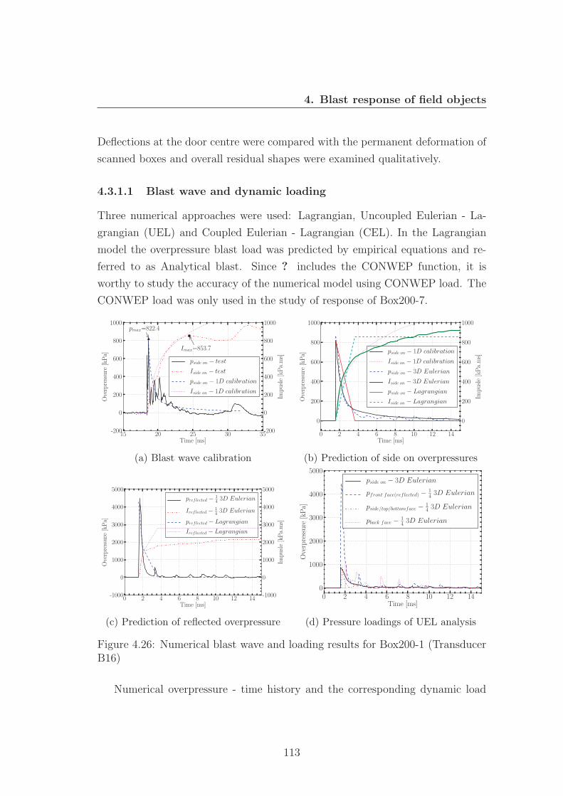
4. Blast response of field objects
Deflections at the door centre were compared with the permanent deformation of
scanned boxes and overall residual shapes were examined qualitatively.
4.3.1.1 Blast wave and dynamic loading
Three numerical approaches were used: Lagrangian, Uncoupled Eulerian - La-
grangian (UEL) and Coupled Eulerian - Lagrangian (CEL). In the Lagrangian
model the overpressure blast load was predicted by empirical equations and re-
ferred to as Analytical blast. Since ? includes the CONWEP function, it is
worthy to study the accuracy of the numerical model using CONWEP load. The
CONWEP load was only used in the study of response of Box200-7.
15 20 25 30 35Time [ms]
-200
0
200
400
600
800
1000
Overpressure
[kPa]
pmax=822.4
-200
0
200
400
600
800
1000
Impusle[kPa.ms]
Imax=853.7
pside on − test
Iside on − test
pside on − 1D calibration
Iside on − 1D calibration
(a) Blast wave calibration
0 2 4 6 8 10 12 14Time [ms]
0
200
400
600
800
1000
Overpressure
[kPa]
pside on − 1D calibration
Iside on − 1D calibration
pside on − 3D Eulerian
Iside on − 3D Eulerian
pside on − Lagrangian
Iside on − Lagrangian
0
200
400
600
800
1000
Impusle[kPa.ms]
(b) Prediction of side on overpressures
0 2 4 6 8 10 12 14Time [ms]
-1000
0
1000
2000
3000
4000
5000
Overpressure
[kPa]
preflected − 14 3D Eulerian
Ireflected − 14 3D Eulerian
preflected − Lagrangian
Ireflected − Lagrangian
-1000
0
1000
2000
3000
4000
5000
Impusle[kPa.ms]
(c) Prediction of reflected overpressure
0 2 4 6 8 10 12 14Time [ms]
0
1000
2000
3000
4000
5000
Overpressure
[kPa]
pside on − 3D Eulerian
pfront face(reflected) − 14 3D Eulerian
pside/top/bottomface − 14 3D Eulerian
pback face − 14 3D Eulerian
(d) Pressure loadings of UEL analysis
Figure 4.26: Numerical blast wave and loading results for Box200-1 (TransducerB16)
Numerical overpressure - time history and the corresponding dynamic load
113
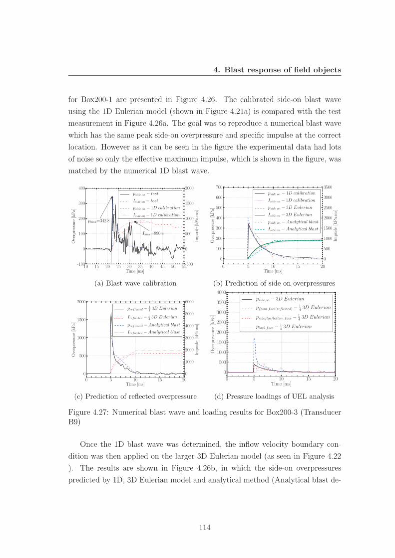
4. Blast response of field objects
for Box200-1 are presented in Figure 4.26. The calibrated side-on blast wave
using the 1D Eulerian model (shown in Figure 4.21a) is compared with the test
measurement in Figure 4.26a. The goal was to reproduce a numerical blast wave
which has the same peak side-on overpressure and specific impulse at the correct
location. However as it can be seen in the figure the experimental data had lots
of noise so only the effective maximum impulse, which is shown in the figure, was
matched by the numerical 1D blast wave.
10 15 20 25 30 35 40 45 50 55Time [ms]
-100
0
100
200
300
400
Overpressure
[kPa]
pmax=342.8
pside on − test
Iside on − test
pside on − 1D calibration
Iside on − 1D calibration
-500
0
500
1000
1500
2000
Impusle[kPa.ms]
Imax=890.4
(a) Blast wave calibration
0 5 10 15 20Time [ms]
0
100
200
300
400
500
600
700
Overpressure
[kPa]
pside on − 1D calibration
Iside on − 1D calibration
pside on − 3D Eulerian
Iside on − 3D Eulerian
pside on − Analytical blast
Iside on − Analytical blast
0
500
1000
1500
2000
2500
3000
3500
Impusle[kPa.ms]
(b) Prediction of side on overpressures
0 5 10 15 20Time [ms]
0
500
1000
1500
2000
Overpressure
[kPa]
preflected − 14 3D Eulerian
Ireflected − 14 3D Eulerian
preflected − Analytical blast
Ireflected − Analytical blast
0
1000
2000
3000
4000
5000
6000
Impusle[kPa.ms]
(c) Prediction of reflected overpressure
0 5 10 15 20Time [ms]
0
500
1000
1500
2000
2500
3000
3500
4000
Overpressure
[kPa]
pside on − 3D Eulerian
pfront face(reflected) − 14 3D Eulerian
pside/top/bottom face − 14 3D Eulerian
pback face − 14 3D Eulerian
(d) Pressure loadings of UEL analysis
Figure 4.27: Numerical blast wave and loading results for Box200-3 (TransducerB9)
Once the 1D blast wave was determined, the inflow velocity boundary con-
dition was then applied on the larger 3D Eulerian model (as seen in Figure 4.22
). The results are shown in Figure 4.26b, in which the side-on overpressures
predicted by 1D, 3D Eulerian model and analytical method (Analytical blast de-
114
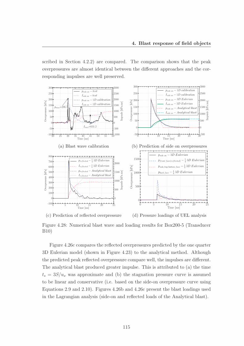
4. Blast response of field objects
scribed in Section 4.2.2) are compared. The comparison shows that the peak
overpressures are almost identical between the different approaches and the cor-
responding impulses are well preserved.
20 25 30 35 40 45 50 55 60Time [ms]
-100
-50
0
50
100
150
200
250
300
Overpressure
[kPa]
pmax=206.7
pside on − test
Iside on − test
pside on − 1D calibration
Iside on − 1D calibration
-1000
-500
0
500
1000
1500
2000
2500
3000
Impusle[kPa.ms]
Imax=631.2
(a) Blast wave calibration
0 5 10 15 20 25 30Time [ms]
-50
0
50
100
150
200
250
300
Overpressure
[kPa]
pside on − 1D calibration
Iside on − 1D calibration
pside on − 3D Eulerian
Iside on − 3D Eulerian
pside on − Analytical blast
Iside on − Analytical blast
-500
0
500
1000
1500
2000
2500
3000
Impusle[kPa.ms]
(b) Prediction of side on overpressures
0 5 10 15 20 25Time [ms]
-100
0
100
200
300
400
500
600
700
800
Overpressure
[kPa]
preflected − 14 3D Eulerian
Ireflected − 14 3D Eulerian
preflected − Analytical blast
Ireflected − Analytical blast
0
500
1000
1500
2000
Impusle[kPa.ms]
(c) Prediction of reflected overpressure
0 5 10 15 20 25Time [ms]
0
500
1000
1500
Overpressure
[kPa]
pside on − 3D Eulerian
pfront face(reflected) − 14 3D Eulerian
pside/top/bottom face − 14 3D Eulerian
pback face − 14 3D Eulerian
(d) Pressure loadings of UEL analysis
Figure 4.28: Numerical blast wave and loading results for Box200-5 (TransducerB10)
Figure 4.26c compares the reflected overpressures predicted by the one quarter
3D Eulerian model (shown in Figure 4.23) to the analytical method. Although
the predicted peak reflected overpressure compare well, the impulses are different.
The analytical blast produced greater impulse. This is attributed to (a) the time
ts = 3S/ux was approximate and (b) the stagnation pressure curve is assumed
to be linear and conservative (i.e. based on the side-on overpressure curve using
Equations 2.9 and 2.10). Figures 4.26b and 4.26c present the blast loadings used
in the Lagrangian analysis (side-on and reflected loads of the Analytical blast).
115
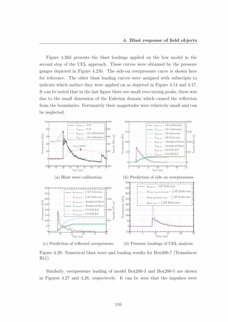
4. Blast response of field objects
Figure 4.26d presents the blast loadings applied on the box model in the
second step of the UEL approach. These curves were obtained by the pressure
gauges depicted in Figure 4.23b. The side-on overpressure curve is shown here
for reference. The other blast loading curves were assigned with subscripts to
indicate which surface they were applied on as depicted in Figure 4.14 and 4.17.
It can be noted that in the last figure there are small reoccurring peaks, these was
due to the small dimension of the Eulerian domain which caused the reflection
from the boundaries. Fortunately their magnitudes were relatively small and can
be neglected.
30 35 40 45 50 55 60 65 70Time [ms]
-20
0
20
40
60
80
100
Overpressure
[kPa]
pmax=73.7
pside on − test
Iside on − test
pside on − 1D calibration
Iside on − 1D calibration
-200
0
200
400
600
800
1000
Impusle[kPa.ms]
Imax=238.8
(a) Blast wave calibration
5 10 15 20 25 30 35Time [ms]
0
50
100
150
200Overpressure
[kPa]
pside on − 1D calibration
Iside on − 1D calibration
pside on − 3D Eulerian
Iside on − 3D Eulerian
pside on − Analytical blast
Iside on − Analytical blast
pside on − CONWEP
Iside on − CONWEP
0
500
1000
1500
2000
Impusle[kPa.ms]
(b) Prediction of side on overpressures
5 10 15 20 25 30Time [ms]
0
50
100
150
200
250
300
350
400
Overpressure
[kPa]
preflected − 14 3D Eulerian
Ireflected − 14 3D Eulerian
preflected − Analytical blast
Ireflected − Analytical blast
preflected − CONWEP
Ireflected − CONWEP
0
500
1000
1500
2000
Impusle[kPa.ms]
(c) Prediction of reflected overpressure
0 5 10 15 20 25Time [ms]
-50
0
50
100
150
200
250
300
350
400
Overpressure
[kPa]
pside on − 3D Eulerian
pfront face(reflected) − 14 3D Eulerian
pside/top/bottom face − 14 3D Eulerian
pback face − 14 3D Eulerian
(d) Pressure loadings of UEL analysis
Figure 4.29: Numerical blast wave and loading results for Box200-7 (TransducerB11)
Similarly, overpressure loading of model Box200-3 and Box200-5 are shown
in Figures 4.27 and 4.28, respectively. It can be seen that the impulses were
116
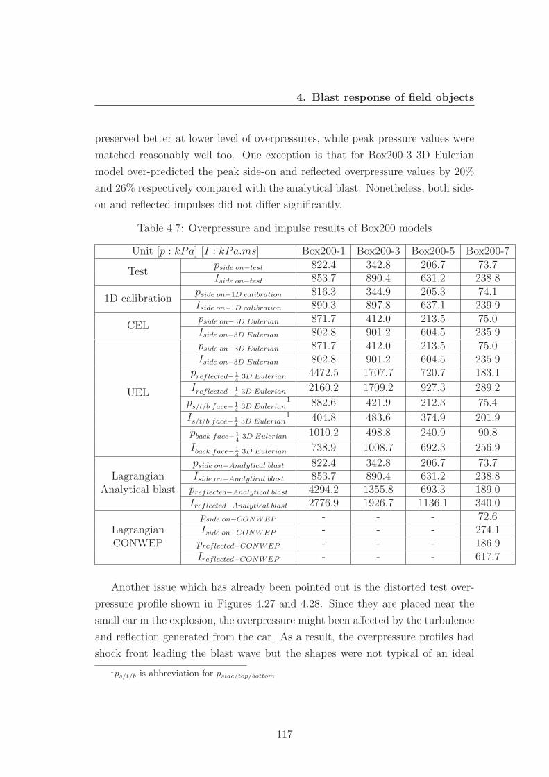
4. Blast response of field objects
preserved better at lower level of overpressures, while peak pressure values were
matched reasonably well too. One exception is that for Box200-3 3D Eulerian
model over-predicted the peak side-on and reflected overpressure values by 20%
and 26% respectively compared with the analytical blast. Nonetheless, both side-
on and reflected impulses did not differ significantly.
Table 4.7: Overpressure and impulse results of Box200 models
Unit [p : kPa] [I : kPa.ms] Box200-1 Box200-3 Box200-5 Box200-7
Testpside on−test 822.4 342.8 206.7 73.7Iside on−test 853.7 890.4 631.2 238.8
1D calibrationpside on−1D calibration 816.3 344.9 205.3 74.1Iside on−1D calibration 890.3 897.8 637.1 239.9
CELpside on−3D Eulerian 871.7 412.0 213.5 75.0Iside on−3D Eulerian 802.8 901.2 604.5 235.9
UEL
pside on−3D Eulerian 871.7 412.0 213.5 75.0Iside on−3D Eulerian 802.8 901.2 604.5 235.9
preflected− 143D Eulerian 4472.5 1707.7 720.7 183.1
Ireflected− 143D Eulerian 2160.2 1709.2 927.3 289.2
ps/t/b face− 143D Eulerian
1 882.6 421.9 212.3 75.4
Is/t/b face− 143D Eulerian
1 404.8 483.6 374.9 201.9
pback face− 143D Eulerian 1010.2 498.8 240.9 90.8
Iback face− 143D Eulerian 738.9 1008.7 692.3 256.9
pside on−Analytical blast 822.4 342.8 206.7 73.7Lagrangian Iside on−Analytical blast 853.7 890.4 631.2 238.8
Analytical blast preflected−Analytical blast 4294.2 1355.8 693.3 189.0Ireflected−Analytical blast 2776.9 1926.7 1136.1 340.0pside on−CONWEP - - - 72.6
Lagrangian Iside on−CONWEP - - - 274.1CONWEP preflected−CONWEP - - - 186.9
Ireflected−CONWEP - - - 617.7
Another issue which has already been pointed out is the distorted test over-
pressure profile shown in Figures 4.27 and 4.28. Since they are placed near the
small car in the explosion, the overpressure might been affected by the turbulence
and reflection generated from the car. As a result, the overpressure profiles had
shock front leading the blast wave but the shapes were not typical of an ideal
1ps/t/b is abbreviation for pside/top/bottom
117
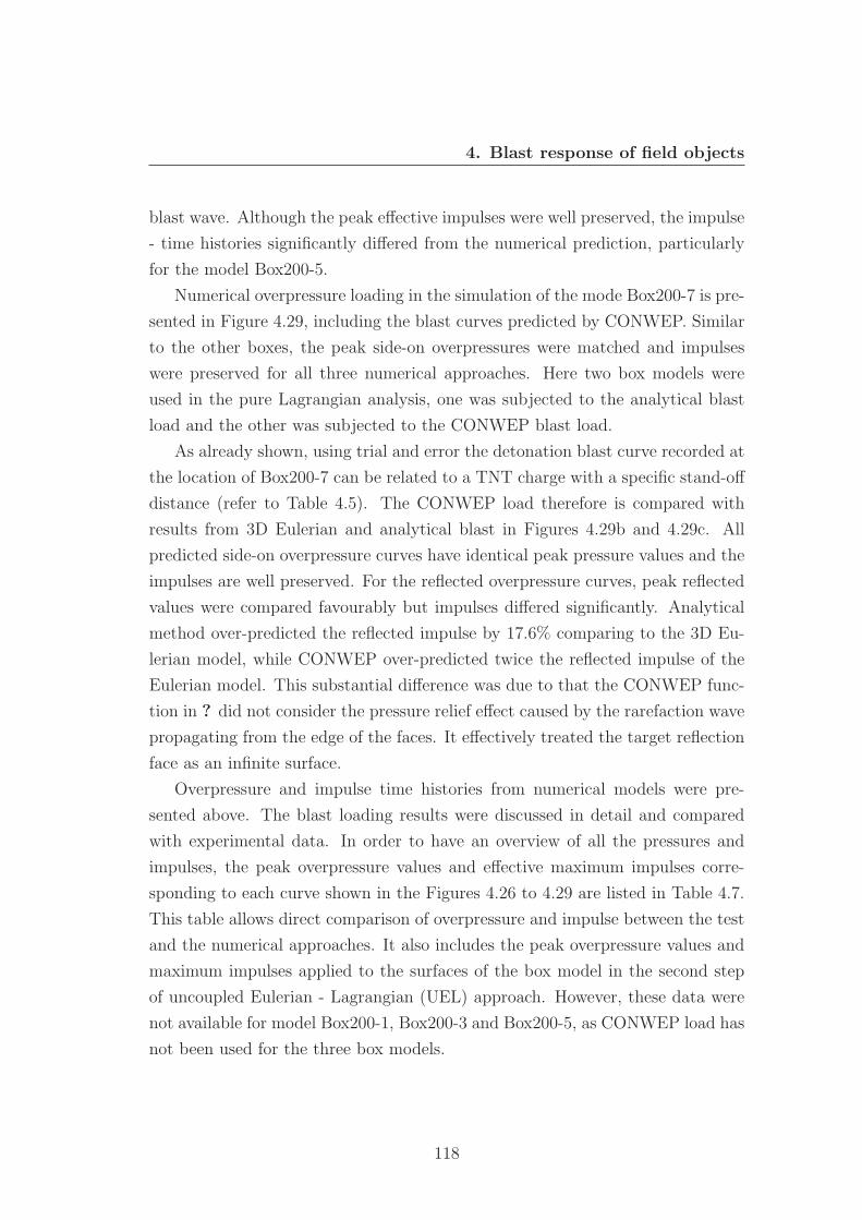
4. Blast response of field objects
blast wave. Although the peak effective impulses were well preserved, the impulse
- time histories significantly differed from the numerical prediction, particularly
for the model Box200-5.
Numerical overpressure loading in the simulation of the mode Box200-7 is pre-
sented in Figure 4.29, including the blast curves predicted by CONWEP. Similar
to the other boxes, the peak side-on overpressures were matched and impulses
were preserved for all three numerical approaches. Here two box models were
used in the pure Lagrangian analysis, one was subjected to the analytical blast
load and the other was subjected to the CONWEP blast load.
As already shown, using trial and error the detonation blast curve recorded at
the location of Box200-7 can be related to a TNT charge with a specific stand-off
distance (refer to Table 4.5). The CONWEP load therefore is compared with
results from 3D Eulerian and analytical blast in Figures 4.29b and 4.29c. All
predicted side-on overpressure curves have identical peak pressure values and the
impulses are well preserved. For the reflected overpressure curves, peak reflected
values were compared favourably but impulses differed significantly. Analytical
method over-predicted the reflected impulse by 17.6% comparing to the 3D Eu-
lerian model, while CONWEP over-predicted twice the reflected impulse of the
Eulerian model. This substantial difference was due to that the CONWEP func-
tion in ? did not consider the pressure relief effect caused by the rarefaction wave
propagating from the edge of the faces. It effectively treated the target reflection
face as an infinite surface.
Overpressure and impulse time histories from numerical models were pre-
sented above. The blast loading results were discussed in detail and compared
with experimental data. In order to have an overview of all the pressures and
impulses, the peak overpressure values and effective maximum impulses corre-
sponding to each curve shown in the Figures 4.26 to 4.29 are listed in Table 4.7.
This table allows direct comparison of overpressure and impulse between the test
and the numerical approaches. It also includes the peak overpressure values and
maximum impulses applied to the surfaces of the box model in the second step
of uncoupled Eulerian - Lagrangian (UEL) approach. However, these data were
not available for model Box200-1, Box200-3 and Box200-5, as CONWEP load has
not been used for the three box models.
118
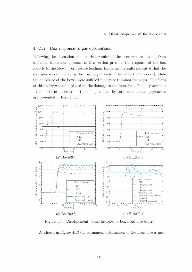
4. Blast response of field objects
4.3.1.2 Box response to gas detonations
Following the discussion of numerical results of the overpressure loading from
different simulation approaches, this section presents the response of the box
models to the above overpressure loading. Experiment results indicated that the
damages are dominated by the crushing of the front face (i.e. the box door), while
the enclosure of the boxes were suffered moderate to minor damages. The focus
of this study was then placed on the damage to the front face. The displacement
- time histories at centre of the door predicted by various numerical approaches
are presented in Figure 4.30.
0 5 10 15 20 25Time [ms]
-20
0
20
40
60
80
100
120
RelativeDeflection
atdoorcentre
[mm]
Test permanent
CEL
UEL
Analytical blast
(a) Box200-1
0 5 10 15 20 25Time [ms]
-10
0
10
20
30
40
50
60Deflection
atdoorcentre
[mm]
Test permanent
CEL
UEL
Analytical blast
(b) Box200-3
0 5 10 15 20 25Time [ms]
-10
0
10
20
30
40
Deflection
atdoorcentre
[mm]
Test permanent
CEL
UEL
UEL-ip
Analytical blast
Analytical blast-ip
(c) Box200-5
0 5 10 15 20 25 30Time [ms]
-25
-20
-15
-10
-5
0
5
10
15
Deflection
atdoorcentre
[mm]
Test permanent
CEL
CEL permanent
UEL
UEL permanent
Analytical blast
Analytical blast permanent
CONWEP
CONWEP permanent
(d) Box200-7
Figure 4.30: Displacement - time histories of box front face centre
As shown in Figure 4.13 the permanent deformation of the front face is mea-
119
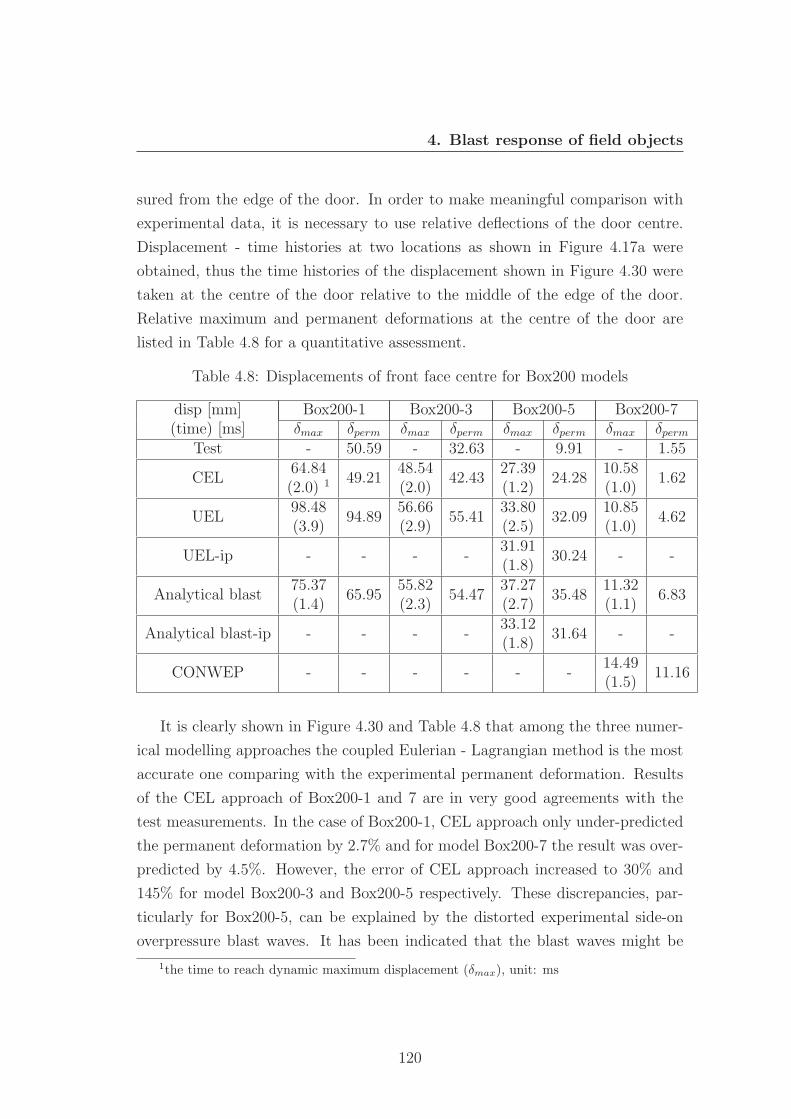
4. Blast response of field objects
sured from the edge of the door. In order to make meaningful comparison with
experimental data, it is necessary to use relative deflections of the door centre.
Displacement - time histories at two locations as shown in Figure 4.17a were
obtained, thus the time histories of the displacement shown in Figure 4.30 were
taken at the centre of the door relative to the middle of the edge of the door.
Relative maximum and permanent deformations at the centre of the door are
listed in Table 4.8 for a quantitative assessment.
Table 4.8: Displacements of front face centre for Box200 models
disp [mm] Box200-1 Box200-3 Box200-5 Box200-7(time) [ms] δmax δperm δmax δperm δmax δperm δmax δperm
Test - 50.59 - 32.63 - 9.91 - 1.55
CEL64.84
49.2148.54
42.4327.39
24.2810.58
1.62(2.0) 1 (2.0) (1.2) (1.0)
UEL98.48
94.8956.66
55.4133.80
32.0910.85
4.62(3.9) (2.9) (2.5) (1.0)
UEL-ip - - - -31.91
30.24 - -(1.8)
Analytical blast75.37
65.9555.82
54.4737.27
35.4811.32
6.83(1.4) (2.3) (2.7) (1.1)
Analytical blast-ip - - - -33.12
31.64 - -(1.8)
CONWEP - - - - - -14.49
11.16(1.5)
It is clearly shown in Figure 4.30 and Table 4.8 that among the three numer-
ical modelling approaches the coupled Eulerian - Lagrangian method is the most
accurate one comparing with the experimental permanent deformation. Results
of the CEL approach of Box200-1 and 7 are in very good agreements with the
test measurements. In the case of Box200-1, CEL approach only under-predicted
the permanent deformation by 2.7% and for model Box200-7 the result was over-
predicted by 4.5%. However, the error of CEL approach increased to 30% and
145% for model Box200-3 and Box200-5 respectively. These discrepancies, par-
ticularly for Box200-5, can be explained by the distorted experimental side-on
overpressure blast waves. It has been indicated that the blast waves might be
1the time to reach dynamic maximum displacement (δmax), unit: ms
120
4. Blast response of field objects
influenced by the presence of the small car near the transducer B9 and B10. The
corresponding overpressure profiles are shown in Figures 4.27a and 4.28a.
It is evident that these two experimental pressure curves do not have typi-
cal shapes and the corresponding impulse curves differed significantly from the
numerical predictions (a typical shape of an ideal blast wave). Although the
numerical peak side-on overpressures and maximum effective impulses were the
same as the test recording, the time histories were significantly different. Table
4.8 shows that it took 1 - 2 ms for the the centre of the front face to reach max-
imum displacement. The duration of the side-on overpressure waves are in the
range of 10 ms. The blast loadings were dynamic/quasi-static thus the shape
of the blast wave profiles are important to the response of the box. It is very
likely that these two distorted side-on detonation overpressures in the gas cloud
test produced much lower damage to the front face of the boxes (Box200-3 and
Box200-5) compared with typical ideal blast waves with the same magnitudes of
overpressure and impulse.
In the study of response of the boxes, the reflected overpressure was the most
influential factor since the damage is dominated by crushing of the front faces.
When presenting the overpressure results in the last section the reflected over-
pressures were compared only among the numerical approaches. This comparison
helped to understand how the front face of the box would respond in different
numerical approaches (i.e. under various predicted overpressures). It should
be noted that the blast loading determined by the analytical method was more
violent than the 3D Eulerian model. With the same level of peak reflected over-
pressure the analytical blast produced larger impulse. Hence referring to the
responses of Box200-5 and Box200-7, it can be seen that the deflections predicted
by analytical blast were greater than the UEL method.
However, it was not the case for Box200-1 and Box200-3. In Figure 4.30a
the response from UEL approach is greater than the analytical method. The
results are misleading since in both approaches the front faces have made contact
with the back panel so that the relative deformations at the door centre are
meaningless due to the contact, as shown in Figure 4.31. When the front face
was not in contact with the back panel in the case of Box200-3, the responses
are approximately the same for analytical and UEL approaches. This might be
121
4. Blast response of field objects
attributed to that the reflected peak overpressure predicted in the UEL approach
by the 3D Eulerian model was 26% higher than the analytical blast but with
11% less impulse. This is due to the combination of the discrepancies in the peak
reflected overpressure and the impulse.
As shown in Figure 4.30c, the response predicted by different approaches has
the order: analytical > UEL > CEL. Moreover, in this box model the effect of
internal pressure (model depicted in Figure 4.20) was studied in the UEL and
analytical approaches. When considering the internal pressure, the permanent
deformation was reduced by 5.5% and 11.1% for UEL and analytical approaches,
respectively. The reduction was only moderate and there was still about 20%
difference compared with the CEL method. This suggests that the method pro-
posed to take into account the internal pressure is not very effective. And the
running time increased substantially (25 times longer) when considering the in-
ternal pressure in the UEL and Lagrangian approaches, as shown in Table 4.6.
Thus to include the internal pressure is excluded for the following parametric
studies.
Response of box to blast loadings determined by CONWEP was studied by
the model Box200-7 and results are shown in Figure 4.30d. The CEL approach
produced the most comparable permanent deformation to the experiment, while
UEL and analytical methods over-predicted by 198% and 340%, respectively.
However despite the substantial discrepancies in the permanent deformation, the
maximum dynamic deflections predicted by the UEL and analytical methods
were in good agreement with the CEL approach, where the differences were only
2.5% and 6.9% respectively. It can be observed that the maximum dynamic
deflections predicted by three numerical approaches were in good agreement with
each other when the damage was minor. However, large discrepancies exist in the
permanent deformation. This is partly due to that the permanent deformation
is small and any slight different would result in a large discrepancy in terms of
percentage. The first rebound of UEL and analytical methods were less than the
CEL, this was somewhat similar to the observation in the results from the general
validation work of the square plate subjected to close range high explosive loading
(first rebound of the UEL approach was much less than the CEL approach). It
was also found that the response of the door to CONWEP loading was much
122
4. Blast response of field objects
greater than other approaches. Comparing with the CEL results, CONWEP
over-predicted the maximum deflection by 37% and permanent deformation by
620%.
The above paragraphs presented a quantitative assessment of the response of
the front face of the box to blast loadings determined by various methods. A
qualitative assessment of the damages is presented in the following paragraphs.
Residual shape of the numerical boxes determined by the three simulation ap-
proaches were compared with the digital scan of the experimental boxes. Photos
of the test boxes after explosion are also presented.
Residual shapes of the model Box200-1 are shown in Figure 4.31 and compared
with the damaged test box. It is evident that the UEL and analytical method
are not able to produce qualitatively comparable results, as the front faces were
in contact with the back panels. On the other hand, CEL approach produced a
rather good residual deformation. The front faces was pushed inwards, while the
side walls of the enclosure were slight deformed outwards. The deformation was
compared favourably with the damaged boxes in a qualitative point of view.
(a) after explosion (b) digital scan
(c) CEL (d) UEL (e) Analytical blast
Figure 4.31: Comparison of residual shapes of Box200-1
Similarly, the residual results of the model Box200-3 are presented and com-
123
4. Blast response of field objects
pared in Figure 4.32. The CEL approach produced the most qualitatively compa-
rable permanent deformation as well, and the damage was dominated by crushing
of the front face and minor outwards deformation was observed on the side face.
Residual deformation from both UEL and analytical approach was less compara-
ble with the actual damaged box, the front face was severely pushed inwards in
the UEL approach, while the side walls of the enclosure were buckled under the
analytical blast loads. The buckling was actually due to the assumption which
was used in the analytical blast. The side-on overpressure curve was applied on
the side, top, bottom and back faces of the numerical model in the pure La-
grangian approach (analytical blast). The side-on impulse was determined to
be 890.4 kPa.ms while in the UEL approach of Box200-3 the impulse was only
421.9 kPa.ms. With similar peak overpressure values the analytical blast pro-
duced more damage to the walls of the enclosure due to greater impulse (refer to
Table 4.7 for peak overpressures and impulses applied on the box model faces in
different approaches).
(a) after explosion (b) digital scan
(c) CEL (d) UEL (e) Analytical blast
Figure 4.32: Comparison of residual shapes of Box200-3
Residual shapes of the model Box200-5 and 7 are presented in Figure 4.33
and 4.34. Qualitatively the results were all comparable to the damaged box,
124
4. Blast response of field objects
due to the overall minor damage. Only the front face was slightly deformed
inwards and no damages were observed at the walls of the enclosure. The only
differences between the numerical results were the magnitude of the deformation
at the front faces which has been discussed (mainly due to impulses) before and
can be observed in the figures.
(a) after explosion (b) digital scan (c) CEL
(d) UEL (e) UEL(ip (f) Anlytcl blast (g) Anly. blast(ip)
Figure 4.33: Comparison of residual shapes of Box200-5
In this section, the numerical results from three simulation approaches were
discussed in detail. They were compared and assessed quantitatively and qual-
itatively against available experimental data which were gathered from the gas
cloud detonation test. It has been shown that the coupled Eulerian - Lagrangian
method can produce accurate results in the analysis of boxes subjected to blast
loading, but its application can be limited by the computational demands. The
pure Lagrangian (with Analytical blast) method was far more efficient in terms
of computation but its accuracy cannot be guaranteed. Based on the coupled
Eulerian - Lagrangian method, further studies of the pure Lagrangian method
have been carried out to justify its application.
125
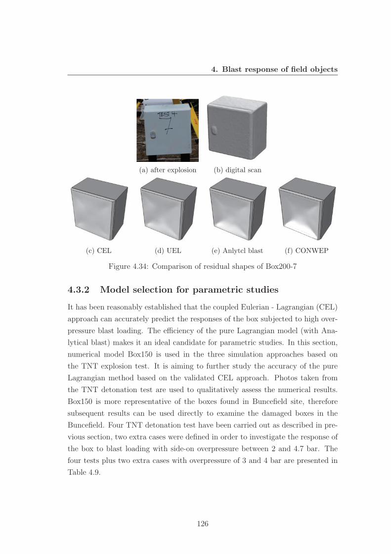
4. Blast response of field objects
(a) after explosion (b) digital scan
(c) CEL (d) UEL (e) Anlytcl blast (f) CONWEP
Figure 4.34: Comparison of residual shapes of Box200-7
4.3.2 Model selection for parametric studies
It has been reasonably established that the coupled Eulerian - Lagrangian (CEL)
approach can accurately predict the responses of the box subjected to high over-
pressure blast loading. The efficiency of the pure Lagrangian model (with Ana-
lytical blast) makes it an ideal candidate for parametric studies. In this section,
numerical model Box150 is used in the three simulation approaches based on
the TNT explosion test. It is aiming to further study the accuracy of the pure
Lagrangian method based on the validated CEL approach. Photos taken from
the TNT detonation test are used to qualitatively assess the numerical results.
Box150 is more representative of the boxes found in Buncefield site, therefore
subsequent results can be used directly to examine the damaged boxes in the
Buncefield. Four TNT detonation test have been carried out as described in pre-
vious section, two extra cases were defined in order to investigate the response of
the box to blast loading with side-on overpressure between 2 and 4.7 bar. The
four tests plus two extra cases with overpressure of 3 and 4 bar are presented in
Table 4.9.
126
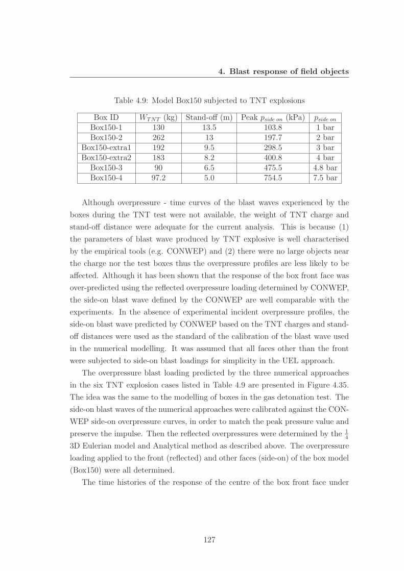
4. Blast response of field objects
Table 4.9: Model Box150 subjected to TNT explosions
Box ID WTNT (kg) Stand-off (m) Peak pside on (kPa) pside on
Box150-1 130 13.5 103.8 1 barBox150-2 262 13 197.7 2 bar
Box150-extra1 192 9.5 298.5 3 barBox150-extra2 183 8.2 400.8 4 bar
Box150-3 90 6.5 475.5 4.8 barBox150-4 97.2 5.0 754.5 7.5 bar
Although overpressure - time curves of the blast waves experienced by the
boxes during the TNT test were not available, the weight of TNT charge and
stand-off distance were adequate for the current analysis. This is because (1)
the parameters of blast wave produced by TNT explosive is well characterised
by the empirical tools (e.g. CONWEP) and (2) there were no large objects near
the charge nor the test boxes thus the overpressure profiles are less likely to be
affected. Although it has been shown that the response of the box front face was
over-predicted using the reflected overpressure loading determined by CONWEP,
the side-on blast wave defined by the CONWEP are well comparable with the
experiments. In the absence of experimental incident overpressure profiles, the
side-on blast wave predicted by CONWEP based on the TNT charges and stand-
off distances were used as the standard of the calibration of the blast wave used
in the numerical modelling. It was assumed that all faces other than the front
were subjected to side-on blast loadings for simplicity in the UEL approach.
The overpressure blast loading predicted by the three numerical approaches
in the six TNT explosion cases listed in Table 4.9 are presented in Figure 4.35.
The idea was the same to the modelling of boxes in the gas detonation test. The
side-on blast waves of the numerical approaches were calibrated against the CON-
WEP side-on overpressure curves, in order to match the peak pressure value and
preserve the impulse. Then the reflected overpressures were determined by the 14
3D Eulerian model and Analytical method as described above. The overpressure
loading applied to the front (reflected) and other faces (side-on) of the box model
(Box150) were all determined.
The time histories of the response of the centre of the box front face under
127
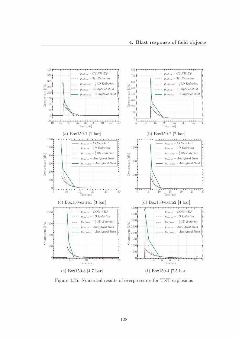
4. Blast response of field objects
10 15 20 25 30 35 40 45 50Time [ms]
-50
0
50
100
150
200
250
300
350
400
Overpressure
[kPa]
pside on − CONWEP
pside on − 3D Eulerian
preflected − 14 3D Eulerian
pside on − Analytical blast
preflected − Analytical blast
(a) Box150-1 [1 bar]
5 10 15 20 25 30 35 40Time [ms]
0
100
200
300
400
500
600
700
800
Overpressure
[kPa]
pside on − CONWEP
pside on − 3D Eulerian
preflected − 14 3D Eulerian
pside on − Analytical blast
preflected − Analytical blast
(b) Box150-2 [2 bar]
5 10 15 20 25 30Time [ms]
0
200
400
600
800
1000
1200
Overpressure
[kPa]
pside on − CONWEP
pside on − 3D Eulerian
preflected − 14 3D Eulerian
pside on − Analytical blast
preflected − Analytical blast
(c) Box150-extra1 [3 bar]
0 5 10 15 20 25 30Time [ms]
0
500
1000
1500
Overpressure
[kPa]
pside on − CONWEP
pside on − 3D Eulerian
preflected − 14 3D Eulerian
pside on − Analytical blast
preflected − Analytical blast
(d) Box150-extra2 [4 bar]
0 5 10 15 20Time [ms]
0
500
1000
1500
2000
Overpressure
[kPa]
pside on − CONWEP
pside on − 3D Eulerian
preflected − 14 3D Eulerian
pside on − Analytical blast
preflected − Analytical blast
(e) Box150-3 [4.7 bar]
2 3 4 5 6 7 8 9 10Time [ms]
0
500
1000
1500
2000
2500
3000
3500
4000
Overpressure
[kPa]
pside on − CONWEP
pside on − 3D Eulerian
preflected − 14 3D Eulerian
pside on − Analytical blast
preflected − Analytical blast
(f) Box150-4 [7.5 bar]
Figure 4.35: Numerical results of overpressures for TNT explosions
128
4. Blast response of field objects
0 5 10 15 20 25Time [ms]
-5
0
5
10
15
20
25
Deflection
atdoorcentre
[mm]
CEL
UEL
Analytical blast
(a) Box150-1 [pside on=1 bar]
0 5 10 15 20 25Time [ms]
-10
0
10
20
30
40
50
60
Deflection
atdoorcentre
[mm]
CEL
UEL
Analytical blast
(b) Box150-2 [pside on=2 bar]
0 5 10 15 20 25Time [ms]
0
20
40
60
80
Deflection
atdoorcentre
[mm]
CEL
UEL
Analytical blast
(c) Box150-extra1 [pside on=3 bar]
0 5 10 15 20 25Time [ms]
0
20
40
60
80
100
120
140
160
Deflection
atdoorcentre
[mm]
CEL
UEL
Analytical blast
(d) Box150-extra2 [pside on=4 bar]
0 5 10 15 20 25Time [ms]
0
50
100
150
Deflection
atdoorcentre
[mm]
CEL
UEL
Analytical blast
(e) Box150-3 [pside on=4.7 bar]
0 5 10 15 20 25Time [ms]
0
50
100
150
200
Deflection
atdoorcentre
[mm]
CEL
UEL
Analytical blast
(f) Box150-4 [pside on=7.5 bar]
Figure 4.36: Numerical results of displacements for boxes in TNT explosions
129
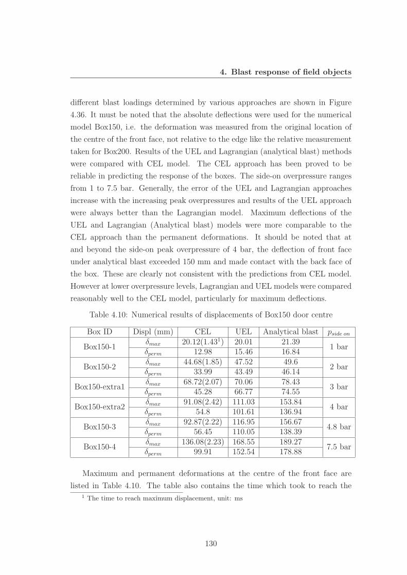
4. Blast response of field objects
different blast loadings determined by various approaches are shown in Figure
4.36. It must be noted that the absolute deflections were used for the numerical
model Box150, i.e. the deformation was measured from the original location of
the centre of the front face, not relative to the edge like the relative measurement
taken for Box200. Results of the UEL and Lagrangian (analytical blast) methods
were compared with CEL model. The CEL approach has been proved to be
reliable in predicting the response of the boxes. The side-on overpressure ranges
from 1 to 7.5 bar. Generally, the error of the UEL and Lagrangian approaches
increase with the increasing peak overpressures and results of the UEL approach
were always better than the Lagrangian model. Maximum deflections of the
UEL and Lagrangian (Analytical blast) models were more comparable to the
CEL approach than the permanent deformations. It should be noted that at
and beyond the side-on peak overpressure of 4 bar, the deflection of front face
under analytical blast exceeded 150 mm and made contact with the back face of
the box. These are clearly not consistent with the predictions from CEL model.
However at lower overpressure levels, Lagrangian and UEL models were compared
reasonably well to the CEL model, particularly for maximum deflections.
Table 4.10: Numerical results of displacements of Box150 door centre
Box ID Displ (mm) CEL UEL Analytical blast pside on
Box150-1δmax 20.12(1.431) 20.01 21.39
1 barδperm 12.98 15.46 16.84
Box150-2δmax 44.68(1.85) 47.52 49.6
2 barδperm 33.99 43.49 46.14
Box150-extra1δmax 68.72(2.07) 70.06 78.43
3 barδperm 45.28 66.77 74.55
Box150-extra2δmax 91.08(2.42) 111.03 153.84
4 barδperm 54.8 101.61 136.94
Box150-3δmax 92.87(2.22) 116.95 156.67
4.8 barδperm 56.45 110.05 138.39
Box150-4δmax 136.08(2.23) 168.55 189.27
7.5 barδperm 99.91 152.54 178.88
Maximum and permanent deformations at the centre of the front face are
listed in Table 4.10. The table also contains the time which took to reach the1 The time to reach maximum displacement, unit: ms
130
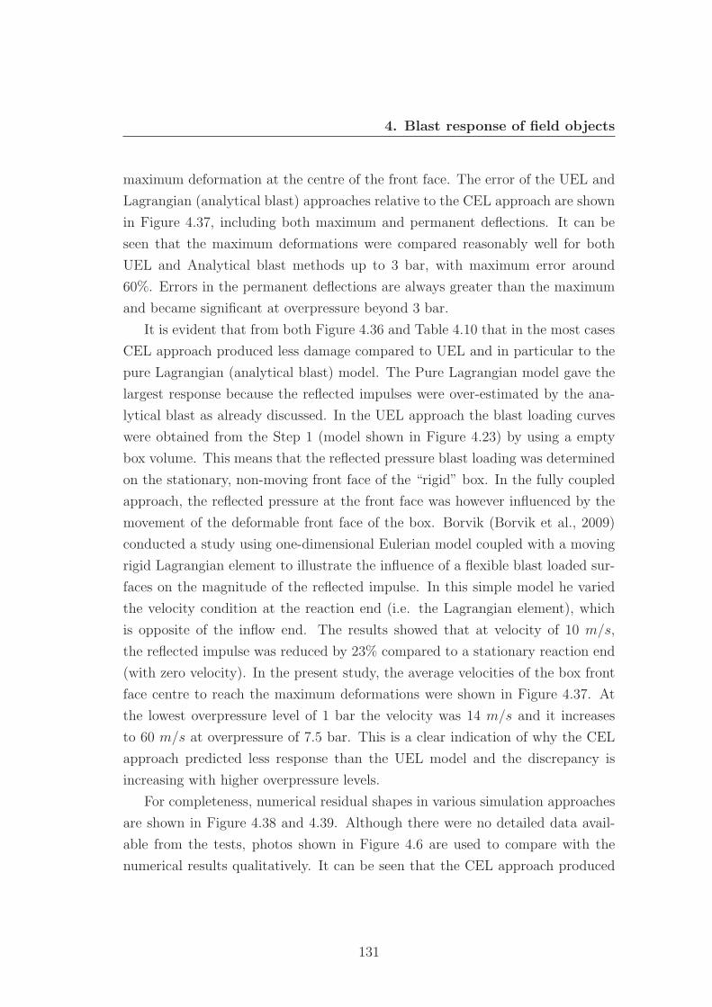
4. Blast response of field objects
maximum deformation at the centre of the front face. The error of the UEL and
Lagrangian (analytical blast) approaches relative to the CEL approach are shown
in Figure 4.37, including both maximum and permanent deflections. It can be
seen that the maximum deformations were compared reasonably well for both
UEL and Analytical blast methods up to 3 bar, with maximum error around
60%. Errors in the permanent deflections are always greater than the maximum
and became significant at overpressure beyond 3 bar.
It is evident that from both Figure 4.36 and Table 4.10 that in the most cases
CEL approach produced less damage compared to UEL and in particular to the
pure Lagrangian (analytical blast) model. The Pure Lagrangian model gave the
largest response because the reflected impulses were over-estimated by the ana-
lytical blast as already discussed. In the UEL approach the blast loading curves
were obtained from the Step 1 (model shown in Figure 4.23) by using a empty
box volume. This means that the reflected pressure blast loading was determined
on the stationary, non-moving front face of the “rigid” box. In the fully coupled
approach, the reflected pressure at the front face was however influenced by the
movement of the deformable front face of the box. Borvik (Borvik et al., 2009)
conducted a study using one-dimensional Eulerian model coupled with a moving
rigid Lagrangian element to illustrate the influence of a flexible blast loaded sur-
faces on the magnitude of the reflected impulse. In this simple model he varied
the velocity condition at the reaction end (i.e. the Lagrangian element), which
is opposite of the inflow end. The results showed that at velocity of 10 m/s,
the reflected impulse was reduced by 23% compared to a stationary reaction end
(with zero velocity). In the present study, the average velocities of the box front
face centre to reach the maximum deformations were shown in Figure 4.37. At
the lowest overpressure level of 1 bar the velocity was 14 m/s and it increases
to 60 m/s at overpressure of 7.5 bar. This is a clear indication of why the CEL
approach predicted less response than the UEL model and the discrepancy is
increasing with higher overpressure levels.
For completeness, numerical residual shapes in various simulation approaches
are shown in Figure 4.38 and 4.39. Although there were no detailed data avail-
able from the tests, photos shown in Figure 4.6 are used to compare with the
numerical results qualitatively. It can be seen that the CEL approach produced
131
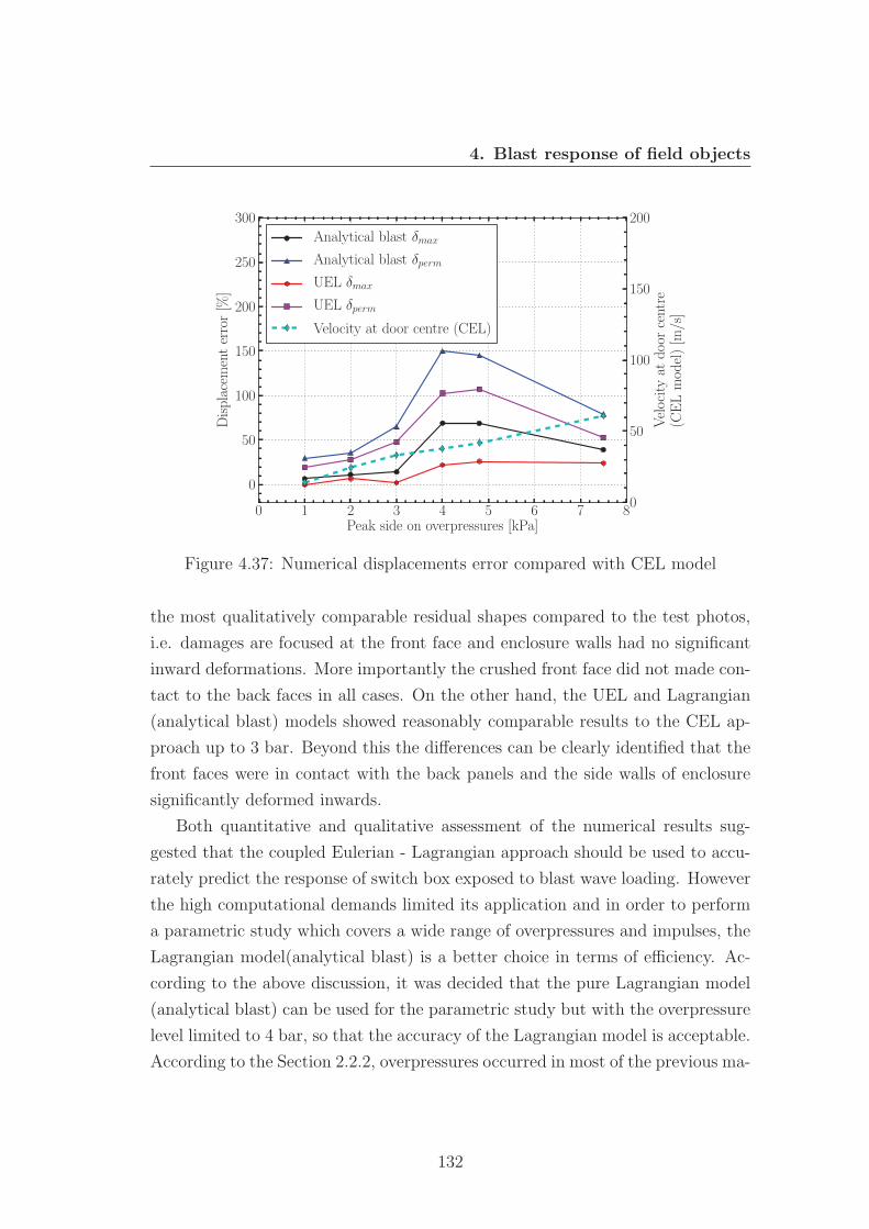
4. Blast response of field objects
0 1 2 3 4 5 6 7 8Peak side on overpressures [kPa]
0
50
100
150
200
250
300Displacementerror[%
]
0
50
100
150
200
Velocityat
doorcentre
(CELmodel)[m
/s]
Analytical blast δmax
Analytical blast δperm
UEL δmax
UEL δperm
Velocity at door centre (CEL)
Figure 4.37: Numerical displacements error compared with CEL model
the most qualitatively comparable residual shapes compared to the test photos,
i.e. damages are focused at the front face and enclosure walls had no significant
inward deformations. More importantly the crushed front face did not made con-
tact to the back faces in all cases. On the other hand, the UEL and Lagrangian
(analytical blast) models showed reasonably comparable results to the CEL ap-
proach up to 3 bar. Beyond this the differences can be clearly identified that the
front faces were in contact with the back panels and the side walls of enclosure
significantly deformed inwards.
Both quantitative and qualitative assessment of the numerical results sug-
gested that the coupled Eulerian - Lagrangian approach should be used to accu-
rately predict the response of switch box exposed to blast wave loading. However
the high computational demands limited its application and in order to perform
a parametric study which covers a wide range of overpressures and impulses, the
Lagrangian model(analytical blast) is a better choice in terms of efficiency. Ac-
cording to the above discussion, it was decided that the pure Lagrangian model
(analytical blast) can be used for the parametric study but with the overpressure
level limited to 4 bar, so that the accuracy of the Lagrangian model is acceptable.
According to the Section 2.2.2, overpressures occurred in most of the previous ma-
132
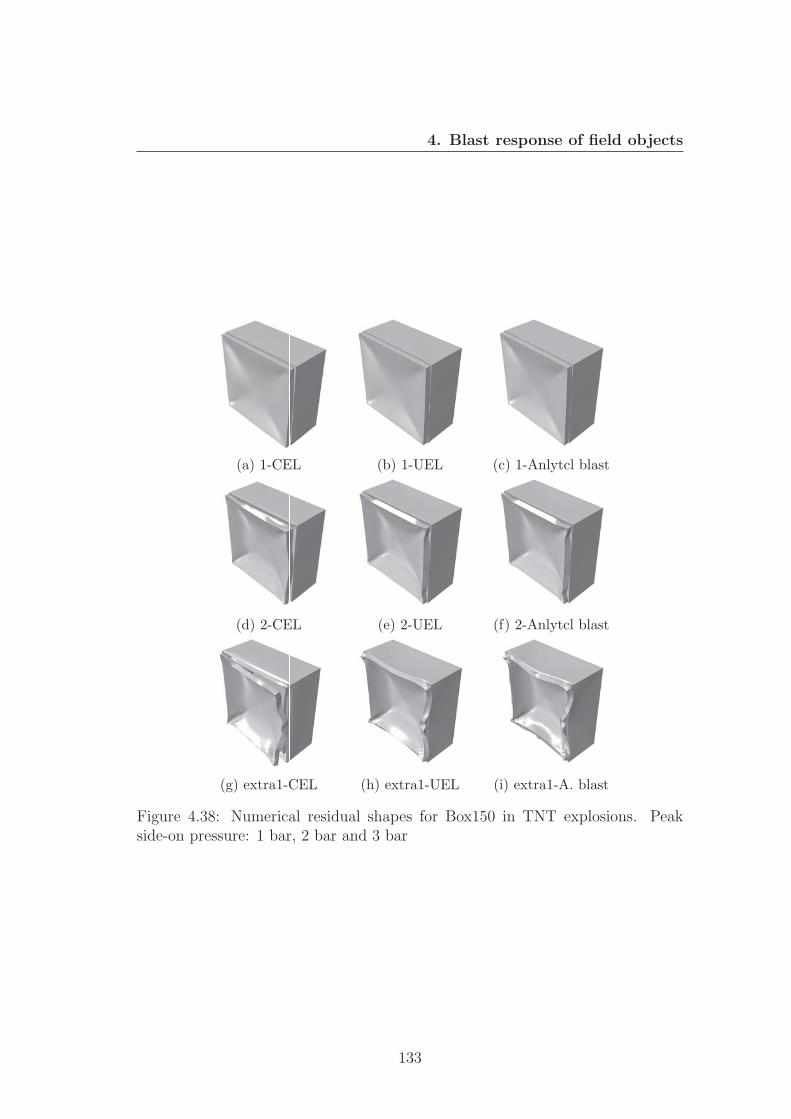
4. Blast response of field objects
(a) 1-CEL (b) 1-UEL (c) 1-Anlytcl blast
(d) 2-CEL (e) 2-UEL (f) 2-Anlytcl blast
(g) extra1-CEL (h) extra1-UEL (i) extra1-A. blast
Figure 4.38: Numerical residual shapes for Box150 in TNT explosions. Peakside-on pressure: 1 bar, 2 bar and 3 bar
133
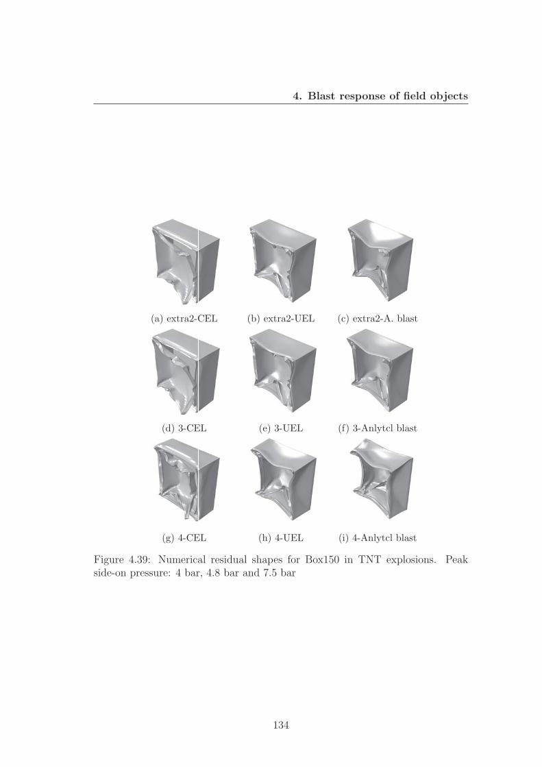
4. Blast response of field objects
(a) extra2-CEL (b) extra2-UEL (c) extra2-A. blast
(d) 3-CEL (e) 3-UEL (f) 3-Anlytcl blast
(g) 4-CEL (h) 4-UEL (i) 4-Anlytcl blast
Figure 4.39: Numerical residual shapes for Box150 in TNT explosions. Peakside-on pressure: 4 bar, 4.8 bar and 7.5 bar
134
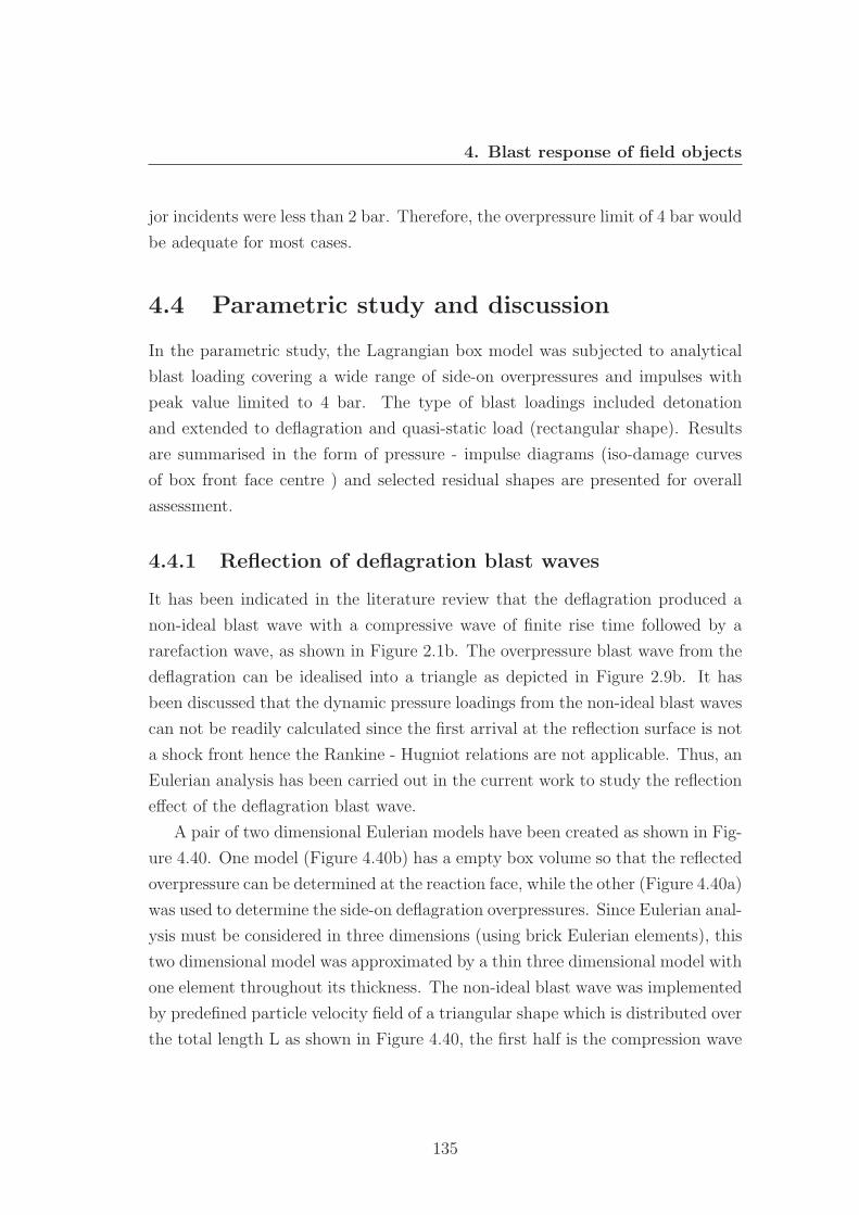
4. Blast response of field objects
jor incidents were less than 2 bar. Therefore, the overpressure limit of 4 bar would
be adequate for most cases.
4.4 Parametric study and discussion
In the parametric study, the Lagrangian box model was subjected to analytical
blast loading covering a wide range of side-on overpressures and impulses with
peak value limited to 4 bar. The type of blast loadings included detonation
and extended to deflagration and quasi-static load (rectangular shape). Results
are summarised in the form of pressure - impulse diagrams (iso-damage curves
of box front face centre ) and selected residual shapes are presented for overall
assessment.
4.4.1 Reflection of deflagration blast waves
It has been indicated in the literature review that the deflagration produced a
non-ideal blast wave with a compressive wave of finite rise time followed by a
rarefaction wave, as shown in Figure 2.1b. The overpressure blast wave from the
deflagration can be idealised into a triangle as depicted in Figure 2.9b. It has
been discussed that the dynamic pressure loadings from the non-ideal blast waves
can not be readily calculated since the first arrival at the reflection surface is not
a shock front hence the Rankine - Hugniot relations are not applicable. Thus, an
Eulerian analysis has been carried out in the current work to study the reflection
effect of the deflagration blast wave.
A pair of two dimensional Eulerian models have been created as shown in Fig-
ure 4.40. One model (Figure 4.40b) has a empty box volume so that the reflected
overpressure can be determined at the reaction face, while the other (Figure 4.40a)
was used to determine the side-on deflagration overpressures. Since Eulerian anal-
ysis must be considered in three dimensions (using brick Eulerian elements), this
two dimensional model was approximated by a thin three dimensional model with
one element throughout its thickness. The non-ideal blast wave was implemented
by predefined particle velocity field of a triangular shape which is distributed over
the total length L as shown in Figure 4.40, the first half is the compression wave
135
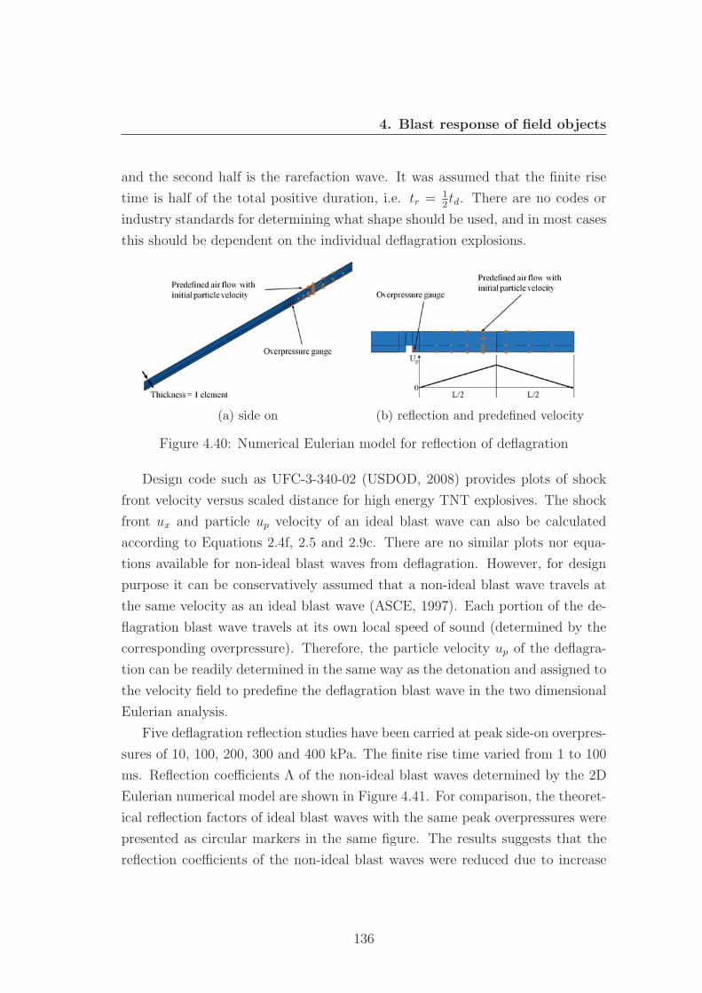
4. Blast response of field objects
and the second half is the rarefaction wave. It was assumed that the finite rise
time is half of the total positive duration, i.e. tr = 12td. There are no codes or
industry standards for determining what shape should be used, and in most cases
this should be dependent on the individual deflagration explosions.
(a) side on (b) reflection and predefined velocity
Figure 4.40: Numerical Eulerian model for reflection of deflagration
Design code such as UFC-3-340-02 (USDOD, 2008) provides plots of shock
front velocity versus scaled distance for high energy TNT explosives. The shock
front ux and particle up velocity of an ideal blast wave can also be calculated
according to Equations 2.4f, 2.5 and 2.9c. There are no similar plots nor equa-
tions available for non-ideal blast waves from deflagration. However, for design
purpose it can be conservatively assumed that a non-ideal blast wave travels at
the same velocity as an ideal blast wave (ASCE, 1997). Each portion of the de-
flagration blast wave travels at its own local speed of sound (determined by the
corresponding overpressure). Therefore, the particle velocity up of the deflagra-
tion can be readily determined in the same way as the detonation and assigned to
the velocity field to predefine the deflagration blast wave in the two dimensional
Eulerian analysis.
Five deflagration reflection studies have been carried at peak side-on overpres-
sures of 10, 100, 200, 300 and 400 kPa. The finite rise time varied from 1 to 100
ms. Reflection coefficients Λ of the non-ideal blast waves determined by the 2D
Eulerian numerical model are shown in Figure 4.41. For comparison, the theoret-
ical reflection factors of ideal blast waves with the same peak overpressures were
presented as circular markers in the same figure. The results suggests that the
reflection coefficients of the non-ideal blast waves were reduced due to increase
136
4. Blast response of field objects
0 20 40 60 80 100Finite rise time tr (ms)
1.0
1.5
2.0
2.5
3.0
3.5
4.0
4.5Reflection
factor
Λ=
p r/p
in
pside on = 10kPa
pside on = 100kPa
pside on = 200kPa
pside on = 300kPa
pside on = 400kPa
Figure 4.41: Reflection coefficient for deflagration(non-ideal blast wave)
of the finite rise time. It can be observed that the reflection factors reduce dra-
matically as the finite rise time become longer, but there is no further significant
reduction beyond approximately 40 ms. The reductions in the reflection coeffi-
cients are 35% and 50% at the side-on peak overpressure of 400 kPa and 10 kPa,
respectively.
In addition, the reflection factors are increasing as the finite rise time decreased
and they gradually approach to the theoretical values for ideal blast wave at zero
finite rise time. It should be noted that this study was based on the switch box
which is much smaller than building structures. Due to the fact that reflection
of the non-ideal blast wave is dependent on the dimensions of the target, so
the reflection factor determined in this study might not be suitable for other
structures. However, the same Eulerian analysis can be readily carried out on
any other targets so that more appropriate reflection coefficients can be obtained.
137
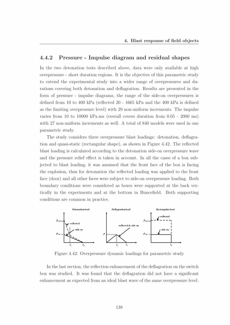
4. Blast response of field objects
4.4.2 Pressure - Impulse diagram and residual shapes
In the two detonation tests described above, data were only available at high
overpressure - short duration regions. It is the objective of this parametric study
to extend the experimental study into a wider range of overpressures and du-
rations covering both detonation and deflagration. Results are presented in the
form of pressure - impulse diagrams, the range of the side-on overpressures is
defined from 10 to 400 kPa (reflected 20 - 1665 kPa and the 400 kPa is defined
as the limiting overpressure level) with 29 non-uniform increments. The impulse
varies from 10 to 10000 kPa.ms (overall covers duration from 0.05 - 2000 ms)
with 27 non-uniform increments as well. A total of 840 models were used in one
parametric study.
The study considers three overpressure blast loadings: detonation, deflagra-
tion and quasi-static (rectangular shape), as shown in Figure 4.42. The reflected
blast loading is calculated according to the detonation side-on overpressure wave
and the pressure relief effect is taken in account. In all the cases of a box sub-
jected to blast loading, it was assumed that the front face of the box is facing
the explosion, thus for detonation the reflected loading was applied to the front
face (door) and all other faces were subject to side-on overpressure loading. Both
boundary conditions were considered as boxes were supported at the back ver-
tically in the experiments and at the bottom in Buncefield. Both supporting
conditions are common in practice.
Figure 4.42: Overpressure dynamic loadings for parametric study
In the last section, the reflection enhancement of the deflagration on the switch
box was studied. It was found that the deflagration did not have a significant
enhancement as expected from an ideal blast wave of the same overpressure level.
138
4. Blast response of field objects
Thus for simplicity the reflection enhancement was neglected for deflagration
loads in the parametric study. Therefore, the reflected and side-on overpressure
loading are identical for deflagration as shown in the figure.
A quasi-static load of a rectangular shape shown on the right of Figure 4.42
is not common in chemical explosions. It is assumed that the quasi-static blast
wave is leading by a shock front, which is the same as the detonation but with
constant magnitude throughout the duration. As depicted in the figure, the
reflected blast loading was obtained by multiplying the side-on overpressure wave
by the reflection coefficient for the shock wave of the same level of overpressure.
Parametric studies were performed for each of the three types of blast load.
Maximum and permanent deformations at the box front face centre under ev-
ery combination of side-on overpressure and impulse were obtained. Then the
iso-damage curves were constructed based on the maximum and permanent de-
formation over the corresponding overpressure and impulse ranges. It should be
noted that in the pressure - impulse diagrams, the overpressure and impulse were
reflected values, which were calculated based on the side-on overpressures and
impulses (the actual load input). The deflection results were also converted ac-
cordingly so that they were corresponding to the reflected pressure and impulse.
This was because the iso-damage curves are obtained at the centre of the front
face of the box model which was subjected to the reflected loadings. In addition,
since it has been assumed that the reflected and side-on overpressures loads are
identical for deflagration, it was necessary to extend the overpressure range of
deflagration from 400 to 1665 kPa so that it can be consistent with other types
of loads.
The structural responses of model Box150 are summarised in a series of pres-
sure - impulse diagrams shown in Figures 4.43 and 4.44, for back and bottom
support respectively. In order to have a visual assessment of the response of
boxes, a group of residual shapes in the impulsive and quasi-static regions were
presented in Figures 4.45 and 4.46. Since the damages were dominated by crush-
ing of the front face of the boxes, the iso-damage curves were plotted based on
the maximum and permanent deformation at the centre of the front face of the
box.
For detonation and quasi-static (rectangular) loads, the front face of the box
139
4. Blast response of field objects
model was subjected to the reflected overpressure blast loading. Therefore, re-
flected values are used for the pressure - impulse diagrams. Using the results
presented in Figures 4.43 and 4.44 it is straight forward to calculate the response
of the box front face based on the side-on overpressure blast wave. One only needs
to determine the corresponding reflected overpressure and impulse and then read
the damage from the diagrams. The pressure - impulse diagrams can also be
used in forensic investigations to determine the side-on overpressure blast wave
based on the known damages to the front face of boxes. This involves converting
the reflected values to the side-on overpressures and impulses. For deflagration,
the reflection coefficients presented in Figure 4.41 can be used to determine the
side-on blast waves but bearing mind that as a result the deformations at the
faces other than the front thus become conservative since the blast applied are
reflected and not side-on as they should be.
Figure 4.43 presents the iso-damage curves at the front face of the box model
vertically supported at the back. Figure 4.43a shows the maximum deformation
curves while Figure 4.43b shows the permanent deformation curves. For both
diagrams the damages levels are set as 0.01, 0.05, 0.1 and 0.15m. The max-
imum damage level suggests that the front face was in contact with the back
panel (0.15m). It can be seen that the iso-damage curves in Figure 4.43a are
shifted slightly towards upper-right direction comparing with Figure 4.43b. This
indicates that the maximum dynamic deflections are close to the residual defor-
mations (small overshot). It can be observed that the quasi-static asymptote of
0.01 iso permanent damage curve approximately ranged from 100 to 240 kPa for
the three types of blast loads. This was a relatively wide range. The impulsive
asymptote ranged from 137 to 144 kPa.ms, which was a relatively small range.
This suggests that the iso-damage curve of 0.01 m was relatively sensitive to the
impulse and relatively insensitive to the peak overpressure. The same observation
can be made to other iso-damage curves as well but overall the sensitivity was
reduced with increased damages.
In Figure 4.43b, there is a noteworthy feature of the response in the dy-
namic and quasi-static region of the 0.01 m iso permanent damage curve. The
quasi-static asymptote of the iso-damage curve of deflagration was slightly shifted
upwards compared to the other two load types. This is a well known phenomena
140
4. Blast response of field objects
due to the resonance of the box front face caused by the finite rise time of the
deflagration load curve. In the dynamic and quasi-static region the rectangular
loading produces more damages than the other two loads. Beyond the damaged
level of 0.05 m it can be seen that in the quasi-static region the deflagration pro-
duces the worst damage to the front face. This can be explained by referring to
Figure 4.45 that among the residual shapes corresponding to quasi-static defla-
gration load the enclosure wall started to buckle when the applied overpressure
exceeded 400 kPa. This significantly promotes the deformation at the centre of
the box front face. It is also the reason that the iso-damage curves of deflagration
positioned very closely in the quasi-static region while the curves for other load
cases spread relatively wider over the overpressure range.
The pressure - impulse diagrams of the model Box150 with bottom support
are presented in Figure 4.44. Iso-damage levels are set to various values as shown
in the diagram. With the defined boundary conditions the back face can deform
significantly under blast loads, so the iso-damage levels at the front face centre
would not be able to reach the same depth as the box with back support. The
front face were frequently in contact with the back face and this made it impos-
sible to construct clear iso-damage curves at large displacement. Therefore, for
deflagration the maximum dynamic iso damage level was set to 0.75 m which is
half of the box depth and the permanent iso damage level was set to only 0.5 m.
The general features of Figure 4.44 are similar to Figure 4.43 discussed above.
The peak dynamic deflections are close to the residual deformations and the up-
ward shifting quasi-static asymptote of 0.01 m iso permanent curve of deflagration
is clearly visible as well. Response of the box front face is sensitive to peak ap-
plied overpressures in the quasi-static region for deflagration loads, due to the
buckling of the enclosure wall which promotes the deformation at the front face
centre, as shown in Figure 4.46. In addition, the buckling of the enclosure wall
near the bottom occurs when the box is subjected to rectangular loading in the
quasi-static region. This also promotes the deformation at the box front face cen-
tre and make the iso-damage curves of rectangular loads closely positioned in this
region, for both maximum and permanent curves. In the contrary, no buckling
occurs in the impulsive series of the residual shapes in Figure 4.46, hence in the
impulsive region the iso-damage curves are positioned relatively wide and evenly
141
4. Blast response of field objects
over the full range of the impulses.
Deflections at the centre of the front face of box models were summarized in
the form of pressure - impulse diagrams and discussed in the above paragraphs.
In order to provide a visual assessment of the response to three different blast
load types, a group of selected residual shapes of the numerical box are presented
in Figure 4.45 and 4.46, for different supporting conditions respectively. Residual
shapes of the numerical models are selected for each load type in the impulsive
and quasi-static regions from the pressure - impulse diagrams. It can be seen
from these two figures that for every load type there are two series of residual
shapes. One is corresponding to a fixed overpressure value (1665 kPa [reflected
value at the front face]) and residual shapes were selected at various impulses
(i.e. in the impulsive region). And the other one is corresponding to a fixed
impulse value (10000 kPa.ms) where the residual shapes are selected at various
pressures (i.e. in the quasi-static region). Permanent deformations at the centre
of the front face are shown in the figures as well. It should be noted that side-on
and reflected values are both shown for detonation and rectangular loads, with
side-on values in the parentheses.
The impulsive series of the residual shapes show the response of the final de-
formation to impulses where peak pressures were less decisive. In the opposite,
the quasi-static series present the box final response mainly related to the peak
overpressures rather than impulses. It is evident from these two figures that
impulsive residual shapes were different to those in the quasi-static region, par-
ticularly for deflagration. In Figure 4.45, it can be seen that the differences for
detonation and rectangular loads are dominated by the buckling of the front face.
In the case of deflagration, the difference is more clear. Buckling of the enclosure
wall occurs at the four corners for impulsive response while for the quasi-static
response the buckling occurs at the mid of the edge of front face.
In Figure 4.46, the differences in permanent responses to detonation load are
also dominated at the front face. For deflagration load, residual shapes change
significantly due to the supporting conditions comparing with Figure 4.45. The
impulsive residual shapes look like they have been equally squeezed from all
directions, while the quasi-static responses show server buckling at the back (of
the enclosure) and the front face was pushed against on the enclosure.
142
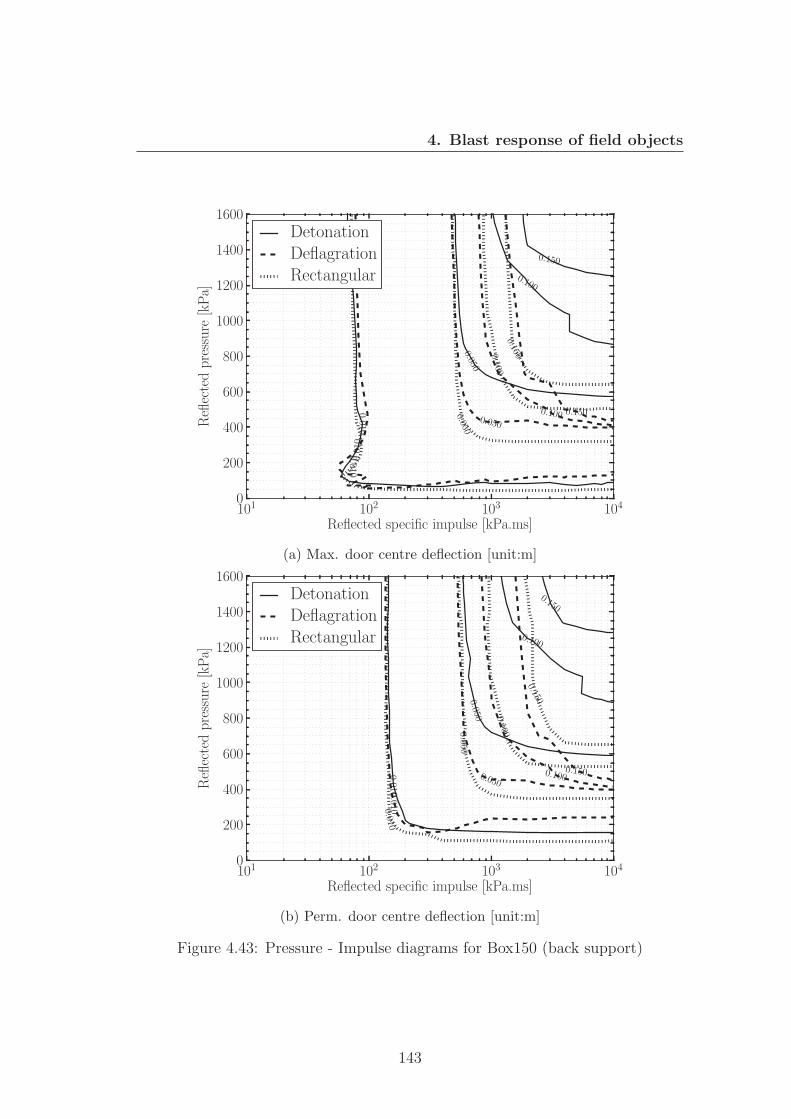
4. Blast response of field objects
101 102 103 104
Reflected specific impulse [kPa.ms]
0
200
400
600
800
1000
1200
1400
1600Reflectedpressure
[kPa]
0.010
0.050
0.100
0.150
0.010
0.050
0.100 0.150
0.010
0.050
0.1000.150
DetonationDeflagrationRectangular
(a) Max. door centre deflection [unit:m]
101 102 103 104
Reflected specific impulse [kPa.ms]
0
200
400
600
800
1000
1200
1400
1600
Reflectedpressure
[kPa]
0.010
0.050
0.100
0.150
0.010
0.0500.100
0.150
0.010
0.050
0.100
0.150
DetonationDeflagrationRectangular
(b) Perm. door centre deflection [unit:m]
Figure 4.43: Pressure - Impulse diagrams for Box150 (back support)
143
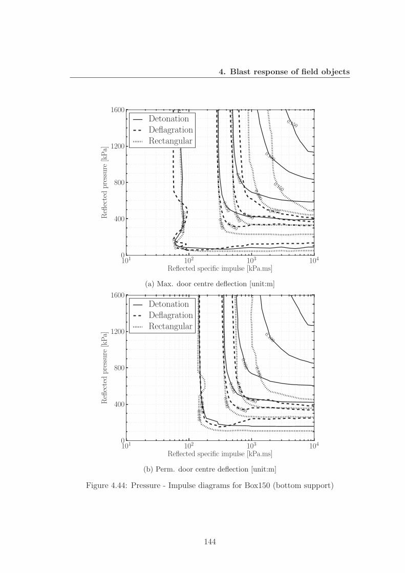
4. Blast response of field objects
101 102 103 104
Reflected specific impulse [kPa.ms]
0
400
800
1200
1600Reflectedpressure
[kPa]
0.010
0.030
0.050
0.100
0.150
0.010 0.030
0.0500.075
0.010
0.030
0.050
0.100
0.150
DetonationDeflagrationRectangular
(a) Max. door centre deflection [unit:m]
101 102 103 104
Reflected specific impulse [kPa.ms]
0
400
800
1200
1600
Reflectedpressure
[kPa]
0.010
0.030
0.050
0.100
0
0.010 0.030
0.050
0.010
0.030
0.050
0.100
DetonationDeflagrationRectangular
(b) Perm. door centre deflection [unit:m]
Figure 4.44: Pressure - Impulse diagrams for Box150 (bottom support)
144
4. Blast response of field objects
Buckling can be observed in the residual shapes at various locations. It is a
clear indication of the minimum overpressure levels which can cause this type of
damage feature, particularly for quasi-static loads. In Figure 4.45 the three series
of residual shapes related to quasi-static loads indicate that for a box with back
supporting conditions the minimum side-on overpressures to initiate a visible
buckling are: detonation - 280 kPa; deflagration - 420 kPa and rectangular -
240 kPa. And for boxes supported at the bottom as shown in Figure 4.46 the
minimum side-on overpressures are: detonation - 260 kPa; deflagration - 380 kPa
and rectangular - 160 kPa.
4.4.3 Comparison with recovered boxes
One of the objectives of the present project is to provide information which can
aid the incident investigation. This section presents a brief comparison between
the numerical results and the damaged boxes found in Buncefield. Three photos
of one damaged box found after the incident are shown in Figure 4.47. The photos
were taken from the front ,side and back of the box (shown from top to down in the
figure respectively). The immediate investigation after the incident determined
the blast directions that the front face (door) of this box was facing the blast
wave during the explosion. This was in consistence with the experiments and the
numerical simulation in this present work. It can be clearly seen that both the
front and back face of the box were significantly deformed in a symmetric way
and so did the side faces shown in the middle. The top face had little deformation
might be due to the extra plate fixed onto it which protected it from the explosion.
Unfortunately, the actual measurement of the damaged box was not available.
It was then assumed that the deformation of the front cover was half of the box
depth (75 mm). Among the residual shapes shown in Figure 4.46, four cases
with similar deformation at the front cover were chosen to compare with the
damaged box. In the quasi-static region, one deflagration and detonation cases
were selected as shown in Figure 4.47, and another two cases were selected in the
impulsive region. It is fairly easy to eliminate the possibility of deflagration case
in the impulsive region and the detonation case in the quasi-static region. Since
145
4. Blast response of field objects
Box150 back support Reflected(Side-on)
residual deflection(m)
Det
onat
ion
Pa.s 333(80) 416(100) 634(200) 824(300) 1027(400) 1236(500) 1447(600) 2301(1000) m 0.028 0.035 0.055 0.073 0.093 0.117 0.134 0.149
Impu
lsiv
e 16
65 k
Pa
kPa 209(80) 344(120) 497(160) 664(200) 844(240) 1035(280) 1237(320) 1341(360) m 0.015 0.025 0.038 0.062 0.095 0.113 0.146 0.166
Qua
si-S
tatic
10
000
kPa.
ms
Def
lagr
atio
n
Pa.s 100 200 400 600 800 1000 2000 4000 m 0.005 0.017 0.036 0.058 0.093 0.127 0.165 0.205
Impu
lsiv
e 16
65 k
Pa
kPa 200 300 360 400 420 440 500 900 m 0.005 0.019 0.035 0.05 0.121 0.145 0.159 0.183
Qua
si-s
tatic
10
000
kPa.
ms
Rec
tang
ular
Pa.s 166(40) 250(60) 333(80) 416(100) 832(200) 1248(300) 1664(400) 2496(600) m 0.013 0.020 0.028 0.036 0.084 0.135 0.148 0.160
Impu
lsiv
e 16
65kP
a
kPa 274(100) 344(120) 418(140) 497(160) 579(180) 664(200) 844(240) 1035(280) m 0.033 0.050 0.069 0.091 0.112 0.154 0.164 0.180
Qua
si-s
tatic
10
000
kPa.
ms
Figure 4.45: Numerical residual shapes of Box150 (back support)
146
4. Blast response of field objects
Box150 bottom support Reflected(Side-on)
residual deflection(m)
Det
onat
ion
Pa.s 83(20) 250(60) 634(200) 1027(400) 1447(600) 1873(800) 2301(1000) 4452(2000) m -0.040 -0.019 -0.055 -0.086 -0.113 -0.126 -0.132 -0.156
Impu
lsiv
e 16
65 k
Pa
kPa 93(40) 664(200) 753(220) 844(240) 938(260) 1035(280) 1447(360) 1665(400) m 0.004 0.038 0.059 0.076 0.106 0.122 0.15 0.184
Qua
si-S
tatic
10
000
kPa.
ms
Def
lagr
atio
n
Pa.s 10 100 200 400 600 800 5000 10000 m 0.0 0.005 0.015 0.037 0.064 0.08 0.089 0.092
Impu
lsiv
e 16
65 k
Pa
kPa 140 260 300 340 380 420 460 900 m 0.002 0.011 0.018 0.033 0.05 0.076 0.095 0.111
Qua
si-s
tatic
10
000
kPa.
ms
Rec
tang
ular
Pa.s 83(20) 250(60) 416(100) 832(200) 1664(400) 3328(800) 4160(1000) 6240(1500) m 0.003 0.022 0.040 0.100 0.125 0.237 0.248 0.256
Impu
lsiv
e 16
65 k
Pa
kPa 67(30) 120(50) 241(90) 344(120) 418(140) 497(160) 579(180) 664(200) m 0.005 0.01 0.026 0.047 0.065 0.161 0.171 0.197
Qua
si-s
tatic
10
000
kPa.
ms
Figure 4.46: Numerical residual shapes of Box150 (bottom support)
147
4. Blast response of field objects
Figure 4.47: Comparison of numerical residual shapes to damaged boxes fromBuncefield (SCI, 2009)
the combination of peak overpressures and positive impulses of these two cases
did not have typical characteristic for the relevant blast waves.The deflagration
blast wave should not be impulsive and the detonation blast wave is unlikely to
be quasi-static.
As a result, there are two cases left: a quasi-static deflagration load and an
impulsive detonation load. In the case of the detonation load, it can be seen that
buckling occurred at the bottom of the front face of the box and the rim of the
door was pushed off from the enclosure. This is inconsistent with the observed
damage of the box in Buncefield. In the case of the deflagration load, the front face
deformed in a similar manner to the damaged box, i.e. no buckling. Moreover,
the back and side of the enclosure were buckled in a similar way to the damaged
box. From the side view of both cases, it is evident that the deformations of
front and back faces in deflagration were more symmetric than detonation. This
is consistent with the observation of the damaged box. This comparison suggests
that within the vapour cloud the explosion is most likely to be deflagration.
The level of peak overpressure of the deflagration inside the vapour cloud can
148
4. Blast response of field objects
be roughly estimated based on the permanent deformation in the quasi-static
deflagration case. The applied overpressure loading on the front face was 420 kPa
with approximately 48 ms positive duration. Using Figure 4.41 as a guidance the
side-on peak overpressure of the deflagration load can be calculated to be around
200 kPa.
4.5 Conclusion
In this chapter, detonation experiments carried out on steel switch boxes by
external parties were presented and measurements and observations discussed.
Various numerical models used to model response of the boxes to detonation
blast loadings were presented in detail. Validation of the numerical models was
carried out and it was found that the coupled Eulerian - Lagrangian model has
the best accuracy and should be used in blast problems if possible.
However, the high computational demands of the coupled Eulerian - La-
grangian model would limit its application, precluding cases requiring a large
number of simulations, particularly for parametric studies. Based on the vali-
dated CEL model, the accuracy of the pure Lagrangian approach has been in-
vestigated and it has been shown that it is able to produce reasonable results
under side-on peak overpressure of 4 bar. With its short running time it is an
ideal candidate for parametric studies and therefore a large number of Lagrangian
models were analysed subjected to a series of combinations of overpressures and
impulses. The range of blast loadings covers both deflagration and detonation for
very long and short durations. Results were summarised in the form of pressure
- impulse diagrams and selected residual shapes were also presented for visual
assessment.
An attempt has been made to compare the numerical results with an actual
damaged box from Buncefield. The comparison showed that the parametric study
did produce reasonably comparable results to the damaged box. This suggested
that the explosion inside the vapour cloud is very likely to be deflagration with a
peak overpressure of around 2 bar. Although the comparison was carried out on
assumed permanent deformation of the damaged box, the forensic study shown
here has given a good insight into the likely loading scenarios.
149
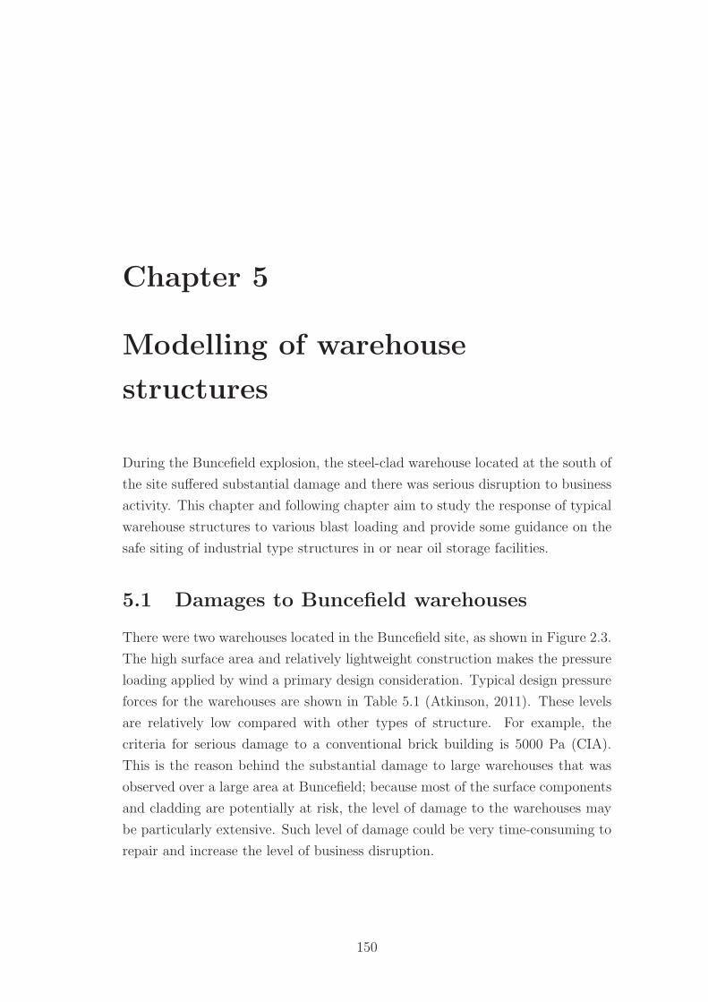
Chapter 5
Modelling of warehouse
structures
During the Buncefield explosion, the steel-clad warehouse located at the south of
the site suffered substantial damage and there was serious disruption to business
activity. This chapter and following chapter aim to study the response of typical
warehouse structures to various blast loading and provide some guidance on the
safe siting of industrial type structures in or near oil storage facilities.
5.1 Damages to Buncefield warehouses
There were two warehouses located in the Buncefield site, as shown in Figure 2.3.
The high surface area and relatively lightweight construction makes the pressure
loading applied by wind a primary design consideration. Typical design pressure
forces for the warehouses are shown in Table 5.1 (Atkinson, 2011). These levels
are relatively low compared with other types of structure. For example, the
criteria for serious damage to a conventional brick building is 5000 Pa (CIA).
This is the reason behind the substantial damage to large warehouses that was
observed over a large area at Buncefield; because most of the surface components
and cladding are potentially at risk, the level of damage to the warehouses may
be particularly extensive. Such level of damage could be very time-consuming to
repair and increase the level of business disruption.
150
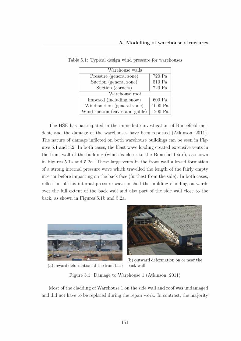
5. Modelling of warehouse structures
Table 5.1: Typical design wind pressure for warehouses
Warehouse wallsPressure (general zone) 720 PaSuction (general zone) 510 Pa
Suction (corners) 720 PaWarehouse roof
Imposed (including snow) 600 PaWind suction (general zone) 1000 Pa
Wind suction (eaves and gable) 1200 Pa
The HSE has participated in the immediate investigation of Buncefield inci-
dent, and the damage of the warehouses have been reported (Atkinson, 2011).
The nature of damage inflicted on both warehouse buildings can be seen in Fig-
ures 5.1 and 5.2. In both cases, the blast wave loading created extensive vents in
the front wall of the building (which is closer to the Buncefield site), as shown
in Figures 5.1a and 5.2a. These large vents in the front wall allowed formation
of a strong internal pressure wave which travelled the length of the fairly empty
interior before impacting on the back face (furthest from the side). In both cases,
reflection of this internal pressure wave pushed the building cladding outwards
over the full extent of the back wall and also part of the side wall close to the
back, as shown in Figures 5.1b and 5.2a.
(a) inward deformation at the front face(b) outward deformation on or near theback wall
Figure 5.1: Damage to Warehouse 1 (Atkinson, 2011)
Most of the cladding of Warehouse 1 on the side wall and roof was undamaged
and did not have to be replaced during the repair work. In contrast, the majority
151
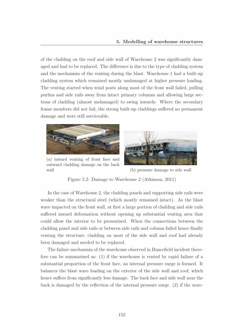
5. Modelling of warehouse structures
of the cladding on the roof and side wall of Warehouse 2 was significantly dam-
aged and had to be replaced. The difference is due to the type of cladding system
and the mechanism of the venting during the blast. Warehouse 1 had a built-up
cladding system which remained mostly undamaged at higher pressure loading.
The venting started when wind posts along most of the front wall failed, pulling
purlins and side rails away from intact primary columns and allowing large sec-
tions of cladding (almost undamaged) to swing inwards. Where the secondary
frame members did not fail, the strong built-up claddings suffered no permanent
damage and were still serviceable.
(a) inward venting of front face andoutward cladding damage on the backwall (b) pressure damage to side wall
Figure 5.2: Damage to Warehouse 2 (Atkinson, 2011)
In the case of Warehouse 2, the cladding panels and supporting side rails were
weaker than the structural steel (which mostly remained intact). As the blast
wave impacted on the front wall, at first a large portion of cladding and side rails
suffered inward deformation without opening up substantial venting area that
could allow the interior to be pressurised. When the connections between the
cladding panel and side rails or between side rails and column failed hence finally
venting the structure, cladding on most of the side wall and roof had already
been damaged and needed to be replaced.
The failure mechanism of the warehouse observed in Buncefield incident there-
fore can be summarised as: (1) if the warehouse is vented by rapid failure of a
substantial proportion of the front face, an internal pressure surge is formed. It
balances the blast wave loading on the exterior of the side wall and roof, which
hence suffers from significantly less damage. The back face and side wall near the
back is damaged by the reflection of the internal pressure surge. (2) if the ware-
152
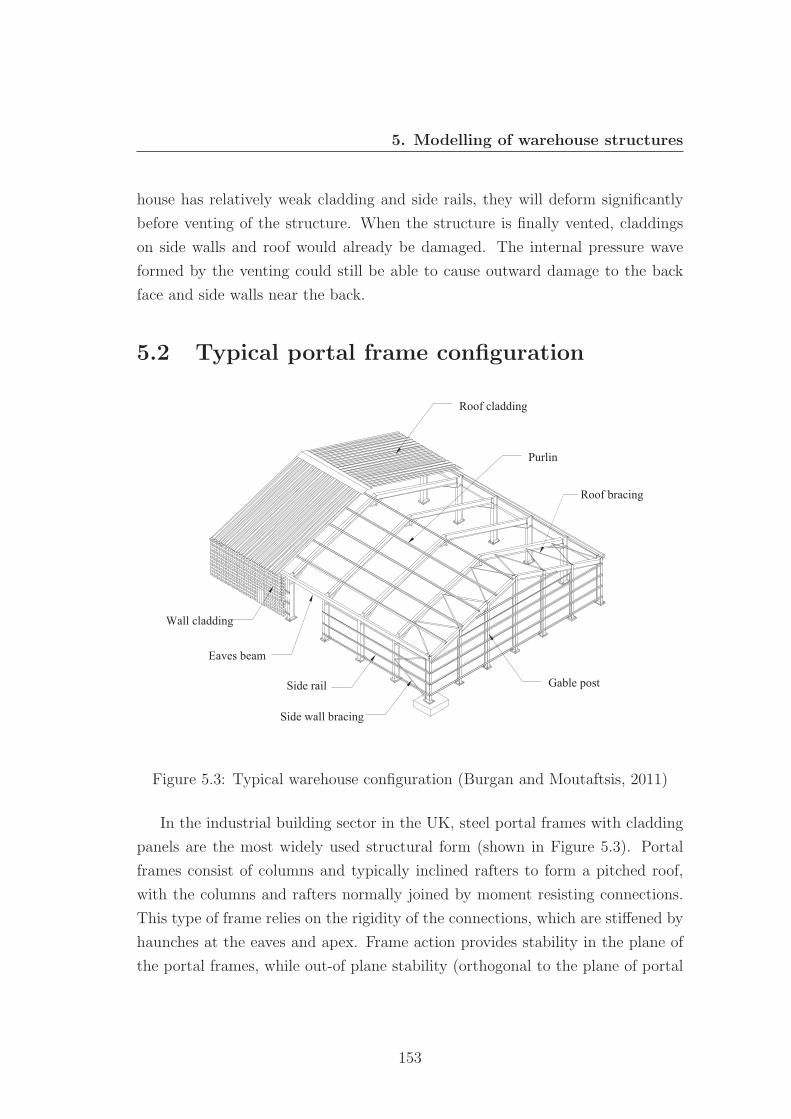
5. Modelling of warehouse structures
house has relatively weak cladding and side rails, they will deform significantly
before venting of the structure. When the structure is finally vented, claddings
on side walls and roof would already be damaged. The internal pressure wave
formed by the venting could still be able to cause outward damage to the back
face and side walls near the back.
5.2 Typical portal frame configuration
Figure 5.3: Typical warehouse configuration (Burgan and Moutaftsis, 2011)
In the industrial building sector in the UK, steel portal frames with cladding
panels are the most widely used structural form (shown in Figure 5.3). Portal
frames consist of columns and typically inclined rafters to form a pitched roof,
with the columns and rafters normally joined by moment resisting connections.
This type of frame relies on the rigidity of the connections, which are stiffened by
haunches at the eaves and apex. Frame action provides stability in the plane of
the portal frames, while out-of plane stability (orthogonal to the plane of portal
153
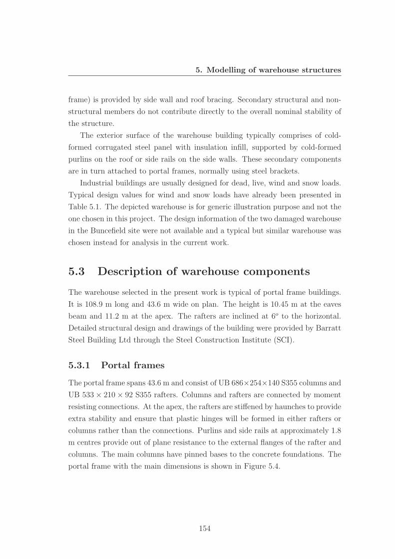
5. Modelling of warehouse structures
frame) is provided by side wall and roof bracing. Secondary structural and non-
structural members do not contribute directly to the overall nominal stability of
the structure.
The exterior surface of the warehouse building typically comprises of cold-
formed corrugated steel panel with insulation infill, supported by cold-formed
purlins on the roof or side rails on the side walls. These secondary components
are in turn attached to portal frames, normally using steel brackets.
Industrial buildings are usually designed for dead, live, wind and snow loads.
Typical design values for wind and snow loads have already been presented in
Table 5.1. The depicted warehouse is for generic illustration purpose and not the
one chosen in this project. The design information of the two damaged warehouse
in the Buncefield site were not available and a typical but similar warehouse was
chosen instead for analysis in the current work.
5.3 Description of warehouse components
The warehouse selected in the present work is typical of portal frame buildings.
It is 108.9 m long and 43.6 m wide on plan. The height is 10.45 m at the eaves
beam and 11.2 m at the apex. The rafters are inclined at 6o to the horizontal.
Detailed structural design and drawings of the building were provided by Barratt
Steel Building Ltd through the Steel Construction Institute (SCI).
5.3.1 Portal frames
The portal frame spans 43.6 m and consist of UB 686×254×140 S355 columns and
UB 533× 210× 92 S355 rafters. Columns and rafters are connected by moment
resisting connections. At the apex, the rafters are stiffened by haunches to provide
extra stability and ensure that plastic hinges will be formed in either rafters or
columns rather than the connections. Purlins and side rails at approximately 1.8
m centres provide out of plane resistance to the external flanges of the rafter and
columns. The main columns have pinned bases to the concrete foundations. The
portal frame with the main dimensions is shown in Figure 5.4.
154
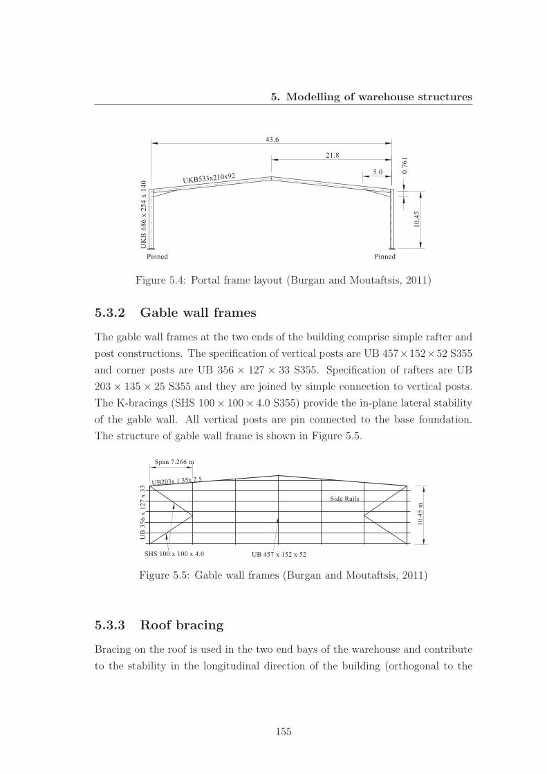
5. Modelling of warehouse structures
Figure 5.4: Portal frame layout (Burgan and Moutaftsis, 2011)
5.3.2 Gable wall frames
The gable wall frames at the two ends of the building comprise simple rafter and
post constructions. The specification of vertical posts are UB 457×152×52 S355
and corner posts are UB 356 × 127 × 33 S355. Specification of rafters are UB
203 × 135 × 25 S355 and they are joined by simple connection to vertical posts.
The K-bracings (SHS 100× 100× 4.0 S355) provide the in-plane lateral stability
of the gable wall. All vertical posts are pin connected to the base foundation.
The structure of gable wall frame is shown in Figure 5.5.
Figure 5.5: Gable wall frames (Burgan and Moutaftsis, 2011)
5.3.3 Roof bracing
Bracing on the roof is used in the two end bays of the warehouse and contribute
to the stability in the longitudinal direction of the building (orthogonal to the
155
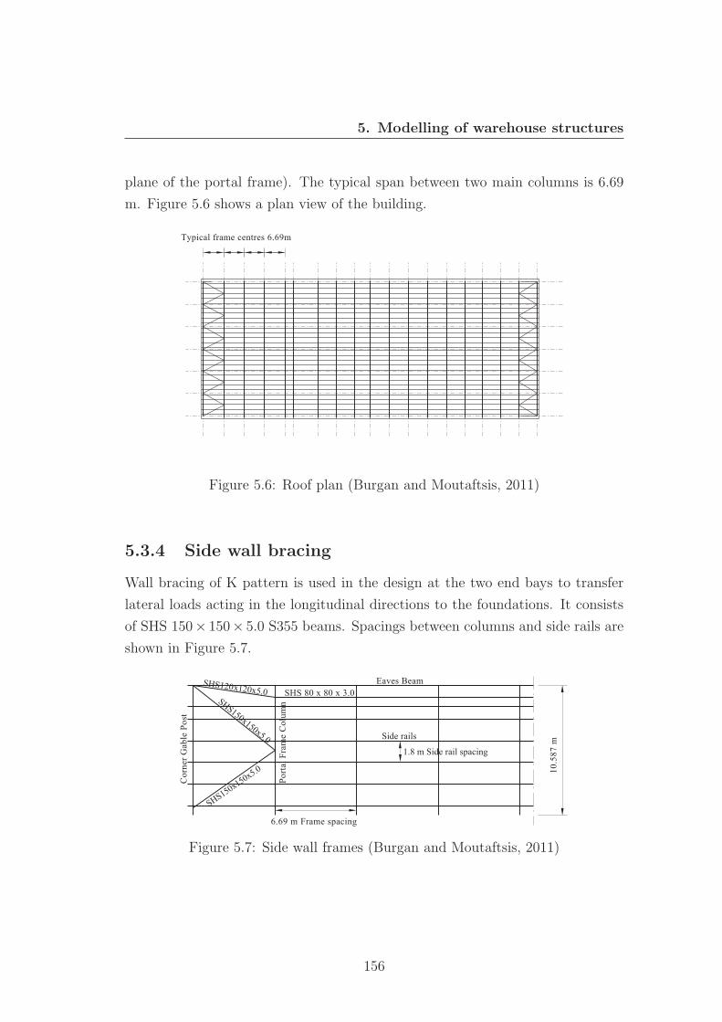
5. Modelling of warehouse structures
plane of the portal frame). The typical span between two main columns is 6.69
m. Figure 5.6 shows a plan view of the building.
Figure 5.6: Roof plan (Burgan and Moutaftsis, 2011)
5.3.4 Side wall bracing
Wall bracing of K pattern is used in the design at the two end bays to transfer
lateral loads acting in the longitudinal directions to the foundations. It consists
of SHS 150× 150× 5.0 S355 beams. Spacings between columns and side rails are
shown in Figure 5.7.
Figure 5.7: Side wall frames (Burgan and Moutaftsis, 2011)
156
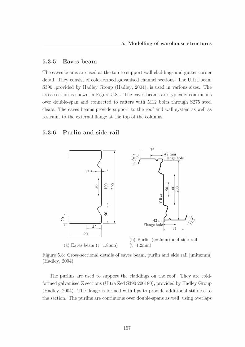
5. Modelling of warehouse structures
5.3.5 Eaves beam
The eaves beams are used at the top to support wall claddings and gutter corner
detail. They consist of cold-formed galvanised channel sections. The Ultra beam
S390 ,provided by Hadley Group (Hadley, 2004), is used in various sizes. The
cross section is shown in Figure 5.8a. The eaves beams are typically continuous
over double-span and connected to rafters with M12 bolts through S275 steel
cleats. The eaves beams provide support to the roof and wall system as well as
restraint to the external flange at the top of the columns.
5.3.6 Purlin and side rail
(a) Eaves beam (t=1.8mm)(b) Purlin (t=2mm) and side rail(t=1.2mm)
Figure 5.8: Cross-sectional details of eaves beam, purlin and side rail [units:mm](Hadley, 2004)
The purlins are used to support the claddings on the roof. They are cold-
formed galvanised Z sections (Ultra Zed S390 200180), provided by Hadley Group
(Hadley, 2004). The flange is formed with lips to provide additional stiffness to
the section. The purlins are continuous over double-spans as well, using overlaps
157
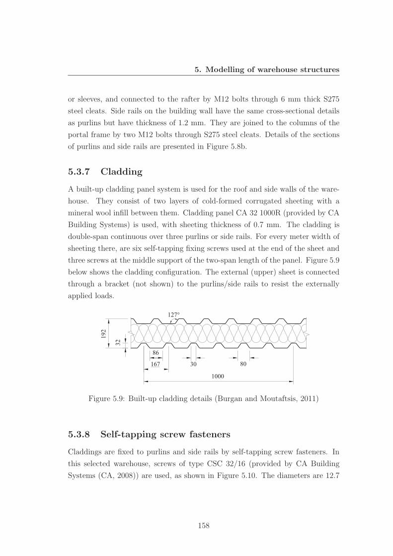
5. Modelling of warehouse structures
or sleeves, and connected to the rafter by M12 bolts through 6 mm thick S275
steel cleats. Side rails on the building wall have the same cross-sectional details
as purlins but have thickness of 1.2 mm. They are joined to the columns of the
portal frame by two M12 bolts through S275 steel cleats. Details of the sections
of purlins and side rails are presented in Figure 5.8b.
5.3.7 Cladding
A built-up cladding panel system is used for the roof and side walls of the ware-
house. They consist of two layers of cold-formed corrugated sheeting with a
mineral wool infill between them. Cladding panel CA 32 1000R (provided by CA
Building Systems) is used, with sheeting thickness of 0.7 mm. The cladding is
double-span continuous over three purlins or side rails. For every meter width of
sheeting there, are six self-tapping fixing screws used at the end of the sheet and
three screws at the middle support of the two-span length of the panel. Figure 5.9
below shows the cladding configuration. The external (upper) sheet is connected
through a bracket (not shown) to the purlins/side rails to resist the externally
applied loads.
Figure 5.9: Built-up cladding details (Burgan and Moutaftsis, 2011)
5.3.8 Self-tapping screw fasteners
Claddings are fixed to purlins and side rails by self-tapping screw fasteners. In
this selected warehouse, screws of type CSC 32/16 (provided by CA Building
Systems (CA, 2008)) are used, as shown in Figure 5.10. The diameters are 12.7
158
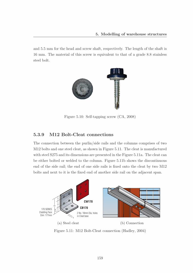
5. Modelling of warehouse structures
and 5.5 mm for the head and screw shaft, respectively. The length of the shaft is
16 mm. The material of this screw is equivalent to that of a grade 8.8 stainless
steel bolt.
Figure 5.10: Self-tapping screw (CA, 2008)
5.3.9 M12 Bolt-Cleat connections
The connection between the purlin/side rails and the columns comprises of two
M12 bolts and one steel cleat, as shown in Figure 5.11. The cleat is manufactured
with steel S275 and its dimensions are presented in the Figure 5.11a. The cleat can
be either bolted or welded to the column. Figure 5.11b shows the discontinuous
end of the side rail; the end of one side rails is fixed onto the cleat by two M12
bolts and next to it is the fixed end of another side rail on the adjacent span.
CW170
60min.
CB170
2 No. 18mm Dia. holesin Cleat base
6
22
62144
170 SERIESCladding FaceDim: 177mm
(a) Steel cleat (b) Connection
Figure 5.11: M12 Bolt-Cleat connection (Hadley, 2004)
159
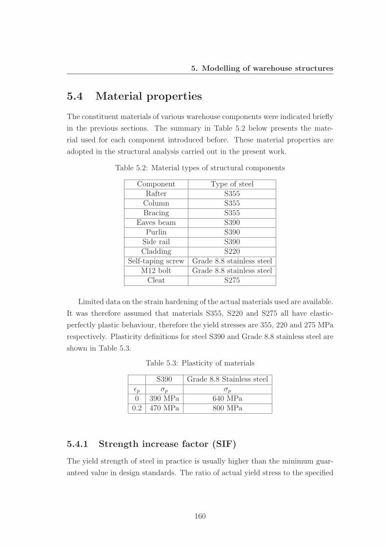
5. Modelling of warehouse structures
5.4 Material properties
The constituent materials of various warehouse components were indicated briefly
in the previous sections. The summary in Table 5.2 below presents the mate-
rial used for each component introduced before. These material properties are
adopted in the structural analysis carried out in the present work.
Table 5.2: Material types of structural components
Component Type of steelRafter S355Column S355Bracing S355
Eaves beam S390Purlin S390Side rail S390Cladding S220
Self-taping screw Grade 8.8 stainless steelM12 bolt Grade 8.8 stainless steelCleat S275
Limited data on the strain hardening of the actual materials used are available.
It was therefore assumed that materials S355, S220 and S275 all have elastic-
perfectly plastic behaviour, therefore the yield stresses are 355, 220 and 275 MPa
respectively. Plasticity definitions for steel S390 and Grade 8.8 stainless steel are
shown in Table 5.3.
Table 5.3: Plasticity of materials
S390 Grade 8.8 Stainless steelεp σp σp
0 390 MPa 640 MPa0.2 470 MPa 800 MPa
5.4.1 Strength increase factor (SIF)
The yield strength of steel in practice is usually higher than the minimum guar-
anteed value in design standards. The ratio of actual yield stress to the specified
160
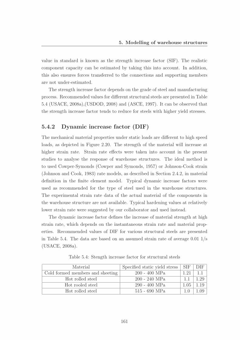
5. Modelling of warehouse structures
value in standard is known as the strength increase factor (SIF). The realistic
component capacity can be estimated by taking this into account. In addition,
this also ensures forces transferred to the connections and supporting members
are not under-estimated.
The strength increase factor depends on the grade of steel and manufacturing
process. Recommended values for different structural steels are presented in Table
5.4 (USACE, 2008a),(USDOD, 2008) and (ASCE, 1997). It can be observed that
the strength increase factor tends to reduce for steels with higher yield stresses.
5.4.2 Dynamic increase factor (DIF)
The mechanical material properties under static loads are different to high speed
loads, as depicted in Figure 2.20. The strength of the material will increase at
higher strain rate. Strain rate effects were taken into account in the present
studies to analyse the response of warehouse structures. The ideal method is
to used Cowper-Symonds (Cowper and Symonds, 1957) or Johnson-Cook strain
(Johnson and Cook, 1983) rate models, as described in Section 2.4.2, in material
definition in the finite element model. Typical dynamic increase factors were
used as recommended for the type of steel used in the warehouse structures.
The experimental strain rate data of the actual material of the components in
the warehouse structure are not available. Typical hardening values at relatively
lower strain rate were suggested by our collaborator and used instead.
The dynamic increase factor defines the increase of material strength at high
strain rate, which depends on the instantaneous strain rate and material prop-
erties. Recommended values of DIF for various structural steels are presented
in Table 5.4. The data are based on an assumed strain rate of average 0.01 1/s
(USACE, 2008a).
Table 5.4: Stength increase factor for structural steels
Material Specified static yield stress SIF DIFCold formed members and sheeting 200 - 400 MPa 1.21 1.1
Hot rolled steel 200 - 240 MPa 1.1 1.29Hot rooled steel 290 - 400 MPa 1.05 1.19Hot rolled steel 515 - 690 MPa 1.0 1.09
161
5. Modelling of warehouse structures
5.5 Numerical models of warehouse
In the previous section, the configuration and components of a typical warehouse
building were described in detail. In this section, the creation of a numerical
finite element model of the warehouse in the non-linear finite element analysis
program ? is described.
In order to simplify the problem, it was assumed that the side wall (either side)
of the warehouse is facing the explosion (i.e. perpendicular to the propagation
path of the blast wave). The side wall, which is subjected to the most severe
loading in the explosion, was chosen to be analysed in the present work.
It is prohibitive to model the whole side wall from end to end of the warehouse
due to the substantial size and the large number of components. It was noted
before that the side rails are continuous over a double span, hence it is reasonable
to model only two typical spans of the side wall, which preserves the continuity
of the side rails. The objective in this section is to select a suitable numerical
modelling level which is efficient to run whilst retaining sufficient accuracy.
5.5.1 Double span full model
The double span model of the side wall is shown in Figure 5.12a. This model
comprises three columns over two spans including the side rails and eaves beams
according to the building design. The cladding system has been simplified to
where only a single corrugated sheeting was used and fixed on the side rails by
self-tapping screws. The mineral wool infill and the other sheeting were simpli-
fied as non-structural mass and added to the modelled cladding panels. It is
important to note that the complete cladding system has a self weight of 0.301
kPa according to the building design, while the non-structural mass used in the
numerical model was determined to be 0.237 kPa (including one sheeting and the
mineral wool infill). As these are only for preliminary purposes, the fasteners and
cleat connections were all assumed rigid in this initial study. The claddings were
fixed to the outer flange of the supporting frames by tie constraints. In a similar
way, the end of the supporting frames were rigidly constrained and connected to
the flange of the main columns using tie constraints.
162
5. Modelling of warehouse structures
(a) Double span full model (b) Single span model
(c) Sub-assembly model (d) Component model
Figure 5.12: Numerical modelling levels
163
5. Modelling of warehouse structures
5.5.2 Single span full model
The single span model was simplified from the double span full model and only
half of the claddings and supporting frames were considered. The columns were
removed for simplicity based on observation after the Buncefield incident that all
primary structural components remained intact during the explosion. The single
span model is shown in Figure 5.12b, in which the far end of the supporting
frames was fully constrained to represent the continuity over the double span and
the near end were simply supported. Fasteners were assumed rigid for this initial
model and the cleat connections were replaced by boundary constraints at the
end of the frames.
5.5.3 Sub-assemblage model
The sub-assemblage model shown in Figure 5.12c was the result of further sim-
plification of the numerical model. It only comprised three side rails and the
claddings over double span (two spans of side rail). Fasteners were rigid and the
same boundary constraints of single span full model were applied at the end of
the side rails. Additional loads were applied directly on the outer flanges of the
upper and lower side rails. This was used to take account of the pressure loads
from the neighbouring claddings (half span). Accordingly, the additional masses
of the neighbouring half span claddings were added to the side rails as well.
5.5.4 Component model
The final simplified model is shown in Figure 5.12d. This component model
consists of only the middle side rail in the sub-assemblage model. The weight of
half the span of the complete cladding system was added to the side rail and the
equivalent pressure loads applied on the outer flange were calculated based on
the tributary width of 1.8 m (half span of side rails). Boundary conditions were
the same as in the other two simplified models.
164
5. Modelling of warehouse structures
5.5.5 Comparison of displacement histories
Claddings of all the numerical models were subjected to a uniformly distributed
blast pressure loads with a peak reflected overpressure of 7 kPa and a duration
of 150 ms (linear decay). It is important to note that the masses of the rele-
vant components were always preserved in the simplified models and so were the
pressure loads.
The analysis time was set to 300 ms. The actual wall clock time used by
double, single, sub-assemblage and components models were approximately 20,
15, 10 and 0.5 hours, respectively. All simulations were performed using high
performance computers as noted in Chapter 4.
0 50 100 150 200 250 300Time [ms]
0
100
200
300
400
500
600
Warehouse
wallcentre
deflection
[mm]
Single span model
Sub-assemblage model
Component model
Figure 5.13: Comparison of displacement histories of side wall models
The predicted displacement time histories at the middle of the central side
rail are shown in Figure 5.13. It can been seen that the numerical models pro-
duced very similar displacement time histories. Results from the double span full
model were not included here. It is because the rigid M12 bolt-cleat connection
assumption made in this model caused substantial deformation and rotation of
the column flange. This is not typical in reality since the connection would fail
165
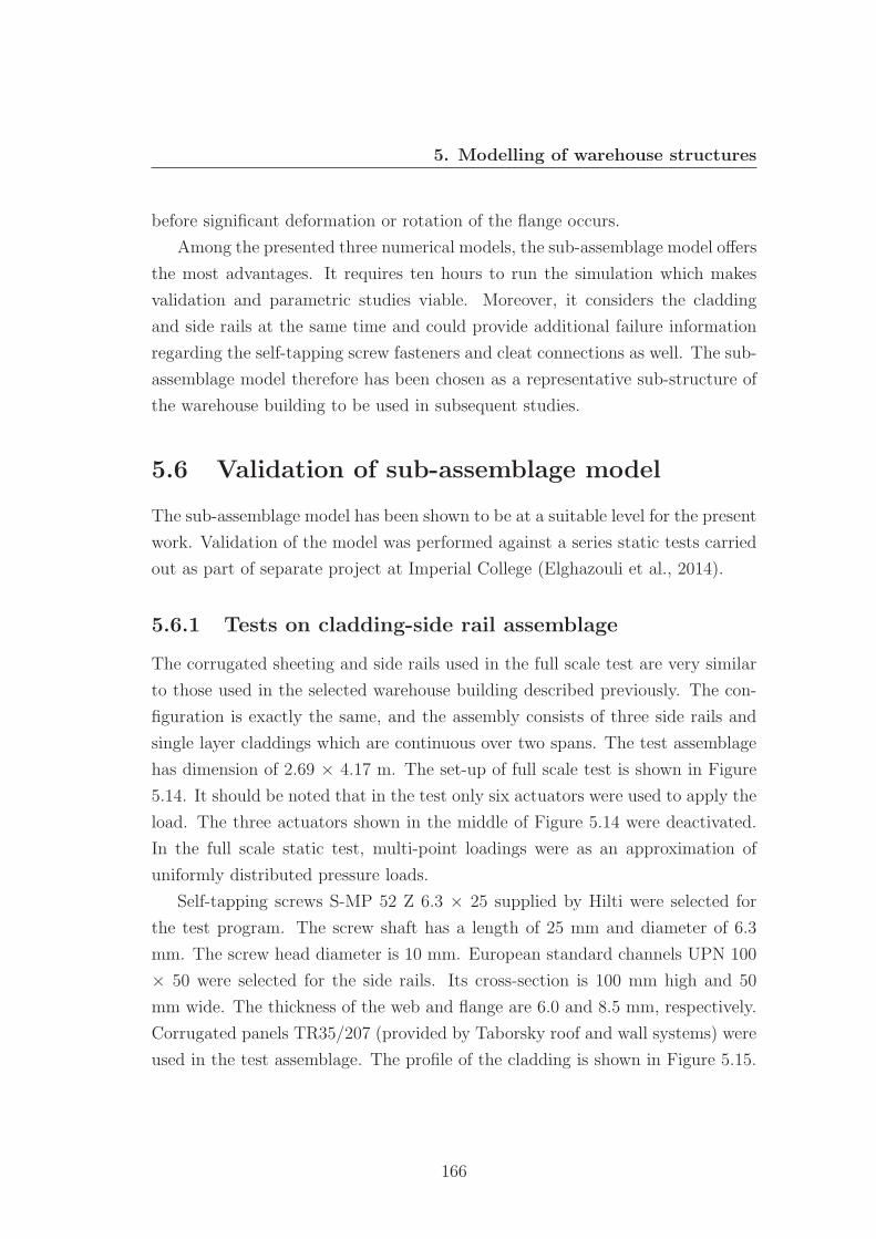
5. Modelling of warehouse structures
before significant deformation or rotation of the flange occurs.
Among the presented three numerical models, the sub-assemblage model offers
the most advantages. It requires ten hours to run the simulation which makes
validation and parametric studies viable. Moreover, it considers the cladding
and side rails at the same time and could provide additional failure information
regarding the self-tapping screw fasteners and cleat connections as well. The sub-
assemblage model therefore has been chosen as a representative sub-structure of
the warehouse building to be used in subsequent studies.
5.6 Validation of sub-assemblage model
The sub-assemblage model has been shown to be at a suitable level for the present
work. Validation of the model was performed against a series static tests carried
out as part of separate project at Imperial College (Elghazouli et al., 2014).
5.6.1 Tests on cladding-side rail assemblage
The corrugated sheeting and side rails used in the full scale test are very similar
to those used in the selected warehouse building described previously. The con-
figuration is exactly the same, and the assembly consists of three side rails and
single layer claddings which are continuous over two spans. The test assemblage
has dimension of 2.69 × 4.17 m. The set-up of full scale test is shown in Figure
5.14. It should be noted that in the test only six actuators were used to apply the
load. The three actuators shown in the middle of Figure 5.14 were deactivated.
In the full scale static test, multi-point loadings were as an approximation of
uniformly distributed pressure loads.
Self-tapping screws S-MP 52 Z 6.3 × 25 supplied by Hilti were selected for
the test program. The screw shaft has a length of 25 mm and diameter of 6.3
mm. The screw head diameter is 10 mm. European standard channels UPN 100
× 50 were selected for the side rails. Its cross-section is 100 mm high and 50
mm wide. The thickness of the web and flange are 6.0 and 8.5 mm, respectively.
Corrugated panels TR35/207 (provided by Taborsky roof and wall systems) were
used in the test assemblage. The profile of the cladding is shown in Figure 5.15.
166
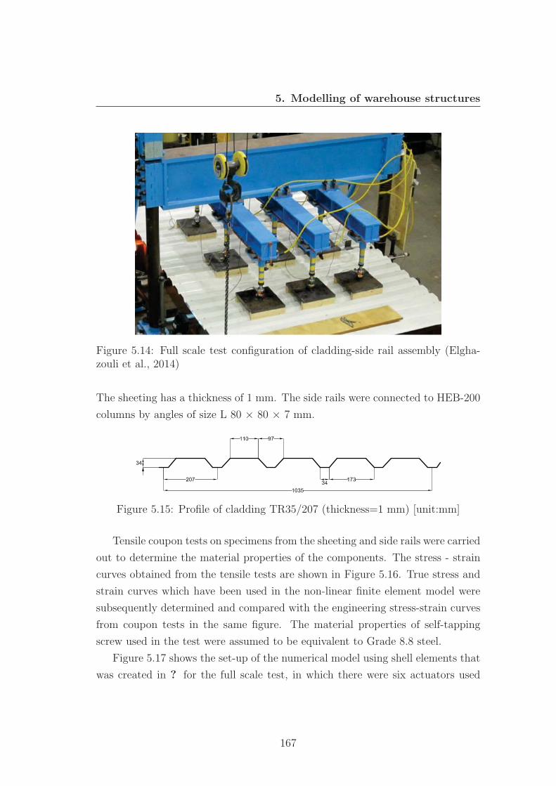
5. Modelling of warehouse structures
Figure 5.14: Full scale test configuration of cladding-side rail assembly (Elgha-zouli et al., 2014)
The sheeting has a thickness of 1 mm. The side rails were connected to HEB-200
columns by angles of size L 80 × 80 × 7 mm.
Figure 5.15: Profile of cladding TR35/207 (thickness=1 mm) [unit:mm]
Tensile coupon tests on specimens from the sheeting and side rails were carried
out to determine the material properties of the components. The stress - strain
curves obtained from the tensile tests are shown in Figure 5.16. True stress and
strain curves which have been used in the non-linear finite element model were
subsequently determined and compared with the engineering stress-strain curves
from coupon tests in the same figure. The material properties of self-tapping
screw used in the test were assumed to be equivalent to Grade 8.8 steel.
Figure 5.17 shows the set-up of the numerical model using shell elements that
was created in ? for the full scale test, in which there were six actuators used
167
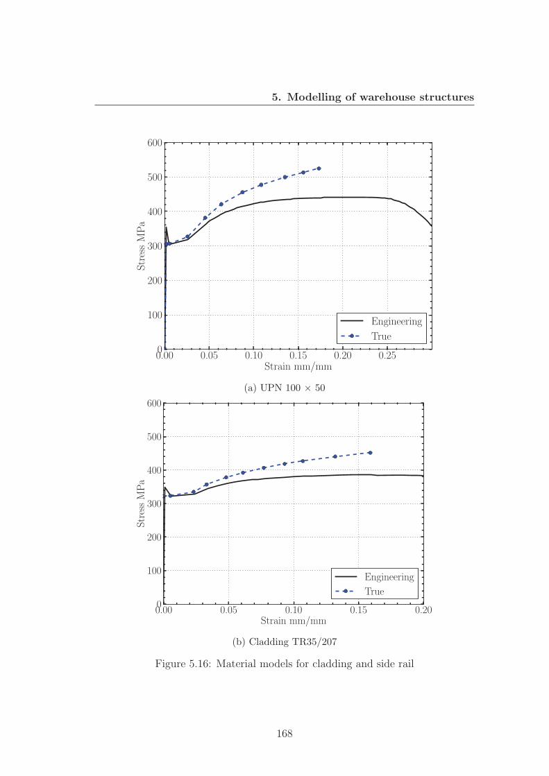
5. Modelling of warehouse structures
0.00 0.05 0.10 0.15 0.20 0.25Strain mm/mm
0
100
200
300
400
500
600StressMPa
Engineering
True
(a) UPN 100 × 50
0.00 0.05 0.10 0.15 0.20Strain mm/mm
0
100
200
300
400
500
600
StressMPa
Engineering
True
(b) Cladding TR35/207
Figure 5.16: Material models for cladding and side rail
168
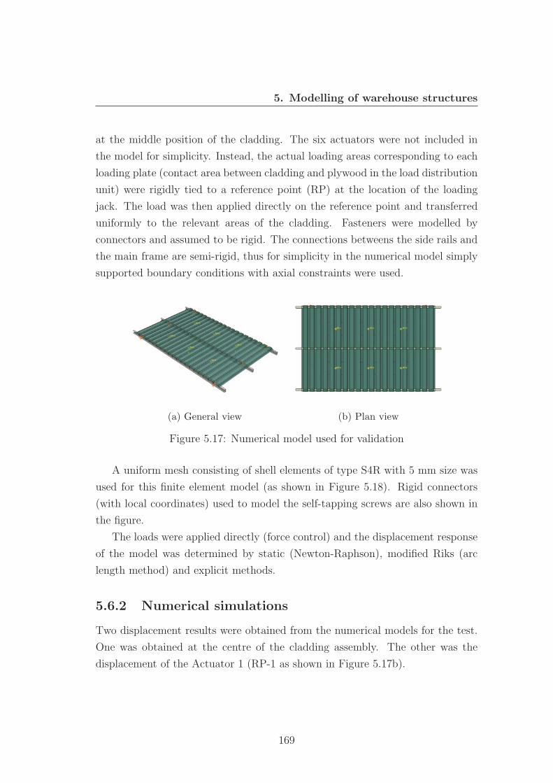
5. Modelling of warehouse structures
at the middle position of the cladding. The six actuators were not included in
the model for simplicity. Instead, the actual loading areas corresponding to each
loading plate (contact area between cladding and plywood in the load distribution
unit) were rigidly tied to a reference point (RP) at the location of the loading
jack. The load was then applied directly on the reference point and transferred
uniformly to the relevant areas of the cladding. Fasteners were modelled by
connectors and assumed to be rigid. The connections betweens the side rails and
the main frame are semi-rigid, thus for simplicity in the numerical model simply
supported boundary conditions with axial constraints were used.
(a) General view (b) Plan view
Figure 5.17: Numerical model used for validation
A uniform mesh consisting of shell elements of type S4R with 5 mm size was
used for this finite element model (as shown in Figure 5.18). Rigid connectors
(with local coordinates) used to model the self-tapping screws are also shown in
the figure.
The loads were applied directly (force control) and the displacement response
of the model was determined by static (Newton-Raphson), modified Riks (arc
length method) and explicit methods.
5.6.2 Numerical simulations
Two displacement results were obtained from the numerical models for the test.
One was obtained at the centre of the cladding assembly. The other was the
displacement of the Actuator 1 (RP-1 as shown in Figure 5.17b).
169
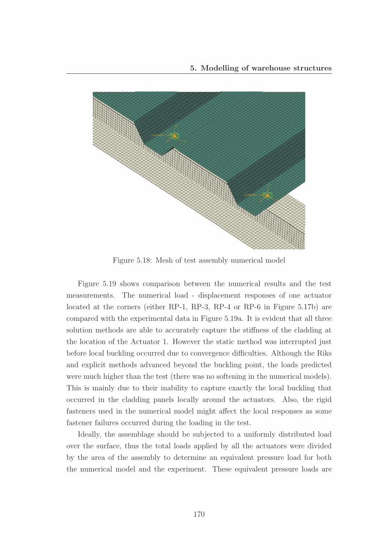
5. Modelling of warehouse structures
Figure 5.18: Mesh of test assembly numerical model
Figure 5.19 shows comparison between the numerical results and the test
measurements. The numerical load - displacement responses of one actuator
located at the corners (either RP-1, RP-3, RP-4 or RP-6 in Figure 5.17b) are
compared with the experimental data in Figure 5.19a. It is evident that all three
solution methods are able to accurately capture the stiffness of the cladding at
the location of the Actuator 1. However the static method was interrupted just
before local buckling occurred due to convergence difficulties. Although the Riks
and explicit methods advanced beyond the buckling point, the loads predicted
were much higher than the test (there was no softening in the numerical models).
This is mainly due to their inability to capture exactly the local buckling that
occurred in the cladding panels locally around the actuators. Also, the rigid
fasteners used in the numerical model might affect the local responses as some
fastener failures occurred during the loading in the test.
Ideally, the assemblage should be subjected to a uniformly distributed load
over the surface, thus the total loads applied by all the actuators were divided
by the area of the assembly to determine an equivalent pressure load for both
the numerical model and the experiment. These equivalent pressure loads are
170
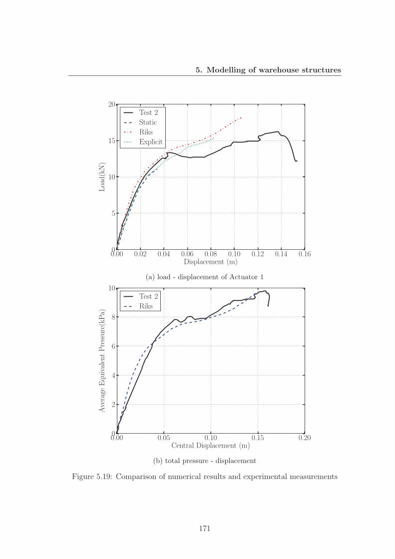
5. Modelling of warehouse structures
0.00 0.02 0.04 0.06 0.08 0.10 0.12 0.14 0.16Displacement (m)
0
5
10
15
20Load(kN)
Test 2
Static
Riks
Explicit
(a) load - displacement of Actuator 1
0.00 0.05 0.10 0.15 0.20Central Displacement (m)
0
2
4
6
8
10
Average
EquivalentPressure(kPa)
Test 2
Riks
(b) total pressure - displacement
Figure 5.19: Comparison of numerical results and experimental measurements
171
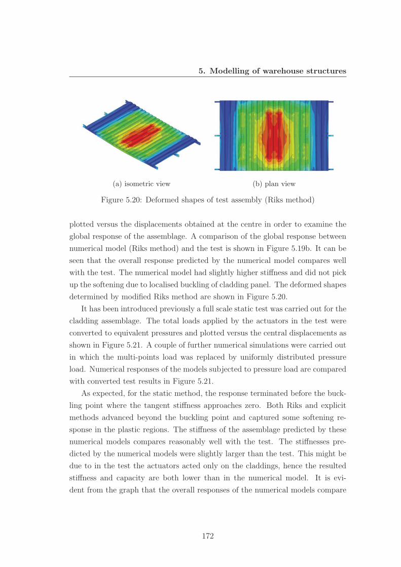
5. Modelling of warehouse structures
(a) isometric view (b) plan view
Figure 5.20: Deformed shapes of test assembly (Riks method)
plotted versus the displacements obtained at the centre in order to examine the
global response of the assemblage. A comparison of the global response between
numerical model (Riks method) and the test is shown in Figure 5.19b. It can be
seen that the overall response predicted by the numerical model compares well
with the test. The numerical model had slightly higher stiffness and did not pick
up the softening due to localised buckling of cladding panel. The deformed shapes
determined by modified Riks method are shown in Figure 5.20.
It has been introduced previously a full scale static test was carried out for the
cladding assemblage. The total loads applied by the actuators in the test were
converted to equivalent pressures and plotted versus the central displacements as
shown in Figure 5.21. A couple of further numerical simulations were carried out
in which the multi-points load was replaced by uniformly distributed pressure
load. Numerical responses of the models subjected to pressure load are compared
with converted test results in Figure 5.21.
As expected, for the static method, the response terminated before the buck-
ling point where the tangent stiffness approaches zero. Both Riks and explicit
methods advanced beyond the buckling point and captured some softening re-
sponse in the plastic regions. The stiffness of the assemblage predicted by these
numerical models compares reasonably well with the test. The stiffnesses pre-
dicted by the numerical models were slightly larger than the test. This might be
due to in the test the actuators acted only on the claddings, hence the resulted
stiffness and capacity are both lower than in the numerical model. It is evi-
dent from the graph that the overall responses of the numerical models compare
172
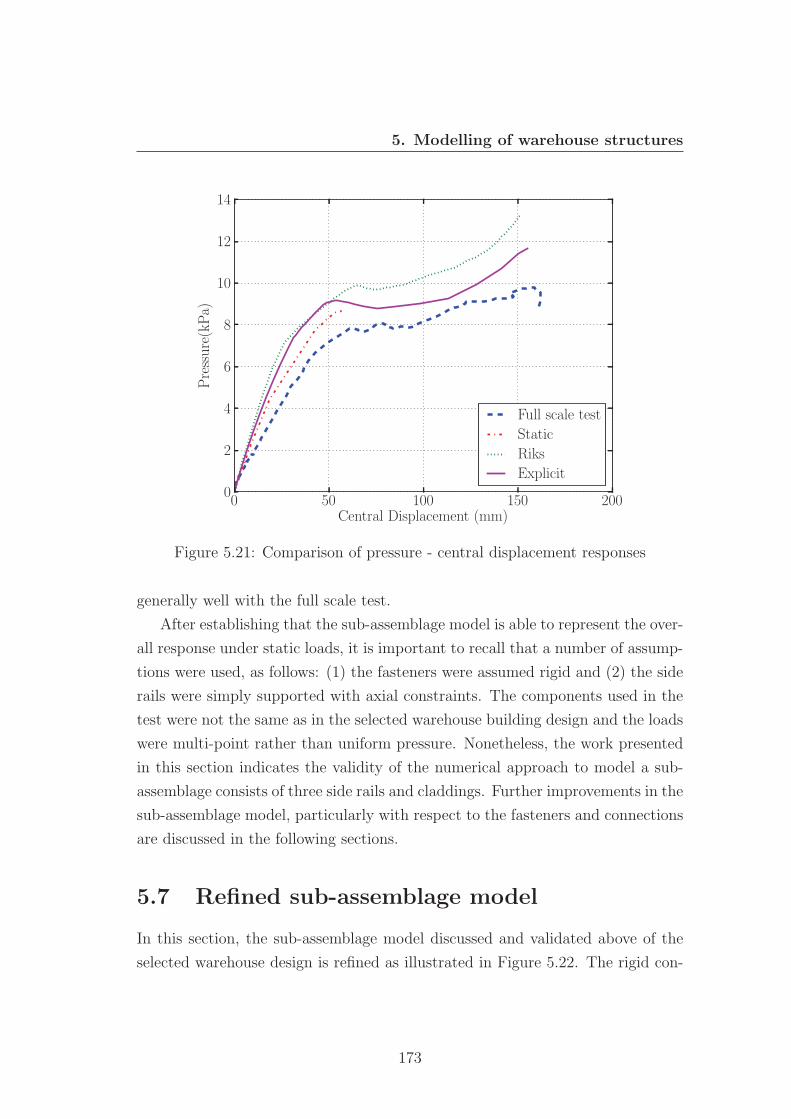
5. Modelling of warehouse structures
0 50 100 150 200Central Displacement (mm)
0
2
4
6
8
10
12
14Pressure(kPa)
Full scale test
Static
Riks
Explicit
Figure 5.21: Comparison of pressure - central displacement responses
generally well with the full scale test.
After establishing that the sub-assemblage model is able to represent the over-
all response under static loads, it is important to recall that a number of assump-
tions were used, as follows: (1) the fasteners were assumed rigid and (2) the side
rails were simply supported with axial constraints. The components used in the
test were not the same as in the selected warehouse building design and the loads
were multi-point rather than uniform pressure. Nonetheless, the work presented
in this section indicates the validity of the numerical approach to model a sub-
assemblage consists of three side rails and claddings. Further improvements in the
sub-assemblage model, particularly with respect to the fasteners and connections
are discussed in the following sections.
5.7 Refined sub-assemblage model
In this section, the sub-assemblage model discussed and validated above of the
selected warehouse design is refined as illustrated in Figure 5.22. The rigid con-
173
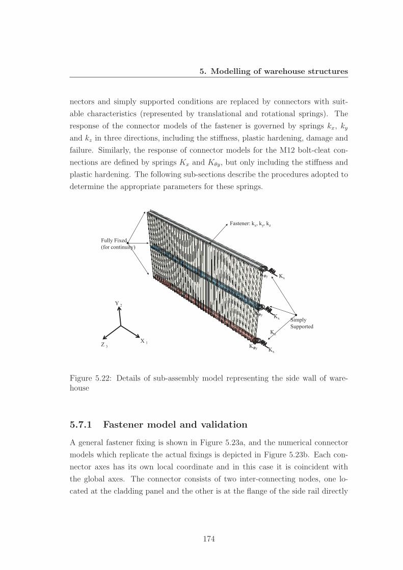
5. Modelling of warehouse structures
nectors and simply supported conditions are replaced by connectors with suit-
able characteristics (represented by translational and rotational springs). The
response of the connector models of the fastener is governed by springs kx, ky
and kz in three directions, including the stiffness, plastic hardening, damage and
failure. Similarly, the response of connector models for the M12 bolt-cleat con-
nections are defined by springs Kx and Kθy, but only including the stiffness and
plastic hardening. The following sub-sections describe the procedures adopted to
determine the appropriate parameters for these springs.
X 1 Z 3
Y 2
Kx
Kz
K y
Kx
Kx
K y
K y
Fastener: kx, ky, kz
Fully Fixed (for continuity)
Simply Supported
Figure 5.22: Details of sub-assembly model representing the side wall of ware-house
5.7.1 Fastener model and validation
A general fastener fixing is shown in Figure 5.23a, and the numerical connector
models which replicate the actual fixings is depicted in Figure 5.23b. Each con-
nector axes has its own local coordinate and in this case it is coincident with
the global axes. The connector consists of two inter-connecting nodes, one lo-
cated at the cladding panel and the other is at the flange of the side rail directly
174
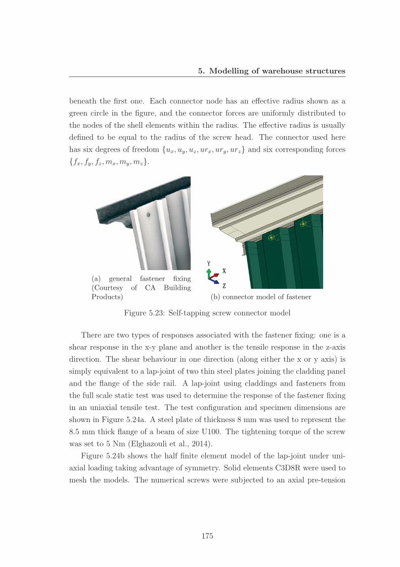
5. Modelling of warehouse structures
beneath the first one. Each connector node has an effective radius shown as a
green circle in the figure, and the connector forces are uniformly distributed to
the nodes of the shell elements within the radius. The effective radius is usually
defined to be equal to the radius of the screw head. The connector used here
has six degrees of freedom {ux, uy, uz, urx, ury, urz} and six corresponding forces
{fx, fy, fz,mx,my,mz}.
(a) general fastener fixing(Courtesy of CA BuildingProducts) (b) connector model of fastener
Figure 5.23: Self-tapping screw connector model
There are two types of responses associated with the fastener fixing: one is a
shear response in the x-y plane and another is the tensile response in the z-axis
direction. The shear behaviour in one direction (along either the x or y axis) is
simply equivalent to a lap-joint of two thin steel plates joining the cladding panel
and the flange of the side rail. A lap-joint using claddings and fasteners from
the full scale static test was used to determine the response of the fastener fixing
in an uniaxial tensile test. The test configuration and specimen dimensions are
shown in Figure 5.24a. A steel plate of thickness 8 mm was used to represent the
8.5 mm thick flange of a beam of size U100. The tightening torque of the screw
was set to 5 Nm (Elghazouli et al., 2014).
Figure 5.24b shows the half finite element model of the lap-joint under uni-
axial loading taking advantage of symmetry. Solid elements C3D8R were used to
mesh the models. The numerical screws were subjected to an axial pre-tension
175
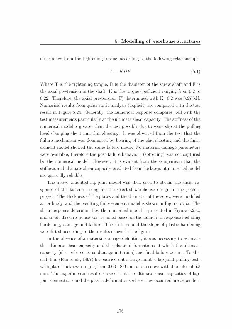
5. Modelling of warehouse structures
determined from the tightening torque, according to the following relationship:
T = KDF (5.1)
Where T is the tightening torque, D is the diameter of the screw shaft and F is
the axial pre-tension in the shaft. K is the torque coefficient ranging from 0.2 to
0.22. Therefore, the axial pre-tension (F) determined with K=0.2 was 3.97 kN.
Numerical results from quasi-static analysis (explicit) are compared with the test
result in Figure 5.24. Generally, the numerical response compares well with the
test measurements particularly at the ultimate shear capacity. The stiffness of the
numerical model is greater than the test possibly due to some slip at the pulling
head clamping the 1 mm thin sheeting. It was observed from the test that the
failure mechanism was dominated by bearing of the clad sheeting and the finite
element model showed the same failure mode. No material damage parameters
were available, therefore the post-failure behaviour (softening) was not captured
by the numerical model. However, it is evident from the comparison that the
stiffness and ultimate shear capacity predicted from the lap-joint numerical model
are generally reliable.
The above validated lap-joint model was then used to obtain the shear re-
sponse of the fastener fixing for the selected warehouse design in the present
project. The thickness of the plates and the diameter of the screw were modified
accordingly, and the resulting finite element model is shown in Figure 5.25a. The
shear response determined by the numerical model is presented in Figure 5.25b,
and an idealised response was assumed based on the numerical response including
hardening, damage and failure. The stiffness and the slope of plastic hardening
were fitted according to the results shown in the figure.
In the absence of a material damage definition, it was necessary to estimate
the ultimate shear capacity and the plastic deformations at which the ultimate
capacity (also referred to as damage initiation) and final failure occurs. To this
end, Fan (Fan et al., 1997) has carried out a large number lap-joint pulling tests
with plate thickness ranging from 0.63 - 8.0 mm and a screw with diameter of 6.3
mm. The experimental results showed that the ultimate shear capacities of lap-
joint connections and the plastic deformations where they occurred are dependent
176
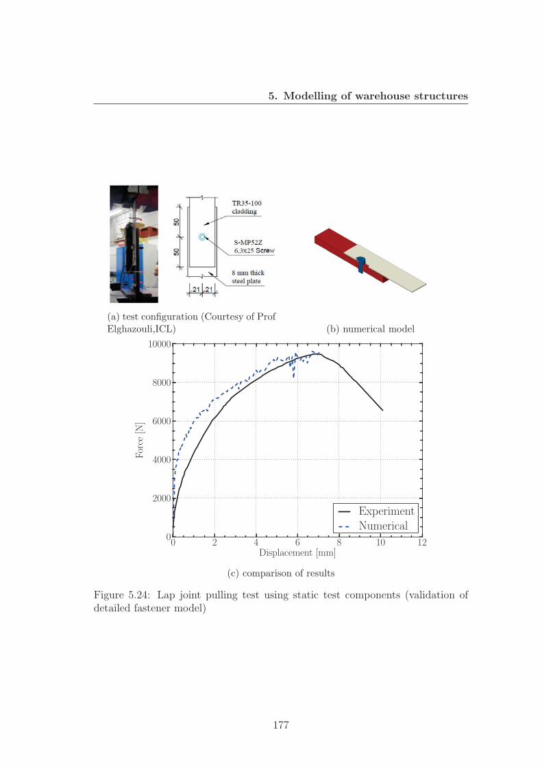
5. Modelling of warehouse structures
(a) test configuration (Courtesy of ProfElghazouli,ICL) (b) numerical model
0 2 4 6 8 10 12Displacement [mm]
0
2000
4000
6000
8000
10000
Force
[N]
ExperimentNumerical
(c) comparison of results
Figure 5.24: Lap joint pulling test using static test components (validation ofdetailed fastener model)
177
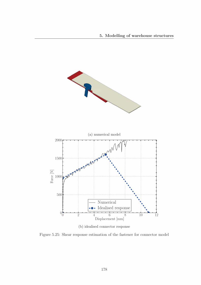
5. Modelling of warehouse structures
(a) numerical model
0 2 4 6 8 10 12Displacement [mm]
0
500
1000
1500
2000
Force
[N]
NumericalIdealised response
(b) idealised connector response
Figure 5.25: Shear response estimation of the fastener for connector model
178
5. Modelling of warehouse structures
on the rotation of the screws, which is in turn dependent on the thickness ratio
of the top and bottom plates in the lap-joint. With minor screw rotations (when
the ratio of the thickness of top plate to bottom is less than 1), the ultimate
capacities usually occur at plastic deformations between 5 - 7 mm. This range is
in the proximity of the screw diameter of 6.3 mm. The ultimate shear capacity
occurred at a plastic deformation of about 7 mm for the lap-joint test shown in
Figure 5.24c, which is also close to the screw diameter of 6.3 mm.
For another study, Lim (Jin-seong et al., 2013) examined the structural be-
haviour of single shear bolted connections using high strength M12 bolt and 3
mm thickness steel plates. Their results suggested that although the plastic de-
formations where the ultimate shear capacities occurred can be dependent on the
distance from the bolt to the end of plate, the values were still well in proximity
of the bolt diameter.
As a result of the observations from tests, it was assumed that for the numer-
ical shear response shown in Figure 5.25b the ultimate shear capacity occurred
at 5.5 mm (equivalent to the diameter of the screw). It is difficult to estimate the
plastic deformation at total failure of the fastener joint, therefore it was assumed
that the failure deformation is twice that of the screw diameter (11 mm). Accord-
ingly the idealised shear response of the numerical fastener lap-joint model can be
completely defined as shown in Figure 5.25b. The elastic modulus was estimated
to be 9.5 MN/m with a yield shear force of 950 N. The tangent modulus was
fitted to be 118.2 kN/m. The connector damage initiation was estimated to be
5.5 mm with the corresponding ultimate shear capacity of 1600 N. Finally, the
connector was assumed to fail at a plastic deformation of 11 mm.
5.7.2 Coupled response of fasteners
The uniaxial shear response of the fastener fixing has been defined in the previous
section. This response was obtained only in either x or y direction by a lap-
joint model. However the fastener joint is indeed axisymmetric, hence the shear
response should be identical in any direction in the x-y plane. In this sub-section,
a procedure is presented to couple the response in the x and y directions so
that the shear response can be identical in any direction in the x-y plane. In
179
5. Modelling of warehouse structures
addition, the uncoupled tensile response is also presented to complete the response
definition of the connector model for the fastener fixings.
• Coupled shear response
The orientation of the connector model for the screw fixings is shown in Figure
5.23b. The connector model has six degrees of freedom, {ux, uy, uz, urx, ury, urz}and six corresponding connector forces and moments {fx, fy, fz,mx,my,mz}. Un-coupled elastic behaviour was assumed for the connector. The same shear elastic
modulus was used for the two shear directions (x and y) based on the assumption
of isotropic sheets and isotropic cross section of the screw joints. The elastic be-
haviour was assumed to be rigid in the axial direction (z-axis) and for the three
moment components. The moments exerted in the fastener model were neglected
for simplicity.
A connector potential was defined in ? to describe the plastic behaviour of
the connector as shown below, in which FN is the equivalent tensile (normal)
force and FS is the equivalent shear force.
P =
{(FN
RN
)β
+
(FS
RS
)β}1/β
(5.2a)
FN = |fz|+ K
r
√m2
x +m2y (5.2b)
FS =√
f 2x + f 2
y (5.2c)
where β = 2. Assuming FN = 0 (i.e. decouple the tensile force) and ignoring
the FN term in the potential P which can be redefined as:
P =
√(fxRS
)2
+
(fyRS
)2
(5.3)
RS is defined as the yield force of the connector. Equation 5.3 implies that
the redefined shear potential P is a quadratic function of the connector force fx
and fy, and both of the two forces contribute to the equivalent shear force P
180
5. Modelling of warehouse structures
simultaneously. The yield function is then defined as:
Φ({f} , upl) = P ({f})− F 0(upl) ≤ 0 (5.4)
where {f} = (fx, fy)T is the collection of the two connector forces active in
the yield function. F 0 is the equivalent yield shear force and defines the yield
surface size as a function of the equivalent plastic relative motion upl, using a
hardening law in ?.
If yield occurs, the associated plastic flow rule is used to calculate the plastic
relative motion as: {upl}= ¨upl ∂Φ
∂ {f} (5.5)
where{upl}={uplx , u
ply
}is the collection of plastic relative motion rate in the
components active in the yield function. ˙upl is the equivalent plastic relative
motion rate and is defined as:
˙upl =
√√√√{upl}T {upl}∂Φ
∂{f}T∂Φ∂{f}
(5.6)
The equivalent plastic relative motion upl is then defined as:
upl =
t∫0
upldt (5.7)
And finally the isotropic hardening assigned to the connector as shown in
Figure 5.25b is given in Table 5.5 below. The size of the yield surface F 0 is
defined as a function of the equivalent plastic relative motion upl.
Table 5.5: Isotropic hardening of connector model for fastener joint
F 0(N) upl(mm)950 01600 5.5
A schematic of the equivalent shear response of the connector for the fastener
joint is shown in Figure 5.26. The elastic stiffness and plastic isotropic hardening
181
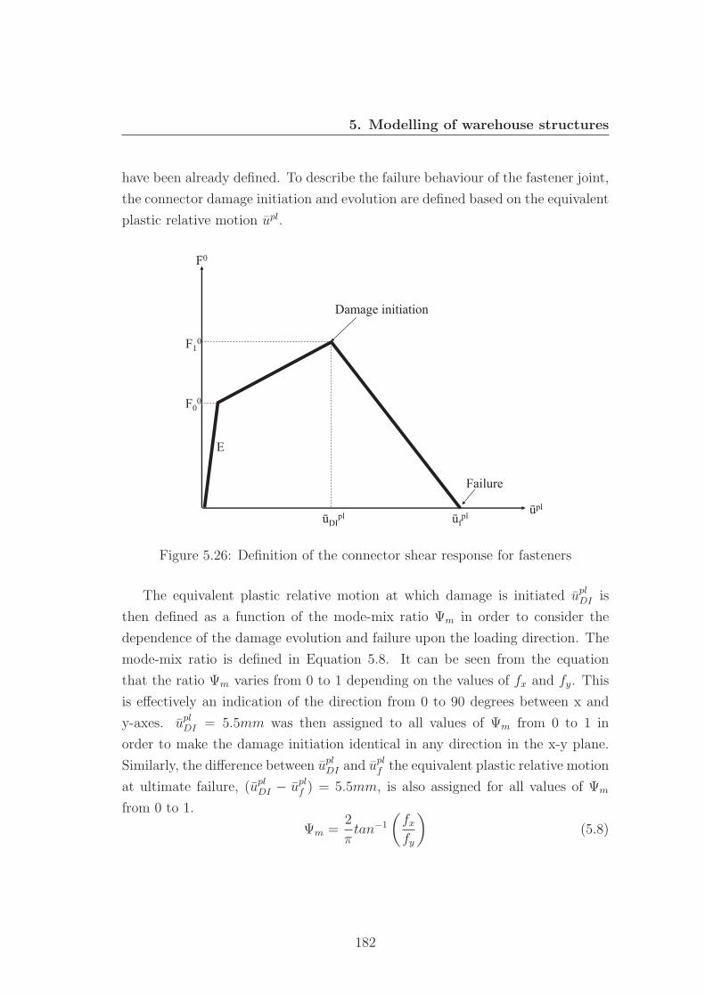
5. Modelling of warehouse structures
have been already defined. To describe the failure behaviour of the fastener joint,
the connector damage initiation and evolution are defined based on the equivalent
plastic relative motion upl.
F00
F10
Damage initiation
Failure
E
ūDIpl ūf
pl ūpl
F0
Figure 5.26: Definition of the connector shear response for fasteners
The equivalent plastic relative motion at which damage is initiated uplDI is
then defined as a function of the mode-mix ratio Ψm in order to consider the
dependence of the damage evolution and failure upon the loading direction. The
mode-mix ratio is defined in Equation 5.8. It can be seen from the equation
that the ratio Ψm varies from 0 to 1 depending on the values of fx and fy. This
is effectively an indication of the direction from 0 to 90 degrees between x and
y-axes. uplDI = 5.5mm was then assigned to all values of Ψm from 0 to 1 in
order to make the damage initiation identical in any direction in the x-y plane.
Similarly, the difference between uplDI and upl
f the equivalent plastic relative motion
at ultimate failure, (uplDI − upl
f ) = 5.5mm, is also assigned for all values of Ψm
from 0 to 1.
Ψm =2
πtan−1
(fxfy
)(5.8)
182
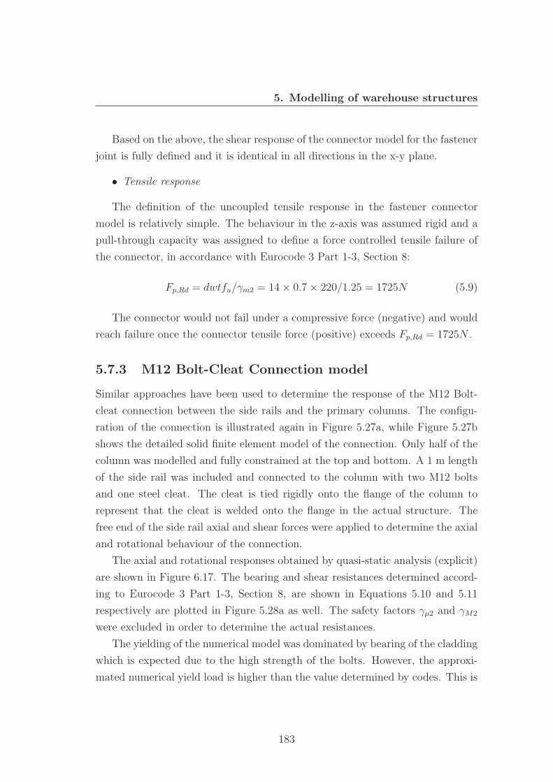
5. Modelling of warehouse structures
Based on the above, the shear response of the connector model for the fastener
joint is fully defined and it is identical in all directions in the x-y plane.
• Tensile response
The definition of the uncoupled tensile response in the fastener connector
model is relatively simple. The behaviour in the z-axis was assumed rigid and a
pull-through capacity was assigned to define a force controlled tensile failure of
the connector, in accordance with Eurocode 3 Part 1-3, Section 8:
Fp,Rd = dwtfu/γm2 = 14× 0.7× 220/1.25 = 1725N (5.9)
The connector would not fail under a compressive force (negative) and would
reach failure once the connector tensile force (positive) exceeds Fp,Rd = 1725N .
5.7.3 M12 Bolt-Cleat Connection model
Similar approaches have been used to determine the response of the M12 Bolt-
cleat connection between the side rails and the primary columns. The configu-
ration of the connection is illustrated again in Figure 5.27a, while Figure 5.27b
shows the detailed solid finite element model of the connection. Only half of the
column was modelled and fully constrained at the top and bottom. A 1 m length
of the side rail was included and connected to the column with two M12 bolts
and one steel cleat. The cleat is tied rigidly onto the flange of the column to
represent that the cleat is welded onto the flange in the actual structure. The
free end of the side rail axial and shear forces were applied to determine the axial
and rotational behaviour of the connection.
The axial and rotational responses obtained by quasi-static analysis (explicit)
are shown in Figure 6.17. The bearing and shear resistances determined accord-
ing to Eurocode 3 Part 1-3, Section 8, are shown in Equations 5.10 and 5.11
respectively are plotted in Figure 5.28a as well. The safety factors γμ2 and γM2
were excluded in order to determine the actual resistances.
The yielding of the numerical model was dominated by bearing of the cladding
which is expected due to the high strength of the bolts. However, the approxi-
mated numerical yield load is higher than the value determined by codes. This is
183
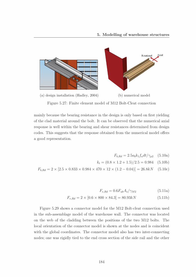
5. Modelling of warehouse structures
(a) design installation (Hadley, 2004) (b) numerical model
Figure 5.27: Finite element model of M12 Bolt-Cleat connection
mainly because the bearing resistance in the design is only based on first yielding
of the clad material around the bolt. It can be observed that the numerical axial
response is well within the bearing and shear resistances determined from design
codes. This suggests that the response obtained from the numerical model offers
a good representation.
Fb,Rd = 2.5abk1fudt/γμ2 (5.10a)
kt = (0.8× 1.2 + 1.5)/2.5 = 0.984 (5.10b)
Fb,Rd = 2× [2.5× 0.833× 0.984× 470× 12× (1.2− 0.04)] = 26.8kN (5.10c)
Fv,Rd = 0.6FubAs/γM2 (5.11a)
Fv,Rd = 2× [0.6× 800× 84.3] = 80.93kN (5.11b)
Figure 5.29 shows a connector model for the M12 Bolt-cleat connection used
in the sub-assemblage model of the warehouse wall. The connector was located
on the web of the cladding between the positions of the two M12 bolts. The
local orientation of the connector model is shown at the nodes and is coincident
with the global coordinates. The connector model also has two inter-connecting
nodes; one was rigidly tied to the end cross section of the side rail and the other
184
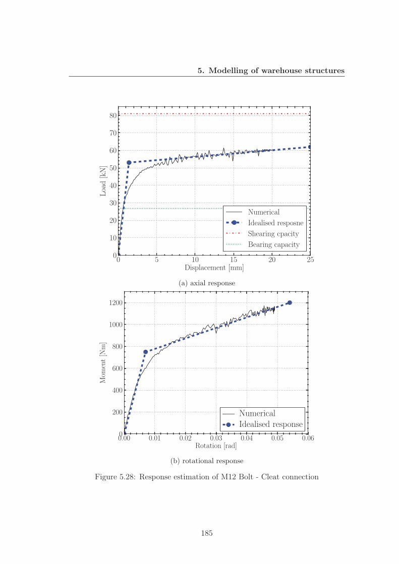
5. Modelling of warehouse structures
0 5 10 15 20 25Displacement [mm]
0
10
20
30
40
50
60
70
80
Load[kN]
Numerical
Idealised resposne
Shearing cpacity
Bearing capacity
(a) axial response
0.00 0.01 0.02 0.03 0.04 0.05 0.06Rotation [rad]
0
200
400
600
800
1000
1200
Mom
ent[Nm]
NumericalIdealised response
(b) rotational response
Figure 5.28: Response estimation of M12 Bolt - Cleat connection
185
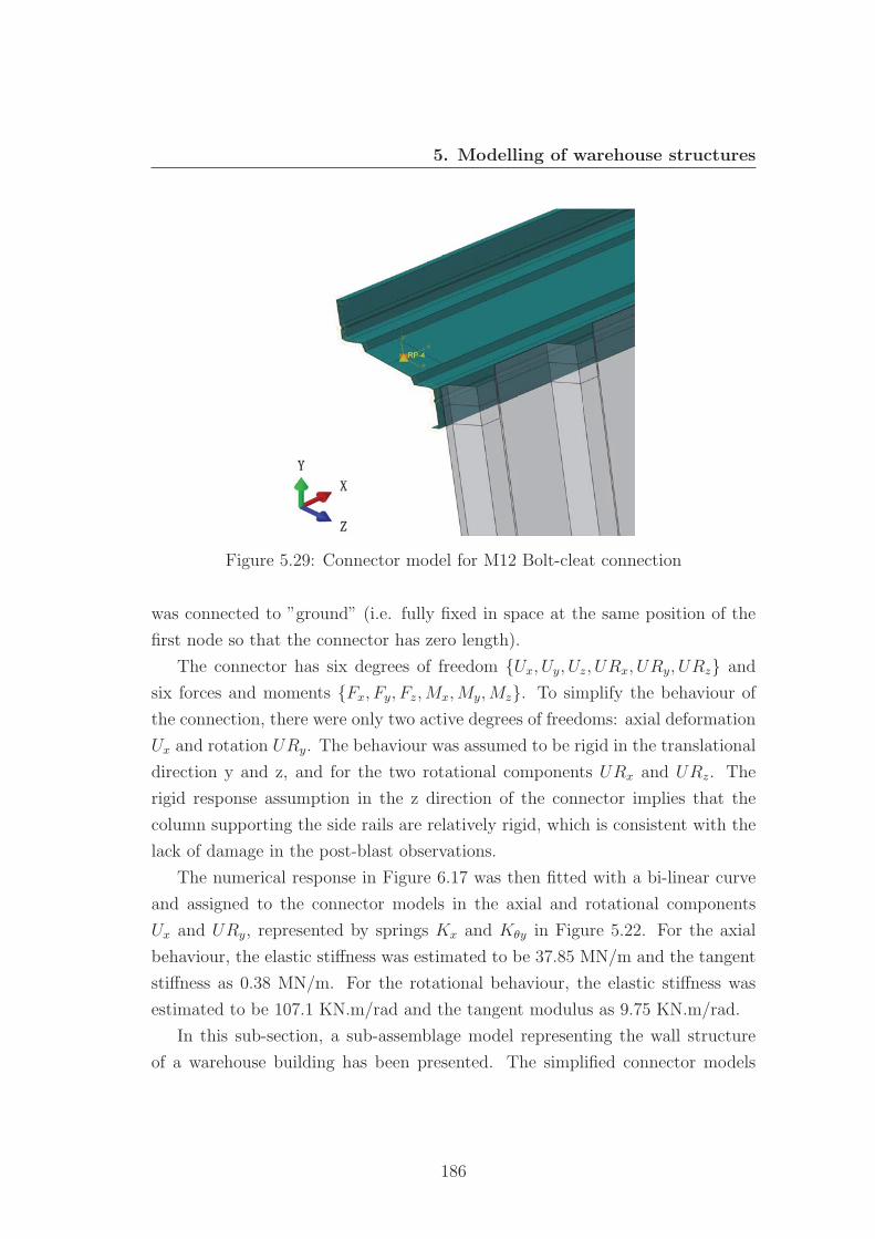
5. Modelling of warehouse structures
Figure 5.29: Connector model for M12 Bolt-cleat connection
was connected to ”ground” (i.e. fully fixed in space at the same position of the
first node so that the connector has zero length).
The connector has six degrees of freedom {Ux, Uy, Uz, URx, URy, URz} and
six forces and moments {Fx, Fy, Fz,Mx,My,Mz}. To simplify the behaviour of
the connection, there were only two active degrees of freedoms: axial deformation
Ux and rotation URy. The behaviour was assumed to be rigid in the translational
direction y and z, and for the two rotational components URx and URz. The
rigid response assumption in the z direction of the connector implies that the
column supporting the side rails are relatively rigid, which is consistent with the
lack of damage in the post-blast observations.
The numerical response in Figure 6.17 was then fitted with a bi-linear curve
and assigned to the connector models in the axial and rotational components
Ux and URy, represented by springs Kx and Kθy in Figure 5.22. For the axial
behaviour, the elastic stiffness was estimated to be 37.85 MN/m and the tangent
stiffness as 0.38 MN/m. For the rotational behaviour, the elastic stiffness was
estimated to be 107.1 KN.m/rad and the tangent modulus as 9.75 KN.m/rad.
In this sub-section, a sub-assemblage model representing the wall structure
of a warehouse building has been presented. The simplified connector models
186
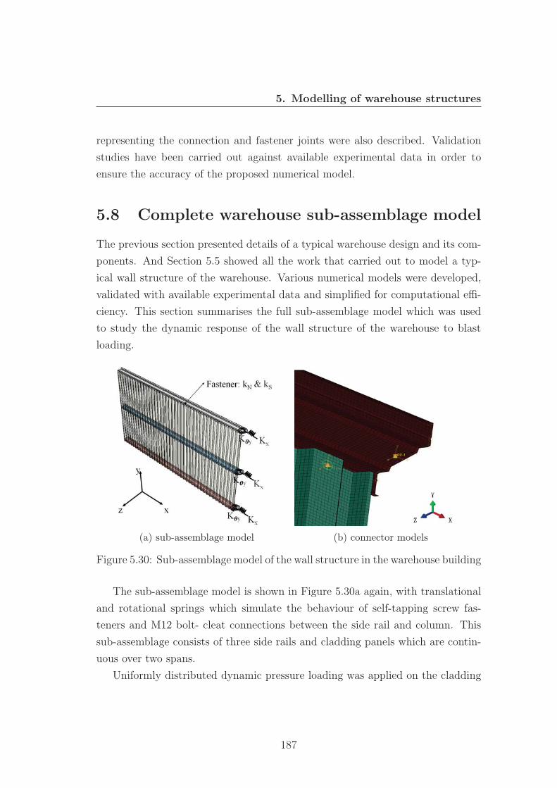
5. Modelling of warehouse structures
representing the connection and fastener joints were also described. Validation
studies have been carried out against available experimental data in order to
ensure the accuracy of the proposed numerical model.
5.8 Complete warehouse sub-assemblage model
The previous section presented details of a typical warehouse design and its com-
ponents. And Section 5.5 showed all the work that carried out to model a typ-
ical wall structure of the warehouse. Various numerical models were developed,
validated with available experimental data and simplified for computational effi-
ciency. This section summarises the full sub-assemblage model which was used
to study the dynamic response of the wall structure of the warehouse to blast
loading.
(a) sub-assemblage model (b) connector models
Figure 5.30: Sub-assemblage model of the wall structure in the warehouse building
The sub-assemblage model is shown in Figure 5.30a again, with translational
and rotational springs which simulate the behaviour of self-tapping screw fas-
teners and M12 bolt- cleat connections between the side rail and column. This
sub-assemblage consists of three side rails and cladding panels which are contin-
uous over two spans.
Uniformly distributed dynamic pressure loading was applied on the cladding
187
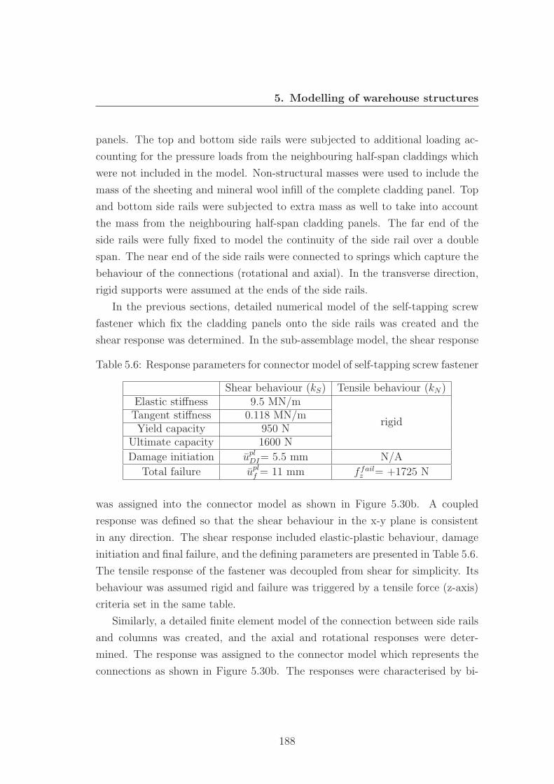
5. Modelling of warehouse structures
panels. The top and bottom side rails were subjected to additional loading ac-
counting for the pressure loads from the neighbouring half-span claddings which
were not included in the model. Non-structural masses were used to include the
mass of the sheeting and mineral wool infill of the complete cladding panel. Top
and bottom side rails were subjected to extra mass as well to take into account
the mass from the neighbouring half-span cladding panels. The far end of the
side rails were fully fixed to model the continuity of the side rail over a double
span. The near end of the side rails were connected to springs which capture the
behaviour of the connections (rotational and axial). In the transverse direction,
rigid supports were assumed at the ends of the side rails.
In the previous sections, detailed numerical model of the self-tapping screw
fastener which fix the cladding panels onto the side rails was created and the
shear response was determined. In the sub-assemblage model, the shear response
Table 5.6: Response parameters for connector model of self-tapping screw fastener
Shear behaviour (kS) Tensile behaviour (kN)Elastic stiffness 9.5 MN/m
rigidTangent stiffness 0.118 MN/mYield capacity 950 N
Ultimate capacity 1600 N
Damage initiation uplDI= 5.5 mm N/A
Total failure uplf = 11 mm f fail
z = +1725 N
was assigned into the connector model as shown in Figure 5.30b. A coupled
response was defined so that the shear behaviour in the x-y plane is consistent
in any direction. The shear response included elastic-plastic behaviour, damage
initiation and final failure, and the defining parameters are presented in Table 5.6.
The tensile response of the fastener was decoupled from shear for simplicity. Its
behaviour was assumed rigid and failure was triggered by a tensile force (z-axis)
criteria set in the same table.
Similarly, a detailed finite element model of the connection between side rails
and columns was created, and the axial and rotational responses were deter-
mined. The response was assigned to the connector model which represents the
connections as shown in Figure 5.30b. The responses were characterised by bi-
188
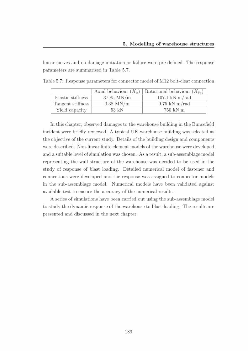
5. Modelling of warehouse structures
linear curves and no damage initiation or failure were pre-defined. The response
parameters are summarised in Table 5.7.
Table 5.7: Response parameters for connector model of M12 bolt-cleat connection
Axial behaviour (Kx) Rotational behaviour (Kθy)Elastic stiffness 37.85 MN/m 107.1 kN.m/radTangent stiffness 0.38 MN/m 9.75 kN.m/radYield capacity 53 kN 750 kN.m
In this chapter, observed damages to the warehouse building in the Buncefield
incident were briefly reviewed. A typical UK warehouse building was selected as
the objective of the current study. Details of the building design and components
were described. Non-linear finite element models of the warehouse were developed
and a suitable level of simulation was chosen. As a result, a sub-assemblage model
representing the wall structure of the warehouse was decided to be used in the
study of response of blast loading. Detailed numerical model of fastener and
connections were developed and the response was assigned to connector models
in the sub-assemblage model. Numerical models have been validated against
available test to ensure the accuracy of the numerical results.
A series of simulations have been carried out using the sub-assemblage model
to study the dynamic response of the warehouse to blast loading. The results are
presented and discussed in the next chapter.
189
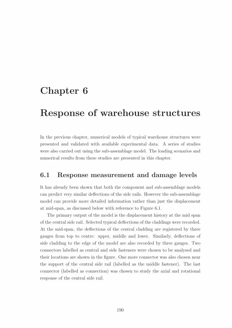
Chapter 6
Response of warehouse structures
In the previous chapter, numerical models of typical warehouse structures were
presented and validated with available experimental data. A series of studies
were also carried out using the sub-assemblage model. The loading scenarios and
numerical results from these studies are presented in this chapter.
6.1 Response measurement and damage levels
It has already been shown that both the component and sub-assemblage models
can predict very similar deflections of the side rails. However the sub-assemblage
model can provide more detailed information rather than just the displacement
at mid-span, as discussed below with reference to Figure 6.1.
The primary output of the model is the displacement history at the mid span
of the central side rail. Selected typical deflections of the claddings were recorded.
At the mid-span, the deflections of the central cladding are registered by three
gauges from top to centre: upper, middle and lower. Similarly, deflections of
side cladding to the edge of the model are also recorded by three gauges. Two
connectors labelled as central and side fasteners were chosen to be analysed and
their locations are shown in the figure. One more connector was also chosen near
the support of the central side rail (labelled as the middle fastener). The last
connector (labelled as connection) was chosen to study the axial and rotational
response of the central side rail.
190
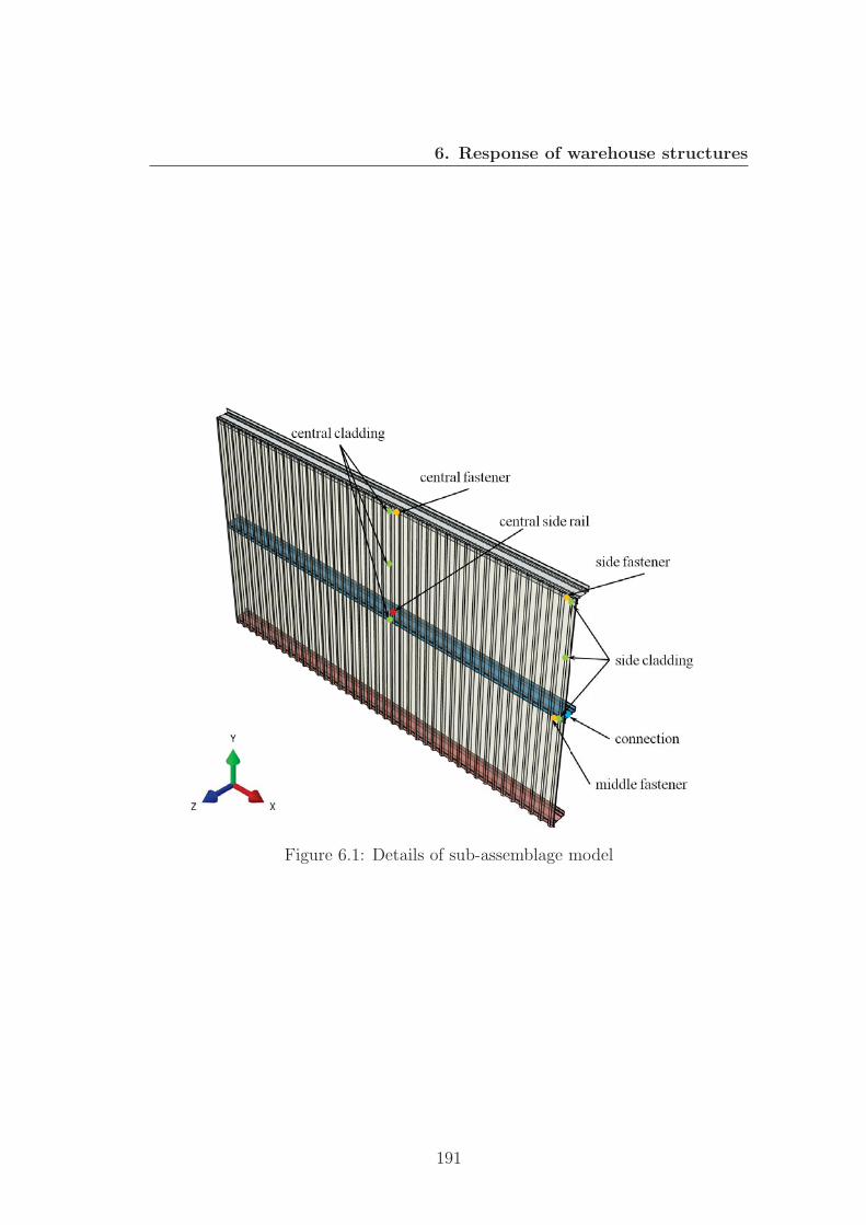
6. Response of warehouse structures
Figure 6.1: Details of sub-assemblage model
191
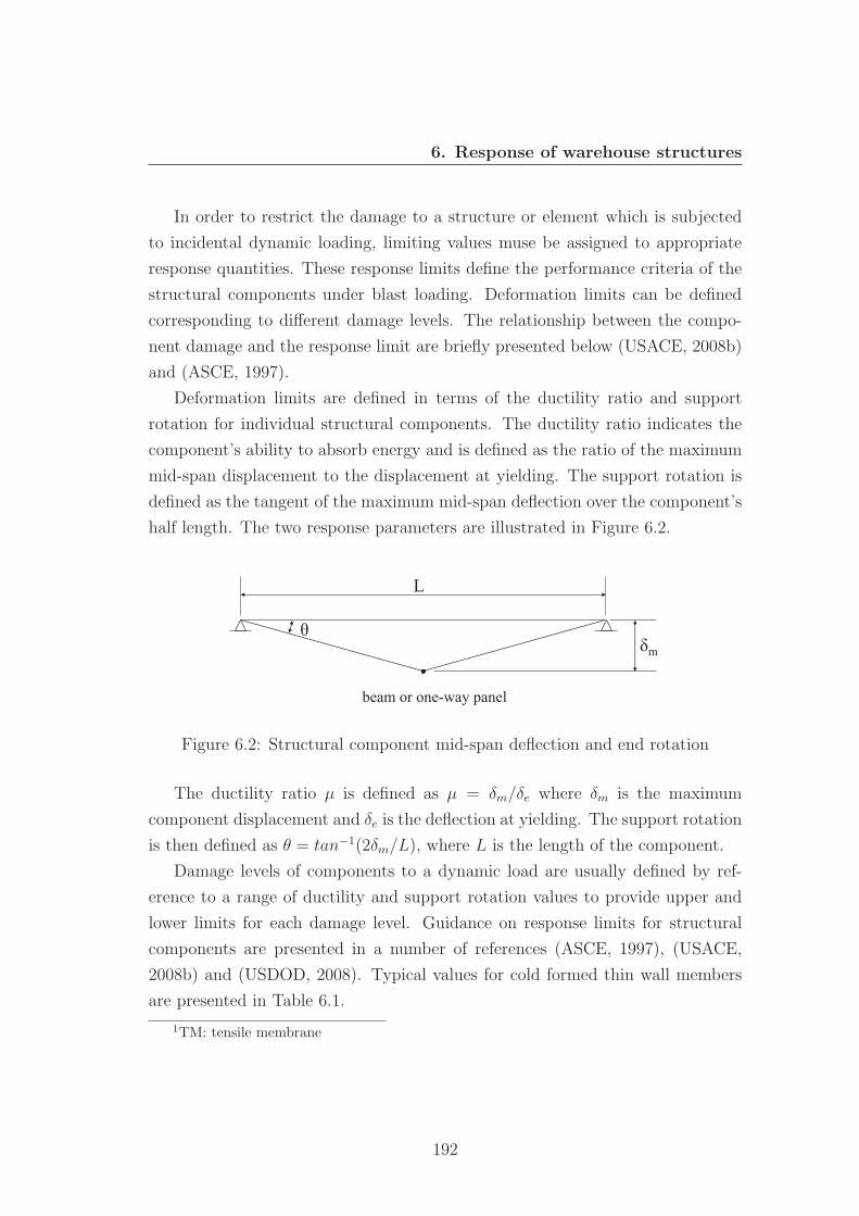
6. Response of warehouse structures
In order to restrict the damage to a structure or element which is subjected
to incidental dynamic loading, limiting values muse be assigned to appropriate
response quantities. These response limits define the performance criteria of the
structural components under blast loading. Deformation limits can be defined
corresponding to different damage levels. The relationship between the compo-
nent damage and the response limit are briefly presented below (USACE, 2008b)
and (ASCE, 1997).
Deformation limits are defined in terms of the ductility ratio and support
rotation for individual structural components. The ductility ratio indicates the
component’s ability to absorb energy and is defined as the ratio of the maximum
mid-span displacement to the displacement at yielding. The support rotation is
defined as the tangent of the maximum mid-span deflection over the component’s
half length. The two response parameters are illustrated in Figure 6.2.
L
δm θ
beam or one-way panel
Figure 6.2: Structural component mid-span deflection and end rotation
The ductility ratio μ is defined as μ = δm/δe where δm is the maximum
component displacement and δe is the deflection at yielding. The support rotation
is then defined as θ = tan−1(2δm/L), where L is the length of the component.
Damage levels of components to a dynamic load are usually defined by ref-
erence to a range of ductility and support rotation values to provide upper and
lower limits for each damage level. Guidance on response limits for structural
components are presented in a number of references (ASCE, 1997), (USACE,
2008b) and (USDOD, 2008). Typical values for cold formed thin wall members
are presented in Table 6.1.
1TM: tensile membrane
192
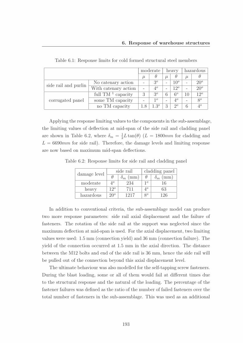
6. Response of warehouse structures
Table 6.1: Response limits for cold formed structural steel members
moderate heavy hazardousμ θ μ θ μ θ
side rail and purlinNo catenary action - 3o - 10o - 20o
With catenary action - 4o - 12o - 20o
corrugated panelfull TM 1 capacity 3 3o 6 6o 10 12o
some TM capacity - 1o - 4o - 8o
no TM capacity 1.8 1.3o 3 2o 6 4o
Applying the response limiting values to the components in the sub-assemblage,
the limiting values of deflection at mid-span of the side rail and cladding panel
are shown in Table 6.2, where δm = 12L tan(θ) (L = 1800mm for cladding and
L = 6690mm for side rail). Therefore, the damage levels and limiting response
are now based on maximum mid-span deflections.
Table 6.2: Response limits for side rail and cladding panel
damage levelside rail cladding panel
θ δm (mm) θ δm (mm)moderate 4o 234 1o 16heavy 12o 711 4o 63
hazardous 20o 1217 8o 126
In addition to conventional criteria, the sub-assemblage model can produce
two more response parameters: side rail axial displacement and the failure of
fasteners. The rotation of the side rail at the support was neglected since the
maximum deflection at mid-span is used. For the axial displacement, two limiting
values were used: 1.5 mm (connection yield) and 36 mm (connection failure). The
yield of the connection occurred at 1.5 mm in the axial direction. The distance
between the M12 bolts and end of the side rail is 36 mm, hence the side rail will
be pulled out of the connection beyond this axial displacement level.
The ultimate behaviour was also modelled for the self-tapping screw fasteners.
During the blast loading, some or all of them would fail at different times due
to the structural response and the natural of the loading. The percentage of the
fastener failures was defined as the ratio of the number of failed fasteners over the
total number of fasteners in the sub-assemblage. This was used as an additional
193
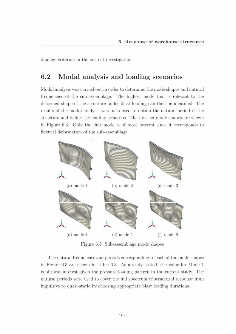
6. Response of warehouse structures
damage criterion in the current investigation.
6.2 Modal analysis and loading scenarios
Modal analysis was carried out in order to determine the mode shapes and natural
frequencies of the sub-assemblage. The highest mode that is relevant to the
deformed shape of the structure under blast loading can then be identified. The
results of the modal analysis were also used to obtain the natural period of the
structure and define the loading scenarios. The first six mode shapes are shown
in Figure 6.3. Only the first mode is of most interest since it corresponds to
flexural deformation of the sub-assemblage.
(a) mode 1 (b) mode 2 (c) mode 3
(d) mode 4 (e) mode 5 (f) mode 6
Figure 6.3: Sub-assemblage mode shapes
The natural frequencies and periods corresponding to each of the mode shapes
in Figure 6.3 are shown in Table 6.3. As already stated, the value for Mode 1
is of most interest given the pressure loading pattern in the current study. The
natural periods were used to cover the full spectrum of structural response from
impulsive to quasi-static by choosing appropriate blast loading durations.
194
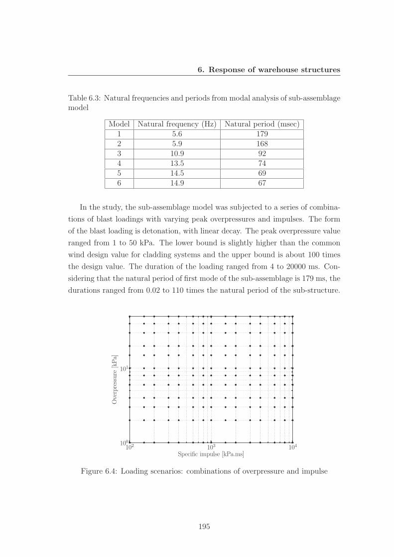
6. Response of warehouse structures
Table 6.3: Natural frequencies and periods from modal analysis of sub-assemblagemodel
Model Natural frequency (Hz) Natural period (msec)1 5.6 1792 5.9 1683 10.9 924 13.5 745 14.5 696 14.9 67
In the study, the sub-assemblage model was subjected to a series of combina-
tions of blast loadings with varying peak overpressures and impulses. The form
of the blast loading is detonation, with linear decay. The peak overpressure value
ranged from 1 to 50 kPa. The lower bound is slightly higher than the common
wind design value for cladding systems and the upper bound is about 100 times
the design value. The duration of the loading ranged from 4 to 20000 ms. Con-
sidering that the natural period of first mode of the sub-assemblage is 179 ms, the
durations ranged from 0.02 to 110 times the natural period of the sub-structure.
102 103 104
Specific impulse [kPa.ms]
100
101
Overpressure
[kPa]
Figure 6.4: Loading scenarios: combinations of overpressure and impulse
195
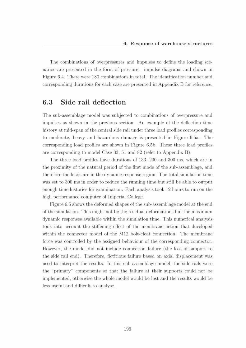
6. Response of warehouse structures
The combinations of overpressures and impulses to define the loading sce-
narios are presented in the form of pressure - impulse diagrams and shown in
Figure 6.4. There were 180 combinations in total. The identification number and
corresponding durations for each case are presented in Appendix B for reference.
6.3 Side rail deflection
The sub-assemblage model was subjected to combinations of overpressure and
impulses as shown in the previous section. An example of the deflection time
history at mid-span of the central side rail under three load profiles corresponding
to moderate, heavy and hazardous damage is presented in Figure 6.5a. The
corresponding load profiles are shown in Figure 6.5b. These three load profiles
are corresponding to model Case 33, 51 and 82 (refer to Appendix B).
The three load profiles have durations of 133, 200 and 300 ms, which are in
the proximity of the natural period of the first mode of the sub-assemblage, and
therefore the loads are in the dynamic response region. The total simulation time
was set to 300 ms in order to reduce the running time but still be able to output
enough time histories for examination. Each analysis took 12 hours to run on the
high performance computer of Imperial College.
Figure 6.6 shows the deformed shapes of the sub-assemblage model at the end
of the simulation. This might not be the residual deformations but the maximum
dynamic responses available within the simulation time. This numerical analysis
took into account the stiffening effect of the membrane action that developed
within the connector model of the M12 bolt-cleat connection. The membrane
force was controlled by the assigned behaviour of the corresponding connector.
However, the model did not include connection failure (the loss of support to
the side rail end). Therefore, fictitious failure based on axial displacement was
used to interpret the results. In this sub-assemblage model, the side rails were
the ”primary” components so that the failure at their supports could not be
implemented, otherwise the whole model would be lost and the results would be
less useful and difficult to analyse.
196
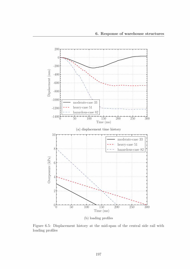
6. Response of warehouse structures
0 50 100 150 200 250 300Time (ms)
-1400
-1200
-1000
-800
-600
-400
-200
0
200Dipslacem
ent(m
m)
moderate-case 33
heavy-case 51
hazardous-case 82
(a) displacement time history
0 50 100 150 200 250 300Time (ms)
0
2
4
6
8
10
Overpessure
(kPa)
moderate-case 33
heavy-case 51
hazardous-case 82
(b) loading profiles
Figure 6.5: Displacement history at the mid-span of the central side rail withloading profiles
197
6. Response of warehouse structures
(a) Case 33 (b) Case 51 (c) Case 82
Figure 6.6: Deformed shapes of the sub-assemblage
6.4 Cladding and fasteners
The behaviour of fasteners was completely defined in the connector model, in-
cluding the stiffness, plastic hardening, damage and failure. An example of the
detailed response of the central fastener in Case 98 (the blast profile has peak
pressure of 10kPa, impulse of 1000kPa.ms and the duration was 200ms) is shown
in Figure 6.7. The load defined in this case is dynamic.
Figure 6.7a presents the details of the time response of the central fastener,
which include the displacements, shear and normal forces, damage and failure.
The damage history indicates the time of initiation and failure. The resultant
displacement (ushear) at the damage initiation and failure were calculated and
noted in the figure (5.35 and 10.81 mm). The resultant displacement ushear was
defined as ushear =√
ux2 + uy
2 by the component displacement ux and uy in
the x and y direction respectively. The shear force fshear was determined in the
same manner, and the numerical relation between shear displacement and force
is presented in Figure 6.7b. The numerical shear response is then compared with
the pre-defined behaviour of the connector model.
It can be seen that the numerical response of the connector is in good agree-
ment with the pre-defined path except for a short unloading-reloading period.
The damage initiated at 5.35 mm and failure occurred at 10.81 mm, and both
are very close to the pre-defined values (5.5 and 11 mm). The discrepancies
are attributed to the cumulative plastic deformation in the connector during the
198
6. Response of warehouse structures
variation of shear force, which shifted the hardening curve slightly upwards and
subsequently the damage degradation curve to the left. The numerical response
path is reasonably clear and the damage initiation as well as failure can be easily
identified.
0 20 40 60 80 100 120 140Time(ms)
-20
-15
-10
-5
0
5
10
15
20
ConnectorDipslacem
ent(m
m) ux
uyushear
fshear
fnormal
failure
damage
dmg int: 5.35mm
failure: 10.81mm
-5
-4
-3
-2
-1
0
1
2
ConnectorForce
(kN)
0.0
0.2
0.4
0.6
0.8
1.0
Dam
age/Failure
(a) details of fastener time response
0 2 4 6 8 10 12Fastener in-plane dispalcement (mm)
0.0
0.5
1.0
1.5
2.0
Fastener
shearforce(kN)
Actual response
Defined response
(b) fastener response curves
Figure 6.7: Response of central fastener of the sub-assemblage model in Case 98
As shown in Figure 6.7a, the resultant displacement curve ushear is almost
identical to the displacement in the y direction uy, which suggests that the fas-
tener damage and failure occurred in the y direction. The normal force exerted
in the connector is also shown in Figure 6.7a, and the results indicate that the
199
6. Response of warehouse structures
fastener was mainly subjected to compressive force throughout the time history
before failure.
The cladding response was measured at three locations as shown in Figure 6.1.
An example of the displacement time response of the central cladding subject to
blast loading as defined in Case 98 is shown in Figure 6.8. Figure 6.8a shows
the displacement time histories at the three locations on the cladding: upper,
middle and lower. The displacement at the middle point relative to the average
displacement of the upper and lower points, determined as Urelative =12(Uupper +
Ulower), is also shown in the figure. Finally, Figure 6.8a was completed with the
failure time history of the corresponding central fastener (presented in Figure
6.7). The relative displacement at the middle of the central cladding was then
related to the failure of the corresponding fastener as shown in Figure 6.8b. It
can be seen that the shear failure in the y-direction of the fastener occurred at a
displacement of -81.66 mm.
The same analysis was applied to both the side and central claddings of the
sub-assemblage in all loading cases. Figure 6.9a represents the relative displace-
ment at the middle of the central cladding with failure of the corresponding
fastener for all cases, while Figure 6.9b represents the same results for the side
cladding. Thus, these two figures aim to relate the displacement at the middle of
the cladding to the failure of end fasteners in the full spectrum of overpressures
and impulses.
It is interesting to note that in these two figures the displacement at failure
of the fastener varies with the response of the cladding. However, in the Region
I of Figure 6.9a, the relative displacement at the central fastener failure was
consistently about 81 mm. Similarly, in the Region I of Figure 6.9b the relative
displacements at failure of the side fastener was typically about 89 mm. Thus,
in general it can be observed that the relative middle displacement at the failure
of the corresponding fasteners is approximately [−81 + (−89)]/2 = −85mm,
although this value only applies to cases in region I in Figure 6.9.
It can be noted that in Region II of Figure 6.9, the results show a very differ-
ent relation between the cladding displacements and the failure of corresponding
fasteners. In Region II of Figure 6.9a the fastener failures occurred much earlier
at lower displacements of central cladding. In fact, most of the failure occurred
200
6. Response of warehouse structures
0 50 100 150 200 250 300Time (ms)
-3000
-2500
-2000
-1500
-1000
-500
0
500
Dipslacem
ent(m
m)
0.0
0.2
0.4
0.6
0.8
1.0
Failure
Status
Uupper
Umiddle
Ulower
Urelative
failure
(a) cladding response
0 50 100 150 200 250 300Time (ms)
-200
-150
-100
-50
0
50
100
Dipslacem
ent(m
m)
Urelative
connector failure
(b) relative displ. with fastener failure
Figure 6.8: Response of central cladding of the sub-assemblage in Case 98
201
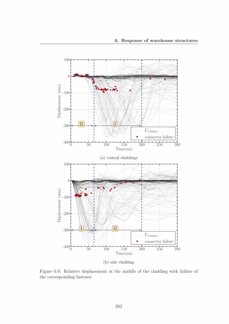
6. Response of warehouse structures
0 50 100 150 200 250 300Time(ms)
-400
-300
-200
-100
0
100Dipslacem
ent(m
m)
II I
Urelative
connector failure
(a) central claddings
0 50 100 150 200 250 300Time(ms)
-400
-300
-200
-100
0
100
Dipslacem
ent(m
m)
I II
Urelative
connector failure
(b) side cladding
Figure 6.9: Relative displacement at the middle of the cladding with failure ofthe corresponding fastener
202
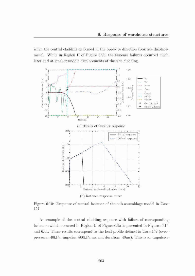
6. Response of warehouse structures
when the central cladding deformed in the opposite direction (positive displace-
ment). While in Region II of Figure 6.9b, the fastener failures occurred much
later and at smaller middle displacements of the side cladding.
0 10 20 30 40 50 60Time(ms)
-20
-15
-10
-5
0
5
10
15
20
ConnectorDipslacem
ent(m
m) ux
uyushear
fshear
fnormal
failure
damage
dmg int: N/A
failure: 2.47mm
-2.5
-2.0
-1.5
-1.0
-0.5
0.0
0.5
1.0
1.5
ConnectorForce
(kN)
0.0
0.2
0.4
0.6
0.8
1.0
Dam
age/Failure
(a) details of fastener response
0 2 4 6 8 10 12Fastener in-plane dispalcement (mm)
0.0
0.5
1.0
1.5
2.0
Fastener
shearforce(kN)
Actual response
Defined response
(b) fastener response curve
Figure 6.10: Response of central fastener of the sub-assemblage model in Case157
An example of the central cladding response with failure of corresponding
fasteners which occurred in Region II of Figure 6.9a is presented in Figures 6.10
and 6.11. These results correspond to the load profile defined in Case 157 (over-
pressure: 40kPa, impulse: 800kPa.ms and duration: 40ms). This is an impulsive
203
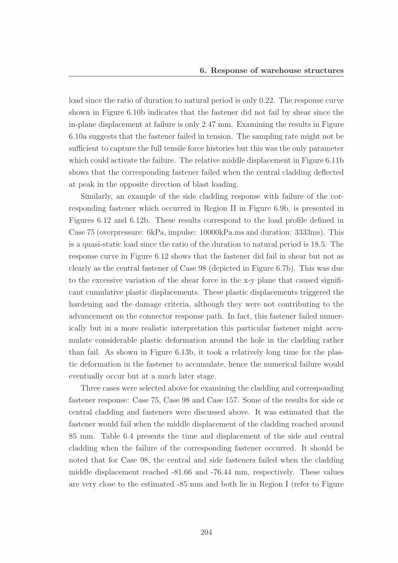
6. Response of warehouse structures
load since the ratio of duration to natural period is only 0.22. The response curve
shown in Figure 6.10b indicates that the fastener did not fail by shear since the
in-plane displacement at failure is only 2.47 mm. Examining the results in Figure
6.10a suggests that the fastener failed in tension. The sampling rate might not be
sufficient to capture the full tensile force histories but this was the only parameter
which could activate the failure. The relative middle displacement in Figure 6.11b
shows that the corresponding fastener failed when the central cladding deflected
at peak in the opposite direction of blast loading.
Similarly, an example of the side cladding response with failure of the cor-
responding fastener which occurred in Region II in Figure 6.9b, is presented in
Figures 6.12 and 6.12b. These results correspond to the load profile defined in
Case 75 (overpressure: 6kPa, impulse: 10000kPa.ms and duration: 3333ms). This
is a quasi-static load since the ratio of the duration to natural period is 18.5. The
response curve in Figure 6.12 shows that the fastener did fail in shear but not as
clearly as the central fastener of Case 98 (depicted in Figure 6.7b). This was due
to the excessive variation of the shear force in the x-y plane that caused signifi-
cant cumulative plastic displacements. These plastic displacements triggered the
hardening and the damage criteria, although they were not contributing to the
advancement on the connector response path. In fact, this fastener failed numer-
ically but in a more realistic interpretation this particular fastener might accu-
mulate considerable plastic deformation around the hole in the cladding rather
than fail. As shown in Figure 6.13b, it took a relatively long time for the plas-
tic deformation in the fastener to accumulate, hence the numerical failure would
eventually occur but at a much later stage.
Three cases were selected above for examining the cladding and corresponding
fastener response: Case 75, Case 98 and Case 157. Some of the results for side or
central cladding and fasteners were discussed above. It was estimated that the
fastener would fail when the middle displacement of the cladding reached around
85 mm. Table 6.4 presents the time and displacement of the side and central
cladding when the failure of the corresponding fastener occurred. It should be
noted that for Case 98, the central and side fasteners failed when the cladding
middle displacement reached -81.66 and -76.44 mm, respectively. These values
are very close to the estimated -85 mm and both lie in Region I (refer to Figure
204
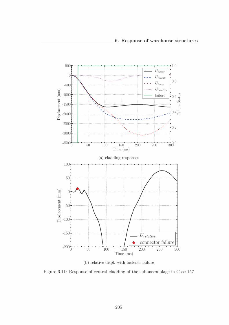
6. Response of warehouse structures
0 50 100 150 200 250 300Time (ms)
-3500
-3000
-2500
-2000
-1500
-1000
-500
0
500
Dipslacem
ent(m
m)
0.0
0.2
0.4
0.6
0.8
1.0
Failure
Status
Uupper
Umiddle
Ulower
Urelative
failure
(a) cladding responses
0 50 100 150 200 250 300Time (ms)
-200
-150
-100
-50
0
50
100
Dipslacem
ent(m
m)
Urelative
connector failure
(b) relative displ. with fastener failure
Figure 6.11: Response of central cladding of the sub-assemblage in Case 157
205
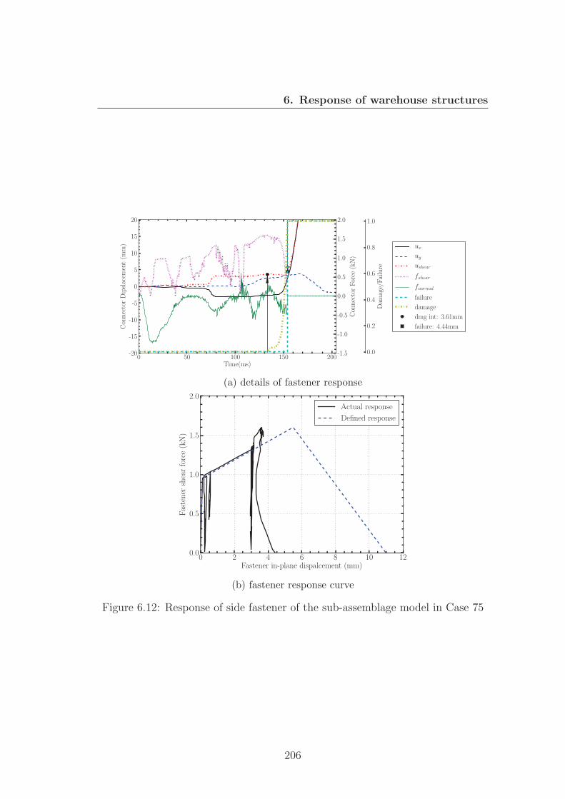
6. Response of warehouse structures
0 50 100 150 200Time(ms)
-20
-15
-10
-5
0
5
10
15
20
ConnectorDipslacem
ent(m
m) ux
uyushear
fshear
fnormal
failure
damage
dmg int: 3.61mm
failure: 4.44mm
-1.5
-1.0
-0.5
0.0
0.5
1.0
1.5
2.0
ConnectorForce
(kN)
0.0
0.2
0.4
0.6
0.8
1.0
Dam
age/Failure
(a) details of fastener response
0 2 4 6 8 10 12Fastener in-plane dispalcement (mm)
0.0
0.5
1.0
1.5
2.0
Fastener
shearforce(kN)
Actual response
Defined response
(b) fastener response curve
Figure 6.12: Response of side fastener of the sub-assemblage model in Case 75
206
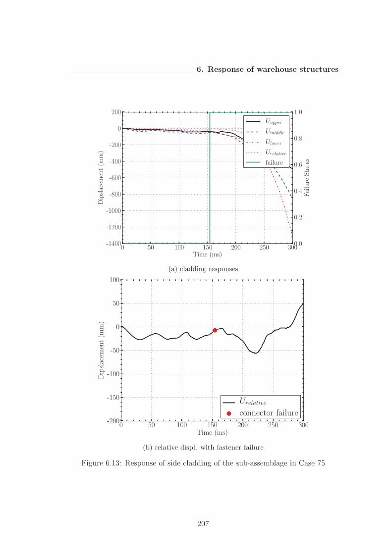
6. Response of warehouse structures
0 50 100 150 200 250 300Time (ms)
-1400
-1200
-1000
-800
-600
-400
-200
0
200
Dipslacem
ent(m
m)
0.0
0.2
0.4
0.6
0.8
1.0
Failure
Status
Uupper
Umiddle
Ulower
Urelative
failure
(a) cladding responses
0 50 100 150 200 250 300Time (ms)
-200
-150
-100
-50
0
50
100
Dipslacem
ent(m
m)
Urelative
connector failure
(b) relative displ. with fastener failure
Figure 6.13: Response of side cladding of the sub-assemblage in Case 75
207
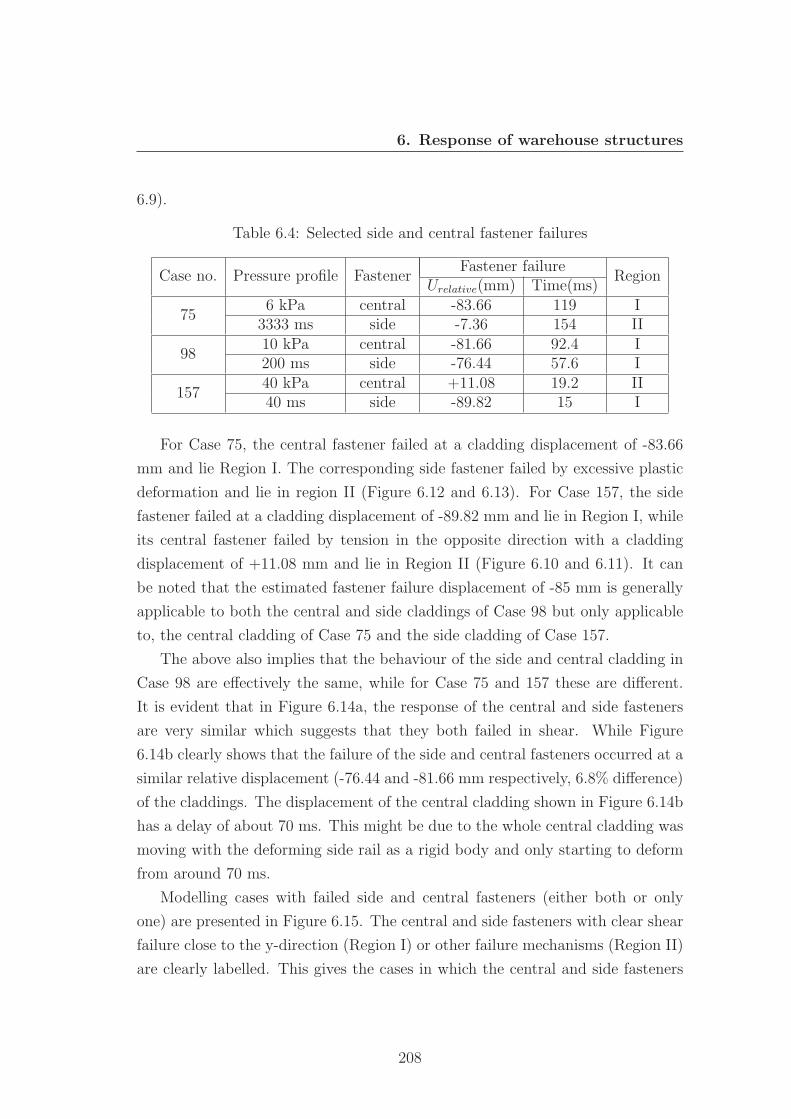
6. Response of warehouse structures
6.9).
Table 6.4: Selected side and central fastener failures
Case no. Pressure profile FastenerFastener failure
RegionUrelative(mm) Time(ms)
756 kPa central -83.66 119 I
3333 ms side -7.36 154 II
9810 kPa central -81.66 92.4 I200 ms side -76.44 57.6 I
15740 kPa central +11.08 19.2 II40 ms side -89.82 15 I
For Case 75, the central fastener failed at a cladding displacement of -83.66
mm and lie Region I. The corresponding side fastener failed by excessive plastic
deformation and lie in region II (Figure 6.12 and 6.13). For Case 157, the side
fastener failed at a cladding displacement of -89.82 mm and lie in Region I, while
its central fastener failed by tension in the opposite direction with a cladding
displacement of +11.08 mm and lie in Region II (Figure 6.10 and 6.11). It can
be noted that the estimated fastener failure displacement of -85 mm is generally
applicable to both the central and side claddings of Case 98 but only applicable
to, the central cladding of Case 75 and the side cladding of Case 157.
The above also implies that the behaviour of the side and central cladding in
Case 98 are effectively the same, while for Case 75 and 157 these are different.
It is evident that in Figure 6.14a, the response of the central and side fasteners
are very similar which suggests that they both failed in shear. While Figure
6.14b clearly shows that the failure of the side and central fasteners occurred at a
similar relative displacement (-76.44 and -81.66 mm respectively, 6.8% difference)
of the claddings. The displacement of the central cladding shown in Figure 6.14b
has a delay of about 70 ms. This might be due to the whole central cladding was
moving with the deforming side rail as a rigid body and only starting to deform
from around 70 ms.
Modelling cases with failed side and central fasteners (either both or only
one) are presented in Figure 6.15. The central and side fasteners with clear shear
failure close to the y-direction (Region I) or other failure mechanisms (Region II)
are clearly labelled. This gives the cases in which the central and side fasteners
208
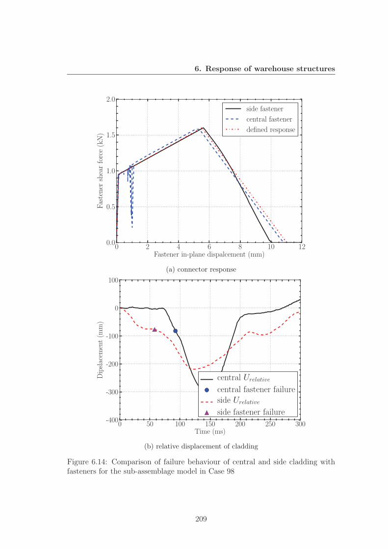
6. Response of warehouse structures
0 2 4 6 8 10 12Fastener in-plane dispalcement (mm)
0.0
0.5
1.0
1.5
2.0Fastener
shearforce(kN)
side fastener
central fastener
defined response
(a) connector response
0 50 100 150 200 250 300Time (ms)
-400
-300
-200
-100
0
100
Dipslacem
ent(m
m)
central Urelative
central fastener failureside Urelative
side fastener failure
(b) relative displacement of cladding
Figure 6.14: Comparison of failure behaviour of central and side cladding withfasteners for the sub-assemblage model in Case 98
209
6. Response of warehouse structures
both failed in shear (Region I): Cases 98, 100-105, 111-113, 126, 127 and 141.
These cases are labelled as ’identical failure F’. Unfortunately, the increments of
overpressure and impulse are not small enough to define precisely a zone in which
the failure response of the cladding and corresponding fasteners are identical at
both the centre and side locations. Nonetheless, these hilighted cases did provide
an indication of the appropriate regions in the pressure - impulse diagrams.
102 103 104
Specific impulse [kPa.ms]
100
101
Overpressure
[kPa]
side cladding-Fshear,I
side cladding-Fother,II
central cladding-Fshear,I
central cladding-Fother,II
identical failure F
Figure 6.15: Cases with identical failure behaviour of cladding and fasteners atcentre and side
The fasteners shown above all failed mainly in or close to the y-direction.
An example of the response of the middle fastener of the sub-assemblage model
subject to loads defined in Case 98 is shown in Figure 6.16. The response curve
in Figure 6.16b indicates that the fastener failed in shear. A close look at Figure
6.16a suggests that the damage and failure actually occurred in the x direction,
since the resultant displacement ushear is almost identical to the displacement
ux. This might be due to the insignificant forces in the y-direction since both
the upper and lower claddings were pulling the middle fastener in the opposite
direction. However, the shear force generated in the x-direction due to the relative
210
6. Response of warehouse structures
longitudinal movement of the cladding and side rail (as in a composite beam) was
significant and able to fail the fastener.
In this section, the response of typical claddings and corresponding fastener
was presented and discussed. Focus was placed on the failure of the fasteners and
the relative displacement of cladding at which the failure occurs. The displace-
ment history of the cladding and the maximum dynamic value were not examined
in detail here. The reason is that due to the inclusion of the fastener failure in the
model, the displacement of the cladding became less important. This is because
0 20 40 60 80 100Time(ms)
-20
-15
-10
-5
0
5
10
15
20
ConnectorDipslacem
ent(m
m) ux
uyushear
fshear
fnormal
failure
damage
dmg int: 5.43mm
failure: 10.71mm
-1.5
-1.0
-0.5
0.0
0.5
1.0
1.5
2.0
ConnectorForce
(kN)
0.0
0.2
0.4
0.6
0.8
1.0
Dam
age/Failure
(a) details of fastener response
0 2 4 6 8 10 12Fastener in-plane dispalcement (mm)
0.0
0.5
1.0
1.5
2.0
Fastener
shearforce(kN)
Actual response
Defined response
(b) fastener response curve
Figure 6.16: Response of middle fastener of the sub-assemblage model in Case 98
211
6. Response of warehouse structures
once the fastener fails, the cladding panels would deform significantly without any
constraints, hence the displacement after fastener failure becomes rather mean-
ingless. The displacement levels can provide useful information for the cladding
damages before fastener failure. However, in view of the overall response in the
full ranges of overpressure and impulses, the displacement can be replaced by
the failure of fasteners as one of the primary damage criteria used in the present
work.
6.5 Side rail axial response and connection be-
haviour
The connection shown in Figure 6.1 was used to represent the M12 bolt - cleat
joint between the side rail and column. In the numerical analysis, it could predict
the behaviour of the connection and the axial response of the side rail.
0 200 400 600 800 1000Connection axial dispalcement (mm)
0
10
20
30
40
50
60
70
80
Connection
axialforce(kN)
(a) axial response
-0.1 0.0 0.1 0.2 0.3 0.4 0.5 0.6 0.7 0.8Connection rotation (rad)
-1.5
-1.0
-0.5
0.0
0.5
1.0
1.5
Connection
mom
ent(kN.m
)
(b) rotational response
Figure 6.17: Numerical response of the M12 bolt-cleat connection
An example of the axial and rotational responses of the connection in the
sub-assemblage model subject to the blast load defined in Case 98 is shown in
Figure 6.17. It can be seen that significant axial displacement and rotation oc-
curred in the connection. The originally pre-defined axial and rotational be-
haviour adopted bi-linear curves with yield capacity, elastic and tangent stiffness.
The tangent stiffness however caused some numerical problems in the model.
212
6. Response of warehouse structures
It exerted large axial forces at the support which caused excessive deformation
of the shell elements and subsequently terminated the simulation prematurely.
In order to overcome this problem, the original bi-linear response curves were
modified so that they exhibit perfect-plastic behaviour after the specified level of
deformation. For the axial response, the tangent stiffness became zero after an
axial displacement of 24 mm was reached at the support (i.e. in the connector).
This is twice the diameter of the M12 bolt. For the rotational response, the tan-
gent stiffness became zero after a rotation of 4o. This corresponds to the heavy
damage of the component at the support end. The responses shown in the figure
were obtained from the modified behaviour.
An example of the axial displacement of the side rail in the sub-assemblage
model subject to load in Case 98 is shown in Figure 6.18a. The transverse dis-
placement of the side rail is shown in the same figure as well for comparison. It
can be seen in Figure 6.18a that pull-out failure (36 mm) of the connection oc-
curred a side rail transverse displacement of -405 mm. Failure of the connection
was not implemented in the model, so the loss of the side rail would not occur.
The side rail would still continue to deform at the pull-out failure but it should
be recalled when interpreting the results.
Moreover, all cases which have the axial displacement equal or greater than the
pull-out failure were plotted in Figure 6.18b. The relationship of the transverse
and axial displacement of the side rail is clear. Under most blast loading cases,
the pull-out failure would occur at a transverse displacement of 400 mm. Subject
to more intensive load and when the deforming velocity of the side rail increases,
the corresponding transverse displacement tends to decrease to 300 mm. This
is mainly due to the deformed mode being slight changed under more intensive
loads.
6.6 Combined response
In the above sections, the failure of the fasteners has been discussed, and a de-
tailed insight into the response was established. In this section, the aim is to
examine the relationship between the failure of fasteners and the displacement of
the middle side rail.
213
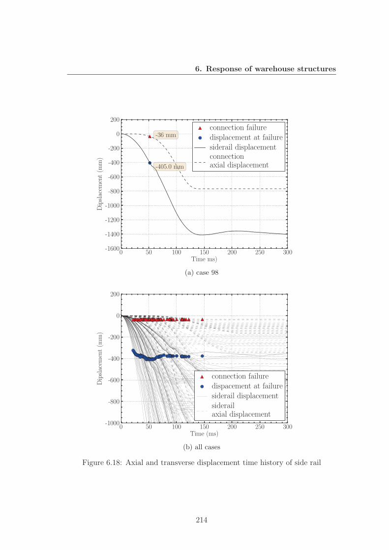
6. Response of warehouse structures
0 50 100 150 200 250 300Time ms)
-1600
-1400
-1200
-1000
-800
-600
-400
-200
0
200
Dipslacem
ent(m
m)
-405.0 mm
-36 mmconnection failuredisplacement at failuresiderail displacementconnectionaxial displacement
(a) case 98
0 50 100 150 200 250 300Time (ms)
-1000
-800
-600
-400
-200
0
200
Dipslacem
ent(m
m)
connection failuredispacement at failuresiderail displacementsiderailaxial displacement
(b) all cases
Figure 6.18: Axial and transverse displacement time history of side rail
214
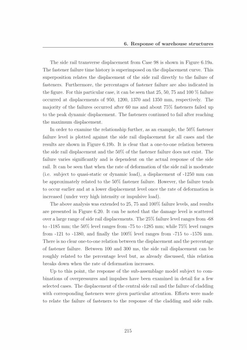
6. Response of warehouse structures
The side rail transverse displacement from Case 98 is shown in Figure 6.19a.
The fastener failure time history is superimposed on the displacement curve. This
superposition relates the displacement of the side rail directly to the failure of
fasteners. Furthermore, the percentages of fastener failure are also indicated in
the figure. For this particular case, it can be seen that 25, 50, 75 and 100 % failure
occurred at displacements of 950, 1200, 1370 and 1350 mm, respectively. The
majority of the failures occurred after 60 ms and about 75% fasteners failed up
to the peak dynamic displacement. The fasteners continued to fail after reaching
the maximum displacement.
In order to examine the relationship further, as an example, the 50% fastener
failure level is plotted against the side rail displacement for all cases and the
results are shown in Figure 6.19b. It is clear that a one-to-one relation between
the side rail displacement and the 50% of the fastener failure does not exist. The
failure varies significantly and is dependent on the actual response of the side
rail. It can be seen that when the rate of deformation of the side rail is moderate
(i.e. subject to quasi-static or dynamic load), a displacement of -1250 mm can
be approximately related to the 50% fastener failure. However, the failure tends
to occur earlier and at a lower displacement level once the rate of deformation is
increased (under very high intensity or impulsive load).
The above analysis was extended to 25, 75 and 100% failure levels, and results
are presented in Figure 6.20. It can be noted that the damage level is scattered
over a large range of side rail displacements. The 25% failure level ranges from -68
to -1185 mm; the 50% level ranges from -75 to -1285 mm; while 75% level ranges
from -121 to -1380, and finally the 100% level ranges from -715 to -1576 mm.
There is no clear one-to-one relation between the displacement and the percentage
of fastener failure. Between 100 and 300 ms, the side rail displacement can be
roughly related to the percentage level but, as already discussed, this relation
breaks down when the rate of deformation increases.
Up to this point, the response of the sub-assemblage model subject to com-
binations of overpressures and impulses have been examined in detail for a few
selected cases. The displacement of the central side rail and the failure of cladding
with corresponding fasteners were given particular attention. Efforts were made
to relate the failure of fasteners to the response of the cladding and side rails.
215
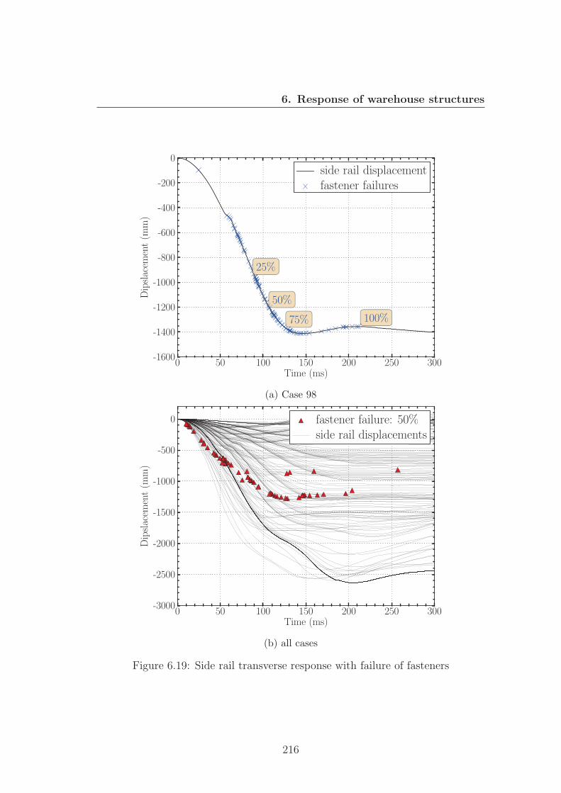
6. Response of warehouse structures
0 50 100 150 200 250 300Time (ms)
-1600
-1400
-1200
-1000
-800
-600
-400
-200
0
Dipslacem
ent(m
m)
25%
50%
75% 100%
side rail displacementfastener failures
(a) Case 98
0 50 100 150 200 250 300Time (ms)
-3000
-2500
-2000
-1500
-1000
-500
0
Dipslacem
ent(m
m)
fastener failure: 50%side rail displacements
(b) all cases
Figure 6.19: Side rail transverse response with failure of fasteners
216
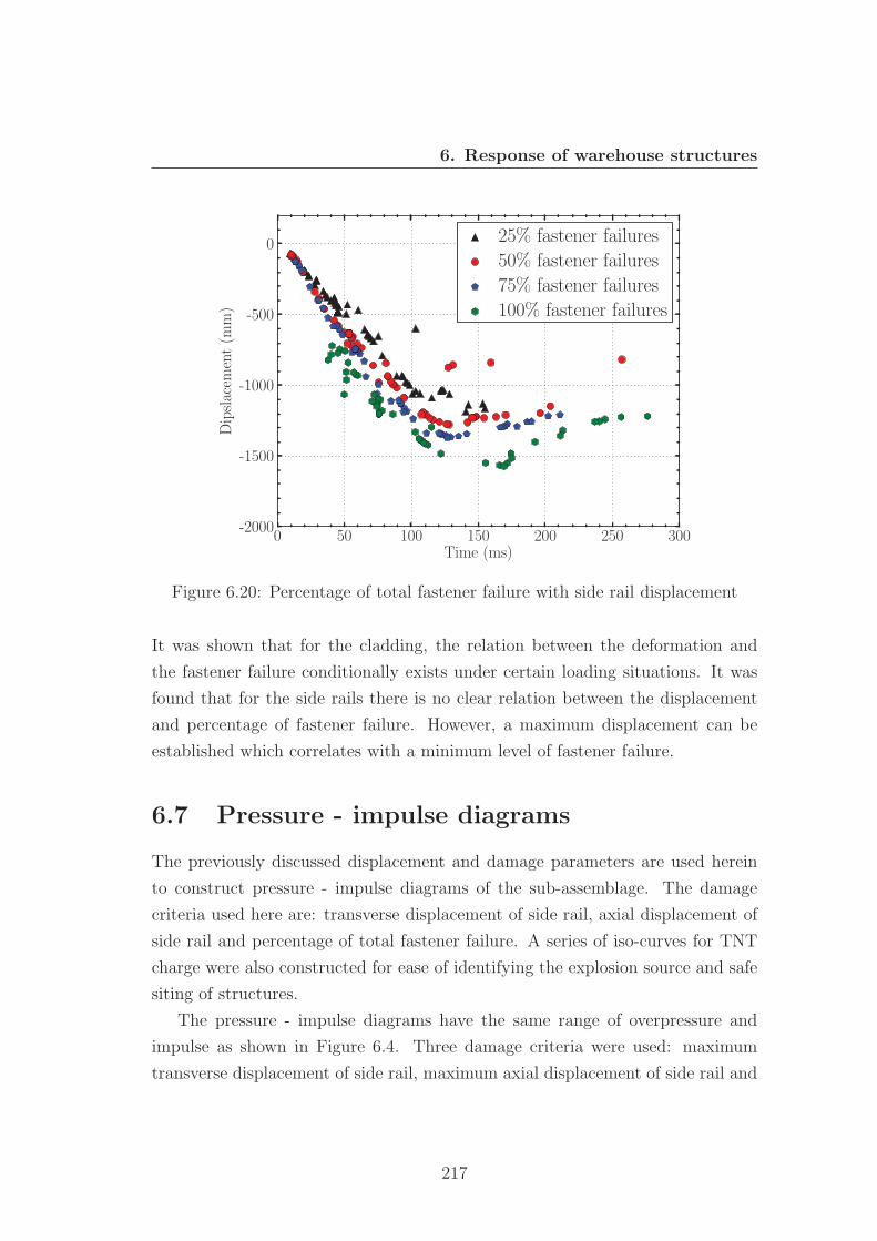
6. Response of warehouse structures
0 50 100 150 200 250 300Time (ms)
-2000
-1500
-1000
-500
0Dipslacem
ent(m
m)
25% fastener failures
50% fastener failures
75% fastener failures
100% fastener failures
Figure 6.20: Percentage of total fastener failure with side rail displacement
It was shown that for the cladding, the relation between the deformation and
the fastener failure conditionally exists under certain loading situations. It was
found that for the side rails there is no clear relation between the displacement
and percentage of fastener failure. However, a maximum displacement can be
established which correlates with a minimum level of fastener failure.
6.7 Pressure - impulse diagrams
The previously discussed displacement and damage parameters are used herein
to construct pressure - impulse diagrams of the sub-assemblage. The damage
criteria used here are: transverse displacement of side rail, axial displacement of
side rail and percentage of total fastener failure. A series of iso-curves for TNT
charge were also constructed for ease of identifying the explosion source and safe
siting of structures.
The pressure - impulse diagrams have the same range of overpressure and
impulse as shown in Figure 6.4. Three damage criteria were used: maximum
transverse displacement of side rail, maximum axial displacement of side rail and
217
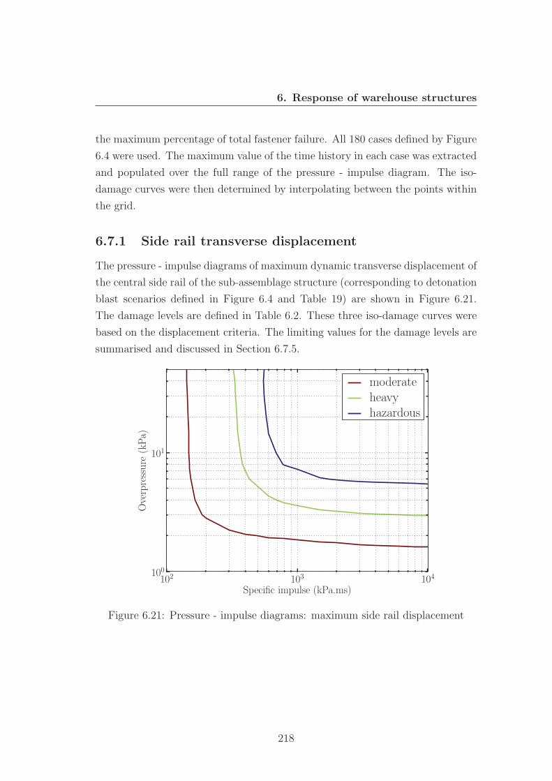
6. Response of warehouse structures
the maximum percentage of total fastener failure. All 180 cases defined by Figure
6.4 were used. The maximum value of the time history in each case was extracted
and populated over the full range of the pressure - impulse diagram. The iso-
damage curves were then determined by interpolating between the points within
the grid.
6.7.1 Side rail transverse displacement
The pressure - impulse diagrams of maximum dynamic transverse displacement of
the central side rail of the sub-assemblage structure (corresponding to detonation
blast scenarios defined in Figure 6.4 and Table 19) are shown in Figure 6.21.
The damage levels are defined in Table 6.2. These three iso-damage curves were
based on the displacement criteria. The limiting values for the damage levels are
summarised and discussed in Section 6.7.5.
102 103 104
Specific impulse (kPa.ms)
100
101
Overpressure
(kPa)
moderateheavyhazardous
Figure 6.21: Pressure - impulse diagrams: maximum side rail displacement
218
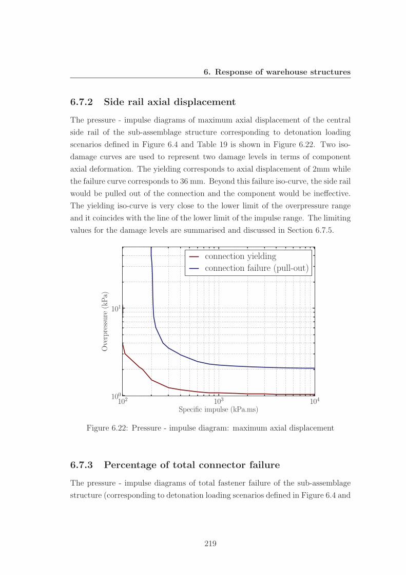
6. Response of warehouse structures
6.7.2 Side rail axial displacement
The pressure - impulse diagrams of maximum axial displacement of the central
side rail of the sub-assemblage structure corresponding to detonation loading
scenarios defined in Figure 6.4 and Table 19 is shown in Figure 6.22. Two iso-
damage curves are used to represent two damage levels in terms of component
axial deformation. The yielding corresponds to axial displacement of 2mm while
the failure curve corresponds to 36 mm. Beyond this failure iso-curve, the side rail
would be pulled out of the connection and the component would be ineffective.
The yielding iso-curve is very close to the lower limit of the overpressure range
and it coincides with the line of the lower limit of the impulse range. The limiting
values for the damage levels are summarised and discussed in Section 6.7.5.
102 103 104
Specific impulse (kPa.ms)
100
101
Overpressure
(kPa)
connection yielding
connection failure (pull-out)
Figure 6.22: Pressure - impulse diagram: maximum axial displacement
6.7.3 Percentage of total connector failure
The pressure - impulse diagrams of total fastener failure of the sub-assemblage
structure (corresponding to detonation loading scenarios defined in Figure 6.4 and
219
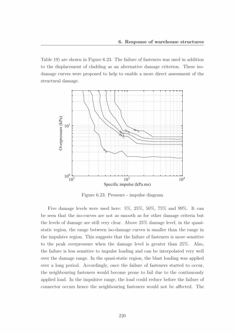
6. Response of warehouse structures
Table 19) are shown in Figure 6.23. The failure of fasteners was used in addition
to the displacement of cladding as an alternative damage criterion. These iso-
damage curves were proposed to help to enable a more direct assessment of the
structural damage.
102 103 104
Specific impulse (kPa.ms)
100
101
Ov
erp
ress
ure
(k
Pa)
5 %
25 %
50 %
75 %99 %
Figure 6.23: Pressure - impulse diagram
Five damage levels were used here: 5%, 25%, 50%, 75% and 99%. It can
be seen that the iso-curves are not as smooth as for other damage criteria but
the levels of damage are still very clear. Above 25% damage level, in the quasi-
static region, the range between iso-damage curves is smaller than the range in
the impulsive region. This suggests that the failure of fasteners is more sensitive
to the peak overpressure when the damage level is greater than 25%. Also,
the failure is less sensitive to impulse loading and can be interpolated very well
over the damage range. In the quasi-static region, the blast loading was applied
over a long period. Accordingly, once the failure of fasteners started to occur,
the neighbouring fasteners would become prone to fail due to the continuously
applied load. In the impulsive range, the load could reduce before the failure of
connector occurs hence the neighbouring fasteners would not be affected. The
220
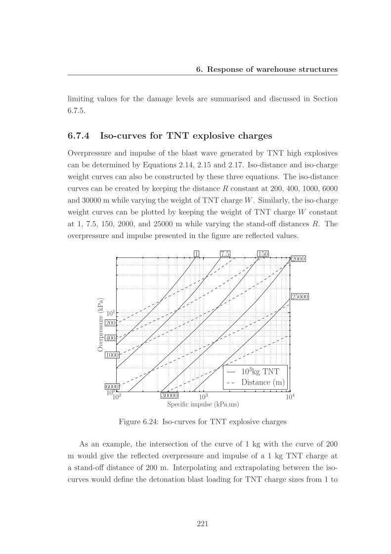
6. Response of warehouse structures
limiting values for the damage levels are summarised and discussed in Section
6.7.5.
6.7.4 Iso-curves for TNT explosive charges
Overpressure and impulse of the blast wave generated by TNT high explosives
can be determined by Equations 2.14, 2.15 and 2.17. Iso-distance and iso-charge
weight curves can also be constructed by these three equations. The iso-distance
curves can be created by keeping the distance R constant at 200, 400, 1000, 6000
and 30000 m while varying the weight of TNT charge W . Similarly, the iso-charge
weight curves can be plotted by keeping the weight of TNT charge W constant
at 1, 7.5, 150, 2000, and 25000 m while varying the stand-off distances R. The
overpressure and impulse presented in the figure are reflected values.
102 103 104
Specific impulse (kPa.ms)
100
101
Overpressure
(kPa)
1 7.5 1502000
25000
200
400
1000
6000
30000
103kg TNT
Distance (m)
Figure 6.24: Iso-curves for TNT explosive charges
As an example, the intersection of the curve of 1 kg with the curve of 200
m would give the reflected overpressure and impulse of a 1 kg TNT charge at
a stand-off distance of 200 m. Interpolating and extrapolating between the iso-
curves would define the detonation blast loading for TNT charge sizes from 1 to
221
6. Response of warehouse structures
25000 kg at stand-off distances from 200 to 30000 m. Combing these iso-curves
of TNT charges to the pressure - impulse diagrams of the structure would make
the estimation of the expected damage or safe distance more straightforward.
6.7.5 Combined pressure - impulse diagrams
The previously discussed three pressure - impulse diagram plots are combined
into one graph as shown in Figure 6.25. The iso-curves of TNT charges are
also superimposed. These combined pressure - impulse diagrams can be used to
identify the most critical component or parameter which controls the response of
the sub-structure. Table 6.5 summarises the limiting pressure and impulse values
for the three damage criteria. For better interpretation, three damage levels were
selected for fastener failures: 5%(moderate), 50%(heavy) and 99%(hazardous).
For the side rail axial response: the yielding and failure criteria were classified as
moderate and hazardous levels.
102 103 104
Specific Reflected Impulse [Pa.s]
100
101
ReflectedPressure
[kPa]
17.5
150
2000
25000200
400
1000
6000
30000
×103kg TNT
stand-off distance (m)
moderateheavyhazardousconnection failureconnection yielding
fastener failure: 5%
fastener failure: 50%
fastener failure: 99%
Figure 6.25: Combined pressure - impulse diagrams
The minimum overpressure values for moderate, heavy and hazardous damage
levels for the transverse displacement of the side rail are 1.62, 2.95 and 5.5 kPa,
222
6. Response of warehouse structures
respectively. The corresponding values for fastener failure are 2.33, 4.86 and 6.0.
Only two damage levels are available for the axial displacement of the side rail.
The minimum overpressure values in this case for the moderate and hazardous
damage levels are 1.04 and 2.07 kPa, respectively. Therefore, the axial displace-
ment is the most critical parameter in the response of the sub-assemblage in both
the impulsive and quasi-static regions. It is worth noting that the design wind
Table 6.5: Minimum overpressure and impulse for various damage criteria [Im-pulse: kPa.ms; Pressure: kPa]
Moderate damage Heavy damage Hazardous damageImpulse Pressure Impulse Pressure Impulse Pressure
side rail (transverse) 141 1.62 326 2.95 546 5.5sdei rail (axial) 100 1.04 - - 197 2.07
fastener failure (%) 158 2.33 308 4.86 591 6.0
pressure for the wall is in the region of 0.5 - 0.6 kPa for this type of structure.
The yielding of the connection (axial) would occur at just two times of the wind
pressure. The side rail supporting the cladding system would only sustain 3-4
times the wind pressure before the hazardous damage level is reached (pull-out
failure and loss of components).
The combined pressure - impulse diagram suggests that for the selected design
of warehouse in the current study, the most critical component in the structure is
the connection between the side rails and columns. The margin of safety is only
around 3-4 times the wind pressure. Increasing the strength of the connection
would shift the corresponding iso-damage curves in the upper right direction,
which would significantly enhance the blast resistance. It should be noted that
once the stiffness and capacity of the connection are increased, the transverse
displacement of the side rail would be decreased and the failure of the fastener
should occur earlier.
The derived iso-damage curves of the overall fastener failure could be fitted
and interpolated as necessary for the design and assessment of such structures.
The damage levels corresponding to percentage of fastener failure can be change
according to design requirements. In the current work, the three levels were
selected arbitrarily for discussion.
223
6. Response of warehouse structures
6.8 Strain rate hardening of fasteners
The strain rate effect of the cladding and side rail materials presented in the
previous chapter was incorporated by a dynamic increase factor (DIF). However,
the behaviour determined from the finite element model of the fastener zone was
only based on static response, and no strain rate effect was considered. This
section examines the possible influence of strain rate in the self-tapping screw
fastener so that the rate effect can be incorporated into the connector response
through a suitable dynamic increase factor if necessary.
6.8.1 Estimation of local strain rate hardening
10−4 10−3 10−2 10−1 100 101 102 103 104
Strain Rate (1/s)
1.0
1.2
1.4
1.6
1.8
2.0
Dynam
icIncrease
FactorDIF
yieldultimateCEB modelfitted Johnson-Cookfitted Cowper-SymondsS275 steel Johnson-CookS275 steel Cowper-Symonds
Figure 6.26: Strain rate effect on dynamic increase factor
The dynamic increase factor is used to account for the increase in the strength
of the material at high strain rates. The increase depends primarily on the strain
rate and material properties. Johnson - Cook (Equation 2.30) and Cowper -
Symonds (Equation 2.31) are two commonly used models to estimate the dy-
namic increase factor. The two models were fitted with available experimental
224
6. Response of warehouse structures
data on steel materials cut from cladding sheets (Elghazouli et al., 2014). As
shown in Figure 6.26, the yield and ultimate factor, were determined from the
experimental data and they represent the ratios of yield or ultimate stress at
high strain rates to low strain rates (quasi-static). Three strain rates have been
achieved in the tests: 0.005(quasi-static), 0.23 and 2.3 s−1. Within the range
where test data are available both fitted curves can predict the increase factor
reasonably well. However, beyond a strain rate of 2.3 s−1 the factors predicted
by Cowper - Symonds model are significantly higher than Johnson - Cook model.
In fact, the accuracy of neither model can be guaranteed in the lack of test data.
The curves of the two models fitted to strain rate data of S275 steel have been
included in the figure as well. The mechanical properties of S275 are similar to
the material of the cladding panels and the test data covers strain rates from
0.0001 to 3000 s−1. These two curves serve as good compliments to our test data.
A curve from the CEB model (Ngo et al., 2007) is also shown here for comparison
only since this is typically proposed for reinforcement steel.
Figure 6.27: Estimation of strain rate in the screw connection
In the sub-assemblage model, the screw connection is modelled as a connector
element with two points tied on to a few shell elements of the cladding and
the flange of the side rail. Strain rates are available for shell elements in the
225
6. Response of warehouse structures
cladding but do not account for the stress/strain concentration in the connector
model. As shown in Figure 6.27, the actual strain rate in the screw connection
can be examined as a function (or a multiplier) of the nominal strain rate from
a sampling shell element at a distance away from the connector element. The
estimation was only made in the y-direction since it is the failure direction of
most of the fasteners.
The sampling sub-assemblage model was subjected to a detonation load of 10
kPa and duration of 200 ms (i.e. Case 98). The stress and strain time histories
of the sampling shell element are shown in Figure 6.28a and the corresponding
strain rate time history is shown in Figure6.28b. The average of the absolute
value of the stain rate history was estimated to be 1.0371 s−1. Thus, the nominal
strain rate in the y direction is approximately 1 s−1.
0.00 0.05 0.10 0.15 0.20 0.25 0.30Time (s)
-400
-300
-200
-100
0
100
200
300
400
Stress(M
Pa)
Stress S11Strain LE11
-0.10
-0.05
0.00
0.05
0.10
0.15
0.20
Strain(%
)
(a) stress and strain
0.00 0.05 0.10 0.15 0.20 0.25 0.30Time (s)
-8
-6
-4
-2
0
2
4
6
8
Strainrate
ER11
(1/s)
Strain rate ER11
Avg = 1.0371/s
(b) strain rate
Figure 6.28: Stress, strain and strain rate time histories in the sampling shellelement
The yield and ultimate capacities of the self-tapping screw connection is pri-
marily based on the bearing strength of the thin cladding sheet. The screw with
the bottom flange of the cladding panel can be idealised by a thin plate loaded
with a rigid pin as shown in Figure 6.29a. The pin represents the shaft of the
screw and the plate represents the bottom flange. The finite element model is
shown in Figure 6.29b.
Similar to the stress and stain concentration around the hole in the pin loaded
plate, the stain rate would also concentrate at the screw connection. In the
226
6. Response of warehouse structures
(a) schematic
(b) finite element model
Figure 6.29: Simplified model to estimate the strain rate in a screw connection
227
6. Response of warehouse structures
analysis, the explicit method cannot be used due to the transient nature of the
problem as the dynamic behaviour would dominate the response. Static analysis
was therefore used, but it should be noted that in order to estimate the strain
rate the step time now becomes real. A displacement of 0.2 mm was applied over
the end of the plate as shown in Figure 6.29a. The displacement was applied
linearly so that the velocity is kept constant as shown in Figure 6.30. Six load
step times were used to achieve different strain rates: 1, 0.5 ,0.1, 0.01, 0.001 and
0.0001 second.
0.000 0.002 0.004 0.006 0.008 0.010Load step time (s)
0.00
0.05
0.10
0.15
0.20
Applieddisplacement(m
m)
displacementvelocity
0.000
0.005
0.010
0.015
0.020
0.025
0.030
0.035
0.040
Velocity(m
/s)
Figure 6.30: Applied 0.2 mm displacement over total time step of 0.01 second
Two sets of strain rate data were measured. The nominal strain rate was
measured across the whole plate away from the hole as shown in Figure 6.29a.
The other set of strain rate was measured around the hole as also shown in the
figure. During the loading process, at an arbitrary time the measured strain rate
around the hole and along the nominal section are shown in Figure 6.31a. The
normalised distances are presented as dashed red lines in Figure 6.29a. It can
be seen from Figure 6.31a that around the hole the first half in contact with
the pin exhibited significant negative strain rate (compression) during loading
(normalised distance 0.0 - 0.3). In the part where the hole was not in contact
with the pin, there was a short length with positive strain rate (tension) and the
rest of the hole did not have any strain rate (normalised distance 0.5 - 1.0). The
distribution of strain rate corresponds exactly to the stress distribution around
228
6. Response of warehouse structures
the hole, since both positive and negative values would contribute to the increase
of strength. The average strain rate in the hole was estimated based on the
absolute values of the distribution around the hole. The variation of nominal
strain rate is much smaller and the average can be readily determined.
0.0 0.2 0.4 0.6 0.8 1.0−15
−10
−5
0
5
10
Strainrate
ER11
(1/s)
circular hole
0.0 0.2 0.4 0.6 0.8 1.0Normalised distance
0.0055
0.0060
0.0065
0.0070
Strainrate
ER11
(1/s)
nominal
(a) strain rate spatial distribution
0.000 0.002 0.004 0.006 0.008 0.0100
1
2
3
4
5
6
7
Strainrate
ER11
(1/s)
hole.s.avg
0.000 0.002 0.004 0.006 0.008 0.010Step Time (s)
0.000.010.020.030.040.050.060.070.08
Strainrate
ER11
(1/s)
nominal.s.avg
(b) Strain rate time histories with steptime of 0.01 second
Figure 6.31: Strain rate analysis around the hole
The spatial average of nominal and hole strain rates have been determined at
each step over the loading period. The time histories of the average strain rates
are shown in Figure 6.31b. It can be noticed that both the nominal and hole
strain rates increased rapidly at early stages of loading. For the model with a
time step of 0.01 second, the maximum average strain rate at the hole was roughly
6.5s−1 while the maximum value for average nominal strain rate was only 0.08s−1.
Extending this analysis to the other five load step times can provide six average
nominal strain rates with corresponding strain rates around the hole. Based on
this, a relationship between the nominal and concentrated strain rate around the
hole can be established, as shown in Figure 6.32.
The average nominal strain rate away from the the connector predicted by
the sub-assemblage model as shown in Figure 6.27 is 1.0371 s−1. Thus, the
approximate strain rate in the self-tapping screw connector can be estimated by
interpolating between the points in Figure 6.32 and the strain rate which was
estimated to be 240 s−1. Referring to the fitted Johnson - Cook curve in Figure
6.26, a strain rate of 240 s−1 would increase the yield strength of the material by
229
6. Response of warehouse structures
10−4 10−3 10−2 10−1 100 101
Nominal average strain rate (s−1)
10−2
10−1
100
101
102
103Concentratedaveragestrain
rate
(s−1) 240s−1
Figure 6.32: Relationship between nominal and concetrated strain rates
0 2 4 6 8 10 12Connector displacement (mm)
0
200
400
600
800
1000
1200
1400
1600
1800
Connectorforce(N
)
nominal
strain rate hardened
Figure 6.33: Connector response with and without the estimated strain rate effect
230
6. Response of warehouse structures
21.3%. The increase of ultimate strength is usually lower than the yield strength
and it is approximately half as indicated by the test data shown in Figure 6.26.
Therefore, the ultimate capacity of the connector was only increased by 10.65%.
Nominal and strain rate strengthened response curves of the screw fastener are
shown in Figure 6.33. The yield and ultimate capacities are expected to increase
by 21.3 and 10.65%, respectively, when the strain rate hardening effect is taken
into account.
6.8.2 Influence of strengthened fasteners
The modified response of fasteners considering the rate effect was then assigned
to the sub-assemblage model. A series of analyses were carried out to examine
the effect of the stiffened fastener on the response of the sub-structure. In this
study, the overpressure ranged from 1.5 to 15 kPa and the impulse ranged from
150 to 1500 kPa.ms.
A comparison of the response of the side rail in the sub-assemblage model
with and without the rate stiffened fastener is shown in Figure 6.34. The same
cases were selected as in Figure 6.5. It can be observed that the response of side
rail was not notably affected by the modified behaviour of the fasteners.
Pressure - impulse diagrams based on the sub-assemblage with stiffened fas-
teners is compared with the original results with rate effect in Figure 6.35. It is
evident that the modified fastener does not have a notable influence on all three
damage curves.
In addition to the above, a comparison of the combined response of the side rail
with fastener failures is presented in Figure 6.36, corresponding to the load defined
in Case 98. Although the response of side rail was not affected, the percentage
of fastener failure was influenced to some extent by the strengthened response.
It can be seen that the fasteners failure was delayed which also corresponds to
a higher displacement of side rail due to the strain rate effect. This is expected
since the strength of the fastener was increased hence was able to sustain more
load which delayed failure.
The final analysis was to investigate the influence of the stiffened fastener on
the pressure - impulse diagram of the fastener failure (as shown in Figure 6.37).
231
6. Response of warehouse structures
0 50 100 150 200 250 300Time (ms)
-250
-200
-150
-100
-50
0
50
Dipslacem
ent(m
m)
rate strengthened
nominal
(a) case 33
0 50 100 150 200 250 300Time (ms)
-700
-600
-500
-400
-300
-200
-100
0
Dipslacem
ent(m
m)
rate strengthened
nominal
(b) case 51
0 50 100 150 200 250 300Time (ms)
-1400
-1200
-1000
-800
-600
-400
-200
0
Dipslacem
ent(m
m)
rate strengthened
nominal
(c) case 82
Figure 6.34: Comparison of response of side rail with and without rate stiffenedfasteners
232
6. Response of warehouse structures
102 103 104
Specific impulse (kPa.ms)
100
101
Overpressure
(kPa)
moderate(ε)heavy(ε)hazardous(ε)moderateheavyhazardous
Figure 6.35: Effect of the rate stiffened fastener on the pressure - impulse diagramsof the side rail maximum displacement
0 50 100 150 200 250 300Time (ms)
-1600
-1400
-1200
-1000
-800
-600
-400
-200
0
Dipslacem
ent(m
m)
25%
50%
75% 100%
25%
50%50%50%50%
75%%%75% 10100%
rate strengthenednominal
Figure 6.36: Effect of the rate stiffened fastener on the percentage failure offasteners
233
6. Response of warehouse structures
The iso-damage curve corresponds to the 50% failure of the fasteners in the sub-
assemblage. It can be seen that the iso-damage curve is shifted slight towards
the upper and right direction. This increase of resistance of fastener failure is
also expected because the iso-curves are directly based on the capacities of the
fasteners. However, the effect of the strengthened fastener on the response of the
sub-assemblage overall is clearly insignificant.
102 103 104
Specific impulse (kPa.ms)
100
101
Ov
erp
ress
ure
(k
Pa)
50 %
nominal
rate strengthened
Figure 6.37: Influence of the rate effect on the pressure - impulse diagram ofmaximum percentage of fastener failure (50% failure)
In this chapter, results from the numerical studies using the sub-assemblage
model were presented and discussed. The response of side rail and cladding were
examined. The failure of selected fasteners was also assessed in detail. Studies
were also performed to relate the cladding and side rail response to fastener
failure. It was found that the failure of fasteners was significantly influenced
by the response of claddings, but under certain loading conditions the failure
can be linked to the displacement of the claddings. It was difficult to relate the
overall percentage of fastener failure to the displacement of the side rail. In order
to understand the fastener failure under blast loading, the pressure - impulse
234
6. Response of warehouse structures
diagram using percentage of fastener failure as iso-damage curves was derived.
This damage criteria was used to replace the displacement of claddings in this
study. Pressure - impulse diagrams using other damage criteria were also created
for the sub-structure. The combined pressure - impulse diagrams would serve as
a useful tool in blast damage assessment and design of similar structures.
In the next chapter, a simplified approach using a single degree of freedom
model is presented and the results are compared with the non-linear finite element
results discussed in this chapter. In addition, a blast simulation study is also
presented in the next chapter. The pressure - impulse diagrams derived here will
be used with the results from the simulation in to highlight key design implications
based on the findings of this investigation.
235
Chapter 7
Simplified approaches and design
considerations
7.1 Single degree of freedom approach
The non-linear finite element method is used in this work as the primary tool to
study the response of warehouse structures. In addition, simplified single degree
of freedom models were used to complement and compare with the numerical
analysis tools. SBEDS (USACE (2008a)) was employed here, which is a spread-
sheet software implementing explicit numerical step integration. The software
accounts for material properties, geometry, boundary conditions, supported mass
and connection capacities of the component modelled. It also accounts for tensile
membrane action which is limited by the lesser of the connection capacity or the
member axial strength. Formulations of the model and tension membrane action
were presented in Section 2.4.1.1.
As noted before, the cladding panels are continuous in two-spans over the side
rails and which in turn are two-span continuous over the columns. The span of the
cladding panel and side rails are 1.8 and 6.69 m respectively. Taking advantage
of symmetry, they are modelled as a beam 1.8 or 6.69 m long with one end fully
fixed and one simply supported end as shown in Figure 7.1, in which L is the
length of the member (L=1.8 for cladding panel and L=6.69 for side rail).
236
7. Simplified approaches and design considerations
L Figure 7.1: Cladding panel and side rail simplified SDOF model
7.1.1 Wall cladding
Cladding panels were described in detail in Section 5.3.7 and the material prop-
erties were presented in Section 5.4. Different section modulus and moment of
inertia values were used for the inbound and rebound response based on the geo-
metric properties provided by the manufacturer. The values used in the analysis
are presented in Table 7.1. It should be noted that in this analysis the total self
weight of the cladding panel (two sheeting plus infill) of 0.301 kPa was included.
The SDOF model here represents a single layer of the sheeting.
Table 7.1: Geometric properties of wall cladding panel
Positive moment of inertia 119.95 mm4/mmNegative moment of inertia 89.02 mm4/mmPositive section modulus 5.763 mm3/mmNegative section modulus 5.409 mm3/mm
The cladding panels are fixed to the side rails by six fasteners (Section 5.3.8)
at the end of the panels and three fasteners over the middle support. Tensile
membrane action is therefore limited by the capacity of the end connections, since
they are smaller than the axial capacity of cladding panel. The end connection
capacity was determined to be 6.32 N/mm according to Eurocode 3, Part 1-3.
237
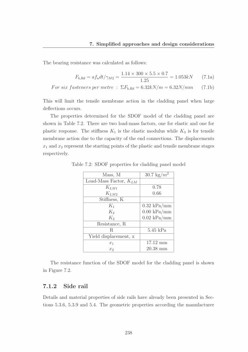
7. Simplified approaches and design considerations
The bearing resistance was calculated as follows:
Fb,Rd = afudt/γM2 =1.14× 300× 5.5× 0.7
1.25= 1.053kN (7.1a)
For six fasteners per metre : ΣFb,Rd = 6.32kN/m = 6.32N/mm (7.1b)
This will limit the tensile membrane action in the cladding panel when large
deflections occurs.
The properties determined for the SDOF model of the cladding panel are
shown in Table 7.2. There are two load-mass factors, one for elastic and one for
plastic response. The stiffness K1 is the elastic modulus while K3 is for tensile
membrane action due to the capacity of the end connections. The displacements
x1 and x2 represent the starting points of the plastic and tensile membrane stages
respectively.
Table 7.2: SDOF properties for cladding panel model
Mass, M 30.7 kg/m2
Load-Mass Factor, KLM
KLM1 0.78KLM2 0.66
Stiffness, KK1 0.32 kPa/mmK2 0.00 kPa/mmK3 0.02 kPa/mm
Resistance, RR 5.45 kPa
Yield displacement, xx1 17.12 mmx2 20.38 mm
The resistance function of the SDOF model for the cladding panel is shown
in Figure 7.2.
7.1.2 Side rail
Details and material properties of side rails have already been presented in Sec-
tions 5.3.6, 5.3.9 and 5.4. The geometric properties according the manufacturer
238
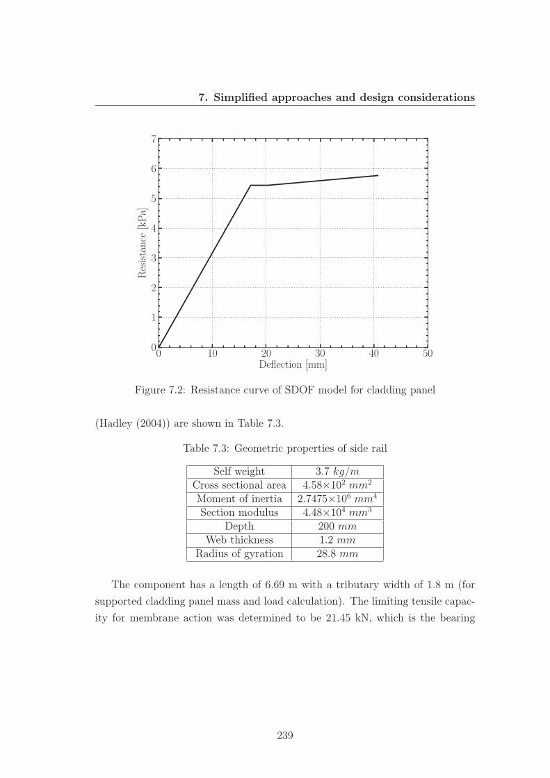
7. Simplified approaches and design considerations
0 10 20 30 40 50Deflection [mm]
0
1
2
3
4
5
6
7Resistance
[kPa]
Figure 7.2: Resistance curve of SDOF model for cladding panel
(Hadley (2004)) are shown in Table 7.3.
Table 7.3: Geometric properties of side rail
Self weight 3.7 kg/mCross sectional area 4.58×102 mm2
Moment of inertia 2.7475×106 mm4
Section modulus 4.48×104 mm3
Depth 200 mmWeb thickness 1.2 mm
Radius of gyration 28.8 mm
The component has a length of 6.69 m with a tributary width of 1.8 m (for
supported cladding panel mass and load calculation). The limiting tensile capac-
ity for membrane action was determined to be 21.45 kN, which is the bearing
239
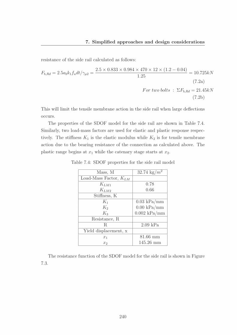
7. Simplified approaches and design considerations
resistance of the side rail calculated as follows:
Fb,Rd = 2.5abk1fudt/γμ2 =2.5× 0.833× 0.984× 470× 12× (1.2− 0.04)
1.25= 10.725kN
(7.2a)
For two bolts : ΣFb,Rd = 21.45kN
(7.2b)
This will limit the tensile membrane action in the side rail when large deflections
occurs.
The properties of the SDOF model for the side rail are shown in Table 7.4.
Similarly, two load-mass factors are used for elastic and plastic response respec-
tively. The stiffness K1 is the elastic modulus while K2 is for tensile membrane
action due to the bearing resistance of the connection as calculated above. The
plastic range begins at x1 while the catenary stage starts at x2.
Table 7.4: SDOF properties for the side rail model
Mass, M 32.74 kg/m2
Load-Mass Factor, KLM
KLM1 0.78KLM2 0.66
Stiffness, KK1 0.03 kPa/mmK2 0.00 kPa/mmK3 0.002 kPa/mm
Resistance, RR 2.09 kPa
Yield displacement, xx1 81.66 mmx2 145.26 mm
The resistance function of the SDOF model for the side rail is shown in Figure
7.3.
240
7. Simplified approaches and design considerations
0 50 100 150 200 250 300 350Deflection [mm]
0.0
0.5
1.0
1.5
2.0
2.5
3.0Resistance
[kPa]
Figure 7.3: Resistance curve of SDOF model for side rail
7.1.3 Component interaction
In the SDOF analysis, each component is modelled individually. The cladding
panels were uncoupled from the side rails and then the blast load was in turn
applied to each of the component. Each component was analysed independently
with the mass of the supported components to account for the the correct inertia
and deflections. This method is generally more conservative and was indicated
to be appropriate when the ratio of the natural frequencies of the supporting and
supported components is greater than two (Biggs (1964)).
The natural period of the equivalent SDOF model for the side rail and cladding
panel can be calculated as:
Tn = 2π
√KLM1m
k1(7.3)
Thus for the side rail the natural period is Tn(siderail) = 198.42ms and for cladding
panel Tn(cladding) = 54.48ms. The ratio of natural frequencies was determined
to be 115.33 rad/sec31.64 rad/sec
= 3.64, and according to Biggs (1964) this approach can be
241
7. Simplified approaches and design considerations
adopted for the analysis of the structural components of the warehouse.
7.1.4 Response of simplified model of side rail
Three examples of the response of the simplified model of the side rail are pre-
sented in Figure 7.4. Their responses correspond to the loads defined in Case
33, 51 and 82. These are the same selected cases in the detailed finite element
study corresponding to moderate, heavy and hazardous damage levels. It can be
noted that at the moderate level, the simplified model compares well with the
finite element model. However, in the case of heavy and hazardous damage levels,
the simplified model significantly over-predicts the maximum dynamic displace-
ment. The reason behind this is that the tensile membrane stiffness defined in
the simplified model was based on the shear capacity of the side rail according to
the Eurocode (Equation 7.2), which was 24.15 kN. This is smaller than the axial
yield capacity of 53 kN determined by the finite element model of the connection.
It can be seen that the responses of the simplified model compares much better
with the finite element model when the numerically determined axial capacity
was used to define the tensile membrane stiffness.
The pressure - impulse diagram based on the simplified model of the side rail
is presented in Figure 7.5 and compared with the iso-damage curves produced
by the finite element sub-assemblage model. Generally the iso-damage curves
based on the simplified model compare well with that of the finite element model,
particularly at the moderate and heavy damage levels. Some discrepancies can
be observed at the hazardous damage level.
At hazardous damage level, the limiting pressure value of the simplified model
in the quasi-static region is lower than the finite element model. This indicates
that in this region the simplified model over-predicts the maximum displacement
at the centre of the side rails. In the finite element model, the axial behaviour
for the end connection of the side rail was defined with plastic hardening; while,
in the simplified model, only one constant axial support capacity was used to
determine the tensile membrane stiffness. Therefore, at large deformation (e.g.
hazardous damage level), the plastic hardening of the connection response results
in a higher tensile membrane stiffness than in the simplified model. Hence, the
242
7. Simplified approaches and design considerations
0 50 100 150 200 250 300Time (ms)
-250
-200
-150
-100
-50
0
50
Dipslacem
ent(m
m)
NLFEM
SDOF
SDOF-modified
(a) Case 33
0 50 100 150 200 250 300Time (ms)
-900
-800
-700
-600
-500
-400
-300
-200
-100
0
Dipslacem
ent(m
m)
NLFEM
SDOF
SDOF-modified
(b) Case 51
0 50 100 150 200 250 300Time (ms)
-2500
-2000
-1500
-1000
-500
0
Dipslacem
ent(m
m)
NLFEM
SDOF
SDOF-modified
(c) Case 82
Figure 7.4: Response of simplified model of side rail
243
7. Simplified approaches and design considerations
displacement predicted by the finite element model is less than in the simplified
model.
102 103 104
Specific impulse (kPa.ms)
100
101
Overpressure
(kPa)
SDOF-moderateSDOF-heavySDOF-hazardousNLFEM-moderateNLFEM-heavyNLFEM-hazardous
Figure 7.5: Comparison of pressure - impulse diagrams (maximum dynamic dis-placement)
In the impulsive loading region, the curves corresponding to the hazardous
damage level predicted by the simplified model and the finite element model
match reasonably well despite the same difference in tensile membrane stiffness.
This is attributed to the combination of higher response modes of the side rails
that are excited by the impulsive loading and the higher tensile membrane stiffness
in the finite element model. Higher modes in the response of side rails increases
the maximum displacement at the centre. The simplified approach was based
only on the fundamental mode of the component. Based on the above discussion,
it can be concluded that both the simplified and finite element model are capable
of accurately predicting the response of the side rails in the sub-assemblage. The
assumption of analysis of the component in a decoupled manner claimed by Biggs
(Biggs, 1964) is valid for the side rails.
244
7. Simplified approaches and design considerations
7.1.5 Response of simplified model of cladding
Two selected cases of the simplified model of cladding panel are presented in
Figure 7.6. The response corresponds to the load defined in Case 33 and 82, for
the moderate and hazardous damage levels of the side rail. It can be seen in
Figure 7.6a that the response of the simplified model is only comparable with
the side cladding of the finite element model. The maximum displacement of the
simplified model is about 16.98 mm while that of the side cladding of the finite
element model is 10 mm. This discrepancy is mainly due to the difference in
elastic stiffness in the simplified and finite element model.
It can be noted that the displacement of 16.98 mm is just within the elastic
range depicted in Figure 7.2, hence in Case 33 the response of cladding was
elastic. The elastic stiffness determined for the simplified model is 0.32 kPa/mm,
and at 16.98 mm displacement the resistance is 0.32 × 16.98 = 5.41 kPa. An
elastic finite element analysis determined that the elastic stiffness of the cladding
is 0.525 kPa/mm, thus at a resistance of 5.41 kPa the elastic displacement is
5.41/0.525 = 10.3mm, which is approximately equal to the maximum deflection
of the side cladding in the finite element model of the sub-assemblage.
It can be seen that the displacement history of the central cladding of the
sub-assemblage is significantly different to the side cladding and the simplified
model. This is mainly due to the dynamic effect and the response interaction
between the central cladding and the side rails. Within the first 30 ms shown in
Figure 7.6a, the central cladding deformed slightly inwards and then outwards
relative to the side rails, before large deformations occurred. Similarly, as shown
in Figure 7.6b, there is a delay in the deflection of the central cladding about 80
ms before it started to deform. These observations suggest that there are strong
dynamic interaction between the central cladding and the side rails.
The displacement history of the simplified model corresponding to Case 82
is shown in Figure 7.6b. The simplified model significantly over-predicted the
response compared to the displacement of the side cladding in the sub-assemblage
model. The maximum displacement predicted by the simplified model was 204
mm. Following the resistance curve in Figure 7.2, it was determined that the
maximum resistance at 204 mm was 8.31 kPa. At this level of pressure, in the
245
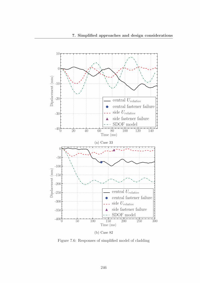
7. Simplified approaches and design considerations
0 20 40 60 80 100 120 140Time (ms)
-40
-30
-20
-10
0
10Dipslacem
ent(m
m)
central Urelative
central fastener failureside Urelative
side fastener failureSDOF model
(a) Case 33
0 50 100 150 200 250 300Time (ms)
-400
-350
-300
-250
-200
-150
-100
-50
0
Dipslacem
ent(m
m)
central Urelative
central fastener failureside Urelative
side fastener failureSDOF model
(b) Case 82
Figure 7.6: Responses of simplified model of cladding
246
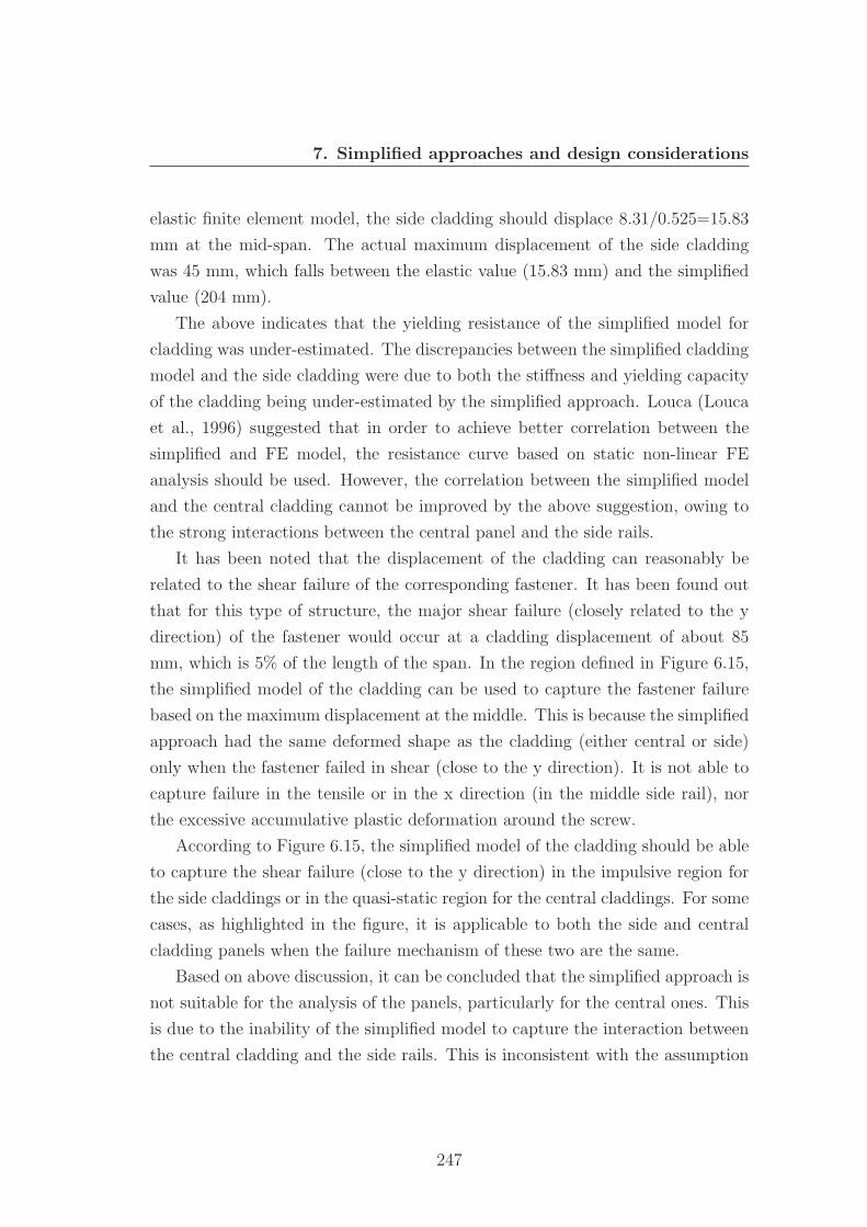
7. Simplified approaches and design considerations
elastic finite element model, the side cladding should displace 8.31/0.525=15.83
mm at the mid-span. The actual maximum displacement of the side cladding
was 45 mm, which falls between the elastic value (15.83 mm) and the simplified
value (204 mm).
The above indicates that the yielding resistance of the simplified model for
cladding was under-estimated. The discrepancies between the simplified cladding
model and the side cladding were due to both the stiffness and yielding capacity
of the cladding being under-estimated by the simplified approach. Louca (Louca
et al., 1996) suggested that in order to achieve better correlation between the
simplified and FE model, the resistance curve based on static non-linear FE
analysis should be used. However, the correlation between the simplified model
and the central cladding cannot be improved by the above suggestion, owing to
the strong interactions between the central panel and the side rails.
It has been noted that the displacement of the cladding can reasonably be
related to the shear failure of the corresponding fastener. It has been found out
that for this type of structure, the major shear failure (closely related to the y
direction) of the fastener would occur at a cladding displacement of about 85
mm, which is 5% of the length of the span. In the region defined in Figure 6.15,
the simplified model of the cladding can be used to capture the fastener failure
based on the maximum displacement at the middle. This is because the simplified
approach had the same deformed shape as the cladding (either central or side)
only when the fastener failed in shear (close to the y direction). It is not able to
capture failure in the tensile or in the x direction (in the middle side rail), nor
the excessive accumulative plastic deformation around the screw.
According to Figure 6.15, the simplified model of the cladding should be able
to capture the shear failure (close to the y direction) in the impulsive region for
the side claddings or in the quasi-static region for the central claddings. For some
cases, as highlighted in the figure, it is applicable to both the side and central
cladding panels when the failure mechanism of these two are the same.
Based on above discussion, it can be concluded that the simplified approach is
not suitable for the analysis of the panels, particularly for the central ones. This
is due to the inability of the simplified model to capture the interaction between
the central cladding and the side rails. This is inconsistent with the assumption
247
7. Simplified approaches and design considerations
made by Biggs (Biggs, 1964) in order to use the simplified model to analyse
two components in a decoupled manner, the natural frequency ratio of the two
components should be more than two. The frequency ratio of the cladding and
side rail used in the present work is 3.64. It has been shown that the fasteners
failed in different modes, and that simplified model should be able to capture the
shear failure close to or in the y direction, where it is unable to capture failure in
the tensile direction nor the excessive accumulative plastic deformation around
the screw.
7.1.6 Pressure - impulse diagrams of simplified models
A combined pressure - impulse diagram using the simplified models presented
above is shown in Figure 7.7. This completes the blast resistance analysis based
on simplified models of the sub-assemblage structure of the selected design in this
work. The limiting values of overpressure and impulses are shown in Table 7.5.
101 102 103 104
Specific impulse (kPa.ms)
100
101
102
Overpressure
(kPa)
cladding-moderatecladding-heavycladding-hazardousside rail-moderateside rail-heavyside rail-hazardous
Figure 7.7: Combined pressure - impulse diagram using the simplified approach
It can be seen that in the quasi-static region the critical component are side rails.
248
7. Simplified approaches and design considerations
In contrast, the claddings become critical in the impulsive region.
Table 7.5: Combined pressure - impulse diagram of simplified model
moderate heavy hazardousP(kPa) I (kPa.ms) P(kPa) I (kPa.ms) P(kPa) I (kPa.ms)
side rail 1.8 155 3.0 357 4.4 553cladding 2.51 43.5 5.06 131 5.9 202
It should be noted that in this pressure - impulse diagram, the iso-damage
curves for the side rails match well with the non-linear finite element model. The
iso-damage curves of the cladding, on the other hand, were over-predicted due to
the smaller stiffness and lower yield capacity. More importantly, the iso-damage
curves did not distinguish between side and central claddings, hence information
on the fastener failure (based on cladding deformation) is difficult to obtain.
No information can be obtained on the total fastener failure from the simplified
approach.
In this section, the simplified approach based on Biggs’ method (Biggs, 1964)
was presented. The results of the simplified approach were compared with the
non-linear finite element model. It was found that the results of the simplified
approach were comparable for side rails but not in good agreement for claddings,
particularly for the central panels. This was mainly due to the inability of the
simplified model to capture the strong interaction between the central cladding
and the side rails.
7.2 Assessment of blast overpressures
7.2.1 Blast wave simulation on rigid warehouse
Assessment of the structural damage from the Buncefield incident was undertaken
by the Defence Ordnance Safety Group (DOSG) of the Ministry of Defence (SCI
(2009)). The work covered a range of buildings in or near the Buncefield depot.
DOSG has access to a variety of tools for predicting the blast effects from high
explosive detonations ranging from simple look-up tables, empirical curves, to
full 3D hydrocodes. For this assessment, an empirical tool based on Kingery -
249
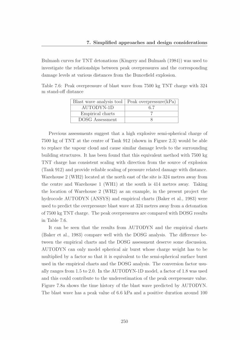
7. Simplified approaches and design considerations
Bulmash curves for TNT detonations (Kingery and Bulmash (1984)) was used to
investigate the relationships between peak overpressures and the corresponding
damage levels at various distances from the Buncefield explosion.
Table 7.6: Peak overpressure of blast wave from 7500 kg TNT charge with 324m stand-off distance
Blast wave analysis tool Peak overpressure(kPa)AUTODYN-1D 6.7Empirical charts 7DOSG Assessment 8
Previous assessments suggest that a high explosive semi-spherical charge of
7500 kg of TNT at the centre of Tank 912 (shown in Figure 2.3) would be able
to replace the vapour cloud and cause similar damage levels to the surrounding
building structures. It has been found that this equivalent method with 7500 kg
TNT charge has consistent scaling with direction from the source of explosion
(Tank 912) and provide reliable scaling of pressure related damage with distance.
Warehouse 2 (WH2) located at the north east of the site is 324 metres away from
the centre and Warehouse 1 (WH1) at the south is 414 metres away. Taking
the location of Warehouse 2 (WH2) as an example, in the present project the
hydrocode AUTODYN (ANSYS) and empirical charts (Baker et al., 1983) were
used to predict the overpressure blast wave at 324 metres away from a detonation
of 7500 kg TNT charge. The peak overpressures are compared with DOSG results
in Table 7.6.
It can be seen that the results from AUTODYN and the empirical charts
(Baker et al., 1983) compare well with the DOSG analysis. The difference be-
tween the empirical charts and the DOSG assessment deserve some discussion.
AUTODYN can only model spherical air burst whose charge weight has to be
multiplied by a factor so that it is equivalent to the semi-spherical surface burst
used in the empirical charts and the DOSG analysis. The conversion factor usu-
ally ranges from 1.5 to 2.0. In the AUTODYN-1D model, a factor of 1.8 was used
and this could contribute to the underestimation of the peak overpressure value.
Figure 7.8a shows the time history of the blast wave predicted by AUTODYN.
The blast wave has a peak value of 6.6 kPa and a positive duration around 100
250
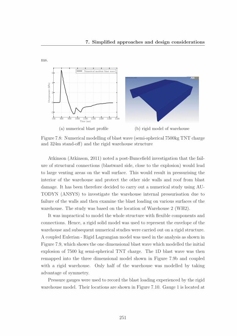
7. Simplified approaches and design considerations
ms.
700 800 900 1000 1100 1200 1300 1400 1500Time (ms)
-2
0
2
4
6
Overpressure
(kPa)
Numerical incident blast wave
(a) numerical blast profile (b) rigid model of warehouse
Figure 7.8: Numerical modelling of blast wave (semi-spherical 7500kg TNT chargeand 324m stand-off) and the rigid warehouse structure
Atkinson (Atkinson, 2011) noted a post-Buncefield investigation that the fail-
ure of structural connections (blastward side, close to the explosion) would lead
to large venting areas on the wall surface. This would result in pressurising the
interior of the warehouse and protect the other side walls and roof from blast
damage. It has been therefore decided to carry out a numerical study using AU-
TODYN (ANSYS) to investigate the warehouse internal pressurisation due to
failure of the walls and then examine the blast loading on various surfaces of the
warehouse. The study was based on the location of Warehouse 2 (WH2).
It was impractical to model the whole structure with flexible components and
connections. Hence, a rigid solid model was used to represent the envelope of the
warehouse and subsequent numerical studies were carried out on a rigid structure.
A coupled Eulerian - Rigid Lagrangian model was used in the analysis as shown in
Figure 7.9, which shows the one dimensional blast wave which modelled the initial
explosion of 7500 kg semi-spherical TNT charge. The 1D blast wave was then
remapped into the three dimensional model shown in Figure 7.9b and coupled
with a rigid warehouse. Only half of the warehouse was modelled by taking
advantage of symmetry.
Pressure gauges were used to record the blast loading experienced by the rigid
warehouse model. Their locations are shown in Figure 7.10. Gauge 1 is located at
251
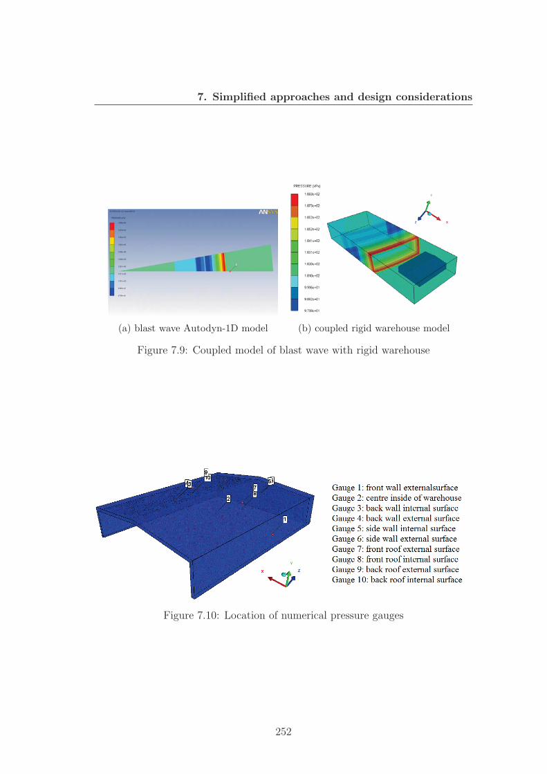
7. Simplified approaches and design considerations
(a) blast wave Autodyn-1D model (b) coupled rigid warehouse model
Figure 7.9: Coupled model of blast wave with rigid warehouse
Figure 7.10: Location of numerical pressure gauges
252
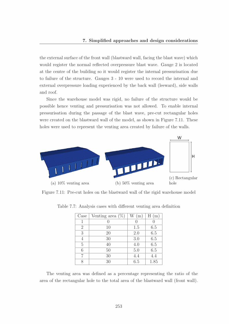
7. Simplified approaches and design considerations
the external surface of the front wall (blastward wall, facing the blast wave) which
would register the normal reflected overpressure blast wave. Gauge 2 is located
at the centre of the building so it would register the internal pressurisation due
to failure of the structure. Gauges 3 - 10 were used to record the internal and
external overpressure loading experienced by the back wall (leeward), side walls
and roof.
Since the warehouse model was rigid, no failure of the structure would be
possible hence venting and pressurisation was not allowed. To enable internal
pressurisation during the passage of the blast wave, pre-cut rectangular holes
were created on the blastward wall of the model, as shown in Figure 7.11. These
holes were used to represent the venting area created by failure of the walls.
(a) 10% venting area (b) 50% venting area(c) Rectangularhole
Figure 7.11: Pre-cut holes on the blastward wall of the rigid warehouse model
Table 7.7: Analysis cases with different venting area definition
Case Venting area (%) W (m) H (m)1 0 0 02 10 1.5 6.53 20 2.0 6.54 30 3.0 6.55 40 4.0 6.56 50 5.0 6.57 30 4.4 4.48 30 6.5 1.85
The venting area was defined as a percentage representing the ratio of the
area of the rectangular hole to the total area of the blastward wall (front wall).
253
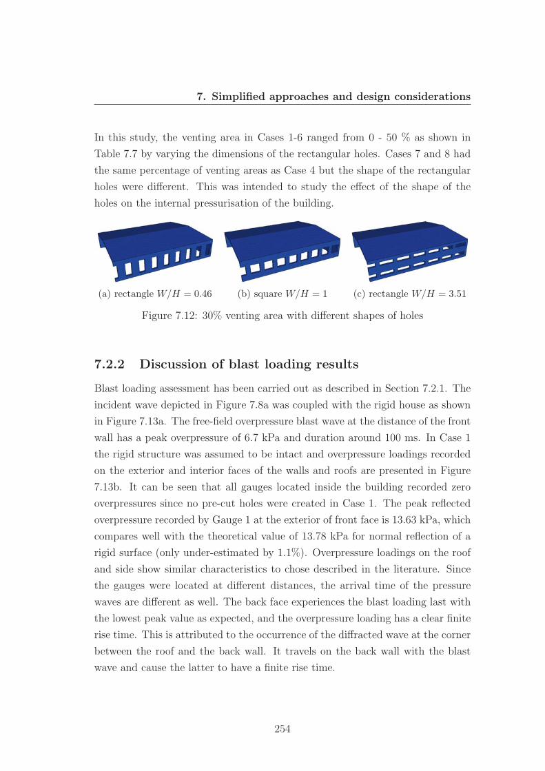
7. Simplified approaches and design considerations
In this study, the venting area in Cases 1-6 ranged from 0 - 50 % as shown in
Table 7.7 by varying the dimensions of the rectangular holes. Cases 7 and 8 had
the same percentage of venting areas as Case 4 but the shape of the rectangular
holes were different. This was intended to study the effect of the shape of the
holes on the internal pressurisation of the building.
(a) rectangle W/H = 0.46 (b) square W/H = 1 (c) rectangle W/H = 3.51
Figure 7.12: 30% venting area with different shapes of holes
7.2.2 Discussion of blast loading results
Blast loading assessment has been carried out as described in Section 7.2.1. The
incident wave depicted in Figure 7.8a was coupled with the rigid house as shown
in Figure 7.13a. The free-field overpressure blast wave at the distance of the front
wall has a peak overpressure of 6.7 kPa and duration around 100 ms. In Case 1
the rigid structure was assumed to be intact and overpressure loadings recorded
on the exterior and interior faces of the walls and roofs are presented in Figure
7.13b. It can be seen that all gauges located inside the building recorded zero
overpressures since no pre-cut holes were created in Case 1. The peak reflected
overpressure recorded by Gauge 1 at the exterior of front face is 13.63 kPa, which
compares well with the theoretical value of 13.78 kPa for normal reflection of a
rigid surface (only under-estimated by 1.1%). Overpressure loadings on the roof
and side show similar characteristics to chose described in the literature. Since
the gauges were located at different distances, the arrival time of the pressure
waves are different as well. The back face experiences the blast loading last with
the lowest peak value as expected, and the overpressure loading has a clear finite
rise time. This is attributed to the occurrence of the diffracted wave at the corner
between the roof and the back wall. It travels on the back wall with the blast
wave and cause the latter to have a finite rise time.
254
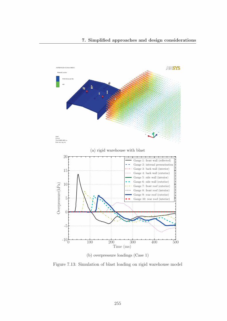
7. Simplified approaches and design considerations
(a) rigid warehouse with blast
0 100 200 300 400 500Time (ms)
-10
-5
0
5
10
15
20
Overpressure(kPa)
Gauge 1: front wall (reflected)
Gauge 2: internal pressurisation
Gauge 3: back wall (interior)
Gauge 4: back wall (exterior)
Gauge 5: side wall (interior)
Gauge 6: side wall (exterior)
Gauge 7: front roof (exterior)
Gauge 8: front roof (interior)
Gauge 9: rear roof (exterior)
Gauge 10: rear roof (interior)
(b) overpressure loadings (Case 1)
Figure 7.13: Simulation of blast loading on rigid warehouse model
255
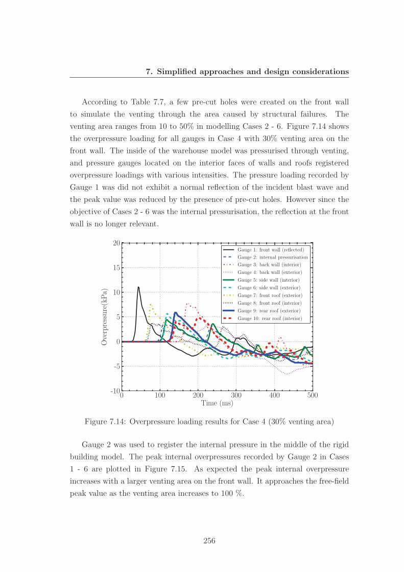
7. Simplified approaches and design considerations
According to Table 7.7, a few pre-cut holes were created on the front wall
to simulate the venting through the area caused by structural failures. The
venting area ranges from 10 to 50% in modelling Cases 2 - 6. Figure 7.14 shows
the overpressure loading for all gauges in Case 4 with 30% venting area on the
front wall. The inside of the warehouse model was pressurised through venting,
and pressure gauges located on the interior faces of walls and roofs registered
overpressure loadings with various intensities. The pressure loading recorded by
Gauge 1 was did not exhibit a normal reflection of the incident blast wave and
the peak value was reduced by the presence of pre-cut holes. However since the
objective of Cases 2 - 6 was the internal pressurisation, the reflection at the front
wall is no longer relevant.
0 100 200 300 400 500Time (ms)
-10
-5
0
5
10
15
20
Overpressure(kPa)
Gauge 1: front wall (reflected)
Gauge 2: internal pressurisation
Gauge 3: back wall (interior)
Gauge 4: back wall (exterior)
Gauge 5: side wall (interior)
Gauge 6: side wall (exterior)
Gauge 7: front roof (exterior)
Gauge 8: front roof (interior)
Gauge 9: rear roof (exterior)
Gauge 10: rear roof (interior)
Figure 7.14: Overpressure loading results for Case 4 (30% venting area)
Gauge 2 was used to register the internal pressure in the middle of the rigid
building model. The peak internal overpressures recorded by Gauge 2 in Cases
1 - 6 are plotted in Figure 7.15. As expected the peak internal overpressure
increases with a larger venting area on the front wall. It approaches the free-field
peak value as the venting area increases to 100 %.
256
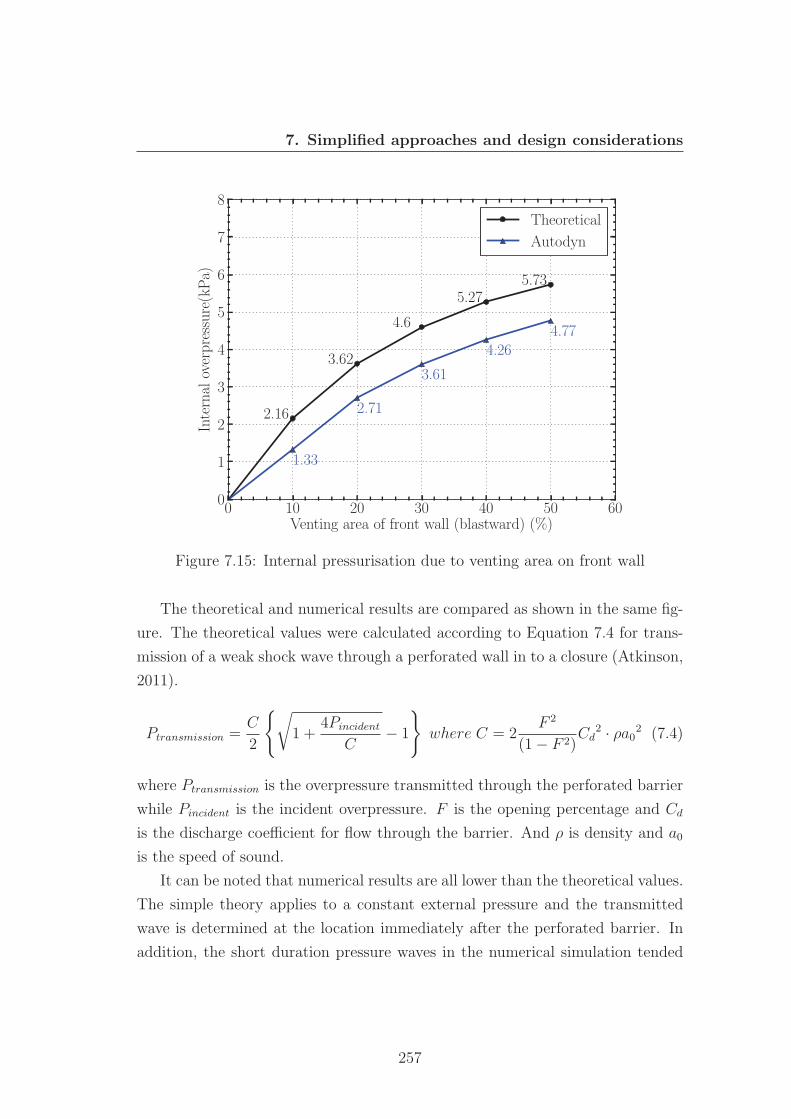
7. Simplified approaches and design considerations
0 10 20 30 40 50 60Venting area of front wall (blastward) (%)
0
1
2
3
4
5
6
7
8Internal
overpressure(kPa)
2.16
3.62
4.6
5.275.73
1.33
2.71
3.61
4.264.77
Theoretical
Autodyn
Figure 7.15: Internal pressurisation due to venting area on front wall
The theoretical and numerical results are compared as shown in the same fig-
ure. The theoretical values were calculated according to Equation 7.4 for trans-
mission of a weak shock wave through a perforated wall in to a closure (Atkinson,
2011).
Ptransmission =C
2
{√1 +
4Pincident
C− 1
}where C = 2
F 2
(1− F 2)Cd
2 · ρa02 (7.4)
where Ptransmission is the overpressure transmitted through the perforated barrier
while Pincident is the incident overpressure. F is the opening percentage and Cd
is the discharge coefficient for flow through the barrier. And ρ is density and a0
is the speed of sound.
It can be noted that numerical results are all lower than the theoretical values.
The simple theory applies to a constant external pressure and the transmitted
wave is determined at the location immediately after the perforated barrier. In
addition, the short duration pressure waves in the numerical simulation tended
257
7. Simplified approaches and design considerations
to broaden, and the maximum pressures were decreasing as they propagated.
In order to examine the internal pressurisation in detail, the pressure loading
at the back and side walls are presented in Figures 7.16 and 7.17. Figure 7.16a
shows the pressure loading on the external and internal surfaces of the back wall.
Since there was no venting at the front, the overpressure at the interior face was
zero and the net loading was equal to the external overpressure measured by
Gauge 4. Thus, the anticipated damage of the back wall would be towards the
inside. When the venting was allowed at the front, as shown in Figure 7.16b, the
overpressure loading at the internal face of the back wall significantly increased
(with help from the reflection effect). It can be noted that the slower rate of
increase of overpressure on the exterior of the back wall caused the net loading
to act outwards (negative value) at the beginning. The peak value of -7.73 kPa
(outwards) would be able to cause severe damage to back wall of the structure.
Similar analysis can be undertaken as shown in Figure 7.17. Figure 7.17a
depicts the overpressure loading on the side wall when there was no venting from
the front wall. There were zero internal overpressures and the net loading was
equal to the overpressure on the exterior, which could cause inward damage in the
side wall elements. On the other hand, if 30% venting existed at the front wall
as shown in Figure 7.17b, the internal overpressures would immediately offset
the external pressure loading and could reduce the damage risk of the side wall.
Overpressure loading on both the interior and exterior of the side wall have similar
rate of increase causing the net loading only has a small negative peak (-0.36 kPa,
acting outward). This then acts inwards throughout the positive phase with an
offset peak value of 1.83 kPa. In Figure 7.17b, the overpressure loading at the
interior of the side wall has two positive phases. The second one was generated by
the reflection from the back wall. The width of the warehouse is 43.6 m; assuming
the blast wave travels at the speed of sound, then the time it takes to depart and
return (after impinging on the back wall) from Gauge 3 would be 43.6m340m/s
= 128ms.
This is approximately equal to the time between the two overpressure peaks at
the side wall interior. Therefore, the second positive phase can be ignored during
the analysis.
The same analyses have been carried out for all cases as well as the roof. Table
7.8 presents a summary of the peak (both negative and positive) overpressures of
258
7. Simplified approaches and design considerations
0 100 200 300 400 500Time (ms)
-10
-5
0
5
10
15
20Overpressure(kPa)
Gauge 3: back wall (interior)
Gauge 4: back wall (exterior)
Net loading (exterior-interior)
(a) Case 1 (0%) venting
0 100 200 300 400 500Time (ms)
-10
-5
0
5
10
15
20
Overpressure(kPa)
Gauge 3: back wall (interior)
Gauge 4: back wall (exterior)
Net loading (exterior-interior)
(b) Case 4 (30%) venting
Figure 7.16: Overpressure loadings at the back wall
259
7. Simplified approaches and design considerations
0 100 200 300 400 500Time (ms)
-10
-5
0
5
10
15
20Overpressure(kPa)
Gauge 3: side wall (interior)
Gauge 4: side wall (exterior)
Net loading (exterior-interior)
(a) Case 1 (0%) venting
0 100 200 300 400 500Time (ms)
-10
-5
0
5
10
15
20
Overpressure(kPa)
Gauge 3: side wall (interior)
Gauge 4: side wall (exterior)
Net loading (exterior-interior)
(b) Case 4 (30%) venting
Figure 7.17: Overpressure loadings of side wall
260
7. Simplified approaches and design considerations
Table 7.8: Peak overpressures on walls and roofs of warehouse
Case Venting(%)Net peak overpressure (kPa)
back wall side wall front roof back roofout in out in out in out in
1 0 0.0 3.38 0.0 5.79 - 7.59 - 5.982 10 -2.77 3.46 0 4.13 - 6.25 - 4.683 20 -5.82 3.2 -0.09 2.43 - 5.26 - 3.464 30 -7.73 3.17 -0.35 1.83 - 4.42 - 2.455 40 -9.25 3.27 -0.95 1.57 - 3.69 - 1.616 50 -10.33 3.53 -1.38 1.42 - 3.04 - 0.85
the net loading in the positive phase. It is evident that the outward acting loading
on the back wall becomes more intensive as the venting area increases. The peak
overpressures at the exterior face of the back wall are not affected by the opening
area at the front. Since the rate of increase of internal and external overpressure
loading on the side wall are similar, the net loading only has a small outward
acting peak and is dominated by the inward external pressures. As it can be
seen in the table, the net outward peak overpressures are small for all cases. The
external overpressure loading is on the other hand significantly offset by internal
pressurisation. The net inward peak overpressure was reduced to 1.42 kPa for
Case 6 with a 50% venting area. A well designed cladding wall system would
prevent fatal damages to the structures under this level of overpressure. There
were no outward (negative) overpressures for roofs, therefore only positive peak
overpressure loading acting inwards (or downwards) are shown. As expected, the
external loading was greatly offset by internal pressurisation because the peak
positive (inward) values decreased quite substantially with the increase in the
venting area.
The final study in the coupled blast wave simulation was to investigate the
effect of the shape of the venting areas. The numerical models of rigid warehouse
with same percentage of venting area with different shapes are shown in Figure
7.12. The internal pressures recorded by Gauge 2 in Cases 4, 7 and 8 are shown
in Figure 7.18. It is evident that the shape and location of the venting openings
on the walls would not affect the blast wave transmitting into the interior of the
building.
261
7. Simplified approaches and design considerations
0 100 200 300 400 500Time (ms)
-4
-2
0
2
4
6Internal
overpressure(kPa)
Case 4
Case 7
Case 8
Figure 7.18: Effect of venting area shapes on internal pressurisation
In this section, an assessment of blast overpressure loading based on explosion
examination of the Buncefield incident was presented. It was observed that the
back wall deformed outwards due to internal pressurisation. The numerical sim-
ulation showed that even with only a 10% venting area the reflected overpressure
at the interior face of back wall would be 2.77 kPa causing outwards damage to
the structure. It was also observed that early failure of the front wall (i.e. opening
up large holes) would allow the inside of the building to be quickly pressurised
hence the damage of the roof and side walls can be reduced. It was found from
the numerical simulations that the peak overpressure loadings on the roofs and
side wall were greatly reduced by increasing of the venting areas (hence more
internal pressurisation). The loading conditions matched reasonably well the ob-
served warehouse structural damage. All numerical results from the blast wave
simulations are presented in Appendix A, which can be referred to for complete
loading histories acting on the roof and sides of the rigid warehouse model.
262
7. Simplified approaches and design considerations
7.3 Design considerations for steel-clad indus-
trial buildings
In the previous chapters and sections, the response of warehouse structures sub-
jected to blast loading was examined in detail, and a series of pressure-impulse
diagrams were derived. Non-linear finite element models as well as simplified
single degree of freedom approaches were employed in order to construct the
iso-damage curves. This section brings into focus some considerations and guid-
ance for the design of steel-clad industrial buildings based on the findings of this
research work.
7.3.1 Pressure - impulse diagrams
The previously-derived pressure-impulse diagrams (either based on FE or SDOF
models) can be used in the evaluation of similar structural forms subjected to blast
loading. This approach combines both dynamic analysis and design evaluation
into a single procedure which can be used for a relatively rapid assessment of
potential damage levels for this type of structure.
Pressure-impulse diagrams derived for the steel-clad warehouse structure sub-
jected to detonation-type blast waves are presented in Figures 6.25 and 7.7. The
Iso-damage curves in Figure 7.7 are based on SDOF models of claddings and side-
rails. Damage levels correspond to deformation states at mid-span of the various
components. Iso-damages curves of cladding are superimposed to those of the
side-rail to provide an overall damage assessment of the structure and identify
the most vulnerable components. The abscissa and ordinate values are directly
given in terms of overpressure and specific impulse. Knowing the peak overpres-
sure and impulse of the blast wave relative to the blast source, enables designers
to extract the damage levels directly from the iso-damage curves.
FE models were used to construct the P-I damage curves in Figure 6.25. The
damage levels are related not only to the displacement state (moderate, heavy and
hazardous, as defined in Section 6.1) of the side-rail but also to the state of the
side-rail connections and the cladding screw fasteners. These superimposed iso-
damage curves suggest that, for this type of structure, the most vulnerable part
263
7. Simplified approaches and design considerations
can be the connection between the side-rails and the primary columns. This P-I
diagram omitted the damage to the claddings due to the explicit inclusion of the
failure of the screw fasteners. It provides more information than the SDOF based
P-I diagram. Moreover, iso-distance and charge curves for high explosive TNT
are also superimposed on the diagram. In such a way, the safe siting distance
can be determined if the anticipated risks (charge size of TNT or equivalent)
are known. These superimposed TNT curves also enable the damage assessment
to be carried out purely on the basis of the estimated charge size and stand-off
distance.
It is important to note that the abscissa and ordinate values are given in terms
of reflected pressure due to the fact that the iso-damage curves were prepared for
the front face of the warehouse. Recognising the values as incident (i.e. freefield)
enables the user to apply these damage curves to other part of the structure;
e.g. side walls, back walls or even the roof, provided that their components are
similar to the front wall. Once the blast overpressure and impulse relative to the
explosion source are known, designers can obtain directly the damage status of
the side-rail, side-rail connection and the failure of the screw fasteners. These
damage states are of more direct use to practising design engineers.
7.3.2 Example of application of P-I diagrams
The previous section presented an assessment of the anticipated blast loading
scenarios of typical warehouse structures in the Buncefield explosion. Using the
blast loading obtained at the surfaces of the assumed rigid warehouse, the damage
levels of the warehouse can be identified using the pressure-impulse diagrams
derived from the finite element model. In this sub-section, an example of using
the pressure-impulse diagrams for damage assessment is presented.
As shown in the blast wave simulation on a rigid warehouse structure (TNT
charge of 7500 kg with 324 m stand-off distance), the peak reflected overpressure
on the front wall of the warehouse facing the explosion was determined to be
13.63 kPa with a specific reflected impulse of 444 kPa.ms. This blast loading
state on front wall is indicated on the pressure-impulse diagrams in Figure 7.19.
It can be observed from the damage curves that the damage to the side-rails
264
7. Simplified approaches and design considerations
102 103 104
Specific Reflected Impulse [Pa.s]
100
101
ReflectedPressure
[kPa]
17.5
150
2000
25000200
400
1000
6000
30000
back wall
front roof
side wall
front wall
×103kg TNT
stand-off distance (m)
moderateheavyhazardousconnection failureconnection yielding
fastener failure: 5%
fastener failure: 50%
fastener failure: 99%
Figure 7.19: Application of pressure - impulse diagram
is between heavy and hazardous, and approximately 50% of the fasteners failed
under this loading scenario. The damage to the connection joining the side-rails
to the columns is far beyond failure. Referring to Figure 5.1a which shows the
damage to the front wall of Warehouse 2 (WH2), the damage identified by the
pressure-impulse diagrams fits reasonably well with the observed actual damage
to the warehouse. During the explosion, many side-rails were pulled off from
the connections and substantial deformation of the side-rails can be observed.
Some of the cladding panels were blown off and others were still attached to the
damaged side-rails.
Since it is estimated that 50% of the fasteners would fail in the assumed ex-
plosion scenario, it can also be assumed that 50% venting exists at the front wall.
This can be used as an idealisation in order to determine the overpressure load-
ing on the other walls as well as on the roof. It was found that opening of the
front wall due to structural failure would pressurise the interior of the building
hence reduce the net overpressure loading. As a result, the actual net overpres-
sure loading on the side/back walls and the roof is not typical of a detonation
due to the internal pressure. The exact point on the pressure-impulse diagram
265
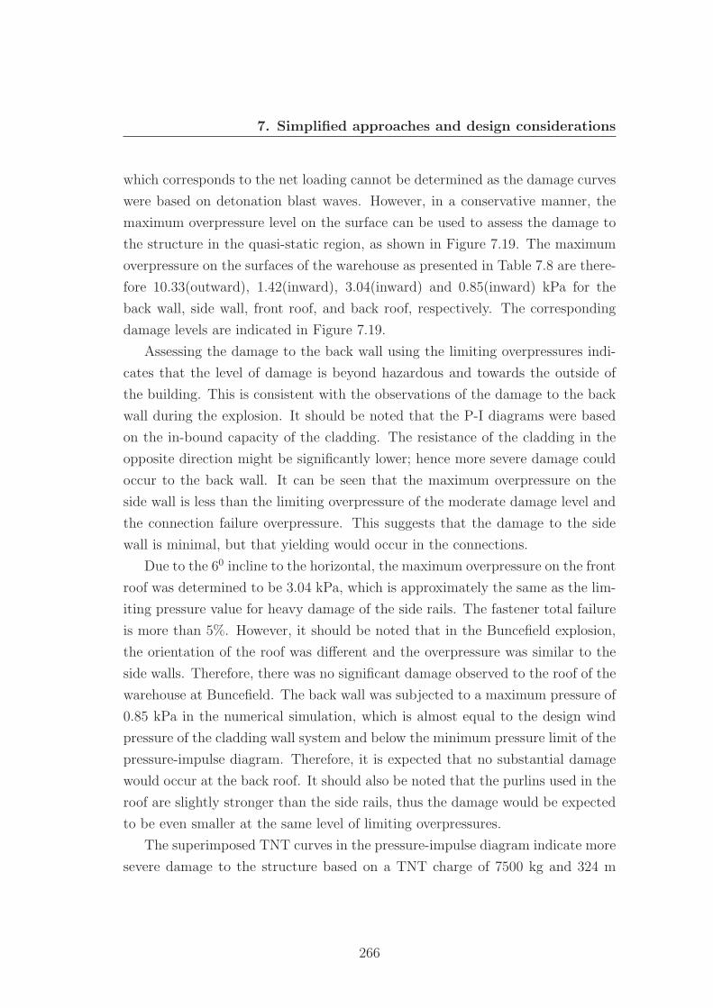
7. Simplified approaches and design considerations
which corresponds to the net loading cannot be determined as the damage curves
were based on detonation blast waves. However, in a conservative manner, the
maximum overpressure level on the surface can be used to assess the damage to
the structure in the quasi-static region, as shown in Figure 7.19. The maximum
overpressure on the surfaces of the warehouse as presented in Table 7.8 are there-
fore 10.33(outward), 1.42(inward), 3.04(inward) and 0.85(inward) kPa for the
back wall, side wall, front roof, and back roof, respectively. The corresponding
damage levels are indicated in Figure 7.19.
Assessing the damage to the back wall using the limiting overpressures indi-
cates that the level of damage is beyond hazardous and towards the outside of
the building. This is consistent with the observations of the damage to the back
wall during the explosion. It should be noted that the P-I diagrams were based
on the in-bound capacity of the cladding. The resistance of the cladding in the
opposite direction might be significantly lower; hence more severe damage could
occur to the back wall. It can be seen that the maximum overpressure on the
side wall is less than the limiting overpressure of the moderate damage level and
the connection failure overpressure. This suggests that the damage to the side
wall is minimal, but that yielding would occur in the connections.
Due to the 60 incline to the horizontal, the maximum overpressure on the front
roof was determined to be 3.04 kPa, which is approximately the same as the lim-
iting pressure value for heavy damage of the side rails. The fastener total failure
is more than 5%. However, it should be noted that in the Buncefield explosion,
the orientation of the roof was different and the overpressure was similar to the
side walls. Therefore, there was no significant damage observed to the roof of the
warehouse at Buncefield. The back wall was subjected to a maximum pressure of
0.85 kPa in the numerical simulation, which is almost equal to the design wind
pressure of the cladding wall system and below the minimum pressure limit of the
pressure-impulse diagram. Therefore, it is expected that no substantial damage
would occur at the back roof. It should also be noted that the purlins used in the
roof are slightly stronger than the side rails, thus the damage would be expected
to be even smaller at the same level of limiting overpressures.
The superimposed TNT curves in the pressure-impulse diagram indicate more
severe damage to the structure based on a TNT charge of 7500 kg and 324 m
266
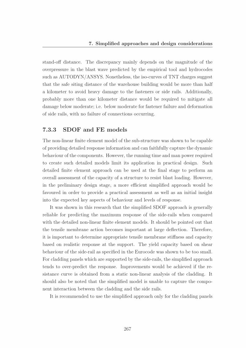
7. Simplified approaches and design considerations
stand-off distance. The discrepancy mainly depends on the magnitude of the
overpressure in the blast wave predicted by the empirical tool and hydrocodes
such as AUTODYN/ANSYS. Nonetheless, the iso-curves of TNT charges suggest
that the safe siting distance of the warehouse building would be more than half
a kilometer to avoid heavy damage to the fasteners or side rails. Additionally,
probably more than one kilometer distance would be required to mitigate all
damage below moderate; i.e. below moderate for fastener failure and deformation
of side rails, with no failure of connections occurring.
7.3.3 SDOF and FE models
The non-linear finite element model of the sub-structure was shown to be capable
of providing detailed response information and can faithfully capture the dynamic
behaviour of the components. However, the running time and man power required
to create such detailed models limit its application in practical design. Such
detailed finite element approach can be used at the final stage to perform an
overall assessment of the capacity of a structure to resist blast loading. However,
in the preliminary design stage, a more efficient simplified approach would be
favoured in order to provide a practical assessment as well as an initial insight
into the expected key aspects of behaviour and levels of response.
It was shown in this research that the simplified SDOF approach is generally
reliable for predicting the maximum response of the side-rails when compared
with the detailed non-linear finite element models. It should be pointed out that
the tensile membrane action becomes important at large deflection. Therefore,
it is important to determine appropriate tensile membrane stiffness and capacity
based on realistic response at the support. The yield capacity based on shear
behaviour of the side-rail as specified in the Eurocode was shown to be too small.
For cladding panels which are supported by the side-rails, the simplified approach
tends to over-predict the response. Improvements would be achieved if the re-
sistance curve is obtained from a static non-linear analysis of the cladding. It
should also be noted that the simplified model is unable to capture the compo-
nent interaction between the cladding and the side rails.
It is recommended to use the simplified approach only for the cladding panels
267
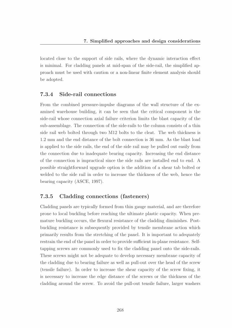
7. Simplified approaches and design considerations
located close to the support of side rails, where the dynamic interaction effect
is minimal. For cladding panels at mid-span of the side-rail, the simplified ap-
proach must be used with caution or a non-linear finite element analysis should
be adopted.
7.3.4 Side-rail connections
From the combined pressure-impulse diagrams of the wall structure of the ex-
amined warehouse building, it can be seen that the critical component is the
side-rail whose connection axial failure criterion limits the blast capacity of the
sub-assemblage. The connection of the side-rails to the column consists of a thin
side rail web bolted through two M12 bolts to the cleat. The web thickness is
1.2 mm and the end distance of the bolt connection is 36 mm. As the blast load
is applied to the side rails, the end of the side rail may be pulled out easily from
the connection due to inadequate bearing capacity. Increasing the end distance
of the connection is impractical since the side rails are installed end to end. A
possible straightforward upgrade option is the addition of a shear tab bolted or
welded to the side rail in order to increase the thickness of the web, hence the
bearing capacity (ASCE, 1997).
7.3.5 Cladding connections (fasteners)
Cladding panels are typically formed from thin gauge material, and are therefore
prone to local buckling before reaching the ultimate plastic capacity. When pre-
mature buckling occurs, the flexural resistance of the cladding diminishes. Post-
buckling resistance is subsequently provided by tensile membrane action which
primarily results from the stretching of the panel. It is important to adequately
restrain the end of the panel in order to provide sufficient in-plane resistance. Self-
tapping screws are commonly used to fix the cladding panel onto the side-rails.
These screws might not be adequate to develop necessary membrane capacity of
the cladding due to bearing failure as well as pull-out over the head of the screw
(tensile failure). In order to increase the shear capacity of the screw fixing, it
is necessary to increase the edge distance of the screws or the thickness of the
cladding around the screw. To avoid the pull-out tensile failure, larger washers
268
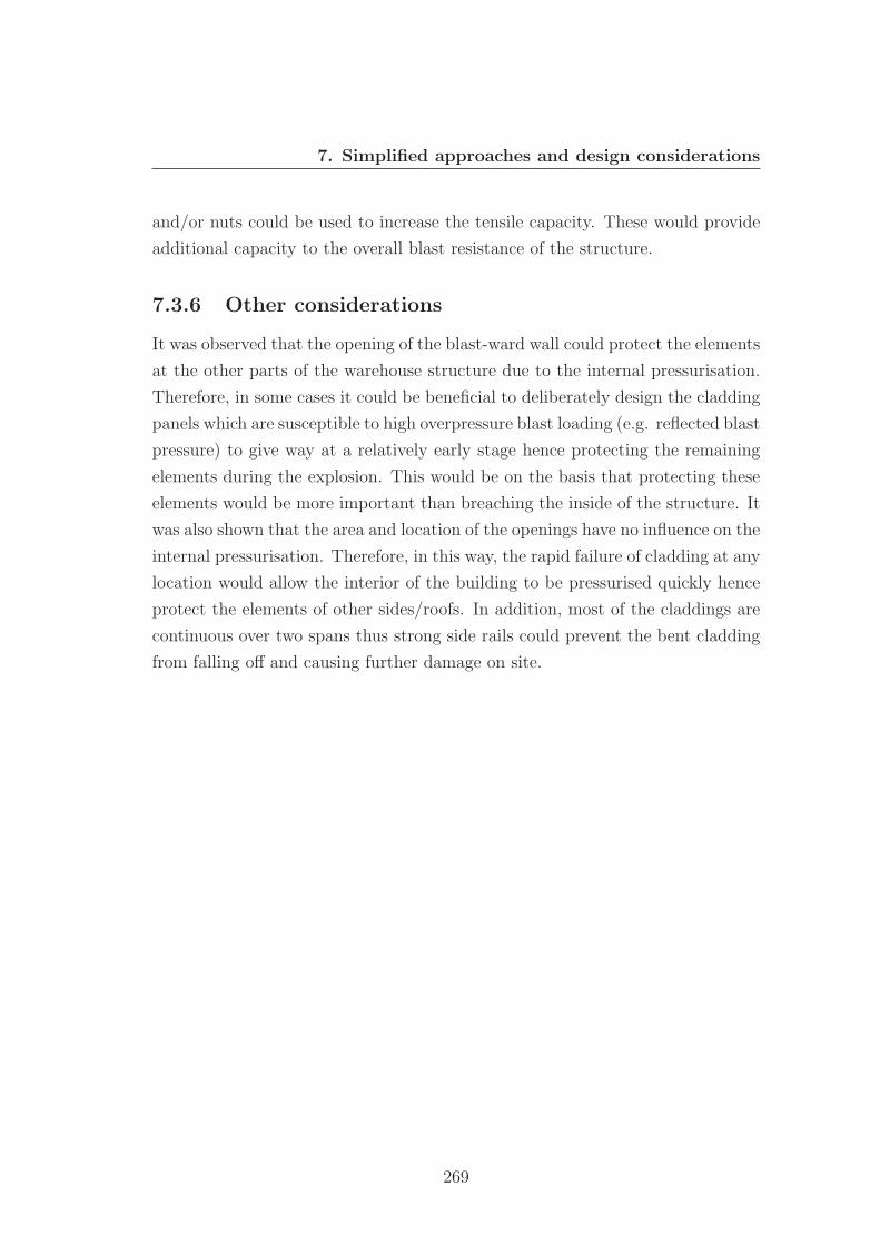
7. Simplified approaches and design considerations
and/or nuts could be used to increase the tensile capacity. These would provide
additional capacity to the overall blast resistance of the structure.
7.3.6 Other considerations
It was observed that the opening of the blast-ward wall could protect the elements
at the other parts of the warehouse structure due to the internal pressurisation.
Therefore, in some cases it could be beneficial to deliberately design the cladding
panels which are susceptible to high overpressure blast loading (e.g. reflected blast
pressure) to give way at a relatively early stage hence protecting the remaining
elements during the explosion. This would be on the basis that protecting these
elements would be more important than breaching the inside of the structure. It
was also shown that the area and location of the openings have no influence on the
internal pressurisation. Therefore, in this way, the rapid failure of cladding at any
location would allow the interior of the building to be pressurised quickly hence
protect the elements of other sides/roofs. In addition, most of the claddings are
continuous over two spans thus strong side rails could prevent the bent cladding
from falling off and causing further damage on site.
269
Chapter 8
Conclusions and further work
The conclusions of the present study are summarised in three parts: blast response
of steel boxes, blast response of warehouse structures and blast simulation. The
recommendations for future research are also presented herein.
8.1 Blast response of field objects
The blast response of steel field boxes was examined in detail in the current work.
Three types of numerical approaches were adopted to study the response of the
steel boxes: Lagrangian, Uncoupled Eulerian-Lagrangian and Coupled Eulerian-
Lagrangian. The pure Eulerian modelling method was used to reproduce the
blast waves that occurred in the test explosions. The numerical blast waves were
shown to be in good agreement with the test results. The Eulerian capability in
? can therefore be used to create blast waves reliably.
Data collected from blast tests carried out independently was used to validate
the numerical models adopted in the current study. Both quantitative and qual-
itative analyses of the response of the test boxes were carried out. The results
indicated that the Coupled Eulerian-Lagrangian approach was the most accurate
method for analysis of blast problems involving small objects such as the steel
boxes, but its running time (more than 10 hours for each model) limits the range
of application. The more efficient Lagrangian approach only requires 3-5 minutes
for each model, but it becomes less accurate at high overpressures due to impulse
reduction effects at the front surface.
270
8. Conclusions and further work
An Eulerian study on the reflection of deflagration blast waves was undertaken
by using a two-dimensional Eulerian model. This study suggested quantitatively
that the reflection enhancement of overpressure loading of the deflagration is not
as strong as for a detonation. The reduction in the reflection coefficient ranged
from 35% to 50% for deflagration loading with peak overpressure from 400 kPa
to 10 kPa, respectively.
Parametric studies covering detonation, deflagration and quasi static overpres-
sure blast loadings cases were carried out to assess systematically the response of
the boxes. In the investigation, the Lagrangian model was used and subjected to
a series of peak overpressure and impulse combinations. The overpressure range
was limited to a side-on pressure of 4 bar in order to retain the accuracy of the
Lagrangian model. The results were presented in the form of pressure-impulse
diagrams and typical residual shapes were selected for visual assessment.
A few selected results from the parametric studies were compared broadly
with an actual damaged box recovered from the Buncefield site. The comparison
suggested that the explosion within the vapour cloud that spread over the Bunce-
field site was likely to be a deflagration with side-on overpressure of 420 kPa or
roughly head-on overpressure of 200 kPa (using the derived reflection coefficients
of deflagration). This showed that the results can be used for future forensic
investigation of explosion incidents.
8.2 Blast responses of warehouse structures
A typical UK warehouse was chosen to study its structural response to blast
loading. The strain rate effect of the material was incorporated through dynamic
increase factors. Different simulation levels of the structure were investigated and
it was shown that a sub-assemblage model is sufficient for representing the re-
sponse of the wall structures. Validation of the sub-assemblage model was carried
out against a full-scale static test conducted at Imperial College (Elghazouli et al.
(2014)). This validated the adequacy of the sub-assemblage model in representing
the material and geometric properties of the structure.
A refined sub-assemblage model was then developed by using connector mod-
271
8. Conclusions and further work
els to realistically represent the behaviour of the self-tapping screw fastener fixings
and the M12 bolt-cleat connections. The connector behaviour was also validated
against available test data at Imperial. The refined model was then employed in
parametric studies to investigate the response of the structure to blast loading
with various overpressures and impulses.
The failure of the fastener models was examined in detail and the results
showed that the fastener can fail by different mechanisms depending on the char-
acteristics of the blast loading and its location. For example, the central fastener
located at the middle of the upper or lower side rail failed by shear (close to the
y-direction) when subjected to a quasi-static loading, while it failed in tension
when subjected to an impulsive loading. Under some blast loading situations,
the failure of the connector can be related to the middle relative displacement of
the cladding. It was shown that the shear failure (close to the y-direction) occurs
when the middle of the cladding deforms to 85 mm relative to the average of two
ends, which is about 5% of the span of the component. However, it was difficult
to relate the middle displacement of the side rail to the failure of the fasteners,
as it was heavily dependent on the nature of the loading and the response of the
structure.
The results of the parametric studies were summarised in the form of pressure-
impulse diagrams. The typical criteria used for the construction of the iso-damage
curves were the transverse and axial displacements of the central side rail in the
sub-assemblage. A new damage criterion based on the failure of the fasteners
was proposed and replaced the displacement of the cladding. The new damage
criterion provides a more straightforward assessment of the damage to the steel
cladding structures. The pressure-impulse diagrams were then superimposed to
form a combined diagram in which the axial connection failure was established
to be the most critical condition for the structure under study. Design considera-
tions were provided in order to offer guidance for mitigating the extent of damage
to the fasteners and connections. Finally iso-curves of high explosive TNT were
also superimposed in the combined diagram with the aim of of providing guid-
ance on the safe siting distances of buildings from possible sources of detonation
explosions.
Since the response assigned to the fastener model was based on static test
272
8. Conclusions and further work
results, a focussed study was carried out to estimate the local strain rate in the
self-tapping screw fastener. It was estimated that the fastener had a typical
strain rate of 240 s-1, assuming a relatively strong dynamic loading condition.
This increased the yield and ultimate capacity of the fastener by approximately
21.3 and 10.65%, respectively. However, in subsequent analyses using strain-rate
strengthened fasteners, it was observed that the displacement of the side rails
was not affected by the increase in fastener capacity. Nonetheless, the failure of
the fastener has been affected slightly. It was suggested that for simplicity the
strain rate effect of the fastener could be ignored without significant influence on
the accuracy of the results.
To complement the non-linear finite element method, the simplified single
degree of freedom approach was also used to analyse the response of the sub-
structure. The interaction between the constituent components of the sub-structure
is typically considered to be insignificant if the ratio in natural frequency is less
than double, which is significantly exceeded in the structure under examination.
It was observed that the simplified approach provided reliable predictions for the
response of the side rails, provided that the tensile membrane action is prop-
erly defined. However, the simplified approach only worked for the side cladding
but not for the central cladding. Examining the response histories of the side
and central cladding revealed that the dynamic interaction between the central
cladding and the side rails was significant. Accordingly, the uncoupled simplified
approach might be not applicable even though the ratio of natural period of the
system was greater than 2. The comparison of the response between the detailed
non-linear FE model and the simplified approach demonstrated the importance
of using a realistic resistance function of the component. To this end, according
to (Louca et al., 1996), the resistance function is recommended to be determined
using a static non-linear finite element analysis.
8.3 Assessment of blast loading
Based on the estimation of the explosion undertaken by DOSG (SCI (2009)), a nu-
merical study was carried out to assess the overpressure loading on the warehouse
273
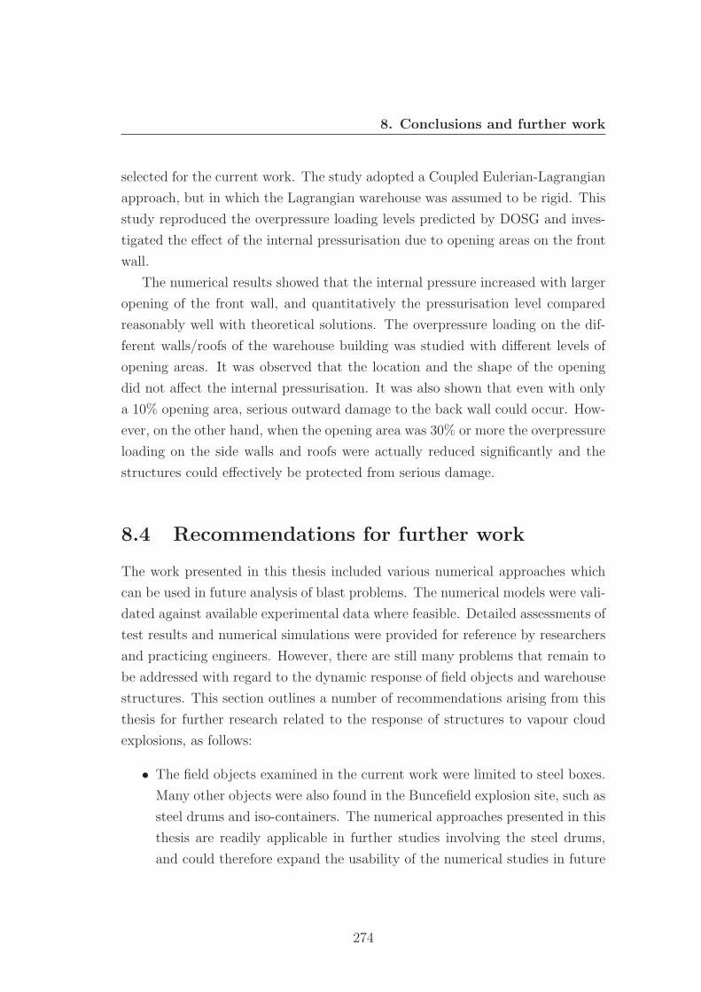
8. Conclusions and further work
selected for the current work. The study adopted a Coupled Eulerian-Lagrangian
approach, but in which the Lagrangian warehouse was assumed to be rigid. This
study reproduced the overpressure loading levels predicted by DOSG and inves-
tigated the effect of the internal pressurisation due to opening areas on the front
wall.
The numerical results showed that the internal pressure increased with larger
opening of the front wall, and quantitatively the pressurisation level compared
reasonably well with theoretical solutions. The overpressure loading on the dif-
ferent walls/roofs of the warehouse building was studied with different levels of
opening areas. It was observed that the location and the shape of the opening
did not affect the internal pressurisation. It was also shown that even with only
a 10% opening area, serious outward damage to the back wall could occur. How-
ever, on the other hand, when the opening area was 30% or more the overpressure
loading on the side walls and roofs were actually reduced significantly and the
structures could effectively be protected from serious damage.
8.4 Recommendations for further work
The work presented in this thesis included various numerical approaches which
can be used in future analysis of blast problems. The numerical models were vali-
dated against available experimental data where feasible. Detailed assessments of
test results and numerical simulations were provided for reference by researchers
and practicing engineers. However, there are still many problems that remain to
be addressed with regard to the dynamic response of field objects and warehouse
structures. This section outlines a number of recommendations arising from this
thesis for further research related to the response of structures to vapour cloud
explosions, as follows:
• The field objects examined in the current work were limited to steel boxes.
Many other objects were also found in the Buncefield explosion site, such as
steel drums and iso-containers. The numerical approaches presented in this
thesis are readily applicable in further studies involving the steel drums,
and could therefore expand the usability of the numerical studies in future
274
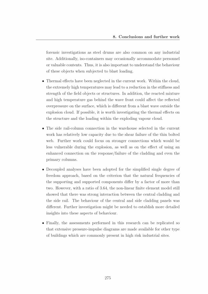
8. Conclusions and further work
forensic investigations as steel drums are also common on any industrial
site. Additionally, iso-containers may occasionally accommodate personnel
or valuable contents. Thus, it is also important to understand the behaviour
of these objects when subjected to blast loading.
• Thermal effects have been neglected in the current work. Within the cloud,
the extremely high temperatures may lead to a reduction in the stiffness and
strength of the field objects or structures. In addition, the reacted mixture
and high temperature gas behind the wave front could affect the reflected
overpressure on the surface, which is different from a blast wave outside the
explosion cloud. If possible, it is worth investigating the thermal effects on
the structure and the loading within the exploding vapour cloud.
• The side rail-column connection in the warehouse selected in the current
work has relatively low capacity due to the shear failure of the thin bolted
web. Further work could focus on stronger connections which would be
less vulnerable during the explosion, as well as on the effect of using an
enhanced connection on the response/failure of the cladding and even the
primary columns.
• Decoupled analyses have been adopted for the simplified single degree of
freedom approach, based on the criterion that the natural frequencies of
the supporting and supported components differ by a factor of more than
two. However, with a ratio of 3.64, the non-linear finite element model still
showed that there was strong interaction between the central cladding and
the side rail. The behaviour of the central and side cladding panels was
different. Further investigation might be needed to establish more detailed
insights into these aspects of behaviour.
• Finally, the assessments performed in this research can be replicated so
that extensive pressure-impulse diagrams are made available for other type
of buildings which are commonly present in high risk industrial sites.
275
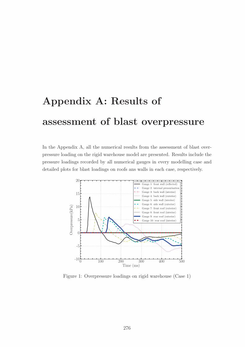
Appendix A: Results of
assessment of blast overpressure
In the Appendix A, all the numerical results from the assessment of blast over-
pressure loading on the rigid warehouse model are presented. Results include the
pressure loadings recorded by all numerical gauges in every modelling case and
detailed plots for blast loadings on roofs ans walls in each case, respectively.
0 100 200 300 400 500Time (ms)
-10
-5
0
5
10
15
20
Overpressure(kPa)
Gauge 1: front wall (reflected)
Gauge 2: internal pressurisation
Gauge 3: back wall (interior)
Gauge 4: back wall (exterior)
Gauge 5: side wall (interior)
Gauge 6: side wall (exterior)
Gauge 7: front roof (exterior)
Gauge 8: front roof (interior)
Gauge 9: rear roof (exterior)
Gauge 10: rear roof (interior)
Figure 1: Overpressure loadings on rigid warehouse (Case 1)
276
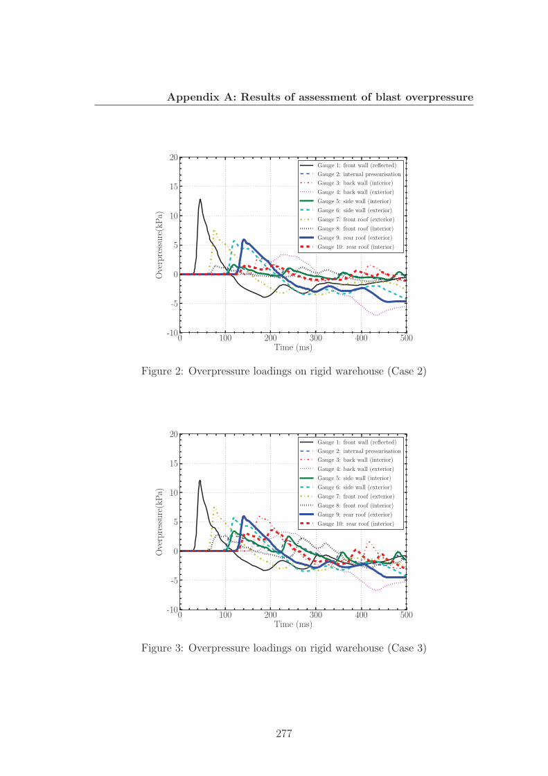
Appendix A: Results of assessment of blast overpressure
0 100 200 300 400 500Time (ms)
-10
-5
0
5
10
15
20Overpressure(kPa)
Gauge 1: front wall (reflected)
Gauge 2: internal pressurisation
Gauge 3: back wall (interior)
Gauge 4: back wall (exterior)
Gauge 5: side wall (interior)
Gauge 6: side wall (exterior)
Gauge 7: front roof (exterior)
Gauge 8: front roof (interior)
Gauge 9: rear roof (exterior)
Gauge 10: rear roof (interior)
Figure 2: Overpressure loadings on rigid warehouse (Case 2)
0 100 200 300 400 500Time (ms)
-10
-5
0
5
10
15
20
Overpressure(kPa)
Gauge 1: front wall (reflected)
Gauge 2: internal pressurisation
Gauge 3: back wall (interior)
Gauge 4: back wall (exterior)
Gauge 5: side wall (interior)
Gauge 6: side wall (exterior)
Gauge 7: front roof (exterior)
Gauge 8: front roof (interior)
Gauge 9: rear roof (exterior)
Gauge 10: rear roof (interior)
Figure 3: Overpressure loadings on rigid warehouse (Case 3)
277
Appendix A: Results of assessment of blast overpressure
0 100 200 300 400 500Time (ms)
-10
-5
0
5
10
15
20Overpressure(kPa)
Gauge 1: front wall (reflected)
Gauge 2: internal pressurisation
Gauge 3: back wall (interior)
Gauge 4: back wall (exterior)
Gauge 5: side wall (interior)
Gauge 6: side wall (exterior)
Gauge 7: front roof (exterior)
Gauge 8: front roof (interior)
Gauge 9: rear roof (exterior)
Gauge 10: rear roof (interior)
Figure 4: Overpressure loadings on rigid warehouse (Case 4)
0 100 200 300 400 500Time (ms)
-10
-5
0
5
10
15
20
Overpressure(kPa)
Gauge 1: front wall (reflected)
Gauge 2: internal pressurisation
Gauge 3: back wall (interior)
Gauge 4: back wall (exterior)
Gauge 5: side wall (interior)
Gauge 6: side wall (exterior)
Gauge 7: front roof (exterior)
Gauge 8: front roof (interior)
Gauge 9: rear roof (exterior)
Gauge 10: rear roof (interior)
Figure 5: Overpressure loadings on rigid warehouse (Case 5)
278
Appendix A: Results of assessment of blast overpressure
0 100 200 300 400 500Time (ms)
-10
-5
0
5
10
15
20
Overpressure(kPa)
Gauge 1: front wall (reflected)
Gauge 2: internal pressurisation
Gauge 3: back wall (interior)
Gauge 4: back wall (exterior)
Gauge 5: side wall (interior)
Gauge 6: side wall (exterior)
Gauge 7: front roof (exterior)
Gauge 8: front roof (interior)
Gauge 9: rear roof (exterior)
Gauge 10: rear roof (interior)
Figure 6: Overpressure loadings on rigid warehouse (Case 6)
0 100 200 300 400 500Time (ms)
-10
-5
0
5
10
15
20
Overpressure(kPa)
Gauge 3: back wall (interior)
Gauge 4: back wall (exterior)
Net loading (exterior-interior)
(a) Case 1
0 100 200 300 400 500Time (ms)
-10
-5
0
5
10
15
20
Overpressure(kPa)
Gauge 3: back wall (interior)
Gauge 4: back wall (exterior)
Net loading (exterior-interior)
(b) Case 2
Figure 7: Overpressure loadings of back wall (Case 1 & 2)
279
Appendix A: Results of assessment of blast overpressure
0 100 200 300 400 500Time (ms)
-10
-5
0
5
10
15
20
Overpressure(kPa)
Gauge 3: back wall (interior)
Gauge 4: back wall (exterior)
Net loading (exterior-interior)
(a) Case 3
0 100 200 300 400 500Time (ms)
-10
-5
0
5
10
15
20
Overpressure(kPa)
Gauge 3: back wall (interior)
Gauge 4: back wall (exterior)
Net loading (exterior-interior)
(b) Case 4
Figure 8: Overpressure loadings of back wall (Case 3 & 4)
0 100 200 300 400 500Time (ms)
-10
-5
0
5
10
15
20
Overpressure(kPa)
Gauge 3: back wall (interior)
Gauge 4: back wall (exterior)
Net loading (exterior-interior)
(a) Case 5
0 100 200 300 400 500Time (ms)
-10
-5
0
5
10
15
20
Overpressure(kPa)
Gauge 3: back wall (interior)
Gauge 4: back wall (exterior)
Net loading (exterior-interior)
(b) Case 6
Figure 9: Overpressure loadings of back wall (Case 5 & 6)
0 100 200 300 400 500Time (ms)
-10
-5
0
5
10
15
20
Overpressure(kPa)
Gauge 3: side wall (interior)
Gauge 4: side wall (exterior)
Net loading (exterior-interior)
(a) Case 1
0 100 200 300 400 500Time (ms)
-10
-5
0
5
10
15
20
Overpressure(kPa)
Gauge 3: side wall (interior)
Gauge 4: side wall (exterior)
Net loading (exterior-interior)
(b) Case 2
Figure 10: Overpressure loadings of side wall (Case 1 & 2)
280
Appendix A: Results of assessment of blast overpressure
0 100 200 300 400 500Time (ms)
-10
-5
0
5
10
15
20
Overpressure(kPa)
Gauge 3: side wall (interior)
Gauge 4: side wall (exterior)
Net loading (exterior-interior)
(a) Case 3
0 100 200 300 400 500Time (ms)
-10
-5
0
5
10
15
20
Overpressure(kPa)
Gauge 3: side wall (interior)
Gauge 4: side wall (exterior)
Net loading (exterior-interior)
(b) Case 4
Figure 11: Overpressure loadings of side wall (Case 3 & 4)
0 100 200 300 400 500Time (ms)
-10
-5
0
5
10
15
20
Overpressure(kPa)
Gauge 3: side wall (interior)
Gauge 4: side wall (exterior)
Net loading (exterior-interior)
(a) Case 5
0 100 200 300 400 500Time (ms)
-10
-5
0
5
10
15
20
Overpressure(kPa)
Gauge 3: side wall (interior)
Gauge 4: side wall (exterior)
Net loading (exterior-interior)
(b) Case 6
Figure 12: Overpressure loadings of side wall (Case 5 & 6)
0 100 200 300 400 500Time (ms)
-10
-5
0
5
10
15
20
Overpressure(kPa)
Gauge 3: front roof (interior)
Gauge 4: front roof (exterior)
Net loading (exterior-interior)
(a) Case 1
0 100 200 300 400 500Time (ms)
-10
-5
0
5
10
15
20
Overpressure(kPa)
Gauge 3: front roof (interior)
Gauge 4: front roof (exterior)
Net loading (exterior-interior)
(b) Case 2
Figure 13: Overpressure loadings of front roof (Case 1 & 2)
281
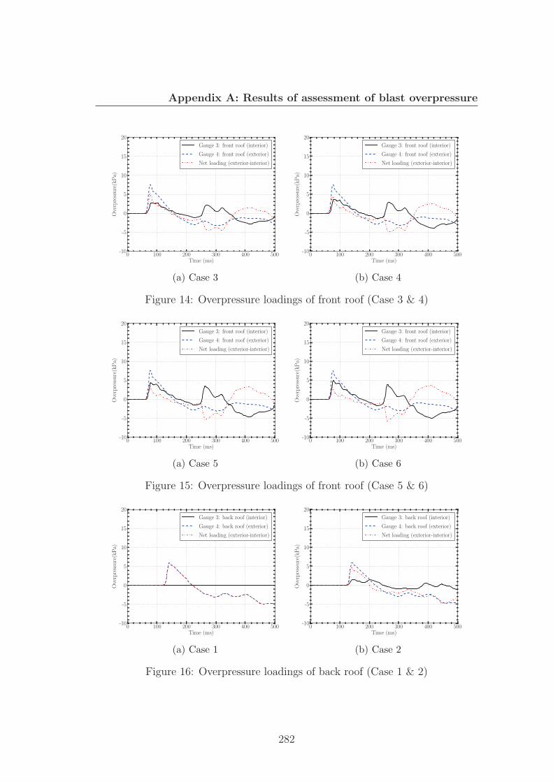
Appendix A: Results of assessment of blast overpressure
0 100 200 300 400 500Time (ms)
-10
-5
0
5
10
15
20
Overpressure(kPa)
Gauge 3: front roof (interior)
Gauge 4: front roof (exterior)
Net loading (exterior-interior)
(a) Case 3
0 100 200 300 400 500Time (ms)
-10
-5
0
5
10
15
20
Overpressure(kPa)
Gauge 3: front roof (interior)
Gauge 4: front roof (exterior)
Net loading (exterior-interior)
(b) Case 4
Figure 14: Overpressure loadings of front roof (Case 3 & 4)
0 100 200 300 400 500Time (ms)
-10
-5
0
5
10
15
20
Overpressure(kPa)
Gauge 3: front roof (interior)
Gauge 4: front roof (exterior)
Net loading (exterior-interior)
(a) Case 5
0 100 200 300 400 500Time (ms)
-10
-5
0
5
10
15
20
Overpressure(kPa)
Gauge 3: front roof (interior)
Gauge 4: front roof (exterior)
Net loading (exterior-interior)
(b) Case 6
Figure 15: Overpressure loadings of front roof (Case 5 & 6)
0 100 200 300 400 500Time (ms)
-10
-5
0
5
10
15
20
Overpressure(kPa)
Gauge 3: back roof (interior)
Gauge 4: back roof (exterior)
Net loading (exterior-interior)
(a) Case 1
0 100 200 300 400 500Time (ms)
-10
-5
0
5
10
15
20
Overpressure(kPa)
Gauge 3: back roof (interior)
Gauge 4: back roof (exterior)
Net loading (exterior-interior)
(b) Case 2
Figure 16: Overpressure loadings of back roof (Case 1 & 2)
282
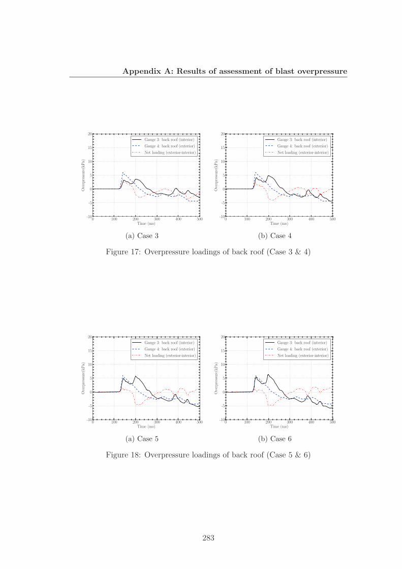
Appendix A: Results of assessment of blast overpressure
0 100 200 300 400 500Time (ms)
-10
-5
0
5
10
15
20
Overpressure(kPa)
Gauge 3: back roof (interior)
Gauge 4: back roof (exterior)
Net loading (exterior-interior)
(a) Case 3
0 100 200 300 400 500Time (ms)
-10
-5
0
5
10
15
20
Overpressure(kPa)
Gauge 3: back roof (interior)
Gauge 4: back roof (exterior)
Net loading (exterior-interior)
(b) Case 4
Figure 17: Overpressure loadings of back roof (Case 3 & 4)
0 100 200 300 400 500Time (ms)
-10
-5
0
5
10
15
20
Overpressure(kPa)
Gauge 3: back roof (interior)
Gauge 4: back roof (exterior)
Net loading (exterior-interior)
(a) Case 5
0 100 200 300 400 500Time (ms)
-10
-5
0
5
10
15
20
Overpressure(kPa)
Gauge 3: back roof (interior)
Gauge 4: back roof (exterior)
Net loading (exterior-interior)
(b) Case 6
Figure 18: Overpressure loadings of back roof (Case 5 & 6)
283
Appendix B: Loading scenarios
for parametric study of
sub-assemblage model
The Appendix B presents the ranges of overpressures and impulses used in the
parametric study of the sub-assemblage finite element model. The overpressures
varied from 1 to 50 kPa and the impulses varied from 100 to 10000 kPa.ms. The
modelling case numbers and corresponding positive durations are presented as
follow:
284
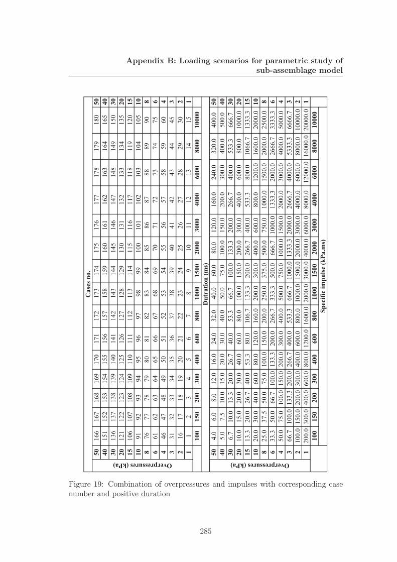
Appendix B: Loading scenarios for parametric study ofsub-assemblage model
5016
616
716
816
917
017
117
217
317
417
517
617
717
817
918
050
4015
115
215
315
415
515
615
715
815
916
016
116
216
316
416
540
3013
613
713
813
914
014
114
214
314
414
514
614
714
814
915
030
2012
112
212
312
412
512
612
712
812
913
013
113
213
313
413
520
1510
610
710
810
911
011
111
211
311
411
511
611
711
811
912
015
1091
9293
9495
9697
9899
100
101
102
103
104
105
108
7677
7879
8081
8283
8485
8687
8889
908
661
6263
6465
6667
6869
7071
7273
7475
64
4647
4849
5051
5253
5455
5657
5859
604
331
3233
3435
3637
3839
4041
4243
4445
32
1617
1819
2021
2223
2425
2627
2829
302
11
23
45
67
89
1011
1213
1415
110
015
020
030
040
060
080
010
0015
0020
0030
0040
0060
0080
0010
000
504.
06.
08.
012
.016
.024
.032
.040
.060
.080
.012
0.0
160.
024
0.0
320.
040
0.0
5040
5.0
7.5
10.0
15.0
20.0
30.0
40.0
50.0
75.0
100.
015
0.0
200.
030
0.0
400.
050
0.0
4030
6.7
10.0
13.3
20.0
26.7
40.0
53.3
66.7
100.
013
3.3
200.
026
6.7
400.
053
3.3
666.
730
2010
.015
.020
.030
.040
.060
.080
.010
0.0
150.
020
0.0
300.
040
0.0
600.
080
0.0
1000
.020
1513
.320
.026
.740
.053
.380
.010
6.7
133.
320
0.0
266.
740
0.0
533.
380
0.0
1066
.713
33.3
1510
20.0
30.0
40.0
60.0
80.0
120.
016
0.0
200.
030
0.0
400.
060
0.0
800.
012
00.0
1600
.020
00.0
108
25.0
37.5
50.0
75.0
100.
015
0.0
200.
025
0.0
375.
050
0.0
750.
010
00.0
1500
.020
00.0
2500
.08
633
.350
.066
.710
0.0
133.
320
0.0
266.
733
3.3
500.
066
6.7
1000
.013
33.3
2000
.026
66.7
3333
.36
450
.075
.010
0.0
150.
020
0.0
300.
040
0.0
500.
075
0.0
1000
.015
00.0
2000
.030
00.0
4000
.050
00.0
43
66.7
100.
013
3.3
200.
026
6.7
400.
053
3.3
666.
710
00.0
1333
.320
00.0
2666
.740
00.0
5333
.366
66.7
32
100.
015
0.0
200.
030
0.0
400.
060
0.0
800.
010
00.0
1500
.020
00.0
3000
.040
00.0
6000
.080
00.0
1000
0.0
21
200.
030
0.0
400.
060
0.0
800.
012
00.0
1600
.020
00.0
3000
.040
00.0
6000
.080
00.0
1200
0.0
1600
0.0
2000
0.0
110
015
020
030
040
060
080
010
0015
0020
0030
0040
0060
0080
0010
000
Cas
es n
o.Overpressures (kPa) Overpressures (kPa)
Spec
ific
impu
lse
(kPa
.ms)
Dut
ratio
n (m
s)
Figure 19: Combination of overpressures and impulses with corresponding casenumber and positive duration
285
References
Dan Allason. Buncefield joint industry phase 2 experimental studies, detonation
test 4. Technical report, GL Noble Denton, 2013. xiv, 87, 91, 93, 96
ANSYS. ANSYS v13.0 Workbench User’s Manual, Centuray Dynamics,2010. 3,
11, 45, 51, 54, 66, 69, 70, 76, 250, 251
ASCE. Design of Blast Resistant Buildings in Petrochemical Facilities. Task
Commitee on Blast Resistance Design, ASCE, Virginia, USA, 1997. 136, 161,
192, 268
G. Atkinson. Blast damage to storage tanks and steel clad buildings. Process
Safety and Environmental Protection, 89:382–390, 2011. xiii, xvi, 16, 150, 151,
152, 251, 257
AutoReaGas. AutoReaGas User Documentation and Theory Manual, Century
Dynamics,1994. 11
W.E. Baker, P.A. Cox, P.S. Westine, J.J. Kulesz, and R.A. Strehlow. Explosion
Hazards and Evaluation. Elsevier, Amsterdam, 1983. 43, 250
A.V. Berg. The multi-energy method. Journal of Hazardous Materials, 12:1–10,
1985. xiii, 13
J.M. Biggs. Introduction to Structural Dynamics. McGraw-Hill, New York, 1964.
3, 36, 40, 241, 244, 248, 249
BMIIB. Explosion mechanics advisory group report. Technical report, London,
2007. 4
286
REFERENCES
T. Borvik, A.G. Hanssen, M. Langseth, and L. Olovsson. Response of structures
to planar blast loads - a finite element approach. Computer and Structures, 87:
507–520, 2009. 3, 50, 66, 131
S.D. Boyd. Acceleration of a plate subject to explosive blast loading - trial
results. Technical report, DSTO Aeronautical and Martitime Research Labo-
ratory, Australia, 2000. xiv, 76, 77, 82
Texas City BP. Investigation report: Refinery explosion and fire. Technical
report, BP Texas City, Texas, 2005. 19
B. A. Burgan and D. Moutaftsis. Screening the vulnerability of buildings near
hazardous sites. Technical report, Steel Construction Institute, 2009. 48
B.A. Burgan and D. Moutaftsis. Screening the vunerability of buildings near
hazardous sites. Technical report, Steel Construction Institute, London, 2011.
xvi, 153, 155, 156, 158
D.S. Burgess and M.G. Zabetakis. Bureau of mines investigation report 7752.
Technical report, U.S. Bureau of Mines, 1973. 18
CA. Cabp standard fastener range, technical note tn-28 rev 3. Technical report,
CA Building Group, 2008. xvi, 158, 159
P. Carlucci, C. Mougeotte, and Huidi J. Validation of ABAQUS explicit - CEL
for classes of problems of interest to the U.S. Army . In Proceedings of 2010
Simulia Customer Conference, 2010. 51
Chemical Industries Association CIA. Guidance for the Location and Design of
Occupied Building on Chemical Manufacturing Sites. CIA/CISHEC. 150
CONWEP. U.S. Army Corps of Engineers, CONWEP - conventional weapons
effects, USA, 1991. 68
R.D. Cook, D.S. Malkus, M.E. Plesha, and R.J. Witt. Concepts and Applications
of Finite Element Analysis, 4th Edition. John Wiley & Sons, U.S., 2002. 56
287
REFERENCES
G.R. Cowper and P.S. Symonds. Strain-hardening and strain-rate effects in the
impact loading of cantilever beam. Technical report, Providence, R.I. : Division
of Applied Mathematics, Brown University, 1957. 47, 161
R.R. Craig. Structural Dynamics An Introduction to Computer Methods. John
Wiley and Son, Inc, 1981. 41
A.Y. Elghazouli, C. Malaga-Chuquitaype, and Y. Liu. Ultimate behaviour of
cladding assemblages in industrial buildings. In Eurosteel 2014 International
Conference, Naples, Italy, 2014, 2014. xvi, 166, 167, 175, 225, 271
G.E. Fairlie. Efficient analysis of high explosive air blast in complex urban geome-
tries using the AUTODYN-2d and 3d hydrocodes, analytical and experimental
methods. In 15th Int Symposium on the Military Aspects of Blast and Shock,
1997. 51
A. Soleiman Fallah and L.A.Louca. Pressure impulse diagrams for elastic-plastic-
hardening and softening single-degree-of-freedom models subjected to blast
loading. International Journal of Impact Engineering, 34(4):823–842, 2007.
50
L. Fan, J. Rondal, and S. Cescotto. Finite element modelling of single lap scew
connection in steel sheeting under static shear. Thin-wall structures, 27:165–
185, 1997. 176
U.S. Homeland Security 2003 FEMA, Federal Emergency Management Agency.
FEMA426 Reference manual to mitigate potential terrorist attack against
buildings. 26, 52
FLACSv9. Users Manual (2009) Users manual for FLACS version 9.0, GexCon
AS, 20 January 2009. 11
Hadley. Ultrazed ultrabeam for purlins, cladding rails and floor joists in building
shell construction. Technical report, Hadley Group, 2004. xvi, 157, 159, 184,
239
B.A. Izzuddin. A simplified model for axially restrained beam subject to extreme
loading. Steel Structures, 5:421–429, 2005. 48
288
REFERENCES
A.C. Jacinto, R.D. Ambrosini, and R.F. Danesi. Experimental and computational
analysis of plates under air blast loading. International Journal of Impact
Engineering, 25:927–947, 2001. 50, 81
LIM Jin-seong, KIM Tae-soo, and KIM Seung-hun. Ultimate strength of single
shear bolted connections with cold-formed ferritic stainless steel. Journal of
Zhejiang University-SIENCE A (Applied Physics and Engineering), 14(2):120–
136, 2013. 179
D.M. Johnson. The potential of vapour cloud explosions - lessons from the Bunce-
field accident. Journal of Loss Prevention in the Process Industries, 23:921–927,
2010. 18
G.R. Johnson and W.H Cook. A constitutive model and data for metals subject
to large strains, high strain rates and high temperatures. In Proceedings of the
7th International Symposium on Ballistics, page 7, 1983. 47, 161
Norman Jones. Structural Impact. Cambridge University Press, U.K., 1997. 50
C.N. Kingery and G. Bulmash. Air blast parameters from TNT spherical air
burst and hemispherical surface burst. Technical report, US Army Armament
Research and Development Centre Ballistic Research Laboratory, 1984. 250
G.F. Kinney and K.I. Graham. Explosive Shocks in Air. Springer-Verlag, New
York, 1985. xiii, 12, 22, 23, 24, 25, 28, 30, 31, 33, 34, 66
G.S. Langdon and G.K Schleyer. Inelastic deformation and failure of clamped
aluminium plates under pulse pressure loading. International Journal of Impact
Engineering, 28:1107–1127, 1999. 50
G.S Langdon and G.K. Schleyer. Inelastic deformation and failure of profiled
stainless steel blast wall panels. part i: experimental investigations. Interna-
tional Journal of Impact Engineering, 31:341–369, 2006a. 49
G.S Langdon and G.K. Schleyer. Inelastic deformation and failure of profiled
stainless steel blast wall panels. part ii: analytical modelling considerations.
International Journal of Impact Engineering, 31:371–399, 2006b. 3, 49
289
REFERENCES
G.S Langdon and G.K. Schleyer. Deformation and failure of profiled stainless
steel blast wall panels. part iii: finite element simulations and overall summary.
International Journal of Impact Engineering, 32:988–1012, 2006c. 3, 49
J.F. Lechaudel and Y. Mouilleau. Assessment of an accidental vapour cloud
explosion. Loss Prevention and Safety Promotion in the Process Industries, 1,
1995. 19
Y.H Liang and L.A. Louca. Corrugated panels under dynamic loads. International
Journal of Impact Engineering, 34:1185–1201, 2007. 49
L.A. Louca, M. Punjani, and J.E. Harding. Non-linear analysis of blast wall and
stiffened panels subjected to hydrocarbon explosions. Journal of Constructional
Steel Research, 37:93–113, 1996. 3, 49, 247, 273
L.A. Louca, J.W. Boh, and Y.S. Choo. Design and analysis of stainless steel
profiled blast barriers. Journal of Constructional Steel Research, 60:1699–1723,
2004. 49
LS-DYNA. LS-DYNA 971 Manual,Livermore Software Technology Corporation.
3, 45, 50, 51
B. Luccioni, D. Ambrosini, and R. Danesi. Blast load assessment using hy-
drocodes. Engineering Structures, 28:1736–1744, 2006. 51
G.M. Makhviladze and S.E. Yakush. Large scale unconfined fires and explosions.
In Proceedings of the Combustion Institute Volume (29), pages 195–210, 2002.
19
M. Maremonti, G. Russo, E. Salzano, and V. Tufano. Post accident analysis of
vapour cloud explosions in fuel storage areas. Trans. IChemE, 77, PartB, 1999.
19
W.P. Mercx, A.V. Berg, C.J. Hauhurst, N.J. Robertson, and K.C.Moran. De-
velopments in vapour cloud explosion blast modeling. Journal of Hazardous
Materials, 71(1-3):301–319, 2000. 14, 15
290
REFERENCES
C. Mougeotte, P. Carlucci, S. Recchia, and H. Ji. Novel approach to conducting
blast load analyses using Abaqus/explicit-cel. In Proceedings of 2010 SIMULIA
Customer Conference, 2010. 52
C.E. Needham. Blast waves (shock wave and high pressure phenomena). Springer,
Amsterdam, 2010. 35
T. Ngo, P. Mendis, A. Gupata, and J. Ramsay. Blast loading and blast effects
on structures - an overview. EJSE Special Issue: Loading on structures, pages
76–91, 2007. 225
O.C.Zienkiewicz and R.L. Taylor. The Finite Element Method for Fluid Dynam-
ics. Butterworth-Heinemann, Burlington, 2000. 66
P.Leach. Design charts for elasto-plastic design of cladding panels subject to
dynamic loading. In Proc. Instn Civ. Engrs Strcts and Bldgs, pages 56–61,
1993. 49
D.K. Pritchard. A review of methods for predicting blast damage from vapour
cloud explosions. Journal of Loss Prevention Process, 2:187–191, 1989. 12, 14
A.M. Rememnikov. A Review of Methods for Predicting Bomb Blast Effects on
Buildings, University of Wollongong Research Online. 51
E. Riks. An incremental approach to the solution of snapping and buckling
problems. International Journal of Solids and Structures, 15:529–551, 1979. 61
C. Sadee, D.E. Samuels, and T.P. O’Brien. The characteristics of the explosion
of cyclohexane at the Nypro (UK) Flixborough plant on 1 june 1974. Journal
of Occupational Accidents, 3:203, 1977. 18
G.K. Schleyer and S.S. Hsu. A modelling scheme for predicting the response of
elastic-plastic structures to pulse pressure loading. International Journal of
Impact Engineering, 24:759–777, 2000. 3
G.K. Schleyer, S.S. Hsu, M.D. White, and R.S. Birch. Pulse pressure loadings
of clamped mild steel plates. International Journal of Impact Engineering, 28:
223–247, 1999. 50
291
REFERENCES
L. Schwer. Optional strain-rate forms for the Johnson Cook constitutive model
and the role of the parameter epsilon0. In Proceedings of LS-DYNA Anwen-
derforum, pages E–I–1–14, 2007. 47
SCI. Technical Note 5, Design Guide for Stainless Steel Blast Walls. Technical
report, Steel Construction Institute, Ascot, 1999a. 49, 53
SCI. Technical note 10, an advanced sdof model for steel members subject to ex-
plosion loading: material rate sensitivity. Technical report, Steel Construction
Institue, Ascot, 1999b. 53
SCI. Technical note 7, simplified methods for analysis of response to dynamic
loading. Technical report, Steel Construction Institute, Ascot, 2002. 3, 48, 53
SCI. Buncefield explosion mechanism phase 1. Technical report, Health and
Safety Excutive, London, 2009. xiii, xiv, xvi, 4, 5, 15, 17, 18, 85, 86, 87, 89,
90, 91, 148, 249, 273
P.D. Smith and J.G. Hetherington. Blast and ballistic loading of structures.
Butterworth-Heinemann, Oxford, 1994. 1, 25
M. Spinelli and R. Vitali. Virtual threaded tire simulation as a desing predic-
tive tool: Application to tire hydrodyplaning. In Proceedings of SIMULIA
Customer Conference, 2009. xiv, 65
USACE. User’s guide for the single-degree-of-freedom blast effects design spread-
sheets (sbeds). Technical report, US. Army Corps of Engineers, 2008a. 40, 161,
236
USACE. Single degree of freedom structural response limits for antiterrorism
design (pdc-tr06-08 rev 1). Technical report, U.S.Army Corps of Engineers,
2008b. 192
USDOA. Fundamentals of protective design of for conventional weapons, tm-5-
855-1. Technical report, US Department of Army (USDOA), 1986. 51, 68
292
REFERENCES
USDOD. Structures to resist the effects of accidental explosions. Technical report,
US Department of Defence (USDOD), 2008. xiii, xiv, 25, 46, 47, 52, 76, 136,
161, 192
Frank M. White. Fluid Mechanics. The McGraw-Hill Companies, Inc., U.S.,
2003. 21
B. Zarkrisson, B. Wikman, and H. Haggblad. Numerical simulations of blast
loads and structural deformation from near-field explosion in air. International
Journal of Impact Engineering, 38:597–612, 2011. 51
293