arX

iv:0

907.

2373

v4 [

q-bi

o.N

C]

11 J

un 2

010

1Structural Properties of theCaenorhabditis elegansNeuronal Network

Lav R. Varshney†, Beth L. Chen∗, Eric Paniagua¶, David H. Hall‡, and Dmitri B. Chklovskii§†Massachusetts Institute of Technology

∗Cold Spring Harbor Laboratory¶California Institute of Technology

‡Albert Einstein College of Medicine§Janelia Farm Research Campus, Howard Hughes Medical Institute

Abstract

Despite recent interest in reconstructing neuronal networks, complete wiring diagrams on the level ofindividual synapses remain scarce and the insights into function they can provide remain unclear. Evenfor Caenorhabditis elegans, whose neuronal network is relatively small and stereotypical from animal toanimal, published wiring diagrams are neither accurate norcomplete and self-consistent. Using materialsfrom White et al. and new electron micrographs we assemble whole, self-consistent gap junction andchemical synapse networks of hermaphroditeC. elegans. We propose a method to visualize the wiringdiagram, which reflects network signal flow. We calculate statistical and topological properties of thenetwork, such as degree distributions, synaptic multiplicities, and small-world properties, that help inunderstanding network signal propagation. We identify neurons that may play central roles in informationprocessing and network motifs that could serve as functional modules of the network. We explorepropagation of neuronal activity in response to sensory or artificial stimulation using linear systemstheory and find several activity patterns that could serve assubstrates of previously described behaviors.Finally, we analyze the interaction between the gap junction and the chemical synapse networks. Sinceseveral statistical properties of theC. elegansnetwork, such as multiplicity and motif distributions aresimilar to those found in mammalian neocortex, they likely point to general principles of neuronalnetworks. The wiring diagram reported here can help in understanding the mechanistic basis of behaviorby generating predictions about future experiments involving genetic perturbations, laser ablations, ormonitoring propagation of neuronal activity in response tostimulation.

INTRODUCTION

Determining and examining base sequences in genomes [1], [2] has revolutionized molecular biology.Similarly, decoding and analyzing connectivity patterns among neurons in nervous systems, the aim ofthe emerging field of connectomics [3]–[6], may make a major impact on neurobiology. Knowledge ofconnectivity wiring diagrams alone may not be sufficient to understand the function of nervous systems,but it is likely necessary. Yet because of the scarcity of reconstructed connectomes, their significanceremains uncertain.

The neuronal network of the nematodeCaenorhabditis elegansis a logical model system for advancingthe connectomics program. It is sufficiently small that it can be reconstructed and analyzed as a whole. The302 neurons in the hermaphrodite worm are identifiable and consistent across individuals [7]. Moreover

L.R.V. was supported by the NSF Graduate Research Fellowship, and NSF Grants 0325774 and 0836720. B.L.C. was therecipient of an Arnold and Mabel Beckman Graduate Student Fellowship of the Watson School of Biological Sciences. D.B.C.was supported by National Institute of Mental Health Grant 69838, the Swartz Foundation and a Klingenstein Foundation Award.The Center forC. elegansAnatomy is supported by National Institutes of Health GrantRR 12596 (to D.H.H.).

the connections between neurons, consisting of chemical synapses and gap junctions, are stereotypicalfrom animal to animal with more than75% reproducibility [7]–[10].

Despite a century of investigation [11], [12], knowledge ofnematode neuronal networks is incomplete.The basic structure of theC. elegansnervous system had been reconstructed using electron micro-graphs [7], but a major gap in the connectivity of ventral cord neurons remained. Previous attemptsto assemble the whole wiring diagram made unjustified assumptions that several reconstructed neuronswere representative of others [13]. Much previous work analyzed the properties of the neuronal network(see e.g. [14]–[20] and references therein and thereto) based on these incomplete or inconsistent wiringdiagrams [7], [13].

In this paper, we advance the experimental phase of the connectomics program [6], [21] by reportinga near-complete wiring diagram ofC. elegansbased on original data from Whiteet al. [7] but alsoincluding new serial section electron microscopy reconstructions and updates. Although this new wiringdiagram has not been published before now, it has been freelyshared with the community through theWormAtlas [22] and has also been used in studies such as [23].1

We advance the theoretical phase of connectomics [24], [25], by characterizing signal propagationthrough the reported neuronal network and its relation to behavior. We compute for the first time, localproperties that may play a computational purpose, such as the distribution of multiplicity and the numberof terminals, as well as global network properties associated with the speed of signal propagation. Unlikethe conventional “hypothesis-driven” mode of biological research, our work is primarily “hypothesis-generating” in the tradition of systems biology.

Our results should help investigate the function of theC. elegansneuronal network in several ways.A full wiring diagram, especially when conveniently visualized using a method proposed here, helpsin designing maximally informative optical ablation [26] or genetic inactivation [27] experiments. Oureigenspectrum analysis characterizes the dynamics of neuronal activity in the network, which should helppredict and interpret the results of experiments using sensory and artificial stimulation and imaging ofneuronal activity.

Organization of the RESULTS section reflects the duality of contribution and follows thetraditionlaid down by genome sequencing [1], [2]. We start by describing and visualizing the wiring diagram.Next, we analyze the non-directional gap junction network and the directional chemical synapse networkseparately. There are two primary reasons for separate analysis. First, understanding the parts beforethe whole provides didactic benefits. Second, separate consideration is valuable since we do not knowthe relative weight of gap junctions and chemical synapses and so any combination of the two involvesadditional assumptions. Finally, we analyze the combined network of gap junctions and chemical synapses.

RESULTS

A. Reconstruction

1) An Updated Wiring Diagram:The C. elegansnervous system contains302 neurons and is dividedinto the pharyngeal nervous system containing20 neurons and the somatic nervous system containing282 neurons. We updated the wiring diagram (see METHODS) of the larger somatic nervous system.Since neurons CANL/R and VC06 do not make synapses with otherneurons, we restrict our attentionto the remaining279 somatic neurons. The wiring diagram consists of6393 chemical synapses,890 gapjunctions, and1410 neuromuscular junctions.

The new version of the wiring diagram incorporates originaldata from Whiteet al. [7], Hall andRussell [10], updates based upon later work [8], [28], as well as new reconstructions. Although neuronal

1See METHODS section for details on freely obtaining the wiring diagram in electronic form.

2

circuitry in the head and tail was previously documented [7], [10], the connection details for 58 motorneurons in the ventral cord of the worm were lacking. We compiled most of the missing data usingoriginal electron micrographs and handwritten notes from White and coworkers. The dorsal side of theworm around the midbody, however, was not previously documented. Using original thin worm sectionsof animalN2U prepared by Whiteet al. [7], we generated new micrographs and reconstructed neuronswith processes in this region. In total, over3000 synaptic contacts, including chemical synapses, gapjunctions, and neuromuscular junctions were either added or updated from the previous version of theC. eleganswiring diagram.

From our compilation of wiring data, including new reconstructions of ventral cord motor neurons, weapplied self-consistency criteria to isolate records withmismatched reciprocal records. The discrepancieswere reconciled by checking against electron micrographs and the laboratory notebooks of Whiteetal. Connections in the posterior region of the animal were alsocross-referenced with reconstructionspublished by Hall and Russell [10]. Reconciliation involved 561 synapses for108 neurons (49% chemical‘sends,’31% chemical ‘receives,’ and20% electrical junctions). The current wiring diagram is consideredself-consistent under the following criteria:

1) A record of NeuronA sending a chemical synapse to NeuronB must be paired with a record ofNeuronB receiving a chemical synapse from NeuronA.

2) A record of gap junction between NeuronC and NeuronD must be paired with a separate recordof gap junction between NeuronD and NeuronC.

Although the updated wiring diagram represents a significant advance, it is only about90% completebecause of missing data and technical difficulties. Due to sparse sampling along lengths of the sublateral,canal-associated lateral, and midbody dorsal cords, about5% of the total chemical synapses are missing,as concluded from antibody staining for synapses [29]. Manygap junctions are likely missing due to thedifficulty in identifying them in electron micrographs using conventional fixation and imaging methods.Hopefully, application of high-pressure freezing techniques and electron tomography will help identifymissing gap junctions [30]. Finally, it should be noted thatthis reconstruction combined partial imagingof three worms, with images for the posterior midbody being from the maleN2Y.

The basic qualitative properties of the updatedC. elegansnervous system remain as reported previ-ously [7]–[9]. Neurons are divided into118 classes, based on morphology, dendritic specialization, andconnectivity. Based on neuronal structural and functionalproperties, the classes can be divided into threecategories: sensory neurons, interneurons, and motor neurons. Neurons known to respond to specificenvironmental conditions, either anatomically, by sensory ending location, or functionally, are classifiedas sensory neurons. They constitute about a third of neuron classes. Motor neurons are recognized by thepresence of neuromuscular junctions. Interneurons are theremainder of the neuron classes and constituteabout half of all classes. A few of the neurons could have dualclassification, such as sensory/motorneurons. Some interneurons are much more important for developmental function than for function inthe final neuronal network [30].

The majority of sensory neuron and interneuron categories contain pairs of bilaterally symmetricneurons. Motor neurons along the body are organized in repeating groups whereas motor neurons inthe head have four- or six-fold symmetry. A large fraction ofneurons send long processes to the nervering in the circumpharyngeal region to make synapses with other neurons [7].

The neurons inC. elegansare structurally simple: most neurons have one or two unbranched processesand formen passantsynapses along them. Dendrites are recognized by being strictly “postsynaptic” or bycontaining a specialized sensory apparatus, such as amphidand phasmid sensory neurons. Interneuronslack clear dendritic specialization. It is interesting to note that a given worm neuron has connectionswith only about15% of neurons with which it has physical contact [7], [8], a similar number to the

3

Sensory Neurons Interneurons Motor Neurons

Mot

or N

euro

ns

I

nter

neur

ons

Sen

sory

Neu

rons

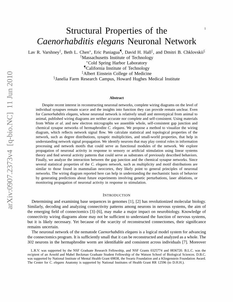
Fig. 1. Adjacency matrices for the gap junction network (blue circles) and the chemical synapse network (red points) withneurons grouped by category (sensory neurons, interneurons, motor neurons). Within each category, neurons are in anteroposteriororder. Among chemical synapse connections, small points indicate less than5 synaptic contacts, whereas large points indicate5 or more synaptic contacts. All gap junction connections aredepicted in the same way, irrespective of number of gap junctioncontacts.

connectivity fraction in other nervous systems [31], [32].2) Wiring Diagram as Adjacency Matrices:In the remainder of the paper, we describe and analyze

the connectivity of gap junction and chemical synapse networks of C. elegansneurons. Gap junctions arechannels that provide electrical coupling between neurons, whereas chemical synapses use neurotrans-mitters to link neurons. The network of gap junctions and thenetwork of chemical synapses are initiallytreated separately, with each represented by its own adjacency matrix, Figure 1. In an adjacency matrixA, the element in theith row andjth column,aij, represents the total number of synaptic contacts fromthe ith neuron to thejth. If neurons are unconnected, the corresponding element of the adjacency matrixis zero. An adjacency matrix may be used due to self-consistency in the gathered data.

Although gap junctions may have directionality, i.e. conduct current in only one direction, this hasnot been demonstrated inC. elegans. Even if directionality existed, such information cannot be extractedfrom electron micrographs. Thus we treat the gap junction network as an undirected network with asymmetric adjacency matrix. Weights in bothaij and aji represent the total number of gap junctions

4

between neuronsi andj.

Since chemical synapses possess clear directionality thatcan be extracted from electron micrographs,we represent the chemical network as a directed network withan asymmetric adjacency matrix. Theelements of the adjacency matrix take nonnegative values, which reflect the number of synaptic contactsbetween corresponding neurons. Contacts are given equal weight, regardless of the apparent size of thesynaptic apposition. We use nonnegative values for most of the paper because we cannot determinewhether a synapse is excitatory, inhibitory, or modulatoryfrom electron micrographs ofC. elegans. Forthe linear systems analysis, we do however make a rough guessof the signs of synapses based onneurotransmitter gene expression data.

Electron micrographs forC. eleganshave a further limitation that causes some synaptic ambiguity.When a presynaptic terminal makes contact with two adjacentprocesses of different neurons (sendjointin Durbin’s notation [8]), it is not known which of these processes acts as a postsynaptic terminal; bothmight be involved. We count all polyadic synaptic connections. Polyadic connections are briefly revisitedin the DISCUSSION.

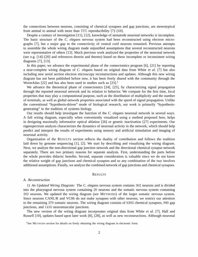
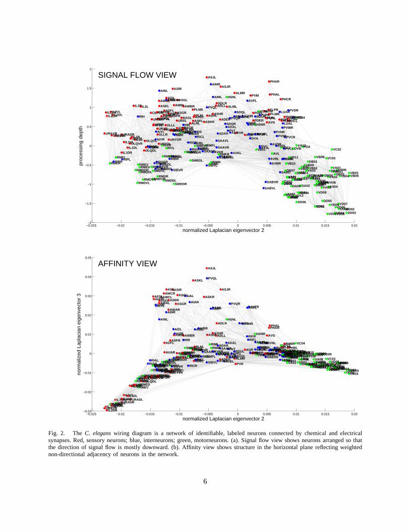
3) Visualization:Although statistical measures that we investigate later inthis paper provide significantinsights, they are no substitute to exploring detailed connectivity in the neuronal network. As the numberof connections between neurons is large even for relativelysimple networks, such analysis requires aconvenient way to visualize the wiring diagram. Previously, various fragments of the wiring diagramwere drawn to illustrate specific pathways [8], [33], [34]. Here, we propose a method to visualize thewhole wiring diagram in a way that reflects signal flow throughthe network as well as the closeness ofneurons in the network, Figure 2. To this end, we use spectralnetwork drawing techniques because theyhave certain optimality properties [35] and aesthetic appeal. Next, we give an intuitive description of ourvisualization method; mathematical details can be found inAppendix A.

The vertical axis in Figure 2(a), represents the position ofneurons in the signal flow hierarchy [36],[37] of the chemical synapse network with sensory neurons atthe top and motor neurons at the bottom,with interneurons in between. We want the vertical coordinate of pre- and post-synaptic neurons to differby one, however due to “frustration” this is not always possible. Frustration happens when distancesmeasured along network connections cannot be made to correspond to the hierarchy distances: there aretwo different hierarchical paths that require a particularneuron to appear in two different places. We lookfor the layout that has smallest deviation from this condition and find a closed form solution [36], [38].The number of synapses from sensory to motor neurons—the signal flow depth of the network—can beread off the vertical coordinate. Depending on the specific neurons considered, the depth is typically 2–3[8].

Neuronal position on the horizontal plane, Figure 2(b), represents the connectivity closeness of neuronsin the combined chemical and electrical synapse network. Neuronal coordinates are given by the secondand third eigenmodes of the symmetrized network’s graph Laplacian (see below). In this representation,pairs of synaptically coupled neurons with larger number ofconnections in parallel tend to be positionedcloser in space.

Thus, Figure 2 represents not the physical placement of neurons in the worm but signal flow andcloseness in the network. Such visualization reveals that motorneurons and some interneurons segregateinto two lobes along the first horizontal axis: the right lobecontains motorneurons in the ventral cord andthe left lobe consists of neck/tail neurons. The bi-lobe structure suggests partial autonomy of motorneuronsin the ventral cord and neck/tail. Interneurons that could coordinate the function of the two lobes can beeasily identified by their central location.

5

−0.025 −0.02 −0.015 −0.01 −0.005 0 0.005 0.01 0.015 0.02−2

−1.5

−1

−0.5

0

0.5

1

1.5

2

VB05VB03

DD03DD02

VB04

DD04

VD07

VB06

VD05

VD06VD04

DB03VC01

VC02

VA07

VD08

DB02

AS04

VA04

VD03

VA06

VC03

DB04

DD05

VA05

DA04DA03

VD09

AS03AS05AS06

VB08

DD01VD02

DA05

VA09VA08AS02VA03

VB02

DB01

PDB

VA02

VB09

VD10

PDA

RID

DA02

VB07

DA06

AS11

VD13

VD01

VA12

DD06

VC04

DA09

VD12

DVB

PVDL

AS09VA11

DA08

DA07

VB11

AS08

PVDR

VA10

PHCLPHBL

VA01AS01

VB10

AS07

DB07

PVCR

PHBR

AS10

PVCL

AVAL

DA01

LUAL

DB05DB06

AVAR

PVWR

PLML

VD11

PHCR

SABD

LUAR

PQR

PVWL

AVDL

PVNR

AVL

AVDR

AVBR

PHAL

AVBL

PLMR

PHAR

FLPR

AVGPVNLFLPL

SABVR

AVM

SABVL

AVJL

PVPR

DVC

VC05

PVPL

VB01

AVJR

BDUR

HSNRPDER

PDEL

PVM

DVAAVFR

RIFL

AVFL

RIFR

AQR

AVHRAVHL

PVR

SDQL

ALMR

BDUL

AVKL

ALA

PVQR

PVT

ALML

ADAL

HSNL

SDQR

AVEL

normalized Laplacian eigenvector 2

ASJR

ADER

SAADLRMFR

ADAR

AVER

ADLR

SAAVR

SAAVL

ADLL

AIML

AVKR

ASHR

RIMR

AIMR

RIML

ASHL

PVQL

SIBVL

ASJL

RMFL

ASKR

SAADRRIGLAIBR

RICL

RIS

SMBVRAIBL

PLNLADELASKL

PLNR

RIGR

SMBDL

ALNL

AIAR

RICR

SMBDR

AIAL

SMBVL

RMGRALNR

AWBR

RIRBAGR

BAGL

RMGL

ASGL

AUAL

URXL

ASGR

AIZR

AWBL

SMDDR

RIBL

AIZL

ASIR

URYVL

SIBVR

URBLURYVR

ADFR

RMHLRIBR

URYDR

ASER

AWARASILAINR

RIVL

OLLLAUAR

ADFLAWCR

SMDDL

RMHR

RIVR

SIBDL

AWCL

SIADL

ASEL

AINL

AWAL

URYDL

CEPDLCEPVL

OLLR

RMDR

URXR

SIAVR

CEPDR

SIADR

AIYL

AIYR

SIAVL

SIBDR

AFDRAFDL

SMDVR

SMDVL

URBR

RMDL

CEPVR

RIALRIAROLQDR

OLQVL

OLQDL

RMDVR

IL2L

RMDDL

RMEDRMEV

RIH

RMDVL

RMDDR

IL1L

IL2R

IL1RURADL

OLQVRIL1DL

IL1VL

RIPL

IL1DR

URADR

RMEL

IL1VR

RIPR

IL2DL

URAVL

IL2VL

RMER

IL2DRIL2VR

URAVR

SIGNAL FLOW VIEWpr

oces

sing

dep

th

−0.025 −0.02 −0.015 −0.01 −0.005 0 0.005 0.01 0.015 0.02−0.03

−0.02

−0.01

0

0.01

0.02

0.03

0.04

0.05

VB05VB03

DD03DD02

VB04

DD04VD07VB06

VD05VD06VD04DB03

VC01VC02VA07VD08

DB02AS04VA04VD03

VA06

VC03

DB04

DD05

VA05DA04DA03

VD09

AS03AS05AS06

VB08

DD01VD02

DA05

VA09VA08

AS02VA03VB02DB01

PDB

VA02

VB09VD10PDA

RID

DA02

VB07DA06AS11VD13

VD01

VA12DD06

VC04

DA09VD12DVB

PVDLAS09VA11DA08

DA07

VB11

AS08PVDRVA10PHCLPHBL

VA01AS01

VB10

AS07DB07PVCR

PHBR

AS10PVCLAVALDA01

LUALDB05DB06AVARPVWR

PLMLVD11

PHCR

SABDLUARPQRPVWLAVDL

PVNRAVLAVDRAVBR

PHAL

AVBLPLMR

PHAR

FLPR

AVG

PVNL

FLPLSABVR

AVMSABVL

AVJL

PVPRDVC

VC05PVPL

VB01

AVJR

BDUR

HSNR

PDERPDELPVMDVA

AVFR

RIFL

AVFL

RIFR

AQR

AVHRAVHL

PVR

SDQLALMR

BDULAVKL

ALA

PVQR

PVT

ALML

ADAL

HSNL

SDQR

AVEL

normalized Laplacian eigenvector 2

ASJR

ADER

SAADLRMFR

ADAR

AVER

ADLR

SAAVRSAAVL

ADLL

AIML

AVKR

ASHR

RIMR

AIMR

RIML

ASHL

PVQL

SIBVL

ASJL

RMFL

ASKR

SAADRRIGL

AIBR

RICLRIS

SMBVR

AIBL

PLNL

ADEL

ASKL

PLNR

RIGR

SMBDL

ALNL

AIAR

RICR

SMBDR

AIAL

SMBVLRMGR

ALNR

AWBRRIR

BAGRBAGLRMGL

ASGL

AUALURXL

ASGR

AIZRAWBL

SMDDRRIBL

AIZL

ASIR

URYVLSIBVRURBLURYVR

ADFR

RMHL

RIBR

URYDR

ASER

AWAR

ASIL

AINR

RIVL

OLLL

AUAR

ADFL

AWCR

SMDDL

RMHR

RIVR

SIBDL

AWCL

SIADL

ASEL

AINL

AWAL

URYDLCEPDLCEPVLOLLR

RMDRURXRSIAVR

CEPDR

SIADR

AIYLAIYR

SIAVLSIBDR

AFDRAFDL

SMDVRSMDVL

URBR

RMDL

CEPVR

RIALRIAR

OLQDROLQVLOLQDL

RMDVR

IL2LRMDDL

RMEDRMEV

RIHRMDVLRMDDRIL1LIL2RIL1R

URADL

OLQVR

IL1DLIL1VLRIPLIL1DRURADRRMEL

IL1VR

RIPRIL2DLURAVLIL2VLRMER

IL2DRIL2VRURAVR

AFFINITY VIEW

norm

aliz

ed L

apla

cian

eig

enve

ctor

3

Fig. 2. TheC. eleganswiring diagram is a network of identifiable, labeled neuronsconnected by chemical and electricalsynapses. Red, sensory neurons; blue, interneurons; green, motorneurons. (a). Signal flow view shows neurons arrangedso thatthe direction of signal flow is mostly downward. (b). Affinityview shows structure in the horizontal plane reflecting weightednon-directional adjacency of neurons in the network.

6

B. Gap Junction Network

For quantitative characterization, we first consider the gap junction network.1) Basic Structure and Connectivity:The gap junction network that we analyze consists of279 neurons

and514 gap junction connections, consisting of one or more junctions. The network is not fully connected,but is divided into a giant component containing248 neurons, two smaller components of2 and3 neurons,and 26 isolated neurons with no gap junctions (Table S1). The giantcomponent has511 connections.An Erdos-Renyi random network2 with 279 neurons and connection probability0.0133 (thus with 514expected connections) would be expected to have271 neurons in the giant component. The true gapjunction giant component is much smaller; the probability of finding such a small giant component in arandom network is on the order of10−14 (see METHODS). A better comparison, however, can be made torandom networks with degree distributions that match the degree distribution of the gap junction network[39]. Here, the degree of a neuron is the number of neurons with which it makes a gap junction. The giantcomponent in a degree-matched random network would be expected to be251 neurons (see METHODS),about the same size as the measured giant component. Using connectivity data from [13], Majewska andYuste had previously pointed out that most neurons inC. elegansbelong to the giant component [40].Our results agree roughly with [40], although our dataset excludes non-neuronal cells and places certainneurons in different connected components.

The adjacency matrix of the network,A, is depicted in Figure 1 (the number of gap junctions in aconnection is not depicted). The matrix is symmetric since the network is undirected. We may explorethe utility of representing the wiring diagram as a three-layer network by grouping neurons by category(sensory neurons, interneurons, motor neurons). As shown in Tables S2A and S2B, each category hasmany recurrent connections; with the exception of connections between sensory and motor neurons, thereare also many connections between categories. In particular, Table S2B indicates that motor neurons sendto interneurons roughly the same number of connections as recurrently sent back to motor neurons. Theseobservations suggest that on the level of gap junctions, thevalue of a three-layer network abstraction isquestionable.

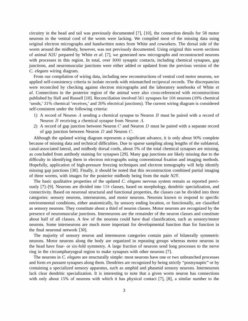
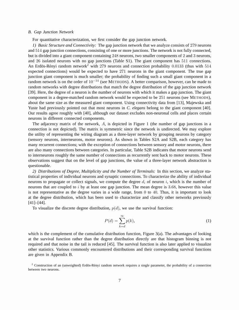
2) Distributions of Degree, Multiplicity and the Number of Terminals: In this section, we analyze sta-tistical properties of individual neurons and synaptic connections. To characterize the ability of individualneurons to propagate or collect signals, we compute the degreedi of neuroni, which is the number ofneurons that are coupled toi by at least one gap junction. The mean degree is3.68, however this valueis not representative as the degree varies in a wide range, from 0 to 40. Thus, it is important to lookat the degree distribution, which has been used to characterize and classify other networks previously[41]–[44].

To visualize the discrete degree distribution,p(d), we use the survival function:

P (d) =

∞∑

k=d

p(k), (1)

which is the complement of the cumulative distribution function, Figure 3(a). The advantages of lookingat the survival function rather than the degree distribution directly are that histogram binning is notrequired and that noise in the tail is reduced [45]. The survival function is also later applied to visualizeother statistics. Various commonly encountered distributions and their corresponding survival functionsare given in Appendix B.

2 Construction of an (unweighted) Erdos-Renyi random network requires a single parameter, the probability of a connectionbetween two neurons.

7

We perform a fitting procedure for the tail of the gap junctiondegree distribution [44] (see METHODS).We find that the tail (d ≥ 4) can be fit by the power law with exponentγ = 3.14, Figure 3(a), but notby the exponential decay (p-value< 0.1). This result is consistent with the view that the gap junctionnetwork is scale-free [42].

To characterize the direct impact that one neuron can have onanother, we quantify the strength ofconnections by the multiplicity,mij, between neuronsi andj, which is the number of synaptic contacts(here gap junctions) connectingi to j. The degree treats synaptic connections as binary, whereasthemultiplicity quantifies the number of contacts. The multiplicity distribution for the gap junction networkis shown in Figure 3(b). We find that the multiplicity distribution for m ≥ 2 obeys a power law withexponentγ = 2.76. Although the exponential decay fit to the tail passes thep-value test, the log-likelihoodis significantly lower than for the power law.

Finally, the number of terminals that lie on a given neuron isthe sum of the multiplicities of all gapjunction connections. The tail of the distribution of the number of synaptic terminals, Figure 3(c), isadequately fit by a power law with exponentγ = 2.53.

100

101

10−2

10−1

100

mean=3.68

degree

degr

ee s

urvi

val f

unct

ion

AVAL

AVAR

AVBRAVBL

RIBL/RAVKL/RIGL

(a)

100

101

10−4

10−3

10−2

10−1

100

mean=1.73

multiplicity

mul

tiplic

ity s

urvi

val f

unct

ion

PVPR−DVCAVFR−AVFL

(b)

100

101

102

10−3

10−2

10−1

100

number of terminals

num

ber

of te

rmin

als

surv

ival

func

tion

mean=6.36

AVAL

AVARAVBR

AVBL

(c)

Fig. 3. Survival functions for the distributions of degree,multiplicity, and number of synaptic terminals in the gap junctionnetwork. Neurons or connections with exceptionally high statistics are labeled. The tails of the distributions can be fit by apower law with the exponent3.14 for the degrees (a);2.76 for the multiplicity distribution (b);2.53 for the number of synapticterminals (c). The exponents for the power law fits of the corresponding survival functions are obtained by subtracting one.

Identifying neurons that play a central or special role in the transmission or processing of informationmay also prove useful [46]–[50]. To rank neurons according to their roles, we introduce several centralityindices. Perhaps the simplest centrality index isdegree centralitycd(i). Degree centrality is simply thedegree of a neuron,cd(i) = di, and is motivated by the idea that a neuron with connections to manyother neurons has a more important or more central role in thenetwork than a neuron connected to onlya few other neurons. Neurons that have unusually high degreecentrality include AVAL/R and AVBL/R.The same neurons lie in the tail of the distribution of the number of synaptic terminals, Figure 3(c),suggesting strong coupling to the network. These neuron pairs are command interneurons responsible forcoordinating backward and forward locomotion, respectively [22], [34], [51]. The high degree centralitiesof RIBL/R suggest a similarly central function for those neurons, though they each only have19 gapjunction terminals, in the middle of the distribution of number of terminals, suggesting weaker couplingto the network.

3) Small World Properties:Having described statistical properties of individual neurons and connec-tions, such as the degree and multiplicity distributions, we now investigate properties that may describethe efficiency of signal transmission across the gap junction network. Traditionally [14], this analysisdoes not consider multiplicity of gap junctions but treats them as binary. We analyze signal propagationwhen including multiplicities in the next subsection.

8

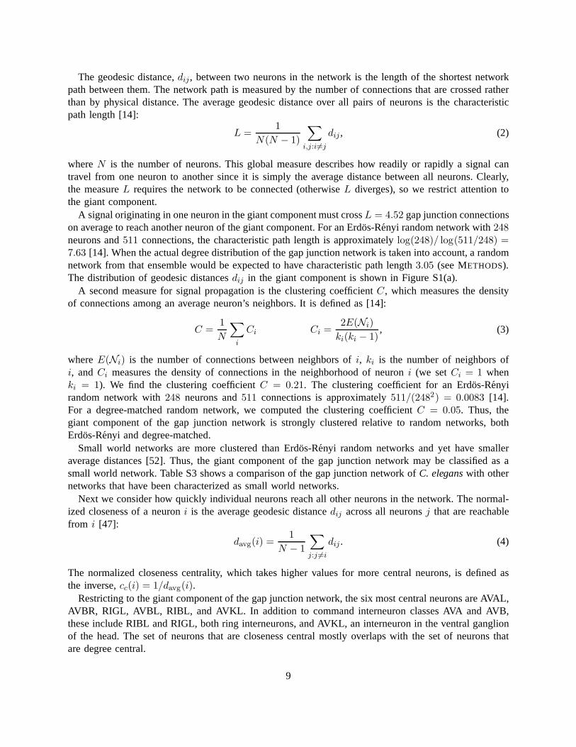
The geodesic distance,dij , between two neurons in the network is the length of the shortest networkpath between them. The network path is measured by the numberof connections that are crossed ratherthan by physical distance. The average geodesic distance over all pairs of neurons is the characteristicpath length [14]:

L =1

N(N − 1)

∑

i,j:i 6=j

dij , (2)

whereN is the number of neurons. This global measure describes how readily or rapidly a signal cantravel from one neuron to another since it is simply the average distance between all neurons. Clearly,the measureL requires the network to be connected (otherwiseL diverges), so we restrict attention tothe giant component.

A signal originating in one neuron in the giant component must crossL = 4.52 gap junction connectionson average to reach another neuron of the giant component. For an Erdos-Renyi random network with248neurons and511 connections, the characteristic path length is approximately log(248)/ log(511/248) =7.63 [14]. When the actual degree distribution of the gap junction network is taken into account, a randomnetwork from that ensemble would be expected to have characteristic path length3.05 (see METHODS).The distribution of geodesic distancesdij in the giant component is shown in Figure S1(a).

A second measure for signal propagation is the clustering coefficientC, which measures the densityof connections among an average neuron’s neighbors. It is defined as [14]:

C =1

N

∑

i

Ci Ci =2E(Ni)

ki(ki − 1), (3)

whereE(Ni) is the number of connections between neighbors ofi, ki is the number of neighbors ofi, andCi measures the density of connections in the neighborhood of neuron i (we setCi = 1 whenki = 1). We find the clustering coefficientC = 0.21. The clustering coefficient for an Erdos-Renyirandom network with248 neurons and511 connections is approximately511/(2482) = 0.0083 [14].For a degree-matched random network, we computed the clustering coefficientC = 0.05. Thus, thegiant component of the gap junction network is strongly clustered relative to random networks, bothErdos-Renyi and degree-matched.

Small world networks are more clustered than Erdos-Renyirandom networks and yet have smalleraverage distances [52]. Thus, the giant component of the gapjunction network may be classified as asmall world network. Table S3 shows a comparison of the gap junction network ofC. eleganswith othernetworks that have been characterized as small world networks.

Next we consider how quickly individual neurons reach all other neurons in the network. The normal-ized closeness of a neuroni is the average geodesic distancedij across all neuronsj that are reachablefrom i [47]:

davg(i) =1

N − 1

∑

j:j 6=i

dij . (4)

The normalized closeness centrality, which takes higher values for more central neurons, is defined asthe inverse,cc(i) = 1/davg(i).

Restricting to the giant component of the gap junction network, the six most central neurons are AVAL,AVBR, RIGL, AVBL, RIBL, and AVKL. In addition to command interneuron classes AVA and AVB,these include RIBL and RIGL, both ring interneurons, and AVKL, an interneuron in the ventral ganglionof the head. The set of neurons that are closeness central mostly overlaps with the set of neurons thatare degree central.

9

The Spearman rank correlation coefficient [53] between degree centralitycd(i) and closeness centralitycc(i) for the entire giant component, however, is only0.036. Since correlation between the two centralitymeasures does not extend to peripheral neurons, ordering ofimportance is different.

4) Spectral Properties:Global network properties discussed in the previous section characterize signaltransmission while ignoring connection weights. As weights affect the effectiveness of signal transmissionand vary among connections, we now analyze the weighted network by using linear systems theory.Although neuronal dynamics can be nonlinear, spectral properties nevertheless provide important insightsinto function. For example, the initial success of the Google search engine is largely attributed to linearspectral analysis of the World Wide Web [54].

We characterize the dynamics of the gap junction network by the following system of linear differentialequations, which follow from charge conservation [55], [56]:

CidVi

dt =∑

j

(Vj − Vi)gij − gmi Vi, (5)

whereVi is the membrane potential of neuroni, Ci is the membrane capacitance of neuroni, gij is theconductance of gap junctions between neuronsi andj, andgmi is the membrane conductance of neuroni.Assuming that each neuron has the same capacitanceC and each gap junction has the same conductanceg, i.e. gij = gAij , we can rewrite this equation in terms of the time constantτ = C/g as:

τ dVi

dt =∑

j

(Vj − Vi)Aij −gmi

g Vi. (6)

Assuming that gap junction conductance is greater than the membrane conductance, we temporarilyneglect the last term and rewrite this equation in matrix form:

τ dVdt = −LV , (7)

whereL is the Laplacian matrix of the weighted network,L = D−A, D contains the number of neurongap junctions on the diagonal and zeros elsewhere, andV is a column vector of the membrane potentials.A different plausible differential equation model is discussed in Appendix C.

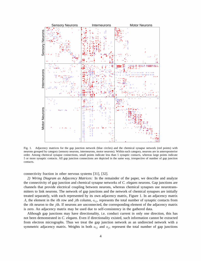
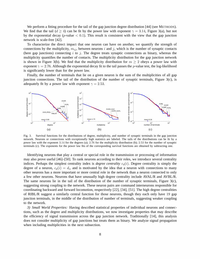
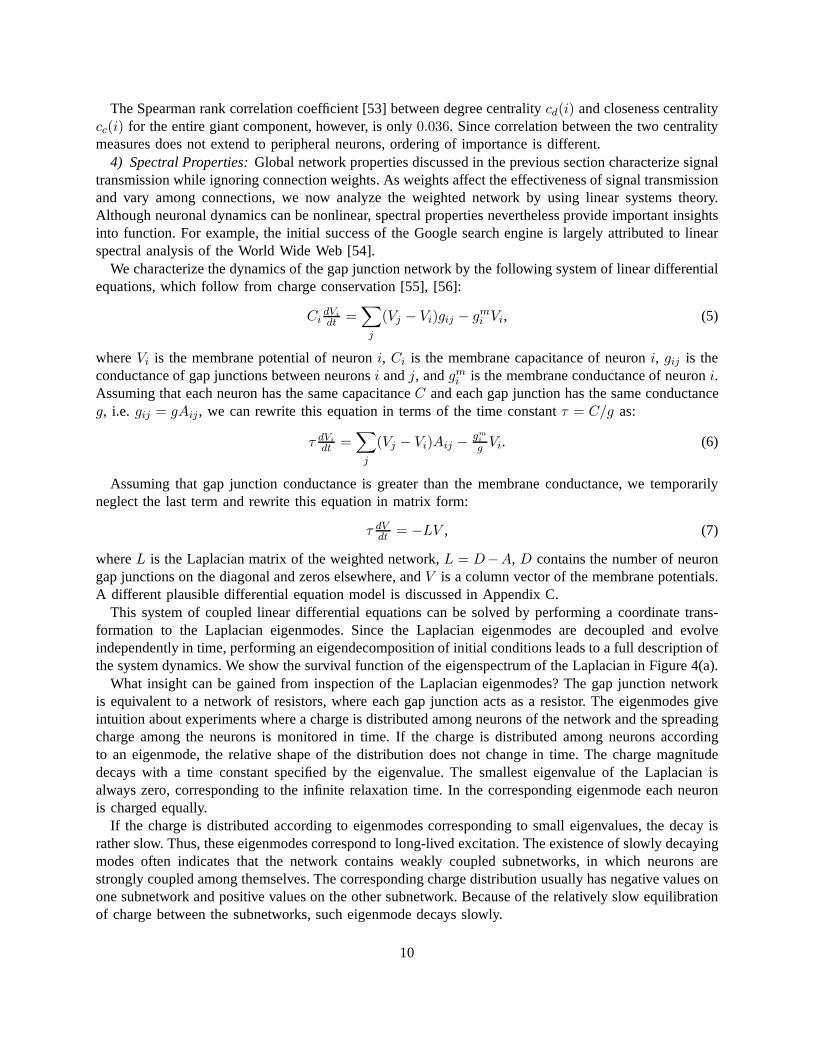
This system of coupled linear differential equations can besolved by performing a coordinate trans-formation to the Laplacian eigenmodes. Since the Laplacianeigenmodes are decoupled and evolveindependently in time, performing an eigendecomposition of initial conditions leads to a full description ofthe system dynamics. We show the survival function of the eigenspectrum of the Laplacian in Figure 4(a).

What insight can be gained from inspection of the Laplacian eigenmodes? The gap junction networkis equivalent to a network of resistors, where each gap junction acts as a resistor. The eigenmodes giveintuition about experiments where a charge is distributed among neurons of the network and the spreadingcharge among the neurons is monitored in time. If the charge is distributed among neurons accordingto an eigenmode, the relative shape of the distribution doesnot change in time. The charge magnitudedecays with a time constant specified by the eigenvalue. The smallest eigenvalue of the Laplacian isalways zero, corresponding to the infinite relaxation time.In the corresponding eigenmode each neuronis charged equally.

If the charge is distributed according to eigenmodes corresponding to small eigenvalues, the decay israther slow. Thus, these eigenmodes correspond to long-lived excitation. The existence of slowly decayingmodes often indicates that the network contains weakly coupled subnetworks, in which neurons arestrongly coupled among themselves. The corresponding charge distribution usually has negative values onone subnetwork and positive values on the other subnetwork.Because of the relatively slow equilibrationof charge between the subnetworks, such eigenmode decays slowly.

10

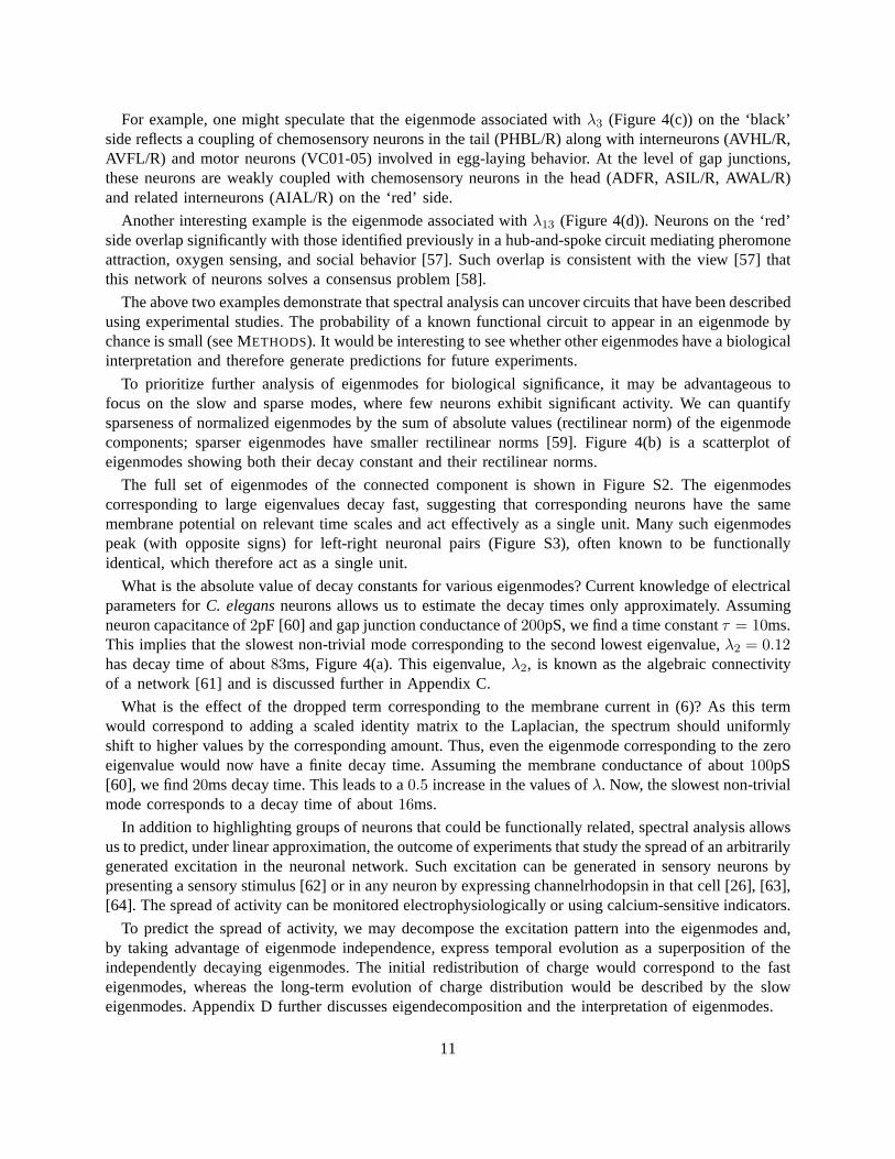
For example, one might speculate that the eigenmode associated with λ3 (Figure 4(c)) on the ‘black’side reflects a coupling of chemosensory neurons in the tail (PHBL/R) along with interneurons (AVHL/R,AVFL/R) and motor neurons (VC01-05) involved in egg-layingbehavior. At the level of gap junctions,these neurons are weakly coupled with chemosensory neuronsin the head (ADFR, ASIL/R, AWAL/R)and related interneurons (AIAL/R) on the ‘red’ side.

Another interesting example is the eigenmode associated with λ13 (Figure 4(d)). Neurons on the ‘red’side overlap significantly with those identified previouslyin a hub-and-spoke circuit mediating pheromoneattraction, oxygen sensing, and social behavior [57]. Suchoverlap is consistent with the view [57] thatthis network of neurons solves a consensus problem [58].

The above two examples demonstrate that spectral analysis can uncover circuits that have been describedusing experimental studies. The probability of a known functional circuit to appear in an eigenmode bychance is small (see METHODS). It would be interesting to see whether other eigenmodes have a biologicalinterpretation and therefore generate predictions for future experiments.

To prioritize further analysis of eigenmodes for biological significance, it may be advantageous tofocus on the slow and sparse modes, where few neurons exhibitsignificant activity. We can quantifysparseness of normalized eigenmodes by the sum of absolute values (rectilinear norm) of the eigenmodecomponents; sparser eigenmodes have smaller rectilinear norms [59]. Figure 4(b) is a scatterplot ofeigenmodes showing both their decay constant and their rectilinear norms.

The full set of eigenmodes of the connected component is shown in Figure S2. The eigenmodescorresponding to large eigenvalues decay fast, suggestingthat corresponding neurons have the samemembrane potential on relevant time scales and act effectively as a single unit. Many such eigenmodespeak (with opposite signs) for left-right neuronal pairs (Figure S3), often known to be functionallyidentical, which therefore act as a single unit.

What is the absolute value of decay constants for various eigenmodes? Current knowledge of electricalparameters forC. elegansneurons allows us to estimate the decay times only approximately. Assumingneuron capacitance of2pF [60] and gap junction conductance of200pS, we find a time constantτ = 10ms.This implies that the slowest non-trivial mode corresponding to the second lowest eigenvalue,λ2 = 0.12has decay time of about83ms, Figure 4(a). This eigenvalue,λ2, is known as the algebraic connectivityof a network [61] and is discussed further in Appendix C.

What is the effect of the dropped term corresponding to the membrane current in (6)? As this termwould correspond to adding a scaled identity matrix to the Laplacian, the spectrum should uniformlyshift to higher values by the corresponding amount. Thus, even the eigenmode corresponding to the zeroeigenvalue would now have a finite decay time. Assuming the membrane conductance of about100pS[60], we find20ms decay time. This leads to a0.5 increase in the values ofλ. Now, the slowest non-trivialmode corresponds to a decay time of about16ms.

In addition to highlighting groups of neurons that could be functionally related, spectral analysis allowsus to predict, under linear approximation, the outcome of experiments that study the spread of an arbitrarilygenerated excitation in the neuronal network. Such excitation can be generated in sensory neurons bypresenting a sensory stimulus [62] or in any neuron by expressing channelrhodopsin in that cell [26], [63],[64]. The spread of activity can be monitored electrophysiologically or using calcium-sensitive indicators.

To predict the spread of activity, we may decompose the excitation pattern into the eigenmodes and,by taking advantage of eigenmode independence, express temporal evolution as a superposition of theindependently decaying eigenmodes. The initial redistribution of charge would correspond to the fasteigenmodes, whereas the long-term evolution of charge distribution would be described by the sloweigenmodes. Appendix D further discusses eigendecomposition and the interpretation of eigenmodes.

11

0 20 40 60 80 100 1200

0.2

0.4

0.6

0.8

1

eigenvalue, λ

eige

nval

ue s

urvi

val f

unct

ion,

P(λ

) estimated decay constant (1/ms)0 2 4 6 8 10 12

0

0.2

0.4

0.6

0.8

1

(a)

0 20 40 60 80 100 1200

0.2

0.4

0.6

0.8

1

eige

nmod

e re

ctili

near

nor

m

eigenvalue, λ

(b)

−0.1

0

0.1

0.2

0.3

0.4

PHBLPHBR

AVHLAVHR AVFR

AVFL

VC04VC05

ASIL AIAL

VC03

ASIRAWAL

VC02

AIAR

VC01

AWAR

DD04

ADFR

neur

on a

ctiv

ity in

eig

enm

ode

v 3

(c)

−0.4

−0.3

−0.2

−0.1

0

0.1

0.2

0.3

RMHR

URXR

IL2R

RIPLRIPR

RMGRIL1VR

AINRASGL ALMRRMED AINL

IL1R

AS11ASGR PDAAUAL AIMLRMER AUAR PDBADEL

AS04RIR

ALAURXLIL2L

ASKR

AVMAIZL

neur

on a

ctiv

ity in

eig

enm

ode

v 13

(d)

Fig. 4. Linear systems analysis of the giant component of thegap junction network. (a). Survival function of the eigenvaluespectrum (blue). The algebraic connectivity,λ2, is 0.12 and the spectral radius,λ248, is 118. A time scale associated withthe decay constant is also given. (b). Scatterplot showing the rectilinear norm and decay constant of the eigenmodes of theLaplacian. The fastest modes from Figure S3 are marked in red. The sparsest and slowest modes, most amenable to biologicalanalysis, are located in the lower-left corner of the diagram. (c). Eigenmode of Laplacian corresponding toλ3 (marked greenin panel (b)). (d). Eigenmode of Laplacian corresponding toλ13 (marked cyan in panel (b)).

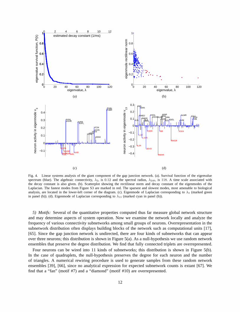
5) Motifs: Several of the quantitative properties computed thus far measure global network structureand may determine aspects of system operation. Now we examine the network locally and analyze thefrequency of various connectivity subnetworks among smallgroups of neurons. Overrepresentation in thesubnetwork distribution often displays building blocks ofthe network such as computational units [17],[65]. Since the gap junction network is undirected, there are four kinds of subnetworks that can appearover three neurons; this distribution is shown in Figure 5(a). As a null-hypothesis we use random networkensembles that preserve the degree distribution. We find that fully connected triplets are overrepresented.

Four neurons can be wired into 11 kinds of subnetworks; this distribution is shown in Figure 5(b).In the case of quadruplets, the null-hypothesis preserves the degree for each neuron and the numberof triangles. A numerical rewiring procedure is used to generate samples from these random networkensembles [39], [66], since no analytical expression for expected subnetwork counts is extant [67]. Wefind that a “fan” (motif #7) and a “diamond” (motif #10) are overrepresented.

12

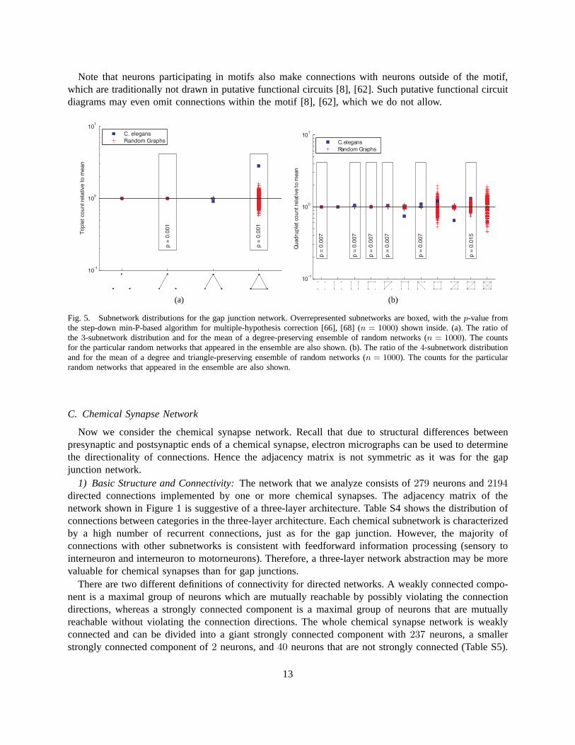
Note that neurons participating in motifs also make connections with neurons outside of the motif,which are traditionally not drawn in putative functional circuits [8], [62]. Such putative functional circuitdiagrams may even omit connections within the motif [8], [62], which we do not allow.

10-1

100

101

Trip

let co

un

t re

lative

to

me

an

C. elegans

Random Graphs

p =

0.0

01

p =

0.0

01

(a)

10-1

100

101

Quad

rup

let co

unt re

lati

ve to m

ean

C. elegans

Random Graphs

p =

0.0

07

p =

0.0

07

p =

0.0

07

p =

0.0

07

p =

0.0

07

p =

0.0

15

(b)

Fig. 5. Subnetwork distributions for the gap junction network. Overrepresented subnetworks are boxed, with thep-value fromthe step-down min-P-based algorithm for multiple-hypothesis correction [66], [68] (n = 1000) shown inside. (a). The ratio ofthe 3-subnetwork distribution and for the mean of a degree-preserving ensemble of random networks (n = 1000). The countsfor the particular random networks that appeared in the ensemble are also shown. (b). The ratio of the4-subnetwork distributionand for the mean of a degree and triangle-preserving ensemble of random networks (n = 1000). The counts for the particularrandom networks that appeared in the ensemble are also shown.

C. Chemical Synapse Network

Now we consider the chemical synapse network. Recall that due to structural differences betweenpresynaptic and postsynaptic ends of a chemical synapse, electron micrographs can be used to determinethe directionality of connections. Hence the adjacency matrix is not symmetric as it was for the gapjunction network.

1) Basic Structure and Connectivity:The network that we analyze consists of279 neurons and2194directed connections implemented by one or more chemical synapses. The adjacency matrix of thenetwork shown in Figure 1 is suggestive of a three-layer architecture. Table S4 shows the distribution ofconnections between categories in the three-layer architecture. Each chemical subnetwork is characterizedby a high number of recurrent connections, just as for the gapjunction. However, the majority ofconnections with other subnetworks is consistent with feedforward information processing (sensory tointerneuron and interneuron to motorneurons). Therefore,a three-layer network abstraction may be morevaluable for chemical synapses than for gap junctions.

There are two different definitions of connectivity for directed networks. A weakly connected compo-nent is a maximal group of neurons which are mutually reachable by possibly violating the connectiondirections, whereas a strongly connected component is a maximal group of neurons that are mutuallyreachable without violating the connection directions. The whole chemical synapse network is weaklyconnected and can be divided into a giant strongly connectedcomponent with237 neurons, a smallerstrongly connected component of2 neurons, and40 neurons that are not strongly connected (Table S5).

13

The random directed network corresponding to the chemical network is fully weakly connected, evenwhen the degree distribution is taken into account (see METHODS). A strongly connected giant componentas small as in the chemical network is not likely in a random network (see [69]). Thus, the chemicalnetwork is more segregated than would be expected for a random network.

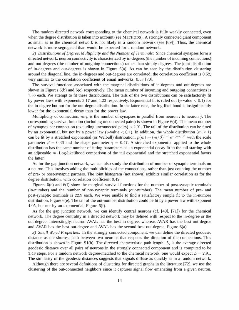
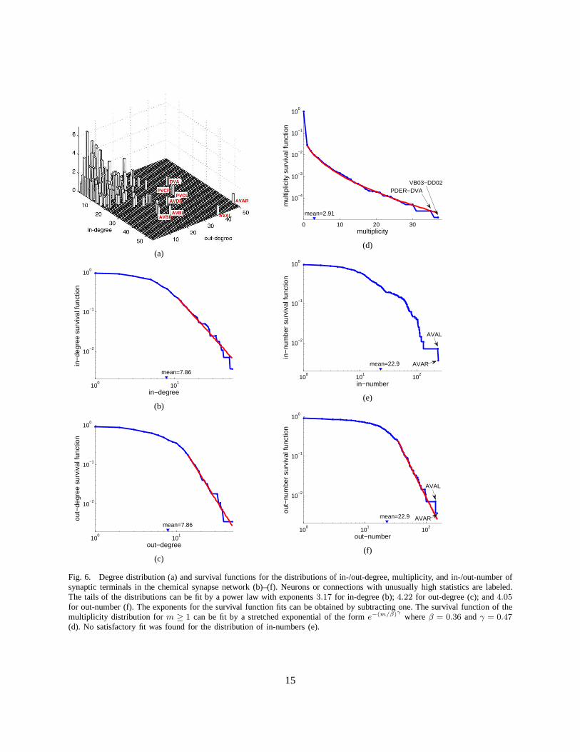
2) Distributions of Degree, Multiplicity and the Number of Terminals: Since chemical synapses form adirected network, neuron connectivity is characterized byin-degrees (the number of incoming connections)and out-degrees (the number of outgoing connections) rather than simply degrees. The joint distributionof in-degrees and out-degrees is shown in Figure 6(a). As canbe seen by the distribution clusteringaround the diagonal line, the in-degrees and out-degrees are correlated; the correlation coefficient is0.52,very similar to the correlation coefficient of email networks, 0.53 [70].

The survival functions associated with the marginal distributions of in-degrees and out-degrees areshown in Figures 6(b) and 6(c) respectively. The mean numberof incoming and outgoing connections is7.86 each. We attempt to fit these distributions. The tails of the two distributions can be satisfactorily fitby power laws with exponents3.17 and4.22 respectively. Exponential fit is ruled out (p-value< 0.1) forthe in-degree but not for the out-degree distribution. In the latter case, the log-likelihood is insignificantlylower for the exponential decay than for the power law.

Multiplicity of connection,mij, is the number of synapses in parallel from neuroni to neuronj. Thecorresponding survival function (including unconnected pairs) is shown in Figure 6(d). The mean numberof synapses per connection (excluding unconnected pairs) is 2.91. The tail of the distribution can be fittedby an exponential, but not by a power law (p-value< 0.1). In addition, the whole distribution (m ≥ 1)can be fit by a stretched exponential (or Weibull) distribution, p(m) ∼ (m/β)γ−1e−(m/β)γ with the scaleparameterβ = 0.36 and the shape parameterγ = 0.47. A stretched exponential applied to the wholedistribution has the same number of fitting parameters as an exponential decay fit to the tail starting withan adjustablem. Log-likelihood comparison of the tail exponential and thestretched exponential favorsthe latter.

As for the gap junction network, we can also study the distribution of number of synaptic terminals ona neuron. This involves adding the multiplicities of the connections, rather than just counting the numberof pre- or post-synaptic partners. The joint histogram (notshown) exhibits similar correlation as for thedegree distribution, with correlation coefficient0.42.

Figures 6(e) and 6(f) show the marginal survival functions for the number of post-synaptic terminals(in-number) and the number of pre-synaptic terminals (out-number). The mean number of pre- andpost-synaptic terminals is22.9 each. We were unable to find a satisfactory simple fit to the in-numberdistribution, Figure 6(e). The tail of the out-number distribution could be fit by a power law with exponent4.05, but not by an exponential, Figure 6(f).

As for the gap junction network, we can identify central neurons (cf. [49], [71]) for the chemicalnetwork. The degree centrality in a directed network may be defined with respect to the in-degree or theout-degree. Interestingly, neuron AVAL has the best in-degree, whereas AVAR has the best out-degreeand AVAR has the best out-degree and AVAL has the second best out-degree, Figure 6(a).

3) Small World Properties:In the strongly connected component, we can define the directed geodesicdistance as the shortest path between two neurons that respects the direction of the connections. Thisdistribution is shown in Figure S1(b). The directed characteristic path length,L, is the average directedgeodesic distance over all pairs of neurons in the strongly connected component and is computed to be3.48 steps. For a random network degree-matched to the chemical network, one would expectL = 2.91.The similarity of the geodesic distances suggests that signals diffuse as quickly as in a random network.

Although there are several definitions of clustering for directed graphs in the literature [72], we use theclustering of the out-connected neighbors since it captures signal flow emanating from a given neuron.

14

(a)

100

101

10−2

10−1

100

mean=7.86

in−degree

in−

degr

ee s

urvi

val f

unct

ion

(b)

100

101

10−2

10−1

100

mean=7.86

out−degree

out−

degr

ee s

urvi

val f

unct

ion

(c)

0 10 20 30

10−4

10−3

10−2

10−1

100

multiplicity

mul

tiplic

ity s

urvi

val f

unct

ion

mean=2.91

VB03−DD02PDER−DVA

(d)

100

101

102

10−2

10−1

100

mean=22.9

in−number

in−

num

ber

surv

ival

func

tion

AVAL

AVAR

(e)

100

101

102

10−2

10−1

100

mean=22.9

out−number

out−

num

ber

surv

ival

func

tion

AVAR

AVAL

(f)

Fig. 6. Degree distribution (a) and survival functions for the distributions of in-/out-degree, multiplicity, and in-/out-number ofsynaptic terminals in the chemical synapse network (b)–(f). Neurons or connections with unusually high statistics arelabeled.The tails of the distributions can be fit by a power law with exponents3.17 for in-degree (b);4.22 for out-degree (c); and4.05for out-number (f). The exponents for the survival functionfits can be obtained by subtracting one. The survival function of themultiplicity distribution form ≥ 1 can be fit by a stretched exponential of the forme−(m/β)γ whereβ = 0.36 andγ = 0.47(d). No satisfactory fit was found for the distribution of in-numbers (e).

15

This is:

C =1

N

∑

i

Ci Ci =E(Ni)

ki(ki − 1), (8)

whereE(Ni) is the number of connections between out-neighbors of neuron i, ki is the number ofout-neighbors ofi, andCi measures the density of connections in the neighborhood of neuroni. For thechemical network, the clustering coefficient is0.22. Using the Watts-Strogatz approximations toL andC, the clustering coefficient for a random network isCr ≈

1N exp( ln(N)

L ); so forN = 279 andL = 3.48,a random network would haveC ∼ 0.018. For a degree-matched random network we computed theclustering coefficientC = 0.079. Since the clustering coefficient for the chemical network is much morethan a similar random directed network, it may be considereda small-world network, cf. Table S3.

For directed networks, measures of in-closeness and out-closeness may be defined using the averagedirected geodesic distance. In particular, the normalizedin-closeness is the average geodesic distancefrom all other neurons to a given neuron:

diavg(i) =1

N − 1

∑

j:j 6=i

dji, (9)

and the out-closeness is the average geodesic distance froma given neuron to all other neurons:

doavg(i) =1

N − 1

∑

j:j 6=i

dij , (10)

whereN is the number of neurons. Normalized centralities are the inverses:cic(i) = 1/diavg(i) andcoc(i) = 1/doavg(i). The motivation behind these indices is similar to that in the gap junction case.In-closeness central neurons can be easily reached from allother neurons in the network. Out-closenesscentral neurons can easily reach all other neurons in the network. Normalized in-closeness centralitycic(i)and normalized out-closeness centralitycoc(i) are weakly anti-correlated, with correlation coefficient−0.12.

For the giant component of the chemical network, the most in-closeness central neurons include AVAL,AVAR, AVBR, AVEL, AVER, and AVBL. All are command interneurons involved in the locomotorycircuit; these neurons are also central in the gap junction network. The in-closeness centrality of commandinterneurons may indicate that in theC. elegansnervous system, signals can propagate efficiently fromvarious sources towards these neurons and that they are in a good position to integrate it.

The most out-closeness central neurons include DVA, ADEL, ADER, PVPR, AVJL, HSNR, PVCL,and BDUR. Only PVCL is a command interneuron involved in locomotion. The neuron DVA is aninterneuron that performs mechanosensory integration; ADEL/R are sensory dopaminergic neurons inthe head; and the other central neurons are interneurons in several parts of the worm. The out-closenesscentrality of these neurons may indicate that signals can propagate efficiently from these neurons to therest of the network and that they are in a good position for broadcast.

4) Spectral Properties:Although chemical synapses are likely to introduce more nonlinearities thangap junctions, linear systems analysis can provide interesting insights, especially in the absence ofother tools. Such an approach has additional merit inC. elegans, where neurons do not fire classicalaction potentials [60] and have chemical synapses that likely release neurotransmitters tonically [56]. Tojustify such analysis, a system of linear equations may be derived by approximating sigmoidal synaptictransmission functions with linear dependencies. This canbe done by expanding synaptic transmissionfunctions into a Taylor series around an equilibrium point [56].

A major source of uncertainty in linear systems analysis of the chemical network is the unknownsign of connections, i.e. excitatory or inhibitory, due to the difficulty in performing electrophysiology

16

experiments. We use a rough approximation that GABAergic synapses are inhibitory, whereas glutamergicand cholinergic synapses are excitatory [73], but see [62].Thus inhibitory neurons are identified by lookingat GABA expression [74].3

Similarly to the gap junction network, we write the system oflinear differential equations for thechemical synapse network [55], [56]:

CidVi

dt =∑

j

Vjgji − gmi Vi, (11)

whereVi is the membrane potential of neuroni measured relative to the equilibrium,Ci is the membranecapacitance of neuroni, gji is the conductance in neuroni contributed by a chemical synapse in responseto voltageVj measured relative to the equilibrium andgmi is the membrane conductance of neuroni.Assuming that each neuron has the same capacitanceC and each chemical synapse contact has the sameconductanceg, i.e. gij = gAij , we can rewrite this equation in terms of the time constantτ = C/g as:

τ dVi

dt =∑

j

VjAji −gmi

g Vi. (12)

To avoid redundancy we defer analyzing this system of differential equations to the next section, wherewe consider the combined system including both gap junctions and chemical synapses.

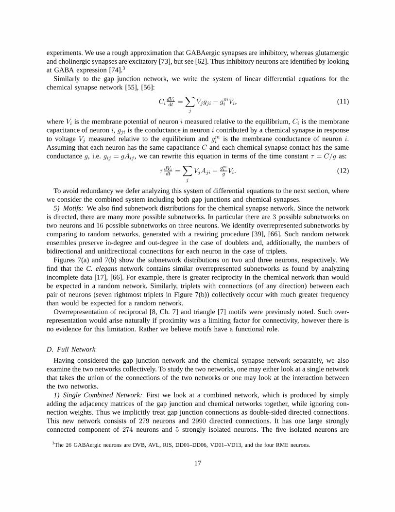
5) Motifs: We also find subnetwork distributions for the chemical synapse network. Since the networkis directed, there are many more possible subnetworks. In particular there are3 possible subnetworks ontwo neurons and16 possible subnetworks on three neurons. We identify overrepresented subnetworks bycomparing to random networks, generated with a rewiring procedure [39], [66]. Such random networkensembles preserve in-degree and out-degree in the case of doublets and, additionally, the numbers ofbidirectional and unidirectional connections for each neuron in the case of triplets.

Figures 7(a) and 7(b) show the subnetwork distributions on two and three neurons, respectively. Wefind that theC. elegansnetwork contains similar overrepresented subnetworks as found by analyzingincomplete data [17], [66]. For example, there is greater reciprocity in the chemical network than wouldbe expected in a random network. Similarly, triplets with connections (of any direction) between eachpair of neurons (seven rightmost triplets in Figure 7(b)) collectively occur with much greater frequencythan would be expected for a random network.

Overrepresentation of reciprocal [8, Ch. 7] and triangle [7] motifs were previously noted. Such over-representation would arise naturally if proximity was a limiting factor for connectivity, however there isno evidence for this limitation. Rather we believe motifs have a functional role.

D. Full Network

Having considered the gap junction network and the chemicalsynapse network separately, we alsoexamine the two networks collectively. To study the two networks, one may either look at a single networkthat takes the union of the connections of the two networks orone may look at the interaction betweenthe two networks.

1) Single Combined Network:First we look at a combined network, which is produced by simplyadding the adjacency matrices of the gap junction and chemical networks together, while ignoring con-nection weights. Thus we implicitly treat gap junction connections as double-sided directed connections.This new network consists of279 neurons and2990 directed connections. It has one large stronglyconnected component of274 neurons and5 strongly isolated neurons. The five isolated neurons are

3The 26 GABAergic neurons are DVB, AVL, RIS, DD01–DD06, VD01–VD13,and the four RME neurons.

17

10-1

100

101

Do

ub

let co

un

t re

lative

to

me

an

C. elegans

Random Graphs

p =

0.0

01

p =

0.0

01

(a)

10-1

100

101

Trip

let co

un

t re

lative

to

me

an

C. elegans

Random Graphs

p =

0.0

15

p =

0.0

15

p =

0.0

15

p =

0.0

15

p =

0.0

15

p =

0.0

15

p =

0.0

15

(b)

Fig. 7. Subnetwork distributions for the chemical synapse network. Overrepresented subnetworks are boxed, with thep-valuefrom the step-down min-P-based algorithm for multiple-hypothesis correction [66], [68] (n = 1000) shown inside. (a). Theratio of the2-subnetwork distribution and the mean of a random network ensemble (n = 1000). Realizations of the randomnetwork ensemble are also shown. (b). The ratio of the3-subnetwork distribution and the mean of a random network ensemble(n = 1000). Realizations of the random network ensemble are also shown.

IL2DL/R, PLNR, DD06, and PVDR; this set is simply the intersection of the isolated neurons in thegap junction and chemical networks and does not seem to have any commonalities among members. Ofcourse, it follows that since the chemical network is a single weakly connected component, this combinednetwork is also a single weakly connected component.

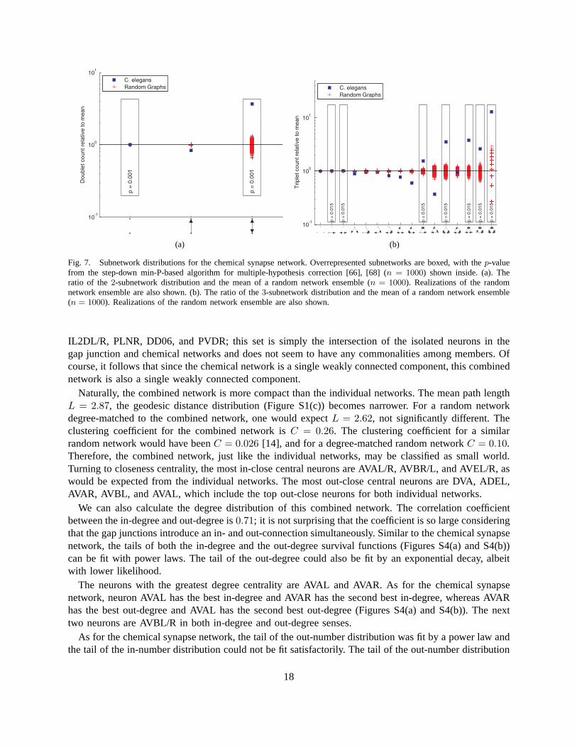
Naturally, the combined network is more compact than the individual networks. The mean path lengthL = 2.87, the geodesic distance distribution (Figure S1(c)) becomes narrower. For a random networkdegree-matched to the combined network, one would expectL = 2.62, not significantly different. Theclustering coefficient for the combined network isC = 0.26. The clustering coefficient for a similarrandom network would have beenC = 0.026 [14], and for a degree-matched random networkC = 0.10.Therefore, the combined network, just like the individual networks, may be classified as small world.Turning to closeness centrality, the most in-close centralneurons are AVAL/R, AVBR/L, and AVEL/R, aswould be expected from the individual networks. The most out-close central neurons are DVA, ADEL,AVAR, AVBL, and AVAL, which include the top out-close neurons for both individual networks.

We can also calculate the degree distribution of this combined network. The correlation coefficientbetween the in-degree and out-degree is0.71; it is not surprising that the coefficient is so large consideringthat the gap junctions introduce an in- and out-connection simultaneously. Similar to the chemical synapsenetwork, the tails of both the in-degree and the out-degree survival functions (Figures S4(a) and S4(b))can be fit with power laws. The tail of the out-degree could also be fit by an exponential decay, albeitwith lower likelihood.

The neurons with the greatest degree centrality are AVAL andAVAR. As for the chemical synapsenetwork, neuron AVAL has the best in-degree and AVAR has the second best in-degree, whereas AVARhas the best out-degree and AVAL has the second best out-degree (Figures S4(a) and S4(b)). The nexttwo neurons are AVBL/R in both in-degree and out-degree senses.

As for the chemical synapse network, the tail of the out-number distribution was fit by a power law andthe tail of the in-number distribution could not be fit satisfactorily. The tail of the out-number distribution

18

could also be fit by an exponential, albeit with lower likelihood. The multiplicity can be fit satisfactorilyby a stretched exponential.

2) Spectral properties:In this section we apply linear systems analysis to the combined network ofchemical synapses and gap junctions taking into account multiplicities of individual connections. Due toour ignorance about the relative conductance of a single gapjunction and of a single chemical synapse,we assume that they are equal. By combining equations (6) and(12) we arrive at:

τ dVi

dt =∑

j

[−VjL(gap)ij + VjA

(chem)ji ]− gm

i

g Vi, (13)

whereA(chem)ji is negative if neuronj is GABAergic and positive otherwise.

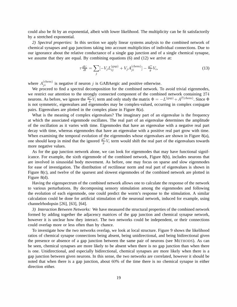
We proceed to find a spectral decomposition for the combined network. To avoid trivial eigenmodes,we restrict our attention to the strongly connected component of the combined network containing274neurons. As before, we ignore theg

mi

g Vi term and only study the matrixΦ = −L(gap)+AT (chem). SinceΦis not symmetric, eigenvalues and eigenmodes may be complex-valued, occurring in complex conjugatepairs. Eigenvalues are plotted in the complex plane in Figure 8(a).

What is the meaning of complex eigenvalues? The imaginary part of an eigenvalue is the frequencyat which the associated eigenmode oscillates. The real partof an eigenvalue determines the amplitudeof the oscillation as it varies with time. Eigenmodes that have an eigenvalue with a negative real partdecay with time, whereas eigenmodes that have an eigenvaluewith a positive real part grow with time.When examining the temporal evolution of the eigenmodes whose eigenvalues are shown in Figure 8(a),one should keep in mind that the ignoredgm

i

g Vi term would shift the real part of the eigenvalues towardsmore negative values.

As for the gap junction network alone, we can look for eigenmodes that may have functional signif-icance. For example, the sixth eigenmode of the combined network, Figure 8(b), includes neurons thatare involved in sinusoidal body movement. As before, one mayfocus on sparse and slow eigenmodesfor ease of investigation. The distribution of rectilinearnorm and real part of eigenvalues is shown inFigure 8(c), and twelve of the sparsest and slowest eigenmodes of the combined network are plotted inFigure 8(d).

Having the eigenspectrum of the combined network allows oneto calculate the response of the networkto various perturbations. By decomposing sensory stimulation among the eigenmodes and followingthe evolution of each eigenmode, one could predict the worm’s response to the stimulation. A similarcalculation could be done for artificial stimulation of the neuronal network, induced for example, usingchannelrhodopsin [26], [63], [64].

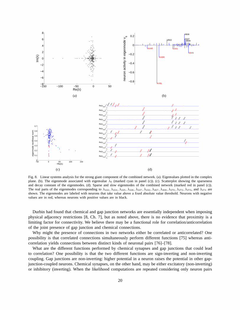
3) Interaction Between Networks:We have measured the structural properties of the combined networkformed by adding together the adjacency matrices of the gap junction and chemical synapse network,however it is unclear how they interact. The two networks could be independent, or their connectionscould overlap more or less often than by chance.

To investigate how the two networks overlap, we look at localstructure. Figure 9 shows the likelihoodratios of chemical synapse connections being absent, beingunidirectional, and being bidirectional giventhe presence or absence of a gap junction between the same pair of neurons (see METHODS). As canbe seen, chemical synapses are more likely to be absent when there is no gap junction than when thereis one. Unidirectional, and especially bidirectional, chemical synapses are more likely when there is agap junction between given neurons. In this sense, the two networks are correlated, however it should benoted that when there is a gap junction, about60% of the time there is no chemical synapse in eitherdirection either.

19

−150 −100 −50 0 50−8

−6

−4

−2

0

2

4

6

8

Re(λ)

Im(λ

)

(a)

−0.8

−0.6

−0.4

−0.2

0

0.2

AVBL

AVBR

VB08

DD05

AS07VB02 VB09

DD01AVAR

neur

on a

ctiv

ity in

eig

enm

ode

v 6

(b)

−50 0 50 100 1500

0.1

0.2

0.3

0.4

0.5

0.6

0.7

eige

nmod

e re

ctili

near

nor

m

−Re(λ)

(c)

RIP

L

RIP

R

DD

03

UR

ADR

RM

ER

UR

ADL

1

−1Re(v

222)

DD

03 VD07

SMD

DR

1

−1Re(v

224)

DD

03 VD07

SMD

DR

1

−1Re(v

225)

DD

03

VD07

SMD

DR

VD08

DD

05 1

−1Re(v

226)

DD

03

VD07

SMD

DR

VD08

DD

05 1

−1Re(v

227)

DD

03

VD08

VD07

VD04

SMD

DR

SMD

DL

VD13 1

−1Re(v

232)

RIP

L

RIP

R SIAD

L

SIAV

R

RM

ER

SIAV

L

1

−1Re(v

267)

RIP

R

RIP

L

SIAV

R

1

−1Re(v

268)

AS10

VA10

1

−1Re(v

270)

RIP

L RIP

R

1

−1Re(v

272)

RIP

RRIP

L

SIAD

RSI

AVR

SIAD

L

SIAV

L 1

−1Re(v

273)

RIP

RRIP

L

SIAD

RSI

AVR

SIAD

L

SIAV

L

1

−1Re(v

274)

(d)

Fig. 8. Linear systems analysis for the strong giant component of the combined network. (a). Eigenvalues plotted in the complexplane. (b). The eigenmode associated with eigenvalueλ6 (marked cyan in panel (c)). (c). Scatterplot showing the sparsenessand decay constant of the eigenmodes. (d). Sparse and slow eigenmodes of the combined network (marked red in panel (c)).The real parts of the eigenmodes corresponding toλ222, λ224, λ225, λ226, λ227, λ232, λ267, λ268, λ270, λ272, λ273, andλ274 areshown. The eigenmodes are labeled with neurons that take value above a fixed absolute value threshold. Neurons with negativevalues are in red, whereas neurons with positive values are in black.

Durbin had found that chemical and gap junction networks areessentially independent when imposingphysical adjacency restrictions [8, Ch. 7], but as noted above, there is no evidence that proximity is alimiting factor for connectivity. We believe there may be a functional role for correlation/anticorrelationof the joint presence of gap junction and chemical connections.

Why might the presence of connections in two networks eitherbe correlated or anticorrelated? Onepossibility is that correlated connections simultaneously perform different functions [75] whereas anti-correlation yields connections between distinct kinds of neuronal pairs [76]–[78].

What are the different functions performed by chemical synapses and gap junctions that could leadto correlation? One possibility is that the two different functions are sign-inverting and non-invertingcoupling. Gap junctions are non-inverting: higher potential in a neuron raises the potential in other gap-junction-coupled neurons. Chemical synapses, on the otherhand, may be either excitatory (non-inverting)or inhibitory (inverting). When the likelihood computations are repeated considering only neuron pairs

20

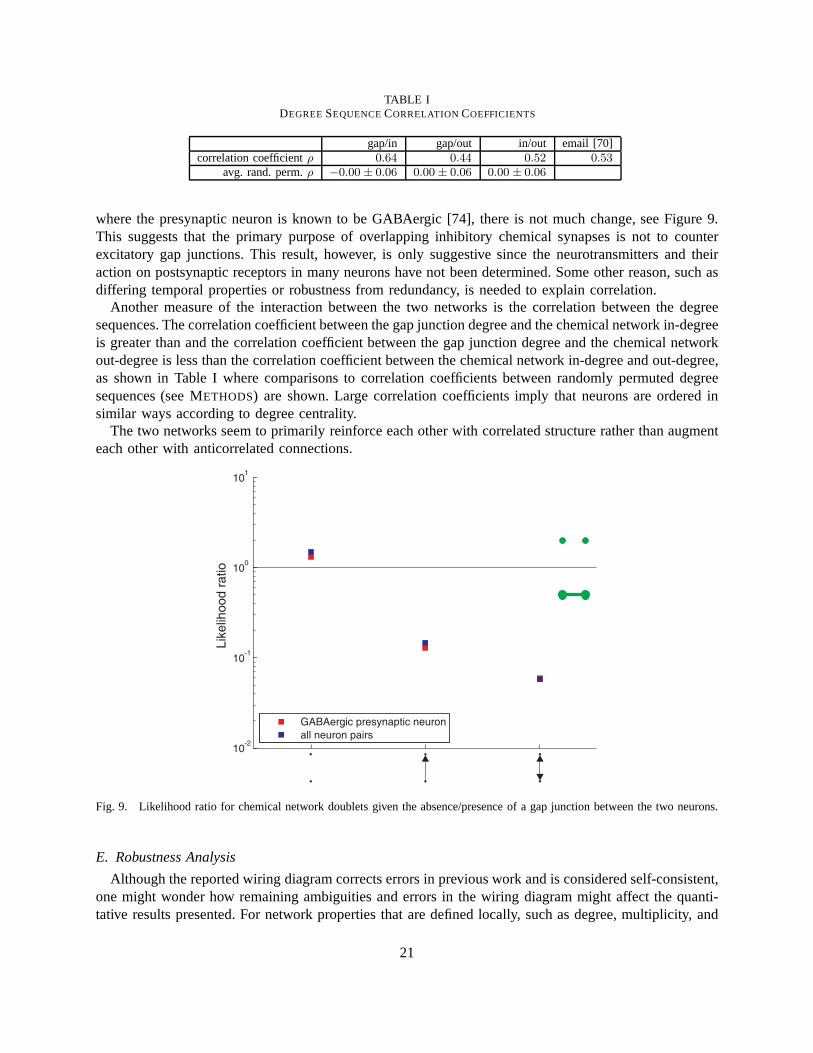
TABLE IDEGREESEQUENCECORRELATION COEFFICIENTS

gap/in gap/out in/out email [70]correlation coefficientρ 0.64 0.44 0.52 0.53

avg. rand. perm.ρ −0.00 ± 0.06 0.00± 0.06 0.00 ± 0.06

where the presynaptic neuron is known to be GABAergic [74], there is not much change, see Figure 9.This suggests that the primary purpose of overlapping inhibitory chemical synapses is not to counterexcitatory gap junctions. This result, however, is only suggestive since the neurotransmitters and theiraction on postsynaptic receptors in many neurons have not been determined. Some other reason, such asdiffering temporal properties or robustness from redundancy, is needed to explain correlation.

Another measure of the interaction between the two networksis the correlation between the degreesequences. The correlation coefficient between the gap junction degree and the chemical network in-degreeis greater than and the correlation coefficient between the gap junction degree and the chemical networkout-degree is less than the correlation coefficient betweenthe chemical network in-degree and out-degree,as shown in Table I where comparisons to correlation coefficients between randomly permuted degreesequences (see METHODS) are shown. Large correlation coefficients imply that neurons are ordered insimilar ways according to degree centrality.

The two networks seem to primarily reinforce each other withcorrelated structure rather than augmenteach other with anticorrelated connections.

10-2

10-1

100

101

Lik

elih

oo

d r

atio

GABAergic presynaptic neuron

all neuron pairs

Fig. 9. Likelihood ratio for chemical network doublets given the absence/presence of a gap junction between the two neurons.

E. Robustness Analysis

Although the reported wiring diagram corrects errors in previous work and is considered self-consistent,one might wonder how remaining ambiguities and errors in thewiring diagram might affect the quanti-tative results presented. For network properties that are defined locally, such as degree, multiplicity, and

21

subnetwork distributions, clearly small errors in the measured wiring diagram lead to small errors in thecalculated properties. For global properties such as characteristic path length and eigenmodes, things areless clear.

To study the robustness of global network properties to errors in the wiring diagram, we recalculatethese properties in the wiring diagrams with simulated errors. We simulate errors by removing randomlychosen synaptic contacts with a certain probability and assigning them to a randomly chosen pair ofneurons. Then, we calculate the global network properties on the ensemble of edited wiring diagrams.The variation of the properties in the ensemble gives us an idea of robustness.

First, we explore the robustness of the small world properties and the giant component calculations. Weedit wiring diagrams by moving each gap junction contact with 10% probability and chemical synapsecontact with5% probability. Tables S6 and S7 show the global properties for 1000 random networksobtained by editing the experimentally measured network. These tables suggest that our quantitativeresults are reasonably robust to ambiguities and errors in the wiring diagram.

Properties for the neuronal network from prior work in [13] are also shown for comparison. The numberof synaptic contacts that must be moved to achieve this network (editing distance) roughly correspondsto that with25.6% probability.

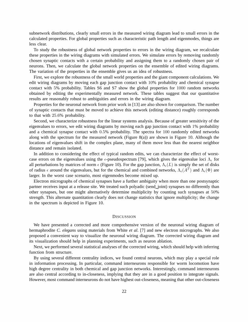
Second, we characterize robustness for the linear systems analysis. Because of greater sensitivity of theeigenvalues to errors, we edit wiring diagrams by moving each gap junction contact with1% probabilityand a chemical synapse contact with0.5% probability. The spectra for100 randomly edited networksalong with the spectrum for the measured network (Figure 8(a)) are shown in Figure 10. Although thelocations of eigenvalues shift in the complex plane, many ofthem move less than the nearest neighbordistance and remain isolated.

In addition to considering the effect of typical random edits, we can characterize the effect of worst-case errors on the eigenvalues using theǫ-pseudospectrum [79], which gives the eigenvalue lociΛǫ forall perturbations by matrices of normǫ (Figure 10). For the gap junction,Λǫ(L) is simply the set of disksof radiusǫ around the eigenvalues, but for the chemical and combined networks,Λǫ(A

T ) andΛǫ(Φ) arelarger. In the worst case scenario, most eigenmodes become mixed up.

Electron micrographs of chemical synapses have a further ambiguity when more than one postsynapticpartner receives input at a release site. We treated such polyadic (sendjoint) synapses no differently thanother synapses, but one might alternatively determine multiplicity by counting such synapses at50%strength. This alternate quantitation clearly does not change statistics that ignore multiplicity; the changein the spectrum is depicted in Figure 10.

DISCUSSION

We have presented a corrected and more comprehensive version of the neuronal wiring diagram ofhermaphroditeC. elegansusing materials from Whiteet al. [7] and new electron micrographs. We alsoproposed a convenient way to visualize the neuronal wiring diagram. The corrected wiring diagram andits visualization should help in planning experiments, such as neuron ablation.

Next, we performed several statistical analyses of the corrected wiring, which should help with inferringfunction from structure.

By using several different centrality indices, we found central neurons, which may play a special rolein information processing. In particular, command interneurons responsible for worm locomotion havehigh degree centrality in both chemical and gap junction networks. Interestingly, command interneuronsare also central according to in-closeness, implying that they are in a good position to integrate signals.However, most command interneurons do not have highest out-closeness, meaning that other out-closeness

22

Re(λ)

Im(λ

)

−120 −100 −80 −60 −40 −20 0 20

−20

−15

−10

−5

0

5

10

15

20

Fig. 10. The spectrum of the giant component of the combined network matrixΦ (red), ǫ-disks around the spectrum (lightblue), spectra of100 randomly edited networks (blue), and theǫ-pseudospectrum (orange). The valueǫ = 4 is used (the averagespectral norm of the100 editing matrices was3.4±0.9). The spectrum of the giant component of the combined network matrixΦ under an alternate quantitation of sendjoint synapses is also shown (green).

central neurons, such as DVA, ADEL/R, PVPR, etc., are in a good position to deliver signals to the restof the network.

Linear systems analysis yielded a principled methodology to hypothesize functional circuits and topredict the outcome of both sensory and artificial stimulation experiments. We have identified severalmodes that map onto previously identified behaviors.

Networks with similar statistical structural properties may share functional properties thus providinginsight into the function of theC. elegansnervous system. To enable comparison of theC. elegansnetwork with other natural and technological networks [80], we computed several structural propertiesof the neuronal network. In particular, the gap junction network, the chemical synapse network, and thecombined neuronal network may all be classified as small world networks because they simultaneouslyhave small average path lengths and large clustering coefficients [14].

The tails of the degree and terminal number distributions for the gap, chemical and combined networks(with the exception of the in-numbers) follow a power law consistent with the network being scale-freein the sense of Barabasi and Albert [42]. The tails of some distributions can also be fit by an exponentialdecay, consistent with a previous report [15]. However, we found that exponential fits for the tails have(sometimes insignificantly) lower log-likelihoods than power laws, making the exponential decay a lesslikely alternative. For whole distributions, neither distribution passes thep-value test; if one is forced tochoose, the exponential decay may be a less poor alternative.

Several statistical properties of theC. elegansnetwork are similar to those of the mammalian cortex.In particular, the whole distribution ofC. eleganschemical synapse multiplicity is well-fit by a stretched

23

exponential (or Weibull) distribution (Figure 6(d)). Taking multiplicity as a proxy of synaptic connec-tion strength, this is reminiscent of the synaptic strengthdistribution in mammalian cortex, which wasmeasured electrophysiologically, [32], [68]. The definition of stretched exponential distribution is slightlydifferent [32], but has the same tail behavior. The stretch factor is∼ 0.5, close to that in the corticalnetwork.

In addition, we found that motif frequencies in the chemicalsynapse network are similar to those in themammalian cortex [68]. Both reciprocally connected neuronpairs and triplets with a connection betweenevery pair of neurons (regardless of direction) are over-represented. The similarity of the connectionstrength and the motif distributions may reflect similar constraints in the two networks. Since proximityis unlikely to be the limiting factor, we suggest that these constraints may reflect functionality. We foundthat the chemical synapse and the gap junction networks are correlated, which may provide insight intotheir relative roles.

To conclude the paper, let us note that our scientific development was not hypothesis-driven, but ratherexploratory. Yet we hope that the reported statistics will help in formulating a theory that explains howfunction arises from structure.

MATERIALS AND METHODS

Data Acquisition

We began assembling the wiring diagram by consolidating existing data from both published andunpublished sources. Using J. G. Whiteet al.’s The Mind of a Worm (MOW) [7] as the starting point,we extracted wiring data from diagrams, figures, tables, andtext (for example, see [7, Appendix A,pp. 118–122] on neuron AVAL/R). Connectivity of each neuron, its synaptic partner, and synaptic type(chemical, gap junction, neuromuscular) was manually entered into an electronic database. In the ventralcord of the worm, this level of synaptic specification was complicated by the fact that connections wererecorded by neuron class. For example, bilateral neurons PVCL and PVCR were simply listed as PVC.We were able to assign proper connections to the appropriateleft/right neuron by referring to White andcoworker’s original laboratory notebooks and original electron micrographs. In some cases, the numberof synapses for a given neuron class in MOW differed from the sum of connections for the bilateralpairs in the notebooks and/or electron micrographs. The synaptic value of these neurons was determinedby appropriating the value in MOW according to proportionality from the notebooks and/or electronmicrographs.

From here, we incorporated R. M. Durbin’s data, which was applicable to the anterior portion of theworm, reconstructed from the animalN2U [8]. For neurons that projected beyond the nerve ring, onlythe anterior connections needed to be updated. Since data from MOW did not specify the location ofsynapses, integration proved difficult. For these neurons,we obtained positional information by cross-referencing Durbin’s data against original electron micrographs and his handwritten annotations in White’slaboratory notebooks. Only synapses located in regions addressed by Durbin were included. Connectionsin the middle and tail regions of the worm were mostly unaffected by these updates.

With the advent of green fluorescent protein (GFP) reporters, researchers are able to visualize theneuroanatomy of individual neurons. Studies based on this technology mostly confirmed the electronmicrograph reconstructions described in MOW. A few differences between GFP-stained neurons andWhite’s work were observed [28]. Notably, the anterior processes of DVB and PVT could have beenmistakenly switched in MOW [7]. Based on these findings, we reversed the connections for neurons DVBand PVT anterior to the vulva.

Most published works have focused in the neck and tail regions of C. elegans, where the majority ofneuron cell bodies reside. Reconstructions of neurons in the mid-body of the worm, on the other hand,

24

are scant and incomplete. From a combination of published works [7], [8], [10], [81], we found thatwiring data for64 neurons had large gaps or were missing entirely. Sixty-one of these are motor neuronsin the ventral cord. Two are excretory neurons (CANL/R) thatdo not appear to make any synapses. Theremaining neuron, RID, is the only process in the dorsal cordthat extends over the length of the animal.

At the C. elegansarchive (Albert Einstein College of Medicine), we uncovered a large number ofreconstruction records in Whiteet al.’s laboratory notebooks. These notebooks identified neurons bydifferent color code labels depending on the animal, the location of the neurite (ventral or dorsal),and magnification of the electron micrograph. To ascertain the identity of the neurons, we relied on acombination of color code tables and comparisons of common anatomical structures between electronmicrograph prints. In the end, we identified notes for full reconstructions of24 of the aforementionedneurons. Partial connectivity data for the remaining38 were also available where22 neurons havepartial/missing dorsal side connections and6 neurons have partial ventral side connections. We checkedthe connections of all (both published and unpublished) neurons in the ventral cord against electronmicrographs used by White and coworkers. Over600 updates were made to the original notes andpublished reconstructions. Many of these updates were additions of previously missed neuromuscularjunctions between ventral cord motor neurons and body wall muscles.

While conducting this work, we found that a large section of the worm on the dorsal side, fromjust anterior to the vulva to the pre-anal ganglion, was never imaged at high power magnification withan electron microscope. This lack of electron micrographs was the reason why so many neurons weremissing dorsal side reconstructions. Using original thin sections for theN2U worm prepared by Whiteetal., we produced new high power electron micrographs of this dorsal region. Due to the condition of thesections, only one of every2–3 sections was imaged. These new electron micrographs extended nearly9µm on the dorsal side. New dorsal side data for 3 neurons (DA5, DB4, DD3) were obtained from theseelectron micrographs. Resource constraints prevented us from covering the entire dorsal gap.

From our compilation of wiring data, including new reconstructions of ventral cord motor neurons, weapplied self-consistency criteria to isolate neurons withmismatched reciprocal records. The discrepancieswere reconciled by checking against electron micrographs and the laboratory notebooks of Whiteetal. Connections in the posterior region of the animal were alsocross-referenced with reconstructionspublished in [10]. Reconciliation involved561 synapses for108 neurons (49% chemical “sends,”31%chemical “receives,” and20% electrical junctions).

Giant Component for Random Networks

For a random network withN neurons and probabilityp of a connection being present, if the constantc = Np > 1, then the size of the giant component is asymptotically normal with meanNα(c) andvarianceNβ(c) [82, p. 120]. These quantities are given by

α(c) = 1−γ

candβ(c) =

γ(1− γc )

c(1 − γ)2, (14)

whereγ = −W

(

−c

ec

)

, (15)

andW (·) is the LambertW -function. If we takeN to be279 andp to be514/(279

2

)

, thenc = 3.698. Usingthe asymptotic approximation, the size of the giant component is distributed approximately normally withmean271 and variance9.22. Thus the probability of having a giant component of size248, which is over7 standard deviations from the mean, is about10−14. If a precise evaluation of this infinitesimal value isdesired, large deviations techniques, rather than the asymptotic approximation may be more valid [83].

25

To apply this method to the weakly connected component of a directed network, we are interested inthe undirected network formed by adding a connection between two neurons if there is a connection ineither direction. For a random directed network with probability q of presence of a directed connection,the probability of a connection existing in either direction is p = q2 + 2q(1 − q). Taking q to be2194/279/278 = 0.0283, p is 0.0558. Then for an undirected random network withN = 279 andthe specifiedp, c is 15.56. Then the size of the giant component is distributed approximately normallywith mean279 and variance0.0000487. Thus the probability of the giant weakly connected componentcontaining all the neurons in such a random network is overwhelming. Again, large deviations techniquesshould be used to get a precise evaluation of the probabilityof being on the order of10000 standarddeviations away from the mean.

Giant Component for Random Networks with Given Degree Distribution

Consider the ensemble of random networks with a given degreedistribution [84]. For the gap junctionnetwork, the generating function corresponding to the measured degree distribution is

G0(x) =(

1279

) [

26 + 39x+ 59x2 + 43x3 + 46x4 + 23x5 + 15x6 + 5x7 + 8x8 + 4x9 + 3x11 + 2x14

+2x15 + x24 + x29 + x34 + x40]

,

with derivative

G′0(x) =

(

1279

) [

39 + 118x + 129x2 + 184x3 + 115x4 + 90x5 + 35x6 + 64x7 + 36x8 + 33x10

+28x13 + 30x14 + 24x23 + 29x28 + 34x33 + 40x39]

.

ThereforeG′0(1) =

1028279 . The generating functionG1 is then

G1(x) =(

11028

) [

39 + 118x+ 129x2 + 184x3 + 115x4 + 90x5 + 35x6 + 64x7 + 36x8 + 33x10 + 28x13

+30x14 + 24x23 + 29x28 + 34x33 + 40x39]

.

As shown in [84], the expected fraction of the network taken up by the giant component,S, is S =1−G0(u), whereu is the smallest non-negative solution tou = G1(u). In our case, we findu = 0.043,and soS = 0.90. That is to say, one would expect the giant component to consist of 251 neurons.

Using the computedS and G′0(1), we can find the average component size excluding the giant

component, which turns out to be1.58.For the symmetrized chemical network, the generating function corresponding to the measured degree

distribution is

H0(x) =(

1279

) [

2x+ 6x2 + 8x3 + 6x4 + 14x5 + 14x6 + 19x7 + 20x8 + 19x9 + 20x10 + 17x11 + 18x12

+14x13 + 9x14 + 10x15 + 9x16 + 4x17 + 9x18 + 7x19 + 3x20 + 9x21 + 8x22 + 3x23 + 4x24

+3x25 + 2x26 + 3x27 + 2x29 + x31 + x32 + 2x33 + x34 + x36 + x42 + x48 + x49 + 2x50

+x51 + x52 + x53 + x56 + x83 + x85]

,

with derivative

H ′0(x) =

(

1279

) [

2 + 12x+ 24x2 + 24x3 + 70x4 + 84x5 + 133x6 + 160x7 + 171x8 + 200x9 + 187x10

+216x11 + 182x12 + 126x13 + 150x14 + 151x15 + 68x16 + 162x17 + 133x18 + 60x19 + 189x20

+176x21 + 69x22 + 96x23 + 75x24 + 52x25 + 81x26 + 58x28 + 31x30 + 32x31 + 66x32

+34x33 + 36x35 + 42x41 + 48x47 + 49x48 + 100x49 + 51x50 + 52x51 + 53x52 + 56x55 + 83x82

+85x84]

.

26

ThereforeH ′0(1) =

3929279 . The generating functionH1 is then

H1(x) =(

13929

) [

2 + 12x+ 24x2 + 24x3 + 70x4 + 84x5 + 133x6 + 160x7 + 171x8 + 200x9 + 187x10

+216x11 + 182x12 + 126x13 + 150x14 + 151x15 + 68x16 + 162x17 + 133x18 + 60x19 + 189x20

+176x21 + 69x22 + 96x23 + 75x24 + 52x25 + 81x26 + 58x28 + 31x30 + 32x31 + 66x32

+34x33 + 36x35 + 42x41 + 48x47 + 49x48 + 100x49 + 51x50 + 52x51 + 53x52 + 56x55 + 83x82

+85x84]

.

The expected fraction of the network taken up by the giant component,S, is S = 1−H0(u), whereuis the smallest non-negative solution tou = H1(u). Hereu is found to be0.00051, and soS = 0.999996.That is to say, one would expect the giant component to consist of 278.9990 neurons.

Path Length for Random Networks with Given Degree Distribution

Continuing from the previous subsection, we find the derivative of the generating functionG1 for thegap junction network to be

G′1(x) =

(

11028

) [

118 + 258x+ 552x2 + 460x3 + 450x4 + 210x5 + 448x6 + 288x7 + 330x9 + 364x12

+420x13 + 552x22 + 812x27 + 1122x32 + 1560x38]

.

ThusG′1(1) =

1986257 . Letting z1 = G′

0(1) =1028279 andz2 = G′

0(1)G′1(1) =

264893 , it is shown in [84, (53)],

that the expected path length is

L =ln[

(N − 1)(z2 − z1) + z21]

− ln z21ln [z2/z1]

= 3.05. (16)

Fitting Tails of Distributions

To find functional forms of the tails of various distributions, we follow the procedure outlined in[44]. For the candidate functional forms—say, the power lawp(d) ∼ d−γ and the exponential decayp(d) ∼ exp(−λd)—we perform the following steps. First, we find the optimal parameter of the fit bymaximizing the log-likelihood and the optimal starting point of the fit by minimizing the Kolmogorov-Smirnov statistic. Second, we evaluate the goodness of fit bycalculating thep-value that the observeddata was generated by the optimized distribution usingp > 0.1 as a criterion for plausibility. Finally, ifseveral distributions pass thep-value test we compare their log-likelihoods to find the mostprobable one.

Circuits in Eigenmodes

Let us bound the probability of finding an eigenmode that comprises a random set of neurons. LetNbe the number of neurons in the network being analyzed. LetKi be the number of neurons that appearstrongly in theith eigenmode and letK = maxi Ki. Furthermore letM be the number of neurons inthe random set, which one might endeavor to investigate as a putative functional circuit derived from aneigenmode.

Now go through each eigenmode and add to a list all possible unorderedM -tuples of strong neurons.Even if all of these are unique, the size of the list is upper-bounded by

∑Ni=1

(Ki

M

)

which itself isupper-bounded byN

(

KM

)

.Additionally, we can compute the number of all unorderedM -tuples of neurons. This number is

(

NM

)

.

27

Thus, if a random set of neurons was selected from all possible sets of neurons, the probabilityp thatthere would be an eigenmode containing all of them is upper-bounded as

p ≤

∑Ni=1

(

Ki

M

)

(NM

) ≤N(

KM

)

(NM

) =NK!

(K −M)!M !

M !(N −M)!

N !=

K(K − 1) · · · (K −M + 1)

(N − 1)(N − 2) · · · (N −M + 1)≤

KM

NM−1.

Suppose we are interested in putative functional circuits of size M = 6 in the giant component ofthe gap junction network, which hasN = 248 and from Figure S2 takeK = 20. Then even the loosestupper-bound yields

p ≤KM

NM−1=

206

2485= 6.8× 10−5,

and so finding a random set of neurons in an eigenmode is unlikely.Suppose we knowL functional circuits of sizeM through molecular biology and want to know the

probability of at least one of them appearing in the eigenmodes by chance. By the union bound (Boole’sinequality), this probability is less thanpL. If we takeL = 20 andM = 6, the probability of a knownfunctional circuit appearing in the eigenmodes by chance isless than1.4×10−3 for the giant componentof the gap junction network.

Gap Junction–Chemical Synapse Likelihoods

The likelihood ratios shown in Figure 9 are the following quantities, empirically estimated from eitherall neuron pairs or pairs with a GABAergic presynaptic neuron. The first is

Pr[chem. absent|gap absent]Pr[chem. absent|gap present]

,

The second isPr[chem. unidirectional|gap absent]Pr[chem. unidirectional|gap present]

,

and the third isPr[chem. bidirectional|gap absent]Pr[chem. bidirectional|gap present]

.

Degree Correlation Coefficients

Table I shows the correlation coefficients between neuron degree sequences. The average correlationcoefficients of randomly permuted degree sequences from10000 trials are also shown for comparison. Thestandard deviation is also shown since the distributions ofthe three randomized correlation coefficientswere all nearly symmetric about zero.

ǫ-Pseudospectrum Computation

We used the MATLAB package EigTool [85] to compute pseudospectra.

MATLAB Code and Data

Note that MATLAB code for computing several network properties is available athttp://mit.edu/lrv/www/elegans/. This collection of software may be used not only to re-produce most of the figures in this paper, but also for future connectomics analyses.

The collected data is available from the WormAtlas [22] as well as from the same website as theMATLAB code.

28

ACKNOWLEDGMENT

We thank John White and Jonathan Hodgkin for the generous donation of the MRC/LMB archivaldocuments and experimental materials to Hall’s laboratoryat AECOM, without which this study wouldnot have been possible. We also thank Markus Reigl for providing some of the software used in thisstudy.

We thank Sanjoy K. Mitter, Scott Emmons, Leon Avery, Mark Goldman, Cori Bargmann, AlexanderTeplyaev, Shawn Lockery and Gonzalo de Polavieja for helpful discussions and for commenting on themanuscript.

REFERENCES

[1] Adams MD, Celniker SE, Holt RA, Evans CA, Gocayne JD, et al. (2000) The genome sequence ofDrosophila melanogaster.Science 287:2185–2195. doi:10.1126/science.287.5461.2185.

[2] Lander ES, Linton LM, Birren B, Nusbaum C, Zody MC, et al. (2001) Initial sequencing and analysis of the humangenome. Nature 409:860–921.

[3] Briggman KL, Denk W (2006) Towards neural circuit reconstruction with volume electron microscopy techniques. CurrOpin Neurobiol 16:562–570. doi:10.1016/j.conb.2006.08.010.

[4] Smith SJ (2007) Circuit reconstruction tools today. Curr Opin Neurobiol 17:601–608. doi:10.1016/j.conb.2007.11.004.[5] Lichtman JW, Livet J, Sanes JR (2008) A technicolour approach to the connectome. Nature Rev Neurosci 9:417–422.

doi:10.1038/nrn2391.[6] Sporns O, Tononi G, Kotter R (2005) The human connectome: A structural description of the human brain. PLoS Comput

Biol 1:0245–0251. doi:10.1371/journal.pcbi.0010042.[7] White JG, Southgate E, Thomson JN, Brenner S (1986) The structure of the nervous system of the nematodeCaenorhabditis

elegans. Phil Trans R Soc Lond B 314:1–340. doi:10.1098/rstb.1986.0056.[8] Durbin RM (1987) Studies on the development and organisation of the nervous system ofCaenorhabditis elegans. Ph.D.

thesis, University of Cambridge.[9] Bargmann CI (1993) Genetic and cellular analysis of behavior in C. elegans. Annu Rev Neurosci 16:47–71. doi:10.1146/

annurev.ne.16.030193.000403.[10] Hall DH, Russell RL (1991) The posterior nervous systemof the nematodeCaenorhabditis elegans: Serial reconstruction

of identified neurons and complete pattern of synaptic interactions. J Neurosci 11:1–22.[11] Goldschmidt RB (1908) Das nervensystem vonAscaris lumbricoidesund megalocephala, I. Z Wissenschaftliche Zoologie

90:73–136.[12] Goldschmidt RB (1909) Das nervensystem vonAscaris lumbricoidesundmegalocephala, II. Z Wissenschaftliche Zoologie

92:306–357.[13] Achacoso TB, Yamamoto WS (1992) AY’s Neuroanatomy ofC. elegansfor Computation. CRC Press.[14] Watts DJ, Strogatz SH (1998) Collective dynamics of ‘small-world’ networks. Nature 393:440–442. doi:10.1038/30918.[15] Amaral LAN, Scala A, Barthelemy M, Stanley HE (2000) Classes of small-world networks. Proc Natl Acad Sci U S A

97:11149–11152. doi:10.1073/pnas.200327197.[16] Latora V, Marchiori M (2003) Economic small-world behavior in weighted networks. Eur Phys J B 32:249–263. doi:

10.1140/epjb/e2003-00095-5.[17] Milo R, Shen-Orr S, Itzkovitz S, Kashtan N, Chklovskii D, et al. (2002) Network motifs: Simple building blocks of

complex networks. Science 298:824–827. doi:10.1126/science.298.5594.824.[18] Sporns O, Kotter R (2004) Motifs in brain networks. PLoS Biol 2:e369. doi:10.1371/journal.pbio.0020369.[19] Morita S, Oshio Ki, Osana Y, Funabashi Y, Oka K, et al. (2001) Geometrical structure of the neuronal network of

Caenorhabditis elegans. Physica A 298:553–561. doi:10.1016/S0378-4371(01)00266-7.[20] Kaiser M, Hilgetag CC (2006) Nonoptimal component placement, but short processing paths, due to long-distance

projections in neural systems. PLoS Comput Biol 2:e95. doi:10.1371/journal.pcbi.0020095.[21] Hagmann P, Kurant M, Gigandet X, Thiran P, Wedeen VJ, et al. (2007) Mapping human whole-brain structural networks

with diffusion MRI. PLoS ONE 2:e597. doi:10.1371/journal.pone.0000597.[22] Altun ZF, Hall DH (2002–2006). Wormatlas. URL http://www.wormatlas.org.[23] Chen BL, Hall DH, Chklovskii DB (2006) Wiring optimization can relate neuronal structure and function. Proc Natl Acad

Sci U S A 103:4723–4728. doi:10.1073/pnas.0506806103.[24] Stam CJ, Reijneveld JC (2007) Graph theoretical analysis of complex networks in the brain. Nonlinear Biomed Phys 1.

doi:10.1186/1753-4631-1-3.[25] Sporns O, Honey CJ, Kotter R (2007) Identification and classification of hubs in brain networks. PLoS ONE 2:e1049.

doi:10.1371/journal.pone.0001049.

29

[26] Zhang F, Wang LP, Brauner M, Liewald JF, Kay K, et al. (2007) Multimodal fast optical interrogation of neural circuitry.Nature 446:633–639. doi:10.1038/nature05744.

[27] Luo L, Callaway EM, Svoboda K (2008) Genetic dissectionof neural circuits. Neuron 57:634–660. doi:10.1016/j.neuron.2008.01.002.

[28] Hobert O, Hall DH. Unpublished.[29] Duerr JS, Hall DH, Rand JB. Unpublished.[30] Hall DH, Lints R, Altun Z (2005) Nematode neurons: Anatomy and anatomical methods inCaenorhabditis elegans. Int

Rev Neurobiol 69:1–35. doi:10.1016/S0074-7742(05)69001-0.[31] Stepanyants A, Chklovskii DB (2005) Neurogeometry andpotential synaptic connectivity. Trends Neurosci 28:387–394.

doi:10.1016/j.tins.2005.05.006.[32] Varshney LR, Sjostrom PJ, Chklovskii DB (2006) Optimal information storage in noisy synapses under resource constraints.

Neuron 52:409–423. doi:10.1016/j.neuron.2006.10.017.[33] Gray JM, Hill JJ, Bargmann CI (2005) A circuit for navigation in Caenorhabditis elegans. Proc Natl Acad Sci U S A

102:3184–3191. doi:10.1073/pnas.0409009101.[34] Chalfie M, Sulston JE, White JG, Southgate E, Thomson JN,et al. (1985) The neural circuit for touch sensitivity in

Caenorhabditis elegans. J Neurosci 5:956–964.[35] Hall KM (1970) An r-dimensional quadratic placement algorithm. Manage Sci 17:219–229.[36] Koren Y (2005) Drawing graphs by eigenvectors: Theory and practice. Comput Math Appl 49:1867–1888. doi:10.1016/j.

camwa.2004.08.015.[37] Seung HS (2009) Reading the book of memory: Sparse sampling versus dense mapping of connectomes. Neuron 62:17–29.

doi:10.1016/j.neuron.2009.03.020.[38] Carmel L, Harel D, Koren Y (2004) Combining hierarchy and energy for drawing directed graphs. IEEE Trans Vis Comput

Graphics 10:46–57. doi:10.1109/TVCG.2004.1260757.[39] Maslov S, Sneppen K (2002) Specificity and stability in topology of protein networks. Science 296:910–913. doi:

10.1126/science.1065103.[40] Majewska A, Yuste R (2001) Topology of gap junction networks in C. elegans. J Theor Biol 212:155–167. doi:10.1006/

jtbi.2001.2364.[41] Strogatz SH (2001) Exploring complex networks. Nature410:268–276. doi:10.1038/35065725.[42] Barabasi AL, Albert R (1999) Emergence of scaling in random networks. Science 286:509–512. doi:10.1126/science.286.

5439.509.[43] Itzkovitz S, Milo R, Kashtan N, Ziv G, Alon U (2003) Subgraphs in random networks. Phys Rev E 68:026127. doi:

10.1103/PhysRevE.68.026127.[44] Clauset A, Shalizi CR, Newman MEJ (2009) Power-law distributions in empirical data. SIAM Rev To appear.[45] Newman MEJ (2003) The structure and function of complexnetworks. SIAM Rev 45:167–256. doi:10.1137/

S003614450342480.[46] Scott J (2000) Social Network Analysis: A Handbook. London: Sage Publications.[47] Brandes U, Erlebach T (2005) Network Analysis: Methodological Foundations. Berlin: Springer. doi:10.1007/b106453.[48] Guimera R, Amaral LAN (2005) Functional cartography of complex metabolic networks. Nature 433:895–900. doi:

10.1038/nature03288.[49] Chatterjee N, Sinha S (2007) Understanding the mind of aworm: Hierarchical network structure underlying nervous system

function in C. elegans. Prog Brain Res 168:145–153. doi:10.1016/S0079-6123(07)68012-1.[50] Pan RK, Chatterjee N, Sinha S (2009). Mesoscopic organization reveals the constraints governingC. elegansnervous

system. arXiv:0905.3887v1 [q-bio.NC].[51] Riddle DL, Blumenthal T, Meyer BJ, Priess JR, editors (1997) C. Elegans II. Cold Spring Harbor Laboratory Press.[52] i Cancho RF, Janssen C, Sole RV (2001) Topology of technology graphs: Small world patterns in electronic circuits. Phys

Rev E 64:046119. doi:10.1103/PhysRevE.64.046119.[53] Spearman C (1904) The proof and measurement of association between two things. Am J Psychol 15:72–101.[54] Bryan K, Leise T (2006) The $25,000,000,000 eigenvector: The linear algebra behind Google. SIAM Rev 48:569–581.

doi:10.1137/050623280.[55] Koch C (1999) Biophysics of Computation: Information Processing in Single Neurons. New York: Oxford University

Press.[56] Ferree TC, Lockery SR (1999) Computational rules for chemotaxis in the nematodeC. elegans. J Comput Neurosci

6:263–277. doi:10.1023/A:1008857906763.[57] Macosko EZ, Pokala N, Feinberg EH, Chalasani SH, Butcher RA, et al. (2009) A hub-and-spoke circuit drives pheromone

attraction and social behaviour inC. elegans. Nature 458:1171–1176. doi:10.1038/nature07886.[58] Olfati-Saber R, Fax JA, Murray RM (2007) Consensus and cooperation in networked multi-agent systems. Proc IEEE

95:215–233. doi:10.1109/JPROC.2006.887293.

30

[59] Zou H, Hastie T, Tibshirani R (2006) Sparse principal component analysis. J Comput Graph Stat 15:265–286. doi:10.1198/106186006X113430.

[60] Goodman MB, Hall DH, Avery L, Lockery SR (1998) Active currents regulate sensitivity and dynamic range inC. elegansneurons. Neuron 20:763–772. doi:10.1016/S0896-6273(00)81014-4.

[61] Mohar B (1991) The Laplacian spectrum of graphs. In: Alavi Y, Chartrand G, Oellermann OR, Schwenk AJ, editors,Graph Theory, Combinatorics, and Applications, Wiley-Interscience, volume 2. pp. 871–898.

[62] Chalasani SH, Chronis N, Tsunozaki M, Gray JM, Ramot D, et al. (2007) Dissecting a circuit for olfactory behaviour inCaenorhabditis elegans. Nature 450:63–70. doi:10.1038/nature06292.

[63] Nagel G, Szellas T, Huhn W, Kateriya S, Adeishvili N, et al. (2003) Channelrhodopsin-2, a directly light-gated cation-selective membrane channel. Proc Natl Acad Sci U S A 100:13940–13945. doi:10.1073/pnas.1936192100.

[64] Nagel G, Brauner M, Liewald JF, Adeishvili N, Bamberg E,et al. (2005) Light activation of channelrhodopsin-2 in excitablecells of Caenorhabditis eleganstriggers rapid behavioral responses. Curr Biol 15:2279–2284. doi:10.1016/j.cub.2005.11.032.

[65] Przulj N (2007) Biological network comparison using graphlet degree distribution. Bioinformatics 23:e177–e183. doi:10.1093/bioinformatics/btl301.

[66] Reigl M, Alon U, Chklovskii DB (2004) Search for computational modules in theC. elegansbrain. BMC Biol 2:25.doi:10.1186/1741-7007-2-25.

[67] Foster JG, Foster DV, Grassberger P, Paczuski M (2007) Link and subgraph likelihoods in random undirected networkswith fixed and partially fixed degree sequences. Phys Rev E 76:046112. doi:10.1103/PhysRevE.76.046112.

[68] Song S, Sjostrom PJ, Reigl M, Nelson S, Chklovskii DB (2005) Highly nonrandom features of synaptic connectivity inlocal cortical circuits. PLoS Biol 3:0507–0519. doi:10.1371/journal.pbio.0030068.

[69] Karp RM (1990) The transitive closure of a random digraph. Random Struct Algorithms 1:73–93. doi:10.1002/rsa.3240010106.

[70] Newman MEJ, Forrest S, Balthrop J (2002) Email networksand the spread of computer viruses. Phys Rev E 66:035101.doi:10.1103/PhysRevE.66.035101.

[71] Masuda N, Kawamura Y, Kori H (2009). Impact of hierarchical modular structure on ranking of individual nodes indirected networks. arXiv:0907.0900v2 [physics.soc-ph].

[72] Fagiolo G (2007) Clustering in complex directed networks. Phys Rev E 76:026107. doi:10.1103/PhysRevE.76.026107.[73] Brownlee DJA, Fairweather I (1999) Exploring the neurotransmitter labyrinth in nematodes. Trends Neurosci 22:16–24.

doi:10.1016/S0166-2236(98)01281-8.[74] McIntire SL, Jorgensen E, Kaplan J, Horvitz HR (1993) The GABAergic nervous system ofCaenorhabditis elegans. Nature

364:337–341. doi:10.1038/364337a0.[75] Garg N, Sobti S, Lai J, Zheng F, Li K, et al. (2005) Bridging the digital divide: storage media + postal network = generic

high-bandwidth communication. ACM Trans Storage 1:246–275. doi:10.1145/1063786.1063791.[76] Tavoularis CR, Wicker SB Energy consumption in sensor networks with small-world shortcuts. Unpublished.[77] Reznik A, Kulkarni SR, Verdu S (2004) A “small world” approach to heterogeneous networks. Commun Inf Syst 3:325–

348.[78] Sharma G, Mazumdar RR (2008) A case for hybrid sensor networks. IEEE/ACM Trans Netw 16:1121–1132. doi:

10.1109/TNET.2007.910666.[79] Trefethen LN (1992) Pseudospectra of matrices. In: Griffiths DF, Watson GA, editors, Numerical Analysis 1991, Longman

Scietific & Technical. pp. 234–265.[80] Boccaletti S, Latora V, Moreno Y, Chavez M, Hwang DU (2006) Complex networks: Structure and dynamics. Phys Rep

424:175–308. doi:10.1016/j.physrep.2005.10.009.[81] White JG, Southgate E, Thomson JN, Brenner S (1976) The structure of the ventral nerve cord ofCaenorhabditis elegans.

Phil Trans R Soc Lond B 275:327–348. doi:10.1098/rstb.1976.0086.[82] Kolchin VE (1998) Random Graphs. Cambridge UniversityPress.[83] Engel A, Monasson R, Hartmann AK (2004) On large deviation properties of Erdos-Renyi random graphs. J Stat Phys

117:387–426. doi:10.1007/s10955-004-2268-6.[84] Newman MEJ, Strogatz SH, Watts DJ (2001) Random graphs with arbitrary degree distributions and their applications.

Phys Rev E 64:026118. doi:10.1103/PhysRevE.64.026118.[85] Wright TG (2002). Eigtool. URL http://www.comlab.ox.ac.uk/pseudospectra/eigtool/.[86] Barahona M, Pecora LM (2002) Synchronization in small-world systems. Phys Rev Lett 89:054101. doi:10.1103/

PhysRevLett.89.054101.[87] Kar S, Aldosari S, Moura JMF (2008) Topology for distributed inference on graphs. IEEE Trans Signal Process 56:2609–

2613. doi:10.1109/TSP.2008.923536.[88] Goldberg F (2006) Bounding the gap between extremal Laplacian eigenvalues of graphs. Linear Algebra Appl 416:68–74.

doi:10.1016/j.laa.2005.07.007.[89] Bien F (1989) Constructions of telephone networks by group representations. Not Am Math Soc 36:5–22.

31

[90] Hoory S, Linial N, Wigderson A (2006) Expander graphs and their applications. Bull, new ser, Am Math Soc 43:439–561.doi:10.1090/S0273-0979-06-01126-8.

[91] Estrada E (2006) Spectral scaling and good expansion properties in complex networks. Europhys Lett 73:649–655. doi:10.1209/epl/i2005-10441-3.

[92] Estrada E (2006) Network robustness to targeted attacks. the interplay of expansibility and degree distribution.Eur PhysJ B 52:563–574. doi:10.1140/epjb/e2006-00330-7.

[93] Fiedler M (1973) Algebraic connectivity of graphs. Czech Math J 23:298–305. doi:10338.dmlcz/101168.[94] Nishikawa T, Motter AE (2006) Synchronization is optimal in nondiagonalizable networks. Phys Rev E 73:065106.

doi:10.1103/PhysRevE.73.065106.[95] Goldman MS (2009) Memory without feedback in a neural network. Neuron 61:621–634. doi:10.1016/j.neuron.2008.12.

012.[96] Edwards CH, Penney DE (2000) Differential Equations and Boundary Value Problems: Computing and Modeling. Upper

Saddle River, NJ: Prentice Hall.[97] Stern TE (1965) Theory of Nonlinear Networks and Systems: An Introduction. Reading, MA: Addison-Wesley.[98] Valverde S, Cancho RF, Sole RV (2002) Scale-free networks from optimal design. Europhys Lett 60:512–517. doi:

10.1209/epl/i2002-00248-2.

APPENDIX AALGORITHM FOR DIRECTED NETWORK DRAWING

To visualize a directed neuronal network we modify an approach suggested in [36], [38]. In thisapproach, the vertical and the horizontal coordinates are chosen independently. The arrangement ofneurons along the vertical axis conveys information about the directionality of the signal flow in thenetwork and the arrangement of neurons along the horizontalaxis or axes conveys information about thestrength of connectivity regardless of directionality.

To find the vertical coordinate,z, we try to arrange the neurons so that for every synapticallyconnectedpair of neurons, the difference inz between a presynaptic neuroni and a postsynaptic neuronj is asclose to one as possible. Specifically, we minimize the following energy function:

E =1

2

n∑

i,j=1

Wij (zi − zj − sgn(Aij −Aji))2 (17)

of the connectivity matrixAij , which is the sum of the gap junction and chemical connectivity matrices,and the symmetrized connectivity matrixWij, which satisfiesWij = (Aij + Aji)/2. By setting thederivative of this expression to zero, we find:

Lz = b, (18)

wherebi =∑n

j=1Wijsgn(Aij − Aji) and the LaplacianL = D −W is defined in terms of a diagonalmatrix D that contains the number of synaptic terminals on corresponding neurons,

Dij = δij

n∑

k=1

Wik. (19)

A unique solution to this equation can be found by using the pseudoinverse.To find the horizontal coordinates, we use the Laplacian,L, normalized by the number-of-terminals

matrix D,Q = D−1/2LD−1/2. (20)

The eigenmodes corresponding to the second and third lowesteigenvalues ofQ are denotedv2 andv3.Then, the horizontal coordinates are

x = D−1/2v2 and y = D−1/2v3. (21)

This method produces an aesthetically appealing drawing because each neuron is placed in the weightedcentroid of its neighbors. Thus strongly coupled neurons tend to be colocated.

32

APPENDIX BALGEBRAIC FORM OF SURVIVAL FUNCTIONS

Here we consider several commonly encountered distributions and their survival functions. If a dis-tribution were to follow a power law,p(d) ∼ d−α, then the survival function (under a continuousapproximation) also follows a power law:

P (d) =

∞∑

k=d

k−α ∼ d−(α−1). (22)

Similarly, if a distribution follows an exponential decay,p(d) ∼ e−d/κ, then the survival function alsohas an exponential decay, with the same exponent:

P (d) =

∞∑

k=d

e−k/κ ∼ e−d/κ. (23)

If a distribution were to follow the (continuous) stretchedexponential distribution,p(d) ∼ (d/β)γ−1e−(d/β)γ ,then the survival function would have a decay given by a stretched exponential function with the samestretch factorγ:

P (d) =

∞∑

k=d

(k/β)γ−1e−(k/β)γ ∼ e−(d/β)γ . (24)

APPENDIX CFURTHER SPECTRAL PROPERTIES OF THEGAP JUNCTION NETWORK

The spectral radius of the Laplacian plays a significant rolein the performance of linear systems withdynamics that are slightly different from charge equilibration, but which have been used to describe thesynchronization of networks of oscillators and the operation of distributed control systems in engineering[86], [87]. The spectral radius is the largest eigenvalue and is denoted byλN for networks of sizeN .For these dynamics, the ratio of the spectral radius and the algebraic connectivity,λN/λ2 determines therate of convergence of synchronization. From Figure 4(a), it may be computed that the eigenratio for thegiant component of the actual gap junction network is1026.

There is a general lower bound for the eigenratio [88]:

λN

λ2≥

dmax + 1

dmin, (25)

wheredmax is the maximum degree of all the neurons in the network. Thereare networks which achievethis bound. For a network with maximum degree40 and minimum degree1, as in the giant componentof the gap junction network, this bound is41. We see that the eigenratio for the actual gap junctionnetwork is1026, off from the optimal.

Another quantity that often arises in discussions of signalpropagation in networks is the magnificationcoefficient,c [89]–[92]. Networks that have large magnification coefficients transmit signals quickly. Themagnification coefficient is difficult to compute, but can be approximated by the algebraic connectivitythrough an unexpected connection between local connectivity properties and spectral properties. A largealgebraic connectivity implies a large magnification coefficient. In particular, there are upper and lowerbounds that relate the two [89].

c ≥2λ2

dmax+ 2λ2, (26)

33

and

λ2 ≥c2

4+ 2c2. (27)

The algebraic connectivity may be compared to a general upper bound [93]:

λ2 ≤Ndmin

N − 1, (28)

wheredmin is the minimum degree of all the neurons in the network. Thereare classes of networks,called Ramanujan graphs that have constant degree and that can get close to the bound. For a networkwith 248 neurons,511 connections, and minimum degree1, as in the giant component of the gap junctionnetwork, the bound is1.00. For the gap junction giant component, the algebraic connectivity is 0.12, sowe see that it is not very close to the upper bound, but is not too far either; the algebraic connectivityis reasonably large. The main cause for deviating from the bound is non-constant degree distribution.

Since the algebraic connectivity is fairly large, the gap junction network also has a fairly largemagnification coefficient.

APPENDIX DEIGENDECOMPOSITION

Physical systems are often represented by linear, constant-coefficient differential equations. Differentialequations provide an implicit specification of the system, giving the relationship between input and output,rather than an explicit expression for the system output as afunction of the input. After specifying initialconditions, differential equations can be solved to find explicit expressions for the output.

Dynamical systems that can store energy in only one form and location are calledfirst-order, since theequation describing time evolution can be written only in terms of a single variable and its first derivative.Storing energy is a form of short-term memory. For a single state variableVi, a canonical first-order,linear, constant-coefficient differential equation is

τdVi(t)

dt+ LiiVi(t) = M(t),

whereτ andLii are fixed constants andM(t) is some signal.The natural (unforced) response of a system corresponds toM(t) = 0 and is completely determined

by the system’seigenvalue. In particular, solving

τdVi(t)

dt+ LiiVi(t) = 0

with initial conditionVi(t = 0) = V0, yields

Vi(t) = V0e(−Lii/τ)t,

where−Lii/τ is the eigenvalue.The forced response occurs when some exogenous perturbation is applied to the system. For example

if a scaled step functionM0u(t) is applied, then the differential equation

τdVi(t)

dt+ LiiVi(t) = M0u(t)

with initial conditionVi(t = 0) = V0 has solution

Vi(t) =

{

M0

Lii+

[

V0 −M0

Lii

]

e(−Lii/τ)t

}

, t > 0.

34

The response of a first-order system to a unit impulse is identical to its natural response; the impulsegenerates the initial condition in such a short time that it has no other effect on the system. That is, thesystem is jarred to the initial position by the impulse.

Generally when a forcing function is applied to a linear constant-coefficient dynamic system, theresponse will consist of the superposition of the forced response (a modification of the input signal) andthe natural response governed by the system’s eigenproperties.

Thus far, we have considered a single state variableVi(t), but in neuronal networks we actuallyhave a vector of states,V (t) =

[

V1(t) V2(t) · · · VN (t)]T

, governed by a system of linear constant-coefficient differential equations. A canonical form is

τdV1(t)

dt+ L11V1(t) + L12V2(t) + · · ·+ L1NVN (t) = M1(t)

τdV2(t)

dt+ L21V1(t) + L22V2(t) + · · ·+ L2NVN (t) = M2(t)

... =...

τdVN (t)

dt+ LN1V1(t) + LN2V2(t) + · · ·+ LNNVN (t) = MN (t)

which can be written in matrix-vector form as

τdV (t)

dt+ LV (t) = M(t).

The natural response of such a system with initial conditionV (t = 0) = V0 is the vector

V (t) = V0e(−L/τ)t.

Although this is in principle the solution to the system of differential equations, it is difficult to examine.Study of system behavior is complicated by the fact that eachof the equations is coupled to the othersthrough the off-diagonal elements ofL. It would be desirable to find a new coordinate system in whichall equations are decoupled (such that the coefficient matrix is diagonal).

A vector v is called an eigenmode of a matrixL if it satisfies

Lv = λv

for some numberλ, which is called the eigenvalue. Decomposing the coefficient matrix into its eigen-decomposition,4

L =[

v1 v2 · · · vN]

λ1 0 · · · 00 λ2 · · · 0...

.... . .

...0 0 · · · λN

[

v1 v2 · · · vN]−1

allows us to write the natural response as

V (t) =

N∑

i=1

viαie(−λi/τ)t,

4Note that not all matrices have an eigendecomposition. Instead, the Jordan decomposition should be used for these non-diagonalizable matrices [94]. The three matrices we consider, L, AT , andΦ are diagonalizable and so the eigendecompositionis identical to the Jordan decomposition.

Another decomposition that has been proposed for use in systems neuroscience is the Schur decomposition [95]. Since thegap junction network is undirected, the Schur decomposition is also identical to the eigendecomposition. For the chemical andcombined networks, the Schur modes may provide additional insights, but we do not consider them in this work.

35

whereαi is the projection of the initial condition vectorV0 onto vi.The essential idea of the eigenmode decomposition is that the natural response of the system can

be viewed as the superposition of a number of distinct types of dynamics—the eigenmodes—each oneassociated with a particular natural frequency of the system. The natural frequencies,−λi/τ , of thesystem are determined by the eigenvaluesλi of L. Each mode involves excitation of one and only onenatural frequency of the system.

If an eigenmode is real, then the dynamics associated with the solution can be described by a straightline in state space. The system moves in the direction of the eigenmode. For example, moving in thedirection of the eigenmode

[

+1 −1 0 0 0 · · · 0]T

would equalize the values ofV1 andV2 butnot affectV3, . . . , VN . A more complicated eigenmode would involve all state variables that are non-zero.

Beyond their simple geometric interpretation in state space, the eigenmodes also have a simple repre-sentation as time functions, since each one involves a single exponential rather than a mixture of severalexponentials with different exponents. The exponent−λi/τ determines how quickly the system responsein the direction of eigenmodevi decays. For fixedτ , the larger the eigenvalueλi, the more quickly theeigenmode decays.

The forced response of a network proceeds in the same way as the forced response of a scalar system.Further details on linear system analysis with eigenmodes can be found, e.g. in the textbooks [96], [97].

36

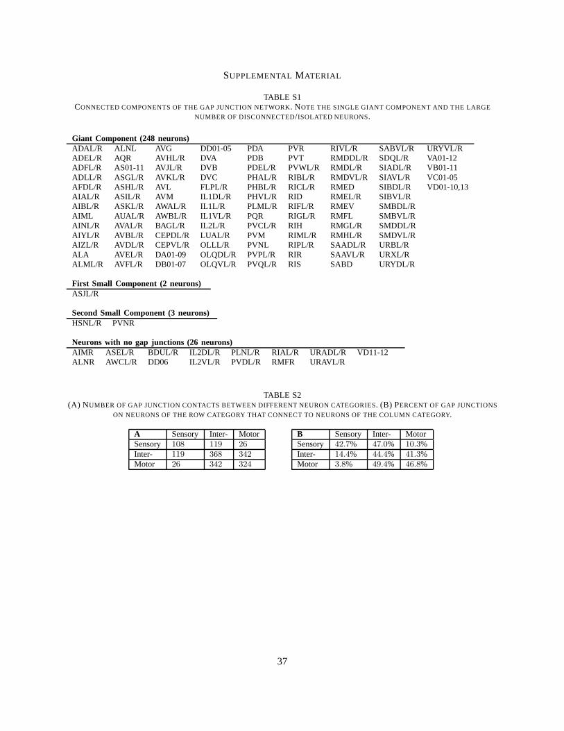
SUPPLEMENTAL MATERIAL

TABLE S1CONNECTED COMPONENTS OF THE GAP JUNCTION NETWORK. NOTE THE SINGLE GIANT COMPONENT AND THE LARGE

NUMBER OF DISCONNECTED/ISOLATED NEURONS.

Giant Component (248 neurons)ADAL/R ALNL AVG DD01-05 PDA PVR RIVL/R SABVL/R URYVL/RADEL/R AQR AVHL/R DVA PDB PVT RMDDL/R SDQL/R VA01-12ADFL/R AS01-11 AVJL/R DVB PDEL/R PVWL/R RMDL/R SIADL/R VB01-11ADLL/R ASGL/R AVKL/R DVC PHAL/R RIBL/R RMDVL/R SIAVL/R VC01-05AFDL/R ASHL/R AVL FLPL/R PHBL/R RICL/R RMED SIBDL/R VD01-10,13AIAL/R ASIL/R AVM IL1DL/R PHVL/R RID RMEL/R SIBVL/RAIBL/R ASKL/R AWAL/R IL1L/R PLML/R RIFL/R RMEV SMBDL/RAIML AUAL/R AWBL/R IL1VL/R PQR RIGL/R RMFL SMBVL/RAINL/R AVAL/R BAGL/R IL2L/R PVCL/R RIH RMGL/R SMDDL/RAIYL/R AVBL/R CEPDL/R LUAL/R PVM RIML/R RMHL/R SMDVL/RAIZL/R AVDL/R CEPVL/R OLLL/R PVNL RIPL/R SAADL/R URBL/RALA AVEL/R DA01-09 OLQDL/R PVPL/R RIR SAAVL/R URXL/RALML/R AVFL/R DB01-07 OLQVL/R PVQL/R RIS SABD URYDL/R

First Small Component (2 neurons)ASJL/R

Second Small Component (3 neurons)HSNL/R PVNR

Neurons with no gap junctions (26 neurons)AIMR ASEL/R BDUL/R IL2DL/R PLNL/R RIAL/R URADL/R VD11-12ALNR AWCL/R DD06 IL2VL/R PVDL/R RMFR URAVL/R

TABLE S2(A) NUMBER OF GAP JUNCTION CONTACTS BETWEEN DIFFERENT NEURON CATEGORIES. (B) PERCENT OF GAP JUNCTIONS

ON NEURONS OF THE ROW CATEGORY THAT CONNECT TO NEURONS OF THE COLUMN CATEGORY.

A Sensory Inter- MotorSensory 108 119 26Inter- 119 368 342Motor 26 342 324

B Sensory Inter- MotorSensory 42.7% 47.0% 10.3%Inter- 14.4% 44.4% 41.3%Motor 3.8% 49.4% 46.8%

37

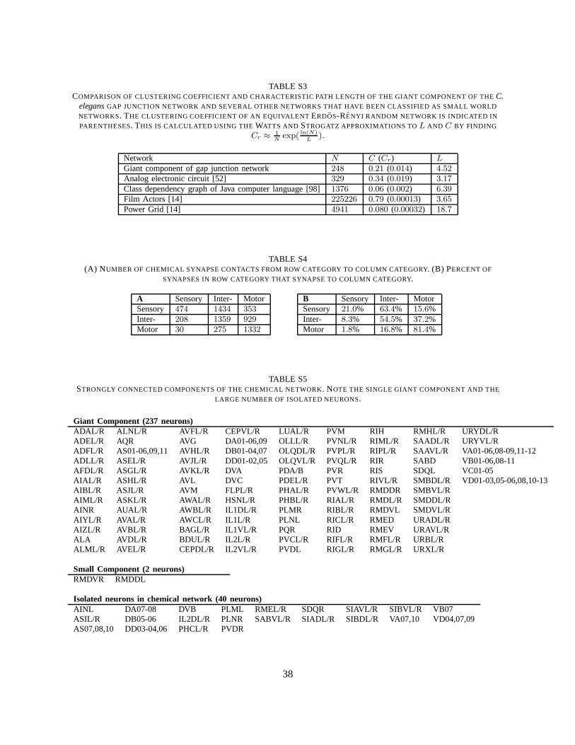
TABLE S3COMPARISON OF CLUSTERING COEFFICIENT AND CHARACTERISTIC PATH LENGTH OF THE GIANT COMPONENT OF THEC.

elegansGAP JUNCTION NETWORK AND SEVERAL OTHER NETWORKS THAT HAVE BEEN CLASSIFIED AS SMALL WORLD

NETWORKS. THE CLUSTERING COEFFICIENT OF AN EQUIVALENTERDOS-RENYI RANDOM NETWORK IS INDICATED IN

PARENTHESES. THIS IS CALCULATED USING THEWATTS AND STROGATZ APPROXIMATIONS TOL AND C BY FINDING

Cr ≈ 1N

exp( ln(N)L

).

Network N C (Cr) L

Giant component of gap junction network 248 0.21 (0.014) 4.52Analog electronic circuit [52] 329 0.34 (0.019) 3.17Class dependency graph of Java computer language [98]1376 0.06 (0.002) 6.39Film Actors [14] 225226 0.79 (0.00013) 3.65Power Grid [14] 4941 0.080 (0.00032) 18.7

TABLE S4(A) NUMBER OF CHEMICAL SYNAPSE CONTACTS FROM ROW CATEGORY TO COLUMN CATEGORY. (B) PERCENT OF

SYNAPSES IN ROW CATEGORY THAT SYNAPSE TO COLUMN CATEGORY.

A Sensory Inter- MotorSensory 474 1434 353Inter- 208 1359 929Motor 30 275 1332

B Sensory Inter- MotorSensory 21.0% 63.4% 15.6%Inter- 8.3% 54.5% 37.2%Motor 1.8% 16.8% 81.4%

TABLE S5STRONGLY CONNECTED COMPONENTS OF THE CHEMICAL NETWORK. NOTE THE SINGLE GIANT COMPONENT AND THE

LARGE NUMBER OF ISOLATED NEURONS.

Giant Component (237 neurons)ADAL/R ALNL/R AVFL/R CEPVL/R LUAL/R PVM RIH RMHL/R URYDL/RADEL/R AQR AVG DA01-06,09 OLLL/R PVNL/R RIML/R SAADL/R URYVL/RADFL/R AS01-06,09,11 AVHL/R DB01-04,07 OLQDL/R PVPL/R RIPL/R SAAVL/R VA01-06,08-09,11-12ADLL/R ASEL/R AVJL/R DD01-02,05 OLQVL/R PVQL/R RIR SABD VB01-06,08-11AFDL/R ASGL/R AVKL/R DVA PDA/B PVR RIS SDQL VC01-05AIAL/R ASHL/R AVL DVC PDEL/R PVT RIVL/R SMBDL/R VD01-03,05-06,08,10-13AIBL/R ASJL/R AVM FLPL/R PHAL/R PVWL/R RMDDR SMBVL/RAIML/R ASKL/R AWAL/R HSNL/R PHBL/R RIAL/R RMDL/R SMDDL/RAINR AUAL/R AWBL/R IL1DL/R PLMR RIBL/R RMDVL SMDVL/RAIYL/R AVAL/R AWCL/R IL1L/R PLNL RICL/R RMED URADL/RAIZL/R AVBL/R BAGL/R IL1VL/R PQR RID RMEV URAVL/RALA AVDL/R BDUL/R IL2L/R PVCL/R RIFL/R RMFL/R URBL/RALML/R AVEL/R CEPDL/R IL2VL/R PVDL RIGL/R RMGL/R URXL/R

Small Component (2 neurons)RMDVR RMDDL

Isolated neurons in chemical network (40 neurons)AINL DA07-08 DVB PLML RMEL/R SDQR SIAVL/R SIBVL/R VB07ASIL/R DB05-06 IL2DL/R PLNR SABVL/R SIADL/R SIBDL/R VA07,10 VD04,07,09AS07,08,10 DD03-04,06 PHCL/R PVDR

38

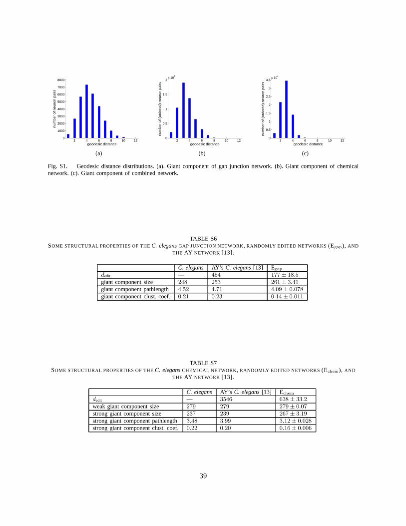
2 4 6 8 10 120

1000

2000

3000

4000

5000

6000

7000

8000

geodesic distance

num

ber

of n

euro

n pa

irs

(a)

2 4 6 8 10 120

0.5

1

1.5

2x 10

4

geodesic distance

num

ber

of (

orde

red)

neu

ron

pairs

(b)

2 4 6 8 10 120

0.5

1

1.5

2

2.5

3

3.5x 10

4

geodesic distance

num

ber

of (

orde

red)

neu

ron

pairs

(c)

Fig. S1. Geodesic distance distributions. (a). Giant component of gap junction network. (b). Giant component of chemicalnetwork. (c). Giant component of combined network.

TABLE S6SOME STRUCTURAL PROPERTIES OF THEC. elegansGAP JUNCTION NETWORK, RANDOMLY EDITED NETWORKS (Egap), AND

THE AY NETWORK [13].

C. elegans AY’s C. elegans[13] Egap

dedit — 454 177± 18.5giant component size 248 253 261± 3.41giant component pathlength 4.52 4.71 4.09± 0.078giant component clust. coef. 0.21 0.23 0.14± 0.011

TABLE S7SOME STRUCTURAL PROPERTIES OF THEC. elegansCHEMICAL NETWORK, RANDOMLY EDITED NETWORKS (Echem), AND

THE AY NETWORK [13].

C. elegans AY’s C. elegans[13] Echem

dedit — 3546 638± 33.2weak giant component size 279 279 279± 0.07strong giant component size 237 239 267± 3.19strong giant component pathlength 3.48 3.99 3.12 ± 0.028strong giant component clust. coef.0.22 0.20 0.16 ± 0.006

39

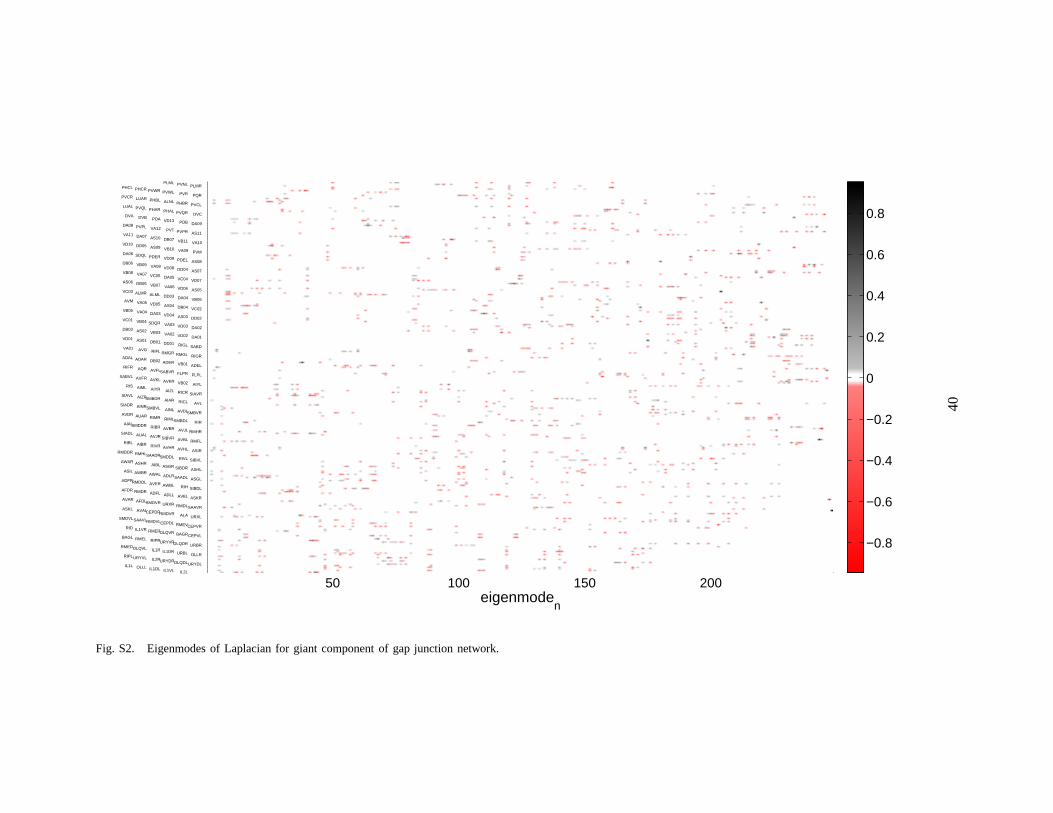
50 100 150 200eigenmode

n

IL2LIL1VLIL1DLOLLLIL1L URYDLOLQDLURYDRIL2RURYVLRIPL OLLRURBLIL1DRIL1ROLQVLRMED URBROLQDRURYVRRIPRRMELBAGL CEPVLBAGROLQVRRMERIL1VRRID CEPVRRMEVCEPDLRMDVLSAAVLSMDVL URXLALARMDVRCEPDRAVALASKL SAAVRRMDLURXRSMDVRAFDLAVAR ASKRAVELADLLADFLRMDRAFDR SIBDLRIHAWBLAVERRMDDLADFR ASGLSAADLADLRAWALAWBRASIL ASHLSIBDRASGRAIBLASHRAWAR SIBVLRIVLSMDDLSAADRRMHLRMDDR ASIRAVHLAVHRRIVRAIBRRIBL RMFLAVBLSIBVRAVJRAUALSIADL RMHRAVJLAVBRRIBRSMDDRAIAL RIRSMBDLRIMLRIMRAUARAVDR SMBVRAVDLAINLSMBVLAINRSIADR AVLRICLAIARSMBDRAIZRSIAVL SIAVRRICRAIZLAIYRAIMLRIS AIYLVB02AVKRAVKLAVFRSABVL FLPLFLPRSABVRAVFLAQRRIFR ADELVB01ADERDB02ADARADAL RIGRRMGLRMGRRIFLAVGVA01 SABDRIGLDD01DB01AS01VD01 DA01VD02VA02VB03AS02DB03 DA02VD03VA03SDQRVB04VC01 DD02AS03VD04DA03VA04VB05 VC02DB04AS04VD05VA05AVM VB06DA04DD03ALMLALMRVC03 AS05VD06VA06VB07DB05AS06 VD07VC04DA05VC05VA07VB08 AS07DD04VD08VA08VB09DB06 AS08PDELVD09PDERSDQLDA06 PVMVA09VB10AS09DD05VD10 VA10VB11DB07AS10DA07VA11 AS11PVPRPVTVA12PVPLDA08 DA09PDBVD13PDADVBDVA DVCPVQRPHALPHARPVQLLUAL PVCLPHBRALNLPHBLLUARPVCR PQRPVRPVWLPVWRPHCRPHCL PLMRPVNLPLML

−0.8

−0.6

−0.4

−0.2

0

0.2

0.4

0.6

0.8

Fig. S2. Eigenmodes of Laplacian for giant component of gap junction network.

40

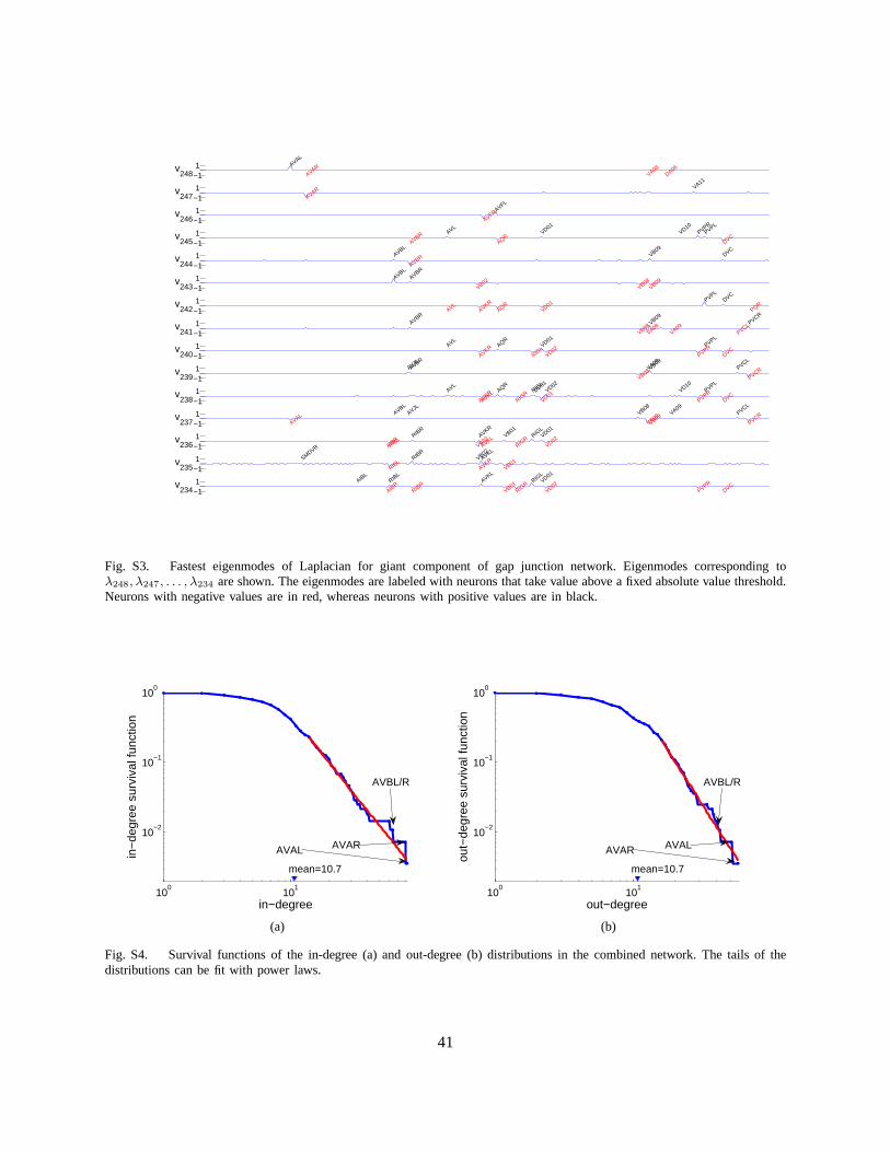
AVAL

VA08DA06

AVAR 1−1

v248

AVAR VA11 1−1

v247

AVFL

AVFR 1−1

v246

DVCPVPR

AQRAVL

VD01PVPL

AVBR VD10

1−1

v245

AVBR VB09AVBL

DVC 1−1

v244

AVBL

VB08AVBR

VB09VB02 1

−1v

243

PVPL

AQRDVC

AVKRVD01

PQRAVL

1−1

v242

VB09

VA08 PVCRAVBR

PVCLVA09

VB08 1−1

v241

VD01

PVPRPVPL

AQR

VD02RIG

LAVKR

DVCAVL

1−1

v240

PVCRVB09

VB08 PVCLVA08

AVJLAVBR

1−1

v239

VD01AQRVD02

DVCPVPRP

VPL

AVKLAVLRIG

L

AVKR VD10

RIGR

DD01

1−1

v238

VA08PVCRVB08

VB09 PVCLAVBL

AVJLVA09

AVAL 1−1

v237

AVKL RIGL

RIBL

RIBR

VB01VD01

RIGR

VD02VB02AVKR

AIBR 1

−1v

236

RIBR

RIBL

AVKL

VB01VB02SMDVR

AVKR 1−1

v235

RIGL

AVKL

RIGR

RIBR

RIBL

VB01AIB

RPVPR

VD02VD01AIB

L

DVC 1−1

v234

Fig. S3. Fastest eigenmodes of Laplacian for giant component of gap junction network. Eigenmodes corresponding toλ248, λ247, . . . , λ234 are shown. The eigenmodes are labeled with neurons that takevalue above a fixed absolute value threshold.Neurons with negative values are in red, whereas neurons with positive values are in black.

100

101

10−2

10−1

100

mean=10.7

in−degree

in−

degr

ee s

urvi

val f

unct

ion

AVAL AVAR

AVBL/R

(a)

100

101

10−2

10−1

100

mean=10.7

out−degree

out−

degr

ee s

urvi

val f

unct

ion

AVAR AVAL

AVBL/R

(b)

Fig. S4. Survival functions of the in-degree (a) and out-degree (b) distributions in the combined network. The tails of thedistributions can be fit with power laws.

41