Robot Positioning System - DiVA Portal

Robot Positioning System

Underwater Ultrasonic Measurement

Advanced Thesis in Electronics

Oliver Roldán Sánchez

([email protected]) David Salido Monzú

([email protected])

Table of contents:

1. Abstract............................................................................................. 1

2. Introduction ...................................................................................... 2

3. Initial approach ................................................................................. 3

3.1. Distance measuring systems ...............................................................................3

3.2. Suitable method choice.......................................................................................5

4. Theoretical basis in ultrasonic measurement..................................... 7

4.1. Ultrasound...........................................................................................................7

4.2. Main effects suffered by ultrasonic waves .........................................................8

4.3. Reflection...........................................................................................................10

4.4. Distance measuring using ultrasound...............................................................12

4.5. State of the art ..................................................................................................16

4.6. Research motivation .........................................................................................17

5. Practical solution............................................................................. 18

5.1. Structure and method .......................................................................................18

5.1.1. General structure ..............................................................................................18

5.1.2. Center positioning method ...............................................................................20

5.1.3. Project stages diagram......................................................................................25

5.2. Air measurement system ..................................................................................26

5.2.1. Introduction ......................................................................................................26

5.2.2. Sensor election..................................................................................................26

5.2.3. Design considerations .......................................................................................29

5.2.4. Design tools.......................................................................................................30 5.2.4.1. Milling machine .............................................................................................. 30 5.2.4.2. Software ......................................................................................................... 30

5.2.5. Circuit Design ....................................................................................................32 5.2.5.1. Conditioning stage.......................................................................................... 32 5.2.5.2. PIC processor .................................................................................................. 33

5.2.5.2.1. USB module ............................................................................................. 34 5.2.5.2.2. ADC module............................................................................................. 34 5.2.5.2.3. External crystal oscillator ........................................................................ 35 5.2.5.2.4. State leds ................................................................................................. 35 5.2.5.2.5. Reset / Programming mode buttons....................................................... 35

5.2.5.3. Power Supply .................................................................................................. 36 5.2.5.4. Protections ..................................................................................................... 39

5.2.6. Absolute error ratings .......................................................................................40

5.2.7. Additional placement element .........................................................................42

5.2.8. Design summary................................................................................................43

5.2.9. Software ............................................................................................................47

5.2.9.1. Oscillator configuration .................................................................................. 47

5.2.9.2. ADC Configuration .......................................................................................... 48

5.2.9.3. USB configuration........................................................................................... 49

5.2.9.4. Programming mode........................................................................................ 49

5.2.9.5. File structure................................................................................................... 50

5.2.9.6. Header file ...................................................................................................... 51

5.2.9.7. Main program................................................................................................. 52

5.3. Water measuring system ..................................................................................55

5.3.1. Introduction ......................................................................................................55

5.3.2. Transducer election...........................................................................................55

5.3.3. Design considerations .......................................................................................57

5.3.4. Circuit design.....................................................................................................59

5.3.4.1. Emitter Stage .................................................................................................. 59

5.3.4.2. Conditioning stage.......................................................................................... 61

5.3.4.3. Detecting Stage............................................................................................... 63

5.3.4.4. PIC Processor .................................................................................................. 64

5.3.4.4.1. External oscillator .................................................................................... 65

5.3.4.5. Power supply .................................................................................................. 66

5.3.5. Additional placement elements........................................................................71

5.3.6. Design summary................................................................................................72

5.3.7. Software ............................................................................................................75

5.3.7.1. Oscillator configuration .................................................................................. 75

5.3.7.2. USB configuration........................................................................................... 76

5.3.7.3. Timer configuration ........................................................................................ 76

5.3.7.4. Programming mode........................................................................................ 77

5.3.7.5. Files structure ................................................................................................. 77

5.3.7.6. Header file ...................................................................................................... 78

5.3.7.7. Main program................................................................................................. 79

5.4. Central controller ..............................................................................................83

5.4.1. Program outline ................................................................................................84

5.4.2. Operation diagram............................................................................................85

5.4.3. User interface....................................................................................................86

5.4.4. File structure .....................................................................................................90

5.5. Robot controller ................................................................................................93

5.5.1. Robot ............................................................................................................................ 93

5.5.2. Rapid program .............................................................................................................. 94

5.5.3. Program diagram .......................................................................................................... 97

5.5.4. Program code................................................................................................................ 97

5.6. Calibration program ........................................................................................102

5.6.1. Program diagram and example.......................................................................103

5.6.2. Calibration structure .......................................................................................105

6. Results, conclusion and improvements.......................................... 106

6.1. Air measurement.............................................................................................106

6.1.1. Possible improvements...................................................................................108

6.2. Water Measurement.......................................................................................109

6.2.1. Measurement for material differentiation and results...................................110

6.2.1.1. Materials....................................................................................................... 110

6.2.1.2. Environment status ...................................................................................... 111

6.2.1.3. Measurement ............................................................................................... 112

6.2.1.4. Water Calibration ......................................................................................... 118

6.2.2. Measurement for shape differentiation and results ......................................120

6.2.2.1. Materials....................................................................................................... 120

6.2.2.2. Measurements.............................................................................................. 122

6.2.2.3. Water calibration.......................................................................................... 124

6.2.3. Possible improvements............................................................................................... 126

Appendix: Matlab code. ..................................................................... 127

1

1 Abstract

This document provides a description about how the problem of the detection of the

center of a defined geometry object was solved.

This named object has been placed in an experimental environment surrounded by

water to be explored using microwaves under the water, to try to find a possible

tumor. The receiver antenna is fixed in the tip of the tool of an ABB robot.

Due to this working method, it was necessary to locate the center of this object to

make correctly the microwave scanning turning always around the actual center. This

work not only consist in give a hypothetic solution to the people who gave us the

responsibility of solve their problem, it is also to actually develop a system which

carries out the function explained before.

For the task of measuring the distance between the tip of the tool where the

microwave antenna is, ultrasonic sensors has been used, as a complement of a

complete system of communication between the sensor and finally the robot handler,

using Matlab as the main controller of the whole system.

One of these sensors will work out of water, measuring the zone of the object which is

out of the water. In the other hand, as the researching side of the thesis, a complete

ultrasonic sensor will be developed to work under water, and the results obtained will

be shown as the conclusion of our investigation.

The document provides a description about how the hardware and software necessary

to implement the system mentioned and some equipment more which were essential

to the final implementation was developed step by step.

2

2 Introduction

Breast cancer is the second most common type of cancer, what makes very important

the existence of detection methods that can be extended to reach as much people as

possible to guarantee early diagnosis. Currently, the first detection method for mass

screening is X-ray and the most effective one is Magnetic Resonance Imaging, whose

use is limited to big hospitals due to the price of the scanner, so the developing of

cheaper systems to be used as a first diagnosis tool means a great advance in cancer

treatment.

Mälardalen University is working on a research project with the aim of developing a

scanner system based on microwaves. Cancer induces changes in the properties of the

affected tissue; one of these changes causes a contrast between the permittivity of

tumor and healthy tissue, which means different behaviors as propagation mediums.

Based on that idea, the analysis of microwaves going through a tissue may be used to

obtain information about the properties of that tissue and check if there is a part of it

affected by a tumor. The developing scanner system uses a microwave emitting

antenna placed behind the phantom to analyze (a plastic cylinder that simulates

healthy breast tissue with a smaller cylinder inside that simulates tumor tissue) and a

receiving antenna placed in robot arm so it can turn around the phantom in order to

get many microwaves signals that can be afterwards reconstructed into a image of the

inner structure of the tissue.

The symmetry in the movement of the receiving antenna is essential to be able to form

a final image from the microwave signals, the robot should move around the phantom

using it as its center with an accuracy as high as possible, what creates the problem this

project is supposed to solve; the design of a system that locates the phantom and

refers its position to the coordinate system of the robot so all the measuring points are

at the same distance from the phantom.

3

3 Initial Approach

Once the aim of the project is set off, it is necessary deciding what method is going to

be used to reach it. The main decision depends on how to calculate the distance

between the axis of the robot tool and the phantom, this election depends on four

main parameters:

• Costs: Due to the condition of this project as a final thesis work, the final costs

of the chosen method will be considered so they are as low as possible.

• Precision: The requirements of the microwave imaging make necessary a

precision in the final location as high as possible, restricted to less than a

millimeter.

• Viability: It must be possible to design and develop the chosen method using

the resources available in the university.

• Simplicity: In case there are two similar options, the simplest one should be

chosen.

3.1 Distance Measuring Systems

After the first considerations two different approaches for distance measuring can be

made:

Systems that uses physical contact with the object to locate:

One of the simplest ideas we handled was based on the idea that we know

the robot position, so if we can move the robot tool until it touches the

cylinder, detecting that moment with some kind of contact sensor, we

would be able to know where the surface of the cylinder is.

Another idea was to use a step motor to move a contact sensor towards the

cylinder, and use the number of steps necessary for that to calculate the

distance.

A very interesting idea was to use the measure the twisting moment when

pushing the cylinder with a lever fixed on the tool of the robot, and

calculating the distance as a proportion to the moment.

4

Systems with non physical contact:

Distance sensors are based on these different physic areas:

Light based:

Infrared: There are two different ways of distance detection using IR.

Both are composed of an IR diode whose light is reflected and received

by a phototransistor. The first one uses the current through the

transistor because it is proportional to the amount of light that reaches

it. In the second method there is more than one receiving transistor so

the distance is calculated by triangulation.

L.A.S.E.R.: This method is based in the detection of the interference

between the emitted and reflected waves. The distance between

maximums and minimums of the resulting wave compared to that of a

wave reflected on a fixed point inside the sensor is proportional to the

distance of the reflecting surface.

Electromagnetic field based:

Inductive: The interference of a metallic surface into the magnetic field

generated by the sensor causes an alteration, proportional to the

distance of the surface.

Capacitive: The metallic surface of the object to detect acts as one of

the dielectric sheets, so the distance to it means a change in the

electrical field into the capacitor formed.

Sound based:

Ultrasonic: These sensors are based on the measurement of the elapsed

time between the emission of an ultrasonic pulse and the reception of

the reflected pressure wave.

5

3.2 Suitable Method Choice

There are three different points of view to analyze in order to take a decision:

• Measuring range:

Due to the dimensions of the robot and the object to detect and its future

applications, the sensor must be able to work between 10 cm to 2 meters.

These limitations make impossible the use of the electromagnetic field based

sensors because of their low range working distances (up to a few millimeters).

• Accuracy:

The system requires less than 1mm of precision. Laser is the most accurate

system with resolutions about tens of microns. The ultrasonic sensors are less

accurate, reaching a resolution of tens of millimeters which still fulfill our

requirements; this does not happen with IR sensors, whose low resolution is

usually not even given by the manufactures.

• Underwater behavior:

The light propagation underwater shows two main disadvantages: scattering,

caused by the non homogeneous water composition, causes a random diffusion

of the light path, and absorption that carries with a loss of the energy of the

light wave. Due to the way laser distance sensors work it is necessary having a

regular behavior of the light path to do the correct analysis of the wave formed

with the superimposition of the emitted and reflected radiations. The biggest

problem is that scattering is an irregular phenomena so it causes a variable

error which is impossible to compensate to obtain a suitable resolution.

Nowadays there are some underwater laser applications but just focused on

short distance communications, lightening, and big scale imaging, which don’t

have so many problems related with precision.

• Compatibility with the microwave system:

The chosen method must not cause any interference with the final aim of the

research, so any method that may cause any change in the working

environment from the microwaves point of view should be discarded. All the

mentioned method that involve physical contact involve the use of metallic

parts, (strain gauge for calculating the twisting moment, contact sensors or

step motors), which would interfere in the microwave propagation.

6

After studying the different options and discarding the ones that initially do not suit the

basics requirements two decisions have been taken considering that there is not an

affordable sensor for underwater accurate measurement.

In the first place it is necessary providing a practical solution to the positioning, so we

will develop a system that works outside water, using the upper part of the phantom

which is not submerged. An ultrasonic sensor will be used for this purpose because it

means a compromise between the required precision and cost. This sensor will be

working close to water so it will be chosen considering its level of protection against

casual contact with it.

In the other hand we have observed that there is no practical options in the industrial

market for short distance and high accuracy measurements underwater so it has been

decided to perform a minor research about the viability of designing a short range

underwater ultrasonic sensor and try to find out what are the main problems and

properties of such systems that make them so insufficient.

7

4 Theoretical Basis in Ultrasonic Measurement

4.1 Ultrasound

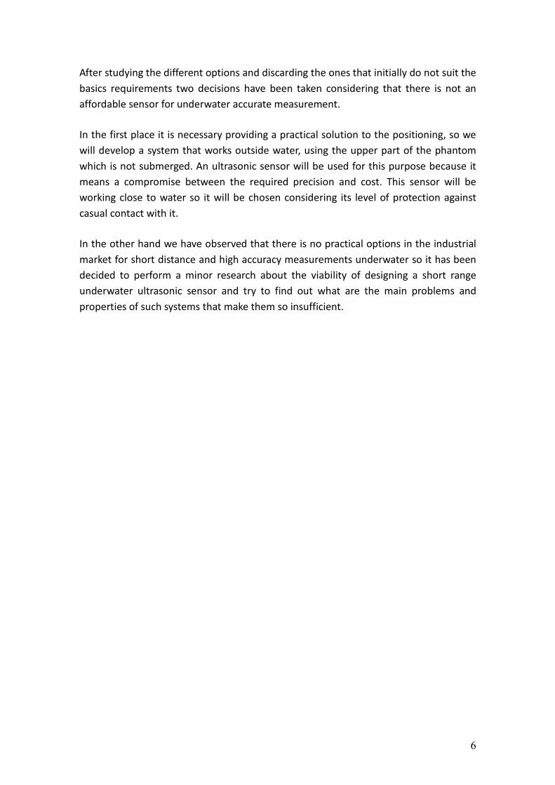
Ultrasounds are pressure waves generated by the vibration of an object that

propagates in longitudinal compression waves in gases and liquids and both

longitudinal and transversal in solids. The term ultrasonic refers its frequency range,

whose lower limit is above the human hearing upper threshold, around 20 KHz.

Figure 4.1

In figure 4.1 the vertical lines represents the real matter displacement while the sinus-

like line represents the amplitude of the pressure wave with the distance, an

interesting comparison since this is the electrical signal an ultrasound transducer would

produce when receiving a continuous ultrasonic wave.

The propagation is caused by local compressions and expansions of matter that

transmit the kinetic energy through the medium, so the speed of this propagation

depends on the capacity of the medium supporting the wave to compress and go back

to its equilibrium, what is directly related to its elasticity and density, usually being

faster in liquids and non-porous solids than in gases. This causes it is highly dependent

with the temperature of the medium because of its effect over the density but hardly

affected by pressure in the case of gas environments.

8

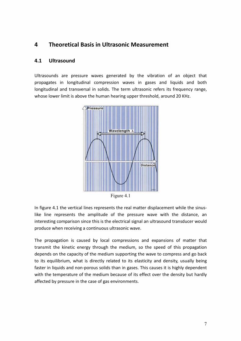
Substance Temperature (ºC) Speed (m/s)

Gases

Carbon Dioxide 0 259

Oxygen 0 316

Air 0 331

Air 20 343

Helium 0 965

Liquids

Chloroform 20 1004

Ethanol 20 1162

Mercury 20 1450

Water 20 1482

Solids

Lead - 1960

Copper - 5010

Glass - 5640

Steel 5960

Figure 4.2

4.2 Main Effects Suffered by Ultrasonic Waves

The effects suffered by ultrasound, and acoustic waves in general, when passing from

one medium to another, finding obstacles, or propagating through certain material are

quite similar to those well known in optics due to its wave nature. The most significant

of these effects will be detailed briefly, deepening afterwards in the most important

one for ultrasonic measurement, the reflection.

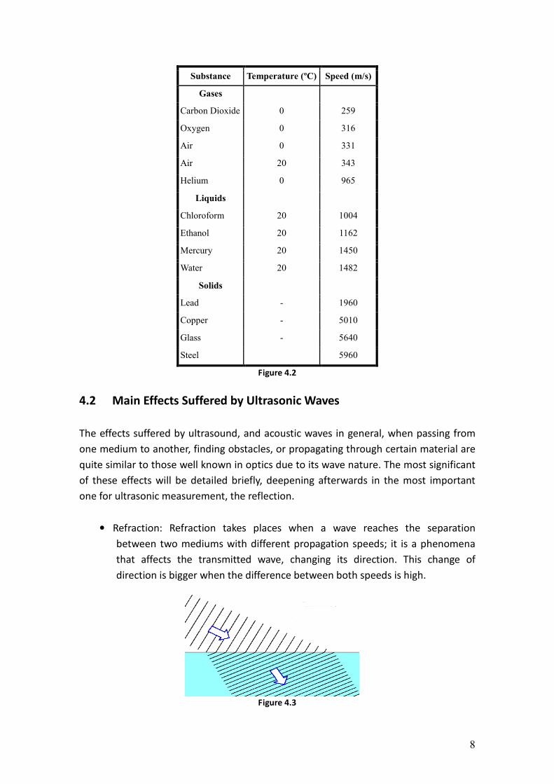
• Refraction: Refraction takes places when a wave reaches the separation

between two mediums with different propagation speeds; it is a phenomena

that affects the transmitted wave, changing its direction. This change of

direction is bigger when the difference between both speeds is high.

Figure 4.3

9

There is another curios effect also caused by refraction. The density of a

medium is directly dependent of the temperature, so if an acoustic wave is

moving through a medium whose temperature is not constant it suffers a

deviation proportional to the change of temperature.

• Diffraction: This phenomena is related with the existence of obstacles in the

propagation path. When an acoustic wave finds an obstacles its borders act as

new emitting point, this can be interpreted as a tendency of the wave to bend

around it. This happens more easily when the wavelength is big in relation with

the obstacle, what makes low frequencies easier to receive behind walls or

obstacles.

Figure 4.4

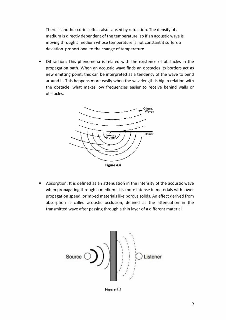
• Absorption: It is defined as an attenuation in the intensity of the acoustic wave

when propagating through a medium. It is more intense in materials with lower

propagation speed, or mixed materials like porous solids. An effect derived from

absorption is called acoustic occlusion, defined as the attenuation in the

transmitted wave after passing through a thin layer of a different material.

Figure 4.5

10

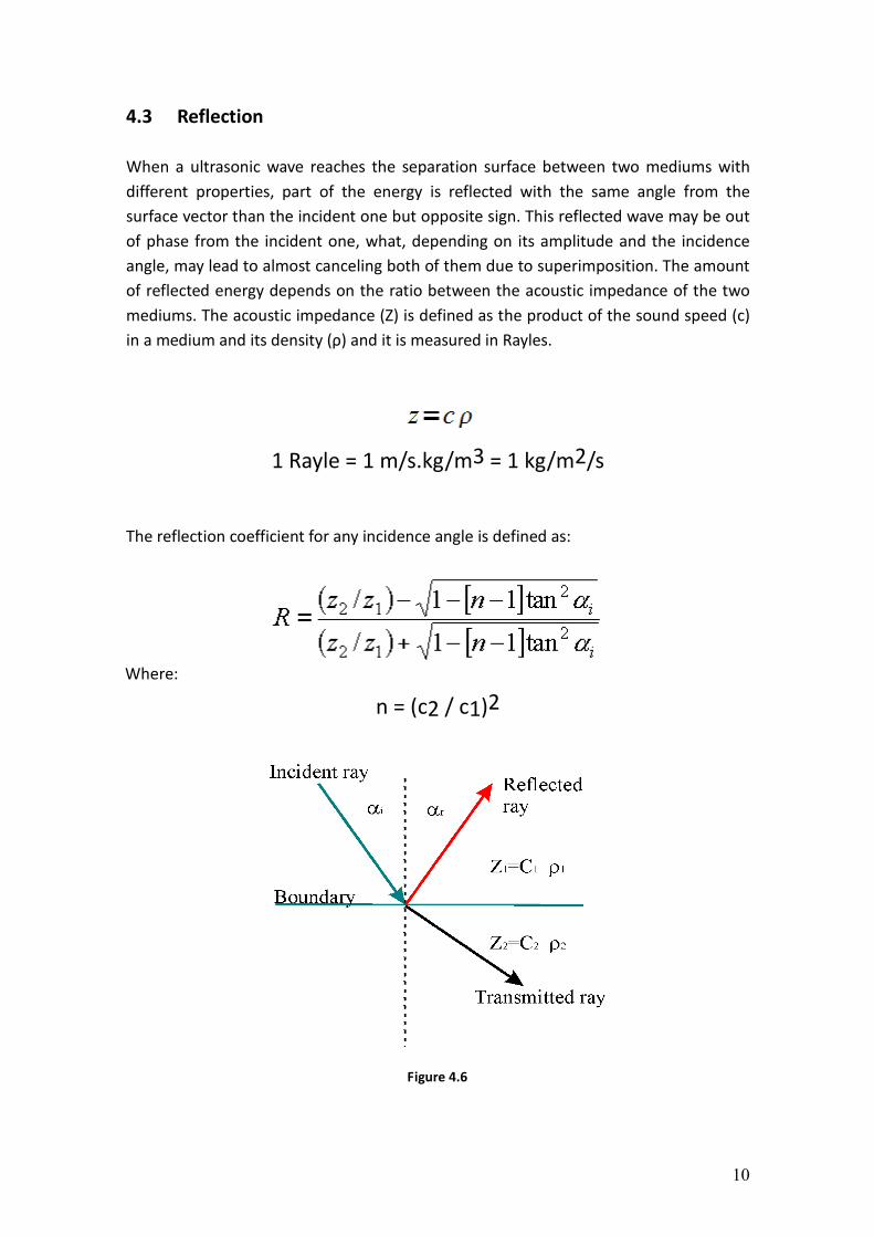
4.3 Reflection

When a ultrasonic wave reaches the separation surface between two mediums with

different properties, part of the energy is reflected with the same angle from the

surface vector than the incident one but opposite sign. This reflected wave may be out

of phase from the incident one, what, depending on its amplitude and the incidence

angle, may lead to almost canceling both of them due to superimposition. The amount

of reflected energy depends on the ratio between the acoustic impedance of the two

mediums. The acoustic impedance (Z) is defined as the product of the sound speed (c)

in a medium and its density (ρ) and it is measured in Rayles.

1 Rayle = 1 m/s.kg/m3 = 1 kg/m2/s

The reflection coefficient for any incidence angle is defined as:

Where:

n = (c2 / c1)2

Figure 4.6

11

In the particular case of normal incidence where αi =0:

R=(Z2 - Z1)/(Z2 + Z1)

From this expression we can deduce that the reflection coefficient will be defined

between (-1, 1), and we can define four different types of reflection:

1) Z1 << Z2 , R=>1: Rigid boundary. Most energy will be reflected without any

phase change.

2) Z1 >> Z2 , R=>-1: Soft or pressure release boundary. Most energy will be

reflected with a 180o

phase change.

3) Z1 = Z2 , R=0: Same medium or same acoustic impedance. No reflection.

4) -1 << R << 1 : Similar acoustic impedance. Small reflection and phase change.

Due to energy conservation we can define the transmission coefficient as:

T=(1-R)

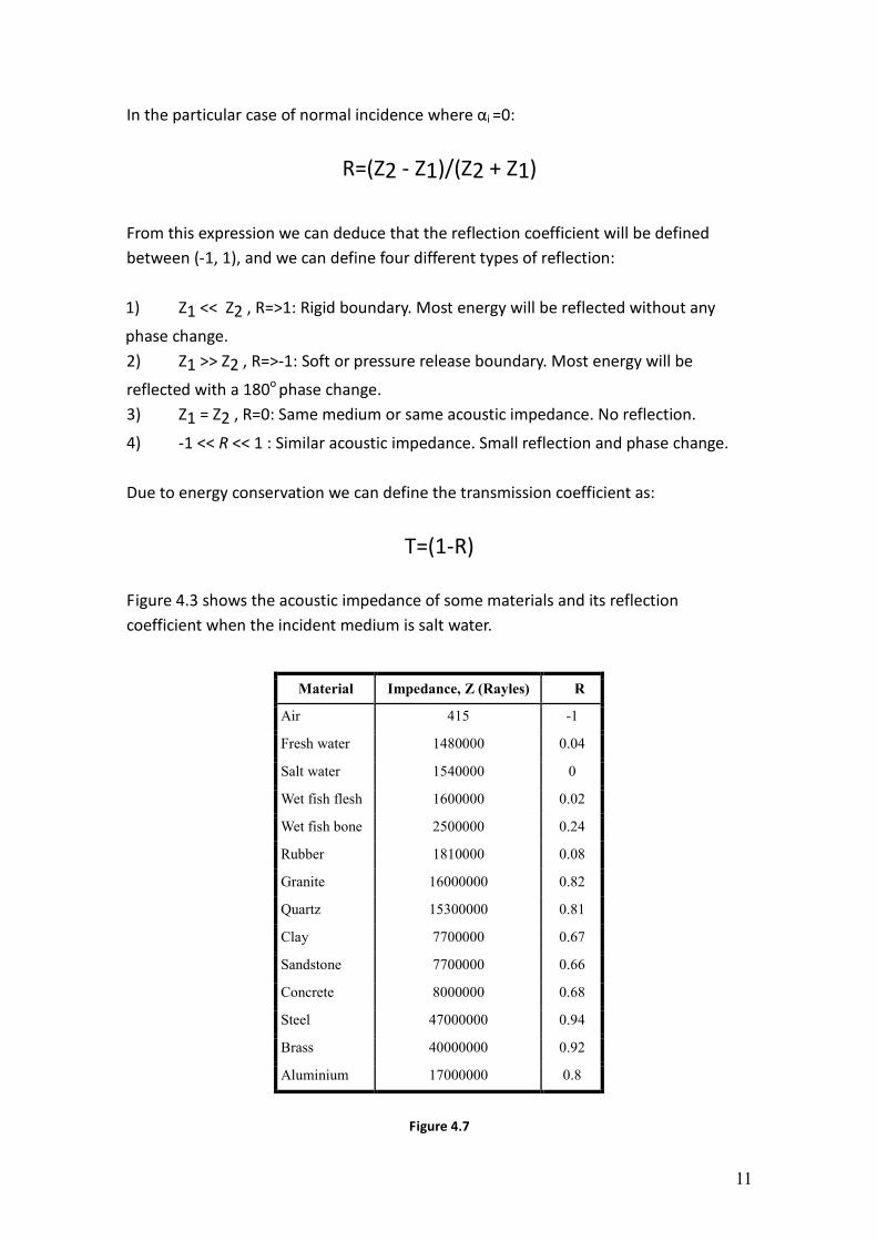
Figure 4.3 shows the acoustic impedance of some materials and its reflection

coefficient when the incident medium is salt water.

Material Impedance, Z (Rayles) R

Air 415 -1

Fresh water 1480000 0.04

Salt water 1540000 0

Wet fish flesh 1600000 0.02

Wet fish bone 2500000 0.24

Rubber 1810000 0.08

Granite 16000000 0.82

Quartz 15300000 0.81

Clay 7700000 0.67

Sandstone 7700000 0.66

Concrete 8000000 0.68

Steel 47000000 0.94

Brass 40000000 0.92

Aluminium 17000000 0.8

Figure 4.7

12

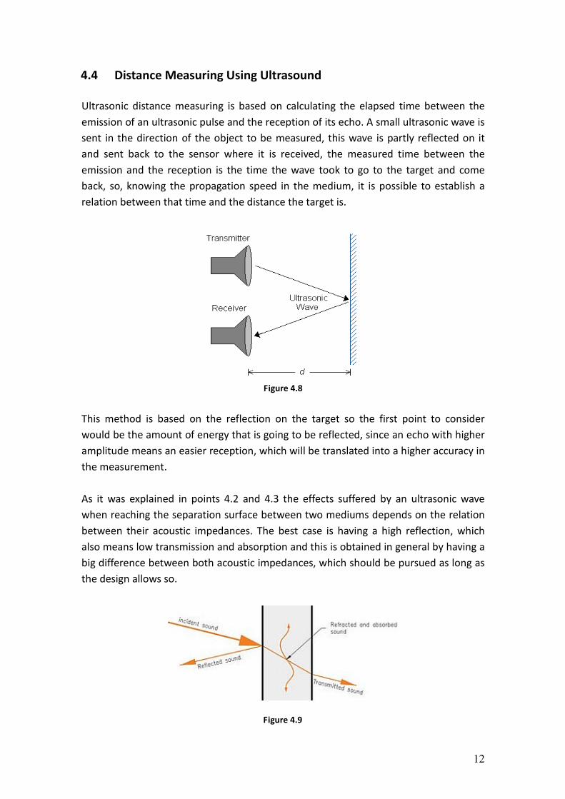
4.4 Distance Measuring Using Ultrasound

Ultrasonic distance measuring is based on calculating the elapsed time between the

emission of an ultrasonic pulse and the reception of its echo. A small ultrasonic wave is

sent in the direction of the object to be measured, this wave is partly reflected on it

and sent back to the sensor where it is received, the measured time between the

emission and the reception is the time the wave took to go to the target and come

back, so, knowing the propagation speed in the medium, it is possible to establish a

relation between that time and the distance the target is.

Figure 4.8

This method is based on the reflection on the target so the first point to consider

would be the amount of energy that is going to be reflected, since an echo with higher

amplitude means an easier reception, which will be translated into a higher accuracy in

the measurement.

As it was explained in points 4.2 and 4.3 the effects suffered by an ultrasonic wave

when reaching the separation surface between two mediums depends on the relation

between their acoustic impedances. The best case is having a high reflection, which

also means low transmission and absorption and this is obtained in general by having a

big difference between both acoustic impedances, which should be pursued as long as

the design allows so.

Figure 4.9

13

This is not a problem in systems working in air environments ranging solid targets since,

as shown in figure 4.7, the impedance of air is very low because of its density and

sound speed compared with the impedance of most solid materials, so, in general, the

reflection coefficient will be close to -1; the wave will suffer an inversion of phase, not

relevant in this systems, but most of the energy will be reflected and the echo will be

easy to detect. The main problem in this environment appears when the object to

detect is a very porous solid; its cavities full with air will lower the impedance and

induce a much higher absorption.

Systems working underwater presents much more problems since the acoustic

impedance of water is high, almost similar to some non-porous solids, what means

very low reflection, for example, as we can see in figure 4.7, the reflection of a rubber

object in water would be almost null. This means that a system measuring underwater

is much more dependent of the material of the target, what makes its design more

complicated. Underwater measurement will be studied deeper in point 6, together

with the results obtained in our small research about the topic.

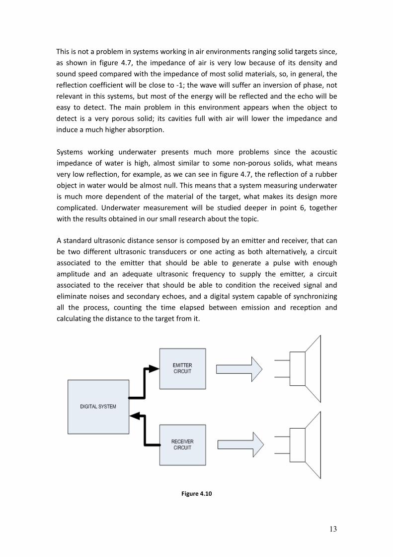
A standard ultrasonic distance sensor is composed by an emitter and receiver, that can

be two different ultrasonic transducers or one acting as both alternatively, a circuit

associated to the emitter that should be able to generate a pulse with enough

amplitude and an adequate ultrasonic frequency to supply the emitter, a circuit

associated to the receiver that should be able to condition the received signal and

eliminate noises and secondary echoes, and a digital system capable of synchronizing

all the process, counting the time elapsed between emission and reception and

calculating the distance to the target from it.

Figure 4.10

14

There are some basic considerations that should be taken into account in the design of

an ultrasonic sensor:

• Range: If the system is composed of two transducers, when the wave is emitted

it will reach the receiver following the direct path between them before the real

echo reaches it. This direct echo should be eliminated or ignored somehow to

avoid wrong detection. This effect causes the necessity of defining a blind zone

for small distance where the echo from the object cannot be distinguished from

the direct one, reducing the working range of the sensor.

If the system is composed of one transducer, acting as both the emitter and the

receiver, the blind zone will be determined by the time necessary to finish the

emission and switch the transducer into receiver.

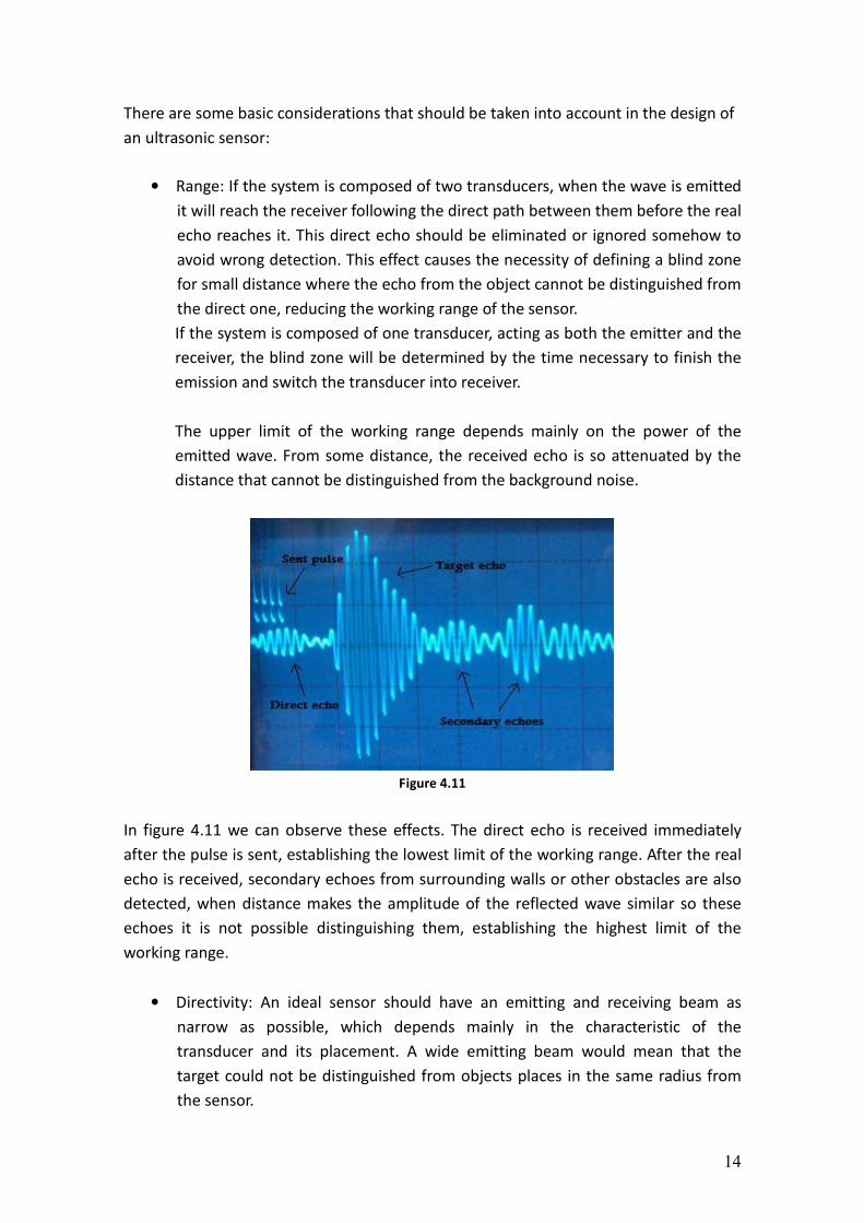
The upper limit of the working range depends mainly on the power of the

emitted wave. From some distance, the received echo is so attenuated by the

distance that cannot be distinguished from the background noise.

Figure 4.11

In figure 4.11 we can observe these effects. The direct echo is received immediately

after the pulse is sent, establishing the lowest limit of the working range. After the real

echo is received, secondary echoes from surrounding walls or other obstacles are also

detected, when distance makes the amplitude of the reflected wave similar so these

echoes it is not possible distinguishing them, establishing the highest limit of the

working range.

• Directivity: An ideal sensor should have an emitting and receiving beam as

narrow as possible, which depends mainly in the characteristic of the

transducer and its placement. A wide emitting beam would mean that the

target could not be distinguished from objects places in the same radius from

the sensor.

15

• Accuracy: The main limitation in the accuracy of an ultrasonic sensor is related

with both the working frequency and the phase in the reflection.

The detection of the sinus like echo causes an error that cannot be fixed. When

the receiver is detecting one cycle of the echo and the target is moved further,

the attenuation because of the longer distance will reduce the amplitude of the

wave and the receiver may not be able to detect the same cycle, jumping to the

next one with higher amplitude. This jump is translated into a non linearity of

the measured time with the distance. The resulting error depends on the time

elapsed between one cycle and the next one. Emitting in higher frequencies

would reduce this time minimizing the error.

A phase related effect adds to this error. The reflectivity in the target is constant

but the amount of reflected energy depends on the phase of the wave when

reaching the surface, causing a variation in the amplitude of the echo not

proportional to the distance, adding non-linearity to the results.

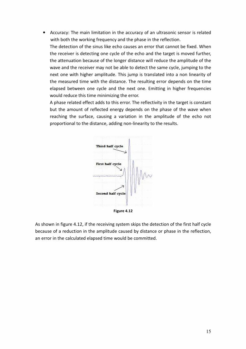
Figure 4.12

As shown in figure 4.12, if the receiving system skips the detection of the first half cycle

because of a reduction in the amplitude caused by distance or phase in the reflection,

an error in the calculated elapsed time would be committed.

16

4.5 State of the Art

The current market of ultrasonic reflective sensors can be divided in two main

categories:

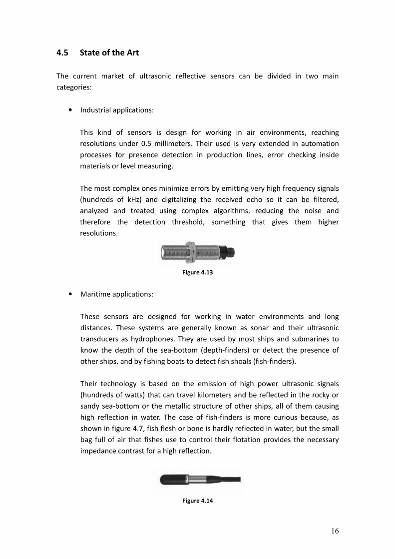
• Industrial applications:

This kind of sensors is design for working in air environments, reaching

resolutions under 0.5 millimeters. Their used is very extended in automation

processes for presence detection in production lines, error checking inside

materials or level measuring.

The most complex ones minimize errors by emitting very high frequency signals

(hundreds of kHz) and digitalizing the received echo so it can be filtered,

analyzed and treated using complex algorithms, reducing the noise and

therefore the detection threshold, something that gives them higher

resolutions.

Figure 4.13

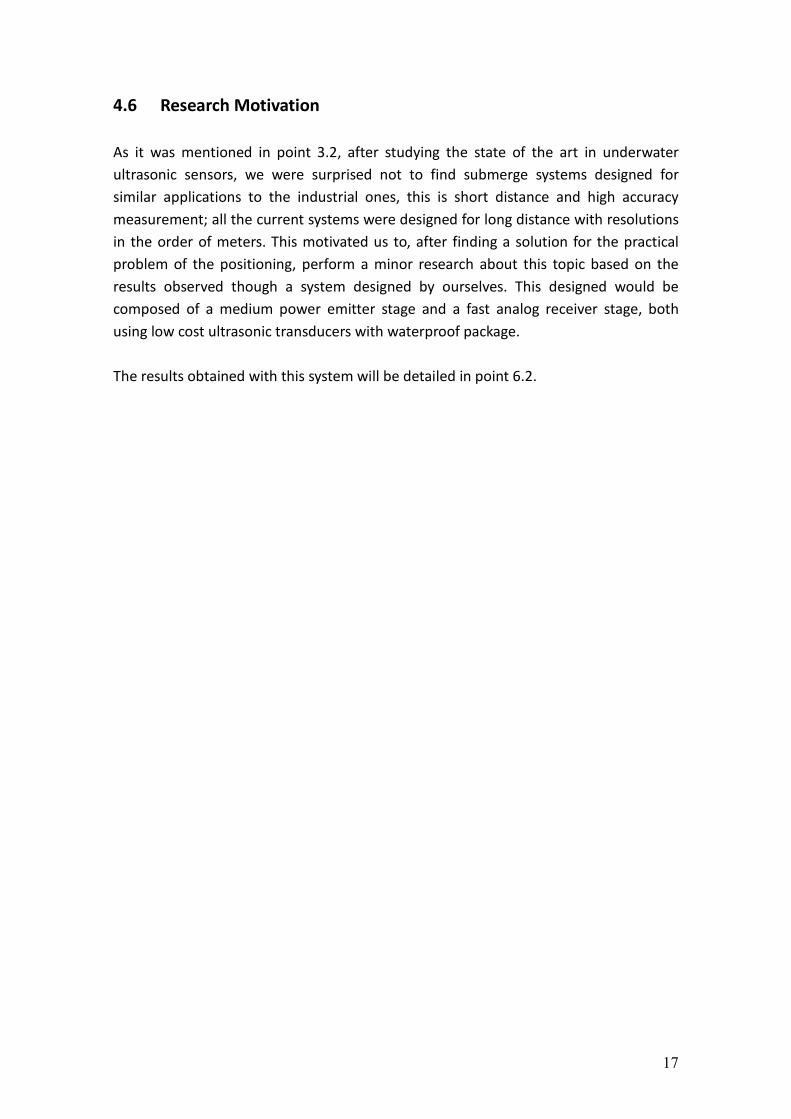
• Maritime applications:

These sensors are designed for working in water environments and long

distances. These systems are generally known as sonar and their ultrasonic

transducers as hydrophones. They are used by most ships and submarines to

know the depth of the sea-bottom (depth-finders) or detect the presence of

other ships, and by fishing boats to detect fish shoals (fish-finders).

Their technology is based on the emission of high power ultrasonic signals

(hundreds of watts) that can travel kilometers and be reflected in the rocky or

sandy sea-bottom or the metallic structure of other ships, all of them causing

high reflection in water. The case of fish-finders is more curious because, as

shown in figure 4.7, fish flesh or bone is hardly reflected in water, but the small

bag full of air that fishes use to control their flotation provides the necessary

impedance contrast for a high reflection.

Figure 4.14

17

4.6 Research Motivation

As it was mentioned in point 3.2, after studying the state of the art in underwater

ultrasonic sensors, we were surprised not to find submerge systems designed for

similar applications to the industrial ones, this is short distance and high accuracy

measurement; all the current systems were designed for long distance with resolutions

in the order of meters. This motivated us to, after finding a solution for the practical

problem of the positioning, perform a minor research about this topic based on the

results observed though a system designed by ourselves. This designed would be

composed of a medium power emitter stage and a fast analog receiver stage, both

using low cost ultrasonic transducers with waterproof package.

The results obtained with this system will be detailed in point 6.2.

18

5 Practical Solution

5.1 Structure and Method

This point will contain the general structure of the complete design and a description

of the method used to localize the center of a cylinder using distance sensors.

5.1.1 General Structure

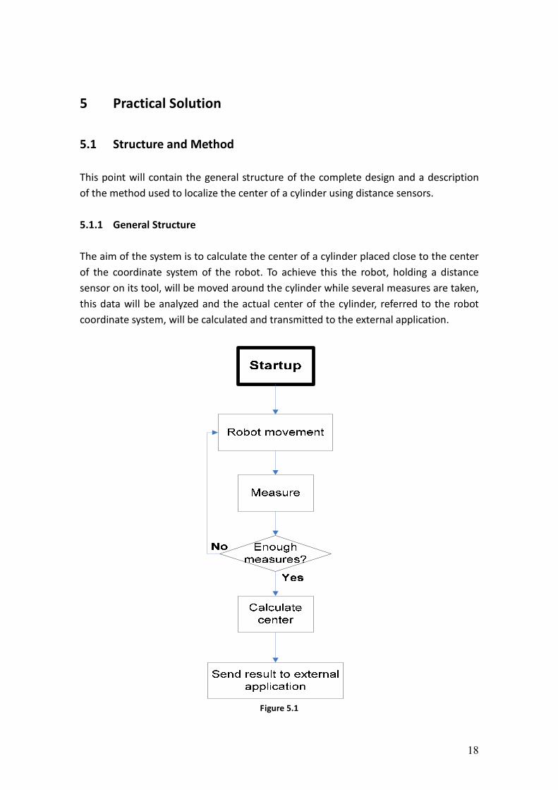
The aim of the system is to calculate the center of a cylinder placed close to the center

of the coordinate system of the robot. To achieve this the robot, holding a distance

sensor on its tool, will be moved around the cylinder while several measures are taken,

this data will be analyzed and the actual center of the cylinder, referred to the robot

coordinate system, will be calculated and transmitted to the external application.

Figure 5.1

19

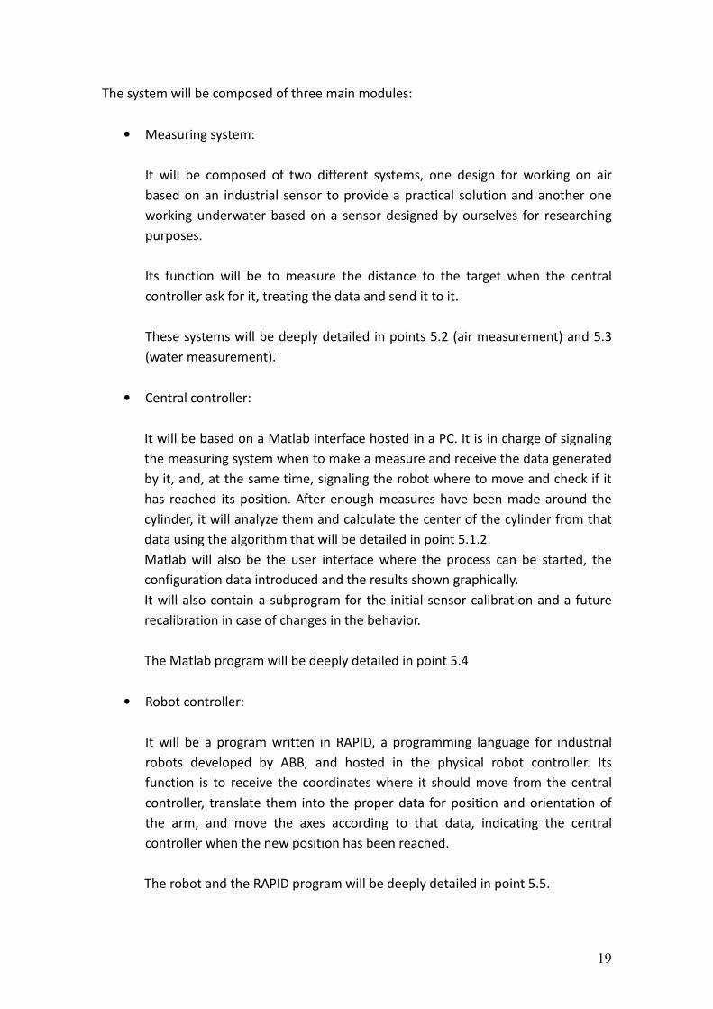
The system will be composed of three main modules:

• Measuring system:

It will be composed of two different systems, one design for working on air

based on an industrial sensor to provide a practical solution and another one

working underwater based on a sensor designed by ourselves for researching

purposes.

Its function will be to measure the distance to the target when the central

controller ask for it, treating the data and send it to it.

These systems will be deeply detailed in points 5.2 (air measurement) and 5.3

(water measurement).

• Central controller:

It will be based on a Matlab interface hosted in a PC. It is in charge of signaling

the measuring system when to make a measure and receive the data generated

by it, and, at the same time, signaling the robot where to move and check if it

has reached its position. After enough measures have been made around the

cylinder, it will analyze them and calculate the center of the cylinder from that

data using the algorithm that will be detailed in point 5.1.2.

Matlab will also be the user interface where the process can be started, the

configuration data introduced and the results shown graphically.

It will also contain a subprogram for the initial sensor calibration and a future

recalibration in case of changes in the behavior.

The Matlab program will be deeply detailed in point 5.4

• Robot controller:

It will be a program written in RAPID, a programming language for industrial

robots developed by ABB, and hosted in the physical robot controller. Its

function is to receive the coordinates where it should move from the central

controller, translate them into the proper data for position and orientation of

the arm, and move the axes according to that data, indicating the central

controller when the new position has been reached.

The robot and the RAPID program will be deeply detailed in point 5.5.

20

Figure 5.2

5.1.2 Center Positioning Method

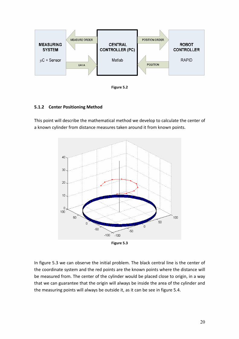
This point will describe the mathematical method we develop to calculate the center of

a known cylinder from distance measures taken around it from known points.

Figure 5.3

In figure 5.3 we can observe the initial problem. The black central line is the center of

the coordinate system and the red points are the known points where the distance will

be measured from. The center of the cylinder would be placed close to origin, in a way

that we can guarantee that the origin will always be inside the area of the cylinder and

the measuring points will always be outside it, as it can be see in figure 5.4.

21

Figure 5.4

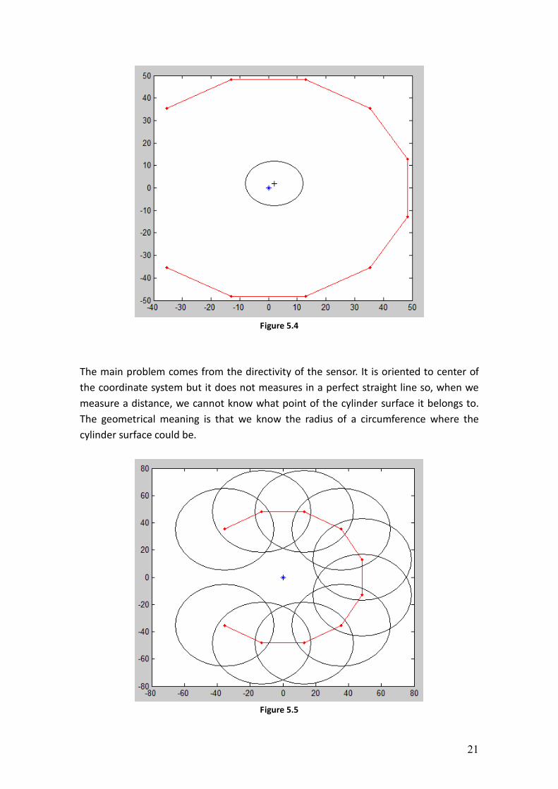
The main problem comes from the directivity of the sensor. It is oriented to center of

the coordinate system but it does not measures in a perfect straight line so, when we

measure a distance, we cannot know what point of the cylinder surface it belongs to.

The geometrical meaning is that we know the radius of a circumference where the

cylinder surface could be.

Figure 5.5

22

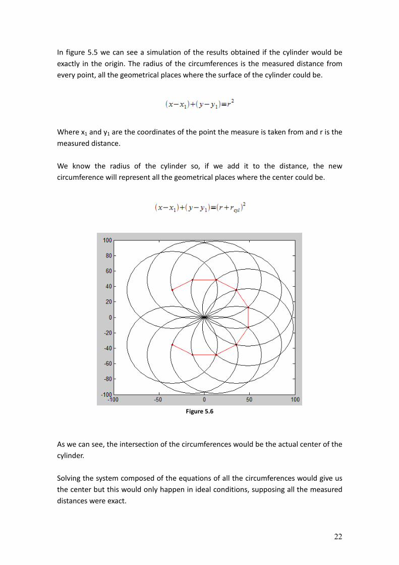
In figure 5.5 we can see a simulation of the results obtained if the cylinder would be

exactly in the origin. The radius of the circumferences is the measured distance from

every point, all the geometrical places where the surface of the cylinder could be.

Where x1 and y1 are the coordinates of the point the measure is taken from and r is the

measured distance.

We know the radius of the cylinder so, if we add it to the distance, the new

circumference will represent all the geometrical places where the center could be.

Figure 5.6

As we can see, the intersection of the circumferences would be the actual center of the

cylinder.

Solving the system composed of the equations of all the circumferences would give us

the center but this would only happen in ideal conditions, supposing all the measured

distances were exact.

23

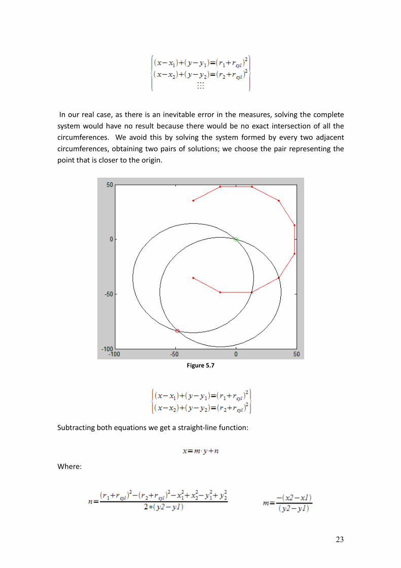
In our real case, as there is an inevitable error in the measures, solving the complete

system would have no result because there would be no exact intersection of all the

circumferences. We avoid this by solving the system formed by every two adjacent

circumferences, obtaining two pairs of solutions; we choose the pair representing the

point that is closer to the origin.

Figure 5.7

Subtracting both equations we get a straight-line function:

Where:

24

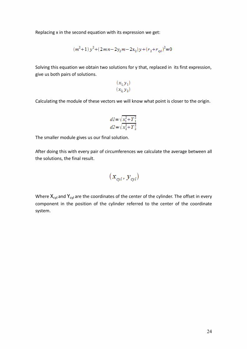
Replacing x in the second equation with its expression we get:

Solving this equation we obtain two solutions for y that, replaced in its first expression,

give us both pairs of solutions.

Calculating the module of these vectors we will know what point is closer to the origin.

The smaller module gives us our final solution.

After doing this with every pair of circumferences we calculate the average between all

the solutions, the final result.

Where Xcyl and Ycyl are the coordinates of the center of the cylinder. The offset in every

component in the position of the cylinder referred to the center of the coordinate

system.

25

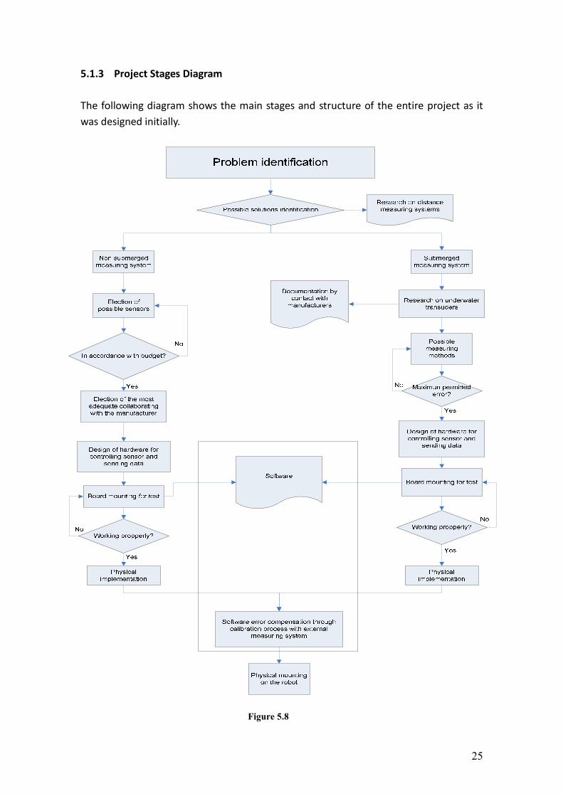
5.1.3 Project Stages Diagram

The following diagram shows the main stages and structure of the entire project as it

was designed initially.

Figure 5.8

26

5.2 Air Measurement System

5.2.1 Introduction

Once decided what kind of ultrasonic sensor we were going to use, it was necessary

selecting a concrete one, which fits in our measurement range needs.

5.2.2 Sensor Election

For this task, a contact and an examination of the products of several manufacturers

was required, so we needed to make a complete comparison between all the

manufacturer ’s products and themselves taking into account some parameters as for

example, the measure range, maximum error allowed through the resolution of the

sensor, price, the shape also should be the most useful possible because later, we have

to design some holder to locate it into the tool of the robot, the housing of the sensor

due to working in a water environment make necessary having a sensor which allows

get wet and finally the output given by the sensor, because the final design of the

hardware will depends on it. It is also necessary to mention the final manufacturer

chosen was located as near as possible to works with our dealers to reduce the cost

produced by transport or intermediaries.

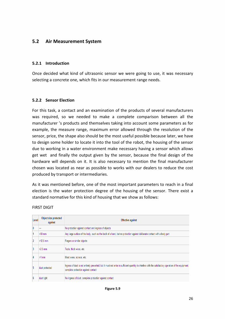
As it was mentioned before, one of the most important parameters to reach in a final

election is the water protection degree of the housing of the sensor. There exist a

standard normative for this kind of housing that we show as follows:

FIRST DIGIT

Figure 5.9

27

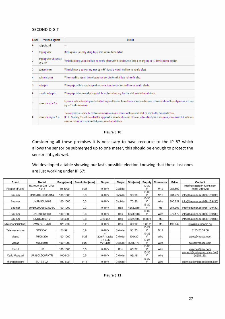
SECOND DIGIT

Figure 5.10

Considering all these premises it is necessary to have recourse to the IP 67 which

allows the sensor be submerged up to one meter, this should be enough to protect the

sensor if it gets wet.

We developed a table showing our lasts possible election knowing that these last ones

are just working under IP 67:

Brand Model Range[mm] Resolution[mm] Output Shape Size[mm] Supply Connector Price Contact

Pepperl+Fuchs UC1000-30GM-IUR2-

KV15 80-1000 0,35 0-10 V Cycilder 10-30

V M12 283.59£ [email protected]

(0303-246070)

Baumer UNAM18U6903/S14 100-1000 0,3 0-10 V Cycilder 90x18 15-30

V M12 201.77£ [email protected] (036-139430)

Baumer UNAM30U9103 100-1000 0,3 0-10 V Cycilder 70x30 15-30

V Wire 300.22£ [email protected] (036-139430)

Baumer UMDK20U6903/S35A 100-1000 0,3 0-10 V Box 42x20x15 15-30

V M8 254.99£ [email protected] (036-139430)

Baumer UNDK30U9103 100-1000 0,3 0-10 V Box 65x30x18 15-30

V Wire 277.17£ [email protected] (036-139430)

Baumer UNDK20I6912 60-400 0,3 4-20 mA Box 42x20x15 15-30V M8 [email protected] (036-139430)

Microsonic(Balluff) ZWS-24CU/QS 120-700 0,2 0-10 V Box 32x12 9-30 V M8 190.04£ [email protected]

Telemecanique XX930A1 51-991 0,9 0-10 V Cylinder 95x35 15-24

V M12 0155-26 54 00

Massa M500/220 100-1000 0,25 4-

20mA+12bits Cylinder 100x30 12-28

V Wire [email protected]

Massa M300/210 100-1000 0,25 0-10.25 V+10bits Cylinder 20x17.75

12-24 V Wire [email protected]

Placid U-B 100-1000 0,3 0-10 V Box 60x27 15-30


Carlo Gavazzi UA18CLD08AKTR 100-800 0,5 0-10 V Cylinder 93x18 15-30

V Wire [email protected] (+46

54851125)

Microdetectors SU1B1-0A 100-600 0,16 0-10 V Cylinder 18-30


Figure 5.11

28

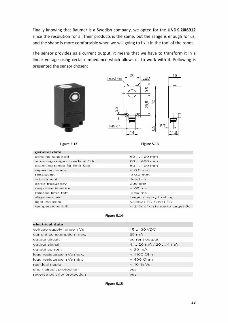
Finally knowing that Baumer is a Swedish company, we opted for the UNDK 20I6912

since the resolution for all their products is the same, but the range is enough for us,

and the shape is more comfortable when we will going to fix it in the tool of the robot.

The sensor provides us a current output, it means that we have to transform it in a

linear voltage using certain impedance which allows us to work with it. Following is

presented the sensor chosen:

Figure 5.12 Figure 5.13

Figure 5.14

Figure 5.15

29

5.2.3 Design Considerations

Our principal restriction in this case is not to have an error bigger than one millimeter,

taking in to account that we have the resolution error of 0.3 mm, when we think how

to send to the computer any data which indicates us the distance measured, we have

to not to commit an error bigger than 0.7 mm.

The current signal given by our sensor will be transform in to a voltage signal, and this

one, should be sent somehow to the computer, which should be able to understand a

code sent with the protocol chosen. To send the value of the voltage signal, firstly

should be digitalized, later codified and then send to the computer using the most

suitable method found.

For this task we can solve the problem using many ways, but probably for future users,

we are going to consider the easiest method, the one which allows us to solve all these

steps of the treatment of the signal given by our sensor.

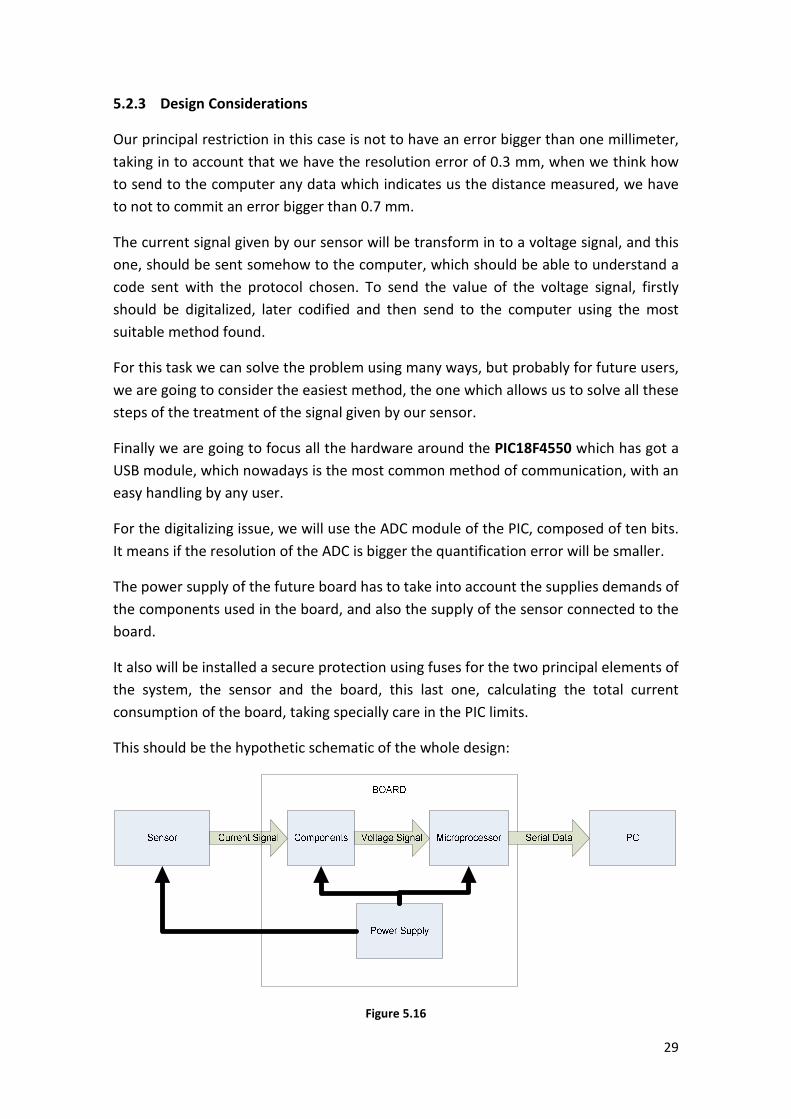
Finally we are going to focus all the hardware around the PIC18F4550 which has got a

USB module, which nowadays is the most common method of communication, with an

easy handling by any user.

For the digitalizing issue, we will use the ADC module of the PIC, composed of ten bits.

It means if the resolution of the ADC is bigger the quantification error will be smaller.

The power supply of the future board has to take into account the supplies demands of

the components used in the board, and also the supply of the sensor connected to the

board.

It also will be installed a secure protection using fuses for the two principal elements of

the system, the sensor and the board, this last one, calculating the total current

consumption of the board, taking specially care in the PIC limits.

This should be the hypothetic schematic of the whole design:

Figure 5.16

30

5.2.4 Design Tools

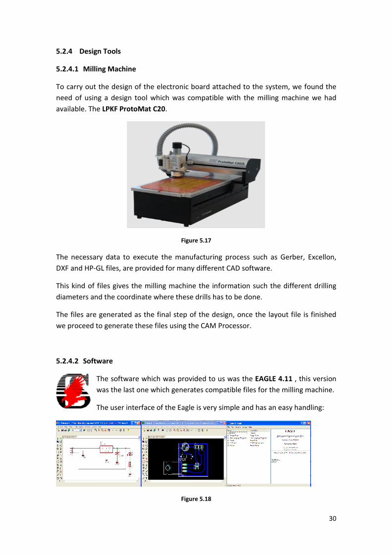
5.2.4.1 Milling Machine

To carry out the design of the electronic board attached to the system, we found the

need of using a design tool which was compatible with the milling machine we had

available. The LPKF ProtoMat C20.

Figure 5.17

The necessary data to execute the manufacturing process such as Gerber, Excellon,

DXF and HP-GL files, are provided for many different CAD software.

This kind of files gives the milling machine the information such the different drilling

diameters and the coordinate where these drills has to be done.

The files are generated as the final step of the design, once the layout file is finished

we proceed to generate these files using the CAM Processor.

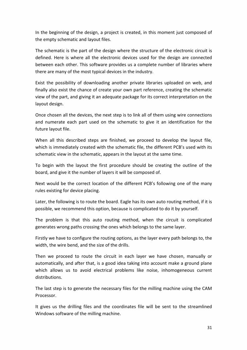
5.2.4.2 Software

The software which was provided to us was the EAGLE 4.11 , this version

was the last one which generates compatible files for the milling machine.

The user interface of the Eagle is very simple and has an easy handling:

Figure 5.18

31

In the beginning of the design, a project is created, in this moment just composed of

the empty schematic and layout files.

The schematic is the part of the design where the structure of the electronic circuit is

defined. Here is where all the electronic devices used for the design are connected

between each other. This software provides us a complete number of libraries where

there are many of the most typical devices in the industry.

Exist the possibility of downloading another private libraries uploaded on web, and

finally also exist the chance of create your own part reference, creating the schematic

view of the part, and giving it an adequate package for its correct interpretation on the

layout design.

Once chosen all the devices, the next step is to link all of them using wire connections

and numerate each part used on the schematic to give it an identification for the

future layout file.

When all this described steps are finished, we proceed to develop the layout file,

which is immediately created with the schematic file, the different PCB’s used with its

schematic view in the schematic, appears in the layout at the same time.

To begin with the layout the first procedure should be creating the outline of the

board, and give it the number of layers it will be composed of.

Next would be the correct location of the different PCB’s following one of the many

rules existing for device placing.

Later, the following is to route the board. Eagle has its own auto routing method, if it is

possible, we recommend this option, because is complicated to do it by yourself.

The problem is that this auto routing method, when the circuit is complicated

generates wrong paths crossing the ones which belongs to the same layer.

Firstly we have to configure the routing options, as the layer every path belongs to, the

width, the wire bend, and the size of the drills.

Then we proceed to route the circuit in each layer we have chosen, manually or

automatically, and after that, is a good idea taking into account make a ground plane

which allows us to avoid electrical problems like noise, inhomogeneous current

distributions.

The last step is to generate the necessary files for the milling machine using the CAM

Processor.

It gives us the drilling files and the coordinates file will be sent to the streamlined

Windows software of the milling machine.

32

5.2.5 Circuit Design

5.2.5.1 Conditioning Stage

To process the current signal into the most adequate voltage signal to be digitalized by

the ADC of the PIC, we make use of a high quality resistor with a ±1% tolerance.

The idea to transform the 4 – 20 mA into a voltage signal is simple. We will make all

the current go through the resistor to ground, and isolate the voltage drop using a

follower. Using a resistor of 250 Ω we will obtain a voltage signal between 1 – 5 V. For

this task we will use a LMC662C CMOS operational amplifier which has special

precision for current-to-voltage converting.

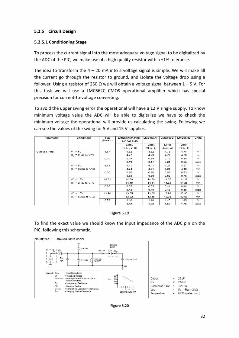
To avoid the upper swing error the operational will have a 12 V single supply. To know

minimum voltage value the ADC will be able to digitalize we have to check the

minimum voltage the operational will provide us calculating the swing. Following we

can see the values of the swing for 5 V and 15 V supplies.

Figure 5.19

To find the exact value we should know the input impedance of the ADC pin on the

PIC, following this schematic.

Figure 5.20

33

Being the signal to digitalize stable, we can assume the input impedance in the range

[2 , 3] kΩ. Our worst case would be a 2 kΩ impedance, and assuming a linear variation

of the swing depending of the supply our values for 12 V single supply are:

Conditions: V+ = 12V; RL = 2 kΩ

≤ VOUT ≤ 0’324 ≤ VOUT ≤ 11’472 V

In that way we can assure a signal between 1 and 5 V will be digitalized without any problem.

The circuit design would be:

Figure 5.21

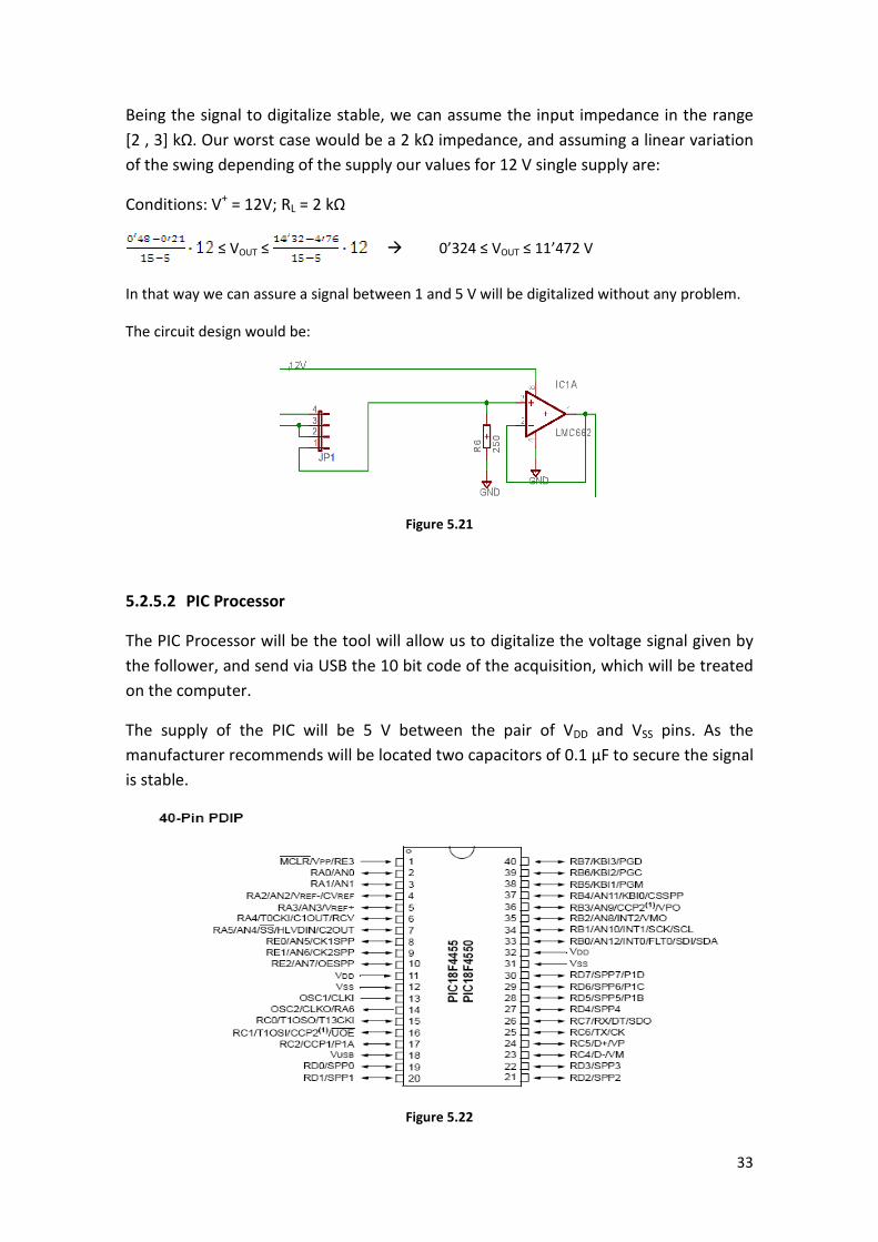
5.2.5.2 PIC Processor

The PIC Processor will be the tool will allow us to digitalize the voltage signal given by

the follower, and send via USB the 10 bit code of the acquisition, which will be treated

on the computer.

The supply of the PIC will be 5 V between the pair of VDD and VSS pins. As the

manufacturer recommends will be located two capacitors of 0.1 μF to secure the signal

is stable.

Figure 5.22

34

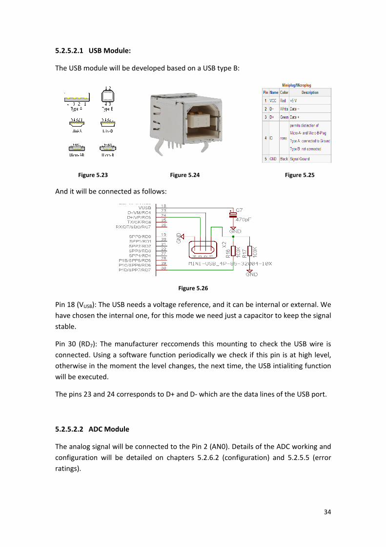
5.2.5.2.1 USB Module:

The USB module will be developed based on a USB type B:

Figure 5.23 Figure 5.24 Figure 5.25

And it will be connected as follows:

Figure 5.26

Pin 18 (VUSB): The USB needs a voltage reference, and it can be internal or external. We

have chosen the internal one, for this mode we need just a capacitor to keep the signal

stable.

Pin 30 (RD7): The manufacturer reccomends this mounting to check the USB wire is

connected. Using a software function periodically we check if this pin is at high level,

otherwise in the moment the level changes, the next time, the USB intialiting function

will be executed.

The pins 23 and 24 corresponds to D+ and D- which are the data lines of the USB port.

5.2.5.2.2 ADC Module

The analog signal will be connected to the Pin 2 (AN0). Details of the ADC working and

configuration will be detailed on chapters 5.2.6.2 (configuration) and 5.2.5.5 (error

ratings).

35

5.2.5.2.3 External Crystal Resonator

The circuit designed is a crystal resonator, the capacitors are used to increase the

stability of the oscillator, and the shunt impedance is used to slightly reduce the input

current. Both pins of the crystal will be connected to OSC1 and OSC2 (Pins 13 and 14).

Figure 5.27

5.2.5.2.4 State Led’s

These led’s are mounted for test settings and state notifications. They are handled by

the port B.

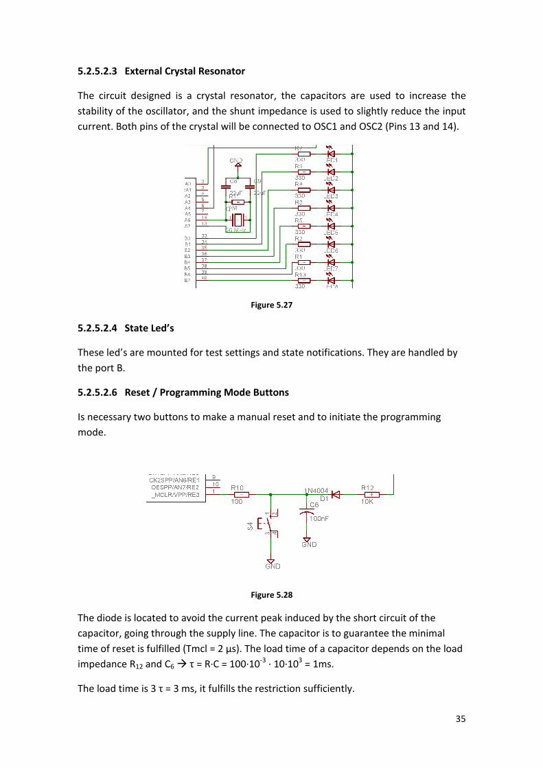
5.2.5.2.6 Reset / Programming Mode Buttons

Is necessary two buttons to make a manual reset and to initiate the programming

mode.

Figure 5.28

The diode is located to avoid the current peak induced by the short circuit of the

capacitor, going through the supply line. The capacitor is to guarantee the minimal

time of reset is fulfilled (Tmcl = 2 μs). The load time of a capacitor depends on the load

impedance R12 and C6 τ = R·C = 100·10-3

· 10·103 = 1ms.

The load time is 3 τ = 3 ms, it fulfills the restriction sufficiently.

36

5.2.5.3 Power Supply

To start with the design of the power supply we should think about the demands of

the devices we are going to supply.

As the mentioned in the previous chapters, the devices to supply are mostly the

PIC18F4550, the LMC662, the Baumer sensor and the led’s.

For the PIC is necessary a 5 V supply, that can be also used for the led’s. We are going

to supply the Baumer with 24 V due to it is the highest voltage model of regulator we

have available, and it adapts to the transformer we have got. For the operational

amplifier LMC662C it is necessary 12 V, because it is also one of the regulator models

we have available.

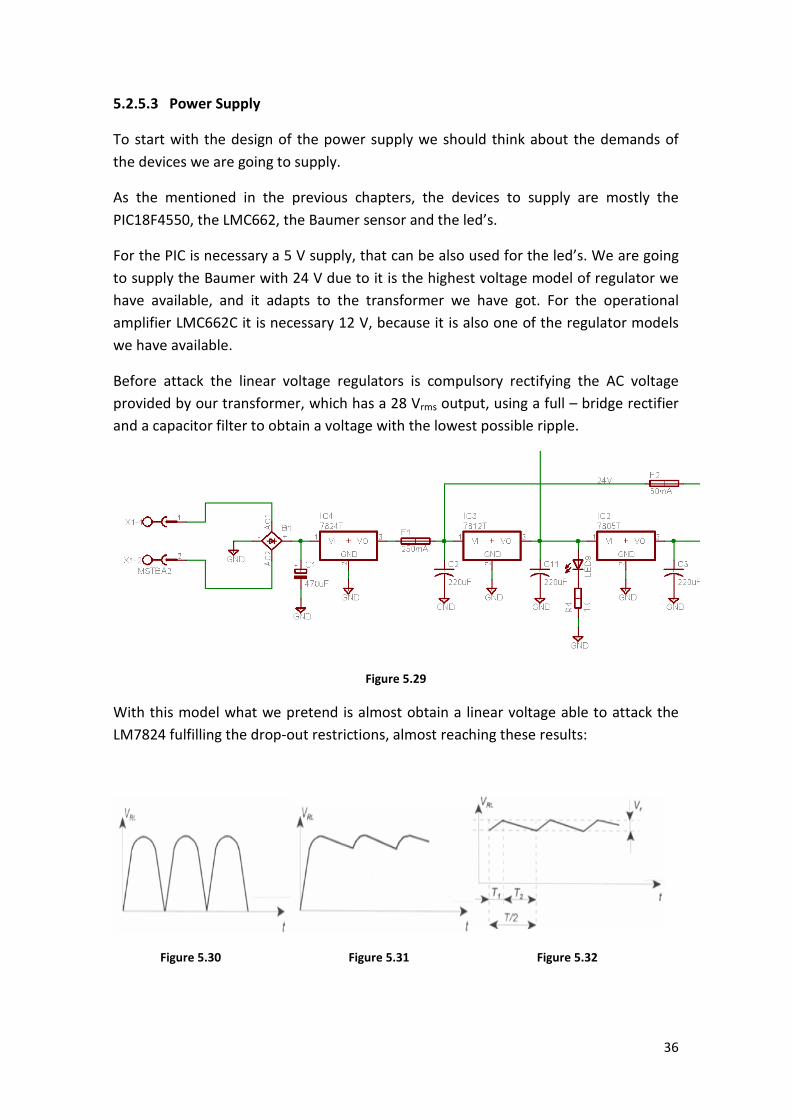
Before attack the linear voltage regulators is compulsory rectifying the AC voltage

provided by our transformer, which has a 28 Vrms output, using a full – bridge rectifier

and a capacitor filter to obtain a voltage with the lowest possible ripple.

Figure 5.29

With this model what we pretend is almost obtain a linear voltage able to attack the

LM7824 fulfilling the drop-out restrictions, almost reaching these results:

Figure 5.30 Figure 5.31 Figure 5.32

37

The Figure 5.30 belongs the signal after the full – bridge, and the Figure 5.31 is the

actual signal form after filtering. The Figure 5.32 is a linear approximation of the

filtered signal to calculate exactly the ripple.

Paying attention to the electrical characteristics of the LM7824 we can observe the

minimum drop-out voltage is VDROP = 2 V

So, in the LM7824 VinMIN = 24+2 V = 26 V

In the rectifier:

Figure 5.33 Figure 5.34

In the technical data of the rectifier we check VF= 1 V = 2·Vγ, it refers to the voltage

drop in the two diodes where the current goes through.

It indicates us the minimum value of the peak to peak voltage ripple which allows the

correct working of the regulator. So:

VrppMAX = VT(peak) – VF – VinMIN = 37 – 1 – 26 = 10 V Vrpp =

Where Ioc is the current through the LM7824, it is, the total current consumption of the

circuit.

Now we proceed to calculate the total consumption of current step by step:

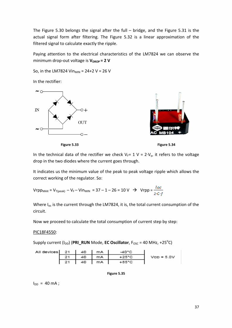
PIC18F4550:

Supply current (IDD) (PRI_RUN Mode, EC Oscillator, FOSC = 40 MHz, +25oC)

Figure 5.35

IDD = 40 mA ;

38

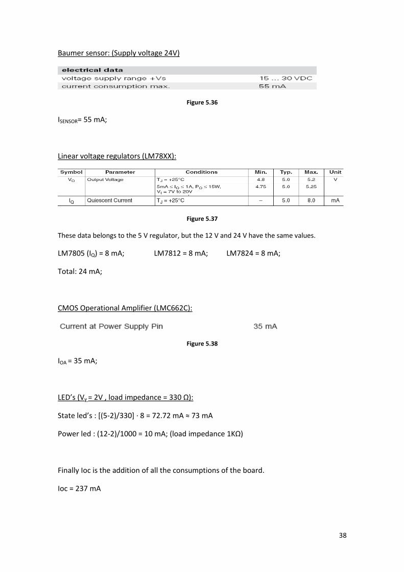
Baumer sensor: (Supply voltage 24V)

Figure 5.36

ISENSOR= 55 mA;

Linear voltage regulators (LM78XX):

Figure 5.37

These data belongs to the 5 V regulator, but the 12 V and 24 V have the same values.

LM7805 (IQ) = 8 mA; LM7812 = 8 mA; LM7824 = 8 mA;

Total: 24 mA;

CMOS Operational Amplifier (LMC662C):

Figure 5.38

IOA = 35 mA;

LED’s (Vγ = 2V , load impedance = 330 Ω):

State led’s : [(5-2)/330] · 8 = 72.72 mA ≈ 73 mA

Power led : (12-2)/1000 = 10 mA; (load impedance 1KΩ)

Finally Ioc is the addition of all the consumptions of the board.

Ioc = 237 mA

39

With this data now we are able to calculate the minimal capacitor necessary to avoid

the ripple (f = 50 Hz):

CMIN = = 237 μF

Taking into account the consumption of the PIC is calculated for a 40 MHz oscillator

instead of our oscillator of 20 MHz and at full performance we will mount a 470 μF.

The rest of the capacitors in the output of the regulators (220 μF) are the typical value

recommended by the manufacturer to keep the output stable.

5.2.5.4 Protections

To safe the normal operating we must protect the board firstly and also the sensor

separately to possible current risings. For this task we will use common fuses for

electronic application.

Figure 5.39

F1 = IOC = 237 mA 250 mA;

F2 = ISENSOR = 55 mA 60 mA;

40

5.2.7 Absolute Error Ratings

The elements that cause a possible error in the measurement are the following:

• Sensor: It has a maximum value of 0.3 mm

• Shielded Twisted Pair: It has an impedance of 150 Ω/Km. It is a fixed error that

will be compensated with the software calibration.

• Current-to-voltage Impedance: It has a maximum tolerance value of 1%. It

means:

ΔRMAX = 2’5 Ω ΔVMAX = ΔRMAX·20 mA = 0.05

Now calculating the gain (mm/V) G = = = 85

ΔdMAX = 4.25 mm

This is a fixed gain error, which will be compensated with the software

calibration.

• Operational amplifier: It subtract a certain amount of current due to the input

current bias error, in this case is 2 pA, we can ignore it. It also introduces an

offset error of voltage of 6 mV which is fixed, so we can reject it.

• ADC module: During the quantification process the ADC separates a small

interval of values that can be codified with the same code. It is called

quantification interval (q).

The maximum error committed will be always q/2

q = = = 0.0039 q/2 = 0.001953 V

Knowing the gain is 85 mm/V the maximum error committed will be:

EADC = 85·0.001953 = 0.166 mm

41

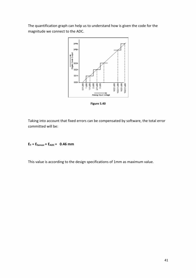
The quantification graph can help us to understand how is given the code for the

magnitude we connect to the ADC.

Figure 5.40

Taking into account that fixed errors can be compensated by software, the total error

committed will be:

ET = ESensor + EADC = 0.46 mm

This value is according to the design specifications of 1mm as maximum value.

42

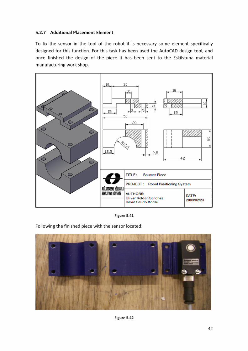
5.2.7 Additional Placement Element

To fix the sensor in the tool of the robot it is necessary some element specifically

designed for this function. For this task has been used the AutoCAD design tool, and

once finished the design of the piece it has been sent to the Eskilstuna material

manufacturing work shop.

Figure 5.41

Following the finished piece with the sensor located:

Figure 5.42

43

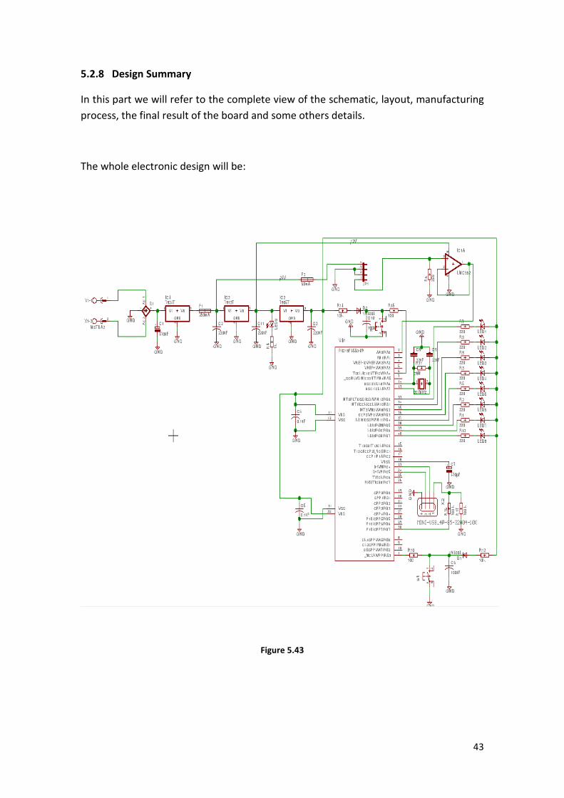
5.2.8 Design Summary

In this part we will refer to the complete view of the schematic, layout, manufacturing

process, the final result of the board and some others details.

The whole electronic design will be:

Figure 5.43

44

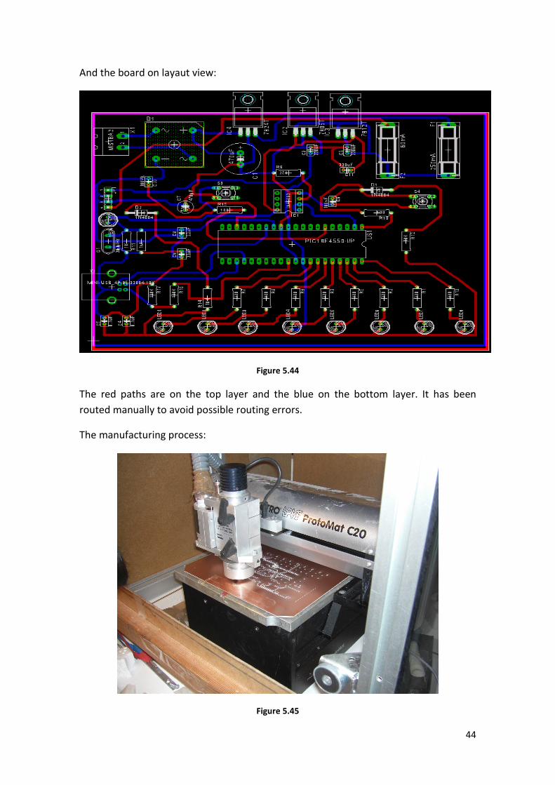
And the board on layaut view:

Figure 5.44

The red paths are on the top layer and the blue on the bottom layer. It has been

routed manually to avoid possible routing errors.

The manufacturing process:

Figure 5.45

45

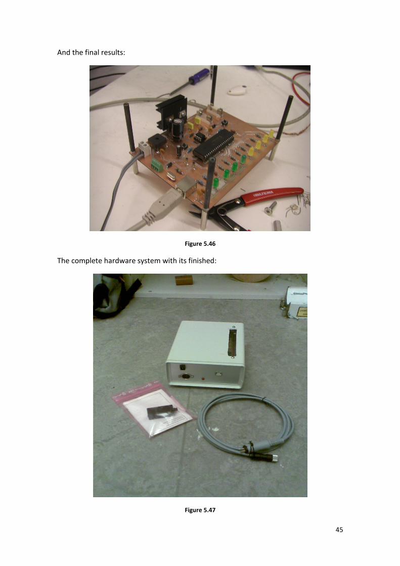
And the final results:

Figure 5.46

The complete hardware system with its finished:

Figure 5.47

46

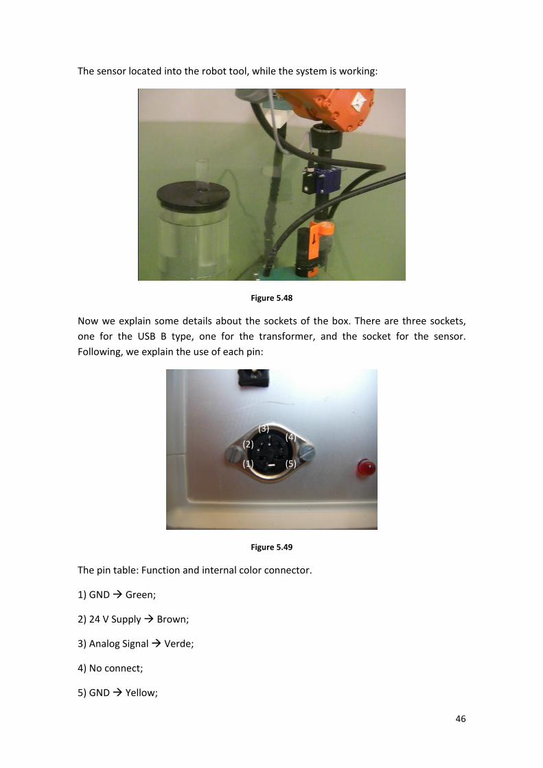
The sensor located into the robot tool, while the system is working:

Figure 5.48

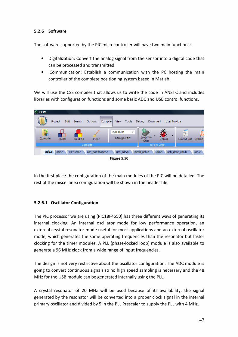
Now we explain some details about the sockets of the box. There are three sockets,

one for the USB B type, one for the transformer, and the socket for the sensor.

Following, we explain the use of each pin:

Figure 5.49

The pin table: Function and internal color connector.

1) GND Green;

2) 24 V Supply Brown;

3) Analog Signal Verde;

4) No connect;

5) GND Yellow;

(1)

(4)

(5)

(2)

(3)

47

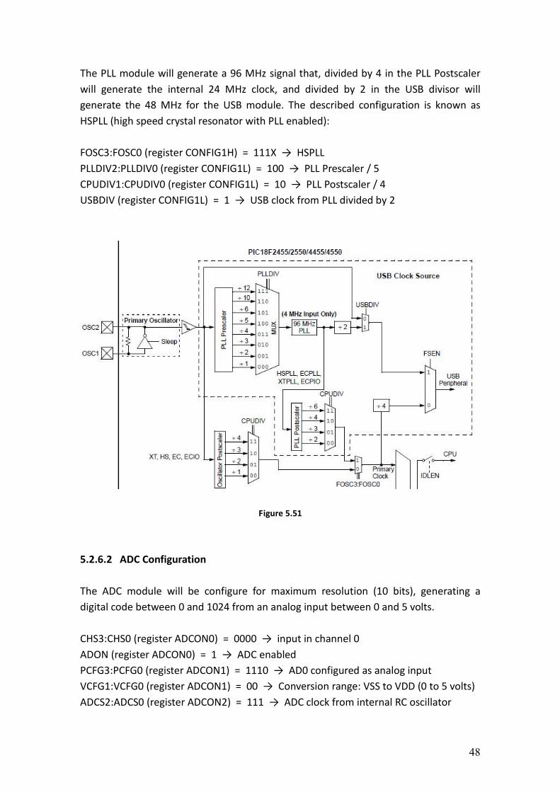
5.2.6 Software

The software supported by the PIC microcontroller will have two main functions:

• Digitalization: Convert the analog signal from the sensor into a digital code that

can be processed and transmitted.

• Communication: Establish a communication with the PC hosting the main

controller of the complete positioning system based in Matlab.

We will use the CSS compiler that allows us to write the code in ANSI C and includes

libraries with configuration functions and some basic ADC and USB control functions.

Figure 5.50

In the first place the configuration of the main modules of the PIC will be detailed. The

rest of the miscellanea configuration will be shown in the header file.

5.2.6.1 Oscillator Configuration

The PIC processor we are using (PIC18F4550) has three different ways of generating its

internal clocking. An internal oscillator mode for low performance operation, an

external crystal resonator mode useful for most applications and an external oscillator

mode, which generates the same operating frequencies than the resonator but faster

clocking for the timer modules. A PLL (phase-locked loop) module is also available to

generate a 96 MHz clock from a wide range of input frequencies.

The design is not very restrictive about the oscillator configuration. The ADC module is

going to convert continuous signals so no high speed sampling is necessary and the 48

MHz for the USB module can be generated internally using the PLL.

A crystal resonator of 20 MHz will be used because of its availability; the signal

generated by the resonator will be converted into a proper clock signal in the internal

primary oscillator and divided by 5 in the PLL Prescaler to supply the PLL with 4 MHz.

48

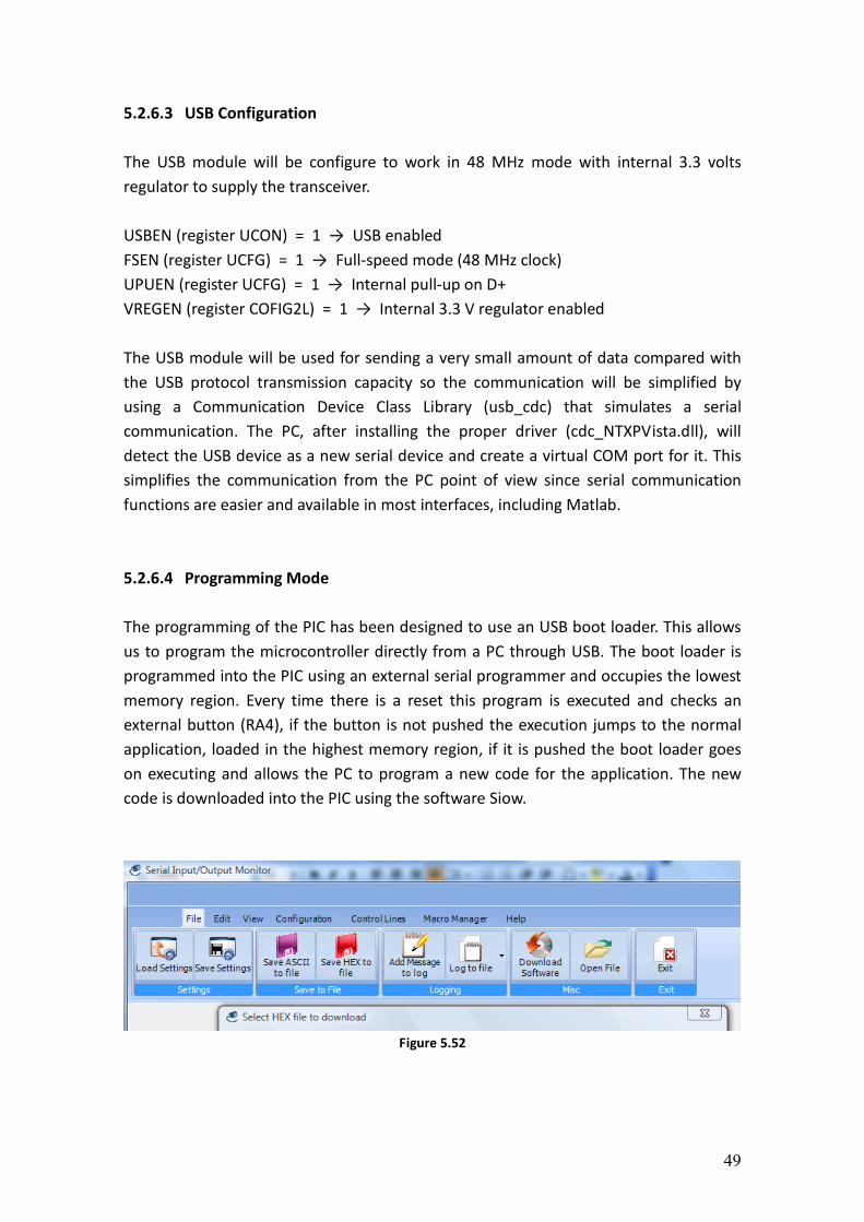
The PLL module will generate a 96 MHz signal that, divided by 4 in the PLL Postscaler

will generate the internal 24 MHz clock, and divided by 2 in the USB divisor will

generate the 48 MHz for the USB module. The described configuration is known as

HSPLL (high speed crystal resonator with PLL enabled):

FOSC3:FOSC0 (register CONFIG1H) = 111X → HSPLL

PLLDIV2:PLLDIV0 (register CONFIG1L) = 100 → PLL Prescaler / 5

CPUDIV1:CPUDIV0 (register CONFIG1L) = 10 → PLL Postscaler / 4

USBDIV (register CONFIG1L) = 1 → USB clock from PLL divided by 2

Figure 5.51

5.2.6.2 ADC Configuration

The ADC module will be configure for maximum resolution (10 bits), generating a

digital code between 0 and 1024 from an analog input between 0 and 5 volts.

CHS3:CHS0 (register ADCON0) = 0000 → input in channel 0

ADON (register ADCON0) = 1 → ADC enabled

PCFG3:PCFG0 (register ADCON1) = 1110 → AD0 configured as analog input

VCFG1:VCFG0 (register ADCON1) = 00 → Conversion range: VSS to VDD (0 to 5 volts)

ADCS2:ADCS0 (register ADCON2) = 111 → ADC clock from internal RC oscillator

49

5.2.6.3 USB Configuration

The USB module will be configure to work in 48 MHz mode with internal 3.3 volts

regulator to supply the transceiver.

USBEN (register UCON) = 1 → USB enabled

FSEN (register UCFG) = 1 → Full-speed mode (48 MHz clock)

UPUEN (register UCFG) = 1 → Internal pull-up on D+

VREGEN (register COFIG2L) = 1 → Internal 3.3 V regulator enabled

The USB module will be used for sending a very small amount of data compared with

the USB protocol transmission capacity so the communication will be simplified by

using a Communication Device Class Library (usb_cdc) that simulates a serial

communication. The PC, after installing the proper driver (cdc_NTXPVista.dll), will

detect the USB device as a new serial device and create a virtual COM port for it. This

simplifies the communication from the PC point of view since serial communication

functions are easier and available in most interfaces, including Matlab.

5.2.6.4 Programming Mode

The programming of the PIC has been designed to use an USB boot loader. This allows

us to program the microcontroller directly from a PC through USB. The boot loader is

programmed into the PIC using an external serial programmer and occupies the lowest

memory region. Every time there is a reset this program is executed and checks an

external button (RA4), if the button is not pushed the execution jumps to the normal

application, loaded in the highest memory region, if it is pushed the boot loader goes

on executing and allows the PC to program a new code for the application. The new

code is downloaded into the PIC using the software Siow.

Figure 5.52

50

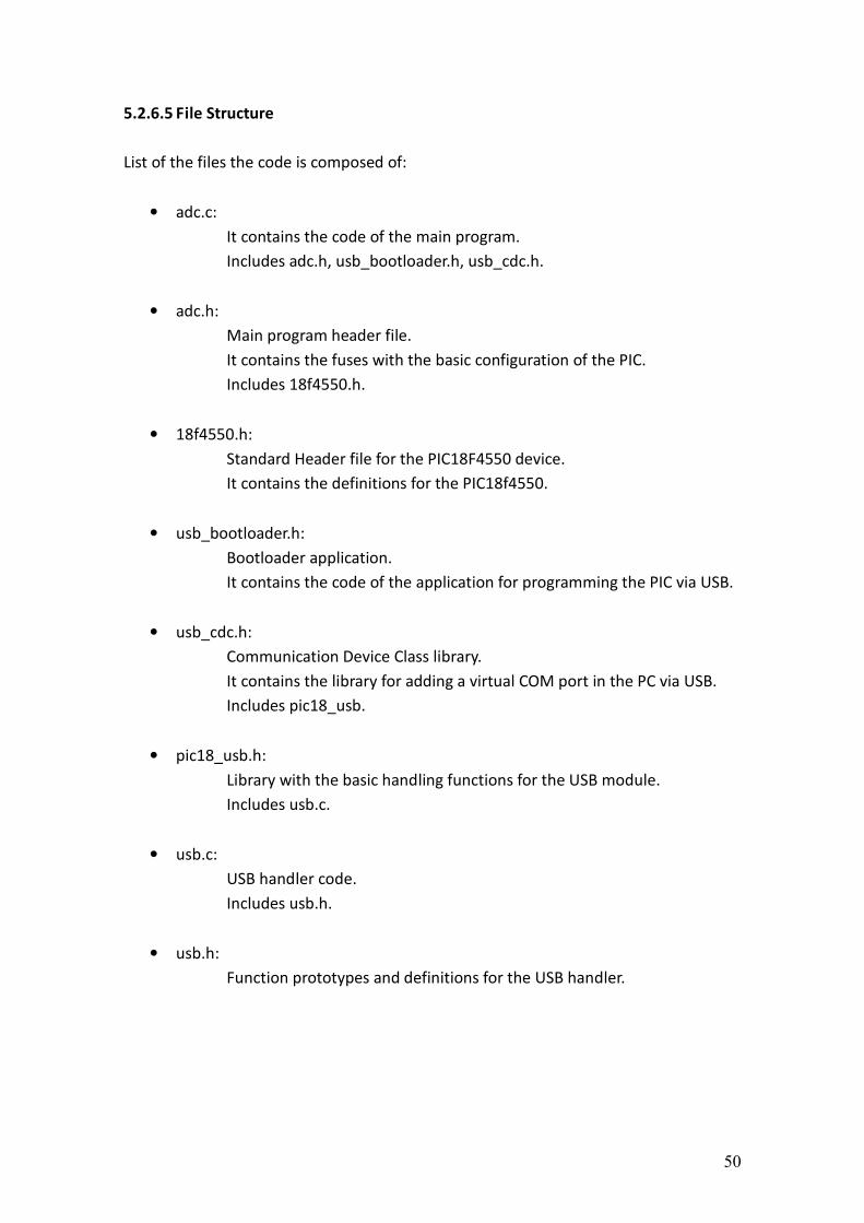
5.2.6.5 File Structure

List of the files the code is composed of:

• adc.c:

It contains the code of the main program.

Includes adc.h, usb_bootloader.h, usb_cdc.h.

• adc.h:

Main program header file.

It contains the fuses with the basic configuration of the PIC.

Includes 18f4550.h.

• 18f4550.h:

Standard Header file for the PIC18F4550 device.

It contains the definitions for the PIC18f4550.

• usb_bootloader.h:

Bootloader application.

It contains the code of the application for programming the PIC via USB.

• usb_cdc.h:

Communication Device Class library.

It contains the library for adding a virtual COM port in the PC via USB.

Includes pic18_usb.

• pic18_usb.h:

Library with the basic handling functions for the USB module.

Includes usb.c.

• usb.c:

USB handler code.

Includes usb.h.

• usb.h:

Function prototypes and definitions for the USB handler.

51

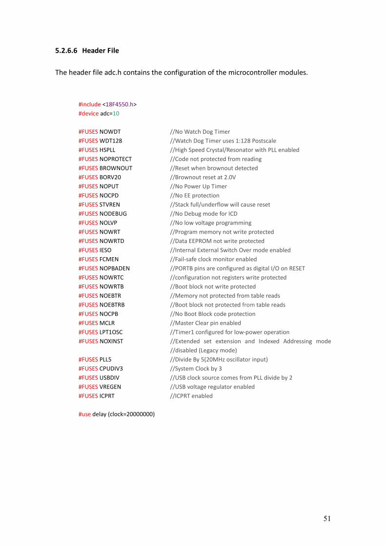
5.2.6.6 Header File

The header file adc.h contains the configuration of the microcontroller modules.

#include <18F4550.h>

#device adc=10

#FUSES NOWDT //No Watch Dog Timer

#FUSES WDT128 //Watch Dog Timer uses 1:128 Postscale

#FUSES HSPLL //High Speed Crystal/Resonator with PLL enabled

#FUSES NOPROTECT //Code not protected from reading

#FUSES BROWNOUT //Reset when brownout detected

#FUSES BORV20 //Brownout reset at 2.0V

#FUSES NOPUT //No Power Up Timer

#FUSES NOCPD //No EE protection

#FUSES STVREN //Stack full/underflow will cause reset

#FUSES NODEBUG //No Debug mode for ICD

#FUSES NOLVP //No low voltage programming

#FUSES NOWRT //Program memory not write protected

#FUSES NOWRTD //Data EEPROM not write protected

#FUSES IESO //Internal External Switch Over mode enabled

#FUSES FCMEN //Fail-safe clock monitor enabled

#FUSES NOPBADEN //PORTB pins are configured as digital I/O on RESET

#FUSES NOWRTC //configuration not registers write protected

#FUSES NOWRTB //Boot block not write protected

#FUSES NOEBTR //Memory not protected from table reads

#FUSES NOEBTRB //Boot block not protected from table reads

#FUSES NOCPB //No Boot Block code protection

#FUSES MCLR //Master Clear pin enabled

#FUSES LPT1OSC //Timer1 configured for low-power operation

#FUSES NOXINST //Extended set extension and Indexed Addressing mode

//disabled (Legacy mode)

#FUSES PLL5 //Divide By 5(20MHz oscillator input)

#FUSES CPUDIV3 //System Clock by 3

#FUSES USBDIV //USB clock source comes from PLL divide by 2

#FUSES VREGEN //USB voltage regulator enabled

#FUSES ICPRT //ICPRT enabled

#use delay (clock=20000000)

52

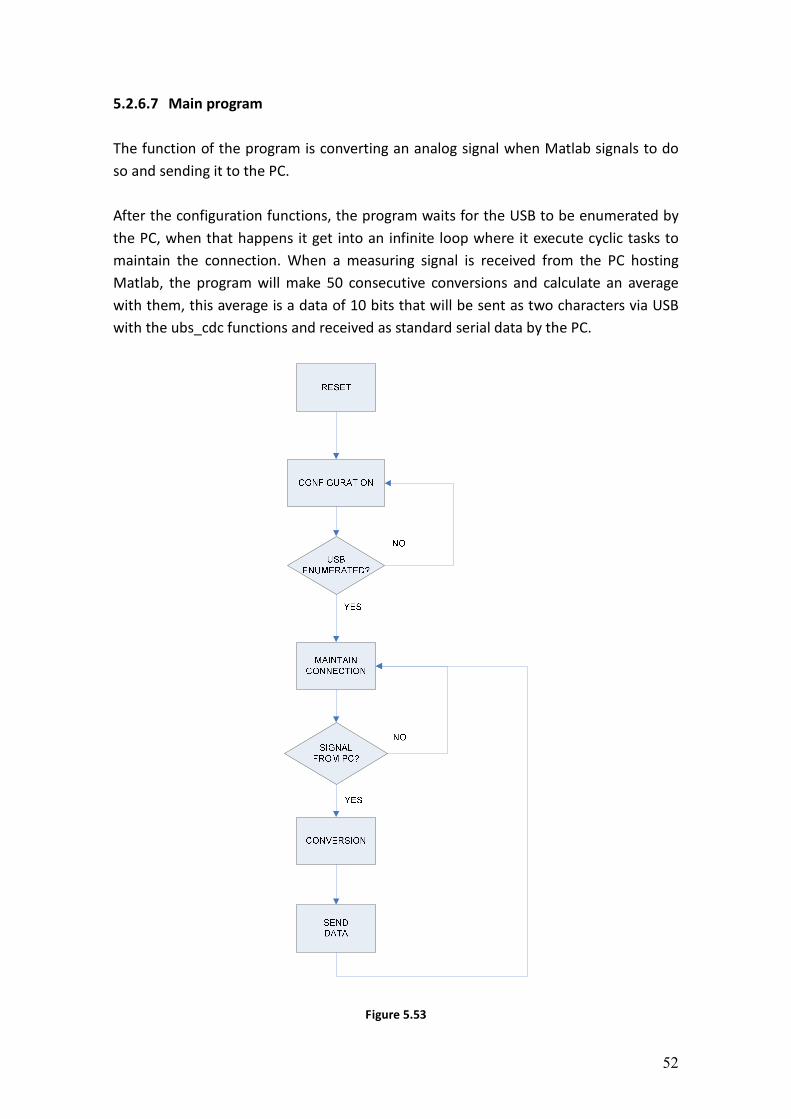
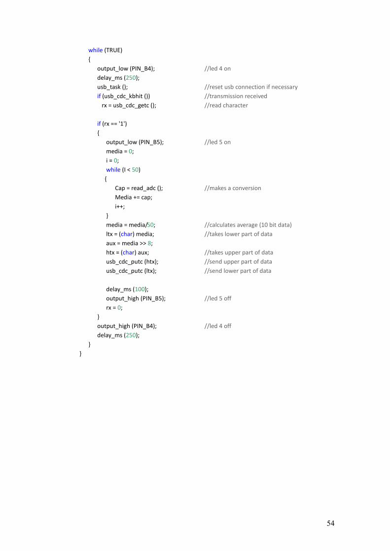
5.2.6.7 Main program

The function of the program is converting an analog signal when Matlab signals to do

so and sending it to the PC.

After the configuration functions, the program waits for the USB to be enumerated by

the PC, when that happens it get into an infinite loop where it execute cyclic tasks to

maintain the connection. When a measuring signal is received from the PC hosting

Matlab, the program will make 50 consecutive conversions and calculate an average

with them, this average is a data of 10 bits that will be sent as two characters via USB

with the ubs_cdc functions and received as standard serial data by the PC.

Figure 5.53

53

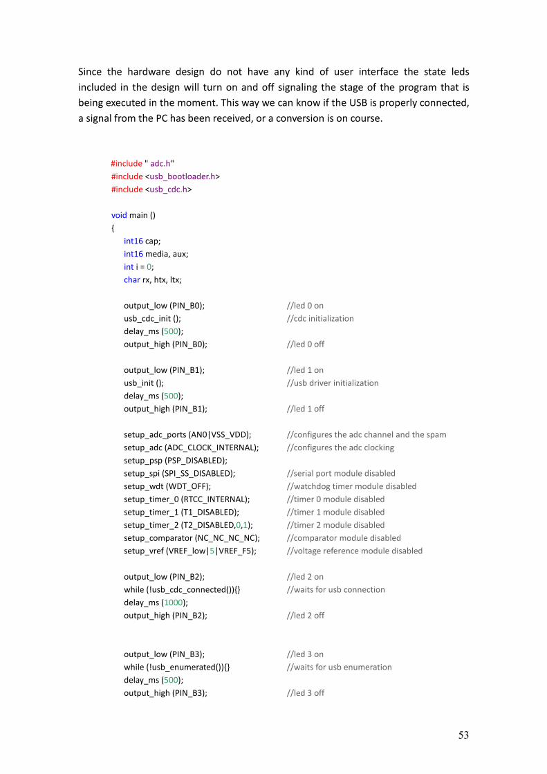
Since the hardware design do not have any kind of user interface the state leds

included in the design will turn on and off signaling the stage of the program that is

being executed in the moment. This way we can know if the USB is properly connected,

a signal from the PC has been received, or a conversion is on course.

#include " adc.h"

#include <usb_bootloader.h>

#include <usb_cdc.h>

void main ()

int16 cap;

int16 media, aux;

int i = 0;

char rx, htx, ltx;

output_low (PIN_B0); //led 0 on

usb_cdc_init (); //cdc initialization

delay_ms (500);

output_high (PIN_B0); //led 0 off


usb_init (); //usb driver initialization

delay_ms (500);


setup_adc_ports (AN0|VSS_VDD); //configures the adc channel and the spam

setup_adc (ADC_CLOCK_INTERNAL); //configures the adc clocking

setup_psp (PSP_DISABLED);

setup_spi (SPI_SS_DISABLED); //serial port module disabled

setup_wdt (WDT_OFF); //watchdog timer module disabled

setup_timer_0 (RTCC_INTERNAL); //timer 0 module disabled

setup_timer_1 (T1_DISABLED); //timer 1 module disabled

setup_timer_2 (T2_DISABLED,0,1); //timer 2 module disabled

setup_comparator (NC_NC_NC_NC); //comparator module disabled

setup_vref (VREF_low|5|VREF_F5); //voltage reference module disabled


while (!usb_cdc_connected()) //waits for usb connection

delay_ms (1000);



while (!usb_enumerated()) //waits for usb enumeration

delay_ms (500);


54

while (TRUE)


delay_ms (250);

usb_task (); //reset usb connection if necessary

if (usb_cdc_kbhit ()) //transmission received

rx = usb_cdc_getc (); //read character

if (rx == '1')


media = 0;

i = 0;

while (I < 50)

Cap = read_adc (); //makes a conversion

Media += cap;

i++;

media = media/50; //calculates average (10 bit data)

ltx = (char) media; //takes lower part of data

aux = media >> 8;

htx = (char) aux; //takes upper part of data

usb_cdc_putc (htx); //send upper part of data

usb_cdc_putc (ltx); //send lower part of data

delay_ms (100);


rx = 0;


delay_ms (250);

55

5.3 Water Measurement System

5.3.1 Introduction

As mentioned before, our intention is to develop a short distance underwater sensor.

The results obtained will be shown in the point 6, together with the conclusion of the

research, and the possible proposed improves.

The structure of the guide will be the same as the air measurement in the hardware

design point of view.

The ideas followed to develop the hardware have been explained on the point 4.4,

anyway every step we have followed will be presented with accuracy.

Due to now, we are going to design a whole sensor, the first step will be to choose the

ultrasonic transducer.

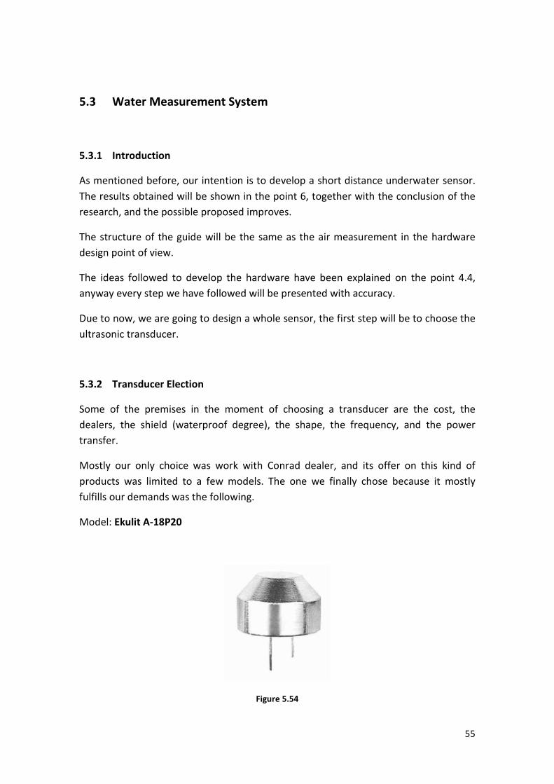
5.3.2 Transducer Election

Some of the premises in the moment of choosing a transducer are the cost, the

dealers, the shield (waterproof degree), the shape, the frequency, and the power

transfer.

Mostly our only choice was work with Conrad dealer, and its offer on this kind of

products was limited to a few models. The one we finally chose because it mostly

fulfills our demands was the following.

Model: Ekulit A-18P20

Figure 5.54

56

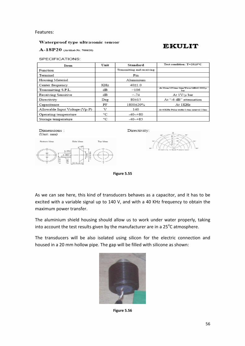
Features:

Figure 5.55

As we can see here, this kind of transducers behaves as a capacitor, and it has to be

excited with a variable signal up to 140 V, and with a 40 KHz frequency to obtain the

maximum power transfer.

The aluminium shield housing should allow us to work under water properly, taking

into account the test results given by the manufacturer are in a 25oC atmosphere.

The transducers will be also isolated using silicon for the electric connection and

housed in a 20 mm hollow pipe. The gap will be filled with silicone as shown:

Figure 5.56

57

5.3.3 Design Considerations

The main idea is to develop a system using a pair of transducers to try to make the

system as fast as possible avoiding the switch between the emitter and receiver

function. Both transducers will be connected though a long shielded twisted pair wire,

to achieve the Faraday Cage effect to isolate the signal from intense electrical fields

such as the physical robot controller that will be close to our system. It also

recommended using a metallic box to safe the electronic board for the same reason.

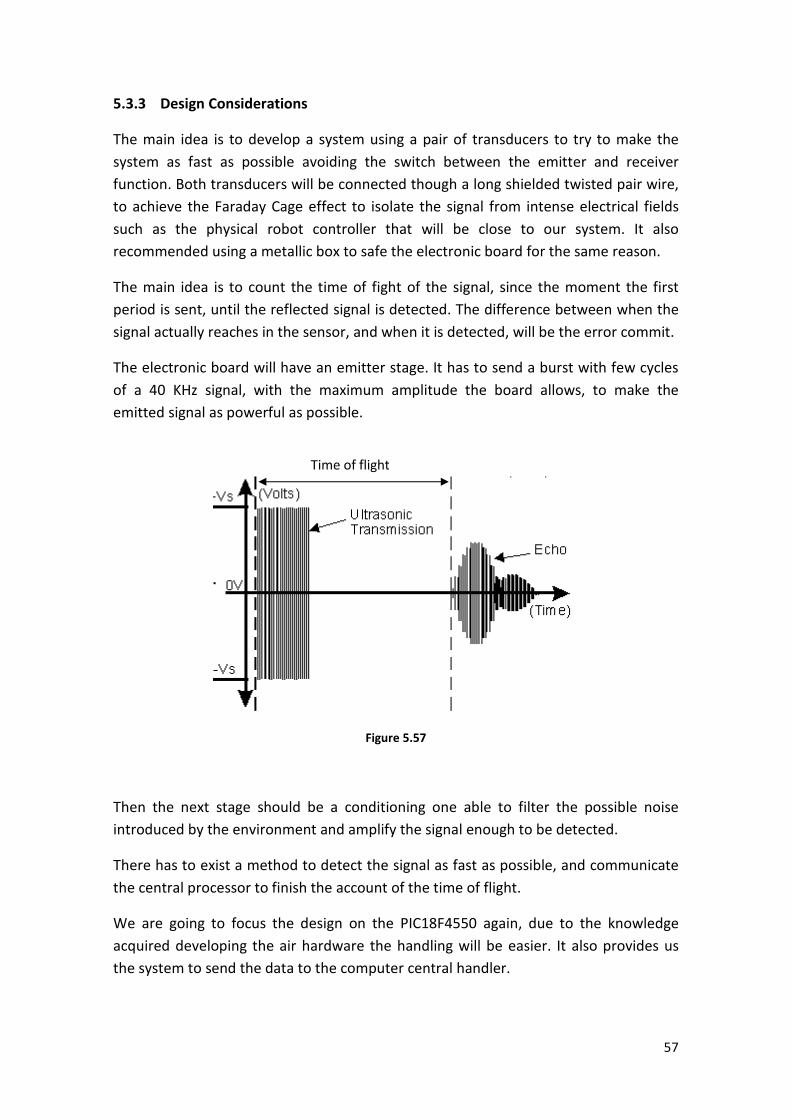
The main idea is to count the time of fight of the signal, since the moment the first

period is sent, until the reflected signal is detected. The difference between when the

signal actually reaches in the sensor, and when it is detected, will be the error commit.

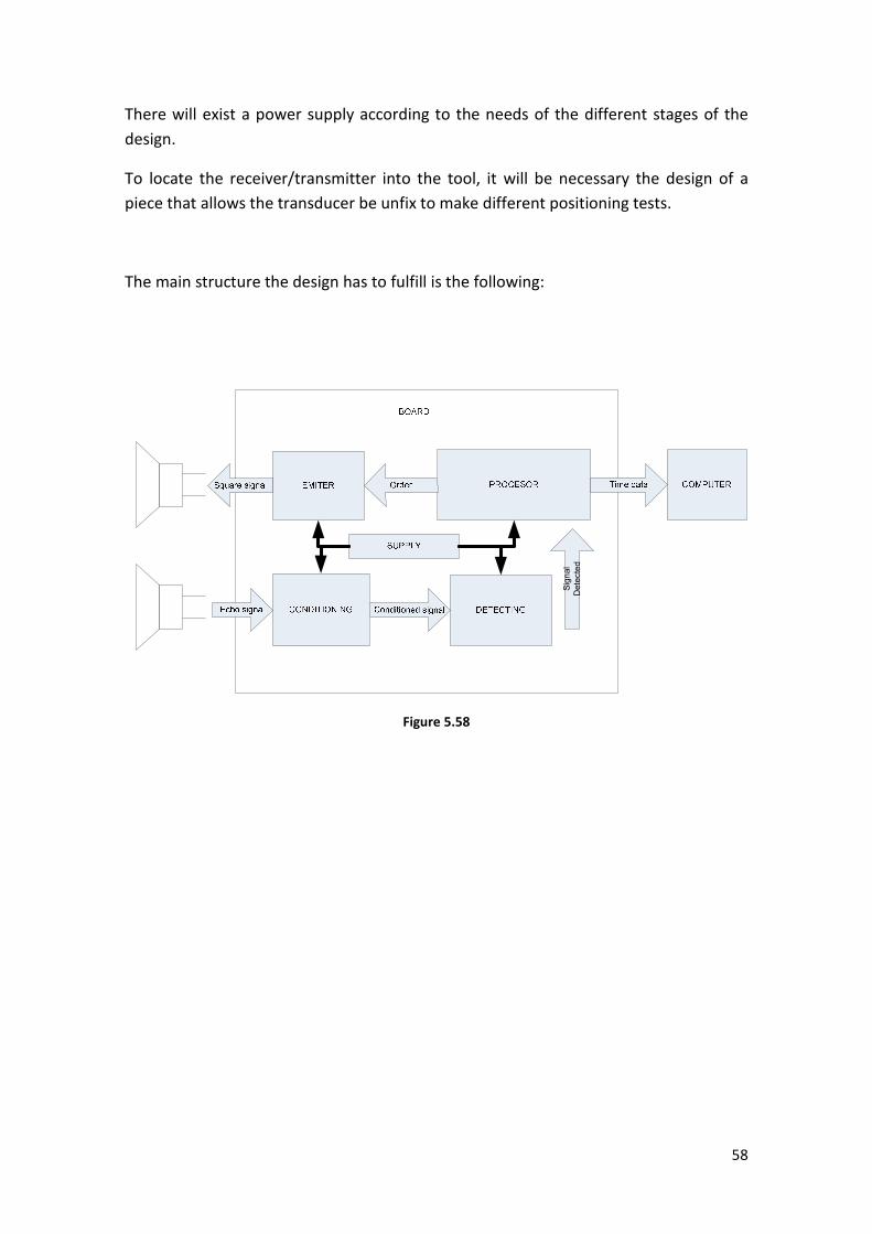
The electronic board will have an emitter stage. It has to send a burst with few cycles

of a 40 KHz signal, with the maximum amplitude the board allows, to make the

emitted signal as powerful as possible.

Figure 5.57

Then the next stage should be a conditioning one able to filter the possible noise

introduced by the environment and amplify the signal enough to be detected.

There has to exist a method to detect the signal as fast as possible, and communicate

the central processor to finish the account of the time of flight.

We are going to focus the design on the PIC18F4550 again, due to the knowledge

acquired developing the air hardware the handling will be easier. It also provides us

the system to send the data to the computer central handler.

Time of flight

58

There will exist a power supply according to the needs of the different stages of the

design.

To locate the receiver/transmitter into the tool, it will be necessary the design of a

piece that allows the transducer be unfix to make different positioning tests.

The main structure the design has to fulfill is the following:

Signal

Detected

Figure 5.58

59

5.3.4 Circuit Design

The tools used on the design will be the same as the ones used on the air hardware.

5.3.4.1 Emitter Stage

For this task is necessary to switch the maximum voltage we have available. Using the

same transformer we have used with the air board. In this case the voltage will be 24 V

and has to be switched with the ground voltage with a 40 KHz signal.

This signal will be provided by the PIC through the pin 17 which belongs to the C port.

For this task we will use a power transistor in switching mode able to handle the

voltage required. We will make use of a TIP29 NPN power transistor, with the load on

collector allowing a maximum switching voltage of 40 V.

Firstly, knowing the maximum power stand by our available power resistors is 10 W, is

necessary to know the value of the collector impedance able to stand the voltage in

saturation mode.

It will be: VceSAT = 0.7 ; 10 W ≥ (24-0.7)2/R R ≥ 54.29 Ω

For the safety of the circuit two resistors of 33 Ω and 10 W will be installed.

To handle the rms value of the emitting signal and the duty cycle, is a good idea have

an regulated non-inverter amplifier which can command this task, powering the signal

given by the processor based in a TL072. The supply of this amplifier will be between

14 and -5 V to have enough handling range, to avoid the swing problems, and for other

reasons that will be commented afterwards.

In this case, we will use a 1KΩ base impedance to obtain a (13-1.3)/1000 = 11.7 mA

base current, for saturation mode. The collector output will be (24-0.7)/66 = 353 mA. It

fulfills the condition IB ≤ β · IC because β = hFE = 75 for saturation mode. Now using the

tables given by the manufacturer we can re-calculate the real values of VceSAT and VBEγ.

Figure 5.59

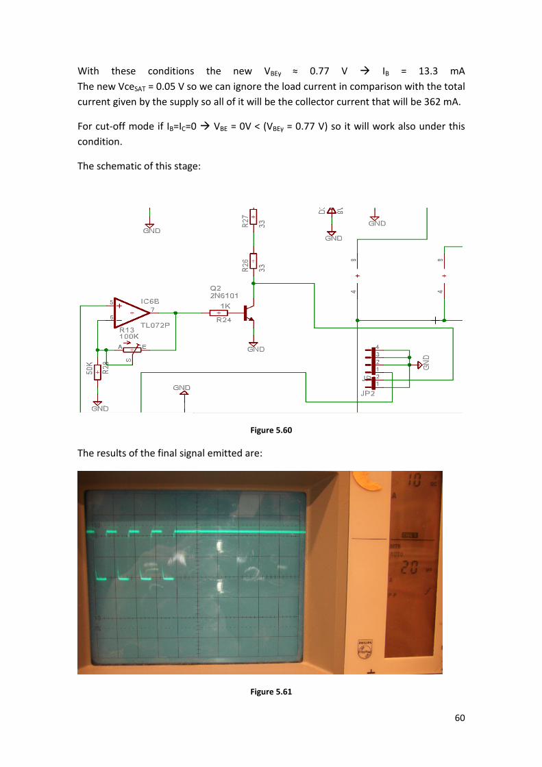
60

With these conditions the new VBEγ ≈ 0.77 V IB = 13.3 mA

The new VceSAT = 0.05 V so we can ignore the load current in comparison with the total

current given by the supply so all of it will be the collector current that will be 362 mA.

For cut-off mode if IB=IC=0 VBE = 0V < (VBEγ = 0.77 V) so it will work also under this

condition.

The schematic of this stage:

Figure 5.60

The results of the final signal emitted are:

Figure 5.61

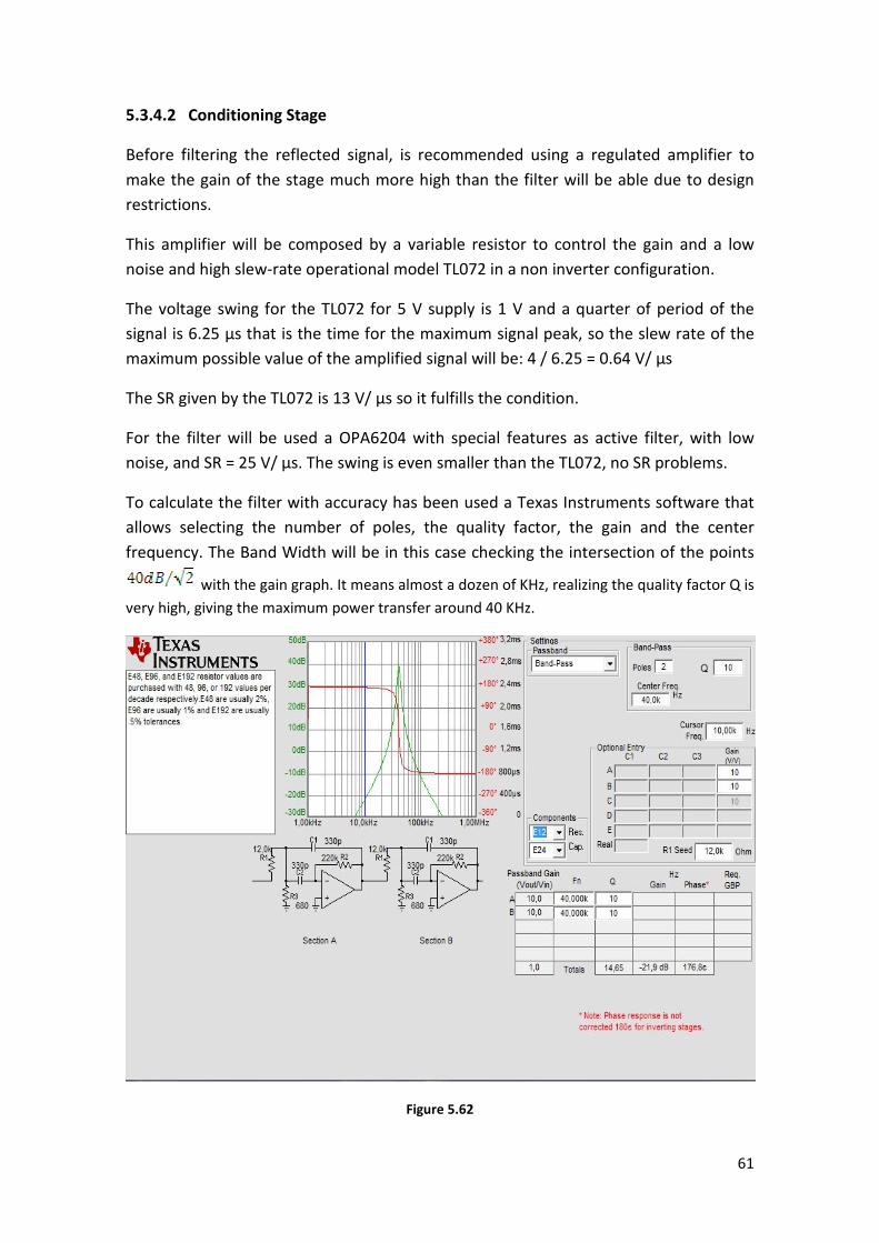
61

5.3.4.2 Conditioning Stage

Before filtering the reflected signal, is recommended using a regulated amplifier to

make the gain of the stage much more high than the filter will be able due to design

restrictions.

This amplifier will be composed by a variable resistor to control the gain and a low

noise and high slew-rate operational model TL072 in a non inverter configuration.

The voltage swing for the TL072 for 5 V supply is 1 V and a quarter of period of the

signal is 6.25 μs that is the time for the maximum signal peak, so the slew rate of the

maximum possible value of the amplified signal will be: 4 / 6.25 = 0.64 V/ μs

The SR given by the TL072 is 13 V/ μs so it fulfills the condition.

For the filter will be used a OPA6204 with special features as active filter, with low

noise, and SR = 25 V/ μs. The swing is even smaller than the TL072, no SR problems.

To calculate the filter with accuracy has been used a Texas Instruments software that

allows selecting the number of poles, the quality factor, the gain and the center

frequency. The Band Width will be in this case checking the intersection of the points

with the gain graph. It means almost a dozen of KHz, realizing the quality factor Q is

very high, giving the maximum power transfer around 40 KHz.

Figure 5.62

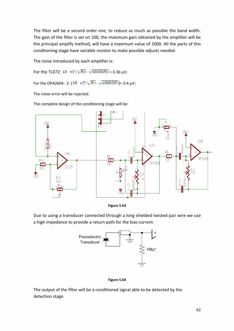
62

The filter will be a second order one, to reduce as much as possible the band width.

The gain of the filter is set on 100, the maximum gain obtained by the amplifier will be

the principal amplify method, will have a maximum value of 1000. All the parts of this

conditioning stage have variable resistor to make possible adjusts needed.

The noise introduced by each amplifier is:

For the TL072: · = 0.36 μV;

For the OPA2604 : 2· ( · )= 0.4 μV;

The noise error will be rejected.

The complete design of the conditioning stage will be:

Figure 5.63

Due to using a transducer connected through a long shielded twisted pair wire we use

a high impedance to provide a return path for the bias current.

Figure 5.64

The output of the filter will be a conditioned signal able to be detected by the

detection stage.

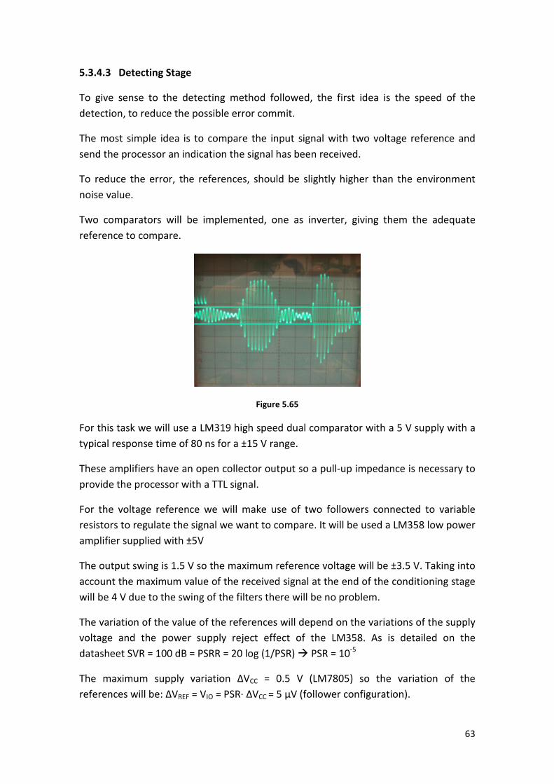
63

5.3.4.3 Detecting Stage

To give sense to the detecting method followed, the first idea is the speed of the

detection, to reduce the possible error commit.

The most simple idea is to compare the input signal with two voltage reference and

send the processor an indication the signal has been received.

To reduce the error, the references, should be slightly higher than the environment

noise value.

Two comparators will be implemented, one as inverter, giving them the adequate

reference to compare.

Figure 5.65

For this task we will use a LM319 high speed dual comparator with a 5 V supply with a

typical response time of 80 ns for a ±15 V range.

These amplifiers have an open collector output so a pull-up impedance is necessary to

provide the processor with a TTL signal.

For the voltage reference we will make use of two followers connected to variable

resistors to regulate the signal we want to compare. It will be used a LM358 low power

amplifier supplied with ±5V

The output swing is 1.5 V so the maximum reference voltage will be ±3.5 V. Taking into

account the maximum value of the received signal at the end of the conditioning stage

will be 4 V due to the swing of the filters there will be no problem.

The variation of the value of the references will depend on the variations of the supply

voltage and the power supply reject effect of the LM358. As is detailed on the

datasheet SVR = 100 dB = PSRR = 20 log (1/PSR) PSR = 10-5

The maximum supply variation ΔVCC = 0.5 V (LM7805) so the variation of the

references will be: ΔVREF = VIO = PSR· ΔVCC = 5 μV (follower configuration).

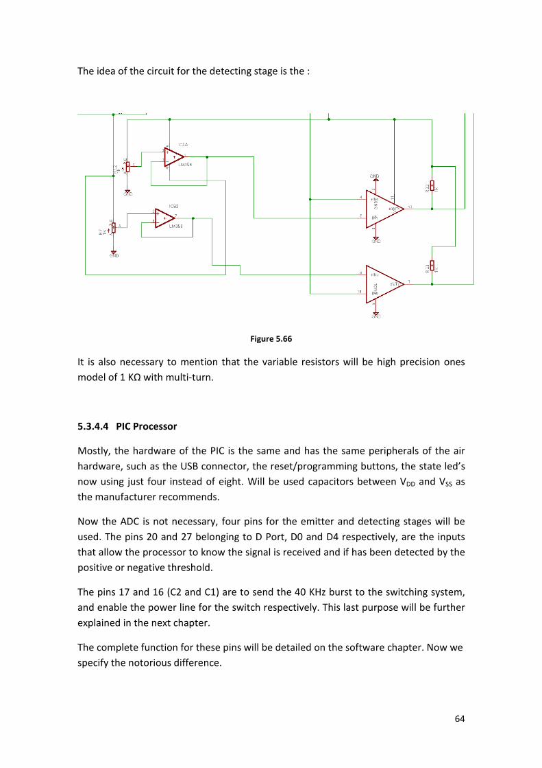
64

The idea of the circuit for the detecting stage is the :

Figure 5.66

It is also necessary to mention that the variable resistors will be high precision ones

model of 1 KΩ with multi-turn.

5.3.4.4 PIC Processor

Mostly, the hardware of the PIC is the same and has the same peripherals of the air

hardware, such as the USB connector, the reset/programming buttons, the state led’s

now using just four instead of eight. Will be used capacitors between VDD and VSS as

the manufacturer recommends.

Now the ADC is not necessary, four pins for the emitter and detecting stages will be

used. The pins 20 and 27 belonging to D Port, D0 and D4 respectively, are the inputs

that allow the processor to know the signal is received and if has been detected by the

positive or negative threshold.

The pins 17 and 16 (C2 and C1) are to send the 40 KHz burst to the switching system,

and enable the power line for the switch respectively. This last purpose will be further

explained in the next chapter.

The complete function for these pins will be detailed on the software chapter. Now we

specify the notorious difference.

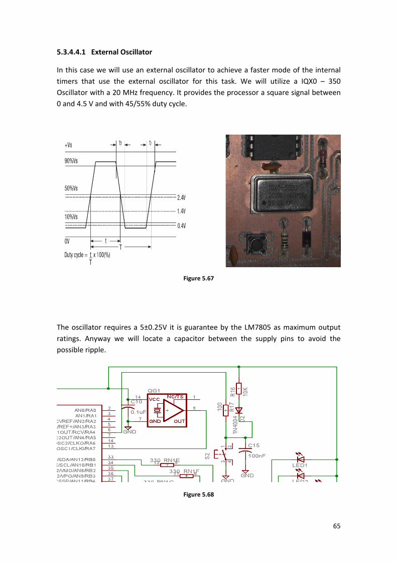
65

5.3.4.4.1 External Oscillator

In this case we will use an external oscillator to achieve a faster mode of the internal

timers that use the external oscillator for this task. We will utilize a IQX0 – 350

Oscillator with a 20 MHz frequency. It provides the processor a square signal between

0 and 4.5 V and with 45/55% duty cycle.

Figure 5.67

The oscillator requires a 5±0.25V it is guarantee by the LM7805 as maximum output

ratings. Anyway we will locate a capacitor between the supply pins to avoid the

possible ripple.

Figure 5.68

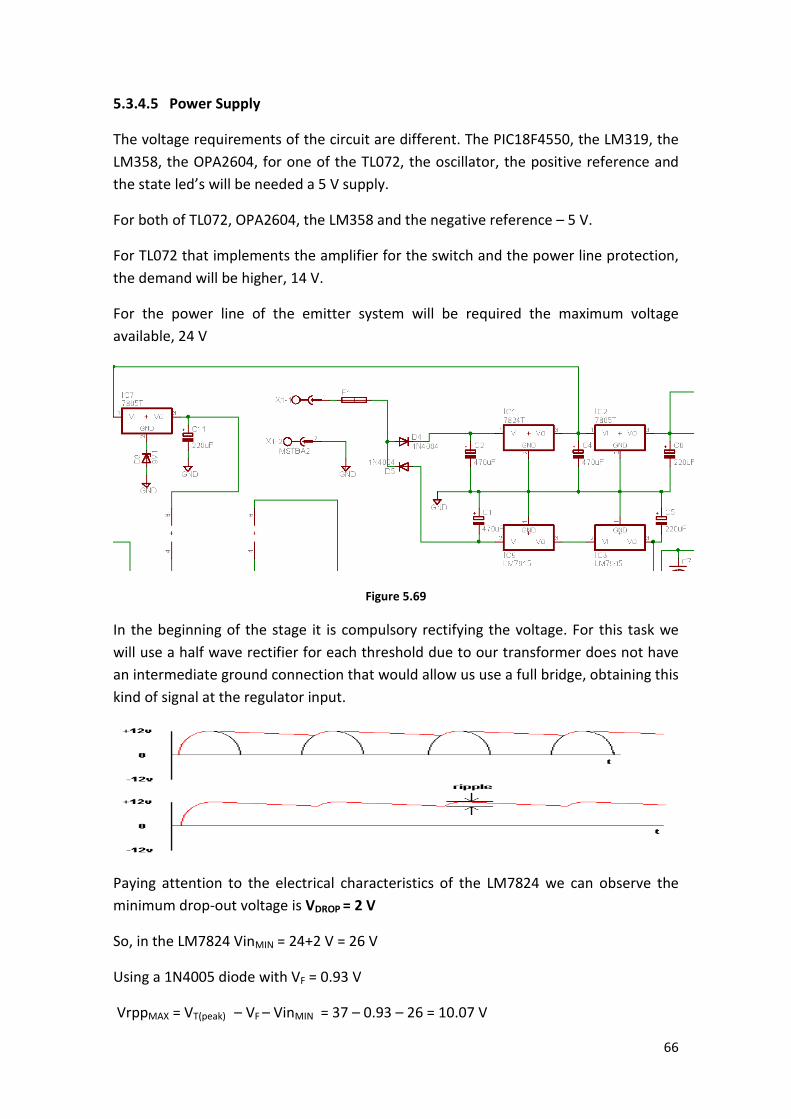
66

5.3.4.5 Power Supply

The voltage requirements of the circuit are different. The PIC18F4550, the LM319, the

LM358, the OPA2604, for one of the TL072, the oscillator, the positive reference and

the state led’s will be needed a 5 V supply.

For both of TL072, OPA2604, the LM358 and the negative reference – 5 V.

For TL072 that implements the amplifier for the switch and the power line protection,

the demand will be higher, 14 V.

For the power line of the emitter system will be required the maximum voltage

available, 24 V

Figure 5.69

In the beginning of the stage it is compulsory rectifying the voltage. For this task we

will use a half wave rectifier for each threshold due to our transformer does not have

an intermediate ground connection that would allow us use a full bridge, obtaining this

kind of signal at the regulator input.

Paying attention to the electrical characteristics of the LM7824 we can observe the

minimum drop-out voltage is VDROP = 2 V

So, in the LM7824 VinMIN = 24+2 V = 26 V

Using a 1N4005 diode with VF = 0.93 V

VrppMAX = VT(peak) – VF – VinMIN = 37 – 0.93 – 26 = 10.07 V

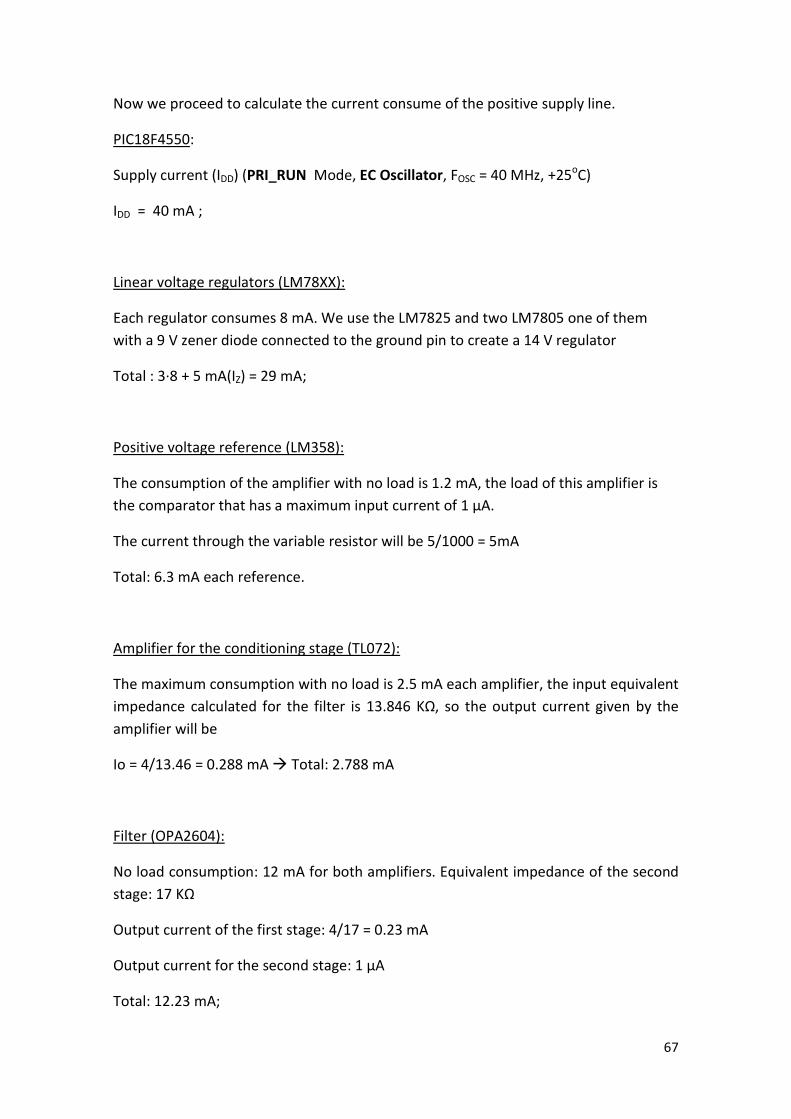
67

Now we proceed to calculate the current consume of the positive supply line.

PIC18F4550:

Supply current (IDD) (PRI_RUN Mode, EC Oscillator, FOSC = 40 MHz, +25oC)

IDD = 40 mA ;


Each regulator consumes 8 mA. We use the LM7825 and two LM7805 one of them

with a 9 V zener diode connected to the ground pin to create a 14 V regulator

Total : 3·8 + 5 mA(IZ) = 29 mA;

Positive voltage reference (LM358):

The consumption of the amplifier with no load is 1.2 mA, the load of this amplifier is

the comparator that has a maximum input current of 1 μA.

The current through the variable resistor will be 5/1000 = 5mA

Total: 6.3 mA each reference.

Amplifier for the conditioning stage (TL072):

The maximum consumption with no load is 2.5 mA each amplifier, the input equivalent

impedance calculated for the filter is 13.846 KΩ, so the output current given by the

amplifier will be

Io = 4/13.46 = 0.288 mA Total: 2.788 mA

Filter (OPA2604):

No load consumption: 12 mA for both amplifiers. Equivalent impedance of the second

stage: 17 KΩ

Output current of the first stage: 4/17 = 0.23 mA

Output current for the second stage: 1 μA

Total: 12.23 mA;

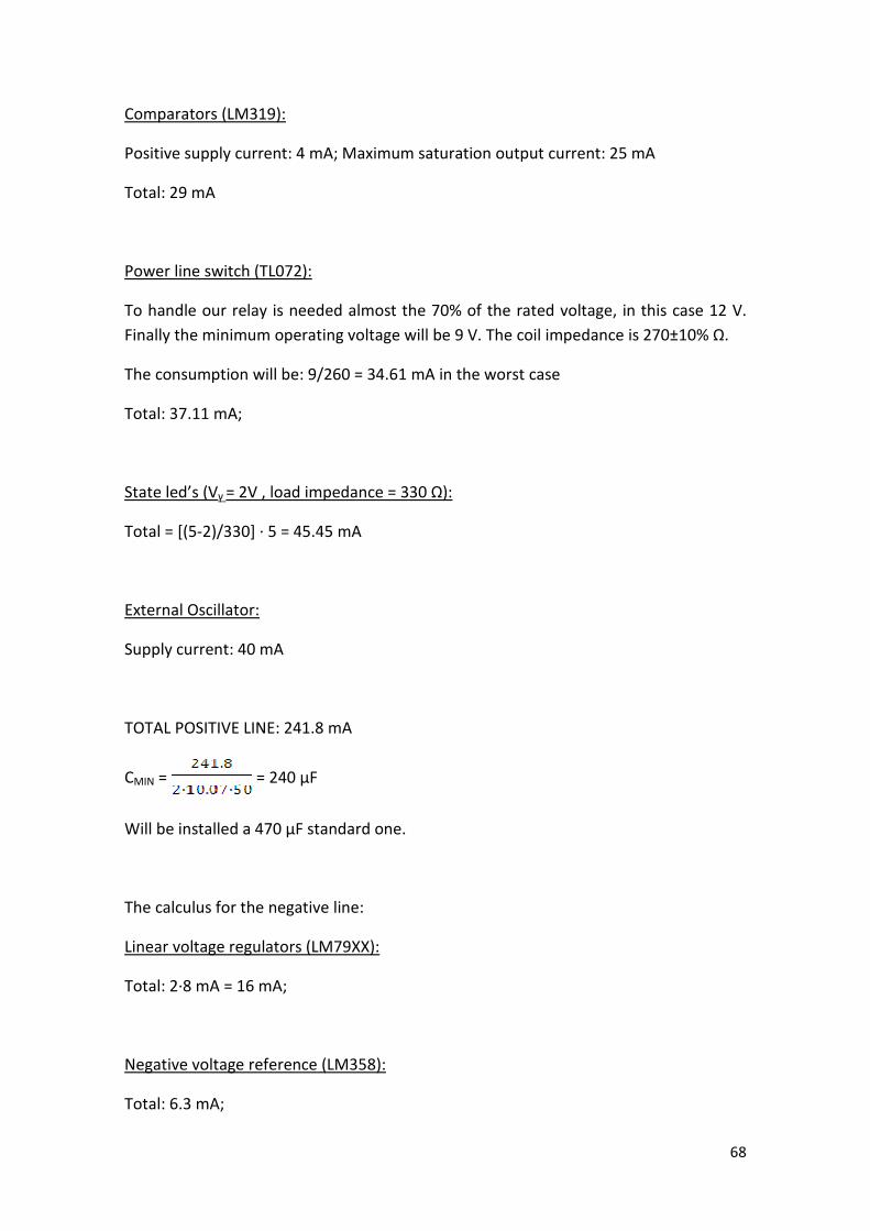
68

Comparators (LM319):

Positive supply current: 4 mA; Maximum saturation output current: 25 mA

Total: 29 mA

Power line switch (TL072):

To handle our relay is needed almost the 70% of the rated voltage, in this case 12 V.

Finally the minimum operating voltage will be 9 V. The coil impedance is 270±10% Ω.

The consumption will be: 9/260 = 34.61 mA in the worst case

Total: 37.11 mA;

State led’s (Vγ = 2V , load impedance = 330 Ω):

Total = [(5-2)/330] · 5 = 45.45 mA

External Oscillator:

Supply current: 40 mA

TOTAL POSITIVE LINE: 241.8 mA

CMIN = = 240 μF

Will be installed a 470 μF standard one.

The calculus for the negative line:


Total: 2·8 mA = 16 mA;

Negative voltage reference (LM358):

Total: 6.3 mA;

69

Filter (OPA2604):

No load consumption: 12 mA for both amplifiers. Equivalent impedance of the second

stage: 17 KΩ

Output current of the first stage: 4/17 = 0.23 mA

Output current for the second stage: 1 μA

Total: 12.23 mA;

Amplifier for the conditioning stage (TL072):

The consumption with no load is 2.5 mA, the input equivalent impedance calculated

for the filter is 13.846 KΩ, so the output current given by the amplifier will be:

Io = 4/13.46 = 0.288 mA Total: 2.788 mA

TOTAL NEGATIVE LINE: 37.318 mA;

CMIN = 37 μF

Will be installed a 470 μF standard one.

5.3.4.5 Protections

Total consumption: 253.58 mA

F1 = IOC = 270.8 mA 300 mA;

We have to reject the consumption of the output current of the amplifiers for the

conditioning stage due to it never happens simultaneously the same consumption due

to the positive and negative threshold, they are alternative.

We use a standard fuse as protection for a current peak.

Figure 5.70

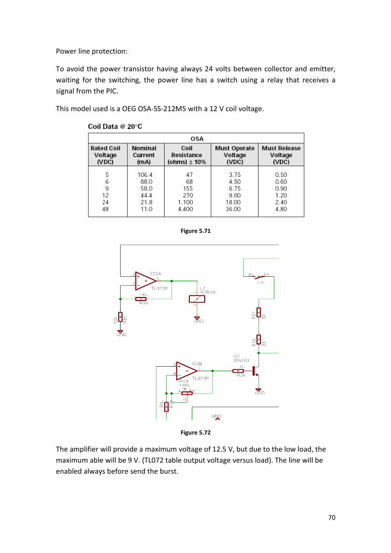
70

Power line protection:

To avoid the power transistor having always 24 volts between collector and emitter,

waiting for the switching, the power line has a switch using a relay that receives a

signal from the PIC.

This model used is a OEG OSA-SS-212M5 with a 12 V coil voltage.

Figure 5.71

Figure 5.72

The amplifier will provide a maximum voltage of 12.5 V, but due to the low load, the

maximum able will be 9 V. (TL072 table output voltage versus load). The line will be

enabled always before send the burst.

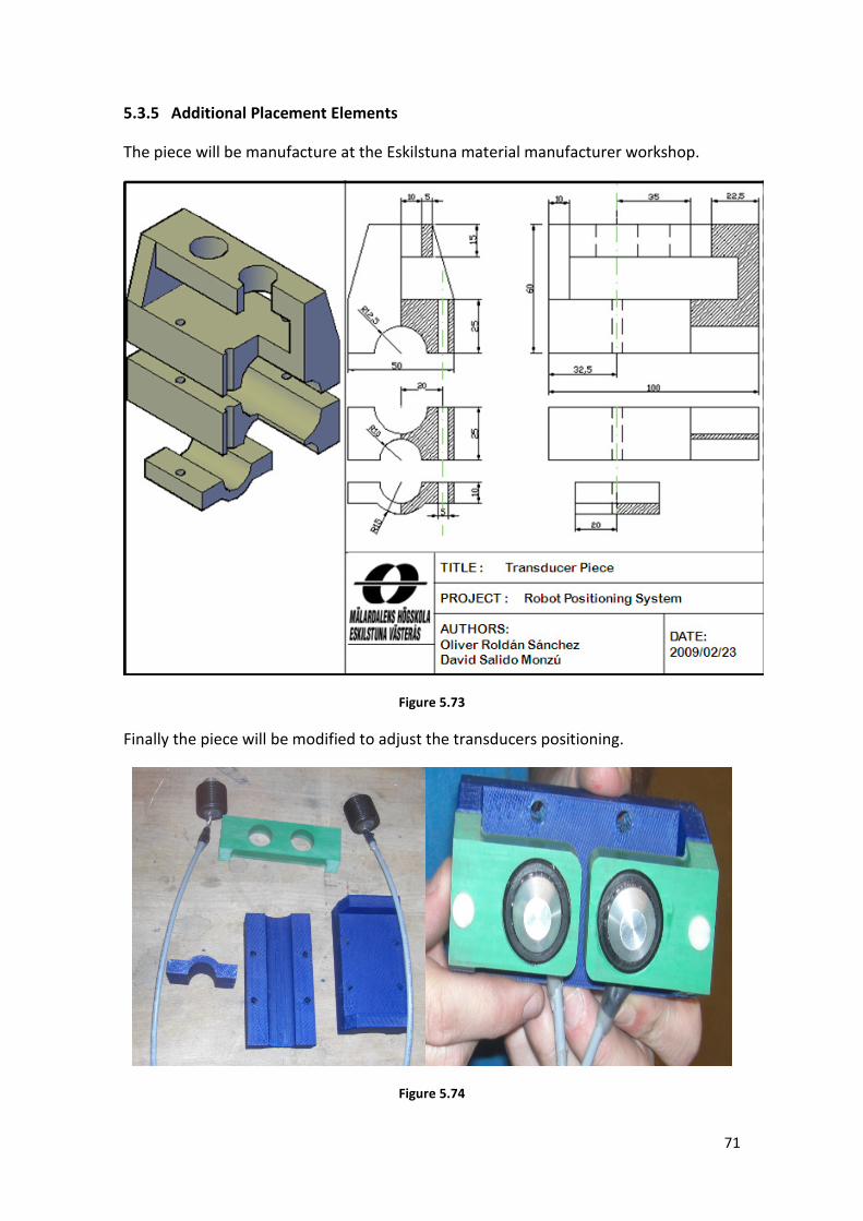
71

5.3.5 Additional Placement Elements

The piece will be manufacture at the Eskilstuna material manufacturer workshop.

Figure 5.73

Finally the piece will be modified to adjust the transducers positioning.

Figure 5.74

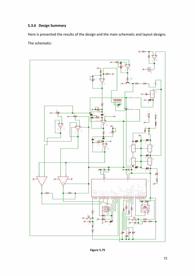
72

5.3.6 Design Summary

Here is presented the results of the design and the main schematic and layout designs.

The schematic:

Figure 5.75

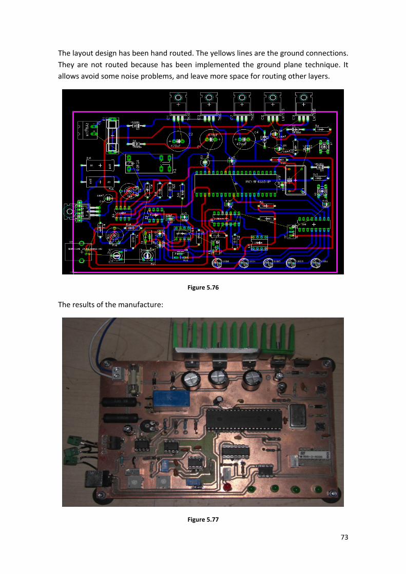
73

The layout design has been hand routed. The yellows lines are the ground connections.

They are not routed because has been implemented the ground plane technique. It

allows avoid some noise problems, and leave more space for routing other layers.

Figure 5.76

The results of the manufacture:

Figure 5.77

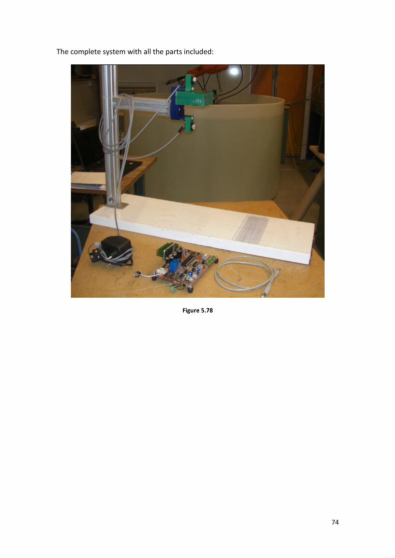
74

The complete system with all the parts included:

Figure 5.78

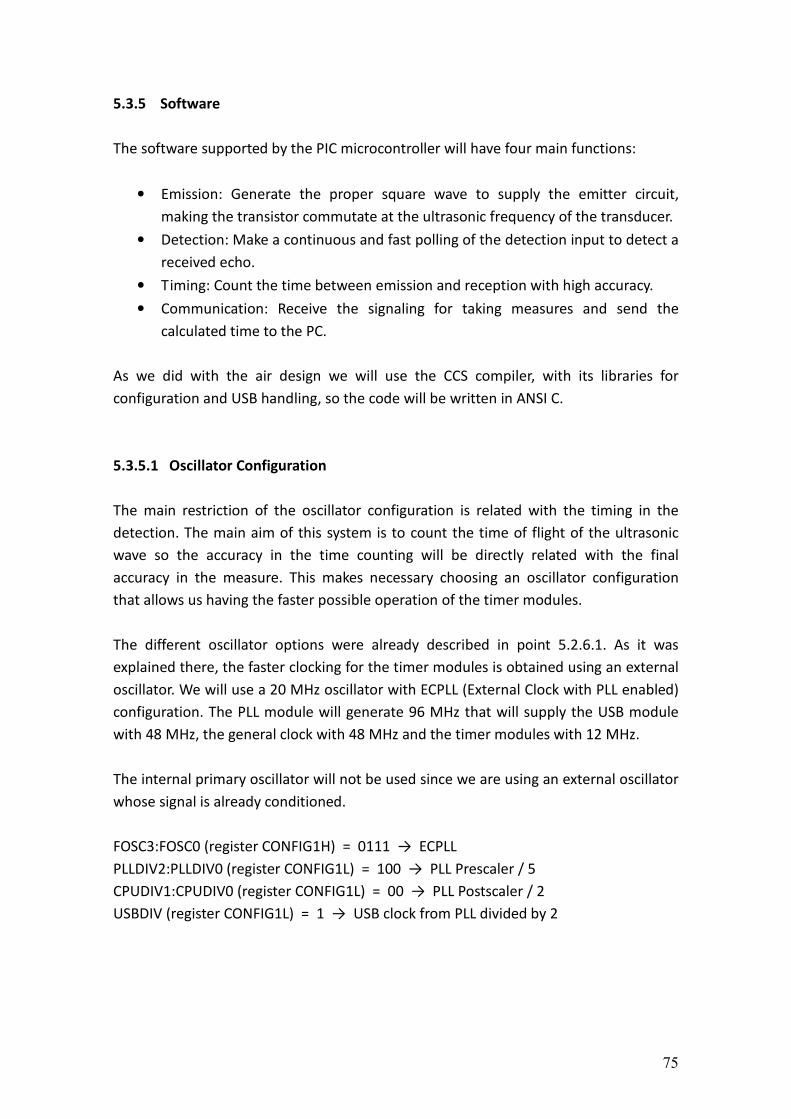
75

5.3.5 Software

The software supported by the PIC microcontroller will have four main functions:

• Emission: Generate the proper square wave to supply the emitter circuit,

making the transistor commutate at the ultrasonic frequency of the transducer.

• Detection: Make a continuous and fast polling of the detection input to detect a

received echo.

• Timing: Count the time between emission and reception with high accuracy.

• Communication: Receive the signaling for taking measures and send the

calculated time to the PC.

As we did with the air design we will use the CCS compiler, with its libraries for

configuration and USB handling, so the code will be written in ANSI C.

5.3.5.1 Oscillator Configuration

The main restriction of the oscillator configuration is related with the timing in the

detection. The main aim of this system is to count the time of flight of the ultrasonic

wave so the accuracy in the time counting will be directly related with the final

accuracy in the measure. This makes necessary choosing an oscillator configuration

that allows us having the faster possible operation of the timer modules.

The different oscillator options were already described in point 5.2.6.1. As it was

explained there, the faster clocking for the timer modules is obtained using an external

oscillator. We will use a 20 MHz oscillator with ECPLL (External Clock with PLL enabled)

configuration. The PLL module will generate 96 MHz that will supply the USB module

with 48 MHz, the general clock with 48 MHz and the timer modules with 12 MHz.

The internal primary oscillator will not be used since we are using an external oscillator

whose signal is already conditioned.

FOSC3:FOSC0 (register CONFIG1H) = 0111 → ECPLL

PLLDIV2:PLLDIV0 (register CONFIG1L) = 100 → PLL Prescaler / 5

CPUDIV1:CPUDIV0 (register CONFIG1L) = 00 → PLL Postscaler / 2

USBDIV (register CONFIG1L) = 1 → USB clock from PLL divided by 2

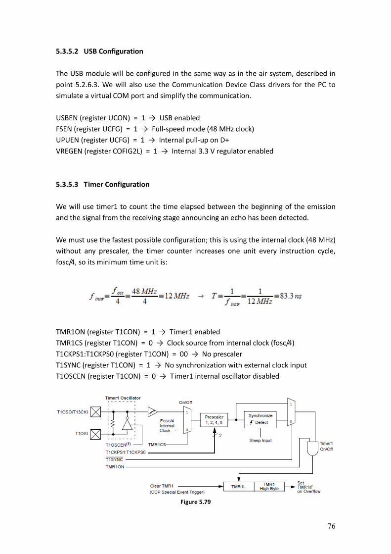
76

5.3.5.2 USB Configuration

The USB module will be configured in the same way as in the air system, described in

point 5.2.6.3. We will also use the Communication Device Class drivers for the PC to

simulate a virtual COM port and simplify the communication.

USBEN (register UCON) = 1 → USB enabled

FSEN (register UCFG) = 1 → Full-speed mode (48 MHz clock)

UPUEN (register UCFG) = 1 → Internal pull-up on D+

VREGEN (register COFIG2L) = 1 → Internal 3.3 V regulator enabled

5.3.5.3 Timer Configuration

We will use timer1 to count the time elapsed between the beginning of the emission

and the signal from the receiving stage announcing an echo has been detected.

We must use the fastest possible configuration; this is using the internal clock (48 MHz)

without any prescaler, the timer counter increases one unit every instruction cycle,

fosc/4, so its minimum time unit is:

TMR1ON (register T1CON) = 1 → Timer1 enabled

TMR1CS (register T1CON) = 0 → Clock source from internal clock (fosc/4)

T1CKPS1:T1CKPS0 (register T1CON) = 00 → No prescaler

T1SYNC (register T1CON) = 1 → No synchronization with external clock input

T1OSCEN (register T1CON) = 0 → Timer1 internal oscillator disabled

Figure 5.79

77

5.3.5.4 Programming Mode

The programming of the microcontroller will be done using the same system as in the

air design. A boot loader application will be loaded into the PIC using an external

programmer and the normal program will be downloaded via USB using the boot

loader. This process has already been explained in point 5.2.6.4.

5.3.5.5 File Structure

• tof.c:

It contains the code of the main program.

Includes tof.h, usb_bootloader.h, usb_cdc.h.

• tof.h:

Main program header file.

It contains the fuses with the basic configuration of the PIC.

Includes 18f4550.h.

• 18f4550.h:

Standard Header file for the PIC18F4550 device.

• usb_bootloader.h:

Bootloader application.

It contains the code of the application for programming the PIC via USB.

• usb_cdc.h:

Communication Device Class library.

It contains the library for adding a virtual COM port in the PC via USB.

Includes pic18_usb.

• pic18_usb.h:

Library with the basic handling functions for the USB module.

Includes usb.c.

• usb.c:

USB handler code.

Includes usb.h.

• usb.h:

Function prototypes and definitions for the USB handler.

78

5.3.5.6 Header File

The header file tof.h contains the configuration of the microcontroller modules.

#include <18F4550.h>

#device adc=8

#FUSES NOWDT //No Watch Dog Timer

#FUSES WDT128 //Watch Dog Timer uses 1:128 Postscale

#FUSES ECPLL //External clock with PLL enabled

#FUSES NOPROTECT //Code not protected from reading

#FUSES BROWNOUT //Reset when brownout detected

#FUSES BORV20 //Brownout reset at 2.0V

#FUSES NOPUT //No Power Up Timer

#FUSES NOCPD //No EE protection

#FUSES STVREN //Stack full/underflow will cause reset

#FUSES NODEBUG //No Debug mode for ICD

#FUSES NOLVP //No low voltage programming

#FUSES NOWRT //Program memory not write protected

#FUSES NOWRTD //Data EEPROM not write protected

#FUSES IESO //Internal External Switch Over mode enabled

#FUSES FCMEN //Fail-safe clock monitor enabled

#FUSES NOPBADEN //PORTB pins are configured as digital I/O on RESET

#FUSES NOWRTC //configuration not registers write protected

#FUSES NOWRTB //Boot block not write protected

#FUSES NOEBTR //Memory not protected from table reads

#FUSES NOEBTRB //Boot block not protected from table reads

#FUSES NOCPB //No Boot Block code protection

#FUSES MCLR //Master Clear pin enabled

#FUSES LPT1OSC //Timer1 configured for low-power operation

#FUSES NOXINST //Extended set extension and Indexed Addressing mode

//disabled (Legacy mode)

#FUSES PLL5 //Divide By 5(20MHz oscillator input)

#FUSES CPUDIV1 //No System Clock Postscaler

#FUSES USBDIV //USB clock source comes from PLL divide by 2

#FUSES VREGEN //USB voltage regulator enabled

#FUSES ICPRT //ICPRT enabled

#use delay(clock=48000000)

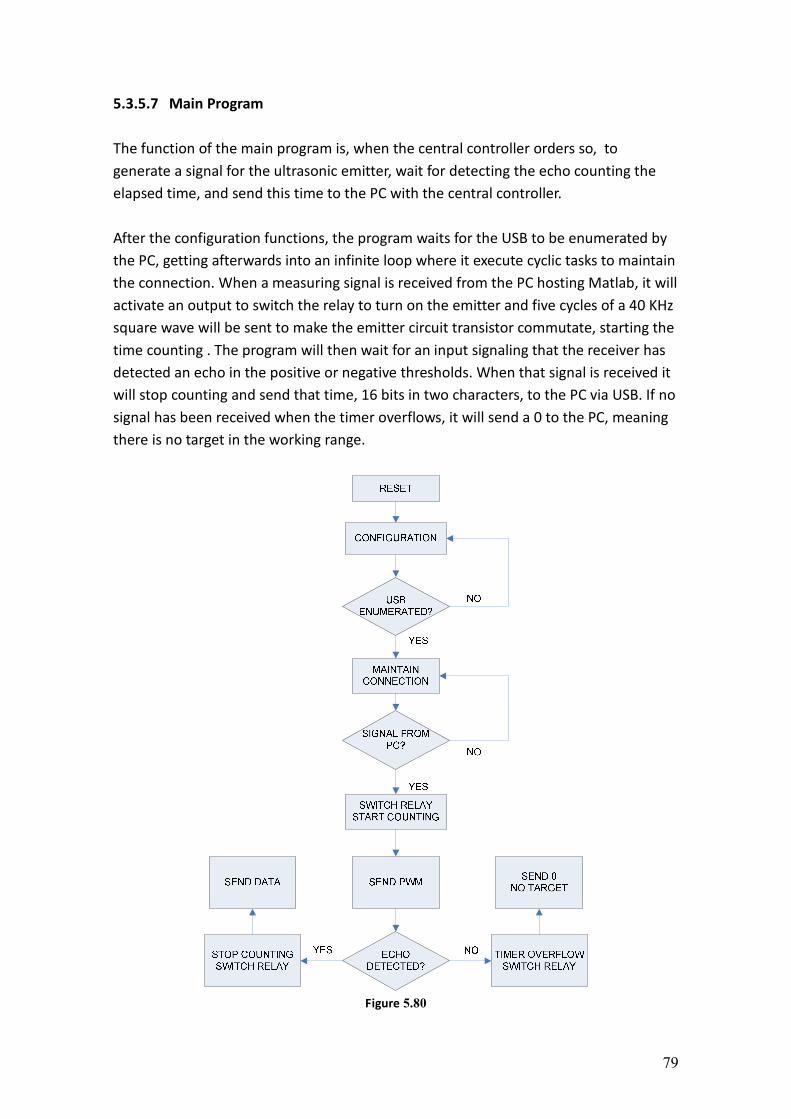
79

5.3.5.7 Main Program

The function of the main program is, when the central controller orders so, to

generate a signal for the ultrasonic emitter, wait for detecting the echo counting the

elapsed time, and send this time to the PC with the central controller.

After the configuration functions, the program waits for the USB to be enumerated by

the PC, getting afterwards into an infinite loop where it execute cyclic tasks to maintain

the connection. When a measuring signal is received from the PC hosting Matlab, it will

activate an output to switch the relay to turn on the emitter and five cycles of a 40 KHz

square wave will be sent to make the emitter circuit transistor commutate, starting the

time counting . The program will then wait for an input signaling that the receiver has

detected an echo in the positive or negative thresholds. When that signal is received it

will stop counting and send that time, 16 bits in two characters, to the PC via USB. If no

signal has been received when the timer overflows, it will send a 0 to the PC, meaning

there is no target in the working range.

Figure 5.80

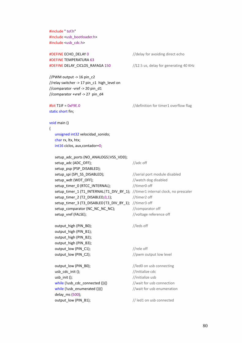
80

#include " tof.h"

#include <usb_bootloader.h>

#include <usb_cdc.h>

#DEFINE ECHO_DELAY 0 //delay for avoiding direct echo

#DEFINE TEMPERATURA 63

#DEFINE DELAY_CICLOS_RAFAGA 150 //12.5 us, delay for generating 40 KHz

//PWM output -> 16 pin_c2

//relay switcher -> 17 pin_c1 high_level on

//comparator -vref -> 20 pin_d1

//comparator +vref -> 27 pin_d4

#bit T1IF = 0xF9E.0 //definition for timer1 overflow flag

static short fin;

void main ()

unsigned int32 velocidad_sonido;

char rx, ltx, htx;

int16 ciclos, aux,contador=0;

setup_adc_ports (NO_ANALOGS|VSS_VDD);

setup_adc (ADC_OFF); //adc off

setup_psp (PSP_DISABLED);

setup_spi (SPI_SS_DISABLED); //serial port module disabled

setup_wdt (WDT_OFF); //watch dog disabled

setup_timer_0 (RTCC_INTERNAL); //timer0 off

setup_timer_1 (T1_INTERNAL|T1_DIV_BY_1); //timer1 internal clock, no prescaler

setup_timer_2 (T2_DISABLED,0,1); //timer2 off

setup_timer_3 (T3_DISABLED|T3_DIV_BY_1); //timer3 off

setup_comparator (NC_NC_NC_NC); //comparator off

setup_vref (FALSE); //voltage reference off

output_high (PIN_B0); //leds off

output_high (PIN_B1);



output_low (PIN_C1); //rele off

output_low (PIN_C2); //pwm output low level

output_low (PIN_B0); //led0 on usb connecting

usb_cdc_init (); //initialize cdc

usb_init (); //initialize usb

while (!usb_cdc_connected ()) //wait for usb connection

while (!usb_enumerated ()) //wait for usb enumeration

delay_ms (500);

output_low (PIN_B1); // led1 on usb connected

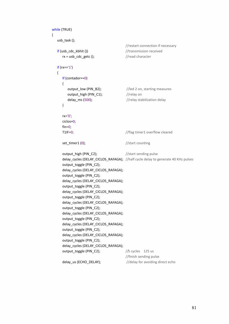
81

while (TRUE)

usb_task ();

//restart connection if necessary

if (usb_cdc_kbhit ()) //transmission received

rx = usb_cdc_getc (); //read character

if (rx=='1')

If (contador==0)

output_low (PIN_B2); //led 2 on, starting measures

output_high (PIN_C1); //relay on

delay_ms (500); //relay stabilization delay

rx='0';

ciclos=0;

fin=0;

T1IF=0; //flag timer1 overflow cleared

set_timer1 (0); //start counting

output_high (PIN_C2); //start sending pulse

delay_cycles (DELAY_CICLOS_RAFAGA); //half cycle delay to generate 40 KHz pulses

output_toggle (PIN_C2);

delay_cycles (DELAY_CICLOS_RAFAGA);















output_toggle (PIN_C2); //5 cycles 125 us

//finish sending pulse

delay_us (ECHO_DELAY); //delay for avoiding direct echo

82

while (fin!=1) //waiting for echo or overflow

If ((input (PIN_D1) == 1) || (input (PIN_D4)==1) || T1IF==1)

//echo detected in positive (D1) or negative

//(D4) threshold or timer1 overflowed

ciclos=get_timer1 (); //read timer – stop counting

if (T1IF==1) //if overflow

T1IF=0; //clear overflow flag

usb_cdc_putc (0); //send 0 – no target

usb_cdc_putc (0);

else

ltx = (char) ciclos; //get lower part of data

aux = ciclos >> 8;

htx = (char) aux; //get higher part of data

usb_cdc_putc (htx); //send higher part of data

usb_cdc_putc (ltx); //send lower part of data

fin=1;

delay_ms (10);

rx='0';

contador++;

if (contador==50) //after 50 measures

output_high (PIN_B2); //led 2 off finish measuring

output_low (PIN_C1); //relay off

contador=0;

83

5.4 Central Controller

The central controller is a Matlab program hosted in a PC whose main functions are:

• User interface: It provides a graphical interface where the user can introduce

some necessary data, check the state of the processes being executed and read

the intermediate and final results.

• Communication with measuring system: It must send the measuring system a

signal to take a measure and received the data from that measure afterwards.

This communication will be done using the CDC drivers, using a USB connection

understood by the PC as a virtual serial port.

• Communication with robot: It must send the robot the position it should reach

together with the orientation of the tool for every position and wait for a signal

from it telling the position has been reached. This communication will be done

using a standard serial port.

• Signaling and synchronization: It is in charge of providing the proper signals and

data to the peripherals, telling the robot where and when to move and the

measuring system when to measure; synchronizing both processes.

• Data analysis: After all the data (sent by the measuring system from every robot

position) has been stored, the program will calculate, based on the

mathematical method explained in point 5.1.2, the actual center of the cylinder

and save it to an external file so it can be used by the microwave application to

correct its movement.

We will explain the general operation of the program and the user interface in the first

place, detailing afterwards the file structure. The code included in every file will be

added as an appendix at the end of the report.

The program will be based on Matlab 7, to

provide the possibility of being integrated into

the microwave application, based on the same

version, as a calibration option.

Figure 5.81

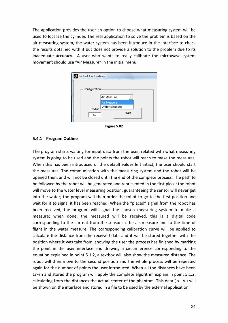
84

The application provides the user an option to choose what measuring system will be

used to localize the cylinder. The real application to solve the problem is based on the

air measuring system, the water system has been introduce in the interface to check

the results obtained with it but does not provide a solution to the problem due to its

inadequate accuracy. A user who wants to really calibrate the microwave system

movement should use “Air Measure” in the initial menu.

Figure 5.82

5.4.1 Program Outline

The program starts waiting for input data from the user, related with what measuring

system is going to be used and the points the robot will reach to make the measures.

When this has been introduced or the default values left intact, the user should start

the measures. The communication with the measuring system and the robot will be

opened then, and will not be closed until the end of the complete process. The path to

be followed by the robot will be generated and represented in the first place; the robot

will move to the water level measuring position, guaranteeing the sensor will never get

into the water; the program will then order the robot to go to the first position and

wait for it to signal it has been reached. When the “placed” signal from the robot has

been received, the program will signal the chosen measuring system to make a

measure; when done, the measured will be received, this is a digital code

corresponding to the current from the sensor in the air measure and to the time of

flight in the water measure. The corresponding calibration curve will be applied to

calculate the distance from the received data and it will be stored together with the

position where it was take from, showing the user the process has finished by marking

the point in the user interface and drawing a circumference corresponding to the

equation explained in point 5.1.2, a textbox will also show the measured distance. The

robot will then move to the second position and the whole process will be repeated

again for the number of points the user introduced. When all the distances have been

taken and stored the program will apply the complete algorithm explain in point 5.1.2,

calculating from the distances the actual center of the phantom. This data ( x , y ) will

be shown on the interface and stored in a file to be used by the external application.

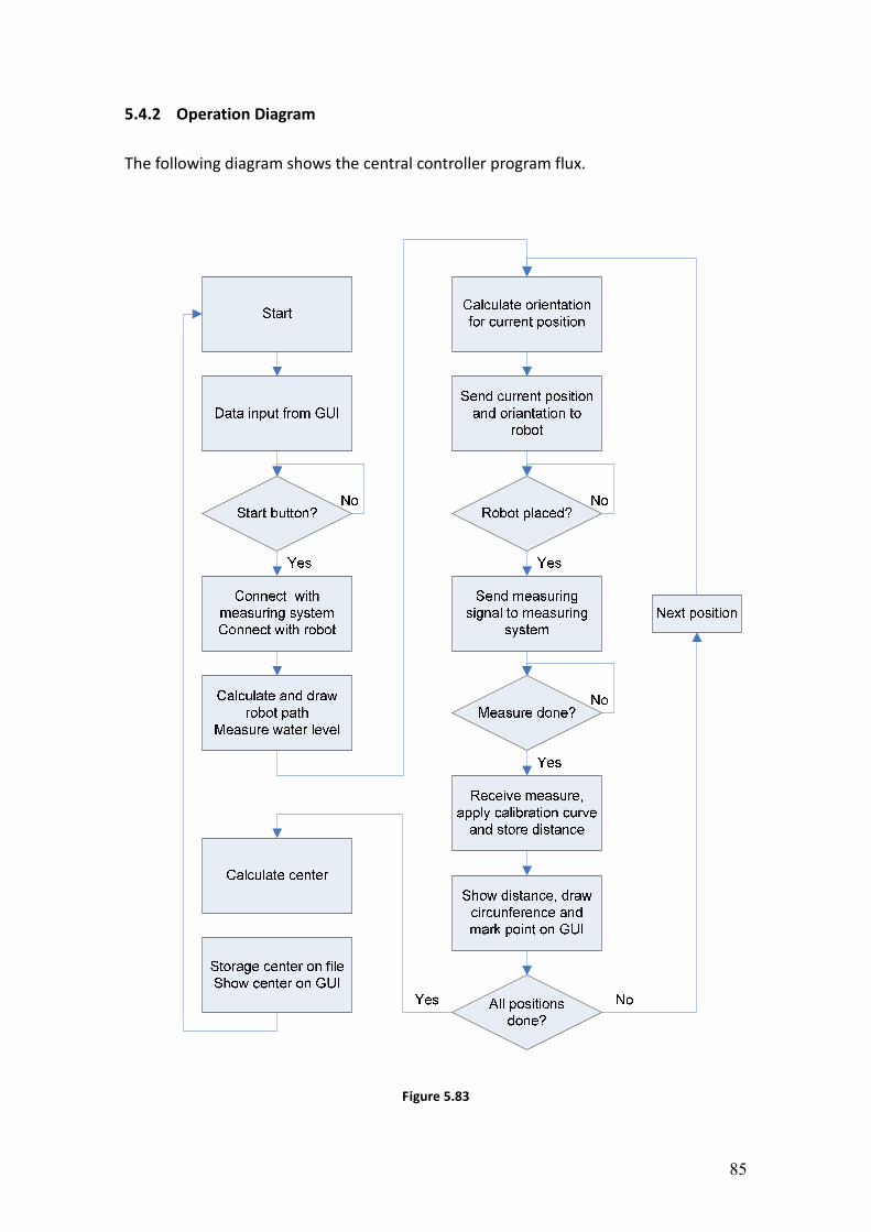
85

5.4.2 Operation Diagram

The following diagram shows the central controller program flux.

Figure 5.83

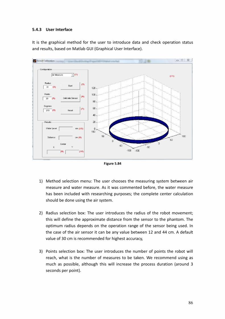
86

5.4.3 User Interface

It is the graphical method for the user to introduce data and check operation status

and results, based on Matlab GUI (Graphical User Interface).

Figure 5.84

1) Method selection menu: The user chooses the measuring system between air

measure and water measure. As it was commented before, the water measure

has been included with researching purposes; the complete center calculation

should be done using the air system.

2) Radius selection box: The user introduces the radius of the robot movement;

this will define the approximate distance from the sensor to the phantom. The

optimum radius depends on the operation range of the sensor being used. In

the case of the air sensor it can be any value between 12 and 44 cm. A default

value of 30 cm is recommended for highest accuracy,

3) Points selection box: The user introduces the number of points the robot will

reach, what is the number of measures to be taken. We recommend using as

much as possible, although this will increase the process duration (around 3

seconds per point).

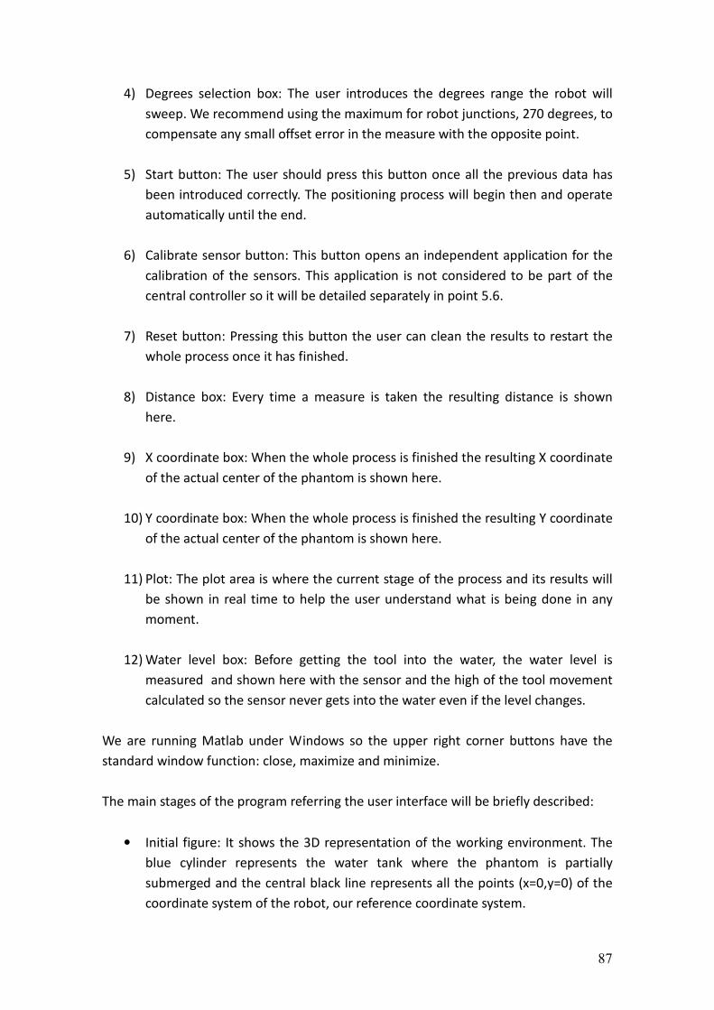
87

4) Degrees selection box: The user introduces the degrees range the robot will

sweep. We recommend using the maximum for robot junctions, 270 degrees, to

compensate any small offset error in the measure with the opposite point.

5) Start button: The user should press this button once all the previous data has

been introduced correctly. The positioning process will begin then and operate

automatically until the end.

6) Calibrate sensor button: This button opens an independent application for the

calibration of the sensors. This application is not considered to be part of the

central controller so it will be detailed separately in point 5.6.

7) Reset button: Pressing this button the user can clean the results to restart the

whole process once it has finished.

8) Distance box: Every time a measure is taken the resulting distance is shown

here.

9) X coordinate box: When the whole process is finished the resulting X coordinate

of the actual center of the phantom is shown here.

10) Y coordinate box: When the whole process is finished the resulting Y coordinate

of the actual center of the phantom is shown here.

11) Plot: The plot area is where the current stage of the process and its results will

be shown in real time to help the user understand what is being done in any

moment.

12) Water level box: Before getting the tool into the water, the water level is

measured and shown here with the sensor and the high of the tool movement

calculated so the sensor never gets into the water even if the level changes.

We are running Matlab under Windows so the upper right corner buttons have the

standard window function: close, maximize and minimize.

The main stages of the program referring the user interface will be briefly described:

• Initial figure: It shows the 3D representation of the working environment. The

blue cylinder represents the water tank where the phantom is partially

submerged and the central black line represents all the points (x=0,y=0) of the

coordinate system of the robot, our reference coordinate system.

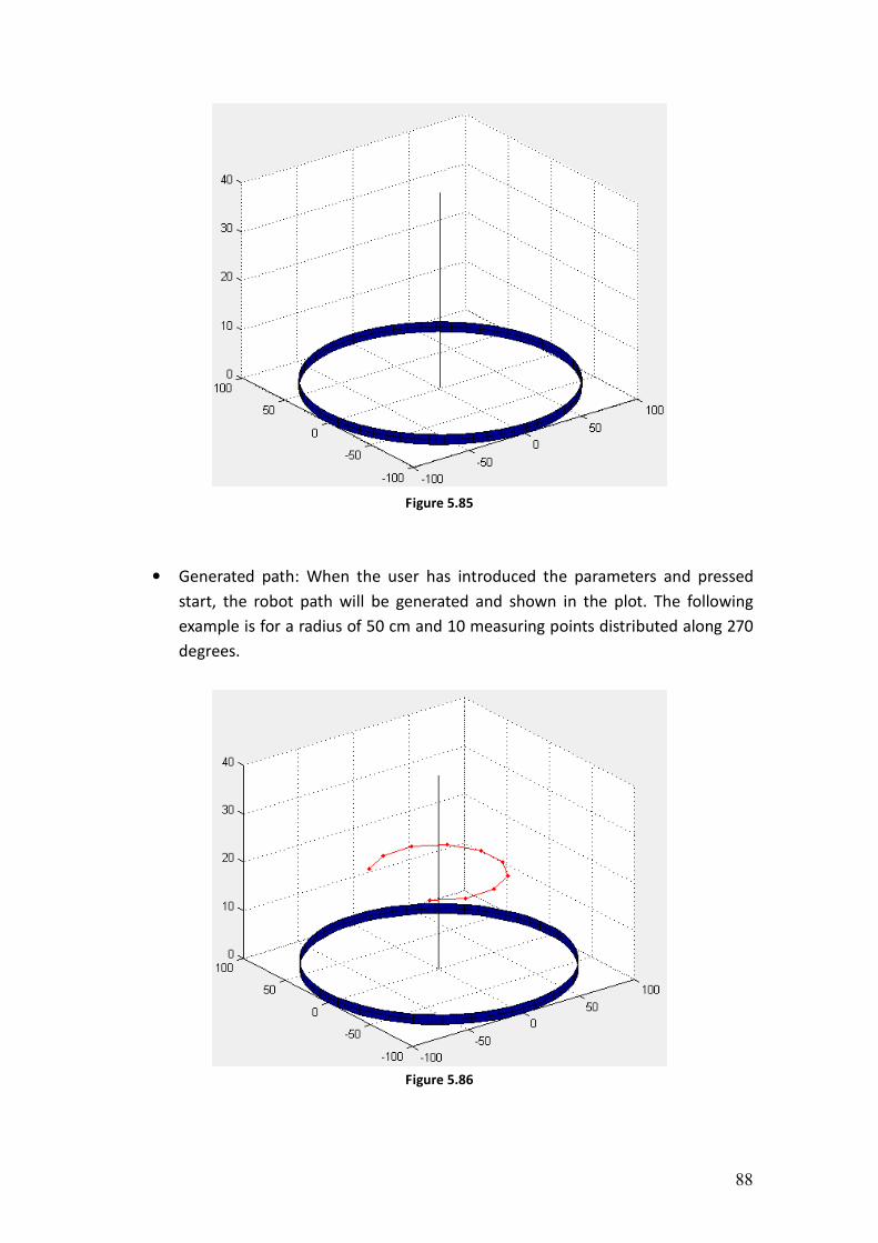
88

Figure 5.85

• Generated path: When the user has introduced the parameters and pressed

start, the robot path will be generated and shown in the plot. The following

example is for a radius of 50 cm and 10 measuring points distributed along 270

degrees.

Figure 5.86

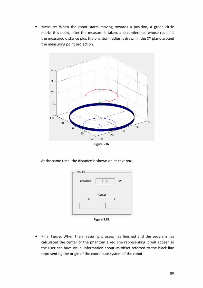
89

• Measure: When the robot starts moving towards a position, a green circle

marks this point, after the measure is taken, a circumference whose radius is

the measured distance plus the phantom radius is drawn in the XY plane around

the measuring point projection.

Figure 5.87

At the same time, the distance is shown on its text box.

Figure 5.88

• Final figure: When the measuring process has finished and the program has

calculated the center of the phantom a red line representing it will appear so

the user can have visual information about its offset referred to the black line

representing the origin of the coordinate system of the robot.

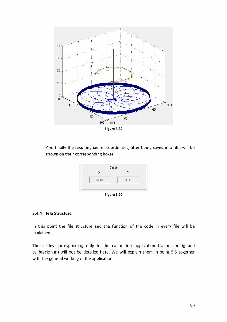
90

Figure 5.89

And finally the resulting center coordinates, after being saved in a file, will be

shown on their corresponding boxes.

Figure 5.90

5.4.4 File Structure

In this point the file structure and the function of the code in every file will be

explained.

Those files corresponding only to the calibration application (calibracion.fig and

calibracion.m) will not be detailed here. We will explain them in point 5.6 together

with the general working of the application.

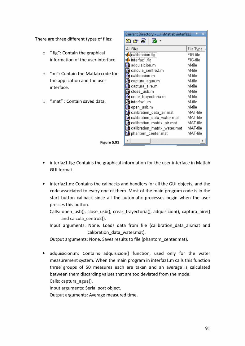
91

There are three different types of files:

o “.fig”: Contain the graphical

information of the user interface.

o “.m”: Contain the Matlab code for

the application and the user

interface.

o “.mat” : Contain saved data.

Figure 5.91

• interfaz1.fig: Contains the graphical information for the user interface in Matlab

GUI format.

• interfaz1.m: Contains the callbacks and handlers for all the GUI objects, and the

code associated to every one of them. Most of the main program code is in the

start button callback since all the automatic processes begin when the user

presses this button.

Calls: open_usb(), close_usb(), crear_trayectoria(), adquisicion(), captura_aire()

and calcula_centro2().

Input arguments: None. Loads data from file (calibration_data_air.mat and

calibration_data_water.mat).

Output arguments: None. Saves results to file (phantom_center.mat).

• adquisicion.m: Contains adquisicion() function, used only for the water

measurement system. When the main program in interfaz1.m calls this function

three groups of 50 measures each are taken and an average is calculated

between them discarding values that are too deviated from the mode.

Calls: captura_agua().

Input arguments: Serial port object.

Output arguments: Average measured time.

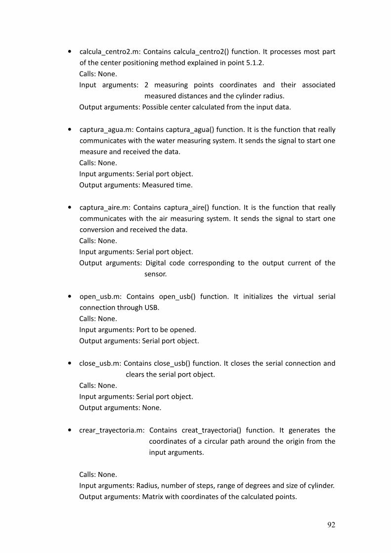
92

• calcula_centro2.m: Contains calcula_centro2() function. It processes most part

of the center positioning method explained in point 5.1.2.

Calls: None.

Input arguments: 2 measuring points coordinates and their associated

measured distances and the cylinder radius.

Output arguments: Possible center calculated from the input data.

• captura_agua.m: Contains captura_agua() function. It is the function that really

communicates with the water measuring system. It sends the signal to start one

measure and received the data.

Calls: None.


Output arguments: Measured time.

• captura_aire.m: Contains captura_aire() function. It is the function that really

communicates with the air measuring system. It sends the signal to start one

conversion and received the data.

Calls: None.


Output arguments: Digital code corresponding to the output current of the

sensor.

• open_usb.m: Contains open_usb() function. It initializes the virtual serial

connection through USB.

Calls: None.

Input arguments: Port to be opened.

Output arguments: Serial port object.

• close_usb.m: Contains close_usb() function. It closes the serial connection and

clears the serial port object.

Calls: None.


Output arguments: None.

• crear_trayectoria.m: Contains creat_trayectoria() function. It generates the

coordinates of a circular path around the origin from the

input arguments.

Calls: None.

Input arguments: Radius, number of steps, range of degrees and size of cylinder.

Output arguments: Matrix with coordinates of the calculated points.

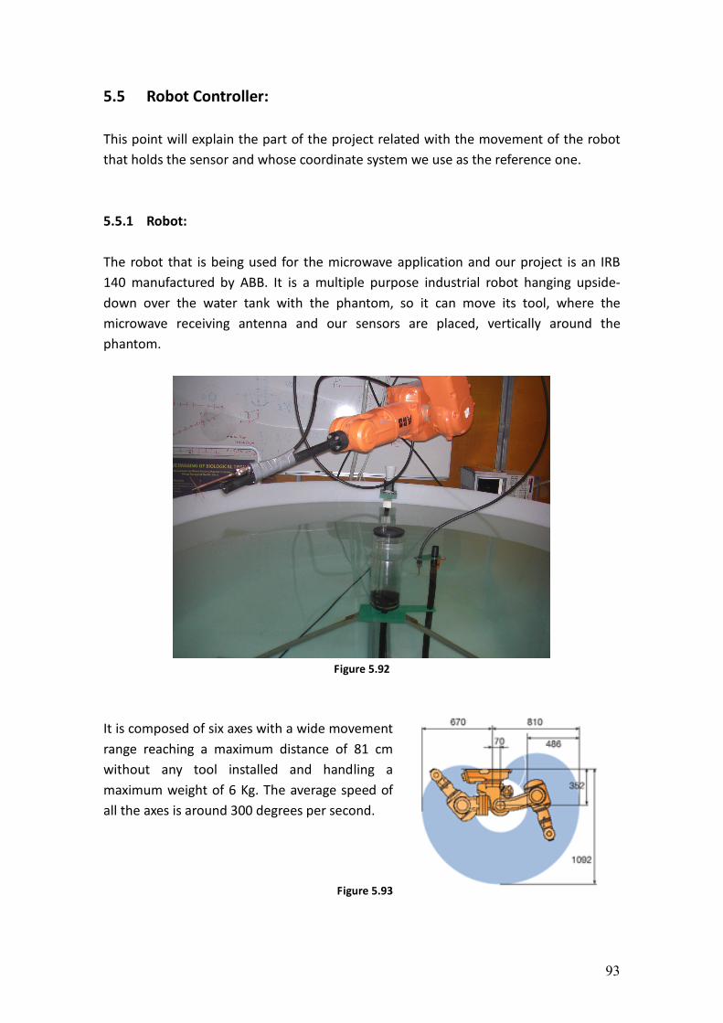
93

5.5 Robot Controller:

This point will explain the part of the project related with the movement of the robot

that holds the sensor and whose coordinate system we use as the reference one.

5.5.1 Robot:

The robot that is being used for the microwave application and our project is an IRB

140 manufactured by ABB. It is a multiple purpose industrial robot hanging upside-

down over the water tank with the phantom, so it can move its tool, where the

microwave receiving antenna and our sensors are placed, vertically around the

phantom.

Figure 5.92

It is composed of six axes with a wide movement

range reaching a maximum distance of 81 cm

without any tool installed and handling a

maximum weight of 6 Kg. The average speed of

all the axes is around 300 degrees per second.

Figure 5.93

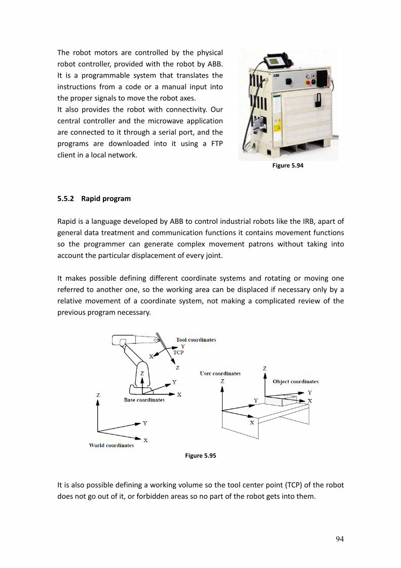
94

The robot motors are controlled by the physical

robot controller, provided with the robot by ABB.

It is a programmable system that translates the

instructions from a code or a manual input into

the proper signals to move the robot axes.

It also provides the robot with connectivity. Our

central controller and the microwave application

are connected to it through a serial port, and the

programs are downloaded into it using a FTP

client in a local network.

Figure 5.94

5.5.2 Rapid program

Rapid is a language developed by ABB to control industrial robots like the IRB, apart of

general data treatment and communication functions it contains movement functions

so the programmer can generate complex movement patrons without taking into

account the particular displacement of every joint.

It makes possible defining different coordinate systems and rotating or moving one

referred to another one, so the working area can be displaced if necessary only by a

relative movement of a coordinate system, not making a complicated review of the

previous program necessary.

Figure 5.95

It is also possible defining a working volume so the tool center point (TCP) of the robot

does not go out of it, or forbidden areas so no part of the robot gets into them.

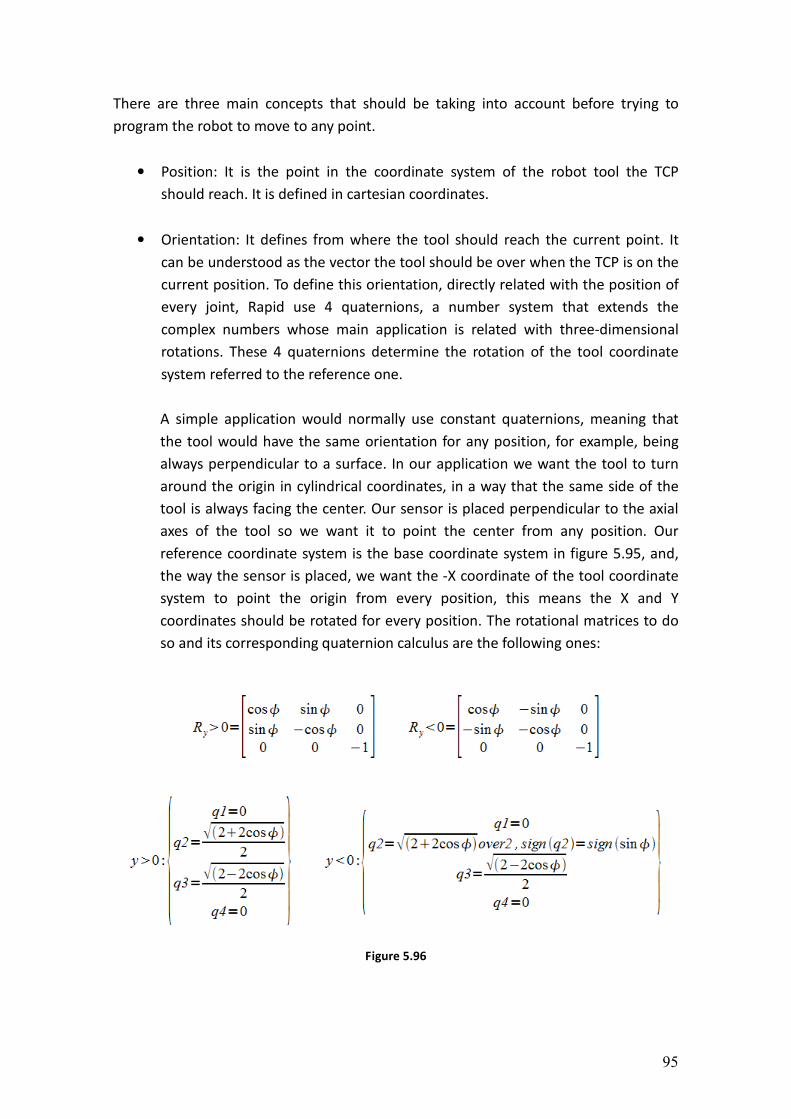
95

There are three main concepts that should be taking into account before trying to

program the robot to move to any point.

• Position: It is the point in the coordinate system of the robot tool the TCP

should reach. It is defined in cartesian coordinates.

• Orientation: It defines from where the tool should reach the current point. It

can be understood as the vector the tool should be over when the TCP is on the

current position. To define this orientation, directly related with the position of

every joint, Rapid use 4 quaternions, a number system that extends the

complex numbers whose main application is related with three-dimensional

rotations. These 4 quaternions determine the rotation of the tool coordinate

system referred to the reference one.

A simple application would normally use constant quaternions, meaning that

the tool would have the same orientation for any position, for example, being

always perpendicular to a surface. In our application we want the tool to turn

around the origin in cylindrical coordinates, in a way that the same side of the

tool is always facing the center. Our sensor is placed perpendicular to the axial

axes of the tool so we want it to point the center from any position. Our

reference coordinate system is the base coordinate system in figure 5.95, and,

the way the sensor is placed, we want the -X coordinate of the tool coordinate

system to point the origin from every position, this means the X and Y

coordinates should be rotated for every position. The rotational matrices to do

so and its corresponding quaternion calculus are the following ones:

Figure 5.96

96

• Configuration: It defines, once a position and orientation have been defined,

what configuration the robot should use in case there is more than one to reach

a defined point with a defined orientation.

Figure 5.97

In figure 5.97 we can see two different configurations for the same position and

orientation. As our working environment is not very restricted we will use the

default orientation because it guarantees us the robot will not bump on

anything.

After describing the main concepts for the robot positioning and how we will use them

we will describe the Rapid program of our application, what we have called before the

robot controller.

The robot can have many programs in its memory but can only execute one at a time;

our complete application is design to act as a calibration system for the microwave

system so the Rapid code for our application will be integrated with the Rapid

application of the microwave system, using also its defined coordinate system.

The operation of our Rapid program begins waiting for a start command from Matlab,

when it is received it will position the robot with its tool into the water in a known

position and signal Matlab that it is placed, afterwards it will wait for the first position,

translating that position into the proper robot target data, calculating the quaternions

for its orientation in every point, and moving the robot to that point, telling Matlab

again that it is placed and waiting for the next position. This process will be repeated

until, instead of receiving a new position, it receives and end command, going then out

of the water to the resting position again.

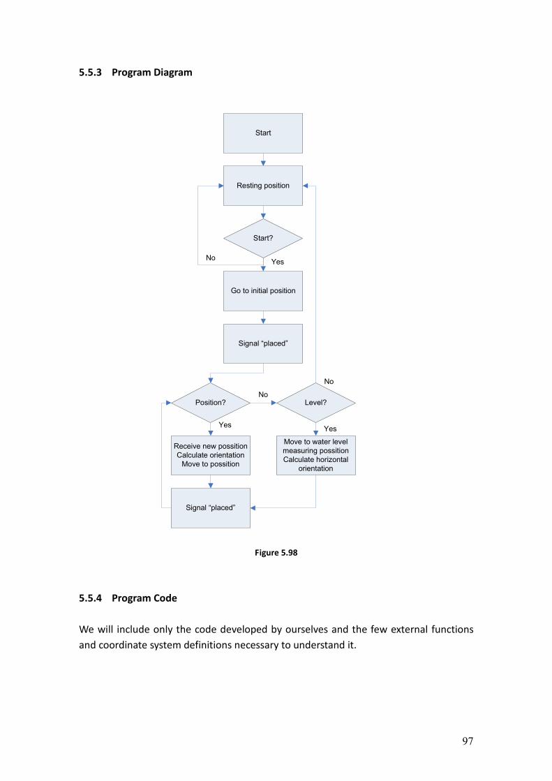
97

5.5.3 Program Diagram

Start

Resting position

Go to initial position

Signal “placed”

Start?

Position?

Receive new possition

Calculate orientation

Move to possition

Signal “placed”

Level?

Move to water level

measuring possition

Calculate horizontal

orientation

NoYes

Yes

No

Yes

No

Figure 5.98

5.5.4 Program Code

We will include only the code developed by ourselves and the few external functions

and coordinate system definitions necessary to understand it.

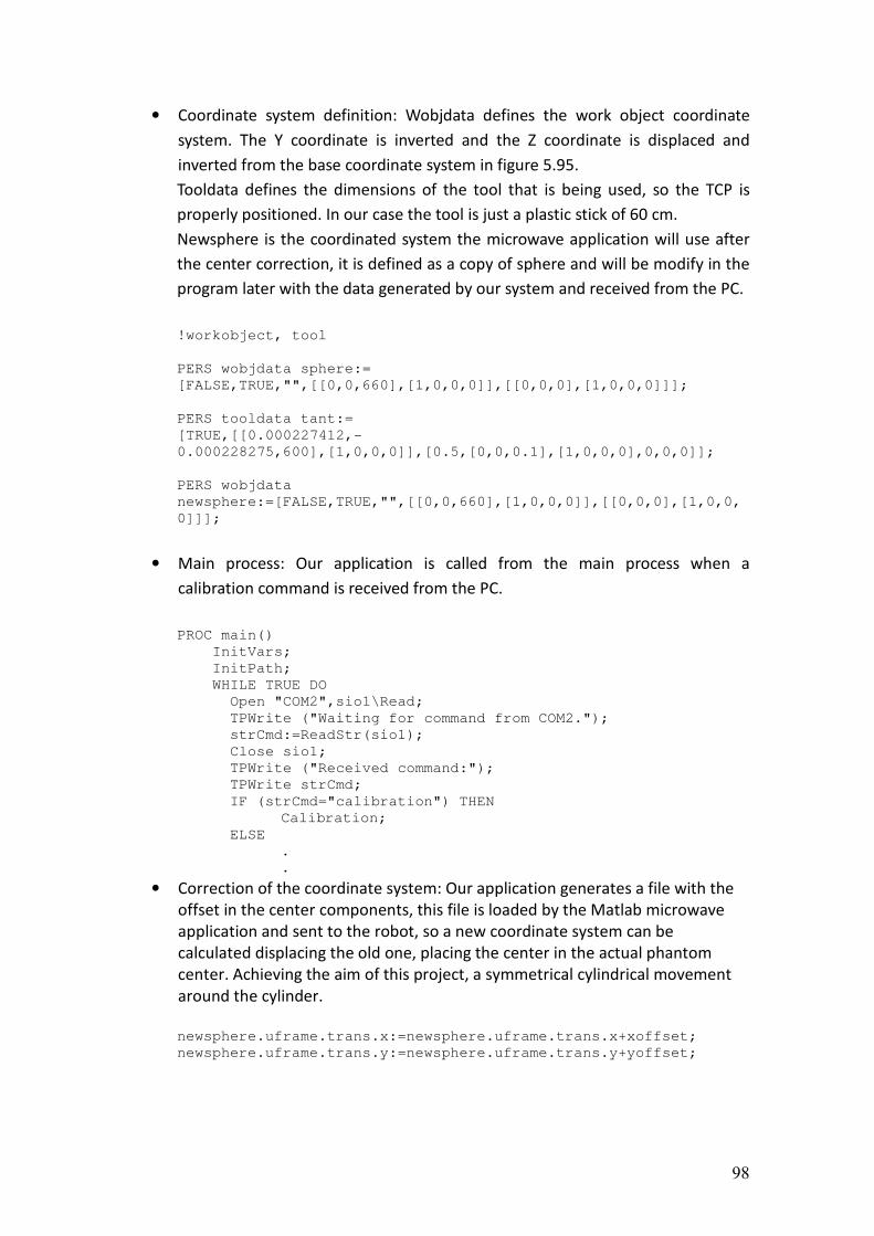
98

• Coordinate system definition: Wobjdata defines the work object coordinate

system. The Y coordinate is inverted and the Z coordinate is displaced and

inverted from the base coordinate system in figure 5.95.

Tooldata defines the dimensions of the tool that is being used, so the TCP is

properly positioned. In our case the tool is just a plastic stick of 60 cm.

Newsphere is the coordinated system the microwave application will use after

the center correction, it is defined as a copy of sphere and will be modify in the

program later with the data generated by our system and received from the PC.

!workobject, tool

PERS wobjdata sphere:=

[FALSE,TRUE,"",[[0,0,660],[1,0,0,0]],[[0,0,0],[1,0,0,0]]];

PERS tooldata tant:=

[TRUE,[[0.000227412,-

0.000228275,600],[1,0,0,0]],[0.5,[0,0,0.1],[1,0,0,0],0,0,0]];

PERS wobjdata

newsphere:=[FALSE,TRUE,"",[[0,0,660],[1,0,0,0]],[[0,0,0],[1,0,0,

0]]];

• Main process: Our application is called from the main process when a

calibration command is received from the PC.

PROC main()

InitVars;

InitPath;

WHILE TRUE DO

Open "COM2",sio1\Read;

TPWrite ("Waiting for command from COM2.");

strCmd:=ReadStr(sio1);

Close sio1;

TPWrite ("Received command:");

TPWrite strCmd;

IF (strCmd="calibration") THEN

Calibration;

ELSE

.

.

• Correction of the coordinate system: Our application generates a file with the

offset in the center components, this file is loaded by the Matlab microwave

application and sent to the robot, so a new coordinate system can be

calculated displacing the old one, placing the center in the actual phantom

center. Achieving the aim of this project, a symmetrical cylindrical movement

around the cylinder.

newsphere.uframe.trans.x:=newsphere.uframe.trans.x+xoffset;

newsphere.uframe.trans.y:=newsphere.uframe.trans.y+yoffset;

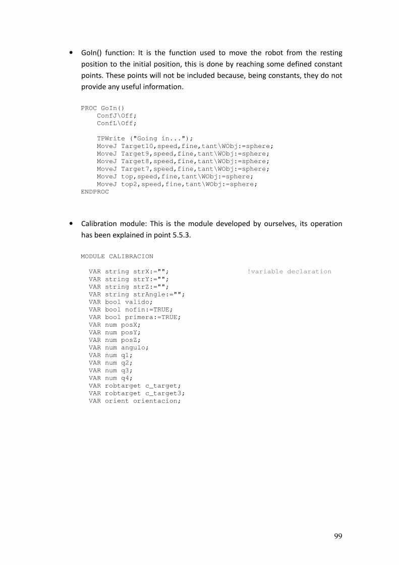
99

• GoIn() function: It is the function used to move the robot from the resting

position to the initial position, this is done by reaching some defined constant

points. These points will not be included because, being constants, they do not

provide any useful information.

PROC GoIn()

ConfJ\Off;

ConfL\Off;

TPWrite ("Going in...");

MoveJ Target10,speed,fine,tant\WObj:=sphere;




MoveJ top,speed,fine,tant\WObj:=sphere;

MoveJ top2,speed,fine,tant\WObj:=sphere;

ENDPROC

• Calibration module: This is the module developed by ourselves, its operation

has been explained in point 5.5.3.

MODULE CALIBRACION

VAR string strX:=""; !variable declaration

VAR string strY:="";

VAR string strZ:="";

VAR string strAngle:="";

VAR bool valido;

VAR bool nofin:=TRUE;

VAR bool primera:=TRUE;

VAR num posX;

VAR num posY;

VAR num posZ;

VAR num angulo;

VAR num q1;

VAR num q2;

VAR num q3;

VAR num q4;

VAR robtarget c_target;

VAR robtarget c_target3;

VAR orient orientacion;

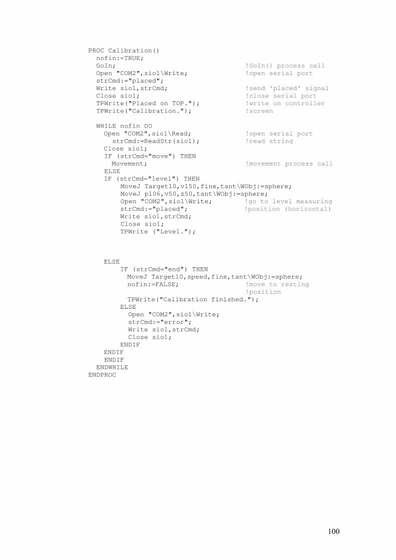
100

PROC Calibration()

nofin:=TRUE;

GoIn; !GoIn() process call

Open "COM2",sio1\Write; !open serial port

strCmd:="placed";

Write sio1,strCmd; !send ‘placed’ signal

Close sio1; !close serial port

TPWrite("Placed on TOP."); !write on controller

TPWrite("Calibration."); !screen

WHILE nofin DO

Open "COM2",sio1\Read; !open serial port

strCmd:=ReadStr(sio1); !read string

Close sio1;

IF (strCmd="move") THEN

Movement; !movement process call

ELSE

IF (strCmd="level") THEN

MoveJ Target10,v150,fine,tant\WObj:=sphere;

MoveJ p106,v50,z50,tant\WObj:=sphere;

Open "COM2",sio1\Write; !go to level measuring

strCmd:="placed"; !position (horizontal)

Write sio1,strCmd;

Close sio1;

TPWrite ("Level.");

ELSE

IF (strCmd="end") THEN


nofin:=FALSE; !move to resting

!position

TPWrite("Calibration finished.");

ELSE

Open "COM2",sio1\Write;

strCmd:="error";

Write sio1,strCmd;

Close sio1;

ENDIF

ENDIF

ENDIF

ENDWHILE

ENDPROC

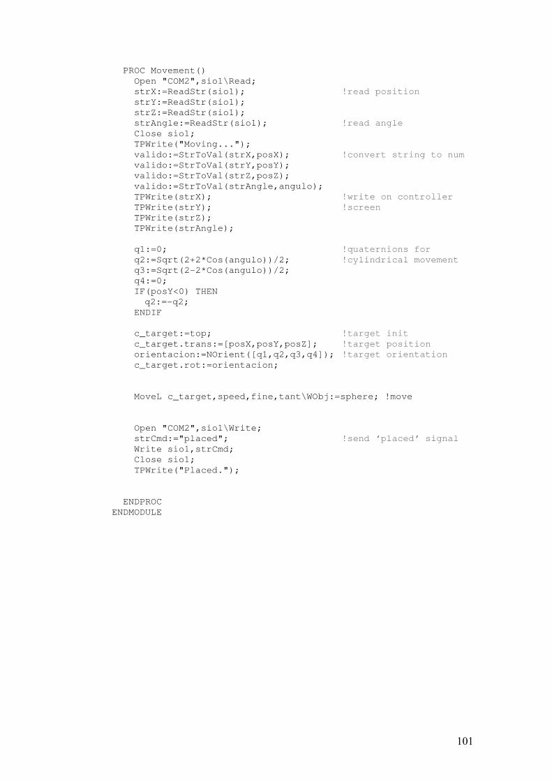
101

PROC Movement()

Open "COM2",sio1\Read;

strX:=ReadStr(sio1); !read position

strY:=ReadStr(sio1);

strZ:=ReadStr(sio1);

strAngle:=ReadStr(sio1); !read angle

Close sio1;

TPWrite("Moving...");

valido:=StrToVal(strX,posX); !convert string to num

valido:=StrToVal(strY,posY);

valido:=StrToVal(strZ,posZ);

valido:=StrToVal(strAngle,angulo);

TPWrite(strX); !write on controller

TPWrite(strY); !screen

TPWrite(strZ);

TPWrite(strAngle);

q1:=0; !quaternions for

q2:=Sqrt(2+2*Cos(angulo))/2; !cylindrical movement

q3:=Sqrt(2-2*Cos(angulo))/2;

q4:=0;

IF(posY<0) THEN

q2:=-q2;

ENDIF

c_target:=top; !target init

c_target.trans:=[posX,posY,posZ]; !target position

orientacion:=NOrient([q1,q2,q3,q4]); !target orientation

c_target.rot:=orientacion;

MoveL c_target,speed,fine,tant\WObj:=sphere; !move

Open "COM2",sio1\Write;

strCmd:="placed"; !send ‘placed’ signal

Write sio1,strCmd;

Close sio1;

TPWrite("Placed.");

ENDPROC

ENDMODULE

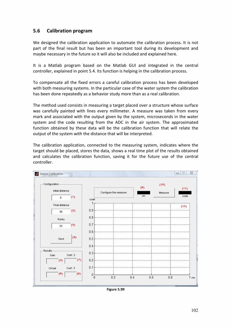
102

5.6 Calibration program

We designed the calibration application to automate the calibration process. It is not

part of the final result but has been an important tool during its development and

maybe necessary in the future so it will also be included and explained here.

It is a Matlab program based on the Matlab GUI and integrated in the central

controller, explained in point 5.4. Its function is helping in the calibration process.

To compensate all the fixed errors a careful calibration process has been developed

with both measuring systems. In the particular case of the water system the calibration

has been done repeatedly as a behavior study more than as a real calibration.

The method used consists in measuring a target placed over a structure whose surface

was carefully painted with lines every millimeter. A measure was taken from every

mark and associated with the output given by the system, microseconds in the water

system and the code resulting from the ADC in the air system. The approximated

function obtained by these data will be the calibration function that will relate the

output of the system with the distance that will be interpreted.

The calibration application, connected to the measuring system, indicates where the

target should be placed, stores the data, shows a real time plot of the results obtained

and calculates the calibration function, saving it for the future use of the central

controller.

Figure 5.99

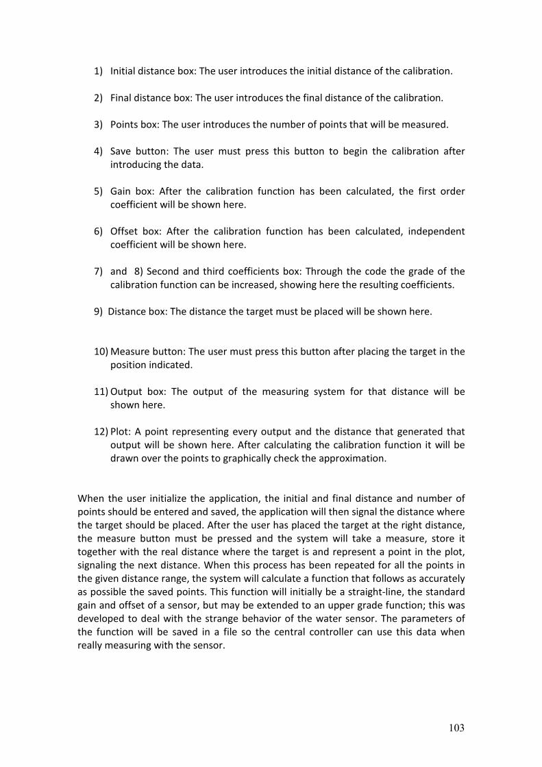
103

1) Initial distance box: The user introduces the initial distance of the calibration.

2) Final distance box: The user introduces the final distance of the calibration.

3) Points box: The user introduces the number of points that will be measured.

4) Save button: The user must press this button to begin the calibration after

introducing the data.

5) Gain box: After the calibration function has been calculated, the first order

coefficient will be shown here.

6) Offset box: After the calibration function has been calculated, independent

coefficient will be shown here.

7) and 8) Second and third coefficients box: Through the code the grade of the

calibration function can be increased, showing here the resulting coefficients.

9) Distance box: The distance the target must be placed will be shown here.

10) Measure button: The user must press this button after placing the target in the

position indicated.

11) Output box: The output of the measuring system for that distance will be

shown here.

12) Plot: A point representing every output and the distance that generated that

output will be shown here. After calculating the calibration function it will be

drawn over the points to graphically check the approximation.

When the user initialize the application, the initial and final distance and number of

points should be entered and saved, the application will then signal the distance where

the target should be placed. After the user has placed the target at the right distance,

the measure button must be pressed and the system will take a measure, store it

together with the real distance where the target is and represent a point in the plot,

signaling the next distance. When this process has been repeated for all the points in

the given distance range, the system will calculate a function that follows as accurately

as possible the saved points. This function will initially be a straight-line, the standard

gain and offset of a sensor, but may be extended to an upper grade function; this was

developed to deal with the strange behavior of the water sensor. The parameters of

the function will be saved in a file so the central controller can use this data when

really measuring with the sensor.

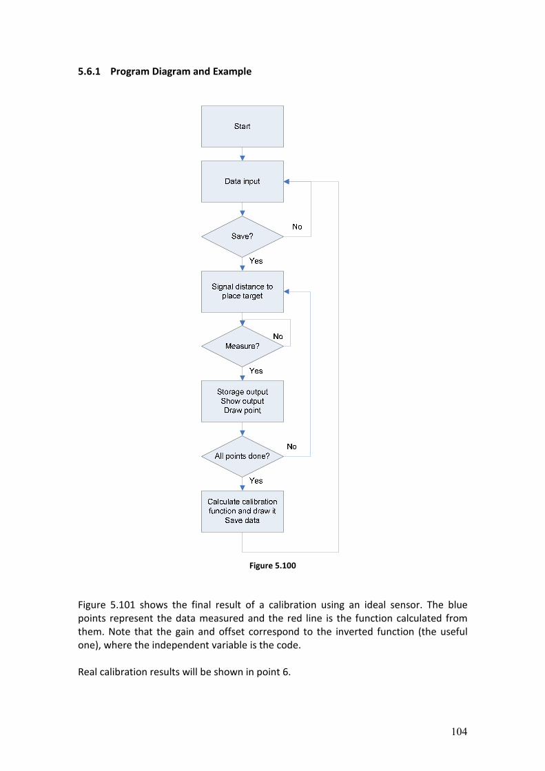
104

5.6.1 Program Diagram and Example

Figure 5.100

Figure 5.101 shows the final result of a calibration using an ideal sensor. The blue

points represent the data measured and the red line is the function calculated from

them. Note that the gain and offset correspond to the inverted function (the useful

one), where the independent variable is the code.

Real calibration results will be shown in point 6.

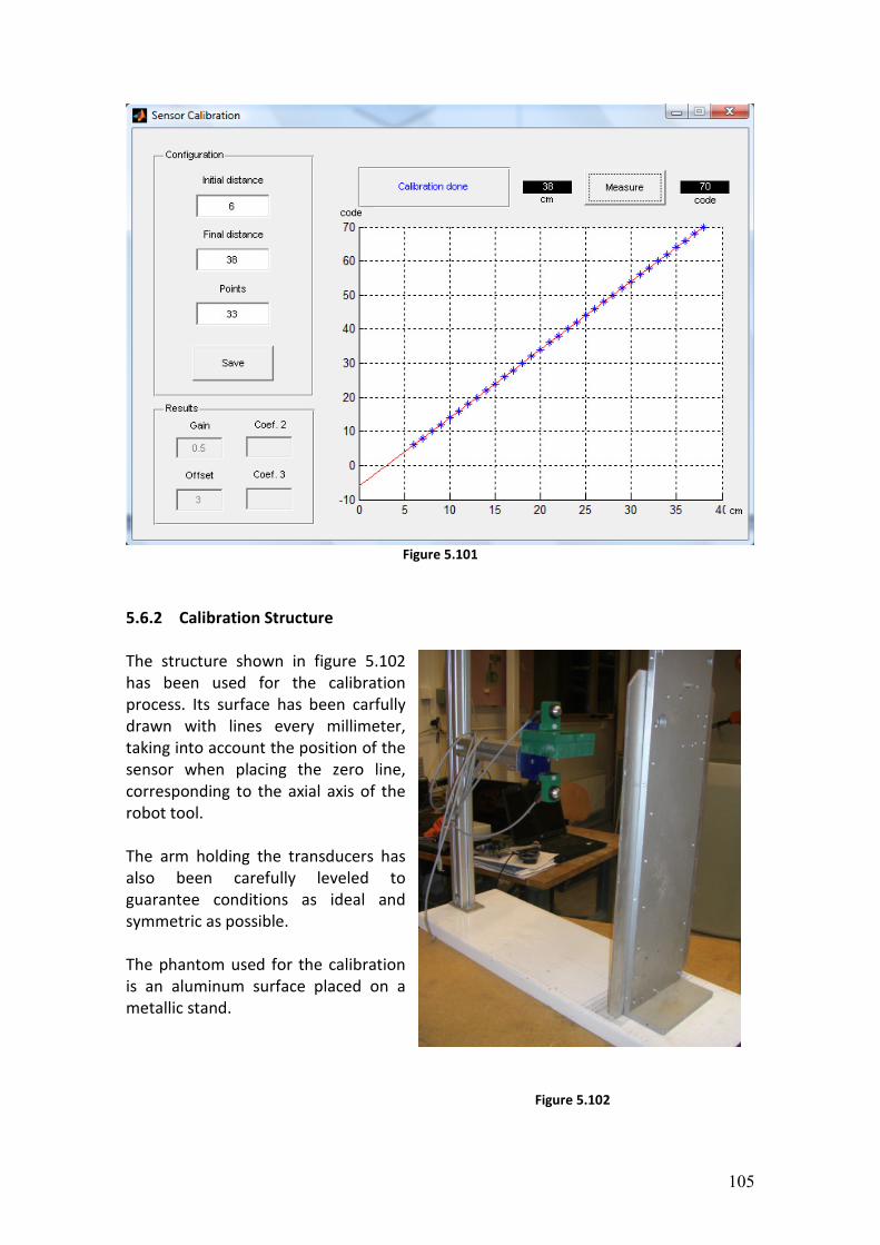
105

Figure 5.101

5.6.2 Calibration Structure

The structure shown in figure 5.102

has been used for the calibration

process. Its surface has been carfully

drawn with lines every millimeter,

taking into account the position of the

sensor when placing the zero line,

corresponding to the axial axis of the

robot tool.

The arm holding the transducers has

also been carefully leveled to

guarantee conditions as ideal and

symmetric as possible.

The phantom used for the calibration

is an aluminum surface placed on a

metallic stand.

Figure 5.102

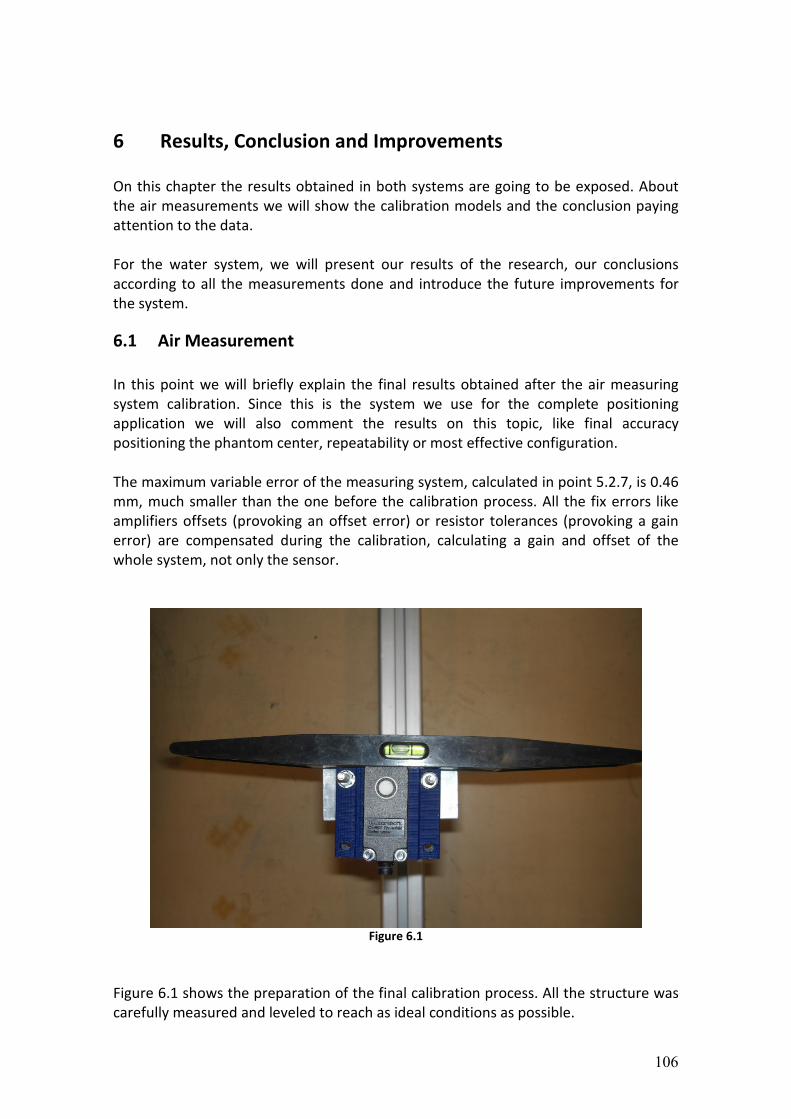
106

6 Results, Conclusion and Improvements

On this chapter the results obtained in both systems are going to be exposed. About

the air measurements we will show the calibration models and the conclusion paying

attention to the data.

For the water system, we will present our results of the research, our conclusions

according to all the measurements done and introduce the future improvements for

the system.

6.1 Air Measurement

In this point we will briefly explain the final results obtained after the air measuring

system calibration. Since this is the system we use for the complete positioning

application we will also comment the results on this topic, like final accuracy

positioning the phantom center, repeatability or most effective configuration.

The maximum variable error of the measuring system, calculated in point 5.2.7, is 0.46

mm, much smaller than the one before the calibration process. All the fix errors like

amplifiers offsets (provoking an offset error) or resistor tolerances (provoking a gain

error) are compensated during the calibration, calculating a gain and offset of the

whole system, not only the sensor.

Figure 6.1

Figure 6.1 shows the preparation of the final calibration process. All the structure was

carefully measured and leveled to reach as ideal conditions as possible.

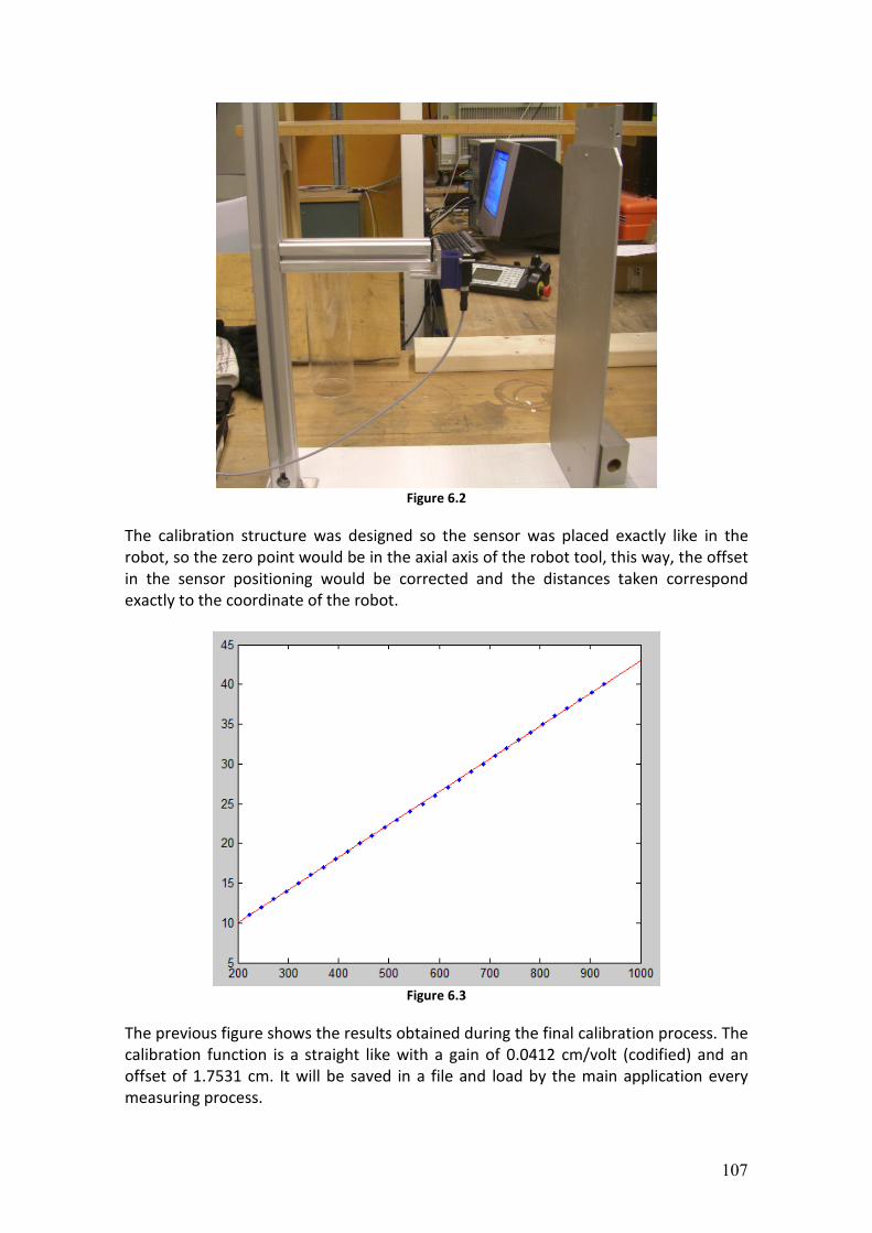
107

Figure 6.2

The calibration structure was designed so the sensor was placed exactly like in the

robot, so the zero point would be in the axial axis of the robot tool, this way, the offset

in the sensor positioning would be corrected and the distances taken correspond

exactly to the coordinate of the robot.

Figure 6.3

The previous figure shows the results obtained during the final calibration process. The

calibration function is a straight like with a gain of 0.0412 cm/volt (codified) and an

offset of 1.7531 cm. It will be saved in a file and load by the main application every

measuring process.

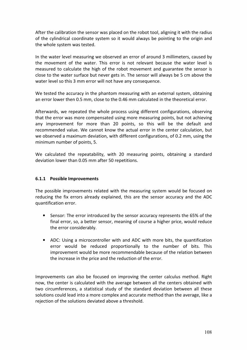
108

After the calibration the sensor was placed on the robot tool, aligning it with the radius

of the cylindrical coordinate system so it would always be pointing to the origin and

the whole system was tested.

In the water level measuring we observed an error of around 3 millimeters, caused by

the movement of the water. This error is not relevant because the water level is

measured to calculate the high of the robot movement and guarantee the sensor is

close to the water surface but never gets in. The sensor will always be 5 cm above the

water level so this 3 mm error will not have any consequence.

We tested the accuracy in the phantom measuring with an external system, obtaining

an error lower then 0.5 mm, close to the 0.46 mm calculated in the theoretical error.

Afterwards, we repeated the whole process using different configurations, observing

that the error was more compensated using more measuring points, but not achieving

any improvement for more than 20 points, so this will be the default and

recommended value. We cannot know the actual error in the center calculation, but

we observed a maximum deviation, with different configurations, of 0.2 mm, using the

minimum number of points, 5.

We calculated the repeatability, with 20 measuring points, obtaining a standard

deviation lower than 0.05 mm after 50 repetitions.

6.1.1 Possible Improvements

The possible improvements related with the measuring system would be focused on

reducing the fix errors already explained, this are the sensor accuracy and the ADC

quantification error.

• Sensor: The error introduced by the sensor accuracy represents the 65% of the

final error, so, a better sensor, meaning of course a higher price, would reduce

the error considerably.

• ADC: Using a microcontroller with and ADC with more bits, the quantification

error would be reduced proportionally to the number of bits. This

improvement would be more recommendable because of the relation between

the increase in the price and the reduction of the error.

Improvements can also be focused on improving the center calculus method. Right

now, the center is calculated with the average between all the centers obtained with

two circumferences, a statistical study of the standard deviation between all these

solutions could lead into a more complex and accurate method than the average, like a

rejection of the solutions deviated above a threshold.

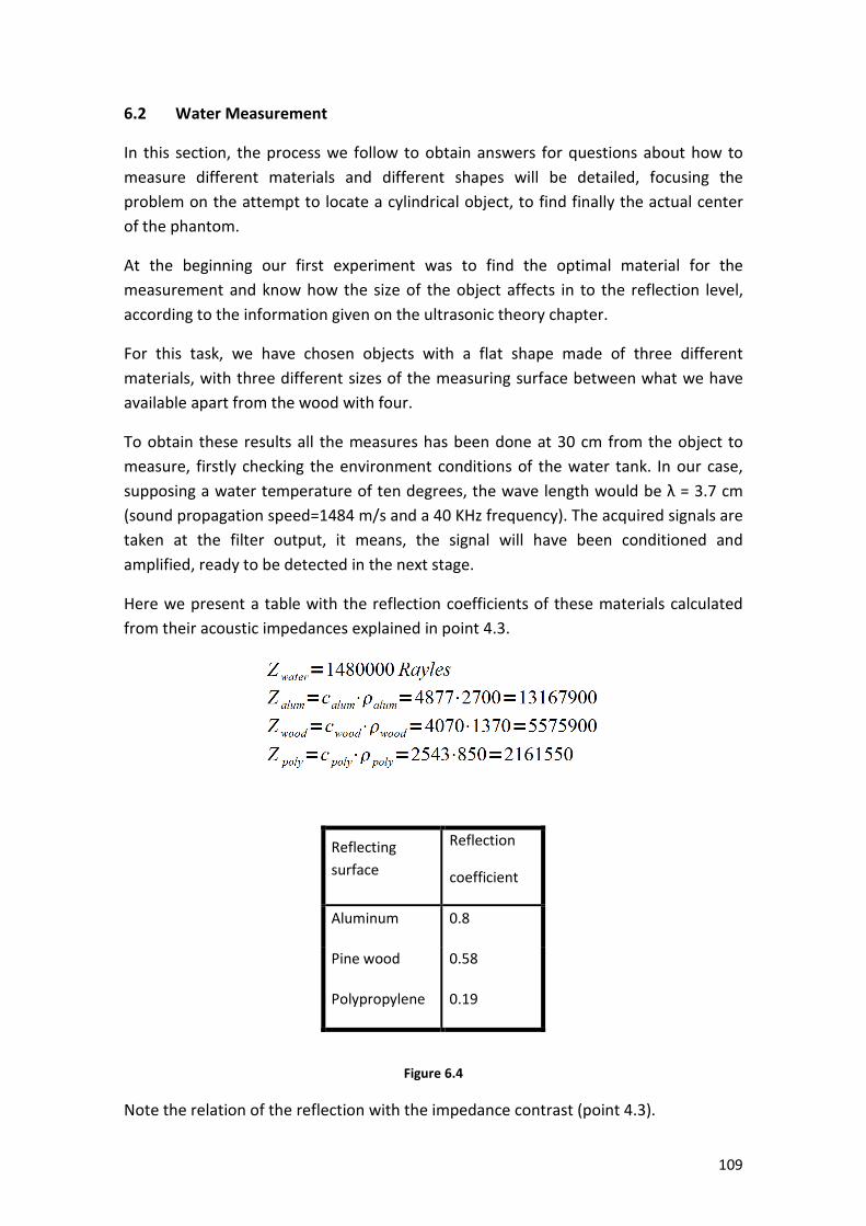
109

6.2 Water Measurement

In this section, the process we follow to obtain answers for questions about how to

measure different materials and different shapes will be detailed, focusing the

problem on the attempt to locate a cylindrical object, to find finally the actual center

of the phantom.

At the beginning our first experiment was to find the optimal material for the

measurement and know how the size of the object affects in to the reflection level,

according to the information given on the ultrasonic theory chapter.

For this task, we have chosen objects with a flat shape made of three different

materials, with three different sizes of the measuring surface between what we have

available apart from the wood with four.

To obtain these results all the measures has been done at 30 cm from the object to

measure, firstly checking the environment conditions of the water tank. In our case,

supposing a water temperature of ten degrees, the wave length would be λ = 3.7 cm

(sound propagation speed=1484 m/s and a 40 KHz frequency). The acquired signals are

taken at the filter output, it means, the signal will have been conditioned and

amplified, ready to be detected in the next stage.

Here we present a table with the reflection coefficients of these materials calculated

from their acoustic impedances explained in point 4.3.

Figure 6.4

Note the relation of the reflection with the impedance contrast (point 4.3).

Reflecting

surface

Reflection

coefficient

Aluminum 0.8

Pine wood 0.58

Polypropylene 0.19

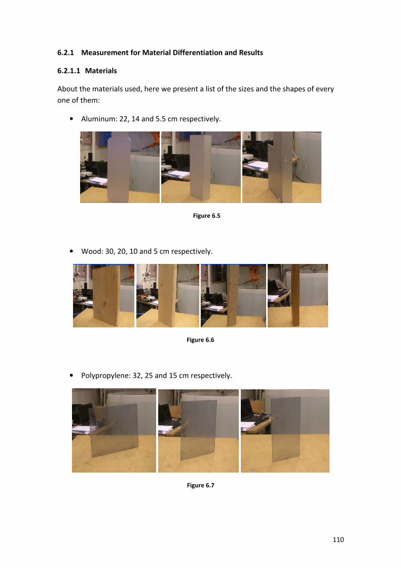
110

6.2.1 Measurement for Material Differentiation and Results

6.2.1.1 Materials

About the materials used, here we present a list of the sizes and the shapes of every

one of them:

• Aluminum: 22, 14 and 5.5 cm respectively.

Figure 6.5

• Wood: 30, 20, 10 and 5 cm respectively.

Figure 6.6

• Polypropylene: 32, 25 and 15 cm respectively.

Figure 6.7

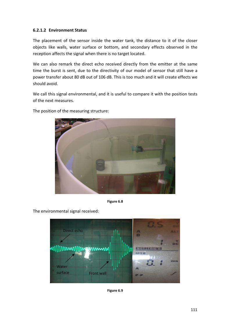
111

6.2.1.2 Environment Status

The placement of the sensor inside the water tank, the distance to it of the closer

objects like walls, water surface or bottom, and secondary effects observed in the

reception affects the signal when there is no target located.

We can also remark the direct echo received directly from the emitter at the same

time the burst is sent, due to the directivity of our model of sensor that still have a

power transfer about 80 dB out of 106 dB. This is too much and it will create effects we

should avoid.

We call this signal environmental, and it is useful to compare it with the position tests

of the next measures.

The position of the measuring structure:

Figure 6.8

The environmental signal received:

Figure 6.9

Front wall

Direct echo

Water

surface

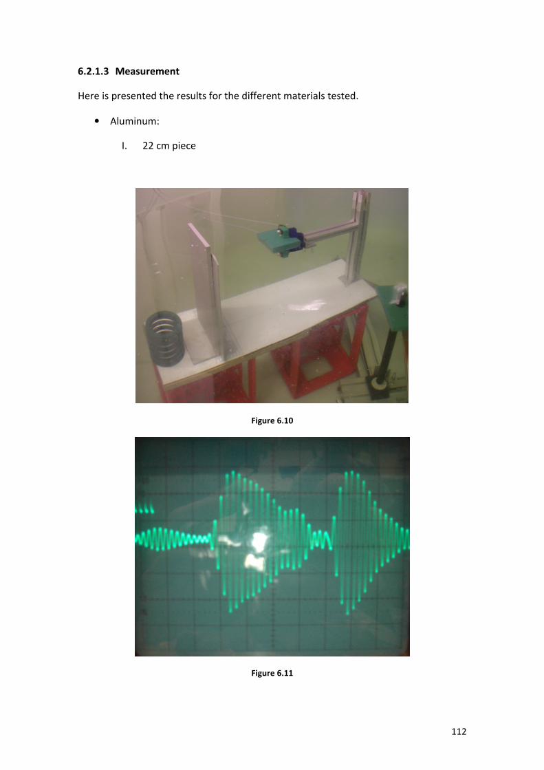
112

6.2.1.3 Measurement

Here is presented the results for the different materials tested.

• Aluminum:

I. 22 cm piece

Figure 6.10

Figure 6.11

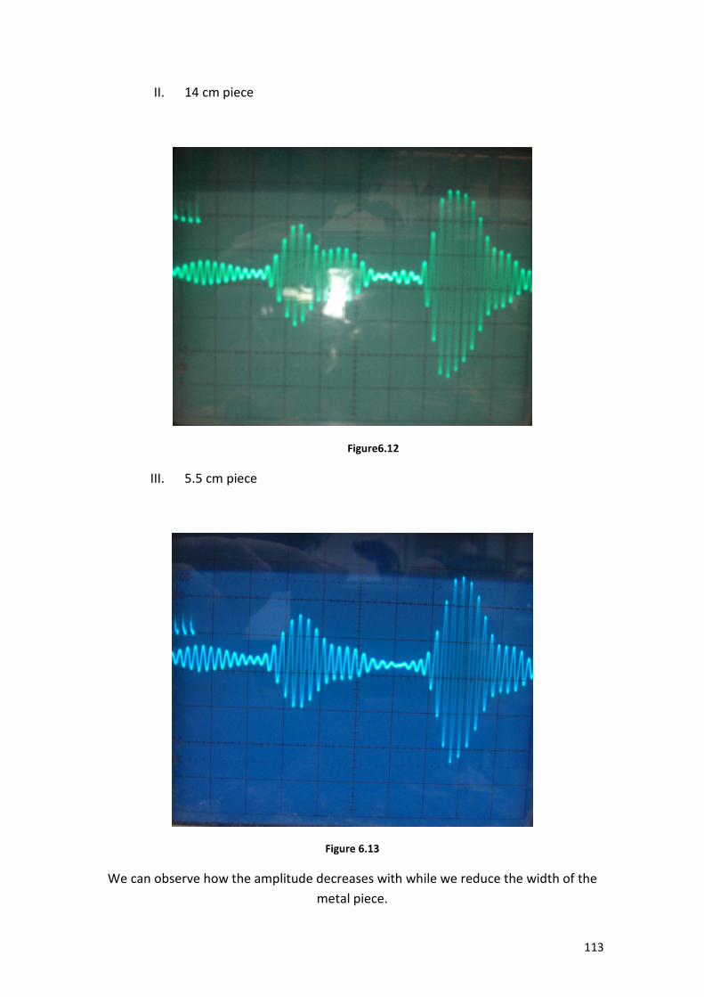
113

II. 14 cm piece

Figure6.12

III. 5.5 cm piece

Figure 6.13

We can observe how the amplitude decreases with while we reduce the width of the

metal piece.

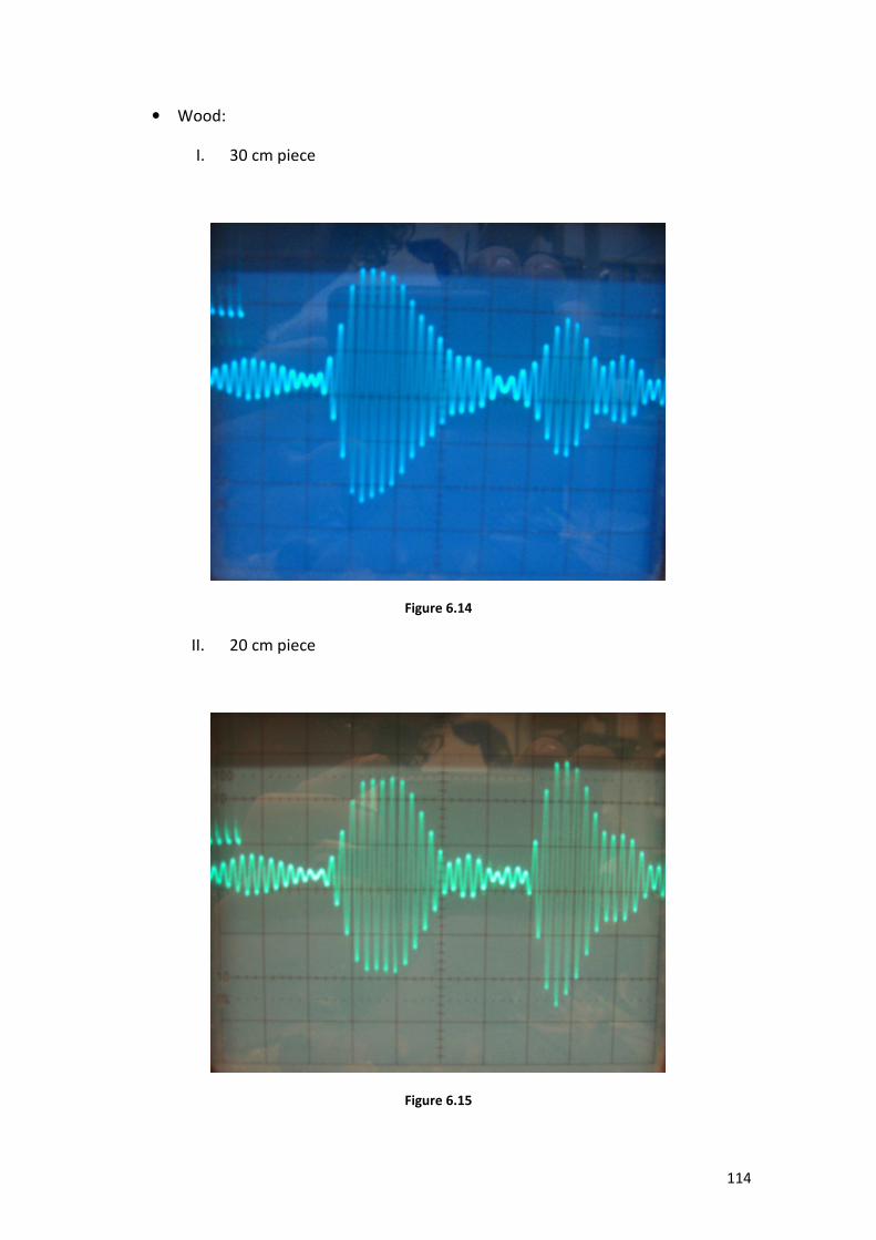
114

• Wood:

I. 30 cm piece

Figure 6.14

II. 20 cm piece

Figure 6.15

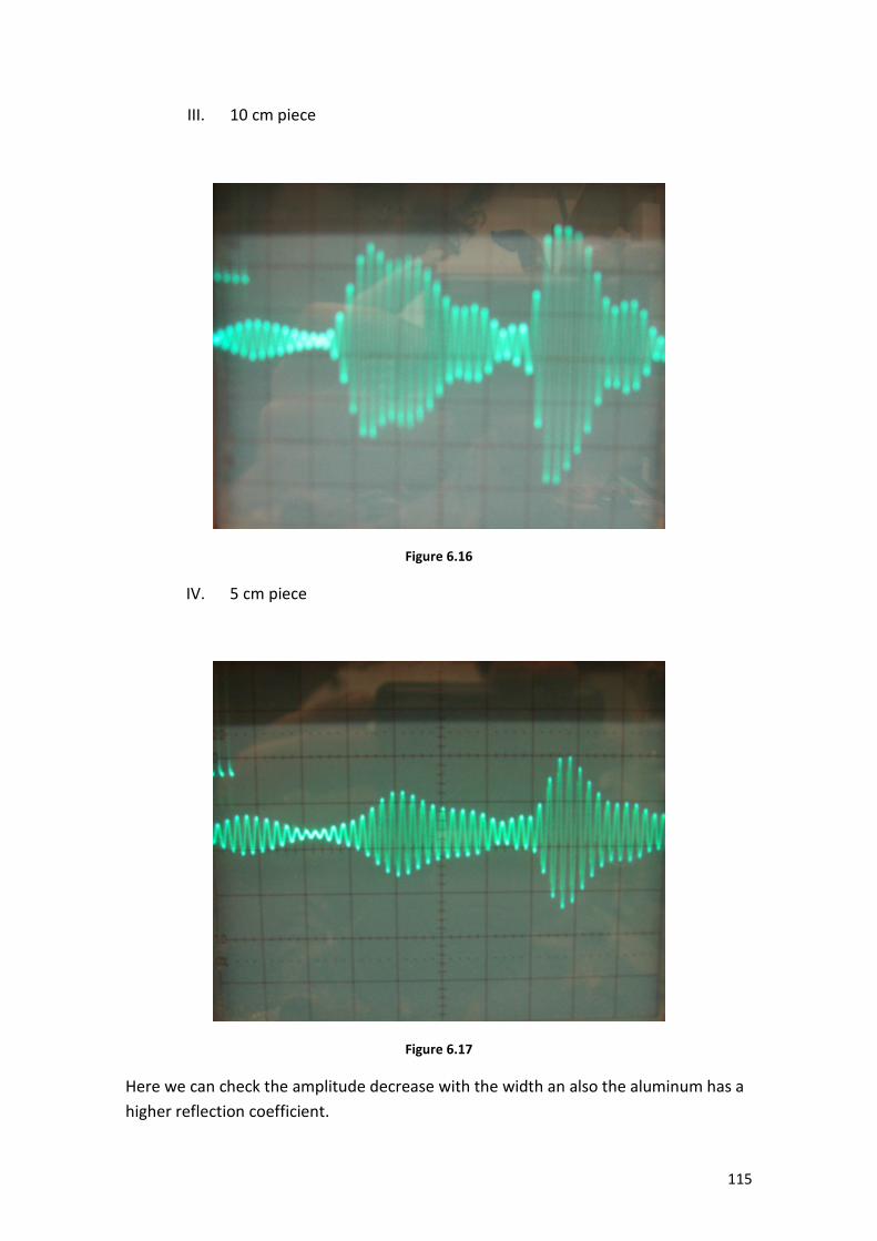
115

III. 10 cm piece

Figure 6.16

IV. 5 cm piece

Figure 6.17

Here we can check the amplitude decrease with the width an also the aluminum has a

higher reflection coefficient.

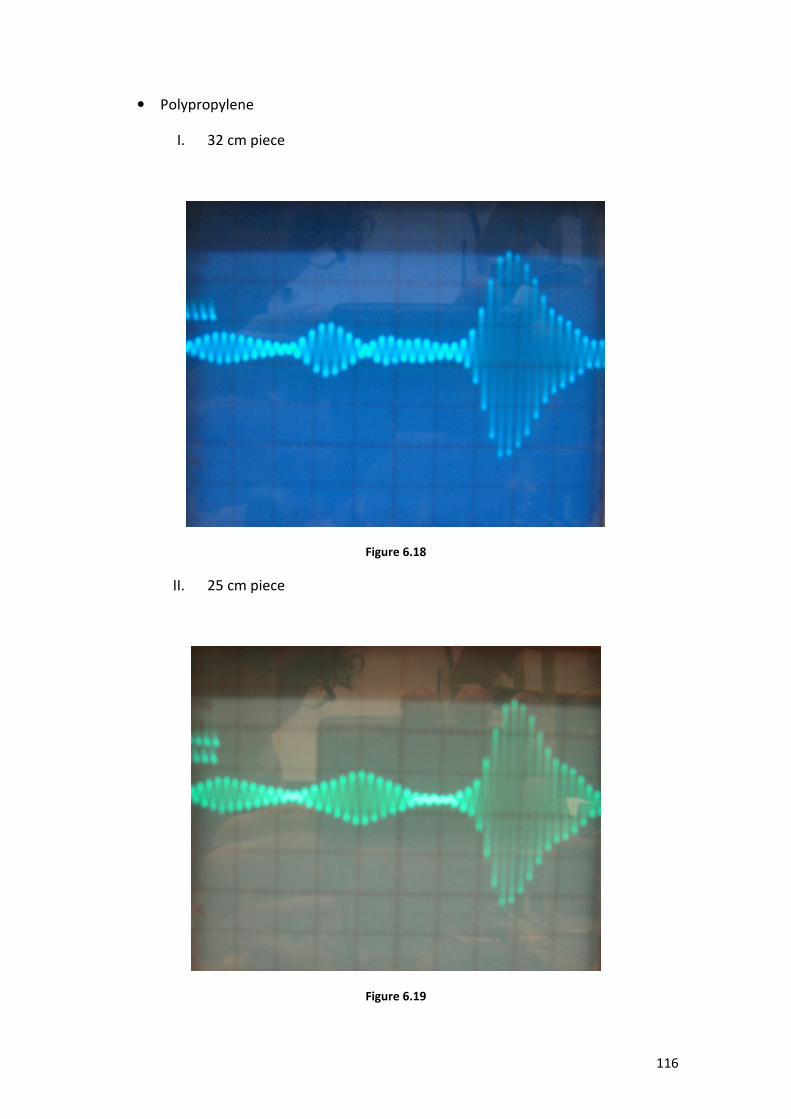
116

• Polypropylene

I. 32 cm piece

Figure 6.18

II. 25 cm piece

Figure 6.19

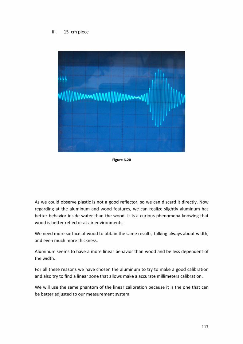
117

III. 15 cm piece

Figure 6.20

As we could observe plastic is not a good reflector, so we can discard it directly. Now

regarding at the aluminum and wood features, we can realize slightly aluminum has

better behavior inside water than the wood. It is a curious phenomena knowing that

wood is better reflector at air environments.

We need more surface of wood to obtain the same results, talking always about width,

and even much more thickness.

Aluminum seems to have a more linear behavior than wood and be less dependent of

the width.

For all these reasons we have chosen the aluminum to try to make a good calibration

and also try to find a linear zone that allows make a accurate millimeters calibration.

We will use the same phantom of the linear calibration because it is the one that can

be better adjusted to our measurement system.

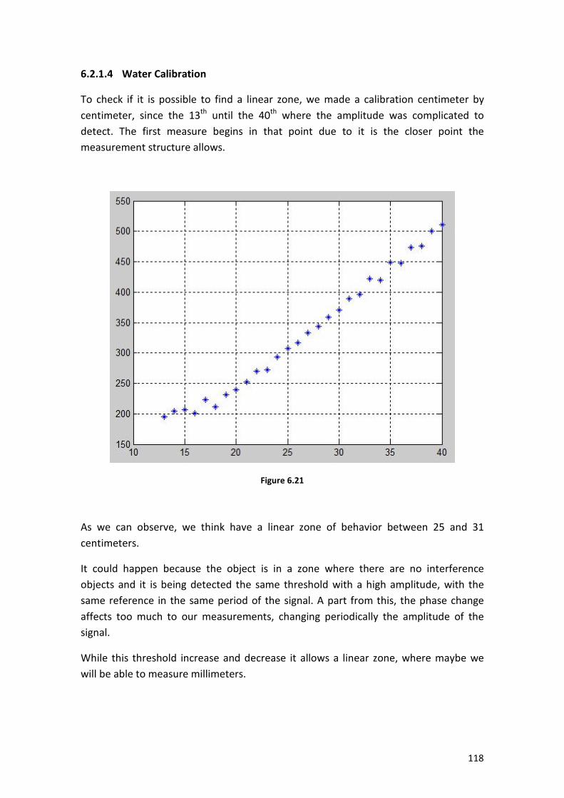
118

6.2.1.4 Water Calibration

To check if it is possible to find a linear zone, we made a calibration centimeter by

centimeter, since the 13th

until the 40th

where the amplitude was complicated to

detect. The first measure begins in that point due to it is the closer point the

measurement structure allows.

Figure 6.21

As we can observe, we think have a linear zone of behavior between 25 and 31

centimeters.

It could happen because the object is in a zone where there are no interference

objects and it is being detected the same threshold with a high amplitude, with the

same reference in the same period of the signal. A part from this, the phase change

affects too much to our measurements, changing periodically the amplitude of the

signal.

While this threshold increase and decrease it allows a linear zone, where maybe we

will be able to measure millimeters.

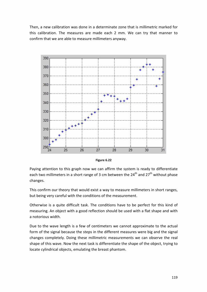
119

Then, a new calibration was done in a determinate zone that is millimetric marked for

this calibration. The measures are made each 2 mm. We can try that manner to

confirm that we are able to measure millimeters anyway.

Figure 6.22

Paying attention to this graph now we can affirm the system is ready to differentiate

each two millimeters in a short range of 3 cm between the 24th

and 27th

without phase

changes.

This confirm our theory that would exist a way to measure millimeters in short ranges,

but being very careful with the conditions of the measurement.

Otherwise is a quite difficult task. The conditions have to be perfect for this kind of

measuring. An object with a good reflection should be used with a flat shape and with

a notorious width.

Due to the wave length is a few of centimeters we cannot approximate to the actual

form of the signal because the steps in the different measures were big and the signal

changes completely. Doing these millimetric measurements we can observe the real

shape of this wave. Now the next task is differentiate the shape of the object, trying to

locate cylindrical objects, emulating the breast phantom.

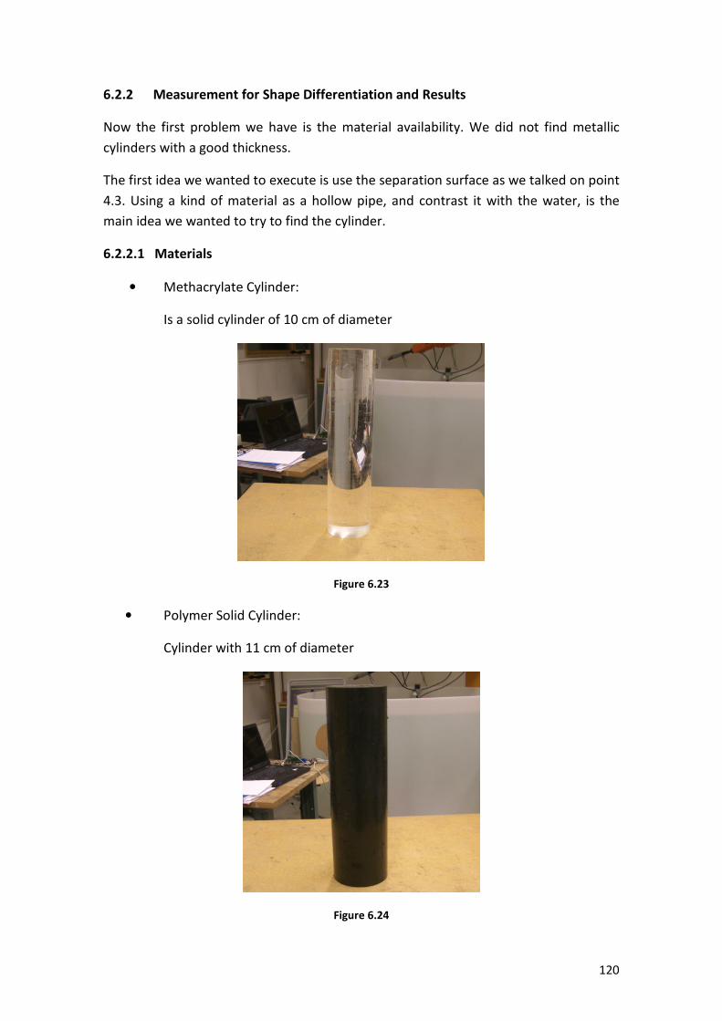
120

6.2.2 Measurement for Shape Differentiation and Results

Now the first problem we have is the material availability. We did not find metallic

cylinders with a good thickness.

The first idea we wanted to execute is use the separation surface as we talked on point

4.3. Using a kind of material as a hollow pipe, and contrast it with the water, is the

main idea we wanted to try to find the cylinder.

6.2.2.1 Materials

• Methacrylate Cylinder:

Is a solid cylinder of 10 cm of diameter

Figure 6.23

• Polymer Solid Cylinder:

Cylinder with 11 cm of diameter

Figure 6.24

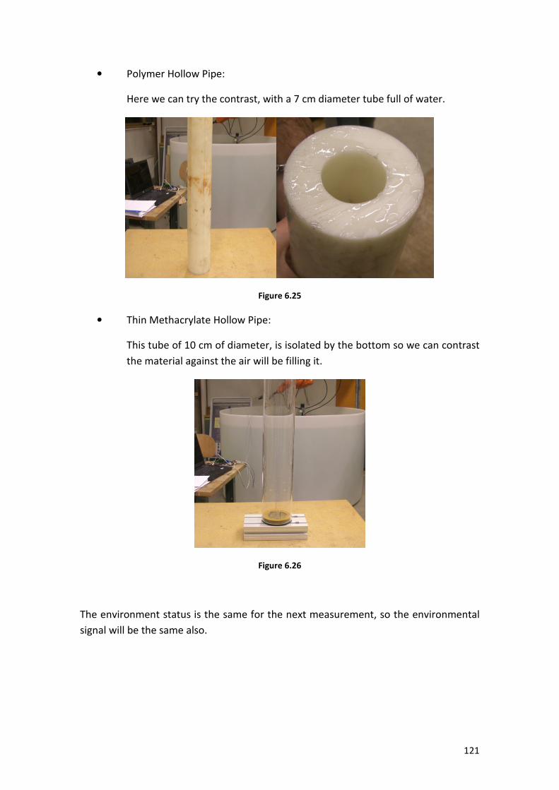
121

• Polymer Hollow Pipe:

Here we can try the contrast, with a 7 cm diameter tube full of water.

Figure 6.25

• Thin Methacrylate Hollow Pipe:

This tube of 10 cm of diameter, is isolated by the bottom so we can contrast

the material against the air will be filling it.

Figure 6.26

The environment status is the same for the next measurement, so the environmental

signal will be the same also.

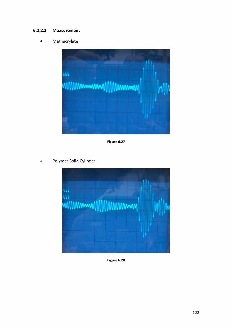
122

6.2.2.2 Measurement

• Methacrylate:

Figure 6.27

• Polymer Solid Cylinder:

Figure 6.28

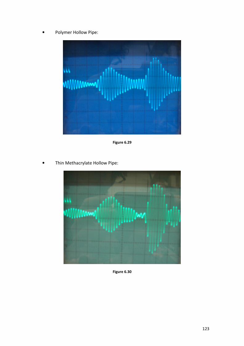
123

• Polymer Hollow Pipe:

Figure 6.29

• Thin Methacrylate Hollow Pipe:

Figure 6.30

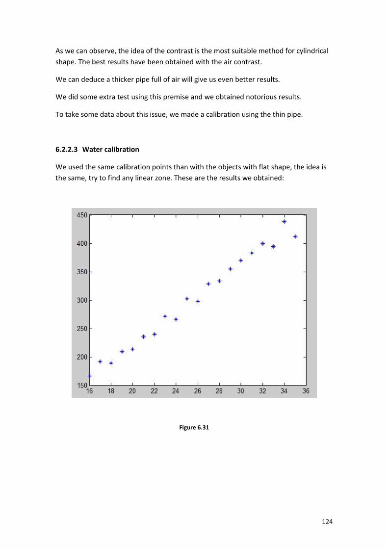
124

As we can observe, the idea of the contrast is the most suitable method for cylindrical

shape. The best results have been obtained with the air contrast.

We can deduce a thicker pipe full of air will give us even better results.

We did some extra test using this premise and we obtained notorious results.

To take some data about this issue, we made a calibration using the thin pipe.

6.2.2.3 Water calibration

We used the same calibration points than with the objects with flat shape, the idea is

the same, try to find any linear zone. These are the results we obtained:

Figure 6.31

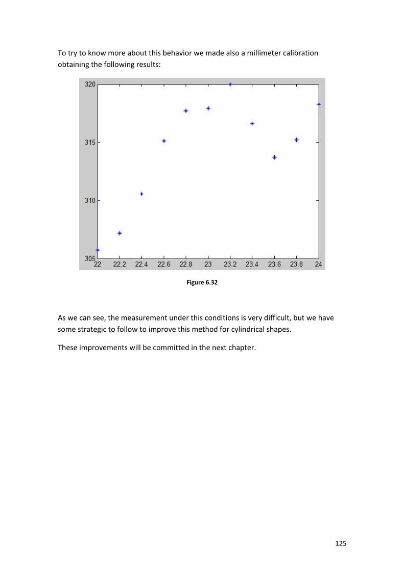
125

To try to know more about this behavior we made also a millimeter calibration

obtaining the following results:

Figure 6.32

As we can see, the measurement under this conditions is very difficult, but we have

some strategic to follow to improve this method for cylindrical shapes.

These improvements will be committed in the next chapter.

126

6.2.3 Possible Improvements

On this chapter we show the immediate improvements to continue with the

development of the underwater sensor, to power up the measurement ability of the

system.

• Firstly focusing on the hardware to use a new processor able to work with a

higher frequency to allow the ADC work with a sampling speed much faster and

increase the number of bits of it, to reduce the quantification interval. All these

changes are to improve the digitalizing skills of the system for a future new

system of detection.

• The new transducers should work also with a higher frequency as much as

possible to help the system reduce the error of detection due to the time spent

for the signal to exceed the detection threshold will be lower as long as we

decide keep on using the current method. If we opt for a new one using the

digitalization, we have to look for a compromise between the two improves

due to the elevation of the emitting frequency is counterproductive for the

quantification interval of the ADC. The directivity of the transducer is

compulsory to be changed to avoid the direct echo, at least for an interval of

[-80, 80] degrees with the maximum power transfer in a short interval in the

central range.

• Making use of a better digitalization ability, we will be able to sample the signal

received and measure the distance between the last high level of the emitting

signal and the maximum value of the signal received that is caused by the last

rising edge of the burst. It is also very interesting before emitting the burst,

make a complete capture of the environment status. This way we can subtract

to the signal received, the environment noise, to avoid possible interference.

This last improve is mostly useful if we keep on using the old detecting system.

• To help the system detecting a cylindrical shape according to our results, we

recommend to use a cylinder made of metal, thick enough (2 cm) and hollow,

isolated on the bottom and full of air, and with a bigger diameter, to increase

the reflection level.

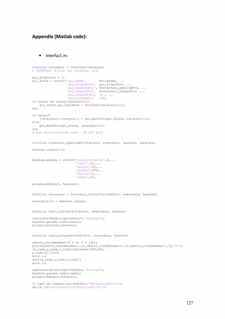
127

Appendix (Matlab code):

• interfaz1.m:

function varargout = interfaz1(varargin)

% INTERFAZ1 M-file for interfaz1.fig

gui_Singleton = 1;

gui_State = struct('gui_Name', mfilename, ...

'gui_Singleton', gui_Singleton, ...

'gui_OpeningFcn', @interfaz1_OpeningFcn, ...

'gui_OutputFcn', @interfaz1_OutputFcn, ...

'gui_LayoutFcn', [] , ...

'gui_Callback', []);

if nargin && ischar(varargin1)

gui_State.gui_Callback = str2func(varargin1);

end

if nargout

[varargout1:nargout] = gui_mainfcn(gui_State, varargin:);

else

gui_mainfcn(gui_State, varargin:);

end

% End initialization code - DO NOT EDIT

function interfaz1_OpeningFcn(hObject, eventdata, handles, varargin)

handles.output=-1;

handles.params = struct('caja_distancia',0,...

'radio',31,...

'puntos',20,...

'grados',270,...

'metodo',1,...

'level',0);

guidata(hObject, handles);

function varargout = interfaz1_OutputFcn(hObject, eventdata, handles)

varargout1 = handles.output;

function radio_Callback(hObject, eventdata, handles)

radio=str2double(get(hObject,'String'));

handles.params.radio=radio;

guidata(hObject,handles);

function radio_CreateFcn(hObject, eventdata, handles)

centro_coordenadas=[0 0 0; 0 0 120];

plot3(centro_coordenadas(:,1),centro_coordenadas(:,2),centro_coordenadas(:,3),'k');

[x_tank,y_tank,z_tank]=cylinder(100,60);

z_tank(2,:)=10;

hold on;

surf(x_tank,y_tank,z_tank);

grid on;

radio=str2double(get(hObject,'String'));

handles.params.radio=radio;


if ispc && isequal(get(hObject,'BackgroundColor'),

get(0,'defaultUicontrolBackgroundColor'))

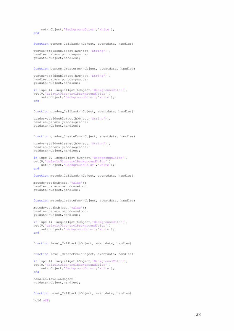
128

set(hObject,'BackgroundColor','white');

end

function puntos_Callback(hObject, eventdata, handles)

puntos=str2double(get(hObject,'String'));

handles.params.puntos=puntos;


function puntos_CreateFcn(hObject, eventdata, handles)







end

function grados_Callback(hObject, eventdata, handles)

grados=str2double(get(hObject,'String'));

handles.params.grados=grados;


function grados_CreateFcn(hObject, eventdata, handles)

grados=str2double(get(hObject,'String'));

handles.params.grados=grados;





end

function metodo_Callback(hObject, eventdata, handles)

metodo=get(hObject,'Value');

handles.params.metodo=metodo;


function metodo_CreateFcn(hObject, eventdata, handles)

metodo=get(hObject,'Value');

handles.params.metodo=metodo;





end

function level_Callback(hObject, eventdata, handles)

function level_CreateFcn(hObject, eventdata, handles)




end

handles.level=hObject;


function reset_Callback(hObject, eventdata, handles)

hold off;

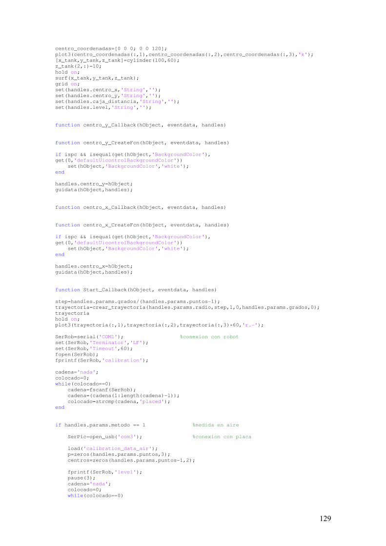
129

centro_coordenadas=[0 0 0; 0 0 120];

plot3(centro_coordenadas(:,1),centro_coordenadas(:,2),centro_coordenadas(:,3),'k');

[x_tank,y_tank,z_tank]=cylinder(100,60);

z_tank(2,:)=10;

hold on;

surf(x_tank,y_tank,z_tank);

grid on;

set(handles.centro_x,'String','');

set(handles.centro_y,'String','');

set(handles.caja_distancia,'String','');

set(handles.level,'String','');

function centro_y_Callback(hObject, eventdata, handles)

function centro_y_CreateFcn(hObject, eventdata, handles)




end

handles.centro_y=hObject;


function centro_x_Callback(hObject, eventdata, handles)

function centro_x_CreateFcn(hObject, eventdata, handles)




end

handles.centro_x=hObject;


function Start_Callback(hObject, eventdata, handles)

step=handles.params.grados/(handles.params.puntos-1);

trayectoria=crear_trayectoria(handles.params.radio,step,1,0,handles.params.grados,0);

trayectoria

hold on;

plot3(trayectoria(:,1),trayectoria(:,2),trayectoria(:,3)+60,'r.-');

SerRob=serial('COM1'); %conexion con robot

set(SerRob,'Terminator','LF');

set(SerRob,'Timeout',60);

fopen(SerRob);

fprintf(SerRob,'calibration');

cadena='nada';

colocado=0;

while(colocado==0)

cadena=fscanf(SerRob);

cadena=(cadena(1:length(cadena)-1));

colocado=strcmp(cadena,'placed');

end

if handles.params.metodo == 1 %medida en aire

SerPic=open_usb('com3'); %conexion con placa

load('calibration_data_air');

p=zeros(handles.params.puntos,3);

centros=zeros(handles.params.puntos-1,2);

fprintf(SerRob,'level');

pause(3);

cadena='nada';

colocado=0;

while(colocado==0)

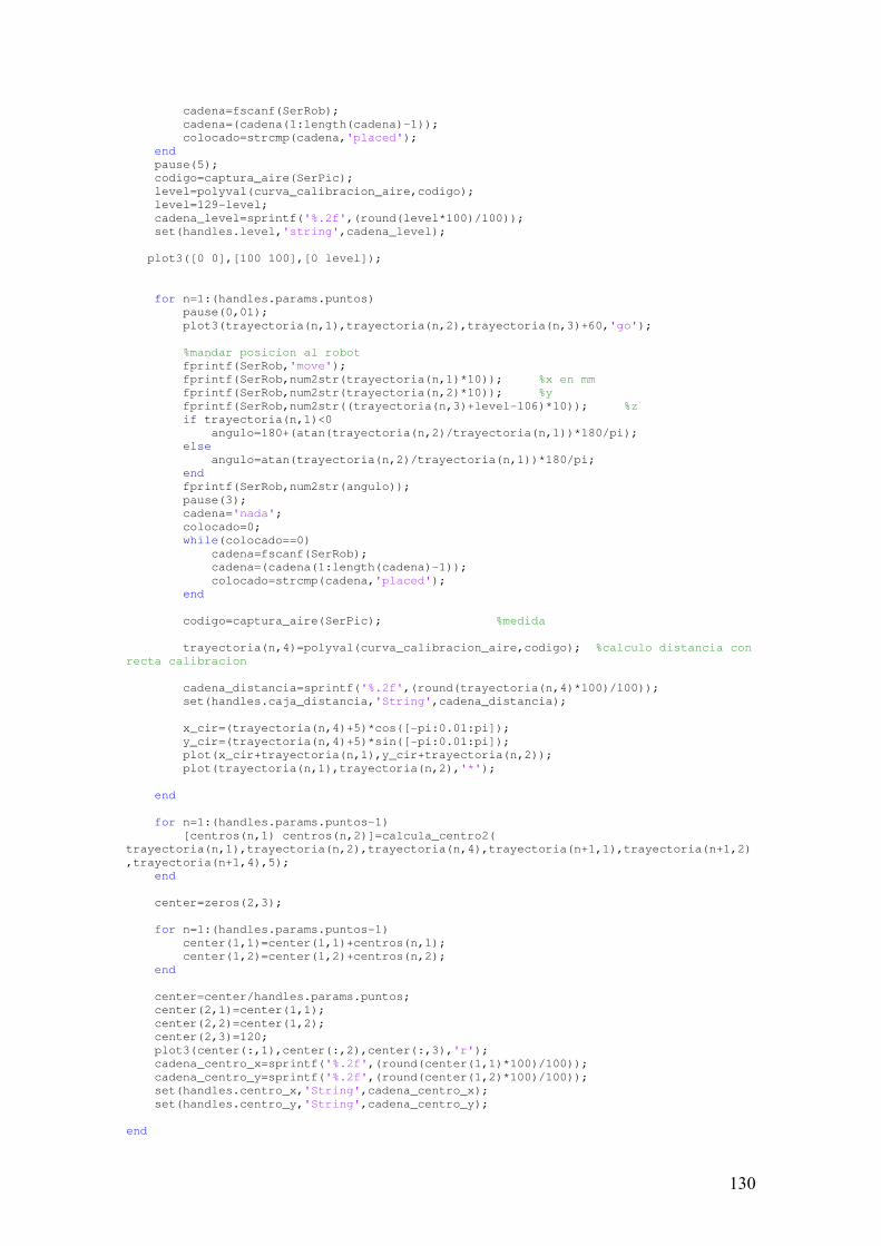
130




end

pause(5);

codigo=captura_aire(SerPic);

level=polyval(curva_calibracion_aire,codigo);

level=129-level;

cadena_level=sprintf('%.2f',(round(level*100)/100));

set(handles.level,'string',cadena_level);

plot3([0 0],[100 100],[0 level]);

for n=1:(handles.params.puntos)

pause(0,01);

plot3(trayectoria(n,1),trayectoria(n,2),trayectoria(n,3)+60,'go');

%mandar posicion al robot

fprintf(SerRob,'move');

fprintf(SerRob,num2str(trayectoria(n,1)*10)); %x en mm

fprintf(SerRob,num2str(trayectoria(n,2)*10)); %y

fprintf(SerRob,num2str((trayectoria(n,3)+level-106)*10)); %z

if trayectoria(n,1)<0

angulo=180+(atan(trayectoria(n,2)/trayectoria(n,1))*180/pi);

else

angulo=atan(trayectoria(n,2)/trayectoria(n,1))*180/pi;

end

fprintf(SerRob,num2str(angulo));

pause(3);

cadena='nada';

colocado=0;

while(colocado==0)




end

codigo=captura_aire(SerPic); %medida

trayectoria(n,4)=polyval(curva_calibracion_aire,codigo); %calculo distancia con

recta calibracion

cadena_distancia=sprintf('%.2f',(round(trayectoria(n,4)*100)/100));

set(handles.caja_distancia,'String',cadena_distancia);

x_cir=(trayectoria(n,4)+5)*cos([-pi:0.01:pi]);

y_cir=(trayectoria(n,4)+5)*sin([-pi:0.01:pi]);

plot(x_cir+trayectoria(n,1),y_cir+trayectoria(n,2));

plot(trayectoria(n,1),trayectoria(n,2),'*');

end

for n=1:(handles.params.puntos-1)

[centros(n,1) centros(n,2)]=calcula_centro2(

trayectoria(n,1),trayectoria(n,2),trayectoria(n,4),trayectoria(n+1,1),trayectoria(n+1,2)

,trayectoria(n+1,4),5);

end

center=zeros(2,3);


center(1,1)=center(1,1)+centros(n,1);

center(1,2)=center(1,2)+centros(n,2);

end

center=center/handles.params.puntos;

center(2,1)=center(1,1);


center(2,3)=120;

plot3(center(:,1),center(:,2),center(:,3),'r');

cadena_centro_x=sprintf('%.2f',(round(center(1,1)*100)/100));

cadena_centro_y=sprintf('%.2f',(round(center(1,2)*100)/100));

set(handles.centro_x,'String',cadena_centro_x);

set(handles.centro_y,'String',cadena_centro_y);

end

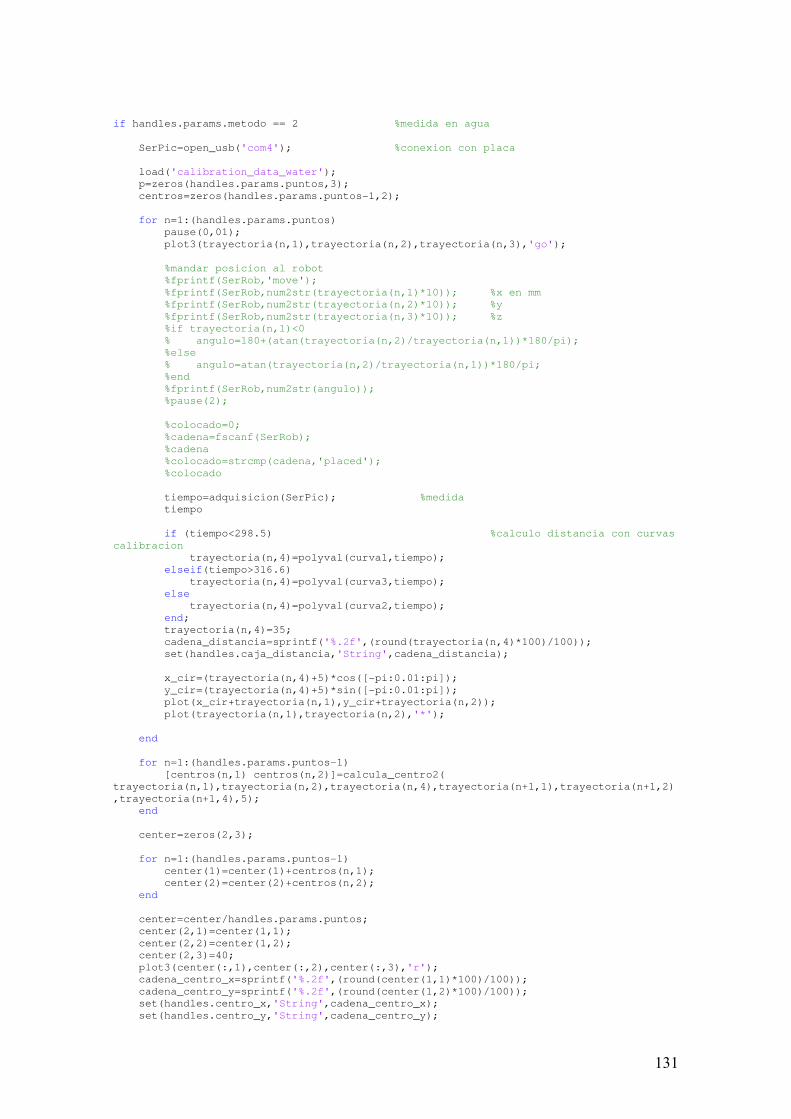
131

if handles.params.metodo == 2 %medida en agua

SerPic=open_usb('com4'); %conexion con placa

load('calibration_data_water');

p=zeros(handles.params.puntos,3);

centros=zeros(handles.params.puntos-1,2);

for n=1:(handles.params.puntos)

pause(0,01);

plot3(trayectoria(n,1),trayectoria(n,2),trayectoria(n,3),'go');

%mandar posicion al robot

%fprintf(SerRob,'move');

%fprintf(SerRob,num2str(trayectoria(n,1)*10)); %x en mm

%fprintf(SerRob,num2str(trayectoria(n,2)*10)); %y

%fprintf(SerRob,num2str(trayectoria(n,3)*10)); %z

%if trayectoria(n,1)<0

% angulo=180+(atan(trayectoria(n,2)/trayectoria(n,1))*180/pi);

%else

% angulo=atan(trayectoria(n,2)/trayectoria(n,1))*180/pi;

%end

%fprintf(SerRob,num2str(angulo));

%pause(2);

%colocado=0;

%cadena=fscanf(SerRob);

%cadena

%colocado=strcmp(cadena,'placed');

%colocado

tiempo=adquisicion(SerPic); %medida

tiempo

if (tiempo<298.5) %calculo distancia con curvas

calibracion

trayectoria(n,4)=polyval(curva1,tiempo);

elseif(tiempo>316.6)


else


end;

trayectoria(n,4)=35;

cadena_distancia=sprintf('%.2f',(round(trayectoria(n,4)*100)/100));

set(handles.caja_distancia,'String',cadena_distancia);

x_cir=(trayectoria(n,4)+5)*cos([-pi:0.01:pi]);

y_cir=(trayectoria(n,4)+5)*sin([-pi:0.01:pi]);

plot(x_cir+trayectoria(n,1),y_cir+trayectoria(n,2));

plot(trayectoria(n,1),trayectoria(n,2),'*');

end


[centros(n,1) centros(n,2)]=calcula_centro2(

trayectoria(n,1),trayectoria(n,2),trayectoria(n,4),trayectoria(n+1,1),trayectoria(n+1,2)

,trayectoria(n+1,4),5);

end

center=zeros(2,3);


center(1)=center(1)+centros(n,1);

center(2)=center(2)+centros(n,2);

end

center=center/handles.params.puntos;



center(2,3)=40;

plot3(center(:,1),center(:,2),center(:,3),'r');

cadena_centro_x=sprintf('%.2f',(round(center(1,1)*100)/100));

cadena_centro_y=sprintf('%.2f',(round(center(1,2)*100)/100));

set(handles.centro_x,'String',cadena_centro_x);

set(handles.centro_y,'String',cadena_centro_y);

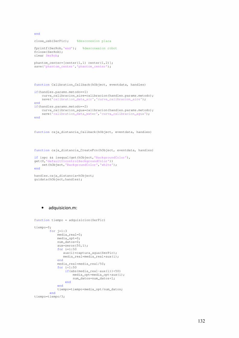
132

end

close_usb(SerPic); %desconexion placa

fprintf(SerRob,'end'); %desconexion robot

fclose(SerRob);

clear SerRob;

phantom_center=[center(1,1) center(1,2)];

save('phantom_center','phantom_center');

function Calibration_Callback(hObject, eventdata, handles)

if(handles.params.metodo==1)

curva_calibracion_aire=calibracion(handles.params.metodo);

save('calibration_data_air','curva_calibracion_aire');

end


curva_calibracion_agua=calibracion(handles.params.metodo);

save('calibration_data_water','curva_calibracion_agua');

end

function caja_distancia_Callback(hObject, eventdata, handles)

function caja_distancia_CreateFcn(hObject, eventdata, handles)




end

handles.caja_distancia=hObject;


• adquisicion.m:

function tiempo = adquisicion(SerPic)

tiempo=0;

for j=1:3

media_real=0;

media_opt=0;

num_datos=0;

aux=zeros(50,1);

for i=1:50

aux(i)=captura_agua(SerPic);

media_real=media_real+aux(i);

end

media_real=media_real/50;

for i=1:50

if(abs(media_real-aux(i))<50)

media_opt=media_opt+aux(i);

num_datos=num_datos+1;

end

end

tiempo=tiempo+media_opt/num_datos;

end

tiempo=tiempo/3;

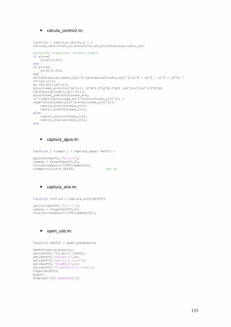
133

• calcula_centro2.m:

function [ centro_x centro_y ] =

calcula_centro2(x1,y1,distancia1,x2,y2,distancia2,radio_cyl)

%restando ecuaciones tenemos x=my+n

if x1==x2

x1=x1+0.001;

end

if y1==y2

y1=y1+0.001;

end

n=((distancia1+radio_cyl)^2-(distancia2+radio_cyl)^2-x1^2 + x2^2 - y1^2 + y2^2) /

(2*(y2-y1));

m=-(x2-x1)/(y2-y1);

soluciones_x=roots([(m^2+1) (2*m*n-2*y2*m-2*x2) (x2^2+n^2+y2^2-2*n*y2-

(distancia2+radio_cyl)^2)]);

soluciones_y=m*soluciones_x+n;

if ((sqrt(soluciones_x(1)^2+soluciones_y(1)^2)) <

(sqrt(soluciones_x(2)^2+soluciones_y(2)^2)))

centro_x=soluciones_x(1);

centro_y=soluciones_y(1);

else

centro_x=soluciones_x(2);

centro_y=soluciones_y(2);

end

• captura_agua.m:

function [ tiempo ] = captura_agua( SerPIC )

fprintf(SerPIC,'%c','1');

cadena = fread(SerPIC,2);

ciclos=cadena(1)*256+cadena(2);

tiempo=ciclos*0.08333; %en us

• captura_aire.m:

function voltios = captura_aire(SerPIC)

fprintf(SerPIC,'%c','1');

cadena = fread(SerPIC,2);

voltios=(cadena(1)*256+cadena(2));

• open_usb.m:

function SerPIC = open_usb(puerto)

SerPIC=serial(puerto);

set(SerPIC,'BaudRate',9600);

set(SerPIC,'DataBits',8);

set(SerPIC,'Parity','none');

set(SerPIC,'StopBits',1);

set(SerPIC,'FlowControl','none');

fopen(SerPIC);

puerto

display('USB conectado');

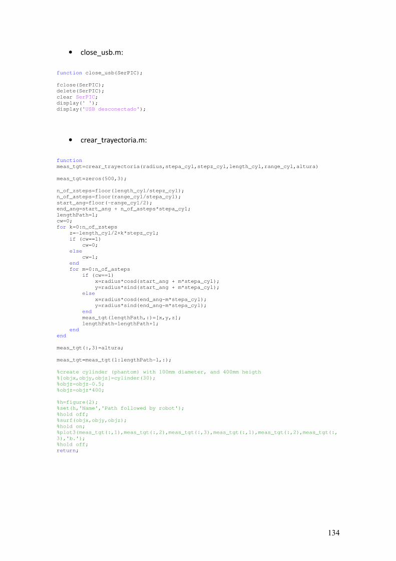
134

• close_usb.m:

function close_usb(SerPIC);

fclose(SerPIC);

delete(SerPIC);

clear SerPIC;

display(' ');

display('USB desconectado');

• crear_trayectoria.m:

function

meas_tgt=crear_trayectoria(radius,stepa_cyl,stepz_cyl,length_cyl,range_cyl,altura)

meas_tgt=zeros(500,3);

n_of_zsteps=floor(length_cyl/stepz_cyl);

n_of_asteps=floor(range_cyl/stepa_cyl);

start_ang=floor(-range_cyl/2);

end_ang=start_ang + n_of_asteps*stepa_cyl;

lengthPath=1;

cw=0;

for k=0:n_of_zsteps

z=-length_cyl/2+k*stepz_cyl;

if (cw==1)

cw=0;

else

cw=1;

end

for m=0:n_of_asteps

if (cw==1)

x=radius*cosd(start_ang + m*stepa_cyl);

y=radius*sind(start_ang + m*stepa_cyl);

else

x=radius*cosd(end_ang-m*stepa_cyl);

y=radius*sind(end_ang-m*stepa_cyl);

end

meas_tgt(lengthPath,:)=[x,y,z];

lengthPath=lengthPath+1;

end

end

meas_tgt(:,3)=altura;

meas_tgt=meas_tgt(1:lengthPath-1,:);

%create cylinder (phantom) with 100mm diameter, and 400mm heigth

%[objx,objy,objz]=cylinder(30);

%objz=objz-0.5;

%objz=objz*400;

%h=figure(2);

%set(h,'Name','Path followed by robot');

%hold off;

%surf(objx,objy,objz);

%hold on;

%plot3(meas_tgt(:,1),meas_tgt(:,2),meas_tgt(:,3),meas_tgt(:,1),meas_tgt(:,2),meas_tgt(:,

3),'b.');

%hold off;

return;

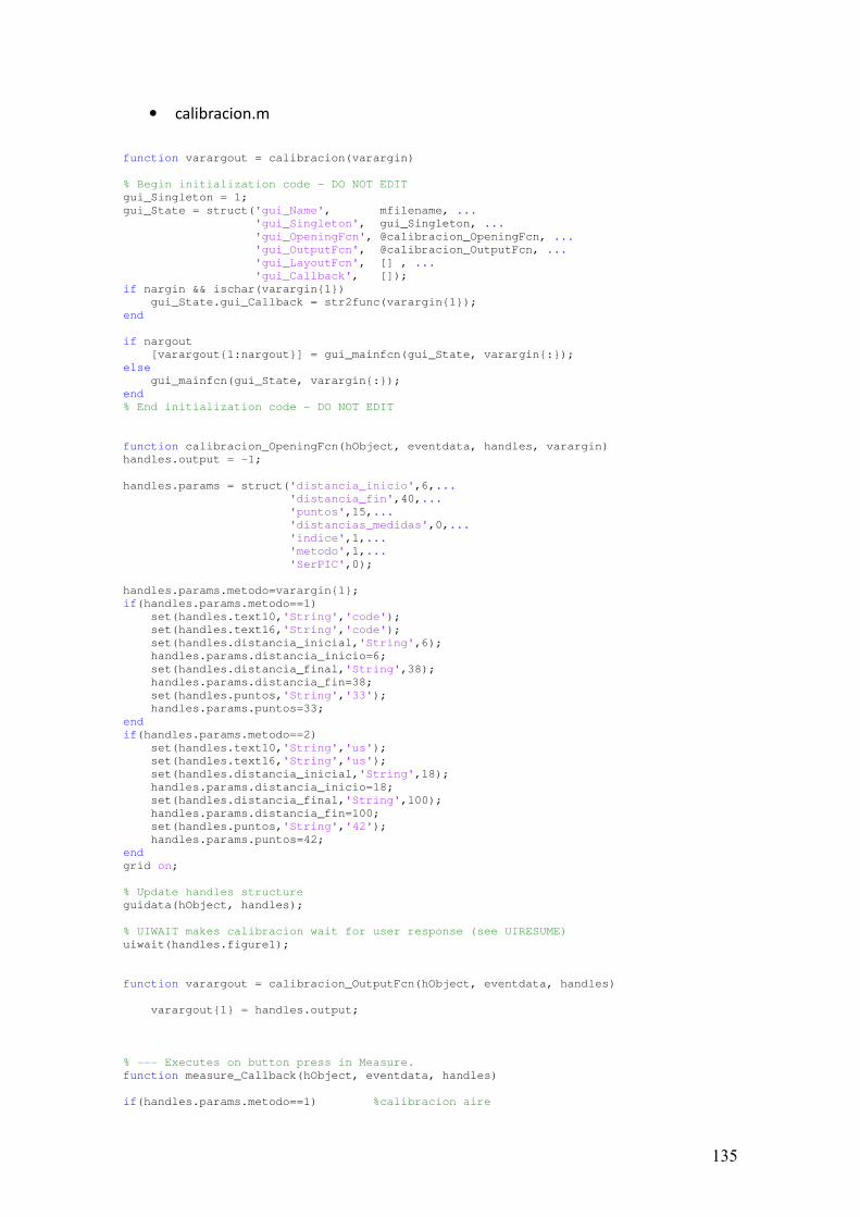
135

• calibracion.m

function varargout = calibracion(varargin)

% Begin initialization code - DO NOT EDIT

gui_Singleton = 1;

gui_State = struct('gui_Name', mfilename, ...

'gui_Singleton', gui_Singleton, ...

'gui_OpeningFcn', @calibracion_OpeningFcn, ...

'gui_OutputFcn', @calibracion_OutputFcn, ...

'gui_LayoutFcn', [] , ...

'gui_Callback', []);

if nargin && ischar(varargin1)

gui_State.gui_Callback = str2func(varargin1);

end

if nargout

[varargout1:nargout] = gui_mainfcn(gui_State, varargin:);

else

gui_mainfcn(gui_State, varargin:);

end

% End initialization code - DO NOT EDIT

function calibracion_OpeningFcn(hObject, eventdata, handles, varargin)

handles.output = -1;

handles.params = struct('distancia_inicio',6,...

'distancia_fin',40,...

'puntos',15,...

'distancias_medidas',0,...

'indice',1,...

'metodo',1,...

'SerPIC',0);

handles.params.metodo=varargin1;


set(handles.text10,'String','code');

set(handles.text16,'String','code');

set(handles.distancia_inicial,'String',6);

handles.params.distancia_inicio=6;

set(handles.distancia_final,'String',38);

handles.params.distancia_fin=38;

set(handles.puntos,'String','33');

handles.params.puntos=33;

end


set(handles.text10,'String','us');

set(handles.text16,'String','us');

set(handles.distancia_inicial,'String',18);

handles.params.distancia_inicio=18;

set(handles.distancia_final,'String',100);

handles.params.distancia_fin=100;

set(handles.puntos,'String','42');

handles.params.puntos=42;

end

grid on;

% Update handles structure


% UIWAIT makes calibracion wait for user response (see UIRESUME)

uiwait(handles.figure1);

function varargout = calibracion_OutputFcn(hObject, eventdata, handles)

varargout1 = handles.output;

% --- Executes on button press in Measure.

function measure_Callback(hObject, eventdata, handles)

if(handles.params.metodo==1) %calibracion aire

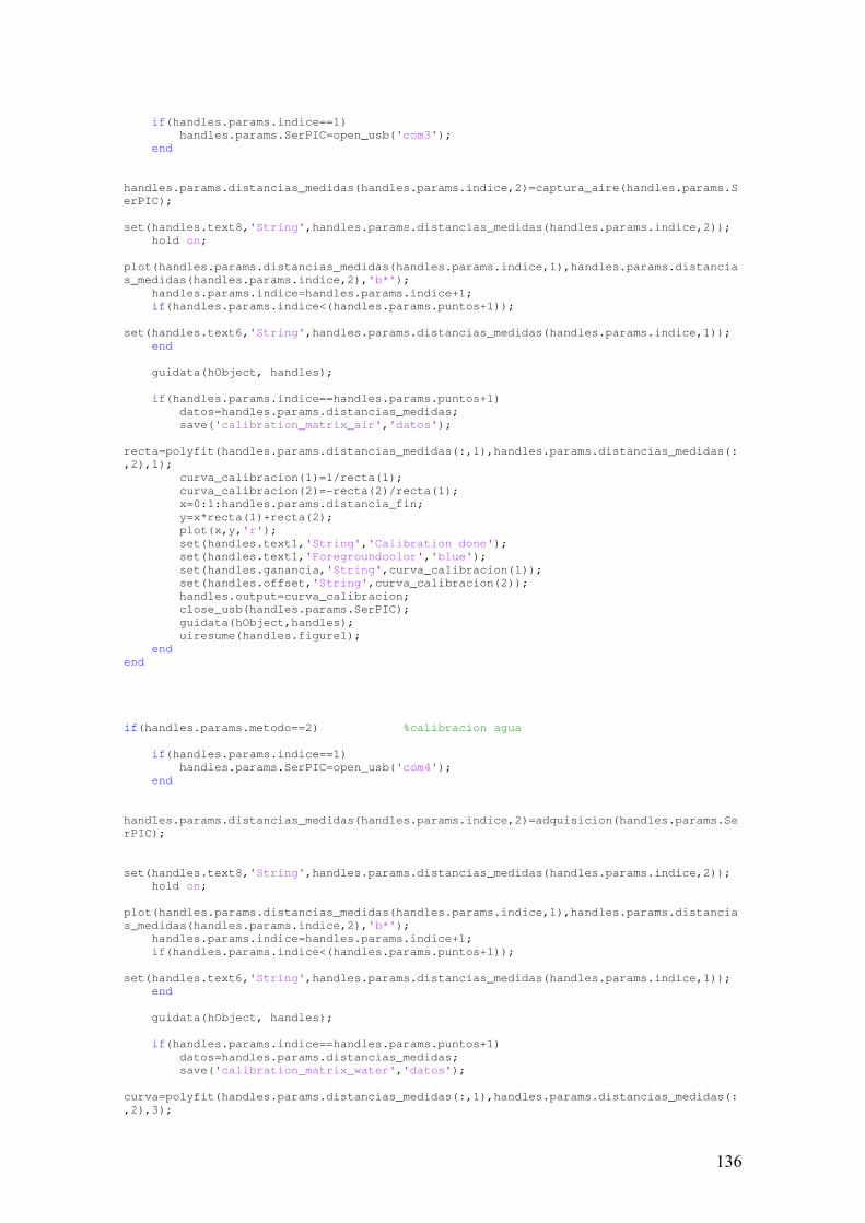
136

if(handles.params.indice==1)

handles.params.SerPIC=open_usb('com3');

end

handles.params.distancias_medidas(handles.params.indice,2)=captura_aire(handles.params.S

erPIC);

set(handles.text8,'String',handles.params.distancias_medidas(handles.params.indice,2));

hold on;

plot(handles.params.distancias_medidas(handles.params.indice,1),handles.params.distancia

s_medidas(handles.params.indice,2),'b*');

handles.params.indice=handles.params.indice+1;

if(handles.params.indice<(handles.params.puntos+1));


end


if(handles.params.indice==handles.params.puntos+1)

datos=handles.params.distancias_medidas;

save('calibration_matrix_air','datos');

recta=polyfit(handles.params.distancias_medidas(:,1),handles.params.distancias_medidas(:

,2),1);

curva_calibracion(1)=1/recta(1);

curva_calibracion(2)=-recta(2)/recta(1);

x=0:1:handles.params.distancia_fin;

y=x*recta(1)+recta(2);

plot(x,y,'r');

set(handles.text1,'String','Calibration done');

set(handles.text1,'Foregroundcolor','blue');

set(handles.ganancia,'String',curva_calibracion(1));

set(handles.offset,'String',curva_calibracion(2));

handles.output=curva_calibracion;

close_usb(handles.params.SerPIC);


uiresume(handles.figure1);

end

end

if(handles.params.metodo==2) %calibracion agua

if(handles.params.indice==1)

handles.params.SerPIC=open_usb('com4');

end

handles.params.distancias_medidas(handles.params.indice,2)=adquisicion(handles.params.Se

rPIC);


hold on;

plot(handles.params.distancias_medidas(handles.params.indice,1),handles.params.distancia

s_medidas(handles.params.indice,2),'b*');

handles.params.indice=handles.params.indice+1;

if(handles.params.indice<(handles.params.puntos+1));


end


if(handles.params.indice==handles.params.puntos+1)

datos=handles.params.distancias_medidas;

save('calibration_matrix_water','datos');

curva=polyfit(handles.params.distancias_medidas(:,1),handles.params.distancias_medidas(:

,2),3);

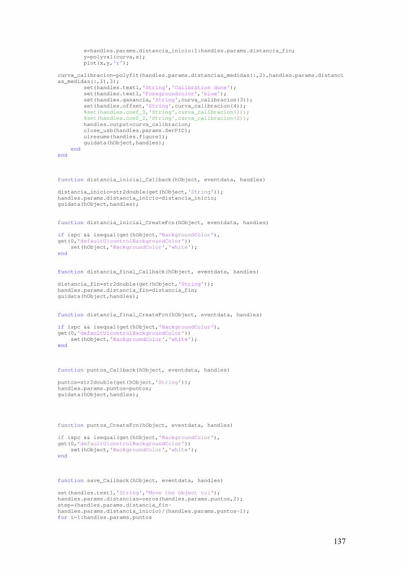
137

x=handles.params.distancia_inicio:1:handles.params.distancia_fin;

y=polyval(curva,x);

plot(x,y,'r');

curva_calibracion=polyfit(handles.params.distancias_medidas(:,2),handles.params.distanci

as_medidas(:,1),3);

set(handles.text1,'String','Calibration done');

set(handles.text1,'Foregroundcolor','blue');

set(handles.ganancia,'String',curva_calibracion(3));

set(handles.offset,'String',curva_calibracion(4));

%set(handles.coef_3,'String',curva_calibracion(1));

%set(handles.coef_2,'String',curva_calibracion(2));

handles.output=curva_calibracion;

close_usb(handles.params.SerPIC);

uiresume(handles.figure1);


end

end

function distancia_inicial_Callback(hObject, eventdata, handles)

distancia_inicio=str2double(get(hObject,'String'));

handles.params.distancia_inicio=distancia_inicio;


function distancia_inicial_CreateFcn(hObject, eventdata, handles)




end

function distancia_final_Callback(hObject, eventdata, handles)

distancia_fin=str2double(get(hObject,'String'));

handles.params.distancia_fin=distancia_fin;


function distancia_final_CreateFcn(hObject, eventdata, handles)




end

function puntos_Callback(hObject, eventdata, handles)




function puntos_CreateFcn(hObject, eventdata, handles)




end

function save_Callback(hObject, eventdata, handles)

set(handles.text1,'String','Move the object to:');

handles.params.distancias=zeros(handles.params.puntos,2);

step=(handles.params.distancia_fin-

handles.params.distancia_inicio)/(handles.params.puntos-1);

for i=1:handles.params.puntos

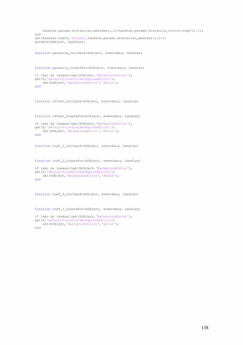
138

handles.params.distancias_medidas(i,1)=handles.params.distancia_inicio+step*(i-1);

end

set(handles.text6,'String',handles.params.distancias_medidas(1,1));


function ganancia_Callback(hObject, eventdata, handles)

function ganancia_CreateFcn(hObject, eventdata, handles)




end

function offset_Callback(hObject, eventdata, handles)

function offset_CreateFcn(hObject, eventdata, handles)




end

function coef_2_Callback(hObject, eventdata, handles)

function coef_2_CreateFcn(hObject, eventdata, handles)




end

function coef_3_Callback(hObject, eventdata, handles)

function coef_3_CreateFcn(hObject, eventdata, handles)




end

Documents

Robot Positioning System - DiVA Portal