Embed Size (px)
Citation preview

Deep Water Acoustic
Positioning
IMCA M 200, IMCA S 013 – Rev. 2
January 2017

The International Marine Contractors Association (IMCA) is the international
trade association representing offshore, marine and underwater engineering
companies.
IMCA promotes improvements in quality, health, safety, environmental and technical standards
through the publication of information notes, codes of practice and by other appropriate means.
Members are self-regulating through the adoption of IMCA guidelines as appropriate. They
commit to act as responsible members by following relevant guidelines and being willing to be
audited against compliance with them by their clients.
There are five core committees that relate to all members:
Competence & Training
Contracts & Insurance
Health, Safety, Security & Environment
Lifting & Rigging
Marine Policy & Regulatory Affairs
The Association is organised through four distinct divisions, each covering a specific area of
members’ interests: Diving, Marine, Offshore Survey and Remote Systems & ROV.
There are also five regions which facilitate work on issues affecting members in their local
geographic area – Asia-Pacific, Europe & Africa, Middle East & India, North America and South
America.
IMCA M 200, IMCA S 013 – Rev. 2
The document was first produced for IMCA by Gordon Johnston, under the direction of its
Offshore Survey Division Management Committee, in October 2009. It has been revised and
republished firstly in July 2014, and secondly, during 2016 as part of the ongoing review of IMCA
documentation.
All the illustrations in this document, unless otherwise stated, have been kindly provided by
Kongsberg, Sonardyne, Sonsub and Valeport.
This document is dedicated to the memory of Brian Beard, who was a long-standing member
of IMCA’s Offshore Survey Division Management Committee, whose ideas and early support
for this document were key to its development
www.imca-int.com
If you have any comments on this document, please click the feedback button below:
Date Reason Revision
October 2009 Initial publication
July 2014 Revised to reflect changes to technology and practice Rev. 1
January 2017 Updated as part of the ongoing review of IMCA
documentation
Rev. 2
The information contained herein is given for guidance only and endeavours to reflect best industry practice. For the avoidance
of doubt no legal liability shall attach to any guidance and/or recommendation and/or statement herein contained.
© 2017 IMCA – International Marine Contractors Association
Deep Water Acoustic Positioning
IMCA M 200, IMCA S 013 – Rev. 2 – January 2017
1 Executive Summary .............................................................................................. 1
1.1 Revision ..................................................................................................................................................................... 1
2 Glossary of Terms ................................................................................................. 2
3 Introduction ........................................................................................................... 5
4 Basics of Deep Water Positioning Systems ........................................................ 6
4.1 Acoustic Positioning Methods ............................................................................................................................. 6
4.2 Equipment Components .................................................................................................................................... 10
4.3 Acoustic Frequency ............................................................................................................................................ 12
4.4 Signalling Techniques .......................................................................................................................................... 12
4.5 Velocity of Sound ................................................................................................................................................ 13
5 Operations ............................................................................................................ 14
5.1 USBL ....................................................................................................................................................................... 14
5.2 LBL .......................................................................................................................................................................... 14
5.3 Array Planning ...................................................................................................................................................... 14
5.4 Mobilisation ........................................................................................................................................................... 17
5.5 Methods of Deployment and Recovery ......................................................................................................... 19
5.6 Methods of Calibration ...................................................................................................................................... 19
5.7 Quality Control ................................................................................................................................................... 23
5.8 System Performance ........................................................................................................................................... 23
6 Associated Topics ................................................................................................ 26
6.1 Integration of Systems ........................................................................................................................................ 26
6.2 Communications .................................................................................................................................................. 26
6.3 Software, Interfacing and Display .................................................................................................................... 26
6.4 Additional Peripheral Sensors and System Interfacing ............................................................................... 26
6.5 Permitting and Legislation ................................................................................................................................. 26
6.6 Training and Competence ................................................................................................................................. 26
7 Applications of Acoustic Positioning in Deep Water ...................................... 28
7.1 Dynamic Positioning ........................................................................................................................................... 28
7.2 Towed Body (‘Towfish’) Positioning .............................................................................................................. 28
7.3 Riser Monitoring .................................................................................................................................................. 29
7.4 Pipelay Positioning ............................................................................................................................................... 30
7.5 AUV and ROV Positioning ................................................................................................................................ 31
7.6 Construction Positioning and Installation of Structures ........................................................................... 32
7.7 Relative Measurement ........................................................................................................................................ 33
7.8 Metrology .............................................................................................................................................................. 33
7.9 Well Positioning ................................................................................................................................................... 34
7.10 Long Term Structure Monitoring and Positioning ...................................................................................... 35
7.11 Acoustic Data Telemetry .................................................................................................................................. 35
7.12 Out-of-Straightness Positioning ....................................................................................................................... 36

Appendices
1 The Sonar Equation ............................................................................................. 37
A1-1 Source Level ......................................................................................................................................................... 37
A1-2 Transmission Loss ............................................................................................................................................... 38
A1-3 Directivity Index .................................................................................................................................................. 39
A1-4 Detection Threshold .......................................................................................................................................... 39
A1-5 Noise Level ........................................................................................................................................................... 40
2 Methods of Acoustic Positioning ........................................................................ 41
A2-1 LBL Systems .......................................................................................................................................................... 41
A2-2 SBL Systems .......................................................................................................................................................... 42
A2-3 USBL Systems ....................................................................................................................................................... 43
A2-4 Combined Acoustic Systems ............................................................................................................................ 43
A2-5 Inverted Arrays .................................................................................................................................................... 45
A2-6 Hybrid Technology Systems ............................................................................................................................. 46
3 Frequency ............................................................................................................. 48
A3-1 Accuracy of Measurement ................................................................................................................................ 48
A3-2 Physical Size and Frequency .............................................................................................................................. 49
A3-3 Range and Coverage Achievable ..................................................................................................................... 50
A3-4 Coverage – the Layout and Geometry of the System ............................................................................... 50
A3-5 Frequency Clashes and Interference .............................................................................................................. 51
4 Spread Spectrum Techniques ............................................................................ 52
A4-1 Measurement Accuracy ..................................................................................................................................... 52
A4-2 Resistance to Multi-Pathing ............................................................................................................................... 52
A4-3 Range and Coverage ........................................................................................................................................... 53
A4-4 Improved Signal to Noise Ratio ....................................................................................................................... 54
A4-5 Signal Measurement Accuracy .......................................................................................................................... 54
5 Velocity of Sound ................................................................................................. 56
A5-1 Temperature ......................................................................................................................................................... 56
A5-2 Pressure ................................................................................................................................................................. 56
A5-3 Density ................................................................................................................................................................... 56
A5-4 Salinity .................................................................................................................................................................... 57
A5-5 Instrumentation ................................................................................................................................................... 57
A5-6 The Sound Velocity Computation .................................................................................................................. 57
6 Acoustic Noise and Interference ....................................................................... 58
A6-1 Acoustic Noise ..................................................................................................................................................... 58
A6-2 Signal Reverberation ........................................................................................................................................... 61
A6-3 Acoustic Interference ......................................................................................................................................... 63
7 Deep Water Acoustic Operations ..................................................................... 66
A7-1 Station Deployment ............................................................................................................................................ 66
A7-2 Deep Water Frame Designs ............................................................................................................................. 66
A7-3 Characteristics and Suitability of Acoustics as DP References ................................................................ 67
A7-4 Depth Ratings ....................................................................................................................................................... 68
A7-5 Data Telemetry .................................................................................................................................................... 68
A7-6 Power Levels ........................................................................................................................................................ 69
A7-7 System Maintenance ........................................................................................................................................... 69
A7-8 Multiple Vessel Users ......................................................................................................................................... 69
A7-9 Interface with Different Sensors ..................................................................................................................... 70
A7-10 Checks and Quality Control ............................................................................................................................ 70
IMCA M 200, IMCA S 013 – Rev. 2 1
1 Executive Summary
This guidance document is intended to provide an authoritative guide for users and potential users of acoustics
for underwater positioning, particularly in deep water. The document covers the basics of acoustics and
signalling, the equipment required, methods of acoustic positioning and their limitations, and the operation and
performance of acoustic positioning systems. The focus is on the use of acoustic positioning systems and
techniques for deep water operations, though it should be recognised that many of the techniques and
applications are also applicable to shallow water.
This document does not attempt to compare and evaluate different manufacturers, their products, services or
the specific performance of systems – nor does it set out to provide a prescriptive set of procedures. Rather,
this document is designed to provide consideration and guidance for the use and operation of any of the main
types of systems.
In considering deep water acoustics, this document focuses on the use and application of acoustics for positioning
tasks and how a user should consider the various factors influencing the selection of operational techniques for
different applications. The main part of the document is intended to inform and bring a general understanding
of deep water acoustics to the reader. More detailed technical appendices are provided for in depth study.
No endorsement or recommendation of a specific type, model or make of system is offered here, however, the
use of diagrams, references to proprietary elements and systems is inevitable in a specialised niche technology
such as acoustic positioning.
There is considerable variation in the definition of ‘deep water’, depending on what sector of the marine and
offshore industry is consulted. Hydrographers concerned with the safety of life and navigation may consider
depths greater than 200 metres (m) as deep, whereas the offshore drilling companies often now consider deep
water as greater than 2,500m.
For the purposes of this document the definition of deep water is greater than 600m.
1.1 Revision
This document was first published in October 2009. It underwent a review in early 2014 and the text
has been revised with minor changes to the wording in places to reflect changes to technology and
practice. It has undergone further revision during 2016 as part of the overall IMCA document
programme taking place at that time.
2 IMCA M 200, IMCA S 013 – Rev. 2
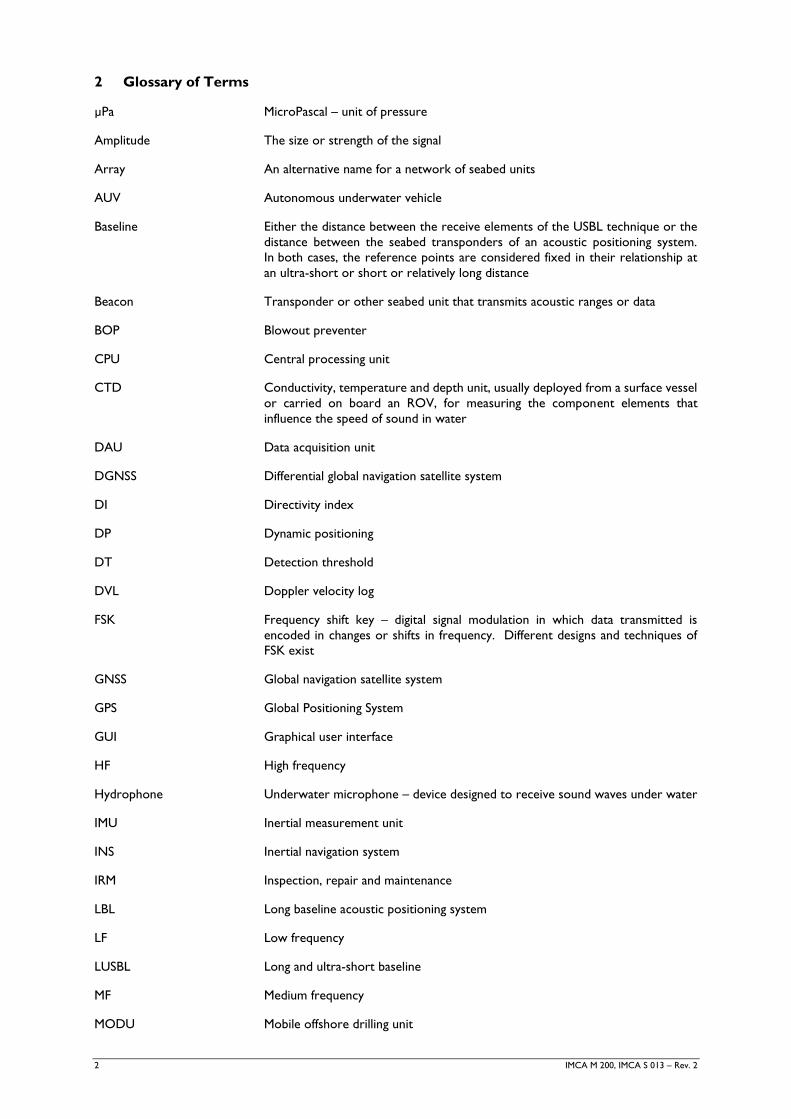
2 Glossary of Terms
µPa MicroPascal – unit of pressure
Amplitude The size or strength of the signal
Array An alternative name for a network of seabed units
AUV Autonomous underwater vehicle
Baseline Either the distance between the receive elements of the USBL technique or the
distance between the seabed transponders of an acoustic positioning system.
In both cases, the reference points are considered fixed in their relationship at
an ultra-short or short or relatively long distance
Beacon Transponder or other seabed unit that transmits acoustic ranges or data
BOP Blowout preventer
CPU Central processing unit
CTD Conductivity, temperature and depth unit, usually deployed from a surface vessel
or carried on board an ROV, for measuring the component elements that
influence the speed of sound in water
DAU Data acquisition unit
DGNSS Differential global navigation satellite system
DI Directivity index
DP Dynamic positioning
DT Detection threshold
DVL Doppler velocity log
FSK Frequency shift key – digital signal modulation in which data transmitted is
encoded in changes or shifts in frequency. Different designs and techniques of
FSK exist
GNSS Global navigation satellite system
GPS Global Positioning System
GUI Graphical user interface
HF High frequency
Hydrophone Underwater microphone – device designed to receive sound waves under water
IMU Inertial measurement unit
INS Inertial navigation system
IRM Inspection, repair and maintenance
LBL Long baseline acoustic positioning system
LF Low frequency
LUSBL Long and ultra-short baseline
MF Medium frequency
MODU Mobile offshore drilling unit
IMCA M 200, IMCA S 013 – Rev. 2 3
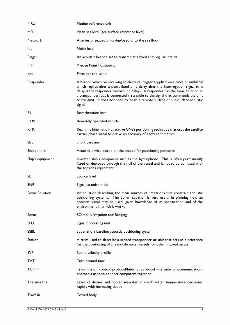
MRU Motion reference unit
MSL Mean sea level (sea surface reference level)
Network A series of seabed units deployed onto the sea floor
NL Noise level
Pinger An acoustic beacon set to transmit at a fixed and regular interval
PPP Precise Point Positioning
ppt Parts per thousand
Responder A beacon which on receiving an electrical trigger supplied via a cable or umbilical
which replies after a short fixed time delay after the interrogation signal (this
delay is the responder turnaround delay). A responder has the same function as
a transponder, but is connected via a cable to the signal that commands the unit
to transmit. It does not need to ‘hear’ a remote surface or sub-surface acoustic
signal
RL Reverberation level
ROV Remotely operated vehicle
RTK Real time kinematic – a relative GNSS positioning technique that uses the satellite
carrier phase signal to derive an accuracy of a few centimetres
SBL Short baseline
Seabed unit Acoustic device placed on the seabed for positioning purposes
Ship’s equipment In-water ship’s equipment such as the hydrophone. This is often permanently
fitted or deployed through the hull of the vessel and is not to be confused with
the topsides equipment
SL Source level
SNR Signal to noise ratio
Sonar Equation An equation describing the main sources of limitations that constrain acoustic
positioning systems. The Sonar Equation is very useful in planning how an
acoustic signal may be used, given knowledge of its specification and of the
environment in which it works
Sonar SOund, NAvigation and Ranging
SPU Signal processing unit
SSBL Super short baseline acoustic positioning system
Station A term used to describe a seabed transponder or unit that acts as a reference
for the positioning of any mobile units (vessels) or other tracked assets
SVP Sound velocity profile
TAT Turn-around time
TCP/IP Transmission control protocol/Internet protocol – a suite of communications
protocols used to connect computers together
Thermocline Layer of denser and cooler seawater in which water temperature decreases
rapidly with increasing depth
Towfish Towed body

4 IMCA M 200, IMCA S 013 – Rev. 2
Transponder, beacons or stations A seabed unit that receives acoustic commands or signals and replies to them
TS Target strength
Turn-around time Time taken for seabed and subsea units to receive a command or an acoustic
signal and transmit a response. If not properly taken into account, turn-around
time can cause biases in position. The settings are normally set by the
manufacturer at the time of construction and will have been tested and calibrated
prior to issue
USBL Ultra-short baseline acoustic positioning system
UTC Universal time co-ordinated
Vp Velocity of propagation in water
IMCA M 200, IMCA S 013 – Rev. 2 5
3 Introduction
Of the various forms of radiation, sound travels best through water. As a result of this characteristic, underwater
sound has been used for many applications. The use of these techniques in a formal process is known as ‘sonar’
or ‘acoustic systems’. The term ‘sonar’ is an acronym derived during World War II for application to military
systems, and is formed from the words SOund, NAvigation and Ranging. In this document the terms ‘acoustics’,
‘acoustic systems’ and ‘acoustic positioning systems’ are used.
Acoustic positioning systems were developed in the 1950s and 60s to support various US research projects and
activities. Over the years, prompted by demand from the offshore energy industry, acoustic positioning and
tracking systems have played an increasingly important role. Applications are common and relatively widespread
in what is essentially a specialised area. The tracking of towed sensors and vehicles, locating underwater pipelines
and cables, the monitoring of drilling and dredging operations as well as the survey and monitoring of numerous
objects, are now common applications.
Acoustic positioning plays a role in every phase of the offshore industry, from exploration, drilling, engineering
and construction, to monitoring and maintenance, and decommissioning. In recent years the significance of
acoustic positioning has increased as more activities have taken place in deep water areas.
Before the development and introduction of GPS satellite technology, radio positioning systems were used for
accurate positioning of vessels on the sea surface. At best, these systems provided regional coverage. Satellite-
based positioning systems have introduced global coverage, whereas acoustic positioning systems remain
localised and typically cover only a few square kilometres at a time. This limitation creates difficulties for certain
projects, particularly pipeline installation and cable-laying work, where accurate positioning is required for a long
linear route. However, many users of acoustic positioning systems accept limited cover and perhaps even limited
accuracy in exchange for reliable and repeatable positioning for their specific area.
The ability of a system to provide accuracy, coverage and reliability is discussed later, but it is important to realise
that no single acoustic positioning system provides all the answers for the various applications. For many, there
will be a trade-off between several systems – each of which offers some advantage relative to another.
It is intended that this document is an aid to the reader in understanding the way in which systems operate as
well as their particular strengths, and the various deep water positioning applications for which any given system
may be considered suitable.
6 IMCA M 200, IMCA S 013 – Rev. 2
4 Basics of Deep Water Positioning Systems
Acoustic positioning systems measure ranges and directions to transponders fitted to underwater vehicles and
objects, or derive acoustic ranges from stations deployed onto the seabed. These latter units are held stationary
by a clump weight with buoyed mooring (or some other form of fixed seabed framework). Several types of
system such as ultra-short baseline and short baseline systems provide positioning relative to a host vessel or
vehicle, whereas long baseline systems allow either a relative or absolute positioning framework to be developed.
Many other scenarios exist including beacons being installed on remotely operated vehicles (ROVs), autonomous
underwater vehicles (AUVs) and other types of towed vehicles. The systems have been developed specifically
to meet the challenges of operating in deep water with sufficient accuracy and system reliability. The main
elements of deep water acoustic positioning systems will include:
transmission and reception of acoustic pulses to track or position a limited number of objects – both static
and mobile;
processing and applying corrections to data to provide accurate and consistent performance parameters;
incorporation of peripheral data such as speed of sound in water, depth, heading and motion;
display of position relative to a certain reference system, e.g. vessel;
some form of noise and interference mitigation to enable continued working in harsh environments.
A full treatment of the physics of underwater acoustics is beyond the scope of this document. However, some
general description is required to enable the reader to appreciate some of the aspects covered later. The Sonar
Equation is often required by underwater acoustics engineers to aid in the design and planning of operations,
rather than during field work. Further discussion of the Sonar Equation can be found in Appendix 1.
The following sub-sections cover some important aspects and critical elements of acoustic positioning systems
and the environment in which they operate.
4.1 Acoustic Positioning Methods
Methods of deep water acoustic positioning vary in terms of accuracy, precision, design and frequency.
How accurate or precise a system will be is dependent on commercial requirements and the operational
and environmental conditions in which they will be used. For the purposes of this document, the
methods under consideration are the most commonly used techniques, long baseline (LBL) short
baseline (SBL) and ultra-short baseline (USBL), which exhibit the key principles and considerations
associated with acoustic positioning. For completeness, however, other methods are briefly covered in
this section.
In all cases, it is only possible to monitor and assess the quality and reliability of the systems if there are
sufficient observations and data redundancy supported by careful system calibration and monitoring
during operation.
System Advantages Disadvantages
LBL Highest potential accuracy
Accuracy preserved over wider operating area
One hydrophone needed
Redundant data for statistical testing/quality
control
Requires multiple subsea/seabed transponders
Update intervals long compared to SBL/USBL
systems
Need to redeploy and recalibrate at each site
SBL Good potential accuracy
Requires only a single subsea pinger
One-time calibration
Accuracy dependent on shipboard MRU and
heading sensor/gyro compass
Multiple hydrophones required through the hull
USBL Good potential accuracy
Requires only a single subsea pinger or
transponder
One-time calibration
Highest noise susceptibility
Accuracy dependent on shipboard MRU
Table 1 – Advantages and disadvantages of acoustic positioning systems
IMCA M 200, IMCA S 013 – Rev. 2 7
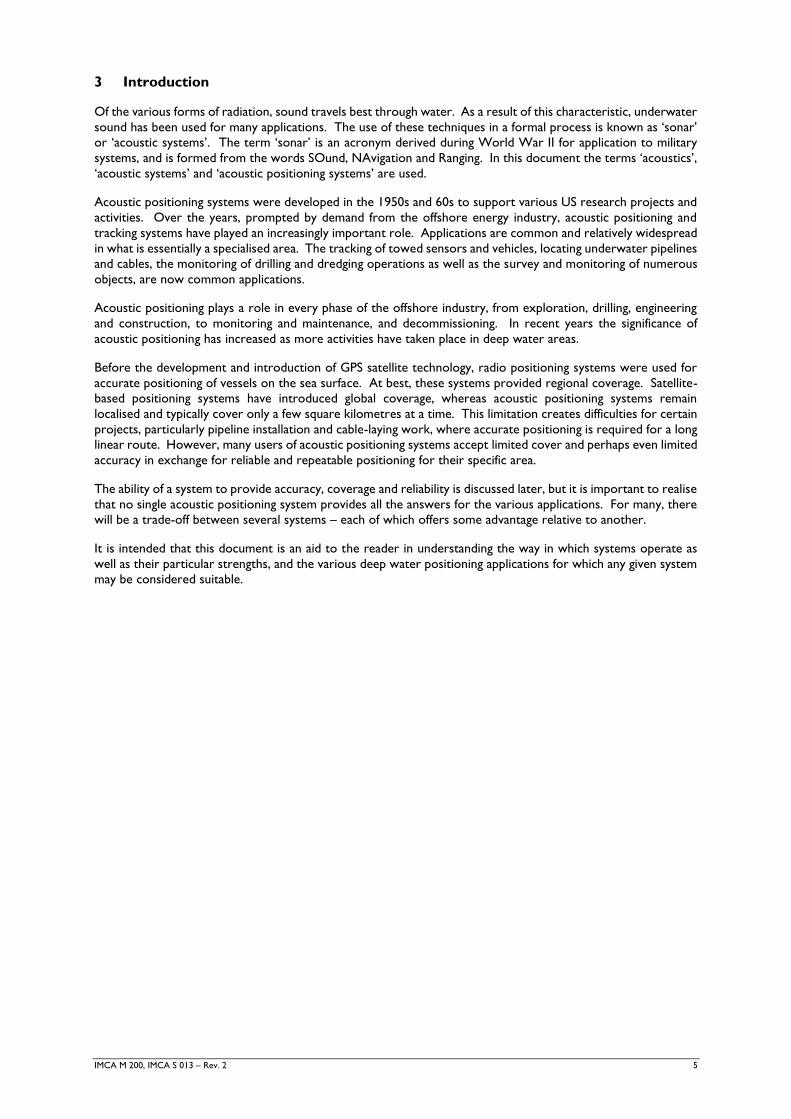
4.1.1 LBL
LBL systems take their name from the distance between seabed transponders or beacons which
can be as much as several kilometres. The beacons are deployed onto the seabed in an array
and are then, as transponders, set to transmit when interrogated by a user hydrophone.
LBL acoustic systems provide accurate fixing over a relatively small area. Three or more
transponders located at known positions on the seabed are interrogated by a transducer fitted
to the surface vessel, towed body or autonomous object. If at least three ranges are measured
from a mobile hydrophone to transponders at fixed co-ordinated seabed locations, then the
hydrophone position co-ordinates can be computed. The LBL method provides accurate local
control and high repeatability. If there is a redundancy (e.g. four or more position lines), the
quality of each position fix can also be estimated and this is often a consideration when selecting
a system for use.
Figure 1 – Illustration showing an LBL system
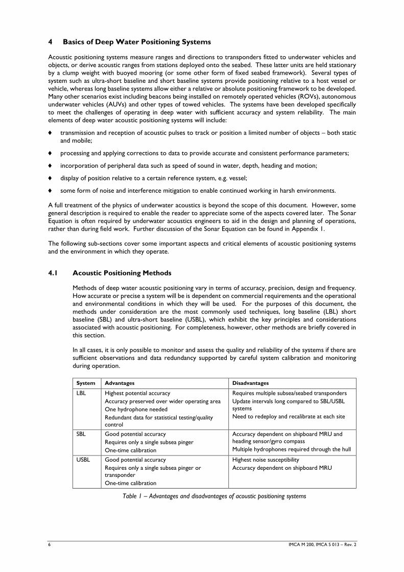
4.1.2 SBL
In this type of system, the baseline referred to is that between the receive transducer
(hydrophone) units on or below the hull of the host vessel. It requires a pinger, responder or
transponder to operate the system. No fixed beacons on the seabed are required and the
system positions relative to the surface vessel. The transducers for such a system are usually
deployed through dedicated tubes in the hull and are generally separated by between 10 and
50m, dependent on the form of vessel on which they are fitted. The SBL system uses relative
range and direction observations to transponders to determine position relative to the surface
vessel.
8 IMCA M 200, IMCA S 013 – Rev. 2
Figure 2 – Illustration showing an SBL system
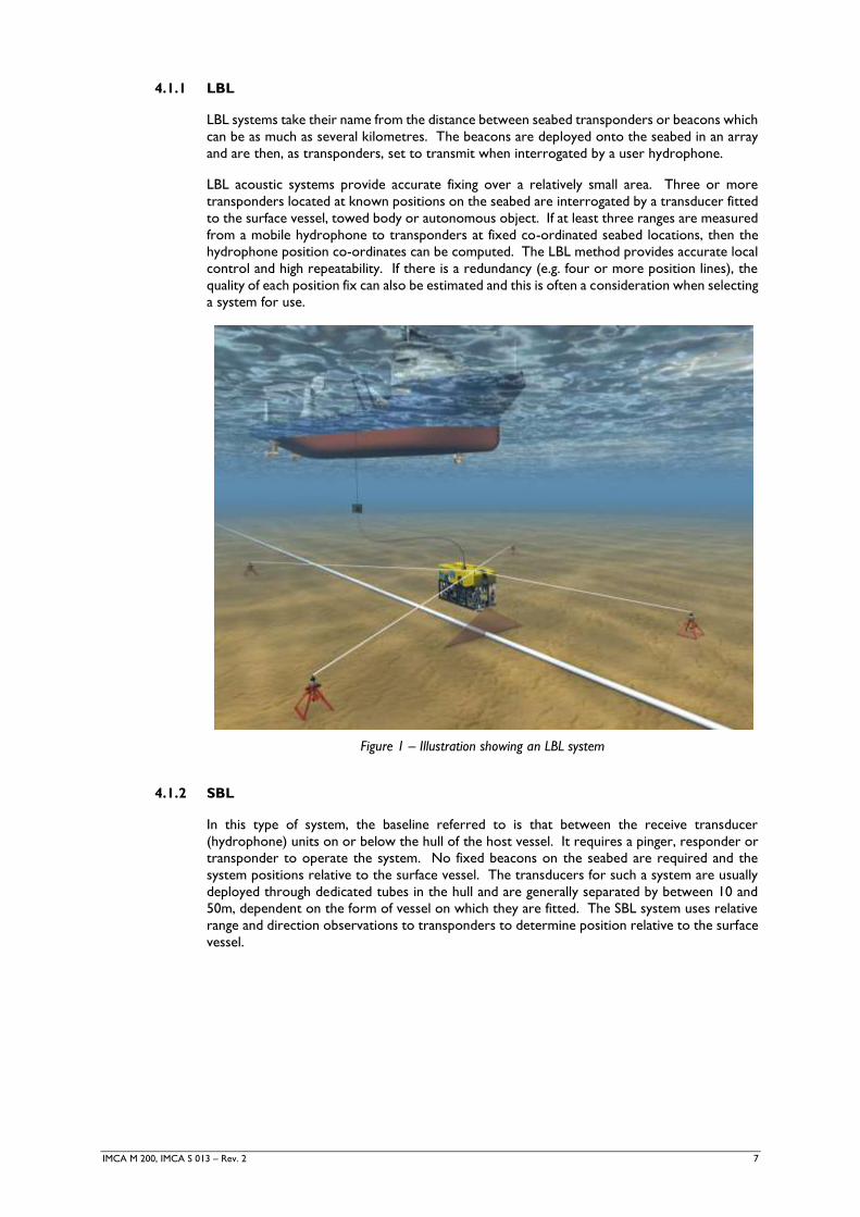
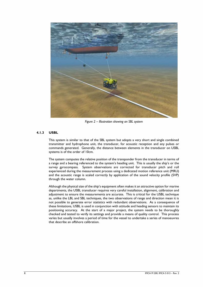
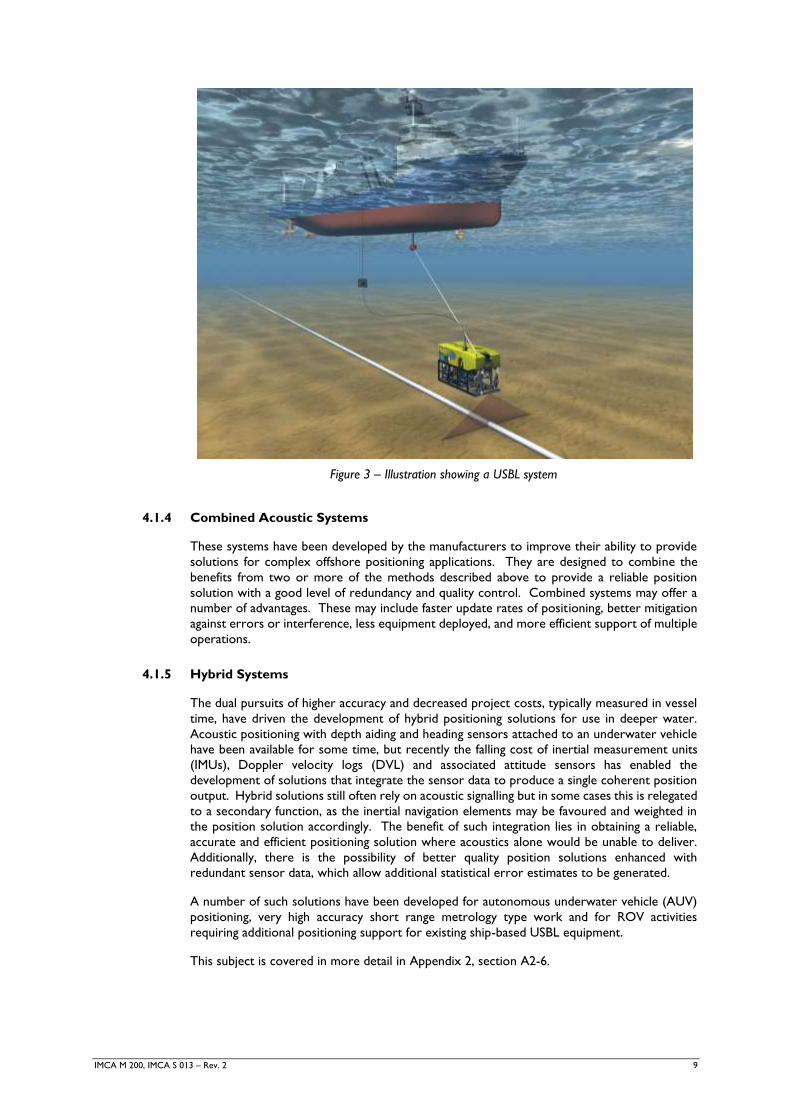
4.1.3 USBL
This system is similar to that of the SBL system but adopts a very short and single combined
transmitter and hydrophone unit, the transducer, for acoustic reception and any pulses or
commands generated. Generally, the distance between elements in the transducer on USBL
systems is of the order of 10cm.
The system computes the relative position of the transponder from the transducer in terms of
a range and a bearing referenced to the system’s heading unit. This is usually the ship’s or the
survey gyrocompass. System observations are corrected for transducer pitch and roll
experienced during the measurement process using a dedicated motion reference unit (MRU)
and the acoustic range is scaled correctly by application of the sound velocity profile (SVP)
through the water column.
Although the physical size of the ship’s equipment often makes it an attractive option for marine
departments, the USBL transducer requires very careful installation, alignment, calibration and
adjustment to ensure the measurements are accurate. This is critical for the USBL technique
as, unlike the LBL and SBL techniques, the two observations of range and direction mean it is
not possible to generate error statistics with redundant observations. As a consequence of
these limitations, USBL is used in conjunction with attitude and heading sensors to maintain its
positioning accuracy. At the start of a major project, the system needs to be thoroughly
checked and tested to verify its settings and provide a means of quality control. This process
varies but usually involves a period of time for the vessel to undertake a series of manoeuvres
that describe an offshore calibration.
IMCA M 200, IMCA S 013 – Rev. 2 9
Figure 3 – Illustration showing a USBL system
4.1.4 Combined Acoustic Systems
These systems have been developed by the manufacturers to improve their ability to provide
solutions for complex offshore positioning applications. They are designed to combine the
benefits from two or more of the methods described above to provide a reliable position
solution with a good level of redundancy and quality control. Combined systems may offer a
number of advantages. These may include faster update rates of positioning, better mitigation
against errors or interference, less equipment deployed, and more efficient support of multiple
operations.
4.1.5 Hybrid Systems
The dual pursuits of higher accuracy and decreased project costs, typically measured in vessel
time, have driven the development of hybrid positioning solutions for use in deeper water.
Acoustic positioning with depth aiding and heading sensors attached to an underwater vehicle
have been available for some time, but recently the falling cost of inertial measurement units
(IMUs), Doppler velocity logs (DVL) and associated attitude sensors has enabled the
development of solutions that integrate the sensor data to produce a single coherent position
output. Hybrid solutions still often rely on acoustic signalling but in some cases this is relegated
to a secondary function, as the inertial navigation elements may be favoured and weighted in
the position solution accordingly. The benefit of such integration lies in obtaining a reliable,
accurate and efficient positioning solution where acoustics alone would be unable to deliver.
Additionally, there is the possibility of better quality position solutions enhanced with
redundant sensor data, which allow additional statistical error estimates to be generated.
A number of such solutions have been developed for autonomous underwater vehicle (AUV)
positioning, very high accuracy short range metrology type work and for ROV activities
requiring additional positioning support for existing ship-based USBL equipment.
This subject is covered in more detail in Appendix 2, section A2-6.
10 IMCA M 200, IMCA S 013 – Rev. 2
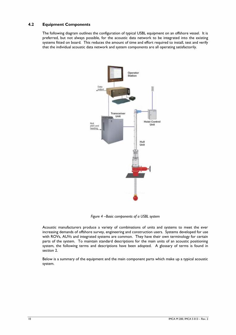
4.2 Equipment Components
The following diagram outlines the configuration of typical USBL equipment on an offshore vessel. It is
preferred, but not always possible, for the acoustic data network to be integrated into the existing
systems fitted on board. This reduces the amount of time and effort required to install, test and verify
that the individual acoustic data network and system components are all operating satisfactorily.
Figure 4 –Basic components of a USBL system
Acoustic manufacturers produce a variety of combinations of units and systems to meet the ever
increasing demands of offshore survey, engineering and construction users. Systems developed for use
with ROVs, AUVs and integrated systems are common. They have their own terminology for certain
parts of the system. To maintain standard descriptions for the main units of an acoustic positioning
system, the following terms and descriptions have been adopted. A glossary of terms is found in
section 2.
Below is a summary of the equipment and the main component parts which make up a typical acoustic
system.

IMCA M 200, IMCA S 013 – Rev. 2 11
4.2.1 Transponder, Beacon or Station
Figure 5 – Typical transponders used for surface and underwater position reference
Each transponder, beacon or station comprises:
subsea housing rated to a specific water depth;
integral battery pack which provides power over a period predetermined for the unit and
its operation;
integrated electronics package to process any acoustic signal commands and maintain
scheduled transmissions;
frame stab, frame collar or flotation collar to secure the beacon in place;
optional acoustic release system;
optional integral serial port to telemeter data from external sensors, such as depth, heading
or pitch/roll.
4.2.2 Ship Receiver Equipment
central processing unit (CPU) or data acquisition unit (DAU) comprising:
transmitter, receiver, central processing and I/O unit
over the side mounted or through-hull deployed transceiver/hydrophone unit
hydrophone deck cable assembly.
4.2.3 User Interface
ruggedized desktop PC workstation with operating system, application software and
monitor;
data port and local area networking units (serial or TCP/IP) for output of serial data for
third party applications.
4.2.4 Heading and Attitude Sensors
Modern heading reference units with fibre-optic units and ring laser gyros providing accurate
observations with high update rates are now commonplace in many acoustic positioning
solutions. Their solid state and low power requirements allow their use underwater where
space, power and weight are at a premium. These units do require careful alignment on their
host vehicle or structure. Their introduction has enabled underwater vehicles to achieve
enhanced positioning solutions.
12 IMCA M 200, IMCA S 013 – Rev. 2
Attitude sensors have also developed rapidly in recent years through the use of micro-
electronics. Solid state and actively damped components provide accurate pitch and roll data
to further reduce positioning errors. Their rapid data update rates, as fast as 100Hz, support
applications such as multi-beam echo-sounders that are used to image and map the seabed.
4.3 Acoustic Frequency
When considering acoustic positioning systems that transmit through the complete water column in
deep water, the availability and selection of frequencies for use is generally limited to the lower and
medium frequencies (8 kHz to 16 kHz). However, for systems operating exclusively at the seabed, the
choice of frequencies is wider (15 kHz to 75 kHz), and for very accurate solutions, still higher frequencies
are used (40-100+ kHz). Many systems already in use with a track record in relatively shallow water
can operate and provide good positioning in deeper water.
A number of factors should be taken into account during planning and selection of acoustic systems of
low, medium or high frequency, including the following:
accuracy of the measurements and positioning;
size of the equipment;
possible range and coverage achievable;
the likelihood of frequency clashes and interference.
These are discussed further in Appendix 3.
4.4 Signalling Techniques
There are various types of signalling available for use in acoustics. These include:
tone based, such as pulsed;
chirp modulation signalling;
digital spread spectrum signalling.
Recently there have been significant developments in the design and application of new signalling
methods that have had a great impact on deep water acoustic positioning systems. To overcome some
of the limitations with conventional narrow band acoustic communications, acoustic transmissions have
been developed that use the spread spectrum technique. This signalling technology spreads the digital
code and messaging over a relatively large (or wide) segment of the frequency spectrum, typically more
than 10 times greater than would be required for conventional narrow band communications. Adopting
this technique has meant that signalling becomes more resilient to interference and has enabled
improvements in the use of power. This allows more signalling, better measurement of the time of
arrival of a signal and potentially greater data throughout, so that more users can operate at the same
time. New signalling techniques offer some significant benefits including:
increased accuracy of measurement;
increased range and coverage;
increased resistance to multi-path (spurious signals reflected by the seabed or subsea structures);
improved signal to noise ratio.
A disadvantage may be that the increased frequency range could open up the possibility of signal
interference in some part of the spectrum but although the wider spectrum is used, the interference
itself should not be any worse than traditional systems.
There is further information in Appendix 4.
IMCA M 200, IMCA S 013 – Rev. 2 13
4.5 Velocity of Sound
Determination of the speed of sound in water is one of the most critical and ultimately limiting factors
in enabling acoustic positioning systems to operate with optimal accuracy and reliability.
The velocity of sound in water is affected by the following factors:
Temperature – seawater temperature varies throughout the water column and may be subject to
diurnal change;
Thermoclines – layers of water in which the temperature changes rapidly with increasing depth.
At the thermocline, the direction of change of the speed of sound in water may suddenly change.
This can cause acoustic signal paths to be bent with resultant loss of acoustic positioning.
The dynamic nature of these thermoclines may not always be apparent as the period of change
could be weeks or months;
Pressure and density – changes in the density of water and the increasing pressure as depth increases
will influence the transfer of acoustic energy;
Salinity – for oceanographic projects, the water’s salinity can affect the speed of sound and the travel
path of the transmitted acoustic signal. Where fresh water remains unmixed, perhaps in sea lochs
or near river mouths, the effect on the speed of sound can be very dramatic.
There are two main instruments used to measure the velocity of sound in water:
Sound velocity profiler – directly measures the time taken to transmit an acoustic signal over a
known baseline of the order of a few decimetres, and directly calculates the local speed of sound;
Conductivity, temperature and depth (CTD) probe – uses sensors to measure conductivity,
temperature and depth. From this data, the velocity of sound may be derived through empirical
formula.
More information on the factors affecting the velocity of sound and the instruments and techniques used
to measure it can be found in Appendix 5.
14 IMCA M 200, IMCA S 013 – Rev. 2
5 Operations
The following sections give some detail on considerations when planning an offshore project requiring acoustic
positioning. It should be noted that there are significant differences between the installation, mobilisation and
calibration of a vessel based USBL system and the equivalent process for an LBL system.
5.1 USBL
For successful USBL operations, the system should be installed and accurately aligned on the vessel.
Installation should be followed by rigorous calibration of the ship’s equipment and seabed units, to
ensure that the expected or specified quality of the positioning is achieved. This process may take as
long as a day and involve the vessel transiting to a suitable site for calibration checks. Once the system
has been tested and the calibration process completed, the ship or vessel is ready to start positioning
as soon as a transponder or beacon has been deployed. Accuracies will vary depending on the water
depth and the precision and thoroughness of calibration of associated sensors.
For further information on USBL positioning refer to IMCA S 017 – Guidance on vessel USBL systems for
use in offshore survey and positioning operations.
5.2 LBL
By contrast, it is only when the network of stations is deployed to the seabed that time can be spent
ensuring acceptable performance and accuracy are achieved by careful calibration of the seabed
transponders (stations). The system, once deployed and calibrated, is then available for the user.
Dependent on the co-ordination of the stations, the performance of an LBL array of stations is not
generally related to the water depth. This is only partly true as the station co-ordinates are essentially
derived from the vessel surface positioning by global navigation satellite system (GNSS). However, the
mobile unit being tracked is positioned relative to the seabed stations.
5.3 Array Planning
Acoustic systems operate in a harsh environment. The subsea environment will have undesired effects
on the signals, causing degradation in the accuracy of the positioning solution. Good acoustic
performance cannot always be guaranteed by careful planning, as some environmental parameters and
sources of acoustic interference will be unpredictable or unforeseeable. Successful deep water
positioning operations depend on clear identification of, and mitigation of, all the potential risks
influencing system performance. Both operational requirements and environmental conditions will
influence selection of equipment, which in turn will influence methods of deployment and recovery.
Array planning applies mainly to the operation of LBL systems in deep water. However, some of the
elements discussed here should be considered for USBL operations as well.
The planning of the layout of an acoustic array should be a logical, objective and methodical process
leading to consistent and reliable results in the field. Unfortunately, the planning of acoustic arrays is
not often totally methodical and logical as it relies on predicted values for the environmental conditions
and the possibility of interference. Several points should be borne in mind:
Appendix 1 relates to the Sonar Equation and outlines the way a consistent assessment may be
derived from the accumulation of a series of parameters. The usefulness of the equation is limited
by the lack of accuracy in the values representing these parameters. This may lead to the surveyor
taking a very conservative and safe approach to planning, which can lead to an apparent over-
abundance of seabed units. But when measured against the risk of signal loss or poor positioning
performance and resulting delays to vessel operations, this is a small price to pay and can be
regarded as a form of insurance.
Planning should consider the SVP and establish whether or not the required signal path will be
achievable and not suffer blanking. Large horizontal offsets between the surface vessel and seabed
objects could be restricted and the inter-station observations of an LBL beacon for calibration
purposes may be limited in range. As a rule, the array design should allow for reduced ranges either
due to the limitation induced by the environment or due to man-made noise during operations.
IMCA M 200, IMCA S 013 – Rev. 2 15
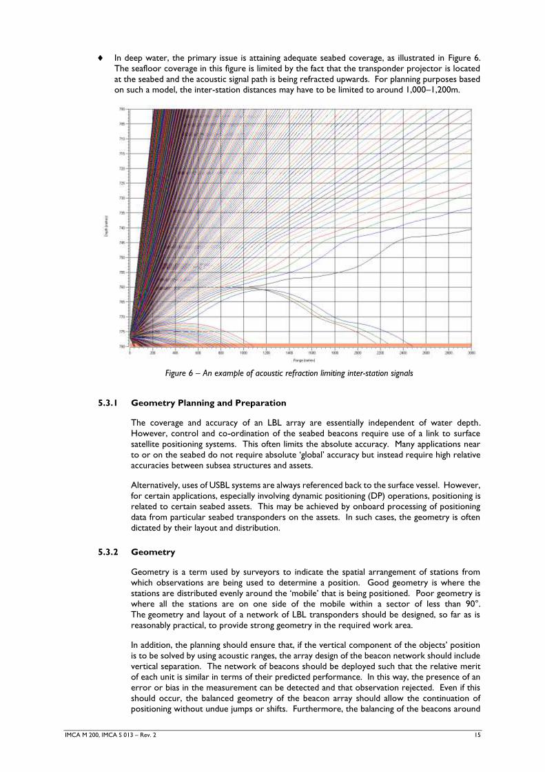
In deep water, the primary issue is attaining adequate seabed coverage, as illustrated in Figure 6.
The seafloor coverage in this figure is limited by the fact that the transponder projector is located
at the seabed and the acoustic signal path is being refracted upwards. For planning purposes based
on such a model, the inter-station distances may have to be limited to around 1,000–1,200m.
Figure 6 – An example of acoustic refraction limiting inter-station signals
5.3.1 Geometry Planning and Preparation
The coverage and accuracy of an LBL array are essentially independent of water depth.
However, control and co-ordination of the seabed beacons require use of a link to surface
satellite positioning systems. This often limits the absolute accuracy. Many applications near
to or on the seabed do not require absolute ‘global’ accuracy but instead require high relative
accuracies between subsea structures and assets.
Alternatively, uses of USBL systems are always referenced back to the surface vessel. However,
for certain applications, especially involving dynamic positioning (DP) operations, positioning is
related to certain seabed assets. This may be achieved by onboard processing of positioning
data from particular seabed transponders on the assets. In such cases, the geometry is often
dictated by their layout and distribution.
5.3.2 Geometry
Geometry is a term used by surveyors to indicate the spatial arrangement of stations from
which observations are being used to determine a position. Good geometry is where the
stations are distributed evenly around the ‘mobile’ that is being positioned. Poor geometry is
where all the stations are on one side of the mobile within a sector of less than 90°.
The geometry and layout of a network of LBL transponders should be designed, so far as is
reasonably practical, to provide strong geometry in the required work area.
In addition, the planning should ensure that, if the vertical component of the objects’ position
is to be solved by using acoustic ranges, the array design of the beacon network should include
vertical separation. The network of beacons should be deployed such that the relative merit
of each unit is similar in terms of their predicted performance. In this way, the presence of an
error or bias in the measurement can be detected and that observation rejected. Even if this
should occur, the balanced geometry of the beacon array should allow the continuation of
positioning without undue jumps or shifts. Furthermore, the balancing of the beacons around
16 IMCA M 200, IMCA S 013 – Rev. 2
an area of work is important for acoustic positioning systems so that the relative distances of
the acoustic signal paths are similar. This will minimise any relative effect of the environment,
such as residual errors in the velocity of sound, on the acoustic signal paths.
For a discrete area of work, the number of beacons or the settings of the USBL system
necessary to ensure all objects are tracked successfully is a function of:
water depth;
coverage required;
the specified accuracy requirements;
the nature of activities taking place.
The situation is made more complex if the activities involve through-water tracking of objects,
or if a long linear route or object is to be positioned, e.g. a pipeline or umbilical. In this case,
the geometry and location of the beacons along the entire route should be carefully considered.
This in order to ensure both good geometry of signals and the availability of at least one
redundant (additional) beacon along the entire route. It may require the use of a large number
of beacons. However, the acoustics engineer and surveyor will have established both a
minimum number and an optimum number of beacons to enable positioning to continue in the
event of a failure. A disadvantage of this is that too many beacons may use too many acoustic
channels and therefore limit the performance of the acoustic systems and hence the operations
in hand.
The geometry planning should also take account of the work area and assess the likelihood of
damage to a beacon or the possibility of blanking or obstruction of acoustic signals by existing
seabed structures.
5.3.3 Distance Restrictions on Range
Of the three main types of systems described in this document, the two that are referenced to
the surface vessel, i.e. the USBL and SBL methods, are limited to providing range and coverage
of an area centred on their host vessel. Based largely on frequency, the range achievable is
represented by the practical depths at which the units can provide seabed positioning. USBL
systems are generally limited to less than 4,000m, whereas SBL systems can extend this range
to over 4,000m. It is expensive and unwieldy to build and install USBL units large enough to
achieve the desired accuracies, in particular, the direction component required by deep water
acoustic operations. LBL systems are not constrained in the same way as the USBL and SBL
systems. LBL can use different frequencies more effectively to develop longer range and cover
greater areas of operation. A note of caution is necessary, as the marine environment has a
strong influence on the way the acoustic signals travel. It is common that close to the seabed
in deep water, acoustic signals will not travel between beacons separated by more than 2,500-
3,000m and in some cases by more than 1,500m.
Appendix 3 also covers some of the effects frequency has on the range of acoustic positioning
systems.
5.3.4 Terrain
The local seabed terrain has the potential to block acoustic signals, and an incline in the seabed
can impact the effective range of acoustic signalling. This is especially the case when operations
are near the seabed.
When planning an LBL array, it is necessary to consider the effects on acoustics of local ridges
or troughs in the seabed, such as sand waves. Also, consideration should be given to any
changes to the overall terrain across the project area. The nature of the seabed is also
important, whether it is solid or consisting of soft mud into which equipment may sink. Clump
weights and strops can be designed to deal with this.
Whilst in general the seabed may be featureless, small undulations can occur with ridges and
troughs of several metres. This could be sufficient to obstruct the acoustic signalling between
the seabed transponders or stations and the mobile unit being tracked. This can be overcome
by designing the seabed frame to allow the transponder to ‘see’ over the undulations. Other
IMCA M 200, IMCA S 013 – Rev. 2 17
designs may allow the transponder to float above the seabed but these may experience some
movement due to currents.
5.4 Mobilisation
Although many deep water operations will be based from dedicated vessels with fully installed, calibrated
and functioning systems, there are times when a vessel of opportunity is used. In such cases, extra care
should be taken during the installation, calibration and operation of the system prior to positioning
operations.
As well as any specific system installations, mobilisations require good planning and properly organised
logistics to ensure that delivery, installation, calibration and set up all lead to a successful start to
operations. Vessel mobilisation should not be underestimated. Sufficient time and resources should be
allowed to complete mobilisation and to verify it has all been carried out properly.
Further information can be found in IMCA S 016 – Mobilisation checklist for offshore survey operations.
5.4.1 Transducer (Hydrophone) Installation and Deployment
The hydrophone should be installed in a relatively noise free location safe from obstructions
and signal blanking, and ideally offering access for maintenance. Generally, some form of
compromise is necessary. In addition, the hydrophone will need to have its linear and rotational
motion compensated for in order to remove biases due to these effects.
It should be recognised that for some specialised operations, the surface vessel will not have a
suitable system already installed. In this case a temporary system may be mobilised and this
installation may take place in less than optimum circumstances. This could result in the acoustic
tracking being prone to performance problems. The consequences of poor installations are
almost impossible to overcome in the field.
The selection of a hydrophone location is usually based on the following criteria:
ease of access for maintenance and possible raising and lowering;
ability to clear the hull by a suitable amount (greater than 2m);
level of noise and freedom from obstructions;
relative motion of the unit with respect to the ship’s centre of gravity and reference points.
For multiple hydrophone installations each unit requires consideration of the above criteria,
and, in addition, the relative distribution of the other hydrophones must be considered.
5.4.2 Transducer Pole Design
The basic criteria for a transducer pole are:
it should withstand the rigours of the motion and forces acted on it by the water when
the vessel is at sea;
it should provide a stable point, with minimal vibration, to generate and receive acoustic
signals;
it should be free from local acoustic interference.
Some operations have used vessels of opportunity and successfully deployed an over-the-side
pole for temporary use. Such a mounting is inherently prone to vibration, which can seriously
affect the acoustic signalling at the transducer head.
Having selected a suitable location point on the vessel, the physical size and length of the
transducer pole should be considered. If it is too long, it could flex in the water when the
vessel is underway. In general, a clearance from the hull of 1-2m is considered adequate, but
it is recommended that the manufacturer is consulted to ensure that their recommendations
and experience are taken into account. The diameter should be of sufficient size to provide a
rigid mounting for the transducer, typically 25cm.
18 IMCA M 200, IMCA S 013 – Rev. 2
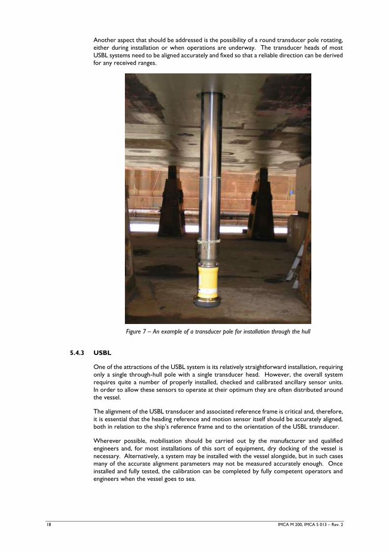
Another aspect that should be addressed is the possibility of a round transducer pole rotating,
either during installation or when operations are underway. The transducer heads of most
USBL systems need to be aligned accurately and fixed so that a reliable direction can be derived
for any received ranges.
Figure 7 – An example of a transducer pole for installation through the hull
5.4.3 USBL
One of the attractions of the USBL system is its relatively straightforward installation, requiring
only a single through-hull pole with a single transducer head. However, the overall system
requires quite a number of properly installed, checked and calibrated ancillary sensor units.
In order to allow these sensors to operate at their optimum they are often distributed around
the vessel.
The alignment of the USBL transducer and associated reference frame is critical and, therefore,
it is essential that the heading reference and motion sensor itself should be accurately aligned,
both in relation to the ship’s reference frame and to the orientation of the USBL transducer.
Wherever possible, mobilisation should be carried out by the manufacturer and qualified
engineers and, for most installations of this sort of equipment, dry docking of the vessel is
necessary. Alternatively, a system may be installed with the vessel alongside, but in such cases
many of the accurate alignment parameters may not be measured accurately enough. Once
installed and fully tested, the calibration can be completed by fully competent operators and
engineers when the vessel goes to sea.
IMCA M 200, IMCA S 013 – Rev. 2 19
5.4.4 LBL
The installation of an LBL system involves a ship-mounted hydrophone and a network of seabed
stations (or transponders). This represents a quite different process than that for a USBL
installation. The LBL ship’s equipment needs to be placed free from any source of noise
interference. There is no alignment or motion sensor involved in the installation. Accurate
range measurement data is necessary for the positioning of the stations or transponders and
their accurate co-ordination or calibration. This involves the time-consuming ‘box-in’
technique (see section 5.6.2.1). A number of alternative and less time-consuming techniques
have been developed to improve the process. The main alternative is to generate inter-station
baselines and only conduct a limited number of box-ins to determine absolute geographic
positions and sufficient data to enable a statistical assessment of network accuracy.
For deep water construction operations where ROVs are present, the requirement for a
transducer deployed from the vessel can be replaced by a similar transducer mounted on the
ROV. This allows the array to be interrogated locally at the seabed rather than through the
entire water column, with the ROV umbilical being used for communications from the surface.
For the box-in technique referred to above, the USBL system’s transducer can be used, subject
to system specification, to interrogate the seabed transponders for ranging requirements.
5.5 Methods of Deployment and Recovery
The use of seabed units and various transponders in deep water requires that they are properly secured
with appropriate fixings and that safe methods for deployment and recovery are adopted. The housings
and pressure vessels required for use in deep water are frequently large and heavy, requiring lifting
equipment and special storage facilities to keep them secure whilst on board. The deployment of
systems starts with the testing and checking of units on deck prior to placing them on the seabed.
For the units being taken to the seabed, there are several approaches used. The simplest is to attach a
clump weight and a flotation collar to the transponder and release the unit over the side. The unit will
then drop to the seabed where it will be monitored for correct operation and its co-ordinates
determined by means of a box-in method.
More sophisticated methods include using an ROV to place the unit directly into a frame or tripod at a
pre-determined location on the seabed. This is, of course, a slower process and requires the ROV
either to transport the units or for a work basket to be used to lower the units to the seabed for
collection by the ROV. This method is used when the acoustic beacons need to be placed in specific
holders on seabed assets.
The above options apply to both USBL transponders/stations as well as LBL stations.
A number of factors influence station deployment, including:
design of deep water transponder frames;
suitability and use of acoustics as DP references;
depth rating of acoustic equipment;
power levels and battery technology.
These and other issues regarding actual deployment of acoustic systems in deep water are covered in
Appendix 7.
5.6 Methods of Calibration
Appropriate calibration of the acoustic system and frequent monitoring of the subsea environment are
vital for successful acoustic positioning. To provide accurate positioning, geodetic control should be
valid, accurate and consistent across the whole area being surveyed. Consequently it is necessary to
derive co-ordinates of an appropriate accuracy and reliability for each beacon or station placed on the
seabed. This is achieved by calibration of the network or array of units. The box-in and network
adjustment of the seabed units are the most common methods adopted. Some of these techniques are
discussed in the following sections.
20 IMCA M 200, IMCA S 013 – Rev. 2
5.6.1 USBL
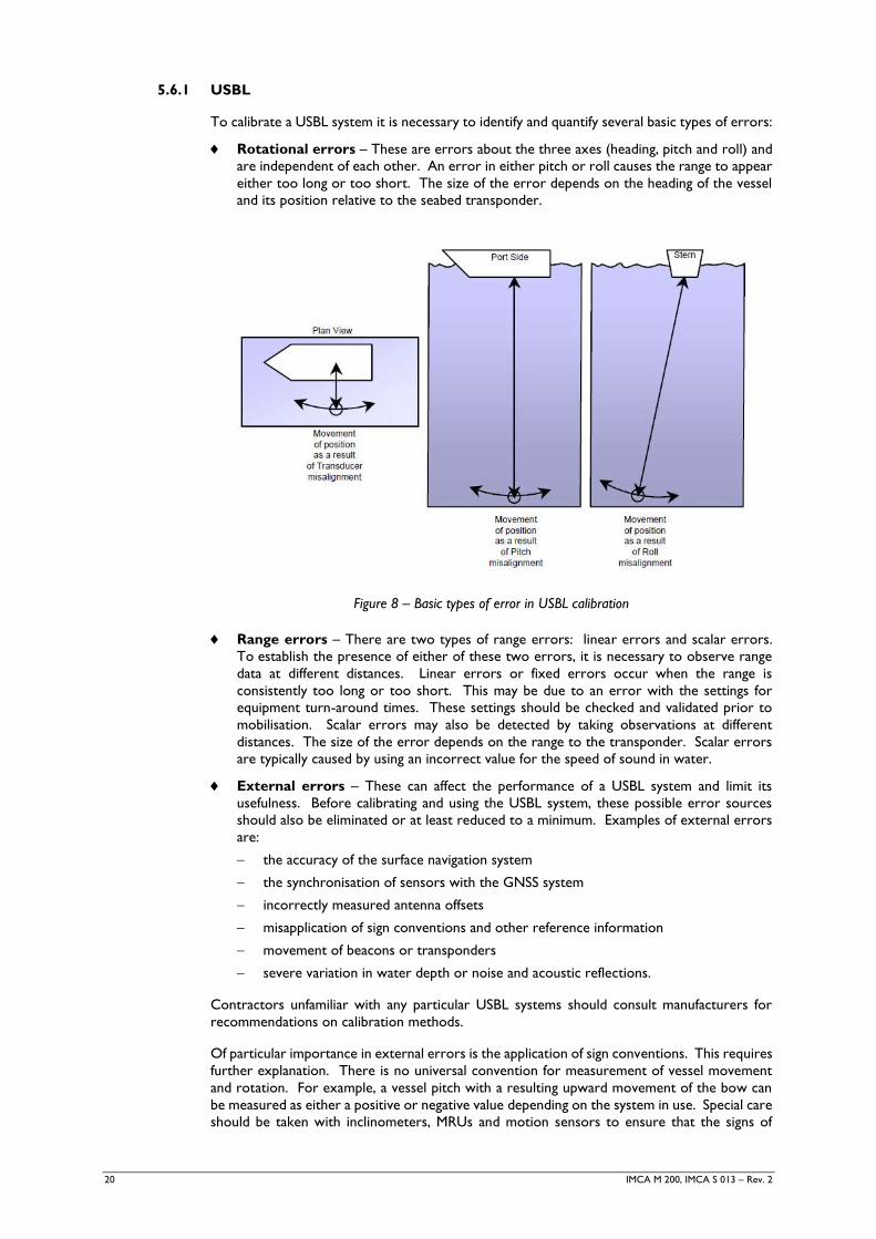
To calibrate a USBL system it is necessary to identify and quantify several basic types of errors:
Rotational errors – These are errors about the three axes (heading, pitch and roll) and
are independent of each other. An error in either pitch or roll causes the range to appear
either too long or too short. The size of the error depends on the heading of the vessel
and its position relative to the seabed transponder.
Figure 8 – Basic types of error in USBL calibration
Range errors – There are two types of range errors: linear errors and scalar errors.
To establish the presence of either of these two errors, it is necessary to observe range
data at different distances. Linear errors or fixed errors occur when the range is
consistently too long or too short. This may be due to an error with the settings for
equipment turn-around times. These settings should be checked and validated prior to
mobilisation. Scalar errors may also be detected by taking observations at different
distances. The size of the error depends on the range to the transponder. Scalar errors
are typically caused by using an incorrect value for the speed of sound in water.
External errors – These can affect the performance of a USBL system and limit its
usefulness. Before calibrating and using the USBL system, these possible error sources
should also be eliminated or at least reduced to a minimum. Examples of external errors
are:
the accuracy of the surface navigation system
the synchronisation of sensors with the GNSS system
incorrectly measured antenna offsets
misapplication of sign conventions and other reference information
movement of beacons or transponders
severe variation in water depth or noise and acoustic reflections.
Contractors unfamiliar with any particular USBL systems should consult manufacturers for
recommendations on calibration methods.
Of particular importance in external errors is the application of sign conventions. This requires
further explanation. There is no universal convention for measurement of vessel movement
and rotation. For example, a vessel pitch with a resulting upward movement of the bow can
be measured as either a positive or negative value depending on the system in use. Special care
should be taken with inclinometers, MRUs and motion sensors to ensure that the signs of
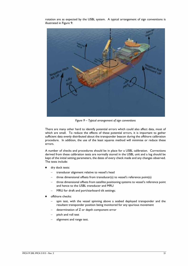
IMCA M 200, IMCA S 013 – Rev. 2 21
rotation are as expected by the USBL system. A typical arrangement of sign conventions is
illustrated in Figure 9:
Figure 9 – Typical arrangement of sign conventions
There are many other hard to identify potential errors which could also affect data, most of
which are small. To reduce the effects of these potential errors, it is important to gather
sufficient data evenly distributed about the transponder beacon during the offshore calibration
procedure. In addition, the use of the least squares method will minimise or reduce these
errors.
A number of checks and procedures should be in place for a USBL calibration. Corrections
derived from these calibration tests are normally stored in the USBL unit and a log should be
kept of the initial setting parameters, the dates of every check made and any changes observed.
The tests include:
dry dock tests:
transducer alignment relative to vessel’s head
three dimensional offsets from transducer(s) to vessel’s reference point(s)
three dimensional offsets from satellite positioning systems to vessel’s reference point
and hence to the USBL transducer and MRU
MRU for draft and port/starboard tilt settings;
offshore checks:
spin test, with the vessel spinning above a seabed deployed transponder and the
resultant transponder position being monitored for any spurious movement
determination of Z or depth component error
pitch and roll test
alignment and range test.
22 IMCA M 200, IMCA S 013 – Rev. 2
5.6.2 LBL
The two main methods to achieve a properly calibrated LBL acoustic array are as follows:
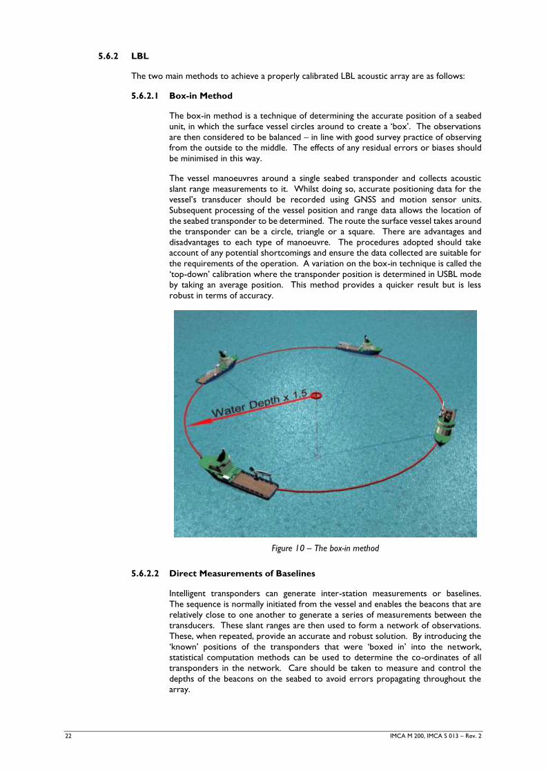
5.6.2.1 Box-in Method
The box-in method is a technique of determining the accurate position of a seabed
unit, in which the surface vessel circles around to create a ‘box’. The observations
are then considered to be balanced – in line with good survey practice of observing
from the outside to the middle. The effects of any residual errors or biases should
be minimised in this way.
The vessel manoeuvres around a single seabed transponder and collects acoustic
slant range measurements to it. Whilst doing so, accurate positioning data for the
vessel’s transducer should be recorded using GNSS and motion sensor units.
Subsequent processing of the vessel position and range data allows the location of
the seabed transponder to be determined. The route the surface vessel takes around
the transponder can be a circle, triangle or a square. There are advantages and
disadvantages to each type of manoeuvre. The procedures adopted should take
account of any potential shortcomings and ensure the data collected are suitable for
the requirements of the operation. A variation on the box-in technique is called the
‘top-down’ calibration where the transponder position is determined in USBL mode
by taking an average position. This method provides a quicker result but is less
robust in terms of accuracy.
Figure 10 – The box-in method
5.6.2.2 Direct Measurements of Baselines
Intelligent transponders can generate inter-station measurements or baselines.
The sequence is normally initiated from the vessel and enables the beacons that are
relatively close to one another to generate a series of measurements between the
transducers. These slant ranges are then used to form a network of observations.
These, when repeated, provide an accurate and robust solution. By introducing the
‘known’ positions of the transponders that were ‘boxed in’ into the network,
statistical computation methods can be used to determine the co-ordinates of all
transponders in the network. Care should be taken to measure and control the
depths of the beacons on the seabed to avoid errors propagating throughout the
array.
IMCA M 200, IMCA S 013 – Rev. 2 23
Although potentially very accurate, as each end of the baseline is fixed, the outer
beacons of an array may suffer from relatively poor geometry. Care should be taken
to ensure the velocity of sound is accurately measured to avoid unwanted scale
errors. This is true of the whole network of beacons but is less well controlled and
identified at the edges of the array. This approach is valid for any network of
transponders that have acoustic signal paths ‘visible’ to one another. Some low
frequency LBL systems may have their beacons distributed a little too far apart to
receive the acoustic signal from an adjacent or relatively nearby beacon. In such
cases the box-in method should be adopted for all transponders.
5.7 Quality Control
To ensure that deep water acoustic positioning is appropriately accurate and reliable, quality tests and
checks should be carried out on various parameters and variables:
Calibration – Accurate set up of positioning equipment prior to operations is vital. The process
is described more fully in section 5.6;
Fundamental positioning variables (position, heading and speed) – Operators should
monitor the positioning solutions in order to detect gross errors such as sudden shifts or jumps in
the data. Duplicate or multiple sensors, though costly, can be of value in checking the accuracy and
reliability of data for critical operations;
Update rate and signal/noise ratio of acoustic systems;
Redundancy – The use of more observations than are required to compute a position. This allows
statistical checks and estimates to confirm good, accurate and reliable data.
5.8 System Performance
The performance of an acoustic system is ultimately limited by the acoustic conditions in the water.
The combination of the various signal losses, noise sources and detection capabilities should not exceed
the signal level available from the desired signal source. Noise from vessel thrusters and other man-
made sources, as well as aeration and turbulence, will all be detrimental to efficient acoustic positioning.
At long ranges, the energy of the acoustic pulse will decrease and decay. If the detector is limited or
insensitive then there will be no measurable acoustic signal. As each project will have its own unique
combination of parameters, the actual limits of a system in a specific set of conditions may be well
defined before operations start. In addition, thermoclines and other environmental effects can cause
errors, especially when the horizontal displacement or range from the vessel is relatively large.
The following sections outline the performance of deep water acoustic systems with respect to various
technical acceptance criteria.
5.8.1 Users and Frequency Allocation
The move into deeper water means that more and more simultaneous acoustic positioning
operations are being carried out in a relatively small area. This puts pressure on the limited
acoustic bandwidths available for the various systems and may lead to acoustic pollution which
can completely blank out the users and objects being tracked.
Interrogation and reply frequencies are assigned to transponders so that the ranging pulses or
data telemetry functions can be achieved without interference. Typical channel separation for
a 24-36kHz system could be 500Hz. Leakage of one signal or acoustic pulse from one channel
to another adjacent channel will result if the chosen frequencies are not separated sufficiently.
When there are multiple users of acoustic systems from a number of different vessels or
installations in close proximity, an acoustic frequency management plan may be required. Such
a plan might pre-assign channels to each transponder in the water, thus avoiding interference
and associated delays to vessel operations. Ideally, one user or vessel is made responsible for
the implementation of the management plan at site and for the control of corrective actions in
the event that there is interference.
24 IMCA M 200, IMCA S 013 – Rev. 2
5.8.2 USBL and LBL Position Updates in Deep Water
A further characteristic of deep water USBL operations is the time required for the acoustic
signal to travel from the surface unit to the seabed, for the seabed unit to reply, and for the
signal to travel back to the surface. In 750m of water this is around 1.5s per transponder.
If interference or corruption of the acoustic signals from one beacon by those of another is to
be avoided, then each beacon may need to transmit at a slightly different time, such that each
beacon transmits its response at a different time offset following reception of an interrogation
message. This may add several seconds to the reply being obtained and leads to an update rate
for sub-surface positions as slow as one position update every 2 or 3 seconds (or even slower
for deeper waters). In water depths measured in kilometres, these time delays may become
critical to the continued success of operations. For ROV positioning in deep water, the
introduction of local motion measuring systems such as Doppler velocity log (DVL) and inertial
navigation system (INS) systems can provide additional data that maintains a position solution
in between acoustic updates. The situation for LBL operations is usually not as severe as the
baseline distances from the seabed transponders to the mobile hydrophones are less than the
water depth. System integration with INS and DVL would still work with reduced use of
acoustics in so-called ‘sparse’ USBL or LBL subsea positioning configurations. In sparse mode
the acoustic measurements are weighted into an integrated subsea positioning system.
5.8.3 Acoustic Noise and Possible Causes of Interference
The most significant problem for acoustic positioning is noise – i.e. unwanted energy in the
frequency band used by the positioning system, leading to degradation of signal. Noise can be
divided into two categories:
environmental or external noise;
external shipping noise
external noise from machinery such as drilling, pile-driving or seismic survey
operations
other acoustic systems – simultaneous operations
biological (marine life) noise
wind and rain;
noise generated on board the host vessel of the acoustic positioning system, such as self
noise (noise generated by the ship or ROV).
Distinguishing between environmental noise and mechanical or artificial interference is not
always straightforward when operating acoustic systems. It is possible to categorise the
possible man-made or self noise sources as acoustic interference.
Interference from other acoustic equipment may be a significant problem, particularly in deep
water developments. It may be appropriate to develop some form of plan to manage
frequencies to mitigate this.
Various other noise sources exist, such as earthquakes and tectonic activity and molecular
agitation noise, but these are normally less significant and, in the case of earthquakes, less
frequent.
There are a number of further possible causes of acoustic interference. These are:
Changes to the velocity of sound in water – The velocity of sound in water is one of
the most critical and ultimately limiting factors affecting acoustic systems;
Internal waves in deep water – These occur below the surface of the sea. They are
normally associated with bodies of water where the density is very well defined and can
be considered stratified or layered. There may be localised rapid changes in water
temperature caused by the internal wave. The change in temperature can be severe,
resulting in significant errors in acoustic positioning and, in some cases, loss of positioning
all together;
Ray bending – A phenomenon produced by the variation in the layering and condition of
the water;
IMCA M 200, IMCA S 013 – Rev. 2 25
Acoustic blanking – A phenomenon produced by ray bending in which there is
inadequate acoustic signal from an area.
Further information on acoustic noise and interference can be found in Appendix 6.
5.8.4 Achievable Accuracies
The accuracy of acoustic positioning is dependent on a number of variables and on a wide
variety of potential errors which need to be minimised or eliminated. The most significant of
these potential errors are discussed elsewhere in this document.
The overall accuracy of acoustic positioning may depend on some of the following factors:
Water depth;
The accuracy with which a transponder array is established relative to a geodetic datum
or relative to the source positioning system used, e.g. GNSS or DGNSS;
Identification and suppression of multi-path effects (reflections). These will be particularly
noticeable in the vicinity of fixed structures such as production platforms. They are often
worse for USBL and SBL systems than for LBL systems;
The accurate determination of sound velocity, velocity gradients and the amount of
refraction;
Frequency used – accuracy and resolution increases with increasing frequency, but at the
expense of the range and the power required;
The geometry of the ranges that create the position solution and, to a degree, seabed
topography, i.e. whether or not there is a ‘line of sight’ between transponders;
The sophistication of the processing system and software being used: digital techniques
often provide better results than analogue results for acoustic tracking;
Integration with other sensors such as subsea DVL and INS;
Errors in time measurement owing to the presence of noise in the received signals.
26 IMCA M 200, IMCA S 013 – Rev. 2
6 Associated Topics
This section provides observations and comments relating to some of the technical, software and engineering
elements which should also be considered for deep water acoustic positioning.
6.1 Integration of Systems
The derivation of position relies on adequate data. An acoustic positioning system on its own in deep
water may have considerable limitations and deficiencies. Peripheral sensors are frequently used to
augment the solution. This complex augmentation process requires the integration of peripheral sensor
data in a computation. To achieve an optimum solution, the timing, relative weights (i.e. how much
merit each observation is given in a position computation) and some form of qualitative estimate of the
errors for quality control is required. This all requires expert design and testing.
6.2 Communications
The fundamental of acoustic positioning is the transfer of an acoustic signal from point to point.
However, associated with this process is the need to command and control the system and to transfer
any peripheral data or information. Such communications can be compromised by excessive range, by
noise in the water column or by other sources of interference described earlier, thus stopping the
overall operation. It is often overlooked in the planning of operations but is an important element in
ensuring the success of the operation of the system.
6.3 Software, Interfacing and Display
Related to the integration of data for the computation of position is the configuration of the hardware
units, their interfacing to allow data flow and the software to manage this. These components of the
acoustic positioning system are internal and usually at least partly hidden from the operator. However,
when testing and planning a project it is good practice to ensure that all the system components are
compatible with the version of software and interfacing available.
6.4 Additional Peripheral Sensors and System Interfacing
Peripheral devices can vary enormously in their capability, quality and purpose. For deep water
operations they are also engineered for the extreme conditions and may be housed in a solid unit for
operation at the seabed. These are important units and should be fully tested as a functioning unit as
part of a complete system in order to ensure that the required data flow can be achieved.
Further information on peripheral sensors can be found in IMCA S 021 – Guidelines for the management
of peripheral survey sensors.
6.5 Permitting and Legislation
Many deep water projects occur in relatively remote places where the logistics of transportation of
system units has to be carefully planned. In addition, project planners should take into account the fact
that the components of some deep water positioning systems are considered to be of dual use (i.e.
potentially of military use). Additional time should be allowed when dealing with such components, for
the preparation and processing of additional forms and certificates.
6.6 Training and Competence
To ensure the success of projects it is necessary to have suitably experienced and qualified personnel
to calibrate, control and operate the systems, so it is important to select the team carefully. This may
not always be possible so it is important to review the team and their knowledge and experience of
deep water acoustic positioning. Manufacturers and other specialist providers offer a number of training
opportunities.

IMCA M 200, IMCA S 013 – Rev. 2 27
6.6.1 Positioning Courses
General courses that cover the basics of geodesy, positioning theory and design as well as some
basic acoustic positioning elements are required. Ideally they should be of short duration and
provide attendees with suitable course notes and practical exercises to demonstrate the most
important elements covered.
6.6.2 Acoustics Courses
Specialist courses covering the basics of acoustics and also relating to practical operations.
As well as covering the theory of acoustics and the operation of specific hardware and software
packages, it is important to provide a practical element, training personnel to handle rigging of
transponders, deployment, calibrations and actual operations.
28 IMCA M 200, IMCA S 013 – Rev. 2
7 Applications of Acoustic Positioning in Deep Water
7.1 Dynamic Positioning
Assets Permanently installed SBL or USBL systems on board the vessel. All positioning
can be maintained from the vessel and is either relative to the vessel to a seabed
transponder or to another reference positioning system such as GNSS. At least
one (but usually four to five) seabed transponders (beacons), are deployed.
Objects tracked The surface vessel that is required to maintain its position.
Accuracies Many DP applications deliver positioning relative to some seabed asset such as a
wellhead or a pipeline. This results in an accuracy that is often not related to
depth. Alternatively the positioning is established relative to the surface GNSS
system on board the vessel. This may result in accuracies of several metres to
over 10m depending on the water depth and the dynamic nature of the sound
velocity profile.
Methodologies The permanently fitted SBL or USBL acts as a reference for the vessel. The
chosen location, such as a well, is entered into the DP console. Then the
positioning systems is checked to ensure correct operations and that there are
no alarm conditions present. The vessel manoeuvres onto the location and the
reference seabed transponder is deployed. If a single transponder for a USBL
system is deployed, this is normally located close to the well location or even
onto a special frame on the well itself. A second back-up unit may also be
deployed to provide some redundancy in the event of failure.
If a combined long and ultra-short baseline (LUSBL) system is being used, then
four seabed transponders should be deployed within their range and within the
beam ‘footprint’ of the vessel transducer units. These units usually have a limited
beam width of around 25-30º.
Limitations The inherent accuracy of the system may be low, relative to the survey
requirements of the project. In 1,000m of water, for example, existing DP
systems may achieve a positioning accuracy of ±4-10m.
Points to note PPP GNSS solutions with accuracy less than a few decimetres are commonly used
nowadays for deep water operations.
A wider range of services may be available. Comparisons should take account of
this when analysing and planning operations. Full survey applications in deep
water will often require the deployment of additional assets. These may
communicate and work with the DP system. It is therefore important that the
flexibility of the DP systems and the availability of data sources and interfacing are
thoroughly checked.
7.2 Towed Body (‘Towfish’) Positioning
Assets USBL systems fitted on board a survey vessel or vessel of opportunity. All
positioning can be maintained from the vessel and the survey data collected is
relative to the towfish. The vessel position can be referenced to the real world
through a positioning system such as GNSS. At least one USBL is installed but
frequently requirements state that it is necessary to have some form of back-up.
It is also recommended that, where possible, two transponders are installed on
the towfish.
Objects tracked The towed body or towfish is required to maintain its position either along a
route or corridor or perhaps along a regular line pattern.
Accuracies Many towed body applications deliver positioning relative to the GNSS used by
the towing vessel. Otherwise the positioning can be established relative to a sub-
surface target. However, this is usually a quality control and verification process.
A permanently fitted USBL system should be able to position a towed body to
better than 0.5% of the slant distance between the towed body and the surface
vessel.
IMCA M 200, IMCA S 013 – Rev. 2 29
Methodologies The permanently fitted SBL or USBL usually acts as a reference from the vessel
to the tracked objects. The transponder is deployed on to the towed fish. If a
single transponder for a USBL system is deployed, this is normally a transponder
or responder type of unit that transmits using either localised battery power or
the integral power from the tow cable, and receives its trigger pulse through the
tow cable rather than through the water column, thus increasing reliability.
Care should be exercised in adopting a pre-installed USBL system if it has not
been designed specifically for tracking towed units. This is due to the required
aft-looking directional sensitivity required of the hydrophone and receiver array.
Typically, these systems have a beam width of around ± 10-35º from the vertical.
If they are downward facing, they may not properly detect the towfish that is laid
back from the vessel whilst under tow. Modern beam steering systems may
overcome this limitation. It is becoming common practice to support the acoustic
positioning with accurate depth data and, where relevant, in deeper towing
situations, altitude data.
Limitations The inherent accuracy of the system may be low, relative to the survey
requirements of the project. In 1,000m of water, existing systems may offer
positioning accuracy of ±10-15m for towed fish astern, dependent on the aspect
ratio of the depth and layback of the towed fish. The larger the fish or the lower
the tow speed the deeper the unit is likely to be. Depending on the sensors
carried the unit may be required to be close to the seabed. Sensors frequently
used include heading reference gyros and motion sensors, as they provide
corrections for the positioning as well as the survey sensors carried. The use of
these sensors increases operational costs as well as the time taken to check and
calibrate the overall sensor and positioning systems. Accuracy is related to the
layback distances, which may be in excess of several thousand metres. This means
that the acoustic path will travel through significant layers of the water column.
Thus, the sound velocity profile (SVP) must be established and frequently updated
to remain as accurate as possible. Position updates may be regular and frequent,
however, the travel path, being astern of the surface vessel, may be prone to
signal interference and loss of signal caused by noise from the vessels propeller
wash.
Points to note The surface positioning is usually referenced to DGNSS systems ranging in
accuracy from ±1-2m to less than two decimetres. A wider range of services
may be available. Comparisons should take account of this when analysing and
planning operations.
7.3 Riser Monitoring
Assets Topsides equipment to operate a USBL system fitted on board the surface vessel,
its associated transceiver or hydrophone unit and the sub-surface transponders
deployed onto the riser and associated well assets (e.g. blowout preventers
(BOP)). The required signalling and measurements may all be maintained from
the vessel and as this system monitors angles, rather than actual position, the
reference is either an absolute inclination from the vertical or some relative
measurement when the values are compared to a reference unit. At least one
(but typically two) transponders are deployed, one to the riser and one to the
BOP.
Objects tracked Monitoring and assessment of any deviation of the riser from the vertical. The
basis of this system is acoustic data telemetry.
Accuracies Many different sensors are available for use in such an application and so it is not
practical to offer specific accuracies or limits of performance. However, there
are a number of acoustic monitoring systems that have integrated inclinometers
installed, providing readings to a fraction of a degree. They have been found to
offer a useful riser inclination dataset, using acoustic telemetry, and are capable
of supporting dynamic drilling operations in deep water.
30 IMCA M 200, IMCA S 013 – Rev. 2
Methodologies The aim is to maintain a vertical drilling arrangement between the drilling vessel,
the drilled well and the seabed riser. The surface vessel DP maintains station in
all weathers and environmental conditions, which may result in some deviation
of the riser. The sub-surface units are installed onto the riser and BOP in order
to monitor verticality and report back to the surface via acoustic telemetry the
inclination values. Either absolute values or relative values between the units are
provided to the surface where the computing system derives any adjustments in
position to be made by the surface vessel in order to maintain a vertical riser.
A back-up unit may also be deployed to provide redundancy in case of failure.
Limitations The system relies on the accurate alignment and stability of the sub-surface units
deployed onto the riser. These units will have either battery power or perhaps
power derived from the BOP or riser. Data telemetry via an acoustic link may
be prone to interference from drilling and vessel noise. However, as this is the
main risk, manufacturers have developed robust systems using frequencies,
power and data codes to mitigate this interference.
Points to note Acoustic positioning is also available during riser monitoring for the surface vessel
or other objects such as ROVs. The use of battery powered units means that
there is no requirement for power to be delivered from the surface.
7.4 Pipelay Positioning
Assets USBL systems or combined LUSBL systems fitted on board the pipelay vessel.
A further vessel may also be associated with this vessel to provide survey and
monitoring capability. Positioning in deep water environments may not always
be maintained from the pipelay vessel and for critical areas use is made of seabed
deployed LBL arrays. The seabed transponders are used at critical points along
a pipe route, such as crossover points with an existing pipeline or where there
may be requirements for high accuracy, as at lay-down of the end of the pipe.
The LBL array will vary in its size and number of units from as little as five or six
to many tens of units for a complex area of work. Objects to be positioned
include the pipelay vessel, the pipe itself and ROVs present to provide visual
monitoring and perform other tasks. As well as ROV and subsea assets being
positioned, the pipeline may have transponders fitted during deployment in a
number of locations, including:
at pipeline start-up;
at crossovers of existing pipelines;
near pipeline termination for the pipeline cut-to-length measurement;
at pipeline head to confirm the pipeline head is installed within the target
box.
The transponders fitted on pipeline structures may have inclinometers and depth
sensors fitted to provide tilt and depth information via acoustic telemetry during
the installation.
Objects tracked The pipelay vessel, the pipeline/structure, seabed reference transponders and
any ROVs present.
Accuracies Many elements influence the accuracy of pipelay positioning. Surface USBL
systems will usually provide an accuracy of less than 0.5% of the range to the
pipeline touch-down point. An LBL array will provide a relative accuracy of
typically ±0.2m in relation to existing seabed infrastructure. Accuracies are
dependent on the survey control and frequencies of the acoustics.
IMCA M 200, IMCA S 013 – Rev. 2 31
Methodologies Transponders may be installed along the pipe at intervals in order to monitor
the catenary and touch-down on the seabed. An ROV may also be positioned,
preferably with the same system, in order to monitor and alert the operators if
the pipe is seen to be misplaced, or if difficulties are encountered on the seabed.
Where the new pipeline is being laid across an existing pipeline, a pair of
transponders are installed on the existing pipeline on either side of the route to
provide a ‘gate’, through which a pipeline mounted transponder is guided. When
approaching a critical area, e.g. across an existing pipeline, use is made of several
LBL transponders to ensure the pipe is placed within its intended corridor.
Limitations The position error of the USBL system increases with range to the transponder.
For deeper water operations the accuracy in X, Y, Z positioning will have
degraded considerably. Where a high relative accuracy is required near the
seabed, e.g. for pipelay close to existing infrastructure, an LBL solution provides
a far more accurate relative positioning solution.
Points to note PPP GNSS solutions with accuracy less than a few decimetres are commonly
used nowadays for deep water operations. A wider range of services may be
available. For deep water, USBL accuracies may be relatively poor, however,
the introduction of inertial navigation systems (INS) to augment acoustic
positioning has meant that USBL systems are more commonly used for
positioning pipelay operations. This should be taken into account when analysing
and planning operations.
7.5 AUV and ROV Positioning
Assets USBL systems fitted on board a surface vessel, sometimes augmented with a
sparse array of seabed LBL units. In addition, the AUV or ROV may have INS
and other associated sensors fitted. The concept of inverted USBL has been
developed to maximise the benefits of the quiet subsea vehicle. More details of
this are included in Appendix 2. Various combinations of systems offer options
for use with underwater vehicles, particularly AUVs, due to their ability to
operate autonomously at significant distances from the surface ship. ROVs are
more restricted in their scope of operation around the surface ship from which
they are deployed. All positioning methods may be applied depending on the
nature of the operation and may require additional sensor data from heading
reference units, altitude, depth and DVL systems.
Objects tracked The ROV or AUV during inspection, repair and maintenance (IRM), or
construction operations, or when using survey sensors over a regular search or
survey grid. The units may also be configured to track a specific underwater cable
or pipeline route using specialist additional sensor units.
Accuracies Many integrated solutions support a variety of applications and deliver absolute
or real world surface positioning, as well as positioning of seabed assets such as
a wellhead or pipeline, relative to an acoustic transponder. Overall accuracies
are typically 0.05%-0.3% water depth with relative values at better than 1m. Note
that the use of tightly integrated solutions means that the acoustic positioning
element may no longer be the main component or the limit for accuracy.
Methodologies ROVs used for survey usually have a USBL responder or a subsea transducer as
well as depth, altitude, gyro and DVL sensors. More recently, inertial navigation
systems have been introduced. These sensors all aid in positioning as their update
rate and resolution combine with the more slowly updating absolute accuracy of
the surface USBL data.
An AUV can also carry depth, altitude, heading and velocity sensors to develop
its onboard integrated position solution.
Note that the acoustic positioning component forms the link to the real world
and is an essential aid to the positioning process, reducing the inherent errors of
an INS solution which may grow larger over a short period of time due to drifts
in the accelerometers.
32 IMCA M 200, IMCA S 013 – Rev. 2
Limitations The inherent accuracy of the USBL system may be low relative to the positioning
requirements for the ROV or AUV. Whilst ROVs carry power, umbilicals and
tethers limit their range from the surface vessel, suiting the use of USBL
positioning which can be augmented by other sensors. Alternatively, the AUV
has to carry its own limited power supply. AUVs must employ a positioning
solution that will cover the range and duration of the sortie. An AUV may travel
relatively long distances and, therefore, its positioning regime needs to be well
planned to allow frequent updates to the onboard INS from acoustic and
associated sensor data.
Points to note There are relatively few types of AUV systems and their positioning needs to be
well planned to ensure adequate coverage and accuracy is achieved. Tightly
integrated position solutions collect a variety of data inputs and combine them in
a way to derive consistent positions. A variety of additional sensors such as
heading reference units, motion sensor, INS system, DVL, depth and altitude unit,
are used to provide sufficient data types to enable the positioning to continue for
long periods of time over relatively large areas.
Many ROV operations and applications exist. However, power, data collection,
telemetry and monitoring are via the ROV tether and the role of acoustics may
be limited.
7.6 Construction Positioning and Installation of Structures
Assets Vessel based systems and seabed units where LBL accuracies are required.
Additional units are attached to the structures to be installed and are used to
monitor and control the lowering and installation of structures onto location.
Additional data, such as heading and attitude sensor data, is frequently used in
order to monitor orientation and settlement on the seabed. Within localised
LBL arrays, the use of multiple acoustic transponders mounted on the structure
can be used as an additional source of information to derive the orientation of
the structures.
Objects tracked The structure being deployed and installed. Acoustic transponders are attached
to the structure to position it. The system may often be configured to also track
a specific underwater object such as an ROV used to confirm the placement of a
structure, or to recover some of the acoustic transponders used.
Accuracies For construction operations, the specified tolerances for placing assets on the
seabed are often based on relative distances, engineering designs and
technologies. For acoustic positioning, the requirement therefore is to maintain
high accuracy (metre or sub-metre) positioning of the structure being deployed
relative to other seabed assets. Over short distances and in a specific area, the
use of LBL is often applied. USBL from the surface vessel can often be too limited
in accuracy for this application, although it is commonplace to use additional
sensors to remove potential error. Accuracy requirements may vary from sub-
metre to several tens of metres depending on the exact operation, thus allowing
USBL to be used for some structure installations.
Methodologies The permanently fitted SBL or USBL offers a link to the outside world and uses
data telemetry to recover sensor data from the transponders deployed on a
structure. SBL or USBL accuracy may be insufficient, and so the use of LBL and
associated sensors can provide a workable solution for many installations. ROVs
may also be used to monitor the installation. Due to engineering tolerances, LBL
systems can be used to provide a relatively accurate and fast update rate.
Limitations The inherent accuracy of vessel based USBL systems may be too low, relative to
the survey requirements of the project. In 1,000m of water, for example, existing
USBL systems may offer a positioning accuracy of ±3-6m, whereas there may be
a requirement for accuracies of ±1m relative to existing structures dependent on
design and engineering. In such cases, installation of additional acoustic
positioning equipment of the desired accuracy such as an LBL array may be
required. Additionally, positioning latency can affect how easily the installation
can be completed. Careful planning and sufficient redundancy are vital to avoid
expensive mistakes or failures.
IMCA M 200, IMCA S 013 – Rev. 2 33
Points to note The surface positioning is usually referenced to either GNSS which has an
accuracy of ±1-2m for standard systems, or to DGNSS which may have higher
accuracy. A wider range of services may be available. For deep water structure
installation, LBL and integrated sensor solutions dominate as well as intelligent
transponders allowing the telemetry of heading and attitude data to support the
installation. This should be taken into account when analysing and planning
operations and their costs.
7.7 Relative Measurement
Assets Transponders being located at the points of measurement and interest as well as
LBL arrays or USBL systems on the surface vessel.
Objects tracked The main objective is not to derive position but is the measurement of distance
or even inclination relative to some reference plane. The system may, however,
need to be configured to track a specific underwater object such as an ROV.
Alternatively, referencing one transponder to another using USBL measurements
can provide a position solution independent of surface satellite positioning
systems. This method can be used for structure installations where a higher
relative accuracy than USBL is required, but the expense of an LBL array is
considered unnecessary.
Accuracies Accuracy here is not absolute but is the accuracy of measurement of distance to
some other object. A common task is assessment of the condition or status of a
seabed asset and, as such, precision and repeatability are of importance rather
than absolute value.
Methodologies The permanently fitted SBL or USBL usually acts as a reference for the vessel.
The chosen application will usually be relative to a specific location of known
co-ordinates.
Limitations Installation of units on existing seabed assets requires ROV deployment and
recovery as well as careful power management.
Points to note Although a relative exercise, the surface positioning is usually referenced to either
GNSS which has an accuracy of ±1-2m for standard systems, or to DGNSS which
may have higher accuracy. These can provide some quality control on the relative
measurements. This should be taken into account when analysing and planning
operations and their costs.
7.8 Metrology
For additional information, please refer to IMCA S 019 – Guidance on subsea metrology.
Assets Two pipeline flanges are to be connected together by a prefabricated spool.
Subsea metrology is the process of determining the spatial relationship between
them. The process involves the determination of the distance between the flange
ends, relative depths, relative angles, relative pitch/roll of each flange and the
profile of the seabed along the intended spool route. There are several non-
acoustic metrology techniques. For the purpose of this document the assets are
an LBL system with transponders installed in special brackets on seabed assets
and special frames/tripods on the seabed. All positioning can be maintained from
and referenced to the vessel, the seabed transponders, or another positioning
system such as GNSS. At least one (but usually four or five) seabed transponders
are deployed depending on the number and relative arrangement of the points to
be measured.
Objects tracked The main objective is not the positioning of a unit but the relative vector between
certain specific points as described above. However, the close attendance of an
ROV means that the system may also be configured to track an underwater object
such as an ROV during associated seabed measurements.
Accuracies With modern acoustic techniques, relative accuracies of 5cm or better can be
achieved with detailed engineering planning and carefully controlled observations
and measurement.
34 IMCA M 200, IMCA S 013 – Rev. 2
Methodologies The very high precision and accuracy required for metrology requires the use of
modern acoustic techniques such as spread spectrum signalling and relatively high
frequencies. Relative distances, vectors and the attitude of some seabed assets
are all important parameters to be derived from metrology techniques.
Positioning itself in terms of co-ordinates and locations is not usually required.
Limitations The inherent accuracy of the system may be low in absolute terms, however, the
aim is to derive relative vectors and separations between assets, such as a spool
piece and riser. Different update rates and the measurement of correct offsets
between key points may mean this kind of positioning system is of little practical
use for any other tasks or positioning operations during the project.
Points to note Absolute positioning as such is not actually required – it is very accurate
measurements that are needed. A specific capability to achieve the required data
may often mean this configuration is not used for any other aspects of the overall
deep water project.
Preparation for metrology measurements is critical. Extensive research of the
assets that are to be tied together, and review of design/engineering drawings are
both required. For new structures it is essential that a dimensional control survey
is conducted in the fabrication yard before deployment and is used to determine
the three dimensional relationship between the transponders and the points of
interest on the flanges.
7.9 Well Positioning
Assets Permanently installed SBL or USBL systems on board the vessel. All positioning
can be maintained from the vessel, and positioning is either relative to the vessel,
the seabed transponder or another positioning system such as GNSS. Usually
four or five seabed transponders are deployed. For well positioning requiring
high accuracy positioning, LBL arrays are used. This is normally required in
situations where the new well has to be positioned relative to an existing
structure such as a manifold or a series of previous installed wellheads.
Objects tracked The surface vessel and/or the associated drill string suspended down to the
seafloor. The system may also be configured to track a specific underwater object
such as the ROV monitoring the drilling and initial spud-in of the well. In deep
water a number of associated units are used to maintain a safe well. The BOP, a
temporary guide base or simply the drill string may require positioning or
monitoring. The transponders deployed will be fitted to specific points to ensure
the well unit and the drill string are correctly placed and accurately positioned.
Accuracies The acoustics should be planned and designed to achieve the required accuracies
for the positioning of each well. From the surface, the positioning of wells will
be to an accuracy of approximately 0.2-0.7% of water depth. For LBL operations,
the accuracy of positioning will be 10-20cm relative to existing structures.
Methodologies The permanently fitted SBL or USBL usually acts as a reference for the vessel.
The chosen location of the well is entered into the DP console and the positioning
systems checked to ensure they are operating correctly and no alarm conditions
are present. The vessel manoeuvres onto the location and the reference seabed
transponder is deployed. If a single transponder for a USBL system is deployed,
this is normally located close to the well location or onto a special frame on the
well guide base or the well itself. Backup units may also be deployed to provide
some redundancy in the event of failure. For LBL operations, the array is either
installed by ROV from the drilling rig and calibrated relative to existing structures
or it is deployed in advance by one of the anchor handling vessels or by a survey
vessel.
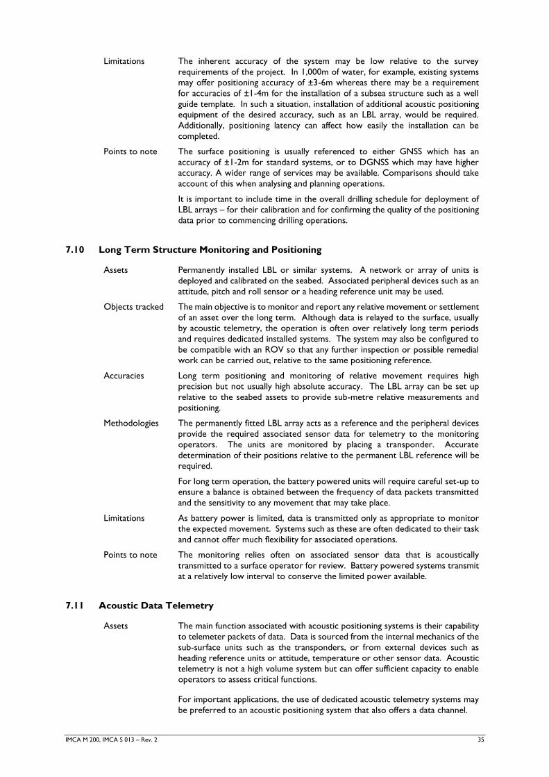
IMCA M 200, IMCA S 013 – Rev. 2 35
Limitations The inherent accuracy of the system may be low relative to the survey
requirements of the project. In 1,000m of water, for example, existing systems
may offer positioning accuracy of ±3-6m whereas there may be a requirement
for accuracies of ±1-4m for the installation of a subsea structure such as a well
guide template. In such a situation, installation of additional acoustic positioning
equipment of the desired accuracy, such as an LBL array, would be required.
Additionally, positioning latency can affect how easily the installation can be
completed.
Points to note The surface positioning is usually referenced to either GNSS which has an
accuracy of ±1-2m for standard systems, or to DGNSS which may have higher
accuracy. A wider range of services may be available. Comparisons should take
account of this when analysing and planning operations.
It is important to include time in the overall drilling schedule for deployment of
LBL arrays – for their calibration and for confirming the quality of the positioning
data prior to commencing drilling operations.
7.10 Long Term Structure Monitoring and Positioning
Assets Permanently installed LBL or similar systems. A network or array of units is
deployed and calibrated on the seabed. Associated peripheral devices such as an
attitude, pitch and roll sensor or a heading reference unit may be used.
Objects tracked The main objective is to monitor and report any relative movement or settlement
of an asset over the long term. Although data is relayed to the surface, usually
by acoustic telemetry, the operation is often over relatively long term periods
and requires dedicated installed systems. The system may also be configured to
be compatible with an ROV so that any further inspection or possible remedial
work can be carried out, relative to the same positioning reference.
Accuracies Long term positioning and monitoring of relative movement requires high
precision but not usually high absolute accuracy. The LBL array can be set up
relative to the seabed assets to provide sub-metre relative measurements and
positioning.
Methodologies The permanently fitted LBL array acts as a reference and the peripheral devices
provide the required associated sensor data for telemetry to the monitoring
operators. The units are monitored by placing a transponder. Accurate
determination of their positions relative to the permanent LBL reference will be
required.
For long term operation, the battery powered units will require careful set-up to
ensure a balance is obtained between the frequency of data packets transmitted
and the sensitivity to any movement that may take place.
Limitations As battery power is limited, data is transmitted only as appropriate to monitor
the expected movement. Systems such as these are often dedicated to their task
and cannot offer much flexibility for associated operations.
Points to note The monitoring relies often on associated sensor data that is acoustically
transmitted to a surface operator for review. Battery powered systems transmit
at a relatively low interval to conserve the limited power available.
7.11 Acoustic Data Telemetry
Assets The main function associated with acoustic positioning systems is their capability
to telemeter packets of data. Data is sourced from the internal mechanics of the
sub-surface units such as the transponders, or from external devices such as
heading reference units or attitude, temperature or other sensor data. Acoustic
telemetry is not a high volume system but can offer sufficient capacity to enable
operators to assess critical functions.
For important applications, the use of dedicated acoustic telemetry systems may
be preferred to an acoustic positioning system that also offers a data channel.
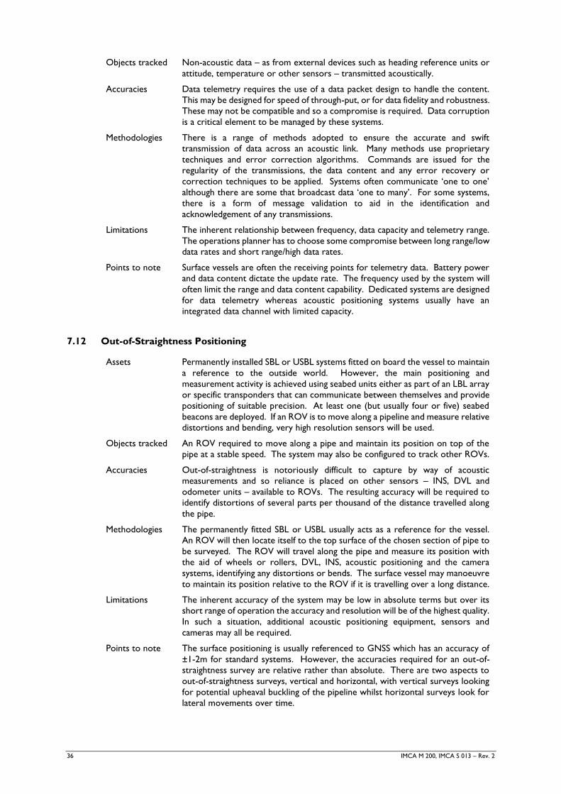
36 IMCA M 200, IMCA S 013 – Rev. 2
Objects tracked Non-acoustic data – as from external devices such as heading reference units or
attitude, temperature or other sensors – transmitted acoustically.
Accuracies Data telemetry requires the use of a data packet design to handle the content.
This may be designed for speed of through-put, or for data fidelity and robustness.
These may not be compatible and so a compromise is required. Data corruption
is a critical element to be managed by these systems.
Methodologies There is a range of methods adopted to ensure the accurate and swift
transmission of data across an acoustic link. Many methods use proprietary
techniques and error correction algorithms. Commands are issued for the
regularity of the transmissions, the data content and any error recovery or
correction techniques to be applied. Systems often communicate ‘one to one’
although there are some that broadcast data ‘one to many’. For some systems,
there is a form of message validation to aid in the identification and
acknowledgement of any transmissions.
Limitations The inherent relationship between frequency, data capacity and telemetry range.
The operations planner has to choose some compromise between long range/low
data rates and short range/high data rates.
Points to note Surface vessels are often the receiving points for telemetry data. Battery power
and data content dictate the update rate. The frequency used by the system will
often limit the range and data content capability. Dedicated systems are designed
for data telemetry whereas acoustic positioning systems usually have an
integrated data channel with limited capacity.
7.12 Out-of-Straightness Positioning
Assets Permanently installed SBL or USBL systems fitted on board the vessel to maintain
a reference to the outside world. However, the main positioning and
measurement activity is achieved using seabed units either as part of an LBL array
or specific transponders that can communicate between themselves and provide
positioning of suitable precision. At least one (but usually four or five) seabed
beacons are deployed. If an ROV is to move along a pipeline and measure relative
distortions and bending, very high resolution sensors will be used.
Objects tracked An ROV required to move along a pipe and maintain its position on top of the
pipe at a stable speed. The system may also be configured to track other ROVs.
Accuracies Out-of-straightness is notoriously difficult to capture by way of acoustic
measurements and so reliance is placed on other sensors – INS, DVL and
odometer units – available to ROVs. The resulting accuracy will be required to
identify distortions of several parts per thousand of the distance travelled along
the pipe.
Methodologies The permanently fitted SBL or USBL usually acts as a reference for the vessel.
An ROV will then locate itself to the top surface of the chosen section of pipe to
be surveyed. The ROV will travel along the pipe and measure its position with
the aid of wheels or rollers, DVL, INS, acoustic positioning and the camera
systems, identifying any distortions or bends. The surface vessel may manoeuvre
to maintain its position relative to the ROV if it is travelling over a long distance.
Limitations The inherent accuracy of the system may be low in absolute terms but over its
short range of operation the accuracy and resolution will be of the highest quality.
In such a situation, additional acoustic positioning equipment, sensors and
cameras may all be required.
Points to note The surface positioning is usually referenced to GNSS which has an accuracy of
±1-2m for standard systems. However, the accuracies required for an out-of-
straightness survey are relative rather than absolute. There are two aspects to
out-of-straightness surveys, vertical and horizontal, with vertical surveys looking
for potential upheaval buckling of the pipeline whilst horizontal surveys look for
lateral movements over time.
IMCA M 200, IMCA S 013 – Rev. 2 37
Appendix 1
The Sonar Equation
The Sonar Equation is often only required by underwater acoustics engineers to aid in the design and planning of
operations, rather than during field work. However, it is useful to understand the basics of the Sonar Equation,
as it is an aid to describing the main sources of limitations that constrain acoustic positioning systems.
Sonar systems may be either active, or passive, in their operation. Active sonars provide their own sound source
and listen for echoes as they are reflected from a target. Passive sonar equipment has no such source. These
are simply listening devices dependent on a target to act as a source and emit its own noise (e.g. the engine noise
from a vessel or communication sounds from a cetacean). Acoustic positioning systems generally use the active
Sonar Equation, although there are positioning systems available that may use each of the approaches.
For an acoustic system to operate, the hydrophone (or receiver) has to detect an acoustic signal. To achieve
this, it is necessary that the signal level is greater than the noise level (NL). This is shown in Equation 1.
SL > NL
Equation 1 – The Sonar Equation
This basic form of the Sonar Equation can then be expanded in terms of the various sources of noise and
associated sonar parameters. These parameters can be separated into three groups relating to:
the equipment – source level (SL), directivity index (DI), detection threshold (DT);
the medium – transmission loss (TL), reverberation level (RL) and noise level (NL);
the target – target strength (TS).
Note: TS is no longer a specific key measure of how good an acoustic reflector or transmitter is the target or
beacon for positioning, as these units transmit their own signal. For acoustic positioning systems this knowledge
is used to aid in determining what the operational limits of the system are.
The Sonar Equation, by incorporating the above elements, provides a consistent approach that forms a basis for
the calculations that determine the range of an acoustic system. In this way, it can be used to aid in the prediction
of a system’s performance.
A1-1 Source Level
Sound is generated by the creation of a mechanical wave. The mechanical element is the displacement of the
medium (in this case water) about the source unit. The wave created is longitudinal, in that the motion of the
particles conveying the energy or wave is parallel to the direction of travel. This motion creates a pressure wave
and its magnitude is measured in microPascals (µPa). A Pascal is a unit of pressure equal to one Newton per m2.
However, acoustic sound levels are normally specified in decibels (dB). Decibels are units used for measuring
the relative strength of a signal. The expression is the logarithmic ratio of the strength of a signal relative to
some reference signal level.
Underwater acoustic signal levels are specified in dB referenced to 1µPa at 1m; thus the relationship may be
stated as:
A = 20 Log10 (a)
where:
a – is the amplitude of the source level in µPa
A – is the amplitude in dB
Unfortunately there are limits to the increase of the source level. These limits depend on the transducer design,
the environment and the frequency of the generated acoustic signals. If too much power is introduced, then
cavitation will occur. When cavitation occurs, the water around the transducer is in effect boiled by the energy
produced. This causes the acoustic signal to fail.
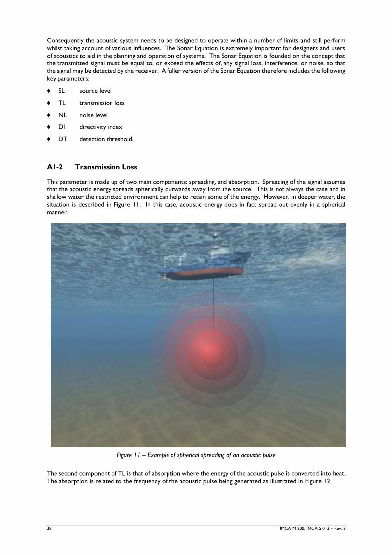
38 IMCA M 200, IMCA S 013 – Rev. 2
Consequently the acoustic system needs to be designed to operate within a number of limits and still perform
whilst taking account of various influences. The Sonar Equation is extremely important for designers and users
of acoustics to aid in the planning and operation of systems. The Sonar Equation is founded on the concept that
the transmitted signal must be equal to, or exceed the effects of, any signal loss, interference, or noise, so that
the signal may be detected by the receiver. A fuller version of the Sonar Equation therefore includes the following
key parameters:
SL source level
TL transmission loss
NL noise level
DI directivity index
DT detection threshold.
A1-2 Transmission Loss
This parameter is made up of two main components: spreading, and absorption. Spreading of the signal assumes
that the acoustic energy spreads spherically outwards away from the source. This is not always the case and in
shallow water the restricted environment can help to retain some of the energy. However, in deeper water, the
situation is described in Figure 11. In this case, acoustic energy does in fact spread out evenly in a spherical
manner.
Figure 11 – Example of spherical spreading of an acoustic pulse
The second component of TL is that of absorption where the energy of the acoustic pulse is converted into heat.
The absorption is related to the frequency of the acoustic pulse being generated as illustrated in Figure 12.
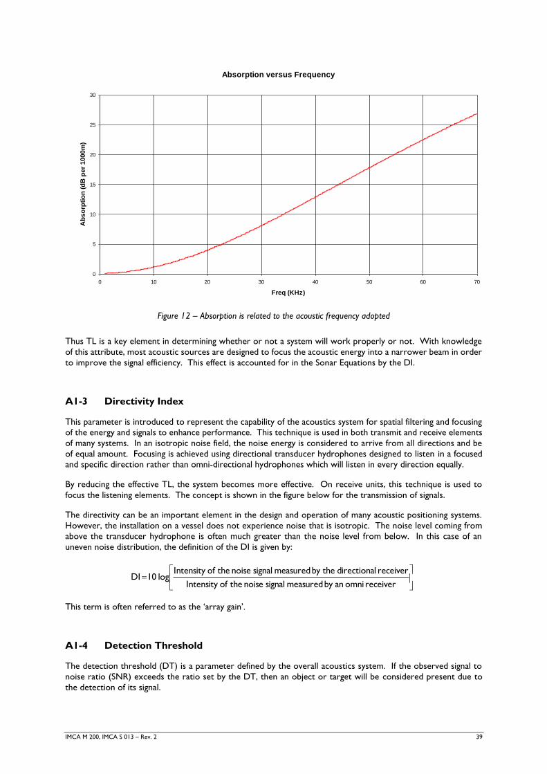
IMCA M 200, IMCA S 013 – Rev. 2 39
Figure 12 – Absorption is related to the acoustic frequency adopted
Thus TL is a key element in determining whether or not a system will work properly or not. With knowledge
of this attribute, most acoustic sources are designed to focus the acoustic energy into a narrower beam in order
to improve the signal efficiency. This effect is accounted for in the Sonar Equations by the DI.
A1-3 Directivity Index
This parameter is introduced to represent the capability of the acoustics system for spatial filtering and focusing
of the energy and signals to enhance performance. This technique is used in both transmit and receive elements
of many systems. In an isotropic noise field, the noise energy is considered to arrive from all directions and be
of equal amount. Focusing is achieved using directional transducer hydrophones designed to listen in a focused
and specific direction rather than omni-directional hydrophones which will listen in every direction equally.
By reducing the effective TL, the system becomes more effective. On receive units, this technique is used to
focus the listening elements. The concept is shown in the figure below for the transmission of signals.
The directivity can be an important element in the design and operation of many acoustic positioning systems.
However, the installation on a vessel does not experience noise that is isotropic. The noise level coming from
above the transducer hydrophone is often much greater than the noise level from below. In this case of an
uneven noise distribution, the definition of the DI is given by:
receiver omni anby measured signal noise theofIntensity
receiver ldirectiona by the measured signal noise theofIntensity log 10 DI
This term is often referred to as the ‘array gain’.
A1-4 Detection Threshold
The detection threshold (DT) is a parameter defined by the overall acoustics system. If the observed signal to
noise ratio (SNR) exceeds the ratio set by the DT, then an object or target will be considered present due to
the detection of its signal.
Absorption versus Frequency
0
5
10
15
20
25
30
0 10 20 30 40 50 60 70
Freq (KHz)
Ab
so
rpti
on
(d
B p
er
10
00
m)
40 IMCA M 200, IMCA S 013 – Rev. 2
A1-5 Noise Level
Another term that has numerous variations is the acoustic noise. This consists of two sources or types of
background noise masking the signal we wish to detect:
Noise background or NL – This is a steady state, isotropic (equal in all directions) sound which is
generated by, amongst other things, wind, waves, biological activity and shipping. For deep water operations
this should be the dominant source of noise;
Reverberation background or RL – This is the slowly decaying portion of the sound that is back-
scattered from the acoustic SL input. In the sea, two excellent reflectors are the sea surface and sea floor.
Additionally, sound may be scattered by particulate matter (e.g. plankton) within the water column. Acoustic
reverberation noises decay relatively rapidly with time. Because of this and because of the distance from
the sound source to the water surface and seabed, it is considered less likely to dominate.
Although both types of background are generally present simultaneously, it is common for one to be dominant.
Sonar performance can be improved by having both directional source and directional hydrophones, provided
that they are directed towards the target and are using appropriate frequencies to avoid signal loss.
In this document the passive Sonar Equation is considered and the specific case where the source and receiving
transducer elements (the hydrophone) are coincident. For a system such as a USBL or SBL where the transducer
emits a pulse to trigger the acoustic return signal from the beacon, the two-way travel path may be significant.
The vessel’s transmission may be of a higher power than the battery powered sub-surface unit and the relative
power levels of the signals should be considered for the operations.
SL – 2TL - NL + DI > DT
Equation 2
The Sonar Equation may have a number of different forms but each one, with or without additional terms, aims
to represent the factors involved in acoustics. For example, a variation on Equation 2 has the parameter 2TL
showing TL to indicate the acoustic signal having to travel in one direction, e.g. for an LBL system. In this case
the equation takes the form:
SL – TL - NL + DI > DT
Equation 3
As most systems transmit their signal and then ‘listen’ for the return transmitted signal, this form of the passive
Sonar Equation is likely to represent the way in which these systems can be represented by the Sonar Equation.
The Sonar Equation is an aid in understanding the influences on acoustic signal performance. The accuracy
achieved will largely depend on the methodology adopted, the frequencies and signalling used by the acoustic
system, the layout of the units and the underwater environment.
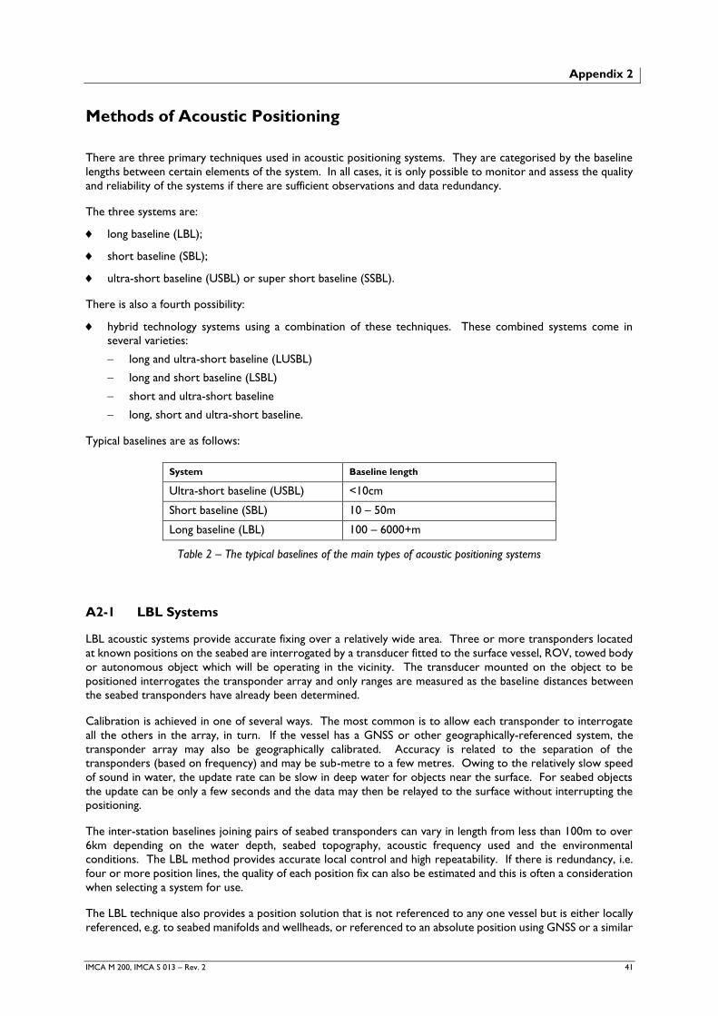
IMCA M 200, IMCA S 013 – Rev. 2 41
Appendix 2
Methods of Acoustic Positioning
There are three primary techniques used in acoustic positioning systems. They are categorised by the baseline
lengths between certain elements of the system. In all cases, it is only possible to monitor and assess the quality
and reliability of the systems if there are sufficient observations and data redundancy.
The three systems are:
long baseline (LBL);
short baseline (SBL);
ultra-short baseline (USBL) or super short baseline (SSBL).
There is also a fourth possibility:
hybrid technology systems using a combination of these techniques. These combined systems come in
several varieties:
long and ultra-short baseline (LUSBL)
long and short baseline (LSBL)
short and ultra-short baseline
long, short and ultra-short baseline.
Typical baselines are as follows:
System Baseline length
Ultra-short baseline (USBL) <10cm
Short baseline (SBL) 10 – 50m
Long baseline (LBL) 100 – 6000+m
Table 2 – The typical baselines of the main types of acoustic positioning systems
A2-1 LBL Systems
LBL acoustic systems provide accurate fixing over a relatively wide area. Three or more transponders located
at known positions on the seabed are interrogated by a transducer fitted to the surface vessel, ROV, towed body
or autonomous object which will be operating in the vicinity. The transducer mounted on the object to be
positioned interrogates the transponder array and only ranges are measured as the baseline distances between
the seabed transponders have already been determined.
Calibration is achieved in one of several ways. The most common is to allow each transponder to interrogate
all the others in the array, in turn. If the vessel has a GNSS or other geographically-referenced system, the
transponder array may also be geographically calibrated. Accuracy is related to the separation of the
transponders (based on frequency) and may be sub-metre to a few metres. Owing to the relatively slow speed
of sound in water, the update rate can be slow in deep water for objects near the surface. For seabed objects
the update can be only a few seconds and the data may then be relayed to the surface without interrupting the
positioning.
The inter-station baselines joining pairs of seabed transponders can vary in length from less than 100m to over
6km depending on the water depth, seabed topography, acoustic frequency used and the environmental
conditions. The LBL method provides accurate local control and high repeatability. If there is redundancy, i.e.
four or more position lines, the quality of each position fix can also be estimated and this is often a consideration
when selecting a system for use.
The LBL technique also provides a position solution that is not referenced to any one vessel but is either locally
referenced, e.g. to seabed manifolds and wellheads, or referenced to an absolute position using GNSS or a similar
42 IMCA M 200, IMCA S 013 – Rev. 2
system. In this respect it differs from other acoustic positioning methods in that it is essentially static equipment
placed on the seabed acting as a reference, giving the system the ability to provide a relatively large area with
high accuracy positioning independent of water depth. Whilst the positioning of objects is carried out relative
to the seabed transponders and benefits from a stable and relatively large coverage, the positions of the
transponders themselves must be accurately determined. This process of calibration or, more correctly, co-
ordination, relies on the links to the surface survey vessel and its positioning system.
For many reasons, the accuracy achieved with such arrays may vary considerably, not least due to the frequency
used, the separation and accuracy of the calibrated position of the beacons and the geometry of the acoustic
ranges they deliver to the hydrophone or receiver. This is discussed in sections 5.3.1 and 5.3.2.
Seabed transponders cannot be fixed or deployed as accurately as land based systems. Once laid, however, a
pattern of transponders needs to be fixed relative to each other and then tied into the geodetic datum in use.
The latter is usually achieved using GNSS. Recalibration of an LBL array of beacons is required each time it is
deployed (the exception is if pre-installed frames are present), the positions of which will have been accurately
surveyed already.
Commonly, the methods adopted are based on either a direct ranging to each beacon from a surface vessel using
the box-in method, or the beacons each transmit to each other over the baseline separation. These distances
are used in a network adjustment to determine a consistent array of beacon co-ordinates. Calibration is covered
in more detail in section 5.6.
In deep water areas and, in particular, water depths of over 1,000m, where the accuracy of the surface referenced
types of positioning deteriorates, LBL systems often become more appropriate. LBL systems are common for
use in drilling and construction operations in deep water areas, and in particular, very deep water.
A2-2 SBL Systems
In this type of system, the baseline referred to is that between the receive transducer (hydrophone) units on the
hull or below the hull of the host vessel. Such systems require a pinger, responder or transponder. No fixed
beacons on the seabed are required and the system provides positioning relative to the surface vessel. These
transducers are deployed through dedicated tubes in the hull and could be as little as a few metres apart to tens
of metres apart on large vessels such as deep water drilling vessels and mobile drilling units (MODUs). The SBL
system uses relative range and direction observations to transponders to determine positions relative to the
surface vessel. The SBL interrogates the transponder and the return signal is received by several transducers
which then discriminate the direction of the return signal. The arrival of the signal allows for the derivation of
the range or distance between the transponder and the reference point on board the vessel. The transducers
form a plane below the hull of the vessel that acts as the reference of the system. This plane must be accurately
determined with respect to any reference datum on board the vessel. Due to vessel movement (pitch and roll),
real-time information on the attitude of the transducer array is required and corrections for pitch and roll applied
to ensure stable and accurate positioning is achieved.
The system operates by requiring the seabed pinger to transmit a signal and the transducer units to receive the
signal. The transducer units all receive the signal at a slightly different time. This enables the system to determine
the direction of the return signal, and the time of arrival at the master unit allows the system to derive the range.
Depth is normally entered either manually or via a sensor to aid in maintaining the accuracy of the system.
Due to the longer baselines of the receive and transmit units below the surface vessel’s hull, the accuracy is
usually better than for USBL systems. Some vessels have as many as eight hull penetrations for tubes or poles
on which the transducers are deployed. All of these should be positioned accurately and their relative offsets
known for the operations to benefit fully from the SBL system.
SBL systems typically operate with a minimum of four transducers to allow some redundancy in the observations.
The introduction of four more units below the hull allows for deep water operations as the larger the array, the
better the directional discrimination of the SBL system.
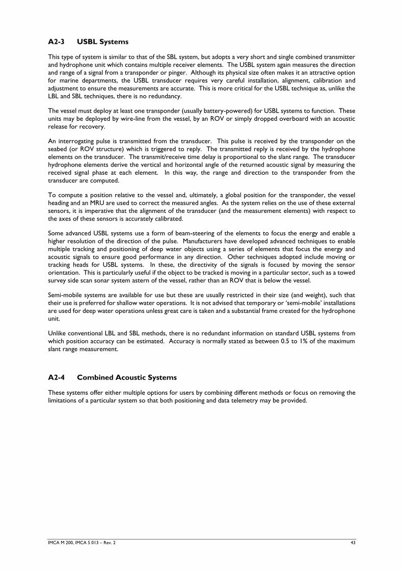
IMCA M 200, IMCA S 013 – Rev. 2 43
A2-3 USBL Systems
This type of system is similar to that of the SBL system, but adopts a very short and single combined transmitter
and hydrophone unit which contains multiple receiver elements. The USBL system again measures the direction
and range of a signal from a transponder or pinger. Although its physical size often makes it an attractive option
for marine departments, the USBL transducer requires very careful installation, alignment, calibration and
adjustment to ensure the measurements are accurate. This is more critical for the USBL technique as, unlike the
LBL and SBL techniques, there is no redundancy.
The vessel must deploy at least one transponder (usually battery-powered) for USBL systems to function. These
units may be deployed by wire-line from the vessel, by an ROV or simply dropped overboard with an acoustic
release for recovery.
An interrogating pulse is transmitted from the transducer. This pulse is received by the transponder on the
seabed (or ROV structure) which is triggered to reply. The transmitted reply is received by the hydrophone
elements on the transducer. The transmit/receive time delay is proportional to the slant range. The transducer
hydrophone elements derive the vertical and horizontal angle of the returned acoustic signal by measuring the
received signal phase at each element. In this way, the range and direction to the transponder from the
transducer are computed.
To compute a position relative to the vessel and, ultimately, a global position for the transponder, the vessel
heading and an MRU are used to correct the measured angles. As the system relies on the use of these external
sensors, it is imperative that the alignment of the transducer (and the measurement elements) with respect to
the axes of these sensors is accurately calibrated.
Some advanced USBL systems use a form of beam-steering of the elements to focus the energy and enable a
higher resolution of the direction of the pulse. Manufacturers have developed advanced techniques to enable
multiple tracking and positioning of deep water objects using a series of elements that focus the energy and
acoustic signals to ensure good performance in any direction. Other techniques adopted include moving or
tracking heads for USBL systems. In these, the directivity of the signals is focused by moving the sensor
orientation. This is particularly useful if the object to be tracked is moving in a particular sector, such as a towed
survey side scan sonar system astern of the vessel, rather than an ROV that is below the vessel.
Semi-mobile systems are available for use but these are usually restricted in their size (and weight), such that
their use is preferred for shallow water operations. It is not advised that temporary or ‘semi-mobile’ installations
are used for deep water operations unless great care is taken and a substantial frame created for the hydrophone
unit.
Unlike conventional LBL and SBL methods, there is no redundant information on standard USBL systems from
which position accuracy can be estimated. Accuracy is normally stated as between 0.5 to 1% of the maximum
slant range measurement.
A2-4 Combined Acoustic Systems
These systems offer either multiple options for users by combining different methods or focus on removing the
limitations of a particular system so that both positioning and data telemetry may be provided.
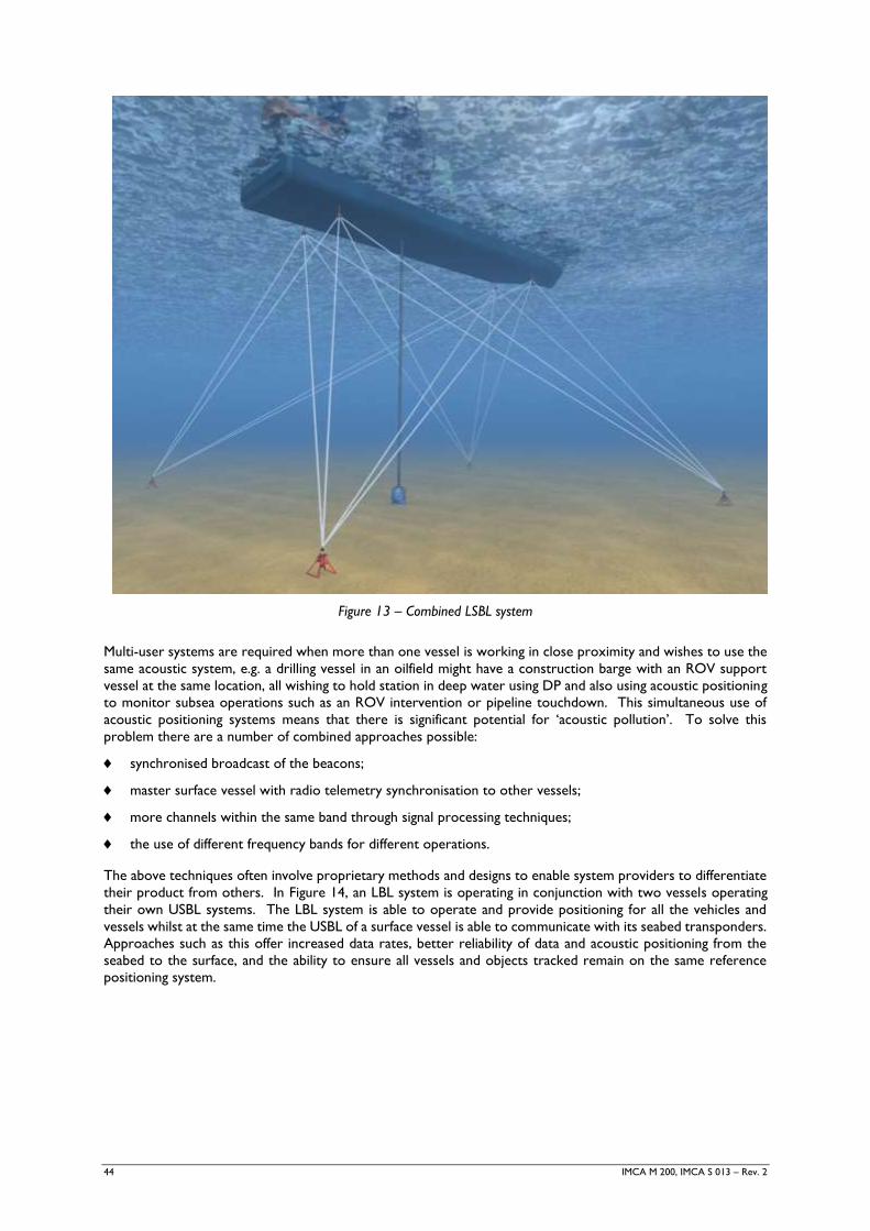
44 IMCA M 200, IMCA S 013 – Rev. 2
Figure 13 – Combined LSBL system
Multi-user systems are required when more than one vessel is working in close proximity and wishes to use the
same acoustic system, e.g. a drilling vessel in an oilfield might have a construction barge with an ROV support
vessel at the same location, all wishing to hold station in deep water using DP and also using acoustic positioning
to monitor subsea operations such as an ROV intervention or pipeline touchdown. This simultaneous use of
acoustic positioning systems means that there is significant potential for ‘acoustic pollution’. To solve this
problem there are a number of combined approaches possible:
synchronised broadcast of the beacons;
master surface vessel with radio telemetry synchronisation to other vessels;
more channels within the same band through signal processing techniques;
the use of different frequency bands for different operations.
The above techniques often involve proprietary methods and designs to enable system providers to differentiate
their product from others. In Figure 14, an LBL system is operating in conjunction with two vessels operating
their own USBL systems. The LBL system is able to operate and provide positioning for all the vehicles and
vessels whilst at the same time the USBL of a surface vessel is able to communicate with its seabed transponders.
Approaches such as this offer increased data rates, better reliability of data and acoustic positioning from the
seabed to the surface, and the ability to ensure all vessels and objects tracked remain on the same reference
positioning system.
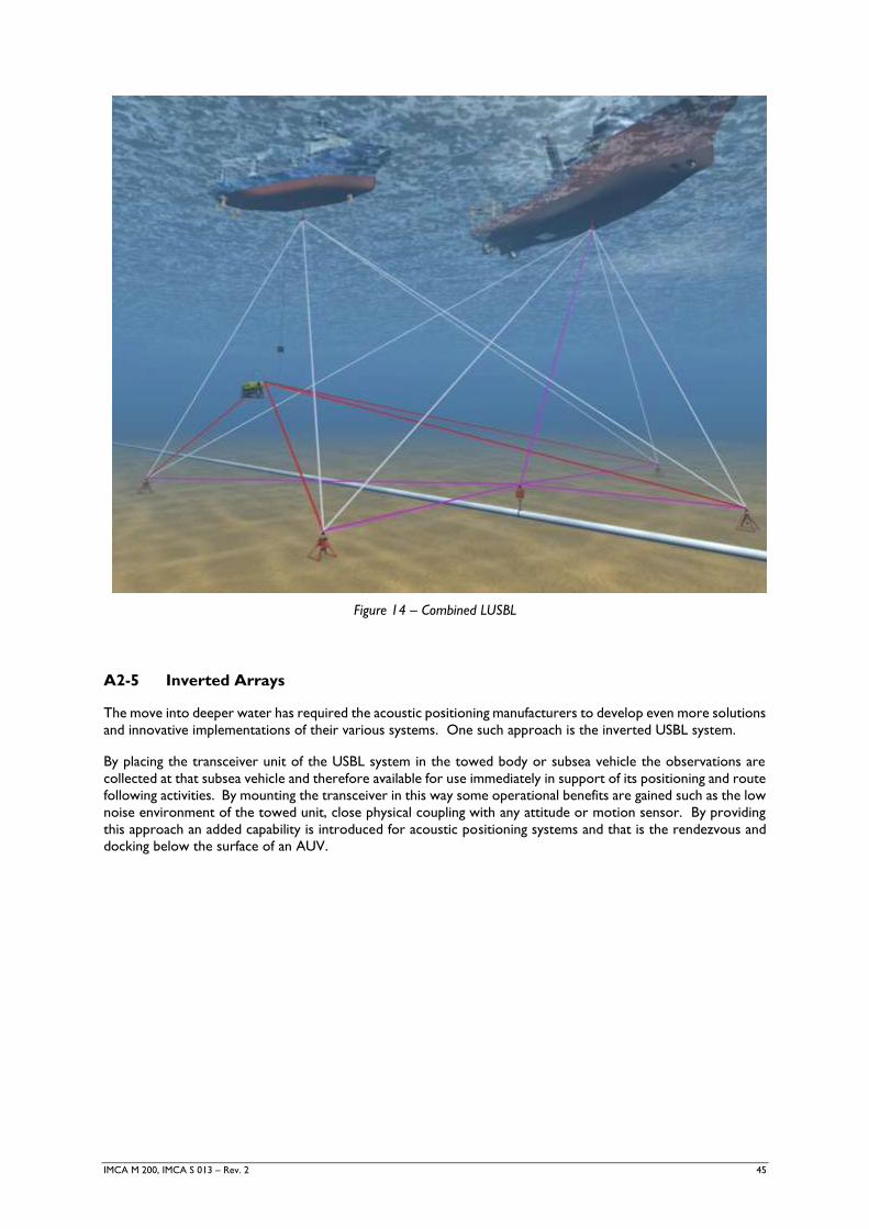
IMCA M 200, IMCA S 013 – Rev. 2 45
Figure 14 – Combined LUSBL
A2-5 Inverted Arrays
The move into deeper water has required the acoustic positioning manufacturers to develop even more solutions
and innovative implementations of their various systems. One such approach is the inverted USBL system.
By placing the transceiver unit of the USBL system in the towed body or subsea vehicle the observations are
collected at that subsea vehicle and therefore available for use immediately in support of its positioning and route
following activities. By mounting the transceiver in this way some operational benefits are gained such as the low
noise environment of the towed unit, close physical coupling with any attitude or motion sensor. By providing
this approach an added capability is introduced for acoustic positioning systems and that is the rendezvous and
docking below the surface of an AUV.

46 IMCA M 200, IMCA S 013 – Rev. 2
Figure 15 – A schematic of an inverted USBL system for a cable burial plough
A2-6 Hybrid Technology Systems
These have developed for a number of reasons and have enabled various survey and construction activities by
removing some of the weaknesses of acoustics systems by combining them with another form of technology.
Commonly, peripheral sensors are used to improve and augment the performance of acoustic positioning. In
this category, however, the sensors have been integrated at a deep level and are essentially part of the product
delivered by the manufacturer rather than an option for the user to select and add sensor data.
Most common among the main systems is the integration of some form of Inertial Measurement Unit (IMU) that
offers specific characteristics complementing acoustic positioning systems. Taken alone, the advantages of
observed data from an IMU may be limited due to short term drifts in the accelerometers, however, when
combined with data from a USBL or LBL system, there can be significant advantages for certain operations.
It is beyond the scope of this document to describe the nature of the integration between acoustics and IMUs.
However, a top level description is provided to provide a basic understanding of the methods.
A2-6.1 Integrated Acoustic and IMU Solutions
A small number of tightly integrated solutions have been developed as ‘off-the-shelf’ systems for
operators. They usually rely quite heavily on the use of satellite positioning systems as a source of
augmentation along with various peripheral units, and in particular, the use of INS.
There may be two primary units: the ship’s surface unit comprising GNSS, inertial motion unit and
subsea transducer, and the sub-surface unit that comprises an acoustic transponder and associated
peripheral devices such as a depth sensor and DVL unit. In deeper water the solutions may include a
sub-surface INS.
IMCA M 200, IMCA S 013 – Rev. 2 47
The system obtains the exact position of the surface vessel using the GNSS and surface heading, INS
and other peripheral units. This position is then used as a reference for the acoustic USBL observations
to establish an exact position for the tracked underwater object. This accurate position of the
underwater unit is then relayed down to the underwater unit. The data is then integrated into the
INS on board the underwater vehicle, or asset being tracked, to establish its own high accuracy
position. Each time there is a position update at the surface, it is relayed acoustically and received by
the underwater system which then incorporates it into the solution by merging it with the associated
peripheral depth, altitude and DVL data.
Accuracies will vary depending on the configuration of units and modules selected but potential
accuracies of better than 0.2% of water depth may be achievable.
An alternative approach to obtain both stable and accurate positioning with a high update rate in deep
water is to integrate acoustics with an inertial motion unit (IMU). The system derives an accurate
solution by linking data from the IMU with accurate surface data and the USBL observations. A typical
configuration would include three main units: the subsea systems, ship’s transducer and an onboard
processing computer.
The underwater unit’s senor data is transmitted to the surface vessel acoustically and integrated with
the surface data to derive an accurate sub-surface position for the underwater object. The underwater
sub-surface unit may comprise an inertial motion unit, DVL, pressure (or depth), altitude and a heading
reference unit. All this sensor data needs to be transferred to the surface. This is achieved through
the use of an acoustic data link. Certain solutions have an integral acoustic modem in the USBL system.
The data, once received, is transferred to the processing computer where the surface reference
positioning GNSS, as well as the USBL positioning and any sensor data, are combined in a tightly
coupled filter solution.
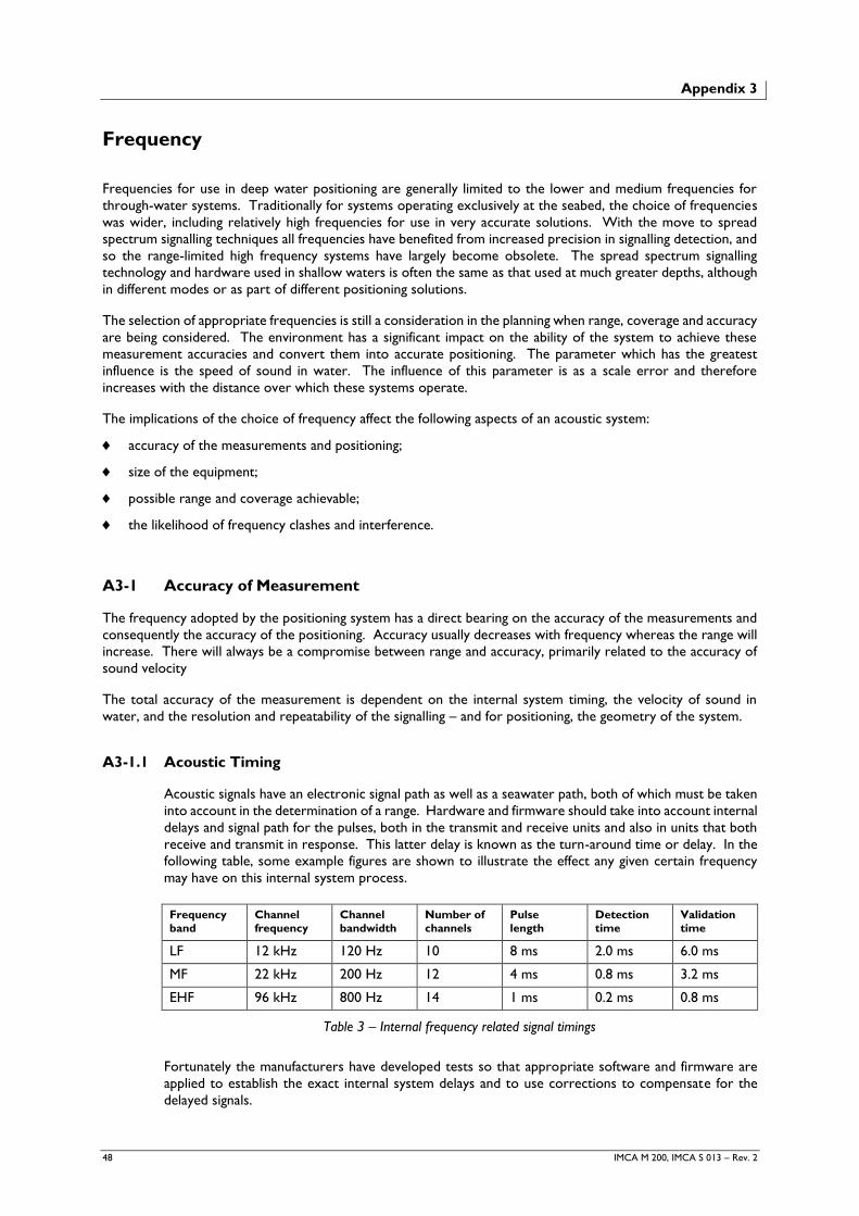
48 IMCA M 200, IMCA S 013 – Rev. 2
Appendix 3
Frequency
Frequencies for use in deep water positioning are generally limited to the lower and medium frequencies for
through-water systems. Traditionally for systems operating exclusively at the seabed, the choice of frequencies
was wider, including relatively high frequencies for use in very accurate solutions. With the move to spread
spectrum signalling techniques all frequencies have benefited from increased precision in signalling detection, and
so the range-limited high frequency systems have largely become obsolete. The spread spectrum signalling
technology and hardware used in shallow waters is often the same as that used at much greater depths, although
in different modes or as part of different positioning solutions.
The selection of appropriate frequencies is still a consideration in the planning when range, coverage and accuracy
are being considered. The environment has a significant impact on the ability of the system to achieve these
measurement accuracies and convert them into accurate positioning. The parameter which has the greatest
influence is the speed of sound in water. The influence of this parameter is as a scale error and therefore
increases with the distance over which these systems operate.
The implications of the choice of frequency affect the following aspects of an acoustic system:
accuracy of the measurements and positioning;
size of the equipment;
possible range and coverage achievable;
the likelihood of frequency clashes and interference.
A3-1 Accuracy of Measurement
The frequency adopted by the positioning system has a direct bearing on the accuracy of the measurements and
consequently the accuracy of the positioning. Accuracy usually decreases with frequency whereas the range will
increase. There will always be a compromise between range and accuracy, primarily related to the accuracy of
sound velocity
The total accuracy of the measurement is dependent on the internal system timing, the velocity of sound in
water, and the resolution and repeatability of the signalling – and for positioning, the geometry of the system.
A3-1.1 Acoustic Timing
Acoustic signals have an electronic signal path as well as a seawater path, both of which must be taken
into account in the determination of a range. Hardware and firmware should take into account internal
delays and signal path for the pulses, both in the transmit and receive units and also in units that both
receive and transmit in response. This latter delay is known as the turn-around time or delay. In the
following table, some example figures are shown to illustrate the effect any given certain frequency
may have on this internal system process.
Frequency
band
Channel
frequency
Channel
bandwidth
Number of
channels
Pulse
length
Detection
time
Validation
time
LF 12 kHz 120 Hz 10 8 ms 2.0 ms 6.0 ms
MF 22 kHz 200 Hz 12 4 ms 0.8 ms 3.2 ms
EHF 96 kHz 800 Hz 14 1 ms 0.2 ms 0.8 ms
Table 3 – Internal frequency related signal timings
Fortunately the manufacturers have developed tests so that appropriate software and firmware are
applied to establish the exact internal system delays and to use corrections to compensate for the
delayed signals.
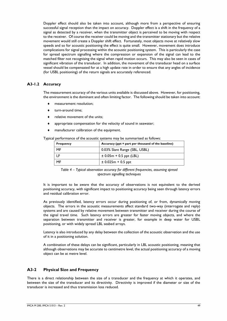
IMCA M 200, IMCA S 013 – Rev. 2 49
Doppler effect should also be taken into account, although more from a perspective of ensuring
successful signal reception than the impact on accuracy. Doppler effect is a shift in the frequency of a
signal as detected by a receiver, when the transmitter object is perceived to be moving with respect
to the receiver. Of course the receiver could be moving and the transmitter stationary but the relative
movement would still create a Doppler shift effect. Fortunately, most objects move at relatively slow
speeds and so for acoustic positioning the effect is quite small. However, movement does introduce
complications for signal processing within the acoustic positioning system. This is particularly the case
for spread spectrum signalling where the compression or expansion of the signal can lead to the
matched filter not recognising the signal when rapid motion occurs. This may also be seen in cases of
significant vibration of the transducer. In addition, the movement of the transducer head on a surface
vessel should be compensated for at a high update rate in order to ensure that any angles of incidence
(for USBL positioning) of the return signals are accurately referenced.
A3-1.2 Accuracy
The measurement accuracy of the various units available is discussed above. However, for positioning,
the environment is the dominant and often limiting factor. The following should be taken into account:
measurement resolution;
turn-around time;
relative movement of the units;
appropriate compensation for the velocity of sound in seawater;
manufacturer calibration of the equipment.
Typical performance of the acoustic systems may be summarised as follows:
Frequency Accuracy (ppt = part per thousand of the baseline)
MF 0.03% Slant Range (SBL, USBL)
LF ± 0.05m + 0.5 ppt (LBL)
MF ± 0.025m + 0.5 ppt
Table 4 – Typical observation accuracy for different frequencies, assuming spread
spectrum signalling techniques
It is important to be aware that the accuracy of observations is not equivalent to the derived
positioning accuracy, with significant impact to positioning accuracy being seen through latency errors
and residual calibration error.
As previously identified, latency errors occur during positioning of, or from, dynamically moving
objects. The errors in the acoustic measurements affect standard two-way (interrogate and reply)
systems and are caused by relative movement between transmitter and receiver during the course of
the signal travel time. Such latency errors are greater for faster moving objects, and where the
separation between transmitter and receiver is greater, for example in deep water for USBL
positioning, or with widely spread LBL seabed arrays.
Latency is also introduced by any delay between the collection of the acoustic observation and the use
of it in a positioning solution.
A combination of these delays can be significant, particularly in LBL acoustic positioning, meaning that
although observations may be accurate to centimetre level, the actual positioning accuracy of a moving
object can be at metre level.
A3-2 Physical Size and Frequency
There is a direct relationship between the size of a transducer and the frequency at which it operates, and
between the size of the transducer and its directivity. Directivity is improved if the diameter or size of the
transducer is increased and thus transmission loss reduced.
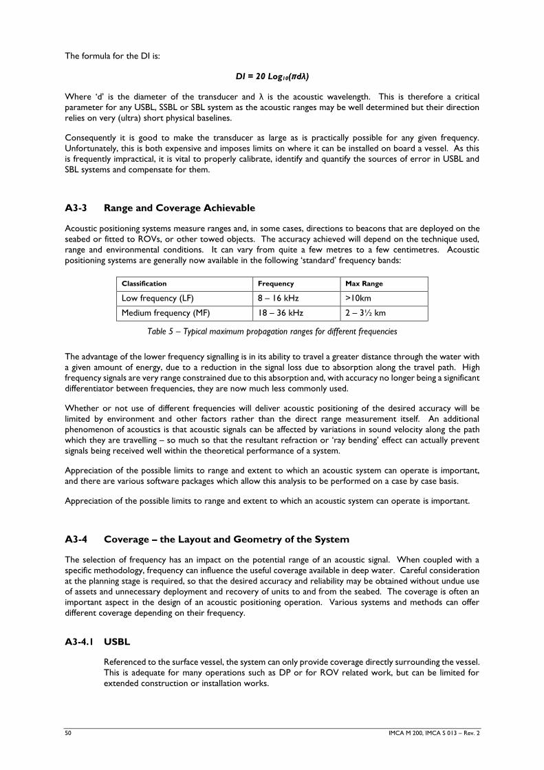
50 IMCA M 200, IMCA S 013 – Rev. 2
The formula for the DI is:
DI = 20 Log10(πdλ)
Where ‘d’ is the diameter of the transducer and λ is the acoustic wavelength. This is therefore a critical
parameter for any USBL, SSBL or SBL system as the acoustic ranges may be well determined but their direction
relies on very (ultra) short physical baselines.
Consequently it is good to make the transducer as large as is practically possible for any given frequency.
Unfortunately, this is both expensive and imposes limits on where it can be installed on board a vessel. As this
is frequently impractical, it is vital to properly calibrate, identify and quantify the sources of error in USBL and
SBL systems and compensate for them.
A3-3 Range and Coverage Achievable
Acoustic positioning systems measure ranges and, in some cases, directions to beacons that are deployed on the
seabed or fitted to ROVs, or other towed objects. The accuracy achieved will depend on the technique used,
range and environmental conditions. It can vary from quite a few metres to a few centimetres. Acoustic
positioning systems are generally now available in the following ‘standard’ frequency bands:
Classification Frequency Max Range
Low frequency (LF) 8 – 16 kHz >10km
Medium frequency (MF) 18 – 36 kHz 2 – 3½ km
Table 5 – Typical maximum propagation ranges for different frequencies
The advantage of the lower frequency signalling is in its ability to travel a greater distance through the water with
a given amount of energy, due to a reduction in the signal loss due to absorption along the travel path. High
frequency signals are very range constrained due to this absorption and, with accuracy no longer being a significant
differentiator between frequencies, they are now much less commonly used.
Whether or not use of different frequencies will deliver acoustic positioning of the desired accuracy will be
limited by environment and other factors rather than the direct range measurement itself. An additional
phenomenon of acoustics is that acoustic signals can be affected by variations in sound velocity along the path
which they are travelling – so much so that the resultant refraction or ‘ray bending’ effect can actually prevent
signals being received well within the theoretical performance of a system.
Appreciation of the possible limits to range and extent to which an acoustic system can operate is important,
and there are various software packages which allow this analysis to be performed on a case by case basis.
Appreciation of the possible limits to range and extent to which an acoustic system can operate is important.
A3-4 Coverage – the Layout and Geometry of the System
The selection of frequency has an impact on the potential range of an acoustic signal. When coupled with a
specific methodology, frequency can influence the useful coverage available in deep water. Careful consideration
at the planning stage is required, so that the desired accuracy and reliability may be obtained without undue use
of assets and unnecessary deployment and recovery of units to and from the seabed. The coverage is often an
important aspect in the design of an acoustic positioning operation. Various systems and methods can offer
different coverage depending on their frequency.
A3-4.1 USBL
Referenced to the surface vessel, the system can only provide coverage directly surrounding the vessel.
This is adequate for many operations such as DP or for ROV related work, but can be limited for
extended construction or installation works.
IMCA M 200, IMCA S 013 – Rev. 2 51
The frequencies used by the typical USBL tend to be towards the high end of any frequency band. This
keeps the physical size of the units to a minimum, as size can influence the accuracy of the signalling
and the installation costs. Ultimately this restriction in size limits the accuracy of the system; as the
signals return from the seabed area their range may be well measured but the resolution of their
direction can become increasingly inaccurate.
A3-4.2 SBL
Whilst providing positioning with reference to the surface vessel, the added transducers and increased
baseline enable an SBL system to better determine the direction of an acoustic signal return and
provide the potential for higher accuracy than USBL. The transducers tend to be simpler and less
costly individually than the more complex multi-element USBL systems. The added complexity and
expense of physically installing the transducer arrays on the hull of a vessel mean that SBL is often built
for long term operations. Reliability becomes a key parameter, more so than accuracy. SBL systems
are often used for operations such as DP for drilling and floating production storage and offloading
unit vessels.
A3-4.3 LBL
As an LBL acoustic positioning system is independent of the surface vessel, it can therefore extend its
coverage over relatively large areas and offer multiple users high accuracy positioning close to the
seabed. In terms of range, the LBL system is more dependent on the frequency selected, as the
methodology enables the system to be scaled up in the number of units to cover an increasingly large
area. LBL tends to be much more subject to range limitations caused by seabed topography when
being used to position objects close to the seabed.
A3-5 Frequency Clashes and Interference
Frequency clashes occur when there are a greater number of users and transmissions in the water than acoustic
positioning systems can sustain at once.
Recent advances in signal technology have, for all practical purposes, removed these limitations. Older, traditional
systems have yet to overcome this problem and may suffer long periods of down time and lost signalling due to
frequency clashes.
The likelihood of frequency clashes should be taken into account at the planning stage of a project. Many USBL
and LBL operations are planned with great care to ensure that there is no frequency clash or interference.
Unfortunately, the demands for faster positioning update rates, the increased use of telemetry in association with
positioning and the extended ranges at which the systems are being operated mean that frequency clashes can
still occur.
A further influence is the nature of the seawater environment. Well layered water bodies exist that can cause
acoustic signals to carry across extended ranges well beyond the normal planned and required distances.
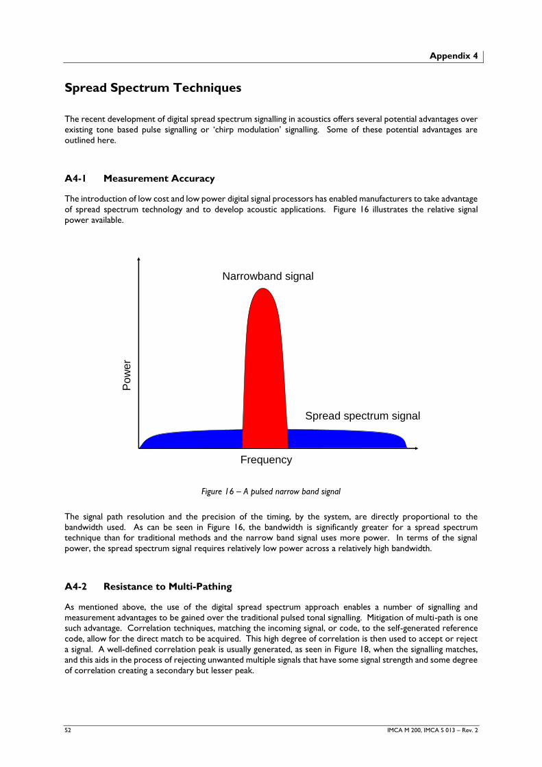
52 IMCA M 200, IMCA S 013 – Rev. 2
Appendix 4
Spread Spectrum Techniques
The recent development of digital spread spectrum signalling in acoustics offers several potential advantages over
existing tone based pulse signalling or ‘chirp modulation’ signalling. Some of these potential advantages are
outlined here.
A4-1 Measurement Accuracy
The introduction of low cost and low power digital signal processors has enabled manufacturers to take advantage
of spread spectrum technology and to develop acoustic applications. Figure 16 illustrates the relative signal
power available.
Figure 16 – A pulsed narrow band signal
The signal path resolution and the precision of the timing, by the system, are directly proportional to the
bandwidth used. As can be seen in Figure 16, the bandwidth is significantly greater for a spread spectrum
technique than for traditional methods and the narrow band signal uses more power. In terms of the signal
power, the spread spectrum signal requires relatively low power across a relatively high bandwidth.
A4-2 Resistance to Multi-Pathing
As mentioned above, the use of the digital spread spectrum approach enables a number of signalling and
measurement advantages to be gained over the traditional pulsed tonal signalling. Mitigation of multi-path is one
such advantage. Correlation techniques, matching the incoming signal, or code, to the self-generated reference
code, allow for the direct match to be acquired. This high degree of correlation is then used to accept or reject
a signal. A well-defined correlation peak is usually generated, as seen in Figure 18, when the signalling matches,
and this aids in the process of rejecting unwanted multiple signals that have some signal strength and some degree
of correlation creating a secondary but lesser peak.
Narrowband signal
Spread spectrum signal
Frequency
Po
we
r
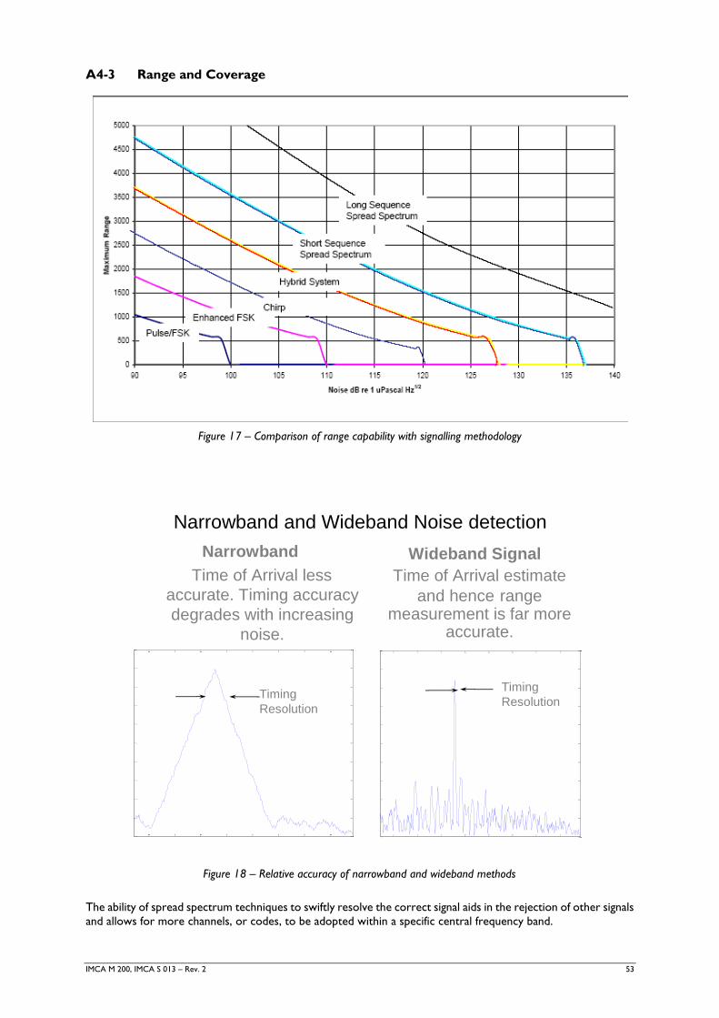
IMCA M 200, IMCA S 013 – Rev. 2 53
A4-3 Range and Coverage
Figure 17 – Comparison of range capability with signalling methodology
Figure 18 – Relative accuracy of narrowband and wideband methods
The ability of spread spectrum techniques to swiftly resolve the correct signal aids in the rejection of other signals
and allows for more channels, or codes, to be adopted within a specific central frequency band.
Narrowband and Wideband Noise detection
Wideband Signal
Time of Arrival estimate
and hence range measurement is far more
accurate.
450 500 550 600 650 700 750 8000
0.1
0.2
0.3
0.4
0.5
0.6
0.7
0.8
0.9
1
8ms wideband plus noise and no multipath
450 500 550 600 650 700 750 8000
0.1
0.2
0.3
0.4
0.5
0.6
0.7
0.8
0.9
1
8ms tone plus noise and no multipath
Timing
Resolution
Narrowband
Time of Arrival less
accurate. Timing accuracy
degrades with increasing
noise.
Timing
Resolution
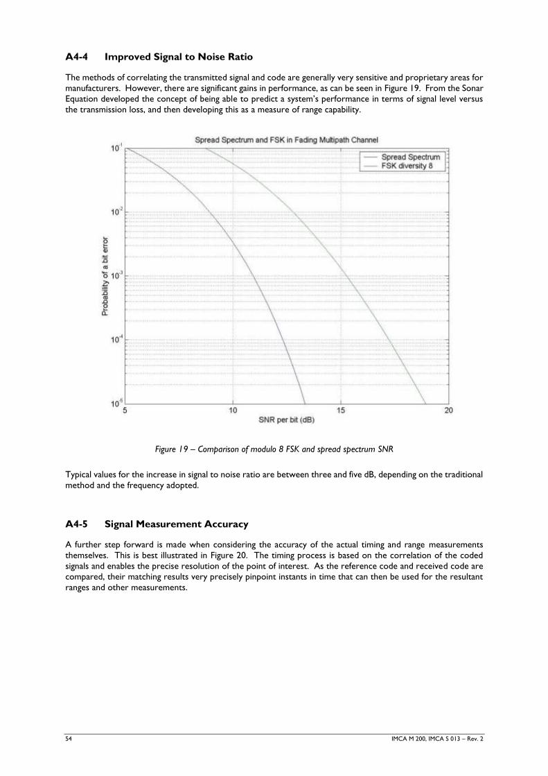
54 IMCA M 200, IMCA S 013 – Rev. 2
A4-4 Improved Signal to Noise Ratio
The methods of correlating the transmitted signal and code are generally very sensitive and proprietary areas for
manufacturers. However, there are significant gains in performance, as can be seen in Figure 19. From the Sonar
Equation developed the concept of being able to predict a system’s performance in terms of signal level versus
the transmission loss, and then developing this as a measure of range capability.
Figure 19 – Comparison of modulo 8 FSK and spread spectrum SNR
Typical values for the increase in signal to noise ratio are between three and five dB, depending on the traditional
method and the frequency adopted.
A4-5 Signal Measurement Accuracy
A further step forward is made when considering the accuracy of the actual timing and range measurements
themselves. This is best illustrated in Figure 20. The timing process is based on the correlation of the coded
signals and enables the precise resolution of the point of interest. As the reference code and received code are
compared, their matching results very precisely pinpoint instants in time that can then be used for the resultant
ranges and other measurements.
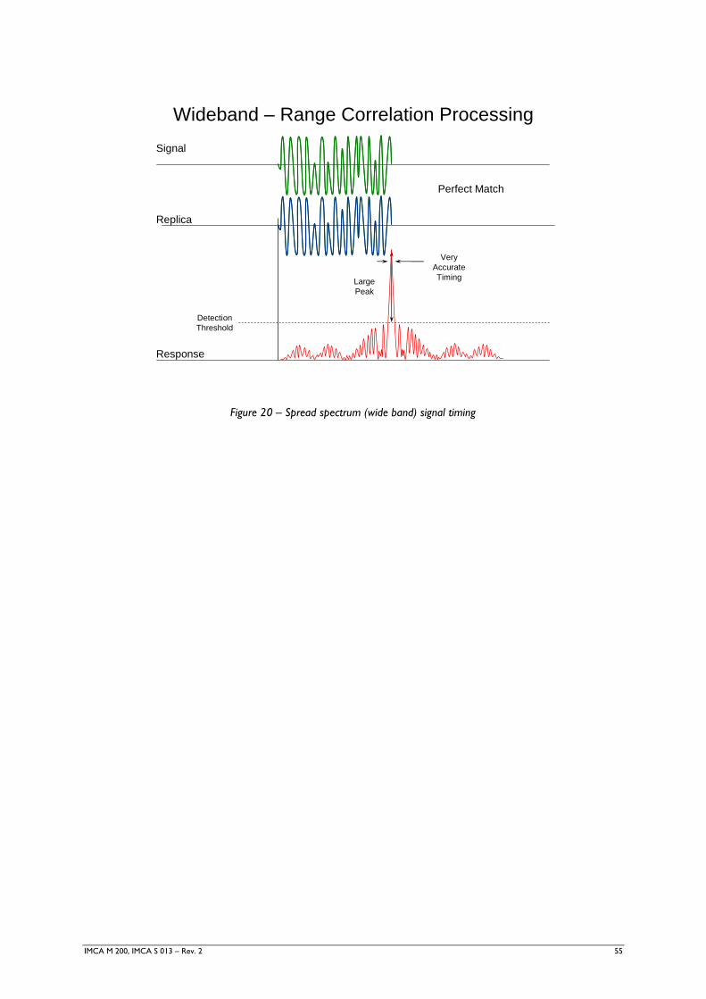
IMCA M 200, IMCA S 013 – Rev. 2 55
Figure 20 – Spread spectrum (wide band) signal timing
Wideband – Range Correlation Processing
Signal
Replica
Response
Large
Peak
Detection
Threshold
Very
Accurate
Timing
Perfect Match
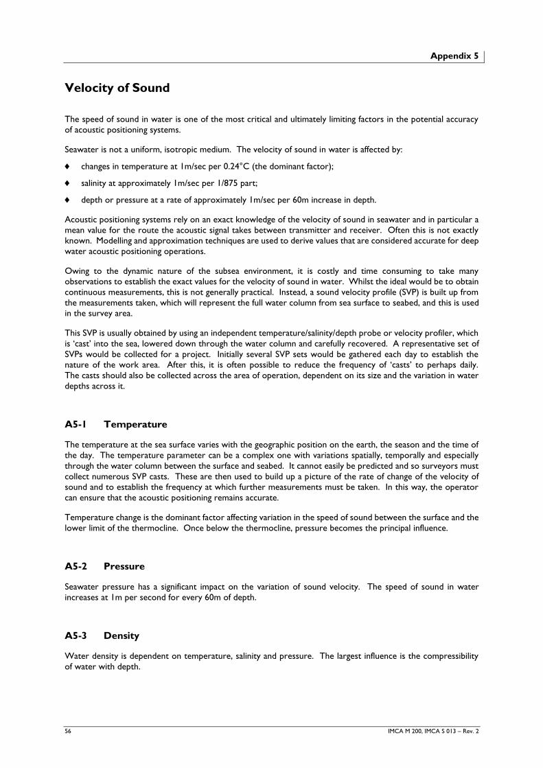
56 IMCA M 200, IMCA S 013 – Rev. 2
Appendix 5
Velocity of Sound
The speed of sound in water is one of the most critical and ultimately limiting factors in the potential accuracy
of acoustic positioning systems.
Seawater is not a uniform, isotropic medium. The velocity of sound in water is affected by:
changes in temperature at 1m/sec per 0.24°C (the dominant factor);
salinity at approximately 1m/sec per 1/875 part;
depth or pressure at a rate of approximately 1m/sec per 60m increase in depth.
Acoustic positioning systems rely on an exact knowledge of the velocity of sound in seawater and in particular a
mean value for the route the acoustic signal takes between transmitter and receiver. Often this is not exactly
known. Modelling and approximation techniques are used to derive values that are considered accurate for deep
water acoustic positioning operations.
Owing to the dynamic nature of the subsea environment, it is costly and time consuming to take many
observations to establish the exact values for the velocity of sound in water. Whilst the ideal would be to obtain
continuous measurements, this is not generally practical. Instead, a sound velocity profile (SVP) is built up from
the measurements taken, which will represent the full water column from sea surface to seabed, and this is used
in the survey area.
This SVP is usually obtained by using an independent temperature/salinity/depth probe or velocity profiler, which
is ‘cast’ into the sea, lowered down through the water column and carefully recovered. A representative set of
SVPs would be collected for a project. Initially several SVP sets would be gathered each day to establish the
nature of the work area. After this, it is often possible to reduce the frequency of ‘casts’ to perhaps daily.
The casts should also be collected across the area of operation, dependent on its size and the variation in water
depths across it.
A5-1 Temperature
The temperature at the sea surface varies with the geographic position on the earth, the season and the time of
the day. The temperature parameter can be a complex one with variations spatially, temporally and especially
through the water column between the surface and seabed. It cannot easily be predicted and so surveyors must
collect numerous SVP casts. These are then used to build up a picture of the rate of change of the velocity of
sound and to establish the frequency at which further measurements must be taken. In this way, the operator
can ensure that the acoustic positioning remains accurate.
Temperature change is the dominant factor affecting variation in the speed of sound between the surface and the
lower limit of the thermocline. Once below the thermocline, pressure becomes the principal influence.
A5-2 Pressure
Seawater pressure has a significant impact on the variation of sound velocity. The speed of sound in water
increases at 1m per second for every 60m of depth.
A5-3 Density
Water density is dependent on temperature, salinity and pressure. The largest influence is the compressibility
of water with depth.
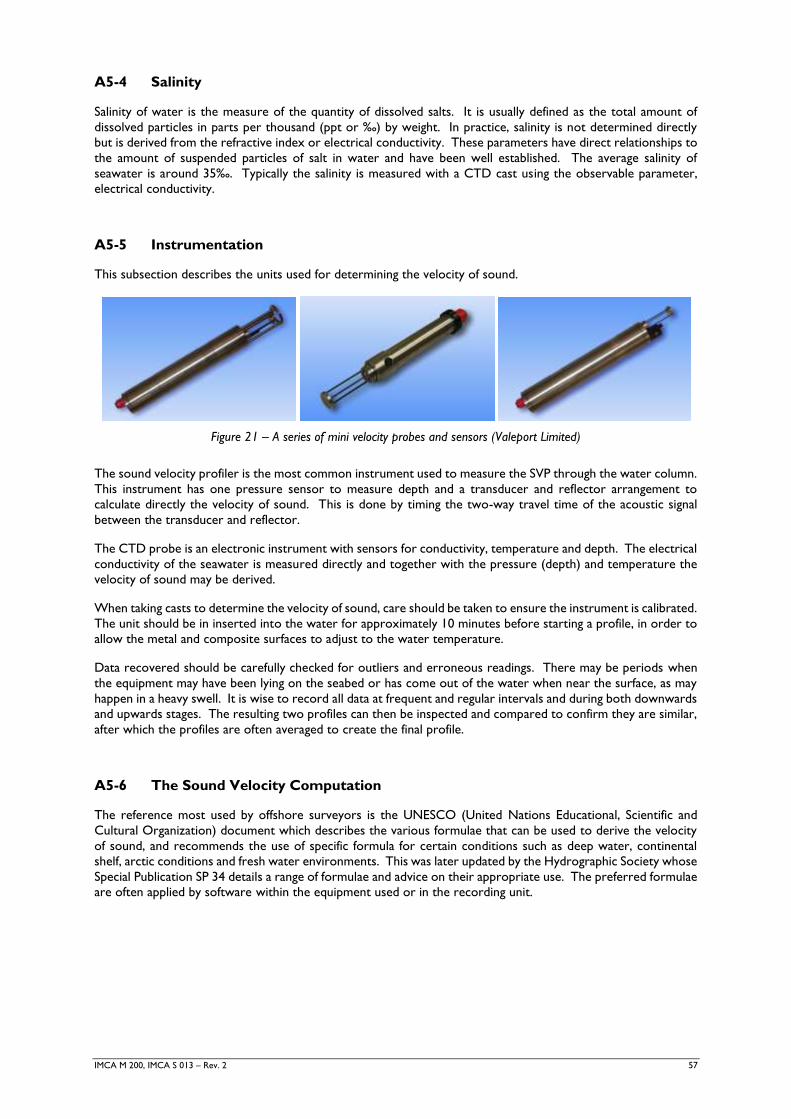
IMCA M 200, IMCA S 013 – Rev. 2 57
A5-4 Salinity
Salinity of water is the measure of the quantity of dissolved salts. It is usually defined as the total amount of
dissolved particles in parts per thousand (ppt or ‰) by weight. In practice, salinity is not determined directly
but is derived from the refractive index or electrical conductivity. These parameters have direct relationships to
the amount of suspended particles of salt in water and have been well established. The average salinity of
seawater is around 35‰. Typically the salinity is measured with a CTD cast using the observable parameter,
electrical conductivity.
A5-5 Instrumentation
This subsection describes the units used for determining the velocity of sound.
Figure 21 – A series of mini velocity probes and sensors (Valeport Limited)
The sound velocity profiler is the most common instrument used to measure the SVP through the water column.
This instrument has one pressure sensor to measure depth and a transducer and reflector arrangement to
calculate directly the velocity of sound. This is done by timing the two-way travel time of the acoustic signal
between the transducer and reflector.
The CTD probe is an electronic instrument with sensors for conductivity, temperature and depth. The electrical
conductivity of the seawater is measured directly and together with the pressure (depth) and temperature the
velocity of sound may be derived.
When taking casts to determine the velocity of sound, care should be taken to ensure the instrument is calibrated.
The unit should be in inserted into the water for approximately 10 minutes before starting a profile, in order to
allow the metal and composite surfaces to adjust to the water temperature.
Data recovered should be carefully checked for outliers and erroneous readings. There may be periods when
the equipment may have been lying on the seabed or has come out of the water when near the surface, as may
happen in a heavy swell. It is wise to record all data at frequent and regular intervals and during both downwards
and upwards stages. The resulting two profiles can then be inspected and compared to confirm they are similar,
after which the profiles are often averaged to create the final profile.
A5-6 The Sound Velocity Computation
The reference most used by offshore surveyors is the UNESCO (United Nations Educational, Scientific and
Cultural Organization) document which describes the various formulae that can be used to derive the velocity
of sound, and recommends the use of specific formula for certain conditions such as deep water, continental
shelf, arctic conditions and fresh water environments. This was later updated by the Hydrographic Society whose
Special Publication SP 34 details a range of formulae and advice on their appropriate use. The preferred formulae
are often applied by software within the equipment used or in the recording unit.
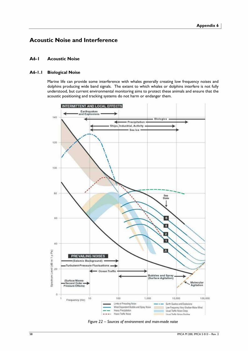
58 IMCA M 200, IMCA S 013 – Rev. 2
Appendix 6
Acoustic Noise and Interference
A6-1 Acoustic Noise
A6-1.1 Biological Noise
Marine life can provide some interference with whales generally creating low frequency noises and
dolphins producing wide band signals. The extent to which whales or dolphins interfere is not fully
understood, but current environmental monitoring aims to protect these animals and ensure that the
acoustic positioning and tracking systems do not harm or endanger them.
Figure 22 – Sources of environment and man-made noise
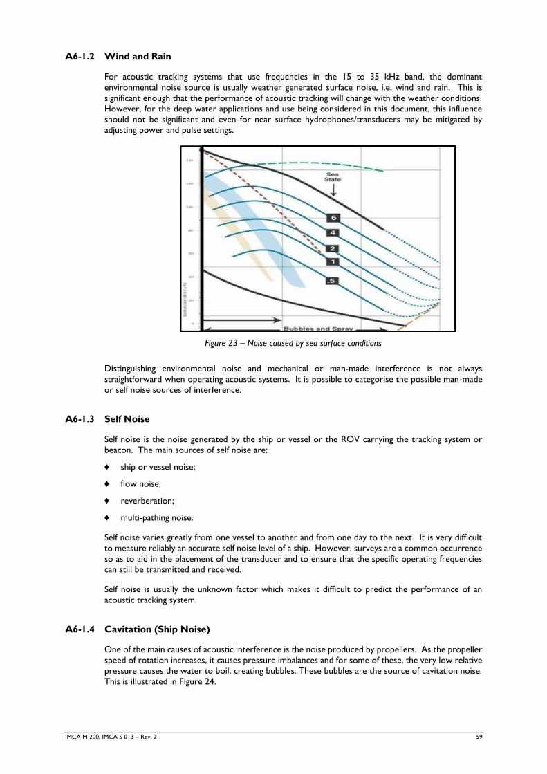
IMCA M 200, IMCA S 013 – Rev. 2 59
A6-1.2 Wind and Rain
For acoustic tracking systems that use frequencies in the 15 to 35 kHz band, the dominant
environmental noise source is usually weather generated surface noise, i.e. wind and rain. This is
significant enough that the performance of acoustic tracking will change with the weather conditions.
However, for the deep water applications and use being considered in this document, this influence
should not be significant and even for near surface hydrophones/transducers may be mitigated by
adjusting power and pulse settings.
Figure 23 – Noise caused by sea surface conditions
Distinguishing environmental noise and mechanical or man-made interference is not always
straightforward when operating acoustic systems. It is possible to categorise the possible man-made
or self noise sources of interference.
A6-1.3 Self Noise
Self noise is the noise generated by the ship or vessel or the ROV carrying the tracking system or
beacon. The main sources of self noise are:
ship or vessel noise;
flow noise;
reverberation;
multi-pathing noise.
Self noise varies greatly from one vessel to another and from one day to the next. It is very difficult
to measure reliably an accurate self noise level of a ship. However, surveys are a common occurrence
so as to aid in the placement of the transducer and to ensure that the specific operating frequencies
can still be transmitted and received.
Self noise is usually the unknown factor which makes it difficult to predict the performance of an
acoustic tracking system.
A6-1.4 Cavitation (Ship Noise)
One of the main causes of acoustic interference is the noise produced by propellers. As the propeller
speed of rotation increases, it causes pressure imbalances and for some of these, the very low relative
pressure causes the water to boil, creating bubbles. These bubbles are the source of cavitation noise.
This is illustrated in Figure 24.
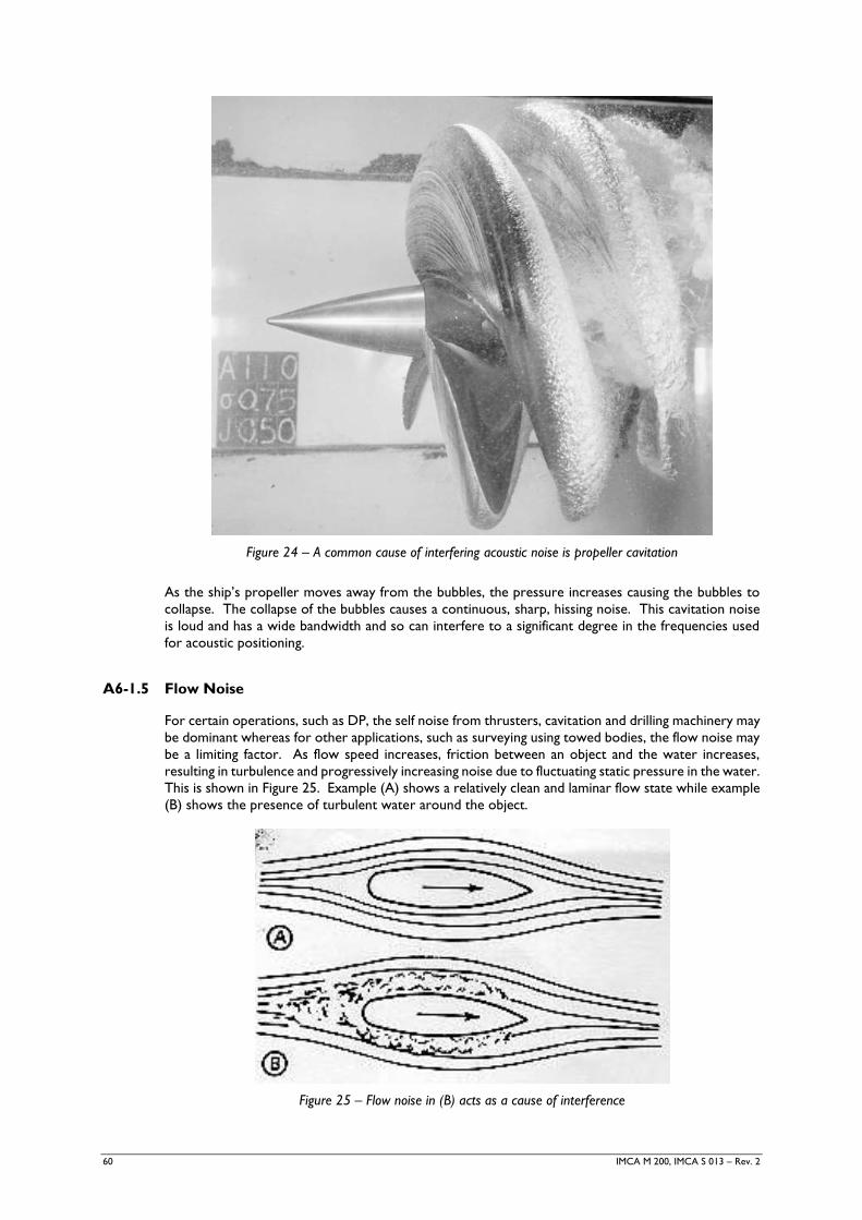
60 IMCA M 200, IMCA S 013 – Rev. 2
Figure 24 – A common cause of interfering acoustic noise is propeller cavitation
As the ship’s propeller moves away from the bubbles, the pressure increases causing the bubbles to
collapse. The collapse of the bubbles causes a continuous, sharp, hissing noise. This cavitation noise
is loud and has a wide bandwidth and so can interfere to a significant degree in the frequencies used
for acoustic positioning.
A6-1.5 Flow Noise
For certain operations, such as DP, the self noise from thrusters, cavitation and drilling machinery may
be dominant whereas for other applications, such as surveying using towed bodies, the flow noise may
be a limiting factor. As flow speed increases, friction between an object and the water increases,
resulting in turbulence and progressively increasing noise due to fluctuating static pressure in the water.
This is shown in Figure 25. Example (A) shows a relatively clean and laminar flow state while example
(B) shows the presence of turbulent water around the object.
Figure 25 – Flow noise in (B) acts as a cause of interference
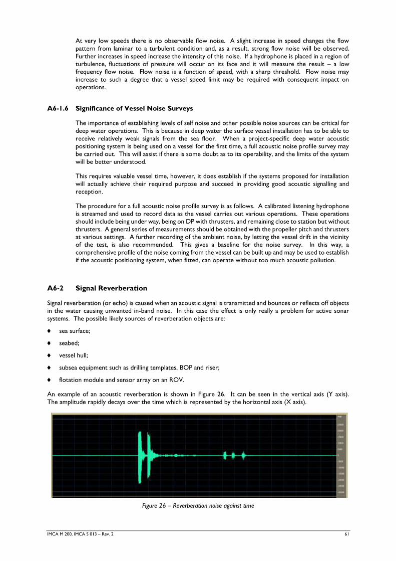
IMCA M 200, IMCA S 013 – Rev. 2 61
At very low speeds there is no observable flow noise. A slight increase in speed changes the flow
pattern from laminar to a turbulent condition and, as a result, strong flow noise will be observed.
Further increases in speed increase the intensity of this noise. If a hydrophone is placed in a region of
turbulence, fluctuations of pressure will occur on its face and it will measure the result – a low
frequency flow noise. Flow noise is a function of speed, with a sharp threshold. Flow noise may
increase to such a degree that a vessel speed limit may be required with consequent impact on
operations.
A6-1.6 Significance of Vessel Noise Surveys
The importance of establishing levels of self noise and other possible noise sources can be critical for
deep water operations. This is because in deep water the surface vessel installation has to be able to
receive relatively weak signals from the sea floor. When a project-specific deep water acoustic
positioning system is being used on a vessel for the first time, a full acoustic noise profile survey may
be carried out. This will assist if there is some doubt as to its operability, and the limits of the system
will be better understood.
This requires valuable vessel time, however, it does establish if the systems proposed for installation
will actually achieve their required purpose and succeed in providing good acoustic signalling and
reception.
The procedure for a full acoustic noise profile survey is as follows. A calibrated listening hydrophone
is streamed and used to record data as the vessel carries out various operations. These operations
should include being under way, being on DP with thrusters, and remaining close to station but without
thrusters. A general series of measurements should be obtained with the propeller pitch and thrusters
at various settings. A further recording of the ambient noise, by letting the vessel drift in the vicinity
of the test, is also recommended. This gives a baseline for the noise survey. In this way, a
comprehensive profile of the noise coming from the vessel can be built up and may be used to establish
if the acoustic positioning system, when fitted, can operate without too much acoustic pollution.
A6-2 Signal Reverberation
Signal reverberation (or echo) is caused when an acoustic signal is transmitted and bounces or reflects off objects
in the water causing unwanted in-band noise. In this case the effect is only really a problem for active sonar
systems. The possible likely sources of reverberation objects are:
sea surface;
seabed;
vessel hull;
subsea equipment such as drilling templates, BOP and riser;
flotation module and sensor array on an ROV.
An example of an acoustic reverberation is shown in Figure 26. It can be seen in the vertical axis (Y axis).
The amplitude rapidly decays over the time which is represented by the horizontal axis (X axis).
Figure 26 – Reverberation noise against time
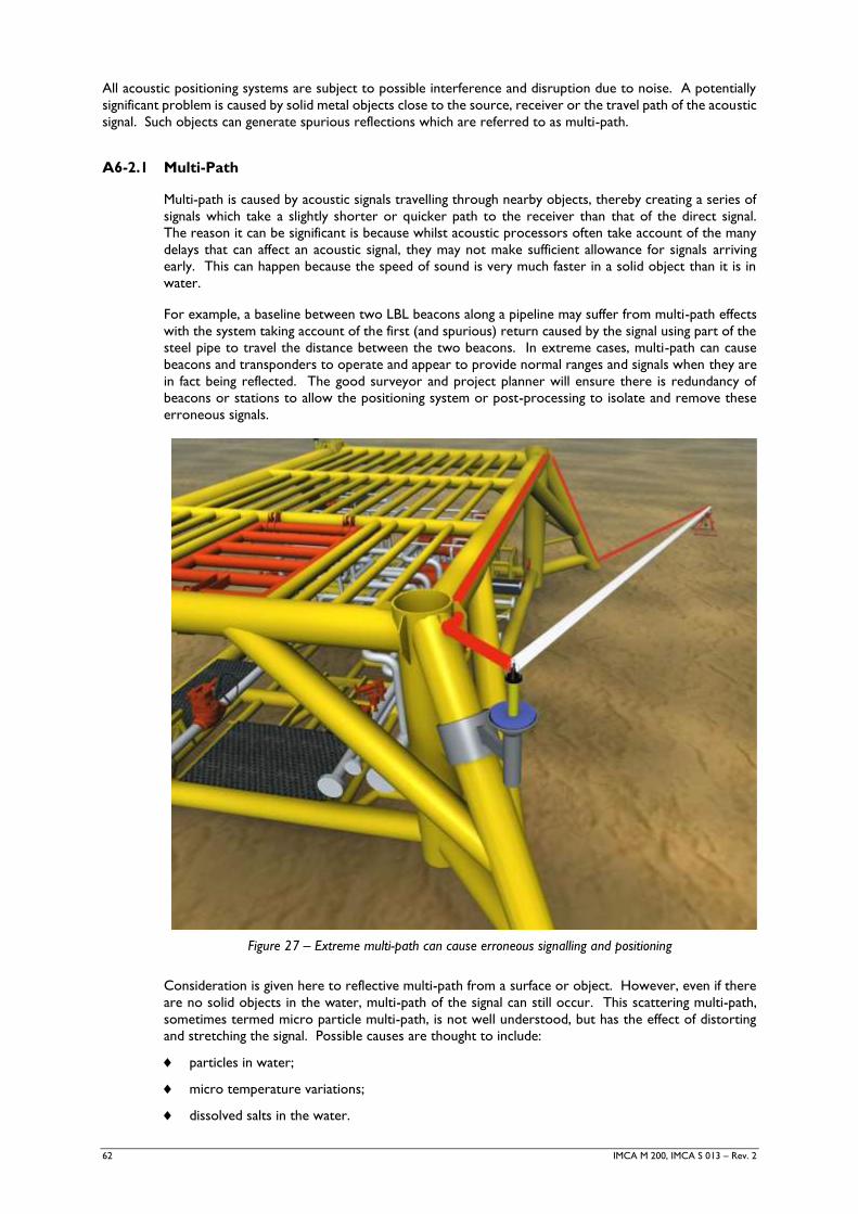
62 IMCA M 200, IMCA S 013 – Rev. 2
All acoustic positioning systems are subject to possible interference and disruption due to noise. A potentially
significant problem is caused by solid metal objects close to the source, receiver or the travel path of the acoustic
signal. Such objects can generate spurious reflections which are referred to as multi-path.
A6-2.1 Multi-Path
Multi-path is caused by acoustic signals travelling through nearby objects, thereby creating a series of
signals which take a slightly shorter or quicker path to the receiver than that of the direct signal.
The reason it can be significant is because whilst acoustic processors often take account of the many
delays that can affect an acoustic signal, they may not make sufficient allowance for signals arriving
early. This can happen because the speed of sound is very much faster in a solid object than it is in
water.
For example, a baseline between two LBL beacons along a pipeline may suffer from multi-path effects
with the system taking account of the first (and spurious) return caused by the signal using part of the
steel pipe to travel the distance between the two beacons. In extreme cases, multi-path can cause
beacons and transponders to operate and appear to provide normal ranges and signals when they are
in fact being reflected. The good surveyor and project planner will ensure there is redundancy of
beacons or stations to allow the positioning system or post-processing to isolate and remove these
erroneous signals.
Figure 27 – Extreme multi-path can cause erroneous signalling and positioning
Consideration is given here to reflective multi-path from a surface or object. However, even if there
are no solid objects in the water, multi-path of the signal can still occur. This scattering multi-path,
sometimes termed micro particle multi-path, is not well understood, but has the effect of distorting
and stretching the signal. Possible causes are thought to include:
particles in water;
micro temperature variations;
dissolved salts in the water.
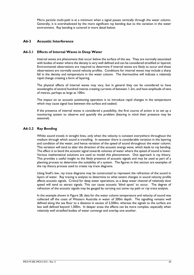
IMCA M 200, IMCA S 013 – Rev. 2 63
Micro particle multi-path is at a minimum when a signal passes vertically through the water column.
Generally, it is overshadowed by the more significant ray bending due to the variation in the water
environment. Ray bending is covered in more detail below.
A6-3 Acoustic Interference
A6-3.1 Effects of Internal Waves in Deep Water
Internal waves are phenomena that occur below the surface of the sea. They are normally associated
with bodies of water where the density is very well defined and can be considered stratified or layered.
Environmental observations are required to determine if internal waves are likely to occur and these
observations are normally sound velocity profiles. Conditions for internal waves may include a sharp
fall in the density and temperature in the water column. The thermocline will indicate a relatively
rapid change creating a form of layering.
The physical effects of internal waves may vary, but in general they can be considered to have
wavelengths of several hundred metres creating currents of between 1-2m, and have amplitude of tens
of metres, perhaps as large as 100m.
The impact on an acoustic positioning operation is to introduce rapid changes in the temperature
which may cause signal loss between the surface and seabed.
If the presence of internal waves is considered a possibility, the first course of action is to set up a
monitoring system to observe and quantify the problem (bearing in mind their presence may be
seasonal).
A6-3.2 Ray Bending
Whilst sound travels in straight lines, only when the velocity is constant everywhere throughout the
medium through which sound is travelling. In seawater there is considerable variation in the layering
and condition of the water, and hence variation of the speed of sound throughout the water column.
This variation will tend to alter the direction of the acoustic energy wave, which leads to ray bending.
The effect is to bend the acoustic signal towards volumes of water where the speed of sound is lower.
Various mathematical solutions are used to model this phenomenon. One approach is ray theory.
This provides a useful insight to the likely presence of acoustic signals and may be used as part of a
planning process to determine the suitability of a system. The figures in this section are examples of
the ray theory process used to create ray trace diagrams.
Using Snell’s law, ray trace diagrams may be constructed to represent the refraction of the sound in
layers of water. Ray tracing is analysis to determine to what extent changes in sound velocity profile
affects acoustic signals. Critical for deep water operations, as a deep water channel of relatively slow
speed will tend to attract signals. This can cause acoustic ‘blind spots’ to occur. The degree of
refraction of the acoustic signals may be gauged by carrying out some ray path or ray trace analysis.
In the example shown in Figure 28, data for the water column temperature and velocity of sound was
collected off the coast of Western Australia in water of 200m depth. The signalling remains well
defined along the sea floor to a distance in excess of 2,500m, whereas the signals to the surface are
less well defined beyond 1,300m. In deeper areas the effects can be more complex, especially when
relatively well stratified bodies of water converge and overlap one another.
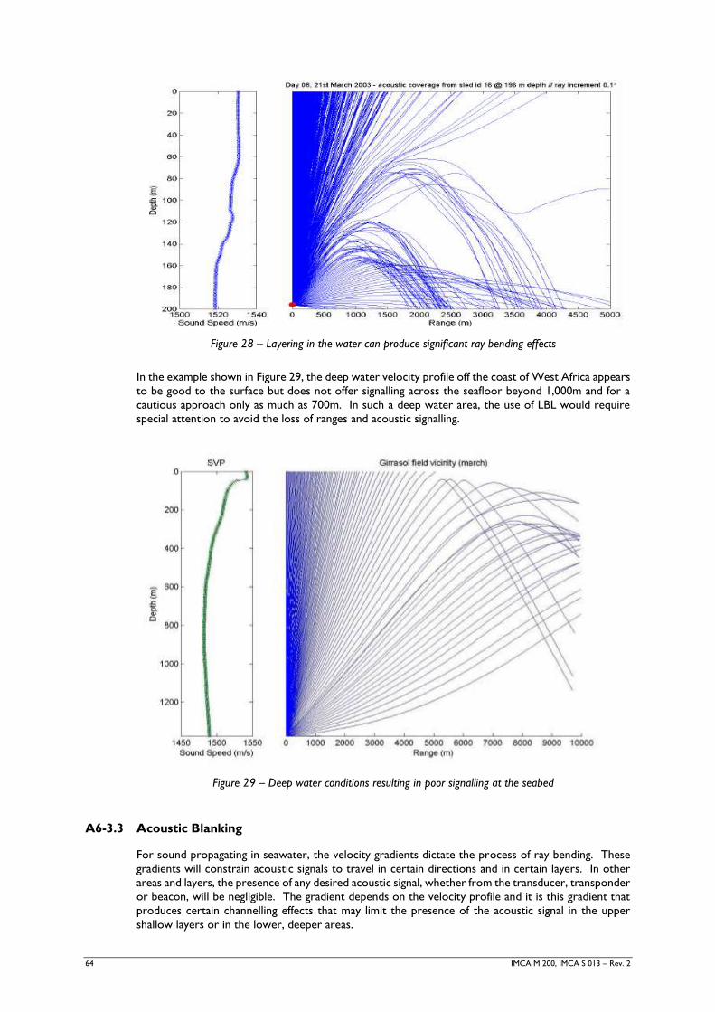
64 IMCA M 200, IMCA S 013 – Rev. 2
Figure 28 – Layering in the water can produce significant ray bending effects
In the example shown in Figure 29, the deep water velocity profile off the coast of West Africa appears
to be good to the surface but does not offer signalling across the seafloor beyond 1,000m and for a
cautious approach only as much as 700m. In such a deep water area, the use of LBL would require
special attention to avoid the loss of ranges and acoustic signalling.
Figure 29 – Deep water conditions resulting in poor signalling at the seabed
A6-3.3 Acoustic Blanking
For sound propagating in seawater, the velocity gradients dictate the process of ray bending. These
gradients will constrain acoustic signals to travel in certain directions and in certain layers. In other
areas and layers, the presence of any desired acoustic signal, whether from the transducer, transponder
or beacon, will be negligible. The gradient depends on the velocity profile and it is this gradient that
produces certain channelling effects that may limit the presence of the acoustic signal in the upper
shallow layers or in the lower, deeper areas.
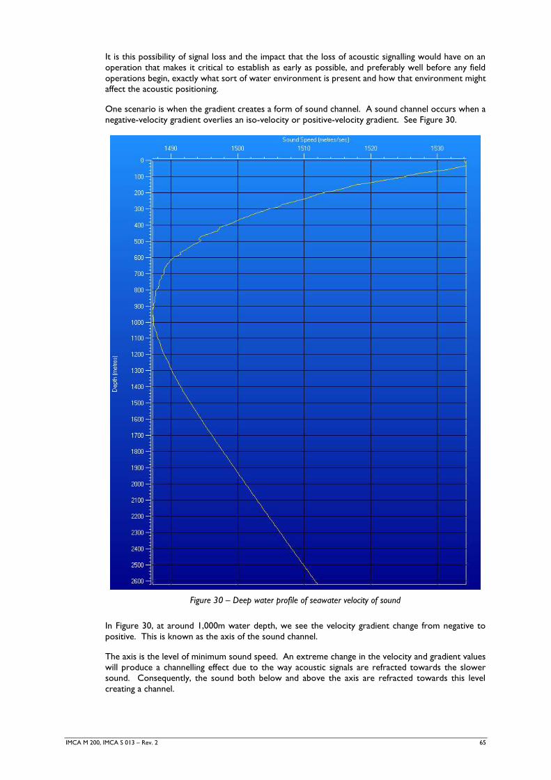
IMCA M 200, IMCA S 013 – Rev. 2 65
It is this possibility of signal loss and the impact that the loss of acoustic signalling would have on an
operation that makes it critical to establish as early as possible, and preferably well before any field
operations begin, exactly what sort of water environment is present and how that environment might
affect the acoustic positioning.
One scenario is when the gradient creates a form of sound channel. A sound channel occurs when a
negative-velocity gradient overlies an iso-velocity or positive-velocity gradient. See Figure 30.
Figure 30 – Deep water profile of seawater velocity of sound
In Figure 30, at around 1,000m water depth, we see the velocity gradient change from negative to
positive. This is known as the axis of the sound channel.
The axis is the level of minimum sound speed. An extreme change in the velocity and gradient values
will produce a channelling effect due to the way acoustic signals are refracted towards the slower
sound. Consequently, the sound both below and above the axis are refracted towards this level
creating a channel.

66 IMCA M 200, IMCA S 013 – Rev. 2
Appendix 7
Deep Water Acoustic Operations
A7-1 Station Deployment
The sequence for the deployment of the seabed beacons and transponders is considered important as it often
dictates the overall level of system performance that can be achieved. The first beacon to be deployed in the
area is a critical one as it must be placed correctly for the required coverage and performance. To avoid
problems, project planning should ensure that a clear signal path is likely without multi-path being present. Before
deploying over the side, the unit should be checked for charged batteries, properly functioning sensors and, if
appropriate, the direction of the reference heading sensor.
The location on the seabed should be clear of localised noise. Once the beacon has made touchdown or is
placed on the seabed, the depth setting and power levels should be checked and the unit set to transmit to check
the transponder functions.
A number of factors influence station deployment, including:
design of deep water transponder frames;
suitability and use of acoustics as DP references;
depth rating of acoustic equipment;
power levels and battery technology.
A7-2 Deep Water Frame Designs
Various designs of seabed frame for transponders exist, generally made of steel and designed to withstand
conditions on the seabed. The likely risks to the frame include: accidental damage by the other vessels and assets
including ROVs; slumping or settling due to the weight of the frame on the seabed; and corrosion that may result
in a failure of some part of the frame or failure to recover the transponder.
For large deep water projects, hundreds of frames may be required but not all will be populated by transponders.
The approach now is to deploy the required number for operations and to move and re-pot the transponders
in the frames for each activity. In this way, only a fraction of the total numbers of frames require a transponder
at any one time.
Transponder frames are typically made of steel and are between 1.5m and 3m high. They generally have a tripod
design with a small plate for the slot into which the transponder is fixed. The weight of the transponder sitting
in a well machined slot with tight tolerance is sufficient to keep it in place. A frame may have between two and
four slots. An alternative design is the sled design with a simple base and column for the transponders. These
appear less rigid but may allow for better recovery due to their slimmer overall shape and, with less material,
could be more cost effective. Various other designs are available and some are recommended by the
manufacturers for the installation of seabed transponders.
Examples of recently used designs are shown in Figure 31.
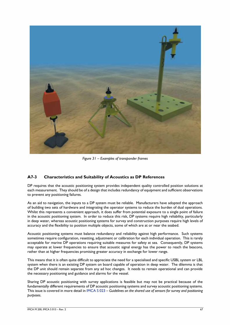
IMCA M 200, IMCA S 013 – Rev. 2 67
Figure 31 – Examples of transponder frames
A7-3 Characteristics and Suitability of Acoustics as DP References
DP requires that the acoustic positioning system provides independent quality controlled position solutions at
each measurement. They should be of a design that includes redundancy of equipment and sufficient observations
to prevent any positioning failures.
As an aid to navigation, the inputs to a DP system must be reliable. Manufacturers have adopted the approach
of building two sets of hardware and integrating the operator systems to reduce the burden of dual operations.
Whilst this represents a convenient approach, it does suffer from potential exposure to a single point of failure
in the acoustic positioning system. In order to reduce this risk, DP systems require high reliability, particularly
in deep water, whereas acoustic positioning systems for survey and construction purposes require high levels of
accuracy and the flexibility to position multiple objects, some of which are at or near the seabed.
Acoustic positioning systems must balance redundancy and reliability against high performance. Such systems
sometimes require configuration, resetting, adjustment or calibration for each individual operation. This is rarely
acceptable for marine DP operations requiring suitable measures for safety at sea. Consequently, DP systems
may operate at lower frequencies to ensure that acoustic signal energy has the power to reach the beacons,
rather than at higher frequencies promising greater accuracy in exchange for lower range.
This means that it is often quite difficult to appreciate the need for a specialised and specific USBL system or LBL
system when there is an existing DP system on board capable of operation in deep water. The dilemma is that
the DP unit should remain separate from any ad hoc changes. It needs to remain operational and can provide
the necessary positioning and guidance and alarms for the vessel.
Sharing DP acoustic positioning with survey applications is feasible but may not be practical because of the
fundamentally different requirements of DP acoustic positioning systems and survey acoustic positioning systems.
This issue is covered in more detail in IMCA S 023 – Guidelines on the shared use of sensors for survey and positioning
purposes.
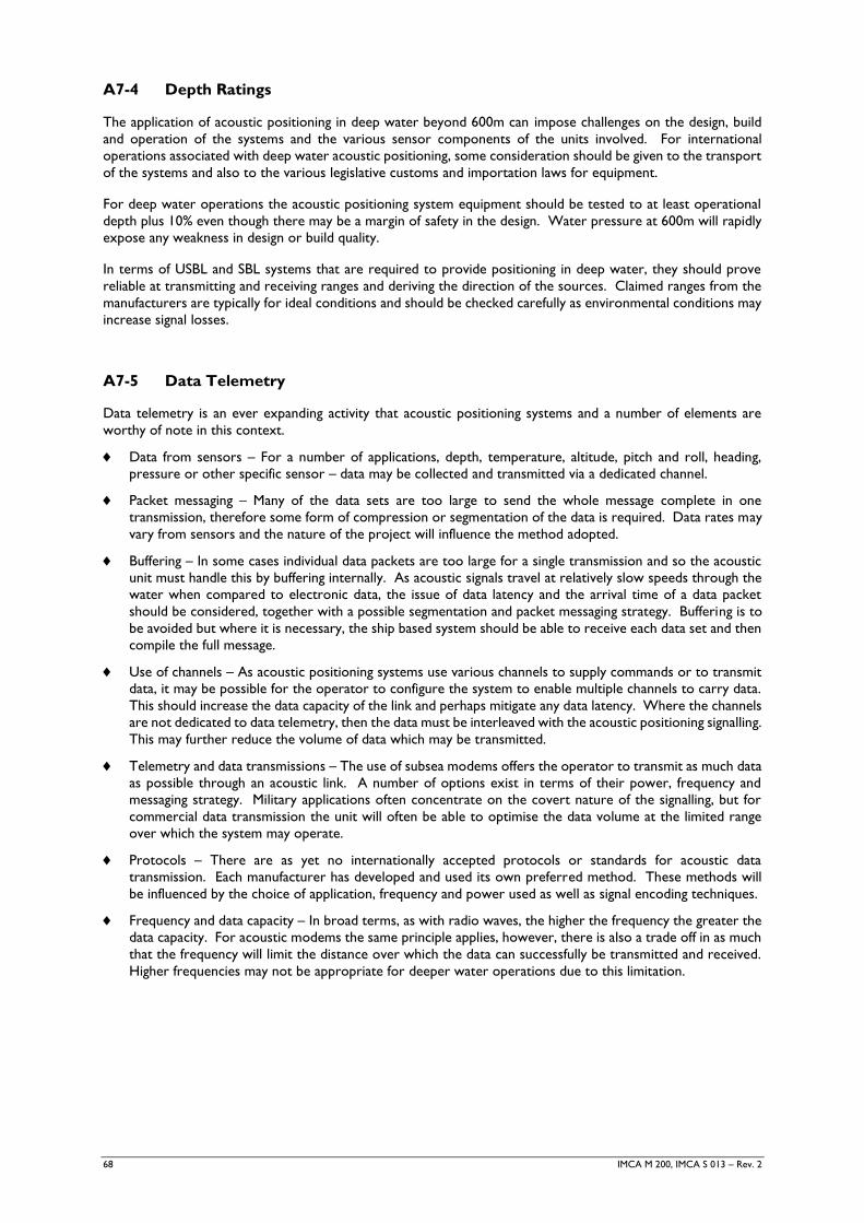
68 IMCA M 200, IMCA S 013 – Rev. 2
A7-4 Depth Ratings
The application of acoustic positioning in deep water beyond 600m can impose challenges on the design, build
and operation of the systems and the various sensor components of the units involved. For international
operations associated with deep water acoustic positioning, some consideration should be given to the transport
of the systems and also to the various legislative customs and importation laws for equipment.
For deep water operations the acoustic positioning system equipment should be tested to at least operational
depth plus 10% even though there may be a margin of safety in the design. Water pressure at 600m will rapidly
expose any weakness in design or build quality.
In terms of USBL and SBL systems that are required to provide positioning in deep water, they should prove
reliable at transmitting and receiving ranges and deriving the direction of the sources. Claimed ranges from the
manufacturers are typically for ideal conditions and should be checked carefully as environmental conditions may
increase signal losses.
A7-5 Data Telemetry
Data telemetry is an ever expanding activity that acoustic positioning systems and a number of elements are
worthy of note in this context.
Data from sensors – For a number of applications, depth, temperature, altitude, pitch and roll, heading,
pressure or other specific sensor – data may be collected and transmitted via a dedicated channel.
Packet messaging – Many of the data sets are too large to send the whole message complete in one
transmission, therefore some form of compression or segmentation of the data is required. Data rates may
vary from sensors and the nature of the project will influence the method adopted.
Buffering – In some cases individual data packets are too large for a single transmission and so the acoustic
unit must handle this by buffering internally. As acoustic signals travel at relatively slow speeds through the
water when compared to electronic data, the issue of data latency and the arrival time of a data packet
should be considered, together with a possible segmentation and packet messaging strategy. Buffering is to
be avoided but where it is necessary, the ship based system should be able to receive each data set and then
compile the full message.
Use of channels – As acoustic positioning systems use various channels to supply commands or to transmit
data, it may be possible for the operator to configure the system to enable multiple channels to carry data.
This should increase the data capacity of the link and perhaps mitigate any data latency. Where the channels
are not dedicated to data telemetry, then the data must be interleaved with the acoustic positioning signalling.
This may further reduce the volume of data which may be transmitted.
Telemetry and data transmissions – The use of subsea modems offers the operator to transmit as much data
as possible through an acoustic link. A number of options exist in terms of their power, frequency and
messaging strategy. Military applications often concentrate on the covert nature of the signalling, but for
commercial data transmission the unit will often be able to optimise the data volume at the limited range
over which the system may operate.
Protocols – There are as yet no internationally accepted protocols or standards for acoustic data
transmission. Each manufacturer has developed and used its own preferred method. These methods will
be influenced by the choice of application, frequency and power used as well as signal encoding techniques.
Frequency and data capacity – In broad terms, as with radio waves, the higher the frequency the greater the
data capacity. For acoustic modems the same principle applies, however, there is also a trade off in as much
that the frequency will limit the distance over which the data can successfully be transmitted and received.
Higher frequencies may not be appropriate for deeper water operations due to this limitation.
IMCA M 200, IMCA S 013 – Rev. 2 69
A7-6 Power Levels
The battery capacity of various elements of an acoustic positioning system may be quoted in terms of its ability
to perform a number of transmissions. This is an important parameter to be considered when designing and
operating the units. Each unit may be set to transmit at a specific power level. However, should the ranges
between units be excessive or should there be significant noise, then power settings may need increasing, which
will lead to lower battery life. The operator should be aware that an increase of 3dB represents a doubling of
power which will have a consequent impact on battery life. There are other environmental parameters, of which
temperature is perhaps the most important, which can influence ‘real world’ battery life. Many modern acoustic
systems have data telemetry capability such that the operator can interrogate the unit and remotely determine
battery status and power levels.
A7-7 System Maintenance
A network of beacons or transponders requires monitoring and some maintenance to ensure good levels of
performance are achieved. This maintenance may include:
setting the transducer and beacon transmit power levels;
measuring battery voltage of each transponder;
regular measurement of the SVP, thus taking into account any variations over time;
measuring the depth of each unit.
A7-8 Multiple Vessel Users
A recent problem for operators of acoustic positioning systems has been the influence of the environment on
the ability of the acoustic positioning system to provide reliable signalling to a number of users. This has occurred
due to several reasons. In deep water the natural ambient noise is quite low and so once a series of transponders
or beacons is deployed, their signals will often transmit across much greater distances than is necessary. This
effectively produces interference for other systems in the local area.
Careful assessment of the subsea environment will be necessary to avoid signal and acoustic pollution. Multiple
vessels and users extend the range and coverage required but, by doing so, they may also increase the number
of acoustic transmissions and hence the opportunities for interference. Planning of the logistics and scheduling
may highlight possible clashes or saturation. Simultaneous acoustic operational issues can be addressed using a
frequency management plan, in which the various frequencies used are mapped and assigned to the various users
and/or vessels.
The widespread adoption of spread spectrum ‘digital coded’ signals has helped to mitigate the impact of frequency
clashes and false detection of signals generated from other systems in the area. However, frequency overlaps do
still increase the risk of not detecting the correct signal, depending on the robustness and power of the signal.
Therefore, minimising overlap through management is still desirable.
Some manufacturers have sought to reduce the quantity of signals in the water by developing broadcast systems,
thereby removing the ‘interrogation’ part of the signal and effectively halving the number of signals in the water.
This approach does add a timing synchronisation requirement to allow distances to be accurately determined
from a one-way travel time, and this has been addressed using different techniques by different manufacturers.
A7-8.1 Simultaneous Position Fixing and Information Supply
Whilst the aim of the acoustic positioning system is to create a series of signals that will enable a
processing unit to derive a position, the system very often needs to also report the condition, status
and measurements from the system or peripheral devices. Acoustic messages with associated data
for the sensors or the condition of the system are vital if the operator is to manage and avoid problems.
These secondary transmissions may actually be more critical as they often carry the sensor data
messages and alert the operator to any problems.
70 IMCA M 200, IMCA S 013 – Rev. 2
A7-9 Interface with Different Sensors
It is not the purpose of this document to provide a thorough review of the sensors listed but to illustrate their
application and some elements of their use that the reader should be made aware of. Further information can
be found in IMCA S 021 – Guidelines for the management of peripheral survey sensors.
A7-9.1 Motion Reference Units
The use of a motion reference unit (MRU) may be for the attitude and orientation of the surface vessel.
The information can be used to compensate observations from a USBL system for pitch, roll and heave.
Other uses include ROVs or AUVs requiring to compensate their motion to ensure accurate
positioning and measurements are obtained. For the former, a variety of units may be considered but
in general they will offer a high data rate, at around 50 Hz.
The subsea application of these units is more considered. For an AUV the power requirements should
be kept to a minimum along with little weight or volume. On an ROV, however, power is not the
limit, but often space to install the pressure housing to contain the unit is a limiting factor.
Data formats are usually relatively simple with the high data rates requiring a simple and uncomplicated
message format that may be issued at 50 Hz, or even at 100 Hz. The critical factors for these units
are their alignment and calibration along with accurate time stamping of data. The timing is critical to
avoid introducing errors due to latency, buffering or signal delays that would put the motion sensor
data out of synchronisation with the other sensors and data sets.
A7-9.2 Heading Sensors
Accurate alignment and timing is critical for heading sensors. Data rates are not too high at perhaps
a few Hz but the lack of an independent check means that these units may experience difficult to
identify bias or error. Frequent checks and calibrations are required to ensure they maintain their
accuracy and secondary systems are carried to avoid any critical system failures.
A7-9.3 GNSS
Surface positioning is referenced by use of GNSS. In deep water, the surface reference will simply be
the starting point for positioning of seabed assets. It is good practice to keep the errors on the surface
to an absolute minimum so as to reduce propagation of errors in positioning of the seabed assets.
Systems with accuracy better than 20cm are now available, with 10cm being typical.
A7-9.4 IMU
These highly sensitive sensor units produce very high data rates of 100 to 500 Hz. Timing is critical
and because they have a high drift rate in absolute terms, they require external or additional
measurements to bind their errors and keep the derived positioning accurate. They are essentially
‘black boxes’ with modelling and filtering requirements that mean a powerful processor is required
and considerable effort is spent on developing accurate elements and parameters for these models to
ensure reliable accuracies can be achieved.
A7-10 Checks and Quality Control
Additional parameters must also be collected and monitored – the most important being the speed of sound in
water. This can often limit the ability of the acoustic system to perform accurate positioning. For each well
location and installation, an accurate value would be required and checks made to ensure no degradation of
quality.