Accuracy Assessment Study of GNSS Precise Point Positioning for Kinematic Positioning

167

Ashraf Abdallah, Volker Schwieger Institute of Engineering Geodesy, Stuttgart University, Stuttgart, Germany.

AbstractGNSS Precise Point Positioning (PPP) technique has received a great deal of attention from scientists in the last few years. The aim of this study is to evaluate the accuracy and the initialization time of PPP solutions compared to Precise Differential GPS (PDGPS) solutions. SAPOS stations were considered as reference

solutions were estimated using GIPSY-OASIS software and CSRS-PPP online service. Two kinematic trajectories have been observed in Stuttgart, Germany. The observations started with 60 minutes static data acquisition as initialization time. The static data was followed by 30 minutes of kinematic measurement. PPP solutions were evaluated with different periods for the initialization time (zero to sixty minutes) to establish the

OASIS software as well as CSRS-PPP online service achieved a RMSE in 3 dimensions of 10 cm from 10 minutes initialization time. The second data set had cycle slip problems during the observation process. CSRS-PPP provided a reliable solution beginning with 20 minutes initialization time. Regarding GIPSY-OASIS software different tropospheric models and approaches were tested in the study to improve the non-reliable

service solution, provides a RMSE of 5 cm in horizontal directions and below 15 cm in height direction from 10 minutes initialization time.

KeywordsGNSS, Kinematic measurement, PPP

1 INTRODUCTIONRecently, there is an increasing interest in implementation of GNSS Precise Point Positioning (PPP) technique. In comparison to Differential GPS (DGPS) and Precise Differential GPS (PDGPS) solutions, which require one or more reference stations (Grinter & Roberts, 2011); PPP technique is a method using only one GPS receiver (Goa, 2006). Generally, the navigation community has interesting on PPP technique to improve its accuracy and cost effectiveness (Gao & Shen, 2002).

Gao & Wojciechowski (2004) investigated the PPP solution using GIPSY-OASIS software for two airborne kinematic data sets. This case study provided centimeter level in the horizontal and a couple of decimeters in the vertical direction. Schwieger et al. (2009) reported a height RMS better than 0.5m in PPP solution with an availability rate around 60%. They compared GIPSY-OASIS solution relative to CSRS-PPP online service. Moreover, Martín et al. (2012) processed a kinematic car track using CSRS-PPP online services. This research presented mean standard deviations of 8.50, 9.50 and 17.40 cm for north, east and height direction.

This paper shows an accuracy assessment study of kinematic PPP solution for two car tracks. This kinematic tracks have been observed in Stuttgart, Germany with 60 minutes static initialization time followed by 30 minutes kinematic mesurements. In this concept the initialization time has been divided into 10 minutes sleeps from 0 to 60 minutes before moving. The main idea of this study is to investigate the effect of convergence time on PPP kinematic solution using GIPSY-OASIS software and CSRS-PPP online service.

http://www.digibib.tu-bs.de/?docid=00056119 30/04/2014

168

2 BASIC CONCEPTS

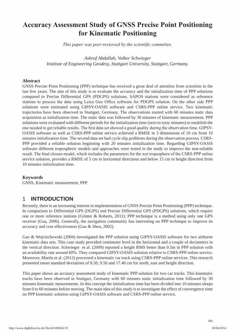
2.1 PPP technique faces several challenges that should be modeled. It needs precise satellite orbits and clock cor-rections that are available from for example IGS (Goa, 2006) and JPL (Jet Propulsion Laboratory). These orbit products include different types related to the availability time and the accuracy; see Table 1. Antenna phase center variations should be considered also for satellite and receiver antennas. NGS (National Geodetic Sur-vey) provides the users with the antenna calibration parameters for different GPS antennas in ANTEX format1.

Table 1: IGS2 and JPL3 products IGS JPL

Latency Latency

~5 cm real time - -<3 cm 3 hours 5 cm < 2 hours

~2.5 cm 17 hours 3.5 cm Next-Day (16:00 UTC)~2.5 cm ~13 days 2.5 cm < 14 days

The evaluation of PPP is based on the ionosphere free (IF) linear combination for code ( IF ) and carrier phase

( IF ) measurements for dual frequency receivers that are formed in equations (1).

)()()()( 22

221

22

122

21

21 elmTcr

fff

fff

zSR

LLL

LL

LL

LIF (1.a)

IFIFzSR

LLL

LL

LL

LIF NelmTcr

fff

fff )()(

)()( 222

21

22

122

21

21 (1.b)

222 )()()( RSRSRS ZZYYXXr (2)

Where 1f , 2f are the frequencies of the GPS 1L and 2L signals; Li , Li are the measured code and phase data. r is the true geometric range that can be calculated as a function of the satellite position

( SX , SY , SZ ) and receiver position ( RX , RY , RZ ) as shown in equation (2). c is the vacuum speed of light; R , S are the receiver and the satellite clock offset. IFN is the combination integer ambiguity and IF refers

to the combination carrier wavelength. Moreover )(elmTz shows the troposphere zenith delay including

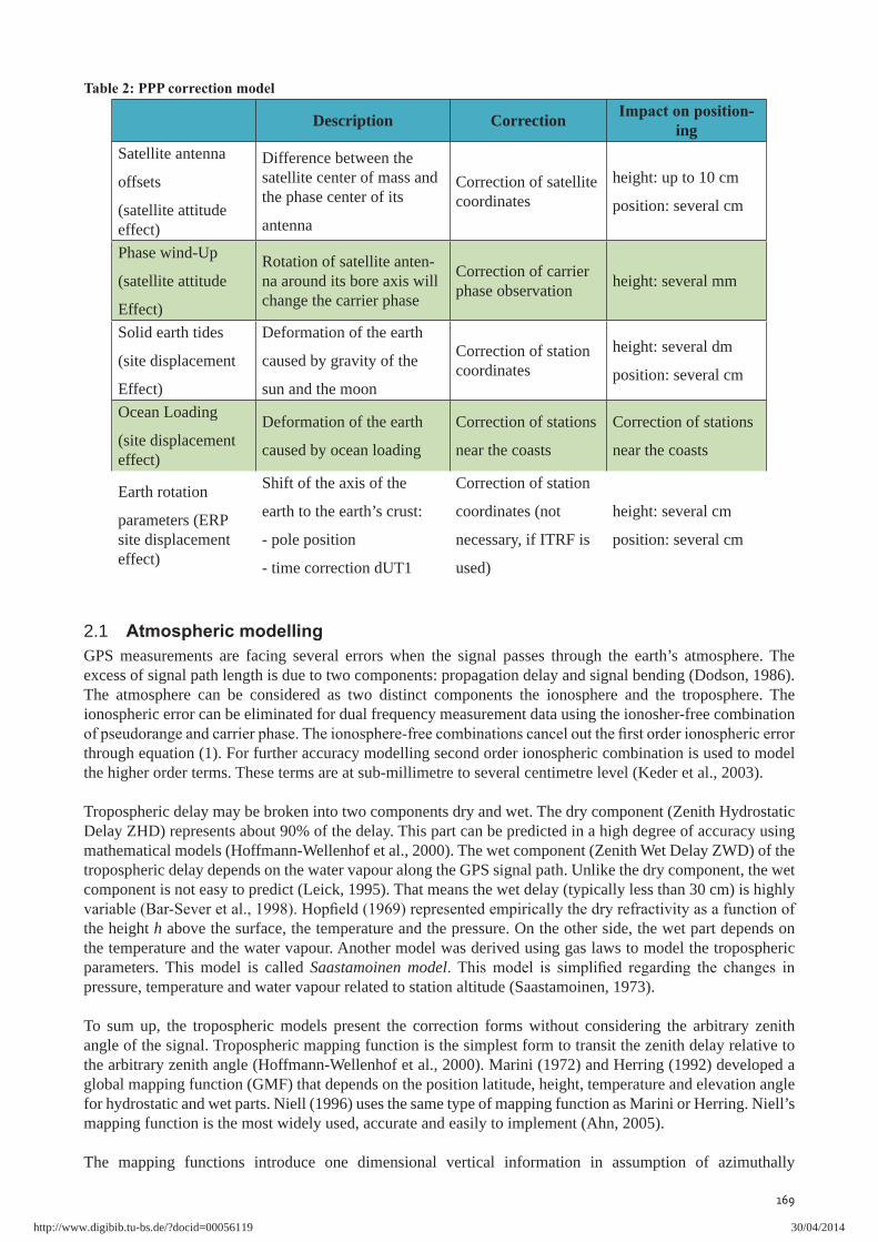
mapping function and , are the relevant measurement noises including the multipath (Mirsa & Enge, 2012). For high accurate PPP solutions some errors should be taken into consideration. Table 2 illustrates the overview of additional correction models that are important for PPP (Heßelbarth, 2009) . The PPP solution is

minutes or more) to obtain a PPP solution with cm positioning level. This convergence time is the disadvan-

differencing (Rizos et al., 2012).

1 http://www.ngs.noaa.gov/ANTCAL/documents/format.txt2 http://igscb.jpl.nasa.gov/components/prods.html3 https://gipsy-oasis.jpl.nasa.gov/index.php?page=data


169

Description Correction ingSatellite antenna

offsets

(satellite attitude effect)

Difference between the satellite center of mass and the phase center of its

antenna

Correction of satellite coordinates

height: up to 10 cm

position: several cm

Phase wind-Up

(satellite attitude

Effect)

Rotation of satellite anten-na around its bore axis will change the carrier phase

Correction of carrier phase observation height: several mm

Solid earth tides

(site displacement

Effect)

Deformation of the earth

caused by gravity of the

sun and the moon

Correction of station coordinates

height: several dm


Ocean Loading

(site displacement effect)

Deformation of the earth

caused by ocean loading

Correction of stations

near the coasts

Correction of stations

near the coasts

Earth rotation

parameters (ERP site displacement effect)

Shift of the axis of the

earth to the earth’s crust:

- pole position

- time correction dUT1

Correction of station

coordinates (not

necessary, if ITRF is

used)

height: several cm


2.1 GPS measurements are facing several errors when the signal passes through the earth’s atmosphere. The excess of signal path length is due to two components: propagation delay and signal bending (Dodson, 1986). The atmosphere can be considered as two distinct components the ionosphere and the troposphere. The ionospheric error can be eliminated for dual frequency measurement data using the ionosher-free combination

through equation (1). For further accuracy modelling second order ionospheric combination is used to model the higher order terms. These terms are at sub-millimetre to several centimetre level (Keder et al., 2003).

Tropospheric delay may be broken into two components dry and wet. The dry component (Zenith Hydrostatic Delay ZHD) represents about 90% of the delay. This part can be predicted in a high degree of accuracy using mathematical models (Hoffmann-Wellenhof et al., 2000). The wet component (Zenith Wet Delay ZWD) of the tropospheric delay depends on the water vapour along the GPS signal path. Unlike the dry component, the wet component is not easy to predict (Leick, 1995). That means the wet delay (typically less than 30 cm) is highly

the height h above the surface, the temperature and the pressure. On the other side, the wet part depends on the temperature and the water vapour. Another model was derived using gas laws to model the tropospheric parameters. This model is called Saastamoinen modelpressure, temperature and water vapour related to station altitude (Saastamoinen, 1973).

To sum up, the tropospheric models present the correction forms without considering the arbitrary zenith angle of the signal. Tropospheric mapping function is the simplest form to transit the zenith delay relative to the arbitrary zenith angle (Hoffmann-Wellenhof et al., 2000). Marini (1972) and Herring (1992) developed a global mapping function (GMF) that depends on the position latitude, height, temperature and elevation angle for hydrostatic and wet parts. Niell (1996) uses the same type of mapping function as Marini or Herring. Niell’s mapping function is the most widely used, accurate and easily to implement (Ahn, 2005).

The mapping functions introduce one dimensional vertical information in assumption of azimuthally


170

homogeneous atmosphere. The estimating of the horizontal gradient adds information for the horizontal dimension. Furthermore the gradient model characterizes the actual atmospheric structure (Bar-Sever et al., 1998). Also, it will improve the processing accuracy by considering the low elevation GPS data (Meindl et al., 2003). In this concept the gradient parameters for ZWD are modelled as random walk process (Tralli & Lichten, 1990, Bar-Sever et al., 1998). The gradient model is estimated as MacMillan (1995) reported.

(3)

where is the elevation mapping function; e is the elevation angle measured from horizontal to line of sight. is the azimuth angle measured eastward from north and (Gn & Ge) are the gradient parameters in north and east directions.

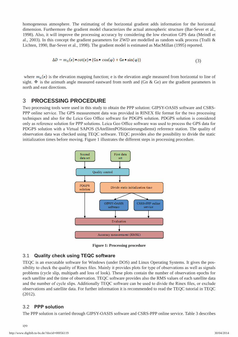
3 PROCESSING PROCEDURETwo processing tools were used in this study to obtain the PPP solution: GIPSY-OASIS software and CSRS-

PDGPS solution with a Virtual SAPOS (SAtellitenPOSitionierungsdienst) reference station. The quality of observation data was checked using TEQC software. TEQC provides also the possibility to divide the static initialization times before moving. Figure 1 illustrates the different steps in processing procedure.

Figure 1: Processing procedure

3.1 TEQC is an executable software for Windows (under DOS) and Linux Operating Systems. It gives the pos-

problems (cycle slip, multipath and loss of look). These plots contain the number of observation epochs for each satellite and the time of observation. TEQC software provides also the RMS values of each satellite data

observations and satellite data. For further information it is recommended to read the TEQC tutorial in TEQC (2012).

3.2 The PPP solution is carried through GIPSY-OASIS software and CSRS-PPP online service. Table 3 describes


171

some of the parameters of the two processing techniques. The reference system for the two processing tech-niques is ITRF2008. The satellite orbits and clock ephemeris are different, where GIPSY uses JPL data but

Ionospheric correction is applied by the second order ionospheric correction for all techniques. Regarding the tropospheric correction, GIPSY-OASIS uses standard hydrostatic priori formula, which is equal to (1.0132.27 exp-0.00011*h [m]) where h is ellipsoidic height of the site. Moreover, it can be modelled also using GPT

gradient using a random walk process (JPL, 2010). GIPSY software uses different mapping functions (e.g. Niell and GMF) for hydrostatic and wet delay. CSRS-PPP estimates the tropospheric delay using GMF. It es-

(GPT) model (CSRS-PPP, 2004). Finally, the elevation angles are set to 10° for all processing techniques

ITRF2008JPL IGS

Satellite phase center offsets IGS ANTEXIGS ANTEX

Tropospheric

Standard Formula

GPT modelDavis (GPT)

Standard (0,10m)

Gradient modelMapping function Niell, LANYI , GMF GMF

Second order ionospheric delay10°

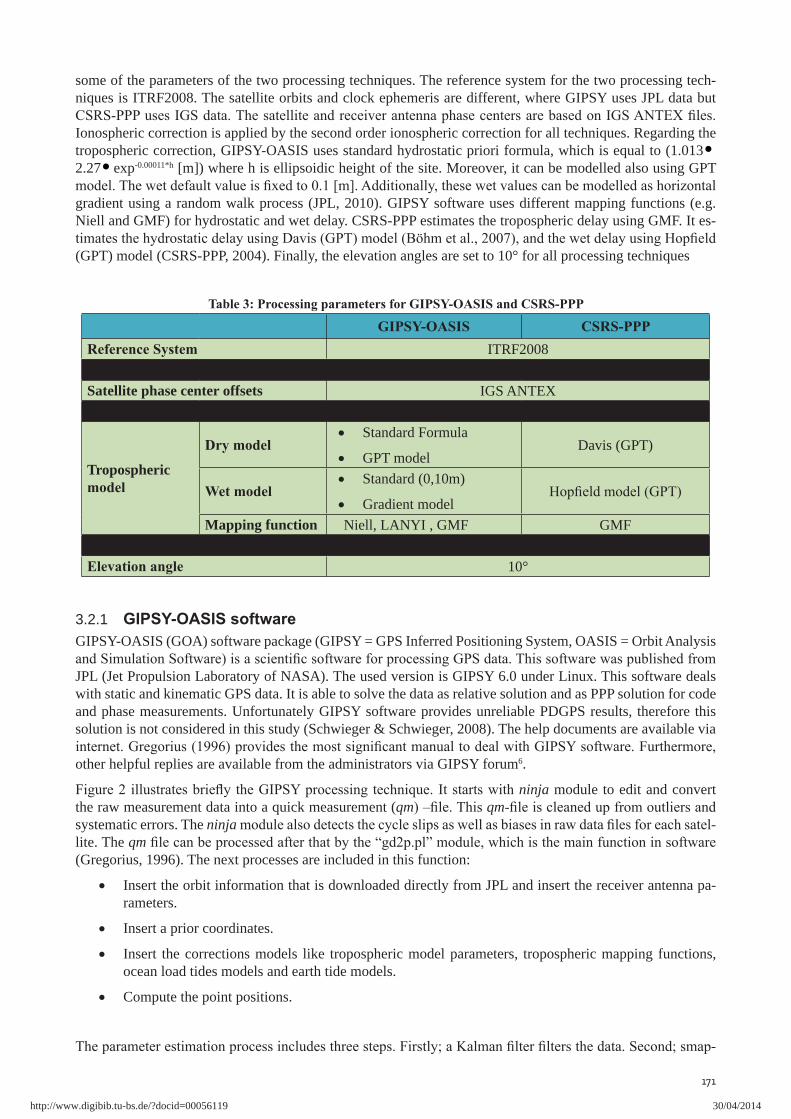
3.2.1 GIPSY-OASIS (GOA) software package (GIPSY = GPS Inferred Positioning System, OASIS = Orbit Analysis

JPL (Jet Propulsion Laboratory of NASA). The used version is GIPSY 6.0 under Linux. This software deals with static and kinematic GPS data. It is able to solve the data as relative solution and as PPP solution for code and phase measurements. Unfortunately GIPSY software provides unreliable PDGPS results, therefore this solution is not considered in this study (Schwieger & Schwieger, 2008). The help documents are available via

other helpful replies are available from the administrators via GIPSY forum6.

ninja module to edit and convert the raw measurement data into a quick measurement (qm qmsystematic errors. The ninja -lite. The qm(Gregorius, 1996). The next processes are included in this function:

Insert the orbit information that is downloaded directly from JPL and insert the receiver antenna pa-rameters.

Insert a prior coordinates.

Insert the corrections models like tropospheric model parameters, tropospheric mapping functions, ocean load tides models and earth tide models.

Compute the point positions.

-


172

coordinates for the points, receiver clock bias, and wet tropospheric values in case of static solution. Since gd2p.pl

solved epochs, standard deviations of solutions and number of outliers. The last step in GIPSY processing is to transform the Cartesian coordinates (XYZ) to the geographic coordinate system (latitude, longitude, ellipsoidal height) using tdp2llh script.

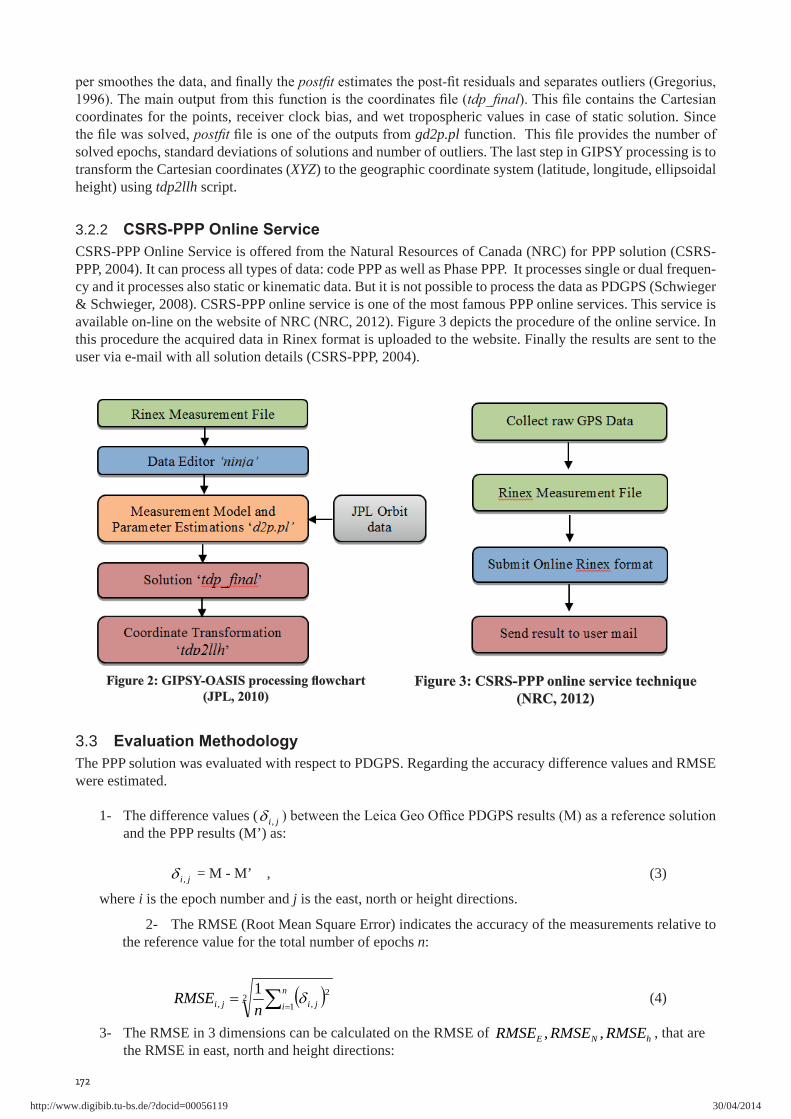
3.2.2 CSRS-PPP Online Service is offered from the Natural Resources of Canada (NRC) for PPP solution (CSRS-PPP, 2004). It can process all types of data: code PPP as well as Phase PPP. It processes single or dual frequen-cy and it processes also static or kinematic data. But it is not possible to process the data as PDGPS (Schwieger & Schwieger, 2008). CSRS-PPP online service is one of the most famous PPP online services. This service is available on-line on the website of NRC (NRC, 2012). Figure 3 depicts the procedure of the online service. In this procedure the acquired data in Rinex format is uploaded to the website. Finally the results are sent to the user via e-mail with all solution details (CSRS-PPP, 2004).

3.3 The PPP solution was evaluated with respect to PDGPS. Regarding the accuracy difference values and RMSE were estimated.

1- The difference values ( ji ,and the PPP results (M’) as:

ji , = M - M’ , (3)

where i is the epoch number and j is the east, north or height directions.

2- The RMSE (Root Mean Square Error) indicates the accuracy of the measurements relative to the reference value for the total number of epochs n:

21

2,,

1 n

i jiji nRMSE (4)

3- The RMSE in 3 dimensions can be calculated on the RMSE of hNE RMSERMSERMSE ,, , that are the RMSE in east, north and height directions:


173

2223 hNED RMSERMSERMSERMSE (5)

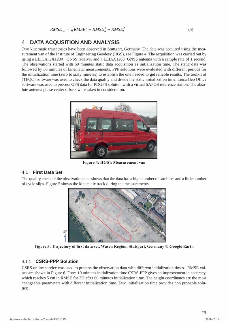
4 DATA ACQUSITION AND ANALYSISTwo kinematic trajectories have been observed in Stuttgart, Germany. The data was acquired using the mea-surement van of the Institute of Engineering Geodesy (IIGS), see Figure 4. The acquisition was carried out by using a LEICA GX1230+ GNSS receiver and a LEIAX1203+GNSS antenna with a sample rate of 1 second. The observations started with 60 minutes static data acquisition as initialization time. The static data was followed by 30 minutes of kinematic measurements. PPP solutions were evaluated with different periods for the initialization time (zero to sixty minutes) to establish the one needed to get reliable results. The toolkit of

software was used to process GPS data for PDGPS solution with a virtual SAPOS reference station. The abso-lute antenna phase center offsets were taken in consideration.

4.1 First Data SetThe quality check of the observation data shows that the data has a high number of satellites and a little number of cycle slips. Figure 5 shows the kinematic track during the measurements.

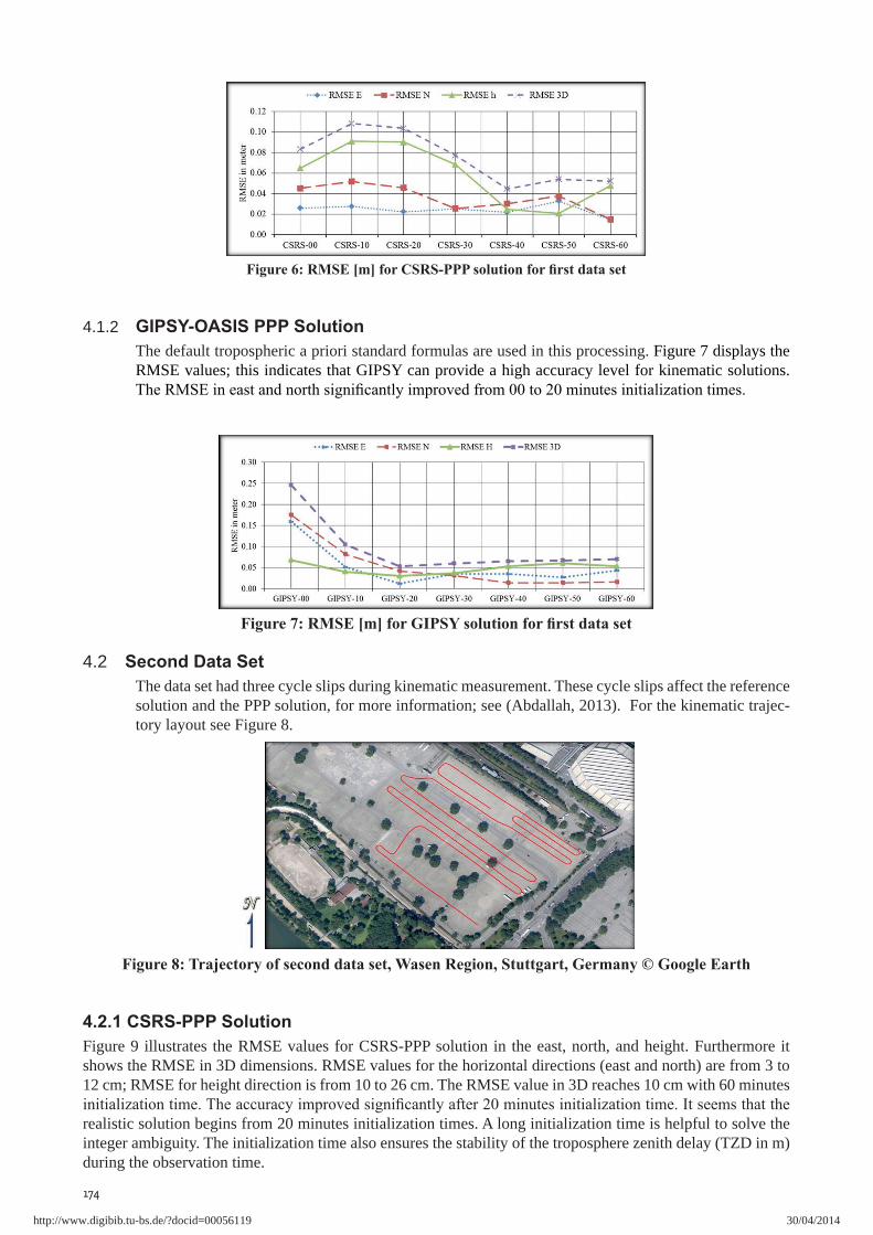
4.1.1 CSRS online service was used to process the observation data with different initialization times. RMSE val-ues are shown in Figure 6. From 10 minutes initialization time CSRS-PPP gives an improvement in accuracy, which reaches 5 cm in RMSE for 3D after 60 minutes initialization time. The height coordinates are the most changeable parameters with different initialization time. Zero initialization time provides non probable solu-tion.


174

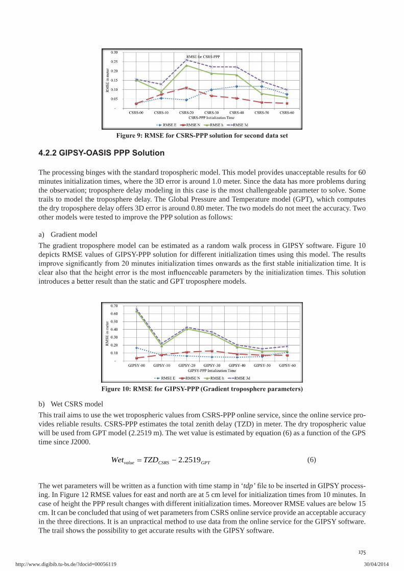
4.1.2 The default tropospheric a priori standard formulas are used in this processing. Figure 7 displays the RMSE values; this indicates that GIPSY can provide a high accuracy level for kinematic solutions.

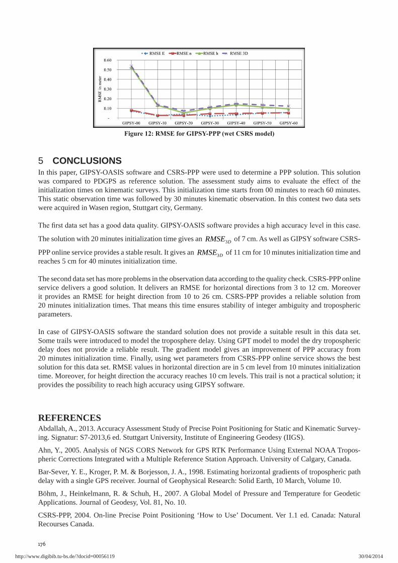
4.2 The data set had three cycle slips during kinematic measurement. These cycle slips affect the reference solution and the PPP solution, for more information; see (Abdallah, 2013). For the kinematic trajec-tory layout see Figure 8.

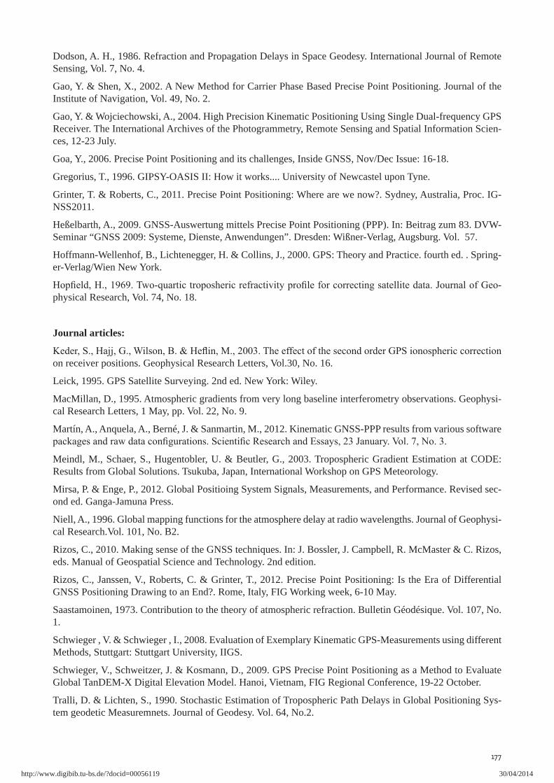
Figure 9 illustrates the RMSE values for CSRS-PPP solution in the east, north, and height. Furthermore it shows the RMSE in 3D dimensions. RMSE values for the horizontal directions (east and north) are from 3 to 12 cm; RMSE for height direction is from 10 to 26 cm. The RMSE value in 3D reaches 10 cm with 60 minutes

realistic solution begins from 20 minutes initialization times. A long initialization time is helpful to solve the integer ambiguity. The initialization time also ensures the stability of the troposphere zenith delay (TZD in m) during the observation time.


175

The processing binges with the standard tropospheric model. This model provides unacceptable results for 60 minutes initialization times, where the 3D error is around 1.0 meter. Since the data has more problems during the observation; troposphere delay modeling in this case is the most challengeable parameter to solve. Some trails to model the troposphere delay. The Global Pressure and Temperature model (GPT), which computes the dry troposphere delay offers 3D error is around 0.80 meter. The two models do not meet the accuracy. Two other models were tested to improve the PPP solution as follows:

a) Gradient modelThe gradient troposphere model can be estimated as a random walk process in GIPSY software. Figure 10 depicts RMSE values of GIPSY-PPP solution for different initialization times using this model. The results

introduces a better result than the static and GPT troposphere models.

b) Wet CSRS modelThis trail aims to use the wet tropospheric values from CSRS-PPP online service, since the online service pro-vides reliable results. CSRS-PPP estimates the total zenith delay (TZD) in meter. The dry tropospheric value will be used from GPT model (2.2519 m). The wet value is estimated by equation (6) as a function of the GPS time since J2000.

GPTCSRSvalue TZDWet 2519.2 (6)

The wet parameters will be written as a function with time stamp in ‘tdp’ing. In Figure 12 RMSE values for east and north are at 5 cm level for initialization times from 10 minutes. In case of height the PPP result changes with different initialization times. Moreover RMSE values are below 15 cm. It can be concluded that using of wet parameters from CSRS online service provide an acceptable accuracy in the three directions. It is an unpractical method to use data from the online service for the GIPSY software. The trail shows the possibility to get accurate results with the GIPSY software.


176

5 CONCLUSIONSIn this paper, GIPSY-OASIS software and CSRS-PPP were used to determine a PPP solution. This solution was compared to PDGPS as reference solution. The assessment study aims to evaluate the effect of the initialization times on kinematic surveys. This initialization time starts from 00 minutes to reach 60 minutes. This static observation time was followed by 30 minutes kinematic observation. In this contest two data sets were acquired in Wasen region, Stuttgart city, Germany.

The solution with 20 minutes initialization time gives an DRMSE3 of 7 cm. As well as GIPSY software CSRS-

PPP online service provides a stable result. It gives an DRMSE3 of 11 cm for 10 minutes initialization time and reaches 5 cm for 40 minutes initialization time.

The second data set has more problems in the observation data according to the quality check. CSRS-PPP online service delivers a good solution. It delivers an RMSE for horizontal directions from 3 to 12 cm. Moreover it provides an RMSE for height direction from 10 to 26 cm. CSRS-PPP provides a reliable solution from 20 minutes initialization times. That means this time ensures stability of integer ambiguity and tropospheric parameters.

In case of GIPSY-OASIS software the standard solution does not provide a suitable result in this data set. Some trails were introduced to model the troposphere delay. Using GPT model to model the dry tropospheric delay does not provide a reliable result. The gradient model gives an improvement of PPP accuracy from 20 minutes initialization time. Finally, using wet parameters from CSRS-PPP online service shows the best solution for this data set. RMSE values in horizontal direction are in 5 cm level from 10 minutes initialization time. Moreover, for height direction the accuracy reaches 10 cm levels. This trail is not a practical solution; it provides the possibility to reach high accuracy using GIPSY software.

REFERENCESAbdallah, A., 2013. Accuracy Assessment Study of Precise Point Positioning for Static and Kinematic Survey-ing. Signatur: S7-2013,6 ed. Stuttgart University, Institute of Engineering Geodesy (IIGS).

Ahn, Y., 2005. Analysis of NGS CORS Network for GPS RTK Performance Using External NOAA Tropos-pheric Corrections Integrated with a Multiple Reference Station Approach. University of Calgary, Canada.

Bar-Sever, Y. E., Kroger, P. M. & Borjesson, J. A., 1998. Estimating horizontal gradients of tropospheric path delay with a single GPS receiver. Journal of Geophysical Research: Solid Earth, 10 March, Volume 10.

Böhm, J., Heinkelmann, R. & Schuh, H., 2007. A Global Model of Pressure and Temperature for Geodetic Applications. Journal of Geodesy, Vol. 81, No. 10.

CSRS-PPP, 2004. On-line Precise Point Positioning ‘How to Use’ Document. Ver 1.1 ed. Canada: Natural Recourses Canada.


177

Dodson, A. H., 1986. Refraction and Propagation Delays in Space Geodesy. International Journal of Remote Sensing, Vol. 7, No. 4.

Gao, Y. & Shen, X., 2002. A New Method for Carrier Phase Based Precise Point Positioning. Journal of the Institute of Navigation, Vol. 49, No. 2.

Gao, Y. & Wojciechowski, A., 2004. High Precision Kinematic Positioning Using Single Dual-frequency GPS Receiver. The International Archives of the Photogrammetry, Remote Sensing and Spatial Information Scien-ces, 12-23 July.

Goa, Y., 2006. Precise Point Positioning and its challenges, Inside GNSS, Nov/Dec Issue: 16-18.

Gregorius, T., 1996. GIPSY-OASIS II: How it works.... University of Newcastel upon Tyne.

Grinter, T. & Roberts, C., 2011. Precise Point Positioning: Where are we now?. Sydney, Australia, Proc. IG-NSS2011.

Heßelbarth, A., 2009. GNSS-Auswertung mittels Precise Point Positioning (PPP). In: Beitrag zum 83. DVW-Seminar “GNSS 2009: Systeme, Dienste, Anwendungen”. Dresden: Wißner-Verlag, Augsburg. Vol. 57.

Hoffmann-Wellenhof, B., Lichtenegger, H. & Collins, J., 2000. GPS: Theory and Practice. fourth ed. . Spring-er-Verlag/Wien New York.

-physical Research, Vol. 74, No. 18.

Journal articles:

on receiver positions. Geophysical Research Letters, Vol.30, No. 16.

Leick, 1995. GPS Satellite Surveying. 2nd ed. New York: Wiley.

MacMillan, D., 1995. Atmospheric gradients from very long baseline interferometry observations. Geophysi-cal Research Letters, 1 May, pp. Vol. 22, No. 9.

Martín, A., Anquela, A., Berné, J. & Sanmartin, M., 2012. Kinematic GNSS-PPP results from various software

Meindl, M., Schaer, S., Hugentobler, U. & Beutler, G., 2003. Tropospheric Gradient Estimation at CODE: Results from Global Solutions. Tsukuba, Japan, International Workshop on GPS Meteorology.

Mirsa, P. & Enge, P., 2012. Global Positioing System Signals, Measurements, and Performance. Revised sec-ond ed. Ganga-Jamuna Press.

Niell, A., 1996. Global mapping functions for the atmosphere delay at radio wavelengths. Journal of Geophysi-cal Research.Vol. 101, No. B2.

Rizos, C., 2010. Making sense of the GNSS techniques. In: J. Bossler, J. Campbell, R. McMaster & C. Rizos, eds. Manual of Geospatial Science and Technology. 2nd edition.

Rizos, C., Janssen, V., Roberts, C. & Grinter, T., 2012. Precise Point Positioning: Is the Era of Differential GNSS Positioning Drawing to an End?. Rome, Italy, FIG Working week, 6-10 May.

Saastamoinen, 1973. Contribution to the theory of atmospheric refraction. Bulletin Géodésique. Vol. 107, No. 1.

Schwieger , V. & Schwieger , I., 2008. Evaluation of Exemplary Kinematic GPS-Measurements using different Methods, Stuttgart: Stuttgart University, IIGS.

Schwieger, V., Schweitzer, J. & Kosmann, D., 2009. GPS Precise Point Positioning as a Method to Evaluate Global TanDEM-X Digital Elevation Model. Hanoi, Vietnam, FIG Regional Conference, 19-22 October.

Tralli, D. & Lichten, S., 1990. Stochastic Estimation of Tropospheric Path Delays in Global Positioning Sys-tem geodetic Measuremnets. Journal of Geodesy. Vol. 64, No.2.


178

Links:

JPL, 2010. GIPSY-OASIS presentation. [Online] Available at:

NRC, 2012. Natural Resources Canada. [Online] Available at: http://www.geod.nrcan.gc.ca/products-produits/ppp_e.php [Accessed June 2012].

TEQC, 2012. TEQC manual. [Online] Available at: http://facility.unavco.org/software/teqc/tutorial.html [Accessed June 2012].

Contact:

M.Sc. Ashraf AbdallahInstitute of Engineering Geodesy, University of Stuttgart Geschwister-Scholl Str. 24D, D-70174 Stuttgart, Germany Email: [email protected]


Documents

Accuracy Assessment Study of GNSS Precise Point Positioning for Kinematic Positioning