Probability of Error Analysis for Hidden Markov Model Filtering With Random Packet Loss

IEEE TRANSACTIONS ON SIGNAL PROCESSING, VOL. 55, NO. 3, MARCH 2007 809

Probability of Error Analysis for Hidden MarkovModel Filtering With Random Packet Loss

Alex S. C. Leong, Member, IEEE, Subhrakanti Dey, Senior Member, IEEE, and Jamie S. Evans, Member, IEEE

Abstract—This paper studies the probability of error for max-imum a posteriori (MAP) estimation of hidden Markov models,where measurements can be either lost or received according to an-other Markov process. Analytical expressions for the error prob-abilities are derived for the noiseless and noisy cases. Some rela-tionships between the error probability and the parameters of theloss process are demonstated via both analysis and numerical re-sults. In the high signal-to-noise ratio (SNR) regime, approximateexpressions which can be more easily computed than the exact an-alytical form for the noisy case are presented.

Index Terms—Hidden Markov model, observation losses, prob-ability of error, state estimation.

I. INTRODUCTION

WIRELESS sensor networks have received huge interestin the research community recently, due to the many

technical challenges which have to be overcome in order to re-alise their full benefits. Algorithms for signal processing andtheir performance in unreliable environments is an importantaspect in the design of such networks. This paper considersthe error probabilities associated with the state estimation ofMarkov chains when measurements can be lost, with the lossprocess modelled by another Markov chain.

Estimation with lossy measurements was considered forlinear systems in [1], for the Kalman filtering problem withlosses modelled by an independent and identically distributed(i.i.d.) Bernoulli process. They showed that for an unstablesystem, there exists a threshold such that if the probabilityof reception exceeds this threshold then the expected value(with respect to the loss process) of the error covariance ma-trix (which is a random quantity due to random losses) willbe bounded, but if the probability of reception is lower thanthis threshold then the error covariance diverges. In a slightlydifferent context, [2] extends these results to Markovian lossprocesses, which allows modelling of more “bursty” typesof errors. Estimation with Markovian packet losses was alsostudied in [3], and suboptimal estimators were derived whichcan be used to provide upper bounds on the estimation errorsof the optimal estimator.

Manuscript received November 9, 2005; revised May 4, 2006. This work wassupported by the Australian Research Council. The associate editor coordinatingthe review of this paper and approving it for publication was Dr. Yonina C. Eldar.

The authors are with the ARC Special Research Centre for Ultra-BroadbandInformation Networks (CUBIN, an affiliate of National ICT Australia), De-partment of Electrical and Electronic Engineering, University of Melbourne,Parkville, Victoria 3010, Australia (e-mail: [email protected];[email protected]; [email protected]).

Color versions of figures available online at http://ieeexplore.ieee.org.Digital Object Identifier 10.1109/TSP.2006.888056

The purpose of this paper is to use some of the ideas relatingto lossy measurement processes, but to apply it to the differentproblem of state estimation for Markov chains. Hidden Markovmodels (HMMs) have found numerous applications [4], and infields such as radar tracking and biology, sensor networks couldpotentially provide additional benefits. For HMM estimationproblems, the state space is often finite, thus, notions of esti-mation stability as in [1] are not appropriate. Instead here wewill use the probability of estimation error as our measure ofperformance, also see [5], [6] for mean square error (mse) cri-terions. Obtaining analytical expressions for the error perfor-mance associated with filtering for HMMs (even without anyloss process) is a difficult problem however, where few generalresults are known. Some results for the continuous time casemay be found in [5]. In discrete time, asymptotic formulae for“slow” Markov chains with finite state space were obtained in[7] for the probability of error, and [6] for a mean square errorcriterion. A general characterization of the error probability forthe two-state hidden Markov model in discrete time was derivedin [8], and a numerical method to calculate it was proposed.

The organization of the paper is as follows. We will first studythe simpler problem with observation losses but no noise in Sec-tion III. Analytical expressions for the error probabilities willbe derived and some special cases presented in Sections III-Aand B, respectively. Some relationships between the error prob-ability and the parameters of the Markovian loss process areestablished in Section III-C and numerical studies presentedin Section III-D. Multi-state Markov chains are considered inSection III-E. We will then shift our attention to the more gen-eral HMM problem with noise in Section IV. In Sections IV-Aand B, we will characterize the error probabilities for the two-state Markov chain, though using quite different methods. Sec-tion IV-C will present some numerical studies for the noisy case.It is more difficult here to prove properties similar to the onesin the noiseless case, and some conjectures which will requirefurther investigation are stated. Section IV-D studies the situa-tion when the signal is i.i.d. In Sections IV-E and F, high SNRapproximations for the two-state and multi-state Markov chainsrespectively are derived and numerical comparisons made.

II. MODEL AND NOTATIONAL CONVENTIONS

The main model of interest is

1053-587X/$25.00 © 2007 IEEE

810 IEEE TRANSACTIONS ON SIGNAL PROCESSING, VOL. 55, NO. 3, MARCH 2007

Here, is the observation process, is the noise processwhich will be i.i.d. and .1 and are homo-geneous two-state Markov chains which are assumed to be in-dependent of each other, with , , ,

. can be interpreted as the signal that we wishto estimate, and as the correlated loss process, with thecorrelation modeled by a Markov chain. We will assume that

is known to us at each time instant. In Sections III-E andIV-F we will look at the situation where is a multi-stateMarkov chain.

In this paper, we will use the conventionand for the transition

probability matrices and , (the columnswill then sum to one). Assuming that , , , ,unique stationary probabilities will then exist and are given by

, ,, .2

Denote the conditional probability vector for the HMM filterby , with the th entry being

. The MAP estimateof , which is well-known to minimize the probability of error,is for the two-state case

otherwise.

III. NOISELESS CASE

We first study the simpler model whichdoes not have the noise term . The probability of estimationerror will be given in terms of an infinite series, which is amore explicit form than that which will be derived for the noisycase in Section IV-A. The noiseless case considered here isquite suitable for the noisy situation at high SNR, since (roughlyspeaking) at high SNR the errors due to the packet loss processtend to dominate the errors due to the noise term, see, for ex-ample, the discussion at the end of Section IV-E. Indeed, thederivation in Section IV-E of an approximation for the errorprobability at high SNR will be based on some of the techniquesof this section.

A. Derivation of Probability of Error

For this simple noiseless model, whenever there is no packetloss, i.e., , the estimate (of ) will be the same asthe measurement. The probability vectors are, therefore,updated as

.

1Other noise types such as noise with state-dependent variances are possible,but some derivations will be more complicated.

2Strictly speaking, this is true if the initial state of the Markov chain has thesame distribution as the stationary distribution, otherwise this holds only in thelimit as k ! 1.

So whenever there is no packet loss, the probability vector will“reset” to either or , a fact we will exploit in ourderivation of the probability of error. When a packet is received,no errors will be made, so

This can be further split up as follows:

where.

Expressions for each term can be derived. Defineand , with

representing the th element of . For brevity, also let.

Then

(1)

where is the indicator function and is the th entry ofthe matrix . For a more explicit expression for , note that

(2)

which may be verified using induction. Also define

(3)

LEONG et al.: HIDDEN MARKOV MODEL FILTERING WITH RANDOM PACKET LOSS 811

TABLE ISIMULATION AND ANALYTICAL COMPARISON OF

NOISELESS ERROR PROBABILITIES

Then it is easily shown that (1) can also be written in the formshown in (4).

.(4)

Hence

where is given by (4), is the th entry of in(2), and and are given by (3). Numerical computation ofsuch infinite series can be easily handled using computer algebrasoftware such as Mathematica.

In Table I, we compare the derived expression with simula-tion results for a selection of different parameter values. We setthe distribution of the initial states of the Markov chains to beequal to the stationary distributions (though by the exponentialforgetting property [9] the effect of the initial state should nothave a major effect for long runs), and then run Monte Carlosimulations of the filtering updates to obtain the probability oferror. The simulations results were averaged over 10 runs, eachrun of length 100 000. It may be seen that, not suprisingly, thereis very close agreement at all values considered.

B. Special Cases

In certain cases, the expression for the error probability canbe further simplified. We present two examples.

(i) If so that is symmetric, thenand always, so that

(ii) Suppose the signal is i.i.d., i.e., . If, then , , , and

If , then , , , and

Fig. 5 of Section III-D contains some simulation results. Thelinear dependence on the stationary probabilitywhen the data is i.i.d. also holds in the noisy case, see Sec-tion IV-D.

C. Theoretical Properties

We now demonstrate some relationships between the prob-ability of error and the parameters of the packet loss process.Proofs of Theorems 1–3 may be found in the Appendix.

Theorem 1: For fixed and , the probability of error ismonotonically increasing in .

Theorem 2: For fixed and , the probability of error ismonotonically decreasing in .

Theorem 1 states that the error probability increases asincreases, when all other parameters are fixed. Intuitively thisis reasonable, since is the probability that the next packet islost given that the current packet has been received, so we aremore likely to drop packets and do worse at estimation when thisparameter is increased. Theorem 2 is also quite intuitive, asis the probability that the next packet will be received correctlygiven that the current packet has been lost, so increasing thisparameter should improve our estimation performance.

For the third result, let be the stationary probability thata measurement is not received, i.e.,

. Theorem 3 shows that in general alone doesnot uniquely determine the error probabilities, but also dependson the sizes of and , which can be interpreted as howquickly/slowly the packet loss process is varying in time. Forexample, when both and are small, transitions from onestate to the other are rare, so that we can regard the Markov chainas being slow. Essentially, Theorem 3 says that for a given ,slower dynamics are worse for state estimation in that we willget a higher probability of error (except perhaps when the signalis i.i.d. as noted in example (ii) of Section III-B).

Theorem 3:(i) For fixed and , the probability of error is nonin-

creasing in (equivalently in ).(ii) The probability of error converges, for fixed and

as , to , whereis the probability of error in the

complete absence of observations.By Theorem 3 (ii), is therefore an upper bound on the

error probability. A lower bound can also be derived, by notingthat for , the largest possible values for and are

and , and for , the largestpossible values are and . Substituting


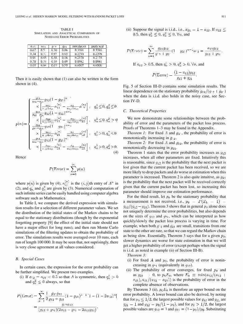
Fig. 1. Noiseless probability of error for various g .

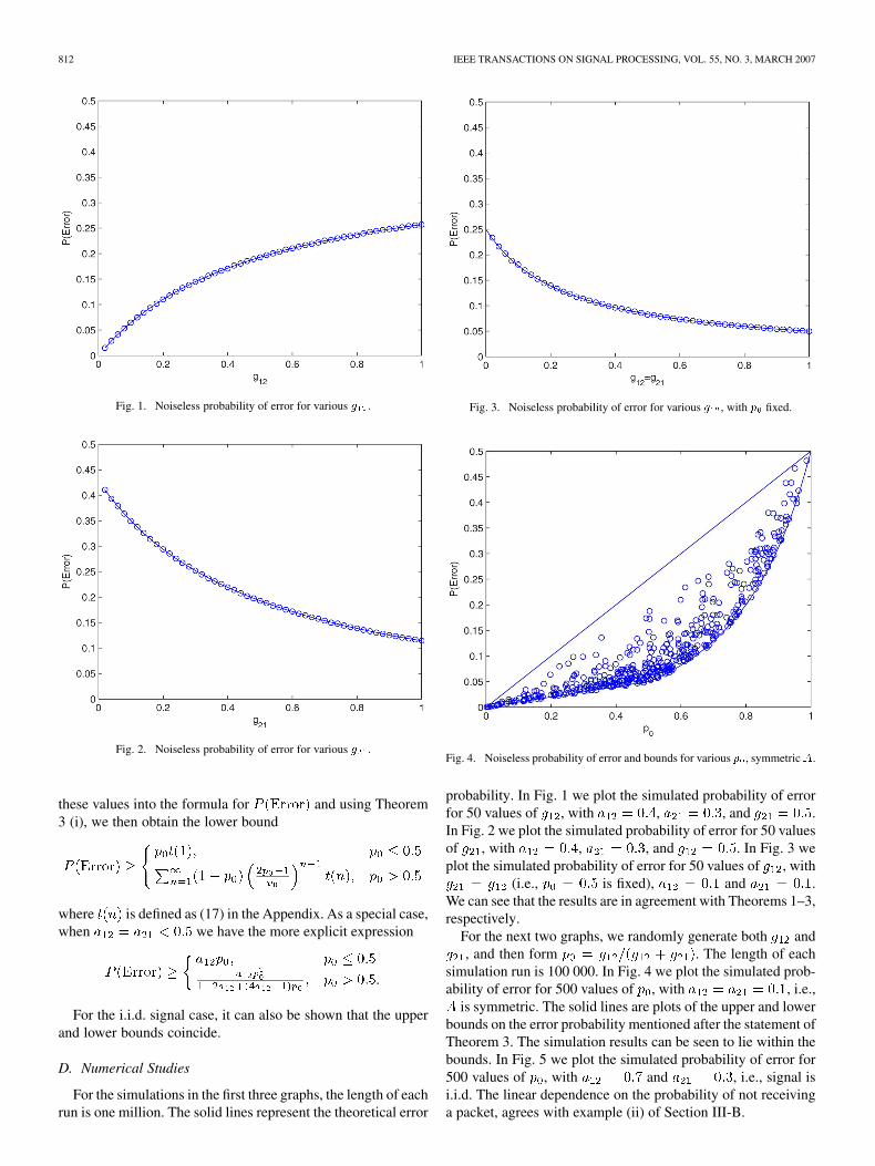
Fig. 2. Noiseless probability of error for various g .

these values into the formula for and using Theorem3 (i), we then obtain the lower bound

where is defined as (17) in the Appendix. As a special case,when we have the more explicit expression

.

For the i.i.d. signal case, it can also be shown that the upperand lower bounds coincide.

D. Numerical Studies

For the simulations in the first three graphs, the length of eachrun is one million. The solid lines represent the theoretical error

Fig. 3. Noiseless probability of error for various g , with p fixed.

Fig. 4. Noiseless probability of error and bounds for various p , symmetric A.

probability. In Fig. 1 we plot the simulated probability of errorfor 50 values of , with , , and .In Fig. 2 we plot the simulated probability of error for 50 valuesof , with , , and . In Fig. 3 weplot the simulated probability of error for 50 values of , with

(i.e., is fixed), and .We can see that the results are in agreement with Theorems 1–3,respectively.

For the next two graphs, we randomly generate both and, and then form . The length of each

simulation run is 100 000. In Fig. 4 we plot the simulated prob-ability of error for 500 values of , with , i.e.,

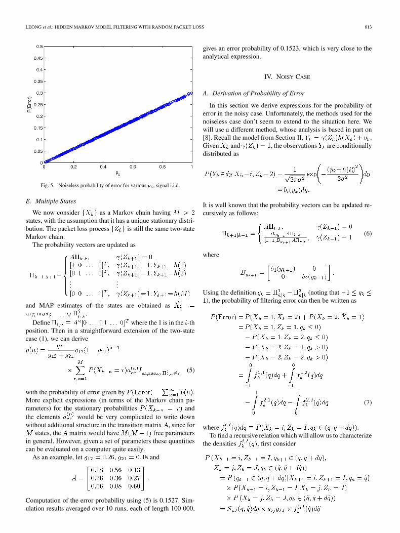
is symmetric. The solid lines are plots of the upper and lowerbounds on the error probability mentioned after the statement ofTheorem 3. The simulation results can be seen to lie within thebounds. In Fig. 5 we plot the simulated probability of error for500 values of , with and , i.e., signal isi.i.d. The linear dependence on the probability of not receivinga packet, agrees with example (ii) of Section III-B.


Fig. 5. Noiseless probability of error for various p , signal i.i.d.

E. Multiple States

We now consider as a Markov chain havingstates, with the assumption that it has a unique stationary distri-bution. The packet loss process is still the same two-stateMarkov chain.

The probability vectors are updated as

......

and MAP estimates of the states are obtained as.

Define where the 1 is in the -thposition. Then in a straightforward extension of the two-statecase (1), we can derive

(5)

with the probability of error given by .More explicit expressions (in terms of the Markov chain pa-rameters) for the stationary probabilities andthe elements would be very complicated to write downwithout additional structure in the transition matrix , since for

states, the matrix would have free parametersin general. However, given a set of parameters these quantitiescan be evaluated on a computer quite easily.

As an example, let , and

Computation of the error probability using (5) is 0.1527. Sim-ulation results averaged over 10 runs, each of length 100 000,

gives an error probability of 0.1523, which is very close to theanalytical expression.

IV. NOISY CASE

A. Derivation of Probability of Error

In this section we derive expressions for the probability oferror in the noisy case. Unfortunately, the methods used for thenoiseless case don’t seem to extend to the situation here. Wewill use a different method, whose analysis is based in part on[8]. Recall the model from Section II, .Given and , the observations are conditionallydistributed as

It is well known that the probability vectors can be updated re-cursively as follows:

(6)

where

Using the definition (noting that), the probability of filtering error can then be written as

(7)

where .To find a recursive relation which will allow us to characterize

the densities , first consider


where we have used the Markov property and the independenceof and , and defined

For , i.e., , we can derive in a similarmanner to [8] (which only contained expressions for symmetric

) the recursion shown in (8) at the bottom of the page, and so

with.

For , i.e., , it is straightforward toshow that the recursion for is now

(9)

Thus

where is the indicator function and.

Hence in the steady state we have the following relations forthe densities, which is a system of four Fredholm integral equa-tions

(10)

B. Numerical Method

To compute the error probability we will need to numeri-cally solve the system of integral equations (10). We will presentan existing method which is slightly different from that of [8],where convergence analysis is perhaps more readily obtained.3

From p. 151 of [10], we can transform (10) into a single in-tegral equation as follows. Define

3The method presented here and its analysis can also be applied with slightmodifications to the problem in [8]

...

.

(11)

Then it can be seen that (10) is equivalent to the homogeneousFredholm equation

(12)

with also satisfying the normalising condition. For the numerical solution of (12), con-

sider the related eigenvalue problem [11]

(13)

which corresponds to (12) when . We will solve (13)using the Nyström method [11], [12]. Replacing the integral bya -point quadrature rule,4 and defining

.... . .

...

we obtain

......

where represent the weights and the quadrature points ofthe quadrature rule. In the results presented in this paper, themidpoint rule is used, though other alternatives such as com-posite Gauss-Legendre quadrature are possible [12, p.110.].

To obtain an approximation for , we then take the eigen-vector that corresponds to the largest real eigenvalue of , andnormalise it so that is satisfied. Using a “weak”version of the Perron-Frobenius theorem [13, p. 28] on showsthat this eigenvector will have nonnegative entries, which is re-quired if it is to approximate a probability density. The proba-bility of error can then be calculated from (7) and (11).

4We call it a 4N -point rather an N -point quadrature rule for convenience,since �(q) is a combination of four densities

(8)


We would like the largest eigenvalue to be close to one. As, will tend to a stochastic matrix, in the sense that

the sum of each column will converge to one. For example, forthe first column

where convergence is achieved for any reasonable compositequadrature scheme, such as the midpoint rule [14, p.116]. Sim-ilarly this holds for the other columns of . Since a stochasticmatrix has largest eigenvalue one, and by the continuity ofeigenvalues [15], it then follows that the largest eigenvalue of

can be made arbitrarily close to one for sufficiently large.We can also show that the eigenvector corresponding to thelargest eigenvalue is unique. Note that we can partition as

(14)with each element representing an matrix. Referring to(14) and the definition of , it may be easily shown that theblocks and contain strictly positive en-tries. The blocks and can each be furtherdivided into the form

where blocks 1 and 3 contain all zeros, while block 2 has atleast one positive entry in each row and column, with the sizesof these blocks being the same for all and .The matrix is thus reducible since it will have a number ofrows which consist entirely of zeros, and the Perron-Frobeniustheorem [13] is not directly applicable. We can however forma submatrix by deleting the all-zero rows and the associatedcolumns, without changing the largest eigenvalue. Due to thestructure in the blocks and , it can be seenthat this submatrix is primitive. The Perron-Frobenius theoremmay then be applied to conclude that there is an eigenvalue withmagnitude greater than any other, with a unique eigenvector (upto constant multiples). By the comments above, this will alsohold for the original matrix .

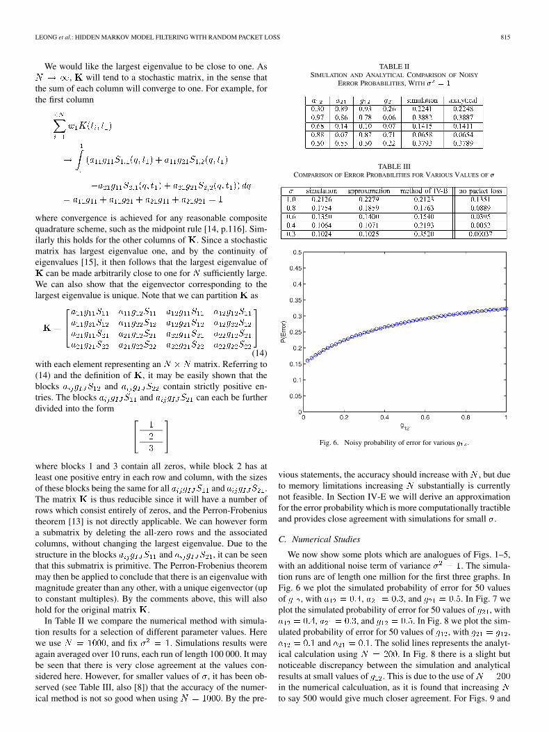
In Table II we compare the numerical method with simula-tion results for a selection of different parameter values. Herewe use , and fix . Simulations results wereagain averaged over 10 runs, each run of length 100 000. It maybe seen that there is very close agreement at the values con-sidered here. However, for smaller values of , it has been ob-served (see Table III, also [8]) that the accuracy of the numer-ical method is not so good when using . By the pre-

TABLE IISIMULATION AND ANALYTICAL COMPARISON OF NOISY

ERROR PROBABILITIES, WITH � = 1

TABLE IIICOMPARISON OF ERROR PROBABILITIES FOR VARIOUS VALUES OF �

Fig. 6. Noisy probability of error for various g .

vious statements, the accuracy should increase with , but dueto memory limitations increasing substantially is currentlynot feasible. In Section IV-E we will derive an approximationfor the error probability which is more computationally tractibleand provides close agreement with simulations for small .

C. Numerical Studies

We now show some plots which are analogues of Figs. 1–5,with an additional noise term of variance . The simula-tion runs are of length one million for the first three graphs. InFig. 6 we plot the simulated probability of error for 50 valuesof , with , , and . In Fig. 7 weplot the simulated probability of error for 50 values of , with

, , and . In Fig. 8 we plot the sim-ulated probability of error for 50 values of , with ,

and . The solid lines represents the analyt-ical calculation using . In Fig. 8 there is a slight butnoticeable discrepancy between the simulation and analyticalresults at small values of . This is due to the use ofin the numerical calculuation, as it is found that increasingto say 500 would give much closer agreement. For Figs. 9 and


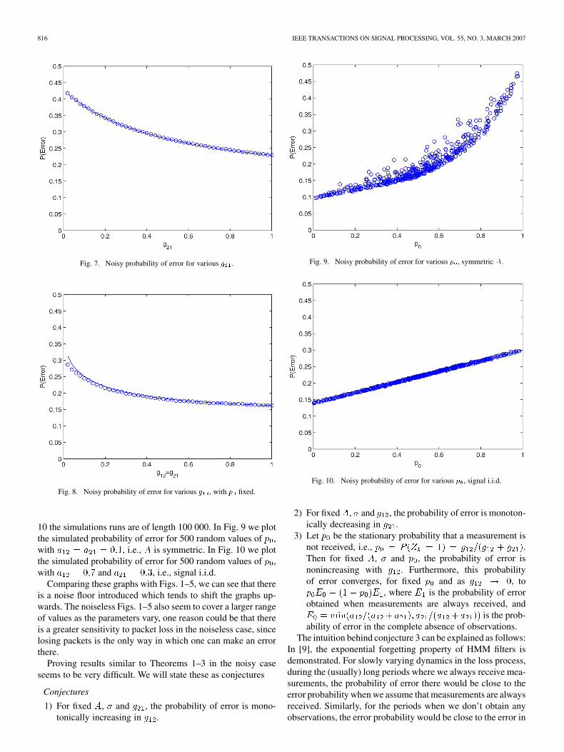
Fig. 7. Noisy probability of error for various g .

Fig. 8. Noisy probability of error for various g , with p fixed.

10 the simulations runs are of length 100 000. In Fig. 9 we plotthe simulated probability of error for 500 random values of ,with , i.e., is symmetric. In Fig. 10 we plotthe simulated probability of error for 500 random values of ,with and , i.e., signal i.i.d.

Comparing these graphs with Figs. 1–5, we can see that thereis a noise floor introduced which tends to shift the graphs up-wards. The noiseless Figs. 1–5 also seem to cover a larger rangeof values as the parameters vary, one reason could be that thereis a greater sensitivity to packet loss in the noiseless case, sincelosing packets is the only way in which one can make an errorthere.

Proving results similar to Theorems 1–3 in the noisy caseseems to be very difficult. We will state these as conjectures

Conjectures

1) For fixed , and , the probability of error is mono-tonically increasing in .

Fig. 9. Noisy probability of error for various p , symmetric A.

Fig. 10. Noisy probability of error for various p , signal i.i.d.

2) For fixed , and , the probability of error is monoton-ically decreasing in .

3) Let be the stationary probability that a measurement isnot received, i.e., .Then for fixed , and , the probability of error isnonincreasing with . Furthermore, this probabilityof error converges, for fixed and as , to

, where is the probability of errorobtained when measurements are always received, and

is the prob-ability of error in the complete absence of observations.

The intuition behind conjecture 3 can be explained as follows:In [9], the exponential forgetting property of HMM filters isdemonstrated. For slowly varying dynamics in the loss process,during the (usually) long periods where we always receive mea-surements, the probability of error there would be close to theerror probability when we assume that measurements are alwaysreceived. Similarly, for the periods when we don’t obtain anyobservations, the error probability would be close to the error in


the complete absence of observations. The overall error proba-bility should then be able to be averaged over these two situa-tions, giving as the conjectured limit.

D. Signal Is i.i.d.

Signals which are i.i.d. (or close to i.i.d.) are commonly en-countered in digital communications. In Fig. 10, we saw thatwhen the signal is i.i.d., there seems to be a linear rela-tionship between and the probability of error even when theloss process is Markovian. In this section, we will show that thisis indeed the case. If the signal is i.i.d., the matrix has the form

and the probability vector updates (6) become

which depends on the values and but which impor-tantly does not depend on values at previous times. Using thisfact, an explicit expression for the error probability can then bederived quite easily.

Given , the recursion (9) for is just .If , then , and

If , then , and so

This can be written more compactly as. Next, we have

where is . Similarly,, and so

(15)

The probability of error in the case of i.i.d. data is therefore

where we use the expressions for and (15),together with the stationary probabilities for the loss process

and. Since , this probability of

error is linear in , for fixed and . The solid linein Fig. 10 is a plot of this linear expression, which can be seento coincide with the simulation results.

E. High SNR Approximation

Here we will derive an approximate expression for the errorin the high SNR, or small regime. When is small, we cansee from (8) that for , , and for

, . So at high SNR, the probability updates can beapproximated by the simpler suboptimal scheme

.

where we have defined the sets and. To derive the probability of error using such a scheme,

first note thatand , where

is . Using to denote the complement of ,

where we have again used the independence of and .The derivation of the term is similar to

the noiseless error probability derived in Section III-A, we willuse the same notation and point out the main differences. Wecan still write where


, but now

As in the noiseless case, we can write this in a more explicitform as shown in (16) at the bottom of the page. The probabilityof error of this scheme is, therefore

In Table III we compare simulation results of the optimal filtertogether with the “exact” analytical calculation of Section IV-B,and the suboptimal approximation just derived. We use

, , , and various values of .The computation using the method of Section IV-B was donewith . For a further comparison, in the final columnwe also include simulation results when there is no packet loss.The simulation runs are of length 10 million.

Firstly, we can see that for values of smaller than approxi-mately 0.8, the numerical method of Section IV-B does not giveaccurate results when using , in fact the accuracyworsens the smaller is. Improving the accuracy would involveincreasing substantially, which in turn increases the com-putation time and memory requirements dramatically. We canalso see that the suboptimal expression gives very good agree-ment with simulations for small values of , moreover it can becomputed very easily with current computer algebra software.Indeed, the noiseless probability of error can be computed tobe 0.1022, so that even for , the difference betweenthe noisy and noiseless error probabilities are almost negligible.Since our approximation (16) converges to the noiseless expres-sion (4) as , this is one reason why the approximationperforms so well at high SNR.

Comparing the noiseless error probability of 0.1022, theerror probabilities with no packet loss and the error proba-bilities with both packet loss and noise, it appears that forsmaller than around 0.4–0.5, the packet loss starts to dominatefor this example. In general, the value where the packetloss term starts to dominate will depend on other parameterssuch as and , and is an issue that requires further study.However through our numerical investigations, we have foundthat around 0.4–0.5 seems to be a reasonable figure for most(randomly generated) sets of parameter values.

F. Multiple States—High SNR

For the noisy case with multiple states (and no packet loss),asymptotic results for the error performance of slow Markovchains exist in the literature, e.g., [6], [7], but general expres-sions for arbitrary Markov chains are not known. In this section,we will treat arbitrary Markov chains with packet loss at highSNR. We will choose the signal levels to be of -aryPulse-amplitude-modulation (PAM) type. Without loss of gen-erality, we let these levels be situated at , i.e.

.

(16)


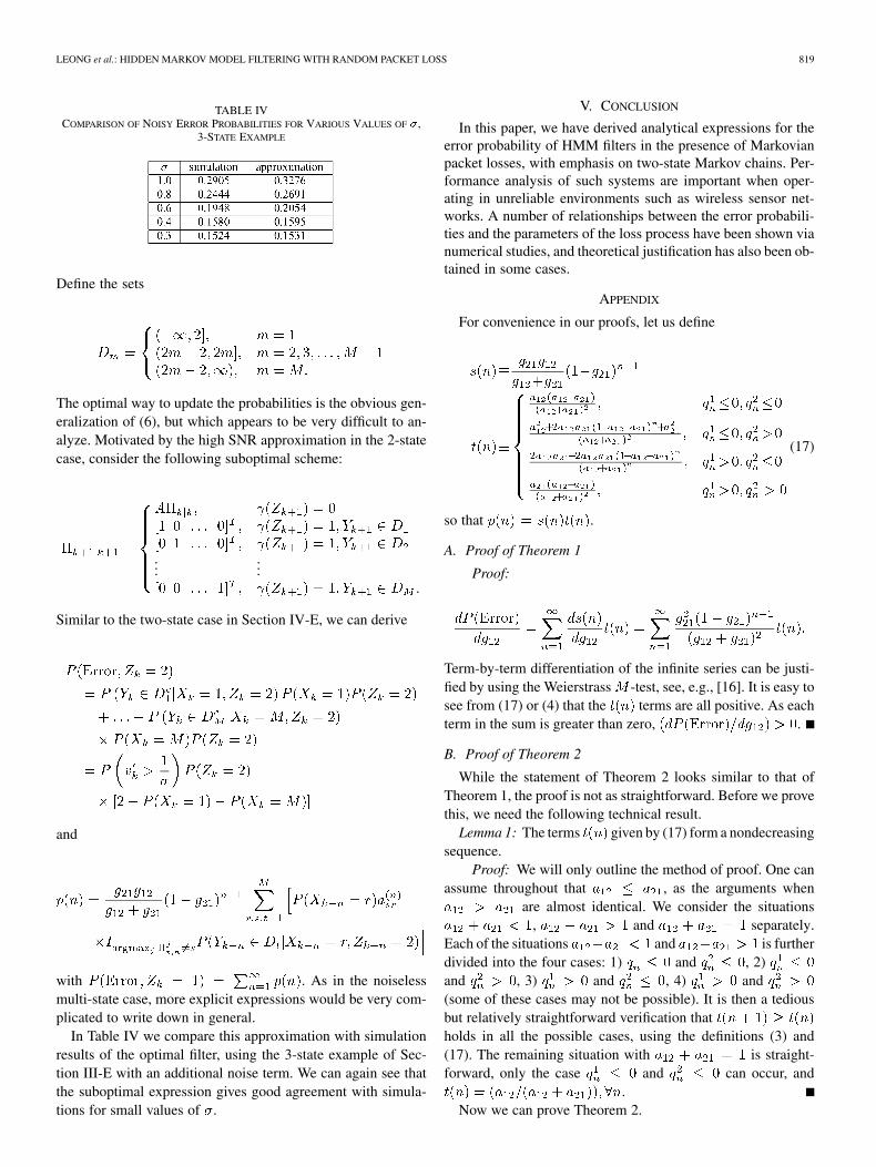
TABLE IVCOMPARISON OF NOISY ERROR PROBABILITIES FOR VARIOUS VALUES OF �,

3-STATE EXAMPLE

Define the sets

The optimal way to update the probabilities is the obvious gen-eralization of (6), but which appears to be very difficult to an-alyze. Motivated by the high SNR approximation in the 2-statecase, consider the following suboptimal scheme:

......

.

Similar to the two-state case in Section IV-E, we can derive

and

with . As in the noiselessmulti-state case, more explicit expressions would be very com-plicated to write down in general.

In Table IV we compare this approximation with simulationresults of the optimal filter, using the 3-state example of Sec-tion III-E with an additional noise term. We can again see thatthe suboptimal expression gives good agreement with simula-tions for small values of .

V. CONCLUSION

In this paper, we have derived analytical expressions for theerror probability of HMM filters in the presence of Markovianpacket losses, with emphasis on two-state Markov chains. Per-formance analysis of such systems are important when oper-ating in unreliable environments such as wireless sensor net-works. A number of relationships between the error probabili-ties and the parameters of the loss process have been shown vianumerical studies, and theoretical justification has also been ob-tained in some cases.

APPENDIX

For convenience in our proofs, let us define

(17)

so that .

A. Proof of Theorem 1

Proof:

Term-by-term differentiation of the infinite series can be justi-fied by using the Weierstrass -test, see, e.g., [16]. It is easy tosee from (17) or (4) that the terms are all positive. As eachterm in the sum is greater than zero, .

B. Proof of Theorem 2

While the statement of Theorem 2 looks similar to that ofTheorem 1, the proof is not as straightforward. Before we provethis, we need the following technical result.

Lemma 1: The terms given by (17) form a nondecreasingsequence.

Proof: We will only outline the method of proof. One canassume throughout that , as the arguments when

are almost identical. We consider the situations, and separately.

Each of the situations and is furtherdivided into the four cases: 1) and , 2)and , 3) and , 4) and(some of these cases may not be possible). It is then a tediousbut relatively straightforward verification thatholds in all the possible cases, using the definitions (3) and(17). The remaining situation with is straight-forward, only the case and can occur, and

.Now we can prove Theorem 2.


Proof: First

(18)

Showing that this quantity is negative is equivalent to showingthat

Unlike the proof of Theorem 1, not every term in the summationhere is negative. However, it is not difficult to show that for

, the first terms will be positive,while the rest will be negative. We may then use Lemma 1 toobtain the bound

To complete the proof, we note the following closed form ex-pression, which can be verified using induction:

(Note that this expression also allows us to apply the Weierstrass-test to justify the term-by-term differentiation (18).) Hence,

and,therefore

C. Proof of Theorem 3

Proof: That actually is the error probability in the com-plete absence of observations is not difficult to show. For ex-ample, one can use the fact that converges to a rank 1 matrix(with the stationary probabilities in the columns) as , sothat without observations, one would choose the state estimatewhich on average is more likely to occur.

(i) The proof of this part is similar to that of Theorem 2. Since, we have

It can be easily seen that for , the firstterms in the series will be positive, while the rest will benegative. Using Lemma 1, we obtain the bound

We have the following closed form expression:

so , and therefore

(ii) We consider the cases and sepa-rately. First assume that . From (3) it can beseen that there exists an such that either

(when ), or(when ). Hence, and

Applying Lemma 1, we can obtain the bounds

or. Taking the limit as then gives

the result for .Now assume that . We further divide into three

cases.1) For , we have , and

irrespective of .2) For , we have , so

which converges to as .


3) For , we have , for odd, and, for even, so

which also converges to as .

ACKNOWLEDGMENT

The authors thank the reviewers for their comments and sug-gestions, which significantly improved the quality of the manu-script.

REFERENCES

[1] B. Sinopoli, L. Schenato, M. Franceschetti, K. Poolla, M. I. Jordan, andS. S. Sastry, “Kalman filtering with intermittent observations,” IEEETrans. Autom. Control, vol. 49, no. 9, pp. 1453–1464, Sep. 2004.

[2] A. Tiwari, M. Jun, D. E. Jeffcoat, and R. M. Murray, “Analysis of dy-namic sensor coverage problem using Kalman filters for estimation,”in Proc. IFAC World Congress, Prague, Czech Republic, Jul. 2005.

[3] S. C. Smith and P. Seiler, “Estimation with lossy measurements: jumpestimators for jump systems,” IEEE Trans. Autom. Control, vol. 48, no.12, pp. 2163–2171, Dec. 2003.

[4] Y. Ephraim and N. Merhav, “Hidden Markov processes,” IEEE Trans.Inf. Theory, vol. 48, no. 6, pp. 1518–1569, Jun. 2002.

[5] W. M. Wonham, “Some applications of stochastic differential equa-tions to optimal nonlinear filtering,” SIAM J. Contr. , vol. 2, no. 3, pp.347–369, 1965.

[6] G. K. Golubev, “On filtering for a hidden Markov chain under squareperformance criterion,” Probl. Inf. Transmiss., vol. 36, no. 3, pp.213–219, 2000.

[7] R. Khasminskii and O. Zeitouni, “Asymptotic filtering for finite stateMarkov chains,” Stochastic Processes Their Applicat., vol. 63, pp.1–10, 1996.

[8] L. Shue, S. Dey, B. D. O. Anderson, and F. De Bruyne, “On state-esti-mation of a two-state hidden Markov model with quantization,” IEEETrans. Signal Process., vol. 49, no. 1, pp. 202–208, Jan. 2001.

[9] L. Shue, B. D. O. Anderson, and S. Dey, “Exponential stability of fil-ters and smoothers for hidden Markov models,” IEEE Trans. SignalProcess., vol. 46, no. 8, pp. 2180–2194, Aug. 1998.

[10] F. G. Tricomi, Integral Equations. New York: Interscience, 1957.[11] W. Hackbusch, Integral Equations: Theory and Numerical Treat-

ment. Basel, Switzerland: Birkhauser Verlag, 1995.[12] K. E. Atkinson, The Numerical Solution of Integral Equations of the

Second Kind. Cambridge, U.K.: Cambridge Univ. Press, 1997.[13] E. Seneta, Non-Negative Matrices and Markov Chains, 2nd ed. New

York: Springer-Verlag, 1981.[14] A. Ralston and P. Rabinowitz, A First Course in Numerical Analysis,

2nd ed. New York: McGraw-Hill, 1978.[15] G. W. Stewart and J.-G. Sun, Matrix Perturbation Theory. San Diego,

CA: Academic , 1990.

[16] W. Rudin, Principles of Mathematical Analysis, 3rd ed. New York:McGraw-Hill, 1976.

Alex S. C. Leong (S’03–M’03) was born in Macauin 1980. He received the B.S. degree in mathematicsand the B.E. degree in electrical engineering fromthe University of Melbourne, Melbourne, Australia,in 2003.

He is currently pursuing the Ph.D. degree in theDepartment of Electrical and Electronic Engineering,University of Melbourne. His research interests in-clude statistical signal processing and wireless com-munications.

Mr. Leong was the recipient of the L. R. EastMedal from Engineers Australia in 2003.

Subhrakanti Dey (S’94–M’96–SM’06) was born inCalcutta, India, in 1968. He received the Bachelorof Technology and Master of Technology degreesfrom the Department of Electronics and ElectricalCommunication Engineering, Indian Institute ofTechnology, Kharagpur, in 1991 and 1993, re-spectively. He received the Ph.D. degree from theDepartment of Systems Engineering, ResearchSchool of Information Sciences and Engineering,Australian National University, Canberra, in 1996.

He is currently appointed an Associate Professorwith the Department of Electrical and Electronic Engineering, Universityof Melbourne, Melbourne, Australia, where he has been since 2000. During1995–2000, he was a Postdoctoral Research Fellow with the Department ofSystems Engineering, Australian National University (ANU), and a Postdoc-toral Research Associate with the Institute for Systems Research, Universityof Maryland, College Park. His current research interests include signalprocessing for telecommunications, wireless communications and networks,networked control systems, and statistical and adaptive signal processing. Heis currently an academic staff member of the ARC Special Research Centrefor Ultra-Broadband Information Networks, Department of Electrical andElectronic Engineering, University of Melbourne. He has held numerousresearch grants and authored and coauthored more than 60 internationallyrefereed papers.

Dr. Dey is an Associate Editor for the Systems and Control Letters and theIEEE TRANSACTIONS ON AUTOMATIC CONTROL. He has also been on severalmajor international conference program committees.

Jamie S. Evans (S’93–M’98) was born in New-castle, Australia, in 1970. He received the B.S.degree in physics and the B.E. degree in computerengineering from the University of Newcastle, New-castle, Australia, in 1992 and 1993, respectively,and the M.S. and Ph.D. degrees from the Universityof Melbourne, Australia, in 1996 and 1998, respec-tively, both in electrical engineering.

From March 1998 to June 1999, he was a VisitingResearcher with the Department of Electrical Engi-neering and Computer Science, University of Cali-

fornia, Berkeley. He returned to Australia to take up a position as Lecturer atthe University of Sydney, Sydney, Australia, where he stayed until July 2001.Since that time, he has been with the Department of Electrical and ElectronicEngineering, University of Melbourne, where he is now an Associate Professor.His research interests are in communications theory, information theory, andstatistical signal processing with current focus on wireless communications net-works.

Dr. Evans was the recipient of the University Medal of the University of New-castle and the Chancellor’s Prize for Excellence for his Ph.D. dissertation.

Documents

Probability of Error Analysis for Hidden Markov Model Filtering With Random Packet Loss