Numerical modelling of combined erosion and weathering of slopes in weak rock

EARTH SURFACE PROCESSES AND LANDFORMSEarth Surf. Process. Landforms 36, 1705–1714 (2011)Copyright © 2011 John Wiley & Sons, Ltd.Published online 27 June 2011 in Wiley Online Library(wileyonlinelibrary.com) DOI: 10.1002/esp.2179

Numerical modelling of combined erosion andweathering of slopes in weak rockM. Huisman,1* J. D. Nieuwenhuis2 and H. R. G. K. Hack31 Bluewater Energy Services BV, Mooring & Subsea Technology, Hoofddorp, Netherlands2 Delft University of Technology, Civil Engineering & Geosciences, Delft, Netherlands3 University of Twente, Faculty ITC, Enschede, Netherlands

Received 22 March 2010; Revised 2 May 2011; Accepted 8 May 2011

*Correspondence to: M. Huisman, Bluewater Energy Services BV, Mooring & Subsea Technology, Hoofddorp, Netherlands. E‐mail: [email protected]

ABSTRACT: Due to various decay processes associated with weathering, the stability of artificial slopes in weak rocks may beaffected well within their envisaged engineering lifetime. Conceptually, the decay following the initial stress release after excavationcan be described as a process seeking equilibrium between weathering and erosion. The extent to which such an equilibrium isactually reached influences the outcome of the weathering‐erosion decay process as well as the effects that the decay has on thegeotechnical properties of the exposed rock mass, and thus ultimately the stability of slopes affected by erosion and weathering. Thispaper combines two conceptual models for erosion and weathering, and derives a numerical model which predicts the resultingslope development. This can help to predict the development of a slope profile excavated in a weak rock in time, and can beextended with the addition of strength parameters to the weathering profile to enable prediction of slope stability as a function oftime. Copyright © 2011 John Wiley & Sons, Ltd.

KEYWORDS: erosion; weathering; denudation; numerical modelling; slope stability; shale

Introduction

The problem of infrastructure works that become unsafe withtime due to decay of rock and soil masses in artificial and naturalslopes is a well‐known feature in every part of the world. Manyeconomically hazardous and potentially life‐threatening massmovements in artificial as well as natural slopes are caused orfacilitated by decay of soil and rock (Hencher and McNicholl,1995). This time‐related decay of soil and rock affects allengineering structures that involve natural, in situmaterials, andis easily recognized in artificial, engineered slopes in rapidlyweathering and easily eroding shales.The combined processes of weathering and erosion will cause

decay of any rockmass exposed in a slope, with stress release andstress–strain redistribution as catalysts; an elaborate example ofthis is given by Nieuwenhuis (1991) for relatively weak groundmasses that show rapid deterioration. The relative rates of erosionand weathering determine how the rock mass actually developsand as will be shown later, the ratio of those rates can changewithin a single slope as a function of both space (i.e. at differentlocations in the slope) and time. Depending on the relative rates,three main decay situations can be distinguished:

• imbalance favouring erosion;• equilibrium between weathering and erosion;• imbalance favouring weathering.

Assuming that natural hillslopes are in equilibrium, excava-tions are by definition a disturbance of that equilibrium, and the

development of the excavation profile is an evolutionarymodel.The boundary conditions for this model are set by the principalslope properties after excavation: the slope profile and theremaining weathering profile resulting from weathering of theoriginal surface, prior to excavation. The response of the slopematerial to the environmental conditions then determines theslope evolution after excavation, and this paper combinesconceptual models for erosion andweathering of slopes in orderto assess what stages of equilibrium and imbalance an artificialslope can go through in its engineering lifetime.

Carson (1969) provides an overview of what can beconsidered the starting point of mathematical modelling ofsuch processes, through process‐response models. The devel-opment of such models was done in three separate steps: theidentification of a particular process (or set of processes) andthe variables which control the rate at which the processesoperate; the definition of the way in which that processoperates to change the form of the system in an infinitely smallincrement of time; and the extrapolation of the geometricchange in that small increment of time until the system reachesequilibrium.

This process‐based approach saw pioneering work done byKirkby and by Ahnert. Kirkby (1971) focused on a mass balanceapproach and the resulting continuity equation in differentialform. Ahnert’s approach (Ahnert, 1976) investigated the equilib-rium (or lack thereof) of debris supply and transport, which isagain essentially a mass balance, but without the differentialequations of Kirkby. He found that the assumed transportmechanism has a major influence on the resulting slope profile,

1706 M. HUISMAN, J. D. NIEUWENHUIS AND H. R. G. K. HACK

with the twopossibilities for a control volume (i.e. the slope) beingcomplete removal of eroded material, or point‐to‐point transportwith re‐deposition, resulting in an accumulation of re‐depositederosion products at the toe of the slope.As is apparent when setting up process‐based slope

development models, a great number of parameters needs tobe considered, and the number and non‐linearity of theirparameters renders their predictions ambiguous and oftenunrealistic (Brazier et al., 2000). A revival of conceptualmodels, such as the one described in this paper, may be helpfulto obtain somewhat crude but nevertheless reliable predictionsand also show how processes may interact on a fundamentalmathematical level, the second step defined by Carson (1969)as being essential for process‐based modelling. It is for thesetwo reasons, to find and understand physical relations and tocompare the outcome with available field data, that aconceptual model is derived in this paper.

Models for Weathering and Erosion

The combined action of weathering and erosion can bequantified by combining two concepts supported in theliterature on this subject into a conceptual model. This modelcombines the Bakker – Le Heux erosion model (Bakker andLe Heux, 1946, 1952) with a weathering penetration model inwhich the penetration rate is a decreasing function of thethickness of the weathering cover (Heimsath et al., 1997).With regard to erosion, Bakker and Le Heux (1946, 1952)

formulated two models for slope evolution with time, in orderto explain slope forms found in nature, in particular those inhigh mountain areas in Anatolia (Turkey) where the slopes arecovered at their toe by pediments. In both models the down‐wasted weathering products are deposited in the form of agrowing scree slope at the original slope’s toe. The nature ofthe down‐wasting process (rolling downward, landslides,avalanches or water/snow erosion) was not discussed. For thedown‐wasting of the exposed slopes two potential mechanismswere considered: parallel slope retreat through down‐wastingof slices of constant thickness over the full slope height (Bakkerand Le Heux, 1946), and rotating slope retreat through down‐wasting of triangular slices that are thick at the top and thin atthe toe (Bakker and Le Heux, 1952). The second mechanismresults in a decreasing slope angle. It must be noted that bothmodels are applicable to slopes where the eroding particles aresmall compared with the slope size.Whereas Bakker and Le Heux (1946) found that the parallel

slope retreat mechanism appeared well applicable to theAnatolian mountains, the rotating slope retreat mechanismseems to be a better fit for Western European slopes. In theinvestigated slopes of road cuts in the research area nearTarragona in Spain, angular rotation of the retreating slope facehas been observed. In view of this the rotating slope retreatmodel has been adopted here, and developed further. Thismodel has been described in detail by Hutchinson (1998), whoperformed small‐scale field tests that showed good agreementbetween the predicted and measured final slope profiles.One of the few examples of a quantified relation for

weathering depth and time is given by Heimsath et al. (1997),who determined soil production rates (calculated from in situproduced cosmogenic 10Be and 26Al in bedrock samples) as afunction of the thickness of the weathered soil cover forhillslopes in northern California. The soil production rate,which is equal to the increase of the thickness of the weatheredzone in time, is shown to decrease with an increasing thicknessof that same weathered zone. A similar formulation was used tointegrate weathering into slope erosion models by Martin

Copyright © 2011 John Wiley & Sons, Ltd.

(2000). This is the likely development for a weathering profileas found in the case study slope described later in this paper, inwhich the material underneath the weathered cover is protectedfrom the dominant weathering processes.

Since the thickness of the weathered zone in slopes isaffected by the erosion acting on it, applying this sameweathering model to slopes that evolve in a rotating manner asdescribed by Bakker and Le Heux (1952) leads to a set ofequations that describe the development of the slope profile aswell as the penetration of the weathering front. This set ofequations can be solved numerically by time‐stepping.Depending on erosion and weathering penetration rates,different decay situations are shown to occur at a given pointin time for different locations along the slope profile, just asdifferent situations occur for a given location along the slopeprofile for different exposure times.

The Bakker–Le Heux model for erosion and the Heimsathmodel for weathering are described in more detail in thefollowing paragraphs.

Erosion: Bakker–Le Heux

The rotating Bakker–LeHeuxmodel describes the ultimate slopeprofile of a linearly retreating, initially straight slope, excludingerosion from any surface above the slope. The model makes thefollowing assumptions, as summarized by Hutchinson (1998):

• An initially straight slope of uniform material of inclinationβ exists, steep enough for debris removal not to betransport‐limited.

• The slope has horizontal ground at its toe and past its crest.• No standing water is present at the foot.• In a given amount of time, weathering weakens the surface

material, giving rise to retreat of all parts of the exposed freeface due to the erosion of fine debris. This can beapproximated theoretically by infinitesimal increments;larger falls, where volumes larger than the individualparticles are affected, are not considered.

• The resulting debris accumulates at the cliff foot as arectilinear scree with a constant slope angle α (α< β).

• Beneath the accumulating scree, the rock surface isprotected from further erosion, while the rock face abovecontinues to retreat.

• Thus, with time, a convex‐outward shape is produced in thesurface of the intact rock beneath the scree. Ultimately theoriginal cliff develops into a straight slope with an inclinationequal to the scree angle α, to which, in its last formed upperpart, the underlying convex rock core is tangential.

Basically, the model considers a decreasing angle of theapex line through the origin (the initial slope toe) and the uppersection of the slope. A change in this angle results in a smallincrement of the eroded volume, and thus a correspondingsmall increment in the debris covering the toe of the slope in ascree wedge, while taking into account volume changes anderosion at the toe (Figure 1).

The original Bakker–Le Heux model describes only theultimate state of the eroded slope and gives an expression forthe ultimate rock profile, as used by Hutchinson (1998) for asmall‐scale field check. The ultimate profile of the convex rockcore underneath the scree is given by the following expression(for c≠½):

y ¼ az− a−bð Þz h2 þ 1−2cð Þz2h2

� � c−11−2c

(1)

Earth Surf. Process. Landforms, Vol. 36, 1705–1714 (2011)

Figure 1. Definition sketch of the Bakker–Le Heux model for sloperetreat (after Hutchinson, 1998).

Figure 2. Definition of parameters in time‐dependent model for sloperetreat.

1707COMBINED EROSION AND WEATHERING OF SLOPES IN WEAK ROCK

with parameters y and z as defined in Figure 1 (y=0 and z=0at the foot of the initial slope profile), and:

a

Copyrig

cotangent of stable slope angle for scree, cot(α)

ht © 2011 John Wiley & Sons, Ltd.

[−]
b cotangent of initial slope angle at time of
excavation, cot(β)
[−]
c
1 – (volume of rock) / (volume of scree) [−] h height of the slope [m]
A ratio of the volumes of rock to scree smaller than 1 (i.e. c>0)indicates a volume increase of material during erosion andsedimentation. A value larger than 1 (c<0) indicates removal ofsediment at the foot of the slope. The model is not defined forc=0.5, and c=1 is the maximum value. For the results presentedin this paper, it has been assumed that c is constant in time but thisassumption does not affect the methodology. This parameter isnot only the result of the rock mass and debris properties, but alsoof outside influences – e.g. human action (physical removal ofdebris at the toe of the slope), further erosion in the debris zone,etc. If there is no removal of debris from the site, c can bepredicted by considering the unit weights of the in situ materialand the debris. For artificial slopes such as road cuts, outsideinfluences are likely to act on the debris and thus affect c, whichimplies that this parameter will vary from site to site.The development of the slope profile in time can be

simulated quantitatively by assigning a time function to theinclination of the apex line through the origin γ and takingappropriately small time steps. At any time t, the profile of theeroded rock surface is then given by (Figure 2):

if 0≤ z ≤ zint ⇒ ye ¼ az − a − bð Þz h2 þ 1−2cð Þz2h2

� � c−11−2c

if zint ≤ z ≤ h⇒ ye ¼ ztan γð Þ

(2)

with

ye
y‐coordinate of eroded rock profile [m] z vertical coordinate [m] zint z‐coordinate of interception between scree
wedge and eroded rock
[m] γ inclination of the apex line through the crest
and toe (function of time)
[°]
The profile of the overlying scree is given at any time t by:

if 0≤ z ≤ zint ⇒ ys ¼ yint−zint−ztan αð Þ (3)

with

ys
y‐coordinate of scree profile
Earth Surf. Process. Landforms, Vol. 36, 1705–1714 (2

[m]
yint y‐coordinate of interception between scree wedge
and eroded rock
[m]
Field data gathered in the course of this study suggest thatthe slope retreat is linear in time at least for the first years afterexcavation, as will be discussed later in this paper.

If this observed linear trend for γ is extrapolated until thestable scree angle α is reached, then:

if 0≤ t ≤β − αRs

⇒ γ ¼ β−Rst

if t ≥β−αRs

⇒ γ ¼ α(4)

with

Rs
rate of angular slope retreat [°/year] t time [years] α stable slope angle for scree [°] β initial slope angle at time of excavation [°]
It should be noted that non‐linear functions of γ(t) wouldalso be allowed. The data reported by Hutchinson (1998)suggest that the rate of slope retreat decreases with longerexposure times. However, the time span covered by the fieldstudies undertaken for the present paper is too short toconfirm this. The observed linear decrease may not remainvalid for longer time intervals. Furthermore it is likely that thetrend will be influenced by the weathering of the slopesurface, and Equation (4) should be considered as an exampleonly. However, the methodology for derivation of the modeland the qualitative results do not depend on the nature ofEquation (4).

011)


Continuity of the rock profile in yint and zint (the coordinatesof the point where the surface of the scree wedge intercepts theintact rock, Figure 2) gives:

yint ¼ zinttan γð Þ (5)

zint ¼ h1−2c

ffiffiffiffiffiffiffiffiffiffiffiffiffiffiffiffiffiffiffiffiffiffiffiffiffiffiffiffiffiffiffiffiffiffiffiffiffiffiffiffiffiffiffiffiffiffiffiffiffiffiffiffiffiffiffiffiffiffiffiffiffiffiffiffiffiffiffiffiffiffiffiffiffiffiffiffi1−2cð Þ e

1−2cc−1 ln

a tan γð Þ−1a−bð Þ tan γð Þ

� �−1

0B@

1CA

vuuuut (6)

with

a

Copyrig

cotangent of stable slope angle for scree, cot(α)

ht © 2011 John Wiley & Sons, Ltd.

[−]
b cotangent of initial slope angle at time of
excavation, cot(β)
[−] h slope height [m]
Starting at the point defined by the coordinates given byEquations (5) and (6), the scree wedge stretches downwardwith an inclination equal to α and the rock face upward withan inclination γ (Figure 2).At any time t, the profiles of the eroded rock surface and of

the overlying scree are given by Equations (2) and (3), in whichyint and zint are found by combining Equations (5) and (6) with(4). Provided that an expression for γ(t) is known, Equations (2)and (3) therefore define the slope profile and the profile of theeroded rock core at any time t. The limiting case of this slopedevelopment model is a convex, uneroded core of rock witha curve that has an inclination equal to the scree angle α aty(z = h) and equal to the initial slope angle β in the origin. Thecurved rock core is covered completely by scree inclined atangle α in this limiting case.

Weathering Penetration: Heimsath

The empirical relation derived by Heimsath et al. (1997)has the following general shape defining the weatheringdepth as a function of time, with the penetration rate of theweathering front inversely proportional to the thickness of theweathered cover:

dDw

dt¼ eAþBDw (7)

with

Dw
depth (thickness) of weathered layer [m] A, B constants
A relation of this form has also been adopted by Martin(2000) to combine weathering and erosion. It must be notedthat it only defines the thickness of the weathered cover intime, not the intensity of weathering in that cover, and this is animportant aspect: if the goal is to calculate the amount ofsediment available for transport, as is the basis of models suchas that of Anderson and Humphrey (1989) and Tucker andSlingerland (1994), this alone would not be sufficient, and thisespecially applies to weak rock in which even weatheredmaterial may show a considerable resistance against erosion.

This is not further addressed in this paper, since the mode oferosion is pre‐defined (by the Bakker–Le Heux model) and theerosion rate is empirically fitted to field observations.

Note that if in Equation (7) A= ln(Ws) and B=−1/Ws , withWs a penetration rate coefficient (m/ln(year)) other than zero,this can be simplified to:

dDw

dt¼ Ws

1þ t(8)

In that case, the weathering depth at any time t can bedirectly computed from:

Dw ¼ Ws ln 1þ tð Þ (9)

Equation (9) assumes that there is zero erosion from thesurface; if erosion occurs, the actual weathering depth will beless than predicted by this equation.

Following this model, the weathering penetration ratedecreases with increasing thickness of the weathering mantle.Since the weathering mantle may be subject to erosion, thepenetration rate of the weathering front is affected by the erosionrate. In order to investigate the interaction between erosion andweathering penetration processes acting on a slope, the erosion–time description of Equations (2) and (3) are combined here withthe empirical weathering‐time description of Equation (7). In thiscombination (to be described in the next paragraph) the term‘conceptual model’ needs some explanation. The Bakker–LeHeux model is conceptual as it prescribes the nature of slopedenudation as linearly increasing upslope. In the previousparagraph a linear rate of rotation was added (although thetime‐step computation described in this paper allows for non‐linear rotation rates). Heimsath’s weatheringmodel is conceptualonly in the sense that weathering is considered to be independentfrom z (vertical location in the slope). Heimsath’s furtherdescription is empirical however, and based on field observa-tions. As explained previously the same applies to the functionthat describes the slope angle as a function of time, γ(t).

Combined Model for Erosion andWeathering Penetration

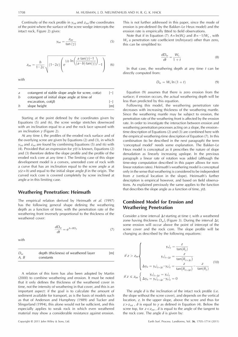
Consider a time interval Δt starting at time t, with a weatheredzone having thickness Dw|t (Figure 3). During the interval Δt,some erosion will occur above the point of intercept of thescree cover and the rock core. The slope profile will bechanging as described by the following equations:

if z > zintf ye jt ¼z

tan δjtð Þye jtþΔt ¼

z

tan δjtþΔt

� �Δye ¼ yejtþΔt−yejt ¼

z

tan δjtþΔt

� �− ztan δjtð Þ

if z ≤ zintye jtþΔt ¼ yejt

Δye ¼ ye jtþΔt−ye jt ¼ 0

(10)

The angle δ is the inclination of the intact rock profile (i.e.the slope without the scree cover), and depends on the verticallocation, z. In the upper slope, above the scree and thus forz > zint , δ is equal to γ as defined in Equation (4). Below thescree top, for z < zint , δ is equal to the angle of the tangent tothe rock core. The angle δ is given by:


S

ay2−Sh2

� � 1−c2c−1−bh2

−Sh2

� � 1−c2c−1 þ by2

−Sh2

� � 1−c2c−1

1CCCCA

Figure 3. Representation of a weathering profile developed in a slopeat time t.

(11)


if 0≤z≤zint ⇒ δjt ¼ atan

aS þ ah2−Sh2

� � 1−c2c−1−

0BBBB@

if zint≤z≤h ⇒ δjt ¼ γjt(11)

with

S

Copyright © 2011 John Wile

−h2− y2 + 2cy

y & Sons, Ltd.

[m2]

Simultaneously, some small penetration of the weatheringfront will occur in that same interval, on top of the penetrationthat had already been achieved at time t. The erosion during Δtwill however remove some of the weathered material that waspresent at time t and therefore the additional weatheringpenetration leads to a smaller depth than suggested on thebasis of the weathering depth Dw|t alone. Depending on howmuch of the weathered material is removed by erosion (none,some or all), the maximum increase of the weathering depth atany height z is only partially obtained. With Dw,y being thehorizontal weathering depth, measured along the y‐axis(Figure 3), the weathering depth is given by:

Dw;y jtþΔt ¼ Dw jt þ eAþBDw jtΔtsin δjtð Þ −Δye

ifeAþBDw jtΔtsin δjtð Þ −Δye > 0

Dw ;y jtþΔt ¼ Dw ;y jt ¼Dw jtsin δjtð Þ

ifeAþBDw jtΔtsin δjtð Þ −Δye ¼ 0

Dw ;y jtþΔt ¼ max 0;Dw jt þ eAþBDw jtΔt

sin δjtð Þ −Δye

� �

ifeAþBDw jtΔtsin δjtð Þ −Δye < 0

(12)

The first line in Equation (12) represents a case wherepenetration of weathering can exceed erosion, the second

exact equilibrium, and the third a case where erosion exceedspenetration of weathering. Since the weathering depth cannotbecome negative, the weathering depth in the latter case isrestricted to values larger than or equal to zero.

In terms of y‐coordinates, the weathering front is defined by:

yw jtþΔt ¼ ye jtþΔt þDw ;y jtþΔt (13)

with

yw
horizontal coordinate of weathering penetration front (m)
Using Equation (13) the profile of the weathering front can becalculated through an iterative procedure with the boundarycondition:

Dw jt¼0 ¼ 0⇒yw jt¼0 ¼ yejt¼0 (14)

In a similar way, the weathering penetration extendingvertically downward from the (assumed) horizontal surfaceabove the slope can be taken into account. Any weatheringdepth along the slope profile and the top surface above itpredating excavation can also be incorporated by adapting theboundary condition of Equation (14) to reflect the pre‐existingweathering profile.

In the above equations it is assumed that the coefficients Aand B are not influenced by the presence of a scree cover, inother words that for the rock covered by scree and for the rockthat is not yet covered, the same coefficients A and B can beused. Although it is generally accepted (Heimsath et al., 1997;Martin, 2000) that the penetration rate of a weathering frontdecreases with increasing penetration depth with unerodedweathered material acting as a protective cover over theunweathered part of a rock mass, it is quite possible that acover of loose slope waste such as scree, with a higher porositythan the in situ material it is covering, may retain more waterafter rainfall than the in situ rock and enhance the potential forchemical weathering. In rock types where chemical weather-ing processes are dominant, this would lead to higherweathering rates for scree‐covered sections of the slope profile.If weathering penetration rates thus change because of theinfluence of a scree cover, this can be included in the iterationby defining Ac and Bc in Equation (12) for all z< zint, and As

and Bs for all z≥ zint (Ac≠As and Bc≠Bs, with the indices c and

s indicating ‘covered by scree’ and ‘slope surface’, respective-ly). For the results presented, A and B have, however, beenkept constant for simplicity.

Field Investigations

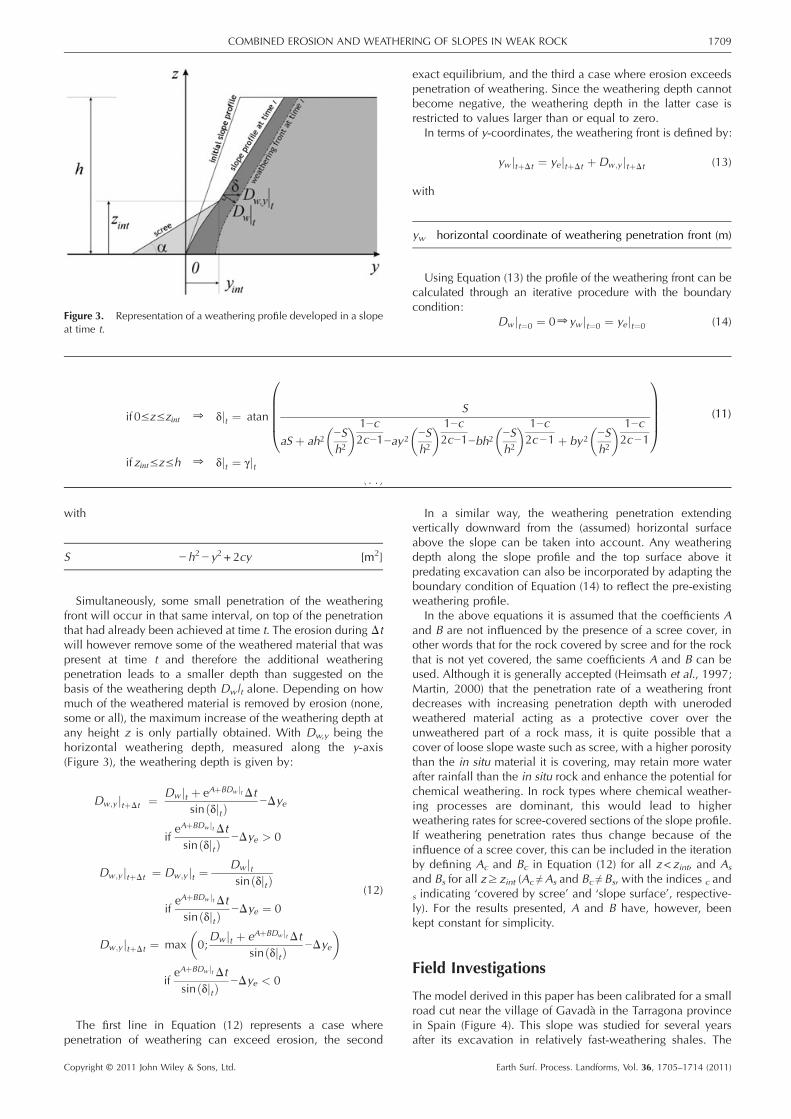
The model derived in this paper has been calibrated for a smallroad cut near the village of Gavadà in the Tarragona provincein Spain (Figure 4). This slope was studied for several yearsafter its excavation in relatively fast‐weathering shales. The


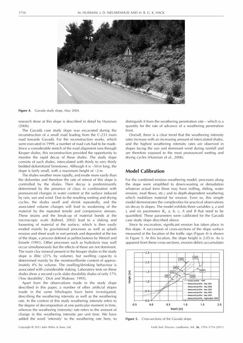
Figure 4. Gavada study slope, May 2004.

igure 5. Cross‐sections of the Gavada slope.


research done at this slope is described in detail by Huisman(2006).The Gavadà case study slope was excavated during the

reconstruction of a small road leading from the C‐233 mainroad towards Gavadà. For the reconstruction works, whichwere executed in 1999, a number of road cuts had to be made.Since a considerable stretch of the road alignment runs throughKeuper shales, this reconstruction provided the opportunity tomonitor the rapid decay of these shales. The study slopeconsists of such shales, intercalated with thinly to very thinlybedded dolomitized limestones. Although it is ~50m long, theslope is fairly small, with a maximum height of ~2m.The shales weather more rapidly, and erode more easily than

the dolomites and therefore the rate of retreat of this slope iscontrolled by the shales. Their decay is predominantlydetermined by the presence of clays in combination withpronounced changes in water content at the surface inducedby rain, sun and wind. Due to the resulting wetting and dryingcycles, the shales swell and shrink repeatedly, and theassociated volume changes will lead to weakening of thematerial by the repeated tensile and compressive stresses.These strains and the break‐up of material bonds at themicroscopic scale (Kühnel, 2002) lead to a slaking andloosening of material at the surface, which is then easilyeroded mainly by gravitational processes as well as splasherosion and sheet wash in wet periods and deposited at the toeof the slope, a process defined as pelitoclastesis by Wetzel andEinsele (1991). Other processes such as hydrolysis may welloccur simultaneously but the effects of these are not dominant.The main clay mineral present in the Keuper shales in the studyslope is illite (21% by volume), but swelling capacity isdetermined mainly by the montmorillonite content of approx-imately 4% by volume. The swelling/shrinking behaviour isassociated with considerable slaking. Laboratory tests on theseshales show a second cycle slake durability shales of only 17%(‘low durability’, Dick and Shakoor, 1995).Apart from the observations made in the study slope

described in this paper, a number of other artificial slopesmade in the same lithologies have been investigated,describing the weathering intensity as well as the weatheringrate. In the context of this study weathering intensity refers tothe degree of decomposition at one particular moment in time,whereas the weathering (intensity) rate refers to the amount ofchange in this weathering intensity per unit time. We haveadded the word ‘intensity’ to the weathering rate here, to


distinguish it from the weathering penetration rate – which is aquantity for the rate of advance of a weathering penetrationfront.

Overall, there is a clear trend that the weathering intensityrates increase with an increasing amount of intercalated shales,and the highest weathering intensity rates are observed inslopes facing the sun and dominant wind during rainfall andare therefore exposed to the most pronounced wetting anddrying cycles (Huisman et al., 2006).

Model Calibration

For the combined erosion–weathering model, processes alongthe slope were simplified to down‐wasting or denudationwhatever actual form these may have (rolling, sliding, watererosion, mud flows, etc.) and to depth‐dependent weatheringwhich mobilizes material for erosion. Even so, this simplemodel demonstrates the complexities for practical observationson decay in slopes. The model exhibits three variables y, z andt, and six parameters Rs, a, b, c, A and B that need to bequantified. These parameters were calibrated for the Gavadàcase study slope described above.

Since its excavation, significant erosion has taken place inthis slope. A succession of cross‐sections of the slope surfacemeasured at the location of the traffic sign (Figure 4) is shownin Figure 5. At this location, the slope height is 2.05m. As isapparent from these cross‐sections, erosion debris accumulates

F



at the foot of the slope, whereas the top of the slope recedes.The initial slope angle was 62°. The stable angle of the

erosion debris was determined to be approximately 35° bymeasuring the stable angle of repose of a small pile of screecollected from the slope. Thus the parameters a and b of theerosion model are taken as cot(35) and cot(62), respectively. Itis noted that a constant scree angle and therefore a constantvalue for a is valid for relatively small slope heights only, sincethe scree profile at the slope toe would have a concave profilefor high slopes in which the fall energy of particles, whichdecreases as the slope development progresses, has a notableinfluence on the angle of repose.A comparison of the eroded volume and the debris volume

in each cross‐section shows that a larger volume erodes thanwhat is actually present as scree at the foot of the slope. The‘missing’ debris is transported away from the slope by rainfallrunoff; a ditch at the toe of the slope connects to a culvert and asmall circular pond, where the eroded and transported materialaccumulates. On average, the volume of eroded rock isapproximately twice the volume of the remaining scree,resulting in a negative value for c (c=1– (volume of rock)/(volume of scree) =−1).In Figure 6 the inclination of the apex through the upper

section of the slope is plotted against time. For the first 5 yearsafter excavation this angle γ decreased at an approximatelylinear rate of 1.2°/year. The latest measurement seems toindicate that this rate of retreat is decreasing. This would be inline with the data reported by Hutchinson (1998), which alsosuggested a decreasing rate of slope retreat. However, the timespan covered by the observations in the study slope is too shortto verify this, and for the present paper a linear rate of Rs=1.2°/year has been assumed as an example. A non‐linear decreaseof γ can nevertheless easily be incorporated in the model (infact any function would be allowed for γ(t)).In order to confirm the uniform rotating retreat mechanism

that is assumed for the Bakker–Le Heux model used in thispaper, a detailed scan was made of a part of the slope in May2004 with an Optech Ilris 3D laser scanner. This provided ahigh resolution point cloud with x, y and z‐coordinates andreflection intensity for each of the reflection points (see Sloband Hack (2004) for a description of this LIDAR method). Theresulting point cloud was compared with the initial planarslope surface. By calculating the retreat of the slope in ahorizontal direction for each reflection point, a contour plotcan be made showing the amount of erosion or accumulation.The results showed erosion contours with respect to theoriginal excavated slope surface that are approximatelyparallel to the toe of the slope, with accumulation in thebottom section of the slope and an increasing amount of

Figure 6. Development of gamma with time.


erosion towards the top, in accordance with the rotating retreatmodel (Huisman, 2006). Since the contours showed uniformamounts of erosion over the length of the slope, thedevelopment shown in the local cross‐sections of Figure 5 isconsidered representative for the entire slope.

While the erosion parameters are relatively easy to obtainfrom a sequence of slope cross‐sections, the parameters relatedto the weathering penetration are more difficult to quantify. Inthe study slope, small excavations were made at sufficientdistance from the cross‐section location so as not to influencefuture measurements, to estimate the penetration depth of theweathering front. In 2004, 5 years after excavation, it wasfound that the irregular pattern of disintegrated weak materialcovering the slope turned into a weak rock with clearlydistinguishable discontinuity sets, with a block size ofapproximately 4 to 5 cm, within 10 to 12 cm from the slopesurface and at a height of 1m above the toe of the slope. Thistransition was taken as the depth of the weathering front. Sinceerosion occurs on the surface, it is not possible to directlycompute the Heimsath A and B parameters of Equation (7) orWs in the simplified Equation (9), which would otherwisesimply be equal to Ws=Dw / ln(1+ t). Therefore the combinederosion‐weathering model was run to find the best fitting valuefor these parameters. It was found that in combination with thelinear slope retreat rate of Rs=1.2°/year, values of Ws=0.1m/ln(year), A= ln(Ws) =−2.30, and B=−1/Ws=−10 gave a goodmatch for the weathering penetration depth estimated from theexcavations. Due to the destructive nature of determining theweathering penetration depth by excavation thiswas not repeatedin later years, and finding representative values for A and Bremains a difficult aspect of the method presented in this paper.

Example of Modelling Results

Figures 7 and 8 show results of a numerical calculation basedon the model described above, using the parameters calibratedfor the Gavadà case study slope. The example calculationsexclude weathering from the top surface for ease of interpre-tation. If this is included, the top parts of the slope will beaffected by that too, and weathering depths calculated for thetop of the slope will be larger than on the basis of weatheringfrom the slope surface alone.

The model parameter values used for these graphs are givenin Table I. Figure 7 shows the calculated slope profile atdifferent exposure times, with the eroded rock core, a screecover, and the weathering penetration front. The developmentof the modelled slope through the years as shown in Figure 7indicates that (when assuming constant values for Rs, a and c)after some 20 years a situation will be reached in which thefinal convex shape of the rock core is reached, the whole slopeis covered by scree, and erosion has come to an end. Beforethis occurs, the section of the eroded rock face that is notcovered by scree extends linearly upward, creating a knickpoint at the intersection with the convex section underneaththe scree cover, and the surface of the scree itself. This sameknick point is reflected in the weathering penetration front; thisis most pronounced in Figure 7(c). Note that for an exposuretime of 5 years the cross‐section of May 2004 has beenincluded in the figure. The modelled and measured profiles area close match but obviously this also results from the fact thatthe model parameters that describe the erosion process havebeen derived directly from the set of cross‐sections.

Although cross‐sections as in Figure 7 are visually appealing,a better insight into the fine balance between erosion andweathering is obtained in the graphs in Figure 8, which showthe thickness of the weathered layer perpendicular to the slope


Figure 8. Example of modelling results weathering depths changing in time, for different rates of slope retreat: (a) 0° per year; (b) 1° per year; (c) 2°per year; (d) 3° per year.

Figure 7. Examplesof modelling results for Gavadà slope, for different exposure times and corresponding years (excavation in 1999): (a) exposuretime 0 years; (b) exposure time 5 years; (c) exposure time 10 years; (d) exposure time 20 years.


surface as a function of (exposure) time. Figure 8(a) shows theresult for the case where the rate of slope retreat is set at 0°/year, so zero erosion. A single curve is found representingpoints at all heights throughout the slope profile. Since thesimplified Heimsath model was assumed to derive A and Bfrom field observations, with A= ln(Ws) and B=−1/Ws , thiscurve is given by Equation (9).


Figure 8(b)–(d) presents cases where erosion rates in terms ofslope angle decrease are larger than zero. Points at differentheights in the slope profile now show different curves; lines aregiven for points at 0.0*h, 0.1*h, 0.2*h, …, 1.0*h (with h theslope height). At the foot of the slope (height 0.0*h), no erosionoccurs and the same curve as in Figure 8(a) is obtained; this isthe limiting situation, visible in all graphs of Figure 8(b)–(d).


Table I. Model parameters used for results shown in Figure 7

Parameter Symbol Value Unit

Stable angle of scree α 35 [°]Initial slope angle β 62 [°]Slope height h 2.05 [m]1–(volume of rock)/(volume of scree) c −1.0 [−]Rate of slope retreat Rs 1.2 [°/yr]Weathering penetration parameter As −2.30 [−]Weathering penetration parameter Bs −10 [1/m]Weathering penetration parameter Ac −2.30 [−]Weathering penetration parameter Bc −10 [1/m]


The curves representing the development of a weathered layerat the other points do however show clear differences.In the graphs of Figure 8(b) and (c), with erosion rates of 1°/

year and 2°/year, a weathering layer develops at the start of thedecay processes at all heights in the slope profile; this can berecognized as an increase in the weathering thickness (risingcurves) although not as fast as in the limiting case for the curverepresenting height 0.0*h. These initially rising curves repre-sent decay situations where some erosion occurs, but animbalance favouring weathering exists. The curves for pointshigher in the slope profile tend to become horizontal aftersome time; this signifies equilibrium between erosion andweathering penetration, resulting in a constant thickness of theweathered zone. Some curves even develop a negative slopesignifying a decrease in the thickness of the weathered zone,and therefore an imbalance favouring erosion. This may evenextend to the case where the weathered layer disappearsaltogether with Dw becoming zero (a situation almost reachedin Figure 8(c) for 1.0*h). All curves finally trend upward againafter a sudden knick point. This knick point occurs at the timeat which the scree extends to the height that is represented byeach curve, resulting in erosion coming to an end at thatparticular height. The small sharp step, which is also visible inmost curves at this knick point, results from the step‐wisechange of the slope angle at this specific point in time. Thiscauses the weathering depth perpendicular to the slope to havea discontinuous first‐order derivative. In the limiting case oft→∞ all curves tend to become equal to the curve for 0.0*h,implying that the whole slope is then covered by scree anderosion has ended, and the simplified Heimsath relation ofEquation (9) applies.Figure 8(d) shows the same basic decay situations existing at

various times and locations; however, with the relatively higherosion rate of 3°/year, the curves for the upper section of theslope profile show a zero thickness of the weathered zone untilthe scree has built up to that particular height. These horizontalcurves at Dw=0 represent a decay situation in which erosionoutpaces weathering, and no weathering mantle can establishitself because any weathered material is continuously eroded(a weathering‐limited situation). With a further increase inerosion rates, the knick points at which the scree wedge passesthe height represented by each curve will shift to the left, towardsshorter exposure times. In the limiting case for Rs→∞ the finalslope profile is reached after an infinitely short time, and allcurves will fall on the same line again, given by Equation (9).Points at different heights in the slope profile will generally

be in different decay situations at the same time, and the decaysituation at a specific location may change in time. The mosthomogeneous slope development will occur with either verysmall (relative to weathering penetration rates) erosion rates, orwith very large erosion rates (again relative to weatheringpenetration rates). With intermediate combinations of erosionand weathering penetration rates, the upper slope will tend to


show imbalance favouring erosion whereas the lower slopewill show imbalance favouring weathering.

Discussion and Conclusions

The model derived in this paper combines the Bakker–Le Heuxerosion model (with rotating slope retreat mechanism) with aweathering penetration model in which the weatheringpenetration rate decreases with increasing thickness of theweathering cover. The resulting set of equations has been solvednumerically by time‐stepping, and gives both the slope profileand the weathering front as a function of time. The simplicity ofthe derived conceptual modelmaywell be preferable over moresophisticated process‐based models for predictions based onscarce observations on actual slopes or for back‐analysis ofexisting slopes. Although in this paper the model parametershave been assumed to remain constant in time for simplicity, themodelling approach allows for time‐variable parameters, mostnotably for the erosion parameters Rs, a and c.

An interesting discussion point is the general observation inthe study area that the rotational Bakker–Le Heux model forslope evolution is the better fit for the observations. In this modelthe down wasting is represented by the erosion of triangularslices that are thick at the top and thin at the toe. At first sight thismay seem to be in conflict with the modelling results presentedin Figures 7 and 8, which show that in all cases the weatheringpenetration depth is greater at the toe than at the top of the slopesection which is not covered by scree material. It must be notedthat if the slope profile development is transport‐limited, with animbalance of decay processes favouringweathering and the rateof erosion and transport of weatheredmaterial being the limitingfactor, removal of sediment from the slope surface will not berelated to the depth of the weathering front (at least if the degreeof weathering on the slope surface does not vary over the slopeheight). As long as this situation remains, weathered materialaccumulates, and transport processes act at their full capacity(Kirkby, 1971). As shown in Huisman (2006), the slope profiledevelopment in the study area and the case study slope is indeedalmost uniquely transport‐limited.

The better fit of the rotational slope development model musttherefore be explained from the following factors: the possibilityof a higher weathering intensity at the top of the slope, due to theexistence of an old weathering mantle parallel to the original(natural) slope profile before excavation, increasing the soilerodibility near the top; weathering from the top of the slope,which is not incorporated in the results shown in Figures 7 and8 (but can easily be included in the model), and the specifictransport processes. Although nodetailed observations havebeenmade regarding the latter, it is believed that soil creep and sheetwash are the dominant transport processes in the study slope.

Depending on erosion and weathering penetration rates,various possible decay situations are shown to occur at a givenpoint in time for different locations along the slope profile, just asdifferent situations occur for a given location along the slopeprofile for different exposure times. This is demonstrated for alinear decrease of the slope anglewith time; the qualitative resultsare independent of the precise nature of this particular trend.

The most homogeneous slope development will occur witheither very small (relative to weathering penetration rates) orzero erosion rates, or with very large erosion rates (againrelative to weathering penetration rates). Intermediate combi-nations of erosion and weathering penetration rates will causedifferent behaviour in the upper and lower parts of the slope. Ithas to be noted that the lower part of a slope may be coveredby scree after some time, which will probably affect theweathering penetration rate in that part. Different penetration



rates for these parts of the slope can easily be incorporated inthe model but this does not affect the general shape of thecurves as presented in Figure 8.The greatest difficulty in determining realistic values for the

parameters of this model lies with the determination of theweathering depth and weathering penetration parameters A andB. For the study presented in this paper these were estimatedbased on a few shallow and destructive excavations. Futureresearch should investigate the possibilities of non‐destructivetechniques to monitor the weathering depth (e.g. ground radarbased methods).In engineering practice, models such as the one presented in

this paper can help to predict the development of a slopeprofile excavated in a weak rock in time. With the addition ofstrength parameters to the weathering profile, the presentedmodel may be extended to serve as the basis for the predictionof the stability of slopes in weak rock as a function of time aswell. Perhaps of even greater value is that the model resultsclearly show just how intricate the balance between erosionand weathering in a slope can become, and that this balancewill change and shift in time and vary for different locations inthe slope. This implies that rock mass classifications and slopestability assessments carried out in the field may not only be asnapshot at a particular time, but also a snapshot of a particularlocation in a slope. With this understanding, engineers inthe field shall carefully assess whether even with a singlelithology, a slope is actually homogeneous enough in terms ofweathering and erosion to warrant a classification as a singleunit, or that the slope needs to be split up into various levelswith a similar development.

ReferencesAhnert F. 1976. Brief description of a comprehensive three‐dimensionalprocess‐response model of landform development. Zeitschrift fürGeomorphologie, Supplement 25: 29–49.

Anderson RS, Humphrey NF. 1989. Interaction of weathering andtransport processes in the evolution of arid landscapes. InQuantitative Dynamic Stratigraphy, Cross TA (ed). Prentice‐Hall:Englewood Cliffs, NJ; 349–361.

Bakker JP, Le Heux JWN. 1946. Projective‐geometric treatment of O.Lehmann’s theory of the transformation of steep mountain slopes.Proceedings Koninklijke Nederlandse Akademie van Wetenschappen(KNAW) 49(5): 533–547.


Bakker JP, Le Heux JWN. 1952. A remarkable new geomorphologicallaw. The law of the denudation slope with recti‐linear cross‐profileI‐III. Proceedings Koninklijke Nederlandse Akademie vanWetenschap-pen (KNAW) 55(4): 399–410 and 554–571.

Brazier RE, Beven KJ, Freer J, Rowan JS. 2000. Equifinality anduncertainty in physically based soil erosion models – application ofthe GLUE methodology to WEPP for sites in the UK and USA. EarthSurface Processes and Landforms 25: 825–845.

Carson MA. 1969. Models of hillslope development under mass failure.Geographical Analysis 1: 76–100.

Dick JC, Shakoor A. 1995. Characterizing durability of mudrocks forslope stability purposes. In Clay and Shale Slope Instability ‐ Reviewsin Engineering Geology Volume X, Haneberg WC, Anderson SA(eds). The Geological Society of America: Boulder, CO; 121–130.

Heimsath AM, Dietrich WE, Nishiizumi K, Finkel RC. 1997. Thesoil production function and landscape equilibrium. Nature 388:358–361.

Hencher SR, McNicholl DP. 1995. Engineering in weathered rock. TheQuarterly Journal of Engineering Geology 28: 253–266.

Huisman M. 2006. Assessment of rock mass decay in artificial slopes.PhD thesis, ITC, Enschede.

Huisman M, Hack HRGK, Nieuwenhuis JD. 2006. Predicting rock massdecay in engineering lifetimes: the influence of slope aspect andclimate. Environmental and Engineering Geoscience 12(1): 39–51.

Hutchinson JN. 1998. A small‐scale field check on the Fisher‐Lehmannand Bakker‐Le Heux cliff degradation models. Earth SurfaceProcesses and Landforms 23: 913–926.

Kirkby MJ. 1971. Hillslope process‐response models based on the con-tinuity equation. In Slopes Form and Process, Brunsden D (ed). Instituteof British Geographers, London, UK: Special Publication no. 3; 15–30.

Kühnel RA. 2002. Driving forces of rock degradation. In ProceedingsProtection and Conservation of the Cultural Heritage of theMediterranean Cities, Sevilla, Spain, Galán and Zezza (eds). A.A.Balkema: Rotterdam; 11–17.

Martin Y. 2000. Modelling hillslope evolution: linear and nonlineartransport relations. Geomorphology 34: 1–21.

Nieuwenhuis JD. 1991. The Lifetime of a Landslide; Investigations inthe French Alps. Balkema: Rotterdam.

Slob S, Hack HRGK. 2004. 3D terrestrial laser scanning as a new fieldmeasurement and monitoring technique. In Engineering Geology forInfrastructure Planning in Europe. A European Perspective, HackHRGK, Azzam R, Charlier R (eds). Springer Verlag: Berlin; 179–190.

Tucker GE, Slingerland RL. 1994. Erosional dynamics, flexural isostasy,and long‐lived escarpments: a numerical modeling study. Journal ofGeophysical Research 99: 12229–12243.

Wetzel A, Einsele G. 1991. On the physical weathering of variousmudrocks. Bulletin of the International Association of EngineeringGeology 44: 89–99.


Documents

Numerical modelling of combined erosion and weathering of slopes in weak rock