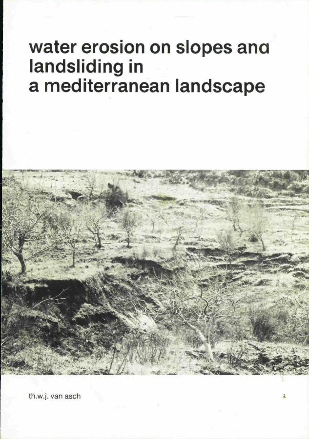
water erosion on slopes analandsliding ina mediterranean landscape

th.w.j. van asch

WATER EROSION ON SLOPES ANDLANDSLIDING INA MEDITERRANEAN LANDSCAPE

Aan mijn MoederWillemAnne-Marie

ISBN 90 6266 026 6 Utrechtse Geografische StudiesISBN 90 6266 027 4 Thesis

All rights reserved. No part of this publication may be reproduced in anyform, by print, photoprint, microfilm or any other means, without writtenpermission from the publishers.

Cover: A slumping area in the Collonci valley(Photo: Th. W.J. van Asch)

»RUK: ELINKWIJK BV - UTRECHT - 030-444921

/ r I9BO ,02

WATER EROSION ON SLOPES ANDLANDSLIDING IN

A MEDITERRANEAN LANDSCAPE

PROEFSCHRIFT

TER VERKRIJGING VAN DE GRAAD VAN DOCTOR INDE WISKUNDE EN NATUURWETENSCHAPPEN AAN DERIJKSUNIVERSITEIT TE UTRECHT, OP GEZAG VANDE RECTOR MAGNIFICUS PROF. DR. M.A. BOUMAN,VOLGENS BESLUIT VAN HET COLLEGE VAN DECANENIN HET OPENBAAR TE VERDEDIGEN OP WOENSDAG

3 DECEMBER 1980 DES NAMIDDAGS TE 2.45 UUR

DOOR

THEODOOR WOUTERUS JOHANNES VAN ASCH

GEBOREN OP 29 JANUARI 1944 TE BAARN

Scanned from original by ISRIC - World Soil Information, as ICSUWorld Data Centre for Soils. The purpose is to make a safedepository for endangered documents and to make the accruedinformation available for consultation, following Fair UseGuidelines. Every effort is taken to respect Copyright of thematerials within the archives where the identification of theCopyright holder is clear and, where feasible, to contact theoriginators. For questions please contact soil.isric@wur.nlindicating the item reference number concerned.

DRUKKERIJ ELINKWIJK BV - UTRECHT

PROMOTOR: PROF. DR. J.I.S. ZONNEVELD

CONTENTS

List of figures 7

List of tables 9

List of plates 10

Foreword 13

1 Introduction 15

2 The environmental conditions of the study area 23

2.1 Climate 232.2 Geology 272.3 Geomorphology 292.4 . Soils 312.5 Landuse and vegetation 33

3 The specification of the water erosion cascade 35

3.1 The splash erosion cascade 353.2 The hydrological cascade as a generator of overlandflow 403.3 The overlandflow erosion cascade 433.4 Empirical measurements as regarded to the total output of the

water erosion cascade 47

4 The effect of landscape variables on the output of different process (sub-systems of the hydrological and water erosion cascade in the study area 51

4.1 The effect of landscape variables on the outputs of the splash erosioncascade 52

4.2 The effect of landscape variables on the amount of overlandflow in thehydrological cascade 64

4.3 The effect of landscape variables on the output of the overland-flow erosion cascade 68

4.4 Summary and conclusions 77

5 The distinction in landunits in relation to the output of the water erosion cascade 79

5.1 The definition of landunits 795.2 The differences in outputs of the water erosion cascade and hydrological

cascade in relation to landunits 865.3 Summary and conclusions 103

6 The specification of the massmovement cascading system 105

6.1 The influence of landscape variables on the degree of stability ofsoil and rock mass 105

6.2 The influence of landscape variables on the type of initial failureof landslides 110

6.3 The influence of landscape variables on the type of transportof landslides 123

7 The influence of landscape variables on the massmovement cascading systemin the study area 127

7.1 Landscape variables in relation to different types of rockslides 1307.2 The influence of landscape variables on the development of debris

slides 1407.3 The influence of landscape variables on the development of

rotational slides 1467.4 The influence of landscape variables on landslides with a dominant

mudflow character 1647.5 Summary and conclusions 173

8 Landunits in relation to the output of the massmovement cascading system 175

8.1 The definition of landunits 1758.2 The differences in output of the massmovement cascade in

relation to landunits 1778.3 Summary and conclusions 184

9 Summary 187

10 Samenvatting 191

Appendix Al Measurement of splash detachment and infiltration rate by meansof a portable rainfall simulator. 195

Appendix A2 Methods of measuring splash and overlandflow erosion 199

Appendix A3 Description of measuring plots. 201

Appendix A4 Erosion data of measuring plots. 204

Appendix AS Some physical and mineralogical characteristics of the slided material 209

Appendix A6 Laboratory analysis. 213

Appendix A7 Three maps showing landslides in relation to different landunits

Bibliography

list of figures

1.1 The water erosion cascading system 16-171.2 The massmovement cascading system 191.3 Decrease of the stability factor F with time 202.1 Mean monthly precipitation and temperature for the Station Fiume

Freddo (1921-1950) 232.2 Tectonic units of Central Calabria (after Dubois, 1950) 274.1 The measuring of output in the water erosion cascade 514.2 The relation between splashdetachment measured with the rainfall simu-

lator and different landscape parameters 53-574.3 Grainsize distributions of splashed material compared with the original soil

material 60-62

4.4 Distribution of splashed up- and downslope material in relation to slopeangle 63

4.5 The relation between the rate of infiltration (fc-value), measured with therainfall simulator and different landscape parameters 66-67

4.6 Grainsize distributions of material transported by overland flow comparedwith the original soil material 72-76

5.1 Three maps of the study area showing the type of landunits in whicherosion measurements have been carried out 82-83

6.1 Stress-strain relationships at different moisture contents (m) of the soil(after Kezdi, 1974) 108

6.2 Stability of a cliff and the influence of tension cracks (after Carson, 1971 ) 1106.3 Stability of a cliff with bedding planes towards the free face 1126.4 Stability of a rock slope with bedding planes towards the free face (a < 0), 1146.5 Stability of a rock slope with bedding planes towards the free face (a > ß) 1146.6 Increase of shear strength and shear stress with depth beneath a slope in

cohesive material (after Carson & Kirkby, 1971) 1156.7 Three types of slumping: a) base failure; b) toe failure; c) face failure

(after Sowers, 1970) 1156.8 Relation between slope angle and the stability factor Ns for various values

of <p (after Taylor, 1937) 1166.9 The stability of a slump in relation to slope angle 1186.10 Features of a rotational slide (slump) 1196.11 The stability of a translational slide 1197.1 The rock slide of San Pietro 1347.2 Frequency distributions of the strike of joint planes in weakly cohesive

sandstones (Mars) near the rock slide of San Pietro 1357.3 A cross section at the head of the rockslide of San Pietro 1367.4 Debrisflow of San Antonio 138-1397.5 Shallow debris slides in the Irroiti valley 1427.6 Shallow debris slide in the Fabrica valley 1447.7. Shallow rotational slide in the Savuto valley (Nicoli) 1477.8. Shallow rotational slides in the Savuto valley (Nicoli) 1487.9 The stability of a slump. The method of slices (after Fellenius) 1517.10 Relation between length and maximum depth of shallow rotational slides

developed in weathered material on metamorphic rocks 1537.11 Rotational slides in weathered Mars-sandstone in the valley of the Fiume

Ste. Maria 154-1557.12 Reconstruction of a slipsurface in a slump developed in Ma-claystone 1587.13 Morphometric map of a fossile slump area in the valley of the Fiume

Torbido 1607.14 Correlation between morphometric parameters of slumps developed in

claystone 1637.15 The slow mudflow of the Torrente Secco (Valle Collonci) 1657.16 Striage lines in rigid clay-blocks on top of a slow mudflow 167

7.17 Schematic picture of the types of movements in the slow mudflow ofthe Torrente Secco

7.18 The slow mudflow of Cozzo Ravo8.1 The influence of landslide variables on the number of slides per landunit

(frequency) and the size of the landslides

Al The portable rainfall simulatorA2 The infiltration rate of a soil developed in metamorphic rocks.A3 Splash shields and "Gerlach" troughs for measuring splash erosion and

overlandflow erosionA4 The relation between liquid limit and plasticity index for different soil

materials of landslides

168170-171

175

195197

199

209

List of tables

2.1 The mean monthly precipitation of three stations in the study area (ob-servation period 1922-1970) and the monthly precipitation during themeasuring periods 24

2.2 Estimated annual erosion yield in tons km'2 in the study area calculatedaccording to Fournier's Erosion Index 25

2.3 The mean monthly and mean annual temperature of two stations near thestudy area (observation period 1926-1955) 26

2.4 The mean slope angle in relation to the lithological units in the study area 293.1 A survey of regulators of the water erosion cascade and the hydrological

cascade and the related landscape parameters (variables) 494.1 The relation of the output of the measuring plots to the results of the rain-

fall simulator on these plots 524.2 .The relation of different landscape parameters to the output of the splash

erosion cascade 584.3 The relation of landscape parameters to overlandflow 654.4 Input-output relationships of the overlandflow erosion cascade 684.5 The relation of different landscape parameters to the output of the over-

landflow erosion cascade 705.1 The description of landunits in which measurements have been carried out 84-855.2 Splash erosion values and infiltration rates in landunits distinguished accor-

ding to respectively degree of agricultural activity, vegetation structure andthe parent rock of soils measured with the rainfall simulator. The signifi-cance of differences between the mean values of landunits 88-89

5.3 Splash erosion values and infiltration rates in landunits distinguished accor-ding to: 1. degree of agricultural activity of man 2. respectively vegetationstructure and the parent rock of soils measured with the rainfall simulator.The significance of differences between the mean values of landunits 90-92

5.4 Splash erosion values and infiltration rates in landunits distinguished accor-ding to: 1. degree of agricultural activity of man 2. vegetation structure 3.

the parent rock of soils measured with the rainfall simulator. The signifi-cance of differences between the mean values of landunits 94

5.5 Water erosion, splash erosion and overlandflow values of landunits distin-guished according to: 1. degree of agricultural activity of man 2. vegeta-tion structure 3. the parent rock of soils, measured on erosion plots. Thesignificance of differences between the mean values of landunits 97

5.6 Water erosion values of landunits distinguished according to: 1. degree ofagricultural activity of man 2. vegetation structure 3. slope length, measuredon erosion plots. The significance of differences between the mean valuesof landunits . 100

5.7 Water erosion values of landunits distinguished according to: 1. degree ofagricultural activity of man 2. vegetation structure 3. slope angle, measured,on erosion plots. The significance of differences between the mean valuesof landunits 101

5.8 Output of water and splash erosion from all measuring plots comparedwith water erosion data from other climatological regions 102

6.1 A summary of limited equilibrium conditions for different type of land-slides 122

7.1 Description of landslide types in the study area 128-1297.2 The strength parameters of Mar-sandstone compared with representative

strength parameters of some other rocks as given by Statham (1977) 1317.3 Calculated groundwater depths for six rotational slides (type number 8) in

weathered me tamorphic rocks 1527.4 Calculated groundwater depths for five rotational slides (type number 9

and 10) in weathered claystone 1628.1 The output of the massmovement cascade in different lithological landunits 1788.2 The output of the massmovement cascade in landunits with different slope

angle 1818.3 The output of the massmovement cascade in landunits distinguished accor-

ding to landuse and vegetation structure 183

Al Physical and mineralogical characteristics of the slided material 210

List of plates

Plate 1 Lateral erosion of the Torrente Collonci 215Plate 2 Saturated overlandflow on measuring plot 11. 215Plate 3 Surface sealing on a freshly ploughed sandstone soil (plot 10) after

3 months with rain 216Plate 4 The formation of a slab in a cliff of Mar-sandstone 216Plate 5 Granular désintégration of Mar-sandstone cliffs 217Plate 6 The head region of the blockslide of San Pietro 218

Plate 7 Retrogressive slumping along a fault in the Ste. Maria valley 217Plate 8 Shallow debris slides in regoliths on metamorphic rocks in the Fabrica

valley 219Plate 9 Shallow debris slides in regoliths on metamorphic rocks near Molino

Longo 219Plate 10 Shallow rotational slides in regoliths on metamorphic rocks in the

Savuto valley 220Plate 11 Different types of massmovements in the Ste. Maria valley 221Plate 12 A slumping area in Mars weathered sandstone in the Ste. Maria valley 222Plate 13 The supply area of a slow mudflow of the Torrente Secco (Valle Col-

lonci) 223Plate 14 Striage stripes in a side of the slow mudflow in the Collonci valley 223Plate 15 Badlands in metamorphic rocks near Terrati 224Plate 16 Field instrumentation on plot 11 225

FOREWORD

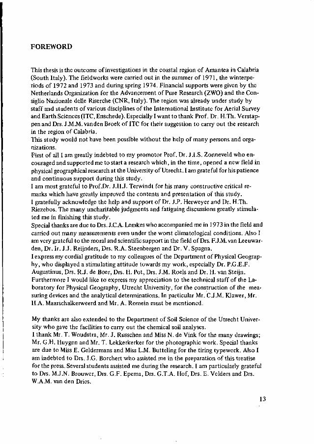
This thesis is the outcome of investigations in the coastal region of Amantea in Calabria(South Italy). The fieldworks were carried out in the summer of 1971, the winterpe-riods of 1972 and 1973 and during spring 1974. Financial supports were given by theNetherlands Organization for the Advancement of Pure Research (ZWO) and the Con-siglio Nazionale delle Riserche (CNR, Italy). The region was already under study bystaff and students of various disciplines of the International Institute for Aerial Surveyand Earth Sciences (ITC, Enschede). Especially I want to thank Prof. Dr. H.Th. Verstap-pen and Drs. J.M.M, vanden Broek of ITC for their suggestion to carry out the researchin the region of Calabria.This study would not have been possible without the help of many persons and orga-nizations.First of all I am greatly indebted to my promotor Prof. Dr. J.I.S. Zonneveld who en-couraged and supported me to start a research which, in the time, opened a new field inphysical geographical research at the University of Utrecht. I am grateful for his patienceand continuous support during this study.I am most grateful to Prof.Dr. J.H.J. Terwindt for his many constructive critical re-marks which have greatly improved the contents and presentation of this study.I gratefully acknowledge the help and support of Dr. J.P. Herweyer and Dr. H.Th.Riezebos. The many uncharitable judgments and fatiguing discussions greatly stimula-ted me in finishing this study.Special thanks are due to Drs. J.C.A. Lemkes who accompanied me in 1973 in the field andcarried out many measurements even under the worst climatological conditions. Also Iam very grateful to the moral and scientific support in the field of Drs. F.J.M, van Leeuwar-den, Dr. Ir. J.J. Reijnders, Drs. R.A. Steenbergen and Dr. V. Spagna.I express my cordial gratitude to my colleagues of the Department of Physical Geograp-hy, who displayed a stimulating attitude towards my work, especially Dr. P.G.E.F.Augustinus, Drs. R.J. de Boer, Drs. H. Pot, Drs. J.M. Roels and Dr. H. van Steijn.Furthermore I would like to express my appreciation to the technical staff of the La-boratory for Physical Geography, Utrecht University, for the construction of the mea-suring devices and the analytical determinations. In particular Mr. C.J.M. Klawer, Mr.H.A. Maarschalkerweerd and Mr. A. Romein must be mentioned.

My thanks are also extended to the Department of Soil Science of the Utrecht Univer-sity who gave the facilities to carry out the chemical soil analyses.I thank Mr. T. Woudstra, Mr. J. Russchen and Miss N. de Vink for the many drawings;Mr. G.H. Huygen and Mr. T. Lekkerkerker for the photographic work. Special thanksare due to Miss E. Geldermans and Miss L.M. Butteling for the tiring typework. Also Iam indebted to Drs. J.G. Borchert who assisted me in the preparation of this treatisefor the press. Several students assisted me during the research. I am particularly gratefulto Drs. M.J.N. Brouwer, Drs. G.F. Epema, Drs. G.T.A. Hof, Drs. E. Velders and Drs.W.A.M. van den Dries.

13

I wish to thank Mrs. H. Berendsen-Hilferink and Mrs. E.Y. Kos-Jacobs for preparingparts of the english text.Finally I acknowledge my gratitude to my wife Anne-Marie, who assisted with manyworks in the field, in the laboratory and at home. I thank her for her patience of livingwith and supporting a husband who stayed too many times in another world.

14

1

INTRODUCTION

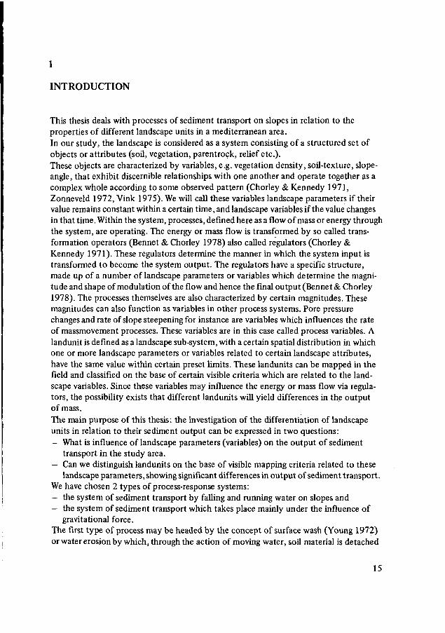
This thesis deals with processes of sediment transport on slopes in relation to theproperties of different landscape units in a mediterranean area.In our study, the landscape is considered as a system consisting of a structured set ofobjects or attributes (soil, vegetation, parentrock, relief etc.).These objects are characterized by variables, e.g. vegetation density, soil-texture, slope-angle, that exhibit discernible relationships with one another and operate together as acomplex whole according to some observed pattern (Chorley & Kennedy 1971,Zonneveld 1972, Vink 1975). We will call these variables landscape parameters if theirvalue remains constant within a certain time, and landscape variables if the value changesin that time. Within the system, processes, defined here as a flow of mass or energy throughthe system, are operating. The energy or mass flow is transformed by so called trans-formation operators (Bennet & Chorley 1978) also called regulators (Chorley &Kennedy 1971). These regulators determine the manner in which the system input istransformed to become the system output. The regulators have a specific structure,made up of a number of landscape parameters or variables which determine the magni-tude and shape of modulation of the flow and hence the final output (Bennet & Chorley1978). The processes themselves are also characterized by certain magnitudes. Thesemagnitudes can also function as variables in other process systems. Pore pressurechanges and rate of slope steepening for instance are variables which influences the rateof massmovement processes. These variables are in this case called process variables. Alandunit is defined as a landscape sub-system, with a certain spatial distribution in whichone or more landscape parameters or variables related to certain landscape attributes,have the same value within certain preset limits. These landunits can be mapped in thefield and classified on the base of certain visible criteria which are related to the land-scape variables. Since these variables may influence the energy or mass flow via regula-tors, the possibility exists that different landunits will yield differences in the outputof mass.

The main purpose of this thesis: the investigation of the differentiation of landscapeunits in relation to their sediment output can be expressed in two questions:— What is influence of landscape parameters (variables) on the output of sediment

transport in the study area.— Can we distinguish landunits on the base of visible mapping criteria related to these

landscape parameters, showing significant differences in output of sediment transport.We have chosen 2 types of process-response systems:— the system of sediment transport by falling and running water on slopes and— the system of sediment transport which takes place mainly under the influence of

gravitational force.The first type of process may be headed by the concept of surface wash (Young 1972)or water erosion by which, through the action of moving water, soil material is detached

15

hydrological cascading system

input or output

R rainmass

E evapotranspiration

S stemflow

Q H Horton's overlandflow

Q S saturated overlandftow

PR peculation to lower zones

TF through flow

PS splash detached material

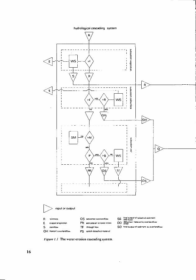
Figure I.I The water erosion cascading system.

DO J»»*«'™te,,al by overlandflo»

SO *'na' output of sediment by overlandflow

16

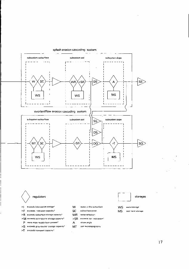
splash erosion cascading system

subsystem slope

overlandflow erosion cascading system

regulators

> | exceeds interception storage?

> F exceeds infiltration capacity?

> R exceeds soilsurface storage capacity?

> |\/| exceeds soilmoisture storage capacity?

P more impermeable layer present?

> B exceeds groundwater storage capacity?

>T exceeds transport capacity'

W water at the soilsurface

SC soilsurface cover

W R waterreflection

>SR exceeds soil resistence?

/ \ slope angle

|\/[~]" soil microtopography

storages

W S waterstorage

M S sediment storage

17

and transported. The grain or soil particles in the fluid medium are separated, resultingin a reduction of the importance of grain to grain contact and interaction to smallproportions. The second type of process is called massmovement which comprises ofsediment transport processes by which large quantities of weathering products movetogether is close grain to grain contact (Statham 1977).The above mentioned processes can be considered as debris cascading systems (Chorley& Kennedy 1971). These cascading systems are one of the most important types ofdynamic systems. They are defined as structures in which the output of energy or massof one landscape attribute (also called spatial sub-system: vegetation, soil surface, soil,slope etc.) forms the input of another attribute. Within these attributes there are regu-lators which either divert a part of the input of mass or energy into a store or create athroughput. One of the purposes of our study is to investigate the influence of land-scape variables on the regulators within the system and hence the throughflow and out-put of sediment material.The cascading system of water erosion is schematically depicted in Figure 1.1. The out-put of rainmass(R) and overland flow (Q) from the hydrological cascade are consideredas inputs for the water erosion cascade. There is a storage of water mass (WS) withinthe system. If the forces of the water mass exceed certain threshold values (SR) of thesoil material, sediment can be set into motion and the output of the system consists inthat case of sediment and water mass (SS and SO). The water erosion cascading systemcan be subdivided into two important process sub-systems: a) the splash erosion cas-cading sub-system, b) the overlandflow erosion cascading sub-system (Figure 1.1).The amount of material which is set into motion within the splash erosion system isrelated a.o. to the amount of kinetic energy in the falling raindrops. The first regulator,reducing the mass of rain with a certain kinetic energy, is the vegetation structurewhich intercepts a part of the falling drops (I). The impact forces of the falling raindropson the ground may be reduced by the presence of a water film (W) and the protective ef-fect of not transportable surface stones and litter cover (SC). Most of the energy is absor-bed in the soil and only a small part of the energy is used to set soil particles into motion.The amount of material set into motion depends a.o. on soil properties regulating thedegree of reflection of the waterdrop momentum (WR) (e.g. soil elasticity, bulk density,soil moisture content) and soil properties regulating the resistance against the shearingforces of the waterdrop impact (SR) (e.g. soil texture, soil strength and aggregate sta-bility).The detached particles can be divided into portions ejected in an upslope direction anda downslope direction. The ratio between the splashed upward and downward materialis determined by the slope angle (A). The travelling distance of the particles having acertain kinetic energy is also determined by the slope angle. The final output of splashedsediment (SS) is defined as the amount of sediment mass passing a unit width of slopeper unit of time in a downslope direction.The amount of overlandflow from the hydrological cascade is considered as an inputfor the overland flow erosion cascading system (Gregory & Walling 1973). A part ofthe hydrological cascade is depicted in Figure 1.1. The occurrence and amount of over-land flow depends on four inportant threshold regulators: the infiltration capacity (F),

18

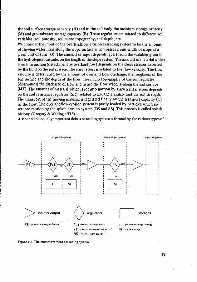
the soil surface storage capacity (R) and in the soil body the moisture storage capacity(M) and groundwater storage capacity (B). These regulators are related to different soilvariables: soil porosity, soil micro topography, soil depth, etc.We consider the input of the overlandflow erosion cascading system to be the amountof flowing water mass along the slope surface which passes a unit width of slope at agiven unit of time (Q). The amount of input depends, apart from the variables given inthe hydrological cascade, on the length of the slope system. The amount of material whichis set into motion (detachment by overlandflow) depends on the shear stresses excertedby the fluid on the soil surface. The shear stress is related to the flow velocity. The flowvelocity is determined by the amount of overland flow discharge, the roughness of thesoil surface and the depth of the flow. The micro topography of the soil regulates(distributes) the discharge of flow and hence the flow velocity along the soil surface(MT). The amount of material which is set into motion by a given shear stress dependson the soil resistance regulator (SR), related to a.o. the grainsize and the soil strength.The transport of the moving material is regulated finally by the transport capacity (T)of the flow. The overlandflow erosion system is partly loaded by particles which areset into motion by the splash erosion system (DS and SS). This process is called splashpick-up (Gregory & Walling 1973).A second and equally important debris cascading system is formed by the various types of

slope subsystem basal slope system river subsystem

O input or output

PE potential energy of mass

regulators

p > 1 exceeds safetyfactor?

>X exceeds transport capacity?

B S basal stream present?

storages

£ potential energy storage

[\/| mass storage

Figure 1.2 The massmovement cascading system.

19

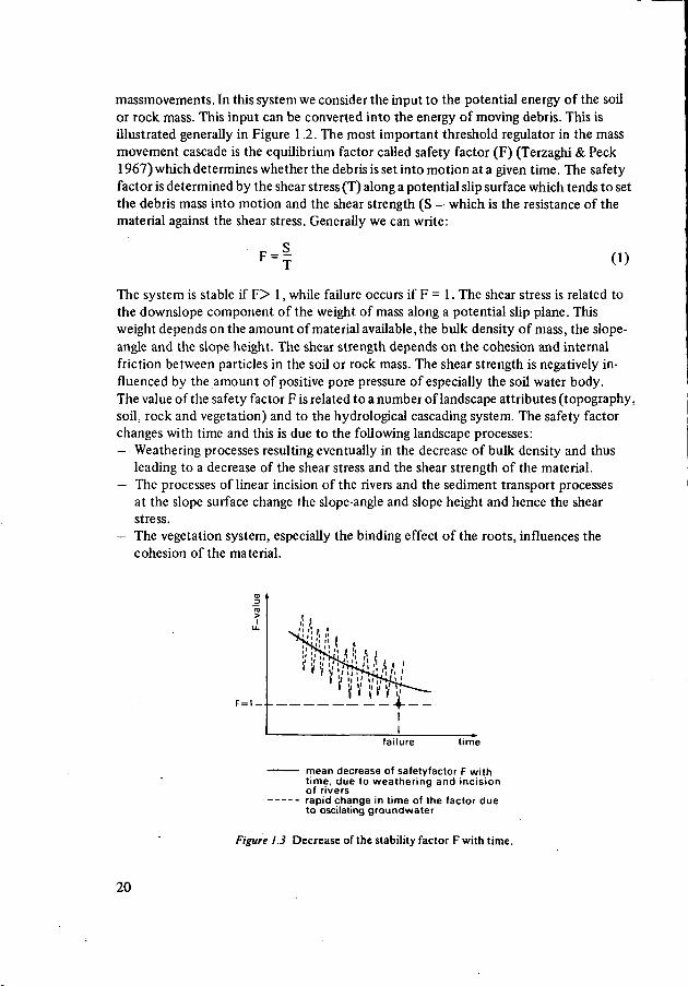
massmovements. In this system we consider the input to the potential energy of the soilor rock mass. This input can be converted into the energy of moving debris. This isillustrated generally in Figure 1.2. The most important threshold regulator in the massmovement cascade is the equilibrium factor called safety factor (F) (Terzaghi & Peck1967) which determines whether the debris is set into motion at a given time. The safetyfactor is determined by the shear stress (T) along a potential slip surface which tends to setthe debris mass into motion and the shear strength (S — which is the resistance of thematerial against the shear stress. Generally we can write:

F = | 0)

The system is stable if F> 1, while failure occurs if F = 1. The shear stress is related tothe downslope component of the weight of mass along a potential slip plane. Thisweight depends on the amount of material available, the bulk density of mass, the slope-angle and the slope height. The shear strength depends on the cohesion and internalfriction between particles in the soil or rock mass. The shear strength is negatively in-fluenced by the amount of positive pore pressure of especially the soil water body.The value of the safety factor F is related to a number of landscape attributes (topography,soil, rock and vegetation) and to the hydrological cascading system. The safety factorchanges with time and this is due to the following landscape processes:— Weathering processes resulting eventually in the decrease of bulk density and thus

leading to a decrease of the shear stress and the shear strength of the material.— The processes of linear incision of the rivers and the sediment transport processes

at the slope surface change the slope-angle and slope height and hence the shearstress.

— The vegetation system, especially the binding effect of the roots, influences thecohesion of the material.

failure time

mean decrease of safetyfactor F withtime, due to weathering and incisionof riversrapid change in time of the factor dueto oscilating groundwater

Figure 1.3 Decrease of the stability factor F with time.

20

— The hydrological system controls the variation of the amount of ground water andthus the pore water pressure.

Generally speaking in the course of time the F-factor decreases due to the weatheringof the soil and rock material and the erosion processes (Statham 1977). The oscillatinginfluence of the hydrological system is superimposed on this general trend. Figure 1.3gives an illustration.The figure shows that the fluctuating groundwater may act as a "trigger" in the star-ting of massmovements.When the material is set into motion the transport capacity regulator (T) determinesthe distance of transport which depends on a.o. a) nature of initial rupture b) the slope-angle c) the mechanical characteristics of the debris after failure and d) the soil mechani-cal characteristics of the receiving material over which the debris is moving. Debris storageis possible mainly due to a loss of ground water. In this case a new state of equilibriumis created. The value of topographical, soil- and vegetation-variables influencing the F-factorhas completely changed. The state of equilibrium can be of a short duration: anew rising of the ground water level to a certain critical height may cause new move-ments. When the sliding material reaches the base of the slope the amount of debristransport is then regulated by the presence of a basal stream, which is able to removethe mass from the slope. Up slope of the sliding area, topographical and hydrologicalconditions in the regolith are changed, which on its turn may provoke a disequilibrium.In the foregoing, we have shortly described two systems of sediment transport processes,which are considered as flows of mass through a number of landscape attributes. Thefinal output of the sediment in which we are interested is determined by the value ofcertain regulators in the system, which are related to a number of landscape variables.Landunits which are distinguished according to certain criteria, based on these variablesmay give differences in sediment output. The general problem of our study is whethersuch landunits can be distinguished in the study area. In relation to this problem thefollowing subjects will be discussed:

- The environmental conditions of the study area.— The specification of the sediment transport processes on slopes and the influence

of different landscape variables on these processes.- An analysis of the influence of landscape variables on the output of these processes

in the study area.- The selection of mapping criteria related to these landscape variables and the defini-

tion of landscape units on the base of these criteria.— An analysis of the differences in output of sediment transport processes between

the defined land units.

21

THE ENVIRONMENTAL CONDITIONS OF THE STUDY AREA

2.1 Climate

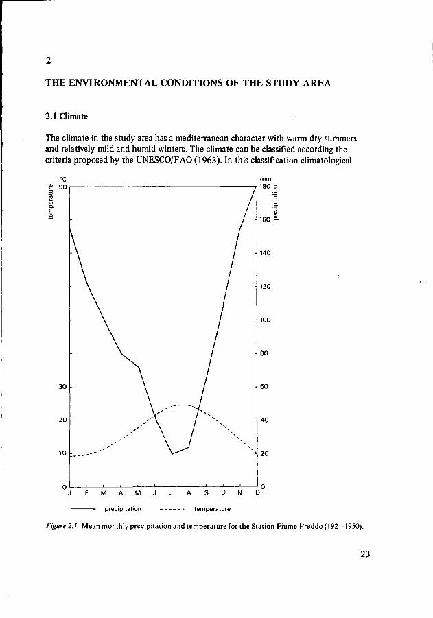
The climate in the study area has a mediterranean character with warm dry summersand relatively mild and humid winters. The climate can be classified according thecriteria proposed by the UNESCO/FAO (1963). In this classification climatological

J F M A M J J A S O N D

precipitation temperature

Figure2.l Mean monthly precipitation and temperature for the Station Fiume Freddo(192l-1950).

23

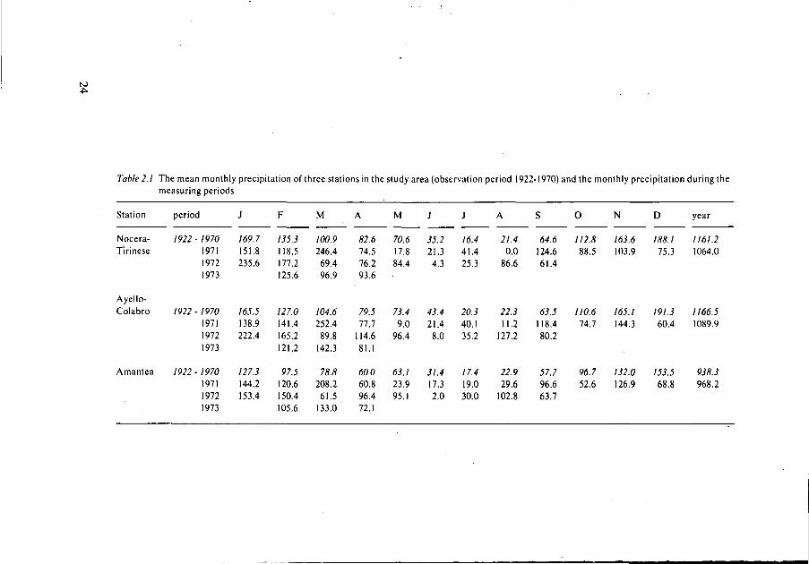
Table 2.I The mean monthly precipitation of three stations in the study area (observation period 1922-1970) and the monthly precipitation during themeasuring periods

Station

Nocera-Tirinese

Ayello-Colabro

Amantea

period

1922-

1922-

1922-

1970197119721973

1970197119721973

1970197119721973

J

169.7151.8235.6

165.5138.9222.4

127.3144.2153.4

F

135.3118.5177.2125.6

127.0141.4165.2121.2

97.5120.6150.4105.6

M

100.9246.469.496.9

104.6252.4

89.8142.3

78.8208.261.5

133.0

A

82.674.576.293.6

79.577.7

114.681.1

60060.896.472.1

M

70.617.884.4

73.49.0

96.4

63.123.995.1

J

35.221.34.3

43.421.4

8.0

31.417.32.0

J

16.441.425.3

20.340.135.2

17.419.030.0

A

21.40.0

86.6

22.311.2

127.2

22.929.6

102.8

S

64.6124.661.4

63.5118.480.2

57.796.663.7

0

112.888.5

110.674.7.

96.752.6

N

163.6103.9

165.1144.3

132.0126.9

D

188.175.3

191.360.4

153.568.8

year

1161.21064.0

1166.51089.9

938.3968.2

characteristics are related to the natural vegetation. This UNESCO/FAO classificationdefines the mediterranean climate as having a mean monthly temperature which isalways higer than 6° C and a dry period from one to eight months, during which thelongest day must occur. According to Bagnouls and Gaussen (1957) the dry period isdefined as "the period in which the precipitation in mm is less than twice the tempera-ture in °C". A further subdivision of the climate is based on the so-called "xerothermicindex". This index is defined as the number of days in the above defined dry periodwhich can be deemed dry from the biological point of view. This means that days withfog and dew are considered to be humid (UNESCO/FAO 1963).The mean monthly precipitation and temperature at one station, 10 km north of thestudy area is shown in Figure 2.1. The dry period in the study area averages approxi-mately 2Vi month according to UNESCO/FAO (1963), the number of "biologically"dry days amounts to 40-50. The climate can be classified as a "meso-mediterranean"climate.Table 2.1 shows the distribution of precipitation for 3 stations in the study area duringthe year, based on the mean monthly precipitation measured over the period 1921-1950.Obviously the precipitation falls primarily in the period from autumn to spring. Thisconcentration of precipitation in the winter is of great importance to soil erosion. Thereis little evaporation. As a result the soil remains damp for a longer period thus givingrise to a greater overlandflow. Furthermore the erodibility of the soil increases as aresult of the higher soil humidity. The precipitation often falls in showers of greatintensity especially during the winter months (Nochese 1959). During our measuringperiods, occasional showers with an intensity up to 40 mm per hour were measured.Considerable variations in precipitation occur from year to year. Table 2.1 shows alsothe monthly precipitation in the years 1971-1972-1973 in relation to the mean monthlyprecipitation measured over 30 years. It can be infered from the Table that during themeasuring period lasting from February to April in 1972, February and April were re-

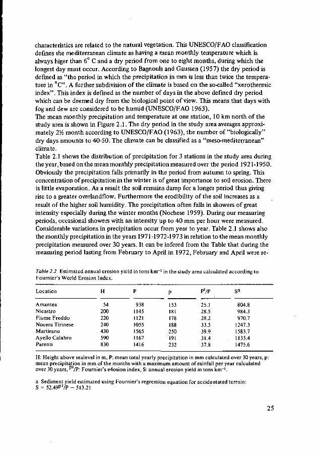
Table 2.2 Estimated annual erosion yield in tons km"2 in the study area calculated according toFournier's World Erosion Index.

Location

AmanteaNicastroFiume FreddoNocera TirineseMartiranoAyello CalabroParenti

H

54200220240430590830

P

938114511211055156511671416

P

153181178188250191232

PVP

25.128.528.233.539.931.437.8

S a

804.8984.3970.7

1247.31583.71133.41475.6

H: Height above sealevel in m, P: mean total yearly precipitation in mm calculated over 30 years, p:mean precipitation in mm of the months with a maximum amount of rainfall per year calculatedover 30 years, P2/P: Fournier's e4osion index, S: annual erosion yield in tons km"2.

a Sediment yield estimated using Fournier's regression equation for accidentated terrain:S = 52.49PVP-513.21

25

latively wet months while March was relatively dry. In 1973 the monthly precipitationdidn't differ much from the mean.Table 2.2 shows how the mean annual precipitation measured on 7 stations within thestudy area and in the neighbourhood varies with the height above sealevel. In this tablewe have also tried to give an indication towards the effect of the rain in this climaticzone on the water erosion processes compared to the effect of other climatic zones ofthe world. We have used an index developed by Fournier (1960) which fits a correlationbetween erosion and precipation from data all over the world. This precipitation indexis

P2/P (1)

in which p = the mean amount of precipitation in the month with the maximumprecipitation.

P = the mean yearly precipitationp and P are based on long term measurements.Founder's correlation diagram, which relates p2/P to the amount of erosion, was usedto translate the computed p2 /P values for the different stations (based on precipitationdata over the period 1921-1950) into erosion values (see table 2.2). Accordingly themean erosion in the hilly study area is put to approximately 1000 tons per squarekilometer annually. On Founder's world erosion map (Fournier 1960 pp. 186-187) itcan be seen that this value is exceeded only in the tropical areas of Africa and South

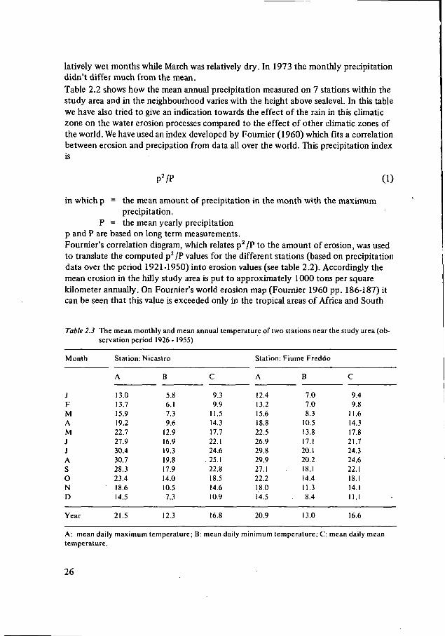
Table 2.3 The mean monthly and mean annual temperature of two stations near the study area (ob-servation period 1926 - 1955)

Month

JFMAMJJASOND

Year

Station

A

13.013.715.919.222.727.930.430.728.323.418.614.5

21.5

Nicastro

B

5.86.17.39.6

12.916.919.319.817.914.010.57.3

12.3

C

9.39.9

11.514.317.722.124.625.122.818.514.610.9

16.8

Station:

A

12.413.215.618.822.526.929.829.927.122.218.014.5

20.9

Fiume Freddo

B

7.07.08.3

10.513.817.120.120.218.114.411.38.4

13.0

C

9.49.8

11.614.317.821.724.324.622.118.114.111.1

16.6

A: mean daily maximum temperature; B: mean daily minimum temperature; C: mean daily meantemperature.

26

East Asia (over 3000 tons per square kilometer annually). There are no snow falls inthe study area.Table 2.3 shows mean monthly temperatures at two stations located just outside thestudy area. January is the coldest month with a mean temperature of 9°C and Augustthe warmest, with a mean temperature of 24°C. Calculated in the period 1922-1955, themonth with the lowest mean temperature , occurred in January: 23°C; the highest cal-culated mean temperature occurred in August: 34.4°C. The number of days duringwhich it freezes is few. During the winter from 1922 to 1955 November, December,January, February and March were respectively 28,24, 22, 23 and 26 times out of 30years free of frost. The temperature was never much below 0°C; on the average onedegree.

2.2 Geology

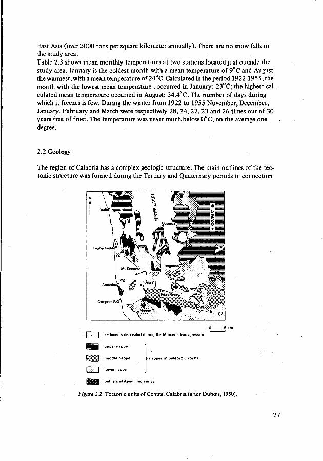
The region of Calabria has a complex geologic structure. The main outlines of the tec-tonic structure was formed during the Tertiary and Quaternary periods in connection

- | | sediments deposited during the Miocene transgression

upper nappe

middle nappe

lower nappe

nappes of paleozoic rocks

outliers of Apenninic series

Figure 2.2 Tectonic units of Central Calabria (after Dubois, 1950).

27

with the Alpine orogenesis. The backbone of Calabria is formed by the massifs ofAspromonte and Serre in the South and the Sila massif (see Fig. 2.3) in the central area.These are the remnants of a Paleozoic basement consisting of crystalline and metamor-phic rocks. In Central Calabria in which the study area lies, these formations are thrusta great distance over the southern extremity of the apenninic domain which is charac-te'rizedby. thick series of Mesozoic 'carbonatic rocks containing "Alpine" Triassic rocksat their base (Dubois 1970). The calcareous dolomitic massif of the Monte Pollino andjust north of our study area the Monte Cocuzzo belongs to these apenninic series (seeFigure 2.2). Aided by recent."horst-graben" structures these series appear under thenapps in a succession of inliers (Burton 1970, Dubois 1970). These large overthruststook place during the Lower Miocene in a WNW - ESE direction. (The "paroxysmalphase" of Burton (1970) ). Dubois (1970) distinguished three napps (see Figure 2.2),the upper one containing the Paleozoic gneisses of the the Sila massif and the Triassiclimestone of Longobucco, the middle one found in the south of the area (containingorthogneisses, granites, contact metamorphosed phyllites and sections of Jurassic series)and the lower riäpp being composed of phyllites.

The apenninic series, underlying these napps range from Trias to Titonic-Neocomien.As in the case of the deeper parts of the Calabrian napps these underlying series beartraces of a dynamic metamorphism.Burton (1970) distinguished a second important ("postparoxysmal phase") in whichthe napps formed during the paroxysmal phase are folded. These movements datedmainly of middle Miocene age. After these two important phases of tectonic movementsthere was a major transgression during the middle Miocene, when flyshlike sedimentsconsisting of basal conglomerates, sandstones, clays and calcareous sediments weredeposited (see Figure 2.3). It is evident from the configuration of these rocks that sincethe deposition of these middle Miocene sediments there has been considerable renewedtectonic activity. This is the third tectonic phase which started in the Pliocene accordingto Burton (1970) and it is characterized by intensive faulting, involving an uplift of theCalabrian area up to 1000 mtr. (Bousquet & Gueremy 1968,1969). Faulting occurredparticularly during the Pleistocene period with throws of from 100 up to 300 mtr. Minorfaulting took place during the late Pleistocene period. These observations are in agree-ment with the conclusions which can be drawn from the genesis of marine terraces;furthermore the difference in height among the different terrace levels also indicates astronger tectonic movement during the early Pleistocene (Burton 1960).Figure 2.3 shows that the southern and eastern part of the study area consists ofPaleozoic rocks belonging to the lower and middle napp. Inside this arc of older rockssandstone, clay and conglomerates dating from the period of the middle Miocene trans-gression can be found. On the coast a.o. Triassic limestone from the Apenninic seriesappears via normal faults as tectonic inliers. The Miocene rocks are characterized bystrong faulting, which is a cause of many massmovements.We will now give a description of the main lithological units in the study area. Thelargest part of the Paleozoic rocks in the study area consists of gray phyllites and schists(sf) (from the lower napp) with numerous intercallations of quartzite and locally lamina

28

of cristalline limestone. The phyllites consist mainly of chlorite, sericites and quartz.Epidote is sometimes present at the transition zone bordering on the green schists (sfe).At some places the green schists in the southern part of the area (sfe) comprise mainlyepidote, chlorite and quartz. In the eastern and central part of the study area outcropsof medium to coarse grained biotite or muscovite granite (7) belonging to the middlenapp are found.At some places in the area Mesozoic rocks from the Apenninic series appear as outliers.We can distinguish a) the Triassic compact dolomites and limestones (Tdl) light gray andbrown in colour, which are well-stratified and b) Jurassic compact cristalline gray-brownlimestone (Gc) locally in combination with light-brown dolomite.The Tertiairy sediments deposited during the Miocene trangression period consist ofsandy conglomeratic rocks (Mel 2-3) at the base containing well arounded boulders ofmetamorphic rocks including the granites. A weakly cemented sandstone (Mars 2-3)with a light-gray or brown colour lies on these conglomeratic series. Sometimes thereare intercalations of siltstone. The sediments are generally speaking well layered. Thissandstone formation is followed by a limy sandstone which is more cemented (Mar 2-3)and has a light-gray or brown colour. Locally these series are followed by fine cristallinelimestone (Me 2-3) with a light-gray or brown colour. The upper Miocene formationsconsist of siltic claystones, silts and sandy silts (Ma 2-3). They have a dark-gray toblackish-gray colour.The gravel deposits from marine and fluvial origin which are found in the higher fluvialand marine terraces belong to the Pleistocene formations. The fluvial deposits of thelower terraces, the alluvial fan deposits and the coastal plain formations were formedduring the Holocene period.

2.3 Geomorphology

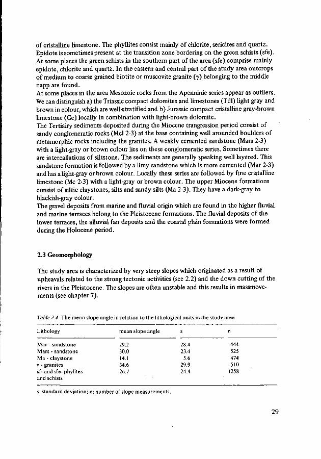
The study area is characterized by very steep slopes which originated as a result ofupheavals related to the strong tectonic activities (see 2.2) and the down cutting of therivers in the Pleistocene. The slopes are often unstable and this results in massmove-ments (see chapter 7).

Table 2.4 The mean slope angle in relation to the lithological units in the study area

Lithology

Mar - sandstoneMars - sandstoneMa - claystoneY - granitessf- and sfe- phylitesand schists

mean slope angle

29.230.014.134.626.7

s

28.423.4

5.629.924.4

n

444525474510

1258

s: standard deviation; n: number of slope measurements.

29

Table 2.4 gives an impression of the mean slope angle in relation to different rock types.The data were assembled from the topographical map 1:10.000. Sampling of the slopeprofiles was done according to the method proposed by Young (1971 p. 145). Alongthe slope profile measurements were taken at a equidistance of 20 mtr. The table showssignificant differences (a = 0.1) in most cases between the different lithological units. Itappears that the silty claystone areas show distinctively the lowest mean slope anglevalues. The presence of marine terraces in these areas forms an indication towards thestrong upheavel during Pleistocene times. In the study area 6 marine terrace levels lyingabove each other were found south of the Fiume Grande at respectively 1000-1020 mtr,940-950 mtr, 640-670 mtr, 400-440 mtr, 140-170 mtr, 20-40 mtr. Burton (1964)assumes that the marine terraces in Calabria between 300 and 100 mtr. date from theCalabrian age (early Pleistocene) which lasted about 350.000 years. From this it maybe concluded that the greatest tectonic movements took place during the early Pleisto-cene and this corresponds to the results of Bousquet & Gueremy (1968) (see 2.2).The rivers in the study area have a typically mediterranean character. They have a broadalluvial plain in combination with a relative steep gradient. The riverbed contains coarsedebris and the discharge fluctuates strongly. In the summer the river plain may fall com-pletely dry. The greatest fluctations in discharge occur in the winter as a result of heavyshowers. During the periods of heavy precipitation large amounts of debris can be trans-ported in the river. This could be shown by the study of sediment transport in the riversand the study of fans, which can be found in the study area on places where small riverswith a steep gradient discharge into a broad alluvial or coastal plain. Ergenziger et al.(1975) measured the sediment transport of a river in another part of Calabria fromJanuary 1972 to January 1973. He measured a net decrease in the riverbed of 27 cmto 3 cm in the upper course of the river and a net accumulation of the riverbed in themiddle course varying from 2 cm -150 cm. The largest variation in erosion and sedimen-tation took place in January; days with heavy precipitation occurred with an extremeof 300 mm per day. This extremity occurs only four times every century.Another indication for the fact that the largest sediment transport is concentrated inperiods of catastrophic rainfall is found in the study of the sediment deposits of thedifferent fans. In several cuts made along the Autostrada we found in the fans an alter-nation of well stratified river deposits and layers several meters in thickness, which havethe character of mudflow deposits. These mudflow layers can be related to catastrophicrainy periods.

Another example of a great change in the morphological conditions could be found inthe alluvial fan of the Fiume Ste Maria, south of America. The water and debris is guidedover the fan by means of two walls. The walls date from 1905 and are 8 m high. Thecanal is 40 m wide and 650 m long. It was completely filled in 1925. When calculatedover the surface of the fan the original surface of the fan would have risen 70 cm in 20years. Due to an enormous rainstorm in 1925 a large part of the debris in the canal wasswept away.We can infer from the above given examples that we must be very careful in dating thedifferent geomorphological phenomena. E.g. the accumulation terraces along the mainrivers which rise 1-2 meter above the alluvial plane may be recently formed under

30

catastrophic conditions with strong accumulation of material in the lower course of theriver. Therefore it is to be doubted whether these terraces should be dated from the earlyHolocene as suggested by Rao & Ghanem (1972). It is also doubtful whether a distinc-tion could be made between late Holocene fans and recent fans on the base of vegeta-tion and landuse: certain fans with a vegetation cover or under recent agriculture neednot to be fossile because depositions on these fans may take place only a few timesper 100 years during catastrophic conditions.Dams have been constructed in several rivers with steep gradient in order to slowdown the irregular and often catastrophic large amounts of debris transport. Due tothe stepped profile of the river resulting from the sedimentation which develops behindthese dams, the stream velocity of the water is slowed down and hence the transportcapacity is decreased. Observations in the field revealed that in the lower course manyrivers cut down sharply into their own riverbed. This may be the result of, on the average,less debris supply from upstreams caused by the construction of the dams. This effectis also favoured by the removal of debris from the mouth of the river by men, keepingthe local base level of erosion artificially low. Concrete blocks placed approximatelyten years ago to protect the riverbanks and the alluvial terraces with cultivated groundsare being undercut by the running water at an increasing rate (see Plate 1).

2.4 Soils

The soils were classified in the field according to the French system of soil classifica-tion, which is also used in many African countries. The higher classification categoriesare resp. the "Classe", "Sous-classe", "Groupe" and "Sous-Groupe". In the study areaa variety of soil types were found:- "Classe des sols minéraux bruts" ( (A)C or (A)R ). A typical feature for this type of

soil is the very poorly developed A-horizon in which there are only traces of organicmatter in the upper 20 cm and/or not more than 1.5% organic matter in the upper 2- 3 cm. It is possible that due to strong colluviation in this erosive area, these tracesof organic matter can be present at all places in the soil profile. This soil type is rela-ted to the steepest slope in the study area and on several dune deposits along the coast.

— "Classe des sols peu évolués" (AC or AR). In this class the A-horizon is more dis-tinct with traces of organic matter in the upper 20 cm and/or in the upper 2 - 3 cma C-content of more than 1.5%. Most of the soils in this highly erosive area belongto the above mentioned classes. On the level of the "Sous-classe" the above mentionedsoil types belong to resp. "Sous-classe des sols minéraux bruts non climatique" andthe "Sous-classe des sols peu évolués non climatiques". On the level of the groupeswe will find in the area the "sols minéraux bruts ou peu évolués non climatiquesd'érosion ou d'apport alluvial and colluvial".

More important for the study of the erodibility of these poorly developed soils is thesub-division according to the parent material. In the French classification this is done

31

on the level of "La Famille" which is a subdivision of the "Sous-groupes". The followingsoil types are very important on this level:— "Sols minéraux bruts and sols peu évolués non climatiques d'érosion sur roche dur" on

phyllites and schists. Due to strong erosion and colluviation a very vague A-horizonmay be distinguished with only traces of organic matter up to 30 - 60 cm. (C-con tent0.5-1.5%).Sometimes under denser shrub vegetation and (or) forest a more distinct Al 1 orAl (Modeux) was found (3 - 6 cm) (C-content 1 - 2%). Laboratory analyses showeda high amount of Calcium-ions at the complex in the upper horizon.The C.E.C. varies from 12 to 15 ppm.; pH varies from 5 - 7.5. The soil texture ismainly sandy loam (USDA-classification). The content of gravel is relatively high inthese soils in relation to other soils (20 to 50%) which is important with regard tothe erodibility.

— "Sols minéraux bruts and peu évolués non climatiques d'érosion sur roche meuble",on sand stones (Mars - Mar).These soils also have a very vague A-horizon with traces of organic matter up to 20cm (0.5 - 1.5%). A distinct All up to 3 cm with a C-content from 1.5 to4%candevelop under denser vegetation. The pH varies from 6.5 - 8. The complex is com-pletely saturated (C.E.C.-values 5-15 ppm with a dominance of Ca-ions. Further-more free Ca-ions are present. According to the USDA-classification the texture isloamy sand. Aggregate stability is weak and the soils have a moderate gravel content(5-15%).

— A third important groupe of soil types is the "sols minéraux bruts ou sols peu évoluésnon climatiques d'érosion sur roche dur" on Miocene clay stone (Ma). The A-horizon(mostly an Ap-horizon) varies from 20 - 40 cm in depth and has a C-content from 2- 4% ; pH varies from 7.5 - 8. In these soils the complex is also completely saturated(C.E.C.-values 15-20 ppm) with a dominance of Ca-ions.

The texture varies from clay to silty clay. The soils show strong dissecation fissures andin the lower horizons often hydromorphic characteristics. According to Palmer's teststhe aggregate stability is moderate to strong.These soils may locally be classified as vertisoils showing clear prismatic structures andslickenside phenomena.On sandy limestone (Mar and Me) and hard Triassie limestone (Tdl) soiltypes were locallyfound belonging to the "classe de sols calcimagnésiques", "sous-classe des soils carbonates"(AC). Rendzinas were sometimes developed on hard calcarous rocks ("groupe des rend-zines"). On the cemented limestone rocks (Mar) soils belonging to the groupe des solsbrun calcaires" could also be distinguished.On places where soil erosion has been less intensive due to a denser vegetation or lesssteeper slopes soils were found belonging to the "Classe des sols brunifiés" ("Sous -classe des soils brunifiés des climats tempérés humides - Groupe des sols bruns"). Thesesoils have generally speaking a more distinct A-horizon up to 20 cm (C-content 2 - 4%and a structural B-horizon). On metamorphic rocks the A-horizons were "modeux" and

32

under forest may reach a humus content of 10% . On sandstone (Mars) a Bt.-horizon wasfound locally ("Groupe des sols lessivés").In the coastal plains hydromorphic soils belonging to the "Classe des sols hydromorphes"("Sous-classe peu humifère; Groupe à gley") were found.On the marine terraces remnants of paleosols belonging to the "Classe des sols à sesquiox-ides de fer" ("Sous-classe des sols fersiallitiques") were found. They were covered by ayounger colluvial layer with "sols minéraux bruts ou peu évolués".

2.5 Landuseand vegetation

The fragile equilibrium existing in the Mediterranean areas between soil and vegetationhas been disturbed by man in many places; such is also the case in Calabria.In entire Calabria there is still, despite the explosive growth of the agrarian population,relatively much natural forest especially in the higher parts of the Sila, Aspromonte andSenne (44%) (Tichy 1962). In addition many shrub and grass areas are found. In Cala-bria it is possible to distinguish four natural vegetation zones related to altitude:- Zone up to 500 m:

This is the Mediterranean vegetation zone with evergreens, such as quercus illex, pis-tacca lantiscum, lentiscu macchie, cistus macchie;

- Zone from 500 -1200 m :Lower mountain zone with deciduous mixed forest, such as quercus cerris andcastanea sativa and spartium junceum and deciduous shrubs;

- Zone from 1200 - 2000 m:Upper mountain zone with mixed forest vegetation, e .g. fagus enabies. This type of ve-getations with undergrowth is comparable to the natural forests in the European moun-tains;

- Zone above 2000 m:This zone is largely composed of conifers, e.g. pinus heldreichii and pinus leucoder-mis.

The natural vegetation has disappeared especially in the coastal area due to pressurefrom the agrarian population.Agricultural grounds were extended in the second half of the 19th Century as a resultof the population explosion. This led to deforestation and hence increased erosion(Tichy 1962).A large percentage of the working population in Calabria works in the agrarian sector(Huson 1970). In 1960 this was 60%(Meyriat 1970). Most farms have mixed cultiva-tion. They are small and not mechanized. The yield is largely for personal use.Calabria, which is one of the most densely populated areas in Italy, has the lowest pro-duction per acre. As a result the standard of living is very low.One of the most important products is grain which is sown twice a year (Milone 1956).The heavy precipitation does a lot of damage to the winter grain and the summer grainsuffers from the drought. The productivity on the steep, rocky slopes subject to erosion

33

is low. The cultivation of olives is, next to the growing of grain, very important. Dueto drought, poor soils and diseases the production is not up to standard. Only the pro-duction of fruit in the irrigated coastel areas is of such quality and quantity that it canbe exported (Meyriat 1960).Cattle breeding is, like agriculture, not highly developed. The live-stock consists mainlyof sheep and goats. Their numbers decreased sharply, especially after the war, as a resultof the discontinuation of transhumance and agrarian reforms. Overgrazing is common.Areas covered with grass and shrubs serve as pastures which are then subject to strongerosion. These natural pastures are not very nutritious; additional food is provided byagricultural products and often garbage from around the house.In the study area the percentage of land used for agriculture is fairly high. The narrowcoastal plain and the terraces in the river valleys are generally used for horticulture. Onthe steep, terraced slopes mainly grains and fodder crops are grown in combination withhorticulture (e.g. olives). As far as we could determine the yield is for personal use. Onthe steep slopes of metamorphic rocks, e.g. in the Savuto valley and on the siltstones ofthe Fiume Grande valley olives are cultivated. The less steep slopes, usually occurring insiltstone areas, are used exclusively for agriculture. The parcels of land are usually largerin these areas.Weakly cemented sandstone, disintegrates easily and after tilling forms new soilalthough it is not nutritious.When comparing the present amount of land used for agriculture with that of 1955on aerial photographs a decrease in agrarian activity can be ascertained. Abandonedfarms can be recognized in the field by the rocky ground with pavements resulting fromthe erosion which took place during farming, the presence of terraces, and neglectedolive trees and fruit trees. Grasses, herbs and sometimes shrubs grow abundantly onthese farmlands. Ruins of farmhouses are numerous in the study area.The more or less natural vegetation of grasses, herbs and shrubs grows on the steepestslopes of the hard Triassic dolomitic rock, the even harder Mar-sandstone and on thesteeper slopes of the granite and metamorphic rocks. The areas less densely overgrownwith shrubs and grasses served as natural pastures. Gullies are still visible in thesepastures. A spectacular example of this can be seen in the Mar-sandstone area east ofCleto where 40% of the soil has disappeared and the remaining weathering layer is heldtogether only by sparse vegetation.

There are not many forests in the study area. They consist mostly of oaks and havedeteriorated. At higher altitudes just outside the study area oak- and chestnutforestare found.The steepest slopes in the study area, such as sandstone slopes, are partly being re-forested. These are the areas where the original vegetation of grasses and shrubs hasbeen destroyed by overgrazing to such an extent that restoration is impossible. This isdue to the fact that water erosion led to the partial disappearance of the soil. Terraceridges are hewn into the slopes of the less-cemented rock (Mars-sandstone) yielding anew soil in which shrubs are planted. These shrubs take root easily and help preventwater erosion. In the badlands the new plants are often destroyed by surfacial sliding.

34

3

THE SPECIFICATION OF THE WATER EROSION CASCADE

3.1 The splash erosion cascade

In chapter 1 we have already illustrated (Figure 1.1) that the splash erosion cascade isan important process sub-system of the water erosion cascade. While the overland flowerosion cascade depends on the production of overland flow by the hydrological cas-cade, the splash cascade only depends on the direct input of rain. We will now discussthis process cascade in relation to various landscape variables in more detail.The input of the splash cascade (Figure 1.1) is formed by the mass of raindrops. Thekinetic energy of the falling raindrops is used to set the sediment material into motionwithin the system. The kinetic energy per unit of time is determined by the total massof rain per unit of time (= the rainfall intensity) multiplied by the terminal velocity ofthe falling drops. This velocity depends on their size (drop diameter). Laws (1941) andGunn & Kinzer (1949) measured the terminal velocity by each raindrop diameter. Thetotal kinetic energy of the rain which is called the erosivity of the rain (Hudson 1973)can be calculated from the drop size distribution of a rainshower. The measurement ofdropsize distribution is a rather laborious and difficult technique (Hudson 1973), butthrough these measurements empirical relationships were found between dropsize dis-tribution and the intensity of the rain in different parts of the world (Laws & Parson1943, Best 1950, Hudson 1963).

A relationship was set up between rainfall intensity (which is easy to measure duringthe rainstorms) and the kinetic energy of the rain in different parts of the world (seeHudson 1973).For the United States, e.g. Wischmeier (1962) found that the kinetic energy per unitof rain mass and per unit area is correlated with the 0.14 power of rainfall intensity.More precise methods of measurements of the kinetic energy or the momentum of thefalling raindrops have been developed by Rose (1958), Hudson (1965), Kinell (1968),Forest (1970), Imeson (oral com.).A number of experiments were carried out in which the input of the rain energy iscompared with the output of splash discharge. The rest of the system was consideredas a black box. Ellison (1944) found under laboratory conditions that splash detach-ment is correlated with the velocity of raindrops to the 4.33 power, the drop diameterto the 1.07 power and the rainfall intensity to the 0.65 power. Bisal (1960) found arelation between splash detachment with the drop diameter (linear) and with the dropvelocity to the 1.4 power. Mihara (1951), Free (1960), Rose (1960), van Asch & Roels(1979) correlated splash detachment and transport with the total mass and velocity ofthe rain. It was found that depending on soil type, soil detachment can be correlatedwith the kinetic energy of the raindrops with an exponent varying from 0.9 (soil mate-rial with aggregates) to 2.5 (glass pearls). Van Asch & Roels (1979) calculated that only

35

5%of the kinetic energy from falling raindrops is transmitted into the the kinetic energyof moving grain material.Based on a large number of data from experimental plots, Wischmeier et al. (1958) pro-posed a good erosivity parameter for natural rainshowers, the so-called EI-30 index. TheEI-30 index (see also Ekern, 1950) is calculated by the multiplication of the kineticenergy from a rainstorm with the 1-30 index which is the greatest average intensity,experienced in any 30 minute period during the storm. Given this relationship and thefact that for moderate up to intense rainstorms the kinetic energy per unit of rainmassper unit of area is correlated with I0"14 (where I is rainfall intensity). Meyer & Wisch-meier (1969) proposed that during steady state conditions the splash erosion S is corre-lated to the rainfall intensity to approximately the 2.14 power. Similar values are ob-tained when the laboratory data of Ellison ( 1944) (Meyer & Wischmeier 1969) are used.David & Beer (1975) concluded that S * I2 . Hudson (1973) showed that there is acertain threshold rain intensity value which is in Africa 25 mm/hr (one inch). Belowthis intensity the rain has little or no erosive power. He therefore introduced the KE> 1index which is defined as the total kinetic energy of rain falling at intensities of morethan 25 mm/hr (1 inch/hr). He found good correlation figures between this index andthe amount of splashed sandy soils.

In Figure 1.1 the first regulator in the splash cascade is called vegetation structure.Important factors of the vegetation structure are the density of the vegetation and theheight of the vegetation canopy. The vegetation canopy intercepts a part of the fallingraindrops (I). A part of the water remains on the leaves until it is evaporated. A partof the water flows down the plants or trees to emerge as stemflow around the base andthe third part drops to the ground from the leaves.Depending on the height of the leaves above the soil surface the third part of the inter-cepted water can regain a certain kinetic energy which together with a part fallingdirectly on the ground (through fäll) form the input of kinetic energy to the soil sur-face sub-system. Therefore a dense vegetation canopy near the ground considerablyreduces the transference of kinetic energy to the soil surface.However, under forest (with a high canopy) the total kinetic energy delivered to theground can be the same as in an open landscape (Chapman 1948, Trimble & Weitz-mann 1954, Rougerie 1960, Ruxton 1967, Geiger 1975, Van Zon 1978). The studiesshow more or less directly that the mean dropsize of water falling from the leaves islarger than of rainwater in the open field. When the tree canopy is high enough (> 9mtr, see Laws 1941) these drops can reach their terminal velocity again. Due to thisincrease in mean dropsize the kinetic energy of drops that fall from the canopy isincreased.This increase in kinetic energy of a part of the total rainmass may counterbalance theloss of kinetic energy due to evaporation and stemflow.The second regulator in the splash cascade is the presence of a water film (W) due tooverlandflbw. According to Palmer (1964) and Mutchler & Young (1975) the way ofenergy transmission to the grains depends on the depth of the waterfilm. Up to a criticalwaterfilm thickness (which is according to Mutchler and Young 0.14 - 0.20 x the dropdiameter and Palmer 3 x the drop diameter) the impact force on the grains will be

36

greater than when the soil surface is bare. Above this critical value the waterfilm worksas a protective cover, absorbing all the kinetic energy while the impact force exertedon the grains is strongly reduced.

The soil grains may also be protected by the presence of a stone pavement and/or alitter-layer (SC), which can absorb a part or all the kinetic energy of the drops.A third important category of regulators is formed by the transmission of a part of thekinetic energy of the rainmass into the kinetic energy of moving particles. The "waterreflection regulator" (WR),see Figure 1.1 determines which part of the momentum ofthe failing raindrops is reflected. The reflected water droplets carry some soil particles in-to the air. According to Carson & Kirkby (1972) the amount of momentum reflectiondepends on the presence of water in the soil surface pores or at the soil surface. VanAsch & Roels (1979) suggested that the elasticity and the bulk density of the soil bodyare also important factors. If no soil water is present in or at the surface no reflectionof raindrop momentum takes place and therefore no ejection of soil particles (Carson& Kirkby 1972). For this condition the exerted force of the raindrops on the soil bodycan be resolved in a normal force and a shear force along the surface. The normal forcecauses a consolidation of the surface particles down into the soil pore space, or theformation of small craters. In this manner a great part of the kinetic energy is lost. Theshear force along the soil surface causes the soil particles to be transported a certain dis-tance along the surface (Carson & Kirkby 1972). This type of process is called splash-creep.

The most important regulator is the soil resistance (threshold) regulator (SR, see Figure1.1), which determines if the exerted forces of the water energy are large enough to setthe material into motion. The resistance against these forces is determined by thecohesion and internal friction of the soil particles which build up the soil strength. Thesoil strength is influenced by the amount of water pressure or air pressure in the pores.The air pressure and (or) pore pressure increases particularly during the impact of rainand this (according to Coulomb's Law) means a reduction of the soil strength. The_par-ticle size is also of importance since it determines whether a given exerted forse of araindrop mass is large enough to carry the particle into the air. Up till now littleexperimental work has been done to determine the effect of the above mentioned regu-lators and their related variables on the energy and mass flow.We have already mentioned the effect of the waterfilm on the surface. Sloneker et al.(1976) investigated the effect of the pore water pressure of water saturated soils. Theymeasured an increase in splash amount at first as the pore pressure decreases to around- 20 mb, followed by a decrease of splash, which is especially rapid in coarser sand. Itis clear that techniques have to be evaluated in order to measure the soil strength andcohesion of the material and the change in pore pressure during the impact of raindropssuch as done by Sloneker et al. (1976).In the above the soil body is considered as an accumulation of loose grains. In most soilsthe grains are bound together in aggregates, which have a certain cohesion. It is thestrength of these aggregates, expressed as an aggregate stability parameter, which provedto be an important parameter in the determination of soil resistance (or erodibility)

37

against splash detachment (Bryan 1968,1976). The cohesive strength of the soil par-ticles or aggregate stability is determined by the binding effects of organic compounds,the clay content, types of absorbed cations, the Ph and Al- and Fe-hydroxides (Chesteret al. 1957, Allison 1968, Baver et al. 1972). The decrease of the cohesive strength ofthese aggregates is possible due to the differential swelling of mainly clay minerals(Henin 1938) and compression of entrapped air.Yoder (1936) proposed a method of measuring the stability of the aggregates by agita-ting them in water. Other methods essentially based on mechanical analysis have beenproposed by e.g. Nishikata & Takeudi (1955), Henin (1963). Another method used forthe measurement of the stability of the aggregates is to subject the aggregates directlyto the process of rain fall impact (McCalla 1944, Pereira 1956). Bryan (1968) suggestedthat the aggregate stability, determined by the water drop technique of McCalla (1944),modified by Smith & Cernuda (1951)-, proved to be a more efficient index of soil erodi-bility than the indices derived from other methods, because soil aggregates whichshowed to be waterstable by the gently shaking activity of wet sieving may not in factbe stable when subjected to the impact of raindrops with high fall velocity.Another soil resistance factor which can be measured is the grain size distribution. Thegrain size is of importance to the soil resistance regulator in two ways:- It has already been stated that smaller particles are much easier to detach and trans-

port than coarser particles. Ellison (1944) showed that, compared to coarse particles,finer soil particles are preferentially lifted from the surface (see also Rose 1960, DePloey & Savat 1968, Yariv 1976).

- However, very fine particles like clay are much more difficult to detach since theyhave strong cohesive bindings.

Various textural indices have been-eväluäted but the work of Bryan (1968), who tes-ted these indices, shows that no strong correlation exists with the amount splash detach-ment on natural soils with aggregate building. The erodibility of the soil may be reducedstrongly due to the formation of a crust at the soil surface, Mclntire (1958), Epstein &Grant (1973).These crusts have a greater bulk density, shearing resistance, a lower degree of aggrega-tion and a higher content of finer material in comparison to the subsurface (Lemos &Lutz 1957). Soil crusts are formed by the impact of raindrops, which results in a physi-cal compaction of the soil surface material (Epstein & Grant 1973) and by long periodsof heating and drying (Lemos & Lutz 1957)'. Soils which are susceptible to crust for-mation have a large content of silt or total material < 0.10 mm and 2:1 type clay mine-rals (Lemos & Lutz 1975).The vegetation system influences the resistance regulator: the production of organicmaterial and the stimulation of biological activity leads to a better structure and greaterstability of the aggregates. Yarhato & Anderson (1973) stressed the importance ofbinding effects of especially the grass roots on the soil resistance against splash detach-ment.

The effect of the slope regulator (A), see Figure 1.1, on the final output of sedimentdischarge is explained in 3 ways:

38

— Slope steepness determines the ratio between the amount of soil which is splashedupwards and downwards through the air. At higher slope angles more soil particlesare transported downwards due to the increasing downslope component of the im-pact of the raindrops. Ratios are given by Ellison (1944), Mosely (1974), De Ploey& Moeyerson (1976), Morgan (1978), Savat (in prep.).

— By an increasing slope angle, the splashed particle will reach the soil surface at agreater distance downslope and a shorter distance upslope from the point of impactDe Ploey & Savat (1968), Mosley (1974), Savat (in prep.).

— By an increasing slope angle the downslope impact shear force is able to carry moresoil particles along the slope over a greater distance (Carson & Kirkby, 1972).

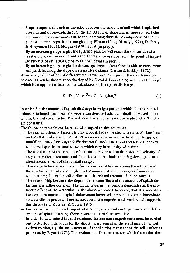
A summary of the effect of different regulators on the output of the splash erosioncascade is given by the equation developed by David & Beer (1975) and Savat (in prep.)which is an approximation for the calculation of the splash discharge.

S = I a . V . e~Pü . C . R . (sina)T (1)

in which S = the amount of splash discharge in weight per unit width, I = the rainfallintensity in length per hour, V = vegetation density factor, d = depth of waterfilm inlength, C = soil cover factor, R = soil Resistance factor, a = slope angle and a, ß and 7are constants.The following remarks can be made with regard to this equation:— The rainfall intensity factor I is only a rough index for steady state conditions based

on the relationships which exist between rainfall energy of natural rainstorms andrainfall intensity (see Meyer & Wischmeier (1969). The EI-30 and KE > I indexeswere developed.for natural showers which vary in intensity with time.The calculation of the amount of kinetic energy based on drop size and velocity ofdrops are rather inaccurate, and for this reason methods are being developed for adirect measurement of the rainfall energy.

— There is only limited empirical information available concerning the influence ofthe vegetation density and height on the amount of kinetic energy of rainwater,which is supplied to the soil surface and the related amount of splash-output.

— The relationship between the depth of the waterfilm and the amount of splash de-tachment is rather complex. The factor given in the formula demonstrates the pro-tective effect of the waterfilm. In the above we stated, however, that at a very shal-low depth the amount of splash detachment increased compared to conditions whereno waterfilm is present. There is, however, little experimental work which supportsthis theory (e.g. Mutchler & Young 1975).

— Few experimental data relating vegetation cover and soil cover parameters with theamount of splash discharge (Screenivas et al. 1947) are available.

— In order to determined the soil resistance factors more experiments must be carriedout to develop techniques for the direct measurement of the resistance of the soilagainst erosion, e.g. the measurement of the shearing resistance at the soil surface asproposed by Bryan (1976). The evoluation of soil parameters which determine the

39

amount of waterdrop reflection (soil moisture conditions, bulk density, etc.) is alsovery important.

— Many experiments have been carried out under laboratory conditions so that the in-fluence of slope angle on the netto sediment discharge could be measured. Due todifferences in measuring techniques it is difficult to compare the results.

Equation ( 1 ) is a first step in the evaluation of an empirical equation for the amount ofsplash discharge on the slope.We will show in Chapter 5 that this type of transport is very important especially onslopes with more or less natural vegetation. In the evaluation of such an empirical equa-tion we must develop an uniform definition of splash discharge and use the same mea-suring techniques. In this way uniform parameters can be evaluated for e.g. vegetationstructure, soil resistance, soil moisture, conditions and water conditions.In Chapter 4 some of the appropriate parameters used for the splash transport modelwill be treated.

3.2 The hydrological cascade as a generator of overlandflow

In Chapter 1 we considered the output of overlandflow from the hydrological cascadeas an input in the overlandflow erosion cascade (Figure 1.1). It was stated that fourimportant threshold regulators are involved in the production of overlandflow (givena certain input of rain). Therefore, for the purpose of our study this part of the hy-drological cycle and particularly the influence of the landscape variables on thesethreshold regulators must be discussed in more detail.The most important regulator is the infiltration capacity regulator (F) (Figure 1.1). Itcan be defined as the maximum rate at which water can infiltrate the soil body duringa given time t. If the rainfall rate (intensity) at that time is in excess of the infiltrationrate water is stored on the soil surface.Two components are involved in the infiltration process of water into the soil:— the transmission- or conductivity component, which can be described as an unim-

peded laminar flow through a continuous network of large pores, due to the effectof gravity,

— a diffusion component, which can be described as a flow in very small discrete stepsgoing from one pore space to the next in a random fashion due to capillary suction(Kirkby 1969, Knapp 1978).

Several authors have given theoretical and empirical formulas to describe the infiltrationof water into the soil (see for a summary Seyhan (1977). A wellknown empirical equa-tion was set up by Horton (1945):

f=fc + ( f o - f C ) e - k t (2)

in which f = the instantaneous infiltration rate at time t, in volume per unit of time,fc = the minimum infiltration rate in volume per unit of time at time t = a and f0 isthe maximum infiltration rate in volume per unit of time at t = o; k = a constant which

40

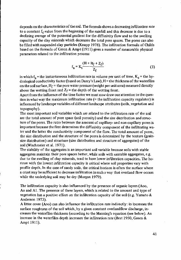
depends on the characteristics of the soil. The formula shows a decreasing infiltration rateto a constant fc-value from the beginning of the rainfall and this decrease is due to adeclining average of the potential gradient for the diffusivity flow and to the swellingcapacity of the clay minerals which decreases the total pore spaces. The pores can alsobe filled with suspended clay particles (Knapp 1978). The infiltration formula of Childsbased on the formula of Green & Ampt (1911) gives a number of measurable physicalparameters related to the infiltration process:

(H Hf + Zf)fa - ^ — ~ r

L (3)

in which fa = the instantaneous infiltration rate in volume per unit of time, Ks = the hy-drological conductivity factor (based on Darcy's Law), H = the thickness of the waterfilmon the soil surface, Hf = the pore water pressure (weight per unit area) measured directlyabove the wetting front and Zf = the depth of the wetting front.Apart from the influence of the time factor we must now draw our attention to the ques-tion in what way the maximum infiltration rate (= the infiltration capacity regulator) isinfluenced by landscape variables of different landscape attributes (soils, vegetation andtopography).The most important soil variables which are related to the infiltration rate of the soilare the total amount of pore space (soil porosity) and the size distribution and struc-ture of the pores. The ratio between the amount of capillary- and non-capillary pores isimportant because the first determines the diffusivity component of the infiltrating wa-ter and the latter the conductivity component of the flow. The total amount of pores,the size distribution and the structure of the pores is determined by the texture (grain-size distribution) and structure (size distribution and structure of aggregates) of thesoil (Wischmeier et al. 1971).The stability of the aggregates is an important soil variable because soils with stableaggregates maintain their pore spaces better, while soils with unstable aggregates, e.g.due to the swelling of clay minerals, tend to have lower infiltration capacities. The ho-rizon with the lowest infiltration capacity is critical where soil properties vary withprofile depth. In the case of sandy soils, the critical horizon is often the surface wherea crust may be sufficient to decrease infiltration in such a way that overland flow occurswhile the underlying soil may be dry (Morgan 1979).

The infiltration capacity is also influenced by the presence of organic layers (Aoo,Ao and Al. The presence of these layers, which is related to the amount and type ofvegetation has a positive effect on the infiltration capacity of the soil (e.g. Yamato &Anderson 1973).A litter cover (Aoo) can also influence the infiltration rate indirectly: in increases thesurface roughness of the soil which, by a given constant overlandflow discharge, in-creases the waterfilm thickness (according to the Manning's equation (see below). Anincrease in the waterfilm depth increases the infiltration rate (Best 1950, Green &Ampt 1911).

41

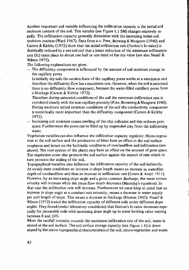
Another important soil variable influencing the infiltration capacity is the initial soilmoisture content of the soil. This variable (see Figure 1.1 SM) changes relatively ra-pidly. The infiltration capacity generally diminishes with the increasing initial soilmoisture content (Ward 1967). Data from a.o. Free, Browing & Musgrave (1940) andCarson & Kirkby (1972) show that the initial infiltration rate (Horton's fo-value) isdrastically reduced by a wet soil and that a lesser reduction of the minimum infiltrationrate (fc) takes place to about one half or one third of the dry value (see also Nassif &Wilson 1975).The following explanations are given:— The diffusivity component is influenced by the amount of soil moisture storage in

the capillary pores.In initially dry soils the suction force of the capillary pores works at a maximum andtherefore the diffusivity flow has a maximum rate. However, when the soil is saturatedthere is no diffusivity flow component, because the water-filled capillary pores froma blockage (Carson & Kirkby 1972).Therefore during saturated conditions of the soil the minimum infiltration rate iscorrelated closely with the non-capillary porosity (Free, Browning & Musgrave 1940).During moderate initial moisture conditions of the soil the conductivity componentis numerically more important than the diffusivity component (Carson & Kirkby1972).

— Increasing soil moisture causes swelling of the clay colloides and this reduces porespace. Furthermore the pores can be filled up by suspended clay from the infiltratingwater.

Vegetation variables can also influence the infiltration capacity regulator. Micro-vegeta-tion at the soil surface and the production of litter have an effect in the soil surfaceroughness and hence on the hydraulic conditions of overlandflow and infiltration (seeabove). The root-system of the plants may have an effect on the amount of pore space.The vegetation cover also protects the soil surface against the impact of rain which inturn prevents the sealing of the soil.Topographical variables also influence the infiltration capacity of the soil indirectly.At steady state conditions an increase in slope length means an increase in waterfilmdepth of overlandflow and thus an increase in infiltration rate (Green & Ampt 1911).However, by an increasing slope angle and a given constant discharge, the mean streamvelocity will increase while the mean flow depth decreases (Manning's equation). Inthat case the infiltration rate will decrease. Furthermore we must keep in mind that anincrease in slope angle at a constant rain intensity, means a decrease in water supplyper unit length of slope. This means a decrease in discharge (Horton 1945). Nassif &Wilson (1973) tested the infiltration capacity of different soils under different slopeangles. They found (under laboratory conditions) that Horton's fc-value decreases espe-cially for permeable soils with increasing slope angle up to some limiting value varyingbetween 8 and 24%.When the rainfall intensity exceeds the maximum infiltration rate of the soil, water isstored at the soil surface. The soil surface storage capacity (see Figure 1.1) is deter-mined by the micro-topographical characteristics of the soil, micro-vegetation and waste

42

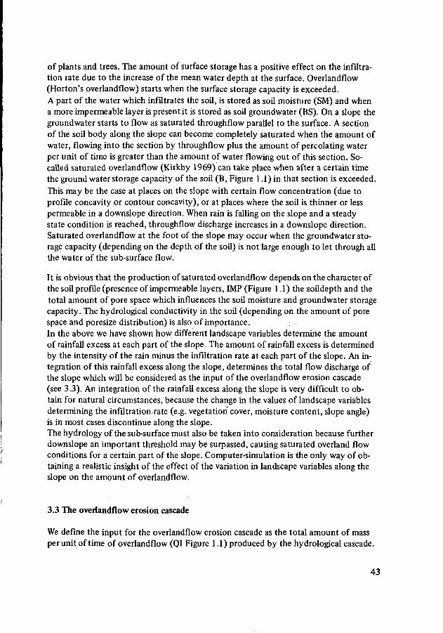
of plants and trees. The amount of surface storage has a positive effect on the infiltra-tion rate due to the increase of the mean water depth at the surface. Overlandflow(Horton's overlandflow) starts when the surface storage capacity is exceeded.A part of the water which infiltrates the soil, is stored as soil moisture (SM) and whena more impermeable layer is present it is stored as soil groundwater (BS). On a slope thegroundwater starts to flow as saturated throughflow parallel to the surface. A sectionof the soil body along the slope can become completely saturated when the amount ofwater, flowing into the section by throughflow plus the amount of percolating waterper unit of time is greater than the amount of water flowing out of this section. So-called saturated overlandflow (Kirkby 1969) can take place when after a certain timethe ground water storage capacity of the soil (B, Figure 1.1) in that section is exceeded.This may be the case at places on the slope with certain flow concentration (due toprofile concavity or contour concavity), or at places where the soil is thinner or lesspermeable in a downslope direction. When rain is falling on the slope and a steadystate condition is reached, throughflow discharge increases in a downslope direction.Saturated overlandflow at the foot of the slope may occur when the groundwater sto-rage capacity (depending on the depth of the soil) is not large enough to let through allthe water of the sub-surface flow.

It is obvious that the production of saturated overlandflow depends on the character ofthe soil profile (presence of impermeable layers, IMP (Figure 1.1) the soildepth and thetotal amount of pore space which influences the soil moisture and groundwater storagecapacity. The hydrological conductivity in the soil (depending on the amount of porespace and poresize distribution) is also of importance.In the above we have shown how different landscape variables determine the amountof rainfall excess at each part of the slope. The amount of rainfall excess is determinedby the intensity of the rain minus the infiltration rate at each part of the slope. An in-tegration of this rainfall excess along the slope, determines the total flow discharge ofthe slope which will be considered as the input of the overlandflow erosion cascade(see 3.3). An integration of the rainfall excess along the slope is very difficult to ob-tain for natural circumstances, because the change in the values of landscape variablesdetermining the infiltration rate (e.g. vegetation cover, moisture content, slope angle)is in most cases discontinue along the slope.The hydrology of the sub-surface must also be taken into consideration because furtherdownslope an important threshold may be surpassed, causing saturated overland flowconditions for a certain part of the slope. Computer-simulation is the only way of ob-taining a realistic insight of the effect of the variation in landscape variables along theslope on the amount of overlandflow.

3.3 The overlandflow erosion cascade

We define the input for the overlandflow erosion cascade as the total amount of massperunitoftime of overlandflow (QI Figure 1.1) produced by the hydrological cascade.

43

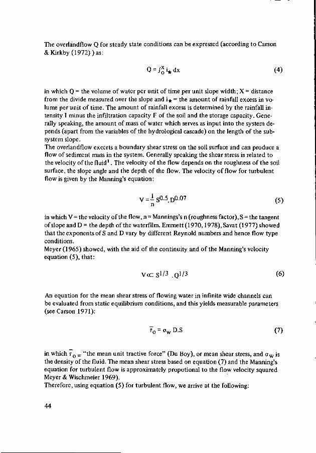
The overlàndflow Q for steady state conditions can be expressed (according to Carson&Kirkby(1972))as:

(4)

in which Q = the volume of water per unit of time per unit slope width ; X = distancefrom the divide measured over the slope and i* = the amount of rainfall excess in vo-lume per unit of time. The amount of rainfall excess is determined by the rainfall in-tensity I minus the infiltration capacity F of the soil and the storage capacity. Gene-rally speaking, the amount of mass of water which serves as input into the system de-pends (apart from the variables of the hydrological cascade) on the length of the sub-system slope.The overlândflow excerts a boundary shear stress on the soil surface and can produce aflow of sediment mass in the system. Generally speaking the shear stress is related tothe velocity of the fluid1. The velocity of the flow depends on the roughness of the soilsurface, the slope angle and the depth of the flow. The velocity of flow for turbulentflow is given by the Manning's equation:

V=ls°-5D007 (5)n v '

in which V = the velocity of the flow, n = Mannings's n (roughness factor), S = the tangentof slope and D = the depth of the waterfilm. Emmett (1970,1978), Savat (1977) showedthat the exponents of S and D vary by different Reynold numbers and hence flow typeconditions.Meyer (1965) showed, with the aid of the continuity and of the Manning's velocityequation (5), that:

(6)

An equation for the mean shear stress of flowing water in infinite wide channels canbe evaluated from static equilibrium conditions, and this yields measurable parameters(see Carson 1971):

T 0 = o w D.S (7)

in which TQ _ "the mean unit tractive force" (Du Boy), or mean shear stress, and a w isthe density of the fluid. The mean shear stress based on equation (7) and the Manning'sequation for turbulent flow is approximately propotional to the flow velocity squaredMeyer & Wischmeier 1969).Therefore, using equation (5) for turbulent flow, we arrive at the following:

44

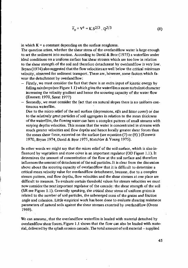
in which K = a constant depending on the surface roughness.The question arises, whether the shear stress of the overlandflow water is large enoughto set the sediment into motion. According to David & Beer (1975) a waterfilm underideal conditions on a uniform surface has shear stresses which are too low in relationto the shear strength of the soil and therefore detachment by overlandflow is very low.Bryan (1974) also suggested that the flow velocities are well below the critical minimumvelocity, observed for sediment transport. There are, however, some factors which fa-vour the detachment by overlandflow:— Firstly, we must consider the fact that there is an extra input of kinetic energy by

falling raindrops (see Figure 1.1) which gives the waterfilm a more turbulent characterincreasing the velocity gradient and hence the scouring capacity of the water flow(Emmett 1970, Savat 1977)

— Secondly, we must consider the fact that on natural slopes there is no uniform con-tinuous waterfilm.Due to the micro relief of the soil surface (depressions, rills and litter cover) or dueto the relatively great particles of soil aggregates in relation to the mean thicknessof the waterfilm, the flowing water can have a complex pattern of small streams withvarying depths velocities. This means that the water is concentrated in streams withmuch greater velocities and flow depths and hence locally greater shear forces thanthe mean shear force, excerted on the surface (see equation (7) or (8) ) (Emmett1970, Bryan 1974, David & Beer 1975, Mutchler & Young 1975).

In other words we might say that the micro relief of the soil surface, which is also in-fluenced by vegetation and stone cover is an important regulator (OD Figure 1.1). Itdetermines the amount of concentration of the flow at the soil surface and thereforeinfluences the amount of detachment of the soil particles. It is clear from the discussionabove about the scouring capacity of overlandflow that it is difficult to determine acritical mean velocity value for overlandflow detachment, because, due to a complexstream pattern, real flow depths, flow velocities and the shear stresses at one place aredifficult to measure. To evaluate certain threshold values for stream velocities we mustnow consider the next important regulator of the cascade: the shear strength of the soil(SR see Figure 1.1). Generally speaking, the critical shear stress of uniform grains isrelated to the number of soil particles, the submerged mass of the grains and frictionangle and cohesion. Little empirical work has been done to evaluate shearing resistanceparameters of natural soils against the shear stresses excerted by overlandflow (Ovens1969).

We can asssume, that the overlandflow waterfilm is loaded with material detached byoverlandflow shear forces. Figure 1.1 shows that the flow can also be loaded with mate-rial, delivered by the splash erosion cascade. The total amount of soil material — supplied

45

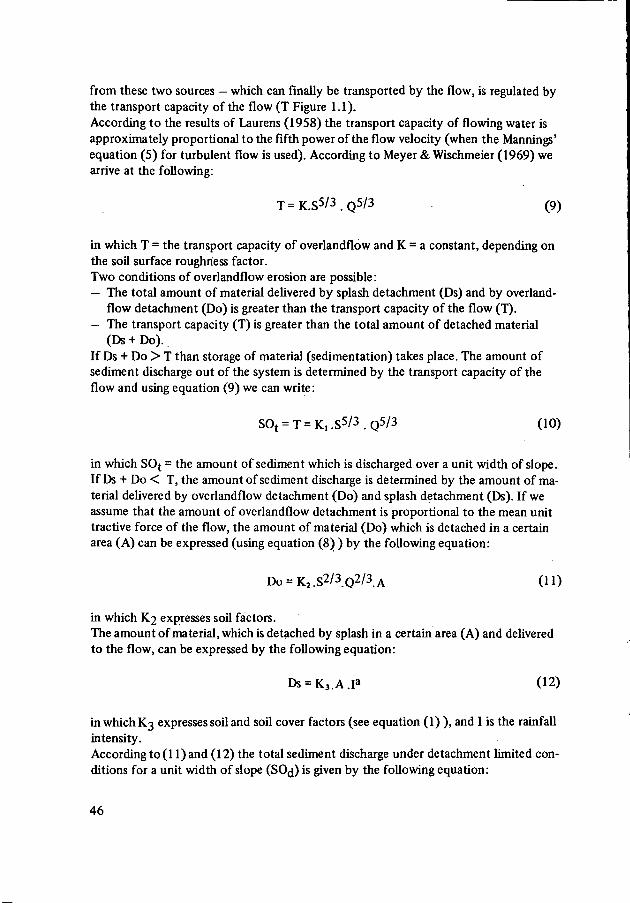
from these two sources — which can finally be transported by the flow, is regulated bythe transport capacity of the flow (T Figure 1.1).According to the results of Laurens (1958) the transport capacity of flowing water isapproximately proportional to the fifth power of the flow velocity (when the Mannings'equation (5) for turbulent flow is used). According to Meyer & Wischmeier (1969) wearrive at the following:

T = K.S5/3 . Q5/3 (9)

in which T = the transport capacity of overlandflow and K = a constant, depending onthe soil surface roughness factor.Two conditions of overlandflow erosion are possible :— The total amount of material delivered by splash detachment (Ds) and by overland-

flow detachment (Do) is greater than the transport capacity of the flow (T).- The transport capacity (T) is greater than the total amount of detached material

(Ds + Do).If Ds + Do > T than storage of material (sedimentation) takes place. The amount ofsediment discharge out of the system is determined by the transport capacity of theflow and using equation (9) we can write:

SOt = T = K,.S5 /3.Q5/3 (10)

in which SO^ = the amount of sediment which is discharged over a unit width of slope.If Ds + Do < T, the amount of sediment discharge is determined by the amount of ma-terial delivered by overlandflow detachment (Do) and splash detachment (Ds). If weassume that the amount of overlandflow detachment is proportional to the mean unittractive force of the flow, the amount of material (Do) which is detached in a certainarea (A) can be expressed (using equation (8) ) by the following equation:

DO = K 2 . S 2 / 3 . Q 2 / 3 . A (11)

in which K2 expresses soil factors.The amount of material, which is detached by splash in a certain area (A) and deliveredto the flow, can be expressed by the following equation:

Ds = K3.A.Ia (12)

in which K3 expresses soil and soil cover factors (see equation (1) ), and I is the rainfallintensity.Accordingto(l l)and (12) the total sediment discharge under detachment limited con-ditions for a unit width of slope (SOj) is given by the following equation:

46

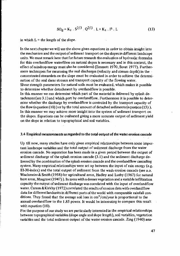
SOd = K2 . S 2 / 3 . Q 2 / 3 . L + K 3 . I a . L (13)

in which L = the length of the slope.

In the next chapter we will use the above given equations in order to obtain insight intothe mechanism and the output of sediment transport on the slopes in different landscapeunits. We must remark here that for future research the evaluation of hydraulic formulasfor thin overlandflow waterfilms on natural slopes is necessary and in this context, theeffect of raindrop energy must also be considered (Emmett 1970, Savat 1977). Further-more techniques for measuring the real discharges (velocity and stream depth) in theconcentrated streamlets on the slope must be evaluated in order to achieve the determi-nation of the real shear stresses and transport capacity of the flowing water.Shear strength parameters for natural soils must be evaluated, which makes it possibleto determine whether detachment by overlandflow is possible.In this manner we can determine which part of the material is delivered by splash de-tachment(see 3.1)and which part by overlandflow. Furthermore it is possible to deter-mine whether the discharge by overlandflow is controled by the transport capacity ofthe flow (equation (10) ) or by the total amount of detached sediments (equation (13) ).In this manner we may achieve more insight into the system of sediment transport onthe slopes. Equations can be evaluated giving a more accurate output of sediment yieldon the slope in relation to topographical and soil variables.

3.4 Empirical measurements as regarded to the total output of the water erosion cascade

Up till now, many studies have only given empirical relationships between some impor-tant landscape variables and the total output of sediment discharge from the watererosion cascade. No separation has been made in a given period between the output ofsediment discharge of the splash erosion cascade (3.1) and the sediment discharge de-livered by the combination of the splash erosion cascade and the overlandflow cascadingsystem. Many empirical relationships were set up between the input of rain energy (e.g.EI-30-index) and the total output of sediment from the wash erosion cascade (see a.o.Wischmeier&Smith(1958) for agricultural areas, Hadley and Lusby (1967) for naturalbare areas, Musgrave (1947) ). In areas with a denser vegetation and a variable infiltrationcapacity the output of sediment discharge was correlated with the input of overlandflowwater. Carson &Kirkby (1972) correlated the results of erosion data with overlandflowdata for different landunits in different parts of the world with comparable rainfall con-ditions. They found that the average soil loss in cm3 /cm/year is proportional to theannual overlandflow to the 1.85 power. It would be interesting to compare this resultwith equation (10).For the purpose of our study we are particularly interested in the empirical relationshipsbetween topographical variables (slope angle and slope length), soil variables, vegetationvariables and the total sediment output of the water erosion cascade. Zing (1940) ana-

47

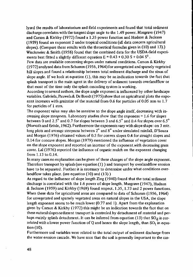
lysed the results of laboratorium and field experiments and found that total sedimentdischarge correlates with the tangent slope angle to the 1.49 power. Musgrave (1947)and Carson & Kirkby (1972) found a 1.35 power function and Hudson & Jackson(1959) found an exponent 2 under tropical conditions (all data concern agriculturalslopes). (Compare these results with the theoretical formulas given in (10) and 13).)Wischmeier & Smith (1958) found that the combined data for the USDA-field experi-ments best fitted a slightly different equation E = 0.43 + 0.30 S + 0.04 S2 .Few data are available concerning slopes under natural conditions. Carson & Kirkby(1972) analysed data from Schumm (1956,1964) for unvegetated and sparsely vegetatedhill slopes and found a relationship between total, sediment discharge and the sinus ofslope angle. If we look at equation (1), this may be an indication towards the fact thatsplash transport is the main agent in the delivery of sediment towards overlandflow orthat most of the time only the splash cascading system is working.According to several authors, the slope angle exponent is influenced by other landscapevariables. Gabriels, Pauwels& De Boodt (1975) show that on agricultural plots the expo-nent increases with grainsize of the material from 0.6 for particles of 0.05 mm to 1.7for particles of 1 mm.

The exponent value may also be sensitive to the slope angle itself, decreasing with in-creasing slope steepness. Laboratory studies show that the exponent = 1.6 for slopesbetween 0 and 2.5° and 0.7 for slopes between 3 and 6.5° and 0.4 for slopes over 6.5°(Horvath and Erode, 1962). Furthermore the exponents vary with slope shape: on 3 mtr.long plots and average steepness between 2° and 8° under simulated rainfall, D'Souzaand Morgan (1976) obtained values of 0.5 for convex slopes 0.4 for straight slopes and0.14 for concave slopes. Morgan (1979) mentioned the influence of vegetation coveron the slope exponent and reported an increase of the exponent.with decreasing grasscover. Lai (1976) reported the influence of organic mulch on the exponent changingfrom 1.13 to 0.14.In many cases no explanation can be given of these changes of the slope angle exponent.Therefore transport by splash (see equation (1) ) and transport by overlandflow erosionhave to be separated. Further it is necessary to determine under what conditions over-landflow takes place, (see equation (10) and (13) )As regard to the influence of slope length Zing (1940) found that the total sedimentdischarge is correlated with the 1.6 power of slope length. Musgrave (1947), Hudson& Jackson (1959) and Kirkby (1969) found respect. 1.35,1.73 and 2 power functions.When these data for agricultural areas are compared to data of Schumm (1956,1964)for unvegetated and sparsely vegetated areas on natural slopes in the USA, the slopelength exponent seems to be much lower (0.77 and 1). Apart from the explanationgiven by Carson & Kirkby (1972) this might be an indication towards the fact that onthese natural slopes sediment transport is controled.by detachment of material and per-haps mainly splash detachment. It can be inferred from equation (13) that SOj is cor-related with a lower power function of Q and hence the slope length, than SO^ in equa-tion (10).Furthermore soil variables were related to the total output of sediment discharge fromthe water erosion cascade. We have seen that the soil is generally important to the cas-

48

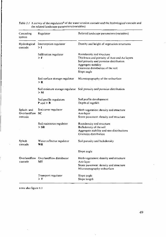
Table 3.1 A survey of the regulators3 of the water erosion cascade and the hydrological cascade andthe related landscape parameters (variables)

Cascadingsystem

Regulator Related landscape parameters (variables)

Hydrological Interception regulatorcascade > I

Density and height of vegetation structures

Infiltration regulator> F

Soil surface storage regulator> R

Rootdensity and structureThickness and porosity of Aoo and Ao layersSoil porosity and poresize distributionAggregate stabilityGrainsize distribution of the soilSlope angle

Microtopography of the soilsurface

Soil moisture storage regulator> M

Soil profile regulatorsP and > B

Splash- and Sou cover regulatorOverlandflow SCcascade

Soil porosity and poresize distribution

Soil profile developmentDepth of regolith

Herb vegetation: density and structureAoo layerStone pavement: density and structure

Splashcascade

Overlandflowcascade

Soil resistance regulator> S R

Water reflector regulatorWR

Overlandflow distributorMT

Rootdensity and structureBulkdensity of the soilAggregate stability and size distributioGrainsize distribution

Soil porosity and bulkdensity

Slope angle

Herb vegetation: density and structureAoo layerStone pavement: density and structureMicrotopography soilsurface

Transport regulator> T

Slope angleSlope length

a see also figure 1.1

49

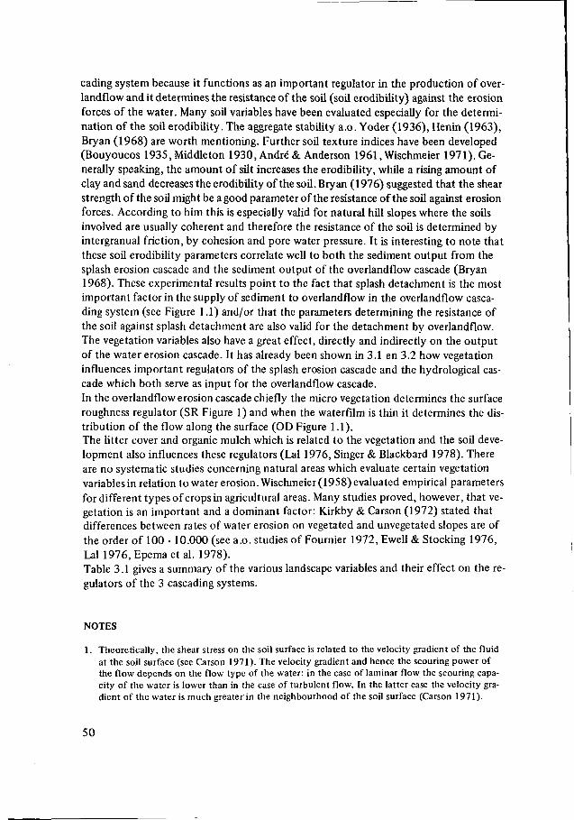
cading system because it functions as an important regulator in the production of over-landflow and it determines the resistance of the soil (soil erodibility) against the erosionforces of the water. Many soil variables have been evaluated especially for the determi-nation of the soil erodibility. The aggregate stability a.o. Yoder (1936), Henin (1963),Bryan (1968) are worth mentioning. Further soil texture indices have been developed(Bouyoucos 1935, Middleton 1930, André & Anderson 1961, Wischmeier 1971). Ge-nerally speaking, the amount of silt increases the erodibility, while a rising amount ofclayandsand decreasestheerodibility of the soil. Bryan (1976) suggested that the shearstrength of the soil might be a good parameter of the resistance of the soil against erosionforces. According to him this is especially valid for natural hill slopes where the soilsinvolved are usually coherent and therefore the resistance of the soil is determined byintergranual friction, by cohesion and pore water pressure. It is interesting to note thatthese soil erodibility parameters correlate well to both the sediment output from thesplash erosion cascade and the sediment output of the overlandflow cascade (Bryan1968). These experimental results point to the fact that splash detachment is the mostimportant factor in the supply of sediment to overlandflow in the overlandflow casca-ding system (see Figure 1.1) and/or that the parameters determining the resistance ofthe soil against splash detachment are also valid for the detachment by overlandflow.The vegetation variables also have a great effect, directly and indirectly on the outputof the water erosion cascade. It has already been shown in 3.1 en 3.2 how vegetationinfluences important regulators of the splash erosion cascade and the hydrological cas-cade which both serve as input for the overlandflow cascade.

In the overlandflow erosion cascade chiefly the micro vegetation determines the surfaceroughness regulator (SR Figure 1) and when the waterfilm is thin it determines the dis-tribution of the flow along the surface (OD Figure 1.1).The litter cover and organic mulch which is related to the vegetation and the soil deve-lopment also influences these regulators (Lai 1976, Singer & Blackbard 1978). Thereare no systematic studies concerning natural areas which evaluate certain vegetationvariables in relation to water erosion. Wischmeier (1958) evaluated empirical parametersfor different types of crops in agricultural areas. Many studies proved, however, that ve-getation is an important and a dominant factor: Kirkby & Carson (1972) stated thatdifferences between rates of water erosion on vegetated and unvegetated slopes are ofthe order of 100 - 10.000 (see a.o. studies of Fournier 1972, Ewell & Stocking 1976,Lai 1976, Epema et al. 1978).Table 3.1 gives a summary of the various landscape variables and their effect on the re-gulators of the 3 cascading systems.

NOTES

1. Theoretically, the shear stress on the soil surface is related to the velocity gradient of the fluidat the soil surface (see Carson 1971). The velocity gradient and hence the scouring power ofthe flow depends on the flow type of the water: in the case of laminar flow the scouring capa-city of the water is lower than in the case of turbulent flow. In the latter case the velocity gra-dient of the water is much greater in the neighbourhood of the soil surface (Carson 1971).

50

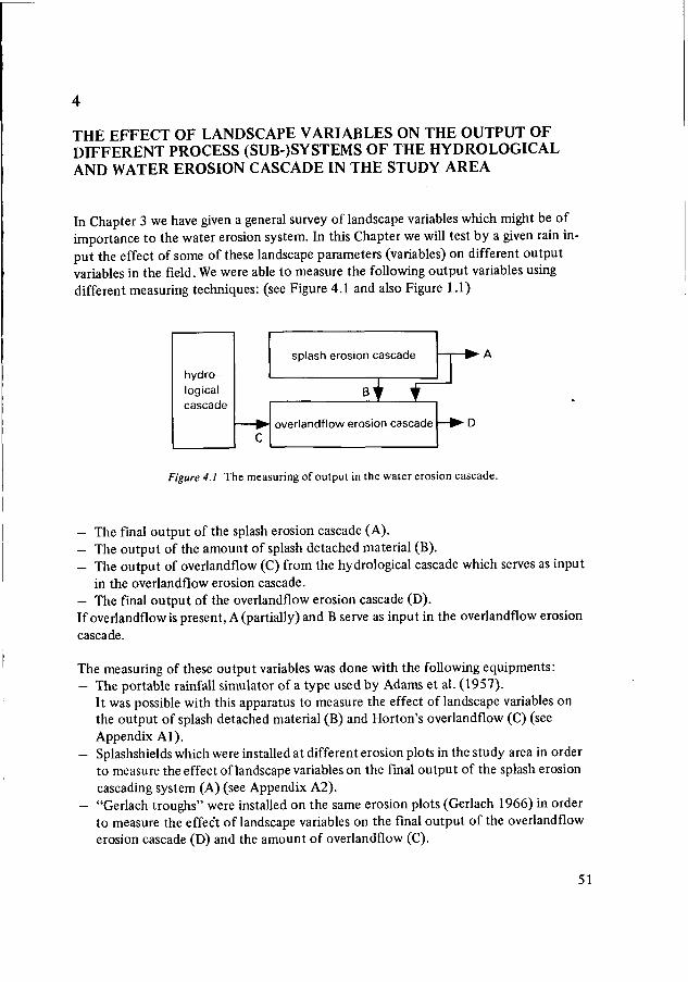
THE EFFECT OF LANDSCAPE VARIABLES ON THE OUTPUT OFDIFFERENT PROCESS (SUB-)SYSTEMS OF THE HYDROLOGICALAND WATER EROSION CASCADE IN THE STUDY AREA

In Chapter 3 we have given a general survey of landscape variables which might be ofimportance to the water erosion system. In this Chapter we will test by a given rain in-put the effect of some of these landscape parameters (variables) on different outputvariables in the field. We were able to measure the following output variables usingdifferent measuring techniques: (see Figure 4.1 and also Figure 1.1)

hydro-logicalcascade

splash erosion cascade

•+- • A

overlandflow erosion cascade

Figure 4.1 The measuring of output in the water erosion cascade.

- The final output of the splash erosion cascade (A).- The output of the amount of splash detached material (B).- The output of overlandflow (C) from the hydrological cascade which serves as input

in the overlandflow erosion cascade.- The final output of the overlandflow erosion cascade (D).If overlandflow is present, A (partially) and B serve as input in the overlandflow erosioncascade.

The measuring of these output variables was done with the following equipments:- The portable rainfall simulator of a type used by Adams et al. (1957).

It was possible with this apparatus to measure the effect of landscape variables onthe output of splash detached material (B) and Horton's overlandflow (C) (seeAppendix Al).

- Splashshields which were installed at different erosion plots in the study area in orderto measure the effect of landscape variables on the final output of the splash erosioncascading system (A) (see Appendix A2).

- "Gerlach troughs" were installed on the same erosion plots (Gerlach 1966) in orderto measure the effect of landscape variables on the final output of the overlandflowerosion cascade (D) and the amount of overlandflow (C).

51

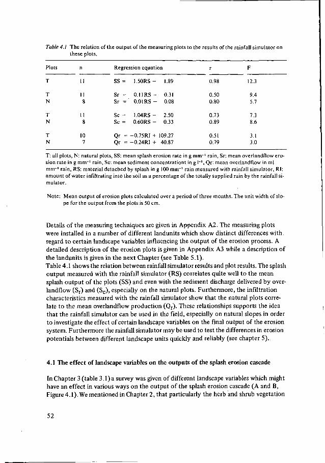
Table 4.1 The relation of the output of the measuring plots to the results of the rainfall simulator onthese plots.

Plots

T

TN

TN

TN

n

11

118

11g

107

Regression equation

SS =

Sr =Sr =

Sc =Sc =

Qr =Qr =

1.50RS -

= 0.11RS-= 0.01 R S -

1.04RS-0.60RS -

= -O.75RI += -0.24RI +

1.89

0.310.08

2.500.33

109.2740.87

r

0.98

0.500.80

0.730.89

0.510.79

F

12.3

9.45.7

7.38.6

3.13.0

T: all plots, N: natural plots, SS: mean splash erosion rate in g mm-' rain, Sr: mean overlandflow ero-sion rate in g mm"1 rain, Sc: mean sediment concentration! in g I"1, Qr: mean overlandflow in mlmm"1 rain, RS: material detached by splash in g 100 mm"1 rain measured with rainfall simulator, RI:amount of water infiltrating into the soil as a percentage of the totally supplied rain by the rainfall si-mulator.

Note: Mean output of erosion plots calculated over a period of three months. The unit width of slo-pe for the output from the plots is 50 cm.

Details of the measuring techniques are given in Appendix A2. The measuring plotswere installed in a number of different landunits which show distinct differences with,regard to certain landscape variables influencing the output of the erosion process. Adetailed description of the erosion plots is given in Appendix A3 while a description ofthe landunits is given in the next Chapter (see Table 5.1).Table 4.1 shows the relation between rainfall simulator results and plot results. The splashoutput measured with the rainfall simulator (RS) correlates quite well to the meansplash output of the plots (SS) and even with the sediment discharge delivered by over-landflow (Sr) and (Sc), especially on the natural plots. Furthermore, the infiltrationcharacteristics measured with the rainfall simulator show that the natural plots corre-late to the mean overlandflow production (Qr). These relationships supports the ideathat the rainfall simulator can be used in the field, especially on natural slopes in orderto investigate the effect of certain landscape variables on the final output of the erosionsystem. Furthermore the rainfall simulator may be used to test the differences in erosionpotentials between different landscape units quickly and reliably (see chapter 5).

4.1 The effect of landscape variables on the outputs of the splash erosion cascade

In Chapter 3 (table 3.1) a survey was given of different landscape variables which mighthave an effect in various ways on the output of the splash erosion cascade (A and B,Figure 4.1). We mentioned in Chapter 2, that particularly the herb and shrub vegetation

52

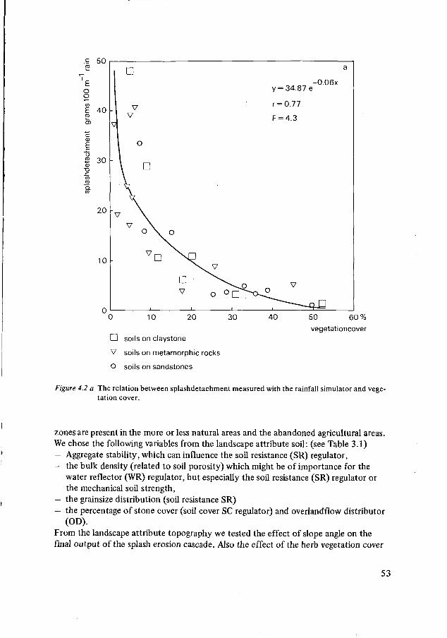
.= 50

oo

E 40 -raO)

u

u2 30

enJ5a

20 -

10 -

D

VV

o

\ D

o \

V D

O

D •V o ° D

V

r

F

"~--VV °

a

-0.06x= 34.87 e

= 0.77

= 4.3

V

o 10 20 30 40

Q soils on claystone

V soils on metamorphic rocks

O soils on sandstones

50 60 %vegetationcover

Figure 4.2 a The relation between splashdetachment measured with the rainfall simulator and vege-tation cover.

zones are present in the more or less natural areas and the abandoned agricultural areas.We chose the following variables from the landscape attribute soil: (see Table 3.1)- Aggregate stability, which can influence the soil resistance (SR) regulator,- the bulk density (related to soil porosity) which might be of importance for the

water reflector (WR) regulator, but especially the soil resistance (SR) regulator orthe mechanical soil strength,

- the grainsize distribution (soil resistance SR)- the percentage of stone cover (soil cover SC regulator) and overlandflow distributor

(OD).From the landscape attribute topography we tested the effect of slope angle on thefinal output of the splash erosion cascade. Also the effect of the herb vegetation cover

53

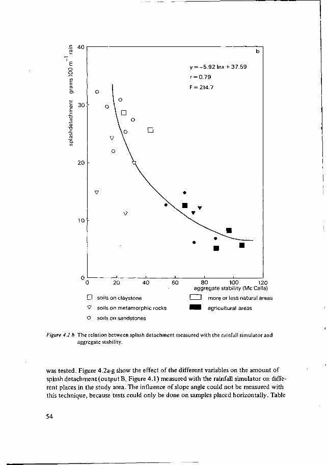
S 40

oo

O)

<u

o•2T3

30

20

10

y =-5.92 lnx +37.59

r = 0.79

F = 214.7

D

v

o 20 40

D soils on claystone

V soils on metamorphic rocks

O soils on sandstones

60 80 100 120

aggregate stability (Mc Calla)

I I more or less natural areas

1^1 agricultural areas

Figure 4.2 b The relation between splash detachment measured with the rainfall simulator andaggregate stability.

was tested. Figure 4.2a-g show the effect of the different variables on the amount ofsplash detachment (output B, Figure 4.1) measured with the rainfall simulator on diffe-rent places in the study area. The influence of slope angle could not be measured withthis technique, because tests could only be done on samples placed horizontally. Table

54

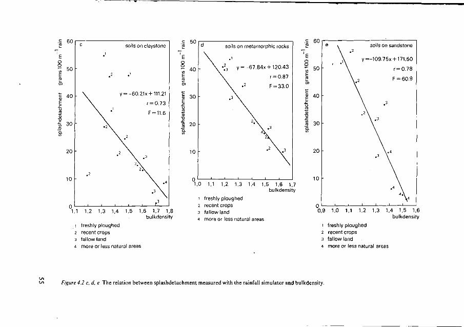
E 60

i 50

S 4 0

E

30 -

20 •

10

c

1

2

• \ V

*2

\

2

. 2

soils on claystone

= -60.21x +111.21

r = 0.73

F = 11.6

2

\

c 50

1,1 1,2 1,3 1,4 1,5 1,6 1,7 1,8bulkdensity

1 freshly ploughed2 recent crops3 fallow land4 more or less natural areas

10

soils on metamorphic rocks

,i

•23 y = -67.84x + 120.43

r = 0.87

• 2 F = 33.0

01,0 1,1 1,2 1,3 1,4 1,5 1,6 1,7

bulkdensity1 freshly ploughed2 recent crops3 fallow land4 more or less natural areas

S 60

o

! 50

| 40JZu{O

15•o

30

20

10

soils on sandstone

y—109.75x +171.50

r = 0.78

F = 60.9

0,9 1,0 1,1 1,2 1,3 1,4 1,5 1,6bulkdensity

1 freshly ploughed2 recent crops3 fallow land4 more or less natural areas

Figure 4.2 c. d, e The relation between splashdetachment measured with the rainfall simulator and bulkdensity.

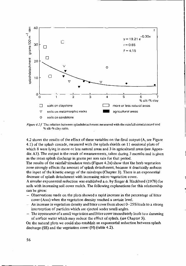
S 40

Eo°. 30

öS 20

CD

C10

DD

D

y = 19.21 e

r = 0.65

F = 4.15

-0.30x

D

o 1

• soils on claystone

V soils on metamorphic rocks

O soils on sandstone

4 5 6 7% silt/% clay

I I more or less natural areas

^ H agricultural areas

Figure 4.2 ƒ The relation between splashdetachment measured with the rainfall simulatorand and% silt-% clay ratio.

4.2 shows the results of the effect of these variables on the final output (A, see Figure4.1) of the splash cascade, measured with the splash shields on 11 erosional plots ofwhich 8 were lying in more or less natural areas and 3 in agricultural areas (see Appen-dix A3). The output is the result of measurements, taken during 3 months and is givenas the mean splash discharge in grams per mm rain for that period.The results of the rainfall'simulator tests (Figure 4.2a) show that the herb vegetationzone strongly effects the amount of splash detachment, because it drastically reducesthe input of the kinetic energy of the raindrops (Chapter 3). There is an exponentialdecrease of splash detachment with increasing micro vegetation cover.A simular exponential reduction was etablished a.o. by Singer & Blackbard (1978) forsoils with increasing soil cover mulch. The following explanations for this relationshipcan be given:— Observations made on the plots showed a rapid increase in the percentage of litter

cover (Aoo) when the vegetation density reached a certain level.— An increase in vegetation density and litter cover from about 0 - 25% leads to a strong

interception of particles which are ejected under small angles.— The appearance of a small vegetation and litter cover immediately leads to a damming

of surface water which may reduce the effect of splash, (see Chapter 3).On the natural plots we could also establish an exponential reduction between splashdischarge (SS) and the vegetation cover (H) (table 4.2).

56

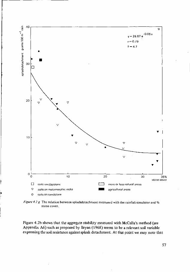
S 40

30D

10

y = 26.67 e

r = 0.79

F = 4.7

-0.06 x

0 10 20 30 35%stone cover

ÎZI soils on claystone

V soils on metamorphic rocks

O soils on sandstone

I I more or less natural areas

^ H agricultural areas

Figure 4.2 g The relation between splashdetachment measured with the rainfall simulator and %stone cover.

Figure 4.2b shows that the aggregate stability measured with McCalla's method (seeAppendix A6) such as proposed by Bryan (1968) seems to be a relevant soil variableexpressing the soil resistance against splash detachment. At this point we may note that

57

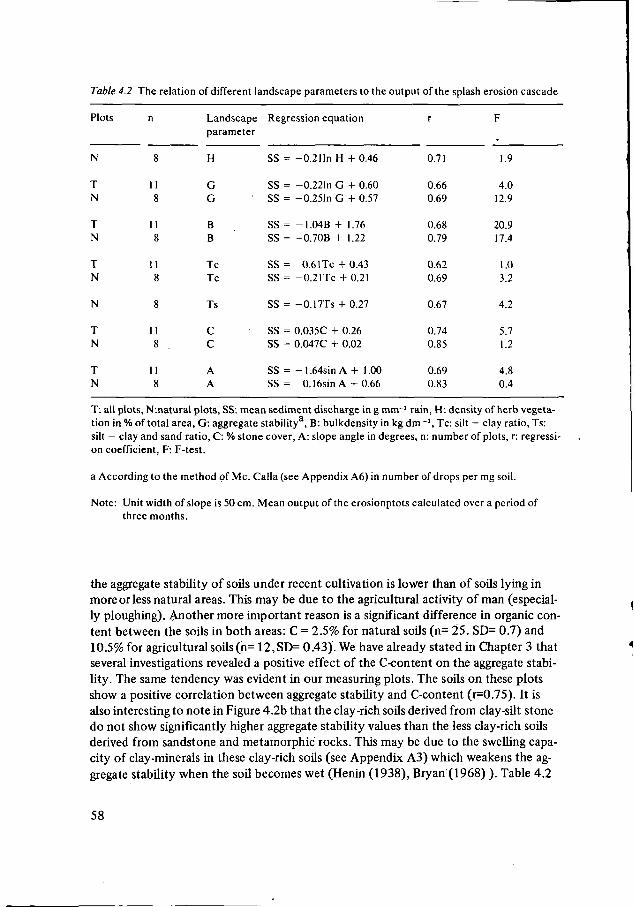
Table 4.2 The relation of different landscape parameters to the output of the splash erosion cascade

Plots

N

TN

TN

TN

N

TN

TN

n

8

118

118

118

8

118

118

Landscapeparameter

H

GG

BB

TcTc

Ts

CC

AA

Regression equation

SS = -0.21 In H +0.46

SS = -O.221n G + 0.60SS = -0.25ln G + 0.57

SS = -1.04B + 1.76SS = -0.70B + 1.22

SS = O.ólTc + 0.43SS = -0.21TC + 0.21

SS= -0.17TS + 0.27

SS = O.O35C + 0.26SS = 0.047C + 0.02

SS = -1.64sin A + 1.00SS = 0.16sin A + 0.66

r

0.71

0.660.69

0.680.79

0.620.69

0.67

0.740.85

0.690.83

F

1.9

4.012.9

20.917.4

1.03.2

4.2

5.71.2

4.80.4

T: all plots, N:natural plots, SS: mean sediment discharge in g mm"1 rain, H: density of herb vegeta-tion in % of total area, G: aggregate stabilitya, B: bulkdensity in kg dm ~3, Tc: silt — clay ratio, Ts:silt — clay and sand ratio, C: % stone cover, A: slope angle in degrees, n: number of plots, r: regressi-on coefficient, F: F-test.

a According to the method of Me. Calla (see Appendix A6) in number of drops per mg soil.

Note: Unit width of slope is 50 cm. Mean output of the erosionptots calculated over a period ofthree months.

the aggregate stability of soils under recent cultivation is lower than of soils lying inmore or less natural areas. This may be due to the agricultural activity of man (especial-ly ploughing). Another more important reason is a significant difference in organic con-tent between the soils in both areas: C = 2.5% for natural soils (n= 25. SD= 0.7) and10.5% for agricultural soils(n= 12,SD= 0.43). We have already stated in Chapter 3 thatseveral investigations revealed a positive effect of the C-content on the aggregate stabi-lity. The same tendency was evident in our measuring plots. The soils on these plotsshow a positive correlation between aggregate stability and C-content (r=0.75). It isalso interesting to note in Figure 4.2b that the clay-rich soils derived from clay-silt stonedo not show significantly higher aggregate stability values than the less clay-rich soilsderived from sandstone and metamorphic rocks. This may be due to the swelling capa-city of clay-minerals in these clay-rich soils (see Appendix A3) which weakens the ag-gregate stability when the soil becomes wet (Henin (1938), Bryan (1968).). Table 4.2

58

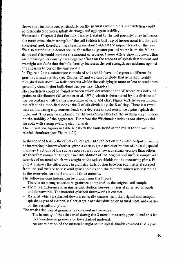
shows that furthermore, particularly on the natural erosion plots, a correlation couldbe established between splash discharge and aggregate stability.We stated in Chapter 3 that the bulk density (related to the soil porosity) may influencethe mechanical shear strength of the soil (which is built up of intergranual friction andcohesion) and, therefore, the shearing resistance against the impact forces of the rain.We also stated that a denser soil might reflect a greater part of water from the fallingdrops and this would increase the amount of erosion. Figure 4.2c-e show, however, thatan increasing bulk density has a negative effect on the amount of splash detachment andwe might conclude that the bulk density increases the soil strength or resistance againstthe shearing forces of the rain impact.In Figure 4.2c-e a subdivision is made of soils which have undergone a different de-gree in cultural activity (see Chapter 2) and we can conclude that generally freshlyploughed soils show low bulk densities whilde the soils lying in more or less natural areasgenerally show higher bulk densities (see next Chapter).No correlation could be found between splash detachment and Wischmeier's index ofgrainsize distribution (Wischmeier et al. 1971) which is determined by the division ofthe percentage of silt by the percentage of sand and clay. Figure 4.2f, however, showsthe effect of a modified index: the % of silt divided by the % of clay. There is a trendthat an increasing clay content leads to a decrease in soil resistance against splash de-tachment. This may be explained by the weakening effect of the swelling clay mineralson the stability of the aggregates. Therefore the Wischmeier index is not always validfor soils with strong swelling clay minerals.The correlation figures in table 4.2 show the same trend as the result found with therainfall simulator (see Figure 4.2f).

In the scope of testing the effect of these grainsize indices on the splash output, it wouldbe interesting to know whether, given a certain grainsize distribution of the soil, specialgrainsize fractions of the soil are more susceptible towards splash erosion than others.We therefore compared the grainsize distribution of the original soil surface sample withsamples of material which was caught in the splash shields on the measuring plots. Fi-gure 4.3 shows the differences in grainsize distribution between soil material scrapedfrom the soil surface near several splash shields and the material which was assembledin the reservoirs for the duration of three months.The following conclusions can be drawn from the Figure:— There is no strong selection in grainsize compared to the original soil sample— There is a difference in grainsize distribution between material splashed upwards

and downwards. The material splashed downwards is coarser— Material which is splashed down is generally coarser than the original soil sample;

splashed upward material is finer in grainsize distribution on natural plots and coarseron the agricultural plots.

The weak selection of grainsize is explained in two ways:— The intensity of the rain varied during the 3-month measuring period and this led

to a variation in grainsize of the splashed material.— An examination of the material caught in the splash shields revealed that a part

59

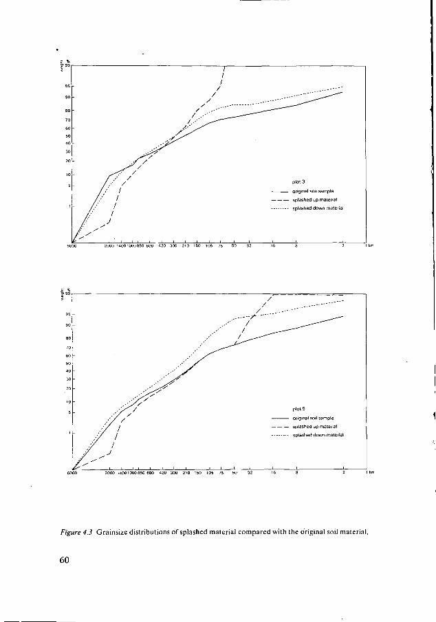
plot 3

original soil sample

splashed up material

splashed down material

2000 14001000850 600 420 300 210 150 105 75

plot 5

original s

splashed up material

splashed down material

2000 14001000850 600 420 300 210 150 105 75

Figure 4.3 Grainsize distributions of splashed material compared with the original soil material.

60

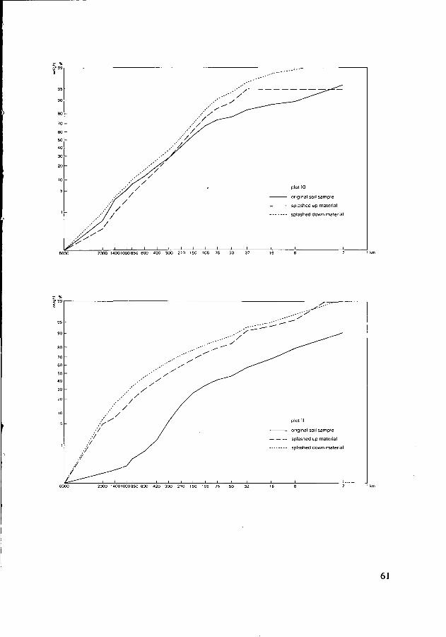
plot 10

original soil sample

splashed up material

- - splashed down material

2000 14001000850 600 420 300 210 150

-

-

-

//,'/

y/

./ _ ^ -

x 'x'

x '

.--' / /

••' / /

• / /x' /

/

/

/

yi i

plot 11

" original son sampiesplashed up material

i i i i i i

2000 14001000850 600 420 300 210 150 105 75

61

-

, - - • ' /

• - • • • • • /

- '

/

' /

/

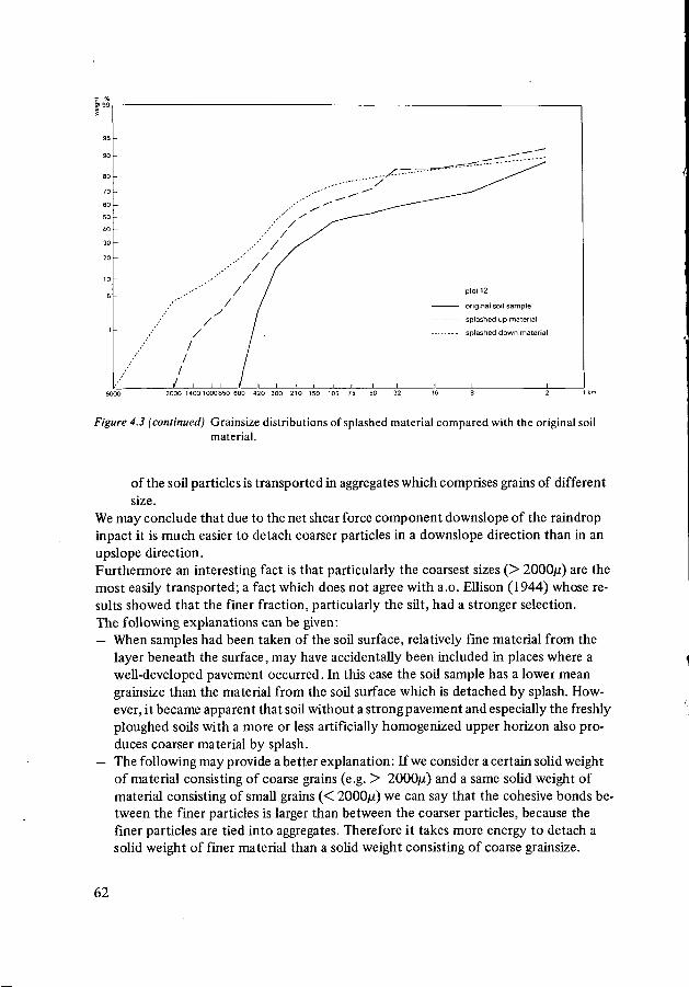
s. — — • — • — • " r f ^ ^

plol 12

splashed up material

splashed down material

2000 1400 1000850 600 420 300 210 150 105 75 50 32

Figure 4.3 (continued) Grainsize distributions of splashed material compared with the original soilmaterial.

of the soil particles is transported in aggregates which comprises grains of differentsize.

We may conclude that due to the net shear force component downslope of the raindropinpact it is much easier to detach coarser particles in a downslope direction than in anupslope direction.Furthermore an interesting fact is that particularly the coarsest sizes Ç> 2000/z) are themost easily transported; a fact which does not agree with a.o. Ellison (1944) whose re-sults showed that the finer fraction, particularly the silt, had a stronger selection.The following explanations can be given:— When samples had been taken of the soil surface, relatively fine material from the

layer beneath the surface, may have accidentally been included in places where awell-developed pavement occurred. In this case the soil sample has a lower meangrainsize than the material from the soil surface which is detached by splash. How-ever, it became apparent that soil without a strong pavement and especially the freshlyploughed soils with a more or less artificially homogenized upper horizon also pro-duces coarser material by splash.

— The following may provide a better explanation: If we consider a certain solid weightof material consisting of coarse grains (e.g. > 2000/z) and a same solid weight ofmaterial consisting of small grains (< 2000/z) we can say that the cohesive bonds be-tween the finer particles is larger than between the coarser particles, because thefiner particles are tied into aggregates. Therefore it takes more energy to detach asolid weight of finer material than a solid weight consisting of coarse grainsize.

62

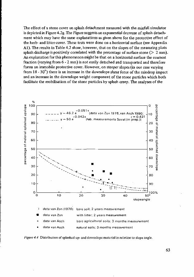
The effect of a stone cover on splash detachment measured with the rainfall simulatoris depicted in Figure 4.2g. The Figure suggests an exponential decrease of splash detach-ment which may have the same explanations as given above for the protective effect ofthe herb- and litter-cover. These tests were done on a horizontal surface (see AppendixAl). The results in Table 4.2 show, however, that on the slopes of the measuring plotssplash discharge is positively correlated with the percentage of surface stone (> 2 mm).An explanation for this phenomenon might be that on a horizontal surface the coarsestfraction (varying from 6 - 2 mm) is not easily detached and transported and thereforeforms an immobile protective cover. However, on steeper slopes (in our case varyingfrom 18 - 30°) there is an increase in the downslope shear force of the raindrop impactand an increase in the downslope weight component of the stone particles which bothfacilitate the mobilisation of the stone particles by splash creep. The analyses of the

-0.051Xy = 46.2 e (data van Zon 1976, van Asch 1980; -

-0.042X r = 0.42)y = 50 e (lab. measurements Savat (in prep.))

40 50°slopeangle

100%

• data van Zon (1976)- bare soil; 2 years measurement

• data van Zon with litter; 2 years measurement

o data van Asch bare agricultural soils; 3 months measurement

• data van Asch natural soils; 3 months measurement

Figure 4.4 Distribution of splashed up- and downslope material in relation to slope angle.

63

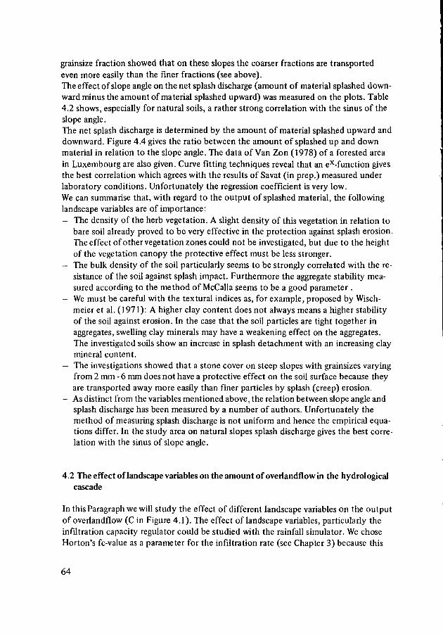
grainsize fraction showed that on these slopes the coarser fractions are transportedeven more easily than the finer fractions (see above).The effect of slope angle on the net splash discharge (amount of material splashed down-ward minus the amount of material splashed upward) was measured on the plots. Table4.2 shows, especially for natural soils, a rather strong correlation with the sinus of theslope angle.The net splash discharge is determined by the amount of material splashed upward anddownward. Figure 4.4 gives the ratio between the amount of splashed up and downmaterial in relation to the slope angle. The data of Van Zon (1978) of a forested areain Luxembourg are also given. Curve fitting techniques reveal that an ex-function givesthe best correlation which agrees with the results of Savat (in prep.) measured underlaboratory conditions. Unfortunately the regression coefficient is very low.We can summarise that, with regard to the output of splashed material, the followinglandscape variables are of importance:— The density of the herb vegetation. A slight density of this vegetation in relation to

bare soil already proved to be very effective in the protection against splash erosion.The effect of other vegetation zones could not be investigated, but due to the heightof the vegetation canopy the protective effect must be less stronger.

— The bulk density of the soil particularly seems to be strongly correlated with the re-sistance of the soil against splash impact. Furthermore the aggregate stability mea-sured according to the method of McCalla seems to be a good parameter .

— We must be careful with the textural indices as, for example, proposed by Wisch-meier et al. (1971): A higher clay content does not always means a higher stabilityof the soil against erosion. In the case that the soil particles are tight together inaggregates, swelling clay minerals may have a weakening effect on the aggregates.The investigated soils show an increase in splash detachment with an increasing claymineral content.

— The investigations showed that a stone cover on steep slopes with grainsizes varyingfrom 2 mm - 6 mm does not have a protective effect on the soil surface because theyare transported away more easily than finer particles by splash (creep) erosion.

— As distinct from the variables mentioned above, the relation between slope angle andsplash discharge has been measured by a number of authors. Unfortunately themethod of measuring splash discharge is not uniform and hence the empirical equa-tions differ. In the study area on natural slopes splash discharge gives the best corre-lation with the sinus of slope angle.

4.2 The effect of landscape variables on the amount of overlandflow in the hydrologicalcascade

In this Paragraph we will study the effect of different landscape variables on the outputof overlandflow (C in Figure 4.1). The effect of landscape variables, particularly theinfiltration capacity regulator could be studied with the rainfall simulator. We choseHorton's fc-value as a parameter for the infiltration rate (see Chapter 3) because this

64

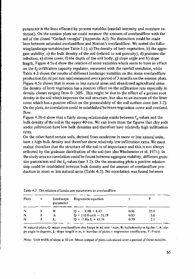
parameter is the least effected by process variables (rainfall intensity and moisture va-riation). On the erosion plots we could measure the amount of overlandflow with theaid of the closed "Gerlach troughs" (Appendix A2). No distinction could be madehere between saturated overlandflow and Horton's overlandflow. We tested the follo-wing landscape variables (see Table 3.1): a) The density of herb vegetation, b) the aggre-gate stability, c) the bulk density of the soil (related to soil porosity), d) grainsize dis-tribution, e) stone cover, f) the depth of the soil body, g) slope angle and h) slopelength. Figure 4.5a-d show the relation of some variables which seem to have an effecton the fc-infiltration capacity regulator, measured with the rainfall simulator, whileTable 4.3 shows the results of different landscape variables on the mean overlandflowproduction (in ml per mm rain) measured over a period of 3 months on the erosion plots.Figure 4.5a shows that in more or less natural areas and abandoned agricultural areasthe density of herb vegetation has a positive effect on the infiltration rate especially indensity classes ranging from 0 - 30%. This might be due to the effect of a greater rootdensity in the soil which improves the soil structure, but also to an increase of the littercover which has a positive effect on the permeability of the soil surface zone (see 3.2).On the plots, no correlation could be established between vegetation cover and overland-flow.

Figure 4.5b-d show that a fairly strong relationship exists between fc-values and thebulk density of the soil in the upper 40 cm. We can learn from the figures that clay soilsunder cultivation have low bulk densities and therefore have relatively high infiltrationrates.On the other hand certain soils, derived from sandstone in more or less natural units,have a high bulk density and therefore show relatively low infiltration rates. We mustrealize therefore that the structure of the soil is of importance and this is not alwaysreflected by the grainsize distribution of the soil (see also Wischmeier et al. 1971). Inthe study area no correlation could be found between aggregate stability, different grain-size parameters and the fc-values (see 3.2). On the measuring plots a positive relation-ship could be established between bulk density and the amount of overlandflow pro-duction in more or less natural areas (Table 4.3). No correlation was found between

Table 4.3

Plots

NNN

The

n

888

relation of landscape parameters to overlandflow

Landscapeparameter

BAL

Regression equation

Q = -9.9B + 8.43Q = 110.9sinA -33.19Q = -7.61n L + 43.74

r

0.860.850.70

F

25.03.62.1

N: natural plots, Q: mean overlandflow discharge in ml mm"1 rain, B: bulkdensity in kg dm"3, A: slo-pe angle in degrees, L: slope length in m, n: number of plots, r: regression coefficient, F: F-test.

Note: Unit width of slope is 50 cm. Mean output of plots calculated over a period of three months.

65

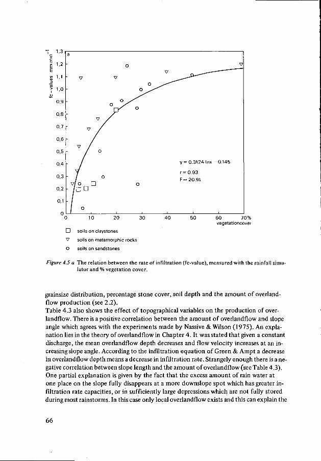
7 1.3

30 40 50 60 70%vegetationcover

D soils on claystones

V soils on metamorphic rocks

O soils on sandstones

Figure 4.5 a The relation between the rate of infiltration (fc-value), measured with the rainfall simu-lator and % vegetation cover.

grainsize distribution, percentage stone cover, soil depth and the amount of overland-flow production (see 2.2).Table 4.3 also shows the effect of topographical variables on the production of over-landflow. There is a positive correlation between the amount of overlandflow and slopeangle which agrees with the experiments made by Nassive & Wilson (1975). An expla-nation lies in the theory of overlandflow in Chapter 4. It was stated that given a constantdischarge, the mean overlandflow depth decreases and flow velocity increases at an in-creasing slope angle. According to the infiltration equation of Green & Ampt a decreasein overlandflow depth means a decrease in infiltration rate. Strangely enough there is a ne-gative correlation between slope length and the amount of overlandflow (see Table 4.3).One partial explanation is given by the fact that the excess amount of rain water atone place on the slope fully disappears at a more downslope spot which has greater in-filtration rate capacities, or in sufficiently large depressions which are not fully storedduring most rainstorms. In this case only local overlandflow exists and this can explain the

66

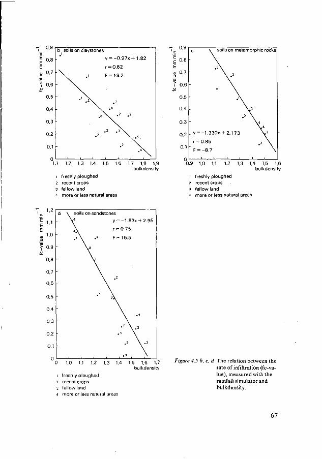
b soils on claystones soils on metamorphic rocks

1,1 1.2 1,3 1,4 1,5 1,6 1,7 1,8 1,9bulkdensity

1 freshly ploughed2 recent crops3 fallow land4 more or less natural areas

0,9 1,0 1.1 1,2 1,3 1,4 1,5 1.6bulkdensity

1 freshly ploughed2 recent crops3 fallow land4 more or less natural areas

1 . *

1,1

1.0

0.9

0.8

0,7

0,6

0,5

0,4

0,3

0,2

0,1

n

d

•

-

•

\ soils on sandstones

Y y

4\ '

\ .

i i « i

= -1.83x + 2.95

= 0.75

= 16.5

\\ •"

.4 \

.2 \ .3

0 1,0 1,1 1,2 1,3 1,4 1,5 1,6 1,7bulkdensity

1 freshly ploughed2 recent crops3 fallow land4 more or less natural areas

Figure 4.5 b, c, d The relation between therate of infiltration (fc-va-lue), measured with therainfall simulator andbulkdensity.

67

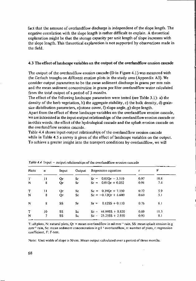
fact that the amount of overlandflow discharge is independent of the slope length. Thenegative correlation with the slope length is rather difficult to explain. A theoreticalexplanation might be that the storage capacity per unit length of slope increases withthe slope length. This theoretical explanation is not supported by observations made inthe field.

4.3 The effect of landscape variables on the output of the overlandflow erosion cascade

The output of the overlandflow erosion cascade (D in Figure 4.1) was measured withthe Gerlach troughs on different erosion plots in the study area (Appendix A3). Weconsider output parameters to be the mean sediment discharge in grams per mm rainand the mean sediment concentration in grams per liter overlandflow water calculatedfrom the total output of a period of 3 months.The effect of the following landscape parameters were tested (see Table 3.1): a) thedensity of the herb vegetation, b) the aggregate stability, c) the bulk density, d) grain-size distribution parameters, e) stone cover, f) slope angle, g) slope length.Apart from the effect of these landscape variables on the overlandflow erosion cascade,we are interested in the input-output relationships of the overlandflow erosion cascade orin other words: the effect of the hydrological cascade and the splash erosion cascade onthe overlandflow erosion cascade.Table 4.4 shows input-output relationships of the overlandflow erosion cascadewhile in Table 4.5 a survey is given of the effect of landscape variables on the output.To achieve a greater insight into the transport conditions by overlandflow, we will

Table 4.4 Input — output relationships of the overlandflow erosion cascade

Plots

TN

TN

N

TN

n

118

118

8

107

Input

QrQr

QrQr

SS

ssSS

Output

SrSr

ScSc

Sr

ScSc

Regression equation

Sr =Sr =

Sc =Sc =

Sr =

Sc =Sc =

0.03Qr-3.5100.01 Q r + 0.032

O.39Qr + 7.150-0.12Qr + 6.600

0.12SS + 0.110

44.89SS + 0.82025.25SS + 2.930

r

0.970.91

0.720.69

0.76

0.890.93

F

18.87.4

5.95.1

6.1

11.38.1

T: all plots, N: natural plots, Qr = mean overlandflow in ml mrrr' rain, SS: mean splash erosion in gmm"1 rain, Sc: mean sediment concentration in g h' overlandflow, n: number of plots, r: regressioncoefficient, F: F-test.

Note: Unit width of slope is 50 cm. Mean output calculated over a period of three months.

68

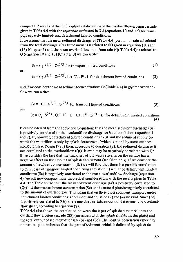
compare the results of the input-output relationships of the overlandflow erosion cascadegiven in Table 4.4 with the equations evaluated in 3.3 (equations 10 and 13) for trans-port capacity limited- and detachment limited conditions.If we assume that the mean sediment discharge Sr (Table 4.4) per mm of rain calculatedfrom the total discharge after three months is related to SO given in equation (10) and(13) (Chapter 3) and the mean overlandflow in ml/mm rain (Qr Table 4.4) is related toQ (equation 10 and 13) (Chapter 3) we can write:

Sr = Ci .S 5 / 3 . Qr5/3 for transport limited conditions (1)

Sr = C2.S2/3 . Qr2/3 . L + C3 . Ia . L for detachment limited conditions (2)or:

and if we consider the mean sediment concentrations Sc (Table 4.4) in gr/liter overland-flow we can write :

Sc = C] . S5 /3 . Qr2/3 for transport limited conditions (3)or:

Sc = O>. S 2 / 3 . Qr"1/3 . L + C3 . I a . Qr"1 . L for detachment limited conditions(4)

It can be inferred from the above given equations that the mean sediment discharge (Sr)is positively correlated to the overlandflow discharge for both conditions (equation 1and 2). If, however, detachment limited conditions exist and the sediment supply to-wards the waterfilms is only by splash detachment (which is stated by some authors,a.o.Mutchler& Young 1975) then, according to equation (2), the sediment discharge isnot correlated to the overlandflow (Qr). It even may be negatively correlated with Qrif we consider the fact that the thickness of the water streams on the surface has anegative effect on the amount of splash detachment (see Chapter 3). If we consider theamount of sediment concentration (Sc) we will find that there is a possible correlationto Qr in case of transport limited conditions (equation 3) while for detachment limitedconditions (Sc) is negatively correlated to the mean overlandflow discharge (equation4). We will now compare these theoretical considerations with the results given in Table4.4. The Table shows that the mean sediment discharge (Sr) is positively correlated to(Qr) but the mean sediment concentration (Sc) on the natural plots is negatively correlatedto the amount of overlandflow. This means that on these plots sediment transport underdetachment limited conditions is dominant and equation (2) and (4) are valid. Since (Sr)is positively correlated to (Qr), there must be a certain amount of detachment by overland-flow shear, according to equation (2).Table 4.4 also shows the correlation between the input of splashed material into theoverlandflow erosion cascade (SS) (measured with the splash shields on the plots) andthe total output of sediment discharge (Sr) and (Sc). The positive correlation especiallyon natural plots indicates that the part of sediment, which is delivered by splash de-

69

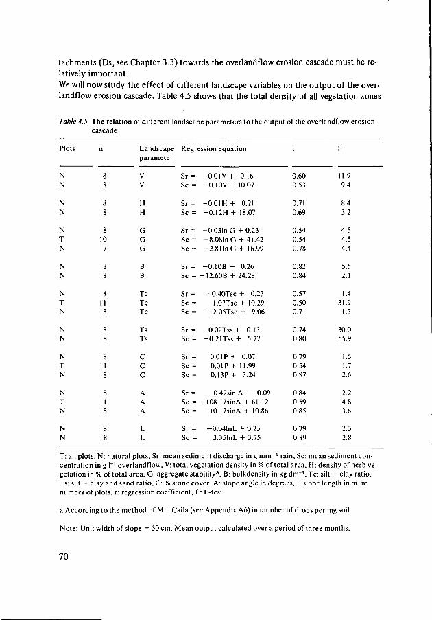
tachments (Ds, see Chapter 3.3) towards the overlandflow erosion cascade must be re-latively important.

We will now study the effect of different landscape variables on the output of the over-landflow erosion cascade. Table 4.5 shows that the total density of all vegetation zones

Table 4.5 The relation of different landscape parameters to the output of the overlandflow erosioncascade

Plots

NN

NN

NTN

NN

NTN

NN

NTN

NTN

NN

n

88

88

8107

88

8118

88

8118

8II8

88

Landscapeparameter

VV

HH

GGG

BB

TeTeTe

TsTs

CCC

AAA

LL

Regression equation

Sr =Sc =

Sr =Sc =

Sr =Sc =Sc =

Sr =Sc =

Sr =Sc =Sc =

Sr =Sc =

Sr =Sc =Sc =

Sr =Sc =Sc =

Sr =Sc =

-0.01V + 0.16-0.10V + 10.07

-0.01 H + 0.21-0.12H + 18.07

-0.03ln G + 0.23-8.08lnG +41.42-2.81lnG + 16.99

-0.10B + 0.26-12.60B + 24.28

-0.40TSC + 0.23I.07Tsc + 10.29

-12.O5TSC+ 9.06

-0.02TSS + 0.13-0.21TSS+ 5.72

0.01 P + 0.070.01 P + 11.990.13P+ 3.24

0.42sin A - 0.09-108.17sinA + 61.12-10.17sinA + 10.86

-0.041nL + 0.233.351nL + 3.75

r

0.600.53

0.710.69

0.540.540.78

0.820.84

0.570.500.71

0.740.80

0.790.540.87

0.840.590.85

0.790.89

F

11.99.4

8.43.2

4.54.54.4

5.52.1

1.431.9

1.3

30.055.9

1.51.72.6

2.24.83.6

2.32.8

T: all plots, N: natural plots, Sr: mean sediment discharge in g mm ~' rain, Sc: mean sediment con-centration in g 1~' overlandflow, V: total vegetation density in % of total area. H: density of herb ve-getation in % of total area, G: aggregate stability3, B: bulkdensity in kg dm"', Tc: silt - clay ratio,Ts: silt — clay and sand ratio, C: % stone cover. A: slope angle in degrees, L slope length in m, n:number of plots, r: regression coefficient, F: F-test

a According to the method of Me. Calla (see Appendix A6) in number of drops per mg soil.

Note: Unit width of slope = 50 cm. Mean output calculated over a period of three months.

70

(shrubs, trees and herbs) (V) is weakly correlated to the amount of sediment discharge,while there is a stronger correlation to the density of herb vegetation (H). We must con-sider the fact that the density of shrub- and tree vegetation is rather difficult to estimate.However, the stronger correlation of especially the herb vegetation density in the neigh-bourhood of measuring troughs might indicate that a) herb vegetation is the most ef-fective zone as protection against overlandflow detachment and splash detachment, b)the Gerlach troughs are fed by local overlandflow and the related sediment discharge(see 4.2).The correlation of different soil variables with the amount of sediment discharge or se-diment concentration in Table 4.5 shows that aggregate stability (G) and bulk density(B) are important factors which must influence the soil resistance regulator of the over-landflow erosion system. In the foregoing paragraph, we found that an increasing bulk-density increases the amount of overlandflow, which means an increase in shear stressof the water. This obiously did not have a positive effect on the amount of sediment dis-charge (Sr, Sc; see Table 4.5). The following explanations can be given:- The resistance of the soil against detachment by splash and overlandflow shear, de-

creases with increasing bulkdensity.— Detachment by overlandflow shear is of minor importance in the overlandflow ero-

sion system, in comparison with detachment by splash.We can conclude, if we regard the %silt/clay (Tc) and the %silt/sand + clay indices (Ts)that the clay content has a negative effect on the soil resistance. As was stated in Chap-ter 4.1, this may be explained by the weakening effect of swelling clay minerals on theaggregate stability. An interesting fact is that the landscape variables influencing the (SR)regulator in the splash erosion cascade, also have an effect on the output of the overland-flow erosion cascade (see 4.1). For example the aggregate stability, measured with MeCalla's raindrop impact test (see Appendix A6), is a typical soil resistance factor in splashdetachment. When we look at the textural indices we can establish that it is not theamount of silt (which normally is most easily detached by overlandflow) that has a po-sitive effect on the sediment discharge, but, on the contrary, the amount of clay whichtends to reduce the stability of the aggregates in these soils. We may therefore suggestthat an important part of the sediment delivered to the overlandflow waterfilm is doneby splash detachment, as was stated a.o. by Mutchler and Young (1975).This was also proved by the fact that there is a positive correlation between the totalamount of splash discharge measured in the plots and the mean sediment concentration(see Table 4.4).In Table 4.5 the effect of surface stones (C) on the amount of sediment discharge andconcentration is also given. An interesting fact is that the amount of surface stones has apositive effect on the sediment discharge and concentration. In Chapter 3 it was statedthat a stone cover can increase the surface roughness and hence decrease the shearingforce of the water (equation (8), Chapter 3). This will lead to a negative correlation be-tween sediment output and % surface stones. If, however, the waterfilm is thin in com-parison to the surface stones, the water is more concentrated in streams with higherflow velocities and flow depths and this increases the shearing force of the water (Chap-ter 3). In our view a better explanation is that especially on steep slopes the surface

71

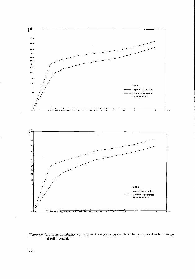
2000 1400 1000850 600 420 300 210 150 105 75 50

plot 3

Original soil sample

sediment transportedby overlandf low

2000 14001000850 600 420 300 210 150 105 75

Figure 4.6 Grainsize distributions of material transported by overland flow compared with the origi-nal soil material.

72

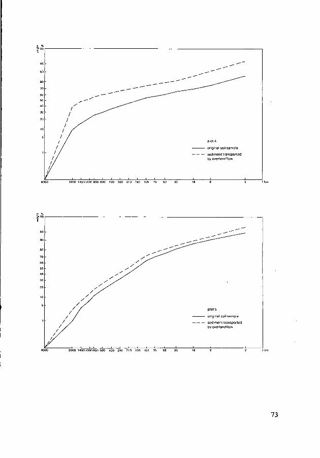
plot 4

original soil sample

sediment transportedby overlandflow

2000 14001000 850 600 420 300 210 150 105 75

2000 14001000 850 600 420 300 210 150 105 75 50

73

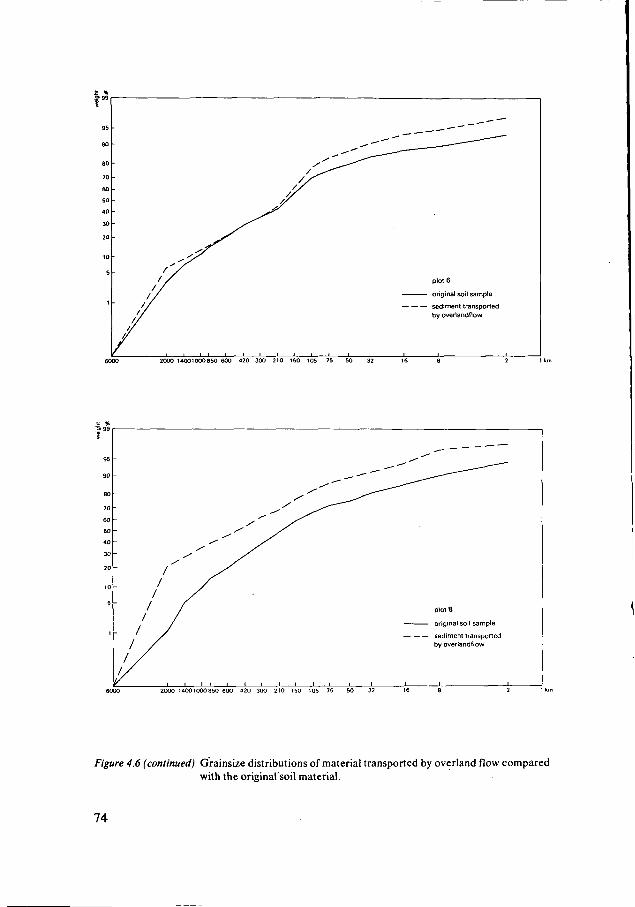
S3

95

90

80

70

60

50

40

30

20

10

5

1

,yr //

'/

//

/

plot 6

sediment transportedby overlandflow

2000 14001000850 600 420 300 210 150 105 75 50

-

-

-

-

/

/ //

s*x '

/ /

1 f! /1 ///

1 1 L_l 1 ! 1 1

plot 8

sediment transportedby overlandflow

i i •

2000 14001000850 600 420 300 210 150 105 75

Figure 4.6 (continued) Grainsize distributions of material transported by overland flow comparedwith the originalsoil material.

74

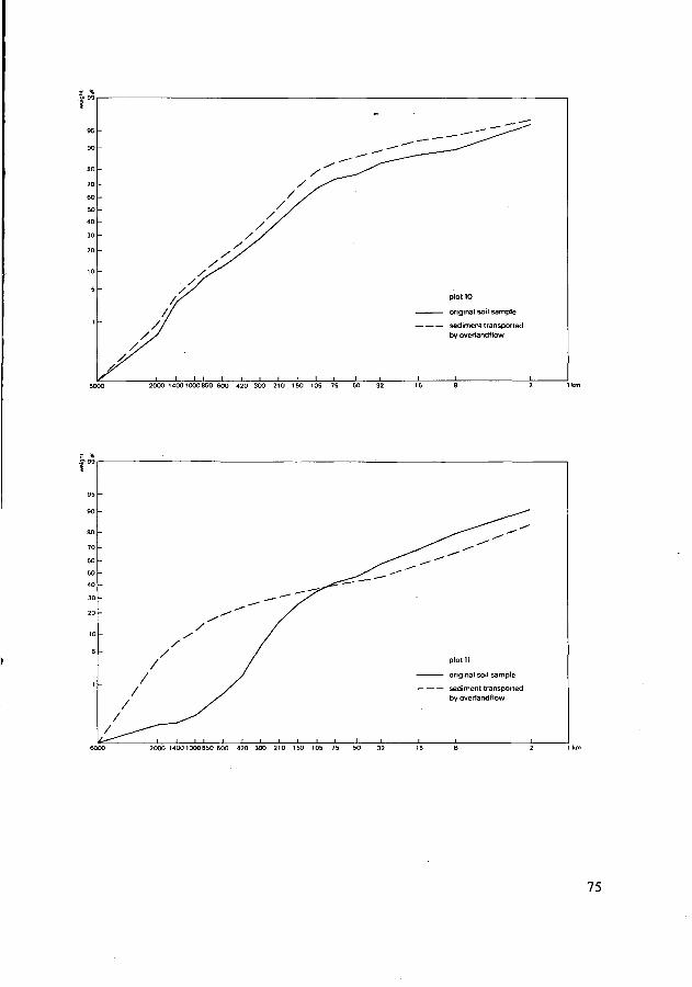
95

90

80

70

60

50

40

30

20

10

5

1

-

-

-

-

-

-

-

-

-

-

y

//1

i i i i

/ /

/ /

/ /

1 1 1 1 1 1 1

plot 10

sediment transportedby overlandflow

i i i i

2000 14001000850 600 420 300 210 150 105 75

2000 1400 1000350 600 420 300 210 150 105 75

75

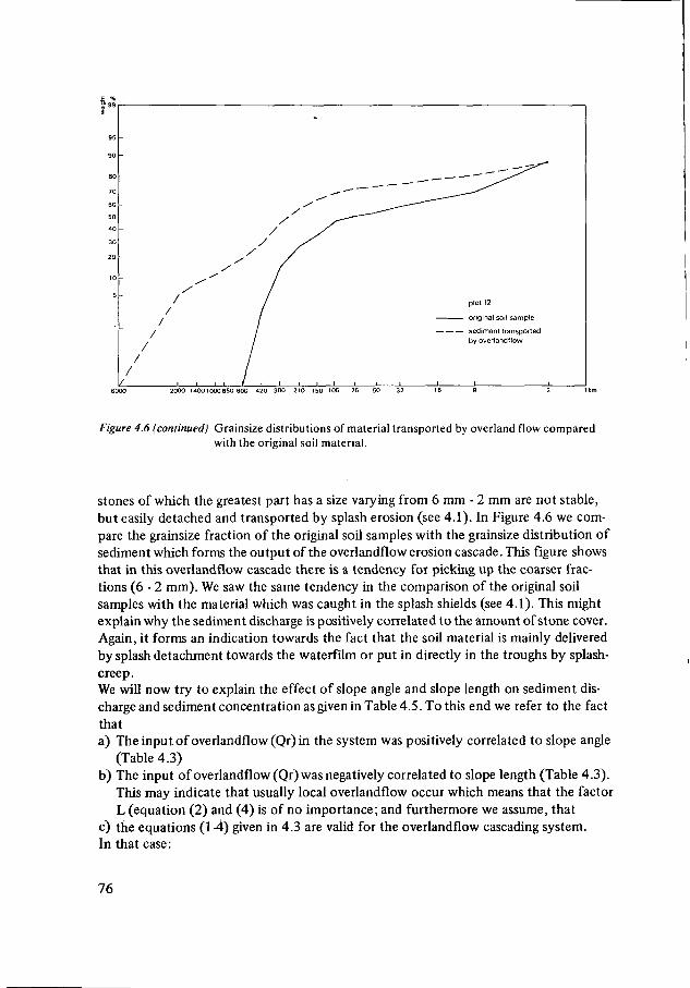
y

plot 12

original soil sample

sediment transportedby overlandflow

2000 14001000 8S0 600 420 300 210 150 105 75 50 32

Figure 4.6 (continued) Grainsize distributions of material transported by overland flow comparedwith the original soil material.

stones of which the greatest part has a size varying from 6 mm - 2 mm are not stable,but easily detached and transported by splash erosion (see 4.1). In Figure 4.6 we com-pare the grainsize fraction of the original soil samples with the grainsize distribution ofsediment which forms the output of the overlandflow erosion cascade. This figure showsthat in this overlandflow cascade there is a tendency for picking up the coarser frac-tions (6 - 2 mm). We saw the same tendency in the comparison of the original soilsamples with the material which was caught in the splash shields (see 4.1). This mightexplain why the sediment discharge is positively correlated to the amount of stone cover.Again, it forms an indication towards the fact that the soil material is mainly deliveredby splash detachment towards the waterfilm or put in directly in the troughs by splash-creep.We will now try to explain the effect of slope angle and slope length on sediment dis-charge and sediment concentration as given in Table 4.5. To this end we refer to the factthata) Theinputof overlandflow (Qr) in the system was positively correlated to slope angle

(Table 4.3)b) The input of overlandflow (Qr) was negatively correlated to slope length (Table 4.3).

This may indicate that usually local overlandflow occur which means that the factorL (equation (2) and (4) is of no importance; and furthermore we assume, that

c) the equations (1-4) given in 4.3 are valid for the overlandflow cascading system.In that case :

76

1. The positive correlation of the mean sediment discharge to the slope angle is ex-plained by a) and equation (1) or (2)

2. The negative correlation of the mean sediment discharge to the slope length is ex-plained by b) and equation (1) or (2)

3. The negative correlation of the mean sediment concentration to the slope angle isexplained by a) and equation (4)

4. The positive correlation of the mean sediment concentration to the slope length maybe explained by b) and equation (4).

We may conclude that the relationship of both the output of mean sediment dischargeand mean sediment concentration to slope angle and slope length can be explained bythe conditions in which the sediment output is controled by detachment of splash andoverlandflow shear and not by the transport capacity of the flow.

4.4 Summary and conclusions

In this chapter we have analyzed the effect of different landscape variables on the out-put of the water erosion cascade. On the erosion plots we were able to measure the finaloutput of the splash and overlandflow cascade under natural conditions. With the aidof the portable rainfall simulator we could test, over a larger area, the effect of certainlandscape variables on the output of the amount of detached material and the infil-tration regulator of the hydrological cascade. The relationships between landscapevariables and the output of the rainfall simulator are important since we could prove thatthe amount of splash detachment and the infiltration capacity correlate strongly to re-spectively the mean output of the water erosion cascade and to the amount of overland-flow measured on the plots.

We found that the density of the micro-vegetation, the aggregate stability and thestone cover pavements have a relatively strong effect on the outputs of the watererosion cascade. We could establish that the stone pavement with gravel, varying in sizefrom 6 - 2 mm, has a protective effect on a horizontal surface, but on steep slopes (20 -30°) the gravel is easily transported by splash and overlandflow processes.The bulk density and the soil texture have also an effect on the output of the cascade. Wecould establish that particularly the bulk density, which must be related to the mecha-nical strength of the soil, shows strong correlations with output of splash and overland-flow erosion and, therefore seems to be a good parameter for the determination ofthe erodibility of the soil. The textural indices seem to be of lesser importance. Theamount of clay particularly seems to have a negative effect on the erodibility of the soildue to the weakening effect of the swelling clay minerals on the aggregate stability.Slope angle had a positive effect on the water erosion outputs. It was interesting to findthat the slope length has a negative effect on the output of the overlandflow erosioncascade. This was due to the fact that the amount of overlandflow production was ne-gatively correlated with slope length. We concluded that particularly during naturalconditions overlandflow occurs locally on the slopes most of the time and thereforeoverlandflow erosion is not effected by slope length. Transport by overlandflow on na-

77

tural slopes must therefore be considered as a "point to point transfer" of sedimentand not as an "instant removal" of material from the slope (Ahnert 1977). The studyof the input-output relationship of overlandflow and sediment discharge in the over-landflow erosion cascade reveals, that especially on natural slopes the transport of se-diment is controled by the amount of material which is detached by splash impactshear and overlandflow shear and not by the transport capacity of the flow. The posi-tive correlation of the input of splashed material and the output of sediment from theoverlandflow erosion cascade, shows that an important part of the sediment is suppliedtowards this cascading system by means of the splash process.

78

THE DISTINCTION OF LANDUNITS IN RELATION TO THE OUTPUTOF THE WATER EROSION CASCADE

5.1 The definition of landunits

In this Chapter we will discuss whether landunits can be distinguished on the base of oneor more visible landscape characteristics which can be used as mapping criteria resul-ting in significant differences in erosion output between the landunits.An alternative approach is to take measurements in the field of the important erosionparameters, mentioned in the previous Chapter systematically and according to a certainpattern. Estimation can be made on the base of these parameters of the output of thewater erosion cascade. In this manner a map can be constructed with isopleths of diffe-rent erosion values. Landscape units can also be constructed with different erosion valueclasses. The use of this so called "parametric" approach of landscape classification(Mitchell 1973) requires a good knowledge of the erosion model and the quantitativeeffect of different landscape parameters on the output. Empirical relationships havebeen evaluated for certain agricultural areas to enable the prediction of the amount ofoutput (Wischmeier et al. 1958) but there is not much empirical information availableon the water erosion processes, working on more or less natural slopes (see previousChapters). A second difficulty in constructing such a map is the large amount of requiredmeasurements and this might be very time-consuming from a practical point of view.This method is therefore appropriate for mapping on a detailed scale (e.g. 1:1000 -5000). A second approach is the "physiographic" or landscape ecological classification.Theoretically the visible characteristics of different landscape attributes are the resultsof the interaction of a complex of landscape variables and their related process-systemswhich are not directly visible (Vink 1975, Zonneveld 1972, Mitchell 1973). This typeof classification of the landscape units forms the base for landscape ecological research.It is also used as a base for information for practical needs in agriculture, forestry,engineering etc. ("pragmatic landscape classification"; see Zonneveld 1972). Dependingon the information which is requested in a "pragmatic landscape classification", spe-cific information can be given within the units on the values of certain landscape varia-bles. For the purpose of our study we must deliniate landscape units on the base of thecharacterics of landscape attributes which are related to landscape variables influencingthe water erosion output. The "physiographic" method of landscape classification haspractical advantanges since, with limited techniques, a differentiation of the landscapeinto landunits can be made, showing different kind of erosion potentials over a largearea(a.o. Van Asch& Steenbergen 1972,Zonneveld 1972). A great disadvantage of themethod might be that for certain problems, e.g. in our case the output of sediment fromthe water erosion cascade, there is no certainty whether such a classification leads tolandscape units with significant differences in output, because:

79

— Certain landscape variables which have a strong effect on the output of water erosionmight not be constant within the landunits,

- The different landscape variables have an opposite effect on the output of watererosion (see Chapter 3 and 4) within a given landunit and this does not always leadto a differentiation in output between different landunits. It is therefore importantto test whether a proposed classification system is appropriate for showing significantdifferences in erosion output between landunits. Apart from classification systemsin agricultural areas (based on numerous measurements carried out in the UnitedStates (see Wischmeier et al. 1958) classification systems are not tested for more orless natural areas.

In this study the second approach of landscape classification has been chosen in orderto find an appropriate classification system. The following steps have been taken:- The selection of mapping critteria based on the characteristics of certain landscape

attributes which were visible in the field and which are related to important land-scape variables influencing the water erosion system.

- Maps were made of landscape units in the field which were based on the definedcriteria.

— Tests were made of differences in erosion output between the distinguished landunits.

— A hierarchical system of classification criteria, based on these tests was set up. Thissystem shows an optimal differentiation in erosion output between the distinguisedunits on each classification level.

We considered types of vegetation structure, soil types and topographical characteristics(slope angle, -length) based on the information given in the previous Chapters to be im-portant criteria for the deliniation of landscape units. The agricultural activity of man,which is reflected in many ways by the characteristics of the landscape attributes arealso considered to be an important classification criterium. We will discuss at this pointin more detail the criteria which are used for the mapping of the landscape units.The agricultural activities of man were taken into consideration because these activitiesstrongly effect the vegetation and soil variables which are of importance to the watererosion cascade. In Chapter 4 we found that the agricultural areas have lower bulk den-sity and aggregate stability values than the more or less natural areas. The ploughing ofthe soil might particularly have a strong effect on the bulk density, aggregate stabilityand on the soil surface variables (litter and stone cover). Furthermore, the type of cropmanagement is of importance (Hudson 1973). Observations made in the field revealedthat the areas under recent cultivation show distinct traces of severe erosion (formationof earth pillars due to splash erosion, rills, stone pavements, depositions of fresh, coarsermaterial behind soil surface obstacles).In the study area are also abandoned fields which show clear traces of agricultural acti-vities from the past (olive- and fruit-trees, remnants of cultivation terraces). We consi-dered these areas to be different from other areas because the soil has traces of the agri-cultural activities from the past (lower bulk densities, stone pavements due to acceleratederosion). On the other hand these areas are characterized by a relatively strong develop-

80

ment of especially the herb vegetation cover. These areas generally show less traces ofrecent soil erosion. We concluded from our observations (in the field) that the degreeof agricultural activity of man must be considered as an important mapping criterium.We have made a division into the following classes: 1. Areas under recent cultivation. 2.Areas with fallow land which mostly forms a complex unit with areas under recent cul-tivation. 3. Areas with fallow land where no tillage has taken place for at least the lastten years. 4. Areas with no traces of tillage (more or less natural areas).A second important criterium is the vegetation structure. In Chapter 3 we discussed theinfluence of vegetation on the erosion system and in Chapter 4 we established the re-lationship of especially the herb vegetation zone on different outputs of the system. Inthe agricultural areas the crop vegetation changes within the year, according to certaintypes of crop management. We could not study these types in detail and as was dis-cussed above, we only made a distinction between areas under recent crops and fallowland on which the herb vegetation can grow rather fast to a certain density of 70-80%cover. The more or less natural areas with no activity of agricultural tillage and mostlya sparse vegetation cover show traces of severe erosion in the past. Particularly in areaswith cemented sandstone (Mar) sparsely covered with tussocks of grass the soil has com-pletely disappeared on many places. The soils are also truncated (see Chapter 2). Thereare some areas with a dense shrub and herb vegetation cover and on the soil surface astrong litter layer. On other places traces of decideous forest could be mapped, especiallyon higher altitudes in the Savuto drainage basin. These forests usually have very littleunderbrush such as shrubs and grasses. The forest soil surface is basely protected exceptfor a thin litter layer which is easily transported downslope. We could also find distincttraces pointing to strong erosion processes (high splash pillars, stone pavements usuallyobserved at the foot of the slope, accumulation of debris and litter behind obstacles).We have subdivided the vegetation zone in 4 density classes: 1. dense: 85 - 100% cover,2. scattered: 40 - 85%, 3. sparsely covered areas 5 - 40% and 4. bare areas 0 - 5%.A third important criterium is the soil type and the related soil variables. Soils wereclassified in the field according to the French system of Soil Classification which is basedon the degree of horizon development of soils. We assumed that in general the degreeof horizon development is connected to differences in soil variables which are of im-portance to the water erosion cascade (e.g. character of A-horizon, aggregate stability,soil texture).

As we have shown in Chapter 2, soils with an (A) C or (A) R profile ("classe des solsminéraux bruts") and soils with an AC or AR profile ("classe des sols peu évolués) fre-quently occur in the study area on different parent materials. On places where soilerosion is less intensive soils which belong to the "classe des sols brunifiés" with an A(B) C profile occur locally. The practice of mapping revealed that within a bounded areathere is a strong alternation between "classe des sols minéraux bruts" and "sols peuévolués", and therefore we mapped these groupes of soils as a complex unit. We consi-dered it more appropriate for our purpose to made a further distinction of the soilsaccording to the parent material, because the parent material determines the soil tex-ture, especially for these poorly developed soils. Based on the instruction given in theGuidelines for soil profile description (F.A.O. 1966) we further classified the textural

81

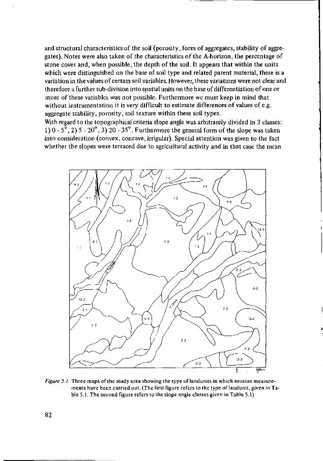
and structural characteristics of the soil (porosity, form of aggregates, stability of aggre-gates). Notes were also taken of the characteristics of the A-horizon, the percentage ofstone cover and, when possible, the depth of the soil. It appears that within the unitswhich were distinguished on the base of soil type and related parent material, there is avariation in the values of certain soil variables. However, these variations were not clear andtherefore a further sub-division into spatial units on the base of differentiation of one ormore of these variables was not possible. Furthermore we must keep in mind thatwithout instrumentation it is very difficult to estimate differences of values of e.g.aggregate stability, porosity, soil texture within these soil types.With regard to the topographical criteria slope angle was arbitrarely divided in 3 classes:1) 0 - 5°, 2) 5 - 20°, 3) 20 - 35°. Furthermore the general form of the slope was takeninto consideration (convex, concave, irrigular). Special attention was given to the factwhether the slopes were terraced due to agricultural activity and in that case the mean

Figure 5.1 Three maps of the study area showing the type of landunits in which erosion measure-ments have been carried out. (The first figure refers to the type of landunit, given in Ta-ble 5.1. The second figure refers to the slope angle classes given in Table 5.1 )

82

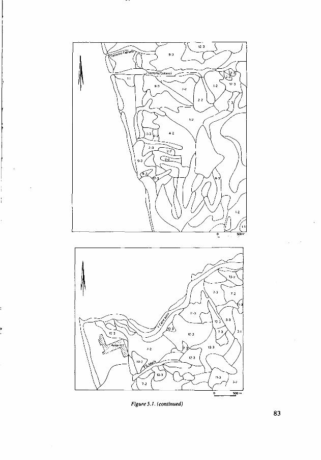
Figure 5.1. (continued)

83

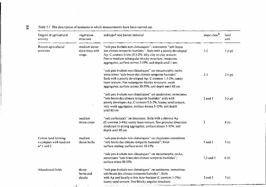
00 Table 5.1 The description of landunits in which measurements have been carried out.

Degree of agriculturalactivity

vegetationstructure

soil typea and parent material slope class" landunit

Recent agriculturalactivities

Follow land forminga complex with landunitn° I and 2

Abandoned fields

medium dense "sols peu évolués non climatiques"; sometimes "sols brunsolive trees with des climats tempérés humides". Soils with a poorly developedcrops Ap; C content is low (0.5-2%; silty clay to clay texture;

fine to medium subangular blocky structure; moderateaggregates; surface stones 3-10%; soil depth until 1 mtr.

"sols peu évolués non climatiques" on metamorphic rochssome times "sols bruns des climats tempérés humides"Soils with a poorly developed Ap; C-content 1.5-2%; sandyloam texture; fine subangular blocky structure; weakaggregates; surface stones 30-50%; soil depth until 60 cm.

"sols peu évolués non climatiques" on sandstones; sometimes"sols bruns des climats tempérés humides" soils withpoorly developes Ap; C-content 0.5-2%; loamy sand texture;very weak aggregates; surface stones 5-15%; soil depthuntil 80 cm

medium "sols carbonates" on limestone. Soils with a distinct Apdense crops (C-content 3-4%); sandy loam texture, fine granular structure;

moderate to strong aggregates; surface stones 5-15%; soildepth until 80 cm

medium "sols peu évolués non climatiques" on claystones sometimesdense herbs "sols bruns des climats tempérés humides"; local

surface sealing; surface stone 10-15%

"sols peu évolués non climatiques" on metamorphic rocks;sometimes "sols bruns des climats tempérés humides";surface stone 40-50%

dense "sols peu évolués non climatiques" on sandstone; sometimesherbs and sols bruns des climats tempérés humides"; Soilsshrubs with Ap and locally a thin Aoo-horizon (C-content 1-2%);

loamy sand texture; fine blocky angular structure;

1-2 I (r.p)

2-3 2 (r,p)

2 and 3 3 (r.p)

I and 2

1,2 and 3

2 and 3

4(r)

5(r)

6(r)

7(0

soil depth until I mtr.

More or less naturalareas

scattered "sols peu évolués non climatiques" on claystone; sometimesherbs "sols bruns des climats tempérés humides"; C-content

3-4% in A, horizon; silty clay structure; moderate fineto coarse subangular blocky structure; stable aggregates;surface stones 5-10%; soil depth until I mtr.

"sols peu évolués non climatiques" on metamorphic rocks;sometimes "sols bruns des climats tempérés humides"; soilswith locally a thin Aoo cover; C-content of A1 : ± 2%; sandyloam texture; fine subangular blocky structure; weakaggregates; surface stones until 25%; soil depth until 60 cm

"sols peu évolués non climatiques" on sandstones;sometimes "sols bruns des climats tempérés humides"; soilwith locally a thin Aoo cover; C-content of Al: ± 1.5%;loamy sand texture; fine subangular blocky structure;weak aggregates; surface stones 5%; soil depth until I mtr.

dense shrubs "sols bruns des climats tempérés humides" soils with withand herbs Aoo, Ao and AI horizons; C-content A1, 5-6%) sandy loam

texture; fine granular loose structure; weak to moderatestrong aggregates; surface stones 5-10%; soil depthuntil 1 mtr.

2 and 3 8 (r,p)

2 and 3 9(r,p)

2 and 3 IO(r,p)

H(P)

dense forest "sols bruns des climats tempérés humides" on metamorphicrocks; C-conten A1 horizon 5-6%; sandy loam texture;fine subangular blocky structure; medium strong aggregates;surface stones 20-30%; soil depth until I mtr.

"sols bruns des climats tempere's humides; on sandstone;C-content AI-horizon 4-6%; locally a Aoo horizon;sandy loamy texture; fine granular loose structure;weak aggregates; surface stones 20-40%; soil depthuntil 1 mtr

12(r,p)

I3(p)

r; landunits in which rainfall simulator measurements were carried out; p: landunits in which measuring plots were constructed.Note: a) soils classified in the field according to French C.P.C.S.-system

b) slope classes: a) 0-5° b) 5-20° c) 20-35°

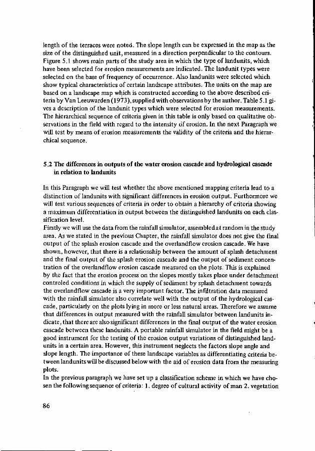
length of the terraces were noted. The slope length can be expressed in the map as thesize of the distinguished unit, measured in a direction perpendicular to the contours.Figure 5.1 shows main parts of the study area in which the type of landunits, whichhave been selected for erosion measurements are indicated. The landunit types wereselected on the base of frequency of occurrence. Also landunits were selected whichshow typical characteristics of certain landscape attributes. The units on the map arebased on a landscape map which is constructed according to the above described cri-teria by Van Leeuwarden (1973), supplied with observations by the author. Table 5.1 gi-ves a description of the landunit types which were selected for erosion measurements.The hierarchical sequence of criteria given in this table is only based on qualitative ob-servations in the field with regard to the intensity of erosion. In the next Paragraph wewill test by means of erosion measurements the validity of the criteria and the hierar-chical sequence.

5.2 The differences in outputs of the water erosion cascade and hydrological cascadein relation to landunits

In this Paragraph we will test whether the above mentioned mapping criteria lead to adistinction of landunits with significant differences in erosion output. Furthermore wewill test various sequences of criteria in order to obtain a hierarchy of criteria showinga maximum differentiation in output between the distinguished landunits on each clas-sification level.Firstly we will use the data from the rainfall simulator, assembled at random in the studyarea. As we stated in the previous Chapter, the rainfall simulator does not give the finaloutput of the splash erosion cascade and the overlandflow erosion cascade. We haveshown, however, that there is a relationship between the amount of splash detachmentand the final output of the splash erosion cascade and the output of sediment concen-tration of the overlandflow erosion cascade measured on the plots. This is explainedby the fact that the erosion process on the slopes mostly takes place under detachmentcontroled conditions in which the supply of sediment by splash detachment towardsthe overlandflow cascade is a very important factor. The infiltration data measuredwith the rainfall simulator also correlate well with the output of the hydrological cas-cade, particularly on the plots lying in more or less natural areas. Therefore we assumethat differences in output measured with the rainfall simulator between landunits in-dicate, that there are also significant differences in the final output of the water erosioncascade between these landunits. A portable rainfall simulator in the field might be agood instrument for the testing of the erosion output variations of distinguished land-units in a certain area. However, this instrument neglects the factors slope angle andslope length. The importance of these landscape variables as differentiating criteria be-tween landunits will be discussed below with the aid of erosion data from the measuringplots.

In the previous paragraph we have set up a classification scheme in which we have cho-sen the following sequence of criteria: 1. degree of cultural activity of man 2. vegetation

86

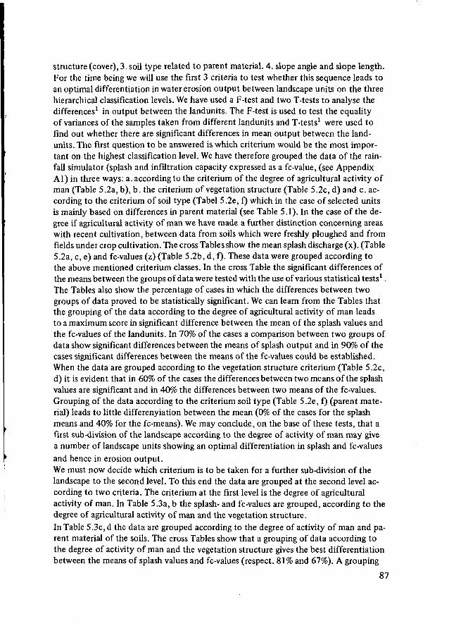
structure (cover), 3. soil type related to parent material. 4. slope angle and slope length.For the time being we will use the first 3 criteria to test whether this sequence leads toan optimal differentiation in water erosion output between landscape units on the threehierarchical classification levels. We have used a F-test and two T-tests to analyse thedifferences1 in output between the landunits. The F-test is used to test the equalityof variances of the samples taken from different landunits and T-tests1 were used tofind out whether there are significant differences in mean output between the land-units. The first question to be answered is which criterium would be the most impor-tant on the highest classification level. We have therefore grouped the data of the rain-fall simulator (splash and infiltration capacity expressed as a fc-value, (see AppendixAl) in three ways: a. according to the criterium of the degree of agricultural activity ofman (Table 5.2a, b), b. the criterium of vegetation structure (Table 5.2c, d) and c. ac-cording to the criterium of soil type (Tabel 5.2e, f) which in the case of selected unitsis mainly based on differences in parent material (see Table 5.1). In the case of the de-gree if agricultural activity of man we have made a further distinction concerning areaswith recent cultivation, between data from soils which were freshly ploughed and fromfields under crop cultivation. The cross Tables show the mean splash discharge (x). (Table5.2a, c, e) and fc-values (z) (Table 5.2b, d, f). These data were grouped according tothe above mentioned criterium classes. In the cross Table the significant differences ofthe means between the groups of data were tested with the use of various statistical tests1.The Tables also show the percentage of cases in which the differences between twogroups of data proved to be statistically significant. We can learn from the Tables thatthe grouping of the data according to the degree of agricultural activity of man leadsto a maximum score in significant difference between the mean of the splash values andthe fc-values of the landunits. In 70% of the cases a comparison between two groups ofdata show significant differences between the means of splash output and in 90% of thecases significant differences between the means of the fc-values could be established.When the data are grouped according to the vegetation structure criterium (Table 5.2c,d) it is evident that in 60% of the cases the differences between two means of the splashvalues are significant and in 40% the differences between two means of the fc-values.Grouping of the data according to the criterium soil type (Table 5.2e, f) (parent mate-rial) leads to little differenyiation between the mean (0% of the cases for the splashmeans and 40% for the fc-means). We may conclude, on the base of these tests, that afirst sub-division of the landscape according to the degree of activity of man may givea number of landscape units showing an optimal differentiation in splash and fc-valuesand hence in erosion output.

We must now decide which criterium is to be taken for a further sub-division of thelandscape to the second level. To this end the data are grouped at the second level ac-cording to two criteria. The criterium at the first level is the degree of agriculturalactivity of man. In Table 5.3a, b the splash- and fc-values are grouped, according to thedegree of agricultural activity of man and the vegetation structure.In Table 5.3c, d the data are grouped according to the degree of activity of man and pa-rent material of the soils. The cross Tables show that a grouping of data according tothe degree of activity of man and the vegetation structure gives the best differentiationbetween the means of splash values and fc-values (respect. 81% and 67%). A grouping

87

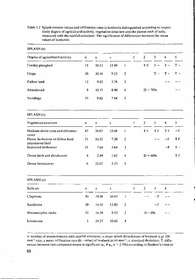
Table 5.2 Splash erosion values and infiltration rates in landunits distinguished according to respec-tively degree of agricultural activity, vegetation structure and the parent rock of soils,measured with the rainfall simulator. The significance of differences between the meanvalues of landunits

SPLASH (a)

Degree of agricultural activity n x s 1 2 3 4

Freshly ploughed

Crops

Fallow land

Abandoned

No tillage

15 50.53 15.49 1

30 30.16 9.23 2

12 9.82 5.78 3

9 10.77 8.40 4

33 9.82 7.44 5

T F T - T - T

T - T - T

D = 70%

SPLASH (c)

Vegetation structure n

Medium dense crop and olivetree-coverDense herbcover on fallow landabandoned field

Scattered herbcover

Dense herb and shrubcover

Dense forestcover

47 24.67 15.08 1

21 10.25 7.20 2

21 7.64 5.64 3

4 2.89 1.62 4

6 22.07 3.33 5

TF TF TF - F

- F TF

- F T -

D = 60% T F

SPLASH (e)

Soils on:

Claystone

Sandstone

Metamorphic rocks

Limestone

30 19.04 16.82 I

30 14.35 13.80 2

33 16.59 9.53 3

5 21.27 10.60 4

- - - F

_ F

D = 0%

n: number of measurements with rainfall simulator; x mean splash detachment of landunit is gr 100mm"1 rain; z mean infiltration rate (fc - value) of landunit in ml mm"'; s; standard deviation; T; diffe-rences between two compared means is significant (n, ^ (i2,a = 2.5%) according to Student's t-test or

88

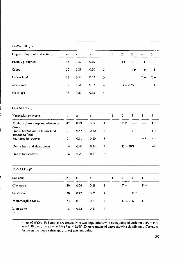
Fc-VALUE (b)

Degree of agricultural activity

Freshly ploughed

Crops

Fallow land

Abadoned

No tillage

15

30

12

9

33

0.32

0.21

0.50

0.54

0.30

0.16

0.10

0.27

0.32

0.18

1

2

3

4

5

T F

D =

T -

T F

90%

T F

T F

T -

—

T F

T -

T F

Fc-VALUE (d)

Vegetation structure

Medium dense crop and olivetree-coverDense herbcover on fallow landabadoned field

Scattered herbcover

Dense herb and shrubcover

Dense forestcover

47

21

21

4

6

0.29

0.52

0.31

0.40

0.20

0.19

0.30

0.20

0.24

0.07

1

2

3

4

5

TF - - -

TF -

-

D = 40%

- TF

- TF

F —

p

Fc-VALUE (0

Soils on:

Claystone

Sandstone

Metamorphic rocks

Limestone

30

30

33

5

0.24

0.42

0.31

0.62

0.21

0.25

0.17

0.27

1

2

3

4

T -

D =

T F

67%

T

-

T

t-test of Welch: F: Samples are drawn from two populations with no equality of variances (o12 = o2

2 ;a = 2.5%; —: n, = n2; ~

: °i2 = °22 (a = 2.5%); D: percentage of cases showing significant differencesbetween the mean values (n, + \i2) of two landunits.

89

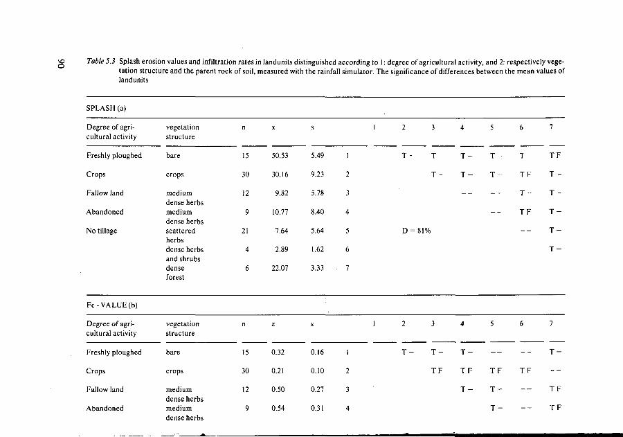
o Table 5.3 Splash erosion values and infiltration rates in landunits distinguished according to 1 : degree of agricultural activity, and 2; respectively vege-tation structure and the parent rock of soil, measured with the rainfall simulator. The significance of differences between the mean values oflandunits

SPLASH (a)

Degree of agri-cultural activity

vegetationstructure

3 5

Freshly ploughed

Crops

Fallow land

Abandoned

No tillage

bare

crops

mediumdense herbsmediumdense herbsscatteredherbsdense herbsand shrubsdenseforest

15

30

12

9

21

4

6

50.53

30.16

9.82

10.77

7.64

2.89

22.07

5.49

9.23

5.78

8.40

5.64

1.62

3.33

1

2

3

4

5

6

. 7

T - T - T - T

T - T - T

D

T -

TF

T -

TF

TF

T -

T -

T -

T -

T -

Fe-VALUE (b)

Degree of agri-cultural activity

vegetationstructure

Freshly ploughed

Crops

Fallow land

Abandoned

bare

crops

mediumdense herbsmediumdense herbs

15

30

12

9

0.32

0.21

0.50

0.54

0.16

0.10

0.27

0.31

1

2

3

4

T - T - T -

TF TF

T -

TF

T -

T -

T F

T -

TF

TF

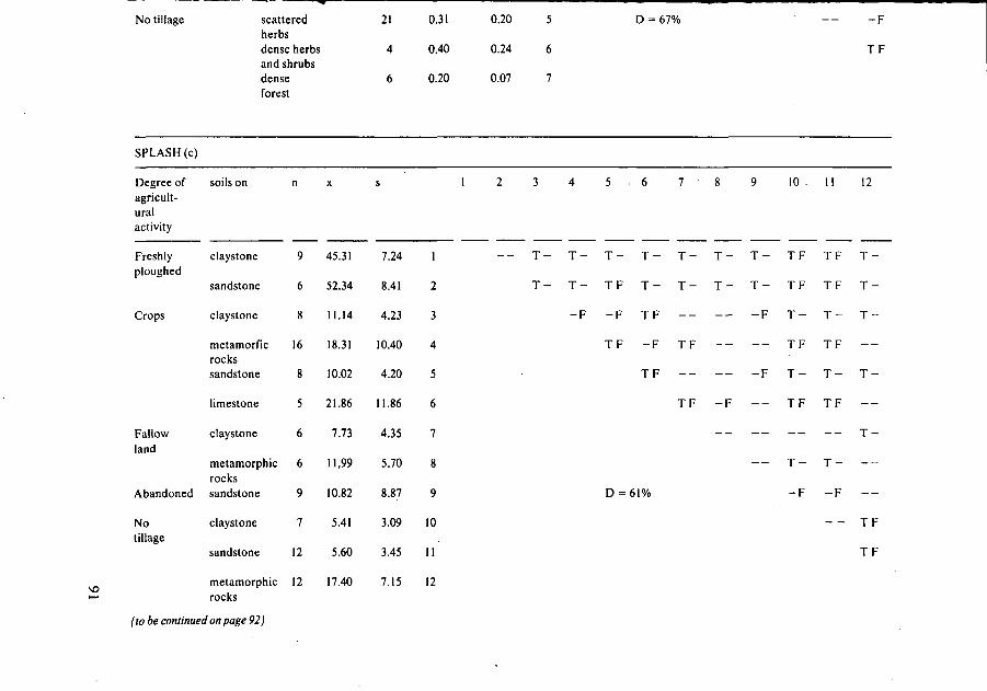
No tillage scatteredherbsdense herbsand shrubsdenseforest

21

4

6

0.31

0.40

0.20

0.20

0.24

0.07

5

6

7

D = 67% - F

TF

SPLASH (c)

Degree ofagricult-uralactivity

Freshlyploughed

Crops

Fallowland

Abandoned

Notillage

soils on

claystone

sandstone

claystone

metamorficrockssandstone

limestone

claystone

metamorphicrockssandstone

claystone

sandstone

metamorphicrocks

n

9

6

8

16

8

5

6

6

9

7

12

12

X

45.31

52.34

11.14

18.31

10.02

21.86

7.73

11,99

10.82

5.41

5.60

17.40

s

7.24

8.41

4.23

10.40

4.20

11.86

4.35

5.70

8.87

3.09

3.45

7.15

1

1

2

3

4

5

6

7

8

9

10

II

12

2 3

T -

T -

5 6 10 . 11 12

T - T - T - T - T - T - T F T F T -

T - T F T - T - T - T - T F T F T -

- F - F T F — — - F T - T - T -

T F - F T F — — T F T F —

T F — — _ F T _ T _ T _

T F - F — T F TF —

— — — — T _

— T - T - - -

D = 61% - F - F —

- - TF

TF

(to be continued on page 92)

Table 5.3 (continued)

Fc-VALUE(d)

Degree ofagricult-ural ,activity

Freshlyploughed

Crops

Fallowland

Abandoned

Notillage

soils on

claystone

sandstone

claystone

metamorphicrockssandstone

limestone

claystone

metamorphicrockssandstone

claystone

sandstone

metamorphicrocks

n

9

6

8

16

8

5

6

6

9

7

12

12

z

0.29

0.35

0.11

0.37

0.15

0.62

0.55

0.41

0.54

0.13

0.48

0.22

s

0.15

0.18

0.7

0.16

0.8

0.28

0.30

0.21

0.33

0.05

0.16

0.11

1

2

3

4

5

6

7

8

9

10

11

12

2 3 4 5 6 7 10 12

— — — — T _ T .

- F — - F — - -

- F T - T - —

D = 35%

- F TF — - -

— TF — —

TF — — - -

TF TF T - T -

TF — — —

— TF — TF

— TF — TF

— TF — TF

TF - F TF

TF TF

T -

n: number of measurements with rainfall simulator; x : mean splash detachment of landunit ingr 100 mm"1 rain;z.: mean infiltration rate (fc-value) oflandunit in ml mm"1; s: standard deviation; T: differences between two compared means is significant (n, ^ n2)a = 2.5%) according to Student's t-testort-test of Welch; F: Samples are drawn from'two populations with no equality of variances (o,2 # a2

2;a = 2.5%); — :n, = |i2; ~: o i 2 = °:2 (a = 2.5%); D:

percentage of cases showing significant differences between the mean values (n2 f ji2) of two landunits.

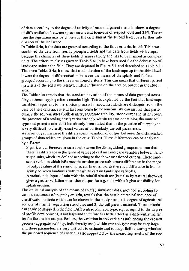
of data according to the degree of activity of man and parent material shows a degreeof differentiation between splash means and fc-means of respect. 60% and 35%. There-fore the vegetation may be chosen as the criterium at the second level for a further sub-division of the landscape.In Table 5.4a, b the data are grouped according to the three criteria. In this Table wecombined the data from freshly ploughed fields and the data from fields with crops,because the character of these fields changes rapidly and has to be mapped as complexunits. The criterium classes given in Table 5.4a, b have been used for the deliniation oflandscape units in the field. They are depicted in Figure 5.1 and described in Table 5.1.The cross Tables 5.4a, b show that a sub-division of the landscape up to the third levellowers the degree of differentiation between the means of the splash- and fc-datagrouped according to the three mentioned criteria. This can mean that different parentmaterials of the soil have relatively little influence on the erosion output in the studyarea.

The Table also reveals that the standard deviation of the means of data grouped accor-ding to three mapping criteria remains high. This is explained by the fact that landscapevariables, important to the erosion process in landunits, which are distinguished on thebase of these criteria, are still far from being homogeneous. We can assume that parti-cularly the soil variables (bulk density, aggregate stability, stone cover and litter cover,the presence of a sealing crust) varies strongly within an area containing the same soiltype and parent material. It has already been stated that in the practice of mapping itis very difficult to classify exact values of particularly the soil parameters.We have not yet discussed the differences in variation of output between the distinguishedgroups of data which are given in the cross Tables. These differences can be analysedby a F-test1.

— Significant differences in variation between the distinguished groups can mean thatthere is a difference in the range of values of certain landscape variables between land-scape units, which are defined according to the above mentioned criteria. These land-scape variables which influence the erosion process also cause differences in the rangeof output values of the erosion process. In other words there is a difference in homo-genity between landunits with regard to certain landscape variables.

— A variation in input of rain with the rainfall simulator (but also by natural showers)gives a greater variation in erosion output for e.g. soils with a higher sensibility forsplash erosion.

The statistical analysis of the means of rainfall simulator data, grouped according tovarious sequences of mapping criteria, reveals that the best hierarchical sequence of iclassification criteria which can be chosen in the study area, is 1. degree of agriculturalactivity of man, 2. vegetation structures and 3. the soil parent material. These criteriacan easily be mapped in the field. Differentiation in soil type, e.g. as regard to the degreeof profile development, is not large and therefore has little effect as a differentiating fac-tor for the erosion output. Besides, the variation in soil variables influencing the erosionprocess (aggregate stability, bulk density etc.) within one soil type may be very largeand these parameters are very difficult to estimate and to map. Before testing whetherthe proposed sequence of criteria is also supported by the measuring results of the ero-

93

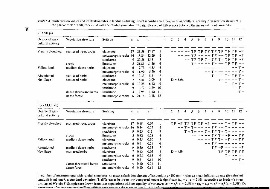
Table 5.4 Slash erosion values and infiltration rates in landunits distinguished according to 1. degree of agricultural activity 2. vegetation structure 3.the parent rock of soils, measered with the rainfall simulator. The significance of differences between the mean values of landunits.

SLASH (a)

Degree of agri-cultural activity

Freshly ploughed

Fallow land

AbandonedNo tillage

Fc-VALUE(b)

Degree of agri-cultural activity

Freshly ploughed

Fallow land

AbandonedNo tillage

Vegetation structure

scattered trees, crops

cropsmedium dense herbs

scattered herbsscattered herbs

dense shrubs and herbsdense forest

Vegetation structure

scattered trees, crops

cropsmedium dense herbs

medium dense herbsscattered herbs

dense shrubs and herbsdense forest

Soils on

claystonemetamorphic rockssandstonelimestoneclaystonemetamorphic rockssandstoneclaystonemetamorphic rockssandstonesandstonemetamorphic rocks

Soils on:

claystonemetamorphic rocks

. sandstonelimestoneclaystonemetamorphic rockssandstoneclaystonemetamorphic rockssandstonesandstonemetamorphic rocks

n

17169566976946

n

17169566976946

X

28.5818.8429.5621.867.73

11.9912.335.41

12.256.772.96

21.16

z

0.180.340.230.620.550.410.500.130.250.510.400.20

s

17.1712.2915.3111.864.355.708.513.096.423.291.403.18

s

0.070.170160.280.300.210.330.050.130.110.210.11

1

123456789

101112

1

123456789

101112

2 3 4

— — —

—

D = 52%

2 3 4

TF - F TF— T -

T -

D = 45%

5

T FT FTFT -

5

T FT -T -

6

TF- -T F——

6

T F——

—

7

TF- -T -—

- -

7

- F—T -

—- -

8

TTTT

TT

8

_

TTTTTT

FFF—

--

_FFFFFF

9

TF- -T -—

- -—

9

—T -T -T -- -- FT F

10

TFTFT FT F

- -T -—T -

10

T -T -T -- F- F- -—T FT -

11

TFTFT FT F_ _—T F—T -—

Il

T F————- -—T F——

12

- F- F- F—T -*r

T -T

T -T -T -

12

—

——T FT F- -- FT F—T -—

n: number of measurements with rainfall simulator; x : mean splash detachment of landunit in gr 100 mm*1 rain; z.: mean infiltration rate (fc-value) oflandunit in ml mm"1; s: standard deviation; T: differences between two.compared means is significant fti, = |i2,a = 2.5%) according to Student's t-testort-test of Welch; F: Samples are drawn fromitwo populations with no equality of variances (o,2 = a2

2;a = 2.5%); — : (i, = n2; — :a,2 = o22(a = 2.5%); D:

sion plots, we will give some comments on the established differences between the meansof groups of data related to different landunits.Table 5.2a shows that the amount of splash detachment is large in comparison to land-units of fallow land or abandoned fields and to areas with no traces of crop cultivation.The freshly ploughed fields particularly show a very high sensibility towards splash. InChapter 4 (Figure 4.2) we have established a clear differentiation in bulk density andaggregate stability and hence splash sensibility between areas under recent cultivationand more or less natural areas, which must be due to the ploughing activity of man. Thelower splash sensibility of the abandoned areas in relation to areas with fallow land isexplained by a denser herb vegetation in the abandoned areas and the absence ofploughing activity which leads to compaction of the soil surface due to the impact ofrain.Table 5.2b shows that apart from a decrease in splash sensibility there is also a decreasein infiltration capacity between areas, which are freshly ploughed, and areas under cropvegetation. The impact of raindrops on the bare freshly ploughed soils leads to a rapidcompaction and even a sealing of the soil surface. The Table also shows that the deve-lopment of a denser herb cover, which we could observe on fallow land and abandonedfields, has a positive effect on the infiltration capacity. The abandoned areas show highinfiltration capacities in comparison to other areas (including the more or less naturalareas). In combination with the relative low sensibility for splash (see above) these areasmay be considered as the most stable regions within the study area.In Table 5.2c we may see, that there are no significant splash differences between land-units with scattered herb vegetation (20-40%) and areas with denser herb and shrubvegetation (90-100%). An explanation is found in the previous Chapter (Figure 4.2).There it was shown that the effect of (herb) vegetation cover on splash erosion is parti-cularly strong in the range of a 0%to 30% vegetation cover. Another interesting fact isthat soils under a dense decideous forest cover with no herb vegetation have significantlyhigher splash values than the other areas with natural vegetation. They seem to be moresensitive to splash erosion as areas under recent crop cultivation.Unfortunately we have limited information concerning these soils (see e.g. AppendixA3 site 2 and 9) but on the base of soil description we may assume that the absence ofa herb vegetation cover in combination with a loose structure of the soil (low bulk den-sity) explains the high splash sensibility.

Table 5.2d reveals that areas with a dense herb cover 50-100% show the highest infil-tration capacities which points to a positive effect of the herb vegetation cover on theinfiltration rate (see Figure 4.5, Chapter 4).Table 5.3c shows that within the freshly ploughed areas we could not establish signifi-cant differences in splash erosion between soils derived from sandstone and from clay-stone. The differences in output between these two soil groups in areas under crop cul-tivation is not significant either. We would generally expect lower splash values for themore cohesive clay soils, but as we have already mentioned in Chapter 4, the swellingcapacity of these clay minerals decreases the aggregate stability during wetting. Soilsderived from metamorphic rocks and limestone show generally significant higher splashvalues within the agricultural areas. We could not find significant lower aggregate stabili-

95

ties and (or) bulk densities, for these groups of soils (see Figure 4.2 in Chapter 4). How-ever, observations in the field, especially on the measuring plots (see below) show thatparticularly on clay soils and sandstone soils, in many spots traces of sealing may be dis-cerned, which were not observed on soils on metamorphic rocks and on limestone soils.This might be an explanation for the lower splash values of the sandstone and claystonesoils. The same trend in the differences between these groups of soils can be observed inareas with fallow land and in more or less natural areas. However, the differences arenot always significant. As regard to the fc-values (Table 5.3d) no significant differenceswere measured between claystone and sandstone soils on freshly ploughed fields.Within areas under recent crop cultivation claystone and sandstone soils show signifi-cantly lower fc-values than soils derived from metamorphic rocks and limestone. Weassume that the sealing which was observed on the sandstone and claystone soils alsohas a negative effect on the infiltration rate.

Sandstone soils show remarkable high infiltration rates within areas with no tillage andin areas with scattered vegetation (see Table 5.4b). This might be due to the high poro-sity (low bulk density) of some natural sandstone soils (see Figure 4.2 Chapter 4). Wemust keep in mind, however, that particularly on calcareous sandstone soils (Mar) cleartraces of sealing with surface crusts of 0.5 mm with very low infiltration capacities werefound.We will now investigate whether the relative importance of the classification criteria,based on differences in output and measured with the rainfall simulator, is supportedby the differences in the final output of the water erosion cascade and also the hydro-logical cascade measured on the erosion plots.Table 5.1 shows that in 9 of the 13 basic landscape units, which were described in theprevious Paragraphs, measuring plots were installed. Since the Gerlach throughs wereconcentrated in a certain area of maximal 20 x 50 mtr the samples are not randomlydistributed within a certain landscape unit. We must therefore be very careful with theconclusions drawn from statistical tests and with the comparison of rainfall simulatorresults with plot results. However, we may assume that clear differences in the meanoutput of the erosion plots over a period of 3 months forms a good indication whetherthe distinction of landunits on the base of certain criteria is significant or not.We first give the following comments on the differences in output: Table 5.5a gives thetotal output of the water erosion cascade (= splash + overlandflow) (x). The amount ofmaterial which was transported by splash over a unit distance of slope (50 cm) duringthat period, is given as a percentage of the total output (% Sp). We may conclude that onslopes with various slope lengths a great deal of the totally transported material varyingfrom 40 - 80% passes a unit width of slope in a given period via splash transport.This is explained by 2 reasons:

— Splash transport occurs on the slopes while there is (still) no overlandflow on theslopes during a rain storm.

— The catchment area of the overlandflow is local and limited (see Chapter 4) and mayhave the same size as the source area of splashed material (1-2 mtr according toMosley 1974; Van Asch & Roels 1979).

Table 5.5 shows that the relative importance of splash in agricultural areas with meta-

96

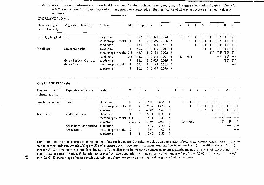
Table 5.5 Water erosion, splash erosion and overlandflow values of landunits distinguished according to 1 : degree of agricultural activity of man 2.vegetation structure 3. the parent rock of soils, measured on erosion plots. The significance of differences between the mean values oflandunits.

OVERLANDFLOW (a)

Degree of agri-cultural activity

Freshly ploughed

No tillage

Vegetation structure

bare

scattered herbs

dense herbs and shrubsdense forest

OVERLANDFLOW (b)

Degree of agri-cultural activity

Freshly ploughed

No tillage

Vegetation structure

bare

scattered herbs

dense herbs and shrubsdense forest

Soils on

claystonemetamorphic rockssandstoneclaystonemetamorphic rockssandstonesandstonemetamorphic rockssandstone

Soils on

claystonemetamorphic rockssandstoneclaystonemetamorphic rockssandstonesandstonemetamorphic rockssandstone

MP

12II10

13,45,6,7928

MP

121110

13,45,6,7928

%Sp

76.93.3

18.446.245.756.582.568.482.5

n

222367245

n

22248

10355

z

15,321,68,22,18,

X

0.8239.5893.9210.0190.1910.2410.0390.4850.317

s

,83,32 186,14 1,31

s

0.1242.7860.5610.0110.0920.0910.0160.2050.096

4.760.386.671.367.43

30.05 20.075.,17

13.6413.60

2.504.093.57

1

123456789

1

123456789

2

T F

D =

2

T

D

3 4

T - T F— TF

T F

86%

3 4

- T - - -T - T -

T -

= 50%

5

T -T FT FT F

5

—

T -T- -

6

TTTTT

_FFFF

6

- F-r

TF——

7

T FT FT FT -T F- F

7

—

T -T -- F- F- F

8

T -T FT FT FT FT FT F

8

—

T -T -- -—- F—

9

T -T FT FT FT -—T F—

9

—

TFT -- -—- FT -- -

VO

MP: Identification of measuring plots; n: number of measuring points; Sp: splash erosion as a percentage of total water erosion (x); x: mean water ero-sion in gr mm-' rain (unit width of slope = 50 cm) measured over three months; z: mean overlandflow in ml mm"1 rain (unit width of slope = 50 cm)measured over three months; s: standard deviation; T: the difference between two compared means is significant (n, ^ n2, a = 2.5%) according to Stu-dent's t-test or t-test of Welch; F: Samples are drawn from two populations with no equality of variances a,2 ^ <j2

2,a = 2.5%); — : n, = n2; — : a,2 = a22

(a = 2.5%); D: percentage of cases showing significant differences between the mean values (\it + \i2) of two landunits.

morphic rocks and sandstone is relatively low. On these plots a high overlandflow pro-duction was measured and in combination with the low shear strengths of the freshlyploughed soils, detachment by overlandflow shear is thought to be relatively large.We can further conclude from Table 5.5a that the total water erosion (splash + over-landflow) on freshly ploughed field is generally 10 to 20 times higher than the more orless natural areas with no tillage. An interesting point is that the water erosion output,measured during the winter period in the decideous forest areas, is significantly higherthan areas with scattered and dense herbs and shrubs (compare with Table 5.3a).The output, measured on the erosion plots, also shows interesting differences betweensoil types. The soils on metamorphic rocks in the freshly ploughed areas show a veryhigh production of overlandflow erosion, while the portion of splash output is relati-vely low. This is due to the fact that in these plots we measured a relatively high over-landflow production. Observations in the field revealed that during rain storms strongoverlandflow occurred in the lowest part of the measuring plot and we concluded thatin these areas with a shallow soil up to 30 cm and an impermeable rock, conditionsof saturated overlandflow (Chapter 3) must have existed (see Plate 2).

The high amount of overlandflow in combination with the low shear strength of thesoil, due to ploughing and the relatively high silt content might indicate that the amountof detachment by overlandflow shear is very large.Furthermore an interesting point is that claystone soils on the freshly ploughed fields :show a very low overlandflow erosion output. As we will see below, on these soils theamount of overlandflow production is also very low. Particularly in the first measuringperiods, shortly after the soils were ploughed (± one month) no overlandflow was mea-sured even after high rain storms, whereas the other plots (10 and 11 ) gave large amountsof overlandflow (see Appendix A4). During the last periods we found that overlandflowproduction began and this was due to a certain sealing of the soil surface. This also ex-plains why the percentage of splash is high in relation to the other agricultural plots(76.9% of the total water erosion output). In areas with scattered vegetation we canobserve in Table 5.5a that the overlandflow erosion output in claystone soils is rela-tively low. The rainfall simulator test also showed low values for splash detachment.These claystone soils under scattered vegetation are compact and have high bulk densi-ties. In many cases they also show traces of sealing. We observed in these plots that theinfiltration capacity of these soils increases due to the formation of cracks. This decreasesthe mean amount of overlandflow production and hence the overlandflow erosion. Therelatively high overlandflow erosion output in areas with scattered vegetation on sand-stone soils, was unexpected in view of the splash results with the rainfall simulator (seee.g. Table 5.4a). But also in this case the final output of the overlandflow erosion cascadeis connected with a high input from the hydrological cascade, which was relatively highat least on one plot (Site no 5, Appendix A4).

Table 5.5b shows the differences in overlandflow production between the differentbasic landunits. It becomes obvious that overlandflow production in freshly ploughedareas, particularly on sandstone and metamorphic rocks, is relative high in comparisonwith more or less natural areas. This is not quite in accordance with the rainfall simu-

98

lator results which show a relative high infiltration rate on freshly ploughed soils(Table 5.3b and d).The following explanations can be given:— On the freshly ploughed measuring plots lying in sandstone soils, we could observe

a rapid sealing after some heavy showers (see Plate 3). We already mentioned thatthe rainfall simulator test also generally showed a decrease in infiltration ratebetween freshly ploughed soils and soils under crop vegetation.

— On the measuring plot, lying in metamorphic rocks, saturated overlandflowcould be observed which was due to a locally shallower soilcover lying on the relativeimpermeable metamorphic rocks.

We also mentioned already the remarkably low overlandflow production on the measu-ring plot lying in freshly ploughed claystone soils (plot 12 see Appendix A4).Apart from the effect of the large cracks (which could not be measured with the rain-fall simulator due to the small infiltration surface) on the infiltration rate, we will pointto the fact that the upper 30 cm of these freshly ploughed claystone soils must beconsidered as a loose package of strong cohesive clods (under dry circumstances) withmany large fissures and non-capillary spaces connected to each other. The water rapidlyinfiltrated in this upper layer and a rapid sub-surface flow may develop along the slope.Unfortunately we did not measure this rapid sub-surface flow which might also producea sort of sub-surface erosion.

Within the areas with scattered vegetation the sandstone soils on the plots show a rela-tively high run-off production which also results in a high output of overlandflow erosion.This contradicts the mean high fc-values measured with the rainfall simulator. We muststress again here the fact that particularly in calcareous sandstone (Mar), a crust can beformed locally especially after dry periods, which makes the soil impermeable. Thiscould be observed on plot 5 (see Appendix A4) . Here a high overlandflow productionwas measured (56.04 ml/mm rain). On plot 6 with a somewhat denser herb vegetationon the contrary, the mean overlandflow production was relatively low (4.05 ml/mm rain).

Table 5.5 shows that a landscape sub-division based on (1 ) degree of agricultural activityof man (2) vegetation structure and (3) soil type related to parent material results in anumber of landunits showing a high degree of differentiation between the units (86%)regarding the total output of the water erosion cascade. The question arises whetherslope length and slope angle are also important differentiating landscape variables on acertain hierarchic level. The results given in Table 5.2a, b, 5.3a, b from the rainfall si-mulator and in Table 5.5 from the measuring plots showed that the activity of man andthe vegetation structure are the best differentiating criteria on the first and second level.If we introduce slope angle or slope length at the second level the degree of differentia-tion as regard to the total output of the water erosion cascade is much lower (60% and30% respect.). The question remains whether on the third hierarchical level slope angleand slope length give a better degree of differentiation than a sub-division according tosoil type related to parent material. We can learn from Table 5.6 and 5.7 compared withTable 5.5 that a sub-division according to slope angle (range 25-35°), leads to approxi-

99

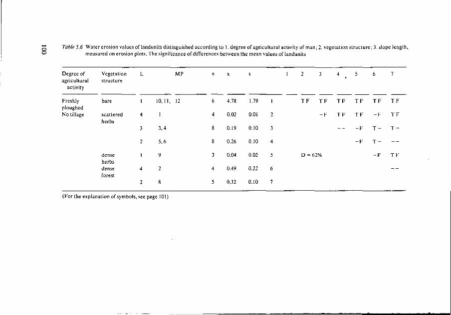
Q Table 5.6 Water erosion values of landunits distinguished according to 1. degree of agricultural activity of man; 2. vegetation structure: 3. slope length,° measured on erosion plots. The significance of differences between the mean values of landunits

Degree ofagricultural

activity

FreshlyploughedNo tillage

Vegetation Lstructure

MP

bare

scatteredherbs

denseherbsdenseforest

10,11, 12

1

3,4

5,6

9

2

6

4

8

8

3

4

5

4.78

0.02

0.19

0.26

0.04

0.49

0.32

1.79

0.01

0.10

0.10

0.02

0.22

0.10

1

2

3

4

5

6

7

TF TF TF TF TF TF

- F TF TF - F TF

- F T - T -

- F T -

D = 62% - F TF

(For the explanation of symbols, see page 101)

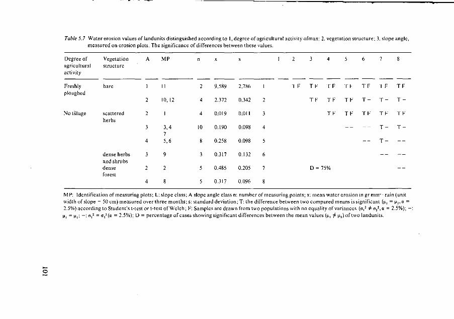
Table 5.7 Water erosion values of landunits distinguished according to 1, degree of agricultural activity ofman: 2. vegetation structure; 3. slope angle,measured on erosion plots. The significance of differences between these values.

Degree ofagriculturalactivity

Freshlyploughed

No tillage

Vegetationstructure

bare

scatteredherbs

dense herbsand shrubsdenseforest

A

1

2

2

3

4

3

2

4

MP

11

10,12

1

3,475,6

9

2

8

n

2

4

4

10

8

3

5

5

X

9.589

2.372

0.019

0.190

0.258

0.317

0.485

0.317

s

2.786

0.342

0.011

0.098

0.098

0.132

0.205

0.096

1

2

3

4

5

6

7

8

1 8

TF TF TF TF TF TF TF

TF TF TF T- T- T-

TF TF TF TF TF

— — T- T-

— T- —

D = 75%

MP: Identification of measuring plots; L; slope class; A slope angle class n: number of measuring points; x: mean water erosion in gr mm"' rain (unitwidth of slope = 50cm) measured over three months; s; standard deviation; T: the difference between two compared means is significant (n, = i,a =

2.5%) according to Student's t-test or t-test of Welch; F: Samples are drawn from two populations with no equality of variances (a,2 ^ a22,a = 2.5%); •

H, = (i,; - : a,2 = o22(a = 2.5%); D = percentage of cases showing significant differences between the mean values (H, J= |i2) of two landunits.

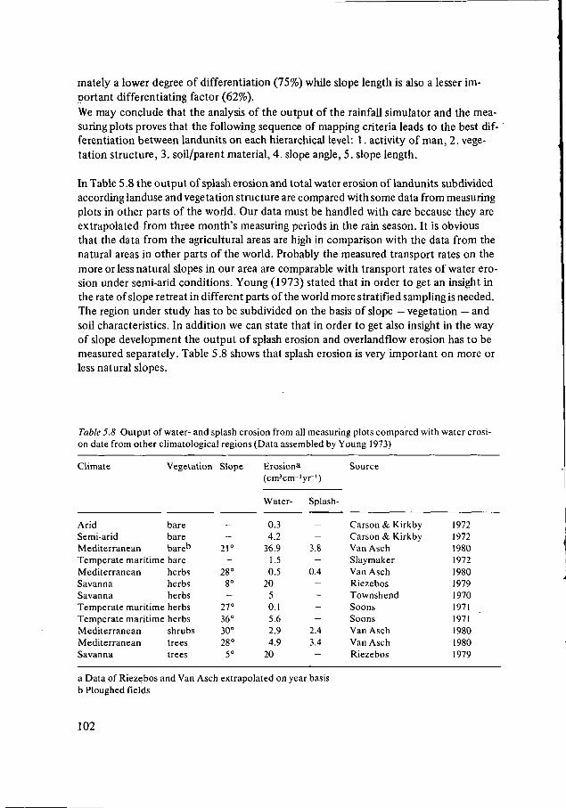
mately a lower degree of differentiation (75%) while slope length is also a lesser im-portant differentiating factor (62%).We may conclude that the analysis of the output of the rainfall simulator and the mea-suring plots proves that the following sequence of mapping criteria leads to the best dif-ferentiation between landunits on each hierarchical level: 1. activity of man, 2. vege-tation structure, 3. soil/parent material, 4. slope angle, 5. slope length.

In Table 5.8 the output of splash erosion and total water erosion of landunits subdividedaccording landuse and vegetation structure are compared with some data from measuringplots in other parts of the world. Our data must be handled with care because they areextrapolated from three month's measuring periods in the rain season. It is obviousthat the data from the agricultural areas are high in comparison with the data from thenatural areas in other parts of the world. Probably the measured transport rates on themore or less natural slopes in our area are comparable with transport rates of water ero-sion under semi-arid conditions. Young (1973) stated that in order to get an insight inthe rate of slope retreat in different parts of the world more stratified sampling is needed.The region under study has to be subdivided on the basis of slope — vegetation — andsoil characteristics. In addition we can state that in order to get also insight in the wayof slope development the output of splash erosion and overlandflow erosion has to bemeasured separately. Table 5.8 shows that splash erosion is very important on more orless natural slopes.

Table 5.8 Output of water- and splash erosion from all measuring plots compared with water erosi-on date from other climatological regions (Data assembled by Young 1973)

Climate

AridSemi-aridMediterraneanTemperate maritimeMediterraneanSavannaSavannaTemperate maritimeTemperate maritimeMediterraneanMediterraneanSavanna

Vegetation

barebarebareb

bareherbsherbsherbsherbsherbsshrubstreestrees

Slope

_

-21°

-28°

8°-

27°36°30°28°

5°

Erosiona

(cm'crrr1

Water-

0.34.2

36.91.50.5

2050.15.62.94.9

20

yr ' )

Splash-

—

-3.8

-0.4

----

2.43.4

—

Source

Carson & KirkbyCarson & KirkbyVan AschSlaymakerVan AschRiezebosTownshendSoonsSoonsVan AschVan AschRiezebos

197219721980197219801979197019711971198019801979

a Data of Riezebos and Van Asch extrapolated on year basisb Ploughed fields

102

5.3 Summary and conclusions

In this Chapter the differences in output of the hydrological cascade and the water erosioncascade of landunits on different classification levels were compared in order to finda sequence of mapping criteria for the classification of the landscape in units, whichshow a maximum degree of differentiation in erosion output on each level. The resultsof the rainfall simulator and erosion plots indicated that the following sequence of cri-teria leads to an optimum differentiation between units on different hierarchical levels:1. Degree of agricultural activity of man, 2. vegetation structure, 3. soil type related toparent material, 4. slope angle, 5. slope length.With respect to the primary sub-division based upon the degree of agricultural activityof man it was found that the units with recent agricultural activity show a high watererosion output compared to that of the other units. The highest splash detachment out-put was measured with the rainfall stimulator on freshly ploughed plots. We found alsothe highest output of total water erosion on these plots. This is generally due to the lowsoil resistance against splash and overlandflow detachment, the high overlandflow produc-tion on some of these plots and the scarce vegetation cover. The results of the rainfall simu-lator and, to some extent less obvious, the output results on the measuring plots show thatthere is a relatively large decrease of the soil sensibility towards splash and overland-flow detachment in the period between the ploughing of soil and the growing of thecrops. In this period the infiltration capacity of the soils decreases. This is generallycaused by a consolidation and sealing of the soil by the impact of rain. In the areaswith fallow land and abandoned fields the results of the rainfall simulator showed afurther decrease of the sensibility against splash erosion in comparison to the areas un-der crop cultivation. The infiltration capacity is relatively high in the abandoned areas,and this is probably due to the strong growth of the herb vegetation. It may thereforebe concluded that the decrease in the agricultural population, particularly after WorldWar 2 (see Chapter 2), has generally led to a stabilisation of the erosion.With respect to the vegetation structure which we selected in the base of the outputresults of the different landunits as a second classification criterium, we found that inthe more or less natural areas a dense vegetation cover (80 -100%) shows the lowestoutput of splash detachment and total water erosion and the highest infiltration capa-cities. However, particularly with regard to splash detachment, we found that the dif-ferences are not large or significant in relation to areas with a more scattered vegetationcover of about 20-40%. Chapter 4 has revealed that the effect of the vegetation coverrapidly decreases above a 30% vegetation cover. An interesting fact is that the soilsunder a dense decideous forest cover with no shrub and herb vegetation show a rela-tively high output of splash and total water erosion which can reach an amount com-parable to the landunits under recent crop cultivation. The infiltration capacity inthese units is much lower than the values measured in areas with a dense herb vegetationcover (30-100%).

The differences between units with different soil type and related parent material arenot always significant and sometimes contradicting, when the results of the rainfall si-mulator are compared with the results of the erosion plots. Rainfall simulator output

103

shows lower splash values for sandstone and claystone than for soils on metamorphicrocks, while on the freshly ploughed plots metamorphic rock and sandstone soils givea high overlandflow erosion output in relation to claystone. We found that particularlythe high production of overlandflow on the sandstone and metamorphic plots produceda large overlandflow erosion, whereas in claystone soils the overlandflow productionand related erosion is low, due to the formation of large cracks in dry periods.The output of data from the plots showed that excepting cases with a very high over-landflow production and a low soil erodibility (plot 10 and 11 ), the amount of materialwhich is transported by splash erosion over a certain unit width of slope length duringa given period is relatively large (2 to 4 times) in comparison to the amount of material,transported by overlandflow. In Chapter 4 we have stated that an important part of thesediment is delivered by splash towards the overlandflow. Furthermore we found thaton natural slopes the amount of sediment transport by overlandflow is not positivelycorrelated to the slope length. We must conclude that on natural slopes transport bysplash is the dominant factor in the water erosion cascade. The amount of sedimenttransport by water is positively correlated to slope angle but not to the length of slope.

NOTES

1 The F-test is described in Davis (1973) pp. 99-105. If the variances of data of two landunits,tested with the F-test proved to be equal a T-test was used, described in Davis (1973), to testthe significance of the differences between the means. In case the variances of data of two land-units are not equal, a T-test developed by Welch (1937) was used.

104

THE SPECIFICATION OF THE MASSMOVEMENT CASCADINGSYSTEM

In the next Chapters attention will be paid to the relation of output of the massmove-ment cascading system to different landscape units. Firstly, a study was made of thelandscape variables building up the massmovement cascading system. Mapping criteriawill be defined on the base of the study of these variables, and an analysis will be givenof these criteria eventually leading to a differentiation in output between the distin-guished units.In this Chapter the effect of landscape variables on the degree of stability (F-value) ofa given slope will be considered. In the next Paragraph we will show how a combinationof landscape variables determine the type of initial failure and the amount of mass whichwill be involved in the movement. In the last Paragraph we will discuss the effect oflandscape variables on the transport of the moving mass.

6.1 The influence of landscape variables on the degree of stability of soil and rock mass

As we have stated in Chapter 1 the degree of stability is determined by the total shearstrength S(kg/m2) along a given shear surface and the amount of total shear stressT(kg/m2) developed along this surface:

F = | ( F > 1 ) (1)

The mass reaches the state of initial failure when F = 1.We will first discuss the influence of soil and rock variables on the shear strength andalso the shear stresses. In the study of massmovements "rock" defined as a natural aggre-gate of minerals connected by strong and permanent cohesive forces whereas "soil" isan aggregate of mineral grains that can be separated by such gentle means as agitation inwater. Since the terms "strong" and "permanent" are subjective to different interpreta-tions the boundary between soil and rock is necessarily an arbitrary one (Terzaghi &Peck, 1967).The shear strength of the rock and soil mass is made up of 2 components: the cohesionof the material and the amount of internal friction between grains. The amount of inter-nal friction is expressed by a coefficient of internal friction (<p), which is the ratio betweenthe frictional strength along a certain shear surface and the effective normal stress(a) on this plane which tends to push the particles together. This ratio is assumed tobe constant for a certain soil type in the case that the range of normal stress valuesis not too wide. The ratio is expressed as tan y in which y is called the angle of internalfriction of the material. An agglomeration of soil or rock particles has a frictional re-

105

sistance along a certain shear surface which is built up by a certain plane friction pro-duced where one grain attempts to slide past another and a structural resistance dueto the interlocking of the particles. This interlocking effect determines the amount offorce necessary for the lifting of one grain over another in order to move (Kézdi 1974).In addition to the frictional strength between grain particles there may be forces whichpull the particles together and this source of strength, which is independent of the nor-mal effective stress on a given shear plane is called the cohesion (c). The total strengthis given by the most common empirical equation of Coulomb:

s = c + a tan tp (2a)

in which s = the total shear strength (kg/m2), c = the cohesion (kg/m2), a = the normalstress (kg/m2 ) and tan cp = the coefficient of internal friction. The total strength of thematerial decreases with an increasing pore pressure of water (or air) in the pores. Thepore pressure reduces the amount of effective normal stress (a') on a given shear surfaceand when a positive pore pressure u(kg/m2) exists equation (2) can be written as

s = c' + (a - u) tan <p' (2b)

in which a = the total normal stress (kg/m2), u = the pore pressure (kg/m2) and (a - u) =the effective stress, also written as a' and c' the effective cohesion. As far as the rockmaterial is concerned we can state that the cohesive strength of an intact rock mass dueto cementing and fusion of the mineral particles, is very important. In many cases thestrength of the intact rock mass is not as important as the mechanical structure of themany discontinuities in the rock mass (joints, cleavage-, shear-, and bedding planes, faultsfissures, but also dikes, cavaties and contact zones between different rocks). Generallythe pattern of these discontinuities, combined with the orientation of the shear surfacedetermines the shear strength of the rock material. (See references given in Yatsu 1966,Carson & Kirkby 1972 and Sowers 1979).Terzaghi (1962) introduced the term effective cohesion (Ci) in a rock mass which is givenby

(3)

where Ci = the cohesion of the intact rock, A = the total area of the section through therock and Ag = the total area of joints and other gaps in the considered section. Due to asevere tectonic activity in the past or an increasing stress within the rock mass, the rockcan be fractured in such a degree that it must be considered, according to Terzaghi, asan agglomerate of cohesionless angular rock fragments with a high degree of interlockingand hence a high angle of internal friction. With respect to sedimentary rocks, the alter-nation in mechanical characteristics must be investigated between layers, the thicknessof the different layers, the character of the interface between layers, and the orientation

106

of the bedding planes in relation to the potential shear surface (Sowers 1979).Another important factor is the strength of the weathering products that fill up thejoints or the breccious material which fill up the faults (Pitau, 1970). The system ofjoints and other discontinuities is also of importance to the building up of an excessivepore water pressure, which decreases the shear strength (equation 2b). A system of conti-nuous joints favours a free water flow and prevents the building up of locally excessivewater pressure. However, a system of continuous joints also decreases the mechanicalstrength of the rocks (Terzaghi, 1962). In rocks with soluble minerals, the water in thejoints dissolves the material and the widening of the joints leads to a gradual decreasein the shear strength.

An important component of the soil which determines the strength is the content ofclay minerals. Between the clay mineral particles there are attractive and repulsive phy-sicochemical forces and the net force determines the amount of cohesion and thus thestrength within the soil mass (see a.o. Kézdi 1974). The attractive forces consist of theso-called v.d. Waals' forces which increase as the size of the particles decrease and thusthe area of contact between mineral particles (Sowers 1979). The repulsive forces arerelated to an electric potential which exists between the clay particles. The electric po-tential is determined by the amount of negative charge of the clay minerals at the con-tact surface and the amount of water molecules and cat-ions which surround the clayparticles. The type of clay minerals and the type and concentration of cat-ions determinethe thickness of the film of water absorbed around the clay particles. This waterfilmplays a major role in the development of the cohesive strength of the clayrich soil mass.Sullivan (1939) (in Kézdi 1974) investigated the strength of the soil in relation to thevarious cat-ions absorbed and he found a decreasing strength in the following order:N H 4

+ > H + > K + > F e 3 + > A l 3 + > Mg 2 + > Ba2 + > C a 2 + > Na + > l i + . It islikely that the absorbed layer is of considerable thickness in the case of Li+ or Na+ where-as it is very thin in the case of H+-ions. (Kézdi 1974). The type of clay minerals andcat-ions absorbed also determines the empirical parameters known as the Atterberg li-mits. These Atterberg limits give indirect qualitative information concerning the strengthcharacteristics of the soil in relation to the soil moisture content. The most commonlimits are the Plastic limit (Wp) and the Liquid limit (Wl). At moisture contents lowerthan given by the plastic limit the soil is brittle and will show a given finite strain defor-mation (e) at a given applied stress (r) and will finally fail at a given shear stress TO (seeFigure 6.1).

The soil has a viscous component at a water content between these two limits. At a cer-tain applied shear stress r (kg/m2 ) (called the yield stress, see Figure 6.1b), which is lowerthan TO the soil begins to deform continuously and the velocity ofi deformation é1 . (=strain rate) depends on the applied stress. When the soil has reached the liquid limitthe soil has no strength and is in a completely viscous state. It starts to deform underany applied stress (Figure 6.1a). The difference between the Liquid limit and the Plas-tic limit is called the Plasticity index (Ip). The Plasticity index represents the range inwater content in which the soil has a plastic character with a certain yield stress. Accor-ding to Kézdi (1974) it is a measure for the cohesiveness of the soil: the greater thePlasticity index the higher, generally, the attraction between particles of the soil. At

107

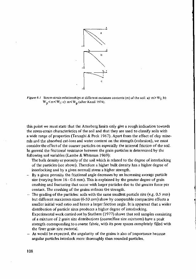
Figure 6.1 Stress-strain relationships at different moisture contents (m) of the soil, a): m>W|; b):Wp<m<W|; c): m< Wp (after Kezdi 1974).

this point we must state that the Atterberg limits only give a rough indication towardsthe stress-strain characteristics of the soil and that they are used to classify soils witha wide range of properties (Terzaghi & Peck 1967). Apart from the effect of clay mine-rals and the absorbed cat-ions and water content on the strength (cohesion), we mustconsider the effect of the coarser particles on especially the internal friction of the soil.In general the frictional resistance between the grain particles is determined by thefollowing soil variables (Lambe & Whitman 1969):- The bulk density or porosity of the soil which is related to the degree of interlocking

of the particles (see above). Therefore a higher bulk density has a higher degree ofinterlocking and by a given normall stress a higher strength.

- By a given porosity the frictional angle decreases by an increasing average particlesize (varying from 16 - 0.6 mm). This is explained by the greater degree of graincrushing and fracturing that occur with larger particles due to the greater force percontact. The crushing of the grains reduces the strength.

- The grading of the particles: soils with the same smallest particle size (e.g. 0.5 mm)but different maximum sizes (6-50 mm) show by comparable compactive efforts asmaller initial void ratio and hence a larger friction angle. It is apparent that a widerdistribution of particle sizes produces a higher degree of interlocking.Experimental work carried out by Stathem (1977) shows that soil samples consistingof a mixture of 2 grain size distributions (coarse/fine size mixtures) have a peakstrength corresponding to a coarse fabric, with its pore spaces completely filled withthe finer grain size material.

- As would be expected, the angularity of the grains is also of importance becauseangular particles interlock more thoroughly than rounded particles.

108

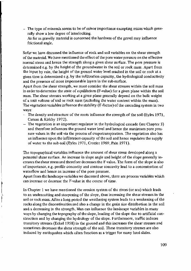
- The type of minerals seems to be of minor importance excepting micas which gene-rally show a low degree of interlocking.As far as gravelly material is concerned the hardness of the gravel may influencefactional angle.

Sofar we have discussed the influence of rock and soil variables on the shear strengthof the material. We have mentioned the effect of the pore water pressure on the effectivenormal stress and hence the strength along a given shear surface. The pore pressure isdetermined e.g. by the height of the groundwater in the soil or rock mass. Apart fromthe input by rain, the height of the ground water level reached in the soil or rock at agiven time is determined e.g. by the infiltration capacity, the hydrological conductivityand the presence of more impermeable layers in the sub-surface.Apart from the shear strength, we must consider the shear stresses within the soil massin order to determine the state of equilibrium (F-value) for a given plane within the soilmass. The shear stresses working at a given plane generally depend on the bulk weightof a unit volume of soil or rock mass (including the water content within the mass).The vegetation variables influence the stability (F-factor) of the cascading system in twoways:- The density and structure of the roots influence the strength of the soil (Eyles 1971,

Carson & Kirkby 1972).- The vegetation is an important regulator in the hydrological cascade (see Chapter 3)

and therefore influences the ground water level and hence the maximum pore pres-sure values in the soil via the process of evapotranspiration. The vegetation also hasan influence upon the infiltration capacity of the soil and hence regulates the supplyof water to the sub-soil (Eyles 1971, Crozier 1969, Pain 1971).

The topographical variables influence the amount of shear stress developed along apotential shear surface. An increase in slope angle and height of the slope generally in-creases the shear stress and therefore decreases the F-value. The form of the slope is alsoof importance, e.g. profile concavity and contour concavity lead to a concentration ofwaterflow and hence an increase of the pore pressure.Apart from the landscape variables we discussed above, there are process variables whichcan increase or decrease the F-value in the course of time.

In Chapter 1 we have mentioned the erosion system of the rivers (or sea) which leadsto an undercutting and steepening of the slope, thus increasing the shear stresses in thesoil or rock mass. After a long period the weathering system leads to a weakening of therocks along the discontinuities and also a change in the grain size distribution in the soiland a decreasing in the strength. Man can influence the landscape variables in manyways by changing the topography of the slope, loading of the slope due to artificial con-struction and by changing the hydrology of the slope. Furthermore, traffic inducestransitory stresses (Eckel 1958) in the ground and this increases the shear stresses andsometimes decreases the shear strength of the soil. These transitory stresses are alsoinduced by earthquakes which often function as a trigger for many land slides.

109

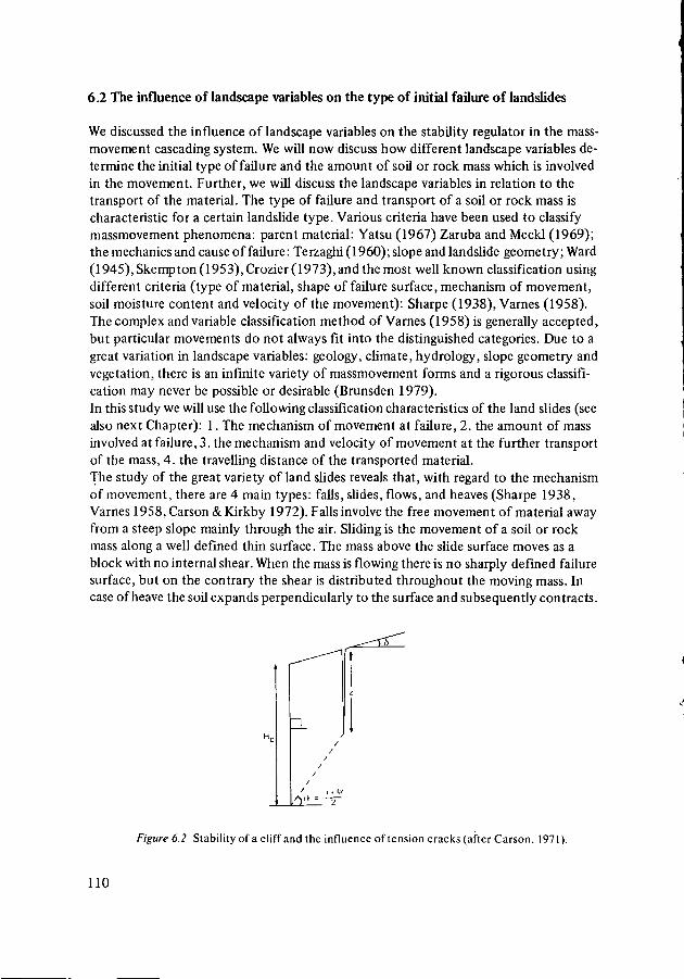
6.2 The influence of landscape variables on the type of initial failure of landslides

We discussed the influence of landscape variables on the stability regulator in the mass-movement cascading system. We will now discuss how different landscape variables de-termine the initial type of failure and the amount of soil or rock mass which is involvedin the movement. Further, we will discuss the landscape variables in relation to thetransport of the material. The type of failure and transport of a soil or rock mass ischaracteristic for a certain landslide type. Various criteria have been used to classifymassmovement phenomena: parent material: Yatsu (1967) Zaruba and Meckl (1969);the mechanics and cause of failure: Terzaghi (1960); slope and landslide geometry; Ward(1945), Skempton (1953), Crozier (1973), and the most well known classification usingdifferent criteria (type of material, shape of failure surface, mechanism of movement,soil moisture content and velocity of the movement): Sharpe (1938), Varnes (1958).The complex and variable classification method of Varnes (1958) is generally accepted,but particular movements do not always fit into the distinguished categories. Due to agreat variation in landscape variables: geology, climate, hydrology, slope geometry andvegetation, there is an infinite variety of massmovement forms and a rigorous classifi-cation may never be possible or desirable (Brunsden 1979).

In this study we will use the following classification characteristics of the land slides (seealso next Chapter): 1. The mechanism of movement at failure, 2. the amount of massinvolved at failure, 3. the mechanism and velocity of movement at the further transportof the mass, 4. the travelling distance of the transported material.The study of the great variety of land slides reveals that, with regard to the mechanismof movement, there are 4 main types: falls, slides, flows, and heaves (Sharpe 1938,Varnes 1958, Carson &Kirkby 1972). Falls involve the free movement of material awayfrom a steep slope mainly through the air. Sliding is the movement of a soil or rockmass along a well defined thin surface. The mass above the slide surface moves as ablock with no internal shear. When the mass is flowing there is no sharply defined failuresurface, but on the contrary the shear is distributed throughout the moving mass. Incase of heave the soil expands perpendicularly to the surface and subsequently contracts.

IL

/V' = —

Figure 6.2 Stability of a cliff and the influence of tension cracks (after Carson. 1971).

110

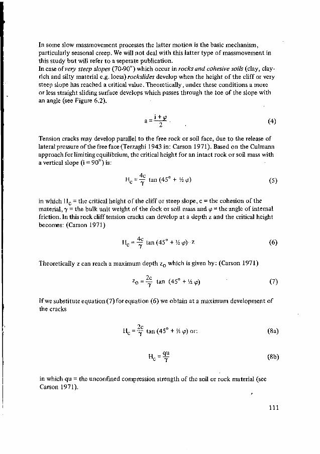
In some slow massmovement processes the latter motion is the basic mechanism,particularly seasonal creep. We will not deal with this latter type of massmovement inthis study but will refer to a seperate publication.In case of very steep slopes (70-90") which occur in rocks and cohesive soils (clay, clay-rich and silty material e.g. loess) rockslides develop when the height of the cliff or verysteep slope has reached a critical value. Theoretically, under these conditions a moreor less straight sliding surface develops which passes through the toe of the slope withan angle (see Figure 6.2).

Tension cracks may develop parallel to the free rock or soil face, due to the release oflateral pressure of the free face (Terzaghi 1943 in: Carson 1971). Based on the Culmannapproach for limiting equilibrium, the critical height for an intact rock or soil mass witha vertical slope (i = 90°) is:

Hc = j tan (45° + J4 *) (5)

in which Hc = the critical height of the cliff or steep slope, c = the cohesion of thematerial, y - the bulk unit weight of the rock or soil mass and ip = the angle of internalfriction. In this rock cliff tension cracks can develop at a depth z and the critical heightbecomes: (Carson 1971)

Hc = ^ tan (45° + Vi v?)-z (6)

Theoretically z can reach a maximum depth z0 which is given by: (Carson 1971)

z0 = y tan (45° +%<p) ' (7)

If we substitute equation (7) for equation (6) we obtain at a maximum development ofthe cracks

Hc = Y tan (45° + V2 </?) or: (8a)

Hc = -^- (8b)

in which qu = the unconfmed compression strength of the soil or rock material (seeCarson 1971).

I l l

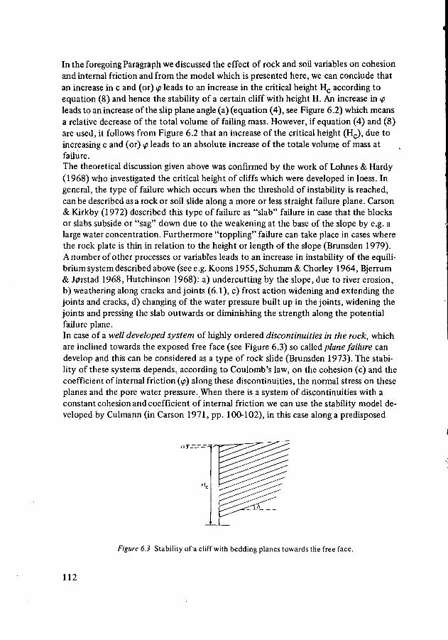
In the foregoing Paragraph we discussed the effect of rock and soil variables on cohesionand internal friction and from the model which is presented here, we can conclude thatan increase in c and (or) <p leads to an increase in the critical height Hc according toequation (8) and hence the stability of a certain cliff with height H. An increase in <pleads to an increase of the slip plane angle (a) (equation (4), see Figure 6.2) which meansa relative decrease of the total volume of failing mass. However, if equation (4) and (8)are used, it follows from Figure 6.2 that an increase of the critical height (Hc), due toincreasing c and (or) ip leads to an absolute increase of the totale volume of mass atfailure.

The theoretical discussion given above was confirmed by the work of Lohnes & Hardy(1968) who investigated the critical height of cliffs which were developed in loess. Ingeneral, the type of failure which occurs when the threshold of instability is reached,can be described as a rock or soil slide along a more or less straight failure plane. Carson& Kirkby (1972) described this type of failure as "slab" failure in case that the blocksor slabs subside or "sag" down due to the weakening at the base of the slope by e.g. alarge water concentration. Furthermore "toppling" failure can take place in cases wherethe rock plate is thin in relation to the height or length of the slope (Brunsden 1979).A number of other processes or variables leads to an increase in instability of the equili-brium system described above (see e.g. Koons 1955, Schumm & Chorley 1964, Bjerrum& J0rstad 1968, Hutchinson 1968): a) undercutting by the slope, due to river erosion,b) weathering along cracks and joints (6.1), c) frost action widening and extending thejoints and cracks, d) changing of the water pressure built up in the joints, widening thejoints and pressing the slab outwards or diminishing the strength along the potentialfailure plane.

In case of a well developed system of highly ordered discontinuities in the rock, whichare inclined towards the exposed free face (see Figure 6.3) so called plane failure candevelop and this can be considered as a type of rock slide (Brunsden 1973). The stabi-lity of these systems depends, according to Coulomb's law, on the cohesion (c) and thecoefficient of internal friction (tp) along these discontinuities, the normal stress on theseplanes and the pore water pressure. When there is a system of discontinuities with aconstant cohesion and coefficient of internal friction we can use the stability model de-veloped by Culmann (in Carson 1971, pp. 100-102), in this case along a predisposed

Figure 6.3 Stability of a cliff with bedding planes towards the free face.

112

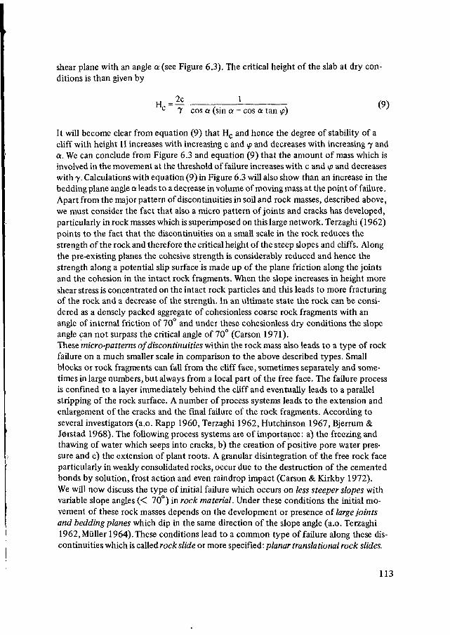
shear plane with an angle a (see Figure 6.3). The critical height of the slab at dry con-ditions is than given by

H = 2 cc 7 ( 9 )

7 cos a (sin a - cos a tan ip)

It will become clear from equation (9) that Hc and hence the degree of stability of acliff with height H increases with increasing c and y and decreases with increasing y anda. We can conclude from Figure 6.3 and equation (9) that the amount of mass which isinvolved in the movement at the threshold of failure increases with c and <p and decreaseswith y. Calculations with equation (9) in Figure 6.3 will also show than an increase in thebedding plane angle a leads to a decrease in volume of moving mass at the point of failure.Apart from the major pattern of discontinuities in soil and rock masses, described above,we must consider the fact that also a micro pattern of joints and cracks has developed,particularly in rock masses which is superimposed on this large network. Terzaghi (1962)points to the fact that the discontinuities on a small scale in the rock reduces thestrength of the rock and therefore the critical height of the steep slopes and cliffs. Alongthe pre-existing planes the cohesive strength is considerably reduced and hence thestrength along a potential slip surface is made up of the plane friction along the jointsand the cohesion in the intact rock fragments. When the slope increases in height moreshear stress is concentrated on the intact rock particles and this leads to more fracturingof the rock and a decrease of the strength. In an ultimate state the rock can be consi-dered as a densely packed aggregate of cohesionless coarse rock fragments with anangle of internal friction of 70° and under these cohesionless dry conditions the slopeangle can not surpass the critical angle of 70° (Carson 1971).

These micro-patterns of discontinuities within the rock mass also leads to a type of rockfailure on a much smaller scale in comparison to the above described types. Smallblocks or rock fragments can fall from the cliff face, sometimes separately and some-times in large numbers, but always from a local part of the free face. The failure processis confined to a layer immediately behind the cliff and eventually leads to a parallelstripping of the rock surface. A number of process systems leads to the extension andenlargement of the cracks and the final failure of the rock fragments. According toseveral investigators (a.o. Rapp 1960, Terzaghi 1962, Hutchinson 1967, Bjerrum &J0rstad 1968). The following process systems are of importance: a) the freezing andthawing of water which seeps into cracks, b) the creation of positive pore water pres-sure and c) the extension of plant roots. A granular disintegration of the free rock faceparticularly in weakly consolidated rocks, occur due to the destruction of the cementedbonds by solution, frost action and even raindrop impact (Carson & Kirkby 1972).We will now discuss the type of initial failure which occurs on less steeper slopes withvariable slope angles (< 70°) in rock material. Under these conditions the initial mo-vement of these rock masses depends on the development or presence of large jointsand bedding planes which dip in the same direction of the slope angle (a.o. Terzaghi1962, Müller 1964). These conditions lead to a common type of failure along these dis-continuities which is called rock slide or more specified : planar translational rock slides.

113

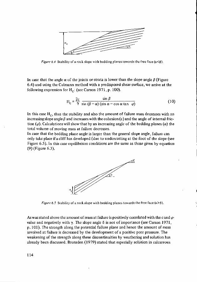
Figure 6.4 Stability of a rock slope with bedding planes towards the free face (a<ß).

In case that the angle a of the joints or strata is lower than the slope angle ß (Figure6.4) and using the Culmann method with a predisposed shear surface, we arrive at thefollowing expression for Hc: (see Carson 1971, p. 100).

= 2c sinjîc If sin (ß — a) (sin a - cos a tan

(10)

In this case Hc, thus the stability and also the amount of failure mass decreases with anincreasing slope angle ß and increases with the cohesion (c) and the angle of internal fric-tion (ip). Calculations will show that by an increasing angle of the bedding planes (a) thetotal volume of moving mass at failure decreases.In case that the bedding plane angle is larger than the general slope angle, failure canonly take place if a cliff has developed (due to undercutting at the foot of the slope (seeFigure 6.5). In this case equilibrium conditions are the same as those given by equation(9) (Figure 6.3).

Figure 6.5 Stability of a rock slope with bedding planes towards the free face (a>ß).

As was stated above the amount of mass at failure is positively correlated with the c and <p-value and negatively with -y. The slope angle S is not of importance (see Carson 1971,p. 101). The strength along the potential failure plane and hence the amount of massinvolved at failure is decreased by the development of a positive pore pressure. Theweakening of the strength along these discontinuities by weathering and solution hasalready been discussed. Brunsden (1979) stated that especially solution in calcareous

114

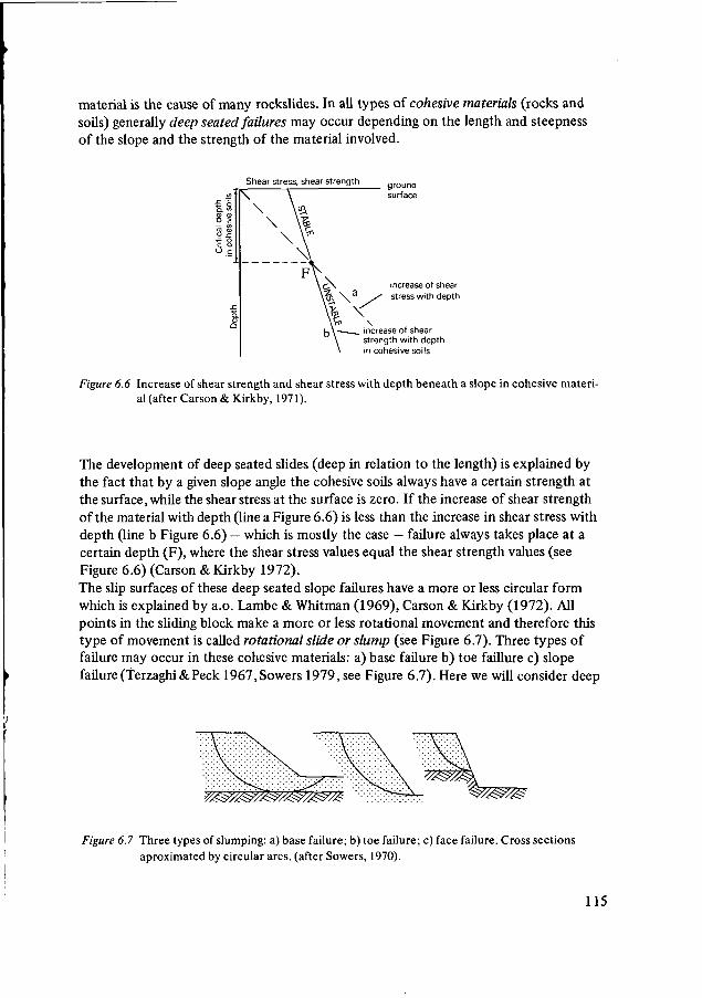
material is the cause of many rockslides. In all types of cohesive materials (rocks andsoils) generally deep seated failures may occur depending on the length and steepnessof the slope and the strength of the material involved.

Shear stress, shear strength

increase of shearstress with depth

increase of shearstrength with depthin cohesive soils

Figure 6.6 Increase of shear strength and shear stress with depth beneath a slope in cohesive materi-al (after Carson & Kirkby, 1971 ).

The development of deep seated slides (deep in relation to the length) is explained bythe fact that by a given slope angle the cohesive soils always have a certain strength atthe surface, while the shear stress at the surface is zero. If the increase of shear strengthof the material with depth (line a Figure 6.6) is less than the increase in shear stress withdepth (line b Figure 6.6) — which is mostly the case — failure always takes place at acertain depth (F), where the shear stress values equal the shear strength values (seeFigure 6.6) (Carson & Kirkby 1972).The slip surfaces of these deep seated slope failures have a more or less circular formwhich is explained by a.o. Lambe & Whitman (1969), Carson & Kirkby (1972). Allpoints in the sliding block make a more or less rotational movement and therefore thistype of movement is called rotational slide or slump (see Figure 6.7). Three types offailure may occur in these cohesive materials: a) base failure b) toe faillure c) slopefailure (Terzaghi&Peck 1967,Sowers 1979, see Figure 6.7). Here we will consider deep

Figure 6.7 Three types of slumping: a) base failure; b) toe failure; c) face failure. Cross sectionsaproximated by circular arcs, (after Sowers, 1970).

115

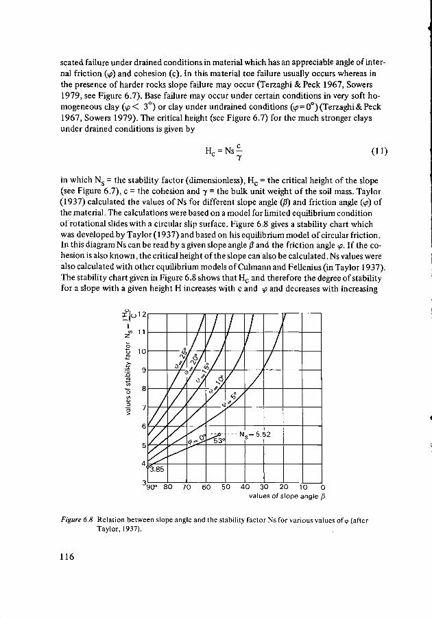
seated failure under drained conditions in material which has an appreciable angle of inter-nal friction (#) and cohesion (c). In this material toe failure usually occurs whereas inthe presence of harder rocks slope failure may occur (Terzaghi & Peck 1967, Sowers1979, see Figure 6.7). Base failure may occur under certain conditions in very soft ho-mogeneous clay (y < 3°) or clay under undrained conditions (tp = 0°) (Terzaghi & Peck1967, Sowers 1979). The critical height (see Figure 6.7) for the much stronger claysunder drained conditions is given by

Hc = N s -C y

(11)

in which Ns = the stability factor (dimensionless), Hc = the critical height of the slope(see Figure 6.7), c = the cohesion and y = the bulk unit weight of the soil mass. Taylor(1937) calculated the values of Ns for different slope angle (ß) and friction angle (ip) ofthe material. The calculations were based on a model for limited equilibrium conditionof rotational slides with a circular slip surface. Figure 6.8 gives a stability chart whichwas developedby Taylor (1937) andbased on his equilibrium model of circular friction.In this diagram Ns can be read by a given slope angle ß and the friction angle <p. If the co-hesion is also known, the critical height of the slope can also be calculated. Ns values werealso calculated with other equilibrium models of Culmann and Fellenius (in Taylor 1937).The stability chart given in Figure 6.8 shows that Hc and therefore the degree of stabilityfor a slope with a given height H increases with c and ip and decreases with increasing

11

ou 10

CO

V,'S

COCD

/

/ /

/ / /

/ /

"3.85

1/

\ i\//C$*"

1

j[4Ay

ji

1

-—N

/

/

/

s -5 .5

1/

>2

90° 80 70 60 50 40 30 20 10 0values of slope angle ß

Figure 6.8 Relation between slope angle and the stability factor Ns for various values of cp (afterTaylor, 1937).

116

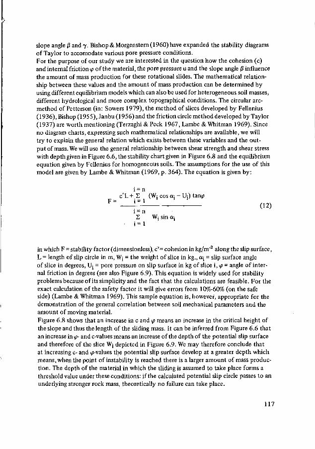
slope angle ß and 7. Bishop & Morgenstern (1960) have expanded the stability diagramsof Taylor to accomodate various pore pressure conditions.For the purpose of our study we are interested in the question how the cohesion (c)and internal friction ^ of the material, the pore pressure u and the slope angle ß influencethe amount of mass production for these rotational slides. The mathematical relation-ship between these values and the amount of mass production can be determined byusing different equilibrium models which can also be used for heterogeneous soil masses,different hydrological and more complex topographical conditions. The circular arc-method of Petterson (in: Sowers 1979), the method of slices developed by Fellenius(1936), Bishop (1955), Janbu (1956) and the friction circle method developed by Taylor(1937) are worth mentioning (Terzaghi & Peck 1967, Lambe & Whitman 1969). Sinceno diagram charts, expressing such mathematical relationships are available, we willtry to explain the general relation which exists between these variables and the out-put of mass. We will use the general relationship between shear strength and shear stresswith depth given in Figure 6.6, the stability chart given in Figure 6.8 and the equilibriumequation given by Fellenius for homogeneous soils. The assumptions for the use of thismodel are given by Lambe & Whitman (1969, p. 364). The equation is given by:

i = nc'L + S (Wj cos aj - Uj) tamp

F = — ± üi = nS Wj sin a,

l

in which F = stability factor (dimensionless), c'= cohesion in kg/m"2 along the slip surface,L = length of slip circle in m, Wj = the weight of slice in kg., CKJ = slip surface angleof slice in degrees, Uj = pore pressure on slip surface in kg of slice i, <p = angle of inter-nal friction in degrees (see also Figure 6.9). This equation is widely used for stabilityproblems because of its simplicity and the fact that the calculations are feasible. For theexact calculation of the safety factor it will give errors from 10%-60% (on the safeside) (Lambe & Whitman 1969). This sample equation is, however, appropriate for thedemonstration of the general correlation between soil mechanical parameters and theamount of moving material.Figure 6.8 shows that an increase in c and ip means an increase in the critical height ofthe slope and thus the length of the sliding mass. It can be inferred from Figure 6.6 thatan increase in <p- and c-values means an increase of the depth of the potential slip surfaceand therefore of the slice Wj depicted in Figure 6.9. We may therefore conclude thatat increasing c- and <p-values the potential slip surface develop at a greater depth whichmeans, when the point of instability is reached there is a larger amount of mass produc-tion. The depth of the material in which the sliding is assumed to take place forms athreshold value under these conditions: if the calculated potential slip circle passes to anunderlying stronger rock mass, theoretically no failure can take place.

117

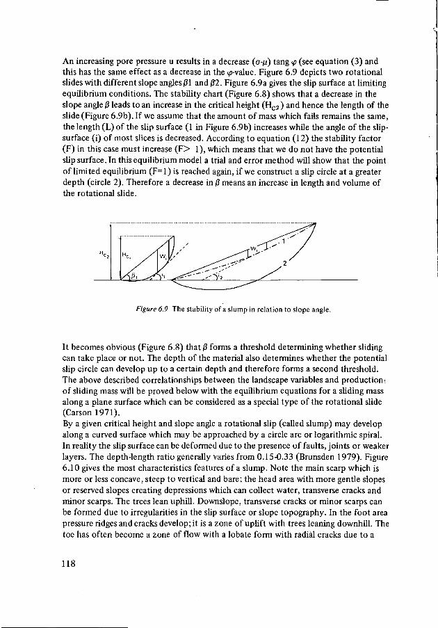
An increasing pore pressure u results in a decrease (0-/1) tang <p (see equation (3) andthis has the same effect as a decrease in the Rvalue. Figure 6.9 depicts two rotationalslides with different slope angles 01 and 02. Figure 6.9a gives the slip surface at limitingequilibrium conditions. The stability chart (Figure 6.8) shows that a decrease in theslope angle ß leads to an increase in the critical height (Hc2 ) and hence the length of theslide (Figure 6.9b). If we assume that the amount of mass which fails remains the same,the length (L) of the slip surface (1 in Figure 6.9b) increases while the angle of the slip-surface (i) of most slices is decreased. According to equation (12) the stability factor(F) in this case must increase (F> 1), which means that we do not have the potentialslip surface. In this equilibrium model a trial and error method will show that the pointof limited equilibrium (F=l) is reached again, if we construct a slip circle at a greaterdepth (circle 2). Therefore a decrease in j3 means an increase in length and volume ofthe rotational slide.

Figure 6.9 The stability of a slump in relation to slope angle.

It becomes obvious (Figure 6.8) that ß forms a threshold determining whether slidingcan take place or not. The depth of the material also determines whether the potentialslip circle can develop up to a certain depth and therefore forms a second threshold.The above described correlationships between the landscape variables and production,of sliding mass will be proved below with the equilibrium equations for a sliding massalong a plane surface which can be considered as a special type of the rotational slide(Carson 1971).By a given critical height and slope angle a rotational slip (called slump) may developalong a curved surface which may be approached by a circle arc or logarithmic spiral.In reality the slip surface can be deformed due to the presence of faults, joints or weakerlayers. The depth-length ratio generally varies from 0.15-0.33 (Brunsden 1979). Figure6.10 gives the most characteristics features of a slump. Note the main scarp which ismore or less concave, steep to vertical and bare; the head area with more gentle slopesor reserved slopes creating depressions which can collect water, transverse cracks andminor scarps. The trees lean uphill. Downslope, transverse cracks or minor scarps canbe formed due to irregularities in the slip surface or slope topography. In the foot areapressure ridges and cracks develop; it is a zone of uplift with trees leaning downhill. Thetoe has often become a zone of flow with a lobate form with radial cracks due to a

118

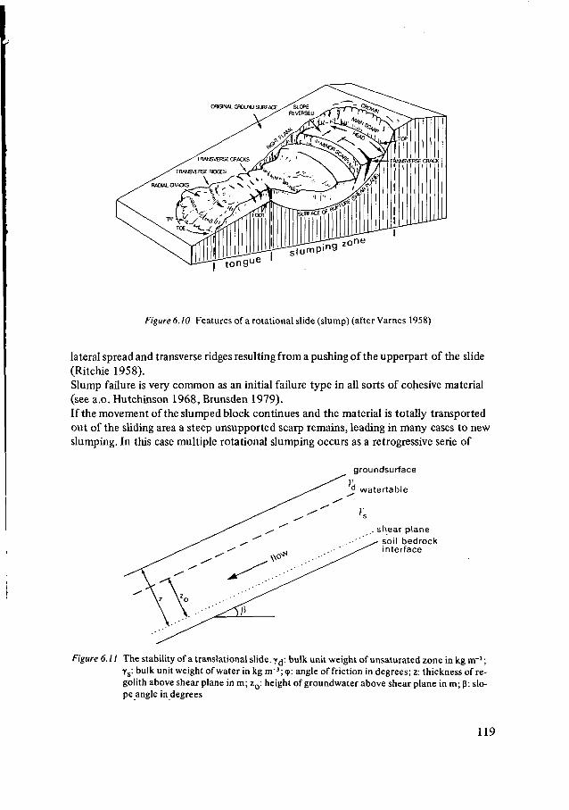
ORION«. GROUND SURFACE

ne

Figure 6.10 Features of a rotational slide (slump) (after Varnes 1958)

lateral spread and transverse ridges resulting from a pushing of the upperpart of the slide(Ritchie 1958).Slump failure is very common as an initial failure type in all sorts of cohesive material(see a.o. Hutchinson 1968, Brunsden 1979).If the movement of the slumped block continues and the material is totally transportedout of the sliding area a steep unsupported scarp remains, leading in many cases to newslumping. In this case multiple rotational slumping occurs as a retrogressive serie of

groundsurface

d watertable

.. shear planesoil bedrockinterface

Figure 6.11 The stability of a translational slide, y^: bulk unit weight of unsaturated zone in kg rrr3;ys: bulk unit weight of water in kg nr3;<p: angle of friction in degrees; z: thickness of re-golith above shear plane in m; zo: height of groundwater above shear plane in m; ß: slo-pe angle in degrees

119

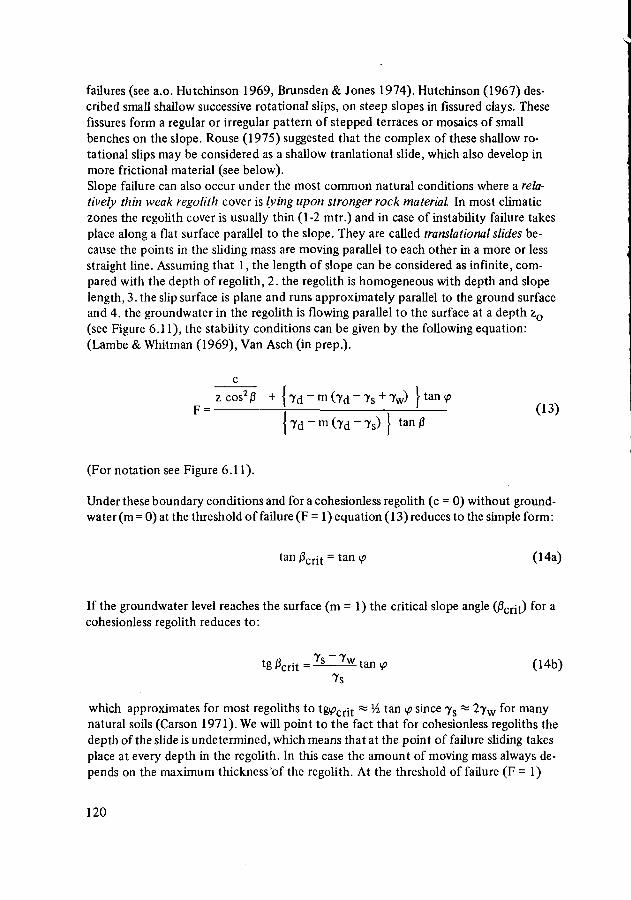
failures (see a.o. Hutchinson 1969, Brunsden & Jones 1974). Hutchinson (1967) des-cribed small shallow successive rotational slips, on steep slopes in fissured clays. Thesefissures form a regular or irregular pattern of stepped terraces or mosaics of smallbenches on the slope. Rouse (1975) suggested that the complex of these shallow ro-tational slips may be considered as a shallow tranlational slide, which also develop inmore frictional material (see below).Slope failure can also occur under the most common natural conditions where a rela-tively thin weak regolith cover is lying upon stronger rock material In most climaticzones the regolith cover is usually thin (1-2 mtr.) and in case of instability failure takesplace along a flat surface parallel to the slope. They are called translational slides be-cause the points in the sliding mass are moving parallel to each other in a more or lessstraight line. Assuming that 1, the length of slope can be considered as infinite, com-pared with the depth of regolith, 2. the regolith is homogeneous with depth and slopelength, 3. the slip surface is plane and runs approximately parallel to the ground surfaceand 4. the groundwater in the regolith is flowing parallel to the surface at a depth z0

(see Figure 6.11), the stability conditions can be given by the following equation:(Lambe & Whitman (1969), Van Asch (in prep.).

z cos2j3 + { 7d - m (7d - 7s + 7w) } t a n f>F = ? j (13)

| 7 d - m (7d - 7S) I tan 0

(For notation see Figure 6.11).

Under these boundary conditions and for a cohesionless regolith (c = 0) without ground-water (m = 0) at the threshold of failure (F = 1 ) equation (13) reduces to the simple form :

tan 0c rj t = tan ip (14a)

If the groundwater level reaches the surface (m = 1) the critical slope angle (0crjt) for acohesionless regolith reduces to:

( 1 4 b )

7s

which approximates for most regoliths to tg<^crjt «= VL tan ip since 7S « 27W for manynatural soils (Carson 1971). We will point to the fact that for cohesionless regoliths thedepth of the slide is undetermined, which means that at the point of failure sliding takesplace at every depth in the regolith. In this case the amount of moving mass always de-pends on the maximum thickness "of the regolith. At the threshold of failure (F = 1)

120

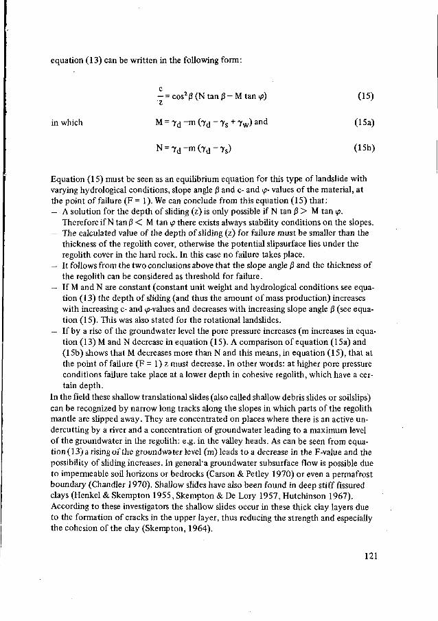
equation (13) can be written in the following form:

c—=cos20(Ntan|3-Mtanip) (15)

in which M = 7 d -m (7^ - 7S + 7W) and (15a)

N = 7 d - m ( 7 d - T s ) (15b)

Equation (15) must be seen as an equilibrium equation for this type of landslide withvarying hydrological conditions, slope angle ß and c- and \p- values of the material, atthe point of failure (F = 1). We can conclude from this equation (15) that:— A solution for the depth of sliding (z) is only possible if N tan ß > M tan ip.

Therefore if N tan ß < M tan ip there exists always stability conditions on the slopes.— The calculated value of the depth of sliding (z) for failure must be smaller than the

thickness of the regolith cover, otherwise the potential slipsurface lies under theregolith cover in the hard rock. In this case no failure takes place.

— It follows from the two conclusions above that the slope angle ß and the thickness ofthe regolith can be considered as threshold for failure.

— If M and N are constant (constant unit weight and hydrological conditions see equa-tion (13) the depth of sliding (and thus the amount of mass production) increaseswith increasing c- and ( -values and decreases with increasing slope angle ß (see equa-tion (15). This was also stated for the rotational landslides.

— If by a rise of the groundwater level the pore pressure increases (m increases in equa-tion (13) M and N decrease in equation (15). A comparison of equation (15a) and(15b) shows that M decreases more than N and this means, in equation (15), that atthe point of failure (F = 1) z must decrease. In other words: at higher pore pressureconditions failure take place at a lower depth in cohesive regolith, which have a cer-tain depth.

In the field these shallow translational slides (also called shallow debris slides or soilslips)can be recognized by narrow long tracks along the slopes in which parts of the regolithmantle are slipped away. They are concentrated on places where there is an active un-dercutting by a river and a concentration of groundwater leading to a maximum levelof the groundwater in the regolith: e.g. in the valley heads. As can be seen from equa-tion (13) a rising of the groundwater level (m) leads to a decrease in the F-value and thepossibility of sliding increases. In general'a groundwater subsurface flow is possible dueto impermeable soil horizons or bedrocks (Carson & Petley 1970) or even a permafrostboundary (Chandler 1970). Shallow slides have also been found in deep stiff fissuredclays (Henkel & Skempton 1955, Skempton & De Lory 1957, Hutchinson 1967).According to these investigators the shallow slides occur in these thick clay layers dueto the formation of cracks in the upper layer, thus reducing the strength and especiallythe cohesion of the clay (Skempton, 1964).

121

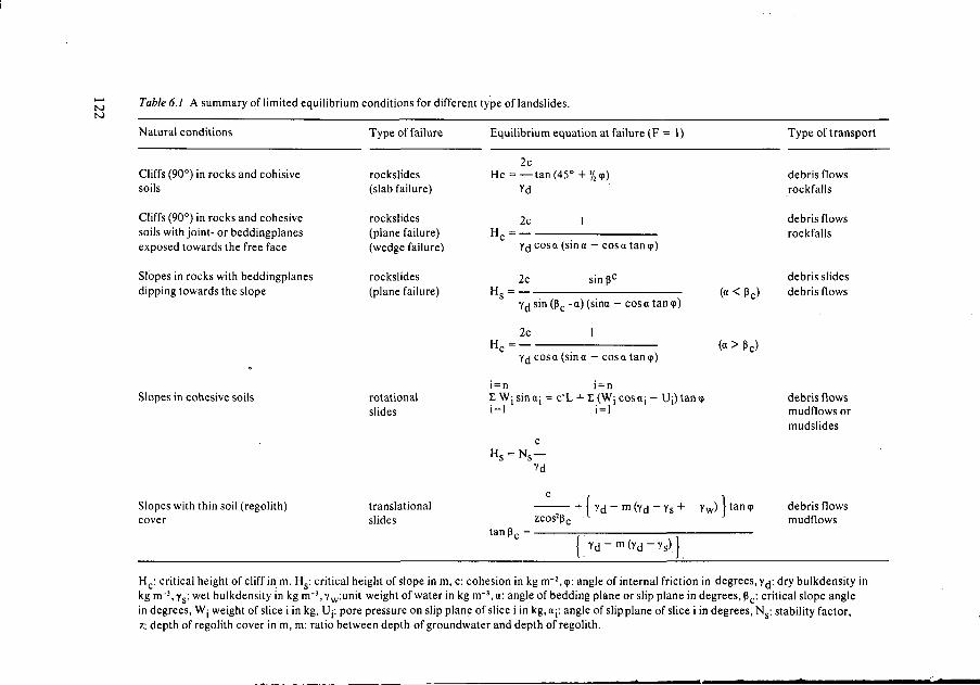
toto

Table 6.1 A summary of limited equilibrium conditions for different type of landslides.

Natural conditions Type of failure Equilibrium equation at failure (F = 1) Type of transport

Cliffs (90°) in rocks and cohisivesoils

Cliffs (90°) in rocks and cohesivesoils with joint- or beddingplanesexposed towards the free face

Slopes in rocks with beddingplanesdipping towards the slope

Slopes in cohesive soils

rockslides(slab failure)

rockslides(plane failure)(wedge failure)

rockslides(plane failure)

rotationalslides

2cH c = — tan (45° + y2 <p)

Yd

2c 1n c

Yd cos a (sin a — cos a tan p)

2cHs = —

sin ßc

Yd sin (ßc - a) (sina — cos a tan p)

2c 1H c = -

Yd cos a (sin a - cos a tan <p)

i=n i=nÏ Wjsinaj = c'L + E(Wjcosaj - Uj)tan<p

(a < ßc)

(a > ßc)

debris flowsrockfalls

debris flowsrockfalls

debris slidesdebris flows

debris flowsmudflows ormudslides

Slopes with thin soil (regolith)cover

translationalslides

Yd

tan ßc = •zcos2ßc

+ I Yd- m (Yd-Ys+ Yw) ftanp

1

debris flowsmudflows

Hc: critical height of cliff in m. Hs: critical height of slope in m, c: cohesion in kg m~2, p: angle of internal friction in degrees, Yd'- dry bulkdensity inkg nr3,Ys: wet bulkdensity in kgnr3,Yw:unit weight of water in kgm~3,a: angle of bedding plane or slip plane in degrees, ßc: critical slope anglein degrees, Wj weight of slice i in kg, UJ: pore pressure on slip plane of slice i in kg, a;: angle of slip.plane of slice i in degrees, Ns: stability factor,z: depth of regolith cover in m, m: ratio between depth of groundwater and depth of regolith.

In the foregoing we have discussed the influence of soil and rock variables and topo-graphical variables on the initial state of equilibrium and the amount of mass which isinvolved at sliding for different types. Table 6.1 summarizes the equilibrium equationsfor the different landslide types discussed above. We can deduce from the equationsthat for all the types an increase in c- and Rvalue leads to an increase of stability. Sincethe pore pressure (u) in all these equations are related to tan <p (according to Coulomb'sequation), an increase in pore pressure always leads to a decrease in strength and there-fore the stability of the system. The equation will also show that an increasing slopeangle and bulkdensity decreases the stability of the system. In other words in an areawith variable slope angles and different materials, the chance or frequency of landslidingmust increase with increasing slope angles and decrease with increasing strength valuesof the material. In cohesive materials the depth of the material in which potential sli-ding takes place is an important threshold (see e.g.: equation (13).At the threshold of failure the F-value is 1 or the height of the slope is critical (Hc).We can deduce from the discussions given above and the equations summarized in Table6.1 that at the point of failure the amount of sliding mass is determined by variousvariables. Steeper slope angles and a rising bulkdensity at failure lead to a decrease ofsliding mass, whereas higher c- and ^-values at failure lead to an increase in sliding mass.Since (u) is related to (ip) (see above) we can also conclude that rising pore pressure lo-wers the value (cr-u) tan ip and therefore leads to a decrease of mass at failure. Thedepth of weathered regoliths determines the maximum depth at which sliding can takeplace and it is therefore also a variable which determines the potential maximumamount of mass production at failure.

6.3 The influence of landscape variables on the type of transport of landslides

In this Paragraph the influence of landscape variables on the transport of the materialafter failure has taken place, will be discussed. In the massmovement cascading systemthe distance and velocity of transport of the moving material are subjects of particularinterest. We have already stated that the type of initial failure may influence the furthertransportation of the material and therefore the main type of transport in relation todifferent types of initial failure will be discussed here.First the mobilisation of debris after the initial failure of a rock mass (rock slides) willbe discussed. Heim (1936) found from empirical evidence that the travelling distanceof a slab along the slope depends on the initial height of fall, the irregularity of the ter-rain and the size (volume) of the slide. During the movement the rock slab can be frac-tured along the sliding path in a mass of loose debris which, due to a change in physicalcharacteristics, increases the mobility of the mass. The data collected by Brunsden(1979) from different authors reveal that the material travels many kilometers beyondthe point that might be expected of a rigid mass sliding down an inclined plane. Duringmovement of the fractured rock material air may be trapped. The effective stress be-tween particles suddenly decreases, resulting in a high fluidity of the material and cata-strophic rapid flows (Kent 1966). Shreve (1968) hypothised that a cushion of air is

123

trapped at the base of the flow thus forming a near frictionless surface for the movingmass, which in this case behaves as sliding blocks with a slip surface at the base. Hsü(1975) proposed that the factional resistance is reduced by the boyunt effect of dustsuspensions acting as a fluid medium between the "floating" blocks.The velocity of the above debris flow (or slidej-Uampoit process is very fast, i.e. 150-300 km/hour (Brunsden 1979). These flows have the features of a lavaflow or glacierin planform, sometimes with a wide lobe as it extends over a wide flat riverplain. The flowmay sometimes run up the opposite valley side (see Brunsden 1979 pp. 156-157). Thelongitudinal profile slopes gently. A trough can be found between the head and scarand the surface of the flow shows a humockly topography with ponds and enclosed de-pressions, transverse ridges and longitudinal ridges. The material is very heterogeneous,with a tendency towards a concentration of coarser material on the surface. In the flowlarge blocks up to several meters can be transported. In thick soil and regolith of variablegrainsizes shallow slides and also rotational slides can develop (see above). If failure takesplace under the influence of a high water table and high pore water pressure and if thematerial disintegrates after initial failure, the moving material changes into a rapid vis-cous flow. These flows are described as debrisflow, debris avalanche, mudflow or mud-avalanche or flowslide (a.o. Rapp 1960, Johnson & Rahn 1970, Prior et al. 1970,Bishop 1973 and Blong 1973). The travelling distance may be related to the slope angleand the thickness of the mass, (Curly 1966, Sulebak 1969, Cambel 1974) which deter-mine the amount of shear stress. The water content of the material (varying from 15-40%) determines the viscosity and the topography within the track pass.

The flows, which may reach velocities from 1-14 mtr/sec. generally have, a relatively largelength-depth ratio varying from 9-270 (Brunsden 1979). The track of the flow may bewidened downslope after the break up of the initial sliding material. Along the sideslevees can be formed. These are characteristic for rapid and very wet flows. They showcircular heads and in the toe area single or multiple lobes. Initial failure can take placeby shallow slides and slope angles varying from 25-20°, while flow transport occurs onangles varying from 10-15° (Statham 1977).Initial failure of soil material can also be followed by a much slower transportation ofsliding material in the form of either flow or sliding movements. The initial rotated massparticularly in clay rich material can be broken and can assemble large quantities ofwater which give the clay a more viscous component with lower yield strength (see 6.1).When the topographical situation is appropriate the material can be further transportedover a long distance, by means of flowing or sliding processes (Hutchinson 1970, Prior& Stephens 1972). The detailed investigations of Hutchinson & Bhandari (1971) showthat mechanism of transport may be explained by the effect of the rapid loading ofmaterial falling from upslope at the flow which creates undrained pore water pressuresand a loss of strength in the soil mass. This leads to a sliding movement of the wholeblock along a well defined slip surface (slope angles > 14°).Another suggestion is that due to a high water content the material has a viscous com-ponent with a relatively low yield strength (see 6.1). In this case, at a certain depth andslope angle, shear stresses in the soil mass surpasses the yield strength of the material

124

and transport via viscous flow can take place (Yen 1969, Ter-Stephanian 1965). There-fore investigations on stress-strain behaviour under different water contents are very im-portant to these types of flows. The morphometry of these so-called mudflows (orslides) is very characteristic. In general we can distinguish a supply area, in which slum-ping movements take place, a central neck or track, and a lobate toe area (Brunsden1979). In the track the mudflow has very sharp shear surfaces on sides and base. In thetrack and toe area there are radial cracks (toe), transverse cracks (where the slide passessteeper slopes) and shear cracks along the sides. The flow may consist of unweatheredmaterial in a matrix of softened and weathered material. A dry crust may develop atthe surface during dry periods in summer. The rate of movements is generally slow ±5-25 mtr. per year (Brunsden 1979) on slopes averaging 7°. Movements occur seasonallyand may be related to seasonal rainfall patterns.

NOTES

1 The amount of strain of a specimen of soil or lock can be defined as e = dl/lo where 1Q is the initiallength of the specimen, (1Q - dl) in the length after compression, è = de/dt), which is a functionof the stress.

125

THE INFLUENCE OF LANDSCAPE VARIABLES ON THE MASS-MOVEMENT CASCADING SYSTEM IN THE STUDY AREA

In this Chapter we will discuss the influence of landscape variables on the amount ofproduction of soil and rock mass and the transport characteristics of the failed massin the massmovement cascading system in the study area..The amount of mass production by landslides in a given area is determined by thenumber of slides, and the amount of mass which is produced at each individual slide.In order to obtain an insight into the frequency of sliding within a certain area, wemust determine the landscape variables giving the boundary conditions for failure bydifferent types of slide. We will also analyse the influence of these landscape variableson the amount of mass production at each individual type of slide (see Chapter 6,Table 6.1).Table 7.1 is a survey of the type of landslides which have been distinguished in thestudy area. The types are distinguished according to the following characteristics: a)the mechanism of movement at initial failure, b) the mechanism of movement at afurther transport, c) the type of material involved at initial failure, d) the range ofslope angle values at which failure took place, e) an indication of the amount of massinvolved at failure, f) specific landscape•— and process variables which have initiatedmovement and g) the stability conditions at present. A detailed description of thecharacteristics of the slides will be given below in the various typical examples. We willuse the following terminology (with regard to the mechanism of movement):— planar rock or debris slides: sliding of respectively a rock or soil (devris) mass along

a more or less plane slip surface;— rotational rock or soil slides (slumps): rotational sliding or soil (debris) mass along

along a more or less circular slipsurface.— rapid debris flow: rapid flowing of debris or (finer) soil mass from a sliding area.— slow mudflow: slow flowing of fine soil material out of a sliding area into valley

systems. Mechanism of movement can also take place via sliding processes.

As regard to the velocity of movement (Table 7.1 see: column 2), we propose, accordingto Varnes (1958) the following classification:a) extremely rapid > 3 mtr/sec, b) very rapid 3 mtr/sec — 0.30 mtr/min, c) rapid 0.30mtr/min - 2 mtr/day, d) moderate 2 mtr/day - 2 mtr/month, e) slow 2 mtr/month —2 mtr/year, 0 very slow 2 mtr/year - 0.30 mtr/5 year, g) extremely slow < 0.30 m/5year.In column 3 is indicated the dominant length, width and depth of the landslide type.Also is roughly indicated in this column the proportion of the surface of the slidingmass (T), which is lying out of the source area of the slide T is the distance from toe tosource area for different characteristic landslide types, which gives also an indicationof transport. In column 5 is indicated the type of material which was involved at initial

127

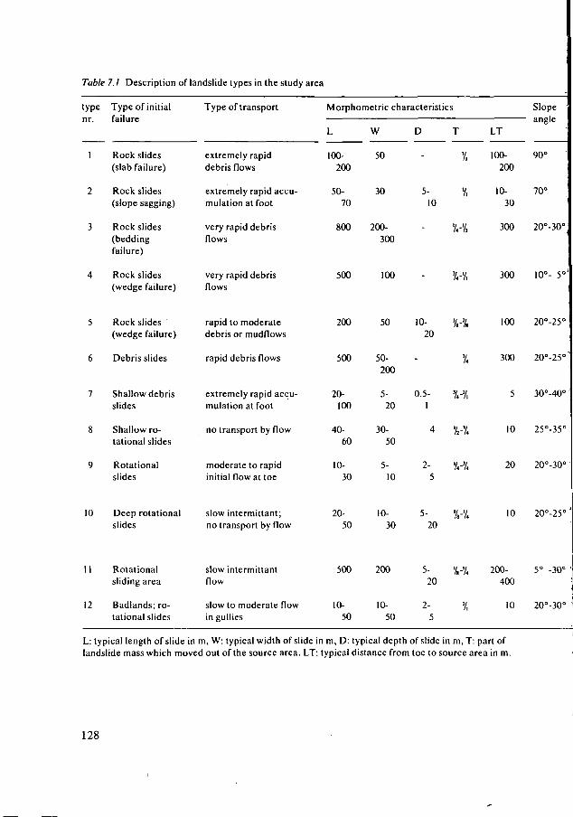
Table 7.1 Description of landslide types in the study area

typenr.

1

2

3

4

5

6

7

8

9

10

II

12

Type of initialfailure

Rock slides(slab failure)

Rock slides(slope sagging)

Rock slides(beddingfailure)

Rock slides(wedge failure)

Rock slides(wedge failure)

Debris slides

Shallow debrisslides

Shallow ro-tational slides

Rotationalslides

Deep rotationalslides

Rotationalsliding area

Badlands; ro-tational slides

Type of transport

extremely rapiddebris flows

extremely rapid accu-mulation at foot

very rapid debrisflows

very rapid debrisflows

rapid to moderatedebris or mudflows

rapid debris flows

extremely rapid accu-mulation at foot

no transport by flow

moderate to rapidinitial flow at toe

slow intermittant;no transport by flow

slow intermittantflow

slow to moderate flowin gullies

Morphometric characteristics

L

100-200

50-70

800

500

200

500

20-100

40-60

10-30

20-50

500

10-50

W

50

30

200-300

100

50

50-200

5-20

30-50

5-10

10-30

200

10-50

D

-

5-10

-

-

10-20

-

0.5-1

4

2-5

5-20

5-20

2-5

T

V,

'/•

%-'/,

3/,-y,

i

'/.-'/•

%-'/.

y,-1/.

y,-y,

y,

LT

100-200

10-30

300

300

100

300

5

10

20

10

200-400

10

Slope •• angle

90°

70°

2O°-3O°

10°- 5°'

2O°-25°

2O°-25°n

30°-40° '

25°-35°

2O°-3O°

20°-25° '

5° -30° '

2O°-3O° '

L: typical length of slide in m, W: typical width of slide in m, D: typical depth of slide in m, T: part oflandslide mass which moved out of the source area. LT: typical distance from toe to source area in m.

128

ock and soillaterial

Characteristic factors affecting landslides Activity

mdstones

indstones

retrogressive erosion by rivers; undercutting of theslope by rivers; earthquakes

undercutting of the slope by rivers; earthquakes

notactive

notactive

letamorphic rocks andmstones

lay- siltstones

indstones

ractured metamorphicocks and claystones

egoliths on clay- and,andstones and sf-rocks

fractured rock due to faulting; contact zones between notrocks; retrogressive erosion by rivers; dip of rock activelayers towards slope

weakening of the rock by joints and faults; supply of notwater from adjacent sandstones mass; dip of rock layers activetowards slope; earthquakes

dip of rocklayers and joints towards slope ; retro- activegressive erosion by rivers; impermeable clay-layers

fractured rock due to faulting; retrogressive erosion notby rivers; accumulation of groundwater at riverhead active

steepening of the foot of the slope and undercutting by rivers active

egoliths on meta-lorphic rocks

«•eathered claystones andandstones

weathered claystonesind metamorphic rocks

veathered claystonesind sandstones

accumulation of water due to slope- and contour con- activecavity; undercutting of the slope by man

undercutting and retrogressive erosion by rivers; activeaccumulation of groundwater at riverhead; impermeablerocks in subsurface: joints; terracing and irrigation

accumulation of groundwater at slope- and contour activeconcavities and riverhead ; presence of impermeablerock; steepening of the foot of the slope by rivers;weakening of the rock by joints and faults

water accumulation at riverhead; active

veathered metamorphicocks and sandstones

formation of gullies in scarps of landslides or insteep slip surfaces of shallow debris slides

active

129

failure. Column 4 gives the range of slope angles at which failure took place. The in-fluence of the soil mechanical parameters are discussed below, while in column 6 speciallocal landscape variable, which have initiated failure, are mentioned. In column 7 wehave indicated, among other remarks, whether the landslides are stable, or whethertransport (periodically) took place during the period of investigation (which was about3 years).

7.1. Landscape variables in relation to different types of rockslides

We have distinguished 5 types of rockslides, which were found in 4 different types ofrocks. The cohesive limy sandstones (Mar), the weakly cohesive sandstones (Mars), themetamorphic rocks (sf) and the claystones (Ma) (see Table 7.1).Most landslides of these types have big sizes and are stable at present. They probablydate from historical periods, which are characterized by many earthquakes.In the valley of the Torrente Guarno and the Torrente Pescio, south and south-east ofAyello Calabro and the Torrente La Fumerella, south east of San Pietro (see AppendixA 7) cliffs have developed in the cohesive limy sandstones (Mar). These sandstonepackages are underlain by weak cohesive sandstones (Mars) in which lesser steep slopeshave developed. The sandstone beds show almost no dip.In these sandstones rockslides of type no 1. (see Table 7.1) have developed. The cliffshave a height of 70-80 mtr. The cliff planes have two directions which probably corres-pond to dominant directions of joint planes in this area. At some spots along these jointplanes, the massive sandstone blocks have shifted away a little from the upper edge ofthe main scarp (see Plate 4). At some places at the foot of the cliff we observed anerosional slope developed in sandstone with an angle of 60°, which could be a slip sur-face. These slip surfaces are partly covered with blocks. They continue out of a wideand shallow upper valley end.In this flat valley system (slope 25°-30°) lies a debris mass which is concentrated alongthis valley and extends far below up to 200 mtr. from the cliff. In this debris mass Mar-sandstone boulders up to 30 meters in size have been transported from the cliff. Thedebris mass consists of a sandy loam to sandy clay matrix. The debris mass is at presentpartly terraced, evidence that the slides are fossil. The blocks which are partly inbeddedin the debris mass show, due to a difference in weathering at the sides, that the originalsurface of the debris mass must have lain at a higher level. Due to erosion of the originalsurface the blocks are further exposed in the mass. This also points to the fact that theactivity of these landslides is not of a recent date. The cliff also shows a difference inweathering of the rock also indicating that the landslides are not recent. Parts of thecliff wall are affected by more recent processes. Due to the dissolving of the limy ce-mentation material the sand looses its cohesion. The granular disintegration leads tothe formation of hollows (see Plate 5).

Wherever the hard limy sandstone (Mar) and the soft cohesive Mars-sandstone cropsout in the form of high steep valley walls these spectacular rockfalls were found (seemap Appendix A7). The height of the Mar-sandstone cliffs has lead to instability.

130

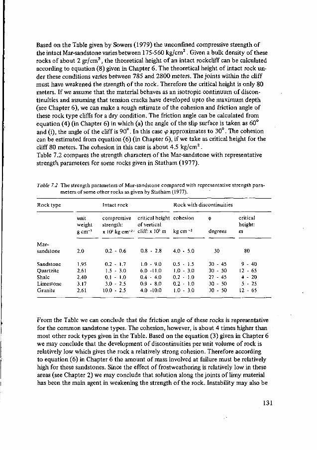
Based on the Table given by Sowers (1979) the unconfined compressive strength ofthe intact Mar-sandstone varies between 175-560 kg/cm2. Given a bulk density of theserocks of about 2 gr/cm3, the theoretical height of an intact rockcliff can be calculatedaccording to equation (8) given in Chapter 6. The theoretical height of intact rock un-der these conditions varies between 785 and 2800 meters. The joints within the cliffmust have weakened the strength of the rock. Therefore the critical height is only 80meters. If we assume that the material behaves as an isotropic continuum of discon-tinuities and assuming that tension cracks have developed upto the maximum depth(see Chapter 6), we can make a rough estimate of the cohesion and friction angle ofthese rock type cliffs for a dry condition. The friction angle can be calculated fromequation (4) (in Chapter 6) in which (a) the angle of the slip surface is taken as 60°and (i), the angle of the cliff is 90°. In this case <p approximates to 30°. The cohesioncan be estimated from equation (6) (in Chapter 6), if we take as critical height for thecliff 80 meters. The cohesion in this case is about 4.5 kg/cm2.Table 7.2 compares the strength characters of the Mar-sandstone with representativestrength parameters for some rocks given in Statham (1977).

Table 7.2 The strength parameters of Mar-sandstone compared with representative strength para-meters of some other rocks as given by Statham ( 1977).

Rock type

Mar-sandstone

SandstoneQuartziteShaleLimestoneGranite

unitweightgem'3

2.0

1.952.612.403.172.61

Intact rock

compressivestrength:x lCkgcm-1 '

0.2 - 0.6

0.2 - 1.71.5 - 3.00.1 - 1.03.0 - 2.5

10.0 - 2.5

critical heightof verticalcliff:

0.8

1.06.00.40.94.0

x lCm

- 2.8

- 9.0-11.0- 4.0- 8.0-10.0

Rock with discontinuities

cohesion

kg cm - !

4.0 - 5.0

0.5 - 1.51.0 - 3.00.2 - 1.00.2 - 1.01.0 - 3.0

<P

degrees

30

3 0 •

3 0 •

2 7 •

30 •3 0 •

• 4 5

• 5 0

• 4 5

• 5 0

• 50

criticalheight:m

80

9124 •5

12

- 40- 65• 20- 25- 65

From the Table we can conclude that the friction angle of these rocks is representativefor the common sandstone types. The cohesion, however, is about 4 times higher thanmost other rock types given in the Table. Based on the equation (3) given in Chapter 6we may conclude that the development of discontinuities per unit volume of rock isrelatively low which gives the rock a relatively strong cohesion. Therefore accordingto equation (6) in Chapter 6 the amount of mass involved at failure must be relativelyhigh for these sandstones. Since the effect of frostweathering is relatively low in theseareas (see Chapter 2) we may conclude that solution along the joints of limy materialhas been the main agent in weakening the strength of the rock. Instability may also be

131

induced by earthquakes, which increase the shear stresses in the rockmass. This meansthat the above calculated cohesive strength may even be higher. It is rather difficult todeterminate the mechanism of transport downward along the slope, but since the flowis limited to the steepest part of the slope, the rock mass probably has tumbled downalong the slope, which we will call a rapid dry debris flow (see Varnes 1958).Sagging down of valley walls in rockmasses along well developed joints and faults (typeno. 2) were found in the valley of Fiume Fumerella and the tributary valleys of FiumeCatacastro east and west of San Pietro (see map Appendix A7). The valley walls alongwhich this type of failure (type no. 2 see Table 7.1) has taken place are very steep (upto 70°) and can reach a height of 100 meters. The slided material has accumulated atthe foot of the slope. The material has been rapidly discharged down the river by watertransport. The sagging of the slabs along the valley walls can be compared with a typeof slabfalls (Carson & Kirkby, 1972, see Chapter 6).

The strong incision of the river and the undercutting action of the running water andthe weakening of the rock by joint planes lead to the results that parts of the slope aresagging.The valley head of the Torrente Collonci is dominated by a huge landslide, which maybe described as a rockslide in which the slip surface has developed along a bedding planeof Mar-sandstone (type 3, Table 7.1). The landslide has a length of 800 m. and a widthof 150 m. A volume of roughly 3 x 10s m3 sandstone has started to move along a slopewhich averages about 25-30°. Large sandstone blocks rise up out of the debris mass atmany spots. The upper part of the landslide is under cultivation and is intensively ter-raced. Downstream are many blocks on the surface an there can be no agriculture. Thelandslide has developed partly along a fault system of the flanc side of an anticline inMar-sandstone.

The displacement of the material was not far. Investigations in the field reveal that atleast 3A to a V& of the material stayed in the source area, while the travelling distance outof the sliding area is about 300 meters. Given the relative high slope angle and the factthat the slide did not reach the foot of the slope we must conclude that the rockslidepasses into a dry debris flow with a low mobility. Possibly earthquakes in the past havefunctioned as a trigger to set the debris into motion.A second example of this type no. 3 is formed above, Nocera Tirinese (Aqua Fredda)where traces of a large "fossilised" landslide has been found in metamorphic rocks (seemap Appendix A7). In the terrain it can be seen how the slope is covered with blocksupto 5 mtr. in size which lie in a clay loamy matrix over a large area. Near the waterdivide lies a steep wall of 40-60 mtr. in height with a width of 300 mtr. which probablycould have been the original scarp. In the blockfield with an irregular topography aremany small springs. This whole process has taken place on a slope angle with an ave-rage of 25°. It is possible that here a weakened zone of rock, due to tectonic acti-vities has started to slide, and that the schistosity of the material has contributed todevelop a slip surface. In this case the displacement of the material was not great either,because the material stayed at the head of the slope and was not transported down thevalley floor. Therefore we assume that, after failure, the moving mass was transformedin a dry debris flow with limited transport capacity.

132

On claystone we found 2 examples of large landslide areas which, at the present state,have the character of a debris flow (type 4, Table 7.1). They have probably started asrockslides. These "fossile" slide complexes were found in the valley Ruzza, which is atributary of the Fiume Torbido, and in the riverbasin of the Torrente Scala (see Appen-dix A7). These slides have developed in unweathered claystone which dip into the di-rection of the slope. The material after failure must have had a greater mobility andprobably had the character of a wet debrisflow. Indications for this greater mobility thanthe above described types are: a) the greater displacement from the source area on alower slope angle, b) the elongate form and lobate forms in the toe area. The two land-slides developed in both cases on the boundary of claystone lying above the sandstone(Mar) which forms a dipslope at the side of the slide. Apart from the fact that litholo-gical boundaries are always weak zones, the many springs which have developed at thefoot of the sandstone slope, due to ponding of water by the claystone formation, musthave been of great importance to the development of the landslide complex. Further-more, the development of faults and macrojoints can have contributed to the instabi-lity of the area. In the field the uneven topography (relief differences of an average of5 meters over a distance of 20 mtr.), the closed depressions and the many springs arecharacteristic for the debrisflows. The area now used for agriculture and the smallbricksheds, which were found in the landslide of the Valle Ruzza, are an indication forthe fact that the complexes are stable now. Only the upper edge of this slide still ex-tends by slumping, which is tied to a number of upper stream branches of the ValleRuzza. At present slumping is still taking place in the most western branch of the com-plex and this will definitely form a threat to the newly made road within a few years.

We now come to a new type of rockslide (type 5, see Table 7.1), which could be studiedin more detail, because we were able to follow the development during our stays in thefield in 1972, '73 and '74. The landslide has developed at the head of a moderately in-cised part of the tributary of the valley of Angro near San Pietro (see map, AppendixA7) in a (Mars)-weakly cemented sandstone. This formation is characterized by the al-ternation of sandstone and siltstone with intercalations of thin beds of claystones.

In 1972, during the very heavy precipitation period of March 6 and 7, a part of the road to SanPietro sagged. Precipitation amounted to 40 mm in these days. A scarp ± 35 meters wide, couldbe observed due to the sagging of a large block of sandstone (see Plate 6). This sagging appearedto form part of the enormous blockslide complex whereby, over a 100 meters in the extensionof a branch of the river, the rock had begun to move. The dense shrub and tree vegetation up-holded itself as a fairly united whole over the moved mass. The movement of the rubble masscontinued during the following days and as a result a gradually deepening hole arose with ascarp of 10-20 mtr., extending in a backward direction due to the effect of secondary rock-falls. A temporary road which had been built in a few days' time, about 10 meters behind thescarp, was therefore damaged again.In February 1973 it appeared that the upper scarp had not developed any further. Since thedense tree and shrub vegetation had been, for the greatest part, carried away or "ploughed un-der", a debriss mass appeared which apparently had undergone a strong movement down towardsthe valley. The total length of the debriss mass was 220 meters. The width varied between 20 to50 meters. The slope angle varied between 20-35°. The debris mass discharges into an older val-ley head cliff with an angle of 45° and a height of 50 meters, where the debris dropped down in

133

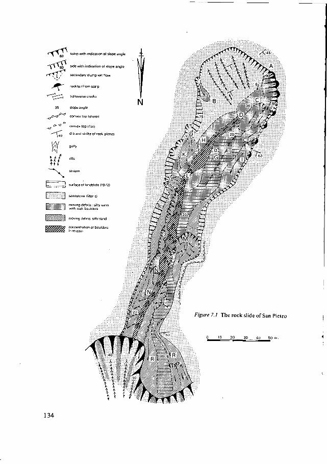
scarp with indication of slope angle

* 80 side with indication of slope angle

M / secondary slump wit flow

rockfall from scarp

* V ^ ^ H transverse cracks

35 slope angle

^/xr convex top (sharp!

__ 0-

convex top (flat)

dip and strike of rock planes

.. surface of landslide (1972)

sandstone (Mar-s)

moving debris; silty sandwith rock boulders

moving debris silty sand

concentration of bouldersin stream

Figure 7.1 The rock slide of San Pietro

0 10 20 30 40 50 r

134

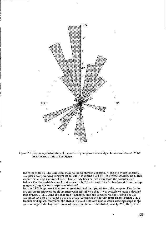
2 %

270--

Figure 7.2 Frequency distribution of the strike of joint planes in weakly cohesive sandstones (Mars)near the rock slide of San Pietro.

the form of flows. The sandstone mass no longer showed cohesion. Along the whole landslidecomplex a scarp (varying in height from lOmtr.attheheadto 1 mtr. at the toe) could be seen. Thismeant that a large amount of debris had already been carried away from the complex (seebelow). On the landslide complex at respectively 2,5 mtr. and 135 mtr. (measured from the top-scarp) two less obvious scarps were observed.In June 1974 it appeared that even more debris had disappeared from the complex. Due to thedry season the relatively stable landslide was accessable so that it was possible to make a detailedmap (Figure 7.1). During this mapping it appeared that the topscarp was not round but wascomposed of a set of straight segments which corresponds to certain joint planes. Figure 7.2, afrequency diagram, represents the strikes of about 150 joint planes which were measured in thesurroundings of the landslide. Some of these directions of the strikes, namely 25°, 180°, 335°

135

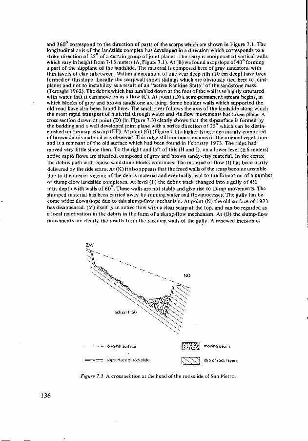
and 360° correspond to the direction of parts of the scarps which are shown in Figure 7.1. Thelongitudinal axis of the landslide complex has developed in a direction which corresponds to astrike direction of 25° of a certain group of joint planes. The scarp is composed of vertical wallswhich vary in height from 7-13 meters (A, Figure 7.1 ). At (B) we found a dipslope of 40° forminga part of the slipplane of the landslide. The material is composed here of gray sandstone withthin layers of clay inbetween. Within a maximum of one year deep rills (10 cm deep) have beenformed on this slope. Locally the scarpwall shows slidings which are obviously tied here to joint-planes and not to instability as a result of an "active Rankine State" of the sandstone mass(Terzaghi 1962). The debris which has tumbled down at the foot of the wall is so highly saturatedwith water that it can move on as a flow (C). At point (D) a semi-permanent stream begins, inwhich blocks of grey and brown sandstone are lying. Some boulder walls which supported theold road have also been found here. The small river follows the axis of the landslide along whichthe most rapid transport of material through water and via flow movements has taken place. Across section drawn at point (D) (in Figure 7.3) clearly shows that the slipsurface is formed bythe bedding and a well developed joint plane with a strike direction of 25° which can be distin-guished on the map as scarp (EF). At point (G) (Figure 7.1) a higher lying ridge mainly composedof brown debris material was observed. This ridge still contains remains of the original vegetationand is a remnant of the old surface which had been found in February 1973. The ridge hadmoved very little since then. To the right and left of this (H and I), on a lower level (± 6 meters)active rapid flows are situated, composed of grey and brown sandy-clay material. In the centrethe debris path with coarse sandstone blocks continues. The material of flow (I) has been partlydelivered by the side scaro. At (K) it also appears that the freed walls of the scarp become unstabledue to the deeper sagging of the debris material and eventually lead to the formation of a numberof slump-flow landslide complexes. At level (L) the debris track changed into a gully of 4Vimtr. depth with walls of 60 . These walls are not stable and give rise to slump movements. Theslumped material has been carried away by running water and flowprocesses. The gully has be-come wider downslope due to this slump-flow mechanism. At point (N) the old surface of 1973has disappeared. (M) itself is an active flow with a clear scarp at the top, and can be regarded asa local reactivation in the debris in the form of a slump-flow mechanism. At (O) the slump-flowmovements are clearly the results from the receding walls of the gully. A renewed incision of

ZW

pVjc2^rJ moving debris

r \ \ S clip of rock layers

Figure 7.3 A cross section at the head of the rockslide of San Pietro.

original surface

— - slipsurface of rockslide

136

the gully has taken place here. Two flows (R) are of a recent date. Inbetween them lies an olderflow, somewhat covered by vegetation (apparently from 1973). At (P) asphalt from the road wasfound in this flow. The whole complex discharges over a steep wall of 40-60 ; the river lies 60meters deeper.

The detailed description given about showed that a number of landscape variables hasinfluenced the type of initial failure of the landslide:— The slightly cohesive sandstone rock, with well developed major joint planes and

bedding planes dipping in the direction of the slope angle.— A rapid retrogression and a deep downcutting of the branch of the river Angio, which

has given rise to a severe steepening of the valley wall head, mainly by slabfalls (seeFigure 7.1 at T) at the foot of the sliding area.

— A concentration of groundwater in the source area of this river-branch which couldbe partly ponded by impermeable clay layers in the sandstone mass.

— The heavy precipitation, which has been registrated in the period of March 4 to 71972, which in this case has functioned as a "trigger".

The intial movement which we could observe in March 1972 had the character of awedge failure with a relative slight displacement of the moving mass (see Figure 7.3 anddetailed description given above). However, due to the weak cementation of the sand-stone, the rock mass was already disintegrated into a debris mass. The further displace-ment of these debris masses took place in later periods especially during the wintertimeafter heavy rainy periods. During this heavy rain-periods the debriss became saturatedwith water and the material must have reached the viscous state. The debris mass wascarried away further via flows. The detailed mapping of 1974 revealed (see Figure 7.1)that at first, flow movements particularly took place in the underground: the vegetatedsurface was pushed along with it and partly sagged down due to the loss in mass in theunderground. For this reason one can explain the fact that the partly intact and vege-tated surface (G) (Figure 7.1) is still present.The detailed mapping also showed, that new elements began to play a part in the trans-port of debris:— Acceleration of the removal of debris, due to the development of a rapidly incising

gully. The water in the gully was able to transport blocks from the damaged wallsprotecting the road over a distance of some tens of meters. This gully incised rapid-ly into some four meters of the debris with the result that the steep walls of thesegullies became unstable and retreated rapidly via slump movements (O in Figure7.1). It was established that the walls of the gully retreated, and that downstream anew incision in the lowered surface had begun. The rapid headward incision of thegully functions as a catalyst for an accelerated removal of debris via slump-flow mo-vements.Since more debris disappears from the complex, the walls of the scarps and sides be-come increasingly more liberated. These walls become unstable and as a result rock-fall (see B) and slump-flow movements (S) at the sides take place.

— The debris mass can also undergo a renewed movement without the influence ofan incising gully. The still active (slump-flow) movements which have been observedat (L), (N) and (I) form an example (see detailed description). We may conclude from

137

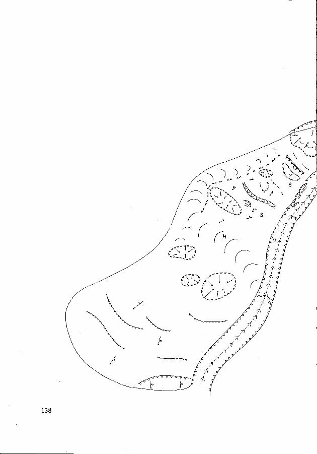
138

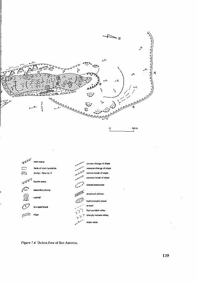
I I

1777

flank of main landslide

slump-flow no. II

fossile scarp

r ^ secondary slump

rockfall

slumped block

ridge

convex change of slope

concave change of slope

convex break of slope

concave break of slope

closed depression

structural plateau

hydromorphic place

s- ' stream

—\~) flat rounded valley

,"7"7 sharply incised valley

slope value

Figure 7.4 Debris flow of San Antonio.

139

this, that movements do not take place continuously over the whole surface but via anumber of clearly differentiated slump-flow complexes.

— Movements can be activated by a local concentration of water of the continuouslyvarying stream patterns of the groundwater. The differentiated movements may alsobe activated by a rapid loss of debris downstream (see (N) in Figure 7.1).

The original topographical surface before the mass movements took place can be re-constructed with the aid of a number of cross sections, which have been measured inthe field. The topographical surface of the slide of 1973 may also be reconstructed (al-though less accurately), and also the relief of the measurements carried out in 1974.This enables us to estimate the loss of debris out of the sliding area. For the period of1972-1973 it amounts to ± 62.000 m3 and for the period 1973-1974 to ± 13.500 m3

which gives a total loss of ± 75.500 m3 .

7.2 The influence of landscape variables on the development of debris slides

In the foregoing paragraph, we discussed different types of slide and related transportphenomena, which started in a more or less cohesive rock mass, along more or less,straight dipping surfaces. In this Paragraph two types of landslides (no. 6 and 7, Table7.1) will be discussed, which started in weathered material or in very fine fractured rockalong more or less flat slip surfaces. In general, there is a larger displacement of materialout of the source area of the slide. Two landslides of type no. 6 were observed on thesteeper northwestern slope, averaging 25°, of the Fiume Torbido, in the neighbourhoodof St. Antonio and Casino Vespario (see map Appendix A7). These landslides, whichhave a elongated form, have developed in fine layered, and fractured claystone. Theclaybeds dip with an angle of 20° in the opposite direction of the topographical slope.The slides are situated at the head of the tributary valley of the Fiume Torbido, whichhas sharply incised this valley slope.

A detailed description of the complex of St. Antonio is given here as an example (see Figure7.4). The complex was bounded at the top by scarp (A), which has the form of an amphitheatrewith slopes, averaging 30 . They have been affected by recent slump processes. Slightly furtherdownstream was a relative small round scarp (B), with an angle of 35°. Even further downstreama bare cliff (C), with a height reaching 40 mtrs. could be observed. The slided mass showed trans-verse cracks with steps upto 3 mtrs. It is possible that these steps at the head of the slide, stillreveal the sliding in blocks at initial failure of the debris mass. The western side (D) averages20 mtrs. height, with a slope angle of 20-30°. On the steepest parts of these sides (>25°) shallowplanar debris slides (type no. 7) has taken place. At (E) the toe of a secondary flow complexcould be observed, which was limited by a distinct front, with a slope angle of 20° (F). The de-bris mass lying above this front had a dense shrub vegetation, a greater density of cracks and amore irrigular topography. The landslide complex further downstream was used for pastures andstill further downstream for agriculture. This part consisted of a soft undulating landscapewith close depressions and slopes v rvin,<r from 0 to 5 .In this area reverse slopes (for instanceunder (S)) were measured, which were interpreted as parts of transverse ridges. The olive trees inthis area were all crooked, pointing to a displacement of the surface. The fairly flat valley (H)cuts the complex in two parts. The valley system (G) with rather steep walls, also affected thecomplex. Landslides were also found along the steep sides of this valley. The lower part of the

140

landslide spreads out in a wide fanshape towards the main valley floor. According to the des-criptions, from a number of inhabitants, movements must have taken place during the Fifties.The greatest part of the displacement of the material must have occurred within a few hours.The house (see Figure 7.4) was just saved. After the movement scarp (D) and supposedly also apart of scarp (C) developed. It took about seven days for the landslide complex to stabilizecompletely. The secondary flow with scarpwall (B) and a different topography and vegeta-tion could have been developed in later years. During the beginning of 1960 the toe area belowdepression (H) was cultivated again.

An analysis of the landscape variables reveals that these relative steep slopes in veryfracturated clay probably in combination with the development of high pore pressuresat the head of the tributary rivers, have lead to the development of debris slides whichmust have rapidly passes into a debris flow. The transverse steps (minor scarps), thearcuate head scarp and the marked sides at the head of the complex form diagnosticfeatures for the fact that initial movement might have taken place in the form of adebris slide (see Chapter 7, Varnes 1958, Brunsden 1979). The high water content ofthis sliding debris mass, has changed the mass into a viscous state and further transportof the material must have occurred via flow processes (see Appendix A5). The flowingcharacter of this landslide is accentuated by (see detailed description above and Varnes(1958), Brunsden (1979):— The large distance of transport from the source area towards the valley floor.— The elongated form of the complex and the lobated form at the foot of the slide.— The hummocky topography, with many close depressions and transverse ridges in

the lower part of the slide.Since eyewitnesses have stated, that the greatest displacement occurred in a few hours,we can estimate that the velocity of the mass must have been in the order of 2-5 mtr./min.,which is relative low in relation to the mean velocities of debris flows, given by Bruns-den (1979) which amount to 1-100 mtr./sec.

The second type of debris slide is the most common type of slide which occurs in thestudy area on the steepest slopes with a relative thin regolith cover (type no. 7 Table7.1). They were found on weathered regolith derived from sandstone (Mars) at thesteepened foot of the slope (angle 35°) in the Valley of the Fiume Sante Maria. Thistype of slide was also found in weathered regolith on claystone along the steepenedvalley walls of the tributary rivers of the Fiume Torbido, e.g. the Valle Irroiti. On theeastern side of this valley on slopes varying from 32-36°, shallow planar slides developedat a mean depth of 80 cm (Figure 7.5, a, b, c, d). The slipsurface developed well belowthe rootzone, of tussock grasses, which reaches to a depth of ± 50 cm. It developed justabove the transition zone of weathered regolith to non-weathered regolith. Four sam-ples were taken from the regolith at a depth of 60 cm. In these samples no roots werepresent. Direct shear tests in the laboratory under wet conditions show a mean angleof internal friction of 31.8° and a mean cohesive strength of 260 kg/m2. The mean bulkdensity of the saturated soil was 2.27 x 103 kg/m3 and the unit weight of dry clayregolith was 1.98 x 103 kg/m3. The slip surface developed at the maximum depth with-in the regolith (80 cm) and, given the soil mechanical and topographical values mentio-ned above, we can calculate from equation (13) (in Chapter 6) that the groundwater

141

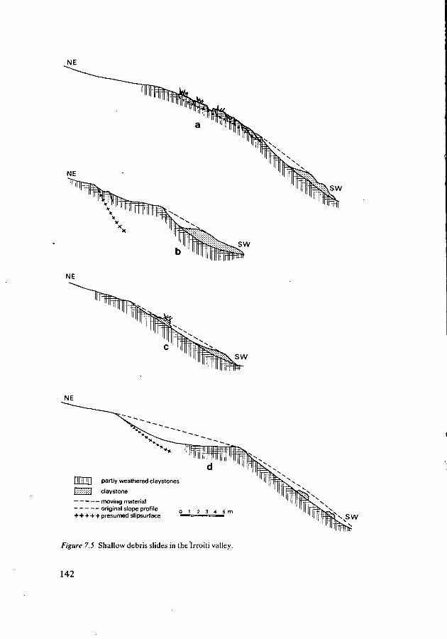
SW

SW

partly weathered claystones

USS:":) claystone

moving materialoriginal slope profile

+++++presumed slipsurface0 1 2 3 4 5 m

SW

Figure 7.5 Shallow debris slides in the Irroiti valley.

142

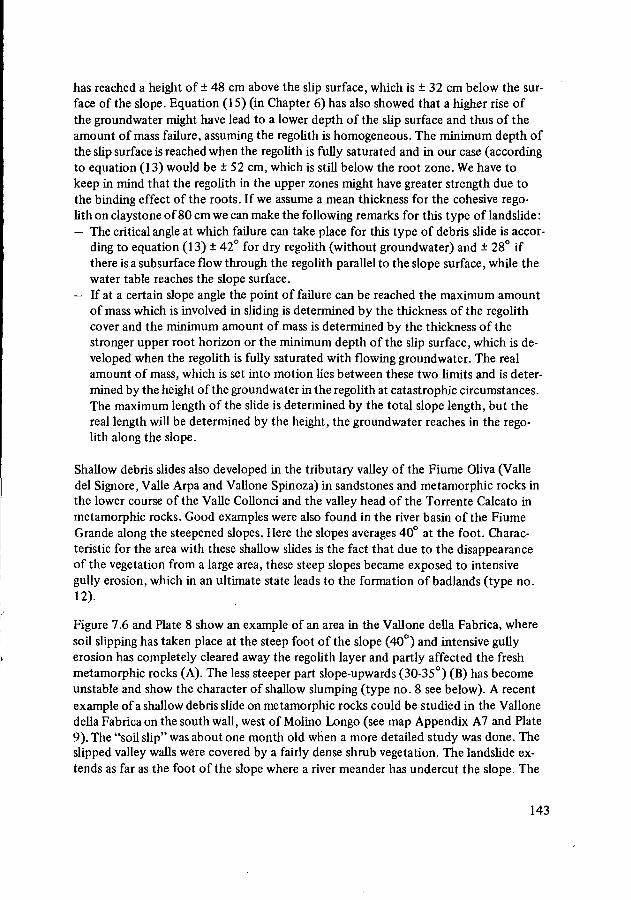
has reached a height of ± 48 cm above the slip surface, which is ± 32 cm below the sur-face of the slope. Equation (15) (in Chapter 6) has also showed that a higher rise ofthe groundwater might have lead to a lower depth of the slip surface and thus of theamount of mass failure, assuming the regolith is homogeneous. The minimum depth ofthe slip surface is reached when the regolith is fully saturated and in our case (accordingto equation (13) would be ± 52 cm, which is still below the root zone. We have tokeep in mind that the regolith in the upper zones might have greater strength due tothe binding effect of the roots. If we assume a mean thickness for the cohesive rego-lith on claystone of 80 cm we can make the following remarks for this type of landslide :

— The critical angle at which failure can take place for this type of debris slide is accor-ding to equation (13) ± 42° for dry regolith (without groundwater) and ± 28° ifthere is a subsurface flow through the regolith parallel to the slope surface, while thewater table reaches the slope surface.

— If at a certain slope angle the point of failure can be reached the maximum amountof mass which is involved in sliding is determined by the thickness of the regolithcover and the minimum amount of mass is determined by the thickness of thestronger upper root horizon or the minimum depth of the slip surface, which is de-veloped when the regolith is fully saturated with flowing groundwater. The realamount of mass, which is set into motion lies between these two limits and is deter-mined by the height of the groundwater in the regolith at catastrophic circumstances.The maximum length of the slide is determined by the total slope length, but thereal length will be determined by the height, the groundwater reaches in the rego-lith along the slope.

Shallow debris slides also developed in the tributary valley of the Fiume Oliva (Valledel Signore, Valle Arpa and Vallone Spinoza) in sandstones and metamorphic rocks inthe lower course of the Valle Collonci and the valley head of the Torrente Calcato inmetamorphic rocks. Good examples were also found in the river basin of the FiumeGrande along the steepened slopes. Here the slopes averages 40° at the foot. Charac-teristic for the area with these shallow slides is the fact that due to the disappearanceof the vegetation from a large area, these steep slopes became exposed to intensivegully erosion, which in an ultimate state leads to the formation of badlands (type no.12).

Figure 7.6 and Plate 8 show an example of an area in the Vallone della Fabrica, wheresoil slipping has taken place at the steep foot of the slope (40°) and intensive gullyerosion has completely cleared away the regolith layer and partly affected the freshmetamorphic rocks (A). The less steeper part slope-upwards (30-35°) (B) has becomeunstable and show the character of shallow slumping (type no. 8 see below). A recentexample of a shallow debris slide on metamorphic rocks could be studied in the Vallonedella Fabrica on the south wall, west of Molino Longo (see map Appendix A7 and Plate9). The "soil slip" was about one month old when a more detailed study was done. Theslipped valley walls were covered by a fairly dense shrub vegetation. The landslide ex-tends as far as the foot of the slope where a river meander has undercut the slope. The

143

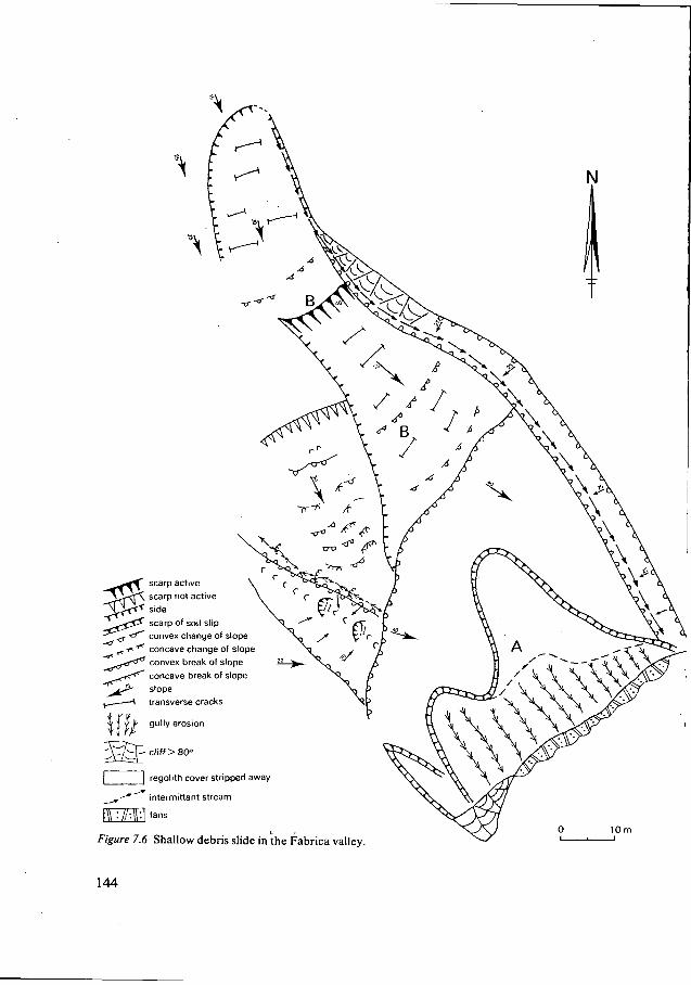
-rr\

scarp activescarp not activesidescarp of soil slipconvex change of slope

r r concave change of slope3° convex break of slopef*"* concave break of slope

slopei transverse cracks

V gully erosion

P cliff > 80°

| regolith cover stripped away

intermittant stream

Figure 7.6 Shallow debris slide in the Fabrica valley

144

total length of the slide was 50 meters, the width 13 meters. The average thickness ofthe slipped layer was 85 cm. The slipsurface undulates highly and the cross sectionshows a light concave form. Eighty percent of the debris has slipped away from thesliding area and was accumulated at the foot of the slope. A few pieces of regolithwith shrub vegetation were present as remains in this flat "gutter". The detailed studyrevealed that the slipsurface lies within the regolith and the rock. The regolith can besubdivided in three zones: An upper horizon with dense roots of about 60 cm thick-ness, with angular rock fragments (1 -3 cm, 15%) and a sandyloam matrix (bulk density,1.54); a middle horizon (60-90 cm) with angular rock fragments (1-3 cm, 15%) and asandy loam matrix (bulk density 1.62); a lowest horizon (90-120 cm) with a large rockfragment content (20-50%, size 2-5 cm) and the highest bulk density (± 1.83). The slip-plane has developed in the middle zone. In this zone samples were taken in order tomeasure the strength values of the regolith. There was no cohesion and the angle ofinternal friction (</?) had a mean value of 46°. The friction angle is somewhat higherthan the slope angle, which for this slide was 42°.

As was stated in Chapter 6 the depth of the slide in a cohesionless homogeneous rego-lith is determined by the total thickness of the regolith. For a layered regolith as in thiscase, the position of the slipsurface is determined by the horizon with the lowest angleof internal friction.Therefore the upper horizon must have had higher strength values, probably due to thebinding effect of the roots, and also the lowest zone had higher strength values, whichmust be due to the higher bulk density and to the fabric of large angular rock fragmentswhich have been filled up by a finer matrix (Chapter 6).Since the angle of internal friction of probably the weakest middle horizon is somewhathigher than the critical slope angle, the positive pore pressure of the groundwatermust have played a part in initiating failure. If we assume for the zone above the slip-plane a mean dry bulk density of 1.58 and a mean wet bulk density of 1.73 we can es-timate, according to equation (13) (Chapter 6) that the water has to rise ± 18 cm abovethe slipplane (which is ± 66 cm below the slope surface). The critical slope angle forthis cohesionless regolith is not determined by the depth of the regolith as is the casewith cohesive clay material (see above and equation (15) Chapter 6). Equation (14a) and(14b) (Chapter 6) show that the critical slope angle for these debris slides inmetamorphicrocks varies between ± 24° for fully saturated regolith with groundwater running parallelto the surface and ± 46° for dry circumstances. We have stated that in this cohesionlessmaterial the depth of the slide and therefore the amount of mass is determined by thedepth of the weakest zone within the regolith.

With regard to the shallow debris slides (type no.7) we were able to quantify for two typesof material, the boundary conditions for failure and the effect of certain variables onthe amount of mass production. In the cohesive claymaterial the critical slope angle forfailure depends a.o. on the thickness of the regolith. For regoliths with a thickness of80 cm (which is assumed to be the normal thickness), the critical slope angle for dryconditions is ± 42°, and ± 28° for regoliths fully saturated with groundwater. In thesefairly homogeneous regoliths the slipsurface developed at a maximum depth; we might

145

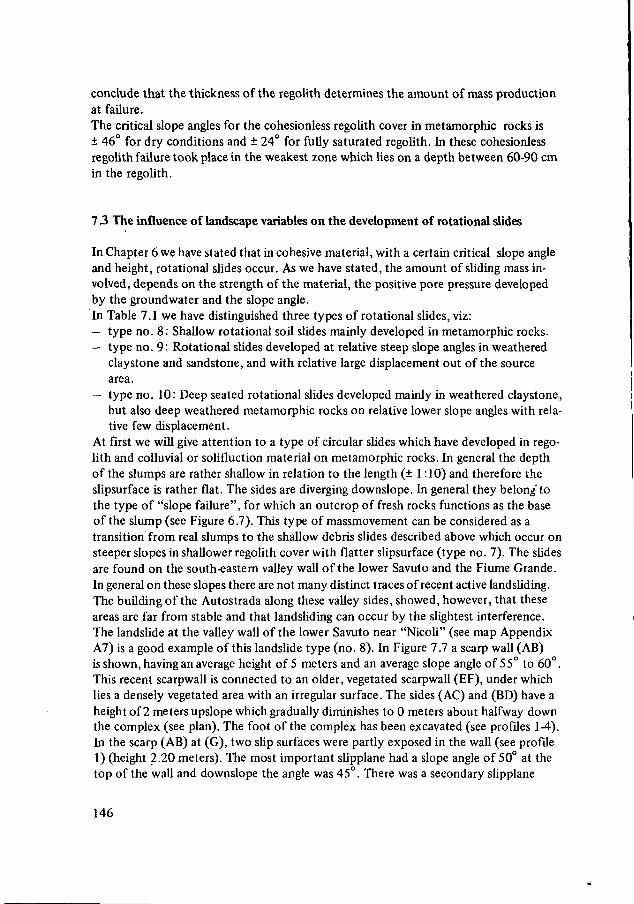
conclude that the thickness of the regolith determines the amount of mass productionat failure.The critical slope angles for the cohesionless regolith cover in metamorphic rocks is± 46° for dry conditions and ± 24° for fully saturated regolith. In these cohesionlessregolith failure took place in the weakest zone which lies on a depth between 60-90 cmin the regolith.

7.3 The influence of landscape variables on the development of rotational slides

In Chapter 6 we have stated that in cohesive material, with a certain critical slope angleand height, rotational slides occur. As we have stated, the amount of sliding mass in-volved, depends on the strength of the material, the positive pore pressure developedby the ground water and the slope angle.In Table 7.1 we have distinguished three types of rotational slides, viz:— type no. 8: Shallow rotational soil slides mainly developed in metamorphic rocks.— type no. 9: Rotational slides developed at relative steep slope angles in weathered

claystone and sandstone, and with relative large displacement out of the sourcearea.

— type no. 10: Deep seated rotational slides developed mainly in weathered claystone,but also deep weathered metamorphic rocks on relative lower slope angles with rela-tive few displacement.

At first we will give attention to a type of circular slides which have developed in rego-lith and colluvial or solifluction material on metamorphic rocks. In general the depthof the slumps are rather shallow in relation to the length (± 1:10) and therefore theslipsurface is rather flat. The sides are diverging downslope. In general they belong'tothe type of "slope failure", for which an outcrop of fresh rocks functions as the baseof the slump (see Figure 6.7). This type of massmovement can be considered as atransition from real slumps to the shallow debris slides described above which occur onsteeper slopes in shallower regolith cover with flatter slipsurface (type no. 7). The slidesare found on the south-eastern valley wall of the lower Savuto and the Fiume Grande.In general on these slopes there are not many distinct traces of recent active landsliding.The building of the Autostrada along these valley sides, showed, however, that theseareas are far from stable and that landsliding can occur by the slightest interference.The landslide at the valley wall of the lower Savuto near "Nicoli" (see map AppendixA7) is a good example of this landslide type (no. 8). In Figure 7.7 a scarp wall (AB)is shown, having an average height of 5 meters and an average slope angle of 55° to 60°.This recent scarpwall is connected to an older, vegetated scarpwall (EF), under whichlies a densely vegetated area with an irregular surface. The sides (AC) and (BD) have aheight of 2 meters upslope which gradually diminishes to 0 meters about halfway downthe complex (see plan). The foot of the complex has been excavated (see profiles 1-4).In the scarp (AB) at (G), two slip surfaces were partly exposed in the wall (see profile1) (height 2.20 meters). The most important slipplane had a slope angle of 50° at thetop of the wall and downslope the angle was 45°. There was a secondary slipplane

146

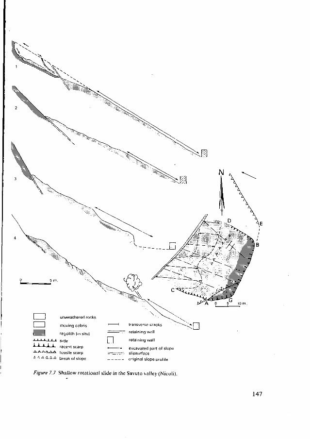
I i unweathered rocks

I I moving debris

I \ regolith (in situ)

siderecent scarpfossile scarp

- - - break of slope

D

transverse cracks

retaining wall

retaining wall

excavated part of slopeslipsurfaceoriginal slope profile

Figure 7.7 Shallow rotational slide in the Savuto valley (Nicoli).

147

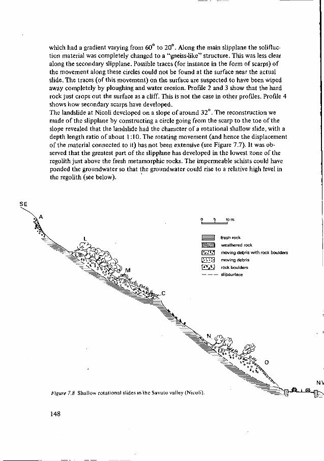
which had a gradient varying from 60° to 20°. Along the main slipplane the solifluc-tion material was completely changed to a "gneiss-like" structure. This was less clearalong the secondary slipplane. Possible traces (for instance in the form of scarps) ofthe movement along these circles could not be found at the surface near the actualslide. The traces (of this movement) on the surface are suspected to have been wipedaway completely by ploughing and water erosion. Profile 2 and 3 show that the hardrock just crops out the surface as a cliff. This is not the case in other profiles. Profile 4shows how secondary scarps have developed.The landslide at Nicoli developed on a slope of around 32°. The reconstruction wemade of the slipplane by constructing a circle going from the scarp to the toe of theslope revealed that the landslide had the character of a rotational shallow slide, with adepth length ratio of about 1:10. The rotating movement (and hence the displacementof the material connected to it) has not been extensive (see Figure 7.7). It was ob-served that the greatest part of the slipplane has developed in the lowest zone of theregolith just above the fresh metamorphic rocks. The impermeable schists could haveponded the groundwater so that the groundwater could rise to a relative high level inthe regolith (see below).

I | fresh rock

J8S8S 3 weathered rock

|y . 'V I moving debris with rock boulders

E- '. • H moving debris

I ' W ! rock boulders

slipsurf ace

Figure 7.8 Shallow rotational slides in the Savuto valley (Nicoli).

148

The recent complex forms a part of an older complex to which the old scarpwall (EF)belongs (see Figure 7.7 a). At the side at (G) a part of the slipcircle of the old landslidecomplex was exposed. Due to excavation at the toe area (see Figure 7.7b) for the con-struction of the Autostrada, probably a part of the old landslide has slid further down-wards. The question arises whether sufficient material has been excavated at the foot andwhether the block has sufficiently slided in order to create a new stable situation, es-pecially when there occurs a large accumulation of groundwater in the slided mass.Precautions were taken to protect the landslide from an excess of runoff water, whichcan flow from the slope above into the complex. To this purpose a ditch was construc-ted around the scarpwall. This ditch was destroyed by further retreat of the scarp. Thistechnique of protecting the landslide against a concentration of surface water has beenoften used along the Autostrada. It is obvious, that only a part of the water, whichcomes from the slope surface will be chanelled away by the ditch. A large part of thewater still enters the landslide complex via subsurface flow through the mainscarp atthe head (see Figure 7.7b).

A second typical landslide complex of type no. 8 lies 300 meters downstream on thesame valleyside along the Autostrade.

Plate 10 shows that the slope has become unstable over a distance of 500 meters. A number ofscaipwalls which has been indicated on this photograph shows that a complex of differentlandslides is involved. In the central part lies a landslide of which the outlines are easily recog-nized. This part of the valleywall must have recently, i.e. during the construction of the Auto-strada, started to move. This can be ascertained among other by the presence of the recentrounded scarpwall (A), which goes over into two downhill diverging sides (B). The form is cha-racteristic for surficial slides on metamorphic rock. Halfway down this landslide lies a secondscarp (C) in the hard rock (see also Figure 7.8). Upstream from the complex at (D) a fossilizedscarpwall can be observed. Residuals can also be distinguished ad (E) (see Plate 10). The materialbelow the scarp (D) has been excavated. Downstream from the most central complex lies a lessobvious, but recently formed scarpwall (G). Under this more or less recent scarpwall lies alikewiserecently slided block, probably due to excavations at the foot (see photograph). The scarp liespartly in hard rock and is 4 meters high and ±30 meters wide. The slope angle is 70°. The slidedmass consists for the greatest part of loose material except at the top where a few blocks of hardrockhave slided along with the rest. The thickness of the whole slided layer is not more than 2 me-ters. The sliding plane down to the excavation (edge H) is flatly curved. Just above the recentscarpwall (G) there are traces of a fossible scarp (1). The scarp (C) continues as a slipsurface inthe scarpwall (A) at point (K).

A profile study has been made along the central complex in order to obtain more insight intothe structure of these landslides (see Figure 7.8). The rounded scarpwall (A) is 6 to 8 metershigh and has a slope angle of 50°. This wall passes into a slipsurface comprising of hard rockwith an slope angle of 36°. Furtheron there is a part of the slided rock (L) on which the treesof an old forest vegetation chiefly lean forwards or sidewards. In this forest complex decayedrock was enclosed in a steep wall (height 3 meters, slope angle 45 ). At (M) ons leaves the forestcomplex (see also Plate 10). In a steep wall rotten gneiss has been found again. The scarpwall(C) is reached via a slope with steps on which blocks lie scattered around. The scarpwall has aslope angle of 55 which passes over into a slipplane with a slope angle of 30°. The slope con-sists completely of hard rock. To the northeast of the profile-line the slided mass has for thegreater part been excavated below (F) (see Plate 10). It must furthermore be noted that thehard rock there lies somewhat deeper. In the section between (C) and (N) the slipsurface is ex-

149

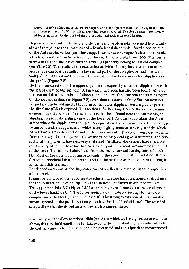
posed. At (N) a slided block can be seen again, and the original tree and shrub vegetation hasalso been retained. At (O) the slided block has been excavated. The slope consists completelyof loose material. At the tracé of the Autostrada hard rock is exposed in situ.

Research carried out in the field and the maps and photographs presented here clearlyshowed that, due to the excavations of a fossile landslide complex for the constructionof the Autostrada, various parts have sagged further down. Vague indications towardsa landslide complex are to befound on the aerial photographs from 1955. The fossilescarpwall (D) and the less distinct scarpwall (I) probably belong to this old complex(see Plate 10). The results of the excavation activities during the construction of theAutostrada can best be studied in the central part of the complex beneath the scarp-wall (A). An attempt has been made to reconstruct the two consecutive slipplanes inthe profile (Figure 7.8).By the reconstruction of the upper slipplane the exposed part of the slipplane beneaththe scarps was used and the point (C) in which hard rock has also been found. Althoughit is assumed that the landslide follows a circular curve (and this was the starting pointby the reconstruction, see Figure 7.8); even then the curve is fairly flat. An even bet-ter picture can be obtained of the form of the lower slipplane. Here, a greater part ofthe slipplane (C-N) is exposed. This section is fairly straight. Since the slip circle mustemerge above the Autostrada (the hard rock has been found near the Autostrada) theslipplane has to make a slight curve in the lower part. At other spots along the Auto-strada where the slipplane was completely exposed due to the excavations, the same cur-ve can be found: an upper section which is very slightly concave to nearly straight whichpasses downwards into a section with a stronger concavity. The conclusion must be drawnfrom the study of the slipplanes that we are principally dealing with slumping. The con-cavity of the planes is, however, very slight and the slided blocks must have thereforerotated very little, but have had for the greatest part a "translative" movement parallelto the slope. This can be deduced also from the many forward leaning trees of block(L). Most of the trees would lean backwards in the event of a distinct rotation. It canfurther be concluded that the depth of which the mass moves in relation to the lengthof the landslide is small.The slipped mass consists for the greater part of solifluction material and the slipsurfaceof hard rock.It must be concluded that impermeable schists therefore have functioned as slipplanesfor the solifluction layer on top. This has also been confirmed in other complexes.The upper landslide A-C (Figure 7.8) has probably been formed after the developmentof the lower landslide C-O. The lower landslide C-0 probably belongs to the scarp-complex indicated by F, C and G in Plate 10. The strong excavation of this complexstream upward of the profile A-0 may also have initiated landslide A-C. The roundedscarpwall (A) has developed on a somewhat less steeper slope.

For this type of shallow rotational slide (no. 8) of which we have given some examplesabove, the threshold conditions for failure could be quantified. For a number of slidesthe soil mechanical characteristics could be measured and the slipsurface reconstructed.

150

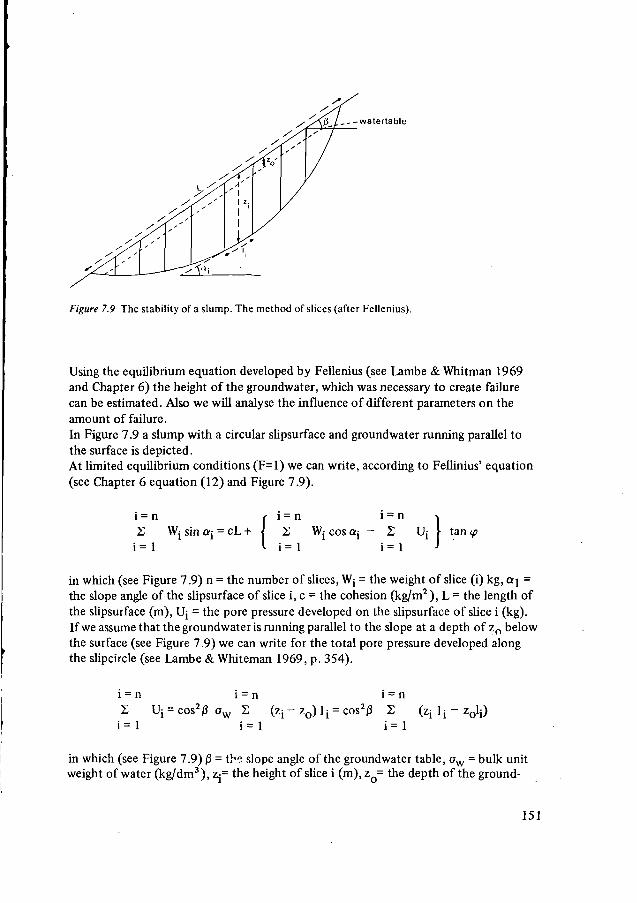
Figure 7.9 The stability of a slump. The method of slices (after Fellenius).

Using the equilibrium equation developed by Fellenius (see Lambe & Whitman 1969and Chapter 6) the height of the groundwater, which was necessary to create failurecan be estimated. Also we will analyse the influence of different parameters on theamount of failure.In Figure 7.9 a slump with a circular slipsurf ace and groundwater running parallel tothe surface is depicted.At limited equilibrium conditions (F=l) we can write, according to Fellinius' equation(see Chapter 6 equation (12) and Figure 7.9).

i = n2

i= 1

i = n i = n ~>2 Wj cos a-x - 2 Uj \

i = 1 i= 1 J

in which (see Figure 7.9) n = the number of slices, Wj = the weight of slice (i) kg, a j =the slope angle of the slipsurface of slice i, c = the cohesion (kg/m2 ), L = the length ofthe slipsurface (m), Uj = the pore pressure developed on the slipsurface of slice i (kg).If we assume that the groundwater is running parallel to the slope at a depth of zo belowthe surface (see Figure 7.9) we can write for the total pore pressure developed alongthe slipcircle (see Lambe & Whiteman 1969, p. 354).

l = n2

i= 1

l = n l = naw 2 (zj-zo)lj=cos20 2 (z, lj - z0lj)

i=1 i= 1

in which (see Figure 7.9) ß = the slope angle of the groundwater table, CTW = bulk unitweight of water (kg/dm3), Zj= the height of slice i (m), zQ= the depth of the ground-

151

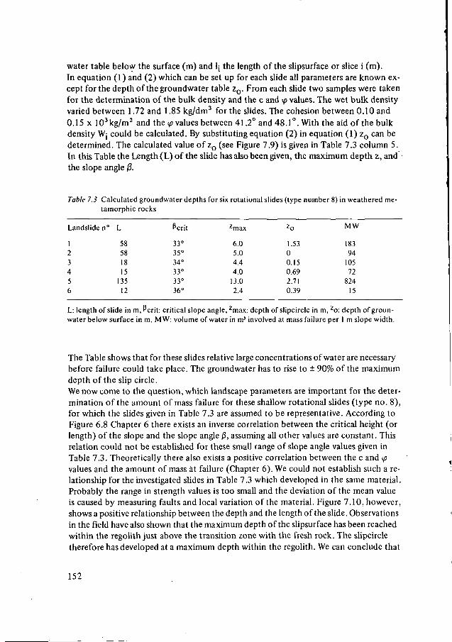
water table below the surface (m) and lj the length of the slipsurface or slice i (m).In equation (1 ) and (2) which can be set up for each slide all parameters are known ex-cept for the depth of the groundwater table z0. From each slide two samples were takenfor the determination of the bulk density and the c and ip values. The wet bulk densityvaried between 1.72 and 1.85 kg/dm3 for the slides. The cohesion between 0.10 and0.15 x 103kg/m2 and the y values between 41.2° and 48.1°. With the aid of the bulkdensity Wj could be calculated. By substituting equation (2) in equation (1) z0 can bedetermined. The calculated value of z0 (see Figure 7.9) is given in Table 7.3 column 5.In this Table the Length (L) of the slide has also been given, the maximum depth z, andthe slope angle ß.

Table 7.3 Calculated groundwater depths for six rotational slides (type number 8) in weathered me-tamorphic rocks

Landslide n°

123456

L

58581815

13512

ßcrit

33°35°34°33°33°36°

zmax

6.05.04.44.0

13.02.4

z o

1.5300.150.692.710.39

MW

18394

10572

82415

L: length of slide in m,Pcrit: critical slope angle, zmax: depth of slipcircle in m, zo: depth ofgroun-water below surface in m, MW: volume of water in m3 involved at mass failure per I m slope width.

The Table shows that for these slides relative large concentrations of water are necessarybefore failure could take place. The groundwater has to rise to ± 90% of the maximumdepth of the slip circle.We now come to the question, which landscape parameters are important for the deter-mination of the amount of mass failure for these shallow rotational slides (type no. 8),for which the slides given in Table 7.3 are assumed to be representative. According toFigure 6.8 Chapter 6 there exists an inverse correlation between the critical height (orlength) of the slope and the slope angle |3, assuming all other values are constant. Thisrelation could not be established for these small range of slope angle values given inTable 7.3. Theoretically there also exists a positive correlation between the c and </>values and the amount of mass àt failure (Chapter 6). We could not establish such a re-lationship for the investigated slides in Table 7.3 which developed in the same material.Probably the range in strength values is too small and the deviation of the mean valueis caused by measuring faults and local variation of the material. Figure 7.10, however,shows a positive relationship between the depth and the length of the slide. Observationsin the field have also shown that the maximum depth of the slipsurface has been reachedwithin the regolith just above the transition zone with the fresh rock. The slipcircletherefore has developed at a maximum depth within the regolith. We can conclude that

152

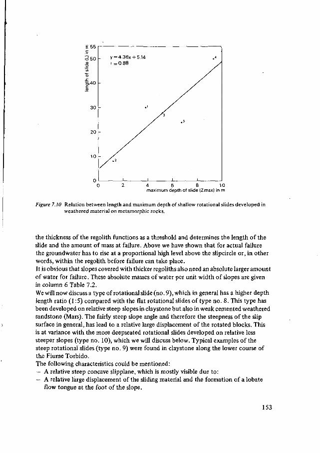
E 55

4 6 8 10maximum depth of slide (Zmax) in m

Figure 7.10 Relation between length and maximum depth of shallow rotational slides developed inweathered material on metamorphic rocks.

the thickness of the regolith functions as a threshold and determines the length of theslide and the amount of mass at failure. Above we have shown that for actual failurethe groundwater has to rise at a proportional high level above the slipcircle or, in otherwords, within the regolith before failure can take place.It is obvious that slopes covered with thicker regoliths also need an absolute larger amountof water for failure. These absolute masses of water per unit width of slopes are givenin column 6 Table 7.2.We will now discuss a type of rotational slide (no. 9), which in general has a higher depthlength ratio (1:5) compared with the flat rotational slides of type no. 8. This type hasbeen developed on relative steep slopes in claystone but also in weak cemented weatheredsandstone (Mars). The fairly steep slope angle and therefore the steepness of the slipsurface in general, has lead to a relative large displacement of the rotated blocks. Thisis at variance with the more deepseated rotational slides developed on relative lesssteeper slopes (type no. 10), which we will discuss below. Typical examples of thesteep rotational slides (type no. 9) were found in claystone along the lower course ofthe Fiume Torbido.The following characteristics could be mentioned:— A relative steep concave slipplane, which is mostly visible due to:— A relative large displacement of the sliding material and the formation of a lobate

flow tongue at the foot of the slope.

153

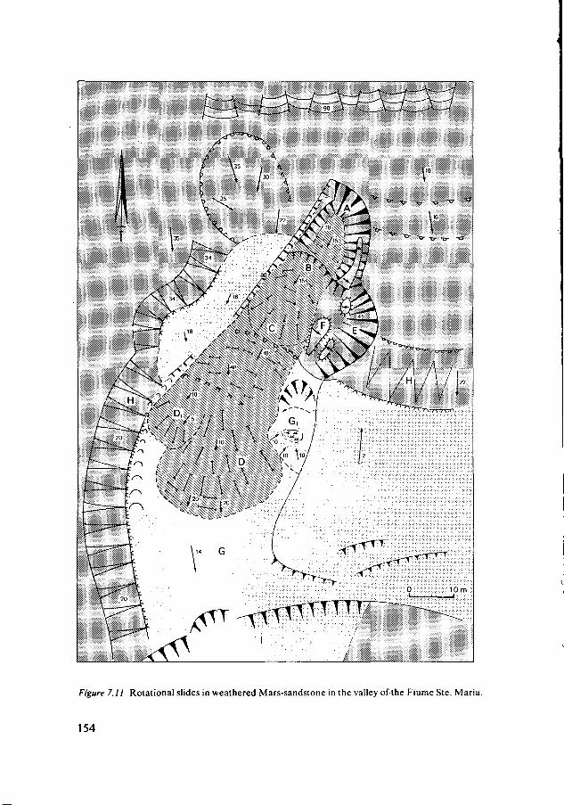
.•-0^^^^^^^^^E0^^^^^^^E.

Figure 7.11 Rotational slides in weathered Mars-sandstone in the valley of the Fiume Ste. Maria.

154

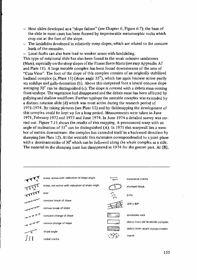
— Most slides developed as a "slope failure" (see Chapter 6, Figure 6.7); the base ofthe slide in most cases has been formed by impermeable metamorphic rocks whichcrop out at the foot of the slope.

— The landslides developed in relatively steep slopes, which are related to the concavebank of the meander.

— Local faults can also have lead to weaker zones with landsliding.This type of rotational slide has also been found in the weak cohesive sandstones(Mars), especially on the steep slopes of the Fiume Sante Maria (see map Appendix A7and Plate 11). A large instable complex has been found downstreams of the area of"Casa Vino". The foot of the slope of this complex consists of an originally stabilizedbadland complex (a, Plate 11) (slope angle 35°), which has again become active partlyvia soilslips and gully-formation (b). Above this steepened foot a lateral concave slopeaveraging 30° can be distinguished (c). The slope is covered with a debris mass comingfrom upslope. The vegetation had disappeared and the debris mass has been affected bygullying and shallow mudflows. Further upslope the unstable complex was extended bya distinct rotation slide (d) which was most active during the research period of1971-1974. By taking pictures (see Plate 12) and by fieldmapping the development ofthis complex could be kept up for a long period. Measurements were taken in June1971, February 1972 and 1973 and June 1974. In June 1974 a detailed survey was car-ried out. Figure 7.11 shows the results of this mapping. A pronounced scarp with anangle of inclination of 55° can be distinguished (A). In 1971 this scarpwall lies a num-ber of meters downstream: the complex has extended itself in a backward direction byslumping (see Plate 12). At the westside this extension correspondended to a joint planewith a dominant strike of 30° which can be followed along the whole complex as a side.The material in the slumping zone has disappeared in 1974 for the greater part. At (B),

scarp, active with indication of slope angle

scarp, not active with indication of slope angle

side

concave break of slope

convex break of slope

^ -rï *** concave change of slope

j -O" *^^ convex change of slope

slope angle

radial cracks

transverse cracks

slumped block

gully

cliff > 80°

sandstone rock

debris from old landslide complex

debris from recent slumpcomplex

marsh

155

in 1974, lies a second scarp which must have developed after 1973. The height is 4meters and the angle of slope is 50°. About twenty meters furtheron a tongue area (C)with radial cracks was mapped. This tongue area is connected to the slump area underscarp (B). At (E) a secondary slump area, with a backwall of 8 meters length and an angleof 45° could be distinguished in the side of the main complex. The slumped block has,with exception of a few remains (F), completely disappeared. Further downstreams liesa second tongue area (D) with radial cracks and transverse cracks. These tongues lie onthe older flowcomplex (G) which has, for the greatest part, been stabilized for years,as evidenced by the electricity pole which must be at least ten years old. Cross-sectionsof the old flow complex show a convex profile.

The rotational slide with a distinct flow tongue forms the further extension of an oldunstable area, which already could be observed on aerial photographs of 1955. The scarpsat (H) and the irregular topography at (G) (Figure 7.11) are the outer limits of thisolder landslide complex. Downslope (I) the area has become unstable again. The vege-tation cover has disappeared and mudflows and gullying have strongly affected thedebris (see c. Plate 12). In 1971 a pronounced rotational slump complex, with a distinctlobate toe area had developed (Figure 7.11). The rotated character of the slide indicatesthat the material before failure had a cohesive component (see Chapter 6), and thereforewe assume that initial failure took place in partly weathered weakly cohesive sandstone.This is also indicated by the fact that the western side of the slide (see Figure 7.11) isvery straight and tied to a marked joint strike direction. The material rapidly desintegra-ted after failure and due to wetting at the toe a lobate flow tongue could develop. In1972 the material has been transported further downwards. The tongue area (D) hadundergone a pronounced push. This could be observed, among others by the damageson the fields which have been cultivated on the tongue (Plate 12) and the fact thatmarkers set out between (C) and (B) in 1971 (see Figure 7.11) could not be found. In1973 the slump area had extended itself further upwards from the valley. The scarpwalls became clearly visible because the material had sagged further downwards. Thusa second tongue (D) developed. The detailed mapping of 1974 (Figure 7.11) revealedthe following developments:— rapid discharge of material from the head region below the main scarp (A); only rem-

nants of the old slump area of 1973 are still preserved here.— the development of a new scarp (B) in the old debris material with a tongue area

(C) connected to it. Consequently this is a local reactivation of the debris via a new(slump) flow movement, inside the older slump complex.

— the development of new slumps in the side scarp at (E) and the old flow material at(G).

It can be established how, particularly between 1973 and 1974, the activity of thiscomplex has strongly increased. The continuous propulsion of the debris results in theinstability of the flanks, so that the complex can extend itself further. The general pic-ture we got from this slope is the development of an unstable area, which started viasurfical debris slides at the foot of the slope, and extended further upwards via slumpand flow processes which developed especially along various joint planes (see Plate 12).

156

Another example of this form of "retrogressive" landsliding can be found at a smalldistance further upstream. On Plate 7, a large more or less stabilized landslide complex,can be distinguished at the foot of the slope. Traces of recent activities can be observedonly at the top of this complex (a). Investigations in the field revealed that a number ofslump-flow complexes has developed along a fault plane (f). The top complex has af-fected the road to San Pietro. Under the complex (a) the metamorphic rocks crop out(m). The contactzones between the two types of rock generally form unstable areas.This particularly applies to the contact zone between sandstone and metamorphic rockssince these can pond the groundwater, which causes massmovements in the sandstone.The scarp (f) forms a fault plane which can easily be followed upslope and which canbe seen as a slightly gaping crack in the wall along the road to San Pietro. A pronouncedknick (k) in the white excavated wall on the photo shows, that the sandstone has movedalong this plane. The road to San Pietro had already been affected by a slump move-ment at the top of the complex before 1971. The road had sagged down and thereforea new road had been constructed, which has resulted in an excavation of the slope at (g).Before 1971 two "walls" had been placed in order to support the old road. This hadno effect at all, because the heavy walls were constructed in the head of the slumpingarea, and therefore functioned as an extra loading on this slumping block. In 1972 theslumping block moved further and the area extended even backwards. The desintegratedsandstones rapidly flowed away downslope via mudflows.

Summarizing we can state that on steeper slopes rotational slides develop. The materialof these slides will be transported relatively rapidly out of the sliding areas. This is dueto the steeper slipsurface but also to the wetting of the desintegrated material, especiallyin the case of sandstone debris, which causes the material to move as a mudflow alongthe steepened slope. Metamorphic rocks at the base and the ponding of groundwaterby these rocks lead to instability of the claystone and sandstone. Especially in sand-stone we observed that there occurs retrogressive slumping slope upwards along well-developed joint planes.We now come to a type of rotational slide (type no. 10 Table 7.1), which is connectedwith relative lower slope angles compared with the types described above. As we haveshown in the previous Chapter the lower slope angle, in general, leads to a greater lengthof the slide and greater depth of the slipcircle. Characteristics for this type of slides isthe relative small displacement of the material out of the sliding area. Stabilized slideswere found showing a main scarp, which forms only a very limited part of the slidingsurface, while further transport by flow processes occurred in a very limited way. Thistype of slide was found on weathered material of claystone on slopes varying from 5-15°,and metamorphic rocks on slopes varying from 20-25°. Good examples of this type ofslide developed in claystone in the "Valle degli Angeli" and the valley of the FiumeTorbido. In the "Valle degli Angeli", along a new constructed road, a typical slump ofthis type developed in a basin-shaped depression (lateral concavity) of a slope with anangle averaging 18°. The slope has been cut at the foot in view of the construction of thenew road. The height of the main scarp of this slide (see Figure 7.12) is not more than90 cm. A slight camber in the road talus points to recent movements of the slide justbefore mapping. The movements probably have taken place intermittently, during pe-

157

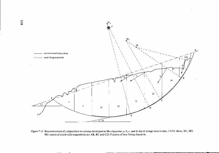
00

reconstructed slipsurface

best fitting slipcircle

Figure 7.12 Reconstruction of a slipsurface in a slump developed in Ma-claystone; a, b, c, and d: dip of striage lines in side; 1-VIII; slices; Ml , M2,M3: centre of circle with respectively arc AB, BC and CD; P centre of best fitting slipcircle.

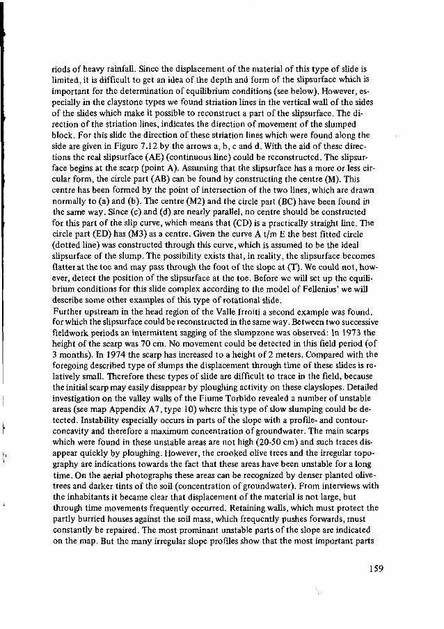
riods of heavy rainfall. Since the displacement of the material of this type of slide islimited, it is difficult to get an idea of the depth and form of the slipsurface which isimportant for the determination of equilibrium conditions (see below). However, es-pecially in the claystone types we found striation lines in the vertical wall of the sidesof the slides which make it possible to reconstruct a part of the slipsurface. The di-rection of the striation Unes, indicates the direction of movement of the slumpedblock. For this slide the direction of these striation lines which were found along theside are given in Figure 7.12 by the arrows a, b, c and d. With the aid of these direc-tions the real slipsurface (AE) (continuous line) could be reconstructed. The slipsur-face begins at the scarp (point A). Assuming that the slipsurface has a more or less cir-cular form, the circle part (AB) can be found by constructing the centre (M). Thiscentre has been formed by the point of intersection of the two lines, which are drawnnormally to (a) and (b). The centre (M2) and the circle part (BC) have been found inthe same way. Since (c) and (d) are nearly parallel, no centre should be constructedfor this part of the slip curve, which means that (CD) is a practically straight line. Thecircle part (ED) has (M3) as a centre. Given the curve A t/m E the best fitted circle(dotted line) was constructed through this curve, which is assumed to be the idealslipsurface of the slump. The possibility exists that, in reality, the slipsurface becomesflatter at the toe and may pass through the foot of the slope at (T). We could not, how-ever, detect the position of the slipsurface at the toe. Before we will set up the equili-brium conditions for this slide complex according to the model of Fellenius' we willdescribe some other examples of this type of rotational slide.

Further upstream in the head region of the Valle Irroiti a second example was found,for which the slipsurface could be reconstructed in the same way. Between two successivefieldwork periods an intermittent sagging of the slumpzone was observed: In 1973 theheight of the scarp was 70 cm. No movement could be detected in this field period (of3 months). In 1974 the scarp has increased to a height of 2 meters. Compared with theforegoing described type of slumps the displacement through time of these slides is re-latively small. Therefore these types of slide are difficult to trace in the field, becausethe initial scarp may easily disappear by ploughing activity on these clay slopes. Detailedinvestigation on the valley walls of the Fiume Torbido revealed a number of unstableareas (see map Appendix A7, type 10) where this type of slow slumping could be de-tected. Instability especially occurs in parts of the slope with a profile- and contour-concavity and therefore a maximum concentration of groundwater. The main scarpswhich were found in these unstable areas are not high (20-50 cm) and such traces dis-appear quickly by ploughing. However, the crooked olive trees and the irregular topo-graphy are indications towards the fact that these areas have been unstable for a longtime. On the aerial photographs these areas can be recognized by denser planted olive-trees and darker tints of the soil (concentration of groundwater). From interviews withthe inhabitants it became clear that displacement of the material is not large, butthrough time movements frequently occurred. Retaining walls, which must protect thepartly burried houses against the soil mass, which frequently pushes forwards, mustconstantly be repaired. The most prominant unstable parts of the slope are indicatedon the map. But the many irregular slope profiles show that the most important parts

159

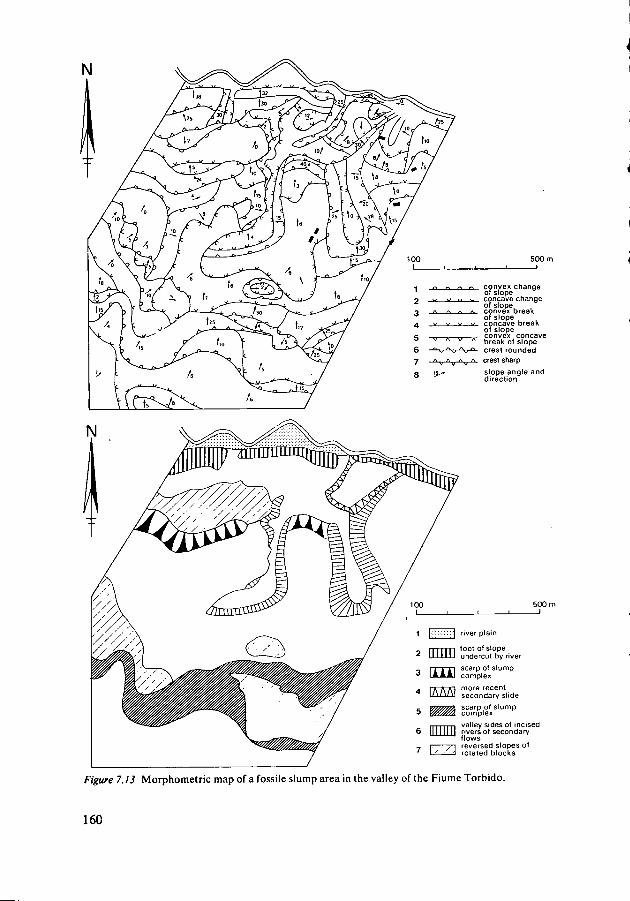
N

convex changeof slopeconcave changeof slope^convex breakof slopeconcave breakof slopeconvex-concavebreak of slopecrest roundedcrest sharpslope angle anddirection

river plain

foot of slopeundercut by river

scarp of stumpcomplex

more recentsecondary slidescarp of slumpcomplex

valley sides of incisedrivers of secondaryflowsreversed slopes ofrotated blocks

Figure 7.13 Morphometric map of a fossile slump area in the valley of the Fiume Torbido.

160

of the denudation of these slopes have taken place by massmovements. Water erosionand surface creep have, on the geological time scale, contributed in a much smallerway in the transport of the slope material. A stabilized example of this type of slide(10) was found in the upper valley and of the Valle Irroiti. At this point, the river showsa narrow incision of ± 10 mtr. The material of the landslide consists of heavily weatheredclaystone. No traces of fresh rock in situ could be observed in the scarp walls and inthe incision of the river at the toe. A number of outcrops in the neighbourhood showssandy layers which are practically horizontal. Scarps have developed in a slope of about"5° (except at the toe). The depth of the landslide is not known but the profile of theslide suggests, that in the underground the slipsurface must partially follow the hardsubstratum, since the mean thickness of the regolith is much lesser as the maximaldepth of the reconstructed slipcircle would suggest. Also we may think of two retro-gressive slumps developed in weathered clay, with the slipcircle resting on the base offresh claystone, which lies nearly horizontal in this area.A much older landslide complex of probably this type is found in the south easternslope further downstream in the valley of the Fiume Torbido at Marina Savuto. It canbe seen on the map that the expansion of this complex has been extensive.The incision o f the Fiume Torbido had steepened the foot of the slope of this complex.The clay beds gently dip in the direction of the slope. The complex is characterized bya slope with a softly undulating topography and closed depressions. The area is com-pletely stable and is now under cultivation. In the area we performed a detailed mor-phometric mapping following Savigear's method and applied by Brunsden (1976) fordetecting the characteristics of "fossile slides" (see Figure 7.13a).The detailed morphometric survey revealed a scarp complex at the top (5) (see Figure7.13b) and a secondary scarp halfway down (3). Before these scarps traces of backwardrotated blocks with nearly horizontal or reversed slopes (7) could be distinguished.The landslide complex has been affected in the lower part by broad valleys (6) and (4),which might be traces of secondary flows, having further transported a part of theslumped material to the river Torbido. The landslide complex can be considered as acomplex of at least two large retrogressive slumps. The slipsurface may be partly deter-mined by dipping clay siltstone layers towards the river.Also in the area of metamorphic rocks, on slopes with a relative thick solifluction cover,and especially on parts of the slope with a profile and contour concavity, unstableareas with slow slumping movements can be found. Compared with the unstable areasdeveloped in claystone, described above, the slope angle in this area is steeper (20-25°)(see Table 7.1). More pronounced slides show clearly the character of a slump, with around crown at the head and a somewhat bulged toe area. In general the displacementis relatively small and therefore pronounced scarps are not always visible and in mostcases are ploughed away. Indications toward these unstable areas are: a) locally denserolive planting and leaning trees, b) irregular topography, c) frequent sagging of roads,which necessitates constant reparation, d) the hydromorphic character of the lateralconcave slope facets and many springs.In one case we could find evidence for the depth of the slipcircle, which gave a depth-length ratio of the slide of 1:5. This ratio is larger than the depth/length ratio of the

161

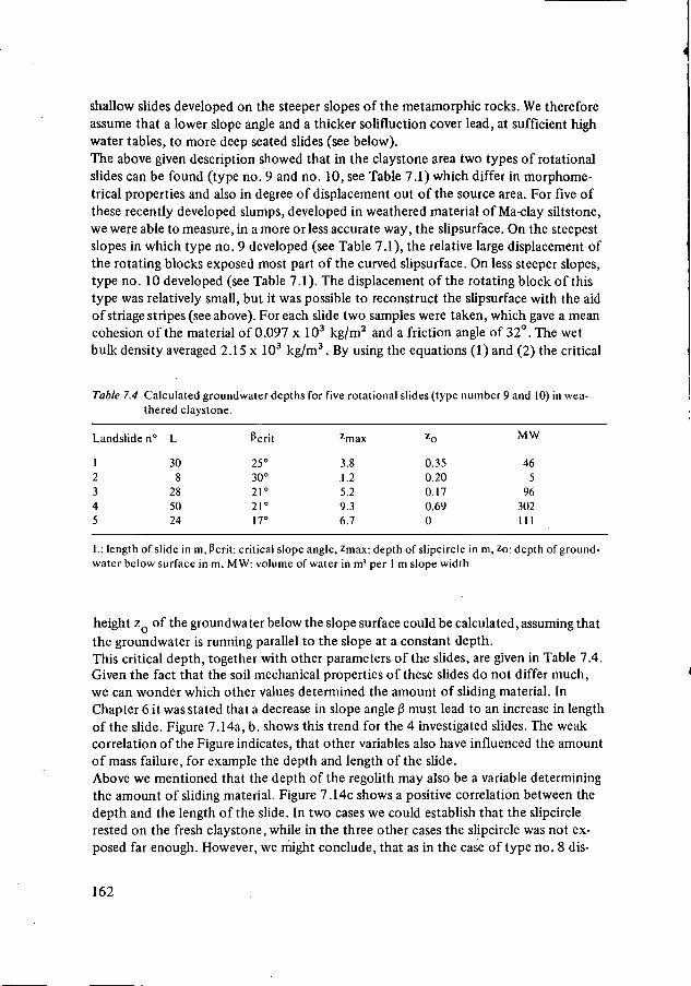
shallow slides developed on the steeper slopes of the metamorphic rocks. We thereforeassume that a lower slope angle and a thicker solifluction cover lead, at sufficient highwater tables, to more deep seated slides (see below).The above given description showed that in the claystone area two types of rotationalslides can be found (type no. 9 and no. 10, see Table 7.1) which differ in morphome-trical properties and also in degree of displacement out of the source area. For five ofthese recently developed slumps, developed in weathered material of Ma-clay siltstone,we were able to measure, in a more or less accurate way, the slipsurface. On the steepestslopes in which type no. 9 developed (see Table 7.1), the relative large displacement ofthe rotating blocks exposed most part of the curved slipsurface. On less steeper slopes,type no. 10 developed (see Table 7.1). The displacement of the rotating block of thistype was relatively small, but it was possible to reconstruct the slipsurface with the aidof striage stripes (see above). For each slide two samples were taken, which gave a meancohesion of the material of 0.097 x 103 kg/m2 and a friction angle of 32°. The wetbulk density averaged 2.15 x 103 kg/m3. By using the equations (1) and (2) the critical

Table 7.4 Calculated groundwater depths for five rotational slides (type number 9 and 10) in wea-thered claystone.

Landslide n°

12345

L

30g

285024

ßcrit

25°30°21°21°17°

zmax

3.81.25.29.36.7

z o

0.350.200.170.690

MW

465

96302111

L: length of slide in m, ßcrit: critical slope angle, Zmax: depth of slipcircle in m, zo: depth of ground-water below surface in m, MW: volume of water in m3 per 1 m slope width

height zQ of the groundwater below the slope surface could be calculated, assuming thatthe groundwater is running parallel to the slope at a constant depth.This critical depth, together with other parameters of the slides, are given in Table 7.4.Given the fact that the soil mechanical properties of these slides do not differ much,we can wonder which other values determined the amount of sliding material. InChapter 6 it was stated that a decrease in slope angle ß must lead to an increase in lengthof the slide. Figure 7.14a, b. shows this trend for the 4 investigated slides. The weakcorrelation of the Figure indicates, that other variables also have influenced the amountof mass failure, for example the depth and length of the slide.Above we mentioned that the depth of the regolith may also be a variable determiningthe amount of sliding material. Figure 7.14c shows a positive correlation between thedepth and the length of the slide. In two cases we could establish that the slipcirclerested on the fresh claystone, while in the three other cases the slipcircle was not ex-posed far enough. However, we might conclude, that as in the case of type no. 8 dis-

162

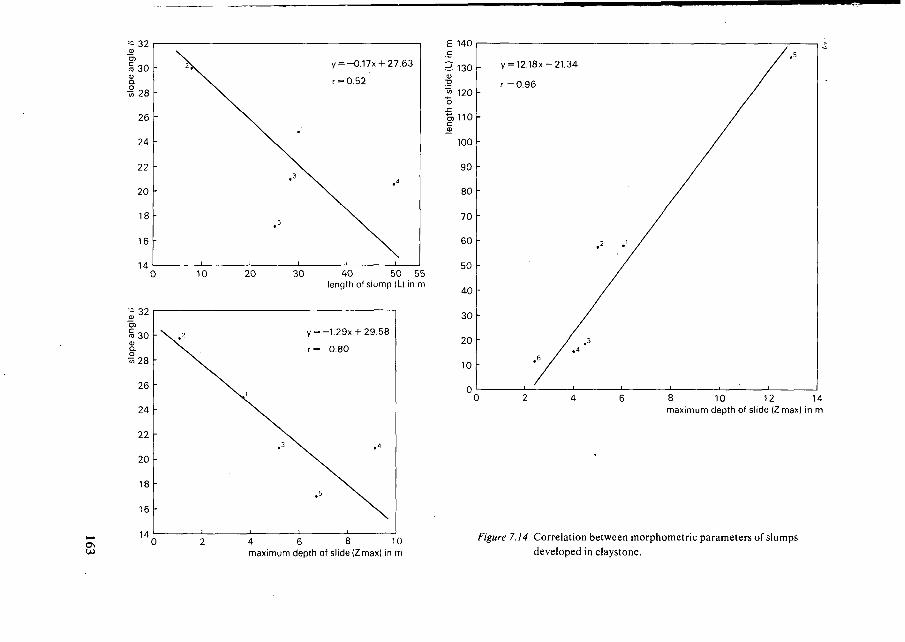
<D

O)

S 30CD

a•§ 28

26

24

22

20

18

16

1 A

S .

.3 \ ^

. 5

i i i

y = -0.17x + 27.63

r = 0.52

\

\I t

E 140

10 20 30 40 50 55length of slump (L) in m

ile

/ K

cn

S 30<DQ.

^ 2 8

26

24

22

20

18

16

1 A

>

-

•

-

y = -1.29x + 29.58

r = 0.80

8 10 12 14maximum depth of slide (Z max) in m

Os 4 6 8 10maximum depth of slide (Zmax) in m

Figure 7.14 Correlation between morphometric parameters of slumpsdeveloped in claystone.

cussed above, the depth of regolith determines the amount of mass failure and that inshallower regoliths failure is only possible in steeper slope angels. In all cases the ground-water level has to rise to 9/10 of the depth of the regolith (see Table 7.4 column 6).

7.4 The influence of landscape variables on landslides with a dominant mud flow character

In this paragraph we will deal with landslides in which the material, after failure, hasbeen further transported by slow mudflows (type no. 11) (Table 7.1). Movements aremore or less continuous in the periods with high rainfall, which in the study area es-pecially occur in the winter period (Chapter 2). The first examples given here are relatedto unstable areas in clay stone with deep seated slumping (compare type no. 10) andlarge concentrations of water due to profile and contour concavity. In distinction withthe unstable areas, described in the foregoing Paragraph (type no. 10), the displacementof the material is more rapid, due to the fact that the unstable area is captured by asteep valley which enables the material to "drain" via an elongated mudflow furtherdownwards.Examples of this type of landslide are found in the Timpa Caruso area (in the river basinof the Fiume Oliva, see map Appendix A7). In this area claystone crops out withsandstone (Mar) and metamorphic rocks underneath. In the lower course a steep valleyhas developed in the metamorphic rocks and in the sandstone. This valley branches inthe upper part in the claystone area and in the extension of these branches large slum-ping areas have developed, which are partly still active. At some places, the materialmoved downwards through the valleys in the form of slow elongated mudflows. A simi-lar complex developed in the river basin of the Torrente Collonci in the area of thePianotorre (see map Appendix A7).This area is a gently sloping depression consisting of claystone. Around this area meta-morphic rocks and sandstone crop out. The tributary, the Torrente Zecco, which has avery straight course, incises into this claystone area. The whole clay area betrays thetraces of instability. Large portions of the area are used for agriculture. In the wetwinterperiod certain areas are inaccessible because of the oversaturation of water. Theclay reaches a completely fluid phase. The most recent and active movements havetaken place during the last few years in the headwater region of the Torrente Secco.Here fresh scarps have developed.Further to the east at the same height is also a beginning of scarp formation. It appearsfrom interviews from inhabitants that the complex is still expanding further backwardsand forms a real threat to the surrounding farms. The most active area in the uppercourse of the Torrente Secco expands according to a pattern, which corresponds to thebranching (of the river) or the supplying veins of water of this river in the headwaterregion (Plate 13).

In Figure 7.15aprominent "supplying area" with a mainly slump character can be distinguished,which passes out into a long elongated tongue which moves downstream in the flat valley of theTorrente Secco. This long flow track forms evidence for the good "flowing" properties of thematerial (see Appendix A5).

164

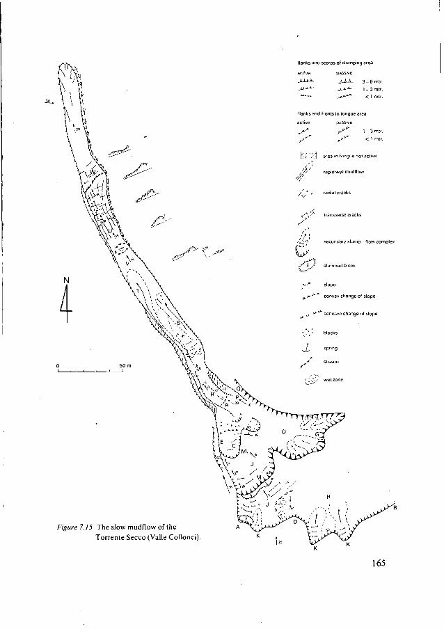
flanks and scarps of slumping area

active passive

_iXi>- J-À.A- 3 _ 6 mtr.

- ^ -*""*" _*-*-*" 1 - 3 mtr.

****** _>-*"*'*" < 1 mtr.

flanks and fronts in tongue area

active passive

*'* cr^ 1 - 3 mtr.

area m tongue not active

rapid wet mudflow

radial cracks

transverse cracks

secondary slump- flow complex

•f \ / slumped block

slope

convex change of slope

concave change of slope

Figure 7.15 The slow mudflow of theTorrente Secco (Valle Collonci).

165

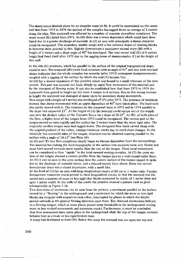
The slump area is limited above by an irregular scarp (A-B). It could be ascertained on this scarp-wall that from 1973 to 1974 the surface of the complex has sagged down an average of 2 metresalong the edge. This scarpwall was affected by a number of separate slumpflow complexes. Themost recent (K) dated from 1973. At (H) there was a lower depression which could have deve-loped due to a greater discharge of material. At (J) an area with principally a slump charactercould be recognized. The secundary smaller scarps with a few reversed slopes of rotating blocksin between them pointed to this. Slightly downstream a prominent second scarp (M) with aheight of 5 metres and a slope angle of 40° has developed. The very recent wall (E) of 6 metresheight had freed itself after 1973 due to the sagging down of slumpcomplex (C) at the height ofthis wall.

In the side (E) striations, which lay parallel to the surface of the original topographical slope,could be seen. The scarpwall (Ml) with fresh striations with an angle of 45 and also with reversedslopes indicates that the whole complex has recently (after 1973) undergone slumpmovements.coupled with a sagging of the surface by which the wall (E) became free.At (O) lay a second expansion of the complex which was bound to a small tributary of the riversystem. This part was scoured out fairly deeply by rapid flow movements of the material andby the transport of flowing water. It can also be established here that from 1973 to 1974 thescarpwalls have gained in height (at (G) from 3 metres to 8 metres). Due to this strong increasein height the scarpwall was damaged at many spots by secondary slump movements.New scarps with a height of 5 metres also developed off (P) after 1973. The presence of striationsshowed that slump movements with an upper slipsurface of 40° have taken place. The hard rockalso partly moved with it. The striations in this scarpwall were in 1973 and in 1974 parallel tothe slope and measured 15°. At the height of (A) the material could escape out of the supplyarea into the shallow valley of the Torrente Secco via a slope of 20-25°. At (R), at both sides ofthe flow, a higher level of the tongue from 1973 could be recognized. The central part of thetongue moved on more rapidly and the surface lay 2 metres lower than the more rigid sides. Theoriginally swollen tongue mass had sagged down. The elongated flow track curved along withthe original gradient of the valley, causing transverse cracks due to rapid slope changes. In therelatively less moveable sides of the tongue, striations can be observed running parallel to thesurface with a angle of 10-12 (see Plate 14).At (S) and (T) two flow complexes clearly began to discern themselves from the surroundings.The material has (taking the microtopography at the surface into account) been very fluidal andmust have moved onwards more rapidly than the rest of the tongue. These local movementscan be considered as flow "rapids" in the total onward moving complex. At (T) the cross sec-tion of the tongue showed a convex profile. Here the tongue lays on a wide round valley floor.At (V) it can be seen in the cross section how the convex surface of the tongue sagged in againdue to the discharge of material below, and a delayed supply from above. Some ten metersdownstream there was a closed depression, with a small lake.At the level of (U) lay an area with large longitudinal cracks of 60 cm to 1 meter wide. Furtherdownstream transverse cracks joined to these longitudinal cracks, so that the material was dis-sected into a number of more or less rigid clay blocks separated by cracks of 1 meter deep andupto 1 meter width. In the walls of the cracks the striation showed a pattern such as givenschematically in Figure 7.16.Two directions of movement can be seen from the pattern: a movement parallel to the surfacecaused by a "flowing" in the underground, and a movement by which the more or less rigidblocks sag irregular with respect to each other, interrupted by phases in which the blocksmoved onwards in the general flowing direction once more. The observed movements indicateto a flowing tongue, which at some places passed steep thresholds in the underground causingmore or less vertical movements and transverse cracks. Furthermore, it must be concludedthat flow movements have taken place in the underground while the top of the tongue materialbehaves here as a more or less rigid broken mass.A scarp had developed at level (W). Below this scarp the material was wet upto the top and

166

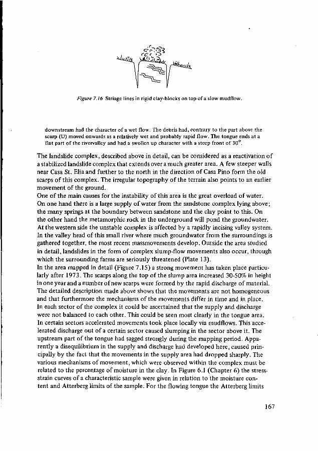
Figure 7.16 Striage lines in rigid clay-blocks on top of a slow mudflow.

downstream had the character of a wet flow. The debris had, contrary to the part above thescarp (U) moved onwards as a relatively wet and probably rapid flow. The tongue ends at aflat part of the rivervalley and had a swollen up character with a steep front of 30°.

The landslide complex, described above in detail, can be considered as a reactivation ofa stabilized landslide complex that extends over a much greater area. A few steeper wallsnear Casa St. Elia and further to the north in the direction of Casa Pino form the oldscarps of this complex. The irregular topography of the terrain also points to an earliermovement of the ground.One of the main causes for the instability of this area is the great overload of water.On one hand there is a large supply of water from the sandstone complex lying above;the many springs at the boundary between sandstone and the clay point to this. Onthe other hand the metamorphic rock in the underground will pond the groundwater.At the western side the unstable complex is affected by a rapidly incising valley system.In the valley head of this small river where much groundwater from the surroundings isgathered together, the most recent massmovements develop. Outside the area studiedin detail, landslides in the form of complex slump-flow movements also occur, throughwhich the surrounding farms are seriously threatened (Plate 13).In the area mapped in detail (Figure 7.15) a strong movement has taken place particu-larly after 1973. The scarps along the top of the slump area increased 30-50% in heightin one year and a number of new scarps were formed by the rapid discharge of material.The detailed description made above shows that the movements are not homogeneousand that furthermore the mechanisms of the movements differ in time and in place.In each sector of the complex it could be ascertained that the supply and dischargewere not balanced to each other. This could be seen most clearly in the tongue area.In certain sectors accelerated movements took place locally via mudflows. This acce-lerated discharge out of a certain sector caused slumping in the sector above it. Theupstream part of the tongue had sagged strongly during the mapping period. Appa-rently a disequilibrium in the supply and discharge had developed here, caused prin-cipally by the fact that the movements in the supply area had dropped sharply. Thevarious mechanisms of movement, which were observed within the complex must berelated to the percentage of moisture in the clay. In Figure 6.1 (Chapter 6) the stress-strain curves of a characteristic sample were given in relation to the moisture con-tent and Atterberg limits of the sample. For the flowing tongue the Atterberg limits

167

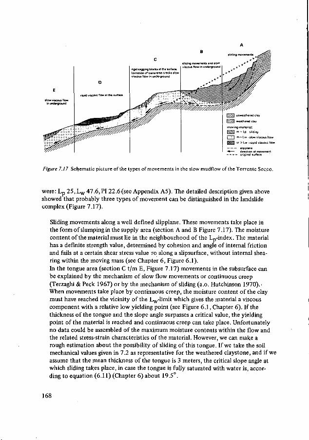
rigid sagging blocks at the surface:formation ot transverse cracks slowviscous flow in underground

unweathered clay

weathered clav

moving material:

~ Lp -sliding

| -.:<•;] m ~ Lw -slow viscous flow

I H 3 m > Lw -rapid viscous flow

slipplane• direction ot movement

-t- + + + original surface

Figure 7.17 Schematic picture of the types of movements in the slow mudflow of the Torrente Secco.

were: Lp 25,1^, 47.6,PI 22.6(see Appendix A5). The detailed description given aboveshowed that probably three types of movement can be distinguished in the landslidecomplex (Figure 7.17).

Sliding movements along a well defined slipplane. These movements take place inthe form of slumping in the supply area (section A and B Figure 7.17). The moisturecontent of the material must lie in the neighbourhood of the Lp-index. The materialhas a definite strength value, determined by cohesion and angle of internal frictionand fails at a certain shear stress value TO along a slipsurface, without internal shea-ring within the moving mass (see Chapter 6, Figure 6.1).In the tongue area (section C t/m E, Figure 7.17) movements in the subsurface canbe explained by the mechanism of slow flow movements or continuous creep(Terzaghi & Peck 1967) or by the mechanism of sliding (a.o. Hutchinson 1970).'When movements take place by continuous creep, the moisture content of the claymust have reached the vicinity of the L^y-limit which gives the material a viscouscomponent with a relative low yielding point (see Figure 6.1, Chapter 6). If thethickness of the tongue and the slope angle surpasses a critical value, the yieldingpoint of the material is reached and continuous creep can take place. Unfortunatelyno data could be assembled of the maximum moisture contents within the flow andthe related stress-strain characteristics of the material. However, we can make arough estimation about the possibility of sliding of this tongue. If we take the soilmechanical values given in 7.2 as representative for the weathered claystone, and if weassume that the mean thickness of the tongue is 3 meters, the critical slope angle atwhich sliding takes place, in case the tongue is fully saturated with water is, accor-ding to equation (6.11) (Chapter 6) about 19.5°.

168

This critical angle is higher than the mean slope angle of the tongue (10-12°). Wemust conclude that, when the material is in a more plastic state, the slope angle istoo flat to cause failure via sliding. Probably the material in the subsurface is in amore viscous state, due to a high moisture content, which enables the material toflow at lower slope angles. At the surface of this flow we observed rigid blocks ofclay (see detailed description) with striage at the sides. It may be assumed that theseblocks float as rigid masses on the flowing material in the subsurface (see Figure7.17, section C).

— The detailed description given above showed also that flowing can take place at thesurface. Elongated tracks of mud with a high liquidity has been observed (see Figure7.18, section D). The material must have had a water content above the l^-limitand started to move at low slope angles, superficially, which is due to the fact thatthe yielding point is very low to practically zero.

South and West of "Cozzo Ravo" in the neighbourhood of San Pietro (see map AppendixA7) extensive complexes of massmovements can be found. A special type with a do-minant flow character (type no. 11) had developed in the head of the tributary valleysof the Fiume Catacastro. The lower course of the river profile has a steep gradient andthe valley walls are very steep. These steep walls are partly sagged down by rockfall,particularly at the concave bend of the river along joint planes (type no. 2). Upstream theriver profile shows a prominent "knick". Furtherup the valley branches. Here the riverprofile has a smaller angle and the valley walls are less steep. This section of the valleypresumably dates from an earlier incision phase: it forms a relict of an older less steepdissected relief to which the flatter part of San Pietro may also belong. They areespecially parts of this elder valley systems which have become unstable.

In 1974 a detail-mapping (see Figure 7.18) has been carried out along a longitudinal section takenthrough the Southwest branch. The Southwest branch of the landslide complex is limited at thetop by a rockfall. The cliff of this rockfall has a strike of 260° and 330°. The wall has a gradientof 75° and is 26 meters long. The wall is unvegetated, as well as the side, which has a strike of180°, which corresponds to a dominant direction of strike of joint planes measured in the neigh-bourhood (see joint plane frequently diagram Figure 7.2). This unvegetated side is not visibleon the aerial photograph. It is assumed that the scarp has retreated some forty meters since theaerial photograph was taken. It could be ascertained during the mapping that the wall is stillbeing affected by small falls. In front of the wall lay a block field with an maximum angle of35°. At (A) a prominent scarp was present which means that the landslide complex is still ex-tending further backwards. At the level of (B) a densely vegetated more or less stable tonguewas found. At the level of (C) the profile became somewhat steeper. A number of scarps ofof 1-3 meters and transverse cracks of 20-60 cm wide were found here and were active duringthe mapping. At (D) a reversed scarp is visible which points to a locally backwards slumpingof material in an unslope direction (Ritchie 1958, Zaruba & Meckl 1969). The scarps and re-versed scarps between (C) and (D) indicate that in this zone a complex of slumps have deve-loped. This slumping area continues downslope un till the lake which was dammed by a reversedscarp with a slope angle of 40 (E). The lake itself is lying in a so-called "graben" (see Ritchie1959).Downstream of the lakeold valley system passed over into the younger valley stream witha steeper gradient. Here we found an active zone with prominent transverse cracks and stepswith a height of 50 cm. The main scarp found here had a slope angle of 40° and a height of 8

169

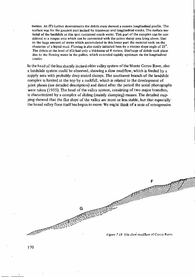
meters. At (F) further downstreams the debris mass showed a convex longitudinal profile. Thesurface was for the greatest part incised by transverse and longitudinal cracks. The surface ma-terial of the landslide at this spot contained much water. This part of the complex can be con-sidered as a tongue area which can be connected with the active slump area lying above. Dueto the large amount of water which accumulated in this lower part the material took on thecharacter of a liquid mud. Flowing is also easily initiated here by a steeper slope angle of 25°.The debris at the level of (G) had only a thickness of 4 meters. Discharge of debris took placedue to the flowing water in the gullies, which extended rapidly upstream via the longitudinalcracks.

In the head of the less sharply incised older valley system of the Monte Cozzo Ravo, alsoa landslide system could be observed, showing a slow mudflow, which is feeded by asupply area with probably deep seated slumps. The southwest branch of the landslidecomplex is limited at the top by a rockfall, which is related to the development ofjoint planes (see detailed description) and dated after the period the aerial photographswere taken (1955). The head of the valley system, consisting of two major branches,is characterized by a complex of sliding (mainly slumping) masses. The detailed map-ping showed that the flat slope of the valley are more or less stable, but that especiallythe broad valley floor itself has begun to move. We might think of a serie of retrogressive

Figure 7.18 The slow mudflow of Cozzo Ravo.

170

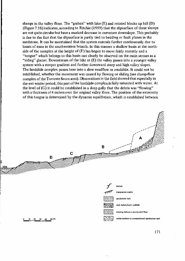
slumps in the valley floor. The "graben" with lake (E) and rotated blocks up hill (D)(Figure 7.18) indicates, according to Ritchie (1959) that the slipsurface of these slumpsare not quite circular but have a marked decrease in curvature downslope. This probablyis due to the fact that the slipsurface is partly tied to bedding or fault planes in thesandstone. It can be ascertained that the system extends further continuously due tolosses of mass in the southwestern branch. In this manner a shallow basin at the north-side of the complex at the height of (F) has begun to move fairly recently and a"tongue" which belongs to this basin can clearly be observed on the main stream as a"riding" glacier. Downstream of the lake at (E) the valley passes into a younger valleysystem with a steeper gradient and further downward steep and high valley slopes.The landslide complex passes here into a slow mudflow or mudslide. It could not beestablished, whether the movement was caused by flowing or sliding (see slump-flowcomplex of the Torrente Secco area). Observations in the field showed that especially inthe wet winter period, this part of the landslide complex is fully saturated with water. Atthe level of (G) it could be established in a deep gully that the debris was "flowing"with a thickness of 4 meters over the original valley floor. The position of the extremityof this tongue is determined by the dynamic equilibrium, which is established between

O 10 20 30 4O 50 m.

scarps

transverse cracks

sandstone rock

i & & £ l rock debris from rockfa"

moving debris in slump and flow

valley bottom in unweathered sandstone rock

171

the supply of debris from above and the discharge of debris by means of gully erosionand water erosion or secundary rapid mudflows to the water. The toe of the tongue hasmoved downward since 1955 due to a greater supply from above, which may be con-nected to the extension of total landslide complex. Apart from the effect of the litho-logical characteristics of the partly weathered rock, other factors also play a part:— The strong retrogressive erosion of the lower river part, through which the upper

valley system has become unstable.— Concentration of water in the old flat valley system, causing development of a sys-

tems in which massmovements and intensive gully erosion operate at the same time.The complexes described under type no. 12 (see Table 7.1) are complex erosion sys-tems in which massmovements and intensive gully erosion operate at the same time.These so-called "badland" complexes are completely devoid of vegetation and havedeveloped on steep slopes ( > 35°). They are characterized by a gully system which isdetermined by the lithological characteristics and the age of the system (Plate 15).Since the complexes were found on the steepest slopes in the study area, we have con-cluded that in most cases these badlands have developed in areas where shallow debrisslides (type no. 7) rapidly have slipped large parts of the slopes of soil and vegetation. Onthese steep slopes it was impossible that the vegetation could regenerate becauseweathered material immediately is carried away by intensive gully erosion and mudflowprocesses (Plate 15). The badlands have developed in many places of the study area (seemap Appendix A7) especially in the riverbasin of the Fiume Oliva. Extensive badlandsare found in the upper basin of the Valle del Signore and the Valle Spinoza in meta-morphic rocks and weakly cemented sandstones and in the Valle Grecci (in granites).Also in the lower course of the Valle Callonci and in the valley head of the TorrenteCalcato active badland complexes with deep gully systems were found. In the riverbasin of the Fiume Grande we found that at the steepest foot of the slope gully sys-tems have developed in areas which are recently affected by soil slips.The installation of pegs in a number of gullies, varying in depth from 0.5-2 metersand in width from 1 -4 meters, revealed that two processes are important in thesegully systems:

— Surface water erosion at the interfluves (0-1 cm) after one year.— Slump and flow processes on parts of the interfluves and at the gully bottom,

which locally reaches depths of ± 1 meter.The slided material is rapidly carried away via mudflow processes in the gullies down-stream. River basin with extensive badland complexes, as e.g. the Valle del Signore,delivers in rainy periods relative large masses of sediment of the rivers. Measurementsof sediment concentration after heavy rain period show concentrations which are 10-100 x higher in comparison with rivers which have no badland complexes in theirdrainage brain.In the Vallone della Fabrica (Fiume Grande drainage basin) we have described debrisslides (7.2) which are already affected by gullying (see Figure 7.6 and Plate 8). Thegullied soilslip complexes have developed on slope angles of 40° about 50 years ago(oral communication from the inhabitants). The greatest part of the regolith layer hasbeen cleared away. The complex consists of a lightly branched gully system. The gullies

172

are on an average 50 cm deep and 2 meters wide, with a maximum depth of 3 metersand a maximum width of 7 meters. The slopes have a slightly concave profile and onsome waterdivides between the gullies are still some remains of the regolith cover. Fromthe geometry of the gullies it can be estimated that ± 800 m3 material has been carriedaway in the estimated 50 years period, which means a mean thickness of net erosionover the surface of ± 1 cm per year in these metamorphic rocks.

7.5 Summary and conclusions

In the foregoing we have discussed the development of different types of landslide inrelation to landscape and process variables. Attention was given to the amount of pro-duction of moving material and the transport characteristics of the landslides (see Table7.1).In the sandstone regions the rapid incision of the river has led to the development ofa large number of rockslides, which generally produce large amounts of debris material.Special landscape and process variables which initiate motion in these sandstone regionare a.o. the undercutting by rivers of the slope, weakening of the rock by faulting anddevelopment of joint planes dipping toward the free slope face and ponding of water inimpermeable layers. However, the strength characteristics of the weakly cemented andcemented sandstone are such that steep and high slopes are needed before the point ofinstability is reached. The rockslide of type no. 1 (see Table 7.1) forms a good exampleof this system. It was shown that due to a relative high cohesive strength of the sand-stone rocks, high cliffs could develop, which at the point of instability produced largequantities of rockmass. Relative high strength values must exist also along the beddingplanes and joint planes of the sandstone rock, producing on places with a high reliefenergy large amount of rockmasses (see type no. 2,3 and 5). High shear stresses werealso induced in the past by earthquakes, which also led to large rockslides in areas,which nowadays are stable (type 1,3 and 4).As regard to the transport characteristics of the rockslides we found that for type no.1 and 3 the debris must have rapidly come to rest, even on steeper slope angles. The li-mited travelling distance may be explained by two facts: a) failure in wellcementedMar-sandstone rock leads to a disintegration in large blocks, with a limited amount offiner matrix, which prevents a high fluidity of the flow under wet conditions; b) failureis not induced for this type of slides by a high pore pressure of the groundwater but bya rapid rise in shear stresses due to earthquakes. This means that failure may have takenplace under relative dry conditions. In variance with this is the type of transport des-cribed under type no. 5. This recent rockslide occured after heavy rain periods. Theweakly cemented sandstone (Mars) rapidly desintegrated after failure in large quantitiesof mud, which is continuously set into motion via flows during wet periods.Steep slope angles, especially at the foot of the slope, has led on places undercut byrivers to instability of the relative shallow regolith cover (type no. 7). In the claystonearea instability occured on slopes between 32° and 36° while on slopes in metamorphicrocks shallow slides occured on slopes around 42°. Given the strength characteristics

173

of the regolith, we concluded that positive pore pressure of groundwater was neededto initiate failure and the groundwater table has to rise to 2/3 (claystone) or halfway(metamorphic rocks) of the depth of the regolith above the shear plane. In the cohesiveclaystone regolith material the slipsurface developed at a maximum depth in the rego-lith just above the fresh rock which needed a minimum amount of pore pressure. There-fore, apart from the length of the slope over which sliding can take place, the depth ofthe regolith cover determines the amount of moving material. In the cohesionless rego-lith cover of the metamorphic rocks case-studies show that the slipsurface developed inthe horizons with the weakest strength which was lying about in the middle of the re-golith profile. It is the position of this zone which determines the amount of mass mo-ving at failure.On metamorphic rocks, with a thick regolith and solifluction cover (upto 10 meters)"flat" rotational slides developed on slopes varying from 30-35°, with a depth-lengthratio of 1:10. These slides were especially activated by mass during the construction ofthe Autostrada. We established a positive correlation between the length and depth ofthese rotational slides and we estimated that for a number of these slides the point offailure was reached in case the groundwater table has risen to 80-90% of the maximumdepth of the slip in the regolith profile. We concluded that this was the minimum depththe groundwater has to rise in the profile,because we found that the slipcircle developedat a maximum depth in the regolith profile just above the fresh rock. Therefore, themaximum depth of the regolith for these cases determines at last the amount of masswhich can be taken into motion. We have to keep in mind, however, that a thicker re-golith cover means a greater potential amount of sliding mass, but it needs also a largerwater concentration before the point of disequilibrium is reached. On less steeper slo-pes (< 30°) rotational slides have developed (type no. 8 and 9) which generally had alower depth-length ratio (1:5) than type no. 7. The slides developed in weatheredclaystone, sandstone and metamorphic rocks, especially on places where water assem-bles in the head-region of the streams. The study of these rotational slumps on varyingslope angles reveals that in general the size of the slides increases with decreasing slopeangle, while at steeper slopes the degree of displacement of the rotating block out ofthe area is larger than on less steeper slopes. This general trend could be establishedby the detailed study of a number of rotational slides in weathered claystone. Apartfrom the effect of slope angle on the amount of sliding mass, it was also the localthickness of the weathered regolith, which determines the potential maximum amountof sliding material. At the head of the river valleys in areas with deepseated rotationalslides, the material can be further transported via relative slow mudflows which moveinto the valleys downstream (type no. 11). Movements take place especially in the wetseason when large amounts of groundwater are available. The mechanism of movementmay be either by sliding along the slipsurface or by internal shear (flowing) due to thehigh viscosity of the flow.

174

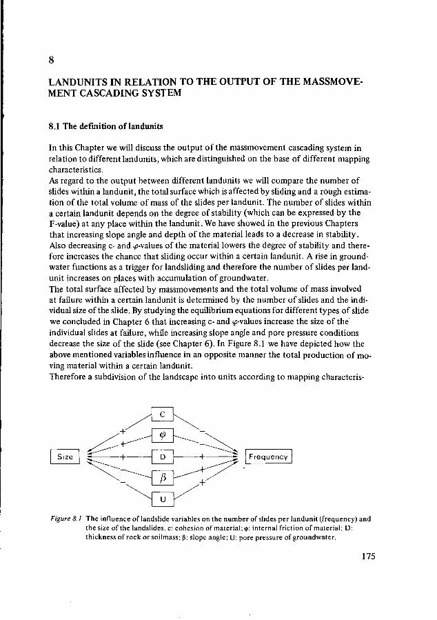
8

LANDUNITS IN RELATION TO THE OUTPUT OF THE MASSMOVE-MENT CASCADING SYSTEM

8.1 The definition of landunits

In this Chapter we will discuss the output of the massmovement cascading system inrelation to different landunits, which are distinguished on the base of different mappingcharacteristics.As regard to the output between different landunits we will compare the number ofslides within a landunit, the total surface which is affected by sliding and a rough estima-tion of the total volume of mass of the slides per landunit. The number of slides withina certain landunit depends on the degree of stability (which can be expressed by theF-value) at any place within the landunit. We have showed in the previous Chaptersthat increasing slope angle and depth of the material leads to a decrease in stability.Also decreasing c- and cp-values of the material lowers the degree of stability and there-fore increases the chance that sliding occur within a certain landunit. A rise in ground-water functions as a trigger for landsliding and therefore the number of slides per land-unit increases on places with accumulation of groundwater.The total surface affected by massmovements and the total volume of mass involvedat failure within a certain landunit is determined by the number of slides and the indi-vidual size of the slide. By studying the equilibrium equations for different types of slidewe concluded in Chapter 6 that increasing c- and ip-values increase the size of theindividual slides at failure, while increasing slope angle and pore pressure conditionsdecrease the size of the slide (see Chapter 6). In Figure 8.1 we have depicted how theabove mentioned variables influence in an opposite manner the total production of mo-ving material within a certain landunit.Therefore a subdivision of the landscape into units according to mapping characteris-

Size Frequency

Figure 8.1 The influence of landslide variables on the number of slides per landunit (frequency) andthe size of the landslides, c: cohesion of material;<p: internal friction of material; D:thickness of rock or soilmass; ß: slope angle; U: pore pressure of groundwater.

175

tics based on these variables does not necessarily give significant differences in total vo-lume of mass production between these units. We will test whether this statement,which is based on the theoretical considerations given above, is valid for the study area.Therefore the study area is subdivided into landunits according to some simple mappingcharacteristics which are related to the variables depicted in Figure 8.1. The landunitsare distinguished on the base of one mapping characteristic. A further subdivision accor-ding to two or more characteristics, leads to smaller total areas per landunit in whichthe frequency of sliding is too limited to make liable comparisons in output.A first possibility is to subdivide the landscape into units according to mapping charac-teristics, which are related with the strength properties (c and <p) of the material. Forthis purpose we can distinguish landunits with different rock and "soil" types. InChapter 6 and 7 it was shown that not the strength of the intact rock is of importancebut especially the tectonic structure of the rock: frequency of joints, faults, strengthalong bedding planes and dip of these discontinuities in relation to slope. It is difficultto distinguish within one rock type differences in tectonic structure, e.g. the density ofjoints. Further: differences in structure may be very locally, e.g. faulting zones, contactzones with other rocks, dip of joint - and bedding planes towards the free slope. MapI (Appendix A7) shows a distinction according to lithological units. Within these units,as far as possible, information is given about local conditions of the tectonic structureof the rock.

The "soil" (weathered regolith in situ or displaced deposits from Pleistocene and Holo-cene periods) is in the study area related to the lithological units. Therefore a subdivi-sion on the base of the lithological characteristics also give a spatial differentiation ofthe related weathered material. As we have shown in the previous Chapters it mightbe of importance to differentiate landunits according to the available depth of especial-ly the weaker weathered material, because the depth of the regolith cover forming athreshold influences the frequency and size of the landslides in the same manner. Un-fortunately it is very difficult and often impossible without special techniques to makea primary subdivision of the landscape according to the depth of weathered material.The study of the landslides in weathered material reveals some general outlines as regardto the depth of the weathered material. The many steep slopes in sandstone and lime-stone (see Chapter 2) have only a thin to very thin regolith cover, with a maximumthickness of 1 meter. Locally the weakly cemented Mars-sandstone may have a thickerweathered regolith cover especially in the more flatter valley heads. In claystone areason relative flatter slopes (see Chapter 2) weathering must have gone also to a greaterdepth, while the slope may be covered by deposits of clay material of previous landslides.In the area of metamorphic rocks, especially in the southern part of the study area(Savuto valley) the slopes are locally covered by thick packages of colluvial (solifluc-tion) material, which can reach a thickness of more than 20 meters.The next parameter which may be of importance as a differentiating factor in outputbetween landunits in the slope angle (see Figure 8.1). Therefore in map II AppendixA7 the landslides are depicted in relation to landunits with different slope classes. Wehave distinguished four slope classes: 5-10°, 10-20°, 20-30° and > 30°.These classes are more or less based on the range of slope angle values in which different

176

types of landslide have developed (see Table 7.1). The last importance variable deter-mining the frequency of sliding and the size (see Figure 8.1) is the amount of porepressure which is built up in a certain area. It is difficult to find a mapping criteriawhich enables us to distinguish landunits with differences in maximum pore pressureconditions. These differences in groundwater conditions are related to soil- and rockvariables, vegetation- and topographical variables and the hydrographie network. Diffe-rences as regard to the maximum pore pressure conditions may be very locally, due toponding of groundwater by impermeable layers, local slope curvatures, concentration ofwater at the foot of the slope. More generally groundwater concentration is tied to thestructure of the hydrological network. It can be stated that accumulation of groundwateroccur especially in the source area at the head of the stream. Therefore we have drawnthe hydrographie network in the maps in order to show the relation between the spatialdistribution of the slides and the stream network.

Differentiation in maximum pore pressure conditions between landunits might be dueto differentiations in vegetation structure. Differences in vegetation structure lead todifferences in evaporation and perception of rainwater and hence in groundwater levelvariations (Chapter 6). Also the infiltration capacity of the soils might be related tothe vegetation structure and landuse (see Chapter 5) which also leads to differences ingroundwater conditions.Apart from this the rootsystems of vegetation influence the strength of the soil (Chap-ter 6). Tichy (1962) made a deforestation map of Basilicata (north-east Calabria) andcompared this map with a landslide map by Kayser (1958). It appears that massmove-ments often take place in areas which have been deforested especially after 1879. Un-fortunately such comparisons are not possible in the study area because the total areawas deforested in the past and the vegetation structure consists mainly of more or lessdense shrub and tree vegetation (see Chapter 5) alternated with areas under recentcrop cultivation.In map III (Appendix A7) the study area is distinguished in three types of landunitbased on the vegetation structure c.q. landuse. We have distinguished arbitrary 1. den-sely vegetated areas Ç> 60%), 2. scarcely vegetated areas (0-60%) and 3. areas withrecent crop cultivation.

8 2 The differences in output of the massmovement cascade in relation to landunits

On the base of the above mentioned three landunit maps we will discuss the output be-tween the distinguished landunits. In the Tabels 8.1 - 8.3 a survey is given of the outputof different types of landslide per landunit. As output we have considered for differenttypes of slide the number (frequency) of slides per unit (column 3). The total surface (inm2) affected by sliding (column 4) and the estimated total volume of the slides (m3)(column 6). The last was the most difficult to estimate, because especially for the deepseated slides the slip circle could not always been reconstructed. As far as possible extra-polation has been made from landslides of the same type and size order, from whichthe depth of sliding was known.

177

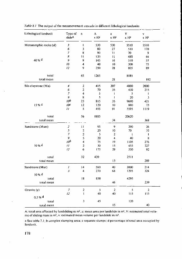
Table 8.1 The output of the massmovement cascade in different lithological landunits

Lithological landunit

Metamorphic rocks (sf)

40 % d

totaltotal mean

Silt-claystone (Ma)

15 % d

totaltotal mean

Sandstone (Mars)

10 % d

totaltotal mean

Sandstone (Mar)

10% dtotal

total mean

Granite (y)

0.5 % d

totaltotal mean

Type ofslidea

36789

1012

4679

10bIOC11

2579

10b

1112

13

712

n

138

11949

45

2248

23125

56

11225426

32

144

18

21

3

AxlO3

5308090

12014540

250

1265

41570

55

815120455

1885

9520

5207530

175

420

560270

830

LA

40

45

axlO3

530271111161028

28

20735

11

351091

34

91024

191529

13

4068

46

240

15

Vx 103

551051070480510300805

8185

4000430

520

9690880

5595

20620

29070

140

1105455550

2511

30001295

4295

5115

120

V

x 103

5510170

944577589

182

2000215

13

42173

1119

368

2635

18

276227

92

209

214324

239

2115

40

A: total area affected by landsliding in m2, a: mean area per landslide in m2, V: estimated total volu-me of sliding mass in m3, v: estimated mean volume per landslide in m3.

a See table 7.1 ; b complex slumping area; c separate slumps; d percentage of total area occupied bylandunit.

178

To get an impression of the mean area and volume which is involved in failure for a'given landslide, we divided resp. the total area and volume per landslide type by thenumber of landslides (resp. column 5 and 7).Map I and Table 8.1 show the differences in output in relation to different lithologicalunits. We will first compare the number of slides for different types per landunit. TheTable shows that compared with the total percentage of area, occupied by this unit(15%), the silt claystone region produced the highest number (frequency) of landslides(column 3). A dominant number of slides show type no. 9, 10 and 11 which developedin thick weathered claystone covers. The reason for this relative high frequency mightbe the relative thick weathered regolith cover (see Figure 8.1). The material also haverelative the lowest strength values, but this might be compensated by the relative lowerslope angles in the claystone area (see Chapter 2).It can be mentioned further that the infiltration capacity of the clay soils can becomevery high after desseccation due to the formation of cracks (see Chapter 5). This maylead to a relatively high rise of the groundwater table after heavy rainstorms.A relative high number of slides per landunit is also found in the area with weakly ce-mented sandstone (Mars) (column 3). In these Mars landunits a dominant number ofslides developed as well on the fresh sandstone rock (type no. 2) as in the weatheredrock (type no. 9, 10,12) (Table 8.1, column 3). The landslides are concentrated in thenorth-western part of the sandstone area in the neighbourhood of Amantea (map I). Ex-planations for this concentration might be : 1. The rocks in this area are stronger affectedby tectonic activity, which leads to higher concentration of joint and fault systems, 2.A stronger erosive activity of the main rivers and their tributaries downstreams. Thelandslides in landunits of metamorphic rocks are concentrated in the southern part ofthe study area (Savuto and Fiume Grande region). The reason might be that thesesouthern region is covered with thicker regolith mantles than in the north easternregion. A relative high number of slides which are related to the thicker weathered layersin metamorphic rocks belong to type no. 8, 9 and 10 (see Table 8.1 column 3). Alsosurficial slides (type no. 8) and the related badlands (type no. 2) are frequent in thisregion. The map I shows that unstable areas in this metamorphic landunits are especiallyconcentrated along the main rivers at the foot of the slope and at the head of tributaryrivers with very steep slopes. A relative low frequency of sliding occurs in the landunitswith cemented sandstone (Mar) with mainly type no. 1. A glance on the map showsthat the slides are concentrated at the boundary of these units in the steep high sand-stone cliffs (type no. 1, see Chapter 7). All these slides dated from the past periods andare probably trigged by earthquakes. The slopes in these sandstones with a thin cover(or no cover) can be considered as stable at present times. The granite and limestoneunits cover a very small part of the total area, which hampers a comparison as regardto the output. In the granite area a number of landslides were observed in weatheredmaterial (a.o. type no. 7 and 12). As regard to the total mass production per landunitTable 8.1 .column 4 t/m 7 shows that in the claystone region the largest area is affectedby landsliding and these units produced together the largest volume of sliding material.This is explained by the high frequency of sliding (see above) and the fact that in thisdeep weathered material with relative low strength values a large number of deep seated

179

rotational slides (type no. 10 and 11) developed on relative flat slopes which means ahigh production of mass per landslide (see Table 8.1).It is interesting to note the high mean mass-production per landslide of the fossilizedcomplexes in different lithologial units (see Table 8.1, type no. 1,3,4 column 5 and 7).An explanation was already given in the previous Chapters. We will mention here that:— The rocks, in which these fossilized slides (type no. 1, 3 and 4) have developed, have

higher strength values (especially cohesion) than the weathered material, whichmeans a potential higher production of mass if failure takes place (Figure 8.1).

— Instability in these rocks occurred due to the development of high shear stresseswhich were induced by earhquakes in the past. This means that places with strongmaterial are brought to the point of disequilibrium, which also leads to a high pro-duction of mass.

We can conclude that a subdivision of the landscape according to lithology and relatedweathered material shows in the study area a differentiation as regard to the numberof slides and landslide types. We also could observe from the map that the distributionwithin the landunits is far from homogeneous, due to the fact that strong local deviationof variables have created unstable situations (see below). Differentiations as regard tothe total volume and (or) area are less clear per lithological unit. We may distinguishthree groups: 1. high production in silt clay stone and Mar-sandstone (the latter havingonly "fossile" complexes concentrated at the boundary of the units), 2. a medium pro-duction of the Mars-sandstone regions and the metamorphic rock regions and 3. a lowproduction in the granite and limestone regions.

Table 8.2 and map II (Appendix A7) show the frequency and output of different typesof landslides in relation to landunits, which are subdivided according to different slopeangle classes. From the Table we can infer that generally there is an increase in frequen-cy of slides with increasing slope angle values. The following explanations are given:— At increasing slope angle values an increasing number of types of material with va-

rious strength values reaches the point of failure.— At higher slope angles smaller amounts of groundwater are needed to cause instabi-

lity (see Chapter 6).— At higher slope angles the depth of sliding is lower which means that sliding is also

possible in shallower regolith material (see Chapter 6).The Table shows a differentiation in landslide types with different slope classes. In thelower slope classes (5-20°) predominately deep seated rotational slides in weathered ma-terial (especially clay) have developed (type no. ,10 and 11). Also in these slope classes"fossilized" rockslides could develop (type no. 3 and 4), but we stated already thatearthquakes must have induced the necessarily high shear stresses in this stronger rockmaterial. In the slope class 20-30°, more shallow rotational slides (type no. 8 and 9)have developed, which confirms the thoughts given in the previous Chapter. In the slopeclass > 30° also surficial debris slides have developed (type no. 7) and the badlands(type no. 12) related to this type of slides. Based on the different equilibrium models,given in Chapter 6, it was stated that'given certain strength values of the material thesize of the slides decreases with increasing slope angle (see also Figure 8.1). This is in

180

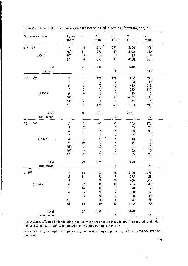
Table 8.2 The output of the massmovement cascade in landunits with different slope angle.

Slope angle class

5 ° - 10°

(15%)d

totaltotal mean

10° - 20°

(15%)d

totaltotal mean

20° - 30°

(15%)d

totaltotal mean

> 30°

(25%) d

totaltotal mean

Type ofslidea

410b

10e

II

3568910bWc11

35678910b

10e

12

12367891112

n

21144

21

112261562

35

2212410332

29

1211121656113

67

Ax 10s

5152955

365

1180

1951070805

5501

125

1036

601015520 '5040520

225

460957090902070

. 5360

1260

ax 103

25727191

56

195103540137162

30

3051525513210

. 8

38970456412528

19

Vx 103

3590351535

4270

11410

15004043033010

645525980

9770

335459051015452550

620

2100235660485706024075

1165

5090

V

xlO3

17953209

1067

543

1500402151152

4305

490

279

1702590222151025

22

17521660242412407590

76

A: total area affected by landsliding in m\ a: mean area per landslide in m2, V: estimated total volu-me of sliding mass in m3, v: estimated mean volume per landslide in m3

a See table 7.1 ; b complex slumping area; c separate slumps; d percentage of total area occupied bylandunit.

181

partially accordance with the results found in the study area because for most landslidetypes the mean output (area or volume) decreases in the first three slope classes (co-lumn 5 and 7). The Table also shows that the total production per landslide type(column 4 and 6) which is determined by the number of slides and the mass per indivi-dual slide decreases in the first three slope classes. Increasing slope angle class valuesshow generally an increasing number of landslide per landunit, but a decreasing mean vo-lume per landslide which results in a decrease in the total production per landunit. Theslope angle class > 30° shows again an increase in the total massproduction which mustbe related to the rapid increase in the number of slides per landunit.Concluding we can state that a subdivision of the landscape according to differentslope angle value classes results in a differentiation as regard to the frequency and typeof landslides between these units. As regard to the differentiation in total volume andsurface affected by sliding we found a decrease in output in the first three classes andagain a rise in output in the last class with the highest slope angle values.Table 8.3 and map III (Appendix A7) show the relation between landslides and landunitsdistinguished according to vegetation structure and landuse.

The Table shows a relative high frequency of slides in the areas with open vegetationcompared with the agricultural areas and the areas with a closed vegetation structure.The agricultural areas show the highest amount of mass production (column 6) in rela-tion to the other areas. The more densely vegetated areas seem to be more stable thanthe areas with open vegetation. The following possible explanations can be given:— The areas with open vegetation are lying in more steeper slope classes, while the

agricultural areas are in regions with more flatter slopes. This explains the highernumber of landslides in the open areas (see above). On the other hand on these flatterslopes more deep seated slides can develop which obviously results in a greater totalmass production.

— The greater total mass production in the agricultural areas might also be explainedby the fact that the infiltration capacity in these areas is higher than in areas withopen vegetation (see Chapter 7), which can result at a given rain input in a higherrise of the groundwater table and thus a higher frequency of failure.

— Areas in open vegetation are less stable than areas with closed vegetation due to agreater density of the roots which increases the strength of the soil (Eyles 1971) anda greater interception and evaporation of the biomass which reduces the maximumrise of the groundwater table. However, the depth of the roots most times is notsufficient enough to strengthen the total regolith even in the shallow slides (type no.7). Further we established in Chapter 5 that the densely vegetated areas show higherinfiltration capacities.

As a conclusion we can say that a subdivision according to the vegetation structure leadsalso to differentiation in output, but an explanation for this differentiation is ratherdifficult to give. Further there may exist an autocorrelation between slope angle at oneside and vegetation structure and landuse on the other side.In the above given analysis of the relationbetween landunits and landslides, we mentionedalready occasionly the fact that the distribution of landslides within the landunits is

182

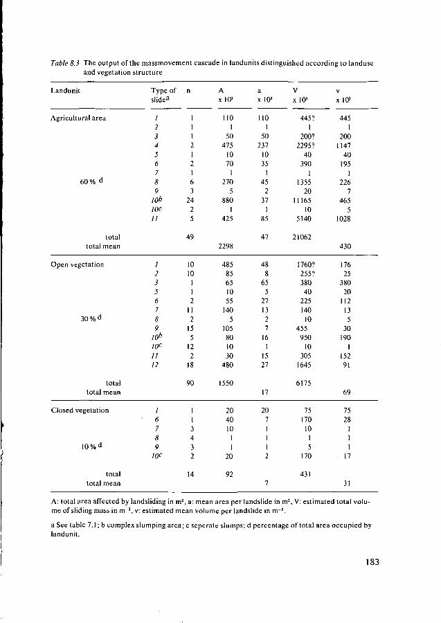
Table 8.3 The output of the massmovement cascade in landunits distinguished according to landuseand vegetation structure

Landunit

Agricultural area

60 % <J

totaltotal mean

Open vegetation

30 % d

totaltotal mean

Closed vegetation

10 % d

totaltotal mean

Type ofslidea

/2345678910bIOC11

1235678910b

10c

1112

1678910e

n

1112121632425

49

101011211215512218

90

113432

14

Ax 10*

11015047510701

2705

8801

425

2298

485856510551405

105801030480

1550

20401011

20

92

ax 10»

11015023710351

45237185

47

4886552713271611527

17

2071112

7

Vx 101

445?1

200?2295?403901

135520

1116510

5140

21062

1760?255?3804022514010

455950103051645

6175

751701015

170

431

V

x I03

4451

2001147401951

2267

4655

1028

430

1762538020112135301901

15291

69

7528111

. 17

31

A: total area affected by landsliding in m2, a: mean area per landslide in m2, V: estimated total volu-me of sliding mass in m~3, v: estimated mean volume per landslide in m~3.

a See table 7.1 ; b complex slumping area; c seperate slumps; d percentage of total area occupied bylandunit.

183

not homogeneous. This is due to the fact that instability is also caused by local deviationof the value of variables within the landunit.This local deviation of variables are related to:— Local weakening of the strength of the rock, due to faults and on contact zones with

other rocks.— Local water concentration at the head of steams, at places with impermeable layers,

and contact zones with other impermeable rocks.— Local erosion activity of the river at the foot of the slope.— Local instabilities caused by previous slides (retrogressive sliding).— Local instabilities created by man due to the construction of roads or irrigation acti-

vities.A glance at the map shows that a great-number of landslides (45%) are concentrated atthe head of the streams. Further 75% of the sliding are related to the active erosion ofthe river while 6% of the landslides were activated by man due to road constructionand irrigation activities. We found that 35% of the slides developed along faults orstrong developed fault systems, while 5% of the slides developed at the contact zonebetween 2 rocktypes. Further we could detect that in 10% of the cases water concen-tration was due to ponding of groundwater by local impermeable layers, while 5% ofthe cases retrogressive sliding must have taken place.

8.3 Summary and conclusions

In the discussion given above we have tried to analyse, whether the landscape can besubdivided into landunits according to certain criteria, which show differences in fre-quency and the total mass production of various types of landslides. Such a map maygive an impression of the spatial differentiation in degree of stability of the landscape.We have shown that subdivision of the landscape for this purpose faces two problems:— A number of variables influences in an opposite manner the frequency of sliding and

the mass production per landslide. This means that a subdivision of the landscapebased on the above given variables does not necessarily give significant differences asregard to the total produced mass of a landunit.

— The distribution of landslides within the landunit and therefore the possibility thatfailure should occur, is not homogeneous which is due to local deviation of certainvariables.

— The depth of the overlying weaker material i.e. the regolith cover is a very importantvariable which determines both in a positive way the frequency of sliding and theamount of mass production per landslide. However, this parameter cannot always bedetermined in the ordinary practice of mapping.

In the study area a subdivision of the landscape according to the lithological characteris-tics of the rock and the related weathered material have shown a differentation regardingthe number of slides per landunit and the landslide types. It was more difficult to dis-cern a differentiation regarding the total volume: the highest total volume productionwas found in the silt-claystone region and in the Mar-sandstone region (with only fos-

184

silized slides), a medium production in the Mars-sandstone and metamorphic rocks,while granite and limestone regions showed the lowest production.Also a dubdivision according to slope angle classes shows a differentiation regardingthe frequency and type of sliding. As regard to the totally produced volume we couldestablish a decrease in output with slope angle in the first three slope classes, while inthe class with slope angle values > 30° the amount of mass production increases. Asubdivision of the landscape according to vegetation structure revealed that the unitswith open vegetation shows the highest frequency and total production of mass.A landscape map which is based on the above described criteria must be completed, witha number of mapping criteria, which show the local influence of certain variables onthe degree of stability and hence the possibility of sliding on particular localities withinthelandunit. Therefore local information has to be given about fault and joint systems,contact zones between lithological units, special areas with water concentration, localerosion activity of rivers, indication of activity of man.

185

9

SUMMARY

Various types of "pragmatic" landscape maps, in which the distinguished units are sup-posed to show differences in potentials with regard to a particular problem, have beenproduced for many purposes. However, the differences of these potentials are seldommeasured. In this thesis a discussion has been made whether in a mediterranean landscape,landunits can be distinguished on the base of some general visible landscape characteris-tics, which show significant differences in output as regard to the sediment transporton slopes.Two systems of sediment transport were chosen: the system of sediment transport byfalling and running water (water erosion) and the system of sediment transport whichtakes place mainly under the influence of gravitational forces (landsliding or massmo-vement). In order to study the differences in output of these transport processes be-tween the distinguished landunits, the following steps were taken :- An analysis was made of the influence of landscape variables (or parameters) on the

output of the sediment transport processes.- A selection was carried out of visible mapping criteria, related to these variables,

and the definition of landscape units based on these criteria.An analysis of the differences in output of the transport processes between the landunits,was carried out.

The influence of landscape variables on the output of the sediment transport processes.Two systems of the water erosion transport processes could be distinguished: the trans-port by splash erosion and the transport by overlandflow erosion. Measurements onthe output were done by using a portable rainfall simulator and measuring plots. Itappeared that the density of the herb vegetation, the aggregate stability and the stonecover pavement have a strong effect on the output of splash erosion and overlandflowerosion. Compared to the bare soil a slight density of the herb vegetation proved to bea very effective factor in the protection of the soil particularly against splash erosion.A stone pavement with gravel varying in size from 2-6 mm had a protective effectagainst water erosion on a horizontal surface, but on steeper slopes (20-30°) thegravel is transported even more easily than the finer fractions. It was established, thatthe bulkdensity which must be related to the mechanical strength of the soil showeda marked correlation to the output of the water erosion processes. Textural indices

didn't show a marked relationship to the output: The clay mineral content seems tohave on one hand a binding effect on the aggregates, while on the other hand the swel-ling clay minerals weaken the aggregates during wetting. The slope length seemed tohave no effect on the output of overlandflow erosion and hence the total water erosionoutput, particularly on the more or less natural slopes. This is explained by two facts:

- A great part of the sediment is transported by splash erosion; on more or less natu-ral slopes the transport rate of splash erosion was two to four times higher than thetransport rate of overlandflow erosion.

187

- Transport of sediment by overlandflow erosion is local since no correlation could beestablished between slope length and overland flow on the more or less natural slopes.

Therefore we consider the water erosion on natural slopes in this area to be a "point topoint transfer" of sediment.

The study of the input-output relationships of the overlandflow erosion process alsoreveals that particularly on the more or less natural slopes the transport rate by over-landflow erosion is controlled by the amount of material which is detached by splashimpact shear and (or) by overlandflow shear, and not by transport capacity of theflow. Further more an important part of the transported sediments by overlandflowseemed to be supplied by splash erosion. Four main variables are important to the degreeof stability of the slope against massmovements, the type of massmovement and amountof transport by massmovements. These are the mechanical characteristics of the material,the angle and height of the slope, the thickness of the rock- or soil material and theamount of groundwater in the material. In the study area twelve types of massmovementcomplexes were distinguished mainly on the base of the mechanism of initial failure,the mechanism and amount of transport, the morphometrical and material characteris-tics of the slides. Five types of rockslides have been distinguished which mainly deve-loped in cemented — and weakly cemented sandstones. One type concerns the instabilityof steep cliffs developed in the cemented sandstone. The other four types showed failurealong bedding and joint planes facing toward the free slope face.A further subdivision of these rockslides was based mainly on the character and thetransportability of the mass after failure. The great quantities of rock mass involved inthese rockslides (especially the "fossilized" ones) point to the fact that the strengthof the rock material is relatively high, and further more that the old landslides are in-duced by earthquakes which produce high shear stresses and hence high quantities ofmass at failure.Shallow translational slides developed on steep slopes (20°-40°) in relatively thin re-golith covers (± 1 mtr) lying over different types of rock. The steepness of the criticalslope varied with the strength of the regolith. Stability analyses revealed that the in-stability must have occurred under the influence of positive porewater pressure of thegroundwater which must have risen up to approximately one third to one half of thedepth of the regolith. The amount of material involved at failure depends on the thick-ness of the regolith or the depth of the weakest zone within the regolith. Flat rotationalslides developed on less steeper slopes of metamorphic rocks, covered by a thicker re-golith or solifluction mantle (up to 10 mtrs.). Stability analyses showed that the ground-water must have risen nearly to the soil surface in order to start failure. On less steeperslopes (< 30°) in all types of weathered rocks more deepseated rotational slides witha depth-length ratio of 1:5 developed. Most of these slides were found at the head ofthe streams, which showed a concentration of the groundwater. The study of these ro-tational slides showed that the size of these slides increase with a decreasing slope angle.The displacement of the rotating blocks seems to be larger on the steeper slopes. Thesedeepseated slides may form complexes in the head of river valleys. The material maybe transported further downstream via relatively slow mudflows.

188

Landunits related to the output of the sediment transport processes.

Five mapping criteria related to the variables influencing the output of water erosion werechosen, in order to subdivide the landscape into landunits. The following sequence ofcriteria seems to give the best differentiation in output on each classification level in thearea: 1 the degree of agricultural activity of man, 2 the vegation structure, 3 soil andrelated parent material,4. slope angle, 5. slope length.Landunits under recent cultivation have much higher erosion outputs than the otherlandunits. Landunits with abandoned fields proved to be the most resistant againsterosion, due to a denser herb growth, which also increases the infiltration rate of thesoil. Furthermore the landunits with a decedeous forest cover without a shrub andherb cover appeared to be very sensitive to water erosion, due to a relatively higherodibility of the soil and a lower infiltration capacity compared to soils under a herb-cover. The searing of the soil surface, particularly in soils derived from sandstone andmetamorphic rocks, may locally produce high amounts of overlandflow and sediment.Satured overlandflow could occur locally in thin soils on metamorphic rocks which re-sulted in a very high production of sediment. On the contrary the production of over-landflow and sediment was locally very low in soils on claystone mainly due to the for-mation of dessication cracks.

Three mapping criteria were chosen to subdivide the landscape into landunits in orderto compare the differences in output of the massmovement cascading system betweenthese units: 1. the different rock and related "soil types", 2. the slope angle and 3. landuse and vegetation structure. As output of the landunits we considered the number ofslides per landunit and the total area and mass involved in sliding per landunit. In analysingthe differences in output between the landunits we faced two problems:— Theoretically it appeared that the landscape variables in the landslide equilibrium

model influences in an opposite manner the degree of stability of the slope (andhence the frequency of sliding per landunit) and the mass production per landslide.This means that the total production per landunit, which is determined by the num-ber of slides and the amount of mass per landslide does not necessarily differ be-tween landunits of which the subdivision is based on one of these equilibrium para-meters.

— The distribution of landslides within the landunit and therefore the possibility thatfailure should occur is far from homogeneous due to local strong deviation of certainequilibrium parameters. Therefore landscape maps showing differences in slope sta-bility, and mass production of landslides between landunits must be completed by anumber of mapping criteria, which show the influence of certain variables on thedegree of stability on particular localities within the landunit.

In the study area a subdivision of the landscape according to the lithological charac-teristics of the rock and the related weathered material have shown a differentation asfar as the frequency of sliding and type of sliding are concerned. It was more difficultto discern a differentiation regarding the total mass of slided material. The highest massproduction was found in the silt-claystone region and in the Mar-sandstone region(with only fossilized slides) a medium production was found in the Mars-sandstone regions

189

and metamorphic rocks, while granite and limestone regions showed the lowest pro-duction.A subdivision of the landscape according to slope angle also showed a differentiationin the types of landslide and number of slides per landunit. It appeared that with higherslope angle classes the number of slides per landunit increased but the mean mass perlandslide decreased. This resulted in a net decrease of total mass production with in-creasing slope angles for the first three slope classes. A subdivision of the landscape ac-cording to the vegetation structure revealed that units with an open vegetation covershowed the highest number of landslides and total sliding mass.

190

10

SAMENVATTING

De "pragmatische" landschapskartering heeft o.a. als doel verschillen in potentieel aante geven tussen de onderscheiden eenheden. Zelden worden deze verschillen tussen land-schappelijke eenheden via metingen geanalyseerd. In deze studie wordt nagegaanof op basis van zichtbare en karteerbare kenmerken landschappelijke eenheden kunnenworden onderscheiden, die significante verschillen in transport van sediment op hellingenvertonen. Voor dit doel zijn twee processystemen gekozen: a) het transport van sedimentdoor vallend en stromend water (water erosie) en b) het transport van materiaal, voor-namelijk onder invloed van de zwaartekracht (massa beweging). De volgende problemenkregen in deze studie de aandacht:- Een analyse van de invloed van verschillende landschaps-variabelen (-parameters op

de hoeveelheid transport van sediment op hellingen.- Een selectie van zichtbare karterings criteria, die in verband staan met deze land-

schaps-variabelen en de definiëring van bepaalde landschappelijke eenheden.— Een analyse van de verschillen in hoeveelheid sediment transport tussen de onder-

scheiden landschappelijke eenheden.

De invloed van landschaps-variabelen op de transport hoeveelheid van sediment ophellingen.Het water erosie proces werd onderverdeeld in twee proces systemen: het transportvan sediment door spat erosie (splash erosie) en door stromend water over de helling(overlandflow erosie). Metingen werden verricht met een draagbare regenval simulator,en met behulp van proefvelden. Vastgesteld kon worden dat de dichtheid van de krui-denvegetatie, de aggregaat stabiliteit van de bodem en de grindbedekking aan het opper-vlak van invloed zijn op de hoeveelheid transport door water erosie. Het bleek verderdat een geringe toename van de dichtheid van de vegetatie t.o.v. de onbedekte bodemeen sterke daling van met name de hoeveelheid splash erosie liet zien. Een grindbedek-king (korrelgrootte 2-6 mm) beschermt op een horizontaal oppervlak de bodem tegenerosie. Op steile hellingen daarentegen, bleek dit grind gemakkelijker transporteerbaardan de fijnere bodemfracties. Ook de bulkdensity van de bodem, die mede bepalendis voor de schuifweerstand van de bodem, bleek van invloed op de hoeveelheid trans-port van sediment. De invloed van bepaalde textuur indices op de hoeveelheid watererosie was minder duidelijk. Geconcludeerd werd, dat de kleifractie in de bodem ener-zijds een bindend effect heeft op de aggregaten, anderzijds wordt de stabiliteit van dezeaggregaten verzwakt door de zwellende eigenschap van bepaalde typen kleimineralenbij bevochtiging van de grond.De helling lengte bleek geen invloed te hebben op de hoeveelheid sediment transportmet name op min of meer natuurlijke hellingen. Er werden twee verklaringen gegeven:— Een groot gedeelte van het sediment bleek getransporteerd te worden door splash

erosie. Dit proces geschiedt onafhankelijk van de helling lengte. Op de min of meer

191

natuurlijke hellingen werd twee tot vier maal meer sediment vervoerd via splasherosie dan via overlandflow erosie.

— Het transport van sediment via overlandflow erosie is vermoedelijk lokaal omdat ergeen positief verband gevonden kon worden tussen de helling lengte en de hoeveel-heid overlandflow.

Het water erosie proces op min of meer natuurlijke hellingen in het studie gebied wordtdaarom gezien als een locale verplaatsing van sediment van het ene punt naar het anderepunt. ("point to point transfer").Vastgesteld kon worden dat de hoeveelheid sediment die door overlandflow verplaatstwordt niet bepaald wordt door de maximale transport capaciteit van het stromend wa-ter (transport limited conditions), maar door de hoeveelheid sediment, die losgemaaktwordt door de impuls van vallende regendruppels en de schuifspanning van het stromendwater (detachment limited conditions).De mate van stabiliteit van de helling, het type massabeweging en de hoeveelheid mate-riaal dat wordt getransporteerd hangt af van een aantal variabelen: a) de mechanischeeigenschappen van het materiaal, de hoeveelheid grondwater in het materiaal, de hoog-te en hoek van de helling en de dikte van het materiaal. In het studie gebied werdentwaalf typen van transport door massabeweging onderscheiden, voornamelijk op basisvan het type beweging bij het punt van bezwijken, het type beweging tijdens het trans-port, en verder de morfometrische en materiaal eigenschappen van de aardverschuiving.In zandsteen konden vijf typen rockslide-complexen worden onderscheiden. Een ver-dere onderverdeling van deze rockslides geschiedde op basis van het karakter en detransporteerbaarheid van de massa na het bezwijken. De grote hoeveelheid materiaaldie bij deze typen aardverschuiving in beweging wordt gezet, duidt op het feit dat desterkte van het gesteente relatief hoog is. Instabiliteit in deze rotsmassa's kan wordenveroorzaakt door de ontwikkeling van hoge schuifspanningen tijdens aardbevingen. Opsteile hellingen (20°-40°) ontwikkelden zich ondiepe verschuivingen in regolithen vanongeveer een meter dikte met een min of meer recht schuifvlak evenwijdig aan de hel-ling. De sterkte van de regolith was mede bepalend voor de kritische hellingshoek.Stabiliteitsanalysen brachten aan het licht, dat het grondwater tot ongeveer halvehoogte in de regolith moet stijgen alvorens beweging kan optreden. De hoeveelheid ma-teriaal, die in beweging komt hangt af van de dikte van de regolith of de diepte van dezwakste zone in de regolith.

Ondiepe roterende aardverschuivingen werden aangetroffen in solifluctie pakketten opmetamorfe gesteenten met een dikte tot 10 meter. Het grondwater moet in deze pak-ketten tot vlak onder het maaiveld stijgen alvorens beweging optreedt. Meer diepe ro-terende aardverschuivingen meteen diepte -lengte van ongeveer een op vijf, komen voorop minder steile hellingen (< 30°) in diverse verweerde gesteenten.De meeste van deze aardverschuivingen werden gevonden in de brongebieden van rivie-ren, waar concentratie van grondwater optreedt. Vastgesteld kon worden, dat de afme-tingen van de aardverschuivingen toenemen met afnemende hellingshoek. De verplaat-sing van de roterende blokken bleek in het algemeen groter op steilere hellingen. De

192

diepe roterende aardverschuivingen kunnen in de brongebieden van rivieren uitgebreideinstabiele complexen vormen. Het bewegende materiaal kan over grote afstanden verdergetransporteerd worden via langzame modder stromen.

Landschappelijke eenheden in relatie met de hoeveelheid sediment transport.Vijf karterings criteria werden gekozen waarmee het landschap op verschillende klassi-ficatie niveaus kan worden onderverdeeld. Deze criteria staan in relatie met belangrijkelandschapsvariabelen, die van invloed zijn op de invloed transport door water erosie.Voor een indeling van bovenaf van het landschap, was de opeenvolging van criteria dieop elk niveau een maximale differentiatie in output tussen de eenheden liet zien alsvolgt: 1. de mate van agrarische activiteit van de mens, 2. de vegetatie structuur, 3. debodem in relatie met het moedergesteente , 4. de hellingshoek, 5. helling lengte.Landschappelijke eenheden waarin akkerbouw wordt bedreven, produceren in vergelij-king met de andere eenheden een grote hoeveelheid sediment door water erosie. Land-schappelijke eenheden met akkers die al meer dan 10 jaar zijn verlaten hebben daaren-tegen de laagste sediment productie, door de dichte kruiden vegetatie en relatief hogereinfiltratie capaciteit van de bodem. Verslemping aan het bodem oppervlak, wat vooralwerd waargenomen op bodems ontwikkeld in zandsteen en in metamorf gesteente —bleek lokaal aanleiding te geven tot veel overlandflow en sediment transport. „Saturatedoverlandflow" ontwikkelde zich in dunne regolith bodems op metamorfe gesteenten,hetgeen eveneens resulteerde in een grote sediment productie. Een zeer lage sediment-productie kon voorkomen op kleibodems waarbij door de snelle infiltratie van water viakrimpscheuren in de bodem de hoeveelheid afstromend water en sediment transportsterk vermindert.

De landschappelijke eenheden met loofbos bedekking zonder ondergroei bleken zeergevoelig voor water erosie. Dit werd veroorzaakt door een hoge erodabiliteit van de bo-dem en een relatief lagere infiltratie capaciteit in vergelijking met bodems onder eenkruiden vegetatie.Drie karteringscriteria werden gekozen teneinde het landschap te verdelen in eenhedendie eventueel verschillen in hoeveelheid massabeweging konden opleveren: a) de litho-logie en het verweerde gesteente materiaal, b) de hellingshoek, c) vegetatie structuuren landgebruik. Geanalyseerd werden o.a. de verschillen in aantal aardverschuivingen tus-sen de landschappelijke eenheden, het totale oppervlak, aangetast door aardverschui-vingen en het totale volume materiaal dat in beweging is gekomen. Bij een bestuderingvan deze verschillen kwamen twee problemen naar voren.— Op theoretische gronden kon worden aangetoond, dat de parameters in het even-

wichts model van een bepaald type aardverschuiving een tegengestelde invloed uit-oefenen op enerzijds de mate van stabiliteit van de helling (en dus het aantal aardver-schuivingen per landschappelijke eenheid) anderzij ds het volume grond c.q. gesteenteper landslide, dat bij bezwijking in beweging komt. Dit betekent, dat het totale vo-lume materiaal dat per landschappelijke eenheid in beweging komt niet veel hoeft teverschillen met eenheden waarin de evenwichts parameters andere waarden hebben.

— De verspreiding van aardverschuivingen binnen een landschappelijk eenheid is niethomogeen. Dit hangt samen met locale sterke afwijkingen van de waarden van even-wichtsparameters binnen eenheden of op de grens tussen twee eenheden. Daarom

193

moeten landschapskaarten, die informatie verschaffen omtrent de mate van stabili-teit en materiaal productie tussen de eenheden, aangevuld worden met gegevensover locale afwijkingen van belangrijke parameterwaarden.

In het studie gebied geeft een indeling van het landschap op basis van lithologische cri-teria verschillen in aantallen aardverschuivingen per eenheid en type aardverschuiving.Verschillen in totale massa productie per eenheid waren minder duidelijk; vastgesteldkon worden dat de productie in de kleisteen gebieden en de Mar-zandsteen gebieden(met alleen fossile landslides) het hoogst was. De gebieden met metamorfe gesteentenen Mars-zandsteen vertoonden een middelmatige productie, terwijl de graniet en kalk-steen gebieden de laagste materiaal productie opleverden.Een onderverdeling van het landschap volgens de hellingshoek vertoonde eveneens eendifferentiatie in aantallen en typen aardverschuivingen. Het bleek dat in eenheden meteen hogere hellingshoek klasse meer aardverschuivingen voorkomen, maar dat het ge-middelde volume per aardverschuiving afnam. Dit resulteerde in een netto afname vanhet totale volume per landschappelijke eenheid. Een onderverdeling van het landschapvolgens de vegetatie structuur en het landgebruik, liet zien dat eenheden met open vegeta-tie het grootst aantal aardverschuivingen en totale massa productie opleverden.

194

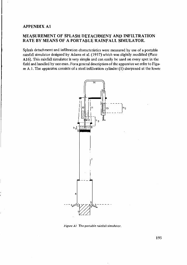
APPENDIX AI

MEASUREMENT OF SPLASH DETACHMENT AND INFILTRATIONRATE BY MEANS OF A PORTABLE RAINFALL SIMULATOR.

Splash detachment and infiltration characteristics were measured by use of a portablerainfall simulator designed by Adams et al. (1957) which was slightly modified (PlateA16). This rainfall simulator is very simple and can easily be used on every spot in thefield and handled by one man. For a general description of the apparatus we refer to Figu-re A.I. The apparatus consists of a steel infiltration cylinder (1) sharpened at the lower

13 h2

Figure A1 The portable rainfall simulator.

195

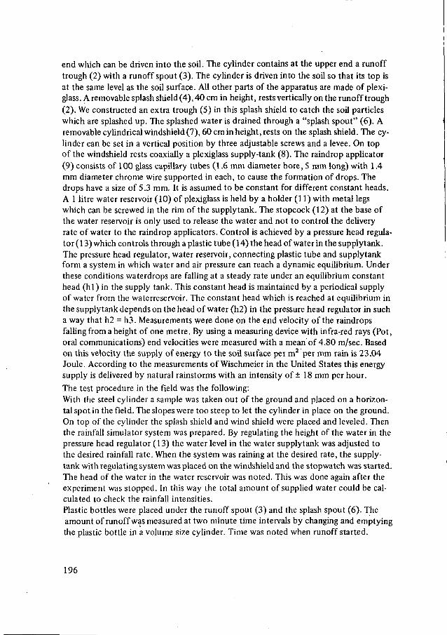
end which can be driven into the soil. The cylinder contains at the upper end a runofftrough (2) with a runoff spout (3). The cylinder is driven into the soil so that its top isat the same level as the soil surface. All other parts of the apparatus are made of plexi-glass. A removable splash shield (4), 40 cm in height, rests vertically on the runoff trough(2). We constructed an extra trough (5) in this splash shield to catch the soil particleswhich are splashed up. The splashed water is drained through a "splash spout" (6). Aremovable cylindrical windshield (7), 60 cm in height, rests on the splash shield. The cy-linder can be set in a vertical position by three adjustable screws and a levee. On topof the windshield rests coaxially a plexiglass supply-tank (8). The raindrop applicator(9) consists of 100 glass capillary tubes (1.6 mm diameter bore, 5 mm long) with 1.4mm diameter chrome wire supported in each, to cause the formation of drops. Thedrops have a size of 5.3 mm. It is assumed to be constant for different constant heads.A 1 litre water reservoir (10) of plexiglass is held by a holder (11) with metal legswhich can be screwed in the rim of the supplytank. The stopcock (12) at the base ofthe water reservoir is only used to release the water and not to control the deliveryrate of water to the raindrop applicators. Control is achieved by a pressure head regula-tor ( 13) which controls through a plastic tube (14) the head of water in the supplytank.The pressure head regulator, water reservoir, connecting plastic tube and supplytankform a system in which water and air pressure can reach a dynamic equilibrium. Underthese conditions waterdrops are falling at a steady rate under an equilibrium constanthead (hi) in the supply tank. This constant head is maintained by a periodical supplyof water from the waterreservoir. The constant head which is reached at equilibrium inthe supplytank depends on the head of water (h2) in the pressure head regulator in sucha way that h2 = h3. Measurements were done on the end velocity of the raindropsfalling from a height of one metre. By using a measuring device with infra-red rays (Pot,oral communications) end velocities were measured with a mean of 4.80 m/sec. Basedon this velocity the supply of energy to the soil surface per m2 per mm rain is 23.04Joule. According to the measurements of Wischmeier in the United States this energysupply is delivered by natural rainstorms with an intensity of ± 18 mm per hour.The test procedure in the field was the following:

With the steel cylinder a sample was taken out of the ground and placed on a horizon-tal spot in the field. The slopes were too steep to let the cylinder in place on the ground.On top of the cylinder the splash shield and wind shield were placed and leveled. Thenthe rainfall simulator system was prepared. By regulating the height of the water in thepressure head regulator (13) the water level in the water supplytank was adjusted tothe desired rainfall rate. When the system was raining at the desired rate, the supply-tank with regulating system was placed on the windshield and the stopwatch was started.The head of the water in the water reservoir was noted. This was done again after theexperiment was stopped. In this way the total amount of supplied water could be cal-culated to check the rainfall intensities.Plastic bottles were placed under the runoff spout (3) and the splash spout (6). Theamount of runoff was measured at two minute time intervals by changing and emptyingthe plastic bottle in a volume size cylinder. Time was noted when runoff started.

196

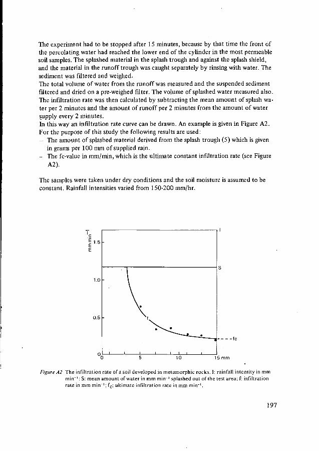
The experiment had to be stopped after 15 minutes, because by that time the front ofthe percolating water had reached the lower end of the cylinder in the most permeablesoil samples. The splashed material in the splash trough and against the splash shield,and the material in the runoff trough was caught separately by rinsing with water. Thesediment was filtered and weighed.-The total volume of water from the runoff was measured and the suspended sedimentfiltered and dried on a pre-weighed filter. The volume of splashed water measured also.The infiltration rate was then calculated by subtracting the mean amount of splash wa-ter per 2 minutes and the amount of runoff per 2 minutes from the amount of watersupply every 2 minutes.In this way an infiltration rate curve can be drawn. An example is given in Figure A2.For the purpose of this study the following results are used:— The amount of splashed material derived from the splash trough (5) which is given

in grams per 100 mm of supplied rain.- The fc-value in mm/min, which is the ultimate constant infiltration rate (see Figure

A2).

The samples were taken under dry conditions and the soil moisture is assumed to beconstant. Rainfall intensities varied from 150-200 mm/hr.

10

fc

1 5 mm

Figure A2 The infiltration rate of a soil developed in metamorphic rocks. I: rainfall intensity in mmmin"1; S: mean amount of water in mm min"1 splashed out of the test area; f: infiltrationrate in mm min"1; fc; ultimate infiltration rate in mm min"1.

197

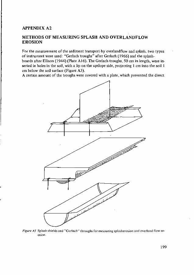
APPENDIX A2

METHODS OF MEASURING SPLASH AND OVERLANDFLOWEROSION

For the measurement of the sediment transport by overlandflow and splash, two typesof instrument were used: "Gerlach troughs" after Gerlach (1966) and the splash-boards after Ellison (1944) (Plate A16). The Gerlach troughs, 50 cm in length, were in-serted in holes in the soil, with a lip on the upslope side, projecting 1 cm into the soil 1cm below the soil surface (Figure A3).A certain amount of the troughs were covered with a plate, which prevented the direct

Figure A3 Splash shields and "Gerlach" throughs for measuring splasherosion and overland flow er-

199

input of rain (Figure A3). A provision was made for the overlandflow water to run fromthe trough in a plastic reservoir of 10 litres. With this equipment sediment transportedby overlandflow and the amount of runoff could be measured. A number of troughswere not covered by a plate and with the equipment sediment transported by overland-flow and splash could be measured. Protections were made to prevent the sedimentfrom splashing out of the troughs by using a canopy of gauze. To catch the materialwhich is transported by splash erosion alone, a splashboard 50 cm in width was usedwith on both sides troughs (Figure A3). This allows material coming from upslope anddownslope direction to be distinguished. A small canopy of gauze was placed over thetroughs to prevent material splashing out again. The troughs were not sunk into theground but were laid flat on the ground. A drain was made at the upper edge to preventoverlandflow sediment from coming into the troughs. The Gerlach troughs and splashtroughs are relatively small in regard to the great variation in transport of sedimentsbetween certain spots on a slope. The material also has a tendency to wash in at anaccelerated rate from the small vertical free faced exposed soil horizon especially inthe first periods.

Measurements were done in the spring of 1972 and 1973 during the rainy season. In1972 eight slopes were selected in landunits with a more or less natural character. Onthese slopes 4-6 Gerlach troughs were placed and 2-4 splash shields. In 1973 four slopeswere selected in the agricultural area. On these slopes measuring plots were constructed1 metre in width and 4 metres long. Rainfall data were assembled from the nearby sta-tions and from rain gauges placed near the plots.

200

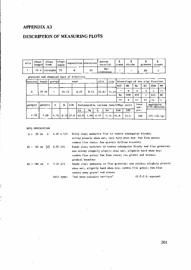
APPENDIX A3

DESCRIPTION OF MEASURING PLOTS

site

1

slopelength

45 m

slopeform

straight

slopeangle

25

exposition

N

elevation

65

parent

Ma-claystone

7.

-

Zshrubs

-

Z

80

Z

3

physical and chemical data of A-horizon

horizon

A

pH(H2O)

7.78

depth

10 cm

gravel

-

pH(KCl)

7.09

C

4.15

sand

14.12 6.47 8.73

silt

55.61 15.07

N

0.15

C/N

27.6

M/C

-

Be

tr

MM

X

M2M

X

Exchangeable cations (meq/100gr soil)

Ca

62.0

Mg

1.99

K

0.47

Na

0. 14

Sum

64.8

CEC

15.4

Bn

X

M3T

XX

SI

X

I

XX

basesat.pet.

100

CNM

x

G/C

XX

NM

tr

BK

X

aggregatestab.CMcCalla)

105.1/0.Igr

SOIL DESCRIPTION

0 - 20 cm

20 60 cm

60 - 180 cm C 7.5Y 4/3

A 2.5Y 4.5/2 Silty clay; moderate fine to coarse subangular blocky;

sticky plastic when wet, very hard when dry; few fine pores;

common fine roots; few gravel; diffuse boundary

'B) 2.5Y 5/4 Sandy clay; moderate to coarse subangular blocky and fine granular;

non sticky slightly plastic when wet, slightly hard when dry;

common fine pores; few fine roots; few gravel and stones;

gradual boundary

Sandy clay; moderate to fine granular; non sticky; slightly plastic

when wet, slightly hard when dry; common fine pores; few fine

roots; many gravel and stones

Soil type: "sol brun calcaire vertique" (C.P.C.S.-system)

201

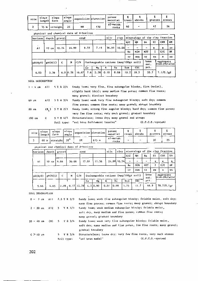
site

2

slopelength

35 m

slopeform

straight

slope

angle

25

exposition

NW

elevation

430

parentmaterial

sf-metam.rocks

Ztrees

90

Zshrubs

-

Zgrasses

42

Z

26

physical and chemical

horizon

AI

depth

10 cm

gravel

10.76

data 3t Ä-horizon

sand

24.99 9.59 7.19

silt

36.50

clay

10.00

pH(H2O)

6.05

pH(KCl)

5.36

C

6.0

N

0.36

C/N

16.67

Exchä

Ca

7.6

mineralogy

M/C

-

Be

tr

MM

M2M

XXX

ngeable cations (meq/IOOgr soil)

Mg

2.38

K

0. 10

Na

0.08

Sum

10.2

CEC

18.3

of the clay

Bn

-

M3T

tr

SI

X

I

XX

basesat.pet.

55.7

fraction

CNM

X

G/C

X

NM

tr

BK

XX

aggregatestab.(McCalla)

7.1/0.Igr

SOIL DESCRIPTION

1 - 4 cm All 5 Y R 2/4 Sandy loam; very fine, fine subangular blocky, firm (moist),

slighly hard (dry); many medium fine pores; common fine roots;

many gravel; distinct boundary

60 cm A12 5 Y R 3/4 Sandy loam; weak very fine subangular blocky; soft dry; common

fine pores; common fine roots; many gravel; abrupt boundary

80 cm (B ) 5 Y R 2/3 Sandy loam; strong fine angular blocky; hard dry; common fine pores;

very few fine roots; very much gravel; gradual boundary

100 cm C 5 Y R 4/3 Structureless; loose dry; many gravel and stones

Soil type: "sol brun faiblement lessive" (C.P.C.S.-system)

site

3

slopelength

60 m

slopeform

s t r a i gh t

slopeangle

28°

^position

SE 615 m

material

sf-metam.rocks

%trees

-

7.shrubs

-

%grasses

20

Zstones

25

physical and chemical

horizon

AI

depth

10 cm

gravel

4.64

data Df \-horizon

sand

30.66 17.81 11.36

silt

24 88

clay

10.56

pH(H20)

5.66

pH(KCl)

4.65

C

2.09

N

0. 17

C/N

12.29

miner

M/C

-

Be

tr

Exchangeable cations (meq/100gr

Ca

4.2

Mg

0.90

K

0.07

Na

0.08 5

Sum

.25

a logy

MM

-

M2M

XXX

soil)

CEC

11.7

of the clay fraction

Bn

-

M3T

tr

SI

X

I

XX

basesat.pet

44.9

CNM

X

G/C

X

NM

X

BK

XX

aggregatestab.(McCalla)

78.7/0.Igr

SOIL DESCRIPTION

0 - 2 cm All 7.5 Y R 2/3 Sandy loam; weak fine subangular blocky; friable moist, soft dry;

many fine proces; common fine roots; many gravel; abrupt boundary

2 - 20 cm A12 5 Y R 3/3 Sandy loam; weak medium subangular blocky; friable moist,

soft dry, many medium and fine pores; common fine roots;

many gravel; gradual boundary

20 - 40 cm (B) 5 Y R 3/4 Sandy loam; weak very fine subangular blocky; friable moist,

soft dry; many medium and fine pores, few fine roots; many gravel;

gradual boundary

C > 40 cm 5 Y R 3/4 Structureless; loose dry; very few fine roots, very much stones

Soil type: "sol brun modal" (C.P.C.S.-system)

202

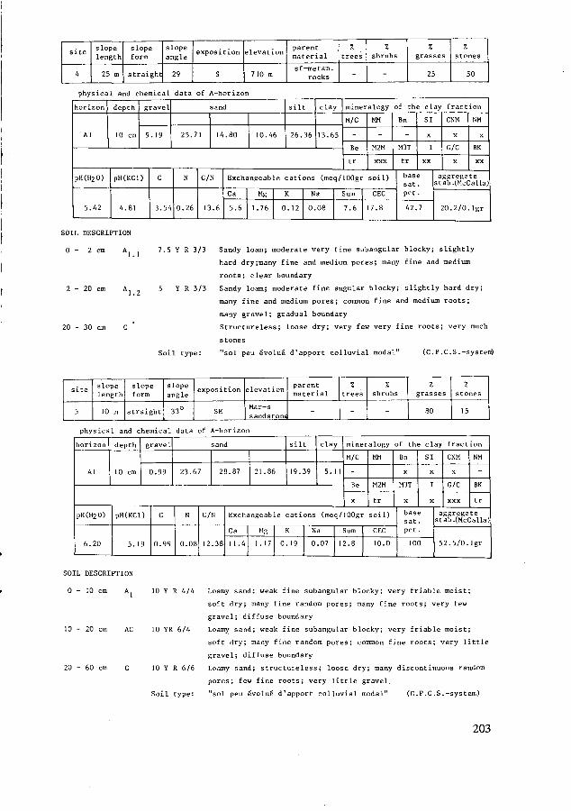
site

4

slopelength

25 m

slopeform

straight

slope

angle

29

exposition

S 710 m

parent

sf-metam.rocks

%

-

%shrubs

-

7.grasses

25

%

50

physical and chemical

horizon

Al

pH(H2O)

5.42

depth

10 cm

gravel

9.19

data it A-horizon

sand

25.71 14.80 10.46

silt

26.36

clay

13.65

pH(KCl)

4.81

C

3.54

N

0.26

C/N

13.6

Exchangeable cations

Ca

5.6

Mg

1.76

K

0.12

mineralogy

M/C

-

Be

tr

MM

-

M2M

XXX

(meq/100gr soil)

Na

0 08

Sum

7.6

CEC

17.8

of the clay fraction

Bn

-

M3T

tr

SI

X

I

XX

basesat.pet.

42.7

CNM

X

G/C

X

NM

X

BK

XX

aggregatestab.(McCalla)

20.2/0.lgr

SOIL DESCRIPTION

1.1

2 - 20 cm

7.5 Y R 3/3 Sandy loam; moderate very fine subangular blocky; slightly

hard dry;many fine and medium pores; many fine and medium

roots; clear boundary

5 Y R 3/3 Sandy loam; moderate fine angular blocky; slightly hard dry;

many fine and medium pores; common fine and medium roots;

many gravel; gradual boundary

Structureless; loose dry; very few very fine roots; very much

stones

Soil type: "sol peu évolué d'apport colluvial modal" (C.P.C.S.-system)

site

5

slopelength

10 m

slopeform

straight

slopeangle

33°

exposition

SE

élevât ion

Mar-ssands tont

parentmaterial

-

7.trees

-

7.shrubs

-

%grasses

80

%stones

15

physical and chemical

horizon

Al

depth

10 cm

gravel

0.99

data it ^-horizon

sand

23.67 28.87 21.86

silt

19. S9

clay

5.11

pH(H2O)

6.20

pH(KCl)

5. 19

C

0.99

N

0.08

C/N

12.38

Exchangeable

Ca

1 1.4

Mg

1.17 0

mineralogy

M/C

-

Be

X

MM

-

M2M

tr

cations (meq/lOOgr soil)

K

19

Na

0.07

Sum

12.8

CEC

10.0

of the clay fraction

Bn

X

M3T

X

SI

X

I

X

basesat.pet.

100

CNM

X

G/C

XXX

NM

-

BK

tr

aggregatestab.(McCalla)

52.5/0.lgr

SOIL DESCRIPTION

0 - 10 cm

10 - 20 cm

20 - 60 cm

10 Y R 4/4 Loamy sand; weak fine subangular blocky; very friable moist;

soft dry; many fine random pores ; many fine roots ; very few

gravel; diffuse boundary

10 YR 6/4 Loamy sand; weak fine subangular blocky; very friable moist;

soft dry ; many fine random pores ; common fine roots ; very little

gravel; diffuse boundary

10 Y R 6/6 Loamy sand; structureless; loose dry; many discontinuous random

pores ; few fine roots ; very little gravel.

Soil type: "sol peu évolué d'apport colluvial modal" (C.P.C.S.-system)

203

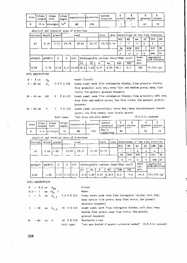
sice

6

slopelength

15 m

slopeform

straight

slopeangle

34°

exposition

NE

elev.it ion

430

parentmaterial

%trees

-

%

shrubs

-

%grasses

45

%stones

15

physical and ehe

horizon

ÂI

pH(H2O)

8.00

6 cm

meal

gravel

3.12

data ot A-horizori

sand

25.78 28.62 22.17

silt

13 75

clay

6.54

pH(KCl)

7.70

C

1.55

N

0. 1 1

C/N

14.09

Exchangeable

Ca

36.5

MS

1.28

cations

K

0 31

mineralogy

M/C

-

Be

x

MM

-

M2M

tr

(meq/100gr soil)

Na

0 04

Sum

38. 1

CEC

9.7

af the clay

Bn

X

M3T

X

SI

X

I

X

basesat.pet.

100

fraction

CNM

X

G/C

XXX

NM

-

BK

tr

aggregatestab.(McCalla)

37.3/0.Igr

SOIL DESCRIPTION

0 - 3 cm A

3 - 20 cm A

20 - A0 cm (B)

A0 - 60 cm

moder (local)

7.5 Y R 3/6 Loamy sand; weak fine subangular blocky; fine granular blocky;

fine granular ; soft dry ; many fine and medium pores ; many fine

roots; few gravel; gradual boundary

5 Y R A/3 Loamy sand; weak fine subangular blocky; fine granular; soft dry;

many fine and medium pores; few fine roots; few gravel; gradual

boundary

5 Y R 5/3 Loamy sand; structureless; loose dry; many discontinuous random

pores; few fine roots; very little gravel

Soil type: "sol brun calcaire modal" (C.P.C.S.-system)

site

8

slopelength

15 m

slopeform

straight

slopeangle

32

exposit ion

NW

elevat ion

430

parent

Mar-ssandstone

%trees

80

%shrubs

-

7.grasses

10

X

13

physical and chemical

horizon

Al

depth

5 cm

gravel

4.05

data jt

33.98

\-horizon

sand

28.51 1 2.50

silt

15.51

clay

pH(H2O)

5.63

pH(KCl)

4.86

C

1 .53

N

0. 10

C/N

15 3

Exchangeable

Ca

4.3

Mg

1.69

cations

K

0 07

mineralogy

M/C

-

Be

x

MM

-

M2M

tr

(meq/100gr soil)

Na

0.013

Sum

6.2

CEC

9.6

of the clay fraction

Bn

X

M3T

X

SI

X

I

X

basesat.pet.

64.6

CNM

X

G/C

XXX

NM

-

BK

tr

aggregatestab.(McCalla)

103.4/0 •Igr

SOIL DESCRIPTION

0 - 0.5 cm A

0 . 5 - 1

1 - 3 cm

3 - 30 cm

30 - 60 cm

Litter

Moder

7.5 Y R 3/3 Loamy sand; weak very fine subangular blocky; soft dry;

many medium fine pores; many fine roots; few gravel;

distinct boundary

10 Y R 4/4 Loamy sand; weak fine subangular blocky; soft dry; many

medium fine pores; many fine roots; few gravel;

gradual boundary

10 Y R 5/8 Weathered slope

Soil type: "sol peu évolué d'apport colluvial modal" (C.P.C.S.-system)

204

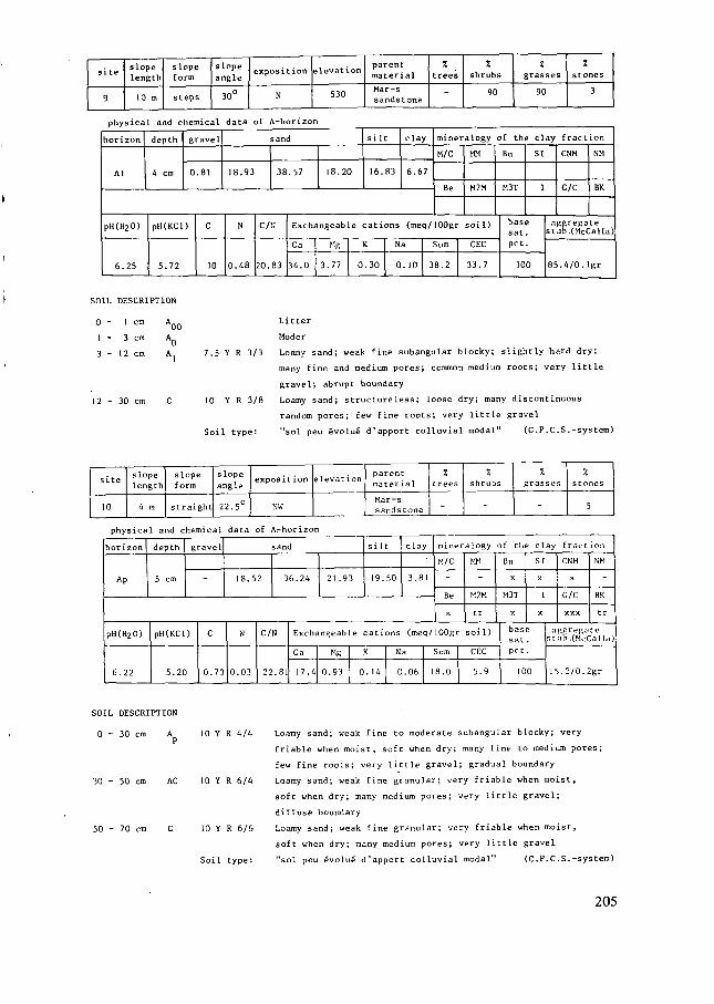
site

9

slopelength

10 m

slopeform

steps

slope

angle

30°

exposition

N

elevation

530

parentmaterial

Mar-ssandstone

7.trees

-

%shrubs

90

7.grasses

90

Zstones

3

physical and chemical

horizon

AI

depth

4 cm

gravel

0.81

data Dt /\-horizor

sand

18.93 38.57 18.20

silt

16.83

clay

6.67

pH(H2O)

6.25

pH(KCl)

5.72

C

10

N

0.48

C/N

20.83

Exclu

Ca

34.0

mineralogy

M/C

Be

MM

M2M

ngeable cations (meq/IOOgr soil)

Mg

3.77

K

0.30

Na

0. 10

I Sum

38.2

CEC

33.7

of the clay fraction

Bn

M3T

SI

I

basesat.pet.

100

CNM

G/C

NM

BK

aggregatestab.(McCalla)

85.4/0.Igr

SOIL DESCRIPTION

0 - 1 cm

1 - 3 cm

3 - 12 cm

12 - 30 cm

"00Litter

Moder

7.5 Y R 3/3 Loamy sand; weak fine subangular blocky; slightly hard dry;

many fine and medium pores; common medium roots; very little

gravel; abrupt boundary

10 Y R 3/8 Loamy sand; structureless; loose dry; many discontinuous

random pores; few fine roots; very little gravel

Soil type: "sol peu évolué d'apport colluvial modal" (C.P.C.S.-system)

site

10

slopelength

4 m

slopeform

straight

slopeangle

22.5°

expos it ion

NW

elevationparentmaterial

Mar-ssandstone

%trees

-

%shrubs

-

7.grasses

-

%stones

5

physical and ehe

horizon

Ap

depth

5 cm

nical

gravel

-

data of hrhor ïzor

sand

18.52 36.24 21 .93

silt

19.50

clay

3.81

pH(H2O)

6.22

pH(KCl)

5.20

C

0.73

N

0.03

C/N

22.81

minera logy

M/C

-

Be

X

MM

-

M2M

tr

Exchangeable cations (meq/100gr soil)

Ca

17.4

Mg

0.93

K

0. 14

Na

0.06

Sum

18.0

CEC

5.9

of the clay

Bn

X

H3T

X

SI

X

I

X

basesat.pet.

100

f raition

CNM

X

G/C

XXX

NM

-

BK

tr

aggregate•il.-ib.CMcCallu)

15 .2/0.2gr

SOIL DESCRIPTION

0 ~ 30 cm A

30 - 50 cm AC

50 - 70 cm C

10 Y R 4/4 Loamy sand; weak fine to moderate subangular blocky; very

friable when moist, soft when dry; many fine to medium pores;

few fine roots; very little gravel; gradual boundary

10 Y R 6/4 Loamy sand; weak fine granular; very friable when moist,

soft when dry; many medium pores; very little gravel;

diffuse boundary

10 Y R 6/6 Loamy sand; weak fine granular; very friable when moist,

soft when dry; many medium pores; very little gravel

Soil type: "sol peu évolué d'apport colluvial modal" (C.P.C.S.-system)

205

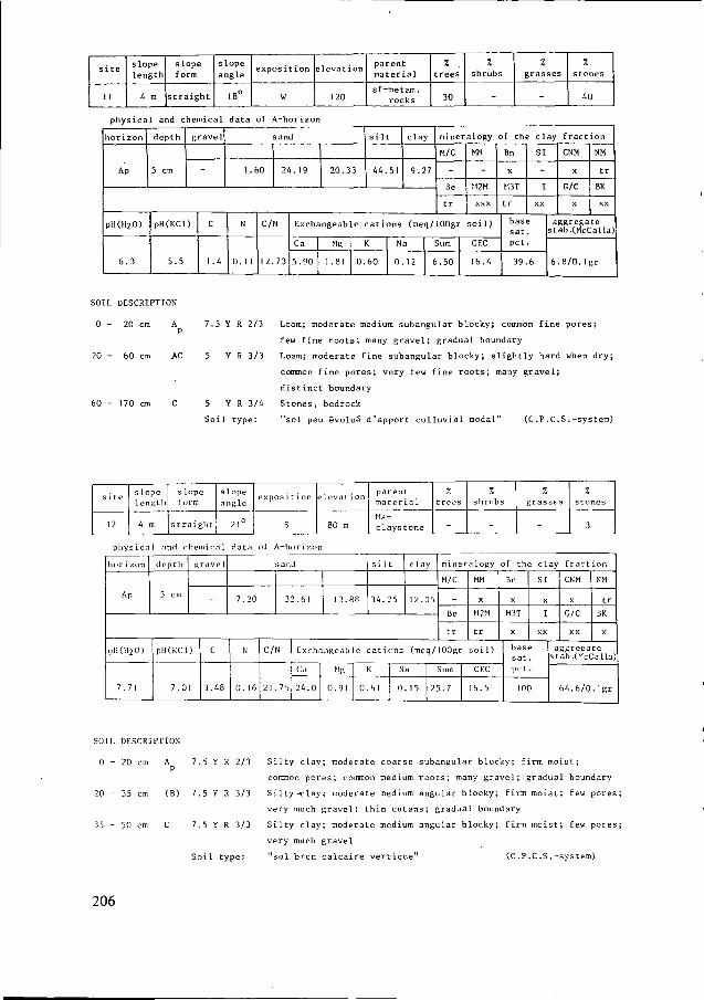
site

1 1

slopelength

k m

slopeform

straight

slopeangle

18°

expos it ion

W

elev.it ion

120

parentmaterial

sf-metam.rocks

Ztrees

30

%shrubs

%grasses

-

%stones

40

physical and chemical

horizon

Ap

pH(H2O)

6.3

depth

5 cm

gravel

-

data Dt k-horlzon

sand

1.60 24. 19 20.33

silt

44. 51

clay

9.27

pH(KCl)

5.5

C

1 .4

N

0. 1 1

C/N

12.73

Exchangeable

Ca

5.90

MR

1.81 0.

mineralogy

M/C

-

Be

tr

MM

-

M2M

XXX

cations (meq/100gr soil)

K

60

Na

0. 12

Sum

6.50

CEC

16.4

of the clay

Bn

X

M3T

tr

SI

-

I

XX

basesat.pet.

39.6

fract ion

CNM

X

G/C

X

NM

tr

BK

XX

aggregatestab.(McCalla)

6 8/0.Igr

SOIL DESCRIPTION

0 - 20 cm

20 - 60 cm

60 - 170 cm

P

AC

7.5 Y R 2/3 Loam; moderate medium subangular blocky; common fine pores;

few fine roots; many gravel; gradual boundary

5 Y R 3/3 Loam; moderate fine subangular blocky; slightly hard when dry;

common fine pores; very few fine roots; many gravel;

distinct boundary

5 Y R 3/4 Stones, bedrock

Soil type: "sol peu évolué d'apport colluvial modal" (C.P.C.S.-system)

site

12

s lopelength

k m

slopeform

straight

slopeangle

21°

expos it ion

S

elev.-it ion

80 m

parentmaterial

lla-claystone

7.trees

-

7.shrubs

-

7.grasses

-

7.stones

3

physica1 and c

horizon

Ap

pll(H2O)

7.71

depth

5 cm

ïemical

gravel

-

pll(KCl)

7.01

C

3.48

data Dt \-h >rizon

sand

7.20

N

0. 16

32.61 13.88

sil t

34.25

c lay

12.05

C/N

21.75

Exchangeable

Ca

24.0

MR |

0.91 0

= ati

K

61

minera logy

M/C

-

Be

tr

MM

X

M2M

tr

ins (meq/100gr soil)

Na

0. 15

Sum

25.7

CFX

16.5

of the clay fraction

Bn

X

M3T

X

SI

X

I

XX

basesat.pet.

100

CNM

X

C/C

XX

NM

tr

BK

X

aggregatestab.(McCalla)

64.6/0.Igr

SOIL DESCRIPTION

0 - 2 0 cm A 7.5Y R 2/3 Silty clay; moderate coarse subangular blocky; firm moist ;

common pores; common medium roots; many gravel; gradual boundary

20 - 35 cm (B) 7.5 Y R 3/3 Silty-»clay; moderate medium angular blocky; firm moist; few pores;

very much gravel ; thin cutans ; gradual boundary

35 - 50 cm C 7.5 Y R 3/3 Silty clay; moderate medium angular blocky; firm moist; few pores;

very much gravel

Soil type: "sol brun calcaire vertique" (C.P.C.S.-system)

206

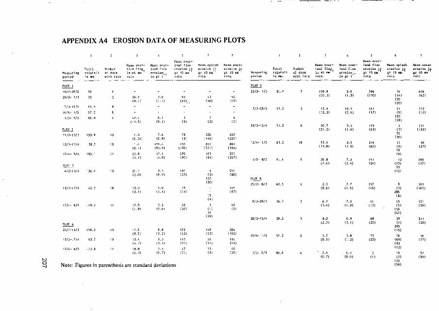
APPENDIX A4 EROSION DATA OF MEASURING PLOTS

Total NumberMeasuring rainfall of daysperiod in nun. wich rain

Mean over-land flow,in ml mmrain

Mean over-land flow

land flo1

erosion_in gr 1

Mean splash Mean water.

on ID erosion ingr 10 mm""1

erosion IDgr 10 mm

19/2-29/2

29/2- 7/3

7/3-16/4

16/4- 1/5

1/5- 8/5

PLOT 2

21/2-13/3

13/3-17/4

17-4- 5/6

PLOT 3

4/2-13/3

13/3-17/4

17/4- 6/5

58

35

65.5

57.2

89.8

150.9

38.5

105.1

156.6

42.3

110.2

6

2

8

8

4

10

10

11

10

10

11

PLOT 4

24/2-13/3 158.2

13/3-17/4 43.7

17/4- 6/5 112.8

10

10

34.9(8.7)

47.4(12.5)

1.0(0.24)

1 .4(0.7)

22.8(9.1)

21.7(2.0)

13.0(2.1)

17.9(1.8)

2.6(1.1)

0.3(0.1)

7.6(0.8)

109.4(83.9)

12.1(4.0)

8.3(0.9)

6.0(2.1)

3.5(0.6)

17.5(8.5)

13.4(4.7)

9.8(3.2)

8.3(3.3)

2.5(0.7)

92(42)

13(8)

78(8)

270(80)

78(25)

62(20)

172(62)

1 12(51)

43(40)

320(146)

812(321)

163(64) .

(2)137(50)

19(4)

3(I)36(29)

149(53)

26

(II)

33(8)

50(48)

6(2)

437(229)

395(257)

250(88)

146(87)

45(9)

304(192)

104(49)

«0(35)

Measuringperiod

PLOT 5

25/2- 7/3

28/3-15/4

PLOT 6

25/2- 8/3

1/5- 8/5

1 2 3 A 5 6 7

Mean over-Mean over- Mean over- land flow Mean splash Mean water

Total Number land flow land flow erosion in erosion in erosion inrainfall of days in ml mm erosion , gr 10 mm gr 10 mm gr 10 ranin nun. with rain rain in gr 1 rain rain rain

toO

oNote: Figures in parenthesis are standard deviations

109.9(33.3)

43.4(12.3)

50.7(21.2)

55.4(13.8)

20.8(7.4)

2.0(0.6)

6.2(3.6)

8.0(2.3)

1.7(0.5)

2.4(0.7)

3.6(1.0)

10.3(2.4)

3.5(1.6)

3.9(1.8)

7.3(2.4)

7.7(1.5)

8.0(1.9)

0.9(3.1)

3.8(1.2)

0.1(0.0)

396(170)

447(57)

179(62)

214(65)

151(24)

157(49)

46(13)

68(25)

73(20)

2

(1)

16(14)120(20)

21(9)100(38)

9(3)50(30)

12(8)70(9)

12(10)70(12)

9(3)

286(8)

15(5)156(42)

39(1)

295(15)

76(69)183(12)

15(2)122(56)

416(63)

223(14)

231(152)

50(27)

285(37)

353(162)

15!(59)

311(20)

36(17)

57(50)

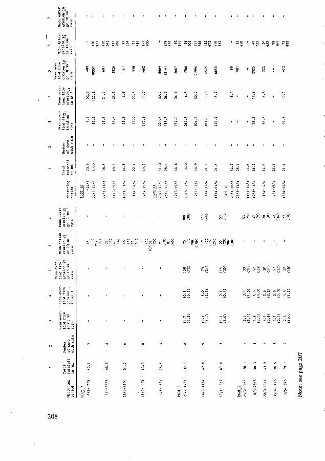
c « — e

I s s, s

ift

il1»c -g 'S c

5 s * S

«Ï i

g K 5

7 7 7 , 7 7 "5 S i S - 5 S

7 7 7 7 7 7 7 -

CM CM — — — a .

7 7 7 T T 7 7O »û — O> — «a- u"

i " S! ï S ï

i 8 - ' i

c -a m — c

I I S »'S

E * .5 2

T — r- ^ . o —

tu

o

208

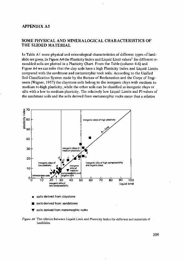
APPENDIX A5

SOME PHYSICAL AND MINERALOGICAL CHARACTERISTICS OFTHE SLIDED MATERIAL

In Table Al some physical and mineralogical characteristics of different types of land-slide are given. In Figure A4 the Plasticity Index and Liquid limit values1 for different re-moulded soils are plotted in a Plasticity Chart. From the Table (column 4-6) andFigure A4 we can infer that the clay soils have a high Plasticity Index and Liquid Limitscompared with the sandstone and metamorphic rock soils. According to the UnifiedSoil Classification System made by the Bureau of Reclamation and the Corps of Engi-neers (Wagner, 1957) the claystone soils belong to the inorganic clays with medium tomedium to-high plasticity, while the other soils can be classified as inorganic clays orsilts with a low to medium plasticity. The relatively low Liquid Limits and Pi-values ofthe sandstone soils and the soils derived from metamorphic rocks mean that a relative

g 70

•f 60

40

30

20

10

0

inorganic days oflow plasticity

inorganic days ofmedium plastidty

inorganicsilts ofmedium

compressibility ancorganic silts

inorganic days of high plastidty

inorganic silts of high compressibilityand organic days

10 20 I 30 40inorganic silts oflow compressibility

50 60 70 80 90 100liquid limit

• soils derived from claystone

• soils derived from sandstones

T soils derived from metamorphic rocks

Figure A4 The relation between Liquid Limit and Plasticity Index for different soil materials oflandslides.

209

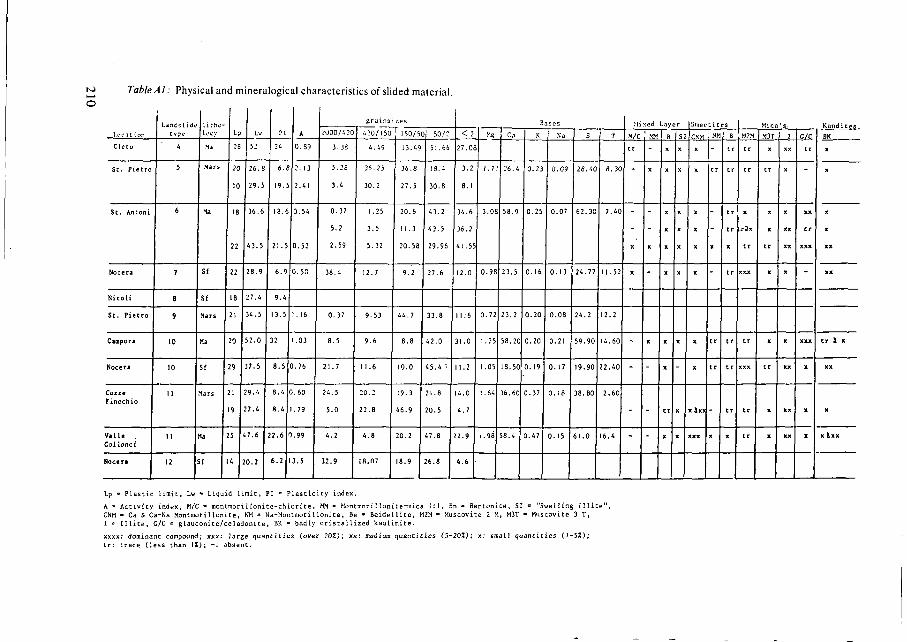
Table Al : Physical and mineralogical characteristics of slided material.

tcc.it ion

Clcto

St. Pietro

St. Antoni

Nocera

Nicoli

St. Pietro

Campora

Nocera

CozzeFinochio

Valle .Collonci

Nocera

Landslidtype

4

5

6

7

S

9

10

10

II

II

12

Litho

Ma

Mars

Ma

Sf

Sf

Mars

Ma

Sf

ars

a

f

L

28

20

10

18

22

22

8

21

0

9

1

9

5

i

Lu

52

26.8

29.5

36.6

43.5

28.9

7.4

4.5

2.0

7.5

9.4

7.4

7.6

0.2

PI

24

6.

19.

18.

21.

6.9

9.4

13.5

32

8.5

8.4

S.4

2.6

6.2

A

0.S9

2.13

2.41

0.54

0.52

0.53

.16

.03

.76

.60

79

99

3.5

2000/120

3.38

5.28

3.4

0.32

5.2

2.59

38.4

0.37

8.5

21.7

24.5

5.0

4.2

32.9

grains

420/150

4.49

36.25

30.2

1.25

3.5

5.32

12.7

9.53

9.6

11.6

20.2

22.8

4.8

1(1.07

zes

150/5

13.49

36.8

27.5

20.6

11.3

20.58

9.2

44.7

8.8

10.0

19.3

46.9

70.2

18.9

50/:

51.66

18.4

30.8

43.2

43.5

29.96

27.6

33.8

42.0

45.4 r-

21.8

70.5

47.8

6.8

< 2

27.0

3.2

8.1

34.6

36.2

41.5

12.0

II.'6

31.0

1.2

4.0

4.7

2.9

4.6

Mg

1.7

3.0

0.98

0.72

1.25

1.05

1.64

1.98

Ca

26.4

58.9

23.5

23.2

58.20

8.50

6.60

8.4

B

K

0.2

0.25

0.16

0.20

0.20

0.19

0.37

0.47

ases

Na

0.09

0.07

0.13

0.08

0.21

0.17

0.18

0.15

S

28.40

62.30

24.77

24.2

59.90

19.90

38.80

61.0

T

fl.3

7.40

11.52

12.2

14.60

22.40

2.60

6.4

M/c MM

tr

-

x

-

-

-

-

-

X

-

-

-

-

Lav

R

x

X

X

X

X

tr

S

X

X

X

X

-

X

|S

CNM

X

X

X

X

X

xâxx

NM

Cr

-

-

tr

-

B

tr

cr

tr

cr

tr

M2M

tr

X

XXX

XXX

Mica

M3T

tr

X

X

X

tr

I

X

X

XX

XX

X

XX

C/C

XX

tr

XXX

-

X

BK

X

X

X

XX

XX

XX

X

Lp • Plastic limit, Lw • Liquid limit, PI » Plasticity index.

A - Activity index, M/C « montmorillonite-chlorite, MM = Montmorillonite-mica 1:1, Bn - Bentonite, SI » "Swelling illite",CNM - Ca & Ca-Na Monttnori 1 lonite, NM a Na-Montmoril lonite, Be • Beidellite, M2M = Muscovite 2 M, M3T «• Muscovite 3 T,I «= Illîte, G/C = glauconite/celadonite, BK • badly cristallized kaolinite.

xxxx: dominant compound; xxx: large quantities (over 20£); xx : medium quantities (5-20%); x: small quantities (1-5Z);

tr: trace (less than iZ); -: absent•

small increase in water content between the Plastic limit and the Liquid limit, leads toa rapid decrease in strength. During high intensive rainstorms the Liquid limit may be re-latively easily reached and the material changes in a liquid mud, with very low to zeroyield strength. In this case wet mud flows with a fairly high flow velocity may develop.The claystone soils need a higher water content to reach such a liquid state, but belowthis ultimate value there lies a larger range of moisture content values between the Li-quid Limit and the Plastic Limit (IP index) in which the clay has a viscous component.If the yield strength (see Figure 6.1) of the clay is surpassed under these conditions thematerial is going to move as a relatively slow viscous flow. It is interesting to note inFigure A4 that the flow of Valle Collonci (a in Figure A4) (see page 166) shows a highPlasticity Index, which means that this flow has the capacity to move as a slow viscousflow at lower slope angles. The same can be said for the fossile flow near Cleto (b inFigure A4) (see page 135) and in a lesser way for the flow of St. Antonio (c) (see page140) which is mapped as a more rapid debris flow, developing at a steeper slope angle.The flow developed after failure in the rockslide near S. Pietro (d) (see page 135) has rela-tively low Liquid Limits and therefore has the character of a rapid mud flow. It is in-teresting to note that the landslide complex of Cozze Finochio (e) (see page 170)developed in sandstone has also low Liquid Limits. Therefore it can be discussed whetherin this slow moving sandy mass there exist slow viscous flows. Probably the mass in the up-per end moves as a sliding mass while in the wet tongue area rapid mud flows are present.The Pi-index is determined by the activity of the clay minerals which can be defined asthe capacity to atttract a certain amount of water at their surface. This depends on thetype of clayminerals and the type of cat-ions attracted to the surface. The activity of theclay in the soil can be expressed as the ratio between the Pi-index and the percentageof clay fraction (> 2 n) in the soil (see Table Al column 7). According to Grimm(1962) Na+ montmorillonites have activity values varying from 3-7.Ca2+ montmoril-lonites from 1.2 - 1.3. Mites from 0.3 - 0.6, kaolinite poorly christalised from 0.3 - 0.4and kaolinite well christalized> 0.1. The Table shows that the activity of the soils mayreach above 1.2 which points to the presence of Ca-montmorillonite or Na-montmoril-lonite. The clay mineral analyses2 show that Ca2 +-montmorillonites dominate in allsamples over Na+-montmorillonite. The Table also shows that a dominant content ofillite and/or kaolinite lowers the activity of the clays below 1.

NOTES

1 Foi the determination of the Atterberg limits see Sowers (1965, pp. 391-399).

2 The current clay mineralogical identification method in the laboratory of the Department ofPhysical Geography of the University of Utrecht has been described by Romein (in prep.). Ananalysis of the clay content of the samples in given by Romein (1980).

211

APPENDIX A6

LABORATORY ANALYSIS

1 Particle size analysis

Determinations were performed on the fine earth of all samples by sieving and the pipettemethod. Air dry samples were gently crushed and sieved through a 2 mm sieve. The fineearth fraction has thereupon been treated with H2O2 to remove organic carbon. Aggre-gation by ferric oxides was broken up by boiling the samples with 1 N HC1. A sodium-pyrophosphate - sodium-carbonate mixture has been used as a peptizing agent.

2 pH-H2OandpH-KCI

The soil is shaken with water or 1 N KC1 during 2 hours. In the suspension the pH ismeasured with a glass electrode pH-meter.

3 Exchangeable bases and cation exchange capacity

The soil is mixed with purified sand, put into percolation tubes and subsequently treatedas follows:— Percolation with water/96% alcohol (1 : 1) to leach water-soluble salts.— Percolation with 1 N NH4-acetate/96% alcohol (1 : 1) pH 8.2, determination of Ca,

K and Na in the percolate with the flame-photometer and Mg by atomic absorption.The results expressed as me/100 gram of oven-dry soil give the content of exchange-able Ca, Mg, K and Na respectively.

— Percolation with 1 N Na-acetate pH 8.2 to saturate the soil complex with sodium.— Percolation with pure 96% alcohol to leach excess Na-acetate.— Percolation with 1 NNH4-acetate pH 8.2 to exchange the absorbed Na and determi-

nation of sodium with the flame-photometer.The results in me/100 gram of oven-dry soil give the total exchange capacity, or C.E.C.

4 %C (Walkley & Black)

The soil is oxidized with potassium-di-chromate and sulphuric acid without applicationof external heat. The amount of potassium-di-chromate used is determined by titrationwith ferrous sulphate.According to Walkley & Black, working with American soils, only 77% of the carbonin the organic matter is oxidized. Therefore, in calculating the %C of the oven drysoil the 77% recovery factor is used. The %C gives the content of carbon present in thereadily oxidizable organic matter, which is assumed to be well humified.

213

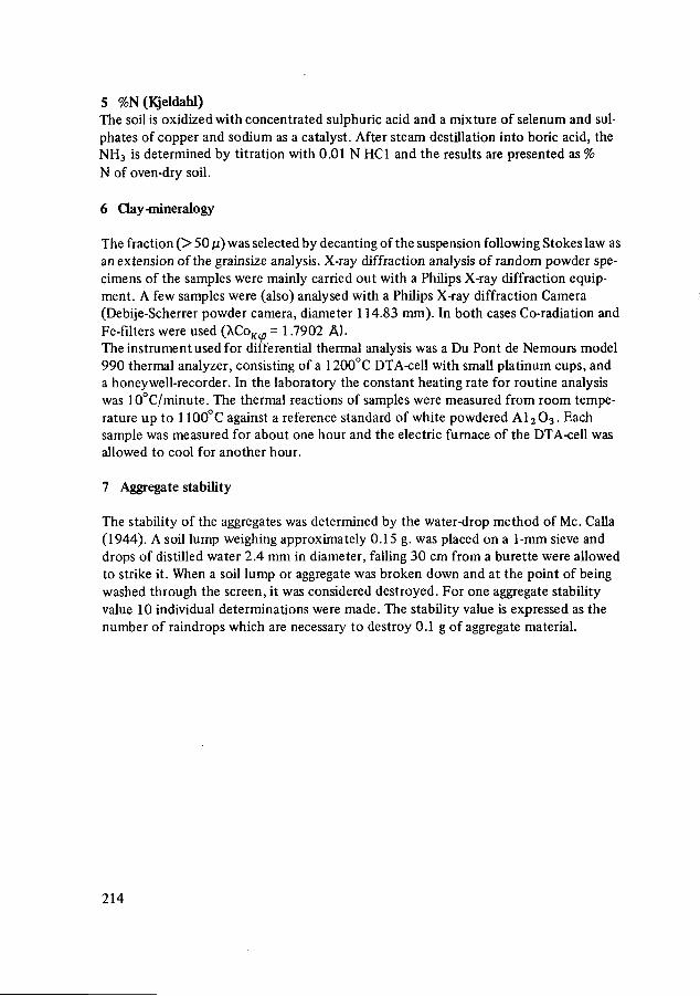
5 %N(Kjeldahl)The soil is oxidized with concentrated sulphuric acid and a mixture of selenum and sul-phates of copper and sodium as a catalyst. After steam destination into boric acid, theNH3 is determined by titration with 0.01 N HC1 and the results are presented as %N of oven-dry soil.

6 Clay-mineralogy

The fraction (> 50 M) was selected by decanting of the suspension following Stokes law asan extension of the grainsize analysis. X-ray diffraction analysis of random powder spe-cimens of the samples were mainly carried out with a Philips X-ray diffraction equip-ment. A few samples were (also) analysed with a Philips X-ray diffraction Camera(Debije-Scherrer powder camera, diameter 114.83 mm). In both cases Co-radiation andFe-filters were used (~KCoKif) = 1.7902 Ä).The instrument used for differential thermal analysis was a Du Pont de Nemours model990 thermal analyzer, consisting of a 1200°C DTA-cell with small platinum cups, anda honey well-recorder. In the laboratory the constant heating rate for routine analysiswas 10°C/minute. The thermal reactions of samples were measured from room tempe-rature up to 1100°C against a reference standard of white powdered AI2O3. Eachsample was measured for about one hour and the electric furnace of the DTA-cell wasallowed to cool for another hour.

7 Aggregate stability

The stability of the aggregates was determined by the water-drop method of Me. Calla(1944). A soil lump weighing approximately 0.15 g. was placed on a 1-mm sieve anddrops of distilled water 2.4 mm in diameter, falling 30 cm from a burette were allowedto strike it. When a soil lump or aggregate was broken down and at the point of beingwashed through the screen, it was considered destroyed. For one aggregate stabilityvalue 10 individual determinations were made. The stability value is expressed as thenumber of raindrops which are necessary to destroy 0.1 g of aggregate material.

214

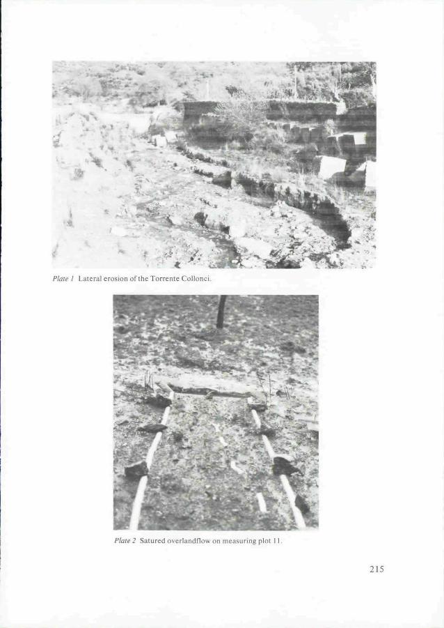
/ Lateral erosion of the Torrente Collonci.

Satured overlandfiow on measuring plot 11.

215

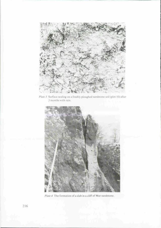
J Surface sealing on a freshlv ploughed sandstone soil (plot 10) after3 months with rain.

Plate 4 The formation of a slab in a cliff of Mar-sandstone.

216

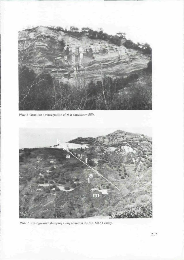
Plate 5 Granular désintégration of Mar-sandstone cliffs.

Plaie 7 Retrogressive slumping along a fault in the Ste. Maria valley.

217

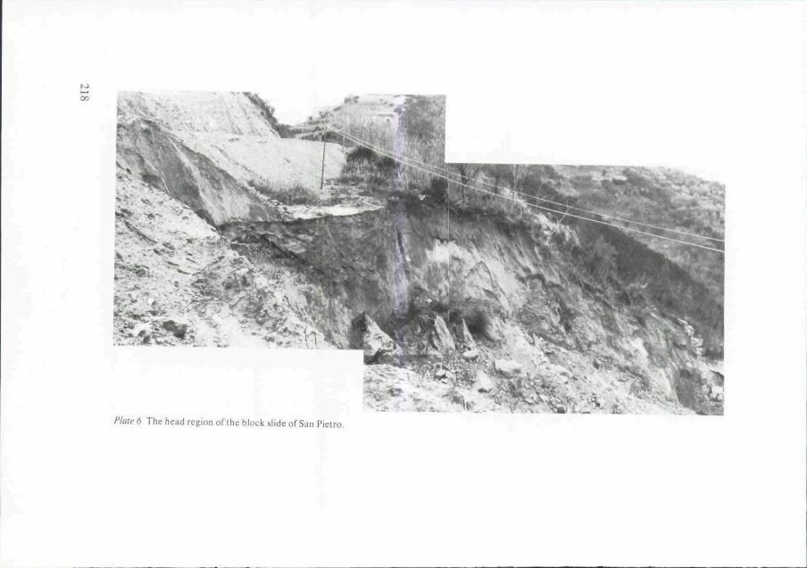
' - J * ":' i

tfi16 The bead region of the block slide of San Pietro.

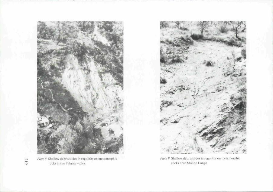
.11

to Plate 8 Shallow debris slides in regoliths on melamorphic

\O rocks in the Fabrica valley.

Plate 9 Shallow debris slides in regoliths on metamorphic

rocks near Molino Longo

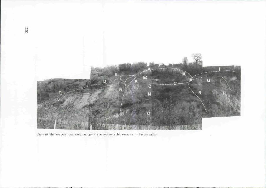
(Otoo

/ ' l u w l u M i . L i k m l u i a i i u n . i l . s l i d e s i n [ c g o l i t h s o n m e t a m o r p h i c r o c k ; - i n i l i c S ; i < u i i

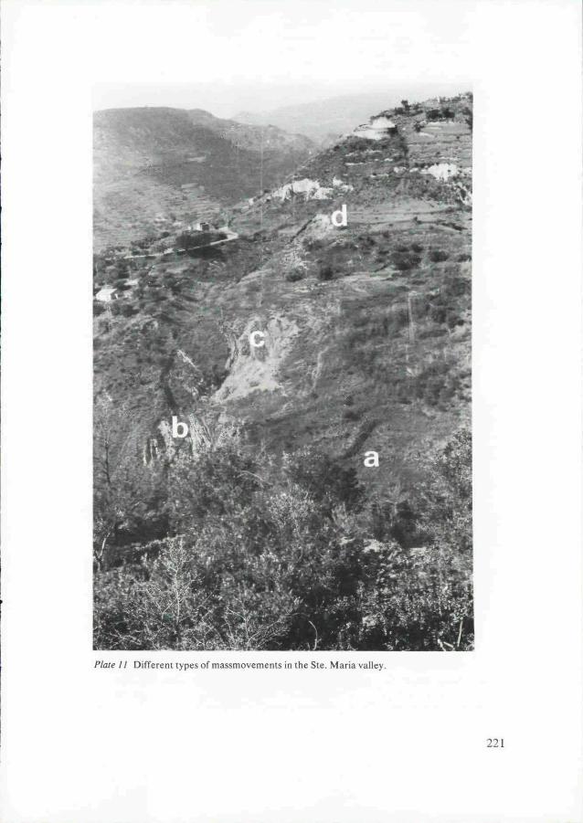
Plaie 11 Different types of massmovements in the Ste. Maria valley.

221

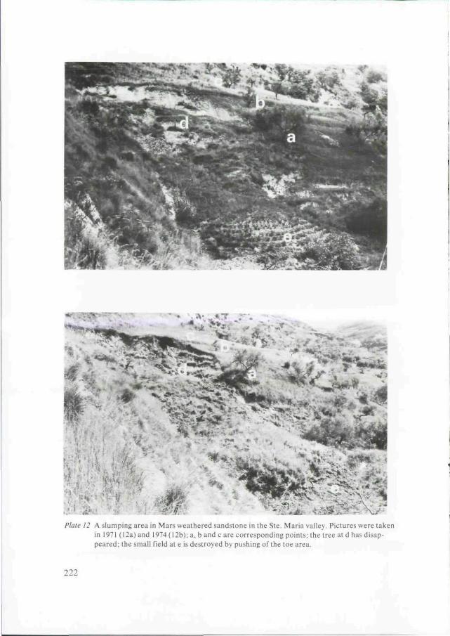
Plate 12 A slumping area in Mars weathered sandstone in the Ste. Maria valley. Pictures were takenin 1971 (12a) and 1974 (12b); a, b and c are corresponding points; the tree at d has disap-peared; the small field at e is destroyed by pushing of the toe area.

222

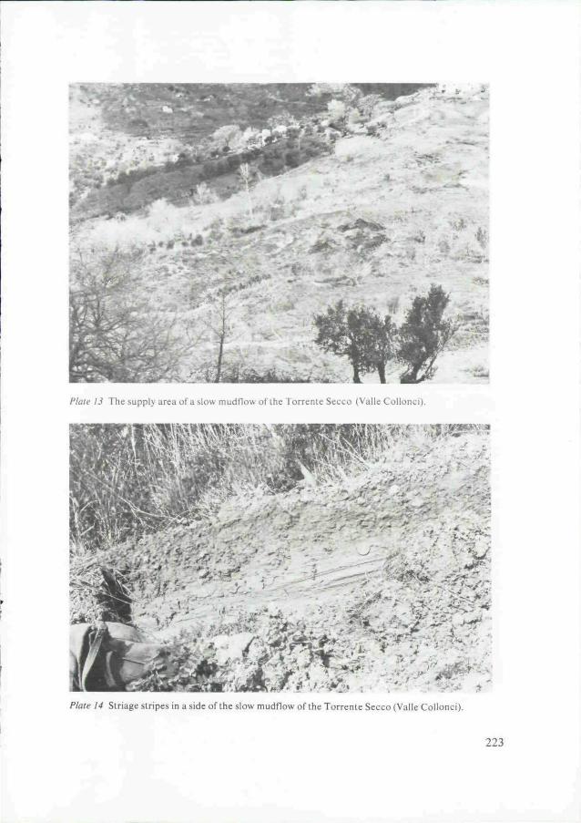
The supply area of a slow mudflow of ihe Torrente Secco (Valle Collonci).

Plate 14 Striage stripes in a side of the slow mudflow of ihe Torrente Secco (Valle Collonci).

223

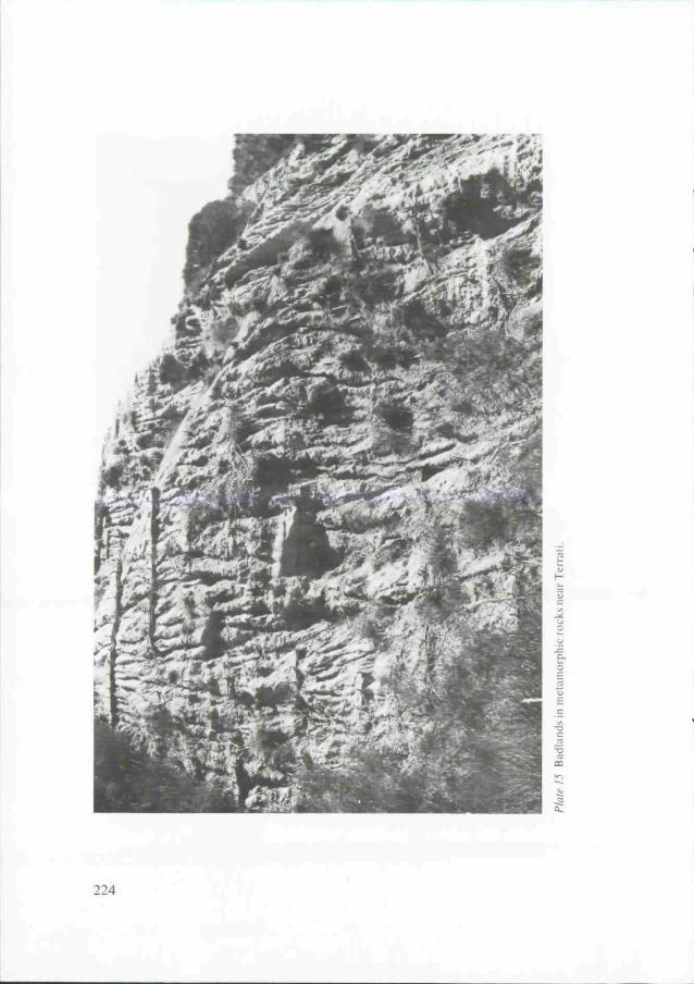
224

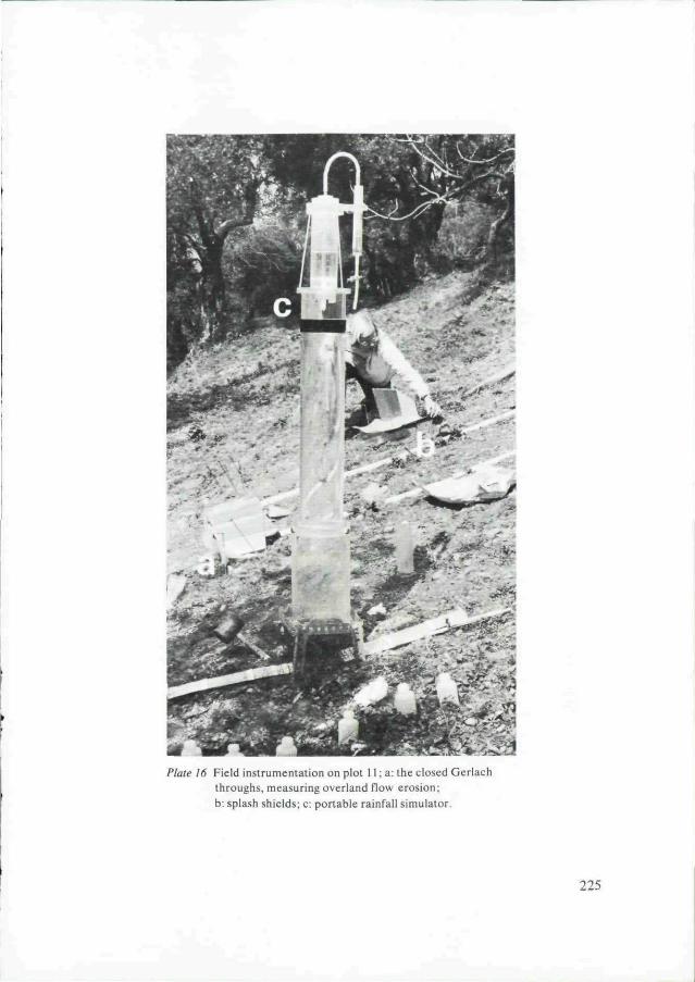
Plate 16 Field instrumentation on plot 11 ; a: the closed Gerlachthroughs, measuring overland flow erosion;b: splash shields; c: portable rainfall simulator.

225

BIBLIOGRAPHY

ADAMS, J.E., D. KIRKHAM & D.R. NIELSEN (1957), A portable rainfall simulator -infiltrometerand physical measurements of the soil in place. Soil Science Society Proceedings 21, pp. 474-477

AHNERT.F.(1977),Some comments on the quantitative formulation of geomorphological proces-ses in a theoretical model. Earth Surface Processes 2, pp. 191-201.

ALLISON, F.E. (1968), Soil aggregation - some facts and fallacies as seen by a microbiologist. SoilScience 106 (2), pp. 136-143.

ANDRE, J.E. & H.W. ANDERSON (1961), Variation of soil erodibility with geology, geographiczone, elevation and vegetation type in northern California wildlands. Journal of GeographicalResearch 66, pp. 3351-3358.

ASCH,TH.W.J. van & R.A. STEENBERGEN (1972), Een landschapskartering ten behoeve van heterosie-onderzoek. K.N.A.G. Geografisch Tijdschrift 6, pp. 454-460.

ASCH, TH.W.J. van & J.M. ROELS (1979), Een beginpoging tot het opstellen van een splash modelen de resultaten van enkele metingen. Berichten Fysisch Geografische Afdeling 12, pp. 59-69.

BARNETT, A.P., J.S. ROGERS, J.H. HOLLADAY & A.E. DOOLEY (1965), Soil erodibility fac-tors for selected soil in Georgia and South Carolina. Transactions of the American Society ofAgricultural Engineering 8, pp. 393-396.

BAVER, L.D., W.H. GARDNER &W.R. GARDNER (1972), Soil Physics. New York; Wiley.

BENNET.R.J.&RJ. CHORLEY (1978), Environmental systems. Philosophy, analysis and control.London: Methuen & Co.

BEST, A.C. (1950), The size distribution of raindrops. Quaternly Journal of the Royal Meteorolo-gical Society 76, p. 16.

BISAL. F. (1960), The effect of raindrop size and impact velocity on sand splash. Canadian Journalof Soil Science 40, pp. 242-245.

BISHOP, A.W. (1973), The stability of tips and spoil heaps. Quaternly Journal of Engineering Geo-logy 6, pp. 335-376.

BISHOP, A.W. & N.R.MORGENSTERN (1960), Stability coefficients for earth slopes, Geotechnique10, pp. 29-150.

BJERRUM, L. & F. J0RSTAD (1968), Stability of rockslopes in Norway. Norwegian GeotechnicalInstitue 79, pp. 1-11.

BLONG, R.J. (1973), A numerical classification of selected landslides of the debris slide-avalancheflowtype. Engineering Geology 7, pp. 99-114.

BOUSQUET, J.C.& P. GUEREMY (1968),Quelques phénomènes de néotectonique dans l'ApenninCalabro-Lucanien et leurs consequences morphologiques. 1 - Bassin du Mercure et haute valléedu Sinni - Revue de Géographie Physique et de Géologie Dynamique 10, pp. 225-238.

BOUSQUET, J.C. & P. GUEREMY(1969),Quelquesphénomènes de néotectonique dans l'ApenninCalabro—Lucanien et leurs conséquences morphologiques 2-1'Escarpement méridional duPollino et son piedmont. Revue de Géographie Physique et de Géologie Dynamique 11, pp. 223-236.

BOUYOUCOS, G J . (1935), The clay ratio as a criterion of susceptibility of soils to erosion. Jour-nal of the American Society of Agronomy 27, pp. 738-741.

227

BRUNSDEN, D. (1979), Massmovements. In: EMBLETON, C. & J. THORNES (1979), Process inGeomorphology.pp. 130-186. London: Edward Arnold.

BRYAN, R.B. (1968), The development, use and efficiency of indices of soil erodibility. Geoderma2, pp. 5-26.

BRYAN, R.B. (1969), The relative erodibility of soils developed in the Peak District of Derbyshire.Geografiska Annaler 51-A, pp. 145-159.

BRYAN, R.B. (1974), Water erosion by splash and wash and the erodibility of Albertan soils. Geo-grafiska Annaler 56-A.pp. 159-181.

BRYAN, R.B. (1976), Considerations on soil erodibility indices and sheet wash. Catena 3, pp. 99-111.

BURTON, A.N. (1964), Marine levels in South Italy. Nature 203, p. 1060.

BURTON, A.N. (1970), Note on the Alpine Orogeny in Calabria, Southern Italy. Quaternly Journalof the Geological Society London 126, pp. 369-381.

CARSON, M.A. (1971), The mechanics of erosion. London: Pion.

CARSON, M.A. & M J . KIRKBY (1972), Hillslope form and process. Cambridge: The UniversityPress.

CARSON, M.A. & DJ. PETLEY (1970), The existence of threshold hillslopes in the denudationof the landscape. Transactions of the Institute of British Geographers 49, pp. 71-95.

CARTA GEOLOGICA DELLA CALABRIA (1968), Foglio 236-III N.E., 236-III S.E. Cassa peropere straordinarie di pubblico interesse nell'Italia Meridionale.

CHANDLER, R.J. (1970), A shallow slab slide in the Lias clay near Uppingham, Rutland, Géotech-nique 20, pp. 253-260.

CHANDLER, R.J. (1972), Pcriglacial mudslides in Vestspilzbergen and their bearing on the originof fossil solifluction shears in low-angled clay slopes. Quaternly Journal of Engineering Geology5, pp. 223-241.

CHANDLER, R.J. (1977), The application of soil mechanic methods to the study of slopes. In:HAILS, J.R. (1977), Applied Geomorphology. Amsterdam: Elzevier.

CHAPMAN, G. (1948), Size of raindrops and their striking force at the soil surface in a red pineplantation. Transaction of the American Geophysical Union 29(5), pp. 664-670.

CHESTERS, G., O.J. ATTOE & O.N. Allen (1957), Soil aggregation in relation to various soil con-stituents. Soil Science Society of America Proceedings 21, pp. 272-277.

CHILDS, E.C. (1969), An introduction to the physical basis of soil water phenomena. New York:McGraw-Hill.

CHORLEY, J.R. & A.B. Kennedy (1971), Physical Geography. A systems approach. London: Pren-tice-Hall International Inc.

COMMISSION DE PEDOLOGIE ET DE CARTOGRAPHIE DES SOLS (1967), Classification dessols. Grignon: Laboratoire de Géologie - Pédologie de l'E.N.S.A.

CROZIER, M.J. (1969), Earthflow occurrence during high intensity rainfall in Eastern Otago (NewZeeland). Engineering Geology 3, pp. 325-334.

CROZIER, M.J. (1973), Techniques for the morphometric analysis of landslides. Zeitschrift fürGeomorphologie 17, pp. 78-101.

CRUDEN, D.M. (1976), Major rock slides in the Rockies. Canadian Geotechnical Journal 13, pp.8-20.

228

DAVID, WJ>. & C.E. BEER (1975), Simulation of soil erosion. Part 1: Development of a mathema-tical erosion model. Transactions of the American Society of Agricultural Engineering 18, pp.126-199, 133.

DOTY.C.W. &C.E. CARTER (1965), Rates and particle size distributions of soil erosion from unitsource areas. Transactions of the American Society of Agricultural Engineering 8, pp. 309-311.

D'SOUZA, V.P. & R.P.C. MORGAN (1976), A laboratory study of the effect of slope steepnessand curvature on soil erosion. Journal of the Agricultural Engineering Research 21, pp. 21-31.

DUBOIS, R. (1970), Phases de serrage, nappes de socle et métamorphisme Alpin à la jonction Ca-labre - Apennin: La suture Calabro - Apenninique. Revue de Géographie Physique et de Géo-logie Dynamique 12, pp. 221-253.

ECKEL, E.B. (ed.) (1958), Landslides and engineering practice. Special Report on Highway Research,Bd. 29, Washington D.C.

ELLISON, W.D. (1944), Studies of raindrop erosion. Agricultural Engineering 25, pp. 131-136,181-182.

ELWELL.H.A.&M.A. STOCKING (1976), Vegetal cover to estimate soil erosion hazard in Rhode-sia. Geoderma 15, pp. 61-70.

EMMETT,W.W.(1978),Overlandflow.In: KIRKBY.M.J. (1978),Hillslopehydrology,pp. 145-176.New York: Wiley & Son.

EMMETT, W.W. (1970), The hydraulics of overlandflow on hillslopes. United States GeologicalSurvey Professional Paper 662-A.

EPEMA, G.F., H. POT, J.M. ROELS & P.M. Schoot (1979), Respons van een stroomgebied op ge-simuleerde en natuurlijke neerslag. M.Sc. thesis. Utrecht: Geografisch Instituut R.U.

EPSTEIN, E. & W.J. GRANT (1973), Soil crust formation as affected by raindrop impact. In:HADAS, A., D. SWARTZENDRUBER, P.E. REITEMA, M. FUCHS & B. YARON (1973). Phy-sical aspects of soil, water and salts in ecosystems. Berlin: Springer Verlag, pp. 195-201.

ERGENZINGER, P., K.P. OBENAUF & K. SIJMONS (1975), Erster Versuch einer Abschätzungvon Erosions und Akkumulation betragen einer Torrente Kalabriens. Würburger GeographischeArbeiten 43, pp. 174-186.

EYLES, R.J. (1971), Massmovement in Tangoio conservation reserve Northern Hawkes Bay. EarthScience Journal 5-2, pp. 79-91.

F.A.O. (1966), Guidelines for soil profile description. Rome: Food and Agriculture Organizationof the United Nations.

FELLENIUS.W. (1927), Erdstatische Berechnungen mit Reibung und Kohäsion. Berlin: Ernst.

FORREN, P.M. (1970), The development of two field instruments to measure erosivity: A simplerainfall intensity meter and an acoustic rainfall record tested with a rotating disk simulator. B.Sc.(Hons.) dissertation, National College of Agricultural Engineering.

FOSTER, L.R. & G.L. Martin (1969), Effect of unit weight and slope on erosion. Journal of theirrigation and drainage division. Proceedings of the American Society of Civil Engineers I.R.-4, pp. 551-561.

FOURNIER, F. (I960), Climat et Erosion. Paris: Presses Universitaires de France.

FREE.G.R. (1960), Erosion characteristics of rainfall. Agricultural Engineering 41(7), pp. 447-449.

229

FREE, G.R., CM. BROWNING & G.W. MUSGRAVE (1940), Relative infiltration and related phy-sical characteristics of certain soils. United States Department of Agriculture Technical Bulletin729.

GABRIELS, D., J.M. PAUWELS & M. DE BOODT (1975), The slope gradient as it affects theamount and size distribution of soil loss material from runoff on silt aggregates. Medische Facul-teit Landbouwwetenschappen. R.U.Gent 40, pp. 1333-1338.

GEIGER, R. (1975), The climate near the ground. Cambridge: Harvard University Press.

GERLACH, T. (1966), Développement actuel des versants dans le bassin du Haut Grajcarek (LesHautes Beskides — Les Carpates Occidentales). Warsawa: Wydawnictwa Geologiczne (TravauxGéographiques 52).

GREEN, W.H.& CA. AMPT (1911), Flow of air and water through soils. Journal of AgriculturalSciences 4, pp. 1-24.

GREGORY, K.J. & D.E. WALLING (1973), Drainage basin form and process. London: EdwardArnold.

GUNN, R. &G.D. KINZER (1949), Terminal velocity of water droplets in stagnant air. Journal ofMeteorology 6, p. 243.

HADLEY, R.F. & G.C. LUSBY (1967), Runoff and hillslope erosion resulting from ahigh intensitythunderstorm near Mack, Western Colorado. Water Resources Research 3, pp. 139-146.

HENIN, S. (1938), Etude physico - chimique de la stabilité structurale des terres. Monograph Na-tional Centre of Agronomie Research, Paris, pp. 52-54.

HENIN, S. (1963), L'appréciation des propriétés physiques du sol. Annales Gembloux 3, pp. 631-633.

HENKEL, D.J. & A.W. SKEMPTON (1955), A landslide at Jacksfield, Shropshire, in an over-conso-lidated clay.Proceedingsof the Conferenceof stability of Earthslopes (Stockholm) 1, pp. 90-101.

HORTON, R.E. (1945), Erosional development of streams and their drainage basins: hydrologicalapproach to quantitative morphology. Bulletin of Geological Society of America 56, pp. 275-370.

HSÜ, K.J. (1975), Catastrophic debris streams generated by rockfalls. Bulletin of the Geologic So-ciety of America 86, pp. 129-140.

HUDSON, N.W. (1963), Raindrop size distribution in high intensity storms. Rhodesian Journal ofAgricultural Research 1 (1), pp. 6-11.

HUDSON, N.W. (1965), The influence of rainfall on the mechanics of soil erosion. M. Sc.Thesis,University of Cape Town.

HUDSON, N.W. (1973), Soil Conservation. New York: Cornell University Press.

HUDSON, N.W. & D.C. JACKSON (1959), Results achieved in the measurement of erosion andrunoff in southern Rhodesia. Proceedings, Third Inter-African Soils Conference, Dalaba, pp. 575-583.

HUDSON, J.J. (1970), Land utilization in the Crati Valley (Calabria - Italy). Delft: ITC.

HUTCHINSON, J.N. (1967), The free degradation of London clay cliffs. Proceedings of the Geo-technical Conference Oslo 1, pp. 113-118.

HUTCHINSON, J.N. (1968), Field meeting on the coastal landslides of Kent. Proceedings of theGeological Association 791, pp. 227-237.

230

HUTCHINSON, J.N.(1969),Areconsiderationof the coastal landslides of Folkestone Warren, Kent.Géotechnique 19, pp. 6-38.

HUTCHINSON, J.N. (1970), A coastal mudflow on the London clay cliffs at Beltinge, North Kent,Géotechnique 20, pp. 412^38.

HUTCHINSON, J.N. (1974),Periglacial solifluction: an approximate mechanism for clay soils. Geo-technique 24, pp. 438-443.

HUTCHINSON, J.N. & R.K. BHANDARI (1971), Undrained loading, a fundamental mechanism ofmudflows and other massmovements. Geotechnique 21, pp. 353-358.

JOHNSON, A.M. & P.H. RAHN (1970), Mobilisation of debris flows. Zeitschrift für Geomorpho-logie. Supplement Band 9, pp. 168-186.

KAYSER, B. (1958), Recherches sur les sols et l'érosion en Italie Méridionale - Lucanie. Paris: Sedes.

KENT, P. (1966), The transport mechanism of catastrophic rockfalls. Journal of Geology 74, pp.79-83.

KEZDI, A. (1974), Handbook of Soil Mechanics. Volume 1 Soil Physics. Amsterdam: Elsevier.

KIRKBY, M.J. (1969), Infiltration, through flow and overlandflow. In: CHORLEY, J. (1969), Wa-ter, Earth and Man. London: Methuen & Co.

KNAPP, B.J. (1978), Infiltration and storage of soil water. In: KIRKBY, M.J. (1978), HiUslope hy-drology. New York: Wiley & Son.

KOONS, D. (1955), Cliff retreat in the south-west United States of America. American Journal ofScience 253, pp. 44-52.

LAL, R. (1976), Soil erosion on alfisols in Nigeria, the changes in physical properties and theresponse of crops. Geoderma 16, pp. 419-431.

LAMBE, T.W. & R.V. WHITMAN (1969), Soil mechanics. New York: Wiley & Sons.

LAURENS, F.M. (1958), Sediment transport mechanics in stable channel designs. Transactions ofthe American Society of Civil Engineers 123, pp. 195-206.

LAWS, J.O. (1941), Measurements of fall-velocity of water-drops and raindrops. Transactions of theAmerican Geophysical Union 22, p. 709.

LAWS, J.O. & D.A. Parson (1943), The relation of raindrop size to intensity. Transactions of theAmerican Geophysical Union 24, p. 452.

LEMOS,P.&J.F. LUTZ (1957), Soil crusting and some factors affecting it. Soil Science Society ofAmerica Proceedings 21, pp. 485-490.

LEEUWARDEN, F.J.M, van (1973), Een landschapskarteringin Zuid-Italië (Calabrië). M.Sc. Thesis.Utrecht: Geografisch Instituut R.U.

LOHNES, R.A. & R.L. HANDY (1968), Slope angles in friable loess. Journal of Geology 76, pp.247-258.

McCALLA, T.M. (1944), Water-drop method of determining stability of soil structure. Soil Science,58, pp. 117-123.

McINTYRE, D.S. (1958), Soil splash and the formation of surface crusts by raindrop impact. SoilScience 85, pp. 261-266.

MEYER, L.D. (1965), Mathematical relationships governing soil erosion by water (Resumé). Journalof Soil and Water Conservation 20, pp. 149-150.

231

MEYER, L.D., G.R. FOSTER & H.JM. ROMKENS (1975), Soil-detachment by raindrops, in: Pre-sent and prospective technology for predicting sediment yields and sources. U.S. Department ofAgriculture, Agricultural Research Service, Publ. ARS-S-40, pp. 177-189.

MEYER, L.D. & E J . MONKE (1965), Mechanics of soil erosion by rainfall and overland flow.Transactions of the American Society of Agricultural Engineering 8, pp. 572-580.

MEYER, L.D. & W.H. WISCHMEIER (1969), Mathematical simulation of the process of soil erosionby water. Transactions of the American Society of Agricultural Engineering 12, pp. 754-758,762.

MEYRIAT, J. (1960), La Calabre. Une région sous-développée de l'Europe méditerranéenne. Cahiersde la fondation nationale des sciences politiques 104. Paris: Armand Colin.

MIDDLETON, H.E. (1930), Properties of soils which influence soil erosion. U.S. Department ofAgricultural Technical Bulletin 178.

MIHARA, Y. (1951), Raindrops and soil erosion. Bulletin of the National Institute of AgriculturalScience, Series A, 1.

MILONE, F. (1956), Memoria illustrativa della carta della ut'lizzazione del suolo della Calabria.Napoli: Consiglio Nazionale della Ricerche, centrodi studi par la geografia economica.

MITCHELL, C. (1973), Terrain evaluation. London: Longman Group.

MORGAN, R.P.C. (1978), Field studies of rainsplash erosion. Earth Surface processes, 3, pp. 259-269.

MORGAN, R.P.C. (1979), Soil erosion. London: Longman.

MOSLEY, MJ\ (1974), Rainsplash and the convexity of badland divides. Zeitschrift für Geomor-phologie, N.F. Supplement Band 18, pp. 10-25.

MULLER, L. (1964), The rockslide in the Vaiont Valley. Rock Mechanical Engineering Geology 2,pp. 148-212.

MUSGRAVE, G.W. (1947), The quantitative evaluation of factors in water erosion: a first approxi-mation. Journal Soil and Water Conservation 2, pp. 133-138.

MUTCHLER, C.K. & R.A. YOUNG (1975), Soil detachment by raindrops, in: Present and prospec-tive technology for predicting sediment yields and sources. U.S. Department of Agriculture,Agricultural Research Service, Pub. ARS-S-40, pp. 113-117.

NASSIF, S.H. & E.M. WILSON (1975), The influence of slope and rain intensity on runoff and in-filtration. Hydrological Sciences, Bulletin des Sciences Hydrologiques 20 (4), pp. 539-553.

NISHIKATA, T. & Y. TAKRUCHI (1955), Relation between physico chemical properties and ero-dibility of soil, part 2. Research Bulletin Hokkaido National Agricultural experimental station68, pp. 49-54.

OSCHOWY, G. (1963), Bodenerosion und Bodenschutz auf Tertiären Tonböden unter besondererBerücksichtigung Italienischer Erosionsgebiete. In: BUCHWALD, K., W. LENDHOLT & K.MEYER (1963), Beiträge zur Landespflege 1. Stuttgart: Eugen Ulmer.

OVENS, G. (1969), A study of soil erodibility by separation of the primary stages of the erosionprocess. M.Sc. Thesis, University of Reading.

PAIN, CF. (1971), Rapid massmovement under forest and grass in the Hunua Range, New Zealand.Australian Geographical Studies 9-1, pp. 17-26.

PALMER, R.S. (1964), The influence of a thin water layer on waterdrop impact forces. Internatio-nal Association of Scientific Hydrological Publications 65, pp. 141-148.

232

PALMER, R.S. (1965), Waterdrops impact forces. Transactions of the American Society of Agricul-tural Engineering 8, pp. 69-72.

PEREIRA, M.C. (1956), A rainfall test for structure in tropical soils. Journal of Soil Science 7, (1),pp. 68-74.

PITAU, D.R. (1970), Geological factors significant to the stability of slopes cut in rock. In: REN-BURG, P.W.J. van (1970), Planning Open Pit Mines, South Africa, Institute of Mining and Me-tallurgy, pp. 33-35.

PLOEY, J. de & SA VAT (1968), Contribution à l'étude de l'érosion des sols par les splash. Zeit-schrift für Geomorphologie N.F. 12 band, pp. 174-193.

PLOEY, J. de & J. MOEYERSONS (1976), Quantitative data on splash erosion, simulated on un-vegetated slopes. Zeistschrift für Geomorphologie, Supplement Band 25, pp. 120-131.

PLOEY, J. de, J. SAVAT & J. MOEYERSONS (1976), The differential impact of some soil factorson flow, runoff creep and rainwash. Earth Surface Processes 1, pp. 151-161.

PRIOR, D.B. & N. STEPHENS (1972), Some movement patterns of temperate mud flows fromNorthern Ireland. Bulletin of the Geological Society of America 38, pp. 2533-2544.

PRIOR, D.B., N. STEPHENS & G.R. DOUGLAS (1970), Some examples of modern debris flowsfrom Northern Ireland. Zeitschrift für Geomorphologie 14, pp. 275-288.

RAO, D.P. & H.GHANEM (1972), A geomorphologjcal survey of the Savuto and Oliva Basins,Calabria, Italy. Enschede: I.T.C.

RAPP, A. (1960), Recent development of mountain slopes in Kärkevagge and surroundings, Nor-thern Scandinavia. Geografiska Annaler 42, pp. 65-200.

RIEZEBOS, H.Th. (1979), Geomorphology and soils of Sipalawini Savanna (South Suriname),Utrechtse Geografische Studies 12. Utrecht: Geografisch Instituut R.U.

RITCHIE, P. (1958), Recognition and identification. In: ECKEL, E.B. (1958), Landslides and engi-neering practise. Special Report on Highway Research Bd. 29. Washington D.C.

ROMEIN, A., (in preparation). Aspects of X-ray and thermal analyses of (clay)minerals.

ROMEIN, A. (1980), X-ray and therminal analysis of some samples from Calabria. 37th internalreport. Geografisch Instituut R.U.

ROSE, C.W. (1958), Effects of Rainfall and soil-factors on soil detachment, and the rate of waterpenetration into soils. Ph.D. Thesis, University of London.

ROSE, C.W. (1960), Soil detachment caused by rainfall. Soil Sience 89 (1), pp. 28-35.

ROUGERIE, G. (1960), Le façonnement actuel des modelés en Côte d'Ivoire forestière. Diss.Paris.

ROUSE, W.C. (1975), Engineering properties and slope form in granular soils. Engineering Geology9. pp. 221-235.

RUXTON, B.P. (1967), Slope wash under mature primary rainforest in Northern Papua. In:JENNINGS, J.N. & J.A. MABBUTT (1967), Landform studies from Australia and New Guinea.Cambridge, London.

SAVAT, J. (1977), The hydraulics of sheet flow on a smooth surface and the effect of simulatedrainfall. Earth Surface Processes 2, pp. 125-140.

SCHUMM, S.A. (1956), Evolution of drainage systems on slopes of badlands at Perth Amboy, NewJersey. Bulletin of the Geological Society of America 67, pp. 579-646.

233

SCHUMM, S.A. (1964), Seasonal variations of erosion rates and processes on hillslopes in WesternColorado. Zeitschrift für Geomorphologie. Supplement Band 5, pp. 215-238.

SCHUMM, S.A. & R.J. CHORLEY (1964), The fall of Threatening Rock. American Journal ofScience 262, pp. 1041-1054.

SEYHAN, E. (1977), Fundamentals of hydrology. Utrecht: Geografisch Instituut R.U.

SHARPE, C.F.S. (1938), Landslides and related phenomena. New York: Columbia.

SHREVE, R.L. (1968), Leakage and fluidization in air-layer lubrication avalanches. Bulletin of theGeologic Society of America 79, pp. 653-658.

SINGER, M.J. & J. BLACKBARD (1978), Effect of mulching on sediment in runoff from simula-ted rainfall. Soil Science of American Journal 42 (1), pp. 481-485.

SKEMPTON, A.W. (1953), Soil mechanics in relation to geology. Proceedings of the Yorkshire Geo-logical Society 29, pp. 33-62.

SKEMPTON, A.W. (1964), Long term stability of clay slopes. Geotechnique 14, pp. 71-200.

SKEMPTON, A.W. & F.A. DE LORY (1957), Stability of natural slopes in London Clay. Procee-dings of the 4th International Conference of Soil Mechanics and Foundation Engineering, Lon-don, 2, pp. 378-381.

SLONEKER, L.L., F.C. ALSON & W.C. MOLDENHAUER (1976), Effect of pore water pressureon sand splash. Soil Science Society of America. Proceedings 40, pp. 948-951.

SMITH, R.M. & CF . CERNUDA (1951), Some applications of water-drop stability testing to tro-pical soils of Puerto Rico. Soil Science 71, pp. 337-346.

SOIL SURVEY STAFF (1951), Soil Survey Manual. U.S. Department of Agriculture. AgriculturalHandbook 18, Washington D.C.

SOWERS, G.F. (1965), Consistency. In: BLACK, C.A. (1965), Method of soil analysis. Part 1.Madison: American Society of Agronomy, Inc.

SOWERS, G.F. (1979), Introductory soil mechanics & foundations: Geotechnical Engineering.New York: MacMillan.

STATHAM, I. (1977), Earth Surface sediment transport. Oxford: Clarendon Press.

SULEBAK, J.R. (1969), Mudflows in the low Alpine Region. Norsk Geografik Tidsskrift 23, pp.15-23.

SREENIVAS, L., J.R. JOHNSTON & H.O. HILL (1947), Some relationships of vegetation and soildetachment in the erosion process. Soil Science Society of America. Proceedings 11, pp. 471-474.

TAKAHASHI, T. (1978), Mechanical characteristics of debris flow. Journal of the Hydraulics Divi-sion 104 (8) pp. 1153-1170.

TAYLOR, D.W. (1937), Stability of earth slopes. Journal of the Boston Society of Civil Engineers24, pp. 197-246.

TER-STEPHANIAN, G. (1965), In-situ determination of the Theological characteristics of soil onslope. Proceedings of the 6th international Conference of Soil Mechanics and Foundation Engi-neering 2, pp. 375-377.

TERZAGHI, K. (1960), Mechanism of landslides. Bulletin of the Geological Society of America,Berkeley Volume, pp. 83-122.

TERZAGHI, K. (1962), Stability of steep slopes on hard unweathered rock. Géotechnique 12, pp.199-208.

234

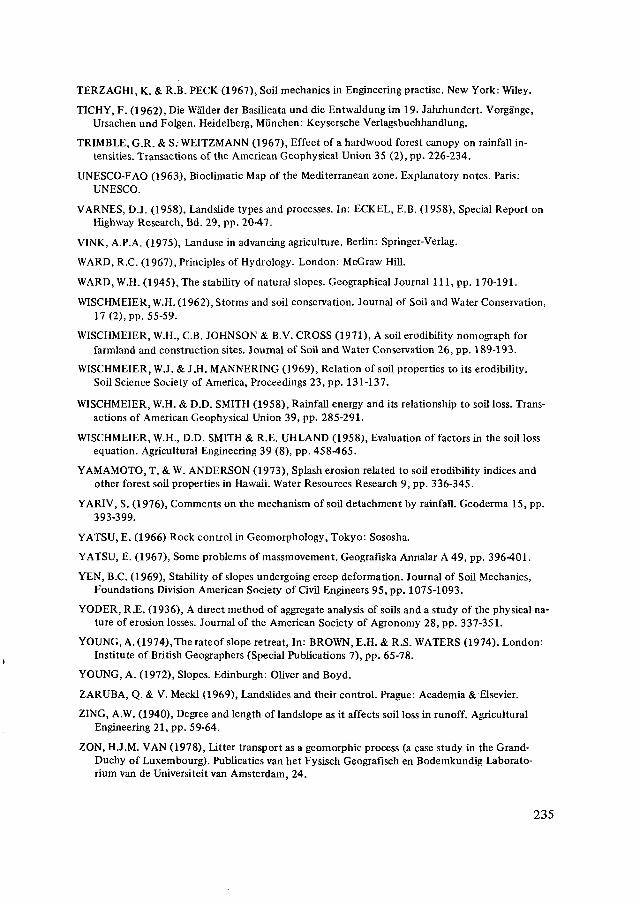
TERZAGHI, K. & R.B. PECK (1967), Soil mechanics in Engineering practise. New York: Wiley.

TICHY, F. (1962), Die Wälder der Basilicata und die Entwaldung im 19. Jahrhundert. Vorgänge,Ursachen und Folgen. Heidelberg, München: Keysersche Verlagsbuchhandlung.

TRIMBLE, G.R. & S; WEITZMANN (1967), Effect of a hardwood forest canopy on rainfall in-tensities. Transactions of the American Geophysical Union 35 (2), pp. 226-234.

UNESCO-FAO (1963), Bioclimatic Map of the Mediterranean zone. Explanatory notes. Paris:UNESCO.

VARNES, D.J. (1958), Landslide types and processes. In: ECKEL, E.B. (1958), Special Report onHighway Research, Bd. 29, pp. 20-47.

VINK, A.P.A. (1975), Landuse in advancing agriculture. Berlin: Springer-Verlag.

WARD, R.C. (1967), Principles of Hydrology. London: McGraw Hill.

WARD, W.H. (1945), The stability of natural slopes. Geographical Journal 111, pp. 170-191.

WISCHMEIER,W.H.(1962), Storms and soil conservation. Journal of Soil and Water Conservation,17 (2), pp. 55-59.

WISCHMEIER, W.H., C.B. JOHNSON & B.V. CROSS (1971), A soU erodibility nomograph forfarmland and construction sites. Journal of Soil and Water Conservation 26, pp. 189-193.

WISCHMEIER, W.J. & JM. MANNERING (1969), Relation of soil properties to its erodibility.Soil Science Society of America, Proceedings 23, pp. 131-137.

WISCHMEIER, W.H. & D.D. SMITH (1958), Rainfall energy and its relationship to soil loss. Trans-actions of American Geophysical Union 39, pp. 285-291.

WISCHMEIER, W.H., D.D. SMITH & R.E. UHLAND (1958), Evaluation of factors in the sou lossequation. Agricultural Engineering 39 (8), pp. 458-465.

YAMAMOTO, T. & W. ANDERSON (1973), Splash erosion related to soil erodibility indices andother forest soil properties in Hawaii. Water Resources Research 9, pp. 336-345.

YARIV, S. (1976), Comments on the mechanism of soil detachment by rainfall. Geoderma 15, pp.393-399.

YATSU, E. (1966) Rock control in Geomorphology, Tokyo: Sososha.

YATSU, E. (1967), Some problems of massmovement. Geografiska Annalar A 49, pp. 396-401.

YEN, B.C. (1969), Stability of slopes undergoing creep deformation. Journal of Soil Mechanics,Foundations Division American Society of Civil Engineers 95, pp. 1075-1093.

YODER, R.E. (1936), A direct method of aggregate analysis of soils and a study of the physical na-ture of erosion losses. Journal of the American Society of Agronomy 28, pp. 337-351.

YOUNG, A. (1974),Therateof slope retreat, In: BROWN, E.H. & R.S. WATERS (1974). London:Institute of British Geographers (Special Publications 7), pp. 65-78.

YOUNG, A. (1972), Slopes. Edinburgh: Oliver and Boyd.

ZARUBA, Q. & V. Meckl (1969), Landslides and their control. Prague: Academia & Elsevier.

ZING, A.W. (1940), Degree and length of landslope as it affects soil loss in runoff. AgriculturalEngineering 21, pp. 59-64.

ZON, H.J.M. VAN (1978), Litter transport as a geomorphic process (a case study in the Grand-Duchy of Luxembourg). Publicaties van het Fysisch Geografisch en Bodemkundig Laborato-rium van de Universiteit van Amsterdam, 24.

235

ZONNEVELD, I.S. (1972), Land evaluation and land(scape) science. ITC Textbook of photointerpretation VII-4. Enschede: I.T.C.

236

CURRICULUM VITA

De schrijver van dit proefschrift werd geboren op 29 januari 1944 te Baarn.In 1962 behaalde hij het diploma H.B.S.-B aan het Constantijn College te Amers-foort. In 1966 werd het kandidaatsexamen Fysische Geografie afgelegd aan de Rijks-universiteit te Utrecht. Het doctoraal diploma Fysische Geografie werd behaald in1970. Sinds zijn afstuderen is de auteur als wetenschappelijk medewerker verbondenaan het Georgrafisch Instituut der Rijksuniversiteit te Utrecht.

237

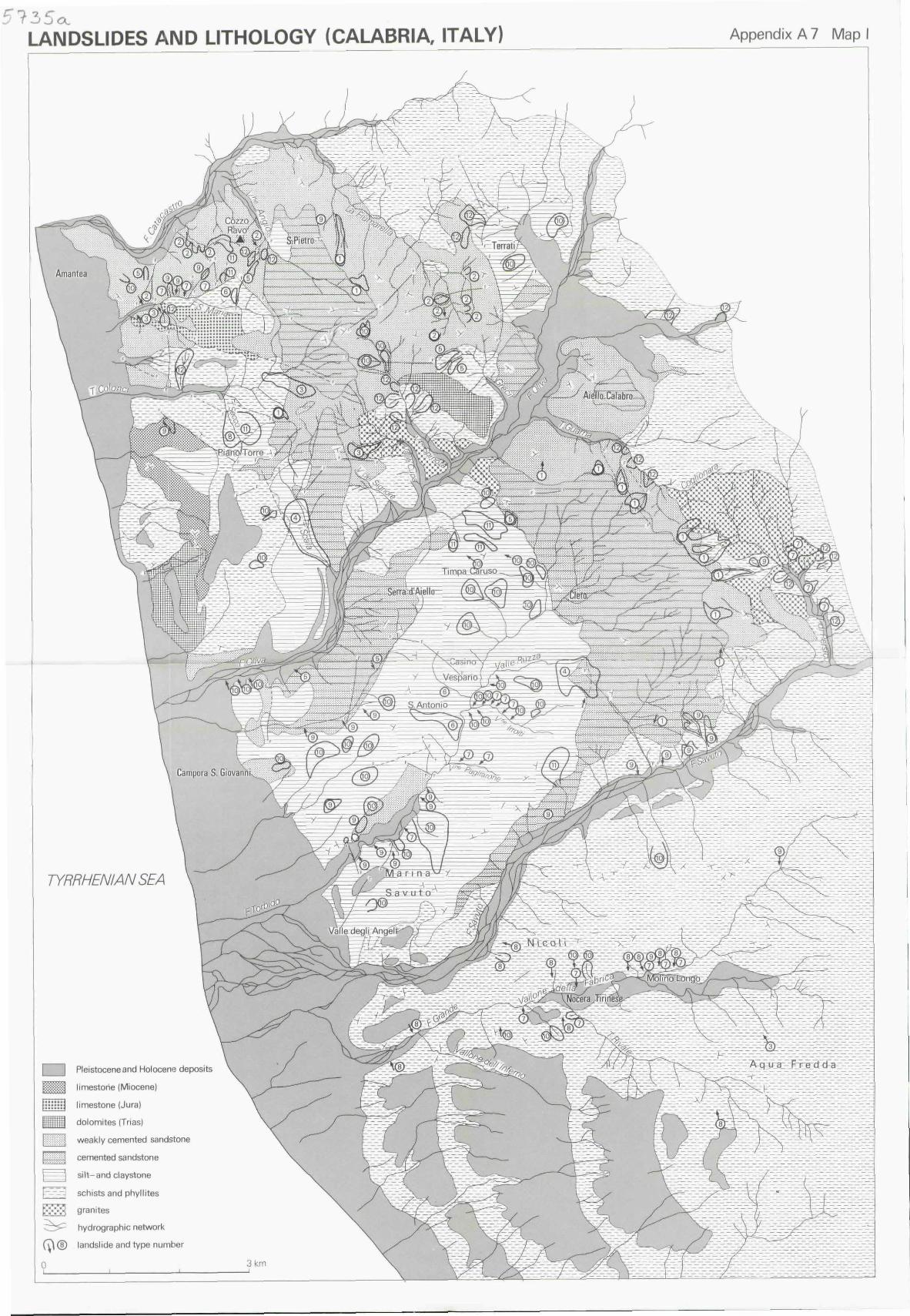
LANDSLIDES AND UTHOLOGY (CALABRIA, ITALY) Appendix A 7 Map

TYRRHENIAN SEA

f ^ J Pleistocene and Holocene deposits

|ji;i;||;;| limestone (Miocene)

t;:::::j limestone (Jura)

BüifftfH dolomites (Trias)

tisilllÉ weakly cemented sandstone

[; :i; ;] cemented sandstone

| I silt-and claystone

P~~7~j schists and phyllites

t'sl*ï\ granites

^ 5 ^ hydrographie network

(v\ ® landslide and type number

ï , . 3 km

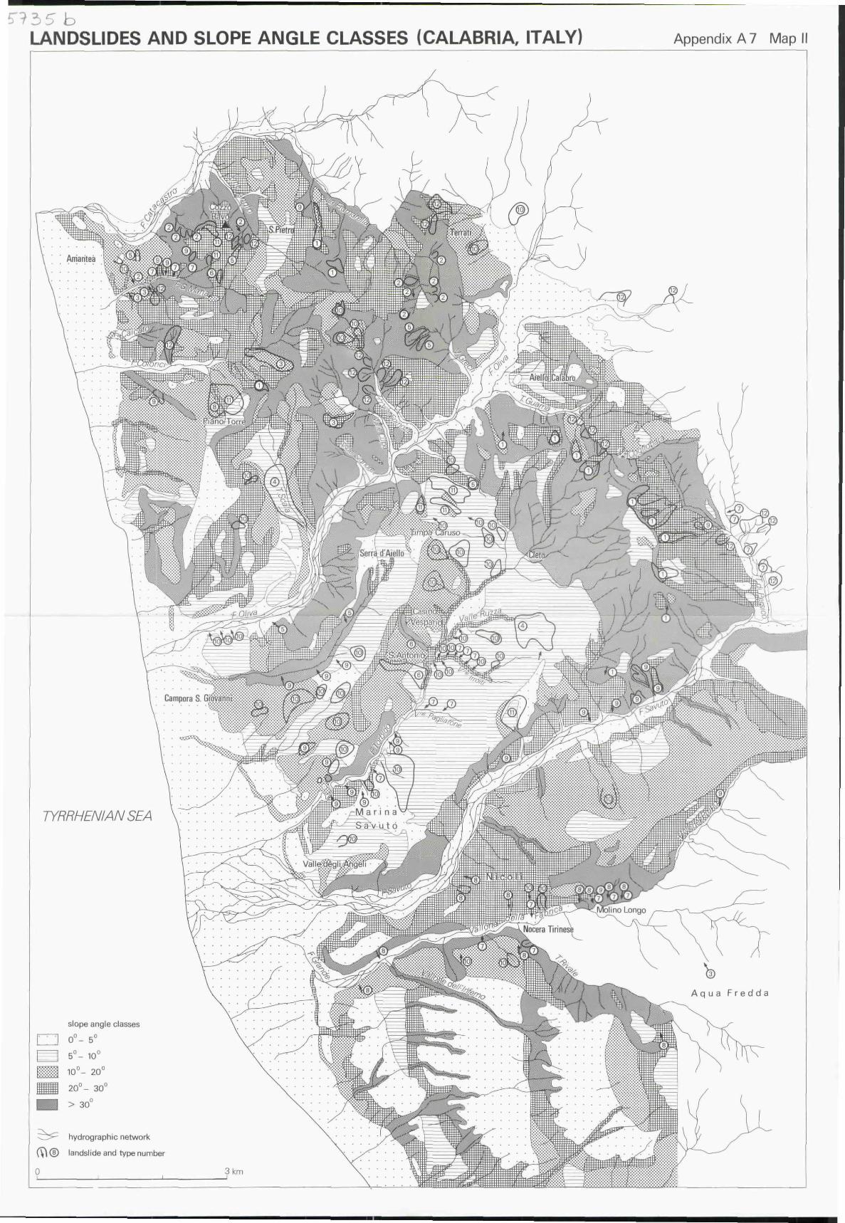
LANDSLIDES AND SLOPE ANGLE CLASSES (CALABRIA, ITALY) Appendix A 7 Map II

TYRRHENIAN SEA

slope angle classes

hydrographie network

§) landslide and type number

3^cLANDSLIDES AND VEGETATION STRUCTURE / LANDUSE (CALABRIAJTALY)

Appendix A 7 Map

TYRRHENIAN SEA

scattered vegetated areas (0 - 60%)

densely vegetated areas ( > 60%

agricultural areas

hydrographie network

landslide and type number

3 km