Computer simulation of progressive failure in soil slopes

University of WollongongResearch Online

University of Wollongong Thesis Collection University of Wollongong Thesis Collections

1988

Computer simulation of progressive failure in soilslopesCarlo Ernest BertoldiUniversity of Wollongong

Research Online is the open access institutional repository for theUniversity of Wollongong. For further information contact ManagerRepository Services: [email protected].

Recommended CitationBertoldi, Carlo Ernest, Computer simulation of progressive failure in soil slopes, Doctor of Philosophy thesis, Department of Civil andMining Engineering, University of Wollongong, 1988. http://ro.uow.edu.au/theses/1232

http://ro.uow.edu.au/


http://ro.uow.edu.au

http://ro.uow.edu.au/theses

http://ro.uow.edu.au/thesesuow



COMPUTER SIMULATION OF

PROGRESSIVE FAILURE IN SOIL SLOPES

A thesis submitted in fulfilment of the

requirements for the award of the degree of

DOCTOR OF PHILOSOPHY

from

THE UNIVERSITY OF WOLLONGONG

by

CARLO ERNEST BERTOLDI, B.E. (Hons) N.S.W. (Civil)

DEPARTMENT OF CIVIL AND MINING ENGINEERING

1988

STATEMEBT

I hereby certify that the work presented in this

thesis has not been submitted for a degree to any

other university or similar institution.

CE. BERTOLDI

Page i

ABSTRACT

This thesis is concerned with the simulation of progressive

failure within soil slopes considering, as a basis, the widely

accepted concept of limit equilibrium. In particular, the

investigations reported here concern the influence of strain-softening

on the overall safety factor, the identification of local failures and

the propagation of failure within a slope. Several methods of

analysis were developed and successfully implemented. A number of

case histories were analysed using these methods and the influence of

progressive failure evaluated. Some of these methods take the initial

stress field into consideration.

Theories of progressive failure are often based on the well

established mechanism of strain-softening associated with soils. The

extent of strain-softening at different locations within a slope or

along a slip surface is generally unknown. Complete strain-softening

(a residual factor of one) along a slip surface must occur after

overall failure of a slope and, if no overstress has occurred anywhere

and relative deformations have been small, no strain-softening would

have occurred (a residual factor of zero). These are the limiting

cases and thus the overall residual factor may have a value between

zero and unity. More importantly, the local residual factor (as

distinct from the overall residual factor) may vary from point to

point along a slip surface.

A method of simulation was developed to study the factor of

safety of a slope considering any arbitrary distribution of the local

residual factor along the potential slip surface. Typical

distributions represent failure initiating from the crest of a slope

or the toe of a slope or from somewhere in the interior. The effect

of the type of shear strength distributions on the factor of safety

was examined. Moreover, a relationship between the average shear

strength and the factor of safety was established. Criteria for

acceptability of rigorous (Morgenstern and Price type) methods of

slices were highlighted.

Page ii

A number of methods for simulating local failure and its

propagation were developed. In these methods the excess shear stress

resulting from strain-softening of failed segments of the slip

surface must be redistributed to other segments. Once this

redistribution occurs, more segments may fail and then further

redistribution occurs. This process of progressive failure continues

until no more failures occur. At that stage the factor of safety is

the lowest one associated with progressive failure. In one of the

methods an assumption is made on the manner of this redistribution

e.g. uniform distribution over the segments or linear distribution

with its maximum near the last failed segment. In other methods no

such assumption is made and the new 'failed' segments are identified

during successive limit equilibrium calculations, one for the stage

corresponding to no failures and the other for the stage with initial

local failures. Considering all the failed segments, a new analysis

is made and, comparing this with the previous one, further local

failures may be identified. In this way, the iterative technique

enables the simulation of the progressive failure process and the

associated redistribution of shear stress occurs automatically.

It is well known that an initial stress field in a slope may have

a significant influence on its stability. Therefore, it was

considered appropriate to develop methods of analysis of progressive

failure which took a given initial stress field into consideration.

Two different approaches were considered for the development of these

methods. The first approach is to consider the initial stress field

in the identification of local failures and then to follow up with

methods similar to those mentioned in the previous paragraph. The

second approach is to simulate progressive failure as a transformation

from the initial stress field to the stress field associated with

limit equilibrium. In the latter case two different types of analysis

are required for two parts of a sloping mass at each stage of

progressive failure. As the failure progression process continues,

the relative size of these masses changes. The interaction between

the two masses is taken into consideration by including the limiting

earth pressures as extreme cases of possible interaction.

Page iii

The successful implementation of all the methods is demonstrated

in relation to a number of case histories. The influence of

progressive failure on the stability is influenced not only by the

soil shear strength and brittleness but also by slope and slip surface

geometry. The initial stress field may have a significant influence

on the extent of progressive failure.

Page iv

ACKNOWLEDGEMENTS

The author wishes to thank the chairman and staff of the

Department of Civil and Mining Engineering at the University of

Wollongong for their assistance and for study and research facilities

provided during the research and computer work related to this thesis.

In particular, the author wishes to thank his supervisor,

Dr. R.N. Chowdhury, for the ongoing assistance and advice provided

over the years and especially for his assistance in compiling the

final draft of this thesis.

Special acknowledgement is made of the encouragement and help

provided by Dr. G.J. Montagner of the Department of Mechanical

Engineering and Dr. Y.W. Wong of the Department of Civil and Mining

Engineering.

Most of the computer programming and analysis work was carried

out on the University of Wollongong UNIVAC computer. The author

would, therefore, like to thank the staff of the University of

Wollongong Computer Centre, especially Mr. Ian Piper for his

assistance with many computer related problems.

In addition, the author gratefully acknowledges the assistance of

those persons who, at various stages, transferred handwritten sections

of this thesis into computer files for eventual processing into this

finished document.

Finally, but certainly not in the least, the author wishes to

thank his wife, Manuela, and his and her families for the ongoing

support and encouragement received which led to the completion of this

thesis.

Page v

CONTENTS

Page

ABSTRACT i

ACKNOWLEDGEMENTS iv

CONTENTS v

FIGURES xii

CHAPTER 1: INTRODUCTION AND SCOPE 1-1

1.1 The Slope Stability Problem 1-1

1.2 The Relevance of Progressive Failure 1-2

1.3 The Range of Slope Analysis Approaches 1-3

1.4 The Role of the Finite Element Method 1-4

1.5 The Probabilistic Approach 1-7

1.6 Scope of this Thesis 1-9

CHAPTER 2: CONVENTIONAL LIMIT EQUILIBRIUM METHODS OF STABILITY

ANALYSIS 2-1

2.1 Introduction 2-1

2.1.1 The Fellenius method or the ordinary method of slices

(also known as the Swedish method of slices) . . . . 2-7

2.1.2 The Bishop simplified method 2-10

2.1.3 Janbu's method of analysis 2-11

2.1.4 The Morgenstern-Price method 2-13

2.2 General Comments on Limit Equilibrium Methods of Analysis . 2-15

Page vi

CHAPTER 3: PROGRESSIVE FAILURE AND THE CONCEPT OF RESIDUAL

STRENGTH 3-1

3.1 General 3-1

3.2 Definitions of Progressive Failure 3-3

3.3 Residual Strength 3-3

3.4 Conditions Necessary for Progressive Failure . . . . . . . . 3-7

3.5 The Residual Factor 3-9

3.6 Reduction of Shear Strength 3-10

3.7 Mechanisms of Progressive Failure 3-12

3.7.1 General notes on progressive failure mechanisms . . . 3-12

3.7.2 Bjerrum's comments on the mechanism of progressive

failure 3-15

3.7.3 Skempton's approach to progressive failure 3-16

3.7.4 Bishop's approach to progressive failure 3-17

3.8 Concluding Remarks 3-19

CHAPTER 4: SIMULATION OF VARIABLE SHEAR STRENGTH MOBILISED

ALONG A SLIP SURFACE 4-1

4.1 Aim and Scope 4-1

4.2 Variation of Shear Strength Approach 4-2

4.2.1 Definition of residual factor in this research . . . 4-2

4.2.2 Proposed method for generating local residual

factor distributions 4-3

4.2.3 Proposed approach - variable mobilisation of c'

and 0' 4-6

4.2.4 Types of distributions assumed 4-7

4.2.5 Basis of solution method 4-8

4.2.6 Calculation of average shear strength along

failure surface 4-9

Page vii

4.3 Computer Programming Considerations 4-9

4.3.1 Program MGSTRN for general stability analysis .... 4-9

4.3.2 Program MGSPROG for variation of c' and <f>'

along slip surface 4-11

4.3.3 Program MGSDIST for calculation of average

shear strength 4-13

4.3.4 Program BISHDIST for varying c' and </>' using

Bishop's method of analysis 4-15

4.3.5 Calculation of distribution parameters a,b,c and d . 4-16

4.3.6 A significant difficulty encountered using the

programs and how this was tackled 4-17

4.4 Slopes and Types of Analyses Considered 4-18

4.4.1 Northolt slip in cutting 4-18

4.4.2 Vajont slide 4-19

4.4.3 Brilliant Cut slide 4-20

4.4.4 Hypothetical slip number 1 4-21

4.5 Results and Discussion 4-21

4.5.1 Solution admissibility - a new proposal 4-21

4.5.2 Northolt slip in cutting 4-22

4.5.3 The Vajont slide 4-28

4.5.4 The Brilliant Cut slide 4-30

4.5.5 Hypothetical slip number 1 4-32

4.6 Relationship between Local and Overall Residual Factor . . . 4-33

4.6.1 RT defined in terms of mobilised shear strength

at a point 4-33

4.6.2 R defined in terms of mobilised shear strength

parameters c and <p at a point 4-34

4.7 Relationship between Overall Residual Factor R and

Factor of Safety F 4"36

4.8 Summary and Conclusions *~39

Page viii

CHAPTER 5: STRAIN SOFTENING - LOCAL FAILURE AND STRESS

REDISTRIBUTION 5-1


5.2 Bjerrum's Approach to Strain Softening and Progressive

Failure 5-1

5.3 Law and Lumb's Strain Softening Approach to Progressive

Failure 5-6

5.4 Effects of Crack Propagation in Progressive Failure . . . . 5-11

5.5 Other Research Related to the Concept of Strain Softening . 5-14

CHAPTER 6: SIMULATION OF PROGRESSIVE FAILURE BY LOCALISED STRAIN

SOFTENING 6-1

6.1 Introduction and Scope 6-1

6.2 Redistribution of Excess Shear (Method 1) 6-2

6.2.1 Description of simulation procedure: uniform

redistribution of excess shear 6-3

6.2.2 Description of alternate procedure: linear

redistribution of excess shear 6-7

6.2.3 Definition of propagation factor 6-11

6.2.4 Computer program STRAIN1 6-11

6.2.5 Case histories considered 6-15

6.2.6 Results and discussion 6-17

6.3 Calculation of Overall Factor of Safety by Iterative

Methods (Method 2) 6-20

6.3.1 Iterative methods of analysis used 6-20

6.3.2 Computer program BSTRAIN2 6-21

6.3.3 Computer program MPSTRAIN2 6-21


6.4 Alternate Method for Redistribution of Excess Shear

(Method 3) 6-26

6.4.1 General description of method 6-26

Page ix

6.4.2 Description of computer program BSTRAIN3 6-29

6.4.3 Description of computer program MPSTRAIN3 6-30


6.5 Redistribution of Normal and Shear Forces using the

Concept of Virtual Weight (Method 4) 6-33

6.6 General Description of Method 6-34

6.6.1 Computer programs BSTRAIN4 and MPSTRAIN4 6-36


6.7 Summary and Conclusions 6-37

CHAPTER 7: THE CONCEPT OF INITIAL STRESS 7-1

7.1 Introduction and General Comments 7-1

7.2 Simulation of 'Failure' Development in Clays 7-2

7.3 Other Findings Related to the Initial Stress Concept . . . . 7-5

7.4 Initial Stresses Components 7-7

7.4.1 Definition of conjugate stress ratio 7-7

7.4.2 Calculation of initial stresses in an inclined slope 7-7

7.4.3 Effective stress considerations 7-9

CHAPTER 8: INITIAL STRESS CONSIDERATIONS IN THE SIMULATION OF

PROGRESSIVE FAILURE 8-1

8.1 General 8-1

8.2 Simulation of Failure Considering both Strain Softening

and Initial Stresses 8-2

8.2.1 Description of method 8-2

8.2.2 Modification of computer program BSTRAIN2 8-5

8.2.3 Case histories considered for analysis 8-6


Page x

8.3 Simulation of Progressive Failure by Sequential Local

Failure of Soil Slices 8-8

8.3.1 General description of method 8-9

8.3.2 Details of methods used 8-11

8.3.3 Use of conjugate stress ratio 8-14

8.3.4 Direction of propagation of failure . 8-14

8.3.5 Definition of propagation factor 8-15

8.4 Boundary Condition Considerations 8-16

8.4.1 Different modes for treatment of boundaries 8-16

8.4.2 Consideration of forces at boundaries 8-17

8.4.3 Consideration of active and passive earth pressures . 8-18

8.4.4 Calculation of factor of safety considering earth

pressures at the imaginary vertical boundary . . . . 8-19


8.4.6 Conclusions concerning comparative study 8-22

8.5 Calculation of Overall Factor of Safety 8-24

8.5.1 Case histories considered 8-25


8.6 Summary and Conclusions 8-28

CHAPTER 9: SUMMARY AND CONCLUSIONS 9-1


9.2 Progressive Failure Concepts 9-1

9.3 Relationship between Shear Strength Distribution and

Factor of Safety 9-3

9.4 Progression of Failure Considering Strain Softening . . . . 9-5

9.5 Incorporation of Initial Stresses 9-8

9.6 Concluding Remarks 9-11

Page xi

APPENDIX A: DESCRIPTION OF SLOPES USED IN CASE HISTORIES . . . . A-l

A.l Northolt Slip in Cutting A-l

A.2 Selset Landslide A-4

A.3 Sudbury Hill Slip in Cutting A-5

A.4 The Jackfield Slide A-6

A.5 The Balgheim Slide A-7

A.6 The Vajont Slide A-9

A.7 The Saskatchewan Slide A-10

A.8 The Brilliant Cut Slide A-ll

A.9 Hypothetical Slip Number 1 A-13

A. 10 Hypothetical Slip Number 2 A-14

APPENDIX B: RESIDUAL FACTOR DISTRIBUTIONS USED IN CHAPTER 4 . . . B-l

B.l Profiles of Residual Factor Distributions B-l

B.2 Residual Factor Coefficients used in Equation (4.3) . . . . B-3

APPENDIX C: ADDITIONAL INFORMATION ON COMPUTER PROGRAM MGSTRN . . C-l

Cl Brief Description of Subroutines C-l

C.2 Input Data Required for Program C-3

C 3 Column Headings for Detailed Force Output C-6

C.4 Schematic Layout of MGSTRN Program C-7

APPENDIX D: BIBLIOGRAPHY D-l

Page xii

FIGURES

Page

Fig. 2.1 Forces acting on a typical slice 2-5

Fig. 2.2 Forces acting on a typical slice using Janbu's method 2-12

Fig. 3.1 Strain softening curve suggested by Skempton 3-4

Fig. 3.2 Idealised strain softening curve suggested by

Lo and Lee 3-5

Fig. 3.3 Shearing characteristics of clays (Skempton) 3-6

Fig. 3.4 Stress and deformation characteristics in Lake

Agassiz clay (Conlon) 3-14

Fig. 3.5 R distributions suggested by Bishop 3-19

Fig. 4.1 Sample R distribution 4-5

Fig. 4.2 Slope cross-section with typical slice coordinates . . 4-13

Fig. 4.3 Slope cross-section with angles used in BISHDIST . . . 4-17

Fig. 4.4 Factor of safety vs. average shear strength on slip

surface for Northolt slip - analysis group A 4-23

Fig. 4.5 General form of shear strength distribution 4-25


surface for Northolt slip - analysis group B 4-28


surface for Vajont slide . 4-29


surface for Brilliant Cut slide 4-31


surface for arbitrary slip surface - analysis group A 4-33

Fig. 4.10 Relationship between F and R 4-37

Fig. 4.11 Relationship between F, s and R 4-38

Page xiii

Fig. 5.1 Development of continuous sliding surface by

progressive failure (Bjerrum) 5-2

Fig. 5.2 Cross-section of slope considered by Law and Lumb . . 5-7

Fig. 5.3 Forces acting on a typical slice using Law and

Lumb's technique 5-8

Fig. 5.3 Slope cross-section showing method of Romani et. al. . 5-12

Fig. 5.5 Results obtained by Romani et. al 5-14

Fig. 6.1 Cross-section through a hypothetical failure mass

with failure starting from centre of mass 6-8

Fig. 6.2 One-dimensional representation of failure surface

showing stress redistribution profile 6-8

Fig. 6.3 Flowchart for program STRAIN1 6-13

Fig. 7.1 Changes in stress during excavation (from Duncan

and Dunlop) 7-3

Fig. 7.2 Effect of initial stress on development of failed

regions (from Dunlop and Duncan) 7-4

Fig. 7.3 Development of failure zones in overconsolidated and

normally consolidated clay layers (Dunlop and Duncan) 7-5

Fig. 7.4 In-situ stresses within a natural slope 7-8

Fig. 8.1 Typical slope cross-section showing propagation

of failure 8-9

Fig. 8.2 Slope cross-section during progression of failure

using tension crack approach 8-17

Fig. 8.3 Slope cross-section showing boundary forces considered 8-18

Fig. 8.4 Slope cross-section showing active and passive

earth pressure components 8-20

Fig. 8.5 Boundary force considerations for progressive

failure starting from bottom of slope 8-23

Fig. 8.6 Boundary force considerations for progressive

failure starting from top of slope 8-23

Fig. 8.7 Variation in factor of safety with different modes

of propagation (Northolt slide) 8-26

Page xiv

Fig. 8.8 Variation in factor of safety with different

values of K (Northolt slide) 8-27


of propagation (Vajont slide) 8-29


values of K (Vajont slide) 8-29


of propagation (hypothetical slip 1) 8-30


values of K (hypothetical slip 1) 8-30

Fig. A.l Northolt slip in cutting A-2

Fig. A.2 Selset landslide A-4

Fig. A.3 Sudbury hill slip in cutting A-5

Fig. A.4 Jackfield slide A-7

Fig. A.5 Balgheim slide A-8

Fig. A.6 Vajont slide eastern central slope A-9

Fig. A.7 Saskatchewan slide A-ll

Fig. A.8 Brilliant Cut slide A-12

Fig. A.9 Hypothetical slip number 1 A-13

Fig. A. 10 Hypothetical slip number 2 A-15

CHAPTER 1

INTRODUCTION AND SCOPE.

1.1 THE SLOPE STABILITY PROBLEM.

In the study of soil mechanics it is often necessary to assess

the stability of slopes or to predict the likelihood of failure of a

body of soil with a sloping surface. The soil mass under

consideration may be part of a natural slope or it may be a man-made

slope such as a cutting or embankment. The assessment of stability is

important both from the point of view of identifying potentially

unstable areas or zones in existing slopes and for the design of new

slopes. For engineers it is often necessary to consider the integrity

and future performance of slopes associated with planned engineering

constructions.

Since the earliest attempts at the mathematical and numerical

analysis of the stability of earth slopes, engineers have been plagued

with inconsistencies and discrepancies in the results obtained. There

have been difficulties concerned with the modelling of specific

situations and uncertainties with respect to relevant soil properties

to be incorporated in any analysis. For example, an engineer must

decide whether and when to use a 'total stress' type of analysis

rather than an 'effective stress' one. Decisions must be made about

the magnitudes of shear strength parameters which will be mobilised in

the field. The results of laboratory tests on small samples or a

limited number of field tests often form the basis of these decisions.

Moreover, in each test the mobilised shear stress is a function of

strain, and interpretation of the 'failure shear stress' is largely

left to the judgement of the geotechnical engineer.

Page 1-2

The difficulties faced by slope engineers are not limited to

complex slope stability problems. Even apparently 'straight forward'

cases of failure have not been succesfully explained by existing

methods of analysis. Therefore, the accuracy of these methods in

simulating field behaviour has to be questioned. Moreover, many cases

have been reported of slopes which had at some stage been analysed and

classified as 'safe' but which did, in fact, fail.

1.2 THE RELEVANCE OF PROGRESSIVE FAILURE.

Existing methods of slope stability analysis have not proved to

be sufficient for a complete understanding of the performance of

slopes and of the factors influencing their stability. Conventional

methods of analysis are still popular and widely accepted; yet their

limitations are increasingly being emphasised in the literature. The

development and use of stress analysis methods such as the finite

element method has, in some cases, facilitated slope engineering.

Probabilistic methods have also been developed to supplement

conventional methods of analysis. Yet, conventional limit equilibrium

remains the dominant basis of most studies related to slopes.

These methods tend to take a 'snapshot' or 'static' perspective

whereby an analysis is performed for assumed conditions existing at a

certain instant in time without sufficient consideration of (a) the

spatial differences and local effects within a soil mass, (b) the

changes which may occur as a result of stress concentrations and

localised failures, and (c) time-dependent characteristics which may

influence stability within the design period or life of a slope.

Most importantly, all limit equilibrium methods assume that

'failure' or the assumed condition of 'limit equilibrium' occurs

simultaneously within a soil mass. Thus the factor of safety is

regarded explicitly or by implication to be constant over the extent

of the surface forming the lower boundary of the potential sliding

mass. Thus 'progressive effects' are either ignored completely or

given inadequate consideration.

Page 1-3

The need to consider progressive effects is highlighted by tests

which have shown that significant soil properties (such as the shear

strength parameters of the soil along an actual slip surface) have

values after failure which are different to those measured before

failure. Cases have been documented where post-failure values of the

shear strength parameters of the soil were significantly lower than

the corresponding pre-failure values. Also, the shear strength values

mobilised at different points along a slip plane have been measured as

increasing or decreasing in a particular direction.

Such evidence would tend to support some form of progressive

mechanism which is responsible for these changes in shear strength,

spatially and over time. The concept of 'progressive failure' may

explain some of the slips or landslides or failures of slopes which

were predicted to be safe or stable on the basis of conventional

stability analyses.

Many investigators have regarded it as highly likely that shear

failure does not occur simultaneously over the entire slope. One may

visualise a number of small or localised failures at different

locations and the progression of this local failure from one location

to another within the slope. After a significant length of the

failure surface has been involved in some sort of progressive

mechanism, the overall factor of safety of the slope may reduce to

unity and there could be a slide or slip.

1.3 THE RANGE OF SLOPE ANALYSIS APPROACHES.

At this stage it is relevant to consider very briefly the

different slope analysis approaches which are available to the

geotechnical engineer today. With this background, the scope of this

thesis will then be outlined.

First of all. one must distinguish between the two main

approaches to analytical geomechanics available today, i.e.,

(a) the deterministic approach,

Page 1-4

and (b) the probabilistic approach.

The conventional deterministic approach has held sway in

geomechanics from the very beginning of individual developments which

led to the consolidation of soil mechanics as a discipline in its own

right. In respect of slope stability analyses, the significant

deterministic methods have been as follows:

(a) Plasticity solutions

(b) Limit Equilibrium methods

(c) Stress Analysis methods and especially the Finite Element

method of stress deformation analysis.

There are very few plasticity solutions relevant to real slope

stability problems and most attention has been devoted to limit

equilibrium methods. A separate chapter is, therefore, devoted to

these methods. In the following section a very brief reference i3

made to the role of the finite element method in slope analysis.

Further consideration will, however, be given to the stress

deformation approach while discussing the role of initial stress state

in the performance of slopes in chapter 7. After introducing the

finite element method, a brief reference to probabilistic methods will

be made before outlining the scope of this thesis.

1.4 THE ROLE OF THE FINITE ELEMENT METHOD.

The assumption of linear elasticity has often been made to obtain

solutions to geomechanics problems. The application of such solutions

is valid in some situations but only under working loads considering

high factors of safety. Few elastic solutions are available for slope

stability problems and, in any case, results of analyses of slope

stability problems on the basis of linear elasticity would be of

limited value. The behaviour of any real soil is non-linear and

Page 1-5

stress-dependent. For geomechanics problems involving collapse or

failure of a soil mass, plasticity solutions have proved to be useful.

However, as stated earlier, few solutions relevant to real slope

stability problems have been obtained.

Against this background, the development of the finite element

method of stress deformation analysis was a major benefit to research

and practice in geomechanics. The finite element approach is a

versatile tool of numerical analysis which has developed rapidly and

which has been applied with great success in all branches of

engineering. In fact, stress-deformation analysis is the aim of only

one class of finite element methods.

For stress-deformation problems related to any continuum, the

finite element method can handle complex geometrical configurations

and boundary conditions, any number of material types, anisotropy,

non-linearity and stress-dependent behaviour. Therefore, its value in

geomechanics cannot be over-emphasised. A continuum is subdivided

into a number of elements separated by imaginary lines or planes and

joined together at a number of nodal points forming the corners of the

elements. A choice may be made about the shape of the elements and

their sizes can vary from one region of the continuum to another.

The displacement formulation is popular in structural and

geomechanics problems and in this formulation a choice is made as to

the variation of displacement within each element. The boundary

loads, the body forces, and boundary deformation conditions are

specified. The results for stresses, strains and displacements are

obtained for the whole region.

The accuracy of the results depends not only on the choice of

element sizes and shapes and the assumed displacement functions but

also on the manner in which the material behaviour has been idealised.

For example, a soil mass may be idealised as a linearly elastic

material and the formulation would then have the great advantage of

simplicity. One could consider complex geometry and many soil layers

and even anisotropy without significant changes to the basic

formulation. However, as stated earlier, elastic solutions are often

of very limited value in geomechanics and this is particularly true

Page 1-6

for slope stability problems.

With further developments in the finite element method, and

advances in the understanding of soil behaviour, the way has been

opened up for more realistic studies of stresses and deformations and

earth media. The effects of various stress paths or loading sequences

can be considered. Also, incremental loading and unloading can be

simulated. These features of any stress-deformation approach are of

great value in geomechanics where body forces are often the most

important. Many studies have been made to follow the growth of

failure zones within a soil mass either on the assumption of soil

behaviour as elastic-plastic or on the basis of some non-linear

stress-strain relationships. The feasibility of modelling

discontinuities and discontinua in general has also been investigated.

The rapid development of computers has facilitated the

application of the finite element method. As the versatility and

sophistication of the finite element formulation is improved, the need

for powerful or fast computation increases. Even if the availability

of a powerful computer is taken for granted, there are serious

limitations to the use of such sophisticated methods of analysis. The

more versatile and comprehensive the formulation, the greater is the

input data required. For linear-elastic, isotropic analysis only two

elestic parameters are required to model each type of soil but for a

material with transverse isotropy, for example, this number increases

to five.

To model soil as a non-linear material whose behaviour is

stress-dependent as well, the number of parameters, even for the

isotropic assumption, is significantly greater than that for an

elastic material. Often there is not enough data available to obtain

the values of required parameters. The success of the finite element

approach also depends on the accuracy of the deformation parameters

which are required in addition to the shear strength parameters. In

limit equilibrium slope stability analyses, on the other hand,

deformation parameters are not required at all. Moreover,

quantitative information about the initial stress state is of key

importance in finite element analyses of natural slopes and

excavations. Again, this is not required for conventional limit

Page 1-7

equilibrium calculations. The usefulness of an initial stress

approach in modelling progressive change in stability on the basis of

a limit equilibrium type analysis will, however, be discussed in the

concluding part of this thesis.

Although the finite element approach allows step-by-step

simulation of slope formation, the simulation of slip surface

formation and critical equilibrium has not been demonstrated. Even

the prediction of overall slope failure is not easy. Moreover, the

calculation of an overall safety factor for the general case of a

'stable slope' still requires some form of limit equilibrium

calculation after the stresses and deformations have been computed on

the basis of a finite element analysis. A refined and comprehensive

analysis may enable the growth of 'failed' zones to be simulated.

Yet, because of complexity and also bacause of the quantity and

quality of input data required, such an approach is seldom feasible in

most slope stability work.

Even in situations where there are enough resources available for

performing significant finite element studies and for obtaining

relevant data based on comprehensive investigations, limit equilibrium

slope stability analyses are still considered essential. Therefore,

at best, finite element studies, which are indeed very useful, may be

used to supplement limit equilibrium studies.

1.5 THE PROBABILISTIC APPROACH.

During the last two decades there has been an increasing

recognition of uncertainties in geotechnical engineering.

Geotechnical parameters may be regarded as random variables and not

single-valued quantities or constants. The parameter values used in

conventional deterministic studies are single-valued estimates of

these variables based on available data and engineering judgement.

The factor of safety of a slope calculated on the basis of these

single-valued estimates is itself a random variable. Therefore, a

factor of safety greater than unity does not indicate absolute

stability. In fact, an interpretation of the calculated values of the

Page 1-8

factor of safety requires a different perspective from the one of

deterministic soil mechanics. There is an increasing acceptance that

the framework of statistics and probability can prove to be very

useful. Such a framework allows a logical analysis of various

uncertainties which may be due to many factors such as:-

(a) Spatial variability of soil properties.

(b) Spatial variability of pore water pressures.

(c) Testing errors in both field and laboratory tests.

(d) Modelling errors for geotechnical parameters.

(e) Idealisations required in development of geotechnical models

and methods of analysis and related uncertainties in choice

of model.

According to Yuceman, Tang and Ang [115] there are three main

types of applications of statistics and probability in geotechnical

engineering.

1. Statistical methods for estimating soil parameters for the

development of empirical relations for various soil

properties. Fitting probability distributions to soil data

and performing regression analyses on soil properties are two

of the more common examples of this type of application.

2. Probabilistic methods for calculating the probability of

failure of a structure such as a soil slope and hence also

the probability of success or reliability.

3. Concepts and methods relevant to statistical decision theory.

Slope stability studies have been carried out over a number of

years within the framework of statistics and probability, and recent

developments have been reported by Chowdhury [30]. It is interesting

Page 1-9

to note that limit equilibrium slope stability models are almost

invariably the basis for probabilistic formulations. Therefore,

further development of limit equilibrium methods will also facilitate

the improvement and development of probabilistic approaches related to

slope stability. The feasibility and scope of progressive failure

studies on a probabilistic basis has been demonstrated by Chowdhury

and A-Grivas [32], Tang, Chowdhury and Sidi [100], and Chowdhury

[30],[31].

The subject of this thesis is simulation of progressive failure

and it is treated within a deterministic framework. The time is not

yet ripe to dispense with the conventional framework for complex

phenomena involving slope stability and especially progressive

failure. However, these developments are relevant to probabilistic

approaches as well which will no doubt be influenced in their own

development. It must be emphasised that at this point in the

development of soil mechanics, deterministic and probabilistic studies

are regarded as complementary.

1.6 SCOPE OF THIS THESIS.

For several decades, significant work has been carried out by

researchers in areas of geomechanics related to the phenomena of

'progressive failure'. Basic concepts have been explained and

attempts have been made to study the possible influence of progressive

failure on slope stability. However, few detailed limit equilibrium

studies have been made which incorporate the simulation of progressive

failure.

The main aims of the work reported in this thesis have been as

follows:

(a) to review limit equilibrium methods.

(b) to review the principles and concepts relevant to the

understanding of progressive phenomena related to slopes.

Page 1-

(c) to study the influence of mobilisation of shear strength

along a slip surface on the computed factor of safety

assuming widely differing distributions of mobilised shear

strength between the limits of 'peak' and 'residual' shear

strength.

(d) to discuss approaches for simulation of progressive failure

and to develop detailed methods and procedures for their

implementation within the framework of limit equilibrium.

(e) to consider the relevance of the initial stress state to

slope stability and to develop simple limit equilibrium type

procedures for simulating progressive failure taking the

initial stress state into consideration.

(f) to analyse well-documented case histories on the basis of

progressive failure concepts.

A major part of this work has been concerned with the development

of computer programs for slope stability analysis with provision for

simulating progressive failure and stress redistribution. Both so

called 'simplified' and 'rigorous' limit equilibrium methods have been

used as a basis for the development of these computer programs. Based

on these proposed methods, simulations have been carried out for

well-known cases of slope failure and the results are discussed where

appropriate. The main conclusions are again reviewed in the

concluding chapter of this thesis.

The use of stress-deformation methods such as the finite element

method is relevant to slope stability and progressive failure as

discussed in an earlier section. However, further development of the

stress-deformation approach is outside the scope of this thesis.

The work presented in this thesis was not concerned with time

effects such as

Page 1-11

(a) the time rate of any shear strength decrease that may occur

in some soils, or

(b) the rate at which pore pressure equilibrium occurs in

excavated slopes.

Consequently the prediction of time to failure is outside the scope of

this thesis. Using the methods described here, it would certainly be

feasible to simulate the factor of safety as a function of completed

slope height and of pore water pressure which fluctuates with time.

These would be legitimate extensions of this thesis and , in that

sense, the work is relevant to time-related aspects of analyses

related to slope stability and progressive failure.

In this context it is relevant to mention that aspects related to

time of failure have been considered by several investigators e.g. Lo

and Lee [61],[62] Skempton [90], Nelson and Thompson [69] and Sidharta

[84].

The case histories used in this thesis are essentially those in

which 'effective stress' type analyses are unquestionably appropriate.

Thus the work is directly relevant to the study and simulation of

slope stability in the 'long-term' and transient pore-pressures are,

therefore, not considered here. However, the extension to the study

of 'short-term' slope stability problems is feasible. Finally, this

thesis is not concerned with search techniques for theoretical

critical slip surfaces.

The concept of strain-softening is of fundamental importance to

the understanding of progressive failure and, as such, both the 'peak'

shear strength parameters and the 'residual' shear strength parameters

are required for interpretation of progressive failure studies. In

some cases, the lower bounds for shear strength parameters may be

higher than their 'residual' values. Care is required in

distinguishing between alternative studies in which different sets of

shear strength parameters relevant to the same soil mass have been

used for comparison. Several stress-redistribution techniques have

been suggested and again it is necessary to distinguish between these.

Page 1-12

Finally results have, in some cases, been obtained based on both

a simplified (Bishop) and a rigorous (Morgenstern and Price) method of

analysis. It is necessary to mention all these alternatives in the

very beginning to emphasise the scope of the thesis and to facilitate

its study.

CHAPTER 2

CONVENTIONAL LIMIT EQUILIBRIUM METHODS OF STABILITY ANALYSIS.

2.1 INTRODUCTION.

Conventional methods of slope stability analysis are based on the

concept of 'limit equilibrium' which essentially involves

considerations, for a body of sloping soil, of the balance between

resisting forces and disturbing forces (or between resisting moments

and disturbing moments). Under certain circumstances a sloping soil

mass may be on the verge of failure, a state referred to as one of

'critical' or 'limiting' equilibrium. However, in general, a slope

may be stable under certain conditions and unstable under other

conditions. The concept of 'limit equilibrium' is applicable

regardless of the degree of safety of a soil mass under the assumed

conditions. Therefore, it may be invoked for all possible equilibrium

states. The aim of any method of analysis based on this concept is to

get a quantitative measure of safety or of the balance between

resisting and disturbing forces.

In every method of analysis based on this concept a 'free body'

is considered. This is the relevant sloping body separated from the

rest of the soil mass by an assumed continuous rupture surface

generally called a 'slip surface'. The soil along this surface is

assumed to behave as a rigid plastic material satisfying the

Mohr-Coulomb failure criterion. With known body forces and any other

forces acting on the free body a 'solution' may be obtained after

making certain assumptions.

The main aim of the solution is to estimate the magnitude of a

'safety factor' (or 'factor of safety') for the 'free body' under

consideration. The shear stresses are calculated from the applied

Page 2-2

forces and the shear strength is calculated on the basis of (a) the

normal forces acting on the slip surface, and (b) the shear strength

parameters of the soil. The 'factor of safety' is generally defined

as the ratio of the available shear strength to that required for

exactly balancing the shear stress (or just maintaining stability).

In most methods of analysis, the factor of safety is assumed to be

constant all along the slip surface [58]. Various intuitive

simplifying assumptions are often made and the assumption of a single

rupture surface of simple shape is one of them.

Originally, methods based on the concept of limit equilibrium

were developed as two-dimensional methods of analysis. Although some

interesting papers on three-dimensional methods of analysis have been

published, practical applications and research developments are

primarily based on simple two-dimensional considerations especially

for slopes composed of soil. Fredlund [44], in his review of

analytical methods for slope analysis, cited results by various

authors which showed that in three-dimensional analyses, the factors

of safety were generally greater than in the two-dimensional case,

sometimes by as much as 40%. He said that this implied that results

from two-dimensional back-analyses will overestimate the strength and

can lead to unsafe situations when these values are used in design.

Azzouz et. al. [5], similarly found that the end effects considered

in a three-dimensional stability analysis increase the factor of

safety by between 7% and 30% and again, neglecting these

three-dimensional effects tends to overestimate the back-calculated

shear strength.

Based on observation, assumed slip surfaces of cylindrical shape

in soil quickly replaced the concept of planar slip surfaces (planar

slip surfaces are still relevant, however, to failures along

discontinuities .. especially in rock). Slip surfaces of circular

and log-spiral shape were also originally considered. In recent

decades, however, most methods have been developed either for circular

slip surfaces or for non-circular slip surfaces of arbitrary shape.

There are a number of implicit assumptions in these methods of

analysis and according to Lo [60] the following are the most

important, at least in the original context of the development of

Page 2-3

these methods.

1. At the moment of incipient failure, every point along the

failure surface, whether circular or non-circular,

simultaneously attains the maximum strength, drained or

undrained, as the drainage conditions dictate.

2. The undrained or drained strengths are isotropic, ie. they

are independent of the direction of the applied stresses on

the plane of failure.

3. The distinction in the time element between 'short-term' and

'long-term' stability refers to the drainage condition only.

Various methods of slope analysis exist which use the concept of

limit equilibrium. Basically, they fall into one of the following

three categories.

(a) The friction circle method

(b) The wedge or sliding block methods

(c) The methods of slices

In each category, many potential failure surfaces can be

considered individually in order to locate the position of the

'critical' slip surface. The critical surface is defined as one

having the lowest factor of safety and, therefore, represents the

surface on which failure is most likely to occur. Various techniques

have been developed for automatically locating this critical slip

surface. Examples of such techniques are reported by Celestino and

Duncan [A9], Siegel, Kovacs and Lovell [104], and Fredlund [44].

The friction circle method consists of a procedure whereby the

resultant cohesive force along a circular slip surface is replaced by

a force of the same magnitude parallel to the chord of the failure arc

acting at a certain distance from the centre of the circle of failure.

For each trial surface equilibrium is considered either analytically

or graphically. The factor of safety is defined as the ratio of the

Page 2-4

available unit cohesion to the value of cohesion required for

equilibrium. A complete description of the friction circle method is

available in most literature on soil mechanics and will not be

presented here as it is not relevant to this research. Several

simplified methods were developed using the friction circle method

(Taylor 1937,1948 , Frohlich 1951) in which assumptions were made

about the distribution of normal stresses but the use is limited to

cases of constant angle of internal friction over the whole failure

surface. Essentially, the method is suitable only for homogeneous

soils.

In the method of wedges the potential sliding mass is divided

into two or more wedges by line boundaries and the conditions for

force equilibrium are considered for each wedge in turn. Assuming a

value for the factor of safety (say 1.0) and considering the

equilibrium of the first wedge (in the two wedge case) the value of

the interface force is obtained. Knowing this force, the equilibrium

of the second wedge is then checked. If the forces in this wedge are

not in equilibrium then the initial factor of safety estimate must be

incorrect. Thus, a new assumption of the factor of safety is made and

a further analysis is carried out until all wedges are in equilibrium

at which point the final factor of safety is obtained. As the number

of wedges increases, so does the complexity of the computational

procedure.

Perhaps the most widely used of the limit equilibrium methods is

the method of slices. There are actually a number of methods of

analysis which come under this classification. The methods of

Fellenius, Bishop, Janbu, and Morgenstern and Price are the most

commonly used while others such as Sarma's method and Spencer's method

are also well known. Every one of the methods in this group can

handle non-homogeneous soil masses. However, some methods are

suitable for slip surfaces of circular shape only while others are

suitable for surfaces of arbitrary shape as well.

The method of slices was first developed by Fellenius [42] and

Taylor [102],[80] , and widely used versions have since been developed

by Bishop [12], Janbu [51],[52], [53] , Morgenstern and Price [68] and

various others.

Page 2-5

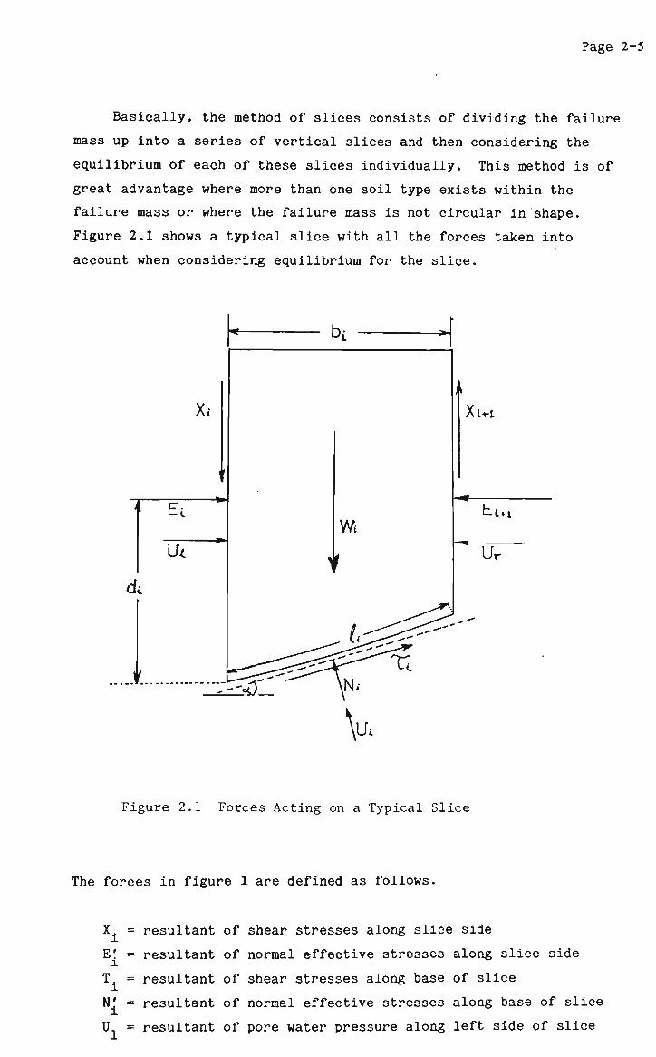
Basically, the method of slices consists of dividing the failure

mass up into a series of vertical slices and then considering the

equilibrium of each of these slices individually. This method is of

great advantage where more than one soil type exists within the

failure mass or where the failure mass is not circular in shape.

Figure 2.1 shows a typical slice with all the forces taken into

account when considering equilibrium for the slice.

Xc

Ei

Ui

<k

-*»

b_

Wi

X_H

Eu_

Ur

Figure 2.1 Forces Acting on a Typical Slice

The forces in figure 1 are defined as follows.

X. = l

E: = i

T. = l

N: = i u, =

resultant of shear stresses along slice side

resultant of normal effective stresses along slice side

resultant of shear stresses along base of slice

resultant of normal effective stresses along base of slice

resultant of pore water pressure along left side of slice

Page 2-6

°r ~ resultant of pore water pressure along right side of slice

UA = resultant of pore water pressures along base of slice

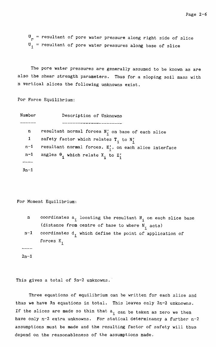
The pore water pressures are generally assumed to be known as are

also the shear strength parameters. Thus for a sloping soil mass with

n vertical slices the following unknowns exist.

For Force Equilibrium:

Number Description of Unknowns

n resultant normal forces N.' on base of each slice

1 safety factor which relates T. to N! 1 l

n-1 resultant normal forces, E' on each slice interface n-1 angles 0. which relate X. to E!

i i i

3n-l

For Moment Equilibrium:

n coordinates a locating the resultant N. on each slice base

(distance from centre of base to where N. acts)

n-1 coordinates d. which define the point of application of

forces E.

2n-l

This gives a total of 5n-2 unknowns.

Three equations of equilibrium can be written for each slice and

thus we have 3n equations in total. This leaves only 2n-2 unknowns.

If the slices are made so thin that a± c a n te taken as zero we then

have only n-2 extra unknowns. For statical determinancy a further n-2

assumptions must be made and the resulting factor of safety will thus

depend on the reasonableness of the assumptions made.

Page 2-7

The most usual assumptions made concern the forces that act

against the sides of the slices (interslice forces or sidewall

forces). Certain limitations exist on the way in which these

assumptions are made and acceptability criteria for solutions should

include the following:-

1. the shear forces on the sides of the slices cannot exceed the

shear resistance of the soil.

2. the normal side forces E. should fall within the central

third of the slice height.

There are some methods generally known as 'rigorous' methods in

which the aim is to satisfy all the statical equilibrium equations and

therefore suitable assumptions are made to achieve that aim while

satisfying reasonable acceptability criteria. However, there are a

number of well known methods which give reasonably 'correct' answers

for most problems although all statical equilibrium equations are not

satisfied (the word 'correct' is used here in the sense that the

answers are very close to those obtained with the so-called rigorous

methods in which all the equilibrium equations are satisfied). The

most widely used methods in both categories are discussed in the

following sub-sections.

2.1.1 The Fellenius Method or the Ordinary Method of Slices (also

known as the Swedish Method of Slices).

In this method the interslice or sidewall forces T and E are

ignored. In other words, the normal and tangential forces on the base

of each slice depend only on the slice weight.

Summing the forces normal to the base of the slice we obtain

N.' + Uf = W.cosa. (2.1) i i i i

or N.' = W.cosa. - U. i i l l

Page 2-8

= W.cosa. - u.l ,,, „v 1 1 1 (2.2)

For a circular surface of sliding the factor of safety is defined as

MR Moment of Resisting forces F = ___. = (2.3)

M^ Moment of Driving forces

where moments are taken about the centre of the failure arc.

For a non-circular surface of sliding however, the factor of

safety can be approximated as

SFD Sum of Resisting forces F = _ = (2.3a)

SF Sum of Driving forces

Therefore, again considering a circular surface of rupture, the

factor of safety F thus becomes equal to the ratio of the moment of

the shear strength along the failure surface to the moment of the

weight of the failure mass.

In equation (2.3) above the moments M and MR may be defined

as

n

^ = r J Wisinai <2-4)

and

r _

MD = r ̂ (c'+ffltantf') 1. in general, which can simplify to n _- i i

_»i

..

MD = r (c'L + tan0' / N.') for homogeneous soil. (2.5) R »r 1 «.»«

since Nf = a'.l. I i i

where r = radius of failure arc

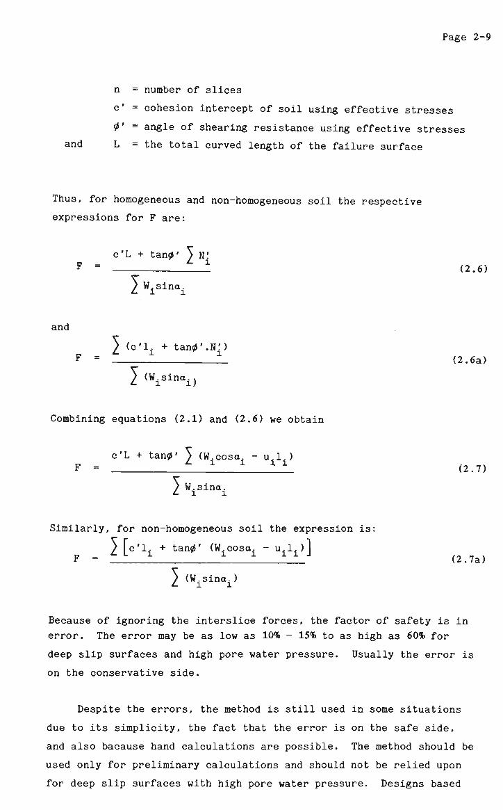
Page 2-9

n = number of slices

c' = cohesion intercept of soil using effective stresses

0' = angle of shearing resistance using effective stresses

and L = the total curved length of the failure surface

Thus, for homogeneous and non-homogeneous soil the respective

expressions for F are:

c'L + tan0' ^ N! F - (2.6)

2 W.sina.

and

> (c'l. + tan^'.Nf) F = L (2.6a)

$ (W.sina.,

Combining equations (2.1) and (2.6) we obtain

c'L + tan0' 3 (W.cosa. - u.l.) F = X X (2.7)

2 W.sina.

Similarly, for non-homogeneous soil the expression is:

> [c'l. + tan*.' (W.cosa. - u.l. )1 F = x (2.7a)

/ (W.sina.!

Because of ignoring the interslice forces, the factor of safety is in

error. The error may be as low as 10% - 15% to as high as 60% for

deep slip surfaces and high pore water pressure. Usually the error is

on the conservative side.

Despite the errors, the method is still used in some situations

due to its simplicity, the fact that the error is on the safe side,

and also bacause hand calculations are possible. The method should be

used only for preliminary calculations and should not be relied upon

for deep slip surfaces with high pore water pressure. Designs based

Page 2-10

on this method may be highly conservative and, in some cases, the

results can be very misleading.

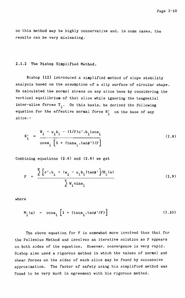
2.1.2 The Bishop Simplified Method.

Bishop [12] introduced a simplified method of slope stability

analysis based on the assumption of a slip surface of circular shape.

He calculated the normal stress on any slice base by considering the

vertical equilibrium of that slice while ignoring the tangential

inter-slice forces T... On this basis, he derived the following

equation for the effective normal force N! on the base of any

slice:-

W. - u.b. - (1/F)c'.b.tana N! = X 1 1 1 (2.8) l ' cosa. jl + (tana. .tan0')/F|

Combining equations (2.6) and (2.8) we get

5 fc'.b. + (w. - u.b.)tan0'l/M.(a) F = L L 1 in J * (2.9)

/ W.sina. L l I

where

M.(a) = cosa. [l + (tana. .tan<_ '/F) ] (2.10)

The above equation for F is somewhat more involved than that for

the Fellenius Method and involves an iterative solution as F appears

on both sides of the equation. However, convergence is very rapid.

Bishop also used a rigorous method in which the values of normal and

shear forces on the sides of each slice may be found by successive

approximation. The factor of safety using his simplified method was

found to be very much in agreement with his rigorous method.

Page 2-11

The Bishop simplified method gives values of F within the range

given by rigorous methods except for deep failure circles when F is

less than one. In cases where deep failure occurs the angle a of the

slice base near the toe of the slope becomes negative. From the above

equations it can be seen that when a is negative the denominator of

equation (2.8) can become negative or zero, leading to errors or

computational difficulties.

In order for the solution obtained by Bishop's simplified method

to be regarded as an admissible solution the factor of safety against

sliding on the vertical sections should also be satisfactory.

Bishop also suggested that for cases where errors have already

been introduced into the estimate of stability by testing and sampling

procedures then the approximate method will suffice but in cases where

considerable care is exercised at each stage then a more rigorous

method may be necessary.

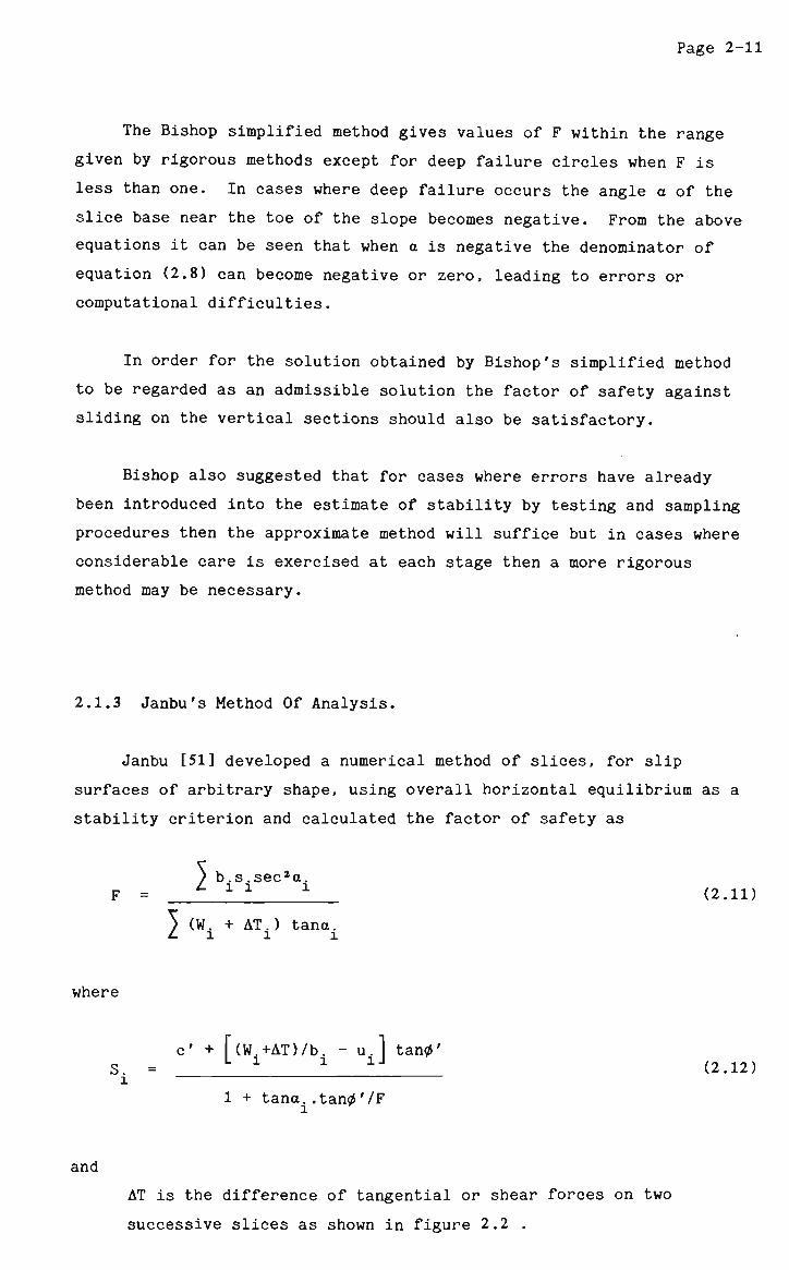
2.1.3 Janbu's Method Of Analysis.

Janbu [51] developed a numerical method of slices, for slip

surfaces of arbitrary shape, using overall horizontal equilibrium as a

stability criterion and calculated the factor of safety as

/ b.s.sec2a. F = X X 1 (2.11)

^ (W. + AT.) tana. _ l i i I

where

c' + [(W.+AT)/b. - u.] tan0' S. = (2.12) l

1 + tana..tan^'/F

and

AT is the difference of tangential or shear forces on two

successive slices as shown in figure 2.2 .

Page 2-12

T+AT

E+AE W

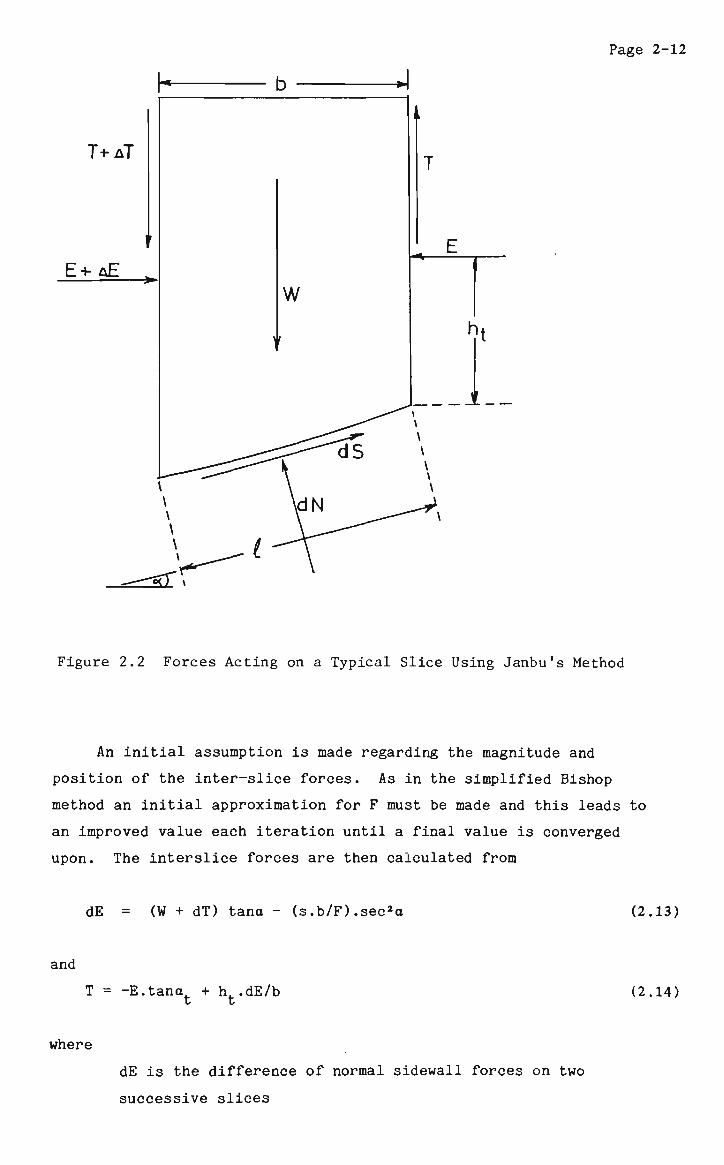
Figure 2.2 Forces Acting on a Typical Slice Using Janbu's Method

An initial assumption is made regarding the magnitude and

position of the inter-slice forces. As in the simplified Bishop

method an initial approximation for F must be made and this leads to

an improved value each iteration until a final value is converged

upon. The interslice forces are then calculated from

dE = (W + dT) tana - (s.b/F).sec2a (2.13)

and

T = -E.tana + h..dE/b (2.14)

where

dE is the difference of normal sidewall forces on two

successive slices

Page 2-13

and a and h define the direction and position of the

line of thrust.

The procedure is then repeated until two consecutive iterations yield

almost identical results. Janbu gave a simplified version of his

method which does not require iterative calculations.

A check must be made to ensure that the position of the line of

thrust is not such that tension is implied in a significant portion of

the sliding mass. If this is so then the solution may not be

acceptable.

The big advantage of the Janbu method over other exact methods

such as the Morgenstern-Price method is the simplicity of the

calculations and the fact that a computer is not always necessary. A

disadvantage, however, is that while Janbu's numerical solution can be

applied to elongated shallow slip surfaces, it is in error when

applied to deep slip surfaces. This is especially the case with

Janbu's simplified method. Janbu's method considers the force and

moment equilibrium of every single slice but for the sliding mass as a

whole it considers only force equilibrium and remains unbalanced for

moments (as shown by Nonveiller [70]).

Janbu's simplified method is easier to use but correction factors

are required to be applied depending on the geometry of the slip

surface. The multiplying factor is 1.0 for very shallow slip surfaces

and as high as 1.2 for deep slip surfaces.

2.1.4 The Morgenstern-Price Method.

The method of analysis of Morgenstern and Price, being very

complex and involving a large number of equations, is not presented

here in any detail. Full descriptions of the method are given by

Morgenstern and Price [68], Hamel [45] and Chowdhury [29]. However, a

very brief description of the method is given here to allow

comparisons with the methods already described.

Page 2-14

In order to make the problem statically determinate, an

assumption is made by Morgenstern and Price regarding the relationship

between the normal force on the side of any slice, E., and the shear

force on the same slice side, T.. This relationship is assumed as

follows

T = J..f(x).E (2.15)

where X. = a constant parameter to be determined from the solution

and f(x) = an arbitrary specified function

Moment equilibrium is considered about the base of each slice, i,

assuming that each slice is very thin. Conditions of equilibrium are

applied in the directions normal and tangential to the base of the

slice. Combining these equations with the Coulomb-Terzaghi failure

criterion will then lead to a further set of equations. A number of

linear and polynomial approximations are then made within each slice

to give an expression in terms of dE/dx and x. Integrating this

equation over a slice from x. _.,„__ _„ __,,,..,___,<_.,.._ *>_.», v 1 gives an expression tor h.

Combining equations (2.15) and the above mentioned equation for

moment equilibrium about the slice base and integrating with respect

to x gives an expression for M, the moment about the slice base.

Using the boundary conditions an iterative procedure is started where

assumed values of X and F are needed to calculate E and M at the end

of the first slice. This leads to values of E and M for each slice.

The procedure is repeated until equations (2.16) are satisfied and the

correct values of X and F are thus found. A computer is essential to

obtain this solution.

E(x-) = 0, M(xn) = 0, E(x ) = 0, M(x ) = 0 (2.16) u o m m

As stated earlier, the Morgenstern-Price method, unlike the

methods previously mentioned, satisfies all conditions of statical

equilibrium, although the results are still dependent on the

assumptions made i.e. (a) the fact that X is assumed constant, and

(b) the form of the function f(x) which is specified by the user.

Page 2-15

2.2 GENERAL COMMENTS ON LIMIT EQUILIBRIUM METHODS OF ANALYSIS.

As has been noted earlier in this chapter, some limit equilibrium

methods, including the ordinary method of slices, Bishop's simplified

method, and the wedge method do not satisfy all the conditions of

equilibrium. Wright, Kulhawy and Duncan [113] pointed out, as have

many other authors, that most equilibrium methods involve the

assumption that the factor of safety is the same for each slice even

though this is not really true except at failure when F = 1. Because

the soil is assumed to behave as a perfectly plastic or rigid plastic

material, limit equilibrium methods of analysis would not be expected

to simulate the actual behaviour of slopes except perhaps at failure

when, as mentioned above, the factor of safety is equal to unity.

Ching and Fredlund [25] pointed out a number of difficulties or

limitations when using limit equilibrium methods of analysis. These

problems arise mainly in the numerical procedure as a result of the

interslice force assumptions and geometric conditions imposed on the

stability computations. These difficulties are summarised as

follows:-

(a) When the variable m approaches zero or becomes negative,

unreasonable normal forces and misleading results may be

computed. The solution is to restrict inclinations of the

slip surface to values indicated by classical earth pressure

theory.

(b) In highly cohesive slopes, negative normal forces (indicating

tension) can be computed thus causing uncertainties in the

results. This is particularly true in relatively shallow

slices. The solution is to assume a tension crack zone.

(c) Convergence problems can arise as a result of using an

inappropriate interslice force function. The solution is to

use a side force assumption more consistent with the geometry

of the slope and the stress distribution within the soil

mass.

Page 2-16

Wright, Kulhawy and Duncan [113] developed a stability analysis

methodology using internal stresses determined by performing finite

element analyses. For a number of slopes with wide variations in

geometry and shear strength parameters they investigated the

following:-

1. the variations of normal stress and factor of safety along

the shear surface.

2. the overall factor of safety for each slope.

Since they simulated only built-up slopes, no assumption was necessary

in respect of initial stress states. This would have been necessary

for excavations or natural slopes. Using the Bishop's simplified

method for comparison, they concluded as follows.

1. Normal stress distributions were very nearly the same for

flat slopes and large values of X _,

where X = (y.H.tan0)/c

and where H = slope height

and y = unit weight of soil

2. Although the variations of normal stress and factor of safety

along the shear surface are not the same, in general the

average values of F were very nearly the same. For all cases

studied, the difference was found to be between 0% and 8% .

3. Since the two methods involve a substantially different

approach, the close agreement in F indicates that the

assumptions involved in Bishop's simplified method (and thus

Janbu's method and Morgenstern and Price's method) do not

lead to large errors in comparison to a method in which

stresses are computed exactly by the versatile finite element

method.

Fredlund [44] presented a review of general limit equilibrium

theory and discussed and compared a number of well-known methods of

analysis including those mentioned above. He gave comparisons of

Page 2-17

calculated factors of safety using the various methods. Fredlund also

stated that limit equilibrium methods fall short of a complete

solution in that no consideration is given to kinematics and that

equilibrium conditions are only satisfied in a limited sense (e.g.

failure conditions are not ensured at the interslice surfaces).

In conclusion, although limit equilibrium methods of stability

analysis have certain limitations (e.g. inability to calculate

strains and deformations), their simplicity and ease of use compared

to finite element or probabilistic methods certainly keep them among

the most widely used of all stability analysis methods. These methods

are especially welcome in the more practical situations where users do

not always have the necessary expertise required for complex methods.

Also, as has been mentioned above, the error involved in using limit

equilibrium methods of analysis is not great and is usually on the

safe side. This is especially true of the more rigorous methods such

as the Morgenstern-Price method, the Janbu method, and in some cases

the Bishop simplified method. The bulk of the research in this thesis

was based on the limit equilibrium concept of analysis. Methods

mentioned previously have been used as a basis for the relevant

developments. These methods are:-

1. the Bishop Simplified method, and

2. the Morgenstern-Price method.

CHAPTER 3

PROGRESSIVE FAILURE AND THE CONCEPT OF RESIDUAL STRENGTH.

3.1 GENERAL.

This chapter is devoted to a discussion of the concepts which

have been introduced to understand the progressive failure of soil

slopes. Attention has been drawn to previous studies concerning the

significance of soil brittleness and residual shear strength.

Different analytical approaches involving simulation of local failure

and stress redistribution are discussed in chapter 5.

Conventional methods of stability analysis described in the

previous chapter are usually adequate for most cases of slope

analysis. However, analyses by various authors have shown that in

many instances conventional methods of analysis do not adequately

explain failures which have already occured and predictions of failure

or stability may not be successful. There are a number of recorded

cases of failures in slopes where the factor of safety calculated by

conventional methods of analysis prior to failure was greater than

one.

For a slope in a perfectly plastic material (e.g. rigid-plastic

or even elastic-plastic) limit equilibrium methods would be expected

to prove highly reliable. However, real soils behave in ways which

show marked departures from the assumption of perfect plasticity.

Most soils are strain-softening to some degree and many soils exhibit

a 'brittle' behaviour in undrained or drained deformation or both.

Therefore, there may be discrepancies in the results of limit

equilibrium studies. Often these discrepancies can be attributed to

progressive failure phenomena.

Page 3-2

In comparison to limit equilibrium methods, the finite element

method can be used to obtain valuable information on the state of

stresses and strains within the soil mass. It does not, however, show

directly the stability condition of the slope. On the other hand,

limit equilibrium methods give a factor of safety as a direct measure

of the stability of the slope but fail to account for the constitutive

relationships of the soil or the effects of initial stresses.

In all problems of slope stability, bearing capacity and earth

pressure, even in ideally homogeneous soils, the state of limiting

equilibrium is associated with a non-uniform mobilization of shearing

resistance and thus with progressive failure (e.g. Bishop [13],

Taylor [80]). Moreover, progressive failure should be considered not

only in its spatial manifestation but also as a time-dependent

process.

Bjerrum [18] also attributed certain slope failures to processes

involving some mechanism of progressive failure. He pointed out cases

of slides in weathered clay where the average shear stress along the

failure surface due to gravity force was much less than the shear

strength of the clay. Such a slide would have occured along a slip

surface which was already formed and on part of which the shear

strength was less than the peak. The slip plane must thus be formed

by progressive failure preceeding the actual slide (the existence of

pre-existing slip surfaces had been ruled out on the basis of

investigation and consideration of geotechnical and geological

factors). Bjerrum stated that as the shear stresses due to gravity

force are lower than the shear strength, a progressive failure can

only be explained by taking into account the internal stresses in the

mass.

Chandler [24] cited case records which demonstrate that

post-excavation pore pressure recovery in London clay and other

heavily overconsolidated clays may involve a time period of many

years, consistent with low values of coefficient of swelling.

Therefore, the process of swelling is a major contributory factor in

the occurrence of delayed failures in cutting slopes of brown London

clay in cases where time delays prior to failure are less than or

equal to 50 years. Beyond that period, long term pore pressures have

Page 3-3

become established and other factors must control the occurrence of

slope failures.

3.2 DEFINITIONS OF PROGRESSIVE FAILURE.

As early as 1936 Terzaghi [105] presented a definition of

progressive failure in which he implied that the time element was

necessary for progressive failure to occur. Later (1948) Terzaghi and

Peck [106], Taylor [80] and (in 1967) Bishop [13] appeared to consider

progressive failure in the context of a spreading of failed or

overstressed zones in space. The definition given by Terzaghi and

Peck [106] is presented here in detail as follows. "The term

progressive failure indicates the spreading of the failure over the

potential surface of sliding from a point or line towards the

boundaries of the surface. While the stresses in the clay near the

periphery of this surface approach the peak value, the shearing

resistance of the clay at the area where the failure started is

already approaching the much smaller 'ultimate' value. As a

consequence the total shearing force that acts on a surface of sliding

at the instant of complete failure is considerably smaller than the

shearing resistance computed on the basis of the peak values."

James [50] defined progressive failure as a simultaneous (or

quasi-simultaneous) decay in both the c' and the 0' parameters

preceding actual failure. Lo [60], however, defined progressive

failure as the process of successive failure of individual soil

elements in a soil mass. This process spreads in space and requires

time to occur. While time aspects may not always be important under

some conditions, an understanding of spatial progression of failure is

most essential.

3.3 RESIDUAL STRENGTH.

In his studies on the long-term stability of clay slopes,

Skempton [88] stated that as clay is strained, it builds up an

Page 3-4

increasing shearing resistance. Under a given effective pressure,

however, there is a definite limit to the resistance a clay can offer

and this is the peak strength s . If displacement is continued the

resistance, or strength, of the clay decreases and this 'strain

softening' continues until a certain 'residual strength' s is

reached. The decrease of shear strength to a residual value is

associated with relative displacements along a slip plane or

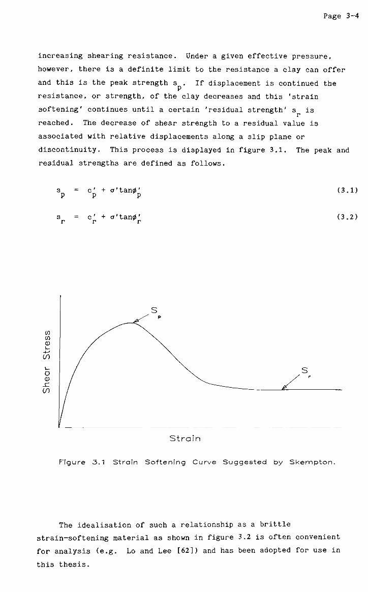
discontinuity. This process is displayed in figure 3.1. The peak and

residual strengths are defined as follows.

c' + cr'tantf' P P

(3.1)

c' + or'tan̂ ' r r

(3.2)

00

__

c/. l_-

o XL if)

Strain

Figure 3.1 Strain Softening Curve Suggested by Skempton.

The idealisation of such a relationship as a brittle

strain-softening material as shown in figure 3.2 is often convenient

for analysis (e.g. Lo and Lee [62]) and has been adopted for use in

this thesis.

Page 3-5

to tn i _

V)

© _c CO

Strain

Figure 3.2 Idealised Strain Softening Curve Suggested by Lo 8c Lee.

Skempton [88] noted that during the shearing process,

over-consolidated clays tend to expand, expecially after passing the

peak. Part of the drop in strength is due to an increase in water

content. Thin bands or domains are developed in which the flakey clay

particles are orientated in the direction of shear and the strength is

further reduced. Skempton also suggested that the residual strength

of a clay, under any given effective pressure, is the same whether the

clay has been normally or over-consolidated. Thus 0' should

be the same for normally or over-consolidated clay (as shown in figure

3.3).

Skempton [89] stated that for a certain clay, the moisture

content at its 'critical state' is the same no matter what its

consolidation history was. After this critical state is reached, no

amount of deformation will alter the moisture content (constant stress

and volume are attained). The 'critical state' corresponds to the

strength of a normally consolidated clay. It is possible in some

over-consolidated clays that a more aggressive reduction in strength

occurs before first-time slides take place, as against the very small

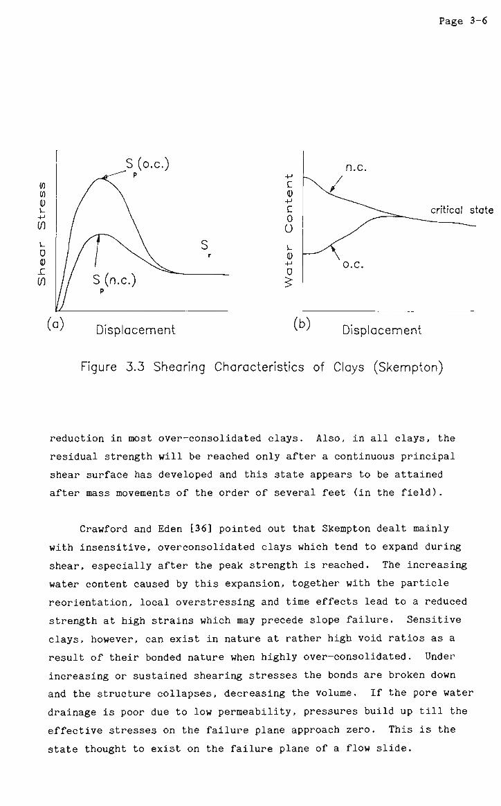
Page 3-6

critical state

Displacement Displacement

Figure 3.3 Shearing Characteristics of Clays (Skempton)

reduction in most over-consolidated clays. Also, in all clays, the

residual strength will be reached only after a continuous principal

shear surface has developed and this state appears to be attained

after mass movements of the order of several feet (in the field).

Crawford and Eden [36] pointed out that Skempton dealt mainly

with insensitive, overconsolidated clays which tend to expand during

shear, especially after the peak strength is reached. The increasing

water content caused by this expansion, together with the particle

reorientation, local overstressing and time effects lead to a reduced

strength at high strains which may precede slope failure. Sensitive

clays, however, can exist in nature at rather high void ratios as a

result of their bonded nature when highly over-consolidated. Under

increasing or sustained shearing stresses the bonds are broken down

and the structure collapses, decreasing the volume. If the pore water

drainage is poor due to low permeability, pressures build up till the

effective stresses on the failure plane approach zero. This is the

state thought to exist on the failure plane of a flow slide.

Page 3-7

Bishop [16] indicated that residual strength should correspond to

extremely large displacements within the soil mass. Lo and Lee [63],

however, used the term residual strength to designate the slowly

decreasing strength in the post-peak range corresponding to moderately

large displacements in the field. From back analyses of landslides

involving Lias clay Chandler [23] found that residual strength

decreases with increasing normal stress.

Tavenas and Leroueil [101], while investigating cuts in slopes,

suggested that the residual strength situation is only relevant to the

case of failure along a pre-sheared sliding surface.

3.4 CONDITIONS NECESSARY FOR PROGRESSIVE FAILURE.

At this stage it is necessary to consider the conditions under

which progressive failure is most likely to occur . Skempton and

LaRochelle [66] suggested that fissures in the soil may adversely

influence the strength of heavily over-consolidated clays and shales

in the following ways.

1. Open fissures may form portion of the failure surface across

which the shear resistance is zero.

2. Closed fissures may form portion of the failure surface

across which only the residual strength is mobilised.

3. Fissures (closed or open) adversely influence stresses within

the slope. This increases the likelihood of progressive

failure.

Also, open fissures might increase the rate of swelling and stress

redistribution.

Bjerrum [18] concluded that the development of a surface of

sliding by progressive failure is possible in over-consolidated

plastic clays provided the following conditions are satisfied.

Page 3-8

(a) internal lateral stresses are large enough to cause stress

concentrations in front of an advancing sliding surface,

where the shear stresses are greater than the peak shear

strength.

(b) the clay contains a sufficient amount of recoverable strain

energy to produce the neccessary expansion of the clay in the

direction of sliding to strain the clay in the zone of

failure.

(c) the residual shear strength is relatively low compared with

the peak shear strength.

Skempton and Petley [96] showed that for tests performed on

over-consolidated clays, the strength along principal slip surfaces in

landslides and tectonic shear zones, is at, or very close to, the

residual. Along minor shears, however, with somewhat irregular

surfaces on which the relative movements have been small, the strength

is appreciably above the residual.

Since residual conditions are reached slightly more rapidly under

low stress levels than under high, Peck [71] and James [50],

hypothesized that in larger landslides the slip zones in the toe area,

will exhibit a lower strength than further back into the slipping

mass, where the stress level is higher. Lo and Lee [62] stated that

conditions pertinent to the occurrence of progressive failure in

slopes are

(a) brittleness of soil

(b) non-uniformity in distribution of shear stresses and

sometimes

(c) deterioration of strength with time due to softening, change

of ground water conditions or rheological effects.

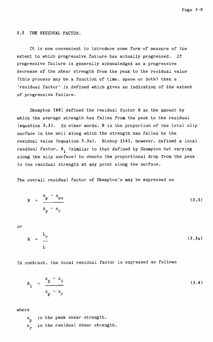
Page 3-9

3.5 THE RESIDUAL FACTOR.

It is now convenient to introduce some form of measure of the

extent to which progressive failure has actually progressed. If

progressive failure is generally acknowledged as a progressive

decrease of the shear strength from the peak to the residual value

(this process may be a function of time, space or both) then a

'residual factor' is defined which gives an indication of the extent

of progressive failure.

Skempton [88] defined the residual factor R as the amount by

which the average strength has fallen from the peak to the residual

(equation 3.3). In other words, R is the proportion of the total slip

surface in the soil along which the strength has fallen to the

residual value (equation 3.3a). Bishop [14], however, defined a local

residual factor, R (similar to that defined by Skempton but varying

along the slip surface) to denote the proportional drop from the peak

to the residual strength at any point along the surface.

The overall residual factor of Skempton's may be expressed as

R = J J^ (3.3)

s - s p r

or L

R = r (3.3a)

In contrast, the local residual factor is expressed as follows

Ri

s - s.

JP I (3.4) s - s p r

where

s is the peak shear strength,

s is the residual shear strength, r

Page 3-10

si is the actual shear strength at point i,

sav is the average shear strength along the slip surface,

L is the total length of the slip surface, and

Lr i s fcbe length of slip surface over which the shear strength has

fallen to the residual value.

3.6 REDUCTION OF SHEAR STRENGTH.

Skempton [88], [89] made the following comments on the role of

strength reduction in progressive failure with particular reference to

his investigation of slides in London clay:

(a) After a slide has taken place, the shear strength of soil

along the slip surface is equal to the residual value.

(b) First-time slides in slopes in non-fissured clays correspond

to strengths only slightly less than the peak.

(c) First-time slides in fissured clays correspond to strengths

well below the peak.

(d) Some form of progressive failure must be operative to take

the clay past the peak. Possibly, a non-uniform stress to

strength ratio along the slip surface or fissures acting as

stress concentrators and leading to a softening of the clay

mass may be responsible.

(e) In natural slopes in London clay the strength had fallen to

the residual value.

(f) On pre-existing shear surfaces the residual strength obtains.

Skempton and Hutchinson [94] analysed the stability of structures

and natural slopes in the London clay and concluded that the strength

of highly over-consolidated, fissured clays dropped to the normally

consolidated value. That is, the effective cohesion approached zero

Page 3-11

as a consequence of open fissures and the softening effect facilitated

by the fissures.

Bjerrum [19] suggested that the combined effect of weakening and

softening could be taken into account by assuming that the cohesion

intercept would approach zero while the friction angle would remain

the same as for an intact clay. This concept was also invoked by

James [50] who found that the loss in strength before actual failure

was almost entirely due to a loss in terms of the parameter c' as

suggested originally by deLory [39] and quoted by Skempton [89].

During this phase the value of parameter #' remains at, or very

near to, the peak value since the effect of weathering on this

parameter within engineering time scales is generally negligible.

Skempton [91] stated that the post-peak drop in drained strength

of an intact overconsolidated clay may be considered as being due,

firstly, to an increase in water content (dilatancy) and secondly, to

re-orientation of clay particles parallel to the direction of

shearing. In normally consolidated clays, the post-peak drop in

strength is due entirely to particle re-orientation.

Rivard and Lu [78] calculated factors of safety close to 1.0

based on measured embankment and foundation strengths and observed

pore pressures thus strengthening the case for the use of normally

consolidated strength for soils with structural discontinuities. In

addition to the presence of structural discontinuities, softening of

the clay may be a contributing factor in reducing the strength to the

normally consolidated value. These structural discontinuities are

difficult to observe in soft clays, whereas they are readily apparent

in stiff soils, thus in soft clays special attention should be devoted

to searching for structural defects.

Skempton [88] said that in clays where no fissures or joints

exist the decrease in strength from the peak to the residual state is

small or even negligible. However, much of his research experience

was with cuttings in fissured London clay and he did not analyse many

examples of failures in intact or non-fissured clays. He did

emphasise that, if failure has already occurred, any subsequent

movements on the existing slip surface will be controlled by the

Page 3-12

residual strength, no matter what type of clay is involved.

From tests carried out on overconsolidated blue marl,

Sotiropoulos and Cavounidis [97] suggested the possibility that

'portions of clayey soil mass, when sheared, may pass to the softening

side of the stress-strain curve without ever reaching the peak

strength of the material exhibited by different portions of the same

mass'. They further suggested that this behaviour may be due to the

existence of small, non-apparent fissures. In relating this type of

behaviour to the process of progressive failure, Sotiropoulos and

Cavounidis concluded that 'if part of a clay slope is characterised by

this behaviour, a slide may be initiated without the shear stress

exceeding what normally would be expected to be the peak strength

value'.

3.7 MECHANISMS OF PROGRESSIVE FAILURE.

3.7.1 General Notes On Progressive Failure Mechanisms.

Taylor [80], while considering primarily the shearing resistance

of sands in an effective stress context, associated progressive

failure with the redistribution of shear stress along a potential

failure surface. No mention was made, however, regarding the

direction of propagation of progressive failure. Thomson and Tweedie

[107], while investigating the Edgerton landslide found strong

evidence to suggest that failure was progressing from a scarp at the

top of the slide down towards the toe. Field evidence indicated that

the lower part of the failure surface had reactivated an old failure

surface, whereas the scarp area represented a first-time slide.

Analyses of the failure indicated that residual angles of shearing

resistance were being mobilised along the other, pre-sheared part of

the failure surface due to old landslides. Along the latter portion

of the failure surface the soil parameters yielding the most

reasonable factor of safety were a peak angle of shearing resistance

and a cohesion very much less than that determined from laboratory

testing.

Page 3-13

Wilson [111], in field studies aimed at investigating the

mechanisms associated with progressive ground movements, made a number

of important observations. Using inclinometers to measure relative

displacements, he found that in progressive landslides in excavated

slopes, failure tended to start at the toe of the slope, progressing

upwards to the crest. In slides where fill is added to the upper part

of the slope, however, Wilson found that the opposite happens and

rupture develops and progresses downwards from the crest to the toe of

the slope.

Peck [71] presented the results of a series of tests carried out

by R.J.Conlon on clays from Winnipeg in the bed of old glacial lake

Agassiz and his important observations concerning progressive failure

(based on these results) are summarised below.

Assuming that failure occurs along a circular arc with no

deformation or distortion of the sliding mass, relative deformations

can be achieved along the failure surface, of sufficient magnitude for

shear strength to drop to a residual value. The peak shear strength

obviously cannot be mobilised simultaneously along the surface of

sliding because normal pressure varies along the surface of sliding

and the strain necessary to reach the peak strength depends on the

normal pressure (see figure 3.4).

In as much as real soils are deformable and compressible, the

displacement along the surface of sliding is not uniform from one end

to the other. Near the upper portion of the surface, the shearing

forces are somewhat greater than the shearing resistances

corresponding to any amount of deformation. Therefore, the support of

slices along the upper surface of sliding requires the development of

forces between slices. Part of the load is transferred down the mass

through inter-slice forces. Part is carried by the tensile resistance

between the slices and those higher up. The transfer of the load from

the upper slices to those below involves a compressive strain roughly

parallel to the slope.

Conlon set forth a quantitative procedure for estimating the

available shearing resistance along the surface of sliding. He took

the shearing resistance on the upper portion of the failure surface

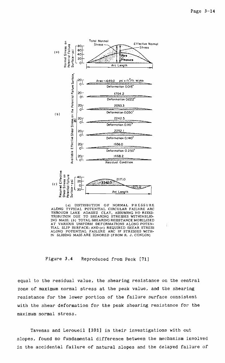
Page 3-14

ta — —

i n\ Z O -I

t°) — U. Q 0. — I

- .9 « O — O

E c 5 _:*••_: O 5 3 Z _L 0.

80

60

40

20

0

Total Normol Stress Effective Normal

Stress

(b)

J.

-O „, ">£__

CO

-

.? <J a

LJ

« J3

r20 "(" Areo = 1649.0 psi x ft/ft. Width Q[_ _JI '...'.. v.' ..'..•; '•••;••".. t i • • -

Deformation 0.015"

20

"r 0L

20r 0 L

T OL 20,

20

20r ii __r 9 L ftL

1754.2 v.i.'.' •••'•'•:

[

I

DeformotionOC22"

2053.3 -n. ' •:...'."•••,-.••>

Def ormotioo 0.050

20r 2242.5 . . . I I j

DeformotionO.IIO*

2252.1 T.\'.'.>f.'.'.::'.'•.'}.'...•.:-• I . . . i i n i • • 1 1 1

Deformation 0.140"

1936.0

Deformation 0.250"

1468.2

Residual Condition

..J £ —

lC' -D - - I

•3 s I i. L 2° a: co d. o.

(a) DISTRIBUTION O F NORMAL P R E S S U R E ALONG TYPICAL POTENTIAL CIRCULAR FAILURE ARC THROUGH LAKE AGASSIZ CLAY. ASSUMING NO REDISTRIBUTION DUE TO SHEARING STRESSES WITHIN SLIDING MASS; (ft) TOTAL SHEARING RESISTANCE MOBILIZED AT VARIOUS UNIFORM DEFORMATIONS ALONG POTENTIAL SLIP SURFACE; AND (c) REQUIRED SHEAR STRESS ALONG POTENTIAL FAILURE ARC IF STRESSES WITHIN SLIDING MASS ARE IGNORED (FROM R. J. CONLON)

Figure 3.4 Reproduced from Peck [71]

equal to the residual value, the shearing resistance on the central

zone of maximum normal stress at the peak value, and the shearing

resistance for the lower portion of the failure surface consistent

with the shear deformation for the peak shearing resistance for the

maximum normal stress.

Tavenas and Leroueil [101] in their investigations with cut

slopes, found no fundamental difference between the mechanism involved

in the accidental failure of natural slopes and the delayed failure of

Page 3-15

cut slopes.

Athanasiu [4] proposed a method of slope stability analysis

whereby the non-linear stress-strain behaviour of the soil adjacent to

the sliding surface can be simulated. He considered only horizontal

forces on each side of the slices in the soil mass. Before failure,

the state of stresses could be approximately described by the

horizontal forces (which remain larger than the vertical ones).

Assuming failure to start by a discontinuity in the slope (resulting

in the removal of lateral support) his results show that this release

of horizontal stresses at the toe of the slope induces shear stresses

on the slip surface leading to progressive shear strength

concentration and release, meaning progressive failure.

3.7.2 Bjerrum's Comments On The Mechanism Of Progressive Failure.

Bjerrum [18] stated that, in the process of progressive failure

in slopes in unweathered clay, when a slip face has developed over a

certain length and the resistance against horizontal displacement of

the whole block above the slip plane has been reduced so much, that it

cannot resist the active earth pressure of the soil mass above,

progressive failure will develop into a massive slide. In excavations

in deep deposits of heavily over-consolidated plastic clays, the

progressive failure can also start as follows.

When an excavation is made, a reduction in the overburden

pressure will occur and the ratio of horizontal to vertical stress

will increase in the clay beneath the bottom of the excavation. "At a

certain depth of the excavation, this ratio can exceed the critical

value at which shear stress equals peak shear strength and a passive

shear failure will occur. This results in a heave at the bottom of

the excavation, followed by a horizontal movement of the clay next to

the excavation. This causes a decrease in the horizontal thrust of

the clay, leading to a local concentration of shear stresses in the

clay beneath the slope. If these shear stresses exceed the peak shear

strength, progressive failure will proceed and finally, a continuous

failure surface will be formed." In both of the above cases, the

Page 3-16

movement of the slope will be predominantly horizontal. Refer to

figure 5.1 in chapter 5.

3.7.3 Skempton's Approach To Progressive Failure.

Skempton [88], modified his earlier ideas that the strength along

the slip surface at the time of failure, is at some places peak and

some places residual, the point of demarcation being described by

Skempton's residual factor. He argued that stiff, fissured clays

possibly undergo a loss in strength in cuttings, tending towards the

fully softened value which may be regarded as approximately equal to

the ultimate value of the soil in the normally consolidated state.

The softened strength is also approximately equal to the critical

state strength. In such clays, there must be a mechanism of

progressive failure and/or softening which takes them past the peak

and just before a first-time slide occurs, there is a softened shear

zone with many minor shears. Some over-consolidated clays may exhibit

a more aggressive reduction in strength, before a first-time slide

takes place.

Residual strength is only reached (in all clays), after a

continuous principal shear surface has developed, corresponding to

mass movements in the order of several feet in the field. Skempton

[90] later confirmed some of his earlier findings and made further

comments as follows.

1. The shear strength of brown London clay for first-time slides

is considerably less than the peak, so some progressive

failure mechanism appears to be involved.

2. The in-situ strength is given approximately by the 'fully

softened' value and also by the lower limit of the strength

measured on structural discontinuities.

3. The residual strength is much smaller than this. Residual

strength is mobilised after the slip has occured and large (1

to 2 metres) displacements have taken place.

Page 3-17

4. Slides in London clay generally occur many years after the

cutting is made.

The main reason for this last point is the very slow rate of pore

pressure equilibration, despite the fissured structure of the clay.

That is, when a cutting is made, the mass of overlying soil is

decreased, which leads to an immediate reduction in pore pressure due

to the development of negative excess pore pressure. It had been

postulated earlier that, due to the presence of fissures, the pore

pressures would very rapidly increase to equilibrium values. However,

this is not so. Detailed studies based on field observations of pore

water pressure over many years (at sites where piezometers have been

installed) revealed (Skempton [90] ) that, in some slopes, negative

pore pressures still existed many years after cutting and that pore

pressure equilibrium was not reached for decades. Therefore, the

presence of fissures does not necessarily lead to a high value of soil

mass permeability in the field. It may be that the fissures are not

perfectly inter-connected for drainage to occur.

3.7.4 Bishop's Approach To Progressive Failure.

Bishop [13] postulated that, in a short-term analysis in terms of

undrained strength, failure may be expected to commence within the

soil mass and propagate towards the surface in both directions. In a

long-term analysis, where effective strength parameters are used and

the shear strength is a function of normal stress, this failure might,

in contrast, be expected to begin at the surface, possibly, at both

toe and crest and propagate inwards into the soil mass (see case 2 in

figure 3.5). Detailed case studies were, however, not analysed.

It should be noted that in the case of a cut or natural slope,

the stresses and hence the initiation of progressive failure will be

influenced by the state of stress in the ground before excavation or

before erosion.

Page 3-18

Associated with the limiting or critical equilibrium state

leading to the first-time sliding of a slope in overconsolidated soil,

Bishop [14] proposed that for some part of the slip surface the

drained peak strength will be mobilised while the post-peak and

pre-peak strengths will be operative over the remainder of the slip

surface. A small further displacement will then bring the whole

surface into the peak and post-peak states. At this point of complete

failure the strength at all points will lie between the two limits of

the peak and residual states.

As mentioned earlier in this chapter. Bishop proposed a local

residual factor R which varies along the slip surface and which

denotes the proportional drop from the peak to the residual strength

at any point along the surface. The shear strength mobilised at a

point on the failure surface may be represented using Bishop's local

residual factor, by the following expression

s = s - R_(s -s ) (3.5) P 1 p r

It is noted that a local residual factor of zero implies a

mobilised shear strength equal to the peak value whereas a local

residual factor of one implies a mobilised shear strength equal to the

residual value. The distribution of R. varies along the rupture

surface and actual values in practice are mainly speculative.

Although some part of the surface must have an R, value of zero, it

is less certain that some part exists where R. equals one especially

in first-time slides.

Ring shear tests on undisturbed samples of London clay have shown

that while the initial drop in strength is rather rapid, relative

displacements of earth masses of the order of 30 centimetres are

required before residual strengths are approached. However, tests in

the laboratory may not be an effective method of determining the

strains and deformations required to decrease shear strength to

residual values. The determination of the distribution of R based

on laboratory tests is also difficult with the equipment and

techniques available at the present time. Bishop considered the two

distributions shown in figure 3.5. One distribution implies

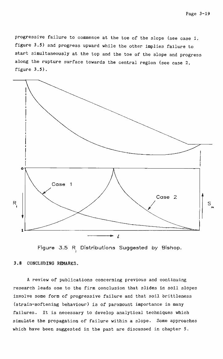
Page 3-19

progressive failure to commence at the toe of the slope (see case 1,

figure 3.5) and progress upward while the other implies failure to

start simultaneously at the top and the toe of the slope and progress

along the rupture surface towards the central region (see case 2,

figure 3.5).

•" I

Figure 3.5 R Distributions Suggested by Bishop.

3.8 CONCLUDING REMARKS.

A review of publications concerning previous and continuing

research leads one to the firm conclusion that slides in soil slopes

involve some form of progressive failure and that soil brittleness

(strain-softening behaviour) is of paramount importance in many

failures. It is necessary to develop analytical techniques which

simulate the propagation of failure within a slope. Some approaches

which have been suggested in the past are discussed in chapter 5.

CHAPTER 4

SIMULATION OF VARIABLE SHEAR STREBGTH MOBILISED ALONG A SLIP SURFACE.

4.1 AIM AND SCOPE.

In the previous chapter, a number of approaches to the problem of

progressive failure were discussed. In particular, the description of

a mechanism of progressive failure presented by A.W.Bishop [13],[14]

was discussed in which Bishop suggested that in a slope in

over-consolidated clay, at the point of complete failure, the strength

at all points along the failure surface will lie between the limiting

values of the peak and residual states. Bishop also went on to

suggest two possible distributions for the shear strength mobilised

along the slip surface at the time of failure.

As well as the distributions suggested by Bishop, which varied

gradually over the length of the failure surface, some different

distributions were implied by Skempton [88] and Lo and Lee [62] who

considered part of the slip surface to be at the peak and part at the

residual value of shear strength at the instant of failure. This

would imply an abrupt drop from the peak to the residual value at some

point along the slip surface. This then leaves part of the failure

surface at peak strength while the remainder is at the residual value.

The primary objective of the present chapter is to study the

significance of variable shear strength distributions along the

failure surface. The distribution may have any form provided the

shear strength at any point on the slip surface is between the peak

and residual values. There may be a gradually varying shear strength

(i.e. a smooth distribution) or there may be an abrupt drop of shear

strength at some point on the slip surface.

Page 4-2

Several distributions have been assumed to describe the variation

of shear strength along the slip surface. For each distribution, the

limit equilibrium factor of safety and the average shear strength

along the failure may be calculated. An important and specific aim of

the work presented in this chapter is thus to determine the

relationship, if any, between the assumed shear strength distribution,

the calculated average shear strength along the failure surface and

the resulting factor of safety obtained by limit equilibrium stability

analyses. Another aim is to study the results in the light of

proposed acceptability criteria for a particular method of analysis

and to propose new citeria if necessary.

This chapter deals with an important aspect of progressive

failure, namely, the variable mobilisation of shear strength along a

slip surface which would be associated with different modes of failure

progression. However, the analytical procedures developed for the

relevant studies are based firmly on limit equilibrium concepts and

new or additional assumptions are not necessary to carry out the

analyses. On the other hand, the development of a limit equilibrium

state (or a failure state where critical equilibrium is reached) may

be regarded as non-simultaneous because of the variable mobilisation

of shear strength. This is the major distinction between the analyses

reported here and those which might be made in conventional studies.

Although the analyses deal with homogeneous soil, non-uniform strength

mobilisation implies a form of non-homogeneity as regards the analysis

procedure presented here.

4.2 VARIATION OF SHEAR STRENGTH APPROACH.

4.2.1 Definition of Residual Factor in this Research.

In order to represent shear strength distributions in this

chapter, the concept of a residual factor will be used. Whereas

Skempton [88] defined his residual factor as the proportion of the

failure surface over which the strength has fallen to the residual

value, Bishop [14],[13] defined a local residual factor, R^ as the

proportional drop in strength from the peak to the residual state at

Page 4-3

any point along the failure surface.

For the purpose of the work presented in this chapter, the local

residual factor defined by Bishop will be used. As mentioned above,

and in greater detail in the previous chapter, this local residual

factor is considered to be a function of the position along the

failure surface.

4.2.2 Proposed Method for Generating Local Residual Factor

Distributions.

Bishop considered distributions of mobilised shear strength which

are consistent with failure progression either from the toe or from

somewhere in the interior of the slope. In this chapter, a wider

range of distributions is considered since failure may start from the

crest or toe of the slope or anywhere in the interior. The shear

strength distribution (and thus the R distribution) need not be of

the form suggested by Bishop and may have any arbitrary form.

Distributions where shear strength varies linearly from the peak to

the residual value in either direction or, even where no variation

exists and the peak strength or the residual strength is obtained

throughout the failure surface are, of course, included. Also, cases

where shear strength may fall sharply from the peak to the residual

value in either direction (as suggested by Skempton [88] and Lo and

Lee [62],[63] are also included. Detailed descriptions of

distributions of shear strength used will be given later in this

chapter.

It is now necessary to find a relationship between the local

shear strength s and the local residual factor R1 and also to derive

an expression for the residual factor R in terms of the horizontal

distance along the failure surface. The value of the residual factor

R, is given by

s - s h - __ « .

s - s P r

Page 4-4

where s and s are the peak and residual values of shear strength

respectively. Therefore,

3 = Sp " V S p " Sr) (4'2)

Now in order to represent a number of distributions of R which

may be straight lines, exponential curves or combinations of both,

R, is defined by the following general equation.

R-L = aebx + ex + d (4.3)

where x is the horizontal distance from the toe end of the assumed or

known failure surface to the point in question on the same surface and

where a,b,c, and d are constants.

Figure 4.1 shows just a sample distribution for R R and

R2 are the values of the local residual factor at the toe and crest

of the slope respectively. In this diagram R- is greater than R2,

indicating that the shear strength at the toe is less than the shear

strength at the crest and thus failure has started from the toe end.

When R. is less than R2, the shear strength at the toe is greater

than the shear strength at the crest of the slope and failure is

assumed to start from the crest. In other words, the point of

initiation of failure can usually be located by the point with the

highest value of R. (and thus the lowest value of shear strength).

It is useful to consider the expanded form of equation (4.2) as

follows:-

3 = Cp + CTAtan^ ~ Rl[(cp " Cr) + °;<tan^-tan*;>] (4.4)

where c , <& , c and <t> are known and a distribution p p r r

for R may be assumed. However, in general, <x' is not known in advance because it is a part of the particular limit equilibrium

solution. Therefore it is difficult, if not impossible, to simulate

the distribution of mobilised shear strength s even if the R.̂ is

known or assumed. To overcome this obstacle, the approach described

in the following section is proposed in this thesis.

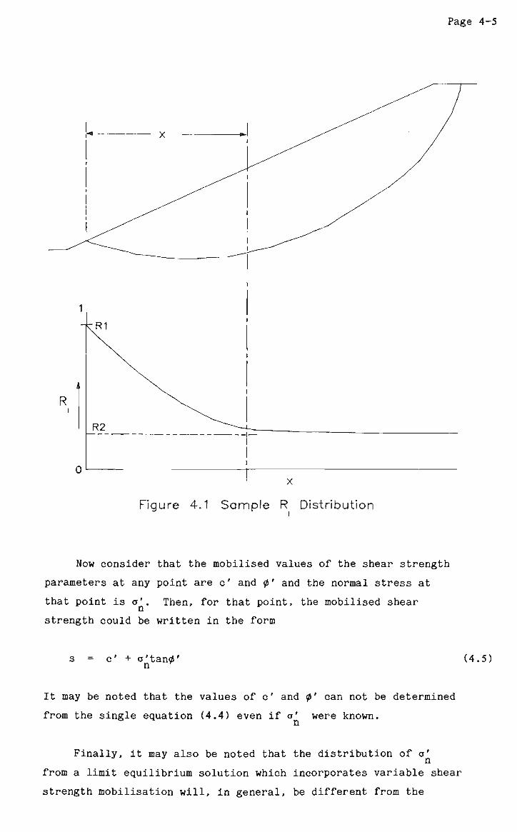
Page 4-5

R

Figure 4.1 Sample R Distribution

Now consider that the mobilised values of the shear strength

parameters at any point are c' and <p' and the normal stress at

that point is a'. Then, for that point, the mobilised shear

strength could be written in the form

s = c' + o'tantf' (4.5)

It may be noted that the values of c' and $' can not be determined

from the single equation (4.4) even if o' were known.

Finally, it may also be noted that the distribution of a'

from a limit equilibrium solution which incorporates variable shear

strength mobilisation will, in general, be different from the

Page 4-6

distribution obtained from a solution which assumes simultaneous

failure.

4.2.3 Proposed Approach - Variable Mobilisation of c' and 6'.

Prior knowledge or the assumption of c' and 0' values in

limit equilibrium methods is essential for their implementation. In

the Morgenstern-Price method, as with most limit equilibrium methods

of analysis, the overall factor of safety and the normal stresses on

each slice along the failure surface are calculated using known values

of shear strength parameters c' and 0' along with various other

parameters, and not directly from the local shear strength s. Given a

distribution for s, the overall factor of safety cannot be calculated,

as it depends on values of c' and 0' and these cannot uniquely be

calculated from known values of s using the Mohr-Coulomb equation.

Therefore, the following procedure has been developed. The local

shear strength s at any point along the failure surface is defined by

equation (4.5). The local values of the mobilised shear strength

parameters may be defined in terms of their respective peak and

residual values as

c' = c' - Rn(c' - c') (4.6a) P 1 P r

r = 0^ - R1(0E; - *;> (4-6b)

where R is the local residual factor for both c' and </>' defined

in the same way as the residual factor for the shear strength s. Its

distribution may assume a general form such as the polynomial equation

suggested in equation (4.3). Also, c', </>', c^ and

0' are the peak and residual values respectively of the shear

strength parameters.

In this work, the same value of R. is used for both c' and

0'. In other words, c' and 0' vary along the slip surface

according to the same distribution curve between their respective peak

and residual values. Nevertheless, it would be quite feasible

(without significant additional effort) to incorporate different

Page 4-7

arbitrary distributions of c' and 0'.

4.2.4 Types of Distributions Assumed.

A wide range of R distributions was chosen as shown in

Appendix B. The distributions, however, fall into two major

categories.

1. Failure starting from the bottom of the slope, that is, R

is 1 at the toe and %1 is 0 at the top of the slope, which

indicates that residual conditions have been reached at the

toe first.

2. Failure starting from the top of the slope, that is, R is

1 at the top and R.̂ is 0 at the bottom, indicating that

residual conditions have been reached first at the top.

Within these two categories, many sub-categories exist, where

R, has a constant value of 1 or 0 throughout, where the distribution

is broken up into more than one part, and where distributions may be

linear, exponential, or a combination of both. These can be seen in

appendix B. The distributions suggested by Bishop [14] are included

(distributions Al and LI) as are some similar to those of Lo and Lee

[62] where a sudden drop from peak to residual conditions is assumed

(distributions Q and R).

Work by various authors, including James [50] and Peck [71], has

shown that in many cases failure is more likely to start from the

bottom of the slope. This is because residual conditions are reached

slightly more rapidly under low stress levels than under high levels,

and the toe, or bottom of the slip surface, is under lower stress

levels than further into the slope. Thus more emphasis has been

placed on distributions where failure is assumed to start from the

bottom of the slope, although a number of cases of failure starting

from the top are also considered. The results are then compared to

see if it can be determined which case is the more critical.

Page 4-8

4.2.5 Basis of Solution Method.

As mentioned earlier, the stability analyses procedure developed

for the studies reported in this chapter is based on the limit

equilibrium approach. Of the various limit equilibrium methods, the

four described in chapter two were considered, and the one most suited

to the requirements of this research, was found to be the

Morgenstern-Price method although the Bishop's simplified method was

used for slopes having circular surfaces of sliding. The Janbu method

was eliminated due to the fact that it gives increased errors as the

depth of the failure surface increases.

Not all solutions obtained by this method, however, may be

regarded as admissible for the general limiting equilibrium problem.

Morgenstern and Price defined an admissible solution as one which

gives a reasonable distribution of normal force N, along the failure

surface. A reasonable distribution of N, was defined as one which

does not require a potential sliding mass to sustain internal forces

which it is physically incapable of sustaining. Other criteria for

the admissibility of a solution to a soil slope stability problem have

been given by Morgenstern and Price [68], Bailey [7] and Whitman and

Bailey [109] as,

1. There must be no effective tensile stresses on the sides of

slices.

2. The shear stresses on the sides of slices must be less than

those which would exist if a condition of limiting

equilibrium existed on these surfaces.

Hamel [14] also discussed the acceptability of solutions and

developed specific criteria or guidelines as discussed in subsequent

sections.

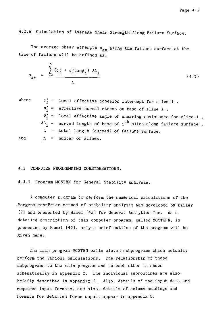
Page 4-9

4.2.6 Calculation of Average Shear Strength Along Failure Surface.

The average shear strength say along the failure surface at the

time of failure will be defined as,

) (c: + a.tan0!) AL. _ r. 1 1 1 I

(4.7) L

local effective cohesion intercept for slice i ,

effective normal stress on base of slice i ,

local effective angle of shearing resistance for slice i ,

curved length of base of i slice along failure surface ,

total length (curved) of failure surface,

number of slices.

4.3 COMPUTER PROGRAMMING CONSIDERATIONS.

4.3.1 Program MGSTRN for General Stability Analysis.

A computer program to perform the numerical calculations of the

Morgenstern-Price method of stability analysis was developed by Bailey

[7] and presented by Hamel [45] for General Analytics Inc. As a

detailed description of this computer program, called MGSTGRN, is

presented by Hamel [45], only a brief outline of the program will be

given here.

The main program MGSTRN calls eleven subprograms which actually

perform the various calculations. The relationship of these

subprograms to the main program and to each other is shown

schematically in appendix C. The individual subroutines are also

briefly described in appendix C. Also, details of the input data and

required input formats, and also, details of column headings and

formats for detailed force ouput, appear in appendix C.

where c. = l

n = AL. =

l

L = and n =

Page 4-10

It should be noted that two versions of MGSTRN were written by

Bailey. These will be called MGSTRN1 and MGSTRN2. MGSTRN1 is a

conversational, time-sharing program, with input solicited by the

computer through a remote teletype. The program asks questions

regarding input data and is better suited for persons not familiar

with the type and format of the input required. MGSTRN2 is a batch

program, where all data is read in from a data file, without

conversing with the user. Output is then automatically directed to

the output device selected. In this research, emphasis was given to

the extension of MGSTRN2, the batch version of MGSTRN. The main

development for the work reported in this chapter was the

incorporation of different distributions of mobilised values of the

shear strength parameters implying different progressive failure

modes.

From the detailed output obtained from MGSTRN, checks must be

made to ensure that the criteria for an admissible solution are

satisfied. These criteria are stated in terms of stresses, while the

solution of Morgenstern's equations and the output of MGSTRN, gives

only forces. Hamel [45], recommended the following criteria for

purposes of evaluating Morgenstern-Price solutions to soil slope

stability problems.

1. The effective normal forces on the sides and bases of slices

should be compressive.

2. The height of the point of application of each of the

effective normal side forces, should be between 0.25H and

0.65H, where H is the height of the slice side.

3. The average friction angle required on the side of each slice

when full cohesion is mobilized, should be less than 80% of

the average available friction angle along that surface.

The results obtained are examined in the light of these criteria and

recommendations for revised criteria are then given.

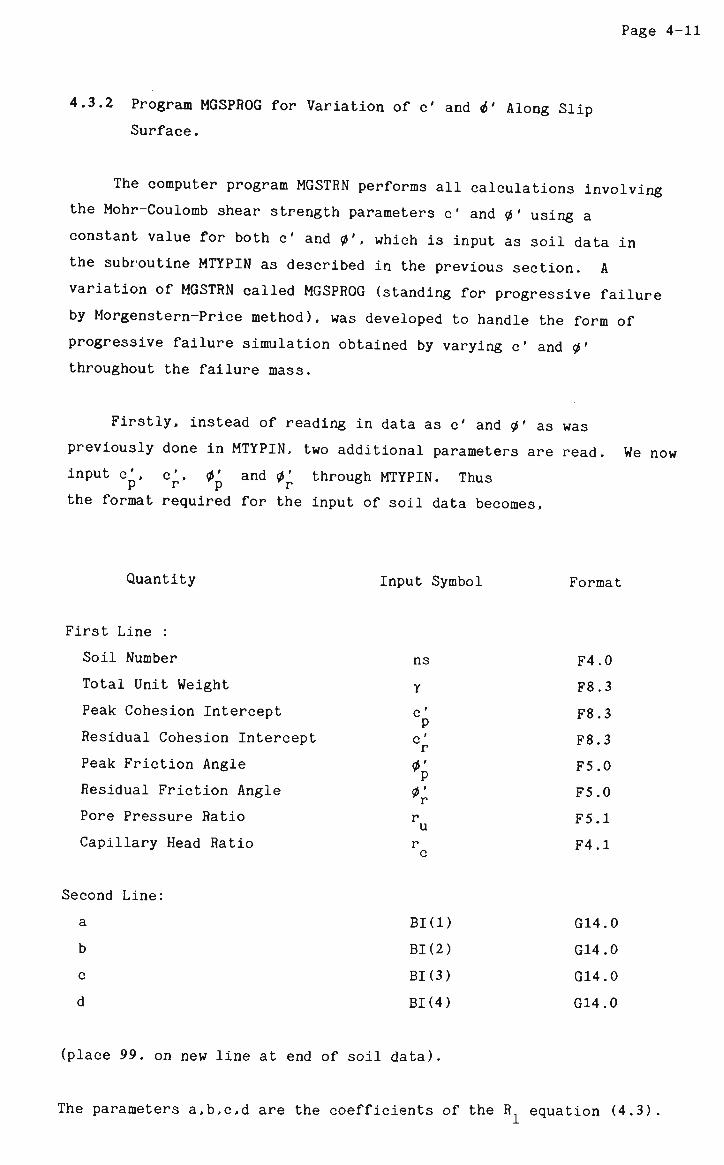
Page 4-11

4.3.2 Program MGSPROG for Variation of c' and <_•' Along Slip

Surface.

The computer program MGSTRN performs all calculations involving

the Mohr-Coulomb shear strength parameters c' and 0' using a

constant value for both c' and 0', which is input as soil data in

the subroutine MTYPIN as described in the previous section. A

variation of MGSTRN called MGSPROG (standing for progressive failure

by Morgenstern-Price method), was developed to handle the form of

progressive failure simulation obtained by varying c' and 0'

throughout the failure mass.

Firstly, instead of reading in data as c' and 0' as was

previously done in MTYPIN, two additional parameters are read We now

input c', P

.' and <f>'v through MTYPIN. Thus

the format required for the input of soil data becomes,

Quantity Input Symbol Format

First Line :

Soil Number

Total Unit Weight

Peak Cohesion Intercept

Residual Cohesion Intercept

Peak Friction Angle

Residual Friction Angle

Pore Pressure Ratio

Capillary Head Ratio

ns

y

c'

*r

u

F4.0

F8.3

F8.3

F8.3

F5.0

F5.0

F5.1

F4.1

Second Line:

a

b

c

d

Bid)

BK2)

BIO)

BK4)

G14.0

G14.0

G14.0

G14.0

(place 99. on new line at end of soil data)

The parameters a,b,c,d are the coefficients of the R equation (4.3).

Page 4-12

In MTYPIN, the soil parameters are given new names.

ns becomes K ,

Y becomes S0IL(K,1) ,

c' becomes SOIL(K,2) , P c' becomes CSNRL(K) , r 0' becomes SOIL(K,3) , 0' becomes PHIRL(K) , r r becomes RU(K) or SOIL(K,4) , r becomes SOIL(K,5) , c

If only one soil is considered, then K is always 1. If not, then K is

equal to the soil number (=1,2,3, .. .etc.).

In the subroutine NEWFSZ, which does most of the detailed

calculations involving c' and 0', the local values of c' and

0' are defined for each slice, i, for all n slices.

ci = c' - <V,<c' - c') (4.8) l p l i p r

and

0! = 0« - (Rn).(0* - 0') l *D 1 i *p r

(4.9)

where

(Rx). = aeb'XRL + c.XRL + d (4.10)

and XRL is the function (decimal from 0 to 1.0) of the horizontal

distance from X̂ ^ (x co-ordinate of first point on failure surface)

to X (x co-ordinate of last point on failure surface) of the centre

of slice i and is defined as;

(X. + X.^^/2 - Xt (XRL). = X 1 + 1 1 (4.1D

Xn " Xl

These co-ordinates are explained in figure 4.2 .

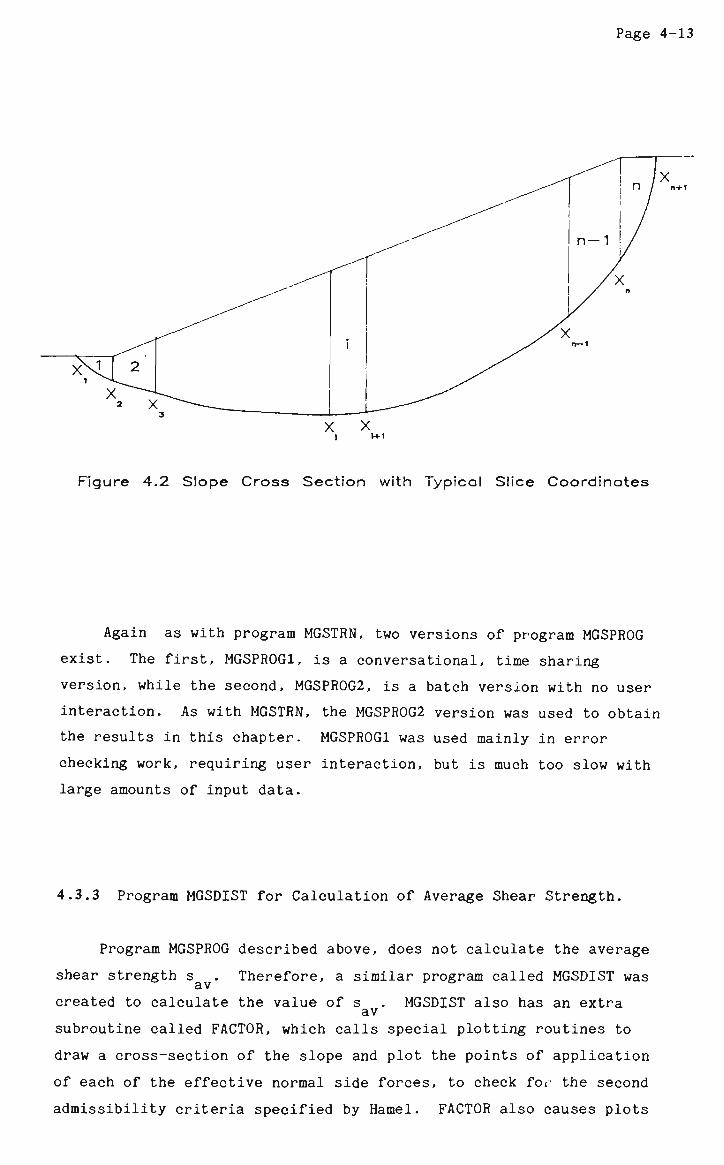
Page 4-13

Figure 4.2 Slope Cross Section with Typical Slice Coordinates

Again as with program MGSTRN, two versions of program MGSPROG

exist. The first, MGSPR0G1, is a conversational, time sharing

version, while the second, MGSPR0G2, is a batch version with no user

interaction. As with MGSTRN, the MGSPR0G2 version was used to obtain

the results in this chapter. MGSPR0G1 was used mainly in error

checking work, requiring user interaction, but is much too slow with

large amounts of input data.

4.3.3 Program MGSDIST for Calculation of Average Shear Strength.

Program MGSPROG described above, does not calculate the average

shear strength s . Therefore, a similar program called MGSDIST was

created to calculate the value of s . MGSDIST also has an extra av

subroutine called FACTOR, which calls special plotting routines to draw a cross-section of the slope and plot the points of application

of each of the effective normal side forces, to check for the second

admissibility criteria specified by Hamel. FACTOR also causes plots

Page 4-14

of the R distribution and resulting a', and s. distribution

along the failure surface. The value of s is calculated in av

subroutine OUTPUT using equation (4.7) after values of CT' for each slice have been calculated. Equation (4.7) may be rewritten as follows.

n

.AL 1S±" sa v - __- (4.12)

where

s. = cf + a:tan0. (4.13) l i i i

and where c' and 0. are calculated in subroutine NEWFSZ, I *i

(using equations (4.8) and (4.9)) and a', is calculated earlier in OUTPUT.

AL is calculated from the geometry of the failure surface as

[«_•_ - v2 + <r_+i - v2]0'5 <4-14' AL

The values of c' and 0' are calculated as mentioned av *av

above by the following equations.

Y c' .AL C' = £.

x (4.15) av

/ 0.'.AL 0' __ £ 1 (4.16) av

Page 4-15

4.3.4 Program BISHDIST for Varying c* and 6' Using Bishop's

Method of Analysis.

BISHDIST is a program (written in FORTRAN) which was developed on

the basis of Bishop's simplified method of analysis to determine the

factor of safety of slopes with circular surfaces of sliding. The

program has the capability for arbitrary variation of the Mohr-Coulomb

shear strength parameters c' and 0' along the failure surface and

for calculation of the average shear strength acting along that

failure surface at the time of failure. In order to do this, peak and

residual values of the parameters must be input to the program, along

with the other soil and slope data as follows. Refer to figure 4.3

for explanation of some of the following parameters.

Symbol

R

D

BE

SN

G

CPK

CRL

RU

PHPK

PHRL

Description

Slip circle radius

Sector angle, 6

Slope angle, p

Number of strips to be taken

Unit weight of soil, y

Peak values of cohesion c' P

Residual value of cohesion, c' Pore Pressure Ratio, r

Peak value of angle of shearing resistance, 0'

Residual value of angle of shearing resistance, 0^

The above data may be input on a single line, with each data element

separated by a blank or comma. To describe the distribution of c' and

0' along the failure surface, the parameters a,b,c and d of the

R, equation (4.3) must be input to the program. This distribution

data is read in as follows;

Symbol

DI

BI(1)

BK2)

BK3)

Description

Distribution Number

A

B

C

Page 4-16

BK4)

Again, these values may be input on one line, each separated by blanks

or commas. If more than one distribution is used, the above data is

repeated for each distribution, using the respective distribution

number DI for each one. At the end of all distribution data, a number

greater than 20 must be input to signal the end of the distribution

data. If N distributions are used (and thus the highest value of DI

is N), the program then divides the slope sector angle 5 into N equal

subsectors, thus dividing the length of the failure surface into N

equal lengths, each having a different location and R_ value.

Equations (4.8), (4.9) and (4.10) are then used to evaluate local

values c', 0? and (R.).. However, in this case, the

parameter (XRL). is defined as the fraction (decimal from 0 to 1.0),

obtained by dividing the angle 0 by the sector angle 6, where 0 is

the angle made by that fraction of the failure arc, exhibiting

residual conditions as shown in figure 4.3. The value of XRL is

thus given by the expression

(XRL). = 0. / 5 (4.17) l i

The average shear strength along the failure surface is then

calculated using equation (4.12) where, in this case,

AL = AO.R (4.18)

and

AO = e. - e. - (4.19) i 1-1

4.3.5 Calculation of Distribution Parameters a,b,c and d.

In order to input the R, distributions shown in appendix B into

the programs MGSPROG, MGSDIST and BISHDIST, it was necessary to

calculate the coefficients a,b,c and d of equation 4.3. This was done

with the aid of a curve fitting program called CURFIT, which used the

method of least squares to obtain the equation of the line of best fit

(in the form y = aebx + ex + d) of a number of points.

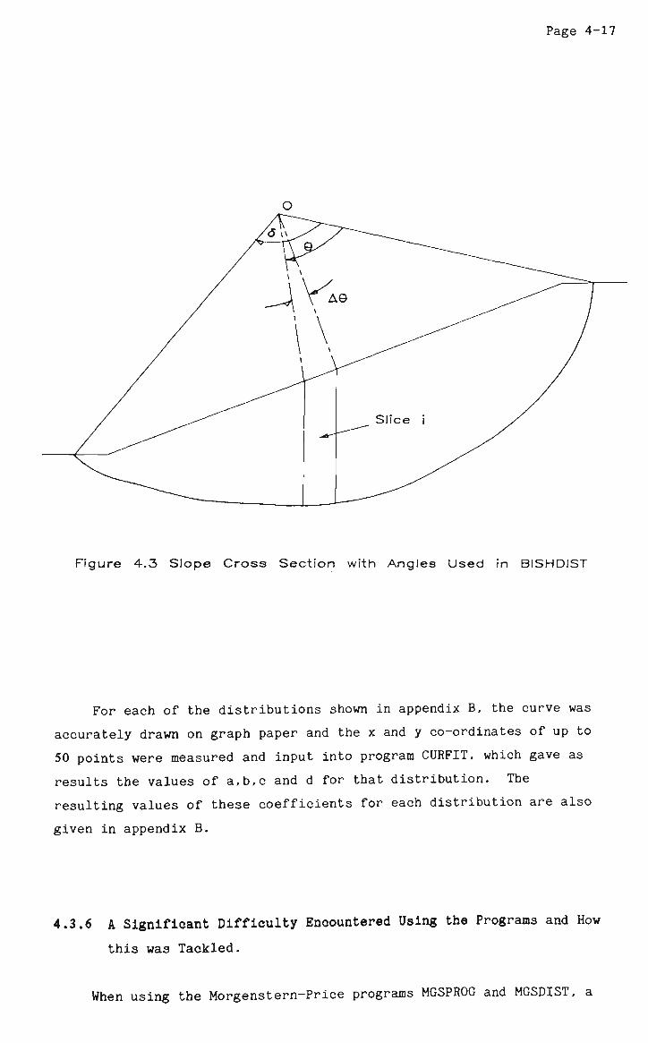
Page 4-17

Figure 4.3 Slope Cross Section with Angles Used in BISHDIST

For each of the distributions shown in appendix B, the curve was

accurately drawn on graph paper and the x and y co-ordinates of up to

50 points were measured and input into program CURFIT, which gave as

results the values of a,b,c and d for that distribution. The

resulting values of these coefficients for each distribution are also

given in appendix B.

4.3.6 A Significant Difficulty Encountered Using the Programs and How

this was Tackled.

When using the Morgenstern-Price programs MGSPROG and MGSDIST, a

Page 4-18

problem was encountered in cases where the R distribution was not

the same throughout the failure mass (i.e. where discontinuous

distributions were used). In cases such as distribution D2, H2, K2, Q

and R, there are in fact two distributions for R within the soil

mass. As a strength distribution is herein assumed to be a property

of the soil along the failure surface, the problem is overcome by

assuming that a different type of soil exists for each different R

distribution within the failure mass. The values of a, b, c and d are

then input as soil parameters. All other soil parameters remain the

same as for the original soil, so in fact, only the value of R will

change as a 'new soil' is encountered.

4.4 SLOPES AND TYPES OF ANALYSES CONSIDERED.

For the analyses carried out in this chapter it was decided to

use three well-known slip case histories. These were the Northolt

Slip in cutting, the Vajont Slide, and the Brilliant Cut slide. As

well as these three cases, a fourth example was also analysed. This

case will be referred to as Hypothetical Slip Number 1 (HS1) and

consists of a simple slope of uniform inclination, homogeneous soil

and an assumed circular failure surface. The reason for using slope

HS1 is to eliminate any effects of irregularities in slope geometry on

the results obtained. Full descriptions of these four slopes are

presented in appendix A.

The first three slopes were analysed using programs MGSPROG and

MGSDIST. Slope HS1, however, was analysed both by the above two

programs and also by program BISHDIST to allow direct comparison of

results obtained using the two different methods of stability

analysis.

4.4.1 Northolt Slip in Cutting (Henkel [48], Skempton [88]).

For the purpose of this research, the slope geometry used is as

shown in appendix A. However, the actual slip surface is used rather

Page 4-19

than the approximated circular surface used by Skempton. Also, the

shear strength parameters consistant with a factor of safety of 1.0

(as given by Skempton [88]) were used. These parameters are

18° 0' = 9.5° r

6.7 kPa c' = 0 r

Two series of analyses were performed on the Northolt slip. The

first of these is denoted by the name 'Series A' and consists of a

large number of individual runs of programs MGSPROG and MGSDIST, each

corresponding to one of the R distributions presented in appendix

B. In these analyses, a constant pore-pressure ratio of 0.34 is used

for the slope.

'Series B' is a series of analyses aimed at observing the

influence of the pore-pressure ratio r on the relationship between

the factor of safety obtained and the value of average shear strength

along the failure surface. Pore-pressure values of 0, 0.34 and 0.68

were used as well as a fourth case, in which the position of the

piezometric surface was assumed to be known. This case gave a value

of average r of approximately 0.35).

4.4.2 Vajont Slide (Broili [21], Lo, Lee And Gelinas [64]).

The slope geometry and shear strength parameters used for the

Vajont slope are presented in appendix A. The shear strength

parameters are varied in a number of ways for each R^ distribution

used. These strength variations are as follows.

(a) c' remains constant at the peak value, while 0' varies

between the peak and residual values.

0.

Page 4-20

(b) both c' and 0' vary between the peak and residual values,

(c) c' remains constant at the residual value, while 0'

varies between the peak and residual values,

(d) c' varies between the peak and residual values, while 0'

remains constant at the peak value,

(e) c' varies between the peak and residual values while 0'

remains constant at the residual value.

4.4.3 Brilliant Cut Slide (Ackenheil [1], Hamel [45],[46]).

In both the previous cases, the soil was taken to be uniform

throughout the length of the failure surface. The Brilliant Cut

failure mass on the other hand, encompasses five approximately

homogeneous zones of soil or rock material. It was chosen to enable a

study of the relationship between the resulting factor of safety for

the slope and the R distributions and calculated shear strengths in

a case where the soil is not uniform throughout the slope (and hence

also non-uniform in shear strength along the slip surface).

Having calculated the value of R, for various points along the

failure surface, the local values of c' and 0' are then found

using equations (4.5) and (4.6). The peak and residual values of c'

and 0' in these equations vary from one soil to another and thus

the respective values must be used depending on the soil existing on

the failure surface at the point being considered. For the purpose of

this work the soil and rock parameters given in appendix A are used.

For studies concerning the two previous examples, a constant

side-force function assumption was used for the Morgenstern-Price

method. For studies concerning this case history, two alternatives

were used. These two side-force assumptions are (1) constant, and (2)

full sine wave added to a trapezoid function (see Hamel [45]).

Experience had shown that the other side force function assumptions

Page 4-21

described by Hamel did not produce feasible results.

4.4.4 Hypothetical Slip Number 1.

As mentioned earlier, a hypothetical slope stability problem was

also used as an example. The slope geometry and soil parameters used

are as shown in appendix A.

As with the Northolt Slip, a number of analyses were carried out

with the aim of gaining some insight into the effect of pore water

pressure on the relationship between the average shear strength

obtained along the failure surface and the resulting factor of safety.

In order to do this a number of different analyses were carried out,

each using a different value of pore pressure ratio r . The values

of r used were 0, 0.25, 0.34 and 0.68.

Two sets of analyses were performed. The first is based on the

Morgenstern-Price method of analysis as for the previous case

histories, while the second is based on the Bishop simplified method.

Program MGSDIST was used for the first series which is denoted series

A while program BISHDIST was used for the second series denoted series

B. For both series, all the above values of r were used. u

Furthermore, five distributions of shear strength parameters c' and 0' were considered. These five correspond to R_ distributions

Al, B, M, N and P shown in appendix B.

4.5 RESULTS AND DISCUSSION.

4.5.1 Solution Admissibility - A New Proposal.

This section contains the results of the analyses described

earlier in this chapter. These results are presented in graphical

form. The resulting factors of safety should be evaluated for

admissibility using the three admissibility criteria stated earlier.

These admissibility criteria should alse serve as a measure of the

Page 4-22

acceptability of the R distributions used.

In order to facilitate the evaluation of the overall

admissibility of a given result for a particular slope, the following

reliability factor to is defined. For each of the three admissibility

criteria noted earlier, the number of slices within the slope which

satisfy that particular criteria N is divided by the total number s

of slices in the slope N . The three results are averaged and expressed as a percentage as shown in equation (4.20) below.

b. = (100/3) ^(N )./N. (4.20) L s l t

The procedure suggested above is only an approximate one and

gives a reasonable indication of the reliability of any given result.

However, it cannot be used as a cut and dry rule for assessing the

admissibility of a solution. It can be said, however, that solutions

with reliability factors of, say, over 60% are fairly reliable whereas

solutions with factors under 20% may be disregarded. This conclusion

is based on experience of the author.

4.5.2 Northolt Slip in Cutting.

As mentioned in the previous section, the first of the two series

of analyses performed on the Northolt Slip involved a large number of

R, distributions used in conjunction with the Morgenstern-Price

method of stability analysis.

The calculated values of average shear strength and their

corresponding values of factor of safety were plotted against each

other as shown in figure 4-4. From an analysis of this plot it is

evident that a definite relationship exists between the factor of

safety, F for the slope and the average shear strength, S&v along

the failure surface. This relationship is of linear form.

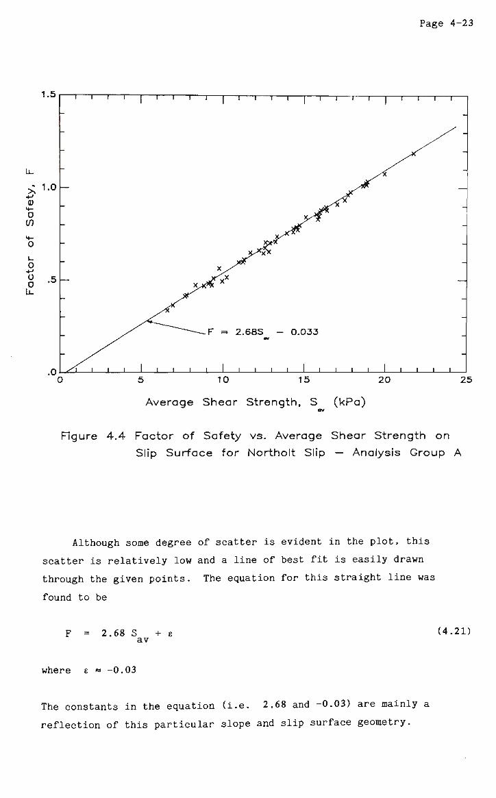
Page 4-23

i i i i | i i i i | — i — i — t — i — | — i — t — t — t — | — i — i — t — r

Average Shear Strength, S (kPa) av

Figure 4.4 Factor of Safety vs. Average Shear Strength on

Slip Surface for Northolt Slip — Analysis Group A

Although some degree of scatter is evident in the plot, this

scatter is relatively low and a line of best fit is easily drawn

through the given points. The equation for this straight line was

found to be

F = 2.68 S +e (4.21) av

where e « -0.03

The constants in the equation (i.e. 2.68 and -0.03) are mainly a

reflection of this particular slope and slip surface geometry.

Page 4-24

Primarily, this empirical equation serves to indicate that, for

this particular slope, given this specific set of soil data, a given

relationship exists between F and S irrespective of which cl V

distribution of R, is used for c' and 0'. The resulting factor of safety, therefore, depends only on the value of the average shear

strength over the failure surface, regardless of the mode or direction

of failure progression. In an absolutely accurate solution, one might

expect the straight line shown in figure 4.4 (i.e. e » 0).

Earlier in this chapter, it was pointed out that the results

presented here are attributed to various distributions of c' and

0'. Not much mention has yet been made, however, of the actual

distribution of the shear strength mobilised along the failure

surface, or, of its relationship to the c' and 0' distributions

used. It may be recalled that values for a distribution of shear

strength could not be directly used in any limit equilibrium method of

analysis since specific data on the values of the effective shear

strength parameters c' and 0' is always required. Therefore, the

distribution of mobilised shear strength is obtained from the known

local values of c' and 0', and values are then obtained from the

actual solution for a' along the failure surface (<r̂ is the value

of the effective normal stress on the base of a soil slice).

The above mentioned shear strength distributions were plotted and

examined. In general, it was noted that the resulting shear strength

distributions bear little resemblance to the assumed R1

distributions for c' and 0'. In other words, the manner in which

c' and 0' are mobilised along the slip surface as a consequence of

some mechanism of progressive failure does not have a significant

influence on the form of the spatial distribution of mobilised shear

strength along the slip surface.

The most prevalent type of shear strength distribution was found

to be as shown in figure 4.5. It is worthy of note that the value of

s decreases towards both ends of the slip surface and may approach

zero. This is not surprising considering that the normal effective

stress a' approaches zero at the extreme boundaries of the failure

surface, and that the value of s then depends only on the value of c'

which, in many of the above examples, is taken as zero. This factor

Page 4-25

would suggest that the R.̂ distributions given by Bishop and

presented in figure 3.4 may be somewhat unrealistic and not relevant

to the limit equilibrium method of slope analysis. If Bishop's

distributions were to be taken, not as shear strength distributions,

but as distributions of the shear strength parameters c' and 0',

then they are certainly feasible in a progressive failure context.

For ' 0 = 0 ' situations, the conclusions will be different.

However, this thesis is concerned primarily with effective stress

slope stability analyses.

Figure 4.5 General Form of Shear Strength Distribution

As a further comment on Bishop's proposed distributions, it is

worth comparing the results obtained by similar but opposite

distributions. In other words, comparing the results of distributions

B, Q and 0 (where failure appears to start at the toe of the slope) to

those of B2, R and P (where failure is assumed to start at the crest)

Page 4-26

shows a slightly lower factor of safety for the latter. It could be

said that in cases where local failure starts at the crest of the

slope, the chances of overall slope failure are greater. Also, cases

where local failure is assumed to start near the centre of the slope

and proceed outwards were found to yield low factors of safety

compared to cases where local failure started from the toe or where

local failure started from both the toe and crest of the slope

simultaneously.

It would therefore appear that while the variations in the

factors of safety were small and may have been due largely to the

geometrical properties of the slope, local failures starting from the

crest of the slope or from the centre of the slope are most likely to

cause overall slope failure.

The Reliability Factor _> gives a measure of the extent to which

the admissibility criteria given by Hamel [45] are satisfied. Most

values of to were found to be between 30% and 60% with a few as low as

27% or as high as 73%. It must be remembered that the three

admissibility criteria were presented firstly by Morgernstern and

Price [68] and later reviewed by Hamel [14], with the view of

developing guidelines for the acceptabiltiy of solutions obtained by

the Morgernsten-Price method of slope stability analysis. Since the

Morgernstern-Price method is a limit equilibrium method and the

assumption made in all limit equilibrium methods is that the factor of

safety, F is constant throughout the Slope (an assumption which is

actually true only at failure when F=l), then the admissibility

criteria can be said to apply only in the region of F=l. Thus if F is

less than say 0.6, or much greater than 1.0, then o. would be expected

to be low. This is supported by the fact that cases in which F lies

between the limits of 0.95 and 1.15 have to values between 56% and 73%,

while for cases where F is less than 0.5, to is usually less than 30%.

From this, it would appear that the reliability factor o. can only

be effectively used as a measure of admissibility if the solution lies

in the region of F=l. However, the value of to is never higher than

73%, which means that the admissibility criteria are never fully

satisfied. Upon a more detailed investigation of the results, it is

found that criterion number 1, which states that the effective normal

Page 4-27

forces on the sides and bases of slices should be compressive, is

satisfied most of the time (that is, only a few slices exist in each

analysis, where the criterion is not satisfied). Looking at criterion

number 2, it is found that the height of the point of application of

each of the effective normal side forces, lies between 0.25H and 0.65H

(where H is the height of the slice) in less than half of the total

number of slices. Also the third criterion, which states that the

average friction angle required on the side of each slice when full

cohesion is mobililized, should be less than 80% of the average

available friction angle along that surface, is only satisfied to a

certain degree (about 80% of slices for F=1.0).

It would seem that of the three criteria given, the first can be

taken as a fair indication to acceptability, the third sould be looked

into in more detail and the second can be said to be unacceptable for

consideration, as it seems highly unlikely that it would ever be

satisfied to a reasonable degree except under ideal conditions.

To facilitate analyses in the following sections, the number of

R, distributions used was reduced to ten only. This was done in

order to save time and reduce the number of calculations. Many of the

distributions give similar results and thus can be eliminated. Those

distributions were chosen which gave the widest range of results, the

least repetition of results and the largest variation of distribution

shapes. They are A2, Bl, M, P, H2, Kl, K2, Q and R, as described in

appendix B.

The second series of analyses performed on the Northolt Slip was,

as mentioned earlier, an attempt to observe the effects of different

pore water pressure values on the relationship between the factor of

safety F and the average shear strength mobilised along the failure

surface s . To do this, four sets of analyses were carried out

using values of pore-pressure ratio equal to 0, 0.34 and 0.68 for the

first three respectively while providing an assumed piezometric

surface for the fourth. Only the ten R distributions mentioned

above are used in these analyses. The results of these analyses were

plotted and are shown in figure 4.6.

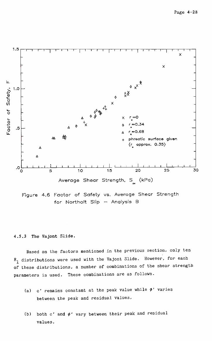
Page 4-28

1.5 T — i — i — i — | — i — i — i — i — | — i — i — i — i — | — i — i — i — i — [ — i — i — i — i — | — i — i — i — r

x

0

1.0

O 5

Q\ 1 1 L

tt\

*x*

+X

0

X

+ X

X

0

A

+

*

r=0 u r =0.34 y

r =0.68 0

phreotic surface given

(r approx. 0.35)

.1 _J I I I I 1 I L I i i i i I I I I 1 1 1 1 1 L 5 10 15 20 25

Average Shear Strength, S (kPa)

30

Figure 4.6 Factor of Safety vs. Average Shear Strength

for Northolt Slip — Analysis B

4.5.3 The Vajont Slide.

Based on the factors mentioned in the previous section, only ten

Rx distributions were used with the Vajont Slide. However, for each

of these distributions, a number of combinations of the shear strength

parameters is used. These combinations are as follows.

(a) c' remains constant at the peak value while 0' varies

between the peak and residual values.

(b) both c' and <p' vary between their peak and residual

values,

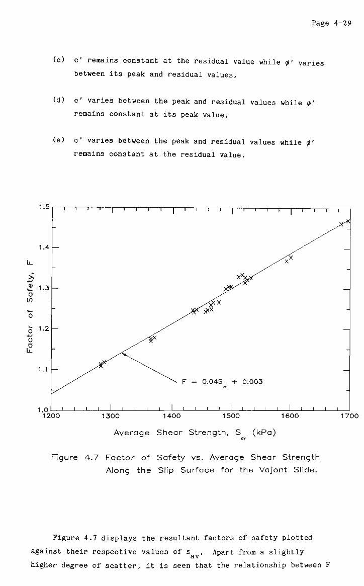
Page 4-29

(c) c' remains constant at the residual value while 0' varies

between its peak and residual values,

(d) c' varies between the peak and residual values while 0'

remains constant at its peak value,

(e) c' varies between the peak and residual values while 0'

remains constant at the residual value.

0)

o if)

o

1 .V.

1.4

1.3

1.2

1.1

1 n

I

i i i

i | t i • t —

i 1 i i i

t | t i t r -

^<5<x

^ - F = 0.04S

1... 1 1 1 1 1

1 1 1 1

+ 0.003

1 l l l

i | i l

t i l l

I i

-

~"~

—

1 1

1200 1300 1400 1500 1600


1700


Along the Slip Surface for the Vajont Slide.

Figure 4.7 displays the resultant factors of safety plotted

against their respective values of s . Apart from a slightly

higher degree of scatter, it is seen that the relationship between F

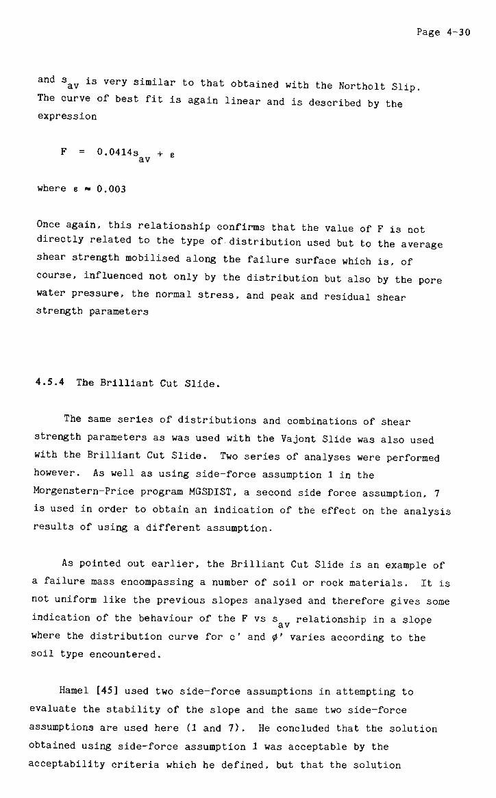
Page 4-30

and say is very similar to that obtained with the Northolt Slip,

The curve of best fit is again linear and is described by the

expression

F = 0.0414s + e av

where e » 0.003

Once again, this relationship confirms that the value of F is not

directly related to the type of distribution used but to the average

shear strength mobilised along the failure surface which is, of

course, influenced not only by the distribution but also by the pore

water pressure, the normal stress, and peak and residual shear

strength parameters

4.5.4 The Brilliant Cut Slide.

The same series of distributions and combinations of shear

strength parameters as was used with the Vajont Slide was also used

with the Brilliant Cut Slide. Two series of analyses were performed

however. As well as using side-force assumption 1 in the

Morgenstern-Price program MGSDIST, a second side force assumption, 7

is used in order to obtain an indication of the effect on the analysis

results of using a different assumption.

As pointed out earlier, the Brilliant Cut Slide is an example of

a failure mass encompassing a number of soil or rock materials. It is

not uniform like the previous slopes analysed and therefore gives some

indication of the behaviour of the F vs s relationship in a slope

where the distribution curve for c' and 0' varies according to the

soil type encountered.

Hamel [45] used two side-force assumptions in attempting to

evaluate the stability of the slope and the same two side-force

assumptions are used here (1 and 7). He concluded that the solution

obtained using side-force assumption 1 was acceptable by the

acceptability criteria which he defined, but that the solution

Page 4-31

1.2

1.0

0) 4-

0 CO

0 •fj

o D LL_

.8

.4 -

1 1

—

~

—

~"

1 1

1 1 1 I 1 1 1

o xx X

F = 4.27x10~»S -

1 1 1 1 1 1 1

1 1 1 1 1 1 1 1 1 I

• X X*

• 0

\ * ** v <Xx*X0 X OX*

X X Side force assumption 1

(f(x)=1 =constant)

0 Side force assumption 7

(f(x)=trapezoid+bell)

0.014 (for S.F. assumption 1)

I i i i i 1 • i I i

-

—

—

~

—

"

.6 -

50 100 150 200


250


for Brilliant Cut Slide

obtained from side-force assumption 7 was not. By comparing the two

sets of results, which are displayed in figure 4.8, it can be seen

that there is a large degree of scatter in the results obtained using

side-force assumption 7 while only a small amount of scatter exists in

the set of results obtained using side-force assumption 1. The

relationship based on a constant side force assumption is again linear

and can be expressed as

F = 4.3x10 s + e av

where e » -0.014

The above observations reinforce the decision made earlier to use

Page 4-32

side-force assumption 1 as the standard assumption throughout this

research. They also support the findings of the previous two cases

analysed.

4.5.5 Hypothetical Slip Number 1.

As was mentioned in the previous section two further series of

analyses were carried out on Hypothetical Slip number 1. The first,

series A, was based on the Morgenstern-Price method of analysis to

calculate the factor of safety of a number of cases. A number of R,

distributions was used, each with three different pore pressure

values. The second, series B, uses the same R distributions and

pore-pressure values, but this time Bishop's simplified method was

used to perform the stability analyses.

The results of these analyses are shown in figure 4.9. Apart

from the fact that the results obtained by the Morgenstern-Price

method have, in general, a higher degree of scatter when plotted than

those results obtained by the Bishop simplified method, the line of

best fit of the Morgenstern-Price results appears to be slightly

higher and to the left of the Bishop method results. Also, the data

from the three sets of analyses using the three different values of

pore-pressure ratio appears to lie on the same line. This implies

that pore-water pressure has no effect on the relationship between the

factor of safety and the average shear strength. It is well known

that the factor of safety F decreases as r increases, but the

average mobilised shear strength decreases by a proportionate amount

so as to leave the relationship between the two unchanged. Also, the

relationship between F and s is again linear as has been found to

be the case in earlier analyses.

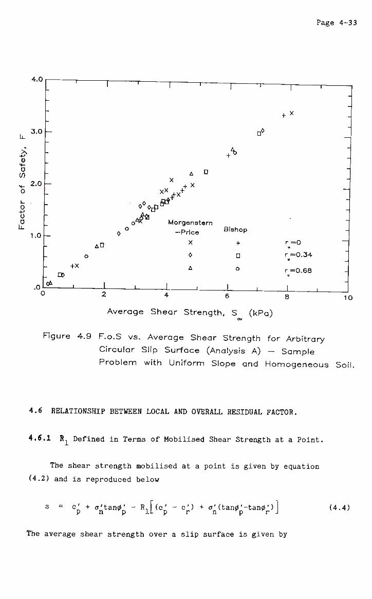
Page 4-33

4.0

3.0 -

<D 4-

o 2.0

0 0

1.0

A>

* x+ + x

+ + x

AD

+x

Morgenstern —Price

X

0

A a>

<*

Bishop

+

D

0

J

r=0 U

r =0.34 W

r =0.68

0 2 4 6 8

Average Shear Strength, S (kPa) av

Figure 4.9 F.o.S vs. Average Shear Strength for Arbitrary

Circular Slip Surface (Analysis A) - Sample

Problem with Uniform Slope and Homogeneous

10

Soil

4.6 RELATIONSHIP BETWEEN LOCAL AND OVERALL RESIDUAL FACTOR.

A.6,1 R Defined in Terms of Mobilised Shear Strength at a Point.

The shear strength mobilised at a point is given by equation

(4.2) and is reproduced below

s = c' + <y'tan0' - BA(C' - c') + a' (tan0'-tan0') 1 p n p 1L p r n p r J

(4.4)

The average shear strength over a slip surface is given by

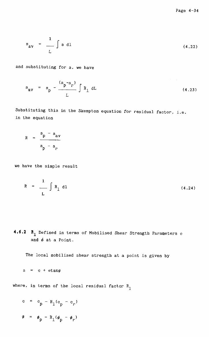
Page 4-34

Sav J s dl (4.22) L

and substituting for s, we have

(s..-s ) , p r f

Sav sp " J Ri dL (4.23)

Substituting this in the Skempton equation for residual factor, i.e.

in the equation

R = _? ^

s - s P r

we have the simple result

R = _ j\dl (4.24)

4.6.2 R1 Defined in terms of Mobilised Shear Strength Parameters c

and 6 at a Point.

The local mobilised shear strength at a point is given by

s = c + otan0

where, in terms of the local residual factor R, 1

° = °p " R 1 ( CP "

Cr )

0 = 0 - R]_(0 - 0r)

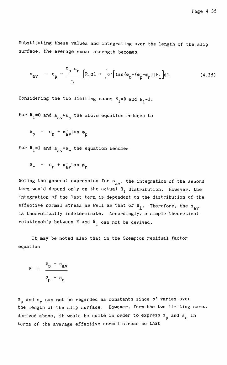
Page 4-35

Substituting these values and integrating over the length of the slip

surface, the average shear strength becomes

c —c sav = cp - _Z_J_ J^dl + Ja'[tan{0 -(0 ^HRjdl (4.25)

Considering the two limiting cases R =0 and R =1.

For R.j=0 and sav=s the above equation reduces to

s„ = c + a' tan 0 p p av vp

For Rn=l and s =s the equation becomes

s = c + a' tan 0 r r av *r

Noting the general expression for s , the integration of the second cl V

term would depend only on the actual R distribution. However, the integration of the last term is dependent on the distribution of the

effective normal stress as well as that of R. . Therefore, the s l av

is theoretically indeterminate. Accordingly, a simple theoretical relationship between R and R can not be derived.

It may be noted also that in the Skempton residual factor

equation

s - s R __ P av

s - s P r

s and s can not be regarded as constants since a' varies over

the length of the slip surface. However, from the two limiting cases

derived above, it would be quite in order to express s and s in

terms of the average effective normal stress so that

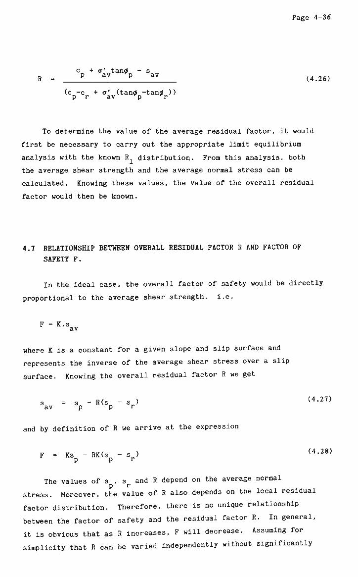
Page 4-36

c + a' tan0 - s R = P a V P a V (4.26)

(c -c + ff' (tan0 -tan0 )) p r av ^p *r

To determine the value of the average residual factor, it would

first be necessary to carry out the appropriate limit equilibrium

analysis with the known R. distribution. From this analysis, both

the average shear strength and the average normal stress can be

calculated. Knowing these values, the value of the overall residual

factor would then be known.

4.7 RELATIONSHIP BETWEEN OVERALL RESIDUAL FACTOR R AND FACTOR OF

SAFETY F.

In the ideal case, the overall factor of safety would be directly

proportional to the average shear strength, i.e.

F = K.s av

where K is a constant for a given slope and slip surface and

represents the inverse of the average shear stress over a slip

surface. Knowing the overall residual factor R we get

s = s - R(s„ - s ) av p p r

(4.27)

and by definition of R we arrive at the expression

F = Ks - RK(s - s ) p P r

(4.28)

The values of s , s and R depend on the average normal

stress. Moreover, the value of R also depends on the local residual

factor distribution. Therefore, there is no unique relationship

between the factor of safety and the residual factor R. In general,

it is obvious that as R increases, F will decrease. Assuming for

simplicity that R can be varied independently without significantly

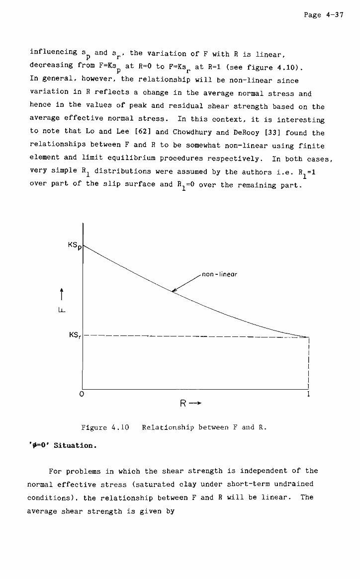
Page 4-37

influencing sp and sr, the variation of F with R is linear,

decreasing from F=Ksp at R=0 to F=Ksr at R=l (see figure 4.10).

In general, however, the relationship will be non-linear since

variation in R reflects a change in the average normal stress and

hence in the values of peak and residual shear strength based on the

average effective normal stress. In this context, it is interesting

to note that Lo and Lee [62] and Chowdhury and DeRooy [33] found the

relationships between F and R to be somewhat non-linear using finite

element and limit equilibrium procedures respectively. In both cases

very simple R_̂ distributions were assumed by the authors i.e. R =1

over part of the slip surface and R,=0 over the remaining part.

non-linear

Figure 4.10 Relationship between F and R,

'0=0' Situation.

For problems in which the shear strength is independent of the

normal effective stress (saturated clay under short-term undrained

conditions), the relationship between F and R will be linear. The

average shear strength is given by

Page 4-38

av j,, - (c -c ) fR.dl u^ u_ u J 1 P r

Using the result obtained in equation (4.24) we have

s = c - (c -c )R av u u u

P P r This result could also have been obtained directly from (4.26) or

(4.27). Moreover, from equation (4.28)

F = Kcu - RK(cu - cu ) P p r

Thus both the average shear strength and the factor of safety are

linear functions of the overall residual factor as shown in figure

4.11.

Cu,

KCu.

Ov

|KCur

R

Figure 4.11 Relationship between F, s and R.

Page 4-39

4.8 SUMMARY AND CONCLUSIONS.

During progressive failure the shear strength along the potential

slip surface may vary gradually from a peak value to a residual value.

The distribution of mobilised shear strength will depend primarily on

the mode and direction of failure progression. However, the exact

nature of the distribution of mobilised shear strength parameters can

not be determined. Therefore, it is useful to generate a number of

distributions and study the results of stability analyses based on

them. It should be noted that an arbitrary distribution of mobilised

shear strength parameters may be associated with the instant of

complete slope failure or sliding. However, even if complete sliding

does not occur, a slip surface may have propagated and there may be

sufficient movements and deformations associated with progressive

decrease of shear strength. Accordingly, arbitrary distributions of

mobilised shear strength parameters can be expected in slopes which

are currently stable but which may have suffered some degree of

deformation and distortion.

Various distributions of the local residual factor R were

generated to simulate the mobilisation of shear strength parameters c'

and 0' along a slip surface. New procedures were developed so

that stability analyses could be carried out within the framework of

limit equilibrium using any arbitrary distribution of the local

residual factor. These procedures can handle slip surfaces of

circular shape as well as slip surfaces of arbitrary shape. The new

generalised procedures were found to be feasible and proved successful

for all the problems that were analysed.

One aim of the analyses was to determine whether the shape of a

distribution of R, has any influence on the overall factor of

safety. However, the factor of safety was found to be directly

proportional to the average mobilised shear strength regardless of

other factors. This result appears intuitively reasonable for

simulation of slope stability in homogeneous soil when progressive

effects are ignored. However, for analyses which include progressive

effects leading to the non-uniform mobilisation of shear strength

parameters, such a simple and neat relationship could not have been

predicted without the new procedures for analysis established in this

Page 4-40

thesis.

In the ideal case, the straight line relating F to s would

pass through the origin. Computed results show a small intercept on

the X or Y axes even though a rigorous limit equilibrium approach

(Morgenstern-Price) is used as the basis for the development of the

new analysis procedures. The results of the analyses by any method

would be unacceptable if the intercept were significant and the

following criterion is proposed on the basis of experience gained so

far.

F = Ksay + e . e_< 0.05

This may be regarded as a criterion for the acceptability of the

solution method.

The three criteria proposed by Hamel [45] for the admissibility

of the Morgenstern and Price solution were also examined. The first

criterion requiring that the effective normal forces on the sides and

bases of slices be compressive was almost always satisfied. The

second criterion, which required that the point of application of the

effective normal side forces should lie between 0.25H and 0.65H (H

being the slice height) was found to be very stringent and was not

satisfied for all the slices.

A 'reliability factor' <a was proposed as a measure of the extent

to which any given solution satisfies those criteria and this factor

has been defined in equation (4.20). Considering all the slices into

which a slope has been divided, the reliability factor never

approached 100% and was generally below 80%. On the basis of

experience, the satisfaction of the first of Hamel's three criteria is

a good yardstick of the admissibility of a solution.

Keeping everything else constant, the value of the factor of

safety F decreases linearly with increase in porewater pressure ratio

ru because such an increase leads to a corresponding decrease in the

average shear strength. Analyses were carried out to study the

influence of r on the relationship between F and sQ_, and this u <*»

influence was found to be insignificant. In other words, for a given

Page 4-41

fixed value of mobilised shear strength, F changes very little even if

r changes significantly.

In general, the mobilised shear strength is of the form shown in

figure 4.5 regardless of the type of distribution chosen for the local

residual factor R . This form does not resemble the distributions

of mobilised shear strength suggested by Bishop [14] which are

unrealistic. It is not appropriate to apply an arbitrary distribution

of the residual factor to the shear strength. However, as proposed in

this thesis, such distributions may be assumed for the shear strength

parameters c' and 0'. If the distributions of R, were intended

for c' and 0', such distributions have indeed been shown to be

feasible in respect of progressive failure along slip surfaces in

slopes. However, other types of distributions of the residual factor

R, are equally feasible.

Based on the relationship that the factor of safety is directly

proportional to the average shear strength, it has been shown that the

factor of safety decreases with an increase in the residual factor R.

The relationship is expected to be non-linear in the general case and

linear under '0=0' conditions.

The average shear strength s and the overall residual factor

R may be related to the local residual factor R. . The relationships

are, in general, not simple except for the case where R_ is applied

to the mobilised shear strength.

CHAPTER 5

STRAIN SOFTENIHG: LOCAL FAILURE AND STRESS REDISTRIBUTION.

5.1 INTRODUCTION.

A considerable amount of research has been carried out by various

authors on the subject of strain softening in soils. This chapter

presents a brief summary of some different approaches to the

associated concepts of strain softening, local failure of soil

elements, and redistribution of excess shear stresses along rupture

surfaces.

5.2 BJERRUM'S APPROACH TO STRAIN SOFTENING AND PROGRESSIVE FAILURE.

Bjerrum [18] presented an explanation for the mechanism of a

progressive slope failure. He noted that it is world-wide experience

from slides in over-consolidated plastic clays and clay shales, that

the average shear stress along the failure surface is much smaller

than the shear strength measured in relevant shear tests in the

laboratory. Bjerrum stated that this finding holds true for slides in

fresh cuts as well as for slides in natural slopes.

Bjerrum also stated that under certain conditions, slides in

over-consolidated plastic clays and clay shales are preceded by the

development of a continuous failure surface by a mechanism of

progressive failure. He then postulated a possible mechanism which

explored how a progressive failure can occur and how it can lead to

the development of a continuous sliding surface. Bjerrum's

postulation is presented here in some detail.

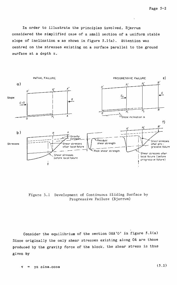
Page 5-2

In order to illustrate the principles involved, Bjerrum

considered the simplified case of a small section of a uniform stable

slope of inclination a as shown in figure 5.1(a). Attention was

centred on the stresses existing on a surface parallel to the ground

surface at a depth z.

INITIAL FAILURE PROGRESSIVE FAILURE e)

Figure 5.1 Development of Continuous Sliding Surface by Progressive Failure (Bjerrum)

Consider the equilibrium of the section OAA'O' in figure 5.1(a)

Since originally the only shear stresses existing along OA are those

produced by the gravity force of the block, the shear stress is thus

given by

T = yz sina.cosa (5.1)

Page 5-3

Since the slope is stable, the above shear is less than the peak shear

strength of the clay.

In order to initiate a progressive failure, a discontinuity of

some type must exist somewhere in the slope. Assuming that a cut with

vertical walls is made down to a depth z adjacent to the considered

section, removal of the lateral support on O'O by excavation, produces

a redistribution of the internal stresses in the block OAA'O'. If AA'

is sufficiently far from 00' so that the lateral stresses on AA' are

unaltered, equilibrium of OAA'O' is only maintained if the shear force

along 0A increases, by the amount E, the total internal lateral earth

pressure on AA'. In other words,

E = j"rE dl (5.2)

The additional shear stresses are not uniformly distributed.

However, we know that the maximum will be at 0 (see figure 5.1(b)).

If we let k be the concentration factor which expresses the ratio

between the maximum and the average stress on plane 0A, we find that

the maximum shear stress due to E is therefore

(O = k.E/(0A) (5.3) E max

The total shear stress at point 0 is then

t = vz sina.cosa + k.E/(0A) (5.4) o '

This equation is deduced on the basis of equilibrium conditions only,

assuming that shear stresses are not greater than the shear strength.

It is now necessary to determine whether the excavation will

initiate progressive failure. This depends on whether the maximum

value of x is greater than the peak shear strength of the clay and

this in turn depends on the value of the magnitude of E. Provided

that the value of E is large enough for the theoretical value of x to

be greater than the peak shear strength, a local failure will occur.

Page 5-4

Local failure will start at point 0 and proceed as far as the

shear stresses exceed strength (up to P1 in figure 5.1(b)). The

occurrence of shear failure at the base of block OO'P'P will

mean that

1. a reduction of shear stresses on OP will occur from the

theoretical value above to the peak shear strength.

2. the internal lateral stresses in the block of clay

O O ' P ^ will diminish.

Due to the elastic behaviour of clay, this lateral unloading

causes the clay to expand towards the excavation by sliding on the

newly-formed failure plane OP^ The resulting differential strain

across the failure zone is governed by the recoverable strain energy

of the clay and if this is large enough the strain will be sufficient

to reduce s from the peak to the residual value.

Provided that s is low compared to s , the failure surface

and consequent strain will cause a larger reduction of shear stresses

along OPj and a corresponding increase of shear stress on the

surface to the right of ?-. Thus progressive failure is initiated

and the slip plane has advanced to point P-. Next, investigate in a

similar manner the conditions for further advancement beyond point

P̂ in figure 5.1(e).

The above procedure is repeated, considering the equilibrium of

block P1BB'P' Section BB' is so far from P-jPj. that the

lateral stresses on BB' are unaffected by what happened on the left of

P.,. Again, consider the shear stresses along the base of the block.

Now, the additional shear stresses, due to the lateral stresses in the

clay, are dependent on the difference between the lateral forces E and

E acting on the upslope and downslope sections of the block

respectively. The maximum x is now at P and equals

T max

yz cosa.sina + (E-E )/(P1B) (5.5) D 1

If t is greater than s , the local failure will develop into a max p

Page 5-5

progressive failure. The smaller the value of E , the greater the

likelihood of failure progressing. The maximum value that E can p

have is

(Vmax ~ 0P1 (sr ~ y z cosa-sina) (5.6)

Bjerrum concluded that if sr is so low, or the inclination of

the slope is so high, that the block of clay resting on an

already-formed slip plane will slide downhill, the maximum value that

E can have will be very small. Thus x at P. will be v max l

approximately equal to x m a x at 0 when initial failure occurred and the failure surface will proceed from P.. to P,.

If conditions do not change in the upslope direction, the progressive failure continues to proceed uphill, gradually leading to

the development of a continuous sliding surface along which the shear

resistance is reduced to the residual value. On the other hand, if

s is greater than yz.cosa.sina, (e.g. if s is so high or the

inclination so low, that if the block is cut loose at its base, it has

no tendency to slide downhill), the value of E gradually increases

up the slope and progressive failure will come to a halt at a certain

distance from the excavation.

Bjerrum also concluded that in order for progressive failure to

start, leading to the development of a continuous failure surface,

there must be a discontinuity somewhere in the clay mass, or at its

boundary, where failure can be initiated and the deformations required

for a further development can be produced.

Bjerrum arrived at the following conclusions on the process of

progressive failure.

1. The development of a continuous failure surface by

progressive failure is only possible if there exist, or can

develop, local shear stresses exceeding s . Thus, the

danger of local failure increases with the ratio PJT/S

where P„ is the lateral internal stress. n

Page 5-6

2. The advance of a failure zone must be accompanied by local

differential strain in the zone of shear failure, sufficient

to strain the clay beyond failure.

3. The clay must show a large and rapid decrease in shear

strength with strain after the failure strength has been

mobilized, so that the shear resistance in the failure zone

will not obstruct the movement required to obtain the

differential strain and thus, to move the zone of stress

concentration into the neighbouring zone of unfailed clay.

The ratio s /s expresses the degree of strain softening

in the clay.

Finally, Bjerrum made the following general comments on the

process of progressive failure.

(a) Different over-consolidated clays will not have equal

susceptibilities to progressive failure.

(b) The more over-consolidated the clay, the greater the content

of recoverable strain energy and the greater the danger of


(c) The steeper the slope and the deeper the cut which initiates

failure, the more favourable are the conditions for


It should be noted that Bjerrum's approach is limited to propagation

of failure along a predominantly planar slip surface.

5.3 LAW AND LUMB'S STRAIN SOFTENING APPROACH TO PROGRESSIVE FAILURE.

Law and Lumb [58] proposed a limit equilibrium method of analysis

for the study of progressive failure in slope stability under a long

term condition. By dividing the soil mass into a number of vertical

slices, the soil at the base of each slice can be tested for local

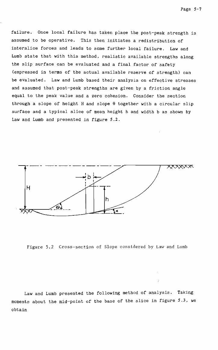
Page 5-7

failure. Once local failure has taken place the post-peak strength is

assumed to be operative. This then initiates a redistribution of

interslice forces and leads to some further local failure. Law and

Lumb state that with this method, realistic available strengths along

the slip surface can be evaluated and a final factor of safety

(expressed in terms of the actual available reserve of strength) can

be evaluated. Law and Lumb based their analysis on effective stresses

and assumed that post-peak strengths are given by a friction angle

equal to the peak value and a zero cohesion. Consider the section

through a slope of height H and slope 0 together with a circular slip

surface and a typical slice of mean height h and width b as shown by

Law and Lumb and presented in figure 5.2.

TWSX}A*S

Figure 5.2 Cross-section of Slope considered by Law and Lumb

Law and Lumb presented the following method of analysis. Taking

moments about the mid-point of the base of the slice in figure 5.3, we

obtain

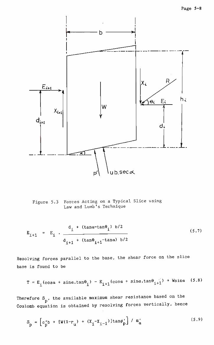
Page 5-8

E< +i

Xtî

'At!

w

Xi

f^\e<

R^

Ei > ,

di

h^

p'\ \ub.secc<

Figure 5.3 Forces Acting on a Typical Slice using Law and Lumb's Technique

E-__i = E. . l+l l

d. + (tano-tanOi) b/2

d. . + (tanO.Ll-tana) b/2 l+l 1+1

(5.7)

Resolving forces parallel to the base, the shear force on the slice

base is found to be

T = E.(cosct + sina.tanej - Ei+1(cosa + sino.tanO^) + Wsino (5.8)

Therefore S , the available maximum shear resistance based on the p

Coulomb equation is obtained by resolving forces vertically, hence

S = [c'b + [W(l-ru) + (X.-X._1)]tan0^] / *; (5.9)

Page 5-9

where cp, 0' are the peak values of the cohesion and angle

of internal friction of the soil in terms of effective stress,

ru = ub/W (Morgenstern and Price, 1960) (5.10)

and

m' = cosa + tan0'.sino (5.11)

By comparing T and S , Law and Lumb recognised the existence of

local failure. Law and Lumb assumed the process of local failure to

occur when, at some location, the shear stress due to the effect of

gravity and pore pressure has exceeded the maximum available soil

strength. This assumes that, prior to any local failure, the

resultant of all the interslice forces acting on a slice is zero. The

condition for local failure is thus expressed as

Wsina > fc'b + W(l-r )tan0'l / m' (5.12) L p u pJ a

Once local failure takes place, the slice is in limiting

equilibrium and the stress mobilized at the base is equal to the

post-peak resistance of the soil. Law and Lumb assumed that

immediately after reaching peak value, the soil resistance would drop

abruptly to the final post-peak value, hence

Sr = [crb + £w(1-ru} + (VXi+l)]tan0r] ' (mi}r (5-13)

where

(m') = cosa + tan0'.sina (5.14)

Owing to a decrease in resistance in the failed slice, additional forces are transmitted to neighbouring slices. This leads to the

second process of local failure. Thus for propagation of local

failure, the following must be true for a slice to be deemed to have

failed locally.

T > S <5-15> P

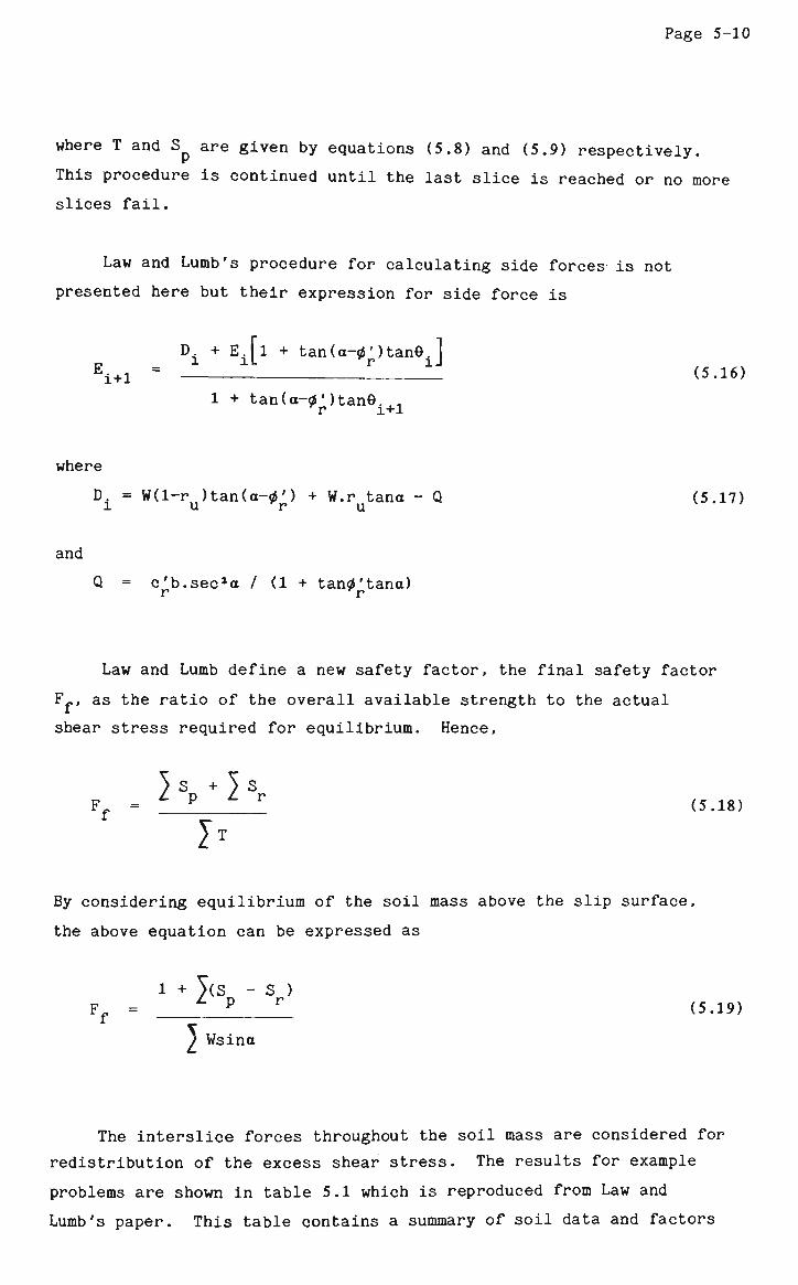
Page 5-10

where T and Sp are given by equations (5.8) and (5.9) respectively.

This procedure is continued until the last slice is reached or no more

slices fail.

Law and Lumb's procedure for calculating side forces is not

presented here but their expression for side force is

D + E,[l + tan(a-0')tanO.l « i + . - - - - - " • " >

1 + tan(a-0')tanO.^. Tr l+l

where

D± = W(l-ru)tan(a-0') + W.r tana - Q (5.17)

and

Q = c'b.sec2a / (1 + tan0'tana) r r

Law and Lumb define a new safety factor, the final safety factor

Ff, as the ratio of the overall available strength to the actual

shear stress required for equilibrium. Hence,

1 SP_+ 1 s

I Ff = " P (5.18)

By considering equilibrium of the soil mass above the slip surface,

the above equation can be expressed as

1 + T(S - S ) L n r F. = y * (5.19)

f y Wsina

The interslice forces throughout the soil mass are considered for

redistribution of the excess shear stress. The results for example

problems are shown in table 5.1 which is reproduced from Law and

Lumb's paper. This table contains a summary of soil data and factors

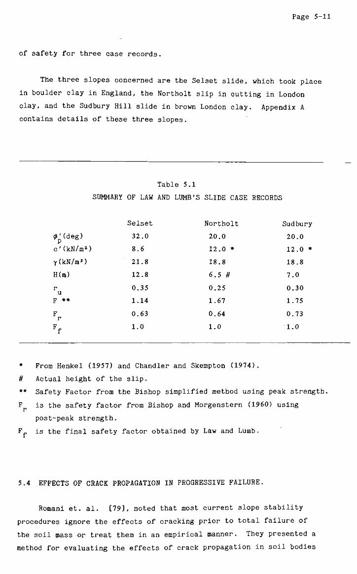
Page 5-11

of safety for three case records.

The three slopes concerned are the Selset slide, which took place

in boulder clay in England, the Northolt slip in cutting in London

clay, and the Sudbury Hill slide in brown London clay. Appendix A

contains details of these three slopes.

Table 5.1

SUMMARY OF LAW AND LUMB'S SLIDE CASE RECORDS

0'(deg)

c'(kN/ma)

y(kN/m3)

H(m)

r u p **

F r F f

Selset

32.0

8.6

21.8

12.8

0.35

1.14

0.63

1.0

Northolt

20.0

12.0 *

18.8

6.5 #

0.25

1.67

0.64

1.0

Sudbury

20.0

12.0 *

18.8

7.0

0.30

1.75

0.73

1.0

* From Henkel (1957) and Chandler and Skempton (1974).

# Actual height of the slip.

** Safety Factor from the Bishop simplified method using peak strength.

F is the safety factor from Bishop and Morgenstern (1960) using

post-peak strength.

F is the final safety factor obtained by Law and Lumb.

5.4 EFFECTS OF CRACK PROPAGATION IN PROGRESSIVE FAILURE.

Romani et. al. [79], noted that most current slope stability

procedures ignore the effects of cracking prior to total failure of

the soil mass or treat them in an empirical manner. They presented a

method for evaluating the effects of crack propagation in soil bodies

Page 5-12

with sloping boundaries. The following assumptions were applied.

(a) the body is a linear elastic material

(b) the problem is two-dimensional only

(c) the most critical sliding surface progresses along a circular

path which passes through the toe of the slope.

Romani et. al. presented a method which, briefly explained, is as

follows.

Elastic Stress

Figure 5.4 Slope Cross-section Showing Method of Romani et. al.

Referring to figure 5.4, a slit is assumed to start at point B. When

the slit has progressed to point B', the line of discontinuity B'E

appears above it. Having assumed a circular crack, BB'B", the

material above this crack defined by the body BB'EB", is taken

Page 5-13

as a rigid body and its stability is analysed by the method of slices.

The region to the right, B'FE, is assumed to be in a condition of

elastic stress.

This mixed approach is required due to surface BB'B", which

constitutes a surface of discontinuity of stress vectors and causes

elastic stresses to be undetermined along that surface. The resisting

and driving forces of each part are calculated and the factor of

safety is defined as

(5.20) F

where

Sff + SC + SBB'

Dr + DBB

S = tan0 ff ds

SC = ca J ds

(5.21)

(5.22)

ST-_.. = ̂ c + N.tan0) (5.23) BB' L p p

D = ft ds (5.24)

DBB' = 5(Wsina) (5.25)

and where

and

CT = ff cos20 + ffxsin20 + T sin20 (5.26)

x = [(ff -<y )/2] sin20 - T cos20 (5.27) y x xy

where 0 is the inclination of the plane on which a and x act.

The results obtained by Romani et.al. are shown in figure 5.5

These results show that local failures starting at the crest of the

slope are potentially more dangerous than local failures starting at

the toe of the slope. Romani used the Bishop Simplified Method for

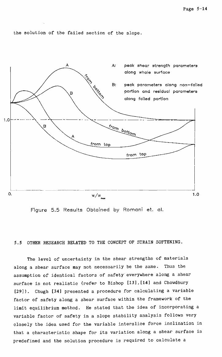
Page 5-14

the solution of the failed section of the slope.

peak shear strength parameters

along whole surface

peak parameters along non—failed

portion and residual parameters

along failed portion

Figure 5.5 Results Obtained by Romani et. al

5.5 OTHER RESEARCH RELATED TO THE CONCEPT OF STRAIN SOFTENING.

The level of uncertainty in the shear strengths of materials

along a shear surface may not necessarily be the same. Thus the

assumption of identical factors of safety everywhere along a shear

surface is not realistic (refer to Bishop [13],[14] and Chowdhury

[29]). Chugh [34] presented a procedure for calculating a variable

factor of safety along a shear surface within the framework of the

limit equilibrium method. He stated that the idea of incorporating a

variable factor of safety in a slope stability analysis follows very

closely the idea used for the variable interslice force inclination in

that a characteristic shape for its variation along a shear surface is

predefined and the solution procedure is required to calculate a

Page 5-15

scalar factor which scales the characteristic.

Chugh defined the F value at any point along the slip surface as

the ratio of available shear strength to the driving shear stress at

that point. He thus stated that since a' and x (induced) values n

fall on one curve and there may be several curves (one for each material) the ratio of mobilised shear strength to shear stress

induced is different, and hence the factor of safety along the shear

surface is varying.

Tavenas and Leroueil [101], in their investigations with cut

slopes, found that as a result of the dissipation of negative pore

pressures, the effective stress condition at any point in the slope

progressively moves towards the limit state. The shear strength which

governs the initiation of local failure at any point in a slope cut in

intact clay corresponds to an effective stress condition on the limit

state curve. The time-dependent displacement of the limit state

combines with the time-dependent modification of the effective stress

condition in the slope to result in a delayed failure.

At any point in the slope, the strength mobilised at the onset of

local failure is in the limit state. Following local failure, strain

softening occurs and the effective stress condition tends towards the

critical state. Along with this, local failure can be initiated in

neighbouring clay elements as a result of shear stress transfer from

the strain softening clay. Full failure of the slope occurs when the

loss of strength in those areas which have already failed cannot be

compensated by the reserve resistance in the other non-failed areas.

Foerster and Georgi [43] presented a method of analysis which

incorporated a progressive mechanism of failure as a function of time.

Using the finite element method, they formulated an iterative

procedure whereby the state of stress in elements was compared to a

predefined value, that of the residual strength. By failing elements

where the stress value exceeded the residual strength and by stress

redistribution a situation was obtained whereby general failure of the

structure occured. Their analyses showed that the extent of the

overstressed zone increases with time.

Page 5-16

Sallfors and Larsson [80] stated that in a slope where the factor

of safety against failure is low, consolidation and creep will result

in the redistribution of stresses with time. They showed that this

redistribution of stresses has an effect on the preconsolidation

pressure and also results in a rotation of the principal stresses.

The shear strength and the anisotropy is thereby also affected.

Reddy and Venkatakrishna Rao [77] suggested that only the points

along the failure surface are in critical equilibrium and, at other

points above the failure surface, the mobilised shear strengths are

less than those at critical equilibrium. Using the method of

characteristics, they assumed that mobilised shear strength varies

with depth and treated the whole soil mass as a series of layers and

obtained a series of factors of safety for different heights in a

goven slope. They found their results to be in fair agreement with

and slightly lower in value than similar results obtained by the

friction circle method.

Nelson and Thompson [69] presented a theory of creep failure to

explain the relationship between creep, strain softening, and

time-dependent failures in overconsoliated clays. They based their

theory on the principle that time-dependent irreversible strains

(creep) have the same detrimental effect on a soil's internal bonds as

do the plastic strains associated with strain softening during a

triaxial test.

They hypothesised that 'interparticle bonds form at points of

high local stress during application of large consolidation pressures.

Such bonds are the primary cause of the peak strengths observed in

overconsolidated clays. Under conditions of sustained shear stress,

plastic deformations occur across these bonds resulting in their

deterioration', thereby causing 'irreversible time-dependent

deformations recognised as creep and a corresponding reduction of the

peak strength toward the residual strength of the soil.

Also, Nelson and Thompson reported that laboratory tests have

shown that 'some critical strain exists at which point all of the

internal bonds in the soil will have failed' and 'the shear strength

of the soil will have been reduced to its residual strength. If, at

Page 5-17

this point, the applied stress were greater than the residual

strength, equilibrium would not be maintained and the tertiary stage

of creep would begin'.

Nelson and Thompson reasoned that at low stress states, just

above the residual strength, the number of bonds which must fail

before tertiary creep begins is greater than at high stress states,

therefore indicating that the critical strain should increase for

lower stresses.

This finding was supported by Ter-Stepanian [104] who, while

studying creep in clays, found that failure takes place only at high

stress levels and comparatively short stress age. Thus failure is

much less likely to occur at slightly lower stress levels.

Sidharta [38] developed a practical engineering method to

predict, by means of a creep-failure approach, the time to failure of

a slope of moderately to heavily overconsolidated clay after a cut or

excavation. He considered the potential for progressive failure to

occur due to the simultaneous accumulation of creep strain and

decrease in strength due to dissipation of negative excess porewater

pressure. The analysis uses a limit equilibrium approach and Bishop's

simplified method of analysis was used for circular slip surface

cases.

Sidharta used a value of shear strength between the peak and

residual values and defined a residual factor similar to that defined

by Skempton. He assumed stress redistribution to begin after the

first point on the critical failure surface reaches the post-peak

(strain-softening) side of the stress-strain curve. He simulated

progressive failure starting from a number of points within the

* failure mass and found that regardless of where the progressive

failure is assumed to be initiated, as long as the average initial

deviator stress is held constant, the predicted time to failure was

about the same. His model used data on Brown London clay and

considered the clay to be homogeneous.

Page 5-18

Bernander [10] stated that deformations and the time factor must

be taken into account when analysing slopes in strain rate softening

materials.

Wu et.al [114] investigated a number of slopes in soft shales

containing discontinuities in the form of slickensides. They measured

the shear strengths of the intact shales and slickensides and

performed stability analyses to calculate the shear strength of the

shale in the failed slopes. They attempted to estimate the effect of

slickensides and stress redistribution on the reduction of shear

strength below its peak value.

They suggested that the residual strength is a limiting strength

where an appreciable portion of the surface may follow slickensides or

local shear zones. Also, in the cases of slopes that failed, neither

slickensides nor local failure alone would have reduced the overall

shear strength sufficiently to induce slope failure. Failure in these

cases was caused by the combined effect of large slickensides

intensity and local failure.

Andrei and Athanasiu [3] considered the mechanism of progressive

mobilisation of shear strength in developing a method of slope

stability analysis using Janbu's method as its basis. They determined

a relationship between the assumed displacement of the material along

the proposed surface of sliding and the factor of safety.

CHAPTER 6

SIMULATION OP PROGRESSIVE FAILURE BY LOCALISED STRAIN SOFTENING.

6.1 INTRODUCTION AND SCOPE.

In the previous chapter, a number of approaches to the problem of

progressive failure were discussed. These approaches varied basically

in the mechanism considered responsible for the initiation of the

process of progressive failure. Bjerrum [18] argued that a

discontinuity of some type must exist in the slope in order to

initiate a progressive failure and emphasised the role of lateral

stress. Romani et. al. [79] assumed that a crack-type discontinuity

would facilitate the initiation of the process of progressive failure

Law and Lumb [58], on the other hand, approached the problem from

a different angle. They considered the stress state at the base of a

number of soil slices to determine whether conditions were favourable

for local failure to occur. Once overstress in terms of Mohr-Coulomb

failure criteria had occurred, the assumption was made that failure

had occurred locally and that conditions on the bases of 'failed'

slices corresponded to those obtained when the residual strength of

the soil was reached. The excess shear stress remaining was then

redistributed by a complex procedure as discussed in the previous

chapter.

The primary objective of this chapter is to present new methods

for the simulation of stress redistribution associated with local

failure and strain-softening within a slope. Specifically, possible

local failure and strain-softening is considered along the bases of

individual slices. However, in the methods proposed here

consideration of interslice forces is not required for stress

redistribution although either simplified or rigorous methods are used

Page 6-2

to calculate safety factors for a slope iteratively. Thus for the

calculation of each safety factor, due consideration may be given to

interslice forces and to force and moment equilibrium. However,

simulation of the redistribution of stress associated with progressive

failure does not require the consideration of these interslice forces.

Therefore, the methods proposed are easy to use in comparison to

others that have been suggested in the past.

In order to explain the salient features of the proposed methods

and to demonstrate their implementation, a number of case histories of

slope failures were analysed and the results are presented in this

chapter. These include the three case records referred to in the

previous chapter (i.e. Northolt, Selset and Sudbury Hill) as well as

the Jackfield slide (England), the Balgheim slide (Germany), the

Vajont slide (Italy), the Saskatchewan slide (Canada), the Brilliant

Cut slide and two hypothetical slides. Details of all these appear in

appendix A. Reasons for the introduction of the two hypothetical

slides are also given in appendix A.

6.2 REDISTRIBUTION OF EXCESS SHEAR (METHOD 1).

As defined by Law and Lumb, a local failure is initiated when at

some location, the shear stress due to the effect of gravity and pore

pressure has exceeded the maximum available soil strength. 'Once

local failure takes place, the slice is in limiting equilibrium and

the stress mobilised at the base is equal to the post-peak resistance

of the soil' [58]. In other words the shear strength on the slice

base has dropped to the residual value. Since the shear stress cannot

exceed the available shear strength, the excess stress must be

transmitted to the unfailed slices.

Whereas Law and Lumb transmit these excess stresses by a complex

procedure which incorporates the excess stresses into newly calculated

interslice forces, the technique presented here attempts to simplify

the solution of the problem by neglecting interslice forces

altogether. The excess shear is transmitted to the unfailed slices by

distributing it across the unfailed length of the failure surface.

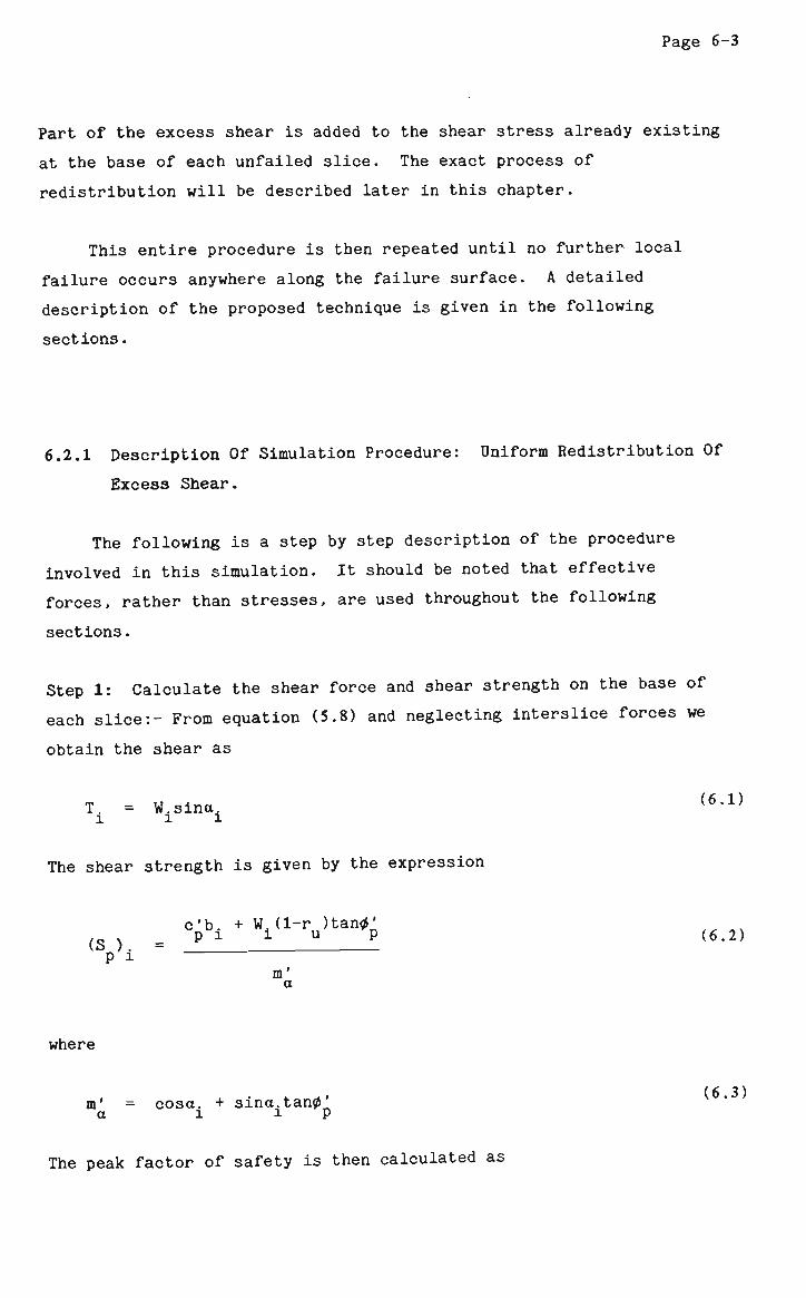
Page 6-3

Part of the excess shear is added to the shear stress already existing

at the base of each unfailed slice. The exact process of

redistribution will be described later in this chapter.

This entire procedure is then repeated until no further local

failure occurs anywhere along the failure surface. A detailed

description of the proposed technique is given in the following

sections.

6.2.1 Description Of Simulation Procedure: Uniform Redistribution Of

Excess Shear.

The following is a step by step description of the procedure

involved in this simulation. It should be noted that effective

forces, rather than stresses, are used throughout the following

sections.

Step 1: Calculate the shear force and shear strength on the base of

each slice:- From equation (5.8) and neglecting interslice forces we

obtain the shear as

T. = W.sina. (6-1)

l i i

The shear strength is given by the expression

(S ). P i

c'b. + W.(1-r )tan0' .̂ . p i i u *p (6.2)

m' a

where

(6 3) m' = cosa. + sina.tan0' a l i p

The peak factor of safety is then calculated as

Page 6-4

F - K " x (..4) . T _

Step 2: Check for local failure:- Local failure is deemed to occur on

any slice where the mobilised shear force calculated equals, or

exceeds, the calculated shear strength. Thus, local failure occurs on

any slice where

Ti i < v ± (6-5)

where T and (S ). are described in equations (6.1) and (6.2).

If no slices satisfy this condition (i.e. if no local failure

occurs), then the previously calculated factor of safety is taken as

the final factor of safety.

Since the occurrence of local failure is only checked on one

slice at the time and the stresses and strengths on slices are

dependent on the width and position of a slice, it is possible that by

combining into one slice, two adjacent slices, one of which has failed

locally while the other has not, overall local failure of the combined

slice may accur. The following procedure is thus followed for each

slice, i, where local failure is deemed to have occurred.

If slice i-1 has not failed, the combined slice consisting of

slices i and i-1 is tested for local failure. Local failure for the

combined slice is said to occur if

T. , + T. > S. , + S. (6.6) l-l l l-l l

where T and S are defined by equations (6.1) and (6.2). If local

failure occurs, part of the excess shear force on slice i is

redistributed to slice i-1. The amount of redistributed shear force

is equal to

AT = S. , - T. , (6.7) l-l l-l

Thus, the shear forces on the two slices become

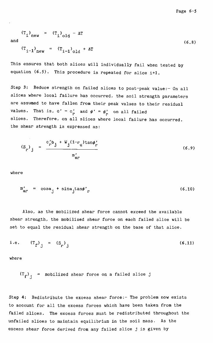
Page 6-5

and

(Vnew " ( V o l d - A T

'Vl'new = (Ti-l>old + AT

(6.8)

This ensures that both slices will individually fail when tested by

equation (6.5). This procedure is repeated for slice i+1.

Step 3: Reduce strength on failed slices to post-peak value:- On all

slices where local failure has occurred, the soil strength parameters

are assumed to have fallen from their peak values to their residual

values. That is, c' = c^ and 0' = 0' on all failed

slices. Therefore, on all slices where local failure has occurred,

the shear strength is expressed as:

c'b. + W,(l-r )tan0'

«„>. - JJ <_.-> r J m' ar

where

m' = cosa. + sina.tan0' (6.10)

Also, as the mobilized shear force cannot exceed the available

shear strength, the mobilized shear force on each failed slice will be

set to equal the residual shear strength on the base of that slice.

i.e. (T ) = (S ) (6.11)

where

(Tf) . = mobilized shear force on a failed slice j

Step 4: Redistribute the excess shear force:- The problem now exists

to account for all the excess forces which have been taken from the

failed slices. The excess forces must be redistributed throughout the

unfailed slices to maintain equilibrium in the soil mass. As the

excess shear force derived from any failed slice j is given by

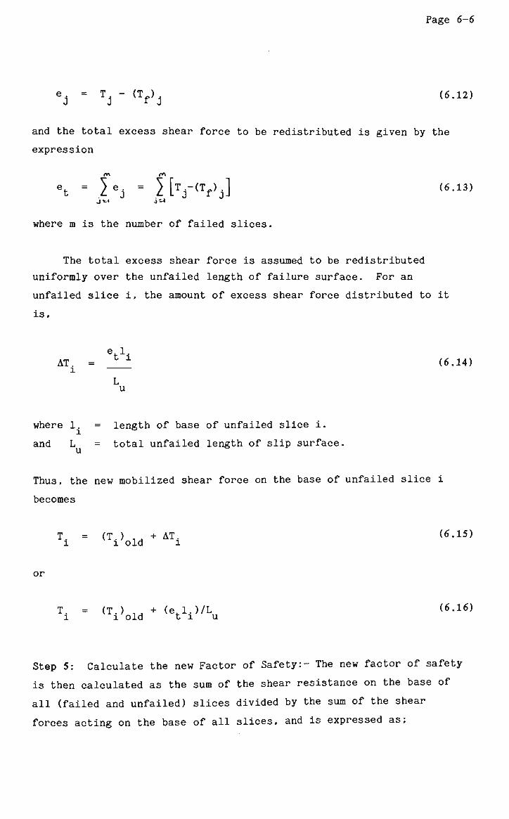
Page 6-6

ej = Tj " ( V j (6-12>

and the total excess shear force to be redistributed is given by the

expression

et - l*j = Hv(Vj] (6-i3)

where m is the number of failed slices.

The total excess shear force is assumed to be redistributed

uniformly over the unfailed length of failure surface. For an

unfailed slice i, the amount of excess shear force distributed to it

is,

Vi AT. = Z X (6.14)

l

L u

where 1. = length of base of unfailed slice i.

and L = total unfailed length of slip surface. u

Thus, the new mobilized shear force on the base of unfailed slice i

becomes

T. = (T.) ,. + AT. (6.15) l I old i

or

T. = (T.) .. + (e.l.)/L, <6-16> l I old t I u

Step 5: Calculate the new Factor of Safety:- The new factor of safety

is then calculated as the sum of the shear resistance on the base of

all (failed and unfailed) slices divided by the sum of the shear

forces acting on the base of all slices, and is expressed as:

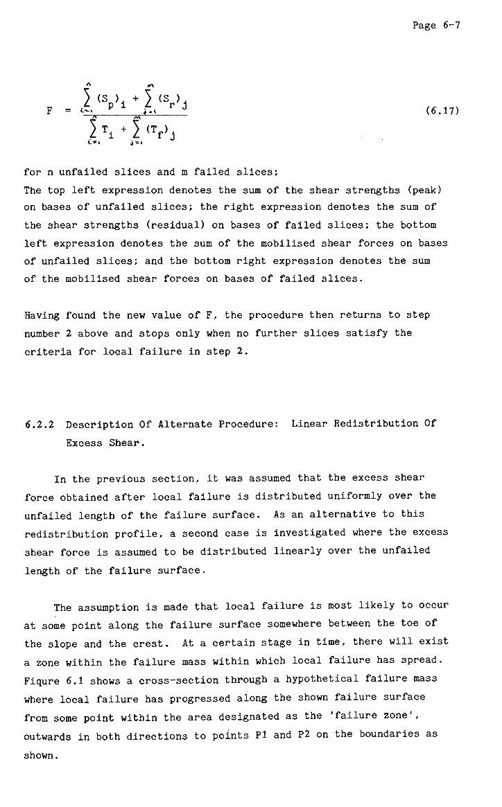
Page 6-7

F = A P 1 J*. r J (6.1

K+5<Vj

for n unfailed slices and m failed slices;

The top left expression denotes the sum of the shear strengths (peak)

on bases of unfailed slices; the right expression denotes the sum of

the shear strengths (residual) on bases of failed slices; the bottom

left expression denotes the sum of the mobilised shear forces on bases

of unfailed slices; and the bottom right expression denotes the sum

of the mobilised shear forces on bases of failed slices.

Having found the new value of F, the procedure then returns to step

number 2 above and stops only when no further slices satisfy the

criteria for local failure in step 2.

6.2.2 Description Of Alternate Procedure: Linear Redistribution Of

Excess Shear.

In the previous section, it was assumed that the excess shear

force obtained after local failure is distributed uniformly over the

unfailed length of the failure surface. As an alternative to this

redistribution profile, a second case is investigated where the excess

shear force is assumed to be distributed linearly over the unfailed

length of the failure surface.

The assumption is made that local failure is most likely to occur

at some point along the failure surface somewhere between the toe of

the slope and the crest. At a certain stage in time, there will exist

a zone within the failure mass within which local failure has spread.

Fiqure 6.1 shows a cross-section through a hypothetical failure mass

where local failure has progressed along the shown failure surface

from some point within the area designated as the 'failure zone',

outwards in both directions to points Pi and P2 on the boundaries as

shown.

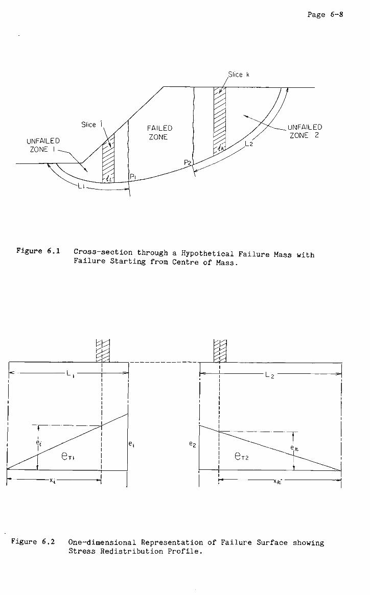
Page 6-8

Slice k

UNFAILED ZONE I

UNFAILED ZONE 2

Figure 6.1 Cross-section through a Hypothetical Failure Mass with Failure Starting from Centre of Mass.

Figure 6.2 One-dimensional Representation of Failure Surface showing Stress Redistribution Profile.

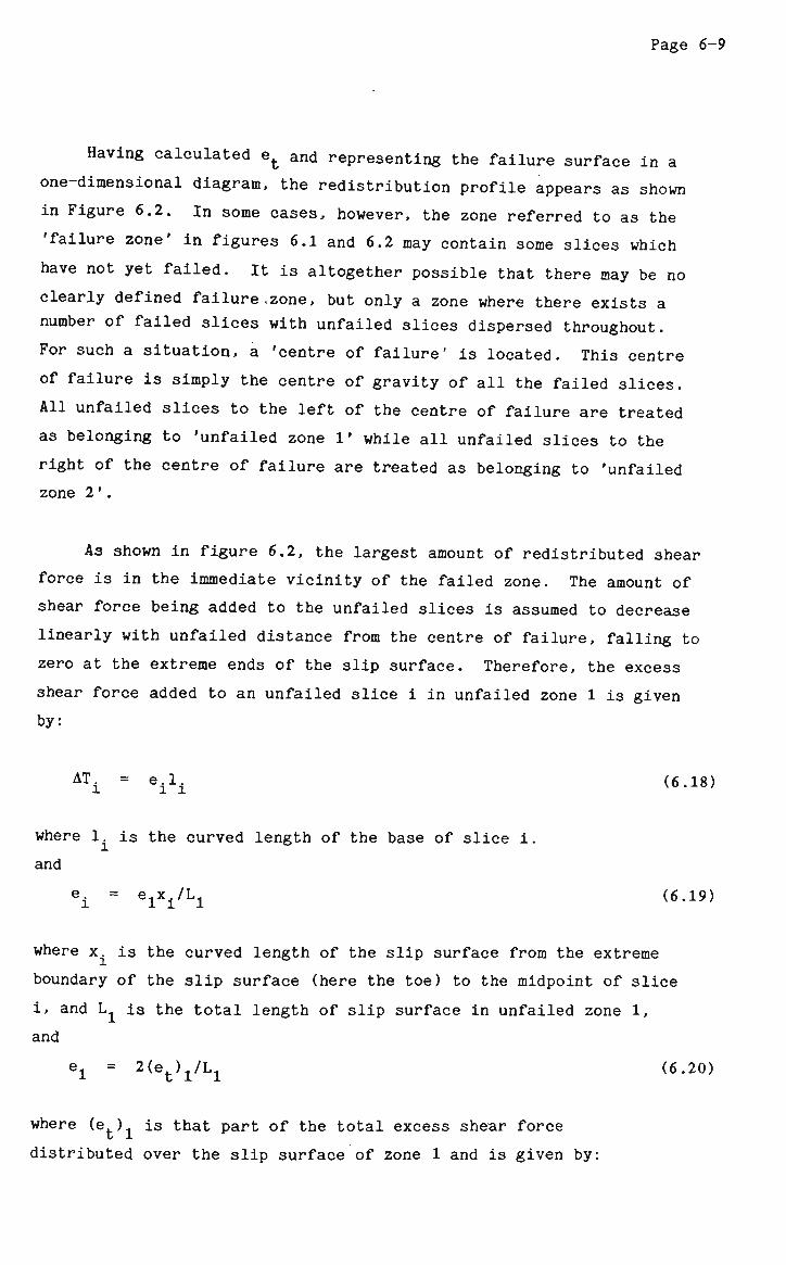
Page 6-9

Having calculated efc and representing the failure surface in a

one-dimensional diagram, the redistribution profile appears as shown

in Figure 6.2. In some cases, however, the zone referred to as the

'failure zone' in figures 6.1 and 6.2 may contain some slices which

have not yet failed. It is altogether possible that there may be no

clearly defined failure .zone, but only a zone where there exists a

number of failed slices with unfailed slices dispersed throughout.

For such a situation, a 'centre of failure' is located. This centre

of failure is simply the centre of gravity of all the failed slices.

All unfailed slices to the left of the centre of failure are treated

as belonging to 'unfailed zone 1' while all unfailed slices to the

right of the centre of failure are treated as belonging to 'unfailed

zone 2'.

As shown in figure 6.2, the largest amount of redistributed shear

force is in the immediate vicinity of the failed zone. The amount of

shear force being added to the unfailed slices is assumed to decrease

linearly with unfailed distance from the centre of failure, falling to

zero at the extreme ends of the slip surface. Therefore, the excess

shear force added to an unfailed slice i in unfailed zone 1 is given

by:

AT. = e.l. (6.18)

where 1 is the curved length of the base of slice i.

and

ei = elxi/Ll (6.19)

where x is the curved length of the slip surface from the extreme

boundary of the slip surface (here the toe) to the midpoint of slice

i, and L. is the total length of slip surface in unfailed zone 1,

and

el = 2(et)l/Ll (6.20)

where (e )^ is that part of the total excess shear force

distributed over the slip surface of zone 1 and is given by:

Page 6-10

VL1 (e.)1 = (6.21) t'l

L l + L 2

e being the total excess shear force given by equation (6.13) and

L2 the total length of slip surface in unfailed zone 2.

Thus equation (6.18)becomes

2e x.l. AT. = t X X (6.22)

L1(L1+L2)

Similarly for unfailed zone 2, the excess shear force to be added to

an unfailed slice is given by

2e x 1. ATk = U K K (6.23)

L2(L1+L2)

Therefore, the new modified shear force on the base of an unfailed

slice, i in unfailed zone 1 becomes

T, = (T.) ,, + AT. i I old I

or

2e x.l. T. = (T.) .. + (6.24) i I old

L2(L1+L2)

and for an unfailed slice k in unfailed zone 2

2e x.l Ik - (Tk)_ld + __________ <6.25)

L2<LU,)

Page 6-11

The overall procedure involved is the same as that described in

the previous section. Step 4, however, is replaced by the above

procedure for linearly redistributing excess shear force.

6.2.3 Definition Of Propagation Factor.

As an indication of the extent to which progressive failure has

occured, a factor is introduced here which shall be called the

'Propagation Factor'. This propagation factor is defined as the

fraction of the total length of the assumed failure surface over which

local failure has occurred. More specifically, the propagation factor

is defined as that fraction (expressed as a decimal between 0 and 1)

derived by dividing the sum of the base lengths of all slices in the

failure mass where local failure has occurred by the sum of the base

lengths of all the slices in the failure mass. This is expressed as

PF = «

n n

} <Vi 1 (Vi (6.26)

_ 1 k

where (lf). = the base length of a failed slice i.

1 = the base length of any slice k , it

n = the number of failed slices ,

N = the total number of slices ,

and L = the total curved length of the failure surface

6.2.4 Computer Program STRAIN1.

As the calculations involved in the simulation of progressive

failure using method 1 are highly repetitive, and therefore time

consuming, the process is greatly facilitated by the use of a digital

computer. Also, the degree of accuracy is greatly increased by using

a computer since random errors, which would normally occur due to the

large number of calculations, are eliminated.

Page 6-12

Written in FORTRAN 77, the computer program STRAIN1 was developed

and run on the UNIVAC 1100 computer at the University of Wollongong.

Figure 6.3 contains a flowchart which describes the internal structure

of the main program.

The program is capable of handling both cases of excess shear

distribution detailed above. A parameter called the 'shear force

distribution option' (1 = uniform and 2 = linear distribution of

excess shear) is read in as data and this parameter controls the

internal operation of the program according to the required

distribution method. As each new value of the factor of safety is

calculated, the program also calculates the corresponding value of the

propagation factor. These two values, along with detailed data for

each soil slice, are printed as output from the program after each new

factor of safety is calculated. The detailed slice data includes

values of shear force and shear resistance on the base of each slice

as well as an indicator which tells if the slice has undergone local

failure. Once the final factor of safety is obtained, final values of

the factor of safety and the propagation factor are output as well as

values of the peak and residual factors of safety, and the value of

the factor of safety before shear redistribution commenced (ie. after

the first set of slices have failed locally but before any excess

shear has been redistributed). Subroutine SPARAM, which reads in the

soil parameter data and the slope geometry data, also calculates other

necessary soil data such as angles of slice bases and toplines, slice

weights and the pore water pressure acting on the base of each slice.

In calculating the pore-water pressure acting on the base of each

slice, subroutine SPARAM considers two options. If the value of the

pore-pressure ratio read from the data file is less than 1.0 the

pore-water pressure, u for each slice base is calculated from this

value of r using the following expression.

u. = vz r (6.27) l ' i u

where y = unit weight of soil

and z = height of midpoint of slice i.

If, on the other hand, the given value of r is greater than 1.0,

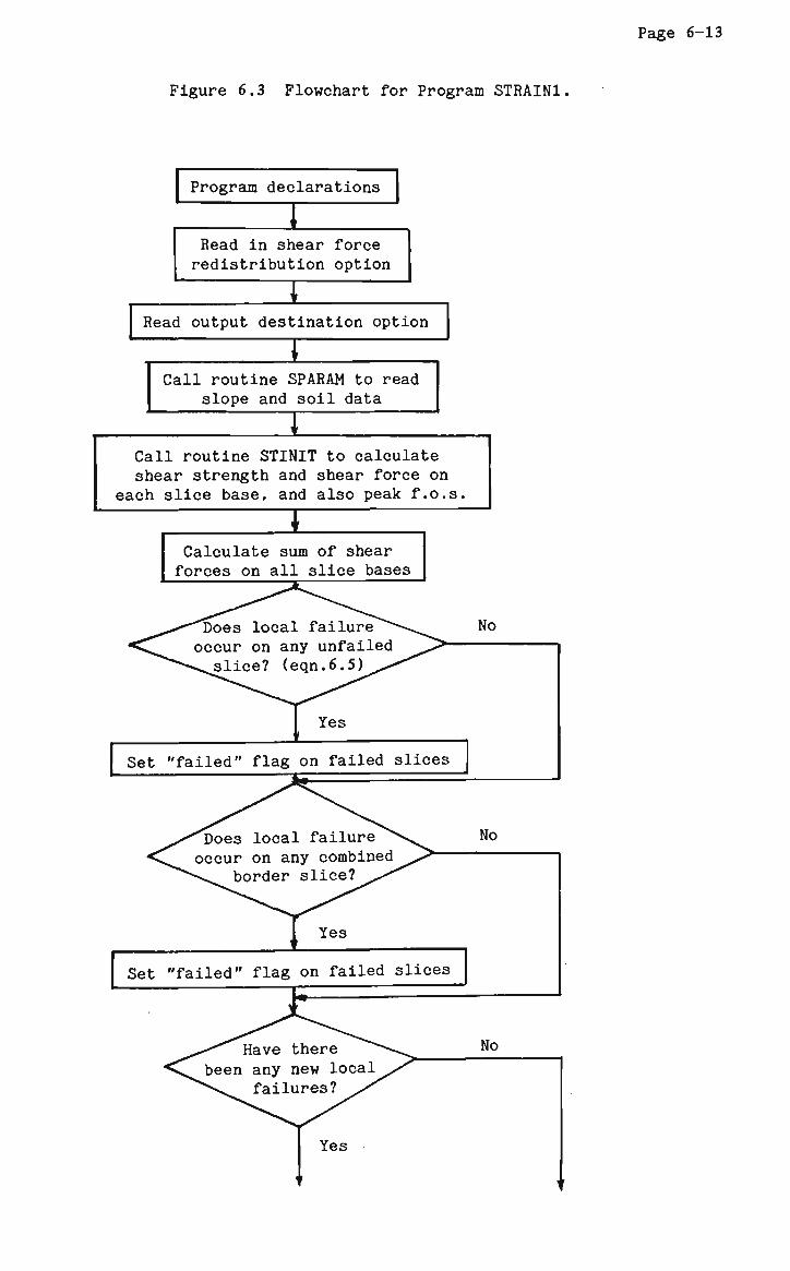
Page 6-13

Figure 6.3 Flowchart for Program STRAIN1

Program declarations

Read in shear force redistribution option

Read output destination option

Call routine SPARAM to read slope and soil data

Call routine STINIT to calculate shear strength and shear force on

each slice base, and also peak f.o.s.

I Calculate sum of shear forces on all slice bases

Does local failure occur on any unfailed slice? (eqn.6.5)

Yes

Set "failed" flag on failed slices

No

Does local failure occur on any combined

border slice?

Yes

No

Set "failed" flag on failed slices

No

Yes

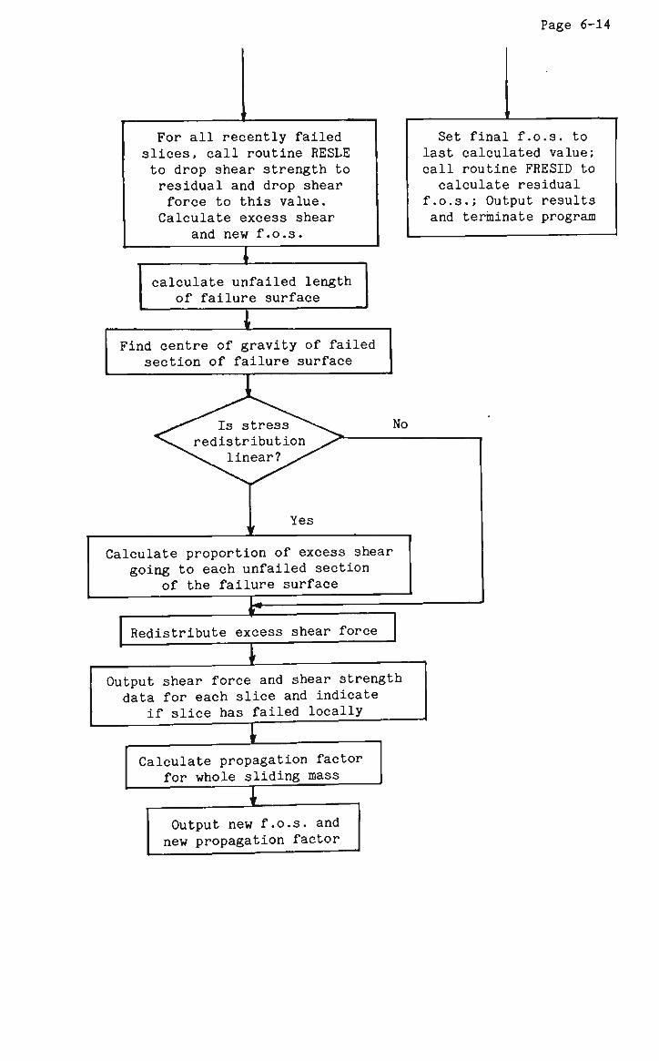
Page 6-14

For all recently failed slices, call routine RESLE to drop shear strength to residual and drop shear force to this value.

Calculate excess shear and new f.o.s.

Set final f.o.s. to last calculated value; call routine FRESID to calculate residual

f.o.s.; Output results and terminate program

calculate unfailed length of failure surface

I Find centre of gravity of failed section of failure surface

No

Yes

Calculate proportion of excess shear going to each unfailed section

of the failure surface

Redistribute excess shear force

IE Output shear force and shear strength data for each slice and indicate

if slice has failed locally

_C Calculate propagation factor for whole sliding mass

I Output new f.o.s. and new propagation factor

Page 6-15

this indicates that the phreatic surface co-ordinates are specified

and the pore-water pressure for each slice base is calculated from the

height of the phreatic surface at that slice. The pore-water pressure

on the base of a slice i is given by

u± = Yw

zi (6.28)

where y = unit weight of water , w

and z = height of phreatic surface above slice base ,

Subroutine STINIT calculates the peak shear strengths on the

bases of each soil slice and the initial (peak) factor of safety using

equation (6.17). Subroutine FRESID is identical to subroutine STINIT

except that residual values of shear strength parameters are used

instead of peak values. Therefore, the residual value of the factor

of safety is calculated intead of the peak value, again using equation

(6.17).

Finally, subroutine RESLE performs a similar function to

subroutine STINIT except that it differentiates between slices where

local failure has occurred and those where it has not. If local

failure has occurred, the shear strength is calculated using residual

shear strength parameters c and 0 , whereas if local failure

has not occurred peak values of shear strength parameters are used.

6.2.5 Case Histories Considered.

As mentioned earlier in this chapter, the simulation technique

presented above was applied to a number of case histories in order to

study the feasibility of the proposed method. There were a total of

ten case histories used, each of which is described in detail in

appendix A. The relevant soil data for each of the slopes described

is also presented in appendix A.

Page 6-16

At this stage a mention must be made of the shear strength

parameters assumed to exist on the failure surface at the time of

failure. It is understood, from the previous sections, that at the

time of overall failure there may exist parts of the failure surface

along which peak conditions prevail while at other points residual

conditions exist. No mention has been made however, about the actual

values of the residual shear strength parameters of the soils

concerned.

When considering the value of the residual cohesion intercept

c' it is widely accepted that this value is given by the fully

softened strength value of zero. The residual value of the effective

angle of shearing resistance, however, is subject to greater debate.

Various authors (including Law and Lumb [58]) argue that this residual

value of 0' should equal its peak value. The majority, on the

other hand, regard the fully softened value of 0' to be somewhat

lower than the peak value.

In order to attempt to verify the results obtained by Law and

Lumb, and also to obtain results for the case histories as analysed by

Skempton, Henkel, Romani and other authors, two separate sets of

analyses are performed on the ten slopes described in appendix A.

The first of these, named 'system A', uses the following combination

of shear strength parameters.

(a) peak c' and 0' as given in appendix A ,

(b) residual value of c' equal to zero ,

(c) residual value of 0' equal to the peak value.

The second system, 'system B', uses the following combination of shear

strength parameters.

(a) peak c' and 0' as given in appendix A ,

Page 6-17

(b) residual value of c' equal to zero ,

(c) residual value of 0' is less than the peak value and is

as given in appendix A.

As well as the two systems of shear strength parameters mentioned

above, three of the case histories were also analysed using a number

of different pore-water pressure conditions. The Northolt slip is

firstly analysed using a pore-pressure ratio of 0.25 as used by Law

and Lumb. Secondly, a pore-pressure ratio of 0.34 is applied to this

slip as this is the average value quoted by Skempton as existing along

the failure surface. Thirdly, the piezometric surface obtained from

the soil data presented by Skempton is used directly in calculating

the pore water pressure on the base of each slice.

Similarly an r value of 0.35 was used for the Selset slide and

a value of 0.30 for the Sudbury Hill slide. As well as this, a

piezometric surface is defined for both slides. The main object of

this dual analysis is to allow comparisons between

(a) the results obtained by previous investigators and the

results obtained in this chapter, and

(b) the more realistic results obtained by using the given

piezometric surface to calculate pore-water pressure.

6.2.6 Results And Discussion.

Table 6.2 contains the results obtained using program STRAIN1 and

the theoretical procedure described in method 1. Results for both

system A and system B are shown. The meanings of the symbols in the

table are as follows.

Page 6-18

- Fp is the peak factor of safety for the slope.

- Fp is the residual factor of safety for the slope.

- Ffe is the factor of safety obtained just prior to the

commencement of stress redistribution. P Fb is the value o f the propagation factor when the factor of safety is equal to Fv.

b " F

c Is the final factor of safety with uniform stress redistribution.

~ P Fc is the Pr°Pa8a t i o n factor value after uniform stress redistribution.

- F1 is the final factor of safety with linear stress

redistribution.

- PF1 is the propagation factor value after linear stress

redistribution.

It would appear from the results in table 6.2 that no clear-cut

conclusions can be reached regarding the feasibility of the proposed

method applied to the given case histories. Certain trends can,

however, be observed and these will be discussed here. A more

comprehensive discussion will be presented at the conclusion of this

chapter and a number of conclusions will be drawn there.

The most obvious point to note is that, in all cases where the

resulting factors of safety due to constant and linear redistribution

of excess shear, respectively, are not equal, the factor of safety

obtained by linearly redistributing excess shear is lower than the

other. In other words, F. is less than or equal to F . 1 c

Some slopes (Balgheim, Hypothetical Slope 1) show no drop in F

from the peak value. Others (Jackfield, Hypothetical Slope 2) show a

small drop in factor of safety after the initially overloaded slices

have failed but produce no further reduction in F upon redistributing

excess shear in any manner. The results for system B data showed, in

general, lower values of factor of safety as would be expected since

lower values of 0' are used. In certain cases, however, no local

failure was noticed and, as in the case of system A, no drop in F from

the peak value was observed.

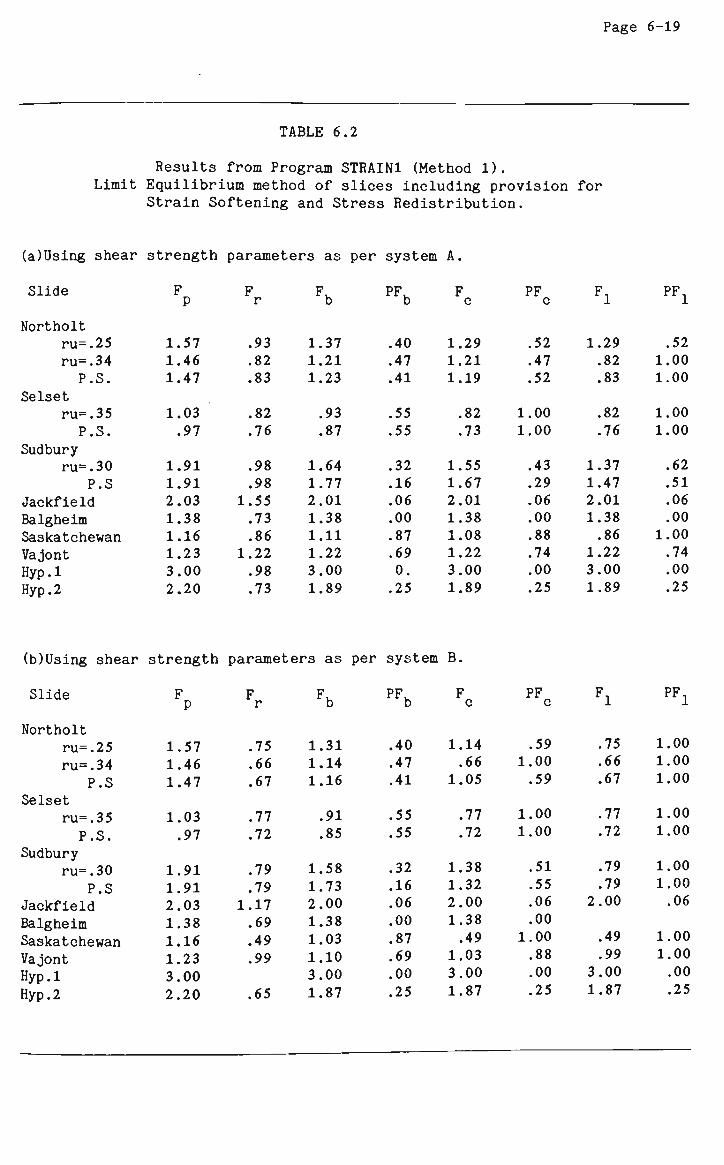
Page 6-19

TABLE 6.2

Results from Program STRAIN1 (Method 1). Limit Equilibrium method of slices including provision for

Strain Softening and Stress Redistribution.

(a)Using shear strength parameters as per system A.

Slide

Northolt ru=.25

ru=.34

P.S.

Selset ru=.35

P.S.

Sudbury ru=.30

P.S Jackfield

Balgheim Saskatchewan

Vajont

Hyp.l Hyp. 2

F P

1.57 1.46

1.47

1.03

.97

1.91 1.91

2.03

1.38

1.16

1.23

3.00

2.20

F r

.93

.82

.83

.82

.76

.98

.98 1.55

.73

.86 1.22

.98

.73

Fb

1.37 1.21 1.23

.93

.87

1.64

1.77 2.01

1.38

1.11 1.22

3.00

1.89

PFb

.40

.47

.41

.55

.55

.32

.16

.06

.00

.87

.69 0. .25

F c

1.29 1.21

1.19

.82

.73

1.55

1.67 2.01

1.38 1.08 1.22

3.00

1.89

PF c

.52

.47

.52

1.00 1.00

.43

.29

.06

.00

.88

.74

.00

.25

Fl

1.29 .82 .83

.82

.76

1.37 1.47 2.01

1.38

.86 1.22

3.00

1.89

PF1

.52 1.00

1.00

1.00

1.00

.62

.51

.06

.00 1.00

.74

.00

.25

(b)Using shear strength parameters as per system B,

Slide

Northolt ru=.25

ru=.34

P.S Selset

ru=.35

P.S.

Sudbury ru=.30

P.S Jackfield

Balgheim

Saskatchewan

Vajont

Hyp.l Hyp. 2

F P

1.57 1.46

1.47

1.03

.97

1.91

1.91 2.03

1.38

1.16

1.23

3.00

2.20

F r

.75

.66

.61

.11

.72

.79

.79 1.17

.69

.49

.99

.65

Fb

1.31

1.14

1.16

.91

.85

1.58

1.73 2.00

1.38

1.03

1.10

3.00

1.87

PFb

.40

.47

.41

.55

.55

.32

.16

.06

.00

.87

.69

.00

.25

F c

1.14 .66

1.05

.77

.72

1.38 1.32

2.00

1.38

.49 1.03

3.00

1.87

PF c

.59 1.00

.59

1.00

1.00

.51

.55

.06

.00 1.00

.88

.00

.25

Fl

.75

.66

.67

.77

.72

.79

.79 2.00

.49

.99 3.00

1.87

PF.̂

1.00 1.00

1.00

1.00 1.00

1.00 1.00

.06

1.00 1.00

.00

.25

Page 6-

In cases where a number of values of the pore-pressure ratio were

used, or where the phreatic surface was used to indicate pore-pressure

levels, the results obtained showed nothing unexpected. Factors of

safety obtained using phreatic surface points to indicate

pore-pressure levels corresponded very closely to factors of safety

obtained using corresponding average r values.

6.3 CALCULATION OF OVERALL FACTOR OF SAFETY BY ITERATIVE METHODS

(METHOD 2).

6.3.1 Iterative Methods Of Analysis Used.

As an alternative to calculating the overall factor of safety as

shown in the previous section from equation (6.17), it was decided to

investigate the consequences of calculating the overall factor of

safety using some more rigorous methods of stability analysis. The

first method of stability analysis considered is the Bishop simplified

method. This method is used because of its simplicity in application

and its suitability to many of the case histories used.

Since Bishop's method of analysis is only applicable to slopes

with circular slip surfaces, it is therefore necessary to use a more

general, rigorous method such as that of Morgenstern and Price for

slopes not exhibiting a circular surface of sliding. It is also of

interest to compare the results obtained by these two methods of

analysis. Therefore, both of the above mentioned methods of analysis

will be used on each of the ten case histories analysed.

The overall procedure remains basically the same as that

described in the previous section. In step 5 of the procedure

described, however, rather than using equation (6.17) to calculate the

new factor of safety a complete limit equilibrium analysis is

performed in the form of either the Bishop simplified method or the

Morgenstern-Price method. From this analysis the new factor of safety

is obtained.

Page 6-21

The analysis is performed using the current local values of shear

strength parameters c' and 0'. I n o t h e r w o r d s, a l l s l i c e s w h e r e

local failure has occurred are treated as having residual shear

strength parameters while all others are treated as being at the peak

condition.

6.3.2 Computer Program BSTRAIN2.

Program BSTRAIN2, standing for Bishop Strain-softening Method 2,

is again very similar to program STRAIN1 described in the previous

section. It is in fact a modified version of program STRAIN1. Due to

this fact, a detailed description of the program will not be presented

here.

The major difference between the two above mentioned programs

occurs within subroutines STINIT, FRESID and RESLE which perform the

same functions as they do in program STRAIN1, except that in this case

the factor of safety calculated within each is found using Bishop's

simplified method of analysis rather than equation (6.17).

6.3.3 Computer Program MPSTRAIN2.

Program MPSTRAIN2 is an extension of program MGSTRN2 described in

chapter 4. The basic structure of MPSTRAIN2 remains the same as for

MGSTRN2. Routines CNSTNT and MTYPIN are called as in MGSTRN2 except

that in this case MTYPIN reads in both peak and residual values of the

shear strength parameters c' and 0'. MSLOPE, FRBODY, FBGEOM and

FUNCTN are then called followed by routine SOLUTN which calculates the

initial, peak factor of safety of the slope under consideration.

Following this, comes the major difference between program

MPSTRAIN2 and its predecessor. A new routine named STRAIN is called

to perform the strain-softening simulation. In actual fact, STRAIN is

identical to the main body of program BSTRAIN2, with two exceptions.

Firstly, there is no need to call routine SPARAM to read soil data and

Page 6-22

slope geometry data as this has already been done in routines MTYPIN

and FRBODY. Secondly, instead of using the Bishop simplified method

to obtain values of the factor of safety for the slope, subroutine

SOLUTN is called to perform this task. Once the situation is reached

(as for program BSTRAIN2) where no further soil elements, or slices,

fail then results are printed out and control is transferred back to

the main program of MPSTRAIN2.


As for the method described in the previous section, the results

from trial runs using method 2 are presented here in tabular form.

Two complete sets of results are presented. The first was obtained

using program BSTRAIN2 and the second using program MPSTRAIN2. These

two sets of results are shown in tables 6.3 and 6.4 respectively. The

symbols shown have the same meanings as for program STRAIN1 (method 1)

described earlier and will not be repeated here.

Again, as with the results presented in the previous section, no

distinct conclusions can be reached by observing the results in this

section. Similar trends to those observed in the previous section are

observed here in that F is generally smaller than (if not equal to)

F . Also, the same slopes show no drop in factor of safety from the

peak value as in the previous section. This is also true for those

slopes which show an initial drop in factor of safety after overloaded

slices have failed but which show no further drop in factor of safety

after stress redistribution has taken place. Finally, similar

observations were made regarding the relationship between the results

obtained using system A data and those obtained using system B data.

Comparisons between the results obtained from program STRAIN1

using method 1 and program BSTRAIN2 using method 2 produced the

following observations. It is noted that in most cases, the factor of

safety produced by program STRAIN1 was less than that produced by

program BSTRAIN2. This observation also holds true for calculated

values of the peak factor of safety, thus indicating that these

differences in F are not due to the method of simulating progressive

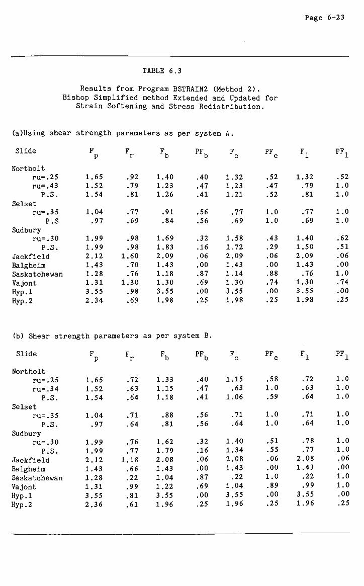
Page 6-23

TABLE 6.3

Results from Program BSTRAIN2 (Method 2). Bishop Simplified method Extended and Updated for



Slide PF. PF PF,

Northolt ru=.25 ru=.43 P.S.

Selset ru=.35

P.S Sudbury

ru=.30 P.S.

Jackfield Balgheim Saskatchewan Vajont Hyp.l Hyp. 2

1.65 1.52 1.54

1.04 .97

1.99 1.99 2.12 1.43 1.28 1.31 3.55 2.34

.92

.79

.81

.77

.69

.98

.98 1.60 .70 .76

1.30 .98 .69

1.40 1.23 1.26

.91

.84

1.69 1.83 2.09 1.43 1.18 1.30 3.55 1.98

.40

.47

.41

.56

.56

.32

.16

.06

.00

.87

.69

.00

.25

1.32 1.23 1.21

.77

.69

1.58 1.72 2.09 1.43 1.14 1.30 3.55 1.98

.52

.47

.52

1.0 1.0

.43

.29

.06

.00

.88

.74

.00

.25

1.32 .79 .81

.77

.69

1.40 1.50 2.09 1.43 .76

1.30 3.55 1.98

.52 1.0 1.0

1.0 1.0

.62

.51

.06

.00 1.0 .74 .00 .25

(b) Shear strength parameters as per system B,

Slide PF. PF. PF.


Selset ru=.35 P.S.

Sudbury ru=.30 P.S.


1.65 1.52 1.54

1.04 .97

1.99 1.99 2.12 1.43 1.28 1.31 3.55 2.36

.72

.63

.64

.71

.64

.76

.77 1.18 .66 .22 .99 .81 .61

1.33 1.15 1.18

.88

.81

1.62 1.79 2.08 1.43 1.04 1.22 3.55 1.96

.40

.47

.41

.56

.56

.32

.16

.06

.00

.87

.69

.00

.25

1.15 .63

1.06

.71

.64

1.40 1.34 2.08 1.43 .22

1.04 3.55 1.96

.58 1.0 .59

1.0 1.0

.51

.55

.06

.00 1.0 .89 .00 .25

.72

.63

.64

.71

.64

.78

.77 2.08 1.43

.22

.99 3.55 1.96

1.0 1.0 1.0

1.0 1.0

1.0 1.0 .06 .00 1.0 1.0 .00 .25

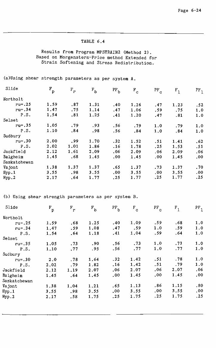
TABLE 6.4

Results from Program MPSTRAIN2 (Method 2). Based on Morgenstern-Price method Extended for Strain Softening and Stress Redistribution.

(a)Using shear strength parameters as per system A,

Slide


Selset ru=.35 P.S.

Sudbury ru=.30 P.S.


F P

1.59 1.47 1.54

1.05 1.10

2.00 2.02 2.12 1.45

1.38 3.55 2.17

Fr

.87

.75

.81

.79

.84

.99 1.01 1.61 .68

1.37 .98 .64

Fb

1.31 1.14 1.25

.93

.98

1.70 1.86 2.09 1.45

1.37 3.55 1.77

PFb

.40

.47

.41

.56

.56

.32

.16

.06

.00

.65

.00

.25

F c

1.26 1.06 1.20

.79

.84

1.52 1.78 2.09 1.45

1.37 3.55 1.77

PF c

.47

.59

.47

1.0 1.0

.51

.25

.06

.00

.73

.00

.25

Fl

1.23 .75 .81

.79

.84

1.41 1.53 2.09 1.45

1.37 3.55 1.77

PF1

.52 1.0 1.0

1.0 1.0

.62

.51

.06

.00

.70

.00

.25

(b) Using shear strength parameters as per system B,

Slide


Selset ru=.35 P.S.

Sudbury ru=.30 P.S.


F P

1.59 1.47 1.54

1.05 1.10

2.0 2.02 2.12 1.45

1.38 3.55 2.17

F r

.68

.59

.64

.73

.77

.78

.79 1.19 .64

1.04 .98 .58

Fb

1.25 1.08 1.18

.90

.95

1.64 1.82 2.07 1.45

1.21 3.55 1.75

PFb

.40

.47

.41

.56

.56

.32

.16

.06

.00

.65

.00

.25

F c

1.09 .59

1.04

.73

.77

1.42 1.42 2.07 1.45

1.13 3.55 1.75

PF c

.59 1.0 .59

1.0 1.0

.51

.51

.06

.00

.86

.00

.25

Fl

.68

.59

.64

.73

.77

.78

.79 2.07 1.45

1.15 3.55 1.75

PF1

1.0 1.0 1.0

1.0 1.0

1.0 1.0 .06 .00

.80

.00

.25

Page 6-25

failure used but are due simply to the method used for calculating the

factor of safety for a slope. It is interesting to note, however,

that calculated values of the residual factor of safety which are less

than 1.0 in value are found to be greater when using program STRAIN1.

We can therefore conclude that calculated values of the factor of

safety F obtained from program STRAIN1 appear to be closer to 1.0 than

the values obtained using program BSTRAIN2.

In virtually all cases, the values of the propagation factor PF

obtained by programs STRAIN1 and BSTRAIN2 are identical. This

reinforces the suggestion made earlier that the two simulation methods

produce the same results. It can be seen that the two simulation

techniques induce the same amount of local failure in the slopes

tested and that any discrepancies in calculated values of the factor

of safety F are due entirely to differences in the methods of

calculating F.

When comparing results obtained by the two programs based on

method 2, BSTRAIN2 and MPSTRAIN2, the following points are noted. The

values of the factors of safety obtained by the program MPSTRAIN2

appear, in general, to be slightly higher than those obtained by

program BSTRAIN2. Values of the propagation factor PF, on the other

hand, seem to be the same in most cases, again emphasizing the point

that differences in the final factor of safety are due mainly to

differences in the methods used for calculating F. In this case, the

more rigorous Morgenstern-Price method used in program MPSTRAIN2 would

be expected to give the more reliable results. It is also noted that

the largest differences in values of PF obtained by the two different

programs, occur in slopes where the failure surface is of irregular

shape and where the Bishop simplified method used in program BSTRAIN2

is the least reliable.

Due to the close correlation between values of PF obtained from

the two programs BSTRAIN2 and MPSTRAIN2, it can be said that the

method of simulation presented in this section appears to give valid

results. The main discrepancies seem to be in areas where the Bishop

simplified method of slope analysis is not expected to give reliable

results and program MPSTRAIN2 results should therefore be used in such

cases.

Page 6-26

6.4 ALTERNATE METHOD FOR REDISTRIBUTION OF EXCESS SHEAR (METHOD 3).

A method of simulating progressive failure is presented here

which, while similar to the methods presented in the previous two

sections in its detection of local failure on the base of a soil

slice, is inherently different in its approach to the calculation and

subsequent redistribution of excess shear forces over the failure

surface.

6.4.1 General Description Of Method.

Again, making use of the Bishop simplified method for limit

equilibrium analyses, the following procedure is derived for method 3.

Step 1: Perform a limit equilibrium analysis on the slope and obtain

an initial (peak) factor of safety, F .

Step 2: Calculate the mobilised shear force on the base of each

slice, i, using the expression

(Mi>0

(T.) i P

F0

c^l. + (W.cosa. - uili)tan0^ ^ ^

F0

Note that for the first iteration, FQ = F .

Step 3: Check for local failure:- Each unfailed slice is checked for

local failure. Local failure is deemed to have occurred if the shear

force on the base of the slice is greater than the available shear

strength on the slice base (i.e. if the inequality expressed in

equation (6.5) is satisfied). The shear force on the base of the

slice is given by equation (6.1) while in this case the available

shear strength on the slice base is given by

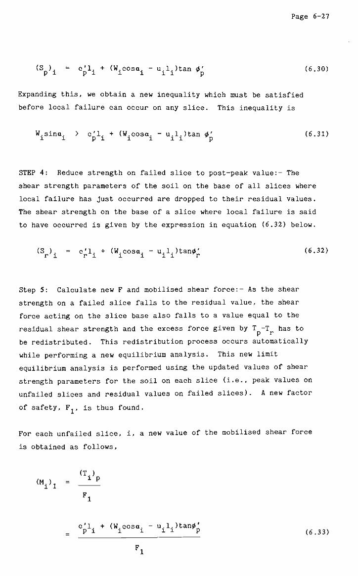
Page 6-27

(sr.). = c^1. + (W.cosa. -u.l.)tan0' (6.30) p i p i 1 1 i i *p

Expanding this, we obtain a new inequality which must be satisfied

before local failure can occur on any slice. This inequality is

W.sina. > c'l. + (W.cosa. - u.l.)tan 0' (6.31) i i p i 1 1 1 1 *D

STEP 4: Reduce strength on failed slice to post-peak value:- The

shear strength parameters of the soil on the base of all slices where

local failure has just occurred are dropped to their residual values.

The shear strength on the base of a slice where local failure is said

to have occurred is given by the expression in equation (6.32) below.

(S ). = c'l. + (W.cosa. -u.l.)tan0' (6.32) r i r i l i i i r

Step 5: Calculate new F and mobilised shear force:- As the shear

strength on a failed slice falls to the residual value, the shear

force acting on the slice base also falls to a value equal to the

residual shear strength and the excess force given by T -T has to

be redistributed. This redistribution process occurs automatically

while performing a new equilibrium analysis. This new limit

equilibrium analysis is performed using the updated values of shear

strength parameters for the soil on each slice (i.e., peak values on

unfailed slices and residual values on failed slices). A new factor

of safety, F1, is thus found.

For each unfailed slice, i, a new value of the mobilised shear force

is obtained as follows,

(M.)1 (T.) i P

Fl

c'l. + (W.cosa. - u.l.)tan0' P i i i x ! P (6.33)

Fl

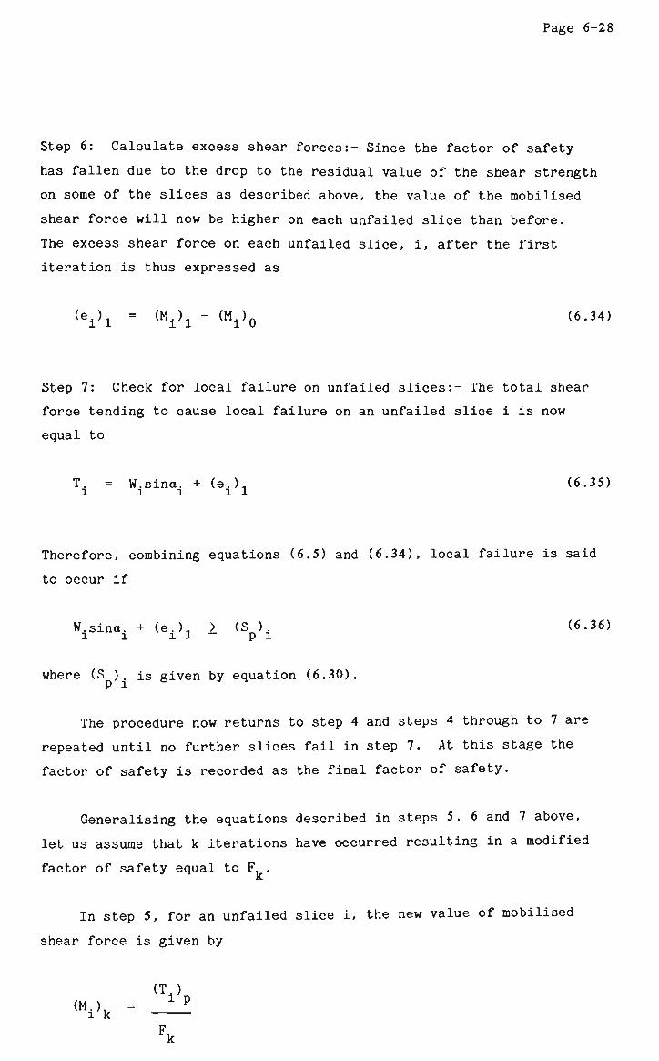
Page 6-28

Step 6: Calculate excess shear forces:- Since the factor of safety

has fallen due to the drop to the residual value of the shear strength

on some of the slices as described above, the value of the mobilised

shear force will now be higher on each unfailed slice than before.

The excess shear force on each unfailed slice, i, after the first

iteration is thus expressed as

(e±)1 = (M±)1 - (Mi)Q (6.34)

Step 7: Check for local failure on unfailed slices:- The total shear

force tending to cause local failure on an unfailed slice i is now

equal to

T. = W.sina. + (e.)1 (6.35) I i i l 1

Therefore, combining equations (6.5) and (6.34), local failure is said

to occur if

W.sina. + (e.). > (S ), (6.36) l I I 1 — pi

where (S ). is given by equation (6.30).

The procedure now returns to step 4 and steps 4 through to 7 are

repeated until no further slices fail in step 7. At this stage the

factor of safety is recorded as the final factor of safety.

Generalising the equations described in steps 5, 6 and 7 above,

let us assume that k iterations have occurred resulting in a modified

factor of safety equal to F .

In step 5, for an unfailed slice i, the new value of mobilised

shear force is given by

(T.) < " _ > _ • - ^

p_

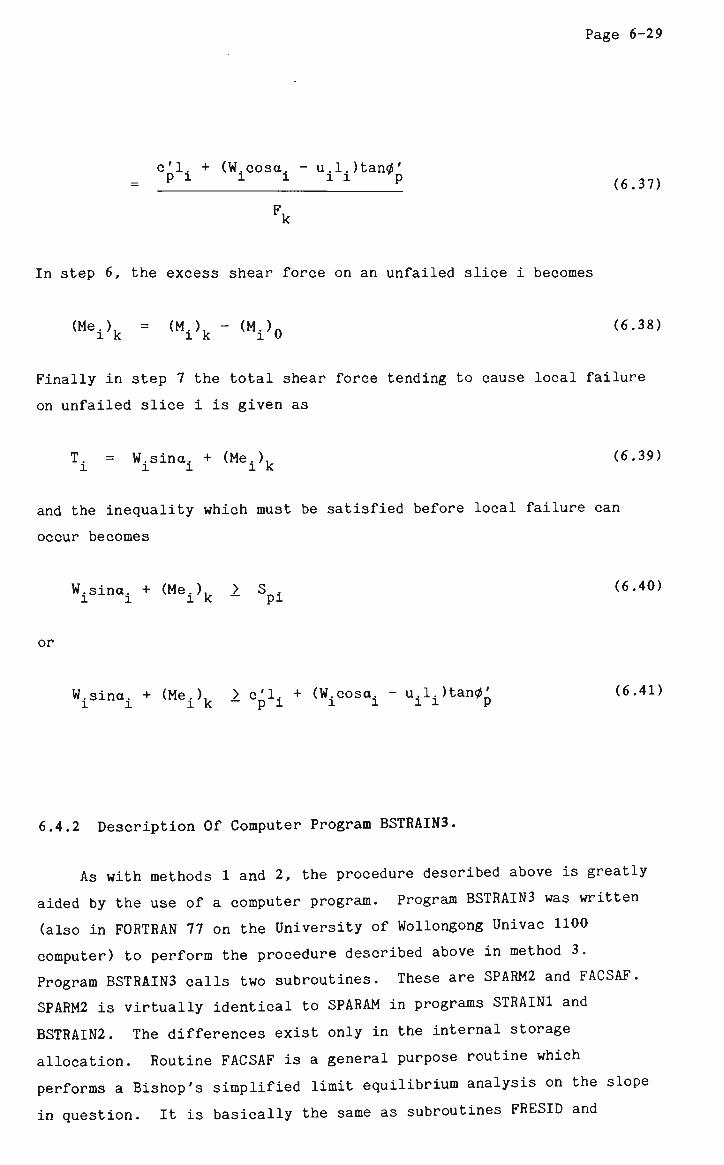
Page 6-29

c'l. + (W.cosa. - u.l.)tan0' P 1 1 1 1 1 P ( 6 > 3 7 )

Fk

In step 6, the excess shear force on an unfailed slice i becomes

(Me.), = (M.), - (M.)n (6.38) l k l k l 0

Finally in step 7 the total shear force tending to cause local failure

on unfailed slice i is given as

T. = W.sina. + (Me.), (6.39) l i i I k

and the inequality which must be satisfied before local failure can

occur becomes

W.sina. + (Me.), > S . (6.40) l l I k — pi

or

W.sina. + (Me.), > c'l. + (W.cosa. -u.l.)tan*' (6.41) l i 1 k — pi i i ii P

6.4.2 Description Of Computer Program BSTRAIN3.

As with methods 1 and 2, the procedure described above is greatly

aided by the use of a computer program. Program BSTRAIN3 was written

(also in FORTRAN 77 on the University of Wollongong Univac 1100

computer) to perform the procedure described above in method 3.

Program BSTRAIN3 calls two subroutines. These are SPARM2 and FACSAF.

SPARM2 is virtually identical to SPARAM in programs STRAIN1 and

BSTRAIN2. The differences exist only in the internal storage

allocation. Routine FACSAF is a general purpose routine which

performs a Bishop's simplified limit equilibrium analysis on the slope

in question. It is basically the same as subroutines FRESID and

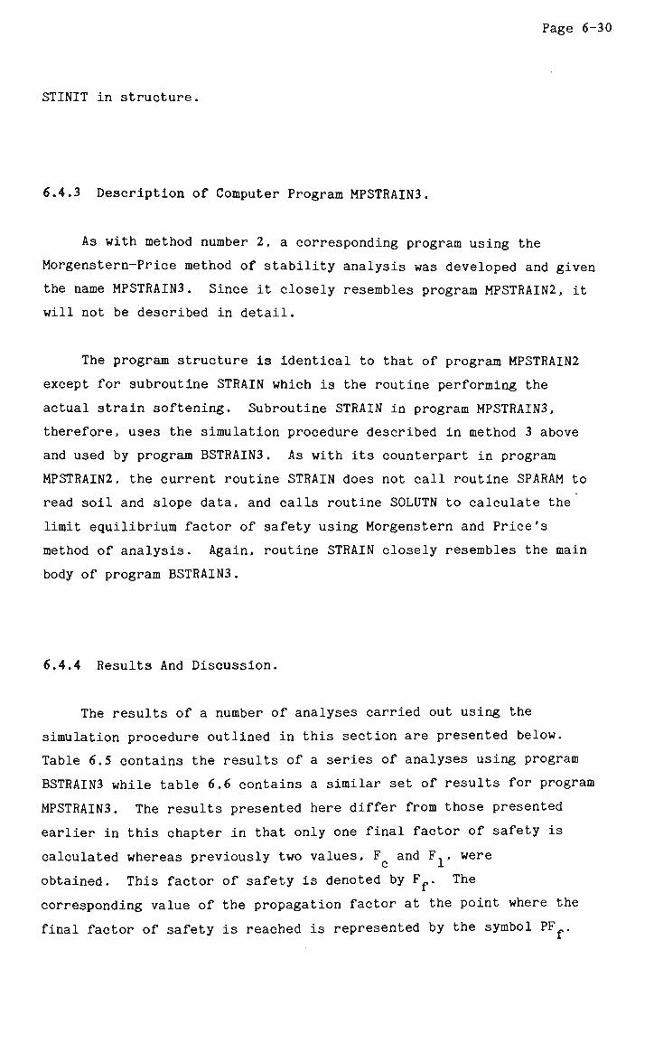
Page 6-30

STINIT in structure.

6.4.3 Description of Computer Program MPSTRAIN3.

As with method number 2, a corresponding program using the

Morgenstern-Price method of stability analysis was developed and given

the name MPSTRAIN3. Since it closely resembles program MPSTRAIN2, it

will not be described in detail.

The program structure is identical to that of program MPSTRAIN2

except for subroutine STRAIN which is the routine performing the

actual strain softening. Subroutine STRAIN in program MPSTRAIN3,

therefore, uses the simulation procedure described in method 3 above

and used by program BSTRAIN3. As with its counterpart in program

MPSTRAIN2, the current routine STRAIN does not call routine SPARAM to

read soil and slope data, and calls routine SOLUTN to calculate the

limit equilibrium factor of safety using Morgenstern and Price's

method of analysis. Again, routine STRAIN closely resembles the main

body of program BSTRAIN3.


The results of a number of analyses carried out using the

simulation procedure outlined in this section are presented below.

Table 6.5 contains the results of a series of analyses using program

BSTRAIN3 while table 6.6 contains a similar set of results for program

MPSTRAIN3. The results presented here differ from those presented

earlier in this chapter in that only one final factor of safety is

calculated whereas previously two values, F and F^, were

obtained. This factor of safety is denoted by Ff. The

corresponding value of the propagation factor at the point where the

final factor of safety is reached is represented by the symbol PF .

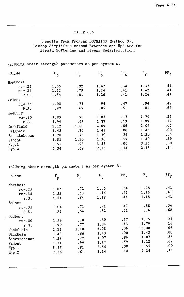
Page 6-31

TABLE 6.5




Slide Fp Fr Ffa PFb Ff PFf

Northolt ru=.25 1.65 .92 1.42 .34 1.37 .41 ru=.34 1.52 .79 1.24 .41 1.42 .41 P.S. 1.54 .81 1.26 .41 1.26 .41

S____Lsst ru=.35 1.03 .77 .94 .47 .94 .47 P.S. .97 .69 .85 .51 .81 .64

P.S. Jackfield Balgheim Saskatchewan

Hyp.l Hyp. 2

F P

1.65 1.52 1.54

1.03 .91

1.99 1.99 2.12 1.43 1.28 1.31 3.55 2.36

F r

.92

.79

.81

.77

.69

.98

.98 1.60 .70 .76

1.30 .98 .69

Fb

1.42 1.24 1.26

.94

.85

1.83 1.87 2.09 1.43 1.20 1.30 3.55 2.15

Sudbury ru=.30 1.99 .98 1.83 .17 1.79 .21

Vajont 1.31 1.30 1.30 .59 1.30 .59

PF. D

.34

.41

.41

.47

.51

.17

.13

.06

.00

.86

.59

.00

.14

Ff

1.37 1.42 1.26

.94

.81

1.79 1.87 2.09 1.43 1.20 1.30 3.55 2.15


Selset ru=.35 P.S.

Sudbury ru=.30 P.S.


F P

1.65 1.52 1.54

1.04 .97

1.99 1.99 2.12 1.43 1.28 1.31 3.55 2.36

F r

.72

.63

.64

.71

.64

.78

.77 1.18 .66 .22 .99 .81 .61

Fb

1.35 1.16 1.18

.91

.82

.80 1.84 2.08 1.43 1.07 1.17 3.55 2.14

PFb

.34

.41

.41

.47

.51

.17

.13

.06

.00

.86

.59

.00

.14

Ff

1.28 1.16 1.18

.88

.76

1.75 1.79 2.08 1.43 1.07 1.12 3.55 2.14

.12

.06

.00

.86

.00

.14

(b)Using shear strength parameters as per system B.

Slide F_ F_ FK PFK Ff PFf

.41

.41

.41

.56

.68

.21

.16

.06

.00

.86

.69

.00

.14

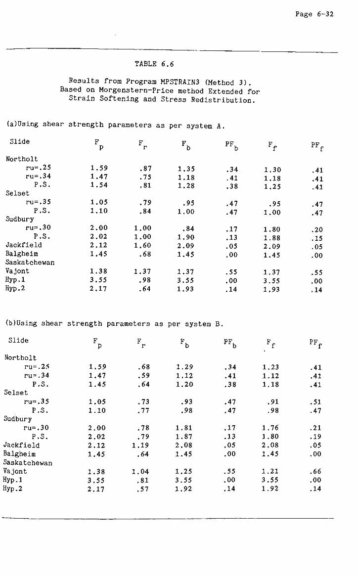
Page 6

TABLE 6.6



Slide

P.S. Jackfield

F P

1.59 1.47 1.54

1.05 1.10

2.00 2.02 2.12 1.45

1.38 3.55 2.17

F r

.87

.75

.81

.79

.84

1.00 1.00 1.60 .68

1.37 .98 .64

Fb

1.35 1.18 1.28

.95 1.00

.84 1.90 2.09 1.45

1.37 3.55 1.93


Selset ru=.35 P.S.

Sudbury ru=.30 2.00 1.00 .84 .17 1.80 .20

PFb

.34

.41

.38

.47

.47

.17

.13

.05

.00

.55

.00

.14

Ff

1.30 1.18 1.25

.95 1.00

1.80 1.88 2.09 1.45

1.37 3.55 1.93

PF f

.41

.41

.41

.47

.47

15 .05

Balgheim 1.45 .68 1.45 .00 1.45 .00 Saskatchewan Vajont 1.38 1.37 1.37 .55 1.37 .55 Hyp.l 3.55 .98 3.55 .00 3.55 .00 Hyp.2 2.17 .64 1.93 .14 1.93 .14


Slide Fp Fr Fb PFb Ff PFf

Northolt ru=.25 1.59 .68 1.29 .34 1.23 .41 ru=.34 1.47 .59 1.12 .41 1.12 .41 P.S. 1.45 .64 1.20 .38 1.18 .41

Selset ru=.35 1.05 .73 .93 .47 .91 .51 P.S. 1.10 .77 .98 .47 .98 .47

Sudbury ru=.30 2.00 .78 1.81 .17 1.76 .21 P.S. 2.02 .79 1.87 .13 1.80 .19

Jackfield 2.12 1.19 2.08 .05 2.08 .05 Balgheim 1.45 .64 1.45 .00 1.45 .00 Saskatchewan Vajont 1.38 1.04 1.25 .55 1.21 .66 Hyp.l 3.55 .81 3.55 .00 3.55 .00 Hyp.2 2.17 .57 1.92 .14 1.92 .14

Page 6-33

From the results shown in tables 6.5 and 6.6 the following

observations were made. The final factor of safety F iSj l n the

majority of cases, greater than FQ obtained from programs BSTRAIN1

and BSTRAINS2. Consequently, the value of PFf i s considerably less

than the value of PFc> Also, there appears to be less tendency for

the value of the factor of safety to decrease past F , and it is

noted that Fb ±s slightly higher using program BSTRAIN3 than using BSTRAIN2.

Comparing the results of programs BSTRAIN3 and MPSTRAIN3 the same

observations are made as for previous sections. The main differences

in values of factor of safety are due simply to the method used to

calculate the factor of safety (i.e. Bishop's simplified method or

Morgenstern-Price method) and not on the simulation process used. The

fact that, in most cases, the values of PF obtained from the two

programs BSTRAIN3 and MPSTRAIN3 are identical reinforces this

observation.

6.5 REDISTRIBUTION OF NORMAL AND SHEAR FORCES USING THE CONCEPT OF

VIRTUAL WEIGHT (METHOD 4).

In method 3, which was described in the previous section, a

procedure for simulating progressive failure using strain softening

was described. As a slice of soil in a failure mass was said to have

failed locally by satisfying the inequality in equation (6.5), the

shear strength of the soil in that slice was assumed to have dropped

to its residual value and the shear force was also dropped to equal

the shear strength. A process was then described whereby the excess

shear force was redistribruted throughout the unfailed soil mass and a

new factor of safety calculated.

However, the shear force is not the only force acting on the base

of a slice. In order to maintain equilibrium, the normal force on the

base of each slice should also be considered and redistributed after

local failure. This section describes a method of simulating

progressive failure along a surface of sliding, taking into account

both shear and normal forces on the base of each individual slice.

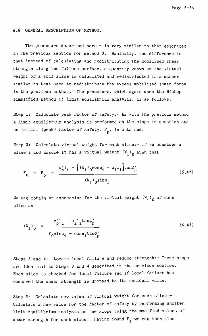
Page 6-34

6.6 GENERAL DESCRIPTION OF METHOD.

The procedure described herein is very similar to that described

in the previous section for method 3. Basically, the difference is

that instead of calculating and redistributing the mobilised shear

strength along the failure surface, a quantity known as the virtual

weight of a soil slice is calculated and redistributed in a manner

similar to that used to redistribute the excess mobilised shear force

in the previous method. The procedure, which again uses the Bishop

simplified method of limit equilibrium analysis, is as follows.

Step 1: Calculate peak factor of safety:- As with the previous method

a limit equilibrium analysis is performed on the slope in question and

an initial (peak) factor of safety, F , is obtained.

Step 2: Calculate virtual weight for each slice:- If we consider a

slice i and assume it has a virtual weight (W.)0 such that

Cvh + KV0 3 0!^!1!]^,. Fn = F = " ' " ' " ' ' " (6.42) 0 P

(W.)Asina. l 0 I

We can obtain an expression for the virtual weight (W.)Q of each

slice as

c'l. - u.l.tan0' (W.) = P x X X P (6-43) i'0

FQsina. - cosa tan0'

Steps 3 and 4: Locate local failure and reduce strength:- These steps

are identical to Steps 3 and 4 described in the previous section.

Each slice is checked for local failure and if local failure has

occurred the shear strength is dropped to its residual value.

Step 5: Calculate new value of virtual weight for each slice:-

Calculate a new value for the factor of safety by performing another

limit equilibrium analysis on the slope using the modified values of

shear strength for each slice. Having found F1 we can then also

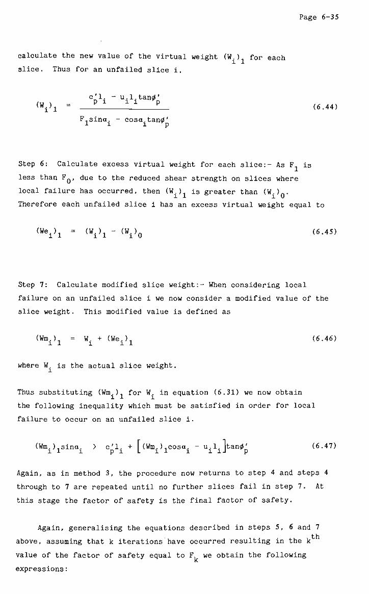
Page 6-35

calculate the new value of the virtual weight (W.) for each

slice. Thus for an unfailed slice i,

GT.-_. - u. 1.tan0^

'i'l F1sina. - cosa.tan0' 1 1 1 D

(W,), = _L1 X1 P (6.44)

Step 6: Calculate excess virtual weight for each slice:- As F.. is

less than F^, due to the reduced shear strength on slices where

local failure has occurred, then (W.) is greater than (W.)0.

Therefore each unfailed slice i has an excess virtual weight equal to

(We.)1 = (W±)1 - (W.)Q (6.45)

Step 7: Calculate modified slice weight:- When considering local

failure on an unfailed slice i we now consider a modified value of the

slice weight. This modified value is defined as

(Wm.)_ = W. + (We.), (6.46) I 1 I l 1

where W. is the actual slice weight.

Thus substituting (Wm.)1 for W. in equation (6.31) we now obtain

the following inequality which must be satisfied in order for local

failure to occur on an unfailed slice i.

(Wm.Ksina. > c'l. + f(Wm. )1coso. -u.l.ltan0' (6.47) i i l p i L i l I iiJ p

Again, as in method 3, the procedure now returns to step 4 and steps 4

through to 7 are repeated until no further slices fail in step 7. At

this stage the factor of safety is the final factor of safety.

Again, generalising the equations described in steps 5, 6 and 7 i_. \~

above, assuming that k iterations have occurred resulting in the k

value of the factor of safety equal to F we obtain the following

expressions:

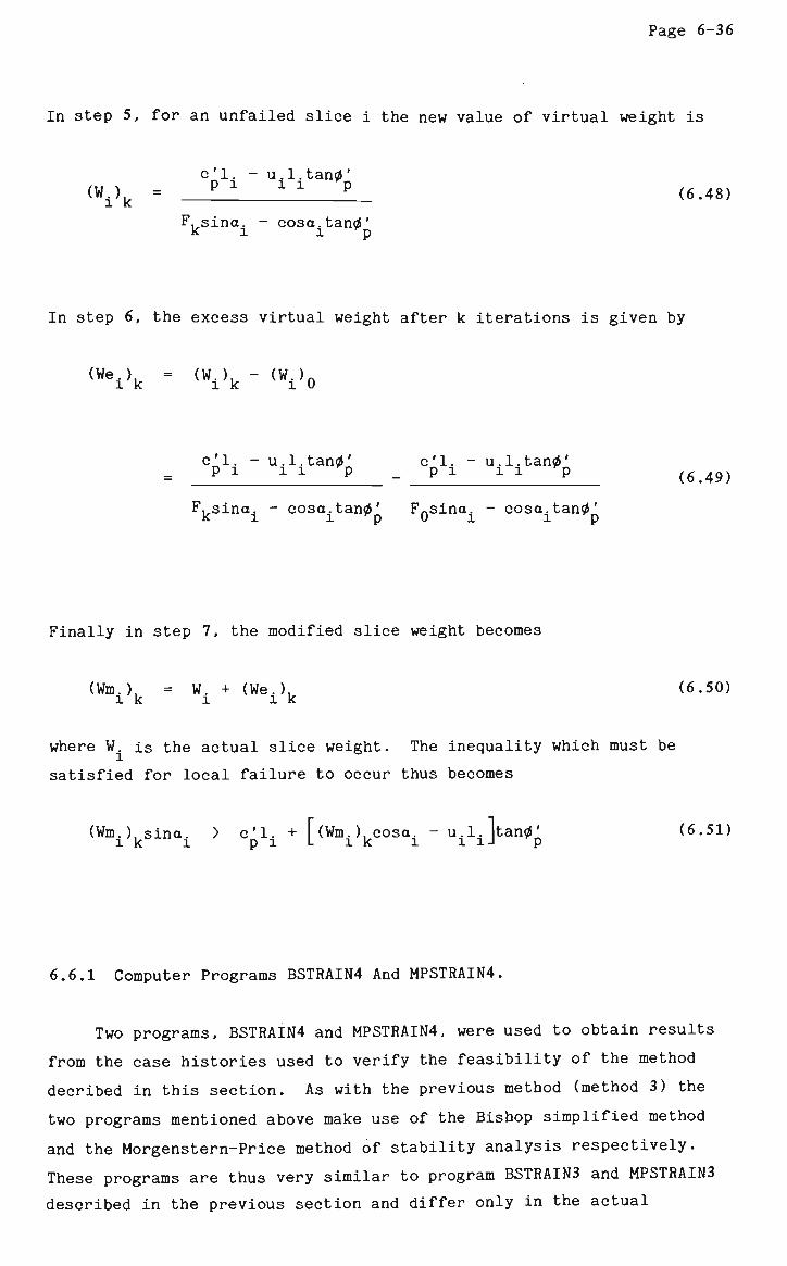
Page 6-36

In step 5, for an unfailed slice i the new value of virtual weight is

c'l. - u.l.tan0' p i 1 1 "p

F. sina. - cosa.tan0' K 1 I D

(W±)k - F " ^ v (6.48)

In step 6, the excess virtual weight after k iterations is given by

(We.), = (W.), - (W.)n

l k l k l 0

c'l. - u.l.tan0' c'l. - u.l.tan0' p i i i p p i i i *p (6.49)

F. sina. - cosa.tan0' F^sina. - cosa.tan0' k i I *p 0 I l *p

Finally in step 7, the modified slice weight becomes

(Wm.), = W. + (We.), (6.50) I k l I k

where W. is the actual slice weight. The inequality which must be

satisfied for local failure to occur thus becomes

(Wm.),sina. > c'l. + [(Win.). cosa. -u.l.ltan0' (6.51) i k I p i L i k I 11J p

6.6.1 Computer Programs BSTRAIN4 And MPSTRAIN4.

Two programs, BSTRAIN4 and MPSTRAIN4, were used to obtain results

from the case histories used to verify the feasibility of the method

decribed in this section. As with the previous method (method 3) the

two programs mentioned above make use of the Bishop simplified method

and the Morgenstern-Price method of stability analysis respectively.

These programs are thus very similar to program BSTRAIN3 and MPSTRAIN3

described in the previous section and differ only in the actual

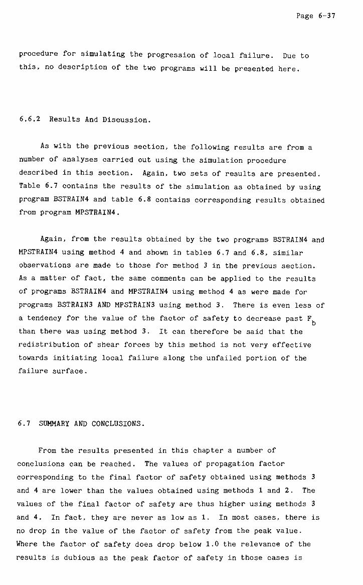
Page 6-37

procedure for simulating the progression of local failure. Due to

this, no description of the two programs will be presented here.


As with the previous section, the following results are from a

number of analyses carried out using the simulation procedure

described in this section. Again, two sets of results are presented.

Table 6.7 contains the results of the simulation as obtained by using

program BSTRAIN4 and table 6.8 contains corresponding results obtained

from program MPSTRAIN4.

Again, from the results obtained by the two programs BSTRAIN4 and

MPSTRAIN4 using method 4 and shown in tables 6.7 and 6.8, similar

observations are made to those for method 3 in the previous section.

As a matter of fact, the same comments can be applied to the results

of programs BSTRAIN4 and MPSTRAIN4 using method 4 as were made for

programs BSTRAIN3 AND MPSTRAIN3 using method 3. There is even less of

a tendency for the value of the factor of safety to decrease past F

than there was using method 3. It can therefore be said that the

redistribution of shear forces by this method is not very effective

towards initiating local failure along the unfailed portion of the

failure surface.


From the results presented in this chapter a number of

conclusions can be reached. The values of propagation factor

corresponding to the final factor of safety obtained using methods 3

and 4 are lower than the values obtained using methods 1 and 2. The

values of the final factor of safety are thus higher using methods 3

and 4. In fact, they are never as low as 1. In most cases, there is

no drop in the value of the factor of safety from the peak value.

Where the factor of safety does drop below 1.0 the relevance of the

results is dubious as the peak factor of safety in those cases is

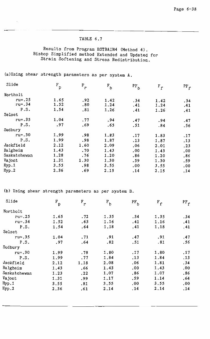
TABLE 6.7




Slide F^ F F_. PF F PF P r rb rrb f r*f

Northolt ru=.25 1.65 .92 1.42 .34 1.42 .34 ru=.34 1.52 .80 1.24 .41 1.24 .41 P.S. 1.54 .81 1.26 .41 1.26 .41

Selset ru=.35 1.04 .77 .94 .47 .94 .47 P.S. .97 .69 .65 .51 .84 .56

Sudbury ru=.30 1.99 .98 1.83 .17 1.83 .17 P.S. 1.99 .98 1.87 .13 1.87 .13

Jackfield 2.12 1.60 2.09 .06 2.01 .23 Balgheim 1.43 .70 1.43 .00 1.43 .00 Saskatchewan 1.28 .76 1.20 .86 1.20 .86 Vajont 1.31 1.30 1.30 .59 1.30 .59 Hyp.l 3.55 .98 3.55 .00 3.55 .00 Hyp.2 2.36 .69 2.15 .14 2.15 .14

(b) Using shear strength parameters as per system B.

Slide F^ F F. PF. F_ PF„ p r b b f f

Northolt ru=.25 1.65 .72 1.35 .34 1.35 .34 ru=.34 1.52 .63 1.16 .41 1.16 .41 P.S. 1.54 .64 1.18 .41 1.18 .41

Selset ru=.35 1.04 .71 .91 .47 .91 .47 P.S. .97 .64 .82 .51 .81 .56

Sudbury ru=.30 1.99 .78 1.80 .17 1.80 .17 P.S. 1.99 .77 1.84 .13 1.84 .13

Jackfield 2.12 1.18 2.08 .06 1.81 .34 Balgheim 1.43 .66 1.43 .00 1.43 .00 Saskatchewan 1.23 .22 1.07 .86 1.07 .86 Vajont 1.31 .99 1.17 .59 1.14 .64 Hyp.l 3.55 .81 3.55 .00 3.55 .00 Hyp.2 2.36 .61 2.14 .14 2.14 .14

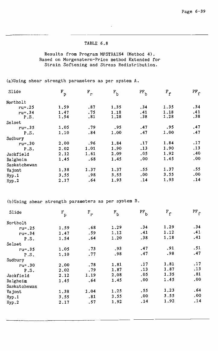
Page 6-39

TABLE 6.8



Slide


Selset ru=.35 P.S.

Sudbury ru=.30 P.S.

Jackfield Balgheim Saskatchewan Vajont

Hyp.l Hyp. 2

F P

1.59 1.47 1.54

1.05 1.10

2.00 2.02 2.12 1.45

1.38 3.55 2.17

F r

.87

.75

.81

.79

.84

.96 1.01 1.61 .68

1.37 .98 .64

Fu b

1.35 1.18 1.28

.95 1.00

1.84 1.90 2.09 1.45

1.37 3.55 1.93

PFu b

.34

.41

.38

.47

.47

.17

.13

.05

.00

.55

.00

.14

F* f

1.35 1.18 1.28

.95 1.00

1.84 1.90 1.92 1.45

1.37 3.55 1.93

PF„ f

.34

.41

.38

.47

.47

.17

.13

.40

.00

.55

.00

.14


Slide


Selset ru=.35 P.S.

Sudbury ru=.30 P.S.


F P

1.59 1.47 1.54

1.05 1.10

2.00 2.02 2.12 1.45

1.38 3.55 2.17

F r

.68

.59

.64

.73

.77

.78

.79 1.19 .64

1.04 .81 .57

Fb

1.29 1.12 1.20

.93

.98

1.81 1.87 2.08 1.45

1.25 3.55 1.92

PFb

.34

.41

.38

.47

.47

.17

.13

.05

.00

.55

.00

.14

Ff

1.29 1.12 1.18

.91

.98

1.81 1.87 1.35 1.45

1.23 3.55 1.92

PF rrf

.34

.41

.41

.51

.47

.17

.13

.81

.00

.64

.00

.14

Page 6-40

extremely close to 1.0 .

It would therefore appear that, for the case histories

considered, methods 3 and 4 are not very successful at initiating and

propagating local failure, method 4 being the least successful.

Methods 1 and 2, on the other hand, seem to be much more effective in

simulating the propagation of the zone of strain softening after local

failure along the assumed surface of sliding. Since methods 1 and 2

are basically the same method and differ only in the fact that method

1 uses a less refined procedure for calculating the factor of safety,

we can hence concentrate on method 2 which appears to give the most

feasible results.

Considering the results obtained in method 2 using the shear

strength parameters as per system A (these shear strength parameters

correspond to those used by Law and Lumb [58]) and comparing them to

the results obtained by Law and Lumb, the following comments can be

made. Law and Lumb applied their technique to only three case

histories all of which were assumed to have circular surfaces of

sliding. These three case histories are the Northolt, Selset and

Sudbury Hill slides. Firstly, the Selset slide is a bad example to

demonstrate strain softening as its peak factor of safety was found to

be 1.05 using a pore pressure ratio value of 0.35. For the Northolt

slide, using an ru value of 0.25, and the Sudbury Hill slide, using

an r value of 0.30, the final factors of safety calculated using a

linear stress redistribution profile were 1.23 and 1.41 respectively,

corresponding to propagation factors of 0.52 and 0.69 respectively.

It is feasible to suppose that by using a more severe stress

redistribution profile, perhaps an exponential distribution, local

failure may have propagated further to give a final factor of safety

closer to 1. However, comparing these results with those obtained

using shear strength parameters as per system B, it can be seen that

sufficient strain, softening can be induced in the latter to bring the

factor of safety down below 1.

Although, by using the shear strength parameters according to

system B, a larger number of slopes give factors of safety below 1.0,

a certain number of cases show no significant change (or none at all)

when using different stress redistribution profiles or shear strength

Page 6-41

parameters. These cases, namely the Jackfield, Balgheim, Vajont,

Hyp.l and Hyp.2 slides, show very little tendency towards stress

redistribution on the basis of limit equilibriumeven though the

Balgheim slope and the two hypothetical slopes have residual factors

of safety less than 1. It would thus appear that the proposed method

does not function for these cases, the reason perhaps being the

geometry of the slopes in question.

It is known that in cases where the failure surface is parallel

to the top surface, especially if the failure surface is shallow, then

the chances of strain softening occuring using limit equilibrium

methods of analysis are very low. In such cases, the final factor of

safety will be approximately (if not exactly) equal to the peak factor

of safety. This is exactly what would be expected in the case of the

Jackfield and Balgheim slopes. It is not, therefore, an error in the

proposed method, but more precisely, a limitation of the limit

equilibrium method of analysis. The obvious next step would be to

investigate alternatives to the limit equilibrium approach.

It may not be necessary to discard the limit equilibrium methods

entirely in order to present a technique which accurately predicts the

likelihood of the soil mass to fail. It may, in fact, be possible to

extend the method of analysis to incorporate certain factors which are

not considered by conventional limit equilibrium methods. One such

factor, and one which has been considered of increasing significance

in recent years, is the initial stress state of the soil in the slope

prior to the commencement of strain softening. The following chapters

will attempt to investigate this initial stress state and the

consequences of incorporating its influence in the progressive failure

simulation techniques presented herein.

CHAPTER 7

THE CONCEPT OF INITIAL STRESS.

7.1 INTRODUCTION AND GENERAL COMMENTS.

In recent years consideration of initial stresses in the analysis

of stress conditions in soil masses has been given increasing

importance. This is especially so in the case of over-consolidated

clays or soils where the consolidation history of the soil mass

determines, to a large extent, the ratio and magnitude of the

horizontal and vertical stresses within it. In this chapter,

reference is made to a number of investigations concerned with initial

stresses in soils and rocks. Some research results which concern the

initial stress conditions existing in soil and rock masses and their

influence on ground conditions are summarised. From the findings of

various research investigators some understanding may be achieved

regarding the role of stress conditions in the development of

progressive failure in soil slopes.

Evidence of stress conditions in which the magnitudes of the

stresses in the horizontal direction were found to be much greater

than the magnitudes of stresses in the vertical direction has been

reported by various authors. Petersen [74] in his studies of the

Bearpaw shale at Saskatchewan, in Canada, estimated that the

horizontal stresses in the shale were about 1.5 times as great as the

overburden pressure at a point approximately 20 metres beneath the

ground surface. Skempton [87] showed that, for London clay, the ratio

of the horizontal stresses to the vertical effective stresses, varied

with depth from about 1.5 at a depth of 30 metres to approximately 2.5

at a depth of 3 metres. Skempton concluded, therefore, that near the

surface, the horizontal pressure was sufficiently near the maximum

passive pressure to cause failure of the clay. Langer [57] also gave

Page 7-2

evidence of horizontal stresses of the order of three times the

overburden pressure. Bjerrum [18] showed that high initial lateral

stresses could result in large shear stresses at the base of an

excavated slope, and thus increase the likelihood of progressive

failure. Among others, Chowdhury [26] has referred to a number of

publications concerned with the existence, importance and role of

initial stresses in soil and rock slopes.

In their analyses of embankments. Brown and King [22] considered

different potential slip surfaces for both excavated and built-up

slopes. In their analyses, the actual incremental process of slope

construction was simulated. The effects of the initial state of

stress on the embankment stresses in linearly elastic materials was

studied in detail. They showed that in a built-up slope, the maximum

shear stresses in the foundation material are influened by the ratio

of horizontal stresses to vertical overburden stresses. Brown and

King also pointed out that the possibility of failure originating was

more likely in embankment slopes.

7.2 SIMULATION OF 'FAILURE' DEVELOPMENT IN CLAYS.

Duncan and Dunlop [40] developed a method of analysis of slopes

excavated in materials with low and high initial horizontal stresses

representative of either (a)normally consolidated or (b)heavily

over-consolidated clays. They included the effects of various initial

stress conditions by simulating the excavation of a slope in an

initially horizontal deposit of clay in a series of incremental steps.

Referring to figure 7.1, the initial stresses on a slope to be

excavated are represented by ff . On the inclined surface, these

initial stresses include both shear and normal components.

Excavation of the slope was simulated by Duncan and Dunlop by

applying changes in the stresses Ao to the excavated surface.

Application of these changes in stress, which are equal in value and

apposite in sign to the initial stresses a , results in a

stress-free condition on the excavated surface. The applied changes

in stress are resisted only by the remaining material in the slope and

Page 7-3

(a)

1 1 1 1 | T f t l , ^^p^^mmzr

__er

(b)

w % s w —

(e)

Figure 7.1 Changes in Stress during Excavation (from Duncan and Dunlop [40]).

they induce changes in stress away from the excavated surface which

may be calculated by the finite element method. These changes in

stress are then added to the initial stress values to obtain the

combined or final stresses.

For purposes of analysis the real soil was represented by a

homogeneous, linear elastic, isotropic material. The effects of

nonlinear stress-dependent behaviour and the role of stress

concentration due to fissures were ignored. They noted that field

investigations had shown that the horizontal stresses in heavily

over-consolidated clays may exceed the overburden pressure by 50% or

even more in some cases.

Duncan and Dunlop concluded that the higher the horizontal

stresses before construction, the lower the factor of safety

corresponding to the development of local failure around the slope.

Therefore, the existence of high horizontal stresses in heavily over-

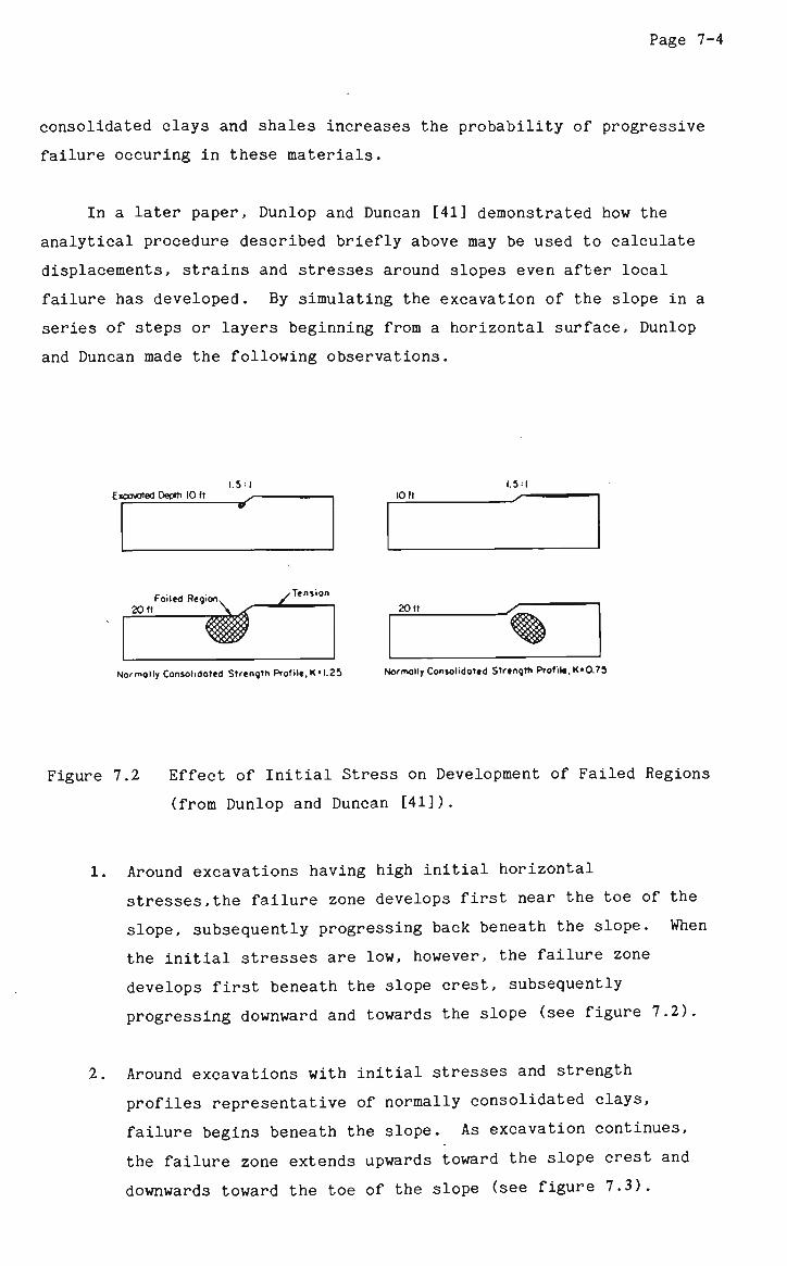
Page 7-4

consolidated clays and shales increases the probability of progressive

failure occuring in these materials.

In a later paper, Dunlop and Duncan [41] demonstrated how the

analytical procedure described briefly above may be used to calculate

displacements, strains and stresses around slopes even after local

failure has developed. By simulating the excavation of the slope in a

series of steps or layers beginning from a horizontal surface, Dunlop

and Duncan made the following observations.

E-covote. Depth 10 ft 1.5:1

S~ 10 It

1.5 = 1

20 fl Foiled Region _z

Tension

2 0 f I sz.

Normolly Consolidated Strength Profile, K« 1.25 Normolly Consolidated Strength Profile, K«0.73

Figure 7.2 Effect of Initial Stress on Development of Failed Regions

(from Dunlop and Duncan [41]).

1. Around excavations having high initial horizontal

stresses,the failure zone develops first near the toe of the

slope, subsequently progressing back beneath the slope. When

the initial stresses are low, however, the failure zone

develops first beneath the slope crest, subsequently

progressing downward and towards the slope (see figure 7.2).

Around excavations with initial stresses and strength

profiles representative of normally consolidated clays,

failure begins beneath the slope. As excavation continues,

the failure zone extends upwards toward the slope crest and

downwards toward the toe of the slope (see figure 7.3).

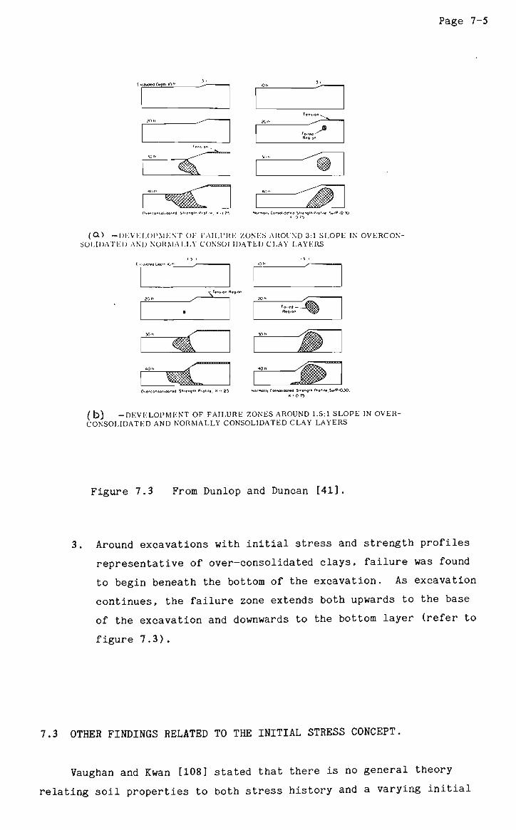
Page 7-5

E -coveted Pcpm O f

.^»

(O) -D E V E L O P M E N T OK I-AILURE ZONKS AROUND 3:i SLOPE IN OVERCONSOLIDATED AND NORMALLY CONSOLIDATED CLAY LAYERS

t •: J-Ot__l tXt"* <0 '*

Fa-ed —

_/_$

0..fC0ntOlnJ0»ta St'.ngth Profile. -•) 25 -Ofmollr C0_~_tf-_- Str._?th Pf.f .1*. S-^^1-0.

- • 0 75

( b) -DEVELOPMENT OF FAILURE ZONES AROUND 1.5:1 SLOPE IN OVER-CONSOLIDATED AND NORMALLY CONSOLIDATED CLAY LAYERS

Figure 7.3 From Dunlop and Duncan [41].

Around excavations with initial stress and strength profiles

representative of over-consolidated clays, failure was found

to begin beneath the bottom of the excavation. As excavation

continues, the failure zone extends both upwards to the base

of the excavation and downwards to the bottom layer (refer to

figure 7.3).

7.3 OTHER FINDINGS RELATED TO THE INITIAL STRESS CONCEPT.

Vaughan and Kwan [108] stated that there is no general theory

relating soil properties to both stress history and a varying initial

Page 7-6

structure. Stress history is linked with in-situ stress but few

attempts have been made to relate the degree of weathering directly to

engineering properties, and no attempt seems to have been made to

relate it to in-situ effective stress.

Vaughan and Kwan attempted to predict the effective stress

changes and in-situ effective stresses in a residual soil by

considering weathering as a weakening process which involves

decreasing unit weight, strength and stiffness. They found that the

combination of low horizontal stress with decreasing shear strength

due to weathering is likely to cause shear failure, particularly in

slopes. During shear failure, disintegration and particle wastage,

horizontal stress is likely to tend towards the value given by the

active earth pressure coefficient.

Kirkpatric, Khan and Mirza [56], in their studies on

overconsolidated clays, produced results which showed that compared

with in-situ soils, stress-relieved samples suffered appreciable loss

of strength and increase in failure strain and produced considerably

different effective stress paths to failure. This behaviour was more

pronounced with increasing sample age and was more acute for kaolin

than for the less permeable illites.

Bernander and Olofsson [11] found that certain parameters such as

the brittleness index, deviatoric strain at peak strength and the

initial stress level greatly affect the mechanism of progressive

failure. They proposed a method of solution which takes into account

the relevant deformations in the soil mass. They suggested that this

approach and the results obtained by the analyses convincingly explain

the formation, propagation and final configuration of major landslides

in Sweden.

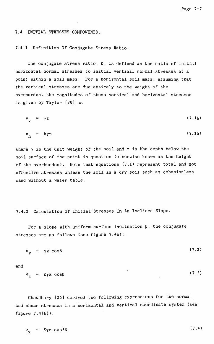
Page 7-7

7.4 INITIAL STRESSES COMPONENTS.

7.4.1 Definition Of Conjugate Stress Ratio.

The conjugate stress ratio, K, is defined as the ratio of initial

horizontal normal stresses to initial vertical normal stresses at a

point within a soil mass. For a horizontal soil mass, assuming that

the vertical stresses are due entirely to the weight of the

overburden, the magnitudes of these vertical and horizontal stresses

is given by Taylor [80] as

ff = yz (7.1a) v '

a = kyz (7.1b)

where y is the unit weight of the soil and z is the depth below the

soil surface of the point in question (otherwise known as the height

of the overburden). Note that equations (7.1) represent total and not

effective stresses unless the soil is a dry soil such as cohesionless

sand without a water table.

7.4.2 Calculation Of Initial Stresses In An Inclined Slope.

For a slope with uniform surface inclination 0, the conjugate

stresses are as follows (see figure 7.4a):-

o = yz cosP (7.2)

and

o„ = Kyz cos0 (7.3)

Chowdhury [26] derived the following expressions for the normal

and shear stresses in a horizontal and vertical coordinate system (see

figure 7.4(b)).

<*x = Kyz cos*0 (7-4)

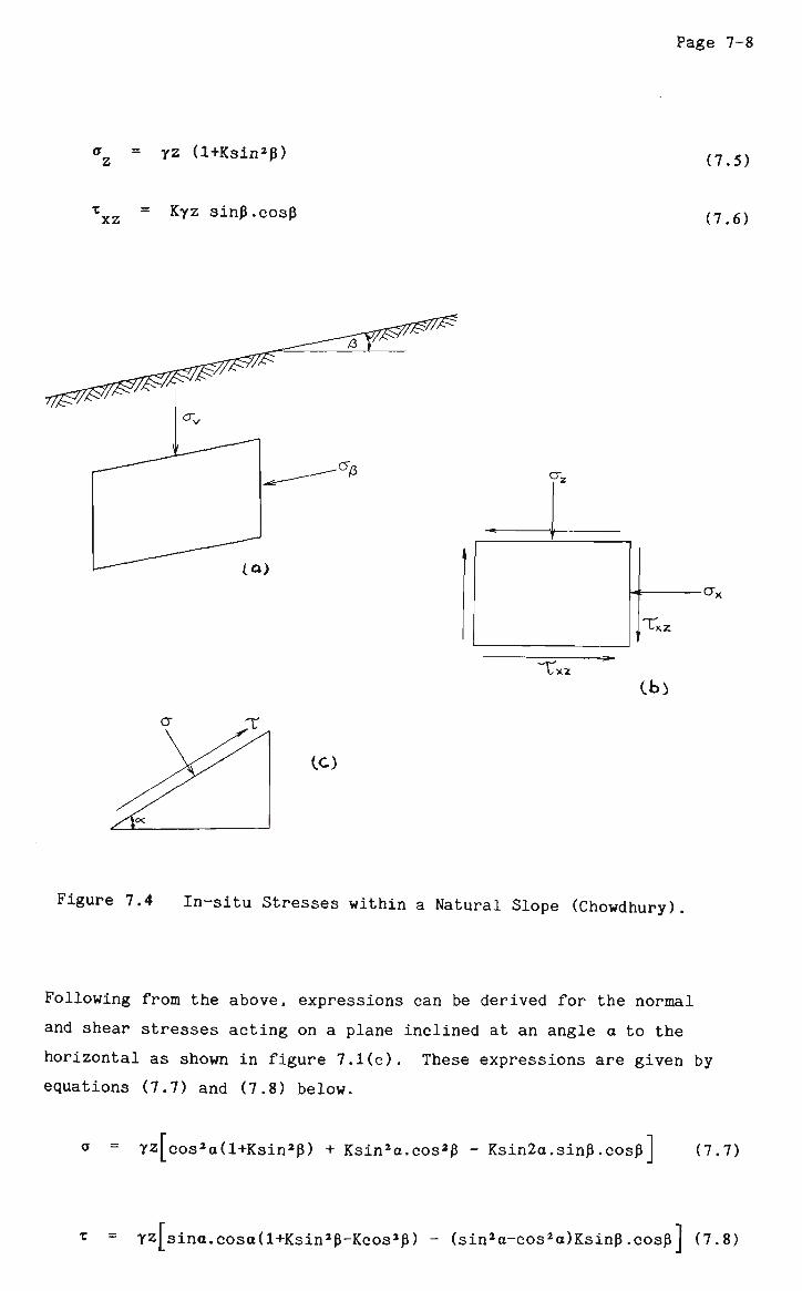
Page 7-8

o - yz (l+Ksin2B) ___i

vxz = Kyz sin0.cosp

(7.5)

(7.6)

_o)

CC)

T: xz Cb_

Figure 7.4 In-situ Stresses within a Natural Slope (Chowdhury)

Following from the above, expressions can be derived for the normal

and shear stresses acting on a plane inclined at an angle o to the

horizontal as shown in figure 7.1(c). These expressions are given by

equations (7.7) and (7.8) below.

ff = Yz[cos2a(l+Ksin2p) + Ksin2a.cos2p - Ksin2a.sinp.cosp] (7.7)

* - yz[sina.cosa(l+Ksin2p-Kcos2p) - (sin2a-cos2a)Ksin0.cos0j (7.8]

http://Ksin2a.sinp.cosp

Page 7-9

7.4.3 Effective Stress Considerations.

For cases where pore-water pressures exist within the slope, it

is useful to define a ratio K Q of horizontal and vertical normal

effective stresses. This ratio is given by the expression [26]

Kcos2p - r v U Kn ~ (7.9) 0

1 + Ksin2p - r u

where

ru = u/yz (7.10)

and is a dimensionless pore pressure ratio.

This definition of K is in accord with normal geotechnical

practice. It would be incorrect to define K as a ratio of o

effective conjugate stresses as conjugate stresses are resultant total stresses (involving both normal and shear components) and not normal

stresses and thus the application of effective stress hypothesis to

such stresses is not valid [26].

However, considering soil with a horizontal surface i.e. p=0,

equation (7.9) becomes

(7.11) K 0

= K - r

u

1 - r u

= «_

<r' V

where ff' and or' are the effective horizontal and vertical

normal stresses at any point. Moreover, if the pore water pressure at

the point is zero (i.e. p=0, u=0) then

KQ = K (7.12)

CHAPTER 8

INITIAL STRESS CONSIDERATIONS IN THE SIMULATION OF PROGRESSIVE

FAILURE.

8.1 GENERAL.

In Chapter 6, concepts concerning strain softening of soils and

associated stress redistribution were used to facilitate the

simulation of progressive failure in slopes. Methods of analysis were

proposed for soil slope problems with consideration for progressive

failure and a series of results were obtained. Results of individual

methods were compared with previously published ones for particular

case histories [58] and it was also possible to assess the results

obtained by alternative methods proposed. In many cases, the

progressive failure resulting from strain softening was not sufficient

to cause overall slope failure. However, since most of the slopes

analysed had failed at some time in the past, it could be argued that

the strain softening approach on its own may be insufficient for

predicting or simulating overall slope failure under all conditions.

In recent years it has been found that the in-situ or initial

stresses inherent in a soil mass are of considerable importance in

geotechnical investigations. As detailed in Chapter 7, several

authors have emphasized the considerable role of in-situ stresses in

the development of failure zones within soil masses. Consequently,

the initial stress state must be taken into consideration in

simulating progressive failure.

Most soils are found to have some degree of anisotrophy where,

depending on the consolidation history of the soil mass, the stresses

in one direction (usually horizontal) are greater than those in other

directions. In an over-consolidated clay slope, for example, it is

Page 8-2

commonly found that the horizontal stress is in excess of the vertical

stress at any point within the mass. Cases have been reported where

the horizontal effective stresses at a point within a soil mass have

been found to be up to three times as great in magnitude as the

vertical effective stresses at the same point.

In this chapter, the problem of progressive failure is tackled by

considering the initial stresses inherent in a slope. The simulation

of change in safety factor with the development of progressive failure

is attempted in a number of ways. One of these methods involves the

extension of techniques presented in Chapter 6 for soils in which

strain softening is the most important factor for the development of


8.2 SIMULATION OF FAILURE CONSIDERING BOTH STRAIN SOFTENING AND

INITIAL STRESSES.

In Chapter 6 a number of techniques were used for a strain

softening soil to simulate progressive failure. It was concluded that

the technique referred to as Method 2 appeared to be the most

successful in simulating the process of initiation and propagation of

local failure which may lead to overall failure of a given sloping

soil mass. It is therefore intended to extend this technique to

include initial stress considerations and to observe the effect of

including these initial stresses in the analysis of the case histories

considered earlier in Chapter 6.

8.2.1 Description of Method.

The method proposed below is similar to that described as Method

number 2 in Chapter 6.

Step 1: Calculate the shear force and shear strength on the base of

each slice:- The shear force on the base of a given slice i is denoted

by the following expression.

Page 8-3

where x± is the initial shear stress existing in the slope before

failure starts as defined by equation (7.8), and where 1. is the

length of the slice base.

The shear strength on the base of slice i is given as

(Vi = (CP + ffitan0P)1i (8-2)

where ff is the initial normal stress existing in the slope before

failure occurs and is given by equation (7.7).

The factor of safety F is found from equation (6.4) as in the previous

method.

Step 2: Check for local failure:- The procedure followed in this step

is identical to the procedure described in step 2 of methods 1 and 2

in Chapter 6. In the current method, however, the values of S and P

T are obtained using the expressions given in equations (6.1) and (6.2) for normal and shear stresses respectively.

Step 3: Reduce strength on failed slices to the post-peak value under

conditions of limiting equilibrium:- As with the methods described in

Chapter 6, on all slices where local failure has occurred, the soil

strength parameters are assumed to have fallen from their peak values

to their residual values. In addition, the newly failed zone is

assumed to behave as if it were in limiting or critical equilibrium

whereas the remaining unfailed sections of the slope are still under

conditions of initial stress. Therefore, on all slices where local

failure has occurred, the shear strength is expressed by equation

(6.9). Again, as in Chapter 6, since the mobilised shear force cannot

exceed the available shear strength, the mobilised shear force on each

failed slice will be set equal to the residual shear strength on the

base of that slice as shown by equation (6.11).

Step 4: Redistribute the excess shear force:- The procedure followed

in this step is again the same as that followed in step 4 of methods 1

Page 8-4

and 2 presented in Chapter 6. It is, therefore, not repeated here.

Step 5: Calculate the new factor of safety:- The procedure used to

calculate the new factor of safety is similar to that described in

method 2 in Chapter 6. An iterative procedure is used whereby a

complete limit equilibrium analysis (using Bishop's simplified method)

is carried out on the slope using the last known value of the factor

of safety F, and a new value of F is then calculated. This procedure

continues until the difference between two successive values of F is

negligible. The difference between the calculation of F in this

current method and the calculation of F in method 2 of Chapter 6 is in

the equation used to calculate each successive value of F.

Equation (6.17) is used to calculate the value of the factor of safety

in methods 1 and 2 of chapter 6. Although this equation also holds

true for the current method, it will be expressed differently since we

are now dealing with two different models for simulation of stress

conditions within one method of analysis, namely initial stress and

limit equilibrium models. All unfailed slices are assumed to be still

under conditions of initial stress, and all failed slices are assumed

to be in limiting equilibrium. Therefore, the overall factor of

safety may be calculated by using the expression given in equation

(8.3) below.

, (S ). +5 <S), F = P 1 S P (».•

Ks + K e

where the terms with the 'is' subscript refer to those slices which

have not yet failed and the terms with the 'le' subscript refer to

those slices which have failed and which are in limiting equilibrium.

Again, as with the previous method, the procedure returns to step

2 above and halts only when no further slices satisfy the criteria for

local failure in step 2.

Page 8-5

8.2.2 Modification of Computer Program BSTRAIN2.

As the present method is basically similar to that referred to as

method 2 in Chapter 6 and varies mainly in the equations used for the

calculation of forces on slice bases, the program BSTRAIN2 which was

used in the previous method can also be used here with some

alterations. The program was modified to include the following

additions.

1. a user specified option is read in at the start of the

program to indicate whether initial stresses are to be

included. This is in the form of a YES/NO answer to a

generated question and initialises a flag variable in the

program.

2. subroutine STINIT is modified to enable calculation of

initial values of slice forces according to equations (8.1)

and (8.2) incorporating equations (7.7) and (7.8). This

addition to routine STINIT is used when the slope is assumed

to be under initial stress conditions.

3. an 'initial stress' counterpart to routine RESLE was written

and called routine RESIS. This new routine performs the

iterative procedure for calculating the new factor of safety.

In calculating the new value of F, subroutine RESIS uses

equation (8.3) in conjunction with equations (8.1), (8.2),

(7.7) and (7.8).

The overall procedure followed in program BSTRAIN2 is the same as

it was in Chapter 6 except that when subroutine STINIT is called to

calculate the initial values of normal and shear forces on the slice

bases as well as the factor of safety F, a check is made as to whether

initial stresses are to be included in the analysis. According to the

result of this test the relevant parts of subroutine STINIT are

processed. Secondly, in subsequent iterations, a check is again made

for initial stress inclusions. If initial stresses are to be

included, then subroutine RESIS is used to calculate forces on slice

bases and subsequent values of the factor of safety F. If initial

Page 8-6

stresses are not to be included, then subroutine RESLE is used as for

method 2 in Chapter 6.

8.2.3 Case Histories Considered for Analysis.

In order to present comparative results using the present method,

the nine case histories considered in Chapter 6 were analysed again by

the method presented here. These case histories represent slides at

Northolt, Selset, Sudbury Hill, Jackfield, Balgheim, Saskatchewan and

Vajont as well as two hypothetical cases and are all fully documented

in Appendix A and Chapter 6. Some of the actual cases are omitted

however. For example, in the Northolt, Selset and Sudbury Hill slides

only the cases where the actual phreatic surface is given are used.

In addition, the shear strength parameters used here will be in

accordance with system B as defined in Chapter 6. This combination of

shear strength is as follows.

1. peak values of c' and $.' as given in Appendix A.

2. residual value of c' equal to zero

3. residual value of 0' is less than the peak value with

magnitude as shown in Appendix A

8.2.4 Results and Discussion.

Table 8.1 shows a summary of results obtained by performing the

above analytical procedure on the case histories detailed above. It

is seen that in some cases (e.g. Northolt, Selset) the factor of

safety obtained decreases during the process of stress redistribution.

However, the other case histories show no decrease in factor of safety

with stress redistribution. In other words, little or no stress

redistribution occurs.

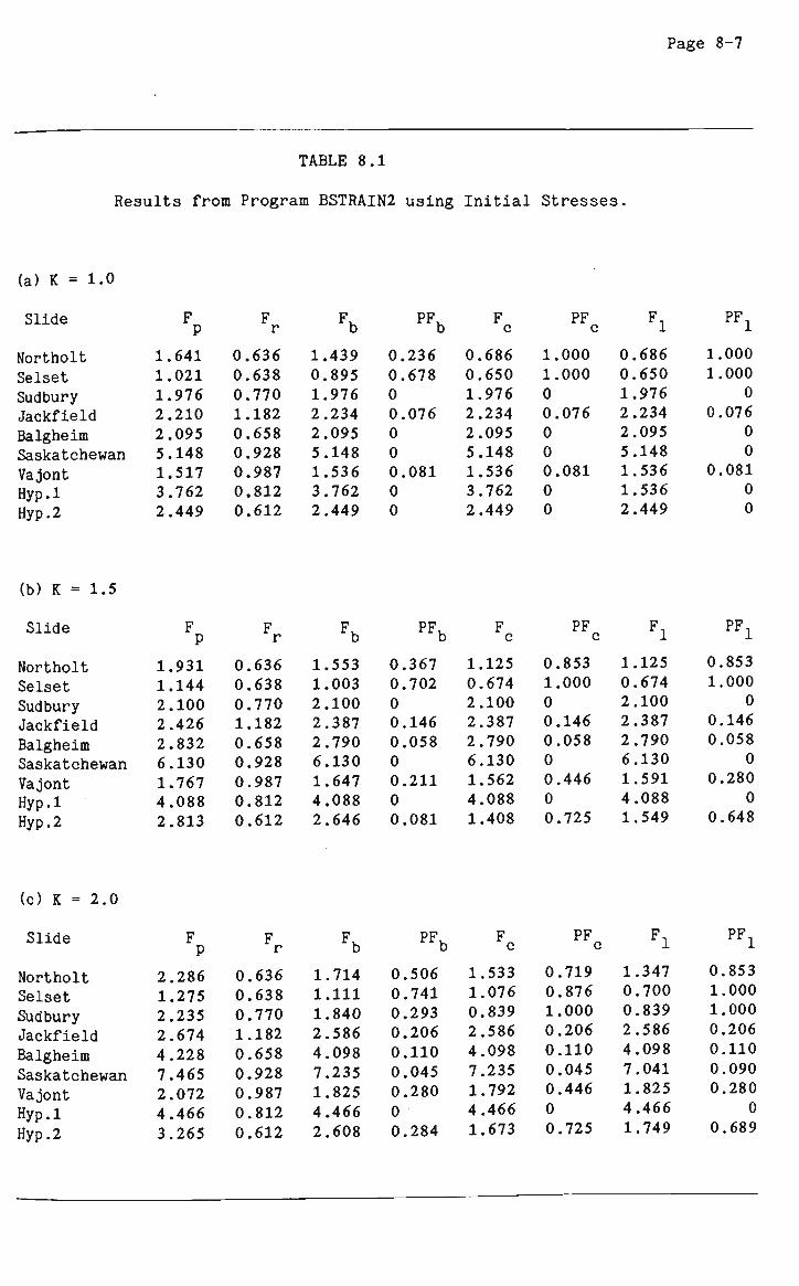
Page 8-7

TABLE 8.1

Results from Program BSTRAIN2 using Initial Stresses.

(a) K = 1.0

Slide

Northolt Selset Sudbury Jackfield Balgheim Saskatchewan Vajont Hyp.l Hyp. 2

(b) K = 1.5

Slide


(c) K = 2.0

Slide


F P

1.641 1.021 1.976 2.210 2.095 5.148 1.517 3.762 2.449

F P

1.931 1.144 2.100 2.426 2.832 6.130 1.767 4.088 2.813

F P

2.286 1.275 2.235 2.674 4.228 7.465 2.072 4.466 3.265

F r

0.636 0.638 0.770 1.182 0.658 0.928 0.987 0.812 0.612

F r

0.636 0.638 0.770 1.182 0.658 0.928 0.987 0.812 0.612

Fr

0.636 0.638 0.770 1.182 0.658 0.928 0.987 0.812 0.612

Fb

1.439 0.895 1.976 2.234 2.095 5.148 1.536 3.762 2.449

Fb

1.553 1.003 2.100 2.387 2.790 6.130 1.647 4.088 2.646

Fb

1.714 1.111 1.840 2.586 4.098 7.235 1.825 4.466 2.608

PFb

0.236 0.678 0 0.076 0 0 0.081 0 0

PFb

0.367 0.702 0 0.146 0.058 0 0.211 0 0.081

PFb

0.506 0.741 0.293 0.206 0.110 0.045 0.280 0 0.284

F c

0.686 0.650 1.976 2.234 2.095 5.148 1.536 3.762 2.449

F c

1.125 0.674 2.100 2.387 2.790 6.130 1.562 4.088 1.408

F c

1.533 1.076 0.839 2.586 4.098 7.235 1.792 4.466 1.673

PF c

1.000 1.000 0 0.076 0 0 0.081 0 0

PF c

0.853 1.000 0 0.146 0.058 0 0.446

0 0.725

PF c

0.719 0.876 1.000 0.206 0.110 0.045 0.446

0 0.725

Fl

0.686 0.650 1.976 2.234 2.095 5.148 1.536 1.536 2.449

Fl

1.125 0.674 2.100 2.387 2.790 6.130 1.591 4.088 1.549

Fl

1.347 0.700 0.839 2.586 4.098 7.041 1.825 4.466 1.749

PF1

1.000 1.000

0 0.076

0 0

0.081 0 0

PF1

0.853 1.000

0 0.146 0.058

0 0.280

0 0.648

PF1

0.853 1.000 1.000 0.206 0.110 0.090 0.280

0 0.689

Page 8-8

As the value of the coefficient K is increased from 1.0 to 1.5

and then to 2.0, the value of the factor of safety for the Sudbury

case decreases to less than 1.0 . For the other slopes, however,

increasing the value of K does produce some small drop in the factor

of safety but does not reduce it to anywhere near 1.0 .

It appears, therefore, that the proposed method of analysis or

simulation procedure does not sufficiently explain the failure of the

case histories studied. It is therefore necessary to consider other

possible factors and mechanisms which facilitate the development and

propagation of slope failure.

One reason for the limited success of the above approach is that

reorientation of principal stresses which occurs during the process of

excavation of a slope (or during embankment construction) has not been

considered. The method as developed here is applicable only to

natural slopes with a uniform initial stress field. For built-up

slopes, stress analyses using the finite element method would be

required to get the true initial state of stress before the proposed

method could be applied with complete success.

8.3 SIMULATION OF PROGRESSIVE FAILURE BY SEQUENTIAL LOCAL FAILURE OF

SOIL SLICES.

Attempts were made in the previous section to evaluate strain

softening effects on the propagation of local failure in a soil slope.

It was found that in many cases these strain softening effects

appeared not to have caused an overall failure of the slope. At this

stage, it is not clear whether this lack of overall failure was due to

insufficient local failure occurring or due to the method of

simulating the progression of failure through the failure mass.

In order to help resolve this question, a method of simulating

progressive failure was devised which assumes that the initial stress

state changes to a simple gravitational stress field progressively

along the potential slip surface. Thus a simulation procedure is

proposed which links the initial stress state of a slope to the

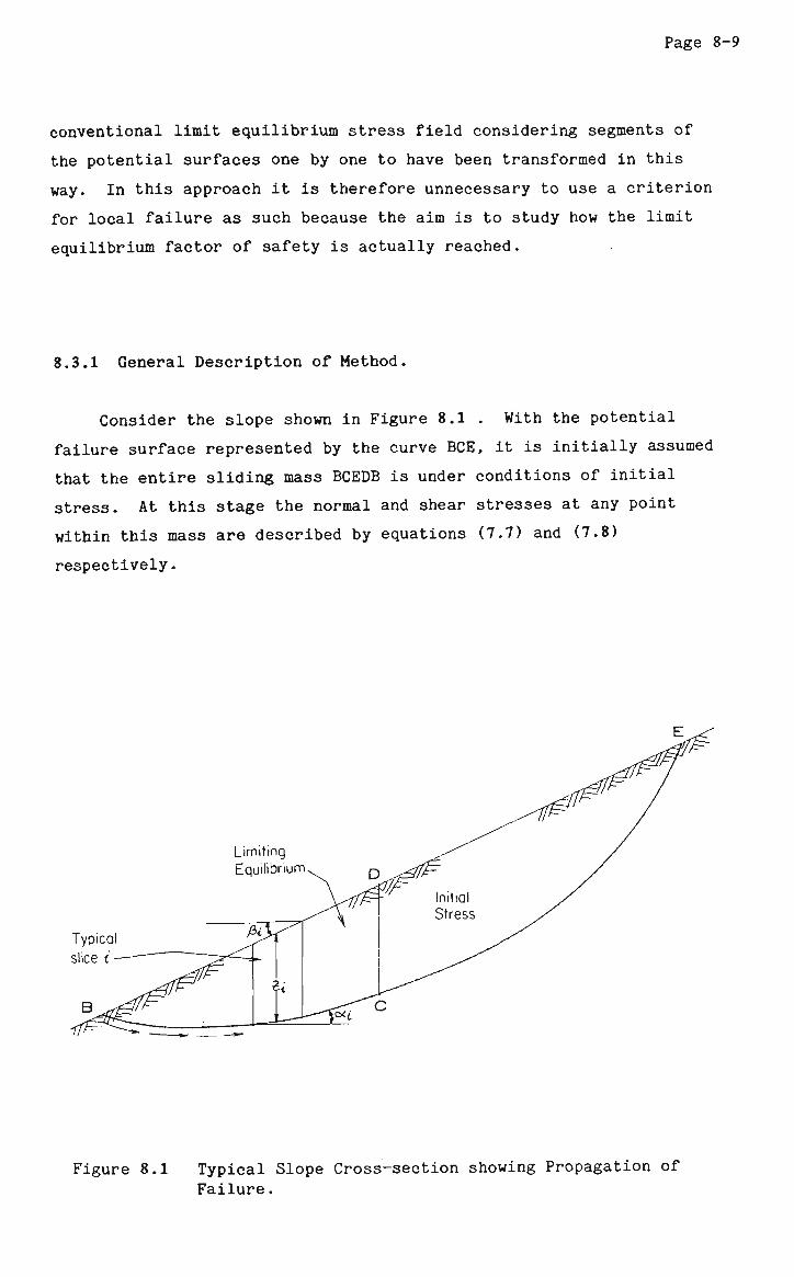
Page 8-9

conventional limit equilibrium stress field considering segments of

the potential surfaces one by one to have been transformed in this

way. In this approach it is therefore unnecessary to use a criterion

for local failure as such because the aim is to study how the limit

equilibrium factor of safety is actually reached.

8.3.1 General Description of Method.

Consider the slope shown in Figure 8.1 . With the potential

failure surface represented by the curve BCE, it is initially assumed

that the entire sliding mass BCEDB is under conditions of initial

stress. At this stage the normal and shear stresses at any point

within this mass are described by equations (7.7) and (7.8)

respectively.

Figure 8.1 Typical Slope Cross-section showing Propagation of Failure.

Page 8-

A procedure similar to that described by Romani et. al. [79] and

Chowdhury [29] is used. However, in this research the scope of the

analysis is extended beyond that of the previous work done in this

field.

As described in section 5.4, Romani et. al. presented a method

of analysis which involved a crack or slit which begins at one end of

the failure surface and proceeds towards the other end. At any point

in time when the crack has progressed to a certain point, the part of

the slope beyond that point and not yet reached by the crack is

analysed under assumed conditions of elastic stress. Considering

propagation from B to D, the section of the slope above the crack

i.e. DCE is analysed as a rigid body using the concept of limit

equilibrium. The Bishop simplified method is used for this part. The

resisting and driving forces are thus calculated for each part and the

overall factor of safety for the slope obtained. This is repeated for

a large number of points and curves are obtained of the value of the

factor of safety for failure starting from either the crest or the toe

of the slope.

Chowdhury used a similar method except that the uncracked portion

of the slope is considered to be under the influences only of the

initial stresses inherent in the soil mass. Again the resisting and

driving forces are calculated for each section and the overall factor

of safety obtained. The results for variation of factor of safety

obtained by Chowdhury are similar in trend to those of Romani et. al.

considering the progression of the limit equilibrium stress field

either from the crest or from the toe of the slope.

For this research, previous work was modified and the main

improvement results from the following:-

1. Instead of using the Bishop simplified method for the section

of the slope under limiting equilibrium, the

Morgenstern-Price method of analysis has been used. Apart

from advantages in the way of accuracy, this method allows

non-circular failure surfaces to be analysed.

Page 8-11

2. A number of ways of defining the section of the failure mass

assumed to be in limiting equilibrium have been considered in

the method proposed here.

3. Consideration has been given to the internal forces at the

assumed boundary between the two parts of a potential failure

mass, one at initial stress and the other at limiting

equilibrium.

8.3.2 Details of Methods Used.

Failure will initiate in a natural slope either from the crest or

from the toe. Divide the soil mass above the potential failure

surface into a number of vertical slices as is usual with conventional

limit equilibrium studies. Assume that local failure commenced at

point B (figure 8.1) and has extended some distance. By local

failure, it is meant that the shear stress has exceeded the peak shear

strength and that the shear strength parameters c' and </>' at that

particular point have fallen to their residual values. Moreover, the

soil in that part of the failure mass which has thus failed is now

locally in a state of limiting equilibrium.

Consider that local failure has progressed along the potential

slip surface from point B to point C (figure 8.1). Therefore, while

the mass CEDC is still considered to be totally under initial stress

conditions with shear strength parameters c' and <p' at their peak

values, the mass BCDB is assumed to now be under conditions of

limiting equilibrium with c' and 0' having dropped to their

residual values along the surface BC. At this stage, the normal and

shear stresses acting on the base of a slice i within the mass BCDB

are given by the following equations in accordance with the concepts

referred to in chapter 7 and, in particular, equations (7.7) and

(7.8).

a = yz. cos2o.(1+Ksin2p.) + Ksin2a..cos2P. - Ksin2o..sinp..cosp.1 l lL i *i i i i i iJ

(8.4)

Page 8-12

x = yz. 1 sina..coso.(l+Ksin2p.-Kcos2p.)

- (sin2a.-cos2a.)Ksinp..cosp.J (8.5)

where z. is the height of the slice,

a. is the angle of the slice base to the horizontal,

and p. is the average angle of the topslope above the slice.

In order to obtain a measure of the overall stability of the

combined mass, an expression is formulated to calculate the overall

factor of safety for this mass. As the factor of safety of a soil or

rock mass is generally defined as the ratio of the sum of the

resisting forces to the sum of the driving forces in the mass, the

overall factor of safety is expressed as given in equation (8.6)

below.

F =

_

(8.6)

Ti

where ̂ s. is the sum of the resisting stresses from both sections

of the failure mass,

and 3 x. is the sum of the driving stresses from both sections

of the failure mass.

The above equation can be re-written as

F = 1 sle + 1 s is (8.7)

T.. + > X. Ie L is

where M is the number of slices which have experienced local failure,

In equation (8.7) above

s. = c' + cr' tan#' (8-8)

le r le r

Page 8-13

where or' is the effective normal stress on the base of the slice

obtained from limit equilibrium considerations;

s. = c' + ff.' tan0' (8.9) is p is *p

where ff. is the effective normal stress on the base of the slice is obtained from equation (8.4);

c' + ff' tan0' t. = r ie r (8.10) le "le

where F and o,' are both found by the application of the

Morgenstern-Price limiting equilibrium method; and

T. is the effective is

from equation (8.5).

T. is the effective shear stress on the base of a slice obtained is

At the point in time before progressive failure or transformation

of stress state has started, equation (8.7) reduces to equation (8.11)

below.

F = *• Sj-S (8.11)

L i.

where s. and x. are defined by equations (8.9) and (8.5) is is

respectively.

On the other hand if progression to 'limit equilibrium' stress

state has occurred through the entire failure mass, equation (8.7)

will reduce to equation (8.12) below.

F = S l e (8.12)

rle

where s. and t, are defined by equations (8.8) and (8.10)

respectively.

Page 8-14

8.3.3 Use of Conjugate Stress Ratio.

It is important to note here that while the equations for normal

and shear stress on the base of any slice i (refer to equations (8.4)

and (8.5)) both depend on the conjugate stress ratio K, in practice

the value of K is not readily known. On the other hand K , the o

ratio of effective horizontal and vertical normal stresses, is more readily determined from measured laboratory or field data. It is this

parameter K which is commonly encountered in geotechnical

literature.

For the cases examined in this chapter, therefore, it is assumed

that the value of K Q is known and is uniform throughout the failure

mass. The value of K is then calculated for each slice within this

mass using equation (8.13) below which is obtained as a rearrangement

of equation (7.9).

K + r (1-K ) K± = ° U ° (8.13)

cos2Pi - K(.sin2pi

in which K. is the value of K for vertical slice i.

8.3.4 Direction of Propagation of Failure.

In the description of the method above, local failure was assumed

to start at the toe of the failure surface. It is possible, however,

that local failure may follow a different path.

Bishop [14] suggests that the shear strength in a slope may fall

to the residual quicker at the toe of the slope or possibly at both

ends simultaneously, thus suggesting that local failure may start more

easily in one of these two modes. Romani et. al., [79] and Chowdhury

[29] both have obtained results to indicate that failure tends to

propagate, or is potentially more dangerous, when starting from the

top end of the failure surface. Also, results described in Chapter 6

Page 8-15

seem to indicate that local failure starting from some point near the

centre of the slope may also be critical.

8.3.5 Definition of Propagation Factor.

At this stage, it is convenient to introduce a means of defining

the extent to which the 'failure' or the transformation of stress has

progressed. In other words, a factor, which shall be called the

Propagation Factor, is introduced which describes the fraction of the

total length of the failure surface which has changed from a condition

of initial stress to a condition of limiting equilibrium. The

propagation factor therefore indicates the fraction of the failure

surface length which has experienced 'local failure'. Thi3 fraction

is expressed as a decimal value between 0 and 1.

As failure can progress from more than one point at the one time,

a more general definition of the propagation factor must be used.

Thus, the Propagation Factor (expressed as a decimal value between 0

and 1.) is defined as that value derived by dividing the sum of the

base lengths of all slices in the failure mass which have reached

conditions of limiting equilibrium by the sum of the base lengths of

the total number of slices. The expression for the propagation factor

thus becomes;

PF = ie (8.14)

_ A L i I

where N is the total number of slices,

n is the number of slices where limiting equilibrium conditions exist

Al is the length of the base of slice i where limiting equilibrium ie

conditions exist, and AL. is the length of the base of any slice i.

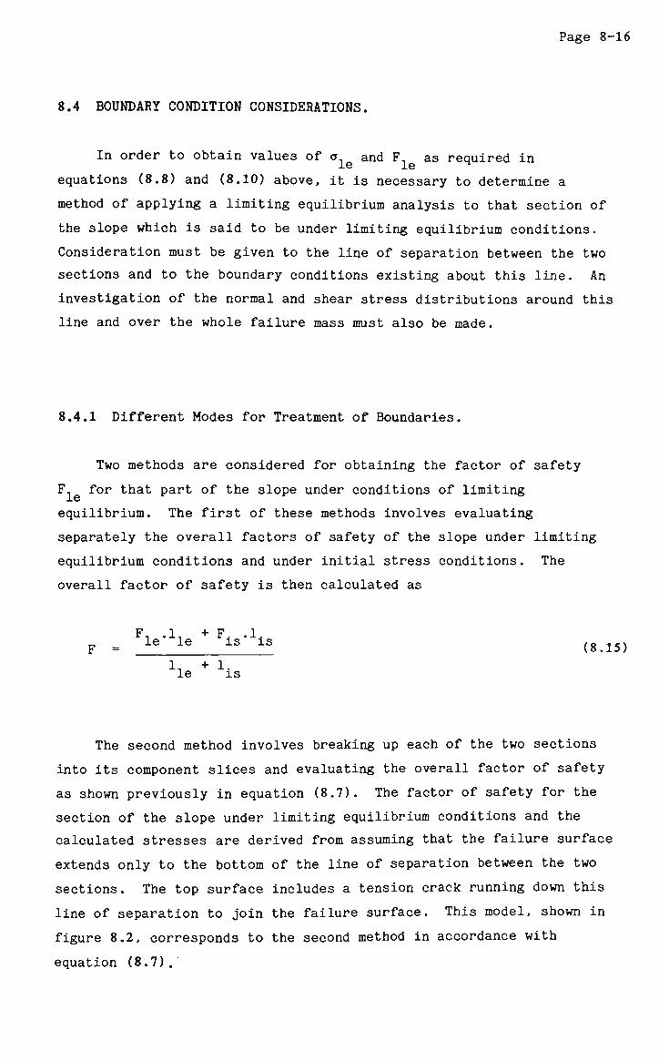
Page 8-16

8.4 BOUNDARY CONDITION CONSIDERATIONS.

In order to obtain values of a and F, as required in

equations (8.8) and (8.10) above, it is necessary to determine a

method of applying a limiting equilibrium analysis to that section of

the slope which is said to be under limiting equilibrium conditions.

Consideration must be given to the line of separation between the two

sections and to the boundary conditions existing about this line. An

investigation of the normal and shear stress distributions around this

line and over the whole failure mass must also be made.

8.4.1 Different Modes for Treatment of Boundaries.

Two methods are considered for obtaining the factor of safety

F for that part of the slope under conditions of limiting

equilibrium. The first of these methods involves evaluating

separately the overall factors of safety of the slope under limiting

equilibrium conditions and under initial stress conditions. The

overall factor of safety is then calculated as

F. .1. + F. .1. F - l e l e 1 S l s (8.15)

1, + 1. le is

The second method involves breaking up each of the two sections

into its component slices and evaluating the overall factor of safety

as shown previously in equation (8.7). The factor of safety for the

section of the slope under limiting equilibrium conditions and the

calculated stresses are derived from assuming that the failure surface

extends only to the bottom of the line of separation between the two

sections. The top surface includes a tension crack running down this

line of separation to join the failure surface. This model, shown in

figure 8.2, corresponds to the second method in accordance with

equation (8.7).

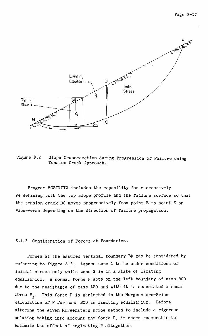
Page 8-17

Figure 8.2 Slope Cross-section during Progression of Failure using Tension Crack Approach.

Program MGSINIT2 includes the capability for successively

re-defining both the top slope profile and the failure surface so that

the tension crack DC moves progressively from point B to point E or

vice-versa depending on the direction of failure propagation.

8.4.2 Consideration of Forces at Boundaries.

Forces at the assumed vertical boundary BD may be considered by

referring to figure 8.3. Assume zone 1 to be under conditions of

initial stress only while zone 2 is in a state of limiting

equilibrium. A normal force P acts on the left boundary of mass BCD

due to the resistance of mass ABD and with it is associated a shear

force P1. This force P is neglected in the Morgenstern-Price

calculation of F for mass BCD in limiting equilibrium. Before

altering the given Morgenstern-price method to include a rigorous

solution taking into account the force P, it seems reasonable to

estimate the effect of neglecting P altogether.

Page 8-18

Figure 8.3 Slope Cross-section showing Boundary Forces Considered.

Let us consider the two possible extreme cases for P, say the

active and passive Rankine pressures. If the difference in result

between these cases and that without P is sufficiently small, it may

be argued that the omission of P (and thus Pj) is justified to

simplify calculations.

8.4.3 Consideration of Active and Passive Earth Pressures.

The sample slope analysed was the arbitrary circular slip surface

described earlier in chapter 6. The soil was considered to be a

cohesive soil with little or no adherence along the imaginary boundary

BD. No water table, and thus no pore water pressures, will be

assumed. Thus the active and passive Rankine earth pressures will be

given by the following equations respectively.

PA = 0.5yH2/N - 2cH/N°'5 + 2c2/y (8.16)

Page 8-19

Pp = O.5yH2N0 + 2CHNJ*5 (8.17)

where N = tan2(45+0/2)

Three series of trials were made on the arbitrary circular slip mass.

i) Neglecting P and P1

ii) Assuming P = PA and P1 = P tan0'/F

iii) Assuming P = Pp and P̂^ = Pptan0'/F

In each case the proposed failure mass was divided Into ten

vertical slices of equal width and failure was assumed to propagate

from the top of the slope (RHS) to the toe (LHS). Zone 2 which is

assumed to be under limit equilibrium conditions becomes larger by one

additional slice at a time and P and ?1 are correspondingly shifted

to the left one slice until the whole mass ABCDA is in limiting

equilibrium.

The factor of safety for the section of the slope considered to

be in limiting equilibrium was found first. For the case where no

active or passive pressures were assumed to act, the calculation of

F, was made according to equation (2.9).

8.4.4 Calculation of Factor of Safety Considering Earth Pressures at

the Imaginary Vertical Boundary.

For the cases involving active or passive earth pressure as shown

in figure 8.4 below, we have;

For the active pressure case three different components must be considered in

equation (8.16).

P. = P., + P„ + P., A 1 2 3

where

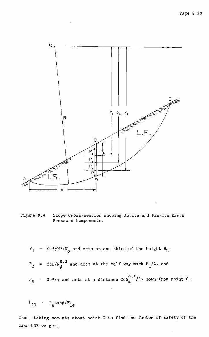
Page 8-20

s.

y y y

c

p 2 , P 1 , P

>

I-I r

' f .

^^ ' 1

L.E.

D

Figure 8.4 Slope Cross-section showing Active and Passive Earth Pressure Components.

'- = 0.5yH2/N and acts at one third of the height H.,

.0.5 P2 = 2cH/N * and acts at the half way mark H./2, and

P3 = 2c2/y and acts at a distance 2cN * /3y down from point C.

PA1 = PAtan0/Fle

Thus, taking moments about point 0 to find the factor of safety of the

mass CDE we get.

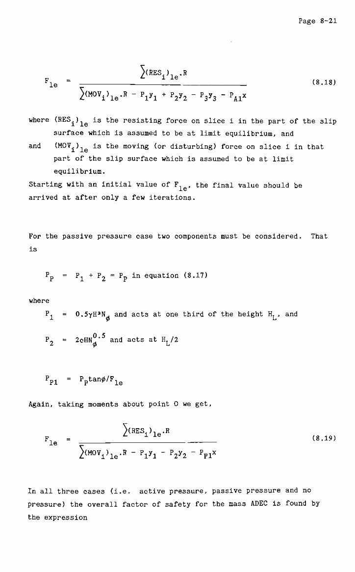
Page 8-21

/\RES,) .R Fle - t __J_f (8.18)

5(M0Vi)le.R - Pl7l + P2y2 - P3y3 - P^x

where Ê^)^ is tne resisting force on slice i in the part of the slip

surface which is assumed to be at limit equilibrium, and

and ^M 0 Viî e is the moving (or disturbing) force on slice i in that

part of the slip surface which is assumed to be at limit

equilibrium.

Starting with an initial value of F., the final value should be

arrived at after only a few iterations.

For the passive pressure case two components must be considered. That

is

Pp = Pj + P2 = Pp in equation (8.17)

where

P I = 0.5yH2N. and acts at one third of the height H., and

P2 = 2cHN°*5 and acts at HL/2

PP1 = PPtan*/Fle

Again, taking moments about point 0 we get,

^ R E S ^ . R F. (8.19) le

- Pr,.x 5(M0V.)le.R - Pl7l - P2y2 - Ppl

In all three cases (i.e. active pressure, passive pressure and no

pressure) the overall factor of safety for the mass ADEC is found by

the expression

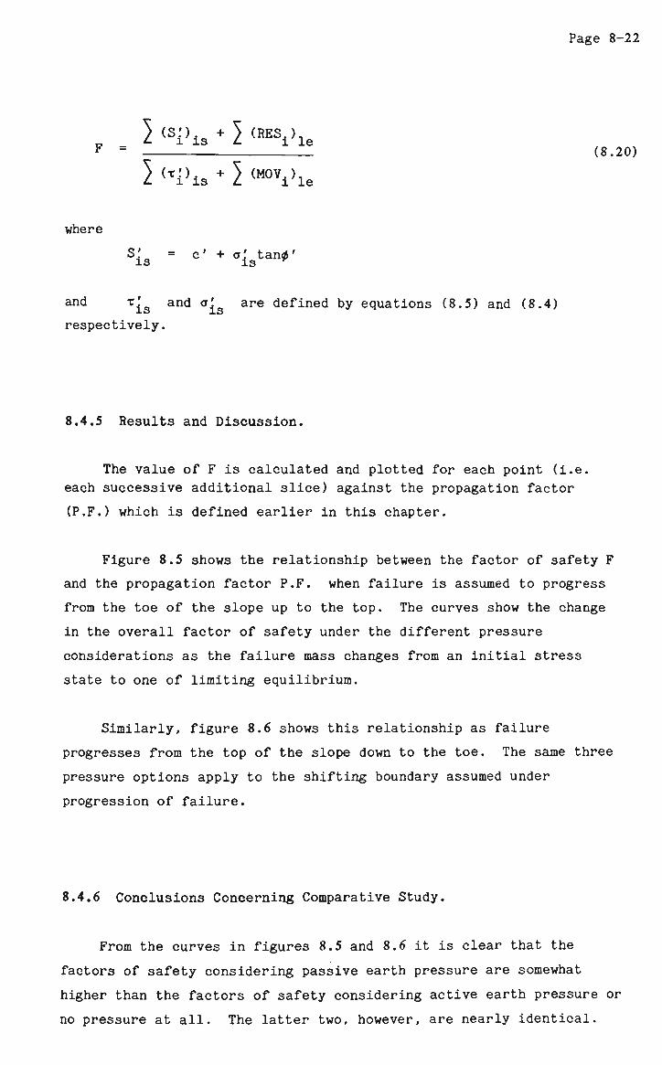
Page 8-22

r I iSlhs + 1 <RESi>le F = (8.20)

} (xp±3 -, I (MD V le

where

S' = c' + fff tan0' is is r

and T^S and «|g are defined by equations (8.5) and (8.4)

respectively.


The value of F is calculated and plotted for each point (i.e. each successive additional slice) against the propagation factor

(P.F.) which is defined earlier in this chapter.

Figure 8.5 shows the relationship between the factor of safety F

and the propagation factor P.F. when failure is assumed to progress

from the toe of the slope up to the top. The curves show the change

in the overall factor of safety under the different pressure

considerations as the failure mass changes from an initial stress

state to one of limiting equilibrium.

Similarly, figure 8.6 shows this relationship as failure

progresses from the top of the slope down to the toe. The same three

pressure options apply to the shifting boundary assumed under

progression of failure.

8.4.6 Conclusions Concerning Comparative Study.

From the curves in figures 8.5 and 8.6 it is clear that the

factors of safety considering passive earth pressure are somewhat

higher than the factors of safety considering active earth pressure or

no pressure at all. The latter two, however, are nearly identical.

Page 8-23

2 . 0 1 i i i i ) i i T I ) i i i i | i i i i ; i i i i | i i i i | ; i i i j i ) ) i | , , , , j t l i i

1 , 0 1 i i i i 1 • i i i I i i i i 1 i i i i I i i i i 1 i i i i I i i i i I i i i i I i i i i I i i t i .0 .1 .2 .3 A .5 .6 .7 .8 .9 1.0

Propagation Factor

Figure 8.5 Boundary Force Considerations for Progressive Failure

Starting From Bottom of Slope

1 . 5 1 i i i i | i i i i | i i i i | i i i i | i i i i | i i i i | i i i i | i i i i [ i i i i | i i i r

, 5 1 i i i i I i i i i I i i i i I i i i i I i i i i I i .i i _ i I i i i i 1 i i t__i I i i i l 1 i i i i .0 .1 .2 .3 .4 .5 .6 .7 .8 .9 1.0

Propagation Factor

Figure 8.6 Boundary Force Considerations for Progressive Failure

Starting From Top of Slope

Page 8-24

The case with no earth pressure appears to have slightly lower values

than the corresponding one considering active pressure. Thus the case

with P=0 is the most conservative.

The differences in results between the three alternative cases

are not significant in general. Therefore, the forces P and P.. can

be omitted altogether to simplify the calculations and the results are

guaranteed to be conservative.

The second method for calculating the overall factor of safety

(as described in section 8.4.1) appears to be attractive and has been

used for the analysis of case histories as discussed in the subsequent

sections.

8.5 CALCULATION OF OVERALL FACTOR OF SAFETY.

The calculation of the overall factor of safety is carried out

using equation (8.7) as mentioned earlier. Program MGSINIT2 is used

to calculate the factors of safety. The results obtained by this

method will be discussed later. As stated in the previous section,

the effect of any forces acting on the vertical boundary between the

'failed' and 'unfailed' slices is ignored.

In the calculation of the overall factor of safety, the effective

shear stress x. on the base of slices under initial stress is

conditions is given by equation (8.5). This equation contains the conjugate stress ratio K. The relationship between K and the ratio of

horizontal and vertical stresses K was shown in equation (8.13).

It is the intention here to compare the results obtained using

different values of K and K . o

Page 8-25

8.5.1 Case Histories Considered.

The slopes considered in this section are a subset of those used

and described in section 8.2. A number of slopes was analysed but

only the results of three are reported here as they represent a good

cross-section of the results obtained. These three slopes are

Northolt, Vajont and the hypothetical case number one.


Figure 8.7 shows four curves indicating the change in the overall

factor of safety of the Northolt slope as propagation of failure is

simulated so that the slope mass moves from an initial stress state

(P.F.=0) to a state where it is entirely in a state of limiting

equilibrium (P.F.=1). The four curves correspond to four possible

modes of failure. These are ;

1. failure starting at the toe (bottom) of the slope,

2. failure starting at the crest of the slope,

3. failure starting simultaneously from both ends of the slope,

and

4. failure starting from the centre of the slope and progressing

outwards.

From the four curves shown and from various other cases

investigated it is obvious that failure modes (1) and (4) are

unrealistic and that the factors of safety obtained are always higher

than those obtained with the whole slope under either initial stress

or limiting equilibrium conditions. Therefore, the curves

corresponding to these methods are omitted from the subsequent figures

showing the results.

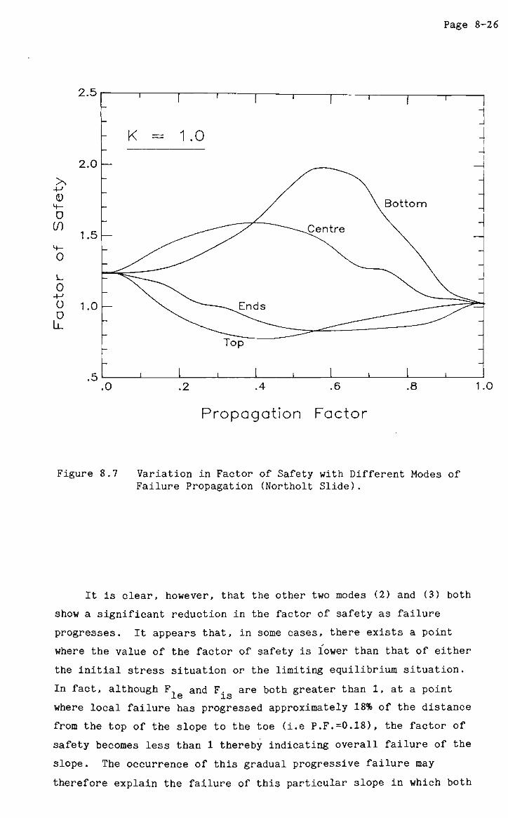
Page 8-26

<D 4-

0 (/) >+-

0 -_

0 u D l_L

Propagation Factor

Figure 8.7 Variation in Factor of Safety with Different Modes of Failure Propagation (Northolt Slide).

It is clear, however, that the other two modes (2) and (3) both

show a significant reduction in the factor of safety as failure

progresses. It appears that, in some cases, there exists a point

where the value of the factor of safety is lower than that of either

the initial stress situation or the limiting equilibrium situation.

In fact, although F. and F. are both greater than 1, at a point __L6 IS

where local failure has progressed approximately 18% of the distance from the top of the slope to the toe (i.e P.F.=0.18), the factor of

safety becomes less than 1 thereby indicating overall failure of the

slope. The occurrence of this gradual progressive failure may

therefore explain the failure of this particular slope in which both

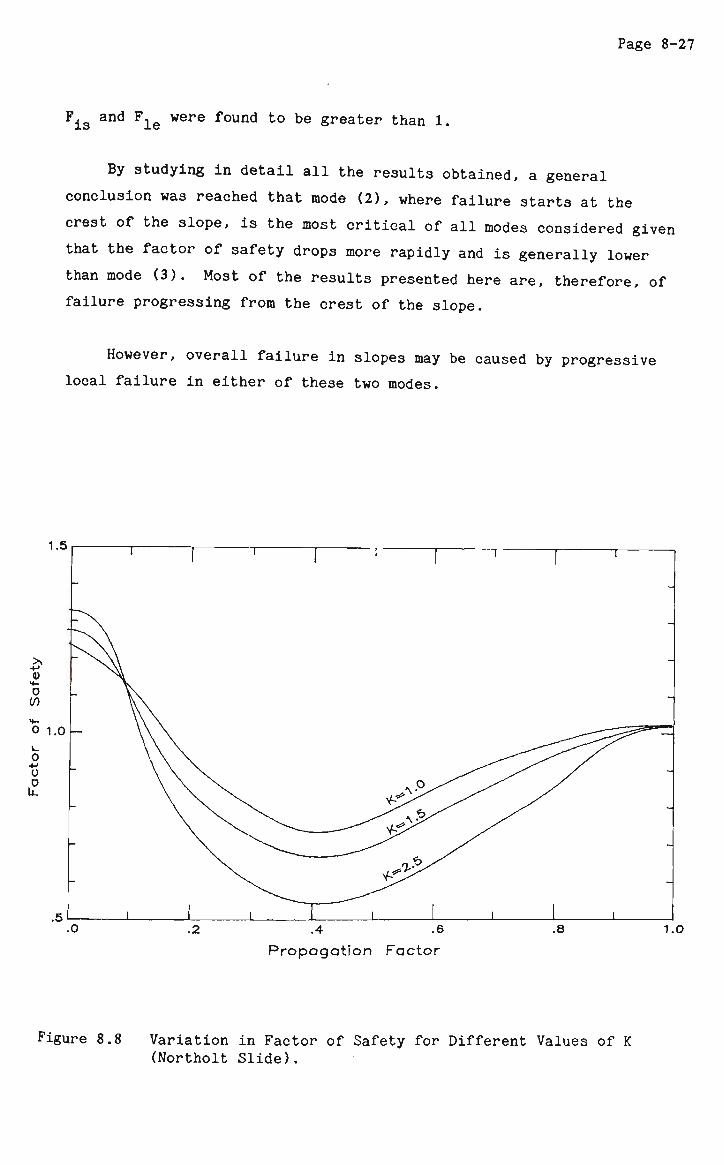
Page 8-27

Fis a n d Fle w e r e f o u n d t o b e greater than 1.

By studying in detail all the results obtained, a general

conclusion was reached that mode (2), where failure starts at the

crest of the slope, is the most critical of all modes considered give:

that the factor of safety drops more rapidly and is generally lower

than mode (3). Most of the results presented here are, therefore, of

failure progressing from the crest of the slope.

However, overall failure in slopes may be caused by progressive

local failure in either of these two modes.

Propagation Factor

Figure 8.8 Variation in Factor of Safety for Different Values of K (Northolt Slide).

Page 8-28

Figure 8.8 shows the variation in the curve obtained by failure

mode (2) for different values of the factors K and K it is

evident that as K or K Q increases, the curve for factor of safety

becomes more critical (i.e. the factors of safety decrease) therefore

increasing the chance of overall slope failure.

Figures 8.9 and 8.10 show similar information for the Vajont

slide. It is seen that although F±s is approximately 1.6 and F

is approximately 1.1, a value of less than 1 is obtained with values

of K greater than or equal to 1.5 and with failure originating from

the top of the slope (mode 2).

Similarly, figures 8.11 and 8.12 describe the variation of the

factor of safety with the abovementioned modes of progressive failure

for the arbitrary slip circle number one. In this case, F is is

approximately 2.3 and Fle is approximately 1.26. Here, however, the curve of factor of safety values for failure starting at the top of

the slope only reaches as low as 1 for values of K of 3.5 or over.

Although such a state of initial stress may be rare, the analysis

still demonstrates the principle that failures starting at the crest

of the slope are critical and that the overall factor of safety can

reduce to as low as 1, thereby initiating overall slope failure.


From the results presented in section 8.2 it was clear that

simulation of stress re-distribution following local failure and

strain softening within limit equilibrium does not necessarily predict

slope behaviour accurately. Considering case histories, the analyses

were not fully successful in explaining how failure occurred. The

modes of re-distribution of the excess stresses created as a result of

local failure did produce additional local failures up to a point but

did not really come close, in most cases, to causing overall failure.

Primarily, this is because a uniform initial stress field is

considered to exist and therefore few initial local failures occur.

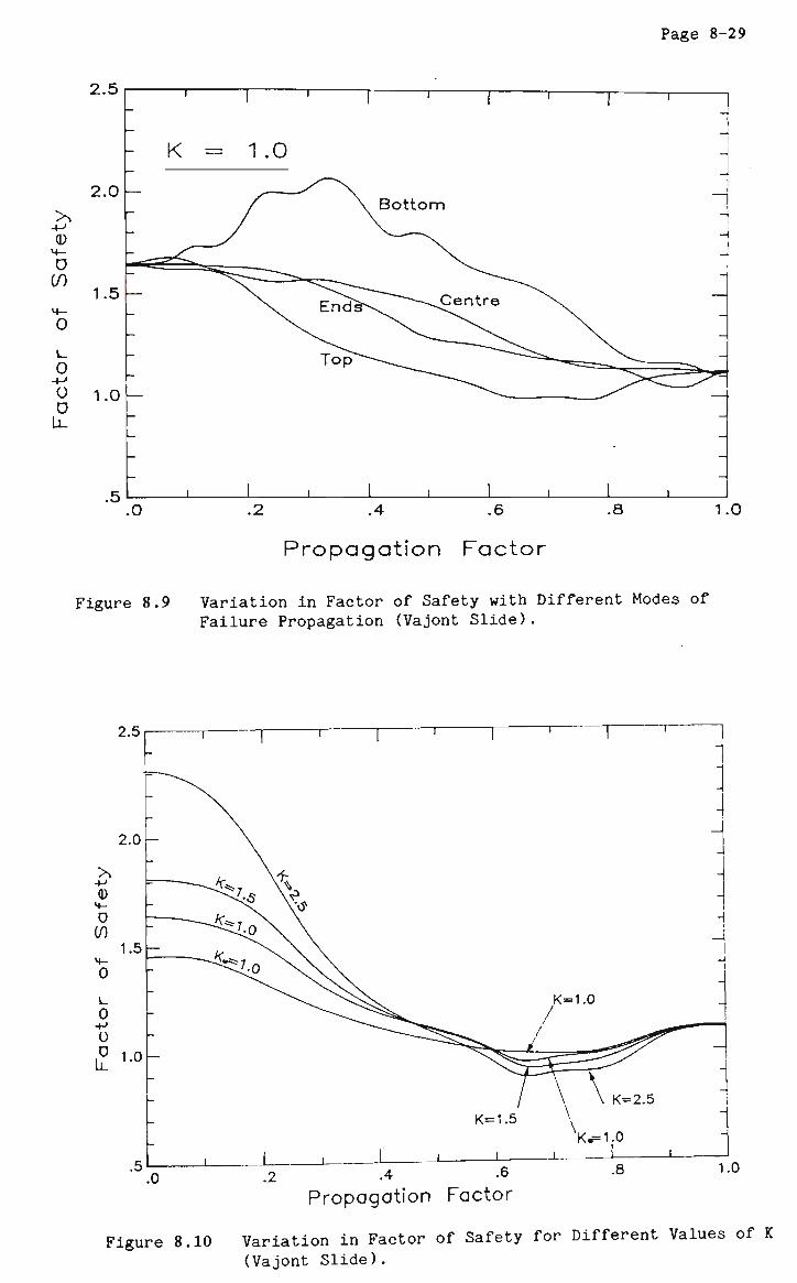
Page 8-29

_l.i_>

2.0

1.5

1 O

^

-

-

i

K =

i

1

= 1.0

I

i 1 i 1 . •-

\ Bottom

Er7o5\^^^ntre \ .

Top^--~-___^ ^~~~î5*~^=___-

. 1 . 1 i

__j

-

i

"1

-j

-

\.

~ _ _ > < c — _ i ^ =

1 .2 .4 .6

Propagation Factor

.8 1.0

Figure 8.9 Variation in Factor of Safety with Different Modes of Failure Propagation (Vajont Slide).

.0

Figure 8.10

.2 .4 -6

Propagation Factor 1.0

Variation in Factor of Safety for Different Values of K

(Vajont Slide).

Page 8-30

.5' ' ' ' ' ' 1 " I i I •0 .2 .4 .6 .8 1.0

Propagation Factor

Figure 8.11 Variation in Factor of Safety with Different Modes of Failure Propagation (Hypothetical Slip 1).

Propagation Factor

Figure 8.12 Variation in Factor of Safety for Different Values of (Hypothetical Slip 1).

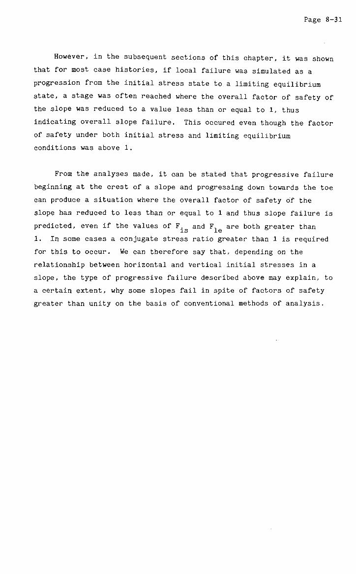
Page 8-31

However, in the subsequent sections of this chapter, it was shown

that for most case histories, if local failure was simulated as a

progression from the initial stress state to a limiting equilibrium

state, a stage was often reached where the overall factor of safety of

the slope was reduced to a value less than or equal to 1, thus

indicating overall slope failure. This occured even though the factor

of safety under both initial stress and limiting equilibrium

conditions was above 1.

From the analyses made, it can be stated that progressive failure

beginning at the crest of a slope and progressing down towards the toe

can produce a situation where the overall factor of safety of the

slope has reduced to less than or equal to 1 and thus slope failure is

predicted, even if the values of F. and F. are both greater than is le

1. In some cases a conjugate stress ratio greater than 1 is required for this to occur. We can therefore say that, depending on the

relationship between horizontal and vertical initial stresses in a

slope, the type of progressive failure described above may explain, to

a certain extent, why some slopes fail in spite of factors of safety

greater than unity on the basis of conventional methods of analysis.

CHAPTER 9

SUMMARY AND CONCLUSIONS.

9.1 INTRODUCTION.

The research reported in this thesis is primarily concerned with

the simulation of progressive failure within a sloping soil mass

considering alternative mechanisms of strain-softening and different

modes of failure propagation. The studies have been carried out

within a conventional deterministic framework and the basis for the

investigations is the widely accepted limit equilibrium model. The

methods reported here for analysis of progressive failure have been

found suitable whether a simplified (Bishop type) or rigorous

(Morgenstern-Price type) method of slices is used. However, most of

the work has been carried out using the 'rigorous' approach associated

with the well known Morgenstern-Price method of slope stability

analysis. To the author's knowledge, this is the first time methods

of analysis of progressive failure have been developed in this way and

successfully implemented for a number of case histories.

The scope of the thesis is clearly outlined in chapter 1

(especially section 1.6) and conventional limit equilibrium methods of

analysis have been discussed briefly in chapter 2.

9.2 PROGRESSIVE FAILURE CONCEPTS.

In chapter 3, different interpretations of the term progressive

failure were discussed. The relationship between any progressive

failure mechanism and the concept of residual strength is of

fundamental importance. At some stage during the progressive failure

Page 9-2

process, the strength of the soil along the potential slip surface

reduces from the peak value towards a residual (or fully softened)

value. The manner and extent of this reduction has been a matter of

some controversy.

The two most popular theories assume the following;

1. As local failure progresses and passes some location along a

slip surface, the soil strength there will drop suddenly from

the peak value to the residual value. Therefore, all points

along the failure surface to which local failure has

progressed will exhibit a residual or fully softened strength

while all other points will still be at the peak value. In

other words, this theory assumes a perfectly brittle material

response.

2. As local failure progresses along the slip surface there will

be segments of the surface where sufficient movement has

taken place to reduce the strength to its residual value

while other segments have suffered no movement (or local

failure) and, therefore, are at the peak strength. The

remaining parts of the slip surface would have values of

shear strength varying between the lower limit of residual

strength and the upper limit of peak strength.

The latter theory was postulated by Bishop [13] who defined a

residual factor which varies along the slip surface and which denotes

the proportional drop from the peak to the residual strength at any

point along the surface. Bishop went on to suggest possible

distributions of this residual factor, and hence of the shear strength

along the slip surface, which indicate that progressive failure may

start at the (a) top of the slope and progress downward, (b) toe and

progress upward, or (c) both ends and progress inwards towards the

centre.

Page 9-3

9.3 RELATIONSHIP BETWEEN SHEAR STRENGTH DISTRIBUTION AND FACTOR OF

SAFETY.

As reported in chapter 4, investigations were carried out to

ascertain whether there was any relationship between the shear

strength distribution existing along the slip surface and the

calculated factor of safety of the soil mass. A number of

distributions of the residual factor R was chosen to be used in

conjunction with the limit equilibrium stability analysis. Although a

wide range of R, distributions was used, most of the distributions

fell into two major groups:-

1. Failure starting from the bottom of the slope (R. equal to

1 at toe and 0 at crest).

2. Failure starting from the crest of the slope (R, equal to 1

at crest and 0 at toe).

The aim was to see whether some R distributions produced lower

factors of safety (and therefore indicated a higher likelihood of

failure) than others.

As it was not possible to directly set the shear strength values

along the failure surface to match the chosen R distribution, it

was decided to set the values of the shear strength parameters c' and

0' to match this distribution. Expressions were derived for c'

and 0' in terms of the local residual factor (equations 4.6).

The Morgenstern-Price method of analysis was used as a basis for

the simulation and calculation of the factor of safety. The

calculated values of c' and 0' were used in this analysis to

arrive at a value for F. For some slopes with circular surfaces of

sliding, the Bishop simplified method was also used.

The results obtained using the Morgenstern-Price method of

analysis were tested for acceptability according to a number of

acceptability criteria defined by Morgenstern and Price, Hamel [14]

and other authors. These criteria were found to be, in general, too

stringent and recommendations were made in this chapter as to their

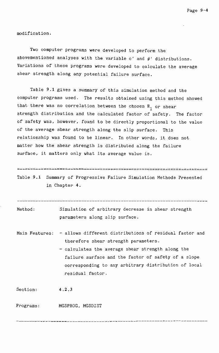
Page 9-4

modification.

Two computer programs were developed to perform the

abovementioned analyses with the variable c' and 0' distributions.

Variations of these programs were developed to calculate the average

shear strength along any potential failure surface.

Table 9.1 gives a summary of this simulation method and the

computer programs used. The results obtained using this method showed

that there was no correlation between the chosen R or shear

strength distribution and the calculated factor of safety. The factor

of safety was, however, found to be directly proportional to the value

of the average shear strength along the slip surface. This

relationship was found to be linear. In other words, it does not

matter how the shear strength is distributed along the failure

surface, it matters only what its average value is.

Table 9.1 Summary of Progressive Failure Simulation Methods Presented

in Chapter 4.

Method: Simulation of arbitrary decrease in shear strength

parameters along slip surface.

Main Features: - allows different distributions of residual factor and

therefore shear strength parameters.

- calculates the average shear strength along the

failure surface and the factor of safety of a slope

corresponding to any arbitrary distribution of local

residual factor.

Section: 4.2.3

Programs: MGSPROG, MGSDIST

Page 9-5

9.4 PROGRESSION OF FAILURE CONSIDERING STRAIN SOFTENING.

The mechanism of strain-softening and stress redistribution in

slopes is considered in detail in chapters 5 and 6. Four methods

developed for simulating progressive failure on the basis of these

mechanisms have been presented in chapter 6.

Method 1 is based on the assumption that once local failure has

occurred on the bases of one or more slices, the excess shear stress

may be redistributed either uniformly or according to a linear

function (with maximum near the failed slice) across the unfailed

segments of the slip surface. Once a slice has failed locally, the

shear strength parameters c and 0 on its base are assumed to have

dropped to their residual values. The factor of safety is then found

by dividing the sum of the resisting forces by the sum of the

disturbing forces. The results of method 1 analyses showed that a

linear function for the redistribution of excess shear stress leads to

lower factors of safety than a uniform function. In some cases,

however, little or no drop in factor of safety occurred as a result of

redistribution of shear stress.

Method 2 is inherently similar to method 1 except that the

factors of safety are determined by performing Morgenstern-price and

Bishop simplified analyses on each case history considered. Residual

values of the shear strength parameters were again used for failed

slices in these analyses. In virtually all cases, the results

obtained were almost identical to those obtained using method 1. The

two simulation techniques induced the same amount of local failure and

any discrepancies are due entirely to the differences in methods used

to obtain the factor of safety.

Method 3 is different from methods 1 and 2 in so far as no

assumption is made in advance regarding the manner in which excess

shear stress will be redistributed. The mobilised shear force on each

unfailed slice is recalculated after successive limit equilibrium

analyses. After this, the excess shear force on each unfailed slice

is determined. The total shear force tending to cause local failure

on an unfailed slice is then calculated using equation (6.35) and all

unfailed slices are again examined for local failure using equation

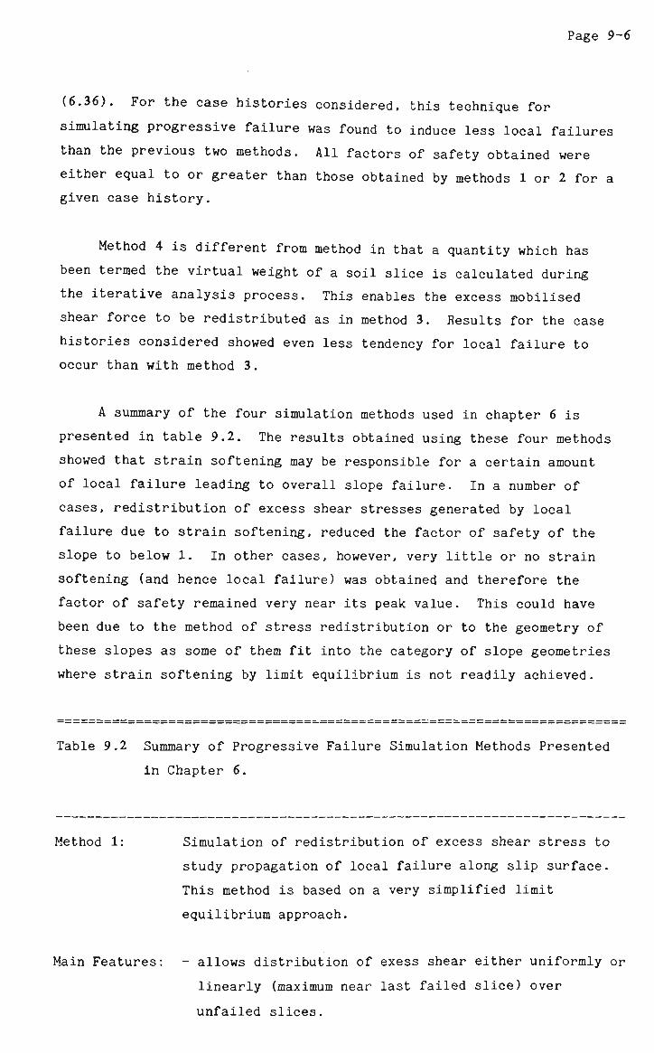
Page 9-6

(6.36). For the case histories considered, this technique for

simulating progressive failure was found to induce less local failures

than the previous two methods. All factors of safety obtained were

either equal to or greater than those obtained by methods 1 or 2 for a

given case history.

Method 4 is different from method in that a quantity which has

been termed the virtual weight of a soil slice is calculated during

the iterative analysis process. This enables the excess mobilised

shear force to be redistributed as in method 3. Results for the case

histories considered showed even less tendency for local failure to

occur than with method 3.

A summary of the four simulation methods used in chapter 6 is

presented in table 9.2. The results obtained using these four methods

showed that strain softening may be responsible for a certain amount

of local failure leading to overall slope failure. In a number of

cases, redistribution of excess shear stresses generated by local

failure due to strain softening, reduced the factor of safety of the

slope to below 1. In other cases, however, very little or no strain

softening (and hence local failure) was obtained and therefore the

factor of safety remained very near its peak value. This could have

been due to the method of stress redistribution or to the geometry of

these slopes as some of them fit into the category of slope geometries

where strain softening by limit equilibrium is not readily achieved.


in Chapter 6.

Method 1: Simulation of redistribution of excess shear stress to

study propagation of local failure along slip surface.

This method is based on a very simplified limit

equilibrium approach.

Main Features: - allows distribution of exess shear either uniformly or

linearly (maximum near last failed slice) over

unfailed slices.

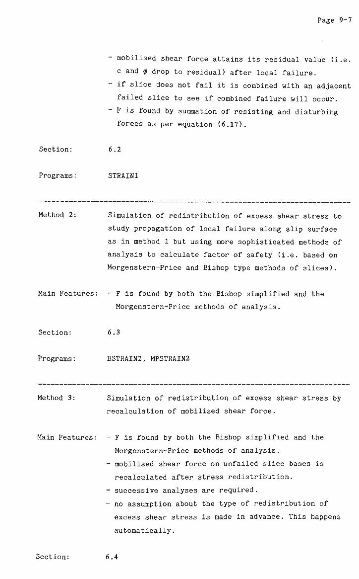
Page 9-7

- mobilised shear force attains its residual value (i.e.

c and 0 drop to residual) after local failure.

- if slice does not fail it is combined with an adjacent

failed slice to see if combined failure will occur.

- F is found by summation of resisting and disturbing

forces as per equation (6.17).

Section: 6.2

Programs: STRAIN1

Method 2: Simulation of redistribution of excess shear stress to

study propagation of local failure along slip surface

as in method 1 but using more sophisticated methods of

analysis to calculate factor of safety (i.e. based on

Morgenstern-Price and Bishop type methods of slices).

Main Features: F is found by both the Bishop simplified and the

Morgenstern-Price methods of analysis.

Section: 6.3

Programs: BSTRAIN2, MPSTRAIN2

Method 3: Simulation of redistribution of excess shear stress by

recalculation of mobilised shear force.

Main Features: - F is found by both the Bishop simplified and the


- mobilised shear force on unfailed slice bases is

recalculated after stress redistribution.

- successive analyses are required.

- no assumption about the type of redistribution of

excess shear stress is made in advance. This happens

automatically.

Section: 6.4

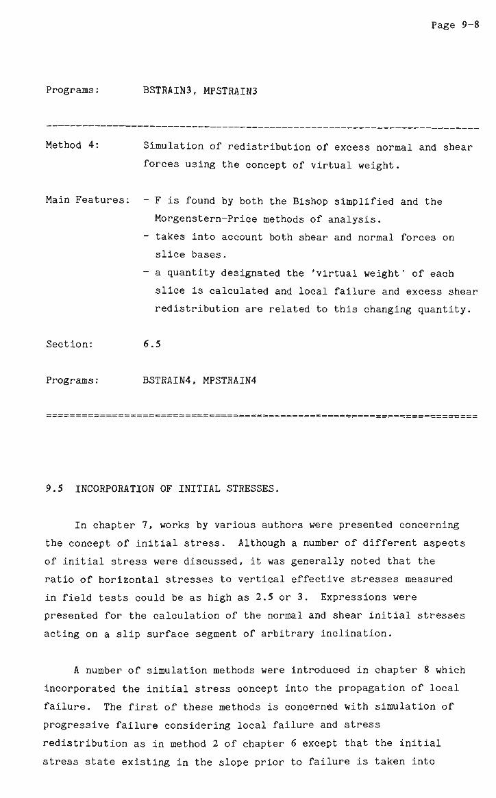
Page 9-8


Method 4: Simulation of redistribution of excess normal and shear

forces using the concept of virtual weight.

Main Features: - F is found by both the Bishop simplified and the


- takes into account both shear and normal forces on

slice bases.

- a quantity designated the 'virtual weight' of each

slice is calculated and local failure and excess shear

redistribution are related to this changing quantity.

Section: 6.5


9.5 INCORPORATION OF INITIAL STRESSES.

In chapter 7, works by various authors were presented concerning

the concept of initial stress. Although a number of different aspects

of initial stress were discussed, it was generally noted that the

ratio of horizontal stresses to vertical effective stresses measured

in field tests could be as high as 2.5 or 3. Expressions were

presented for the calculation of the normal and shear initial stresses

acting on a slip surface segment of arbitrary inclination.

A number of simulation methods were introduced in chapter 8 which

incorporated the initial stress concept into the propagation of local

failure. The first of these methods is concerned with simulation of

progressive failure considering local failure and stress

redistribution as in method 2 of chapter 6 except that the initial

stress state existing in the slope prior to failure is taken into

Page 9-9

consideration. Basically, the method is identical to method 2 of

chapter 6 except that the normal and shear forces on the bases of

unfailed slices were calculated using initial stress expressions given

in equations (8.1) and (8.2). The normal and shear forces on bases of

failed slices were calculated using limit equilibrium expressions

given in equations (6.9) and (6.11). The factor of safety was

calculated using equation (8.3). It was shown that in cases of

initial stress corresponding to a conjugate stress ratio greater than

say 1.5 there was a significant reduction in the final factor of

safety, sometimes to a value below 1. However, little additional

strain softening occurred and the reduction in overall factor of

safety was probably due only to the increased shear stresses in the

slope resulting from higher values of K. This was supported by the

fact that those slopes where little or no strain softening occurred

using the simulation methods of chapter 6 still exhibited a similar

extent of strain softening.

The situation was then considered where local failure was assumed

to have extended beyond the limits achieved in the above procedures.

The slope was initially assumed to be totally under initial stress

conditions and as failure progressed, areas which had failed locally

were then assumed to be in limiting equilibrium. A limit equilibrium

analysis using the Morgenstern-Price method was carried out on the

failed section of the slope. From this, the normal and shear forces

on the failed slices were calculated using equations (8.8) and (8.10).

For the unfailed slices, the normal and shear forces were calculated

using the initial stress equations mentioned previously. The overall

factor of safety for the entire slope was then calculated using

equation (8.7). The interaction between the two masses of changing

size was considered at each stage.

The possibility of failure starting at either the crest, toe,

centre or both ends of the slope was considered. It was found that,

in virtually all cases, local failure starting at the crest of the

slope was potentially more dangerous than from other areas. The

factor of safety reduced, as failure progressed, to a minimum value.

This value, especially at higher values of K was usually less than 1

which indicated that if conditions favour the progression of local

failure along an assumed slip surface, a point may be reached where

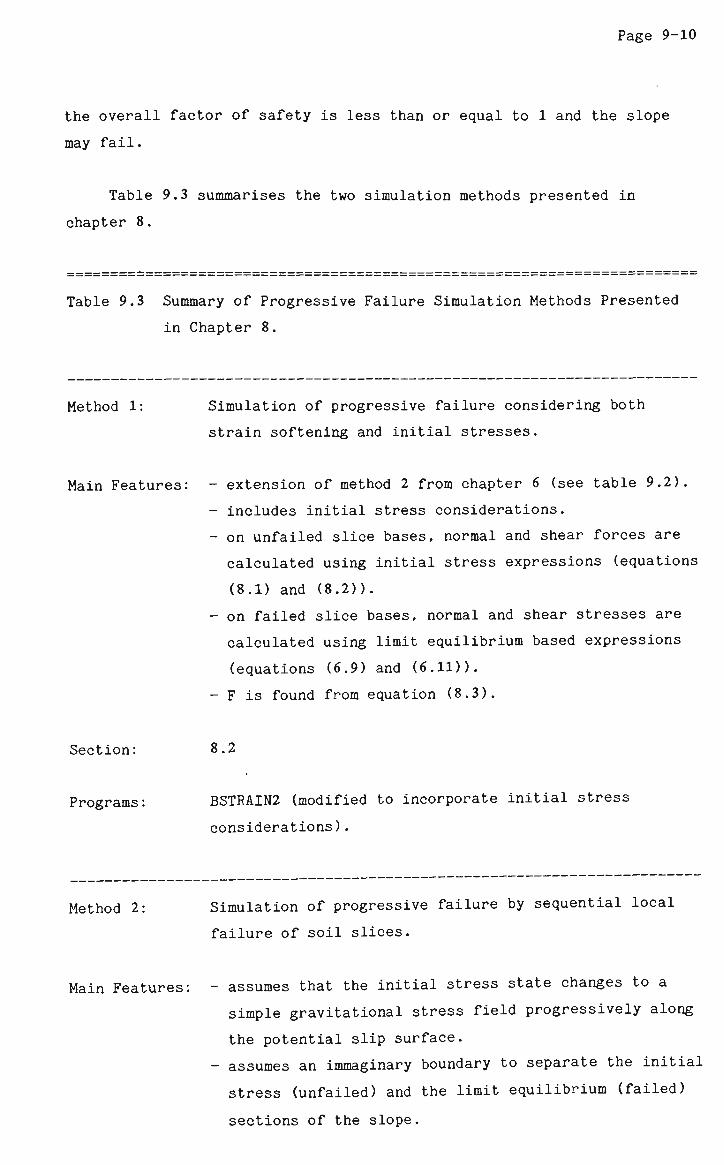
Page 9-10

the overall factor of safety is less than or equal to 1 and the slope

may fail.

Table 9.3 summarises the two simulation methods presented in

chapter 8.


in Chapter 8.

Simulation of progressive failure considering both

strain softening and initial stresses.

- extension of method 2 from chapter 6 (see table 9.2).

- includes initial stress considerations.

- on unfailed slice bases, normal and shear forces are

calculated using initial stress expressions (equations

(8.1) and (8.2)).

- on failed slice bases, normal and shear stresses are

calculated using limit equilibrium based expressions

(equations (6.9) and (6.11)).

- F is found from equation (8.3).

8.2

BSTRAIN2 (modified to incorporate initial stress

considerations).

Method 2: Simulation of progressive failure by sequential local

failure of soil slices.

Main Features: - assumes that the initial stress state changes to a

simple gravitational stress field progressively along

the potential slip surface.

- assumes an immaginary boundary to separate the initial

stress (unfailed) and the limit equilibrium (failed)

sections of the slope.

Method 1:

Main Features:

Section:

Programs:

Page 9-11

- the overall factor of safety is calculated according

to equation (8.7).

- normal and shear stresses on bases of slices in the

unfailed section are found using initial stress

equations.

- those on slice bases in the failed section are found

by performing a Morgenstern-Price limit equilibrium

analysis on the failed section and then obtaining the

stresses using equations (8.8) and (8.10).

Section: 8.3, 8.5

Programs: MGSINIT2

9.6 CONCLUDING REMARKS.

In this thesis a number of methods of slope analysis have been

presented which were developed to simulate progressive failure and to

relate the extent of strain softening and stress redistribution to the

overall factor of safety of a soil slope. The methods have been

successfully implemented and used for the analysis of a number of case

histories. In some methods an initial stress field is also taken into

consideration.

The investigations reported in this thesis show that progressive

failure may lead to a significant drop in the overall safety factor

for some slopes but not for others. The values of shear strength

parameters and the extent of soil brittleness are important but are

not the only factors which determine the likelihood of failure

progression. The slope and slip surface geometry may have an

important influence on the extent to which redistribution of excess

shear stress will lead to new local failures. An initial stress field

is important and the higher the value of the conjugate stress ratio K,

the lower is the value of the minimum safety factor during

progression.

Page 9-12

There is no single method of analysis which will be suitable for

all situations. However, the methods developed here offer a wide

choice for the simulation of progressive failure and the selection of

an appropriate method would be based on the type of problem, the

available data and the actual requirements of analysis.

The work reported in this thesis has also highlighted the

importance of acceptability criteria for rigorous methods of analysis.

The linear relationship between average shear strength along the slip

surface and the factor of safety has been confirmed for a very wide

range of conditions. Such a relationship may, in itself, provide the

best acceptability criteria.

APPENDIX A

DESCRIPTION OF SLOPES USED IN CASE HISTORIES.

This appendix contains descriptions of all the soil or rock

slopes referred to within this text and used as case histories in the

validation of the various methods of analysis presented.

A.l NORTHOLT SLIP IN CUTTING.

The analysis of a slip in a cutting at Northolt, England was

carried out by Skempton, Henkel and Delory in 1955 and described by

Henkel in 1957 [48] and Skempton in 1964 [88]. The excavation was

made in 1936 and occurred 19 years later in 1955.

The analysis was made on a circular arc approximating to the

observed slip surface. The average values of peak and residual

strength were found to be 28.5 kPa and 10.3 kPa respectively. The

average shear stress, and hence, the average shear strength acting

along the slip surface at the time of failure was 18.2 kPa.

Consequently, Skempton calculated the value of his residual

factor, R (see chapter 3), to be 0.56 and the strength parameters

consistent with a factor of safety of 1.0 were found to be c' = 6.7

kPa and 0' = 18° .

The Northolt slip is situated in London clay. Fissures and

joints and occasional slickensides can be seen throughout the full

depth of the London clay but such features are much more conspicuous

in the weathered zone, characterised by the brown colour of the clay

(in contrast to the blue or slatey grey colour of the unweathered

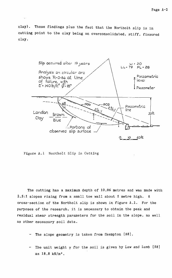
Page A-2

clay). These findings plus the fact that the Northolt slip is in

cutting point to the clay being an overconsolidated, stiff, fissured

clay.

o io aoft

Figure A.l Northolt Slip in Cutting

The cutting has a maximum depth of 10.06 metres and was made with

2.5:1 slopes rising from a small toe wall about 1 metre high. A

cross-section of the Northolt slip is shown in figure A.l. For the

purposes of the research, it is necessary to obtain the peak and

residual shear strength parameters for the soil in the slope, as well

as other necessary soil data.

- The slope geometry is taken from Skempton [88].

- The unit weight y for the soil is given by Law and Lumb [58]

as 18.8 kN/m3.

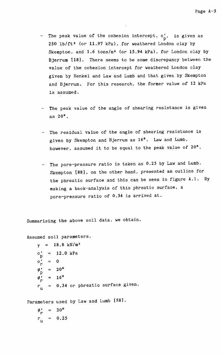
Page A-3

The peak value of the cohesion intercept, c', is given as

250 lb/ft2 (or 11.97 kPa), for weathered London clay by

Skempton, and 1.6 tons/m2 (or 15.94 kPa), for London clay by

Bjerrum [18]. There seems to be some discrepancy between the

value of the cohesion intercept for weathered London clay

given by Henkel and Law and Lumb and that given by Skempton

and Bjerrum. For this research, the former value of 12 kPa

is assumed.

The peak value of the angle of shearing resistance is given

as 20°.

The residual value of the angle of shearing resistance is

given by Skempton and Bjerrum as 16°. Law and Lumb,

however, assumed it to be equal to the peak value of 20°.

The pore-pressure ratio is taken as 0.25 by Law and Lumb.

Skempton [88], on the other hand, presented an outline for

the phreatic surface and this can be seen in figure A.l. By

making a back-analysis of this phreatic surface, a

pore-pressure ratio of 0.34 is arrived at.

Summarising the above soil data, we obtain,

Assumed soil parameters.

y = 18.8 kN/m3

c' = 12.0 kPa P c' = 0 r 0' = 20° P 0' = 16° r r = 0.34 or phreatic surface given. u Parameters used by Law and Lumb [58].

0' = 20° r r = 0.25 u

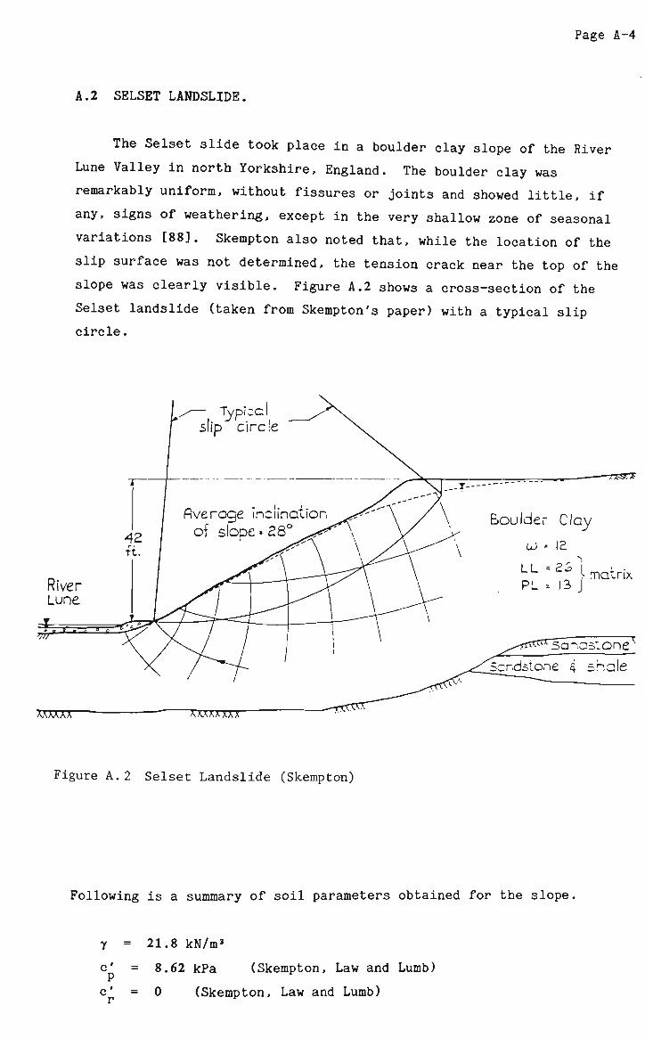
Page A-4

A.2 SELSET LANDSLIDE.

The Selset slide took place in a boulder clay slope of the River

Lune Valley in north Yorkshire, England. The boulder clay was

remarkably uniform, without fissures or joints and showed little, if

any, signs of weathering, except in the very shallow zone of seasonal

variations [88]. Skempton also noted that, while the location of the

slip surface was not determined, the tension crack near the top of the

slope was clearly visible. Figure A.2 shows a cross-section of the

Selset landslide (taken from Skempton's paper) with a typical slip

circle.

Figure A. 2 Selset Landslide (Skempton)

Following is a summary of soil parameters obtained for the slope.

y = 21.8 kN/m3

c' = 8.62 kPa (Skempton, Law and Lumb)

c' = 0 (Skempton, Law and Lumb)

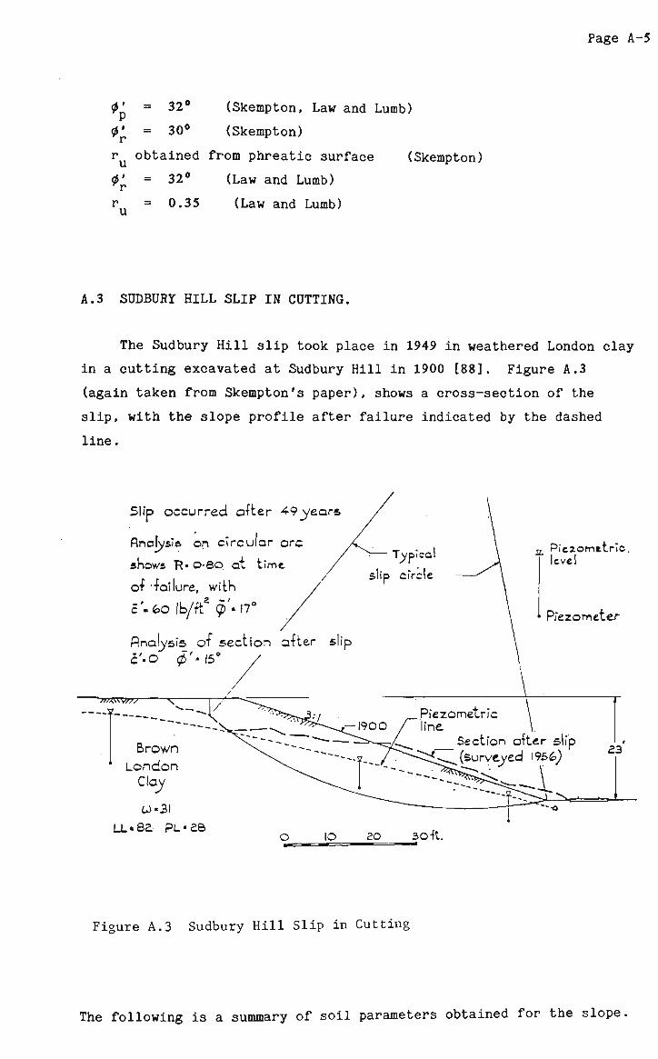
Page A-5

(Skempton, Law and Lumb)

(Skempton)

0' = 32° P 0' = 30° r r obtained from phreatic surface 0' = 32° rr r = 0.35 u

(Law and Lumb)

(Law and Lumb)

(Skempton)

A.3 SUDBURY HILL SLIP IN CUTTING.

The Sudbury Hill slip took place in 1949 in weathered London clay

in a cutting excavated at Sudbury Hill in 1900 [88]. Figure A.3

(again taken from Skempton's paper), shows a cross-section of the

slip, with the slope profile after failure indicated by the dashed

line.

51 fp occurred after 49_years

flr.aly_.is on circular arc

shows R« O-eo at time

of "failure, with

c'-fcO lb/ft2 <?'-l7e

Analysis of section a-fter slip C'.O 0'- 15°

cal

slip Circle

•m. "\Vf77 ' "\ ' | / '

Brown ' London

Clay

c_>__l

LL«8a PL '£8

Piezometric.

level

Piezometer

Piezometric ine

Section after slip (surveyed \9S6>)

23

=.-1

io ao soft.

Figure A.3 Sudbury Hill Slip in Cutting

The following is a summary of soil parameters obtained for the slope.

http://flr.aly_.is

file:///Vf77

Page A-6

y = 18.8 kN/m3

cp = 12.0 kPa

0p = 20°

^r = 16° (Skempton, Bjerrum)

ru = 0.30 (Law and Lumb, Delory [39], James [49] Phreatic surface given by Skempton [88].

A.4 THE JACKFIELD SLIDE.

This slide, which took place in England in 1952, exhibited a very

small rate of advance and was preceded by creep movements. Movements

were fist noticed in 1950, continued in 1951 and developed alarmingly

during January of 1951 [18]. The total downhill displacement amounted

to 18.3 metres. The slide had the characteristic shape of a flake

with the dimensions 198 metres by 213 metres and the average depth of

the slip plane was 5.5 metres.

According to Bjerrum [18], the slide was confined wholly within

the upper zone of disintegrated and weathered clay. The sliding

surface ran parallel to the slope and followed closely the boundary of

the lower intact shale. It was found that the failure zone consisted

of a soft clay layer only 5 centimetres thick.

Both Bjerrum [18] and Skempton [88] remarked that the shear

stresses along the failure surface due to gravity forces were well

below the drained peak shear strength of the clay and practically

equal to the residual shear strength. Bjerrum stated that it was

clear that the shear strength of the clay had been gradually exceeded

by a mechanism of progressive failure.

Figure A.4, taken from Bjerrum's paper [18], shows a

cross-section of the Jackfield slide.

The following soil data was obtained from Skempton [88] and Bjerrum

[18].

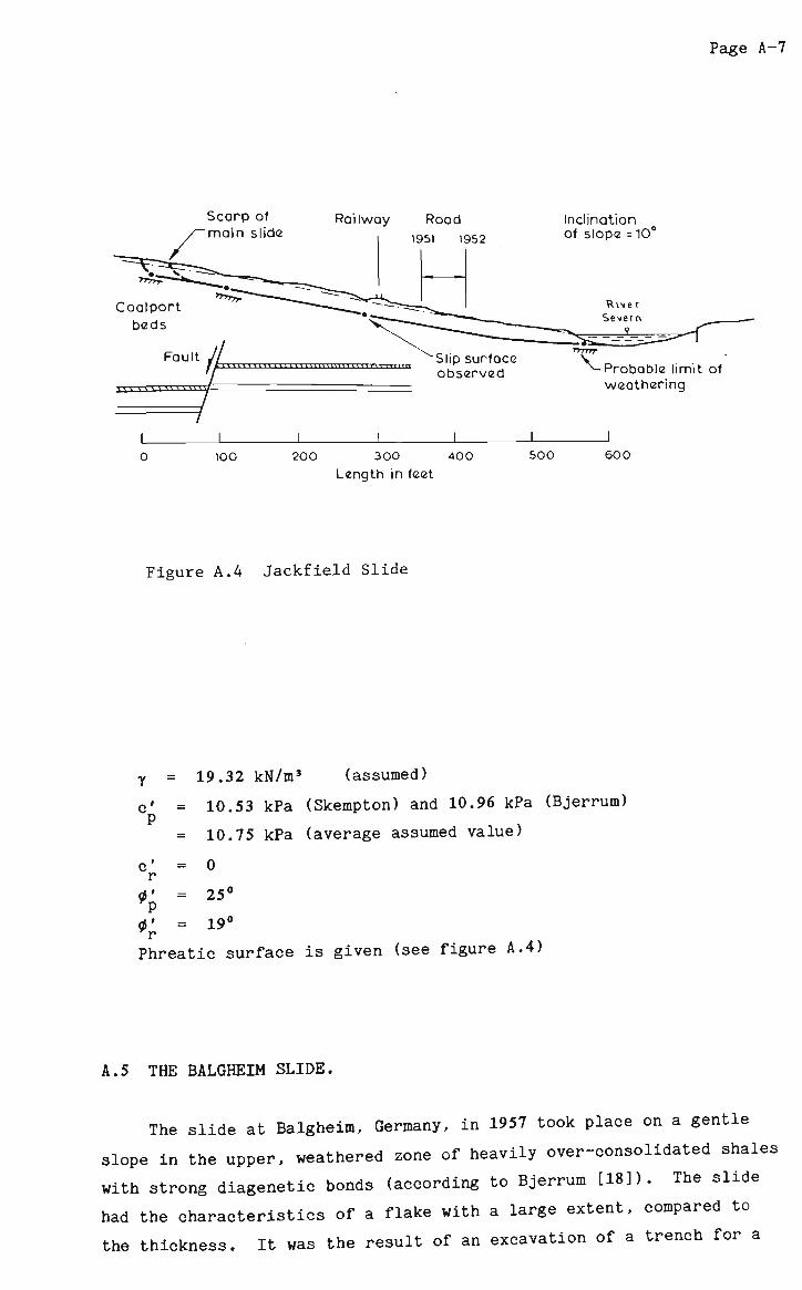
Page A-7

Scarp of main slide

Railway Road 1951 1952

Inclination of slope =10°

Coalport beds

Fa ult J I Slip surface fl M i n i m . " " " " " " " " ' '""" 1111111 r

n i » i _ m i m i y

_L _L _L 100 200 300 400

Length in feet

HTTTT

^-Probable limit of weathering

500 6O0

Figure A.4 Jackfield Slide

= 19.32 kN/m3 (assumed)

= 10.53 kPa (Skempton) and 10.96 kPa (Bjerrum)

= 10.75 kPa (average assumed value)

= 0

= 25°

= 19°

Phreatic surface is given (see figure A.4)

c' P

0' P

rr

A.5 THE BALGHEIM SLIDE.

The slide at Balgheim, Germany, in 1957 took place on a gentle

slope in the upper, weathered zone of heavily over-consolidated shales

with strong diagenetic bonds (according to Bjerrum [18]). The slide

had the characteristics of a flake with a large extent, compared to

the thickness. It was the result of an excavation of a trench for a

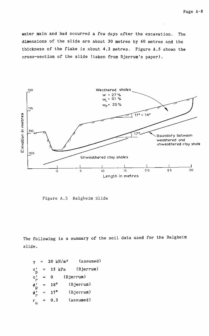
Page A-8

water main and had occurred a few days after the excavation. The

dimensions of the slide are about 30 metres by 60 metres and the

thickness of the flake is about 4.3 metres. Figure A.5 shows the

cross-section of the slide (taken from Bjerrum's paper).

720

715

(A W f_

C o o > LJ

710

705

Weathered shales w = 27 % wL= 61 •/.

Boundary between weathered and unweathered clay shale

Unweathered clay shales

JL 10 15 20

Length in metres

25 30

Figure A.5 Balgheim Slide

The following is a summary of the soil data used for the Balgheim

slide.

Y

c' n C' r

r r

= 20 kN/m3 (assumed

= 15 kPa (Bjerrum)

= 0 (Bjerrum)

= 18° (Bjerrum)

= 17° (Bjerrum)

= 0.3 (assumed) u

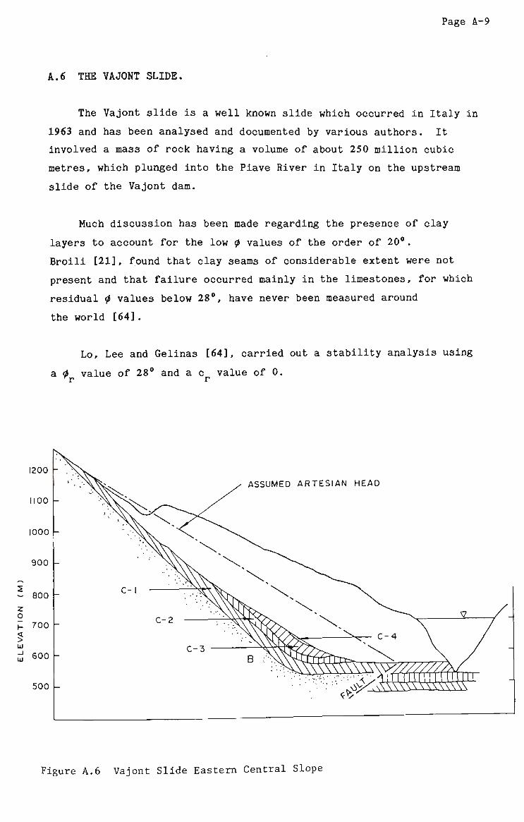
Page A-9

A.6 THE VAJONT SLIDE.

The Vajont slide is a well known slide which occurred in Italy in

1963 and has been analysed and documented by various authors. It

involved a mass of rock having a volume of about 250 million cubic

metres, which plunged into the Piave River in Italy on the upstream

slide of the Vajont dam.

Much discussion has been made regarding the presence of clay

layers to account for the low 0 values of the order of 20°.

Broili [21], found that clay seams of considerable extent were not

present and that failure occurred mainly in the limestones, for which

residual 0 values below 28°, have never been measured around

the world [64].

Lo, Lee and Gelinas [64], carried out a stability analysis using

a 0 value of 28° and a c value of 0. rr r

Figure A.6 Vajont Slide Eastern Central Slope

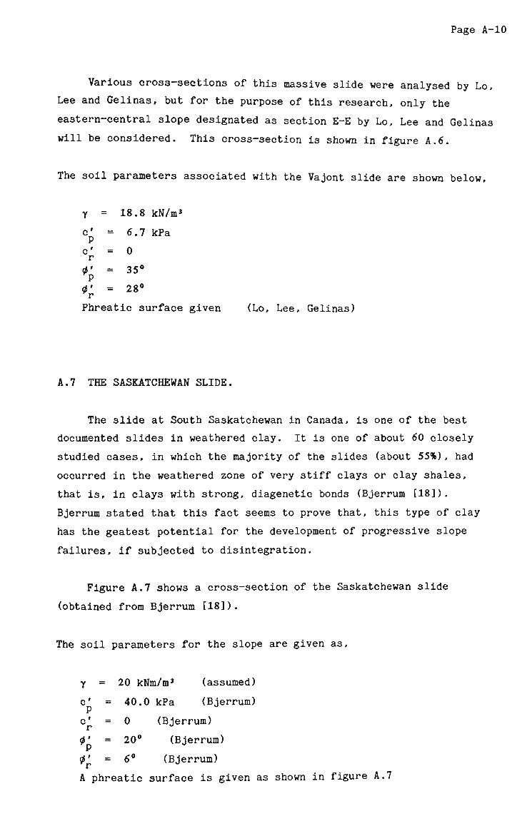
Page A-10

Various cross-sections of this massive slide were analysed by Lo,

Lee and Gelinas, but for the purpose of this research, only the

eastern-central slope designated as section E-E by Lo, Lee and Gelinas

will be considered. This cross-section is shown in figure A.6.

The soil parameters associated with the Vajont slide are shown below,

y = 18.8 kN/m3

o' = 6.7 kPa

c' = 0 r 0' = 35° P 0' = 28° rr Phreatic surface given (Lo, Lee, Gelinas)

A.7 THE SASKATCHEWAN SLIDE.

The slide at South Saskatchewan in Canada, is one of the best

documented slides in weathered clay. It is one of about 60 closely

studied cases, in which the majority of the slides (about 55%), had

occurred in the weathered zone of very stiff clays or clay shales,

that is, in clays with strong, diagenetic bonds (Bjerrum [18]).

Bjerrum stated that this fact seems to prove that, this type of clay

has the geatest potential for the development of progressive slope

failures, if subjected to disintegration.

Figure A.7 shows a cross-section of the Saskatchewan slide

(obtained from Bjerrum [18]).

The soil parameters for the slope are given as,

y = 20 kNm/m3 (assumed)

c' = 40.0 kPa (Bjerrum)

c' = 0 (Bjerrum) r 0' = 20° (Bjerrum) 0' = 6 ° (Bjerrum)

A phreatic surface is given as shown in figure A.7

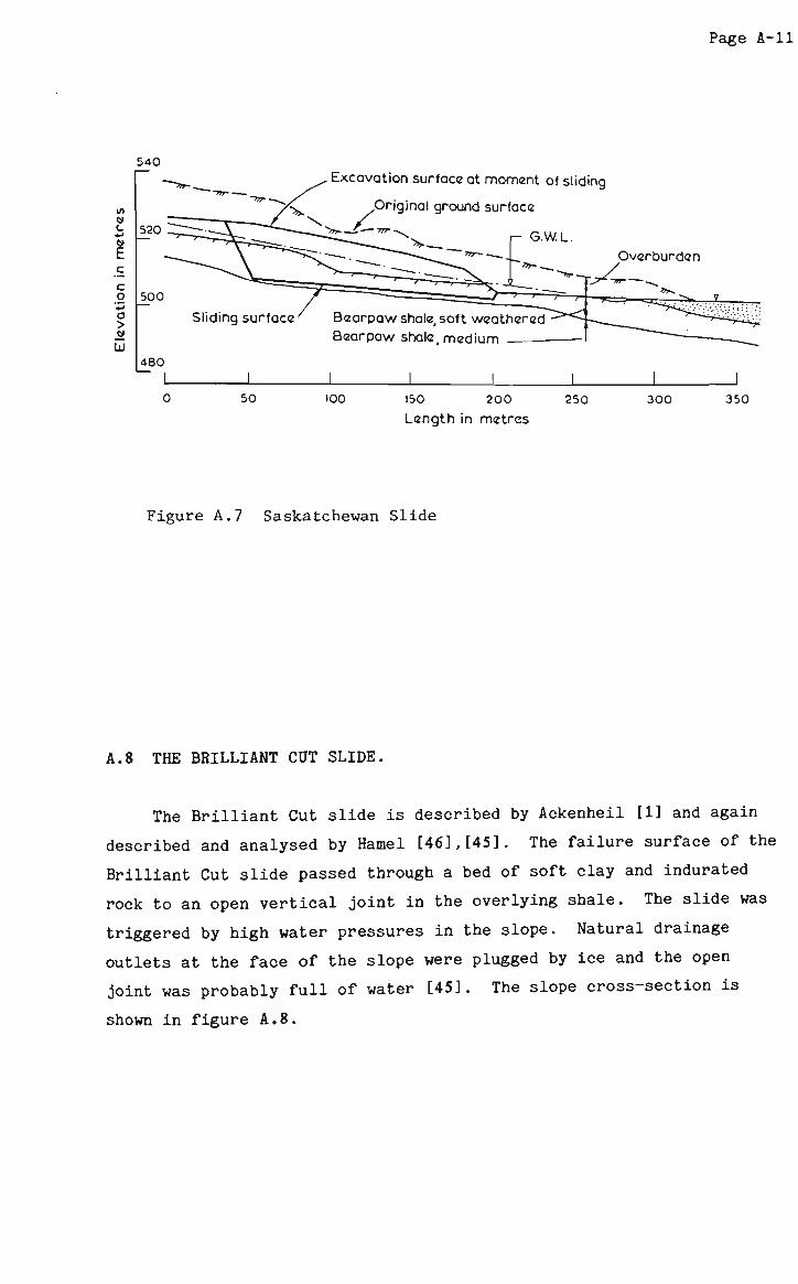
Page A-ll

01

a <_

c o '*> o > LU

540

520

500

480

Excavation surface at moment of sliding ~vr-

>_._/_:

Original ground surface

*^>* -____T—— 777" -

>»•-__. Overburden

Sliding surface ' Bearpaw shale, soft weathered Bearpaw shale medium

J_ 50 100 150 200

Length in metres 250 300 350

Figure A.7 Saskatchewan Slide

A.8 THE BRILLIANT CUT SLIDE.

The Brilliant Cut slide is described by Ackenheil [1] and again

described and analysed by Hamel [46],[45], The failure surface of the

Brilliant Cut slide passed through a bed of soft clay and indurated

rock to an open vertical joint in the overlying shale. The slide was

triggered by high water pressures in the slope. Natural drainage

outlets at the face of the slope were plugged by ice and the open

joint was probably full of water [45]. The slope cross-section is

shown in figure A.8.

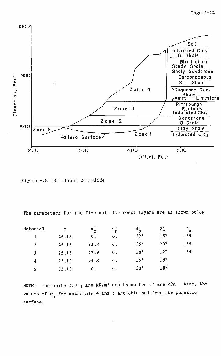
200 300 400

Page A-l2

1000"

90O

800-

i

Zone 5^

— y

/

y/ Zone 4

,y Zone 3 /

y,' Zone Z /

^ ^ - ^ ^ _ _ ____ ^ r- >• -. x > Zone 1 Failure Surface'

i i

^^So\\

Indurated Clay 8i__Shale_

Birmingham Sandy Shale Shaly Sandstone

Carbonaceous Silt Shale

^Duquesne Coal Shale. .

Âmes Limesto Pittsburgh

Redbeds Indurated Clay Sandstone a Shale Clay Shale

Indurated Clay

500

Offset, Feet

Figure A.8 Brilliant Cut Slide

The parameters for the five soil (or rock) layers are as shown below.

Material

1

2

3

4

5

Y

25

25

25

25

25

.13

.13

.13

.13

.13

c' P 0.

95.8

47.9

95.8

0.

c' r 0. 0.

0.

0.

0.

0' P 32° 35°

28°

35°

30°

0' *r 15° 20°

12°

15°

18°

r u

.39

.39

.39

NOTE: The units for y are kN/m3 and those for c' are kPa. Also, the

o:

surface.

values of r for materials 4 and 5 are obtained from the phreatic u

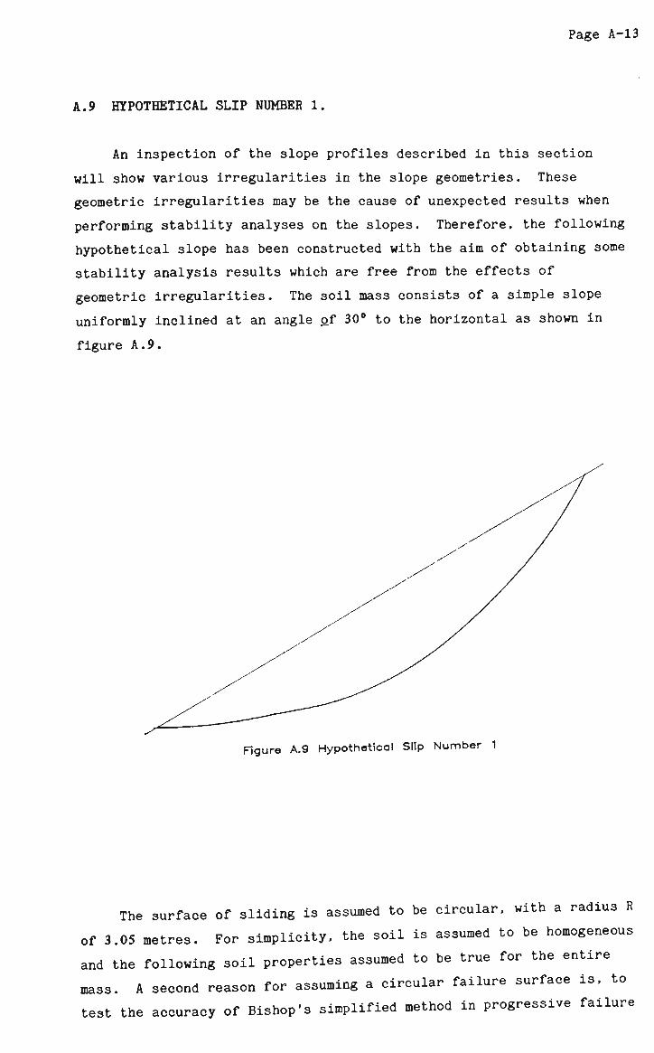
Page A-l3

A.9 HYPOTHETICAL SLIP NUMBER 1.

An inspection of the slope profiles described in this section

will show various irregularities in the slope geometries. These

geometric irregularities may be the cause of unexpected results when

performing stability analyses on the slopes. Therefore, the following

hypothetical slope has been constructed with the aim of obtaining some

stability analysis results which are free from the effects of

geometric irregularities. The soil mass consists of a simple slope

uniformly inclined at an angle of 30° to the horizontal as shown in

figure A.9.

Figure A.9 Hypothetical Slip Number 1

The surface of sliding is assumed to be circular, with a radius R

of 3.05 metres. For simplicity, the soil is assumed to be homogeneous

and the following soil properties assumed to be true for the entire

mass. A second reason for assuming a circular failure surface is, to

test the accuracy of Bishop's simplified method in progressive failure

Page A-14

simulation techniques, described in this text.

The soil and slope parameters are assumbed to be as follows

Y

C'

P c' r

r u

=

—

=

=

18.8 kN/m3

6 kPa

0

26°

22°

0

A. 10 HYPOTHETICAL SLIP NUMBER 2.

For reasons similar to those described above, a second

hypothetical soil mass is described here. In this case, however, a

planar failure surface is chosen. This planar (actually bi-planar)

surface and the slope profile, are shown in figure A.10.

The assumed soil parameters associated with this soil mass are as

given below.

Y

C'

P c' r

r u

=

=

=

=

20 kN/m3

12.0 kPa

0

22°

18°

0.32

Page A-l5

Figure A.10 Hypothetical Slip Number 2

APPENDIX B

RESIDUAL FACTOR DISTRIBUTIONS USED IN CHAPTER 4.

B.l PROFILES OF RESIDUAL FACTOR DISTRIBUTIONS.

D1 H2

D2

H3

Page B-2

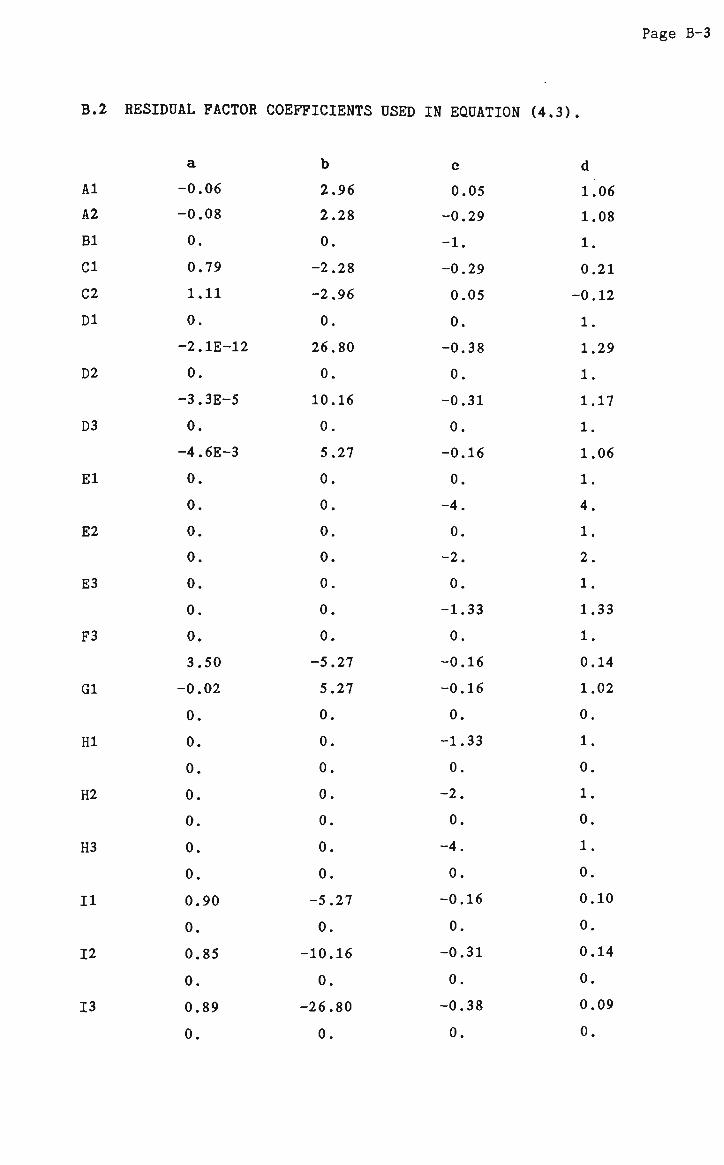
B.2 RESIDUAL FACTOR COEFFICIENTS USED IN EQUATION (4.3).

Al

A2

Bl

Cl

C2

DI

D2

D3

El

E2

E3

F3

Gl

HI

H2

H3

II

12

13

a

-0.06

-0.08

0.

0.79

1.11

0.

-2.1E-12

0.

-3.3E-5

0.

-4.6E-3

0.

0.

0.

0.

0.

0.

0.

3.50

-0.02

0.

0.

0.

0.

0.

0.

0.

0.90

0.

0.85

0.

0.89

0.

b

2.96

2.28

0.

-2.28

-2.96

0.

26.80

0.

10.16

0.

5.27

0.

0.

0.

0.

0.

0.

0.

-5.27

5.27

0.

0.

0.

0.

0.

0.

0.

-5.27

0.

-10.16

0.

-26.80

0.

c

0.05

-0.29

-1.

-0.29

0.05

0.

-0.38

0.

-0.31

0.

-0.16

0.

-4.

0.

-2.

0.

-1.33

0.

-0.16

-0.16

0.

-1.33

0.

-2.

0.

-4.

0.

-0.16

0.

-0.31

0.

-0.38

0.

1

1

1

0

-0

1

1

1

1

1

1

1

4

1

2

1

1

1

0

1

0

1

0

1

0

1

0

0

0

0

0

0

0

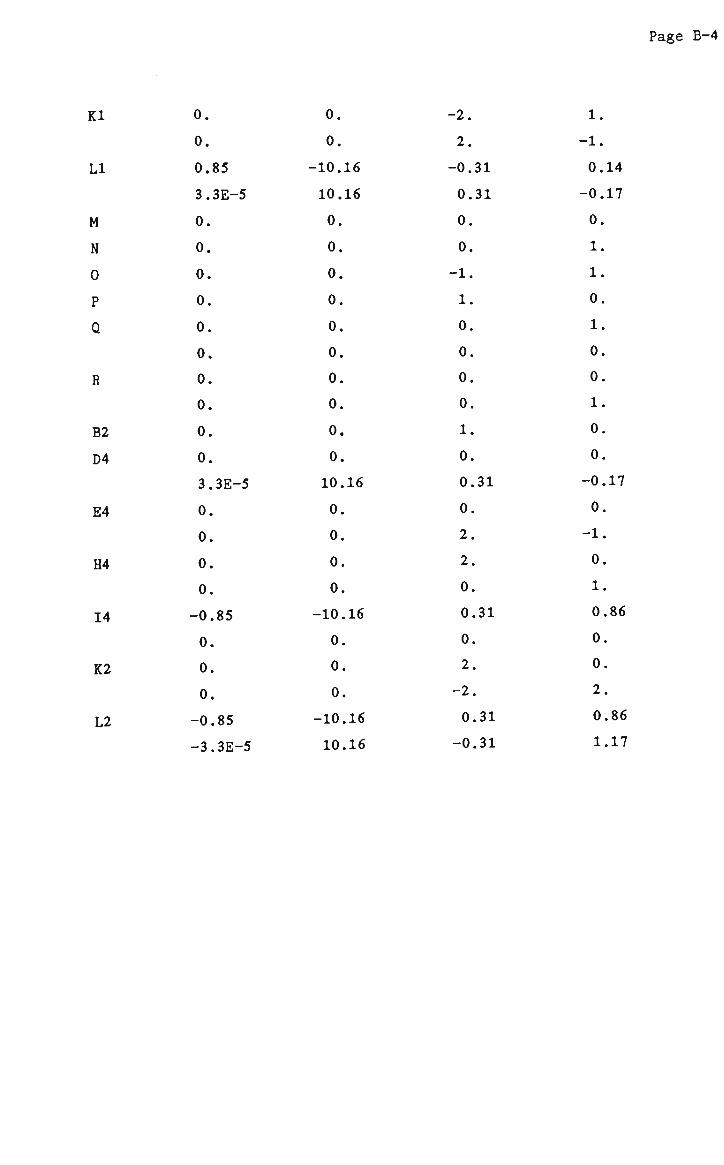
Page B-4

Kl

LI

M

N

0

P

Q

R

B2

D4

E4

H4

14

K2

L2

0.

0.

0.85

3.3E-5

0.

0.

0.

0.

0.

0.

0.

0.

0.

0.

3.3E-5

0.

0.

0.

0.

-0.85

0.

0.

0.

-0.85

-3.3E-5

0.

0.

-10.16

10.16

0.

0.

0.

0.

0.

0.

0.

0.

0.

0.

10.16

0.

0.

0.

0.

-10.16

0.

0.

0.

-10.16

10.16

-2.

2.

-0.31

0.31

0.

0.

-1.

1.

0.

0.

0.

0.

1.

0.

0.31

0.

2.

2.

0.

0.31

0.

2.

-2.

0.31

-0.31

1.

-1.

0.14

-0.17

0.

1.

1.

0.

1.

0.

0.

1.

0.

0.

-0.17

0.

-1.

0.

1.

0.86

0.

0.

2.

0.86

1.17

APPENDIX C

ADDITIONAL INFORMATION ON COMPUTER PROGRAM MGSTRN.

C l BRIEF DESCRIPTION OF SUBROUTINES.

CNSTNT computes and stores values for the Gaussian integration

constants used later when the moment equilibrium equations are solved

It is called once at the beginning of each new problem.

MTYPIN reads in the data describing the slope cross-section. Four

sets of data are required.

(a) Point data: points used to outline the slope profile or

topline.

(b) Line data: joins sets of two points to form lines and

includes the assigned number of the soil underlying these

lines.

(c) Soil data: includes the total unit weight y, the cohesion

intercept c, friction angle 0, pore pressure ratio r u

and the capillary head ratio r

(d) Phreatic Surface data: x and y co-ordinates of points

forming the phreatic surface. Pore pressures will be

calculated from this phreatic surface data if the value of

r above is specified as 1.1.

MSLOPE sorts out randomly input point and line data and reassembles it

into orderly arrays.

Page C-2

FRBODY reads in the x and y co-ordinates of the failure surface and

divides the potential sliding mass into about 24 slices. Vertical

slice boundaries are erected at the x co-ordinates of each of the

following points:

(a) All point data on or within the potential sliding mass.

(b) All points where soil zone boundaries intersect the failure

surface.

(c) All points where the phreatic surface intersects the failure

surface.

(d) All points defining the failure surface.

If the number of slices created by this method is less than 24,

boundaries will be erected at the centre of each slice which is wider

than 7 percent of the overall width of the sliding mass. This process

begins at the left end and stops when the number of slices equals 24

or when the right end is reached.

FBGEOM computes for each slice, the constants in Morgenstern and

Price's equations and also determines the pore pressure ratio on the

base of each slice. If pore pressure is represented by a phreatic

surface, the subroutine NEUTRAL is called to compute ru at each

slice interface. The pore pressure ratio on each slice base is then

taken as the average of the ru values at the two sides of the slice.

JUNCTN is used by FBGEOM and OUTPUT to identify the soil boundaries

which intersect each vertical slice interface. The soil on the right

hand side of the interface is used as the effective soil type.

NEUTRL is used by FBGEOM and OUTPUT to compute the pore pressure ratio

on slice bases in cases where the phreatic surface is used to define

the piezometric head. The capillary head for points above the

phreatic surface is computed as the vertical distance down to the

phreatic surface, times the capillary head ratio.

FUNCTN reads in the side-force assumption and computes

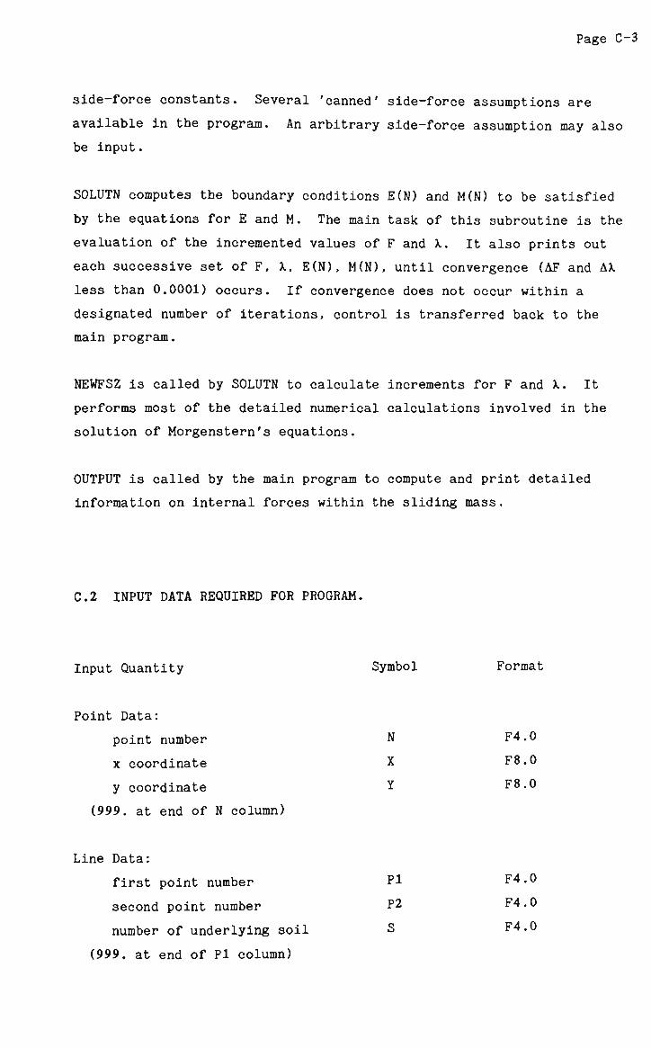
Page C-3

side-force constants. Several 'canned' side-force assumptions are

available in the program. An arbitrary side-force assumption may also

be input.

SOLUTN computes the boundary conditions E(N) and M(N) to be satisfied

by the equations for E and M. The main task of this subroutine is the

evaluation of the incremented values of F and X. It also prints out

each successive set of F, X, E(N), M(N), until convergence (AF and AX

less than 0.0001) occurs. If convergence does not occur within a

designated number of iterations, control is transferred back to the

main program.

NEWFSZ is called by SOLUTN to calculate increments for F and X. It

performs most of the detailed numerical calculations involved in the

solution of Morgenstern's equations.

OUTPUT is called by the main program to compute and print detailed

information on internal forces within the sliding mass.

C.2 INPUT DATA REQUIRED FOR PROGRAM.

Input Quantity Symbol Format

Point Data:

point number

x coordinate

y coordinate

(999. at end of N column)

N

X

Y

F4.0

F8.0

F8.0

Line Data:

first point number

second point number

number of underlying soil

(999. at end of PI column)

PI

P2

S

F4.0

F4.0

F4.0

Soil Data:

soil number N F4.0

total unit weight G F8.3

cohesion intercept C F8.3

angle of shearing resistance p F5.0

pore pressure ratio ru F5.1

capillary head ratio re F5.1

(99. at end of N column)

Phreatic Surface Points:

x coordinate X F8.0

y coordinate Y F8.0

(9999999. at end of X column)

Failure Surface Points:

x coordinate X F8.0

y coordinate Y F8.0

(9999999. at end of X column)

Side Force Assumption ICHK II

A number corresponding to one of the side force assumptions

presented later in this appendix must be entered here.

If assumptions 4 or 7 are used, the following additional data i

required.

amplitude at left F6.5

amplitude at right F6.5

If assumption 8 is used, the function value, along with its

corresponding x coordinate must be entered as follows.

x coordinate

function value

(9999999. at end of X column

X

FX

F8.0

F8.0

Factor of Safety estimate F F70.0

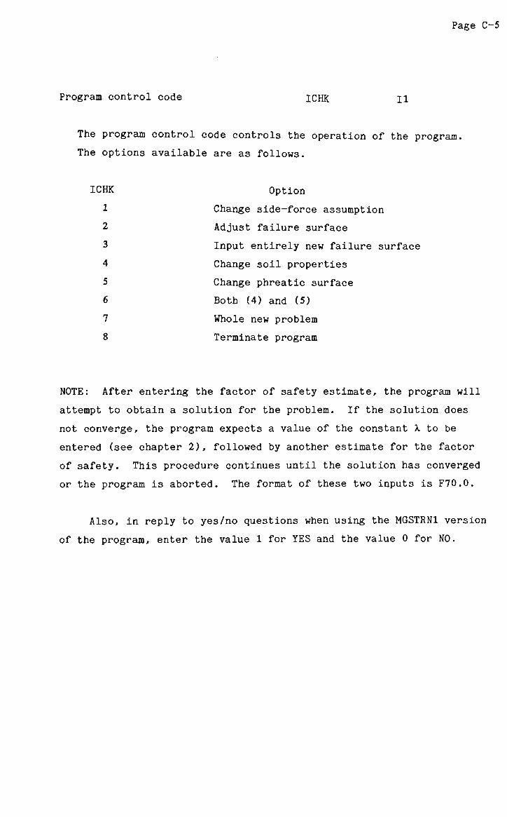
Page C-5

Program control code ICHK il

The program control code controls the operation of the program.

The options available are as follows.

ICHK Option

1 Change side-force assumption

2 Adjust failure surface

3 Input entirely new failure surface

4 Change soil properties

5 Change phreatic surface

6 Both (4) and (5)

7 Whole new problem

8 Terminate program

NOTE: After entering the factor of safety estimate, the program will

attempt to obtain a solution for the problem. If the solution does

not converge, the program expects a value of the constant X to be

entered (see chapter 2), followed by another estimate for the factor

of safety. This procedure continues until the solution has converged

or the program is aborted. The format of these two inputs is F70.0.

Also, in reply to yes/no questions when using the MGSTRN1 version

of the program, enter the value 1 for YES and the value 0 for NO.

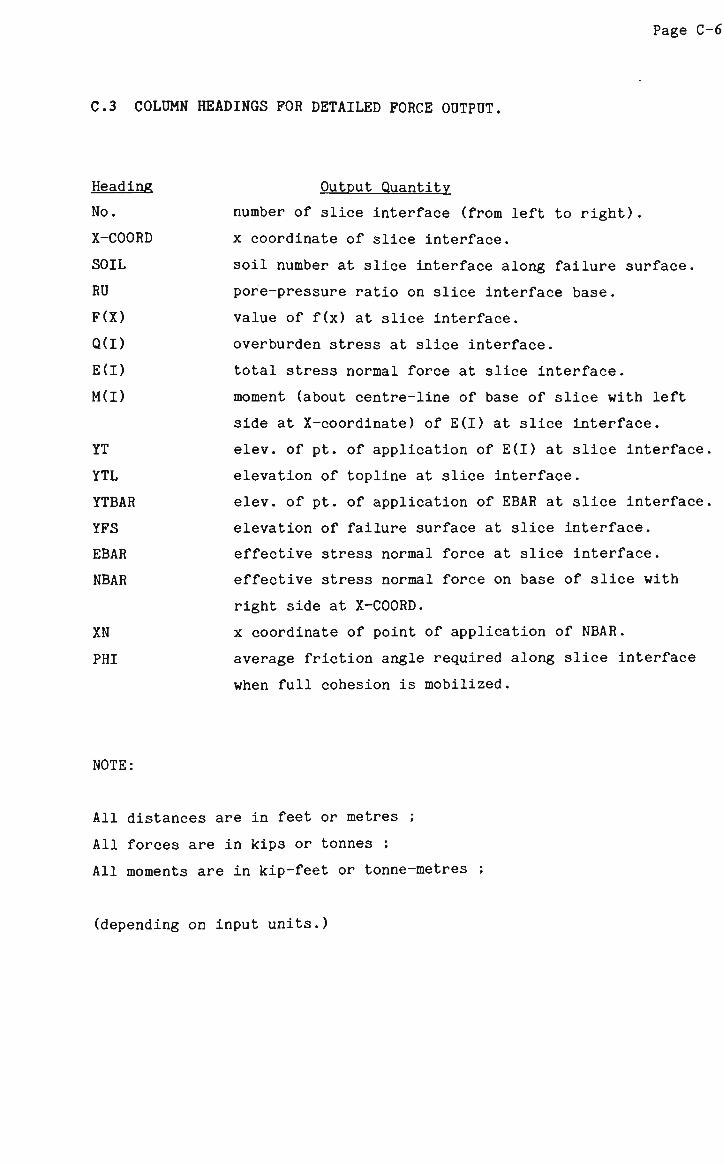
Page C-6

C.3 COLUMN HEADINGS FOR DETAILED FORCE OUTPUT.

Heading

No.

X-COORD

SOIL

RU

F(X)

Q(I)

E(I)

M(I)

YT

YTL

YTBAR

YFS

EBAR

NBAR

XN

PHI

Output Quantity

number of slice interface (from left to right) .

x coordinate of slice interface.

soil number at slice interface along failure surface.

pore-pressure ratio on slice interface base.

value of f(x) at slice interface.

overburden stress at slice interface.

total stress normal force at slice interface.

moment (about centre-line of base of slice with left

side at X-coordinate) of E(I) at slice interface.

elev. of pt. of application of E(I) at slice interface.

elevation of topline at slice interface.

elev. of pt. of application of EBAR at slice interface.

elevation of failure surface at slice interface.

effective stress normal force at slice interface.

effective stress normal force on base of slice with

right side at X-COORD.

x coordinate of point of application of NBAR.

average friction angle required along slice interface

when full cohesion is mobilized.

NOTE:

All distances are in feet or metres ;

All forces are in kips or tonnes ;

All moments are in kip-feet or tonne-metres ;

(depending on input units.)

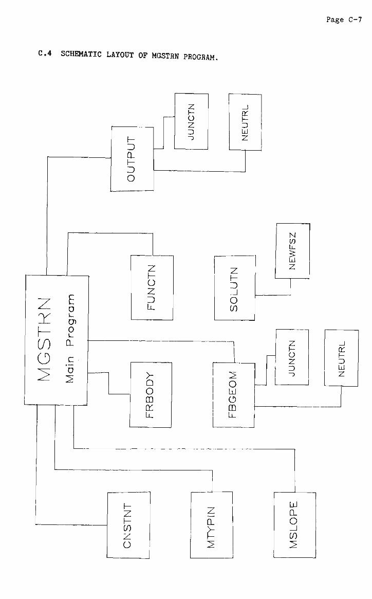
Page C-7

C.4 SCHEMATIC LAYOUT OF MGSTRN PROGRAM.

_J ___ (-D LJ Z

-

z h-D _J

O if)

__.

LU Z

| 1

^-i

1

2 o LJ o CD Li_

z h-o z D -_•

_J _._ f-D LJ

z

Z h-(/)

z o

APPENDIX D

BIBLIOGRAPHY

Ackenheil,A.C, 1954, 'A Soil Mechanics and Engineering Geology Analysis of Landslides in the Area of Pittsburgh, Pennsylvania', unpublished Ph.D. dissertation, University of Pittsburgh, pp. 83-87.

Alonso,E.E., 1976, 'Risk Analysis of Slopes and its Application to Slopes in Canadian Sensitive Clays', Geotechnique, Vol. 26, No. 3, pp. 453-473.

Andrei,S and Athanasiu.R., 1980, 'Stress Relation in Slope Stability Analysis', Proceedings of the International Symposium on Landslides, New Delhi, Vol. 1, pp. 105-108.

Athanasium,C., 1980, 'Non-Linear Slope Stability Analysis', Proceedings of the International Symposium on Landslides, Delhi, Vol. 1, pp. 259-262.

Azzouz,A.S., Baligh,M.M. and Ladd,C.C, 1981, 'Three-Dimensional Stability Analyses of Four Embankment Failures', Proceedings of the 10th International Conference on Soil Mechanics and Foundation Engineering, Stockholm, Vol. 3, pp. 343-346.

Barker,R. and Garber,M., 1978, 'Theoretical Analysis of the Stability of Slopes', Geotechnique, Vol. 28, No. 4, pp. 395-411.

Bailey,W.A., 1966, 'Stability Analysis by Limit Equilibrium', C E . Thesis, Massachusetts Institute of Technology.

Barton,N., 1972, 'Progressive Failure of Excavated Rock Slopes', 13th Symposium for Rock Mechanics, Urbana (Illinois), Ed. E.J.Cording, ASCE, pp. 139-171.

Bell.,J.M., 1968, 'General Slope Stability Analysis', Journal of the Soil mechanics and Foundation Division, ASCE, Vol. 94, No. SM6, pp. 1253-1270.

Bernander,S., 1985, 'On Limit Criteria for Plastic Failure in Strain Rate Softening Soils', Proceedings of the 11th International Conference on Soil Mechanics and Foundation Engineering, San Francisco, Vol. 2, pp. 397-400.

Bernander,S. and 01ofsson,I., 1981, 'On Formation of Progressive Failure in Slopes', Proceedings of the 10th International Conference on Soil Mechanics and Foundation Engineering, Stockholm, Vol. 3, pp. 357-362.

Page D-2

12. Bishop,A.W., 1955, 'Use of the Slip Circle in the Stability Analysis of Slopes', Geotechnique, Vol. 5, pp. 7-17.

13. Bishop,A.W., 1967, 'Progressive Failure with Special Reference to the Mechanism Causing It', Proceedings of the Geotechnical Conference, Oslo, Vol. 2, pp. 142-150.

14. Bishop,A.W., 1971, 'The Influence of Progressive Failure on the Choice of the Method of Stability Analysis', Geotechnique, Vol. 21, pp. 168-172.

15. Bishop,A.W. and Bjerrum,L., 1960, 'The Relevance of the Triaxial Test to the Solution of Stability Problems', Proceedings of the ASCE Research Conference on the Shear Strength of Cohesive Soils, Boulder, Colorado, pp.437-501.

16. Bishop,A.W. et.al., 1971, 'A New Ring Shear Apparatus and it's Application to the Measurement of Residual Strength', Geotechnique, Vol. 21, No. 4, pp. 273-328.

17. Bishop,A.W. and Morgenstern,N.R., 1960, 'Stability Coefficients for Earth Slopes', Geotechnique, Vol. 10, pp. 129-150.

18. Bjerrum.L., 1967, 'Progressive Failure in Slopes in Overconsolidated Plastic Clays and Clay Shales', Terzaghi Lecture, Journal of the Soil Mechanics and Foundation Division, ASCE, Vol. 93, No. SM5, pp. 3-49.

19. Bjerrum,L., 1969, 'Discussion of Main Session 5, Stability of Natural Slopes and Embankment Foundations', Seventh International Conference on Soil Mechanics and Foundation Engineering, Mexico City, Mexico, Vol. iii, pp. 377-414.

20. Booker,J.R., 1977, 'Introduction to the Finite Element Method', Geotechnical Analysis and Computer Applications, University of Sydney School of Civil Engineering Course Notes.

21. Broili,L., 1967, 'New Knowledge on the Geomorphology of the Vajont Slide Slip Surface', Rock Mechanics and Engineering Geology, Vol. 5, pp. 38-88.

22. Brown,CB. and King,I.P., 1966, 'Automatic Embankment Analysis: Equilibrium and Instability Conditions', Geotechnique, Vol. 16, No. 3, pp. 209-219.

23. Chandler,R.J., 1977, 'Back Analysis Techniques for Slope Stabilisation Works: A Case Record', Geotechnique, Vol. 27, No. 4, pp. 479-495.

24. Chandler,R.J., 1984, 'Recent European Experience of Landslides in Overconsolidated Clays and Soft Rocks', Proceedings of the 4th International Symposium on Landslides, Toronto, Vol. 1, pp. 61—68.

25. Ching,R.K.H. and Fredlund,D.G., 1983, 'Some Difficulties Associated with the Limit Equilibrium Method of Slices', Canadian Geotechnical Journal, Vol. 20 pp. 661-672.

Page D-3

26. Chowdhury,R.N., 1976, 'Initial Stresses in Natural Slope Analysis', Rock Engineering for Foundations and Slopes, ASCE, Geotechnical Engineering Specialty Conference, Boulder(Colorado), Vol. 1, pp. 404-415.

27. Chowdhury,R.N., 1977, 'A New Approach to Slope Stability Studies', Research Report, Department of Civil Engineering, University of Wollongong, N.S.W., Australia.

28. Chowdhury,R.N., 1977, 'Propagation of Failure Surfaces in Natural Slopes', Research Report, Department of Civil Engineering, University of Wollongong, N.S.W., Australia.

29. Chowdhury,R.N., 1978, 'Slope Analysis', Elsevier Scientific Publishing Company, Amsterdam and New York.

30. Chowdhury,R.N., 1984, 'Recent Developments in Landslide Studies: Probabilistic Methods - State of the Art Report', Proceedings of the 4th International Symposium on Landslides, Toronto, Vol. 1, pp. 209-228.

31. Chowdhury,R.N., 1985, 'Successive Failures: A Probabilistic Approach', Proceedings of the 11th International Conference on Soil Mechanics and Foundation Engineering, San Francisco, Vol. 2, pp. 819-824.

32. Chowdhury,R.N. and A-Grivas,D., 1982, 'Probabilistic Model of Progressive failure of Slopes', Journal of the Geotechnical Engineering Division, ASCE, No. GT6, pp. 803-819.

33. Chowdhury,R.N. and DeRooy,E.R., 1985, 'Progressive Reliability of a Strain Softening Slope', Civil Engineering Transactions, Institution of Civil Engineers Australia, Vol. CE27, No. 1, pp. 79-94.

34. Chugh,A.K., 1986, 'Variable Factor of Safety in Slope Stability Analysis', Geotechnique, Vol. 36, No. 1, pp. 57-64.

35. Clough,R.W. and Woodward,R.J., 1967, 'Analysis of Embankment Stresses and Deformations', Journal of the Soil Mechanics and Foundation Division, ASCE, Vol. 93, No. SM4, pp. 529-549.

36. Crawford,CB. and Eden,W.J., 1967, 'Stability of Natural Slopes in Sensitive Clays', Journal of the Soil Mechanics and Foundation Division, ASCE, Vol. 93, July, pp. 419-436.

37. Davis,E.H., 1977, 'Geotechnical Analysis and Computer Applications', University of Sydney School of Civil Engineering Course Notes.

38. Deere,D.U. and Patton,F.D., 1971, 'Slope Stability in Residual Soils', Proceedings of the Fourth Conference on Soil Mechanics for the Foundation of Engineers, State of the Art Report, 1, pp. 88-171.

39. DeLory.F.A., 1957, 'Long Term Stability of Slopes in Overconsolidated Clays', PH.D. Thesis, University of London.

Page D-4

40. Duncan,J.M. and Dunlop,P., 1969, 'Slopes in Stiff-fissured Clays and Shales', Journal of the Soil Mechanics and Foundation Division, ASCE, Vol. 95, No. SM2, pp. 467-491.

41. Dunlop,P. and Duncan,J.M., 1970, 'Development of Failure Around Excavated Slopes', Journal of the Soil Mechanics and Foundation Division, ASCE, Vol. 96, No. SM2, pp. 471-495.

42. Fellenius,W., 1936, 'Calculation of the Stability of Earth Dams', Transactions of the Second Congress on Large Dams (Washington), Vol. 4, p. 445.

43. Foerster,W. and Georgi,P., 1981, 'Application of a Stress-Strain-Time Relation', Proceedings of the 10th International Conference on Soil Mechanics and Foundation Engineering, Stockholm, Vol. 3, pp. 405-408.

44. Fredlund,D.G., 1984, 'Analytical Methods for Slope Stability Analysis', Proceedings of the 4th International Symposium on Landslides, Toronto, Vol. 1, pp. 229-250.

45. Hamel,J.V., 1968, 'Morgenstern and Price Method of Slope Stability Analysis', Report by the Department of Civil Engineering, University of Pittsburgh, to the U.S. Bureau of Mines, p. 149.

46. Hamel,J.V., 1972, 'The Slide at Brilliant Cut', Proceedings of the Thirteenth Symposium on Rock Mechanics, Urbana (Illinois), Edited by E.J.Cording, ASCE, pp. 487-510.

47. Hast,N., 1974, 'The State of Stress in the Upper Part of the Earths Crust as Determined by Measurements of Absolute Rock Stresses', Naturwissenschaften, Vol. 61, pp. 468-475.

48. Henkel,D.J., 1957, 'Investigations of Two Long-term Failures in London Clay Slopes at Woodgreen and Northolt', Proceedings of the Fourth International Conference on Soil Mechanics, London, Vol. 2, pp. 315-320.

49. James,P.M., 1970, 'Time Effects and Progressive Failure in Clay Slopes', PH.D. Thesis, University of London.

50. James,P.M., 1971, 'The Role of Progressive Failure in Clay Slopes', Proceedings of the First Australia - New Zealand Conference on Geomechanics, Vol. 1, pp. 344-348.

51. Janbu,N., 1954, 'Stability Analysis of Slopes with Dimensionless Parameters', Harvard Soil Mechanics Series, No. 46, p. 811.

52. Janbu,N., 1957, 'Earth Pressure and Bearing Capacity Calculations by Generalised Procedure of Slices', Proceedings of the Fourth International Conference and Foundation Engineering, Vol. 2, pp. 207-212.

53. Janbu,N., 1973, 'Soil Stability Computations', Embankment Dam Engineering, Casagrande Volume, Edited by R.CHirschfeld and S.J.Poulos, Wiley, New York, pp. 47-87.

Page D-5

54. Kenney.T.C.. 1963, 'Stability of Cuts in Soft Soils', Journal of the Soil Mechanics and Foundation Division, ASCE, Vol. 89, No. SM5, pp. 17-37.

55. Kenney,T.C, 1967, 'The Influence of Mineral Composition on the Residual Strength of Natural Soils', Proceedings of the Geotechnical Conference, Oslo, Vol. 1, pp. 123-129.

56. KirkpatricW.M., Khan,A.J. and Mirza,A.A., 1986, 'The effects of Stress Relief on some Overconsolidated Clays ', Geotechnique, Vol. 36, No. 4, pp. 511-525.

57. Langer,K., 1963, 'Discussion on Field Observations reported by K.Terzaghi', Proceedings 1st International Conference on Soil Mechanics and Foundation Engineering, Vol. 3, pp. 152-155.

58. Law,K.T. and Lumb,P., 1978, 'A Limit Equilibrium Analysis of Progressive Failure in the Stability of Slopes', Canadian Geotechnical Journal, Vol. 11, pp. 113-122.

59. Lo,K.Y., 1965, 'Stability of Slopes in Anisotropic" Soils', Journal of the Soil Mechanics and Foundation Division, ASCE, Vol. 90, No. SM4, pp. 85-106.

60. Lo,K.Y., 1972, 'An Approach to the Problem of Progessive Failure', Canadian Geotechnical Journal, Vol. 9, p. 407.

61. Lo,K.Y., 1978, 'Regional Redistribution of In-situ Horizontal Stresses in Rocks of Southern Ontario', Canadian Geotechnical Journal, Vol. 15, pp. 371-381.

62. Lo,K.Y. and Lee,CF., 1973, 'Stress Analysis and Slope Stability in Strain-softening Materials', Geotechnique, Vol. 23, No. 1, pp. 1-11.

63. Lo,K.Y. and Lee,CF., 1973, 'Analysis of Progressive Failure in Clay Slopes'

64. Lo,K.Y., Lee,CF. and Gelinas,P., 1972, 'An Alternative Interpretation of the Vajont Slide, Stability of Rock Slopes', Proceedings of the 13th Symposium on Rock Mechanics, ASCE, pp. 597-625.

65. Meyerhof,G.G., 1965, Discussion on paper 'Stability of Slopes in Anisotropic Soil', Journal of the Soil Mechanics and Foundation Division, ASCE, Vol. 91, No. SM6, p. 132.

66. Meyerhof,G.G. and Brown,J.D., 1967, Discussion on paper 'Boundary Conditions of Footings on Layered Clays', Journal of the Soil Mechanics and Foundation Division, ASCE, Sept. 1967, No. SM5.

67. Morgenstern,N.R., 1968, ''Ultimate Behaviour of Rock Structures', Rock Mechanics in Engineering Practice, Edited by O.CZienkiewicz and K.G.Stagg, Wiley, pp. 321-346.

68. Morgenstern,N.R. and Price,V.E., 1965, 'The Analysis of the Stability of General Slip Surfaces', Geotechnique, Vol. 15, No. 1, pp. 79-93.

Page D-6

69. Nelson,J.D. and Thompson,E.G., 1977, 'A Theory of Creep Failure in Overconsolidated Clay', Journal of the Geotechnical Engineering Division, ASCE, Vol. 103, No. GT11, pp. 1281-1294.

70. Nonveiller,E., 1965, 'The Stability Analysis of Slopes with a Slip Surface of General Shape', Proceedings of the 6th International Conference on Soil Mechanics and Foundation Engineering, Vol. 2, pp. 522-525.

71. Peck,R.B., 1967, 'Stability of natural Slopes', Journal of the Soil Mechanics and Foundation Division, ASCE, Vol. 93, No. SM4, pp. 403-417.

72. Pells,P.J.N., 1977, 'Slope Stability Analysis', Geotechnical Analysis and Computer Applications, University of Sydney School of Civil Engineering Notes.

73. Peterson,R., 1954, 'Studies of Bearpaw Shale at a Dam Site in Saskatchewan', Proceedings of the Soil Mechanics and Foundation Division, ASCE, Vol. 80, Separates No. 476 and 759.

74. Peterson,R., 1955, Closure of 'Studies of Bearpaw Shale at a Dam Site in Saskatchewan', Proceedings of the Soil Mechanics and Foundation Division, ASCE, paper No. 759, pp.1-2

75. Peterson,R., Jasper J.L., Rivard,P.J. and Iverson,N.L., 1960, 'Limitations of Laboratory Shear Strength in Evaluating Stability of Highly Plastic Clays', ASCE Research Conference on Shear Strength of Cohesive Soils, Boulder, Colorado, pp. 765-791.

76. Reddy,A.S. and Srinivasan, 1967, 'Boundary Conditions of Footings on Layered Clays', Journal of the Soil Mechanics and Foundation Division, ASCE, March 1967, pp. 83-99.

77. Reddy,A.S. and Venkatakrishna Rao,K.N., 1982, 'Stability of Slopes by Method of Characteristics', Journal of the Geotechnical Engineering Division, ASCE, No. GT9, pp. 1182-1186.

78. Rivard,P.J. and Lu,Y., 1978, 'Shear Strength of Soft Fissured Clays', Canadian Geotechnical Journal, Vol. 15, pp. 382-390.

79. Romani,F., Lovell.C.W. and Barr,M.E., 1972, 'Influence of Progressive Failure on Slope Stability', Journal of the Soil Mechanics and Foundation Division, ASCE, Vol. 98, No. SM11, pp. 1209-1223.

80. Sallfors,G.B. and Larsson,R., 1984, 'State of the Art report: Soft Clays in Sweden', Proceedings of the 4th International Symposium on Landslides, Toronto, Vol. 1, pp. 131-140,

81. Sarma,S.K., 1973, 'Stability Analysis of Embankments and Slopes', Geotechnique, Vol. 23, pp. 423-433.

82. Sarma,S.K. and Bhave,M.V., 1974, 'Critical Acceleration vs. Static Factor of Safety in Stability Analysis of Earth Dams and Embankments', Geotechnique, Vol. 24, pp. 661-665.

Page D-7

83. Sevaldson,R.A., 1956, 'The Slide in Lodalen, October 6th 1954', Geotechnique, Vol. 6, No. 4, pp. 167-182.

84. Sidharta,A.S., 1985, 'Prediction of Creep Failure of Excavations in Overconsolidated Clay with Pore Pressure Dissipation', Postgraduate Research Thesis, Department of Civil Engineering, Colorado State University.

85. Skempton.A.W., 1945, 'A Slip in the West Bank of the Eau Brink Cut', Journal of the Institute of Civil Engineers, London, Vol. 24, No. 7, pp.267-289.

86. Skempton,A.W., 1948, 'The 0=0 Analysis of Stability and its Theoretical Basis', Proceedings of the 2nd International Conference on Soil Mechanics and Foundation Engineering, Rotterdam, Vol. 1, pp. 145-150.

87. Skempton.A.W., 1961, 'Horizontal Stresses in Over-consolidated Eocene Clay', Proceedings of the 5th International Conference on Soil Mechanics and Foundation Engineering, Paris, Vol. 1, pp. 351-357.

88. Skempton.A.W., 1964, 'Long Term Stability of Clay Slopes', Rankine Lecture, Geotechnique, Vol. 14, pp. 77-101.

89. Skempton.A.W., 1970, 'First Time Slides in Over-consolidated Clays', Geotechnique, Vol. 20, pp. 320-324.

90. Skempton.A.W., 1977, 'Slope Stability in Cuttings in Brown London Clay', Proceedings of the 9th International Conference on Soil Mechanics and Foundation Engineering, Tokyo, Vol. 3, pp. 261-271.

91. Skempton,A.W., 1985, 'Residual Strength of Clays in Landslides, Folded Strata and the Laboratory', Special Lecture, Geotechnique, Vol. 35, No. 1, pp. 3-18.

92. Skempton,A.W. and Brown,J.D., 1961, 'A Landslide in Boulder Clay at Selset, Yorkshire', Geotechnique, Vol. 1, No. 4, pp. 280-293.

93. Skempton.A.W. and Delory.F.A., 1957, 'Stability of Natural Slopes in London Clay', Proceedings of the 4th International Conference on Soil Mechanics and Foundation Engineering, London, Vol. 2, pp. 378-381.

94. Skempton.A.W. and Hutchinson,J.N., 1969, 'Stability of Natural Slopes and Embankment Foundations, State of the Art Report', Proceedings of the 7th International Conference on Soil Mechanics and Foundation Engineering, Mexico, pp. 291-335.

95. Skempton,A.W. and LaRochelle,P., 1965, 'The Bradwell Slip: A Short-term Failure in London Clay', Geotechnique, Vol. 15, No. 3, pp. 221-242.

96. Skempton.A.W. and Petley.D.J., 1967, 'The Strength Along Structural Discontinuities in Stiff Clays', Proceedings of the European Conference on Soil Mechanics and Foundation Engineering, Vol. 2, pp. 29-46.

Page D-8

97. Sotiropoulos,E. and Cavounidis,S., 1981, 'Irregular Stress-Strain and Progressive Failure', Proceedings of the 10th International Conference on Soil Mechanics and Foundation Engineering, Stockholm, Vol. 3, pp. 527-531.

98. Spencer,E., 1968, 'Effect of Tension on Stability of Embankments', Journal of the Soil Mechanics and Foundation Division, ASCE, Vol. 94, No. SM5, pp. 1159-1173.

99. Spencer,E., 1968, 'Stability of Earth Embankments', Reprint from Civil Engineering journal.

100. Tang,W.H., Chowdhury,R.N. and Sidi, 1985, 'Progressive Failure Probability of Soil Slopes', Proceedings of ICOSSAR, Kobe, Japan, T34B, III. pp. 363-372.

101. Tavenas,F. and Leroueil,S., 1981, 'Creep and Delayed Failure of Slopes in Clays', Canadian Geotechnical Journal, Vol. 18, pp. 106-120.

102. Taylor,D.W., 1937, 'Stability of Earth Slopes', J. Boston Society of Civil Engineering, Vol. 24, p. 197.

103. Taylor,D.W., 1948, 'Fundamentals of Soil Mechanics', John Wiley and Sons, N.Y.

104. Ter-Stepanian,G., 1977, 'Behaviour of Clays Close to Failure', Proceedings of the 9th International Conference on Soil Mechanics and Foundation Engineering, Tokyo, Vol. 1, pp. 327-328.

105. Terzaghi,K., 1936, 'Stability of Slopes in Natural Clay', Proceedings of the 1st International Conference on Soil Mechanics and Foundation Engineering, Harvard, Vol. 1, pp. 161-165.

106. Terzaghi,K. and Peck,R.B., 1948, 'Soil Mechanics in Engineering Practice', John Wiley and Sons, N.Y.

107. Thompson,S. and Tweedie,R.W., 1978, 'The Edgerton Landslide', Canadian Geotechnical Journal, Vol. 15, pp. 510-521.

108. Vaughan,P.R. and Kwan,CW., 1984, 'Weathering, Structure and In-situ Stress in Residual Soils', Geotechnique, Vol. 34, No. 1, pp. 43-59.

109. Whitman,R.V. and Bailey,W.A., 1967, 'Use of Computers for Slope Stability Analysis, Journal of the Soil Mechanics and Foundation Division, ASCE, Vol. 93, No. SM4, pp. 475-498.

110. Whitman,R.V. and Moore, 1963, 'Thoughts Concerning the Mechanics of Slope Stability Analysis', Proceedings of the 2nd Pan American Conference on Soil Mechanics and Foundation Engineering, Vol. 1, pp. 391-411

111. Wilson,S.D., 1970, 'Observational Data on Ground Movements Related to Slope Instability', Sixth Terzaghi Lecture, Journal of the Soil Mechanics and Foundation Division, ASCE, Vol. 96, No. SM5

Page D-9

112. Wright,S.G., 1975, 'Evaluation of Slope Stability Analysis Procedures', Preprint 2616, ASCE National Conference, Denver, Colorado.

113. Wright,S.G., Kulhawy,E.D. and Duncan,J.M., 1973, 'Accuracy of Equilibrium Slope Stability Analysis', Journal of the Soil Mechanics and Foundation Division, ASCE, Vol. 99, No. SM10, pp. 783-793.

114. Wu,T.H., Williams,R.L., Lynch,J.E. and Kulatilake,P.H.S.W., 1987, 'Stability of Slopes in Red Conemaugh Sale of Ohio', Journal of the Geotechnical Engineering Division, ASCE, Vol. 113, No. 3, pp. 248-264.

115. Yucemen,M.S., Tang,W.H. and Ang,A.H., 1973, 'A Probabilistic Study of Safety and Design of Earth Slopes', Civil Engineering Studies, Structural Research Series No. 402, University of Illinois, Urbane, Illinois.

Documents

Computer simulation of progressive failure in soil slopes