Non-parametric Learning To Aid Path Planning

Over Slopes

Sisir Karumanchi, Thomas Allen, Tim Bailey and Steve Scheding

ARC Centre of Excellence For Autonomous Systems (CAS),

Australian Centre For Field Robotics (ACFR),

The University of Sydney,

NSW. 2006, Australia.

Email: s.karumanchi/t.allen/t.bailey/s.scheding@cas.edu.au

Abstract— This paper addresses the problem of closing theloop from perception to action selection for unmanned groundvehicles, with a focus on navigating slopes. A new non-parametriclearning technique is presented to generate a mobility repre-sentation where maximum feasible speed is used as a criterionto classify the world. The inputs to the algorithm are terraingradients derived from an elevation map and past observationsof wheel slip. It is argued that such a representation can aid inpath planning with improved selection of vehicle heading andoperating velocity in off-road slopes. Results of mobility mapgeneration and its benefits to path planning are shown.

I. INTRODUCTION

Learning techniques that close the loop from perception to

action selection are of particular interest for off-road robotics.

This loop closure refers to the need for an intermediate

module that processes sensed exteroceptive1 information into

a representation which can directly aid in decision making

(such as path planning). In ground vehicle robotics the focus

is usually on identifying hard hazards such as obstacles

or classifying predefined environmental states into different

degrees of traversibility [6], [7], [10], [13]. Assumptions such

as terrain homogeneity, or perpetual existence of a road are

often made to simplify the problem. In the absence of such

assumptions, theoretical techniques that use sensed informa-

tion to aid decision making need to be investigated. In this

paper an intermediate scene interpretation module is proposed

in Section II to close the loop from perception to action.

Autonomous navigation in unstructured conditions such as

non-homogeneous uneven terrain is a challenging problem

to solve. In such environments two main issues need to be

addressed. First, explicit assumptions about the terrain should

be avoided. Second, in addition to hard hazards (such as

obstacles), soft hazards (situations where behaviour needs to

be adapted) need to be identified and dealt with. For example,

terrain slopes are soft hazards and to successfully negotiate

them, vehicle behaviour such as velocity, operating gear and

vehicle heading needs to be adjusted.

Due to recent developments in Bayesian non-parametric

techniques, learning from experience architectures offer

promise. In such architectures, no assumptions need to be

1Exteroception: perception of external factors that are not under agentcontrol

made about the environment. The environment representation

is only limited by the available sensor suite and the variables

used to define the exteroceptive state. Therefore, experience-

based learning techniques are viable to address the problem

of closing the loop from perception to action.

Existing ‘learning from experience’ techniques include Re-

inforcement Learning [15] and model predictive techniques

[5]. However, they make assumptions such as the existence of

a reward function in Reinforcement Learning, or the existence

of accurate models for model predictive techniques. It is

difficult to quantify such reward functions or develop accurate

models in unstructured environments.

Imitation Learning [14] and Inverse Reinforcement Learn-

ing [1] are relatively new concepts and have been applied

to the problem of learning a reward function from exam-

ple behaviour. However, they rely heavily on expert input.

Controller limitations are usually ignored when systems rely

heavily on human input. For example, tuning involved in a

PID controller limits the mobility of the platform as it was

tuned for a few selected conditions. Such limitations can be

dealt with implicitly when the vehicle explores its behavioural

capabilities on its own terms.

A learning from proprioception2 approach is demonstrated

in [2] for a Mars-Rover platform where the authors represent

the environment in proprioception space in terms of expected

slip. This approach ignores the influence of operating velocity

on wheel slip. For a Mars-Rover, proprioceptive measures

(such as wheel slip) are mainly dependent on environment

conditions and behavioral influences (such as velocity) could

be ignored because the platform moves slowly. However, this

assumption cannot be made for larger platforms where there is

a distribution of slip values for a given condition pertaining to

all possible behaviours. Also, such an approach is limited to

the case when proprioception is a scalar or a weighted average

of scalars. The latter usually involves manual tuning of weights

which is not an intuitive process. A single scalar cost cannot

capture all the objectives in unstructured conditions. Instead it

is beneficial to use a collage of proprioceptive stimuli to judge

actions.

2Proprioception: perception of internal factors that are affected by environ-ment and one’s own behaviour.

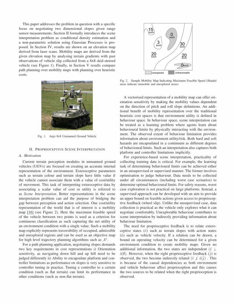
This paper addresses the problem in question with a specific

focus on negotiating two dimensional slopes given range

sensor measurements. Section II formally introduces the scene

interpretation problem as conditional density estimation and

a non-parametric solution using Gaussian Processes is pro-

posed. In Section IV, results are shown on an elevation map

derived from laser scans. Mobility maps are derived from the

given elevation map by analysing terrain gradients with past

observations of vehicle slip collected from a 8x8 skid-steered

vehicle (see Figure 1). Finally, in Section V results compare

path planning over mobility maps with planning over heuristic

costs.

Fig. 1. Argo 8x8 Unmanned Ground Vehicle

II. PROPRIOCEPTIVE SCENE INTERPRETATION

A. Motivation

Current terrain perception modules in unmanned ground

vehicles (UGVs) are focused on creating an accurate internal

representation of the environment. Exteroceptive parameters

such as terrain colour and terrain slope have little value if

the vehicle cannot associate them with a value of cost/utility

of movement. This task of interpreting exteroceptive data by

associating a scalar value of cost or utility is referred to

as Scene Interpretation. Better representations in the scene

interpretation problem can aid the purpose of bridging the

gap between perception and action selection. One cost/utility

representation of the world that is of interest is a mobility

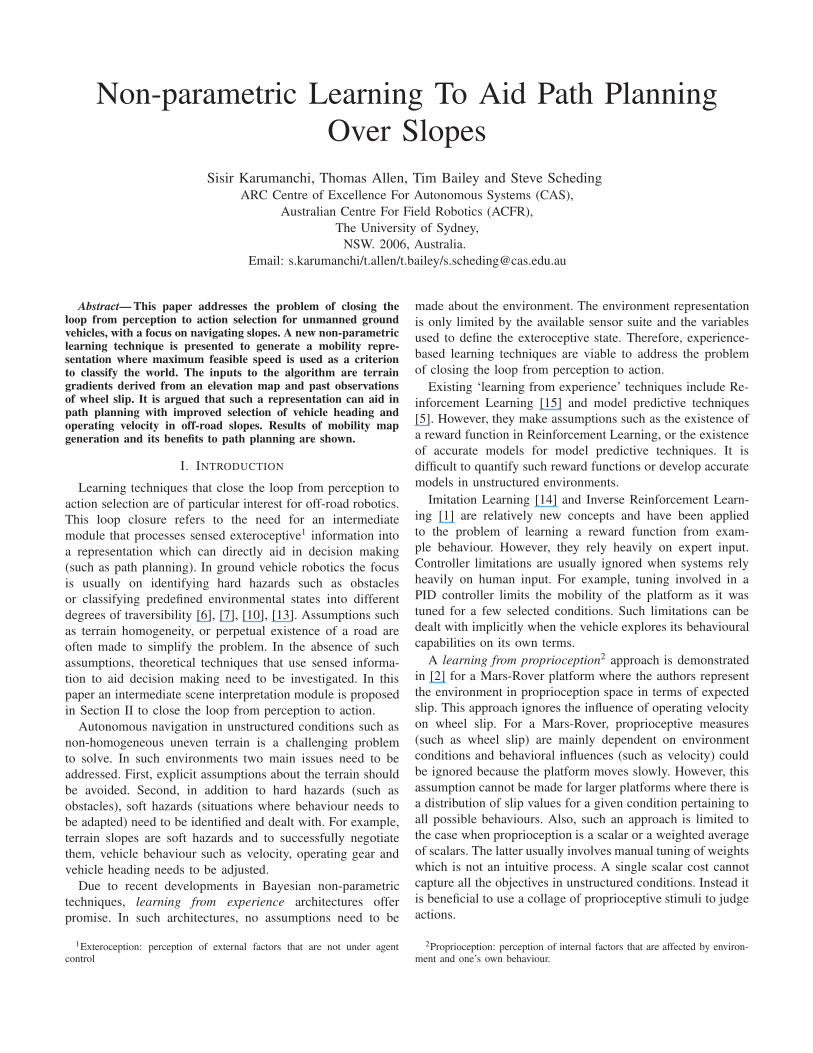
map [16] (see Figure 2). Here the maximum feasible speed

of the vehicle between two points is used as a criterion for

continuous classification as such capturing the net utility of

an environment condition with a single value. Such a mobility

map explicitly represents traversibility of occupied, admissible

and unexplored regions and can be used as an objective map

for high level trajectory planning algorithms such as A∗.

For a path planning application, negotiating slopes demands

two key requirements in cost representations i) Orientation

sensitivity, as navigating down hill and up hill need to be

judged differently ii) Ability to encapsulate platform and con-

troller limitations as performance on slopes is very sensitive to

controller tuning in practice. Tuning a controller to a certain

condition (such as flat terrain) can limit its performance in

other conditions (such as non-flat terrain).

Fig. 2. Sample Mobility Map Indicating Maximum Feasible Speed (Shadedareas indicate immobile and unexplored areas)

A vectorised representation of a mobility map can offer ori-

entation sensitivity by making the mobility values dependent

on the direction of pitch and roll slope definitions. An addi-

tional benefit of mobility representation over the traditional

heuristic cost spaces is that environment utility is defined in

behaviour space. In behaviour space, scene interpretation can

be treated as a learning problem where agents learn about

behavioural limits by physically interacting with the environ-

ment. The observed extent of behaviour limitation provides

information about environment utility/risk. Both hard and soft

hazards are encapsulated in a continuum as different degrees

of behavioural limits. Such an interpretation also captures both

platform and controller limitations implicitly.

For experience-based scene interpretation, practicality of

collecting training data is critical. For example, the learning

task of determining behavioural limits can be achieved either

in an unsupervised or supervised manner. The former involves

optimisation to judge behaviour. Data needs to be collected

under all circumstances (including worst case scenarios) to

determine optimal behavioural limits. For safety reasons, worst

case exploration is not practical on large platforms. Instead, a

supervised approach can be developed with an aim to provide

an upper bound on feasible actions given access to propriocep-

tive feedback (wheel slip). Unlike the unsupervised case, data

collection is practical as the vehicle only explores what it can

negotiate comfortably. Unexplorable behaviour contributes to

scene interpretation by indirectly providing information about

behaviour limitation.

The need for proprioceptive feedback is to relate extero-

ceptive states (e) such as terrain slopes with action states

(a) such as vehicle velocity. If a relation can be drawn, a

bound on operating velocity can be determined for a given

environment condition to create mobility maps. Given no

additional information, the two states are independent (e ⊥a|∅). However, when the right proprioceptive feedback (j) is

observed, the two become indirectly related (e 6⊥ a|j) . This

is because of the causal dependencies as both environment

and vehicle behaviour affect proprioception and this causes

the two sources to be related when the right proprioception is

observed.

The process of analysing and selecting useful proprioceptive

measures is a separate problem of its own, and is not dealt

with in this paper. For the skid-steered vehicle of interest,

slip estimates are chosen as proprioceptive feedback. The slip

values cannot be measured directly, so they are estimated

with an Unscented Kalman Filter [8] (UKF) using the two-

track process model mentioned in [9]. The reason for using

a Kalman filter is to efficiently deal with sensor noise. The

test platform has an onboard Inertial Navigation System (INS)

and its used to sense vehicle actions such as velocity with

good accuracy. In addition, pitch and roll information from the

INS are used to sense the current terrain slope (exteroceptive

conditions)3.

In the next subsections, the notation is summarised in one

place to provide easy reference to all the variables and then

the theory is introduced.

B. Nomenclature

x - tilde is used to indicate that a particular variable is

a vector.

a - Action vector (operating velocity)

e - Exteroceptive stimuli (terrain slopes)

j - Proprioceptive stimuli (wheel slips): A vector of

measures that indicate dependence of performance

on environmental conditions and vehicle behaviour.

H - Experience set (training set)

e1 e2 · · · eN

j1 j2 · · · jN

a1 a2 · · · aN

J∗ - Set of proprioceptive stimuli observed in ideal

conditions -{j∗1, j∗

2, · · ·, j∗M}.

J∗ is the set of samples derived from a constrained

region in proprioception space that is indicative of

feasible conditions.

Etest - Set of test conditions which need to be interpreted

(Test set) - {etest1, etest2, · · ·, etestT }.

for example, the set of both horizontal and

vertical gradients for each grid cell form the set of

test conditions to interpret terrain slopes from an

elevation map.

C. Problem Definition

Gathering experience corresponds to collecting co-occurrent

observations of e, a and j in as many varied conditions as

possible4. This experience set (H) serves as a training set for

learning. The exploration philosophy for collecting training

data is to explore the natural feasibility of vehicle behaviour in

3The test platform used in this work does not have any suspension, so pitchand roll information from the INS reflects the terrain slope accurately. Forother platforms, terrain slopes must be derived from exteroceptive sensors.

4Existence of a stationary joint distribution p(e, j, a) is assumed. Thereforethe experience/training set is a collection of i.i.d samples from the joint.

as many varied conditions as possible either under manual or

autonomous control. The latter has the advantage of exploring

controller limitations.

Before velocity limits can be derived from experience

data, an intermediate goal is to infer the feasible behaviour

distribution for any test condition given the set of all past

observations (H) and the comfortable proprioception set (J∗)

which is chosen by the user to be observations in ideal/nominal

conditions. For interpreting slopes, observations from flat

terrain conditions are labelled as ideal and used as a reference.

This process can be intuitively understood as training the robot

what to look for (in proprioception) when exploring feasibility

of actions in unknown conditions.

Once feasible behaviour distribution is inferred, an upper

bound using the commulative density function (CDF) can

determine velocity limits for use in mobility maps. The process

of deriving a mobility map given a set of test conditions is

outlined below.

Scene Interpretation Process For An Elevation Map

Input: Elevation Map (A set of elevation values)

- Apply the Sobel operator [4] to determine gradient

maps in pitch and roll directions (Test set−Etest).

foreach etest in Etest do- Infer feasible behaviour distribution from past

experience (H & J∗)

- Determine operational limit (Maximum Feasible

Speed)end

Output: Mobility Map (Set of all associated mobility

values ordered according to their respective test

condition in Etest)

Determining the feasible behaviour distribution is a con-

ditional density estimation problem. The feasible behav-

iour distribution for a selected environment condition is

p(a|etest, i = 1)5 where i is an indicator variable to represent

the feasibility constraint j ∈ J∗.

i =

{

1 j ∈ J∗

0 j /∈ J∗

(1)

p(a|etest, i = 1) is a measure of confidence in taking an

action a given past experience (H). Confidence for an action is

based on how often proprioception observed under that action

was within the set of proprioceptive stimuli observed in ideal

conditions (J∗) i.e. actions that generated stimuli in the region

of accustomed proprioception J∗ are preferred.

D. A Non-Parametric Approximation

In this section a hierarchical non-parametric6 approach

is presented to approximate the global conditional density

5Equivalent to p(a|etest, i = 1, H)- dependence on the training set H isnot shown for conciseness.

6Non-parametric techniques are preferred for learning from experience(memory-based learning) problems as they make the least assumptions aboutthe global form of the distribution.

p(a|etest, i = 1). The local module approximates the function

a = f(e, j) within a Bayesian non-parametric framework

using Gaussian Processes. While the regression module infers

local conditional distributions, the global conditional distrib-

ution is treated as a kernel density estimation problem where

the number of kernels grow as the number of elements in the

J∗ set grows. Together, the density p(a|etest, i = 1,H) can

be adapted online as the sets J∗ and H grow.

The whole process is captured in the following equation

where the desired distribution is derived by marginalising

p(a, j|e, i) over j.

p(a|e, i = 1) =

∫

p(a, j|e, i = 1)dj (2)

=

∫

p(a|e, j)p(j|i = 1)dj (3)

p(j|i = 1) corresponds to the distribution of desired

proprioception. In this application, since one has access to Msamples of j in the J

∗ region (i.i.d. samples from p(j|i = 1)),the above equation can be approximated as a weighted sum

of conditional distributions at the observed j locations.

p(a|e, i = 1) ≈∑

ji∈J∗

πjip(a|e, j = ji) (4)

where πjiare mixing components;

∑

πji= 1

If all samples in the J∗ set are given equal importance.

p(a|e, i = 1) ≈1

M

∑

ji∈J∗

p(a|e, j = ji) (5)

Equation 5 is in the form of kernel density estimation, but

with variable kernels, as p(a|e = etest, j = ji) is inferred from

data. This can be viewed as an infinite mixture of conditional

densities as the number of components grows when the J∗ set

is allowed to grow. If the local conditionals are approximated

to be Gaussian then the global approximation turns out to be

a Gaussian mixture.

1) Gaussian Process Regression: Inferring the local condi-

tional distribution p(a|e, j = ji) from observed data at each

ji location can be treated as a Bayesian Regression problem

(f :{

e, j}

→ a) [3], [12], where e, j are augmented together

to form the input vector x and a is the output y.

ai = f(ei, ji) + ε (6)

where

ε - Noise − N(0, β−1)

β − Noise precision

A Gaussian Process (GP) is completely specified by its

covariance function K(x, x′) and its choice defines the space

of functions (latent variables - f ) that can be generated [12].

Further, the output is assumed to be zero mean. This is

reflected in the prior over the latent variables p(f). Because

of this zero mean assumption in GP’s , predictions are biased

towards null behaviour region (zero) if no data is observed in

the test conditions. In the scene interpretation problem, this

translates to being cautious in unexplored or underexplored

environments which is desired.

P (f) = N(0, K) - Prior On Functions (7)

where

f − latent variables

K(x, x′) − covariance function

x = {e, j} − input values

The predictive distribution is a Gaussian with the following

form:

P (a|etest, jtest,H) = N(µ(x), var(x)) (8)

where

µ(x) = K(xtest, X)[K(X, X) + β−1IN ]−1y

var(x) = Ktest,test + β−1 − KTtest[K + β−1IN ]−1Ktest

H− {atrain, etrain, jtrain}1...N − Training data

y − {atrain}1...N − Training outputs

X − {etrain, jtrain}1...N − Training inputs

xtest − {etest, jtest} − Test input

Ktest = K(X, xtest)

Ktest,test = K(xtest, xtest)

For the scene interpretation problem, the commonly used

squared exponential covariance function is chosen. This choice

has the stationarity property of associating observations within

a local neighbourhood which is desired.

K(x, x′) = σ2

f exp

(

−1

2l2(x − x′)2

)

(9)

The hyper-parameters of the GP θ = {l, σf , β−1} are

learned by maximising the log likelihood of the training data

(H) using a numerical optimisation technique.

GP regression is a discriminative approach, additional ex-

teroceptive or proprioceptive states could be augmented into

the input vector. This allows for incorporating additional sen-

sors or proprioceptive measures into the scene interpretation

process. However, inversion of an N×N matrix ([K(X, X)+β−1IN ]−1) is its main limitation which is an O(N3) operation

(N is the size of the dataset). In this work, the inversion

was done off-line after the experience data was collected. For

online viability, further work needs to be done to investigate

techniques that limit the size of the dataset on the fly by either

selecting an informative subset within the dataset or dividing

the input space with a gating network in a mixture of experts

architecture as mentioned in [11].

III. TEST PLATFORM, TESTING ENVIRONMENT AND DATA

COLLECTION

The testing platform is a skid-steered vehicle (Figure 1).

The platform is equipped with sensors to measure wheel

speed, engine RPM, gearbox RPM and brake pressures. It

also has an onboard Inertial Navigation System (INS) with

access to raw accelerometer and gyro readings from the

onboard IMU. The testing environment has access to DGPS

(Differential GPS) corrections for the navigation module. The

INS system along with GPS/DGPS observations delivers very

good localisation (5cm accuracy) and vehicle actions such

as velocity are available with good accuracy. Pitch and roll

information from the INS are used to sense terrain slope

(exteroceptive conditions) so that an elevation map can be

interpreted from terrain gradients.

Training data was collected while executing 30 second

exploration maneuvers in various terrain conditions. The ex-

ploration maneuvers included an acceleration phase, a coasting

phase, a turning phase (both left and right turning) and a

braking phase to ensure sufficient proprioceptive excitation.

The different terrain conditions include flat terrain, uphill,

downhill, positive and negative side slope conditions on grass,

and a few runs over flat tarmac and a flat gravel road. The

exploration runs were repeated for three distinct behaviours

(slow: < 1m/s, normal: 1− 2m/s and fast: 2 − 3m/s) on each

of the terrain conditions, so as to achieve sufficient exploration

in behaviour space. In total, 20 minutes of data was collected

at 20Hz.

IV. SCENE INTERPRETATION RESULTS

Given training data, and the set of test conditions, the

extent of observed movement limitation for each of the test

condition needs to be derived. In this section, laser data

collected over 100x100m off-road terrain is used to derive an

elevation map shown in Figure 3 (top). The Sobel operator [4]

was applied to the elevation map image to derive pitch and

roll gradients, that together form the set of test conditions

(Etest). Each grid cell has its corresponding exteroceptive

state (etest − {slopePitch, slopeRoll}) value which needs to

be associated with a corresponding velocity limit.

Etest −

(

slopePitch1 slopePitch2 · · · slopePitchT

slopeRoll1 slopeRoll2 · · · slopeRollT

)

The slip estimate is two dimensional as observations from

the UKF using the two-track process model mentioned in [9]

consist of slips observations for both left and right tracks (j−{slipLeft, slipRight}).

The set of all slip observations obtained from flat terrain

conditions are chosen to be the nominal proprioception set

J∗. Given the desired proprioception set and the experience

data from the training runs, a Gaussian Process with a

squared exponential covariance function was optimised and

the proprioceptive scene interpretation process mentioned in

Section II-C was implemented for the set of slope queries

(Etest) derived from the gradient maps (see Figure 3).

Each slope condition query results in a Gaussian mixture

(see Equation 5). By selecting an upper bound on each of

such conditional distribution the maximum feasible speed is

determined. The upper bound can be determined from the

cumulative density function. Also, a caching data structure is

used to prevent interpretation of the same condition twice. This

significantly improves the speed of the interpretation process.

The end result of such queries on an elevation map is a

mobility map shown in Figure 3. The mobility map interprets

the obstacles in the scene (trees) as untraversable with a

velocity limit of zero, and the rest of the traversable regions

on a continuous scale between 0-7kmph. Brighter the pixel

intensity easier it is to traverse.

Mobility is defined in vehicle frame, the direction of move-

ment affects pitch and roll slopes which in turn affects mobility

values. In this paper, A∗ path planning in performed on a grid

based representation, hence eight possible directions for slope

are considered. Mobility for a given grid cell is a vector of

values pertaining to eight possible orientations. Only one such

mobility map is shown in Figure 3. All the eight mobility maps

are shown in Figure 4. Particularly of interest are maps in

Subfigures 4(e) and 4(a), the values for going downhill (4(e))

are significantly smaller than going uphill (4(a)), indicating

the need for increased caution.

V. PATH PLANNING FOR SLOPES

In Figure 5, path planning over a vector of mobility maps

is compared with planning over a scalar cost map. This scalar

cost is the maximum gradient of all eight orientations, and the

corresponding ‘traversibility’ map is shown in Figure 4(i).

The key benefit of these mobility maps with respect to

planning is that the cost is orientation sensitive. To leverage

this benefit in the A∗ algorithm, the arc cost of a connection

between two nodes was given as a function of the particu-

lar mobility map associated with the direction of this arc.

Figure 5(b) demonstrates the desired sensitivity to platform

configuration, whereby the path−−→AB, and the reverse path

−−→BA

take different routes, since the path taken to go downhill is

treated differently from going uphill. In the scalar cost map

case, shown in Figure 5(a), the paths−−→AB and

−−→BA are the

same.

The A∗ paths in Figure 5 only offer heading commands

and no information about velocity, so the heuristic cost path

in Figure 5(a) needs to be operated with a constant speed

preselected for cautious navigation (usually about 1m/s or

3.6 km/hr for the platform in question). For the second

case, information from the eight mobility maps can be used

to regulate or bound velocities. Average ‘maximum feasible

speeds’ for the paths in Figure 5(b) are 6.1121 km/hr in

the forward path (white) and 5.9079 km/hr in the backward

path (green). These values are an improvement from that of

the cautious case as the mobility values adjust to situations

of caution by slowing down and situations of confidence by

speeding up.

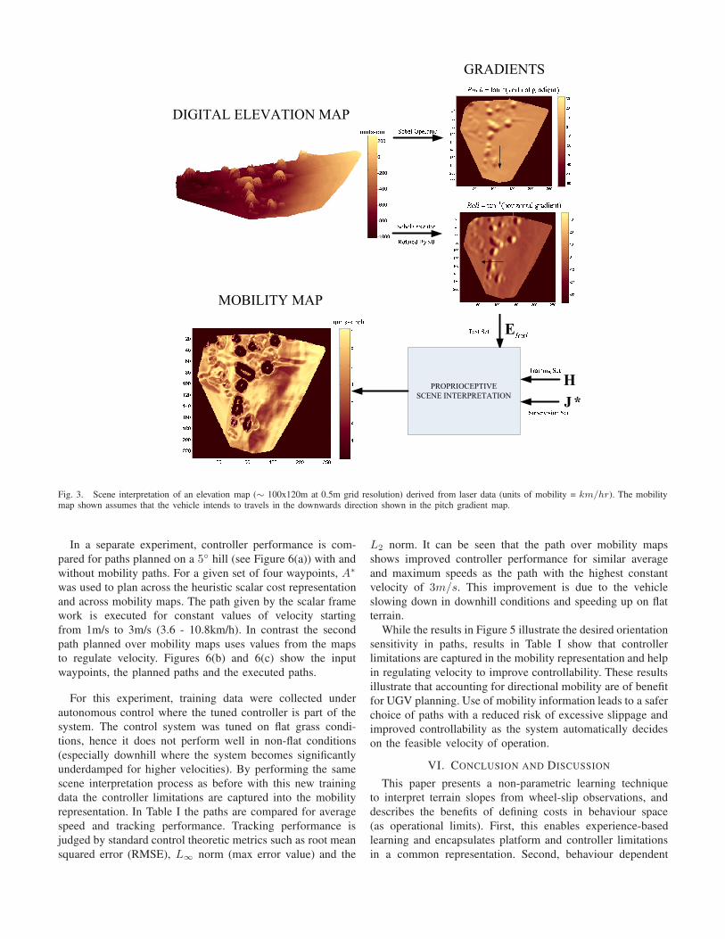
Fig. 3. Scene interpretation of an elevation map (∼ 100x120m at 0.5m grid resolution) derived from laser data (units of mobility = km/hr). The mobilitymap shown assumes that the vehicle intends to travels in the downwards direction shown in the pitch gradient map.

In a separate experiment, controller performance is com-

pared for paths planned on a 5◦ hill (see Figure 6(a)) with and

without mobility paths. For a given set of four waypoints, A∗

was used to plan across the heuristic scalar cost representation

and across mobility maps. The path given by the scalar frame

work is executed for constant values of velocity starting

from 1m/s to 3m/s (3.6 - 10.8km/h). In contrast the second

path planned over mobility maps uses values from the maps

to regulate velocity. Figures 6(b) and 6(c) show the input

waypoints, the planned paths and the executed paths.

For this experiment, training data were collected under

autonomous control where the tuned controller is part of the

system. The control system was tuned on flat grass condi-

tions, hence it does not perform well in non-flat conditions

(especially downhill where the system becomes significantly

underdamped for higher velocities). By performing the same

scene interpretation process as before with this new training

data the controller limitations are captured into the mobility

representation. In Table I the paths are compared for average

speed and tracking performance. Tracking performance is

judged by standard control theoretic metrics such as root mean

squared error (RMSE), L∞ norm (max error value) and the

L2 norm. It can be seen that the path over mobility maps

shows improved controller performance for similar average

and maximum speeds as the path with the highest constant

velocity of 3m/s. This improvement is due to the vehicle

slowing down in downhill conditions and speeding up on flat

terrain.

While the results in Figure 5 illustrate the desired orientation

sensitivity in paths, results in Table I show that controller

limitations are captured in the mobility representation and help

in regulating velocity to improve controllability. These results

illustrate that accounting for directional mobility are of benefit

for UGV planning. Use of mobility information leads to a safer

choice of paths with a reduced risk of excessive slippage and

improved controllability as the system automatically decides

on the feasible velocity of operation.

VI. CONCLUSION AND DISCUSSION

This paper presents a non-parametric learning technique

to interpret terrain slopes from wheel-slip observations, and

describes the benefits of defining costs in behaviour space

(as operational limits). First, this enables experience-based

learning and encapsulates platform and controller limitations

in a common representation. Second, behaviour dependent

(a) Uphill (b) (c)

(d) (e) Downhill (f)

(g) (h) (i) A scalar heuristic cost: max.possible slope (brighter pixels havehigher cost; notice that unknown re-gions have high cost)

Fig. 4. Mobility Maps for eight possible vehicle headings (a-h) and an alternative scalar cost representation (i)

(a) A∗ path planning on heuristic cost map (pathdistance: 101m)

(b) A∗ path planning on directional mobility maps(path distance: 121m forward and 109m backward)

Fig. 5. Path planning on heuristic cost maps vs. directional mobility maps. [white •(start) → white path → green ∗(goal) → green path → start]

TABLE I

TRAJECTORY FOLLOWING RESULTS: AVERAGE SPEED AND TRACKING PERFORMANCE

Speed performance Cross track error performance

time(s) Mean Vel(m/s) Max. Vel(m/s) RMSE L∞ norm L2 norm

A∗ + 1m/s 130 0.95 1.70 1.15 2.34 158.65A∗ + 2m/s 73 1.71 2.62 1.61 3.66 254.56A∗ + 3m/s 65 1.99 3.41 2.14 5.69 536.04

A∗+Mobility Maps 64 2.07 3.29 1.98 4.54 360.03

(a) Trajectory test environment - A 5◦ Hill

(b) A∗ Path on scalar heuristic cost (black) andthe executed trajectories with different constantvelocities (green-1m/s,blue-2m/s,red-3m/s)

(c) A∗ Path on mobility maps (black) and theexecuted trajectory with mobility values (green)

Fig. 6. Trajectory following experiment

costs can be created for aiding decision making, such as

orientation sensitive costs for UGV path planning. Finally,

proprioceptive feedback such as wheel slip can be incorporated

and used to learn effectively in complex environments.

The current process of creating the mobility map is slow,

as it involves inverting an N×N matrix (where N is the

size of the dataset). In this work, the inversion was done off-

line, and the size of dataset was of the order of 10000 data

points. The mobility maps shown took about 15 minutes to

generate on a 2GHz PC in a Matlab implementation. After

the first interpretation, the inverted matrix and the interpreted

values were cached and the subsequent queries were very

quick in comparison. A new query for an unknown test

condition took approximately 0.3 seconds, but cached queries

took approximately 0.03 seconds. Depending on the number

of repeated test conditions, the speed of the process will vary

for a given scene.

Non-parametric techniques and experience based learning,

although not viable as a full online process at present, are a

sensible approach in off-road unstructured conditions where

simplifying assumptions about the environment cannot be

made. They are practical for off-line analysis of sensor in-

formation to be used as prior data for path planning. More

importantly, they provide a theoretical approach to the process

of defining and generating costs. Sparsification and local

approximations in GP’s is an active area of research, and these

techniques can be used in the future to make it more viable.

ACKNOWLEDGMENT

This work is supported by the ARC Centre of Excellence

programme, funded by the Australian Research Council (ARC)

and the New South Wales State Government.

REFERENCES

[1] Pieter Abbeel and Andrew Y. Ng. Apprenticeship learning via inversereinforcement learning. In 21st International Conference on Machine

Learning, Banff, Canada, 2004.[2] Anelia Angelova, L. Matthies, D. Helmick, and P. Perona. Learning and

prediction of slip using visual information. Journal of Field Robotics,2007.

[3] C. M. Bishop. Pattern Recognition And Machine Learning. Springer,2006.

[4] Rafael C. Gonzalez and Richard E. Woods. Digital Image Processing.Prentice Hall, 3rd edition edition, 2008.

[5] Alexander R. Green and David Rye. Sensible planning for vehiclesoperating over difficult unstructured terrains. In IEEE Aerospace

Conference, pages 1–8, 2007.[6] R. Hadsell, P. Sermanet, A. N. Erkan, J. Ben, J. Han, B. Flepp, U. Muller,

and Y. LeCun. Online learning for offroad robots: Using spatiallabel propagation to learn by long-range traversability. Proceedings of

Robotics: Science and Systems, 2007.[7] L. D. Jackel, Eric Krotkov, Michael Perschbacher, Jim Pippine, and Chad

Sullivan. The darpa lagr program: Goals, challenges, methodology, andphase i results. Journal of Field Robotics, 23(11-12):945–973, 2006.

[8] S. J. Julier, J. K. Uhlmann, and H. F. Durrant-Whyte. A new methodfor the nonlinear transformation of means and covariances in filters andestimators. In IEEE Transactions on Automatic Control, volume 45,2000.

[9] Anh Tuan Le, D.C. Rye, and H.F. Durrant-Whyte. Estimation oftrack-soil interactions for autonomous tracked vehicles. Robotics and

Automation, 1997. Proceedings., 1997 IEEE International Conference

on, 2:1388–1393 vol.2, Apr 1997.[10] L. Ojeda, J. Borenstein, G. Witus, and R. Karlsen. Terrain characteriza-

tion and classification with a mobile robot. Journal Of Field Robotics,2006.

[11] C. E. Rasmussen and Z. Ghahramani. Infinite mixtures of gaussianprocess experts. In In Advances in Neural Information Processing

Systems 14, pages 881–888. MIT Press, 2002.[12] C. E. Rasmussen and C. K. I. Williams. Gaussian Processes for Machine

Learning. MIT Press, 2006.[13] Michael Shneier, Tommy Chang, Tsai Hong, Will Shackleford, Roger

Bostelman, and James S. Albus. Learning traversability models forautonomous mobile vehicles. Autonomous Robots, 24(1), 2008.

[14] David Silver, James Bagnell, and Anthony Stentz. High performanceoutdoor navigation from overhead data using imitation learning. InRobotics: Science and Systems IV, Zurich, Switzerland, 2008.

[15] R. S. Sutton and A. G. Barto. Reinforcement Learning: An Introduction.The MIT Press, 1998.

[16] J. Y. Wong. Theory Of Ground Vehicles. New York: Wiley, 3rd editionedition, 2001.