Embed Size (px)
Citation preview
Sustainability 2022, 14, 3188. https://doi.org/10.3390/su14063188 www.mdpi.com/journal/sustainability
Article
Parametric and Non-Parametric Analyses for Pedestrian Crash
Severity Prediction in Great Britain
Maria Rella Riccardi 1,*, Filomena Mauriello 1, Sobhan Sarkar 2, Francesco Galante 1, Antonella Scarano 1
and Alfonso Montella 1
1 Department of Civil, Architectural and Environmental Engineering, University of Naples Federico II,
80125 Naples, Italy; [email protected] (F.M.); [email protected] (F.G.);
[email protected] (A.S.); [email protected] (A.M.) 2 Information Systems & Business Analytics, Indian Institute of Management Ranchi, Ranchi 834 008, India;
* Correspondence: [email protected]; Tel.: +39-081-7683977
Abstract: The study aims to investigate the factors that are associated with fatal and severe vehicle–
pedestrian crashes in Great Britain by developing four parametric models and five non-parametric
tools to predict the crash severity. Even though the models have already been applied to model the
pedestrian injury severity, a comparative analysis to assess the predictive power of such modeling
techniques is limited. Hence, this study contributes to the road safety literature by comparing the
models by their capabilities of identifying the significant explanatory variables, and by their perfor-
mances in terms of the F-measure, the G-mean, and the area under curve. The analyses were carried
out using data that refer to the vehicle–pedestrian crashes that occurred in the period of 2016–2018.
The parametric models confirm their advantages in offering easy-to-interpret outputs and under-
standable relations between the dependent and independent variables, whereas the non-parametric
tools exhibited higher classification accuracies, identified more explanatory variables, and provided
insights into the interdependencies among the factors. The study results suggest that the combined
use of parametric and non-parametric methods may effectively overcome the limits of each group
of methods, with satisfactory prediction accuracies and the interpretation of the factors contributing
to fatal and serious crashes. In the conclusion, several engineering, social, and management pedes-
trian safety countermeasures are recommended.
Keywords: random parameter multinomial logit; ordered logit; association rules;
classification trees; random forests; artificial neural networks; support vector machines;
pedestrian crashes
1. Introduction
The identifying factors that affect the crash injury severity, and understanding how
these factors affect the injury severity, are critical in the planning and implementation of
highway safety improvement programs. There is also great emphasis on serious injury
crashes in the EU Road Safety Policy Framework 2021–2030 [1], which has the target of
halving the serious injuries by 2030, and the goal of enhancing the accessibility and safety
of vulnerable road users. Moreover, the number of pedestrians that were injured or that
are dead as a consequence of vehicle–pedestrian crashes is increasing over time. As an
example, in Great Britain, the proportion of fatal and severe injuries that involved pedes-
trians increased from 22.5% in 2011, to 28.9% in 2019 [2].
Since the risk factors that are associated with pedestrian-related crashes on transpor-
tation networks are usually different than those for motor vehicles, further actions are
strongly needed to improve pedestrian safety. The main aim of our study is to investigate
the factors that are associated with fatal and severe pedestrian crashes in Great Britain by
Citation: Rella Riccardi, M.;
Mauriello, F.; Sarkar, S.; Galante, F.;
Scarano, A.; Montella, A. Parametric
and Non-Parametric Analyses for
Pedestrian Crash Severity Prediction
in Great Britain. Sustainability 2022,
14, 3188. https://doi.org/10.3390/
su14063188
Academic Editor:
Ripon Kumar Chakrabortty
Received: 4 February 2022
Accepted: 4 March 2022
Published: 8 March 2022
Publisher’s Note: MDPI stays neu-
tral with regard to jurisdictional
claims in published maps and institu-
tional affiliations.
Copyright: © 2022 by the authors. Li-
censee MDPI, Basel, Switzerland.
This article is an open access article
distributed under the terms and con-
ditions of the Creative Commons At-
tribution (CC BY) license (https://cre-
ativecommons.org/licenses/by/4.0/).
Sustainability 2022, 14, 3188 2 of 45
developing four parametric models and five non-parametric tools in order to explore the
coexistence of the pedestrian, driver, vehicle, roadway, and environmental factors. When
the interactions between these factors and the severity are co-considered and co-investi-
gated, the severe injury causes and the related solutions can be better identified [3], which
can assist in the selection of appropriate safety countermeasures in order to contribute to
the EU goals. Furthermore, in order to provide support for the choice of the appropriate
prediction method, the nine parametric and non-parametric methods are compared by
their capabilities of identifying the significant explanatory variables that affect the crash
severity, and by their performances. Finally, the study also addresses the issue of the im-
balanced distributions of the crash severity levels. A small proportion of fatal crashes is a
common feature of most crash datasets [4] and, hence, many researchers merge fatal
crashes with severe crashes in order to gain better performances from the implemented
models [5–7]. However, in our study, we decided not to join fatal and serious injury
crashes together in order to identify both of the factors that contribute to fatal and serious
injury crashes. The unbalanced data issue was treated by introducing weights, which
forced the estimator to learn on the basis of the importance (which is based on the weight)
that was given to a particular severity level.
2. Prior Research
The analysis of prior research highlights the presence of two main groups of methods
that are usually implemented in crash severity analyses. The two groups consist of para-
metric models and non-parametric tools.
Among the parametric models, the most widely used is the multinomial logit (MNL)
model (e.g., [8–10]). However, over the past decade, several studies have highlighted
some multinomial logit methodological limitations that could affect the study results with
erroneous inferences and biased crash predictions [11,12]. Indeed, the multinomial logit
model does not account for the unobserved heterogeneity, which forces the effects of the
observable variables to be the same across all observations. Consequently, the model may
be misspecified, and the estimated parameters may be biased and inefficient.
Thus, methodological approaches have been performed in order to gain more precise
estimations by explicitly accounting for the observation-specific variations in the effects
of the explanatory variables [13,14]. Among them, the random parameter (or simply the
“mixed” parameter) model allows the parameters to vary across individual crashes, which
range from negative to positive, and which are of varying magnitudes [15].
On the other hand, by recognizing the ordinal nature of the crash severity data, other
studies have been conducted by performing ordered response models [12,16]. Thus,
among the most popular discrete choice approaches, discrete ordered probability meth-
ods (such as ordered logit models) have shown great appeal. Yamamoto et al. [17] further
suggest that the traditional unordered models may provide unbiased estimates of the pa-
rameters, especially in cases of missing data and under-reporting. Despite the ordinal na-
ture of the injury severity variable, many researchers [18–20] point out that the traditional
ordered response structure may impose a certain kind of monotonic effect of the inde-
pendent variables on the injury severity levels. A chance to overcome the ordered logit
model limitation comes with the mixed ordered response logit model, which generalizes
the standard ordered response model, allows the flexibility of the effects of the covariates
on the threshold value for each ordinal category, and captures the heterogeneous effects
[21].
Hence, both the ordered and unordered models have their benefits and limitations,
and the choice of one method over the others is governed by the availability and charac-
teristics of the data and involves considering the trade-offs [16]. However, all of the para-
metric models suffer fundamental limitations, such as the presumption of the crash data
distribution, and their restrictions on the linear relationship between the severity out-
comes and the explanatory variables. Furthermore, it is also well known that no-injury
and minor injury crashes are very rarely reported to the police [14,16], and an outcome-
Sustainability 2022, 14, 3188 3 of 45
based model may result in biased parameter estimates when traditional statistical estima-
tion techniques are used, which limits the ability to manage road safety. Another down-
side of the traditional statistical models is related to their difficulties in handling and pro-
cessing very large amounts of data, so that, in the last few years, data-driven methods
have been applied to crash analyses in an attempt to overcome the issue.
Free from a priori parametric assumptions [5], data-driven methods, which are also
known as “non-parametric algorithms”, include association rules (ARs), classification
trees (CTs), random forests (RFs), artificial neural networks (ANNs), and support vector
machines (SVMs). Association rules discovery (which is also known as the “supervised
association mining technique”) has been widely used to discover patterns from crash da-
tabases [22–24]. Classification trees have already been developed to uncover the patterns
that influence the crash severity for different road users in several papers [25]. Recently,
other researchers have implemented the random forest in lieu of the classification tree
since it considers an ensemble of trees instead of one [26,27]. Another tree-structure algo-
rithm is the ANN tool [28], which has been used to investigate vehicle–pedestrian crashes.
Among the non-parametric methods, there is also an increasing interest in using the SVM
tool to investigate the patterns that contribute to the pedestrian crash severity [29], which
is due to the straightforward algorithm abilities that the tool has demonstrated in provid-
ing a better prediction performance than other traditional methods.
The parametric and non-parametric model limitations in predicting the fatal and se-
rious injury crashes in the presence of imbalanced data have been demonstrated by sev-
eral studies [30,31]. To date, two common approaches have been proposed over the years
to address the problem [32,33]: (1) The application of learning approaches at the algorithm
level, and then, the calculation of the performance measures on the original dataset; and
(2) Sampling techniques that are used at the database level. The latter implies both over-
sampling and undersampling. Oversampling replicates the instances from the minor
class, and it repeats them until all of the classes have an equal frequency. Undersampling
discards the majority class instances until the majority class reaches the size of the minor
classes. It only considers the closeness of the data, and the intrinsic characteristics are not
taken into consideration [34]. The main drawback of the two sampling techniques is that
they change the original dataset by creating a new distorted sample around the decision
boundary of the majority and minority classes. Table 1 provides a summary of the key
literature findings.
Table 1. Summary of the key literature findings.
Issue References
The MNL is the most widely used model to investigate the crash contributory fac-
tors. [8–10]
The MNL limits the effect of each attribute so that they are the same across all obser-
vations. [11,12]
Random parameter models overcome the limits of the fixed formulation of the
MNL. [13–15]
Multinomial parametric models do not consider the ordered nature of the crash se-
verity. [16,17]
Standard ordered models impose a monotonic effect of the independent variables on
all the injury severity levels. [18,20]
Random parameter models overcome the limits of the fixed formulations of the
standard unordered and ordered models. [11–15,21]
All parametric models require a priori assumptions. [14]
Non-parametric models do not require a priori assumptions and they handle large
amounts of data. [13]
Limited prediction abilities of both parametric and non-parametric models in the
presence of imbalanced data. [30,31]
Sustainability 2022, 14, 3188 4 of 45
3. Crash Data
The crash data that was used in this study refer to the crashes that occurred in Great
Britain in the three-year period of 2016–2018. The detailed road safety data were collected
in the STATS19 dataset that is provided by the Department of Transport. The crash infor-
mation was collected by the police at the scene of the crash, or it was reported by a member
of the public at a police station. All of the reported crashes occurred on public highways
(including footways), and they included crashes with at least one vehicle (or a vehicle in
collision with a pedestrian) that was involved, and that resulted in personal injury. Orig-
inally, the crash data were provided in three subsets that reported the crash, the vehicle,
and the casualty-related information. In order to obtain a unique set of information, the
three subsets were merged by using the crash index as a key reference. Finally, only the
pedestrian crashes (67,356 pedestrian crashes, or 17.3% of the total crashes) were consid-
ered. The final dataset was rearranged by using 34 explanatory variables, as is shown in
the Appendix A section, Tables A1–A6. The variables were divided into: crash (Tables A1
and A2); vehicle (Tables A3 and A4); driver (Table A5); and pedestrian (Table A6) charac-
teristics. Several of the categories were aggregated and recoded in order to avoid ex-
tremely small occurrences, to remove redundant information, and to make the models
easier to interpret.
The Great Britain crash database provides three different crash severity levels: slight
injury, serious injury, and fatal crashes. The crash severity is classified according to the
injury severity of the most seriously injured person involved in the crash. A fatal crash is
a crash where at least one person dies within 30 days of the crash. A serious injury crash
is a crash where a person is detained in the hospital as an “in-patient”, or where a person
suffers from any of the following injuries: fractures, concussion, internal injuries, burns,
severe cuts, severe general shock that requires medical treatment, and injuries that result
in death within 30 days of the crash. Lastly, it is considered that a slight injury of a minor
character, such as a sprain (which includes a neck whiplash injury), a bruise or a cut that
is not judged to be severe, or a slight shock that requires roadside attention, are injuries
for which medical treatment is not required. In our database, the crash severities were as
follows: fatal (n = 1366; 2.0% of the total crashes); serious (n = 16,359; 24.3% of the total
crashes); and slight (n = 49,631; 73.7% of the total crashes).
4. Method
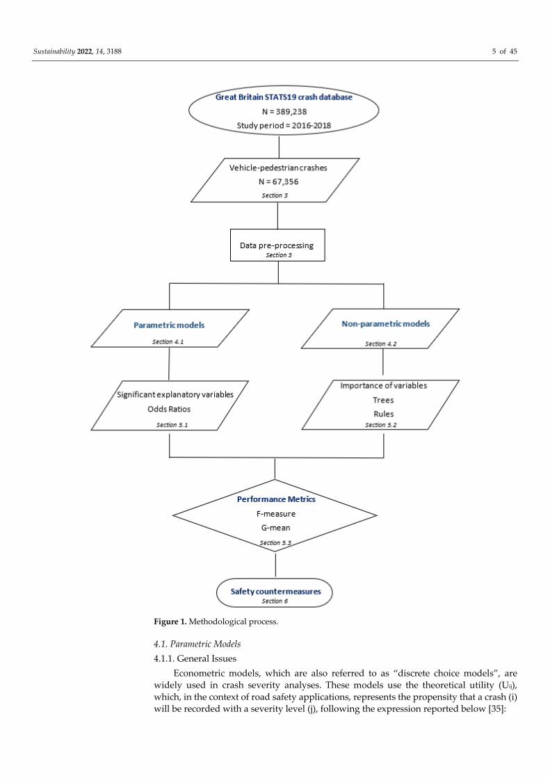
In our study, the crash severity is assumed to be the dependent variable. The inves-
tigation of the contributory factors that affect the crash severity was carried out using par-
ametric and non-parametric models. The methodological process is presented in Figure 1.
Figure 1 also contains information on the kinds of outputs that were provided by each
group of models. Furthermore, links to the paper sections are provided as well.
Sustainability 2022, 14, 3188 5 of 45
Figure 1. Methodological process.
4.1. Parametric Models
4.1.1. General Issues
Econometric models, which are also referred to as “discrete choice models”, are
widely used in crash severity analyses. These models use the theoretical utility (Uij),
which, in the context of road safety applications, represents the propensity that a crash (i)
will be recorded with a severity level (j), following the expression reported below [35]:
Sustainability 2022, 14, 3188 6 of 45
Uij = Vij + εij (1)
where Vij is the systematic component; and εij is the disturbance term.
The crash severity, as a three-level variable, is very adaptable to econometric models
with both unordered and ordered formulations. Indeed, each level of crash severity is
linked to: (1) The increasing severity of the most seriously injured person that is involved
in the crash; and to (2) The increasing costs in terms of the human, medical, and damage
factors, which involve losses in terms of the life years and the quality of life. Thus, the
crash severity has an ordinal nature, which could be addressed by performing the analysis
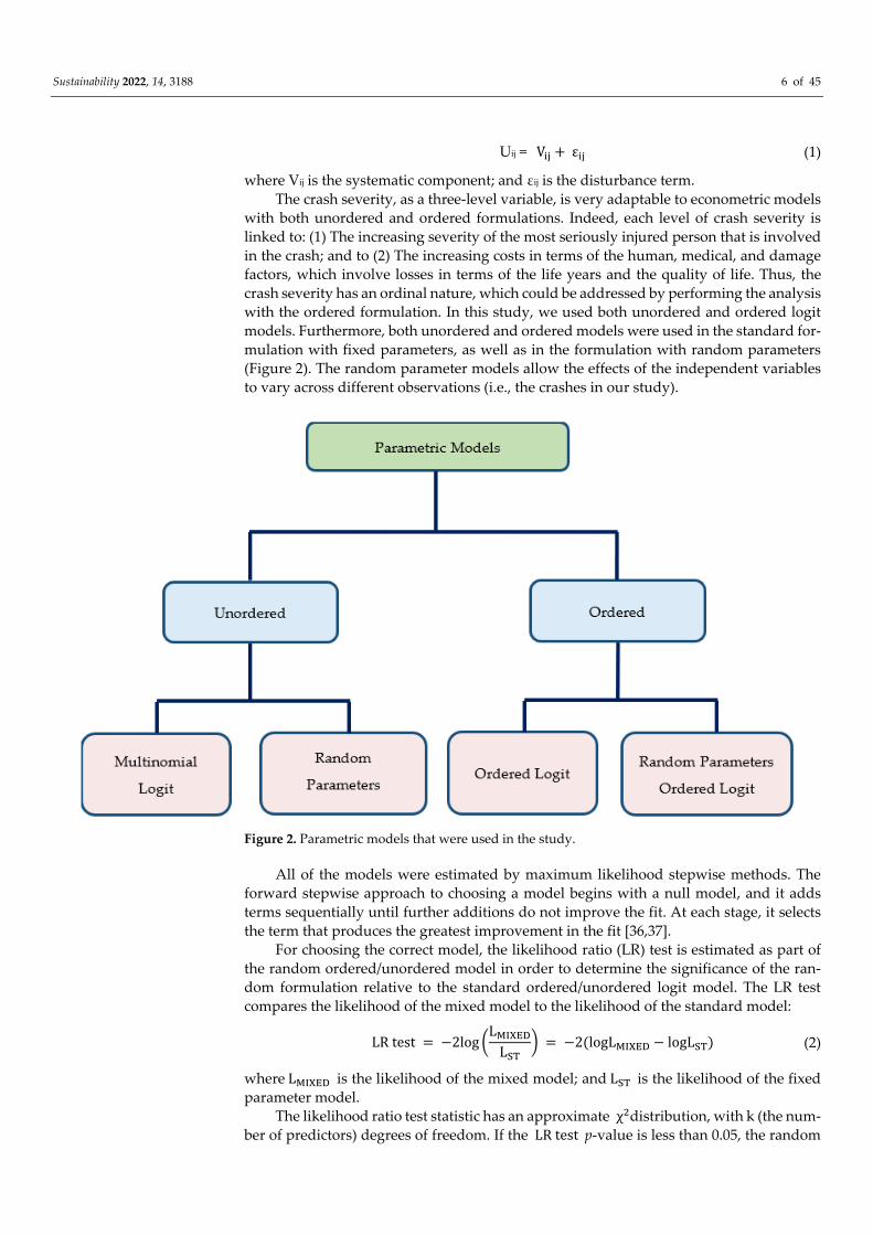
with the ordered formulation. In this study, we used both unordered and ordered logit
models. Furthermore, both unordered and ordered models were used in the standard for-
mulation with fixed parameters, as well as in the formulation with random parameters
(Figure 2). The random parameter models allow the effects of the independent variables
to vary across different observations (i.e., the crashes in our study).
Figure 2. Parametric models that were used in the study.
All of the models were estimated by maximum likelihood stepwise methods. The
forward stepwise approach to choosing a model begins with a null model, and it adds
terms sequentially until further additions do not improve the fit. At each stage, it selects
the term that produces the greatest improvement in the fit [36,37].
For choosing the correct model, the likelihood ratio (LR) test is estimated as part of
the random ordered/unordered model in order to determine the significance of the ran-
dom formulation relative to the standard ordered/unordered logit model. The LR test
compares the likelihood of the mixed model to the likelihood of the standard model:
LR test = −2log (LMIXED
LST) = −2(logLMIXED − logLST) (2)
where LMIXED is the likelihood of the mixed model; and LST is the likelihood of the fixed
parameter model.
The likelihood ratio test statistic has an approximate χ2distribution, with k (the num-
ber of predictors) degrees of freedom. If the LR test p-value is less than 0.05, the random
Sustainability 2022, 14, 3188 7 of 45
parameter logit model is superior to the standard model, with over 95% confidence. This
indicates that the random parameter multinomial logit model provides a statistically su-
perior fit relative to the traditional fixed parameter model [38].
Cross-validation was used to determine the generalizability and the overall utility of
the prediction models.
All of the explanatory variables were transformed into dummy variables through a
complete disjunctive decoding process. The predictors with multiple categories (k) were
converted to a series of indicator variables (dummy variables) with k−1 variables, and the
k-th dummy variable was not inserted into the model in order to avoid incurring the prob-
lem of perfect multicollinearity. All of the indicator variables were used to estimate the
four logistic regression models and were tested for inclusion. Each indicator variable was
assessed for its importance to the injury severity by using the z-test, with a significance
level of 10%. All four models were developed using the STATA software.
4.1.2. Multinomial Logit Model
The crash severity analysis can be carried out by considering the three classes (slight
injury, serious injury, and fatal crashes) as the possible discrete outcomes. In the general
case of a multinomial logit model for the crash injury severity outcomes, the propensity
of the crash (i) (i = 1, …, I) towards the severity category (j) (j = 1, …, J) is represented by
the severity propensity function [14]:
Uij = Vij + εij = βj′xij + εij (3)
where Vij is the systematic component;
εij is the disturbance term, which is assumed to be independently and identically distrib-
uted following the Type I generalized extreme value distribution (i.e., the Gumbel distri-
bution), with the mean equal to zero and the variance equal to one, and the scale param-
eter is η [14,39];
xij is a (K × 1) column vector of K exogenous attributes (geometric variables, environmen-
tal conditions, driver characteristics, etc.) that affects the pedestrian injury severity level
(j); and
βj is a (K × 1) column vector of the estimable parameters for the crash severity category
(j).
For a standard multinomial logit, the utility is linear in β, and then Vij = βjxij. Each
βj represents the estimated impact of the variable, xij, on the response variable, yi. The
standard multinomial logit formulation takes the following form:
P(yi = j) = Pi(j) = e(βj
′xij + εij)
∑ e(βj′xij + εij)J
j = 1
(4)
In a standard multinomial logit formulation, the βs are assumed to be fixed across
the observations, and the standard multinomial logit model is considered to be a fixed
parameter model.
The factor exp(β) is the odds ratio (OR), and it indicates the relative amount by which
the odds of the outcome increase (OR > 1) or decrease (OR < 1) when the value of the
corresponding indicator variable is 1.
4.1.3. Random Parameter Multinomial Logit Model
The random parameter multinomial logit model, which is also known as the “mixed
multinomial logit model”, is the generalized form of the multinomial logistic regression
model, in which the coefficients of any of the variables are not limited to a fixed value but
are allowed to vary across observations, or the analyst-specified groups of observations.
This specification is the same as for the standard logit, except that, instead of being fixed,
Sustainability 2022, 14, 3188 8 of 45
the β varies among the observations. The β coefficients are random and can be decom-
posed into their means and standard deviations [11]:
Uij = Vij + εij = βj′ xij + εij; β′j = b + βj (5)
where Vij is the systematic component; 𝜀𝑖𝑗 is the disturbance term, which is assumed to be
independently and identically distributed across the crash severity levels and the
crashes; xij is a (K × 1) column vector of K exogenous attributes (geometric variables, en-
vironmental conditions, driver characteristics, etc.) that are specific to the crash (i) and
that affect the pedestrian injury severity level (j); β′j is a crash-specific (K × 1) column vec-
tor of the corresponding parameters that varies across the crashes on the basis of the un-
observed crash-specific attributes; b are the means of the β’ random coefficients; and βj
are the standard deviations of the β’ random coefficients.
Hence, the standard multinomial logit hypotheses are relaxed (i.e., the mixed logit
does not exhibit independence from the irrelevant alternatives), and one or more param-
eters can be randomly distributed in the mixed model. Indeed, the presence of correlations
between the unobserved characteristics of each observation violates the disturbance inde-
pendence assumptions for the error terms, which leads to erroneous parameter estimates,
whereas the random parameter model addresses the unobserved heterogeneity within the
parameters that vary across the individual observations. If unobserved heterogeneity is
allowed, then βj is a vector with a continuous density function, which means that the un-
conditional probability of an individual (i) experiencing the severity level (j) from the set
of severity outcomes (J) is obtained by considering the integrals of the standard multino-
mial logit probabilities over the density of the parameters, and it can be expressed in the
form [40]:
Pi(j) = ∫e βj
′xij
∑ e βj′xij
J
f (β|ϴ)dβ (6)
where xij is a (K × 1) column vector of K exogenous attributes (geometric variables, envi-
ronmental conditions, driver characteristics, etc.) that are specific to the crash (i), and that
affect the pedestrian injury severity level (j); β′j is a crash-specific (K × 1) column vector
of the corresponding parameters that varies across the crashes on the basis of the unob-
served crash-specific attributes; f (β|ϴ) is the density function of the β coefficients; and ϴ
is a vector of the parameters that describes the density function of the β coefficients in
terms of the mean and the variance.
The random multinomial logit probability is expressed as the weighted average of
the probability that is evaluated with the multinomial logit formula at different values of
β, with the weights provided by the density function (f(β)). The standard multinomial
logit is a special case of the mixed logit formulation because if βj = b for each observation,
there is no crash-specific unobserved heterogeneity among the data, and the random pa-
rameter model coincides with the standard multinomial logit with fixed parameters (b),
and f(β) = 1 for βj = b, while it is 0 for βj ≠ b.
4.1.4. Ordered Logit Model
The multinomial logit model disregards the ordered nature of the injury severity lev-
els and treats them as independent alternatives; thus, the ordering information is lost [21].
The model is based on the cumulative probabilities of the response variables, and it is
assumed that the logit of each cumulative probability is a linear function of the covariates,
with regression coefficients that are constant across the response categories. In this case,
the effects of the explanatory variables on the severity levels are assumed to be fixed
across the observations. In other words, ordered logistic regression assumes that the coef-
ficients that describe the relationship between the lowest versus all of the higher catego-
ries of the dependent variable (which is the crash severity in our study) are the same as
those that describe the relationship between the next lowest category and all of the higher
Sustainability 2022, 14, 3188 9 of 45
categories. This is also called the “proportional odds assumption”, “the parallel regression
assumption”, or the “grouped continuous model” [41]. Assuming that the severity of a
crash is an ordered discrete variable with j categories (slight, serious, and fatal), three lev-
els are given meaningful numeric values, usually 0, 1, ..., J (J is the upper limit). Slight,
serious, and fatal might be labeled as “0”, “1”, and “2”, respectively, and the numerical
values represent a ranking so that, for the crash severity, the “1” label is more severe than
the “0” label in a qualitative sense, and the difference between the “2” and the “1” is not
the same as for that between the “1” and the “0”. In this case, although the numerical
outcomes are merely the labels of the non-quantitative outcomes, the analysis will none-
theless have a regression-style motivation [42]. The severity propensity function is as-
sumed as it is reported in Equation (7), and the ordinal response (yi) can be expressed as:
yi = {
0 if − ∞ ≤ Ui ≤ μ1 j if μj−1 < Ui ≤ μj
J if μJ−1 < Ui ≤ +∞ (7)
where μj represents the upper threshold for the injury severity (J); μj−1 represents the lower
threshold for the injury severity (J); and μj and μj−1
are the values of the cutoff, or the cut-
points.
The cumulative probability can be written as [41]:
Pi(j) = e(βj
′xij + εij −μj)
1 + e(βj′xij + εij−μj)
, j = 1,2, … , J − 1 (8)
4.1.5. Random Parameter Ordered Logit Model
The random parameter ordered logit model allows the thresholds in the ordered logit
model to vary on the basis of both the observed, as well as the unobserved, characteristics.
It also accommodates the unobserved heterogeneity in the effects of the exogenous varia-
bles on the injury propensity and on the threshold values through a suitable specification
of the thresholds that relaxes the restriction of identical thresholds [21]. As for the mixed
multinomial logit model, Equation (10) determines the probability that the crash (i) will
result in the injury-severity level (j). Hence, both the βs and the threshold (μ) can system-
atically vary across crashes because of the observed and unobserved factors: in an ordered
random parameter logit model, the thresholds also consist of a systematic component and
unobserved disturbance error terms, which thus allows for unobserved variability and
randomness in the thresholds, as is expressed by the formula below:
μij = Vj + τij (9)
where Vj is a systematic component; and τij is the unobserved disturbance error term.
Finally, the likelihood function for the individual (i) represents the probability of the
injury severity that will be experienced by that individual, and it can be evaluated as:
Pi(j) = ∫e(βj
′xij + εij −μj)
1 + e(βj′xij + εij−μj)
f (β|ϴ)dβ j = 1,2, … , J − 1 (10)
Therefore, in order to account for these circumstances, a random parameter ordered
logit model was developed to capture the unobserved heterogeneity, which is achieved
by adding a randomly distributed error term.
4.2. Non-Parametric Models
Five popular non-parametric algorithms, namely, association rules, classification
trees, random forests, artificial neural networks, and support vector machines, were used
Sustainability 2022, 14, 3188 10 of 45
to predict the injury severities of the pedestrian crashes. As data-driven and non-paramet-
ric methods, the machine learning algorithms do not require any a priori assumptions
about the relationships between the variables.
4.2.1. Association Rules
As a descriptive–analytic methodology, the association rules are used for extracting
knowledge from large datasets by generating rules that have the form: A→B. Each rule
contains at least one pattern, which is called the “antecedent” (A), as well as a “conse-
quent” (B). In our study, the latter consists of the fatal or serious injury severities. The a
priori algorithm (which was introduced by Agrawal et al. [43]) generates rules by using
simple and repetitive steps, and by examining all of the candidate item-sets in order to
find the frequent item-sets, until no new ones can be produced. All of the valid rules sat-
isfy the support, confidence, and lift thresholds, where the support is the percentage of
the entire dataset that is covered by the rule (Equation (11)), the confidence measures the
reliability of the inference of the rule (Equation (12)), and the lift is a measure of the sta-
tistical interdependence of the rule (Equation (13)):
S (A → B) = #(A∩B)
N; S(A) =
#(A)
N; S (B) =
#(B)
N; (11)
Confidence = S (A→B)
S(A) (12)
Lift = S (A → B)
(S (A) × S (B)) (13)
where S(A→B) is the support of the association rule; S(A) is the support of the antecedent;
S(B) is the support of the consequent; #(A→B) is the number of crashes, where both Con-
ditions A and B occur; #(A) is the number of crashes with A as the antecedent; #(B) is the
number of crashes with B as the consequent; and N is the total number of crashes in the
dataset.
A rule with a single antecedent and a single consequent is defined as a “two-item
rule”; similarly, a rule with two antecedents and a single consequent is defined as a “three-
item rule”. Each rule with n + 1 items is validated by verifying that each variable produces
a lift increase (LIC). The LIC ensures that each additional item in the rules leads to an
increase in terms of the lift.
The rules with only one item in the antecedent are used as a starting point, and the
rules with more items are selected over simpler ones by verifying that each variable pro-
duces a lift increase (LIC) that is not smaller than 1.05 [44]. The LIC ensures that each
additional item in the rules leads to an increase in terms of the lift. The LIC is calculated
as follows:
LIC = LiftAn
LiftAn−1
(14)
where An−1 is the antecedent of the rule with n−1 items; and An is the antecedent of the rule
with n items.
The threshold values of the support (S), the confidence (C), and the lift (L) were set
as follows: S ≥ 0.1%; C ≥ 4.0%; L ≥ 1.2; and LIC ≥ 1.05. The association rules were performed
in the R-CRAN software environment using the package, “arules”.
4.2.2. Classification Trees
A classification tree is a nonlinear tool and an oriented graph, where the root node is
divided into leaf nodes by an explanatory variable that is also called the “splitter”. All of
the independent variables are candidates for the splits at each internal node of the tree.
However, only the predictor that provides the best partition is chosen. In our study, we
developed the CART algorithm, which was introduced by Breiman et al. [45], and the
impurity at each node was assessed by the Gini reduction criterion (the higher the value
Sustainability 2022, 14, 3188 11 of 45
of the Gini index, the higher the homogeneity of the node that is due to the split), which
can be calculated as follows:
iY (t) = 1 − ∑ p(j|t)2
j
(15)
where P(j|t) is the proportion of the observations in the node (t) that belong to the class
(j).
If a node is “pure”, all of the observations in the node belong to one class, and the
impurity of that node is zero.
The total impurity of any tree (T) is defined as follows:
iY (T) = ∑ iY (t)p(t)
t ∈ T
(16)
where iY(t) is the impurity of the node (t); p(t) = N(t)/N is the weight of the node (t); N(t)
is the number of observations that fall in the node (t); N is the total number of observa-
tions; and �� is the set of terminal nodes of the tree (T).
By definition, the terminal nodes present low degrees of impurity compared with the
root node.
The total impurity of the tree is reduced by finding, at each node of the tree, the best
partition of the observations into disjoint classes, which are externally heterogeneous and
internally homogeneous.
The choice of the best classification rule was made through the V-fold cross-valida-
tion estimate. The initial set (S) is randomly divided into a V > 2-fold (Sv for v = 1, 2 ..., V).
The corresponding estimate of the error rate is given by:
ERvCART =
∑ (YCART(Xi) ≠ Yi)Nvi = 1
Nv (17)
where YCART(Xi) is the predicted class for the ith observation; Xi is the vector of the de-
scriptors of the ith observation; Yi is the class label of the ith observation; and Nv is the nu-
merosity of the set (Sv).
The estimate of the error rate, which is based on cross-validation (ER), is obtained by
combining the individual estimates for all the possible subsets (Sv).
ER = ∑ ERv
CARTVv = 1
V (18)
The tree growing was stopped on the basis of two criteria: (1) If the reduction in the
Gini measures was less than a prespecified minimum fixed value that was equal to 0.0001
(default value); and (2) If the maximum number of levels of the tree were equal to 4. These
parameters were chosen to minimize the error rate.
The class assigned to each node was selected according to the greatest value of the
posterior classification ratio (PCR) that was evaluated for that node. The PCR compares
the classification of the terminal nodes of the tree with the classification of the root node,
and it is calculated as follows [24]:
PCR (j|t) = p (j|t)
p (j|troot) (19)
where p(j|t) is the proportion of the observations in the node (t) that belong to the class
(j); and troot is the root node of the tree.
One of the outputs that is provided by the CART technique is the variable im-
portance, which defines the variable’s ability to influence the model. The relative im-
portance of the variable (VI) (Xj) is calculated as follows:
VI = ∑N(t)
N
T
t = 1 ∆iY(t, s) (20)
Sustainability 2022, 14, 3188 12 of 45
where VI represents the relative importance of the variable (Xj); ∆𝑖𝑌(𝑡, 𝑠) is the reduction
in the Gini index that is obtained by splitting the variable (Xj) at the node (t); N is the total
number of observations; and T is the number of nodes in the tree.
The classification trees were carried out with SPSS software.
4.2.3. Random Forests
Classification trees, despite their advantages, have sometimes been found to generate
unstable predictions given certain perturbations; thus, in order to improve the stability,
Breiman [46] proposed the RF method. RFs are an ensemble of B trees {T1(X), ..., TB(X)},
where Xi = {xi1, ..., xip} is a p-dimensional vector of the descriptors or properties that are
associated with the ith crash. The ensemble produces B outputs {Ŷ1 = T1(X), ..., ŶB = TB(X)},
where Ŷb, b = 1, ..., B, is the prediction for a crash by the bth tree. The outputs of all of the
trees are aggregated to produce one final prediction: Ŷ. For classification problems, Ŷ is
the class that is predicted by the majority of the trees.
Given the data on a set of n crashes, D = {(X1, Y1), ..., (Xn, Yn)}, where Xi is a vector of
the descriptors, and Yi is the corresponding class label for the ith crash, with i = 1, ..., n. The
algorithm proceeds as follows:
1. A bootstrap sample, which creates a random sample with a replacement from the
original sample, with the sample size (Nt) replicated B times.
2. For each bootstrap sample, the growing of a tree uses the CART algorithm, and
chooses, at each node, the best split among a randomly selected subset of descriptors;
3. Repeat the above steps until B trees are generated.
However, it has been shown that there is a potential overestimate of the true predic-
tion error, depending on the choices of the random forest hyperparameters, such as the
number of trees (B), and the number of descriptors. To reduce the true prediction error,
the out-of-bag estimate of the error rate (EROOB) was estimated by varying the B and the
number of descriptors:
EROOB = ∑ (YOOB(Xi) ≠ Yi)
Ni = 1
N (21)
where YOOB(Xi) is the predicted class for the ith crash; Xi is the vector of the descriptors of
the ith crash; Yi is the class label of the ith crash; and N is the total number of crashes.
The values of the number of trees and the number of descriptors were chosen so that
the EROOB tends to stabilize around the minimum value.
The variable importance measure for the variable, xj, (VI(xj)), is computed as the
sum of the importances over all of the trees in the forest:
VI(xj) = ∑ VIt(xj)
ntreest = 1
ntrees (22)
wher VIt(xj) eis the variable importance of the tth tree that is calculated using Equation
(20); and ntrees is the number of trees.
The RF was performed in the R-CRAN software environment using the packages,
“randomForest”, and “randomForestSRC”.
4.2.4. Artificial Neural Networks
As is the classification tree and the RF, the ANN is also an oriented graph that is
inspired by a biological neural network. Similar to the structure of the human brain, the
ANN models consist of neurons in complex and nonlinear forms. The ANN models work
by creating a nonlinear relationship between the dependent and independent variables,
depending on a set of experimental data. The neurons are connected to each other by
weighted links. ANNs consist of a layer of input nodes and a layer of output nodes that
are connected by one or more layers of hidden nodes. The input-layer nodes pass infor-
mation to the hidden-layer nodes by firing the activation functions, and the hidden-layer
Sustainability 2022, 14, 3188 13 of 45
nodes fire, or remain dormant, depending on the evidence that is presented. The hidden
layers apply weighting functions to the evidence, and, when the value of a particular node
or set of nodes in the hidden layer reaches a certain threshold, the value is passed to one
or more nodes in the output layer.
The technique creates a feed-forward multilayer perceptron ANN, which consists of
multiple nodes (or neurons) that are organized into three or more layers, with a backprop-
agation learning process to minimize the classification errors. In our study, a three-layer
network was implemented, as previous studies suggest that ANNs with singular hidden
layers are less likely to be trapped at a local minimum [47,48]. Thus, the information flows
from the input layer, passes through the hidden layer, and then flows to the output layer
to produce a classification. The hidden layer has 1 + ∑ kpPp = 1 neurons (consider a dataset
that contains P independent variables that are classified on the kp potential risk factors
that have effects on the crash severity), and each risk factor is represented by a node, while
another constant node is included, which represents the bias. The output layer has three
neurons, which accord with the three severity levels in the study.
The neurons of the input layer transfer information to the hidden layer through the
hyperbolic tangent activation function, and from the hidden layer to the output layer
through the softmax function.
z = softmax[∑ wj(2)
tanh ( ∑ wj,p(1)
kp
P
p = 1
)]
J
j = 1
(23)
where J is the number of neurons in the hidden layer; wj,p(1)
is the connection weight be-
tween the hidden node (j, j = 1, … J) and the input node (p, p = 1, …, P); kp are the factors;
and wj(2)
is the weight of the connection between the output node (z) and the hidden node
(j).
In the output layer, Z = 3 nodes expresses the severity outcomes that are predicted
by the ANN, and yi is the ith observed response in the dataset. If, for the ith crash, yi = z,
then z = 1, while z = 0 if otherwise.
The connection weights were estimated by using a backpropagation learning process
to minimize the classification errors. Standard backpropagation is a gradient descent al-
gorithm in which the network weights are moved along the negative of the gradient of
the performance function. The combination of weights that minimize the error function is
considered to be a solution to the learning problem. The backpropagation algorithm pro-
ceeds as follows:
1. The backpropagation algorithm starts with random weights, and the goal is to adjust
them to reduce this error until the ANN learns the training data;
2. If the expected output is not obtained, backward propagation begins. The difference
between the actual and the expected outputs is calculated recursively and step by
step, and the error is returned through the original link access;
3. The weight and the value of each neuron are then modified and are transmitted suc-
cessively to the input layer, and the forward multilayer perceptron restarts.
These two processes (forward multilayer perceptron and backpropagation error) are
repeated so that the error gradually decreases. The goal is to minimize the error by adjust-
ing the weights so that the optimum weights are obtained after the error backpropagation.
The gradient (G) of a weighting to the error, the total error (E), and the total mean
square errors (ep) are defined as:
G = ∂E
∂w (24)
E = ∑ ep (25)
Sustainability 2022, 14, 3188 14 of 45
ep = 1
2∑(yk
p− yk
p)
2m
k−1
(26)
where 𝑤 is one of the network weightings (wpl, wjp, wkj); ykp is the actual output; and yk
p is
the expected output.
The adjustment of the weight is calculated as:
∆wnew = −ηG + α∆wold (27)
where ∆wnewis the present adjustment for the weighting or for the threshold; ∆wold is the
immediate past value of its counterpart; α is a dynamic coefficient, and it takes a value in
the range of between 0 and 1; and G is the gradient of a weighting to the error.
This procedure was applied to the categorical data after transforming the categorical
variables into dummy variables through a complete disjunctive decoding process. The
predictors with multiple categories (k) were converted into a series of indicator variables
(dummy variables) with k variables.
Moreover, the k-fold cross-validation procedure was used in each modeling phase of
the ANN.
The importance of a specific explanatory variable is determined by identifying all of
the weighted connections between the nodes of interest. All of the weights that connect
the specific input node, which passes through the hidden layer to the specific response
variable, are identified. This is repeated for all of the other explanatory variables, until all
of the weights that are specific to each input variable are determined.
The ANN was performed with the SPSS software.
4.2.5. Support Vector Machines
A SVM, which was developed by Cortes and Vapnik [49], is used to develop an op-
timal separating hyperplane to categorize the observations into several groups, while
maximizing the margin between the decision boundaries and minimizing the empirical
error. The predictors are defined as the vectors (Xi = {xi1, ..., xip}), where p represents the
full set of crash-related variables, and the outcome is defined as yk, which represents the
injury severity levels of the crashes. Hence, the plane constitutes the decision boundaries,
and the hyperplane is a p−1 dimensional plane. The decision boundaries may or may not
be linear, depending on the pre-set kernel function. The radial basis function (RBF) is the
most commonly used for crash severity analyses since it is capable of capturing the non-
linearity relationships between the crash severity and the explanatory variables [50]:
K (Xi, Xj) = exp (−ϒ |Xi−Xj |2), ϒ > 0 (28)
where Xi and Xj are the vectors of the explanatory variables for the ith and the jth crashes;
|Xi−Xj |2 is the Euclidean distance between the two crashes, Xi and Xj; and ϒ = 1/σ2, where
σ2 is the variance of the samples selected by the model as support vectors.
The development of the SVM model also depends on the penalty parameter (C) of
the error term. It controls the trade-off between smooth decision boundaries, and the cor-
rect classification of the points, and it is calculated as follows:
ERSVM = ∑ (YSVM(Xi) ≠ Yi)
Ni = 1
N (29)
where YSVM(Xi) is the predicted class for the ith crash; 𝑋𝑖 is the vector of the descriptors of
the ith crash; 𝑌𝑖 is the lass label of the ith crash; and N is the total number of crashes.
To determine the separability of the optimal hyperplane, a grid search was used for
the joint optimization of the C and γ parameters and for the feature selection. This ap-
proach methodically builds and evaluates a model for each combination of algorithm pa-
rameters (γ and C) that are specified in a grid. For each model, the classification error was
used as a performance measure. The combination of the hyperparameters with the lower
classification error was chosen in order to develop the optimal hyperplane.
Sustainability 2022, 14, 3188 15 of 45
To effectively combine these parameters, and to avoid overfitting, the cross-valida-
tion method was used for each developed model, which provided information about how
well the SVM generalizes, specifically in terms of the range of expected errors.
The variables that contribute to the separability of the optimal hyperplane provide
an indication of the relative importances of the variables to the separation.
The SVM was performed in the R-CRAN software environment using the packages,
“caret” and “e1071”.
4.3. Dealing with Imbalanced Data
The study data are characterized by imbalanced classes, with order ratios of 2:100 for
the fatal crashes, and of 25:100 for the serious injury crashes. The issues that are relative
to the classification performance with imbalanced data have been highlighted in previous
studies (e.g., [30,31,33,51]).
To take into account the skewed distribution of the classes, different weights were
given to both the majority and minority classes. The difference in the weights influenced
the classification of the classes during the learning phase. The whole purpose is to penalize
the misclassification that is made by the minority class by setting a higher class weight
and, at the same time, reducing the weight for the majority class. The weight was assigned
so that the response variable was equally distributed among the categories. The class
weights are inversely proportional to their respective frequencies [52–54]. Each weight
can be assessed as follows:
Wk = 𝑁𝑐𝑟𝑎𝑠ℎ𝑒𝑠
𝑛𝑐 × 𝑁𝑘 (30)
where k is the number of the crash severity level, with 1 = slight injury; 2 = serious injury;
and 3 = fatal; wk is the weight that is assigned to the respective level of severity (k); Ncrashes
is the total number of crashes in the dataset; nc = 3, which is equal to the number of crash
severity levels that are considered in the study; and Nk is the number of crashes with a
severity level (k).
4.4. Comparison among the Models
A classifier aims to minimize the false positive rates (which represent Type I errors)
and the false negative rates (which represent Type II errors), which maximizes the true
negative and positive rates. Among the common performance metrics that are used to
evaluate the classification performance, the accuracy and the error rate are the most
widely used. However, when the distribution of the response variable is extremely imbal-
anced, the accuracy has certain limitations. The error rate suffers from similar drawbacks.
First, it is easy to obtain high accuracies (or low error rates) under highly imbalanced
problems. Secondly, these classifiers assume that the errors are of equal value, which is
not true for the imbalanced data, where misclassifying the instances of the minority clas-
ses (fatal and serious injury crashes) is generally much costlier than misclassifying the
instances of the majority class (slight injury crashes) [55,56]. Moreover, the correct classi-
fication of the factors that contribute to fatal and serious injury crashes is a far cry from
the correct identification of the factors that contribute to slight injury crashes.
Hence, we chose to assess the multiparameter indicators, namely, the F-measure, the
G-mean, and the area under the curve (AUC), in order to evaluate the performances of the
implemented models in a single measure.
The performance measures are expressed as follows [33]:
Acc− = TN
TN + FP = specificity (31)
where Acc− is the true negative rate, which is also known as the “specificity”; TN is the
number of true negatives; and FP is the number of false positives.
Sustainability 2022, 14, 3188 16 of 45
Acc+ = TP
TP + FN = Recall = sensitivity (32)
where Acc+ is the true positive rate, which is also known as the “recall”, or the “sensitiv-
ity”; TP is the number of true positives; and FN is the number of false negatives.
G-mean = (Acc− × Acc+)1
2 (33)
Precision = 𝑇𝑃
𝑇𝑃 + 𝐹𝑃 (34)
F-measure = (1+β2) × Precision × Recall
Precision + Recall (35)
where β is a coefficient for adjusting the relative importance of the precision and recall,
which is set at a value that is equal to 1.
The G-mean combines the performances of the positive and negative classes, whereas
the F-measure combines the cases that are correctly classified with the Type I and Type II
errors. Indeed, when the errors increase, the F-measure decreases. The F-measure is also
the weighted harmonic mean of the precision and recall (which are both referred to as the
“minority class”), and a high F-measure usually indicates the model’s good overall per-
formance. The AUC is the area under the receiving operating curve (ROC), and it is a
widely used graphical plot that illustrates the ability of a classifier that is assessed by plot-
ting the true positive rate (TPR) (which is also known as the “sensitivity”) on the vertical
axis against the false positive rate (FPR) (which is also known as the “specificity”) on the
horizontal axis at various threshold settings. When the ROC curve is created, the AUC can
be assessed. The AUC represents the probability that the classifier correctly identifies an
observation that is randomly selected among the positive cases. An AUC value varies be-
tween 0 and 1. An AUC greater than 0.60 is considered satisfactory [57].
Once the performance metrics for each class are evaluated, the final values are the
weighted mean, in which the relative frequencies of the classes on the data are their
weights [58].
5. Results
5.1. Parametric Models
All the explanatory variables that are reported in the appendix section (Tables A1–
A6) were tested for inclusion in the econometric models. The estimation results are re-
ported in Tables 2–5. The variable indicators that are not statistically significant at the 0.10
level of significance, either for the fatal crashes or for the serious injury crashes, were re-
moved from the tables.
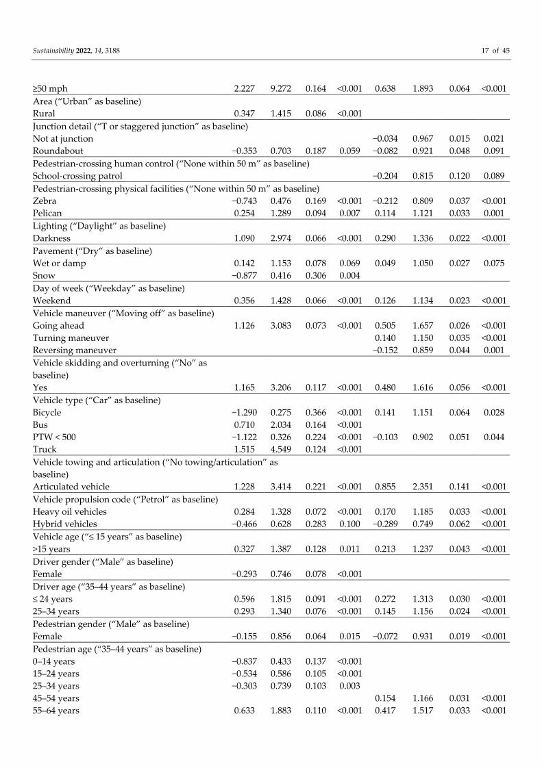
Table 2. Multinomial logit model: parameter estimates and goodness-of-fit measures.
Variable Fatal Serious
Estimate OR Std. Err. P > |z| Estimate OR Std. Err. P > |z|
Intercept −5.215 0.005 0.129 <0.001 −1.529 0.217 0.031 <0.001
Number of vehicles (“1 vehicle” as baseline)
2 0.682 1.978 0.106 <0.001 0.183 1.201 0.042 <0.001
≥3 1.170 3.222 0.187 <0.001 0.498 1.645 0.091 <0.001
First Road class (“C” as baseline)
B 0.091 1.095 0.031 0.004
A 0.558 1.747 0.067 <0.001 0.095 1.100 0.022 <0.001
Motorway 0.979 2.662 0.263 <0.001 0.484 1.623 0.230 0.035
Speed limit (“20 mph” as baseline)
30 mph 0.382 1.465 0.125 0.002 0.073 1.076 0.037 0.044
40 mph 1.384 3.991 0.163 <0.001 0.565 1.759 0.057 <0.001
Sustainability 2022, 14, 3188 17 of 45
≥50 mph 2.227 9.272 0.164 <0.001 0.638 1.893 0.064 <0.001
Area (“Urban” as baseline)
Rural 0.347 1.415 0.086 <0.001
Junction detail (“T or staggered junction” as baseline)
Not at junction −0.034 0.967 0.015 0.021
Roundabout −0.353 0.703 0.187 0.059 −0.082 0.921 0.048 0.091
Pedestrian-crossing human control (“None within 50 m” as baseline)
School-crossing patrol −0.204 0.815 0.120 0.089
Pedestrian-crossing physical facilities (“None within 50 m” as baseline)
Zebra −0.743 0.476 0.169 <0.001 −0.212 0.809 0.037 <0.001
Pelican 0.254 1.289 0.094 0.007 0.114 1.121 0.033 0.001
Lighting (“Daylight” as baseline)
Darkness 1.090 2.974 0.066 <0.001 0.290 1.336 0.022 <0.001
Pavement (“Dry” as baseline)
Wet or damp 0.142 1.153 0.078 0.069 0.049 1.050 0.027 0.075
Snow −0.877 0.416 0.306 0.004
Day of week (“Weekday” as baseline)
Weekend 0.356 1.428 0.066 <0.001 0.126 1.134 0.023 <0.001
Vehicle maneuver (“Moving off” as baseline)
Going ahead 1.126 3.083 0.073 <0.001 0.505 1.657 0.026 <0.001
Turning maneuver 0.140 1.150 0.035 <0.001
Reversing maneuver −0.152 0.859 0.044 0.001
Vehicle skidding and overturning (“No” as
baseline)
Yes 1.165 3.206 0.117 <0.001 0.480 1.616 0.056 <0.001
Vehicle type (“Car” as baseline)
Bicycle −1.290 0.275 0.366 <0.001 0.141 1.151 0.064 0.028
Bus 0.710 2.034 0.164 <0.001
PTW < 500 −1.122 0.326 0.224 <0.001 −0.103 0.902 0.051 0.044
Truck 1.515 4.549 0.124 <0.001
Vehicle towing and articulation (“No towing/articulation” as
baseline)
Articulated vehicle 1.228 3.414 0.221 <0.001 0.855 2.351 0.141 <0.001
Vehicle propulsion code (“Petrol” as baseline)
Heavy oil vehicles 0.284 1.328 0.072 <0.001 0.170 1.185 0.033 <0.001
Hybrid vehicles −0.466 0.628 0.283 0.100 −0.289 0.749 0.062 <0.001
Vehicle age (“≤ 15 years” as baseline)
>15 years 0.327 1.387 0.128 0.011 0.213 1.237 0.043 <0.001
Driver gender (“Male” as baseline)
Female −0.293 0.746 0.078 <0.001
Driver age (“35–44 years” as baseline)
≤ 24 years 0.596 1.815 0.091 <0.001 0.272 1.313 0.030 <0.001
25–34 years 0.293 1.340 0.076 <0.001 0.145 1.156 0.024 <0.001
Pedestrian gender (“Male” as baseline)
Female −0.155 0.856 0.064 0.015 −0.072 0.931 0.019 <0.001
Pedestrian age (“35–44 years” as baseline)
0–14 years −0.837 0.433 0.137 <0.001
15–24 years −0.534 0.586 0.105 <0.001
25–34 years −0.303 0.739 0.103 0.003
45–54 years 0.154 1.166 0.031 <0.001
55–64 years 0.633 1.883 0.110 <0.001 0.417 1.517 0.033 <0.001
Sustainability 2022, 14, 3188 18 of 45
65–74 years 1.295 3.651 0.111 <0.001 0.770 2.160 0.035 <0.001
≥75 years 2.578 13.171 0.092 <0.001 1.111 3.037 0.034 <0.001
Log likelihood null model −48,217.27
Log likelihood full model −40,469.52
R2McFadden 0.161
AIC 81,079.04
BIC 81,717.28
Note: “Slight injury” was the severity outcome baseline, and its severity function was constrained
to zero.
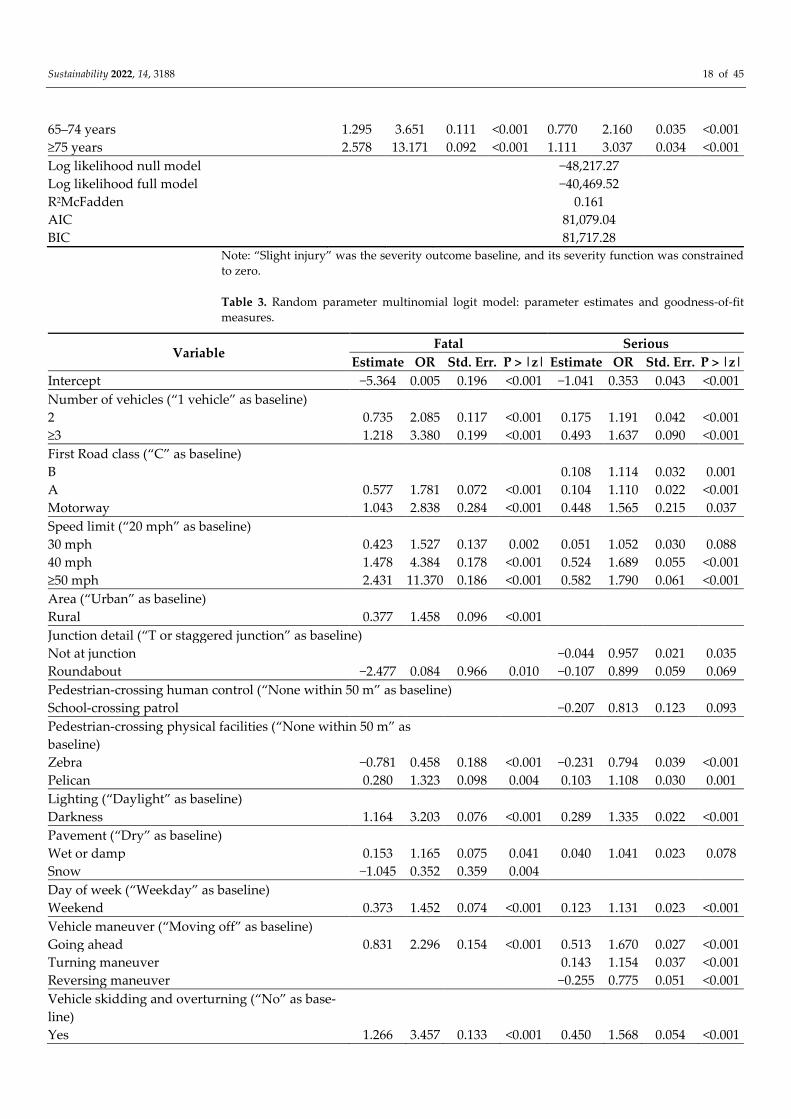
Table 3. Random parameter multinomial logit model: parameter estimates and goodness-of-fit
measures.
Variable Fatal Serious
Estimate OR Std. Err. P > |z| Estimate OR Std. Err. P > |z|
Intercept −5.364 0.005 0.196 <0.001 −1.041 0.353 0.043 <0.001
Number of vehicles (“1 vehicle” as baseline)
2 0.735 2.085 0.117 <0.001 0.175 1.191 0.042 <0.001
≥3 1.218 3.380 0.199 <0.001 0.493 1.637 0.090 <0.001
First Road class (“C” as baseline)
B 0.108 1.114 0.032 0.001
A 0.577 1.781 0.072 <0.001 0.104 1.110 0.022 <0.001
Motorway 1.043 2.838 0.284 <0.001 0.448 1.565 0.215 0.037
Speed limit (“20 mph” as baseline)
30 mph 0.423 1.527 0.137 0.002 0.051 1.052 0.030 0.088
40 mph 1.478 4.384 0.178 <0.001 0.524 1.689 0.055 <0.001
≥50 mph 2.431 11.370 0.186 <0.001 0.582 1.790 0.061 <0.001
Area (“Urban” as baseline)
Rural 0.377 1.458 0.096 <0.001
Junction detail (“T or staggered junction” as baseline)
Not at junction −0.044 0.957 0.021 0.035
Roundabout −2.477 0.084 0.966 0.010 −0.107 0.899 0.059 0.069
Pedestrian-crossing human control (“None within 50 m” as baseline)
School-crossing patrol −0.207 0.813 0.123 0.093
Pedestrian-crossing physical facilities (“None within 50 m” as
baseline)
Zebra −0.781 0.458 0.188 <0.001 −0.231 0.794 0.039 <0.001
Pelican 0.280 1.323 0.098 0.004 0.103 1.108 0.030 0.001
Lighting (“Daylight” as baseline)
Darkness 1.164 3.203 0.076 <0.001 0.289 1.335 0.022 <0.001
Pavement (“Dry” as baseline)
Wet or damp 0.153 1.165 0.075 0.041 0.040 1.041 0.023 0.078
Snow −1.045 0.352 0.359 0.004
Day of week (“Weekday” as baseline)
Weekend 0.373 1.452 0.074 <0.001 0.123 1.131 0.023 <0.001
Vehicle maneuver (“Moving off” as baseline)
Going ahead 0.831 2.296 0.154 <0.001 0.513 1.670 0.027 <0.001
Turning maneuver 0.143 1.154 0.037 <0.001
Reversing maneuver −0.255 0.775 0.051 <0.001
Vehicle skidding and overturning (“No” as base-
line)
Yes 1.266 3.457 0.133 <0.001 0.450 1.568 0.054 <0.001
Sustainability 2022, 14, 3188 19 of 45
Vehicle type (“Car” as baseline)
Bicycle −1.427 0.240 0.403 <0.001 0.223 1.250 0.067 0.001
Bus 0.634 1.885 0.147 <0.001
PTW<500 −1.288 0.276 0.254 <0.001 −0.112 0.894 0.053 0.033
Truck 1.674 5.333 0.151 <0.001
Vehicle towing and articulation (“No towing/articulation” as base-
line)
Articulated vehicle 1.272 3.568 0.234 <0.001 0.833 2.300 0.141 <0.001
Vehicle propulsion code (“Petrol” as baseline)
Heavy oil vehicles 0.284 1.328 0.072 <0.001 0.170 1.185 0.033 <0.001
Hybrid vehicles −0.466 0.628 0.283 0.100 −0.289 0.749 0.062 <0.001
Vehicle age (“≤ 15 years” as baseline)
>15 years 0.317 1.373 0.086 <0.001 0.153 1.165 0.023 <0.001
Driver gender (“Male” as baseline)
Female −0.343 0.710 0.092 <0.001
Driver age (“35–44 years” as baseline)
≤ 24 years 0.635 1.887 0.101 <0.001 0.294 1.342 0.031 <0.001
25–34 years 0.336 1.399 0.084 <0.001 0.152 1.164 0.025 <0.001
Pedestrian gender (“Male” as baseline)
Female −0.156 0.856 0.070 0.027 −0.097 0.908 0.020 <0.001
Pedestrian age (“35–44 years” as baseline)
0–14 years −0.884 0.413 0.148 <0.001
15–24 years −0.592 0.553 0.116 <0.001
25–34 years −0.342 0.710 0.114 0.003
45–54 years 0.157 1.170 0.031 <0.001
55–64 years 0.668 1.950 0.118 <0.001 0.426 1.531 0.033 <0.001
65–74 years 1.367 3.924 0.120 <0.001 0.785 2.192 0.035 <0.001
≥75 years 2.279 9.767 0.223 <0.001 0.297 1.346 0.179 0.097
Standard deviation of random parameter
Going-ahead vehicle maneuver 0.997 2.710 0.195 <0.001
Roundabout 2.583 13.237 0.643 <0.001
Pedestrian age ≥75 years 3.853 47.134 1.036 <0.001
Log likelihood null model −48,217.21
Log likelihood full model −39,565.46
R2McFadden 0.179
AIC 79,274.93
BIC 79,931.41
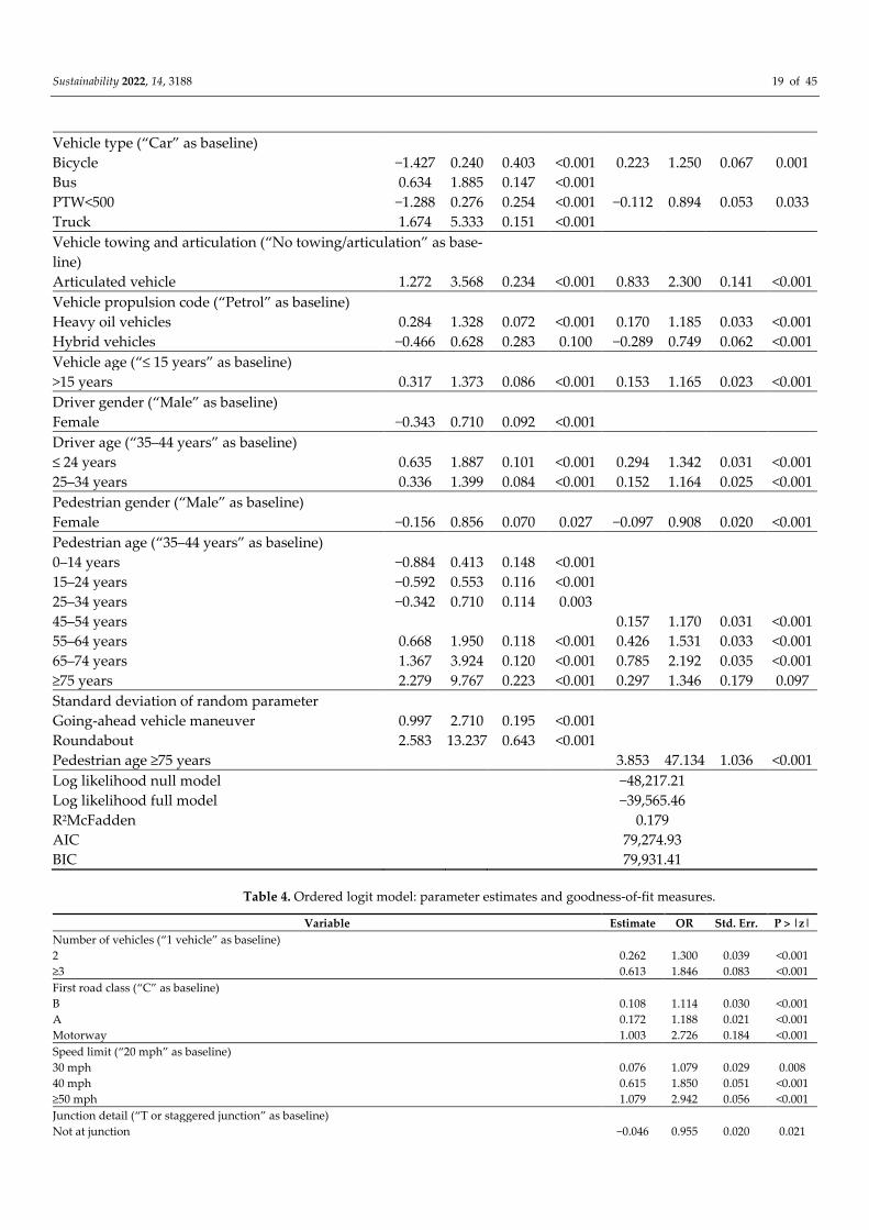
Table 4. Ordered logit model: parameter estimates and goodness-of-fit measures.
Variable Estimate OR Std. Err. P > |z|
Number of vehicles (“1 vehicle” as baseline)
2 0.262 1.300 0.039 <0.001
≥3 0.613 1.846 0.083 <0.001
First road class (“C” as baseline)
B 0.108 1.114 0.030 <0.001
A 0.172 1.188 0.021 <0.001
Motorway 1.003 2.726 0.184 <0.001
Speed limit (“20 mph” as baseline)
30 mph 0.076 1.079 0.029 0.008
40 mph 0.615 1.850 0.051 <0.001
≥50 mph 1.079 2.942 0.056 <0.001
Junction detail (“T or staggered junction” as baseline)
Not at junction −0.046 0.955 0.020 0.021
Sustainability 2022, 14, 3188 20 of 45
Roundabout −0.099 0.906 0.055 0.071
Pedestrian-crossing human control (“None within 50 m” as baseline)
School-crossing patrol −0.244 0.783 0.120 0.042
Pedestrian-crossing physical facilities (“None within 50 m” as baseline)
Zebra −0.226 0.798 0.037 <0.001
Pelican 0.103 1.108 0.028 <0.001
Lighting (“Daylight” as baseline)
Darkness 0.409 1.505 0.021 <0.001
Pavement (“Dry” as baseline)
Wet or damp 0.047 1.048 0.022 0.035
Snow −0.236 0.790 0.091 0.010
Day of week (“Weekday” as baseline)
Weekend 0.150 1.162 0.022 <0.001
Vehicle maneuver (“Moving off” as baseline)
Going ahead 0.587 1.799 0.023 <0.001
Turning maneuver 0.187 1.206 0.032 <0.001
Vehicle skidding and overturning (“No” as baseline)
Yes 0.607 1.835 0.051 <0.001
Vehicle type (“Car” as baseline)
Bus 0.184 1.202 0.046 <0.001
PTW<500 −0.158 0.854 0.051 0.002
Truck 0.462 1.587 0.066 <0.001
Vehicle towing and articulation (“No towing/articulation” as baseline)
Yes 1.260 3.525 0.129 <0.001
Vehicle propulsion code (“Petrol” as baseline)
Heavy oil vehicles 0.119 1.126 0.022 <0.001
Hybrid vehicles −0.340 0.712 0.071 <0.001
Vehicle age (“≤ 15 years” as baseline)
>15 years 0.232 1.261 0.042 <0.001
Driver age (“35–44 years” as baseline)
≤ 24 years 0.304 1.355 0.029 <0.001
25–34 years 0.155 1.168 0.024 <0.001
Pedestrian gender (“Male” as baseline)
Female −0.080 0.923 0.019 <0.001
Pedestrian age (“35–44 years” as baseline)
0–14 years −0.171 0.843 0.025 <0.001
45–54 years 0.233 1.262 0.031 <0.001
55–64 years 0.516 1.675 0.033 <0.001
65–74 years 0.895 2.447 0.035 <0.001
≥75 years 1.393 4.027 0.033 <0.001
Cut points
Cut1 2.381 0.039
Cut2 5.385 0.049
Log likelihood null model −48,217.27
Log likelihood full model −41,017.92
R2McFadden 0.149
AIC 82,101.85
BIC 82,402.74
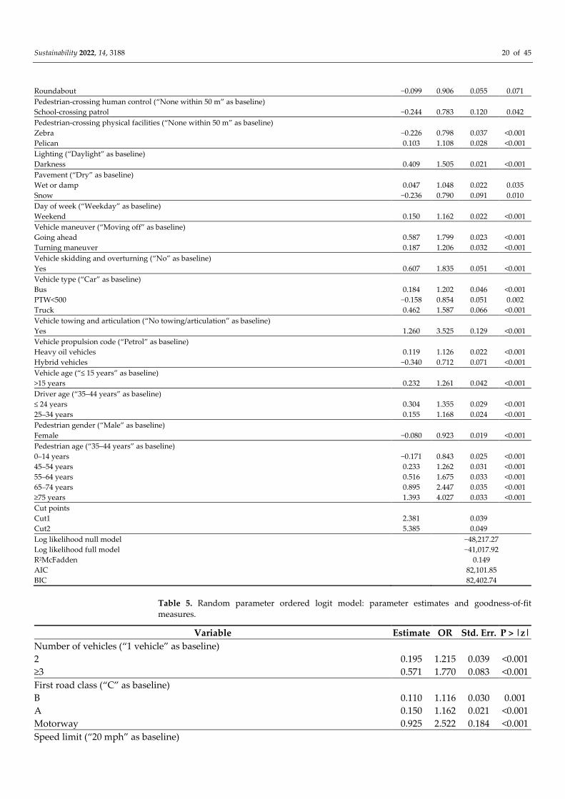
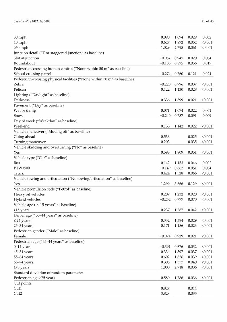
Table 5. Random parameter ordered logit model: parameter estimates and goodness-of-fit
measures.
Variable Estimate OR Std. Err. P > |z|
Number of vehicles (“1 vehicle” as baseline)
2 0.195 1.215 0.039 <0.001
≥3 0.571 1.770 0.083 <0.001
First road class (“C” as baseline)
B 0.110 1.116 0.030 0.001
A 0.150 1.162 0.021 <0.001
Motorway 0.925 2.522 0.184 <0.001
Speed limit (“20 mph” as baseline)
Sustainability 2022, 14, 3188 21 of 45
30 mph 0.090 1.094 0.029 0.002
40 mph 0.627 1.872 0.052 <0.001
≥50 mph 1.029 2.798 0.061 <0.001
Junction detail (“T or staggered junction” as baseline)
Not at junction −0.057 0.945 0.020 0.004
Roundabout −0.133 0.875 0.056 0.017
Pedestrian-crossing human control (“None within 50 m” as baseline)
School-crossing patrol −0.274 0.760 0.121 0.024
Pedestrian-crossing physical facilities (“None within 50 m” as baseline)
Zebra −0.228 0.796 0.037 <0.001
Pelican 0.122 1.130 0.028 <0.001
Lighting (“Daylight” as baseline)
Darkness 0.336 1.399 0.021 <0.001
Pavement (“Dry” as baseline)
Wet or damp 0.071 1.074 0.022 0.001
Snow −0.240 0.787 0.091 0.009
Day of week (“Weekday” as baseline)
Weekend 0.133 1.142 0.022 <0.001
Vehicle maneuver (“Moving off” as baseline)
Going ahead 0.536 0.025 <0.001
Turning maneuver 0.203 0.035 <0.001
Vehicle skidding and overturning (“No” as baseline)
Yes 0.593 1.809 0.051 <0.001
Vehicle type (“Car” as baseline)
Bus 0.142 1.153 0.046 0.002
PTW<500 −0.149 0.862 0.051 0.004
Truck 0.424 1.528 0.066 <0.001
Vehicle towing and articulation (“No towing/articulation” as baseline)
Yes 1.299 3.666 0.129 <0.001
Vehicle propulsion code (“Petrol” as baseline)
Heavy oil vehicles 0.209 1.232 0.020 <0.001
Hybrid vehicles −0.252 0.777 0.070 <0.001
Vehicle age (“≤ 15 years” as baseline)
>15 years 0.237 1.267 0.042 <0.001
Driver age (“35–44 years” as baseline)
≤ 24 years 0.332 1.394 0.029 <0.001
25–34 years 0.171 1.186 0.023 <0.001
Pedestrian gender (“Male” as baseline)
Female −0.074 0.929 0.021 <0.001
Pedestrian age (“35–44 years” as baseline)
0–14 years −0.391 0.676 0.032 <0.001
45–54 years 0.334 1.397 0.037 <0.001
55–64 years 0.602 1.826 0.039 <0.001
65–74 years 0.305 1.357 0.040 <0.001
≥75 years 1.000 2.718 0.036 <0.001
Standard deviation of random parameter
Pedestrian age ≥75 years 0.580 1.786 0.036 <0.001
Cut points
Cut1 0.827 0.014
Cut2 3.828 0.035
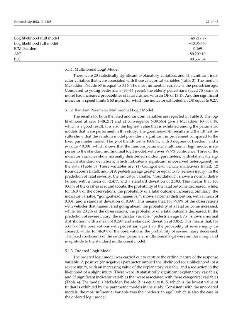
Sustainability 2022, 14, 3188 22 of 45
Log likelihood null model −48,217.27
Log likelihood full model −40,068.60
R2McFadden 0.169
AIC 80,209.10
BIC 80,537.34
5.1.1. Multinomial Logit Model
There were 20 statistically significant explanatory variables, and 41 significant indi-
cator variables that were associated with these categorical variables (Table 2). The model’s
McFadden Pseudo R2 is equal to 0.16. The most influential variable is the pedestrian age.
Compared to young pedestrians (35–44 years), the elderly pedestrians (aged 75 years or
more) had increased probabilities of fatal crashes, with an OR of 13.17. Another significant
indicator is speed limits ≥ 50 mph., for which the indicator exhibited an OR equal to 9.27.
5.1.2. Random Parameter Multinomial Logit Model
The results for both the fixed and random variables are reported in Table 3. The log-
likelihood at zero (−48,217) and at convergence (−39,565) give a McFadden R2 of 0.18,
which is a good result. It is also the highest value that is exhibited among the parametric
models that were performed in this study. The goodness-of-fit results and the LR test re-
sults show that the random model provides a significant improvement compared to the
fixed parameter model. The χ2 of the LR test is 1808.11, with 3 degrees of freedom, and a
p-value < 0.001, which shows that the random parameter multinomial logit model is su-
perior to the standard multinomial logit model, with over 99.9% confidence. Three of the
indicator variables show normally distributed random parameters, with statistically sig-
nificant standard deviations, which indicates a significant unobserved heterogeneity in
the data (Table 3). These variables are: (1) Going-ahead vehicle maneuvers (fatal); (2)
Roundabouts (fatal); and (3) A pedestrian age greater or equal to 75 (serious injury). In the
prediction of fatal severity, the indicator variable, “roundabout”, shows a normal distri-
bution, with a mean of −2.477, and a standard deviation of 2.583. This means that, for
83.1% of the crashes at roundabouts, the probability of the fatal outcome decreased, while,
for 16.9% of the observations, the probability of a fatal outcome increased. Similarly, the
indicator variable, “going-ahead maneuver”, shows a normal distribution, with a mean of
0.831, and a standard deviation of 0.997. This means that, for 79.8% of the observations
with vehicles that maneuvered going ahead, the probability of a fatal outcome increased,
while, for 20.2% of the observations, the probability of a fatal outcome decreased. In the
prediction of severe injury, the indicator variable, “pedestrian age ≥ 75”, shows a normal
distribution, with a mean of 0.297, and a standard deviation of 3.852. This means that, for
53.1% of the observations with pedestrian ages ≥ 75, the probability of severe injury in-
creased, while, for 46.9% of the observations, the probability of severe injury decreased.
The fixed coefficients of the random parameter multinomial logit were similar in sign and
magnitude to the standard multinomial model.
5.1.3. Ordered Logit Model
The ordered logit model was carried out to capture the ordinal nature of the response
variable. A positive (or negative) parameter implied the likelihood (or unlikelihood) of a
severe injury, with an increasing value of the explanatory variable, and a reduction in the
likelihood of a slight injury. There were 18 statistically significant explanatory variables,
and 35 significant indicator variables that were associated with these categorical variables
(Table 4). The model’s McFadden Pseudo R2 is equal to 0.15, which is the lowest value of
fit that is exhibited by the parametric models in the study. Consistent with the unordered
models, the most influential variable was the “pedestrian age”, which is also the case in
the ordered logit model.
Sustainability 2022, 14, 3188 23 of 45
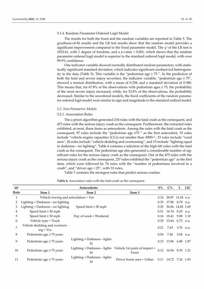
5.1.4. Random Parameter Ordered Logit Model
The results for both the fixed and the random variables are reported in Table 5. The
goodness-of-fit results and the LR test results show that the random model provides a
significant improvement compared to the fixed parameter model. The χ2 of the LR test is
1832.61, with 1 degree of freedom, and a p-value < 0.001, which shows that the random
parameter ordered logit model is superior to the standard ordered logit model, with over
99.9% confidence.
One indicator variable showed normally distributed random parameters, with statis-
tically significant standard deviation, which indicates significant unobserved heterogene-
ity in the data (Table 5). This variable is the “pedestrian age ≥ 75 ”. In the prediction of
both the fatal and severe injury severities, the indicator variable, “pedestrian age ≥ 75”,
showed a normal distribution, with a mean of 0.258, and a standard deviation of 0.580.
This means that, for 67.8% of the observations with pedestrian ages ≥ 75, the probability
of the most severe injury increased, while, for 32.8% of the observations, the probability
decreased. Similar to the unordered models, the fixed coefficients of the random parame-
ter ordered logit model were similar in sign and magnitude to the standard ordinal model.
5.2. Non-Parametric Models
5.2.1. Association Rules
The a priori algorithm generated 254 rules with the fatal crash as the consequent, and
475 rules with the serious injury crash as the consequent. Furthermore, the extracted rules
exhibited, at most, three items as antecedents. Among the rules with the fatal crash as the
consequent, 97 rules include the “pedestrian age ≥75 ” as the first antecedent, 53 rules
include “vehicle engine capacities (CCs) not smaller than 3000+”, 33 rules include “rural
area”, 26 rules include “vehicle skidding and overturning”, and 15 include “lighting equal
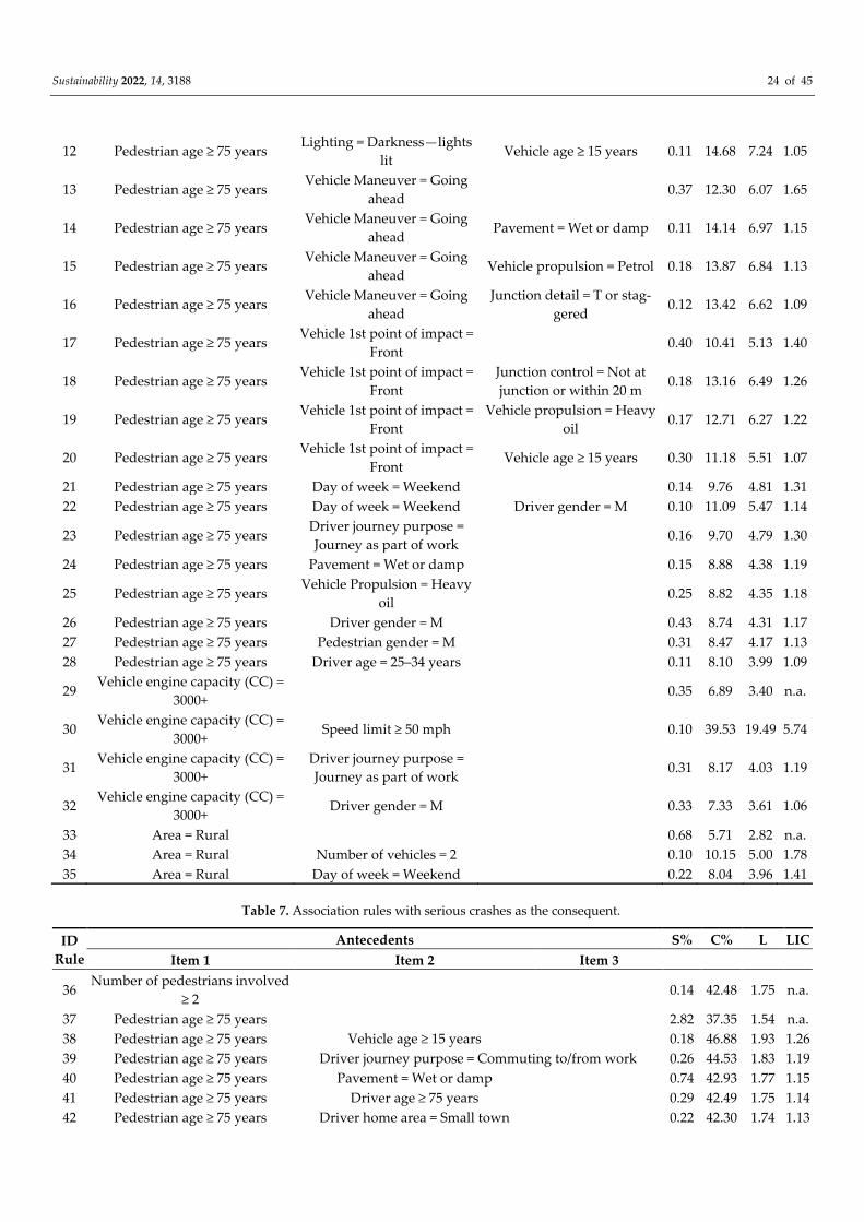
to darkness—no lighting”. Table 6 contains a selection of the high-lift rules with the fatal
crash as the consequent. The pedestrian age also generated a considerable number of sig-
nificant rules for the serious injury crash as the consequent. Out of the 475 rules with the
serious injury crash as the consequent, 237 rules exhibited the “pedestrian age” as the first
item, which were followed by 74 rules with the “number of pedestrians involved in a
crash”, and “driver age < 25”, with 33 rules.
Table 7 contains the strongest rules that predict serious crashes.
Table 6. Association rules with the fatal crash as the consequent.
ID
Rule
Antecedents S% C% L LIC
Item 1 Item 2 Item 3
1 Vehicle towing and articulation = Yes 0.14 28.87 14.24 n.a.
2 Lighting = Darkness—no lighting 0.33 17.80 8.78 n.a.
3 Lighting = Darkness—no lighting Speed limit ≥ 50 mph 0.29 30.06 14.82 1.69
4 Speed limit ≥ 50 mph 0.51 16.74 8.25 n.a.
5 Speed limit ≥ 50 mph Day of week = Weekend 0.16 18.41 9.08 1.10
6 Vehicle type = Truck 0.30 13.64 6.73 n.a.
7 Vehicle skidding and overturn-
ing = Yes 0.21 7.63 3.76 n.a.
8 Pedestrian age ≥ 75 years 0.56 7.46 3.68 n.a.
9 Pedestrian age ≥ 75 years Lighting = Darkness—lights
lit 0.15 13.96 6.88 1.87
10 Pedestrian age ≥ 75 years Lighting = Darkness—lights
lit
Vehicle 1st point of impact =
Front 0.12 16.94 8.35 1.21
11 Pedestrian age ≥ 75 years Lighting = Darkness—lights
lit Driver home area = Urban 0.11 14.72 7.26 1.05
Sustainability 2022, 14, 3188 24 of 45
12 Pedestrian age ≥ 75 years Lighting = Darkness—lights
lit Vehicle age ≥ 15 years 0.11 14.68 7.24 1.05
13 Pedestrian age ≥ 75 years Vehicle Maneuver = Going
ahead 0.37 12.30 6.07 1.65
14 Pedestrian age ≥ 75 years Vehicle Maneuver = Going
ahead Pavement = Wet or damp 0.11 14.14 6.97 1.15
15 Pedestrian age ≥ 75 years Vehicle Maneuver = Going
ahead Vehicle propulsion = Petrol 0.18 13.87 6.84 1.13
16 Pedestrian age ≥ 75 years Vehicle Maneuver = Going
ahead
Junction detail = T or stag-
gered 0.12 13.42 6.62 1.09
17 Pedestrian age ≥ 75 years Vehicle 1st point of impact =
Front 0.40 10.41 5.13 1.40
18 Pedestrian age ≥ 75 years Vehicle 1st point of impact =
Front
Junction control = Not at
junction or within 20 m 0.18 13.16 6.49 1.26
19 Pedestrian age ≥ 75 years Vehicle 1st point of impact =
Front
Vehicle propulsion = Heavy
oil 0.17 12.71 6.27 1.22
20 Pedestrian age ≥ 75 years Vehicle 1st point of impact =
Front Vehicle age ≥ 15 years 0.30 11.18 5.51 1.07
21 Pedestrian age ≥ 75 years Day of week = Weekend 0.14 9.76 4.81 1.31
22 Pedestrian age ≥ 75 years Day of week = Weekend Driver gender = M 0.10 11.09 5.47 1.14
23 Pedestrian age ≥ 75 years Driver journey purpose =
Journey as part of work 0.16 9.70 4.79 1.30
24 Pedestrian age ≥ 75 years Pavement = Wet or damp 0.15 8.88 4.38 1.19
25 Pedestrian age ≥ 75 years Vehicle Propulsion = Heavy
oil 0.25 8.82 4.35 1.18
26 Pedestrian age ≥ 75 years Driver gender = M 0.43 8.74 4.31 1.17
27 Pedestrian age ≥ 75 years Pedestrian gender = M 0.31 8.47 4.17 1.13
28 Pedestrian age ≥ 75 years Driver age = 25–34 years 0.11 8.10 3.99 1.09
29 Vehicle engine capacity (CC) =
3000+ 0.35 6.89 3.40 n.a.
30 Vehicle engine capacity (CC) =
3000+ Speed limit ≥ 50 mph 0.10 39.53 19.49 5.74
31 Vehicle engine capacity (CC) =
3000+
Driver journey purpose =
Journey as part of work 0.31 8.17 4.03 1.19
32 Vehicle engine capacity (CC) =
3000+ Driver gender = M 0.33 7.33 3.61 1.06
33 Area = Rural 0.68 5.71 2.82 n.a.
34 Area = Rural Number of vehicles = 2 0.10 10.15 5.00 1.78
35 Area = Rural Day of week = Weekend 0.22 8.04 3.96 1.41
Table 7. Association rules with serious crashes as the consequent.
ID
Rule
Antecedents S% C% L LIC
Item 1 Item 2 Item 3
36 Number of pedestrians involved
≥ 2 0.14 42.48 1.75 n.a.
37 Pedestrian age ≥ 75 years 2.82 37.35 1.54 n.a.
38 Pedestrian age ≥ 75 years Vehicle age ≥ 15 years 0.18 46.88 1.93 1.26
39 Pedestrian age ≥ 75 years Driver journey purpose = Commuting to/from work 0.26 44.53 1.83 1.19
40 Pedestrian age ≥ 75 years Pavement = Wet or damp 0.74 42.93 1.77 1.15
41 Pedestrian age ≥ 75 years Driver age ≥ 75 years 0.29 42.49 1.75 1.14
42 Pedestrian age ≥ 75 years Driver home area = Small town 0.22 42.30 1.74 1.13
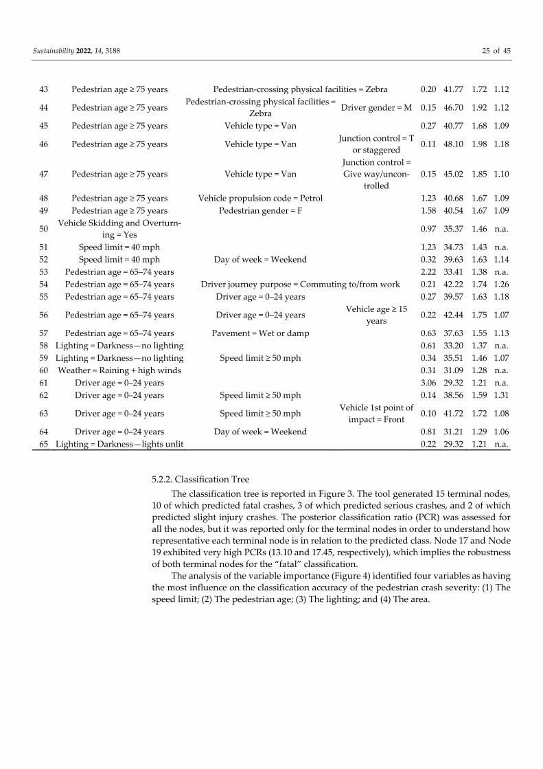
Sustainability 2022, 14, 3188 25 of 45
43 Pedestrian age ≥ 75 years Pedestrian-crossing physical facilities = Zebra 0.20 41.77 1.72 1.12
44 Pedestrian age ≥ 75 years Pedestrian-crossing physical facilities =
Zebra Driver gender = M 0.15 46.70 1.92 1.12
45 Pedestrian age ≥ 75 years Vehicle type = Van 0.27 40.77 1.68 1.09
46 Pedestrian age ≥ 75 years Vehicle type = Van Junction control = T
or staggered 0.11 48.10 1.98 1.18
47 Pedestrian age ≥ 75 years Vehicle type = Van
Junction control =
Give way/uncon-
trolled
0.15 45.02 1.85 1.10
48 Pedestrian age ≥ 75 years Vehicle propulsion code = Petrol 1.23 40.68 1.67 1.09
49 Pedestrian age ≥ 75 years Pedestrian gender = F 1.58 40.54 1.67 1.09
50 Vehicle Skidding and Overturn-
ing = Yes 0.97 35.37 1.46 n.a.
51 Speed limit = 40 mph 1.23 34.73 1.43 n.a.
52 Speed limit = 40 mph Day of week = Weekend 0.32 39.63 1.63 1.14
53 Pedestrian age = 65–74 years 2.22 33.41 1.38 n.a.
54 Pedestrian age = 65–74 years Driver journey purpose = Commuting to/from work 0.21 42.22 1.74 1.26
55 Pedestrian age = 65–74 years Driver age = 0–24 years 0.27 39.57 1.63 1.18
56 Pedestrian age = 65–74 years Driver age = 0–24 years Vehicle age ≥ 15
years 0.22 42.44 1.75 1.07
57 Pedestrian age = 65–74 years Pavement = Wet or damp 0.63 37.63 1.55 1.13
58 Lighting = Darkness—no lighting 0.61 33.20 1.37 n.a.
59 Lighting = Darkness—no lighting Speed limit ≥ 50 mph 0.34 35.51 1.46 1.07
60 Weather = Raining + high winds 0.31 31.09 1.28 n.a.
61 Driver age = 0–24 years 3.06 29.32 1.21 n.a.
62 Driver age = 0–24 years Speed limit ≥ 50 mph 0.14 38.56 1.59 1.31
63 Driver age = 0–24 years Speed limit ≥ 50 mph Vehicle 1st point of
impact = Front 0.10 41.72 1.72 1.08
64 Driver age = 0–24 years Day of week = Weekend 0.81 31.21 1.29 1.06
65 Lighting = Darkness—lights unlit 0.22 29.32 1.21 n.a.
5.2.2. Classification Tree
The classification tree is reported in Figure 3. The tool generated 15 terminal nodes,
10 of which predicted fatal crashes, 3 of which predicted serious crashes, and 2 of which
predicted slight injury crashes. The posterior classification ratio (PCR) was assessed for
all the nodes, but it was reported only for the terminal nodes in order to understand how
representative each terminal node is in relation to the predicted class. Node 17 and Node
19 exhibited very high PCRs (13.10 and 17.45, respectively), which implies the robustness
of both terminal nodes for the “fatal” classification.
The analysis of the variable importance (Figure 4) identified four variables as having
the most influence on the classification accuracy of the pedestrian crash severity: (1) The
speed limit; (2) The pedestrian age; (3) The lighting; and (4) The area.
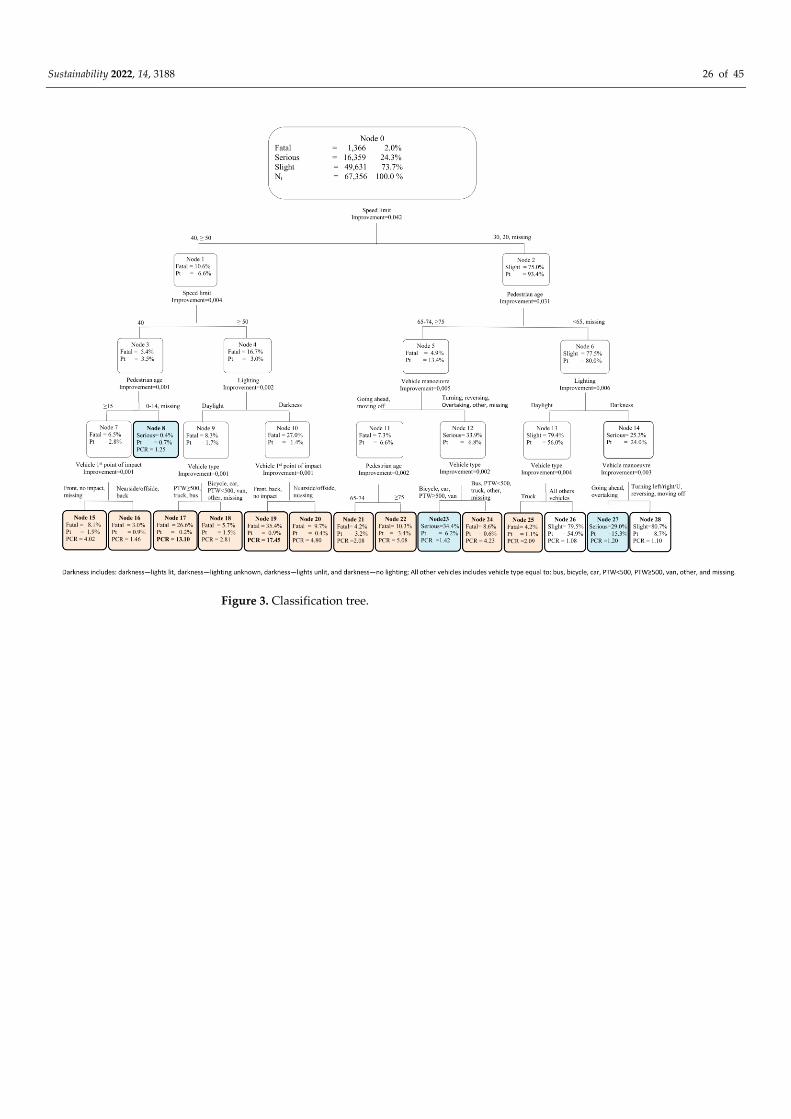
Sustainability 2022, 14, 3188 26 of 45
Figure 3. Classification tree.
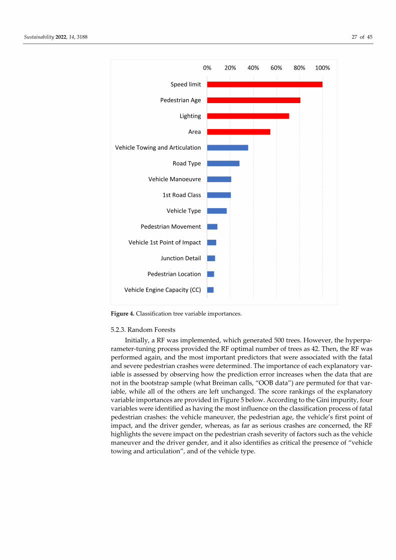
Sustainability 2022, 14, 3188 27 of 45
Figure 4. Classification tree variable importances.
5.2.3. Random Forests
Initially, a RF was implemented, which generated 500 trees. However, the hyperpa-
rameter-tuning process provided the RF optimal number of trees as 42. Then, the RF was
performed again, and the most important predictors that were associated with the fatal
and severe pedestrian crashes were determined. The importance of each explanatory var-
iable is assessed by observing how the prediction error increases when the data that are
not in the bootstrap sample (what Breiman calls, “OOB data”) are permuted for that var-
iable, while all of the others are left unchanged. The score rankings of the explanatory
variable importances are provided in Figure 5 below. According to the Gini impurity, four
variables were identified as having the most influence on the classification process of fatal
pedestrian crashes: the vehicle maneuver, the pedestrian age, the vehicle’s first point of
impact, and the driver gender, whereas, as far as serious crashes are concerned, the RF
highlights the severe impact on the pedestrian crash severity of factors such as the vehicle
maneuver and the driver gender, and it also identifies as critical the presence of “vehicle
towing and articulation”, and of the vehicle type.
0% 20% 40% 60% 80% 100%
Speed limit
Pedestrian Age
Lighting
Area
Vehicle Towing and Articulation
Road Type
Vehicle Manoeuvre
1st Road Class
Vehicle Type
Pedestrian Movement
Vehicle 1st Point of Impact
Junction Detail
Pedestrian Location
Vehicle Engine Capacity (CC)
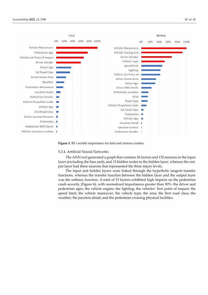
Sustainability 2022, 14, 3188 28 of 45
Figure 5. RF variable importance for fatal and serious crashes.
5.2.4. Artificial Neural Networks
The ANN tool generated a graph that contains 26 factors and 132 neurons in the input
layer (excluding the bias unit), and 13 hidden nodes in the hidden layer, whereas the out-
put layer had three neurons that represented the three injury levels.
The input and hidden layers were linked through the hyperbolic tangent transfer
functions, whereas the transfer function between the hidden layer and the output layer
was the softmax function. A total of 13 factors exhibited high impacts on the pedestrian
crash severity (Figure 6), with normalized importances greater than 50%: the driver and
pedestrian ages; the vehicle engine; the lighting; the vehicles’ first point of impact; the
speed limit; the vehicle maneuver; the vehicle type; the area; the first road class; the
weather; the junction detail; and the pedestrian-crossing physical facilities.
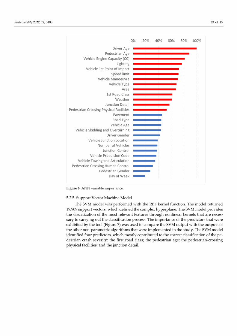
Sustainability 2022, 14, 3188 29 of 45
Figure 6. ANN variable importance.
5.2.5. Support Vector Machine Model
The SVM model was performed with the RBF kernel function. The model returned
19,909 support vectors, which defined the complex hyperplane. The SVM model provides
the visualization of the most relevant features through nonlinear kernels that are neces-
sary to carrying out the classification process. The importance of the predictors that were
exhibited by the tool (Figure 7) was used to compare the SVM output with the outputs of
the other non-parametric algorithms that were implemented in the study. The SVM model
identified four predictors, which mostly contributed to the correct classification of the pe-
destrian crash severity: the first road class; the pedestrian age; the pedestrian-crossing
physical facilities; and the junction detail.
0% 20% 40% 60% 80% 100%
Driver Age
Pedestrian Age
Vehicle Engine Capacity (CC)
Lighting
Vehicle 1st Point of Impact
Speed limit
Vehicle Manoeuvre
Vehicle Type
Area
1st Road Class
Weather
Junction Detail
Pedestrian Crossing Physical Facilities
Pavement
Road Type
Vehicle Age
Vehicle Skidding and Overturning
Driver Gender
Vehicle Junction Location
Number of Vehicles
Junction Control
Vehicle Propulsion Code
Vehicle Towing and Articulation
Pedestrian Crossing Human Control
Pedestrian Gender
Day of Week
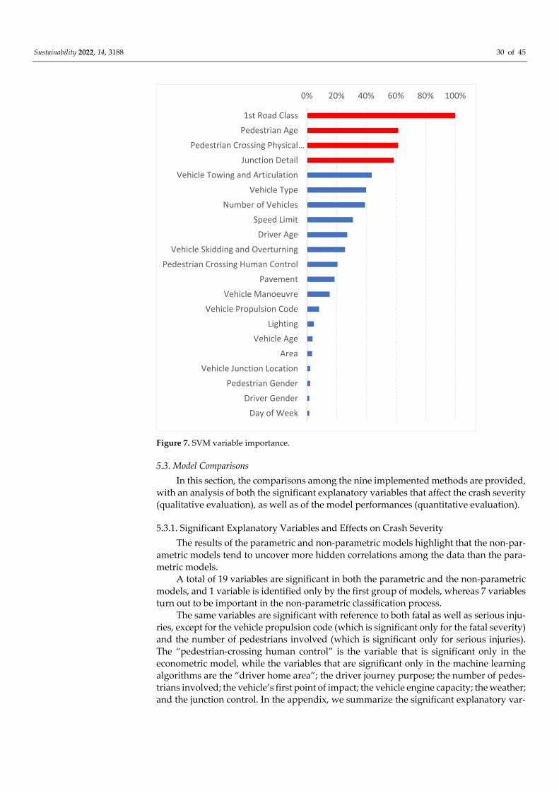
Sustainability 2022, 14, 3188 30 of 45
Figure 7. SVM variable importance.
5.3. Model Comparisons
In this section, the comparisons among the nine implemented methods are provided,
with an analysis of both the significant explanatory variables that affect the crash severity
(qualitative evaluation), as well as of the model performances (quantitative evaluation).
5.3.1. Significant Explanatory Variables and Effects on Crash Severity
The results of the parametric and non-parametric models highlight that the non-par-
ametric models tend to uncover more hidden correlations among the data than the para-
metric models.
A total of 19 variables are significant in both the parametric and the non-parametric
models, and 1 variable is identified only by the first group of models, whereas 7 variables
turn out to be important in the non-parametric classification process.
The same variables are significant with reference to both fatal as well as serious inju-
ries, except for the vehicle propulsion code (which is significant only for the fatal severity)
and the number of pedestrians involved (which is significant only for serious injuries).
The “pedestrian-crossing human control” is the variable that is significant only in the
econometric model, while the variables that are significant only in the machine learning
algorithms are the “driver home area”; the driver journey purpose; the number of pedes-
trians involved; the vehicle’s first point of impact; the vehicle engine capacity; the weather;
and the junction control. In the appendix, we summarize the significant explanatory var-
0% 20% 40% 60% 80% 100%
1st Road Class
Pedestrian Age
Pedestrian Crossing Physical…
Junction Detail
Vehicle Towing and Articulation
Vehicle Type
Number of Vehicles
Speed Limit
Driver Age
Vehicle Skidding and Overturning
Pedestrian Crossing Human Control
Pavement
Vehicle Manoeuvre
Vehicle Propulsion Code
Lighting
Vehicle Age
Area
Vehicle Junction Location
Pedestrian Gender
Driver Gender
Day of Week
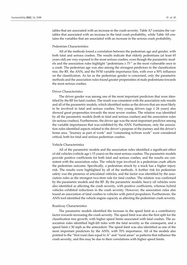
Sustainability 2022, 14, 3188 31 of 45
iables that are associated with an increase in the crash severity. Table A7 contains the var-
iables that associated with an increase in the fatal crash probability, while Table A8 con-
tains the variables that are associated with an increase in the serious crash probability.
Pedestrian Characteristics
All of the methods found a correlation between the pedestrian age and gender, with
both fatal and serious crashes. The results indicate that elderly pedestrians (at least 65
years old) are very exposed to the most serious crashes, even though the parametric mod-
els and the association rules highlight “pedestrians ≥ 75 ” as the most vulnerable once in
a crash. The pedestrian age was also among the strongest predictors in the classification
tree, the RF, the ANN, and the SVM variable importance lists, with over a 50% influence
on the classification. As far as the pedestrian gender is concerned, only the parametric
methods and the association rules found greater propensities of male pedestrians towards
the most serious crashes.
Driver Characteristics
The driver gender was among one of the most important predictors that were iden-
tified by the RF for fatal crashes. The result was consistent with the association rule results
and all of the parametric models, which identified males as the drivers that are most likely
to be involved in fatal and serious crashes. Very young drivers (age ≤ 24 years) also
showed great propensities towards the most severe crashes. The relation was identified
by all the parametric models (both in fatal and serious crashes) and the association rules
(in serious crashes). Furthermore, the driver age was the most important predictor among
the variable importances that was exhibited by the ANN. Furthermore, only the associa-
tion rules identified aspects related to the driver’s purpose of the journey and the driver’s
home area. “Journey as part of work” and “commuting to/from work” were considered
critical, both for fatal and serious pedestrian crashes.
Vehicle Characteristics
All of the parametric models and the association rules identified a significant effect
of old vehicles (vehicle age ≥ 15 years) on the most serious crashes. The parametric models
provide positive coefficients for both fatal and serious crashes, and the results are con-
sistent with the association rules. The vehicle type involved in a pedestrian crash affects
the pedestrian outcome. Specifically, a pedestrian struck by a truck has a higher injury
risk. The results were highlighted by all of the methods. A further risk for pedestrian
safety was the presence of articulated vehicles, and the factor was identified by the asso-
ciation rules as the strongest two-item rule for fatal crashes. The relation was confirmed
by the parametric models and the RF. By the parametric models, heavy oil vehicles were
also identified as affecting the crash severity, with positive coefficients, whereas hybrid
vehicles exhibited reductions in the crash severity. However, the association rules also
found an association of fatal crashes to vehicles with petrol propulsion. Furthermore, the
ANN tool identified the vehicle engine capacity as affecting the pedestrian crash severity.
Roadway Characteristics
The parametric models identified the increase in the speed limit as a contributory
factor towards increasing the crash severity. The speed limit was also the first split for the
classification tree growth, with higher speed limits associated with fatal crashes. The as-
sociation rules identified high-lift rules with the fatal severity as the consequent, and a
speed limit ≥ 50 mph as the antecedent. The speed limit was also identified as one of the
most important predictors by the ANN, with 70% importance. All of the models also
pointed to the “first road class equal to A” and “rural areas” as patterns that influence the
crash severity, and this may be due to their correlations with higher speed limits.
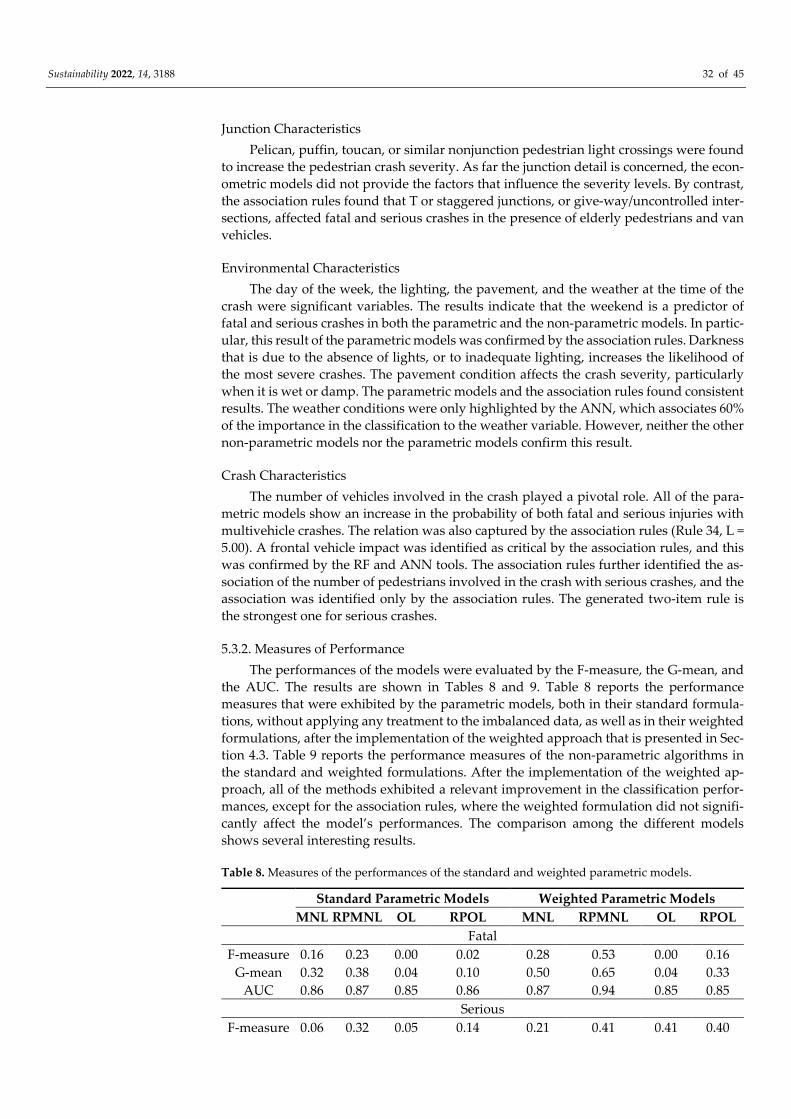
Sustainability 2022, 14, 3188 32 of 45
Junction Characteristics
Pelican, puffin, toucan, or similar nonjunction pedestrian light crossings were found
to increase the pedestrian crash severity. As far the junction detail is concerned, the econ-
ometric models did not provide the factors that influence the severity levels. By contrast,
the association rules found that T or staggered junctions, or give-way/uncontrolled inter-
sections, affected fatal and serious crashes in the presence of elderly pedestrians and van
vehicles.
Environmental Characteristics
The day of the week, the lighting, the pavement, and the weather at the time of the
crash were significant variables. The results indicate that the weekend is a predictor of
fatal and serious crashes in both the parametric and the non-parametric models. In partic-
ular, this result of the parametric models was confirmed by the association rules. Darkness
that is due to the absence of lights, or to inadequate lighting, increases the likelihood of
the most severe crashes. The pavement condition affects the crash severity, particularly
when it is wet or damp. The parametric models and the association rules found consistent
results. The weather conditions were only highlighted by the ANN, which associates 60%
of the importance in the classification to the weather variable. However, neither the other
non-parametric models nor the parametric models confirm this result.
Crash Characteristics
The number of vehicles involved in the crash played a pivotal role. All of the para-
metric models show an increase in the probability of both fatal and serious injuries with
multivehicle crashes. The relation was also captured by the association rules (Rule 34, L =
5.00). A frontal vehicle impact was identified as critical by the association rules, and this
was confirmed by the RF and ANN tools. The association rules further identified the as-
sociation of the number of pedestrians involved in the crash with serious crashes, and the
association was identified only by the association rules. The generated two-item rule is
the strongest one for serious crashes.
5.3.2. Measures of Performance
The performances of the models were evaluated by the F-measure, the G-mean, and
the AUC. The results are shown in Tables 8 and 9. Table 8 reports the performance
measures that were exhibited by the parametric models, both in their standard formula-
tions, without applying any treatment to the imbalanced data, as well as in their weighted
formulations, after the implementation of the weighted approach that is presented in Sec-
tion 4.3. Table 9 reports the performance measures of the non-parametric algorithms in
the standard and weighted formulations. After the implementation of the weighted ap-
proach, all of the methods exhibited a relevant improvement in the classification perfor-
mances, except for the association rules, where the weighted formulation did not signifi-
cantly affect the model’s performances. The comparison among the different models
shows several interesting results.
Table 8. Measures of the performances of the standard and weighted parametric models.
Standard Parametric Models Weighted Parametric Models
MNL RPMNL OL RPOL MNL RPMNL OL RPOL
Fatal
F-measure 0.16 0.23 0.00 0.02 0.28 0.53 0.00 0.16
G-mean 0.32 0.38 0.04 0.10 0.50 0.65 0.04 0.33
AUC 0.86 0.87 0.85 0.86 0.87 0.94 0.85 0.85
Serious
F-measure 0.06 0.32 0.05 0.14 0.21 0.41 0.41 0.40
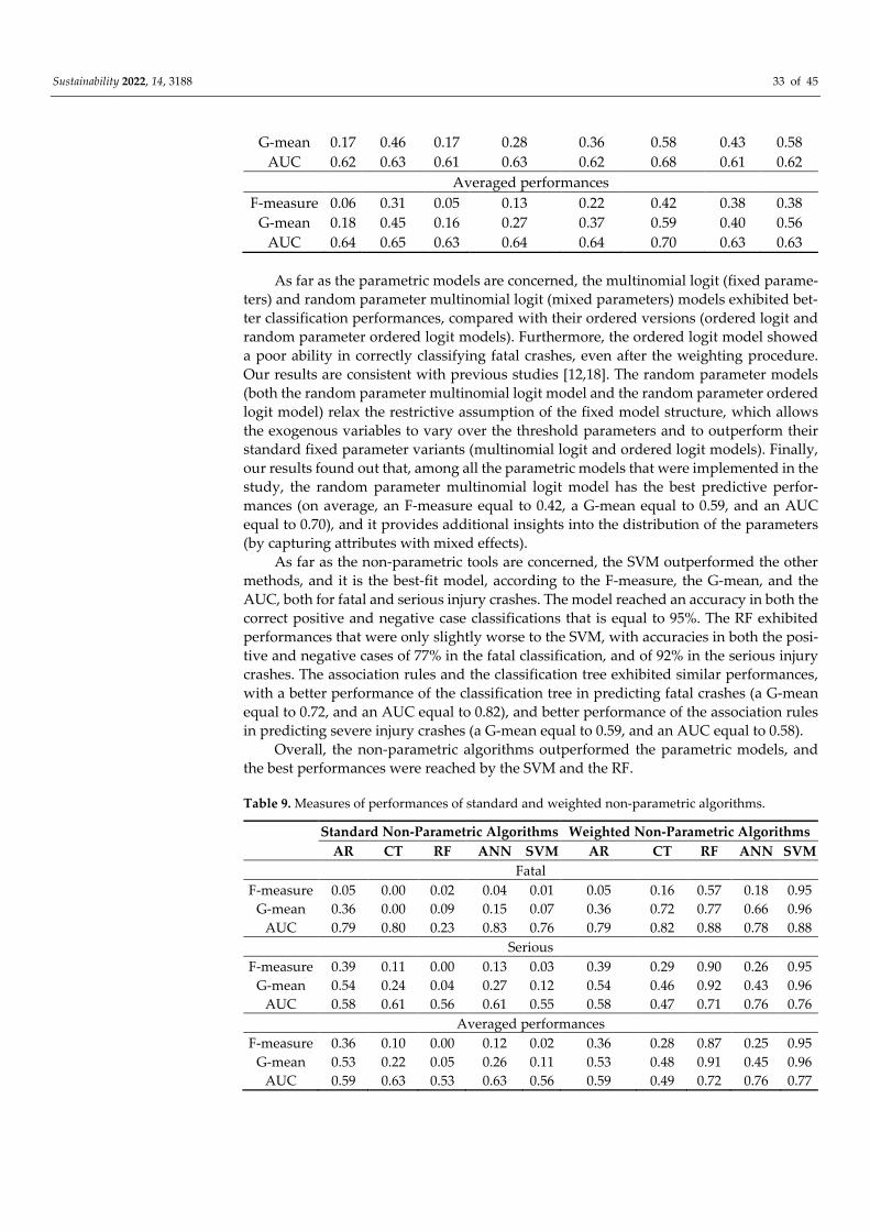
Sustainability 2022, 14, 3188 33 of 45
G-mean 0.17 0.46 0.17 0.28 0.36 0.58 0.43 0.58
AUC 0.62 0.63 0.61 0.63 0.62 0.68 0.61 0.62
Averaged performances
F-measure 0.06 0.31 0.05 0.13 0.22 0.42 0.38 0.38
G-mean 0.18 0.45 0.16 0.27 0.37 0.59 0.40 0.56
AUC 0.64 0.65 0.63 0.64 0.64 0.70 0.63 0.63
As far as the parametric models are concerned, the multinomial logit (fixed parame-
ters) and random parameter multinomial logit (mixed parameters) models exhibited bet-
ter classification performances, compared with their ordered versions (ordered logit and
random parameter ordered logit models). Furthermore, the ordered logit model showed
a poor ability in correctly classifying fatal crashes, even after the weighting procedure.
Our results are consistent with previous studies [12,18]. The random parameter models
(both the random parameter multinomial logit model and the random parameter ordered
logit model) relax the restrictive assumption of the fixed model structure, which allows
the exogenous variables to vary over the threshold parameters and to outperform their
standard fixed parameter variants (multinomial logit and ordered logit models). Finally,
our results found out that, among all the parametric models that were implemented in the
study, the random parameter multinomial logit model has the best predictive perfor-
mances (on average, an F-measure equal to 0.42, a G-mean equal to 0.59, and an AUC
equal to 0.70), and it provides additional insights into the distribution of the parameters
(by capturing attributes with mixed effects).
As far as the non-parametric tools are concerned, the SVM outperformed the other
methods, and it is the best-fit model, according to the F-measure, the G-mean, and the
AUC, both for fatal and serious injury crashes. The model reached an accuracy in both the
correct positive and negative case classifications that is equal to 95%. The RF exhibited
performances that were only slightly worse to the SVM, with accuracies in both the posi-
tive and negative cases of 77% in the fatal classification, and of 92% in the serious injury
crashes. The association rules and the classification tree exhibited similar performances,
with a better performance of the classification tree in predicting fatal crashes (a G-mean
equal to 0.72, and an AUC equal to 0.82), and better performance of the association rules
in predicting severe injury crashes (a G-mean equal to 0.59, and an AUC equal to 0.58).
Overall, the non-parametric algorithms outperformed the parametric models, and
the best performances were reached by the SVM and the RF.
Table 9. Measures of performances of standard and weighted non-parametric algorithms.
Standard Non-Parametric Algorithms Weighted Non-Parametric Algorithms AR CT RF ANN SVM AR CT RF ANN SVM
Fatal
F-measure 0.05 0.00 0.02 0.04 0.01 0.05 0.16 0.57 0.18 0.95
G-mean 0.36 0.00 0.09 0.15 0.07 0.36 0.72 0.77 0.66 0.96
AUC 0.79 0.80 0.23 0.83 0.76 0.79 0.82 0.88 0.78 0.88
Serious
F-measure 0.39 0.11 0.00 0.13 0.03 0.39 0.29 0.90 0.26 0.95
G-mean 0.54 0.24 0.04 0.27 0.12 0.54 0.46 0.92 0.43 0.96
AUC 0.58 0.61 0.56 0.61 0.55 0.58 0.47 0.71 0.76 0.76
Averaged performances
F-measure 0.36 0.10 0.00 0.12 0.02 0.36 0.28 0.87 0.25 0.95
G-mean 0.53 0.22 0.05 0.26 0.11 0.53 0.48 0.91 0.45 0.96
AUC 0.59 0.63 0.53 0.63 0.56 0.59 0.49 0.72 0.76 0.77
Sustainability 2022, 14, 3188 34 of 45
6. Discussion and Conclusions
This study presents the results of a comprehensive analysis of four parametric mod-
els and five non-parametric tools to investigate the factors that contribute to fatal and se-
rious injury crashes in Great Britain. Even though the models have already been applied
to model the pedestrian injury severity, a comparative analysis of the predictive power of
such modeling techniques is limited.
With regard to the parametric models, the multinomial logit model outperformed the
ordered logit model. The main explanation for this difference is that ordered probability
models place a strict restriction on how the exogenous variables affect the outcome prob-
abilities. Previous studies [59] have already found the inconsistent estimates that were
produced by the ordered logit model produced inconsistent estimates, as well as the elas-
ticity effects that were constrained to be monotonic, from the lowest category of severity
to the highest. This implies that the ordered logit model does not allow the probabilities
of both the highest and lowest severity levels to increase or decrease. Thus, in order to
increase the probability of the highest severity class (which is the “fatal” class in this
study), a decrease in the probability of the lowest severity levels (which is “slight” in this
study) is observed, and vice versa. Our study confirms that implementing the ordered
crash severity nature on logistic regression models does not necessarily improve their pre-
dictive performances across all the severity levels, as the relationships between the pre-
dictors and the crash severity outcomes might not be monotonic.
As was expected, the random parameter models (the random parameter multinomial
logit and random parameter ordered logit models) were statistically superior to their
standard formulations, as they could accommodate the unobserved heterogeneity among
the observations. Furthermore, their use provides evidence of the existence of heteroge-
neity among the data.
The likelihood ratio test shows that the random parameter multinomial logit model
is superior to the standard multinomial logit model, with over 99.9% confidence. Similar
results are also observed between the random parameter ordered logit model and the
standard ordered logit model.
The significant variables that impacted the pedestrian crash severity in the standard
logit models were tested for heterogeneity in the random parameter models: the random
parameter multinomial logit identified two random variables (the “going-ahead vehicle
maneuver” and the “roundabout”) in predicting fatal crashes, and one random variable
(the “pedestrian age greater ≥ 75 ”) that affect the serious crashes. The random parameter
ordered logit, instead, found one random variable (the “pedestrian age ≥ 75”) that im-
pacted both of the severity levels. The presence of such variability in the effect of the var-
iables across the sample population highlights the need to account for the potential unob-
served heterogeneity, as this will improve our understanding, reduce erroneous infer-
ences and predictions, and provide more accurate and informative results. Finally, in
terms of the statistical fit, the value of the McFadden R2 was the highest for the random
parameter multinomial logit model, which indicates that the model statistically outper-
formed the other parametric models.
As far as the non-parametric methods are concerned, these models produced better
prediction performances than the parametric models. The SVM outperformed the other
methods, and it was the best fit model according to the F-measure, the G-mean, and the
AUC, both for fatal and serious injury crashes. The RF also exhibited high predictive per-
formances. However, the interpretability of the results of some of the non-parametric
models is lower compared to the parametric models. For instance, a common output of
the non-parametric models is the importance that the independent variables exhibit dur-
ing the classification process. Even though the results of the most important variables that
were identified by the non-parametric tools provide interesting information as well as a
ranking of the most explanatory variables, the variable importance does not provide in-
formation about the directions and magnitudes of their impacts. Nevertheless, some algo-
rithms also offer other interesting outputs. This is the case of the classification tree and the
Sustainability 2022, 14, 3188 35 of 45
RF, which can both be graphically displayed as trees. Their structure enhances compre-
hension, with intuitive results. The association rules identify the specific patterns that are
associated with pedestrian crashes and assign strength to the co-occurrence of several fac-
tors that affect the crash severity. For instance, the contributory factors that are associated
with pedestrian crashes are the patterns with higher lift values, which can be considered
as the parameters for determining the significance of the patterns from the base condition
[23]. Furthermore, the rule structure allows for a clear framework of the attribute combi-
nations.
Several factors were found to significantly increase the probability of fatal and seri-
ous injuries in pedestrian–vehicle crashes. Nineteen variables were significant, both in the
parametric models as well as in the non-parametric algorithms, with one variable that was
significant only in the parametric models, and seven variables that were significant only
in the non-parametric algorithms. This means that the non-parametric algorithms uncover
more hidden correlations among the data than the parametric models.
The type of vehicle that is involved in a pedestrian crash influences the crash severity.
As is found in previous studies [8,60], the presence of a truck increases the crash severity
because of the larger mass and the greater stiffness, the larger area of impact for pedestri-
ans, the higher bumper height, the blunter geometry, and the longer stopping distances
compared to other vehicles. Furthermore, the presence of articulated vehicles has been
identified as a contributor to the most severe pedestrian crashes. The direct link of fatal/se-
rious crashes with trucks, as well as with articulated vehicles, suggests the importance of
planning specific routes for trucks. In order to avoid the transit of heavy vehicles in places
that are highly frequented by pedestrians, it is crucial to establish a road hierarchy that
gives the highest priority to pedestrians, and then to the other road users. Another rele-
vant aspect is the point of the first impact in a crash. The frontal impacts resulted in more
severe crashes, compared to all other kinds of impacts. This finding is also consistent with
previous studies [20]. Rural areas and higher speed limits characterize the roads where
the most severe crashes occurred. This may be a consequence of the typical rural road
configuration, which has higher vehicle speeds combined with fewer separated facilities
for pedestrians, such as sidewalk paths and trails, compared to urban areas.
As is found in previous studies [8,61], young drivers increase the probability of fatal
and serious crashes. A possible explanation is that older drivers tend to drive more care-
fully and at lower speeds. Hence, as motorists become older, pedestrians are more likely
to suffer no injuries once in a crash. Male drivers were also more likely to be involved in
the most serious crashes, and our results confirm previous findings [22,62]. These factors
may reflect the typically more aggressive way of driving of young male drivers. To reduce
pedestrian crashes, programs are essential to the enforcement of the existing traffic laws
and ordinances for drivers. Furthermore, safety education should be integrated with
school programs, and targeted safety campaigns should be a priority government task.
As was expected, the pedestrian crashes occurred during the night or under low-light
conditions, which increased the likelihood of fatal consequences [63]. The driver may fail
to see a pedestrian at night, and this was also associated with frontal vehicle impacts. This
pattern highlights the importance of improving the pedestrian conspicuity. Babić et al.
[64] found that drivers showed more active eye movements after noticing pedestrians in
reflective vests than they did after noticing pedestrians in non–reflective clothing. Other
than reflective clothes and markings, some studies [65,66] have examined elements of
clothing (electroluminescent panels) that may be useful supplements since they are visible
even when a pedestrian is not illuminated by approaching headlamps. Nevertheless,
roads should be effectively illuminated as well, especially in areas where there is a high
probability of observing pedestrians, such as in the proximity of pedestrian crossings.
Furthermore, although pedestrian crashes are more likely to occur during the week, it is
during the weekend that crashes are more likely to be severe. This may be due to more
relaxed or distracted driver/pedestrian behaviors. The elderly pedestrians were more
prone to severe outcomes relative to the younger individuals, once in a crash. This is due
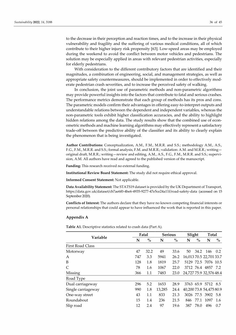
Sustainability 2022, 14, 3188 36 of 45
to the decrease in their perception and reaction times, and to the increase in their physical
vulnerability and fragility and the suffering of various medical conditions, all of which
contribute to their higher injury risk propensity [63]. Low-speed areas may be employed
during the weekend to avoid the conflict between motor vehicles and pedestrians. The
solution may be especially applied in areas with relevant pedestrian activities, especially
for elderly pedestrians.
With consideration to the different contributory factors that are identified and their
magnitudes, a combination of engineering, social, and management strategies, as well as
appropriate safety countermeasures, should be implemented in order to effectively mod-
erate pedestrian crash severities, and to increase the perceived safety of walking.
In conclusion, the joint use of parametric methods and non-parametric algorithms
may provide powerful insights into the factors that contribute to fatal and serious crashes.
The performance metrics demonstrate that each group of methods has its pros and cons.
The parametric models confirm their advantages in offering easy-to-interpret outputs and
understandable relations between the dependent and independent variables, whereas the
non-parametric tools exhibit higher classification accuracies, and the ability to highlight
hidden relations among the data. The study results show that the combined use of econ-
ometric methods and machine learning algorithms may effectively represent a satisfactory
trade-off between the predictive ability of the classifier and its ability to clearly explain
the phenomenon that is being investigated.
Author Contributions: Conceptualization, A.M., F.M., M.R.R. and S.S.; methodology A.M., A.S.,
F.G., F.M., M.R.R. and S.S.; formal analysis, F.M. and M.R.R.; validation: A.M. and M.R.R.; writing—
original draft, M.R.R.; writing—review and editing, A.M., A.S., F.G., F.M., M.R.R. and S.S.; supervi-
sion, A.M. All authors have read and agreed to the published version of the manuscript.
Funding: This research received no external funding.
Institutional Review Board Statement: The study did not require ethical approval.
Informed Consent Statement: Not applicable.
Data Availability Statement: The STATS19 dataset is provided by the UK Department of Transport,
https://data.gov.uk/dataset/cb7ae6f0-4be6-4935-9277-47e5ce24a11f/road-safety-data (accessed on 15
September 2020).
Conflicts of Interest: The authors declare that they have no known competing financial interests or
personal relationships that could appear to have influenced the work that is reported in this paper.
Appendix A
Table A1. Descriptive statistics related to crash data (Part A).
Variable Fatal Serious Slight Total
N % N % N % N %
First Road Class
Motorway 47 32.2 49 33.6 50 34.2 146 0.2
A 747 3.3 5941 26.2 16,013 70.5 22,701 33.7
B 128 1.8 1819 25.7 5129 72.5 7076 10.5
C 78 1.6 1067 22.0 3712 76.4 4857 7.2
Missing 366 1.1 7483 23.0 24,727 75.9 32,576 48.4
Road Type
Dual carriageway 296 5.2 1653 28.9 3763 65.9 5712 8.5
Single carriageway 990 1.8 13,285 24.4 40,200 73.8 54,475 80.9
One-way street 43 1.1 833 21.3 3026 77.5 3902 5.8
Roundabout 15 1.4 236 21.5 846 77.1 1097 1.6
Slip road 12 2.4 97 19.6 387 78.0 496 0.7
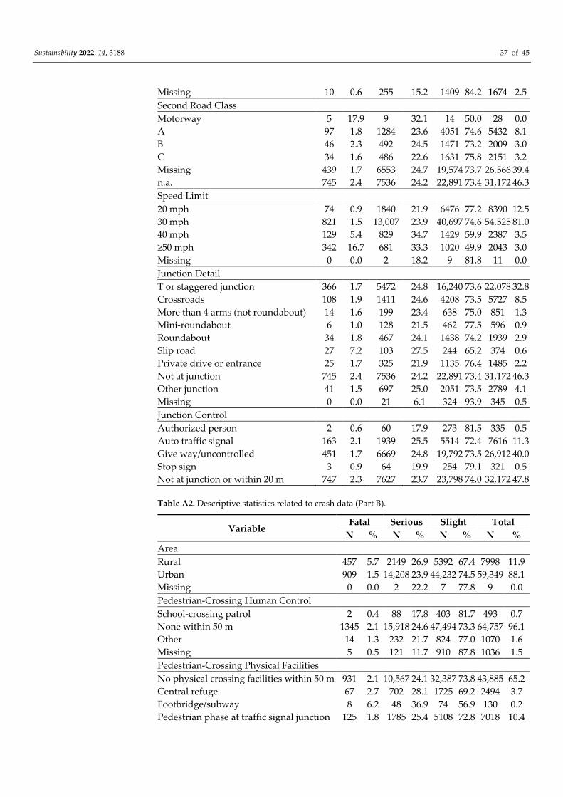
Sustainability 2022, 14, 3188 37 of 45
Missing 10 0.6 255 15.2 1409 84.2 1674 2.5
Second Road Class
Motorway 5 17.9 9 32.1 14 50.0 28 0.0
A 97 1.8 1284 23.6 4051 74.6 5432 8.1
B 46 2.3 492 24.5 1471 73.2 2009 3.0
C 34 1.6 486 22.6 1631 75.8 2151 3.2
Missing 439 1.7 6553 24.7 19,574 73.7 26,566 39.4
n.a. 745 2.4 7536 24.2 22,891 73.4 31,172 46.3
Speed Limit
20 mph 74 0.9 1840 21.9 6476 77.2 8390 12.5
30 mph 821 1.5 13,007 23.9 40,697 74.6 54,525 81.0
40 mph 129 5.4 829 34.7 1429 59.9 2387 3.5
≥50 mph 342 16.7 681 33.3 1020 49.9 2043 3.0
Missing 0 0.0 2 18.2 9 81.8 11 0.0
Junction Detail
T or staggered junction 366 1.7 5472 24.8 16,240 73.6 22,078 32.8
Crossroads 108 1.9 1411 24.6 4208 73.5 5727 8.5
More than 4 arms (not roundabout) 14 1.6 199 23.4 638 75.0 851 1.3
Mini-roundabout 6 1.0 128 21.5 462 77.5 596 0.9
Roundabout 34 1.8 467 24.1 1438 74.2 1939 2.9
Slip road 27 7.2 103 27.5 244 65.2 374 0.6
Private drive or entrance 25 1.7 325 21.9 1135 76.4 1485 2.2
Not at junction 745 2.4 7536 24.2 22,891 73.4 31,172 46.3
Other junction 41 1.5 697 25.0 2051 73.5 2789 4.1
Missing 0 0.0 21 6.1 324 93.9 345 0.5
Junction Control
Authorized person 2 0.6 60 17.9 273 81.5 335 0.5
Auto traffic signal 163 2.1 1939 25.5 5514 72.4 7616 11.3
Give way/uncontrolled 451 1.7 6669 24.8 19,792 73.5 26,912 40.0
Stop sign 3 0.9 64 19.9 254 79.1 321 0.5
Not at junction or within 20 m 747 2.3 7627 23.7 23,798 74.0 32,172 47.8
Table A2. Descriptive statistics related to crash data (Part B).
Variable Fatal Serious Slight Total
N % N % N % N %
Area
Rural 457 5.7 2149 26.9 5392 67.4 7998 11.9
Urban 909 1.5 14,208 23.9 44,232 74.5 59,349 88.1
Missing 0 0.0 2 22.2 7 77.8 9 0.0
Pedestrian-Crossing Human Control
School-crossing patrol 2 0.4 88 17.8 403 81.7 493 0.7
None within 50 m 1345 2.1 15,918 24.6 47,494 73.3 64,757 96.1
Other 14 1.3 232 21.7 824 77.0 1070 1.6
Missing 5 0.5 121 11.7 910 87.8 1036 1.5
Pedestrian-Crossing Physical Facilities
No physical crossing facilities within 50 m 931 2.1 10,567 24.1 32,387 73.8 43,885 65.2
Central refuge 67 2.7 702 28.1 1725 69.2 2494 3.7
Footbridge/subway 8 6.2 48 36.9 74 56.9 130 0.2
Pedestrian phase at traffic signal junction 125 1.8 1785 25.4 5108 72.8 7018 10.4
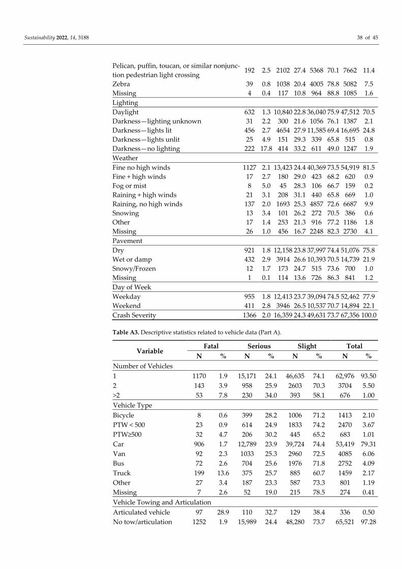
Sustainability 2022, 14, 3188 38 of 45
Pelican, puffin, toucan, or similar nonjunc-
tion pedestrian light crossing 192 2.5 2102 27.4 5368 70.1 7662 11.4
Zebra 39 0.8 1038 20.4 4005 78.8 5082 7.5
Missing 4 0.4 117 10.8 964 88.8 1085 1.6
Lighting
Daylight 632 1.3 10,840 22.8 36,040 75.9 47,512 70.5
Darkness—lighting unknown 31 2.2 300 21.6 1056 76.1 1387 2.1
Darkness—lights lit 456 2.7 4654 27.9 11,585 69.4 16,695 24.8
Darkness—lights unlit 25 4.9 151 29.3 339 65.8 515 0.8
Darkness—no lighting 222 17.8 414 33.2 611 49.0 1247 1.9
Weather
Fine no high winds 1127 2.1 13,423 24.4 40,369 73.5 54,919 81.5
Fine + high winds 17 2.7 180 29.0 423 68.2 620 0.9
Fog or mist 8 5.0 45 28.3 106 66.7 159 0.2
Raining + high winds 21 3.1 208 31.1 440 65.8 669 1.0
Raining, no high winds 137 2.0 1693 25.3 4857 72.6 6687 9.9
Snowing 13 3.4 101 26.2 272 70.5 386 0.6
Other 17 1.4 253 21.3 916 77.2 1186 1.8
Missing 26 1.0 456 16.7 2248 82.3 2730 4.1
Pavement
Dry 921 1.8 12,158 23.8 37,997 74.4 51,076 75.8
Wet or damp 432 2.9 3914 26.6 10,393 70.5 14,739 21.9
Snowy/Frozen 12 1.7 173 24.7 515 73.6 700 1.0
Missing 1 0.1 114 13.6 726 86.3 841 1.2
Day of Week
Weekday 955 1.8 12,413 23.7 39,094 74.5 52,462 77.9
Weekend 411 2.8 3946 26.5 10,537 70.7 14,894 22.1
Crash Severity 1366 2.0 16,359 24.3 49,631 73.7 67,356 100.0
Table A3. Descriptive statistics related to vehicle data (Part A).
Variable Fatal Serious Slight Total
N % N % N % N %
Number of Vehicles
1 1170 1.9 15,171 24.1 46,635 74.1 62,976 93.50
2 143 3.9 958 25.9 2603 70.3 3704 5.50
>2 53 7.8 230 34.0 393 58.1 676 1.00
Vehicle Type
Bicycle 8 0.6 399 28.2 1006 71.2 1413 2.10
PTW < 500 23 0.9 614 24.9 1833 74.2 2470 3.67
PTW≥500 32 4.7 206 30.2 445 65.2 683 1.01
Car 906 1.7 12,789 23.9 39,724 74.4 53,419 79.31
Van 92 2.3 1033 25.3 2960 72.5 4085 6.06
Bus 72 2.6 704 25.6 1976 71.8 2752 4.09
Truck 199 13.6 375 25.7 885 60.7 1459 2.17
Other 27 3.4 187 23.3 587 73.3 801 1.19
Missing 7 2.6 52 19.0 215 78.5 274 0.41
Vehicle Towing and Articulation
Articulated vehicle 97 28.9 110 32.7 129 38.4 336 0.50
No tow/articulation 1252 1.9 15,989 24.4 48,280 73.7 65,521 97.28
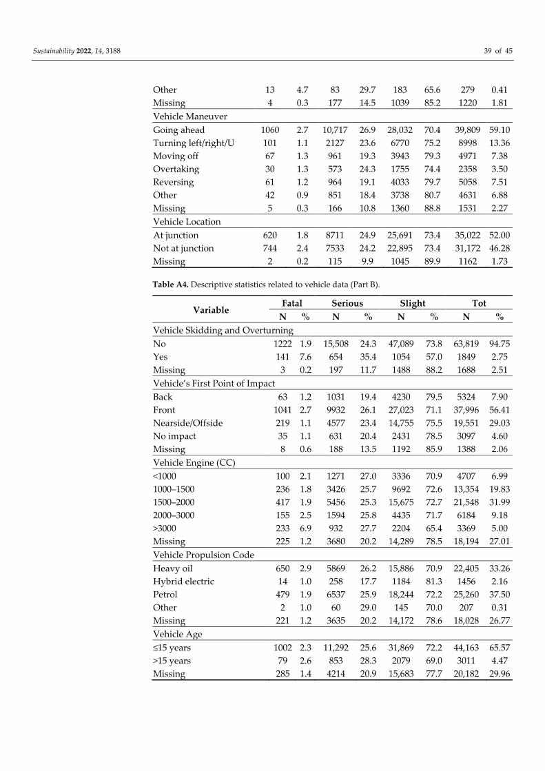
Sustainability 2022, 14, 3188 39 of 45
Other 13 4.7 83 29.7 183 65.6 279 0.41
Missing 4 0.3 177 14.5 1039 85.2 1220 1.81
Vehicle Maneuver
Going ahead 1060 2.7 10,717 26.9 28,032 70.4 39,809 59.10
Turning left/right/U 101 1.1 2127 23.6 6770 75.2 8998 13.36
Moving off 67 1.3 961 19.3 3943 79.3 4971 7.38
Overtaking 30 1.3 573 24.3 1755 74.4 2358 3.50
Reversing 61 1.2 964 19.1 4033 79.7 5058 7.51
Other 42 0.9 851 18.4 3738 80.7 4631 6.88
Missing 5 0.3 166 10.8 1360 88.8 1531 2.27
Vehicle Location
At junction 620 1.8 8711 24.9 25,691 73.4 35,022 52.00
Not at junction 744 2.4 7533 24.2 22,895 73.4 31,172 46.28
Missing 2 0.2 115 9.9 1045 89.9 1162 1.73
Table A4. Descriptive statistics related to vehicle data (Part B).
Variable Fatal Serious Slight Tot
N % N % N % N %
Vehicle Skidding and Overturning
No 1222 1.9 15,508 24.3 47,089 73.8 63,819 94.75
Yes 141 7.6 654 35.4 1054 57.0 1849 2.75
Missing 3 0.2 197 11.7 1488 88.2 1688 2.51
Vehicle’s First Point of Impact
Back 63 1.2 1031 19.4 4230 79.5 5324 7.90
Front 1041 2.7 9932 26.1 27,023 71.1 37,996 56.41
Nearside/Offside 219 1.1 4577 23.4 14,755 75.5 19,551 29.03
No impact 35 1.1 631 20.4 2431 78.5 3097 4.60
Missing 8 0.6 188 13.5 1192 85.9 1388 2.06
Vehicle Engine (CC)
<1000 100 2.1 1271 27.0 3336 70.9 4707 6.99
1000–1500 236 1.8 3426 25.7 9692 72.6 13,354 19.83
1500–2000 417 1.9 5456 25.3 15,675 72.7 21,548 31.99
2000–3000 155 2.5 1594 25.8 4435 71.7 6184 9.18
>3000 233 6.9 932 27.7 2204 65.4 3369 5.00
Missing 225 1.2 3680 20.2 14,289 78.5 18,194 27.01
Vehicle Propulsion Code
Heavy oil 650 2.9 5869 26.2 15,886 70.9 22,405 33.26
Hybrid electric 14 1.0 258 17.7 1184 81.3 1456 2.16
Petrol 479 1.9 6537 25.9 18,244 72.2 25,260 37.50
Other 2 1.0 60 29.0 145 70.0 207 0.31
Missing 221 1.2 3635 20.2 14,172 78.6 18,028 26.77
Vehicle Age
≤15 years 1002 2.3 11,292 25.6 31,869 72.2 44,163 65.57
>15 years 79 2.6 853 28.3 2079 69.0 3011 4.47
Missing 285 1.4 4214 20.9 15,683 77.7 20,182 29.96
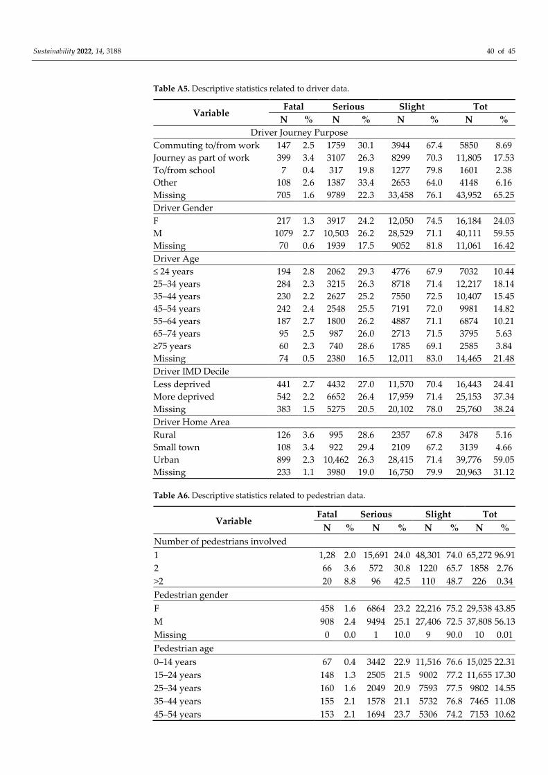
Sustainability 2022, 14, 3188 40 of 45
Table A5. Descriptive statistics related to driver data.
Variable Fatal Serious Slight Tot
N % N % N % N %
Driver Journey Purpose
Commuting to/from work 147 2.5 1759 30.1 3944 67.4 5850 8.69
Journey as part of work 399 3.4 3107 26.3 8299 70.3 11,805 17.53
To/from school 7 0.4 317 19.8 1277 79.8 1601 2.38
Other 108 2.6 1387 33.4 2653 64.0 4148 6.16
Missing 705 1.6 9789 22.3 33,458 76.1 43,952 65.25
Driver Gender
F 217 1.3 3917 24.2 12,050 74.5 16,184 24.03
M 1079 2.7 10,503 26.2 28,529 71.1 40,111 59.55
Missing 70 0.6 1939 17.5 9052 81.8 11,061 16.42
Driver Age
≤ 24 years 194 2.8 2062 29.3 4776 67.9 7032 10.44
25–34 years 284 2.3 3215 26.3 8718 71.4 12,217 18.14
35–44 years 230 2.2 2627 25.2 7550 72.5 10,407 15.45
45–54 years 242 2.4 2548 25.5 7191 72.0 9981 14.82
55–64 years 187 2.7 1800 26.2 4887 71.1 6874 10.21
65–74 years 95 2.5 987 26.0 2713 71.5 3795 5.63
≥75 years 60 2.3 740 28.6 1785 69.1 2585 3.84
Missing 74 0.5 2380 16.5 12,011 83.0 14,465 21.48
Driver IMD Decile
Less deprived 441 2.7 4432 27.0 11,570 70.4 16,443 24.41
More deprived 542 2.2 6652 26.4 17,959 71.4 25,153 37.34
Missing 383 1.5 5275 20.5 20,102 78.0 25,760 38.24
Driver Home Area
Rural 126 3.6 995 28.6 2357 67.8 3478 5.16
Small town 108 3.4 922 29.4 2109 67.2 3139 4.66
Urban 899 2.3 10,462 26.3 28,415 71.4 39,776 59.05
Missing 233 1.1 3980 19.0 16,750 79.9 20,963 31.12
Table A6. Descriptive statistics related to pedestrian data.
Variable Fatal Serious Slight Tot
N % N % N % N %
Number of pedestrians involved
1 1,28 2.0 15,691 24.0 48,301 74.0 65,272 96.91
2 66 3.6 572 30.8 1220 65.7 1858 2.76
>2 20 8.8 96 42.5 110 48.7 226 0.34
Pedestrian gender
F 458 1.6 6864 23.2 22,216 75.2 29,538 43.85
M 908 2.4 9494 25.1 27,406 72.5 37,808 56.13
Missing 0 0.0 1 10.0 9 90.0 10 0.01
Pedestrian age
0–14 years 67 0.4 3442 22.9 11,516 76.6 15,025 22.31
15–24 years 148 1.3 2505 21.5 9002 77.2 11,655 17.30
25–34 years 160 1.6 2049 20.9 7593 77.5 9802 14.55
35–44 years 155 2.1 1578 21.1 5732 76.8 7465 11.08
45–54 years 153 2.1 1694 23.7 5306 74.2 7153 10.62
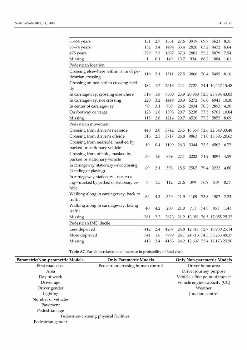
Sustainability 2022, 14, 3188 41 of 45
55–64 years 151 2.7 1551 27.6 3919 69.7 5621 8.35
65–74 years 152 3.4 1494 33.4 2826 63.2 4472 6.64
≥75 years 379 7.5 1897 37.3 2803 55.2 5079 7.54
Missing 1 0.1 149 13.7 934 86.2 1084 1.61
Pedestrian location
Crossing elsewhere within 50 m of pe-
destrian crossing 118 2.1 1511 27.5 3866 70.4 5495 8.16
Crossing on pedestrian crossing facil-
ity 182 1.7 2518 24.1 7727 74.1 10,427 15.48
In carriageway, crossing elsewhere 516 1.8 7500 25.9 20,968 72.3 28,984 43.03
In carriageway, not crossing 220 3.2 1449 20.9 5272 76.0 6941 10.30
In center of carriageway 90 3.1 769 26.6 2034 70.3 2893 4.30
On footway or verge 125 1.8 1398 20.7 5238 77.5 6761 10.04
Missing 115 2.0 1214 20.7 4526 77.3 5855 8.69
Pedestrian movement
Crossing from driver’s nearside 440 2.0 5742 25.5 16,367 72.6 22,549 33.48
Crossing from driver’s offside 315 2.3 3717 26.8 9863 71.0 13,895 20.63
Crossing from nearside, masked by
parked or stationary vehicle 19 0.4 1199 26.3 3344 73.3 4562 6.77
Crossing from offside, masked by
parked or stationary vehicle 30 1.0 839 27.1 2222 71.9 3091 4.59
In carriageway, stationary—not crossing
(standing or playing) 69 2.1 598 18.5 2565 79.4 3232 4.80
In carriageway, stationary—not cross-
ing—masked by parked or stationary ve-
hicle
8 1.5 112 21.6 399 76.9 519 0.77
Walking along in carriageway, back to
traffic 64 4.3 329 21.9 1109 73.8 1502 2.23
Walking along in carriageway, facing
traffic 40 4.2 200 21.0 711 74.8 951 1.41
Missing 381 2.2 3623 21.2 13,051 76.5 17,055 25.32
Pedestrian IMD decile
Less deprived 412 2.4 4207 24.8 12,311 72.7 16,930 25.14
More deprived 541 1.6 7999 24.1 24,713 74.3 33,253 49.37
Missing 413 2.4 4153 24.2 12,607 73.4 17,173 25.50
Table A7. Variables related to an increase in probability of fatal crash.
Parametric/Non-parametric Models. Only Parametric Models Only Non-parametric Models
First road class Pedestrian-crossing human control Driver home area
Area Driver journey purpose
Day of week Vehicle’s first point of impact
Driver age Vehicle engine capacity (CC)
Driver gender Weather
Lighting Junction control
Number of vehicles
Pavement
Pedestrian age
Pedestrian-crossing physical facilities
Pedestrian gender

Sustainability 2022, 14, 3188 42 of 45
Speed limit
Vehicle age
Vehicle maneuver
Vehicle propulsion code
Vehicle skidding and overturning
Vehicle towing and articulation
Vehicle type
Junction detail
Table A8. Variables related to an increase in the probability of a serious crash.
Parametric/Non-parametric Models Only Parametric Models Only Non-parametric Models
First road class Pedestrian-crossing human control Driver home area
Area Driver journey purpose
Day of week Number of pedestrians involved
Driver age Vehicle’s first point of impact
Driver gender Vehicle engine capacity (CC)
Lighting Weather
Number of vehicles Junction control
Pavement
Pedestrian age
Pedestrian-crossing physical facilities
Pedestrian gender
Speed limit
Vehicle age
Vehicle maneuver
Vehicle skidding and overturning
Vehicle towing and articulation
Vehicle type
Junction detail
References
1. European Commission. EU Road Safety Policy Framework 2021–2030-Next Steps towards “Vision Zero”. 2019. Available online:
https://ec.europa.eu/transport/sites/transport/files/legislation/swd20190283-roadsafety-vision-zero.pdf (accessed on 15 September 2020).
2. Department for Transport. Road Accidents and Safety Statistics. 2020. Available online: https://www.gov.uk/government/col-
lections/road-accidents-and-safety-statistics (accessed on 30 September 2020).
3. Theofilatos, A.; Yannis, G. A review of powered-two-wheeler behaviour and safety. Int. J. Inj. Control. Saf. Promot. 2015, 22, 284–
307. https://doi.org/10.1080/17457300.2014.908224.
4. Montella, A.; Andreassen, D.; Tarko, A.; Turner, S.; Mauriello, F.; Imbriani, L.L.; Romero, M. Crash databases in Australasia,
the European Union, and the United States. Trans. Res. Rec. 2013, 2386, 128–136. https://doi.org/10.3141/2386-15.
5. Cerwick, D.M.; Gkritza, K.; Shaheed, M.S.; Hans, Z. A comparison of the mixed logit and latent class methods for crash severity
analysis. Anal. Methods Accid. Res. 2014, 3, 11–27. http://doi.org/10.1016/j.amar.2014.09.002.
6. Haleem, K.; Alluri, P.; Gan, A. Analyzing pedestrian crash injury severity at signalized and non-signalized locations. Acc. Anal.
Prev. 2015, 81, 14–23. https://doi.org/10.1016/j.aap.2015.04.025.
7. Uddin, M.; Huynh, N. Factors influencing injury severity of crashes involving HAZMAT trucks. Int. J. Transp. Sci. Technol. 2018,
7, 1–9. https://doi.org/10.1016/j.ijtst.2017.06.004.
8. Tay, R.; Choi, J.; Kattan, L.; Khan, A. A Multinomial Logit Model of Pedestrian–Vehicle Crash Severity. Int. J. Sustain. Transp.
2011, 5, 233–249. https://doi.org/10.1080/15568318.2010.497547.
9. Rothman, L.; Howard, A.W.; Camden, A.; Macarthur, C. Pedestrian crossing location influences injury severity in urban areas.
Inj. Prev. 2012, 18, 365–370. http://doi.org/10.1136/injuryprev-2011-040246.
10. Chen, Z.; Fan, W.D. A multinomial logit model of pedestrian-vehicle crash severity in North Carolina. Int. J. Transp. Sci. Technol.
2019, 8, 43–52. https://doi.org/10.1016/j.ijtst.2018.10.001.
11. Mannering, F.L.; Shankar, V.; Bhat, C.R. Unobserved heterogeneity and the statistical analysis of highway accident data. Anal.
Methods Accid. Res. 2016, 11, 1–16. http://doi.org/10.1016/j.amar.2016.04.001.
Sustainability 2022, 14, 3188 43 of 45
12. Savolainen, P.; Mannering, F.; Lord, D.; Quddus, M. The statistical analysis of highway crash-injury severities: A review and
assessment of methodological alternatives. Acc. Anal. Prev. 2011, 43, 1666–1676. https://doi.org/10.1016/j.aap.2011.03.025.
13. Mannering, F.L.; Bhat, C.R.; Shankar, V.; Abdel-Aty, M. Big data, traditional data and the tradeoffs between prediction and
causality in highway-safety analysis. Anal. Methods Accid. Res. 2020, 25, 100113. https://doi.org/10.1016/j.amar.2020.100113.
14. Washington, S.P.; Karlaftis, M.G.; Mannering, F.L. Statistical and Econometric Methods for Transportation Data Analysis, 3rd ed.;
Chapman and Hall/CRC: Boca Raton, FL, USA. 2020.
15. Milton, J. Highway accident severities and the mixed logit model: An exploratory empirical analysis. Acc. Anal. Prev. 2006, 40,
260–266. https://doi.org/10.1016/j.aap.2007.06.006.
16. Yasmin, S.; Eluru, N. Evaluating alternate discrete outcome frameworks for modeling crash injury severity. Acc. Anal. Prev.
2014, 59, 506–521. https://doi.org/10.1016/j.aap.2013.06.040.
17. Yamamoto, T.; Hashiji, J.; Shankar, N. Underreporting in traffic accident data, bias in parameters and the structure of injury
severity models. Acc. Anal. Prev. 2008, 40, 1320–1329. https://doi.org/10.1016/j.aap.2007.10.016.
18. Abay, K.A. Examining pedestrian-injury severity using alternative disaggregate models. Res. Transp. Econ. 2013, 43, 123–136.
http://doi.org/10.1016/j.retrec.2012.12.002.
19. Eluru, N.; Bhat, C.R.; Hensher, D.A. A mixed generalized ordered response model for examining pedestrian and bicyclist injury
severity level in traffic crashes. Acc. Anal. Prev. 2008, 40, 1033–1054. https://doi.org/10.1016/j.aap.2007.11.010.
20. Paleti, R.; Eluru, N.; Bhat, C.R. Examining the influence of aggressive driving behavior on driver injury severity in traffic crashes.
Acc. Anal. Prev. 2010, 42, 1839–1854. https://doi.org/10.1016/j.aap.2010.05.005.
21. Srinivasan, K.K. Injury Severity Analysis with Variable and Correlated Thresholds: Ordered Mixed Logit Formulation. Trans.
Res. Rec. 2002, 1784, 132–142. https://doi.org/10.3141%2F1784-17.
22. Das, S.; Dutta, A.; Dixon, K.; Sun, X.; Jalayer, M. Supervised association rules mining on pedestrian crashes in urban areas:
Identifying patterns for appropriate countermeasures. Int. J. Urban Sci. 2018, 23, 30–48.
https://doi.org/10.1080/12265934.2018.1431146.
23. Das, S.; Tamakloe, R.; Zubaidi, H.; Obaid, I. Fatal pedestrian crashes at intersections: Trend mining using association rules. Acc.
Anal. Prev. 2021, 160, 106306. http://doi.org/10.1016/j.aap.2021.106306.
24. Montella, A.; Aria, M.; D’Ambrosio, A.; Mauriello, F. Data-Mining Techniques for Exploratory Analysis of Pedestrian Crashes.
Trans. Res. Rec. 2011, 2237, 107–116. https://doi.org/10.3141/2237-12.
25. Montella, A.; de Oña, R.; Mauriello, F.; Rella Riccardi, M.; Silvestro, G. A data mining approach to investigate patterns of pow-
ered two-wheeler crashes in Spain. Accid. Anal. Prev. 2020, 134, 105251. https://doi.org/10.1016/j.aap.2019.07.027.
26. Li, D.; Ranjitkar, P.; Zhao, Y.; Yi, H.; Rashidi, S. Analyzing pedestrian crash injury severity under different weather conditions.
Traffic Inj. Prev. 2017, 18, 427–430. https://doi.org/10.1080/15389588.2016.1207762.
27. Mafi, S.; AbdelRazing, Y.; Doczy, R. Machine Learning Methods to Analyze Injury Severity of Drivers from Different Age and
Gender Groups. Trans. Res. Rec. 2018, 2672, 171–183. https://doi.org/10.1177/0361198118794292.
28. Mokhtarimousavi, S.; Anderson, J.C.; Azizinamini, A.; Hadi, M. Factors affecting injury severity in vehicle-pedestrian crashes:
A day-of-week analysis using random parameter ordered response models and Artificial Neural Networks. Int. J. Transp. Sci.
Technol. 2020, 9, 100–115. https://doi.org/10.1016/j.ijtst.2020.01.001.
29. Ni, Y.; Wang, M.; Sun, J.; Li, K. Evaluation of pedestrian safety at intersections: A theoretical framework based on pedestrian-
vehicle interaction patterns. Acc. Anal. Prev. 2016, 96, 118–129. http://doi.org/10.1016/j.aap.2016.07.030.
30. King, G.; Zeng, L. Logistic regression in rare events data. Political Anal. 2001, 9, 137–163. https://doi.org/10.1093/oxfordjour-
nals.pan.a004868.
31. Ndour, C.; Diop, A.; Dossou-Gbété, S. Classification Approach Based on Association Rules Mining for Unbalanced Data. arXiv
2012, arXiv:1202.5514.
32. He, H.; Garcia, E.A. Learning from Imbalanced Data. IEEE Trans. Knowl. Data Eng. 2009, 21, 1263–1284.
https://doi.org/10.1109/TKDE.2008.239.
33. Guo, X.; Yin, Y.; Dong, C.; Yang, G.; Zhou, G. On the Class Imbalance Problem. In Proceedings of the 2008 Fourth International
Conference on Natural Computation, Jinan, China, 18–20 October 2008; Volume 4, pp. 192–201.
https://doi.org/10.1109/ICNC.2008.871.
34. Sáez, J.A.; Luengo, J.; Stefanowski, J.; Herrera, F. SMOTE--IPF: Addressing the noisy and borderline examples problem in im-
balanced classification by a re-sampling method with filtering. Inf. Sci. 2015, 291, 184–203.
https://doi.org/10.1016/j.ins.2014.08.051.
35. Tinessa, F.; Papola, A.; Marzano, V. The importance of choosing appropriate random utility models in complex choice contexts.
In Proceedings of the 2017 Fifth International Conference on Models and Technologies for Intelligent Transportation Systems
(MT-ITS), Naples, Italy, 26–28 June 2017; pp. 884–888. https://doi.org/10.1109/MTITS.2017.8005638.
36. Agresti, A. Categorical Data Analysis, 3rd ed.; John Wiley & Sons: New York, NY, USA, 2002; ISBN 978-0-470-46363-5.
37. Jobson, J. Applied Multivariate Data Analysis: Volume II: Categorical and Multivariate Methods; Springer: New York, NY, USA, 2012;
ISBN 978-0-387-97804-8. https://doi.org/10.1007/978-1-4612-0921-8.
Sustainability 2022, 14, 3188 44 of 45
38. Seraneeprakarn, P.; Huang, S.; Shankar, V.; Mannering, F.; Venkataraman, N.; Milton, J. Occupant injury severities in hybrid-
vehicle involved crashes: A random parameters approach with heterogeneity in means and variances. Anal. Methods Accid. Res.
2017, 15, 41–55. https://doi.org/10.1016/j.amar.2017.05.003.
39. McFadden, D. Structural Analysis of Discrete Data with Econometric Applications; The MIT Press: Cambridge, MA, USA, 1981; ISBN
9780262131599.
40. Train, K. Discrete Choice Methods with Simulation, 2nd ed.; Cambridge University Press: New York, NY, 2009; ISBN 978-0-521-
76655-5.
41. Long, J.S. Regression Models for Categorical and Limited Dependent Variables; SAGE Publications, Thousand Oaks, CA, USA, 1997;
ISBN 0803973748.
42. Greene, W.H.; Hensher, D.A. Modeling Ordered Choices; Cambridge University Press: New York, NY, USA, 2010; ISBN
9780511845062. https://doi.org/10.1017/CBO9780511845062.
43. Agrawal, R.; Imieliński, T.; Swami, A. Mining association rules between sets of items in large databases. In Proceedings of the
1993 ACM SIGMOD International Conference on Management of Data; Association for Computing Machinery, New York, NY,
USA, 25–28 May 1993; pp. 207–216. https://doi.org/10.1145/170035.170072.
44. López, G.; Abellán, J.; Montella, A.; de Oña, J. Patterns of Single-Vehicle Crashes on Two-Lane Rural Highways in Granada
Province, Spain: In-Depth Analysis through Decision Rules. Transp. Res. Rec. 2014, 2432, 133–141. https://doi.org/10.3141/2432-
16.
45. Breiman, L.; Friedman, J.H.; Olshen, R.A.; Stone, C.J. Classification and Regression Trees; Wadsworth International Group: Bel-
mont, CA, USA, 1984.
46. Breiman, L. Random forests. Mach. Learn. 2001, 45, 5–32.
47. de Villiers, J.; Barnard, E. Backpropagation neural nets with one and two hidden layers. IEEE Trans. Neural Netw. 1993, 4, 136–
141. http://doi.org/10.1109/72.182704.
48. Zeng, Q.; Huang, H.; Pei, X.; Wong, S.C.; Gao, M. Rule extraction from an optimized neural network for traffic crash frequency
modelling. Acc. Anal. Prev. 2016, 97, 87–95. http://doi.org/10.1016/j.aap.2016.08.017.
49. Cortes, C.; Vapnik, V. Support-Vector Networks. Mach. Learn. 1995, 20, 273–297. http://doi.org/10.1007/BF00994018.
50. Assi, K.; Rahaman, S.M.; Monsoor, U.; Rtrout, N. Predicting Crash Injury Severity with Machine Learning Algorithm Syner-
gized with Clustering Technique: A Promising Protocol. Int. J. Environ. Res. Public Health 2020, 17, 5497.
https://doi.org/10.3390/ijerph17155497.
51. Menardi, G.; Torelli, N. Training and assessing classification rules with imbalanced data. Data Min. Knowl. Discov. 2012, 28, 92–
122. https://doi.org/10.1007/s10618-012-0295-5.
52. Oh, S.H. Error back-propagation algorithm for classification of imbalanced data. Neurocomputing 2011, 74, 1058–1061.
https://doi.org/10.1016/j.neucom.2010.11.024.
53. Huang, W.; Song, G.; Li, M.; Hu, W.; Xie, K. Adaptive Weight Optimization for Classification of Imbalanced Data. In IScIDE
2013, Intelligence Science and Big Data Engineering, Proceedings of the International Conference on Intelligent Science and Big Data
Engineering, Beijing, China, 31 July–2 August 2013; Lecture Notes in Computer Science; Sun, C., Fang, F., Zhou, Z.H., Yang, W.,
Liu, Z.Y., Eds.; Springer: Berlin/Heidelberg, Germany, 2013; Volume 8261. https://doi.org/10.1007/978-3-642-42057-3_69.
54. Kamaldeep, S. How to Improve Class Imbalance Using Class Weights in Machine Learning. 2020. Available online:
https://www.analyticsvidhya.com/blog/author/procrastinator/ (accessed on 15 September 2020).
55. Damju, J.S.; Wening, B.; Das, T.; Lee, D. Learning Spark: Lightning-Fast Big Data Analytics, 2nd ed.; O’Reilly Media: Sebastopol,
CA, USA, 2020. Available online: https://pages.databricks.com/rs/094-YMS-629/images/LearningSpark2.0.pdf. (accessed on 11
October 2020).
56. Fernandez, A.; Garcìa, S.; Galar, M.; Prati, R.C.; Krawczyk, B.; Herrera, F. Learning from Imbalanced Data Sets; Springer: New
York, NY, USA, 2018; ISBN 978-3-319-98073-7. https://doi.org/10.1007/978-3-319-98074-4.
57. Kashani, A.; Rabieyan, R.; Besharati, M. A data mining approach to investigate the factors influencing the crash severity of
motorcycle pillion passengers. J. Saf. Res. 2014, 51, 93–98. http://doi.org/10.1016/j.jsr.2014.09.004.
58. Bina, B.; Schulte, O.; Crawford, B.; Qian, Z.; Xiong, Y. Simple decision forests for multi-relational classification. Decis. Support
Syst. 2013, 54, 1269–1279. https://doi.org/10.1016/j.dss.2012.11.017.
59. Ye, F.; Lord, D. Investigating the Effects of Underreporting of Crash Data on Three Commonly Used Traffic Crash Severity
Models: Multinomial Logit, Ordered Probit and Mixed Logit Models. Transp. Res. Rec. 2011, 2241, 51–58.
http://doi.org/10.3141/2241-06.
60. Kim, J.K.; Ulfarsson, G.F.; Sarkar, V.N.; Mannering, F.L. A note on modeling pedestrian-injury severity in motor-vehicle crashes
with the mixed logit model. Acc. Anal. Prev. 2010, 42, 1751–1758. https://doi.org/ 10.1016/j.aap.2010.04.016.
61. Moral-Garcia, S.; Castellano, J.G.; Mantas, J.G.; Montella, A.; Abellan, J. Decision tree ensemble method for analyzing traffic
accidents of novice drivers in urban areas. Entropy 2019, 21, 360. https://doi.org/10.3390/e21040360.
62. Montella, A.; Mauriello, F.; Pernetti, M.; Rella Riccardi, M. Rule discovery to identify patterns contributing to overrepresentation
and severity of run-off-the-road crashes. Acc. Anal. Prev. 2021, 155, 106119. https://doi.org/10.1016/j.aap.2021.106119.
63. Noh, Y.; Kim, M.; Yoon, Y. Elderly pedestrian safety in a rapidly aging society—Commonality and diversity between the
younger-old and older-old. Traffic Inj. Prev. 2019, 19, 874–879. https://doi.org/10.1080/15389588.2018.1509209.

Sustainability 2022, 14, 3188 45 of 45
64. Babić, D.; Babić, D.; Fiolić, M.; Ferko, M. Factors affecting pedestrian conspicuity at night: Analysis based on driver eye tracking.
Saf. Sci. 2021, 139, 105257. https://doi.org/10.1016/j.ssci.2021.105257.
65. Fekety, D.K.; Edewaard, D.E.; Stafford Sewall, A.A.; Tyrrell, R.A. Electroluminescent Materials Can Further Enhance the
Nighttime Conspicuity of Pedestrians Wearing Retroreflective Materials. Hum. Factors 2016, 58, 976–985.
https://doi.org/10.1177/0018720816651535.
66. Wood, J.M.; Tyrrell, R.A.; Lacherez, P.; Black, A.A. Night-time Pedestrian Conspicuity: Effects of Clothing on Drivers’ Eye
Movements. Ophthalmic Physiol. Opt. 2017, 37, 184–190. https://doi.org/10.1111/opo.12351.


