Embed Size (px)
Citation preview
University of Calgary
PRISM: University of Calgary's Digital Repository
Graduate Studies Legacy Theses
1999
Soil: Pipeline interaction in slopes
Chan, Peter D. S.
Chan, P. D. (1999). Soil: Pipeline interaction in slopes (Unpublished master's thesis). University of
Calgary, Calgary, AB. doi:10.11575/PRISM/16457
http://hdl.handle.net/1880/42245
master thesis
University of Calgary graduate students retain copyright ownership and moral rights for their
thesis. You may use this material in any way that is permitted by the Copyright Act or through
licensing that has been assigned to the document. For uses that are not allowable under
copyright legislation or licensing, you are required to seek permission.
Downloaded from PRISM: https://prism.ucalgary.ca
THE LNIVERSITY OF CALGARY
Soil - Pipeline Interaction In Slopes
BY
Peter D.S. Chan
.A THESIS
SLrBh.1 ITTED TO THE FACULTY OF GR.IDLI.4TE STUDIES
IN P.ARTL.IL FULFILLMENT OF THE REQUIREMENTS FOR THE
DEGREE OF MASTER OF SCIENCE
DEPARTMENT OF CIVIL ENGINEERING
CALGARY, ALBERTA
OCTOBER, 1999
O PETER D.S. CHAN 1999

National Library u * I of Canada Bibliothkque nationale du Canada
Acquisitions and Acquisitions et Bibliographic Services sewices bibliographiques
395 Wellington Street 395, rue WelfingtMl OttawaON KIA ON4 OttawaON K I A OW Canada Canada
The author has granted a non- L'auteur a accord6 me licence non exclusive licence allowing the exclusive pennettant a la National Library of Canada to Bibliotheque nationale du Canada de reproduce, loan, distribute or sell reproduire, preter, distriiiuer ou copies of this thesis in microform, vendre des copies de cette these sous paper or electronic formats. la forme de microfiche/fiJm, de
reproduction sur papier ou sur format electronique.
The author retains ownership of the L'auteur conserve la propriete du copyright in this thesis. Neither the droit d'auteur qui protege cette these. thesis nor substantial extracts fkom it Ni la these ni des extraits substantiels may be printed or otherwise de ceIle-ci ne doivent &e imprimes reproduced without the author's ou autrement reproduits sans son permission. autorisation.

Good engineering requires that economic designs be provided at acceptable levels
of safety. This usually means predicting the system performance for which there exists
Little or no previous experience. The problem is often compounded by the variability of
the raw data, on which the risk analysis is based.
In Canada buried pipelines are used for economical m s p o n of oil and natural
gas. Due to circumstances such as difficult ternin. the pipelines sometimes may be
constructed in unstable slopes. In such situation. the owner of the pipeline has an
intrinsic interest in guaranteeing that his or her pipeline would not rupture or break due to
unstable soil movements,
In this research. analytical and numerical solutions have been derived to
determine the deflection profile of a buried pipeline in a slope subjected to a longitudinal.
transverse and deep seated fklure.
Application of statistical analysis on the relationships between the soil movement
and the pipe deformation strain allows one to assess the risk of pipeline rupture with a
given soil movement.
.-* I l l

I m indebted to my supervisor, Dr. Ron Wong. for dowing me to conduct this
research and For his helpful suggestions and guidance throughout the project. I wish to
thank Drs. A. K m t m and P. Hettiwtchi for their careful review o f this thesis, and Dr.
R. Dawson and Mr. Mike McCarthy for providing the data for my rase study.
Rnmcial supports from NSERC and the department of Civil Engineering,
University of Calgary are gratefully acknowledged.
To my parents who have provided suppon and encouragement throughout the
prognm. I express grateful gratitude.

This thesis is dedicated to my parents whom I love very much.
TABLE OF CONTENT
... Abstmct .......................................................................................... 111
............................................................................ Acknowledgements iv Dedication ....................................................................................... v Table of contents ................................................................................ vi ... List of tables .................................................................................. VIIL
List of figures ................................................................................... ix List of Symbols ................................................................................. xi
Chapter 1 Introduction ........................................................................... 1 .................................................. 1 . 1 The nature and Scope of' the Problem 1
1.2 Contributions of this thesis.. ............................................................. 1 . 9 1.3 Orgruuzlttton of thesis ..................................................................... - ................................................................... Chapter 2 Literature review 3
2.1 Introduction ................................................................................ 3 * ............................................................. 7.2 D~tferent types of landslides 3
9.3 Previous studies on pipeline subjected to soil movements .......................... 4 1.4 Previous probabilistic studies ............................................................ 8 1.5 Cri tiqur ................................................................................... 12
............................................... Chapter 3 Soil-Pipeline interaction on slopes 17 ................................................................................ 3-1 Introduction L7
3.1 Longitudinal Landslide .................................................................... 17 3 .2.1 Elastic soil reaction.. .............................................................. 20
33 3.2.2 Elasto-plastic soil reaction ........................................................ -- 74 3.3 Transverse Landslide.. ............................ -
3.3.1 [nfinite width transverse landslide ............................................. -17 33.2 Finite width transverse Iandslide ................................. .......... 3 1
3.1 Deep-seated Landslide .................................................................... 34 3 .4.1 Behavior of pipeline subjected to transverse displacement component ... -34 3.4.2 Behavior of pipeline subjected to longitudinal displacement component . 37
3.5 Summary ......................................................................*.......... 41
.................................................................. Chapter 4 Statistical Analysis 53 4 I o d u c t i o n ............................................................................... 53 4.2 Fundamentals ............................................................................... 55
................................................. 4.3 Erst Order Second Moment (FOSM) -58 ......................................... 4.4 Rosenblueth's Point Estimate Method (PEM) 61
................................................................ 43 Monte Carlo Simulation -62 ............................................................................ 4.6 Other Methods 63
................................................................................... 4.7 Summary 63
Chapter 5 Case History of a Pipeline in Unstable Slope ...... ....... . . .. . . . . .. .. .. .. .... . -65 5.1 Background .......... .. . ...... ... ... . .. .... ..... .. .. ... . .... .... .. . .. . . .. . . . . . . .... . . . . .. ..65 5.2 Statistical Andysis.Based on Simple Model (O'Rourke eta!. 1995).. . . .. .. ... .. 67 5.3 Strain Analyzed From New Pipeline Models.. . . . . . . . . . . . . . . . . . . . . . . . . . . . . . . . . . . . . . . 7 1
5.3.1 Sain from longitudinal lands tide.. . . . . . . . . . . . . . . . . . . . . . . . . . . . . . . . . . . . . . . . . . . . . 7 I 5.3 -2 Strain from deep-seated landslide . . . . . . . . . . . . . . . . . . . . . . . . . . . . . . . . . . . . . . . . . . . . . . .7 1
Chapter 6 Conclusions and Recommendations.. . . . . . . . . . . . . . . . . . . . . . . . . . . . . . . . . . . . . . . . . ... 90 6.1 Conclusions.. . . . . . . -. . . . . . . + . . . . . . ., . . . -. . . . . . . . . . . . . . . . . . . . . . . . . . . . . . . . - . . -. - -. . . . . . . . -. - 90 6.2 Recommendations.. . . . . . . . .. ... . . . . . . . . .. . . . . . . . . . . . . . . . . . . . . . . . . . . . . . . . . . . . . . . . . . . . . . . 92
References.. .. . . .. . ,,,, . .. ,, . . . . . ,.. ... . . . . . . . . . . . . . . . . . . . . . . . . . . . . . . . . . . . . . . . . . . . . . . . . . . . 94
.Appendix .A: Derivations for Longitudinal Landslides 98
Appendix B: Derivations for Transverse Landslide 107
Appendix C: Derivations for the Longitudinal and Perpendicular Components of Soil Movement in Deep-seated Circular Landslide 130
Appendix D: Numerical Solution of IClultiple Nonlinear Equations Using Newton- Raphson Method 1-40
.4ppendix E: Computer Implementatioo of the Longitudinal Landslide 155

LIST OF TABLES
4.1 Basic statistical functions 56
5.1 Input data for statistical analysis of a steel pipeline subjected to longitudinal landslide 68
5.2 Results of statistical analysis 69
LIST OF FIGURES
Longitudinal lands tide 43 Force-displacement relationship of soil 43 Force equilibrium on a finite element of pipe 44 Soil and pipeline displacement profile For longitudinal landslide 44 Assumed soil displacement profiles for 6 < 2 4 in longitudinal landslide 44 Transverse landslide of tini te width 45 Tensile and bending strain 46 Example of tensile. bending and total pipe stress in a transverse landslide 47 The 4 regions of soil-pipeline interaction under transverse landslide of finite width 47 Pipe deflections using elastic soil and elastoplastic soil models 48 Maximum pipe strains at 30 degrees to landslide direction 49 Maximum pipe strains at 60 degrees to landslide direction 49 Comparing maximum pipe strain at 30 degrees to landslide direction for infinite width and finite width transverse landslides 50 Circular deep-seated landslide 50 Perpendicular displacement component of deep-seated landslide 5 I Longitudind displacement component of deep-seated landslide 5 1 Longitudinal displacement component of deep-seated landslide for 6 c ZD, 52 Maximum pipe suain due to circular deep-seated failure 52
3-D landslide surface contour of Willesden Green East with pipeline location 73 Lateral edge of landstide at top of slope 73 Exposed 6 inch oil emulsion line near slope crest 74 Groundwater in pipeline trench behind the slope crest 74 6 inch oil emulsion line 75 View of oil emulsion line from top of slope 75 Borehole No. I 76 Borehole No. 2 77 Borehole No. 3 78 Explanation of terms and symbols used on borehole logs (part I ) 79 Explanation of terms and symbols used on borehole logs (part 2) 80 Grain size distribution for borehole 2 8 L Grain size distribution for borehole 3 82 hclinometer S 1-2 83 Inclinometer S 1-3 83 Inclinometer S I 4 85 Inclinometer S 1-5 86 Mean values of maximum rnicrosain on pipeline subjected to longitudinal landslide 87 Robability density distribution at L= lorn 87 Probability density distribution at L=130m 88
5.2 1 Maximum s a i n for given length and amount of longitudinal landslide 88 5 . 2 Maximum strain for given deep-seated landslide with ( R d S m and Rm = 25m)
and amount of soil movement 89
A. I Force equilibrium on a finite element of pipe A.2 Ramp landslide movement A.3 Step Iandslide movement
B. 1 Transverse landstide with finite width 2 Transverse landslide with infinite width
C. 1 Soil movement C.2 Coordinate system C.3 Direction of soil movement C.1 components of soil movement C.5 New starting position of x-axis
A,.s,.io, cross-sectionai area of the pipe (m')
B transition point between the plastic and elastic soil reaction region (m)
c cohesive strength ( ~ / m ' )
d pipe diameter (m)
D, soil displacement to reach ultimate reaction force (m)
E modulus of elasticity for steel (N/m)
E,, combined pipe strain for the plastic soil reaction region
E, combined pipe strain for the elastic soil reaction region
F factor of safety
t;, maximum axial force per unit of length at the soil pipe interface (Nfm)
F,, maximum axial force developed on the pipe (N)
Y unit weight of soil ( ~ / r n ~ )
H burial depth to pipe centerline (m)
Ks elastic subpde modulus or soil stiffness ( ~ / r n ~ )
4) friction angle of'soil (degrees)
L length of landslide (m)
P mean vdue
n r Ramberg-Osgood parmetea
Nc bearing capacity factor
radius of deep seated circular landslide (m)
perpendicular distance of the center of circular landslide and the pipeline (m)
ultimate reaction force (N)
undnined shear strength (N/&')
axial stress ( ~ l m ' ) or standard deviation
effective yield stress ( ~ / m ' )
maximum axial stress (~lrn')
pipe thickness (m)
width of landslide (m)
Chapter 1
Introduction
1.1 The nature and scope of the problem
Good engineering requires ihat economic designs be provided aat acceptable levels of
sdety. This usually means predicting the system performance for which there exists little
or no previous experience. The probkm is often compounded by the variability of the
raw data on which the risk analysis is based.
[n Canada. buried pipelines are used for economical transport of oil and natural
gas. Due to circumstances such as difficult terrain. the pipelines sometimes may be
constructed in unstable slopes. In such situation. the owner of the pipeline has an
intrinsic interest in gumteeing that his or her pipeline would not rupture or break due to
unstable soil movements.
1.2 Contributions of this thesis
This thesis will present new analytical and numerical solutions for the design of
pipelines subjected to transverse, longitudinal and deep-seated landslides.
3 m
The model for pipeline in a deep-seated landslide is completely new and has
never been done before.
For the pipeline in transverse [andslide, the stretching effect has been added to the
bending stnin to produce a new total s&n. which has not been considered in other
works. Previous works investigated transverse landslide of infinite width only. A
transverse Imdslide of finite width has been modeled.
Several statistical analysis methods are also applied to a simplified pipeline strain
model to assess the risk of probability of pipeline yielding on an unstable slope. These
methods include First Order Second Moment method ( FOS M), Rosenblueth's Point
Estimate Method (PEM). and the: Monte Carlo simulation method.
1.3 Organization of Thesis
This chapter has presented the nature of the problem. Chapter 2 will review the
Literature pertaining to soil-pipeline interaction and statistical analysis. Chapter 3 will
summarize the new mathematical models for the longitudinal. transverse and deep-seated
landslides and present the find resulting stnin equations. The more detailed explanation
of' how the new models we derived is shown in appendices A. B and C. Chapter 4
describes the statistical methods to be used in assessing pipeline safety. Chapter 5 is a
case study of a pipeline in an unstable slope. followed by conclusion and
recommendations in Chapter 6.
Chapter 2
Literature review
2.1 Introduction
Buried steel pipelines have been and will continue to be damaged from permanent
ground deformations ( PGD). Permanent ground deformation refers to nonrecoverable
soil movement such as a landslide. An understanding of how a pipeline behaves under
such permanent ground deformations is essential to implementing a successful tirld
monitoring and remediation program needed to prevent pipeline fdures. The following
literature review attempts to summarize the past work done in the pursuit of
understanding soil-pipeline interaction subjected to permanent ground deformation.
2.2 Different types of landslides
A pipeline could be exposed to r planar landslide or a deep-seated landslide (see
Figures 2.1.2.1 and 1.3).
In n planar landslide, the sliding surface is pade l to the surface of the slope and
often occurs when a soil has r specific lane of weakness. A pipeline would be exposed to
some combination of longitudinal and transverse PGD depending on the pipeline
4
orientation with respect to the direction of ground movement (see Wgures 3.1 and 3.6).
For longitudinal landslide, the soil movement is p d l e l to the pipeline axis. while for
transverse landslide the soil movement is perpendicular to the pipeline axis.
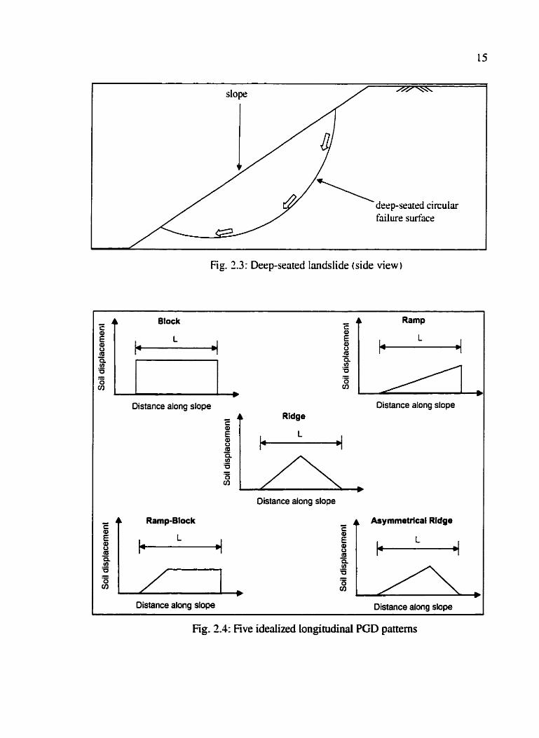
In a deep-seated landslide. the sliding surface ciosely resembles arcs of circles.
For a pipeline laid parallel to the direction of the slope. the deep-seated soil movement
creates both a longitudinal and transverse force on the pipeline.
2.3 Previous studies on pipeline subjected to soil movements
Simplified design methods for pipelines subjected to transverse and longitudinal
landslides have been proposed and developed by several researchers (e.g.. O'Rourke cmd
Nordberg, 1992; FIores-Brrrones and 0' Rourkr ( 1992); Rajmi a a/.. 1995: 0' Rourkr et
al.. 1995).
O'Rourke and Nordberg. ( 1993). and mores-Berronrs and O'Rourke ( 1992)
studied the behavior of buried pipelines subjected to longitudinal permmmt ground
deformations (PGD). Five idealized longitudinal PGD patterns (see figure 1.4) based on
observed patterns from previous earthquakes were used and analytical relations for the
axial strain in the pipe were developed. The five patterns considered were Block. Ramp.
Ridge, Ramp-Block. and Asymmetricd Ridge. It was shown that the Block pattern
produces the highest axid strain on the pipeline. but that the variations between different
patterns ye negligible compared to the effect of the length of the PGD. Their
assumptions for their model are more fully described below as 0' Rourke et a!. ( 1995)
continued and expanded on this work.
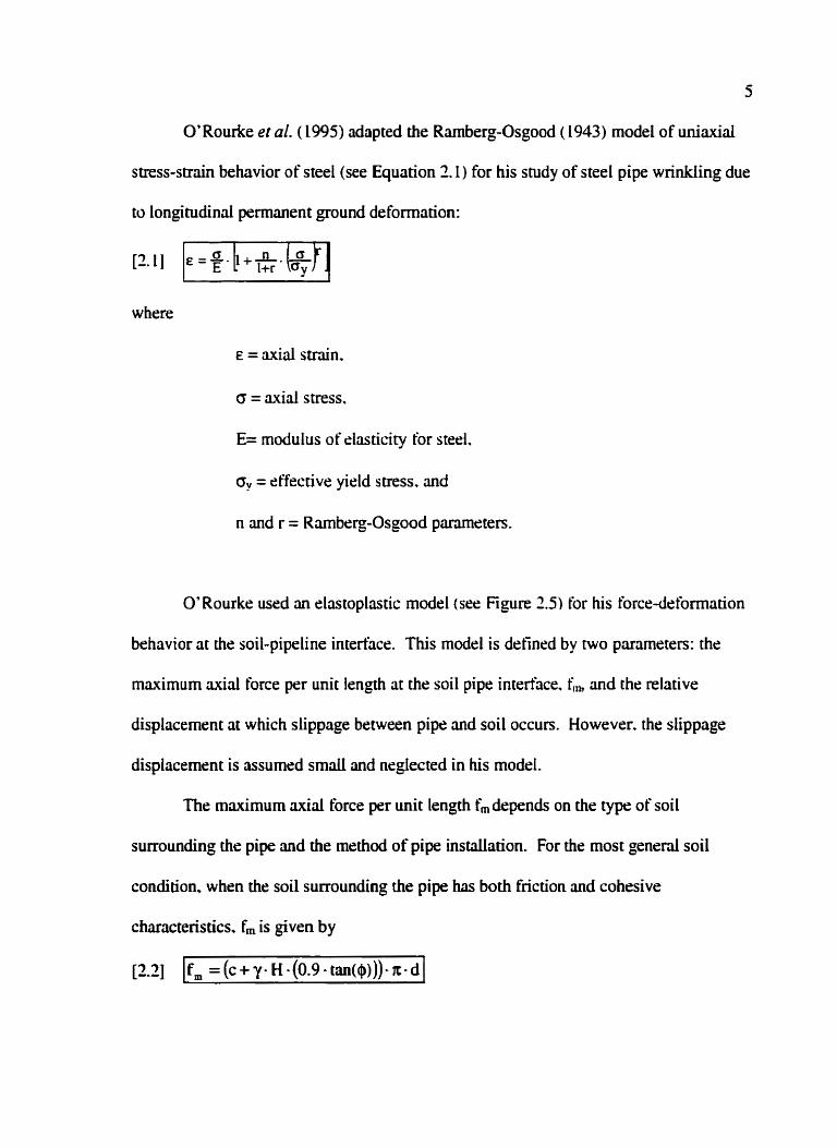
0' Rourke et al- ( 1995) adapted the Rmberg-Osgood ( 1943) model o f uniaxial
stress-strain behavior of steel (see Equation 1.1) for his study of steel pipe wrinkling due
to longitudinal permanent ground deformation:
where
E = axid strain,
G = axial stress.
E= modulus of elasticity for steel.
o, = cffeccive yield stress. and
n and r = Rmberg-Osgood panmeters.
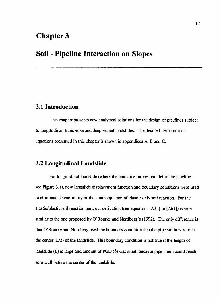
O'Rourke used an elastoplastic model (see Figure 2.5) for his force-deformation
behavior at the soil-pipeline interthcr. This model is detincd by two panmeters: the
maximum axial force per unit length at the soil pipe interface. f , and the relative
displacement at which slippage between pipe and soil occurs. However. the slippage
displacement is assumed small and neglected in his model.
The maximum axid force per unit length f, depends on the type of soil
surrounding the pipe and the method of pipe instidlation. For the most genenl soil
condition. when the soil sumounding the pipe has both friction and cohesive
characteristics, F, is given by
6
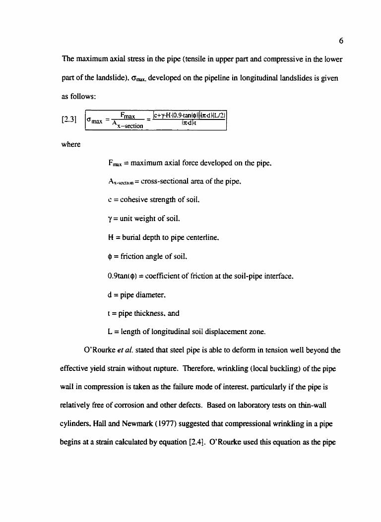
The maximum axial stress in the pipe (tensile in upper part and compressive in the lower
p m of the landslide), 0,. developed on the pipeline in longitudinal landslides is given
rrs follows:
[2.3]
where
F,, = maximum axial force developed on the pipe.
Ax-sealLn = cross-sectional area of the pipe.
c = cohesive strength of soil.
y = unit weight of soil.
H = burial depth to pipe centerline.
(I = friction mgle of soil.
0.9tan($) = coefficient of Friction at the soil-pipe interhcr.
d = pipe diameter.
t = pipe thickness. and
L = length of longitudinal soil displacement zone.
O'Rourke et al. smted that steel pipe is able to deform in tension well beyond the
effective yield strain without rupture. Therefore, wrinkling (local buckling) of the pipe
wdl in compression is taken as the failure mode of interest. particularIy if the pipe is
relatively Free of corrosion and other defects. Based on laboratory tests on thin-wall
cylinders, Hall and Newmuk ( L977) suggested that compressionaI wrinkling in a pipe
begins at a strain calculated by equation [ly. O'Rourke used this equation as the pipe
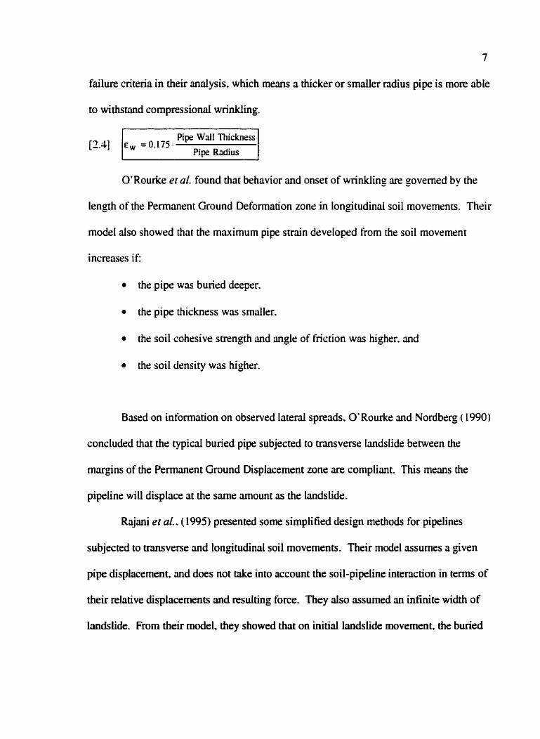
failure criteria in their analysis, which means a thicker or smaller radius pipe is more able
to withstand compressiond wrinkling.
O'Rourke era!. found that behavior and onset of wrinkling are governed by the
length of the Permanent Ground Deformation zone in longitudinal soil movements. Their
model also showed that the maximum pipe swain developed from the soil movement
increases if:
the pipe was buried deeper.
the pipe thickness was smaller.
the soil cohesive strength and angle of friction was higher. and
the soil density was higher.
Baed on information on observed lateral spreads. O'Rourke and Nordbrrg ( 1990)
concluded that the typical buried pipe subjected to transverse Iandslide between the
margins of the Permanent Ground Displacement zone are compliant. This means the
pipeline will displace at the same amount as the landslide.
Rajani et aL, (1995) presented some simplified design methods for pipelines
subjected to transverse and longitudinal soil movements. Their model assumes a given
pipe displacement, and does not take into account the soil-pipeline interaction in terms of
their relative displacements and resulting force. They Jso assumed an infinite width of
Imdslide. From their model, they showed that on initial landslide movement, the buried
8
pipeline and the soil behaves elastically. As the landslide movement increases. ultimate
passive resistance is developed in the surrounding soil medium. but the pipe will remain
elastic. On further landslide movement, 3 plastic hinge or wrinkle begins to develop in
the pipeline. They also showed that using cohesive soil in the model for the soil reaction
produces the most conservative numbers because the undrained npid response produces
the highest soil resistance. They performed a parmetric study for a pipeline subjected to
transverse landslide. and they found that the soil strength has the most dominant effect on
pipeline response. They found that the soil stifmess in terms of the elastic subgrade
modulus. Ks. has large effect at small pipeline displacements t when the soil is elastic) but
small effect for larger pipeline displacements (when the soil is plastic).
2.4 Previous probabilistic studies
The objective of statistied analysis. as applied to pipelines in unstable slopes. is
to assess the risk and probability of pipeline failure. Three main techniques are used for
statistical analysis. md they are the Monte Carlo simulations. the First Order Second
Moment (FOSM). and the Rosenblueth's Point Estimate Method (PEM). The Monte
Carlo technique involves generating random numbers using the mean and standard
deviations for each variable of the function. FOSM is obtained from the Taylor series
expansion of the Function about the expectations of the random variables. This Taylor
series approximation may impose excessive restrictions on the function (existence and
continuity of the first or k t few derivatives) and requires the computation of derivatives.
These difficulties can be overcome with the use of point estimates (PEM) of the function,
9
which leads to expressions akin to finite differences. Of these three methods. only the
Monte Carlo simulation method uses the whole statistical distribution of the variables.
The FOSM and PEM both only use one standard deviation from the mean for their
caiculntions,
Appropriate actions could be taken for a given level of probability of pipeline
failure. At low hilure probability. perhaps implementing a monitoring program for the
slope and the pipeline is dl that is needed. At medium Mlure probability, some remedial
action such s construction of a berm or improving drainage dong the slope to stop the
slope movement could be implemented. The induced pipe strain could be reduced by
increasing the pipe wall thickness. decrese the burial depth of the pipe or use lower
density soil with lower angle of fictional angle. It may also be 3 good idea to install
block valves both upstream and downstream of the potential landslide zone to
automatically shutoff the pipe in case of pipe failure. At high failure probability. major
action could be needed such as rerouting the pipeline to a more stable area.
Nguyen and Chowdhury ( 1984) used Monte Carlo simulations and Rosenblueth's
point estimate method for assessing slope stability of spoil piles in strip coal mims.
Cdculdons for failure probability were first made using Monte Carlo simulations and
assuming a potential two-wedge failure mechanism for the spoil piles. The Monte CuIo
technique involves generating pseudo-random numbers based on the mean and standard
deviations of the shear strength parameters. From 500 simulations, the kquency
distribution of the factor of sdety was obtained. The probability of failure was calculated
10
as the ratio of area under the kquency distribution curve from the left-hand tail up the
factor of sdety of unity, and that bound by the whole curve.
An alternative procedure based on Rosenblueth's method of estimating moments
was then used to compare the results with the Monte Carlo simulation method. Excellent
agreement was found and it was recommended that for practical purposes. the relatively
quick Rosenblueth method should be used in estimating the probability of slope failures.
Nguyen and Chowdhury dso concluded that estimates of strength parmetes of spoil
piles based on test results and associated geomechmics considerations must be made for
each particular mine. Due to the variation in soil parameters at each different site. it
would not be feasible to construct design charts that are univmally applicable to (111 spoil
piles.
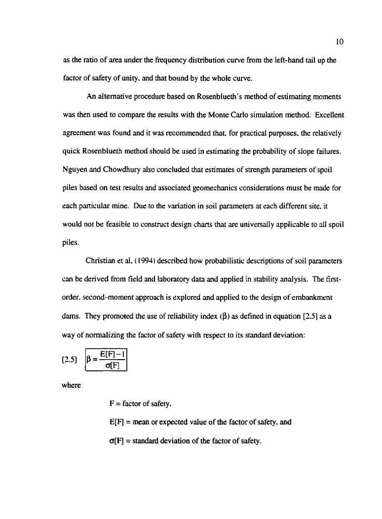
Christian t t d. ( 1994) described how probabiiistic descriptions of' soil parameters
can be derived from field and labontory data and applied in stability analysis. The first-
order. second-moment approach is explored and applied to the design of embankment
dams. They promoted the use of reliability index (P) as defined in equation [2.5] as a
way of normalizing the factor of safety with respect to its standard deviation:
where
F = factor of safety.
Em = mean or expected value of the factor of sdkty, and
am = standard deviation of the factor of sdety.
1 1
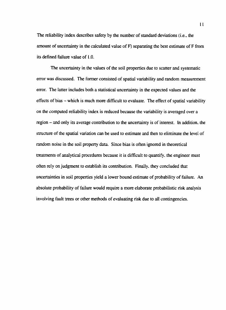
The reliability index describes safety by the number of standard deviations (i.e.. the
amount of uncertainty in the calculated value of F) separating the best estimate of F from
its defined failure value of 1.0.
The uncertainty in the values of the soil properties due to scatter and systematic
error was discussed. The former consisted of spatial variability and random measurement
error. The latter includes both a statistical uncertainty in the expected values and the
effects of bias - which is much more difficult to evaluate. The effect of spatial variability
on the computed reliability index is reduced because the variability is averaged over a
region - and only its average contribution to the uncertainty is of interest. In addition. the
structure of the spatial vluiation can be used to estimate and then to eliminate the kvel of
random noise in the soil property data. Since bias is often ignored in theoretical
treatments of analytical procedures because it is difficult to quantify. the engineer must
often rely on judgment to establish its contribution. Findly. they concluded that
uncertainties in soil properties yield a lower bound estimate of probability of failure. An
absolute probability of failure would require a more elaborate probabilistic risk andysis
involving fault trees or other methods of evaluating risk due to ail contingencies.
2.5 Critique
Obviously missing from previous research is the study of pipeline-soil interaction
in a deep-seated landslide. All previous studies only have been for pipelines subjected to
planar fiiilure surfaces.
mores-Berrones and O'Rourke ( 1992) and 0' Rourke et a[. ( 1995) ignored the
relative displacement at which slippage between pipe and soil occurs. Their model
ignores the elastic soil reaction by using only the maximum fictional force per unit
length. f,,,, to calculate the forces acting on the pipeline.
In addition. O'Rourke et ul. assumed symmetricd force development between the
stable and unstable soil regions. This could only be true if there is no elmtic soil
reaction. so that dl force developed on the pipeline comes only from the maximum
frictional force per unit length (plastic soil). G If both plastic and elastic soil reaction
were to be considered. then there should be a longer zone of plastic soil developed inside
the landslide in order to balance the infinite length of stable soil.
Finally. O'Rourke's model is only set up for the simple case of finding the peak
strain for n given length of landslide (L) with an unlimited amount of PGD (8) and vice
versa. Solving both of these variables together at the same time would have allowed one
to predict the peak strain for a given length of landslide by monitoring the PGD.
Rajmi et aL, ( 1995) assumed a given pipe displacement for their model of
pipeline subjected to transverse and longitudinal soil movements instead of basing their
model for given amount of PGD. They ignored the soil-pipeline interaction in terms of
their relative displacements and resulting force. They also did not consider transverse

13
landslides of f ~ t e width. Finally, Rajani et al. ignored the effect of pipeline tensile
strain because they assumed that flexure is the dominant behavior of the pipeline for
small transverse displacements
This thesis will derive models for pipeline subjected to longitudinal. transverse.
combined longitudinal and transverse. and deep-seated landslides. Transverse lmdslides
of finite width will be studied. and tensile strain will be included as well, The models
will allow one to predict the maximum pipeline strain for given dimensions of landslide
by monitoring the mount of PGD. finally. srntisrical analysis using the FOSM. PEM
and Monte Cario simulation methods will be applied to a pipeline subjected to
longitudinal landslide in order to assess the probability of pipeline yielding.
Fig. 1.1: Planar landslide (top view)
///\\\
deep-seated circular failure sufiice
Fig. 2.3 : Deep-seated landslide (side view )
Fig. 2.4: Five idealized longitudinal PGD patterns
- Block @ Ramp
L c z 8 (II -
c
L i! 8 a -
% .- a - .- a V)
8 .- u - .& 0 V)
w Distance along slope Distance along slope
- Ridge t
i! 0 - 3 a - .- 0 cn
Distance along slope
t
C Ramp-Block - Asymmetrical Ridge
C:
E L t L 8 0 - 8
aJ - B 0 5 U) , - - 5 - *-
53 0 4
cn b
Distance along slope Distance along slope
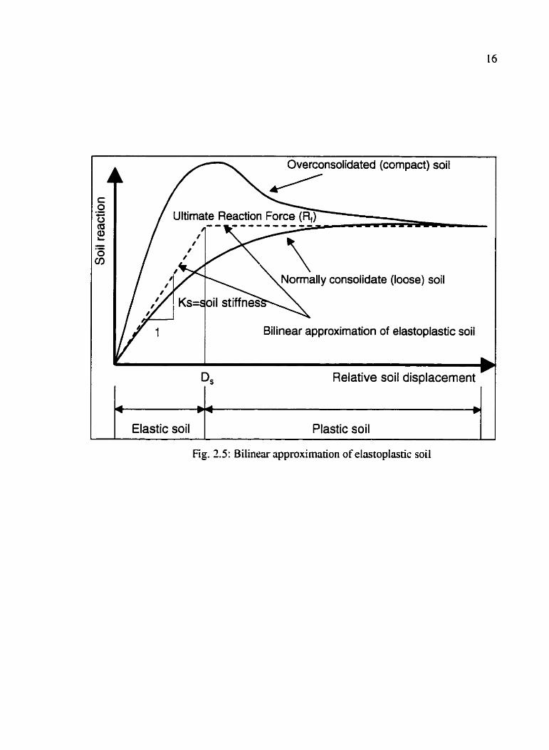
Fig. 1.5: Bilinear approximation of elastoplastic soil
Overconsolidated (compact) soil
C 0 .- c. U Ca 2 - .- 0 a
Bilinear approximation of elastoplastic soil
DS Relative soil displacement ' Elastic soil
b 4
Plastic soil
Chapter 3
Soil - Pipeline Interaction on Slopes
3.1 Introduction
This chapter presents new analytical solutions for the design of pipelines subject
to longitudinal. transverse and deep-seated imdslides. The detailed derivation of
equations presented in this chapter is shown in appendices A. B and C.
3.2 Longitudinal Landslide
For longitudinal landslide (where the landslide moves pamilel to the pipeline -
see Figure 3.1). new landslide displacement function and boundary conditions were used
to eliminate discontinuity of the stnin equation of elastic-only soil reaction. For the
rlastic/plastic soil reaction pact. our derivation (see equations [A341 to [A6 11) is very
similar to the one proposed by 0' Rourke and Nordberg's ( 1991). The on1 y difference is
that O'Rourke and Nordberg used the boundary condition that the pipe stnin is zero at
the center (U1) of the landslide. This boundary condition is not true if the length of
landslide (L) is large and amount of PGD (6) was smdl because pipe strain could reach
zero weil before the center of the landslide.

18
We assume elastoplastic soiVpipeline interaction using a bilinear approximation
of soil's stress-strain curves (see Figures 2.5 and 3.2). This is like the stress-strain curves
for steel with elastic and plastic ranges. The ultimate force developed as a Function of
soil displacement is expressed in equation [3. la]. where the subgrade modulus (Ks) is like
the Young's Modulus of Elasticity (E) for steel. The ultimate force can dso be expressed
as a function of the horizontal bearing capacity and undrained strength for clay in
equation [3. lb]. It is dso possible to represent it as a function of the cohrsive strength
and frictional angle for a general soil type with cohesive and Mctional chmcterisacs in
equations [3.1 c] .
where
Nc is the bearing capacity factor depending on the material properties.
Su is the undrained strength.
K, is the elastic subgnde modulus.
Ds is the soil displacement to reach the ultimate reaction force (typically 5-
10 mrn according to Committee on Gas and Liquid Fuel Life
Lines, L 984).
c is the soil cohesive strength.
y is unit weight of soil,
H is burial depth to pipe centerline.
0 is friction angle of soil, and
d is pipe diameter
c3--ri
where.
The force equilibrium for a finite element piece of pipe (see Figure 3.3) is given
in equation [3.1]. Combining this with the relationship between force and strain in
equation [3.3], we obtain a second-order differential equilibrium equation in the stable
and unstable regions in equation [3.4]:
N is the axid force on the pipe.
u is the pipe movement. and
6 is the soil movement.
[ 3 * 4
We assume the longitudinal landslide movement function as indicated in Figure
3.4 (note that it is a plot of the magnitude of soil and pipeline displacement dong the
length of the pipe axis). This is identical to the model of pipeline subjected to rigid block
PGD by O'Rourke and Nordberg ( 1992), but they had erroneously used the boundary
condition of zero sfrain at the center of PGD (U2).
- -- - - - -- -- -
20
The pipeline deflection is derived fiom solving the second-order differential
equilibrium equation [3.4] with appropriate boundary conditions. We have a stable
region From x = - to x = 0. and an unstable region from x = 0 to x = U1. The pipeline
from x = - - to U2 is in tension. and from x = U2 and beyond is in compression-
32.1 Elastic soil reaction
For 6 c ZDs, the soil is in elastic domain. The entire pipeline deflection profile can
be determined by applying the second-order differential equilibrium equation in the
stable and unstable regions (Figure 3.5). The continuity of svllin at x = 0 cannot be
satisfied using the step function indicated in Figure 3.4 for the soil displacement. Thus.
we change the soil displacemmt profile to increase at an angle (a) at x = 0. instead of
instantaneously as tbr the case of the step function when solving for 6 > 1D,. Also. the
boundary condition of e = 0 at x = U2 is not used because this is not true it' the length of
the imdslide (L) is very large. Instead. we replace the above boundary condition with the
continuity condition of strain at the transition point between the plastic and elastic soil
zones.
The analysis involves determination of 8 integration constants and position A.
The 8 integration constants are denoted by (CI and Cz in stable region; kl, kz, k3, IQ, kj,
and k6 in unstable region). We use the Following boundary conditions and equation to
determine the 9 constants:
At x = -o~ u = 0 (1 constant) where u is the displacement:
At x = 0, u and u' are continuous (2 constants);
At x = A, u and u' are continuous where u' is the first derivative (2
constants);
At x = B. u and u' are continuous where u' is the f i s t derivative (2
cons tan ts ) ;
At x = A. u = ur\ where u , ~ is the soil displacement at position A and equal
to the pipeline dehction ( 1 constant):
Force equilibrium equation in longitudinal direction ( I constant).
The following ;ire the equations to be used to solve the maximum strain in the
pipe at 6 < ZD, (see the derivations in Appendix A.2 from equations [A 121 to [A33]):
and
22
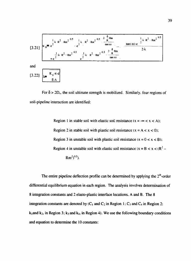
322 Elasto-plastic soil reaction
For 6 > 7Ds, the soil ultimate strength is mobilized. Four regions of soil-pipeline
interaction are identified (see Figure 3.4):
Region 1 in stable soil with elastic soil resistance (x = -a < x < x,);
Region 2 in stable soil with plastic soil resistance (x = x, c x c 0);
Region 3 in unstable soil with plastic soil resistance (x = 0 < x < xh):
Rrgion 4 in unstable soil with elastic soil resistance (x = xh < x < U2
where L is the width ofthe landsiide).
The entire pipeline detlection profile can be determined by applying the second-
order differential equilibrium equation in each region. The analysis involves
determination of 8 integration constants and 2 elasto-plastic interface locations. x, and .uh.
The 8 integration constants are denoted by (CI and Cl in Region 1: C3 and C in Rrgion
1: klmd k2, in Rrgion 3: k~ and b, in Region 4). We use the following boundmy
conditions and equation to determine the 10 constants:
At x = a. u = 0 ( 1 constant) where u is the displacrmmt:
At x = x,, u = D, ( I constant);
At x = x,, u and u'are continuous where u' is the first derivative (2
consmts);
At x = 0, u and u'are continuous (2 constants);
At x = xb, u and u'ae continuous where u' is the first derivative ( 2
constants);
At x = xb, u = 8 - Ds where 6 is the landslide movement ( I constant);
Force equilibrium equation in longitudinal direction ( 1 constant).
For the case of 6 > ZDs, the maximum pipe strain occurs at intertkce between stable and
unstable soil and is expressed in equation [3.7]. The expression is derived in Appendiv
A.3 from equations [A341 to (A6'71. The strain is taken as the first derivative of the pipe
deflection with respect to the pipe axis.
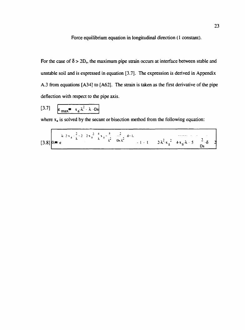
[3-71
where x, is solved by the secant or bisection method from the following equation:
3.3 Transverse Landslide
For transverse landslide (where the landslide is moving at 90' or perpendicular to
the pipeline - see Figure 3.6), a new analytical solution has been developed to include
both the bending and tensile strain on the pipe. The tensile strain is caused by the axid
stretching of the pipe due to axial forces (see Figure 3.7). Bending strain is caused by the
bending of the pipe such that the outer fiber of the pipe is stretched in comparison to its
neutral rutis (where the fiber kngth remains constant). See Equations [I33 11 and [B37-1
for the general tensile and bending strain equations. figure 3.8 shows that the tensile
stress is much higher than the bending stress near the intertier between stable and
unstable soil. It is therefore very important to account for the tensile stress as a pan of
the total stress,
Previous methods (e.g.. Hetenyi. 1946: Rajani et 01.. 1995) assumed a prior
knowledge of the pipe displacement or the force acting on the pipeline at the edge of the
landslide. They did not take into account the soil-pipeline interaction in terms of their
relative displacements and resulting force. They also assumed an intinite landslide width.
Rajmi et al. for example also employed the fourth-order differential equation of a
beam on elastic foundation. However. they ignored relative soil-pipeline displacement.
assumed intinite landslide width, and consequently they must also assume a double
curvature at the interface between stable and unstable soil. They calculated the stress
(strain) on a pipeline by Fiding the mvrimum moment developed due to an applied end
load. The applied end Load is derived as a hnction of end displacement of the pipe -
which is assumed known.
25
Like previous methods. we also use the bilinear approximation of the elastoplastic
soil. We have investigated nansverse landslides with infinite and finite landslide width,
and modeled the force acting on the pipeline as a function of relative soil-pipeline
displacement. Equilibrium of forces between stable and unstable soil is also imposed.
We also account for the tensile strain as a part of the total strain developed in the pipe -
by adding the tensile strain to the tensile part of the bending strain.
For most practical or conservative case. the relative soil movement exceeds D,. In
such case. the ultimate soil resistance is mobilized. There are four different soil-pipeline
interaction regions (see Figure 3.9 1:
Region 1 in stable soil with elastic soil resistance ( x = -- < x < A):
Region 2 in stable soil with plastic soil resistance ( x = A < x < 0):
Region 3 in unstable soil with plastic soil resistance ( x = 0 < x c B):
Region 4 in unstable soil with elastic soil resistance ( x = B < x c (R' -
~m')" .~)
The entire pipeline deflection profile can be determined by applying the fourth-
order differential equilibrium equation in each region (see equation [BJ]). This equation
is perfectly valid m Iong as the pipeline remains elmtic. Once the soil's elastic
displacement limit (Ds) is exceeded. then the ultimate reaction force (RI) will be acting on
that portion of the pipeline. while the rest of the pipeline-foundation is still elastic.
Equation [BJ] is solved to get pipeline displacement equation [B24] by assuming that the
soil displacement is a constant dong the width of the iandslide and combining the
homogeneous and nonhomogeneous solutions.
26
Using equation [B24], the analysis comes down to determining the 16 integration
constants and 2 elasto-plastic interface locations. A and B. The 16 integration constants
are denoted by (CI, Cr, C3, and CJ. in Region I: Cj. C6. C7r and CX, in Region 1; kl, kr, kr.
and b, in Region 3: kj, kn, k7. and t. in Region I). We use the following boundary
conditions and equation to determine the 18 constants:
At x = --. u = 0 (3 constants) where u is the displacement:
At x = A. u = Ds ( 1 constant);
At x = A, u, u*. u", and u" are continuous where u'. u" and u" are first.
second and third derivatives (4 constants):
At x = 0. u, u'. u". and u" are continuous (4 constants):
At x = B. u = up - Ds are continuous ( I constant):
At x = B. u. u'. u". and u" are continuous (4 constants):
At x = ( R' -~m')1"~. u = 0 ( 1 constant):
Force quiIibrium equation in transverse direction ( I constant).
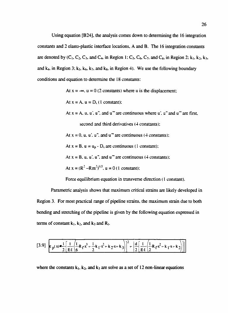
Parametric analysis shows that maximum critical strains ye likely developed in
Region 3. For most practical range of pipeline strains. the maximum strain due to both
bending and stretching of the pipeline is given by the following equation expressed in
terms of constant kl. k7, and k3 and Ri,
where the constants k,, kz, and k3 are solve as a set of 12 non-linear equations
27
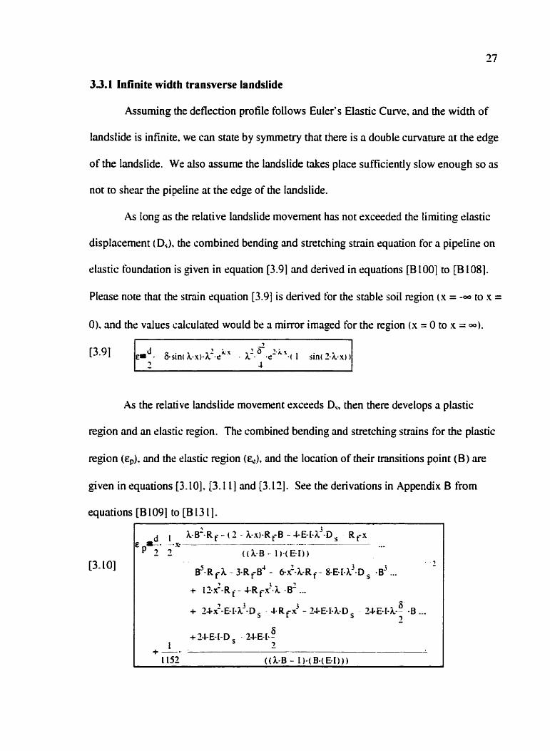
3.3.1 Infinite width transverse landslide
Assuming the detlection profile follows Euler's Elastic Curve. llnd the width of
landslide is infinite, we can state by symmetry that there is a double curvature at the edge
of the landslide. We also assume the landslide takes place sufficiently slow enough so as
not to shear the pipeiine at the edge of the landslide.
As long as the relative landslide movement has not exceeded the limiting elastic
displacement (D,). the combined bending and stretching strain equation for n pipeline on
elastic foundation is given in equation [3.9] and derived in equations [B 1001 to [B 1081.
Please note that the stnin equation [3.9] is derived for the stable soil region (x = -- to n =
0). and the values calculated would be a mirror imaged for the region (x = 0 to x = =).
13-91
As the relative landslide movement exceeds Ds, then there develops a plastic
region and an elastic region. The combined bending and stretching strains for the plastic
region ( E ~ ) . and the elastic region (G). and the location of their msitions point (B) are
given in equations [3.10], 13.1 11 and [3.12]. See the derivations in Appendix B from
equations [B 1 091 to [B 13 1 1.
d B' - CkB.2 E ey- (sin( 'B)-sin( Lx) - cos( LB)-cos( A-x) )-R FI ... . -. . - .*.
- 3
I (k-B - 1 I-( E-1) ).eA.' + ( sin( A-B) - cos( k B ) )-sin( Lx) ... -E-1-h -D ,-B ...
_+( COS( k-B) - sin( A-B) ).cos( h-.r) 1
+( sin( kx)-cos( LB) - cos( k-x)-sin( LB) 1-E-I-k--D
R (cos( L B ) sin( A-B) )-sin( h-x) ... . CB2 .-.
+ I - ( sin( k B ) - cos( LB) ).cos( Lx) +( cos( Lx)-cos( LB) sin( k-x).sint LB) ) - ~ - E . I - ~ J . D ,-B ...
1
+ (sin(k-B) cos(LB)).cosckx) ... -E-I-A--D, I + I-( sin( 1-B) - cost h-B) )-sin( h-x) + - 7 - ( k-( ( k-B - 1 I . ( E.1) 1 ).ek' I3 - t'
In equation [3.11]. B is the point of the transition between the plastic and elastic
zones. and it may be solved using the secant or bisection method.
Some of the results of this investigation are listed below:
I ) At small pipe deflections. the plastic zone is small. The
displacement. tensile suain. and bending strain profiles of the
elastoplastic equation look like that of the pure elastic
equation.
2) At Iarger pipe detlections, the plastic zone increases. The
elastoplastic soil deflects more than the pure elastic soil, but
the pipe in the elastoplastic soil curves less and subsequently
has lower bending and tensile strains (see Figure 3.10).
3) Depending on the various soil and pipe chncteristics. the
tensile stress from the stretching of the pipe has a significant
effect to the total stnin.
1) The plastic zone and total strain increases with the increase
of elastic modulus of the pipe (E). and the soil subgndr
modulus ( Ks).
5 ) The plastic zone increases but the total swain decreases
with increasing pipe thickness (t). and pipe diameter (dl.
6) If the soil density was less. the cohesive strength and
Frictional angle wm lower. and the pipe was not buried as
deep. then the totd strain developed is less. In other words. a
high soil resistance (Ri is high) will produce larger stress in
the pipe for any given ground displacement.
When the pipeline lies at an angle to the direction of Iandslide, the pipeline will be
subjected to both longitudinal and transverse loading. Since the resulting displacement-
strain relationships, as presented in this thesis. is modeled as elastic-plastic soil response.
it is not possible to simply add the effects of combined transverse and longitudinal
movements. However, it should be possible to take a combined longitudinal and
transverse loading and divide the loading vectoridy into each component. then
30
determine the strain in the pipe due to each component of loading and sum up the effects
on the pipe.
Figures 3.1 1 and 3.11 are plots of the maximum pipeline stnin developed for a
pipeline lying at 30 and 60 degrees to the landslide direction. respectively. for different
lengths of landslide. At 60 degrees, the pipe is subjected to higher m s v e n e loading and
lower longitudinal loading than at 30 degrees. As the angle between the axis of' the
pipeline and the landslide direction increases. the bending strain component increases and
become more dominant. while the tensile strain decreases.
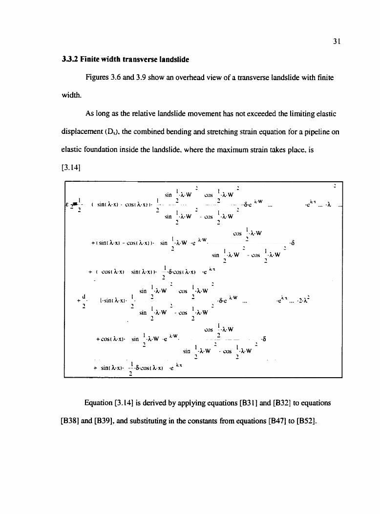
3.3.2 Finite width transverse landslide
Figures 3.6 and 3.9 show an overhead view of a transverse landslide with finite
width.
As long as the relative landslide movement has not exceeded the limiting elastic
dispiacemmt (Ds), the combined bending and stretching strain equation for a pipeline on
elastic foundation inside the landslide. where the maximum suain takes place. is
[3.141
, 7 ? ..
sin ' -A-w " cos '-L-w - 1 1 2 .a.C i. k. t E?,- I sin( h-XI - cia( A-r) I - - - - ... -c ... -A ...
7 v - ' sin '-L-w - - cos '*A-w - - - ci~s ' -LW
I k W +~sln(k.xl-cos(;C-x))- sin -A-W -t. - - - -- - - --- - 6 7 -
sm I - L W - - sos '+L.w - - -
A. K + I sost LK, sin[ b x , 1. I-ii-cus, A-x, -c - T 7
sin '-L.W ' sos l-LW - d 1 - - + - l-sinc L-XI- . -6.r kW ... 1 '1 - -
sin l -LW -- ,us ' -A-w - - - sos I-X-W
+ cmt ~ = x , sin '+L-w -e "-w. 2 -- --- -6 7 -
sin I - L W - - Lws I -A-w ' - 7 - I k s + sin( k--x). --6-cos( k-xl -t:
2
Equation [3.14] is derived by applying equations p 3 I and @32] to equations
[B38] and [B39], and substituting in the constants fioom equations @347] to [B52].
32
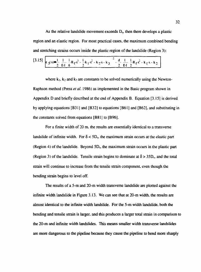
As the relative landslide movement exceeds Ds, then there develops a plastic
region and an elastic region. For most practical cases. the maximum combined bending
and stretching strains occurs inside the plastic region of the landslide (Region 3):
1
I 1 1 - 1 -, E J( XI-. -- - R r < - --k - k,.r - k3 - - d- I- - k l . ~ - k
2 E-I 6 7 - - Z E-I Z J
where kl. k2 and k3 are constants to be solved numerically using the Newton-
Raphson method (Press eta!. 1986) as implemented in the Basic program shown in
Appendix D and brir fly described at the end of Appendix B. Equation [3.15] is derived
by applying cquations [B3 I ] and [B32] to equations [B6 11 and [B621, and substituting in
the constants solved from equations [B8 11 to [B96].
For a finite width of 20 m. the results are essmtidly identical to a transverse
landslide of infinite width. For 6 < 5D,. the maximum strain occurs at the elastic part
(Region 4) of the landslide. Beyond 5D,. the maximum strain occurs in the plastic pan
(Region 3) of the landslide. Tensile strain begins to dominate at 6 > 35D,, and the total
strain will continue to increase from the tensile strain component. even though the
bending strain begins to level off.
The results of a 5-m and 20-m width transverse landslide m plotted against the
infinite width landslide in Figure 3.13. We can see that at 20-m width. the results are
almost identical to the infinite width landslide. For the 5-m width Iandstide, both the
bending and tensile strain is larger, and this produces a larger total strain in comparison to
the 20-rn and infinite width landslides. This means smaller width transverse Iandstides
are more dangerous to the pipeline because they cause the pipeline to bend more sharply
33
and stretch more than they would have for larger width landslides. They do this because
the soil is relatively stiff, and a small width landslide will act like a concentrated load that
tends to shear the pipeline along the interface between stable and unstable soil. The s l o p
of the pipeline in the middle of the landslide must be zero because of symmetry. and to
accomplish this for a small width landslide. the pipeline develops greater stretching and
bending strain near the interface of the landslide and stable soil. U the soil was less
dense. less cohesive and has lower internal frictional angle (lower soil resistance ). then
this problem would be reduced.
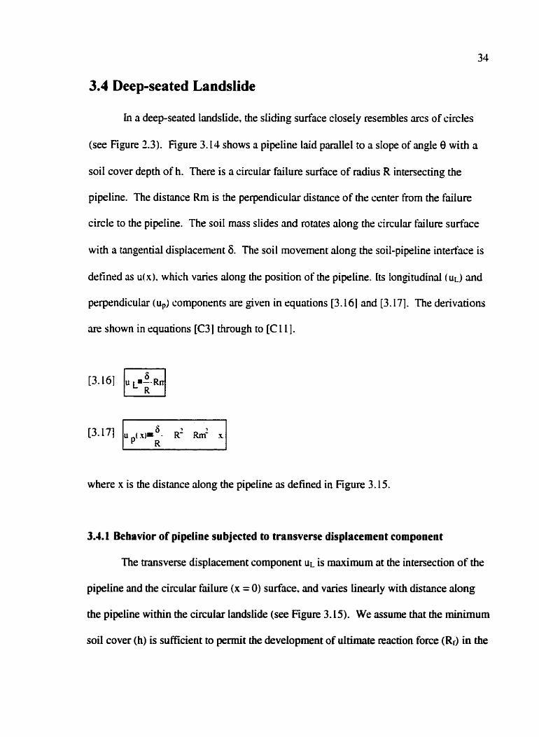
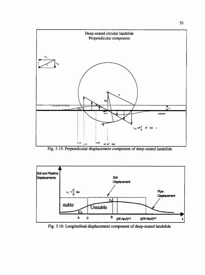
3.4 Deep-seated Landslide
In a deep-seated landslide, the sliding surface closely resembles arcs of circles
(see Figure 2.3). Figure 3.14 shows a pipeline laid parallel to a slope of angle 8 with a
soil cover depth of h. There is a circular failure surface of radius R intersecting the
pipeline. The distance Rm is the perpendicular distance of the center from the Failure
circle to the pipeline. The soil mass slides and rotates along the circular fiilure surhce
with a tangential displacement 6. The soil movement dong the soil-pipeline interface is
detined as u(x). which varies dong the position of the pipeline. Its longitudinal ( uL) and
perpendicular (up) components are given in equations [3.16] and [3.17]. The derivations
are shown in equations [C3] through to [C 1 I].
where x is the distance along the pipeline as defined in Rgure 3.15.
3.1.1 Behavior o f pipeline subjected to transverse displacement component
The transverse displacement component UL is maximum at the intersection of the
pipeline and the circular f~ lure (x = 0) surface, and varies Iinedy with distance along
the pipeline within the circular landslide (see Rgure 3.15). We assume that the minimum
soil cover (h) is sufficient to permit the development of ultimate reaction force (Rd in the
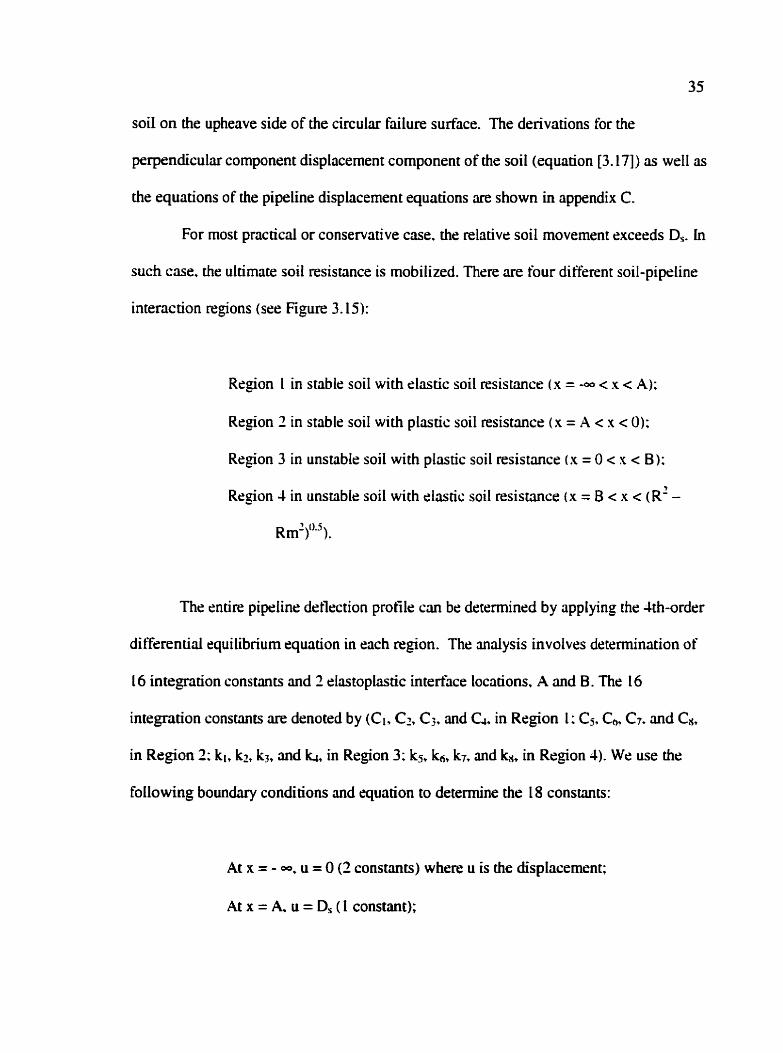
soil on the upheave side of the circular failure surface. The derivations for the
perpendicular component displacement component of the soil (equation [3.17]) as well as
the equations of the pipeline displacement equations ye shown in appendix C.
For most practical or conservative case. the relative soil movement exceeds Ds. In
such case. the ultimate soil resistance is mobilized. There are four different soil-pipeline
interaction regions (see figure 3.15):
Region I in stable soil with elmtic soil resistance (x = -m < x c A):
Region 2 in stable soil with plastic soil resistance ( x = A c .u < 0):
Region 3 in unstable soil with plastic soil resistance ( x = 0 c I c B ):
Region 4 in unstable soil with elastic soil resistance ( x = 0 < x < (R' -
~m')O.j).
The entire pipeline det'ection protile can be determined by applying the 4th-order
differential equilibrium equation in each region. The analysis involves determination of
16 integration constmts and ? sIastoplastic interface locations, A and B. The L6
integration constants are denoted by (CIT C2, C3* and C.4. in Regon 1 : Cj, C,, Ct. and C8.
in Region 2: kl, kzT k3, and b, in Region 3: ks, k6, k7. and b, in Region 4). We use the
following boundary conditions and quation to determine the 18 constants:
At x = - =, u = 0 (1 constants) where u is the displacement;
At x = A, u = Ds ( I constant);
36
At x = AT u. u', u", and u" are continuous where u', u" and u" are first,
second and third derivatives (4 constants):
At x = 0. u. u', u", and urn are continuous (4 constants);
At x = B. u = up - Ds are continuous ( L constant):
At x = B. u. u', u". and u" are continuous (4 consrants):
At x = (R' -~rn')'.'. u = 0 ( 1 constant):
Force equilibrium equation in transverse direction ( L constant).
Parametric analysis shows that the maximum combined bending and tensile strain
occurs in the plastic soil region of the soil movement (Region 3) 3s represented in
equation [3.18]. This equation is derived by applying equations [B3 I ] and [B321 to
equation [C 171. The constants in the equation are solved simultaneously as a set of 18
non-linear equations [C21] to [C38].
d l l + - . - . R f i - k i . " - k , - E-r 2
37
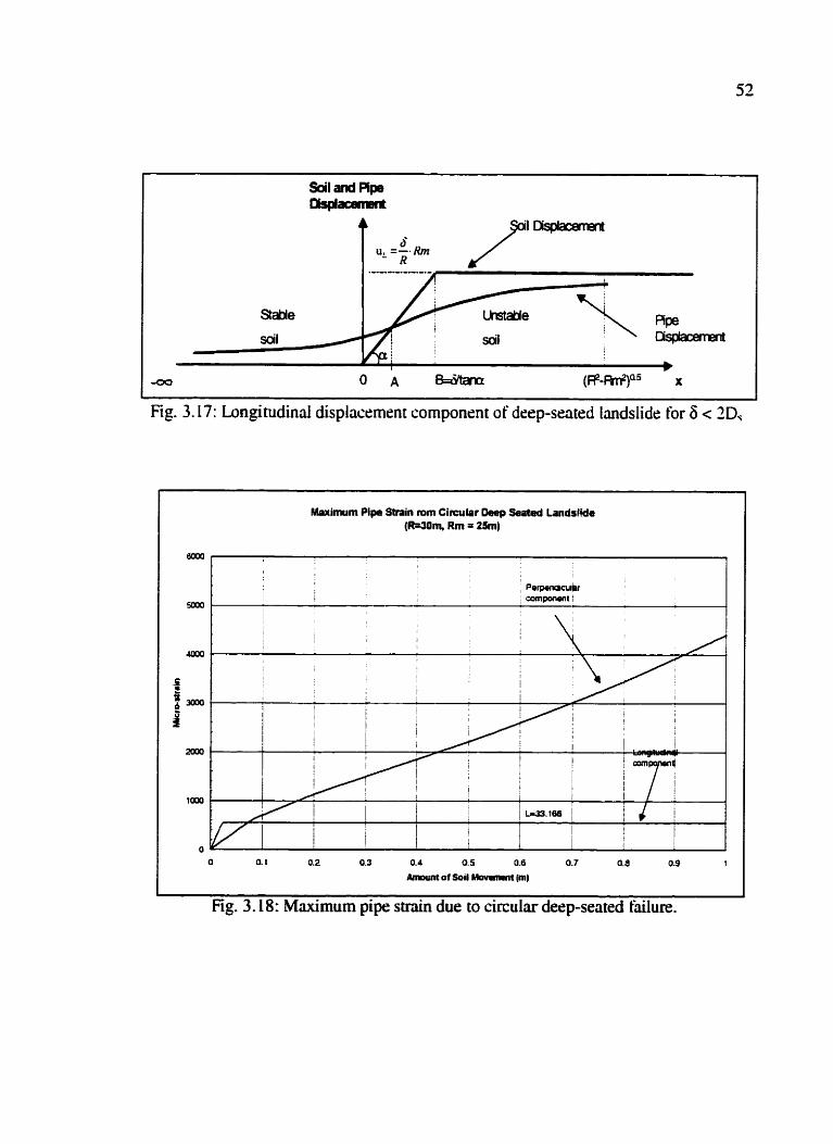
3.42 Behavior of pipeline subjected to longitudinal displacement component
The longitudinal component of the soil movement from n circular deep-seated
failure is constant dong the pipeline. The soil-pipeline interaction problem is solved
iteratively exactly using the method proposed by Chm and Wong ( 1997). The pipeline
detlection is derived from solving the second-order differential equilibrium equation with
appropriate boundary conditions as described already in section 3.2. The only difference
is that in all the equations (for example. equation [3.4]). the displacement magnitude (8)
md landslide length (L) for the planar landslide is replaced by ( t G/R)Rrn) and (71 R' -
~rn'f'.') for the longitudinal component of deep-seated landslide (see Figure 3.16 and
3.17).
We have a stable region from x = - = to x = 0. a d an unstable region From ?r = 0
to x = (@R)Rm. The pipeline from x = - = to tG/R)Rrn is in compression. and from x =
(6lR)Rm to - is in tension.
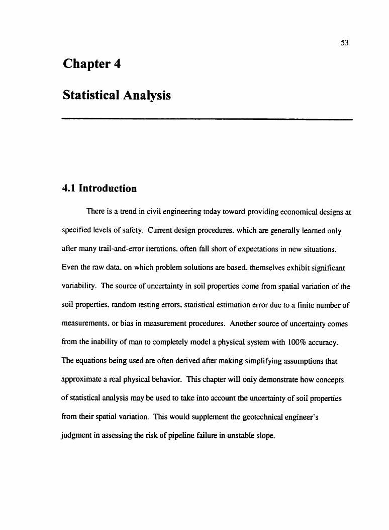
For 6 c 2 4 , the soil is in elastic domain. The entire pipeline de tlection pro tile
can be determined by applying the 21h-order differential equilibrium equation in the stable
and unstable regions (Figure 3.17). The continuity of strain at x = 0 c m o t be satisfied
using the step function indicated in figure 3.16 for the soil displacement. Thus. we
change the soil displacement profile to increase at an mgie (a) at x = 0. instead of
instantaneously as for the case of the step function when solving b r 6 > ZDs. Also. the
boundary condition of E = 0 at x = (R' -E2m2)"' is not used because this is not true if the
length OF the longitudinal component ( 2 ( ~ ' - R ~ ' ) O - ~ ) is very large. The analysis involves
determination of 8 integration constants and position A. The 8 integration constants ye
38
denoted by (CI and C2 in stable region; kl, kl, k3. IQ, kj, and k6 in unstable region). We
use the following boundary conditions and equation to determine the 9 constants:
At x = --. u = 0 ( 1 constant) where u is the displacement;
At x = 0, u and u' are continuous (2 constants):
At x = A, u and u ' m continuous where u' is the tirst derivative (2
constants 1:
At x = B, u and u'm continuous where u* is the first derivative ( 2
constants):
At x = A. u = uh where u,, is the soil displacement at position A and equal
to the pipeline de tlection ( 1 constant):
Force equilibrium equation in longitudinal direction ( 1 constant).
The following are the equations are used to solve the maximum strain in the pipe
at 6 < l D s :
E3.191
For 6 > 2 4 , the soil ultimate strength is mobilized. Similarly. four regions of
soil-pipeline interaction are identified:
Region 1 in stable soil with elastic soil resistance ( x = - c x < A):
Region 1 in stable soil with plastic soil resistance ( x = A e x < 0):
Region 3 in unstabk soil with plastic soil resistance tx = 0 c x < B):
Region 4 in unstable soil with elastic soil resistance (x = B c x < (R' -
~m~)". ') .
The entire pipeline deflection profile can be determined by applying the ??order
differential equilibrium equation in each region. The analysis involves determination of
8 integration constants and 1 elasto-plastic interthce locations. A and B. The 8
integration constants are denoted by (C I and C2 in Region 1 : C3 and C in Region 2:
klmd kr, in Region 3; k3 and h. in Region 4). We use the following boundary conditions
and equation to determine the 10 constants:
At x = --. u = 0 ( 1 constant) where u is the displacement;
At x = A, u = Ds ( 1 constant);
At x = A. u and u'are continuous where u' is the t-mt derivative (2 constants):
At x = 0. u and u' are continuous (2 constants):
At x = B. u and u' are continuous where u' is the First derivative (2 constants);
At r = B. u = h - Ds where id is the landslide movement ( I constant):
Force equilibrium equation in longitudinal direction ( I constant).
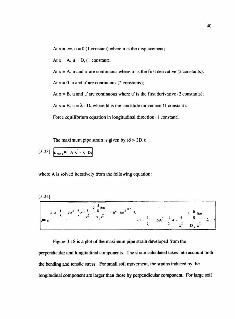
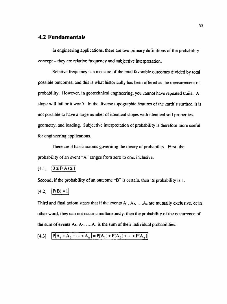
The maximum pipe s a i n is given by (6 > l D s ) :
where A is solved iteratively from the following equation:
E5gure 3.18 is a plot of the rnzlxirnurn pipe strain developed From the
perpendicular and longitudinal components. The strain calculated takes into account both
the bending and tensile stress. For small soil movement the s a i n s induced by the
longitudinal component ace larger than those by perpendicular component. For large soil
41
movement, the perpendicular component dominates the deformation mode. which
indicates the most probable mode of failure is shearing near the intersection of the pipe
and the circular failure surface,
3.5 Summary
Permanent Ground Displacement (PGD) refers to my type of a nonrecoverable
soil movemenr such as a landslide. This thesis studied the soil-pipeline interaction for 3
pipeline in longitudinal. transverse and deep-seated landslides.
The tensile strain was added on top of the bending strain in the transverse
landslide analysis. and it was shown to contribute significantly to the total strain
developed in a pipeline.
It was shown that uansversc landslides with a smaller width would produce
greater strain on the pipeline than a landslide of larger width. Also shown was that
pipelines in m s v e n e landslides of greater than about 10-rn width acts as if it was in a
transverse landslide of infinite width. Our analysis indicates that if the width of the
landslide (W) is greater thm IO-m. the pipeline will act as a compliant pipe. that is, the
pipeline will displace at the same amount as the landslide. This agrees with the
conclusion made by O'Rourke and Nordberg ( L990) based on information on observed
lateral spreads.
Of the three different types of landslides, the deep-seated landslide is the most
dangerous for pipeline fhiIure. It does not take very much deep-seated soil movement to
shear the pipeline near the interface between stable and unstable soil. It is wise to
42
construct berms at the foot of slopes to prevent any such deep-seated landslides. The
next most dangerous landslide is the transverse landslide because it can also shear the
pipeline at the interface between stable and unstable soils.
The maximum strain developed in a pipeline in a longitudinal landslide reaches a
plateau after and beyond a certain soil displacement. Since most longitudinal landslides
are less than 100-m long, it would mean most pipelines could withstand most typicd
longitudinal landslides for my amount of soil displacement.
The most critical parameters in the safe design of pipelines in unstable slopes are
the soil resistance ( Rt). pipe modulus of elasticity ( E). and pipe thickness (t). Using light
weight aggregate (LWA) as a backtill not only provides dninage. but it will reduce the
strain induced in the pipeline in a landslide. Using a more elastic steel pipe (lower
modulus of elasticity) and thicker pipe would reduce the strain induced in the pipeline as
well.
fig. 3.1 : Longitudind landslide
Fig. 3.1: Force-displacement relationship of soil
Fig. 3.3: Force equilibrium on a finite element of pipe
Soil and Pipeline Displacements Soll
Displacement stable unstable soil soil Pipe
d Displacement
x@ 0 X
Realon 1 t / Realon 3 t fl II t . / /
Regton 2 Region 4
Fig. 3.4: Soil and pipeline displacement profile for longitudinal landslide
Soil and Pipe Oisp lacement
4 oil Displacement Stable unstable
8
Pipe Oisplacement
Fig. 3.5: Assumed soil displacement protile for 6 < 7Ds in longitudinal landslide
Fig. 3.6: Transverse Imdslide of finite width
r""""""""" I
I I
Unstable soil pushing pipeline I I
I
down the slope
Pipeline I 1
()We*
Stable soil resisting Stable soil
pipeline movement Unstable soil
u +
Wl2 b4 b
Wl2
1 Axial loading
I r z , L AL
)I
Tensile strain
Neutral axis
AL (p+y ) -0 -p -0 y Bending strain ,h = - =
=- E l
Bending load
7
Rg. 3.7: Tensile and bending suain
C ~ O ~
3.5'10 8
3* 1 I)*
c 2.5'10 8
Z rn V)
2*10 X
5 Q) c .- - a 1.5'10 X
Q b-
111111
5'10 7
I ) f 1 1 - 3 4 5 7
Distance from edge of landslide(m)
Fig. 3.8: Example of tensile. bending and total pipe stress in a transverse landslide
Stale Unstable -66 A soil soil B w/2 x
1 b
Region t
Displacement Plastic soil ~s 1 Elastic sol(
Soil Displacement Displacement
Fig. 3.9: The 4 regions of soil-pipeline interaction under nansverse landslide of finite width
fig. 3.1 1: Maximum pipe strains at 30 degrees to [andslide direction
----
Maxhmrn St rain fiom Landslide 9 . 6
Angle of Pipdine w.r.t Landslide = 30 degrees 7
-- -- - - --
W m m Pipe Strain from Landslide 6 .6 Angk of Pipelina w.r.t bndslkk = 60 dagmes 1
- - .
~ . O O
- - - - - - - - - e - - - - - Stmn
1m.00 - - - - 1mOO -
0.00 la00 20.00 30.00 a00 Y).m Amom of Soil Mwment (in multiples of 0.008m) -
m.00
C - s m , m -
Fig. 3.11: Maximum pipe stnins at 60 degrees to landslide direction
. r#K).m--- - -- - - --.- - -- - 40()000------------------.
JjOO.W----- - - - - - -Eikdi i - - -
- - - - - - - --- S t " ? ! ? - - -
stwa'm - - - - 1500 00 - -
Goo 10 00 20.00 30.00 .law 5a 00 Amowtof So11 Movement (in rnutliples of O.OO8m)
Maximum Pipe Strain from Transverse Landslide Angle of Pipeline w.r.t Landslide = 30 dug-
- . - - - - -
- - -
- . - - . - - -
- - - a - -
-. .
0 20 Jd a 80 100 120
Amount of POD (multiples of 0.0081~1) - - - -- - - - -- - -- -- -- - - - -- - --
-~nlinttm wfdm landallde -2Om --lty+~ds +jm mdm land3I1~ - -
Fig. 3.13: Comparing maximum pipe stnin at 30 degrees to landslide direction for infinite width and finite width transverse landslides
Fig. 3-14: Circular deep-seated landslide
Deep-seated circular landslide Perpendicular component
r--A e t r t . K' ~m'
Fig. 3 - 1 5: Perpendicular displacement component of deep-seated landslide
Soil and Pipeline w-
8 u, =-. h
R
stable
A 0 ( F P . W O . 5 2(FP-Rn30*5 X
Fig. 3.1 6: Longi tudind displacement component of deep-seated landslide
Soil and PIP
A 3'
UL =-. Rm R
Stable \ AW
R'-
I b -06 O A 6=&m (e-Wa5 X
Rg. 3.17: Longitudinal displacement component of deep-seated landslide for 6 < l D s
Maximum Pipe Strain rom Circular Deep Seated LandslMe (-Om, Rm = 2Sm)
0 0 0.1 0.2 0.3 0.4 0.5 0.6 0.7 0.9 0.9 1
Amount of Soil Movarnt (m)
Fig. 3.18: Maximum pipe strain due to circular deep-seated failure.
Chapter 4
Statistical Analysis
4.1 Introduction
There is a trend in civil engineering today toward providing economical designs at
specitied levels of satkty. Current design procedures. which ye generally learned only
after many trail-and-error itmtions. often fall short of expectations in new situations.
Even the raw data. on which problem solutions are based. themselves exhibit significant
variability. The source of uncertainty in soil properties come from spatial variation of the
soil properties. mdom testing errors. smtisticd estimation error due to a finite number of
measurements, or bias in measurement procedures. Another source of uncertainty comes
from the inability of man to completely model a physical system with 100% accuracy.
The equations being used clre often derived after making simplibng assumptions that
approximate a red physical behavior. This chapter will only demonstrate how concepts
of statistical analysis may be used to take into account the uncertainty of soil properties
from their spdal variation. This would supplement the geo technical engineer's
judgment in assessing the risk of pipeline f&ilure in unstable slope.

54
Three main techniques are used and they are the Monte Carlo simulations. the
First Order Second Moment (FOSM), and the Rosenblueth's Point Estimate Method
(PEW-
4.2 Fundamentals
h engineering applications, there are two primary definitions of the probability
concept - they are relative frequency and subjective interpretation.
Relative Frequency is a measure of the total favorable outcomes divided by total
possible outcomes. and this is what historically has been offered as the measurement of
probability. However. in geotechnicd engineering, you cannot have repeated mils. A
slope will fail or it won't. In the diverse topographic features of the earth's surface. it is
not possible to have a large number of identical slopes with identical soil properties.
geometry. and loading. Subjective interpretation of probability is therefore more useful
for engineering applications.
There are 3 basic axioms governing the theory of probability. First. the
probability of an event "A" ranges from zero to one. inclusive.
[4.1] I O I P ( A ) S I ~ Second. if the probability of an outcome "B" is certain. then its probability is I .
[4.1] I P ( B ) = I ~ Third and find axiom states that if the events A,, A?, .... A, are mutually exclusive. or in
other word, they can not occur simultmeously. then the probability of the occurrence of
the sum of events A[, A?, . . ..Ao is the sum of their individual probabilities.
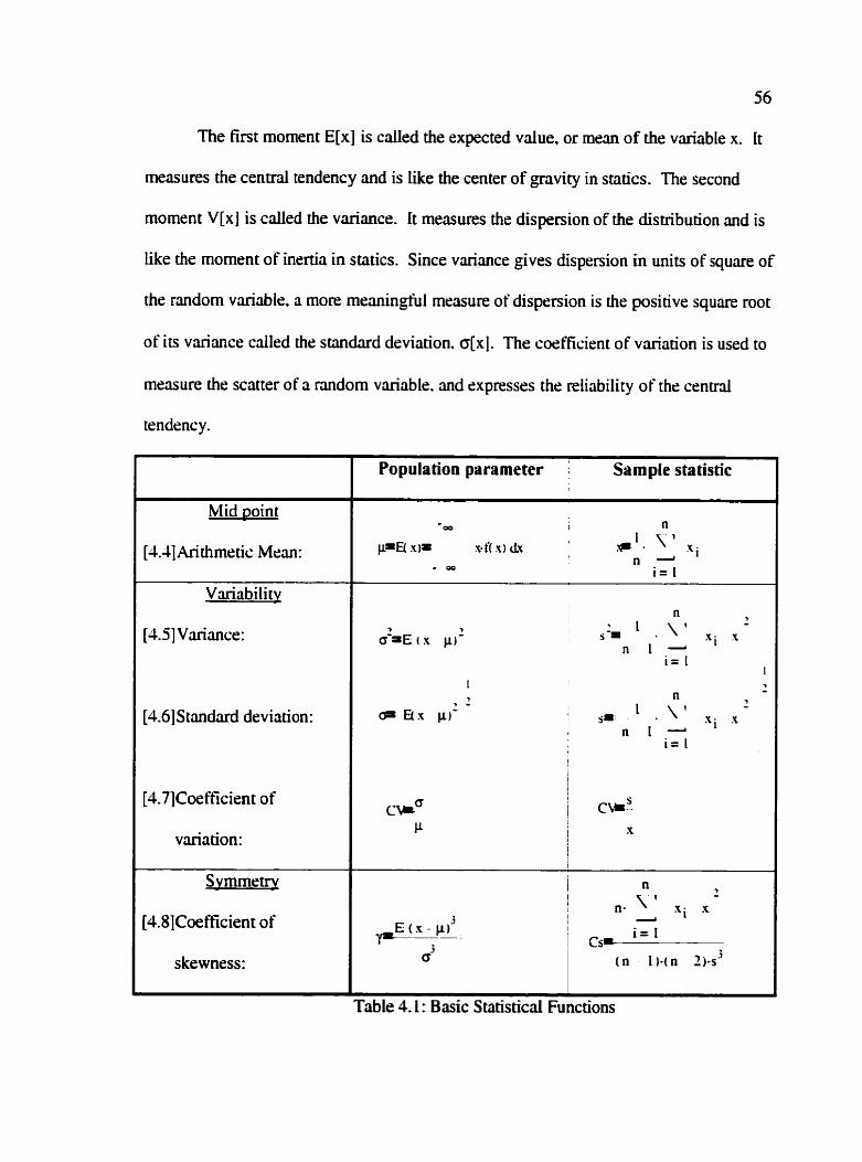
The tirst moment E[x] is called the expected value, or mean of the variable x. It
measures the central tendency and is Like the center of gravity in statics. The second
moment V[x] is called the variance. It measures the dispersion of the distribution and is
Like the moment of inertia in statics. Since variance gives dispersion in units of square of
the random variable, a more meaningful measure of dispersion is the positive square root
of its variance cdled the standard deviation. ~ [ x ] . The coeficient of variation is used to
measure the scatter of n random vuiable. and expresses the reliability of the central
tendency.
Mid ~ o i n t
[4.4 Arithmetic Mean:
Variability
[4.5] Variance:
[4.6] S tandard deviation:
[LCJJCoefficient of
variation:
skewness:
. -.
Population parameter i Sample statistic
Table 4.1 : Basic statistical Functions
57
According to Chow et al. ( 1988). the sample estimate of the variance is divided
by "n- 1" rather than "n" to ensure that the sample statistic is "~nbiased". that is. not
having a tendency. on avenge. to be higher or lower than the true value. The coefficient
of skewness measures the symmetry of the data. For positive skewness (Cs>O). the data
are skewed to the right. with a longer tail of data on the right of the mean.
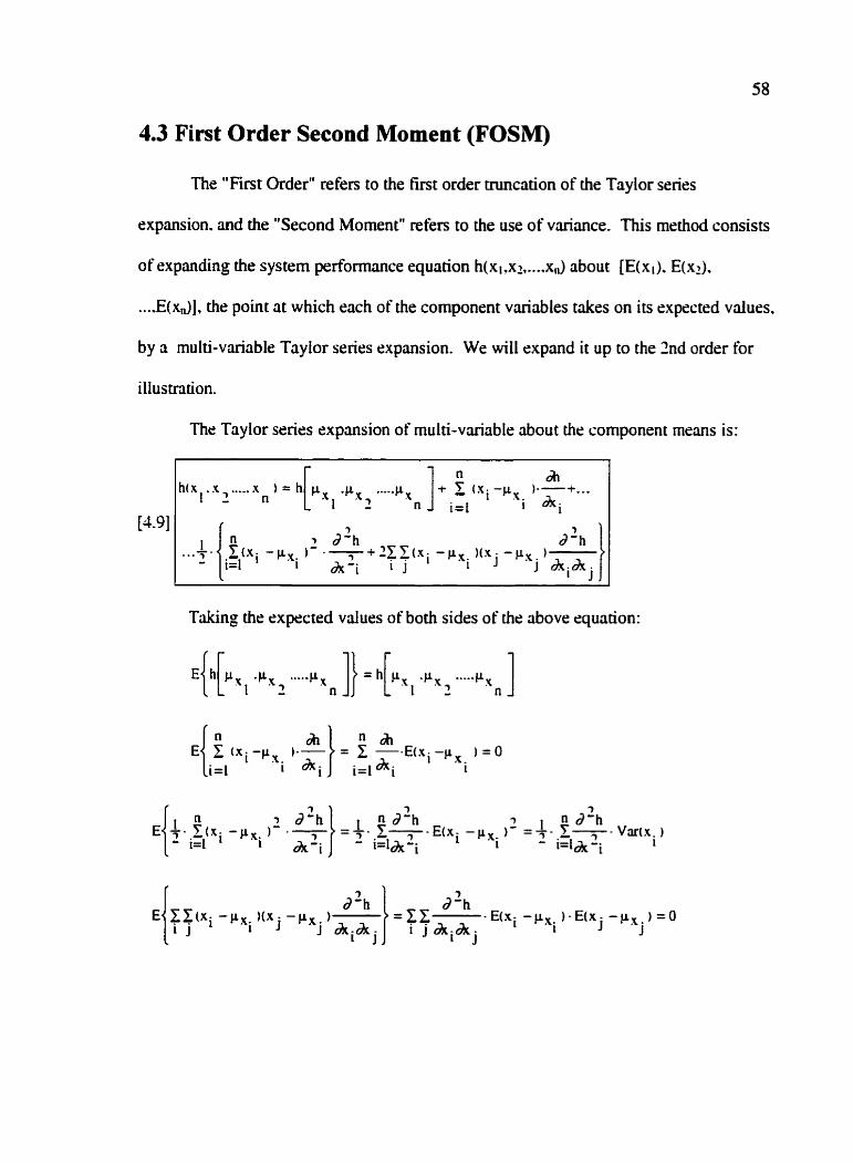
4.3 First Order Second Moment (FOSM)
The "First Order" refers to the F i t order truncation of the Taylor series
expansion. and the "Second Moment" refers to the use of vdance. This method consists
of expanding the system performance equation h(x1,xr, .... xJ about [E(xl). E(xr).
...J5( xJ], the point at which each of the component variables takes on its expected values.
by a multi-variable Taylor series expansion. We will expand it up to the 2nd order for
illustration.
The Taylor series expansion of multi-variable about the component means is:
Taking the expected values of both sides of the above equation:
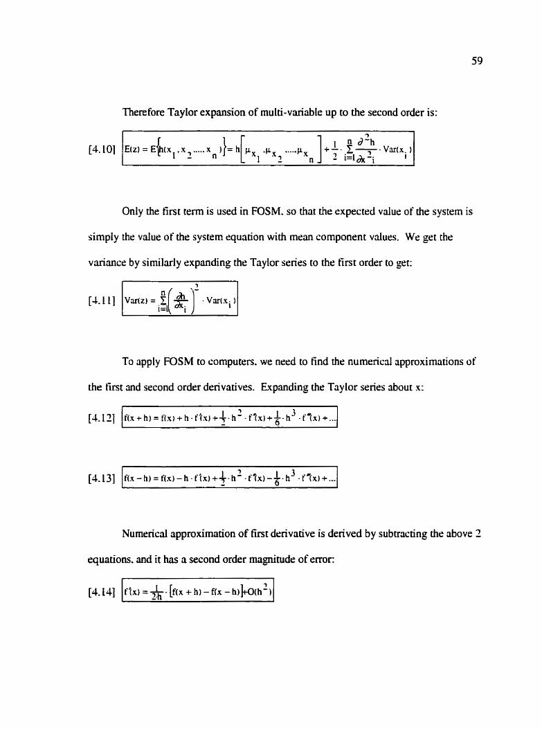
Therefore Taylor expansion of multi-variable up to the second order is:
Only the first term is used in FOSM. so that the expected value of the system is
simply the value of the system equation with mean component vdues. We pt the
variance by similarly expanding the Taylor series to the fiat order to get:
To apply FOSM to computers. we nerd to find the numerical approximations of
the tint and second order derivatives. Expanding the Taylor series about x:
Numerical approximation of first derivative is derived by subtracting the above 1
equations. and it has a second order magnitude of error:
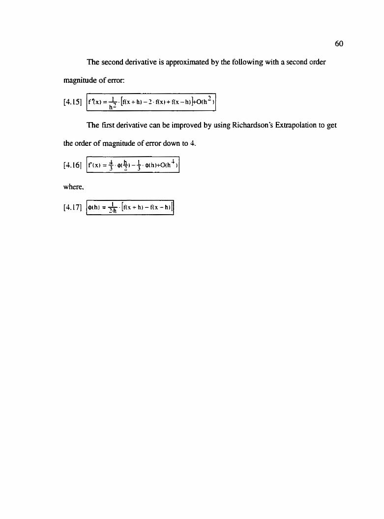
The second derivative is approximated by the following with a second order
magnitude of error:
The t - i t derivative can be improved by using Richardson's Extrapolation to get
the order of rna,htude of error down to 4.
f-1.161
where.
14.171
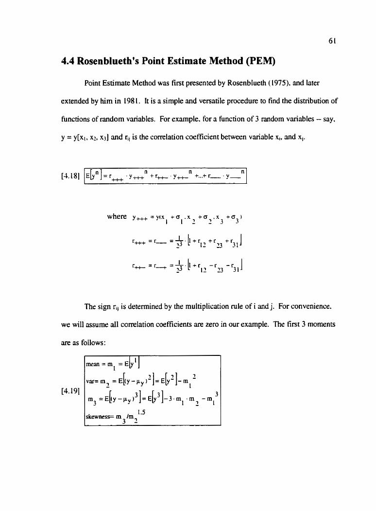
4.4 Rosenblueth's Point Estimate Method (PEM)
Point Estimate Method was first presented by Rosenblueth (1975). and later
extended by him in 198 1. It is n simple and versatile procedure to hind the distribution of
functions of random variables. For example. for a function of 3 random variables -- say.
y = y[xl, XI, x3] and 9, is the correlation coefficient between variable x,, and .u,.
where y,, = ycx to . X + +o 1 1 2 - 3 3
The sign r , is determined by the multiplication ruIe of i and j. For convenience.
we will assume dl correlation coefficients are zero in our example. The first 3 moments
rue as tbilows:

4.5 Monte Carlo Simulation
Monte Carlo Simulation is simply a repeated process of generating deterministic
solutions to r given problem. The main element of a Monte Carlo simulation procedure
is the generation of random numbers for a specific distribution. Previously. with slow
computers. Monte Carlo simulations are costly in its application to complex problems.
because it requires a large number of repetitions. With faster computers. this method can
be readily used as a check for approximate methods of probability calculations.
If ul and u2 are 3 pair of independent uniformly distributed random numbers, then
a pair of independent random numbers from 3 normal distribution with mean p and
standard deviation o. may be generated by: -
[4.20]
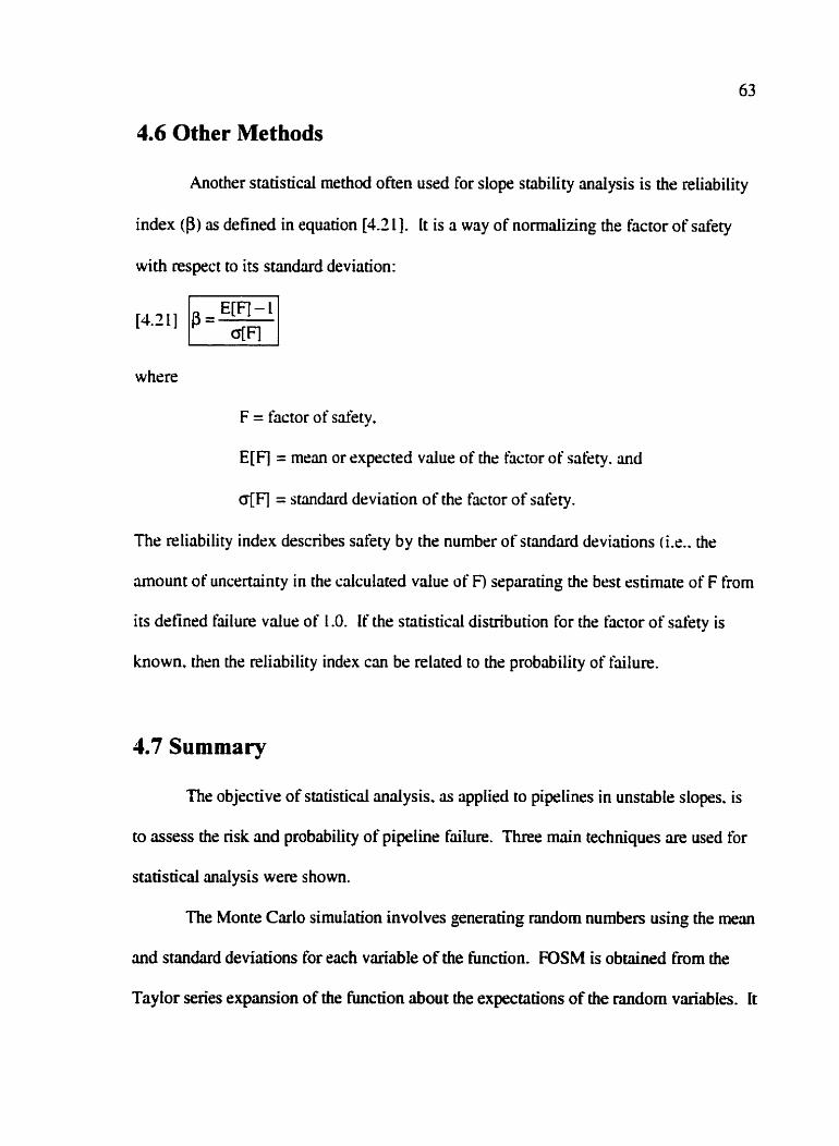
4.6 Other Methods
Another statistical method often used for slope stability analysis is the reliability
index (p) as defined in equation l4.2 I]. It is a way of normalizing the bctor of satkty
with respect to its standard deviation:
where
F = factor of safety.
E[FJ = mean or expected value of the factor of safety. m d
a[W = standard deviation of the factor of safety.
The reliability index describes safety by the number of standard deviations (i.r.. the
amount of uncertainty in the calculated value of F) separating the best estimate of F from
its detined Ulure value of 1 .O. If the statistical distribution for the factor of sclfety is
known. then the reliability index can be related to the probability of failure.
1.7 Summary
The objective of statistical analysis. as applied to pipelines in unstabke slopes. is
to assess the risk and probability of pipeline failure. Three main techniques are used for
statistical analysis were shown.
The Monte Carlo simulation involves generating random numbers using the mean
and standard deviations for each variable of the function. FOSM is obtained from the
Taylor series expansion of the function about the expectations of the random variables. It
64
may not always be possible to use the Taylor series approximation. because the function
itself must satisfy the existence and continuity condition of the first or first few
derivatives. and the computation of derivatives may be difficult. These difficulties can be
overcome by using Rosenblueth's point estimates (PEM) of the function, which leads to
expressions akin to finite differences.
Of these three methods. only the Monte Carlo simulation method uses the whole
statistical distribution of the variables. The FOSkI and PEM both only use one standard
deviation from the mean for their cdculations.
The PEM usually gives results very close to the Monte Carlo simulation. It is
very easy to use. and the derivatives of the function need not be derived. It is
recommended that PEM be used for analyzing soil-pipeline interaction. and the use the
Monte Car10 simulation as a check on the results.
Chapter 5
Case History of a Pipeline in Unstable Slope
5.1 Background
Amoco Canada Resources Limited had a 6-inch ( 168.3mm) oil emulsion pipeline
located in Willesden Green East near Rocky Mountain House. Calgary. Alberta. The
Right of Way contains 6 pipelines. Active slope movements were &fecting only the 6-
inch oil emulsion line dong the southern edge of the Right of Way.
The pipeline was laid about 2-m deep in a slope that is 43-rn high and 185-m
long. Landslide movements were occurring at depths of 2 to 2.5-m. Elastic stress
cdculations by Bun Engineering Limited (AGRA Earth & Environmental Limited. 1995)
indicated that the oil emulsion line had not been stressed beyond the yield point. They
determined the stress induced on the pipeline From the soil movement by multiplying the
soil mction per meter by the total length of the unstable soil slab and divided by the
cross-sectional area of the pipe. They dso included the Posson effect and hoop pressure
as a part of the longitudinal stress
The tine was exposed in the landslide toe area. Some bending along-the-slope
was observed in the pipeline. Approximate measurements and simple strain cdcuIations
66
indicated that the bending was within the tolerable limits. Excavations did not show signs
of upwards trending shearing within the soil, and the line did not appear to be in
immediate risk of being ruptured by landslide movements according to the 1995 repon by
AGRA Earth and Environmental Ltd.
A 3-D plot of the slope with a sketch of the pipeline location as well as the
locations of the inclinometers and boreholes are shown in Figure 5.1. Figures 5.1 to 5.6
are photographs of the pipeline in the slope. The toe of the slope was separated by a 200-
m wide tlood plain from the North Saskatchewan River. The active hilure appears to be
about 100-m wide (across the slope) and 70 to 80-rn long (down the slope).
Figures 5.7 to 5.9 are boreholr logs 1 to 3. and Figures 5.12 and 5.13 are the grain
size distributions for borehoks 2 and 3. The soil consists of 25% clay and 74% silt at
2.59 to 2.74-m drpth, and 37% clay and 60% silt at L .68-m depth. BorehoIrs indicate
that the soil is made up of sand and clay at depth zero to 5.1-m.
Figures 5.14 to 5.17 are the inclinometer data from May I 1 '95 to July 16 '95.
Detlections direction A is towards West (downslope and parallel to the pipeline) and
direction B is towards South. The slope has shown I -rnm/day movement p d I e 1 to the
pipeline. and from May I I" to July 25". 1995. inclinometer "SI-2" registered a
cumulative deflection of about 68-mm downslope. The surface of the slope indicator
"SI-3" appears to be impacted between May 1 I and May 18. 1995 resulting in the
inclinometer showing up slope movement above 1 -9-m. Slope indicators indicate teat the
possible slip plane is relatively shallow (less than 3m). and that there ye no deep-seated
movement,
67
The AGRA report does not contain any soil stlength data. The soil strength
parmeters used in this chapter are based on empirical correlation.
5.2 Statistical Analysis Based on Simple Model (O'Rourke et
Table 5.1 consists of data used in the statistical analysis of a steel pipeline
subjected to longitudinal Iandslide. The values were provided by AGRA outside of the
AGRA report. Lumb ( 1966. and 1970) studied the statistical distributions of cohesion c
and angle of friction 4 for Hong Kong soils and found that tmQ has an approximately
normal distribution while c conforms more to a Bern distribution. The cmtrd region of
this Beta distribution ran be practically approximated by a normal distribution. Lumb's
conclusions were later supported by Schulue ( 1972). and H m ( 1977). For this rase
study. a normal distribution is assumed for the soil cohesion and frictional angle. since in
the practical rang of 0 (0" 5 $ 5 45"). 0 is approximately proportional to tan@. Lumb
( 1980) and other workers have found that variability of the unit weight of soil yon the
determinations statistical results to be insignificant. therefore the unit weight of soil is
assumed to be a deterministic quantity for this case study.
The statistical analysis is based on the simplified models of uniaxial stress-strain
behavior of steel by Ramberg-Osgood ( 1943) and the longitudind strain equation from
O'Rourke et al. ( 1995) (i-e., equations [2.1] and [2.31).
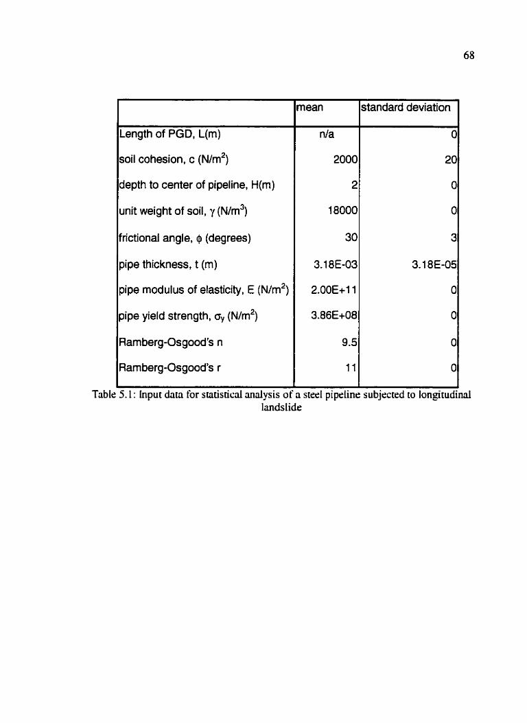
Length of PGD, L(m)
soil cohesion. c ( ~ / r n ~ )
I depth to center of pipeline, H(m)
unit weight of soil, ( ~ / r n ~ )
I frictional angle, 0 (degrees)
lpipe thickness, t (m)
lpipe modulus of elasticity, E ( ~ l r n ~ )
I pipe yield strength, o, (N/ITI~)
I
Table 5.1 : Input data for statisticd mdysis 01 Imdsli
mean lstandard deviation 1
a steel pipeline subjected to longitudinal
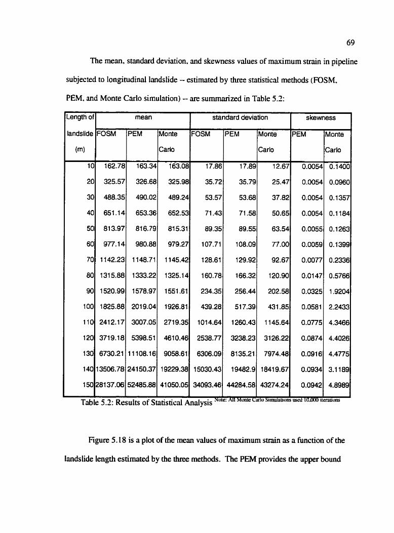
The mean. standard deviation, and skewness values of maximum s a i n in pipeline
subjected to longitudinal landslide - estimated by three statistic3 methods (FOSM.
PEM, and Monte Carlo simulation) - are summarized in Table 5.2:
Figure 5-18 is a plot of the mean values of maximum strain as a function of the
Length of
landslide
(m)
10
20
30
40
50
60
70
80
90
100
1 10
120
130
140
1 50
Table
Iandslide length estimated by the three methods. The PEM provides the upper bound
mean L
FOSM
162-78
325.57
488.35
651 -14
813.97
977.14
1142.23
131 5.88
1520.99
1825.88
241 2.17
371 9.1 8
6730.21
1 3506.78
281 37.06
5-21
standard deviation
PEM
163-34
326.68
490.02
653.36
81 6.79
980.88
1148.71
1333.22
1578.97
201 9.04
3007.05
5398.51
1 1 108.1 6
241 50.37
52485.88
Results of
Monte
Carlo
12.67
25.47
37.82
50.65
63.54
77.OC
92.67
120.90
202.58
431.85
1 145.64
3126.22
7974.48
1841 9.67
43274.24
'Uiu "-")a
FOSM
17.86
35.72
53.57
71.43
89.35
107.71
128.61
160.78
234.35
439.28
101 4.64
2538.77
6306.09
15030.43
34093.46
An;llysis "~'e:
Monte
Carlo
163.08
325.98
489.24
652.53
815.31
979.27
1145.42
1325.14
1551.61
1926.81
271 9.35
461 0.46
9058.61
19229.38
41 050.05
Smtisticd
PEM
17.89
35.79
53.68
71.58
89.55
108.09
129.92
166.32
256.44
51 7.39
1 260.43
3238.23
81 35.21
19482.9
44284.58
" ~ n k
70
estimation on the mean value. whereas the FOSM gives the lower bound. The difference
between these two bounds increases with increasing landslide length. Considering the
coefficient of skewness. the Monte Carlo method yields a higher positive coefficient of
skewness when L exceeds 90 m as illustrated in Figures. 5.19 and 5.20. The coefficient
of skewness yielded by PEM is srndl -- which may be due to the clssumption of zero
correlation coefficients. The probability density distributions as shown in Figures 5.19
and 5.20 can be used to tind the probability of pipeline Failure. For example, if we
consider pipeline failure to occur at the start of pipe yielding at E,,,IJ= 3458 microstrains.
then the probability of pipeline Failure is about 1008 at L = 130-m. and 1-78 at L = 100-
m. The strains obtained from this simple model are similar to those Found by Burt
Engineering Limited.
The Monte Carlo simulation method is the most accurate of' the three statistical
methods. Lf the complex soil-pipeline interactions models. which ye solved iteratively.
are written into a computer prognm. then the Monte Cxlo simulation method should be
used for the statistical analysis.
Both FOSM and PEM do not require the large number of iterations used in Monte
Car10 simulation. PEM results are very similar those from the Monte Carlo simulation
for landslide lengths of up to 100-m. and they are more conservative than those from
Monte Carlo simulation. For example. PEM produced a 3.8% higher strain value for a
100-m length ImdsIide. Further. PEM does not require deriving derivatives of the
bnction as required by FOSM. Therefore. if the complex soil-pipeline interaction
modeIs derived in this thesis were not implemented as a computer program, then it is
7 1
recommended that PEM be used for the statistical analysis. The more time comsurning
and computationdy intensive Monte Car10 simulation can be used as a check on the
PEM results.
5.3 Strain analyzed from new pipeline models
53.1 Strain from longitudinal landslide
The strains developed for different mount of soil movement a d length of
landslide is calculated from equations [3.2] and L3.71 and is shown in Figure 5.11.
For a pipeline diameter of 168.3 mm. the wrinkling strain. from equation [1.J]. is
ew = 66 13 microstnins. The yielding of the pipeline starts at e,, , ,~ = ~ lu lJ /Ep lp = 1930
microstrains. or if we used the Rambeg-Osgood equation Eylrld = 3458 microstrains. The
result of longitudinal landslide analysis indicates that the pipeline would not yield for cl
landslide length of up to LOO-m.
5 3 2 Strain from deep-seated landslide
Although there are no evidence of deep-seated fidures developing in the actual
slope itself, it is wise to calculate hypothetical deep-seated f'ailures to determine the
mount of such soil deep-seated movements needed to yield the pipeline.
If the slope were to have r circular deepseated landslide with radius R = 15 m
and Rm = 25 m. The length for the longitudinal displacement component is ?*(R'-
l t r n L ) O S 5 = 74.8 m. The maximum pipe strain developed from the transverse and
72
longitudinal components of the deep-seated landslide, as analyzed using the method
described in section 3.3, is presented in Figure 5.22. We see that there is no imminent
danger of the pipeline yielding from the longitudinal component of the rotational soil
movement. However. the pipe will begin to yield from the transverse component when
the soil movement reaches 31Ds or only about 0.256 m. This indicates hat any deep-
seated soil movement is very dangerous for the pipeline because it would shear the
pipeline near the intersection of the pipe and the circular failure surface. or at the very
least . create wrinkles on the pipeline.
Willesden Green East
Fig. 5.1 : 3-D Landslide surface contour of Willesden Green East with pipeline location
Fig. 5.2: Lateral edge of Iandslide at top of slope
Fig. 5.3: Exposed 6 inch oil emulsion tine near slope crest
Wg. 5.4: Groundwater in pipeline trench behind the slope crest
Fig. 5.5: 6 inch oil emulsion line
Fig. 5.6: View of oil emulsion line tkom top of slope
Fig. 5.7: Borehole No. I
Fig. 5.8: Borehole No. 2
Fig. 5.9: Borehole No. 3
EXPIANNION OF TERMS AND SYMBOLS
The terms and symbols u8a8 on the bomhak logs to rummaria tho nrults of f i d invmtig8tion md subrrquent labontory tasting am dewikd in the& pagu,
It should be notod that materials. boundrriu and conditions haw bean #t.blishad only at Me bonhole locations at the time of inmtigrtion and are not n.E#urily mpraont8tiw of ru68urfaee conditions elsewhere across the sit..
TEST DATA
Oau 0bt8tnsd dur~ng the field investigation and from labomtory tosting a n shown I t thr approprim d.pth i n l m l .
Abbrevtations. gwhic symbols. and mlenmnt t.rt r~ th0d drrignrtim m 88 follom:
'C Canso~idation tmt 'Sf Sd l ing taat OR RJattw denaity (formarty specific gravity) N Tomm rhur strength Fines Percentage by wsignl smaller than #2W sieve VS VInO shwr atrm@t (undkturkbnmolw) k Parmeability coattictent w NItunl w.1.r tontrnt (ASTM 0 2216)
'MA Mschantc8l grain size mrlylis md wl bquid limit (ASTM D 423) hydrometer test w, Plastic limit (AStM b 424)
N St8nd8fd p.netntion t a t (CSA Alla.tdb) ,, Unfi anin at fdlu" Nd Dyn8mic cone penatmion tost r Unit weight of soil or rack NP Non pl88tic soil rd Dry unit Wght of roil or rock pp Pocket penetrometer strength p Dsnrlty of roil or rock
'q Triural compnaslon test pa Dry density of soit or rotk q, Unconfined comptaasitm nrength
'SB Shearbox test - MprgU SO. Concentrat~on of W ~ C O ~ - S O ~ U ~ ~ O sulphrte I. oc~wrwd a t a r I ~ I
'The mum or tmso tosm u s u ~ y m repartrd sapannty
SOIL CLASSIFICATION AND ommmoru Soils are ctualfied and dwcribod according to tbtr mginaring pmpefli88 and ~ w i o u r . The sail of each stratum is describhd uslng the Unitiad Sorl Cluslfic+tion Syrtemr modified slightly so Hut
an rnorgrnlc clay of "mdiurn plasticity* 1s ncognlud.
the use ot modifying adjectives may b. employad to M i n e the actual or antimted prcenl8ge mnge by welght ot rntnor components. Thrs IS s~milrr to a systm developad by D.M. Burm1ster.2
The soil classifiation system IS shown In grsrter detril on prQe 2
SAMPLE l7PE - The type of sample ts shown at the rgpropriate depth in1mN.l using the follawing 8bbmv18tions:
A a u g e r m p h B block runpk C rock can, O r fmmn mil cafe D dnve umpk/SPT s8mpte P p ~ t w r t u b sample U tube sample (usually thln-wallwl) W wash or air return mrnpla 0 otnar (sme mport tm) 61 indicrtn no umple mcowy
Kg. 5. LO: Explanation of terms and symbols used on borehoIe logs (put i )
Fig. 5.1 1 : Explanation of terms and symbols used on borehole logs (part 1)
COBBLES , GRAVEL SIZES ~~
F1S
GRAIN SIZE IN MILLTMETRES
Fig. 5. L2: Gnin size distribution for borehole 2.
SlLT
REMARXS:
a AGRA b r t n 8 Environmental GRAIN SIZE DISTRIBUTION -
CLAY
PROJECT No:CG2SM8 DATE= 95.05.!2
LOCATION: HOLE: ,,, 2 SMlOm
259-274 rn TECHNICU LR 26
P
SUlllMaRY
Dta = rnm
DSO = 0.0052 mm
Dlo = 0.01 1 mm
GRAVEL %
SIN0 1, L
SILT SIZES 74. S
Fig. 5. L 3: Gnin size dismiution for borehole 3.
T
COBBLES . GRAVEL SIZES SAND SIZES SILT I
CLAY
US, STANDARD SIEVE SIZES
t e a M s 1s OJ US ma ao 1% 78 a
MR.TIMEms ! MICRONS I 1 T 1 I i
1000 roo 10 1 0.1 ,O f .MI .ooai GRAIN SIZE IN MILKMETRES
REMARKS: WL-41 W-18 IP-23 s-
010 = mm
030 = mm
DdO = 0.0085 mm
c, =
Cc =
AGRA EstW 8 Environmental GRAIN SIZE DISTRIBUTION -
I
GRAVEL t
SAND 3. 1
SILT SIZES 60. %
cur SUES 37. %
PRO- No: CG25048 DATE: 9S.05.19
LOCATION: H r n : ,,, SA SAMPLE:
1-66 m TECE~MCUN: LR 26s
Eg. 5.14: Inclinometer S 1-2
Hardy BBT Limited - Calgary, Alberta
Dsf lection C n ) Daf leetion (am) -8Q -40
0 0 ca
r
lnftlrl 1 l J m y a S - 18 R O Y ' S
t - -
4 -
6 -
8 - Dapth 0-h
(rnl trn)
10 -
12 - - 12 I t -
mo
2
4
6
8
10
t2
14 - - tL 1L
16 -110 -10 0 60 80 - 16
16 & 16 -80 -60 0 00 80
Cumulative Deflection Cumulative Deflection Direction A Direction B
CG25048, Inclinometer SI-2 AMOCO
Hardy BBT Limited - Calgary, A l b e r t a
Def l m i a r , tmJ D.f iurf m (-1
0 Initial 11 May'% - 18 my8% - 30 Hnry'95 . . 26 JultQ5
4
8
12
Pth 0-h :m) (m)
16
20
24
-eO -20 0 20 4 -40 -20 0 20 Ul
Cumulative Deflection Cumulative Deflection Direction A Direction B
CG2S040, Inclinometer Sf-3 AMOCO
Fig. 5.15: Inclinometer S 1-3
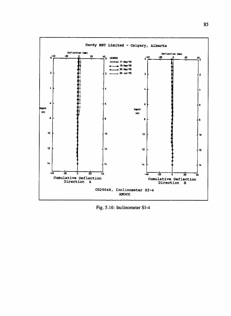
Hardy BBT Limited - C a l g q , Alberta
Oef laction <n) bcflectian tm)
Ini ti81 11 My'95 - 18 Ww'95 -- 30 Mw'95 2 4-b 26 Jut'=
epth Olpth (m) CuI)
-10 -M 0 20 10 Cumulative Deflection Cumulative Deflection
Direction A Direct ion B
CG25048, Inclinometer Sf -4 AMOCO
b
Fig. 5.16: Inclinometer S I4

Fig. 5.17: Inclinometer S 1-5
Hardy BET Limited - C a l g a r y , Alberta
Def lrction tml Oaf lecrim C r )
Coo LEGEND tni t ie1 t 1 W'9S - -6 wry8-
-30 W'OS - 26 26~1'95
2
4
0-h (In)
6
8 8 -
to 10 , - la
I
4 . 12
12-;o - 20 0 20 at2
2
C
Depth
(a) 6
8
10
12-*
Cumulative Deflection Cumulative Deflect ion Direction A Direction B
CG25048, Inclinometer Sf-5 AMOCO
b
640 -20 0 20 t I 1
. - - -
- 4
t
- .
- f 3
?J
? - 1
1
I
I
*A a 20 40
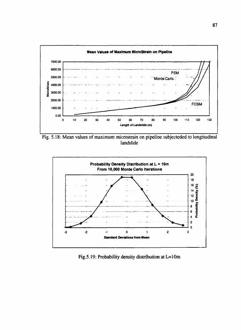
Mean Values of Maximum Microstrain on Pipeline
Length of Landslkfa (m)
Fig. 5.18: Mean values of maximum microstrain on pipeline subjecteded to longitudinal landslide
- Probability Density Distribution at L = lorn
From 10,000 Monte Carlo Iterations
- ---
-3 -2 -1 0 1 2 3
Standard Oeviations from Mean
Fig.5.19: Probability density distribution at ElOm
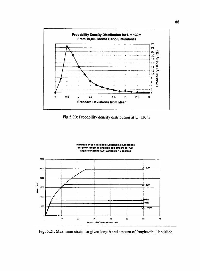
Probability Density Distn'bution for L = 130111 From 10,000 Monte Carlo Simulations
26 24
"2 20
E 10 , 16 E 14 8 12 3 - I0 - 5 8 e P e
4 e 2 0
- 1 -0.5 0 0.5 1 I .5 2 2.5 3
Standard Deviations from Mean
Fig.5.20: Probability density distribution at k130m
Maximum Plpe Strain from Longitudinal Landslides (for given length of landrlide and amount of PGD)
Angle of PIpellne w.r.t Landslide = 0 degraas
Fig. 5.21 : Maximum strain for given length and mount of longitudinal landslide
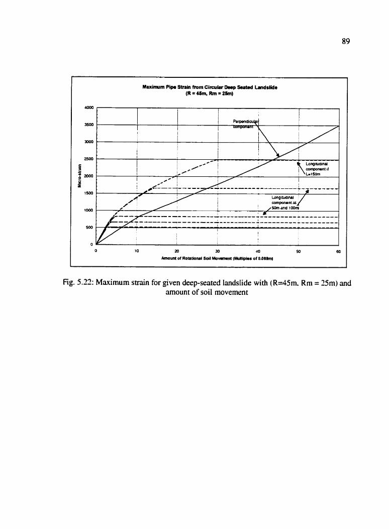
Maximum Pipe Strain from Circular Deep Seated Landslide (R = 45m. Rm = 2Sm)
sOOa
3500 -- I ..m"ruyi *
0 t 0 20 30 40 SO 60
Amaunt of R o m l k ~ l soil ~ o v n # n t t ~ u ~ l p k r or o.oomn)
Rg. 5.12: Maximum stnin for given deep-seated landslide with (R45m. Rm = 25m) and amount of soil movement
Chapter 6
Conclusions and Recommendations
6.1 Conclusions
Andytical md numerical solutions have been derived to determine the detlection
profile of a buried pipeline in r slope subjected to a longitudinal. transverse and deep-
seated failure. Unlike previous methods, the methods presented in this thesis recognize
that the force acting on the pipe is o function of the relative displacement between the
pipeline and the landslide. and vice versa.
[t was found that shear-type rupture and tlexure bending are the two possible and
dominant deformation modes of a buried steel pipe in a deep-seated slide. It was also
found that for transverse landslide widths greater than about 10 m the pipeline shows
displacement and stnin as if the width of the landslide is infinite. Relationships between
the soil movement and the pipe deformation strain for different modes have been
established so that one can assess the risk of pipeline rupture with a given soil movement.
This allows consulting engineers to monitor the soil movements in r slope in order to
predict pipeline strains.
9 1
The most critical parameters in the safe design of pipelines in unstable slopes are
the soil resistance (Rf), pipe modulus of elasticity (E), and pipe thickness (t). Using light
weight aggregate (LWA) as a backfill not only provides drainage, but it will reduce the
stnin induced in the pipeline in a landslide. Using n more elastic steel pipe (lower
modulus of elasticity) and thicker pipe would reduce the strain induced in the pipeline as
well. A small width transverse landslide produces higher stnin than a larger width
landslide - the difference is s m d at the beginning of soil movement but it becomes
larger for larger amounts of PGD.
A luge number of case studies clre needed to compare the results of the statistical
analysis so that realistic conclusions can be drawn in the future about the correlation
between observed behavior md statistical predictions. Estimates of strength panmetes
of slopes based on test results and associated geomechmics considerations must be made
for each particular slope - and these properties would vary from one site to another.
Therefore. a quick method of calculation is needed to determine the probability of
pipeline hilure - such as the Monte Carlo Simulation and PEM method.
One must devise a remediation strategy based on the risk of pipeline hilure from
a statistical cmadysis. For low risk. one may improve the surface and near-surface
dninage and establish a soil movement-monitoring program. At intermediate risk one
may try to bury the pipeline below the shdow Iandslide. but there wouId be r risk of
inducing a higher strain on the pipeline if a deeper planar landslide or a deep-seared
landslide were to develop. Another option is to instail valves both upstream and
downstream of the unstable slope for automatic shut-off of the pipeline. One may also
92
try resloping and backfilling with LWA. If deep-seated landslides are possible, then
constructing a toe berm is recommended. At high risk, one may reroute the pipeline to a
stable slope.
6.2 Recommendations
It was assumed in this thesis that the soil properties such as cohesion c and
tiictiond angle 4 were all independent mdom variables. At present there are no
available data concerning the magnitude of such correlations. 4 new area of research is
needed to establish that such correlations exist and then to quantify them.
The statistical analysis. such as PmI. can be applied to the more complex
pipeline strain equations presented in this thesis. However. it must be advised that it
would be very cumbersome to implement FOSM. or require large computer power to
apply Monte Cwlo simulation.
The pipeline stnin equations can be expanded to include the thermal stnin. and
pipline operating pressure. The effect of pore pressure on the soil-pipeline interaction
should also be investigated. Instead of the simple elastoplastic soil behavior. the model
could be revised to use the stress-strain behavior of overconsolidated and normally
consolidated soil.
The present model should be verified by using scaled physical model of a pipeline
in a sliding mass of soil. Full scale testing requires suitable test sites and is costly.
Centrifuge mode1 testing is cheaper. but is limited by the size of the centrifuge available.
93
For example, it would be difficult to centrifuge model a pipeline with a distinct backfill
material unless a large size centrifuge is available. Finite element modelling (FEM) is
great for modelling complex slope and pipeline geometries. The parameters describing
soil-pipeline intenction could be adopted from soiVstructure interactions for foundations
such as anchors and piles. However. E M is limited by the assumptions used in
modelling the soiVpipelinr interaction m well.
References
AGRA Eruth & Environmental Limited. 1995. Geotechnicd Assessment of the
Willesden Green East. Pipeline Right-of-way and Slope Instability. 1- 16.
Alonso. E.E. 1976. Risk miysis of dopes and its application to slopes in Canadian
sensitive clays. Geotechniqur 16. No. 3.453471.
Chan. P. and Wong. R. 1997. Performance of Buried Steel Pipe in Unstable slope. The
Second International Symposium on Structures md Foundations in Civil
Engineering. Hong Kong.
Chan. P. and Wong. R. 1997. Pipelines in unstable slopes. Risk assessment in
Geotechnicd and Gro-environmental Engineering One Day Symposium. C d g q
Geotechnicd Society / University of Calgary.
Chenry. W. and Kincaid. D. 1985. Numerical Mathematics and Computing. Broo ks/Cole
Publishing. 115- 146.
Chow. V.T,. Midment. D l . and Mays. L.W. 1988. Applied Hydrology. McGraw-Hill
I ~ c . 350-376,
Christian. IT., Ladd. C.C. md Baecher, G.B. 1994. Reliability Applied to Slope Stability
Andysis. Journal of Geotechnical Engineering. Vol. 130, No. 17? 2180-2206.
95
Committee on Gas and Liquid Fuel Lifelines. 1984. Guidelines for the seismic design of
oil and gas pipeline systems. American Society of Civil Engineers, New York.
473.
Flores-Berrones, R. and O'Rourke, M. L991. Seismic effects on underground pipelines
due to ~manmt longitudinal ground deformation. Proceedings of the 4th Japan-
U.S. Workshop on Earthquake Resistant Design of Likline Facilities and
Countermeasures for Soil Liquefaction: Technical Report NCEER-92-00 19.
National Center for Earthquake Engineering Research. Buffalo. N.Y. 465479.
Hasofir. A.M. and Lind. Niel. N.C. 1974. Exact and Invariant Second-Moment Code
Format. ASCE Journal of The Engineering. Mechanics Division. Vol. 100. 1 1 1-
12 1.
Hall. W. and Newmark. N. 1977. Seismic design criteria for pipelines and facilities.
Current state of knowledge of lifeline earthquake engineering, I\SCE. New York.
N.Y., 18-34.
Hm. M. E. 1 977. Mechanics of Particular Media - A Probabilistic Approach. p. 543
McGraw-Hill. New York,
Hetenyi. M.L 1946. B e r n on Elastic Foundation. Ann Arbor. University of Michigan
Press.
Lumb, P. L966. Variriabiliity of natural soils. Canadian Geotechnicd Journal. Vol. 1, No.
3-74-97,
Lumb, P. 1970. SaEety factors and the probability distribution of soil strength. Canadian
Geo~echnicaI Journd. Vol, 7, No.3.
96
Lumb. P. 1980. Application of probabilistic methods in geotechnical engineering.
Workshop lecture notes. University of New South Wales LJNISEARCH.
September.
Nguyen. V. U. and Chowdhury. R.N. 1984. Probabilistic Study of Spoil Pile S [ability in
Strip Cod Mines -- Two Techniques Compared. Int. I. Rock Mrch. Min. Sct. &
Geomech. Abstr. Vol. 2 1. No.6. 303-3 12,
0' Rourke. M.J. and Nordberg. C. 1992. Longitudinal permanent ground deformation
effects on buried continuous pipelines. Technicd Repon. NCEER-92-00 14. June
15. Chaper5. 1-1 1
O'Rourke. M.J.. Liu. X.md Rores-Berrones. R. 1995. Steel Pipe Wrinkling Due to
Longitudinal Permanent Ground Deformation. Journal of Transportation
Engineering. VoI. 1 2 1. No. 5. 44345 1
Press. W.. F'lmnrry. B.. Teukolsky. S. and Veterrling, W. 1986. Numerical Recipes.
Cambridge. University Press. 169-272.
Rajmi. B.B.. Robertson. P.K. and Morgenstrrn. N.R. 1995. Simplified design methods
for pipelines subjected to transverse and Iongitudinal soil movements. Canadian
Geotechnical Journal. No. 32.309-323.
Ramberg, W. and Osgood. W. 1943. Description of stress-strain curves by three
parameters. Tech. Note, No. 902. Nat. Advisory Committee for Aeronautics. 98.
Rosenblueth, E. 1975. Point estimates for probability moments. Proc. Nat. Acad. Sci.
USA. VOC. 72, NO. 10, 38 12-38 14.
97
Schultze, E. 197 1. Frequency distributions and correlations of soil properties. Proc. 1''
Int. Conf. Applications of Statistics and Ebbability in Soil and Structural
Engineering. Hong Kong University Press. 37 1-387.
Tang, A.H.S. and Ang.. W.H. 1984. Probability concepts in engineering planning and
design. John Wiley & Son. hc. Vol2. 284-285.
Appendix A
Derivations for Longitudinal Landslide
A.l General 2"d order equilibrium equation for pipeline:
From Figure A. 1 :
[A11 Irir .V 4 N-d~ - r-c a-d ,-dm: K ,.( u 8 -( K-J I-dx dx
[A31
From the stress-strain relationship:
lA4l
[AS3
Combine equations [A31 and [AS]
[A61
Homogeneous solution of equation [A71 :
[A81
where,
~ 9 1
Nonhomogeneous solution of equation [A71 :
Therefore. the general 2" order equilibrium equation is as follows:
A 3 Pipeline equations for 6 < 2D, (see Figure A.2):
Region 1 (-.. < x c 0,:
[A L 21
[A131
Region 2 (0 < x < A):
[A 1 51
[A163
[A171
Apply the continuity condition at a s .
[A 181
Region 3 (A < x < B):
I"" u ,,il - u 3 =L-- 3 wnca)-r- u d xd x
.Apply the continuity condition at x = A
Region 4 ( 6 < x < U2):
[ a 9 1
Apply the continuity condition at x = B.
[A301
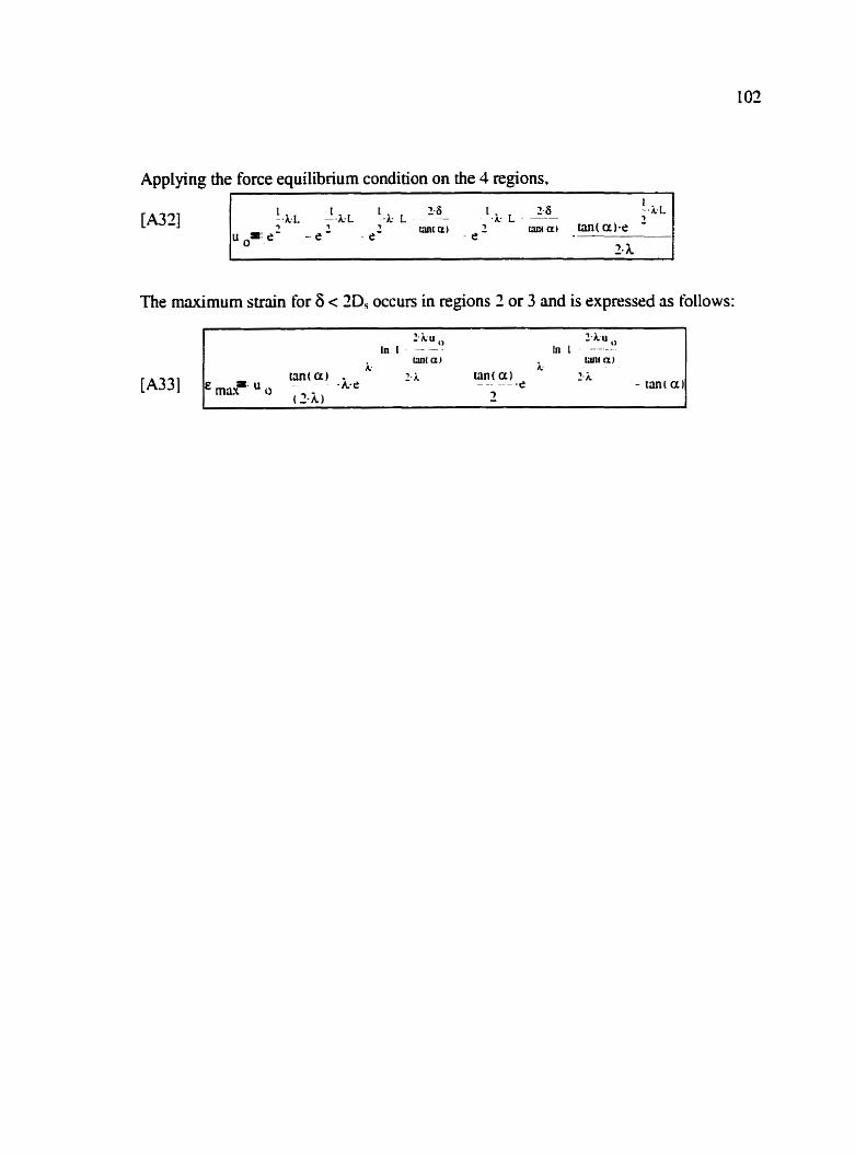
Applying the force equilibrium condition on the 4 regions.
[A311
The maximum strain for 6 c ?D, occurs in regions 2 or 3 and is expressed as follows:
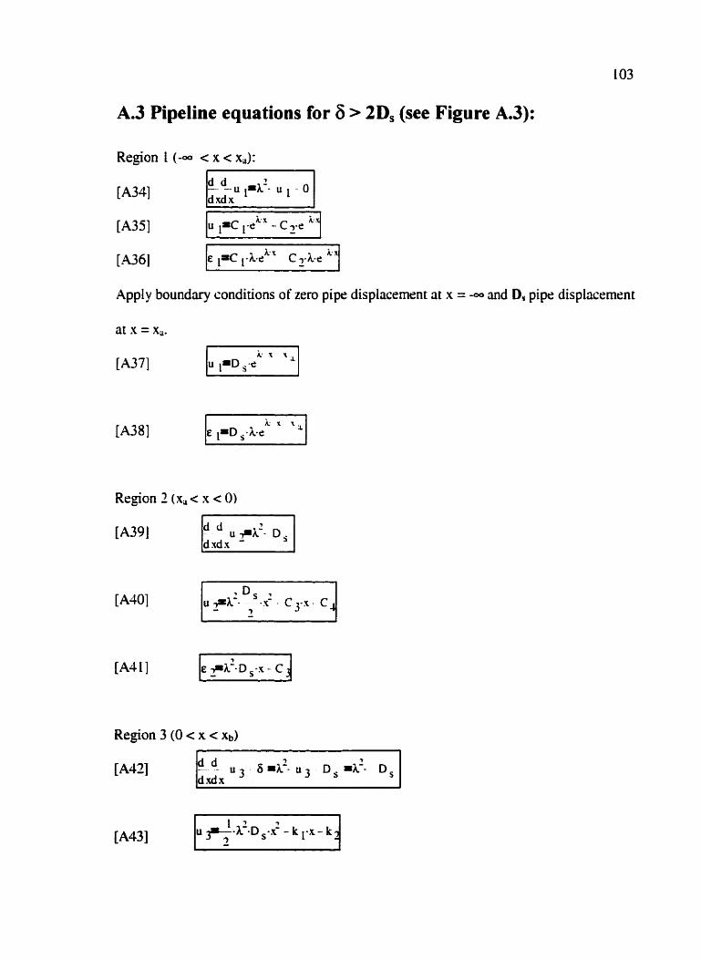
A.3 Pipeline equations for 6 > 2 4 (see Figure A.3):
Region 1 (-- < x < x,):
[A341
[A351
[-G61
Apply boundary conditions of zero pipe displacement at x = -. and Dr pipe displacement
at .Y = Xa.
dxdx
1-1 11 6
Region 2 (x,c x < 0)
u,-k2- D, dxdx -
Region 3 (0 < x < xb)
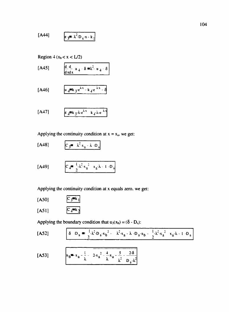
Region 4 (xb c x < U2)
Applying the continuity condition at x = x,, we get:
Applying the continuity condition at x equals zero. we get:
Applying the boundary condition that ul(xb) = ( 8 - 4):
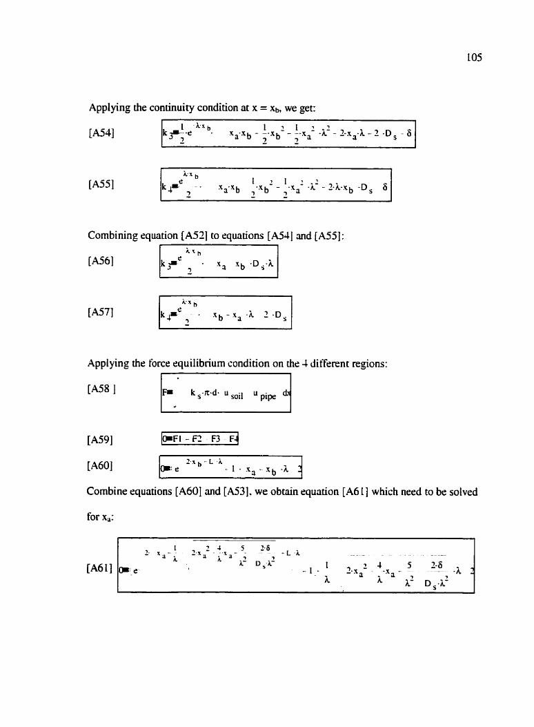
Applying the continuity condition at x = xb, we get:
Combining equation [A521 to equations [A541 and [A551 :
Applying the Force equilibrium condition on the 4 different regions:
[A58 I
[A591 PFI -P- n ~4
[A601
Combine equations [A601 and [A53]. we obtain equation [A6 I ] which need to be solved
for xa:
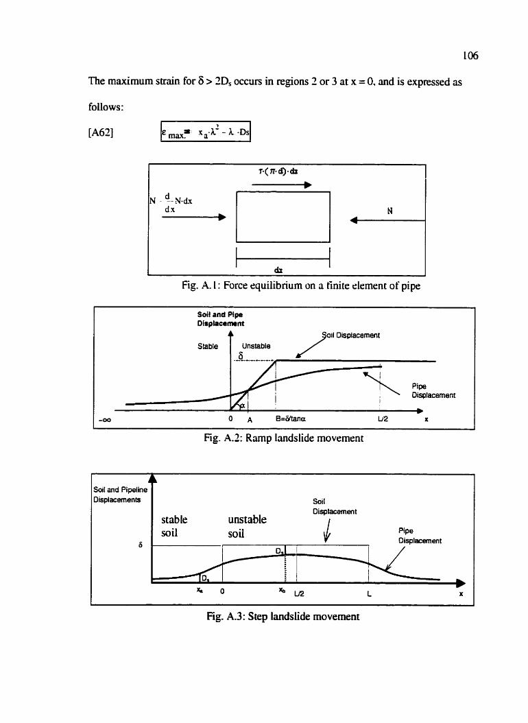
The maximum strain br 6 > ?Ds occurs in regions 2 or 3 at x = 0, and is expressed as
follows:
[A621
Fig. A. 1 : Force equilibrium on a tinite element of pipe
Soil and Pipe Displacement
o ~ l Displacement Stable Unstable
6 C
Y, Pipe Displacement
t
, b -00 0 A B=6/tana U2 x
fig. A.2: Ramp landslide movement
Soil and Pipeline Displacements Soil
Oisplacemen t stable unstable soil soil i Pipe
Displacement
' 1--+! 0 '6 IR L X
Fig. A3: Step landslide movement
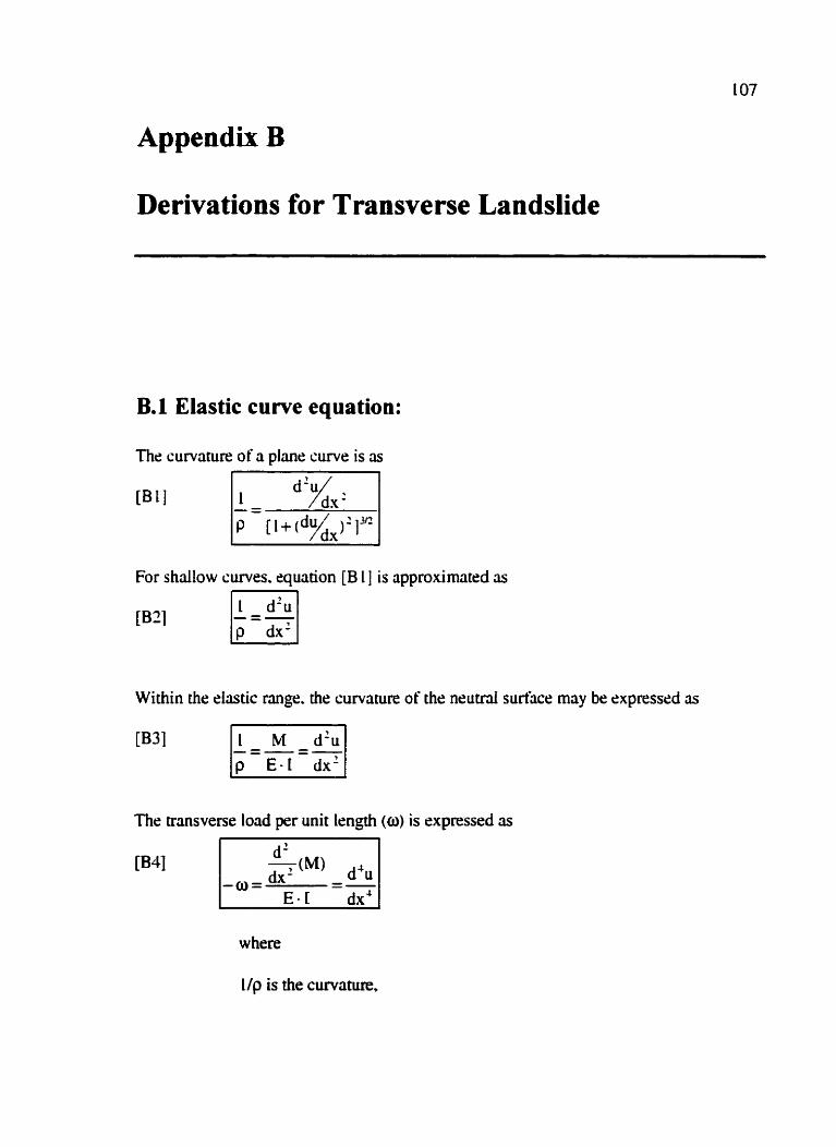
Appendix B
Derivations for Transverse Landslide
B.l Elastic curve equation:
The curvature ofa plane curve is as --
PI1
For shallow curves. equation [B 1 ] is approximated as
2
P [I+$% )'lJZ I;.
Within the elastic range. the curvature of the neutni surface may be expressed as
p E - I dx-
The transverse load per unit length (a) is expressed as
where
llp is the curvature,

u is the transverse displacement,
M is the bending moment,
E is Young's modulus of elasticity, and
I is the moment of inertia.
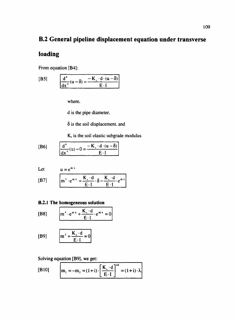
1 09
B.2 General pipeline displacement equation under transverse
loading
From equation m4]:
where.
d is the pipe diameter.
6 is the soil displacement. and
K, is the soil elastic subgrade modulus
Let
~ 7 1
62.1 The homogeneous solution
Solving equation [B9]. we get:
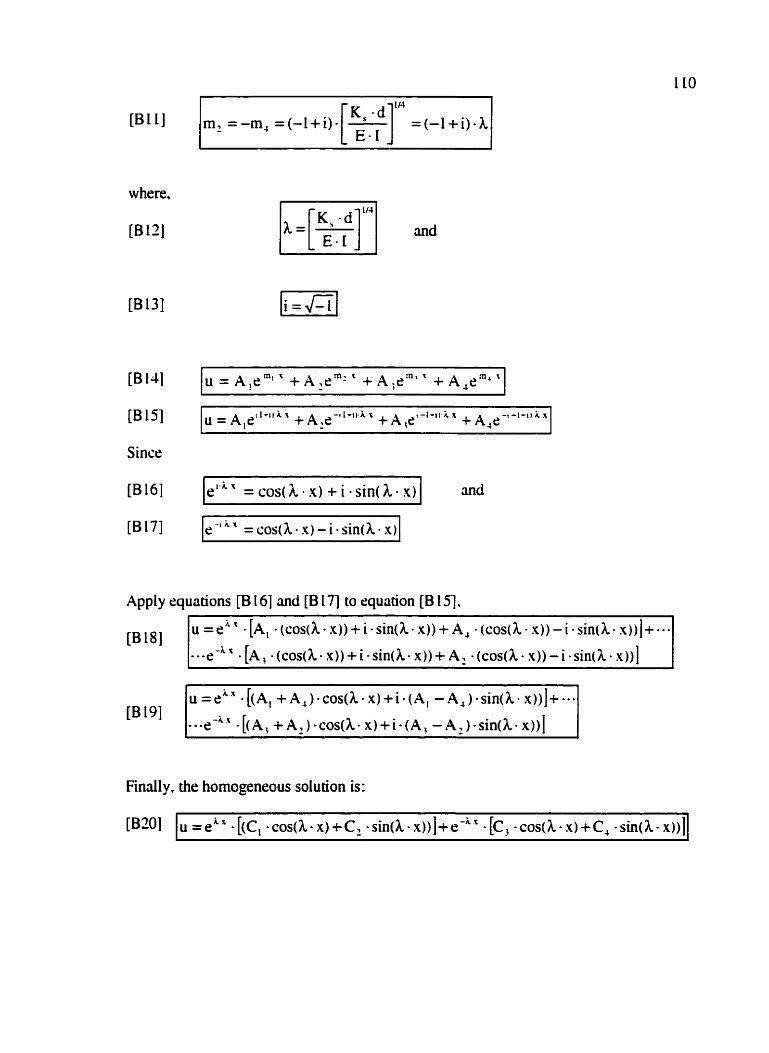
where,
[B 121
[B t 41
lB 151
Since
CB 161
I k = [2p]1/41 - and
Apply equations [B 161 and [B 171 to equation [B 157.
[B 181 u =ri" -[A, . (cos( l -x))+i-s in(k-x))+A, -(oos(k- x))- i-sin(h-I))]+---
---e-" -[A, - (cos(k-x))+i-s in(k-x))+A, -(cos(k+ x))-i.sin(k. x))]
findly, the homogeneous solution is:
[B?OI IU =ei" -[(c, -cos(h- x)+C, -sin(k-x))]+e-" -[c, -cos(h-x)+C, -sin(h. XI)][
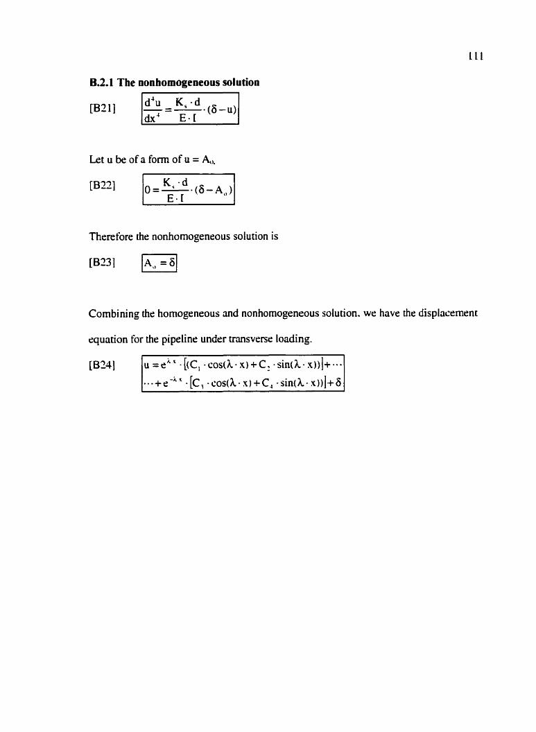
82.1 The nonhomogeneous solution
d'u K;d -=-. (8 - u) p211 ldx' ~ - 1 (
Therefore the nonhomogenrous solution is
[B23 1
Combining the homogeneous and nonhomogeneous solution. we have the displacement
equation for the pipeline under transverse loading.
[ B X j
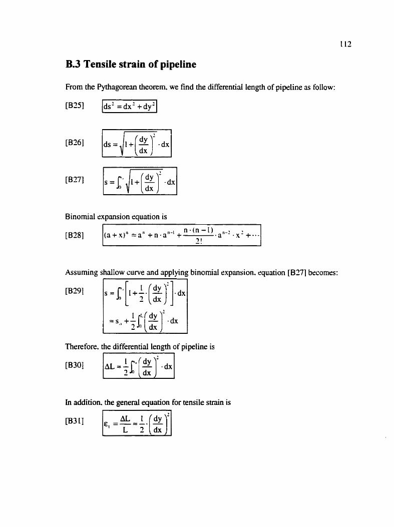
B.3 Tensile strain of pipeline
From the Pythagorean theorem. we find the differential length of pipeline as follow:
I3251
Binomial expansion equation is
[I3281
Assuming shallow curve and applying binomial expansion. equation [B27] becomes:
'"91 '1 Therefore. the differential length of pipeline is
In addition. the generd equation for tensile strain is ,
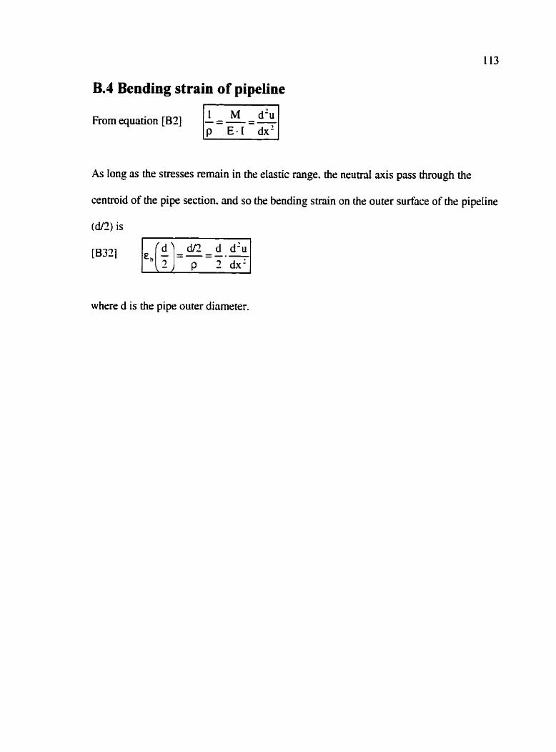
B.4 Bending strain of pipeline
From equation [B2]
As tong as the stresses remain in the elastic range. the neutral axis pass through the
centroid of the pipe section. and so the bending strain on the outer surtice of the pipeline
(&2) is 21 2 dx-
[B32]
where d is the pipe outer diameter.
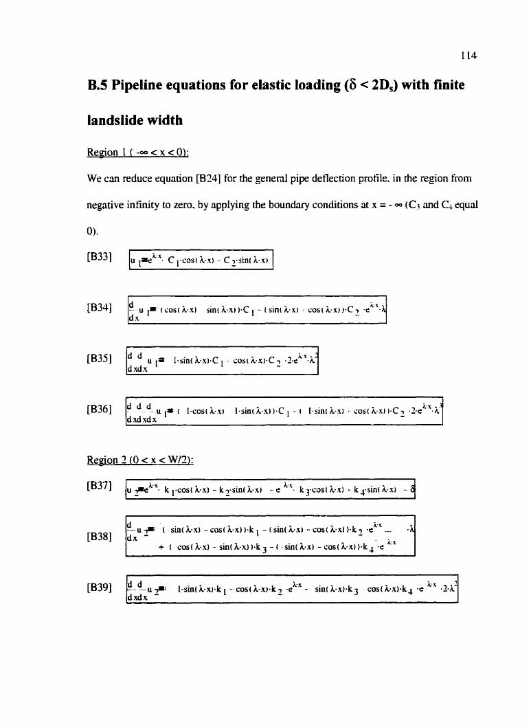
B.5 Pipeline equations for elastic loading (6 < 2D,) with finite
landslide width
Regon - I ( -= < x < 0):
We can reduce equation [B?41 for the gnen l pipe deflection profile. in the region from
negative infinity to zero. by applying the boundary conditions at x = - (C3 and C equal
0).
[B361 d d d - - - u ( 1-cosc A-x) l-sinc b-r) 1.C I - I I-sin{ La, - cos( k-XI 1.C - -2.ek"-k3 dxdxdx
Applying the following boundary conditions:
At x = 0, u, u', u", u',' are continuous;
At x = Wf2, u'=O:
Force equilibrium in the transverse direction:
We obtain the following 6 equations:
IB41 I
sin ' .k.W . ,,, i. w k sin w c o s I-LW - k , - e ...
'I 7 7 'I - - - - + cos '-h-w sin ' - LW .k3 - sin '-i-~ - cos I -L -w -k - 'I - - 7 - 4
1 ' L W
(t sin !-L.w c o s --LW .e' - 1 - k I --. 7 - 7 -
1 1 ' A+W
+ cos --k-W sin -.k-W -e' - I -k7 ..- 7 7 - - -
-k* 1 + cos ' -LW -s in --LW -e2 - I .k3 ...
7 - 7 - 1 I
[ . k w + sin --k-W - cos --h-W -e ' - I - k 4 - C I -CI
7 7 - - - -
Solving for the 6 unknown constants, we get
h, w *c - -
- sin '-L.w - - cos '-A.-W -
cos l-k.w
- sin I-L-w - c o s '-L-w - -
B.6 Pipeline equations for 6 > 2D, with finite landslide width
(see Figure B1)
Region 1 (-- < x <A)
F531
At x = -. therefore CX and C4 are both zero:
[ ~ 5 5 1
A.X - u COS( A-x) sin, A-x) 1-C I - ( sint kxl - cos( A-r) ) .C2 -e - A
dx L
Region 2 (A < x < 0):
r ~ 5 8 1 L x- h' * d u [a: ( I-cost b x ) i-sin( k-11 ).C - ( I-sinc 1-x) - cost A.x) 1-C 7 -2-e - P xd xdx
Region 3 (0 < x c B):
Region 4 (B c x < W/1):
~ 6 9 1
[B6J] d d d d k-d- u 3 6 R - . .- u 3 )j=-.- --.... u -
dxd.dxdir E-I E.1
d d Ics Ica 2 - - - u 1U sin( L-xI-k - COS( h-x)-k6 -e - sin( k-x).k7 - cos( Lx)-kg -e -1-I dxdx
L.s cu p; ( sin( k x ) - cost A-x) 1-k - ( sin( h-r) - eosc h-n) ).k6 -2 ... -1 dx - . i . x + ( cos ( h-x) - sin( k r ) 1-k - ( - sin( Lx) - cos( A-x) 1.k -r
r,' X d - d - d up: ( cosli-x) s l n t ~ x ) ) - k ~ - ( c o s ( i . n ) s i n ( ~ - x ) ) - k ~ -e' ... -2-A' dxdxdx
+ (cost La) sin( A-x))-k7 - csinck-x) - cosck-.c))-kg -e "*
L
Apply the displaccemmt boundary condition at x = A: - -
W-Cl
Apply the displacement boundary condition at x = B:
Apply the strain boundary condition at x = W/7 (middle of landslide): 1
W W W W k W
W r ~ : sink- -cask.-- . k g - s i n L - - - c o s A . - +.- - "4 ; A dx - 7 7 7 - - - 1 -
W W W W + cos I - s i n k - - - k 7 - s i n L -cos t-- s k y - e 2 1 - 7 1 - 7 -
Apply the force equilibrium condition for the 4 regions:
. L-kl ( t i ( c o s ( L A ) - sin(71-A))-C - ( cos (h-A) - sin(k-A))-C 7 -e D,-( A - Bb2-h. ... -
LI3 + 1- (cos( A-B) - sin(l-B) )-kg - ( cos( L B ) - sin(LB) ).kg -s ... ! .;c-W
1 1 I 1 ? + cos --kW - sin --k-W -kg - sin --h-W - cos - - L W -kg -e- ..- 7 - 3 - '7 - 7 -
+ ( cost A-B) - sin( LB) )-k7 - sin( A-B1 cost A-B) ).kg -e "B ...
1 I + sin --A-W - cos - - k W -k - cos '-A-w - sin '-x-w .k -c ' 2 - 7 7 7 - - -
Apply the continuity condition at x = A -where ul = ul, ul'=u<. ul"=u2" and
u 1" '=u2' * . Four unknown constants are removed:
CB8 L 1
Applying the other 1 continuity boundary conditions at x = zero and x = B. we obtain 11
equations for 12. unknowns
[B851
k- 11. (cos( h - A ) sin( a - A ) ) - C I - (sin( A.A) - cost k A ) ) - C 1 -e k... -
1 1 + -.-. -.R.*J - -.k l-A2 - k , . ~ - k 3
E-I 6 7 - -
b
[B88] a: ( cos ( kA sin( L A ) I-C - ( cos( h-A ) - sin( h-A ) 1-C -2-e ht\*);J - 1 - - R-A - k I E- I
b
I 1 4 1 3 m-- --R-B - --k [-B ... - eLB- ~ ~ ~ C O S ( L B ) - k6sinth-B) ... E-I 23 6
1 7 +e "B- k7-cost h - B ) - kg-sinth-0) - 8 + - s k 3 . B - - k 3 - B - k 4 -
3 -
--! . 1.R.B2 - k l . ~ - k, bR .7.h2 - sin( kB 1.k - eosc l + B j - k 6 -e ... - E-I 2
+ sin( l - B ) - k 7 cost h.B)-k -e kn
.iAw -1 sin - cos - k j . sin - cos +k6 -e2 ...
7 - 7 - 7 - 7 - i . k . W
+ cos ' - A - ~ sin I - L W -k7 - sin '-Lw - cos '-L+W -kg - e 2 7 - 7 - 1 - 7 -
.kw I 1 I + cos !-A-w - sin --kW -k - sin --hew - c o s --LW -k -e2 ...
3 - 3 - 7 - 1 - 6
kB + ( cos( bB) - sin( A-B) )-k7 - ( sin( LB) - cost LB) ) -kg -a ... 1
I I I 1 . k W
+ - sin - t W - cos --A-W -11, - cos --A-W - sin --LW -kg - c 2 3 - ? - 7 - 3 -
These 12 equations can be solved numerically by using Newton-Raphson Method for
Nonlinear Systems of Equations with LU decomposition and back substitution.
Richardson's extrapolation are used to obtain the f i t derivatives of each equation:
[B981
where
t 6991
See EPPE3.BAS prognm in appendix D for the implementation of Newton-Rnphson
method of solving system of nonlinear equations.
B.7 Pipeline equations for 6 < 2D, with infinite landslide
We can reduce equation [B24] for the general pipe deflection profile. in the region from
negative infinity to zero. by applying the boundary conditions at x = - = (C3 and C4 equal
0).
[B 1001
Since there would be o doubk: curvature for inf nite width imdslidrs. the bending
moment at the interface between the stable and unstable soil ( x = 0) would be zero. Thus
tiom equation [B 1021 C2 = 0. - -
[B 1031
The pipe dispiacrment at x = 0 would be half of the landslide movement (6)
[Bl 041
From the general tensile suain and bending strain equations [B3 I] and [B32]. we obtain
the Following strain equation for a pipeline in an infinite width transverse landslide for 6
< 2D,:
[B 108)
Note that equation [B LO81 is derived from x = - to x = 0. but since intinite width
landslide is assume. the stnin values obtained are equivalent for the region from x = 0 to
.Y =-.
d d d R f x - CS [B1191 I d . ~ d d $ " ( f l i
[BI 181
Region 1 (B oc < -)
[B 1201
1 . - - R r i - C j-x 7 dd -
d.dx 1- (E-1)
At x = 00. pipe displacement is zero. md so CI and Cr are zero
[B121]
2 ~~~u 91 t sin( i - x , - cost L x , PC, - (cost ~ x ) - sin( l i - x , 1-c - ------7 - dxd.dx - ex@ Lx)
At x = B, the continuity boundary conditions for u, u'. u". and u"' ye applied. In
addition, the pipe displacement is equal to 4 at x = B. The remaining constants of the
pipe equation are solved:
1 exp h- B 1 C sin( A-B ).B--R ... . -- - - - .
3 + ( sin( LB) - cost A-B) 1- JE-I-L -D , -B ... ( LB - 1 I+ ( E-I)--I-IL'
From the general tensile and bending strain equation [B3 11 and [B32]. the total stnin on
the pipeline in the plastic and elastic soil regions are obtained:
d B~ 2kB.2 E e ~ - ( sin( LB)-sin(L.x) - COS( A-B)-COS( Lx) 1-U f y ... - .-.
- 3
I ( k-B - I ) - ( E-I) 1-cL' + ( sin( LB) - cos( A-B) )-sin( Lx) ... .E.I.1 -D ,-B ...
+I cos( L-B) - sin( h-BI )-cos( X-x) >
+( sin( kx).cos( k-B) sos( Lx)-sin( h-B) )-E-I-k--D,
( cosl A-B sin( k.6) )-sin( x.xl ... t B 2 . - ... + I.( sin( 1.B) - CQS( A-B) )-COS( A-X) 4
+ ( cost kx)-cos( LB) sin( Ln)-sinc k-B ) * ~ - E - I . ~ ' . D ,-B ... 7
+ ( sin( l-B) cos( l B ) ).cost 1-n) ... +E.I-L--Ds 1 + I . ( sin( k.B) - cos( h-B) 1-sint h-x) + . - - - - - -- - -
7 - c 1-c r h-B - 1 1 . t E-1) 1.c: i t U - t , .
r
-#) A 0 B Wl2 x b
i f j
Pipe Soil j Ds b
Displacement 6 '
t Soil and Pipe Displacement
\ Soil Displacement
Fig. B. 1 : Transverse landslide with finite width
Fig. 8.2: Transverse landslide with inflte width
Pipe Displacement
R ion 1 plastic soil Region 2 elastic soil 4 b
-00
4 0 6 +=
b
I
i Unstable Soil
6 Stable Soil
Soil Displacement Soil and Pipe Displacement
Appendix C
Derivations for the Longitudinal and
Perpendicular Components of Soil Movement in
Deep-seated Circular Landslide
This appendix shows the derivations for the longitudinal (ul.) and perpendicular
(u3 components of the soil movement dong the soil-pipeline interface 3s detined as u(x):
[Cll
The soil mass slides and rotates dong the circular fdure surface with a mgential
displacement 6. Assume that the amount of soil movement varies uniformly from the
center of the fiilure circle (see figure C I ):
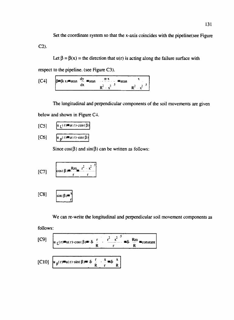
13 t
Set the coordinate system so that the x-axis coincides with the pipeline(see Figure
C2).
Let p = P(x) = the direction that u(r) is acting dong the fiilure surFace with
respect to the pipeline. (see figure C3).
rc41
The longitudinal and perpendicular components of the soil movements are given
below and shown in Figure C-l.
LC51
EC61
Since cos(p) and sin@) can be written as follows:
sint Q)*
We can re-write the longitudinal and perpendicular soil movement components 3s
follows:
LC91
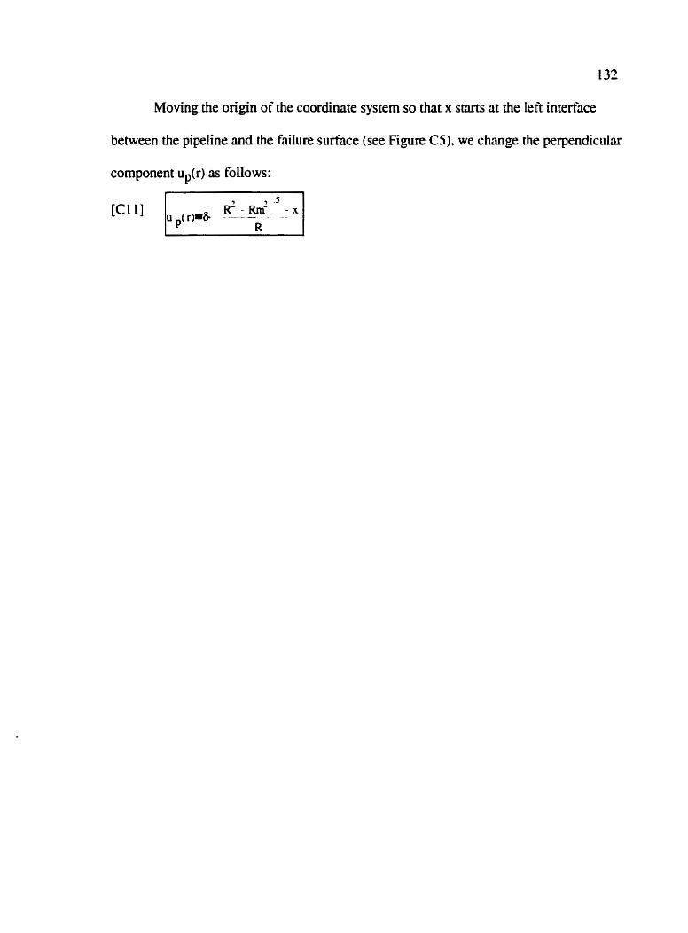
132
Moving the origin of the coordinate system so that x starts at the left interface
between the pipeline and the filure surface (see Figure CS), we change the perpendicular
component up&) as follows: -- -
LC1 11
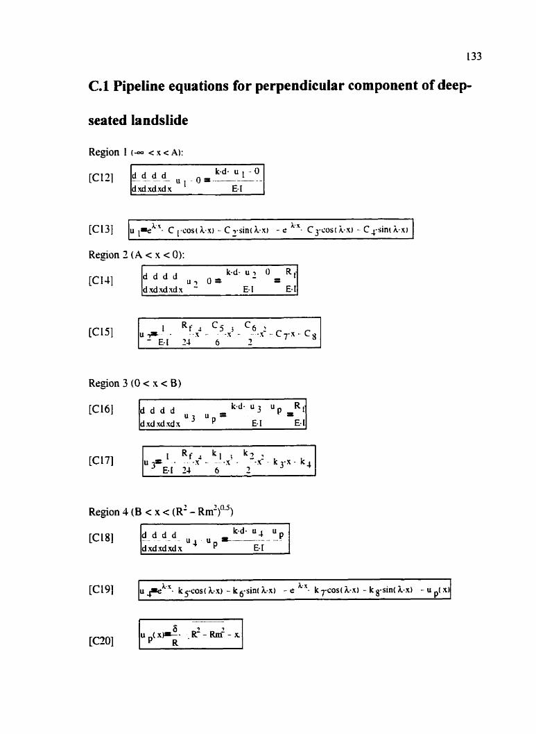
C.l Pipeline equations for perpendicular component of deep-
seated landslide
Region 1 (-- < x c A,:
LC131
Region 2 (A c x < 0):
Region 3 (0 < x < B)
Region 4 (B < x < (R' - ~rn')".')
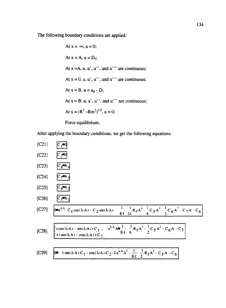
The following boundary conditions are applied:
Atx=-= ,u=O;
At x=A, u=DS;
At x =A, u, u', u". md u"' are continuous;
At x = 0, U. u*, u", and u' * * are continuous;
At x = B, u, u*. u". and u"' are continuous;
Force equilibrium.
After applying the boundary conditions, we get the following equations:
I - l.sin( A-A 1.C - cos ( &-A 1-C -2-eL"-x- - -- --R f~' - C j-A - C - E-1 2 6
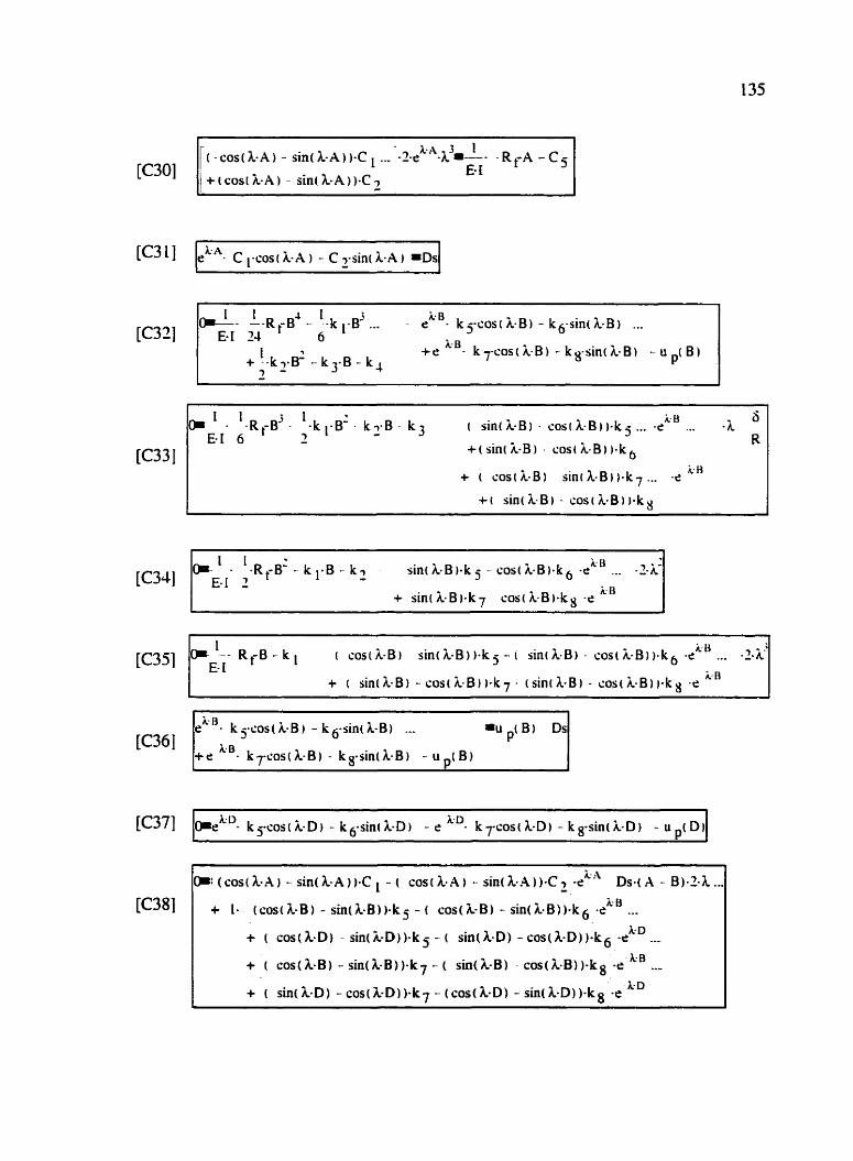
1 ;c. U - ' - R ~ B J - -k 1 - ~ ' - k9.B . k 3 ( sin( LB, . cosc LB1 I-k ... .e ... -1 6 E-I 6 - 7
+( sin( LB) . cos( LB) ).kt, R
isl3 + ( coscLB) sinth-BII-k ,... .e
+( zin(LB1 - c.os(b-B))-ky
I * I - ~ ~ 0 : - k ~ . B - k , sin( h-B I - k - eos( h-B 1.k -e hR ... 3.2 - E-I 2
E; I3 + sin( k B ) . k 7 cos( l . B ~ - k ~ -e

These 18 equations ([C21] to [C38]) can be solved numerically by using Newton-
Raphson Method for Nonlinear Systems of Equations with LU decomposition and back
substitution as described in appendix 6.
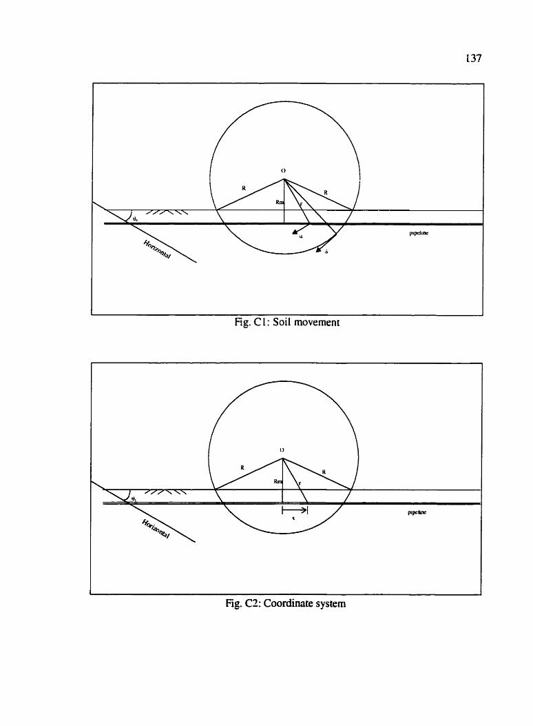
Fig. C 1 : Soil movement
Fig. C2: Coordinate system
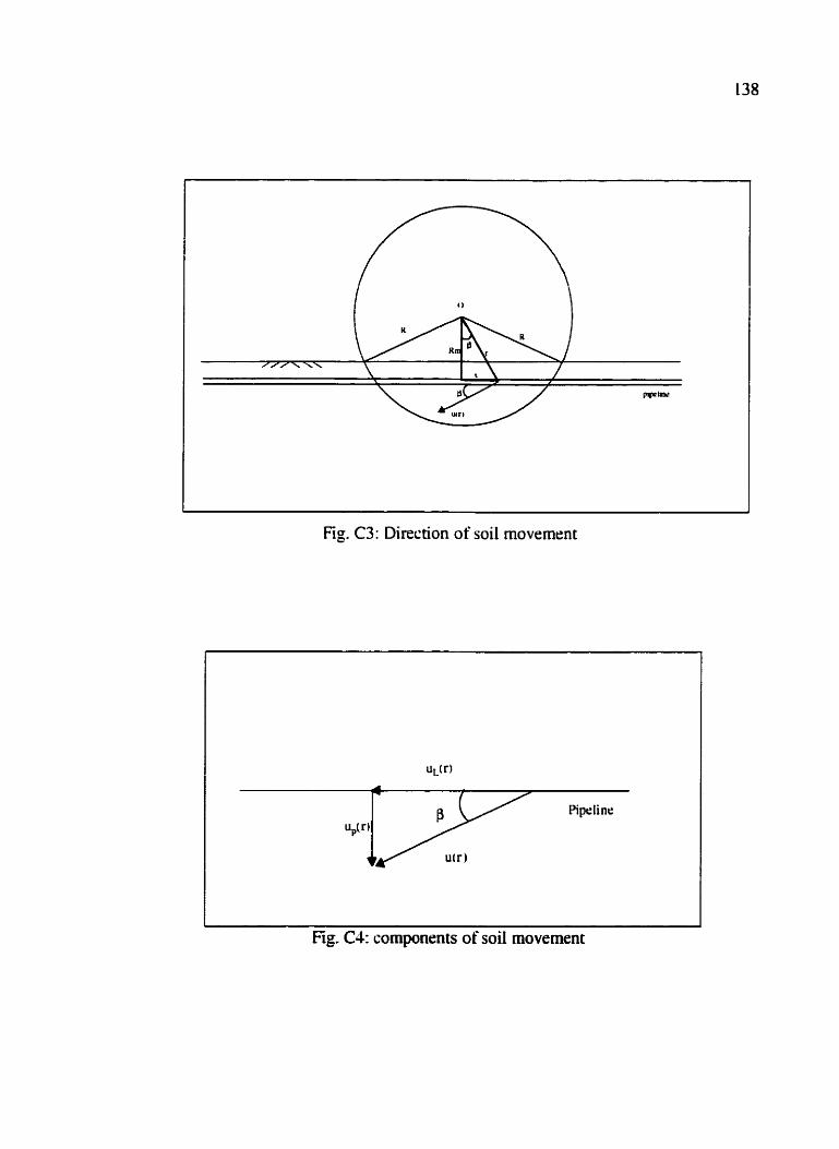
Fig. C3: Direction of soil movement
Fg. C4: components of soil movement
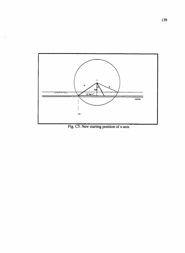
i
Ag. C5: New starting position of x-axis
Appendix D
Numerical Solution of Multiple Nonlinear
Equations Using Newton-Raphson Method
'-EPPE3.BAS '--We use partial pivoting in LUDCMP and LUBKS8. '-Multiple non-linear roots sowed by Newton-Raphson method and LU decomposition '- and back substitution - for Pipe bending with E/P and E/P regions. '-(c) PETER D.S. CHAN APR. 1997 t - DEFINT I-K I P- -- DECLARE SUB MNewton (x#(), n, df#(), f#()) DECLARE SUB LUDCMP (x# ( ) , n, df#(), f#(), index%()) DECLARE SUB LUBKSB (x#(), n, df#(), f#(), index!%()) DECLARE SUB printdf (n, df#()) DECLARE SUB printx (x#(), f#(), n) DECLARE SUB printf (n, f # ( ) ) DECLARE SUB pause () DECLARE SUB UsrEqns (x#(), n, df#(), f#()) DECLARE FUNCTlON x l givenW (x#()) DECLARE FUNCTION x2givenW (x#()) DECLARE FUNCTION x3givenW (x#()) DECLARE FUNCTION StrainEqns# (i, a(), x) DEClARE FUNCTION dStrain€qns# (i, j, x#(), x) DECLARE FUNCTION FirstDerv# (i, j, x#(), x) CLS CONST Pi# = 3.1 41 592653589793# CONST expon# = 2.71 8281 828459045# CONST No = 0, Yes = 1
CONST Ks# = 6500000#, d# = -1 683#, t# = .00318# CONST Ep# = 200000000000#, sigy = 3.86€+08, Ds# = .OO8# CONST TINY = 1 E-20 CONST TOL = 1 E-12
CONST W = 20, delta = 55.901
CONST ntrial = 1000, n = 12 DIM x#(n), df#(n, n), f#(n) ~#(1) = -768.709372# ~#(2) = -1 256.94# x#(3) = -70 1 31.02# ~#(4) = -371 99.1 2# x#(5) = 2420488# x#(6) = 194801 60# x#(7) = .0000938643# x#(8) = -.000080 1 4427# ~# (9 ) = -89.336369# x#(10) = 1 26.822848# x#( 1 1 ) = - 1 4.05369# x#(12) = 9.4401 85# CALL MNewton(x#(), n, df#(), f#())
END
FUNCTION dStrainEqns# (i, j, x#(). x)
SELECT CASE i CASE IS = 1
temp#=(-C#*S#+ 1 -C#A2) *C1#A2 temp#=temp#+(-2*C#* S#+2*C4tA2- 1) C2#*C1# temp# = temp# + (C# A 2 + C# ' SU) * C2# A 2 temp# = temp# * 2 E# dStrainEqnst = tempt t (-(C# + SW) ' C l t - (S# - C#) C2#) d
CASE IS = 2 temp#= 1 /(Ep#* Ip#) * ( - I / 6 *R#*xA3+ .5 * k l#*xA2+k2#*x+k3#) temp#= temp#* (--5 ' R#* x A 2 + k l # * x + k2#) IF j = 1 THEN
d~train~qns# = tempt + -5 * d# * (-R# * x + kl#) ELSEIF j = 2 THEN
dStrainEqns# = temp# - .5 * d# * (-R# ' x + kl#) END IF
CASE IS = 3 temp#= 1 /(Ep#*Ip#)* (1 16' R # ' x A 3 + . 5 * k i # * x A 2 + ~ # * x + l r 3 # )
ternp#=temp#* (-5' R# " x A 2 + k l # * x + k2#) IF j = 1 THEN
dStrainEqns# = temp# + .5 * d# (R# ' x + kl#) ELSEIF j = 2 THEN
dStrainEqns# = temp# - .5 d# * (R# x + kl#) END IF
END SELECT
END FUNCTION
FUNCTION FirstDerv# (i, j, x#(), x) '--P(x)=1 /(Pdx)"[f(~+dx)-f (x-dx)]-0'(dxA2) ,
'--Using Richardson's Extrapolation: I-P(x)=4/3"p hi(dxl2)-113'~ hi(&) - O'(dx%) '-- where phi(dx) = 1/(2"dx)*[f(x+dx)-f(x-dx)] ,
'-df=[df 1 /dxl df 1 /dx2] = [dfiidxj ...I '- [df2/d~l df2/d><2] [ ...,....... I '->"in refers to the ith f eqn, & "j" refers to the jth partial derv. '-ie: df l/dx2 = df(1 )/dy = Zy, and dfUdxl = df(2)ldx = 1.
d x = x / 1 0 A 2 / 2 Xf=x+dx x t 2 = x - d ~ phil = (dStrainEqns#(i, j, x#(), xt) - dStrainEqns#(i, j, x#(), xt2)) / (2 dx]
phi2 = (dStrainEqns#(i, j, x#(), xt) - dStrainEqns#(i, j, x#(), xt2)) I (2 * dx)
FirstDerv# = 4 13 ' phil - 1 / 3 phi2
END FUNCTION
SUB LUBKSB (x#(), n, df#(), f#() , indexO/oo) i2 = 0
F O R i = l T O n k = indexo/o(i) '<--unscrambling the permutation as we go. sum# = f#(k) '-WIO pivoting this would simply be y(l)=f(l) and f#(k) = f#(i) '-y(2)=f(2)-df(2,1)"y(l) or y(i)=f(i)-sum(fromj=l to i-1
'- of df(i,j)'y(j)}. '-Note we don't need the vector yo, we simply place y(i) '- into f(i)
IF (i2 o 0) THEN FORj= i2TOi-1
sum# = sum# - df#(i, j) ' f#(j) NEXT j
ELSEIF sum# o 0 THEN i2 = i '-A nonzero element was encountered, so from now on we
END IF '-will have to do the sums in the loop above. This is '-just some optimization because if the first sum was 0, '-then we don't have to do the loop for the second sum. '-ie: y(2) = f(2)-df(2,l)*y(l) and y(1) = 0.
f#(i) = sum# NUCTi
'-use f(i) to store the deRaX(i): '-for the Newton-Raphson iteration of xnew(i) = xold(i) t deltaX(i), '-we now have x(i) = x(i) + f(i) FOR i = n TO 1 STEP -1 '--Back Substitution
sum# = f#(i) IF (i < n) THEN
FORj= i+1 T o n sum# = sum# - df#(i, j) * f#(j)
NEXT j END IF f#(i) = sum# / df#(i, i)
NEXT i
END SUB
SUB LUDCMP (x#(), n, df#(), f#(), index%()) '-instead of decomposing df() into L() and U(), we will decompose df() back '-into itself (since we only use df() once for each iteration): '-ie:[l Oj and [ul 1 u121 into [ul 1 u121 '- [L 1 2 1 ] [ 0 u22j [Lt 2 u221 - DIM VV#(n) flag = 1 '-no row interchange yet '--loop over rows to get the implicit scaling information F O R i = l T O n
AAmax# = 0 FORj=1 T o n
IF ABS(df#(i, j)) > AArnax# THEN AAmax# = ABS(df#(i, j))
END IF N M j IF (AAmax# = 0) THEN
PRINT "Singular matrix" *-no nonzero largest eiement AArnax# = TINY
END IF W#(i) = 1 # 1 AAmax# 'c-VV(i) = 1IAAma.x of the ith row
NEXTi
FOR j = 1 TO n '-loop over the columns of Crout's method FOR i = 1 TO j - 1 '--U(ij) = df(ij) - surn(k=l to i-1 of L(ik)'U(kj))
sum# = df#(i, j) F O R k = l T O i - l
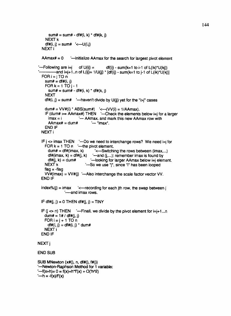
sum# = sum# - df#(i, k) ' df#(k, j) NEXT k df#(i, j) = sum# 'c-U(i,j)
NEXl i
AAmaxt = 0 '--initialize AAmax for the search for largest pivot element
'-Following are i=j of U(ij) = df(ij) - sum(k=l to i-I of L(ik)'U(kj)) I and i=j+l ..n of L(ij)= 1/U(jj) @f(ij) - sum(k1 to j-1 of L(ik)*U(kj)]
FORi= jTOn sum# = df#(i, j) FORk=1 T O j - 1
sum# = sum# - df#(i, k) ' df#(k, j) NEXT df#(i. j) = sum# '-haven't divide by U(0) yet for the "iajj" cases
dum# = W#(i) ABS(sum#) 'c-(VV(i) = 1JAAmax). IF (durn# >= AAmaxt) THEN '--Check the elements below i=j for a larger
imax = i '- AAmax, and mark this new AArnax row with AAmax# = dum# '- "imaxfi.
END IF NEXT i
IF j C> imax THEN '--Do we need to interchange rows? We need i=j for FOR k = 1 TO n '--the pivot element,
dum# = df#(imax, k) '<--Switching the rows between (imax,.,.) df#(imax. k) = df#(i, k) '-and (j, ...) : remember imax is found by df#(j, k) = durn# '--looking for larger AAmax below i=j element.
NUCT k -So we use "j", since "i" has been looped flag = -flag W#(imax) = W#(j) '-Also interchange the scale factor vector VV.
END IF
inde&(j) = imax '<-recording for each jth row, the swap between j '-and imax rows.
IF df#(j, j) = 0 THEN df#(j, j) = TINY
IF (j 0 n) THEN '--Finall, we divide by the pivot element for i=j+1 ... n durn# = 1 # / df#(j, j) FORi= j+1 T o n
df#(i, j) = df#(i, j) durn# NEXTi
END IF
END SUB
SUB MNewton (x#(), n, df#(), f#()) '--Newton-Raphson Method for 1 variable: *-f(x+h)= 0 = f(x)+h*f(x) + O('W2) I-h = -f(x)/f (x)
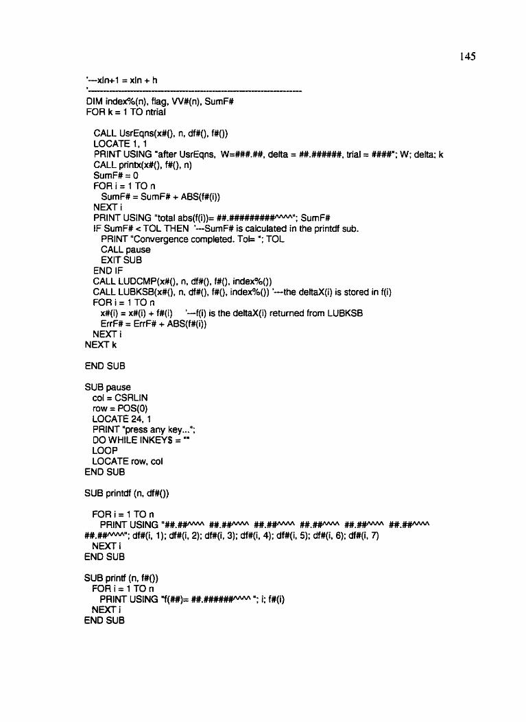
'-xIn+l = xln + h ,
DIM index%(n), flag, W#(n), SumF# FOR k = 1 TO ntrial
CALL UsrEqns(x#(), n, df#(), f#()) LOCATE 1 , l PRINT USING "after UsrEqns, W=###.##, delta = ##I.######, trial = # # # # W; delta; k CALL printx(x#(), f#(), n) SumF# = 0 F O R i = l T O n
SumF# = SumF# t ABS(f#(i)) NEXTi PRINT USING "total abs(f(i))= ##.#########MM"; SumF# IF SumF# c TOL THEN '-SumF# is calculated in the printdf sub,
PRINT "Convergence completed. ToI= "; TOL CALL pause EXIT SUB
END IF CALL LUDCMP(x#(), n, (If#(), f#(), indexoh()) CALL LUBKS8(x#(), n, (If#(), f#(), indexyo()) '--the deRzX(i) is stored in f(i) FORi= lTOn
x#(i) = x#(i) + f#(i) '-f(i) is the deltaX(i) returned from LUBKSB ErrF# = ErrF# + ASS(f#(i))
NEXT i NEXT k
END SUB
SUB pause col = CSRLlN row = POS(0) LOCATE 24, I PRINT "press any key..."; DO WHILE INKEY$ = "" LOOP LOCATE row, col
END SUB
SUB printdf (n, df#())
FORi= lTOn PRINT USING "##.#WVW\ ##.W ##.- ##.F ##.W ##-W
##.#WM"; df#(i, 1); df#(i, 2); df#(i, 3); df#(i, 4); df#(i, 5); df#(i+ 6); df#(i, 7) N M i
END SUB
SUB printf (n, f#()) FORi= lTOn
PRINT USlNG Y(##)= ##.P "; i; f#(i) NEXTi
END SUB
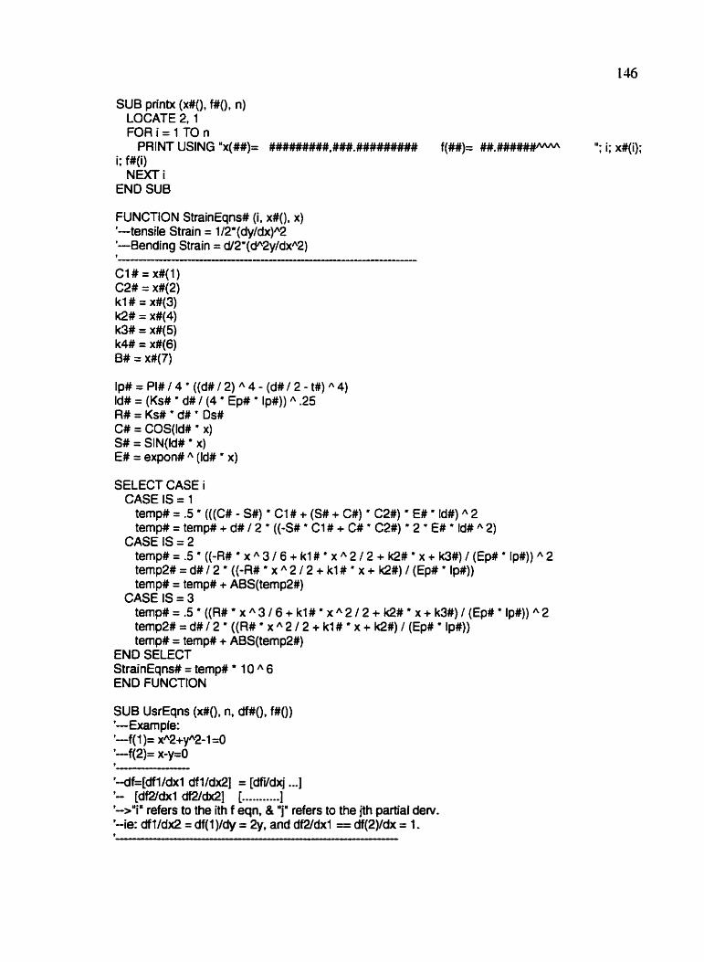
SUB printx (x#(), f#(), n) LOCATE 2.1 FOR i= lTOn
PRINT USING "x(##)= #########,###.######### f(##)= ##.######MM "; i; x#(i); i; f#(i)
NEXTi END SUB
FUNCTION StrainEqns# (i, x#(), x) '--tensite Strain = 1 /2*(dy/dx)A2 '--Bending Strain = d/2'(dn2y/dxA2) t
SELECT CASE i CASE IS = 1
temp# = .5 * (((C# - S#) Ct # + (S# + C#) C2#) ' E# ' Id#) A 2 temp#=temp#+d#/2*( ( -S#*C1#+C#*C2#)*2*E#*fd#A2)
CASE IS = 2 t e m p # = . 5 ' ( ( - R # " ~ ~ 3 / 6 + k l # ' x ~ 2 / 2 + k 2 # * x + k 3 # ) / ( E p # ' I p # ) ) ~ 2 tempZ#=d#/2* ( ( - R # * x A 2 / 2 + kl#* x + W#)/(Ep#' Ip#)) temp# = temp# + ABS(temp2#)
CASE IS = 3 t e m p # = . 5 * ( ( R # * ~ ~ 3 / 6 + k f # * x ~ 2 / 2 + k 2 # * ~ + k 3 # ) / ( E p # * I p # ) ) ~ 2 ternp2#=d#/2* ((R#* x A 2 / 2 + k l# * x + k2#)/ (Ep#* Ip#)) temp# = temp# + ABS(temp2#)
END SELECT StrainEqns# = temp# * 10 A 6 END FUNCTION
SUB UsrEqns (x#(), n, df#(), f#()) '-Example: '-f(l )= x"2tyA2-1=0 '--f(2)= x-y=O ,
'-df=[dfl/dxl dflldm = [dfvdxj .,,I '- [df2/dxl df2/d1Q] [.......,... I '->"in refers to the ith f eqn, & "j" refers to the jth partial dew. '-ie: dflIdx2 = df(1 )/dy = 2y, and df2/dx1 = df(2)/dx = I .
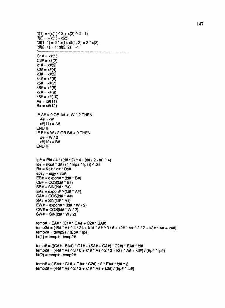
IFA#>OORA#c-WW2THEN A# = -W x#(11) = A#
END IF IFB#>W/2ORB#<OTHEN
B # = W / 2 x#(12) = B#
END IF
Ip#=P I# /4 ' ( (d# /2 )A4 - (d# /2 - t# )A4 ) Id# = (Ks# ' d# 1 (4 ' Ep# ' Ip#)) A .25 R# = Ks# * d# * Ds# epsy = sigy I Ep# EB# = expon# A (Id# " 8#) CB# = COS(W# ' B#) SB# = SIN(Id# ' B#) EA# = expon# A (Id# ' A#) CA# = COS(ld# ' A#) SA# = SIN(ld# ' A#) EW# = expon# A (Id# ' W I 2) CW# = COS(ld# * W 1 2) SW# = SIN(ld#' W 12)
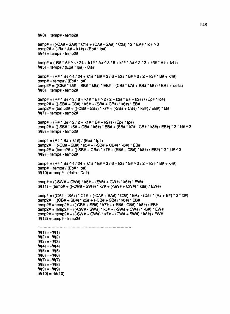
temp#=(R#*B4kA4/24+ k l # * 8 # A 3 / 6 + k 2 # * B # A 2 / 2 + k 3 # * 8 # + k4#) temp# = temp# / (Ep# * Ip#) temp2# = ((CB# k5# + SB# ' kW) * EB# + (CB# * k7# + SB# * k8#) / EB# + delta) f#(6) = temp# - temp2#
ternp#=(R#" B # A 4 / 2 4 + k l # ' B # A 3 / 6 + k 2 # * 8#"2/2+ k3#*B#+ k M ) temp# = temp# / (Ep# Ip#) f#(lO) = temp# - (delta - Ds#)
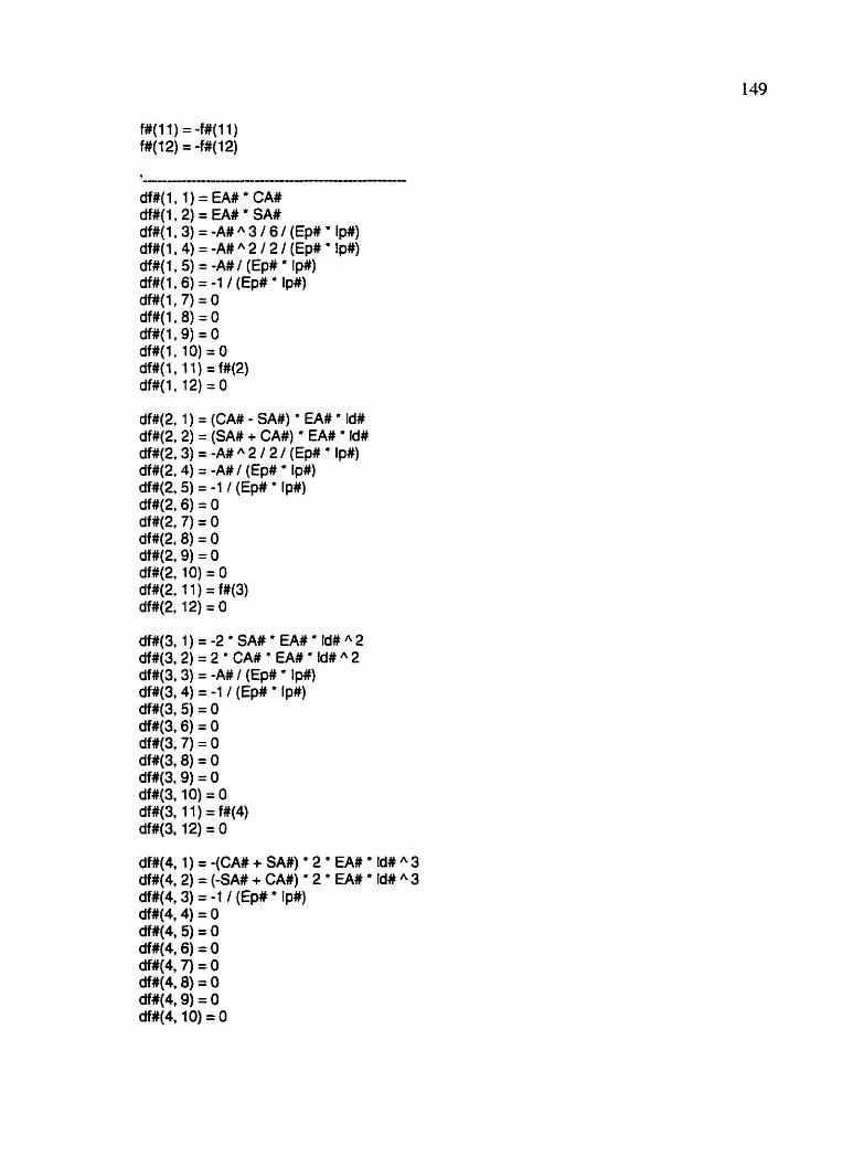
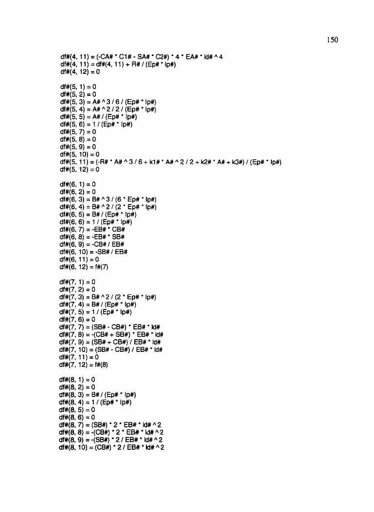
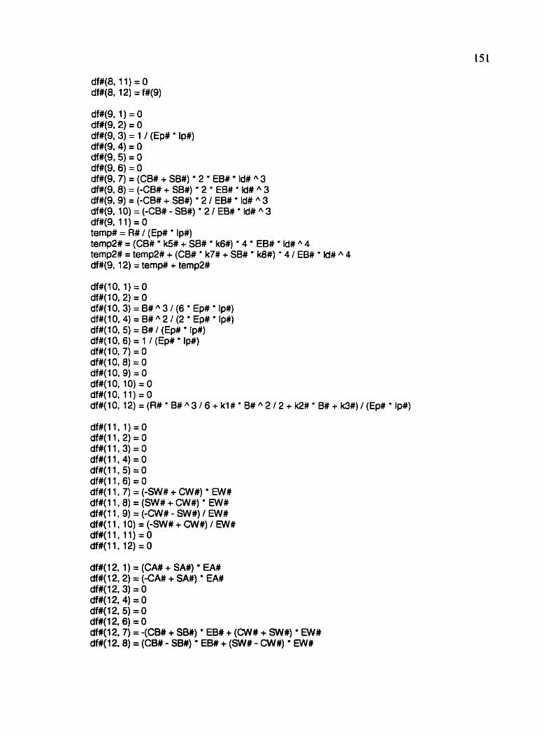
END SUB
FUNCTION x l givenW (x#()) '--Find the "x" for maximum values of strains. L- This means using Newton-Raphson to find "x" at which the "derivative '- of the strain equations (dStrainEqns#())" is equal to 0. '-Tensile Strain = 1 /2'(dyld~)~2 \ '--Bending Strain = d/2'(cP2y/dxA2) \-> function SlainEqns#() I
'--Newton-Raphson Method for 1 variable: '--f(x+h)= 0 = f(x)+hWf (x) + O('W2) '--h = -f(x)/f (x) '-xln+l = xln + h ' - - p--
8# = x#(7) x=B# CLS FOR i = 1 TO ntrial
f# = dStrainEqns#(l '0, x#(), x) df# = FirstDerv#(l , 0, x#(), x) x = x - f# / df# LOCATE 1, I PRINT "i="; i PRINT "xl="; x: " Strain'1O"G = "; StrainEqns#(l , xi(), x) IF ABS(f# / df#) < 1 0 A -5 THEN EXIT FOR IF ABS(x) > 100 THEN
x = 8# EXIT FOR
END IF NEXTi
x l givenW = x END FUNCTION
FUNCTION x2givenW (x#()) '--Find the "x" for maximum values of strains. '- This means using Newton-Raphson to find "x' at which the "derivative '-of the strain equations (dStrainEqns#())" is equal to 0. , - - '-Newton-Raphson Method for 1 variable: '--f(x+h)= 0 = f(~)+h'f'(x) + O('h"2) '-h = -f(x)/f'(x) '--xtn+l = xln + h '
CI
B# = x#(7)
x = . l *B# @ = . I '8# CLS FOR i = 1 TO ntrial
f# = dStrainEqns#(2, 1, x#(), x) df# = FirstDenr#(2, 1, x#(), x) X=X- f# l d f# LOCATE 1.1 PRINT "i="; i PRINT "x2a="; x: " Strain'lM = ": StrainEqns#(Z, x#(), x) IF ABS(f# / df#) < 10 A -5 THEN EXIT FOR
NEXTi CALL pause FOR i = 1 TO ntrial
f# = dStrainEqns#(2, 2, x#(), x2) df# = FirstDew#(2,2, x#(), x2) &=a-f#/ df# LOCATE 1 , l PRINT "i=": i PRlNT "x2b1': x2: " Strain*lW = "; StrainEqns#(2, x#(), x2) IF ABS(f# / df#) < 10 A -5 THEN EXIT FOR
NEXTi CALL pause IF StrainEqns#(2, x#(), x) > StrainEqns#(2, x#(), x2) THEN
x2givenW = x ELSE
x2givenW = x2 END IF END FUNCTION
FUNCTION x3givenW (x#()) - B# = x#(7) x = W / 4 x 2 = W / 4 CtS FOR i = 1 TO ntrial
f# = dStrainEqns#(3, 1, x#(), x) df# = FirstDew#(3, 1 , x#(), x) x = x - f# 1 df# LOCATE 1,1 PRlNT 'i="; i PRlNT "x3a="; x; " Strainel 0% = ": StrainEqns#(3, x#(), x) IF ABS(f# / df#) < 10 A -5 THEN EXIT FOR
NUCTi CALL pause CLS FOR i = 1 TO ntrial
f# = dStrainEqns#(3,2, x#(), x2) df# = FirstDen/#(3,2, x#(), IQ) ~2=x2 - f# /d f# LOCATE 1.1 PRINT "i="; i

PRINT "x3b="; x2; " Strain'l 0% = "; StrainEqns#(3, x#(), x2) IF ABS(f# / df#) c 10 A -5 THEN EXIT FOR
NEXTi CALL pause IF StrainEqns#(3, x#(), x) > StrainEqns#(3, x#(), x2) THEN
x3givenW = x ELSE
x3givenW = x2 END IF
END FUNCTION
Appendix E
Computer Implementation of the Longitudinal
Landslide
DEFINT A-Z 'PROGRAM: PLANAR LANDSLIDE: 'CREATOR: PETER D.S. CWAN 'DATE: OCT. 18 '97 'PURPOSE: to find max strain of pipe buried in planar landslide. '
'd# = -1 683# 't# = -0031 8# 'E#=200 ' 10A9 'H =2 'coh#=2' 10A3 'gamma#= 18' 10A3 'phi# = 30 pi# / 180 'Ds# = .008# 'L# = 1 OOO# 'deftatunit# = 2.5 Ds# f
_tl
DECLARE SUB tongslide () DECLARE SUB graph (delta.ds#. ernax#, deltaemin#) DECLARE FUNCTION next.higher.value# (given.value#) DECLARE FUNCTION interval.stepl (given.value, rnax.num.divisions) DECLARE SUB ReadlnputFite () '--for 2Ds c delta-min < delta c deIta.max DECLARE SUB BisectXa (a#, b#, fa#, fb#) DECLARE FUNCTION GetDelta.min# (L#, Id#, Ds#) DECLARE FUNCTION f.xa# (y#) '--f.xa = eq'm+comp. eqn in terms of xa DECLARE FUNCTION xb.xa# (y#) '-xb.xa = xb compatibility eqn in terms of xa DECLARE FUNCTION emanxa# (p) '--emanxa = rnax strain eqn in terms of xa DECLARE FUNCTION f.deltamin# (y#) *--eqn for find delta.min D €CLARE SUB initvalues () '--for delta c 20s DECLARE SUB BisectUo (a#, b#, fa#, fb#) DECLARE FUNCTION f.uo# (y#)
DECLARE FUNCTION ernax.uo# (y#) '-emax-uo = max strain eqn in terms of uo '--Menu Handling-- DECLARE SUB Initialize () DECLARE SUB Menu1 () DECLARE SUB Checkscreen () DECLARE SUB DrawFrame (Topside, Bottomside, Leftside, Rightside) DECLARE SUB 8oxlnit () DECLARE SUB printmenustring (menustring$, char.posOh, num-chars. hiliteds) '-Values for keys on the numeric keypad and the spacebar: CONST UP = 72, DOWN = 80, LIT = 75, RGHT = n CONST UPLFT = 71, UPRGHT = 73, DOWNLFT = 79, DOWNRGHT = 81 CONST SPACEBAR = " " CONST F1 = 59, F2 = 60, F3 = 61, F4 =62, F5 = 63 CONST F6 = 64, F7 = 65, F8 = 66, F9 =67, F10 = 68
'-Null$ is the first character of the two-character INKEY$ '-value returned for direction keys such as UP and DOWN: 'NULL$ = CHR$(O): ESCAPE$ = CHR$(27): ENTER$ = CHR$(13) CONST ESCAPE = 27, ENTER = 13, NULL = 0 C O N S FALSE = 0, TRUE = NOT FALSE
DIM SHARED InitRow, MaxRow, MaxColors, Foreground, Background, Hilite, selection DIM SHARED d#, tit, E#, H, coh#, gamma#, phi,deg#, phi.rad#, Ds#, L#, L.rnin# DIM SHARED delta.ds#, delta.unit#, delta.min#, deRa.max# DIM SHARED angle.rad#, angle.deg#, delta.unit.parallel#, delta.ds.parallel# DIM SHARED ks#, Id#, Area#, runlong3f, runlong6b DIM SHARED outfilename$, Deltaswitch CtS
ReadlnputFile initvalues
CONST mnustn'nglength = 51 '- - TYPE mnuType
mnustring AS STRING * mnuStringLength mnuHotKey AS IMEGER '-position of the hotkey rnnuHiliteWidth AS INTEGER '-number of chars displayed for the hotkey
END TYPE '---main menu items: string and position of hilite--- CONST MainMenultems = 17 DIM SHARED MainMenu(MainMenu1tems) AS mnuType DATA " 1 ) pipe diarneter(rn): ", 1 ,I DATA "2) pipe thickness(m) : ', 1 , 1 DATA "3) pipe modu Ius of elasticity( Pa/m): ,1,1 DATA "4) depth to center of pipe(m): ", 1 ,1 DATA "5) soil cohesion(NlmA2): ", 1 ,1 DATA "6) soil density(NlW3): ", 1 ,I DATA "7) soii internal frictional angle(degrees): ", 1.1 DATA "8) limit elastic displacement of soil(Ds (m)): ", 1 ,1 DATA '9) length of landslide (m): ", 1,1 DATA '0) landslide rnagnitude(in multiples of Ds) : "?I DATA "F 1 ) landslide magnitude entry toggle : *,1,2
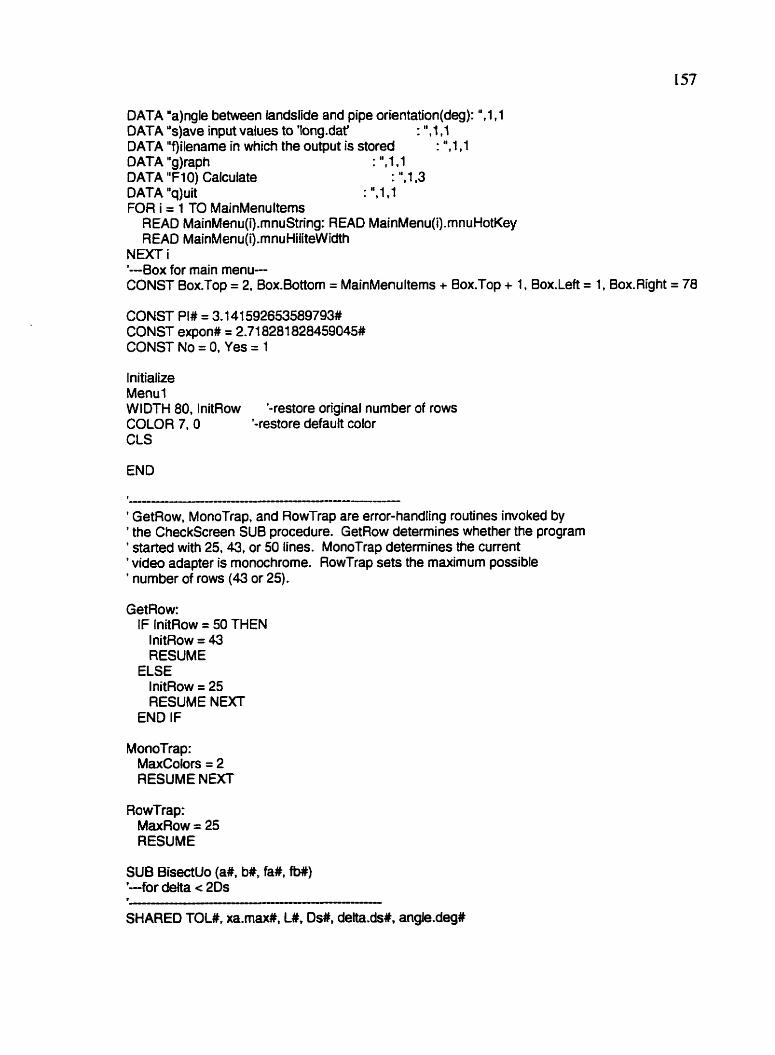
DATA "a)ngle between landslide and pipe orientation(deg): ",I ,1 DATA "s)ave input values to 'fong.dat' : ",I ,I DATA "f)ilename in which the output is stored : '@,I ,I DATA "g)raph : 11,1 ,I DATA "F10) Calculate : ",I ,3 DATA "q)uit : 11,1,1 FOR i = 1 TO MainMenultems
READ MainMenu(i).mnuString: READ MainMenu(i).rnnuHotKey READ MainMenu(i).mnuHiliteWidth
NEXTi '--Box for main menu- CONST Box.Top = 2, 6ox.Bottorn = MainMenultems + Box.Top + 1, Box.Left = 1, Box-Right = 78
CONST PI# = 3.1 41 592653589793# CONST expon# = 2.71 8281 828459045# CONST No = 0, Yes = 1
Initialize Menu1 WIDTH 80, InitRow '-restore original number of rows COLOR 7,0 '-restore default color CtS
END
-- ' GetRow, MonoTrap, and RowTrap are error-handling routines invoked by ' the Checkscreen SUB procedure. GetRow determines whether the program ' started with 25,43, or 50 lines. MonoTrap determines the current ' video adapter is monochrome. RowTrap sets the maximum possible ' number of rows (43 or 25).
GetRow: IF Initflow = 50 THEN
InitRow = 43 RESUME
ELSE Initflow = 25 RESUME NEXT
END IF
MonoTrap: MaxColors = 2 RESUME NEXT
RowTrap: MaxRow = 25 RESUME
SUB BisectUo (a#, b#, fa#, fb#) '--for delta c 2Ds
SHARED TOM, xa.max#, L#, Ds#, delta.ds#, angle.deg#
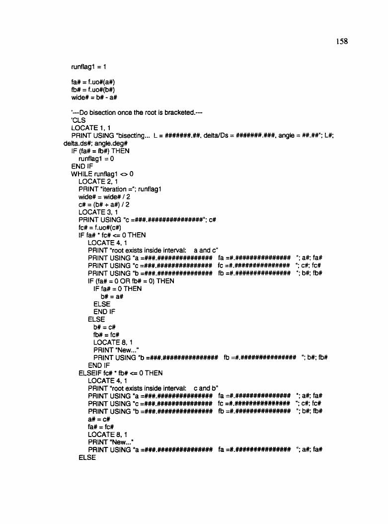
runflagl = 1
'-Do bisection once the root is bracketed.-- 'CLS LOCATE 1.1 PRINT USING "bisecting.., L = #######.##, delta/Ds = #######.###, angle = ##.##"; L#:
delta-ds#; angle.deg# IF (fa# = fb#) THEN
runflagl = 0 END IF WHILE runflagl o 0
LOCATE 2.1 PRlNT "iteration ="; runflagl wide# = wide# / 2 c#=(b#+a#) l2 LOCATE 3.1 PRINT USING "c =###.###############"; c# fc# = f .uo#(c#) IF fa# ' fc# (= 0 THEN
LOCATE 4, t PRlNT "root exists inside interval: a and c" PRINT USING "a =###.############## fa =#.################ ": a#; fa# PRINT USING "c =###,############### fc =#.############# "; c#; fc# PRlNT USING "b =###.############## fb =#-############## "; b # ~ fb# IF (fa# = 0 OR fb# = 0) THEN
IFfa#=O THEN b# = a#
ELSE END IF
ELSE b# = c# fb# = fc# LOCATE 8,1 PRINT "New ...I' PRINT USING "b =###.############### fb =#.############### "I b#; fb#
END IF ELSEIF fc# * fb# c.= 0 THEN
LOCATE 4.1 PRINT 'root exists inside interval: c and b" PRIM- USING "a =###.- fa =#.- "; a#; fa# PRINT USING "C =##HI,- f~ =#.- "; c#; f ~ # PRINT USING "b =###.- fb =#.- "5 b4k fb# a# = c# fa# = fc# LOCATE 8,1 PRINT "New. .." PRlNT USING "a =###.- fa =#.-###### '; a#; fa#
ELSE
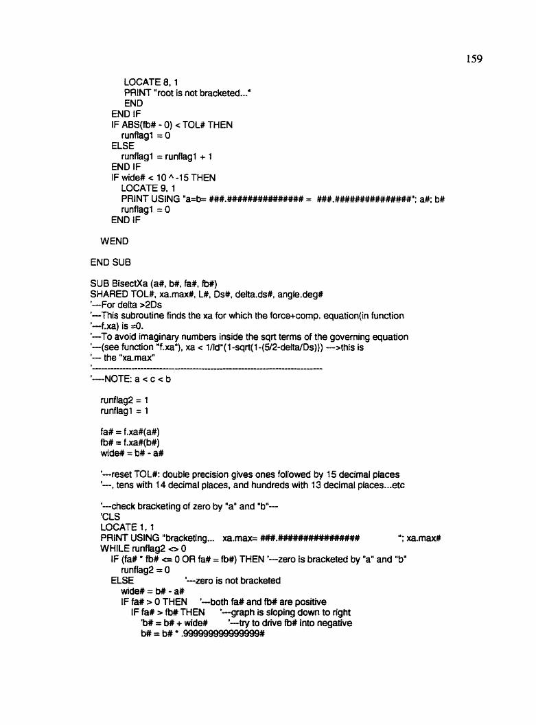
LOCATE 8,1 PRINT "root is not bracketed ..." END
END IF IF ABS(fb# - 0) < TOL# THEN
runflagl = 0 ELSE
runflagl = runflagl + 1 END IF IFwide#c loA-15THEN
LOCATE 9'1 PRINT USING "a=b= ###.############### = ###.#########*##''; a#; b# runf lag 1 = 0
END IF
WEND
END SUB
SUB BisectXa (a#, b#, fa#, fb#) SHARED TOL#, xa.max#, L#, Ds#, delta.ds#, angle.deg# '--For delta w2Ds '--This subroutine finds the xa for which the forcwcornp. equation(in function '--f.xa) is =0. '-To avoid imaginary numbers inside the sqrt terms of the governing equation '-(see function "f.xaN), xa c t/ldw(l -sqrt(l -(Y2-delta/Ds))) ->this is '- the "xa.maxU t - m_-__Ul_m_
'-NOTE: a c c c b
runflag2 = 1 runflagl = 1
'-reset TOL#: double precision gives ones followed by 15 decimal places '--, tens with 14 decimal places, and hundreds with 13 decimal places ... etc
'-check bracketing of zero by "a" and "b"- 'CLS LOCATE 1,1 PRINT USING "bracketing ... xa.max= ###.-###### "; xa.max# W H 1 LE runf lag2 o 0
IF (fa# fb# <= 0 OR fa# = fb#) THEN '-zero is bracketed by "an and "b" runflag2 = 0
ELSE '-zero is not bracketed wide# = b# - a# IF fa# > 0 THEN '--both fa# and W are positive
IF fa# > fb#t THEN '--graph is sloping down to right 'b# = b# + wide# '-try to drive fb# into negative
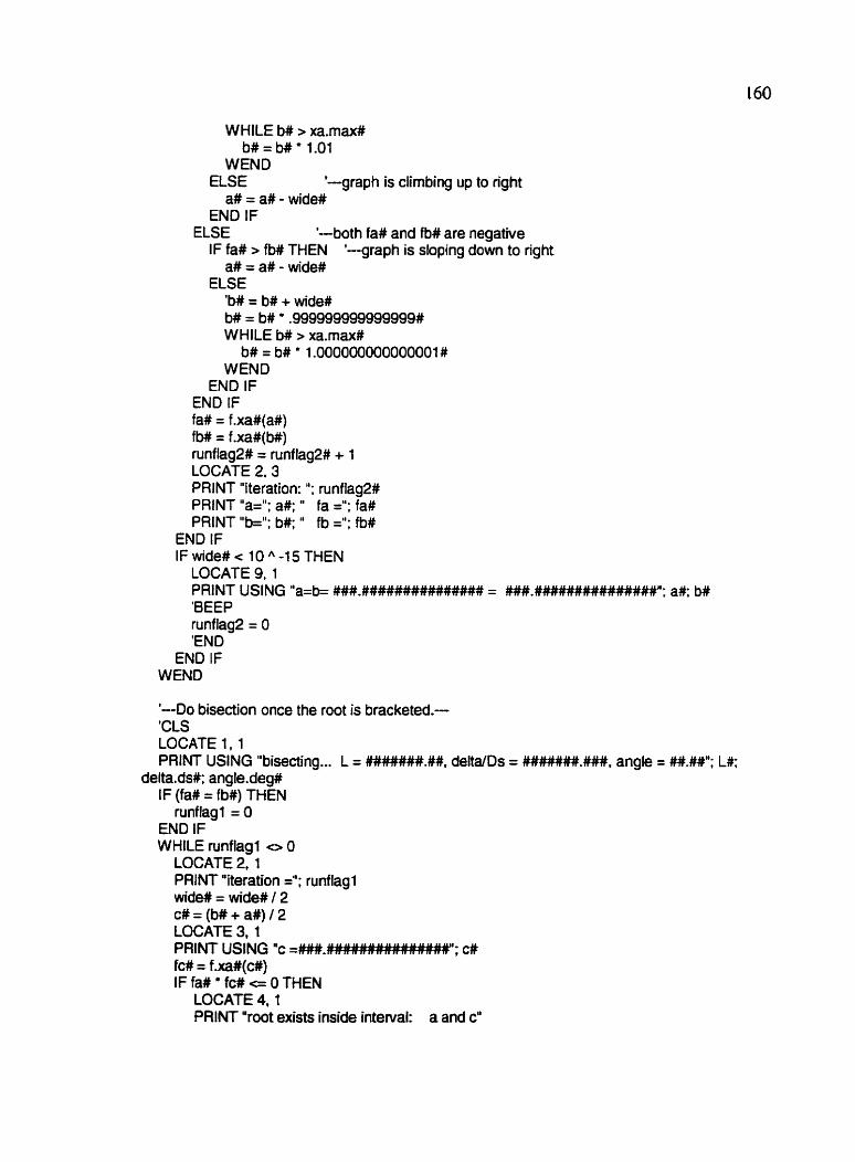
WHILE b# > xa.max# b# = b# ' 1.01
WEND ELSE '-graph is climbing up to right
a# = a# - wide# END IF
ELSE '-both fa# and fb# are negative IF fa# > fb# THEN -graph is sloping down to tight
a# = a# - wide# ELSE
'b# = b# + wide# b# = b# ' .999999999999999# WHILE b# > xa.max#
b# = b# ' 1.000000000000001 # WEND
END IF END IF fa# = f.xa#(a#) fb# = f.xa#(b#) runflag2# = runfhg2# + 1 LOCATE 2.3 PRlNT "iteration: "; runflag2# PRlNT "a="; a#; " fa ="; fa# PRlNT "El; b#; " fb =I8: fb#
END IF IF wide# < 10 A -1 5 THEN
LOCATE 9,1 PRlNT USING "a=b= ###.############### = ###.###############": a#; b# 'BEEP runflag2 = 0 'END
END IF WEND
'-Do bisection once the root is bracketed.- 'CLS LOCATE 1 ,1 PRINT USING "bisecting ... L = #######.##, deWDs = #######.###, angle = ##.##"; L#;
deita.ds#; angle.deg# IF (fa# = fb#) THEN
runflagl = 0 END IF WHILE runflagl o 0
LOCATE 2'1 PRIM "iteration ="; runflagl wide# = wide# / 2 c#=(b#+a#)/2 LOCATE 3.1 PRINT USING "c =###.-; C# fc# = f.xa#(c#) IF fa# " fc# C= 0 THEN
LOCATE 4.1 PRlNT "root exists inside interval: a and c"
PRlNT USING "a =###.WL##- fa = # . # # "; a#; fa# PRlNT USlNG "c =###.-## fc =#-###I#- c#; fc# PRlNT USING "b =###.##WM#W###### fb =#.#####- "; b#: fb# IF (fa# = 0 OR fb# = 0) THEN
IF fa# = 0 THEN b# = a#
ELSE END IF
ELSE b# = c# fb# = fc# LOCATE 8.1 PRINT "New .,." PRINT US1 NG "b =###.############### fb =#.############### ": b#; fb#
END IF ELSEIF fc# ' fb# c= 0 THEN
LOCATE 4.1 PRlNT "root exists inside interval: c and b" PRl NT USlNG "a =###.############### fa =#.#############I## "; a#; fa# PRINT USING "c =###.############## fc =#.############### "; c#: fc# PRlNT USING "b =###.############### fb =#.############### "; b#: fb# a# = c# fa# = fc# LOCATE 8.1 PRINT "New ..." PRINT USING "a =###.############### fa =#.############### "; a#; fa#
ELSE LOCATE 8,1 PRlNT "root is not bracketed ..." END
END IF IF A8S(fb# - 0) < TOL# THEN
runf lag 1 = 0 ELSE
runflagl = runflagl + 1 END IF IF wide# c 10 A -1 5 THEN
LOCATE 9.1 PRINT USING "a&= ###t.####t#####WW#### = ### .############## I8 ; a#; b# 'BEEP 'END runflagl = 0
END IF
WEND
END SUB
SUB Boxlnit STATIC I Boxlnit
' Calls the DrawFrame procedure to draw the frame around the sort menu, ' then prints the different options stored in the OptionTitle array.
Drawframe BoxTop, Sox.Bottorn, Box-Left, Box-Right
LOCATE Box-Top - 1, BonLeft + 5: PRlNT "Pipe Strain Program (copyrighted 1996 Peter D.S. Chan)";
LOCATE Box.Top + 1 FOR i = 1 TO MainMenultems
LOCATE , 8ox.Left + 2 IF i = selection THEN Foreground = 0: Background = 7: Hilite = 10 '-reverse video
ELSE Foreground = 7: Background = 0: Hilite = 15
END IF printmenustring MainMenu(i).mnuString, MainMenu(i).rnnuHotKey,
MainMenu(i).mnuHiliteWidth NEXTi Foreground = 7: Background = 0 '-Turn off reverse video COLOR Foreground, Background
'
LOCATE Box.Top + 1, mnuStringLength + 3 PRlNT USING "#######.######"; d#
LOCATE Box.Top + 2, mnustringlength + 3 PRINT USING "#######.######"; t#
LOCATE Box.Top + 3, mnuStringLength + 3 PRINT USING " # # # , . # Y o ; E# LOCATE Box.Top + 4, mnuStringLength + 3 PRINT USING "#######.##"; H
LOCATE Box-Top + 5, rnnuStringLength + 3 PRINT USING "######,.##"; coh# LOCATE Box-Top + 6, mnuStringLength + 3 PRINT USING "######,.##"; gamma#
LOCATE Box-Top + 7, mnuStringLength + 3 PRINT USING "#######.##"; phi.deg#
LOCATE Box-Top + 8, mnuStringLength + 3 PRINT USING "#######.######": Ds# LOCATE Box.Top + 9, mnuStringLength + 3 PRINT USING "#######.##"; L#
LOCATE Box.Top + 10, mnustringtength t 3 IF Deltaswitch = FALSE THEN
PRINT USING "#######.###"; delta.ds# LOCATE Box-Top + t 1, mnustringlength + 3 PRINT "{manual 1 )"
ELSE PRINT USING "0.00 to ###.######"; deltaamax# I Ds# LOCATE 6ox.Top + 1 1, mnuStringLength + 3 PRINT "( I auto )"
END IF LOCATE BoxTop + 12, mnustringlength + 3 PRINT USING " #.#W; angle.deg# LOCATE BolcTop + 14, mnustringlength + 3
PRINT USING " &"; outfilename$
'-for printing input statements- LOCATE 23,t PRINT " LOCATE 23.1
END SUB
SUB CheckScreen STATIC ' --- - Checkscreen -- -- - ' Checks for type of monitor (VGA, EGA, CGA, or monochrome) and ' starting number of screen lines (50, 43, or 25). *
'SCREEN 0 WIDTH 80'50 -Find out what how many rows the user was using initially. '-Try locating to the 50th row; if that fails, try the 43rd. Finally, '-if that fails, the user was using 25-line mode: Initflow = 50 ON ERROR GOT0 GetRow LOCATE InitRow, 1
' Try a SCREEN 1 1 statement to see if the current adapter has color ' graphics; if that causes an error, reset MaxColors to 2: MaxColors = 1 5 ON ERROR GOT0 MonoTrap SCREEN 11 SCREEN 0
'-See if 43-line mode is accepted; if not, run this program in 25-line '-mode: 'MaxRow = 43 MaxRow = 25 ON ERROR GOT0 RowTrap WIDTH 80, MaxRow ON ERROR GOT0 0 ' Turn off error trapping.
END SUB
SUB DrawFrame (Tapside, Bottomside, LeftSide, RightSide) , DrawF rame
' Draws a rectangular frame using the high-order ASCl 1 characters E (201 ) . (1 87) . E (200) . %(I 88) , (1 86) . and i (205). The parameters
Topside. Bottomside. LeftSide, and RightSide are the row and column ' arguments for the upper-left and lower-right corners of the frame. ' ~dditional:i (204). ' ( 1 85)
CONST ULEFT = 201, URIGHT = 187, L L E F = 200, LRIGHT = 188 CONST VERTICAL = 186, HORIZONTAL = 205 CONST BEAMLEFT = 204, BEAMRIGHT = 185
Framewidth = Rightside - LeftSide - 1 LOCATE Topside, LeftSide PRINT CHR$(ULEFT): STRING$(FrarneWidth. HORIZONTAL); CHR$(URIGHT); FOR Row = Topside + 1 TO BottomSide - 1
LOCATE Row, LeftSide PRINT CHR$(VERTICAL); SPClFrameWidth); CHR$(VERTICAL);
NUCT Row LOCATE BottomSide, Leftside PRINT CHR$(LLEW: STRING$(FrarneWidth, HORIZONTAL); CHRS(LR1GHT);
END SUB
FUNCTION emax.uo# (uo#) '--for delta < 2Ds *
SHARED Id#, Ds#
p l # = (uo# - TAN(alfa#) 1 (2# ' Id#)) ' (expon# A (Id# ' xi#)) p2# = TAN(alfa#) 1 (2# ' Id#) expon# A (-Id# xi#) emax.uo# = id# (pl # - p2#) + TAN(atfa#) END FUNCTION
FUNCTION emax.xa# (xa#) '-the max strain for delta > 2Ds
SHARED Id#, Ds# emax.xa# = Ds# * (-xa# ' Id# A 2 + Id#)
END FUNCTION
FUNCTION f.deltamin# (delta.min#) '--For defta >2Ds '-This is the force+comp. equation with xa=O substituted in.
-.
SHARED L#, Id#, Ds# b# = (5 - 2 ' delta.min# / Ds#) A -5 f.deltamin# = (expon# A (2 ' b# - 2 + L# * Id#) + 1) ' (1 - b#) - 2
END FUNCTION
FUNCTION f.uo# (uo#) '--for delta c 2Ds '--note: e = 2,718281 828459045 9
SHARED Id#, Ds#, delta.~nit.paralleI#~ L#
aIfa# = 89.98999999999999# (PI# / 180#) 'xr# = delta.unit# / TAN(alfa#) xr# = delta.unit.parallel# 1 TAN(alfa#) xi# = -LOG(1# - 2# * uo# ' Id# I TAN(alfa#)) I (2# ' Id#) '-note: LOG is basic is the natural logarithm "LN" p l # = uo# ' expon# A (Id# ' (L# + xr#)) 'pl# = uo#
END FUNCTION
FUNCTION f.xa# (xa#) '-For delta >2Ds '-this is the force+comp. equation in terms of 'xa' '--Idea is to balance the forces with the cornp. conditions in finding the xa '--for which this function 'f.xa#' = 0 1 ----- P
SHARED Id#, Ds#, delta.unit.parallel#, L#
'p1 # = (2 ' xa# A 2) - (4 I Id# ' xa#) + (5 1 Id# A 2) - (2 1 (Ds# ' Id# A 2) delta.unit#) p l# = (2 ' xa# A 2) - (4 I Id# ' xa#) + (5 I Id# A 2) - (2 I (Ds# ' Id# A 2) ' delta.unit.parallel#) 'IF (pl#) < 10 A -(I 3 - LOG(L#) / LOG(10)) THEN IFpl#cOTHEN
pl#=O END IF '-limitation U(P(n) has the limit of n <= 88.02969 '-expon#(n) =2.718281828459045#(n) has the limit of n <= 709.78 plb#= Id# ' (2 '~a#-2 / Id#+2 ' (p1#)~ .5+L#) IF p l b# > 709.78 THEN
LOCATE 23, t PRINT " It.
T
LOCATE 23'1 P R I M "Overflow: L is too large!" LOCATE 24.1 PRINT "Press any key to continue,.."; DO LOOP WHILE INKEY$ = '" END
END IF
IF p2# c 0 THEN p2# = 0
END IF f.xa# = eq# ' (1 - (p2#) A .5) - 2
END FUNCTION
FUNCTION GetDe(ta.min# (L#, Id#, Ds#) '-For delta >2Ds '--this function is to find the deka.min (at which xa=O) '--It finds the root of the force+comp. equation for which xa=O (equation is '-located in f.deltamin function. '--Note: the min. L for which forces will balance is 2/ld#: this is found '--from the force+cornp. equation with xa=O and x k U 2 -> subst and sohe for L.
a# = 2.5 Ds# '--this is the absolute max delta for xa=O: above this you'ld get complex numbers
b# = 2 * Ds# '--this is the abs min delta for xa-0 fa# = f.deltarnin#(a#) fb# = f.dettamin#(b#) wide# = a# - b# T "getting deltaernin ..." runflagl = 1 IF (fa# = fb#) THEN
runflagl = 0 END IF WHILE runflagl a 0
wide# = wide# / 2 c#=(b#+a#) /2 fc# = f.deltamin#(c#) IF fa# ' fc# C= 0 THEN
IF (fa# = 0 OR fb# = 0) THEN IF fa# = 0 THEN
b# = a# ELSE END IF
ELSE b# = c# fb# = fc#
END IF ELSElF fc# fb# <= 0 THEN
a# = c# fa# = fc#
END IF IF ABS(fb# - 0) c TOL# THEN
runflagl = 0 ELSE
runflag? = runflagl + 1 END IF IF wide# c 10 A -15 THEN
runflagl = 0 END IF
WEND
IF ABS(fa#) < ABS(fb#) THEN GetDelta.min# = a#
ELSE GetDetta.min# = b#
END IF
END FUNCTION
SUB graph (delta.ds#, emax#, delta.min#) SHARED Ds#, outfilename$ Style% = &HFFOO ' Use to make dashed line.
'--get maximum of all deta.ds# and ernax# (i-e. the last data):begin OPEN outfilename$ FOR INPUT AS #I blank$ = INPUT$(44, #I ) INPUT #1 , landslide# '--...reading the length of landslide. FORn=2TO9
LlNE INPUT #I, blank$ NEXTn blank$ = INPUT$(Sl, #1) INPUT #I1 angle.deg# '-...reading the angle between landslide and pipeline. F O R n = l l T O 1 2
LlNE INPUT #I, blank$ NUCTn
n=O 00
INPUT # I , delta-ds#, ernax# LOOP UNTIL EOF(1) CLOSE #I delta.ds.max# = delta.ds# ernax.rnax# = emax# '--get maximum of all delta.ds# and ernax# (i-e. the last data):end
SCREEN 12 WIDTH 80,60
' View port sized to proper scale for graph: '--VtEW makes: (0,O) at top left of screen 'VIEW (60,30)-(620,400), , 16 view.x.start = 60 view-y-start = 50 viewx-end = 600 view-y-end = 390 VIEW (view.x.start, view.y.start)-(view-x-end, view-y-end) , , 16
'-Make window large enough for strain from 0 to emax, and delta from 0 to delta.ds.rnax '--WINDOW makes: (0,O) at bottom left of screen window.x.end = delta.ds.max#
window,y.end = next. higher.value(lNT(emax.max#) + 1 )
WINDOW (0, 0)-(window.x.end, window.y.end)
OPEN outfilename$ FOR INPUT AS #1 FORn= lTO11
LlNE INPUT #1, blank$ NExTn n=O
CLS LlNE (0.0)-(0.0) DO
INPUT #I, delta.&#, emax# x# = delta.ds# y# = emax# ' Calculate the y coordinate. IF ABS(deRa.ds# - delta+min# 1 Ds#) <= 10 A -4 THEN
LINE (x#. Y#)-(x#, y#). 1 I ELSE
LlNE -(x#, y#), 11 ' Draw a line from the last ' point to the new point.
END IF LOOP UNTIL EOF(1) CLOSE #1
'--draw x-axis ticks '-height of tick is 1/100 of the height of window y-axis window.x.tick.height = window,y.end window.x.tick.stepl = intewal.step!(window.x.end, 1 5) window.x.tick.begin! = window.x.tick.step! FOR n = window.x.tick.begin! TO window.x.end STEP window.x.tick.step!
LlNE (n, 0)-(n, window.x.tick.height), 7, , Style% NEXTn
'--draw y-axis ticks - '-height of tick is 111 00 of the width of window y-axis window.y.tick.height = window.x.end '--draw dashed line across graph. window.y.tick.stepl = interval.stepl(window.y.end, 1 5) window.y.tick.begin! = window.y.tick.stepl FOR n = window.y.tick.begin! TO window.y.end STEP window.y.tick.step!
LlNE (0, 0)-(window-y.tick.height, n), 7, ,Style% NEXTn
'-Label x-axis data values '-note: in screen mode 11 or 12 '--x-axis: 640pixels/801ext = 8pixels/txt '--y-axis: 480pixe td30text = 1 6pixeIdtxt or 480pixeW60text = 8pixeIdtxt LOCATE 51.8: PRINT "O" prev.col = 8 FOR nl = window.ntickbegin! TO window-x-end STEP window.x.tickstepl
col = (view.x.start + nl 1 window.x.end * (view-x-end - view-x-start)) I 8 LOCATE 51, col
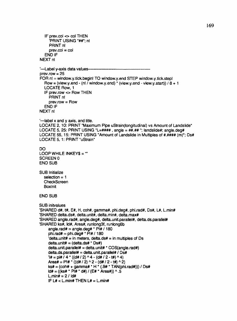
IF prev-col o col THEN 'PRINT USING "##"; nl PRINT n! prev.co1 = col
END IF NEXT nl
'-Label y-axis data values I__m__-
prev.row = 25 FOR nl = window.y.tick.begin! TO window.y.end STEP window.y.tickstepf
Row = (view.y.end - (n! / window.y.end) ' (view.y.end - view.y.start)) 1 8 + 1 LOCATE Row, 1 IF prev.row o Row THEN
PRINT n! prev.row = ROW
END IF NEXT n!
'-label x and y axis, and title, LOCATE 2, 1 0: PRINT "Maximum Pipe uStrain(longitudina1) vs Amount of Landslide" LOCATE 5.25: PRINT USING "L=#### . angle = ##.## ": landslide#: angle.deg# LOCATE 55, 15: PRINT USING "Amount of Landslide in Multiples of #.#### (m)"; Ds# LOCATE 5, 1 : PRINT "ustrain"
DO LOOP WHILE INKEY$ = '"' SCREEN 0 END SUB
SUB Initialize selection = 1 Checkscreen Boxlnit
END SUB
SUB initvalues 'SHARED d#, t#, E#, H, coh#, gamma#, phi.deg#, phi.rad#, Ds#, L#, L.min# 'SHARED delta.ds#, delta,unit#, delta.min#, delta.max# 'SHARED angle.rad#, angle.deg#, delta.unit.parallel#, delta.ds.parallel# 'SHARED ks#, Id#, Area#, runlong3f, runlong6b
angle.rad# = angle.deg# PI# 1 180 phi.rad# = phi.deg# * PI# / 180 'deRa.unit# = in meters, delta.ds# = in multiples of Ds delta.unit# = (delta.ds# Ds#) delta.unitparallel# = delta.unit# * COS(angle.rad#) delta.ds.parallel# = delta.unit.parallel# I Ds# '[# = pi#/ 4 ' ((d#/ 2) A 4 - (d#/ 2 - t#) "4) Area#= PI#* ((d#/ 2) A 2 - (d#/ 2 - t#) A2) ks# = (coh# + gamma# ' H (.9# * TAN(phi.rad#))) 1 Ds# Id# = ((ks# * PI# d#) I (E# * Area#)) A -5 Lmin# = 2 1 Id# IF L# c L.min# THEN L# = L.min#
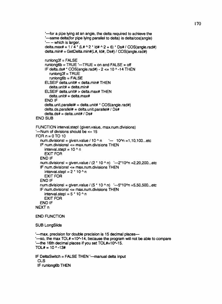
'--for a pipe lying at an angle, the delta required to achieve the '-same delta(for pipe lying parallel to delta) is delta/cos(angle) '- - which is larger. delta.max# = 1 / 4 (L# A 2 ' Id# A 2 + 6) ' Ds# I COS(angle.rad#) delta.min# = GetDelta.min#(L#, Id#, Ds#) I CQS(angle.rad#)
runlong3f = FALSE runlong6b = TRUE '-TRUE = on and FALSE = off IF delta.ds# ' COS(angle.rad#) - 2 <= 1 0 A -1 4 THEN
runlong3f = TRUE runlong6b = FALSE
ELSEIF delta.unit# < delta.min# THEN deIta.unit# = delta.min#
ELSEIF delta.unit# > delta.max# THEN delta-unit# = delta.max#
END IF delta.unit.parallel# = delta.unit# COS(angle.rad#) delta.ds.parallel# = delta.unit.parallel# / Ds# delta.ds# = delta.unit# / Ds#
END SUB
FUNCTION interva1.stepl (given.value, rnax.num.divisions) '-Num of divisions should be <= 15 FORn=OTO 10
num.divisionsl = given-value / 10 A n '- 1091 =1 '1 0.1 00 ... etc IF nurn.divisionsl c= max.num.divisions THEN
interva1,stepl = 10 A n EXIT FOR
END IF num.divisionsl = given-value / (2 ' 10 A n) '-2*109I =2,20,200 ... etc IF num.divisions! <= max.num.divisions THEN
interval.step! = 2 ' 10 A n EXIT FOR
END IF num.divisions1 = given-value 1 (5 " 10 A n) '--5"109I =5,50,50O..-etc IF num-divisionsi <= max.num-divisions THEN
interval.stepl = 5 ' 10 A n B I T FOR
END IF NEXTn
END FUNCTION
SUB Longslide
'--max. precision for double precision is 15 decimal places- '--so, the rnax TOL# =1W14, because the program wilt not be able to compare '-the 16th decimal places if you set TOL#=1 W15. TOL# = 10 A-13#
IF DehaSwitch = FALSE THEN '--manual delta input CLS IF runlong6b THEN
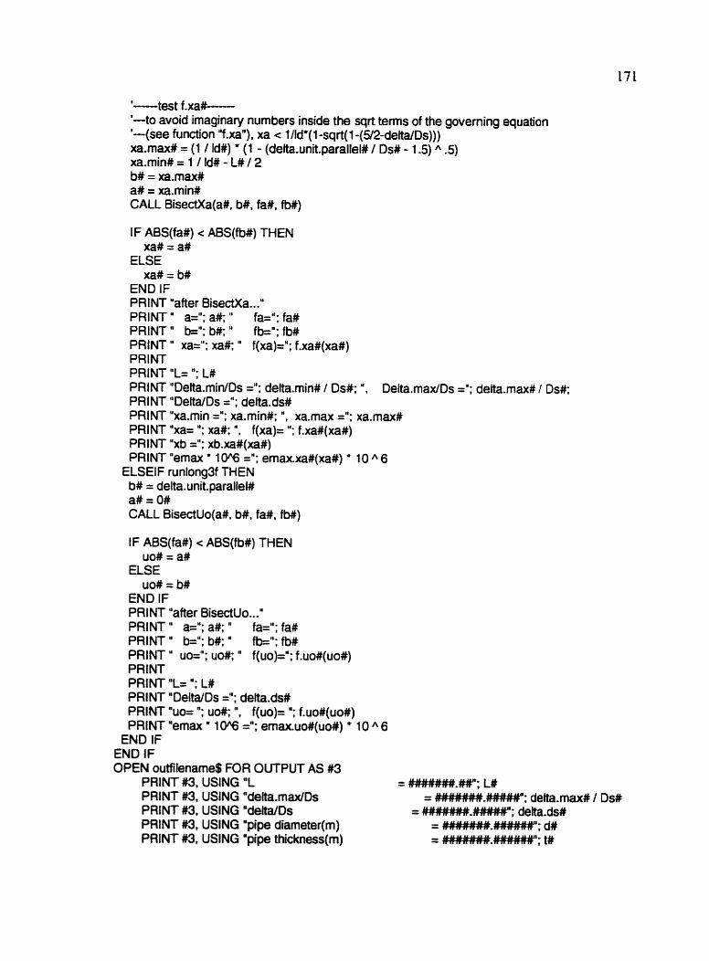
'----test f.xa#--- '-to avoid imaginary numbers inside the sqrt terms of the governing equation '--(see function "f.xan), xa < Illd'(1 -sqrt(l-(32-deltdDs))) xa.max# = (1 I Id#) ' (1 - (deta.unit.parallel# 1 Ds# - 1.5) A .5) xa.min# = 1 I Id# - L# / 2 b# = xa,max# a# = xa,min# CALL BisectXa(a#, b#, fa#, W)
IF ABS(fa#) < ABS(fb#) THEN xa# = a#
ELSE xa# = b#
END IF PRl NT "after BisectXa.. ." PRINT " a="; a#; " fa=": fa# PRINT " b="; b#; " fb="; fb# PRINT" xa="; xa#; " f(xa)="; f.xa#(xa#) PRlNT PRlNT "L= "; L# PRINT "Delta.min/Ds ="; delta.min# 1 Ds#; ", Delta.max/Ds ="; delta.max# I Ds#; PRlNT "Delta/Ds ="; delta.ds# PRINT "xa.min ="; xa.min#; ", xa.max =": xa.max# PRINT "xa= "; xa#; ", f(xa)= "; f.xa#(xa#) PRlNT "xb ="; xb.xa#(xa#) PRlNT "emax 1 O"6 =I*; emax.xa#(xa#) ' 10 A 6
ELSEIF runlong3f THEN b# = delta.unit.parallel# a# = 0# CALL BisectUo(a#, b#, fa#, fb#)
IF ABS(fa#) c ABS(fb#) THEN UO# = a#
ELSE uo# = b#
END IF PRf NT "after BisectUo ..." PRINT " a="; a#; " fa="; fa# PRINT " b="; b#; " fb="; fb# P R I M " uo="; uo#; " f(uo)="; f.uo#(uo#) PRlNT PR1NT "L= ": L# PRlNT "DeWDs ="; delta.ds# PRlNT "uo= "; uo#; ", f(uo)= "; f.uo#(uo#) P R I M "ernax * 1 0% ="; emax.uo#(uo#) * 10 A 6 END IF
END IF OPEN outfilename$ FOR OUTPUT AS #3
PRINT #3, USING "L = #######.###"; L# PRINT #3, USING "delta.max/Ds = #######-#####"; delta.max# / Ds# PRINT #3, USING "delta/Ds = #######.#####"; delta.ds# PRINT #3, USING "pipe diameter(m) = ###I###.######*; d# PRINT #3, USING "pipe thickness(m) = -.#####ii"; t#

PRINT #3, USING "pipe modulus of elasticity(Pa/m) = # # # k , , W a ; E# PRINT #3, USING "depth to center of pipe(m) = #######.##"; H PRINT #3, USING "soil cohesion(NlmA2) = ######,.##"; coh# PRINT #3, USING "soil density(N/mA3) = #####,.##"; gamma# PRlNT #3, USlNG "soil internal frictional angle(degrees) = #######.##"; phi.deg# PRINT #3, USING "limit elastic displacement of soil(Ds (m)) = #######.######"; Ds# PA1 NT #3, USlNG "angle between Landslide and pipe orientation(deg) = W.##"; ang le.deg# PRlNT #3, *xa.rnin =": xa.min#; " xa.max ="; xa.max# PRlNT #3, "xa= "; xa#; ", f(xa)= "; f.xa#(b#) PRlNT #3, "xb ="; xb.xa#(xa#) PRlNT #3, "emax ' 10% ="; emax.xa#(xa#) ' 10 A 6
CLOSE #3 IF Deltaswitch = TRUE THEN '-auto delta input
CLS OPEN outfilename$ FOR OUTPUT AS #3 '---to clear content of file for new CLOSE #3 '--storage. OPEN outfilename$ FOR APPEND AS #3
PRINT #3, USING "L = #######.##"; t# PRINT #3, USING "pipe diameter(m) = #######,######I; d# PRINT #3, USING "pipe thickness(rn) = #######. ######" ; t# PRINT #3, USING "pipe modulus of elasticity(Pa/m) = ###,,#W; E# PRINT #3, USING "depth to center of pipe(m) = #######.##": H PRINT #3, USING "soil cohesion(N/mA2) = ######,.##": coh# PRINT #3, USING "soil density(NImA3) = ######,.##I1; gamma# PRlNT #3. USlNG "soil internal frictional angle(degrees) = #######.##: phi.deg#
PRlNT #3, USING "limit elastic displacement of soil(Ds (m)) = ########.######"; Ds# PRlNT #3. USING "angle between landslide and pipe orientation(deg) = ##.##"; angle.deg# PRlNT #3, PRlNT #3, " delta/Ds Max pipe strain*lWM
'-0 <delta c 2Ds=2*0.008 FOR n# = 0 TO (2 Ds#) I COS(angle.rad#) STEP ((Ds# / 4) / COS(angle.rad#))
delta.ds# = n# / Ds# CALL initualues b# = delta.unit.parallel# a# = 0# CALL BisectUo(a#, b#, fa#, fb#) IF ABS(fa#) c ABS(fb#) THEN
uo# = a# ELSE
uo# = b# END fF LOCATE 20.1 PRINT " deltdDs Max pipe strain'l 0%" PRINT USING "#####.#####I ###HI#.#####"; delta.ds#; emax.uo#(uo#) ' 10 A 6 PRINT #3, USlNG "#####.##### #####.#####"; delta.ds#; emuuo#(uo#) ' 10 A 6
NEXT n# detta.ds.min.int.md.dn% = INT(delta-min# / Ds#) delta.ds.max.int.rnd.dn% = INT(delta.rnax# / Ds#) n.end% = detta.ds.max.int.md.dn% - (delta.ds.min.int.rnd-dn%) + 2 Speedup-Fhg = No '--delta.min c delta < delta.max
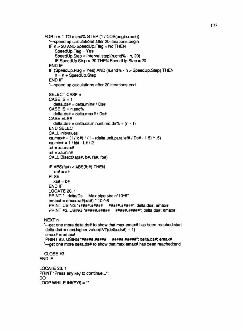
FOR n = 1 TO n.end% STEP (1 / COS(angle.rad#)) '-speed up calculations after 20 iteratiowbegin IF n > 20 AND Speedup-Flag = No THEN
SpeedUp.Flag = Yes Speedup-Step = interval.stepl(n.end% - n, 20) IF SpeedUp.Step > 20 THEN Speedup-Step = 20
END IF IF (SpeedUp.Flag = Yes) AND (n.end% - n > Speedup-Step) THEN
n = n t Speedup-Step END IF '-speed up calculations after 20 iterations:end
SELECT CASE n CASE IS = t
delta-ds# = delta,min# / Ds# CASE IS = n.end0/o
delta.ds# = delta.max# 1 Ds# CASE ELSE
delta.ds# = delta.ds.min.int,rnd.dnO/~ + (n - 1) END SELECT CALL initvalues xa.max# = (1 I Id#) ' (1 - (delta.unit.parallel# / Ds# - 1.5) A -5) xa.min# = 1 / Id# - L# 1 2 b# = xa.max# a# = xa.min# CALL BisectXa(a#, b#, fa#, fb#)
IF ABS(fa#) < ABS(fb#) THEN xa# = a#
ELSE xa# = b#
END IF LOCATE 20, t PRINT " delta/Ds Max pipe strainml 0%" emax# = emax.xa#(xa#) 1 0 A 6 PRINTUSING "#####.##### #####,#####";delta.ds#;emax# PRINT#3, USING "#####.##### #####.#####";delta.ds#;emax#
NEXT n '-get one more delta.ds# to show that max emax# has been reached:start delta.ds# = next.higher.value(lNT(delta.ds#) + I ) emax# = ernax# PRlNT#3, USING"#####.##### #####.#####";delta.ds#;emax#
'-get one more defta.ds# to show that max emax# has been reached:end
CLOSE #3 END IF
LOCATE 23,1 PRIM "Press any key to continue..."; 130 LOOP WHILE INKEY$ = ""
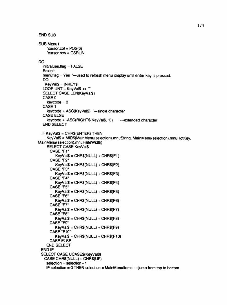
END SUB
SUB Menut 'cursor.col = POS(0) 'cursor.row = CSRLIN
DO initvalues.flag = FALSE Boxlnit menuflag = Yes '-used to refresh menu display until enter key is pressed. DO KeyVal$ = INKEY$
LOOP UNTIL KeyVal$ o "" SELECT CASE LEN(KeyVal$) CASE 0
keycode = 0 CASE 1
keycode = ASC(KeyVal$) '-single character CASE ELSE
keycode = -ASC(RIG HT$(KeyVal$, 1 )) '--extended character END SELECT
IF KeyVal$ = CHR$(ENTER) THEN KeyVal$ = MID$(MainMenu(selection).mnuString, MainMenu(selection).rnnuHotKey,
MainMenu(selection).mnuHiliteWidth) SELECT CASE KeyVal$
CASE "Ff" KeyVal$ = CHR$(NULL) + CHR$(F1)
CASE "F2" KeyVal$ = CHR$(NULL) + CHR${F2)
CASE "F3" KeyVal$ = CHR$(NULL) + CHR$(F3)
CASE "F4" KeyVal$ = CHR$(NULL) + CHR$(F4)
CASE "F5" KeyVal$ = CHR$(NULL) + CHR$(FS)
CASE "F6" KeyVal$ = CHR$(NULL) + CHR$(F6)
CASE "F7" KeyVal$ = CHR$(NULL) + CHR$(F7)
CASE "F8 KeyVal$ = CHR$(NULL) + CHR$(FB)
CASE "F9" KeyVal$ = CHR$(NULL) + CHR$(FS)
CASE "Ft 0" KeyVal$ = CHR$(NULL) + CHR$(F10)
CASE ELSE END SELECT
END IF SELECT CASE UCASE$(KeyVal$)
CASE CHR$(NULL) + CHR$(UP) selection = selection - 1 IF selection = 0 THEN selection = MainMenulterns '-jump from top to bottom
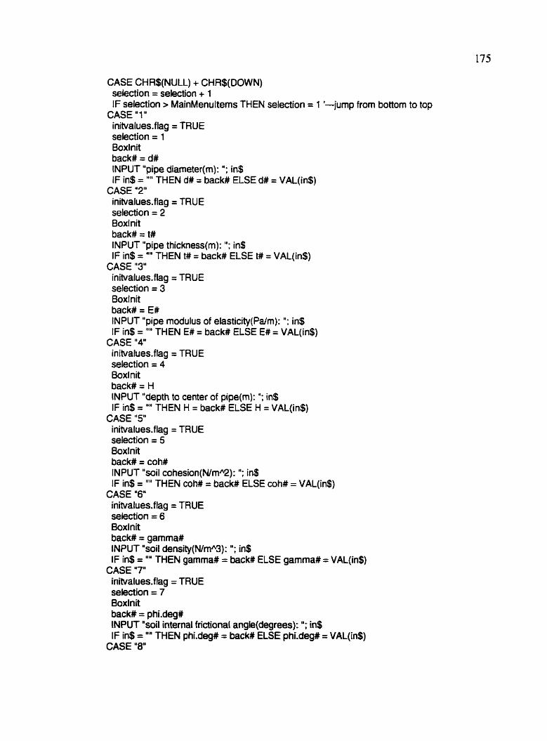
CASE CHR$(NULL) + CHR$(DOWN) selection = selection + 1 IF selection > MainMenultems THEN selection = 1 '-jump from bottom to top
CASE "Iu initvaluesflag = TRUE selection = 1 Boxlnit back# = d# INPUT "pipe diameter(rn): "; in$ IF in$ = "" THEN d# = back# ELSE d# = VAL(in$)
CASE "2" initvalues.flag = TRUE selection = 2 Box1 nit back# = t# INPUT "pipe thickness(m): "; in$ IF in$ = "" THEN t# = back# ELSE t# = VAL(in$)
CASE "3" initvalues-flag = TRUE selection = 3 Boxfnit back# = E# INPUT "pipe modulus of elasticity(Pa/m): "; in$ IF in$ = "" THEN E# = back# ELSE E# = VAL(in$)
CASE "4" initvalues.flag = TRUE selection = 4 Boxlnit back# = H INPUT "depth to center of pipe(m): "; in$ IF in$ = "I' THEN H = back# ELSE H = VAL(in$)
CASE "5" initvalues.flag = TRUE selection = 5 Boxfnit back# = coh# INPUT "soil cohesion(N/mA2): "; in$ IF in$ = "" THEN coh# = back# ELSE coh# = VAL(in$)
CASE "6" initvalues.flag = TRUE selection = 6 Boxlnit back# = gamma# INPUT "soil density(N/mA3): "; in$ IF in$ = "" THEN gamma# = backlt ELSE gamma# = VAL(in$)
CASE "7" initvalues.flag = TRUE selection = 7 Boxlnit back# = phi.deg# INPUT "soil internal frictional angle(degrees): "; in$ IF in$ = "" THEN phi.deg# = back# ELSE phi.deg# = VAL(in$)
CASE "8*
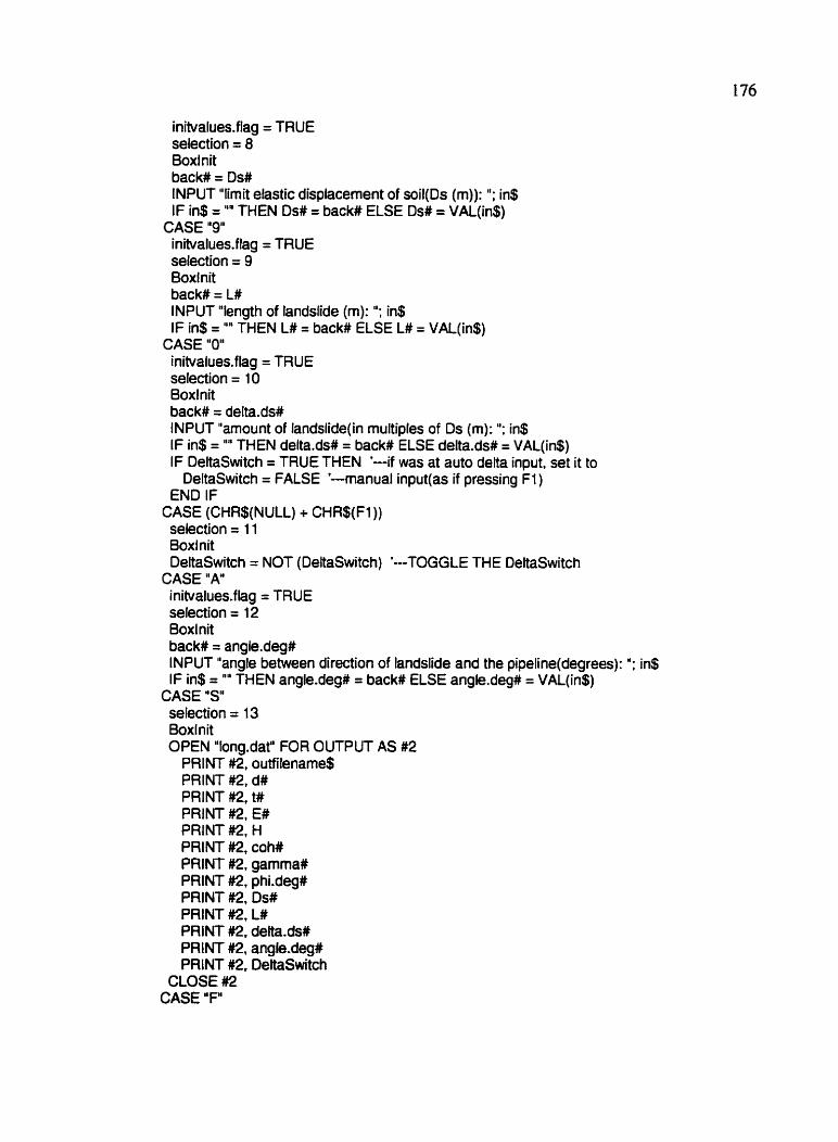
initvalues.flag = TRUE selection = 8 Box1 nit back# = Ds# INPUT "limit elastic displacement of soil(Ds (m)): "; in$ IF in$ = "" THEN Ds# = back# ELSE Ds# = VAL(in$)
CASE "9" inih/alues.flag = TRUE selection = 9 Boxlnit back# = L# INPUT "length of landslide (m): "; in$ IF in$ = "" THEN L# = back# ELSE L# = VAL(in$)
CASE "0" initvalues.flag = TRUE selection = 10 60x1 nit back# = delta.ds# INPUT "amount of landslide(in multiples of Ds (m): "; in$ IF in$ = "" THEN delta.ds# = back# ELSE delta.ds# = VAL(in$) IF DeltaSwitch = TRUE THEN '-if was at auto delta input, set it to
Deltaswitch = FALSE '-manual input(as if pressing F1) END IF
CASE (CHR$(NULL) + CHR$(Fl)) selection = 11 Boxlnit DeltaSwitch = NOT (DeltaSwitch) '--TOGGLE THE DeltaSwitch
CASE " A initvalues.flag = TRUE selection = 12 Boxlnit back# = angle.deg# INPUT "angle between direction of landslide and the pipeline(degrees): "; in$ IF in$ = "" THEN angle.deg# = back# ELSE angle.deg# = VAL(in$)
CASE "S" selection = 13 Boxlnit OPEN "Iong.datu FOR OUTPUT AS #2
PRINT #2, outfilename$ PRINT #2, d# PRINT #2, t# PRINT #2, E# PRtNT #2, H PRINT #2, coh# PRINT #2, gamma# PRINT #2, phi.deg# PRINT #2, Ds# PRINT #2, L# PRINT #2, delta.ds# PRINT #2, angle.deg# PRINT #2, DeltaSwitch
CLOSE #2 CASE "F"
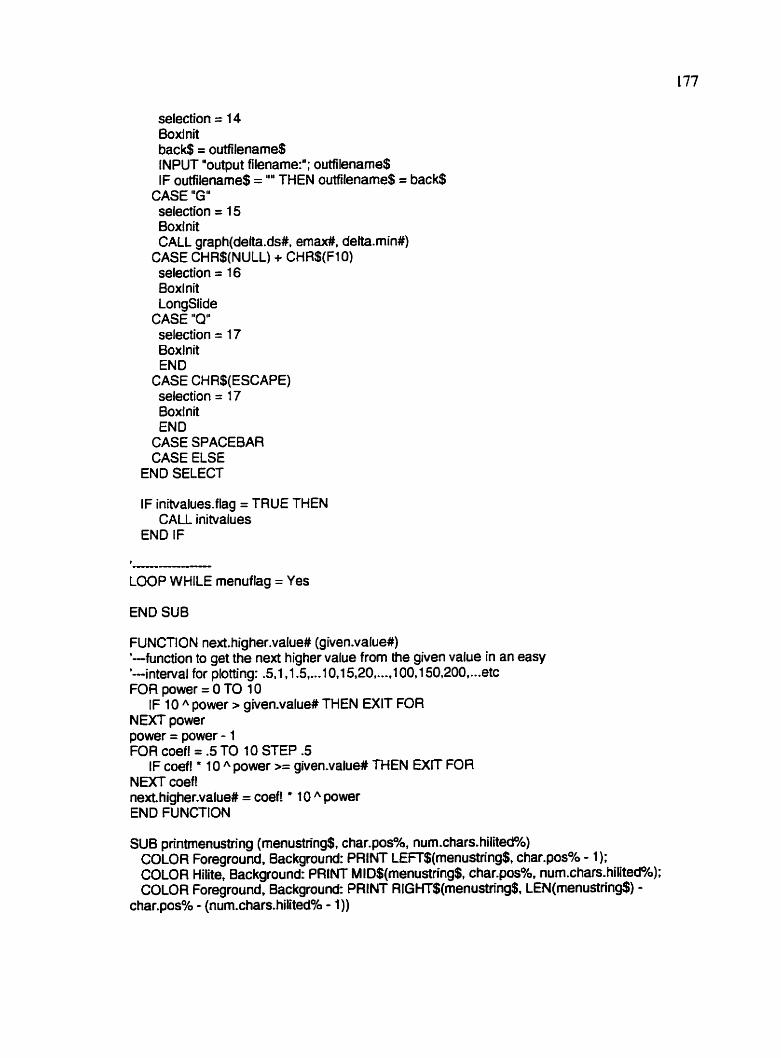
selection = 14 Box1 nit back$ = outfilename$ INPUT "output filename:'; outfilename$ IF outfilename$ = "" THEN outfilename$ = back$
CASE "G" selection = 15 Boxlnit CALL graph(delta.ds#. ernax#, detta.min#)
CASE CHR$(NULL) + CHR$(FIO) selection = 16 Boxlnit Longslide
CASE "Q" selection = 17 Boxlnit END
CASE CHR$(ESCAPE) selection = 17 Boxlnit END
CASE SPACEBAR CASE ELSE
END SELECT
IF initvalues.flag = TRUE THEN CALL initvalues
END IF
LOOP WHILE menuflag = Yes
END SUB
FUNCTION next.hig her.value# (g iven.value#) '--function to get the next higher value from h e given value in an easy '--interval for plotting: .5.1,1.5,...10.15.20 ,..., 100,150,200 .... etc FOR power = 0 TO 10
IF 10 A power > given.value# THEN WIT FOR NEXT power power = power - 1 FOR coef! = .5 TO 10 STEP .5
IF coefl ' 10 A power >= given.value# THEN EXIT FOR NEXT coefl next higher-value# = coef! * 1 0 A power END FUNCTION
SUB printmenustring (menustring$. char.pos%, num.chars.hilited%) COLOR Foreground, Background: PRINT LEFT$(menustring$, char.pos% - 1): COLOR Hilite, Background: P R I M M ID$(menustring$, char.pos%. num.cha~.hilited%): COLOR Foreground, Background: PRINT RIGfiT$(menumng$. LEN(menustring$) )-
char.posYo - (num.chars.hilited% - I))
END SUB
SUB ReadlnputFile PRINT "opening file long.dat" OPEN "long.datb' FOR INPUT AS #1
INPUT #I, ouffilename$ INPUT #1, d# INPUT #I, t# INPUT #I, E# INPUT #I, H INPUT #1, coh# INPUT #I, gamma# INPUT #I, phi.deg# INPUT #I, Ds# INPUT #1, L# INPUT #1, delta.ds# INPUT #I, angle.deg# '-angle between direction of landslide and pipeline(deg) INPUT #I, Deltaswitch '-used to switch between Manual calculation(-1) or Auto
calculation(1)
CLOSE #I
END SUB
FUNCTION xb.xa# (xa#) '-For delta >2Ds P - - SHARED Id#, Ds#, deita.unit.parallel#, L# p l # = 2 ' xa# A 2 - 4 ' xa# I Id# + 1 1 Id# A 2 (5 - 2 * delta.unit.paraliel# I Ds#) IF p l # COTHEN
pl#=O END IF xb# = 1 I Id# - xa# - (pl#) A .5 xb.xa# = xb#
END FUNCTION


