Modeling genome-wide replication kinetics revealsa mechanism for regulation of replication timing

Scott Cheng-Hsin Yang1,*, Nicholas Rhind2 and John Bechhoefer1

1 Department of Physics, Simon Fraser University, Burnaby, British Columbia, Canada and 2 Department of Biochemistry and Molecular Pharmacology,University of Massachusetts Medical School, Worcester, MA, USA* Corresponding author. Department of Physics, Simon Fraser University, 8888 University Drive, Burnaby, British Columbia, Canada V5A 1S6.Tel.: þ 1 778 782 5924; Fax: þ 1 778 782 3592; E-mail: scotty@sfu.ca

Received 25.11.09; accepted 16.7.10

Microarrays are powerful tools to probe genome-wide replication kinetics. The rich data sets thatresult contain more information than has been extracted by current methods of analysis. In thispaper, we present an analytical model that incorporates probabilistic initiation of origins andpassive replication. Using the model, we performed least-squares fits to a set of recently publishedtime course microarray data on Saccharomyces cerevisiae. We extracted the distribution of firingtimes for each origin and found that the later an origin fires on average, the greater the variation infiring times. To explain this trend, we propose a model where earlier-firing origins have moreinitiator complexes loaded and a more accessible chromatin environment. The model demonstrateshow initiation can be stochastic and yet occur at defined times during S phase, without an explicittiming program. Furthermore, we hypothesize that the initiators in this model correspond to loadedminichromosome maintenance complexes. This model is the first to suggest a detailed, testable,biochemically plausible mechanism for the regulation of replication timing in eukaryotes.Molecular Systems Biology 6: 404; published online 24 August 2010; doi:10.1038/msb.2010.61Subject Categories: simulation and data analysis; cell cycleKeywords: DNA replication program; genome-wide analysis; microarray data; replication-originefficiency; stochastic modeling

This is an open-access article distributed under the terms of the Creative Commons AttributionNoncommercial No Derivative Works 3.0 Unported License, which permits distribution and reproductioninanymedium,providedtheoriginalauthorandsourcearecredited.This licensedoesnotpermitcommercialexploitation or the creation of derivative works without specific permission.

Introduction

The kinetics of DNA replication in eukaryotic cells are carefullycontrolled, with some parts of the genome replicating early andothers replicating later. Patterns of replication timing correlatewith gene expression, chromatin structure, and subnuclearlocalization, suggesting that replication timing may have animportant function organizing the nucleus and regulating itsfunction (Goren and Cedar, 2003). The timing of DNA replicationis regulated largely by the timing of replication-origin activation.Although the biochemical steps of origin firing are increasinglywell understood, the regulation that leads to defined patterns ofreplication timing is still a mystery (Sclafani and Holzen, 2007).

Over the past 15 years, the development of two newtechnologies has led to significant progress in the descriptionof DNA replication kinetics. The first development, molecularcombing, is a single-molecule technique in which one labelsreplicated and unreplicated DNA and then stretches out thefibers to detect replication patterns (Herrick and Bensimon,1999; Herrick et al, 2000). The technique yields ‘snapshots’ ofthe replication state of individual fragments of chromosomes.

Advantages include high spatial resolution (E2 kb) and datafrom individual DNA molecules, rather than ensembleaverages (Patel et al, 2006; Czajkowsky et al, 2008). The maindisadvantage is that the size of combed fragments (100 kb to1 Mb) is small relative to the typical size of full chromosomes,which limits the information available about patterns ofreplication timing on larger scales and complicates analysis(Zhang and Bechhoefer, 2006).

The second development applies microarrays to probeensemble averages of replication extent across the genome(Raghuraman et al, 2001; Yabuki et al, 2002; Feng et al, 2006;Heichinger et al, 2006). Compared with molecular combing,the main disadvantages of microarrays are the loss ofinformation about cell-to-cell variability and the need forcomplicated post-signal processing. On the other hand, themain advantages are the experiment’s high throughput andcomplete coverage of the genome that result in bothtemporally and spatially resolved data. The availability ofhigh-resolution, genome-wide data allows one to measure andmodel variations in firing time and origin efficiency at a level ofdetail that exceeds that provided by past studies.

Molecular Systems Biology 6; Article number 404; doi:10.1038/msb.2010.61Citation: Molecular Systems Biology 6:404& 2010 EMBO and Macmillan Publishers Limited All rights reserved 1744-4292/10www.molecularsystemsbiology.com

& 2010 EMBO and Macmillan Publishers Limited Molecular Systems Biology 2010 1

The common feature of both technologies is their ability togenerate large data sets for the analysis of replication. Withlarge data sets comes the potential to construct a much moredetailed picture of how replication occurs and is regulated(Hyrien and Goldar, 2010). For molecular-combing experi-ments, previous work has shown that quantitative informationsuch as replication-origin firing rates and replication-forkvelocities can be extracted (Yang et al, 2009). Such informationhas led to an appreciation of the function of stochastic effectsin initiation (Herrick and Bensimon, 1999), to a greaterunderstanding of the ‘random-completion problem’ for em-bryonic replication (Yang and Bechhoefer, 2008), to modelshighlighting searching and binding kinetics in initiation timing(Gauthier and Bechhoefer, 2009), and to suggestions thatinitiation patterns may be universal across species (Goldaret al, 2009).

A prevailing picture of eukaryotic replication is that originsare positioned at defined sites and initiated at preprogrammedtimes (Donaldson, 2005). In Saccharomyces cerevisiae, originpositions are defined, in part, by 11–17 base pair autonomousreplicating sequence (ARS) consensus motifs, which bind theorigin recognition complex (ORC) (Sclafani and Holzen, 2007).The timing of origin initiation is more controversial: althoughmicroarray experiments have generally been interpreted basedon the assumption of a deterministic temporal program(Raghuraman et al, 2001), recent molecular-combing experi-ments suggest that origin initiation is stochastic (Patel et al,2006; Czajkowsky et al, 2008). A more subtle issue is that theconsequences of the spatiotemporal connection betweenorigin initiation and fork progression in multiple-originsystems are often not taken into account. The replicationextent of an origin site is sometimes implicitly assumed to besolely from the origin itself (Eshaghi et al, 2007), even thoughthe locus can also be replicated by nearby origins. Our thesis isthat a more rigorous analysis of microarray replication databased on the same type of stochastic models used tounderstand combing experiments can yield greater insightinto the replication process and contribute to forming a moreaccurate picture of the replication program. We argue that bothmicroarray and combing experiments are compatible withstochastic origin initiation and that the apparent disagreementis resolved after performing a more sophisticated analysis ofthe microarray data.

The analytical model of DNA replication we present extendsprevious work that focused on replication in Xenopus laevis(Jun et al, 2005). The present version includes defined originposition, variable-elongation rates, and probabilistic initia-tion. Our model is sufficiently general to describe bothdeterministic and stochastic replication-kinetics scenariosand assumes only that initiation events are not correlated. Toshow the kinds of questions our model can address, we fit themodel to a recent set of time course microarray data onS. cerevisiae (McCune et al, 2008) and extracted originpositions, the firing-time distribution for each origin, originefficiencies, and a global fork velocity. We found that the trendof origin firing embedded in the data is incompatible with anaive deterministic model. Based on this finding, we propose astochastic-initiator model where temporal patterns in replica-tion can arise in the absence of an explicit mechanism forcontrolling the timing of origin initiation. The details of this

model support a specific molecular mechanism for theregulation of replication timing, in which the number ofminichromosome maintenance (MCM) complexes loaded atan origin regulates, in part, the origin firing time.

More generally, the model can be used to reconstruct thecomplete spatiotemporal program quantitatively, as reflectedby its ability to fit genome-wide microarray data. It is lessbiased than current empirical models, as it accounts for theeffects of passive replication (Raghuraman et al, 2001; Eshaghiet al, 2007). As it is analytic, it is also faster than simulation-based models (Lygeros et al, 2008; Blow and Ge, 2009; deMoura et al, 2010). For these reasons, we believe the modelintroduced here to be a powerful tool for analyzing spatio-temporally resolved DNA replication data. Moreover, theprobabilistic nature of the model allows analysis of a broadrange of dynamics, from deterministic to completely randomtiming, and thus offers new ways to look at replication. Inparticular, we show that reproducible replication patterns donot necessarily indicate a temporal program where theinitiation involves time-measuring mechanisms; rather, tem-poral order can emerge as a consequence of stochasticinitiations.

Results

The time and precision of origin firing arecorrelated

To investigate the regulation of replication kinetics, we havedeveloped a general mathematical model of replication andused it to analyze the recent budding yeast replication timecourse data of McCune et al (2008). Such microarrayexperiments yield the fraction of cells in a population thathave a specific site replicated after a given time in S phase (seeSupplementary Material Section A for more experimentaldetails). The positions of origins are determined by peaks inthe graphs of replication fraction, as an origin site is replicatedbefore its neighboring sites (Figure 1). Following standardanalytical methods, we define a time trep as the time by whichhalf of the cells show replication of the origin locus (Raghura-man et al, 2001). Implicit in this picture are the assumptionsthat the variation of firing times of an origin, twidth, is small andthat trep is independent of twidth.

A simple analysis of the data suggests a more complexpicture. We first analyzed the data by fitting a sigmoid throughthe time course associated with each origin (Figure 1). Eachsigmoid yields a trep and twidth (defined as the time for theorigin locus to go from 25 to 75% replicated). In contrast to thedeterministic timing scenario that assumes twidth is much lessthan trep, the extracted twidth approximately equals trep

(Figure 1C). The apparent variability in origin timings suggeststhat stochasticity is important to an accurate description of thereplication kinetics. Moreover, in a model where the timing oforigin firing is regulated by external triggers (Goren and Cedar,2003), one expects no correlation between trep and twidth. Inother words, the twidth points would scatter about a horizontalline in Figure 1C, implying that variations in twidth areindependent of trep. Instead, we see a strong correlationbetween twidth and trep, suggesting the two are mechanisticallyrelated.

Genome-wide modeling of replication dataSC-H Yang et al

2 Molecular Systems Biology 2010 & 2010 EMBO and Macmillan Publishers Limited

An analytical model for replication kinetics

The discrepancies between a naive picture of origin firing controland the data motivate a more detailed approach. We havedeveloped an analytical model that can generate genome-widetime course data sets comparable to those from microarray-basedreplication experiments (see Materials and methods). The modeltakes into account probabilistic initiation and the effects ofpassive replication. Its parameters can be separated into a ‘local’group that describes the properties of each origin and a ‘genome-wide’ group that describes quantities that are roughly constantacross the genome. Limitations of the model and the microarraydata used are discussed in the Discussion.

We first introduce the ‘sigmoid model’ (SM), which describeseach origin with three local parameters: the origin position, themedian time of the firing-time distribution (t1/2), and the width ofthe firing-time distribution (tw, defined as t0.75�t0.25). The lasttwo parameters define a sigmoidal curve for the cumulativefiring-time distribution. These two parameters t1/2 and tw differfrom trep and twidth. The former describes the firing time of anorigin, whereas the latter describes the replication time of anorigin site, which is replicated by both the origin on the site andnearby origins. The fit to chromosome XI is shown in Figure 2 todemonstrate that the model captures the replication process well.Fits to all chromosomes can be found in Supplementary Figure 1.A detailed statistical analysis of the fits is presented inSupplementary Material Section B.

Extracted origins and fork velocity

The initial list of origins consisted of 732 positions from theOriDB database that had previously been identified using a

variety of methods (Nieduszynski et al, 2007). The results donot depend sensitively on this initial list, as we allowed thepositions to vary in the fit. After eliminating origins accordingto the criteria described in Materials and methods, the SM gave342 origins (origin parameters tabulated in SupplementaryTable I). Out of the 342 we identify, 236 colocalize with the 275origins identified previously using a similar data set (Alvinoet al, 2007). The remaining 106 origins were not previouslyrecognized by Alvino et al, mostly because they are notassociated with apparent peaks in the microarray data. Wefound that 75% of the 106 colocalize (within 5 kb) with originsin the OriDB database (Nieduszynski et al, 2007).

The SM can be modified to include variable-fork ratesacross the genome (see Supplementary Material Section C).Fitting the data with a model that uses spatially varyingfork velocities, we found that both the constant-velocity SMand variable-velocity SM fit the data well (SupplementaryFigures 6 and 7). Both capture 498% of the variance in thedata (see Supplementary Material Section C). This suggeststhat a spatially constant velocity is plausible. The genome-wide fork velocity we extracted from the SM is 1.9 kb/min. Ourstatistical analysis of the fits suggests an error of 0.2 kb/min onv (see Supplementary Material Section B). Consistent with thisconclusion, recent work using ChIP-chip to monitor themovement of GINS, an integral member of replication forks,shows a fork progression rate of about 1.6±0.3 kb/min thatdoes not vary significantly across the genome (Sekedat et al,2010). Our conclusion contrasts with that of Raghuraman et al(2001), where variations in slope from peak to trough wereinterpreted as fork-velocity variations. In our model, thesevariations can be mostly accounted for by different levels ofpassive replication from origins with different distributions of

C50

40

30

20

10

0

50403020100

trep (min)

t wid

th (m

in)

B

100

50

0

Rep

licat

ion

frac

tion

(%)

200150100500

Chromosome position (kb)

A

100

50

0

Rep

licat

ion

frac

tion

(%)

6040200

Time (min)

twidth

trep

Figure 1 (A) Smoothed time course microarray data for chromosome I. Triangles are origins identified in Alvino et al (2007). The arrow indicates the origin analyzed in(B). (B) Replication fraction of the indicated origin versus time. Fitting the data with Equation (1) gives the median time trep and the 25–75% time width twidth. (C) Timewidths versus median times for all 275 origin loci identified in Alvino et al (2007).

Genome-wide modeling of replication dataSC-H Yang et al

& 2010 EMBO and Macmillan Publishers Limited Molecular Systems Biology 2010 3

firing times, including the above-mentioned origins that lackdistinct peaks.

The SM recapitulates observed firing-timedistributions and initiation rates

The least-understood aspect of the replication process is itstemporal program (Sclafani and Holzen, 2007). One reason isthat there has been no direct way of visualizing both the spatialand temporal aspects of replication at high resolution. Anotherreason is that the implications of temporal stochasticity ininitiations have often been neglected. We extracted the firing-time distributions of the 342 origins identified in the SM(Figure 3A). The widths are comparable to the length of Sphase, confirming that stochastic effects have an importantfunction. The kinetic curves of the origins extracted from themodel also show that tw increases with t1/2 (Figure 3B and D;compare with Figure 1). Further, we show that four repre-sentative, previously studied origins (ARS413, ARS501,ARS606, and ARS1114.5) are typical origins that follow thisglobal t1/2–tw relationship (Figure 3).

The rate of initiation, defined as the number of initiationsper time per unreplicated length, is a crucial parameter inkinetics (see Materials and methods). It has been proposedthat an increasing rate of initiation later in S phase would leadto robust completion of replication, even if origin firing isstochastic (Hyrien et al, 2003). To investigate the initiation ratein the SM, we plotted initiation rates averaged over the genomeand over individual chromosomes (Figure 3C). Our resultsshow the initiation rate rising for most of S phase and thendeclining in late S phase. A similar pattern has been describedin a number of organisms (Goldar et al, 2009). However, the

genome-wide-averaged initiation rate we extracted does notdecay to zero before S phase ends as it did in the previousanalysis. In Goldar et al (2009), the use of trep rather than thefull distribution of firing times of an origin leads to anunderestimation of origin initiation at late times. Nonetheless,as the proposed universality of the initiation rate acrossspecies was for scaled initiation rates, that conclusion maywell survive reanalysis of the data with a stochastic model thatwould modify the extracted average rates and scalings.

Geometric effect from passive replication affectsvariability in origin efficiencies

Understanding origin efficiency is important because theseefficiencies determine the replication completion time and therobustness of the replication program (Lygeros et al, 2008;Blow and Ge, 2009). The efficiency of an origin is closelyrelated to its geometry—its location relative to other origins.Imagine two highly efficient origins placed near each other;only one of the two origins will fire in any given cell becausethe initiation of one origin will passively replicate the otherorigin. Placing an efficient origin next to an inefficient oneshould decrease the firing of each by different amounts. For anisolated origin, one expects that its efficiency would beunaffected by passive replication.

In our analysis, we distinguish between ‘efficiency,’ which istraditionally defined as the probability that an origin firesduring normal replication, taking into account passivereplication effects, and ‘potential efficiency.’ The latter termis defined to be the probability that an origin would haveinitiated before the end of S phase if there were no passivereplication (Rhind et al, 2010). We will occasionally use

100

80

60

40

20

0

Rep

licat

ion

frac

tion

(%)

0 200 400 600

Genome position (kb)

15

30

40

Figure 2 Chromosome-XI section of the genome-wide fits. Markers are data, solid lines are fits from SM, and dotted lines are fits from MIM. Upper row of solid trianglesat the bottom denote origin positions identified in Alvino et al (2007). In the middle row, open circles are estimated origin positions in the SM, whereas crosses are fromthe MIM. The lower row of triangles correspond to origins in the OriDB database (Nieduszynski et al, 2007). The three curves from bottom to top correspond to thereplication fraction f(x) at 15, 30, and 40 min after release from the cdc7-1 block. The data set covers the genome at E2 kb resolution.

Genome-wide modeling of replication dataSC-H Yang et al

4 Molecular Systems Biology 2010 & 2010 EMBO and Macmillan Publishers Limited

‘observed efficiency’ instead of just ‘efficiency’ to emphasizethe effect of passive replication. Experimentally, techniquesthat hinder fork progression to avoid passive replication havebeen applied to extract the potential efficiencies of origins(Heichinger et al, 2006). However, such approaches provideonly rough estimates of potential efficiency because they blockorigin firing in late S phase. Thus, to determine whether theobserved efficiency of origins is due primarily to their potentialefficiency or to their proximity to neighboring origins, weinvestigated the relationship between efficiency and potentialefficiency.

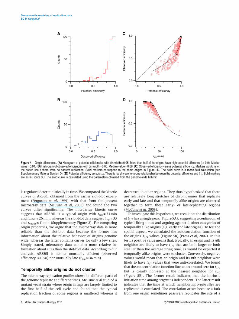
We used the extracted origin positions and firing-timedistributions to calculate both the observed efficiencies (viaEquation 11) and potential efficiencies of all identified origins(via evaluating Fi(t¼tend), the cumulative firing probabilitydistribution in our model, see Materials and methods). Here,tend is the length of S phase, and we estimate it to be 60 minfrom flow-cytometric determination of replication progress(see Supplementary Material Section A). We found that morethan half of the origins have high potential efficiency (40.9),but the observed efficiencies of origins vary much more

(compare Figure 4A and B). Furthermore, we found that therelation between observed efficiency and potential efficiencycan be approximately accounted for by a mean-field argument(see Supplementary Material Section D), where all neighbor-ing origins are replaced by an average neighbor that has thegenome-wide-averaged firing-time distribution (Figure 4C).Thus, the efficiency of origins in S. cerevisiae can largely beexplained by geometric effects because of neighboring origins.

Late-firing origins are less efficient

As seen in Figure 4D, later-firing origins have lower potentialefficiency. The monotonic decrease in efficiency with increas-ing t1/2 is a consequence of the tw-versus-t1/2 relationshipmentioned above. The larger tw associated with later-firingorigins imply that the chance for them to initiate within Sphase is less than that of earlier-firing origins.

A previous experiment reported that although the ARS501origin is late firing, its kinetics and efficiency resemble that ofan early-firing origin (Ferguson et al, 1991). The ARS501kinetics was used to support a scenario where origin activation

0.05

0.00

Initi

atio

n ra

te (

min

–1 kb

–1)

500

Time (min)

C

100

0

t w (

min

)

100500

t1/2 (min)

D

A 0.06

0.04

0.02

0.00

Firi

ng-t

ime

dist

ribut

ion

(min

–1)

500

Time (min)

606

413

501

1114.5

B 1.0

0.5

0.0

Cum

ulat

ive

firin

g-tim

e di

strib

utio

n

500

Time (min)

606

413

1114.5

501

Figure 3 (A) Firing-time distribution for the 342 origins extracted using the SM. Darker curves are representative distributions chosen to illustrate origins with differentvalues of t1/2. Numbers denote their ARS number in the OriDB database (Nieduszynski et al, 2007). Gray background corresponds to times not included in the data(to10 and t445 min); curves in these domains are extrapolated. The length of S phase is roughly 60 min. (B) Cumulative firing-time distributions for the 342 origins.Each trace is the kinetic curve that would be measured for the corresponding origin site if there were no neighboring origins. Darker curves correspond to darker curves in(A). The potential efficiencies of the origins are the curves’ values at t¼60 min. (C) Averaged initiation rates. The heavy dark curve is the genome-wide averaged rate,whereas the lighter curves are chromosome-averaged rates. (D) Trend of t1/2 versus tw. Markers are results from the SM. The curve is the result from the multiple-initiatormodel (MIM) using Fo(t)¼1/[1þ (76/t)3]. The values 76 and 3 are the resulting parameters of the genome-wide MIM fit. Solid square, triangle, inverted triangle, andcircle correspond to ARS413, 501, 606, and 1114.5, respectively.

Genome-wide modeling of replication dataSC-H Yang et al

& 2010 EMBO and Macmillan Publishers Limited Molecular Systems Biology 2010 5

is regulated deterministically in time. We compared the kineticcurves of ARS501 obtained from the earlier slot-blot experi-ment (Ferguson et al, 1991) with that from the presentmicroarray data (McCune et al, 2008) and found the twocurves differ significantly. The microarray kinetic curvesuggests that ARS501 is a typical origin with trepE33 minand twidthE26 min, whereas the slot-blot data suggest trepE33and twidthE11 min (Supplementary Figure 2). For comparingorigin properties, we argue that the microarray data is morereliable than the slot-blot data because the former hasinformation about the relative behavior of origins genomewide, whereas the latter contains curves for only a few sites.Simply stated, microarray data contains more relative in-formation about sites than the slot-blot data. According to ouranalysis, ARS501 is neither unusually efficient (observedefficiency E0.58) nor unusually late (t1/2E36 min).

Temporally alike origins do not cluster

The microarray replication profiles show that different parts ofthe genome replicate at different times. McCune et al studied amutant yeast strain where origin firings are largely limited tothe first half of the cell cycle and found that the typicalreplication fraction of some regions is unaltered whereas it

decreased in other regions. They thus hypothesized that thereare relatively long stretches of chromosomes that replicateearly and late and that temporally alike origins are clusteredtogether to form these early- or late-replicating regions(McCune et al, 2008).

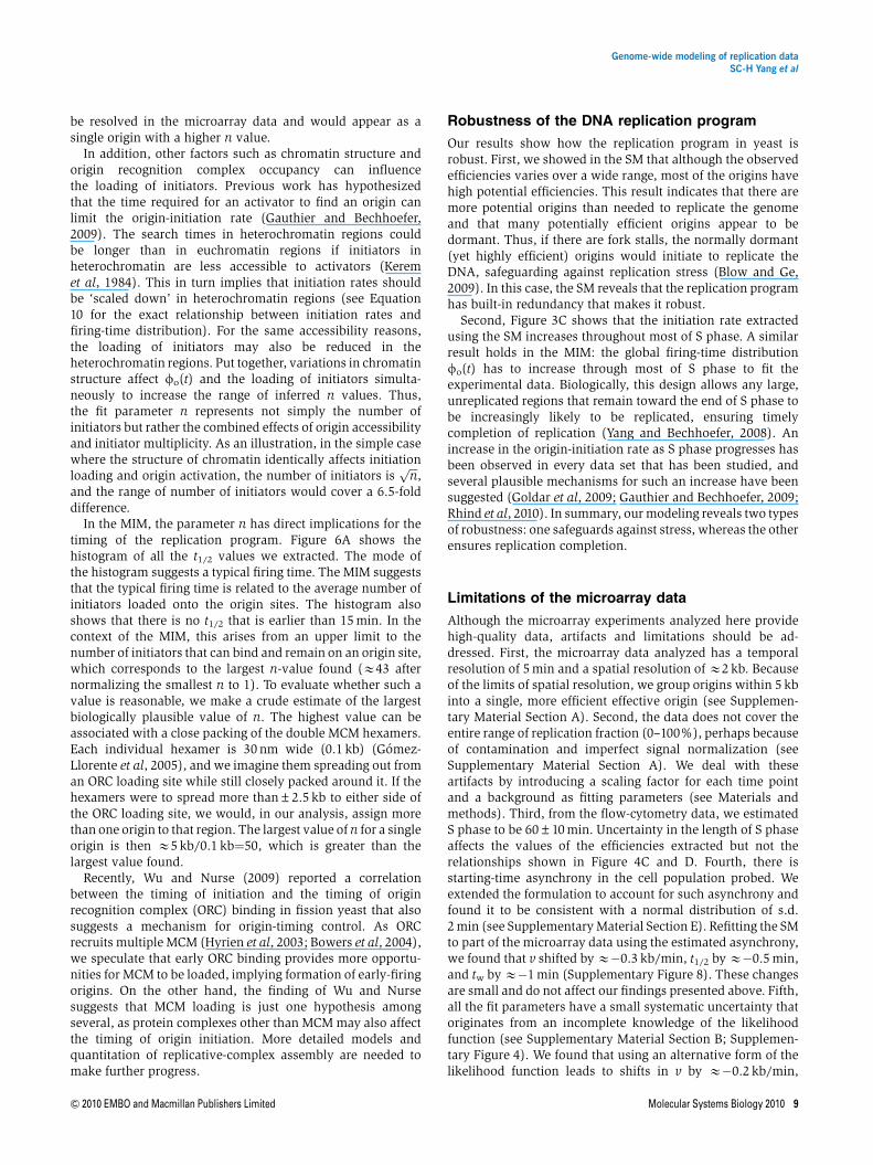
To investigate this hypothesis, we recall that the distributionof t1/2 has a single peak (Figure 5A), suggesting a continuum oftypical firing times and arguing against distinct categories oftemporally alike origins (e.g. early and late origins). To test thespatial aspect, we calculated the autocorrelation function ofthe origins’ t1/2 values (Figure 5B) (Press et al, 2007). In thistest, a positive value means that, typically, an origin and its nthneighbor are likely to have t1/2 that are both larger or bothsmaller than the average firing time, as would be expected iftemporally alike origins were to cluster. Conversely, negativevalues would mean that an origin and its nth neighbor werelikely to have t1/2 values that were anti-correlated. We foundthat the autocorrelation function fluctuates around zero for t1/2

but is clearly non-zero at the nearest neighbor for trep

(Figure 5B). The former result indicates that the intrinsicinitiation time among origins is independent. The latter resultindicates that the time at which neighboring origin sites arereplicated is correlated. The correlation arises because a forkfrom one origin sometimes passively replicates the site of a

Potential efficiency

1.0

0.5

0.0

Obs

erve

d ef

ficie

ncy

1.00.50.0

C

1.0

0.5

0.0

Pot

entia

l effi

cien

cy

100500

t1/2 (min)

D100

50

0

Cou

nts

1.00.50.0

Observed efficiency

B

100

50

0

Cou

nts

1.00.50.0

Potential efficiency

A

Figure 4 Origin efficiencies. (A) Histogram of potential efficiencies with bin width¼0.05. More than half of the origins have high potential efficiency (40.9). Medianvalue¼0.91. (B) Histogram of observed efficiencies with bin width¼0.05. Median value¼0.68. (C) Observed efficiency versus potential efficiency. Markers would lie onthe dotted line if there were no passive replication. Solid markers correspond to the same origins in Figure 3D. The solid curve is a mean-field calculation (seeSupplementary Material Section D). (D) Potential efficiency versus t1/2. There is roughly a one-to-one relationship between the potential efficiency and t1/2. Solid markersare as in Figure 3D. The solid curve is calculated using the parameters obtained from the genome-wide MIM fit.

Genome-wide modeling of replication dataSC-H Yang et al

6 Molecular Systems Biology 2010 & 2010 EMBO and Macmillan Publishers Limited

neighboring origin. Thus, the observation that neighboringorigin sites tend to replicate at similar times is consistent withthe inference that neighboring origins initiate independently.

The multiple-initiator model can explain thecorrelation between t1/2 and tw

The SM allows for any combination of t1/2 and tw. Thetightness of the trend in Figure 3D is thus remarkable: itsuggests that although local variations in origins lead todifferent t1/2 and tw, replication is organized by a globalcontrolling mechanism that connects the two quantities. Inother words, the trend is that earlier-firing origins have tightercontrol of their initiation timing, whereas later-firing originsshow progressively less control. What kind of global and localmechanism can account for such a trend? Here, we proposeone plausible scenario.

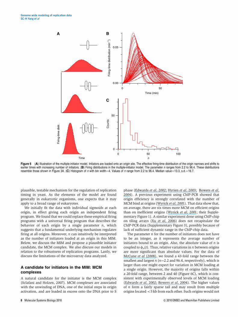
Replication initiates at origins because there are initiatorproteins bound to them. Suppose that every initiator firesaccording to a global firing-time distribution fo(t). Then,origins that have more initiators loaded will be more efficient.This situation arises because, when multiple initiators bindnear an origin site, it is always the earliest firing that counts.Other initiators cannot fire to re-replicate the same site(Sclafani and Holzen, 2007). One can assign an effective firingdistribution feff(t, n) to the initiator cluster at an origin, with nbeing the number of initiators in the cluster. This distributionof the earliest firing times shows the same trend as the curvesextracted from the microarray data: earlier-firing origins havenarrower distributions (Figure 6A and B).

For moderately large n (n\10), the selection of the firstinitiation among many causes feff(t, n) to tend to a universaldistribution, the Weibull distribution, regardless of the ‘de-tails’ of the fo(t) used (Kotz and Nadarajah, 2000). As anexample, the shape of feff(t, n) would differ between using anincreasing and a decreasing fo(t) but would not altersignificantly between a linearly and a quadratically increasingfo(t). This robustness is an advantage of the model because itobviates the need for an accurate form of fo(t).

As the firing-time distribution is shaped by the number ofinitiators, we call this the ‘multiple-initiator model’ (MIM).Results of the MIM fits are shown in Figure 2 andSupplementary Figure 1. The MIM fits are similar to the SMfits (see Supplementary Material Section B), although thenumber of parameters used decreased by nearly 1/3. In theSM, each origin has three parameters—x, t1/2, and tw. In theMIM, each origin needs only two—x and n. Furthermore, thetrend for tw versus t1/2 are similar between the SM and MIM(Figure 3D). The relationship between potential efficiency andt1/2 is also captured (Figure 4D). We emphasize that thesesimilarities are biologically significant because the SM andMIM correspond to two distinct views of replication. Theflexibility of allowing each origin its own t1/2 and tw in the SMcorresponds to the view that the firing of origins is controlledby an explicit time-counting mechanism, a ‘clock.’ In the MIM,there is no such mechanism; the order in timing is built fromstochasticity. Thus, the MIM suggests a new, plausiblemechanism for replication timing in S. cerevisiae.

Lastly, following what is done for SM, the MIM gave 337origins (origin parameters tabulated in Supplementary TableII). Out of the 337, 234 colocalize with the 275 originsidentified by Alvino et al (2007). Out of the remaining 103origins, 70% colocalize with known origins from the OriDBdatabase (Nieduszynski et al, 2007) within 5 kb. Together, theSM and MIM gave 357 distinct origins. Among these, 116 werenot identified by Alvino et al, and 71% of them colocalize withknown origins from the OriDB database within 5 kb.

Discussion

We have developed a general model of replication kinetics andapplied it to recently published data from a budding-yeastgenome-wide replication time course experiment. We foundthat origin firing in budding yeast is best described as astochastic process, in which the average firing time of an origincorrelates strongly with its timing precision. The regulation ofthe timing of origin firing can be explained by the number ofinitiators loaded at each origin. Our model provides a specific,

50

0

Cou

nts

10050

t1/2 (min)

A1.0

0.5

0.0

Aut

ocor

rela

tion

20100

nth neighboring origin

t1/2

trep

B

Figure 5 (A) Histogram of t1/2 with bin width¼4 min. There is no sharp distinction between early and late origins. Median value¼31.0 min, s.d.¼11.2 min.(B) Autocorrelation of t1/2 and trep. The graph shows the t1/2 and trep correlation between an origin and its nth neighbor. The range of the x axis corresponds to roughly700 kb of genome distance, as the average interorigin distance extracted is 35 kb.

Genome-wide modeling of replication dataSC-H Yang et al

& 2010 EMBO and Macmillan Publishers Limited Molecular Systems Biology 2010 7

plausible, testable mechanism for the regulation of replicationtiming in yeast. As the elements of the model are foundgenerally in eukaryotic organisms, one expects that it mayapply to a broad range of eukaryotes.

We initially fit the data with individual sigmoids at eachorigin, in effect giving each origin an independent firingprogram. We found that we could replace these empirical firingprograms with a universal firing program that describes thebehavior of each origin by a single parameter n, whichsuggests that a fundamental underlying mechanism regulatesfiring at all origins. Moreover, n can intuitively be interpretedas the number of initiators loaded at an origin in this MIM.Below, we discuss the MIM and propose a plausible initiatorcandidate, the MCM complex. We also discuss our models inrelation to the robustness of replication programs. Lastly, wediscuss the limitations of the microarray data analyzed.

A candidate for initiators in the MIM: MCMcomplexes

A natural candidate for the initiator is the MCM complex(Sclafani and Holzen, 2007). MCM complexes are associatedwith the unwinding of DNA, one of the initial steps in originactivation, and are loaded in excess onto the DNA prior to S

phase (Edwards et al, 2002; Hyrien et al, 2003; Bowers et al,2004). A previous experiment using ChIP-PCR showed thatorigin efficiency is strongly correlated with the number ofMCM bind at origins (Wyrick et al, 2001). That data show that,on average, there are six times more MCM on efficient originsthan on inefficient origins (Wyrick et al, 2001; their Supple-mentary Figure 1). A similar experiment done using ChIP-chipon tiling arrays (Xu et al, 2006) does not recapitulate theChIP-PCR data (Supplementary Figure 3), possibly because oflack of sufficient dynamic range in the ChIP-chip data.

The parameter n for the number of initiators does not haveto be an integer, as it represents the average number ofinitiators bound to an origin. Also, the absolute value of n iscoupled to fo(t). Thus, relative variations in n between originsare more significant than absolute values. For the data ofMcCune et al (2008), we found a 43-fold range between thesmallest and largest n (n¼2.2 and 96.4, respectively), which islarger than one might expect for variation in MCM loading ata single origin. However, the majority of origins falls withina 20-fold range, between 2 and 40 (Figure 6C), which is con-sistent with experimentally observed levels of MCM loading(Edwards et al, 2002; Bowers et al, 2004). The higher valuesof n form a fairly sparse tail and may result from multipleorigins located o5 kb from each other. Such origins would not

0.05

0.00

Firi

ng-t

ime

dist

ribut

ion

(min

–1)

500

Time (min)

B

50

0

Cou

nts

100500

n

C

Time

Firi

ng-t

ime

dist

r.

A

Figure 6 (A) Illustration of the multiple-initiator model. Initiators are loaded onto an origin site. The effective firing-time distribution of the origin narrows and shifts toearlier times with increasing number of initiators. (B) Firing distributions in the multiple-initiator model. The parameter n ranges from 2.2 to 96.4. These distributionsresemble those shown in Figure 3A. (C) Histogram of n with bin width¼4. Values of n range from 2.2 to 96.4. Median value¼13.3, s.d.¼16.7.

Genome-wide modeling of replication dataSC-H Yang et al

8 Molecular Systems Biology 2010 & 2010 EMBO and Macmillan Publishers Limited

be resolved in the microarray data and would appear as asingle origin with a higher n value.

In addition, other factors such as chromatin structure andorigin recognition complex occupancy can influencethe loading of initiators. Previous work has hypothesizedthat the time required for an activator to find an origin canlimit the origin-initiation rate (Gauthier and Bechhoefer,2009). The search times in heterochromatin regions couldbe longer than in euchromatin regions if initiators inheterochromatin are less accessible to activators (Keremet al, 1984). This in turn implies that initiation rates shouldbe ‘scaled down’ in heterochromatin regions (see Equation10 for the exact relationship between initiation rates andfiring-time distribution). For the same accessibility reasons,the loading of initiators may also be reduced in theheterochromatin regions. Put together, variations in chromatinstructure affect fo(t) and the loading of initiators simulta-neously to increase the range of inferred n values. Thus,the fit parameter n represents not simply the number ofinitiators but rather the combined effects of origin accessibilityand initiator multiplicity. As an illustration, in the simple casewhere the structure of chromatin identically affects initiationloading and origin activation, the number of initiators is

ffiffiffinp

,and the range of number of initiators would cover a 6.5-folddifference.

In the MIM, the parameter n has direct implications for thetiming of the replication program. Figure 6A shows thehistogram of all the t1/2 values we extracted. The mode ofthe histogram suggests a typical firing time. The MIM suggeststhat the typical firing time is related to the average number ofinitiators loaded onto the origin sites. The histogram alsoshows that there is no t1/2 that is earlier than 15 min. In thecontext of the MIM, this arises from an upper limit to thenumber of initiators that can bind and remain on an origin site,which corresponds to the largest n-value found (E43 afternormalizing the smallest n to 1). To evaluate whether such avalue is reasonable, we make a crude estimate of the largestbiologically plausible value of n. The highest value can beassociated with a close packing of the double MCM hexamers.Each individual hexamer is 30 nm wide (0.1 kb) (Gomez-Llorente et al, 2005), and we imagine them spreading out froman ORC loading site while still closely packed around it. If thehexamers were to spread more than±2.5 kb to either side ofthe ORC loading site, we would, in our analysis, assign morethan one origin to that region. The largest value of n for a singleorigin is then E5 kb/0.1 kb¼50, which is greater than thelargest value found.

Recently, Wu and Nurse (2009) reported a correlationbetween the timing of initiation and the timing of originrecognition complex (ORC) binding in fission yeast that alsosuggests a mechanism for origin-timing control. As ORCrecruits multiple MCM (Hyrien et al, 2003; Bowers et al, 2004),we speculate that early ORC binding provides more opportu-nities for MCM to be loaded, implying formation of early-firingorigins. On the other hand, the finding of Wu and Nursesuggests that MCM loading is just one hypothesis amongseveral, as protein complexes other than MCM may also affectthe timing of origin initiation. More detailed models andquantitation of replicative-complex assembly are needed tomake further progress.

Robustness of the DNA replication program

Our results show how the replication program in yeast isrobust. First, we showed in the SM that although the observedefficiencies varies over a wide range, most of the origins havehigh potential efficiencies. This result indicates that there aremore potential origins than needed to replicate the genomeand that many potentially efficient origins appear to bedormant. Thus, if there are fork stalls, the normally dormant(yet highly efficient) origins would initiate to replicate theDNA, safeguarding against replication stress (Blow and Ge,2009). In this case, the SM reveals that the replication programhas built-in redundancy that makes it robust.

Second, Figure 3C shows that the initiation rate extractedusing the SM increases throughout most of S phase. A similarresult holds in the MIM: the global firing-time distributionfo(t) has to increase through most of S phase to fit theexperimental data. Biologically, this design allows any large,unreplicated regions that remain toward the end of S phase tobe increasingly likely to be replicated, ensuring timelycompletion of replication (Yang and Bechhoefer, 2008). Anincrease in the origin-initiation rate as S phase progresses hasbeen observed in every data set that has been studied, andseveral plausible mechanisms for such an increase have beensuggested (Goldar et al, 2009; Gauthier and Bechhoefer, 2009;Rhind et al, 2010). In summary, our modeling reveals two typesof robustness: one safeguards against stress, whereas the otherensures replication completion.

Limitations of the microarray data

Although the microarray experiments analyzed here providehigh-quality data, artifacts and limitations should be ad-dressed. First, the microarray data analyzed has a temporalresolution of 5 min and a spatial resolution of E2 kb. Becauseof the limits of spatial resolution, we group origins within 5 kbinto a single, more efficient effective origin (see Supplemen-tary Material Section A). Second, the data does not cover theentire range of replication fraction (0–100%), perhaps becauseof contamination and imperfect signal normalization (seeSupplementary Material Section A). We deal with theseartifacts by introducing a scaling factor for each time pointand a background as fitting parameters (see Materials andmethods). Third, from the flow-cytometry data, we estimatedS phase to be 60±10 min. Uncertainty in the length of S phaseaffects the values of the efficiencies extracted but not therelationships shown in Figure 4C and D. Fourth, there isstarting-time asynchrony in the cell population probed. Weextended the formulation to account for such asynchrony andfound it to be consistent with a normal distribution of s.d.2 min (see Supplementary Material Section E). Refitting the SMto part of the microarray data using the estimated asynchrony,we found that v shifted by E�0.3 kb/min, t1/2 by E�0.5 min,and tw by E�1 min (Supplementary Figure 8). These changesare small and do not affect our findings presented above. Fifth,all the fit parameters have a small systematic uncertainty thatoriginates from an incomplete knowledge of the likelihoodfunction (see Supplementary Material Section B; Supplemen-tary Figure 4). We found that using an alternative form of thelikelihood function leads to shifts in v by E�0.2 kb/min,

Genome-wide modeling of replication dataSC-H Yang et al

& 2010 EMBO and Macmillan Publishers Limited Molecular Systems Biology 2010 9

origin positions byE±1 kb, t1/2 byE�3 min, tw byE�2 min,and n by E�1 (Supplementary Figure 5). Again, these smalluncertainties do not affect our overall conclusions.

In summary, artifacts in the microarray data result in smalluncertainties in the absolute values of the extracted para-meters that do not alter significantly our findings. In particular,the relationship that t1/2Etw remains valid. The t1/2–tw trendclearly reveals that initiation times and the precision of timingare correlated. This relationship has also been observed by arecent analysis (de Moura et al, 2010) and is contrary to theview of replication in which origin initiation is timed in anearly deterministic manner. We hypothesize that the correla-tion emerges from the multiplicity of stochastic initiators, andwe account for it quantitatively via the MIM.

Materials and methods

Methods summary

Our analysis is described in four parts below. First, we fit sigmoids tothe replication fraction of origins from the microarray data and inferthat the timing and the variation in timing of origin initiation arecorrelated. Second, we present the SM, which is based on twoelements: origin initiation and fork progression. The model takes intoaccount the effect of passive replication because of all other origins.This framework allows one to calculate the potential efficiency oforigins, which is difficult to measure because of passive replication.Third, we detail the parameters used in the SM fits. These parametersinclude the origin positions, the t1/2 and tw of the firing-timedistributions, fork velocity, and factors to deal with experimentalartifacts. Last, we describe the parameters used in the MIM and discussits relationship with the firing-time distribution. Analysis codes areavailable upon request.

Fitting sigmoids to array data

Let the replication fraction be f(x, t), where x is the genome positionand t is the time elapsed since the start of S phase. For microarray data,f(x, t) represents the fraction of the population that has replicated locusx by time t. Looking at the spatial part of the replication fraction, oneexpects that an early-firing origin that is rarely passively replicatedwould show a peak at the origin position, as the site is almost alwaysreplicated before its surrounding. Thus, peaks in f(x, t) correspond toorigin sites. At a fixed x where an origin resides, the peak height thenscales with the number of initiations of the particular origin in thepopulation. If an origin fires at a distinct time, the correspondingf(t) would resemble a step function. By contrast, if an origin firesstochastically, f(t) would be smooth.

Using 275 previously identified origin sites (Alvino et al, 2007), weextracted the corresponding 275 f(t) curves from the microarray data.These f(t) curves are well described by sigmoids with parameters trep

and twidth. We used the Hill equation

fðtÞ ¼ 1

1þ trep

t

� �r ; ð1Þ

where r is related to twidth via

twidth ¼ 31=r � 3�1=r� �

trep; ð2Þ

to fit the 275 f(t) and extracted 275 pairs of trep and twidth. The result isplotted in Figure 1C.

There is a distinction between the replication fraction of a locus andthe cumulative firing-time distribution of the origin at the locus. Thecomplication is that the locus is replicated by all nearby origins and notjust the origin on the site. To untangle these composite effects, wepresent a more general theory that accounts for passive replication.

A general formalism describing DNA replication

The replication program is determined by the properties of origins,which are specified through their positions and ability to initiatethroughout S phase. Following previous work (Jun et al, 2005), wedescribe the replication program by an initiation rate I(x, t), defined asthe number of times an origin at x would initiate per time perunreplicated length (meaning that the origin has not been passivelyreplicated). Origin positions in budding yeast are well defined andare associated with autonomous replication sequences (Sclafani andHolzen, 2007); we denote these positions by xi. An origin is thendescribed by the initiation rate Ii(x, t)¼d(x�xi)I0(x, t), where d(x) is theDirac d function (Boas, 2006) that sets the rate to zero for all xaxi. Theprogram I(x, t) is the sum of all Ii(x, t).

Given I(x, t), we can calculate the replication fraction f(x, t) of site xon the genome at a time t after the start of S phase (Kolmogorov, 1937).The result is

fðx; tÞ ¼ 1�Y4

1� Iðx0; t0ÞDx0Dt0½ �; ð3Þ

where the product is over all area elements of DxDt in the shadedtriangle D depicted in Figure 7 (Kolmogorov, 1937). In words, thefraction of replication at a specific position and time is one minus theprobability that the position has not been replicated before that time. Inthe limit Dx-0 and Dt-0, one finds

fðx; tÞ ¼ 1� e�R R4

Iðx0 ; t0 Þdx0dt0

: ð4ÞTo make the double integral explicit, we define a local measure oforigin firing,

gðDxp; tÞ ¼Zxpþ1

xp

dðx� xiÞdx

Zt0

I0ðx; t0Þdt0 ð5Þ

for the interval (xp, xpþ 1), where the index p comes from discretizing agenome of length L:

Dx ¼ L

N; xp ¼ pðDxÞ; p ¼ 0; 1; . . . ; N � 1: ð6Þ

The function g(Dxp, t)¼0 unless there is an origin contained in theinterval (xp, xpþ 1). Replacing the double integral in Equation (4) by asum using Equation (5), we obtain

fðx; tÞ ¼ 1� exp �XN�1

p¼0

g Dxp; t � jx� xpjv

� �" #; ð7Þ

where v is the fork velocity. TheDxp in the first argument of g(x, t) is aninterval, whereas the xp in the second argument is a point. The secondargument, t�|x�xp|/v, is the time along the edge of the triangle. This

TimeOriginal index i

2 3 4 5 6 ...

t

Position

xi = 1

×

Figure 7 Illustration of Kolmogorov’s argument. The replication fraction at (x, t )equals to ‘1�probability that no origins initiated within the shaded triangle D.’Vertical lines indicates the positions of discrete origins; initiation can only occuralong these lines.

Genome-wide modeling of replication dataSC-H Yang et al

10 Molecular Systems Biology 2010 & 2010 EMBO and Macmillan Publishers Limited

equation is used to fit the microarray time course data. Biologicallyrelevant g(x, t) should satisfy the following constraints:

1. g(Dxp, to0)¼0. This means that the initiation rate is zero[I(x, to0)¼0] before the start of replication. Applying this con-straint to Equation (7), we see that the sum is limited to thedomain (x�t/v)pxp(xþ t/v).

2. ddtgðDxp; tÞX0. As gðDxp; tÞ ¼

R xþDxx

R t0 Iðx0; t0Þdt0dx0, this is equiva-

lent to I(x, t)X0, meaning that the initiation rate cannot benegative.

3. g(Dxp, t)X0. This is a direct consequence of constraints 1 and 2.

We derive a useful quantity, the cumulative initiation probabilityF(xp, t), from g(Dxp, t) following a Poisson-process calculation(Rieke et al, 1999):

Fðxp; tÞ ¼ 1� e�g Dxp ; tð Þ: ð8ÞAs F(xp, t) is only non-zero for xppxipxpþ 1, we introduce

fiðtÞ �d

dtFðxi 2 Dxp; tÞ � d

dtFiðtÞ ð9Þ

to denote the initiation probability density of each origin i. The xp inEquation (8) is related to the discretization, whereas the subscript i inEquation (9) relates to the origin position. Rearranging Equation (8) forg(Dxp, t) and differentiating, we obtain the relationship between theinitiation rate and the firing-time distribution:

IiðtÞ � Iðxi 2 Dxp; tÞ ¼ fiðtÞ1� FiðtÞ

: ð10Þ

We note that Equation (10) is also the firing probability density of anorigin given that it has not initiated before time t.

Using the probability distributions in Equation (9), we definepotential efficiency as the probability that an origin would fire by theend of S phase if there is no passive replication, that is, Fi(t¼tend) withtend being the time that S phase ends. By contrast, the efficiency of anyorigin decreases because of passive replication by neighboring origins.The observed efficiency of the jth origin thus depends not only on fj(t)but also with the fk(t) of neighboring origins. Mathematically, theobserved efficiency Ej of the jth origin is then

Ej �Ztend

0

dtfjðtÞYk6¼j

1� Fk t � jxk � xjjv

� �� �; ð11Þ

where the integrand is an effective initiation probability density thatrepresents the probability that the jth origin initiates between t andtþdt times the probability that all the other origins have not initiatedto passively replicate the jth origin before time t.

A group of origins is effectively a more-efficient origin. In light ofthis, consider a tightly packed cluster of initiators in the MIM. As it isalways the earliest initiation in the cluster that counts, the effectiveinitiation probability of the cluster is the extreme (smallest) valuedistribution of all the fj(t)s in the cluster. For n initiators near x, theeffective cumulative initiation probability is

Feffðx; t; nÞ ¼ 1�Ynj¼1

1� Fj t � jx� xjjv

� �� �: ð12Þ

For large n, Equation (12) tends toward the Weibull distribution fora large class of functions Fj, a feature of extreme-value statistics(Kotz and Nadarajah, 2000). This is a desirable feature for the MIM(see Results).

Fitting parameters for the SM

Using the model presented above, we performed least-squares fits tothe time course microarray data in McCune et al (2008). The fit is doneusing the Global Fit package in Igor Pro 6.1 (Wavemetrics Inc.; http://www.wavemetrics.com). We fit to the unsmoothed microarray data(Supplementary Material Section F; Supplementary Figure 9). To speedup the code, the fit program calls external C-language code for keyfunction evaluations. On a personal computer with an Intel Core2 DuoCPU @ 3.16 GHz, the fit for an average chromosome (E900 points and

E150 parameters) takes about 5 min. The time to fit the entire genomeof S. cerevisiae is about 10 h. All local parameters of the SM aretabulated in Supplementary Table I. Global ones are in SupplementaryTable III. There are three types of genome-wide parameters:

Fork velocity vEven though the model allows for variable-fork velocity, we found thatto fit the microarray data, a constant v across the genome andthroughout S phase suffices (see Supplementary Material Section C).

Background bgThe reason for introducing this parameter comes from the observationthat the 10-min time point data do not start close to f¼0 (Supplemen-tary Material Section A). Although introducing a variable backgroundis possible, we found that a simple constant background is sufficientfor the global fit. This parameter is also global in space and time.

Normalization factors atThese parameters correct for various artifacts that cause themicroarray data to not cover the entire range of possible fractions,0–100% (see Supplementary Material Section A). We propose anormalization factor at for each time point that is genome wide.Combining the normalization factors with the background parameter,we generate a modified replication fraction

fmodðx; tÞ ¼ at fðx; tÞ þ bg

ð13Þ

to fit the data. Again, in Equation (13), at is global in space but nottime, whereas bg is global both in time and space.

There are two types of local parameters pertaining to origins. Theseparameters are local in space but global in time:

Origin positionEach origin was associated with a unique location xi along the genome.Initial guesses of the xi include all 732 origins recorded in the OriDBdatabase (Nieduszynski et al, 2007). We counted origins that wereo5 kb apart as a single origin throughout the fitting process, as thedata (resolution E2 kb) cannot distinguish between a single-efficientorigin and a group of less-efficient origins (see Supplementary MaterialSection A). Before the genome-wide fit, we first fit each chromosomeseparately to eliminate false origins and origins that do not contributeenough to the replication fraction. This allowed the genome-wide fitto run more smoothly. The criteria for elimination were (1) modeof firing-time distribution o10 min and efficiency o0.5 and (2)cumulative firing-time probability o0.3 at end of S phase (estimatedto be 60 min). The first criterion aims to identify peaks in microarraydata that originate from contamination instead of origin activity (smallfragments of unreplicated DNA along with A-T rich sequence can becounted as replicated DNA, as mentioned in the SupplementaryMaterial Section A). Contamination produces microarray peaks in theearly but not the mid and late time points. In the model, this iseffectively the same as an origin that fires very early (before the firsttime point at 10 min) but is inefficient. The second criterion simplyeliminates origins that do not contribute much throughout S phase.

Firing-time-distribution parametersWe used the Hill equation (same form as Equation 1) to describe thecumulative firing-time distribution F(t). The two parameters are themedian time t1/2 at which F(t¼t1/2)¼0.5 and the width tw, defined asthe difference t0.75–t0.25. This function is a valid cumulative initiationprobability function, satisfying the constraints 0pF(t)p1,F(to0)¼0,and dF(t)/dtX0.

Fitting parameters for the MIM

The MIM, like SM, is also parameterized with the fork velocity,background, normalization factors, and origin positions. The two

Genome-wide modeling of replication dataSC-H Yang et al

& 2010 EMBO and Macmillan Publishers Limited Molecular Systems Biology 2010 11

firing-time-distribution parameters for each origin in SM are replacedby a single parameter n in MIM. As discussed in the Discussion, nrepresents the number of initiator molecules that is modified by effectssuch as chromatin structure and ORC loading. There are additionalparameters (t1/2

* and r*) to describe the global firing-time distributionof all initiators (see Equation 15 below). These are absent from the SM,as the SM does not assume that the firing distributions are related. Alllocal parameters of the MIM are tabulated in Supplementary Table IIand all global parameters in Supplementary Table III.

We still use the Hill equation to describe the global cumulativedistribution Fo(t). Using Equation 12, the Feff(t, n) for a cluster of ninitiators is

Feffðt; nÞ ¼ 1� 1� FoðtÞ½ �n; ð14Þwhere

FoðtÞ ¼1

1þ t�1=2

t

� �r� : ð15Þ

The quantity t1/2* is the median time of the firing-time distribution for a

single initiator, and r* is its rate of increase.Because of the different form of firing-time distribution used in the

MIM, the criteria for origin elimination are slightly modified from theSM ones. The MIM predicts strictly that earlier-firing origins are moreefficient; thus, no contamination effects are modeled by the MIM.We then eliminated origins via a single criterion of Fi(t¼60 min)o0.4.The change is consistent with the observation that the firing-timedistribution in Equation (14) tends to result in more efficient originsthan the Hill function does. Similar to the SM fits, individual-chromo-some fits were done first before performing the genome-wide fit.

Supplementary information

Supplementary information is available at the Molecular SystemsBiology website (http://www.nature.com/msb).

AcknowledgementsWe thank MK Raghuraman and Gina M Alvino for making availablethe raw data from McCune et al (2008). We thank Olivier Hyrien forcomments and suggestions concerning the upper bound for allowedinitiator numbers. We thank Ollie Rando and Melissa Moore for usefulcomments on the manuscript. We thank Michel Gauthier fordiscussions and helping with coding for fits. This work was fundedby the Natural Sciences and Engineering Research Council of Canada(NSERC), the American Cancer Society (ACS), and the Human FrontierScience Program (HFSP).

Conflict of interestThe authors declare that they have no conflict of interest.

References

Alvino GM, Collingwood D, Murphy JM, Delrow J, Brewer BJ,Raghuraman MK (2007) Replication in hydroxyurea: it’s a matterof time. Mol Cell Biol 27: 6396–6404

Blow JJ, Ge XQ (2009) A model for DNA replication showing howdormant origins safeguard against replication fork failure. EMBORep 10: 406–412

Boas ML (2006) Mathematical Methods in the Physical Sciences, 3rdedn, New York, NY, USA: John Wiley & Sons

Bowers J, Randell J, Chen S, Bell S (2004) ATP hydrolysis by ORCcatalyzes reiterative Mcm2–7 assembly at a defined origin ofreplication. Mol Cell 22: 967–978

Czajkowsky DM, Liu J, Hamlin JL, Shao Z (2008) DNA combingreveals intrinsic temporal disorder in the replication of yeastchromosome VI. Mol Biol Cell 375: 12–19

Donaldson AD (2005) Shaping time: chromatin structure and the DNAreplication programme. Trends Genet 21: 444–449

Edwards MC, Tutter AV, Cvetic C, Gilbert CH, Prokhorova TA, Walter JC(2002) MCM2-7 complexes bind chromatin in a distributed patternsurrounding the origin recognition complex in Xenopus eggextracts. J Biol Chem 277: 33049–33057

Eshaghi M, Karuturi RKM, Li J, Chu Z, Liu ET, Liu J (2007) Globalprofiling of DNA replication timing and efficiency reveals thatefficient replication/firing occurs late during S-phase in S. pombe.PLoS ONE 2: e722

Feng W, Max E, Boeck DC, Fox LA, Alvino GM, Fangman WL,Raghuraman MK, Brewer BJ (2006) Genomic mapping of single-stranded DNA in hydroxyurea-challenged yeasts identifies originsof replication. Nat Cell Biol 8: 148–155

Ferguson BM, Brewer BJ, Reynolds AE, Fangman WL (1991) A yeastorigin of replication is activated late in S phase. Cell 65: 507–515

Gomez-Llorente Y, Fletcher RJ, Chen XS, Carazo JM, Martın CS (2005)Polymorphism and double hexamer structure in the archaealminichromosome maintenance (MCM) helicase fromMethanobacterium thermoautotrophicum. J Biol Chem 280:40909–40915

Gauthier MG, Bechhoefer J (2009) Control of DNA replication byanomalous reaction-diffusion kinetics. Phys Rev Lett 102: 158104

Goldar A, Marsolier-Kergoat MC, Hyrien O (2009) Universal temporalprofile of replication origin activation in Eukaryotes. PLoS ONE 4:e5899

Goren A, Cedar H (2003) Replicating by the clock. Nat Rev Mol Cell Biol4: 25–32

Heichinger C, Penkett CJ, Bahler J, Nurse P (2006) Genome-widecharacterization of fission yeast DNA replication origins. EMBO J25: 5171–5179

Herrick J, Bensimon A (1999) Single molecule analysis of DNAreplication. Biochimie 81: 859–871

Herrick J, Stanislawski P, Hyrien O, Bensimon A (2000) Replicationfork density increases during DNA synthesis in X. laevis eggextracts. J Mol Biol 300: 1133–1142

Hyrien O, Goldar A (2010) Mathematical modeling of eukaryotic DNAreplication. Chromosome Res 18: 147–161

Hyrien O, Marheineke K, Goldar A (2003) Paradoxes of eukaryoticDNA replication: MCM proteins and the random completionproblem. BioEssays 25: 116–125

Jun S, Zhang H, Bechhoefer J (2005) Nucleation and growth in onedimension. I. The generalized Kolmogorov-Johnson-Mehl-Avramimodel. Phys Rev E 71: 011908

Kerem BS, Goitein R, Diamond G, Cedar H, Marcus M (1984) Mappingof DNAase I sensitive regions on mitotic chromosomes. Cell 38:493–499

Kolmogorov AN (1937) On the static theory of crystallization inmetals. Bull Acad Sci USSR, Phys Ser 1: 335

Kotz S, Nadarajah S (2000) Extreme Value Distributions: Theory andApplications. River Edge, NJ, USA: Imperial College Press

Lygeros J, Koutroumpas K, Dimopoulos S, Legouras I, Kouretas P,Heichinger C, Nurse P, Lygerou Z (2008) Stochastic hybridmodeling of DNA replication across a complete genome. Proc NatlAcad Sci USA 105: 12295–12300

McCune HJ, Danielson LS, Alvino GM, Collingwood D, Delrow JJ,Fangman WL, Brewer BJ, Raghuraman MK (2008) The temporalprogram of chromosome replication: genomewide replication inclb5D Saccharomyces cerevisiae. Genetics 180: 1833–1847

de Moura APS, Retkute R, Hawkins M, Nieduszynski CA (2010)Mathematical modelling of whole chromosome replication. NucleicAcids Res (advance online publication 10 May 2010; doi:10.1093/nar/gkq343)

Nieduszynski CA, Hiraga S, Ak P, Benham CJ, Donaldson AD (2007)OriDB: a DNA replication origin database. Nucleic Acids Res 35:D40–D46 (http://www.oridb.org)

Patel PK, Arcangioli B, Baker SP, Bensimon A, Rhind N (2006) DNAreplication origins fire stochastically in fission yeast. Mol Biol Cell17: 308–316

Genome-wide modeling of replication dataSC-H Yang et al

12 Molecular Systems Biology 2010 & 2010 EMBO and Macmillan Publishers Limited

Press WH, Teukolsky SA, Vetterling WT, Flannery BP (2007) NumericalRecipes: The Art of Scientific Computing, 3rd edn. CambridgeCambridge, NY, USA: University Press

Raghuraman MK, Winzeler EA, Collingwood D, Hunt S, Wodicka L,Conway A, Lockhart DJ, Davis RW, Brewer BJ, Fangman WL(2001) Replication dynamics of the yeast genome. Science 294:115–121

Rhind N, Yang SCH, Bechhoefer J (2010) Reconciling stochastic originfiring with defined replication timing. Chromosome Res 18: 35–43

Rieke F, Warland D, Steveninck R, Bialek W (1999) Spikes: Exploringthe Neural Code. London, UK: The MIT Press

Sclafani RA, Holzen TM (2007) Cell cycle regulation of DNAreplication. Annu Rev Genet 41: 237–280

Sekedat MD, Fenyo D, Rogers RS, Tackett AJ, Aitchison JD, Chait BT(2010) GINS motion reveals replication fork progression is remar-kably uniform throughout the yeast genome. Mol Sys Biol 6: 353

Wu PYJ, Nurse P (2009) Establishing the program of origin firingduring S phase in fission yeast. Cell 136: 852–864

Wyrick JJ, Aparicio JG, Chen T, Barnett JD, Jennings EG, Young RA,Bell SP, Aparicio OM (2001) Genome-wide distribution of ORC andMCM proteins in S. cerevisiae: high-resolution mapping ofreplication origins. Science 294: 2357–23650

Xu W, Aparicio JG, Aparicio OM, Tavare S (2006) Genome-widemapping of ORC and Mcm2p binding sites on tiling arrays andidentification of essential ARS consensus sequences in S. cerevisiae.BMC Genomics 7: 276

Yabuki N, Terashima H, Kitada K (2002) Mapping of early firing originson a replication profile of budding yeast. Genes Cells 7: 781–789

Yang SCH, Bechhoefer J (2008) How Xenopus laevis embryos replicatereliably: investigating the random-completion problem. Phys Rev E78: 041917

Yang SCH, Gauthier MG, Bechhoefer J (2009) Computational methodsto study kinetics of DNA replication. In DNA Replication: Methodsand Protocols, Vengrova S, Dalgaard JZ (eds), pp 555–574. HumanaPress: New York c/o Springer Science+Business Media

Zhang H, Bechhoefer J (2006) Reconstructing DNA replication kineticsfrom small DNA fragments. Phys Rev E 73: 051903

Molecular Systems Biology is an open-access journalpublished by European Molecular Biology Organiza-

tion and Nature Publishing Group. This work is licensed under aCreative Commons Attribution-Noncommercial-No DerivativeWorks 3.0 Unported License.

Genome-wide modeling of replication dataSC-H Yang et al

& 2010 EMBO and Macmillan Publishers Limited Molecular Systems Biology 2010 13