Chemistry 601 Lecture 7

Steady State Kinetic Analysis

Your body needs a steady supply of amino acids for use in growth and repairs. Each day, a typical adult needs something in the range of 35-90 grams of protein, depending on their weight. Quite surprisingly, a large fraction of this may come from inside. A typical North American diet may contain 70-100 grams of protein each day. But your body also secretes 20-30 grams of digestive proteins, which are themselves digested when their finish their duties. Dead intestinal cells and proteins leaking out of blood vessels are also digested and reabsorbed as amino acids, showing that our bodies are experts at recycling.

Steady State Kinetics

Steady State Analysis

Algebraic Conventions

A, B, C Substrates P, Q, R Products I, J, K Inhibitors

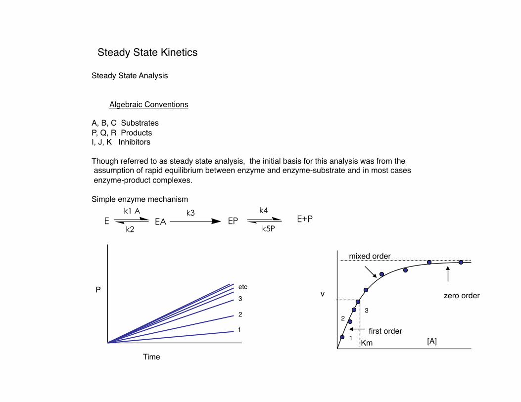
Though referred to as steady state analysis, the initial basis for this analysis was from the assumption of rapid equilibrium between enzyme and enzyme-substrate and in most cases enzyme-product complexes.

Simple enzyme mechanism

E EA EP E+Pk1 A

k2

k4

k5P

k3

P

Time

first order

zero order

mixed order

v

[A] Km 1 2

3 etc

1

2 3

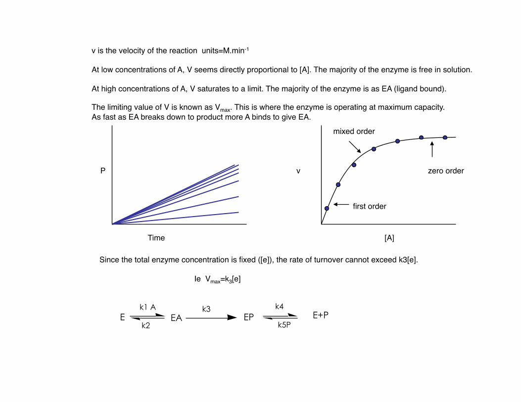
v is the velocity of the reaction units=M.min-1

At low concentrations of A, V seems directly proportional to [A]. The majority of the enzyme is free in solution.

At high concentrations of A, V saturates to a limit. The majority of the enzyme is as EA (ligand bound).

The limiting value of V is known as Vmax. This is where the enzyme is operating at maximum capacity. As fast as EA breaks down to product more A binds to give EA.

P v

Time [A]

first order

zero order

mixed order

Since the total enzyme concentration is fixed ([e]), the rate of turnover cannot exceed k3[e].

Ie Vmax=k3[e]

E EA EP E+Pk1 A

k2

k4

k5P

k3

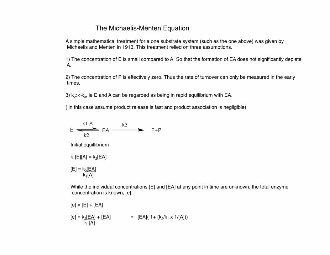
The Michaelis-Menten Equation

A simple mathematical treatment for a one substrate system (such as the one above) was given by Michaelis and Menten in 1913. This treatment relied on three assumptions.

1) The concentration of E is small compared to A. So that the formation of EA does not significantly deplete A.

2) The concentration of P is effectively zero. Thus the rate of turnover can only be measured in the early times.

3) k2>>k3, ie E and A can be regarded as being in rapid equilibrium with EA.

( in this case assume product release is fast and product association is negligible)

E EA E+Pk1 A

k2

k3

Initial equillibrium

k1[E][A] = k2[EA]

[E] = k2[EA] k1[A]

While the individual concentrations [E] and [EA] at any point in time are unknown, the total enzyme concentration is known, [e].

[e] = [E] + [EA]

[e] = k2[EA] + [EA] = [EA]( 1+ (k2/k1 x 1/[A])) k1[A]

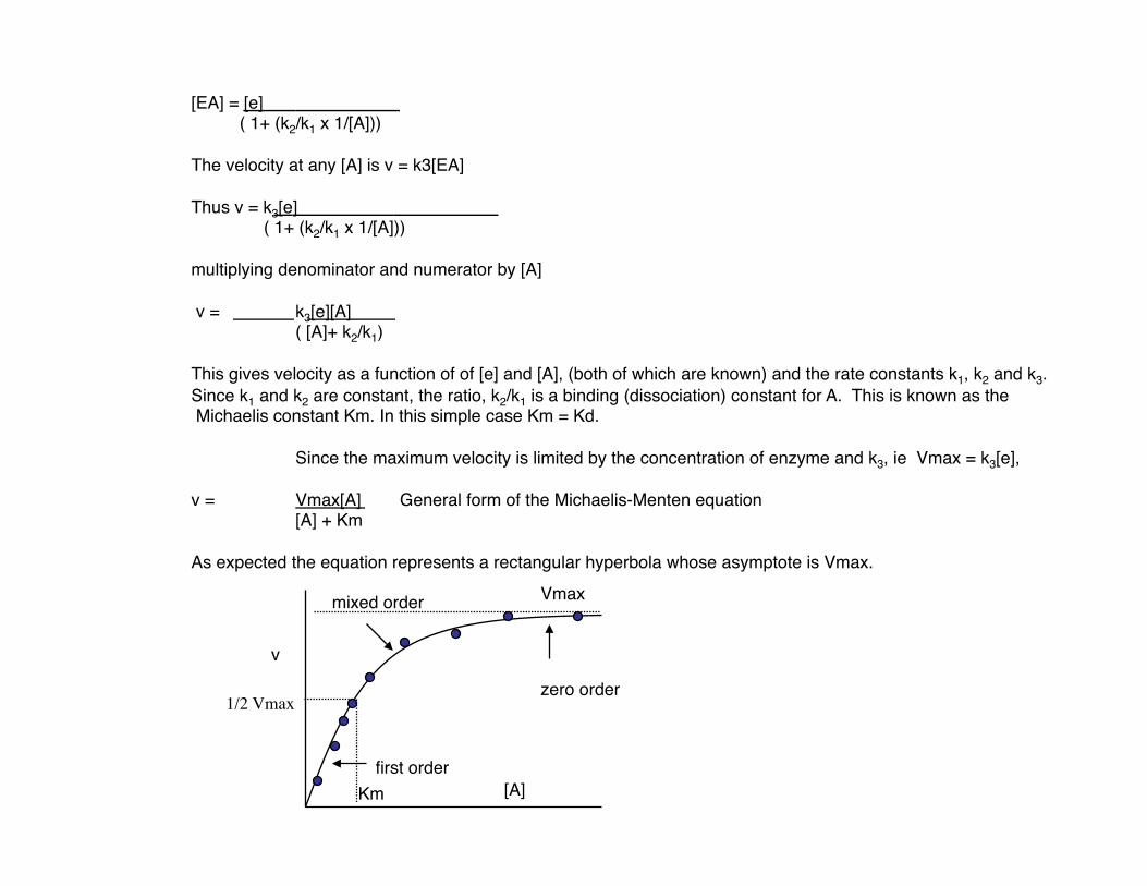
[EA] = [e] ( 1+ (k2/k1 x 1/[A]))

The velocity at any [A] is v = k3[EA]

Thus v = k3[e] ( 1+ (k2/k1 x 1/[A]))

multiplying denominator and numerator by [A]

v = k3[e][A] ( [A]+ k2/k1)

This gives velocity as a function of of [e] and [A], (both of which are known) and the rate constants k1, k2 and k3. Since k1 and k2 are constant, the ratio, k2/k1 is a binding (dissociation) constant for A. This is known as the Michaelis constant Km. In this simple case Km = Kd.

Since the maximum velocity is limited by the concentration of enzyme and k3, ie Vmax = k3[e],

v = Vmax[A] General form of the Michaelis-Menten equation [A] + Km

As expected the equation represents a rectangular hyperbola whose asymptote is Vmax.

first order

zero order

mixed order

v

[A] Km

Vmax

1/2 Vmax

When [A]>>Km, v = Vmax[A] = Vmax [A]

When [A]<<Km, v = Vmax [A] Km

Thus at low [A] a tangent to the hyperbola gives the rate constant for the apparent second order dependence (M-1s-1).

When [A] = Km, v=Vmax[A] = Vmax [A] + [A] 2

Thus the definition of Km is the substrate concentration at which reaction velocity is half maximal.

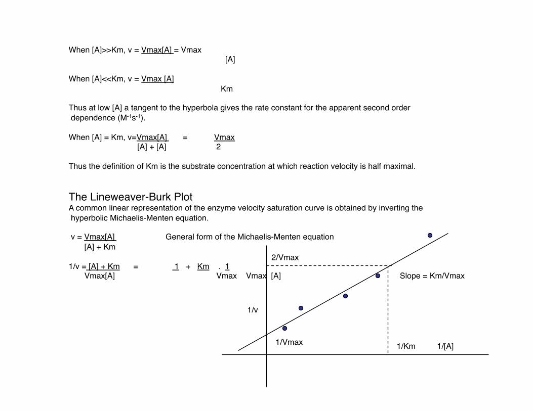
The Lineweaver-Burk Plot A common linear representation of the enzyme velocity saturation curve is obtained by inverting the hyperbolic Michaelis-Menten equation.

v = Vmax[A] General form of the Michaelis-Menten equation [A] + Km

1/v = [A] + Km = 1 + Km . 1 Vmax[A] Vmax Vmax [A]

1/v

1/[A] 1/Km

2/Vmax

Slope = Km/Vmax

1/Vmax

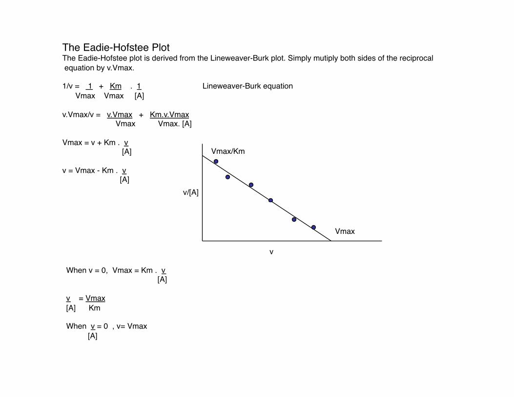
The Eadie-Hofstee Plot The Eadie-Hofstee plot is derived from the Lineweaver-Burk plot. Simply mutiply both sides of the reciprocal equation by v.Vmax.

1/v = 1 + Km . 1 Lineweaver-Burk equation Vmax Vmax [A]

v.Vmax/v = v.Vmax + Km.v.Vmax Vmax Vmax. [A]

Vmax = v + Km . v [A]

v = Vmax - Km . v [A]

v/[A]

v

Vmax/Km

Vmax

When v = 0, Vmax = Km . v [A]

v = Vmax [A] Km

When v = 0 , v= Vmax [A]

Definition of terms and units Vmax = k3[e] units are M s-1

Turnover number =TN= Vmax/[e] = kcat units are Ms-1/M = s-1 (k3)

Kcat/km = Vmax/[e]Km units are Ms-1/MM = M-1s-1

ie the units of a second order reaction. The expression kcat/Km is easily one of the most over-used expressions in biochemistry.

Some researchers refer to Kcat/Km as the “apparent second order rate constant that refers to the properties and the reactions of the free enzyme and free substrate”

It is often equated with the rate constant k1 for the formation of the EA complex.

Even for our simple case this is not true

Kcat/Km = k3k1/k2

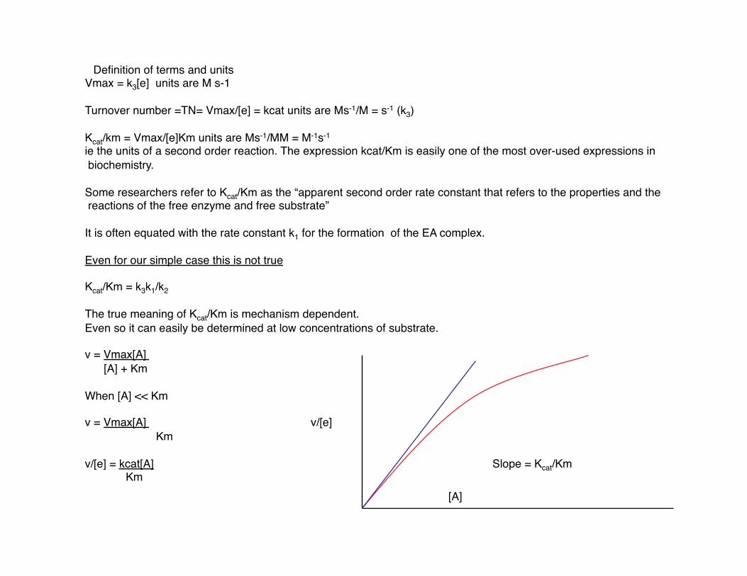
The true meaning of Kcat/Km is mechanism dependent. Even so it can easily be determined at low concentrations of substrate.

v = Vmax[A] [A] + Km

When [A] << Km

v = Vmax[A] v/[e] Km

v/[e] = kcat[A] Slope = Kcat/Km Km

[A]

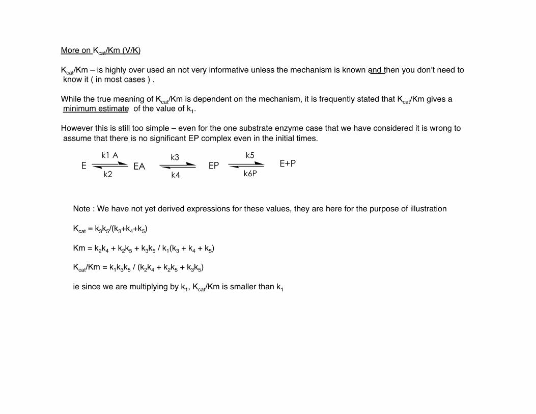
More on Kcat/Km (V/K)

Kcat/Km – is highly over used an not very informative unless the mechanism is known and then you donʼt need to know it ( in most cases ) .

While the true meaning of Kcat/Km is dependent on the mechanism, it is frequently stated that Kcat/Km gives a minimum estimate of the value of k1.

However this is still too simple – even for the one substrate enzyme case that we have considered it is wrong to assume that there is no significant EP complex even in the initial times.

E EA EP E+Pk1 A

k2 k4 k6P

k3 k5

Note : We have not yet derived expressions for these values, they are here for the purpose of illustration

Kcat = k3k5/(k3+k4+k5)

Km = k2k4 + k2k5 + k3k5 / k1(k3 + k4 + k5)

Kcat/Km = k1k3k5 / (k2k4 + k2k5 + k3k5)

ie since we are multiplying by k1, Kcat/Km is smaller than k1

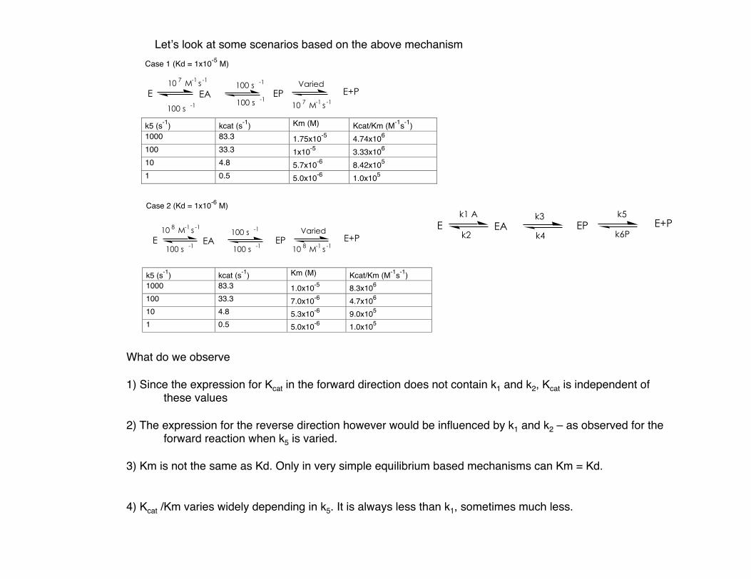
Case 1 (Kd = 1x10-5 M)

k5 (s-1) kcat (s-1) Km (M) Kcat/Km (M-1s-1)1000 83.3 1.75x10-5 4.74x106

100 33.3 1x10-5 3.33x106

10 4.8 5.7x10-6 8.42x105

1 0.5 5.0x10-6 1.0x105

E EA EP E+P10 7 M-1 s -1

100 s -1 100 s -110 7 M-1 s -1

100 s -1 Varied

Case 2 (Kd = 1x10-6 M)

k5 (s-1) kcat (s-1) Km (M) Kcat/Km (M-1s-1)1000 83.3 1.0x10-5 8.3x106

100 33.3 7.0x10-6 4.7x106

10 4.8 5.3x10-6 9.0x105

1 0.5 5.0x10-6 1.0x105

E EA EP E+P10 8 M-1 s -1

100 s -1 100 s -1 10 8 M-1 s -1

100 s -1 Varied

What do we observe

1) Since the expression for Kcat in the forward direction does not contain k1 and k2, Kcat is independent of these values

2) The expression for the reverse direction however would be influenced by k1 and k2 – as observed for the forward reaction when k5 is varied.

3) Km is not the same as Kd. Only in very simple equilibrium based mechanisms can Km = Kd.

4) Kcat /Km varies widely depending in k5. It is always less than k1, sometimes much less.

Letʼs look at some scenarios based on the above mechanism

E EA EP E+Pk1 A

k2 k4 k6P

k3 k5

0

50

100

150

200

250

0 20 40 60

[E] µM[A] µM[EA] µM[EP] µM[P] µM

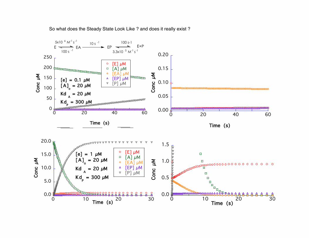
E EA EP E+P5x10 6 M-1 s -1

100 s -1

100 s-1

3.3x10 5 M-1 s-1

10 s -1

[e] = 0.1 µM[A]

o = 20 µM

Kd A = 20 µM

KdP = 300 µM

Conc

µM

Time (s)

So what does the Steady State Look Like ? and does it really exist ?

0.00

0.05

0.10

0.15

0.20

0 20 40 60

Conc

µM

Time (s)

0.0

5.0

10.0

15.0

20.0

0 10 20 30

[E] µM[A] µM[EA] µM[EP] µM[P] µM

Conc

µM

Time (s)

[e] = 1 µM[A]

o = 20 µM

Kd A = 20 µM

KdP = 300 µM

E EA EP E+P5x10 6 M-1 s -1

100 s -1

100 s-1

3.3x10 5 M-1 s-1

10 s -1

0.0

0.5

1.0

1.5

0 10 20 30

Conc

µM

Time (s)

0.0

5.0

10.0

15.0

20.0

0 10 20 30

[E] µM[A] µM[EA] µM[EP] µM[P] µM

Conc

µM

Time (s)

[e] = 1 µM[A]

o = 20 µM

Kd A = 20 µM

KdP = 300 µM

E EA EP E+P5x10 6 M-1 s -1

100 s -1

100 s-1

3.3x10 5 M-1 s-1

10 s -1

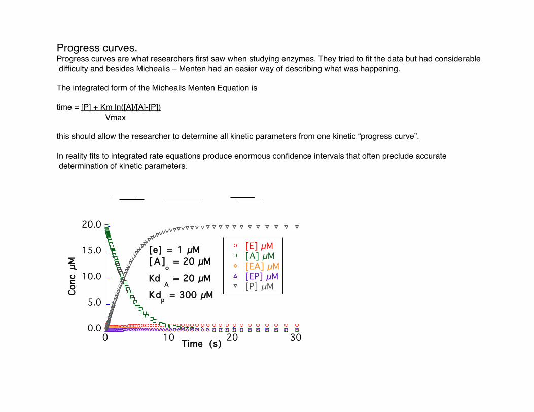
Progress curves. Progress curves are what researchers first saw when studying enzymes. They tried to fit the data but had considerable difficulty and besides Michealis – Menten had an easier way of describing what was happening.

The integrated form of the Michealis Menten Equation is

time = [P] + Km ln([A]/[A]-[P]) Vmax

this should allow the researcher to determine all kinetic parameters from one kinetic “progress curve”.

In reality fits to integrated rate equations produce enormous confidence intervals that often preclude accurate determination of kinetic parameters.

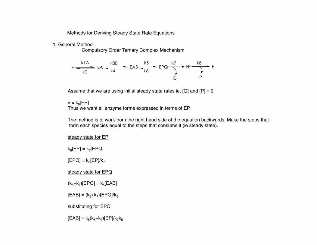
Methods for Deriving Steady State Rate Equations

1. General Method Compulsory Order Ternary Complex Mechanism

E EA EAB EPQ EP E

Q P

k1A

k2

k3B

k4

k5

k6

k7 k8

Assume that we are using initial steady state rates ie, [Q] and [P] = 0

v = k8[EP] Thus we want all enzyme forms expressed in terms of EP.

The method is to work from the right hand side of the equation backwards. Make the steps that form each species equal to the steps that consume it (ie steady state).

steady state for EP

k8[EP] = k7[EPQ]

[EPQ] = k8[EP]/k7

steady state for EPQ

(k6+k7)[EPQ] = k5[EAB]

[EAB] = (k6+k7)[EPQ]/k5

substituting for EPQ

[EAB] = k8(k6+k7)[EP]/k7k5

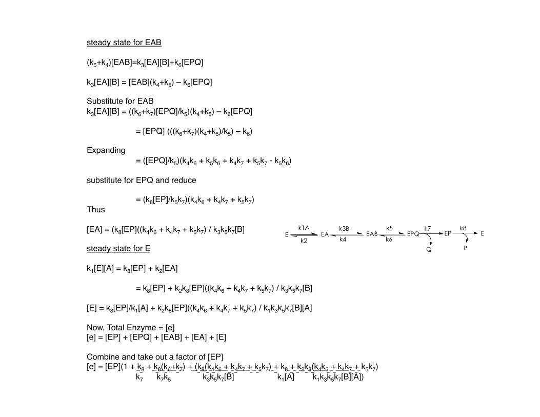
steady state for EAB

(k5+k4)[EAB]=k3[EA][B]+k6[EPQ]

k3[EA][B] = [EAB](k4+k5) – k6[EPQ]

Substitute for EAB k3[EA][B] = ((k6+k7)[EPQ]/k5)(k4+k5) – k6[EPQ]

= [EPQ] (((k6+k7)(k4+k5)/k5) – k6)

Expanding = ([EPQ]/k5)(k4k6 + k5k6 + k4k7 + k5k7 - k5k6)

substitute for EPQ and reduce

= (k8[EP]/k5k7)(k4k6 + k4k7 + k5k7) Thus

[EA] = (k8[EP]((k4k6 + k4k7 + k5k7) / k3k5k7[B]

steady state for E

k1[E][A] = k8[EP] + k2[EA]

= k8[EP] + k2k8[EP]((k4k6 + k4k7 + k5k7) / k3k5k7[B]

[E] = k8[EP]/k1[A] + k2k8[EP]((k4k6 + k4k7 + k5k7) / k1k3k5k7[B][A]

Now, Total Enzyme = [e] [e] = [EP] + [EPQ] + [EAB] + [EA] + [E]

Combine and take out a factor of [EP] [e] = [EP](1 + k8 + k8(k6+k7) + (k8(k4k6 + k4k7 + k5k7) + k8 + k2k8(k4k6 + k4k7 + k5k7) k7 k7k5 k3k5k7[B] k1[A] k1k3k5k7[B][A])

E EA EAB EPQ EP E

Q P

k1A

k2

k3B

k4

k5

k6

k7 k8

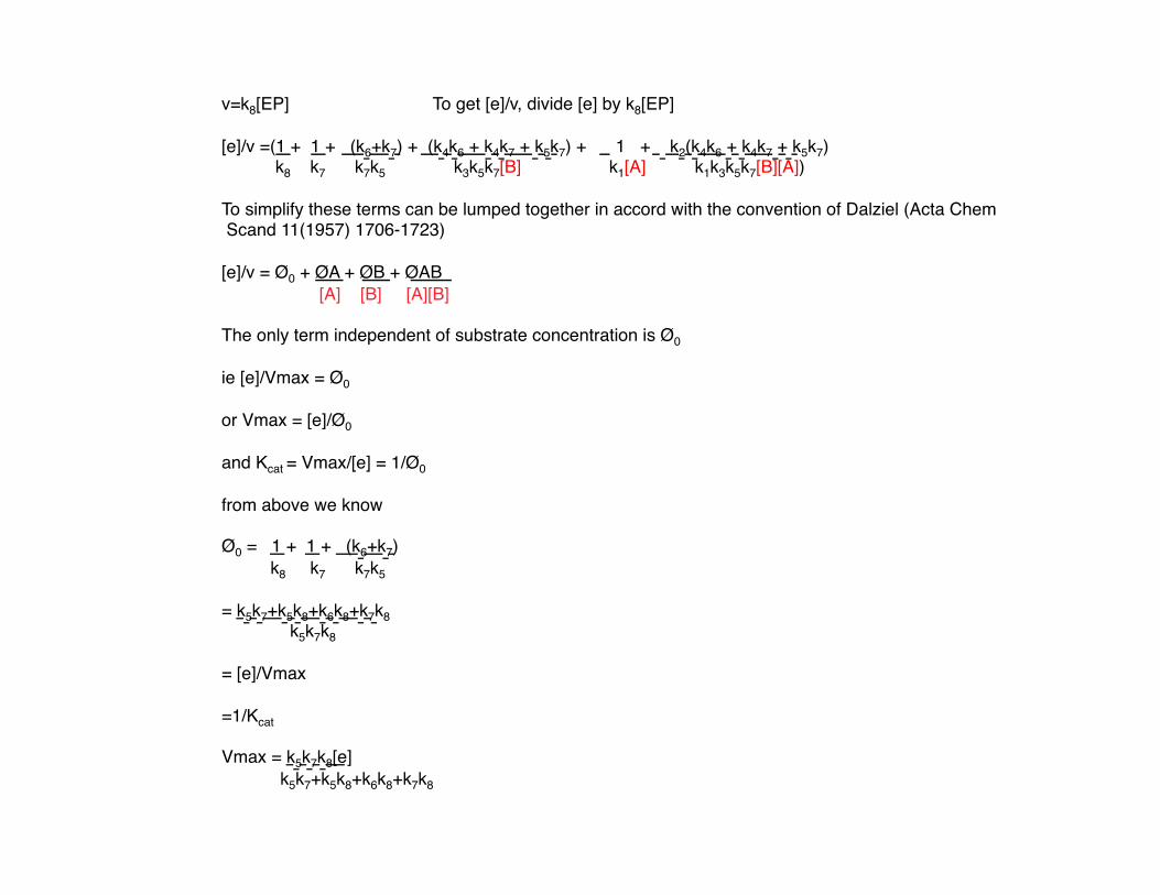
v=k8[EP] To get [e]/v, divide [e] by k8[EP]

[e]/v =(1 + 1 + (k6+k7) + (k4k6 + k4k7 + k5k7) + 1 + k2(k4k6 + k4k7 + k5k7) k8 k7 k7k5 k3k5k7[B] k1[A] k1k3k5k7[B][A])

To simplify these terms can be lumped together in accord with the convention of Dalziel (Acta Chem Scand 11(1957) 1706-1723)

[e]/v = Ø0 + ØA + ØB + ØAB [A] [B] [A][B]

The only term independent of substrate concentration is Ø0

ie [e]/Vmax = Ø0

or Vmax = [e]/Ø0

and Kcat = Vmax/[e] = 1/Ø0

from above we know

Ø0 = 1 + 1 + (k6+k7) k8 k7 k7k5

= k5k7+k5k8+k6k8+k7k8 k5k7k8

= [e]/Vmax

=1/Kcat

Vmax = k5k7k8[e] k5k7+k5k8+k6k8+k7k8

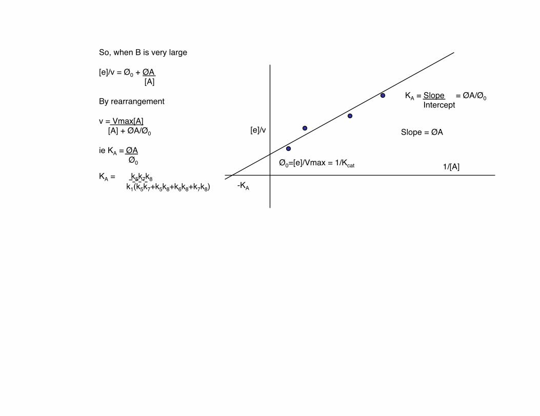
So, when B is very large

[e]/v = Ø0 + ØA [A]

By rearrangement

v = Vmax[A] [A] + ØA/Ø0

ie KA = ØA Ø0

KA = k5k7k8 k1(k5k7+k5k8+k6k8+k7k8)

[e]/v

1/[A]

KA = Slope = ØA/Ø0 Intercept

Ø0=[e]/Vmax = 1/Kcat

Slope = ØA

-KA

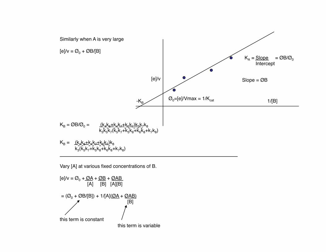
[e]/v

1/[B]

KA = Slope = ØB/Ø0 Intercept

Ø0=[e]/Vmax = 1/Kcat

Slope = ØB

Similarly when A is very large

[e]/v = Ø0 + ØB/[B]

KB = ØB/Ø0 = (k4k6+k4k7+k5k7)k5k7k8 k3k5k7(k5k7+k5k8+k6k8+k7k8)

KB = (k4k6+k4k7+k5k7)k8 k3(k5k7+k5k8+k6k8+k7k8)

Vary [A] at various fixed concentrations of B.

[e]/v = Ø0 + ØA + ØB + ØAB [A] [B] [A][B]

= (Ø0 + ØB/[B]) + 1/[A](ØA + ØAB) [B]

this term is constant this term is variable

-KB

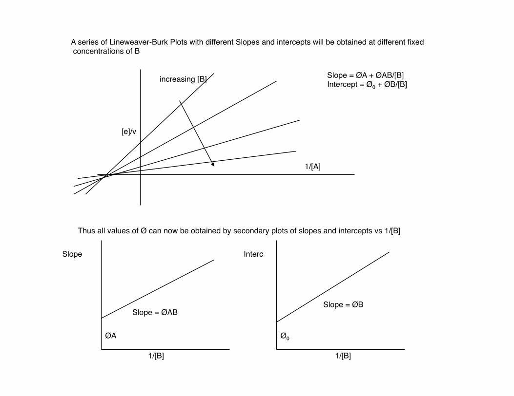
A series of Lineweaver-Burk Plots with different Slopes and intercepts will be obtained at different fixed concentrations of B

[e]/v

1/[A]

increasing [B] Slope = ØA + ØAB/[B] Intercept = Ø0 + ØB/[B]

Thus all values of Ø can now be obtained by secondary plots of slopes and intercepts vs 1/[B]

Slope Interc

1/[B] 1/[B]

Slope = ØABSlope = ØB

ØA Ø0