Embed Size (px)
Citation preview

January 4, 2001
Lectures on Geometry
Christer O. Kiselman
Contents:1. Introduction2. Closure operators and Galois correspondences3. Convex sets and functions4. Infimal convolution5. Convex duality: the Fenchel transformation6. The Monge–Kantorovich problem7. The Brunn–Minkowski inequality8. Non-convex sets9. Notions of topology
10. Smallest neighborhood spaces11. Digital Jordan curve theorems
References
1. IntroductionThese notes comprise the main part of a course presented at Uppsala University inthe Fall of 1999. (The original name of the course was Geometry and Analysis.) Myinitial idea was to present duality in geometry, or how to use analysis to solve geomet-ric problems. This I did, not dodging the more difficult aspects of this duality—seeTheorems 5.10 and 5.11 and the nasty Examples 5.7–5.9 and 5.12. A natural appli-cation was Kantorovich’s theorem, to which I found a new proof (Theorem 6.1). Alsoduality of sets which are not convex was considered (Section 8). Finally, my interestin image analysis led me to an attempt to survey some results in digital geometry;since existing proofs of Khalimsky’s Jordan curve theorem turned out to be difficultto present, I tried to find a simple one, which appears now in Section 11.
I am grateful to Bjorn Ivarsson for valuable criticism of an early draft of Section 2;to Thomas Kaijser for sharing his knowledge on the Monge–Kantorovich problem;and to Ingela Nystrom and Erik Palmgren for helpful comments on an early versionof Section 11.
2. Closure operators and Galois correspondencesAn order relation in a set X is a relation (a subset of X2) which satisfies threeconditions: it is reflexive, antisymmetric and transitive. This means, if we denote therelation by 6, that for all x, y, z ∈ X,
(2.1) x 6 x;
(2.2) x 6 y and y 6 x implies x = y;

2 C. O. Kiselman
(2.3) x 6 y and y 6 z implies x 6 z.
An ordered set is a set X together with an order relation. (Sometimes one sayspartially ordered set.)
A basic example is the set P (W ) of all subsets of a set W , with the order relationgiven by inclusion, thus A 6 B being defined as A ⊂ B for A,B ∈ P (W ).
A closure operator in an ordered set X is a mapping X 3 x 7→ x ∈ X which isexpanding, increasing (or order preserving), and idempotent ; in other words, whichsatisfies the following three conditions for all x, y ∈ X:
(2.4) x 6 x;
(2.5) x 6 y implies x 6 y;
(2.6) x = x.
In checking (2.6) it is of course enough to prove that x 6 x if we have alreadyproved (2.4).
The element x is said to be the closure of x. Elements x such that x = x arecalled closed (for this operator). An element is closed if and only if it is the closureof some element (and then it is the closure of itself).
A basic example of a closure operator is of course the topological closure operatorwhich associates to a set in a topological space its topological closure, i.e., the smallestclosed set containing the given set. In fact a closure operator in P (W ) defines atopology in W if and only if it satisfies, in addition to (2.4), (2.5), (2.6) above, twoextra conditions, viz. that Ø = Ø and
(2.7) A ∪B = A ∪B for all A,B ⊂W.Another closure operator of great importance is the operator which associates
to a set in Rn its convex hull, the smallest convex set containing the given set.In both these examples X is the power set of some set W , and the closure
operator is given as an intersection:
A =⋂
(Y ;Y is closed and Y ⊃ A).
More generally, if a closure operator x 7→ x is given and we denote by F the set ofits closed elements, then
(2.8) x = inf(y ∈ F ; y > x).
Conversely, any subset F of X such that the infimum of a subset of F always existsdefines a closure operator by formula (2.8).
A Galois correspondence is a pair (f, g) of two decreasing mappings f :X → Y ,g:Y → X of two given ordered sets X,Y such that g f and f g are expanding. Inother words we have f(x1) > f(x2) and g(y1) > g(y2) if x1 6 x2 and y1 6 y2, andg(f(x)) > x and f(g(y)) > y for all x ∈ X, y ∈ Y ; Kuros [1962:6:11].
The name Galois correspondence alludes to the first correspondence of that kind,established by Galois1 with X as the subsets of a field, Y as the sets of isomorphismsof this field, f(x) as the group of all isomorphisms leaving all elements of x invariant,and g(y) as the subfield the elements of which are left fixed by all elements of y.
1Evariste Galois, 1811–1832.

Lectures on Geometry 3
Proposition 2.1. Let f :X → Y , g:Y → X be a Galois correspondence. Theng f :X → X and f g:Y → Y are closure operators. Moreover, f g f = f andg f g = g.
Proof. That g f and f g are expanding is part of the definition of a Galois corre-spondence; that they are increasing follows from the fact that they are compositionsof two decreasing mappings. We know that f g is expanding, so (f g)(f(x)) > f(x);thus f g f > f . On the other hand, also g f is expanding, i.e., g f > idX , sof g f 6 f idX = f , hence f g f = f . By symmetry, g f g = g. From eitherone of these identities we easily obtain that g f and f g are idempotent.
It is now natural to ask whether the closure operators one obtains from Galoiscorrespondences have some special property. The answer is no: every closure operatorcomes in a trivial way from some Galois correspondence.
Proposition 2.2. Let x 7→ x be a closure operator defined in an ordered set X.Then there exist an ordered set Y and a Galois correspondence f :X → Y , g:Y → Xsuch that x = g(f(x)) for all x ∈ X.
Proof. We define Y as the set of all closed elements in X with the opposite order,thus y1 6Y y2 shall mean that y1 >X y2. Let f :X → Y and g:Y → X be defined byf(x) = x and g(y) = y. Then both f and g are decreasing, and g f(x) = x >X x,f g(y) = y >Y y. So g f and f g are expanding, and x = g(f(x)) as desired.
This proposition is, in a sense, completely uninteresting. This is because theGalois correspondence is obtained from X and the closure operator in a totally trivialway. However, there are many Galois correspondences in mathematics that are highlyinteresting and represent a given closure operator. This is because they allow forimportant calculations to be made or for new insights into the theory.
We now ask whether the composition of two closure operators is a closure oper-ator.
Example. Let A be the set of all points (x, y) in R2 satisfying y > 1/(1 + x2). Thisis a closed set, so A = A if we let the bar denote topological closure. The convexhull of A is the set cvxA = (x, y) ∈ R2; y > 0, which is not closed; its closure iscvxA = (x, y); y > 0. Hence we see that it is not true that the convex hull of aclosed set is closed; on the other hand we shall see that the closure of a convex setis convex. Define f(A) = cvxA and g(A) = A. Then the composition h = g f is aclosure operator, whereas the other composition k(A) = f g(A) = cvxA defines amapping k = f g which is not a closure operator (k k 6= k).
Proposition 2.3. Let f, g:X → X be two closure operators. The following propertiesare equivalent:(i) g f is a closure operator;(ii) g f is idempotent;(iii) g f g = g f ;(iv) f g f = g f ;(v) g(x) is f-closed if x is f-closed.If one of these conditions is satisfied, then g f is the supremum of the two closureoperators f and g in the ordered set of all closure operators; moreover f g 6 g f .

4 C. O. Kiselman
Proof. That h = g f is expanding and increasing is true for any composition ofexpanding and increasing mappings, so it is clear that (i) and (ii) are equivalent.It is also easy to see that (iv) and (v) are equivalent. If (iii) holds, then h h =g f g f = g f f = g f = h, so h is idempotent. Similarly, (iv) implies (ii).Conversely, if (ii) holds, then
g f 6 g f g 6 h h = h = g fand
g f 6 f g f 6 h h = h = g f,
so we must have equality all the way in both chains of inequalities, which proves that(iii) and (iv) hold. The last statement is easy to verify.
Corollary 2.4. Two closure operators f and g commute if and only if both g f andf g are closure operators.
Proof. If g f = f g, then (iii) obviously holds, so g f is a closure operator.Conversely, if g f is a closure operator, then (iii) applied to f and g says thatg f g = g f ; if also f g is a closure operator, then (iv) applied to g and f saysthat g f g = f g. Thus f and g commute.
When two closure operators f and g are given, it may happen that f 6 g. Thenthe semigroup generated by f and g consists of at most three elements, idX , f, g. Ifboth g f and f g are closure operators, then the semigroup generated by f and ghas at most four elements, idX , f, g, and g f = f g. If precisely one of g f andf g is a closure operator, then the semigroup generated has exactly five elements,idX , f, g, g f , and f g, of which four are closure operators. When none of g fand f g is a closure operator, the semigroup of all compositions fm · · · f1, withfj = f or fj = g, m ∈ N, may be finite or infinite.
Applying Proposition 2.3 to the case f(A) = cvxA, g(A) = A we see thatthe operation of taking the topological closure of the convex hull, A 7→ cvxA is aclosure operator. We call cvxA the closed convex hull of A. This is a case where thesemigroup generated by f and g consists of five elements.
Example. Let E be a finite-dimensional vector space over R and let E∗ denote itsdual. (We can think of Rn, but it is often clarifying to distinguish E and its dual.) Weshall define a Galois correspondence: the ordered set X shall be the power set of E,the set of all subsets of E, with inclusion as the order, and the set Y = [−∞,+∞]E
∗
shall be the set of all functions with values in the extended real line and defined onthe dual of E, the order being the opposite of the usual order, defined by set inclusionof the epigraphs, so that ϕ 6Y ψ iff ϕ(ξ) > ψ(ξ) for all ξ ∈ E∗; see Definition 3.10.Thus the constant +∞ is the smallest function, corresponding to vacuum, while −∞is the largest element, corresponding to an infinitely dense neutron star. We definemappings f :X → Y and g:Y → X as follows. Let HA denote the supporting functionof a subset A of E, i.e.,
HA(ξ) = supx∈A
ξ(x), ξ ∈ E∗.

Lectures on Geometry 5
Let f(A) = HA. To any function ϕ on E∗ with values in the extended real line[−∞,+∞] = R ∪ −∞,+∞ we associate a set
g(ϕ) =⋂ξ∈E∗x; ξ(x) 6 ϕ(ξ).
It is an intersection of closed half-spaces (including possibly the whole space and theempty set). Then both f and g are decreasing, and g f and f g are expanding asshown by the formulas
(g f)(A) =⋂ξ∈E∗x ∈ E; ξ(x) 6 HA(ξ) ⊃ A for all setsA,
(f g)(ϕ) = Hg(ϕ) >Y ϕ for all functions ϕ.
This is a highly interesting Galois correspondence. We shall determine its closedelements in Section 5.
3. Convex sets and functionsGiven two points a, b in a vector space E we define the segment between a and b asthe set
[a, b] = (1− t)a+ tb; 0 6 t 6 1.A subset A of E is said to be convex if it contains the whole segment [a, b] as soonit contains a and b. The convex subsets of the real line are precisely the intervals.The definition can therefore be given as follows: for any affine mapping ϕ: R → Ethe inverse image ϕ−1(A) shall be an interval.
The notion of a convex set has a sense in affine spaces, which, roughly speaking,are like vector spaces without a determined origin. In affine spaces sums like
∑λjxj
have a sense if and only if∑λj = 1, which is the case in the sums we need to work
with when considering convexity. If under this hypothesis we perform a translationby a vector a, then form the sum, and finally perform a translation by the vector −a,we get a result independent of the translation. Indeed,
∑λj(xj − a) + a =
∑λjxj .
The convex hull of a set X is the set
(3.1) cvxX =⋂Y
(Y ;Y is convex and contains X) ;
cf. (2.8). It is clear that cvxX is convex and that it is the smallest convex setcontaining X.
The description (3.1) of the convex hull is a description from the outside: weapproach the hull by convex sets containing it. There is also a description fromwithin:
Theorem 3.1. Let X be any subset of a vector space E. Then cvxX is the set ofall linear combinations
∑Nj=1 λjxj, where N is an arbitrary integer > 1, where the
points xj belong to X, and where the coefficients λj satisfy λj > 0,∑λj = 1.
The proof of this proposition is left to the reader; cf. Hiriart-Urruty & Lemarechal[1993: Prop. 1.3.4], Kiselman [1991a or b: Theorem 2.1], or Rockafellar [1970: The-orem 2.3].
The linear combinations that occur in the proposition are called convex combina-tions. (The requirement that N be at least 1 is important; thanks to this requirementwe obtain that the convex hull of the empty set is empty.)

6 C. O. Kiselman
Theorem 3.2 (Caratheodory’s2 theorem). Let X and E be as in Theorem 3.1 andassume that E is of finite dimension n. Then it is enough to take N in the represen-tation equal to n+ 1.For the proof of this result see Kiselman [1991a or b: Theorem 6.1] or Rockafellar[1970: Theorem 17.1]. In one and two dimensions, maybe even three, it is intuitivelyobvious.
Corollary 3.3. The convex hull of a compact subset of Rn is compact.
Proof. It is clear that for N = 1, 2, ... the set
KN =∑N
1 λjxj ;λj > 0,∑N
1 λj = 1
is compact, for it is the continuous image of a compact set under a continuous map-ping. In general, the convex hull of K is the union of all the KN , N > 1. But thanksto Caratheodory’s theorem, the sequence is stationary and the union of the sequenceis equal to Kn+1.
Theorem 3.4. The closure of a convex set in a topological vector space is convex;more generally, this is true in a vector space E equipped with a topology such that alltranslations x 7→ x− a, a ∈ E, and all dilations x 7→ λx, λ ∈ R, are continuous.
Proof. Suppose that A is convex and let a0, a1 ∈ A. We have to prove that [a0, a1] ⊂A. Consider a = (1 − t)a0 + ta1 for an arbitrary fixed t ∈ [0, 1], and let V be anarbitrary neighborhood of a. Then we can choose a neighborhood V0 of a0 suchthat (1 − t)V0 + ta1 ⊂ V . Since a0 belongs to the closure of A, there exists a pointb0 ∈ A∩V0. Next we can find a neighborhood V1 of a1 such that (1− t)b0 + tV1 ⊂ V .There exists a point b1 ∈ A∩V1. Hence the linear combination (1− t)b0 + tb1 belongsto A and since it also belongs to V , we have proved that V intersects A, thus thata ∈ A.
Thanks to this theorem we can state that cvxX is the smallest closed and convexset which contains X. The set is called the closed convex hull of X.
We shall now study the possibility of separating two convex sets by a hyperplane.A hyperplane is an affine subspace of codimension one; in other words it consists
of all solutions to a single linear equation ξ(x) = b, where ξ is a nonzero linearform on the space and where b is a real number. In general we need to distinguishbetween a general hyperplane, defined by a not necessarily continuous linear form onthe one hand, and a closed hyperplane, defined by a continuous linear form on theother hand. However, we shall restrict attention here to finite-dimensional spacesequipped with the unique separated vector space topology—when in the sequel weconsider a finite-dimensional vector space we shall always assume that it carries thistopology. For these finite-dimensional spaces all linear forms are continuous and allaffine subspaces closed. To every hyperplane we associate two closed half-spaces,D+ = x; ξ(x) > b and D− = x; ξ(x) 6 b. There is a choice to be made here,since −ξ(x) = −b defines the same hyperplane as ξ(x) = b.
We shall say that a hyperplane H = x; ξ(x) = b separates two subsets X andY of E if ξ(x) 6 b 6 ξ(y) for all x ∈ X and all y ∈ Y . We shall say that H separatesX and Y strictly if we have ξ(x) < b < ξ(y) for all x ∈ X and all y ∈ Y .
2Constantin Caratheodory, 1873–1950.

Lectures on Geometry 7
Theorem 3.5. Let F be a closed convex subset of a finite-dimensional vector spaceE, and y ∈ E a point which does not belong to F Then there exists a hyperplanewhich separates F and y strictly, even in the strong sense that for some numbersb0, b1 we have ξ(x) < b0 < b < b1 < ξ(y) for all x ∈ F .
Theorem 3.6. Let A be a convex subset of a finite-dimensional vector space E, andy ∈ E a point which does not belong to A or which belongs to the boundary of A.Then there exists a hyperplane which separates A and y.
Theorem 3.7. Let F and K be closed convex subsets of a finite-dimensional vectorspace E, and assume that they are disjoint and that K is compact. Then there existsa hyperplane which separates F and K strictly, even in the strong sense that for somenumbers b0, b1 we have ξ(x) < b0 < b < b1 < ξ(y) for all x ∈ F and all y ∈ K.
Theorem 3.8. Let X and Y be convex subsets of a finite-dimensional vector spaceE, and assume that they are disjoint. Then there exists a hyperplane which separatesX and Y .
Proof of Theorem 3.5. We may assume that y = 0. If F = Ø the result is certainlytrue, so we may assume that F is nonempty. Let d = infx∈F ‖x‖, where we usea Euclidean norm. Then d is positive, since F is closed, and d < +∞, since F isnonempty. Moreover, there exists a point a in (the possibly unbounded set) F wherethe infimum is attained. This is because the infimum over all of F is the same asthe infimum over the compact set K = x ∈ F ; ‖x‖ 6 2d. I claim that a · x > ‖a‖2for all x ∈ F . Study the function f(t) = ‖(1 − t)a + tx‖2, where x is a point inF . We must have f ′(0) > 0, for if f ′(0) were negative, f(t) would be smaller thanf(0) = d2 for small positive t contrary to the definition of d and a; note that allpoints (1− t)a+ tx with t ∈ [0, 1] belong to F . Now it is easy to calculate f ′:
f ′(t) = −2(1− t)‖a‖2 − 2ta · x+ 2(1− t)a · x+ 2t‖x‖2;
in particular f ′(0) = −2‖a‖2 + 2a · x. Since this quantity has to be nonnegative, wemust have a · x > a · a as claimed. Any hyperplane a · x = b with 0 < b < a · a is nowstrictly separating.Proof of Theorem 3.6. Let (aj)j∈N be a sequence which is dense in A. We applyTheorem 3.5 to the compact set Fm = cvxa0, ..., am, m ∈ N. If y does not belongto A, it does not belong to Fm either. If y belongs to the boundary of A, it maybelong to A, and some care is needed to avoid that y belongs to Fm. We can chooseym /∈ A such that ym tends to y and apply Theorem 3.5 to Fm and ym.
For every m there is a hyperplane ξm(x) = bm which separates ym and Fm. Wemay assume that ‖ξm‖ = 1. Then the sequence (bm) is also bounded, so there aresubsequences (ξmj )j and (bmj )j which converge to limits ξ and b respectively. Thehyperplane ξ(x) = b separates y from A.Proof of Theorem 3.7. The set F −K is closed and does not contain the origin. Ifξ(x) = b is a hyperplane which separates the origin from F −K in the strong senseindicated in Theorem 3.5, we know that 0 = ξ(0) < b0 < b < b1 < ξ(x − y) for allx ∈ F and all y ∈ K, so that
b1 6 infx∈F,y∈K
(ξ(x− y)) = infx∈F
ξ(x)− supy∈K
ξ(y),

8 C. O. Kiselman
implying that supK ξ + b1 6 infF ξ, an inequality which proves the theorem.Proof of Theorem 3.8. We observe that if X and Y are as in the theorem, thenA = X − Y does not contain the origin. We apply Theorem 3.6 and argue as in theproof of Theorem 3.7.
An immediate consequence of Theorem 3.5 is that every closed convex set isequal to the intersection of all the closed half-spaces which contain it. But the proofactually gives more: the half-spaces used to form the intersection can all be chosen sothat their boundaries contain a point of the given set. More precisely, we consideredthe largest open ball B(y, r) with center at y /∈ F which does not meet F and foundthat there is a unique point a common to its closure and F ; the tangent plane to theball at a is a separating hyperplane. A supporting half-space of a set A is a half-spaceD such that its boundary H (a hyperplane) contains a point of A. We also say in thissituation that H is a supporting hyperplane of A. Sometimes, to a given separatinghyperplane there is a parallel hyperplane which is supporting, but not always:Example. The set (x, y) ∈ R2; x > 0, xy > 1 is convex, and the hyperplaneH = (x, y); x = 0 lies in its complement, but there is no supporting hyperplaneparallel to H.
Theorem 3.9. Every closed convex set in a finite-dimensional vector space is equalto an intersection of closed, supporting half-spaces.
Proof. We just have to note that the half-space D = x; x · a > a · a found in theproof of Theorem 3.5 is indeed a supporting half-space: the point a lies both in Fand the hyperplane which bounds D.
Definition 3.10. Let f :X → [−∞,+∞] be a function defined on an arbitrary setX. Then its epigraph is the subset of X ×R defined as
epi f = (x, t) ∈ X ×R; t > f(x).
The strict epigraph is the set
epis f = (x, t) ∈ X ×R; t > f(x).
Definition 3.11. A function f :X → [−∞,+∞] defined on a subset X of a vectorspace E is said to be convex if its epigraph is a convex set in E ×R.It is equivalent to require that the strict epigraph be convex. We shall use thenotation CVX(X) for the set of all convex functions defined in a set X ⊂ E and withvalues in the extended real line [−∞,+∞].
If we extend f to a function g defined in all of E by putting g(x) equal to +∞outside X we see that the extended function is convex at the same time as f , sincethe two functions have the same epigraph. Therefore we may always assume (if welike) that convex functions are defined in the whole space.
The constants +∞ and −∞ are convex, since their epigraphs are, respectively,Ø and all of E. Furthermore, the maximum max(f1, ..., fm) of finitely many convexfunctions is convex, since its epigraph is the intersection of the convex sets epi fj .

Lectures on Geometry 9
However, if we want to prove for instance that the sum of two convex functions isconvex, it is convenient to have an inequality to test: the inequality which says thatthe graph hangs below the chord. Since convex functions may assume both +∞ and−∞ as values, we must handle undefined sums like (+∞)+(−∞). It is convenient tointroduce upper addition +· and lower addition +· . These operations are extensionsof the usual addition R × R 3 (x, y) 7→ x + y ∈ R. We define without hesitation(+∞) + (+∞) = +∞, (−∞) + (−∞) = −∞, and use these definitions for both +·
and +· . In the ambiguous cases we define
(3.2) (+∞) +· (−∞) = +∞, (+∞) +· (−∞) = −∞.
Upper addition defines an upper semicontinuous function [−∞,+∞]2 → [−∞,+∞],and, similarly, lower addition a lower semicontinuous mapping.
Very useful rules for computing infima and suprema are
(3.3) infx∈X
(a+· f(x)) = a+· infx∈X
f(x), supx∈X
(a+· f(x)) = a+· supx∈X
f(x),
which are valid without exception. The proof of (3.3) consists in checking the equal-ities for a = +∞,−∞ and X empty.
Proposition 3.12. Let E be a vector space. A function f :E → [−∞,+∞] is convexif and only if
f((1− t)x0 + tx1
)6 (1− t)f(x0) +· tf(x1)
for all x0, x1 ∈ E and all numbers t with 0 < t < 1.We leave the simple proof as an exercise.
The proposition implies that the values of a convex function must satisfy aninfinity of inequalities, and in general that means that the values are severely re-stricted. However, note that this is not always the case. As an example consider afunction which is +∞ for ‖x‖ > 1 and −∞ for ‖x‖ < 1. Such a function is convexirrespective of its values on the unit sphere ‖x‖ = 1. This phenomenon is related tothe fact that all sets A containing the open unit ball and contained in the closed unitball are convex. (Of course in these examples we need Euclidean norms, or at leaststrictly convex norms.) We shall exploit this phenomenon in Section 8.
The effective domain of a function f :X → [−∞,+∞] is the set where it issmaller than plus infinity:
(3.4) dom f = x ∈ X; f(x) < +∞.
If f is convex, so is its effective domain.
Theorem 3.13. Let E be a finite-dimensional vector space, let f :E → [−∞,+∞]be a convex function and define Ω = (dom f). (Thus Ω is the interior of the setwhere the function is less than plus infinity.) Then Ω is convex and the restriction off to Ω is either equal to the constant −∞ or else a real-valued continuous function.We leave the proof as an exercise. See Kiselman [1991a or b, Theorem 9.5].

10 C. O. Kiselman
Corollary 3.14. Let f and Ω be as in the theorem and suppose that there exists apoint x ∈ Ω such that f(x) is real. Then there exists a linear functional ξ on E suchthat ξ(x) 6 f(x) for all x ∈ E. Moreover, g(x) = lim infy→x f(y) is convex and doesnot take the value −∞ if f > −∞. We have g = f except on ∂Ω.In analogy with (3.1) we define the convex hull of a function as the largest convexminorant of the function:
(3.5) cvx f = sup(g ∈ CVX(E); g 6 f).
This is the approach from below. There is also an approach from above, as in Theorem3.1:
Theorem 3.15. Let f :E → [−∞,+∞] be any function on a vector space E. Thenits convex hull is given as an infimum of linear combination of values of f :
(3.6) cvx f(x) = inf[ N∑
1
λjf(xj);N > 1, λj > 0,N∑1
λj = 1,N∑1
λjxj = x
], x ∈ E.
The proof is analogous to that of Theorem 3.1.When f is positively homogeneous, i.e., f(tx) = tf(x) for all t > 0 and all x ∈ E,
then (3.6) can be simplified to
(3.7) cvx f(x) = inf[ N∑
1
f(xj);N > 1,N∑1
xj = x
], x ∈ E.
4. Infimal convolution
Definition 4.1. Let G be an abelian group and let f, g:G → [−∞,+∞] be twofunctions defined on G and with values in the extended real axis. Then their infimalconvolution f ut g is defined by
(4.1) (f ut g)(x) = infy∈G
(f(y) +· g(x− y)
), x ∈ G.
Often we take G = Rn, but it is important to note that the definition works in anyabelian group G. In image analysis Z2 and, more generally, Zn are very commongroups.
Points outside dom f and dom g play no role in (4.1). This is in accordance withthe interpretation already mentioned of the constant +∞ as vacuum and of −∞ asan infinitely dense neutron star. Think of e−f as a particle—there is an interestinganalogy between infimal convolution of f and g and ordinary convolution of e−f ande−g; see Kiselman [1999a or b, Chapters 8 and 9].
Infimal convolution generalizes vector addition (Minkowski addition) of sets. IfX and Y are subsets of G we have
(4.2) iX ut iY = iX+Y ,

Lectures on Geometry 11
where iX denotes the indicator function of the set X; it takes the value 0 in X and+∞ in its complement.
Another important relation to vector addition—a relation which can actuallyserve to define infimal convolution—is
(4.3) epis(f ut g) = epis(f) + epis(g),
where the plus sign denotes vector addition in G × R. This equation leads to ageometric interpretation of infimal convolution.
For a thorough study of infimal convolution, see Stromberg [1996].
Proposition 4.2. The infimal convolution is commutative and associative.
Proof. Since vector addition is commutative and associative, the same is true forinfimal convolution in view of (4.3).
Thanks to this proposition we can define generally f1 ut · · · ut fm; no paranthesesare needed. It is easy to see that
(4.4) dom(f1 ut · · · ut fm) = dom f1 + · · ·+ dom fm.
Example. The function i0 is the neutral element for infimal convolution: f ut i0 =f for all functions f .Example. If g:G→ R is additive, then f ut g = g +C for some constant C = Cf,g ∈[−∞,+∞]. Actually Cf,g = (f ut g)(0).Example. Define gk(x) = k‖x‖ on a normed space E with norm ‖·‖, with k a positiveconstant. Study the infimal convolution fk = f ut gk. Assuming that f is boundedwe see that fk is Lipschitz continuous. Moreover fk f as k → +∞ if f is boundedand lower semicontinuous.
Let us say that a function f :G → [−∞,+∞] is subadditive if it satisfies theinequality f(x+ y) 6 f(x) +· f(y), x, y ∈ G.
Proposition 4.3. A function f :G → [−∞,+∞] defined on an abelian group G issubadditive if and only if it satisfies the inequality f ut f > f . If in addition weassume that f(0) 6 0, then this is equivalent to f ut f = f .
Proof. If f is subadditive we have f(x − y) +· f(y) > f(x), so taking the infimumover all y ∈ G gives f ut f > f . Conversely, we have
f(x) +· f(y) > (f ut f)(x+ y),
so f ut f > f implies subadditivity. Finally, since the inequality (f ut f)(x) 6f(x) +· f(0) always holds, we conclude that f(0) 6 0 implies f ut f 6 f .
Theorem 4.4. If f and g are subadditive, then so is f ut g.
Proof. Using the associativity and commutativity of infimal convolution we can write
(f ut g) ut (f ut g) = (f ut f) ut (g ut g) > f ut g.

12 C. O. Kiselman
Subadditive functions are of interest because of their relation to metrics onabelian groups, a fact which we shall discuss now.
Let us call a function d:X ×X → R a distance if it is positive definite, i.e., forall x, y ∈ X,
d(x, y) > 0 with equality precisely when x = y,
and symmetric, i.e.,d(x, y) = d(y, x), x, y ∈ X.
We shall say that a distance is a metric if it satisfies in addition the triangle inequality,i.e.,
d(x, z) 6 d(x, y) + d(y, z), x, y, z ∈ X.
If X = G is an abelian group, translation-invariant distances are of interest, i.e.,those that satisfy
d(x− a, y − a) = d(x, y), a, x, y ∈ G.
Lemma 4.5. Any translation-invariant distance on an abelian group G defines afunction f(x) = d(x, 0) on G which is positive definite,
f(x) > 0 with equality precisely when x = 0;
and symmetric,f(−x) = f(x), x ∈ X.
Conversely, a function f which is positive definite and symmetric defines a trans-lation-invariant distance d(x, y) = f(x− y).The proof is easy.
Lemma 4.6. Let d be a translation-invariant distance on an abelian group G andf(x) = d(x, 0). Then d is a metric if and only if f is subadditive,
f(x+ y) 6 f(x) + f(y), x, y ∈ G.
Proof. If d is a metric, we can write, using the triangle inequality and the translationinvariance,
f(x+ y) = d(x+ y, 0) 6 d(x+ y, y) + d(y, 0) = d(x, 0) + d(y, 0) = f(x) + f(y).
Conversely, if f is subadditive,
d(x, z) = f(x− z) 6 f(x− y) + f(y − z) = d(x, y) + d(y, z).
Theorem 4.7 (Kiselman [1996]). Let F :G → [0,+∞] be a function on an abeliangroup G satisfying F (0) = 0. Define a sequence of functions (Fj)∞j=1 by puttingF1 = F and Fj = Fj−1 ut F , j = 2, 3, ... . Then the sequence (Fj) is decreasing andits limit limFj = f is subadditive. Moreover dom f = N · domF , i.e., f is finiteprecisely in the semigroup generated by domF .

Lectures on Geometry 13
Proof. That the sequence is decreasing is obvious if we take y = 0 in the definitionof Fj+1:
Fj+1(x) = infy
(Fj(x− y) + F (y)) 6 Fj(x) + F (0) = Fj(x).
Next we shall prove that f(x+ y) 6 f(x) + f(y). If one of f(x) and f(y) is equal to+∞, there is nothing to prove, so let us assume that f(x), f(y) < +∞ and let us fixa positive number ε. Then there exists numbers j and k such that Fj(x) 6 f(x) + εand Fk(y) 6 f(y) + ε. By associativity Fj+k = Fj ut Fk, so we get
f(x+ y) 6 Fj+k(x+ y) 6 Fj(x) + Fk(y) 6 f(x) + f(y) + 2ε.
Since ε is arbitrary, the inequality f(x+y) 6 f(x)+f(y) follows. The last statementfollows from (4.4).
In image analysis it is customary to define distances between adjacent points andthen extend the definition to arbitrary pairs of points by going on a path, assigning toeach path the sum of the distances between the adjacent points, and finally taking theinfimum over all paths. In the translation-invariant case, this amounts to assigningvalues to a function F at finitely many points, and then define the distance by thefunction f = limFj of Theorem 4.7. (Of course some extra conditions are needed toensure that the limit is symmetric and positive definite.) Indeed the paths consistsof segments [0, x1], [x1, x1 + x2],..., [x + · · · + xk−1, x] and we evaluate the sumF (x1) + F (x2) + · · ·+ F (xk) for all possible choices of x1, ..., xk with sum x.
Examples of such functions are the following. We always define F (0) = 0 andlet F (x) < +∞ for x in a finite set P only. The following distances have beenstudied, assuming P and F to be invariant under permutation and reflection of thecoordinates. If we take P = x ∈ Z2;
∑|xj | 6 1 and F (1, 0) = 1 we get the city-
block distance, also called l1. If we let P = x ∈ Z2; |xj | 6 1 and F (1, 0) = F (1, 1) =1 we get the chess-board metric, or l∞ distance. Other choices are F (1, 0) = a,F (1, 1) = b with (a, b) = (1,
√2), (2, 3), (3, 4). We can also increase the size of P and
define G(1, 0) = 5, G(1, 1) = 7, G(2, 1) = 11. For references to the work mentionedhere see Kiselman [1996].
Proposition 4.8. Let f :E → [−∞,+∞] be a function defined on a vector space Eand define fs by fs(x) = sf(x/s), x ∈ E, s ∈ Rr 0. Then f is convex if and onlyif fs ut ft > fs+t for all s, t > 0, and if and only if fs ut ft = fs+t for all s, t > 0.
Proof. We note that the inequality fs ut ft 6 fs+t always holds, so the two lastproperties are indeed equivalent, and the convex functions are those that satisfythe functional equation fs ut ft = fs+t; in other words the mapping s 7→ fs is ahomomorphism of semigroups.
If f is convex, we can write
fs(y) +· ft(x− y) = sf(y/s) +· tf((x− y)/t) > (s+ t)f( y
s+ t+x− ys+ t
)= fs+t(x).
If we now vary y we obtain fs ut ft > fs+t. Conversely, suppose that this inequalityholds. Then we obtain, writing xt = (1− t)x0 + tx1, that
f(xt) = f1(xt) 6 (f1−t ut ft)(xt) 6 f1−t(y) +· ft(xt − y)

14 C. O. Kiselman
for every y. We now choose y = (1− t)x0 and get
f(xt) 6 f1−t((1− t)x0) +· ft(xt − (1− t)x0) = (1− t)f(x0) +· tf(x1),
which means that f is convex.
Theorem 4.9. If f and g are convex, then so is f ut g.
Proof. It is easy to verify that (f ut g)s = fs ut gs. We now perform a calculation likethat in the proof of Theorem 4.4:
(f ut g)s ut (f ut g)t = (fs ut gs) ut (ft ut gt) = (fs ut ft) ut (gs ut gt)> fs+t ut gs+t = (f ut g)s+t.
Thus f ut g satisfies the criterion of Proposition 4.8 and so is convex.
For a positively homogeneous function convexity is equivalent to subadditivity.This observation will yield a nice formula for the supporting function of the inter-section of two closed convex sets, see formula (5.9). Here we note the following easyresult.
Proposition 4.10. Let f, g be two positively homogeneous convex functions. Thenf ut g is the convex hull of their minimum:
(4.5) cvx(min(f, g)) = f ut g.
Proof. We always have f ut g 6 f , f ut g 6 g since f(0), g(0) 6 0. If h is convex andpositively homogeneous and h 6 f, g, then h = h ut h 6 f ut g. Thus f ut g is thelargest positively homogeneous convex minorant of min(f, g). However, it is easy tosee that it is also the largest convex minorant of min(f, g), whence (4.5).
5. Convex duality: the Fenchel transformationThe affine functions x 7→ ξ(x) + c, where ξ is a linear form and c a real constant, arethe simplest convex functions. It is natural to ask whether all convex functions can besomehow represented in terms of these simple functions. The question is analogousto the problem of representing an arbitrary function in Fourier analysis in terms ofthe simplest functions, the pure oscillations. The Fenchel transformation, which weshall introduce now, plays a role in convexity theory analogous to that of the Fouriertransformation in Fourier analysis.
More precisely we ask whether, given a function f on a vector space E, thereexists a subset A of E∗ ×R such that
(5.1) f(x) = sup(ξ,c)∈A
(ξ(x) + c
), x ∈ E.
Here E∗ denotes the algebraic dual of E, i.e., the vector space of all linear formson E. We first note that if this is at all possible, then c 6 f(x) − ξ(x) for allx ∈ E and all (ξ, c) ∈ A, so that c 6 infx∈E(f(x) − ξ(x)). For reasons which will

Lectures on Geometry 15
be apparent in a moment, it is convenient to consider instead −c; we must have−c > supx∈E(ξ(x)− f(x)) for all (ξ, c) ∈ A. We define
(5.2) f(ξ) = supx∈E
(ξ(x)− f(x)
), ξ ∈ E∗.
The function f is called the Fenchel3 transform of f . Other names are the Legendre4
transform of f and the function conjugate to f . Since the constant c in (5.1) mustsatisfy c 6 −f(ξ), and since f(x) > ξ(x)− f(ξ) for all x ∈ E and all ξ ∈ E∗, we canconclude that (5.1) implies
f(x) = supξ∈E∗
(ξ(x)− f(ξ)
), x ∈ E.
In other words, the supremum in (5.1) does not change if we add points outside Aand replace c everywhere by −f(ξ).
Now the right-hand side of this formula looks like (5.2), so it is natural to applythe transformation a second time. It is convenient here to consider an arbitrary vectorsubspace F of E∗, and to introduce topologies on E and F as follows. There is aweakest topology on E such that all elements of F are continuous; this is denoted byσ(E,F ). There is similarly a weakest topology σ(F,E) on F such that all evaluationmappings F 3 ξ 7→ ξ(x), x ∈ E, are continuous. We may for instance choose F = E∗,or F = E′, the topological dual of E under a given topology, i.e., the space of allcontinuous linear forms on E. Actually E∗ is the topological dual of E equippedwith the topology σ(E,E∗). Thus, when we speak about the topological dual in thesequel, the case of the algebraic dual is always included as a special case. If E isfinite-dimensional and we equip it with the separated vector space topology, thenE′ = E∗. If E is a normed space of infinite dimension, we always have E′ 6= E∗. Itis not necessary that E and F be in duality; we may even choose F = 0.
The Fenchel transform of a function g on F is of course a function on the algebraicdual F ∗ of F :
(5.3) g(X) = supξ∈F
(X(ξ)− g(ξ)
), X ∈ F ∗.
Given any element x of E we define an element X of F ∗ by the formula X(ξ) = ξ(x),ξ ∈ F . Using this idea we may define for any function g on F ,
(5.4) g(x) = supξ∈F
(ξ(x)− g(ξ)
), x ∈ E.
We also note that f ut ξ is an affine function and that in fact (f ut ξ)(x) =ξ(x) − f(ξ) for all x ∈ E and all ξ ∈ E∗. The function f ut ξ is a minorant of fand in fact the largest affine minorant of f which has linear part equal to ξ. So thesupremum of all affine minorants of f with linear part in F is
supξ∈F
(ξ(x)− f(ξ)) = supξ∈F
(f ut ξ)(x) = ˜f(x), x ∈ E.
3Werner Fenchel, 1905–1988.4Adrien Marie Legendre, 1752–1833.

16 C. O. Kiselman
The question whether (5.1) holds for A = F × R can therefore be formulated
very succintly: is it true that ˜f = f? However, it might still be of interest to find asmaller A for which (5.1) holds.
From the definition of f we immediately obtain the inequality
(5.5) ξ(x) 6 f(x) +· f(ξ), x ∈ E, ξ ∈ E∗,
called Fenchel’s inequality. It can be stated equivalently as
ξ(x)− f(ξ) 6 f(x), x ∈ E, ξ ∈ E∗.
If f is the indicator function of a set A, f = iA, then f = HA, the supportingfunction of A. So the question about closed elements for the Galois correspondencestudied in the example after Proposition 2.3 will be answered in the more generalframework of Fenchel transforms.
We summarize the properties of the Fenchel transformation that we have foundso far.
Proposition 5.1. The Fenchel transformations defined by (5.2) and (5.4) for func-tions on a vector space E and a subspace F of its algebraic dual form a Galoiscorrespondence, the order of the functions being that of inclusion of their epigraphs.Thus, in terms of the usual order between functions, f 6 g implies f > g, the second
transform satisfies ˜f 6 f , and the third transform is equal to the first,(f)˜ = f .
All Fenchel transforms are convex, lower semicontinuous with respect to the topologyσ(E,F ) or σ(F,E), and take the value −∞ only when they are identically −∞.
Proof. Only the last statement does not follow from general properties of Galoiscorrespondences; cf. Proposition 2.1. A supremum of a family of convex functions isconvex, in particular so is f . Also the supremum of a family of lower semicontinuousfunctions is lower semicontinuous. The last property is obvious: if a Fenchel transformf assumes the value −∞ for a particular ξ, then f must be equal to +∞ identically,and so f is equal to −∞ identically.
For examples of Fenchel transforms, see for instance Kiselman [1991a or b].
Proposition 5.2. For any function f :E → [−∞,+∞] on a finite-dimensional vectorspace the following three conditions are equivalent:
1. f is lower semicontinuous, i.e., lim infy→x f(y) = f(x) for all x ∈ E;2. epi f is closed in E ×R;3. For every real number a the sublevel set x ∈ E; f(x) 6 a is closed in E.
We leave the proof as an exercise.
Theorem 5.3. Let a function f :E → [−∞,+∞] on a finite-dimensional vectorspace E be given. Then the following properties are equivalent:(A) f is a Fenchel transform;(B) f is equal to the supremum of all its affine minorants;(C) f is equal to the supremum of some family of affine functions;(D) f is convex, lower semicontinuous, and takes the value −∞ only if it is identicallyequal to −∞.

Lectures on Geometry 17
Proof. From Proposition 5.1 and the discussion preceding it is clear that (A), (B),and (C) are all equivalent, and that they imply (D). We need to prove that (D)implies (B), say.
Let us first note that (B) certainly holds if f is either +∞ or −∞. We maytherefore suppose that epi f is nonempty and not equal to the whole space.
We shall prove, assuming that (D) holds, that for any point x0 the supremumof all affine minorants of f is equal to f(x0); equivalently, that for any point (x0, t0)not in the epigraph of f there is an affine function which takes a value greater thant0 at x0. Since (x0, t0) /∈ epi f there is a supporting half-space containing epi f andnot containing (x0, t0). Such a half-space in E ×R is defined by an inequality
ξ(x) + bt > c
for some ξ ∈ E′ and some real numbers b, c. Since the half-space is supporting, weknow that there is some point (x1, t1) ∈ epi f which satisfies ξ(x1)+bt1 = c. If b < 0,the half-space is the epigraph of an affine function, and since its value at x0 is largerthan t0, we are done. If b > 0, the half-space is the hypograph of an affine function,and it can contain epi f only if the latter is empty, i.e., f = +∞ identically, a case wealready considered. Thus only the case b = 0, that of a vertical half-space, remainsto be considered. A vertical hyperplane is not the graph of an affine function, andwe need to prove that these vertical hyperplanes, although they can occur, do notinfluence the intersection of all supporting half-spaces.
Thus we have a point (x0, t0) not belonging to epi f and a vertical half-space(x, t) ∈ E × R; ξ(x) > c which contains epi f and is such that the closest point(x1, t1) in epi f lies in the boundary of the half-space. Then this point must have thesame t-coordinate as (x0, t0), so t1 = t0. Since (x1, t1) belongs to epi f , the value t2of f at x1 must satisfy −∞ < t2 = f(x1) 6 t1 = t0. It is now clear that the closestpoint in epi f to the point (x0, t2) is (x1, t2) and that the hyperplane obtained fromour construction is the same, ξ(x) > c = ξ(x1). But for points (x0, t3) with t3 < t2the supporting hyperplane cannot be vertical. Even more interesting is the fact thatthe supporting hyperplane has a large slope when t3 is close to t2. Consider thelargest open ball which does not meet epi f and has its center at (x0, t3). Its closurecontains a single point of epi f ; denote that point by (x2, t4) and let R be the radiusof the ball. We must have t4 > t3. The tangent plane to the ball at (x2, t4) intersectsthe line x = x0 at a point (x0, t3 + T ), where T = R2/(t4 − t3). Since (x1, t3) doesnot belong to epi f we must have R > ‖x1 − x0‖ and t4 > t3. On the other hand
R =√‖x2 − x0‖2 + (t4 − t3)2 6
√‖x1 − x0‖2 + (t2 − t3)2,
since (x2, t4) is the point in epi f closest to (x0, t3) and (x1, t2) is a point in epi f .Now ‖x2 − x0‖ > ‖x1 − x0‖, so
(t4 − t3)2 6 ‖x1 − x0‖2 + (t2 − t3)2 − ‖x2 − x0‖2 < (t2 − t3)2.
Thus 0 < t4 − t3 < t2 − t3. The value at x0 of the affine function defined by thetangent plane is t3 + T and tends to plus infinity as t3 t2 since
T =R2
t4 − t3>‖x1 − x0‖2
t2 − t3;

18 C. O. Kiselman
in particular t3 + T is larger than t0 for some t3 close to t2. This proves that theintersection of all supporting half-spaces is not affected if we remove the verticalhalf-spaces and completes the proof of the theorem.
We now know that the closed elements for the Galois correspondence defined inProposition 5.1 consists of the functions satisfying condition (D) of Theorem 5.3. Anindicator function iA is closed if and only if the set A is closed and convex. Underthe Fenchel transformation these functions are in bijective correspondence with thesupporting functions of closed convex sets.
The supporting function mapping A 7→ HA embeds the semigroup of all non-empty compact convex subsets of a vector space E into the group of real-valuedfunctions on E′. Thus for instance the equation A + X = B, which for nonemptycompact convex sets is equivalent to HA + HX = HB , can sometimes be solved bya set X, viz. when HX = HB − HA is convex. For applications of the supportingfunction in image analysis, see Ghosh & Kumar [1998].
Next we shall study the relation between infimal convolution and the Fencheltransformation. The first result is very easy.
Proposition 5.4. For all functions f, g: Rn → [−∞,+∞] we have
(5.6) (f ut g)˜ = f +· g.
In particular, if we take f = iX , g = iY with arbitrary sets X and Y ,
(5.7) HX+Y = (iX ut iY )˜ = HX +· HY .
Proof. An easy calculation thanks to the rule (3.3).
We note that we have lower addition in (5.6). We know that f +· g is convex.However, it turns out that f +· g = f +· g except when f +· g is the constant−∞. Thus
also f +· g is convex. In (5.7) we can write HX+HY without risk of misunderstandingif X and Y are nonempty.
Corollary 5.5. If ˜f = f and ˜g = g, then
(5.8) (f +· g)˜ = (f ut g)˜.In particular, taking f = iX , g = iY with X and Y closed and convex we have
(5.9) HX∩Y = (iX + iY )˜ = (HX ut HY )˜ = (min(HX ,HY ))˜,and, taking f = HX , g = HY with X and Y closed and convex,
(5.10) (HX +· HY )˜ = (iX ut iY )˜ = (iX+Y )˜ = iX+Y .
Proof. The proof consists of a straightforward application of the proposition, exceptfor the last equality in (5.10), which follows from Theorem 5.3.

Lectures on Geometry 19
More generally, we can obtain the supporting function of an intersection X =⋂i∈I Xi of closed convex sets Xi, i ∈ I, as
(5.11) HX =[
cvx(
infi∈I
HXi
)]˜ =(
infi∈I
HXi
)˜.Theorem 5.6. Suppose that ˜f = f , ˜g = g and that f ut g is lower semicontinuousand either nowhere minus infinity or else identically minus infinity. Then
(5.12) (f +· g)˜ = f ut g.
In particular we can take the value at the origin of both sides and obtain
(5.13) − infx
(f(x) +· g(x)) = infξ
(f(ξ) +· g(−ξ)).
Proof. For the proof we only need to combine Corollary 5.5 with Theorem 5.3.
If (5.12) holds, then f ut g is of course lower semicontinuous, so in this respectthe result cannot be improved, but it is unpleasant to have lower semicontinuity as anassumption to be verified. Formula (5.12) can be obtained from (5.13) by translation.
We remark that the assumption on f ut g is satisfied if the function is real-valuedeverywhere, for such functions are automatically continuous as shown by Theorem3.13. However, in applications it is important to allow the value +∞.
There are important cases when (5.12) does not hold.
Example 5.7. Let f = iX and g = iY (then X and Y are automatically closed andconvex). Then f ut g = iX+Y and Theorem 5.3 shows that
(f ut g
) ˜ = iX+Y , theindicator function of the closure of the convex set X + Y . However, X + Y is notnecessarily closed. A simple example is
X = x ∈ R2; x2 > 0, x1x2 > 1, Y = x ∈ R2; x2 = 0,
X + Y = x ∈ R2; x2 > 0, X + Y = x ∈ R2; x2 > 0.
Then f ut g 6=(f ut g
) ˜. The formula (5.12) does not hold.
Example 5.8. Define two functions f, g: R2 → [0,+∞] by
f(x) =
0, x1 6 −1,+∞, otherwise;
g(x) =
0, x1 > 1,+∞, otherwise.
Thus f = iX , g = iY where X and Y are disjoint closed half-spaces. Then f +· g =
+∞ identically and f(ξ) = HX(ξ) = −ξ1 when ξ2 = 0, ξ1 > 0 and +∞ otherwise,whereas g(ξ) = HY (ξ) = ξ1 when ξ2 = 0, ξ1 6 0 and +∞ otherwise. The convexfunction f ut g takes the value −∞ when ξ2 = 0 and +∞ otherwise. Therefore

20 C. O. Kiselman
(f +· g) =(f ut g
) ˜ = −∞ identically while(f ut g
)(ξ) = +∞ when ξ2 6= 0. Thus
(5.12) does not hold.
The next example is similar to the one we just considered, but in a sense worse,since now (f ut g)(0) = 0.Example 5.9. Let
X = x ∈ R2; x1 > 0, x1x2 > 1, Y = x ∈ R2; x1 6 0,
and considerf = iX , g = iY . Then X∩Y = Ø, so HX∩Y = −∞ identically. However,
f(ξ) = HX(ξ) =−2
√ξ1ξ2, ξ1 6 0, ξ2 6 0,
+∞, otherwise,
and
g(ξ) = HY (ξ) =
0, ξ1 > 0, ξ2 = 0,+∞, otherwise,
so that, by Proposition 4.10,
(f ut g)(ξ) = (HX ut HY )(ξ) = cvx(min(HX ,HY ))(ξ) =
−∞, ξ2 < 0,0, ξ2 = 0,+∞, ξ2 > 0.
In particular we note that HX∩Y (0) = −∞ while cvx(min(HX ,HY ))(0) = 0.
Thus the double tilde in (5.8), (5.9) or (5.10) cannot be omitted in general.The formulas (5.12) and (5.13) are important in optimization, but they are quitesubtle—in contrast to (5.6).
Theorem 5.10. If I is a finite or infinite index set and the Ai are compact con-vex subsets of a finite-dimensional vector space, then (5.11) can be simplified: thesupporting function of the intersection A =
⋂Ai is
(5.14) HA = cvx(
infiHAi
).
In particular A is nonempty if and only if
(5.15)
∑HAi(ξ
i) > 0 for all vectors ξi, i ∈ I, such that ξi 6= 0
for only finitely many indices i ∈ I and∑
ξi = 0.
Proof. Let us denote by g the right-hand side of (5.14). Clearly HA 6 g. On theother hand, ˜g is the supporting function of some set, say ˜g = HY , and this set mustbe contained in every Ai, thus Y ⊂ A and ˜g = HY 6 HA. So ˜g 6 HA 6 g; it remainsto be proved that ˜g = g.

Lectures on Geometry 21
If I is empty, both sides of (5.14) equal +∞ identically; if one of the Ai is empty,both sides equal −∞. So let us assume that I 6= Ø and that Ai 6= Ø for all i ∈ I.Then the HAi are real-valued and the right-hand side g of (5.14) never takes thevalue +∞, so (dom g) is the whole space. By Theorem 3.13 g is either the constant−∞ or else a continuous real-valued function. So it satisfies ˜g = g in all cases. Thisproves (5.14). The last statement follows if we use the expression (3.7) for the convexhull of infiHAi and note that HA(0) > 0 if and only if A 6= Ø. This completes theproof.
As shown by Example 5.8, (5.14) does not necessarily hold if the Ai are closedhalf-spaces and I is finite. Moreover, Example 5.9 shows that (5.15) does not implythat the intersection is nonempty if the Ai are finitely many closed convex subsets.In spite of this, (5.15) does imply that the intersection is nonempty if the Ai areclosed half-spaces, finite in number:
Theorem 5.11. Let Ai, i ∈ I, be finitely many closed half-spaces in a finite-dimen-sional vector space E. Then their intersection A =
⋂Ai is nonempty if and only if
(5.15) holds; more explicitly, if we assume that the half-spaces are defined by
(5.16) Ai = x ∈ E; ηi(x) 6 αi, i ∈ I,
for some nonzero linear forms ηi ∈ E′ and some real numbers αi, then (5.15) takesthe form
(5.17)∑i
λαi > 0 for all λi > 0 with∑i
λiηi = 0.
Proof. The setM = (ηi, αi); i ∈ I ⊂ E′ ×R
is finite and its convex hull is
cvxM =∑
λi(ηi, αi); λi > 0,∑
λi = 1.
We define M+ as the set of all points (ξ, τ ′) with τ ′ > τ for some point (ξ, τ) inM . Then cvx(M+) = (cvxM)+. Condition (5.15) means that a point of the form(0, τ) ∈ cvxM must satisfy τ > 0. Therefore either 0 /∈ cvxM or 0 ∈ ∂(cvxM); wealso have 0 /∈ (cvxM)+ or 0 ∈ ∂
((cvxM)+
). There exists a half-space
D = (ξ, τ) ∈ E′ ×R; ξ(x) + τt 6 0
which contains M+. Because M+ contains points with large τ , t must be negativeor zero—unless M is empty, but then the conclusion is true anyway. If t < 0, theinequality defining D can be written ξ(−x/t) 6 τ , and the fact that D contains Mcan be expressed as ηi(−x/t) 6 αi, which means that −x/t ∈ A; we are done.
In case t = 0 we have a vertical hyperplane in E′ × R. We cannot use thetechnique in the proof of Theorem 5.3 to tilt the hyperplane, for we are not allowedto lower it, i.e., change the value at the origin of the linear function defining it. But

22 C. O. Kiselman
on the other hand, (cvxM)+ is a polyhedron, which will enable us to use anothermethod: we can tilt the hyperplane and still let it pass through the origin.
So assume that t = 0, meaning that we have a vertical half-space
D = (ξ, τ); ξ(x) 6 0
containing M . We must then have x 6= 0. Consider the set
J = i ∈ I; ηi(x) = 0.
If J is empty, we have ηi(x) < 0 for all i and we see that ηi(sx) 6 αi, thus sx ∈ A,if only s is large enough. Otherwise we consider the problem with points (ηi, αi),i ∈ J , and the subspace
F = ξ ∈ E′; ξ(x) = 0.
We may assume that the result is already proved in the space F , which is of smallerdimension. (For spaces of dimension 0 the result is certainly true.) So there exists apoint y such that ηi · y 6 αi for all i ∈ J . We now have sx + y ∈ A for s large: ifi /∈ J , then ηi(x) < 0 and ηi(sx) + ηi · y 6 αi for s 0; if on the other hand i ∈ J ,then ηi(sx+ y) = ηi(y) 6 αi by hypothesis. Thus A is nonempty.
Finally, to see that (5.15) takes the form (5.17), it is enough to remark that thesupporting functions are
HAi(ξ) =λαi if ξ = ληi for some λ > 0, and+∞ otherwise.
Example 5.12. The conclusion of Theorem 5.11 is not necessarily true if we admitinfinite intersections. Let E = R2 and define infinitely many half-spaces as in (5.16),taking ηi = (1, i) ∈ R2, i ∈ Z, and αi as arbitrary real numbers. Then (5.17) issatisfied regardless of the choice of the αi. But A 6= Ø if and only if
(5.18) ∃C1 ∃C2 ∀i ∈ Z αi > −C1 − iC2.
Thus for instance the choice αi = γ|i| yields a nonempty intersection if and onlyif γ > 0. If we take a look at the proof of Theorem 5.11 in this situation, we seethat the set M is contained in a vertical half-space (ξ, τ); ξ1 > 0. This half-spacecan be tilted to a non-vertical half-space (ξ, τ); τ > −C1ξ1 − C2ξ2 containing Mif and only if αi > −C1 − iC2 for some constants C1, C2. (Half-spaces of the form(ξ, τ); τ > −Cξ1 −C2ξ2 − ε with ε > 0 are not allowed here.) Thus the method ofproof we have used works if and only if (5.18) holds.
Maybe we can sum up our experience concerning Theorems 5.10 and 5.11 andthe related counterexamples as follows. The calculus of infimal convolution and theFenchel transformation is highly successful and also quite easy when we considercompact convex sets. When the sets are unbounded, certain difficulties appear—but they have to be confronted! Then again polyhedra with finitely many faces arequite well-behaved even if they happen to be unbounded—but the proofs are quitedifferent!

Lectures on Geometry 23
6. The Monge–Kantorovich problemWe shall now discuss an application of convex duality, the Monge–Kantorovich5 prob-lem. It is about moving masses of earth around in the most economical way. Butthe masses could also be images. Kantorovich’s theory has applications in economicsand image analysis.
Given two probability measures as finite sums of Dirac measures
(6.1) µ =∑
Ajδaj and ν =∑
Bkδbk ,
the Kantorovich cost functional is
(6.2) C(µ, ν) = infM
∑mjkc(aj , bk),
where c(a, b) denotes the cost in Euro to move one ton of earth from place a to placeb, or the cost in ore to move one pixel from a to b on the screen, and where theinfimum is taken over all matrices M = (mjk) such that
∑kmjk = Aj (moving the
mass Aj out from aj to the various bk) and∑jmjk = Bk (moving the mass Bk to
bk from all possible aj).On a screen we may have 512 × 1024 = 219 pixels, so M is a matrix with 238
entries. Therefore the problem is unwieldy. Thomas Kaijser [1998] has studied it anddevised algorithms to calculate the functional.
Kantorovich let the measures be arbitrary probability measures and defined thecost (or work) as an integral.
We can approximate the Aj and Bk by rational numbers, and then we can evenassume that they are all equal to 1/m for some m, for the locations aj and bk can berepeated at will. This is the situation we shall consider here; it can be viewed as anapproximation to the general problem.
So let us consider a metric space X with metric d and linear combinations ofDirac measures
(6.3) µ =1m
m∑j=1
δaj , ν =1m
m∑j=1
δbj ,
where m ∈ N r 0 and aj and bj are points in X, j = 1, ...,m. The points couldrepresent pixels in an image, and the number of indices j such that aj is equal to aparticular point represents the brightness of the image at that point.
Let us define a distance d1 for such measures by putting
(6.4) d1(µ, ν) = infσ
1m
m∑j=1
d(aj , bσ(j)),
where the infimum is taken over all permutations σ of 1, 2, ...,m. In this case M isequal to 1/m times a permutation matrix, and the cost c(a, b) is a metric d(a, b); the
5Gaspar Monge, 1746–1818; Leonid Vital′evic Kantorovic, 1912–1986.

24 C. O. Kiselman
triangle inequality will be needed. (It is probably of interest to consider other costfunctionals, but then they can hardly be equal to the dual distance defined below.)Thus d1 measures the work needed to move µ to ν: we choose to move each aj tosome bk and then take the most economical permutation. This is the Kantorovichdistance between µ and ν. With m = 219 pixels, the infimum in (6.4) is taken over(219)! permutations—it is indeed unwieldy.
The dual distance d2 between two measures is defined by
(6.5) d2(µ, ν) = supf∈Lip
|µ(f)− ν(f)|,
where Lip denotes the set of all Lipschitz functions with Lipschitz constant 1; i.e.,functions f :X → R such that
|f(x)− f(y)| 6 d(x, y), x, y ∈ X.
Theorem 6.1 (Kantorovich [1942]). For any two measures as in (6.3) we haved1(µ, ν) = d2(µ, ν).This is Kantorovich’s classical theorem restricted to this special case, which, however,can be easily extended to the general case by approximating arbitrary probabilitymeasures by sums of Dirac measures. We shall present a new proof here using convexduality, more precisely Theorem 5.11.Proof. It is easy to see that d2 6 d1. To prove the inequality in the other directionwe shall construct a function f = minj fj ∈ Lip, where
fj(x) = cj + d(x, bj), x ∈ X, j = 1, ...,m,
for some skilfully chosen real numbers cj . We want that, after some permutation ofthe bj , f(x) = fj(x) for x = aj , bj . If we succeed in this construction, we will havef(aj)− f(bj) = d(aj , bj) for all j and we shall obtain
d2(µ, ν) > |µ(f)− ν(f)| = 1m
∑(f(aj)− f(bj)) =
1m
∑d(aj , bj) > d1(µ, ν),
which will finish the proof.Thus the question is to find levels cj so that f(aj) = fj(aj) and f(bj) = fj(bj).
Here the first equality holds if and only if fk(aj) > fj(aj) for all k, i.e., ck+d(aj , bk) >cj + d(aj , bj). The second holds if and only if fk(bj) > fj(bj) for all k, i.e., ck +d(bj , bk) > cj . We note that the second condition follows from the first, for if thefirst is satisfied, then ck−cj > d(aj , bj)−d(aj , bk) > −d(bj , bk) in view of the triangleinequality. So let us forget about the second condition. We introduce the numbersθjk = d(aj , bk). Our task is to find numbers cj such that ck − cj > θjj − θjk forall j, k. Such numbers can be found if and only if the θjk satisfy the condition (6.7)below.
Proposition 6.2. Given real numbers θjk, j, k = 1, ...,m, there exists numbers cj,j = 1, ...,m, such that
(6.6) ck − cj > θjj − θjk, j, k = 1, ...,m,

Lectures on Geometry 25
if and only if
(6.7)m∑1
θjj 6m∑1
θj,σ(j) for all permutations σ of 1, ...,m.
Proof. It is clear that (6.7) follows from (6.6). For the converse we note that we havea purely geometric problem in Rm with m2 closed half-spaces
(6.8) Ajk = c ∈ Rm; cj − ck 6 θjk − θjj;
we wish to show that their intersection A is nonempty. We shall use Theorem 5.11and the criterion (5.17); thus A is nonempty if and only if (5.17) holds. We now applythis criterion to the situation we have in the proposition. We have m2 half-spaces(6.8), where, in the notation of (5.16), ηjk = e(j) − e(k) and αjk = θjk − θjj . Weconclude that the intersection A is nonempty if and only if
(6.9)∑jk
λjk(θjk − θjj) > 0 for all λjk > 0 such that∑k
λsk =∑j
λjs for all s.
Since we can add diagonal matrices freely to (λjk) without changing either the as-sumption or the conclusion in (6.9), it is enough that (6.9) be satisfied for bistochasticmatrices (λjk). It is even enough to require it for a special type of bistochastic matri-ces, viz. the permutation matrices, for the convex hull of all permutation matrices isprecisely the set of bistochastic matrices. This is because the permutation matricesare the extremal points of the set of all bistochastic matrices, and a well-known theo-rem states that a compact convex set is the closed convex hull of its extremal points.But when (λjk) is a permutation matrix, (6.9) reduces to (6.7). This concludes theproof the proposition.
Proof of Theorem 6.1, cont’d. Is condition (6.7) satisfied in the situation of Theorem6.1? If we put θjk = d(aj , bk), then (6.7) becomes∑
d(aj , bj) 6∑
d(aj , bσ(j)).
There exists a permutation π such that∑d(aj , bπ(j)) = inf
σ
∑d(aj , bσ(j)).
We can now renumber the points bj so that π becomes the identity. Then (6.7) holds,and we have proved the theorem.
7. The Brunn–Minkowski inequalityIn my lectures on the Brunn–Minkowski inequality and the Prekopa–Leindler in-equality I followed Ball [1997] closely. Therefore I do not include anything fromthese lectures here.
8. Non-convex setsCan we extend the techniques used in convexity theory to non-convex sets? Here Ishall indicate very briefly how it is possible to use the supporting function of a convexset to describe faithfully also non-convex closed sets.

26 C. O. Kiselman
Proposition 8.1. Consider the mapping p:x 7→(x, 1
2‖x‖2)
from Rn into Rn+1,where ‖ · ‖ is a Euclidean norm. The inverse image of the convex hull of the imageof any set in Rn is equal to the set itself:
(8.1) p−1(
cvx p(A))
= A, A ⊂ Rn.
For closed subsets A of Rn we can take the closed convex hull:
(8.2) p−1(
cvx p(A))
= A, A closed in Rn.
Proof. The mapping p is an embedding of Rn into Rn+1, preserves the C∞ structureof Rn, and realizes Rn as the paraboloid P = p(Rn) = (x, t) ∈ Rn+1; t = 1
2‖x‖2.
Also P is the graph of the mapping ϕ:x 7→ 12‖x‖
2, which has the property thatgradϕ = idRn .
Clearly A is contained in p−1(cvx p(A)). To prove the other inclusion, observethat the tangent plane to P at a point (a, s) ∈ P is (x, t); t− s = a · (x− a). Theclosed half-space (x, t); t− s > a · (x− a) contains the paraboloid. If a /∈ A, thenthe corresponding open half-space D = (x, t); t− s > x · (x− a) contains p(A) andtherefore also its convex hull. Now D does not contain (a, s), so p−1(D) does notcontain a. This proves (8.1).
If A is closed and a /∈ A, then there is even a closed half-space of the formDε = (x, t); t− s > a · (x− a) + ε for some positive ε which contains p(A), hencealso its closed convex hull. More precisely, if (x, t) ∈ P ∩Dε, then ‖x − a‖ >
√2ε.
Hence a /∈ p−1(
cvx p(A)). This proves (8.2).
The supporting function of the paraboloid P is given by
HP (ξ, τ) =
− 1
2τ ‖ξ‖2, τ < 0,
+∞, τ > 0 or τ = 0, ξ 6= 0,0, (ξ, τ) = (0, 0).
The closed convex hull of the image of a set A is the intersection of all closedhalf-spaces containing p(A), thus
cvx p(A) =⋂ξ,τ
(x, t) ∈ Rn+1; ξ · x+ τt 6 Hp(A)(ξ, τ).
Hence the inverse image of cvx p(A) is
(8.3) p−1(
cvx p(A))
=⋂ξ,τ
x ∈ Rn; ξ · x+ 12τ‖x‖
2 6 Hp(A)(ξ, τ).
Therefore any closed set A can be recovered from the supporting function of p(A).We can simplify (8.3): it is not necessary to take the intersection over all (ξ, τ) ∈
Rn ×R. With the notation
Eτ =⋂ξ
(x, t) ∈ Rn ×R; ξ · x+ τt 6 Hp(A)(ξ, τ),

Lectures on Geometry 27
we can write cvx p(A) =⋂τ Eτ = E1 ∩ E0 ∩ E−1, for Eτ = E1 if τ is positive,
Eτ = E−1 if τ is negative. I claim that E−1∩P = E1∩E0∩E−1∩P . Indeed, if (x, t)belongs to E−1 ∩ P , then x belongs to A, as shown by the proof of Proposition 8.1,for there we used the half-spaces Dε which have τ = −1. And if x ∈ A, then clearlyp(x) belongs to all Eτ . Therefore it is enough to take τ = −1 in the intersection in(8.3).
Finally we note that p(A) = p(A)
and that cvx p(A) = cvx(p(A)
)(cf. Propo-
sition 2.3), so that A = p−1(cvx(p(A)); cf. (8.2). We may now write
A = p−1(
cvx p(A))
=⋂ξ
x ∈ Rn; ξ · x− 12‖x‖
2 6 Hp(A)(ξ,−1).
We also note that Hp(A)(a,−1) 6 HP (a,−1) with equality precisely when a ∈ A. Wesum up the discussion as follows.
Proposition 8.2. Define for any subset A of Rn a function
ΓA(ξ) = supx∈A
(ξ · x− 1
2‖x‖2)
= Hp(A)(ξ,−1), ξ ∈ Rn.
Then ΓA(a) 6 12‖a‖
2 everywhere, with equality if and only if a belongs to the closureof A.This idea can be used to recover the support, not just the convex hull of the support,from the Fourier transform of a distribution with compact support; see Kiselman[1981].
9. Notions of topology
9.1. MappingsLet f :X → Y be a mapping from a set X into a set Y , and denote by P (X) thepower set of X, i.e., the set of all subsets of X. We associate with f a mappingf∗:P (Y )→ P (X) and a mapping f∗:P (X)→ P (Y ) defined as follows.(9.1.1)
f∗(B) = x ∈ X; f(x) ∈ B = f−1(B), f∗(A) = f(x) ∈ Y ; x ∈ A = f(A).
Thus f∗(B) = f−1(B) is the preimage (inverse image) of B ⊂ Y and f∗(A) = f(A)is the direct image (or just image) of A ⊂ X. It is however sometimes convenientto have a special notation for f∗:P (X) → P (Y ), so that it is not confused withf :X → Y ; similarly f∗ is not the pointwise inverse of f .
We note that
(9.1.2) f∗ f∗ > idP (X) and f∗ f∗ 6 idP (Y ).
Thus f∗(f∗(A)) ⊃ A; equality holds for all A if and only if f is injective, andf∗(f∗(B)) = B ∩ im f ⊂ B; equality holds for all B if and only if f is surjective.
We also note that f∗ is a homomorphism of Boolean algebras: it satisfies
(9.1.3) f∗(B1 ∪B2) = f∗(B1) ∪ f∗(B2), f∗(B1 ∩B2) = f∗(B1) ∩ f∗(B2),

28 C. O. Kiselman
(9.1.4) f∗(B1 rB2) = f∗(B1)r f∗(B2), in particular f∗(B)
= f∗(B).
More generally, (9.1.3) can be generalized to infinite unions and intersections. Thehomomorphism f∗ is an endomorphism if and only if f is surjective, and an epimor-phism if and only if f is injective.
The mapping f∗ is not so well-behaved: it always satisfies
f∗(A1 ∪A2) = f∗(A1) ∪ f∗(A2),
but only f∗(A1 ∩A2) ⊂ f∗(A1)∩ f∗(A2), and there is in general no inclusion relationbetween f∗
(A)
and f∗(A).
9.2. Definition of topologiesA topology on a set X is a collection U(X) of subsets of X, thus an element ofP (P (X)), which is stable under arbitrary unions and finite intersections. The ele-ments of U(X) are called open sets; thus any union of open sets is open and anyfinite intersection of open sets is open. In particular, the union and the intersectionof the empty family is open, so Ø and X are always open subsets of X.
However, a topology can be given in several different ways. We define a set asclosed if its complement is open. Then the family F(X) of all closed sets is stableunder arbitrary intersections and finite unions. We may also impose these conditionsas axioms, and define a set to be open if its complement is closed. A topology canbe equivalently defined using open or closed sets.
Another notion is that of neighborhood. If a topology U(X) is given, we saythat a set V is a neighborhood of a point x if there exists an open set U such thatx ∈ U ⊂ V . The families V(x), x ∈ X, of neighborhoods of points in X satisfy thefollowing conditions:
(9.2.1) If V ∈ V(x), then x ∈ V ;
(9.2.2) If V ∈ V(x) and W ⊃ V , then W ∈ V(x);
(9.2.3) If V1, V2 ∈ V(x), then V1 ∩ V2 ∈ V(x);
(9.2.4) If V ∈ V(x), then there exists W ∈ V(x) such that V ∈ V(y) for all y ∈W .
These properties are easy to verify if the topology is given and the neighborhoods aredefined as above. On the other hand, if we have a collection V(x) for every x ∈ Xsatisfying the axioms (9.2.1)–(9.2.4) and define a set U to be open if it belongs toV(x) for every x ∈ U , then we get a topology for which the neighborhoods are thegiven ones.
We can also define a topology using closure operators. If a topology is given,then we can define a closure operator by taking A as the intersection of all closedsets containing A. Then this closure operator satisfies Ø = Ø and A ∪B = A ∪ B.Conversely, if a closure operator is defined satisfying these conditions we can define aset to be closed if A = A; we then get a topology, a topology for which the topologicalclosure operator is the given one.

Lectures on Geometry 29
Finally, the interior A of a set A is the largest open set contained in the set. Itis related to the closure by the formula
A = (A).
The operation A 7→ A is shrinking, increasing (order preserving), and idempotent:
A ⊂ A;
A1 ⊂ A2 implies A1 ⊂ A2; and
(A) = A.
This means that it is a closure operator if we reverse the order: A 6 B shall meanA ⊃ B. In addition to being a closure operator, it satisfies X = X and (A ∩B) =A ∩B. Conversely, we may take these properties as axioms and define a set to beopen if it is in the image of the operator. Then we get a topology and the operationof taking the interior of a set for this topology is equal to the original operator.
Summing up, we have five equivalent ways to define a topology: using open sets,closed sets, neighborhoods, taking the topological closure, and taking the interior.
If we have two topologies U1(X) and U2(X) on the same set X we say that thefirst is weaker or coarser than the second, and that the second is finer or strongerthan the first, if U1(X) ⊂ U2(X). Expressed in terms of closure operators, this meansthat c2 6 c1 if cj denotes the closure operator associated with Uj(X), j = 1, 2. Theweakest topology is the chaotic topology Ø, X and the strongest is the discretetopology P (X). The closure of a nonempty set in the chaotic topology is always thewhole space, wheras the closure of a set in the discrete topology is the set itself.
A two-point space can have four topologies: in addition to the two just men-tioned, they are Ø, x, x, y and Ø, y, x, y. The two latter are calledSierpinski6 topologies. How many topologies are there on a three-point space?
9.3. Transport of topologiesIf f :X → Y is a mapping from a set X into a topological space Y we can transportthe topology on Y to X by defining a subset of X to be open if and only if it is of theform f∗(U) for some open subset U of Y . Because of (9.1.3) and the correspondingformula for infinite unions it is clear that the family of all sets
(f∗)∗(U(Y )) = f∗(U); U ∈ U(Y )
is a topology. Here we have used the notation introduced in (9.1.1) at the next higherlevel: f∗:P (Y ) → P (X), (f∗)∗:P (P (Y )) → P (P (X)). For brevity we shall denote(f∗)∗(U(Y )) by f
←(U(Y )), the pull-back of U(Y ).
If d:Y → Y is a closure operator in Y , then d←
= f∗df∗ is a closure operator inX, and if d satisfies the topological axioms d(Ø) = Ø and d(B1∪B2) = d(B1)∪d(B2),then d
←does the same. Thus we can transport topological closure operators from Y
6Wac law Sierpinski, 1882–1969.

30 C. O. Kiselman
to X. One can verify that the transported open sets correspond to the transportedclosure operator.
A particularly common case is when X is a subset of Y and f is the inclusionmapping. Then we say that the topology f
←(U(Y )) defined on X is the induced
topology. We see that U is open in X if and only if U = V ∩ Y for some open set inY ; we also see that the closure operator d
←in X is defined as d
←(A) = d(A) ∩X.
If X is a topological space and f :X → Y a mapping of X into a set Y , wecan of course consider the family f∗(A); A ∈ U(X). However, since f∗ is not sowell-behaved, it is usually not a topology on Y . Instead we use again f∗ and declarea subset B of Y to be open if f∗(B) is open in X. And we can verify that this isindeed a topology on Y ; we shall denote it by
f→(U(X)) = (f∗)∗(U(X)) = B ∈ P (Y ); f∗(B) ∈ U(X),
the push-forward of U(X).A common instance of this definition is when Y is a quotient set of X, i.e., when
we have an equivalence relation ∼ in X and let Y = X/∼ be the set of all equivalenceclasses in X with respect to the relation. The mapping f associates to each elementin X its equivalence class in Y . Then a subset B of Y is open in Y with respect to thetopology we have pushed forward from X if and only if the union of all equivalenceclasses in B is open in X. The topology obtained in this way on X/∼ is called thequotient topology.
If f :X → Y is injective, and if we have a topology on X, push it forwardto Y and then pull it back to X, the new topology agrees with the original one:f←
(f→(U(X))) = U(X). Similarly, if f is surjective and we start with a topology onY , pull it back to X and then push it forward to Y , we obtain the original topology;f→(f
←(U(Y ))) = U(Y ). (This works so well because we did not use f∗ but f∗ in the
definition.)However, if we have a closure operator c in X, we cannot define a closure operator
in Y by something like c→ = f∗ c f∗. In general c→ will not be expanding,nor idempotent. (Construct examples!) How shall we define the closure operatorconnected with the topology f→(U(X)) on Y ?
9.4. Continuous mappingsLet f :X → Y be a mapping of a topological space X into a topological space Y andx a point in X. We say that f is continuous at x if f∗(V ) is a neighborhood of xfor every neighborhood V of f(x). It is called continuous if it is continuous at everypoint in X. We now translate this well-known notion into the language of open sets,closed sets, and closure operators. Then we can prove that f is continuous if andonly if f∗(U) ∈ U(X) for every U ∈ U(Y ); in other words if and only if the topologyf←
(U(Y )) is weaker than the topology U(X).
9.5. ConnectednessThe family of all open and closed sets of a topological space X (sometimes calledthe clopen sets) forms a Boolean algebra. This algebra must contain the two setsØ, X, for they are always both open and closed. (If X is empty there is only onesuch set, of course.) A topological space is said to be connected if it is nonempty andthe only sets which are both open and closed are the empty set and the whole space.

Lectures on Geometry 31
A subset of a topological space is called connected if it is connected as a topologicalspace with the induced topology.7 A connectivity component of a topological space isa connected subset which is maximal with respect to inclusion.
A connected subset which is both open and closed is a component. It is easy toprove that the closure of a connected subset is connected. Therefore all componentsare closed. They need not be open.
Proposition 9.5.1. Let f :X → Y be a continuous mapping of a topological spaceX into a topological space Y . If X is connected, then so is f∗(X) = im f .
Proof. Let B be a clopen subset of im f . Then f∗(B) is clopen in X. Hence f∗(B)is either empty or equal to X. Therefore f∗(f∗(B)) = B ∩ im f = B is either emptyor equal to im f . This means that im f is connected.
Corollary 9.5.2. Let f :X → Y be a mapping of a topological space X into a setY . Equip Y with the strongest topology such that f is continuous. Suppose that Xis connected. Then im f is connected, and the points in Y r im f are isolated. Inparticular, any quotient space of a connected topological space is connected.
Proof. For any point y ∈ Y not in the image of f , the inverse image f−1(y) = f∗(y)is empty, thus both open and closed. This means that Y r im f has the discretetopology and the connectivity components are just the singleton sets.
In particular we shall use Corollary 9.5.2 with X = R and Y = Z to defineconnected topologies on the digital line Z. Let f : R → Z be a surjective mapping.Then Z equipped with the strongest topology such that f is continuous is a connectedtopological space. Thus we consider Z as a quotient space of R, not as a subspace.It is not unnatural to restrict attention to increasing mappings f : R→ Z. For everyn ∈ Z we then have two numbers an < bn such that
]an, bn[ ⊂ f∗(n) ⊂ [an, bn].
We can normalize the situation to an = n, bn = n + 1; this does not change thetopology on Z. Then f(x) = bxc for all x ∈ R r Z, and f(n) = n or f(n) = n − 1,n ∈ Z. The topology is therefore determined if we know for which n we have f(n) =n−1. For every subset A of Z we get a topology on Z by declaring that f(n) = n−1for a ∈ A and that, for all other real numbers x, we have f(x) = bxc.
Another normalization is to take an = n− 12 , bn = n+ 1
2 . This can be explainedas follows. It is natural to think of Z as an approximation of the real line R andto consider mappings f : R → Z expressing this idea. We may define f(x) to be theinteger closest to x; this is well-defined unless x is a half-integer. So when x = n+ 1
2 wehave a choice for each n: shall we define f(n+ 1
2 ) = n or f(n+ 12 ) = n+1? If we choose
the first alternative for every n, thus putting f∗(n) =]n− 1
2 , n+ 12
], the topology
defined in Corollary 9.5.2 is called the right topology on Z; if we choose the second,we obtain the left topology on Z; cf. Bourbaki [1961:I:§1: Exerc. 2]. Another choice is
7According to Bourbaki [1961:I:§11:1] the empty space is connected. Here I followinstead the advice of Adrien Douady (personal communication, June 26, 2000). Inthese notes it will not matter whether the empty set is said to be connected or not.

32 C. O. Kiselman
to always choose an even integer as the best approximant of a half-integer. Then theclosed interval [− 1
2 ,12 ] is mapped to 0, so 0 is closed, whereas the inverse image
of 1 is the open interval]
12 ,
32
[, so that 1 is open. This topology was introduced
by E. D. Halimskiı (Efim Khalimsky), and we shall call it the Khalimsky topology ;Z with this topology is called the Khalimsky line. The Khalimsky line is connected,but the complement of any point is disconnected. Among all the topologies definedby increasing surjections f : R→ Z only two have this property: the one just definedand the one obtained by translating everything by one step.
9.6. Separation axioms and adjacencyThe closure of a subset A of a topological space X will be denoted by A. Theintersection of all neighborhoods of a point x will be denoted by N(x). We note thatx ∈ y if and only if y ∈ N(x). The relation x ∈ y defines a preorder in X,i.e., a relation satisfying (2.1) and (2.3) but not necessarily (2.2). We shall denoteit by x 4 y; thus x 4 y if and only if x ∈ y. It was introduced by Aleksandrov[1937:503]. We shall call it the specialization preorder ; cf. Kong et al. [1991:905].
A Kolmogorov space (Bourbaki [1961:I:§1: Exerc. 2]), also called a T0-space, is atopological space such that x ∈ N(y) and y ∈ N(x) only if x = y, thus precisely whenthe specialization preorder is an order (satisfies (2.2)). Conversely, every ordered setcan be made into a T0-space by defining the smallest neighborhood of a point x to beN(x) = y ∈ X; x 4 y. It is quite reasonable to impose this axiom; if x belongs tothe closure of y and vice versa, then x and y are indistinguishable from the point ofview of topology. (We should therefore identify them and consider a quotient space.)
The separation axiom T1 states that N(x) = x. It is too strong to be ofinterest for the spaces considered here. Also the specialization preorder becomesuninteresting: we have x 4 y if and only if x = y.
Two points x and y in a topological space Y are said to be adjacent if x 6= y andx, y is connected. We note that x, y is connected if and only if either x ∈ N(y)or y ∈ N(x). We shall say that two points x, z are second adjacent if x 6= z; x and zare not adjacent; and there exists a third point y ∈ Y such that x and y are adjacentand y and z are adjacent.
10. Smallest neighborhood spacesIn a topological space the union of any family of open sets is open. It may happenthat also the intersection of any family of open sets is open. Equivalently, everypoint in the space possesses a smallest neighborhood. A space with this propertywe shall call here a smallest neighborhood space. Another suitable name would bea P. S. Aleksandrov space, in honor of P. S. Aleksandrov,8 who introduced them in[1935, 1937]. It is equivalent to require that the union of an arbitrary family of closedsets is closed.
The intersection N(x) of all neighborhoods of a point x is open for all x if andonly if the space is a smallest neighborhood space.
Aleksandrov [1935, 1937] introduced the term espace discret, diskreter Raum(discrete space) for a topological space such that the intersection of any family of
8Pavel Sergeevic Aleksandrov, 1896–1982; not to be confused with Aleksandr Danilo-vic Aleksandrov, b. 1912.

Lectures on Geometry 33
open sets is open. The intersection of all closed sets containing a set M he called itsHulle (hull), and denoted it by M or AM . The intersection of all open sets containinga set M he called its Stern (star) and denoted it by OM . He noted that the star of aset is a closure operation, and therefore defines a topology, which he called reciproque[1935] or dual [1937]. The closed set of a smallest neighborhood space satisfies theaxioms of the open sets of a topology, so there is a complete symmetry between thetwo topologies in such a space.
Alexandrov’s choice of terms seems fortunate, but nowadays it is not possibleto use the term discrete space in Aleksandrov’s sense, since the discrete topology inmodern usage refers only to the topology where every set is open, the strongest ofall topologies. This is why I propose to call a discrete space in Aleksandrov’s sensea smallest neighborhood space or a P. S. Aleksandrov space.
The closed points, i.e., the points x such that x = x, Aleksandrov calledEckpunkte (vertices), and the open points, i.e., the points x such that the singletonx is open, he called Grundpunkte (base points).
We can define a topology on the digital line Z by declaring all odd points to beopen, thus N(2k+1) = 2k+1, and all even points to have a smallest neighborhoodN(2k) = 2k − 1, 2k, 2k + 1. It follows that the even points are closed, for thecomplement of an even point 2k is the union of all N(x) with x 6= 2k, thus anopen set. This is the Khalimsky topology already defined in Section 9.5. Thusin the Khalimsky topology the even points are Eckpunkte and the odd points areGrundpunkte in Aleksandrov’s terminology. In the specialization order, the basepoints are higher than the vertices...
A Khalimsky interval is an interval [a, b]∩Z equipped with the topology inducedby the Khalimsky topology on Z. A Khalimsky circle is a quotient space Zm = Z/mZof the Khalimsky line for some even integer m > 4. (If m is odd, the quotient spacereceives the chaotic topology, which is not interesting.)
The Khalimsky plane is the Cartesian product of two Khalimsky lines, and moregenerally, Khalimsky n-space is the Cartesian product of n copies of Z. Equivalently,we can define Khalimsky n-space on Zn by declaring x ∈ Zn; ‖x− c‖∞ 6 1 to beopen for any point c ∈ (2Z)n and then taking all intersections of such sets as opensets, then all unions of such intersections.
There are, however, other topologies in Z2 which are of interest: we may declarex ∈ Z2; ‖x − c‖1 6 1 to be open for any c such that
∑cj ∈ 2Z as well as all
intersections of such sets.9 The Khalimsky topology and the topology just definedare not comparable: none is stronger than the other. However, they are related, for ifwe turn the Khalimsky plane 45 and delete all points which are not open or closed,we obtain the new topology; see the proof of Theorem 11.3.1.
11. Digital Jordan curve theorems
The classical Jordan curve theorem says that the complement of a Jordan curvein the Euclidean plane R2 consists of exactly two connectivity components. Efim
9I found this topology in response to a question asked by Timur Sadykov on Febru-ary 1, 2000. However, I found out later that it was defined already by Wyse [1970];see Section 11.3.

34 C. O. Kiselman
Khalimsky’s digital Jordan curve theorem states the same thing for the digital planeZ2. Of course we must use a suitable definition of the concept of digital Jordan curve,as well as a suitable topology on Z2. In this case Z2 is given the Cartesian producttopology of two copies of the digital line Z equipped with the Khalimsky topology.
A proof of Khalimsky’s theorem was published in 1990 by Khalimsky, Kopper-man and Meyer [1990]. They refer to earlier proofs by Khalimsky (E. D. Halimskiı)[1970, 1977]. We shall present a new, short proof here.
The idea of the proof is simple. For the smallest Jordan curves (having four oreight points) the conclusion of the theorem can be proved by inspection. Given anyother Jordan curve J , we construct a Jordan curve J ′ which has shorter Euclideanlength and is such that its complement has as many components as the complementof J . Since the possible Euclidean lengths form a discrete set, this procedure will leadto one of the smallest Jordan curves, for which the theorem is already established.The construction of J ′ can intuitively be described as follows: attack J where itscurvature is maximal and shorten it there; it cannot offer resistance from within.
We then consider a topology on Z2 which is not a product topology. In con-trast to the Khalimsky topology it has the property that every point is either openor closed. We prove that the Jordan curve theorem holds for this topology for arestricted class of Jordan curves.
11.1. Khalimsky Jordan curvesKhalimsky, Kopperman and Meyer [1990: 3.1] used the following definitions of pathand arc in the Khalimsky plane. We just extend them here to any topological space.We modify slightly their definition of a Jordan curve [1990: 5.1]. A Jordan curve inthe Euclidean plane R2 is a homeomorphic image of the circle R/Z, and similarly aKhalimsky Jordan curve is a homeomorphic image of a Khalimsky circle.
Definition 11.1.1. Let Y be any topological space. A Khalimsky path in Y is acontinuous image of a Khalimsky interval. A Khalimsky arc is a homeomorphicimage of a Khalimsky interval. A Khalimsky Jordan curve in Y is a homeomor-phic image of a Khalimsky circle.
Sometimes Khalimsky Jordan curves are too narrow. We impose a condition on themto make their interior fatter:
Definition 11.1.2. Let J be a Khalimsky Jordan curve in a topological space Y . Weshall say that J is strict if every point in J is second adjacent to exactly two pointsin J .
We note that if x, z ∈ J are second adjacent, then the intermediary y required bythe definition need not belong to J . Thus the concept of strict Jordan curve is notintrinsic.
A three-set x, y, z such that all three points are adjacent to each other can bea Khalimsky path but never a Khalimsky arc. This follows from the fact that in aKhalimsky interval [a, b], the endpoints a and b are not adjacent unless b = a + 1.Let us say that a three-set x, y, z in a topological space is a forbidden triangle ifall points are adjacent to each other. The absence of forbidden triangles is thereforea necessary condition for Khalimsky arcs and consequently for Khalimsky Jordancurves, and it is often easy to check.
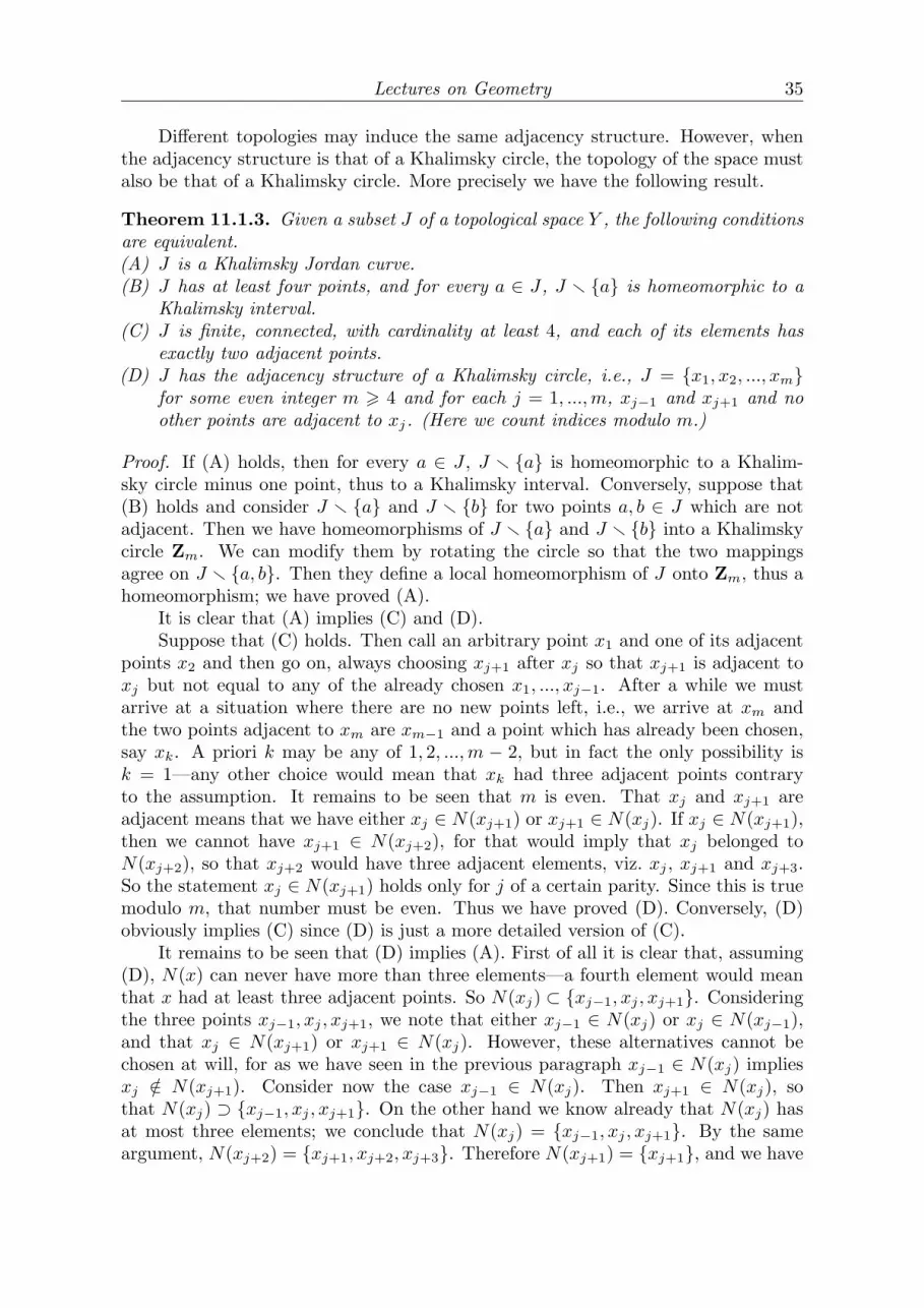
Lectures on Geometry 35
Different topologies may induce the same adjacency structure. However, whenthe adjacency structure is that of a Khalimsky circle, the topology of the space mustalso be that of a Khalimsky circle. More precisely we have the following result.
Theorem 11.1.3. Given a subset J of a topological space Y , the following conditionsare equivalent.(A) J is a Khalimsky Jordan curve.(B) J has at least four points, and for every a ∈ J , J r a is homeomorphic to a
Khalimsky interval.(C) J is finite, connected, with cardinality at least 4, and each of its elements has
exactly two adjacent points.(D) J has the adjacency structure of a Khalimsky circle, i.e., J = x1, x2, ..., xm
for some even integer m > 4 and for each j = 1, ...,m, xj−1 and xj+1 and noother points are adjacent to xj. (Here we count indices modulo m.)
Proof. If (A) holds, then for every a ∈ J , J r a is homeomorphic to a Khalim-sky circle minus one point, thus to a Khalimsky interval. Conversely, suppose that(B) holds and consider J r a and J r b for two points a, b ∈ J which are notadjacent. Then we have homeomorphisms of J r a and J r b into a Khalimskycircle Zm. We can modify them by rotating the circle so that the two mappingsagree on J r a, b. Then they define a local homeomorphism of J onto Zm, thus ahomeomorphism; we have proved (A).
It is clear that (A) implies (C) and (D).Suppose that (C) holds. Then call an arbitrary point x1 and one of its adjacent
points x2 and then go on, always choosing xj+1 after xj so that xj+1 is adjacent toxj but not equal to any of the already chosen x1, ..., xj−1. After a while we mustarrive at a situation where there are no new points left, i.e., we arrive at xm andthe two points adjacent to xm are xm−1 and a point which has already been chosen,say xk. A priori k may be any of 1, 2, ...,m − 2, but in fact the only possibility isk = 1—any other choice would mean that xk had three adjacent points contraryto the assumption. It remains to be seen that m is even. That xj and xj+1 areadjacent means that we have either xj ∈ N(xj+1) or xj+1 ∈ N(xj). If xj ∈ N(xj+1),then we cannot have xj+1 ∈ N(xj+2), for that would imply that xj belonged toN(xj+2), so that xj+2 would have three adjacent elements, viz. xj , xj+1 and xj+3.So the statement xj ∈ N(xj+1) holds only for j of a certain parity. Since this is truemodulo m, that number must be even. Thus we have proved (D). Conversely, (D)obviously implies (C) since (D) is just a more detailed version of (C).
It remains to be seen that (D) implies (A). First of all it is clear that, assuming(D), N(x) can never have more than three elements—a fourth element would meanthat x had at least three adjacent points. So N(xj) ⊂ xj−1, xj , xj+1. Consideringthe three points xj−1, xj , xj+1, we note that either xj−1 ∈ N(xj) or xj ∈ N(xj−1),and that xj ∈ N(xj+1) or xj+1 ∈ N(xj). However, these alternatives cannot bechosen at will, for as we have seen in the previous paragraph xj−1 ∈ N(xj) impliesxj /∈ N(xj+1). Consider now the case xj−1 ∈ N(xj). Then xj+1 ∈ N(xj), sothat N(xj) ⊃ xj−1, xj , xj+1. On the other hand we know already that N(xj) hasat most three elements; we conclude that N(xj) = xj−1, xj , xj+1. By the sameargument, N(xj+2) = xj+1, xj+2, xj+3. Therefore N(xj+1) = xj+1, and we have

36 C. O. Kiselman
proved that Y is a Khalimsky circle where points with indices of the same parityas j have three-neighborhoods and points with indices of the other parity are open.The other possibility, viz. that xj ∈ N(xj−1), can be reduced to the former by justshifting the indices one step.
It follows from property (C) that two Khalimsky Jordan curves can never becontained in each other. More precisely, if J and K are Khalimsky Jordan curvesand J ⊂ K, then J = K.
A point on a Khalimsky Jordan curve J consisting of at least six points has atleast two second adjacent points; with the order introduced in property (D), xj−2 andxj+2 are second adjacent to xj and xj−2 6= xj+2 when m > 4. Then xj±1 serve asintermediaries, but there may also exist other intermediaries. When a Jordan curveis not strict and m > 4, then some point, say xj , has at least one second adjacentpoint in addition to xj−2 and xj+2, say xk. Then an intermediary b such that xj andb are adjacent and b and xk are adjacent cannot belong to J .
Suppose now that Y is a metric space with metric d. Since every Khalimsky arcΓ is homeomorphic either to [0,m−1]∩Z or to [1,m]∩Z for some m, it can be indexedas x1, ..., xm, where the indices are uniquely determined except for inversion. Wemay define its length as
length(Γ) =m−1∑
1
d(xj+1, xj).
Similarly, a Khalimsky Jordan curve can be indexed as x1, ..., xm, where theindices are uniquely determined up to inversion and circular permutations, and itslength can be defined as
length(J) =m∑1
d(xj+1, xj),
where we count the indices modulo m.We shall use the following norms in R2 to measure distances in Z2:
‖x‖p = ‖(x1, x2)‖p =
(|x1|p + |x2|p
)1/p, x ∈ R2, 1 6 p < +∞;
max(|x1|, |x2|
), x ∈ R2, p =∞.
11.2. Khalimsky’s digital Jordan curve theoremThe Khalimsky topology of the digital plane is the Cartesian product topology oftwo copies of the Khalimsky line Z. A point x = (x1, x2) in the product Z2 = Z×Zis closed if and only if both x1 and x2 are closed, thus if and only if both x1 and x2
are even; similarly x is open if and only if both coordinates are odd. These pointsare called pure; the other points, which are neither open nor closed, are called mixed.
Perhaps the quickest way to describe Khalimsky’s topology τ∞ on Z2 is this:We first declare the nine-set
(11.2.1) U∞ = x ∈ Z2; ‖x‖∞ 6 1 = (0, 0),±(1, 0),±(1, 1),±(0, 1),±(−1, 1)

Lectures on Geometry 37
to be open, as well as all translates U∞ + c with c1, c2 ∈ 2Z. Then all intersectionsof such translates are open, as well as all unions of the sets so obtained. As aconsequence, (1,−1), (1, 0), (1, 1), the intersection of U∞ and U∞ + (2, 0), and(1, 1), the intersection of U∞ and U∞ + (2, 2), are open sets, and (0, 0) is aclosed set. The sets (1, 0) and (0, 1) are neither open nor closed.
Theorem 11.2.1. Given a subset J of Z2 equipped with the Khalimsky topology, theconditions A, B, C and D of Theorem 11.1.3 are all equivalent to the following.(E) J = x(1), x(2), ..., x(m) for some even integer m > 4 and for all j, x(j−1) andx(j+1) and no other points are adjacent to x(j); moreover each path consisting of threeconsecutive points x(j−1), x(j), x(j+1) turns at x(j) by 45 or 90 or not at all if x(j)
is a pure point, and goes straight ahead if x(j) is mixed.Here we use the informal expression “turn by 45” etc. with reference to angles inthe Euclidean plane of which we consider the Khalimsky plane to be a subset (not asubspace).Proof. If (D) holds, we see that J cannot turn at a mixed point and cannot turn135 at a pure point—otherwise we would have a forbidden triangle. So (D) implies(E). Conversely, (E) is just a more precise version of (D), so (E) implies (D).
In this section we shall measure the lengths of Khalimsky Jordan curves usingthe Euclidean metric, d(x, y) = ‖x− y‖2. It is not possible to use ‖ · ‖1 or ‖ · ‖∞ inthe proof of the Jordan curve theorem.
The smallest possible Jordan curve in Z2 is the four-set
J4 = x ∈ Z2; ‖x− (1, 0)‖1 = 1 = (0, 0), (1,−1), (2, 0), (1, 1).
We add all translates of J4 by a vector c ∈ Z2 with c1 + c2 even and call these theJordan curves of type J4.
There is also a Jordan curve having eight points,
(11.2.2) J8 = x ∈ Z2; ‖x‖∞ = 1 = U∞ r (0, 0).
This curve and all its translates by a vector c ∈ Z2 with c1 + c2 even we call theJordan curves of type J8.
Let us agree to call the three-set
(11.2.3) T = (1, 1), (0, 0), (1,−1)
and rotations of T by 90, 180 and 270, as well as all translates of these sets byvectors c ∈ Z2 with c1 + c2 even, a removable triangle. It turns out that eliminationof removable triangles is a convenient way to reduce Jordan curves, as shown by thefollowing lemma.
Lemma 11.2.2. Let J be a Jordan curve in the Khalimsky plane and assume thatJ contains the three-set T defined by (11.2.3). Define
J ′ = (J r (0, 0)) ∪ (1, 0).
Then either J = J4 or else J ′ is a Jordan curve such that J ′ and J have the samenumber of components, and length(J ′) = length(J)− 2
√2 + 2.

38 C. O. Kiselman
Proof. Assume first that (2, 0) ∈ J , thus that J ⊃ J4. Then necessarily J = J4.Next we suppose that (2, 0) /∈ J . Then J ′ is a Jordan curve: J ′ is a set where
the new point (1, 0) plays exactly the same role topologically as the old point (0, 0)in J . Thus J ′ is also homeomorphic to a Khalimsky circle.
Finally we must check that the number of components in J ′ is the same as thatof J ′. Indeed, (1, 0) and (2, 0) belong to the same component of J , and (0, 0) and(−1, 0) belong to the same component of J ′.
Theorem 11.2.3 (Khalimsky’s Jordan curve theorem). Let us equip the digital planeZ2 with the Khalimsky topology τ∞ (see (11.2.1)). Then for any Khalimsky Jordancurve J in Z2, the complement J = Z2
rJ has exactly two connectivity components.
Proof. The complement of J4 consists of A = (1, 0) and the set B of all points xwith |x1 − 1| + |x2| > 1. It is obvious that these two sets are connected. Moreover,A is closed and open in J4, so it is a component. Therefore, also B is closed andopen in J4 and also a component. The proof for J8 is similar.
Thus we know that the conclusion of the theorem holds for Jordan curves oftypes J4 and J8.
Next we shall prove that if J is not of the kind already treated, then there existsa Jordan curve J ′ of strictly smaller Euclidean length such that J and J ′ havethe same number of components. After a finite number of steps we must arrive ata situation where the hypothesis is no longer satisfied, which means that we have aJordan curve of type J4 or J8, for which the complement has two components as wealready proved.
The construction of J ′ is as follows. First we may assume, in view of Lemma11.2.2, that J contains no removable triangles. Define
a2 = inf(x2;x ∈ J).
Thus x2 > a2 for all points x ∈ J with equality for at least one x. Consider ahorizontal interval
H = (x1, a2)+ (0, 0), (1, 0), ..., (p, 0)
which is maximal with respect to inclusion and consists of points in J with ordinateequal to a2. The maximality implies that the two points (x1−1, a2) and (x1+p+1, a2)do not belong to J . Then we see that p must be an even number, but we cannot havep = 0, since that would imply that J contained a removable triangle, contrary to theassumption. Thus H contains at least three points. Moreover, at the endpoints of H,J must turn upwards. Indeed, since (x1 − 1, a2) does not belong to J , exactly one ofthe points (x1−1, a2 +1), (x1, a2 +1) belongs to J ; when we go left from (x1, a2), thecurve must turn upwards by either 45 or 90; it cannot turn downwards. Similarly,the curve turns upwards by 45 or 90 when we go right from the last point in H,viz. from (x1 + p, a2).
We now consider the set I of all maximal horizontal intervals I in J such thatJ turns upwards at the endpoints of I. The previous argument served just to provethat there exists such an interval. Now there exists an interval K ∈ I of smallestlength,
K = y+ (0, 0), (1, 0), ..., (q, 0),

Lectures on Geometry 39
containing q + 1 points for some even number q > 2. We shall assume that K is ofsmallest length also among all intervals that can be obtained from the intervals in I
by rotating them 90, 180 or 270.To simplify the notation we may assume (after a translation if necessary) that
y = (0, 0), so that
K = (0, 0), (1, 0), ..., (q, 0) = [(0, 0), (q, 0)] ∩ Z2.
Case 1. J turns upwards by 45 at both ends of K. This means that (−1, 1)and (q + 1, 1) both belong to J . In this case, we define
J ′ = (J rK) ∪ (K + (0, 1)).
This operation shortens the Euclidean length by 2√
2−2 (but it does not shorten thel∞ length). We note that the interval K + (0, 1) is disjoint from J ; otherwise somepoint in K would have three adjacent points. Moreover K + (0, 2) must be disjointfrom J . Indeed, if (K + (0, 2)) ∩ J were nonempty, then either J would contain aremovable triangle (contrary to our assumption) or there would exist a subintervalK ′ of K + (0, 2) contained in J and such that J turns upwards at its endpoints; thusK ′ ∈ I. This subinterval must have fewer than q + 1 points, since (0, 2) and (q, 2)cannot belong to J—otherwise there would be a removable triangle in J . Now ashorter interval is impossible, since K is by assumption an interval in I of shortestlength. One checks that J ′ is a Jordan curve. Indeed, the points of K+(0, 1) play thesame role topologically in J ′ as do the points of K in J . The number of componentsin the complement of J ′ is the same as for J .
Case 2. J turns upwards by 90 at one end of K. Assume that (0, 1) ∈ J , thecase (q, 1) ∈ J being symmetric. Then also (0, 2) ∈ J . We consider the subcases 2.1and 2.2.
Case 2.1. (2, 2) /∈ J . We cut off a corner, i.e., we remove (0, 1), (0, 0), (1, 0),and add (1, 1). This operation shortens the Euclidean length by 4− 2
√2 (but J ′ has
the same l1-length as J). Since (1, 1) and (2, 2) belong to the same component ofJ , and (0, 1), (0, 0), (1, 0), and (−1, 0) belong to the same component of J ′, thenumber of components in the respective complements are the same.
Case 2.2. (2, 2) ∈ J . We consider four subcases, 2.2.1.1, 2.2.1.2, 2.2.2.1 and2.2.2.2.
Case 2.2.1.1. (2, 1) ∈ J , (1, 2) ∈ J . Then J contains a Jordan curve of type J8,more precisely J ⊃ (1, 1) + J8. So J must be equal to that curve.
Case 2.2.1.2. (2, 1) ∈ J , (1, 2) /∈ J . Remove the five points (0, 1), (0, 0), (1, 0),(2, 0), (2, 1), and add (1, 2). Thus J ′ is shorter by 4. We can check that J ′ has alldesired properties.
Case 2.2.2.1. (2, 1) /∈ J , (1, 2) ∈ J . Turn 90 to reduce to case 2.2.1.2.Case 2.2.2.2. (2, 1) /∈ J , (1, 2) /∈ J . This case cannot occur since q is smallest
possible. To see this, define I ′ as the set of all points (2, 2), (3, 2), ..., (q′, 2) ∈ J withq′ as large as possible. If J turns upwards at (q′, 2), then I ′ belongs to I with q′ < q,which contradicts the definition of K and q. If on the other hand J turns downwardsat (q′, 2), then there exists a vertical interval consisting of three points, which becomesan interval in I if we turn it 90, thus again contradicting the definition of I.

40 C. O. Kiselman
11.3. The Jordan curve theorem for another topologyWe define a topology τ1 on Z2 by first declaring the five-set
(11.3.1) U1 = x ∈ Z2; ‖x‖1 6 1 = (0, 0),±(1, 0),±(0, 1)
to be open, then all translates U + c with c ∈ Z2, c1 + c2 ∈ 2Z to be open, as well asall intersections of such translates. This implies that (1, 0) is open, and that theorigin is closed. In fact, all points x ∈ Z2 with x1 +x2 ∈ 2Z are closed, and all pointswith x1 + x2 /∈ 2Z are open; there are no mixed points. This topology was describedby Wyse et al. [1970] and Rosenfeld [1979: 624].
The four-setJ ′4 = (0, 0), (1, 0), (1, 1), (0, 1)
is a Jordan curve for τ1. However, it is not strict, for a point in J ′4 has only onesecond adjacent point. Its complement is connected, so the Jordan curve theoremdoes not hold. The set J8 defined by (11.2.2) is a Khalimsky Jordan curve and itscomplement has exactly two components. Also J8 is not strict, because the point(1, 0) has three second adjacent points, viz. (0, 1), (0,−1) and (−1, 0).
Another example is the twelve-set
J12 = (0, 0), (1, 0), (2, 0), (2, 1), (3, 1), (3, 2), (3, 3), (2, 3), (1, 3), (1, 2), (0, 2), (0, 1).
It is a Jordan curve, not strict, and its complement has three connectivity compo-nents, viz. an infinite component and the two singleton sets (1, 1) and (2, 2).
Theorem 11.3.1. Let Z2 be equipped with the topology τ1 just defined (see (11.3.1)).Then the complement of every strict Jordan curve has exactly two components.
Proof. For the proof we shall use the fact that Z2 equipped with the topology τ1 ishomeomorphic to the subspace of all pure points in the Khalimsky plane. This factwas used also by Kong, Kopperman and Meyer [1991: 915].
Let X be the digital plane Z2 with the topology τ1, and Y the Khalimskyplane (Z2 with the topology τ∞). Consider the mapping ϕ:X → Y defined byϕ(x) = (x1 − x2, x1 + x2). Its image ϕ(X) is the set of all pure points in Y , andif we equip it with the topology induced by Y it is homeomorphic to X. Moreover,the image of any Khalimsky Jordan curve J in X is a Khalimsky Jordan curve in Y .Therefore Y r ϕ(J) has exactly two components by Theorem 11.2.3. We claim thatϕ(X) r ϕ(J) has exactly two components. It is clear that this set has at least twocomponents, so the problem is to prove that a component A of Y r ϕ(J) gives riseto a connected set A ∩ ϕ(X), i.e., that the pure points in A form a connected set.
To this end, assume that a, a′ ∈ A ∩ ϕ(X), and consider a Khalimsky arc
a = a(0), a(1), ..., a(s) = a′
contained in Y rϕ(J). (Connectedness in Y is the same as arcwise connectedness; cf.Khalimsky et al. [1990: Theorem 3.2].) We shall prove that this arc can be replacedby another consisting only of pure points. So assume that a(j) is a mixed point. Thenits predecessor a(j−1) and its successor a(j+1) are both pure points. Without loss ofgenerality, we may assume that a(j−1) = (0, 0), a(j) = (0, 1), and a(j+1) = (0, 2).

Lectures on Geometry 41
We may then replace a(j) by one of the pure points (−1, 1), (1, 1), because bothof them cannot belong to ϕ(J). To see this, suppose that (1, 1), (−1, 1) ∈ ϕ(J).Then (−1, 1) would be a second adjacent point to (1, 1), and this point has, byhypothesis, exactly two second adjacent points in ϕ(J) (considering everything in thespace ϕ(X)). However, none of them can be equal to (−1, 1), for the only possibleintermediaries would then be (0, 0) and (0, 2), none of which belongs to ϕ(J). (Ina strict Jordan curve, one of the possible intermediaries to a second adjacent pointmust belong to the curve.) This contradiction shows that not both of (1, 1) and(−1, 1) can belong to ϕ(J). Thus we may define b = (−1, 1) or b = (1, 1) so thatb /∈ ϕ(J) and observe that
a(0), ..., a(j−1), b, a(j+1), ..., a(s)
is a Khalimsky arc with a mixed point replaced by a pure point. After finitely manysuch replacements we obtain an arc connecting a and a′ and consisting only of purepoints. This shows that ϕ(X)rϕ(J) has at most as many components as Y rϕ(J);therefore exactly two components, and then the same is true of X r J .
References
Alexandroff, Paul [Aleksandrov, P. S.] (1896–1982)1935 Sur les espaces discrets. C. R. Acad. Sci. Paris 200, 1649–1651.1937 Diskrete Raume. Mat. Sb. 2 (44), 501–519.
Ball, Keith1997 An elementary introduction to modern convex geometry. In: Flavors of
Geometry, 1–58. Math. Sci. Res. Inst. Publ. 31. Cambridge: CambridgeUniversity Press.
Bourbaki, Nicolas1961 Topologie generale. Elements de mathematique, premiere partie, livre III,
chapitres 1 & 2. Third edition. Hermann.Ghosh, Pijush K.; Kumar, K. Vinod
1998 Support function representation of convex bodies, its application in geo-metric computing, and some related representations. Computer Vision andImage Understanding 72, 379–403.
Halimskiı, E. D.1970 Applications of connected ordered topological spaces in topology. Confer-
ence of Math. Departments of Povolsia.1977 Uporyadochennnye topologicheskie prostranstva. Kiev: Naukova Dumka.
92 pp.Hiriart-Urruty, Jean-Baptiste; Lemarechal, Claude
1993 Convex Analysis and Minimization Algorithms I. Fundamentals. Springer-Verlag, vxii + 417 pp.
Kaijser, Thomas1998 Computing the Kantorovich distance for images. Journal of Mathematical
Imaging and Vision 9, 173–191.

42 C. O. Kiselman
Kantorovich, L.1942 On the translocation of masses. Comptes Rendus (Doklady) de l’Academie
des Sciences de l’URSS 37, 199–201.Khalimsky, Efim; Kopperman, Ralph; Meyer Paul R.
1990a Computer graphics and connected topologies on finite ordered sets. Topol.Appl. 36, 1–17.
1990b Boundaries in digital planes. J. Appl. Math. Stoch. Anal. 3, 27–55.
Kiselman, Christer O.1981 How to recognize supports from the growth of functional transforms in real
and complex analysis. In: Functional analysis, Holomorphy, and Approxi-mation Theory (Ed. S. Machado); Lecture Notes in Mathematics 843, pp.366–372. Springer-Verlag.
1991a Konvexa mangder och funktioner. Uppsala University, Department ofMathematics, Report No. 1991:LN1. 34 pp.
1991b Konveksaj aroj kaj funkcioj. Uppsala University, Department of Mathe-matics, Report No. 1991:LN2. 35 pp.
1996 Regularity properties of distance transformations in image analysis. Com-puter Vision and Image Understanding, 64, No. 3, 390–398.
2000 Digital Jordan curve theorems. Discrete Geometry for Computer Imagery,9th International Conference, DGCI 2000, Uppsala, Sweden, December13–15, 2000. (Eds. Gunilla Borgefors, Ingela Nystrom, Gabriella Sanniti diBaja.) Lecture Notes in Computer Science 1953, pp. 46–56. Springer.
Kong, T. Y.; Rosenfeld, A.1989 Digital topology: Introduction and Survey. Computer vision, graphics, and
image processing 48, 357–393.Kong, Yung; Kopperman, Ralph; Meyer, Paul R.
1991 A topological approach to digital topology. Amer. Math. Monthly 98, 901–917.
Kuros, A. G.1962 Lekcii po obscej algebre. Moscow: F.M.
Rockafellar, R. Tyrrell1970 Convex Analysis. Princeton, NJ: Princeton University Press.
Rosenfeld, Azriel1979 Digital topology. Amer. Math. Monthly 86, 621–630.
Stromberg, Thomas1996 The operation of infimal convolution. Dissertationes Math. 352. 58 pp.
Wyse, Frank, et al.1970 Solution to problem 5712. Amer. Math. Monthly 77, 1119.
Author’s address: Uppsala University, Department of Mathematics,
P. O. Box 480, SE-751 06 Uppsala, Sweden.
Telephone: +46 18 4713216 (office); +46 18 300708 (home) Fax: +46 18 4713201
Electronic mail: kiselman @ math.uu.se URL: http://www.math.uu.se/~kiselman


