Ann Oper Res (2007) 150:31–46

DOI 10.1007/s10479-006-0151-3

Minimum cost multi-product flow lines

Arianna Alfieri · Gaia Nicosia

Published online: 21 December 2006C© Springer Science + Business Media, LLC 2007

Abstract In this paper, the problem of finding the minimum cost flow line able to produce

different products is considered. This problem can be formulated as a shortest path prob-

lem on an acyclic di-graph when the machines graph associated with each product family

is a chain or a comb. These graphs are relevant in production planning when dealing with

pipelined assembly systems. We solve the problem using A∗ algorithm which can be effi-

ciently exploited when there is a good estimate on the value of an optimal solution. Therefore,

we adapt a known bound for the Shortest Common Supersequence problem to our case and

show the effectiveness of the approach by presenting an extensive computational experience.

Keywords Flow lines optimization . Shortest path algorithms

1 Introduction

In this paper we are concerned with the problem of selecting the machines to be laid out in

a line that must process a number of different products families.

This work stems from an idea of Mario Lucertini, which has been developed under his

supervision in one of the authors’ thesis. We owe to Mario and to his brightness our passion

for research.

Flow lines are a very important class of manufacturing systems characterized by a set of

sequential workstations, typically connected by a continuous material handling system. The

line is designed to assemble component parts and to perform any related operation necessary

A. Alfieri (�)

Politecnico di Torino, Dipt. Sistemi di Produzione ed Economia, Corso Duca degli Abruzzi 24,

10129 Torino, Italy

e-mail: arianna.alfieri@polito.it

G. Nicosia

Universita “Roma Tre”, Dipartimento di Informatica e Automazione, Via della Vasca Navale 79,

00146 Rome, Italy

e-mail: nicosia@dia.uniroma3.it

Springer

32 Ann Oper Res (2007) 150:31–46

M1 M2Mm

Transportation SystemFig. 1 Scheme of a flow line

to produce a finished product. The product is passed down the line, visiting the stations in

sequence, so that it can move from machine (station) M j to Mk only if k > j (see Fig. 1).

In general, flow lines are preferred in order to reduce the transportation and information

system complexity and workload. In particular, in mechanical production the transportation

system can be a critical issue when the products are difficult to handle for weight and/or size

reasons; in electronic production, the information system can be critical when thousands of

operations are required by each single product unit (Askin and Standridge, 1993). In assembly

processes realized through a flexible assembly line, a pipelined organization is very common

when each product unit has a main component and all the other components are assembled

directly on it in a given sequence.

In production planning, the process plan of a product can be described as an acyclic

directed graph D(N , A, f )—often a directed-in-tree1—where N is the set of nodes, A is the

set of arcs and f is a function that associates with every node a character from an alphabet �.

Each node represents a set of homogeneous operations, a cluster, which can be performed by

a same machine (for the sake of simplicity, from now on, we will refer to each of these clusters

as a single operation); each arc (u, v) expresses precedence constraints between operations uand v and each node v is labeled with a character f (v) representing the machine performing

the corresponding operation (hence f : N → �, where the alphabet � corresponds to the set

of the machines types). In the following, we will refer to D as the machines graph.

In practice, D(N , A, f ) is obtained from the merging of the nodes of the so called op-erations graph or operations tree. Usually, in an assembly systems the operations graph is

an assembly tree (see Fig. 2), where the leaves represent the components loading and the

root represents the final product downloading. The nodes are associated either with assembly

operations or with machining operations.

In many production settings, as in the case of pipelined assembly, it is common for D to

have the particular topology of a comb, with a handle and several teeth (see Fig. 2(d)), and in

the simplest cases, of a chain (Fig. 2(c)). In a comb the nodes of the handle, the dominating

path, represent the main operations and the tooth nodes the preprocessing operations (see

Agnetis et al., 1995 for the analysis of a similar case).

We model the problem of designing a minimum cost multi-product flow line as the problem

of finding a minimum cost common supersequence (MCCS) of a particular set of sequences.

If we want to keep the length of the line as short as possible, the problem is modeled as

the shortest common supersequence (SCS) problem. Finding such a flow line is a long-term

decision problem which usually defines the production capabilities for several years. From

now on we will refer to the minimum cost multi-product flow line problem as MCCS.

In Kimms (2000), the same problem is considered and it is solved by means of heuristic

algorithms based on column generation. In Askin and Zhou (1998) an approach based on the

1 A tree T is a directed-in-tree rooted at node s if any element of S belongs to at least one subsequence Si ∈ R,

i.e. if there exist a surjective function f that associates with each character of the sequences of R a character

of S.

Springer

Ann Oper Res (2007) 150:31–46 33

(a)

(b)

(c)

(d)

Fig. 2 Examples of assembly trees

determination of shortest common supersequences is used for determining cells layout in a

cellular manufacturing problem.

In Foulser, Li, and Yang (1992), the authors consider the problem of merging tasks in

order to minimize plan costs and denote the problem as the Plan Merging Problem. The

plan to be merged can be represented by a directed acyclic graph and the authors propose

a dynamic programming algorithm (which can take exponential time in the worst case) for

solving it. It is possible to show that the MCCS problem is a special case of the Plan Merging

problem; however, when the machines graphs associated with each product family are combs,

the algorithm here proposed outperforms, in terms of time complexity, the one presented in

Foulser, Li and Yang (1992).

MCCS can also be see as a special case of a well-known problem, the Multiple-ProductAssembly-System Design Problem (Wilhelm and Gadidov, 2004). Both the MCCS and

Multiple-Product Assembly-System Design Problem prescribe the number of stations and

the type of machine to be placed in each station in order to minimize the machine purchasing

costs in accordance with operation precedence relations. However, in the Multiple-Product

Assembly-System Design problem other constraints and costs are considered, therefore the

two problems are at a different aggregation degree. In fact, in this paper, as in Askin adn Zhou

(1998), and Kimms (2000), we assume that the relevant costs are only fixed machines costs,

i.e., we implicitly assume that variable costs are negligible since similar for all machines

types. It has been shown, in Fine and Freund (1990), that this is approximately true when

material costs or capital costs are large.

Other problems to some extent related to MCCS are Assembly Line Design problems,

where operations need to be assigned to machines (with different equipments) in order to

satisfy a cycle time constraint. Note, however, that in this case the input is the operations

graph and not the machines graph as in the MCCS case. Many papers in the literature deal

with these problems, here we cite only a few. In Bukchin and Tzur (2000) the authors present

an exact and a heuristic algorithm for solving an Assembly Line Design problem with equip-

ment alternatives and with the objective of minimizing the total equipment costs for a given

cycle time. The branch-and-bound procedure, based on the operations-oriented construction

scheme, solves problems of moderate size with up to 30 operations and 5 equipment types. In

Pinto, Dannenbring, and Khumawala (1983) a model which combines the balancing problem

with the decision on process alternatives is considered. The authors propose a branch-and-

bound procedure which branches by selecting/discarding single alternatives and computes

Springer

34 Ann Oper Res (2007) 150:31–46

lower and upper bounds by solving respective Simple Assembly Line Balancing Problems

instances. For a recent survey on assembly line balancing problems see (Becker and Scholl,

2003).

In this paper, in the design of the line, we take explicitly into account the machines graph

associated with each product and propose a shortest-path-based method for finding an optimal

solution. In particular, we consider the case of pipelined assembly in which the machines

graph is a comb and exploit the fact that on each comb there is a dominating path to derive

an algorithm that solves the problem with almost the same time complexity as in the case

of chains. In fact, the structure of the combs allows us to reduce the time complexity of our

algorithm of an exponential factor, with respect to known results in the literature in which

no particular configuration of the operations graph is identified (Foulser, Li, and Yang, 1992;

Fraser, 1995; Timkovskii, 1990).

The shortest path problem associated with the minimization of the cost of the flow line is

solved by using A∗ Algorithm. A∗, introduced in 1969 by Hart, Nilsson, and Raphael (1968),

is a powerful search algorithm which is very useful for solving dynamic programs since, in

practice, it carries out concurrently the construction of a graph and the solution of a shortest

path problem on it. Since it is possible to use A∗ when there is an estimate e on the value of

an optimal solution, we adapt a known bound for the SCS problem to our case.

A∗ Algorithm, is not the shortest path algorithm with best time complexity in the worst

case, however since the size of the graph may become very large, in practice, it allows us to

consistently reduce the number of generated/visited nodes (see Section 6).

In the next section we give some preliminary notions. In particular, we formally define the

SCS and MCCS problems on sequences and introduce some notation that will be useful in the

sequel. The rest of the paper is organized as follows. In Section 3 a formal description of the

problem is given. In Section 4 an algorithm for solving the problem when the machines graphs

are chains is described. Such algorithm is then extended to the case of combs (Section 5). We

solve the derived shortest path problems by using A∗ algorithm (described in Section 5.1)

with a lower bound obtained by adapting a known bound for SCS problem (Section 5.2). In

Section 6 our computational experience is described. Finally, in Section 7 some conclusions

are drawn.

2 Common supersequences

The problem of minimizing the length of a flow line can be modeled as a well-known problem

in string processing, called Shortest Common Supersequence problem (SCS) Maier (1978).

In this section, we formally define the problem and give some definitions which will be useful

in the sequel.

Let S = a1 . . . an be a sequence over an alphabet �. The length of S, denoted by

|S|, is the integer n. A sequence S′ is a subsequence of a sequence S, S′ < S, if S′

can be obtained by deleting (zero or more) characters from S. Conversely, we say that

S is a supersequence of S′. For instance, the set of all the subsequences of S = abc is

P(S) = {abc, ab, ac, bc, a, b, c, ∅}. Given a sequence S = a1 . . . an , we denote by S − ai

the sequence a1 . . . ai−1ai+1 . . . , an . Moreover, we say that the sequence S(i) = a1a2 . . . ai

is the prefix of length i of S and that S(i) = S − S(i) = ai+1, . . . an is the residual sequences

of S with respect to S(i).A sequence S is a common supersequence of a set of sequences R = {S1, . . . , Sr } if

Si < S for all i = 1, 2, . . . , r . (In the following, for sake of shortness, when we refer to a set

R we mean a set of sequences). S is a shortest common supersequence of R, SCS(R), if it is

Springer

Ann Oper Res (2007) 150:31–46 35

a common supersequence of R with minimal length. For instance, if R = {abdc, bca}, then

abdca is a shortest common supersequence.

SCS is a well known problem with several applications (Foulser, Li, and Yang, 1992;

Rodeh, Pratt, and Even, 1981). It is known to be NP-complete (Maier, 1978; Raiha

and Ukkonen, 1981) and in many particular cases, as shown in Middendorf (1994), and

Timkovskii (1990), it remains NP-complete. Also, several authors have studied the approx-

imation complexity of SCS (see for instance, Fraser and Irving, 1995; Jiang and Li, 1995;

Kimms, 2000).

To find optimal solutions, dynamic programming (or shortest path) algorithms (Fraser,

1995; Timkovskii, 1990) and branch-and-bound algorithms (Fraser, 1995) have been in-

vestigated. However, they are successful only for a very small number of given sequences,

since for r sequences of length n their time complexity is O(nr ) (Timkovskii, 1990) or

O(rn(s − n)r−1), where s is the length of the shortest common supersequence (Fraser, 1995).

Most of the authors assume that the input sequences are independent. However, in the

application we are considering, this is not the case; sequences may belong to a common

general frame that can be used to simplify the solution.

In our application we are mainly interested in a modification of the SCS problem which we

denote as the minimum cost common supersequence problem (MCCS). We assume that there

is a cost wc associated with every character c ∈ � and we want to find the supersequence of

the given set of sequences R of minimum cost, i.e. the sequence that minimizes the sum of

the costs associated with every character in the sequence. Clearly, when the costs wc are the

same for all c ∈ � the MCCS problem is equivalent to the SCS problem.

3 Statement of the problem

In this section we formally define the problem of building a minimum cost flow line. The input

consists of a machines graph D for each considered product family. As already mentioned

in the Introduction, a machines graph D(N , A, f ) is an acyclic directed graph, where each

node v ∈ N corresponds to a set of operations that are to be performed by a same machine

identified by character f (v) ∈ �. Each type of machine c ∈ � may have a different cost

wc > 0. A directed path π = {v1, v2, . . . vm} in D is maximal if v1 has no ingoing arcs and

vm no outgoing arcs, i.e. δ−(v1) = δ+(vm) = 0; we denote by �(D) the set of all the maximal

paths in D. With each maximal path in D, we can associate a sequence of characters in �.

Thus, given the machines graphs D1, D2, . . . , Dr , one for each product, we consider

the problem of finding the minimum cost flow line able to execute all the operations and

satisfying the precedence constraints for each product.

This problem is equivalent to that of finding a minimum cost common supersequence

(MCCS) of the sequences corresponding to all the maximal paths of each digraph Di asso-

ciated with each product.

Strictly related to the above described problem is the problem of minimizing the length

of the flow line. Clearly, this corresponds to having uniform machine costs and therefore,

it is equivalent to the problem of finding the SCS of the sequences corresponding to all the

maximal paths of each digraph Di associated with each product.

The different sequences induced by the maximal paths in the machines graph often have

common substrings (S′ = a j a j+1 . . . ak is a substring of S = a1a2 . . . al if 1 ≤ j ≤ k ≤ l)and, therefore, are interdependent.

It is easy to observe that if, for each product, D is a chain, the sequences are independent

and therefore, the problem we are dealing with is a standard MCCS problem. In Section 4

Springer

36 Ann Oper Res (2007) 150:31–46

we describe an algorithm for solving the problem in polynomial time for any fixed number

of products. If D is a comb, we are able to exploit the fact that on each comb there is a

dominating path and therefore, produce an algorithm that solves the SCS problem on a set

of combs (SCSC) with almost the same time complexity as in the case of chains, even if

the number of paths (sequences) is much higher. If D is an assembly tree with no particular

structure or is a general acyclic digraph, in order to solve the problem, we may consider each

maximal path separately and then find the MCCS or SCS of the sequences corresponding to

those paths.

Note that, the supersequences we are interested in satisfy the so-called square-freenessassumption, i.e., consecutive characters in a sequence are always different. In fact, if two

consecutive operations require the same machine, they can be considered as a single occur-

rence of that machine. In our case, when the machines graph is a chain, we can preprocess

the corresponding sequences so that they satisfy the square-freeness assumption and devise

the optimal solution as shown in the next section. When the machines graph is a comb, this

preprocessing is not possible since by shrinking adjacent nodes the topology of the graph

changes (a comb may become a caterpillar). So, we take explicitly into account the fact that

two adjacent nodes in the machines graph may require the same machine, in order to find a

solution that satisfies the square-freeness assumption. In the following, we will use the terms

SCS and MCCS to indicate the two above described problems in the particular case in which

the square-freeness assumption holds.

4 The problem for r chains

In this section, we first consider the SCS problem and describe a shortest-path-based algorithm

for its solution (for a similar approach, see Timkovskii, 1990; Fraser, 1995). It is possible to

extend this solution method to the MCCS problem and to the case of combs, which will be

studied in the next section.

Let R = {S1, S2, . . . Sr } be a finite set of sequences where Si = ai,1ai,2 . . . ai,ni for

i = 1, 2, . . . , r . The SCS problem can be solved by dynamic programming techniques in

which the number of states is (n1 + 1)(n2 + 1) . . . (nr + 1) and, therefore, this approach is

effective only for instances with a few sequences (Timkovskii, 1990). Equivalently, SCS can

be formulated as a shortest path problem on an acyclic directed graph in which each node

represents one of the states of the dynamic program.

To reduce the number of nodes of the graph, it is possible to proceed in the following way

(Nicosia and Oriolo, 2003). With any instance of SCS we can associate an acyclic directed

graph GR that can be inductively built in the following way. Let any node in GR be denoted

by an r -tuple (i1, . . . , ir ), 0 ≤ ih ≤ nh for h = 1, 2 . . . r . First, create node (0, 0, . . . , 0) and

expand it, i.e. generate all its successors (if not already generated). Then, every generated

node is selected once and expanded. In particular, a node ( j1, . . . , jr ) with jh ≤ nh for each

h = 1, 2 . . . r , is a successor of a node (i1, . . . , ir ), i.e. there is an arc from the latter to the

former if and only if the following conditions are all satisfied:

1. either jh = ih or jh = ih + 1, 1 ≤ h ≤ r ;

2. the set X = {h : jh = ih + 1, 1 ≤ h ≤ r} is non-empty;

3. there exists c ∈ � such that ah,ih+1 = c if and only if h ∈ X . In this case we label the arc

with character c.

Let F = (n1, . . . , nr ), trivially, any path from O = (0, 0, . . . , 0) to F in GR corresponds

to a common supersequence of the set R. It is easy to show that, vice versa, there always

Springer

Ann Oper Res (2007) 150:31–46 37

4, 3

3, 33, 2

2, 32, 22, 1

1, 31, 21, 11, 0

0, 20, 10, 0

a a

a

a

a

a

b

b b b b

d d

c

c

c

a

d

3, 1

c

4, 2

c c

Fig. 3 A di-graph obtained from

two sequences

exists a SCS of the set R corresponding to a shortest path (assuming each arc has unitary

weight) from O to F on this graph.

Example 4.1. Let S1 = abdc and S2 = bca, then |S1| = 4 and |S2| = 3. The graph GR ob-

tained from S1 and S2 is depicted in Fig. 3.

On this graph, the shortest path from node (0, 0) to node (4, 3) is � = {(0, 0), (1, 0), (2, 1),

(3, 1), (4, 2), (4, 3)} and therefore the SCS is abdca.

Observe that, even if, in the worst-case, the number of nodes of GR is O((n1 + 1) · (n2 +1) . . . (nr + 1)), in practice, this number is considerably less than the number of states of

the dynamic program. Therefore, the presented approach allows us to find the SCS more

efficiently and, as we will see in the sequel, by using Algorithm A∗ it is possible, on the

average, to further reduce the number of nodes of GR.

The extension of this solution method for SCS problem to MCCS problem is immediate.

It is enough to assign as weights of the arcs in GR the costs of the corresponding character

and solve the resulting shortest path instance.

Example 4.2. Consider the same sequences as in Example 4.1 and let the costs of the

characters be 3, 1, 1, 2 for a, b, c and d, respectively. Clearly, the shortest path from

node (0, 0) to node (4, 3) with this weighting of the arcs is � = {(0, 0), (0, 1), (0, 2),

(1, 3), (2, 3)(3, 3), (4, 3)} and therefore the MCCS is bcabdc with cost 9. (Note that the

previously evaluated SCS, abdca, has cost 10.)

5 The problem on a set of combs

A comb is a rooted directed-in-tree where (i) the inner nodes form a path ending at the root

and (i i) each inner node has at most one son which is a leaf. Formally, a complete comb

C(N , A), with 2n nodes, is such that:

N = {i : i = 1, 2, . . . , 2n}A = {(i, j) : (i = 2k ∧ j = 2k + 2 for k = 1, ..n − 1) ∨ (i = 2k − 1 ∧ j = 2k for k =

1, 2, . . . , n)}Each node i is associated with an element ai ∈ �. The main characteristic of a comb is

that there exists a dominating path, the handle, consisting of nodes 2, 4, 6, . . . , 2n (see Fig. 4).

The set of sequences derived from a comb are obtained as the sequence of characters

assigned to the nodes on each path from a leaf, or tooth, to the root. Therefore, for comb

Springer

38 Ann Oper Res (2007) 150:31–46

a1

a2n

a3

a2a4

a2n-1Fig. 4 A complete comb

C(N , A) the corresponding sequences are: S1 = a1a2a4a6 . . . a2n , S2 = a3a4a6 . . . a2n , . . . ,

Sn−1 = a2n−3a2n−2a2n , and Sn = a2n−1a2n .

The minimum cost common supersequence of the set of combs C is defined as the MCCS

of all the sequences corresponding to the combs inC. The MCCS problem on a complete comb

with 2n nodes corresponds to a particular MCCS problem with n interdependent sequences,

since each sequence obtained from a comb contains a tooth node and a part of the handle.

We now extend the shortest path based algorithm presented in the previous section to deal

with combs. The proposed algorithm solves the MCCS problem on r combs with almost the

same time complexity as in the case for r sequences by exploiting the interdependence of

the sequences.

If the input consists of only one comb the optimal MCCS can be easily found and it

coincides with the SCS, since there are no choices to make among characters when building

a supersequence. In fact, it is easy to see that all the labels of the nodes of the handle must

be contained in the supersequence to be found (with the exception of identical consecutive

characters). As far as the teeth are concerned, the label of node 2i − 1, a2i−1, must be in the

supersequence only if a2i−1 �= a2i and if it is not contained in the subcomb containing nodes

{1, 2, . . . , 2i − 2}. This remark leads to a simple O(n) algorithm. Notice that, if the size of

the alphabet � is not part of the input, we need O(n log |�|) time to obtain the ordered set

of characters.

As already mentioned, the case with two or more combs can be solved by using the same

kind of approach presented in Section 4 for the case of two or more sequences.

Let C = {C1, C2, . . . Cr } be a finite set of combs where Ci has labels ai,1ai,2 . . . ai,2ni for

i = 1, 2, . . . , r . Let us recall that the nodes of the handle are identified by a even label and

teeth nodes by a odd label. So, ai,2ai,4 . . . ai,2ni are the characters assigned to the handle and

ai,1ai,3 . . . ai,2ni −1 are the teeth characters. Analogously to the chains case, with any instance

of SCS and MCCS on combs, we can associate an acyclic directed graph GC that can be built

in the following way. Let any node i in GC be denoted by an (r + 1)-tuple (i1, . . . , ir , ci ),

with 0 ≤ ih ≤ nh for h = 1, 2 . . . r and ci ∈ �. Each element ih of node i represents a scanof each comb Ch up to node 2ih . So, as with graph GR, each node of GC can be seen as a

state of a dynamic program. The character ci associated with every node i is needed to store

the last character in a sequence corresponding to a path from the source node O to node i .The source node O is (0, 0, . . . , 0, �), where � indicates the null character and the desti-

nation node is F = (n1, n2, . . . , nr , �). All successors of node O are generated. Then, every

generated node is selected once and expanded. In particular, a node j = ( j1, . . . , jr , c j ) with

jh ≤ nh for each h = 1, 2 . . . r , is a successor of a node (i1, . . . , ir , ci ), if and only if� jk = ik + 1 for k ∈ {1, 2, . . . r},� jh = ih for all h �= k with 1 ≤ h ≤ r , and� c j = ak,2 jk (unless jh = nh for all h = 1, . . . r , in this case c j = �).

So, at most r arcs emanate from each node i . We can represent the situation with Fig. 5.

Springer

Ann Oper Res (2007) 150:31–46 39

i1,i2 ,.. , ir

ci

(1)

(h)

i1 +1,i2 ,.., ir

a1,2i1

i1,..,ih +1,..,ir

ah,2ih

i1,i2 ,.., ir +1ar,2i r

(r)

.

.

.

.

.

.

.

.

Fig. 5 A node connection in

GC (N , A)

Each arc (i, j) in GC represents the transition from state, or scan, i to state j . Thus, we

assign to each arc one or more characters (and the corresponding costs) in the following way.

First, let �i be a set of characters associated with each node i that contains all the characters of

the teeth and the handle of each comb h = 1, . . . r up to node 2ih , i.e.�i = ⋃rh=1(

⋃2ihj=1{ah, j }).

Case 1: ci �= ak,2 jk (= c j ). In this case, the newly considered handle node is associated with

character ak,2 jk which is different from ci (that corresponds to the last character in any

sequence obtained as a path from the source node O to node i). Then,� if ak,2 jk−1 ∈ � j , the character ak,2 jk is assigned to arc (i, j);� if ak,2 jk−1 /∈ � j , the characters assigned to arc (i, j) are ak,2 jk−1ak,2 jk .

Case 2: ci = ak,2 jk (= c j ). In this case, the newly considered handle node has the same

character, ak,2 jk , as ci . So, there is no need to assign such character to arc (i, j). Then,� if ak,2 jk−1 ∈ � j , the null character is associated with arc (i, j). Therefore, the cost of the

arc is 0.� If ak,2 jk−1 /∈ � j , then character a∗k,2 jk−1 is assigned to arc (i, j).

Thus, we assigned to each arc of the graph zero, one or two characters of the alphabet �.

Each path on this graph corresponds to a sequence obtained by concatenating the characters

associated to each arc of the path. The characters that we pointed out with an asterisk ∗ will

be inserted in the sequence on the left of the characters that immediately precede them (i.e.

if c∗ is the k-th character that we have to insert, we swap c with the letter that was put in

position k − 1).

Clearly, the cost of each arc equals the sum of the costs associated with each character

assigned to the arc.

The sequences obtained as paths from node O to node F on GC are non-redundant,2

satisfy the square-freeness condition and all the characters of the teeth appear in the rightmost

possible position (i.e. if they are not already in the sequence, they appear immediately on the

left of the corresponding handle node). It is easy to show that a shortest path from O to Fon graph GC corresponds to a minimum cost common supersequence of the combs in C.

The number of nodes in GC is O(nr · min{|�|, r}) and the number of arcs is O(nr ·max{|�|, r}). Therefore, the ratio in size between graphs GC and GR is min{|�|, r}, while

the difference in the number of sequences is n · r vs. r . So, by applying the standard approach

presented in Section 4 without considering the structure of the combs, we would obtain a

graph with O(nnr ) nodes instead of O(nr · min{|�|, r}) (thus reducing the exponent of a

factor of n).

2 A common supersequence S of a set of sequences R is non-redundant common supersequence if the unique

path in the tree from any node to node s is a directed path.

Springer

40 Ann Oper Res (2007) 150:31–46

0,0#

1,0b

0,1b

1,1b

cb2

c*1

0,2d1

d 0,3a1

a

2,0d

3,0c

2,1b

2,1d

3,1b

3,1c

ab

cd

c

2

2

1,2 b1,2

d1,3 b

1,3

a

cc

b

b1

1

111

d 1

aba* 1

2,3a

2,3d

2,2d

2 b 1

d 1

d1

d1

d1

#0

# 0

1a

1a

d 1

1a

3,2 c3,2

d

d

1c

1d1 #

3,3

c

1

a

1

1a

c

1

Fig. 6 A graph obtained from

two combs

Regarding space complexity, for each node of graph GC we have to store |�| val-

ues (in order to decide whether the characters of the teeth need to be inserted in the

MCCS) and 1 value corresponding to the character associated to the node. Moreover, build-

ing the graph requires O(max{|�|, r} · nr ) time, since we need O(1) for each node and

arc.

Example 5.1. Let C1 and C2 be two complete combs with nodes a, b, c, d, a, c and c, b, c,d, b, a, respectively. The graph GC associated with this instance is depicted in Fig. 6. The

sets associated with the nodes of GC are: �(0,0) = ∅, �(1,0) = {a, b}, �(0,1) = {b, c}, �(1,1) ={a, b, c}, �2,1 = �1,2 = �2,2 = · · · = �3,3 = {a, b, c, d}.

If all characters have the same cost (i.e. if we are interested in minimizing the length

of the line) a shortest path from node (0, 0, �) to node (3, 3, �) is � = {(0, 0, �), (1, 0, b),

(1, 1, b), (1, 2, d), (2, 2, d), (2, 3, a), (3, 3, �)} and the corresponding SCS is acbdac. If, as

in Example 4.2, the costs of the characters are 3, 1, 1, 2 for a, b, c and d , respectively, then

� is still a shortest path of cost 11.

Note that the above described shortest-path-based algorithm can also be used when the

machines graphs are caterpillars (see Fig. 2(b)) with only a slight modification. A caterpillar

is an in-tree, similar to a comb, such that in correspondence to each handle node there might

be more than one leaf. Similarly to the case of combs, we may associate to the MCCS

problem a di-graph in which each node corresponds to a scan of the caterpillars. Each arc

represents the transition from a scan to another; thus, the characters (and the corresponding

costs) associated to it are:� those of the teeth (possibly more than one), if such characters do not appear in any path

from the root node to the current node, and� one of the handle node.

Then, with each arc is associated a number of characters that goes from 0 to the number

of teeth plus one. As with GC , each path on this graph corresponds to a sequence obtained

by concatenating the characters associated to each arc of the path. Finally, the size of this

graph is exactly the same as in the case of combs, only the time required to build the graph

increases. In fact, at each step, the test on whether the character associated with the tooth

node has appeared before, must be done not only once, as in the case of combs, but once

for each tooth. So, if the number of leaves (teeth) of each caterpillar is l, we need an extra

O(rl · nr−1) time to build the graph.

Springer

Ann Oper Res (2007) 150:31–46 41

5.1 A∗ Algorithm

We have shown that it is possible to solve an instance of MCCS on a set of combs by

building a di-graph GC and then finding a shortest path on GC . By applying algorithm A∗,

we are able to build only a subgraph of GC since we bind the construction of the di-graph to

requirements of optimality; moreover, we carry out the two phases (graph building and path

finding) concurrently.

Algorithm A∗ was first introduced by Hart, Nilsson and Raphael (1968), and later devel-

oped, mainly in the field of Artificial Intelligence (for a general discussion see Hart, Nilsson,

and Raphael, 1968; Nilsson, 1971).

Suppose we are given a network D, which is initially unknown, a node O and we want to

find a shortest path from O to a node F representing some kind of final state for our search.

Let d(v, u) denote the length of each arc (v, u) of D and �vu the length of a shortest path

from a node v to a node u (�vu = ∞ if there are no directed paths from v to u).

The application of A∗ is based on the possibility, for each node u of D, of giving an

estimate f (u) on the length of the best path through node u connecting O to F . In par-

ticular, f (u) will be given by the sum of two terms g(u) and e(u), where g(u) is the

length of a shortest path found so far from O to u by the algorithm and e(u) is an off-line estimate of the length �uF of a shortest path connecting u to F (of course, e(F) = 0).

The estimate e(u) is called consistent if, for each arc (u, v), e(u) − e(v) ≤ d(u, v). Ob-

serve that, if consistency holds, then we are guaranteed that e(u) is a lower bound on

�uF .

A∗ with consistent estimates works in the following way. At each step, we choose the

most “promising” node (i.e. the one for which f (u) is the smallest) among all the nodes

which have not been expanded yet and expand it finding all its successors. Of course, the

first node we expand is node O . The process goes on, expanding at each step the node with

the smallest value of f , until F becomes the most promising node. Clearly, the idea of A∗ is

very close to that of branch and bound; moreover, when the estimate e(u) is, for each node u,

equal to 0 and the network is known from the outset, then A∗ reduces to Dijkstra’s shortest

path algorithm.

It has been shown (Nilsson, 1971) that, if e(u) is a lower bound on �uF , the length of a

shortest path from u to F , then A∗ finds a shortest O − F path (whereas for general estimate

functions this is not guaranteed). Since this is true with consistent estimates, it follows that

the previous algorithm finds a shortest O − F path.

Observe that, in general, the tighter e the more efficient the algorithm, since a good estimate

keeps “low” the number of expanded nodes in D (Nilsson, 1971). On the other hand, if e is

too time consuming to compute, efficiency can be as well jeopardized.

Here we apply A∗ for solving the MCCS and SCS problems on a set C = {C1, . . . , Cr }of sequences derived from combs, when we have a consistent estimate for the length of a

shortest path from any node u of GC to node F = (n1, . . . , nr , �). So, in the next subsection

we extend a lower bound for the general SCS problem to deal with combs and with the MCCS

problem and show that it is a consistent estimate.

Observe that GC is an acyclic directed graph and therefore a shortest path problem on it

can be solved by using an algorithm which is linear in the number of arcs. However, since

the size of the graph becomes very large when the number of combs grows we implemented

A∗ Algorithm (see Section 6)—that in the worst case has a lower performance in terms of

running time—since no other optimal algorithm is guaranteed to expand fewer nodes than

A∗.

Springer

42 Ann Oper Res (2007) 150:31–46

5.2 Lower bound

In this section we discuss a lower bound on the cost of a MCCS of a set of sequences derived

from combs. This lower bound is used for the implementation of algorithm A∗.

LetR be a set of sequences from an alphabet �. In particular, let R = {S1, . . . , Sr }, where

Si = ai,1 . . . ai,ni . For each character c in �, let us denote by o(c) the maximum number of

occurrences of c in a same sequence of the set R, that is:

o(c) = maxi∈{1,...,r}

|{ai, j : ai, j = c, 1 ≤ j ≤ ni }|.

Observe that each character c has to appear in the SCS at least o(c) times. Therefore, a

lower bound on the length of a SCS is given by∑

c∈� o(c). This lower bound can be trivially

extended to the case of problem MCCS by simply considering:

LB :=∑c∈�

wco(c).

The extension to the comb case is easy, too. First, among the different sequences that can

be derived from each comb Ci , we consider only the main sequence, from now on denoted as

Hi , that is, the one derived from the path on the handle. Then, we have to take into account

the fact that, in our application, the optimal supersequence must not contain two identical

consecutive characters. We consider o′(c) to be the maximum number of occurrences of c in

a same sequence obtained by not considering identical consecutive characters. For instance,

if the considered sequence Hi is cabcccabc then, o′(b) = 2 and o′(c) = 3. Then, a lower

bound on the cost of a MCCS for a set of combs is LB′ := ∑c∈� wco′(c).

Note that during the execution of A∗ algorithm we need a lower bound LB(i) on

the length of a shortest path from i to F . So, we may proceed as follows. With any

node i = (i1, . . . , ir , ci ) of graph G(C) we may associate the set of residual sequences

R(i) = {H1(i1), . . . , Hr (ir )}. To evaluate LB(i), we first eliminate any number of possi-

ble consecutive occurrences of ci from the beginning of each sequence Hk(ik), k = 1, . . . rand then, we calculate o′

i (c), the maximum number of non-repetitive occurrences of c in a

same sequence of the set of the modified residual sequences in R(i), for each c ∈ �. Then,

LB(i) := ∑c∈� wco′

i (c).

Example 5.2. Consider the two combs of Example 5.1 and the resulting graph depicted in

Fig. 6. The two main sequences are H1 = bdc and H2 = bda. Some of the values of the above

described lower bound, assuming wc = 1 for all characters, are:� LB(O) = 4, since R(O) = {bdc, bda} and o′(a) = o′(b) = o′(c) = o′(d) = 1;� LB(0, 1, b) = 3, since R((0, 1, b)) = {bdc, da}, o′(a) = o′(c) = o′(d) = 1, and o′(b) = 0;� LB(2, 1, d) = 2, since R((2, 1, d)) = {c, da}, o′(a) = o′(c) = 1, and o′(b) = o′(d) = 0;� LB(F) = 0, since R(F) = {�, �} and o′(a) = o′(b) = o′(c) = o′(d) = 0.

In the next lemma we show that the above defined lower bound is a consistent estimate,

so that we can use the previously described (simpler) version of A∗ algorithm.

Lemma 5.3. The lower bound LB(i) is consistent.

Springer

Ann Oper Res (2007) 150:31–46 43

Proof: We must show that for each pair i and j of connected nodes, the cost of arc (i, j),

d(i, j), is greater than or equal to LB(i) − L B( j). We consider two different cases depending

on whether ci = c j or not.

Case A: ci �= c j . This case corresponds to Case 1 in the description of graph GC . So, we have

only two possibilities for arc (i, j), we either (i) assigned to it only the handle character

c j = ak,2 jk or (i i) we assigned both tooth and handle characters ak,2 jk−1ak,2 jk . In case

(i), d(i, j) = wak,2 jkand when evaluating LB( j) the characters maximum occurrences

o′(c) remain the same as for LB(i) for all c �= c j ; while o′(c j ) might decrease of one

unit. Therefore, LB(i) − L B( j) ≤ wak,2 jk, so the thesis is proved. In case (i i), d(i, j) =

wak,2 jk+ wak,2 jk −1

and, with the same argument as in case (i) we may say that LB(i) −L B( j) ≤ wak,2 jk

, so the thesis holds.

Case B: ci = c j . This case corresponds to Case 2 in the description of graph GC . So, we

have only two possibilities for arc (i, j), we either (i) assigned to it only the tooth character

ak,2 jk−1 or (i i) we assigned no characters. In both cases, LB(i) = L B( j), therefore LB(i) −L B( j) ≤ d(i, j).

�

6 Computational results

In this section we present the results of two different computational experiments on several

classes of randomly generated instances. All the computational tests here reported were run

on a workstation IBM RISC/6000 model 44P. In the first set of experiments we tested the

performance of A∗ algorithm on different classes of SCS and MCCS instances when the

machines graphs are combs. The second set of experiments deals only with problem MCCS

and was undertaken to evaluate the impact of machine costs on computation times. The

estimate used in the implementation of the algorithm, for all the sets of experiments, is the

lower bound presented in Section 5.2.

The characteristics of the instances of the two sets of experiments are reported in Table 1,

where r is the number of combs, n the length of the combs (the considered combs are all

complete and with 2n nodes), and t the cardinality of the alphabet, that is the number of

different available machines.

Let us recall that an instance of MCCS (or SCS) problem with r combs of length nconsists of r · n interdependent sequences, and therefore, the test instances reported in Table 1

correspond to instances with 50, 75 and 100 sequences.

For each class we randomly generated 20 instances. The results of the first set of exper-

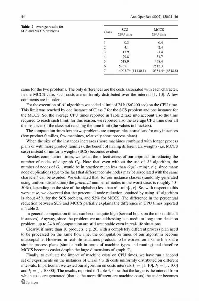
iments are summarized in Table 2. Each entry shows average CPU time (in seconds) over

the 20 instances both for the SCS and the MCCS problems. The test instances are exactly the

Table 1 Instances classesClass r n t

1 5 10 5

2 5 10 7

3 5 10 10

4 5 15 5

5 5 15 7

6 5 15 10

7 10 10 5

Springer

44 Ann Oper Res (2007) 150:31–46

Table 2 Average results for

SCS and MCCS problems ClassSCS

CPU time

MCCS

CPU time

1 0.3 0.4

2 4.1 2.4

3 17.9 21.4

4 29.8 31.7

5 618.9 458.4

6 5735.1 2512.3

7 14903.7* (11130.1) 10351.4* (6348.8)

same for the two problems. The only differences are the costs associated with each character.

In the MCCS case, such costs are uniformly distributed over the interval [1, 10]. A few

comments are in order.

For the execution of A∗ algorithm we added a limit of 24 h (86’400 sec) on the CPU time.

This limit was reached by one instance of Class 7 for the SCS problem and one instance for

the MCCS. So, the average CPU times reported in Table 2 take into account also the time

required to reach such limit; for this reason, we reported also the average CPU time over all

the instances of the class not reaching the time limit (the values in brackets).

The computation times for the two problems are comparable on small and/or easy instances

(few product families, few machines, relatively short process plans).

When the size of the instances increases (more machines combined with longer process

plans or with more product families), the benefit of having different arc weights (i.e. MCCS

case) instead of uniform weights (SCS) becomes evident.

Besides computation times, we tested the effectiveness of our approach in reducing the

number of nodes of di-graph GC . Note that, even without the use of A∗ algorithm, the

number of nodes of GC , would be in practice much less than O(nr · min{t, r}), since many

node duplications (due to the fact that different combs nodes may be associated with the same

character) can be avoided. We estimated that, for our instance classes (randomly generated

using uniform distribution) the practical number of nodes in the worst case, is roughly 40–

50% (depending on the size of the alphabet) less than nr · min{t, r}. So, with respect to this

worst case, we observed that the percentual node reduction obtained by using A∗ algorithm

is about 45% for the SCS problem, and 52% for MCCS. The difference in the percentual

reduction between SCS and MCCS partially explains the difference in CPU times reported

in Table 2.

In general, computation times, can become quite high (several hours on the most difficult

instances). Anyway, since the problem we are addressing is a medium-long term decision

problem, up to 24 h of computation are still acceptable even in real-life situations.

Clearly, if more than 10 products, e.g. 20, with a completely different process plan need

to be processed on the same flow line, the computation times of our algorithm become

unacceptable. However, in real-life situations products to be worked on a same line share

similar process plans (similar both in terms of machine types and routing) and therefore

MCCS becomes easier despite the huge dimensions of graph GC .

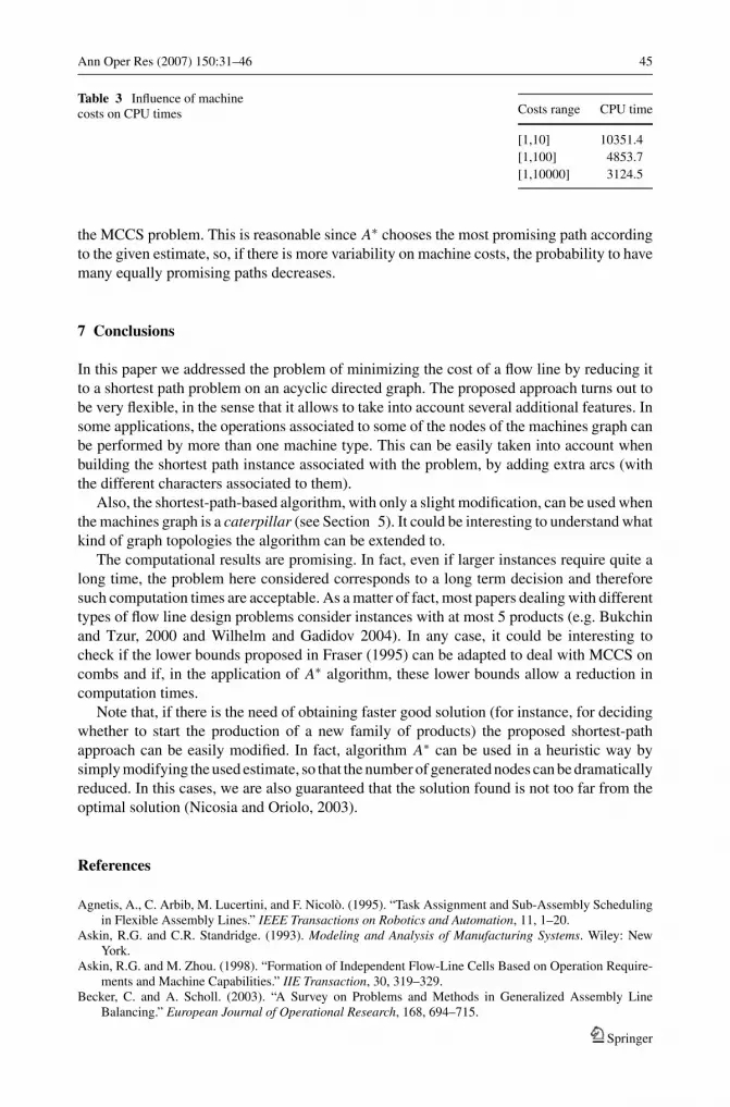
Finally, to evaluate the impact of machine costs on CPU times, we have run a second

set of experiments on the instances of Class 7 with costs uniformly distributed on different

intervals. In particular, we tested our algorithm on costs intervals I1 = [1, 10], I2 = [1, 100]

and I3 = [1, 10000]. The results, reported in Table 3, show that the larger is the interval from

which costs are generated (that is, the more different are machine costs) the easier becomes

Springer

Ann Oper Res (2007) 150:31–46 45

Table 3 Influence of machine

costs on CPU times Costs range CPU time

[1,10] 10351.4

[1,100] 4853.7

[1,10000] 3124.5

the MCCS problem. This is reasonable since A∗ chooses the most promising path according

to the given estimate, so, if there is more variability on machine costs, the probability to have

many equally promising paths decreases.

7 Conclusions

In this paper we addressed the problem of minimizing the cost of a flow line by reducing it

to a shortest path problem on an acyclic directed graph. The proposed approach turns out to

be very flexible, in the sense that it allows to take into account several additional features. In

some applications, the operations associated to some of the nodes of the machines graph can

be performed by more than one machine type. This can be easily taken into account when

building the shortest path instance associated with the problem, by adding extra arcs (with

the different characters associated to them).

Also, the shortest-path-based algorithm, with only a slight modification, can be used when

the machines graph is a caterpillar (see Section 5). It could be interesting to understand what

kind of graph topologies the algorithm can be extended to.

The computational results are promising. In fact, even if larger instances require quite a

long time, the problem here considered corresponds to a long term decision and therefore

such computation times are acceptable. As a matter of fact, most papers dealing with different

types of flow line design problems consider instances with at most 5 products (e.g. Bukchin

and Tzur, 2000 and Wilhelm and Gadidov 2004). In any case, it could be interesting to

check if the lower bounds proposed in Fraser (1995) can be adapted to deal with MCCS on

combs and if, in the application of A∗ algorithm, these lower bounds allow a reduction in

computation times.

Note that, if there is the need of obtaining faster good solution (for instance, for deciding

whether to start the production of a new family of products) the proposed shortest-path

approach can be easily modified. In fact, algorithm A∗ can be used in a heuristic way by

simply modifying the used estimate, so that the number of generated nodes can be dramatically

reduced. In this cases, we are also guaranteed that the solution found is not too far from the

optimal solution (Nicosia and Oriolo, 2003).

References

Agnetis, A., C. Arbib, M. Lucertini, and F. Nicolo. (1995). “Task Assignment and Sub-Assembly Scheduling

in Flexible Assembly Lines.” IEEE Transactions on Robotics and Automation, 11, 1–20.

Askin, R.G. and C.R. Standridge. (1993). Modeling and Analysis of Manufacturing Systems. Wiley: New

York.

Askin, R.G. and M. Zhou. (1998). “Formation of Independent Flow-Line Cells Based on Operation Require-

ments and Machine Capabilities.” IIE Transaction, 30, 319–329.

Becker, C. and A. Scholl. (2003). “A Survey on Problems and Methods in Generalized Assembly Line

Balancing.” European Journal of Operational Research, 168, 694–715.

Springer

46 Ann Oper Res (2007) 150:31–46

Bukchin, J. and M. Tzur. (2000). “Design of Flexible Assembly Line to Minimize Equipment Cost.” IIETransactions, 32, 585–598.

Fine, C. and R. Freund. (1990). “Optimal Investment in Product-Flexible Manufacturing Capacity.” Manage-ment Science, 36, 449–466.

Foulser, D.E., M. Li, and Q. Yang. (1992). “Theory and Algorithms for Plan Merging.” Artificial Intelligence,

57, 143–181.

Fraser, C.B. (1995). Subsequences and Supersequences of String. PhD. Thesis, University of Glasgow, UK.

Fraser, C.B. and R.W. Irving. (1995). “Approximation Algorithms for the Shortest Common Supersequence.”

Nordic Journal of Computing, 2, 303–325.

Hart, P.E., N.J. Nilsson, and B. Raphael. (1968). “A Formal Basis for the Heuristic Determination of Minimum

Cost Paths.” IEEE Transactions on Systems and Cybernetics, 4, 100–108.

Jiang, T. and M. Li. (1995). “On the Approximation of Shortest Common Supersequences and Longest

Common Subsequences.” SIAM Journal on Computing, 24, 1122–1139.

Kimms, A. (2000). “Minimal Investment Budgets for Flow Line Configuration.” IIE Transactions, 32, 287–

298.

Lucertini, M. and G. Nicosia. (1997). “On a Generalized Version of the Shortest Common Supersequence

Problem.” Technical Report n. 275, Dipartimento di Informatica, Sistemi e Produzione—Centro “Vito

Volterra”, Universita di Roma “Tor Vergata”.

Maier, D. (1978). “The Complexity of Some Problems on Subsequences and Supersequences.” Journal ofACM, 25, 322–336.

Middendorf, M. (1994). “More on the Complexity of Common Superstring and Supersequence Problems.”

Theoretical Computer Science, 125, 205–228.

Nicosia, G. and G. Oriolo. (2003). “An Approximate A∗ Algorithm and its Application to the SCS Problem.”

Theoretical Computer Science, 290, 2021–2029.

Nilsson, N.J. (1971). Problem Solving Methods in Artificial Intelligence. McGraw-Hill: New York.

Pinto, P.A., D.G. Dannenbring, and B.M. Khumawala. (1983). “Assembly Line Balancing with Processing

Alternatives: An Application.” Management Science, 29, 817–830.

Raiha, K. and E. Ukkonen. (1981), “The Shortest Common Supersequence Problem Over Binary Alphabet is

NP-Complete.” Theoretical Computer Science, 16, 187–198.

Rodeh, M., V.R. Pratt, and S. Even. (1981). “Linear Algorithm for Data Compression via String Matching.”

Journal of ACM, 28(1), 16–24.

Timkovskii, V.G. (1990). “Complexity of Common Subsequence and Supersequence Problems and Related

Problems.” Cybernetics, 25, 565–580.

Wilhelm, W.E. and R. Gadidov. (2004). “A Branch-and-Cut Approach for a Generic Multiple-Product

Assembly-System Design Problem.” INFORMS Journal on Computing, 16, 39–55.

Springer