A characterization of Kruskal sharing rules for minimum cost spanning tree problems

Int J Game Theory (2009) 38:107–126DOI 10.1007/s00182-008-0147-0

ORIGINAL PAPER

A characterization of Kruskal sharing rulesfor minimum cost spanning tree problems

Leticia Lorenzo · Silvia Lorenzo-Freire

Accepted: 13 November 2008 / Published online: 6 December 2008© Springer-Verlag 2008

Abstract In Tijs et al. (Eur J Oper Res 175:121–134, 2006) a new family of costallocation rules is introduced in the context of cost spanning tree problems. In thispaper we provide the first characterization of this family by means of populationmonotonicity and a property of additivity.

Keywords Minimum cost spanning tree problems · Kruskal’s algorithm ·Sharing rules

1 Introduction

Consider a group of agents demanding a particular service which is provided by acommon supplier, called the source. Agents can be served through connections to thesource, either directly or via other agents. Connections are costly. These situations arestudied in the literature on “minimum cost spanning tree problems”. Many real exam-ples can be modeled in this way. For example, Bergantiños and Lorenzo (2004) studieda real situation where villagers had to pay the cost of constructing pipes from theirrespective houses to a water supply. Other examples are communication networks,such as telephone, Internet, wireless telecommunication, or cable television.

The objective is to minimize the cost of connecting all agents to the source. Thisis achieved by a network of links that has no cycles. Such a network is called a

L. Lorenzo (B)Facultade de CC.EE. e Empresariais, Research Group in Economic Analysis,Universidade de Vigo, 36310 Vigo, Spaine-mail: [email protected]

S. Lorenzo-FreireFacultade de Informática, Universidade da Coruña, 15071 A Coruña, Spaine-mail: [email protected]

123

108 L. Lorenzo, S. Lorenzo-Freire

“minimal cost spanning tree”. Kruskal (1956) and Prim (1957) designed two algo-rithms for obtaining a minimal cost spanning tree. Once such a tree is obtained, itsassociated cost has to be divided among the agents. Bird (1976), Kar (2002), and Du-tta and Kar (2004) introduced several rules for that purpose. Moreover, Bird (1976)associated with each minimum cost spanning tree problem a cooperative game withtransferable utility. In this game, each coalition pays the minimum cost of connectingall of its members to the source, assuming that the agents outside the coalition arenot present. Kar (2002) studied the Shapley value of this game whereas Granot andHuberman (1981) and Granot and Huberman (1984) studied the core and the nucleo-lus. Feltkamp et al. (1994) introduced the equal remaining obligation rule, which wasstudied by Bergantiños and Vidal-Puga (2005, 2007a,b, 2008). This rule belongs to awide family of rules, introduced by Tijs et al. (2006), the family of “obligation rules”.These rules are defined through Kruskal’s algorithm and the philosophy of “constructand charge” (Moretti et al. 2005), i.e., the minimal tree is built arc by arc and the costof each arc is paid by all the agents who benefit from it. We refer to this family as theKruskal family of sharing rules.

We provide the first characterization of the family. For it, we invoke two properties:population monotonicity and a suitable additivity property for this kind of problems.Population monotonicity was introduced by Thomson (1983) in the context of Bar-gaining theory. The literature devoted to the analysis of this property in various modelsis surveyed in Thomson (1995).

The main result of this paper is not only important for the characterization itself,but it also provides us with an easy way to obtain the sharing functions associated withthe rules. We also prove that a family of weighted Shapley rules are Kruskal sharingrules and we calculate the associated sharing functions.

The paper is organized as follows. In Sect. 2 we start with some preliminaries aboutminimum cost spanning tree problems. In Sect. 3 we characterize the Kruskal shar-ing rules. Section 4 connects the Kruskal sharing rules with solutions for cooperativegames.

2 Minimum cost spanning tree problems

In this section, we introduce minimum cost spanning tree problems.Let N ⊂ N = {1, 2, . . .} be the set of all possible agents. Given a finite subset

N ⊂ N , an order π on N is a bijection π : N −→ {1, . . . , |N |} where, for eachi ∈ N , π(i) is the position of agent i . Let�N denote the set of all orders on N . Givenπ ∈ �N , Pre(i, π) denotes the set of elements of N which come before i accordingto π , i.e.,

Pre(i, π) = { j ∈ N | π( j) < π(i)}.

Given π ∈ �N and S ⊂ N , let πS denote the order induced by π on S.We deal with networks whose nodes are elements of a set N0 = N ∪{0}, where N is

the set of agents and 0 is a special node called the source. We consider N = {1, . . . , n}.

123

A characterization of Kruskal sharing rules for minimum cost spanning tree problems 109

A cost matrix C = (ci j )i, j∈N0 gives the cost of a direct link between any twonodes. We assume symmetric costs, i.e., for each i, j ∈ N0, ci j = c ji ≥ 0 and foreach i ∈ N0, cii = 0.

We denote the set of all cost matrices with agent set N by CN . Given C , C ′ ∈ CN

we say that C ≤ C ′ if for each i, j ∈ N0, ci j ≤ c′i j .

A minimum cost spanning tree problem, briefly referred to as an mcstp, is a pair(N0,C) where N ⊂ N is a finite set of agents, 0 is the source, and C ∈ CN is a costmatrix. Given an mcstp (N0,C) and S ⊂ N , we denote the restriction of the mcstp toS0 = S ∪ {0} by (S0,C).

A network g over N0 is a subset of {(i, j) | i, j ∈ N0, i �= j}. The elements of gare called arcs. Since we assume symmetric costs, we work with undirected arcs, i.e.,(i, j) = ( j, i).

Given a network g and a pair of distinct nodes i and j , a path from i to j in g isa sequence of distinct arcs gi j = {(is−1, is)}p

s=1 that satisfy (is−1, is) ∈ g for eachs ∈ {1, 2, . . . , p}, i = i0 and j = i p. A cycle is a path from i to i . Given i, j ∈ N0,we say that i, j are connected in g if there exists a path from i to j .

A tree is a network such that for each i ∈ N , there is a unique path from i to thesource.

We denote the set of all networks over N0 by GN and the set of networks over N0in such a way that every agent in N is connected to the source by GN

0 .Given a network g we say that S ⊂ N0 is a connected component if two conditions

hold. Firstly, for each i, j ∈ S, i and j are connected in g. Secondly, S is maximal,i.e., for each T ⊂ N0 with S � T , there exist i, j ∈ T , i �= j , such that i andj are not connected in g. Note that the set of connected components is a partitionof N0.

The following definitions appear in Norde et al. (2004). We say that i, j ∈ S ⊂ N0,i �= j are (C, S) -connected if there exists a path gi j from i to j such that for each(k, l) ∈ gi j , k, l ∈ S and ckl = 0. We say that S ⊂ N0 is a C-component if twoconditions hold. Firstly, for each i, j ∈ S, i and j are (C, S)-connected. Secondly, Sis maximal, i.e., for each T ⊂ N0 with S � T , there exist i, j ∈ T , i �= j , such that iand j are not (C, T )-connected. The set of C-components is a partition of N0 (Nordeet al. 2004).

Every mcstp can be written as a non-negative combination of mcstp in which thecosts of the arcs are 0 or 1 (Norde et al. 2004). The next lemma states this result in aslightly different but equivalent way, using our notation.

Lemma 1 For each mcstp (N0,C), there exists a family {Cq}m(C)q=1 of cost matrices

and a family {xq}m(C)q=1 of non-negative real numbers satisfying three conditions:

(1) C =∑m(C)q=1 xqCq .

(2) For each q ∈ {1, . . . ,m(C)}, there exists a network gq such that cqi j = 1 if

(i, j) ∈ gq and cqi j = 0 otherwise.

(3) Let q ∈ {1, . . . ,m(C)} and {i, j, k, l} ⊂ N0. If ci j ≤ ckl , then cqi j ≤ cq

kl .

123


Given an mcstp (N0,C) and g ∈ GN , we define the cost of g as

c(N0,C, g) =∑

(i, j)∈g

ci j .

When there is no ambiguity, we write c(g) or c(C, g) instead of c(N0,C, g).A minimal tree for (N0,C), briefly referred to as an mt, is a tree t ∈ GN

0 such thatc(t) = min

g∈GN0

c(g). An mt always exists, although it may not be unique. Given an mcstp

(N0,C), m(N0,C) denotes the cost of any mt t in (N0,C).Given an mcstp (N0,C) and an mt t , the minimal network (N0,Ct ) associated with

t is defined as follows (Bird, 1976): cti j = max

(k,l)∈gi j{ckl}, where gi j denotes the unique

path in t from i to j . The same minimal network is obtained if we consider a differentmt for the original mcstp (Aarts and Driessen 1993).

The irreducible form of an mcstp (N0,C) is defined as the minimal network(N0,C∗) = (N0,Ct ) associated with a particular mt t (Bergantiños and Vidal-Puga2007b). If (N0,C∗) is an irreducible form, we say that C∗ is an irreducible matrix.Moreover, C∗ ≤ C . Note that a matrix is irreducible if reducing the cost of any arc,the cost of connecting agents to the source is also reduced.

After obtaining an mt, one of the most important issues addressed in the literatureon mcstp is how to divide its cost m(N0,C) among the agents.

A cost allocation rule is a map ψ that associates with each mcstp (N0,C) a vectorψ(N0,C) ∈ RN such that

∑

i∈Nψi (N0,C) = m(N0,C). Given an agent i , ψi (N0,C)

denotes its payment.

3 A characterization of Kruskal sharing rules

Kruskal sharing rules are defined following Kruskal’s algorithm (Kruskal 1956). Theidea behind this algorithm is to construct a tree by sequentially adding arcs with thelowest cost without introducing cycles. Formally, Kruskal’s algorithm is defined asfollows.

We start with A0(C) = {(i, j) | i, j ∈ N0, i �= j} and g0(C) = ∅.Stage 1. Let (i, j) ∈ A0(C) be an arc such that ci j = min

(k,l)∈A0(C){ckl}. (If there are

several arcs satisfying this condition, select just one). We have that(i1(C), j1(C)) = (i, j), A1(C) = A0(C)\{(i, j)}, and g1(C) = {(i1(C), j1(C))}.

Stage p+1. We have defined the sets Ap (C) and g p(C). Let (i, j) ∈ Ap(C) be anarc such that ci j = min

(k,l)∈Ap(C){ckl}. (If there are several arcs satisfying this condition,

select just one). Two cases are possible:

1. g p(C)∪{(i, j)} contains a cycle. Go to the beginning of Stage p+1 with Ap(C) =Ap(C)\{(i, j)} and g p(C) the same.

2. g p(C) ∪ {(i, j)} has no cycles. Set(i p+1(C), j p+1(C)

) = (i, j), Ap+1(C) =Ap(C)\{(i, j)}, and g p+1(C) = g p(C) ∪ {(i p+1(C), j p+1(C)

)}. Go to Stage

p+2.

123


This algorithm is completed in n stages. It leads to a tree, which may not be unique.We say that a minimal tree gn(C) obtained at the end of Step n in the Kruskal algorithmis a Kruskal tree.

When there is no ambiguity, we write Ap, g p, and (i p, j p) instead of Ap(C),g p(C), and (i p(C), j p(C)), respectively.

Given a network g, let P(g) = {Tk(g)}n(g)k=1 denote the unique partition of N0 in

connected components induced by g. Formally,

• If i, j ∈ Tk(g), i and j are connected in g.• If i ∈ Tk(g), j ∈ Tl(g) and k �= l, i and j are not connected in g.

Given a network g and i ∈ N0, let S(P(g), i) denote the element of P(g) to whichi belongs.

Tijs et al. (2006) introduce Kruskal sharing rules for mcstp. We present this defini-tion in a different but equivalent way, using our notation.

Let N ⊂ N and S ⊂ N0. A sharing function, o, is a map defined as follows:

• if 0 ∈ S, for each i ∈ S \ {0}, oi (S) = 0.• if 0 /∈ S, o(S) ∈ �(S) = {x ∈ RS+ : ∑i∈S xi = 1} and for each S ⊂ T , and each

i ∈ S, oi (T ) ≤ oi (S).

We can associate a Kruskal sharing rule φo with each sharing function o. The ideais as follows. At each stage of Kruskal’s algorithm an arc (i p, j p) is added to the net-work. The cost of this arc is paid by the agents involved in the connected componentto which the agents i p, j p belong, except for those who were connected to the sourcebefore its construction. Each of these agents pays the difference between his sharebefore the arc is added to the network and after it is added.

We now define Kruskal sharing rules formally. Given an mcstp (N0,C), let gn bea Kruskal tree. For each i ∈ N ,

φoi (N0,C) =

n∑

p=1

ci p j p

(oi

(S(P(g p−1), i)

)− oi

(S(P(g p), i)

))

Note that, from the definition of Kruskal sharing rules, it is not clear that φo is acost allocation rule for mcstp. For instance, φo could depend on the selected Kruskaltree. Tijs et al. (2006) proved that each Kruskal sharing rule φo is a well-defined rule.

In the next example we calculate the family of Kruskal sharing rules related to anmcstp. In this example, there are two different Kruskal trees.

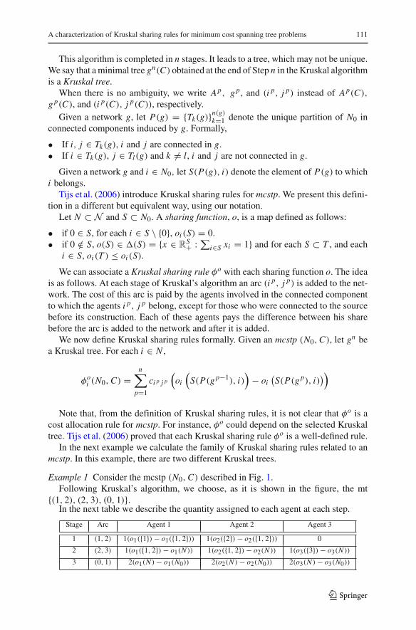
Example 1 Consider the mcstp (N0,C) described in Fig. 1.Following Kruskal’s algorithm, we choose, as it is shown in the figure, the mt

{(1, 2), (2, 3), (0, 1)}.In the next table we describe the quantity assigned to each agent at each step.

Stage Arc Agent 1 Agent 2 Agent 3

1 (1, 2) 1(o1({1})− o1({1, 2})) 1(o2({2})− o2({1, 2})) 0

2 (2, 3) 1(o1({1, 2})− o1(N )) 1(o2({1, 2})− o2(N )) 1(o3({3})− o3(N ))

3 (0, 1) 2(o1(N )− o1(N0)) 2(o2(N )− o2(N0)) 2(o3(N )− o3(N0))

123


Fig. 1 mcstp (N0,C)

Finally, we obtain

φo(N0,C) = (1 + o1(N ), 1 + o2(N ), 1 + o3(N )) ,

with o1(N ), o2(N ), o3(N ) ≥ 0 and o1(N )+ o2(N )+ o3(N ) = 1.Note that if we consider the other Kruskal tree, given by {(2, 3), (1, 2), (0, 1)}, we

obtain the same result because Kruskal sharing rules are well-defined (Tijs et al. 2006).

Next, we give the first characterization of the family of Kruskal sharing rules. Thischaracterization is based on a property of monotonicity over the set of agents anda property of additivity defined in Bergantiños and Vidal-Puga (2008). This resultholds for any set of possible agents N except for two-agent sets. In this situation, it issufficient to add the property of non-negativity.

Population monotonicity (PM): For each mcstp (N0,C), each S ⊂ N , and each i ∈ S

ψi (S0,C) ≥ ψi (N0,C).

This property implies that if some agents leave no remaining agent should be betteroff than before.

Additivity is a standard property and it has been used in many situations. In thecase of mcstp, additivity says that if we have two mcstp (N0,C) and (N0,C ′) then,ψ(N0,C + C ′) = ψ(N0,C)+ψ(N0,C ′). The following example shows that no rulesatisfies this property.

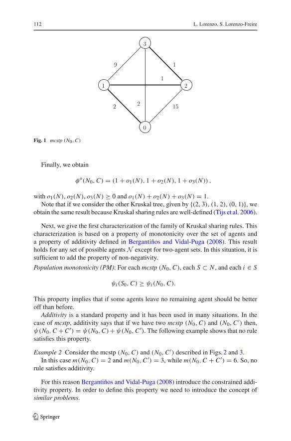
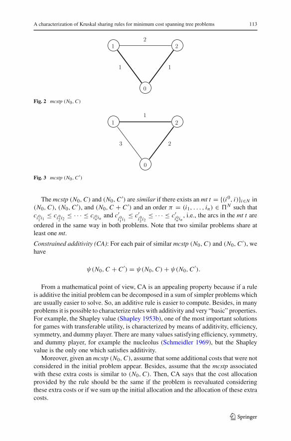
Example 2 Consider the mcstp (N0,C) and (N0,C ′) described in Figs. 2 and 3.In this case m(N0,C) = 2 and m(N0,C ′) = 3, while m(N0,C + C ′) = 6. So, no

rule satisfies additivity.

For this reason Bergantiños and Vidal-Puga (2008) introduce the constrained addi-tivity property. In order to define this property we need to introduce the concept ofsimilar problems.

123


Fig. 2 mcstp (N0,C)

Fig. 3 mcstp (N0,C ′)

The mcstp (N0,C) and (N0,C ′) are similar if there exists an mt t = {(i0, i)}i∈N in(N0,C), (N0,C ′), and (N0,C + C ′) and an order π = (i1, . . . , in) ∈ �N such thatci0

1 i1≤ ci0

2 i2≤ · · · ≤ ci0

n inand c′

i01 i1

≤ c′i02 i2

≤ · · · ≤ c′i0n in

, i.e., the arcs in the mt t are

ordered in the same way in both problems. Note that two similar problems share atleast one mt.

Constrained additivity (CA): For each pair of similar mcstp (N0,C) and (N0,C ′), wehave

ψ(N0,C + C ′) = ψ(N0,C)+ ψ(N0,C ′).

From a mathematical point of view, CA is an appealing property because if a ruleis additive the initial problem can be decomposed in a sum of simpler problems whichare usually easier to solve. So, an additive rule is easier to compute. Besides, in manyproblems it is possible to characterize rules with additivity and very “basic” properties.For example, the Shapley value (Shapley 1953b), one of the most important solutionsfor games with transferable utility, is characterized by means of additivity, efficiency,symmetry, and dummy player. There are many values satisfying efficiency, symmetry,and dummy player, for example the nucleolus (Schmeidler 1969), but the Shapleyvalue is the only one which satisfies additivity.

Moreover, given an mcstp (N0,C), assume that some additional costs that were notconsidered in the initial problem appear. Besides, assume that the mcstp associatedwith these extra costs is similar to (N0,C). Then, CA says that the cost allocationprovided by the rule should be the same if the problem is reevaluated consideringthese extra costs or if we sum up the initial allocation and the allocation of these extracosts.

123


Non-negativity (NN): For each mcstp (N0,C) and each i ∈ N , ψi (N0,C) ≥ 0.Below, we introduce two interesting properties, which are also satisfied by Kruskal

sharing rules.

Strong Cost Monotonicity (SCM): For each pair of mcstp (N0,C) and (N0,C ′) suchthat C ≤ C ′,

ψ (N0,C) ≤ ψ(N0,C ′) .

This property implies that if some connection costs increase, no agent ends up bet-ter off. It was introduced by Bergantiños and Vidal-Puga (2007b). Tijs et al. (2006)proved that Kruskal sharing rules satisfy SCM.

Continuity (CON): ψ is a continuous function of C .

Lemma 2 Consider an mcstp (N0,C) and {Cq}m(C)q=1 and {xq}m(C)

q=1 satisfying the con-

ditions of Lemma 1. Then, the mcstp {(N0, xqCq)}m(C)q=1 are similar.

Proof Suppose that there exists an mt t = {(i0, i)}i∈N in (N0,C) and assume, withoutloss of generality, that c101 ≤ c202 ≤ · · · ≤ cn0n . By Lemma 1 (3), t is an mt in (N0,Cq)

and for each q = 1, . . . ,m(C), cq101

≤ cq202

≤ · · · ≤ cqn0n

. Since xq ≥ 0, t is also an

mt in (N0, xqCq) and for each q = 1, . . . ,m(C), xqcq101

≤ xqcq202

≤ · · · ≤ xqcqn0n

.��

Proposition 1 Kruskal sharing rules satisfy NN, PM, CA, and CON.

Proof Kruskal sharing rules satisfy NN by definition.Kruskal sharing rules satisfy PM (Tijs et al. 2006).To show that Kruskal sharing rules satisfy CA, we consider two similar mcstp

(N0,C) and (N0,C ′). Assume, without loss of generality, that t = {(i0, i)}i∈N is acommon mt for both mcstp such that c101 ≤ c202 ≤ · · · ≤ cn0n and c′

101≤ c′

202≤

· · · ≤ c′n0n

. Note that t = {(i0, i)}i∈N is also an mt in (N0,C + C ′) and c101 + c′101

≤c202+c′

202≤ · · · ≤ cn0n +c′

n0n. Furthermore, Kruskal sharing rules are independent of

the chosen Kruskal tree (Tijs et al. 2006). Therefore, given a Kruskal sharing rule φo,

φoi

(N0,C + C ′) =

n∑

p=1

(cp0 p + c′

p0 p

) (oi (S(P(g

p−1), i))− oi (S(P(gp), i))

)

=n∑

p=1

cp0 p

(oi (S(P(g

p−1), i))− oi (S(P(gp), i))

)

+n∑

p=1

c′p0 p

(oi (S(P(g

p−1), i))− oi (S(P(gp), i))

)

= φoi (N0,C)+ φo

i (N0,C ′).

In the case of CON, we define for each mcstp (N0,C) and each ε > 0, the mcstp(N0,C+ε) and (N0,C−ε), where for each i, j ∈ N0, c+ε

i j = ci j + ε and c−εi j =

123


max{0, ci j −ε}. Given an mt t = {(i0, i)}i∈N for (N0,C) such that c101 ≤ c202 ≤ · · · ≤cn0n , t is also an mt for (N0,C+ε) and (N0,C−ε). Moreover, c+ε

101≤ c+ε

202≤ · · · ≤ c+ε

n0nand c−ε

101≤ c−ε

202≤ · · · ≤ c−ε

n0n.

The allocation generated by the Kruskal sharing rule in the mcstp (N0,C+ε) isgiven by

φoi

(N0,C+ε) =

n∑

p=1

c+εp0 p

(oi (S(P(g

p−1), i))− oi (S(P(gp), i))

)

=n∑

p=1

(cp0 p + ε

) (oi (S(P(g

p−1), i))− oi (S(P(gp), i))

)

=n∑

p=1

cp0 p

(oi (S(P(g

p−1), i))− oi (S(P(gp), i))

)+ ε

= φoi (N0,C)+ ε.

On the other hand, the allocation generated by the Kruskal sharing rule in the mcstp(N0,C−ε) is given by

φoi

(N0,C−ε) =

n∑

p=1

c−εp0 p

(oi (S(P(g

p−1), i))− oi (S(P(gp), i))

)

=n∑

p=1

max{0, cp0 p − ε}(

oi (S(P(gp−1), i))− oi (S(P(g

p), i)))

≥n∑

p=1

cp0 p

(oi (S(P(g

p−1), i))− oi (S(P(gp), i))

)− ε

= φoi (N0,C)− ε.

Consider now the sequence of cost matrices {Cε} such that for each i, j ∈ N0,|cεi j − ci j | < ε . Note that C−ε ≤ Cε ≤ C+ε . Since Kruskal sharing rules satisfySCM (Tijs et al. 2006),

φoi (N0,C)− ε ≤ φo

i

(N0,C−ε) ≤ φo

i

(N0,Cε

) ≤ φoi

(N0,C+ε) = φo

i (N0,C)+ ε.

Thus, for each i ∈ N , |φoi (N0,Cε)− φo

i (N0,C)| < ε. ��Theorem 1 Suppose that |N | ≥ 3. A rule ψ satisfies PM and CA if and only if foreach mcstp (N0,C) such that N ⊂ N ,

ψ(N0,C) = φo(N0,C),

where o is the sharing function defined, for each S ∈ 2N \{∅}, by

o(S) = ψ(S0, C)

123


and the cost matrix C =

⎛

⎜⎜⎜⎝

0 1 · · · 11 0 · · · 0...

.... . .

...

1 0 · · · 0

⎞

⎟⎟⎟⎠

.

Proof Existence. Proposition 1 proves that Kruskal sharing rules satisfy PM and CA.

Uniqueness. Consider a ruleψ satisfying PM and CA. We divide the proof in severalclaims.

Claim 1 o is a sharing function.

Proof of Claim 1 As ψ satisfies PM, for each S ⊂ T ∈ 2N \{∅} and each i ∈ S,oi (T ) ≤ oi (S).

Moreover, since for each S ∈ 2N \{∅}, m(S0, C) = 1, if for each S ∈ 2N \{∅} andeach i ∈ S, oi (S) ≥ 0, then the vector o(S) belongs to the simplex in RS .

Suppose that S = {i}, with i ∈ N . We know that oi (S) = ψi (S0, C) = 1. Next,suppose that |S| > 1. In this case, by PM, for each i ∈ S and each j ∈ S \ {i},ψ j (S0, C) ≤ ψ j ((S0 \{i}), C). Thus, 1 − ψi (S0, C) ≤ ∑

j∈S\{i}ψ j (S0 \{i}, C) = 1

and, hence, oi (S) = ψi (S0, C) ≥ 0. ��Consider C =∑m(C)

q=1 xqCq with {Cq}m(C)q=1 and {xq}m(C)

q=1 satisfying the conditions

of Lemma 1. Since ψ satisfies CA, by Lemma 2, ψ(N0,C) = ∑m(C)q=1 ψ(N0, xqCq).

By Proposition 1, Kruskal sharing rules satisfy CA. Thus, φo(N0,C) = ∑m(C)q=1 φ

o

(N0, xqCq). Therefore, it is sufficient to prove that ψ(N0, xqCq) = φo(N0, xqCq).

Claim 2 Consider a sharing function o and an mcstp (N0,C) such that there exists anetwork g with ci j = x ≥ 0 if (i, j) ∈ g and ci j = 0 otherwise. Let {Tr }m

r=1 be thepartition of N0 in C-components. Then, for each i ∈ Tr and each r = 1, . . . ,m,

φoi (N0,C) =

{0, 0 ∈ Tr

xoi (Tr ), 0 /∈ Tr .

Proof of Claim 2 Given a sharing function o, let us consider the Kruskal sharing ruleφo. If we apply Kruskal’s algorithm, we assume that in the first n − m stages theagents in each component are connected to one another, i.e., P(gn−m) = {Tr }m

r=1.Since for each p = 1, . . . , n − m, ci p j p = 0 and oi (T ) = 0 when the source is in T ,we distinguish two cases:

1. 0 ∈ Tr . In this case, for each i ∈ Tr , φoi (N0,C) = 0.

2. 0 /∈ Tr . At Stage n − m + 1 of Kruskal’s algorithm, it is possible to select the arc(in−m+1, jn−m+1) such that in−m+1 ∈ Tr and jn−m+1 = 0. Therefore, for eachi ∈ Tr ,

φoi (N0,C) = cin−m+10oi

(S(P(gn−m), i)

) = xoi (Tr ).

��

123


Claim 3 Given a mcstp (N0,C) such that there exists a network g with ci j = x ≥ 0if (i, j) ∈ g and ci j = 0 otherwise, φo(N0,C) = ψ(N0,C).

Proof of Claim 3 Since m(N0,C) =∑mr=1 m((Tr )0,C) (Bergantiños and Vidal-Puga

2008) and ψ satisfies PM, for each i ∈ Tr and each r = 1, . . . ,m, ψi (N0,C) ≤ψi ((Tr )0,C). Moreover,

∑i∈Tr

ψi ((Tr )0,C) = m((Tr )0,C) and∑

i∈Nψi (N0,C) =m(N0,C). Thus, for each i ∈ Tr and each r = 1, . . . ,m, ψi (N0,C) = ψi ((Tr )0,C).

We define two cost matrices C and C by

ci j ={

0 if 0 ∈ {i, j}ci j otherwise

and ci j ={

ci j if 0 ∈ {i, j}0 otherwise

for each i, j ∈ N0.

Note that ((Tr )0, C) and ((Tr )0, C) are similar and that C = C + C . By CA,

ψ((Tr )0,C) = ψ((Tr )0, C)+ ψ((Tr )0, C).

Since for each i ∈ Tr and each r = 1, . . . ,m, m((Tr )0, C) = 0 and m({i}0, C) = 0,by PM, for each i ∈ Tr and each r = 1, . . . ,m, ψi ((Tr )0, C) = ψi ({i}0, C) = 0.Therefore, for each r = 1, . . . ,m, ψ((Tr )0,C) = ψ((Tr )0, C).

We distinguish two cases:

Case 1. 0 ∈ Tr . We have to prove that for each i ∈ Tr , ψi (N0,C) = 0 = φoi (N0,C).

We distinguish two subcases:

Subcase 1.a. For each i ∈ Tr , ci0 = 0. In this case, for each i ∈ Tr , ψi (N0,C) =ψi ((Tr )0,C) = 0 = φo

i (N0,C).

Subcase 1.b. There exist j, k ∈ Tr such that c0 j = 0 and c0k = x .Following similar arguments to Bergantiños and Vidal-Puga (2008), weconsider T 1

r = {i ∈ Tr : c0i = x} ∪ { j} and T 2r = {i ∈ Tr : c0i =

0} \ { j}.We know that m((Tr )0, C) = m((T 1

r )0, C)+ m((T 2r )0, C). By PM,

ψi (N0,C) = ψi ((Tr )0, C) ={ψi ((T 1

r )0, C) if i ∈ T 1r

ψi ((T 2r )0, C) if i ∈ T 2

r

By Subcase 1.a., for each i ∈ Tr2, ψi ((T 2

r )0, C) = 0.By CA, ψ((T 1

r )0, C) = ∑i∈T 1

r \{ j} ψ((T 1r )0, (C)

i ) where (c0i )i = x

and (ckl)i = 0 otherwise.

Since m((T 1r )0, (C)

i ) = m({i, j}0, (C)i ) +∑k∈T 1r \{i, j}m({k}0, (C)i ),

by PM,

ψk

((T 1

r )0, (C)i)

= 0 for each k ∈ T 1r \{ j, i},

ψ j

((T 1

r )0, (C)i)

= ψ j

({i, j}0, (C)

i), and

ψi

((Tr

1)0, (C)i)

= ψi

({i, j}0, (C)

i).

123


Ifψ j ((T 1r )0, (C)

i ) = 0 andψi ((T 1r )0, (C)

i ) = 0, then, for each i ∈ T 1r ,

ψi (N0,C) = ψi ((Tr )0, C) = ψi ((T 1r )0, C) = 0 = φo

i (N0,C). It issufficient to prove that ψi ({i, j}0,C) = ψ j ({i, j}0,C) = 0 for themcstp ({i, j}0,C) such that c0 j = ci j = 0 and c0i = x .Since m({i, j}0,C) = 0, we assume that

ψi ({i, j}0,C) = −ψ j ({i, j}0,C) .

We prove that ψ j ({i, j}0,C) = 0.As |N | ≥ 3, consider the mcstp ({i, j, k}0,C ′) such that c′

0i = xand c′

hl = 0 otherwise. Since m({i, j, k}0,C ′) = m({i, j}0,C ′) +m({k}0,C ′) = m({i, k}0,C ′) + m({ j}0,C ′), by PM, ψ j ({i, j, k}0,

C ′) = ψ j ({i, j}0,C) = ψ j ({ j}0,C) = 0.

Case 2. 0 /∈ Tr . In this case, for each i ∈ Tr , c0i = x .

We know that ψ((Tr )0,C) = ψ((Tr )0, C) = ψ((Tr )0, xC). By Claim 2,φo((Tr )0,C) = xo(Tr ) = xψ((Tr )0, C). Then, to show thatψ(N0,C) = φo(N0,C),we only need to prove that

ψ((Tr )0, xC

) = xψ((Tr )0, C

), where x ≥ 0.

We distinguish two subcases:

Subcase 2.a. x = pq where p, q ∈ N. Sinceψ satisfies CA, it is straightforward that

ψ((Tr )0, xC) = xψ((Tr )0, C).

Subcase 2.b. x ∈ R+ \ Q+. There exists {x p}p∈N such that for each p ∈ N,

0 < x p < x , x p ∈ Q+ and lim p→∞x p = x . Thus, for each p ∈ Nand each i ∈ Tr ,

ψi((Tr )0, xC

)−x pψi((Tr )0, C

)=ψi((Tr )0, xC

)−ψi((Tr )0, x pC

).

Since the mcstp ((Tr )0, (x − x p)C) and ((Tr )0, x pC) are similar,

ψi((Tr )0, xC

)− ψi((Tr )0, x pC

) = ψi((Tr )0, (x − x p)C

).

In addition, by PM∑

j∈Tr \{i}ψ j((Tr )0, (x − x p)C

) ≤∑

j∈Tr \{i}ψ j((Tr \{i})0, (x − x p)C

).

So, 0 ≤ ψi ((Tr )0, (x − x p)C) ≤ (x − x p)m((Tr )0, C) = x − x p.Therefore,

0 ≤ limp→∞

[ψi ((Tr )0, xC)− x pψi ((Tr )0, C)

]

= ψi((Tr )0, xC

)− xψi((Tr )0, C

)

≤ limp→∞(x − x p) = 0.

Then, for each i ∈ Tr , ψi ((Tr )0, xC) = xψi ((Tr )0, C). ��

123


According to Theorem 1, we have a characterization of the family of Kruskalsharing rules when |N | ≥ 3. Moreover, we have obtained an expression for the shar-ing function associated with a Kruskal sharing rule. For any set of possible agents N ,we have similar results if we add NN.

Theorem 2 A rule ψ satisfies PM, CA, and NN if and only if

ψ(N0,C) = φo(N0,C),

where o is the sharing function defined, for each S ∈ 2N \{∅}, by

o(S) = ψ(S0, C)

and the cost matrix C =

⎛

⎜⎜⎜⎝

0 1 · · · 11 0 · · · 0...

.... . .

...

1 0 · · · 0

⎞

⎟⎟⎟⎠.

Proof Existence.By Proposition 1, Kruskal sharing rules satisfy PM, CA, and NN.

Uniqueness.Consider a rule ψ satisfying PM, CA, and NN.If |N | ≥ 3, we invoke Theorem 1 and, if |N | = 2, we follow the procedure used

in Theorem 1 except for the mcstp ({i, j}0,C) with c0 j = ci j = 0 and c0i = x . Inthis case, applying NN and considering that ψi ({i, j}0,C)+ ψ j ({i, j}0,C) = 0, weobtain that ψi ({i, j}0,C) = ψ j ({i, j}0,C) = 0. ��

The properties stated in Theorem 2 are independent.

• The equal division rule, δi (N0,C) = 1n m(N0,C) for each i ∈ N , satisfies NN

and CA. However, δ does not satisfy PM. Indeed, consider the mcstp (N0,C),

where N = {1, 2} and C =⎛

⎝0 0 10 0 11 1 0

⎞

⎠. In this case, δ1({1}0,C) = 0 while

δ1(N0,C) = 12 .

• Consider the subset of orders

�N ={π ∈ �N |π(i) < π( j) when c0i ≤ c0 j for each i, j ∈ N , i �= j

}.

Let β be the rule defined, for each i ∈ N , by

βi (N0,C) = 1

|�N |∑

π∈�N

(vC∗(Pre(i, π) ∪ {i})− vC∗(Pre(i, π))) .

123


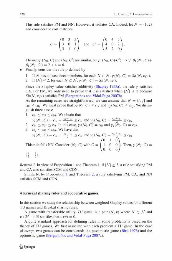
This rule satisfies PM and NN. However, it violates CA. Indeed, let N = {1, 2}and consider the cost matrices

C =⎛

⎝0 3 33 0 13 1 0

⎞

⎠ and C ′ =⎛

⎝0 4 54 0 25 2 0

⎞

⎠ .

The msctp (N0,C) and (N0,C ′) are similar, butβ1(N0,C+C ′)=7 �= β1(N0,C)+β1(N0,C ′) = 2 + 4 = 6.

• Finally, consider the rule γ defined by

1. If N has at least three members, for each N ⊂ N , γ (N0,C) = Sh(N , vC∗).2. If |N | ≤ 2, for each N ⊂ N , γ (N0,C) = Sh(N , vC ).

Since the Shapley value satisfies additivity (Shapley 1953a), the rule γ satisfiesCA. For PM, we only need to prove that it is satisfied when |N | ≤ 2 becauseSh(N , vC∗) satisfies PM (Bergantiños and Vidal-Puga 2007b).As the remaining cases are straightforward, we can assume that N = {i, j} andc0i ≤ c0 j . We must prove that γi (N0,C) ≤ c0i and γ j (N0,C) ≤ c0 j . We distin-guish three cases:1. c0i ≤ ci j ≤ c0 j . We obtain that

γi (N0,C) = c0i + ci j −c0 j2 ≤ c0i and γ j (N0,C) = ci j +c0 j

2 ≤ c0 j .2. c0i ≤ c0 j ≤ ci j . In this case, γi (N0,C) = c0i and γ j (N0,C) = c0 j .3. ci j ≤ c0i ≤ c0 j . We have that

γi (N0,C) = c0i + ci j −c0 j2 ≤ c0i and γ j (N0,C) = ci j +c0 j

2 ≤ c0 j .

This rule fails NN. Consider (N0,C) with C =⎛

⎝0 1 01 0 00 0 0

⎞

⎠. Then, γ (N0,C) =

( 12 ,− 1

2 ).

Remark 1 In view of Proposition 1 and Theorem 1, if |N | ≥ 3, a rule satisfying PMand CA also satisfies SCM and CON.

Similarly, by Proposition 1 and Theorem 2, a rule satisfying PM, CA, and NNsatisfies SCM and CON.

4 Kruskal sharing rules and cooperative games

In this section we study the relationship between weighted Shapley values for differentTU games and Kruskal sharing rules.

A game with transferable utility, TU game, is a pair (N , v) where N ⊂ N andv : 2N → R satisfies that v (∅) = 0.

A quite standard approach for defining rules in some problems is based on thetheory of TU games. We first associate with each problem a TU game. In the caseof mcstp, two games can be considered: the pessimistic game (Bird 1976) and theoptimistic game (Bergantiños and Vidal-Puga 2007a).

123


• The pessimistic game associated with an mcstp (N0,C) is denoted by (N , vC ).The value of each coalition S ⊂ N is the cost of connecting agents in S to thesource, assuming that agents in N \S are not present:

vC (S) = m(S0,C).

• The optimistic game associated with an mcstp (N0,C) is denoted by (N , v+C ). The

value of each coalition S ⊂ N is the cost of connecting agents in S to the source,assuming that agents in N \S are already connected, and agents in S can connectto the source through agents in N \S:

v+C (S) = m

(S0,C+(N\S)

)

where for each i, j ∈ S, c+(N\S)i j =ci j and for each i ∈ S, c+(N\S)

0i =min j∈(N\S)0 c ji .

Given an mcstp (N0,C), we can associate with it two additional TU games usingits irreducible form: (N , vC∗) and (N , v+

C∗).

Once the associated TU game has been chosen, we can compute a solution for TUgames. Thus, the rule in the original problem is defined as the solution applied to theTU game associated with the original problem.

Given a family of TU games H , a solution on H is a function f which assigns toeach TU game (N , v) ∈ H the vector ( f1(N , v), . . . , fn(N , v)) ∈ RN , where the realnumber fi (N , v) is the payoff of i ∈ N in the game (N , v) according to f . Several solu-tions have been defined for TU games. One of the best known solutions is the Shapleyvalue.

The Shapley value (Shapley 1953b) assigns to each TU game (N , v) the vectorSh(N , v) where for each i ∈ N ,

Shi (N , v) = 1

n!∑

π∈�N

[v(Pre(i, π) ∪ {i})− v(Pre(i, π))] .

In the literature on mcstp, several rules have been defined using solutions for anassociated TU game. For instance, Kar (2002) studied the Shapley value of (N , vC ),whereas Bergantiños and Vidal-Puga (2007b) studied the Shapley value of (N , vC∗).

Moreover, Bergantiños and Vidal-Puga (2007a) proved that Sh(N , v+C∗) = Sh(N ,

v+C ) = Sh(N , vC∗).1

Shapley (1953a) introduced the family of weighted Shapley values for TU games.Each weighted Shapley value associates a payoff with each player according to a setof positive weights over the set of players. These weights are the proportions in whichthe players share in unanimity games. Kalai and Samet (1987) studied this family.

1 Bergantiños and Vidal-Puga (2007a) proved that v+C∗ =v+C . Therefore, ShwN (N , v+C∗ )= ShwN (N , v+C ).

123


Given N ⊂ N and w = {wi }i∈N , we say that w is a weight system for N if foreach i ∈ N , wi > 0.

Take N ⊂ N and a weight systemw = {wi }i∈N . The weighted Shapley value Shw

associates with each TU game (N , v) a vector Shw(N , v) ∈ RN such that for eachi ∈ N ,

Shwi (N , v) =∑

π∈�N

pw(π) [v(Pre(π, i) ∪ {i})− v(Pre(π, i))]

where pw(π) =∏nj=1

wπ−1( j)

∑ jk=1wπ−1(k)

.

It is well known that the Shapley value is a weighted Shapley value where for eachi, j ∈ N , wi = w j .

Remark 2 Kalai and Samet (1987) assume that the population of agents is fixed. Thus,they define the weight system with respect to N . Since we work with population mono-tonicity, we can not make this assumption. Hence, we define the weight system withrespect to the set of possible agents N .

From now on, we say thatw = {wi }i∈N is a weight system for N if for each i ∈ N ,wi > 0. Given the weight system w and N ⊂ N , we denote wN = {wi }i∈N .

We now apply the weight system to the mcstp through the optimistic and pessimisticgames.

• We say that ψ is an optimistic weighted Shapley rule for mcstp if there exists aweight system w = {wi }i∈N such that for each mcstp(N0,C),

ψ(N0,C) = ShwN (N , v+C∗)

• We say that ψ is a pessimistic weighted Shapley rule for mcstp if there exists aweight system w = {wi }i∈N such that for each mcstp (N0,C),

ψ(N0,C) = ShwN (N , vC∗).

Bergantiños and Lorenzo (2008) proved that the optimistic weighted Shapley rules areKruskal sharing rules where the sharing function for an agent i in a coalition S is pro-

portional to his weight, i.e., for each S ∈ 2N \{∅} and each i ∈ S, owNi (S) = wi

∑j∈S w j

.

These authors also define the pessimistic weighted Shapley rules, proving that the fam-ilies of optimistic and pessimistic weighted Shapley rules are different. However, theydo not ask whether the pessimistic weighted Shapley rules are Kruskal sharing rulesor not. In this paper we study the relationship between both families, proving that thepessimistic weighted Shapley rules are also Kruskal sharing rules.

In accordance with Theorem 2, it is easy to calculate the sharing function for anyKruskal sharing rule. Then, we will apply this theorem not only to show that thepessimistic weighted Shapley rules are Kruskal sharing rules, but also to calculatethe associated sharing function. The same procedure could be applied in the case of

123


the optimistic weighted Shapley rules, obtaining the same result as Bergantiños andLorenzo (2008), but following a completely different proof.

Corollary 1 Let ϕw be the pessimistic weighted Shapley rule associated with theweight system w. Thus, for each mcstp (N0,C),

ϕw (N0,C) = φowN(N0,C) ,

where the sharing function owN is given, for each S ∈ 2N \{∅} and each i ∈ S, by

owNi (S) =

∑

π∈�(S\{i})

s−1∏

j=1

ωπ−1( j)∑ j

k=1 ωπ−1(k) + ωi

.

Proof Since Bergantiños and Vidal-Puga (2007a) proved that

vC∗ (Pre(i, π) ∪ {i})− vC∗(Pre(i, π)) = minj∈Pre(i,π)0

{c∗i j } ≥ 0,

ϕw satisfies NN.The weighted Shapley value satisfies additivity (Kalai and Samet 1987). Moreover,

v(C+C ′)∗ = v∗C +vC ′∗ , where (N0,C) and (N0,C ′) are two similar mcstp (Bergantiños

and Vidal-Puga 2008).Using these results, for each weight system w

ϕw(N0,C + C ′) = ShwN (N , v(C+C ′)∗)

= ShwN (N , vC∗ + vC ′∗)

= ShwN (N , vC∗)+ ShwN (N , vC ′∗)

= ϕw(N0,C)+ ϕw(N0,C ′).

Then, ϕw satisfies CA.Let us denote N− j = N \{ j}. To prove that the weighted Shapley value satisfies

PM, we need to prove that for each i ∈ N− j

ShwNi (N , vC∗) =

∑

π∈�N

pwN (π) [vC∗(Pre(i, π) ∪ {i})− vC∗(Pre(i, π))]

≤∑

π− j ∈�(N− j )

pwN− j (π− j )[vC∗(Pre(i, π− j )∪{i})−vC∗(Pre(i, π− j ))

]

= ShwN− j

i (N− j , vC∗).

123


We know that

∑

π∈�N

pwN (π)[vC∗(Pre(i, π) ∪ {i})− vC∗(Pre(i, π))]

=∑

π∈�N , j∈Pre(i,π)

pwN (π) mink∈Pre(i,π)0

{c∗ik} +

∑

π∈�N , j /∈Pre(i,π)


{c∗ik}

≤∑


pwN (π) mink∈(Pre(i,π)\{ j})0

{c∗ik}

+∑



{c∗ik}.

Given a cost matrix C , we know that C∗ ≤ C . Considering the connection costs ofagents in N− j

0 , (C∗)− j ≤ C− j , where C− j denotes the restriction of C to the agents inN− j . Moreover, (C∗)− j is an irreducible matrix (Bergantiños and Vidal-Puga 2007b).Thus, (C∗)− j ≤ (C− j )∗.

On the other hand, we denote πN− j as the restriction of π to N− j

Then, for each i ∈ N− j

ShwNi (N , vC∗) ≤

∑


pwN (π) mink∈(Pre(i,π)\{ j})0

{(c− j )∗ik}

+∑



{(c− j )∗ik}

=∑

π− j ∈�(N− j )

⎧⎪⎨

⎪⎩

∑

π∈�N ,πN− j =π− j

pwN (π) mink∈Pre(i,π− j )0

{(c− j )∗ik}

⎫⎪⎬

⎪⎭.

Bergantiños and Lorenzo (2008) prove that

∑

π∈�N ,πN− j =π− j

pwN (π) = pwN− j (π− j ).

Thus, for each i ∈ N− j

ShwNi (N , vC∗) ≤

∑

π− j ∈�(N− j )

pwN− j (π− j )

{

mink∈Pre(i,π− j )0

{(c− j )∗ik}}

= ShwN− j

i (N− j , vC∗).

Then, by Theorem 2, these rules are Kruskal sharing rules. To obtain the corre-sponding sharing function, we consider an mcstp (N0,C) and a weight system w.

123


The sharing function is, for each S ∈ 2N \{∅} and each i ∈ S,

owNi (S) = ϕwi (S0, C)

=∑

π∈�(S)pwS (π)

[vC (Pre(i, π) ∪ {i})− vC (Pre(i, π))

]

=∑

π∈�(S)pwS (π) min

k∈Pre(i,π)0{cik}

=∑

π∈�(S):π(i) �=1

pwS (π)0 +∑

π∈�(S):π(i)=1

pwS (π)1

=∑

π∈�(S):π(i)=1

pwS (π) =∑

π∈�(S\{i})

s−1∏

j=1

wπ−1( j)∑ j

k=1wπ−1(k) + wi

.

Acknowledgments Financial support from Ministerio de Ciencia y Tecnología and FEDER through grantSEJ2005-07637-C02-01 and from Xunta de Galicia through grants PGIDIT06PXIB362390PR and PGI-DIT06PXIC300184PN is gratefully acknowledged. We thank Lars Ehlers, Gustavo Bergantiños, WilliamThomson, and two anonymous referees for their valuable comments on this paper.

References

Aarts H, Driessen T (1993) The irreducible core of a minimum cost spanning tree game. Math MethodsOper Res 38:163–174

Bergantiños G, Lorenzo L (2004) A non-cooperative approach to the cost spanning tree problem. MathMethods Oper Res 59:393–403

Bergantiños G, Lorenzo-Freire S (2008) “Optimistic”weighted Shapley rules in minimum cost spanningtree problems. Eur J Oper Res 185:289–298

Bergantiños G, Vidal-Puga JJ (2005) Several approaches to the same rule in cost spanning tree problems.Working paper. Vigo University. Available at the web page of the authors

Bergantiños G, Vidal-Puga JJ (2007a) The optimistic TU game in minimum cost spanning tree problems.Int J Game Theory 36:223–239

Bergantiños G, Vidal-Puga JJ (2007b) A fair rule in cost spanning tree problems. J Econ Theory 137:326–352

Bergantiños G, Vidal-Puga JJ (2008) Additivity in cost spanning tree problems. J Math Econ (forthcoming)Bird CG (1976) On cost allocation for a spanning tree: a game theoretic approach. Networks 6:335–350Dutta B, Kar A (2004) Cost monotonicity, consistency and minimum cost spanning tree games. Games

Econ Behav 48:223–248Feltkamp V, Tijs S, Muto S (1994) On the irreducible core and the equal remaining obligations rule of

minimum cost spanning extension problems. CentER discussion paper 1994, 106. Tilburg UniversityGranot D, Huberman G (1981) Minimum cost spanning tree games. Math Programming 21:1–18Granot D, Huberman G (1984) On the core and nucleolus of the minimum cost spanning tree games. Math

Programming 29:323–347Kalai E, Samet D (1987) On weighted Shapley values. Int J Game Theory 16:205–222Kar A (2002) Axiomatization of the Shapley value on minimum cost spanning tree games. Games Econ

Behav 38:265–277Kruskal J (1956) On the shortest spanning subtree of a graph and the traveling salesman problem. Proc

Am Math Soc 7:48–50Moretti S, Tijs S, Branzei R, Norde H (2005) Cost monotonic “construct and charge” rules for connection

situations. CentER discussion paper 2005, 104. Tilburg UniversityNorde H, Moretti S, Tijs S (2004) Minimum cost spanning tree games and population monotonic allocation

schemes. Eur J Oper Res 154:84–97Prim RC (1957) Shortest connection networks and some generalizations. Bell Syst Technol J 36:1389–1401

123


Schmeidler D (1969) The nucleolus of a characteristic function game. SIAM J Appl Math 17:1163–1170Shapley LS (1953a) Additive and non-additive set functions. Ph.D. Thesis, Department of Mathematics,

Princeton UniversityShapley LS (1953b) A value for n-person games. In: Kuhn HW, Tucker AW (eds) Contributions to the

Theory of Games II. Princeton University Press, NJ, pp 307–317Thomson W (1983) The fair division of a fixed supply among a growing population. Math Oper Res 8:

319–326Thomson W (1995) Population-monotonic allocation rules. In: Barnett WA, Moulin H, Salles M, Schofield

N (eds) Social choice, welfare and ethics. Cambridge University Press, London, pp 79–124Tijs S, Branzei R, Moretti S, Norde H (2006) Obligation rules for minimum cost spanning tree situations

and their monotonicity properties. Eur J Oper Res 175:121–134

123

Documents

A characterization of Kruskal sharing rules for minimum cost spanning tree problems