Finding minimum spanning trees more efficiently for tile based phase unwrapping

Firas Sawaf and Ralph P. Tatam

Optical Sensors Group

Centre for Photonics and Optical Engineering

School of Engineering

Cranfield University

Cranfield,

Bedford MK43 OAL

Tel: 01234 745360

Fax: 01234 752452

Email: r.p.tatam@cranfield.ac.uk

Short Title: Efficient minimum spanning trees for tile based phase unwrapping

PACS: 02.10.0x, 42.30.Ms,

Keywords: Phase unwrapping, minimum spanning tree, graph theory

Abstract The tile-based phase unwrapping method employs an algorithm for finding the minimum spanning tree (MST) in each tile. We first examine the properties of a tile’s

representation from a graph theory view point, observing that it is possible to make use of a more efficient class of MST algorithms. We then describe a novel linear time

algorithm which reduces the size of the MST problem by half at the least, and solves it completely at best. We also show how this algorithm can be applied to a tile using a

sliding window technique. Finally, we show how the reduction algorithm can be combined with any other standard MST algorithm to achieve a more efficient hybrid,

using Prim’s algorithm for empirical comparison and noting that the reduction algorithm takes only 0.1% of the time taken by the overall hybrid.

1. Introduction

Automatic fringe analysis techniques, such as the Fourier transform [1, 2] and phase

stepping1 [3-6], produce phase information which is inherently wrapped onto the

range - to . The restoration of the unknown multiple of 2 is called phase

unwrapping, and is central to most such algorithms [7].

Phase unwrapping techniques utilising the tiling approach and the minimum spanning tree (MST) method [9-13] have been shown to have good noise immunity and

prevention of error propagation. This is mainly due to dividing the wrapped phase map into tile-like regions. Each tile is then unwrapped independently, and the tiles are

finally assembled to obtain the unwrapped phase map. The path for unwrapping in each tile is selected in a way which minimises the probability of error. This is

achieved by choosing a path whose total phase difference is minimal. Identifying such a path is in fact the MST graph theory problem. Prim’s algorithm [14] is a traditional

way of solving the MST problem, and is employed by tile phase unwrapping [15]. Finding a MST for each tile is a computationally demanding, and impacts the

efficiency of the overall unwrapping algorithm. We first examine how phase information in a tile is converted into a weighted graph, and how the topology of such

a graph enables the use of a more efficient class of MST algorithms. We then describe an algorithm tailored specifically to a tile’s topology. We show that it is linear time

efficient, O(n), where n is the number of pixels in a tile, and that it can be used to reduce the size of the MST problem by half or more. We then show how it can be

applied to a tile using an image processing sliding window technique. Finally, we discuss how any chosen MST algorithm could be attached to ours, creating an

efficient hybrid. We use Prim’s algorithm for empirical comparison.

2. Tile representation from a graph theory perspective

We give here a brief summary of the relevant graph theory principles [16-19] which

are relied upon in the descriptions given in the subsequent sections.

2.1 Graphs and trees

A graph,

Figure 1 (a), can be described as G = [n, e], and consists of a vertex set n connected by an edge set e.

30

65

22

16

17

45

120

30

22

16

17120

a. graph b. tree c. weighted graph d. MST

Figure 1 Graph, trees and MST

A graph is said to be connected if each of its vertices is connected to another vertex by at least one edge. A spanning tree,

1 Phase stepping is also known as quasi-heterodyning.

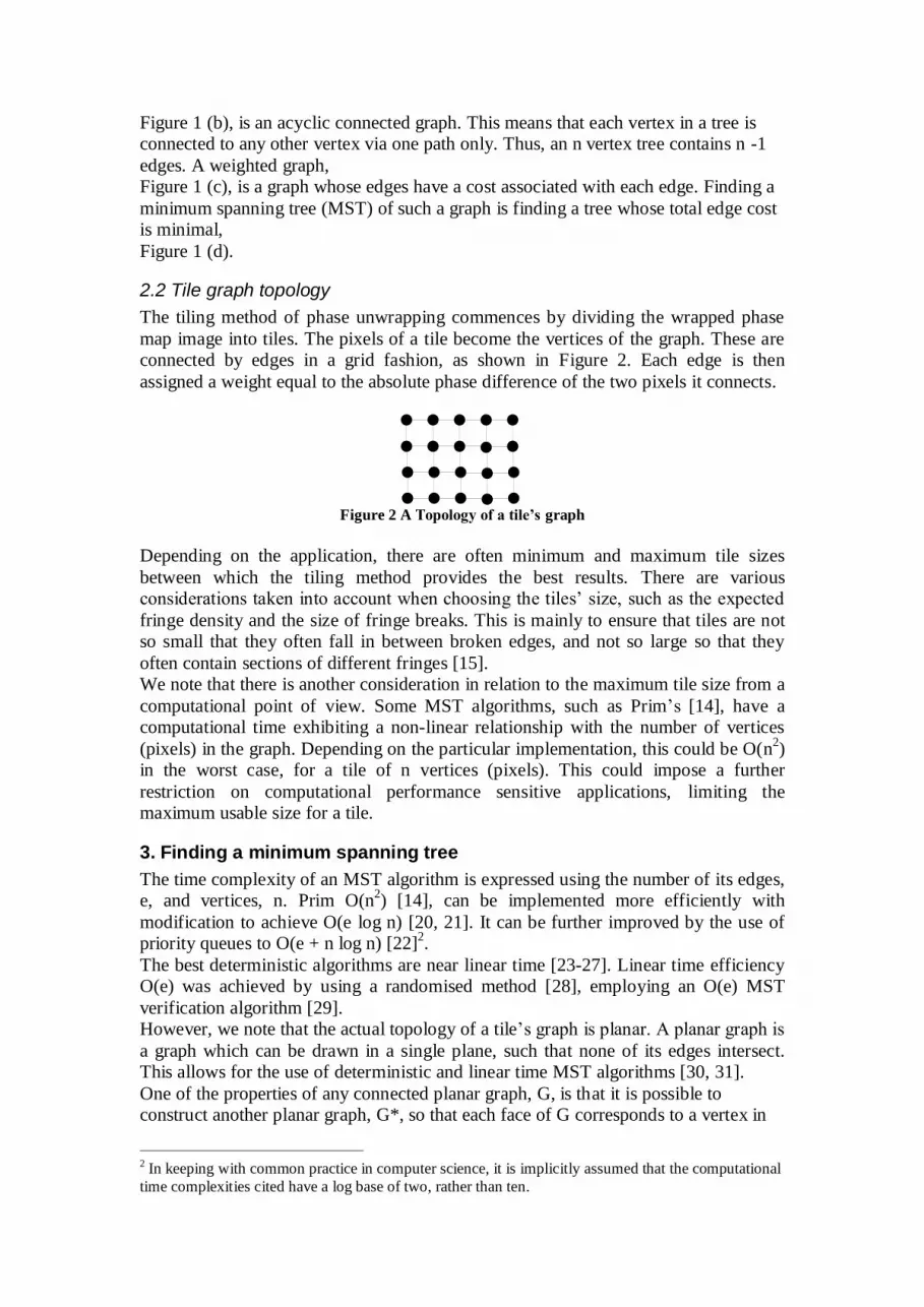
Figure 1 (b), is an acyclic connected graph. This means that each vertex in a tree is connected to any other vertex via one path only. Thus, an n vertex tree contains n -1

edges. A weighted graph, Figure 1 (c), is a graph whose edges have a cost associated with each edge. Finding a

minimum spanning tree (MST) of such a graph is finding a tree whose total edge cost is minimal,

Figure 1 (d).

2.2 Tile graph topology

The tiling method of phase unwrapping commences by dividing the wrapped phase

map image into tiles. The pixels of a tile become the vertices of the graph. These are connected by edges in a grid fashion, as shown in Figure 2. Each edge is then

assigned a weight equal to the absolute phase difference of the two pixels it connects.

Figure 2 A Topology of a tile’s graph

Depending on the application, there are often minimum and maximum tile sizes

between which the tiling method provides the best results. There are various considerations taken into account when choosing the tiles’ size, such as the expected

fringe density and the size of fringe breaks. This is mainly to ensure that tiles are not so small that they often fall in between broken edges, and not so large so that they

often contain sections of different fringes [15]. We note that there is another consideration in relation to the maximum tile size from a

computational point of view. Some MST algorithms, such as Prim’s [14], have a computational time exhibiting a non-linear relationship with the number of vertices

(pixels) in the graph. Depending on the particular implementation, this could be O(n2)

in the worst case, for a tile of n vertices (pixels). This could impose a further

restriction on computational performance sensitive applications, limiting the maximum usable size for a tile.

3. Finding a minimum spanning tree

The time complexity of an MST algorithm is expressed using the number of its edges, e, and vertices, n. Prim O(n

2) [14], can be implemented more efficiently with

modification to achieve O(e log n) [20, 21]. It can be further improved by the use of priority queues to O(e + n log n) [22]

2.

The best deterministic algorithms are near linear time [23-27]. Linear time efficiency O(e) was achieved by using a randomised method [28], employing an O(e) MST

verification algorithm [29]. However, we note that the actual topology of a tile’s graph is planar. A planar graph is

a graph which can be drawn in a single plane, such that none of its edges intersect. This allows for the use of deterministic and linear time MST algorithms [30, 31].

One of the properties of any connected planar graph, G, is that it is possible to construct another planar graph, G*, so that each face of G corresponds to a vertex in

2 In keeping with common practice in computer science, it is implicitly assumed that the computational

time complexities cited have a log base of two, rather than ten.

G*. Each pair of faces in G having an edge in common, has a corresponding edge in G* crossing it. G* is called a dual graph of G,

Figure 3.

Figure 3 A graph G (solid edges and vertices) and it dual G*

Dual graphs have interesting properties, stemming from the fact that each cycle-set of G’s edges is also a cut-set of G*, and vice versa. Matsui [31] relies on these properties

to construct a linear time MST algorithm O(e + n), noting that a maximum edge of a vertex in G* can be ruled out of G’s minimum spanning tress, and a minimal edge of

a vertex in G can be ruled out of G*’s maximum spanning tree.

3.1. Reducing the problem’s size

Theoretically, it is only possible to improve on O(n) efficiency by having prior

knowledge of the MST itself. This is the case for MST maintenance algorithms which

can carry out a single update, such as single weight change, in O( e ) [32], and in

O(log n) for planar graphs [33, 34].

Although prior knowledge of the topology of a graph may not improve on O(n), it can help to improve the overall efficiency of the algorithm in empirical terms. This could

be by reducing the total number of times the edges and vertices are handled, or minimising the total number of edge weight comparisons necessary.

We describe a novel linear time O(n) algorithm which takes advantage of the prior

knowledge of a tile’s graph topology to reduce its size from G(n, e) to somewhere between zero, at best, and G[n/2, e/2] at the very most.

This has the effect of reducing the size of the problem needed to be solved by the underlying MST algorithm of choice.

Image processing algorithms often employ a sliding window technique to apply their various operations to the image in question. Similarly, we show how our algorithm can be applied to a tile using a sliding window.

For clarity, we start by describing the four steps of the algorithm separately. The discrete description is used subsequently for time-performance analysis, and for

describing the sliding window operations.

4. Algorithm fundamentals and performance analysis

4.1 Initial state

The tile, Figure 2, can have any number of rows and columns of vertices. Each corner vertex has two edges, the minimum of which can be immediately ruled in

the MST (if not, the resultant tree is either disconnected or is not minimum). Processing the four corners in this way can be carried out in constant time O(1),

regardless of the number of vertices, n.

Figure 4 illustrates the representation of a tile’s graph G, and its dual G*, once the corners have been processed.

VO

Figure 4 A tile’s graph G (solid edges and vertices) and it dual G*. VO is a G* vertex

corresponding to the outer face3 of G.

The dual graph G* need not be constructed in practice, and is only shown here to help

clarify the underlying interactions of the various steps of the algorithm.

We observe that at this initial state, due to prior knowledge of the topology, the graph fulfils the following criteria:

a Both G[n, e] and G*[n*, e*] are connected and naturally planar

b e = e*, n n*

c The size of e approaches the size of 2n.

d Neither G or G* have two vertices connected to each other by more than one

edge. This is secured by pre-processing the corners, which removes such

edges from G* (as opposed to a counter example shown in Figure 3)

e Each vertex4 in G and G*, has a maximum of 4 edges.

f Any G vertex can be picked from this initial state of G and processed

independently, and its minimum edge can be ruled in the MST.

g Any G* vertex can be picked from this initial state of G* and processed

independently. Its maximum edge can be ruled out of the MST.

h Any edge of G and G* can be processed in the same independent way as

described in f or g, unless one or more of its edges has already been ruled in or out by processing an adjacent vertex in the same graph.

4.2 Step 1 – Process G vertices alternately, ruling in one edge per vertex

The alternate fashion in which the G vertices are targeted,

3 A graph’s outer face is also known as the unbounded or infinite face. 4 As G*’s most outer vertex (VO) does not satisfy this criterion, it will not be relied upon for any of the

steps of the algorithm. Although the edges of VO will still be processed by the algorithm, this will be done in the context of the other vertices in G* which are connected to VO. Therefore, all references to

G* vertices from this point on shall implicitly exclude VO.

Figure 5 (a), ensures that they can be processed independently (criteria f and h). In effect, the G vertices which are not being targeted act as an isolating barrier.

VO

VO

a. G vertices targeted by step 1 b. G* vertices targeted by step 2

VO

VO

c. G vertices targeted by step 3 d. G* vertices targeted by step 4

Figure 5 Targeted vertices (shaded)

Each vertex has a maximum of four edges, therefore the minimum edge of each of

these vertices can be ruled in the MST in O(1).

4.2 Step 2 – Process G* vertices alternately, ruling out one edge per vertex

Each targeted G* vertex,

Figure 5 (b), has a maximum of four edges, therefore the maximum edge of each of these vertices can be found in O(1). This maximum edge of G* crosses an edge in G,

which in turn can be ruled out from the MST. In a similar way to step 1, G* vertices which are targeted can be processed

independently.

4.3 Step 3 – Ensure each remaining G vertex is connected to at least one ruled-in edge

Each of the remaining G vertices, Figure 5 (c), is examined in turn. If it is has an edge which has been already ruled in

the MST, then no further processing is required. Otherwise, it must still have one or more edges which have not been processed, because step 2 could not possibly have

deleted all of its edges. This also means that such a vertex can still be processed independently (criteria f and h), and therefore we can rule in its minimum edge in

O(1).

4.4 Step 4 - Ensure each remaining G* vertex is connected to at least one ruled-out edge

The remaining G* vertices,

Figure 5 (d), are targeted by this step. It can be shown, using arguments similar to those of step 3, that each of the targeted vertices in G* either has a ruled out edge (due

to step 2), or, otherwise, its maximum edge can be found in O(1). This maximum edge of G* crosses an edge in G, which in turn can be ruled out from the MST.

The algorithm ends when step 4 has completed. At this point, none of the vertices in either G or G* can automatically satisfy criteria f, g or h by relying on a prior

knowledge of the initial state.

5. Problem reduction analysis

The consequence of steps 1 and 2 is that n/2 edges are ruled in the MST and n/2 edges

are ruled out. This means that the original G[n, e] graph is now reduced to G[n/2, e/2].

The ruled out edges can be clearly dismissed from the graph. Each ruled in edge, on the other hand, serves to fuse the two vertices it connects into one vertex.

The remaining (i.e. neither ruled in or out) edges of the original two vertices now become incident on the fused vertex.

A B

AB

The dashed edge is contracted. The union of

edges incident onto A and B becomes incident on the merged vertex, AB.

Figure 6 Edge contraction

This process is known as edge contraction,

Figure 6, and naturally results in the reduction of the number of the vertices in the graph.

If the algorithm were only to perform steps 1 and 2, it would still be guaranteed to

reduce the original problem by half. This gives the algorithm the worst case reduction bound.

Steps 3 and 4 of the algorithm may improve on the above reduction, but are not guaranteed to do so; it is possible that by some chance every non-targeted vertex has

one of its edges contracted or removed by an adjacent targeted vertex. In this case steps 3 and 4 would not perform any further edge contraction or deletion.

At the other extreme, steps 3 and 4 could find n/2 edges to contract, therefore completely solving the MST problem. This is because an MST has exactly n-1 edges

to be identified (i.e. ruled in or contracted).

5.1 Edge contraction and dual graph construction

The edge contraction, described above, serves to illustrate the extent of the problem

reduction. Explicit edge contraction as such, however, need not be performed by the algorithm for the above stated reduction in problem size to be realised. The same

applies to the construction of the dual graph G*. Whether or not edge contraction or G* construction need to be performed, solely

depends on the nature of the algorithm chosen to find the remaining edges of the MST. Matsui [31], for example, requires G*, and avoids edge contraction by

employing a constant time bucketing strategy to keep track of the vertices which are less than four-connected. By contrast, algorithms such as [24, 28] do depend on edge

contraction, but do not employ a dual graph as they were not specifically aimed at planar graphs. Such distinction is less obvious in the cases of some algorithms [35,

36, 23] which although make use of edge contraction, their respective asymptotic complexity does not rely on such use.

5.2 Time performance

Steps 1 and 2 visit n/2 G vertices, and carry out each operation in O(1) constant time. Similarly, steps 3 and 4 visit n/2 G vertices, carrying out each operation in O(1).

Therefore the algorithm performs all of its operations in O(n) linear time.

6. A windowing approach

We show here how the various steps of the algorithm are combined and applied to a

tile via a sliding window. In addition, we show how the algorithm can be performed without the construction of a dual graph G*, and how edges to be ruled out can be

directly processed in the context of G. The algorithm is carried out in two phases, processing n/2 vertices in each phase.

6.1 Phase 1 – Combining steps 1 and 2

Over all, phase 1 visits n/2 vertices. Figure 7 shows how each of the vertices and edges targeted by steps 1 and 2 can be

processed using a sliding window. When the window is in position “a” it performs step 1 on vertex a, ruling in the minimum of a1, a2, a3 and a4. It then performs step 2,

ruling out the maximum of a2, a3, a5 and a6. The window is then moved to position “b” and the same process is similarly repeated, and so on.

baa4

b1a1

a3 a5

a6

a2 b2b4

b3

b6

b5

Figure 7 The sliding window visiting position “a” then sliding to position “b”.

Operations of Steps 1 and 2 can in fact be carried out in either order. Each sliding

window operation will process one vertex and a maximum of 6 edges, and is guaranteed to rule in one edge and rule out another.

6.2 Phase 2 – Combining steps 3, and 4

Phase 2 visits the remaining n/2 vertices using the same window shape, Figure 7. The operations of steps 3 and 4 can be carried out, in either order, over the

targeted six edges. During this phase there are no guarantees as to the additional number of edges to be ruled in or out, as discussed in a pervious section.

7. Hybrid algorithms

We have shown how our algorithm can be used to reduce the size of the problem to be found by the MST algorithm of choice. We consider here a selection of MST

algorithms, with no loss to generality, and how they can be applied to find the remainder of the solution.

7.1 Matsui [31]

Matsui is perhaps the best choice of algorithm for the problem; it is linear time efficient, relatively straightforward to implement, and is specifically targeted at planar

graphs. It is theoretically possible to implement Matsui’s algorithm without constructing G*.

On the other hand, G* provides for a more straightforward implementation. Regardless of whether G* is constructed or not, the reduction algorithm needs to keep

track of the number of edges incident on G and G* vertices, as Matsui relies on this information to pick the vertex to be processed next.

This is an additional O(1) operation and does not impact the linearity of the reduction algorithm.

Both the reduction algorithm and Matsui’s are linear time efficient, and the resulting hybrid is dominated by Matsui’s O(e + n) efficiency.

7.2 Kruskal [37]

Kruskal normally performs worse than Prim [14] in O(e log e). This is mainly due to its stipulation that all the edges need to be sorted at the start of the algorithm.

This means that even the edges which are eventually ruled out are also sorted, which results in efficiency loss.

The reduction algorithm decreases the number of edges in the graph from 2n to n or less. This means that a Kruskal hybrid can be then applied in O(n log n), which is

comparable to using Prim’s algorithm without reduction.

7.3 Randomised Karger et al [28]

When Karger is applied to the problem remaining after reduction, it randomly selects

half of the remaining n (or less) edges (those neither ruled in or out) to connect the minimum spanning forests (MSFs) into a candidate MST. It then uses a linear time

O(e) verification algorithm [29] to rule some of these selected edges out of the MST. The process is repeated iteratively until enough edges have been ruled out or a true

MST has been identified. The performance of Karger is shown to be exponentially likely O(e), and thus the hybrid is equally exponentially likely O(n).

7.4 Prim [14] hybrid and empirical comparison

Although Prim algorithm is not linear, it is certainly worth consideration as it is one of the simplest to understand and implement of the minimum spanning tree algorithms

and is commonly available through most graph theory related computer programming libraries.

Significantly, Prim’s is also the algorithm chosen for the tile-based method in its original implementation by Judge [15].

Therefore, we give Prim’s algorithm an empirical treatment as well as theoretical.

8. Theoretical analysis

The reduction algorithm need not carry out any additional chores in addition to marking edges when it rules them in or out of the MST.

The ruled out edges help make Prim more efficient by reducing the number of edges it needs to search at each iteration to identify the next edge to connect the next vertex to

the MST. The edges already ruled in by the reduction algorithm effectively define minimum

spanning forests (MSFs) of vertices. Prim then adds one collection of vertices in a MSF in one of its iterations (as opposed to the usual single vertex), which improves

its overall performance. Prim can thus be used to connect the MSFs identified by the reduction algorithm,

which amounts to the connected MST. Prim’s algorithm is not linear time efficient, therefore its time complexity dominates

the overall performance of the hybrid algorithm.

8.1 Empirical results

For the empirical analysis of our reduction algorithm, we chose to use the Boost

Graph Library (BGL) [38] for the following reasons:

Its credibility. After the Standard Template Library which it extends, the

Boost Library is perhaps the most respected in the C++ domain. The BGL in

particular is very highly acclaimed.

Its generality, wide adoption and applicability. The BGL is rapidly becoming

the C++ graph library of choice for industry and academia alike.

It supports an optimised version of Prim’s algorithm with a well documented

O(e log n) efficiency.

Its data structures and algorithms have been designed, implemented, analysed

and tested sufficiently rigorously for their respective time efficiency

characteristics to be well understood and fully documented.

We implemented our reduction algorithm using the same components which the

BGL uses for its native Prim’s implementation.

Tile edge size Vertex count

Time without

reduction

Time with

reduction

Time for

reduction

64 4,096 31 16 0.016

128 16,384 47 16 0.016

256 65,536 156 110 0.094

512 262,144 843 453 0.438

1,024 1,048,576 3,547 2062 2.031

2,048 4,194,304 3,0781 2,0984 20.781

All times shown are in milliseconds. Data obtained using the Boost library version 1.31.0, compiled with Microsoft® Visual Studio .Net 2003, on a

Mesh® Computers Plc personal computer: Intel® Pentium® 4 CPU 3.0 GHz, RAM 1 Gigabyte, Microsoft® XP Home Edition 2002 – service pack

2.

Table 1 Worst-case analysis of the enhanced time performance due to the

reduction algorithm, in tabular format

Graphs with tile-topology were constructed and assigned random weights using a

pseudo-random number generator. The range of edge weights used was 0 – 255, depicting the intensity range of an 8-bit digital camera.

The analysis results are shown in Table 1 and

Figure 8, and are discussed in the following section.

Em

pir

ical an

aly

sis

of

Pri

m-R

ed

ucti

on

hyb

rid

05

10

15

20

25

30

35

0500

1,0

00

1,5

00

2,0

00

2,5

00

Nu

mb

er

of

pix

els

alo

ng

on

e e

dg

e o

f th

e s

qu

are

tile

Time (seconds)

Tim

e w

itho

ut re

ductio

n

No

rma

lise

d e

log

(n)

Tim

e w

ith r

ed

uctio

n

Tim

e fo

r re

ductio

n

Figure 8 Worst-case analysis of the enhanced time performance due to the

reduction algorithm, in chart format

8.1 Empirical worst-case analysis

Phase 1 of our reduction algorithm is guaranteed to reduce the problem’s size by one

half. Further reduction by phase 2 is certainly possible, however it is not guaranteed, and

its extent is likely to depend on the application in question. Furthermore, the reduction algorithm is linear by nature. Hence, an estimate of the

time performance of phase 2, for a given reduction percentage, can be reliably projected from the analysis results obtained for phase 1.

Therefore, we confined our empirical analysis to phase 1 of the reduction algorithm, and the results of which are shown in the previous section,

Figure 8. Analysis of tile edge size of less than 64 did not produce meaningful time

measurement: Most frequently, the time obtained was zero, indicating that the 1 millisecond resolution of the system clock does not provide sufficient resolution for

such measurements. At the other end of the spectrum, a tile edge size of 2048 (or 4,194,304 vertices)

performed less well than the general trend would have otherwise suggested. This is perhaps due to other factors coming into play, such as hard-disk caching

5.

In general, the results obtained empirically confirm the theoretical performance analysis findings.

It is also interesting to note that the reduction algorithm generally takes 0.1% of the total time taken by the overall hybrid, despite the fact that it reduces the problem’s

size by 50%. Although the reduction algorithm halves the problem size, the overall time taken by

the hybrid is more than half of that taken by the algorithm without reduction. This is due to the inherent non-linearity of Prim’s algorithm.

9. Conclusions

We have shown how the prior knowledge of a tile’s graph can help reduce the size of its MST problem by at least one half in linear time. In the best case the problem is

completely solved. It would be interesting to learn the probability distribution of the size of reduction for a typical tile, and how this knowledge may further enhance the

overall efficiency of the unwrapping algorithm.

It would be interesting to find out if further performance gains can be attained by the relaxation of the criterion of the identification of the unwrapping path from an

“absolute minimum” to “minimal”. If this was the case, it would be then possible to merely connect any disjoints in the path identified by the problem reduction

algorithm, without the need to apply an additional minimum spanning tree algorithm. One could then consider the noise immunity vs. the computational cost achieved by

such a partial approach, which ultimately leads to establishing a typical estimate for the computational performance cost vs. the noise immunity gain for a given

application.

References 1 M Takeda, H Ina and S Khobayashi, S Fourier-transform method of fringe pattern

5 It was observe that hard-disk activity become increasingly pronounced during the progress of this

particular tile size.

analysis for computer based topography and interferometry, J. Opt. Soc. Am., 72, (1981), 156-60.

2 W W Macy Jr., Two-dimensional fringe pattern analysis. Appl. Optics, 22 (23), (1983).

3 B Breuckmann and W Thieme, Computer-aided analysis of holographic interferograms using the phase shift method. Appl. Optics, 24 (14), (1985),

2145-49. 4 R Thalman and R Dandliker, High-resolution video processing for holographic

interferometry applied to contouring and measuring deformations. SPIE ECOOSA, Vol. 429, Amsterdam, (1984).

5 B Breuckmann and W Thieme, Computer-aided analysis of holographic interferograms using the phase shift method. Appl. Optics, 24 (14), (1985),

2145-49. 6 R Dandliker and R Thalmann, Heterodyne and quasi-heterodyne holographic

interferometry,Optical Engng, 24(5), (1989), 824-31. 7 J M Huntley and H Saldner, Temporal phase unwrapping algorithm for

automated interferogram analysis, Applied Optics, 32(17), (1993), 3047-52 8 G T Reid, Automatic fringe analysis - a review, Optics and Lasers in

Engineering, 7, (1986/7), 37-68. 9 A Ettemeyer, U Neupert, H Rottenkolber and C Winter, Schnelle und robuste

bildanalyse von streifenmustern - ein wichtiger schritt der automation von hlografischen profprozessen, Proc. 1st int. Workshop on automatic processing of

fringe patterns. (1989), 23-31. 10 D P Towers, T R Judge and P J Bryanston-Cross, A quasi-heterodyne holograph

technique and automatic algorithms for phase unwrapping, SPIE 1163, 1989. 11 D P Towers, T R Judge and P J Bryanston-Cross, Analysis of holographic fringe

data using the dual reference approach. Opt. Engng, 30 (4), (1991), 452-60. 12 D P Towers, T R Judge and P J Bryanston-Cross, Automatic interferogram

analysis techniques applied to quasi-heterodyne holography and ESP. Optics and Lasers in Engng, 14, (1991), 239-81.

13 T R Judge, T R Quan and P J Bryanston-Cross, Holographic deformation measurements by Fourier reansform technique with automatic phase

unwrapping. Opt Engng, 31 (3), (1992), 533-43. 14 R C Prim, Shortest connection networks and some generalisations, Bell Systems

Tech. J., 36, (1957), 1389-1401. 15 T R Judge, Quantitative digital image processing in fringe analysis and particle

image velocimetry, PhD thesis, Warwick university (1992) 16 C Berge, Graphs and Hypergraphs, North-Holland, Amsterdam, 1973.

17 J A Bondy and U S R Murty, Graph theory with applications, North-Holland, New York, 1976.

18 R G Busacker and T L Saaty, Finite graphs and networks - an introduction with applications, McGraw-Hill, New York, 1965.

19 F Harry, Graph theory, Addison-Wesley, Reading, MA, 1969. 20 R E Tarjan, Data structures and network algorithms, Soc Industrial App Math,

Chap 6 (1993), 72-77 21 A Kerschenbaum and R Van Slyke, Computing minimum spanning trees

efficiently, Proc 25th Ann Conf ACM, (1972), 518-527 22 B M E Moret and H D Shapiro, An empirical analysis of algorithms for

constructing a minimum spanning tress, Lecture notes in computer science 519, (1991), 400-411

23 M L Fredman and R E Tarjan, Fibonacci heaps and their use in improved network optimisation algorithms, J ACM, 34 (3), (1987), 596-615

24 H N Gabow, Z Galil, T Spencer and R E Tarjan, Efficient algorithms for finding minimum spanning trees in undirected and directed graphs, Combinatorica, 6,

(1986), 109-122 25 A C Yao, An O(|E| log log|V|) algorithm for finding minimum spannig trees,

Information Processing Letters, 4 (1), (1975), 21-3. 26 B Chazelle, A minimum spanning tree algorithm with inverse-Ackermann type

complexity, J ACM, 47, (2000), 1028-1047. 27 S Pettie, Finding minimum spanning trees in O(mα(m, n)) time, Tech Rep TR99-

23, Univ Texas at Austin, 1999. 28 D R Karger, P N Klein and R E Tarjan, A randomised linear-time algorithm to

find minimum spanning trees, J. Assoc. Comput. Machinery, 42 (2), (1995), 321-28.

29 V King, A simpler minimum spanning tress verification algorithm, Proc. Workshop on algorithms and data structures, 1995

30 D Cheriton and R E Tarjan, Finding minimum spanning trees, SIAM J. Comput., 5 (4), (1976), 724-42.

31 T Matsui, The minimum spanning tree problem on a planar graph, Discrete Applied Mathematics, 58, (1995), 91-4.

32 G Frederickson, Data structures for on-line updating of minimum spanning tree, with applications, SIAM J Comp. 14 (4), (1985), 781-798

33 D Eppstine, G F Italiano, R Tamassia, R E Tarjan, J Westbrook and M Yung, Maintanace of minimum spanning forest in a dynamic planar graph, Proc 1

st

ACM/SIAM Symp. Discrete Algorithms, (1990), 1-11 34 H N Gabow and M Stallman, Efficient algorithms for graphic matroid

intersection and priority, Proc 12th Int. Conf Automata, Languages, and

Programming, Springer-Verlag LNCS, 194, (1985), 210-220

35 O Boruvka, O jistem problemu minimalnim, Praca Morvavke Prirodovedecke Spolecnosi, 3, (1926), 37-58 (Czech with summary in German, translated in

[36]) 36 J Nesetril, E Milkova and H Nesetrilova, Otakar Boruvka on minimum spanning

tree problem, Discrete Mathematics, 233 (1-3), (2001), 3-36 (English translation of [35])

37 J B Kruskal, On the shortest spanning sub-tree of a graph and the travelling salesman problem, Proc. Amer. Math. Soc., 7, (1956), 48-50.

38 J G Siek, L Q Lee and A Lumsdaine, The boost graph library, Addison-Wesley, 2002.