The family of cost monotonic and costadditive rules in minimum costspanning tree problems1

Gustavo Bergantiños2,a , Leticia Lorenzob , SiliaLorenzo-Freirec

a Research Group in Economic Analysis. Facultade de Económicas. Universidade deVigo. 36310 Vigo. Spain. E-mail: gbergant@uvigo.es.

b Leticia Lorenzo. Facultade de Económicas. Universidade de Vigo. 36310 Vigo.Spain. E-mail: leticiap@uvigo.es

c Silvia Lorenzo-Freire. Facultade de Económicas. Universidade de Vigo. 36310Vigo. Spain. E-mail: silvia_lorenzo@uvigo.es

AbstractIn this paper we define a new family of rules in minimum cost spanning tree

problems related with Kruskal’s algorithm. We characterize this family with acost monotonicity property and a cost additivity property. Adding the propertyof core selection (or separability) to the previous characterization, we obtain thefamily of obligation rules defined in Tijs et al (2006).

Kewwords: minimum cost spanning tree problems, cost monotonicity, cost additivity.JEL classification: C71; C72; D7.

1 IntroductionA group of agents want some particular service which can only be provided by acommon supplier, called the source. Agents will be served through connectionswhich entail some cost. They do not care whether they are connected directlyor indirectly to the source. These kind of situations are studied in minimumcost spanning tree problems, briefly mcstp. Formally, an mcstp is characterizedby a set N ∪ {0} and a matrix C. N is the set of agents, 0 is the source, andfor each i, j ∈ N ∪ {0} , cij denotes the cost of connecting i and j. Many realsituations can be modeled in this way. For instance communication networks,such as telephone, Internet, wireless telecommunication, or cable television.

1We thank Juan Vidal-Puga for helpful comments. Financial support from Ministerio deCiencia y Tecnología and FEDER through grant SEJ2005-07637-C02-01 and from Xunta deGalicia through grants PGIDIT06PXIB362390PR and PGIDIT06PXIC300184PN is gratefullyacknowledged.

2Corresponding author. Phone + 34 986812497. Fax: + 34 986812401.

1

A relevant issue of this literature is to define algorithms for constructingminimum cost spanning trees, briefly mt. Kruskal (1956) provides an algorithmfor finding mt. Another relevant issue is how to allocate the cost associated withthe mt among agents. Bird (1976), Feltkamp et al (1994), Kar (2002), Duttaand Kar (2004), and Bergantiños and Vidal-Puga (2006a) study several rules.In this case, one of the most important topics is the axiomatic characterizationof the rules. The idea is to propose desirable properties and find out which ofthem characterize every rule. Properties often help agents to compare differentrules and to decide which rule is preferred for a particular situation.A dual approach is to study what rules satisfying a set of properties are. This

is the approach followed in this paper. We focus, mainly, on two properties overthe cost matrix: an additivity property called Restricted Additivity (RA) , anda monotonicity property called Strong Cost Monotonicity (SCM).Bergantiños and Vidal-Puga (2006b) introduce RA. They prove that no rule

satisfies additivity over all mcstp. The reason is that a rule must divide thecost of an mt among agents. Thus, they say that a rule f satisfies RA whenf (C + C 0) = f (C)+f (C0) for each pair of "similar" problems C and C 0. Similarproblems means that there exists at least one mt in C and C0 satisfying that ifwe order the arcs of the mt by increasing costs in C and C 0, then we can obtainthe same order in C and C 0.Bergantiños and Vidal-Puga (2006a) introduce SCM . This property says

that if C ≥ C 0, then f (C) ≥ f (C0) . SCM implies that if a number of connectioncosts increase and the rest of connection costs (if any) remain the same, noagent can be better off. SCM demands agents’ contribution to move in thesame direction irrespective of their locations on minimum cost spanning trees.Our main result characterizes the set of rules satisfying RA and SCM. We

prove that these rules are closely related with Kruskal’s algorithm. The ideabehind these rules is the following. At each step of the algorithm, an arc is addedto the network. Once we add the arc, we divide its cost among the agents. Letbe a function, specifying the part of the cost paid by each agent. Each agent, willpay the sum of the costs paid in each arc, selected by Kruskal’s algorithm. Thefunction must satisfy two properties. First, the way in which divides the costof an arc, can only depend on the connected components of the network beforethe arc is added, and the connected components of the network after the arc isadded. Second, must satisfy a path independence property. Assume, that wehave two networks with the same set of connected components. We add to bothnetworks two sequences of arcs, such that, the sets of connected components ofthe new networks also coincide. The path independence condition says, thatthe total part of the cost paid by an agent in both sequences is the same.Some subsets of these rules have been studied in other papers. The optimistic

weighted Shapley rules, are studied in Bergantiños and Lorenzo-Freire (2007a,2007b) and obligation rules are studied in Moretti et al (2005) and Tijs et al(2006)Obligation rules are also defined through Kruskal’s algorithm using some

maps called obligation functions. An obligation function is a map assigning toeach subset of agents S a vector in the simplex of RS . The part of the cost of the

2

arcs selected by Kruskal’s algorithm, that each agent has to pay, is computedthrough these obligation functions. We define generalized obligation functions.Following the same approach as in Tijs et al (2006), we define generalized oblig-ation rules. We prove that the set of generalized obligation rules, is the set ofrules satisfying RA and SCM.We also consider other properties: Core Selection (CS), Separability (SEP ) ,

and Symmetry (SYM) . CS says that the rule is in the core of the problem.Two subsets of agents, S and N \ S, can connect to the source separately orcan connect jointly. If there are no savings when they connect jointly, SEPsays that agents must pay the same in both circumstances. SYM says that iftwo agents are symmetric (with respect to their connection costs), then theymust pay the same. Using these properties and our previous result we providecharacterizations of other rules. We give two characterizations of obligationrules. The first one with RA, SCM, and CS. The second one with RA, SCM,and SEP. If we add SYM to both characterizations of obligation rules weobtain the Equal Remaining Obligation rule (ERO) introduced in Feltkamp etal (1994). This rule is studied later in Branzei et al (2004) and Bergantiños andVidal-Puga (2006a, 2006b, 2006c).The paper is organized as follows. In Section 2 we introduce mcstp. In Sec-

tion 3 we define the family of rules. In Section 4 we present the characterizationof the family with RA and SCM. In Section 5 we prove that the family of rulescan be obtained as generalized obligation rules. In Section 6 we give the chara-terizations of obligation rules and ERO. In Appendix we prove the results ofthe paper.

2 PreliminariesThis section is devoted to introduce minimum cost spanning tree problems andthe notation used in the paper.Let N = {1, 2, . . .} be the set of all possible agents. Given a finite subset

N ⊂ N , an order π on N is a bijection π : N −→ {1, . . . , |N |} where, for alli ∈ N , π(i) is the position of agent i. Let Π(N) denote the set of all orders inN . Given π ∈ Π(N), Pre(i, π) denotes the set of elements of N which comebefore i in the order given by π, namely, Pre(i, π) = {j ∈ N | π(j) < π(i)}.Moreover, given π ∈ Π(N) and S ⊂ N , let πS denote the order induced by πamong agents in S.For each S ∈ 2N \ {∅}, let ∆(S) =

©x ∈ RS+ |

Pi∈S xi = 1

ªbe the simplex

in RS .We deal with networks whose nodes are elements of a set N0 = N ∪ {0},

where N is the set of agents and 0 is a special node called the source. Usuallywe take N = {1, . . . , |N |}.A cost matrix C = (cij)i,j∈N0 represents the cost of a direct link between any

pair of nodes. We assume symmetric costs, i.e., cij = cji ≥ 0 for all i, j ∈ N0

3

and cii = 0 for all i ∈ N0. Since cij = cji we will work with undirected arcs,i.e., (i, j) = (j, i).We denote the set of all cost matrices with set of agents N as CN . Given C,

C 0 ∈ CN we say that C ≤ C0 if cij ≤ c0ij for all i, j ∈ N0.A minimum cost spanning tree problem, more briefly referred to as anmcstp,

is a pair (N0, C) where N ⊂ N is a finite set of agents, 0 is the source, andC ∈ CN is the cost matrix. Given an mcstp (N0, C), we denote the mcstpinduced by C in S ⊂ N as (S0, C).A network g over N0 is a subset of {(i, j) | i, j ∈ N0, i 6= j}. The elements

of g are called arcs.Given a network g and a pair of different nodes i and j, a path from i to j (in

g) is a sequence of different arcs gij = {(is−1, is)}ps=1 that satisfies (is−1, is) ∈ gfor all s ∈ {1, 2, . . . , p}, i = i0 and j = ip. We say that i, j ∈ N0 are connected(in g) if there exists a path from i to j. A cycle is a path from i to i.A tree is a network where, for each i, j ∈ N0, there is a unique path from i

to j.Given a network g, let P (g) = {Sk(g)}n(g)k=1 denote the partition of N0 in

connected components induced by g. Formally, P (g) is the only partition of N0

satisfying the following two properties:

• If i, j ∈ Sk(g), then i and j are connected in g.

• If i ∈ Sk(g), j ∈ Sl(g) and k 6= l, then i and j are not connected in g.

Given a network g and i ∈ N0, let S(P (g), i) denote the element of P (g) towhich i belongs to.

We denote the set of all networks over N0 as GN . Moreover, GN0 denotes theset of networks over N0 such that every agent in N is connected to the source.Given an mcstp (N0, C) and g ∈ GN , we define the cost associated with g as

c(N0, C, g) =X(i,j)∈g

cij .

When there is no ambiguity, we write c(g) or c(C, g) instead of c(N0, C, g).

A minimum cost spanning tree for (N0, C), more briefly referred to as anmt, is a tree t ∈ GN0 such that c(t) = min

g∈GN0c(g). An mt always exists, although

it does not necessarily have to be unique. Given an mcstp (N0, C), m(N0, C)denotes the cost associated with any mt t in (N0, C).After obtaining an mt, one of the most important issues addressed in the

literature on mcstp is how to divide its associated cost m(N0, C) among theagents. To do it, different cost allocation rules can be considered.A (cost allocation) rule is a map f that associates with each mcstp (N0, C)

a vector f(N0, C) ∈ RN satisfying thatPi∈N

fi(N0, C) = m(N0, C) (efficiency).

Given an agent i, fi(N0, C) denotes its allocated cost.

4

A cooperative game with transferable utility, TU game, is a pair (N, v) whereN ⊂ N and v : 2N → R satisfies that v (∅) = 0. We denote by Sh(N, v) the

Shapley value (Shapley, 1953) of the TU game (N, v).We denote by core (N, v) the core of (N, v) . Since we are allocating costs

the core is defined as

core (N, v) =

((xi)i∈N :

Xi∈N

xi = v (N) and ∀S ⊂ N,Xi∈S

xi ≤ v (S)

).

Bird (1976) associates a TU game (N, vC) with each mcstp (N0, C). Foreach coalition S ⊂ N , the value of a coalition is the cost of connecting agents inS to the source by themselves, i.e. vC(S) = m(S0, C). Kar (2002) studies theShapley value of (N, vC) and Granot and Huberman (1981) the core of (N, vC).

3 The family of rulesIn this section we define a family of rules associated with Kruskal’s algorithm.The idea is the following. At each step of the algorithm, an arc is added to thenetwork. Once we add the arc we divide its cost among the agents. Let bea function specifying the part of the cost paid by each agent. Each agent willpay the sum of the costs paid in each arc selected by Kruskal’s algorithm. Thefunction must satisfy two properties. First, the way in which divides the costof an arc can only depend on the connected components of the network beforethe arc is added, and the connected components of the network after the arc isadded. Second, must satisfy a path independence property. Assume that wehave two networks with the same set of connected components. We add to bothnetworks two sequences of arcs such that the sets of connected components ofthe new networks also coincide. The path independence condition says that thetotal part of the cost paid by an agent in both sequences is the same.

Let P (N0) denote the set of all partitions over N0. Let P = {S0, S1, . . . , Sm}be a generic element of P (N0) such that 0 ∈ S0.Given P, P 0 ∈ P (N0) we say that P is finer than P 0 if for each S ∈ P , there

exists T ∈ P 0 such that S ⊂ T .Given P, P 0 ∈ P (N0) we say that P is 1-finer than P 0 if P 0 is obtained from

P joining two elements of P. Namely, if P = {S0, S1, . . . , Sm} and P is 1-finerthan P 0 then, there exist Sk, Sl ∈ P such that P 0 = {P\ {Sk, Sl} , Sk ∪ Sl} .

Kruskal (1956) define an algorithm for constructing an mt. The idea is quitesimple, the mt is constructed by sequentially adding arcs with the lowest costwithout introducing cycles. Formally, Kruskal’s algorithm is defined as follows.

We start with A0(C) = {(i, j) | i, j ∈ N0, i 6= j} and g0(C) = ∅.

5

Stage 1: Take an arc (i, j) ∈ A0 (C) such that cij = min(k,l)∈A0(C)

{ckl} . Ifthere are several arcs satisfying this condition, select just one. We have that¡

i1 (C) , j1 (C)¢= (i, j) ,

A1 (C) = A0 (C) \ {(i, j)} , andg1 (C) =

©¡i1 (C) , j1 (C)

¢ª.

Stage p+ 1. We have defined the sets Ap (C) and gp (C). Take an arc(i, j) ∈ Ap (C) such that cij = min

(k,l)∈Ap(C){ckl} . If there are several arcs satisfy-

ing this condition, select just one. Two cases are possible:

1. gp (C)∪ {(i, j)} has a cycle. Go to the beginning of Stage p+ 1 withAp (C) = Ap (C) \ {(i, j)} and gp (C) the same.

2. gp (C)∪{(i, j)} has no cycles. Take¡ip+1 (C) , jp+1 (C)

¢= (i, j) , Ap+1 (C) =

Ap (C) \ {(i, j)}, and gp+1 (C) = gp (C) ∪©¡ip+1 (C) , jp+1 (C)

¢ª. Go to

Stage p+ 2.

This process is completed in |N | stages. We say that g|N |(C) is a treeobtained following Kruskal’s algorithm. Notice that this algorithm leads to atree, but this is not always unique.When there is no ambiguity, we write Ap, gp, and (ip, jp) instead of Ap(C),

gp(C), and (ip(C), jp(C)), respectively.

We define a family of rules through Kruskal’s algorithm. At each step ofthe algorithm, an arc is added to the network. Once we add the arc, we divideits cost among the agents. Let be a function specifying the part of the costpaid by each agent. Each agent will pay the sum of the costs paid in each arcselected by Kruskal’s algorithm.To each function we can associate a rule f . For each i ∈ N

fi (N0, C) =

|N |Xp=1

cipjp i

¡C, (ip, jp) , p, gp−1, ...

¢where i (C, (i

p, jp) , p, gp (C) , ...) ∈ ∆ (N) .Notice that we allow to depend on many things: C, (ip, jp) (the arc se-

lected), p (the stage), gp−1 (the arcs already selected), and others. In this paperwe concentrate on a class of functions .

A sharing function is a function associating with each pair of partitions(P, P 0) where P is 1-finer than P 0, a vector (P,P 0) ∈ ∆ (N) satisfying thefollowing path independence condition.Let P , P 0 ∈ P (N0) be such that P is finer than P 0. Assume that

©P 11 , P

12 , ..., P

1q

ªand

©P 21 , P

22 , ..., P

2q

ªare two sequences of partitions satisfying that P 11 = P 21 =

6

P, P 1q = P 2q = P 0 and P ip is 1-finer than P

ip+1 for all i = 1, 2 and p = 1, ..., q− 1.

Then, for all i ∈ N,

q−1Xp=1

i

¡P 1p , P

1p+1

¢=

q−1Xp=1

i

¡P 2p , P

2p+1

¢.

We can associate with each sharing function the rule f in mcstp. Foreach mcstp (N0, C) and each i ∈ N, we define

fi (N0, C) =

|N |Xp=1

cipjp£

i

¡P¡gp−1

¢, P (gp)

¢¤.

Let us give an interpretation of the sharing function . It is trivial to seethat P

¡gp−1

¢is 1-finer than P (gp). Thus, once we add an arc to the network

constructed following Kruskal’s algorithm, the cost of the arc is divided amongthe agents taking into account the agents connected before adding the arc,P¡gp−1

¢, and the agents connected after adding the arc, P (gp) . It does not

matter the way in which the agents are connected and the arc we add, wheneverthe arc connect the same components in P

¡gp−1

¢.

Assume that P = P (gp) and P 0 = P (gp+q) are as in the definition of thepath independence condition of . Following Kruskal’s algorithm, we can adddifferent sequences of arcs such that starting in gp, after adding these sequenceof arcs the network is gp+q. The path independence condition says that the totalpart of the cost paid by every agent is independent of the chosen sequence. Thisproperty is crucial in the proof of Proposition 1 below.

Since Kruskal’s algorithm can produce several trees, f could depend on thetree g|N| selected. Next proposition says that this is not the case.

Proposition 1. For each sharing function , f is well defined.Proof. See Appendix.

Let us consider several examples of rules f induced by sharing functions .

Example 1. Constant sharing functions.

• The sharing rule . There exists j ∈ N such that for all P, P 0 ∈ P (N0)with P 1-finer than P 0, i (P, P

0) = 1 if i = j and i (P, P0) = 0 otherwise.

The rule f . For all mcstp (N0, C) , fi (N0, C) = m (N0, C) if i = j andfi (N0, C) = 0 otherwise.

• The sharing rule . For all P, P 0 ∈ P (N0)with P 1-finer than P 0, i (P,P0) =

1/ |N | for all i ∈ N.

The rule f . For all mcstp (N0, C) , fi (N0, C) = m (N0, C) / |N | for alli ∈ N.

7

Example 2. The sharing rule . Let (P, P 0) be such that P 0 is obtainedfrom P = {S0, S1, ..., Sm} joining Sk and Sl. We consider two cases:

1. k > 0 and l > 0. Only agents who benefit directly when adding an arcpay for that, i.e., only agents in Sk ∪Sl pay. All agents in the same grouppay the same. Finally, the total amount paid by a group is proportionalto the new agents to who this group is connected, i.e., agents in Sk payproportionally to |Sl| and agents in Sl pay proportionally to |Sk| . Thus

i (P, P0) =

⎧⎪⎨⎪⎩|Sl|

|Sk∪Sl||Sk| if i ∈ Sk|Sk|

|Sk∪Sl||Sl| if i ∈ Sl0 otherwise.

2. k or l are 0. For instance, assume that l = 0. Only the agents who benefitdirectly when adding an arc pay for that. All agents in the same grouppay the same. Finally, since agents in S0 are already connected to thesource they don’t mind if agents in Sk connect to them. Thus, agents inS0 will pay nothing. Hence,

i (P, P0) =

½ 1|Sk| if i ∈ Sk0 otherwise.

Later we will prove that the rule f is the rule called ERO in Feltkampet al (1994), the P − value in Branzei et al (2004), and ϕ in Bergantiños andVidal-Puga (2006a).

Example 3. Let w = {wi}i∈N be a weight system where wi > 0 for alli ∈ N . We define the sharing rule w as in Example 2 but now agents in thesame group pay proportionally to the weights. For instance, if k > 0 and l > 0then,

wi (P, P

0) =

⎧⎪⎪⎪⎨⎪⎪⎪⎩|Sl|

|Sk∪Sl|wiP

j∈Skwj

if i ∈ Sk

|Sk||Sk∪Sl|

wiPj∈Sl

wjif i ∈ Sl

0 otherwise.

The set of rules©f

wªinduced by sharing functions w as above coincides

with the set of optimistic Shapley rules. These rules are studied in Bergantiñosand Lorenzo-Freire (2007a, 2007b).

Example 4. Tijs et al (2006) introduce the family of obligation rules. Later,we prove that if f is an obligation rule, there exists a sharing function suchthat f = f .

8

4 The axiomatic characterization of the familyIn this section we present the main result of the paper. We prove that the familyof rules associated with sharing functions coincides with the set of rules satisfyinga property of additivity over the cost matrix and a property of monotonicityover the cost matrix.

We say that a cost allocation rule satisfies:Restricted Additivity (RA) if for all mcstp (N0, C) and (N0, C

0) satisfyingthat there exists an mt t = {(i0, i)}i∈N in (N0, C), (N0, C

0), and (N0, C + C 0)and an order π = (i1, . . . , i|N|) ∈ Π(N) such that ci01i1 ≤ ci02i2 ≤ . . . ≤ ci0|N|i|N|

and c0i01i1≤ c0

i02i2≤ . . . ≤ c0

i0|N|i|N|, we have that

f(N0, C + C 0) = f(N0, C) + f(N0, C0).

RA is an additivity property restricted to some subclass of problems. Norule satisfies additivity over all mcstp. The reason is that in the definition ofa rule we are claiming that

Pi∈N

fi (N0, C) = m (N0, C) , which is incompatible

with additivity over all mcstp. See Bergantiños and Vidal-Puga (2006b) for adetailed discussion of RA.

Strong Cost Monotonicity (SCM) if given (N0, C) and (N0, C0) such that

C ≤ C 0, we have that f(N0, C) ≤ f(N0, C0).

SCM is called cost monotonicity in Tijs et al (2006) and solidarity in Bergan-tiños and Vidal-Puga (2006a). Dutta and Kar (2004) introduce a property calledcost monotonicity, which is different from SCM.

We now introduce a result of Norde et al (2004), which will be used later.We say that i, j ∈ S ⊂ N0, i 6= j are (C,S)-connected if there exists a path gijfrom i to j satisfying that for all (k, l) ∈ gij , k, l ∈ S and ckl = 0. We say thatS ⊂ N0 is a C-component if two conditions hold. Firstly, for all i, j ∈ S, i andj are (C,S)-connected. Secondly, S is maximal, i.e., if S Ã T ⊂ N0 there existi, j ∈ T , i 6= j such that i and j are not (C, T )-connected. Norde et al (2004)prove that the set of C-components is a partition of N0.

Norde et al (2004) also prove that every mcstp can be written as a non-negative combination of mcstp where the cost of the arcs are 0 or 1. The nextlemma states this result in a little bit different way in order to adapt it to ourobjectives.Lemma 1. For each mcstp (N0, C), there exists a family {Cq}m(C)q=1 of cost

matrices and a family {xq}m(C)q=1 of non-negative real numbers satisfying threeconditions:

(1) C =m(C)Pq=1

xqCq.

(2) For each q ∈ {1, . . . ,m(C)}, there exists a network gq such that cqij = 1if (i, j) ∈ gq and cqij = 0 otherwise.

9

(3) Take q ∈ {1, . . . ,m(C)} and {i, j, k, l} ⊂ N0. If cij ≤ ckl, then cqij ≤ cqkl.

We now present our axiomatic characterization.

Theorem 1. f satisfies RA and SCM if and only if there exists a sharingfunction such that f = f .Proof. See Appendix.

We end the section by proving that the properties used in Theorem 1 areindependent.

• There exist rules satisfying SCM but not RA.

Given an mcstp (N0, C), consider the rule f such that:

fi(N0, C) =

⎧⎨⎩ 0 when i > 2x when i = 1x2 when i = 2

where x =

p1 + 4m(N0, C)− 1

2, i.e., x+ x2 = m(N0, C).

It is trivial to see that f satisfies SCM .

Nevertheless, f does not satisfy RA. Consider N = {1, 2} and the follow-ing cost matrices

C =

⎛⎝ 0 1 01 0 10 1 0

⎞⎠ and C 0 =

⎛⎝ 0 2 22 0 32 3 0

⎞⎠ .

We have that f1(N0, C)+f1(N0, C0) = 2.1796 6= 1.7912 = f1(N0, C+C 0).

• There exist rules satisfying RA but not SCM.

We consider f(N0, C) = Sh(N, vC).

Lorenzo-Freire and Lorenzo (2006) prove that f satisfies RA.

Bergantiños and Vidal-Puga (2006a) show that f does not satisfy SCM.

5 An alternative definition of the familyTijs et al (2006) introduce obligation rules, a family of cost allocation rulesfor mcstp. They prove that obligation rules satisfy SCM. Lorenzo-Freire andLorenzo (2006) prove that obligation rules satisfy RA. By Theorem 1, obligationrules are rules induced by sharing functions.Obligation rules are defined through obligation functions in the following

way. Given an obligation function o we can associate an obligation rule fo. The

10

set of obligation rules is the set {fo : o is an obligation function}. We definegeneralized obligation functions. Applying the same ideas as in Tijs et al (2006),for each generalized obligation function θ, we define the rule fθ. The mainresult of this section says that the set of rules associated with sharing functionscoincides with the set of rules associated with generalized obligation functions.

Tijs et al (2006) define obligation rules through a matrix called the contribu-tion matrix. They also mention that obligation rules can be obtained throughKruskal’s algorithm. We present the definition of obligation rules throughKruskal’s algorithm in order to adapt it to the interests of this paper.Given N ⊂ N , an obligation function for N is a map o that assigns to each

S ∈ 2N0 \ {∅} a vector o(S) ∈ RS satisfying the following conditions. For eachS ∈ 2N0 \ {∅} such that 0 /∈ S, o(S) ∈ ∆(S). For each S ∈ 2N0 \ {∅} such that0 ∈ S, oi(S) = 0 for all i ∈ S. For each S, T ∈ 2N0 \ {∅} with S ⊂ T and i ∈ S,oi(S) ≥ oi(T ).Tijs et al (2006) associate an obligation rule fo with each obligation function

o. The idea is as follows. At each stage of Kruskal’s algorithm an arc (ip, jp)is added to the network. The cost of this arc will be paid by the agents whobenefit from the construction of this arc.Given an mcstp (N0, C), let g|N| be a tree obtained applying Kruskal’s al-

gorithm to (N0, C). For all i ∈ N ,

foi (N0, C) =

|N|Xp=1

cipjp(oi(S(P (gp−1), i))− oi(S(P (g

p), i)))

where (ip, jp) and gp are obtained through Kruskal’s algorithm.Tijs et al (2006) prove that fo is an allocation rule in mcstp, i.e., it does

not depend on the chosen mt g|N |.

We define a generalized obligation function as a map θ : P (N0) → RNsatisfying three conditions:

1. θi(P ) ≥ 0 for all i ∈ N.

2.Pi∈N

θi(P ) = m.

3. If P is finer than P 0 then, θi(P ) ≥ θi(P0) for all i ∈ N .

We now prove that obligation functions can be considered as a subset ofgeneralized obligation functions.Given an obligation function o, P ∈ P (N), and i ∈ S ∈ P, we define θo :

P (N0)→ RN such that θoi (P ) = oi(S).

Proposition 2. θo is a generalized obligation function.Proof. See Appendix.

11

Given a partition P ∈ P (N) and i ∈ S ∈ P, if o is an obligation functionoi only depends on S. Nevertheless if θ is a generalized obligation function, θidepends on S but also on the rest of the agents (N\S) . Thus, we can thinkin obligation functions as the subset of generalized obligation functions wherethere is not externalities.We say that f is a generalized obligation rule if there exists a generalized

obligation function θ such that for all i ∈ N ,

fi(N0, C) =

|N|Xp=1

cipjp(θi(P (gp−1))− θi(P (g

p))).

In this case we denote f = fθ and we say that fθ is the generalized obligationrule associated with the generalized obligation function θ.

We now prove that the set of generalized obligation rules coincides with theset of rules associated with sharing functions.

Proposition 3.©fθ : θ is a generalized obligation function

ª= {f : is a sharing function}

Proof. See Appendix.

6 Axiomatic characterizations of Obligation rulesAdding some properties to the ones used in Theorem 1, we can obtain char-acterizations of other rules. We firsrt consider two properties: Core selection(the rule is in the core of the problem) and separability (if there are no savingswhen two groups of agents connect jointly, agents must pay the same when theyconnect jointly or separately). We have characterized the rules satisfying RAand SCM. The main result of this section says that if we add core selection orseparability to RA and SCM , we have a characterization of obligation rules.If we add symmetry to the previous characterizations of obligation rules we

obtain a unique rule, the rule of Example 2.

We say that f satisfies:Core Selection (CS) if for all mcstp (N0, C) and all S ⊂ N , we have thatP

i∈Sfi(N0, C) ≤ m(S0, C).

Note that this definition is equivalent to say that f(N0, C) belongs to thecore of (N, vC).

12

Separability (SEP ) if for allmcstp (N0, C) and all S ⊂ N satisfyingm(N0, C) =m(S0, C) +m((N \ S)0, C), we have that

fi(N0, C) =

½fi(S0, C) when i ∈ S

fi((N \ S)0, C) when i ∈ N \ S.

Two subset of agents, S and N \ S, can connect to the source separatelyor can connect jointly. If there are no savings when they connect jointly, SEPsays that agents must pay the same in both circumstances.This property appears in Megiddo (1978), Granot and Huberman (1981),

and Granot and Maschler (1998). They use the name decomposition, instead ofseparability, and study its relation with the core and the nucleolus of (N, vC) .Bergantiños and Vidal-Puga (2006a) call it separability.We now present the characterization of obligation rules.

Theorem 2. (a) f satisfies RA, SCM , and CS if and only if f is anobligation rule.(b) f satisfies RA, SCM , and SEP if and only if f is an obligation rule.Proof. See Appendix.

In Appendix we prove that the properties used in Theorems 2 (a) and (b)are independent.

Lorenzo-Freire and Lorenzo (2006) characterize obligation rules as the uniquerules satisfying RA and PM. Thus, under RA, PM is a strong property. If arule satisfies PM (and RA) it also satisfies SCM. This result is not true ingeneral, there exist rules satisfying PM but failing SCM (see Bergantiños andVidal-Puga (2006a)).

Feltkamp et al (1994) introduce the Equal Remaining Obligation Rule (ERO)in mcstp. This rule is studied later in Branzei et al (2004) and in Bergantiñosand Vidal-Puga (2006a, 2006b, 2006c). As a corollary of Theorem 2 we can givetwo axiomatic characterizations of this rule.We say that i, j ∈ N are symmetric if for all k ∈ N0 \ {i, j}, cik = cjk.We say that f satisfies Symmetry (SYM) if for all mcstp (N0, C) and all

pair of symmetric agents i, j ∈ N ,

fi (N0, C) = fj (N0, C) .

Corollary 1. (a) ERO is the unique rule satisfying RA, SCM , CS, andSYM.(b) ERO is the unique rule satisfying RA, SCM , SEP, and SYM.Proof. See Appendix.

The properties used in Corollary 1 could not be independent. For instance,Bergantiños and Vidal-Puga (2006b) prove that ERO is the unique rule satis-fying RA, SEP, and SYM.

13

7 AppendixWe prove several results stated in the paper.

7.1 Proof of Proposition 1

Given a tree t = {(ip, jp)}|N |p=1 obtained following Kruskal’s algorithm and i ∈ N ,we define

f ,ti (N0, C) =

|N |Xp=1

cipjp£

i

¡P¡gp−1

¢, P (gp)

¢¤.

We prove that f ,t(N0, C) does not depend on the mt t chosen.For each tree t obtained following Kruskal’s algorithm we define recursively

the following:

• B0(t) = ∅.

• c1 (t) = min(k,l)∈t\B0(t)

{ckl} and B1(t) =©(i, j) ∈ t : cij = c1(t)

ª.

• In general, cp (t) = min(k,l)∈t\∪p−1q=0B

q(t){ckl} andBp(t) = {(i, j) ∈ t : cij = cp(t)} .

This process ends when we find m(t) ≤ |N | such that ∪m(t)−1p=0 Bp(t) Ã t =

∪m(t)p=0 Bp(t).

Consider two trees t1 = {(ip1, jp1)}

|N |p=1 and t2 = {(ip2, j

p2)}

|N |p=1 constructed

according to Kruskal’s algorithm. We prove, by induction, that cq(t1) = cq(t2) =cq and P (∪qp=0Bp(t1)) = P (∪qp=0Bp(t2)) = P ({(k, l) : ckl ≤ cq}) for all q.

• q = 1. By Kruskal algorithm we know that c1(t1) = c1(t2) = c1 =min {ckl : k, l ∈ N0, k 6= l}. Next we prove that P (B1(t1)) = P ({(i, j) :cij ≤ c1}) (the proof for P (B1(t2)) is similar and we omit it).

Since B1(t1) ⊂ {(i, j) : cij ≤ c1}, P (B1(t1)) is finer than P ({(i, j) :cij ≤ c1}). Suppose that P (B1(t1)) 6= P ({(i, j) : cij ≤ c1}). Then, thereexist S, S0 ∈ P (B1(t1)), S 6= S0, k ∈ S, and l ∈ S0 such that ckl ≤ c1.Thus, B1(t1) ∪ {(k, l)} has no cycles and (k, l) /∈ t1, which contradictsthe construction of t1 following Kruskal’s algorithm. Then, P (B1(t1)) =P ({(i, j) : cij ≤ c1}).

• Suppose that cr(t1) = cr(t2) = cr and P (∪rp=0Bp(t1)) = P (∪rp=0Bp(t2)) =P ({(k, l) : ckl ≤ cr}) for all r < q.

• Case q. Suppose that cq(t1) < cq(t2) (the case cq(t1) > cq(t2) is sim-ilar and we omit it). Consider (i, j) ∈ t1 such that cij = cq(t1). Weknow that ∪q−1p=0B

p(t1) ∪ {(i, j)} has no cycles. Since P (∪q−1p=0Bp(t1)) =

P (∪q−1p=0Bp(t2)), we have that ∪q−1p=0B

p(t2) ∪ {(i, j)} has no cycles. As

14

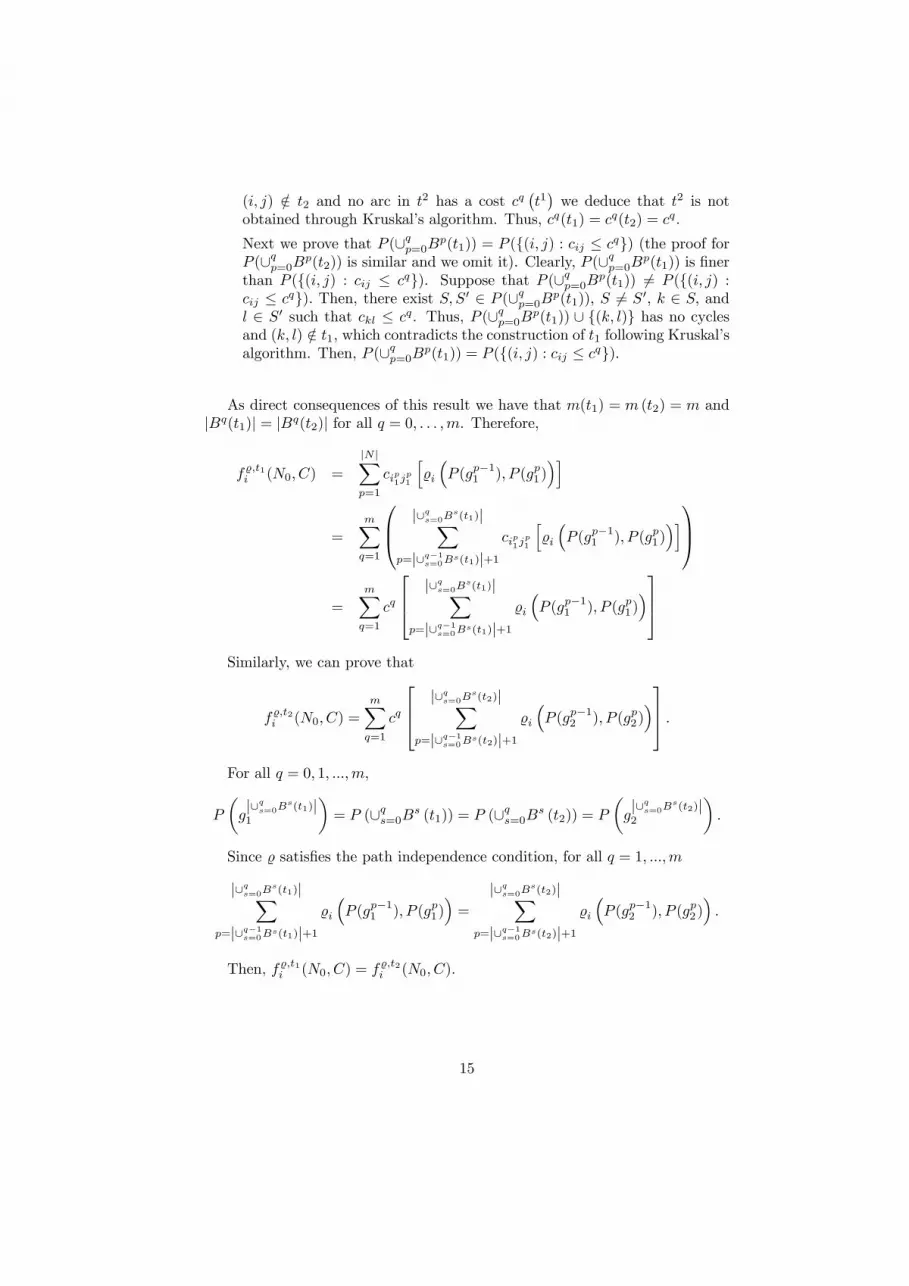
(i, j) /∈ t2 and no arc in t2 has a cost cq¡t1¢we deduce that t2 is not

obtained through Kruskal’s algorithm. Thus, cq(t1) = cq(t2) = cq.

Next we prove that P (∪qp=0Bp(t1)) = P ({(i, j) : cij ≤ cq}) (the proof forP (∪qp=0Bp(t2)) is similar and we omit it). Clearly, P (∪qp=0Bp(t1)) is finerthan P ({(i, j) : cij ≤ cq}). Suppose that P (∪qp=0Bp(t1)) 6= P ({(i, j) :cij ≤ cq}). Then, there exist S, S0 ∈ P (∪qp=0Bp(t1)), S 6= S0, k ∈ S, andl ∈ S0 such that ckl ≤ cq. Thus, P (∪qp=0Bp(t1)) ∪ {(k, l)} has no cyclesand (k, l) /∈ t1, which contradicts the construction of t1 following Kruskal’salgorithm. Then, P (∪qp=0Bp(t1)) = P ({(i, j) : cij ≤ cq}).

As direct consequences of this result we have that m(t1) = m (t2) = m and|Bq(t1)| = |Bq(t2)| for all q = 0, . . . ,m. Therefore,

f ,t1i (N0, C) =

|N|Xp=1

cip1jp1

hi

³P (gp−11 ), P (gp1)

´i

=mXq=1

⎛⎜⎝ |∪qs=0Bs(t1)|Xp=|∪q−1s=0B

s(t1)|+1cip1j

p1

hi

³P (gp−11 ), P (gp1)

´i⎞⎟⎠=

mXq=1

cq

⎡⎢⎣ |∪qs=0Bs(t1)|Xp=|∪q−1s=0B

s(t1)|+1i

³P (gp−11 ), P (gp1)

´⎤⎥⎦Similarly, we can prove that

f ,t2i (N0, C) =

mXq=1

cq

⎡⎢⎣ |∪qs=0Bs(t2)|Xp=|∪q−1s=0B

s(t2)|+1i

³P (gp−12 ), P (gp2)

´⎤⎥⎦ .For all q = 0, 1, ...,m,

P

µg|∪qs=0Bs(t1)|1

¶= P (∪qs=0Bs (t1)) = P (∪qs=0Bs (t2)) = P

µg|∪qs=0Bs(t2)|2

¶.

Since satisfies the path independence condition, for all q = 1, ...,m

|∪qs=0Bs(t1)|Xp=|∪q−1s=0B

s(t1)|+1i

³P (gp−11 ), P (gp1)

´=

|∪qs=0Bs(t2)|Xp=|∪q−1s=0B

s(t2)|+1i

³P (gp−12 ), P (gp2)

´.

Then, f ,t1i (N0, C) = f ,t2

i (N0, C).

15

7.2 Proof of Theorem 1

We first prove that for each sharing function , f satisfies RA and SCM .

Let (N0, C) and (N0, C0) be two mcstp as in the definition of RA. It is well

known that each mt could be obtained through Kruskal’s algorithm. Thus,t = g|N | (C) = g|N | (C0) = g|N | (C + C0) .Because of the definition of Kruskal’s algorithm we can proceed in such a

way that for all p = 1, ...., |N | ,

(ip (C) , jp (C)) = (ip (C0) , jp (C0)) = (ip (C + C0) , jp (C + C 0)) and

gp (C) = gp (C0) = gp (C + C0) .

Let us denote (ip, jp) = (ip (C) , jp (C)) and gp = gp (C) for all p = 1, ...., |N | .Therefore,

fi (N0, C + C0) =

|N|Xp=1

¡cipjp + c0ipjp

¢ £i

¡P (gp−1), P (gp)

¢¤=

|N|Xp=1

cipjp£

i

¡P (gp−1), P (gp)

¢¤+

|N|Xp=1

c0ipjp£

i

¡P (gp−1), P (gp)

¢¤= fi (N0, C) + fi (N0, C

0).

Thus, f satisfies RA.Next we prove that f satisfies SCM . We must prove that f (N0, C) ≤

f (N0, C0) when C ≤ C0. It is enough to prove that f (N0, C) ≤ f (N0, C

0)when there exists (i, j) such that cij < c0ij and ckl = c0kl otherwise.Assume that there exists an mt t in (N0, C) such that (i, j) /∈ t. Thus,

t is also an mt in (N0, C0). Since any mt can be obtained through Kruskal’s

algorithm and Proposition 1, we have that f (N0, C) = f (N0, C0).

Assume that (i, j) ∈ t for every mt t in the problem (N0, C). Consider:G the set of trees that do not involve arc (i, j), t̄ = argmin

t∈Gc(N0, C, t), and

x = c(N0, C, t̄)−m(N0, C). We distinguish two cases:

1. c0ij − cij ≤ x. Given t an mt in the problem (N0, C), t is also an mt

in (N0, C0). Consider t = {(ip, jp)}|N |p=1 = {(i0p, j0p)}|N|p=1 where (i

p, jp)((i0p, j0p)) is the arc added at stage p applying Kruskal’s algorithm to theproblem (N0, C) ((N0, C

0)). Assume that (i, j) = (ir, jr) = (i0r0, j0r

0). We

distinguish two cases:

(a) r = r0. Thus, for all p ∈ {1, . . . , |N |}, (ip, jp) = (i0p, j0p) and gp (C) =

16

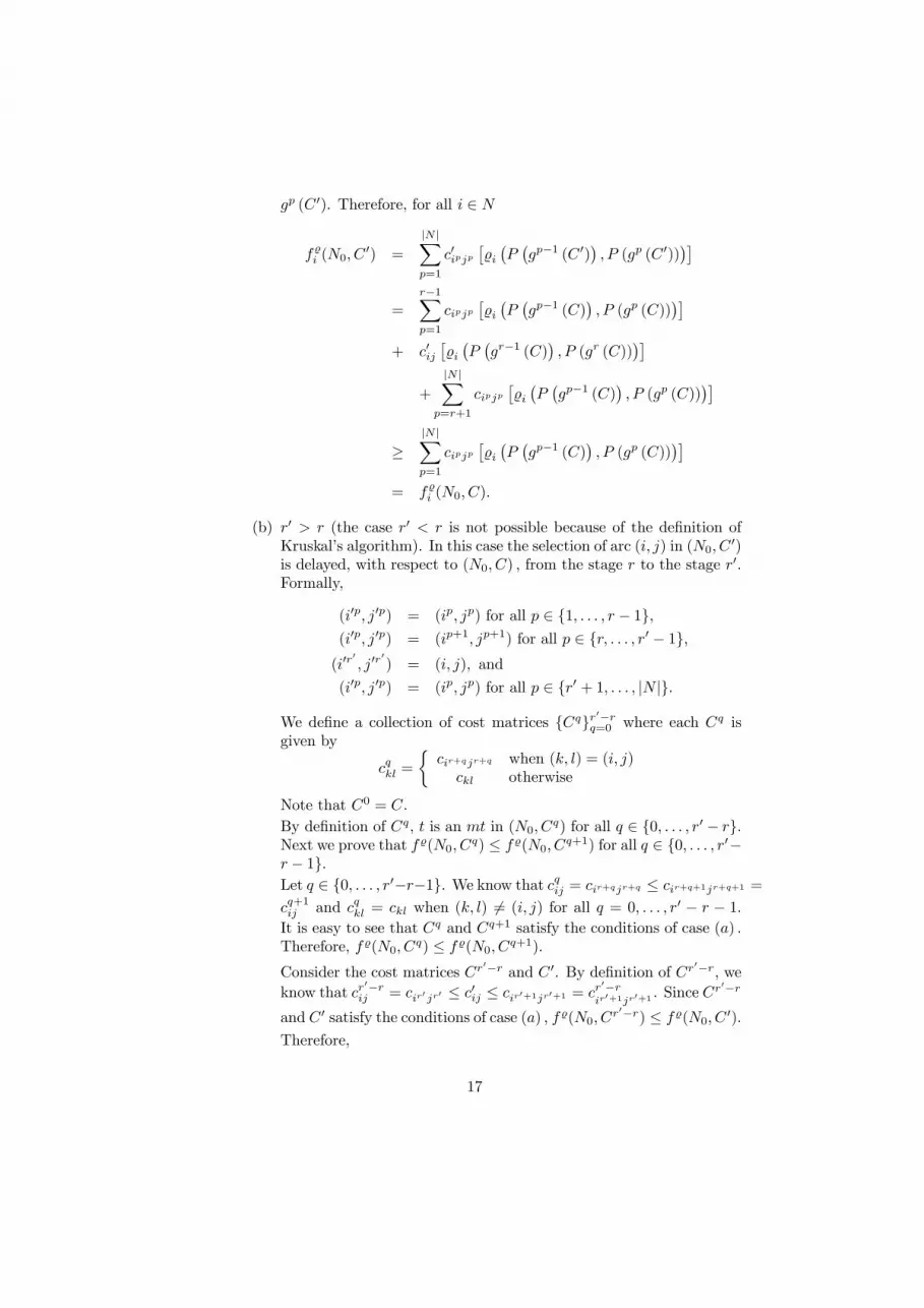
gp (C 0). Therefore, for all i ∈ N

fi (N0, C0) =

|N |Xp=1

c0ipjp£

i

¡P¡gp−1 (C 0)

¢, P (gp (C0))

¢¤=

r−1Xp=1

cipjp£

i

¡P¡gp−1 (C)

¢, P (gp (C))

¢¤+ c0ij

£i

¡P¡gr−1 (C)

¢, P (gr (C))

¢¤+

|N |Xp=r+1

cipjp£

i

¡P¡gp−1 (C)

¢, P (gp (C))

¢¤≥

|N |Xp=1

cipjp£

i

¡P¡gp−1 (C)

¢, P (gp (C))

¢¤= fi (N0, C).

(b) r0 > r (the case r0 < r is not possible because of the definition ofKruskal’s algorithm). In this case the selection of arc (i, j) in (N0, C

0)is delayed, with respect to (N0, C) , from the stage r to the stage r0.Formally,

(i0p, j0p) = (ip, jp) for all p ∈ {1, . . . , r − 1},(i0p, j0p) = (ip+1, jp+1) for all p ∈ {r, . . . , r0 − 1},(i0r

0, j0r

0) = (i, j), and

(i0p, j0p) = (ip, jp) for all p ∈ {r0 + 1, . . . , |N |}.

We define a collection of cost matrices {Cq}r0−rq=0 where each Cq is

given by

cqkl =

½cir+qjr+q when (k, l) = (i, j)

ckl otherwise

Note that C0 = C.By definition of Cq, t is an mt in (N0, C

q) for all q ∈ {0, . . . , r0 − r}.Next we prove that f (N0, C

q) ≤ f (N0, Cq+1) for all q ∈ {0, . . . , r0−

r − 1}.Let q ∈ {0, . . . , r0−r−1}. We know that cqij = cir+qjr+q ≤ cir+q+1jr+q+1 =

cq+1ij and cqkl = ckl when (k, l) 6= (i, j) for all q = 0, . . . , r0 − r − 1.It is easy to see that Cq and Cq+1 satisfy the conditions of case (a) .Therefore, f (N0, C

q) ≤ f (N0, Cq+1).

Consider the cost matrices Cr0−r and C 0. By definition of Cr0−r, weknow that cr

0−rij = cir0 jr0 ≤ c0ij ≤ cir0+1jr0+1 = cr

0−rir0+1jr0+1

. Since Cr0−r

and C0 satisfy the conditions of case (a) , f (N0, Cr0−r) ≤ f (N0, C

0).

Therefore,

17

f (N0, C) = f (N0, C0) ≤ f (N0, C

1) ≤ . . . ≤ f (N0, Cr0−r) ≤ f (N0, C

0).

2. c0ij − cij > x. Consider the mcstp problems (N0, C1) and (N0, C

2) where:

c1kl =

½cij + x if (k, l) = (i, j)ckl otherwise

c2kl =

½c0ij − cij − x if (k, l) = (i, j)

0 otherwise.

Thus, t̄ is an mt in (N0, C1), (N0, C

2) and (N0, C1 + C2) = (N0, C

0).It is trivial to see that (N0, C

1) and (N0, C2) satisfy the conditions of

the definition of RA. Since f satisfies RA, f (N0, C0) = f (N0, C

1) +f (N0, C

2). By definition of f , we have that fi (N0, C2) = 0 for all i ∈ N .

Since C1 and C satisfy the conditions of Case 1, f (N0, C1) ≥ f (N0, C).

Thus,

f (N0, C0) = f (N0, C

1) + f (N0, C2) = f (N0, C

1) ≥ f (N0, C).

We have proved that f satisfies SCM.

We now prove the reciprocal. Consider a cost allocation rule f which satisfiesRA and SCM . We prove that f = f for some sharing function .Given P = {S0, S1, . . . , Sm} ∈ P (N0), we define the mcstp (N0, C

P ) wherecPij = 0 if i, j ∈ Sk for any k ∈ {0, 1, . . . ,m} and cPij = 1 if i ∈ Sk, j ∈ Sk0 withk, k0 ∈ {0, 1, . . . ,m}, k 6= k0.Given P, P 0 ∈ P (N0) where P is 1-finer than P 0, we define

(P, P 0) = f(N0, CP )− f(N0, C

P 0).

Next we prove that is a sharing function:

1. Assume that P is 1-finer than P 0. We prove that (P, P 0) ∈ ∆ (N) .

(a) Since P is 1-finer than P 0, CP ≥ CP 0. By SCM, f(N0, C

P ) ≥f(N0, C

P 0). Hence, i(P, P

0) ≥ 0 for all i ∈ N.

(b) Xi∈N

i(P, P0) =

Xi∈N

fi(N0, CP )−

Xi∈N

fi(N0, CP 0)

= m(N0, CP )−m(N0, C

P 0) = m− (m− 1) = 1.

2. We prove that satisfies the path independence condition. Assume that©P 11 , P

12 , ..., P

1k

ªand

©P 21 , P

22 , ..., P

2k

ªare two sequences of partitions sat-

isfying that P 11 = P 21 = P, P 1k = P 2k = P 0 and P iq is 1-finer than P i

q+1 forall i = 1, 2 and q = 1, ..., k − 1. For all i ∈ N,

k−1Xq=1

i

¡P 1q , P

1q+1

¢=

k−1Xq=1

³fi(N0, C

P 1q )− fi(N0, C

P1q+1)

´= fi(N0, C

P 11 )− fi(N0, C

P1k )

= fi(N0, CP )− fi(N0, C

P 0).

18

Analogously, we can prove that

k−1Xq=1

i

¡P 2q , P

2q+1

¢= fi(N0, C

P )− fi(N0, CP 0).

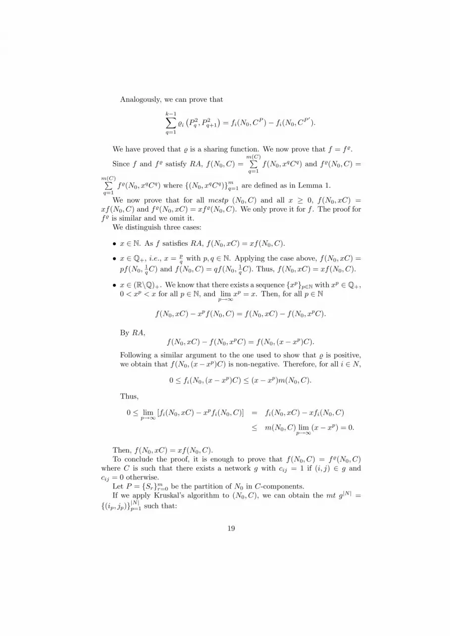
We have proved that is a sharing function. We now prove that f = f .

Since f and f satisfy RA, f(N0, C) =m(C)Pq=1

f(N0, xqCq) and f (N0, C) =

m(C)Pq=1

f (N0, xqCq) where {(N0, x

qCq)}mq=1 are defined as in Lemma 1.

We now prove that for all mcstp (N0, C) and all x ≥ 0, f(N0, xC) =xf(N0, C) and f (N0, xC) = xf (N0, C). We only prove it for f . The proof forf is similar and we omit it.We distinguish three cases:

• x ∈ N. As f satisfies RA, f(N0, xC) = xf(N0, C).

• x ∈ Q+, i.e., x = pq with p, q ∈ N. Applying the case above, f(N0, xC) =

pf(N0,1qC) and f(N0, C) = qf(N0,

1qC). Thus, f(N0, xC) = xf(N0, C).

• x ∈ (R\Q)+. We know that there exists a sequence {xp}p∈N with xp ∈ Q+,0 < xp < x for all p ∈ N, and lim

p→∞xp = x. Then, for all p ∈ N

f(N0, xC)− xpf(N0, C) = f(N0, xC)− f(N0, xpC).

By RA,f(N0, xC)− f(N0, x

pC) = f(N0, (x− xp)C).

Following a similar argument to the one used to show that is positive,we obtain that f(N0, (x− xp)C) is non-negative. Therefore, for all i ∈ N,

0 ≤ fi(N0, (x− xp)C) ≤ (x− xp)m(N0, C).

Thus,

0 ≤ limp→∞

[fi(N0, xC)− xpfi(N0, C)] = fi(N0, xC)− xfi(N0, C)

≤ m(N0, C) limp→∞

(x− xp) = 0.

Then, f(N0, xC) = xf(N0, C).To conclude the proof, it is enough to prove that f(N0, C) = f (N0, C)

where C is such that there exists a network g with cij = 1 if (i, j) ∈ g andcij = 0 otherwise.Let P = {Sr}mr=0 be the partition of N0 in C-components.If we apply Kruskal’s algorithm to (N0, C), we can obtain the mt g|N| =

{(ip, jp)}|N |p=1 such that:

19

• For all p = 1, . . . , |N |−m, cipjp = 0 and {ip, jp} ⊂ Sr with r ∈ {0, ...,m} .

• For all p = |N |−m+ 1, . . . , |N | , cipjp = 1, ip = 0, and jp ∈ Tp−|N |+m.

Note that P¡g|N |−m

¢= P and P

¡g|N|

¢= {N0} . Therefore, for all i ∈ N,

fi (N0, C) =

|N|Xp=1

cipjp£

i

¡P¡gp−1

¢, P (gp)

¢¤=

|N |Xp=|N|−m+1

£i

¡P¡gp−1

¢, P (gp)

¢¤=

|N |Xp=|N|−m+1

³fi

³N0, C

P(gp−1)´− fi

³N0, C

P (gp)´´

= fi

³N0, C

P(g|N|−m)´− fi

³N0, C

P (g|N|)´

= fi¡N0, C

P¢− fi

³N0, C

{N0}´.

Let (N0, CP ) be the mcstp defined as above. It can be easily proved that

CP ≤ C. By SCM we have that f(N0, CP ) ≤ f(N0, C). Since m(N0, C) =

m(N0, CP ), f(N0, C) = f(N0, C

P ).By definition, c{N0}

ij = 0 for all i, j ∈ N0. By RA, for all i ∈ N

fi

³N0, C

{N0} + C{N0}´= fi

³N0, C

{N0}´+ fi

³N0, C

{N0}´.

Then, fi¡N0, C

{N0}¢= 0 for all i ∈ N.

Now, we can conclude that fi (N0, C) = fi(N0, C) for all i ∈ N.

7.3 Proof of Proposition 2

We prove that θo satisfies the three conditions of the definition of a generalizedobligation function.

1. θoi (P ) = oi(S) ≥ 0 because o(S) ∈ ∆(S) for all S ⊂ N.

2. Given P = {S0, ..., Sm} ∈ P (N0),Xi∈N

θoi (P ) =mXq=0

Xi∈Sq

θoi (P ) =mXq=0

Xi∈Sq

oi(Sq).

Since o(S) ∈ ∆(S) for all S ⊂ N and oi(S) = 0 for all i ∈ S such that0 ∈ S we conclude that

mXq=0

Xi∈Sq

oi(Sq) =mXq=1

1 = m.

20

3. Consider P, P 0 ∈ P (N0) such that P is finer than P 0 and i ∈ N . Thus,θoi (P ) = oi(S) where i ∈ S ∈ P . Since P is finer that P 0, there exists T ∈P 0 such that i ∈ S ⊂ T . Therefore, θoi (P

0) = oi (T ) . Since oi(S) ≥ oi(T )when i ∈ S ⊂ T ⊂ N0, we conclude that θ

oi (P ) ≥ θoi (P

0).

7.4 Proof of Proposition 3

“ ⊂ ”Let fθ be such that θ is a generalized obligation function.Given P, P 0 ∈ P (N0) where P is 1-finer than P 0, we define

(P, P 0) = θ (P )− θ (P 0) .

Next we prove that is a sharing function:

1. Assume that P is 1-finer than P 0. We prove that (P, P 0) ∈ ∆ (N) .

(a) Since P is finer than P 0 and θ is a generalized obligation function,θ (P ) ≥ θ (P 0). Hence, i(P, P

0) ≥ 0 for all i ∈ N.

(b) Assume that P = {S0, S1, ..., Sm} . Thus, P 0 =©S00, S

01, ..., S

0m−1

ª.

NowXi∈N

i(P, P0) =

Xi∈N

θi (P )−Xi∈N

θi (P0) = m− (m− 1) = 1.

2. We prove that satisfies the path independence condition. Assume that©P 11 , P

12 , ..., P

1k

ªand

©P 21 , P

22 , ..., P

2k

ªare two sequences of partitions sat-

isfying that P 11 = P 21 = P, P 1k = P 2k = P 0 and P iq is 1-finer than P i

q+1 forall i = 1, 2 and q = 1, ..., k − 1. For all i ∈ N,

k−1Xq=1

i

¡P 1q , P

1q+1

¢=

k−1Xq=1

¡θi¡P 1q¢− θi

¡P 1q+1

¢¢= θi

¡P 11¢− θi

¡P 1k¢

= θi (P )− θi (P0) .

Analogously, we can prove that

k−1Xq=1

i

¡P 2q , P

2q+1

¢= θi (P )− θi (P

0) .

We have proved that is a sharing function.It is trivial to see that fθ = f .

“ ⊃ j

21

Let f be such that is a sharing function.Let P = {S0, S1, ..., Sm} ∈ P (N). There exists a sequence {P0, P1,..., Pm} ⊂

P (N0) such that P0 = P, Pm = {N0} , and for all q = 1, ...,m, Pq−1 is 1-finerthan Pq. Notice that this sequence may not be unique.We define

θ (P ) =mXq=1

(Pq−1, Pq) .

Since satisfies the path independence condition, θ (P ) does not depend onthe sequence {P0, ..., Pm} . Thus, θ (P ) is well defined.We now prove that θ is a generalized obligation function.

1. Since i (P,P0) ≥ 0 for all P, P 0 ∈ P (N) with P 1-finer than P 0 and all

i ∈ N, we deduce that θi(P ) ≥ 0 for all i ∈ N.

2. Xi∈N

θi(P ) =Xi∈N

mXq=1

i (Pq−1, Pq)

=mXq=1

ÃXi∈N

i (Pq−1, Pq)

!

=mXq=1

1 = m.

3. Assume that P is finer than P 0 = {S00, ..., S0m0} . Then, m0 ≤ m and thereexists a sequence {P0, P1,..., Pm} ⊂ P (N0) such that P0 = P, Pm = {N0} ,for all q = 1, ...,m Pq−1 is 1 finer than Pq, and Pm−m0 = P 0. Thus, giveni ∈ N,

θi(P0) =

mXq=m−m0+1

i (Pq−1, Pq) .

Now,

θi(P ) =mXq=1

i (Pq−1, Pq) =m−m0Xq=1

i (Pq−1, Pq) + θi(P0). (1)

By definition of , i (Pq−1, Pq) ≥ 0 for all q = 1, ...,m−m0. Thus, θi(P ) ≥θi(P

0).

We have proved that θ is a generalized obligation function.We now prove that fθ = f . By (1) we have that if P is 1-finer than P 0 and

i ∈ N, thenθi(P )− θi(P

0) = i (P, P0) .

Now it is trivial to see that fθ = f .

22

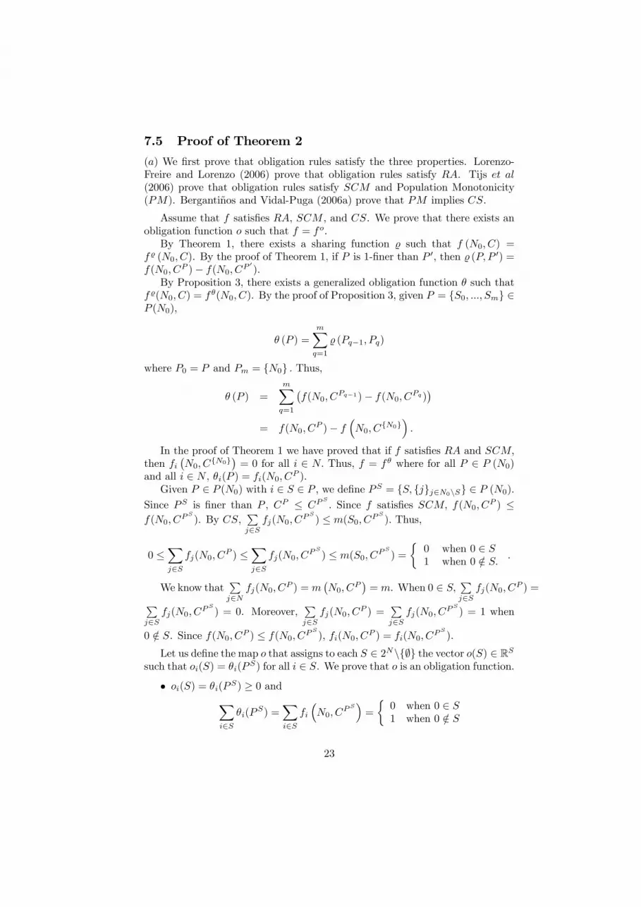
7.5 Proof of Theorem 2

(a) We first prove that obligation rules satisfy the three properties. Lorenzo-Freire and Lorenzo (2006) prove that obligation rules satisfy RA. Tijs et al(2006) prove that obligation rules satisfy SCM and Population Monotonicity(PM). Bergantiños and Vidal-Puga (2006a) prove that PM implies CS.

Assume that f satisfies RA, SCM , and CS. We prove that there exists anobligation function o such that f = fo.By Theorem 1, there exists a sharing function such that f (N0, C) =

f (N0, C). By the proof of Theorem 1, if P is 1-finer than P 0, then (P, P 0) =f(N0, C

P )− f(N0, CP 0).

By Proposition 3, there exists a generalized obligation function θ such thatf (N0, C) = fθ(N0, C). By the proof of Proposition 3, given P = {S0, ..., Sm} ∈P (N0),

θ (P ) =mXq=1

(Pq−1, Pq)

where P0 = P and Pm = {N0} . Thus,

θ (P ) =mXq=1

¡f(N0, C

Pq−1)− f(N0, CPq)¢

= f(N0, CP )− f

³N0, C

{N0}´.

In the proof of Theorem 1 we have proved that if f satisfies RA and SCM,then fi

¡N0, C

{N0}¢= 0 for all i ∈ N. Thus, f = fθ where for all P ∈ P (N0)

and all i ∈ N , θi(P ) = fi(N0, CP ).

Given P ∈ P (N0) with i ∈ S ∈ P , we define PS = {S, {j}j∈N0\S} ∈ P (N0).

Since PS is finer than P , CP ≤ CPS

. Since f satisfies SCM, f(N0, CP ) ≤

f(N0, CPS

). By CS,Pj∈S

fj(N0, CPS

) ≤ m(S0, CPS

). Thus,

0 ≤Xj∈S

fj(N0, CP ) ≤

Xj∈S

fj(N0, CPS

) ≤ m(S0, CPS

) =

½0 when 0 ∈ S1 when 0 /∈ S.

.

We know thatPj∈N

fj(N0, CP ) = m

¡N0, C

P¢= m. When 0 ∈ S,

Pj∈S

fj(N0, CP ) =P

j∈Sfj(N0, C

PS

) = 0. Moreover,Pj∈S

fj(N0, CP ) =

Pj∈S

fj(N0, CPS

) = 1 when

0 /∈ S. Since f(N0, CP ) ≤ f(N0, C

PS

), fi(N0, CP ) = fi(N0, C

PS

).

Let us define the map o that assigns to each S ∈ 2N\{∅} the vector o(S) ∈ RSsuch that oi(S) = θi(P

S) for all i ∈ S. We prove that o is an obligation function.

• oi(S) = θi(PS) ≥ 0 andX

i∈Sθi(P

S) =Xi∈S

fi

³N0, C

PS´=

½0 when 0 ∈ S1 when 0 /∈ S

23

Thus, o(S) ∈ ∆(S) when 0 /∈ S. Moreover, when 0 ∈ S, oi(S) = 0 for alli ∈ S.

• Let i ∈ S ⊂ T . Clearly, PS is finer than PT . Therefore, θi(PS) ≥ θi(PT )

and, hence,oi(S) = θi(P

S) ≥ θi(PT ) = oi(T ).

We now prove that fθ = fo.If i ∈ S ∈ P, then

θi(P ) = fi¡N0, C

P¢= fi

³N0, C

PS´= θi(P

S) = oi (S) .

Given a partition P ∈ P (N0) remember that S(P, i) denotes the element ofthe partition P to which agent i belongs to. Thus,

fθi (N0, C) =

|N |Xp=1

cipjp¡θi(P (g

p−1))− θi(P (gp))¢

=

|N |Xp=1

cipjp¡oi(S(P (g

p−1), i))− oi(S(P (gp), i))

¢= foi (N0, C).

(b) We know that obligation rules satisfy RA, SCM , and PM . Bergantiñosand Vidal-Puga (2006a) prove that PM implies SEP .Consider an allocation rule f satisfying RA, SCM , and SEP . Using similar

arguments to those used in (a), we can conclude that there exists a generalizedobligation function θ such that f = fθ. Moreover, for all P ∈ P (N0) , θ (P ) =

f¡N0, C

P¢.

Given P = {S0, S1, . . . , Sm}, it is easy to prove thatm(N0, CP ) = m(S0, C

P )+mPk=1

m((Sk)0, CP ).

Let i ∈ S0 ∩N. Since f satisfies SEP, fi(N0, CP ) = fi(S0, C

P ). Therefore,Pj∈S0

fj(N0, CP ) =

Pj∈S0

fj(S0, CP ) = m(S0, C

P ) = 0

Let k ∈ {1, ...,m} and i ∈ Sk. Since f satisfies SEP, fi(N0, CP ) = fi((Sk)0, C

P ).Therefore,

Pj∈Sk

fj(N0, CP ) =

Pj∈Sk

fj((Sk)0, CP ) = m((Sk)0, C

P ) = 1.

Using similar arguments to those used in (a), it can be proved that the map oassigning to each S ∈ 2N \{∅} the vector o(S) = θ(PS) is an obligation functionand f = fo.

24

7.6 Independence of the properties in Theorem 2

We prove that the properties used in Theorem 2 (a) and (b) are independent.We will do the following:(i) We define a rule f which satisfies RA and SCM but fails CS and SEP.

Thus, CS is independent of RA and SCM in part (a) . Moreover, SEP isindependent of RA and SCM in part (b) .(ii) We define a rule f which satisfies RA and CS but fails SCM. Thus,

SCM is independent of RA and CS in part (a).(iii) We define a rule f which satisfies SCM, CS, and SEP but fails RA.

Thus, RA is independent of SCM and CS in part (a). Moreover, RA is inde-pendent of SCM and SEP in part (b) .(iv) We define a rule f which satisfies RA and SEP but fails SCM. Thus,

SCM is independent of RA and SEP in part (b).

Proof of (i) .Let f be the egalitarian rule, i.e., fi(N0, C) =

1nm(N0, C) for all i ∈ N.

It is trivial to see that f satisfies RA and SCM .Nevertheless, f does not satisfy SEP and CS. Consider the mcstp (N0, C),

where N = {1, 2} and

C =

⎛⎝ 0 1 21 0 22 2 0

⎞⎠ .

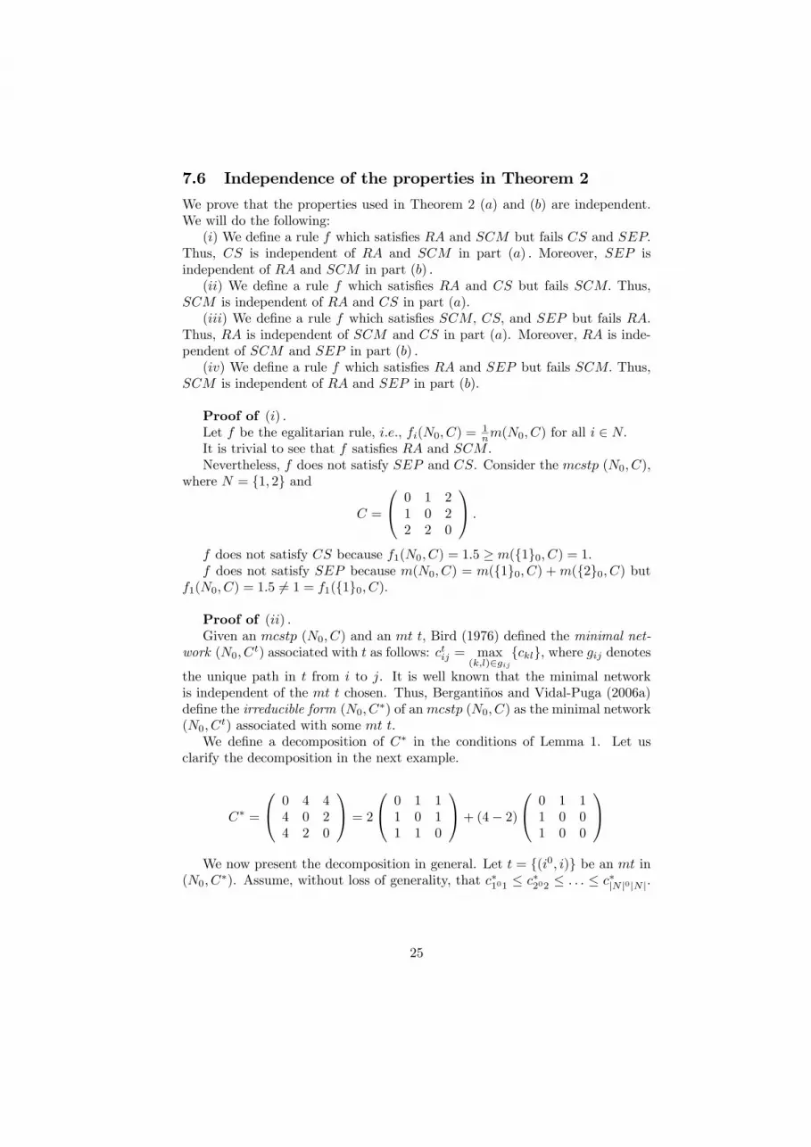
f does not satisfy CS because f1(N0, C) = 1.5 ≥ m({1}0, C) = 1.f does not satisfy SEP because m(N0, C) = m({1}0, C) +m({2}0, C) but

f1(N0, C) = 1.5 6= 1 = f1({1}0, C).

Proof of (ii) .Given an mcstp (N0, C) and an mt t, Bird (1976) defined the minimal net-

work (N0, Ct) associated with t as follows: ctij = max

(k,l)∈gij{ckl}, where gij denotes

the unique path in t from i to j. It is well known that the minimal networkis independent of the mt t chosen. Thus, Bergantiños and Vidal-Puga (2006a)define the irreducible form (N0, C

∗) of anmcstp (N0, C) as the minimal network(N0, C

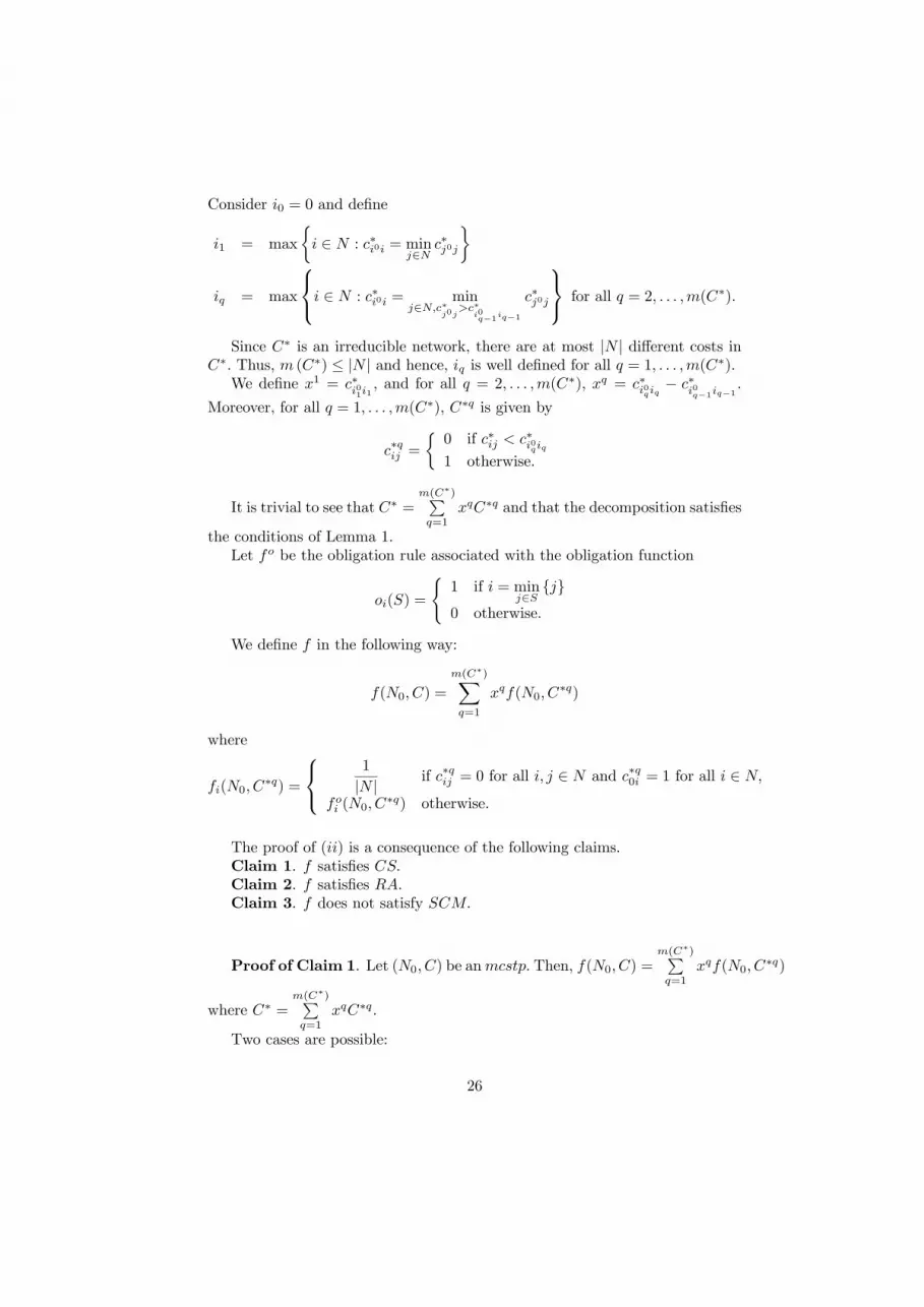
t) associated with some mt t.We define a decomposition of C∗ in the conditions of Lemma 1. Let us

clarify the decomposition in the next example.

C∗ =

⎛⎝ 0 4 44 0 24 2 0

⎞⎠ = 2

⎛⎝ 0 1 11 0 11 1 0

⎞⎠+ (4− 2)⎛⎝ 0 1 11 0 01 0 0

⎞⎠We now present the decomposition in general. Let t = {(i0, i)} be an mt in

(N0, C∗). Assume, without loss of generality, that c∗101 ≤ c∗202 ≤ . . . ≤ c∗|N |0|N|.

25

Consider i0 = 0 and define

i1 = max

½i ∈ N : c∗i0i = min

j∈Nc∗j0j

¾

iq = max

⎧⎨⎩i ∈ N : c∗i0i = minj∈N,c∗

j0j>c∗

i0q−1iq−1

c∗j0j

⎫⎬⎭ for all q = 2, . . . ,m(C∗).

Since C∗ is an irreducible network, there are at most |N | different costs inC∗. Thus, m (C∗) ≤ |N | and hence, iq is well defined for all q = 1, . . . ,m(C∗).We define x1 = c∗

i01i1, and for all q = 2, . . . ,m(C∗), xq = c∗i0qiq

− c∗i0q−1iq−1

.

Moreover, for all q = 1, . . . ,m(C∗), C∗q is given by

c∗qij =

½0 if c∗ij < c∗i0qiq1 otherwise.

It is trivial to see that C∗ =m(C∗)Pq=1

xqC∗q and that the decomposition satisfies

the conditions of Lemma 1.Let fo be the obligation rule associated with the obligation function

oi(S) =

(1 if i = min

j∈S{j}

0 otherwise.

We define f in the following way:

f(N0, C) =

m(C∗)Xq=1

xqf(N0, C∗q)

where

fi(N0, C∗q) =

⎧⎨⎩1

|N | if c∗qij = 0 for all i, j ∈ N and c∗q0i = 1 for all i ∈ N,

foi (N0, C∗q) otherwise.

The proof of (ii) is a consequence of the following claims.Claim 1. f satisfies CS.Claim 2. f satisfies RA.Claim 3. f does not satisfy SCM.

Proof of Claim 1. Let (N0, C) be anmcstp. Then, f(N0, C) =m(C∗)Pq=1

xqf(N0, C∗q)

where C∗ =m(C∗)Pq=1

xqC∗q.

Two cases are possible:

26

1. Assume that c∗qij = 0 for all i, j ∈ N and c∗q0i = 1 for all i ∈ N. Thus, forall i ∈ N, fi(N0, C

∗q) = 1|N| . Moreover, for all S ⊂ N, vC∗q (S) = 1. Thus,

f(N0, C∗q) ∈ core (N, vC∗q) .

2. Otherwise f(N0, C∗q) = fo(N0, C

∗q). By Theorem 2 (a) fo satisfies CS.Hence, f(N0, C

∗q) ∈ core (N, vC∗q ) .

Now, f(N0, C) =m(C∗)Pq=1

xqf(N0, C∗q) ∈ core

ÃN,

m(C∗)Pq=1

xqvC∗q

!.

Bergantiños and Vidal-Puga (2006b) prove that if C,C 0, and C +C0 satisfythe conditions of the definition of RA, then v(C+C0)∗ = vC∗ + vC0∗ . Thus,

m(C∗)Xq=1

xqvC∗q = vm(C∗)Pq=1

xqC∗q= vC∗ .

Hence, f(N0, C) ∈ core (N, vC∗) . Bird (1976) prove that core (N, vC∗) ⊂core (N, vC) . Therefore, f(N0, C) ∈ core (N, vC) , which means that f satisfiesCS. ¥

Proof of Claim 2.Let (N0, C), (N0, C

0) and (N0, C + C 0) in the conditions of the definition ofRA. Bergantiños and Vidal-Puga (2006b) prove that (C + C 0)∗ = C∗ + C0∗.We say that a matrix C is irreducible if C = C∗. Since f only depends on theirreducible matrix, we assume that C, C0, and C + C0 are irreducible.Bergantiños and Vidal-Puga (2006a) prove that (N0, C) is irreducible if and

only if there exists an mt tπ in (N0, C) satisfying two conditions:(A1) tπ = {(πs−1, πs)}|N|s=1 in (N0, C) with π0 = 0.(A2) Given πp, πq ∈ N0 with p < q, cπpπq = max

p<s≤q

©cπs−1πs

ª.

Given an mt t in an irreducible problem (N0, C), Bergantiños and Vidal-Puga (2006a) define a procedure for associating an mt tπ satisfying (A1) and(A2) .Let t = {(i0, i)}i∈N be the mt for the three mcstp given by the definition

of RA. Since t is an mt in (N0, C), (N0, C0) and (N0, C + C 0), applying the

procedure of Bergantiños and Vidal-Puga (2006a) it is straightforward to provethat there exists an mt tπ in (N0, C), (N0, C

0) and (N0, C +C0) satisfying (A1)and (A2) . Moreover, we can order the cost of the arcs of tπ in the same wayin the three problems. Namely, there exist an order π0 of the agents satisfyingthat if 1 ≤ p0 < q0 ≤ |N | , π0p0 = πp, and π0q0 = πq, then cπp−1πp ≤ cπq−1πq andc0πp−1πp ≤ c0πq−1πq .We say that an mcstp (N0, C) satisfies the property PRO if in the decom-

position of f there is no C∗q satisfying that c∗qij = 0 for all i, j ∈ N and c∗q0i = 1for all i ∈ N,We prove that f(N0, C) + f(N0, C

0) = f(N0, C + C0). We distinguish threecases:

27

1. c0π1 ≤ max2<s≤|N|

©cπs−1πs

ªand c00π1 ≤ max

2<s≤|N|

nc0πs−1πs

o.

Thus, (N0, C), (N0, C0) and (N0, C + C0) satisfies PRO. In this case we

know that f(N0, C) = fo(N0, C), f(N0, C0) = fo(N0, C

0), and f(N0, C +C0) = fo(N0, C + C 0). Since all the problems obtained in the decompo-sition of (N0, C), (N0, C

0) and (N0, C + C0) satisfy the conditions of thedefinition of RA and fo satisfies RA,

fo(N0, C) + fo(N0, C0) = fo(N0, C + C0).

2. c0π1 > max2<s≤|N|

©cπs−1πs

ªand c00π1 ≤ max

2<s≤|N |

nc0πs−1πs

o. The case c0π1 ≤

max2<s≤|N |

©cπs−1πs

ªand c00π1 > max

2<s≤|N|

nc0πs−1πs

ois similar and we omit it.

Thus, (N0, C) does not satisfy PRO and (N0, C0) satisfies PRO. Be-

cause of the existence of the order π0, we deduce that c0π1 + c00π1 >

max2<s≤|N |

©cπs−1πs

ª+ max2<s≤|N|

nc0πs−1πs

o. Thus, (N0, C+C

0) does not satisfy

PRO.

Let us define eC as:

ecij = ½ 1 when 0 ∈ {i, j}0 otherwise.

for all i, j ∈ N.

Applying the decomposition to C,

C =

m(C)Xq=1

xqCq =

m(C)−1Xq=1

xqCq + xm(C) eC,where xm(C) = c0π1 − max

2<s≤|N |

©cπs−1πs

ªand

m(C)−1Pq=1

xqCq satisfies PRO.

Analogously, since (N0, C + C0) does not satisfy PRO,

C + C0 =

m(C+C0)−1Xq=1

x∗q(C + C 0)q + x∗m(C+C0) eC,

wherem(C+C0)−1P

q=1x∗q(C + C0)q satisfies PRO.

Moreover,

x∗m(C+C0) =

¡c0π1 + c00π1

¢− max2<s≤|N|

ncπs−1πs + c0πs−1πs

o.

Because of the existence of the order π0,

max2<s≤|N |

ncπs−1πs + c0πs−1πs

o= max

2<s≤|N|

©cπs−1πs

ª+ max2<s≤|N |

nc0πs−1πs

oand

max2<s≤|N |

nc0πs−1πs

o= c00π1 .

28

Hence, x∗m(C+C0) = c0π1 − max

2<s≤|N|

©cπs−1πs

ª= xm(C).

Therefore,

C+C0 =

m(C)−1Xq=1

xqCq+xm(C) eC+C 0 =

m(C+C0)−1Xq=1

x∗q(C+C 0)q+xm(C) eC.Then,

m(C)−1Xq=1

xqCq + C0 =

m(C+C0)−1Xq=1

x∗q(C + C 0)q.

Since all the problems obtained in the decomposition of (N0, C), (N0, C0)

and (N0, C + C 0) satisfy the conditions of the definition of RA and fo

satisfies RA,f(N0, C) + f(N0, C

0) =

= fo

⎛⎝N0,

m(C)−1Xq=1

xqCq

⎞⎠+ xm(C)µ1

|N | , . . . ,1

|N |

¶+ fo(N0, C

0)

= fo

⎛⎝N0,

m(C)−1Xq=1

xqCq + C0

⎞⎠+ xm(C)µ1

|N | , . . . ,1

|N |

¶

= fo

⎛⎝N0,

m(C+C0)−1Xq=1

x∗q(C + C 0)q

⎞⎠+ xm(C)µ1

|N | , . . . ,1

|N |

¶= f(N0, C + C 0).

3. c0π1 > max2<s≤|N|

©cπs−1πs

ªand c00π1 > max

2<s≤|N|

nc0πs−1πs

o.

Thus, (N0, C), (N0, C0), and (N0, C + C 0) do not satisfy PRO.

Using similar arguments as in Case 2 we can prove that

C =

m(C)−1Xq=1

xqCq + xm(C) eC,C 0 =

m(C0)−1Xq=1

x0qC0q + x0m(C0) eC, and

C + C 0 =

m(C+C0)−1Xq=1

x∗q(C + C0)q + x∗m(C+C0) eC

=

m(C)−1Xq=1

xqCq +

m(C0)−1Xq=1

x0qC 0q + (xm(C) + x0m(C0)) eC.

29

where

ÃN0,

m(C)−1Pq=1

xqCq

!,

ÃN0,

m(C0)−1Pq=1

x0qC 0q

!, and

ÃN0,

m(C+C0)−1Pq=1

x∗q(C + C 0)q

!satisfy PRO.

Moreover, xm(C) = c0π1− max2<s≤|N |

©cπs−1πs

ª, x0m(C

0) = c00π1− max2<s≤|N |

nc0πs−1πs

o,

and

x∗m(C+C0) = (c0π1 + c00π1)−

µmax

2<s≤|N |

ncπs−1πs + c0πs−1πs

o¶.

Because of the existence of the order π0,

max2<s≤|N |

ncπs−1πs + c0πs−1πs

o= max2<s≤|N|

©cπs−1πs

ª+ max2<s≤|N |

nc0πs−1πs

o,

and hence, x∗m(C+C0) = xm(C) + x0m(C

0).

Then,

m(C+C0)−1Xq=1

x∗q(C + C)q =

m(C)−1Xq=1

xqCq +

m(C0)−1Xq=1

x0qC0q.

Since all the problems obtained in the decomposition of (N0, C), (N0, C0)

and (N0, C + C 0) satisfy the conditions of the definition of RA and fo

satisfies RA,f(N0, C) + f(N0, C

0) =

= fo

⎛⎝N0,

m(C)−1Xq=1

xqCq

⎞⎠+ xm(C)µ1

|N | , . . . ,1

|N |

¶

+ fo

⎛⎝N0,

m(C0)−1Xq=1

x0qC 0q

⎞⎠+ x0m(C0)

µ1

|N | , . . . ,1

|N |

¶

= fo

⎛⎝N0,

m(C)−1Xq=1

xqCq +

m(C0)−1Xq=1

x0qC 0q

⎞⎠+ (xm(C) + x0m(C

0))

µ1

|N | , . . . ,1

|N |

¶

= fo

⎛⎝N0,

m(C+C0)−1Xq=1

x∗q(C + C 0)q

⎞⎠+ x∗m(C+C0)

µ1

|N | , . . . ,1

|N |

¶= f(N0, C + C0). ¥

Proof of Claim 3. Consider the following example. N = {1, 2, 3} and Csuch that cij = 0 for all i, j ∈ N and c0i = 1 for all i ∈ N . Let C0 be such

30

that c023 = c013 = 1 and c0ij = cij otherwise. C 0 ≥ C but f2(N0, C) =1

3> 0 =

f2(N0, C0). Thus f does not satisfy SCM. ¥

Proof of (iii) .Bergantiños and Kar (2007) prove that there exists a rule f which satisfies

SCM and PM but fails a property called Cone-wise positive linearity (CPL) .Bergantiños and Vidal-Puga (2006a) prove that PM implies SEP and CS.

Thus, f also satisfies SEP and CS.Bergantiños and Vidal-Puga (2006b) prove that RA implies CPL. Thus, f

does not satisfy RA.

Proof of (iv) .Let u be a function assigning to each S ∈ 2N0 \ {∅} a vector u(S) ∈ RS

satisfying the following conditions. For each S ∈ 2N0 \ {∅} such that 0 /∈ S,Pi∈S

ui(S) = 1. For each S ∈ 2N0 \ {∅} such that 0 ∈ S, ui(S) = 0 for all i ∈ S.

By convinience we take ui (∅) = 0 for all i ∈ N.We can associate with each function u a rule fu in mcstp as in the case of

an obligation rule fo associated with an obligation function o. Namely, givenan mcstp (N0, C), let g|N | be a tree obtained applying Kruskal’s algorithm to(N0, C). For all i ∈ N ,

fui (N0, C) =

|N |Xp=1

cipjp¡ui¡S¡P¡gp−1

¢, i¢¢− ui (S (P (g

p) , i))¢.

The proof of (iv) is a consequence of the following claims.Claim 1. fu is well defined for all u.Claim 2. fu satisfies RA for all u.Claim 3. fu satisfies SEP for all u.Claim 4. fu does not satisfy SCM for some u.

Proof of Claim 1.We have seen that we can associate with each obligation function a general-

ized obligation function θ. Moreover, with each generalized obligation functionwe can associate a sharing function . If we employ the same procedure, butstarting with u instead of o, we can associate a function ψ with u.It is easy to see that this function ψ also satisfies the path independence

property. Moreover, for each P, P 0 ∈ P (N) such that P is 1-finer than P 0, wehave that

Pi∈N

ψi (P,P0) = 1.

We can associate with each function ψ a rule fψ in the same way than weassociate f with each sharing function . Moreover, fu = fψ.Using arguments similar to those used in Proposition 1, we can prove that

fψ is well defined. ¥

31

Proof of Claim 2. In Theorem 1 we have proved that f satisfies RA.Using arguments similar to those used in Theorem 1 for f we can prove thatfu satisfies RA. ¥

Proof of Claim 3. Consider an mcstp (N0, C) and T ⊂ N such thatm (N0, C) = m (T0, C) +m ((N \ T )0 , C).Let tT be an mt in (T0, C) and let tN\T be an mt in ((N \ T )0 , C) . It is

trivial to see that tT ∪ tN\T is an mt in (N0, C) .For each T 0 ⊂ N, let (ip (T 0) , jp (T 0)) denote the arc selected in Stage p of

Kruskal’s algorithm when applied to (T 00, C) .We can take g|N | = {(ip (N) , jp (N))}|N |p=1 such that:

• g|N | = tT ∪ tN\T .

• The order in which we select the arcs, following Kruskal’s algorithm,is the same in m (T0, C), m ((N \ T )0 , C) , and (N0, C) . Namely, givenT 0 ∈ {T,N\T} and 1 ≤ p < q ≤ |T 0| such that (ip (T 0) , jp (T 0)) =³ip0(N) , jp

0(N)

´and (iq (T 0) , jq (T 0)) =

³iq0(N) , jq

0(N)

´, then p0 < q0.

We now prove that for each arc (i∗, j∗) ∈ tT ∪ tN\T the way in which itscost ci∗j∗ is divided among the agents is the same when (i∗, j∗) is selectedby Kruskal’s algorithm applied to (N0, C) than when (i∗, j∗) is selected inKruskal’s algorithm applied to (T0, C) (when (i∗, j∗) ∈ tT ) or ((N \ T )0 , C)(when (i∗, j∗) ∈ tN\T ).Let (i∗, j∗) ∈ tT (the case (i∗, j∗) ∈ tN\T is similar and we omit it). Thus,

(i∗, j∗) = (ip (T ) , jp (T )) =³ip

0(N) , jp

0(N)

´where p0 ≥ p.

For each q = 1, ..., |T | , gq (T ) denotes the network obtained at Stage q ofKruskal’s algorithm applied to (T0, C) . For each q = 1, ..., |N | , gq denotes thenetwork obtained at Stage q of Kruskal’s algorithm applied to (N0, C) .We prove that for all i ∈ N,

ui

³S³P³gp

0−1´, i´´−ui

³S³P³gp

0´, i´´= ui

¡S¡P¡gp−1 (T )

¢, i¢¢−ui (S (P (gp (T )) , i)) .

If i ∈ N\T , ui¡S¡P¡gp−1 (T )

¢, i¢¢−ui (S (P (gp (T )) , i)) = ui (∅)−ui (∅) =

0. Notice that agents in N\T pay nothing in m (T0, C) .

We know that gp0is obtained from gp

0−1 joining S³P³gp

0−1´, i∗´and

S³P³gp

0−1´, j∗´.Moreover, gp (T ) is obtained from gp−1 (T ) joining S

¡P¡gp−1 (T )

¢, i∗¢

and S¡P¡gp−1 (T )

¢, j∗¢.

We consider several cases:

1. i /∈ S¡P¡gp−1 (T )

¢, i∗¢∪ S

¡P¡gp−1 (T )

¢, j∗¢.

If i ∈ T , then S¡P¡gp−1 (T )

¢, i¢= S (P (gp (T )) , i). Hence

ui¡S¡P¡gp−1 (T )

¢, i¢¢− ui (S (P (g

p (T )) , i)) = 0.

32

If i ∈ N\T,

ui¡S¡P¡gp−1 (T )

¢, i¢¢− ui (S (P (g

p (T )) , i)) = ui (∅)− ui (∅) = 0.

If i ∈ N, then S³P³gp

0−1´, i´= S

³P³gp

0´, i´. Hence,

ui

³S³P³gp

0−1´, i´´− ui

³S³P³gp

0´, i´´= 0.

2. i ∈ S¡P¡gp−1 (T )

¢, i∗¢∪S¡P¡gp−1 (T )

¢, j∗¢and 0 /∈ S

¡P¡gp−1 (T )

¢, i∗¢∪

S¡P¡gp−1 (T )

¢, j∗¢.

Thus, i ∈ T. Assume, without loss of generality, that i ∈ S¡P¡gp−1 (T )

¢, i∗¢.

Therefore,

S¡P¡gp−1 (T )

¢, i¢= S

¡P¡gp−1 (T )

¢, i∗¢= S

³P³gp

0−1´, i∗´= S

³P³gp

0−1´, i´, and

S (P (gp (T )) , i) = S¡P¡gp−1 (T )

¢, i∗¢∪ S

¡P¡gp−1 (T )

¢, j∗¢= S

³P³gp

0´, i´.

Hence, the result holds.

3. i ∈ S¡P¡gp−1 (T )

¢, i∗¢∪S¡P¡gp−1 (T )

¢, j∗¢and 0 ∈ S

¡P¡gp−1 (T )

¢, i∗¢∪

S¡P¡gp−1 (T )

¢, j∗¢.

Thus, i ∈ T. Assume, without loss of generality, that i ∈ S¡P¡gp−1 (T )

¢, i∗¢.

We consider two cases:

(a) 0 ∈ S¡P¡gp−1 (T )

¢, i∗¢.

Thus, {0, i} ⊂ S (P (gp (T )) , i∗) . Therefore, S¡P¡gp−1 (T )

¢, i¢=

S¡P¡gp−1 (T )

¢, i∗¢and S (P (gp (T )) , i) = S

¡P¡gp−1 (T )

¢, i∗¢∪

S¡P¡gp−1 (T )

¢, j∗¢. Hence,

ui¡S¡P¡gp−1 (T )

¢, i¢¢= ui (S (P (g

p (T )) , i)) = 0.

Moreover, {0, i} ⊂ S³P³gp

0−1´, i∗´⊂ S

³P³gp

0´, i∗´. There-

fore, S³P³gp

0−1´, i´= S

³P³gp

0−1´, i∗´and S

³P³gp

0´, i´=

S³P³gp

0´, i∗´. Hence,

ui

³S³P³gp

0−1´, i∗´´= ui

³S³P³gp

0´, i∗´´= 0.

Thus, the result holds.

(b) 0 ∈ S¡P¡gp−1 (T )

¢, j∗¢.

Thus, S¡P¡gp−1 (T )

¢, i¢= S

¡P¡gp−1 (T )

¢, i∗¢and 0 ∈ S (P (gp (T )) , i) =

S¡P¡gp−1 (T )

¢, i∗¢∪ S

¡P¡gp−1 (T )

¢, j∗¢. Hence,

ui¡S¡P¡gp−1 (T )

¢, i¢¢−ui (S (P (gp (T )) , i)) = ui

¡S¡P¡gp−1 (T )

¢, i∗¢¢.

33

Moreover, S³P³gp

0−1´, i∗´= S

¡P¡gp−1 (T )

¢, i∗¢and 0 ∈ S

³P³gp

0−1´, j∗´.

Thus, S³P³gp

0−1´, i∗´= S

¡P¡gp−1 (T )

¢, i∗¢and 0 ∈ S

³P³gp

0´, i´=

S³P³gp

0´, i∗´. Hence,

ui

³S³P³gp

0−1´, i´´−ui

³S³P³gp

0´, i´´= ui

¡S¡P¡gp−1 (T )

¢, i∗¢¢.

This finishes the proof of Claim 3. ¥

Proof of Claim 4. We define u. Given S ⊂ N,

ui (S) =

⎧⎨⎩−0.5 if S = {i, j} and i < j1.5 if S = {i, j} and i > j1|S| otherwise.

Notice that if 0 ∈ S, ui (S) = 0 for all i ∈ S\ {0} .Let (N0, C

x) be such that N = {1, 2} , x > 0, and

C∗ =

⎛⎝ 0 10 + x 9010 + x 0 290 2 0

⎞⎠ .

Thus,

fu1¡N0, C

4¢= c412 (1 + 0.5) + c401 (−0.5) = −4 and

fu1¡N0, C

8¢= c812 (1 + 0.5) + c801 (−0.5) = −6.

Since C4 ≤ C8 we have that fu does not satisfy SCM. ¥

7.7 Proof of Corollary 1

(a) We first prove that ERO satisfies these properties. Tijs et al (2006) provethat ERO is an obligation rule fo where for all S ⊂ N0 and all i ∈ S ∩N

oi(S) =

⎧⎨⎩1

|S| if 0 /∈ S

0 if 0 ∈ S.

By Theorem 2, ERO satisfies RA, SCM, and CS. Bergantiños and Vidal-Puga (2006b) prove that ERO satisfies SYM.We now prove the reciprocal. Let f be a rule satisfying the four proper-

ties. By the proof of Theorem 2 (a), f is an obligation rule where oi(S) =

fi

³N0, C

PS´and PS = {S, {j}j∈N0\S}. Moreover, we know thatX

i∈Sfi

³N0, C

PS´=

½1 when 0 /∈ S0 when 0 ∈ S

34

All the agents in S are symmetric. As f satisfies SYM , we have that giveni ∈ S,

oi(S) = fi(N0, CPS

) =

⎧⎨⎩1

|S| if 0 /∈ S

0 if 0 ∈ S.

This finishes the proof of (a) . The proof of (b) is similar and we omit it.

8 ReferencesBergantiños G, Kar A (2007) "Monotonicity properties and the irreducible corein minimum cost spanning tree problems". Mimeo. University of Vigo.Bergantiños G, Lorenzo-Freire S (2007a) Optimistic weighted Shapley rules

in minimum cost spanning tree problems. European Journal of OperationalResearch (forthcoming).Available at http://webs.uvigo.es/gbergant/papers/optShapley.pdf.Bergantiños G, Lorenzo-Freire S (2007b) A characterization of optimistic

weighted Shapley rules in minimum cost spanning tree problems. EconomicTheory (forthcoming).Available at http://webs.uvigo.es/gbergant/papers/char-opt-sh.pdfBergantiños G, Vidal-Puga JJ (2006a) A fair rule in minimum cost spanning

tree problems. Journal of Economic Theory (forthcoming).Available at http://webs.uvigo.es/gbergant/papers/cstrule.pdf.Bergantiños G, Vidal-Puga JJ (2006b) Additivity in minimum cost span-

ning tree problems. RGEA working paper. Vigo University. Available athttp://webs.uvigo.es/gbergant/papers/cstaddit.pdf.Bergantiños G, Vidal-Puga JJ (2006c) The optimistic TU game in minimum

cost spanning tree problems. International Journal of Game Theory (forthcom-ing).Available at http://webs.uvigo.es/gbergant/papers/cstShapley.pdf.Bird CG (1976) On cost allocation for a spanning tree: A game theoretic

approach. Networks 6, 335-350.Branzei R, Moretti S, Norde H, Tijs S (2004) The P-value for cost sharing

in minimum cost spanning tree situations. Theory and Decision 56, 47-61.Dutta B, Kar A (2004) Cost monotonicity, consistency and minimum cost

spanning tree games. Games and Economic Behavior 48: 223-248.Feltkamp V, Tijs S, Muto S (1994) On the irreducible core and the equal

remaining obligation rule of minimum cost extension problems. Mimeo. TilburgUniversity.Granot D, Huberman G (1981) Minimum cost spanning tree games. Math-

ematical Programming 21, 1-18.Granot D, Maschler M (1998) Spanning network games. International Jour-

nal of Game Theory 27, 467-500.

35

Kruskal J (1956) On the shortest spanning subtree of a graph and the trav-eling salesman problem. Proceedings of the American Mathematical Society 7,48-50.Lorenzo-Freire S, Lorenzo L (2006) A characterization of obligation rules for

minimum cost spanning tree problems. Mimeo.Available at http://webs.uvigo.es/leticiap/papers/obl_mon_add.pdf.Kar A (2002) Axiomatization of the Shapley value on minimum cost span-

ning tree games. Games and Economic Behavior 38, 265-277.Megiddo N (1978) Computational complexity and the game theory approach

to cost allocation for a tree. Mathematics of Operations Research 3, 189-196.Moretti S, Tijs S, Branzei R, Norde H (2005) Cost monotonic "construct

and charge" rules for connection situations. Mimeo, Tilburg University.Norde H, Moretti S, Tijs S (2004) Minimum cost spanning tree games and

population monotonic allocation schemes. European Journal of OperationalResearch 154, 84-97.Shapley LS (1953) A value for n-person games. In: Kuhn, H.W., Tucker,

A.W., (Eds.), Contributions to the Theory of Games II. Princeton UniversityPress, 307-317.Tijs S, Branzei R, Moretti S, Norde H (2006) Obligation rules for minimum

cost spanning tree situations and their monotonicity properties. European Jour-nal of Operational Research 175, 121-134.

36