Fast Approximation Algorithm forMinimum Cost Multicommodity FlowAnil Kamath� Omri Palmony Serge PlotkinzAbstractMinimum-cost multicommodity ow problem is one of the classical optimization problemsthat arises in a variety of contexts. Applications range from �nding optimal ways to routeinformation through communication networks to VLSI layout.In this paper, we describe an e�cient deterministic approximation algorithm, which giventhat there exists a multicommodity ow of cost B that satis�es all the demands, produces a ow of cost at most (1 + �)B that satis�es (1� �)-fraction of each demand. For constant �and �, our algorithm runs in O�(kmn2) time, which is an improvement over the previouslyfastest (deterministic) approximation algorithm for this problem due to Plotkin, Shmoys,and Tardos, that runs in O�(k2m2) time.The presented algorithm is inherently parallel and can be implemented to run in O�(mn)time on PRAM with linear number of processors, instead of O�(kmn) time with O(n3)processors of the previously known approximation algorithm.1 IntroductionThe multicommodity ow problem involves simultaneously shipping several di�erent commodi-ties from their respective sources to their sinks in a single network so that the total amount of ow going through each edge is no more than its capacity. Associated with each commodityis a demand, which is the amount of that commodity that we wish to ship. In the min-costmulticommodity ow problem, each edge has an associated cost and the goal is to �nd a owof minimum cost that satis�es all the demands. Multicommodity ow arises naturally in manycontexts, including virtual circuit routing in a communication network, VLSI layout, scheduling,and transportation, and hence was extensively studied [5, 7, 17, 11, 15, 16, 2, 13].�Department of Computer Science, Stanford University. Research supported by U.S. Army Research O�ceGrant DAAL-03-91-G-0102.yDepartment of Computer Science, Stanford University. Research supported by a grant from Stanford O�ceof Technology Licensing.zDepartment of Computer Science, Stanford University. Research supported by U.S. Army Research O�ceGrant DAAL-03-91-G-0102, by a grant from Mitsubishi Electric Laboratories, by NSF grant number CCR-9304971 and by Terman Fellowship. 1

Since multicommodity ow approaches based on interior point methods for linear program-ming lead to high asymptotic bounds on running time, recent emphasis was on designing fastcombinatorial approximation algorithms. If there exists a ow of cost B that satis�es all thedemands, the goal of an (�; �)-approximation algorithm is to �nd a ow of cost at most (1+ �)Bthat satis�es (1� �) fraction of each demand.The main result of this paper is anO�(kmn2 log(CU)) deterministic approximation algorithm,1where n, m and k denote the number of nodes, edges, and commodities, respectively, C and Udenotes the maximum cost and the maximum capacity, respectively; the constant in the big-Odepends on ��1 and ��1. The fastest previously known deterministic approximation algorithmfor min-cost multicommodity ow problem, due to Plotkin, Shmoys, and Tardos [12], runs inO�(k2m2 log(CU)) time2 for constant � and �. Our algorithm represents a signi�cant improve-ment in the running time when km � n2, which is the case for majority of multicommodity ow problems arising in the context of routing in high-speed networks and VLSI layout. Forcomparison, the best approximation algorithm based on interior point techniques, is due toKamath and Palmon [6], and is slower by a factor of (k1:5pm=n) for constant �.Combinatorial approximation algorithms for various variants of multicommodity ow canbe divided according to whether they are based on relaxing the capacity [14, 9, 10, 12] orconservation constraints [1, 2]. In particular, the algorithm in [12] is based on relaxing thecapacity and budget constraints. In other words, the algorithm starts with a ow that satis�esthe demands but does not satisfy either the capacity or budget constraints. It repeatedly reroutescommodities in order to keep demands satis�ed while reducing the amount by which the current ow over ows the capacities or overspends the budget.Recently, Awerbuch and Leighton [1, 2] proposed several algorithms for multicommodity ow without costs that are based on relaxing the conservation constraints. More precisely, thesealgorithms do not try to maintain a ow that satis�es all of the demands. Instead, they maintaina pre ow like in the single commodity ow algorithms of Goldberg and Tarjan [3, 4]. Thesealgorithms repeatedly adjust the pre ow on an edge-by-edge basis, with the goal of maintainingcapacity constraints while making pre ow closer to a ow. One of the main advantages ofthis approach is that it leads to algorithms that can be naturally implemented in a distributedsystem.The main problem of extending the algorithms in [1, 2] to the min-cost case is the fact thatthese algorithms are based on minimizing (at each step) a function that de�nes the penaltiesfor not satisfying the conservation constraints. The reason these algorithms are fast is that thisfunction is separable, i.e. it is a sum of non-linear terms where each term depends on a singleedge, and thus this function can be minimized on an edge-by-edge basis. A natural extensionof this approach to the min-cost case is to introduce an additional penalty term that depends onthe cost of the current pre ow. Unfortunately, the resulting function is non-separable since thisterm has to be non-linear for the technique to work. This, in turn, leads to an algorithm thathas to perform a very slow global optimization at each step. In fact, this optimization does notseem to be much easier than solving the original problem.1We say that f(n) = O�(g(n)) if f(n) = O(g(n) logk n) for constant k.2Randomized version of this algorithm runs faster by a factor of k.2

In this paper we propose a di�erent approach that allows us to deal with the min-costmulticommodity ow case. Our algorithm builds on the feasibility multicommodity algorithmof Awerbuch and Leighton [2]. As in their algorithm, we relax the conservation constraints.In addition, we relax the budget constraint. Our algorithm maintains a pre ow that alwayssatis�es capacity constraints; the pre ow is gradually adjusted through local perturbations inorder to make it as cheap and as close to ow as possible. The main innovation lies in the pair oftwo functions { one that is separable (can be minimized on an edge-by-edge basis) and one thatis not separable, that are used to guide the ow adjustment at each step. Essentially, the owadjustment is guided by the separable function that is rede�ned at each step, while the progressis measured by the other function, which is non-separable.Our algorithm can be viewed as a generalization of the algorithm in [2] to the min-cost case,and as such preserves some of the advantages of that algorithm. In particular, the edge-by-edgeadjustment of the ow, done by our algorithm, is inherently parallel. The min-cost multicom-modity ow algorithm in [12] is based on repeated computation of shortest paths. Although thiscomputation can be done in NC, it requires n3 processors, making it impractical. For the casewhere a linear number of processors is available (one for each variable, i.e. commodity-edgepair), the algorithm in [12] runs in O�(kmn logCU) time for constant � and �. In contrast,our algorithm runs in O�(mn) time. We believe that the inherent parallelism in our algorithm,combined with locality of reference, will lead to e�cient implementation on modern superscalarcomputers.Recently, after the publication of the preliminary version of this paper, Karger and Plotkinhave discovered a new min-cost multicommodity ow algorithm [8]. Their algorithm is basedon capacity relaxation, and outperforms the algorithm described here in a sequential setting.Section 3 presents the continuous version of the algorithm and proves fast convergenceassuming that at each iteration the algorithm computes an exact minimization of a quadraticfunction for each edge. In Section 4 we show how to reduce the amortized time per iteration byusing a rounding scheme that allows us to compute approximate minimization at each iteration.Section 5 presents a proof that this rounding does not increase the total number of iterations.2 Preliminaries and De�nitionsAn instance of the multicommodity ow problem consists of a directed graph G = (V;E), a non-negative capacity u(vw) for every edge vw 2 E, and a speci�cation of k commodities, numbered1 through k, where the speci�cation for commodity i consists of a source-sink pair si; ti 2 V anda non-negative demand di. We will denote the number of nodes by n, and the number of edgesby m. We assume that m � n, and that the graph G is connected and has no parallel edges.A multicommodity ow f consists of a non-negative function fi(vw) on the edges of G forevery commodity i, which represents the ow of commodity i on edge vw. Given ow fi(vw),the excess Exi(f; v) of commodity i at node v is de�ned by:3

Exi(f; v) = di(v)� Xw:vw2E fi(vw) + Xw:wv2E fi(wv);(1)where di(si) = di, di(ti) = �di and di(v) = 0 otherwise. Since the algorithm will update thedemands di, we will use d�i to denote the original demands.A ow where all excesses are zero is said to satisfy the conservation constraints. A owsatis�es capacity constraints if Pi fi(vw) � u(vw) for all edges vw. A ow that satis�es boththe capacity and the conservation constraints is feasible.Muticommodity ow with costs problem is to �nd a feasible multicommodity ow whosecost with respect to a given nonnegative cost vector c is below a given budget B:Xvw f(vw)c(vw)� B:During the description of our algorithm it will be convenient to work with pre ow, whichis a ow that satis�es capacity constraints but does not necessarily satisfy the conservationconstraints. An (�; �)-approximation to the multicommodity ow problem is a feasible ow thatsatis�es demands (1��)di and whose cost does not exceed (1+�)B. An (�; �)-pre ow is a pre owof cost at most (1 + �)B where the sum of the absolute value of excesses of each commodity idoes not exceed �di. Note that such pre ow can be transformed into an (�; �)-optimal solutionin O(kmn) time.3 Continuous algorithmIn this section we present the (slow) \continuous" version of the min-cost multicommodity owalgorithm. The improvement in running time due to rounding is addressed in the next section.If a feasible solution of cost B=(1 + �) satisfying all the demands exists, the algorithm producesan (O(�); O(�))-pre ow. We present here the algorithm for directed case; the undirected casecan be treated similarly. We assume without loss of generality that the minimum node degreeis m2n .3.1 The AlgorithmThe algorithm starts with zero ow, which is a valid pre ow. For every node pair v; w suchthat vw 2 E or wv 2 E and commodity i, it maintains an excess Exi(f; vw).3 The excessesExi(f; vw) are maintained such that for every commodity i at node v, the excess Exi(f; v) asde�ned by (1) is equal to the sum of Exi(f; vw) for all w such that vw 2 E or wv 2 E. Given a ow f , we de�ne the following potential function:� = �1 + �2~�13Note that, in general, Exi(f;vw) 6= Exi(f;wv). 4

where �1 = Xi;vw2E or wv2E exp��Exi(f; vw)d�i � ;�2 = 1B Xe2E c(e)f(e):We use d�i to denote the original demand of commodity i. ~�1 is the current approximation tothe current value of �1 and should satisfy:(1 + �)�1�1 � ~�1 � (1 + �)�1:(2)As we show below, the best performance is achieved for� = 8��1m log(2mk); = ��=(2m):Roughly speaking, �1 measures how close the current pre ow is to a ow and �2 measures howclose the cost of the current ow is to the budget B. Unfortunately, it is not clear how to use� to directly measure the progress of the algorithm, since it is rede�ned each time �1 changesby more than a constant factor. Instead, we de�ne another potential function: = log �12mk + 1 + ��2:The algorithm starts from the zero ow and proceeds in phases. In the beginning of a phase,we choose � = �m16�2n0, where 0 is the value of potential function in the beginning of thephase. Each phase proceeds in iterations, where each iteration consists of the following steps:Algorithm 1: (single iteration)1. Add capacity �u(vw) to each edge vw 2 E. Change demand of each commodity i:di = di + �d�i , where d�i is the original demand of commodity i. Update the value ofexcesses accordingly.2. Find the increment �f in the ow vector f that minimizes � under the constraint 0 ��fi(vw) � �d�i and P�fi(vw) is less then the available capacity. Update f = f + �f .3. Recompute new excess Exi(f; v) at each node and distribute it equally among the edgesincident to this node by setting Exi(f; vw) = Exi(f; v)=�(v), where �(v) is the degree of v.4. Update the current value of ~�1, if necessary.A phase is terminated either after 1=� iterations or when the value of falls below 0=2. Inthe end of a phase, we scale down all the ows, the demands, and the capacities (and hence all5

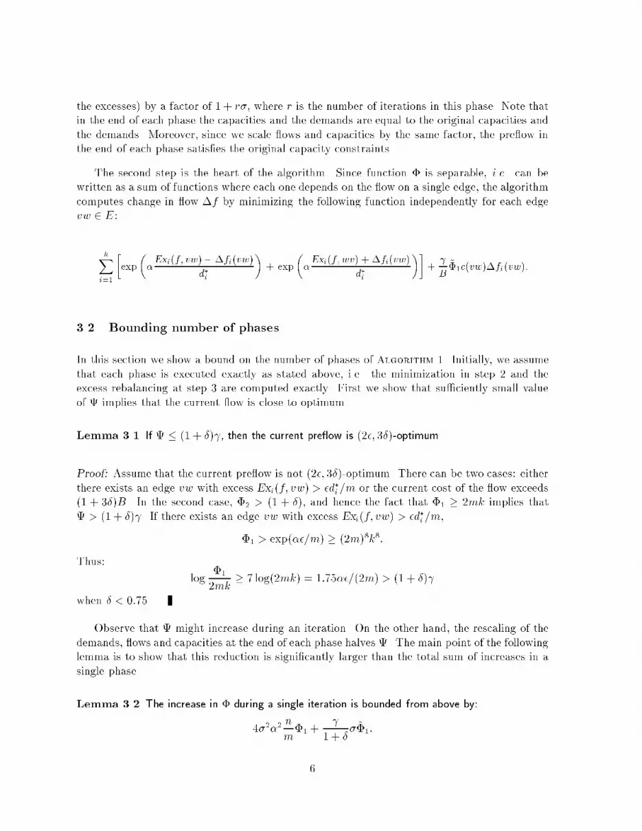
the excesses) by a factor of 1 + r�, where r is the number of iterations in this phase. Note thatin the end of each phase the capacities and the demands are equal to the original capacities andthe demands. Moreover, since we scale ows and capacities by the same factor, the pre ow inthe end of each phase satis�es the original capacity constraints.The second step is the heart of the algorithm. Since function � is separable, i.e. can bewritten as a sum of functions where each one depends on the ow on a single edge, the algorithmcomputes change in ow �f by minimizing the following function independently for each edgevw 2 E:kXi=1 �exp��Exi(f; vw)��fi(vw)d�i � + exp��Exi(f; wv) + �fi(vw)d�i ��+ B ~�1c(vw)�fi(vw):3.2 Bounding number of phasesIn this section we show a bound on the number of phases of Algorithm 1. Initially, we assumethat each phase is executed exactly as stated above, i.e. the minimization in step 2 and theexcess rebalancing at step 3 are computed exactly. First we show that su�ciently small valueof implies that the current ow is close to optimum.Lemma 3.1 If � (1 + �) , then the current pre ow is (2�; 3�)-optimum.Proof: Assume that the current pre ow is not (2�; 3�)-optimum. There can be two cases: eitherthere exists an edge vw with excess Exi(f; vw) > �d�i =m or the current cost of the ow exceeds(1 + 3�)B. In the second case, �2 > (1 + �), and hence the fact that �1 � 2mk implies that > (1 + �) . If there exists an edge vw with excess Exi(f; vw) > �d�i =m,�1 > exp(��=m) � (2m)8k8:Thus: log �12mk � 7 log(2mk) = 1:75��=(2m)> (1 + �) when � < 0:75.Observe that might increase during an iteration. On the other hand, the rescaling of thedemands, ows and capacities at the end of each phase halves . The main point of the followinglemma is to show that this reduction is signi�cantly larger than the total sum of increases in asingle phase.Lemma 3.2 The increase in � during a single iteration is bounded from above by:4�2�2 nm�1 + 1 + � � ~�1:6

We defer the proof of this lemma. Instead, we prove that it implies convergence in a smallnumber of phases. Lemma 3.2, together with the de�nition of gives a bound on the increasein :Lemma 3.3 The increase � in during a single iteration is bounded by 4�2�2 nm + �.Proof: Let ��1 and ��2 denote the change in �1 and �2 during one iteration, respectively.Denote the total increase in � during one iteration by �� = ��1+ ~�1��2. Lemma 3.2 impliesthat: � � log �1 +��1�1 + 1 + ���2 � 1�1 (��1 + ��2 �11 + � )� 1�1 (��1 + ~�1��2) = ���1� 4�2�2 nm + � ~�1�1 1 + � � 4�2�2 nm + � Note that we used the bounds on ~�1, given by (2).Lemma 3.4 Let 0 and s be the value of the potential function at the beginning of a phase andat the end of this phase (after scaling of the demands and capacities), respectively. If 0 � (1+ �)then s � (1� �=4)0.Proof: Observe that scaling down of demands and ows at the end of a phase can not increase. Hence, the claim holds for the case when the phase was terminated because fell below0=2. Otherwise, demands and ows are halved at the end of the iteration, causing halving ofthe excesses. This corresponds to taking a square root of each one out of 2mk terms in �1,which causes log[�1=(2mk)] to go down by at least a factor of 2. Since �2 is linear in the valueof the ow, we have: s � 12 �0 + (4��2 nm + )�= 0 � 12 �0 � (4��2 nm + ))�� 0 � 12 ��0 � 4��2 nm�where the last equality is implied by the assumption that 0 > (1+ �) . The desired result canbe obtained by choosing � = �16�2 nm 0:Initial value of is bounded by O�(�); by Lemma 3.1 the algorithm terminates when it hadsucceeded to reduce to O( ) = O(��=m). Hence we have the following theorem:7

Theorem 3.5 The algorithm terminates in O(��1 log(m��1)) phases, where each phase consistsof O(��1) = O�(��1��2mn) iterations.Proof of Lemma 3.2: Consider a min-cost multicommodity ow f� that satis�es the originaldemands d�i . Note that �f�i (vw) is one of the possibilities for �fi(vw) computed in the secondstep of each iteration. Hence, the total increase in � in a single iteration is not worse than theincrease in � if we set 8i : �fi(vw) = �f�i (vw):In order to bound increase in �, we will use the fact that ex+t � ex+ tex+ t2ex for jtj � 1=2.Observe that our choice of � and � implies that ��d�i � d�i=2 for all i, and hence we can usethe above second order approximation. Consider the contribution to � of the change in excessesdue to increase in demand of every commodity i by �d�i and due to ow change �f = �f�.Observe that for every i, this operation does not change excesses of commodity i at its sourcesi and its sink ti. Recall that we have assumed that there exists a solution of cost B=(1 + �).Thus, the cost of f� is bounded by B=(1 + �). To simplify notation, denote�i(f; v; w) = exp��Exi(f; vw)d�i � :Hence the increase in � during a single iteration can be bounded by:Xi;v 62fsi;tig �� Xw:vw2E (�i(f; w; v) � �i(f; v; w)) f�i (vw)d�i+ Xi;vw2E �2�2 (�i(f; w; v) + �i(f; v; w))�f�i (vw)d�i �2+� 1 + � ~�1:(3)We will bound each term in equation (3) separately. In order to bound the �rst term,decompose f� into a collection of ow paths from sources to their respective sinks. Consider ow path P of commodity i from si to ti and denote its value by �f�i (P ). The contribution ofthis ow path to the �rst term is bounded by:Xwv2Pvw02P �� (�i(f; w; v)� �i(f; v; w0)) f�i (P )d�i(4) Since the excesses associated by node v with all its incident edges are the same (by Step 3of Algorithm-1), the above contribution is zero. The fact that f�i (vw) � d�i , implies that thesecond term can be bounded by: 8

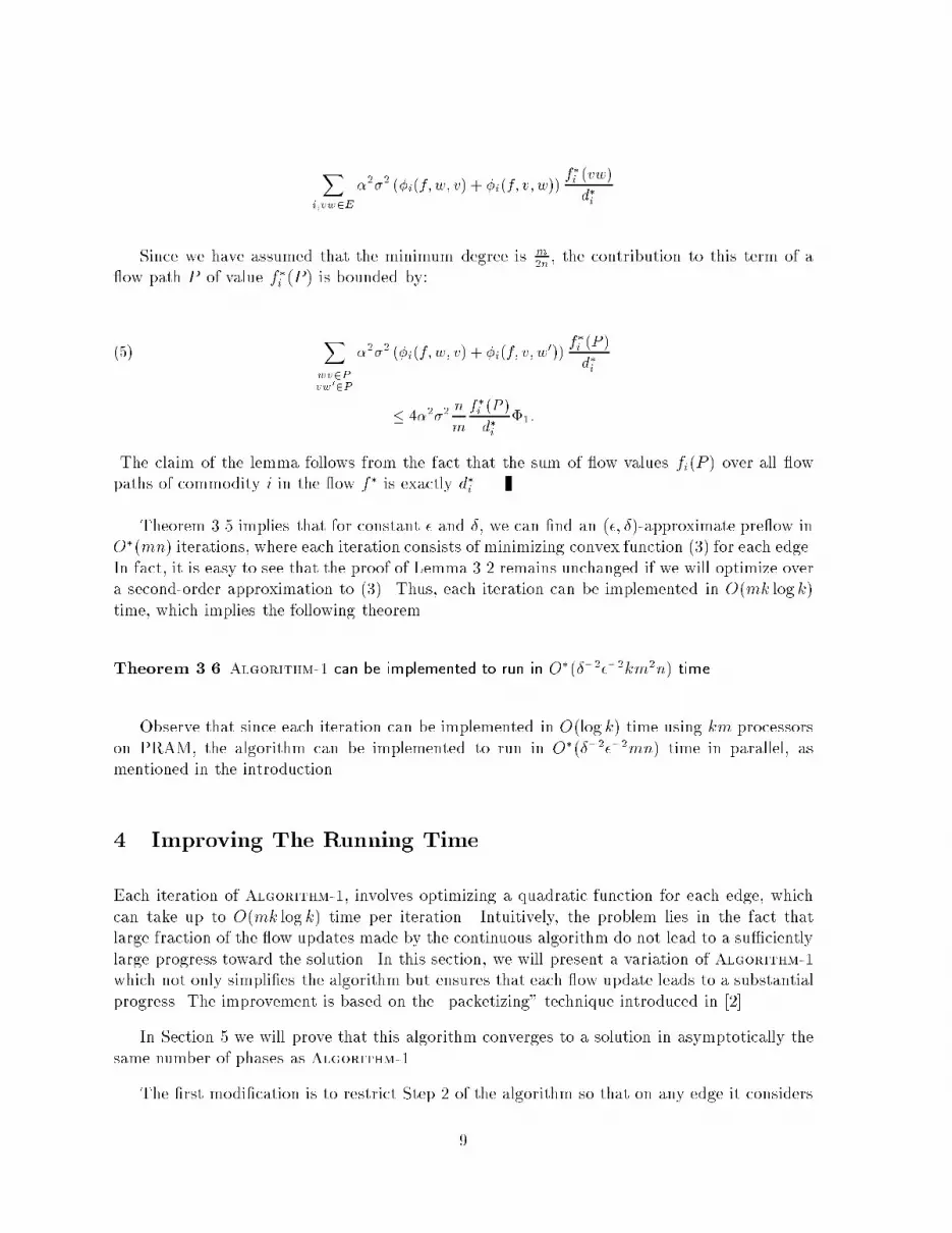
Xi;vw2E�2�2 (�i(f; w; v) + �i(f; v; w)) f�i (vw)d�iSince we have assumed that the minimum degree is m2n , the contribution to this term of a ow path P of value f�i (P ) is bounded by:Xwv2Pvw02P �2�2 (�i(f; w; v) + �i(f; v; w0)) f�i (P )d�i(5) � 4�2�2 nm f�i (P )d�i �1:The claim of the lemma follows from the fact that the sum of ow values fi(P ) over all owpaths of commodity i in the ow f� is exactly d�i .Theorem 3.5 implies that for constant � and �, we can �nd an (�; �)-approximate pre ow inO�(mn) iterations, where each iteration consists of minimizing convex function (3) for each edge.In fact, it is easy to see that the proof of Lemma 3.2 remains unchanged if we will optimize overa second-order approximation to (3). Thus, each iteration can be implemented in O(mk log k)time, which implies the following theorem.Theorem 3.6 Algorithm-1 can be implemented to run in O�(��2��2km2n) time.Observe that since each iteration can be implemented in O(log k) time using km processorson PRAM, the algorithm can be implemented to run in O�(��2��2mn) time in parallel, asmentioned in the introduction.4 Improving The Running TimeEach iteration of Algorithm-1, involves optimizing a quadratic function for each edge, whichcan take up to O(mk log k) time per iteration. Intuitively, the problem lies in the fact thatlarge fraction of the ow updates made by the continuous algorithm do not lead to a su�cientlylarge progress toward the solution. In this section, we will present a variation of Algorithm-1which not only simpli�es the algorithm but ensures that each ow update leads to a substantialprogress. The improvement is based on the \packetizing" technique introduced in [2].In Section 5 we will prove that this algorithm converges to a solution in asymptotically thesame number of phases as Algorithm-1.The �rst modi�cation is to restrict Step 2 of the algorithm so that on any edge it considers9

for optimization only those commodity/edge pairs (i; vw 2 E) that satisfy:Exi(f; vw) � Exi(f; wv) + 4�d�i(6) Exi(f; vw) � ��diwhere � = log(mk��1��1)=�. All the ow and excess vectors considered henceforth will berestricted to the subspace determined by this restriction. Also, the algorithm uses a new set ofexcesses ~Ex, de�ned as follows:~Exi(f; vw) = ( Exi(f; vw)� �di vw 2 EExi(f; vw) + �di wv 2 E :Let �0(i;vw) (Ex) be the negated gradient of the potential function w.r.t. the ow vector forcommodity i in edge vw 2 E, de�ned as:�0(i;vw) (Ex) = � B c(vw)~�1 +�di �exp(�Exi(f; vw)d�i )� exp(�Exi(f; wv)d�i )� :Note that since the edges and commodities obey condition (6) the gradient vector �0( ~Ex) isnon-negative. The updated algorithm is as follows:Algorithm-2 (single iteration)1. Add capacity �u(vw) to each edge vw 2 E. Change demand of each commodity i:di = di + �d�i , where d�i is the original demand of commodity i. Update the value ofexcesses accordingly.2. Find an unsaturated edge and a commodity i satisfying condition (6) with the largestgradient �0(i;vw) � ~Ex� and move a unit �d�i or an amount that is su�cient to saturate thatedge (whichever is less). Update the ow and excesses. Observe that this is equivalentto �nding the change �f in the ow vector f that maximizes P�0(i;vw) � ~Ex��fi(vw)under the constraints that 0 � �fi(vw) � �d�i and Pi�fi(vw) does not exceed availablecapacity.3. Recompute new excesses Exi(f; vw) at each node v. Rebalance excesses inside each nodeto within an additive error of �d�i by moving excess in increments of at least �d�i .4. Update the current value of ~�1, if necessary.As in Algorithm-1, a phase is terminated either after 1=� iterations or when the value of falls below 0=2. In the end of a phase, we scale down all the ows, the demands, and thecapacities (and hence all the excesses) by a factor of 1+ r�, where r is the number of iterationsin this phase. 10

Using a heap on every edge-node pair, it is straightforward to implement Algorithm-2to run in O(log k) time per excess update. Excess updates can be divided into two typesdepending on whether or not the the update was large (exceeded �d�i ) or small. Observe that if ow of commodity i on edge vw was updated by less than �d�i , the only reason this ow mightnot be updated again in the next iteration is if for some commodity j, the excess Exj(f; vw)or Exj(f; wv) was changed by a multiple of �d�j during rebalancing in Step 3 of the currentiteration. If, on the other hand, the excess updates add-up to �di over several iterations, thenwe can precompute the number of iterations and do one single excess update of �di at the end.Hence, the work associated with each update can be ammortized over the large updates, thatrequire O(log k) work each. Thus, it is su�cient to bound the number of large excess updates.Theorem 4.1 The total number of large updates to excesses in a single phase is bounded byO�(��3��2kmn2):Proof: Let � be de�ned as in condition (6), and consider a potential function� = Xi;vw2Emax��� � 2�; Exi(f; vw)di �2Let 0 denote the value of at the start of the phase. The fact that at the start of the phase,log[�1=(2mk)] � 0 together with the fact that 0=� � 2�, implies that the initial value of � isbounded by O(mk20=�2 +mk�2). Increase in � due to increase in demands by �d�i during aniteration is bounded by O(k�(0=� + � + �)) = O(k�(0=�+ �)):Thus, the total increase in � throughout a phase is bounded by O(k(0=� + �)). Note thateach time we move �d�i amount of excess across an edge or within a node, the decrease in � is(�2), and hence the total number of updates can be bounded by1�2O(mk20=�2 +mk�2 + k(0=�+ �))and the claim follows from the observation that( �m�) � 0 � O(�):Thus, we have the following Theorem:Theorem 4.2 Single phase of Algorithm-2 can be implemented to run in O�(��3��2kmn2) time.11

5 Bounding the number of phases of Algorithm-2In this section, we analyze the behavior of Algorithm-2 during a single phase and show abound on the number of phases needed for obtaining an (�; �)-approximate pre ow. There areseveral important di�erences between Algorithm-1 and Algorithm-2. First, instead of exactrebalancing of excesses inside each node, we execute an approximate rebalancing. Second, weignore commodities on edges with small potential di�erences. Third, we do not compute owincrement that leads to the largest reduction in the potential function.First, we will show that the approximate rebalancing and ignoring commodity/edge pairswith small potential di�erence does not increase the number of phases by more than a constantfactor.Lemma 5.1 If redistribution of excesses in Step 3 of Algorithm-1 is done within an additive errorof 2�d�i and if we limit Step 2 to include only those edges and commodities that satisfy condition(6) then the increase in � during a single iteration is bounded from above by:O��2�2 nm��1 + 1 + �� ~�1:Proof: The main ideas in the proof are that relatively small imperfections during rebalancing inStep 3 add-up to only a minor increase in the potential function and that we do not lose muchby ignoring edge-commodity pairs that do not give large reduction in the potential function.Step 3 of Algorithm-2 redistributes excesses inside nodes within an additive error of �d�i . Thatis: 8i; v 2 V; w; w0 adjacent to v either :jExi(f; vw)� Exi(f; vw0)j � 2�d�ior � �d�i � maxfExi(f; vw);Exi(f; vw0)g:Since for x � 1 we have ex � 1 � 3x, the contribution to the �rst term in (3) of a ow pathP of value f�i (P ) can be bounded by:O0BB@ Xwv2Pvw02P �2�2min(�i(f; w; v); �i(f; v; w0)) f�i (P )d�i 1CCA+ O0BB@ Xwv2Pvw02P �� exp(���)f�i (P )d�i 1CCA :If we consider the error due to disregarding commodity/edge pairs that have very small excessesi.e. Exi(f; vw) � ��di12

then the associated error can be bound byO0BB@ Xwv2Pvw02P �� exp(���)f�i (P )d�i 1CCA :Now consider the error introduced by disregarding commodity/edge pairs that do not satisfyExi(f; vw) � Exi(f; wv) + 4�d�i :(7)Again using the fact that for x � 1, we have ex � 1 � 3x, the error associated with edge vw,commodity i and path P can not exceed:���exp��Exi(f; vw)d�i �� exp��Exi(f; wv)d�i �� f�i (P )d�i � �� exp��Exi(f; wv)d�i � (exp (4��)� 1) f�i (P )d�i� O��2�2 exp��Exi(f; wv)d�i � f�i (P )d�i � :By summing up over all the ow paths and over all the commodities, substituting the value of�, and using the fact that �1 � 2mk, we see that each of the three di�erent types of error canbe bounded by O(�2�2 nm�1):Thus, increase in � during a single iteration remains bounded byO��2�2 nm��1 + 1 + �� ~�1:We shall use the notation Ex + �f to indicate the excesses that result after updating the ow by amount �f . The increase in potential function due to incrementing the demand dependsonly on the excesses at the beginning of the iteration and is independent of the technique usedfor incrementing the ow. Hence we need to bound only the change in potential function dueto the ow updates. We �rst claim that using ~Ex instead of Ex does not adversely a�ect thepotential function reduction. The proof of the following Lemma is essentially identical to theproof of Lemma 5.1.Lemma 5.2 If f� is the optimal solution then�( ~Ex+ �f�)� �( ~Ex) � O��2�2 nm��1 + 1 + � � ~�1:Lemma 5.3 The change in potential function due to the ow increment�f used by Algorithm-2can be bounded by �(Ex+�f)� �(Ex) � �( ~Ex+ �f�)� �( ~Ex):13

Proof: Since for all i and vw 2 E the ow �f satis�es 0 � �fi(vw) � �di and the excessessatisfy condition (6), we know that �0(Ex + �f) � �0( ~Ex) . Using �rst-order Taylor seriesexpansion we get�(Ex+ �f)� �(Ex) � ��fT�0(Ex+�f) � ��fT�0( ~Ex):Furthermore, since �f is the optimal solution in the space (that includes �f�) that maximizesthe linear objective �fT�0( ~Ex) we have��fT�0( ~Ex) � ��f�T�0( ~Ex) � �( ~Ex+ �f�)� �( ~Ex):Hence the result follows.Combining Lemmas 5.2 and 5.3 we conclude that the increase in the potential function forthe modi�ed algorithm is a constant multiple of the bound obtained for Algorithm-1. Hencewe have the following theorem.Theorem 5.4 Algorithm-2 terminates in O(��1 log(m��1)) phases.Using the above theorem together with Theorem 4.2, we get the following claim:Theorem 5.5 An (�; �)-approximation to the minimum-cost multicommodity ow problem can beobtained in O�(��3��3kmn2) time.AcknowledgementsWe would like to thank Baruch Awerbuch, Andrew Goldberg, Tom Leighton, and �Eva Tardosfor helpful discussions.References[1] B. Awerbauch and F. T. Leighton. A Simple Local-Control Approximation Algorithmfor Multicommodity Flow. In Proc. 34th IEEE Annual Symposium on Foundations ofComputer Science, pages 459{468, 1993.[2] B. Awerbuch and T. Leighton. Improved approximation algorithms for the multi-commodity ow problem and local competitive routing in dynamic networks. In Proc.26th Annual ACM Symposium on Theory of Computing, pages 487{495, 1994.[3] A. V. Goldberg and R. E. Tarjan. A New Approach to the Maximum Flow Problem. J.Assoc. Comput. Mach., 35:921{940, 1988.[4] A. V. Goldberg and R. E. Tarjan. Finding Minimum-Cost Circulations by SuccessiveApproximation. Math. of Oper. Res., 15:430{466, 1990.14

[5] T. C. Hu. Multi-Commodity Network Flows. J. ORSA, 11:344{360, 1963.[6] A. Kamath and O. Palmon. Improved interior-point algorithms for exact and approxi-mate solutions of multicommodity ow problems. In Proc. 6th ACM-SIAM Symposium onDiscrete Algorithms, 1995.[7] S. Kapoor and P. M. Vaidya. Fast Algorithms for Convex Quadratic Programming andMulticommodity Flows. In Proc. 18th Annual ACM Symposium on Theory of Computing,pages 147{159, 1986.[8] D. Karger and S. Plotkin. Adding multiple cost constraints to combinatorial optimiza-tion problems, with applications to multicommodity ows. In Proc. 27th Annual ACMSymposium on Theory of Computing, May 1995.[9] P. Klein, S. Plotkin, C. Stein, and �E. Tardos. Faster approximation algorithms for theunit capacity concurrent ow problem with applications to routing and �nding sparse cuts.SIAM Journal on Computing, June 1994.[10] T. Leighton, F. Makedon, S. Plotkin, C. Stein, �E. Tardos, and S. Tragoudas. Fast ap-proximation algorithms for multicommodity ow problems. In Proc. 23st Annual ACMSymposium on Theory of Computing, 1991.[11] T. Leighton and S. Rao. An approximate max- ow min-cut theorem for uniform multicom-modity ow problems with applications to approximation algorithms. In Proc. 29th IEEEAnnual Symposium on Foundations of Computer Science, pages 422{431, 1988.[12] S. A. Plotkin, D. Shmoys, and �E. Tardos. Fast Approximation Algorithms for FractionalPacking and Covering. In Proc. 32nd IEEE Annual Symposium on Foundations of Com-puter Science, 1991.[13] T. Radzik. Fast deterministic approximation for the multicommodity ow problem. InProc. 6th ACM-SIAM Symposium on Discrete Algorithms, 1995.[14] F. Shahrokhi and D. Matula. The maximum concurrent ow problem. J. Assoc. Comput.Mach., 37:318{334, 1990.[15] F. Shahrokhi and D. W. Matula. The maximum concurrent ow problem. Technical ReportCSR-183, Department of Computer Science, New Mexico Tech., 1988.[16] C. Stein. Approximation algorithms for multicommodity ow and scheduling problems.PhD thesis, MIT, 1992.[17] P. M. Vaidya. Speeding up Linear Programming Using Fast Matrix Multiplication. InProc. 30th IEEE Annual Symposium on Foundations of Computer Science, 1989.15