Fully Dynamic Spatial Approximation Trees

Dynamic Spatial Approximation Trees

Gonzalo Navarro � Nora Reyes

Dept. of Computer Science Depto. de Inform�atica

University of Chile Universidad Nacional de San Luis

Blanco Encalada 2120, Santiago, Chile Ej�ercito de los Andes 950, San Luis, Argentina

[email protected] [email protected]

Abstract

The Spatial Approximation Tree (sa-tree) is a re-cently proposed data structure for searching in metricspaces. It has been shown that it compares favorablyagainst alternative data structures in spaces of highdimension or queries with low selectivity. The maindrawback of the sa-tree is that it is a static data struc-ture, that is, once built, it is diÆcult to add new el-ements to it. This rules it out for many interestingapplications.

In this paper we overcome this weakness. We pro-pose and study several methods to handle insertionsin the sa-tree. Some are classical folklore solutionswell known in the data structures community, while themost promising ones have been speci�cally developedconsidering the particular properties of the sa-tree, andinvolve new algorithmic insights in the behavior of thisdata structure. As a result, we show that it is viable tomodify the sa-tree so as to permit fast insertions whilekeeping its good search eÆciency.

1. Introduction

The concept of \approximate" searching has appli-cations in a vast number of �elds. Some examples arenon-traditional databases (e.g. storing images, �nger-prints or audio clips, where the concept of exact searchis of no use and we search instead for similar objects);text searching (to �nd words and phrases in a textdatabase allowing a small number of typographical orspelling errors); information retrieval (to look for doc-uments that are similar to a given query or document);machine learning and classi�cation (to classify a newelement according to its closest representative); image

�Partially supported by Fondecyt grant 1-000929.

quantization and compression (where only some vec-tors can be represented and we code the others as theirclosest representable point); computational biology (to�nd a DNA or protein sequence in a database allowingsome errors due to mutations); and function prediction(to search for the most similar behavior of a function inthe past so as to predict its probable future behavior).

All those applications have some common charac-teristics. There is a universe U of objects, and a non-negative distance function d : U � U �! R+ de�nedamong them. This distance satis�es the three axiomsthat make the set a metric space: strict positiveness(d(x; y) = 0 , x = y), symmetry (d(x; y) = d(y; x))and triangle inequality (d(x; z) � d(x; y) + d(y; z)).The smaller the distance between two objects, themore \similar" they are. We have a �nite databaseS � U , which is a subset of the universe of objects andcan be preprocessed (to build an index, for example).Later, given a new object from the universe (a queryq), we must retrieve all similar elements found in thedatabase. There are two typical queries of this kind:

Range query: Retrieve all elements within distancer to q in S. This is, fx 2 S ; d(x; q) � rg.

Nearest neighbor query (k-NN): Retrieve the kclosest elements to q in S. That is, a set A � Ssuch that jAj = k and 8x 2 A; y 2 S�A; d(x; q) �d(y; q).

The distance is considered expensive to compute(think, for instance, in comparing two �ngerprints).Hence, it is customary to de�ne the complexity ofthe search as the number of distance evaluations per-formed, disregarding other components such as CPUtime for side computations, and even I/O time. Givena database of jSj = n objects, queries can be triviallyanswered by performing n distance evaluations. Thegoal is to structure the database such that we performless distance evaluations.

A particular case of this problem arises when thespace is a set of d-dimensional points and the dis-tance belongs to the Minkowski Lp family: Lp =(P

1�i�d jxi � yijp)1=p. The best known special cases

are p = 1 (Manhattan distance), p = 2 (Euclideandistance) and p = 1 (maximum distance), that is,L1 = max1�i�d jxi � yij.

There are e�ective methods to search on d-dimensional spaces, such as kd-trees [2] or R-trees [13].However, for roughly 20 dimensions or more thosestructures cease to work well. We focus in this paper ingeneral metric spaces, although the solutions are wellsuited also for d-dimensional spaces.

It is interesting to notice that the concept of \di-mensionality" can be translated to metric spaces aswell: the typical feature in high dimensional spaceswith Lp distances is that the probability distributionof distances among elements has a very concentratedhistogram (with larger mean as the dimension grows),making the work of any similarity search algorithmmore diÆcult [5, 10]. In the extreme case we have aspace where d(x; x) = 0 and 8y 6= x; d(x; y) = 1, whereit is impossible to avoid a single distance evaluation atsearch time. We say that a general metric space is highdimensional when its histogram of distances is concen-trated.

There are a number of methods to preprocess the setin order to reduce the number of distance evaluations.All those structures work on the basis of discardingelements using the triangle inequality, and most usethe classical divide-and-conquer approach (which is notspeci�c of metric space searching).

The Spatial Approximation Tree (sa-tree) is a re-cently proposed data structure of this kind [16], whichis based on a novel concept: rather than dividing thesearch space, approach the query spatially, that is,start at some point in the space and get closer andcloser to the query. It has been shown that the sa-tree behaves better than the other existing structureson metric spaces of high dimension or queries with lowselectivity, which is the case in many applications.

The sa-tree, unlike other data structures, does nothave parameters to be tuned by the user of each ap-plication. This makes it very appealing as a generalpurpose data structure for metric searching, since anynon-expert seeking for a tool to solve his/her particularproblem can use it as a black box tool, without the needof understanding the complications of an area he/sheis not interested in. Other data structures have manytuning parameters, hence requiring a big e�ort fromthe user in order to obtain an acceptable performance.

On the other hand, the main weakness of the sa-tree is that it is not dynamic. That is, once it is built,

it is diÆcult to add new elements to it. This makesthe sa-tree unsuitable for dynamic applications such asmultimedia databases.

Overcoming this weakness is the aim of this paper.We propose and study several methods to handle inser-tions in the sa-tree. Some are classical folklore solutionswell known in the data structures community, while themost promising ones have been speci�cally developedconsidering the particular properties of the sa-tree. Asa result, we show that it is viable to modify the sa-treeso as to permit fast insertions while keeping its goodsearch eÆciency. As a related byproduct of this study,we give new algorithmic insights in the behavior of thisdata structure.

2. Previous Work

Algorithms to search in general metric spaces can bedivided in two large areas: pivot-based and clusteringalgorithms. (See [10] for a more complete review.)

Pivot-based algorithms. The idea is to use a setof k distinguished elements (\pivots") p1:::pk 2 Sand storing, for each database element x, its dis-tance to the k pivots (d(x; p1):::d(x; pk)). Given thequery q, its distance to the k pivots is computed(d(q; p1):::d(q; pk)). Now, if for some pivot pi it holdsthat jd(q; pi) � d(x; pi)j > r, then we know by the tri-angle inequality that d(q; x) > r and therefore do notneed to explicitly evaluate d(x; p). All the other el-ements that cannot be eliminated using this rule aredirectly compared against the query.

Several algorithms [23, 15, 7, 18, 6, 8] are almostdirect implementations of this idea, and di�er basicallyin their extra structure used to reduce the CPU cost of�nding the candidate points, but not in their numberof distance evaluations.

There are a number of tree-like data structures thatuse this idea in a more indirect way: they select a pivotas the root of the tree and divide the space accordingto the distances to the root. One slice corresponds toeach subtree (the number and width of the slices di�ersacross the strategies). At each subtree, a new pivot isselected and so on. The search backtracks on the treeusing the triangle inequality to prune subtrees, that is,if a is the tree root and b is a children correspondingto d(a; b) 2 [x1; x2], then we can avoid entering in thesubtree of b whenever [d(q; a) � r; d(q; a) + r] has nointersection with [x1; x2].

Several data structures use this idea [3, 22, 14, 24,4, 25].

Clustering algorithms. The second trend consistsin dividing the space in zones as compact as possible,normally recursively, and storing a representative point(\center") for each zone plus a few extra data thatpermits quickly discarding the zone at query time. Twocriteria can be used to delimit a zone.

The �rst one is the Voronoi area, where we select aset of centers and put each other point inside the zoneof its closest center. The areas are limited by hyper-planes and the zones are analogous to Voronoi regionsin vector spaces. Let fc1 : : : cmg be the set of cen-ters. At query time we evaluate (d(q; c1); : : : ; d(q; cm)),choose the closest center c and discard every zonewhose center ci satis�es d(q; ci) > d(q; c) + 2r, as itsVoronoi area cannot intersect with the query ball.

The second criterion is the covering radius cr(ci),which is the maximum distance between ci and an el-ement in its zone. If d(q; ci)� r > cr(ci), then there isno need to consider zone i.

The techniques can be combined. Some techniquesusing only hyperplanes are [22, 19, 12]. Some tech-niques using only covering radii are [11, 9]. One usingboth criteria [5].

Nearest neighbor queries. To answer 1-NNqueries, we simulate a range query with a radius thatis initially r� =1, and reduce r� as we �nd closer andcloser elements to q. At the end, we have in r� thedistance to the closest elements and have seen themall. Unlike a range query, we are now interested inquickly �nding close elements in order to reduce r� asearly as possible, so there are a number of heuristics toachieve this. One of the most interesting is proposed in[21], where the subtrees yet to be processed are storedin a priority queue in a heuristically promising order-ing. The traversal is more general than a backtracking.Each time we process the root of the most promisingsubtree, we may add its children to the priority queue.At some point we can preempt the search using a cuto�criterion given by the triangle inequality.

k-NN queries are handled as a generalization of 1-NN queries. Instead of one closest element, the k clos-est elements known are maintained, and r� is the dis-tance to the farthest to q among those k. Each timea new candidate appears we insert it into the queue,which may displace another element and hence reducer�. At the end, the queue contains the k closest ele-ments to q.

3. The Spatial Approximation Tree

We describe brie y in this section the sa-tree datastructure. It needs linear space O(n), reasonable

construction time O(n log2 n= log logn) and sublinearsearch time O(n1��(1= log logn)) in high dimensions andO(n�) (0 < � < 1) in low dimensions. It is experi-mentally shown to improve over other data structureswhen the dimension is high or the query radius is large.For more details see the original references [16, 17].

3.1. Construction

We select a random element a 2 S to be the rootof the tree. We then select a suitable set of neighborsN(a) satisfying the following property:

Condition 1: (given a; S) 8x 2 S, x 2 N(a) ,8y 2 N(a)� fxg; d(x; y) > d(x; a).

That is, the neighbors of a form a set such that anyneighbor is closer to a than to any other neighbor. The\only if" (() part of the de�nition guarantees that ifwe can get closer to any b 2 S then an element in N(a)is closer to b than a, because we put as direct neigh-bors all those elements that are not closer to anotherneighbor. The \if" part ()) aims at putting as fewneighbors as possible.

Notice that the set N(a) is de�ned in terms of itselfin a non-trivial way and that multiple solutions �t thede�nition. For example, if a is far from b and c andthese are close to each other, then both N(a) = fbgand N(a) = fcg satisfy the de�nition.

Finding the smallest possible set N(a) seems to bea nontrivial combinatorial optimization problem, sinceby including an element we need to take out others(this happens between b and c in the example of theprevious paragraph). However, simple heuristics whichadd more neighbors than necessary work well. We be-gin with the initial node a and its \bag" holding all therest of S. We �rst sort the bag by distance to a.

Then, we start adding nodes to N(a) (which is ini-tially empty). Each time we consider a new node b, wecheck whether it is closer to some element of N(a) thanto a itself. If that is not the case, we add b to N(a).

At this point we have a suitable set of neighbors.Note that Condition 1 is satis�ed thanks to the factthat we have considered the elements in order of in-creasing distance to a. The \only if" part of Condition1 is clearly satis�ed because any element not satisfyingit is inserted in N(a). The \if" part is more delicate.Let x 6= y 2 N(a). If y is closer to a than x then y wasconsidered �rst. Our construction algorithm guaran-tees that if we inserted x inN(a) then d(x; a) < d(x; y).If, on the other hand, x is closer to a than y, thend(y; x) > d(y; a) � d(x; a) (that is, a neighbor cannotbe removed by a new neighbor inserted later).

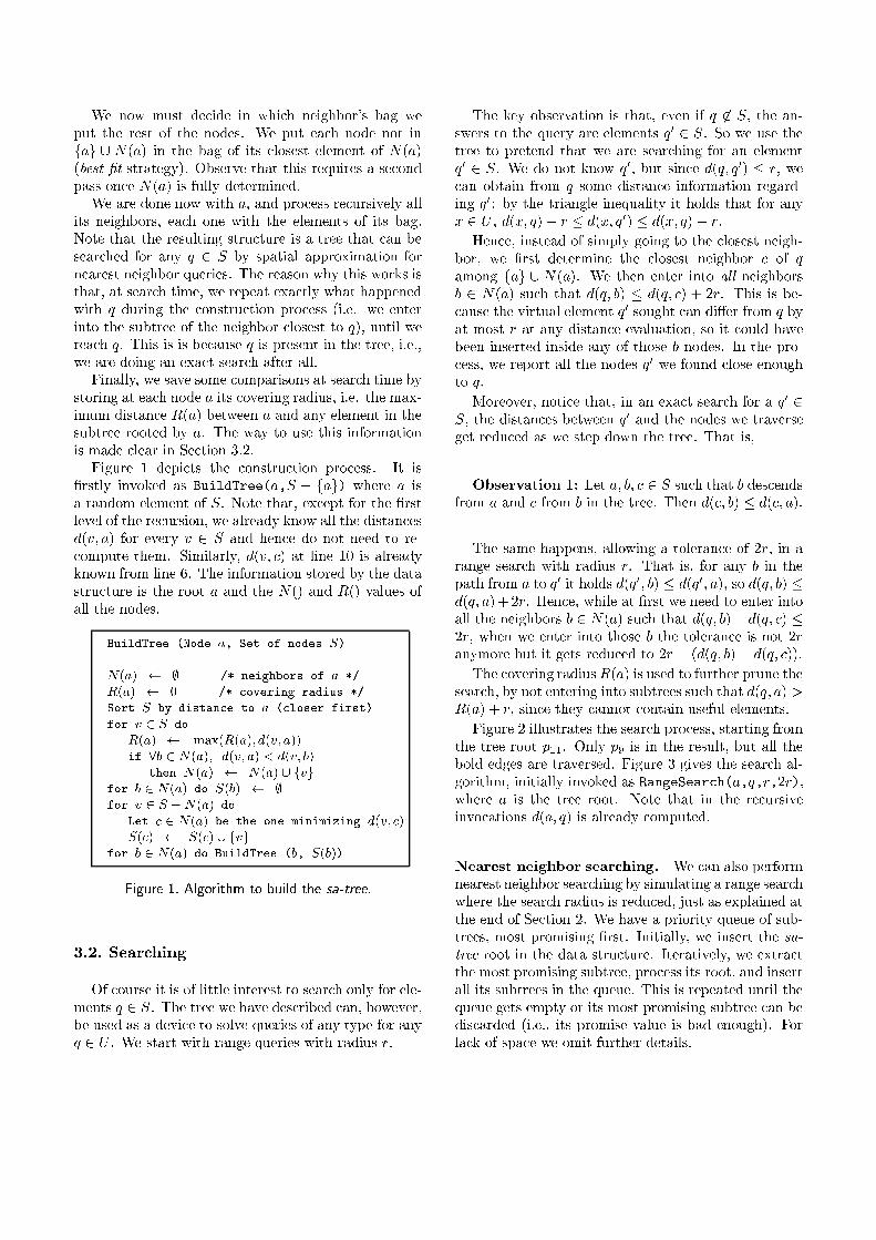
We now must decide in which neighbor's bag weput the rest of the nodes. We put each node not infag [ N(a) in the bag of its closest element of N(a)(best-�t strategy). Observe that this requires a secondpass once N(a) is fully determined.

We are done now with a, and process recursively allits neighbors, each one with the elements of its bag.Note that the resulting structure is a tree that can besearched for any q 2 S by spatial approximation fornearest neighbor queries. The reason why this works isthat, at search time, we repeat exactly what happenedwith q during the construction process (i.e. we enterinto the subtree of the neighbor closest to q), until wereach q. This is is because q is present in the tree, i.e.,we are doing an exact search after all.

Finally, we save some comparisons at search time bystoring at each node a its covering radius, i.e. the max-imum distance R(a) between a and any element in thesubtree rooted by a. The way to use this informationis made clear in Section 3.2.

Figure 1 depicts the construction process. It is�rstly invoked as BuildTree(a,S � fag) where a isa random element of S. Note that, except for the �rstlevel of the recursion, we already know all the distancesd(v; a) for every v 2 S and hence do not need to re-compute them. Similarly, d(v; c) at line 10 is alreadyknown from line 6. The information stored by the datastructure is the root a and the N() and R() values ofall the nodes.

BuildTree (Node a, Set of nodes S)

N(a) ; /* neighbors of a */

R(a) 0 /* covering radius */

Sort S by distance to a (closer first)

for v 2 S do

R(a) max(R(a); d(v; a))if 8b 2 N(a); d(v; a) < d(v; b)

then N(a) N(a) [ fvgfor b 2 N(a) do S(b) ;for v 2 S �N(a) do

Let c 2 N(a) be the one minimizing d(v; c)S(c) S(c) [ fvg

for b 2 N(a) do BuildTree (b, S(b))

Figure 1. Algorithm to build the sa-tree.

3.2. Searching

Of course it is of little interest to search only for ele-ments q 2 S. The tree we have described can, however,be used as a device to solve queries of any type for anyq 2 U . We start with range queries with radius r.

The key observation is that, even if q 62 S, the an-swers to the query are elements q0 2 S. So we use thetree to pretend that we are searching for an elementq0 2 S. We do not know q0, but since d(q; q0) � r, wecan obtain from q some distance information regard-ing q0: by the triangle inequality it holds that for anyx 2 U , d(x; q) � r � d(x; q0) � d(x; q) + r.

Hence, instead of simply going to the closest neigh-bor, we �rst determine the closest neighbor c of qamong fag [ N(a). We then enter into all neighborsb 2 N(a) such that d(q; b) � d(q; c) + 2r. This is be-cause the virtual element q0 sought can di�er from q byat most r at any distance evaluation, so it could havebeen inserted inside any of those b nodes. In the pro-cess, we report all the nodes q0 we found close enoughto q.

Moreover, notice that, in an exact search for a q0 2S, the distances between q0 and the nodes we traverseget reduced as we step down the tree. That is,

Observation 1: Let a; b; c 2 S such that b descendsfrom a and c from b in the tree. Then d(c; b) � d(c; a).

The same happens, allowing a tolerance of 2r, in arange search with radius r. That is, for any b in thepath from a to q0 it holds d(q0; b) � d(q0; a), so d(q; b) �d(q; a)+2r. Hence, while at �rst we need to enter intoall the neighbors b 2 N(a) such that d(q; b)� d(q; c) �2r, when we enter into those b the tolerance is not 2ranymore but it gets reduced to 2r � (d(q; b)� d(q; c)).

The covering radiusR(a) is used to further prune thesearch, by not entering into subtrees such that d(q; a) >R(a) + r, since they cannot contain useful elements.

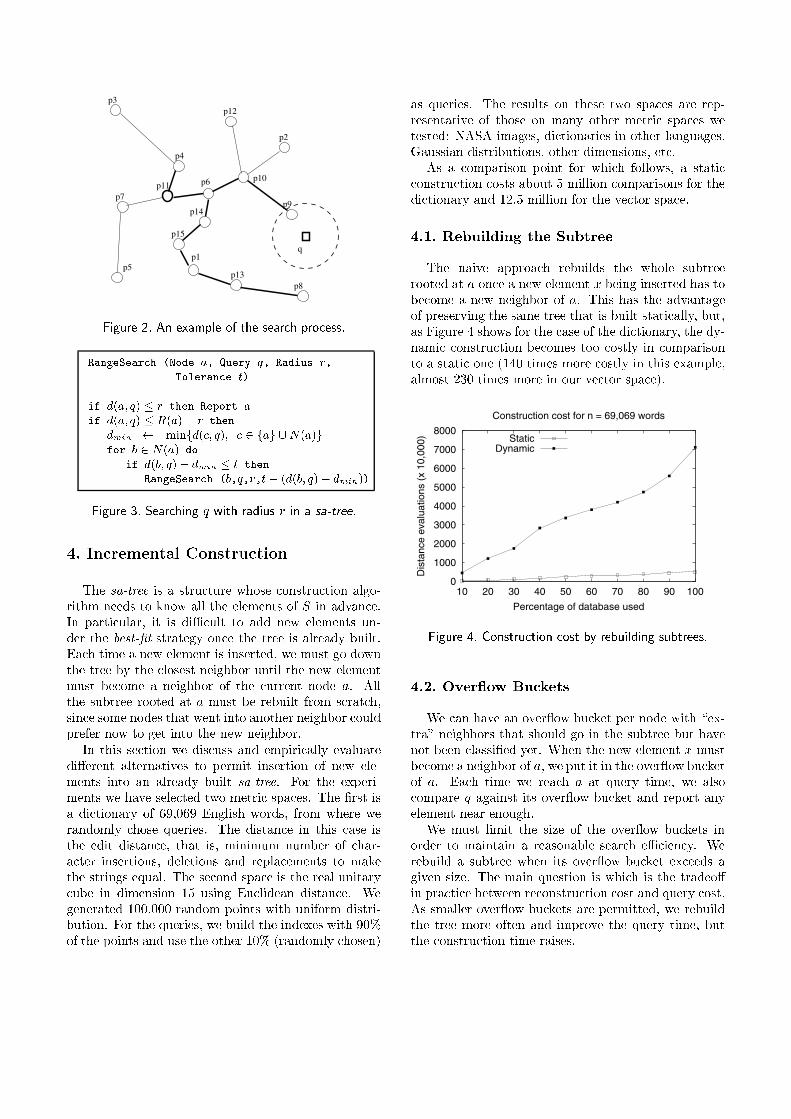
Figure 2 illustrates the search process, starting fromthe tree root p11. Only p9 is in the result, but all thebold edges are traversed. Figure 3 gives the search al-gorithm, initially invoked as RangeSearch(a,q,r,2r),where a is the tree root. Note that in the recursiveinvocations d(a; q) is already computed.

Nearest neighbor searching. We can also performnearest neighbor searching by simulating a range searchwhere the search radius is reduced, just as explained atthe end of Section 2. We have a priority queue of sub-trees, most promising �rst. Initially, we insert the sa-tree root in the data structure. Iteratively, we extractthe most promising subtree, process its root, and insertall its subtrees in the queue. This is repeated until thequeue gets empty or its most promising subtree can bediscarded (i.e., its promise value is bad enough). Forlack of space we omit further details.

p13

p4

p2

p12p3

p7

p15

p6

p8

p9p14

p11

p1q

p5

p10

Figure 2. An example of the search process.

RangeSearch (Node a, Query q, Radius r,

Tolerance t)

if d(a; q) � r then Report a

if d(a; q) � R(a) + r then

dmin minfd(c; q); c 2 fag [N(a)gfor b 2 N(a) do

if d(b; q)� dmin � t then

RangeSearch (b,q,r,t� (d(b; q)� dmin))

Figure 3. Searching q with radius r in a sa-tree.

4. Incremental Construction

The sa-tree is a structure whose construction algo-rithm needs to know all the elements of S in advance.In particular, it is diÆcult to add new elements un-der the best-�t strategy once the tree is already built.Each time a new element is inserted, we must go downthe tree by the closest neighbor until the new elementmust become a neighbor of the current node a. Allthe subtree rooted at a must be rebuilt from scratch,since some nodes that went into another neighbor couldprefer now to get into the new neighbor.

In this section we discuss and empirically evaluatedi�erent alternatives to permit insertion of new ele-ments into an already built sa-tree. For the experi-ments we have selected two metric spaces. The �rst isa dictionary of 69,069 English words, from where werandomly chose queries. The distance in this case isthe edit distance, that is, minimum number of char-acter insertions, deletions and replacements to makethe strings equal. The second space is the real unitarycube in dimension 15 using Euclidean distance. Wegenerated 100,000 random points with uniform distri-bution. For the queries, we build the indexes with 90%of the points and use the other 10% (randomly chosen)

as queries. The results on these two spaces are rep-resentative of those on many other metric spaces wetested: NASA images, dictionaries in other languages,Gaussian distributions, other dimensions, etc.

As a comparison point for which follows, a staticconstruction costs about 5 million comparisons for thedictionary and 12.5 million for the vector space.

4.1. Rebuilding the Subtree

The naive approach rebuilds the whole subtreerooted at a once a new element x being inserted has tobecome a new neighbor of a. This has the advantageof preserving the same tree that is built statically, but,as Figure 4 shows for the case of the dictionary, the dy-namic construction becomes too costly in comparisonto a static one (140 times more costly in this example,almost 230 times more in our vector space).

0

1000

2000

3000

4000

5000

6000

7000

8000

10 20 30 40 50 60 70 80 90 100

Dis

tanc

e ev

alua

tions

(x

10,0

00)

Percentage of database used

Construction cost for n = 69,069 words

StaticDynamic

Figure 4. Construction cost by rebuilding subtrees.

4.2. Over ow Buckets

We can have an over ow bucket per node with \ex-tra" neighbors that should go in the subtree but havenot been classi�ed yet. When the new element x mustbecome a neighbor of a, we put it in the over ow bucketof a. Each time we reach a at query time, we alsocompare q against its over ow bucket and report anyelement near enough.

We must limit the size of the over ow buckets inorder to maintain a reasonable search eÆciency. Werebuild a subtree when its over ow bucket exceeds agiven size. The main question is which is the tradeo�in practice between reconstruction cost and query cost.As smaller over ow buckets are permitted, we rebuildthe tree more often and improve the query time, butthe construction time raises.

100

200

300

400

500

600

700

800

0 100 200 300 400 500 600 700 800 900 1000

Dis

tanc

e ev

alua

tions

(x

10,0

00)

Size of overflow bucket

Construction cost for n = 69,069

400

600

800

1000

1200

1400

1600

1800

0 100 200 300 400 500 600 700 800 900 1000

Dis

tanc

e ev

alua

tions

(x

10,0

00)

Size of overflow bucket

Construction cost for n = 100,000 vectors dim. 15

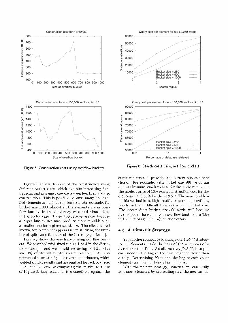
Figure 5. Construction costs using over ow buckets.

Figure 5 shows the cost of the construction usingdi�erent bucket sizes, which exhibits interesting uc-tuations and in some cases costs even less than a staticconstruction. This is possible because many unclassi-�ed elements are left in the buckets. For example, forbucket size 1,000, almost all the elements are in over- ow buckets in the dictionary case and almost 60%in the vector case. These uctuations appear becausea larger bucket size may produce more rebuilds thana smaller one for a given set size n. The e�ect is wellknown, for example it appears when studying the num-ber of splits as a function of the B-tree page size [1].

Figure 6 shows the search costs using over ow buck-ets. We searched with �xed radius 1 to 4 in the dictio-nary example and with radii retrieving 0.01%, 0.1%and 1% of the set in the vector example. We alsoperformed nearest neighbor search experiments, whichyielded similar results and are omitted for lack of space.

As can be seen by comparing the results to thoseof Figure 8, this technique is competitive against the

0

10000

20000

30000

40000

50000

60000

1 2 3 4

Dis

tanc

e ev

alua

tions

Search radius

Query cost per element for n = 69,069 words

Bucket size = 250Bucket size = 500Bucket size = 1000

55000

60000

65000

70000

75000

80000

85000

90000

0.01 0.1 1

Dis

tanc

e ev

alua

tions

Percentage of database retrieved

Query cost per element for n = 100,000 vectors dim. 15

Bucket size = 250Bucket size = 500Bucket size = 1000

Figure 6. Search costs using over ow buckets.

static construction provided the correct bucket size ischosen. For example, with bucket size 500 we obtainalmost the same search costs as for the static version, atthe modest price of 10% extra construction cost for thedictionary and 30% for the vectors. The main problemin this method is its high sensitivity to the uctuations,which makes it diÆcult to select a good bucket size.The intermediate bucket size 500 works well becauseat this point the elements in over ow buckets are 30%in the dictionary and 15% in the vectors.

4.3. A First-Fit Strategy

Yet another solution is to change our best-�t strategyto put elements inside the bags of the neighbors of aat construction time. An alternative, �rst-�t, is to puteach node in the bag of the �rst neighbor closer thana to q. Determining N(a) and the bag of each otherelement can now be done all in one pass.

With the �rst-�t strategy, however, we can easilyadd more elements by pretending that the new incom-

0

200

400

600

800

1000

1200

1400

1600

10 20 30 40 50 60 70 80 90 100

Dis

tanc

e ev

alua

tions

(x

10,0

00)



StaticFirst-Fit

Timestamp (up)Timestamp (down)

0

200

400

600

800

1000

1200

1400

10 20 30 40 50 60 70 80 90 100

Dis

tanc

e ev

alua

tions

(x

10,0

00)



StaticFirst-Fit

Timestamp (down)Timestamp (up)

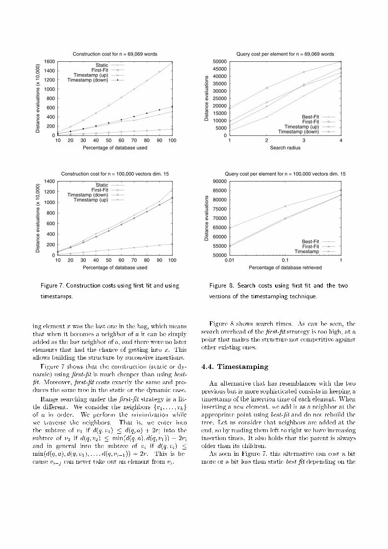
Figure 7. Construction costs using �rst-�t and using

timestamps.

ing element x was the last one in the bag, which meansthat when it becomes a neighbor of a it can be simplyadded as the last neighbor of a, and there were no laterelements that had the chance of getting into x. Thisallows building the structure by successive insertions.

Figure 7 shows that the construction (static or dy-namic) using �rst-�t is much cheaper than using best-�t. Moreover, �rst-�t costs exactly the same and pro-duces the same tree in the static or the dynamic case.

Range searching under the �rst-�t strategy is a lit-tle di�erent. We consider the neighbors fv1; : : : ; vkgof a in order. We perform the minimization whilewe traverse the neighbors. That is, we enter intothe subtree of v1 if d(q; v1) � d(q; a) + 2r; into thesubtree of v2 if d(q; v2) � min(d(q; a); d(q; v1)) + 2r;and in general into the subtree of vi if d(q; vi) �min(d(q; a); d(q; v1); : : : ; d(q; vi�1)) + 2r. This is be-cause vi+j can never take out an element from vi.

0

5000

10000

15000

20000

25000

30000

35000

40000

45000

50000

1 2 3 4

Dis

tanc

e ev

alua

tions

Search radius


Best-FitFirst-Fit

Timestamp (up)Timestamp (down)

50000

55000

60000

65000

70000

75000

80000

85000

90000

0.01 0.1 1

Dis

tanc

e ev

alua

tions



Best-FitFirst-Fit

Timestamp

Figure 8. Search costs using �rst-�t and the two

versions of the timestamping technique.

Figure 8 shows search times. As can be seen, thesearch overhead of the �rst-�t strategy is too high, at apoint that makes the structure not competitive againstother existing ones.

4.4. Timestamping

An alternative that has resemblances with the twoprevious but is more sophisticated consists in keeping atimestamp of the insertion time of each element. Wheninserting a new element, we add it as a neighbor at theappropriate point using best-�t and do not rebuild thetree. Let us consider that neighbors are added at theend, so by reading them left to right we have increasinginsertion times. It also holds that the parent is alwaysolder than its children.

As seen in Figure 7, this alternative can cost a bitmore or a bit less than static best-�t depending on the

case. Two versions of this methods, labeled \up" and\down" in the plot, correspond to how to handle thecase of equal distances to the root and to the closestneighbor when inserting a new element. The formerinserts the element as a new neighbor and the lattersends it to the subtree of the closest neighbor. Thismakes a di�erence only in discrete distances.

At search time, we consider the neighborsfv1; : : : ; vkg of a from oldest to newest. We performthe minimization while we traverse the neighbors, ex-actly as in Section 4.3. This is because between theinsertion of vi and vi+j there may have appeared newelements that preferred vi just because vi+j was notyet a neighbor, so we may miss an element if we do notenter into vi because of the existence of vi+j .

Note that, although the search process is the same asunder �rst-�t, the insertion puts the elements into theirclosest neighbor, so the structure is more balanced.

Up to now we do not really need timestamps butjust to keep the neighbors sorted. Yet a more so-phisticated scheme is to use the timestamps to re-duce the work done inside older neighbors. Say thatd(q; vi) > d(q; vi+j) + 2r. We have to enter into vibecause it is older. However, only the elements withtimestamp smaller than that of vi+j should be consid-ered when searching inside vi; younger elements haveseen vi+j and they cannot be interesting for the searchif they are inside vi. As parent nodes are older thantheir descendants, as soon as we �nd a node inside thesubtree of vi with timestamp larger than that of vi+jwe can stop the search in that branch, because its sub-tree is even younger.

An alternative view, equivalent as before but focus-ing on maximum allowed radius instead of maximumallowed timestamp, is as follows. Each time we enterinto a subtree y of vi, we search for the siblings vi+jof vi that are older than y. Over this set, we computethe maximum radius that permits to avoid processingy, namely ry = max(d(q; vi)� d(q; vi+j ))=2. If it holdsr < ry, we do not need to enter into the subtree y.

Let us now consider nearest neighbor searching. As-sume that we are currently processing node vi and in-sert its children y in the priority queue. We computery as before and insert it together with y in the priorityqueue. Later, when the time to process y comes, weconsider our current search radius r� and discard y ifr� < ry. If we insert a children z of y, we put it thevalue min(ry ; rz).

Figure 8 compares this technique against the staticone. As it can be seen, this is an excellent alterna-tive to the static construction in the case of our vec-tor space example, providing basically the same con-struction and search cost with the added value of dy-

namism. In the case of the dictionary, the timestamp-ing technique is signi�cantly worse than the static one(although the \up" behaves slightly better for nearestneighbor searching). The problem is that the \up" ver-sion is much more costly to build, needing more than3 times the static construction cost.

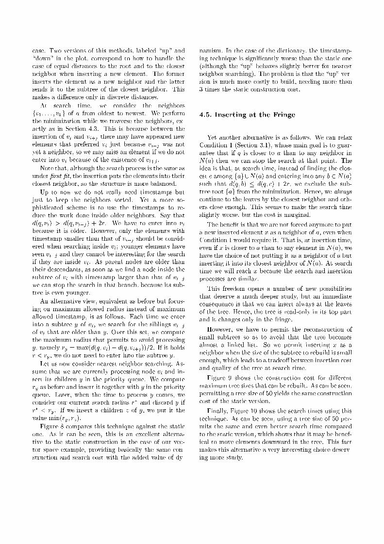
4.5. Inserting at the Fringe

Yet another alternative is as follows. We can relaxCondition 1 (Section 3.1), whose main goal is to guar-antee that if q is closer to a than to any neighbor inN(a) then we can stop the search at that point. Theidea is that, at search time, instead of �nding the clos-est c among fag[N(a) and entering into any b 2 N(a)such that d(q; b) � d(q; c) + 2r, we exclude the sub-tree root fag from the minimization. Hence, we alwayscontinue to the leaves by the closest neighbor and oth-ers close enough. This seems to make the search timeslightly worse, but the cost is marginal.

The bene�t is that we are not forced anymore to puta new inserted element x as a neighbor of a, even whenCondition 1 would require it. That is, at insertion time,even if x is closer to a than to any element in N(a), wehave the choice of not putting it as a neighbor of a butinserting it into its closest neighbor of N(a). At searchtime we will reach x because the search and insertionprocesses are similar.

This freedom opens a number of new possibilitiesthat deserve a much deeper study, but an immediateconsequence is that we can insert always at the leavesof the tree. Hence, the tree is read-only in its top partand it changes only in the fringe.

However, we have to permit the reconstruction ofsmall subtrees so as to avoid that the tree becomesalmost a linked list. So we permit inserting x as aneighbor when the size of the subtree to rebuild is smallenough, which leads to a tradeo� between insertion costand quality of the tree at search time.

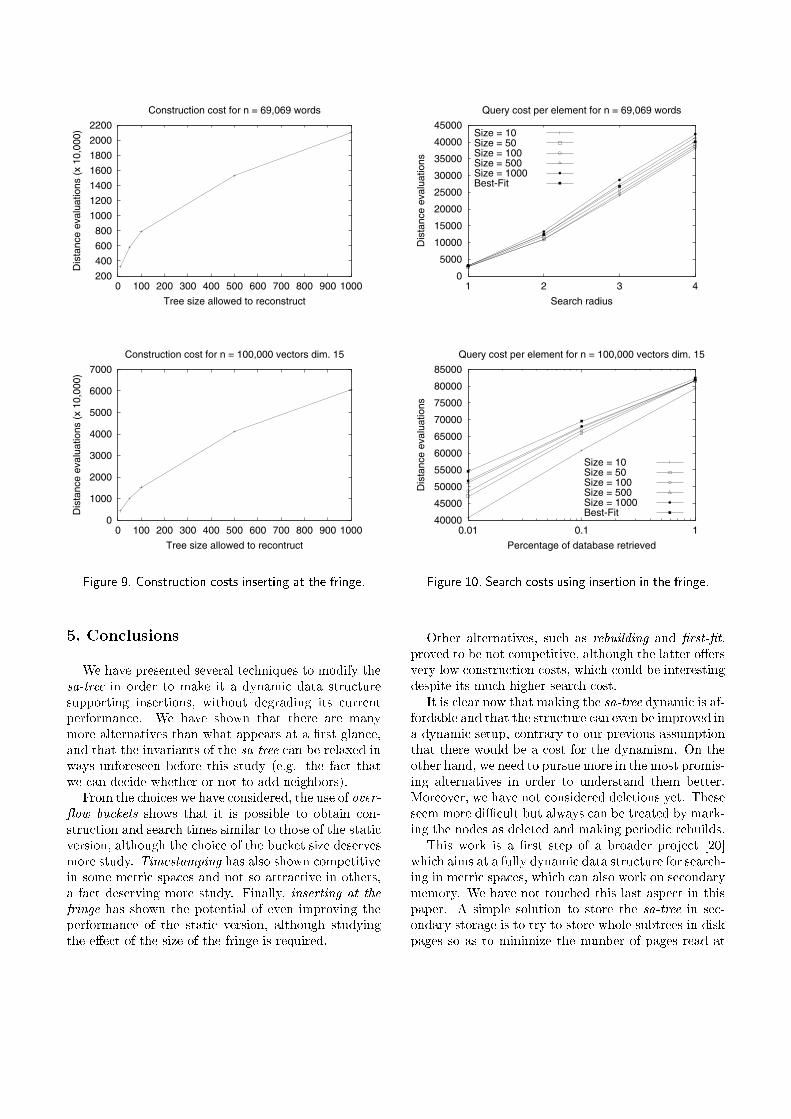
Figure 9 shows the construction cost for di�erentmaximum tree sizes that can be rebuilt. As can be seen,permitting a tree size of 50 yields the same constructioncost of the static version.

Finally, Figure 10 shows the search times using thistechnique. As can be seen, using a tree size of 50 per-mits the same and even better search time comparedto the static version, which shows that it may be benef-ical to move elements downward in the tree. This factmakes this alternative a very interesting choice deserv-ing more study.

200

400

600

800

1000

1200

1400

1600

1800

2000

2200

0 100 200 300 400 500 600 700 800 900 1000

Dis

tanc

e ev

alua

tions

(x

10,0

00)

Tree size allowed to reconstruct


0

1000

2000

3000

4000

5000

6000

7000

0 100 200 300 400 500 600 700 800 900 1000

Dis

tanc

e ev

alua

tions

(x

10,0

00)

Tree size allowed to recontruct


Figure 9. Construction costs inserting at the fringe.

5. Conclusions

We have presented several techniques to modify thesa-tree in order to make it a dynamic data structuresupporting insertions, without degrading its currentperformance. We have shown that there are manymore alternatives than what appears at a �rst glance,and that the invariants of the sa-tree can be relaxed inways unforeseen before this study (e.g. the fact thatwe can decide whether or not to add neighbors).

From the choices we have considered, the use of over- ow buckets shows that it is possible to obtain con-struction and search times similar to those of the staticversion, although the choice of the bucket size deservesmore study. Timestamping has also shown competitivein some metric spaces and not so attractive in others,a fact deserving more study. Finally, inserting at thefringe has shown the potential of even improving theperformance of the static version, although studyingthe e�ect of the size of the fringe is required.

0

5000

10000

15000

20000

25000

30000

35000

40000

45000

1 2 3 4

Dis

tanc

e ev

alua

tions

Search radius


Size = 10Size = 50Size = 100Size = 500Size = 1000Best-Fit

40000

45000

50000

55000

60000

65000

70000

75000

80000

85000

0.01 0.1 1

Dis

tanc

e ev

alua

tions



Size = 10Size = 50Size = 100Size = 500Size = 1000Best-Fit

Figure 10. Search costs using insertion in the fringe.

Other alternatives, such as rebuilding and �rst-�t,proved to be not competitive, although the latter o�ersvery low construction costs, which could be interestingdespite its much higher search cost.

It is clear now that making the sa-tree dynamic is af-fordable and that the structure can even be improved ina dynamic setup, contrary to our previous assumptionthat there would be a cost for the dynamism. On theother hand, we need to pursue more in the most promis-ing alternatives in order to understand them better.Moreover, we have not considered deletions yet. Theseseem more diÆcult but always can be treated by mark-ing the nodes as deleted and making periodic rebuilds.

This work is a �rst step of a broader project [20]which aims at a fully dynamic data structure for search-ing in metric spaces, which can also work on secondarymemory. We have not touched this last aspect in thispaper. A simple solution to store the sa-tree in sec-ondary storage is to try to store whole subtrees in diskpages so as to minimize the number of pages read at

search time. This has an interesting relationship withinserting at the fringe (Section 4.5), not only becausethe top part of the tree is read-only, but also becausewe can control the maximum arity of the tree so as tomake the neighbors �t in a disk page.

References

[1] R. Baeza-Yates and P. Larson. Performance of B+-trees with Partial Expansions. IEEE Transactions onKnowledge and Data Engineering, 1(2):248{257, 1989.

[2] J. Bentley. Multidimensional binary search trees indatabase applications. IEEE Transactions on SoftwareEngineering, 5(4):333{340, 1979.

[3] W. Burkhard and R. Keller. Some approaches to best-match �le searching. Communications of the ACM,16(4):230{236, 1973.

[4] T. Bozkaya and M. Ozsoyoglu. Distance-based index-ing for high-dimensional metric spaces. In Proc. ACMConference on Management of Data (SIGMOD'97),pages 357{368, 1997. Sigmod Record 26(2).

[5] S. Brin. Near neighbor search in large metric spaces. InProc. of the 21st Conference on Very Large Databases(VLDB'95), pages 574{584, 1995.

[6] R. Baeza-Yates, W. Cunto, U. Manber, and S. Wu.Proximity matching using �xed-queries trees. In Proc.5th Conference on Combinatorial Pattern Matching(CPM'94), LNCS 807, pages 198{212, 1994.

[7] E. Ch�avez, J. Marroqu��n, and R. Baeza-Yates.Spaghettis: an array based algorithm for similarityqueries in metric spaces. In Proc. 6th InternationalSymposium on String Processing and Information Re-trieval (SPIRE'99), pages 38{46. IEEE CS Press,1999.

[8] E. Ch�avez, J. Marroqu��n, and G. Navarro. Fixedqueries array: A fast and economical data structurefor proximity searching. Multimedia Tools and Appli-cations, 14(2):113{135, 2001. Kluwer.

[9] E. Ch�avez and G. Navarro. An e�ective clustering al-gorithm to index high dimensional metric spaces. InProc. 7th International Symposium on String Process-ing and Information Retrieval (SPIRE'00), pages 75{86. IEEE CS Press, 2000.

[10] E. Ch�avez, G. Navarro, R. Baeza-Yates, and J. Mar-roqu��n. Searching in metric spaces. ACM ComputingSurveys, 2001. To appear.

[11] P. Ciaccia, M. Patella, and P. Zezula. M-tree: aneÆcient access method for similarity search in metricspaces. In Proc. of the 23rd Conference on Very LargeDatabases (VLDB'97), pages 426{435, 1997.

[12] F. Dehne and H. Nolteimer. Voronoi trees and clus-tering problems. Information Systems, 12(2):171{175,1987. Pergamon Journals.

[13] A. Guttman. R-trees: a dynamic index structure forspatial searching. In Proc. ACM Conference on Man-agement of Data (SIGMOD'84), pages 47{57, 1984.

[14] L. Mic�o, J. Oncina, and R. Carrasco. A fast branchand bound nearest neighbor classi�er in metric spaces.Pattern Recognition Letters, 17:731{739, 1996. Else-vier.

[15] L. Mic�o, J. Oncina, and E. Vidal. A new version ofthe nearest-neighbor approximating and eliminatingsearch (aesa) with linear preprocessing-time and mem-ory requirements. Pattern Recognition Letters, 15:9{17, 1994. Elsevier.

[16] G. Navarro. Searching in metric spaces by spatialapproximation. In Proc. 6th International Sympo-sium on String Processing and Information Retrieval(SPIRE'99), pages 141{148. IEEE CS Press, 1999.

[17] G. Navarro. Searching in metric spaces by spatialapproximation. Technical Report TR/DCC-2001-4,Dept. of Computer Science, Univ. of Chile, 2001.ftp://ftp.dcc.uchile.cl/pub/users/gnavarro/

jsat.ps.gz.[18] S. Nene and S. Nayar. A simple algorithm for nearest

neighbor search in high dimensions. IEEE Transac-tions on Pattern Analysis and Machine Intelligence,19(9):989{1003, 1997.

[19] H. Nolteimer, K. Verbarg, and C. Zirkelbach.Monotonous Bisector� Trees { a tool for eÆcient par-titioning of complex schenes of geometric objects. InData Structures and EÆcient Algorithms, LNCS 594,pages 186{203, 1992.

[20] N. Reyes. Dynamic data structures for searching met-ric spaces. MSc. Thesis, Univ. Nac. de San Luis, Ar-gentina, 2001. In progress. G. Navarro, advisor.

[21] J. Uhlmann. Implementing metric trees to satisfy gen-eral proximity/similarity queries. Manuscript, 1991.

[22] J. Uhlmann. Satisfying general proximity/similarityqueries with metric trees. Information Processing Let-ters, 40:175{179, 1991. Elsevier.

[23] E. Vidal. An algorithm for �nding nearest neighborsin (approximately) constant average time. PatternRecognition Letters, 4:145{157, 1986.

[24] P. Yianilos. Data structures and algorithms for near-est neighbor search in general metric spaces. In Proc.4th ACM-SIAM Symposium on Discrete Algorithms(SODA'93), pages 311{321, 1993.

[25] P. Yianilos. Locally lifting the curse of dimensionalityfor nearest neighbor search. In Proc. 11th ACM-SIAMSymposium on Discrete Algorithms (SODA'00), 2000.

Documents

Fully Dynamic Spatial Approximation Trees