Isotonic Classification Trees

Remon van de Kamp, Ad Feelders, and Nicola Barile

Utrecht University, Department of Information and Computing Sciences,P.O. Box 80089, 3508TB Utrecht, The Netherlands,

{rpkamp,ad,barile}@cs.uu.nl

Abstract. We propose a new algorithm for learning isotonic classifica-tion trees. It relabels non-monotone leaf nodes by performing the isotonicregression on the collection of leaf nodes. In case two leaf nodes with acommon parent have the same class after relabeling, the tree is prunedin the parent node. Since we consider problems with ordered class labels,all results are evaluated on the basis of L1 prediction error. We experi-mentally compare the performance of the new algorithm with standardclassification trees.

1 Introduction

In many applications of data analysis it is reasonable to assume that the responsevariable is increasing (or decreasing) in one or more of the attributes or features.For example, the sale price of a house - all else equal - increases with lot size,and according to economists people tend to buy less of a product if its priceincreases. Such relations between response and attribute are called monotone.Monotonicity constraints can, for example, also be found in medicine [20, 6]and law [12]. Besides being plausible, monotonicity may also be a desirableproperty of a decision model for reasons of explanation, justification and fairness.Pazzani et al.[17], show that rules learned with monotonicity constraints weresignificantly more acceptable to medical experts than rules learned without themonotonicity restrictions.

Because the monotonicity constraint is quite common in practice, many dataanalysis techniques have been adapted to be able to handle such constraints.In this paper we present a new algorithm, called ICT, for learning monotoneclassification trees for problems with ordered class labels. Our approach differsfrom earlier monotone tree algorithms such as [5, 18, 11] in that we adjust theprobability estimates in the leaf nodes in case of a violation. This is done insuch a way that, subject to the monotonicity constraint, the sum of absoluteprediction errors on the training sample is minimized. Another new element ofour algorithm is that we can also handle problems where some, but not all,attributes have a monotone relation with the response. The performance of thenew algorithm is evaluated through experimental studies on real life data sets.

This paper is organized as follows. In the next section we introduce thebasic concepts and notation that will be used throughout the paper. Since theisotonic regression is an important technique for our algorithm, we discuss it

shortly in section 3. In section 4 we discuss the main contribution of this paper,the Isotonic Classification Tree (ICT) algorithm. ICT is evaluated in section 5where we present the results of experiments on real data. Section 6 concludes.

2 Preliminaries

Let X be a feature space X = X1 × X2 × . . . × Xp consisting of vectors x =(x1, x2, . . . , xp) of values on p features or attributes. We assume that each fea-ture takes values xi in a linearly ordered set Xi. The partial ordering � onX will be the ordering induced by the order relations of its coordinates Xi:x = (x1, x2, . . . , xp) � x′ = (x′1, x

′2, . . . , x

′p) if and only if xi ≤ x′i for all i.

Furthermore, let Y be a finite linearly ordered set of classes. Without loss ofgenerality, we assume that Y = {1, 2, . . . , k} where k is the number of classes.

A monotone classification rule is a function c : X → Y for which

x � x′ ⇒ c(x) ≤ c(x′) (1)

for all instances x,x′ ∈ X . A data set {xi, yi}ni=1 is monotone if for all i, j we

have xi � xj ⇒ yi ≤ yj .The classification rules we consider are univariate binary classification trees.

For such trees, at each node a split is made using a test of the form Xi < d forsome d ∈ Xi, 1 ≤ i ≤ p. Thus, for a binary tree, in each node the associated sett ⊂ X is split into the two subsets t` = {x ∈ t : xi < d} and tr = {x ∈ t : xi ≥ d}.The classification rule that is induced by a decision tree T will be denoted bycT .

For any node or leaf t of T , the subset of the instance space correspondingto that node can be written

t = {x ∈ X : a � x ≺ b} = [a,b) (2)

for some a,b ∈ X with a � b. Here X denotes the extension of X with infinity-elements −∞ and ∞. In some cases we need the infinity elements so we canspecify a node as in equation (2).

Below we will call min(t) = a the minimal element and max(t) = b themaximal element of t. Together, we call these the corner elements of node t. Ifmin(t) ≺ max(t′) then node t contains points that are smaller than some pointsin node t′, hence the monotonicity constraint requires that the label assigned tonode t should not be bigger than the label assigned to node t′. Therefore, wecall a pair of leaves t, t′ non-monotone if min(t) ≺ max(t′) and cT (t) > cT (t′)[19]. A tree is non-monotone if it contains at least one non-monotone leaf pair.

It is customary to evaluate a classifier on the basis of its error-rate or 0/1 loss.For classification problems with ordered class labels this choice is less obvious.It makes sense to incur a higher cost for those misclassifications that are “far”from the true label, than to those that are “close”. One loss function that hasthis property is L1 loss:

L1(i, j) = |i− j| i, j = 1, . . . , k (3)

where i is the true label, and j the predicted label. We note that this is not theonly possible choice. One could also choose L2 loss for example, or another lossfunction that has the desired property that misclassifications that are far fromthe true label incur a higher loss. Nevertheless, L1 loss is a reasonable candidate,and in this paper we confine our attention to this loss function.

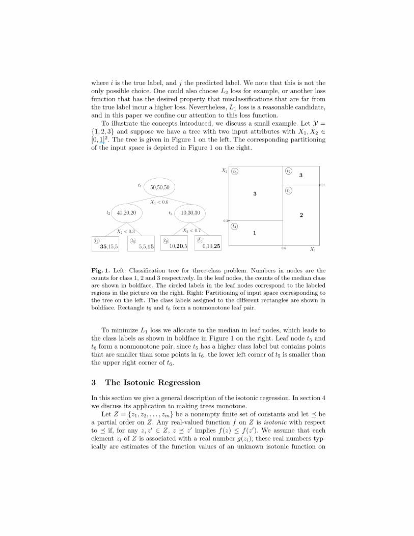
To illustrate the concepts introduced, we discuss a small example. Let Y ={1, 2, 3} and suppose we have a tree with two input attributes with X1, X2 ∈[0, 1]2. The tree is given in Figure 1 on the left. The corresponding partitioningof the input space is depicted in Figure 1 on the right.

50,50,50

40,20,20 10,30,30

35,15,5 5,5,15 10,20,5 0,10,25

X1 < 0.6

X2 < 0.3 X2 < 0.7

t1

t2 t3

t4 t5 t6 t7

X1

X2

0.6

0.3

0.7

1

3

2

3

t4

t5

t6

t7

Fig. 1. Left: Classification tree for three-class problem. Numbers in nodes are thecounts for class 1, 2 and 3 respectively. In the leaf nodes, the counts of the median classare shown in boldface. The circled labels in the leaf nodes correspond to the labeledregions in the picture on the right. Right: Partitioning of input space corresponding tothe tree on the left. The class labels assigned to the different rectangles are shown inboldface. Rectangle t5 and t6 form a nonmonotone leaf pair.

To minimize L1 loss we allocate to the median in leaf nodes, which leads tothe class labels as shown in boldface in Figure 1 on the right. Leaf node t5 andt6 form a nonmonotone pair, since t5 has a higher class label but contains pointsthat are smaller than some points in t6: the lower left corner of t5 is smaller thanthe upper right corner of t6.

3 The Isotonic Regression

In this section we give a general description of the isotonic regression. In section 4we discuss its application to making trees monotone.

Let Z = {z1, z2, . . . , zm} be a nonempty finite set of constants and let � bea partial order on Z. Any real-valued function f on Z is isotonic with respectto � if, for any z, z′ ∈ Z, z � z′ implies f(z) ≤ f(z′). We assume that eachelement zi of Z is associated with a real number g(zi); these real numbers typ-ically are estimates of the function values of an unknown isotonic function on

Z. Furthermore, each element of Z has associated a positive weight w(zi) thattypically indicates the precision of this estimate. An isotonic function g∗ on Znow is an isotonic regression of g with respect to the weight function w and thepartial order � if and only if it minimizes the sum

m∑i=1

w(zi) [f(zi)− g(zi)]2 (4)

in the class of isotonic functions f on Z. Brunk [8] proved the existence of aunique g∗.

Any real-valued function f on Z is antitonic with respect to � if, for anyz, z′ ∈ Z, z � z′ implies f(z) ≥ f(z′). The antitonic regression of g is definedcompletely analogous to the isotonic regression as the function that minimizes(4) within the class of antitonic functions. The isotonic regression with respectto a partial order is equivalent to the antitonic regression with respect to theinverse of that order.

The best time complexity known for an exact solution to the isotonic regres-sion problem for arbitrary partial order is O(m4) [16]. It is based on a divide-and-conquer strategy that involves solving at most m maximal flow problems.

4 Isotonic Classification Trees

The ICT algorithm can in principle be combined with any standard classifica-tion tree algorithm. Here we modify a cart-like algorithm [7] to incorporate themonotonicity constraints. The main principle of ICT is that it makes trees mono-tone by relabeling its leaf nodes. This is done in such a way that of all monotonetrees that can be obtained by relabeling the leaf nodes, the one produced by ICThas lowest absolute error on the training data. The relabeling is not computeddirectly, but is obtained by first adjusting the probability estimates in the leafnodes (using the isotonic regression), and then allocating each leaf node to the(smallest) median of its estimated class distribution.

We first discuss the growing of trees in ICT. Then we discuss the adjustmentof probability estimates in the leaf nodes, and the corresponding relabeling,which may lead to pruning the tree. We also discuss the incorporation of partialmonotonicity constraints in ICT.

4.1 Growing trees

Let T denote the collection of leaf nodes of tree T , n(t, j) denote the number ofobservations in t with class label j, and let

Pj(t) =n(t, j)n(t)

, t ∈ T

denote the relative frequency of class label j in node t. Furthermore, let

Fi(t) =∑j≤i

Pj(t), t ∈ T

denote the unconstrained maximum likelihood estimate of

Fi(t) = P (y ≤ i | x ∈ t), t ∈ T .

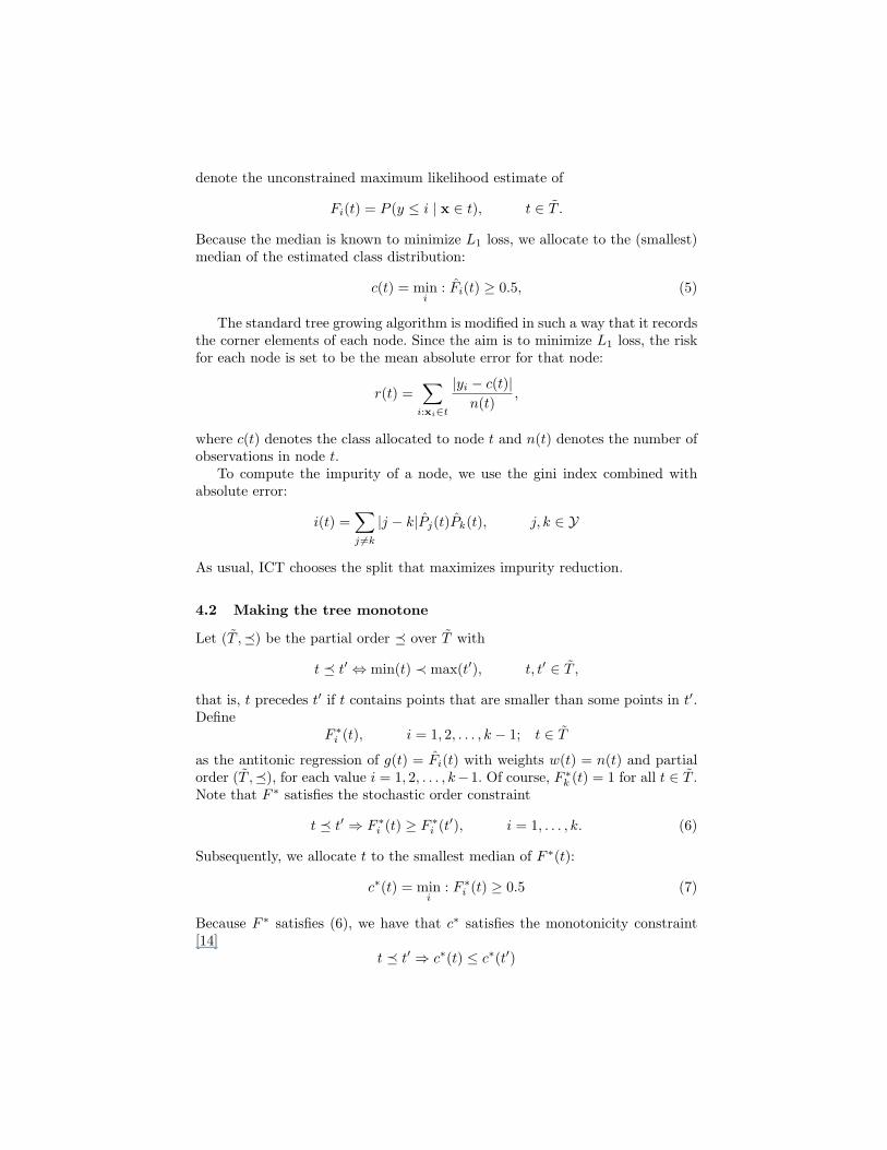
Because the median is known to minimize L1 loss, we allocate to the (smallest)median of the estimated class distribution:

c(t) = mini

: Fi(t) ≥ 0.5, (5)

The standard tree growing algorithm is modified in such a way that it recordsthe corner elements of each node. Since the aim is to minimize L1 loss, the riskfor each node is set to be the mean absolute error for that node:

r(t) =∑

i:xi∈t

|yi − c(t)|n(t)

,

where c(t) denotes the class allocated to node t and n(t) denotes the number ofobservations in node t.

To compute the impurity of a node, we use the gini index combined withabsolute error:

i(t) =∑j 6=k

|j − k|Pj(t)Pk(t), j, k ∈ Y

As usual, ICT chooses the split that maximizes impurity reduction.

4.2 Making the tree monotone

Let (T ,�) be the partial order � over T with

t � t′ ⇔ min(t) ≺ max(t′), t, t′ ∈ T ,

that is, t precedes t′ if t contains points that are smaller than some points in t′.Define

F ∗i (t), i = 1, 2, . . . , k − 1; t ∈ T

as the antitonic regression of g(t) = Fi(t) with weights w(t) = n(t) and partialorder (T ,�), for each value i = 1, 2, . . . , k−1. Of course, F ∗

k (t) = 1 for all t ∈ T .Note that F ∗ satisfies the stochastic order constraint

t � t′ ⇒ F ∗i (t) ≥ F ∗

i (t′), i = 1, . . . , k. (6)

Subsequently, we allocate t to the smallest median of F ∗(t):

c∗(t) = mini

: F ∗i (t) ≥ 0.5 (7)

Because F ∗ satisfies (6), we have that c∗ satisfies the monotonicity constraint[14]

t � t′ ⇒ c∗(t) ≤ c∗(t′)

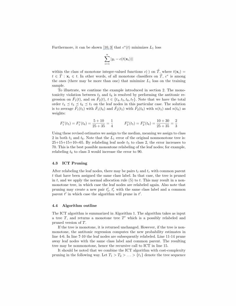
Furthermore, it can be shown [10, 3] that c∗(t) minimizes L1 loss

n∑i=1

|yi − c(t(xi))|

within the class of monotone integer-valued functions c(·) on T , where t(xi) =t ∈ T : xi ∈ t. In other words, of all monotone classifiers on T , c∗ is amongthe ones (there may be more than one) that minimize L1 loss on the trainingsample.

To illustrate, we continue the example introduced in section 2. The mono-tonicity violation between t5 and t6 is resolved by performing the antitonic re-gression on F1(t), and on F2(t), t ∈ {t4, t5, t6, t7}. Note that we have the totalorder t4 � t5 � t6 � t7 on the leaf nodes in this particular case. The solutionis to average F1(t5) with F1(t6) and F2(t5) with F2(t6) with n(t5) and n(t6) asweights:

F ∗1 (t5) = F ∗

1 (t6) =5 + 1025 + 35

=14

F ∗2 (t5) = F ∗

2 (t6) =10 + 3025 + 35

=23

Using these revised estimates we assign to the median, meaning we assign to class2 in both t5 and t6. Note that the L1 error of the original nonmonotone tree is:25+15+15+10=65. By relabeling leaf node t5 to class 2, the error increases to70. This is the best possible monontone relabeling of the leaf nodes; for example,relabeling t6 to class 3 would increase the error to 90.

4.3 ICT Pruning

After relabeling the leaf nodes, there may be pairs t` and tr with common parentt that have been assigned the same class label. In that case, the tree is prunedin t, and we apply the normal allocation rule (5) to t. This may result in a non-monotone tree, in which case the leaf nodes are relabeled again. Also note thatpruning may create a new pair t′`, t′r with the same class label and a commonparent t′ in which case the algorithm will prune in t′.

4.4 Algorithm outline

The ICT algorithm is summarized in Algorithm 1. The algorithm takes as inputa tree T , and returns a monotone tree T ′ which is a possibly relabeled andpruned version of T .

If the tree is monotone, it is returned unchanged. However, if the tree is non-monotone, the antitonic regression computes the new probability estimates inline 4-6. In line 7-10 the leaf nodes are subsequently relabeled. Line 11-14 pruneaway leaf nodes with the same class label and common parent. The resultingtree may be nonmonotone, hence the recursive call to ICT in line 15.

It should be noted that we combine the ICT algorithm with cost-complexitypruning in the following way. Let T1 > T2 > . . . > {t1} denote the tree sequence

Algorithm 1 ICT(T )1: if T is monotone then2: return T3: else4: for i ∈ {1, . . . , k − 1} do5: F ∗

i ← AntitonicRegression(T ,�,n(t) : t ∈ T ,Fi(t) : t ∈ T )6: end for7: for all t ∈ T do8: F ∗

k (t)← 19: cT (t)← mini F ∗

i (t) ≥ 0.510: end for11: while there are t`, tr ∈ T with common parent t and cT (t`) = cT (tr) do12: T ← prune T in t13: cT (t)← mini Fi(t) ≥ 0.514: end while15: T ′ ← ICT(T )16: return T ′

17: end if

produced by standard cost-complexity pruning, where t1 denotes the root nodeof the tree, and Tj > Tk means Tk is obtained by pruning Tj in one or morenodes. We apply ICT pruning to every tree in this sequence (except the rootof course) to obtain a sequence of monotone trees T ′

1 > T ′2 > . . . > {t1}. This

sequence may be shorter than the original sequence, since sometimes two treesfrom the original cost-complexity sequence are pruned back to the same tree byICT.

4.5 Partial monotonicity

In many applications there will be attributes for which there is no reason toassume that they have a monotone relation with the class label. Therefore weextended the ICT algorithm to be able to handle such cases.

The ICT algorithm for partial monotonicity is largely the same as it is forcomplete monotonicity. We just need to change the partial order used in theantitonic regression and the check that determines if two leafs are non-monotone.

First we define a partially monotone classification rule. Let X be defined asbefore, and let Z = ×Zi, i = 1, . . . , q. The values Zi may be either ordered orunordered. A classification rule c : X × Z → Y is monotone in X iff

∀x,x′ ∈ X ,∀z ∈ Z : x � x′ ⇒ c(x, z) ≤ c(x′, z)

Our orginal ordering on T was defined in such a way that t � t′ if node tcontained elements that were smaller than some elements of t′. This was the casewhen min(t) ≺ max(t′). Now we have to add the constraint that t and t′ shouldhave overlapping values on Z. Hence, we define a new partial order (T ,�) witht ⊂ X ×Z as follows:

t � t′ ⇔ min(tX) ≺ max(t′X) ∧ tZ ∩ t′Z 6= ∅, t, t′ ∈ T .

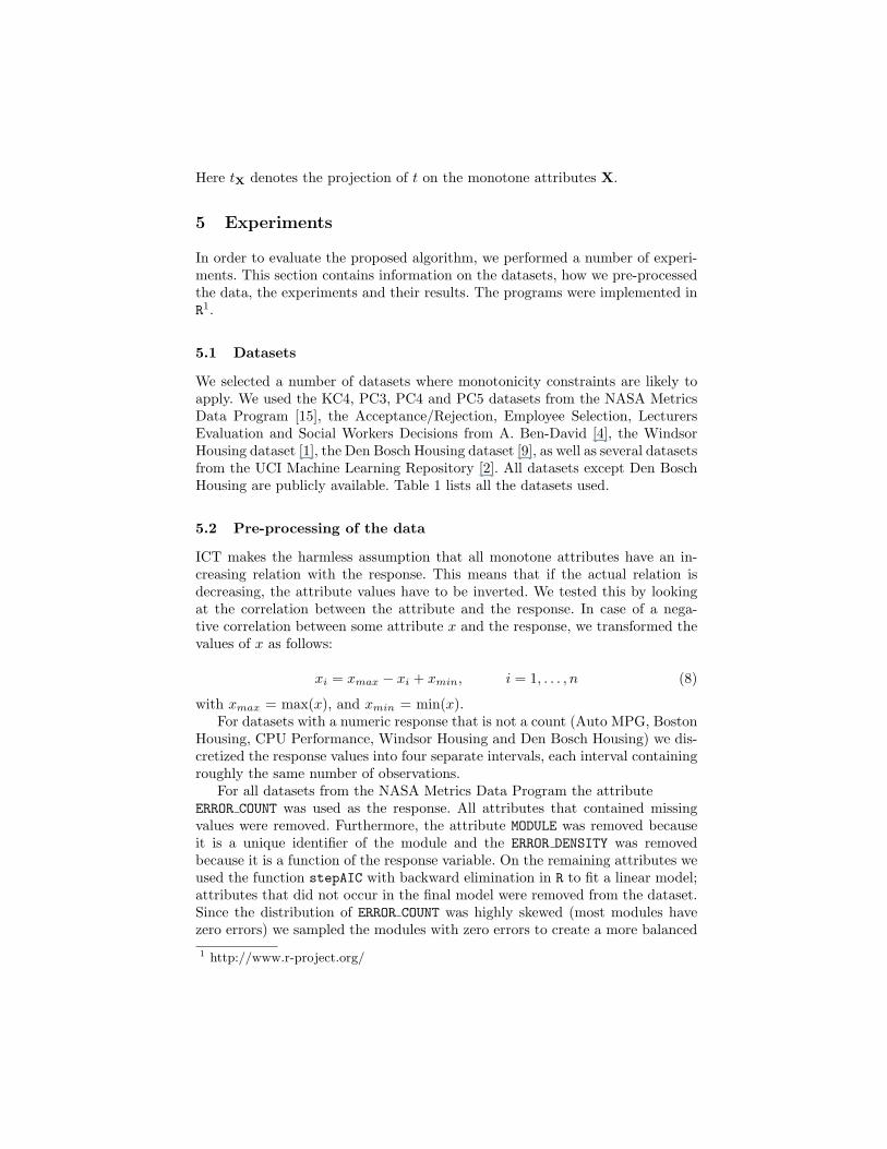
Here tX denotes the projection of t on the monotone attributes X.

5 Experiments

In order to evaluate the proposed algorithm, we performed a number of experi-ments. This section contains information on the datasets, how we pre-processedthe data, the experiments and their results. The programs were implemented inR1.

5.1 Datasets

We selected a number of datasets where monotonicity constraints are likely toapply. We used the KC4, PC3, PC4 and PC5 datasets from the NASA MetricsData Program [15], the Acceptance/Rejection, Employee Selection, LecturersEvaluation and Social Workers Decisions from A. Ben-David [4], the WindsorHousing dataset [1], the Den Bosch Housing dataset [9], as well as several datasetsfrom the UCI Machine Learning Repository [2]. All datasets except Den BoschHousing are publicly available. Table 1 lists all the datasets used.

5.2 Pre-processing of the data

ICT makes the harmless assumption that all monotone attributes have an in-creasing relation with the response. This means that if the actual relation isdecreasing, the attribute values have to be inverted. We tested this by lookingat the correlation between the attribute and the response. In case of a nega-tive correlation between some attribute x and the response, we transformed thevalues of x as follows:

xi = xmax − xi + xmin, i = 1, . . . , n (8)

with xmax = max(x), and xmin = min(x).For datasets with a numeric response that is not a count (Auto MPG, Boston

Housing, CPU Performance, Windsor Housing and Den Bosch Housing) we dis-cretized the response values into four separate intervals, each interval containingroughly the same number of observations.

For all datasets from the NASA Metrics Data Program the attributeERROR COUNT was used as the response. All attributes that contained missingvalues were removed. Furthermore, the attribute MODULE was removed becauseit is a unique identifier of the module and the ERROR DENSITY was removedbecause it is a function of the response variable. On the remaining attributes weused the function stepAIC with backward elimination in R to fit a linear model;attributes that did not occur in the final model were removed from the dataset.Since the distribution of ERROR COUNT was highly skewed (most modules havezero errors) we sampled the modules with zero errors to create a more balanced1 http://www.r-project.org/

distribution. High error counts are less frequent than low error counts. In orderto increase frequencies, the higher counts were merged into a single class. Forexample, for KC4, all class labels greater than five were set to five.

For the CPU Performance dataset the machine cycle time in nanosecondswas converted to clock speed in Khz, in order to make it positively correlatedwith the class label. From this dataset the attributes Vendor Name, Model Nameand ERP were removed.

From the Den Bosch Housing dataset the independent attributes year,x-coordinate and y-coordinate were removed.

5.3 Relabeling toward monotonicity

Besides enforcing a monotone model, one can also use prior knowledge aboutmonotonicity by relabeling the dataset to make it monotone. As shown in [22,13], models learned on relabeled datasets on average perform better than modelslearned with the original class labels.

Therefore, we also tested ICT on relabeled versions of the original datasets.We computed y∗ as the relabeling of the observations that minimizes

ntrain∑i=1

|yi − y′i|

within the class of monotone relabelings y′. Here ntrain denotes the numberof observations in the training sample. The test data was not relabeled in theexperiments.

Table 1 summarizes for all datasets the cardinality, the number of attributesafter pre-processing, the number of distinct class labels and the L1 distancebetween y and y∗. For example, to make the Australian Credit data monotonewe have to relabel for a total absolute error of 14. Since Australian Credit has abinary class label, this means that 14 observations have to be relabeled.

5.4 Experimental results

Each of the datasets was randomly divided one hundred times into a trainingset consisting of four fifth of the data and a test set consisting of the remainingone fifth of the data. On every training set a tree was grown, after which costcomplexity pruning was applied to obtain a sequence of trees. The ICT algorithmwas applied to each tree in this sequence to obtain a sequence of monotone trees.Subsequently, the test set was used to select the best tree from the originalsequence and to select the best tree from the monotone sequence. The test errorsof the best standard trees and the best monotone trees were averaged over theone hundred repititions of the experiment.

Table 2 shows the results of the experiments on all datasets. The errors areindicated as the mean absolute error on the test sample. For each column themean error and the standard deviation of this mean error are indicated, separated

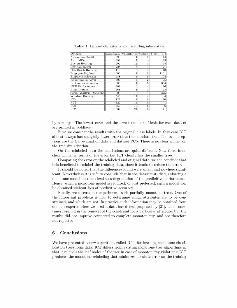
Table 1. Dataset charasterics and relabeling information

Dataset cardinality #attributes #labelsP

|yi − y∗i |Australian Credit 690 14 2 14Auto MPG 392 7 4 23Boston Housing 506 13 4 28Car Evaluation 1728 6 4 21Den Bosch Housing 119 8 4 10Empoyee Rej/Acc 1000 4 9 1161Employee selection 488 4 9 104Haberman survival 306 3 2 55Lecturers evaluation 1000 4 5 364CPU Performance 209 6 4 26Pima Indians 768 8 2 53Social Workers Decisions 1000 10 4 375Windsor Housing 546 11 4 134KC4 122 4 6 80PC3 320 15 5 1PC4 356 16 6 6PC5 1032 21 6 141

by a ± sign. The lowest error and the lowest number of leafs for each datasetare printed in boldface.

First we consider the results with the original class labels. In that case ICTalmost always has a slightly lower error than the standard tree. The two excep-tions are the Car evaluation data and dataset PC5. There is no clear winner onthe tree size criterion.

On the relabeled data the conclusions are quite different. Now there is noclear winner in terms of the error but ICT clearly has the smaller trees.

Comparing the error on the relabeled and original data, we can conclude thatit is beneficial to relabel the training data, since it tends to reduce the error.

It should be noted that the differences found were small, and nowhere signif-icant. Nevertheless it is safe to conclude that in the datasets studied, enforcing amonotone model does not lead to a degradation of the predicitive performance.Hence, when a monotone model is required, or just preferred, such a model canbe obtained without loss of predicitive accuracy.

Finally, we discuss our experiments with partially monotone trees. One ofthe important problems is how to determine which attributes are to be con-strained, and which are not. In practice such information may be obtained fromdomain experts. Here we used a data-based test proposed by [21]. This some-times resulted in the removal of the constraint for a particular attribute, but theresults did not improve compared to complete monotonicity, and are thereforenot reported.

6 Conclusions

We have presented a new algorithm, called ICT, for learning monotone classi-fication trees from data. ICT differs from existing monotone tree algorithms inthat it relabels the leaf nodes of the tree in case of monotonicity violations: ICTproduces the monotone relabeling that minimizes absolute error on the training

Table 2. Results of monotone trees (ICT) and standard trees.

Dataset Label Error ICT Error Standard #Leafs ICT #Leafs StandardAustralian y 0.1426±0.0070 0.1431±0.0068 3.4300±1.9553 3.3500±2.2490Credit y∗ 0.1418±0.0078 0.1426±0.0071 3.3600±1.9515 3.5700±2.9241Auto MPG y 0.2982±0.0292 0.3045±0.0282 9.2800±2.7746 10.6300±5.3497

y∗ 0.2985±0.0295 0.2982±0.0293 10.1100±2.7484 12.3800±4.5964Boston y 0.3966±0.0370 0.4050±0.0376 8.3100±3.1065 7.7100±4.9222Housing y∗ 0.3861±0.0334 0.3935±0.0339 8.3200±2.7957 8.5700±5.2073Car y 0.0871±0.0181 0.0836±0.0164 27.6200±5.4417 32.4400±8.4271Evaluation y∗ 0.0897±0.0190 0.0849±0.0184 28.2300±5.3802 32.3100±7.8787Den Bosch y 0.4922±0.0832 0.5165±0.0852 5.5200±1.5274 5.6600±1.9396Housing y∗ 0.4755±0.0829 0.4856±0.0841 5.5100±1.4106 5.5500±1.6840Employee Rej/Acc y 1.2764±0.0407 1.2926±0.0415 10.3400±3.9778 8.2200±3.4629

y∗ 1.1773±0.0242 1.1627±0.0208 17.0600±2.2103 19.3900±1.1538Employee y 0.4348±0.0369 0.4590±0.0395 23.6900±4.3128 26.9500±8.4452Selection y∗ 0.3829±0.0265 0.3822±0.0304 23.9100±2.9063 27.6300±3.9457Haberman y 0.2585±0.0146 0.2605±0.0139 2.6000±2.1742 1.9900±1.6112Survival y∗ 0.2482±0.0164 0.2484±0.0164 3.8300±2.0003 4.3200±2.4980Lecturers y 0.4764±0.0267 0.4903±0.0267 19.9000±5.1981 19.9200±8.9563Evaluation y∗ 0.4151±0.0233 0.3832±0.0157 21.5300±3.5773 28.7900±3.1311CPU Performance y 0.4556±0.0540 0.4773±0.0554 8.3300±2.3401 9.2900±4.4818

y∗ 0.4323±0.0486 0.4324±0.0453 8.5900±1.9700 9.8800±2.7016Pima y 0.2586±0.0145 0.2619±0.0144 5.6300±3.1866 4.6700±3.1464Indians y∗ 0.2580±0.0130 0.2576±0.0117 4.3900±2.7299 4.5200±3.9936Social Workers y 0.4707±0.0209 0.4772±0.0181 9.3300±4.3579 7.6100±4.5436Decisions y∗ 0.4309±0.0163 0.4045±0.0137 12.6700±3.6350 27.4500±4.7298Windsor y 0.6244±0.0328 0.6619±0.0364 17.0100±5.1198 15.5400±12.8860Housing y∗ 0.5992±0.0333 0.6103±0.0377 18.7900±4.2433 24.9500±12.0566KC4 y 1.1871±0.1349 1.2358±0.1474 4.4300±2.2031 4.6300±3.2649

y∗ 1.0153±0.1298 1.0174±0.1349 4.8400±1.5681 5.0900±1.7529PC3 y 0.5357±0.0440 0.5363±0.0394 2.6000±1.3780 2.4900±1.5986

y∗ 0.5351±0.0443 0.5359±0.0399 2.6100±1.4695 2.4900±1.5986PC4 y 0.5735±0.0492 0.5835±0.0543 4.9500±2.9418 4.5100±3.0600

y∗ 0.5886±0.0617 0.5928±0.0632 5.4200±3.2167 5.1900±4.0394PC5 y 0.4960±0.0188 0.4948±0.0242 6.1600±4.1310 5.8400±4.5543

y∗ 0.4939±0.0189 0.4904±0.0229 6.1111±4.4006 6.8800±5.1410

sample. Furthermore, in contrast to existing monotone tree algorithms, ICT canalso be applied to partially monotone problems.

Our experiments have shown that ICT usually performed slightly better thanstandard trees on the original data. After relabeling, the performance of ICT andthe standard tree algorithm was virtually identical. It should be noted howeverthat a standard tree algorithm applied to monotone data does not necessarilyproduce a monotone tree. Therefore, if a monotone model is required, applicationof a standard algorithm to relabeled data may not be sufficient. Furthermore,on the relabeled data ICT on average produced smaller trees than the standardalgorithm. This warrants the conclusion that ICT trees are easier to understandthan their somewhat larger and possibly non-monotone counterparts.

References

1. P.M. Anglin and R. Gencay. Semiparametric estimation of a hedonic price function.Journal of Applied Econometrics, 11(6):633–648, 1996.

2. A. Asuncion and D.J. Newman. UCI machine learning repository, 2007.

3. N. Barile and A. Feelders. Nonparametric monotone classification with MOCA. InF. Giannotti, editor, Proceedings of the Eighth IEEE International Conference onData Mining (ICDM 2008), pages 731–736. IEEE Computer Society, 2008.

4. A. Ben-David, L. Sterling, and Y. Pao. Learning and classification of monotonicordinal concepts. Computational Intelligence, 5:45–49, 1989.

5. Arie Ben-David. Monotonicity maintenance in information-theoretic machinelearning algorithms. Machine Learning, 19:29–43, 1995.

6. D.A. Bloch and B.W. Silverman. Monotone discriminant functions and theirapplications in rheumatology. Journal of the American Statistical Association,92(437):144–153, 1997.

7. L. Breiman, J.H. Friedman, R.A. Olshen, and C.J. Stone. Classification And Re-gression Trees. Chapman and Hall, 1984.

8. H.D. Brunk. Conditional expectation given a σ-lattice and applications. Annalsof Mathematical Statistics, 36:1339–1350, 1965.

9. H.A.M. Daniels and B. Kamp. Application of MLP networks to bond rating andhouse pricing. Neural Computing & Applications, 8(3):226–234, 1999.

10. R. Dykstra, J. Hewett, and T. Robertson. Nonparametric, isotonic discriminantprocedures. Biometrika, 86(2):429–438, 1999.

11. A. Feelders and M. Pardoel. Pruning for monotone classification trees. In M.R.Berthold, H-J. Lenz, E. Bradley, R. Kruse, and C. Borgelt, editors, Advances inIntelligent Data Analysis V, volume 2810 of LNCS, pages 1–12. Springer, 2003.

12. J. Karpf. Inductive modelling in law: example based expert systems in admin-istrative law. In Proceedings of the third international conference on artificialintelligence in law, pages 297–306. ACM Press, 1991.

13. W. Kotlowski and R. Slowinski. Statistical approach to ordinal classification withmonotonicity constraints. In ECML PKDD 2008 Workshop on Preference Learn-ing, 2008.

14. S. Lievens, B. De Baets, and K. Cao-Van. A probabilistic framework for the designof instance-based supervised ranking algorithms in an ordinal setting. Annals ofOperations Research, 163:115–142, 2008.

15. J. Long. NASA metrics data program [http://mdp.ivv.nasa.gov/repository.html].2008.

16. W.L. Maxwell and J.A. Muckstadt. Establishing consistent and realistic reorder in-tervals in production-distribution systems. Operations Research, 33(6):1316–1341,1985.

17. M.J. Pazzani, S. Mani, and W.R. Shankle. Acceptance of rules generated bymachine learning among medical experts. Methods of Information in Medicine,40:380–385, 2001.

18. R. Potharst and J.C. Bioch. Decision trees for ordinal classification. IntelligentData Analysis, 4(2):97–112, 2000.

19. Rob Potharst. Classification using Decision Trees and Neural Nets. PhD thesis,Erasmus University Rotterdam, 1999.

20. P. Royston. A useful monotonic non-linear model with applications in medicineand epidemiology. Statistics in Medicine, 19(15):2053–2066, 2000.

21. M. Velikova. Monotone Models for Prediction in Data Mining. PhD thesis, TilburgUniversity, 2006.

22. M. Velikova and H. Daniels. Decision trees for monotone price models. Computa-tional Management Science, 1(3-4):231–244, 2004.