Remotely Sensed Image classification: Supervised classification algorithm

1

REMOTELY SENSED IMAGE CLASSIFICATION: SUPERVISED CLASSIFICATION ALGORITHM USING

ENVI 5.0 SOFTWARE

BY TAMARABRAKEMI AKOSO

([email protected])

UNIVERSITY OF LAGOS January, 2013.

ABSTRACT

This paper explores image classification of earth remotely sensed data. It gives an over view on the concept of image classification and the types. The scope of this paper is limited to the Supervised classification and how to develop a Training area. Thus, it focuses on some of the various supervised classification algorithm and their stochastic uniqueness in classification based on the digital numbers of the trained pixel. The paper ends with a practical on some supervised classification algorithm which shows variations classification outputs despites using the same training area. Finally, the paper seeks to explain those distinct classification algorithms are suitable for various interests of earth feature.

1.0 INTRODUCTION

Remote sensing, particularly space borne offers an immense source of data for studying spatial

and temporal variability of environmental parameters. Remotely sensed imagery can be made

use of in a number of applications, encompassing reconnaissance, creation of mapping products

for military and civil applications, evaluation of environmental damage, monitoring of land use,

radiation monitoring, urban planning, growth regulation, soil assessment, and crop yield

appraisal [James et al., 2002]. Generally, remote sensing offers imperative coverage, mapping

and classification of land-cover features, namely vegetation, soil, water and forests. A principal

application of remotely sensed data is to create a classification map of the identifiable or

meaningful features or classes of land cover types in a scene [Jasinski, 1996]. Therefore, the

principal product is a thematic map with themes like land use, geology and vegetation types.

Researches on image classification based remote sensing have long attracted the interest of the

remote sensing community since most environmental and socioeconomic applications are based

on the classification results [Weng, 2007].

2

Image classification in remote sensing belongs to a very active field in computing research, that

of pattern recognition. Image pixels can be classified either by their multivariable statistical

properties, such as the case of multi-spectral classification (clustering), or by segmentation based

on both statistics and spatial relationships with neighbouring pixels [Liu and Mason, 2009].

Several methods of image classification exist and a number of fields apart from remote sensing

like image analysis and pattern recognition make use of a significant concept, classification. In

some cases, the classification itself may form the entity of the analysis and serve as the ultimate

product. In other cases, the classification can serve only as an intermediate step in more intricate

analyses, such as land degradation studies, process studies, landscape modeling, coastal zone

management, resource management and other environment monitoring applications. As a result,

image classification has emerged as a significant tool for investigating digital images. Moreover,

the selection of the appropriate classification technique to be employed can have a considerable

upshot on the results of whether the classification is used as an ultimate product or as one of

numerous analytical procedures applied for deriving information from an image for additional

analyses [Reddy, 2008].

2.0 SUPERVISED CLASSIFICATION

Image classification in the field of remote sensing, is the process of assigning pixels or the basic

units of an image to classes. It is likely to assemble groups of identical pixels found in remotely

sensed data, into classes that match the informational categories of user interest by comparing

pixels to one another and to those of known identity [Weng, 2007]. Several methods of image

classification exist and a number of fields apart from remote sensing like image analysis and

pattern recognition make use of a significant concept, classification.

Supervised classification can be defined informally as the process of using samples of known

identity (i.e., pixels already assigned to informational classes) to classify pixels of unknown

identity (i.e., to assign unclassified pixels to one of several informational classes) [Campbell and

Wynne, 2011]. A supervised classification algorithm requires a training sample for each class,

that is, a collection of data points known to have come from the class of interest. The

classification is thus based on how "close" a point to be classified is to each training sample

3

[Reddy, 2008]. Such areas should typify spectral properties of the categories they represent and,

of course, must be homogeneous in respect to the informational category to be classified. That is,

training areas should not include unusual regions, nor should they straddle boundaries between

categories. Size, shape, and position must favor convenient identification both on the image and

on the ground. Pixels located within these areas form the training samples used to guide the

classification algorithm to assign specific spectral values to appropriate informational classes.

Hence, the selection of these training data is sine qua non in supervised classification.

Campbell and Wynne, 2011 adduce some benefits and limitations the image analyst faces when

performing a supervised classification.

2.1 Key benefits

The pros of supervised classification, relative to unsupervised classification are as follows;

• The image analyst has control of a selected menu of informational categories designed to

a specific purpose and geographic region. This quality may be highly pertinent if it

becomes imperative to generate a classification for the specific purpose of comparison

with another classification of the same area at a different date or if the classification must

be compatible with those of neighboring regions. Under such circumstances, the

unpredictable (i.e., with respect to number, identity, size, and pattern) qualities of

categories generated by unsupervised classification may be inconvenient or unsuitable.

• Supervised classification is tied to specific areas of known identity, determined through

the process of selecting training areas.

• The analyst using supervised classification is not faced with the problem of matching

spectral categories on the final map with the informational categories of interest (this task

has, in effect, been addressed during the process of selecting training data).

• The operator may be able to detect serious errors in classification by examining training

data to determine whether they have been correctly classified by the procedure—

inaccurate classification of training data indicates serious problems in the classification or

selection of training data, although correct classification of training data does not always

indicate correct classification of other data.

4

2.2 Key Limitations

The limiting factors of a supervised classification are enormous, they are as follows;

• The analyst, in effect, imposes a classification structure on the data (recall that

unsupervised classification searches for “natural” classes). These operator-defined classes

may not match the natural classes that exist within the data and therefore may not be

distinct or well defined in multidimensional data space.

• Training data are often defined primarily with reference to informational categories and

only secondarily with reference to spectral properties. A training area that is “100%

forest” may be accurate with respect to the “forest” designation but may still be very

diverse with respect to density, age, shadowing, and the like, and therefore form a poor

training area, mostly in medium resolution multispectral data set.

• Training data selected by the analyst may not be representative of conditions encountered

throughout the image. This may be true despite the best efforts of the analyst, especially

if the area to be classified is large, complex, or inaccessible.

• Conscientious selection of training data can be a time-consuming, expensive, and tedious

undertaking, even if ample resources are at hand. The analyst may experience problems

in matching prospective training areas as defined on maps and aerial photographs to the

image to be classified.

• Supervised classification may not be able to recognize and represent special or unique

categories not represented in the training data, possibly because they are not known to the

analyst or because they occupy very small areas on the image.

Having delved into the distinctiveness of a supervised classification, this paper seeks to expound

the knowledge of the most important quality of a supervised classification which is Selection of

Training data.

3.0 TRAINING DATASET

A training dataset is a set of measurements (points from an image) whose category membership

is known by the analyst. This set must be selected based on additional information derived from

maps, field surveys, aerial photographs, and analyst's knowledge of usual spectral signatures of

different cover classes. Selecting a good set of training points is one of the most critical aspects

5

of the classification procedure. However, an attempt is made to provide some guidelines based

on the Reddy, 2008 experience. These guidelines are as following:

• Select sufficient number of points for each class. If each measurement vector has N

features, then select N+1 points per class and the practical minimum is 10*N per class. If

the class shows a lot of variability (the scatter plot showing considerable spreading or

scatter among training points), select a larger number of points, subject to practical limits

of time, effort and expense. The more the training points, the better the "extra points" to

evaluate the accuracy of the classifier. The more the points, the more accurate the

classification will be.

• Select training data sets which are representative of the classes of interest that show both

typical average feature values and a typical degree of variability. For each class, select

several training areas on the image, instead of just one. Each training area should contain

a moderately large number of pixels.

• Pick training areas from seemingly heterogeneous or appearing regions.

• Pick training areas that are widely and spatially dispersed, across the full image. For each

class, select the training areas which are uniformly distributed across the image and with

high density.

• Check that selected areas have unimodel distributions (histograms). A bimodal histogram

suggests that pixels from two different classes may be included in the training sample.

• Select training sets (physically) using a computer-based classification system

3.1 Significance of Training Data

Scholz et al. (1979) and Hixson et al. (1980) discovered that selection of training data may be as

important as or even more important than choice of classification algorithm in determining

classification accuracies of agricultural areas in the central United States. They concluded that

differences in the selection of training data were more important influences on accuracy than

were differences among some five different classification procedures.

The results of their studies show little difference in the classification accuracies achieved by the

five classification algorithms that were considered, if the same training statistics were used.

However, in one part of the study, a classification algorithm given two alternative training

methods for the same data produced significantly different results. This finding suggests that the

6

choice of training method, at least in some instances, is as important as the choice of classifier.

Scholz et al. (1979) concluded that the most important aspect of training fields is that all cover

types in the scene must be adequately represented by a sufficient number of samples in each

spectral subclass.

Campbell (1981) examined the character of the training data as it influences accuracy of the

classification. His examples showed that adjacent pixels within training fields tended to have

similar values; as a result, the samples that compose each training field may not be independent

samples of the properties within a given category. Training samples collected in contiguous

blocks may tend to underestimate the variability within each class and to overestimate the

distinctness of categories. His examples also show that the degree of similarity varies between

land-cover categories, from band to band, and from date to date. If training samples are selected

randomly within classes, rather than as blocks of contiguous pixels, effects of high similarity are

minimized, and classification accuracies improve. Also, his results suggest that it is probably

better to use a large number of small training fields rather than a few large areas.

4.0 SPECIFIC METHODS FOR SUPERVISED CLASSIFICATION

A variety of different methods have been devised to implement the basic strategy of supervised

classification. All of them use information derived from the training data as a means of

classifying those pixels not assigned to training fields. The most common are highlight below;

4.1 Parallelepiped Classification

Parallelepiped classification, sometimes also known as box decision rule, or level-slice

procedures, are based on the ranges of values within the training data to define regions within a

multidimensional data space. The spectral values of unclassified pixels are projected into data

space; those that fall within the regions defined by the training data are assigned to the

appropriate categories.

As pixels of unknown identity are considered for classification, those that fall within these

regions are assigned to the category associated with each polygon, as derived from the training

data. The procedure can be extended to as many bands, or as many categories, as necessary. In

addition, the decision boundaries can be defined by the standard deviations of the values within

the training areas rather than by their ranges. This kind of strategy is useful because fewer pixels

7

will be placed in an “unclassified” category (a special problem for parallelepiped classification),

but it also increases the opportunity for classes to overlap in spectral data space [Campbell and

Wynne, 2011]

4.2 Minimum Distance Classification

This approach to classification uses the central values of the spectral data that form the training

data as a means of assigning pixels to informational categories. The spectral data from training

fields can be plotted in multidimensional data space in the same manner for unsupervised

classification. Values in several bands determine the positions of each pixel within the clusters

that are formed by training data for each category. These clusters may appear to be the same as

those defined earlier for unsupervised classification. However, in unsupervised classification,

these clusters of pixels were defined according to the “natural” structure of the data. Now, for

supervised classification, these groups are formed by values of pixels within the training fields

defined by the analyst.

Each cluster can be represented by its centroid, often defined as its mean value. As unassigned

pixels are considered for assignment to one of the several classes, the multidimensional distance

to each cluster centroid is calculated, and the pixel is then assigned to the closest cluster. Thus,

the classification proceeds by always using the “minimum distance” from a given pixel to a

cluster centroid defined by the training data as the spectral manifestation of an informational

class [Campbell and Wynne, 2011].

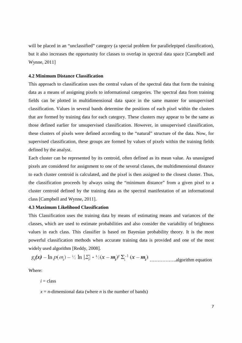
4.3 Maximum Likelihood Classification

This Classification uses the training data by means of estimating means and variances of the

classes, which are used to estimate probabilities and also consider the variability of brightness

values in each class. This classifier is based on Bayesian probability theory. It is the most

powerful classification methods when accurate training data is provided and one of the most

widely used algorithm [Reddy, 2008].

……………..algorithm equation

Where:

i = class

x = n-dimensional data (where n is the number of bands)

8

p(wi) = probability that class wi occurs in the image and is assumed the same for all classes

|Si| = determinant of the covariance matrix of the data in class wi

Si-1 = its inverse matrix

mi = mean vector

4.4 Mahalanobis Distance Classification

The Mahalanobis distance classification is a direction-sensitive distance classifier that uses

statistics for each class. It is similar to the maximum likelihood classification but assumes all

class covariances are equal and therefore is a faster method. All pixels are classified to the

closest training sample class unless you specify a distance threshold, in which case some pixels

may be unclassified if they do not meet the threshold [Liu and Mason, 2009].

4.5 Binary Encoding Classification

The binary encoding classification technique encodes the data and endmember spectra into zeros

and ones, based on whether a band falls below or above the spectrum mean, respectively. An

exclusive OR function compares each encoded reference spectrum with the encoded data spectra

and produces a classification image. All pixels are classified to the endmember with the greatest

number of bands that match, unless you specify a minimum match threshold, in which case some

pixels may be unclassified if they do not meet the criteria [Sabin, 1997].

4.6 Artificial Neural Network (ANN) Classifier

A multi-layered feed-forward ANN is used to perform a non-linear classification. This model

consists of one input layer, at least one hidden layer and one output layer and uses standard back

propagation for supervised learning. Learning occurs by adjusting the weights in the node to

minimize the difference between the output node activation and the output. The error is back

propagated through the network and weight adjustment is made using a recursive method [Weng,

2007].

9

4.7 Support Vector Machine (SVM) Classification

SVM is a classification system derived from statistical learning theory. It separates the classes

with a decision surface that maximizes the margin between the classes. The surface is often

called the optimal hyperplane, and the data points closest to the hyperplane are called support

vectors. The support vectors are the critical elements of the training set.

The SVM can be adapted to become a nonlinear classifier through the use of nonlinear kernels.

While SVM is a binary classifier in its simplest form, it can function as a multiclass classifier by

combining several binary SVM classifiers (creating a binary classifier for each possible pair of

classes).

SVM classification output is the decision values of each pixel for each class, which are used for

probability estimates. This algorithm performs classification by selecting the highest probability.

An optional threshold allows reporting pixels with all probability values less than the threshold

as unclassified [Weng, 2007].

5.0 PRACTICAL: Comparative Analysis of Supervised Classification Algorithms on

Multispectral Images using ENVI 5.0.

The main aim of the study is to evaluate the performance of the different classification

algorithms using the multispectral data. The specific objectives are;

• To create training area that will be used for all classification algorithms

• To perform a supervised classification based on the highlighted algorithms above

• To compares the class statistics for all classes in the various classification algorithms

5.1 Materials and Method

This analysis was implemented using ENVI 5.0 classic imagery software. The data used for this

experiment was Landsat ETM+ of 3rd January 2011, with path and row of 191 and 55,

respectively. The dataset consist of 2764×1111 pixels and covers 18 local government area of

Lagos area except for Ojo and Badagry.

The band combination that enabled the feature extraction was the 742 combination which uses

one region from the visible spectrum, one from the near infrared, and one from the mid infrared

region. It portrays landscapes using “false” colors, but in a manner that resembles their natural

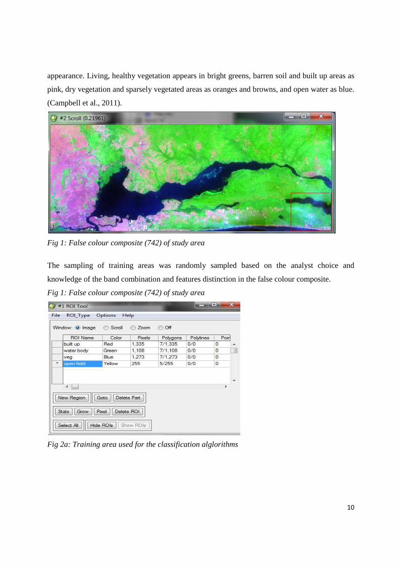
10

appearance. Living, healthy vegetation appears in bright greens, barren soil and built up areas as

pink, dry vegetation and sparsely vegetated areas as oranges and browns, and open water as blue.

(Campbell et al., 2011).

Fig 1: False colour composite (742) of study area

The sampling of training areas was randomly sampled based on the analyst choice and

knowledge of the band combination and features distinction in the false colour composite.

Fig 1: False colour composite (742) of study area

Fig 2a: Training area used for the classification alglorithms

11

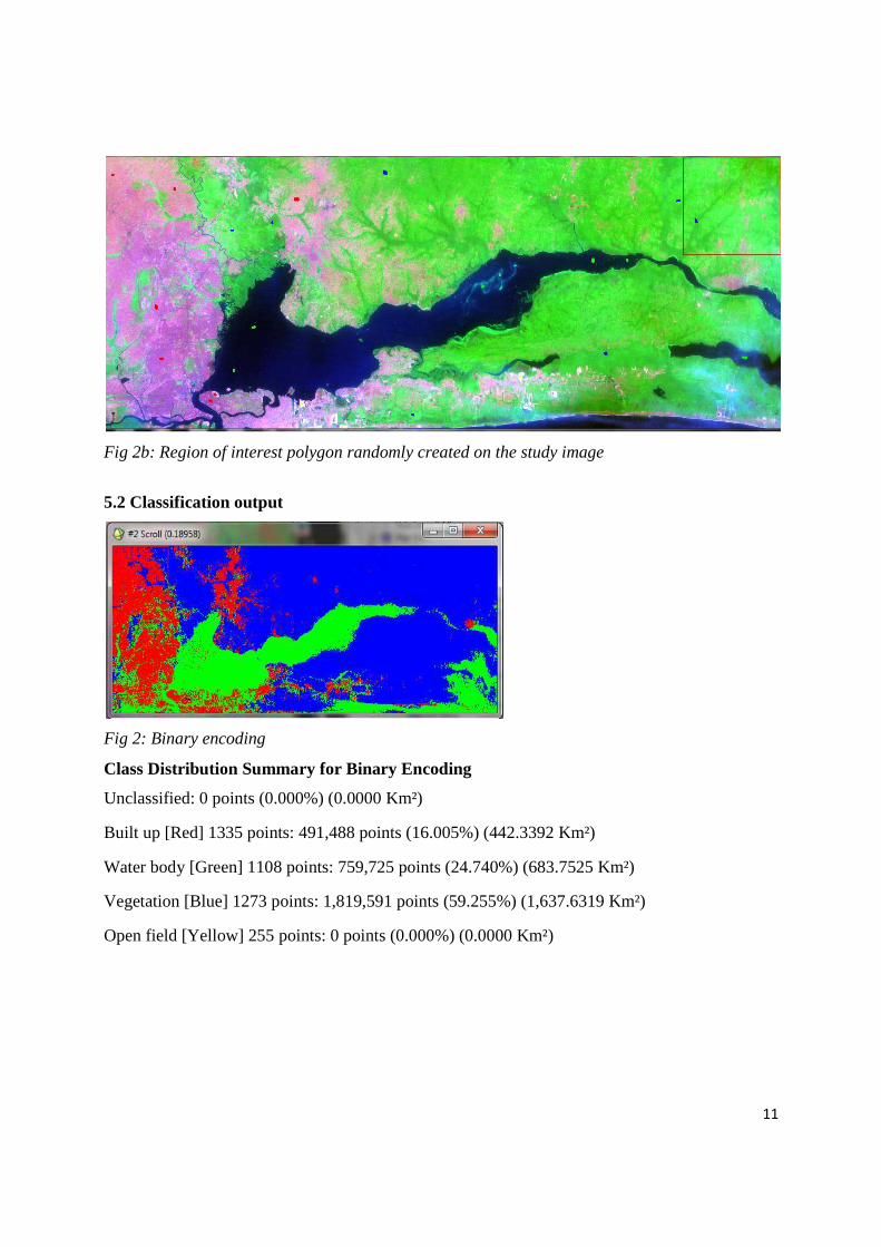
Fig 2b: Region of interest polygon randomly created on the study image

5.2 Classification output

Fig 2: Binary encoding

Class Distribution Summary for Binary Encoding

Unclassified: 0 points (0.000%) (0.0000 Km²)

Built up [Red] 1335 points: 491,488 points (16.005%) (442.3392 Km²)

Water body [Green] 1108 points: 759,725 points (24.740%) (683.7525 Km²)

Vegetation [Blue] 1273 points: 1,819,591 points (59.255%) (1,637.6319 Km²)

Open field [Yellow] 255 points: 0 points (0.000%) (0.0000 Km²)

12

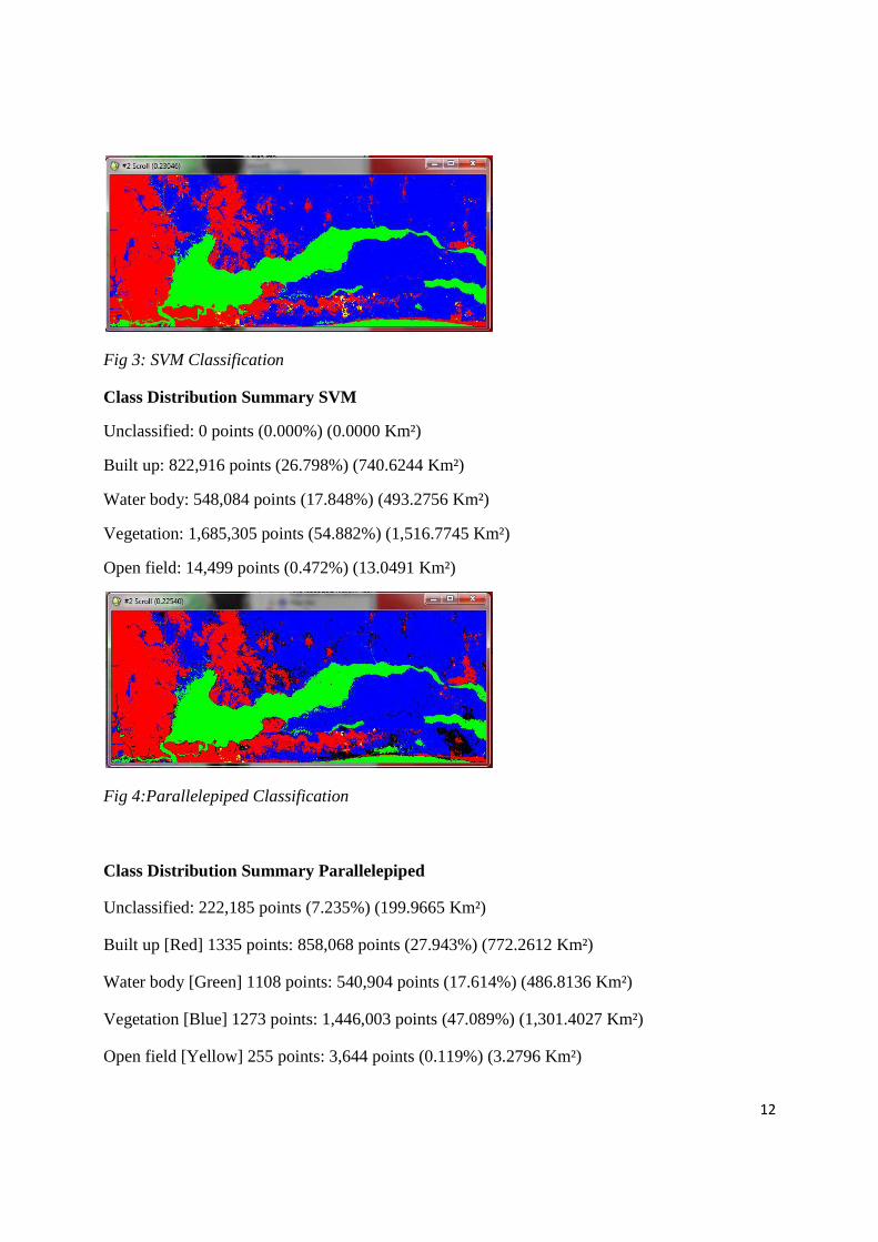
Fig 3: SVM Classification

Class Distribution Summary SVM


Built up: 822,916 points (26.798%) (740.6244 Km²)

Water body: 548,084 points (17.848%) (493.2756 Km²)

Vegetation: 1,685,305 points (54.882%) (1,516.7745 Km²)

Open field: 14,499 points (0.472%) (13.0491 Km²)

Fig 4:Parallelepiped Classification

Class Distribution Summary Parallelepiped

Unclassified: 222,185 points (7.235%) (199.9665 Km²)




Open field [Yellow] 255 points: 3,644 points (0.119%) (3.2796 Km²)

13

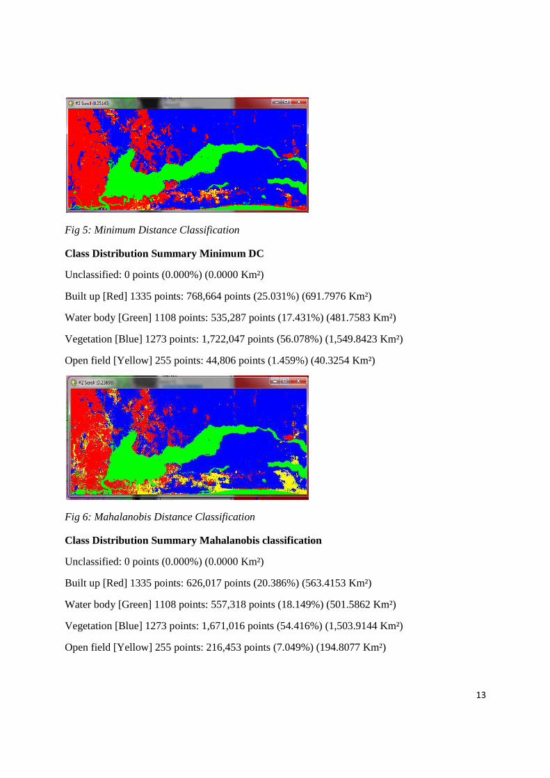
Fig 5: Minimum Distance Classification

Class Distribution Summary Minimum DC






Fig 6: Mahalanobis Distance Classification

Class Distribution Summary Mahalanobis classification






14

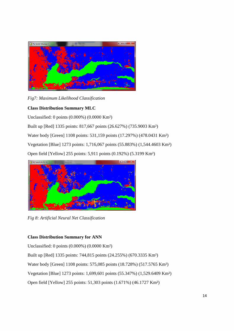
Fig7: Maximum Likelihood Classification

Class Distribution Summary MLC






Fig 8: Artificial Neural Net Classification

Class Distribution Summary for ANN






15

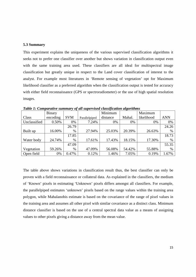
5.3 Summary

This experiment explains the uniqueness of the various supervised classification algorithms it

seeks not to prefer one classifier over another but shows variation in classification output even

with the same training area used. These classifiers are all ideal for multispectral image

classification but greatly unique in respect to the Land cover classification of interest to the

analyst. For example most literatures in ‘Remote sensing of vegetation’ opt for Maximum

likelihood classifier as a preferred algorithm when the classification output is tested for accuracy

with either field reconnaissance (GPS or spectroradiometer) or the use of high spatial resolution

images.

Table 1: Comparative summary of all supervised classification algorithms

Class Binary encoding SVM Parallelpiped

Minimum distance Mahal.

Maximum likelihood ANN

Unclassified 0.50% 0% 7.24% 0% 0% 0% 0%

Built up 16.00% 26.79

% 27.94% 25.03% 20.39% 26.63% 24.26

%

Water body 24.74% 17.85

% 17.61% 17.43% 18.15% 17.30% 18.73

%

Vegetation 59.26% 47.09

% 47.09% 56.08% 54.42% 55.88% 55.35

% Open field 0% 0.47% 0.12% 1.46% 7.05% 0.19% 1.67%

The table above shows variations in classification result thus, the best classifier can only be

proven with a field reconnaissance or collateral data. As explained in the classifiers, the medium

of ‘Known’ pixels in estimating ‘Unknown’ pixels differs amongst all classifiers. For example,

the parallelpiped estimates ‘unknown’ pixels based on the range values within the training area

polygon, while Mahalanobis estimate is based on the covariance of the range of pixel values in

the training area and assumes all other pixel with similar covariance as a distinct class. Minimum

distance classifier is based on the use of a central spectral data value as a means of assigning

values to other pixels giving a distance away from the mean value.

16

References

C. Palaniswami, A. K. Upadhyay and H. P. Maheswarappa, "Spectral mixture analysis for subpixel classification of coconut", Current Science, Vol. 91, No. 12, pp. 1706 -1711, 25 December 2006.

Campbell, J.B. and Wynne, R. 2011: Introduction to Remote Sensing. Taylor & Francis, London.

D. Lu, Q. Weng, "A survey of image classification methods and techniques for improving classification performance", International Journal of Remote Sensing, Vol. 28, No. 5, pp. 823-870, January 2007.

ENVI tutorial (2002): Classification Methods. ITT visual information solution

James A. Shine and Daniel B. Carr, "A Comparison of Classification Methods for Large Imagery Data Sets", JSM 2002 Statistics in an ERA of Technological Change- Statistical computing section, New York City, pp.3205-3207, 11-15 August 2002.

Jasinski, M. F., "Estimation of subpixel vegetation density of natural regions using satellite

multispectral imagery", IEEE Trans. Geosci. Remote Sensing, Vol. 34, pp. 804–813, 1996.

Liu, JG and Mason (2009): Essential image processing and GIS for Remote Sensing. Wiley

Blackwell.

M. Anji Reddy (2008): Remote Sensing and Geographic Information System. Third Edition BS

Publication.

Sabins, F.F. 1997: Remote Sensing and Principles and Image Interpretation. WH Freeman,

Documents

Remotely Sensed Image classification: Supervised classification algorithm