P. Bozanis and E.N. Houstis (Eds.): PCI 2005, LNCS 3746, pp. 328 – 337, 2005. © Springer-Verlag Berlin Heidelberg 2005

Bagging Model Trees for Classification Problems

S.B. Kotsiantis1, G.E. Tsekouras 2, and P.E. Pintelas1

1 Educational Software Development Laboratory, Department of Mathematics, University of Patras, Greece

{sotos, pintelas}@math.upatras.gr 2 Department of Cultural Technology and Communication,

University of the Aegean, Mytilene, Greece gtsek@ct.aegean.gr

Abstract. Structurally, a model tree is a regression method that takes the form of a decision tree with linear regression functions instead of terminal class val-ues at its leaves. In this study, model trees are coupled with bagging for solving classification problems. In order to apply this regression technique to classifica-tion problems, we consider the conditional class probability function and seek a model-tree approximation to it. During classification, the class whose model tree generates the greatest approximated probability value is chosen as the pre-dicted class. We performed a comparison with other well known ensembles of decision trees, on standard benchmark datasets and the performance of the pro-posed technique was greater in most cases.

1 Introduction

The purpose of ensemble learning is to build a learning model which integrates a number of base learning models, so that the model gives better generalization per-formance on application to a particular data-set than any of the individual base models [5]. Ensemble generation can be characterized as being homogeneous if each base learning model uses the same learning algorithm or heterogeneous if the base models can be built from a range of learning algorithms.

A model tree is a regression method that takes the form of a decision tree with lin-ear regression functions instead of terminal class values at its leaves [11]. During the construction of the model tree there are three main problems to be solved: Choosing the best partition of a region of the feature space, determining the leaves of the tree and choosing a model for each leaf.

In this study, model trees are coupled with bagging for solving classification prob-lems. In order to apply the continuous-prediction technique of model trees to discrete classification problems, we consider the conditional class probability function and seek a model-tree approximation to it. During classification, the class whose model tree generates the greatest approximated probability value is chosen as the predicted class. We performed a comparison with other well known ensembles of decision trees, on standard UCI benchmark datasets and the performance of the proposed method was greater in most cases.

Current ensemble approaches of decision trees are described in section 2. In Sec-tion 3 we describe the proposed method and investigate its advantages and limitations.

Bagging Model Trees for Classification Problems 329

In Section 4, we evaluate the proposed method on several UCI datasets by comparing it with bagging, boosting and other ensembles of decision trees. Finally, section 5 concludes the paper and suggests further directions in current research.

2 Ensembles of Classifiers

Empirical studies showed that ensembles are often much more accurate than the indi-vidual base learner that make them up [5], and recently different theoretical explana-tions have been proposed to justify the effectiveness of some commonly used ensem-ble methods [8].

Combining models is not a really new concept for the statistical pattern recogni-tion, machine learning, or engineering communities, though in recent years there has been an explosion of research exploring creative new ways to combine models. Cur-rently, there are two main approaches to model combination. The first is to create a set of learned models by applying an algorithm repeatedly to different training sample data; the second applies various learning algorithms to the same sample data. The predictions of the models are then combined according to a voting scheme. In this work we propose a combining method that uses one learning algorithm for building an ensemble of classifiers. For this reason this section presents the most well-known methods that generate sets of base learners using one base learning algorithm.

Probably the most well-known sampling approach is that exemplified by bagging [3]. Given a training set, bagging generates multiple bootstrapped training sets and calls the base model learning algorithm with each of them to yield a set of base mod-els. Given a training set of size t, bootstrapping generates a new training set by re-peatedly (t times) selecting one of the t examples at random, where all of them have equal probability of being selected. Some training examples may not be selected at all and others may be selected multiple times. A bagged ensemble classifies a new ex-ample by having each of its base models classify the example and returning the class that receives the maximum number of votes. The hope is that the base models gener-ated from the different bootstrapped training sets disagree often enough that the en-semble performs better than the base models.

Breiman [3] made the important observation that instability (responsiveness to changes in the training data) is a prerequisite for bagging to be effective. A committee of classifiers that all agree in all circumstances will give identical performance to any of its members in isolation.

If there is too little data, the gains achieved via a bagged ensemble cannot compen-sate for the decrease in accuracy of individual models, each of which now sees an even smaller training set. On the other end, if the data set is extremely large and com-putation time is not an issue, even a single flexible classifier can be quite adequate.

Another method that uses different subsets of training data with a single learning method is the boosting approach [7]. It assigns weights to the training instances, and these weight values are changed depending upon how well the associated training instance is learned by the classifier; the weights for misclassified instances are in-creased. Thus, re-sampling occurs based on how well the training samples are classi-fied by the previous model. Since the training set for one model depends on the previ-ous model, boosting requires sequential runs and thus is not readily adapted to a paral-

330 S.B. Kotsiantis, G.E. Tsekouras, and P.E. Pintelas

lel environment. After several cycles, the prediction is performed by taking a weighted vote of the predictions of each classifier, with the weights being propor-tional to each classifier’s accuracy on its training set.

AdaBoost is a practical version of the boosting approach [7]. There are two ways that Adaboost can use these weights to construct a new training set to give to the base learning algorithm. In boosting by sampling, examples are drawn with replacement with probability proportional to their weights. The second method, boosting by weighting, can be used with base learning algorithms that can accept a weighted train-ing set directly. With such algorithms, the entire training set (with associated weights) is given to the base-learning algorithm.

Melville and Mooney [12] present a new meta-learner (DECORATE, Diverse En-semble Creation by Oppositional Re-labeling of Artificial Training Examples) that uses an existing “strong” learner (one that provides high accuracy on the training data) to build a diverse committee. This is accomplished by adding different randomly constructed examples to the training set when building new committee members. These artificially constructed examples are given category labels that disagree with the current decision of the committee, thereby directly increasing diversity when a new classifier is trained on the augmented data and added to the committee.

Random Forests [4] grows many classification trees. Each tree gives a classifica-tion (vote). The forest chooses the class having the most votes (over all the trees in the forest). Each tree is grown as follows:

• If the number of cases in the training set is N, sample N cases at random - but with replacement, from the original data. This sample will be the training set for growing the tree.

• If there are M input variables, a number m<<M is specified such that at each node, m variables are selected at random out of the M and the best split on these m is used to split the node. The value of m is held constant during the forest growing.

• Each tree is grown to the largest extent possible. There is no pruning.

3 Proposed Algorithm

Model trees are binary decision trees with linear regression functions at the leaf nodes: thus they can represent any piecewise linear approximation to an unknown function [17]. A model tree is generated in two stages. The first builds an ordinary decision tree, using as splitting criterion the maximization of the intra-subset variation of the target value. The second prunes this tree back by replacing subtrees with linear regression functions wherever this seems appropriate.

The construction and use of model trees is clearly described in [16] account of the M5 scheme. An implementation called M5’ is described in [17] along with further implementation details. The learning procedure of M5’ model tree algorithm effec-tively divides the instance space into regions using a decision tree, and strives to minimize the expected mean squared error between the model tree’s output and the target values. The training instances that lie in a particular region can be viewed as samples from an underlying probability distribution that assigns class values. It is

Bagging Model Trees for Classification Problems 331

standard procedure in statistics to estimate a probability distribution by minimizing the mean square error of samples taken from it.

After the tree has been grown, a linear multiple regression model is built for every inner node, using the data associated with that node and all the features that partici-pate in tests in the subtree rooted at that node. Then the linear regression models are simplified by dropping features if this results in a lower expected error on future data (more specifically, if the decrease in the number of parameters outweighs the increase in the observed training error). After this has been done, every subtree is considered for pruning. Pruning occurs if the estimated error for the linear model at the root of a subtree is smaller or equal to the expected error for the subtree. After pruning has terminated, M5’ applies a ‘smoothing’ process that combines the model at a leaf with the models on the path to the root to form the final model that is placed at the leaf.

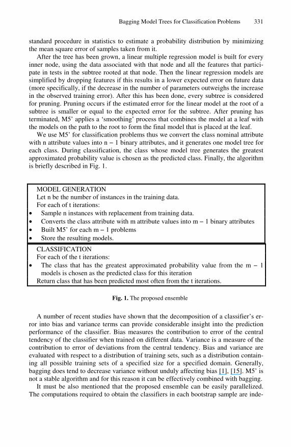
We use M5’ for classification problems thus we convert the class nominal attribute with n attribute values into n − 1 binary attributes, and it generates one model tree for each class. During classification, the class whose model tree generates the greatest approximated probability value is chosen as the predicted class. Finally, the algorithm is briefly described in Fig. 1.

MODEL GENERATION Let n be the number of instances in the training data. For each of t iterations:

• Sample n instances with replacement from training data. • Converts the class attribute with m attribute values into m − 1 binary attributes • Built M5’ for each m − 1 problems • Store the resulting models.

CLASSIFICATION For each of the t iterations:

• The class that has the greatest approximated probability value from the m − 1 models is chosen as the predicted class for this iteration

Return class that has been predicted most often from the t iterations.

Fig. 1. The proposed ensemble

A number of recent studies have shown that the decomposition of a classifier’s er-ror into bias and variance terms can provide considerable insight into the prediction performance of the classifier. Bias measures the contribution to error of the central tendency of the classifier when trained on different data. Variance is a measure of the contribution to error of deviations from the central tendency. Bias and variance are evaluated with respect to a distribution of training sets, such as a distribution contain-ing all possible training sets of a specified size for a specified domain. Generally, bagging does tend to decrease variance without unduly affecting bias [1], [15]. M5’ is not a stable algorithm and for this reason it can be effectively combined with bagging.

It must be also mentioned that the proposed ensemble can be easily parallelized. The computations required to obtain the classifiers in each bootstrap sample are inde-

332 S.B. Kotsiantis, G.E. Tsekouras, and P.E. Pintelas

pendent of each other. Therefore we can assign tasks to each processor in a balanced manner. This parallel execution of the presented ensemble can achieve linear speedup.

4 Experiments Results

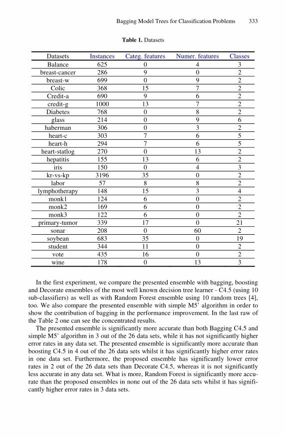
For the comparisons of our study, we used 26 well-known datasets mainly from many domains from the UCI repository [2]. These data sets were hand selected so as to come from real-world problems and to vary in characteristics. Thus, we have used data sets from the domains of: pattern recognition (iris), image recognition (sonar), medical diagnosis (breast-cancer, breast-w, colic, diabetes, heart-c, heart-h, heart-statlog, hepatitis, lymphotherapy, primary-tumor) commodity trading (credit-a, credit-g), computer games (kr-vs-kp, monk1, monk2, monk3), various control applications (balance) and prediction of student performance (student) [9]. Table 1 is a brief de-scription of these data sets presenting the number of output classes, the type of the features and the number of examples.

In order to calculate the classifiers accuracy for our experiments, the whole training set was divided into ten mutually exclusive and equal-sized subsets and for each sub-set the model was trained on the union of all of the other subsets. Then, cross valida-tion was run 10 times for each algorithm and the average value of the 10-cross valida-tions was calculated. It must be mentioned that we used the free available source code for most of the algorithms by [18] for our experiments.

In Table 2, we represent as “v” that the specific algorithm performed statistically better than the proposed ensemble according to t-test with p<0.05. Throughout, we speak of two results for a dataset as being "significant different" if the difference is statistical significant at the 5% level according to the corrected resampled t-test [13], with each pair of data points consisting of the estimates obtained in one of the 100 folds for the two learning methods being compared. On the other hand, “*” indicates that proposed ensemble performed statistically better than the specific algorithm ac-cording to t-test with p<0.05. In all the other cases, there is no significant statistical difference between the results (Draws). In the last row of the table one can also see the aggregated results in the form (α/b/c). In this notation “α” means that the proposed ensemble is significantly less accurate than the compared algorithm in α out of 26 datasets, “c” means that the proposed algorithm is significantly more accurate than the compared algorithm in c out of 26 datasets, while in the remaining cases (b), there is no significant statistical difference.

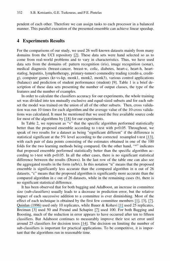
It has been observed that for both bagging and AdaBoost, an increase in committee size (sub-classifiers) usually leads to a decrease in prediction error, but the relative impact of each successive addition to a committee is ever diminishing. Most of the effect of each technique is obtained by the first few committee members [1], [3], [7]. Quinlan (1996) used only 10 replicates, while Bauer & Kohavi [1] used 25 replicates, Breiman [3] used 50 and Freund and Schapire [7] used 100. For both Bagging and Boosting, much of the reduction in error appears to have occurred after ten to fifteen classifiers. But Adaboost continues to measurably improve their test set error until around 25 classifiers for decision trees [14]. The decision on limiting the number of sub-classifiers is important for practical applications. To be competitive, it is impor-tant that the algorithms run in reasonable time.

Bagging Model Trees for Classification Problems 333

Table 1. Datasets

Datasets Instances Categ. features Numer. features Classes Balance 625 0 4 3

breast-cancer 286 9 0 2 breast-w 699 0 9 2

Colic 368 15 7 2 Credit-a 690 9 6 2 credit-g 1000 13 7 2 Diabetes 768 0 8 2

glass 214 0 9 6 haberman 306 0 3 2

heart-c 303 7 6 5 heart-h 294 7 6 5

heart-statlog 270 0 13 2 hepatitis 155 13 6 2

iris 150 0 4 3 kr-vs-kp 3196 35 0 2

labor 57 8 8 2 lymphotherapy 148 15 3 4

monk1 124 6 0 2 monk2 169 6 0 2 monk3 122 6 0 2

primary-tumor 339 17 0 21 sonar 208 0 60 2

soybean 683 35 0 19 student 344 11 0 2

vote 435 16 0 2 wine 178 0 13 3

In the first experiment, we compare the presented ensemble with bagging, boosting and Decorate ensembles of the most well known decision tree learner - C4.5 (using 10 sub-classifiers) as well as with Random Forest ensemble using 10 random trees [4], too. We also compare the presented ensemble with simple M5’ algorithm in order to show the contribution of bagging in the performance improvement. In the last raw of the Table 2 one can see the concentrated results.

The presented ensemble is significantly more accurate than both Bagging C4.5 and simple M5’ algorithm in 3 out of the 26 data sets, while it has not significantly higher error rates in any data set. The presented ensemble is significantly more accurate than boosting C4.5 in 4 out of the 26 data sets whilst it has significantly higher error rates in one data set. Furthermore, the proposed ensemble has significantly lower error rates in 2 out of the 26 data sets than Decorate C4.5, whereas it is not significantly less accurate in any data set. What is more, Random Forest is significantly more accu-rate than the proposed ensembles in none out of the 26 data sets whilst it has signifi-cantly higher error rates in 3 data sets.

334 S.B. Kotsiantis, G.E. Tsekouras, and P.E. Pintelas

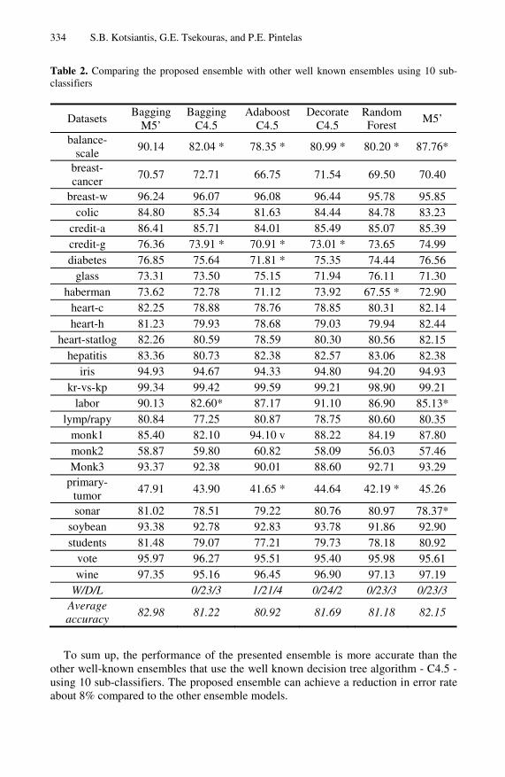
Table 2. Comparing the proposed ensemble with other well known ensembles using 10 sub-classifiers

Datasets Bagging

M5’ Bagging

C4.5 Adaboost

C4.5 Decorate

C4.5 Random Forest

M5’

balance-scale

90.14 82.04 * 78.35 * 80.99 * 80.20 * 87.76*

breast-cancer

70.57 72.71 66.75 71.54 69.50 70.40

breast-w 96.24 96.07 96.08 96.44 95.78 95.85 colic 84.80 85.34 81.63 84.44 84.78 83.23

credit-a 86.41 85.71 84.01 85.49 85.07 85.39 credit-g 76.36 73.91 * 70.91 * 73.01 * 73.65 74.99 diabetes 76.85 75.64 71.81 * 75.35 74.44 76.56

glass 73.31 73.50 75.15 71.94 76.11 71.30 haberman 73.62 72.78 71.12 73.92 67.55 * 72.90

heart-c 82.25 78.88 78.76 78.85 80.31 82.14 heart-h 81.23 79.93 78.68 79.03 79.94 82.44

heart-statlog 82.26 80.59 78.59 80.30 80.56 82.15 hepatitis 83.36 80.73 82.38 82.57 83.06 82.38

iris 94.93 94.67 94.33 94.80 94.20 94.93 kr-vs-kp 99.34 99.42 99.59 99.21 98.90 99.21

labor 90.13 82.60* 87.17 91.10 86.90 85.13* lymp/rapy 80.84 77.25 80.87 78.75 80.60 80.35

monk1 85.40 82.10 94.10 v 88.22 84.19 87.80 monk2 58.87 59.80 60.82 58.09 56.03 57.46 Monk3 93.37 92.38 90.01 88.60 92.71 93.29

primary-tumor

47.91 43.90 41.65 * 44.64 42.19 * 45.26

sonar 81.02 78.51 79.22 80.76 80.97 78.37* soybean 93.38 92.78 92.83 93.78 91.86 92.90 students 81.48 79.07 77.21 79.73 78.18 80.92

vote 95.97 96.27 95.51 95.40 95.98 95.61 wine 97.35 95.16 96.45 96.90 97.13 97.19

W/D/L 0/23/3 1/21/4 0/24/2 0/23/3 0/23/3 Average accuracy

82.98 81.22 80.92 81.69 81.18 82.15

To sum up, the performance of the presented ensemble is more accurate than the other well-known ensembles that use the well known decision tree algorithm - C4.5 - using 10 sub-classifiers. The proposed ensemble can achieve a reduction in error rate about 8% compared to the other ensemble models.

Bagging Model Trees for Classification Problems 335

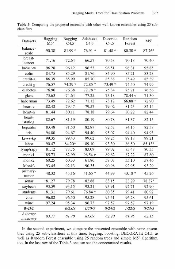
Table 3. Comparing the proposed ensemble with other well known ensembles using 25 sub-classifiers

Datasets Bagging

M5’ Bagging

C4.5 Adaboost

C4.5 Decorate

C4.5 Random Forest

M5’

balance-scale

90.38 81.99 * 76.91 * 81.48 * 80.30 * 87.76*

breast-cancer

71.16 72.64 66.57 70.58 70.18 70.40

breast-w 96.28 96.12 96.53 96.51 96.31 95.85 colic 84.75 85.29 81.76 84.90 85.21 83.23

credit-a 86.39 85.99 85.70 85.88 85.49 85.39 credit-g 76.57 74.29 * 72.85 * 73.49 * 74.50 74.99 diabetes 76.96 76.38 72.78 * 75.34 75.21 76.56

glass 73.63 74.64 77.25 73.18 78.44 v 71.30 haberman 73.49 72.62 71.12 73.12 66.88 * 72.90

heart-c 82.42 79.47 79.57 79.02 81.23 82.14 heart-h 81.44 80.11 78.18 79.64 80.22 82.44 heart-statlog

82.67 81.19 80.19 80.78 81.37 82.15

hepatitis 83.48 81.50 82.87 82.57 84.15 82.38 iris 94.80 94.67 94.40 95.07 94.40 94.93

kr-vs-kp 99.35 99.43 99.62 99.25 99.18 99.21 labor 90.47 84.20* 89.10 93.30 86.50 85.13*

lymp/rapy 81.12 78.75 83.09 79.02 83.48 80.35 monk1 85.73 82.99 96.54 v 89.62 87.22 87.80 monk2 60.25 60.33 61.86 58.03 55.10 57.46 Monk3 93.45 92.13 90.35 90.98 92.95 93.29

primary-tumor

48.32 45.16 41.65 * 44.99 43.18 * 45.26

sonar 81.27 79.78 82.88 83.15 83.29 78.37* soybean 93.59 93.15 93.21 93.91 92.71 92.90 students 81.31 79.61 76.84 * 80.35 79.41 80.92

vote 96.02 96.50 95.28 95.51 96.28 95.61 wine 97.24 95.34 96.73 97.57 97.57 97.19

W/D/L 0/23/3 1/20/5 0/24/2 1/22/3 0/23/3 Average accuracy

83.17 81.70 81.69 82.20 81.95 82.15

In the second experiment, we compare the presented ensemble with same ensem-bles using 25 sub-classifiers at this time: bagging, boosting, DECORATE C4.5, as well as Random Forest ensemble using 25 random trees and simple M5’ algorithm, too. In the last raw of the Table 3 one can see the concentrated results.

336 S.B. Kotsiantis, G.E. Tsekouras, and P.E. Pintelas

The presented ensemble is significantly more accurate than both Bagging C4.5 and simple M5’ algorithm in 3 out of the 26 data sets, while it has not significantly higher error rates in any data set. The presented ensemble is significantly more accurate than boosting C4.5 in 5 out of the 26 data sets whilst it has significantly higher error rates in one data set. Furthermore, the proposed ensemble has significantly lower error rates in 2 out of the 26 data sets than Decorate C4.5, whereas it is not significantly less accurate in any data set. What is more, Random Forest is significantly more accu-rate than the proposed ensembles in 1 out of the 26 data sets whilst it has significantly higher error rates in 3 data sets.

To sum up, the performance of the presented ensemble is more accurate than the other well-known ensembles that use the C4.5 algorithm using 25 sub-classifiers. The proposed ensemble can achieve a reduction in error rate about 7% compared to the other ensemble models.

Finally, it must be mentioned that for the proposed ensemble, much of the reduc-tion in error appears to have occurred after ten sub-classifiers. It seems that the pro-posed method continues to measurably improve test set error until around 25 sub-classifiers. Nevertheless, the decision on limiting the number of sub-classifiers is important for practical applications. To be competitive, our decision is to use 10 sub-classifiers.

5 Conclusion

This work has shown that when classification problems are transformed into problems of function approximation in a standard way, they can be successfully solved by con-structing model trees to produce an approximation to the conditional class probability function of each individual class.

Bagging model trees outperform state-of-the-art decision tree ensembles on prob-lems with numeric and binary attributes, and, more often than not, on problems with multi-valued nominal attributes too.

In a future work, we will combine model trees with a boosting process for solving classification problems. We will also examine the efficiency of bagging with logistic model trees [10] that use logistic regression at the leaves of the model trees, instead of linear regression.

References

1. Bauer, E. & Kohavi, R.: An empirical comparison of voting classification algorithms: Bagging, boosting, and variants. Machine Learning, Vol. 36, (1999) 105–139.

2. Blake, C. & Merz, C.: UCI Repository of machine learning databases. Irvine, CA: Univer-sity of California, Department of Information and Computer Science. [http://www.ics.uci. edu/~mlearn/MLRepository.html] (1998)

3. Breiman, L.: Bagging Predictors. Machine Learning, 24 (1996) 123-140. 4. Breiman, L.: "Random Forests". Machine Learning 45 (2001) 5-32. 5. Dietterich, T.: Ensemble Methods in Machine Learning, In Proc. 1st International Work-

shop on Multiple Classifer Systems, LNCS, Vol 1857, (2000) 1-10, Springer-Verlag.

Bagging Model Trees for Classification Problems 337

6. Frank, E., Wang, Y., Inglis, S., Holmes, G., Witten, I.: Using Model Trees for Classifica-tion, Machine Learning, 32, (1998) 63–76.

7. Freund Y. and Schapire, R. E.: Experiments with a New Boosting Algorithm, in proceed-ings of ICML’96, pp. 148-156.

8. Kleinberg, E.M.: A Mathematically Rigorous Foundation for Supervised Learning. In J. Kittler and F. Roli, editors, Multiple Classifier Systems. First International Workshop, MCS 2000, Cagliari, Italy, volume 1857 of Lecture Notes in Computer Science, (2000) 67–76. Springer-Verlag.

9. Kotsiantis, S., Pierrakeas, C., Pintelas, P.: Predicting Students’ Performance in Distance Learning Using Machine Learning Techniques, Applied Artificial Intelligence (AAI), Vol-ume 18, (2004) 411 – 426.

10. Landwehr, N., Hall, M., Frank, E.: Logistic Model Trees, Lecture Notes in Computer Sci-ence, Volume 2837, Jan 2003, Pages 241 – 252.

11. Malerba, D., Esposito, F., Ceci, M., Appice, A.: Top-Down Induction of Model Trees with Regression and Splitting Nodes. IEEE Trans. Pattern Anal. Mach. Intell. 26(5): 612-625 2004.

12. Melville P. and Mooney R.: Constructing Diverse Classifier Ensembles using Artificial Training Examples, in proceedings of IJCAI-2003, pp.505-510, Acapulco, Mexico, August 2003.

13. Nadeau, C., Bengio, Y.: Inference for the Generalization Error. Machine Learning, 52 (2003) 239-281.

14. Opitz D. & Maclin R.: Popular Ensemble Methods: An Empirical Study, Artificial Intelli-gence Research, Vol. 11, (1999) 169-198.

15. Quinlan, J. R.: Bagging, boosting, and C4.5. In Proceedings of the Thirteenth National Conference on Artificial Intelligence (1996) 725–730. AAAI/MIT Press.

16. Quinlan, J. R.: Learning with continuous classes, Proc. of Australian Joint Conf. on AI, (1992) 343-348, World Scientific, Singapore

17. Wang, Y. & Witten, I. H.: Induction of model trees for predicting continuous classes, In Proc. of the Poster Papers of the European Conference on ML, Prague (1997) 128–137. Prague: University of Economics, Faculty of Informatics and Statistics.

18. Witten, I., Frank, E.: Data Mining: Practical Machine Learning Tools and Techniques with Java Implementations. Morgan Kaufmann, San Mateo, CA, (2000).