Tutz:

Modelling of repeated ordered measurements byisotonic sequential regression

Sonderforschungsbereich 386, Paper 298 (2002)

Online unter: http://epub.ub.uni-muenchen.de/

Projektpartner

Modelling of repeated ordered measurements by

isotonic sequential regression

Gerhard Tutz

Ludwig-Maximilians-Universitat Munchen, Institut fur Statistik

Akademiestrasse 1, 80799 Munchen

tutz@stat.uni-muenchen.de

1

Summary

The paper introduces a simple model for repeated observations of an ordered

categorical response variable which is isotonic over time. It is assumed that

the measurements represent an irreversible process such that the response at

time t is never lower than the response observed at the previous time point

t − 1. Observations of this type occur for example in treatment studies when

improvement is measured on an ordinal scale. Since the response at time t

depends on the previous outcome, the number of ordered response categories

depends on the previous outcome leading to severe problems when simple

threshold models for ordered data are used. In order to avoid these problems

the isotonic sequential model is introduced. It accounts for the irreversible

process by considering the binary transitions to higher scores and allows a

parsimonious parameterization. It is shown how the model may easily be

estimated by using existing software. Moreover, the model is extended to a

random effects version which explicitly takes heterogeneity of individuals and

potential correlations into account.

Key words:

Ordinal data, cumulative model, sequential model, repeated measurements,

isotonic ordinal regression, random effects models.

2

1 Introduction

In many studies in clinical and epidemiologic research a response variable is

measured repeatedly for each subject. Quite frequently the response variable

is categorical with an ordering of the categories refering to severity of disease

or level of improvement following an intervention. The problem considered

here is of the latter type based on a data set given by Davis (1991). In a

randomized study 60 children undergoing surgery were treated with one of

four dosages of an anaesthetic. Upon admission to the recovery room and at

minutes 5, 15 and 30 following admission, recovery scores were assigned on

a categorical scale ranging from 1 (least favourable) to 7 (most favourable).

Therefore one has four repetitions of a variable having 7 categories. Of course

each individual may be assigned to one of the 2401 cells of the 7 × 7 × 7 × 7

contingency tables arising from the four measurements. However, since most

of the cells will be empty it is of no use to try to model the total response .

One approach is to model the marginal distribution of this contingency table.

This marginal approach may be used for example if one wants to know how

dosage determines the recovery level at differing times. It has been used by

Stram, Wei & Ware (1988), Moulton & Zeger (1989), Liang, Zeger & Qaqish

(1992), Stram & Wei (1988) and others.

The data structures considered here have the special feature that observed

response categories are isotonic over time. In our example transitions from

measurement to measurement take place only in the direction of higher re-

covery scores. In consecutive measurements patients never get a lower score

in the measurement taken at a later point in time. This characterizes the

essential structure of data that are considered in this paper. Scores taken

at a later time have always to be equal or higher than in the previous mea-

surement. Marginal modelling of this sort of data faces severe problems since

the contingency tables with margins corresponding to measurements contain

structural zeros. For example all the two dimensional tables have zeros in the

lower (or upper) off-diagonal triangles. Straightforward marginal modelling

which does not take care of these structured zeros will fail since the associa-

tion structure is modelled inadequately. Fahrmeir, Gieger & Heumann (1999)

gave on marginal approach which takes account of the structural zeros. In

the present paper an alternative approach is proposed which focusses on the

transition process. This approach, known as transitional or conditional mod-

3

elling does account not only for the dependence of marginal distributions on

explanatory variables, but also involves the analysis of patterns of change, i.e.

the conditional response given the previous one. For example, Bonney (1987)

considered regressive logistic models which are of the transitional type. For

the type of data considered here where observed categories of later measure-

ments are higher than for earlier measurement the transitions take place only

into the direction of higher scores. Thus the underlying process is irreversible.

Transitional modelling aims directly at modelling this irreversible process. The

objective is to model the effect of covariates on the first measurement and the

following transitions between categories. It is of interest to know e.g. how

dosage determines the recovery level at admission and the successive improve-

ments following admission.

2 Isotonic modelling of irreversible processes

In the following let Yt denote the ordered categorical measurement taken at

time t with values from {1, . . . , k}. Let x′ = (x1, . . . , xm) denote a vector of

covariates. Firstly, in the next section ordinal models for one response variable

are sketched shortly.

2.1 Ordinal models for separate time points

Let us first consider the case of fixed time t, i.e. the case of cross-sectional

data. Then the effect of x upon the response Yt may be modelled by an ordinal

regression model. Since fixed time is considered the index t is omitted. The

most widespread type of model is the threshold or cumulative model

P (Y ≤ r|x) = F (θr + x′β) (2.1)

where F is a distribution function, e.g. the logistic function F (u) = 1/(1 +

exp(−u)). For the logistic function one gets the proportional odds model

logP (Y ≤ r|x)

P (Y > r|x)= θr + x′β,

for the extreme value distribution F (u) = 1 − exp(− exp(u)) one gets the

so-called proportional hazard model. A motivation for the cumulative model

4

is the construction of a latent continuous variable u = x′β + ε where ε has

distribution function F . Then the observed value Y may be considered as a

coarser version of the latent variable given by Y = r if θr−1 ≤ u ≤ θr for

thresholds −∞ = θ0 < θ1 < . . . < θk−1 < θk = ∞. For details and extensions

see McCullagh (1980), Cox (1988), Brant (1990).

An alternative type of ordinal model is the sequential model

P (Y = r|Y ≥ r, x) = F (θr + x′β) (2.2)

where F is again a distribution function. For the logistic distribution function

(2.2) is the continuation ratio logit model

logP (Y = r|x)

P (Y > r|x)= θr + x′β, (2.3)

(e.g. Agresti (2002)). In the special case where F is the extreme value distri-

bution, the sequential model is equivalent to the cumulative model (2.1) (see

Laara & Matthews (1985), Tutz (1991)). To motivate the use of the sequential

model for irreversible processes it is useful to derive the model as a process

model. The reasoning behind (2.2) is that of a latent sequential or step-wise

mechanism, for example the sequential recovering after treatment. The pro-

cess starts in category 1 (lowest score). The first step is the transition from

category 1 to category 2. This transition is determined by the dichotomous

variable Y (1), more general

Y (r) =

⎧⎪⎨⎪⎩

1 process stops, no transition to category r + 1

0 process continues, transition to category r + 1.

If the first (latent) step fails (Y (1) = 1), the process stops and we have the

observation Y = 1. If the first (latent) step succeeds (Y (1) = 0), we will have

an observed score Y ≥ 2. The second step is the transition from category 2 to

category 3 determined by Y (2). In general Y (r) determines the rth (conditional)

step given the r−1 previous steps were successful. We observe Y = r if Y (1) =

. . . = Y (r−1) = 0, Y (r) = 1, meaning that r − 1 transitions to a higher

score have been made but the rth step has failed. Thus model (2.2) may be

seen as a simple model for the successive transitions of dichotomous variables

Y (1), Y (2), . . . .

The sequential model is particularly suited for response categories which

can be arrived only step by step. In fact, in the recovery problem the stages

5

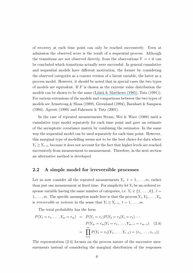
of recovery at each time point can only be reached successively. Even at

admission the observed score is the result of a sequential process. Although

the transitions are not observed directly, from the observations Y = r it can

be concluded which transitions actually were successful. In general cumulative

and sequential models have different motivation, the former by considering

the observed categories as a coarser version of a latent variable, the latter as a

process model. However, it should be noted that in special cases the two types

of models are equivalent. If F is chosen as the extreme value distribution the

models can be shown to be the same (Laara & Matthews (1985), Tutz (1991)).

For various extensions of the models and comparisons between the two types of

models see Armstrong & Sloan (1989), Greenland (1994), Barnhart & Sampson

(1994), Agresti (1999) and Fahrmeir & Tutz (2001).

In the case of repeated measurements Stram, Wei & Ware (1988) used a

cumulative type model separately for each time point and gave an estimate

of the asymptotic covariance matrix by combining the estimates. In the same

way the sequential model can be used separately for each time point. However,

this marginal type of modelling seems not to be the best choice for data where

Yt ≥ Yt−1, because it does not account for the fact that higher levels are reached

successively from measurement to measurement. Therefore, in the next section

an alternative method is developed.

2.2 A simple model for irreversible processes

Let us now consider all the repeated measurements Yt, t = 1, . . . ,m, rather

than just one measurement at fixed time. For simplicity let Yt be an ordered re-

sponse variable having the same number of categories, i.e. Yt ∈ {1, . . . , k}, t =

1, . . . ,m. The specific assumption made here is that the process Y1, Y2, . . . , Ym

is irreversible or isotonic in the sense that Yt ≥ Yt−1, t = 1, . . . ,m.

The total probability has the form

P (Y1 = r1, . . . , Ym = rm) = P (Y1 = r1)P (Y2 = r2|Y1 = r1) · · ·P (Ym = rm|Y1 = r1, . . . , Ym−1 = rm−1) (2.4)

=m∏

t=1

P (Yt = rt|(Y1, . . . , Yt−1) = (r1, . . . , rt−1))

The representation (2.4) focuses on the process nature of the successive mea-

surements instead of considering the marginal distribution of the responses

6

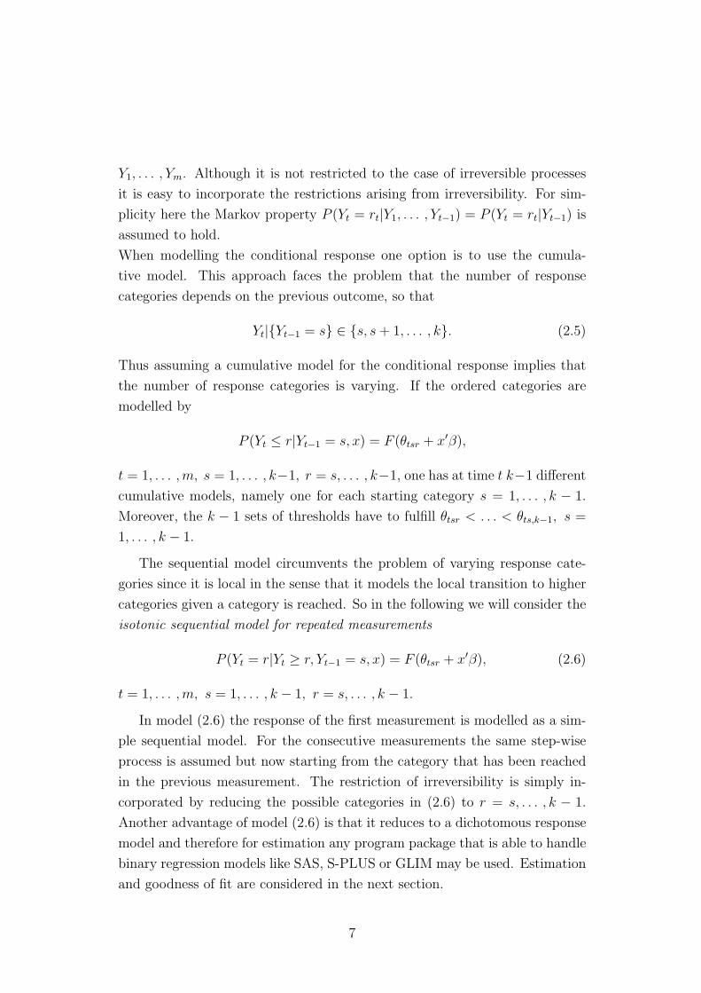
Y1, . . . , Ym. Although it is not restricted to the case of irreversible processes

it is easy to incorporate the restrictions arising from irreversibility. For sim-

plicity here the Markov property P (Yt = rt|Y1, . . . , Yt−1) = P (Yt = rt|Yt−1) is

assumed to hold.

When modelling the conditional response one option is to use the cumula-

tive model. This approach faces the problem that the number of response

categories depends on the previous outcome, so that

Yt|{Yt−1 = s} ∈ {s, s + 1, . . . , k}. (2.5)

Thus assuming a cumulative model for the conditional response implies that

the number of response categories is varying. If the ordered categories are

modelled by

P (Yt ≤ r|Yt−1 = s, x) = F (θtsr + x′β),

t = 1, . . . ,m, s = 1, . . . , k−1, r = s, . . . , k−1, one has at time t k−1 different

cumulative models, namely one for each starting category s = 1, . . . , k − 1.

Moreover, the k − 1 sets of thresholds have to fulfill θtsr < . . . < θts,k−1, s =

1, . . . , k − 1.

The sequential model circumvents the problem of varying response cate-

gories since it is local in the sense that it models the local transition to higher

categories given a category is reached. So in the following we will consider the

isotonic sequential model for repeated measurements

P (Yt = r|Yt ≥ r, Yt−1 = s, x) = F (θtsr + x′β), (2.6)

t = 1, . . . ,m, s = 1, . . . , k − 1, r = s, . . . , k − 1.

In model (2.6) the response of the first measurement is modelled as a sim-

ple sequential model. For the consecutive measurements the same step-wise

process is assumed but now starting from the category that has been reached

in the previous measurement. The restriction of irreversibility is simply in-

corporated by reducing the possible categories in (2.6) to r = s, . . . , k − 1.

Another advantage of model (2.6) is that it reduces to a dichotomous response

model and therefore for estimation any program package that is able to handle

binary regression models like SAS, S-PLUS or GLIM may be used. Estimation

and goodness of fit are considered in the next section.

7

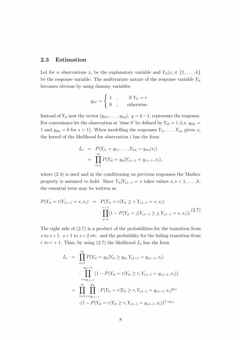
2.3 Estimation

Let for n observations xi be the explanatory variable and Yit|xi ∈ {1, . . . , k}be the response variable. The multivariate nature of the response variable Yit

becomes obvious by using dummy variables

yitr =

{1 , if Yit = r

0 , otherwise.

Instead of Yit now the vector (yit1, . . . , yitq), q = k−1, represents the response.

For convenience let the observation at ’time 0’ be defined by Yi0 = 1 (i.e. yi01 =

1 and yi0s = 0 for s > 1). When modelling the responses Yi1, . . . , Yim given xi

the kernel of the likelihood for observation i has the form

Li = P (Yi1 = yi1, . . . , Yim = yim|xi)

=m∏

t=1

P (Yit = yit|Yi,t−1 = yi,t−1, xi),

where (2.4) is used and in the conditioning on previous responses the Markov

property is assumed to hold. Since Yit|Yi,t−1 = s takes values s, s + 1, . . . , k,

the essential term may be written as

P (Yit = r|Yi,t−1 = s, xi) = P (Yit = r|Yit ≥ r, Yi,t−1 = s, xi)

·r−1∏j=s

(1 − P (Yit = j|Yi,t−1 ≥ j, Yi,t−1 = s, xi)).(2.7)

The right side of (2.7) is a product of the probabilities for the transition from

s to s+1, s+1 to s+2 etc. and the probability for the failing transition from

r to r + 1. Thus, by using (2.7) the likelihood Li has the form

Li =m∏

t=1

P (Yit = yit|Yit ≥ yit, Yi,t−1 = yi,t−1, xi)

·yit−1∏

r=yi,t−1

(1 − P (Yit = r|Yit ≥ r, Yi,t−1 = yi,t−1, xi))

=m∏

t=1

yit∏r=yi,t−1

P (Yit = r|Yit ≥ r, Yi,t−1 = yi,t−1, xi)yitr

·(1 − P (Yit = r|Yit ≥ r, Yi,t−1 = yi,t−1, xi))1−yitr

8

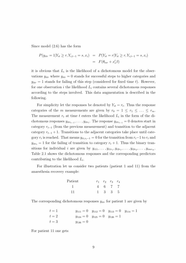
Since model (2.6) has the form

P (yitr = 1|Yit ≥ r, Yi,t−1 = s, xi) = P (Yit = r|Yit ≥ r, Yi,t−1 = s, xi)

= F (θtsr + x′iβ)

it is obvious that Li is the likelihood of a dichotomous model for the obser-

vations yitr where yitr = 0 stands for successful steps to higher categories and

yitr = 1 stands for failing of this step (considered for fixed time t). However,

for one observation i the likelihood Li contains several dichotomous responses

according to the steps involved. This data augmentation is described in the

following.

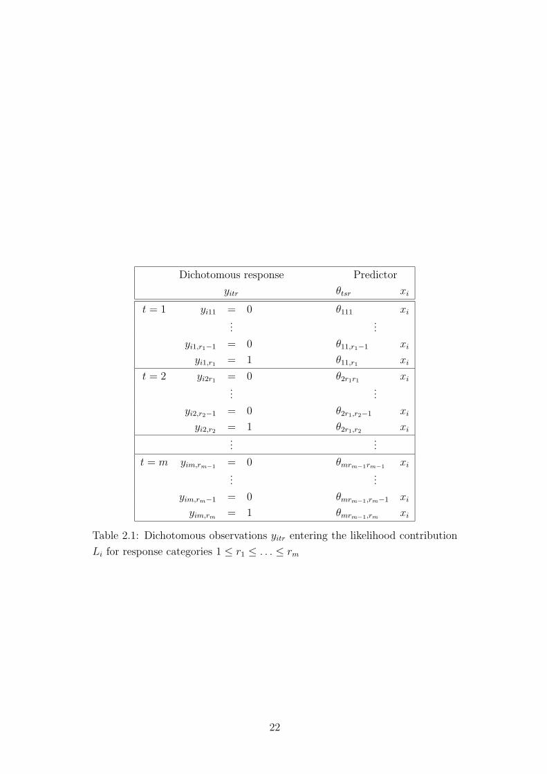
For simplicity let the responses be denoted by Yit = rt. Thus the response

categories of the m measurements are given by r0 = 1 ≤ r1 ≤ . . . ≤ rm.

The measurement rt at time t enters the likelihood Li in the form of the di-

chotomous responses yitrt−1 , . . . , yitrt . The response yitrt−1 = 0 denotes start in

category rt−1 (from the previous measurement) and transition to the adjacent

category rt−1 + 1. Transitions to the adjacent categories take place until cate-

gory rt is reached. That means yit,rt−1 = 0 for the transition from rt−1 to rt and

yitrt = 1 for the failing of transition to category rt + 1. Thus the binary tran-

sitions for individual i are given by yi11, . . . , yi1r1 , yi2r1 , . . . , yi2r2 , . . . , yimrm .

Table 2.1 shows the dichotomous responses and the corresponding predictors

contributing to the likelihood Li.

For illustration let us consider two patients (patient 1 and 11) from the

anaesthesia recovery example:

Patient r1 r2 r3 r4

1 4 6 7 7

11 1 3 3 5

The corresponding dichotomous responses yitr for patient 1 are given by

t = 1 y111 = 0 y112 = 0 y113 = 0 y114 = 1

t = 2 y124 = 0 y125 = 0 y126 = 1

t = 3 y136 = 0

For patient 11 one gets

9

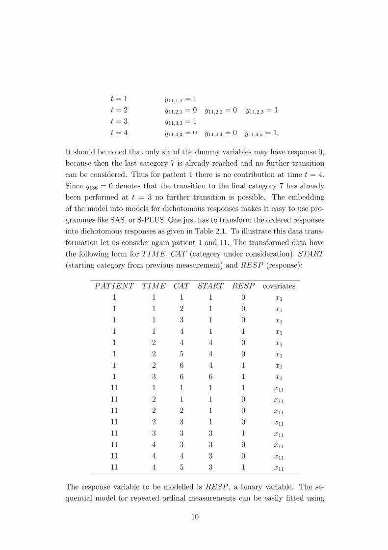
t = 1 y11,1,1 = 1

t = 2 y11,2,1 = 0 y11,2,2 = 0 y11,2,3 = 1

t = 3 y11,3,3 = 1

t = 4 y11,4,3 = 0 y11,4,4 = 0 y11,4,5 = 1.

It should be noted that only six of the dummy variables may have response 0,

because then the last category 7 is already reached and no further transition

can be considered. Thus for patient 1 there is no contribution at time t = 4.

Since y136 = 0 denotes that the transition to the final category 7 has already

been performed at t = 3 no further transition is possible. The embedding

of the model into models for dichotomous responses makes it easy to use pro-

grammes like SAS, or S-PLUS. One just has to transform the ordered responses

into dichotomous responses as given in Table 2.1. To illustrate this data trans-

formation let us consider again patient 1 and 11. The transformed data have

the following form for TIME, CAT (category under consideration), START

(starting category from previous measurement) and RESP (response):

PATIENT TIME CAT START RESP covariates

1 1 1 1 0 x1

1 1 2 1 0 x1

1 1 3 1 0 x1

1 1 4 1 1 x1

1 2 4 4 0 x1

1 2 5 4 0 x1

1 2 6 4 1 x1

1 3 6 6 1 x1

11 1 1 1 1 x11

11 2 1 1 0 x11

11 2 2 1 0 x11

11 2 3 1 0 x11

11 3 3 3 1 x11

11 4 3 3 0 x11

11 4 4 3 0 x11

11 4 5 3 1 x11

The response variable to be modelled is RESP , a binary variable. The se-

quential model for repeated ordinal measurements can be easily fitted using

10

standard procedures for fitting dichotomous responses after the data has been

transformed as shown above (e.g. PROC LOGISTIC in SAS or LOGISTIC

REGRESSION in SPSS/PC+).

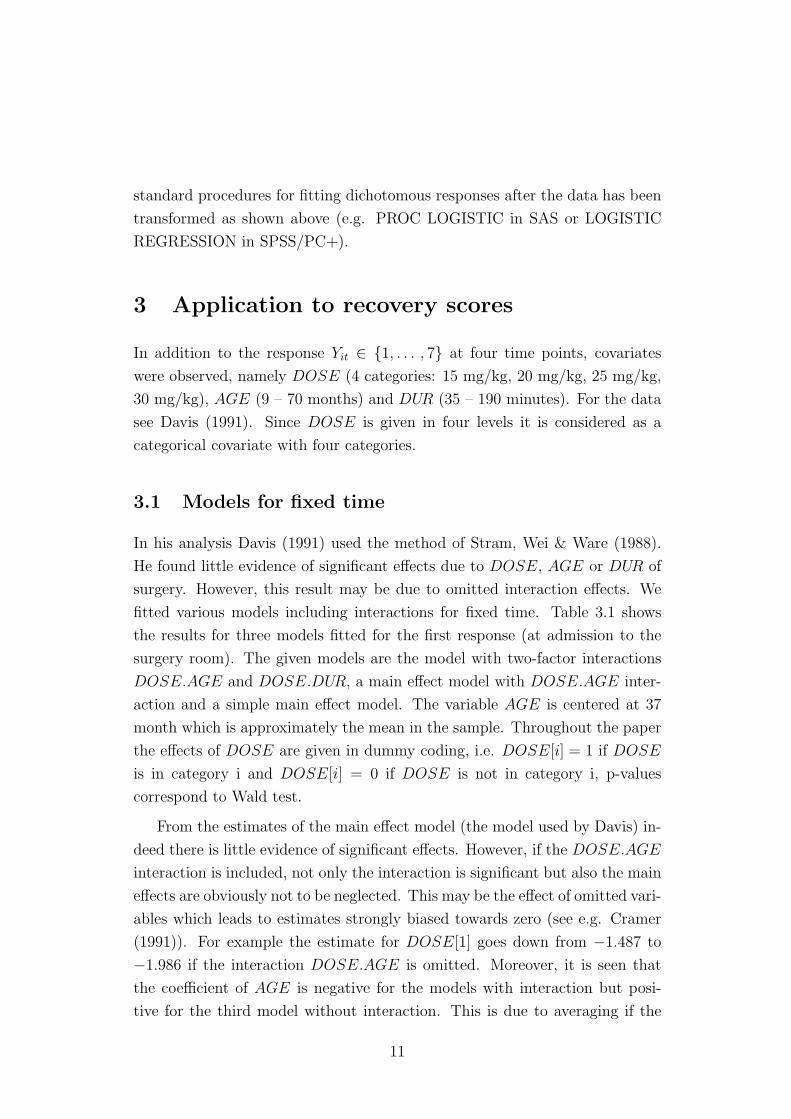
3 Application to recovery scores

In addition to the response Yit ∈ {1, . . . , 7} at four time points, covariates

were observed, namely DOSE (4 categories: 15 mg/kg, 20 mg/kg, 25 mg/kg,

30 mg/kg), AGE (9 – 70 months) and DUR (35 – 190 minutes). For the data

see Davis (1991). Since DOSE is given in four levels it is considered as a

categorical covariate with four categories.

3.1 Models for fixed time

In his analysis Davis (1991) used the method of Stram, Wei & Ware (1988).

He found little evidence of significant effects due to DOSE, AGE or DUR of

surgery. However, this result may be due to omitted interaction effects. We

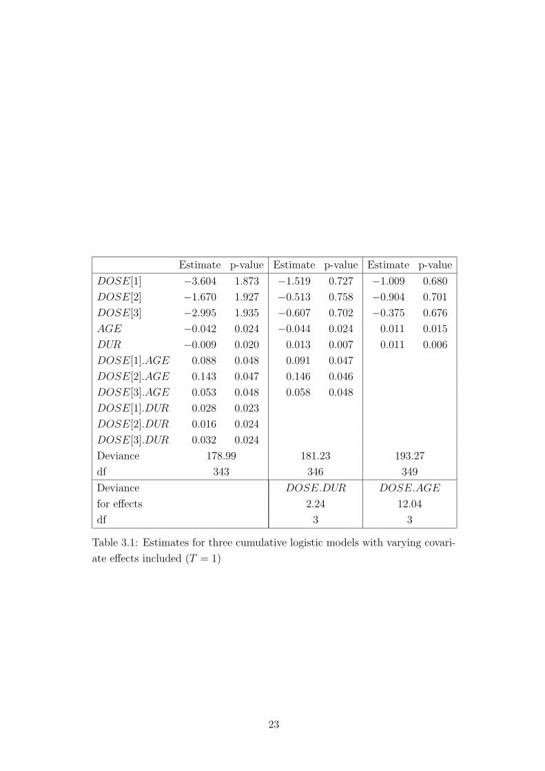
fitted various models including interactions for fixed time. Table 3.1 shows

the results for three models fitted for the first response (at admission to the

surgery room). The given models are the model with two-factor interactions

DOSE.AGE and DOSE.DUR, a main effect model with DOSE.AGE inter-

action and a simple main effect model. The variable AGE is centered at 37

month which is approximately the mean in the sample. Throughout the paper

the effects of DOSE are given in dummy coding, i.e. DOSE[i] = 1 if DOSE

is in category i and DOSE[i] = 0 if DOSE is not in category i, p-values

correspond to Wald test.

From the estimates of the main effect model (the model used by Davis) in-

deed there is little evidence of significant effects. However, if the DOSE.AGE

interaction is included, not only the interaction is significant but also the main

effects are obviously not to be neglected. This may be the effect of omitted vari-

ables which leads to estimates strongly biased towards zero (see e.g. Cramer

(1991)). For example the estimate for DOSE[1] goes down from −1.487 to

−1.986 if the interaction DOSE.AGE is omitted. Moreover, it is seen that

the coefficient of AGE is negative for the models with interaction but posi-

tive for the third model without interaction. This is due to averaging if the

11

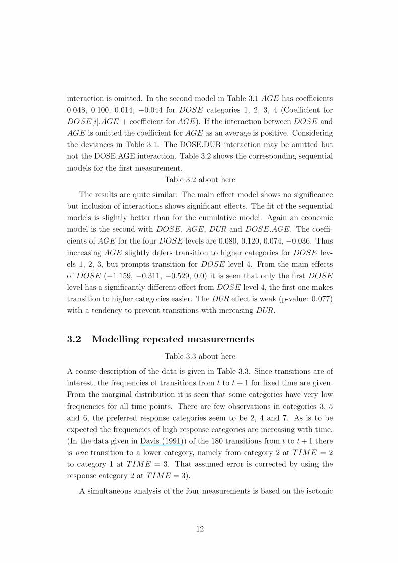
interaction is omitted. In the second model in Table 3.1 AGE has coefficients

0.048, 0.100, 0.014, −0.044 for DOSE categories 1, 2, 3, 4 (Coefficient for

DOSE[i].AGE + coefficient for AGE). If the interaction between DOSE and

AGE is omitted the coefficient for AGE as an average is positive. Considering

the deviances in Table 3.1. The DOSE.DUR interaction may be omitted but

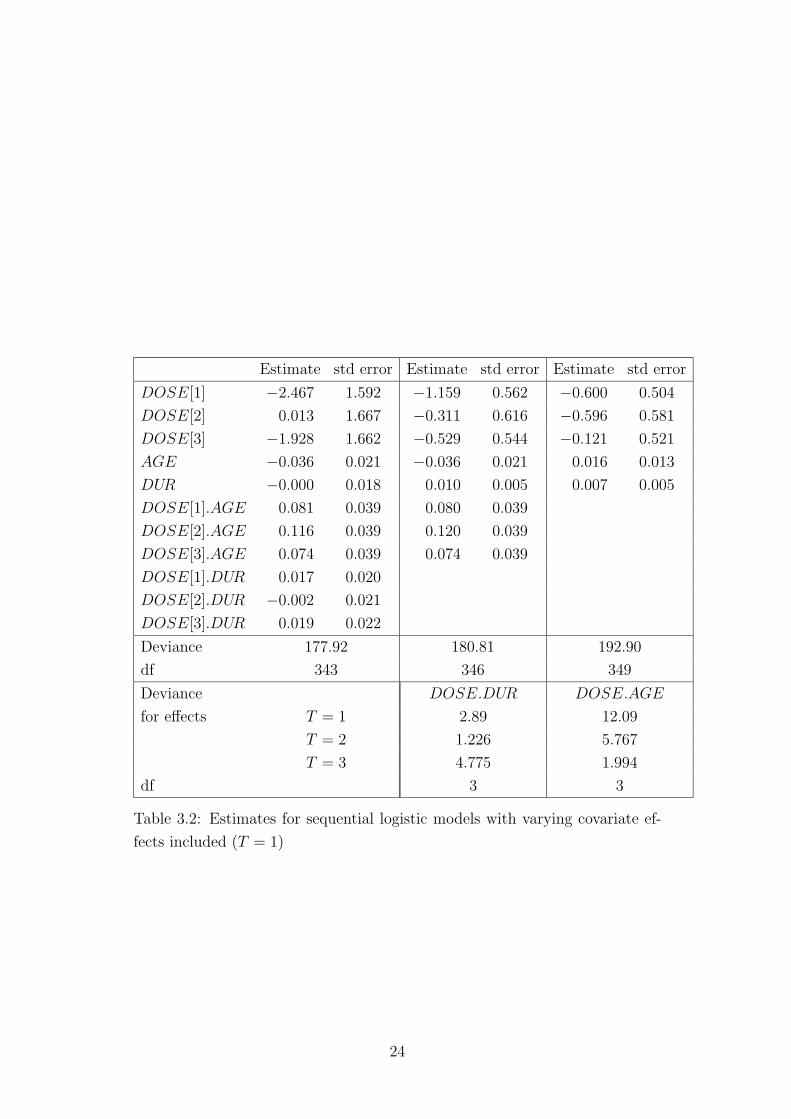
not the DOSE.AGE interaction. Table 3.2 shows the corresponding sequential

models for the first measurement.

Table 3.2 about here

The results are quite similar: The main effect model shows no significance

but inclusion of interactions shows significant effects. The fit of the sequential

models is slightly better than for the cumulative model. Again an economic

model is the second with DOSE, AGE, DUR and DOSE.AGE. The coeffi-

cients of AGE for the four DOSE levels are 0.080, 0.120, 0.074, −0.036. Thus

increasing AGE slightly defers transition to higher categories for DOSE lev-

els 1, 2, 3, but prompts transition for DOSE level 4. From the main effects

of DOSE (−1.159, −0.311, −0.529, 0.0) it is seen that only the first DOSE

level has a significantly different effect from DOSE level 4, the first one makes

transition to higher categories easier. The DUR effect is weak (p-value: 0.077)

with a tendency to prevent transitions with increasing DUR.

3.2 Modelling repeated measurements

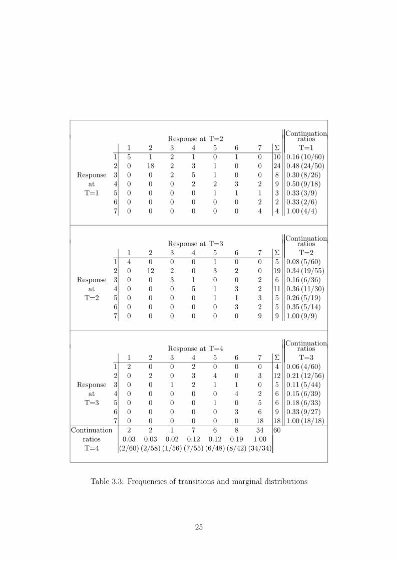
Table 3.3 about here

A coarse description of the data is given in Table 3.3. Since transitions are of

interest, the frequencies of transitions from t to t + 1 for fixed time are given.

From the marginal distribution it is seen that some categories have very low

frequencies for all time points. There are few observations in categories 3, 5

and 6, the preferred response categories seem to be 2, 4 and 7. As is to be

expected the frequencies of high response categories are increasing with time.

(In the data given in Davis (1991)) of the 180 transitions from t to t + 1 there

is one transition to a lower category, namely from category 2 at TIME = 2

to category 1 at TIME = 3. That assumed error is corrected by using the

response category 2 at TIME = 3).

A simultaneous analysis of the four measurements is based on the isotonic

12

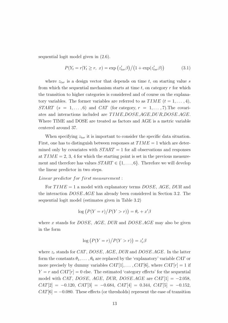
sequential logit model given in (2.6).

P (Yt = r|Yt ≥ r, x) = exp(z′tsrβ

)/(1 + exp(z′tsrβ)

)(3.1)

where ztsr is a design vector that depends on time t, on starting value s

from which the sequential mechanism starts at time t, on category r for which

the transition to higher categories is considered and of course on the explana-

tory variables. The former variables are referred to as TIME (t = 1, . . . , 4),

START (s = 1, . . . , 6) and CAT (for category, r = 1, . . . , 7).The covari-

ates and interactions included are TIME,DOSE,AGE,DUR,DOSE.AGE.

Where TIME and DOSE are treated as factors and AGE is a metric variable

centered around 37.

When specifying ztsr it is important to consider the specific data situation.

First, one has to distinguish between responses at TIME = 1 which are deter-

mined only by covariates with START = 1 for all observations and responses

at TIME = 2, 3, 4 for which the starting point is set in the previous measure-

ment and therefore has values START ∈ {1, . . . , 6}. Therefore we will develop

the linear predictor in two steps.

Linear predictor for first measurement :

For TIME = 1 a model with explanatory terms DOSE, AGE, DUR and

the interaction DOSE.AGE has already been considered in Section 3.2. The

sequential logit model (estimates given in Table 3.2)

log(P (Y = r)

/P (Y > r)

)= θr + x′β

where x stands for DOSE, AGE, DUR and DOSE.AGE may also be given

in the form

log(P (Y = r)

/P (Y > r)

)= z′rβ

where zr stands for CAT , DOSE, AGE, DUR and DOSE.AGE. In the latter

form the constants θ1, . . . , θ6 are replaced by the ‘explanatory’ variable CAT or

more precisely by dummy variables CAT [1], . . . , CAT [6], where CAT [r] = 1 if

Y = r and CAT [r] = 0 else. The estimated ‘category effects’ for the sequential

model with CAT , DOSE, AGE, DUR, DOSE.AGE are CAT [1] = −2.058,

CAT [2] = −0.120, CAT [3] = −0.684, CAT [4] = 0.344, CAT [5] = −0.152,

CAT [6] = −0.080. These effects (or thresholds) represent the ease of transition

13

from category r to r + 1: for large value the response is bound to stay in

category r, low values signal easy transition to r+1. The lowest value is found

for CAT = 1, the highest value is found for CAT = 4. The same effect is found

for T = 1 in Table 3.3 where the continuation ratios are given. Continuation

ratios give the proportion of observations in category r and observations in

category r or higher, that means the relative frequencies in relation to the

number of individuals ‘under risk’.

Linear predictor for later measurements :

Since the starting category at time T = 1 is always the first one, START

has no influence in this case. This is different for T > 1. When modelling

transitions for T > 1 one has to take the starting category into account. The

dependence of category-specific transitions and starting category is modelled

as interaction between the variables CAT and START . However, a simple in-

teraction term START.CAT will not work since structural zeros are implied. If

START = s the response RESP can only take values s, s+1, . . . , k. Therefore

the interaction START.CAT is built from the products of dummy variables

START [s].CAT [r], s = 1, . . . , 6, r = s, . . . , 6

where START [s] = 1 if START = s, START [s] = 0 if START �= s.

Assuming this reduced interaction one considers for T > 1 the predictor.

START.CAT,DOSE.AGE,DUR.DOSE.AGE,DOSE.DUR. The total lin-

ear predictor in model (3.1) distinguish between T = 1 and T > 0 by use of

the dummy variable T1 with T1 = 1 if T = 1, T1 = 0 if T > 1. The explana-

tory term in (3.1) is specified by a nested design where effects are considered

separately for T = 1 and T > 1. The variables included are

TIME,

(CAT,DOSE,AGE,DUR,DOSE.AGE).T1,

(START.CAT,DOSE,AGE,DUR,DOSE.AGE,DOSE.DUR).(1 − T1).

The first factor TIME reflects the effect of the time of measurement. The

second factor specifies the effects of covariates at TIME = 1. The third factor

specifies the effects of covariates at TIME > 1 where the effect of starting

category is taken into account. Table 3.4 gives deviances for models which are

14

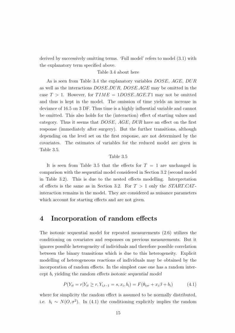
derived by successively omitting terms. ‘Full model’ refers to model (3.1) with

the explanatory term specified above.

Table 3.4 about here

As is seen from Table 3.4 the explanatory variables DOSE, AGE, DUR

as well as the interactions DOSE.DUR, DOSE.AGE may be omitted in the

case T > 1. However, for TIME = 1DOSE.AGE.T1 may not be omitted

and thus is kept in the model. The omission of time yields an increase in

deviance of 16.5 on 3 DF. Thus time is a highly influential variable and cannot

be omitted. This also holds for the (interaction) effect of starting values and

category. Thus it seems that DOSE, AGE, DUR have an effect on the first

response (immediately after surgery). But the further transitions, although

depending on the level set on the first response, are not determined by the

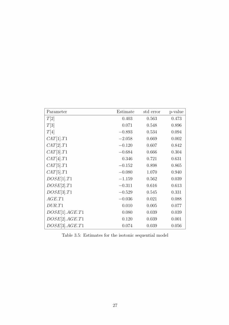
covariates. The estimates of variables for the reduced model are given in

Table 3.5.

Table 3.5

It is seen from Table 3.5 that the effects for T = 1 are unchanged in

comparison with the sequential model considered in Section 3.2 (second model

in Table 3.2). This is due to the nested effects modelling. Interpretation

of effects is the same as in Section 3.2. For T > 1 only the START.CAT -

interaction remains in the model. They are considered as nuisance parameters

which account for starting effects and are not given.

4 Incorporation of random effects

The isotonic sequential model for repeated measurements (2.6) utilizes the

conditioning on covariates and responses on previous measurements. But it

ignores possible heterogeneity of individuals and therefore possible correlation

between the binary transitions which is due to this heterogeneity. Explicit

modelling of heterogeneous reactions of individuals may be obtained by the

incorporation of random effects. In the simplest case one has a random inter-

cept bi yielding the random effects isotonic sequential model

P (Yit = r|Yit ≥ r, Yi,t−1 = s, xi, bi) = F (θtsr + xiβ + bi) (4.1)

where for simplicity the random effect is assumed to be normally distributed,

i.e. bi ∼ N(O, σ2). In (4.1) the conditioning explicitly implies the random

15

effects bi. Estimation of the structured parameters θtsr, β, σ2 is based on the

marginal likelihood. Using the representation as binary transitions derived in

Section 2.3 the marginal log-likelihood has the form

l({θtsr}, β, σ2) =n∑

i=1

log

∫f(yi|bi)p(bi; σ

2)dbi (4.2)

where p(bi; σ2) denotes the density of the random effects bi and the binary

transitions of individual i are collected in

f(yi|bi) =m∏

t=1

yit∏r=yi,t−1

F (ηitr)yitr (1 − F (ηitr))

1−yitr

where

ηitr = θt,yi,t−1,r+ x′

iβ + bi

Since the observations are given as binary variables the framework of uni-

variate generalized linear mixed models (GLMMs) may be used. The main

problem in GLMMs is that the marginal distribution of the response obtained

by integrating out the random effects, does not have closed from. This led to

the development of several methods to obtain analytical approximation for the

likelihood, like numerical integration based on Gauss-Hermite quadrature (e.g.

Hinde (1982), Anderson & Aitkin (1985)) or Monte Carlo techniques within the

EM-algorithm (McCulloch (1994), McCulloch (1997), Booth & Hobert (1999))

or approximation methods as Taylor expansions or Laplace approximation (e.g.

Breslow & Clayton (1993), Wolfinger & O’Connell (1993), Longford (1994)).

A more recent approach is nonparametric maximum likelihood which avoids

the assumption of a fixed distribution for the random effects (Aitkin (1996),

Aitkin (1999)). In the following evaluation of the integral in (4.2) is based

on Gauss-Hermite quadrature within the EM-algorithm and the approach of

Wolfinger & O’Connell (1993) which is implement in the SAS macro GLIM-

MIX. For Gauss-Hermite quadrature let the unknown parameters be collected

in α. Then in the E-step of the (p + 1)th EM cycle one has to determine

M(α|α(p)) =n∑

i=1

k−1i

∫[log f(yi|bi; α) + log g(ai)] f(yi|bi, α

(p))g(bi)dbi

where

ki =

∫f(yi|bi, α

(p))g(bi)dbiα(p)

16

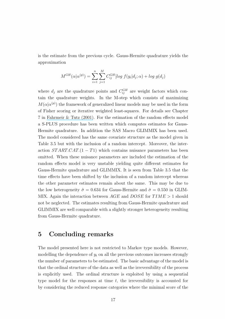
is the estimate from the previous cycle. Gauss-Hermite quadrature yields the

approximation

MGH(α|α(p)) =n∑

i=1

M∑j=1

CGHij [log f(yi|dj; α) + log g(dj)

where dj are the quadrature points and CGHij are weight factors which con-

tain the quadrature weights. In the M-step which consists of maximizing

M(α|α(p)) the framework of generalized linear models may be used in the form

of Fisher scoring or iterative weighted least-squares. For details see Chapter

7 in Fahrmeir & Tutz (2001). For the estimation of the random effects model

a S-PLUS procedure has been written which computes estimates for Gauss-

Hermite quadrature. In addition the SAS Macro GLIMMIX has been used.

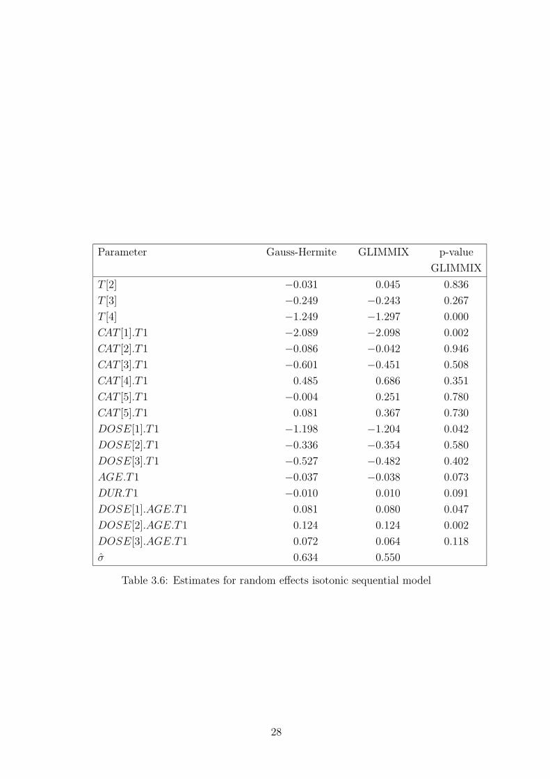
The model considered has the same covariate structure as the model given in

Table 3.5 but with the inclusion of a random intercept. Moreover, the inter-

action START.CAT.(1 − T1) which contains nuisance parameters has been

omitted. When these nuisance parameters are included the estimation of the

random effects model is very unstable yielding quite different estimates for

Gauss-Hermite quadrature and GLIMMIX. It is seen from Table 3.5 that the

time effects have been shifted by the inclusion of a random intercept whereas

the other parameter estimates remain about the same. This may be due to

the low heterogeneity σ = 0.634 for Gauss-Hermite and σ = 0.550 in GLIM-

MIX. Again the interaction between AGE and DOSE for TIME > 1 should

not be neglected. The estimates resulting from Gauss-Hermite quadrature and

GLIMMIX are well comparable with a slightly stronger heterogeneity resulting

from Gauss-Hermite quadrature.

5 Concluding remarks

The model presented here is not restricted to Markov type models. However,

modelling the dependence of yt on all the previous outcomes increases strongly

the number of parameters to be estimated. The basic advantage of the model is

that the ordinal structure of the data as well as the irreversibility of the process

is explicitly used. The ordinal structure is exploited by using a sequential

type model for the responses at time t, the irreversibility is accounted for

by considering the reduced response categories where the minimal score of the

17

present response is set by the outcome of the previous time point measurement.

The analysis is not restricted to effects of covariates on marginal responses. It

allows to analyze the effects on the conditional transitions following the first

response.

An advantage of the model is that it can be embedded into models for

dichotomous responses. Therefore, it can be easily fitted after suitable data

transformation by using standard procedures for dichotomous responses. The

incorporation of heterogeneity uses the same data transformations. With the

increasing availability of programmes which handle mixed models with di-

chotomous responses it may be easily applied to data. Although the model is

developed within a parametric framework the extension to nonparametric mod-

elling where the linear predictor is replaced by additive or varying coefficients

effects is straightforward. Semi- and nonparametric models for dichotomous

models are discussed e.g. in Hastie & Tibshirani (1990).

Acknowledgement:

Support from SFB funded by Deutsche Forschungsgemeinschaft is grateful

acknowledged. Thanks to L. Heigenhauser and F. Reithinger for their support

with computations.

18

References

Agresti, A. (1999). Modelling ordered categorical data: Recent advances

and future challenges. Statistics in Medicine 18, 2191–2207.

Agresti, A. (2002). Categorical Data Analysis. New York: Wiley.

Aitkin, M. (1996). A general maximum likelihood analysis of overdispersion

in generalized linear models. Statistics and Computing 6, 251–262.

Aitkin, M. (1999). A general maximum likelihood analysis of variance com-

ponents in generalized linear models. Biometrics 55, 117–128.

Anderson, D. A. and Aitkin, M. (1985). Variance component models with

binary response: Interviewer variability. Journal of the Royal Statistical

Society Ser. B 47, 203–210.

Armstrong, B. and Sloan, M. (1989). Ordinal regression models for epidemi-

ologic data. American Journal of Epidemiology 129, 191–204.

Barnhart, H. and Sampson, A. (1994). Overviews of multinomial models for

ordinal data. Comm. Stat-Theory & Methods 23(12), 3395–3416.

Bonney, G. (1987). Logistic regression for dependent binary observations.

Biometrics 43, 951–973.

Booth, J. G. and Hobert, J. P. (1999). Maximizing generalized linear mixed

model likelihoods with an automated Monte Carlo EM algorithm. J. R.

Statist. Soc B 61, 265–285.

Brant, R. (1990). Assessing proportionality in the proportional odds model

for ordinal logistic regression. Biometrics 46, 1171–1178.

Breslow, N. E. and Clayton, D. G. (1993). Approximate inference in gener-

alized linear mixed model. Journal of the American Statistical Associa-

tion 88, 9–25.

Cox, C. (1988). Multinomial regression models based on continuation ratios.

Statistics in Medicine 7, 433–441.

Cramer, J. S. (1991). The Logit Model. New York: Routhedge, Chapman &

Hall.

Davis, C. S. (1991). Semi-parametric and non-parametric methods for the

analysis of repeated measurements with applications to clinical trials.

Statistics in Medicine 10, 1959–1980.

19

Fahrmeir, L., Gieger, C., and Heumann, C. (1999). An application of iso-

tonic longitudinal marginal regression to monitoring the healing process.

Biometrics 55, 951–956.

Fahrmeir, L. and Tutz, G. (2001). Multivariate Statistical Modelling based

on Generalized Linear Models (2nd ed.). New York: Springer.

Greenland, S. (1994). Alternative models for ordinal logistic regression.

Statistics in Medicine 13, 1665–1677.

Hastie, T. and Tibshirani, R. (1990). Generalized Additive Models. London:

Chapman & Hall.

Hinde, J. (1982). Compound poisson regression models. In R. Gilchrist (Ed.),

GLIM 1982 Internat. Conf. Generalized Linear Models, New York, pp.

109–121. Springer-Verlag.

Laara, E. and Matthews, J. N. (1985). The equivalence of two models for

ordinal data. Biometrika 72, 206–207.

Liang, K.-Y., Zeger, S. L., and Qaqish, B. (1992). Multivariate regression

analysis for categorical data (with discussion). Journal of the Royal Sta-

tistical Society B 54, 3–40.

Longford, N. T. (1994). Random coefficient models. In G. Arminger,

C. Glogg, & M. Sobel (Eds.), Handbook of Statistical Modelling for the

Behavioural Sciences. New York: Plenum.

McCullagh, P. (1980). Regression model for ordinal data (with discussion).

Journal of the Royal Statistical Society B 42, 109–127.

McCulloch, C. E. (1994). Maximum likelihood variance components estima-

tion for binary data. J. Am. Statist. Assoc. 89, 330–335.

McCulloch, C. E. (1997). Maximum likelihood algorithms for generalized

linear mixed models. Journal of the American Statistical Association 92,

162–170.

Moulton, L. and Zeger, S. (1989). Analysing repeated measures in general-

ized linear models via the bootstrap. Biometrics 45, 381–394.

Stram, D. O. and Wei, L. J. (1988). Analyzing repeated measurements

with possibly missing observations by modelling marginal distributions.

Statistics in Medicine 7, 139–148.

20

Stram, D. O., Wei, L. J., and Ware, J. H. (1988). Analysis of repeated cate-

gorical outcomes with possibly missing observations and time-dependent

covariates. Journal of the American Statistical Association 83, 631–637.

Tutz, G. (1991). Sequential models in ordinal regression. Computational

Statistics & Data Analysis 11, 275–295.

Wolfinger, R. and O’Connell, M. (1993). Generalized linear mixed models;

a pseudolikelihood approach. Journal Statist. Comput. Simulation 48,

233–243.

21

Dichotomous response Predictor

yitr θtsr xi

t = 1 yi11 = 0 θ111 xi

......

yi1,r1−1 = 0 θ11,r1−1 xi

yi1,r1 = 1 θ11,r1 xi

t = 2 yi2r1 = 0 θ2r1r1 xi

......

yi2,r2−1 = 0 θ2r1,r2−1 xi

yi2,r2 = 1 θ2r1,r2 xi

......

t = m yim,rm−1 = 0 θmrm−1rm−1 xi

......

yim,rm−1 = 0 θmrm−1,rm−1 xi

yim,rm = 1 θmrm−1,rm xi

Table 2.1: Dichotomous observations yitr entering the likelihood contribution

Li for response categories 1 ≤ r1 ≤ . . . ≤ rm

22

Estimate p-value Estimate p-value Estimate p-value

DOSE[1] −3.604 1.873 −1.519 0.727 −1.009 0.680

DOSE[2] −1.670 1.927 −0.513 0.758 −0.904 0.701

DOSE[3] −2.995 1.935 −0.607 0.702 −0.375 0.676

AGE −0.042 0.024 −0.044 0.024 0.011 0.015

DUR −0.009 0.020 0.013 0.007 0.011 0.006

DOSE[1].AGE 0.088 0.048 0.091 0.047

DOSE[2].AGE 0.143 0.047 0.146 0.046

DOSE[3].AGE 0.053 0.048 0.058 0.048

DOSE[1].DUR 0.028 0.023

DOSE[2].DUR 0.016 0.024

DOSE[3].DUR 0.032 0.024

Deviance 178.99 181.23 193.27

df 343 346 349

Deviance DOSE.DUR DOSE.AGE

for effects 2.24 12.04

df 3 3

Table 3.1: Estimates for three cumulative logistic models with varying covari-

ate effects included (T = 1)

23

Estimate std error Estimate std error Estimate std error

DOSE[1] −2.467 1.592 −1.159 0.562 −0.600 0.504

DOSE[2] 0.013 1.667 −0.311 0.616 −0.596 0.581

DOSE[3] −1.928 1.662 −0.529 0.544 −0.121 0.521

AGE −0.036 0.021 −0.036 0.021 0.016 0.013

DUR −0.000 0.018 0.010 0.005 0.007 0.005

DOSE[1].AGE 0.081 0.039 0.080 0.039

DOSE[2].AGE 0.116 0.039 0.120 0.039

DOSE[3].AGE 0.074 0.039 0.074 0.039

DOSE[1].DUR 0.017 0.020

DOSE[2].DUR −0.002 0.021

DOSE[3].DUR 0.019 0.022

Deviance 177.92 180.81 192.90

df 343 346 349

Deviance DOSE.DUR DOSE.AGE

for effects T = 1 2.89 12.09

T = 2 1.226 5.767

T = 3 4.775 1.994

df 3 3

Table 3.2: Estimates for sequential logistic models with varying covariate ef-

fects included (T = 1)

24

ContinuationResponse at T=2 ratios

1 2 3 4 5 6 7 Σ T=11 5 1 2 1 0 1 0 10 0.16 (10/60)2 0 18 2 3 1 0 0 24 0.48 (24/50)

Response 3 0 0 2 5 1 0 0 8 0.30 (8/26)at 4 0 0 0 2 2 3 2 9 0.50 (9/18)

T=1 5 0 0 0 0 1 1 1 3 0.33 (3/9)6 0 0 0 0 0 0 2 2 0.33 (2/6)7 0 0 0 0 0 0 4 4 1.00 (4/4)

ContinuationResponse at T=3 ratios

1 2 3 4 5 6 7 Σ T=21 4 0 0 0 1 0 0 5 0.08 (5/60)2 0 12 2 0 3 2 0 19 0.34 (19/55)

Response 3 0 0 3 1 0 0 2 6 0.16 (6/36)at 4 0 0 0 5 1 3 2 11 0.36 (11/30)

T=2 5 0 0 0 0 1 1 3 5 0.26 (5/19)6 0 0 0 0 0 3 2 5 0.35 (5/14)7 0 0 0 0 0 0 9 9 1.00 (9/9)

ContinuationResponse at T=4 ratios

1 2 3 4 5 6 7 Σ T=31 2 0 0 2 0 0 0 4 0.06 (4/60)2 0 2 0 3 4 0 3 12 0.21 (12/56)

Response 3 0 0 1 2 1 1 0 5 0.11 (5/44)at 4 0 0 0 0 0 4 2 6 0.15 (6/39)

T=3 5 0 0 0 0 1 0 5 6 0.18 (6/33)6 0 0 0 0 0 3 6 9 0.33 (9/27)7 0 0 0 0 0 0 18 18 1.00 (18/18)

Continuation 2 2 1 7 6 8 34 60ratios 0.03 0.03 0.02 0.12 0.12 0.19 1.00T=4 (2/60) (2/58) (1/56) (7/55) (6/48) (8/42) (34/34)

Table 3.3: Frequencies of transitions and marginal distributions

25

Successively omitted Deviance df Deviance dfeffect of effects

Full Model 513.58 425

DOSE.DUR.(1 − T ) 516.68 428 3.10 3

DOSE.AGE.(1 − T ) 520.75 431 4.07 3

DUR.(1 − T ) 522.58 432 1.83 1

AGE.(1 − T ) 524.88 433 2.29 1

DOSE.(1 − T ) 526.28 436 1.40 3

TIME.(1 − T ) 538.36 439 12.08 3

Table 3.4: Sequential models for irreversible processes including CAT , DOSE,

AGE, DUR, DOSE.AGE at TIME = 1, START.CAT , DOSE, AGE, DUR,

DOSE.AGE, DOSE.DUR at TIME > 1 and TIME.

26

Parameter Estimate std error p-value

T [2] 0.403 0.563 0.473

T [3] 0.071 0.548 0.896

T [4] −0.893 0.534 0.094

CAT [1].T1 −2.058 0.669 0.002

CAT [2].T1 −0.120 0.607 0.842

CAT [3].T1 −0.684 0.666 0.304

CAT [4].T1 0.346 0.721 0.631

CAT [5].T1 −0.152 0.898 0.865

CAT [5].T1 −0.080 1.070 0.940

DOSE[1].T1 −1.159 0.562 0.039

DOSE[2].T1 −0.311 0.616 0.613

DOSE[3].T1 −0.529 0.545 0.331

AGE.T1 −0.036 0.021 0.088

DUR.T1 0.010 0.005 0.077

DOSE[1].AGE.T1 0.080 0.039 0.039

DOSE[2].AGE.T1 0.120 0.039 0.001

DOSE[3].AGE.T1 0.074 0.039 0.056

Table 3.5: Estimates for the isotonic sequential model

27

Parameter Gauss-Hermite GLIMMIX p-value

GLIMMIX

T [2] −0.031 0.045 0.836

T [3] −0.249 −0.243 0.267

T [4] −1.249 −1.297 0.000

CAT [1].T1 −2.089 −2.098 0.002

CAT [2].T1 −0.086 −0.042 0.946

CAT [3].T1 −0.601 −0.451 0.508

CAT [4].T1 0.485 0.686 0.351

CAT [5].T1 −0.004 0.251 0.780

CAT [5].T1 0.081 0.367 0.730

DOSE[1].T1 −1.198 −1.204 0.042

DOSE[2].T1 −0.336 −0.354 0.580

DOSE[3].T1 −0.527 −0.482 0.402

AGE.T1 −0.037 −0.038 0.073

DUR.T1 −0.010 0.010 0.091

DOSE[1].AGE.T1 0.081 0.080 0.047

DOSE[2].AGE.T1 0.124 0.124 0.002

DOSE[3].AGE.T1 0.072 0.064 0.118

σ 0.634 0.550

Table 3.6: Estimates for random effects isotonic sequential model

28