Private Information in Repeated Auctions∗

Johannes Hörner and Julian S. JamisonMEDS, Kellogg SchoolNorthwestern University

February 7, 2003

Abstract

We study an infinitely repeated two-player game with incomplete information, where the stage game is afirst-price auction with pure common values. Before playing, the bidders receive affiliated private signals aboutthe value, which itself does not change over time. Items sold in such an auction environment include bonds,wine, neighboring oil tracts, and wholesale fish. In this setting, learning occurs only through observation ofthe bids. We show that in the case of one-sided incomplete information, this information is eventually revealedand the seller extracts essentially the entire rent (for large enough discount factors). In contrast, the uniqueequilibrium with patient players under two-sided incomplete information is purely pooling: no information isever revealed. In the special case with only two types of each bidder, we are able to fully characterize theequilibrium for all values of the discount factor and all priors.

1 IntroductionThis paper analyzes an infinitely-repeated, first-price auction between two players with private information aboutthe common value of all the units. It generalizes Engelbrecht-Wiggans and Weber (1983), which solves thefinite-horizon, binary type, one-sided incomplete information case.We are primarily interested in the optimal strategy of the bidders: how can a bidder exploit his private

information without giving it away? How valuable is private information to a bidder? A related concern is theinformational content of the prices: are prices revealing and aggregating the players’ information? In this sense,our motivation is close to Kyle (1985), who analyses continuous auctions and insider trading, although there isno noise trading in our model.1

Information revelation in repeated first-price auctions has already been studied by Hon-Snir, Monderer andSela (1998), in a model with independent private values. They show that information is eventually fully revealed.However, because “equilibrium analysis of repeated first-price auctions in the framework of repeated games withincomplete information is complex”, they assume that players are not rational but use learning schemes.In contrast with these findings, our results imply that when players are patient and rational, prices do not

reveal any information at all. That is, the unique equilibrium (subject to a refinement that actually helps theseller) exhibits the ratchet effect identified in games with one-sided incomplete information by Freixas-Guesnerie-Tirole (1985) and Hart-Tirole (1988). Here, both bidders make low bids consistent with their worst private

∗We thank Olivier Gossner, participants at the Northwestern theory lunch, and especially Bob Weber. All comments are welcome!1Another difference is that in his model, bidders choose quantities and the price clears the markets. Because in his model bidders

foresee how their action affects the price, just as in our model bidders foresee how their action affects their probability of winning,this distinction is merely interpretative.

1

information, even when their estimate is high, and prefer to win half of the time at such a low price, rather thanbreak the tie in their favor and divulge thereby some of their information.This result may appear surprising to the reader familiar with Engelbrecht-Wiggans and Weber (1983). After

all, these authors establish that, with one-sided incomplete information, information is eventually fully revealed,and we show that their insight carries over to the infinite-horizon case and to a more general set-up. However, wealso show that there is a significant difference between one-sided incomplete information and two-sided incompleteinformation, even if beliefs are degenerate.Our results imply that, for repeated first-price auctions, such as treasury bills, the auctioneer’s revenue from

the sequential procedure is lower than under a one-time batch sale if bidders are patient enough, or alternatively,the frequency of auctions is very high.This paper builds on Engelbrecht-Wiggans and Weber (1983), which investigates the undiscounted, finite-

horizon version of this game in which only one player has binary, private information. One of their strikingconclusions is that being uninformed is an advantage if the horizon is long enough. Also, the seller’s expectedrevenue is larger under the one-stage batch sale than under the sequential auction if the initial probability ofa high valuation is sufficiently large. Our results imply that their main conclusions do not rely on backwardinduction and remain valid when the horizon is infinite and players are sufficiently patient, because, as willbe seen, when incomplete information is one-sided, a date T is endogenously determined such that, along anyequilibrium outcome, a high-signalled bidder has revealed his information by time T .Two other papers are closely related to his one. First, Hausch (1986), building on Ortega-Reichert (1968),

considers a two-person, two stage first-price auction with common values. At the beginning of the game, biddersreceive conditionally independent signals about the identical value of the two units. The value of the objects tothe players is additive. Thus, Hausch’s setting corresponds to the two-period, undiscounted symmetric versionof this model (but it is richer inasmuch as signals are not necessarily perfectly informative). He shows that itis impossible that a high-signalled player’s bid always reveals his signal in the first auction. Instead, either healways conceal his signal in the first auction by bidding like a low-signalled player (pooling), or he randomizesbetween concealing and revealing his signal in the first auction (semi-pooling). When each object is worth onewith probability p, and 0 otherwise, the second possibility arises for p sufficiently large.Second, Bikhchandani (1988) examines a finitely repeated second-price auction with common values between

two bidders. The value of the objects to the players is additive, and identically and independently drawn froma common distribution. Both players receive conditionally independent signals about the value of each unit, butone of the bidders is of one of two possible types (and this is private information). The strong type’s valuation ofany given unit is higher, by a multiplicative constant, than the low type’s valuation. Because winning is especiallybad news for the uninformed player when his opponent may be of the high type, the winner’s curse is intensifiedfor the uninformed player, forcing him to submit lower bids in equilibrium. This weakens the winner’s curse forthe informed bidder of the ordinary type and decreases the price he has to pay whenever he wins. The ordinarytype has therefore an initial incentive to mimic the strong type by making high bids.Finally, a more general analysis of repeated games with incomplete information has been carried out by

Aumann, Maschler and Stearns (1966-68).It may be worthwhile to point out that several goods are sold in repeated first-price auctions, such as various

types of government bonds and red Bordeaux wines. See Ashenfelter (1989) for more examples. Pezanis-Christou(2000) has collected and analyzed evidence from a fish market with asymmetric buyers (retailers vs. wholesalers).As he points out, fish markets are characterized by supply uncertainty.Section 2 presents the basic model. Section 3 characterizes the equilibrium for the general case of one-sided

incomplete information. Section 4 proves our central result that the unique equilibrium (for large δ) in the two-sided case is purely pooling. Section 5 explores the special case with only two types of each bidder, where we areable to describe the outcomes for general δ, and prove uniqueness in the symmetric case for all δ and all priors p.Finally, section 6 concludes briefly.

2

2 The ModelThis paper considers an infinitely-repeated game between two risk-neutral bidders, player 1 and player 2. In everyperiod t = 0, 1, . . . one indivisible unit is sold using a sealed-bid first-price auction. In case of a tie, each playerwins with equal probability. We assume common values:Assumption 1: Both bidders value each unit identically.All units auctioned off have the same value, represented by the random variable V . That is, we assume perfect

correlation over time:Assumption 2: The value of the units from one period to the next is perfectly correlated.Before the game starts, each bidder i (i = 1 or 2) receives a signal Si concerning the value of the object. The

signal can take m + 1 different values for player 1, and n + 1 different values for player 2, that is, S1 ∈ M ={0, 1, . . . ,m}, S2 ∈ N = {0, 1, . . . , n}. Signals are also referred to as types. A high (low) signal is statisticalevidence for a high (low) value of the object. This is formalized by:Assumption 3: The variables V , S1 and S2 are affiliated.Affiliation is developed in Milgrom and Weber. Let x = (v, j, k), x0 = (v0, l,m) be elements of R ×M ×N .

Let x̄ and x be respectively the componentwise maximum and componentwise minimum of x and x0. Then if(V, S1, S2) has the joint density f , these variables are affiliated if, for all x and x0, f (x̄) f (x) = f (x) f (x0). Thisimplies that v (j, k) , E [V | S1 = j, S2 = k] is weakly increasing in each of its arguments. Let p (j, k) denote theprobability that S1 = j and S2 = k. Finally,we denote by Ek[v(j, k)] the expected value of a type j player 1:

Ek[v(j, k)] =

Pnk=0 p(j, k)v(j, k)Pn

k=0 p(j, k)

and similarly for Ej [v(j, k)]. The last assumption on parameters can be dispensed with at the expense of trivialcomplications.Assumption 4: (i) The function v (j, k) is strictly increasing in each of its arguments; (ii) v (0, 0) = 0; (iii)

p (j, k) > 0 for all (j, k) ∈M ×N .Players maximize their payoff, which is the discounted sum of their profit in each auction, using a common

discount factor δ ∈ [0, 1). Therefore, their utility does not exhibit “diminishing marginal returns” for winningmore units. We emphasize that players do not learn the value of a unit upon buying it. Learning, therefore, isrestricted to inferring one’s rival’s information.The solution concept used is Perfect Bayesian Equilibrium (P.B.E.). We further wish to prune any equilibrium

which depends on payoff irrelevant information, and therefore assume that continuation play only depends on (allplayers’) current beliefs. That is, if there exist two histories after which every type of every player entertains thesame beliefs about its opponent, then the actions that follow these histories are the same as well.2 In addition,we impose two refinements.First, we assume “no underbidding”. Under perfect information, if all units are known to be worth v > 0,

there exist many equilibria. For instance, for any b ∈ [0, v], there exists an equilibrium in which both players bidb repeatedly on the equilibrium path. Because our focus is not on collusion per se, we assume that bids are atleast as large as what the unit is commonly known to be worth, conditional on winning. In this example, “nounderbidding” requires bids to be at least v in every period. Note that this refinement benefits the seller, and yetone of our main findings is that the auctioneer’s revenue is low.Second, we assume “no overbidding”. That is, a bidder observing a bid b or b+ (see below for explanation of

+ bids) assigns henceforth, if possible, zero probability to all types of his opponent for which such a bid strictlyexceeds the maximal possible value of a unit, given their type and beliefs.A bid is a winning bid if it is equal to the highest bid with strictly positive probability. Formally:Assumption 5: In period t,

2 If this assumption is not imposed, additional “reputational” equilibria exist, as discussed in the concluding comments.

3

(i) (stationarity) Actions chosen only depend on current beliefs.3

(ii) (no underbidding) The lowest winning bid is at least equal, for some player’s type assigned positiveprobability, to his expected value of the unit conditional on winning with this bid. Also, if b is an equilibriumbid, then there is a winning bid no larger than b+ ε, for any ε > 0.(iii) (no overbidding) Upon observing a bid b, i’s beliefs assign thereafter zero probability to any type for

whom b is strictly more than the (conditional) essential supremum of V .Assumptions (i) and (ii) are necessary for our uniqueness result, and other equilibria that can be supported

in their absence are described in the concluding comments. We do not know whether more equilibrium outcomesare introduced if we drop assumption (iii).Finally, given our tie-breaking rule, we cannot always guarantee existence under the assumptions above. In

that case, we allow for a bid b+ that is infinitesimally larger than b. One can think of b+ as b “plus a penny”.Although a player’s utility from a winning bid of b is the same as from a winning bid of b+, a bid of b+ is strictlylarger than a bid of b, so that the distinction matters in light of Assumption 5(iii). Such a nonstandard bidb+ is only necessary for b the lowest bid made with positive probability, so that, unless specified otherwise, allsymbols and commonly used concepts (support, interval, etc.) refer to the real line and its standard structure.Engelbrecht-Wiggans and Weber (1983) introduce the same idea, and it is indeed exactly in our extension of theirmodel that we will require it. Any claims of uniqueness that we make for equilibria that utilize nonstandard bidsare, of course, within the class of all strategies using such bids anywhere in the support.

3 One-sided Incomplete InformationSuppose that M has m+ 1 > 1 elements, while N has only one element. Accordingly, we refer to player 1 as theinformed player, or player I, and to player 2 as the uninformed player, or player U , and we write v (j) instead ofv (j, 0), where (j, 0) ∈M ×N . Given Assumption 5(ii), normalize v (0) to 0. The solution to the one-sided staticmodel is a special case of the two-sided version (see section 4.3).Given an equilibrium, let H∗t be the subset of t−histories Ht (including the null history) that have positive

probability under the equilibrium strategies, and let H 0t ⊆ H∗t be the set of histories in which the bids of the

informed bidder have been equal to zero for all periods up to t. Let γti be the probability with which player I isof type i and makes a strictly positive bid in period t, conditional on some ht ∈ H 0

t, and let pti be the probability

that player I is of type i, conditional on the same event. Because of 5(i), γti does not depend on the specificht ∈ H 0

t. By Bayes’ rule,

pt+1i =pti − γti

1−Pmi=0 γ

ti

,

where p0i = pi. By 5(iii), the informed bidder’s type 0 bids 0 with probability one, so that γt0 = 0, all t, andaccordingly 1−Pm

i=0 γti = pt0/p

t+10 . For i > 0, let Ti = inf

©t ∈ N ; pt+1i = 0, ∀ht ∈ H∗t

ª, that is, Ti is the length

of the longest equilibrium history in which, given that the informed bidder is of type i, all bids by the informedbidder have been 0. Let πti be the (normalized) payoff of the informed player’s type i from period t on, givenht ∈ H∗t . Let Ut denote the uninformed bidding distribution in period t conditional on the same event and πtUthe corresponding (normalized) payoff. Finally, let Sti be the support of the bid distribution by the informedplayer’s i type, in period t, conditional on the same event. Let St = ∪Sti , let StU be the uninformed player’s biddistribution support in period t given ht ∈ H 0

t and set βt = max {x ∈ R | x ∈ StU}. We prove that:

Theorem 1 ∃δ0 < 1: ∀δ ∈ (δ0, 1), Ti = maxj Tj , T < ∞, for all i ∈ M\{0}. In addition, limδ→1 T = ∞,limδ→1 δT = 1, limδ→1 π0U = 0, and limδ→1 π0U/π

0i =∞, all i.

3Formally, we mean beliefs of all orders (so that the assumption is as weak as possible), but note that in any case we will use thisonly when beliefs on one side are [commonly known to be] degenerate.

4

This theorem states that, as players become more patient, type i > 0 of the informed player can bid 0 in upto but no more than T periods, where T is independent of his type. Although limδ→1 T = ∞, δT → 1, so thatplayers’ payoffs depend essentially on their payoff after T . Both players’ normalized payoff tends to zero, but theuninformed bidder still fares better than the informed bidder.Proof. This result will be proved in several steps.

1. π0m > 0: by 5(iii), an informed bidder with signal i does not bid more than v (i). If β0 5 v (m− 1),then π0m = (1− δ) (v (m)− v (m− 1)) > 0. If β0 > v (m− 1), then β0 outbids all types of the informedplayer but the highest, so that, conditional on winning, the unit is worth at most the (unconditional)expected value of V , EV , and because the uninformed player could bid 0 instead, β0 5 EV , so thatπ0m = (1− δ) (v (m)−EV ) > 0 as well.

2. ∀ht ∈ H 0t such that t < T , Ut (0) = 0: indeed, bidding 0+ yields a higher payoff than 0, since, conditional on

the informed bidder’s bid being 0, the unit’s expected value is strictly positive, and the uninformed bidder’scontinuation payoff does not depend on his own bid, by 5(i).

3. Ti < ∞, all i ∈ M : suppose that Tm = ∞. Then the informed bidder’s type m is willing to bid 0 inevery period, which yields a payoff of 0, as Ut (0) = 0 for all t. This contradicts π0m > 0, by (1). In turn,this implies that π0m−1 = δTm (1− δ)

¡v (m− 1)−max ¡Pi<m ptiv (i) , v (m− 2)

¢¢> 0, so that, by the same

argument, Tm−1 <∞. An easy induction establishes now the result.4. ∀ht ∈ H 0

t, βt > 0+: otherwise, the lowest, strictly positive type of the informed bidder which still haspositive probability given ht must bid slightly more than βt with probability one, so that the uninformedbidder could profitably deviate by bidding more.

Let αt = max {x ∈ R | x ∈ St}. ∀ht ∈ H 0t, αt > 0+, since βt > 0+ and the uninformed bidder would gain

otherwise by bidding slightly less than βt. Define also τ = inf {t ∈ N ;βt ∈ St1}.5. If b ∈ St1, b > 0, then (0, b) ⊂ St1: otherwise, there exists either some interval I ⊆ (0, b), I ∩ St = ∅, orthere exists b0 ∈ (0, b) such that j = min {k ∈M | b0 ∈ Stk} > 1. The former is impossible by the standardargument (at least one of the players bidding just slightly above I would gain by bidding less), and thesecond would violate the payoff’s single-crossing property, given that the informed bidder’s type 1 (resp.type j) has no continuation payoff from bidding b (resp. b0).

6. ∀1 5 t 5 T, Ut (0+) > Ut−1 (0+): otherwise, if Ut−1 (0+) = Ut (0+), there exists ε > 0 sufficiently smallso that the informed player’s lowest type bidding ε in period t would gain from bidding ε in period t − 1instead. This implies that, in particular, for ε > 0 sufficiently small, ε ∈ St−11 implies that ε ∈ St1: otherwiseone derives a contradiction as in (5) by considering ε ∈ St−11 and ε ∈ Stj , for j = min {k ∈ N | b ∈ Stk} > 1.

7. T1 = T : if b ∈ St1, b > 0, and t < T , then (0, b) ⊂ St1 by (5), and (6) implies that, for ε > 0 small, ε ∈ St+11 .

8. τ < ∞. If maxi>1 Ti < T , then this is obvious. If not, it must also be that βT ∈ ST1 : Suppose not, thatis, suppose that γ = max

©x ∈ R | x ∈ ST1

ª< β. By definition of T , γ > 0. Recall that by (5), this implies

that (0, γ) ⊂ ST1 , and therefore, for every b < γ, the uninformed player’s posterior upon observing sucha bid assigns positive probability to type 1. For all ε > 0 sufficiently small, there exists a lowest type j(possibly depending on ε) of the informed player for which γ + ε is in his bidding support. We claim thatthere exists ε small enough so that this type j would benefit from bidding γ−ε instead of γ+ε. Because UTis continuous on (γ − 2ε, γ + 2ε), it is sufficient to show that the continuation payoff from bidding γ − ε isbounded away from zero (because j is the lowest type bidding γ+ε, his continuation payoff from such a bidis zero). This is trivial if type 1 is the only type bidding γ − ε, and follows from straightforward argumentsin general (the bid support of the uninformed player in such a subgame has v (1) has a lower extremity, and

5

its distribution function, evaluated, say, at [v (1) + v (j)] /2 is bounded away from zero, ensuring that sucha bid yields strictly positive profit to type j).

9. limδ→1 δT−τ = 1. Clearly, ∀ε > 0, |αt − βt| < ε for all t, ht ∈ H 0t (the lowest type of the player bidding the

higher of the two would gain by bidding less). In addition, neither player’s bidding distribution can havean atom at the maximum of its support: if the uninformed bidder had such an atom, the informed bidder’slowest type j for which αt ∈ Stj would gain by bidding αt + ε instead; if the informed bidder had, thenbecause all informed bidder’s types j making such a bid must have valuation v (j) > βt, the uninformedbidder would gain by bidding βt + ε instead, for ε > 0 small enough. Therefore, if the uninformed bidderbids βt, he wins with probability one. For any t such that τ 5 t 5 T , and any ht ∈ H 0

t, βt must bedecreasing in t, because if βt < βt+1, the lowest type of the informed bidder ’s type i whose support S

t+1i

includes βt+1 would strictly gain from bidding βt in period t instead. Because the uninformed bidder isindifferent between bidding βt and 0+ in any such period,Ã

1−mXi=1

γti

!mXi=1

pt+1i v (i) =mXi=1

ptiv (i)− βt,

which implies that βt =Pm

i=1 γtiv (i) =

Pmi=1

¡pti − pt0p

t+1i /pt+10

¢v (i). Because pti/p

t0 is decreasing in t for

all i, βt > ε > 0 implies

v (m)mXi=1

µptipt0− pt+1i

pt+10

¶=

mXi=1

µptipt0− pt+1i

pt+10

¶v (i) > ε/pt0 > ε,

so that, if βt > ε all t ∈hτ , τ + T̂

i, then κ =

Pi>0 p

τ+T̂i /pτ+T̂0 + T̂ ε/v (m) , so that T̂ 5 v (m)κ/ε. Hence,

for all ε > 0, πτ1 = (1− δ) δv(m)κ/ε (v (1)− ε), which tends to (1− δ) (v (1)− ε), as δ tends to 1. Becausethis argument is independent of ε, πτ1/ (1− δ)→ v (1) as δ → 1, and because the informed bidder’s type 1is willing to bid 0 instead for T − τ additional periods, it must be that limδ→1 δT−τ = 1.

10. τ = 0: otherwise, the lowest type bidding βτ−1 after a history hτ−1 ∈ H 0τ−1 would strictly gain from bidding

0 in the following T − τ + 1 periods, given the arguments developed in (8).

11. limδ→1 δT = 1 follows from (8) and (10).

12. limδ→1 T = ∞: because limδ→1 π0i / (1− δ) = v (i) for all i ∈ M by (11), it must be that limδ→1 αt = 0∀ht ∈ H 0

t, and therefore also limδ→1 βt = 0, implying that limδ→1 γti = 0, all i ∈ M , and thereforelimδ→1 pt+1i = pti. If limδ→1 T <∞, then limδ→1 pTi = p0i , ∀i ∈ M . Hence, by definition of T , limδ→1 γTi =p0i , and thus limδ→1 βT = limδ→1

Pmi=1 γ

tiv (i) =

Pmi=1 p

0i v (i) which does not tend to zero, a contradiction.

The other conclusions follow immediately from (11) and (12). ¥

4 Two-sided Incomplete InformationSuppose now that both M and N have at least two elements. In this section, we establish that there exists aunique equilibrium outcome if players are sufficiently patient. On the equilibrium path, both players fully pool:they bid λ independently of their type, where λ is defined as

λ = min hEk[v(0, k)], Ej [v(j, 0)]i .Thus λ is the smallest expected value that any type of any player has for the object.

6

4.1 Existence

Theorem 2 ∃δ0 < 1: ∀δ ∈ (δ0, 1), it is a Perfect Bayesian Equilibrium (PBE) outcome (satisfying our assump-tions) for all types of both players to bid λ forever along the equilibrium path.

Proof. If beliefs are one-sided degenerate on either type m or type n, the equilibrium play is as in theone-sided model described in the previous section (not pooling). If beliefs are one-sided degenerate on some lowertype k of player 2 (say), then there is instead a pooling equilibrium at the bid λ = v(0, k). This shows clearly thedistinction between knowledge and belief! To see that such an equilibrium exists, simply assume that any playerwho bids more than λ is thought to be the highest type possible (of that player), so that bids immediately jump.For large enough δ, this leads to payoffs that are essentially zero (at most), whereas all types of both players(except player 1 type 0) are making strictly positive profits along the equilibrium path (that are bounded awayfrom zero independently of δ). For type 10, who expects zero profits anyway, bidding above λ leads to a loss inthe current period (because his expected value for the good is precisely λ) and continuation payoffs of exactlyzero (since all bids from then on will be above his value), so there is no incentive for him to deviate either.In the general two-sided case with non-degenerate beliefs, we can use similar strategies to support the equi-

librium. Assume that any player bidding above λ is believed thereafter to be of the highest type (i.e. either mor n respectively), leading to the one-sided equilibrium of the last section and hence continuation payoffs thatapproach zero (for both players), at most, as δ goes to 1. Since all but possibly the lowest types of each player aremaking profits that are bounded away from zero (independently and hence uniformly in δ) in equilibrium, theywill not deviate. But exactly analogously to above, any low type making zero profits can only lose by overbiddingin the current period, and will face continuation payoffs of zero anyway, so has no reason to deviate either.To see that these updating protocols satisfy our refinements, first note that λ is exactly the minimum bid

required by 5(ii). The extreme updating (degenerate on the highest type) is stricter than that required by 5(iii),but goes in the same direction and certainly does not violate it. This particular updating is not unreasonable(the highest type has the strongest incentive to try to win at any stage), but note that the equilibrium outcomesurvives with much weaker protocols: any revised distribution that first-order stochastically dominates the prior(i.e. such that high bids are “good news” about your opponent’s type) will lead to larger expected values andthus a higher pooling bid in the continuation. For high enough δ, this outweighs any possible one-shot gains.Finally, stationarity is clear.

4.2 Uniqueness

There are important differences between the true one-sided asymmetric information case considered above, and atwo-sided asymmetric environment with degenerate beliefs on one player, which is what we now turn to. Let usrefer to the support of the equilibrium bid distribution of player i’s type k as player i’s type k bidding support, andto the union of these over all types k (in the support of his opponent’s beliefs) as player i’s bidding support. Weintroduce the additional requirement that for each player i = 1, 2, player i’s bidding support should be connected.Observe that this does not require that player i’s type k bidding support be connected, nor does it impose anyrestriction whatsoever on the relationship between bids and types. This assumption rules out some equilibriathat we find unconvincing, an example of which is briefly described in the concluding comments.Assumption 5 (iv) (connected supports) Each player i’s bidding support is connected.The intuition behind the proofs of the following results is fairly straightforward. For the case of degenerate

beliefs on one player, if the informed player I is not pooling then he must be making a range of bids. In thatcase the uninformed player U is doing the same, so I enjoys no flow payoff from pooling. Hence there is a lastperiod in which he is willing to pool, but that implies that at least one type of player I would prefer to cheat andmimic the low type from then on rather than separate and be the new low type (with zero payoff). In the generaltwo-sided case, the basic idea is that separating will lead to either more optimistic beliefs by the other player

7

and thus a higher pooling bid level in the future (which offsets any one-shot gains for large δ) or to the one-sidedequilibrium of section 3 in which both players make arbitrarily low payoff for large δ. Even if your opponent isplanning to separate (which is definitely bad for you, but of course you have no way to affect it), your best optionis to pool and keep the new pooling bid relatively low (or in the worst case receive ΠI , which is still your bestoutcome if he does fully reveal as a high type).

Theorem 3 ∃δ0 < 1: ∀δ ∈ (δ0, 1), if beliefs are one-sided degenerate (not on type m or n), then the poolingoutcome of Theorem 2 is the unique outcome among all PBE satisfying our assumptions.

Proof. Recall that if beliefs are degenerate on one of the highest types (m or n), then we play as in thetrue [with certainty] one-sided equilibrium of section 3, in particular not pooling. Here, for concreteness, we takebeliefs to be one-sided degenerate on some type k < n of player 2. In this case, the minimum expected value λ(as defined previously) is v(0, k). We proceed in several steps.1. Player 1 type 0 bids only λ after any history and makes no profit: by 5(ii) no type of any player will ever

bid less than λ, so the type 0 can never hope for positive profits. By bidding above λ, he risks winning (becauseλ+ ε is a winning bid by 5(ii)) and thereby making a loss.2. If all types of player 1 use the same bid distribution strategy (not necessarily stationary), then it is

degenerate on λ at all times (this follows immediately from 1) and player 2 does the same thing: first we notethat by stationarity player 2 will have the same strategy in every period. Player 2 cannot bid strictly above λwith probability one or player 1 would never win and would thus make zero profits (whatever his type), whichis impossible. If player 2 bids both λ and b > λ with positive probability, then by connectedness (i.e. 5(iv)) healso bids λ+ ε with positive probability, for any ε > 0 small enough. However, he would then strictly prefer sucha bid λ + ε to the bid λ (since player 1 puts a mass at λ and player 2’s continuation value is the same for allequilibrium bids), a contradiction. So player 2 bids λ with probability one instead, as claimed.3. If there is ever any period t in which all types of player 1 (in the support of player 2’s beliefs) bid only

λ, then both players do so from then on: this follows directly from 2 and stationarity, noting that beliefs do notchange after such a period t.4. Let βt be the maximum over the bidding supports of players 1 and 2 in period t, assuming that player

1 has bid only λ so far (if not, we have a new lowest type for player 1 and a new lowest bid λ0). Then βt > λimplies that player 2 puts no weight on λ (in period t): certainly player 2 is not bidding only λ, otherwise thelowest type of player 1 who bids above λ (and who then receives zero continuation payoff) would want to bid anarbitrarily small amount above λ. In fact, this implies that 2’s connected support must have λ as its infimum.But given that player 2 does bid above λ in equilibrium, the same reasoning as above shows that player 2 wouldstrictly prefer to bid just above λ than at λ.5. We cannot have βt > λ for an infinite number of periods: if so, by 3, it would have to hold in every period,

but that would mean that at least some type j > 0 of player 1 was willing to bid λ in every period and alwayslose (by 4). This would yield zero profits, a contradiction.6. There can be no last period T in which βT > λ: by the same reasoning as in 2, player 2 must bid λ from

period T +1 on (note that this argument depended on the existence of types j > 0 of player 1, but without them5(iii) still implies that player 2 won’t bid above λ). But now consider the smallest type of player 1 who bids aboveλ with positive probability in period T . Such a bid leads to zero continuation payoff for this type, so for large δhe would strictly prefer instead to pool at λ from period T on.7. Putting 5 and 6 together, we conclude that there can be no period in which βt > λ. So player 1 always

bids λ and, by 2, we’re done.

To obtain uniqueness in the two-sided case when beliefs are nondegenerate, the affiliation property must bestrengthened. More precisely, we assume henceforth that types are conditionally independent, as is often assumedin the literature with common-values.

8

Assumption 3’: The variables S1 and S2 are pairwise affiliated with V , but, conditional on a realization ofV , they are independent.

Lemma ∃δ0 < 1: ∀δ ∈ (δ0, 1), if beliefs are two-sided nondegenerate and the support of beliefs never changesalong the equilibrium path, then under Assumptions 1-2,3’,4-5, any equilibrium must involve full pooling (i.e. bothplayers’ bidding supports are degenerate).Proof. Let µj (k) be the probability assigned by player 1’s type j to his opponent being of type k. Because of

independence, µj (k) is independent of j. So suppose that both type j and type j0 > j are indifferent between all

equilibrium bids, as they must be if the support of player 2’s beliefs does not change. Consider the two strategiesconsisting in always submitting the highest such bid, and always submitting the lowest such bid. Let the totaldiscounted expected payment from such strategies be respectively b̄ and b.4 Let pk (b) be the total expecteddiscounted probability that player 1 wins against player 2’s type k when 1 employs the strategy that correspondsto the payment b = b̄, b. Note that this is the same number for j and j0 since they agree on player 2’s strategyand distribution of types (by independence). Then we must have, for i = j, j0,X

k

µ (k) pk¡b̄¢ ¡v (i, k)− b̄

¢=

Xk

µ (k) pk (b) (v (i, k)− b) , orXk

µ (k)¡pk¡b̄¢− pk (b)

¢v (i, k) =

Xk

µ (k)¡pk¡b̄¢b̄− pk (b) b

¢.

Since the RHS is the same for j and j0, we getXk

µ (k)¡pk¡b̄¢− pk (b)

¢(v (j0, k)− v (j, k)) = 0.

Now note that if b̄ 6= b, then pk¡b̄¢> pk (b) for all k because b̄ corresponds to strictly higher bids and all types of

player 2 are making all equilibrium bids with positive probability (by Theorem 4). But v (i, k) is strictly increasingin i by Assumption 4, so we have a contradiction unless b̄ = b, which implies that player 1 is fully pooling on onebid. The same argument works for player 2, and then it is immediate that these two bids are the same (and theyboth must equal λ by assumption 5(ii) as before).

Theorem 4 ∃δ0 < 1: ∀δ ∈ (δ0, 1), if beliefs are two-sided nondegenerate, then the only PBE outcome satisfyingour assumptions is the pooling equilibrium described in Theorem 2.

Proof. By the lemma and the obvious fact that players can’t fully pool at any bid other than λ, it suffices toshow that the support of beliefs never changes, i.e. that every equilibrium bid by player i is made by all types ofthat player. We proceed by induction on m+n. In particular, any bid that is not made by all types immediatelyleads to the relevant full pooling equilibrium via the inductive hypothesis. By Theorems 1 and 3, we may assumethe first step of the induction.[Proof under revision; most recent version available from the authors upon request.]

4.3 Static Benchmark

Because we have established that the equilibrium outcome is pooling when the discount factor is close to one,and the expected revenue is therefore simply v (0, 0), it may be useful to give the corresponding expected revenuefor the case of a one-stage batch sale, that is, to solve for the static expected revenue. Consider the case inwhich δ = 0, that is, bidders play the static, first-price sealed bid auction in every period. It is not known

4Note that these strategies do not necessarily yield the maximum and minimum expected discounted probabilities of winningagainst player 2’s strategy.

9

whether an equilibrium of such an auction exists under Assumptions 1, 3 and 4. One has to assume further eitherthat: (i) M = N and p (i | j) = p (j | i) ∀i, j ∈ M (see Hausch (1987) for details); (ii) types are (conditionally)independently distributed; or (iii) M and N have at most two elements.Under assumption (i), Hausch has derived explicit formulae for the ex ante profits to each player. Strategies are

symmetric, although this assumption does not imply that the model is symmetric. Under assumption (ii), Wang(1991) has characterized the equilibrium, provided the model is symmetric. Maskin and Riley (2000, Proposition2) prove existence of a monotonic equilibrium when ties are broken using a Vickrey auction. An equilibrium ismonotonic, if, for any two types i > i0 of any player, bi ∈ Si, bi0 ∈ Si0 implies bi = bi0 , where Si, Si0 are thesupports of the bidding distributions of, respectively, type i and type i0. We now give a complete characterizationof this (unique) monotonic equilibrium under independence. Without loss of generality, we normalize v (0, 0) to0.Because there are only two players, the supports of the bidding distributions of two different types of the same

player intersect in one point if these types are consecutive. For each player and every pair of consecutive typesof this player, let α (k) be this bid, where arguments are picked in any way such that α (1) 5 · · · 5 α (m+ n).Let S1i denote the support of the bid distribution of player 1’s type i, and analogously S2j for player 2’s type j.If k is the index that corresponds to the intersection of the supports of player 1’s (resp. player 2’s) type i andi + 1 (resp. type j and j + 1), let m (k) = i + 1 and n (k) = max

©j ∈ N | α (k) ∈ S2j

ª(resp. n (k) = j + 1 and

m (k) = max©i ∈ N | α (k) ∈ S1i

ª). Let α (0) = 0, m (0) = n (0) = 0, and denote the highest bid in either player’s

support by α (m+ n+ 1). Let p (i) (resp. q (j)) be the probability that player 1 (resp. player 2) is of type i (resp.of type j), and let Fm(k) (resp. Gn(k)) be the bid distribution of player 1’s type m (k) (resp. player 2’s type n (k))on [α (k) , α (k + 1)]. Let P (i) =

Pil=0 p (l), Q (j) =

Pjl=0 q (l), and define recursively s (·) by s (0) = 0 and, for

all 1 5 k 5 m+ n+ 1:

s (k) = min {x 5 1 | x = P (i) > s (k − 1) for some i, or x = Q (j) > s (k − 1) for some j} ,Let v (k) , v (m (k) , n (k)). We show in Appendix that α (·) can be define recursively by α (0) = 0, and, for all1 5 k 5 m+ n+ 1 :

α (k) =k−1Xl=0

(s (l + 1)− s (l)) v (l) .

Finally, denote the expected revenue by R. We prove in the Appendix that:

Theorem 5 The expected revenue satisfies

R =m+nXl=0

(1− s (l))2 (v (l + 1)− v (l)) ,

and the distribution functions used by the players are given by, for b ∈ [α (k) , α (k + 1)],

p (m (k))Fm(k) (b) = s (k + 1)v (m (k) , n (k))− α (k + 1)

v (m (k) , n (k))− b−

m(k)Xj=0

p (i) ,

q (n (k))Gn(k) (b) = s (k + 1)v (m (k) , n (k))− α (k + 1)

v (m (k) , n (k))− b−

n(k)Xj=0

q (j) .

5 The 2x2 caseTo gain further understanding into the dynamic game for arbitrary discount factors, we restrict attention in whatfollows to the 2x2 case, that is, m = n = 1. We consider first the case in which the model is symmetric, and we

10

restrict our attention to symmetric equilibria. First it is necessary, however, to give a detailed description of theequilibrium in the one-sided subgame that can arise in the 2x2 case.

5.1 The One-Sided Case

Before developing the analysis, it may be helpful to point out one source of equilibrium multiplicity. As we haveseen in the second step of the proof for the general one-sided case of the proof, the uninformed bidder does notbid v (0) = 0 with positive probability in any period t < T , where T is the maximal number of consecutive periodsin which the informed bidder with a higher signal may bid zero on the equilibrium path. This follows from theobservation that, as continuation play does not depend on the uninformed player’s bid, bidding ε > 0 for ε smallenough strictly dominates bidding 0, since, by bidding 0, the uninformed bidder only wins with probability 1

2 anobject that is worth, conditional on winning with such a bid, strictly more. This is not true in period T , in which,conditional on winning with a bid of zero, the object is worthless. Therefore, the uninformed bidder may bid zerowith discrete probability in this period, and this specification is to some extent arbitrary. Of course, this affectsthe incentives of the high-signalled bidder to mimic the low-signalled one, and therefore the specific equilibriumstrategies. For any such specification for period T , one can uniquely solve for the equilibrium strategies (inparticular, derive what T is). We have therefore a continuum of equilibria, but this multiplicity vanishes as δtends to one. To fix idea and highlight that this is the only source of multiplicity under our maintained assumption,we assume henceforth that, in period T as in the previous periods, the uninformed bidder bids zero with zeroprobability (conditional on observing only bids of zero so far by the informed bidder).We normalize v (0) = 0, v (1) = 1, and let p = p (1). If the informed bidder gets a low signal, he bids 0 in every

period. Therefore, as soon as a strictly positive bid is observed, bids are 1 from then on (“no underbidding”).It remains to determine strategies for histories such that all bids by the informed player have been zero so far,and all notations that follow are conditioned on such a history. We let pt be the probability that the value is 1in period t. By definition p0 = p, which we assume in [0, 1) to avoid trivialities. We define βt to be the highestbid in the support of either player, Ht to be bid distribution in period t used by the informed bidder with a highsignal, and Ut to be the bid distribution in period t used by the uninformed bidder. We claim that:

1. if 1− pt < δ, then the informed player with high valuation must bid 0 with strictly positive probability. Ifhe does not, then given his equilibrium bid, his continuation payoff is zero (because his valuation will beknown) and his payoff in period t must therefore be his payoff in the static auction given beliefs pt, that is1− pt. On the other hand, by bidding 0 instead, he will be able to win the unit in period t+1 at negligiblecost, as the uninformed bidder will wrongly believe that he faces an informed player with low valuation.His payoff from doing so is therefore δ, which must be lower than his equilibrium payoff, an immediatecontradiction.

2. If 1 − pt = δ, then the informed bidder with high valuation cannot bid 0 with positive probability. If hedid, his payoff (in period t) would be strictly bounded above by δ, as he can have a strictly positive rewardin at most one period, this reward is strictly lower than one given that he must make a strictly positive bidto win, and this reward can come no sooner than in period t+ 1.

3. The equilibrium sequence {pt} is weakly decreasing and gets below 1 − δ in finite time. This follows fromobservations 1 and 2, Bayes’ rule, the obvious fact that an informed bidder with low valuation bids zeroin equilibrium, and the fact that the informed bidder with high valuation is only willing to bid zero withpositive probability finitely many times. The last point follows from the fact that his payoff in the initialperiod is bounded below by 1− q, and his payoff in the initial period is bounded above by δt, where t is thenumber of initial periods during which he is willing to bid zero with positive probability.

We can now explicitly solve for the equilibrium strategies. Let T denote the first period t in which 1− pt = δ.

11

Because the informed bidder with high valuation is willing to bid 0 before, we must have, for t < T ,

1− βt = δ¡1− βt+1

¢, or

1− βt = δT−t (1− βT )

In addition, because of Bayes’ rule,

1− pt+1 =1− pt1− βt

.

In period T , as the ‘static’ auction is played, we must have pT = βT , and of course p0 = p. We can thereforesolve for 1− pT .

1− pT =1− p0¡

1− βT−1¢ ¡1− βT−2

¢ · · · (1− β0)=

1− p0

δ (1− βT ) δ2 (1− βT ) · · · δT (1− βT )

=1− p

δT (T+1)/2 (1− pT )T,

and thus:1− pT = (1− p)

1/(T+1)δ−T/2.

Also, 1− pT−1 = δ (1− pT )2. Therefore, T must satisfy 1− pT = δ and δ (1− pT )

2 < δ, i.e. 1− pT < 1, that is:

δ(T+1)(T+2)/2 5 1− p < δT (T+1)/2.

Asnh

δ(n+1)(n+2)/2, δn(n+1)/2´o

n∈Npartition the unit interval, this defines T = min

nt ∈ N; 1− p = δ(T+1)(T+2)/2

oand establishes its existence and uniqueness. Observe that, in accordance with the results proved above moregenerally, limδ→1 T =∞, but limδ→1 δT = 1. Finally, we compute the distribution functions:

Ut (b) = δT−t1− pT1− b

, ptHt (b) = δT−t1− pT1− b

− (1− pt) .

In this simple example, we can solve for the equilibrium payoff of the players, and study the expected bidtrajectory. For the payoff, we get:

ΠI (p) = (1− δ) δT/2 (1− p)1

T+1 ,

ΠU (p) = (1− δ) δT

"TXt=1

δ(t−2)(T+1−t)

2 (1− p)t

T+1

#− (1− p)

³1− δT

´,

where ΠI (p) and ΠU (p) are the (initial) payoffs of the informed high-signalled player and the uninformed player,respectively, given belief p. We observe that ΠI (p) is continuous and decreasing in p and in δ, ΠI (0) = 1 − δ,limp→1ΠI (p) = 0, and ΠI (p). As for ΠU , it is continuous and increasing in p, ΠU (p) = 0, limp→1ΠU (p) = 1,but limδ→1ΠU (p) = 0.Finally, we study the variations of the expected bids. The expected maximum bid (conditional, as usual, on

the informed bidder having bid 0 up to t− 1) is

Et =³1− δT−t (1− pT )

´2,

which is decreasing in t. The unconditional expectation of the winning bid in period t = 1, t 5 T , Ft, is given by:

Ft = 1− δT¡1− pT

¢ δ−t − 1δ−1 − 1

µ1−

³1− δT−t (1− pT )

´2¶,

which is decreasing in t as well. Of course, for t > T , it is equal to the prior, p, and is larger than the correspondingexpectation for all t 5 T . Details for all of the calculations above can be found in the Appendix.

12

5.2 The Symmetric Case

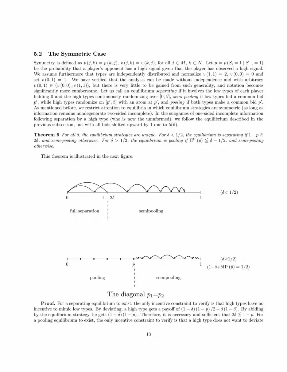
Symmetry is defined as p (j, k) = p (k, j), v (j, k) = v (k, j), for all j ∈ M , k ∈ N . Let p = p (Si = 1 | S−i = 1)be the probability that a player’s opponent has a high signal given that the player has observed a high signal.We assume furthermore that types are independently distributed and normalize v (1, 1) = 2, v (0, 0) = 0 andset v (0, 1) = 1. We have verified that the analysis can be made without independence and with arbitraryv (0, 1) ∈ (v (0, 0) , v (1, 1)), but there is very little to be gained from such generality, and notation becomessignificantly more cumbersome. Let us call an equilibrium separating if it involves the low types of each playerbidding 0 and the high types continuously randomizing over [0, β], semi-pooling if low types bid a common bidp0, while high types randomize on [p0, β] with an atom at p0, and pooling if both types make a common bid p0.As mentioned before, we restrict attention to equilibria in which equilibrium strategies are symmetric (as long asinformation remains nondegenerate two-sided incomplete). In the subgames of one-sided incomplete informationfollowing separation by a high type (who is now the uninformed), we follow the equilibrium described in theprevious subsection, but with all bids shifted upward by 1 due to 5(ii).

Theorem 6 For all δ, the equilibrium strategies are unique. For δ < 1/2, the equilibrium is separating if 1− p =2δ, and semi-pooling otherwise. For δ > 1/2, the equilibrium is pooling if ΠU (p) 5 δ − 1/2, and semi-poolingotherwise.

This theorem is illustrated in the next figure.

...............

...............

full separation semipooling

pooling semipooling

ª ª ® ® ® ® °

ª ªª ªª® ®

(1−δ+δΠu(p̄) = 1/2)r r r r r

0

0

1

1

p̄

1− 2δ(δ< 1/2)

(δ≥1/2)

The diagonal p1=p2Proof. For a separating equilibrium to exist, the only incentive constraint to verify is that high types have no

incentive to mimic low types. By deviating, a high type gets a payoff of (1− δ) (1− p) /2+ δ (1− δ). By abidingby the equilibrium strategy, he gets (1− δ) (1− p) . Therefore, it is necessary and sufficient that 2δ 5 1− p. Fora pooling equilibrium to exist, the only incentive constraint to verify is that a high type does not want to deviate

13

and bid slightly more. By deviating, he can get up to 1− δ+ δΠU (p), and by abiding by the equilibrium, he gets12 . Therefore, a necessary and sufficient condition for a pooling equilibrium to exist is that 1− δ + δΠU (p) 5 1

2 .Consider now a semi-pooling equilibrium. Let γ be the probability that one’s opponent is of the high type

and makes a bid larger than p0 (a separating bid), which is both the lowest bid (the pooling bid) and the posteriorbelief about the opponent’s type, conditional on the pooling being observed. Then, for high types to be indifferentbetween the pooling bid and a slightly higher bid, we need:

V (p) = γδΠI (p0) + (1− γ)

µ(1− δ)

1

2+ δV (p0)

¶| {z }

payoff from bidding p0

(5)

= (1− γ)¡(1− δ) + δΠU (p0)

¢| {z }payoff from bidding p0+

,

where V (p) is the value given belief p, and V (p0) is the value given p0 (uniqueness will be shown), and Bayes’rule gives that

p0 =p− γ

1− γ, or 1− γ =

1− p

1− p0.

Rearranging gives

1− p =δΠI (p0)

(1− δ) 12 + δ (ΠU (p0) +ΠI (p0)− V (p0))(1− p0) , (6)

V (p) =δΠI (p0)

¡1− δ + δΠU (p0)

¢(1− δ) 12 + δ (ΠU (p0) +ΠI (p0)− V (p0))

.

We show that such an equilibrium cannot exist for δ < 1/2 and 2δ 5 1− p (the latter clearly implies the former),nor can it exist for δ = 1/2 and 1 − δ + δΠU (p) 5 1

2 (same remark). Consider the first case. Observe thata (decreasing) sequence (p, p0, p00, . . .) of consecutive semi-pooling equilibria cannot have an accumulation point,for by picking a term arbitrarily far in the sequence, its value V (p) would be arbitrarily close to 1

2 , while thedeviation payoff for a high type would be arbitrarily close to 1− δ+ δΠU (p) > 1

2 , a contradiction (this argumentcovers also the case where the alleged accumulation point is 0); therefore, any sequence of consecutive equilibriamust have a largest term, after which, by necessity, the equilibrium is separating. Pick the largest such term.Equation (5) implies that

(p− p0) δΠI (p0) + (1− p) (δ (1− δ) (1− p0)) = (1− p)

µ(1− δ)

1

2+ δΠU (p0)

¶.

Because ΠI (p0) 5 1− δ and ΠU (p0) = 0, this requires

1− p0 (2− p) = 1− p

2δ.

However, this is impossible if 2δ < 1− p, and only possible for 2δ = 1− p if p0 = 0, that is, if the equilibrium is infact separating. Consider now the second case. Suppose first that there is a sequence (p, p0, p00, . . .) with infinitelymany terms that are semi-pooling. Then we can pick terms such that the payoff must be arbitrarily close to 1/2and 1− δ+ δΠU (p), implying that the limit of such a sequence cannot be such that 1− δ+ δΠU (p) < 1

2 . We canthen suppose without loss of generality that, if a semi-pooling exists with 1− δ + δΠU (p) < 1

2 , then (conditionalon both players making a pooling bid), players pool (forever) at belief p0. Equation (5) then implies that

(p− p0) δΠI (p0) + (1− p)1

2= (1− p)

¡1− δ + δΠU (p0)

¢, (5’)

14

which is impossible because 1− δ + δΠU (p0) < 1− δ+ δΠU (p) < 12 , and Π

I (p0) = 0. In fact, the same argumentrules out a semi-pooling equilibrium with p such that 1− δ + δΠU (p) = 1

2 . This establishes the second claim. Itmay be worthwhile at this point to observe that, if semi-pooling equilibria exists for 1− δ+δΠU (p) > 1

2 , then thesequence of continuation plays (conditional on players making the pooling bid) is an infinite sequence consistingexclusively of semi-pooling equilibria. If there is a limit, it must obviously satisfy 1 − δ + δΠU (p) = 1

2 , so thislimit is unique. As pooling equilibria cannot exist for 1 − δ + δΠU (p) > 1

2 , all we have to show is that such asequence cannot be finite, i.e. such that there exists p, after which (conditional on both players making poolingbids) the equilibrium is pooling (i.e., p0 is such that 1− δ + δΠU (p0) 5 1

2). This immediately follows from (5’).We are left with establishing existence (and uniqueness) of semi-pooling equilibria for δ < 1/2 and 2δ > 1− p,

as well as for δ > 1/2 and 1 − δ + δΠU (p) > 12 . As shown, if such a semi-pooling equilibrium exists, then it

must belong to a sequence of semi-pooling equilibria which is finite in the first case, ending up with a separatingequilibrium, and infinite in the second case, converging to the unique p solving 1− δ + δΠU (p) = 1

2 .Consider first δ < 1/2 and 2δ > 1 − p. We show that (6) determines uniquely (V (p) , p) as a function of

(V (p0) , p0), and that the (first coordinate of the) sets of consecutive solutions of (6), with boundary conditionsgiven by (p, (1− δ) (1− p)) for p ∈ (0, 1− 2δ] partition (1− 2δ, 1). To see this, suppose that V (p0) is decreasingin p0 and smaller than (1− δ). It follows from the first equation of (6) that (1− p) / (1− p0) is decreasing in p0.This follows from the fact that

(1− δ) 12 + δ¡ΠU (p0) +ΠI (p0)− V (p0)

¢δΠI (p0)

= 1 +ΠU (p0)ΠI (p0)

+(1− δ) 12 − δV (p0)

δΠI (p0)

is increasing (ΠU and 1/ΠI is increasing and positive, and so is (1− δ) 12 − δV (p0), because 12 > δ, and, by

hypothesis, (1− δ) = V (p0), and V (p0) is decreasing. The fact that is (1− p) / (1− p0) is decreasing in p0 impliesin particular that p increases with p0, but also, from (5’), since

V (p) =

µ1− 1− p

1− p0

¶δΠI (p0) +

1− p

1− p0

µ(1− δ)

1

2+ δV (p0)

¶,

as δΠI (p0) 5 (1− δ) 12 5 (1− δ) 12 + δV (p0), and both δΠI (p0) and (1− δ) 12 + δV (p0) are decreasing in p0, thatV (p) decreases with p0 (as a weighted average of two decreasing functions with increasing weight on the smallerone).Because V (p) is decreasing, it follows in particular that V (p) 5 1− δ, provided that V is continuous, whichfollows by induction as well once it is established for the first iteration. It is immediate to verify that for p0 = ε > 0arbitrarily small, and associated V (p0) = (1− δ) (1− p0), there exists (p, V (p)) solving (6) arbitrarily close to(1− 2δ, 2δ (1− δ)). Because (the projection on the first coordinate space of) the image by (6) of the interval(0, 1− 2δ] is an interval (1− 2δ, p∗], for some p∗ > 1 − 2δ, and the value V is continuous on that interval, itfollows by induction that the intervals of probabilities constructed this way have neither “gaps” nor “overlaps”,and that V is continuously decreasing in p. Observe that, as p0 = 1 is a fixed point of the first equation of (6),the union of these intervals never stretches above one. Conversely, because, for p0 = 2δ (1− δ) (which is certainlya probability that is “reached”, since it belongs to the “first” interval),

1− p =δΠI (p0)

(1− δ) 12 + δ (ΠU (p0) +ΠI (p0)− V (p0))(1− p0) <

1− p0

1 + (1− δ) (1− 2δ) ,

for any p < 1 is eventually included in the union of intervals recursively obtained by application of (6). Thisproves that for every p > 1 − 2δ, there exists one and only one equilibrium outcome, specifying in particularthat players semi-pool as long as they have pooled, until the common belief p is less than 1− 2δ, at which pointseparation occurs.

15

Let us now study the case δ = 1/2 and 1− δ + δΠU (p) > 12 . Defining q = 1/ (1− p), w = V (p) / (1− p), and

f (q) = 1− δ + δΠU (1− 1/q), we get from (6) the following pair of difference equations(qn+1 − qn =

(f(qn)− 1−δ2 )qn−δwn

δΠI(qn)

wn+1 = f (qn) ,

where calendar time is reversed, that is, qn corresponds to the posterior belief given semi-pooling and a prior

belief qn+1. Observe that the unique critical point of this system is x̄ , (q̄, w̄) =³(1− p̄)

−1, w (p̄)

´, where p̄ is the

unique root of 1− δ + δΠU (p) = 12 . For later use, observe also that this system is equivalent to the second-order

difference equation

qn+1 − qn =(f (qn)− (1− δ) /2) qn − δf (qn−1)

δΠI (qn),

from which it is apparent that qn > qn−1 > q̄ implies qn+1 > qn > q̄ (since then (f (qn)− (1− δ) /2) qn −δf (qn−1) > (1− δ)

¡f (qn)− 1

2

¢). Computing the Jacobian evaluated at this fixed point, we get:"

1 + f 0(q̄)q̄+f(q̄)−(1−δ)/2δΠI(q̄) − 1

ΠI(q̄)

f 0 (q̄) 0

#,

whose roots are real conjugate, one of which has modulus strictly less than one, the other one has modulus strictly

larger than one. Indeed, the discriminant is positive because³1 + f 0(q̄)q̄+f(q̄)−(1−δ)/2

δΠI(q̄)

´2> 4f 0 (q̄) /ΠI (q̄), as the

term which is squared exceeds¡1 + f 0 (q̄) /ΠI (q̄)

¢2(using f (q̄) − (1− δ) /2 > 0 and q̄/δ > 1), and the ordering

of moduli is easily established using the same bounds. Therefore, x̄ is a hyperbolic fixed point, the map definedby the system of difference equations has a saddle point at x̄, and so has its inverse map (the eigenvalues of theinverse matrix are the inverses of the eigenvalues). By the stable manifold theorem (see Devaney (1989)), thereexists a neighborhood of x̄ such that, for each q in this neighborhood, there exists a unique w such that the limitof the system starting from (q, w) is x̄. Because qn = (1− pn)

−1 is strictly increasing in pn, and wn = f (qn−1)is similarly increasing in pn−1, we may therefore conclude that, using standard calendar time, there exists aneigborhood of p̄, such that, for each pn in this neighborhood, there exists a unique pn+1 in this neighborhood,such that the sequence (pk) going consecutively through pn and pn+1 tends to p̄. Evidently, pn+1 > p̄. Asp−n is monotonic since q−n is, and p̄ is the unique fixed point of the second-order difference equation, it followsthat through all points p ∈ (p̄, 1) such a sequence exists, and uniqueness follows from trivial continuity andmonotonicity observations.

5.3 The Asymmetric Case

In this section we extend the case of the diagonal (p1 = p2 = p) to the asymmetric version; WLOG assumep2 > p1. For δ < 1/2 (available from the authors), bidding is fairly complex. Typically, both types of bothplayers bid on overlapping but non-nested supports. However, we can say that there is continuity with both thediagonal and the static game, in that as δ goes to 0 the equilibrium play converges to the equilibrium of the staticcase. The general version of the static case was described in section 4.3, but for concreteness we spell it out nowfor binary types and independent signals.Assuming that p2 = p1 and δ = 0, denote the c.d.f. of player i by Hi or Li, depending upon whether his

valuation (i.e. signal) is high or low. L2 is degenerate with unit mass at 0, H2 has support [0, p1 + p2] (with no

atom at 0), H1 has supporthp2−p11−p1 , p1 + p2

i, and L1 has support

h0, p2−p11−p1

iwith an atom at 0. Low types have

zero payoff, while player i’s high type payoff is 1− pi. There is, of course, full separation of types. The specific

16

distributions are

L1 (b) =1− p2

(1− p1) (1− b), b 5 p2 − p1

1− p1,

H2 (b) =1− p2p2

b

1− b, b 5 p2 − p1

1− p1,

Hi (b) =1− p−i − (1− pi) (1− b)

pi (2− b), b ∈

·p2 − p11− p1

, p1 + p2

¸.

Thus in the symmetric case p1 = p2 = p, both low types bid 0 for sure, and both high types bid in the range[0, 2p] and make profits of 1− p. The expected revenue for the auctioneer, in the general case, is p21 + p22.We study the δ = 1/2 case in more detail here. For existence, we introduce an endogenous tie-breaking rule.

Recall that we denote 1− δ+ δΠU (pi) by f(pi), with p̄ satisfying f(p̄) = 12 . Then if the bid at which the players

tie is at least p̄, they win with equal probability as before. But if their tying bid b is less than p̄, we give player 2a share f(b) < 1

2 and we give player 1 the remaining share 1−f(b). Given that in equilibrium the pooling bid willbe at the posterior beliefs about player 1, this boils down to giving player 2 exactly his outside option. However,the rules are of course independent of the players’ beliefs and can be implemented with observable bids only.First note that the edge p1 = 0 corresponds to the one-sided case with degenerate beliefs on the low type

of player 1. Here the equilibrium is again pooling (for any p2): both players bid 0 and receive the object withprobability δ and 1 − δ respectively, as above. The high type of player 2 weakly prefers his equilibrium payoff,namely f(0) = 1 − δ, to his payoff from deviation, which is also 1 − δ ( = (1 − δ) · 1 + δ · 0). Similarly, theuninformed player 1 (low type) prefers δp2 to (1 − δ)p2 as long as δ = 1/2. If the high type of player 1 werearound (which he isn’t!), he would be willing to pool exactly when

δ(1 + p2) = (1− δ)(1 + p2) + δΠU (p2), or

(2δ − 1)p2 + δ = f(p2).

For δ < 2/3, this yields an upper bound p̄2 = p̄ (with strict inequality as long as δ is strictly larger then 1/2); forδ = 2/3, it is satisfied for any p2. This bound is not crucial at this point, since there is no incentive constraintfor a type who does not exist, but it will arise again below. However, it is the very possibility of a higher type ofplayer 1 that allows us to support a pooling equilibrium in the first place: the difference between knowledge andbelief.The equilibrium we consider for the two-sided case (we have not proven uniqueness) involves pooling below

a boundary connecting the diagonal (i.e. the symmetric case) to either the edge that corresponds to p1 = 0 (forδ < 2/3) or to the edge corresponding to p2 = 1 (for δ = 2/3). This boundary intersects the diagonal at thepoint p = p̄, so this equilibrium truly does extend that of the symmetric case. It intersects the edge p1 = 0 (forδ < 2/3) exactly at the point p̄2 defined above, and it is monotonic in p1 (for any δ). It is described by thefollowing expression:

1 + (δ − f(p1))(p2 − p1) = f(p1) + f(p2).

Above this boundary line, the players semipool, where the low pooling bid is the posterior belief on player 1’s type.That is, both high types pool with positive probability and also make revealing bids with positive probability.They converge toward the pooling region (conditional on no one having yet separated), but do not reach it infinite time, just as in the symmetric case. The specific equations for the evolution of beliefs under semipoolingare given in the Appendix. Of course, given Theorems 2 and 3, as δ approaches 1 the boundary line expands andthe pooling region fills the entire parameter space. In this case the seller’s [normalized] expected revenue is thecommon pooling bid p1, which is certainly lower than the overall expected value of p1 + p2, and may or may notbe lower than the revenue in the static game, p21+p22. On the other hand, as δ approaches 1/2, the pooling regionshrinks and we have only semipooling in the limit.We formalize these results in the following theorem, which is proved in the Appendix.

17

Theorem 7 For δ = 1/2 and any p2 > p1 > 0, there is an equilibrium satisfying all our assumptions; it ischaracterized by pooling if 1 + (δ − f(p1))(p2 − p1) = f(p1) + f(p2) and by semipooling otherwise.

These results are summarized in the following Figure.

ª¼

¼

¼

ª

ª

bb

rrrrrrrrrrr

r

r r rr r

r r r r rr

rr

r

rr r

¾¾¾¾¾¾¾¾¾¾¡¡ª

¡¡ª

¡¡

¡¡¡ª

¡¡

¡¡¡ª

¡¡

¡¡¡ª

¡¡

¡¡ª¡

¡ª¡¡ªª

¡¡

¡¡

¡¡

¡¡

¡¡

¡¡

¡¡

¡¡

¡¡

rrr

rr

rr

rr

r

rrrr

rrr

rr

6

-

p2

p10 1

1

p̄1

1−δ+δΠu(p̄1)= 1/2

(Conditional) evolution of (p1,p2) (given δ≥1/2)18

6 Concluding CommentsThis paper shows that in an infinitely repeated, first-price, common-value auction in which the value of all units isperfectly correlated, rational and patient players prefer to make a low, “pooling” bid in every period rather thandivulge any of their proprietary information. We have imposed four refinements in order to prove uniqueness ofthis equilibrium outcome. First, stationarity: players bids depend only on beliefs. This assumption is necessary toeliminate “reputational” equilibria as described in the durable goods monopoly literature (Ausubel and Deneckere(1989)). Consider for instance the one-sided version of our model (Section 3). By Theorem 1, as the discount factortends to one, both the uninformed and the informed bidder’s payoff tend to zero. Then, without stationarity,there exists a P.B.E. (satisfying the other three refinements) in which both players repeatedly bid v (0) and winthe object with equal probability. The informed bidder has no incentive to deviate if any higher bid is interpretedas evidence of, say, him being the highest possible type, and the uninformed bidder has no incentive to deviateeither if such a bid triggers a reversion to any equilibrium satisfying Theorem 1. In turn, this makes it possibleto construct other equilibria of the repeated game with two-sided incomplete information. Second, it is necessaryto assume “no underbidding”, that is, that players bid at least as much as the object is commonly believed to beworth. Otherwise, there exists a continuum of other pooling equilibrium which differ only in the pooling bid, andour refinement selects the equilibrium with the highest such bid. Third, we assumed that players’ revise theirbelief in such a way as to assign zero probability to a player’s type for which the observed bid is more than whatthe object could conceivably be worth to him (that is, under his most optimistic conjectures). As mentioned,we suspect that this third refinement could be dispensed with. Finally, we assumed in section 3.2 that players(as a union across types) use connected bidding supports. Without this assumption, there is, for instance, anequilibrium of the one-sided degenerate-belief version of our game in which the informed player always bids λ(his lowest possible value for the object), and the uninformed player randomizes between λ and precisely the onebid β > λ so that winning with probability 1 at β gives him the same static payoff as winning half the time at λ(because he would tie). If all out-of-equilibrium bids are interpreted as coming from the highest type and thusleading to the outcome of Theorem 1, no type of any player has an incentive to deviate. We find this equilibriumsomewhat artificial; connectedness rules it out.How could an auctioneer eliminate the tacit collusion that our equilibrium suggests? A reserve price is an

instrument that, used wisely, would allow the auctioneer to fare better. If he can commit to a reserve price policy,then as the discount factor tends to one, his optimal expected revenue tends toward his revenue from settingan optimal fixed reserve price. Players whose signal is sufficiently high pool at a level slightly above the reserveprice, while players with lower signals remain idle. Therefore, the auctioneer’s expected revenue is still lower thanin the static auction. Another commonly used procedure in auctioneering is the option to a winner to purchasefuture units at the current price (See Cassady (1967)). It is clear that such a procedure eliminates the poolingequilibrium, as at least one player would have an incentive to bid a penny more and exercise his option. However,this procedure is not perfect either, as a player with a low signal may exercise his option and win all units at aprice below their real value (assuming that bids are observed before the option decision is made).As in Kyle and the literature on insider trading, we have restricted attention to the case in which the values of

the units are perfectly correlated. This seems to be the most challenging case for information revelation. Indeed,suppose that the value of each unit is an independent draw from some (possibly time-dependent) distribution,for which the static first-price auction admits a unique equilibrium. Then the only equilibrium that is stationaryin the repeated game specifies that the static auction be played in each period.We have also restricted attention to the two player case. We have verified that the pooling equilibrium remains

an equilibrium satisfying our refinements when there are more than two players, but have not proved uniqueness.As soon as a single player has revealed his information, all other players’ private information must be eventuallyrevealed, as such an uninformed bidder cannot be disciplined into pooling (given stationarity) and thus, informedbidders must eventually act. Such information revelation occurs “quickly” relative to the discount factor, whichin turn allows players to enforce tacit collusion when none of them has revealed any information. The intuition

19

for uniqueness appears robust: if none of the opponents reveals his private information, then pooling is certainlyoptimal provided the discount factor is high enough, while if some of them do reveal theirs, it is then still betterto pool and become the informed player, for uninformed bidders have a zero payoff as soon as there is more thanone of them.We have also considered the framework of private values (rather than common) and of second-price auctions

(rather than first-price). However, it is clear that much work remains to be done in the domain of repeatedauctions.

20

References[1] Ashenfelter, O. (1989), “How auctions work for wine and art”, Journal of Economic Perspectives, 3(3), 23-36.

[2] Aumann, R.J. and M. Maschler, with the collaboration of R.E. Stearns (1966-68), Reports of the U.S. ArmsControl and Disarmament Agency ST-80, ST-116, ST-143, Washington, D.C., reprinted in Repeated Gamesof Incomplete Information, MIT Press, 1995, Cambridge, MA.

[3] Ausubel, L. and R. Deneckere (1989), “Reputation in Durable-Goods Monopoly”, Econometrica, 57(3), 511-531.

[4] Bikhchandani, S. (1988), “Reputation in Second-Price Auctions”, Journal of Economic Theory, 46, 97-119.

[5] Cassady, R. Jr. (1967), Auctions and Auctioneering, University of California Press, Los Angeles, CA.

[6] Devaney, R. (1989), An Introduction to Chaotic Dynamical Systems, 2nd Ed., Addison-Wesley, Reading, MA.

[7] Engelbrecht-Wiggans R. and R.J. Weber (1983), “A sequential auction involving asymmetrically-informedbidders”, International Journal of Game Theory, 12(2), 123-127.

[8] Freixas, X., R. Guesnerie, and J. Tirole (1985), “Planning under incomplete Information and the RatchetEffect”, Review of Economic Studies, 52(2), 173-191.

[9] Hart, O. and J. Tirole (1988), “Contract Renegotiation and Coasian Dynamics”, Review of Economic Studies,55(4), 509-540.

[10] Hausch, D. (1986), “Multi-Object Auctions: Sequential vs. Simultaneous Sales”, Management Science,32(12), 1599-1610.

[11] Hausch, D. (1987), “An Asymmetric Common-Value Auction Model”, RAND Journal of Economics, 18(4),611-621.

[12] Hon-Snir, S., D. Monderer, and A. Sela (1998), “A learning approach to auctions”, Journal of EconomicTheory, 82(1), 65-89.

[13] Kyle, A. (1985), “Continous Auctions and Insider Trading”, Econometrica, 53(6), 1315-1336.

[14] Maskin, E. and J. Riley (2000), “Equilibrium in Sealed High-bid Auctions”, Review of Economic Studies,67(30), 455-83.

[15] Ortega-Reichert, A. (1968), “Models for Competitive Bidding under Uncertainty”, Department of OperationsResearch Technical Report No. 8, Stanford University.

[16] Pezanis-Christou, P. (2000), “Sequential Descending-Price Auctions with Asymmetric Buyers: Evidence froma Fish Market”, mimeo, Pompeu Fabra.

[17] Wang, R. (1991), “Common-Value Auctions with Discrete Private Information”, Journal of Economic Theory,54(2), 429-447.

21

7 Appendix

7.1 Static case

Proof of Theorem 5: Because player 1’s type m (k) is indifferent between bidding α (k) and α (k + 1),n(k)−1Xj=0

q (j) + q (n (k))Gn(k) (α (k))

(α (k + 1)− α (k)) = q (n (k))¡Gn(k) (α (k + 1))−Gn(k) (α (k))

¢v (m (k) , n (k)) ,

and, similarly, because player 2’s type n (k) is indifferent between bidding α (k) and α (k + 1),m(k)−1Xi=0

p (i) + p (m (k))Fm(k) (α (k))

(α (k + 1)− α (k)) = p (m (k))¡Fm(k) (α (k + 1))− Fm(k) (α (k))

¢v (m (k) , n (k)) .

Therefore, upon dividing,

q (n (k))¡Gn(k) (α (k + 1))−Gn(k) (α (k))

¢Pn(k)−1j=0 q (j) + q (n (k))Gn(k) (α (k))

=p (m (k))

¡Fm(k) (α (k + 1))− Fm(k) (α (k))

¢Pm(k)−1i=0 p (i) + p (m (k))Fm(k) (α (k))

.

For k 5 m+n+1, define x (k) =Pm(k)−1

i=0 p (i)+p (m (k))Fm(k) (α (k)) and y (k) =Pn(k)−1

i=0 q (j)+q (n (k))Gn(k) (α (k)).It follows that:

x (k + 1)− x (k)

x (k)=

y (k + 1)− y (k)

y (k),

and thus, because x (m+ n+ 1) = y (m+ n+ 1) = 1, x (k) = y (k), for all k 5 m + n + 1. Because for allα (k + 1), either Gn(k) (α (k + 1)) or Fm(k) (α (k + 1)) equals 1, this establishes that s (k) = x (k) can be definedrecursively as: s (0) = 0, and, for P (i) =

Pil=0 p (l), Q (j) =

Pjl=0 q (l),

s (k) = min {x 5 1 | x = P (i) > s (k − 1) for some i, or x = Q (j) > s (k − 1) for some j} ,for all 1 5 k 5 m+ n+ 1. Obviously, s (m+ n+ 1) = 1.Consider again the indifference of player 2’s type n (k) between bids α (k) and α (k + 1) :

m(k)Xi=0

p (i) (v (i, n (k))− α (k)) + p (m (k))Fm(k) (α (k)) (v (m (k) , n (k))− α (k))

=

m(k)Xi=0

p (i) (v (i, n (k))− α (k + 1)) + p (m (k))Fm(k) (α (k + 1)) (v (m (k) , n (k))− α (k + 1)) .

It follows that, for all 0 5 k 5 m+ n :

s (k)

s (k + 1)=

v (m (k) , n (k))− α (k + 1)

v (m (k) , n (k))− α (k),

and therefore, α (0) = 0, and, for all 1 5 k 5 m+ n+ 1 :

α (k) =k−1Xl=0

(s (l + 1)− s (l)) v (m (l) , n (l)) .

22

In the same way, we determine the distribution functions. If b ∈ [α (k) , α (k + 1)],

p (m (k))Fm(k) (b) = s (k + 1)v (m (k) , n (k))− α (k + 1)

v (m (k) , n (k))− b−

m(k)Xj=0

p (i) ,

q (n (k))Gn(k) (b) = s (k + 1)v (m (k) , n (k))− α (k + 1)

v (m (k) , n (k))− b−

n(k)Xj=0

q (j) .

We can now compute the expected revenue R. For 0 5 k 5 m+n, let R (α (k) , α (k + 1)) be the expected revenuefrom bids b ∈ [α (k) , α (k + 1)]. SincePn(k)

j=0 q (j)+q (n (k))Gn(k) (b) =Pm(k)

j=0 p (i)+p (m (k))Fm(k) (b), it followsthat

R (α (k) , α (k + 1)) = s (k + 1)2µv (k)− α (k + 1)

v (k)− b

¶(2b− v (k))

¯̄̄̄α(k+1)α(k)

= s (k + 1)2 (2α (k + 1)− v (k))− s (k)2 (2α (k)− v (k)) ,

where for simplicity, v (k) = v (m (k) , n (k)). It follows that

R =m+nXk=0

R (α (k) , α (k + 1))

= 2α (m+ n+ 1)−m+nXl=0

³s (l + 1)

2 − s (l)2´v (l)

=m+nXl=0

2 (s (l + 1)− s (l)) v (l)−m+nXl=0

³s (l + 1)

2 − s (l)2´v (l)

= v (m+ n+ 1)−m+nXl=0

s (l) (2− s (l)) (v (l + 1)− v (l)) (summation by parts)

=m+nXl=0

(1− s (l))2 (v (l + 1)− v (l)) . ¥

7.2 Calculations for binary one-sided

Additional details for the 2x1 case: Define ΠI (p) and ΠU (p) to be the expected payoff of the informed anduninformed bidder, respectively, given belief p. Obviously, ΠI (p) = (1− δ) δT (1− pT ) = (1− δ) δT/2 (1− p)

1T+1 ,

with T = minnt ∈ N ; 1− p = δ(T+1)(T+2)/2

o. It is simple to verify that ΠI (p) is decreasing in p, limp→0ΠI (p) =

1 − δ, limp→1ΠI (p) = 0, and ΠI (p) is decreasing in δ. Observe that 1 − pt =³δ−t/2 (1− p)

1T+1

´T+1−t,

and, denoting the odds ratio pt/ (1− pt) by lt, we have (pt − βt) /pt = lt+1/lt. By bidding 0+ repeatedly, theuninformed player gets:

ΠU (p) = (1− δ) p

·p0 − β0

p0

µ1 + δ

p1 − β1p1

µ1 + δ

p2 − β2p2

µ· · ·+ δ

pT−1 − βT−1pT−1

¶¶¶¸= (1− δ) p

·l1l0+ δ

l2l0+ · · ·+ δT−1

lTl0

¸= (1− δ) δT

"TXt=1

δ(t−2)(T+1−t)

2 (1− p)t

T+1

#− (1− p)

³1− δT

´.

23

Observe that, because T = minnt ∈ N ; 1− p = δ(T+1)(T+2)/2

o, δT → 1 as δ → 1. Notice also that

ΠU (p) = (1− δ) p

·l1l0+ δ

l2l0+ · · ·+ δT−1

lTl0

¸5 p

³1− δT

´,

so that ΠU (p)→ 0 as δ → 1.Finally, we study the variations of the expected bids. Let ht, ut be the densities correspondingly respectively

to the distributions Ht and Ut. The density of the maximum bid, mt, is given by

mt (b) = u (t) (1− pt + ptHt (b)) + ptht (b)Ut (b) =2δ2(T−t) (1− pT )

2

(1− b)3,

and its expectation (conditional, as usual, on the informed bidder having bid 0 up to t− 1) is

Et = 2δ2(T−t) (1− pT )2Z 1−δT−t(1−pT )

0

tdt

(1− t)3

= 2δ2(T−t) (1− pT )2

12+1− 2δT−t (1− pT )

2³δT−t (1− pT )

´2

=³1− δT−t (1− pT )

´2,

which is decreasing in t. Next, observe that the unconditional expectation of the winning bid in period t = 1,t 5 T , Ft, satisfies

Ft = 1−t−1Yi=0

(1− βi) (1−Et)

= 1− (1− pT ) (1−Et)t−1Xi=0

δT−i

= 1− δT¡1− pT

¢ δ−t − 1δ−1 − 1

µ1−

³1− δT−t (1− pT )

´2¶,

which is decreasing in t as well. Of course, for t > T , it is equal to the prior, p, and is larger than the correspondingexpectation for all t 5 T .

7.3 Asymmetric binary types

Proof of Theorem 7: If both players fully pool, the common bid will be λ = p1 (using the refinements and thefact that p1 < p2). Anyone who bids even λ+ will be considered to be a high type (by fiat, but this is in line with5(iii)). Since p1 5 p̄ throughout the pooling region, we use the endogenous sharing rule. The low type of player2 makes zero profit and can do no better. The low type of player 1 makes profits of (1− f(p1))(p2) > p2/2 andby deviating can obtain (1− δ)(p2) + δ · 0, so he will never wish to deviate. [Recall that f(p) = 1− δ + δΠU (p)and is equal to 1/2 at p̄.] The incentive constraint for the high type of player 2 is

f(p1)(1 + p1 − p1) = (1− δ)(1 + p1 − p1) + δΠU (p1) = f(p1)

24

which is always just satisfied; this is how the tie-breaking rule was constructed. For player 1, we need

(1− f(p1))(1 + p2 − p1) = (1− δ)(1 + p2 − p1) + δΠU (p2).

This determines the boundary of the region where full pooling is an equilibrium. Rearranging, the equation forthe boundary is given by

1 + (δ − f(p1))(p2 − p1) = f(p1) + f(p2).

Note that p1 = p2 = p̄ satisfies this equality, so the boundary hits the diagonal exactly at p̄, as desired. Further-more, this boundary intersects the edge case p1 = 0 (where f(p1) = 1− δ) when

(2δ − 1)p2 + δ = f(p2),

i.e. at p̄2 (as defined in section 5.3 for δ < 2/3). This makes intuitive sense, since that was exactly where thehigh type of player 1 would have no longer been willing to pool. Finally, fixing p1 and p2 less than 1, it is clearthat the RHS of player 1’s original incentive constraint goes to 0 as δ goes to 1. So in the limit for arbitrarilypatient players, we have full pooling for any initial parameter values.If p1 is too large (given some p2), so that we are outside the boundary of the pooling region, then both players

semipool. Renormalize time as time-to-go until we stop semipooling (conditional on both players pooling), i.e.until one player either fully separates or fully pools. Recall that semipooling entails players with low valuationsmaking a low, pooling bid λ (equal to p1,t−1), while high types make the same pooling bid with positive probability,and with positive probability they continuously randomize over some support [λ+, βt]. Let Vi (p1,t, p2,t) denotethe value for player i with high valuation, given the initial beliefs. Let γi be the probability that player j = 3− ifaces a player i making a separating bid. By Bayes’ rule:

pi,t−1 =pi,t − γi,t1− γi,t

or γi,t =pi,t − pi,t−11− pi,t−1

.

Because player 1 is indifferent between pooling and separating (the first equality corresponds to a pooling bid,the second to the lowest separating bid):

V1 (p1,t, p2,t)

= γ2,t¡(1− δ) · 0 + δΠI (p1,t−1)

¢+¡1− γ2,t

¢((1− δ) · (1− f(p1,t−1)) (1 + p2,t−1 − p1,t−1) + δV1 (p1,t−1, p2,t−1))

= γ2,t ((1− δ) · 0 + δ · 0) + ¡1− γ2,t¢ ¡(1− δ) (1 + p2,t−1 − p1,t−1) + δΠU (p2,t−1)

¢.

That is,

V1 (p1,t, p2,t) =1− p2,t1− p2,t−1

¡(1− δ) (1 + p2,t−1 − p1,t−1) + δΠU (p2,t−1)

¢p2,t − p2,t−11− p2,t

δΠI (p1,t−1) = f(p1,t−1) (1− δ) (1 + p2,t−1 − p1,t−1) + δ¡ΠU (p2,t−1)− V1 (p1,t−1, p2,t−1)

¢.

Similarly, player 2 is indifferent between pooling and separating, so that:

V2 (p1,t, p2,t)

= γ1,t¡(1− δ) · 0 + δΠI (p2,t−1)

¢+¡1− γ1,t

¢((1− δ) · f(p1,t−1) + δV2 (p1,t−1, p2,t−1))

= γ1,t ((1− δ) · 0 + δ · 0) + ¡1− γ1,t¢ ¡(1− δ) · 1 + δΠU (p1,t−1)

¢.

Rearranging,

V2 (p1,t, p2,t) =1− p1,t1− p1,t−1

¡(1− δ) + δΠU (p1,t−1)

¢,

p1,t − p1,t−11− p1,t

δΠI (p2,t−1) = (1− δ) (1− f(p1,t−1)) + δ¡ΠU (p1,t−1)− V2 (p1,t−1, p2,t−1)

¢.

25

We now proceed as in section 5.2, defining qi = 1/ (1− pi), wi = Vi (p1, p2) / (1− p−i), and [slightly abusingnotation] f (qi) = 1 − δ + δΠU (1− 1/qi). Then we can rewrite the dynamics above as a set of four differenceequations

q1,t+1 − q1,t =q1,tf(q1,t)−w2,tΠI(q2,t)

q2,t+1 − q2,t =q2,t(f(q2,t)−(1−δ)(1−f(q1,t)(1+q−11,t−q−12,t )))−δw1,t

δΠI(q1,t)

w1,t+1 = q2,t¡f (q2,t) + (1− δ)(q−11,t − q−12,t )

¢w2,t+1 = q1,tf(q1,t).

Observe that if q1 and q2 are on the boundary defined above, and if w1 and w2 are the corresponding poolingvalues, then we get a fixed point for the entire system (i.e. the RHS of the first two equations reduces to zero).We can again write this as a pair of second-order difference equations, if we prefer, from which monotonicity ismore readily apparent. Computing the Jacobian evaluated at the critical point, we get:

1 + f(q1)+q1f0(q1)

ΠI(q2)0 0 − 1

ΠI(q2)

q2(1− δ)f 0(q1)(1+q−11 −q−12 )+(1−f(q1))/q21

δΠI(q1)D − 1

ΠI(q1)0

−(1− δ)q2/q21 f(q2) + (1− δ)q−11 + q2f

0(q2) 0 0f(q1) + q1f

0(q1) 0 0 0

where

D = 1 +f (q2)− (1− δ)(1− f(q1)(1 + q−11 − q−12 )) + q2

¡f 0(q2)− (1− δ)(1− f(q1)/q

22

¢δΠI(q1)

.

We can relabel the Jacobian as A 0 0 −BC D −E 0−F G 0 0H 0 0 0

which has eigenvalues

©12(A±

√A2 − 4BH, 12(D ±

√D2 − 4EGª. Now A2−4BH = (1+2x+x2)−4x = (1−x)2,

where x = BH = f(q1)+q1f0(q1)

ΠI(q2), so the first two eigenvalues simplify to 1 and BH. The product of the remaining

conjugate roots is 14(D

2 − (D2 − 4EG)) = EG, but since f(qi) = 1 − δ + δΠU (1− 1/qi) > 1 − δ > ΠI(q−i)and f 0(qi) > 0, both BH > 1 and EG > 1. Thus at least one of the conjugate pair must have norm greaterthan 1, and overall we have at least two eigenvalues larger than 1, with one unit root. The inverse matrix (sincewe were working in reverse time) thus has two eigenvalues less than 1, so that we have two stable dimensions.There is a center manifold from the unit root, but all that we require is at least one stable dimension. Thus, in aneighborhood of the boundary, given q1 and a point on the boundary, we can find q2, w1, w2 such that the systemwill converge to that point. Reverting to our standard notations and working backward (we use monotonicityhere, which is easy to check), this says that from any initial p1 and p2, we can find values V1 and V2 so that thesystem continuously converges to some point on the boundary (with the appropriate pooling values as the limit).This completes the proof of existence. ¥

26