Embed Size (px)
Citation preview

Minimum Description Length
Model Selection
Problems and Extensions
Steven de Rooij


Minimum Description LengthModel Selection
Problems and Extensions

ILLC Dissertation Series DS-2008-07
For further information about ILLC-publications, please contact
Institute for Logic, Language and ComputationUniversiteit van AmsterdamPlantage Muidergracht 24
1018 TV Amsterdamphone: +31-20-525 6051
fax: +31-20-525 5206e-mail: [email protected]
homepage: http://www.illc.uva.nl/

Minimum Description LengthModel Selection
Problems and Extensions
Academisch Proefschrift
ter verkrijging van de graad van doctor aan deUniversiteit van Amsterdam
op gezag van de Rector Magnificusprof.dr. D. C. van den Boom
ten overstaan van een door het college voorpromoties ingestelde commissie, in het openbaar
te verdedigen in de Agnietenkapelop woensdag 10 september 2008, te 12.00 uur
door
Steven de Rooij
geboren te Amersfoort.

Promotiecommissie:
Promotor: prof.dr.ir. P.M.B. VitanyiCo-promotor: dr. P.D. Grunwald
Overige leden: prof.dr. P.W. Adriaansprof.dr. A.P. Dawidprof.dr. C.A.J. Klaassenprof.dr.ir. R.J.H. Schadr. M.W. van Somerenprof.dr. V. Vovkdr.ir. F.M.J. Willems
Faculteit der Natuurwetenschappen, Wiskunde en Informatica
The investigations were funded by the Netherlands Organization for ScientificResearch (NWO), project 612.052.004 on Universal Learning, and were supportedin part by the IST Programme of the European Community, under the PASCALNetwork of Excellence, IST-2002-506778.
Copyright c© 2008 by Steven de Rooij
Cover inspired by Randall Munroe’s xkcd webcomic (www.xkcd.org)Printed and bound by PrintPartners Ipskamp (www.ppi.nl)ISBN: 978-90-5776-181-2

Parts of this thesis are based on material contained in the following papers:
• An Empirical Study of Minimum Description Length Model Selection with InfiniteParametric ComplexitySteven de Rooij and Peter GrunwaldIn: Journal of Mathematical Psychology, special issue on model selection. Vol.50, pp. 180-190, 2006(Chapter 2)
• Asymptotic Log-Loss of Prequential Maximum Likelihood CodesPeter D. Grunwald and Steven de RooijIn: Proceedings of the 18th Annual Conference on Computational Learning The-ory (COLT), pp. 652-667, June 2005(Chapter 3)
• MDL Model Selection using the ML Plug-in CodeSteven de Rooij and Peter GrunwaldIn: Proceedings of the International Symposium on Information Theory (ISIT),2005(Chapters 2 and 3)
• Approximating Rate-Distortion Graphs of Individual Data: Experiments in LossyCompression and DenoisingSteven de Rooij and Paul VitanyiSubmitted to: IEEE Transactions on Computers(Chapter 6)
• Catching up Faster in Bayesian Model Selection and AveragingTim van Erven, Peter D. Grunwald and Steven de RooijIn: Advances in Neural Information Processing Systems 20 (NIPS 2007)(Chapter 5)
• Expert Automata for Efficient TrackingW. Koolen and S. de RooijIn: Proceedings of the 21st Annual Conference on Computational Learning The-ory (COLT) 2008(Chapter 4)
v


Contents
Acknowledgements xi
1 The MDL Principle for Model Selection 11.1 Encoding Hypotheses . . . . . . . . . . . . . . . . . . . . . . . . . 5
1.1.1 Luckiness . . . . . . . . . . . . . . . . . . . . . . . . . . . 61.1.2 Infinitely Many Hypotheses . . . . . . . . . . . . . . . . . 71.1.3 Ideal MDL . . . . . . . . . . . . . . . . . . . . . . . . . . . 8
1.2 Using Models to Encode the Data . . . . . . . . . . . . . . . . . . 91.2.1 Codes and Probability Distributions . . . . . . . . . . . . 91.2.2 Sequential Observations . . . . . . . . . . . . . . . . . . . 121.2.3 Model Selection and Universal Coding . . . . . . . . . . . 13
1.3 Applications of MDL . . . . . . . . . . . . . . . . . . . . . . . . . 191.3.1 Truth Finding . . . . . . . . . . . . . . . . . . . . . . . . . 191.3.2 Prediction . . . . . . . . . . . . . . . . . . . . . . . . . . . 201.3.3 Separating Structure from Noise . . . . . . . . . . . . . . . 22
1.4 Organisation of this Thesis . . . . . . . . . . . . . . . . . . . . . . 23
2 Dealing with Infinite Parametric Complexity 252.1 Universal codes and Parametric Complexity . . . . . . . . . . . . 262.2 The Poisson and Geometric Models . . . . . . . . . . . . . . . . . 282.3 Four Ways to deal with Infinite Parametric Complexity . . . . . . 29
2.3.1 BIC/ML . . . . . . . . . . . . . . . . . . . . . . . . . . . . 302.3.2 Restricted ANML . . . . . . . . . . . . . . . . . . . . . . . 302.3.3 Two-part ANML . . . . . . . . . . . . . . . . . . . . . . . 312.3.4 Renormalised Maximum Likelihood . . . . . . . . . . . . . 322.3.5 Prequential Maximum Likelihood . . . . . . . . . . . . . . 332.3.6 Objective Bayesian Approach . . . . . . . . . . . . . . . . 33
2.4 Experiments . . . . . . . . . . . . . . . . . . . . . . . . . . . . . . 352.4.1 Error Probability . . . . . . . . . . . . . . . . . . . . . . . 36
vii

2.4.2 Bias . . . . . . . . . . . . . . . . . . . . . . . . . . . . . . 372.4.3 Calibration . . . . . . . . . . . . . . . . . . . . . . . . . . 37
2.5 Discussion of Results . . . . . . . . . . . . . . . . . . . . . . . . . 392.5.1 Poor Performance of the PML Criterion . . . . . . . . . . 392.5.2 ML/BIC . . . . . . . . . . . . . . . . . . . . . . . . . . . . 462.5.3 Basic Restricted ANML . . . . . . . . . . . . . . . . . . . 472.5.4 Objective Bayes and Two-part Restricted ANML . . . . . 47
2.6 Summary and Conclusion . . . . . . . . . . . . . . . . . . . . . . 47
3 Behaviour of Prequential Codes under Misspecification 513.1 Main Result, Informally . . . . . . . . . . . . . . . . . . . . . . . 523.2 Main Result, Formally . . . . . . . . . . . . . . . . . . . . . . . . 553.3 Redundancy vs. Regret . . . . . . . . . . . . . . . . . . . . . . . . 603.4 Discussion . . . . . . . . . . . . . . . . . . . . . . . . . . . . . . . 61
3.4.1 A Justification of Our Modification of the ML Estimator . 613.4.2 Prequential Models with Other Estimators . . . . . . . . . 623.4.3 Practical Significance for Model Selection . . . . . . . . . . 633.4.4 Theoretical Significance . . . . . . . . . . . . . . . . . . . 64
3.5 Building Blocks of the Proof . . . . . . . . . . . . . . . . . . . . . 653.5.1 Results about Deviations between Average and Mean . . . 653.5.2 Lemma 3.5.6: Redundancy for Exponential Families . . . . 683.5.3 Lemma 3.5.8: Convergence of the sum of the remainder terms 69
3.6 Proof of Theorem 3.3.1 . . . . . . . . . . . . . . . . . . . . . . . . 713.7 Conclusion and Future Work . . . . . . . . . . . . . . . . . . . . . 73
4 Interlude: Prediction with Expert Advice 754.1 Expert Sequence Priors . . . . . . . . . . . . . . . . . . . . . . . . 78
4.1.1 Examples . . . . . . . . . . . . . . . . . . . . . . . . . . . 804.2 Expert Tracking using HMMs . . . . . . . . . . . . . . . . . . . . 81
4.2.1 Hidden Markov Models Overview . . . . . . . . . . . . . . 824.2.2 HMMs as ES-Priors . . . . . . . . . . . . . . . . . . . . . . 844.2.3 Examples . . . . . . . . . . . . . . . . . . . . . . . . . . . 864.2.4 The HMM for Data . . . . . . . . . . . . . . . . . . . . . . 874.2.5 The Forward Algorithm and Sequential Prediction . . . . . 88
4.3 Zoology . . . . . . . . . . . . . . . . . . . . . . . . . . . . . . . . 924.3.1 Universal Elementwise Mixtures . . . . . . . . . . . . . . . 924.3.2 Fixed Share . . . . . . . . . . . . . . . . . . . . . . . . . . 944.3.3 Universal Share . . . . . . . . . . . . . . . . . . . . . . . . 964.3.4 Overconfident Experts . . . . . . . . . . . . . . . . . . . . 97
4.4 New Models to Switch between Experts . . . . . . . . . . . . . . . 1014.4.1 Switch Distribution . . . . . . . . . . . . . . . . . . . . . . 1014.4.2 Run-length Model . . . . . . . . . . . . . . . . . . . . . . . 1104.4.3 Comparison . . . . . . . . . . . . . . . . . . . . . . . . . . 113
viii

4.5 Extensions . . . . . . . . . . . . . . . . . . . . . . . . . . . . . . . 1144.5.1 Fast Approximations . . . . . . . . . . . . . . . . . . . . . 1144.5.2 Data-Dependent Priors . . . . . . . . . . . . . . . . . . . . 1184.5.3 An Alternative to MAP Data Analysis . . . . . . . . . . . 118
4.6 Conclusion . . . . . . . . . . . . . . . . . . . . . . . . . . . . . . . 119
5 Slow Convergence: the Catch-up Phenomenon 1215.1 The Switch-Distribution for Model Selection and Prediction . . . 124
5.1.1 Preliminaries . . . . . . . . . . . . . . . . . . . . . . . . . 1245.1.2 Model Selection and Prediction . . . . . . . . . . . . . . . 1255.1.3 The Switch-Distribution . . . . . . . . . . . . . . . . . . . 126
5.2 Consistency . . . . . . . . . . . . . . . . . . . . . . . . . . . . . . 1275.3 Optimal Risk Convergence Rates . . . . . . . . . . . . . . . . . . 129
5.3.1 The Switch-distribution vs Bayesian Model Averaging . . . 1305.3.2 Improved Convergence Rate: Preliminaries . . . . . . . . . 1315.3.3 The Parametric Case . . . . . . . . . . . . . . . . . . . . . 1345.3.4 The Nonparametric Case . . . . . . . . . . . . . . . . . . . 1355.3.5 Example: Histogram Density Estimation . . . . . . . . . . 136
5.4 Further Discussion of Convergence in the Nonparametric Case . . 1395.4.1 Convergence Rates in Sum . . . . . . . . . . . . . . . . . . 1395.4.2 Beyond Histograms . . . . . . . . . . . . . . . . . . . . . . 141
5.5 Efficient Computation . . . . . . . . . . . . . . . . . . . . . . . . 1425.6 Relevance and Earlier Work . . . . . . . . . . . . . . . . . . . . . 143
5.6.1 AIC-BIC; Yang’s Result . . . . . . . . . . . . . . . . . . . 1435.6.2 Prediction with Expert Advice . . . . . . . . . . . . . . . . 145
5.7 The Catch-Up Phenomenon, Bayes and Cross-Validation . . . . . 1455.7.1 The Catch-Up Phenomenon is Unbelievable! (according to
pbma) . . . . . . . . . . . . . . . . . . . . . . . . . . . . . . 1455.7.2 Nonparametric Bayes . . . . . . . . . . . . . . . . . . . . . 1475.7.3 Leave-One-Out Cross-Validation . . . . . . . . . . . . . . . 147
5.8 Conclusion and Future Work . . . . . . . . . . . . . . . . . . . . . 1485.9 Proofs . . . . . . . . . . . . . . . . . . . . . . . . . . . . . . . . . 149
5.9.1 Proof of Theorem 5.2.1 . . . . . . . . . . . . . . . . . . . 1495.9.2 Proof of Theorem 5.2.2 . . . . . . . . . . . . . . . . . . . . 1505.9.3 Mutual Singularity as Used in the Proof of Theorem 5.2.1 1515.9.4 Proof of Theorem 5.5.1 . . . . . . . . . . . . . . . . . . . . 152
6 Individual Sequence Rate Distortion 1576.1 Algorithmic Rate-Distortion . . . . . . . . . . . . . . . . . . . . . 158
6.1.1 Distortion Spheres, the Minimal Sufficient Statistic . . . . 1606.1.2 Applications: Denoising and Lossy Compression . . . . . . 161
6.2 Computing Individual Object Rate-Distortion . . . . . . . . . . . 1636.2.1 Compressor (rate function) . . . . . . . . . . . . . . . . . . 164
ix

6.2.2 Code Length Function . . . . . . . . . . . . . . . . . . . . 1646.2.3 Distortion Functions . . . . . . . . . . . . . . . . . . . . . 1656.2.4 Searching for the Rate-Distortion Function . . . . . . . . . 1676.2.5 Genetic Algorithm . . . . . . . . . . . . . . . . . . . . . . 168
6.3 Experiments . . . . . . . . . . . . . . . . . . . . . . . . . . . . . . 1716.3.1 Names of Objects . . . . . . . . . . . . . . . . . . . . . . . 173
6.4 Results and Discussion . . . . . . . . . . . . . . . . . . . . . . . . 1736.4.1 Lossy Compression . . . . . . . . . . . . . . . . . . . . . . 1746.4.2 Denoising . . . . . . . . . . . . . . . . . . . . . . . . . . . 177
6.5 Quality of the Approximation . . . . . . . . . . . . . . . . . . . . 1876.6 An MDL Perspective . . . . . . . . . . . . . . . . . . . . . . . . . 1886.7 Conclusion . . . . . . . . . . . . . . . . . . . . . . . . . . . . . . . 190
Bibliography 193
Notation 201
Abstract 203
Samenvatting 207
x

Acknowledgements
When I took prof. Vitanyi’s course on Kolmogorov complexity, I was delightedby his seemingly endless supply of anecdotes, opinions and wisdoms that rangedthe whole spectrum from politically incorrect jokes to profound philosophicalinsights. At the time I was working on my master’s thesis on data compressionwith Breanndan O Nuallain, which may have primed me for the course; at anyrate, I did well enough and Paul Vitanyi and Peter Grunwald (who taught a coupleof guest lectures) singled me out as a suitable PhD candidate, which is how I gotthe job. This was a very lucky turn of events for me, because I was then, andam still, very much attracted to that strange mix of computer science, artificialintelligence, information theory and statistics that make up machine learning andlearning theory.
While Paul’s commonsense suggestions and remarks kept me steady, Peter hasperformed the job of PhD supervision to perfection: besides pointing me towardsinteresting research topics, teaching me to write better papers, and introducingme to several conferences, we also enjoyed many interesting discussions and con-versations, as often about work as not, and he said the right things at the righttimes to keep my spirits up. He even helped me think about my future careerand dropped my name here and there. . . In short, I wish to thank Paul and Peterfor their excellent support.
Some time into my research I was joined by fellow PhD students Tim vanErven and Wouter Koolen. I know both of them from during college when Idid some work as a lab assistant; Wouter and I in fact worked together on theKolmogorov complexity course. The three of us are now good friends and wehave had a lot of fun working together on the material that now makes up a largepart of this thesis. Thanks to Wouter and Tim for all their help; hopefully wewill keep working together at least occasionally in the future. Thanks also go toDaniel Navarro, who made my stay in Adelaide very enjoyable and with whom Istill hope to work out the human psyche one day, and to my group members RudiCilibrasi, Lukasz Debowski, Peter Harremoes and Alfonso Martinez. Regards also
xi

to Harry Buhrman, and the people of his excellent quantum computing group.In addition to my supervisors, I wish to thank the following people for mak-
ing technical contributions to this thesis. Chapter 2 is inspired by the work ofAaron D. Lanterman. Thanks to Mark Herbster for a lively discussion and usefulcomments with respect to Chapter 4, and to Tim van Erven for his excellentsuggestions. The ideas in Chapter 5 were inspired by a discussion with YishayMansour. We received technical help from Peter Harremoes and Wouter Koolenand very helpful insights from Andrew Barron.
Outside of work, I have been loved and supported by my wonderful girlfriendNele Beyens. Without her and our son Pepijn, I might still have written a thesis,but I certainly would not have been as happy doing it! Also many thanks to myparents Anca and Piet and my brother Maarten, who probably do not have muchof a clue what I have been doing all this time, but who have been appropriatelyimpressed by it all.
Finally I wish to thank my friends Magiel Bruntink, Mark Thompson, Joerivan Ruth and Nienke Valkhoff, Wouter Vanderstede and Lieselot Decalf, Jan deVos, Daniel Wagenaar and his family, and Thijs Weststeijn and Marieke van denDoel.
xii
Chapter 1
The MDL Principle for Model Selection
Suppose we consider a number of different hypotheses for some phenomenon.We have gathered some data that we want to use somehow to evaluate thesehypotheses and decide which is the “best” one. In case that one of the hypothesesexactly describes the true mechanism that underlies the phenomenon, then thatis the one we hope to find. While this may already be a hard problem, availablehypotheses are often merely approximations in practice. In that case the goalis to select a hypothesis that is useful, in the sense that it provides insight inprevious observations, and matches new observations well. Of course, we canimmediately reject hypotheses that are inconsistent with new experimental data,but hypotheses often allow for some margin of error; as such they are nevertruly inconsistent but they can vary in the degree of success with which theypredict new observations. A quantitative criterion is required to decide betweencompeting hypotheses. The Minimum Description Length (MDL) principle issuch a criterion [67, 71]. It is based on the intuition that, on the basis of a usefultheory, it should be possible to compress the observations, i.e. to describe thedata in full using fewer symbols than we would need using a literal description.According to the MDL principle, the more we can compress a given set of data,the more we have learned about it. The MDL approach to inference requires thatall hypotheses are formally specified in the form of codes. A code is a functionthat maps possible outcomes to binary sequences; thus the length of the encodedrepresentation of the data can be expressed in bits. We can encode the databy first specifying the hypothesis to be used, and then specifying the data withthe help of that hypothesis. Suppose that L(H) is a function that specifies howmany bits we need to identify a hypothesis H in a countable set of consideredhypotheses H. Furthermore let LH(D) denote how many bits we need to specifythe data D using the code associated with hypothesis H. The MDL principle nowtells us to select that hypothesis H for which the total description length of thedata, i.e. the length of the description of the hypothesis L(H), plus the length ofthe description of data using that hypothesis LH(D), is shortest. The minimum
1

2 Chapter 1. The MDL Principle for Model Selection
total description length as a function of the data is denoted Lmdl:
Hmdl := arg minH∈H
(
L(H) + LH(D))
, (1.1)
Lmdl(D) := minH∈H
(
L(H) + LH(D))
. (1.2)
(In case that there are several H that minimise (1.1), we take any one among thosewith smallest L(H).) Intuitively, the term L(H) represents the complexity of thehypothesis while LH(D) represents how well the hypothesis is able to describethe data, often referred to as the goodness of fit. By minimising the sum of thesetwo components, MDL implements a tradeoff between complexity and goodnessof fit. Also note that the selected hypothesis only depends on the lengths of theused code words, and not on the binary sequences that make up the code wordsthemselves. This will make things a lot easier later on.
By its preference for short descriptions, MDL implements a heuristic that iswidely used in science as well as in learning in general. This is the principleof parsimony, also often referred to as Occam’s razor. A parsimonious learningstrategy is sometimes adopted on the basis of a belief that the true state of natureis more likely to be simple than to be complex. We prefer to argue in the oppositedirection: only if the truth is simple, or at least has a simple approximation, westand a chance of learning its mechanics based on a limited data set [39]. Ingeneral, we try to avoid assumptions about the truth as much as possible, andfocus on effective strategies for learning instead. That said, a number of issuesstill need to be addressed if we want to arrive at a practical theory for learning:
1. What code should be used to identify the hypotheses?
2. What codes for the data are suitable as formal representations of the hy-potheses?
3. After answering the previous two questions, to what extent can the MDLcriterion actually be shown to identify a “useful” hypothesis, and what dowe actually mean by “useful”?
These questions, which lie at the heart of MDL research, are illustrated in thefollowing example.
Example 1 (Language Learning). Ray Solomonoff, one of the founding fathersof the concept of Kolmogorov complexity (to be discussed in Section 1.1.3), in-troduced the problem of language inference based on only positive examples asan example application of his new theory [84]; it also serves as a good examplefor MDL inference.
Suppose we want to automatically infer a language based on a list of valid ex-ample sentences D. We assume that the vocabulary Σ, which contains all words

3
that occur in D, is background knowledge: we already know the words of the lan-guage, but we want to learn from valid sentences how the words may be ordered.For the set of our hypotheses H we take all context-free grammars (introducedas “phrase structure grammars” by Chomsky in [19]) that use only words from Σand and additional set N of nonterminal symbols. N contains a special symbolcalled the starting symbol. A grammar is a set of production rules, each of whichmaps a nonterminal symbol to a (possibly empty) sequence consisting of bothother nonterminals and words from Σ. A sentence is grammatical if it can beproduced from the starting symbol by iteratively applying a production rule toone of the matching nonterminal symbols.
We need to define the relevant code length functions: L(H) for the specifi-cation of the grammar H ∈ H, and LH(D) for the specification of the examplesentences with the help of that grammar. In this example we use very simplecode length functions; later in this introduction, after describing in more detailwhat properties good codes should have, we return to language inference with amore in-depth discussion.
We use uniform codes in the definitions of L(H) and LH(D). A uniform codeon a finite set A assigns binary code words of equal length to all elements ofthe set. Since there are 2l binary sequences of length l, a uniform code on Amust have code words of length at least
⌈log |A|
⌉. (Throughout this thesis, ⌈·⌉
denotes rounding up to the nearest integer, and log denotes binary logarithm.Such notation is listed on page 201.) To establish a baseline, we first use uniformcodes to calculate how many bits we need to encode the data literally, withoutthe help of any grammar. Namely, we can specify every word in D with a uniformcode on Σ ∪ ⋄, where ⋄ is a special symbol used to mark the end of a sentence.This way we need |D|
⌈log(|Σ|+ 1)
⌉bits to encode the data. We are looking for
grammars H which allow us to compress the data beyond this baseline value.
We first specify L(H) as follows. For each production rule of H, we use⌈log(|N ∪ ⋄|)
⌉bits to uniformly encode the initial nonterminal symbol, and
⌈log(|N ∪ ⋄ ∪ Σ|)
⌉bits for each of the other symbols. The ⋄ symbol signals the
end of each rule; two consecutive ⋄s signal the end of the entire grammar. If thegrammar H has r rules, and the summed length of the replacement sequences iss, then we can calculate that the number of bits we need to encode the entiregrammar is at most
(s + r)⌈log(|N |+ |Σ|+ 1)
⌉+ (r + 1)
⌈log(|N |+ 1)
⌉. (1.3)
If a context-free grammar H is correct, i.e. all sentences in D are grammaticalaccording to H, then its corresponding code LH can help to compress the data,because it does not need to reserve code words for any sentences that are un-grammatical according to H. In this example we simply encode all words in Din sequence, each time using a uniform code on the set of words that could occurnext according to the grammar. Again, the set of possible words is augmented

4 Chapter 1. The MDL Principle for Model Selection
with a ⋄ symbol to mark the end of each sentence and to mark the end of thedata.
Now we consider two very simple correct grammars, both of which only needone nonterminal symbol S. The “promiscuous” grammar (terminology due toSolomonoff [84]) has rules S → S S and S → σ for each word σ ∈ Σ. This gram-mar generates any sequence of words as a valid sentence. It is very short: wehave r = 1 + |Σ| and s = 2 + |Σ| so the number of bits L(H1) required to encodethe grammar essentially depends only on the size of the dictionary and not onthe amount of available data D. On the other hand, according to H1 all wordsin the dictionary are allowed in all positions, so LH1(D) requires as much as⌈log(|Σ|+ 1)
⌉bits for every word in D, which is equal to the baseline. Thus this
grammar does not enable us to compress the data.Second, we consider the “ad-hoc” grammar H2. This grammar consists of a
production rule S → d for each sentence d ∈ D. Thus according to H2, a sentenceis only grammatical if it matches one of the examples in D exactly. Since thisseverely restricts the number of possible words that can appear at any givenposition in a sentence given the previous words, this grammar allows for veryefficient representation of the data: LH2(D) is small. However, in this case L(H2)is at least as large as the baseline, since in this case the data D appear literallyin H2!
Both grammars are clearly useless: the first does not describe any structurein the data at all and is said to underfit the data. In the second grammar randomfeatures of the data (in this case, the selection of valid sentences that happen tobe in D) are treated as structural information; this grammar is said to overfitthe data. Consequently, for both grammars H ∈ H1, H2, we can say thatwe do not compress the data at all, since in both cases the total code lengthL(H) + LH(D) exceeds the baseline. In contrast, by selecting a grammar Hmdl
that allows for the greatest total compression as per (1.1), we avoid either extreme,thus implementing a natural tradeoff between underfitting and overfitting. Notethat finding this grammar Hmdl may be a quite difficult search problem, butthe algorithmic aspects of finding the best hypothesis in an enormous hypothesisspace is mostly outside the scope of this thesis: only in Chapter 6 we address thissearch problem explicitly.
The Road Ahead
In the remainder of this chapter we describe the basics of MDL inference, withspecial attention to model selection. Model selection is an instance of MDL in-ference where the hypotheses are sets of probability distributions. For example,suppose that Alice claims that the number of hairs on people’s heads is Poissondistributed, while Bob claims that it is in fact geometrically distributed. Aftergathering data (which would involve counting lots of hair on many heads in thiscase), we may use MDL model selection to determine whose model is a better

1.1. Encoding Hypotheses 5
description of the truth.In the course of the following introduction we will come across a number
of puzzling issues in the details of MDL model selection that warrant furtherinvestigation; these topics, which are summarised in Section 1.4, constitute thesubjects of the later chapters of this thesis.
1.1 Encoding Hypotheses
We return to the three questions of the previous section. The intuition behindthe MDL principle was that “useful” hypotheses should help compress the data.For now, we will consider hypotheses that are “useful to compress the data” tobe “useful” in general. We postpone further discussion of the the third question:what this means exactly, to Section 1.3. What remains is the task to find outwhich hypotheses are useful, by using them to compress the data.
Given many hypotheses, we could just test them one at a time on the availabledata until we find one that happens to allow for substantial compression. However,if we were to adopt such a methodology in practice, results would vary fromreasonable to extremely bad. The reason is that among so many hypotheses,there needs only be one that, by sheer force of luck, allows for compression ofthe data. This is the phenomenon of overfitting again, which we mentioned inExample 1. To avoid such pitfalls, we required that a single code Lmdl is proposedon the basis of all available hypotheses. The code has two parts: the first part,with length function L(H), identifies a hypothesis to be used to encode the data,while the second part, with length function LH(D), describes the data using thecode associated with that hypothesis.
The next section is concerned with the definition of LH(D), but for the timebeing we will assume that we have already represented our hypotheses in theform of codes, and we will discuss some of the properties a good choice for L(H)should have. Technically, throughout this thesis we use only length functions thatcorrespond to prefix codes; we will explain what this means in Section 1.2.1.
Consider the case where the best candidate hypothesis, i.e. the hypothesisH = arg minH∈H LH(D), achieves substantial compression. It would be a pity
if we did not discover the usefulness of H because we chose a code word withunnecessarily long length L(H). The regret we incur on the data quantifies howbad this “detection overhead” can be, by comparing the total code length Lmdl(D)to the code length achieved by the best hypothesis LH(D). A general definition,
which also applies if H is undefined, is the following: the regret of a code L ondata D with respect to a set of alternative codes M is
R(L,M, D) := L(D)− infL′∈M
L′(D). (1.4)
The reasoning is now that, since we do not want to make a priori assumptions asto the process that generates the data, the code for the hypotheses L(H) must be

6 Chapter 1. The MDL Principle for Model Selection
chosen such that the regret R(Lmdl, LH : H ∈ H, D) is small, whatever data weobserve. This ensures that whenever H contains a useful hypothesis that allowsfor significant compression of the data, we are able to detect this because Lmdl
compresses the data as well.
Example 2. Suppose that H is finite. Let L be a uniform code that maps everyhypothesis to a binary sequence of length l =
⌈log2 |H|
⌉. The regret incurred
by this uniform code is always exactly l, whatever data we observe. This is thebest possible guarantee: all other length functions L′ on H incur a strictly largerregret for at least one possible outcome (unless H contains useless hypotheses Hwhich have L(H) + LH(D) > Lmdl(D) for all possible D.) In other words, theuniform code minimises the worst-case regret maxDRL,M, D among all codelength functions L. (We discuss the exact conditions we impose on code lengthfunctions in Section 1.2.1.)
Thus, if we consider a finite number of hypotheses we can use MDL with auniform code L(H). Since in this case the L(H) term is the same for all hypothe-ses, it cancels and we find Hmdl = H in this case. What we have gained fromthis possibly anticlimactic analysis is the following sanity check : since we equatedlearning with compression, we should not trust H to exhibit good performanceon future data unless we were able to compress the data using Lmdl.
1.1.1 Luckiness
There are many codes L on H that guarantee small regret, so the next task isto decide which we should pick. As it turns out, given any particular code L,it is possible to select a special subset of hypotheses H′ ⊂ H and modify thecode such that the code lengths for these hypotheses are especially small, at thesmall cost of increasing the code lengths for the other hypotheses by a negligibleamount. This can be desirable, because if a hypothesis in H′ turns out to beuseful, then we are lucky, and we can achieve superior compression. On the otherhand, if all hypotheses in the special subset are poor, then we have not lost much.Thus, while a suitable code must always have small regret, there is quite a lot offreedom to favour such small subsets of special hypotheses.
Examples of this so-called luckiness principle are found throughout the MDLliterature, although they usually remain implicit, possibly because it makes MDLinference appear subjective. Only recently has the luckiness principle been iden-tified as an important part of code design. The concept of luckiness is introducedto the MDL literature in [39]; [6] uses a similar concept but not under the samename. We take the stance that the luckiness principle introduces only a mildform of subjectivity, because it cannot substantially harm inference performance.Paradoxically, it can only really be harmful not to apply the luckiness principle,because that could cause us to miss out on some good opportunities for learning!
Example 3. To illustrate the luckiness principle, we return to the grammar

1.1. Encoding Hypotheses 7
learning of Example 1. To keep things simple we will not modify the code for thedata LH(D) defined there; we will only reconsider L(H) that intuitively seemeda reasonable code for the specification of grammars. Note that L(H) is in fact aluckiness code: it assigns significantly shorter code lengths to shorter grammars.What would happen if we tried to avoid this “subjective” property by optimisingthe worst-case regret without considering luckiness?
To keep things simple, we reduce the hypothesis space to finite size by consid-ering only context-free grammars with at most |N | = 20 nonterminals, |Σ| = 500terminals, r = 100 rules and replacement sequences summing to a total lengthof s = 2, 000. Using (1.3) we can calculate the luckiness code length for such agrammar as at most
⌈2100 log(521) + 101 log(21)
⌉= 19397 bits.
Now we will investigate what happens if we use a uniform code on all possiblegrammars H′ of up to that size instead. One may or may not want to verify that
|H′| =100∑
r=1
|N |r2000∑
s=0
(|N |+ |Σ|)s
(s + r − 1
s
)
.
Calculation on the computer reveals that⌈log(|H′|)
⌉= 19048 bits. Thus, we
compress the data 331 bits better than the code that we used before. While thisshows that there is room for improvement of the luckiness code, the difference isactually not very large compared to the total code length. On the other hand, withthe uniform code we always need 19048 bits to encode the grammar, even whenthe grammar is very short! Suppose that the best grammar uses only r = 10 ands = 100, then the luckiness code requires only
⌈110 log(521) + 11 log(21)
⌉= 1042
bits to describe that grammar and therefore outcompresses the uniform code by18006 bits: in that case we learn a lot more with the luckiness code.
Now that we have computed the minimal worst-case regret we have a targetfor improvement of the luckiness code. A simple way to combine the advantagesof both codes is to define a third code that uses one additional bit to specifywhether to use the luckiness code or the uniform code on the data.
Note that we do not mean to imply that the hypotheses which get specialluckiness treatment are necessarily more likely to be true than any other hypoth-esis. Rather, luckiness codes can be interpreted as saying that this or that specialsubset might be important, in which case we should like to know about it!
1.1.2 Infinitely Many Hypotheses
When H is countably infinite, there can be no upper bound on the lengths of thecode words used to identify the hypotheses. Since any hypothesis might turn outto be the best one in the end, the worst-case regret is typically infinite in this case.In order to retain MDL as a useful inference procedure, we are forced to embracethe luckiness principle. A good way to do this is to order the hypotheses such that

8 Chapter 1. The MDL Principle for Model Selection
H1 is luckier than H2, H2 is luckier than H3, and so on. We then need to consideronly codes L for which the code lengths increase monotonically with the indexof the hypothesis. This immediately gives a lower bound on the code lengthsL(Hn) for n = 1, . . ., because the nonincreasing code that has the shortest codeword for hypothesis n is uniform on the set H1, . . . , Hn (and unable to expresshypotheses with higher indices). Thus L(Hn) ≥ log |H1, . . . , Hn| = log n. It ispossible to define codes L with L(Hn) = log n + O(log log n), i.e. not much largerthan this ideal. Rissanen describes one such code, called the “universal code forthe integers”, in [68] (where the restriction to monotonically increasing code wordlengths is not interpreted as an application of the luckiness principle as we dohere); in Example 4 we describe some codes for the natural numbers that areconvenient in practical applications.
1.1.3 Ideal MDL
In MDL hypothesis selection as described above, it is perfectly well conceivablethat the data generating process has a very simple structure, which neverthelessremains undetected because it is not represented by any of the considered hy-potheses. For example, we may use hypothesis selection to determine the bestMarkov chain order for data which reads“110010010000111111. . . ”, never suspect-ing that this is really just the beginning of the binary expansion of the numberπ. In “ideal MDL” such blind spots are avoided, by interpreting any code lengthfunction LH that can be implemented in the form of a computer program as theformal representation of a hypothesis H. Fix a universal prefix Turing machineU , which can be interpreted as a language in which computer programs are ex-pressed. The result of running program T on U with input D is denoted U(T,D).The Kolmogorov complexity of a hypothesis H, denoted K(H), is the length ofthe shortest program TH that implements LH , i.e. U(TH , D) = LH(D) for all bi-nary sequences D. Now, the hypothesis H can be encoded by literally listing theprogram TH , so that the code length of the hypotheses becomes the Kolmogorovcomplexity. For a thorough introduction to Kolmogorov complexity, see [60].
In the literature the term “ideal MDL” is used for a number of approaches tomodel selection based on Kolmogorov complexity; for more information on theversion described here, refer to [8, 1]. To summarise, our version of ideal MDLtells us to pick
minH∈H
K(H) + LH(D), (1.5)
which is (1.1), except that now H is the set of all hypotheses represented bycomputable length functions, and L(H) = K(H). (Note that LH(D) ≈ K(D|H)iff D is P (·|H)-random.)
In order for this code to be in agreement with MDL philosophy as describedabove, we have to check whether or not it has small regret. It is also natural towonder whether or not it somehow applies the luckiness principle. The following

1.2. Using Models to Encode the Data 9
property of Kolmogorov complexity is relevant for the answer to both questions.Let H be a countable set of hypotheses with computable corresponding lengthfunctions. Then for all computable length functions L on H, we have
∃c > 0 : ∀H ∈ H : K(H) ≤ L(H) + c. (1.6)
Roughly speaking, this means that ideal MDL is ideal in two respects: first, theset of considered hypotheses is expanded to include all computable hypotheses,so that any computable concept is learned given enough data. Second, it matchesall other length functions up to a constant, including all length functions withsmall regret as well as length functions with any clever application of the luckinessprinciple.
On the other hand, performance guarantees such as (1.6) are not very specific,as the constant overhead may be so large that it completely dwarfs the length ofthe data. To avoid this, we would need to specify a particular universal Turingmachine U , and give specific upper bounds on the values that c can take forimportant choices of H and L. While there is some work on such a concretedefinition of Kolmogorov complexity for individual objects [91], there are as yetno concrete performance guarantees for ideal MDL or other forms of algorithmicinference.
The more fundamental reason why ideal MDL is not practical, is that Kol-mogorov complexity is uncomputable. Thus it should be appreciated as a theo-retical ideal that can serve as an inspiration for the development of methods thatcan be applied in practice.
1.2 Using Models to Encode the Data
On page 2 we asked how the codes that formally represent the hypotheses shouldbe constructed. Often many different interpretations are possible and it is amatter of judgement how exactly a hypothesis should be made precise. There isone important special case however, where the hypothesis is formulated in theform of a set of probability distributions. Statisticians call such a set a model.Possible models include the set of all normal distributions with any mean andvariance, or the set of all third order Markov chains, and so on. The problem ofmodel selection is central to this thesis, but before we can discuss how the codesto represent models are chosen, we have to discuss the close relationship betweencoding and probability theory.
1.2.1 Codes and Probability Distributions
We have introduced the MDL principle in terms of coding; here we will make pre-cise what we actually mean by a code and what properties we require our codes to

10 Chapter 1. The MDL Principle for Model Selection
have. We also make the connection to statistics by describing the correspondencebetween code length functions and probability distributions.
A code C : X → 0, 1∗ is an injective mapping from a countable sourcealphabet X to finite binary sequences called code words. We consider only prefixcodes, that is, codes with the property that no code word is the prefix of anothercode word. This restriction ensures that the code is uniquely decodable, i.e. anyconcatenation of code words can be decoded into only one concatenation of sourcesymbols. Furthermore, a prefix code has the practical advantage that no look-ahead is required for decoding, that is, given any concatenation S of code words,the code word boundaries in any prefix of S are determined by that prefix and donot depend on the remainder of S. Prefix codes are as efficient as other uniquelydecodable codes; that is, for any uniquely decodable code with length function LC
there is a prefix code C ′ with LC′(x) ≤ LC(x) for all x ∈ X , see [25, Chapter 5].Since we never consider non-prefix codes, from now on, whenever we say “code”,this should be taken to mean “prefix code”.
Associated with a code C is a length function L : X → N, which maps eachsource symbol x ∈ X to the length of its code word C(x).
Of course we want to use efficient codes, but there is a limit to how short codewords can be made. For example, there is only one binary sequence of lengthzero, two binary sequences of length one, four of length three, and so on. Theprecise limit is expressed by the Kraft inequality:
Lemma 1.2.1 (Kraft inequality). Let X be a countable source alphabet. A func-tion L : X → N is the length function of a prefix code on X if and only if:
∑
x∈X
2−L(x) ≤ 1.
Proof. See for instance [25, page 82].
If the inequality is strict, then the code is called defective, otherwise it is calledcomplete. (The term “defective” is usually reserved for probability distributions,but we apply it to code length functions as well.)
Let C be any prefix code on X with length function L, and define
∀x ∈ X : P (x) := 2−L(x). (1.7)
Since P (x) is always positive and sums to at most one, it can be interpreted asa probability mass function that defines a distribution corresponding to C. Thismass function and distribution are called complete or defective if and only if C is.
Vice versa, given a distribution P , according to the Kraft inequality theremust be a prefix code L satisfying
∀x ∈ X : L(x) :=⌈− log P (x)
⌉. (1.8)

1.2. Using Models to Encode the Data 11
To further clarify the relationship between P and its corresponding L, define theentropy of distribution P on a countable outcome space X by
H(P ) :=∑
x∈X
−P (x) log P (x). (1.9)
(This H should not be confused with the H used for hypotheses.) According toShannon’s noiseless coding theorem [79], the mean number of bits used to encodeoutcomes from P using the most efficient code is at least equal to the entropy,i.e. for all length functions L′ of prefix codes, we have EP [L′(X)] ≥ H(P ). Theexpected code length using the L from (1.8) stays within one bit of entropy. Thisbit is a consequence of the requirement that code lengths have to be integers.
Note that apart from rounding, (1.7) and (1.8) describe a one-to-one corre-spondence between probability distributions and code length functions that aremost efficient for those distributions.
Technically, probability distributions are usually more convenient to work withthan code length functions, because their usage does not involve rounding. Butconceptually, code length functions are often more intuitive objects than prob-ability distributions. A practical reason for this is that the probability of theobservations typically decreases exponentially as the number of observations in-creases, and such small numbers are hard to handle psychologically, or even to plotin a graph. Code lengths typically grow linearly with the number of observations,and have an analogy in the real world, namely the effort required to rememberall the obtained information, or the money spent on storage equipment.
A second disadvantage of probability theory is the philosophical controversyregarding the interpretation of probability [76, 12]: for example, the frequentistschool of thought holds that probability only carries any meaning in the contextof a repeatable experiment. The frequency of a particular observation convergesas more observations are gathered; this limiting value is then called the proba-bility. According to the Bayesian school on the other hand, a probability canalso express a degree of belief in a certain proposition, even outside the contextof a repeatable experiment. In both cases, specifying the probability of an eventusually means making a statement about (ones beliefs about) the true state ofnature. This is problematic, because people of necessity often work with verycrude probabilistic models, which everybody agrees have no real truth to them.In such cases, probabilities are used to represent beliefs/knowledge which one apriori knows to be false! Using code lengths allows us to avoid this philosophicalcan of worms, because code lengths do not carry any such associations. Rather,codes are usually judged on the basis of their performance in practice: a goodcode achieves a short code length on data that we observe in practice, whether it isbased on valid assumptions about the truth or not. We embrace this “engineeringcriterion” because we feel that inference procedures should be motivated solelyon the basis of guarantees that we can give with respect to their performance inpractice.

12 Chapter 1. The MDL Principle for Model Selection
In order to get the best of both worlds: the technical elegance of probabilitytheory combined with the conceptual clarity of coding theory, we generalise theconcept of coding such that code lengths are no longer necessarily integers. Whilethe length functions associated with such “ideal codes” are really just alternativerepresentations of probability mass functions, and probability theory is used un-der the hood, we will nonetheless call negative logarithms of probabilities “codelengths” to aid our intuition and avoid confusion. Since this difference between anideal code length and the length using a real code is at most one bit, this general-isation should not require too large a stretch of the imagination. In applicationswhere it is important to actually encode the data, rather than just compute itscode length, there is a practical technique called arithmetic coding [REF] whichcan usually be applied to achieve the ideal code length to within a few bits; thisis outside the scope of this thesis because for MDL inference we only have tocompute code lengths, and not actual codes.
Example 4. In Section 1.1.2 we remarked that a good code for the naturalnumbers always achieves code length close to log n. Consider the distributionW (n) = f(n) − f(n + 1). If f : N → R is a decreasing function with f(1) = 1and 1/f → 0, then W is an easy to use probability mass function that can beused as a prior distribution on the natural numbers. For f(n) = 1/n we getcode lengths − log W (n) = log(n(n + 1)) ≈ 2 log n, which, depending on theapplication, may be small enough. Even more efficient for high n are f(n) = n−α
for some 0 < α < 1 or f(n) = 1/ log(n + 1).
1.2.2 Sequential Observations
In practice, model selection is often used in a sequential setting, where ratherthan observing one outcome from some space X , we keep making more and moreobservations x1, x2, . . .. Here we discuss how probability theory can be appliedto such a scenario. There are in fact three different ways to do it; while the firstis perhaps easiest to understand, the other two will eventually be used as wellso we will outline all of them here. This section can be skipped by readers whofind themselves unconfused by the technicalities of sequential probability. Weconsider only countable outcome spaces for simplicity; the required definitions foruncountable outcome spaces are given later as they are needed.
A first approach is to define a sequence of distributions P 1, P 2, . . . Each P n
is then a distribution on the n-fold product space X n which is used in reasoningabout outcome sequences of length n. Such a sequence of distributions defines arandom process if it is consistent, which means that for all n ∈ N, all sequencesxn ∈ X n, the mass function satisfies P n(xn) =
∑
x∈X P n+1(xn, x). With someabuse of notation, we often use the same symbol for the mass function and thedistribution; we will sometimes explicitly mention which we mean and sometimesconsider it clear from context.

1.2. Using Models to Encode the Data 13
A mathematically more elegant solution is to define a distribution on infinitesequence of outcomes X∞, called a probability measure. A sequence of outcomesxn ∈ X n can then be interpreted as an event, namely the set of all infinite se-quences of which xn is a prefix; the marginal distributions on prefixes of length0, 1, . . . are automatically consistent. With proper definitions, a probability mea-sure on X∞ uniquely defines a random process and vice versa. Throughout thisthesis, wherever we talk about “distributions” on sequences without further qual-ification we actually mean random processes, or equivalently, suitably definedprobability measures.
A random process or probability measure defines a predictive distributionP (Xn+1|xn) = P (xn; Xn+1)/P (xn) on the next outcome given a sequence of pre-vious observations. A third solution, introduced by Dawid [26, 29, 28] is to turnthis around and start by specifying the predictive distribution, which in turn de-fines a random process. Dawid defines a prequential forecasting system (PFS)as an algorithm which, when input any initial sequence of outcomes xn, issues aprobability distribution on the next outcome. The total “prequential” probabilityof a sequence is then given by the chain rule:
P (xn) = P (x1) · P (x2)
P (x1)· · · P (xn)
P (xn−1)
= P (x1) · P (x2|x1) · · ·P (xn|xn−1). (1.10)
This framework is simple to understand and actually somewhat more powerfulthan that of probability measures. Namely, if a random process assigns prob-ability zero to a sequence of observations xn, then the predictive distributionP (Xn+1|xn) = P (xn; Xn+1)/P (xn) = 0/0 is undefined. This is not the case for aPFS which starts by defining the predictive distributions. This property of FPSsbecomes important in Chapters 4 and 5, because there we consider predictionsmade by experts, who may well assign probability zero to an event that turns outto occur!
1.2.3 Model Selection and Universal Coding
Now that we have identified the link between codes and probability distributionsit is time to address the question which codes we should choose to representhypotheses. In case that the hypothesis is given in terms of a probability dis-tribution or code from the outset, no more work needs to be done and we canproceed straight to doing MDL model selection as described at the start of thischapter. Here we consider instead the case where the hypothesis is given in theform of a model M = Pθ : θ ∈ Θ, which is a set of random processes or proba-bility measures parameterised by a vector θ from some set Θ of allowed parametervectors, called the parameter space. For example, a model could be the set of allfourth order Markov chains, or the set of all normal distributions. Now it is nolonger immediately clear which single code should represent the hypothesis.

14 Chapter 1. The MDL Principle for Model Selection
To motivate the code LM that represents such a model, we apply the samereasoning as we used in Section 1.1. Namely, the code should guarantee a smallregret, but is allowed to favour some small subsets of the model on the basis of theluckiness principle. To make this idea more precise, we first introduce a functionθ : X ∗ → Θ called the maximum likelihood estimator, which is defined by:
θ(xn) := arg maxθ∈Θ
Pθ(xn). (1.11)
(The following can be extended to the case where arg max is undefined, but weomit the details here.) Obviously, the maximum likelihood element of the modelalso minimises the code length. We prefer to abbreviate θ = θ(xn), if the sequenceof outcomes xn is clear from context.
Definition 1.2.2. Let M := Lθ : θ ∈ Θ be a (countable or uncountablyinfinite) model with parameter space Θ. Let f : Θ × N → [0,∞) be somefunction. A code L is called f -universal for a model M if, for all n ∈ N, allxn ∈ X n, we have
R(L,M, xn) ≤ f(θ, n).
This is quite different from the standard definition of universality [25], becauseit is formulated in terms of individual sequences rather than expectation. Also itis a very general formulation, with a function f that needs further specification.Generality is needed because, as it turns out, different degrees of universality arepossible in different circumstances. This definition allows us to express easilywhat we expect a code to live up to in all these cases.
For finite M, a uniform code similar to the one described in Example 2achieves f -universality for f(θ, n) = log |M|. Of course we incur a small overheadon top of this if we decide to use luckiness codes.
For countably infinite M, the regret cannot be bounded by a single con-stant, but we can avoid dependence on the sample size. Namely, if we intro-duce a distribution W on the parameter set, we can achieve f -universality forf(θ, n) = − log W (θ) by using a Bayesian or two-part code (these are explainedin subsequent sections).
Finally for uncountably infinite M it is often impossible to obtain a regretbound that does not depend on n. For parametric models however it is oftenpossible to achieve f -universality for f(θ, n) = k
2log n
2π+ g(θ), where k is the
number of parameters of the model and g : Θ → [0,∞) is some continuousfunction of the maximum likelihood parameter. Examples include the Poissonmodel, which can be parameterised by the mean of the distribution so k = 1, andthe normal model, which can be parameterised by mean and variance so k = 2.Thus, for parametric uncountable models a logarithmic dependence on the samplesize is the norm.
We have now seen that in MDL model selection, universal codes are used ontwo levels: on one level, each model is represented by a universal code. Then

1.2. Using Models to Encode the Data 15
another universal code (a two-part code, see below) is used to combine them intoa single code for the data.
We describe the four most common ways to construct universal codes; andwe illustrate each code by applying it to the model of Bernoulli distributionsM = Pθ : θ ∈ [0, 1]. This is the“biased coin”model, which contains the possibledistributions on heads and tails when a coin is flipped. The distributions areparameterised by the bias of the coin: the probability that the coin lands heads.Thus, θ = 1
2represents the distribution for an unbiased coin. The distributions in
the model are extended to n outcomes by taking the n-fold product distribution:Pθ(x
n) = Pθ(x1) · · ·Pθ(xn).
Two-Part Codes
In Section 1.1 we defined a code Lmdl that we now understand to be universalfor the model LH : H ∈ H. This kind of universal code is called a two-partcode, because it consists first of a specification of an element of the model, andsecond of a specification of the data using that element. Two-part codes may bedefective: this occurs if multiple code words represent the same source symbol. Inthat case one must ensure that the encoding function is well-defined by specifyingexactly which representation is associated with each source word D. Since we areonly concerned with code lengths however, it suffices to adopt the convention thatwe always use one of the shortest representations.
Example 5. We define a two-part code for the Bernoulli model. In the firstpart of the code we specify a parameter value, which requires some discretisationsince the parameter space is uncountable. However, as the maximum likelihoodparameter for the Bernoulli model is just the observed frequency of heads, at asample size of n we know that the ML parameter is in the set 0/n, 1/n, . . . , n/n.We discretise by restricting the parameter space to this set. A uniform codeuses L(θ) = log(n + 1) bits to identify an element of this set. For the data wecan use the code corresponding to θ. The total code length is minimised by MLdistribution, so that we know that the regret is always exactly log(n+1); by usingslightly cleverer discretisation we can bring this regret down even more such thatit grows as 1
2log n, which, as we said, is usually achievable for uncountable single
parameter models.
The Bayesian Universal Distribution
LetM = Pθ : θ ∈ Θ be a countable model; it is convenient to use mass functionsrather than codes as elements of the model here. Now define a distribution withmass function W on the parameter space Θ. This distribution is called the priordistribution in the literature as it is often interpreted as a representation of a prioribeliefs as to which of the hypotheses inM represents the“true state of the world”.More in line with the philosophy outlined above would be the interpretation that
16 Chapter 1. The MDL Principle for Model Selection
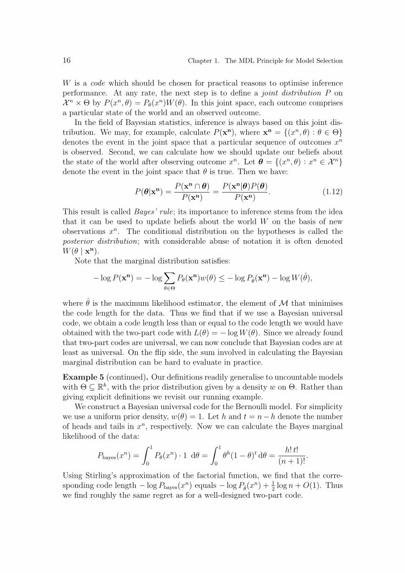
W is a code which should be chosen for practical reasons to optimise inferenceperformance. At any rate, the next step is to define a joint distribution P onX n × Θ by P (xn, θ) = Pθ(x
n)W (θ). In this joint space, each outcome comprisesa particular state of the world and an observed outcome.
In the field of Bayesian statistics, inference is always based on this joint dis-tribution. We may, for example, calculate P (xn), where xn = (xn, θ) : θ ∈ Θdenotes the event in the joint space that a particular sequence of outcomes xn
is observed. Second, we can calculate how we should update our beliefs aboutthe state of the world after observing outcome xn. Let θ = (xn, θ) : xn ∈ X ndenote the event in the joint space that θ is true. Then we have:
P (θ|xn) =P (xn ∩ θ)
P (xn)=
P (xn|θ)P (θ)
P (xn). (1.12)
This result is called Bayes’ rule; its importance to inference stems from the ideathat it can be used to update beliefs about the world W on the basis of newobservations xn. The conditional distribution on the hypotheses is called theposterior distribution; with considerable abuse of notation it is often denotedW (θ | xn).
Note that the marginal distribution satisfies:
− log P (xn) = − log∑
θ∈Θ
Pθ(xn)w(θ) ≤ − log Pθ(x
n)− log W (θ),
where θ is the maximum likelihood estimator, the element of M that minimisesthe code length for the data. Thus we find that if we use a Bayesian universalcode, we obtain a code length less than or equal to the code length we would haveobtained with the two-part code with L(θ) = − log W (θ). Since we already foundthat two-part codes are universal, we can now conclude that Bayesian codes are atleast as universal. On the flip side, the sum involved in calculating the Bayesianmarginal distribution can be hard to evaluate in practice.
Example 5 (continued). Our definitions readily generalise to uncountable modelswith Θ ⊆ R
k, with the prior distribution given by a density w on Θ. Rather thangiving explicit definitions we revisit our running example.
We construct a Bayesian universal code for the Bernoulli model. For simplicitywe use a uniform prior density, w(θ) = 1. Let h and t = n−h denote the numberof heads and tails in xn, respectively. Now we can calculate the Bayes marginallikelihood of the data:
Pbayes(xn) =
∫ 1
0
Pθ(xn) · 1 dθ =
∫ 1
0
θh(1− θ)t dθ =h! t!
(n + 1)!.
Using Stirling’s approximation of the factorial function, we find that the corre-sponding code length − log Pbayes(x
n) equals − log Pθ(xn) + 1
2log n + O(1). Thus
we find roughly the same regret as for a well-designed two-part code.

1.2. Using Models to Encode the Data 17
Prequential Universal Distributions
An algorithm that, given a sequence of previous observations xn, issues a proba-bility distribution on the next outcome P (Xn+1|xn), is called a prequential fore-casting system (PFS) [26, 29, 28]. A PFS defines a random process by thechain rule (1.10). Vice versa, for any random process P on X∞, we can cal-culate the conditional distribution on the next outcome P (Xn+1 | Xn = xn) =P (xn; Xn+1)/P (xn), provided that P (xn) is positive. This so-called predictive dis-tribution of a random process defines a PFS. We give two important prequentialuniversal distributions here.
First, we may take a Bayesian approach and define a joint probability measureon X∞×Θ based on some prior distribution W . As before, this induces a marginalprobability measure on X∞ which in turn defines a PFS. In this way, the Bayesianuniversal distribution can be reinterpreted as a prequential forecasting system.
Second, since the Bayesian predictive distribution can be hard to compute itmay be useful in practice to define a forecasting system that uses a simpler algo-rithm. Perhaps the simplest option is to predict an outcome Xn+1 using the max-imum likelihood estimator for the previous outcomes θ(xn) = arg maxθ Pθ(x
n).We will use this approach in our running example.
Example 5 (continued). The ML estimator for the Bernoulli model parame-terised by the probability of observing heads, equals the frequency of heads in thesample: θ = h/n, where h denotes the number of heads in xn as before. We definea PFS through P (Xn+1|xn) := Pθ. This PFS is ill-defined for the first outcome.Another impractical feature is that it assigns probability 0 to the event that thesecond outcome is different from the first. To address these problems, we slightlytweak the estimator: rather than θ we use θ = (h + 1)/(n + 2).
Perhaps surprisingly, in this case the resulting PFS is equivalent to the Bayesianuniversal distribution approach we defined in the previous section: Pθ turns out tobe the Bayesian predictive distribution for the Bernoulli model if a uniform priordensity w(θ) = 1 is used. In general, the distribution indexed by such a “tweaked”ML estimator may be quite different from the Bayesian predictive distribution.
Although the prequential ML code has been used successfully in practical in-ference problems, the model selection experiments in Chapter 2 show that usageof PFSs based on estimators such as the “tweaked” ML estimator from the ex-ample, leads to significantly worse results than those obtained for the other threeuniversal codes. This is the subject of Chapter 3, where we show that in factthe prequential ML code does achieve the same asymptotic regret as the otheruniversal codes, provided that the distribution that generates the data is an ele-ment of the model. Under misspecification the prequential ML code has differentbehaviour that had not been observed before.

18 Chapter 1. The MDL Principle for Model Selection
Normalised Maximum Likelihood
The last universal code we discuss is the one preferred in the MDL literature,because if we fix some sample size n in advance, it provably minimises the worst-case regret. It turns out that the code minimising the worst-case regret mustachieve equal regret for all possible outcomes xn. In other words, the total codelength must always be some constant longer than the code length achieved on thebasis of the maximum likelihood estimator. This is precisely what the NormalisedMaximum Likelihood (NML) distribution achieves:
Pnml(xn) :=
Pθ(xn)(xn)
∑
yn∈Xn Pθ(yn)(yn)
. (1.13)
For all sequences xn, the regret on the basis of this distribution is exactly equal tothe logarithm of the denominator, called the parametric complexity of the model:
infL
supxnR(L,M, xn) = log
∑
yn∈Xn
Pθ(yn)(yn) (1.14)
Under some regularity conditions on the model it can be shown [72, 39] that thereis a particular continuous function g such that the parametric complexity is lessthan k
2log n
2π+ g(θ), as we required in Section 1.2.3. We return to our Bernoulli
example.
Example 5 (continued). The parametric complexity (1.14) has exponentiallymany terms, but for the Bernoulli model the expression can be significantly sim-plified. Namely, we can group together all terms which have the same maximumlikelihood estimator. Thus the minimal worst-case regret can be rewritten asfollows:
log∑
yn∈Xn
Pθ(yn)(yn) = log
n∑
h=0
(n
h
)(h
n
)h(n− h
n
)n−h
. (1.15)
This term has only linearly many terms and can usually be evaluated in prac-tice. Approximation by Stirling’s formula confirms that the asymptotic regret is12
log n + O(1), the same as for the other universal distributions.
The NML distribution has a number of significant practical problems. First,it is often undefined, because for many models the numerator in (1.13) is infinite,even for such simple models as the model of all Poisson or geometric distributions.Second, |X n| may well be extremely large, in which case it may be impossible toactually calculate the regret. In a sequential setting, the number of terms growsexponentially with the sample size so calculating the NML probability is hopelessexcept in special cases such as the Bernoulli model above, where mathematicaltrickery can be applied to get exact results (for the multinomial model, see [50].)Chapter 2 addresses the question of what can be done when NML is undefinedor too difficult to compute.

1.3. Applications of MDL 19
1.3 Applications of MDL
While we have equated “learning” with “compressing the data” so far, in realitywe often have a more specific goal in mind when we apply machine learningalgorithms. This touches on the third question we asked on page 2: what do wemean by a “useful” hypothesis? In this section we will argue that MDL inference,which is designed to achieving compression of the data, is also suitable to someextent in settings with a different objective, so that, at least to some extent, MDLprovides a reliable one-size-fits-all solution.
1.3.1 Truth Finding
We have described models as formal representations of hypotheses; truth findingis the process of determining which of the hypotheses is “true”, in the sense thatthe corresponding model contains the data generating process. The goal is thento use the available data to identify this true model on the basis of as little dataas possible.
Since the universal code for the true model achieves a code length not muchlarger than the code length of the best code in the model (it was designed toachieve small regret), and the best code in the model achieves code length atmost as large as the data generating distribution, it seems reasonable to assumethat, as more data are being gathered, a true model will eventually be selected byMDL. This intuition is confirmed in the form of the following consistency result,which is one of the pillars of MDL model selection. The result applies to Bayesianmodel selection as well.
Theorem 1.3.1 (Model Selection Consistency). Let H = M1,M2, . . . be acountably infinite set of parametric models. For all n ∈ Z
+, let Mn be 1-to-1parameterised by Θn ⊆ R
k for some k ∈ N and define a prior density wn onΘn. Let W (i) define a prior distribution on the model indices. We require forall integers j > i > 0 that with wj-probability 1, a distribution drawn from Θj ismutually singular with all distributions in Θi. Define the MDL model selectioncriterion based on Bayesian universal codes to represent the models:
δ(xn) = arg mini
(
− log W (i)− log
∫
θ∈Θi
Pθ(xn)wi(θ) dθ
)
.
Then for all δ∗ ∈ Z+, for all θ∗ ∈ Θδ∗, except for a subset of Θδ∗ of Lebesgue
measure 0, it holds for X1, X2, . . . ∼ Pθ∗ that
∃n0 : ∀n ≥ n0 : Pθ∗(δ(Xn) = δ∗) = 1.
Proof. Proofs of various versions of this theorem can be found in [5, 28, 4, 39]and others.

20 Chapter 1. The MDL Principle for Model Selection
The theorem uses Bayesian codes, but as conjectured in [39] and partially inChapter 5, it can probably be extended to other universal codes such as NML.Essentially it expresses that if we are in the ideal situation where one of themodels contains the true distribution, we are guaranteed that this model willbe selected once we have accumulated sufficient data. This property of modelselection criteria is called consistency. Unfortunately, this theorem says nothingabout the more realistic scenario where the models are merely approximationsof the true data generating process. If the true data generating process P ∗ isnot an element of any of the models, it is not known under what circumstancesthe model selection criterion δ selects the model that contains the distributionPθ minimising the Kullback-Leibler divergence D(P ∗‖Pθ). On the other hand,some model selection criteria that are often used in practice (such as maximumlikelihood model selection, or AIC [2]) are known not to be consistent, even in therestricted sense of Theorem 1.3.1. Therefore consistency of MDL and Bayesianmodel selection is reassuring.
1.3.2 Prediction
The second application of model selection is prediction. Here the models are usedto construct a prediction strategy, which is essentially the same as a prequentialforecasting system: an algorithm that issues a probability distribution on thenext outcome given the previous outcomes. There are several ways to define aprediction strategy based on a set of models; we mostly consider what is perhapsthe most straightforward method, namely to apply a model selection criterionsuch as MDL to the available data, and then predict according to some estimatorthat issues a distribution on the next outcome based on the selected model andthe sequence of previous outcomes.1
The performance of a prediction strategy based on a set of models is usuallyanalysed in terms of the rate of convergence, which expresses how quickly thedistribution issued by the prediction strategy starts to behave like the data gen-erating process P ∗. From the information inequality (D(P ∗‖Q) ≥ 0 with equalityfor Q = P ∗) we know that P ∗ itself is optimal for prediction. The expected dis-crepancy between the number of bits needed by the prediction strategy to encodethe next outcome and the number of bits needed by the true distribution P ∗ iscalled the risk ; a prediction strategy has a good rate of convergence if the riskgoes down quickly as a function of the sample size. A number of results thatgive explicit guarantees about the risk convergence rate for prediction strategiesbased on the MDL model selection criterion are given in [39]. Interestingly, the
1This strategy does not take into account the predictions of any of the other models, whileat the same time we can never be sure that the selected model is actually the best one. Itis better to take a weighted average of the predictions of the models in question; the mostcommon practice is to weight the models by their Bayesian posterior probability, a procedurecalled Bayesian model averaging ; see Chapter 5.

1.3. Applications of MDL 21
risk may converge to zero even if P ∗ is not an element of any of the models underconsideration. This is useful in practical applications: for example, if the modelscorrespond to histogram densities with increasing numbers of bins, then the riskconverges to zero if P ∗ is described by any bounded and continuous density; seeChapter 5 for more details.
Roughly speaking, two groups of model selection criteria can be distinguishedin the literature. Model selection criteria of the first group have often been de-veloped for applications of prediction; criteria such as Akaike’s Information Cri-terion (AIC) and Leave One Out Cross-Validation (LOO), exhibit a very goodrisk convergence rate, but they can be inconsistent, i.e. they keep selecting thewrong model regardless of the available amount of data. The second group con-tains criteria such as the Bayesian Information Criterion (BIC), as well as regularBayesian/MDL model selection, which can be proven consistent but which areoften found to yield a somewhat worse rate of convergence. It is a long standingquestion whether these two approaches can be reconciled [103].
An assumption that is implicitly made when MDL or Bayesian model selectionare used for prediction, is that there is one model that exhibits the best predictiveperformance from the start, and our only task is to identify that model. However,in Chapter 5 we argue that this approach is in fact often too simplistic: in reality,which model can provide the best predictive performance may well depend on thesample size. In the histogram density estimation example from above, we typicallydo not expect any particular model to contain the true distribution; instead weexpect to use higher and higher order models as we gain enough data to estimatethe model parameters with sufficient accuracy to make good predictions.
In Chapter 5 we attempt to combine the strong points of the two differ-ent approaches to model selection by dropping the assumption that one modelhas best performance at all sample sizes. This results in a modification ofMDL and Bayesian model selection/averaging, called the switch-distribution, thatachieves better predictive performance, without sacrificing consistency. Note thatthe switch-distribution can be used to improve MDL model selection as wellas Bayesian model selection, although the idea may not agree very well witha Bayesian mindset, as we will discuss.
The switch-distribution ties in with existing universal prediction literature ontracking the best expert, where the assumption that one predictor is best at allsample sizes has already been lifted [94, 46, 95]. In the past, that research hasnot been connected with model selection though. In Chapter 6 we describe howthe switch-code lengths can be computed efficiently, and introduce a formalismthat helps to define other practical methods of combining predictors. These ideashelp understand the connection between many seemingly very different predictionschemes that are described in the literature.

22 Chapter 1. The MDL Principle for Model Selection
1.3.3 Separating Structure from Noise
Algorithmic Rate-Distortion Theory is a generalisation of ideal MDL. Recallfrom 1.1.3 that in ideal MDL, Kolmogorov complexity is used as the code lengthfunction for the hypothesis L(H) = K(H); model selection is then with respectto the set H of all computable hypotheses. This approach is generalised by in-troducing a parameter α, called the rate, that is used to impose a maximum onthe complexity of the hypothesis K(H). The selected hypothesis H, and the codelength it achieves on the data LH(D), now become functions of α. The latterfunction is called the structure function:2
hD(α) = minH∈H,K(H)≤α
LH(D) (1.16)
We write H(α) for the hypothesis that achieves the minimum at rate α. We
use dotted symbols.
=,.< and
.
≤ for (in)equality up to an independent additiveconstant; the dot may be pronounced “roughly”.
A hypothesis H is called a sufficient statistic if K(H) + LH(D).
= K(D). In-tuitively, such hypotheses capture all simple structural properties of the data.Namely, if there are any easily describable properties of D that are not capturedby H, then we would have K(D|H)
.< LH(D). But in that case K(D)
.
≤K(H) +K(D|H)
.< K(H) + LH(D) which is impossible for sufficient statistics H.
If the rate is high enough, certainly for α = K(D), the hypothesis H(α)is a sufficient statistic. The most thorough separation of structure and noiseis obtained at the lowest rate at which H(α) is a sufficient statistic. At evenlower rates, some structural properties of D can no longer be represented; thestructure function can then be used as an indicator of how much structure hasbeen discarded.
Algorithmic rate-distortion theory generalises even further by introducing adistortion function, which allows expression of the kind of properties of the orig-inal object we consider important. It is an analogue of Shannon’s classical rate-distortion theory [79, 37]. The novelty of algorithmic rate-distortion theory com-pared to classical rate-distortion theory is that it allows analysis of individualobjects rather than expected properties of objects drawn from a source distribu-tion. This is useful because it is often impossible to define a source distributionthat is acceptable as a reasonable model of the process of interest. For example,from what source distribution was Tolstoy’s War and Piece drawn?
In Chapter 6 we introduce this new theory of algorithmic rate-distortion inmore detail, and then proceed to put it to the test. To obtain a practical method,we approximate Kolmogorov complexity by the compressed size under a generalpurpose data compression algorithm. We then compute the rate-distortion char-acteristics of four objects from very different domains and apply the results to
2In Kolmogorov’s original formulation, the codes LH for H ∈ H were uniform on finite setsof possible outcomes.

1.4. Organisation of this Thesis 23
denoising and lossy compression. The chapter is written from the point of view ofalgorithmic rate-distortion theory, but includes a discussion of how the approachrelates to MDL as we describe it in this introduction.
1.4 Organisation of this Thesis
In this introduction we have outlined MDL model selection. An important in-gredient of MDL model selection is universal coding (Section 1.2.3). We havedescribed several approaches; the universal code preferred in the MDL literatureis the code that corresponds to the Normalised Maximum Likelihood (NML) dis-tribution (1.13), which achieves minimal regret in the worst case. However itturns out that the NML distribution is often undefined. In those cases, the wayto proceed is not agreed upon. In Chapter 2, we evaluate various alternativesexperimentally by applying MDL to select between the Poisson and geometricmodels. The results provide insight into the strengths and weaknesses of thesevarious methods.
One important result of the experiments described in Chapter 2 is that theprequential forecasting system, one of the universal models introduced in Sec-tion 1.2.3), defined to issues predictions on the basis of the maximum likelihooddistribution, achieves a regret very different from that achieved by other models.This leads to inferior model selection performance. This was unexpected, be-cause in the literature, e.g. [71], the prequential ML universal model is describedas a practical approximation of other universal codes, certainly suitable for modelselection. In Chapter 3 we analyse the regret of the prequential ML universal dis-tribution under misspecification, that is, the data are drawn from a distributionoutside the model. The behaviour under misspecification is important to modelselection, since there the data generating distribution is often in only one of theconsidered models (if that many). Together, chapters 2 and 3 form the first legof this thesis.
The second leg involves the relationship between model selection and predic-tion (see Section 1.3). It is based on the observation that the model that allowsfor the best predictions may vary with the sample size. For example, simple mod-els with only few parameters tend to predict reasonably well at small sample sizeswhile for large models often a lot of data is required before the parameters can beestimated accurately enough to result in good predictions. While this may seemobvious, we show that the codes that are typically used in Bayesian and MDLmodel selection do not take this effect into account and thus the achieved codelengths are longer than they need to be. In Chapter 4 we describe a number ofalternative ways to combine the predictions of multiple codes. It is also shownhow the resulting code lengths can still be computed efficiently. The discussionexpands on results in the source coding and universal prediction. One of thedescribed codes, called the switch-code, is specifically designed to improve model

24 Chapter 1. The MDL Principle for Model Selection
selection results. In Chapter 5 we show how model selection based on the switch-code, while remaining consistent, achieves the best possible rate of convergence.This resolves a perceived distinction between consistent model selection criteriaon the one hand, and criteria that are suitable for prediction, which achieve a fastrate of convergence, on the other hand.
In Chapter 6, the third leg of this thesis, we put the new algorithmic rate-distortion theory to the test. Algorithmic rate-distortion theory is introducedin Section 1.3.3, more thoroughly in Chapter 6 itself, and even more thoroughlyin [92]. It is a generalisation of ideal MDL (Section 1.1.3) and a variation onclassical rate-distortion theory [79]; it allows for analysis of the rate-distortionproperties of individual objects rather than of objects drawn from some source dis-tribution. Algorithmic rate-distortion theory uses Kolmogorov complexity whichis uncomputable. To obtain a practical method, we approximate Kolmogorovcomplexity by the compressed size under a general purpose data compression al-gorithm. We then compute the rate-distortion characteristics of four objects fromvery different domains and apply the results to denoising and lossy compression.

Chapter 2
Dealing with Infinite ParametricComplexity
Model selection is the task of choosing one out of a set of hypotheses for somephenomenon, based on the available data, where each hypothesis is representedby a model, or set of probability distributions. As explained in the introductorychapter, MDL model selection proceeds by associating a so-called universal dis-tribution with each model. The number of bits needed to encode the data D usingthe universal code associated with model M is denoted LM(D). We then pickthe model that minimises this expression and thus achieves the best compressionof the data.
Section 1.2.3 lists the most important such universal codes, all of which resultin slightly different code lengths and thus to different model selection criteria.While any choice of universal code will lead to an asymptotically “consistent”model selection method (eventually the right model will be selected), to get goodresults for small sample sizes it is crucial that we select an efficient code.
The MDL literature emphasises that the used universal code should be efficientwhatever data are observed : whenever the model contains a code or distributionthat fits the data well in the sense that it achieves a small code length, theuniversal code length should not be much larger. More precisely put, the universalcode should achieve small regret in the worst case over all possible observations,where the regret is the difference between the universal code length and theshortest code length achieved by an element of the model M. The normalisedmaximum likelihood (NML) code (Section 1.2.3) minimises this worst-case regret.Moreover, the NML regret is a function of only the sample size n, and doesnot depend on the data. As such it can be viewed as an objective measure ofmodel complexity: the parametric complexity of a model is the regret achievedby the NML code, as a function of the sample size n. For this reason NML is thepreferred universal code in modern MDL.
However, it turns out that the parametric complexity is infinite for manymodels, so that NML-based model selection is not effective. Other universal codes
25

26 Chapter 2. Dealing with Infinite Parametric Complexity
that do achieve finite code lengths can usually still be defined for such models,but those codes have a worst-case regret that depends not only on the sample sizen, but also on the parameter of the best fitting distribution in the model θ; suchcodes are luckiness codes in the sense of Section 1.1.1. Model selection criteriabased on such luckiness codes thus acquire an element of subjectivity.
Several remedies have been proposed for this situation: variations on NML-based model selection that can obviously not be worst case optimal, but that doachieve finite code length without explicitly introducing regret that depends onthe element of the model that best fits the data. In this chapter we evaluate suchalternative procedures empirically for model selection between the simple Poissonand geometric models. We chose these two models since they are just about thesimplest and easiest-to-analyse models for which the NML code is undefined. Wefind that some alternative solutions, such as the use of BIC (or, equivalently, inour context, maximum likelihood testing) lead to relatively poor results. Ourmost surprising finding is the fact that the prequential maximum likelihood code– which was found to perform quite well in some contexts [61, 52] – exhibits poorbehaviour in our experiments. We briefly discuss the reasons for this behaviourin Section 2.5; a full analysis is the subject of Chapter 3.
Since the codes used in these approaches no longer minimise the worst-caseregret they are harder to justify theoretically. In fact, as explained in more detailin Section 2.3.6, the only method that may have an MDL-type justification closelyrelated to that of the original NML code is the Bayesian code with the improperJeffreys’ prior. Perhaps not coincidentally, this also seems the most dependableselection criterion among the ones we tried.
In Section 2.1 we describe the code that achieves worst-case minimal regret.This code does not exist for the Poisson and geometric distributions. We analysethese models in more detail in Section 2.2.
In Section 2.3 we describe four different approaches to MDL model selectionunder such circumstances. We test these criteria by measuring error probability,bias and calibration, as explained in Section 2.4. The results are evaluated inSection 2.5. Our conclusions are summarised in Section 2.6.
2.1 Universal codes and Parametric Complexity
We first briefly review some material from the introductory chapter that is es-pecially important to this chapter. The regret of a code L with respect to aparametric model M = Pθ : θ ∈ Θ with parameter space Θ on a sequence ofoutcomes xn = x1, . . . , xn ∈ X n is
R(L,M, xn) := L(xn)− infθ∈Θ− log Pθ(x
n),
which was first defined in (1.4), page 5. A function θ : X n → Θ that mapsoutcomes xn to a parameter value that achieves this infimum is called a maximum

2.1. Universal codes and Parametric Complexity 27
likelihood estimator. We sometimes abbreviate θ = θ(xn).A code L is f -universal with respect to modelM if R(L,M, xn) ≤ f(θ, n) for
all n and all xn (Definition 1.2.2, page 14). The MDL philosophy [72, 38] has itthat the best universal code minimises the regret in the worst case of all possi-ble data sequences. This “minimax optimal” solution is called the “NormalisedMaximum Likelihood” (NML) code, which was first described by Shtarkov, whoalso observed its minimax optimality properties. The NML-probability of a datasequence for a parametric model is defined as in (1.13), page 18:
Pnml(xn) :=
P (xn|θ(xn))∑
yn P (yn|θ(yn)),
with corresponding code length
Lnml(xn) := − log P (xn|θ(xn)) + log
∑
yn
P (yn|θ(yn)).
This code length is called the stochastic complexity of the data. The first termin the equation is the code length of the data using the maximum likelihoodestimator; the second term is the − log of the normalisation factor of Pnml, calledthe parametric complexity of the model M at sample size n.
It is usually impossible to compute the parametric complexity analytically,but there exists a good approximation Lanml, due to Rissanen, Takeuchi andBarron [72, 88, 89, 87]:
Lanml(xn) := L(xn|θ) +
k
2log
n
2π+ log
∫
Θ
√
det I(θ) dθ. (2.1)
Here, n, k and I(θ) denote the number of outcomes, the number of parametersand the Fisher information matrix respectively. If M is an exponential familymodel such as the Poisson and Geometric models considered in this chapter, and isparameterised by Θ ⊆ R
k for some k ∈ Z+, and if both the parametric complexity
and the integral in (2.1) are finite, then we have the following. For any Θ′ withnonempty interior, and whose closure is a bounded subset of the interior of Θ, wehave
limn→∞
supxn:θ(xn)∈Θ′
|Lnml(xn)− Lanml(x
n)| = 0.
Thus, the approximation uniformly converges to the exact code length for allsequences of outcomes whose maximum likelihood estimator does not converge tothe boundaries of the parameter space. For more information, see [39]. Since thelast term in (2.1) does not depend on the sample size, it has often been disregardedand many people came to associate MDL only with the first two terms. But thethird term can be quite large or even infinite, and it can substantially influencethe inference results for small sample sizes. Interestingly, (2.1) also describes

28 Chapter 2. Dealing with Infinite Parametric Complexity
the asymptotic behaviour of the Bayesian universal code where Jeffreys’ prior isused: here MDL and an objective Bayesian method coincide even though theirmotivation is quite different.
As stated in the introduction, the problem is that for many models the para-metric complexity is infinite. Many strategies have been proposed to deal withthis, but most are somewhat ad-hoc. When Rissanen defines stochastic complex-ity as Lnml(x
n) in [72], he writes that he does so “thereby concluding a decadelong search”, but as Lanterman observes in [53], “in the light of these problemswe may have to postpone concluding the search just a while longer”.
2.2 The Poisson and Geometric Models
We investigate MDL model selection between the Poisson and Geometric models.Figure 2.1 may help form an intuition about the probability mass functions ofthe two distributions. One reason for our choice of models is that they are bothsingle parameter models, so that the dominant k
2log n
2πterm of (2.1) cancels. This
means that at least for large sample sizes, simply picking the model that best fitsthe data should always work. We nevertheless observe that for small sample sizes,data generated by the geometric distribution are misclassified as Poisson muchmore frequently than the other way around (see Section 2.5). So in an informalsense, even though the number of parameters is the same, the Poisson distributionis more prone to “overfitting”.
To counteract the bias in favour of Poisson that is introduced if we just selectthe best fitting model, we would like to compute the third term of (2.1), whichnow characterises the parametric complexity. But as it turns out, both modelshave an infinite parametric complexity! The integral in the third term of theapproximation also diverges. So in this case it is not immediately clear how thebias should be removed. This is the second reason why we chose to study thePoisson and Geometric models. In Section 2.3 we describe a number of methodsthat have been proposed in the literature as ways to deal with infinite parametriccomplexity; in Section 2.5 they are evaluated empirically.
Reassuringly, all methods we investigate tend to compensate for this overfit-ting phenomenon by “punishing” the Poisson model. However, to what extent thebias is compensated depends on the used method, so that different methods givedifferent results.
We parameterise both the Poisson and the Geometric family of distributionsby the mean µ ∈ (0,∞), to allow for easy comparison. This is possible becausefor both models, the empirical mean (average) of the observed data is a sufficientstatistic. For Poisson, parameterisation by the mean is standard. For geometric,the reparameterisation can be arrived at by noting that in the standard parame-terisation, P (x|θ) = (1−θ)xθ, the mean is given by µ = (1−θ)/θ. As a notationalreminder the parameter is called µ henceforth. Conveniently, the ML estimator

2.3. Four Ways to deal with Infinite Parametric Complexity 29
Figure 2.1 The mean 5 Poisson and geometric distributions.
0
0.02
0.04
0.06
0.08
0.1
0.12
0.14
0.16
0.18
0 5 10 15 20
P(n
)
n
PoissonGeometric
µ for both distributions is the average of the data.We will add a subscript p or g to indicate that code lengths are computed
with respect to the Poisson model or the Geometric model, respectively. Fur-thermore, to simplify the equations in the remainder of this chapter somewhatwe will express code lengths in nats (− ln probabilities) rather than bits (− log2
probabilities).
LP
(xn|µ
)= − ln
n∏
i=1
e−µµxi
xi!=
n∑
i=1
ln(xi!) + nµ− ln µ
n∑
i=1
xi, (2.2)
LG
(xn|µ
)= − ln
n∏
i=1
µxi
(µ+1)xi+1= n ln(µ+1)− ln
(µ
µ+1
) n∑
i=1
xi. (2.3)
2.3 Four Ways to deal with Infinite Parametric
Complexity
In this section we discuss four general ways to deal with the infinite parametriccomplexity of the Poisson and Geometric models when the goal is to do model

30 Chapter 2. Dealing with Infinite Parametric Complexity
selection. Each of these four methods leads to one, or sometimes more, concretemodel selection criteria which we evaluate in Section 2.5.
2.3.1 BIC/ML
One way to deal with the diverging integral in the approximation is to just ignoreit. The model selection criterion that results corresponds to only a very roughapproximation of any real universal code, but it has been used and studied ex-tensively. It was first derived by Jeffreys as an approximation to the Bayesianmarginal likelihood [47], but it became well-known only when it was proposed byRissanen [67] and Schwarz [78]. While Schwarz gave the same type of derivationas Jeffreys, Rissanen arrived at it in a quite different manner, as an approximationto a two-part code length. We note that Rissanen already abandoned the ideain the mid 1980’s in favour of more sophisticated code length approximations.Because of its connection to the Bayesian marginal likelihood, it is best known asthe BIC (Bayesian Information Criterion):
LBIC(xn) = L(xn|µ) +k
2ln n.
Comparing BIC to the approximated NML code length we find that in addition tothe diverging term, a k
2ln 1
2πterm has also been dropped. This curious difference
can be safely ignored in our setup, where k is equal to one for both models sothe whole term cancels anyway. According to BIC, we must select the Geometricmodel if
0 < LP,BIC (xn)− LG,BIC (xn) = LP
(xn|µ
)− LG
(xn|µ
).
We are left with a generalised likelihood ratio test (GLRT). In such a test, theratio of the probabilities under the two models, PP
(xn|µ
)/PG
(xn|µ
)is compared
against a fixed constant η; the BIC criterion thus reduces to a GLRT with η = 0,which is also known as maximum likelihood (ML) testing. As we remarked before,experience shows that this approach often leads to overfitting and a bias in favourof the “more complex” Poisson model. (On a side note, this equivalence of BICand ML occurs when all models under consideration have the same numbers ofparameters; if this is not the case, then BIC may or may not overfit and it usuallygives better results than ML.)
2.3.2 Restricted ANML
One often used method of rescuing the NML approach to MDL model selectionis to restrict the range of values that the parameters can take to ensure that thethird term of (2.1) stays finite. Our approach is to impose a maximum on theallowed mean by setting Θ = (0, µ∗).

2.3. Four Ways to deal with Infinite Parametric Complexity 31
To compute the approximated parametric complexity of the restricted modelswe need to establish the Fisher information first. We use I(θ) = −Eθ[
d2
dθ2 L(x|θ)]
to obtain
IP (µ) = −Eµ
[
− x
µ2
]
=1
µ, and (2.4)
IG (µ) = −Eµ
[
− x
µ2+
x + 1
(µ + 1)2
]
=1
µ(µ + 1). (2.5)
Now we can compute the last term in the parametric complexity approximation(2.1):
ln
∫ µ∗
0
√
IP (µ) dµ = ln
∫ µ∗
0
µ− 12 dµ = ln
(2√
µ∗)
; (2.6)
ln
∫ µ∗
0
√
IG (µ) dµ = ln
∫ µ∗
0
1√
µ(µ + 1)dµ = ln
2 ln(√
µ∗ +√
µ∗ + 1)
.(2.7)
Thus, the parametric complexities of the restricted models are both monotonicallyincreasing functions of µ∗. Let the function δ(µ∗) := ln(2
√µ∗) − ln(2 ln(
√µ∗ +√
µ∗ + 1)) measure the difference between the parametric complexities. We obtaina model selection criterion that selects the Geometric model if
0 < LP,ANML(µ∗) (xn)− LG,ANML(µ∗) (xn) = LP
(xn|µ
)− LG
(xn|µ
)+ δ(µ∗).
This is equivalent to a GLRT with threshold δ(µ∗). We have experimented withrestricted models where the parameter range was restricted to (0, µ∗) for µ∗ ∈10, 100, 1000.
It is not hard to show that the parametric complexity of the restricted Poissonmodel grows faster with µ∗ than the parametric complexity of the Geometricmodel: δ(µ∗) is monotonically increasing in µ∗, and grows unboundedly in µ∗.This indicates that the Poisson model has more descriptive power, even thoughthe models have the same number of parameters and both have infinite parametriccomplexity.
An obvious conceptual problem with restricted ANML is that the imposed re-striction is quite arbitrary and requires a priori knowledge about the scale of theobservations. But the parameter range can be interpreted as a hyper-parameter,which can be incorporated into the code using several techniques; two such tech-niques are discussed next.
2.3.3 Two-part ANML
Perhaps the easiest way to get rid of the µ∗ parameter that determines the pa-rameter range, and thereby the restricted ANML code length, is to use a two-part

32 Chapter 2. Dealing with Infinite Parametric Complexity
code. The first part contains a specification of µ∗, which is followed by an encod-ing of the rest of the data with an approximate code length given by restrictedANML for that µ∗. To do this we need to choose some discretisation, such thatwhatever µ is, it does not cost many bits to specify an interval that contains it. Fora sequence with ML parameter µ, we choose to encode the integer b = ⌈log2 µ⌉. Adecoder, upon reception of such a number b, now knows that the ML parametervalue must lie in the range (2b−1, 2b] (for otherwise another value of b would havebeen transmitted). By taking the logarithm we ensure that the number of bitsused in coding the parameter range grows at a negligible rate compared to thecode length of the data itself, but we admit that the code for the parameter rangeallows much more sophistication. We do not really have reason to assume thatthe best discretisation should be the same for the Poisson and Geometric modelsfor example.
The two-part code is slightly redundant, since code words are assigned to datasequences of which the ML estimator lies outside the range that was encoded inthe first part – such data sequences cannot occur, since for such a sequence wewould have encoded a different range. Furthermore, the two-part code is nolonger minimax optimal, so it is no longer clear why it should be better thanother universal codes which are not minimax optimal. However, as argued in[38], whenever the minimax optimal code is not defined, we should aim for a codeL which is “close” to minimax optimal in the sense that, for any compact subsetM′ of the parameter space, the additional regret of L on top of the NML codefor M′ should be small, e.g. O(log log n). The two-part ANML code is one ofmany universal codes satisfying this “almost minimax optimality”. While it maynot be better than another almost minimax optimal universal code, it certainlyis better than universal codes which do not have the almost minimax optimalityproperty.
2.3.4 Renormalised Maximum Likelihood
Related to the two-part restricted ANML, but more elegant, is Rissanen’s renor-malised maximum likelihood (RNML) code, [73, 38]. This is perhaps the mostwidely known approach to deal with infinite parametric complexity. The idea hereis that the NML distribution is well-defined if the parameter range is restrictedto, say, the range (0, µ∗). Letting PNML,µ∗ be the NML distribution relative to thisrestricted model, we can now define a new parametric model, with µ∗ as the pa-rameter and the corresponding restricted NML distributions PNML,µ∗ as elements.For this new model we can again compute the NML distribution! To do this, weneed to compute the ML value for µ∗, which in this case can be seen to be assmall as possible such that µ still falls within the range, in other words, µ∗ = µ.
If this still leads to infinite parametric complexity, we define a hyper-hyper-parameter. We repeat the procedure until the resulting complexity is finite. Un-fortunately, in our case, after the first renormalisation, both parametric complex-

2.3. Four Ways to deal with Infinite Parametric Complexity 33
ities are still infinite; we have not performed a second renormalisation. Therefore,the RNML code is not included in our experiments.
2.3.5 Prequential Maximum Likelihood
The prequential maximum likelihood code, which we will abbreviate PML-code, isan attractive universal code because it is usually a lot easier to implement thaneither NML or a Bayesian code. Moreover, its implementation hardly requiresany arbitrary decisions. Here the outcomes are coded sequentially using theprobability distribution indexed by the ML estimator for the previous outcomes[26, 69]; for a general introduction see [96] or [38].
LPIPC (xn) =n∑
i=1
L(
xi|µ(xi−1))
,
where L(xi|µ(xi−1)
)= − ln P
(xi|µ(xi−1)
)is the number of nats needed to encode
outcome xi using the code based on the ML estimator on xi−1. We further discussthe motivation for this code in Section 2.5.1.
For both the Poisson model and the Geometric model, the maximum likelihoodestimator is not well-defined until after a nonzero outcome has been observed(since 0 is not inside the allowed parameter range). This means that we need touse another code for the first few outcomes. It is not really clear how we can usethe model assumption (Poisson or geometric) here, so we pick a simple code forthe nonnegative integers that does not depend on the model. This will result inthe same code length for both models; therefore it does not influence which modelis selected. Since there are usually only very few initial zero outcomes, we mayreasonably hope that the results are not too distorted by our way of handling thisstart-up problem. We note that this start-up problem is an inherent feature of thePML approach [26, 71], and our way of handling it is in line with the suggestionsin [26].
2.3.6 Objective Bayesian Approach
In the Bayesian framework we select a prior w(θ) on the unknown parameter andcompute the marginal likelihood
PBAYES (xn) =
∫
Θ
P(xn|θ
)w(θ) dθ, (2.8)
with universal code length LBAYES (xn) = − ln PBAYES (xn). Like NML, this canbe approximated with an asymptotic formula. Under conditions similar to thosefor the NML approximation (2.1), we have [3]:
LABAYES (xn) := L(
xn|θ)
+k
2ln
n
2π+ ln
√
det I(θ)
w(θ), (2.9)

34 Chapter 2. Dealing with Infinite Parametric Complexity
where the asymptotic behaviour is the same as for the approximation of the NMLcode length, roughly LABAYES (xn) − LBAYES (xn) → 0 as n → ∞ (see below Eq.(2.1) for details). Objective Bayesian reasoning suggests we use Jeffreys’ prior forseveral reasons; one reason is that it is uniform over all “distinguishable” elementsof the model [3], which implies that the obtained results are independent of theparameterisation of the model [47]. It is defined as follows:
w(θ) =
√
det I(θ)∫
Θ
√
det I(θ) dθ. (2.10)
Unfortunately, the normalisation factor in Jeffreys’ prior diverges for both thePoisson model and the Geometric model. But if one is willing to accept a so-called improper prior, which is not normalised, then it is possible to compute aperfectly proper Bayesian posterior, after observing the first outcome, and usethat as a prior to compute the marginal likelihood of the rest of the data. Referto [14] for more information on objective Bayesian theory. The resulting universalcodes with lengths LBAYES
(x2, . . . , xn | x1
)are, in fact, conditional on the first
outcome. Recent work by [58] suggests that, at least asymptotically and for one-parameter models, the universal code achieving the minimal expected redundancyconditioned on the first outcome is given by the Bayesian universal code with theimproper Jeffreys’ prior. Li and Barron only prove this for scale and locationmodels, but their result does suggest that the same would still hold for generalexponential families such as Poisson and geometric. It is possible to define MDLinference in terms of either the expected redundancy or of the worst-case regret.In fact, the resulting procedures are very similar, see [4]. Thus, we have a tentativejustification for using Jeffreys’ prior also from an MDL point of view, on top ofits justification in terms of objective Bayes.
It can be argued that using the first outcome for conditioning rather thansome other outcome is arbitrary while it does influence the results. On the otherhand, the posterior after having observed all data will be the same whateveroutcome is elected to be the special one that we refrain from encoding. It alsoseems preferable to let results depend on arbitrary properties of the data thanto let it depend on arbitrary decisions of the scientist, such as the choice for amaximum value for µ∗ in the case of the restricted ANML criterion. As advocatedfor instance in [13], arbitrariness can be reduced by conditioning on every outcomein turn and then using the mean or median code length one so obtains. We havenot gone to such lengths in this study.
We compute Jeffreys’ posterior after observing one outcome, and use it tofind the Bayesian marginal likelihoods. We write xj
i to denote xi, . . . , xj andµ(xj
i ) to indicate which outcomes determine the ML estimator, finally we abbre-viate sn = x1 + . . . + xn. The goal is to compute PBAYES
(xn
2 | x1
)for the Poisson
and Geometric models. As before, the difference between the corresponding codelengths defines a model selection criterion. We also compute PABAYES
(xn
2 | x1
)

2.4. Experiments 35
for both models, the approximated version of the same quantity, based on ap-proximation formula (2.9). Equations for the Poisson and Geometric models arepresented below.
Bayesian code for the Poisson model We compute Jeffreys’ improper priorand the posterior after observing one outcome:
wP (µ) ∝√
IP (µ) = µ− 12 ; (2.11)
wP
(µ | x1
)=
PP
(x1|µ
)wP (µ)
∫∞
0PP
(x1|θ
)wP (θ) dθ
=e−µµx1−
12
Γ(x1 + 12). (2.12)
From this we can derive the marginal likelihood of the rest of the data. Thedetails of the computation are omitted for brevity.
PP,BAYES
(xn
2 | x1
)=
∫ ∞
0
PP
(xn
2 |µ)wP
(µ | x1
)dµ =
Γ(sn + 12)
Γ(x1 + 12)/
ns+ 12
n∏
i=2
xi!
.
(2.13)For the approximation (2.9) we obtain:
LP,ABAYES
(xn
2 | x1
)= LP
(xn
2 |µ(xn2
))+ 1
2ln
n
2π+ µ(xn
2 )−x1 ln µ(xn2 )+ln Γ(x1 + 1
2).
(2.14)
Bayesian code for the Geometric model We perform the same computa-tions for the Geometric model. This time we get:
wG (µ) ∝ µ− 12 (µ + 1)−
12 ; (2.15)
wG
(µ | x1
)= (x1 + 1
2)µx1−
12 (µ + 1)−x1−
32 ; (2.16)
PG,BAYES (xn) = (x1 + 12)Γ(s + 1
2)Γ(n)
Γ(n + s + 12). (2.17)
For the approximation we obtain:
LG,ABAYES
(xn
2 | x1
)= LG
(xn
2 |µ(xn2
)) + 1
2ln
n
2π
+ x1 ln
(
1 +1
µ(xn2 )
)
+ 12
ln(µ(xn2 ))− ln(x1 + 1
2). (2.18)
2.4 Experiments
The previous section describes four methods to compute or approximate thelength of a number of different universal codes, which can be used in an MDLmodel selection framework. The MDL principle tells us to select the model using

36 Chapter 2. Dealing with Infinite Parametric Complexity
which we can achieve the shortest code length for the data. This coincides withthe Bayesian maximum a-posteriori (MAP) model with a uniform prior on themodels. In this way each method for computing or approximating universal codelengths defines a model selection criterion, which we want to compare empirically.
Known µ criterion In addition to the criteria that are based on universalcodes, as developed in Section 2.3, we define one additional, “ideal” criterion toserve as a reference by which the others can be evaluated. The known µ criterioncheats a little bit: it computes the code length for the data with knowledge of themean of the generating distribution. If the mean is µ, then the known µ criterionselects the Poisson model if LP
(xn|µ
)< LG
(xn|µ
). Since this criterion uses
extra knowledge about the data, it should be expected to perform better thanthe other criteria. The theoretical analysis of the known µ criterion is helpedby the circumstance that (1) one of the two hypotheses equals the generatingdistribution and (2) the sample consists of outcomes which are i.i.d. according tothis distribution. In [25], Sanov’s Theorem is used to show that in such a situation,the probability that the criterion prefers the wrong model (“error probability”)decreases exponentially in the sample size. If the Bayesian MAP model selectioncriterion is used then the following happens: if the data are generated usingPoisson[µ] then the error probability decreases exponentially in the sample size,with some error exponent; if the data are generated with Geom[µ] then the overallerror probability is exponentially decreasing with the same exponent [25, Theorem12.9.1 on page 312 and text thereafter]. Thus, we expect that the line for the“known µ” criterion is straight on a logarithmic scale, with a slope that is equalwhether the generating distribution is Poisson or geometric. This proves to bethe case, as can be seen from Figure 2.2.
Tests We perform three types of test on the selection criteria, which are de-scribed in detail in the following subsections:
1. Error probability measurements.
2. Bias measurements.
3. Calibration testing.
2.4.1 Error Probability
The error probability for a criterion is the probability that it will select a modelthat does not contain the distribution from which the data were sampled. Inour experiments, samples are always drawn from a Poisson[µ] distribution withprobability p, or from a Geom[µ] distribution with probability 1−p. We measurethe error probability through repeated sampling; strictly speaking we thus obtainerror frequencies which approximate the error probability.

2.4. Experiments 37
Figures 2.2, 2.4, 2.5 and 2.6 plot the sample size against the error frequency,using different means µ and different priors p on the generating distribution. Weuse a log-scale, which allows for easier comparison of the different criteria; aswe pointed out earlier, for the known µ criterion we should expect to obtain astraight line.
In Figures 2.4, 2.5 and 2.6 the log of the error frequency of the known µcriterion is subtracted from the logs of the error frequencies of the other criteria.This brings out the differences in performance in even more detail. The knownµ criterion, which has no bias, is perfectly calibrated (as we will observe later)and which also has a low error probability under all circumstances (althoughbiased criteria can sometimes do better if the bias happens to work in the rightdirection), is thus treated as a baseline of sorts.
2.4.2 Bias
We define the level of evidence in favour of the Poisson model as:
∆ (xn) := LG
(xn|µ
)− LP
(xn|µ
), (2.19)
which is the difference in code lengths according to the known µ criterion. Theother criteria define estimators for this quantity: the estimator for a criterion Cis defined as:
∆C(xn) := LG,C (xn)− LP,C (xn) (2.20)
(Some people are more familiar with Bayes factors, of which this is the logarithm.)In our context the bias of a particular criterion is the expected difference betweenthe level of evidence according to that criterion and the true level of evidence,
E[∆C(Xn)−∆ (Xn)
]. (2.21)
The value of this expectation depends on the generating distribution, which isassumed to be some mixture of the Poisson and geometric distributions of thesame mean.
We measure the bias through sampling. We measure the bias with generatingdistributions Poisson[8] and Geom[8]; as before we vary the sample size. Theresults are in Figure 2.3.
2.4.3 Calibration
The classical interpretation of probability is frequentist: an event has probabilityp if in a repeated experiment the frequency of the event converges to p. Thisinterpretation is no longer really possible in a Bayesian framework, since priorassumptions often cannot be tested in a repeated experiment. For this reason,calibration testing is avoided by some Bayesians who may put forward that it

38 Chapter 2. Dealing with Infinite Parametric Complexity
is a meaningless procedure from a Bayesian perspective. On the other hand, wetake the position that even with a Bayesian hat on, one would like one’s inferenceprocedure to be calibrated – in the idealised case in which identical experimentsare performed repeatedly, probabilities should converge to frequencies. If theydo not behave as we would expect even in this idealised situation, then howcan we trust inferences based on such probabilities in the real world with all itsimperfections?
In the introduction we have indicated the correspondence between code lengthsand probability. If the universal code lengths for the different criteria correspondto probabilities that make sense in a frequentist way, then the Bayesian a posteri-ori probabilities of the two models should too. To test this, we generate sampleswith a fixed mean and a fixed sample size; half of the samples are drawn froma Poisson distribution and half from a geometric distribution. We then computethe a posteriori probability that it is generated by the Poisson model, for eachof the selection criteria. The samples are distributed over 40 bins by discretisingtheir a posteriori probability. For each bin we count the number of sequences thatactually were generated by Poisson. If the a posteriori Bayesian probability thatthe model is Poisson makes any sense in a frequentist way, then the result shouldbe a more or less straight diagonal.
The results are in Figure 2.7. We used mean 8 and sample size 8 because onthe one hand we want a large enough sample size that the posterior has convergedto something reasonable, but on the other hand if we choose the sample size evenlarger it becomes exceedingly unlikely that a sequence is generated of which theprobability that it is Poisson is estimated near 0.5, so we would need to generate aninfeasibly large number of samples to get accurate results. Note that the “knownµ” criterion is perfectly calibrated, because its implicit prior distribution on themean of the generating distribution puts all probability on the actual mean, so theprior perfectly reflects the truth in this case. Under such circumstances Bayesianand frequentist probability become the same, and we get a perfect answer.
We feel that calibration testing is too often ignored, while it can safeguardagainst inferences or predictions that bear little relationship to the real world.Moreover, in the objective Bayesian branch of Bayesian statistics, one does em-phasise procedures with good frequentist behaviour [11]. At least in restrictedcontexts [23, 22], Jeffreys’ prior has the property that the Kullback-Leibler diver-gence between the true distribution and the posterior converges to zero quickly,no matter what the true distribution is. Consequently, after observing only alimited number of outcomes, it should already be possible to interpret the pos-terior as an almost “classical” distribution in the sense that it can be verified byfrequentist experiments [23].

2.5. Discussion of Results 39
2.5 Discussion of Results
Roughly, the results of our tests can be summarised as follows:
• In this toy problem, as one might expect, all criteria perform extremely welleven while the sample size is small. But there are also small but distinctdifferences that illustrate relative strengths and weaknesses of the differentmethods. When extrapolated to a more complicated model selection prob-lem, our results should help to decide which criteria are appropriate for thejob.
• As was to be be expected, the known µ criterion performs excellently on alltests.
• The PML and BIC/ML criteria exhibit the worst performance.
• The basic restricted ANML criterion yields results that range from good tovery bad, depending on the chosen parameter range. Since the range mustbe chosen without any additional knowledge of the properties of the data,this criterion is rather arbitrary.
• The results for the two-part restricted ANML and Objective Bayesian cri-teria are reasonable in all tests we performed; these criteria thus displayrobustness.
In the following subsections we evaluate the results for each model selection cri-terion in turn.
2.5.1 Poor Performance of the PML Criterion
One feature of Figure 2.2 that immediately attracts attention is the unusual slopeof the error rate line of the PML criterion, which clearly favours the geometricdistribution. This is even clearer in Figure 2.3, where the PML criterion canbe observed to become more and more favourable to the Geometric model asthe sample size increases, regardless of whether the data were sampled from aPoisson or geometric distribution. This is also corroborated by the results onthe calibration test, where the PML criterion most severely underestimates theprobability that the data were sampled from a Poisson distribution: of thosesequences that were classified as geometric with 80% confidence, in fact about60% turned out to be sampled from a Poisson distribution.
While this behaviour may seem appropriate if the data really are more likely tocome from a geometric distribution, there is actually a strong argument that evenunder those circumstances it is not the most desirable behaviour, for the followingreason. Suppose that we put a fixed prior p on the generating distribution, withnonzero probability for both distributions Poisson[µ] and Geom[µ]. The marginal

40 Chapter 2. Dealing with Infinite Parametric Complexity
Figure 2.2 The log10 of the error frequency.
-3
-2.5
-2
-1.5
-1
-0.5
0
5 10 15 20 25 30
log
erro
r fr
eque
ncy
sample size
Error frequency when data are sampled from Poisson[4]
Plug-inANML max=1000
Approx. BayesANML max=100
ANML 2partBayesian
known muANML max=10
ML
-3
-2.5
-2
-1.5
-1
-0.5
0
5 10 15 20 25 30
log
erro
r fr
eque
ncy
sample size
Error frequency when data are sampled from Geometric[4]
MLANML max=10
BayesianANML 2part
Approx. BayesANML max=100
known muANML max=1000
Plug-in

2.5. Discussion of Results 41
Figure 2.3 The classification bias in favour of the Poisson model in bits.
-7
-6
-5
-4
-3
-2
-1
0
1
2
5 10 15 20 25 30
bias
in fa
vour
of t
he P
oiss
on m
odel
(bi
ts)
sample size
Bias when data are sampled from Poisson[8]
MLknown mu
ANML max=10Bayesian
ANML 2partANML max=100
Approx. BayesANML max=1000
Plug-in
-10
-8
-6
-4
-2
0
2
4
6
8
5 10 15 20 25 30
bias
in fa
vour
of t
he P
oiss
on m
odel
(bi
ts)
sample size
Bias when data are sampled from Geometric[8]
MLBayesian
ANML 2partANML max=100
ANML max=10ANML max=1000
Approx. Bayesknown mu
Plug-in

42 Chapter 2. Dealing with Infinite Parametric Complexity
Figure 2.4 The difference in the log10 of the frequency of error between eachcriterion and the known µ criterion. The mean is 4. In these graphs, data aresampled from one of the two models with unequal probabilities.
-0.1
0
0.1
0.2
0.3
0.4
0.5
0.6
5 10 15 20 25 30
log
erro
r fr
eque
ncy
diffe
renc
e w
ith b
ase
line
sample size
Distance to base line; sampled from Poisson[4] (90%) and Geom[4] (10%)
Plug-inANML max=1000
Approx. BayesANML max=100
ANML 2partBayesian
ANML max=10known mu
ML
-0.4
-0.3
-0.2
-0.1
0
0.1
0.2
0.3
0.4
5 10 15 20 25 30
log
erro
r fr
eque
ncy
diffe
renc
e w
ith b
ase
line
sample size
Distance to baseline; sampled from Poisson[4] (10%) and Geom[4] (90%)
MLBayesian
ANML max=10ANML 2part
Approx. BayesANML max=100
Plug-inknown mu
ANML max=1000

2.5. Discussion of Results 43
Figure 2.5 The difference in the log10 of the frequency of error between eachcriterion and the known µ criterion. The mean is 4.
0
0.05
0.1
0.15
0.2
0.25
0.3
0.35
5 10 15 20 25 30
log
erro
r fr
eque
ncy
diffe
renc
e w
ith b
ase
line
sample size
Distance to baseline; sampled from Poisson[4] (50%) and Geom[4] (50%)
Plug-inApprox. Bayes
ANML max=1000ML
BayesianANML max=10
ANML 2partANML max=100

44 Chapter 2. Dealing with Infinite Parametric Complexity
Figure 2.6 The difference in the log10 of the frequency of error between eachcriterion and the known µ criterion. The mean is 8 in the top graph and 16 inthe bottom graph.
0
0.1
0.2
0.3
0.4
0.5
4 6 8 10 12 14 16 18 20
log
erro
r fr
eque
ncy
diffe
renc
e w
ith b
ase
line
sample size
Distance to baseline; sampled from Poisson[8] (50%) and Geom[8] (50%)
Plug-inML
Approx. BayesANML max=10
BayesianANML 2part
ANML max=1000ANML max=100
0
0.1
0.2
0.3
0.4
0.5
0.6
0.7
0.8
0.9
4 6 8 10 12 14 16 18 20
log
erro
r fr
eque
ncy
diffe
renc
e w
ith b
ase
line
sample size
Distance to baseline; sampled from Poisson[16] (50%) and Geom[16] (50%)
Plug-inML
Approx. BayesANML max=10
BayesianANML 2part
ANML max=100ANML max=1000

2.5. Discussion of Results 45
error probability is a linear combination of the probabilities of error for the twogenerating distributions; as such it is dominated by the probability of error withthe worst exponent. So if minimising the error probability is our goal, then wemust conclude that the behaviour of the PML criterion is suboptimal. (As anaside, minimising the error probability with respect to a fixed prior is not thegoal of classical hypothesis testing, since in that setting the two hypotheses donot play a symmetrical role.) To illustrate, the bottom graph in Figure 2.4 showsthat, even if there is a 90% chance that the data are geometric, then the PMLcriterion still has a worse (marginal) probability of error than “known µ” as soonas the sample size reaches 25. Figure 2.5 shows what happens if the prior on thegenerating distribution is uniform – using the PML criterion immediately yieldsthe largest error probability of all the criteria under consideration. This effectonly becomes stronger if the mean is higher.
This strangely poor behaviour of the PML criterion initially came as a com-plete surprise to us. Theoretical literature certainly had not suggested it. Ratherthe contrary: in [71] we find that “it is only because of a certain inherent singular-ity in the process [of PML coding], as well as the somewhat restrictive requirementthat the data must be ordered, that we do not consider the resulting predictivecode length to provide another competing definition for the stochastic complexity,but rather regard it as an approximation”. There are also a number of resultsto the effect that the regret for the PML code grows as k
2ln n, the same as the
regret for the NML code, for a variety of models. Examples are [70, 35, 97]. Fi-nally, publications such as [61, 52] show excellent behaviour of the PML criterionfor model selection in regression and classification based on Bayesian networks,respectively. So, we were extremely puzzled by these results at first.
To gain intuition as to why the PML code should behave so strangely, notethat the variance of a geometric distribution is much larger than the variance ofthe Poisson distribution with the same mean. This suggests that the penalty forusing an estimate, µ(xn−1) rather than the optimal µ to encode each outcomexn is higher for the Poisson model. The accumulated difference accounts for thedifference in regret.
This intuition is made precise in the next chapter, where we prove that forsingle parameter exponential families, the regret for the PML code grows with12
ln(n)varP ∗(X)/varPθ∗(X), where P ∗ is the generating distribution, while Pθ∗
is the element of the model that minimises D(P ∗‖Pθ∗). The PML model hasthe same regret (to O(1)) as the NML model if and only if the variance of thegenerating distribution is the same as the variance of the best element of themodel. The existing literature studies the case where P ∗ = Pθ∗ , so that thevariances cancel.
Nevertheless, for some model selection problems, the PML criterion may bethe best choice. For example, the Bayesian integral (2.8) cannot be evaluated an-alytically for many model families. It is then often approximated by, for example,Markov Chain Monte Carlo methods, and it is not at all clear whether the re-

46 Chapter 2. Dealing with Infinite Parametric Complexity
sulting procedure will show better or worse performance than the PML criterion.Theoretical arguments [4] show that there are quite strong limits to how badlythe PML criterion can behave in model selection. For example, whenever a finiteor countably infinite set of parametric models (each containing an uncountablenumber of distributions) are being compared, and data are i.i.d. according to anelement of one of the models, then the error probability of the PML criterion mustgo to 0. If the number of models is finite and they are non-nested, it must evengo to 0 as exp(−cn) for some constant c > 0. The same holds for other criteriaincluding BIC, but not necessarily for ML. The PML criterion may have slightlylower c than other model selection procedures, but the ML criterion is guaranteedto fail (always select the most complex model) in cases such as regression withpolynomials of varying degree, where the number of models being compared isnested and countably infinite. Thus, whereas in our setting the PML criterionperforms somewhat worse (in the sense that more data are needed before the samequality of results is achieved) than the ML criterion, it is guaranteed to displayreasonable behaviour over a wide variety of settings, in many of which the MLcriterion fails utterly.
All in all, our results indicate that the PML criterion should be used withcaution, and may exhibit worse performance than other selection criteria undermisspecification.
2.5.2 ML/BIC
Beside known µ and PML, all criteria seem to share more or less the same errorexponent. Nevertheless, they still show differences in bias. While we have to becareful to avoid over-interpreting our results, we find that the ML/BIC criterionconsistently displays the largest bias in favour of the Poisson model. Figure 2.3shows how the Poisson model is always at least 100.7 ≈ 5 times more likelyaccording to ML/BIC than according to known µ, regardless whether data weresampled from a geometric or a Poisson distribution. Figure 2.7 contains furtherevidence of bias in favour of the Poisson model: together with the PML criterion,the ML/BIC criterion exhibited the worst calibration performance: when theprobability that the data is Poisson distributed is assessed by the ML criterionto be around 0.5, the real frequency of the data being Poisson distributed is onlyabout 0.2.
This illustrates how the Poisson model appears to have a greater descriptivepower, even though the two models have the same number of parameters, anobservation which we hinted at in Section 2.2. Intuitively, the Poisson modelallows more information about the data to be stored in the parameter estimate.All the other selection criteria compensate for this effect, by giving a higherprobability to the Geometric model.

2.6. Summary and Conclusion 47
2.5.3 Basic Restricted ANML
We have seen that the ML/BIC criterion shows the largest bias for the Poissonmodel. Figure 2.3 shows that the second largest bias is achieved by ANMLµ∗ = 10. Apparently the correction term that is applied by ANML criterion isnot sufficient if we choose µ∗ = 10. However, we can obtain any correction term welike since we observed in Section 2.3.2 that ANML is equivalent to a GLRT witha selection threshold that is an unbounded, monotonically increasing functionof µ∗. Essentially, by choosing an appropriate µ∗ we can get any correction infavour of the Geometric model, even one that would lead to a very large bias inthe direction of the Geometric model. We conclude that it does not really makesense to use a fixed restricted parameter domain to repair the NML model whenit does not exist, unless prior knowledge is available.
2.5.4 Objective Bayes and Two-part Restricted ANML
We will not try to interpret the differences in error probability for the (approxi-mated) Bayesian and ANML 2-part criteria. Since we are using different selectioncriteria we should expect at least some differences in the results. These differencesare exaggerated by our setup with its low mean and small sample size.
The Bayesian criterion, as well as its approximation appear to be somewhatbetter calibrated than the two-part ANML but the evidence is too thin to drawany strong conclusions.
Figures 2.4–2.6 show that the error probability for these criteria tends todecrease at a slightly lower rate than for known µ (except when the prior onthe generating distribution is heavily in favour of Poisson). While we do notunderstand this phenomenon well enough so as to prove it mathematically, it isof course consistent with the general rule that with more prior uncertainty, moredata are needed to make the right decision. It may be that all the informationcontained within a sample can be used to improve the resolution of the known µcriterion, while for the other criteria some of that information has to be sacrificedin order to estimate the parameter value.
2.6 Summary and Conclusion
We have experimented with a number of model selection criteria which are basedon the MDL philosophy and involve computing the code length of the data withthe help of the model. There are several ways to define such codes, but thepreferred method, the Normalised Maximum Likelihood (NML) code, cannot beapplied since it does not exist for the Poisson and Geometric models that weconsider.
We have experimented with the following alternative ways of working aroundthis problem: (1) using BIC which is a simplification of approximated NML

48 Chapter 2. Dealing with Infinite Parametric Complexity
Figure 2.7 Calibration: probability that the model assigned to the data beingPoisson against the frequency with which it actually was Poisson.
0
0.1
0.2
0.3
0.4
0.5
0.6
0.7
0.8
0.9
1
0 0.1 0.2 0.3 0.4 0.5 0.6 0.7 0.8 0.9 1
freq
uenc
y w
ith w
hich
the
data
was
sam
pled
from
Poi
sson
criterion confidence that the sample is Poisson
Calibration test for sample size 8, mean 8
Plug-inANML max=1000Approx. Bayesian
known muANML max=100
BayesianANML max=10
ANML 2partML
(ANML), (2) ANML with a restricted parameter range, this range being eitherfixed or encoded separately, (3) a Bayesian model using Jeffreys’ prior, which isimproper for the case at hand but which can be made proper by conditioning onthe first outcome of the sample, (4) its approximation and (5) a PML code whichalways codes the new outcome using the distribution indexed by the maximumlikelihood estimator for the preceding outcomes.
Only the NML code incurs the same regret for all possible data sequencesxn; the regret incurred by the alternatives we studied necessarily depends onthe data. Arguably this dependence is quite weak for the objective Bayesianapproach (see [39] for more details); how the regret depends on the data is atpresent rather unclear for the other approaches. As such they cannot really beviewed as “objective” alternatives to the NML code. However, new developmentsin the field make this distinction between “objective” and “subjective” codes seema bit misleading. It is probably better to think in terms of “luckiness” (also seeSection 1.1.1): while the NML code allows equally good compression (and thuslearning speed) for all data sequences, other methods are able to learn fasterfrom some data sequences than from others. This does not mean that conclusionsdrawn from inference with such luckiness codes are necessarily subjective.
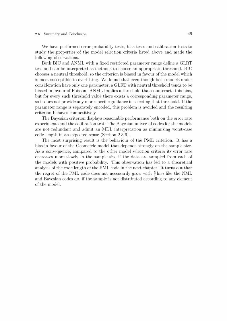
2.6. Summary and Conclusion 49
We have performed error probability tests, bias tests and calibration tests tostudy the properties of the model selection criteria listed above and made thefollowing observations.
Both BIC and ANML with a fixed restricted parameter range define a GLRTtest and can be interpreted as methods to choose an appropriate threshold. BICchooses a neutral threshold, so the criterion is biased in favour of the model whichis most susceptible to overfitting. We found that even though both models underconsideration have only one parameter, a GLRT with neutral threshold tends to bebiased in favour of Poisson. ANML implies a threshold that counteracts this bias,but for every such threshold value there exists a corresponding parameter range,so it does not provide any more specific guidance in selecting that threshold. If theparameter range is separately encoded, this problem is avoided and the resultingcriterion behaves competitively.
The Bayesian criterion displays reasonable performance both on the error rateexperiments and the calibration test. The Bayesian universal codes for the modelsare not redundant and admit an MDL interpretation as minimising worst-casecode length in an expected sense (Section 2.3.6).
The most surprising result is the behaviour of the PML criterion. It has abias in favour of the Geometric model that depends strongly on the sample size.As a consequence, compared to the other model selection criteria its error ratedecreases more slowly in the sample size if the data are sampled from each ofthe models with positive probability. This observation has led to a theoreticalanalysis of the code length of the PML code in the next chapter. It turns out thatthe regret of the PML code does not necessarily grow with k
2ln n like the NML
and Bayesian codes do, if the sample is not distributed according to any elementof the model.


Chapter 3
Behaviour of Prequential Codes underMisspecification
Universal coding lies at the basis Rissanen’s theory of MDL (minimum descriptionlength) learning [4, 39] and Dawid’s theory of prequential model assessment [26].It also underlies on-line prediction algorithms for data compression and gamblingpurposes. In the introductory chapter (Section 1.2.3), we defined universality ofa code in terms of its worst-case regret. Roughly, a code is universal with respectto a modelM if it achieves small worst-case regret: it allows one to encode datausing not many more bits than the optimal code in M. We also described thefour main universal codes: the Shtarkov or NML code, the Bayesian mixturecode, the 2-part MDL code and the prequential maximum likelihood code (PML),also known as the “ML plug-in code” or the “predictive MDL code” [4, 38]. Thiscode was introduced independently by Rissanen [69] and by Dawid [26], whoproposed it as a forecasting strategy rather than as a code. In this chapter westudy the behaviour of the PML code if the considered modelM does not containthe data-generating distribution P ∗. We require that the model is a 1-parameterexponential family, but our results can possibly be extended to models with moreparameters.
Instead of the worst-case regret, we analyse the redundancy, a closely re-lated concept. We find that the redundancy of PML can be quite different fromthat of the other main universal codes. For all these codes, the redundancy is12c ln n+O(1) for some c, but while c = 1 for Bayes, NML and 2-part codes (under
regularity conditions on P ∗ and M), we show here that for PML, any c > 0 ispossible, depending on P ∗ and M.
There are a plethora of results concerning the redundancy and/or the regretfor PML, for a large variety of models including multivariate exponential families,ARMA processes, regression models and so on. Examples are [70, 44, 97, 57].In all these papers it is shown that either the regret or the redundancy growsas k
2ln n + o(ln n), either in expectation or almost surely. Thus, these results
already indicate that c = 1 for those models. The reason that these results do
51

52 Chapter 3. Behaviour of Prequential Codes under Misspecification
not contradict ours, is that they invariably concern the case where the generatingP ∗ is in M, so that automatically varM∗(X) = varP ∗(X).
As discussed in Section 3.4, the result has interesting consequences for pa-rameter estimation and practical data compression, but the most important andsurprising consequence is for MDL learning and model selection, where our re-sult implies that PML may behave suboptimally even if one of the models underconsideration is correct!
In Section 3.1 we informally state and explain our result. Section 3.2 containsthe formal statement of our main result (Theorem 3.2.3), as well as a proof. InSection 3.3 we show that our results remain valid to some extent if“redundancy”isreplaced by “expected regret” (Theorem 3.3.1). We discuss further issues, includ-ing relevance of the result, in Section 3.4. Section 3.5 states and proves variouslemmas needed in the proofs of Theorems 3.2.3 and 3.3.1.
3.1 Main Result, Informally
Suppose M = Pθ : θ ∈ Θ is a k-dimensional parametric family of distribu-tions, and Z1, Z2, . . . are i.i.d. according to some distribution P ∗ ∈ M. A codeis universal for M if it is almost as efficient at coding outcomes from P ∗ as thebest element ofM. (As in previous chapters, we sometimes use codes and distri-butions interchangeably.) In the introductory chapter we measured the overheadincurred on the first n outcomes zn = z1, . . . , zn in terms of the worst-case regret
maxznR(L,M, zn) = max
zn
(
L(zn)− infL′∈M
L′(zn)
)
,
but in this chapter we consider the redundancy instead. We define the redundancyof a distribution Q with respect to a model M as
R(P ∗, Q,M, n) := EZn∼P ∗
[− ln Q(Zn)]− infθ∈Θ
EZn∼P ∗
[− ln Pθ(Zn)], (3.1)
where we use nats rather than bits as units of information to simplify equations.We omit the first three arguments of the redundancy if they are clear from con-text. These and other notational conventions are detailed in Section 3.2. Theredundancy is a close lower bound on the expected regret, see Section 3.3. We donot know the exact relationship to worst-case regret.
The four major types of universal codes, Bayes, NML, 2-part and PML, allachieve redundancies that are (in an appropriate sense) close to optimal. Specifi-cally, under regularity conditions onM and its parameterisation, these four typesof universal codes all satisfy
R(P ∗, Q,M, n) =k
2ln n + O(1), (3.2)

3.1. Main Result, Informally 53
where the O(1) may depend on P ∗, M and the universal code Q that is used.This is the famous “k over 2 log n formula”, refinements of which lie at the basisof most practical approximations to MDL learning, see [38].
Often, the source distribution P ∗ is assumed to be an element of the model. Ifsuch is the case, then by the information inequality [25] the second term of (3.1)is minimised for Pθ = P ∗, so that
R(P ∗, Q,M, n) = EP ∗ [− ln Q(Zn)]− EP ∗ [− ln P ∗(Zn)]. (3.3)
Thus, (3.3) can be interpreted as the expected number of additional nats oneneeds to encode n outcomes if one uses the code corresponding to Q instead ofthe optimal (Shannon-Fano) code with lengths − ln P ∗(Zn). For a good universalcode this quantity is small for all or most P ∗ ∈M.
In this chapter we consider the case where the data are i.i.d. according to anarbitrary P ∗ not necessarily in the model M. It is now appropriate to renamethe redundancy to relative redundancy, since we measure the number of nats welose compared to the best element in the model, rather than compared to thegenerating distribution P ∗. The definition (3.1) remains unchanged. It can nolonger be rewritten as (3.3) however: Assuming it exists and is unique, let Pθ∗ bethe element of M that minimises KL divergence to P ∗:
θ∗ := arg minθ∈Θ
D(P ∗‖Pθ) = arg minθ∈Θ
EP ∗ [− ln Pθ(Z)],
where the equality follows from the definition of the KL divergence [25]. Thenthe relative redundancy satisfies
R(P ∗, Q,M, n) = EP ∗ [− ln Q(Zn)]− EP ∗ [− ln Pθ∗(Zn)]. (3.4)
It turns out that for the NML, 2-part MDL and Bayes codes, the relative redun-dancy (3.4) with P ∗ 6∈ M, still satisfies (3.2), under some conditions on M andP ∗ (Section 3.3). In this chapter we show that (3.2) does not hold for PML. ThePML code with length function L works by sequentially predicting Zi+1 using a(slightly modified) ML or Bayesian MAP estimator θi = θ(zi) based on the pastdata, that is, the first i outcomes zi. The total code length L(zn) on a sequencezn is given by the sum of the individual “predictive” code lengths (log losses):L(zn) =
∑n−1i=0 [− ln Pθi
(zi+1)]. In our main theorem, we show that if and M is aregular one-parameter exponential family (k = 1), then
R(P ∗, Q,M, n) = 12
varP ∗X
varPθ∗X
ln n + O(1), (3.5)
where X is the sufficient statistic of the family. Example 6 below illustrates thephenomenon. Note that if P ∗ ∈M, then Pθ∗ = P ∗ and (3.5) becomes the familiarexpression. The result holds as long asM and P ∗ satisfy a mild condition that isstated and discussed in the next section. Section 3.4 discusses the consequences of

54 Chapter 3. Behaviour of Prequential Codes under Misspecification
this result for compression, estimation and model selection, as well as its relationto the large body of earlier results on PML coding.
Example 6. LetM be the family of Poisson distributions, parameterised by theirmean µ. Since neither the NML universal code nor Jeffreys’ prior are defined forthis model it is attractive to use the PML code as a universal code for this model.The ML estimator µi is the empirical mean of z1, . . . , zi.
Suppose Z, Z1, Z2, . . . are i.i.d. according to a degenerate P with P (Z =4) = 1. Since the sample average is a sufficient statistic for the Poisson family, µi
will be equal to 4 for all i ≥ 1. On the other hand, µ∗, the parameter (mean) ofthe distribution in M closest to P in KL-divergence, will be equal to 4 as well.Thus the relative redundancy (3.4) of the PML code is given by
R(P ∗, Q,M, n) = − ln Pµ0(4) + ln P4(4) +n−1∑
i=1
[− ln P4(4) + ln P4(4)] = O(1),
assuming an appropriate definition of µ0. In the case of the Poisson family, wehave Z = X in (3.5). Thus, since varP ∗Z = 0, this example agrees with (3.5).
Now suppose data are i.i.d. according to some Pτ , with Pτ (Z = z) ∝ (z +1)−3
for all z smaller than τ , and Pτ (Z = z) = 0 for z ≥ τ . It is easy to check that,for τ → ∞, the entropy of Pτ converges to a finite constant, but the variance ofPτ tends to infinity. Thus, by choosing τ large enough, the redundancy obtainedby the Poisson PML code can be made to grow as c log n for arbitrarily large c.
Example 7. The Hardy-Weinberg model deals with genotypes of which the allelesare assumed independently Bernoulli distributed according to some parameter p.There are four combinations of alleles, usually denoted “aa”, “AA”, “aA”, “Aa”;but since “aA” and “Aa” result in the same genotype, the Hardy-Weinberg modelis defined as a probability distribution on three outcomes. We model this byletting X be a random variable on the underlying space, that maps “aA” and“Aa” to the same value: X(aa) = 0, X(aA) = X(Aa) = 1
2and X(AA) = 1. Then
P (X = 0) = (1 − p)2, P (X = 12) = 2p(1 − p) and P (X = 1) = p2. The Hardy-
Weinberg model is an exponential family with sufficient statistic X. To see this,note that for any parameter p ∈ [0, 1], we have EX = µ = P (A) = p, so we canparameterise the model by the mean of X. The variance of the distribution withparameter µ is 1
2µ(1 − µ). Now suppose that we code data in a situation where
the Hardy-Weinberg model is wrong and the genotypes are in fact distributedaccording to P (X = 1
2) = P (X = 1) = 1
2and P (X = 0) = 0, such that mean and
variance of X are 34
and 232
respectively. The closest distribution in the model hasthe same mean (since the mean is a sufficient statistic), and variance 3
32. Thus
PML will achieve a redundancy of 13
ln n rather than 12
ln n (up to O(1)).

3.2. Main Result, Formally 55
3.2 Main Result, Formally
In this section, we define our quantities of interest and we state and prove our mainresult. Throughout this text we use nats rather than bits as units of information.Outcomes are capitalised if they are to be interpreted as random variables insteadof instantiated values. Let P ∗ be a distribution on some set Z, which can be eitherfinite or countably infinite, or a subset of k-dimensional Euclidean space for somek ≥ 1. A sequence of outcomes z1, . . . , zn is abbreviated to zn. Let X : Z → R
k
be a random vector. We write EP ∗ [X] as a shorthand for EX∼P ∗ [X]. When weconsider a sequence of n outcomes independently distributed ∼ P ∗, we even useEP ∗ as a shorthand for the expectation of (X1, . . . , Xn) under the n-fold productdistribution of P ∗. Finally, P ∗(X) denotes the probability mass function of P ∗
in case X is discrete-valued, and the density of P ∗ in case X takes values in acontinuum. When we write “density function of X”, then, if X is discrete-valued,this should be read as “probability mass function of X”. Note however that inour main result, Theorem 3.2.3 below, we do not assume that the data-generatingdistribution P ∗ admits a density.
We define the particular random vector Z(z) := z. Let X : Z → R be arandom variable on Z, and let X = x ∈ R : ∃z ∈ Z : X(z) = x be therange of X. Exponential family models are families of distributions on Z definedrelative to a random variable X (called “sufficient statistic”) as defined above,and a function h : Z → (0,∞). Let Z(η) :=
∫
z∈Ze−ηX(z)h(z)dz (the integral to
be replaced by a sum for countable Z), and Θη := η ∈ R : Z(η) <∞.
Definition 3.2.1 (Exponential family). The single parameter exponential fam-ily [48] with sufficient statistic X and carrier h is the family of distributionswith densities Pη(z) := 1
Z(η)e−ηX(z)h(z), where η ∈ Θη. Θη is called the natural
parameter space. The family is called regular if Θη is an open interval of R.
In the remainder of this text we only consider single parameter, regular expo-nential families with a 1-to-1 parameterisation; this qualification will henceforthbe omitted. Examples include the Poisson, geometric and multinomial families,and the model of all Gaussian distributions with a fixed variance or mean. In thefirst four cases, we can take X to be the identity, so that X = Z and X = Z. Inthe case of the normal family with fixed mean, σ2 becomes the sufficient statisticand we have Z = R, X = [0,∞) and X = Z2.
The statistic X(z) is sufficient for η [48]. This suggests reparameterisingthe distribution by the expected value of X, which is called the mean valueparameterisation. The function µ(η) = EPη [X] maps parameters in the naturalparameterisation to the mean value parameterisation. It is a diffeomorphism(it is one-to-one, onto, infinitely often differentiable and has an infinitely oftendifferentiable inverse) [48]. Therefore the mean value parameter space Θµ is alsoan open interval of R. We note that for some models (such as Bernoulli andPoisson), the parameter space is usually given in terms of the a non-open set

56 Chapter 3. Behaviour of Prequential Codes under Misspecification
of mean-values (e.g., [0, 1] in the Bernoulli case). To make the model a regularexponential family, we have to restrict the set of parameters to its own interior.Henceforth, whenever we refer to a standard statistical model such as Bernoullior Poisson, we assume that the parameter set has been restricted in this sense.
We are now ready to define the PML distribution. This is a distribution oninfinite sequences z1, z2, . . . ∈ Z∞, recursively defined in terms of the distributionsof Zn+1 conditioned on Zn = zn, for all n = 1, 2, . . ., all zn = (z1, . . . , zn) ∈ Zn.In the definition, we use the notation xi := X(zi).
Definition 3.2.2 (PML distribution). Let Θµ be the mean value parameter do-main of an exponential family M = Pµ | µ ∈ Θµ. Given M and constantsx0 ∈ Θµ and n0 > 0, we define the PML distribution U by setting, for all n, allzn+1 ∈ Zn+1:
U(zn+1 | zn) = Pµ(zn)(zn+1),
where U(zn+1 | zn) is the density/mass function of zn+1 conditional on Zn = zn,
µ(zn) :=x0 · n0 +
∑ni=1 xi
n + n0
,
and Pµ(zn)(·) is the density of the distribution in M with mean µ(zn).
We henceforth abbreviate µ(zn) to µn. We usually refer to the PML distribu-tion in terms of the corresponding code length function
LU(zn) =n−1∑
i=0
LU(zi+1 | zi) =n−1∑
i=0
− ln Pµi(zi+1).
To understand this definition, note that for exponential families, for any sequenceof data, the ordinary maximum likelihood parameter is given by the averagen−1
∑xi of the observed values of X [48]. Here we define our PML distribution
in terms of a slightly modified maximum likelihood estimator that introduces a“fake initial outcome”x0 with multiplicity n0 in order to avoid infinite code lengthsfor the first few outcomes (a well-known problem called by Rissanen the “inherentsingularity” of predictive coding [71, 36]) and to ensure that the probability of thefirst outcome is well-defined for the PML distribution. In practice we can taken0 = 1 but our result holds for any n0 > 0. The justification of our modificationto the ML estimator is discussed further in Section 3.4.
Theorem 3.2.3 (Main result). Let X,X1, X2, . . . be i.i.d. ∼ P ∗, with EP ∗ [X] =µ∗. Let M be a single parameter exponential family with sufficient statistic Xand µ∗ an element of the mean value parameter space. Let U denote the PMLdistribution with respect to M. If M and P ∗ satisfy Condition 3.2.4 below, then
R(P ∗, U,M, n) = 12
varP ∗X
varPµ∗ (X)
ln n + O(1). (3.6)

3.2. Main Result, Formally 57
Comparing this to (3.5), note that Pµ∗ is the element ofM achieving smallestexpected code length, i.e. it achieves infµ∈Θµ D(P ∗‖Pµ) [48].
Condition 3.2.4. We require that the following holds both for T := X andT := −X:
• If T is unbounded from above then there is a k ∈ 4, 6, . . . such that the
first k moments of T exist under P ∗ and that d4
dµ4 D(Pµ∗‖Pµ) = O(µk−6
).
• If T is bounded from above by a constant g then d4
dµ4 D(Pµ∗‖Pµ) is polynomial
in 1/(g − µ).
Roughly, this condition expresses a trade-off between the data generating dis-tribution P ∗ and the model. If the model is well-behaved, in the sense that thefourth order derivative of the KL divergence does not grow too fast with the pa-rameter, then we do not require many moments of P ∗ to exist. Vice versa if themodel is not well-behaved, then the theorem only holds for very specific P ∗, ofwhich many moments exist.
The condition holds for most single-parameter exponential families that arerelevant in practice. To illustrate, in Figure 3.2 we give the fourth derivativeof the divergence for a number of common exponential families explicitly. Allparameters beside the mean are treated as fixed values. Note that to interpretthe mean 0 normal distributions as a 1-parameter exponential family the densitywe had to set X(z) = z2, so that its mean E[X] is actually the variance E[Z2]of the normal distribution. As can be seen from the figure, for these exponentialfamilies, our condition applies whenever at least the first four moments of P ∗
exist: a quite weak condition on the data generating distribution.
Proof of Theorem 3.2.3. For exponential families, we have
EP ∗ [− ln Pµ(Z)]− EP ∗ [− ln Pµ′(Z)]
= η(µ)EP ∗ [X(Z)] + ln Z(η(µ)) + EP ∗ [− ln h(Z)]
− η(µ′)EP ∗ [X(Z)]− ln Z(η(µ′))− EP ∗ [− ln h(Z)]
= EP ∗ [− ln Pµ(X)]− EP ∗ [− ln Pµ′(X)],
so that R(P ∗, U,M, n) = EP ∗ [LU(Xn)]− infµ EP ∗ [− ln Pµ(Xn)]. This means thatrelative redundancy, which is the sole quantity of interest in the proof, dependsonly on the sufficient statistic X, not on any other aspect of the outcome thatmay influence Z. Thus, in the proof of Theorem 3.2.3 as well as all the Lemmasand Propositions it makes use of, we will never mention Z again. Wheneverwe refer to a “distribution” we mean a distribution of random variable X, andwe also think of the data generating distribution P ∗ in terms of the distributionit induces on X rather than Z. Whenever we say “the mean” without furtherqualification, we refer to the mean of the random variable X. Whenever we

58 Chapter 3. Behaviour of Prequential Codes under Misspecification
Figure 3.1 d4
dµ4 D(Pµ∗‖Pµ) for a number of exponential families.
Pµ∗(x)d4
dµ4D(Pµ∗‖Pµ)
Bernoulli (µ∗)x(1− µ∗)(1−x) 6µ∗
µ4+
6(1− µ∗)
(1− µ)4
Poissoneµ∗
µ∗x
x!
6µ∗
µ4
Geometric θx(1− θ) =(µ∗)x
(µ∗ + 1)x+1
6µ∗
µ4− 6(µ∗ + 1)
(µ + 1)4
Exponential1
µ∗e−x/µ∗ − 6
µ4+
24µ∗
µ5
Normal (fixed mean = 0)1√
2πµ∗xe−
x2µ∗ − 3
µ4+
12µ∗
µ5
Normal (fixed variance = 1)1√2π
e−12(x−µ∗)2 0
Paretoaba
xa+1for b =
a− 1
aµ∗ 6a
µ4
refer to the Kullback-Leibler (KL) divergence between P and Q, we refer to theKL divergence between the distributions they induce for X. The reader who isconfused by this may simply restrict attention to exponential family models forwhich Z = X, and consider X and Z identical.
The proof refers to a number of theorems and lemmas which will be developedin Section 3.5. In the statement of all these results, we assume, as in the statementof Theorem 3.2.3, that X,X1, X2, . . . are i.i.d. ∼ P ∗ and that µ∗ = EP ∗ [X]. If Xtakes its values in a countable set, then all integrals in the proof should be readas the corresponding sums.
The redundancy can be rewritten further as the sum of the expected risk foreach outcome (Lemma 3.5.6). We obtain
R(P ∗, U,M, n) =n−1∑
i=0
Eµi∼P ∗
[D(Pµ∗‖Pµi
)]. (3.7)
Here, the estimator µi is a random variable that takes on values according to P ∗,while the optimal parameter value µ∗ is fixed (and determined by P ∗). We willwrite D(µ∗‖µi) as shorthand notation for Pµ∗ and Pµi
.We now first rewrite the divergence. We abbreviate δi := µi−µ∗ and D(k)(µ) :=
dk
dµk D(Pµ∗‖Pµ). That is, D(k)(µ) is the k-th derivative of the function f(µ) :=
D(Pµ∗‖Pµ). Taylor-expansion of the divergence around µ∗ yields
D(Pµ∗‖Pµi) = 0 + δiD
(1)(µ∗) +δi
2
2D(2)(µ∗) +
δi3
6D(3)(µ∗) +
δi4
24D(4)(µi).

3.2. Main Result, Formally 59
The last term is the remainder term of the Taylor expansion, in which µi ∈ [µ∗, µi].The second term D(1)(µ∗) is zero, since D(µ∗‖µ) reaches its minimum at µ = µ∗.For the third term we observe that
D(2)(µ) =d2
dµ2E[ln Pµ∗(X)− ln Pµ(X)] = − d2
dµ2E[ln Pµ(X)],
which is equal to the Fisher information. Fisher information is defined as I(θ) :=
E[
( ddθ
ln f(X | θ))2]
, but as is well known [48], for exponential families this is
equal to − d2
dθ2 E[ln f(X | θ)
], which matches D(2)(·) exactly. Furthermore, for
the mean value parameterisation I(µ) = 1/varPµ(X). We obtain
D(Pµ∗‖Pµi) =
1
2δi
2/varPµ∗ (X) +1
6δi
3D(3)(µ∗) +1
24δi
4D(4)(µi). (3.8)
We plug this expression back into (3.7), giving
R(P ∗, U,M, n) =1
2varPµ∗ (X)
n−1∑
i=0
EP ∗
[
δi2]
+ R(n), (3.9)
where the remainder term R(n) is given by
R(n) =n−1∑
i=0
EP ∗
[1
6δi
3D(3)(µ∗) +1
24δi
4D(4)(µi)
]
, (3.10)
and where µ and δi are random variables; note that although µ is not indexed itdoes depend on the index i. In Lemma 3.5.8 we show that R(n) = O(1), giving:
R(P ∗, U,M, n) = O(1) +1
2varPµ∗ (X)
n−1∑
i=0
EP ∗
[(µi − µ∗)2
]. (3.11)
Note that µi is almost the ML estimator. This suggests that each term in thesum of (3.11) should be almost equal to the variance of the ML estimator, whichis varX/i. Because of the slight modification that we made to the estimator, weget a correction term of O(i−2) as established in Theorem 3.5.2:
n−1∑
i=0
EP ∗
[(µi − µ∗)2
]=
n−1∑
i=0
O((i + 1)−2
)+ varP ∗(X)
n−1∑
i=0
(i + 1)−1
= O(1) + varP ∗(X) ln n (3.12)
The combination of (3.11) and (3.12) completes the proof.

60 Chapter 3. Behaviour of Prequential Codes under Misspecification
3.3 Redundancy vs. Regret
The “goodness” of a universal code relative to a model M can be measured inseveral ways: rather than using redundancy (as we did here), one can also chooseto measure code length differences in terms of regret, where one has a furtherchoice between expected regret and worst-case regret [4]. Here we only discuss theimplications of our result for the expected regret measure.
LetM = Pθ | θ ∈ Θ be a family of distributions parameterised by Θ. Givena sequence zn = z1, . . . , zn and a universal code U for M with lengths LU , theregret of U on sequence zn is defined as
LU(zn)− infθ∈Θ
[− ln Pθ(zn)]. (3.13)
Note that if the (unmodified) ML estimator θ(zn) exists, then this is equal toLU(zn) + ln Pθ(zn)(z
n). Thus, one compares the code length achieved on zn by Uto the best possible that could have been achieved on that particular zn, usingany of the codes/distributions in M. Assuming Z1, Z2, . . . are i.i.d. according tosome (arbitrary) P , one may now consider the expected regret
EZn∼P ∗ [R(P ∗, U,M, n)] = EP ∗ [LU(Zn)− infθ∈Θ
[− ln Pθ(Zn)]].
To quantify the difference with redundancy, consider the function
d(n) := infθ∈Θ
EP [− ln Pθ(Zn)]− EP [ inf
θ∈Θ[− ln Pθ(Z
n)]],
and note that for any universal code, R − E[R] = d(n). In case P ∗ ∈ M, thenunder regularity conditions on M and its parameterisation, it can be shown [23]that
limn→∞
d(n) =k
2, (3.14)
where k is the dimension of M. In our case, where P ∗ is not necessarily in M,we have the following :
Theorem 3.3.1. Let X be finite. Let P ∗, Pµ and µ∗ be as in Theorem 3.2.3.Then
limn→∞
d(n) =1
2
varP ∗X
varPµ∗X. (3.15)
Once we are dealing with 1-parameter families, in the special case that P ∗ ∈M, this result reduces to (3.14). We suspect that, under a condition similar toCondition 3.2.4, the same result still holds for general, not necessarily finite orcountable or bounded X , but we do not know the details. In any case, our resultis sufficient to show that in some cases (namely, if X is finite), we have
R(P ∗, U,M, n) =1
2
varP ∗X
varPµ∗Xln n + O(1),

3.4. Discussion 61
so that, up to O(1)-terms, the redundancy and the regret of the prequential MLcode behave in the same way.
Incidentally, we can use Theorem 3.3.1 to substantiate the claim in Section 3.1,which stated that the Bayes (equipped with a strictly positive differentiable prior),NML and 2-part codes still achieve relative redundancy of 1
2ln n if P ∗ 6= M, at
least if X is finite. Let us informally explain why this is the case. It is easyto show that Bayes, NML and (suitably defined) 2-part codes achieve regret12
ln n+O(1) for all sequences z1, z2, . . . such that θ(zn) is bounded away from theboundary of the parameter space Θµ, for all large n [4, 38]. It then follows using,for example, the Chernoff bound that these codes must also achieve expectedregret 1
2ln n + O(1) for all distributions P ∗ on X that satisfy EP ∗ [X] = µ∗ ∈ Θµ.
Theorem 3.3.1 then shows that they also achieve relative redundancy 12
ln n+O(1)for all distributions P ∗ on X that satisfy EP ∗ [X] = µ∗ ∈ Θµ. We omit furtherdetails.
3.4 Discussion
3.4.1 A Justification of Our Modification of the ML Esti-mator
A prequential code cannot be defined in terms of the ordinary ML estimator(n0 = 0 in Definition 3.2.2) for two reasons. First, the ML estimator is undefineduntil the first outcome has been observed. Second, it may achieve infinite codelengths on the observed data. A simple example is the Bernoulli model. If we firstobserve z1 = 0 and then z2 = 1, the code length of z2 according to the ordinaryML estimator of z2 given z1 would be − ln Pµ(z1)(z2) = − ln 0 = ∞. There areseveral ways to resolve this problem. We choose to add an “fake initial outcome”.Another possibility that has been suggested (e.g., [26]) is to use the ordinary MLestimator, but to postpone using it until after m outcomes have been observed,where m is the smallest number such that − ln Pµ(zm)(Zm+1) is guaranteed to befinite, no matter what value Zm+1 is realized. The first m outcomes may then beencoded by repeatedly using some code L0 on outcomes of Z, so that for i ≤ m,the code length of zi does not depend on the outcomes zi−1. In the Bernoulliexample, one could for example use the code corresponding to P (Zi = 1) = 1/2,until and including the first i such that zi includes both a 0 and a 1. It then takesi bits to encode the first zi outcomes, no matter what they are. After that, oneuses the prequential code with the standard ML estimator. It is easy to see (byslight modification of the proof) that our theorem still holds for this variation ofprequential coding. Thus, our particular choice for resolving the startup problemis not crucial to obtaining our result. The advantage of our solution is that, as wenow show, it allows us to interpret our modified ML estimator as a Bayesian MAPand Bayesian mean estimator as well, thereby showing that the same behaviour

62 Chapter 3. Behaviour of Prequential Codes under Misspecification
can be expected for such estimators.
3.4.2 Prequential Models with Other Estimators
An attractive property of our generalisation of the ML estimator is that it actu-ally also generalises two other commonly used estimators, namely the Bayesianmaximum a-posteriori and Bayesian mean estimators.
The Bayesian maximum a-posteriori estimator can always be interpreted asan ML estimator based on the sample and some additional “fake data”, providedthat a conjugate prior is used ([12]; see also the notion of ESS (Equivalent SampleSize) Priors discussed in, for example, [51]). Therefore, the prequential ML modelas defined above can also be interpreted as a prequential MAP model for thatclass of priors, and the whole analysis carries over to that setting.
For the Bayesian mean estimator, the relationship is slightly less direct. How-ever, it follows from the work of Hartigan [42, Chapter 7] on the so-called “max-imum likelihood prior”, that by slightly modifying conjugate priors, we can con-struct priors such that the Bayesian mean also becomes of the form of our modifiedML estimator.
Our whole analysis thus carries over to prequential codes based on these esti-mators. In fact, we believe that our result holds quite generally:
Conjecture 3.4.1. LetM be a regular exponential family with sufficient statisticX and let P be the set of distributions on Z such that EP ∗ [X4] exists. There existsno “in-model” estimator such that the corresponding prequential code achievesredundancy 1
2ln n + O(1) for all P ∗ ∈ P.
Here, by an in-model estimator we mean an algorithm that takes as inputany sample of arbitrary length and outputs a Pµ ∈ M. Let us contrast thiswith “out-model estimators”: fix some prior on the parameter set Θµ and letP (µ | z1, . . . , zn−1) be the Bayesian posterior with respect to this prior anddata z1, . . . , zn−1. One can think of the Bayesian predictive distribution P (zn |z1, . . . , zn−1) :=
∫
µ∈ΘµPµ(zn)P (µ | z1, . . . , zn−1)dµ as an estimate of the distri-
bution of Z, based on data z1, . . . , zn−1. But unlike estimators as defined in theconjecture above, the resulting Bayesian predictive estimator will in general notbe a member ofM, but rather of its convex closure: we call it an out-model estima-tor. The redundancy of the Bayesian universal model is equal to the accumulatedKullback-Leibler (KL) risk of the Bayesian predictive estimator [36]. Thus, theaccumulated KL risk of the Bayesian predictive estimator is 1
2ln n + O(1) even
under misspecification. Thus, if our conjecture above holds true, then in-modelestimators behave in a fundamentally different way from out-model estimators interms of their asymptotic risk.
Example 8. The well-known Laplace and Krichevsky-Trofimov estimators forthe Bernoulli model [38] define PML distributions according to Definition 3.2.2:

3.4. Discussion 63
they correspond to x0 = 1/2, n0 = 2, and x0 = 1/2, n0 = 1 respectively. Yet,they also correspond to Bayesian predictive distributions with uniform prior orJeffreys’ prior respectively. This implies that the code length achieved by theBayesian universal model with Jeffreys’ prior and the PML distribution withx0 = 1/2, n0 = 1 must coincide. We claimed before that the expected regret for aBayesian universal model is 1
2log n + O(1) if data are i.i.d. ∼ P ∗, for essentially
all distributions P ∗. This may seem to contradict our result which says that theexpected regret of the PML distribution can be 0.5c log n + O(1) with c 6= 1 ifP ∗ 6∈ M. But there really is no contradiction: since the Bernoulli model happensto contain all distributions P ∗ on 0, 1, we cannot have P ∗ 6∈ M so Theorem 1indeed says that c = 1 no matter what P ∗ we choose. But with more complicatedmodels such as the Poisson or Hardy-Weinberg model, it is quite possible thatP ∗ 6∈ M. Then the Bayesian predictive distribution will not coincide with anyPML distribution and we can have c 6= 1.
3.4.3 Practical Significance for Model Selection
As mentioned in the introduction, there are many results showing that in variouscontexts, if P ∗ ∈M, then the prequential ML code achieves optimal redundancy.These results strongly suggest that it is a very good alternative for (or at leastapproximation to) the NML or Bayesian codes in MDL model selection. Indeed,quoting Rissanen [71]:
“If the encoder does not look ahead but instead computes the bestparameter values from the past string, only, using an algorithm whichthe decoder knows, then no preamble is needed. The result is a pre-dictive coding process, one which is quite different from the sum orintegral formula in the stochastic complexity.1 And it is only becauseof a certain inherent singularity in the process, as well as the some-what restrictive requirement that the data must be ordered, that wedo not consider the resulting predictive code length to provide anothercompeting definition for the stochastic complexity, but rather regardit as an approximation.”
Our result however shows that the prequential ML code may behave quite differ-ently from the NML and Bayes codes, thereby strengthening the conclusion thatit should not be taken as a definition of stochastic complexity. Although there isonly a significant difference if data are distributed according to some P ∗ 6∈ M,the difference is nevertheless very relevant in an MDL model selection contextwith disjoint models, even if one of the models under consideration does containthe “true”P ∗. To see this, suppose we are comparing two modelsM1 andM2 for
1The stochastic complexity is the code length of the data z1, . . . , zn that can be achievedusing the NML code.

64 Chapter 3. Behaviour of Prequential Codes under Misspecification
the same data, and in fact, P ∗ ∈M1 ∪M2. For concreteness, assumeM1 is thePoisson family andM2 is the geometric family. We want to decide which of thesetwo models best explains the data. According to the MDL Principle, we shouldassociate with each model a universal code (preferably the NML code). We shouldthen pick the model such that the corresponding universal code length of the datais minimised. Now suppose we use the prequential ML code lengths rather thanthe NML code lengths. Without loss of generality suppose that P ∗ ∈ M1. ThenP ∗ 6∈ M2. This means that the code length relative to M1 behaves essentiallylike the NML code length, but the code length relative toM2 behaves differently– at least as long as the variances do not match (which for example, is forciblythe case if M1 is Poisson and M2 is geometric). This introduces a bias in themodel selection scheme. In the previous chapter we found experimentally that theerror rate for model selection based on the prequential ML code decreases moreslowly than when other universal codes are used. Even though in some cases theredundancy grows more slowly than 1
2ln n, so that the prequential ML code is
more efficient than the NML code, we explained that model selection based onthe prequential ML codes must nevertheless always behave worse than Bayesianand NML-based model selection. The practical relevance of this phenomenonstems from the fact that the prequential ML code lengths are often a lot easierto compute than the Bayes or NML codes. They are often used in applications[61, 52], so that is important to determine when this can be done safely.
3.4.4 Theoretical Significance
The result is also of theoretical-statistical interest: our theorem can be re-inter-preted as establishing bounds on the asymptotic Kullback-Leibler risk of densityestimation using ML and Bayes estimators under misspecification (P ∗ 6∈ M). Ourresult implies that, under misspecification, the KL risk of estimators such as ML,which are required to lie in the model M, behaves in a fundamentally differentway from the KL risk of estimators such as the Bayes predictive distribution,which are not restricted to lie in M. Namely, we can think of every universalmodel U defined as a random process on infinite sequences as an estimator in thefollowing way: define, for all n,
Pn := PrU
(Zn+1 = · | Z1 = z1, . . . , Zn = zn),
a function of the sample z1, . . . , zn. Pn can be thought of as the “estimate of thetrue data generating distribution upon observing z1, . . . , zn”. In case U is theprequential ML model, Pn = Pµn is simply our modified ML estimator. However,
universal models other than PML, Pn does not always lie inM. An example is theBayesian universal code defined relative to some prior w. This code has lengthsL′(zn) := − ln
∫Pµ(zn)w(µ) dµ [38]. The corresponding estimator is the Bayesian
posterior predictive distribution PBayes(zi+1 | zi) :=∫
Pµ(zi+1)w(µ | zi) dµ [38].

3.5. Building Blocks of the Proof 65
The Bayesian predictive distribution is a mixture of elements of M. We willcall standard estimators like the ML estimator, which are required to lie in M,in-model estimators. Estimators like the Bayesian predictive distribution will becalled out-model.
Let now Pn be any estimator, in-model or out-model. Let Pzn be the distribu-tion estimated for a particular realized sample zn. We can measure the closenessof Pzn to Pµ∗ , the distribution inM closest to P ∗ in KL-divergence, by consideringthe extended KL divergence
D∗(Pµ∗‖Pzn) = EZ∼P ∗ [− ln Pzn(Z)− [− ln Pµ∗(Z)]].
We can now consider the expected KL divergence between Pµ∗ and Pn after ob-serving a sample of length n:
EZ1,...,Zn∼P ∗ [D∗(Pµ∗‖Pn)]. (3.16)
In analogy to the definition of “ordinary” KL risk [4], we call (3.16) the extendedKL risk. We recognise the redundancy of the PML distribution as the accu-mulated expected KL risk of our modified ML estimator (see Proposition 3.5.7and Lemma 3.5.6). In exactly the same way as for PML, the redundancy of theBayesian code can be re-interpreted as the accumulated KL risk of the Bayesianpredictive distribution. With this interpretation, our Theorem 3.2.3 expressesthat under misspecification, the cumulative KL risk of the ML estimator differsfrom the cumulative KL risk of the Bayes estimator by a term of Θ(ln n). If ourconjecture that no in-model estimator can achieve redundancy 1
2ln n+O(1) for all
µ∗ and all P ∗ with finite variance is true (Section 3.4.2), then it follows that theKL risk for in-model estimators behaves in a fundamentally different way fromthe KL risk for out-model estimators, and that out-model estimators are neededto achieve the optimal constant c = 1 in the redundancy 1
2c ln n + O(1).
3.5 Building Blocks of the Proof
The proof of Theorem 3.2.3 is based on Lemma 3.5.6 and Lemma 3.5.8. TheseLemmas are stated and proved in Sections 3.5.2 and 3.5.3, respectively. The proofsof Theorem 3.2.3 and Theorem 3.3.1, as well as the proof of both Lemmas, arebased on a number of generally useful results about probabilities and expectationsof deviations between the average and the mean of a random variable. We firstlist list these deviation-related results.
3.5.1 Results about Deviations between Average and Mean
Lemma 3.5.1. Let X,X1, X2, . . . be i.i.d. with mean 0. Then E[(∑n
i=1 Xi
)2]
=
nvar(X).

66 Chapter 3. Behaviour of Prequential Codes under Misspecification
Proof. The lemma is clearly true for n = 0. Suppose it is true for some n.Abbreviate Sn :=
∑ni=1 Xi. We have E [Sn] =
∑EX = 0. Now we find
E[S2
n+1
]= E
[
(Sn + X)2]
= E[S2
n
]+ 2E [Sn] EX + E[X2] = (n + 1)var(X).
The proof follows by induction.
Theorem 3.5.2. Let X,X1, . . . be i.i.d. random variables, define µn := (n0 ·x0 +
∑ni=1 Xi)/(n + n0) and µ∗ = E[X]. If varX < ∞, then E
[(µn − µ∗)2
]=
O((n + 1)−2
)+ var(X)/(n + 1).
Proof. We define Yi := Xi − µ∗; this can be seen as a new sequence of i.i.d.random variables with mean 0 and varY = varX. We also set y0 := x0−µ∗. Nowwe have:
E[(µn − µ∗)2
]= E
n0 · y0 +n∑
i=1
Yi
2
(n + n0)
−2
= E
[
(n0 · y0)2 + 2n0 · y0
n∑
i=1
Yi +
n∑
i=1
Yi
2 ]
(n + n0)−2
= O((n + 1)−2
)+ E
n∑
i=1
Yi
2
(n + n0)
−2
(∗)= O
((n + 1)−2
)+ nvar(Y )(n + n0)
−2
= O((n + 1)−2
)+ var(X)/(n + 1),
where (∗) follows by Lemma 3.5.1.
The following theorem is of some independent interest.
Theorem 3.5.3. Suppose X,X1, X2, . . . are i.i.d. with mean 0. If the first k ∈ N
moments of X exist, then we have Then E[(∑n
i=1 Xi
)k]
= O(
n⌊ k2⌋)
.
Remark It follows as a special case of Theorem 2 of [98] that E[|∑n
i=1 Xi|k]
=
O(nk2 ) which almost proves this lemma and which would in fact be sufficient for
our purposes. We use this lemma instead which has an elementary proof.
Proof. We have:
E
n∑
i=1
Xi
k
= E
n∑
i1=1
· · ·n∑
ik=1
Xi1 · · ·Xik
=n∑
i1=1
· · ·n∑
ik=1
E[Xi1 · · ·Xik
].

3.5. Building Blocks of the Proof 67
We define the frequency sequence of a term to be the sequence of exponents ofthe different random variables in the term, in decreasing order. For a frequencysequence f1, . . . , fm, we have
∑mi=1 fi = k. Furthermore, using independence of
the different random variables, we can rewrite E[Xi1 · · ·Xik ] =∏m
i=1 E[Xfi ] sothe value of each term is determined by its frequency sequence. By computingthe number of terms that share a particular frequency sequence, we obtain:
E
n∑
i=1
Xi
k
=
∑
f1+...+fm=k
(n
m
)(k
f1, . . . , fm
) m∏
i=1
E[Xfi ].
To determine the asymptotic behaviour, first observe that the frequency sequencef1, . . . , fm of which the contribution grows fastest in n is the longest sequence,since for that sequence the value of
(nm
)is maximised as n→∞. However, since
the mean is zero, we can discard all sequences with an element 1, because thefor those sequences we have
∏mi=1 E[Xfi ] = 0 so they contribute nothing to the
expectation. Under this constraint, we obtain the longest sequence for even k bysetting fi = 2 for all 1 ≤ i ≤ m; for odd k by setting f1 = 3 and fi = 2 for
all 2 ≤ i ≤ m; in both cases we have m =⌊
k2
⌋
. The number of terms grows
as(
nm
)≤ nm/m! = O(nm); for m =
⌊k2
⌋
we obtain the upper bound O(n⌊ k2⌋).
The number of frequency sequences is finite and does not depend on n; since the
contribution of each one is O(
n⌊ k2⌋)
, so must be the sum.
Theorem 3.5.4. Let X,X1, . . . be i.i.d. random variables, define µn := (n0 ·x0 +
∑ni=1 Xi)/(n + n0) and µ∗ = E[X]. If the first k moments of X exist, then
E[(µn − µ∗)k] = O(n−⌈ k2⌉).
Proof. The proof is similar to the proof for Theorem 3.5.2. We define Yi :=Xi− µ∗; this can be seen as a new sequence of i.i.d. random variables with mean0, and y0 := x0 − µ∗. Now we have:
E[
(µn − µ∗)k]
= E
n0 · y0 +n∑
i=1
Yi
k
(n + n0)
−k
= O(
n−k) k∑
p=0
(k
p
)
(n0 · y0)pE
n∑
i=1
Yi
k−p
= O(
n−k) k∑
p=0
(k
p
)
(n0 · y0)p ·O
(
n⌊ k−p2 ⌋)
.
In the last step we used Theorem 3.5.3 to bound the expectation. We sum k + 1
terms of which the term for p = 0 grows fastest in n, so the expression is O(n−⌈ k2⌉)
as required.

68 Chapter 3. Behaviour of Prequential Codes under Misspecification
Theorem 3.5.4 concerns the expectation of the deviation of µn. We also needa bound on the probability of large deviations. To do that we have the followingseparate theorem:
Theorem 3.5.5. Let X,X1, . . . be i.i.d. random variables, define µn := (n0 ·x0 +∑n
i=1 Xi)/(n + n0) and µ∗ = E[X]. Let k ∈ 0, 2, 4, . . .. If the first k moments
exists then P (|µn − µ∗| ≥ δ) = O(
n− k2 δ−k
)
.
Proof.
P ∗(|µn − µ∗| ≥ δ) = P ∗(
(µn − µ∗)k ≥ δk)
≤ E[
(µn − µ∗)k]
δ−k (by Markov’s inequality)
= O(
n− k2 δ−k
)
(by Theorem 3.5.4)
3.5.2 Lemma 3.5.6: Redundancy for Exponential Families
Lemma 3.5.6. Let U be a PML distribution model and M be an exponentialfamily as in Theorem 3.2.3. We have
R(P ∗, U,M, n) =n−1∑
i=0
Eµi∼P ∗
[D(Pµ∗ ‖ Pµi
)].
(Here, the notation µi ∼ P ∗ means that we take the expectation with respect toP ∗ over data sequences of length i, of which µi is a function.)
Proof. We have:
arg minµ
EP ∗
[− ln Pµ(Xn)
]= arg min
µEP ∗
[
lnPµ∗(Xn)
Pµ(Xn)
]
= arg minµ
D(Pµ∗ ‖ Pµ).
In the last step we used Proposition 3.5.7 below. The divergence is minimisedwhen µ = µ∗ [48], so we find that:
R(P ∗, U,M, n) = EP ∗ [− ln U(Xn)]− EP ∗ [− ln Pµ∗(Xn)] = EP ∗
[
lnPµ∗(Xn)
U(Xn)
]
= EP ∗
n−1∑
i=0
lnPµ∗(Xi)
Pµi(Xi)
=n−1∑
i=0
EP ∗
[
lnPµ∗(Xi)
Pµi(Xi)
]
=n−1∑
i=0
Eµi∼P
[D(Pµ∗ ‖ Pµi
)].
(3.17)
Here, the last step again follows from Proposition 3.5.7.

3.5. Building Blocks of the Proof 69
Proposition 3.5.7. Let X ∼ P ∗ with mean µ∗, and let Pµ index an exponentialfamily with sufficient statistic X, so that Pµ∗ exists. We have:
EP ∗
[
− lnPµ∗(X)
Pθ(X)
]
= D(Pµ∗ ‖ Pθ)
Proof. Let η(·) denote the function mapping parameters in the mean value pa-rameterisation to the natural parameterisation. (It is the inverse of the functionµ(·) which was introduced in the discussion of exponential families.) By workingout both sides of the equation we find that they both reduce to:
η(µ∗)µ∗ + ln Z(η(µ∗))− η(θ)µ∗ − ln Z(η(θ)).
3.5.3 Lemma 3.5.8: Convergence of the sum of the re-mainder terms
Lemma 3.5.8. Let R(n) be defined as in (3.10). Then
R(n) = O(1).
Proof. We omit irrelevant constants. We abbreviate dk
dµk D(Pµ∗‖Pµ) = D(k)(µ) asin the proof of Theorem 3.2.3. First we consider the third order term. We write
Eδi∼P ∗ to indicate that we take the expectation over data which is distributedaccording to P ∗, of which δi is a function. We use Theorem 3.5.4 to bound theexpectation of δi
3; under the condition that the first three moments exist, whichis assumed to be the case, we obtain:
n−1∑
i=0
Eδi∼P ∗
[
δi3D(3)(µ∗)
]
= D(3)(µ∗)n−1∑
i=0
E[δ3i ] = D(3)(µ∗)
n−1∑
i=0
O((i + 1)−2) = O(1).
(The constants implicit in the big-ohs are the same across terms.)The fourth order term is more involved, because D(4)(µ) is not necessarily
constant across terms. To compute it we first distinguish a number of regions inthe value space of δi: let ∆− = (−∞, 0) and let ∆0 = [0, a) for some constantvalue a > 0. If the individual outcomes X are bounded on the right hand sideby a value g then we require that a < g and we define ∆1 = [a, g); otherwise wedefine ∆j = [a + j − 1, a + j) for j ≥ 1. Now we must establish convergence of:
n−1∑
i=0
Eδi∼P ∗
[
δi4D(4)(µi)
]
=n−1∑
i=0
∑
j
P ∗(δi ∈ ∆j) Eδi∼P ∗
[
δi4D(4)(µi) | δi ∈ ∆j
]
If we can establish that the sum converges for all regions ∆j for j ≥ 0, then wecan use a symmetrical argument to establish convergence for ∆− as well, so itsuffices if we restrict attention to j ≥ 0. First we show convergence for ∆0. In

70 Chapter 3. Behaviour of Prequential Codes under Misspecification
this case, the basic idea is that since the remainder D(4)(µi) is well-defined overthe interval µ∗ ≤ µ < µ∗ + a, we can bound it by its extremum on that interval,
namely m := supµ∈[µ∗,µ∗+a)
∣∣∣D(4)(µi)
∣∣∣. Now we get:
∣∣∣∣∣∣
n−1∑
i=0
P ∗(δi ∈ ∆0)E[
δi4D(4)(µi) | δi ∈ ∆0
]
∣∣∣∣∣∣
≤
∣∣∣∣∣∣
n−1∑
i=0
1 · E[
δi4∣∣∣D(4)(µi)
∣∣∣
]∣∣∣∣∣∣
≤
∣∣∣∣∣∣
m∑
i
E[
δi4]
∣∣∣∣∣∣
. (3.18)
Using Theorem 3.5.4 we find that E[δi4] is O((i + 1)−2) of which the sum con-
verges. Theorem 3.5.4 requires that the first four moments of P ∗ exist, but this isguaranteed to be the case: either the outcomes are bounded from both sides, inwhich case all moments necessarily exist, or the existence of the required momentsis part of the condition on the main theorem.
Now we have to distinguish between the unbounded and bounded cases. Firstwe assume that the X are unbounded from above. In this case, we must showconvergence of:
n−1∑
i=0
∞∑
j=1
P ∗(δi ∈ ∆j)E[
δi4D(4)(µi) | δi ∈ ∆j
]
.
To show convergence, we bound the absolute value of this expression from above.The δi in the expectation is at most a + j. Furthermore D(4)(µi) = O(µk−6) byassumption on the main theorem, where µ ∈ [a + j − 1, a + j). Depending onk, both boundaries could maximise this function, but it is easy to check that inboth cases the resulting function is O(jk−6). So we get:
∣∣∣ . . .
∣∣∣ ≤
n−1∑
i=0
∞∑
j=1
P ∗(|δi| ≥ a + j − 1)(a + j)4O(jk−6).
Since we know from the condition on the main theorem that the first k ≥ 4moments exist, we can apply Theorem 3.5.5 to find that P (|δi| ≥ a + j − 1) =
O(i−⌈ k2⌉(a + j − 1)−k) = O(i−
k2 )O(j−k) (since k has to be even); plugging this
into the equation and simplifying we obtain∑
i O(i−k2 )∑
j O(j−2). For k ≥ 4 thisexpression converges.
Now we consider the case where the outcomes are bounded from above by g.This case is more complicated, since now we have made no extra assumptions as toexistence of the moments of P ∗. Of course, if the outcomes are bounded from bothsides, then all moments necessarily exist, but if the outcomes are unbounded frombelow this may not be true. We use a trick to remedy this: we map all outcomes

3.6. Proof of Theorem 3.3.1 71
into a new domain in such a way that all moments of the transformed variablesare guaranteed to exist. Any constant x− defines a mapping g(x) := maxx−, x.Furthermore we define the random variables Yi := g(Xi), the initial outcomey0 := g(x0) and the mapped analogues of µ∗ and µi, respectively: µ† is defined asthe mean of Y under P and µi := (y0 · n0 +
∑ij=1 Yj)/(i + n0). Since µi ≥ µi, we
can bound:
∣∣∣∣∣∣
∑
i
P (δi ∈ ∆1)E[
δi4D(4)(µi) | δi ∈ ∆1
]
∣∣∣∣∣∣
≤∑
i
P (µi − µ∗ ≥ a) supδi∈∆1
∣∣∣δi
4D(4)(µi)∣∣∣
≤∑
i
P (|µi − µ†| ≥ a + µ∗ − µ†)g4 supδi∈∆1
∣∣∣D(4)(µi)
∣∣∣ .
By choosing x− small enough, we can bring µ† and µ∗ arbitrarily close together;in particular we can choose x− such that a + µ∗ − µ† > 0 so that application ofTheorem 3.5.5 is safe. It reveals that the summed probability is O(i−
k2 ). Now we
bound D(4)(µi) which is O((g − µ)−m) for some m ∈ N by the condition on themain theorem. Here we use that µi ≤ µi; the latter is maximised if all outcomesequal the bound g, in which case the estimator equals g − n0(g − x0)/(i + n0) =
g − O(i−1). Putting all of this together, we get sup∣∣∣D(4)(µi)
∣∣∣ = O((g − µ)−m) =
O(im); if we plug this into the equation we obtain:
. . . ≤∑
i
O(i−k2 )g4O(im) = g4
∑
i
O(im− k2 )
This converges if we choose k ≥ m/2. As the construction of the mapping g(·)ensures that all moments exist, the first m/2 moments certainly must exist. Thiscompletes the proof.
3.6 Proof of Theorem 3.3.1
We use the same conventions as in the proof of Theorem 3.2.3. Specifically, weconcentrate on the random variables X1, X2, . . . rather than Z1, Z2, . . ., whichis justified by Equation (3.7). Let f(xn) = − ln Pµ∗(xn) − [infµ∈Θµ − ln Pµ(xn)].Within this section, µ(xn) is defined as the ordinary ML estimator. Note that,if xn is such that its ML estimate is defined, then f(xn) = − ln Pµ∗(xn) +ln Pµ(xn)(x
n).
Note d(n) = EP ∗ [f(Xn)]. Let h(x) be the carrier of the exponential familyunder consideration (see Definition 3.2.1). Without loss of generality, we assume

72 Chapter 3. Behaviour of Prequential Codes under Misspecification
h(x) > 0 for all x in the finite set X . Let a2n = n−1/2. We can write
d(n) = EP ∗ [f(Xn)] = πn EP ∗ [f(Xn) | (µ∗ − µn)2 ≥ a2n]
+ (1− πn) EP ∗ [f(Xn) | (µ∗ − µn)2 < a2n], (3.19)
where πn = P ∗((µ∗ − µn)2 ≥ a2n). We determine d(n) by bounding the two
terms on the right of (3.19). We start with the first term. Since X is bounded,all moments of X exists under P ∗, so we can bound πn using Theorem 3.5.5with k = 8 and δ = an = n−1/4. (Note that the theorem in turn makes use ofTheorem 3.5.4 which remains valid when we use n0 = 0.) This gives
πn = O(n−2). (3.20)
Note that for all xn ∈ X n, we have
0 ≤ f(xn) ≤ supxn∈Xn
f(xn) ≤ supxn∈Xn
− ln Pµ∗(xn) ≤ nC, (3.21)
where C is some constant. Here the first inequality follows because µ maximisesln Pµ(xn)(x
n) over µ; the second is immediate; the third follows because we aredealing with discrete data, so that Pµ is a probability mass function, and Pµ(xn)must be ≤ 1. The final inequality follows because µ∗ is in the interior of the pa-rameter space, so that the natural parameter η(µ∗) is in the interior of the naturalparameter space. Because X is bounded and we assumed h(x) > 0 for all x ∈ X ,it follows by the definition of exponential families that supx∈X − ln Pµ∗(x) <∞.
Together (3.20) and (3.21) show that the expression on the first line of (3.19)converges to 0, so that (3.19) reduces to
d(n) = (1− πn)EP ∗ [f(Xn) | (µ∗ − µn)2 < a2n] + O(n−1). (3.22)
To evaluate the term inside the expectation further we first Taylor approximatef(xn) around µn = µ(xn), for given xn with (µ∗ − µn)2 < a2
n = 1/√
n. We get
f(xn) = −(µ∗ − µn)d
dµln Pµn(xn) + n
1
2(µ∗ − µn)2I(µn), (3.23)
where I is the Fisher information (as defined in the proof of the main theorem)and µn lies in between µ∗ and µ, and depends on the data xn. Since the firstderivative of µ at the ML estimate µ is 0, the first-order term is 0. Thereforef(xn) = 1
2n(µ∗ − µn)2I(µn), so that
1
2ng(n) inf
µ∈[µ∗−an,µ∗+an]I(µ) ≤ EP ∗ [f(Xn) | (µ∗ − µn)2 < a2
n] ≤ 1
2ng(n) sup
µ∈[µ∗−an,µ∗+an]
I(µ),
where we abbreviated g(n) := EP ∗ [(µ∗ − µn)2 | (µ∗ − µn)2 < a2n]. Since I(µ)
is smooth and positive, we can Taylor-approximate it as I(µ∗) + O(n− 14 ), so we
obtain the bound:
EP ∗ [f(Xn) | (µ∗ − µn)2 < a2n] = ng(n)
(1
2I(µ∗) + O(n− 1
4 )
)
. (3.24)

3.7. Conclusion and Future Work 73
To evaluate g(n), note that we have
EP ∗ [(µ∗ − µn)2] = πnEP ∗ [(µ∗ − µn)2 | (µ∗ − µn)2 ≥ a2n] + (1− πn)g(n). (3.25)
Using Theorem 3.5.2 with n0 = 0 we rewrite the expectation on the left hand sideas varP ∗X/n. Subsequently reordering terms we obtain:
g(n) =(varP ∗X)/n− πnEP ∗ [(µ∗ − µn)2 | (µ∗ − µn)2 ≥ a2
n]
1− πn
. (3.26)
Plugging this into bound (3.24), and multiplying both sides by 1− πn, we get:
(1− πn)EP ∗ [f(Xn) | (µ∗ − µn)2 < a2n] =
(varP ∗X − nπnEP ∗ [(µ∗ − µn)2 | (µ∗ − µn)2 ≥ a2
n])(
1
2I(µ∗) + O(n− 1
4 )
)
.
Since X is bounded, the expectation on the right must lie between 0 and someconstant C. Using πn = O(n−2) and the fact that I(µ∗) = 1/varPµ∗X, we get
(1− πn)EP ∗ [f(Xn) | (µ∗ − µn)2 < a2n] =
1
2
varP ∗X
varPµ∗X+ O(n− 1
4 ).
The result follows if we combine this with (3.22).
3.7 Conclusion and Future Work
In this paper we established two theorems about the relative redundancy, definedin Section 3.1:
1. A particular type of universal code, the prequential ML code or ML plug-incode, exhibits behaviour that we found unexpected. While other importantuniversal codes such as the NML/Shtarkov and Bayesian codes, achieve aregret of 1
2ln n, where n is the sample size, the prequential ML code achieves
a relative redundancy of 12
varP∗XvarPµ∗ X
ln n. (Sections 3.1 and 3.2.)
2. At least for finite sample spaces, the relative redundancy is very close tothe expected regret, the difference going to 1
2varP∗XvarPµ∗ X
as the sample size in-
creases (Section 3.3, Theorem 3.3.1). In future work, we hope to extend thistheorem to general 1-parameter exponential families with arbitrary samplespaces.
There is a substantial amount of literature in which the regret for the prequen-tial ML code is proven to grow with 1
2ln n. While this may seem to contradict
our results, in fact it does not: In those articles, settings are considered where

74 Chapter 3. Behaviour of Prequential Codes under Misspecification
P ∗ ∈ M, and under such circumstances our own findings predict precisely thatbehaviour.
The first result is robust with respect to slight variations in the definition ofthe prequential ML code: in our framework the so-called “start-up problem” (theunavailability of an ML estimate for the first few outcomes) is resolved by intro-ducing fake initial outcomes. Our framework thus also covers prequential codesthat use other point estimators such as the Bayesian MAP and mean estimatorsdefined relative to a large class of reasonable priors. In Section 3.4.2 we conjecturethat no matter what in-model estimator is used, the prequential model cannotyield a relative redundancy of 1
2ln n independently of the variance of the data
generating distribution.

Chapter 4
Interlude: Prediction with ExpertAdvice
We cannot predict exactly how complicated processes such as the weather, thestock market, social interactions and so on, will develop into the future. Nev-ertheless, people do make weather forecasts and buy shares all the time. Suchpredictions can be based on formal models, or on human expertise or intuition.An investment company may even want to choose between portfolios on the basisof a combination of these kinds of predictors. In such scenarios, predictors typi-cally cannot be considered “true”. Thus, we may well end up in a position wherewe have a whole collection of prediction strategies, or experts, each of whom hassome insight into some aspects of the process of interest. We address the questionhow a given set of experts can be combined into a single predictive strategy thatis as good as, or if possible even better than, the best individual expert.
The setup is as follows. Let Ξ be a finite set of experts. Each expert ξ ∈ Ξissues a distribution Pξ(xn+1|xn) on the next outcome xn+1 given the previousobservations xn := x1, . . . , xn. Here, each outcome xi is an element of somecountable space X , and random variables are written in bold face. The probabilitythat an expert assigns to a sequence of outcomes is given by the chain rule:Pξ(x
n) = Pξ(x1) · Pξ(x2|x1) · . . . · Pξ(xn|xn−1).A standard Bayesian approach to combine the expert predictions is to de-
fine a prior w on the experts Ξ which induces a joint distribution with massfunction P (xn, ξ) = w(ξ)Pξ(x
n). Inference is then based on this joint distribu-tion. We can compute, for example: (a) the marginal probability of the dataP (xn) =
∑
ξ∈Ξ w(ξ)Pξ(xn), (b) the predictive distribution on the next outcome
P (xn+1|xn) = P (xn,xn+1)/P (xn), which defines a prediction strategy that com-bines those of the individual experts, or (c) the posterior distribution on the ex-perts P (ξ|xn) = Pξ(xn)w(ξ)/P (xn), which tells us how the experts’ predictions
should be weighted. This simple probabilistic approach has the advantage thatit is computationally easy: predicting n outcomes using |Ξ| experts requires onlyO(n · |Ξ|) time. Additionally, this Bayesian strategy guarantees that the overall
75

76 Chapter 4. Interlude: Prediction with Expert Advice
probability of the data is only a factor w(ξ) smaller than the probability of thedata according to the best available expert ξ. On the flip side, with this strategywe never do any better than ξ either: we have Pξ(x
n) ≥ P (xn) ≥ Pξ(xn)w(ξ),
which means that potentially valuable insights from the other experts are notused to our advantage!
More sophisticated combinations of prediction strategies can be found in theliterature under various headings, including (Bayesian) statistics, source codingand universal prediction. In the latter the experts’ predictions are not necessar-ily probabilistic, and scored using an arbitrary loss function. Here we consideronly logarithmic loss, although our results can undoubtedly be generalised to theframework described in, e.g. [95].
The three main contributions of this paper are the following. First, we intro-duce prior distributions on sequences of experts, which allows unified descriptionof many existing models. Second, we show how HMMs can be used as an intuitivegraphical language to describe such priors and obtain computationally efficientprediction strategies. Third, we use this new approach to describe and analyseseveral important existing models, as well as one recent and one completely newmodel for expert tracking.
Overview
In Section 4.1 we develop a new, more general framework for combining expertpredictions, where we consider the possibility that the optimal weights used to mixthe expert predictions may vary over time, i.e. as the sample size increases. Westick to Bayesian methodology, but we define the prior distribution as a probabil-ity measure on sequences of experts rather than on experts. The prior probabilityof a sequence ξ1, ξ2, . . . is the probability that we rely on expert ξ1’s predictionof the first outcome and expert ξ2’s prediction of the second outcome, etc. Thisallows for the expression of more sophisticated models for the combination ofexpert predictions. For example, the nature of the data generating process mayevolve over time; consequently different experts may be better during differentperiods of time. It is also possible that not the data generating process, butthe experts themselves change as more and more outcomes are being observed:they may learn from past mistakes, possibly at different rates, or they may haveoccasional bad days, etc. In both situations we may hope to benefit from moresophisticated modelling.
Of course, not all models for combining expert predictions are computation-ally feasible. Section 4.2 describes a methodology for the specification of modelsthat allow efficient evaluation. We achieve this by using hidden Markov models(HMMs) on two levels. On the first level, we use an HMM as a formal speci-fication of a distribution on sequences of experts as defined in Section 4.1. Weintroduce a graphical language to conveniently represent its structure. Thesegraphs help to understand and compare existing models and to design new ones.

77
We then modify this first HMM to construct a second HMM that specifies thedistribution on sequences of outcomes. Subsequently, we can use the standarddynamic programming algorithms for HMMs (forward, backward and Viterbi) onboth levels to efficiently calculate most relevant quantities, most importantly themarginal probability of the observed outcomes P (xn) and posterior weights onthe next expert given the previous observations P (ξn+1|xn).
It turns out that many existing models for prediction with expert advice canbe specified as HMMs. We provide an overview in Section 4.3 by giving thegraphical representations of the HMMs corresponding to the following models.First, universal elementwise mixtures (sometimes called mixture models) thatlearn the optimal mixture parameter from data. Second, Herbster and Warmuth’sfixed share algorithm for tracking the best expert [45, 46]. Third, universal share,which was introduced by Volf and Willems as the “switching method” [94] andlater independently proposed by Bousquet [15]. Here the goal is to learn theoptimal fixed-share parameter from data. The last considered model safeguardsagainst overconfident experts, a case first considered by Vovk in [95]. We rendereach model as a prior on sequences of experts by giving its HMM. The size ofthe HMM immediately determines the required running time for the forwardalgorithm. The generalisation relationships between these models as well as theirrunning times are displayed in Figure 4.1. In each case this running time coincideswith that of the best known algorithm. We also give a loss bound for each model,relating the loss of the model to the loss of the best competitor among a set ofalternatives in the worst case. Such loss bounds can help select between differentmodels for specific prediction tasks.
Besides the models found in the literature, Figure 4.1 also includes two newgeneralisations of fixed share: the switch distribution and the run-length model.These models are the subject of Section 4.4. In Chapter 5 the switch distributionis used to improve Bayes/Minimum Description Length prediction to achievethe optimal rate of convergence in nonparametric settings. Here we give theconcrete HMM that allows for its linear time computation, and we prove that itmatches its parametric definition. The run-length model is based on a distributionon the number of successive outcomes that are typically well-predicted by thesame expert. Run-length codes are typically applied directly to the data, but inour novel application they define the prior on expert sequences instead. Again,we provide the graphical representation of their defining HMMs as well as lossbounds.
Then in Section 4.5 we discuss a number of extensions of the above approach,such as approximation methods to speed up calculations for large HMMs.

78 Chapter 4. Interlude: Prediction with Expert Advice
Figure 4.1 Expert sequence priors: generalisation relationships and run time
fixedexpert
O(n)
fixedelementwise
mixture
Bayesianmixture
fixedshare
fixedoverconfident
expertsO(n |Ξ|)
switchdistribution
run-lengthmodel
universalshare
universaloverconfident
expertsO(n2 |Ξ|)
universalelementwise
mixtureO(n|Ξ|)
4.1 Expert Sequence Priors
In this section we explain how expert tracking can be described in probabilitytheory using expert sequence priors (ES-priors). These ES-priors are distributionson the space of infinite sequences of experts that are used to express regularities inthe development of the relative quality of the experts’ predictions. As illustrationswe render Bayesian mixtures and elementwise mixtures as ES-priors. In the nextsection we show how ES-priors can be implemented efficiently by hidden Markovmodels.
Notation For n ∈ N, we abbreviate 1, 2, . . . , n by [n], with the understandingthat [0] = ∅. We also define [∞] = Z
+. For any natural number n, we letthe variable qn range over the n-fold Cartesian product Qn, and we write qn =〈q1, . . . , qn〉. We also let q∞ range over Q∞ — the set of infinite sequences overQ — and write q∞ = 〈q1, . . .〉. We read the statement qλ ∈ Q≤∞ to first bindλ ≤ ∞ and subsequently qλ ∈ Qλ. If qλ is a sequence, and κ ≤ λ, then we denoteby qκ the prefix of qλ of length κ.
Forecasting Systems Let X be a countable outcome space. We use the nota-tion X ∗ for the set of all finite sequences over X and let (X ) denote the set of

4.1. Expert Sequence Priors 79
all probability mass functions on X . A (prequential) X -forecasting system (PFS)is a function P : X ∗ → (X ) that maps sequences of previous observations toa predictive distribution on the next outcome. Prequential forecasting systemswere introduced by Dawid in [27].
Distributions We also require probability measures on spaces of infinite se-quences. In such a space, a basic event is the set of all continuations of a givenprefix. We identify such events with their prefix. Thus a distribution on X∞
is defined by a function P : X ∗ → [0, 1] that satisfies P (ǫ) = 1, where ǫ is theempty sequence, and for all n ≥ 0, all xn ∈ X n we have
∑
x∈X P (x1, . . . , xn, x) =P (xn). We identify P with the distribution it defines. We write P (xn|xm) forP (xn)/P (xm) if 0 ≤ m ≤ n.
Note that forecasting systems continue to make predictions even after theyhave assigned probability 0 to a previous outcome, while distributions’ predictionsbecome undefined. Nonetheless we use the same notation: we write P (xn+1|xn)for the probability that a forecasting system P assigns to the n + 1st outcomegiven the first n outcomes, as if P were a distribution.
ES-Priors The slogan of this chapter is, we do not understand the data. Insteadof modelling the data, we work with experts. We assume that there is a fixed setof experts Ξ, and that each expert ξ ∈ Ξ predicts using a forecasting system Pξ.
We are interested in switching between different forecasting systems at differ-ent sample sizes. For a sequence of experts with prefix ξn, the combined forecast,where expert ξi predicts the ith outcome, is denoted
Pξn(xn) :=n∏
i=1
Pξi(xi|xi−1).
Adopting Bayesian methodology, we impose a prior π on infinite sequences ofexperts; this prior is called an expert sequence prior (ES-prior). Inference is thenbased on the distribution on the joint space (X × Ξ)∞, called the ES-joint, whichis defined as follows:
P(
〈ξ1, x1〉 , . . . , 〈ξn, xn〉)
:= π(ξn)Pξn(xn). (4.1)
We adopt shorthand notation for events: when we write P (S), where S is asubsequence of ξn and/or of xn, this means the probability under P of the set ofsequences of pairs which match S exactly. For example, the marginal probabilityof a sequence of outcomes is:
P (xn) =∑
ξn∈Ξn
P (ξn, xn) =∑
ξn
P(
〈ξ1, x1〉 , . . . , 〈ξn, xn〉)
. (4.2)

80 Chapter 4. Interlude: Prediction with Expert Advice
Compare this to the usual Bayesian statistics, where a modelPθ | θ ∈ Θ
is
also endowed with a prior distribution w on Θ. Then, after observing outcomesxn, inference is based on the posterior P (θ|xn) on the parameter, which is neveractually observed. Our approach is exactly the same, but we always considerΘ = Ξ∞. Thus as usual our predictions are based on the posterior P (ξ∞|xn).However, since the predictive distribution of xn+1 only depends on ξn+1 (and xn)we always marginalise as follows:
P (ξn+1|xn) =P (ξn+1, x
n)
P (xn)=
∑
ξn P (ξn, xn) · π(ξn+1|ξn)∑
ξn P (ξn, xn). (4.3)
At each moment in time we predict the data using the posterior, which is a mixtureover our experts’ predictions. Ideally, the ES-prior π should be chosen such thatthe posterior coincides with the optimal mixture weights of the experts at eachsample size. The traditional interpretation of our ES-prior as a representationof belief about an unknown “true” expert sequence is tenuous, as normally theexperts do not generate the data, they only predict it. Moreover, by mixing overdifferent expert sequences, it is often possible to predict significantly better thanby using any single sequence of experts, a feature that is crucial to the performanceof many of the models that will be described below and in Section 4.3. In theremainder of this chapter we motivate ES-priors by giving performance guaranteesin the form of bounds on running time and loss.
4.1.1 Examples
We now show how two ubiquitous models can be rendered as ES-priors.
Example 9 (Bayesian Mixtures). Let Ξ be a set of experts, and let Pξ be aPFS for each ξ ∈ Ξ. Suppose that we do not know which expert will makethe best predictions. Following the usual Bayesian methodology, we combinetheir predictions by conceiving a prior w on Ξ, which (depending on the adheredphilosophy) may or may not be interpreted as an expression of one’s beliefs inthis respect. Then the standard Bayesian mixture Pbayes is given by
Pbayes(xn) =
∑
ξ∈Ξ
Pξ(xn)w(ξ), where Pξ(x
n) =n∏
i=1
Pξ(xi|xi). (4.4)
The Bayesian mixture is not an ES-joint, but it can easily be transformed into oneby using the ES-prior that assigns probability w(ξ) to the identically-ξ sequencefor each ξ ∈ Ξ:
πbayes(ξn) =
w(k) if ξi = k for all i = 1, . . . , n,
0 o.w.
We will use the adjective “Bayesian” generously throughout this paper, but whenwe write the standard Bayesian ES-prior this always refers to πbayes. ♦

4.2. Expert Tracking using HMMs 81
Example 10 (Elementwise Mixtures). The elementwise mixture1 is formed fromsome mixture weights α ∈ (Ξ) by
Pmix,α(xn) :=n∏
i=1
Pα(xi|xi−1), where Pα(xi|xi−1) =∑
ξ∈Ξ
Pξ(xi|xi−1)α(ξ).
In the preceding definition, it may seem that elementwise mixtures do not fit inthe framework of ES-priors. But we can rewrite this definition in the requiredform as follows:
Pmix,α(xn) =n∏
i=1
∑
ξ∈Ξ
Pξ(xi|xi−1)α(ξ) =∑
ξn∈Ξn
n∏
i=1
Pξi(xi|xi−1)α(ξi)
=∑
ξn
Pξn(xn)πmix,α(ξn),
(4.5a)
which is the ES-joint based on the prior
πmix,α(ξn) :=n∏
i=1
α(ξi). (4.5b)
Thus, the ES-prior for elementwise mixtures is just the multinomial distributionwith mixture weights α. ♦
We mentioned above that ES-priors cannot be interpreted as expressions of beliefabout individual expert sequences; this is a prime example where the ES-prior iscrafted such that its posterior πmix,α(ξn+1|ξn) exactly coincides with the desiredmixture of experts.
4.2 Expert Tracking using HMMs
We explained in the previous section how expert tracking can be implementedusing expert sequence priors. In this section we specify ES-priors using hiddenMarkov models (HMMs). The advantage of using HMMs is that the complexity ofthe resulting expert tracking procedure can be read off directly from the structureof the HMM. We first give a short overview of the particular kind of HMMsthat we use throughout this chapter. We then show how HMMs can be used tospecify ES-priors. As illustrations we render the ES-priors that we obtained forBayesian mixtures and elementwise mixtures in the previous sections as HMMs.We conclude by giving the forward algorithm for our particular kind of HMMs.In Section 4.3 we provide an overview of ES-priors and their defining HMMs thatare found in the literature.
1These mixtures are sometimes just called mixtures, or predictive mixtures. We use theterm elementwise mixtures both for descriptive clarity and to avoid confusion with Bayesianmixtures.

82 Chapter 4. Interlude: Prediction with Expert Advice
4.2.1 Hidden Markov Models Overview
Hidden Markov models (HMMs) are a well-known tool for specifying probabilitydistributions on sequences with temporal structure. Furthermore, these distri-butions are very appealing algorithmically: many important probabilities can becomputed efficiently for HMMs. These properties make HMMs ideal models ofexpert sequences: ES-priors. For an introduction to HMMs, see [66]. We requirea slightly more general notion that incorporates silent states and forecasting sys-tems as explained below.
We define our HMMs on a generic set of outcomesO to avoid confusion in latersections, where we use HMMs in two different contexts. First in Section 4.2.2, weuse HMMs to define ES-priors, and instantiate O with the set of experts Ξ. Thenin Section 4.2.4 we modify the HMM that defines the ES-prior to incorporatethe experts’ predictions, whereupon O is instantiated with the set of observableoutcomes X .
Definition 4.2.1. Let O be a finite set of outcomes. We call a quintuple
A =⟨
Q,Qp, P, P,⟨Pq
⟩
q∈Qp
⟩
a hidden Markov model on O if Q is a countable set, Qp ⊆ Q, P ∈ (Q),P : Q→(Q) and Pq is an O-forecasting system for each q ∈ Qp.
Terminology and Notation We call the elements of Q states. We call thestates in Qp productive and the other states silent. We call P the initial distri-bution, let I denote its support (i.e. I :=
q ∈ Q | P(q) > 0
) and call I the set
of initial states. We call P the stochastic transition function. We let Sq denotethe support of P(q), and call each q′ ∈ Sq a direct successor of q. We abbreviateP(q)(q′) to P(q → q′). A finite or infinite sequence of states qλ ∈ Q≤∞ is calleda branch through A. A branch qλ is called a run if either λ = 0 (so qλ = ǫ),or q1 ∈ I and qi+1 ∈ Sqi
for all 1 ≤ i < λ. A finite run qn 6= ǫ is called a runto qn. For each branch qλ, we denote by qλ
p its subsequence of productive states.We denote the elements of qλ
p by qp
1, qp
2 etc. We call an HMM continuous if q∞p isinfinite for each infinite run q∞.
Restriction In this chapter we only work with continuous HMMs. This restric-tion is necessary for the following to be well-defined.
Definition 4.2.2. An HMM A defines the following distribution on sequences ofstates. πA(ǫ) := 1, and for λ ≥ 1
πA(qλ) := P(q1)λ−1∏
i=1
P(qi → qi+1).

4.2. Expert Tracking using HMMs 83
Then via the PFSs, A induces the joint distribution PA on runs and sequences ofoutcomes. Let on ∈ On be a sequence of outcomes and let qλ 6= ǫ be a run withat least n productive states, then
PA(on, qλ) := πA(qλ)n∏
i=1
Pqpi(oi|oi−1).
The value of PA at arguments on, qλ that do not fulfil the condition above isdetermined by the additivity axiom of probability.
Generative Perspective The corresponding generative viewpoint is the fol-lowing. Begin by sampling an initial state q1 from the initial distribution P. Theniteratively sample a direct successor qi+1 from P(qi). Whenever a productive stateqi is sampled, say the nth, also sample an outcome on from the forecasting systemPqi
given all previously sampled outcomes on−1.
The Importance of Silent States Silent states can always be eliminated. Letq′ be a silent state and let Rq′ :=
q | q′ ∈ Sq
be the set of states that have q′
as their direct successor. Now by connecting each state q ∈ Rq′ to each stateq′′ ∈ Sq′ with transition probability P(q → q′) P(q′ → q′′) and removing q′ wepreserve the induced distribution on Q∞. Now if
∣∣Rq′
∣∣ = 1 or
∣∣Sq′∣∣ = 1 then
q′ deserves this treatment. Otherwise, the number of successors has increased,since
∣∣Rq′
∣∣ ·∣∣Sq′∣∣ ≥
∣∣Rq′
∣∣ +∣∣Sq′∣∣, and the increase is quadratic in the worst case.
Thus, silent states are important to keep our HMMs small: they can be viewedas shared common subexpressions. It is important to keep HMMs small, sincethe size of an HMM is directly related to the running time of standard algorithmsthat operate on it. These algorithms are described in the next section.
Algorithms
There are three classical tasks associated with hidden Markov models [66]. Togive the complexity of algorithms for these tasks we need to specify the input size.Here we consider the case where Q is finite. The infinite case will be covered inSection 4.2.5. Let m := |Q| be the number of states and e :=
∑
q∈Q
∣∣Sq
∣∣ be the
number of transitions with nonzero probability. The three tasks are:
1. Computing the marginal probability P (on) of the data on. This task is per-formed by the forward algorithm. This is a dynamic programming algorithmwith time complexity O(ne) and space requirement O(m).
2. MAP estimation: computing a sequence of states qλ with maximal posteriorweight P (qλ|on). Note that λ ≥ n. This task is solved using the Viterbialgorithm, again a dynamic programming algorithm with time complexityO(λe) and space complexity O(λm).

84 Chapter 4. Interlude: Prediction with Expert Advice
3. Parameter estimation. Instead of a single probabilistic transition function P,one often considers a collection of transition functions
⟨Pθ | θ ∈ Θ
⟩indexed
by a set of parameters Θ. In this case one often wants to find the parameter θfor which the HMM using transition function Pθ achieves highest likelihoodP (on|θ) of the data on.
This task is solved using the Baum-Welch algorithm. This is an iterativeimprovement algorithm (in fact an instance of Expectation Maximisation(EM)) built atop the forward algorithm (and a related dynamic program-ming algorithm called the backward algorithm).
Since we apply HMMs to sequential prediction, we are mainly concerned withTask 1 and occasionally with Task 2. Task 3 is outside the scope of this study.
We note that the forward and backward algorithms actually compute moreinformation than just the marginal probability P (on). They compute P (qp
i , oi)
(forward) and P (on|qp
i , oi) (backward) for each i = 1, . . . , n. The forward algo-
rithm can be computed incrementally, and can thus be used for on-line prediction.Forward-backward can be used together to compute P (qp
i |on) for i = 1, . . . , n, auseful tool in data analysis.
Finally, we note that these algorithms are defined e.g. in [66] for HMMs with-out silent states and with simple distributions on outcomes instead of forecastingsystems. All these algorithms can be adapted straightforwardly to our generalcase. We formulate the forward algorithm for general HMMs in Section 4.2.5 asan example.
4.2.2 HMMs as ES-Priors
In applications HMMs are often used to model data. This is a good idea when-ever there are local temporal correlations between outcomes. A graphical modeldepicting this approach is displayed in Figure 4.2(a).
Here we take a different approach; we use HMMs as ES-priors, that is, to spec-ify temporal correlations between the performance of our experts. Thus insteadof concrete observations our HMMs will produce sequences of experts, that arenever actually observed. Figure 4.2(b). illustrates this approach.
Using HMMs as priors allows us to use the standard algorithms of Section 4.2.1to answer questions about the prior. For example, we can use the forward algo-rithm to compute the prior probability of the sequence of one hundred expertsthat issues the first expert at all odd time-points and the second expert at alleven moments.
Of course, we are often interested in questions about the data rather thanabout the prior. In Section 4.2.4 we show how joints based on HMM priors(Figure 4.2(c)) can be transformed into ordinary HMMs (Figure 4.2(a)) with atmost a |Ξ|-fold increase in size, allowing us to use the standard algorithms ofSection 4.2.1 not only for the experts, but for the data as well, with the same

4.2. Expert Tracking using HMMs 85
Figure 4.2 HMMs. qp
i , ξi and xi are the ith productive state, expert and obser-vation.
qp
1 qp
2 qp
2
x1 x2|x1 x3|x2···
(a) Standard use of HMM
qp
1 qp
2 qp
2
ξ1 ξ2 ξ3 ···
(b) HMM ES-prior
qp
1 qp
2 qp
2
ξ1 ξ2 ξ3 ···
x1 x2|x1 x3|x2···
(c) Application to data
increase in complexity. This is the best we can generally hope for, as we nowneed to integrate over all possible expert sequences instead of considering only asingle one. Here we first consider properties of HMMs that represent ES-priors.
Restriction HMM priors “generate”, or define the distribution on, sequencesof experts. But contrary to the data, which are observed, no concrete sequenceof experts is realised. This means that we cannot condition the distribution onexperts in a productive state qp
n on the sequence of previously produced expertsξn−1. In other words, we can only use an HMM on Ξ as an ES-prior if theforecasting systems in its states are simply distributions, so that all dependenciesbetween consecutive experts are carried by the state. This is necessary to avoidhaving to sum over all (exponentially many) possible expert sequences.
Deterministic Under the restriction above, but in the presence of silent states,we can make any HMM deterministic in the sense that each forecasting systemassigns probability one to a single outcome. We just replace each productive stateq ∈ Qp by the following gadget:
q becomes
a
b
c
d
e
In the left diagram, the state q has distribution Pq on outcomes O = a, . . . ,e.In the right diagram, the leftmost silent state has transition probability Pq(o) toa state that deterministically outputs outcome o. We often make the functionalrelationship explicit and call 〈Q,Qp, P, P, Λ〉 a deterministic HMM on O if Λ :Qp → O. Here we slightly abuse notation; the last component of a (general)HMM assigns a PFS to each productive state, while the last component of adeterministic HMM assigns an outcome to each productive states.

86 Chapter 4. Interlude: Prediction with Expert Advice
Figure 4.3 Combination of four experts using a standard Bayesian mixture.
a〈a,1〉
a〈a,2〉
a a
b〈b,1〉
b〈b,2〉
b b
c〈c,1〉
c〈c,2〉
c c
d〈d,1〉
d〈d,2〉
d d
Sequential prediction using a general HMM or its deterministic counterpartcosts the same amount of work: the |O|-fold increase in the number of states iscompensated by the |O|-fold reduction in the number of outcomes that need tobe considered per state.
Diagrams Deterministic HMMs can be graphically represented by pictures. Ingeneral, we draw a node Nq for each state q. We draw a small black dot, e.g., for a silent state, and an ellipse labelled Λ(q), e.g. d , for a productive state.
We draw an arrow from Nq to Nq′ if q′ is a direct successor of q. We often reifythe initial distribution P by including a virtual node, drawn as an open circle,e.g. , with an outgoing arrow to Nq for each initial state q ∈ I. The transitionprobability P (q → q′) is not displayed in the graph.
4.2.3 Examples
We are now ready to give the deterministic HMMs that correspond to the ES-priors of our earlier examples from Section 4.1.1: Bayesian mixtures and elemen-twise mixtures with fixed parameters.
Example 11 (HMM for Bayesian Mixtures). The Bayesian mixture ES-priorπbayes as introduced in Example 9 represents the hypothesis that a single expertpredicts best for all sample sizes. A simple deterministic HMM that generatesthe prior πbayes is given by Abayes = 〈Q,Qp, P, P, Ξ, Λ〉, where
Q = Qp = Ξ× Z+ P
(〈ξ, n〉 → 〈ξ, n + 1〉
)= 1 (4.6a)
Λ(ξ, n) = ξ P (ξ, 1) = w(ξ) (4.6b)
The diagram of (4.6) is displayed in Figure 4.3. From the picture of the HMMit is clear that it computes the Bayesian mixture. Hence, using (4.4), the loss ofthe HMM with prior w is bounded for all xn by
− log PAbayes(xn) + log Pξ(x
n) ≤ − log w(ξ) for all experts ξ. (4.7)

4.2. Expert Tracking using HMMs 87
Figure 4.4 Combination of four experts using a fixed elementwise mixture
a〈a,1〉
a〈a,2〉
a a
b〈b,1〉
b〈b,2〉
b b〈p,0〉 〈p,1〉 〈p,2〉 〈p,3〉
c〈c,1〉
c〈c,2〉
c c
d
〈d,1〉
d
〈d,2〉
d d
In particular this bound holds for ξ = arg maxξ Pξ(xn), so we predict as well as
the single best expert with constant overhead. Also PAbayes(xn) can obviously be
computed in O(n |Ξ|) using its definition (4.4). We show in Section 4.2.5 thatcomputing it using the HMM prior above gives the same running time O(n |Ξ|),a perfect match. ♦
Example 12 (HMM for Elementwise Mixtures). We now present the determinis-tic HMM Amix,α that implements the ES-prior πmix,α of Example 10. Its diagramis displayed in Figure 4.4. The HMM has a single silent state per outcome, andits transition probabilities are the mixture weights α. Formally, Amix,α is givenusing Q = Qs ∪Qp by
Qs = p × N Qp = Ξ× Z+ P(p, 0) = 1 Λ(ξ, n) = ξ (4.8a)
P
(
〈p, n〉 → 〈ξ, n + 1〉〈ξ, n〉 → 〈p, n〉
)
=
(
α(ξ)
1
)
(4.8b)
The vector-style definition of P is shorthand for one P per line. We show inSection 4.2.5 that this HMM allows us to compute PAmix,α
(xn) in time O(n |Ξ|). ♦
4.2.4 The HMM for Data
We obtain our model for the data (Figure 4.2(c)) by composing an HMM prior onΞ∞ with a PFS Pξ for each expert ξ ∈ Ξ. We now show that the resulting marginaldistribution on data can be implemented by a single HMM on X (Figure 4.2(a))with the same number of states as the HMM prior. Let Pξ be an X -forecastingsystem for each ξ ∈ Ξ, and let the ES-prior πA be given by the deterministicHMM A = 〈Q,Qp, P, P, Λ〉 on Ξ. Then the marginal distribution of the data (see(4.1)) is given by
PA(xn) =∑
ξn
πA(ξn)n∏
i=1
Pξi(xi|xi−1).
The HMM X :=⟨
Q,Qp, P, P,⟨PΛ(q)
⟩
q∈Qp
⟩
on X induces the same marginal dis-
tribution (see Definition 4.2.2). That is, PX(xn) = PA(xn). Moreover, X contains

88 Chapter 4. Interlude: Prediction with Expert Advice
only the forecasting systems that also exist in A and it retains the structure ofA. In particular this means that the HMM algorithms of Section 4.2.1 have thesame running time on the prior A as on the marginal X.
4.2.5 The Forward Algorithm and Sequential Prediction
We claimed in Section 4.2.1 that the standard HMM algorithms could easily beextended to our HMMs with silent states and forecasting systems. In this sectionwe give the main example: the forward algorithm. We will also show how it can beapplied to sequential prediction. Recall that the forward algorithm computes themarginal probability P (xn) for fixed xn. On the other hand, sequential predictionmeans predicting the next observation xn+1 for given data xn, i.e. computing itsdistribution. For this it suffices to predict the next expert ξn+1; we then simplypredict xn+1 by averaging the expert’s predictions accordingly: P (xn+1|xn) =E[Pξn+1
(xn+1|xn)].
We first describe the preprocessing step called unfolding and introduce nota-tion for nodes. We then give the forward algorithm, prove its correctness andanalyse its running time and space requirement. The forward algorithm can beused for prediction with expert advice. We conclude by outlining the difficulty ofadapting the Viterbi algorithm for MAP estimation to the expert setting.
Unfolding Every HMM can be transformed into an equivalent HMM in whicheach productive state is involved in the production of a unique outcome. Thesingle node in Figure 4.6(a) is involved in the production of x1,x2, . . . In its un-folding Figure 4.6(b) the ith node is only involved in producing xi. Figures 4.6(c)and 4.6(d) show HMMs that unfold to the Bayesian mixture shown in Figure 4.3and the elementwise mixture shown in Figure 4.4. In full generality, fix an HMMA. The unfolding of A is the HMM
Au :=
⟨
Qu, Qu
p, Pu
, Pu,⟨
P u
q
⟩
q∈Qu
⟩
,
where the states and productive states are given by:
Qu :=
〈qλ, n〉 | qλ is a run through A
, where n =∣∣∣qλ
p
∣∣∣ (4.9a)
Qu
p:= Qu ∩ (Qp × N) (4.9b)
and the initial probability, transition function and forecasting systems are:
Pu
(〈q, 0〉
):= P(q) (4.9c)
Pu
(
〈q, n〉 →⟨q′, n + 1
⟩
〈q, n〉 →⟨q′, n
⟩
)
:=
(
P(q → q′)
P(q → q′)
)
(4.9d)
P u
〈q,n〉 := Pq (4.9e)

4.2. Expert Tracking using HMMs 89
Figure 4.5 Unfolding example
a
(a) Prior to unfolding
a a a
(b) After unfolding
a
b
c
d(c) Bayesian mixture
a
b
c
d(d) Elementwise mixture
First observe that unfolding preserves the marginal: PA(on) = PAu(on). Second,unfolding is an idempotent operation: (Au)u is isomorphic to A
u. Third, unfoldingrenders the set of states infinite, but for each n it preserves the number of statesreachable in exactly n steps.
Order The states in an unfolded HMM have earlier-later structure. Fix q, q′ ∈Qu. We write q < q′ iff there is a run to q′ through q. We call < the naturalorder on Qu. Obviously < is a partial order, furthermore it is the transitiveclosure of the reverse direct successor relation. It is well-founded, allowing usto perform induction on states, an essential ingredient in the forward algorithm(Algorithm 4.1) and its correctness proof (Theorem 4.2.3).
Interval Notation We introduce interval notation to address subsets of statesof unfolded HMMs, as illustrated by Figure 4.6. Our notation associates eachproductive state with the sample size at which it produces its outcome, while thesilent states fall in between. We use intervals with borders in N. The intervalcontains the border i ∈ N iff the addressed set of states includes the states wherethe ith observation is produced.
Qu
[n,m) := Qu ∩ (Q× [n,m)) Qu
[n,m] := Qu
[n,m) ∪Qu
m (4.10a)
Qu
n := Qu ∩ (Qp × n) Qu
(n,m) := Qu
[n,m) \Qu
n (4.10b)
Qu
(n,m] := Qu
[n,m] \Qu
n (4.10c)
Fix n > 0, then Qu
n is a non-empty <-anti-chain (i.e. its states are pairwise <-
incomparable). Furthermore Qu
(n,n+1) is empty iff Qu
n+1 =⋃
q∈Qun
Sq, in other
words, if there are no silent states between sample sizes n and n + 1.
The Forward Algorithm Fix an unfolded deterministic HMM prior A =〈Q,Qp, P, P, Λ〉 on Ξ, and an X -PFS Pξ for each expert ξ ∈ Ξ. The inputconsists of a sequence x∞ that arrives sequentially. Then the forward algorithmfor sequential prediction on models with silent states can be rendered as follows.

90 Chapter 4. Interlude: Prediction with Expert Advice
Figure 4.6 Interval notation
a a
b b
(e) Q1
a a
b b
(f) Q(1,2]
a a
b b
(g) Q(0,2)
Analysis Consider a state q ∈ Q, say q ∈ Q[n,n+1). Initially, q /∈ dom(w). Thenat some point w(q)← P(q). This happens either in the second line because q ∈ Ior in Forward Propagation because q ∈ Su for some u (in this case P(q) = 0).Then w(q) accumulates weight as its direct predecessors are processed in For-ward Propagation. At some point all its predecessors have been processed. Ifq is productive we call its weight at this point (that is, just before Loss Update)Alg(A, xn−1, q). Finally, Forward Propagation removes q from the domain ofw, never to be considered again. We call the weight of q (silent or productive)just before removal Alg(A, xn, q).
Note that we associate two weights with each productive state q ∈ Qn: theweight Alg(A, xn−1, q) is calculated before outcome n is observed, while on theother hand Alg(A, xn, q) denotes the weight after the loss update incorporatesoutcome n.
Theorem 4.2.3. Fix an HMM prior A, n ∈ N and q ∈ Q[n,n+1], then
Alg(A, xn, q) = PA(xn, q).
Note that the theorem applies twice to productive states.
Proof. By <-induction on states. Let q ∈ Q(n,n+1], and suppose that the theoremholds for all q′ < q. Let Bq =
q′ | P(q′ → q) > 0
be the set of direct predecessors
of q. Observe that Bq ⊆ Q[n,n+1). The weight that is accumulated by ForwardPropagation(n) onto q is:
Alg(A, xn, q) = P(q) +∑
q′∈Bq
P(q′ → q) Alg(A, xn, q′)
= P(q) +∑
q′∈Bq
P(q′ → q)PA(xn, q′) = PA(xn, q).
The second equality follows from the induction hypothesis. Additionally if q ∈Qn is productive, say Λ(q) = ξ, then after Loss Update(n) its weight is:
Alg(A, xn, q) = Pξ(xn|xn−1) Alg(A, xn−1, q)
= Pξ(xn|xn−1)PA(xn−1, q) = PA(xn, q).
The second inequality holds by induction on n, and the third by Definition 4.2.2.

4.2. Expert Tracking using HMMs 91
Complexity We are now able to sharpen the complexity results as listed inSection 4.2.1, and extend them to infinite HMMs. Fix A, n ∈ N. The for-ward algorithm processes each state in Q[0,n) once, and at that point this state’sweight is distributed over its successors. Thus, the running time is proportionalto∑
q∈Q[0,n)
∣∣Sq
∣∣. The forward algorithm keeps
∣∣dom(w)
∣∣ many weights. But at
each sample size n, dom(w) ⊆ Q[n,n+1]. Therefore the space needed is at mostproportional to maxm<n
∣∣Q[m,m+1]
∣∣. For both Bayes (Example 11) and element-
wise mixtures (Example 12) one may read from the figures that∑
q∈Q[n,n+1)
∣∣Sq
∣∣
and∣∣Q[n,n+1)
∣∣ are O(|Ξ|), so we indeed get the claimed running time O(n |Ξ|) and
space requirement O(|Ξ|).
MAP Estimation The forward algorithm described above computes the prob-ability of the data, that is
P (xn) =∑
qλ:qλ∈Qn
P (xn, qλ).
Instead of the entire sum, we are sometimes interested in the sequence of statesqλ that contributes most to it:
arg maxqλ P (xn, qλ) = arg maxqλ P (xn|qλ)π(qλ).
The Viterbi algorithm [66] is used to compute the most likely sequence of statesfor HMMs. It can be easily adapted to handle silent states. However, we mayalso write
P (xn) =∑
ξn
P (xn, ξn),
and wonder about the sequence of experts ξn that contributes most. This problemis harder because in general, a single sequence of experts can be generated by manydifferent sequences of states. This is unrelated to the presence of the silent states,but due to different states producing the same expert simultaneously (i.e. in thesame Qn). So we cannot use the Viterbi algorithm as it is. The Viterbi algorithmcan be extended to compute the MAP expert sequence for general HMMs, but theresulting running time explodes. Still, the MAP ξn can be sometimes be obtainedefficiently by exploiting the structure of the HMM at hand. The first exampleis the unambiguous HMMs. A deterministic HMM is ambiguous if it has tworuns that agree on the sequence of experts produced, but not on the sequence ofproductive states. The straightforward extension of the Viterbi algorithm worksfor unambiguous HMMs. The second important example is the (ambiguous)switch HMM that we introduce in Section 4.4.1. We show how to compute itsMAP expert sequence in Section 4.4.1.

92 Chapter 4. Interlude: Prediction with Expert Advice
4.3 Zoology
Perhaps the simplest way to predict using a number of experts is to pick one ofthem and mirror her predictions exactly. Beyond this “fixed expert model”, wehave considered two methods of combining experts so far, namely taking Bayesianmixtures, and taking elementwise mixtures as described in Section 4.2.3. Fig-ure 4.1 shows these and a number of other, more sophisticated methods that fitin our framework. The arrows indicate which methods are generalised by whichother methods. They have been partitioned in groups that can be computed inthe same amount of time using HMMs.
We have presented two examples so far, the Bayesian mixture and the ele-mentwise mixture with fixed coefficients (Examples 11 and 12). The latter modelis parameterised. Choosing a fixed value for the parameter beforehand is oftendifficult. The first model we discuss learns the optimal parameter value on-line,at the cost of only a small additional loss. We then proceed to discuss a numberof important existing expert models.
4.3.1 Universal Elementwise Mixtures
A distribution is “universal” for a family of distributions if it incurs small ad-ditional loss compared to the best member of the family. A standard Bayesianmixture constitutes the simplest example. It is universal for the fixed expertmodel, where the unknown parameter is the used expert. In (4.7) we showed thatthe additional loss is at most log |Ξ| for the uniform prior.
In Example 12 we described elementwise mixtures with fixed coefficients asES-priors. Prior knowledge about the mixture coefficients is often unavailable.We now expand this model to learn the optimal mixture coefficients from thedata. To this end we place a prior distribution w on the space of mixture weights(Ξ). Using (4.5) we obtain the following marginal distribution:
Pumix(xn) =
∫
(Ξ)
Pmix,α(xn)w(α) dα =
∫
(Ξ)
∑
ξn
Pξn(xn)πmix,α(ξn)w(α) dα
=∑
ξn
Pξn(xn)πumix(ξn), where πumix(ξn) =
∫
(Ξ)
πmix,α(ξn)w(α) dα. (4.11)
Thus Pumix is the ES-joint with ES-prior πumix. This applies more generally:parameters α can be integrated out of an ES-prior regardless of which experts areused, since the expert predictions Pξn(xn) do not depend on α.
We will proceed to calculate a loss bound for the universal elementwise mixturemodel, showing that it really is universal. After that we will describe how it canbe implemented as a HMM.

4.3. Zoology 93
A Loss Bound
In this section we relate the loss of a universal elementwise mixture with the lossobtained by the maximum likelihood elementwise mixture. While mixture modelsoccur regularly in the statistical literature, we are not aware of any appearancein universal prediction. Therefore, to the best of our knowledge, the followingsimple loss bound is new. Our goal is to obtain a bound in terms of propertiesof the prior. A difficulty here is that there are many expert sequences exhibitingmixture frequencies close to the maximum likelihood mixture weights, so thateach individual expert sequence contributes relatively little to the total probability(4.11). The following theorem is a general tool to deal with such situations.
Theorem 4.3.1. Let π, ρ be ES-priors s.t. ρ is zero whenever π is. Then for allxn, reading 0/0 = 0,
− logPπ(xn)
Pρ(xn)≤ EPρ
[
− logπ(ξn)
ρ(ξn)
∣∣∣∣xn
]
≤ − log maxξn
π(ξn)
ρ(ξn).
Proof. For non-negative a1, . . . am and b1, . . . bm:
m∑
i=1
ai
log
∑mi=1 ai
∑mi=1 bi
≤m∑
i=1
ai logai
bi
≤
m∑
i=1
ai
maxi
logai
bi
. (4.12)
The first inequality is the log sum inequality [25, Theorem 2.7.1]. The secondinequality is a simple overestimation. We now apply (4.12) substituting m 7→ |Ξn|,aξn 7→ Pρ(xn, ξn) and bξn 7→ Pπ(xn, ξn) and divide by
∑mi=1 ai to complete the
proof.
Using this theorem, we obtain a loss bound for universal elementwise mixturesthat can be computed prior to observation and without reference to the experts’PFSs.
Corollary 4.3.2. Let Pumix be the universal elementwise mixture model definedusing the (1
2, . . . , 1
2)-Dirichlet prior (that is, Jeffreys’ prior) as the prior w(α) in
(4.11). Let α(xn) maximise the likelihood Pmix,α(xn) w.r.t. α. Then for all xn theadditional loss incurred by the universal elementwise mixture is bounded thus
− log Pumix(xn) + log Pmix,α(xn)(xn) ≤ |Ξ| − 1
2log
n
π+ c
for a fixed constant c.
Proof. By Theorem 4.3.1
− log Pumix(xn) + log Pmix,α(xn)(xn) ≤
maxξn
(− log πumix(ξn) + log πmix,α(xn)(ξ
n)). (4.13)

94 Chapter 4. Interlude: Prediction with Expert Advice
We now bound the right hand side. Let α(ξn) maximise πmix,α(ξn) w.r.t. α. Thenfor all xn and ξn
πmix,α(xn)(ξn) ≤ πmix,α(ξn)(ξ
n). (4.14)
For the(
12, . . . , 1
2
)-Dirichlet prior, for all ξn
− log πumix(ξn) + log πmix,α(ξn)(ξn) ≤ |Ξ| − 1
2log
n
π+ c
for some fixed constant c (see e.g. [100]) Combination with (4.14) and (4.13)completes the proof.
Since the overhead incurred as a penalty for not knowing the optimal parameterα in advance is only logarithmic, we find that Pumix is strongly universal for thefixed elementwise mixtures.
HMM
While universal elementwise mixtures can be described using the ES-prior πumix
defined in (4.11), unfortunately any HMM that computes it needs a state foreach possible count vector, and is therefore huge if the number of experts is large.The HMM Aumix for an arbitrary number of experts using the
(12, . . . , 1
2
)-Dirichlet
prior is given using Q = Qs ∪Qp by
Qs = NΞ Qp = N
Ξ × Ξ P(0) = 1 Λ(~n, ξ) = ξ (4.15)
P
(
〈~n〉 → 〈~n, ξ〉〈~n, ξ〉 →
⟨~n + 1ξ
⟩
)
=
1/2+nξ
|Ξ|/2+P
ξ nξ
1
(4.16)
We write NΞ for the set of assignments of counts to experts; 0 for the all zero
assignment, and 1ξ marks one count for expert ξ. We show the diagram of Aumix
for the practical limit of two experts in Figure 4.7. In this case, the forwardalgorithm has running time O(n2). Each productive state in Figure 4.7 corre-sponds to a vector of two counts (n1, n2) that sum to the sample size n, with theinterpretation that of the n experts, the first was used n1 times while the secondwas used n2 times. These counts are a sufficient statistic for the multinomialmodel: per (4.5b) and (4.11) the probability of the next expert only depends onthe counts, and these probabilities are exactly the successor probabilities of thesilent states (4.16).
Other priors on α are possible. In particular, when all mass is placed on asingle value of α, we retrieve the elementwise mixture with fixed coefficients.
4.3.2 Fixed Share
The first publication that considers a scenario where the best predicting expertmay change with the sample size is Herbster and Warmuth’s paper on tracking

4.3. Zoology 95
Figure 4.7 Combination of two experts using a universal elementwise mixture
a〈0,3〉
a b〈0,2〉
a b a〈0,1〉 〈d,2〉
a b a b〈0,0〉 〈d,1〉
b a b a〈d,0〉 〈c,1〉
b a b〈c,0〉
b a〈b,0〉
b
the best expert [45, 46]. They partition the data of size n into m segments, whereeach segment is associated with an expert, and give algorithms to predict almostas well as the best partition where the best expert is selected per segment. Theygive two algorithms called fixed share and dynamic share. The second algorithmdoes not fit in our framework; furthermore its motivation applies only to lossfunctions other than log-loss. We focus on fixed share, which is in fact identicalto our algorithm applied to the HMM depicted in Figure 4.8, where all arcs intothe silent states have fixed probability α ∈ [0, 1] and all arcs from the silent stateshave some fixed distribution w on Ξ.2 The same algorithm is also described asan instance of the Aggregating Algorithm in [95]. Fixed share reduces to fixedelementwise mixtures by setting α = 1 and to Bayesian mixtures by setting α = 0.Formally:
Q = Ξ× Z+ ∪ p × N P(p, 0) = 1
Qp = Ξ× Z+ Λ(ξ, n) = ξ
(4.17a)
P
〈p, n〉 → 〈ξ, n + 1〉〈ξ, n〉 → 〈p, n〉〈ξ, n〉 → 〈ξ, n + 1〉
=
w(ξ)
α
1− α
(4.17b)
Each productive state represents that a particular expert is used at a certain
2This is actually a slight generalisation: the original algorithm uses a uniform w(ξ) = 1/ |Ξ|.

96 Chapter 4. Interlude: Prediction with Expert Advice
Figure 4.8 Combination of four experts using the fixed share algorithm
a a a a
b b b b〈p,0〉 〈p,1〉 〈p,2〉 〈p,3〉
c c c c
d d d d
sample size. Once a transition to a silent state is made, all history is forgottenand a new expert is chosen according to w.3
Let L denote the loss achieved by the best partition, with switching rateα∗ := m/(n − 1). Let Lfs,α denote the loss of fixed share with uniform w andparameter α. Herbster and Warmuth prove4
Lfs,α − L ≤ (n− 1)H(α∗, α) + (m− 1) log(|Ξ| − 1) + log |Ξ| ,
which we for brevity loosen slightly to
Lfs,α − L ≤ nH(α∗, α) + m log |Ξ| . (4.18)
Here H(α∗, α) = −α∗ log α−(1−α∗) log(1−α) is the cross entropy. The best lossguarantee is obtained for α = α∗, in which case the cross entropy reduces to thebinary entropy H(α). A drawback of the method is that the optimal value of αhas to be known in advance in order to minimise the loss. In Sections Section 4.3.3and Section 4.4 we describe a number of generalisations of fixed share that avoidthis problem.
4.3.3 Universal Share
Volf and Willems describe universal share (they call it the switching method) [94],which is very similar to a probabilistic version of Herbster and Warmuth’s fixedshare algorithm, except that they put a prior on the unknown parameter, with theresult that their algorithm adaptively learns the optimal value during prediction.
In [15], Bousquet shows that the overhead for not knowing the optimal pa-rameter value is equal to the overhead of a Bernoulli universal distribution.Let Lfs,α = − log Pfs,α(xn) denote the loss achieved by the fixed share algo-rithm with parameter α on data xn, and let Lus = − log Pus(x
n) denote the
3Contrary to the original fixed share, we allow switching to the same expert. In the HMMframework this is necessary to achieve running-time O(n |Ξ|). Under uniform w, non-reflexive
switching with fixed rate α can be simulated by reflexive switching with fixed rate β = α|Ξ||Ξ|−1
(provided β ≤ 1). For non-uniform w, the rate becomes expert-dependent.4This bound can be obtained for the fixed share HMM using the previous footnote.

4.3. Zoology 97
loss of universal share, where Pus(xn) =
∫Pfs,α(xn)w(α) dα with Jeffreys’ prior
w(α) = α−1/2(1− α)−1/2/π on [0, 1]. Then
Lus −minα
Lfs,α ≤ 1 + 12
log n. (4.19)
Thus Pus is universal for the modelPfs,α | α ∈ [0, 1]
that consists of all ES-joints
where the ES-priors are distributions with a fixed switching rate.Universal share requires quadratic running time O(n2 |Ξ|), restricting its use
to moderately small data sets.In [63], Monteleoni and Jaakkola place a discrete prior on the parameter that
divides its mass over√
n well-chosen points, in a setting where the ultimate samplesize n is known beforehand. This way they still manage to achieve (4.19) up toa constant, while reducing the running time to O(n
√n |Ξ|). In [16], Bousquet
and Warmuth describe yet another generalisation of expert tracking; they derivegood loss bounds in the situation where the best experts for each section in thepartition are drawn from a small pool.
The HMM for universal share with the(
12, 1
2
)-Dirichlet prior on the switching
rate α is displayed in Figure 4.9. It is formally specified (using Q = Qs ∪Qp) by:
Qs = p, q ×〈m,n〉 ∈ N
2 | m ≤ n
Qp = Ξ ×〈m,n〉 ∈ N
2 | m < n (4.20a)
Λ(ξ,m, n) = ξ P(p, 0, 0) = 1 (4.20b)
P
〈p,m, n〉 → 〈ξ,m, n + 1〉〈q,m, n〉 → 〈p,m + 1, n〉〈ξ,m, n〉 → 〈q,m, n〉〈ξ,m, n〉 → 〈ξ,m, n + 1〉
=
w(ξ)
1
(m + 12)/
n
(n−m− 12)/
n
(4.20c)
Each productive state 〈ξ, n,m〉 represents the fact that at sample size n expertξ is used, while there have been m switches in the past. Note that the last twolines of (4.20c) are subtly different from the corresponding topmost line of (4.16).In a sample of size n there are n possible positions to use a given expert, whilethere are only n− 1 possible switch positions.
The presence of the switch count in the state is the new ingredient comparedto fixed share. It allows us to adapt the switching probability to the data, but italso renders the number of states quadratic. We discuss reducing the number ofstates without sacrificing much performance in Section 4.5.1.
4.3.4 Overconfident Experts
In [95], Vovk considers overconfident experts. In this scenario, there is a sin-gle unknown best expert, except that this expert sometimes makes wild (over-categorical) predictions. We assume that the rate at which this happens is a

98 Chapter 4. Interlude: Prediction with Expert Advice
Figure 4.9 Combination of four experts using universal share
a〈a,1,2〉
a a
b〈b,1,2〉
b b〈p,1,1〉
〈q,1,2〉
〈p,1,2〉
〈q,1,3〉
〈p,1,3〉
c〈c,1,2〉
c c
d
〈d,1,2〉
d d
a〈a,0,1〉
a a a
b〈b,0,1〉
b b b〈p,0,0〉
〈q,0,1〉 〈q,0,2〉 〈q,0,3〉c
〈c,0,1〉
c c c
d
〈d,0,1〉
d d d

4.3. Zoology 99
Figure 4.10 Combination of four overconfident experts
a a a a〈a,0〉 〈a,1〉
u u u u
b〈n,3,1〉
b b b〈b,0〉 〈b,1〉
u〈w,3,1〉
u u u
c c c c〈c,0〉 〈c,1〉
u u u u
d d d d〈d,0〉 〈d,1〉
u u u u
known constant α. The overconfident expert model is an attempt to mitigatethe wild predictions using an additional “safe” expert u ∈ Ξ, who always issuesthe uniform distribution on X (which we assume to be finite for simplicity here).Using Q = Qs ∪Qp, it is formally specified by:
Qs = Ξ× N Λ(n, ξ, n) = ξ P(ξ, 0) = w(ξ)
Qp = n, w × Ξ× Z+ Λ(w, ξ, n) = u
(4.21a)
P
〈ξ, n〉 → 〈n, ξ, n + 1〉〈ξ, n〉 → 〈w, ξ, n + 1〉〈n, ξ, n〉 → 〈ξ, n〉〈w, ξ, n〉 → 〈ξ, n〉
=
1− α
α
1
1
(4.21b)
Each productive state corresponds to the idea that a certain expert is best, andadditionally whether the current outcome is normal or wild.
Fix data xn. Let ξn be the expert sequence that maximises the likelihoodPξn(xn) among all expert sequences ξn that switch between a single expert and u.To derive our loss bound, we underestimate the marginal probability Poce,α(xn)
for the HMM defined above, by dropping all terms except the one for ξn.
Poce,α(xn) =∑
ξn∈Ξn
πoce,α(ξn)Pξn(xn) ≥ πoce,α(ξn)Pξn(xn). (4.22)
(This first step is also used in the bounds for the two new models in Section 4.4.)Let α∗ denote the frequency of occurrence of u in ξn, let ξbest be the other expert

100 Chapter 4. Interlude: Prediction with Expert Advice
that occurs in ξn, and let L = − log Pξn(xn). We can now bound our worst-caseadditional loss:
− log Poce,α(xn)− L ≤ − log πoce,α(ξn) = − log w(ξbest) + nH(α∗, α).
Again H denotes the cross entropy. From a coding perspective, after first spec-ifying the best expert ξbest and a binary sequence representing ξn, we can thenuse ξn to encode the actual observations with optimal efficiency.
The optimal misprediction rate α is usually not known in advance, so we canagain learn it from data by placing a prior on it and integrating over this prior.This comes at the cost of an additional loss of 1
2log n + c bits for some constant c
(which is ≤ 1 for two experts), and as will be shown in the next subsection, canbe implemented using a quadratic time algorithm.
Recursive Combination
In Figure 4.10 one may recognise two simpler HMMs: it is in fact just a Bayesiancombination of a set of fixed elementwise mixtures with some parameter α, onefor each expert. Thus two models for combining expert predictions, the Bayesianmodel and fixed elementwise mixtures, have been recursively combined into asingle new model. This view is illustrated in Figure 4.11.
More generally, any method to combine the predictions of multiple expertsinto a single new prediction strategy, can itself be considered an expert. We canapply our method recursively to this new “meta-expert”; the running time of therecursive combination is only the sum of the running times of all the componentpredictors. For example, if all used individual expert models can be evaluatedin quadratic time, then the full recursive combination also has quadratic runningtime, even though it may be impossible to specify using an HMM of quadratic size.
Although a recursive combination to implement overconfident experts maysave some work, the same running time may be achieved by implementing theHMM depicted in Figure 4.10 directly. However, we can also obtain efficientgeneralisations of the overconfident expert model, by replacing any combinator bya more sophisticated one. For example, rather than a fixed elementwise mixture,we could use a universal elementwise mixture for each expert, so that the errorfrequency is learned from data. Or, if we suspect that an expert may not onlymake incidental slip-ups, but actually become completely untrustworthy for longerstretches of time, we may even use a fixed or universal share model.
One may also consider that the fundamental idea behind the overconfidentexpert model is to combine each expert with a uniform predictor using a mispre-diction model. In the example in Figure 4.11, this idea is used to “smooth” theexpert predictions, which are then used at the top level in a Bayesian combina-tion. However, the model that is used at the top level is completely orthogonal tothe model used to smooth expert predictions; we can safeguard against overconfi-dent experts not only in Bayesian combinations but also in other models such as

4.4. New Models to Switch between Experts 101
Figure 4.11 Implementing overconfident experts with recursive combinations.
Bayes
Fix. mix. Fix. mix. Fix. mix. Fix. mix.
a bu
c d
the switch distribution or the run-length model, which are described in the nextsection.
4.4 New Models to Switch between Experts
So far we have considered two models for switching between experts: fixed shareand its generalisation, universal share. While fixed share is an extremely efficientalgorithm, it requires that the frequency of switching between experts is estimateda priori, which can be hard in practice. Moreover, we may have prior knowledgeabout how the switching probability will change over time, but unless we knowthe ultimate sample size in advance, we may be forced to accept a linear overheadcompared to the best parameter value. Universal share overcomes this problemby marginalising over the unknown parameter, but has quadratic running time.
The first model considered in this section, called the switch distribution, avoidsboth problems. It is parameterless and has essentially the same running timeas fixed share. It also achieves a loss bound competitive to that of universalshare. Moreover, for a bounded number of switches the bound has even betterasymptotics.
The second model is called the run-length model because it uses a run-lengthcode (c.f. [62]) as an ES-prior. This may be useful because, while both fixed anduniversal share model the distance between switches with a geometric distribution,the real distribution on these distances may be different. This is the case if, forexample, the switches are highly clustered. This additional expressive powercomes at the cost of quadratic running time, but we discuss a special case wherethis may be reduced to linear. We compare advantages and drawbacks of therun-length model compared to the switch distribution.
4.4.1 Switch Distribution
The switch distribution is a new model for combining expert predictions. Likefixed share, it is intended for settings where the best predicting expert is expectedto change as a function of the sample size, but it has two major innovations.First, we let the probability of switching to a different expert decrease with the

102 Chapter 4. Interlude: Prediction with Expert Advice
sample size. This allows us to derive a loss bound close to that of the fixedshare algorithm, without the need to tune any parameters.5 Second, the switchdistribution has a special provision to ensure that in the case where the numberof switches remains bounded, the incurred loss overhead is O(1).
The switch distribution is the subject of the next chapter, which addressesa long standing open problem in statistical model selection known as the “AICvs BIC dilemma”. Some criteria for model selection, such as AIC, are efficientwhen applied to sequential prediction of future outcomes, while other criteria,such as BIC, are “consistent”: with probability one, the model that containsthe data generating distribution is selected given enough data. Using the switchdistribution, these two goals (truth finding vs prediction) can be reconciled. Referto the paper for more information.
Here we disregard such applications and treat the switch distribution likethe other models for combining expert predictions. We describe an HMM thatcorresponds to the switch distribution; this illuminates the relationship betweenthe switch distribution and the fixed share algorithm which it in fact generalises.
The equivalence between the original definition of the switch distribution andthe HMM is not trivial, so we give a formal proof. The size of the HMM is suchthat calculation of P (xn) requires only O(n |Ξ|) steps.
We provide a loss bound for the switch distribution in Section 4.4.1. Then inSection 4.4.1 we show how the sequence of experts that has maximum a posterioriprobability can be computed. This problem is difficult for general HMMs, but thestructure of the HMM for the switch distribution allows for an efficient algorithmin this case.
Switch HMM
Let σ∞ and τ∞ be sequences of distributions on 0, 1 which we call the switchprobabilities and the stabilisation probabilities. The switch HMM Asw, displayed
5The idea of decreasing the switch probability as 1/(n + 1), which has not previously beenpublished, was independently conceived by Mark Herbster and the authors.

4.4. New Models to Switch between Experts 103
in Figure 4.12, is defined below using Q = Qs ∪Qp:
Qs = p, ps, p
u × N P(p, 0) = 1 Λ(s, ξ, n) = ξ
Qp = s, u × Ξ× Z+ Λ(u, ξ, n) = ξ
(4.23a)
P
〈p, n〉 → 〈pu, n〉
〈p, n〉 → 〈ps, n〉
〈pu, n〉 → 〈u, ξ, n + 1〉
〈ps, n〉 → 〈s, ξ, n + 1〉
〈s, ξ, n〉 → 〈s, ξ, n + 1〉〈u, ξ, n〉 → 〈u, ξ, n + 1〉〈u, ξ, n〉 → 〈p, n〉
=
τn(0)
τn(1)
w(ξ)
w(ξ)
1
σn(0)
σn(1)
(4.23b)
This HMM contains two “expert bands”. Consider a productive state 〈u, ξ, n〉 inthe bottom band, which we call the unstable band, from a generative viewpoint.Two things can happen. With probability σn(0) the process continues horizon-tally to 〈u, ξ, n + 1〉 and the story repeats. We say that no switch occurs. Withprobability σn(1) the process continues to the silent state 〈p, n〉 directly to theright. We say that a switch occurs. Then a new choice has to be made. Withprobability τn(0) the process continues rightward to 〈p
u, n〉 and then branches out
to some productive state 〈u, ξ′, n + 1〉 (possibly ξ = ξ′), and the story repeats.With probability τn(1) the process continues to 〈p
s, n〉 in the top band, called
the stable band. Also here it branches out to some productive state 〈s, ξ′, n + 1〉.But from this point onward there are no choices anymore; expert ξ′ is producedforever. We say that the process has stabilised.
By choosing τn(1) = 0 and σn(1) = θ for all n we essentially remove the stableband and arrive at fixed share with parameter θ. The presence of the stable bandenables us to improve the loss bound of fixed share in the particular case that thenumber of switches is bounded; in that case, the stable band allows us to removethe dependency of the loss bound on n altogether. We will use the particularchoice τn(0) = θ for all n, and σn(1) = πt(Z = n|Z ≥ n) for some fixed value θand an arbitrary distribution πt on N. This allows us to relate the switch HMMto the parametric representation that we present next.
Switch Distribution
In Chapter 5, we give a parametric definition of the switch distribution, andprovide an algorithm that computes it efficiently, i.e. in time O(n |Ξ|), where n isthe sample size and |Ξ| is the number of considered experts. Here we show thatthis algorithm can really be interpreted as the forward algorithm applied to theswitch HMM of Section 4.4.1.
Definition 4.4.1. We first define the countable set of switch parameters
Θsw :=〈tm, km〉 | m ≥ 1, k ∈ Ξm, t ∈ N
m and 0 = t1 < t2 < t3 . . .
.

104 Chapter 4. Interlude: Prediction with Expert Advice
Figure 4.12 Combination of four experts using the switch distribution
a a a a
b b b b˙
ps,0
¸ ˙
ps,1
¸ ˙
ps,2
¸ ˙
ps,3
¸
c〈s,c,1〉
c c c
d d d d
a a a a
b b b b
〈p,0〉
˙
pu,0
¸
〈p,1〉
˙
pu,1
¸
〈p,2〉
˙
pu,2
¸
〈p,3〉
˙
pu,3
¸
c〈u,c,1〉
c c c
d d d d
The switch prior is the discrete distribution on switch parameters given by
πsw(tm, km) := πm(m)πk(k1)m∏
i=2
πt(ti|ti > ti−1)πk(ki),
where πm is geometric with rate θ, πt and πk are arbitrary distributions on N andΞ. We define the mapping ξ : Θsw → Ξ∞ that interprets switch parameters assequences of experts by
ξ(tm, km) := k[t2−t1]1 a k
[t3−t2]2 a . . . a k
[tm−tm−1]m−1 a k[∞]
m ,
where k[λ] is the sequence consisting of λ repetitions of k. This mapping is not1-1: infinitely many switch parameters map to the same infinite sequence, sinceki and ki+1 may coincide. The switch distribution Psw is the ES-joint based onthe ES-prior that is obtained by composing πsw with ξ.
Equivalence
In this section we show that the HMM prior πA and the switch prior πsw define thesame ES-prior. During this section, it is convenient to regard πA as a distributionon sequences of states, allowing us to differentiate between distinct sequences ofstates that map to the same sequence of experts. The function Λ : Q∞ → Ξ∞, thatwe call trace, explicitly performs this mapping; Λ(q∞)(i) := Λ(qp
i ). We cannot

4.4. New Models to Switch between Experts 105
Figure 4.13 Commutativity diagram
Q∞, πA
Λ
Θsw, πsw
ξ
f
#
Ξ∞, π
relate πsw to πA directly as they are carried by different sets (switch parametersvs state sequences), but need to consider the distribution that both induce onsequences of experts via ξ and Λ. Formally:
Definition 4.4.2. If f : Θ → Γ is a random variable and P is a distribution onΘ, then we write f(P ) to denote the distribution on Γ that is induced by f .
Below we will show that Λ(πA) = ξ(πsw), i.e. that πsw and πA induce the samedistribution on the expert sequences Ξ∞ via the trace Λ and the expert-sequencemapping ξ. Our argument will have the structure outlined in Figure 4.13. Insteadof proving the claim directly, we create a random variable f : Θsw → Q∞ mappingswitch parameters into runs. Via f , we can view Θsw as a reparameterisationof Q∞. We then show that the diagram commutes, that is, πA = f(πsw) andΛ f = ξ. This shows that Λ(πA) = Λ(f(πsw)) = ξ(πsw) as required.
Proposition 4.4.3. Let A be the HMM as defined in Section 4.4.1, and πsw, ξand Λ as above. If w = πk then
ξ(πsw) = Λ(πA).
Proof. Recall (4.23) that
Q = s, u × Ξ× Z+ ∪ p, p
s, p
u × N.
We define the random variable f : Θsw → Q∞ by
f(tm, km) := 〈p, 0〉 a u1 a u2 a . . . a um−1 a s, where
ui :=⟨〈p
u, ti〉 , 〈u, ki, ti + 1〉 , 〈u, ki, ti + 2〉 , . . . , 〈u, ki, ti+1〉 , 〈p, ti+1〉
⟩
s :=⟨〈p
s, tm〉 , 〈s, km, tm + 1〉 , 〈s, km, tm + 2〉 , . . .
⟩.
We now show that Λ f = ξ and f(πsw) = πA, from which the theorem followsdirectly. Fix p = 〈tm, km〉 ∈ Θsw. Since the trace of a concatenation equals the

106 Chapter 4. Interlude: Prediction with Expert Advice
concatenation of the traces,
Λ f(p) = Λ(u1) a Λ(u2) a . . . a Λ(um−1) a Λ(s)
= k[t2−t1]1 a k
[t3−t2]2 a . . . a k
[tm−tm−1]2 a k[∞]
m = ξ(p).
which establishes the first part. Second, we need to show that πA and f(πsw) assignthe same probability to all events. Since πsw has countable support, so has f(πsw).By construction f is injective, so the preimage of f(p) equals p, and hencef(πsw)(
f(p)
) = πsw(p). Therefore it suffices to show that πA(
f(p)
) = πsw(p)
for all p ∈ Θsw. Let q∞ = f(p), and define ui and s for this p as above. Then
πA(q∞) = πA(〈p, 0〉)
m−1∏
i=1
πA(ui|ui−1)
πA(s|um−1)
Note that
πA(s|um−1) = (1− θ)πk(ki)
πA(ui|ui−1) = θπk(ki)
ti+1−1∏
j=ti+1
πt(Z > j|Z ≥ j)
πt(Z = ti+1|Z ≥ ti+1).
The product above telescopes, so that
πA(ui|ui−1) = θπk(ki)πt(Z = ti+1|Z ≥ ti+1).
We obtain
πA(q∞) = 1 · θm−1
m−1∏
i=1
πk(ki)πt(ti+1|ti+1 > ti)
(1− θ)πk(km)
= θm−1(1− θ)πk(k1)m∏
i=2
πk(ki)πt(ti|ti > ti−1)
= πsw(p),
under the assumption that πm is geometric with parameter θ.
A Loss Bound
We derive a loss bound of the same type as the bound for the fixed share algorithm(see Section 4.3.2).
Theorem 4.4.4. Fix data xn. Let θ = 〈tm, km〉 maximise the likelihood Pξ(θ)(xn)
among all switch parameters of length m. Let πm(n) = 2−n, πt(n) = 1/(n(n + 1))

4.4. New Models to Switch between Experts 107
and πk be uniform. Then the loss overhead − log Psw(xn) + log Pξ(θ)(xn) of the
switch distribution is bounded by
m + m log |Ξ|+ log
(tm + 1
m
)
+ log(m!).
Proof. We have
− log Psw(xn) + log Pξ(θ)(xn)
≤ − log πsw(θ)
= − log
πm(m)πk(k1)m∏
i=2
πt(ti|ti > ti−1)πk(ki)
= − log πm(m) +m∑
i=1
− log πk(ki) +m∑
i=2
− log πt(ti|ti > ti − 1). (4.24)
The considered prior πt(n) = 1/(n(n + 1)) satisfies
πt(ti|ti > ti−1) =πt(ti)
∑∞i=ti−1+1 πt(i)
=1/(ti(ti + 1))
∑∞i=ti−1+1
1i− 1
i+1
=ti−1 + 1
ti(ti + 1).
If we substitute this in the last term of (4.24), the sum telescopes and we are leftwith
− log(t1 + 1)︸ ︷︷ ︸
= 0
+ log(tm + 1) +m∑
i=2
log ti. (4.25)
If we fix tm, this expression is maximised if t2, . . . , tm−1 take on the values tm −m + 2, . . . , tm − 1, so that (4.25) becomes
tm+1∑
i=tm−m+2
log i = log
((tm + 1)!
(tm −m + 1)!
)
= log
(tm + 1
m
)
+ log(m!).
The theorem follows if we also instantiate πm and πk in (4.24).
Note that this loss bound is a function of the index of the last switch tm ratherthan of the sample size n; this means that in the important scenario where thenumber of switches remains bounded in n, the loss compared to the best partitionis O(1).
The bound can be tightened slightly by using the fact that we allow for switch-ing to the same expert, as also remarked in Footnote 3 on page 96. If we takethis into account, the m log |Ξ| term can be reduced to m log(|Ξ| − 1). If wetake this into account, the bound compares quite favourably with the loss boundfor the fixed share algorithm (see Section 4.3.2). We now investigate how much

108 Chapter 4. Interlude: Prediction with Expert Advice
worse the above guarantees are compared to those of fixed share. The overheadof fixed share (4.18) is bounded from above by nH(α) + m log(|Ξ| − 1). We firstunderestimate this worst-case loss by substituting the optimal value α = m/n,and rewrite
nH(α) ≥ nH(m/n) ≥ log
(n
m
)
.
Second we overestimate the loss of the switch distribution by substituting theworst case tm = n − 1. We then find the maximal difference between the twobounds to be
(
m + m log(|Ξ| − 1) + log
(n
m
)
+ log(m!)
)
−(
log
(n
m
)
+ m log(|Ξ| − 1)
)
= m + log(m!) ≤ m + m log m. (4.26)
Thus using the switch distribution instead of fixed share lowers the guaranteeby at most m + m log m bits, which is significant only if the number of switchesis relatively large. On the flip side, using the switch distribution does not requireany prior knowledge about any parameters. This is a big advantage in a settingwhere we desire to maintain the bound sequentially. This is impossible with thefixed share algorithm in case the optimal value of α varies with n.
MAP Estimation
The particular nature of the switch distribution allows us to perform MAP esti-mation efficiently. The MAP sequence of experts is:
arg maxξn P (xn, ξn).
We observed in Section 4.2.5 that Viterbi can be used on unambiguous HMMs.However, the switch HMM is ambiguous, since a single sequence of experts isproduced by multiple sequences of states. Still, it turns out that for the switchHMM we can jointly consider all these sequences of states efficiently. Consider forexample the expert sequence abaabbbb. The sequences of states that producethis expert sequence are exactly the runs through the pruned HMM shown inFigure 4.14. Runs through this HMM can be decomposed in two parts, as indi-cated in the bottom of the figure. In the right part a single expert is repeated,in our case expert d. The left part is contained in the unstable (lower) band. Tocompute the MAP sequence we proceed as follows. We iterate over the possibleplaces of the transition from left to right, and then optimise the left and rightsegments independently.
In the remainder we first compute the probability of the MAP expert sequenceinstead of the sequence itself. We then show how to compute the MAP sequencefrom the fallout of the probability computation.

4.4. New Models to Switch between Experts 109
Figure 4.14 MAP estimation for the switch distribution. The sequences of statesthat can be obtained by following the arrows are exactly those that produce expertsequence abaabbbb.
a a a a a a a a
b b b b b b b b
a a a a a a a a
b b b b b b b b
Left Right
To optimise both parts, we define two functions L and R.
Li := maxξi
P (xi, ξi, 〈p, i〉) (4.27)
Ri(ξ) := P (xn, ξi = . . . = ξn = ξ|xi−1, 〈p, i− 1〉) (4.28)
Thus Li is the probability of the MAP expert sequence of length i. The require-ment 〈p, i〉 forces all sequences of states that realise it to remain in the unstableband. Ri(ξ) is the probability of the tail xi, . . . , xn when expert ξ is used for alloutcomes, starting in state 〈p, i− 1〉. Combining L and R, we have
maxξn
P (xn, ξn) = maxi∈[n],ξ
Li−1Ri(ξ).
Recurrence Li and Ri can efficiently be computed using the following recur-rence relations. First we define auxiliary quantities
L′i(ξ) := max
ξiP (xi, ξi, 〈u, ξ, i〉) (4.29)
R′i(ξ) := P (xn, ξi = . . . = ξn = ξ|xi−1, 〈u, ξ, i〉) (4.30)
Observe that the requirement 〈u, ξ, i〉 forces ξi = ξ. First, L′i(ξ) is the MAP
probability for length i under the constraint that the last expert used is ξ. Second,R′
i(ξ) is the MAP probability of the tail xi, . . . , xn under the constraint that thesame expert is used all the time. Using these quantities, we have (using the γ(·)
transition probabilities shown in (4.34))
Li = maxξ
L′i(ξ)γ1 Ri(ξ) = γ2R
′i(ξ) + γ3Pξ(x
n|xi−1). (4.31)

110 Chapter 4. Interlude: Prediction with Expert Advice
For L′i(ξ) and R′
i(ξ) we have the following recurrences:
Li+1(ξ) = Pξ(xi+1|xi) maxL′
i(ξ)(γ4 + γ1γ5), Liγ5
(4.32)
R′i(ξ) = Pξ(xi|xi−1)
(γ1Ri+1(ξ) + γ4R
′i+1(ξ)
). (4.33)
The recurrence for L has border case L0 = 1. The recurrence for R has bordercase Rn = 1.
γ1 = P(〈u, ξ, i〉 → 〈p, i〉
)
γ2 = P(〈p, i− 1〉 → 〈p
u, i− 1〉 → 〈u, ξ, i〉
)
γ3 = P(〈p, i− 1〉 → 〈p
s, i− 1〉 → 〈s, ξ, i〉
)
γ4 = P(〈u, ξ, i〉 → 〈u, ξ, i + 1〉
)
γ5 = P(〈p, i〉 → 〈p
u, i〉 → 〈u, ξ, i + 1〉
)
(4.34)
Complexity A single recurrence step of Li costs O(|Ξ|) due to the maximi-sation. All other recurrence steps take O(1). Hence both Li and L′
i(ξ) can becomputed recursively for all i = 1, . . . , n and ξ ∈ Ξ in time O(n |Ξ|), while eachof Ri, R
′i(ξ) and Pξ(x
n|xi−1) can be computed recursively for all i = n, . . . , 1 andξ ∈ Ξ in time O(n |Ξ|) as well. Thus the MAP probability can be computed intime O(n |Ξ|). Storing all intermediate values costs O(n |Ξ|) space as well.
The MAP Expert Sequence As usual in Dynamic Programming, we canretrieve the final solution — the MAP expert sequence — from these intermediatevalues. We redo the computation, and each time that a maximum is computedwe record the expert that achieves it. The experts thus computed form the MAPsequence.
4.4.2 Run-length Model
Run-length codes have been used extensively in the context of data compression,see e.g. [62]. Rather than applying run length codes directly to the observations,we reinterpret the corresponding probability distributions as ES-priors, becausethey may constitute good models for the distances between consecutive switches.
The run length model is especially useful if the switches are clustered, in thesense that some blocks in the expert sequence contain relatively few switches,while other blocks contain many. The fixed share algorithm remains oblivious tosuch properties, as its predictions of the expert sequence are based on a Bernoullimodel: the probability of switching remains the same, regardless of the indexof the previous switch. Essentially the same limitation also applies to the uni-versal share algorithm, whose switching probability normally converges as thesample size increases. The switch distribution is efficient when the switches areclustered toward the beginning of the sample: its switching probability decreases

4.4. New Models to Switch between Experts 111
in the sample size. However, this may be unrealistic and may introduce a newunnecessary loss overhead.
The run-length model is based on the assumption that the intervals betweensuccessive switches are independently distributed according to some distributionπt. After the universal share model and the switch distribution, this is a third gen-eralisation of the fixed share algorithm, which is recovered by taking a geometricdistribution for πt. As may be deduced from the defining HMM, which is givenbelow, we require quadratic running time O(n2 |Ξ|) to evaluate the run-lengthmodel in general.
Run-length HMM
Let S :=〈m,n〉 ∈ N
2 | m < n
, and let πt be a distribution on Z+. The specifi-
cation of the run-length HMM is given using Q = Qs ∪Qp by:
Qs = q × S ∪ p × N Λ(ξ,m, n) = ξ
Qp = Ξ× S P(p, 0) = 1(4.35a)
P
〈p, n〉 → 〈ξ, n, n + 1〉〈ξ,m, n〉 → 〈ξ,m, n + 1〉〈ξ,m, n〉 → 〈q,m, n〉〈q,m, n〉 → 〈p, n〉
=
w(ξ)
πt(Z > n|Z ≥ n)
πt(Z = n|Z ≥ n)
1
(4.35b)
A Loss Bound
Fix an expert sequence ξn with m blocks. For i = 1, . . . ,m, let δi and ki denotethe length and expert of block i. From the definition of the HMM above, weobtain that πrl(ξ
n) equals
m∑
i=1
− log w(ki) +m−1∑
i=1
− log πt(Z = δi)− log πt(Z ≥ δm).
Theorem 4.4.5. Fix data xn. Let ξn maximise the likelihood Pξn(xn) among allexpert sequences with m blocks. Let w be the uniform distribution on experts, andlet πt be log-convex. Then the loss overhead is bounded thus
− log Prl(xn) + log Pξn(xn) ≤ m
(
log |Ξ| − log πt
(nm
))
.

112 Chapter 4. Interlude: Prediction with Expert Advice
Figure 4.15 HMM for the run-length model
a a
b b〈p,2〉
〈q,2,3〉c c
d d
a a a
b b b〈p,1〉
〈q,1,2〉 〈q,1,3〉c
〈c,1,2〉
c c
d d d
a a a a
b b b b〈p,0〉
〈q,0,1〉 〈q,0,2〉 〈q,0,3〉c
〈c,0,1〉
c〈c,0,2〉
c c
d d d d

4.4. New Models to Switch between Experts 113
Proof. Let δi denote the length of block i. We overestimate
− log Prl(xn) + log Pξn(xn) ≤ − log πrl(ξ
n)
= m log |Ξ|+m−1∑
i=1
− log πt(Z = δi)− log πt(Z ≥ δm)
≤ m log |Ξ|+m∑
i=1
− log πt(δi). (4.36)
Since − log πt is concave, by Jensen’s inequality we have
m∑
i=1
− log πt(δi)
m≤ − log πt
m∑
i=1
δi
m
= − log πt
(n
m
)
.
In other words, the block lengths δi are all equal in the worst case. Plugging thisinto (4.36) we obtain the theorem.
Finite Support
We have seen that the run-length model reduces to fixed share if the prior onswitch distances πt is geometric, so that it can be evaluated in linear time in thatcase. We also obtain a linear time algorithm when πt has finite support, becausethen only a constant number of states can receive positive weight at any samplesize. For this reason it can be advantageous to choose a πt with finite support,even if one expects that arbitrarily long distances between consecutive switchesmay occur. Expert sequences with such longer distances between switches canstill be represented with a truncated πt using a sequence of switches from and tothe same expert. This way, long runs of the same expert receive exponentiallysmall, but positive, probability.
4.4.3 Comparison
We have discussed two models for switching: the recent switch distribution andthe new run-length model. It is natural to wonder which model to apply. Onepossibility is to compare asymptotic loss bounds. To compare the bounds givenby Theorems 4.4.4 and 4.4.5, we substitute tm + 1 = n in the bound for theswitch distribution, and use a prior πt for the run-length model that satisfies− log πt(n) ≤ log n + 2 log log(n + 1) + 3 (for instance an Elias code [32]). Thenext step is to determine which bound is better depending on how fast m growsas a function of n. It only makes sense to consider m non-decreasing in n.
Theorem 4.4.6. The loss bound of the switch distribution (with tn = n) isasymptotically lower than that of the run-length model (with πt as above) if

114 Chapter 4. Interlude: Prediction with Expert Advice
m = o(
(log n)2 ), and asymptotically higher if m = Ω(
(log n)2 ).6
Proof sketch. After eliminating terms common to both loss bounds, it remains tocompare
m + m log m to 2m log log
(n
m+ 1
)
+ 3.
If m is bounded, the left hand side is clearly lower for sufficiently large n. Oth-erwise we may divide by m, exponentiate, simplify, and compare
m to (log n− log m)2 ,
from which the theorem follows directly.
For finite samples, the switch distribution can be used in case the switchesare expected to occur early on average, or if the running time is paramount.Otherwise the run-length model is preferable.
4.5 Extensions
The approach described in Sections 4.1 and 4.2 allows efficient evaluation of expertmodels that can be defined using small HMMs. It is natural to look for additionalefficient models for combining experts that cannot be expressed as small HMMsin this way.
In this section we describe a number of such extensions to the model as de-scribed above. In Section 4.5.1 we outline different methods for approximate, butfaster, evaluation of large HMMs. The idea behind Section 4.3.4 is to treat a com-bination of experts as a single expert, and subject it to“meta”expert combination.Then in Section 4.5.2 we outline a possible generalisation of the considered classof HMMs, allowing the ES-prior to depend on observed data. Finally we proposean alternative to MAP expert sequence estimation that is efficiently computablefor general HMMs.
4.5.1 Fast Approximations
For some applications, suitable ES-priors do not admit a description in the formof a small HMM. Under such circumstances we might require an exponentialamount of time to compute quantities such as the predictive distribution on thenext expert (4.3). For example, although the size of the HMM required to describethe elementwise mixtures of Section 4.3.1 grows only polynomially in n, this is stillnot feasible in practice. Consider that the transition probabilities at sample sizen must depend on the number of times that each expert has occurred previously.
6Let f, g : N → N. We say f = o(g) if limn→∞ f(n)/g(n) = 0. We say f = Ω(g) if∃c > 0∃n0∀n ≥ n0 : f(n) ≥ cg(n).

4.5. Extensions 115
The number of states required to represent this information must therefore beat least
(n+k−1
k−1
), where k is the number of experts. For five experts and n =
100, we already require more than four million states! In the special case ofmixtures, various methods exist to efficiently find good parameter values, such asexpectation maximisation, see e.g. [59] and Li and Barron’s approach [55]. Herewe describe a few general methods to speed up expert sequence calculations.
Discretisation
The simplest way to reduce the running time of Algorithm 4.1 is to reduce thenumber of states of the input HMM, either by simply omitting states or by iden-tifying states with similar futures. This is especially useful for HMMs where thenumber of states grows in n, e.g. the HMMs where the parameter of a Bernoullisource is learned: the HMM for universal elementwise mixtures of Figure 4.7 andthe HMM for universal share of Figure 4.9. At each sample size n, these HMMscontain states for count vectors (0, n), (1, n − 1), . . . , (n, 0). In [63] Monteleoniand Jaakkola manage to reduce the number of states to
√n when the sample size
n is known in advance. We conjecture that it is possible to achieve the same lossbound by joining ranges of well-chosen states into roughly
√n super-states, and
adapting the transition probabilities accordingly.
Trimming
Another straightforward way to reduce the running time of Algorithm 4.1 is byrun-time modification of the HMM. We call this trimming. The idea is to drop lowprobability transitions from one sample size to the next. For example, considerthe HMM for elementwise mixtures of two experts, Figure 4.7. The number oftransitions grows linearly in n, but depending on the details of the application, theprobability mass may concentrate on a subset that represents mixture coefficientsclose to the optimal value. A speedup can then be achieved by always retainingonly the smallest set of transitions that are reached with probability p, for somevalue of p which is reasonably close to one. The lost probability mass can berecovered by renormalisation.
The ML Conditioning Trick
A more drastic approach to reducing the running time can be applied wheneverthe ES-prior assigns positive probability to all expert sequences. Consider thedesired marginal probability (4.2) which is equal to:
P (xn) =∑
ξn∈Ξn
π(ξn)P (xn | ξn). (4.37)
In this expression, the sequence of experts ξn can be interpreted as a parameter.While we would ideally compute the Bayes marginal distribution, which means

116 Chapter 4. Interlude: Prediction with Expert Advice
integrating out the parameter under the ES-prior, it may be easier to compute apoint estimator for ξn instead. Such an estimator ξ(xn) can then be used to finda lower bound on the marginal probability:
π(ξ(xn))P (xn | ξ(xn)) ≤ P (xn). (4.38)
The first estimator that suggests itself is the Bayesian maximum a-posteriori:
ξmap(xn) := arg maxξn∈Ξn π(ξn)P (xn | ξn).
In Section 4.2.5 we explain that this estimator is generally hard to compute forambiguous HMMs, and for unambiguous HMMs it is as hard as evaluating themarginal (4.37). One estimator that is much easier to compute is the maximumlikelihood (ML) estimator, which disregards the ES-prior π altogether:
ξml(xn) := arg maxξn∈Ξn P (xn | ξn).
The ML estimator may correspond to a much smaller term in (4.37) than theMAP estimator, but it has the advantage that it is extremely easy to compute.In fact, letting ξn := ξml(x
n), each expert ξi is a function of only the correspondingoutcome xi. Thus, calculation of the ML estimator is cheap. Furthermore, if thegoal is not to find a lower bound, but to predict the outcomes xn with as muchconfidence as possible, we can make an even better use of the estimator if we useit sequentially. Provided that P (xn) > 0, we can approximate:
P (xn) =n∏
i=1
P (xi|xi−1) =n∏
i=1
∑
ξi∈Ξ
P (ξi|xi−1)Pξi(xi|xi−1)
≈n∏
i=1
∑
ξi∈Ξ
π(ξi|ξ i−1)Pξi(xi|xi−1) =: P (xn).
(4.39)
This approximation improves the running time if the conditional distributionπ(ξn|ξn−1) can be computed more efficiently than P (ξn|xn−1), as is often thecase.
Example 13. As can be seen in Figure 4.1, the running time of the universalelementwise mixture model (cf. Section 4.3.1) is O(n|Ξ|), which is prohibitive inpractice, even for small Ξ. We apply the above approximation. For simplicitywe impose the uniform prior density w(α) = 1 on the mixture coefficients. Weuse the generalisation of Laplace’s Rule of Succession to multiple experts, whichstates:
πue(ξn+1|ξn) =
∫
(Ξ)
α(ξn+1)w(α|ξn) dα =
∣∣∣
j ≤ n | ξj = ξn+1
∣∣∣+ 1
n + |Ξ| . (4.40)

4.5. Extensions 117
Substitution in (4.39) yields the following predictive distribution:
P (xn+1|xn) =∑
ξn+1∈Ξ
π(ξn+1 | ξ n)Pξn+1(xn+1 | xn)
=∑
ξn+1
|j ≤ n | ξj(xn) = ξn+1|+ 1
n + |Ξ| Pξn+1(xn+1|xn).
(4.41)
By keeping track of the number of occurrences of each expert in the ML sequence,this expression can easily be evaluated in time proportional to the number ofexperts, so that P (xn) can be computed in the ideal time O(n |Ξ|) (which is alower bound because one has to consider all experts at all sample sizes). ♦
The difference between P (xn) and P (xn) is difficult to analyse in general,but the approximation does have two encouraging properties. First, the lowerbound (4.38) on the marginal probability, instantiated for the ML estimator, alsoprovides a lower bound on P . We have
P (xn) ≥n∏
i=1
π(ξi | ξ i−1)Pξi(xi | xi−1) = π(ξn)P (xn | ξ n).
To see why the approximation gives higher probability than the bound, considerthat the bound corresponds to a defective distribution, unlike P .
Second, the following information processing argument shows that even incircumstances where the approximation of the posterior P (ξi | xi−1) is poor, theapproximation of the predictive distribution P (xi | xi−1) might be acceptable.
Lemma 4.5.1. Let π, ρ be ES-priors. Then for all n ∈ N,
D(Pρ(xn)‖Pπ(xn)
)≤ D
(ρ(ξn)‖π(ξn)
).
Proof. The claim follows from taking an expectation of Theorem 4.3.1 under Pρ:
EPρ
[
− logPπ(xn)
Pρ(xn)
]
≤ EPρ EPρ
[
− logπ(ξn)
ρ(ξn)
∣∣∣∣xn
]
= EPρ
[
− logπ(ξn)
ρ(ξn)
]
.
We apply this lemma to the predictive distribution on the single next outcomeafter observing a sequence xn. Setting π to Pπ(ξn+1|ξ(xn)) and ρ to Pπ(ξn+1|xn),we find that the divergence between the predictive distribution on the next out-come and its approximation, is at most equal to the divergence between theposterior distribution on the next expert and its approximation. In other words,approximation errors in the posterior tend to cancel each other out during pre-diction.

118 Chapter 4. Interlude: Prediction with Expert Advice
Figure 4.16 Conditioning ES-prior on past observations for free
qp
1 qp
2 qp
2
ξ1 ξ2|x1 ξ3|x2 ···
x1 x2|x1 x3|x2 ···
4.5.2 Data-Dependent Priors
To motivate ES-priors we used the slogan we do not understand the data. Whenwe discussed using HMMs as ES-priors we imposed the restriction that for eachstate the associated Ξ-PFS was independent of the previously produced experts.Indeed, conditioning on the expert history increases the running time dramati-cally as all possible histories must be considered. However, conditioning on thepast observations can be done at no additional cost, as the data are observed. Theresulting HMM is shown in Figure 4.16. We consider this technical possibility acuriosity, as it clearly violates our slogan. Of course it is equally feasible to condi-tion on some function of the data. An interesting case is obtained by conditioningon the vector of losses (cumulative or incremental) incurred by the experts. Thisway we maintain ignorance about the data, while extending expressive power: theresulting ES-joints are generally not decomposable into an ES-prior and expertPFSs. An example is the Variable Share algorithm introduced in [46].
4.5.3 An Alternative to MAP Data Analysis
Sometimes we have data xn that we want to analyse. One way to do this is bycomputing the MAP sequence of experts. Unfortunately, we do not know how tocompute the MAP sequence for general HMMs. We propose the following alter-native way to gain in sight into the data. The forward and backward algorithmcompute P (xi, qp
i ) and P (xn|qp
i , xi). Recall that qp
i is the productive state that isused at time i. From these we can compute the a-posteriori probability P (qp
i |xn)of each productive state qp
i . That is, the posterior probability taking the entirefuture into account. This is a standard way to analyse data in the HMM litera-ture. [66] To arrive at a conclusion about experts, we simply project the posterioron states down to obtain the posterior probability P (ξi|xn) of each expert ξ ∈ Ξat each time i = 1, . . . , n. This gives us a sequence of mixture weights over theexperts that we can, for example, plot as a Ξ × n grid of gray shades. On theone hand this gives us mixtures, a richer representation than just single experts.On the other hand we lose temporal correlations, as we treat each time instanceseparately.

4.6. Conclusion 119
4.6 Conclusion
In prediction with expert advice, the goal is to formulate prediction strategiesthat perform as well as the best possible expert (combination). Expert predic-tions can be combined by taking a weighted mixture at every sample size. Thebest combination generally evolves over time. In this chapter we introduced ex-pert sequence priors (ES-priors), which are probability distributions over infinitesequences of experts, to model the trajectory followed by the best expert com-bination. Prediction with expert advice then amounts to marginalising the jointdistribution constructed from the chosen ES-prior and the experts’ predictions.
We employed hidden Markov models (HMMs) to specify ES-priors. HMMs’explicit notion of current state and state-to-state evolution naturally fit the tem-poral correlations we seek to model. For reasons of efficiency we use HMMs withsilent states. The standard algorithms for HMMs (Forward, Backward, Viterbiand Baum-Welch) can be used to answer questions about the ES-prior as well asthe induced distribution on data. The running time of the forward algorithm canbe read off directly from the graphical representation of the HMM.
Our approach allows unification of many existing expert models, includingmixture models and fixed share. We gave their defining HMMs and recoveredthe best known running times. We also introduced two new parameterless gen-eralisations of fixed share. The first, called the switch distribution, was recentlyintroduced to improve model selection performance. We rendered its parametricdefinition as a small HMM, which shows how it can be evaluated in linear time.The second, called the run-length model, uses a run-length code in a novel way,namely as an ES-prior. This model has quadratic running time. We comparedthe loss bounds of the two models asymptotically, and showed that the run-lengthmodel is preferred if the number of switches grows like (log n)2 or faster, whilethe switch distribution is preferred if it grows slower. We provided graphicalrepresentations and loss bounds for all considered models.
Finally we described a number of extensions of the ES-prior/HMM approach,including approximating methods for large HMMs, as well as recursive combina-tions of expert models.

120 Chapter 4. Interlude: Prediction with Expert Advice
Algorithm 4.1 Forward(A). Fix an unfolded deterministic HMM prior A =〈Q,Qp, P, P, Λ〉 on Ξ, and an X -PFS Pξ for each expert ξ ∈ Ξ. The inputconsists of a sequence xω that arrives sequentially.
Declare the weight map (partial function) w ··· Q→ [0, 1].w(v)← P(v) for all v s.t. P(v) > 0.⊲ dom(w) = Ifor n = 1, 2, . . . do
Forward Propagation(n)Predict next expert: P (ξn = ξ|xn−1) =
∑
v∈Qn:Λ(v)=ξ w(v)∑
v∈Qnw(v)
.Loss Update(n)Report probability of data: P (xn) =
∑
v∈Qnw(v).
end for
Procedure Forward Propagation(n):while dom(w) 6= Qn do
⊲ dom(w) ⊆ Q[n−1,n]
Pick a <-minimal state u in dom(w) \Qn.⊲ u ∈ Q[n−1,n)
for v ∈ Su do⊲ v ∈ Q(n−1,n]
w(v)← 0 if v /∈ dom(w).w(v)← w(v) + w(u) P(u→ v).
end forRemove u from the domain of w.
end for
Procedure Loss Update(n):for v ∈ Qn do
⊲ v ∈ Qp
w(v)←w(v)PΛ(v)(xn|xn−1).end for

Chapter 5
Slow Convergence: the Catch-up
Phenomenon
We consider inference based on a countable set of models (sets of probabilitydistributions), focusing on two tasks: model selection and model averaging. Inmodel selection tasks, the goal is to select the model that best explains the givendata. In model averaging, the goal is to find the weighted combination of modelsthat leads to the best prediction of future data from the same source.
An attractive property of some criteria for model selection is that they areconsistent under weak conditions, i.e. if the true distribution P ∗ is in one ofthe models, then the P ∗-probability that this model is selected goes to one asthe sample size increases. BIC [78], Bayes factor model selection [49], MinimumDescription Length (MDL) model selection [4] and prequential model validation[27] are examples of widely used model selection criteria that are usually consis-tent. However, other model selection criteria such as AIC [2] and leave-one-outcross-validation (LOO) [86], while often inconsistent, do typically yield betterpredictions. This is especially the case in nonparametric settings of the followingtype: P ∗ can be arbitrarily well-approximated by a sequence of distributions inthe (parametric) models under consideration, but is not itself contained in anyof these. In many such cases, the predictive distribution converges to the truedistribution at the optimal rate for AIC and LOO [80, 56], whereas in generalBIC, the Bayes factor method and prequential validation only achieve the opti-mal rate to within an O(log n) factor [74, 34, 101, 39]. In this paper we reconcilethese seemingly conflicting approaches [103] by improving the rate of convergenceachieved in Bayesian model selection without losing its consistency properties.First we provide an example to show why Bayes sometimes converges too slowly.
Given priors on models M1, M2, . . . and parameters therein, Bayesian in-ference associates each model Mk with the marginal distribution pk, given in(5.1), obtained by averaging over the parameters according to the prior. InBayes factor model selection the preferred model is the one with maximum aposteriori probability. By Bayes’ rule this is arg maxk pk(xn)w(k), where w(k)
121

122 Chapter 5. Slow Convergence: the Catch-up Phenomenon
denotes the prior probability ofMk. We can further average over model indices,a process called Bayesian Model Averaging (BMA). The resulting distributionpbma(x
n) =∑
k pk(xn)w(k) can be used for prediction. In a sequential setting,the probability of a data sequence xn := x1, . . . , xn under a distribution p typicallydecreases exponentially fast in n. It is therefore common to consider − log p(xn),which we call the code length of xn achieved by p. We take all logarithms tobase 2, allowing us to measure code length in bits. The name code length refersto the correspondence between code length functions and probability distribu-tions based on the Kraft inequality, but one may also think of the code lengthas the accumulated log loss that is incurred if we sequentially predict the xi byconditioning on the past, i.e. using p(·|xi−1) [4, 39, 27, 69]. For BMA, we have− log pbma(x
n) =∑n
i=1− log pbma(xi|xi−1). Here the ith term represents the lossincurred when predicting xi given xi−1 using pbma(·|xi−1), which turns out to beequal to the posterior average: pbma(xi|xi−1) =
∑
k pk(xi|xi−1)w(k|xi−1).
Prediction using pbma has the advantage that the code length it achieves on xn
is close to the code length of pk, where k is the best of the marginals p1, p2, . . ., i.e.
k achieves mink− log pk(xn). More precisely, given a prior w on model indices, thedifference between − log pbma(x
n) = − log(∑
k pk(xn)w(k)) and − log pk(xn) must
be in the range [0,− log w(k)], whatever data xn are observed. Thus, using BMAfor prediction is sensible if we are satisfied with doing essentially as well as thebest model under consideration. However, it is often possible to combine p1, p2, . . .into a distribution that achieves smaller code length than pk! This is possible if
the index k of the best distribution changes with the sample size in a predictableway. This is common in model selection, for example with nested models, sayM1 ⊂M2. In this case p1 typically predicts better at small sample sizes (roughly,because M2 has more parameters that need to be learned than M1), while p2
predicts better eventually. Figure 5.1 illustrates this phenomenon. It shows theaccumulated code length difference − log p2(x
n)− (− log p1(xn)) on “The Picture
of Dorian Gray”by Oscar Wilde, where p1 and p2 are the Bayesian marginal distri-butions for the first-order and second-order Markov chains, respectively, and eachcharacter in the book is an outcome. Note that the example modelsM1 andM2
are very crude; for this particular application much better models are available.However, in more complicated, more realistic model selection scenarios, the mod-els may still be wrong, but it may not be known how to improve them. ThusM1
and M2 serve as a simple illustration only (see the discussion in Section 5.7.1).We used uniform priors on the model parameters, but for other common priorssimilar behaviour can be expected. Clearly p1 is better for about the first 100 000outcomes, gaining a head start of approximately 40 000 bits. Ideally we shouldpredict the initial 100 000 outcomes using p1 and the rest using p2. However, pbma
only starts to behave like p2 when it catches up with p1 at a sample size of about310 000, when the code length of p2 drops below that of p1. Thus, in the shadedarea pbma behaves like p1 while p2 is making better predictions of those outcomes:

123
Figure 5.1 The Catch-up Phenomenon
−100000
−80000
−60000
−40000
−20000
0
20000
40000
60000
0 50000 100000 150000 200000 250000 300000 350000 400000 450000
Cod
elen
gth
diffe
renc
e w
ith M
arko
v or
der
1 (b
its)
Sample size
Markov order 2Bayesian Model Averaging
Switch−Distribution
since at n = 100 000, p2 is 40 000 bits behind, and at n = 310 000, it has caughtup, in between it must have outperformed p1 by 40 000 bits! The general patternthat first one model is better and then another occurs widely, both on real-worlddata and in theoretical settings. We argue that failure to take this effect intoaccount leads to the suboptimal rate of convergence achieved by Bayes factormodel selection and related methods. We have developed an alternative methodto combine distributions p1 and p2 into a single distribution psw, which we callthe switch-distribution, defined in Section 5.1. Figure 5.1 shows that psw behaveslike p1 initially, but in contrast to pbma it starts to mimic p2 almost immediatelyafter p2 starts making better predictions; it essentially does this no matter whatsequence xn is actually observed. psw differs from pbma in that it is based on aprior distribution on sequences of models rather than simply a prior distributionon models. This allows us to avoid the implicit assumption that there is onemodel which is best at all sample sizes. After conditioning on past observations,the posterior we obtain gives a better indication of which model performs best atthe current sample size, thereby achieving a faster rate of convergence. Indeed,the switch-distribution is very closely related to earlier algorithms for tracking thebest expert developed in the universal prediction literature; see also Section 5.6[46, 95, 94, 63]; however, the applications we have in mind and the theorems weprove are completely different.
The remainder of the paper is organised as follows. In Section 5.1 we intro-duce our basic concepts and notation, and we then define the switch-distribution.While in the example above, we switched just between two models, the generaldefinition allows switching between elements of any finite or countably infinite

124 Chapter 5. Slow Convergence: the Catch-up Phenomenon
set of models. In Section 5.2 and 5.3 we show that model selection based on theswitch-distribution is consistent (Theorem 5.2.1). Then in Section 5.3 we showthat the switch-distribution achieves a rate of convergence that is never signifi-cantly worse than that of Bayesian model averaging, and we develop a numberof tools that can be used to bound the rate of convergence “in sum” compared toother model selection criteria. Using these results we show that, in particular, theswitch-distribution achieves the worst-case optimal rate of convergence when itis applied to histogram density estimation. In Section 5.4 we provide additionaldiscussion, where we compare our “in sum” convergence rates to the standarddefinition of convergence rates, and where we motivate our conjecture that theswitch-distribution in fact achieves the worst-case optimal rate of convergence ina very wide class of problems including regression using mean squared error. InSection 5.5 we give a practical algorithm that computes the switch-distribution.Theorem 5.5.1 shows that the run-time for k predictors is Θ(n · k) time. In Sec-tions 5.6 and Section 5.7 we put our work in a broader context and explain howour results fit into the existing literature. Specifically, Section 5.7.1 describes astrange implication of the catch-up phenomenon for Bayes factor model selection.The proofs of all theorems are in Section 5.9.
5.1 The Switch-Distribution for Model Selec-
tion and Prediction
5.1.1 Preliminaries
Suppose X∞ = (X1, X2, . . .) is a sequence of random variables that take valuesin sample space X ⊆ R
d for some d ∈ Z+ = 1, 2, . . .. For n ∈ N = 0, 1, 2, . . .,
let xn = (x1, . . ., xn) denote the first n outcomes of X∞, such that xn takesvalues in the product space X n = X1 × · · · × Xn. (We let x0 denote the emptysequence.) Let X ∗ =
⋃∞n=0X n. For m > n, we write Xm
n+1 for (Xn+1, . . ., Xm),where m =∞ is allowed. We sometimes omit the subscript when n = 0 and writeXm rather than Xm
0 .Any distribution P (X∞) may be defined in terms of a sequential prediction
strategy p that predicts the next outcome at any time n ∈ N. To be precise:Given the previous outcomes xn at time n, this prediction strategy should issuea conditional density p(Xn+1|xn) with corresponding distribution P (Xn+1|xn) forthe next outcome Xn+1. Such sequential prediction strategies are sometimescalled prequential forecasting systems [27]. An instance is given in Example 14below. We assume that the density p(Xn+1|xn) is taken relative to either the usualLebesgue measure (if X is continuous) or the counting measure (if X is countable).In the latter case p(Xn+1|xn) is a probability mass function. It is natural to definethe joint density p(xm|xn) = p(xn+1|xn) · · · p(xm|xm−1) and let P (X∞
n+1|xn) be theunique distribution on X∞ such that, for all m > n, p(Xm
n+1|xn) is the density of

5.1. The Switch-Distribution for Model Selection and Prediction 125
its marginal distribution for Xmn+1. To ensure that P (X∞
n+1|xn) is well-defined evenif X is continuous, we will only allow prediction strategies satisfying the naturalrequirement that for any k ∈ Z
+ and any fixed measurable event Ak+1 ⊆ Xk+1 theprobability P (Ak+1|xk) is a measurable function of xk. This requirement holdsautomatically if X is countable.
5.1.2 Model Selection and Prediction
In model selection the goal is to choose an explanation for observed data xn from apotentially infinite list of candidate modelsM1,M2, . . . We consider parametricmodels, which we define as sets pθ : θ ∈ Θ of prediction strategies pθ that areindexed by elements of Θ ⊆ R
d, for some smallest possible d ∈ N, the number ofdegrees of freedom. A model is more commonly viewed as a set of distributions,but since distributions can be viewed as prediction strategies as explained above,we may think of a model as a set of prediction strategies as well. Examples ofmodel selection are regression based on a set of basis functions such as polynomials(d is the number of coefficients of the polynomial), the variable selection problemin regression [80, 56, 101] (d is the number of variables), and histogram densityestimation [74] (d is the number of bins minus 1). A model selection criterion isa function δ : X ∗ → Z
+ that, given any data sequence xn ∈ X ∗, selects the modelMk with index k = δ(xn).
With each model Mk we associate a single prediction strategy pk. The baremphasises that pk is a meta-strategy based on the prediction strategies in Mk.In many approaches to model selection, for example AIC and LOO, pk is de-fined using some estimator θk, which maps a sequence xn of previous obser-vations to an estimated parameter value that represents a “best guess” of thetrue/best distribution in the model. Prediction is then based on this estima-tor: pk(Xn+1 | xn) = pθk(xn)(Xn+1 | xn), which also defines a joint density
pk(xn) = pk(x1) · · · pk(xn|xn−1). The Bayesian approach to model selection ormodel averaging goes the other way around. It starts out with a prior w on Θk,and then defines the Bayesian marginal density
pk(xn) =
∫
θ∈Θk
pθ(xn)w(θ) dθ. (5.1)
When pk(xn) is non-zero this joint density induces a unique conditional densitypk(Xn+1 | xn) = pk(Xn+1, x
n)/pk(xn), which is equal to the mixture of pθ ∈ Mk
according to the posterior, w(θ|xn) = pθ(xn)w(θ)/
∫pθ(x
n)w(θ) dθ, based on xn.Thus the Bayesian approach also defines a prediction strategy pk(Xn+1|xn), whosecorresponding distribution may be thought of as an estimator. From now on wesometimes call the distributions induced by p1, p2, . . .“estimators”, even if they areBayesian. We may usually think of the estimators pk as universal codes relativeto Mk [39]. This unified view is known as the prequential approach to statisticsor predictive MDL [27, 69].

126 Chapter 5. Slow Convergence: the Catch-up Phenomenon
Example 14. Suppose X = 0, 1. Then a prediction strategy p may be basedon the Bernoulli model M = pθ | θ ∈ [0, 1] that regards X1, X2, . . . as asequence of independent, identically distributed Bernoulli random variables withPθ(Xn+1 = 1) = θ. We may predict Xn+1 using the maximum likelihood (ML)estimator based on the past, i.e. using θ(xn) = n−1
∑ni=1 xi. The prediction for
x1 is then undefined. If we use a smoothed ML estimator such as the Laplaceestimator, θ′(xn) = (n + 2)−1(
∑ni=1 xi + 1), then all predictions are well-defined.
It is well-known that the predictor p′ defined by p′(Xn+1 | xn) = pθ′(xn)(Xn+1)equals the Bayesian predictive distribution based on a uniform prior. Thus in thiscase a Bayesian predictor and an estimation-based predictor coincide!
In general, for a k-dimensional parametric modelMk, we can define pk(Xn+1 |xn) = pθ′k(xn)(Xn+1) for some smoothed ML estimator θ′k. The joint distribution
with density pk(xn) will then resemble, but in general not be precisely equal to,the Bayes marginal distribution with density pk(xn) under some prior onMk [39].
5.1.3 The Switch-Distribution
Suppose p1, p2, . . . is a list of prediction strategies for X∞. (Although here the listis infinitely long, the developments below can with little modification be adjustedto the case where the list is finite.) We first define a family Q = qs : s ∈ Sof combinator prediction strategies that switch between the original predictionstrategies. Here the parameter space S is defined as
S = (t1, k1), . . . , (tm, km) ∈ (N× Z+)m | m ∈ Z
+, 0 = t1 < . . . < tm. (5.2)
The parameter s ∈ S specifies the identities of m constituent prediction strategiesand the sample sizes, called switch-points, at which to switch between them. Fors = ((t′1, k
′1), . . . , (t′m′ , k′
m′)), we define ti(s) = t′i, ki(s) = k′i and m(s) = m′. We
omit the argument when the parameter s is clear from context, e.g. we write t3for t3(s). For each s ∈ S the corresponding qs ∈ Q is defined as:
qs(Xn+1|xn) =
pk1(Xn+1|xn) if n < t2,
pk2(Xn+1|xn) if t2 ≤ n < t3,...
...
pkm−1(Xn+1|xn) if tm−1 ≤ n < tm,
pkm(Xn+1|xn) if tm ≤ n.
(5.3)
Switching to the same predictor multiple times is allowed. The extra switch-pointt1 is included to simplify notation; we always take t1 = 0, so that k1 representsthe strategy that is used in the beginning, before any actual switch takes place.Using (5.3), we may now define the switch-distribution as a Bayesian mixture ofthe elements of Q according to a prior π on S:

5.2. Consistency 127
Definition 5.1.1 (Switch-Distribution). Let π be a probability mass function onS. Then the switch-distribution Psw with prior π is the distribution for X∞ suchthat, for any n ∈ Z
+, the density of its marginal distribution for Xn is given by
psw(xn) =∑
s∈S
qs(xn) · π(s). (5.4)
Although the switch-distribution provides a general way to combine predic-tion strategies (see Section 5.6), in this paper it will only be applied to combineprediction strategies p1, p2, . . . that correspond to parametric models. In thiscase we may define a corresponding model selection criterion δsw. To this end,let Kn+1 : S → Z
+ be a random variable that denotes the strategy/model thatis used to predict Xn+1 given past observations xn. Formally, Kn+1(s) = ki(s)iff ti(s) ≤ n and i = m(s) ∨ n < ti+1(s). Now note that by Bayes’ theorem, theprior π, together with the data xn, induces a posterior π(s | xn) ∝ qs(x
n)π(s) onswitching strategies s. This posterior on switching strategies further induces aposterior on the model Kn+1 that is used to predict Xn+1. Algorithm 5.1, givenin Section 5.5, efficiently computes the posterior distribution on Kn+1 given xn:
π(Kn+1 = k | xn) =
∑
s:Kn+1(s)=k π(s)qs(x
n)
psw(xn), (5.5)
which is defined whenever psw(xn) is non-zero. We turn this into a model selectioncriterion
δsw(xn) = arg maxk
π(Kn+1 = k|xn)
that selects the model with maximum posterior probability.
5.2 Consistency
If one of the models, say with index k∗, is actually true, then it is natural toask whether δsw is consistent, in the sense that it asymptotically selects k∗ withprobability 1. Theorem 5.2.1 states that, if the prediction strategies pk associ-ated with the models are Bayesian predictive distributions, then δsw is consistentunder certain conditions which are only slightly stronger than those required forstandard Bayes factor model selection consistency. Theorem 5.2.2 extends theresult to the situation where the pk are not necessarily Bayesian.
Bayes factor model selection is consistent if for all k, k′ 6= k, Pk(X∞) andPk′(X∞) are mutually singular, that is, if there exists a measurable set A ⊆ X∞
such that Pk(A) = 1 and Pk′(A) = 0 [4]. For example, this can usually be shownto hold if (a) the models are nested and (b) for each k, Θk is a subset of Θk+1
of wk+1-measure 0. In most interesting applications in which (a) holds, (b) alsoholds [39]. For consistency of δsw, we need to strengthen the mutual singularity-condition to a “conditional” mutual singularity-condition: we require that, for all

128 Chapter 5. Slow Convergence: the Catch-up Phenomenon
k′ 6= k and all xn ∈ X ∗, the distributions Pk(X∞n+1 | xn) and Pk′(X∞
n+1 | xn) aremutually singular. For example, if X1, X2, . . . are independent and identicallydistributed (i.i.d.) according to each Pθ in all models, but also if X is countableand pk(xn+1 | xn) > 0 for all k, all xn+1 ∈ X n+1, then this conditional mutualsingularity is automatically implied by ordinary mutual singularity of Pk(X∞)and Pk′(X∞).
Let Es = s′ ∈ S | m(s′) > m(s), (ti(s′), ki(s
′)) = (ti(s), ki(s)) for i =1, . . . ,m(s) denote the set of all possible extensions of s to more switch-points.Let p1, p2, . . . be Bayesian prediction strategies with respective parameter spacesΘ1, Θ2, . . . and priors w1, w2, . . ., and let π be the prior of the correspondingswitch-distribution.
Theorem 5.2.1 (Consistency of the Switch-Distribution). Suppose π is positiveeverywhere on s ∈ S | m(s) = 1 and such that for some positive constantc, for every s ∈ S, c · π(s) ≥ π(Es). Suppose further that Pk(X∞
n+1 | xn) andPk′(X∞
n+1 | xn) are mutually singular for all k, k′ ∈ Z+, k 6= k′, xn ∈ X ∗. Then,
for all k∗ ∈ Z+, for all θ∗ ∈ Θk∗ except for a subset of Θk∗ of wk∗-measure 0, the
posterior distribution on Kn+1 satisfies
π(Kn+1 = k∗ | Xn)n→∞−→ 1 with Pθ∗-probability 1. (5.6)
The requirement that c · π(s) ≥ π(Es) is automatically satisfied if π is of theform:
π(s) = πm(m)πk(k1)m∏
i=2
πt(ti|ti > ti−1)πk(ki), (5.7)
where πm, πk and πt are priors on Z+ with full support, and πm is geometric:
πm(m) = θm−1(1− θ) for some 0 ≤ θ < 1. In this case c = θ/(1− θ).We now extend the theorem to the case where the universal distributions
p1, p2, . . . are not necessarily Bayesian, i.e. they are not necessarily of the form(5.1). It turns out that the “meta-Bayesian” universal distribution Psw is stillconsistent, as long as the following condition holds. The condition essentiallyexpresses that, for each k, pk must not be too different from a Bayesian predictivedistribution based on (5.1). This can be verified if all modelsMk are exponentialfamilies (as in, for example, linear regression problems), and the pk represent MLor smoothed ML estimators (see Theorem 2.1 and 2.2 of [57]). We suspect thatit holds as well for more general parametric models and universal codes, but wedo not know of any proof.
Condition There exist Bayesian prediction strategies pB1 , pB
2 , . . . of form (5.1),with continuous and strictly positive priors w1, w2, . . . such that
1. The conditions of Theorem 5.2.1 hold for pB1 , pB
2 , . . . and the chosen switch-distribution prior π.

5.3. Optimal Risk Convergence Rates 129
2. For all k ∈ N, for each compact subset Θ′ of the interior of Θk, there existsa K such that for all θ ∈ Θ′, with θ-probability 1, for all n
− log pk(Xn) + log pBk (Xn) ≤ K.
3. For all k, k′ ∈ N with k 6= k′, pBk and pk′ are mutually singular.
Theorem 5.2.2 (Consistency of the Switch-Distribution, Part 2). Let p1, p2, . . .be prediction strategies and let π be the prior of the corresponding switch distri-bution. Suppose that the condition above holds relative to p1, p2, . . . and π. Then,for all k∗ ∈ N, for all θ∗ ∈ Θk∗ except for a subset of Θk∗ of Lebesgue-measure 0,the posterior distribution on Kn+1 satisfies
π(Kn+1 = k∗ | Xn)n→∞−→ 1 with Pθ∗-probability 1. (5.8)
5.3 Optimal Risk Convergence Rates
In this section we investigate how well the switch-distribution is able to predictfuture data in terms of its accumulated KL-risk, which will be formally definedshortly. We first compare predictive performance of the switch-distribution tothat achieved by Bayesian model averaging in Section 5.3.1, showing that, reas-suringly, the summed risk achieved by Psw is never more than a small constanthigher than that achieved by Pbma. Then in Section 5.3.2 we describe the generalsetup and establish a lemma that is used as a general tool in the analysis. Sec-tion 5.3.3 treats the case where the data are sampled from a density p∗ which isan element of one of the considered models Mk∗ for some k∗ ∈ Z
+. In this casewe already know from the previous section that the switch-distribution is typi-cally consistent; here we show that it will also avoid the catch-up phenomenonas described in the introduction. Then in Section 5.3.4, we look at the situationwhere p∗ is not in any of the considered models. For this harder, nonparametriccase we compare the loss of the switch distribution to that of any other modelselection criterion, showing that under some conditions that depend on this ref-erence criterion, the two losses are of the same order of magnitude. Finally inSection 5.3.5 we apply our results to the problem of histogram density estima-tion, showing that for the class of densities that are (uniformly) bounded awayfrom zero and infinity, and have bounded first derivatives, the switch-distribution(based on histogram models with Bayesian estimators that have uniform priors)predicts essentially as well as any other procedure whatsoever.
The setup is as follows. Suppose X1, X2, . . . are distributed according to adistribution P ∗ with density p∗ ∈ M∗, where M∗ is an arbitrary set of densitieson X∞. Specifically, X1, X2, . . . do not have to be i.i.d. We abbreviate “P ∗
described by density p∗ ∈M∗” to “P ∗ ∈M∗”.For prediction we use a sequence of parametric models M1,M2, . . . with as-
sociated estimators P1, P2, . . . as before. We writeM = ∪∞i=1Mi. In Section 5.3.3

130 Chapter 5. Slow Convergence: the Catch-up Phenomenon
we assume that P ∗ ∈ M, while in Section 5.3.4 we assume that this is not thecase, i.e. P ∗ ∈M∗ \M.
Given Xn−1 = xn−1, we will measure how well any estimator P predicts Xn
in terms of the Kullback-Leibler (KL) divergence D(P ∗(Xn = · | xn−1)‖P (Xn =· | xn−1)) [6]. Suppose that P and Q are distributions for some random variableY , with densities p and q respectively. Then the KL divergence from P to Q is
D(P‖Q) = EP
[
logp(Y )
q(Y )
]
. (5.9)
KL divergence is never negative, and reaches zero if and only if P equals Q.Taking an expectation over Xn−1 leads to the following (standard) definition ofthe risk of estimator P at sample size n relative to KL divergence:
Rn(P ∗, P ) = EXn−1∼P ∗
[
D(P ∗(Xn = · | Xn−1)‖P (Xn = · | Xn−1)
)]
. (5.10)
The following identity connects accumulated statistical KL-risk to the information-theoretic redundancy (see e.g. [6] or [39, Chapter 15]) : for all n we have
n∑
i=1
Ri(P∗, P ) =
n∑
i=1
E
[
logp∗(Xi | X i−1)
p(Xi | X i−1)
]
= E
[
logp∗(Xn)
p(Xn)
]
= D(
P ∗(n)‖P (n))
,
(5.11)where the superscript (n) denotes taking the marginal of the distribution on thefirst n outcomes.
5.3.1 The Switch-distribution vs Bayesian Model Averag-ing
Here we show that the summed risk achieved by switch-distribution is never muchhigher than that of Bayesian model averaging, which is itself never much higherthan that of any of the estimators Pk under consideration.
Lemma 5.3.1. Let Psw be the switch-distribution for P1, P2, . . . with prior π ofthe form (5.7). Let Pbma be the Bayesian model averaging distribution for thesame estimators, defined with respect to the same prior on the estimators πk.Then, for all n ∈ Z
+, all xn ∈ X n, and all k ∈ Z+,
psw(xn) ≥ πm(1)pbma(xn) ≥ πm(1)πk(k)pk(xn).

5.3. Optimal Risk Convergence Rates 131
Consequently, for all P ∗ ∈M∗ we have
n∑
i=1
Ri(P∗, Psw)
≤n∑
i=1
Ri(P∗, Pbma)− log πm(1)
≤n∑
i=1
Ri(P∗, Pk) − log πm(1)− log πk(k).
Proof. For the first part we underestimate sums:
psw(xn) =∑
m∈Z+
∑
s∈S:m(s)=m
qs(xn)π(s) ≥ πm(1) ·
∑
k′∈Z+
πk(k′)pk′(xn)
= πm(1) · pbma(xn),
pbma(xn) =
∑
k′∈Z+
pk′(xn)πk(k′) ≥ πk(k)pk(xn).
We apply (5.11) to obtain the difference in summed risk:
n∑
i=1
Ri(P∗, Psw) = E
[
logp∗(Xn)
psw(Xn)
]
≤ E
[
logp∗(Xn)
πm(1)pbma(Xn)
]
=n∑
i=1
Ri(P∗, Pbma)− log πm(1),
n∑
i=1
Ri(P∗, Pbma) = E
[
logp∗(Xn)
pbma(Xn)
]
≤ E
[
logp∗(Xn)
πk(k)pk(Xn)
]
=n∑
i=1
Ri(P∗, Pk)− log πk(k).
As mentioned in the introduction, one advantage of model averaging usingpbma is that it always predicts almost as well as the estimator pk for any k,including the pk that yields the best predictions overall. Lemma 5.3.1 showsthat this property is shared by psw, which multiplicatively dominates pbma. Inthe following sections, we will investigate under which circumstances the switch-distribution may achieve a lower summed risk than Bayesian model averaging.
5.3.2 Improved Convergence Rate: Preliminaries
Throughout our analysis of the achieved rate of convergence we will require thatthe prior of the switch-distribution, π, can be factored as in (5.7), and is chosento satisfy
− log πm(m) = O(m), − log πk(k) = O(log k), − log πt(t) = O(log t). (5.12)

132 Chapter 5. Slow Convergence: the Catch-up Phenomenon
Thus πm, the prior on the total number of distinct predictors, is allowed to decreaseeither exponentially (as required for Theorem 5.2.1) or polynomially, but πt andπk cannot decrease faster than polynomially. For example, we could set πt(t) =1/(t(t + 1)) and πk(k) = 1/(k(k + 1)), or we could take the universal prior on theintegers [68].
As competitors to the switch-distribution we introduce a slight generalisationof model selection criteria:
Definition 5.3.2 (Oracle). An oracle is a function σ : M∗ × X ∗ → Z+ that is
given not only the observed data xn ∈ X ∗, but also the generating distributionP ∗ ∈ M∗, which it may use to choose a model index σ(P ∗, xn) ∈ Z
+ for alln ∈ Z
+.
Given an oracle σ, for any P ∗ and n, xn−1, we abbreviate σi = σ(P ∗, xi−1)for 1 ≤ i ≤ n. We define Pσ as the distribution on X∞ with marginal densitiespσ(xn) =
∏ni=1 pσi
(xi|xi−1) for all n, xn. Furthermore, we may split the sequenceσ1, . . . , σn into segments where the same model is chosen. Now let mn(σ) be themaximum number of such distinct segments over all P ∗ and all xn−1 ∈ X n−1.That is, let
mn(σ) = maxP ∗
maxxn−1∈Xn−1
|1 ≤ i ≤ n− 1 : σi 6= σi+1|+ 1. (5.13)
(The maximum always exists, because for any P ∗ and xn−1 the number of seg-ments is at most n.)
The following lemma expresses that any oracle σ that does not select overlycomplex models, can be approximated by the switch-distribution with a maximumoverhead that depends on mn(σ), its maximum number of segments. We willtypically be interested in oracles σ such that this maximum is small in comparisonto the sample size, n. The lemma is a tool in establishing the convergence rate ofPsw, both in the parametric and the nonparametric contexts considered below.
Lemma 5.3.3. Let Psw be the switch-distribution, defined with respect to a se-quence of estimators P1, P2, . . . as introduced above, with any prior π that satisfiesthe conditions in (5.12) and let P ∗ ∈ M∗. Suppose τ is a positive real numberand σ is an oracle such that
σ(P ∗, xi−1) ≤ iτ (5.14)
for all i ∈ Z+, all xi−1 ∈ X i−1. Then
n∑
i=1
Ri(P∗, Psw) =
n∑
i=1
Ri(P∗, Pσ) + mn(σ) ·O(log n), (5.15)
where the multiplicative constant in the big-O notation depends only on τ and theconstants implicit in (5.12).

5.3. Optimal Risk Convergence Rates 133
Proof. Using (5.11) we can rewrite (5.15) into the equivalent claim
E
[
logpσ(Xn)
psw(Xn)
]
= mn(σ) ·O(log n), (5.16)
which we proceed to prove. For all n, xn ∈ X n, there exists a s ∈ S withm(s) ≤ mn(σ) that represents the same sequence of models as σ, so that qs(x
i |xi−1) = pσi
(xi | xi−1) for 1 ≤ i ≤ n. Consequently, we can bound
psw(xn) =∑
s′∈S
qs′(xn) · π(s′) ≥ qs(x
n)π(s) = pσ(xn)π(s). (5.17)
By assumption (5.14) we have that σ, and therefore s, never selects a modelMk
with index k larger than iτ to predict the ith outcome. Together with (5.12) thisimplies that
− log π(s)
= − log πm(m(s))− log πk(k1(s)) +
m(s)∑
j=2
(− log πt(tj(s) | tj−1(s))− log πk(kj(s))
)
= O(m(s)) +
m(s)∑
j=1
O(log tj(s)) + O(log kj(s))
= O(m(s)) +
m(s)∑
j=1
O(log tj(s)) + O(
log((tj(s) + 1)τ
))
= mn(σ) ·O(log n),
(5.18)
where the multiplicative constant in the big-O in the final expression dependsonly on τ and the multiplicative constants in (5.12). Together (5.17) and (5.18)imply (5.16), which was to be shown.
In the following subsections, we compare the accumulated risk of Psw to thatof Pσ for various oracles σ; in all these cases our results are independent of thedata generating distribution P ∗ ∈ M∗. For that reason it will be convenient todefine the worst-case summed risk of the switch-distribution and of oracle σ:
Gsw(n) := supP ∗∈M∗
n∑
i=1
Ri(P∗, Psw), and (5.19)
Gσ(n) := supP ∗∈M∗
n∑
i=1
Ri(P∗, Pσ). (5.20)
We will also compare the accumulated risk of Psw to the minimax risk in sum,defined as
Gmm-fix(n) := infP
supP ∗∈M∗
n∑
i=1
Ri(P∗, P ). (5.21)

134 Chapter 5. Slow Convergence: the Catch-up Phenomenon
Here the infimum is over all prequential forecasting systems P for which, for eachn, xn−1 ∈ X n−1, P (Xn = · | Xn−1 = xn−1) admits a density. Equivalently,the infimum is over all sequences of n estimators P (X1), P (X2 | X1), . . . , P (Xn |Xn−1). Note that there is no requirement that P maps xn to a distribution inM∗
or M; we are looking at the worst case over all possible estimators, irrespectiveof the model M used to approximate M∗. Thus, we may call P an “out-modelestimator” [39]. The notation Gmm-fix will be clarified in Section 5.4, where wecompare convergence in sum with more standard notions of convergence.
5.3.3 The Parametric Case
Here we assume that P ∗ ∈ Mk∗ for some k∗ ∈ Z+, but we also consider that
if M1,M2, . . . are of increasing complexity, then the catch-up phenomenon mayoccur, meaning that at small sample sizes, some estimator Pk with k < k∗ mayachieve lower risk than Pk∗ . The following lemma shows that the predictive per-formance of the switch-distribution is never much higher than the predictive per-formance of the best oracle that iterates through the models in order of increasingcomplexity.
Lemma 5.3.4. Let Psw be the switch distribution, defined with respect to a se-quence of estimators P1, P2, . . . as above, with prior π satisfying (5.12). Letk∗ ∈ Z
+, and let σ be any oracle such that for all P ∗, all x∞, we have thatσ(P ∗, xn) is monotonically nondecreasing in n; furthermore for sufficiently largen, we have σ(P ∗, xn) = k∗. Then
Gsw(n)−Gσ(n) ≤ supP ∗∈M∗
n∑
i=1
Ri(P∗, Psw)−
n∑
i=1
Ri(P∗, Pσ)
= k∗ ·O(log n).
In particular, if for some c′ > 0, for all sufficiently large n, Gσ(n) ≥ c log n (i.e.Gσ = Ω(log n)), then there is a c such that
lim supn→∞
Gsw(n)
Gσ(n)≤ c.
The additional risk compared to Pσ is of order log n. In the parametric case,we often have Gmm-fix(n) proportional to log n (Section 5.4.1). If that is the case,and if, as seems reasonable, there is an oracle σ that satisfies the given restrictionsand that achieves summed risk proportional to Gmm-fix(n), then also the switch-distribution achieves a proportional summed risk.
Proof. The first inequality is a consequence of the general rule that for two func-tions f and g, we have supx f(x) − supx g(x) ≤ supx(f(x) − g(x)). We proceed

5.3. Optimal Risk Convergence Rates 135
to show the asymptotics of the second term, which has the supremum on theoutside. Let s = (0, k∗). We have, uniformly for all n, xn ∈ X n,
− log psw(xn) = − log∑
s′∈S
qs′(xn)π(s′) ≤ − log qs(x
n) + π(s). (5.22)
Since σ satisfies (5.14) for suitably chosen τ , and the properties of σ ensuremn(σ) ≤ k∗, we can apply Lemma 5.3.3. The first part of the lemma is thenobtained by taking the supremum over P ∗. To establish the second part, we canchoose a c such that
lim supn→∞
Gsw(n)
Gσ(n)≤ lim sup
n→∞
Gσ(n) + k∗ ·O(log n)
Gσ(n)≤ 1 + lim sup
n→∞
k∗ ·O(log n)
c′ log n= c.
(5.23)
5.3.4 The Nonparametric Case
In this section we develop an analogue of Lemma 5.3.4 for the nonparametriccase, where there is no k such that P ∗ ∈ Mk. It is then applied to the problemof histogram density estimation.
Lemma 5.3.5. Let Psw be the switch-distribution, defined with respect to a se-quence of estimators P1, P2, . . . as above, with any prior π that satisfies the con-ditions in (5.12). Let f : Z
+ → [0,∞) and let M∗ be a set of distributions onX∞. Suppose there exist an oracle σ and positive constants τ and c such that
(i) σ(P ∗, xi−1) ≤ iτ for all i ∈ Z+, all xi−1 ∈ X i−1,
(ii) mn(σ) log n = o(f(n)), and
(iii) lim supn→∞
Gσ(n)
f(n)≤ c.
Then
lim supn→∞
Gsw(n)
f(n)≤ c. (5.24)
Proof. By (i) we can apply Lemma 5.3.3 to σ. Using conditions (ii) and (iii), aderivation similar to (5.23) completes the proof:
lim supn→∞
Gsw(n)
f(n)≤
lim supn→∞
Gσ(n) + mn(σ)O(log n)
f(n)≤ c + lim sup
n→∞
mn(σ)O(log n)
f(n)= c.

136 Chapter 5. Slow Convergence: the Catch-up Phenomenon
Lemma 5.3.5 can be used to show minimax rates of convergence relative tospecific nonparametric model classesM∗. The general idea is to apply the lemmawith f(n) equal to the minimax risk in sum Gmm-fix(n) (see (5.21)). It will beseen that in many standard nonparametric settings, one can exhibit an oracle σthat only switches sporadically (Condition (ii) of the lemma) and that achievesGmm-fix(n) (Condition (iii)). The lemma then implies that Psw achieves the mini-max risk as well. As a proof of concept, we now show this in detail for histogramdensity estimation. In Section 5.4.2, we discuss possibilities for extending thereasoning to more general settings.
5.3.5 Example: Histogram Density Estimation
Rissanen, Speed and Yu [74] consider density estimation based on histogram mod-els with equal-width bins relative to a restricted set M∗ of “true” distributions,identified in this section by their densities on the unit interval X = [0, 1]. Therestriction on M∗ is that there should exist constants 0 < c0 < 1 < c1 such thatfor every density p ∈ M∗, for all x ∈ X , c0 ≤ p(x) ≤ c1 and |p′(x)| ≤ c, where p′
denotes the first derivative of p; unlike in the paper we require a uniform bound con the derivative which may not depend on p ∈ M∗. The densities are extendedto sequences by independence: p(xn) ≡ pn(xn) =
∏ni=1 p(xi) for xn ∈ X n.
The histogram modelMk is the set of densities on X = [0, 1] that are constantwithin the k bins [0, a1], (a1, a2], . . ., (ak−1, 1], where ai = i/k, i.e. Mk containsall densities with pθ such that, for all x, x′ ∈ [0, 1], if x and x′ lie in the same bin,then pθ(x) = pθ(x
′). The k − 1-dimensional vector θ = (θ1, . . . , θk−1) denotes theprobability masses of the first k − 1 bins. The last bin then gets the remainingmass, 1−∑k−1
j=1 θk. Note that the number of free parameters is one less than thenumber of bins.
Here we model densities fromM∗ by sequences of densities based on histogrammodels of an increasing number of bins as more data become available. Rissanen,Speed and Yu define prediction strategies pk on X∞ relative to each histogrammodel Mk. For model Mk, the conditional predictions are given by
pk(xn+1 | xn) :=nxn+1(x
n) + 1
n + k· k, (5.25)
where nxn+1(xn) denotes the number of outcomes in xn that fall into the same bin
as xn+1. These pk correspond to Bayesian estimators relative to a uniform prioron the set of parameters, θ.
Yu [107] shows that, relative to the M∗ defined above, the minimax-risk insum satisfies
lim supn→∞
Gmm-fix(n)
n1/3= C,
where C is a constant that depends on the constants c, c0, c1 used in the definitionofM∗. In [74] it is shown that the simple strategy that uses the histogram model

5.3. Optimal Risk Convergence Rates 137
with⌈
n1/3⌉
bins to predict the nth outcome achieves this minimax risk in sum
up to a constant multiplicative factor:
Theorem 5.3.6 (Theorem 1 from [74]). For all p∗ ∈M∗
lim supn→∞
∑ni=1 Ri(P
∗, P⌈n1/3⌉)n1/3
≤ Ap∗ , (5.26)
where Ap∗ is a constant that depends only on cp∗, the bound on the first derivativeof p∗.
We will now show that the switch-distribution also achieves the minimax riskin sum up to the same constant factor. The idea is to view P⌈n1/3⌉ as an oracle.
Even though it makes no use of P ∗ in its selection, P⌈n1/3⌉ clearly satisfies Defi-nition 5.3.2, the definition of an oracle. We would like to apply Lemma 5.3.5 tooracle P⌈n1/3⌉, but we cannot do so, since the oracle switches prediction strategies
polynomially often in n. To prove that Psw achieves a rate of n1/3, we first need toconsider a cruder version of P⌈n1/3⌉ that still achieves the minimax rate, but onlyswitches logarithmically often. This is the key to the proof of Theorem 5.3.7.
Theorem 5.3.7. Let psw denote the switch-distribution with prior π that satisfiesthe conditions in (5.12), relative to histogram prediction strategies p1, p2, . . . Forall p∗ ∈M∗ this switch-distribution satisfies
lim supn→∞
∑ni=1 Ri(P
∗, Psw)
n1/3≤ Ap∗ , (5.27)
where Ap∗ is the same constant as in (5.26).
We first note that in [74], Theorem 5.3.6 is proved from the following moregeneral theorem, which gives an upper bound on the risk of any prediction strategy
that uses a histogram model with approximately⌈
n1/3⌉
bins to predict outcomen:
Theorem 5.3.8. For any α ≥ 1, any k ∈ [⌈
(n/α)1/3⌉
,⌈
n1/3⌉
], and any p∗ ∈M∗,
Rn(P ∗, Pk) ≤ α2/3Cp∗n−2/3, (5.28)
where Cp∗ depends only on the upper bound c on the first derivative of p∗.
In [74] the theorem is only proven for α = 1, but the proof remains validunchanged for any α > 1. From this, Theorem 5.3.6 follows by summing (5.28),and approximating
∑ni=1 i−2/3 by an integral. We will now apply it to prove
Theorem 5.3.7 as well.

138 Chapter 5. Slow Convergence: the Catch-up Phenomenon
Proof of Theorem 5.3.7. Choose any p∗ ∈ M∗, and let α > 1 be arbitrary. Lettj =
⌈αj−1
⌉− 1 for j ∈ Z
+ be a sequence of switch-points, and define an oracle
σα(P ∗, xn−1) :=⌈(tj + 1)1/3
⌉for any xn−1 ∈ X n−1, where j is chosen such that
n ∈ [tj + 1, tj+1]. By applying Lemma 5.3.5 to σα with f(n) = n1/3, τ = 1 andc = α2/3Ap∗ , we immediately obtain
lim supn→∞
∑ni=1 Ri(P
∗, Psw)
n1/3≤ α2/3Ap∗ (5.29)
for any α > 1. Theorem 5.3.7 then follows, because the left-hand side of thisexpression does not depend on α. We still need to show that conditions (i)–(iii)of Lemma 5.3.5 are satisfied.
Note that σα uses approximately⌈
n1/3⌉
bins to predict the nth outcome,
but has relatively few switch-points: it satisfies mn(σα) ≤ ⌈logα n⌉ + 2. Thus,conditions (i) and (ii) are comfortably satisfied. To verify (iii), note that the
selected number of bins is close to⌈
n1/3⌉
in the sense of Theorem 5.3.8: For
n ∈ [tj + 1, tj+1] we have
⌈
(tj + 1)1/3⌉
=
⌈(n
n/(tj + 1)
)1/3⌉
∈[⌈
(n/α)1/3⌉
,⌈
n1/3⌉]
(5.30)
using n ≤ tj+1 and (tj+1)/(tj + 1) ≤ α. We can now apply Theorem 5.3.8 toobtain
lim supn→∞
∑ni=1 Ri(P
∗, σα)
n1/3≤ lim sup
n→∞
∑ni=1 α2/3Cp∗i
−2/3
n1/3≤ α2/3Ap∗ , (5.31)
showing that (iii) is satisfied and Lemma 5.3.5 can be applied to prove the theo-rem.
Theorem 5.3.7 shows that the switch distribution obtains the optimal conver-gence rate in sum relative toM∗. In [74] it is also shown that standard two-partMDL does not achieve this rate; it is slower by an O(log n) factor. The anal-ysis leading to this result also strongly suggests that Bayesian model averagingbased on a discrete prior on the Bayesian marginal distributions p1, p2, . . . givenby (5.25) is also a factor O(log n) slower compared to the minimax rate [39]. ByTheorem 5.3.6, δ(xn) := ⌈n1/3⌉ defines a very simple model selection criterionwhich does achieve the optimal rate in sum relative to M∗, but, in contrast tothe switch distribution, it is inconsistent. Moreover, if we are lucky enough tobe in a scenario where p∗ actually allows a faster than minimax optimal in-sumconvergence by letting the number of bins grow as nγ for some γ 6= 1
3, the switch-
distribution would be able to take advantage of this whereas δ cannot.
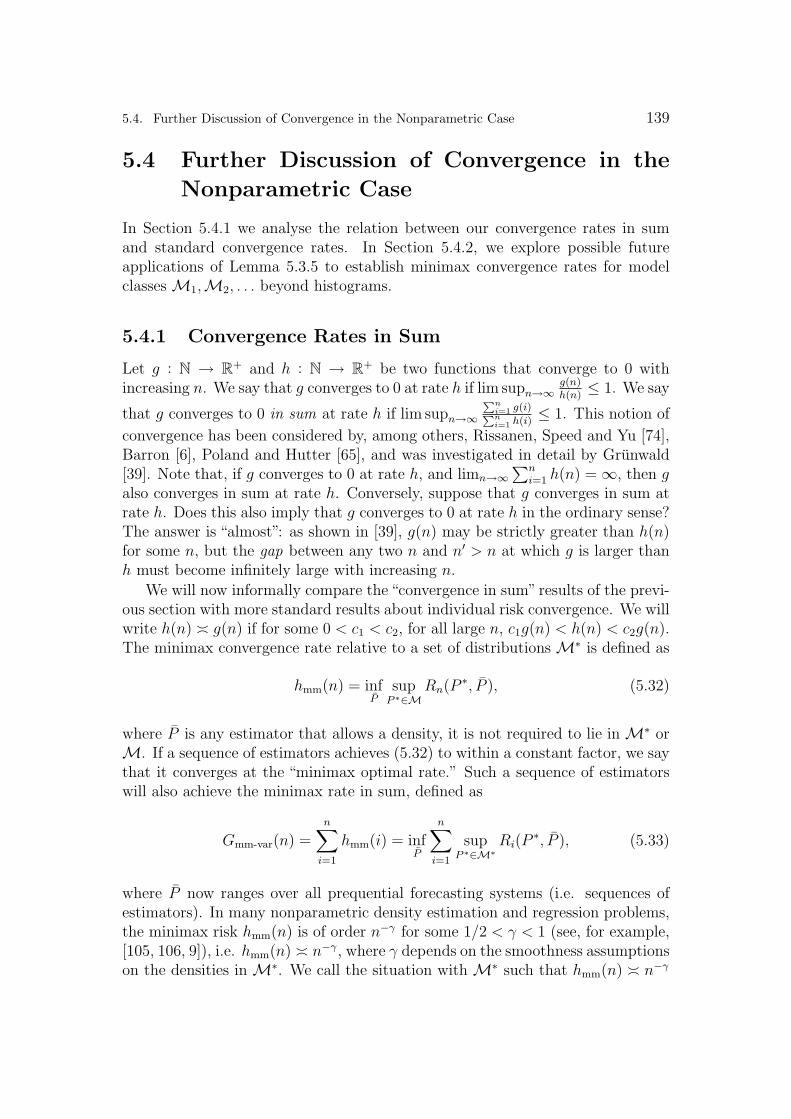
5.4. Further Discussion of Convergence in the Nonparametric Case 139
5.4 Further Discussion of Convergence in the
Nonparametric Case
In Section 5.4.1 we analyse the relation between our convergence rates in sumand standard convergence rates. In Section 5.4.2, we explore possible futureapplications of Lemma 5.3.5 to establish minimax convergence rates for modelclasses M1,M2, . . . beyond histograms.
5.4.1 Convergence Rates in Sum
Let g : N → R+ and h : N → R
+ be two functions that converge to 0 withincreasing n. We say that g converges to 0 at rate h if lim supn→∞
g(n)h(n)≤ 1. We say
that g converges to 0 in sum at rate h if lim supn→∞
Pni=1 g(i)
Pni=1 h(i)
≤ 1. This notion of
convergence has been considered by, among others, Rissanen, Speed and Yu [74],Barron [6], Poland and Hutter [65], and was investigated in detail by Grunwald[39]. Note that, if g converges to 0 at rate h, and limn→∞
∑ni=1 h(n) =∞, then g
also converges in sum at rate h. Conversely, suppose that g converges in sum atrate h. Does this also imply that g converges to 0 at rate h in the ordinary sense?The answer is “almost”: as shown in [39], g(n) may be strictly greater than h(n)for some n, but the gap between any two n and n′ > n at which g is larger thanh must become infinitely large with increasing n.
We will now informally compare the “convergence in sum” results of the previ-ous section with more standard results about individual risk convergence. We willwrite h(n) ≍ g(n) if for some 0 < c1 < c2, for all large n, c1g(n) < h(n) < c2g(n).The minimax convergence rate relative to a set of distributions M∗ is defined as
hmm(n) = infP
supP ∗∈M
Rn(P ∗, P ), (5.32)
where P is any estimator that allows a density, it is not required to lie in M∗ orM. If a sequence of estimators achieves (5.32) to within a constant factor, we saythat it converges at the “minimax optimal rate.” Such a sequence of estimatorswill also achieve the minimax rate in sum, defined as
Gmm-var(n) =n∑
i=1
hmm(i) = infP
n∑
i=1
supP ∗∈M∗
Ri(P∗, P ), (5.33)
where P now ranges over all prequential forecasting systems (i.e. sequences ofestimators). In many nonparametric density estimation and regression problems,the minimax risk hmm(n) is of order n−γ for some 1/2 < γ < 1 (see, for example,[105, 106, 9]), i.e. hmm(n) ≍ n−γ , where γ depends on the smoothness assumptionson the densities in M∗. We call the situation with M∗ such that hmm(n) ≍ n−γ

140 Chapter 5. Slow Convergence: the Catch-up Phenomenon
the “standard nonparametric case.” In this standard case, we have
Gmm-var(n) ≍n∑
i=1
i−γ ≍∫ n
1
x−γ dx ≍ n1−γ . (5.34)
Similarly, in standard parametric problems, the minimax risk hmm(n) ≍ 1/n. Inthat case, analogously to (5.34), we see that the minimax risk in sum Gmm-var isof order log n.
Note, however, that our result for histograms (and, more generally, for anyrate-of-convergence result that may be based on Lemmata 5.3.3, 5.3.4 and 5.3.5),is based on a scenario where P ∗, while allowed to depend on n, is kept fixed overthe terms in the sum from 1 to n. Indeed, in Theorem 5.3.7 we showed that Psw
achieves the minimax rate in sum Gmm-fix(n) as defined in (5.21). Comparingto (5.33), we see that the supremum is moved outside of the sum. Fortunately,Gmm-fix and Gmm-var are usually of the same order: in the parametric case, e.g.M∗ =
⋃
k≤k∗Mk, both Gmm-fix and Gmm-var are of order log n. For Gmm-var, wehave already seen this. For Gmm-fix, this is a standard information-theoretic result,see for example [23]. In the standard nonparametric case, when the standardminimax rate is of order n−γ and therefore Gmm-var ≍ n1−γ , it also holds thatGmm-fix(n) ≍ n1−γ [106, page 1582]. To see this, let Pmm-fix be any prequentialforecasting system that achieves Gmm-fix as defined in (5.21) (if such a Pmm-fix doesnot exist, take any P that, for each n, achieves the infimum to within εn for somesequence ε1, ε2, . . . tending to 0). Now define the prequential forecasting system
PCesaro(xn | xn−1) :=1
n
n∑
i=1
Pmm-fix(xn | xi−1).
Thus, PCesaro is obtained as a time (“Cesaro”-) average of Pmm-fix. It now follows byapplying Jensen’s inequality as in Proposition 15.2 of [39] (or the correspondingresults in [102] or [106]) that
supP ∗
Rn(P ∗, PCesaro) ≤ supP ∗
1
n
n∑
i=1
Ri(P∗, Pmm-fix) = n−1O(n1−γ) = O(n−γ), (5.35)
so that∑n
j=1 supP ∗ Rj(P∗, PCesaro) = O(
∑nj=1 j−γ) = O(n1−γ), and it follows that
Gmm-var(n) = O(n1−γ) = O(Gmm-fix(n)). (5.36)
Since, trivially, Gmm-fix(n) ≤ Gmm-var(n), it follows that Gmm-var(n) ≍ n1−γ . Theunderlying idea of basing predictive distributions on Cesaro-averages is not new;see for example [43, Section 9] and [102]. It is described in detail in [39].
Summarising, both in standard parametric and nonparametric cases, Gmm-fix
and Gmm-var are of comparable size. Therefore, Lemma 5.3.4 and 5.3.5 do suggest

5.4. Further Discussion of Convergence in the Nonparametric Case 141
that, both in standard parametric and nonparametric cases, Psw achieves theminimax convergence rate Gmm-fix (and Theorem 5.3.7 shows that it actuallydoes so in a specific nonparametric case). One caveat is in order though: thefact that Gmm-fix and Gmm-var are of comparable size does not imply that Psw alsoachieves the varying-P ∗-minimax rate Gmm-var. We cannot prove the analogueof Lemma 5.3.4 and Lemma 5.3.5 with the supremum over P ∗ inside the sum inGsw and Gσ. Therefore, we cannot prove even for histogram density estimation,that Psw achieves Gmm-var. Nevertheless, we do suspect that in the standardnonparametric case, Gmm-fix(n) ≍ Gmm-var(n) ≍ n1−γ , whenever Psw achievesthe fixed-P ∗ minimax rate Gmm-fix, it also achieves the varying-P ∗ minimax rateGmm-var. The reason for this conjecture is that, if we can assume that the data arei.i.d. under all P ∗ ∈M∗, then whenever Psw achieves Gmm-fix, a small modificationof Psw will achieve Gmm-var. Indeed, define the Cesaro-switch distribution as
PCesaro-sw(xn | xn−1) :=1
n
n∑
i=1
Psw(xn | xi−1).
Applying (5.35) to PCesaro-sw rather than PCesaro, we see that PCesaro-sw achievesthe varying-P ∗-minimax rate whenever Psw achieves the fixed-P ∗-minimax rate.Since, intuitively, PCesaro-sw learns “slower” than Psw, we suspect that Psw itselfthen achieves the varying-P ∗-minimax rate as well. However, in the parametriccase, hmm(n) ≍ 1/n whereas Gmm-fix(n)/n ≍ (log n)/n. Then the reasoning of(5.35) does not apply any more, and PCesaro-sw may not achieve the minimax ratefor varying P ∗. We suspect that this is not a coincidence — a recent result byYang [103] suggests that, in the parametric case, no model selection/averagingcriterion can achieve both consistency and minimax optimal varying-P ∗ ratesGmm-var (Section 5.6.1).
5.4.2 Beyond Histograms
The key to proving Theorem 5.3.7, the minimax convergence result for histogramdensity estimation, is the existence of an oracle σα which achieves the minimaxconvergence rate, but which, at the same time, switches only a logarithmic num-ber of times. The theorem followed by applying Lemma 5.3.5 with this oracle.It appears that the same technique can be applied in many other standard non-parametric settings (with hmm(n) ≍ n−γ) as well. Important examples includelinear regression based on full approximation sets of functions such as polynomi-als [106, 101] or splines, with random i.i.d. design and i.i.d. normally distributednoise with known variance σ2. The development in Section 6.2 of [101] indicatesthat an analogue of Theorem 5.3.7 can be proven for such cases. Here the modelsMk are families of conditional distributions Pθ for Y ∈ R given X ∈ [0, 1]d forsome d > 0, where θ = (θ1, . . . , θk) and Pθ expresses that Yi =
∑kj=1 θjφj(Xi)+U ,
with φj being the j-th basis function in the approximation set, and U , the noise,

142 Chapter 5. Slow Convergence: the Catch-up Phenomenon
is a zero-mean Gaussian random variable. The forecasting systems p1, p2, . . . arenow based on maximum likelihood estimators rather than Bayes predictive dis-tributions.
Another candidate is density estimation based on sequences of exponentialfamilies as introduced by Barron and Sheu [9], when the estimators p1, p2, . . .are based on Bayesian MAP estimators defined with respect to k-dimensionalexponential families, and M∗ is taken to be the set of densities p such that log pis contained in some Sobolev space with smoothness parameter r [7]. Preliminaryinvestigations suggest that Psw achieves the minimax convergence rates in boththe linear regression and the density estimation setting, but, at the time of writing,we have not yet proven any formal statements.
5.5 Efficient Computation
For priors π as in (5.7), the posterior probability on predictors p1, p2, . . . can beefficiently computed sequentially, provided that πt(Z = n | Z ≥ n) and πk canbe calculated quickly and that πm(m) = θm(1− θ) is geometric with parameter θ,as is also required for Theorem 5.2.1 and permitted in the theorems and lemma’sof Section 5.3 that require (5.12). The algorithm resembles Fixed-Share [46],but whereas Fixed-Share implicitly imposes a geometric distribution for πt,we allow general priors by varying the shared weight with n, and through theaddition of the πm component of the prior, we ensure that the additional losscompared to the best prediction strategy does not grow with the sample size, acrucial property for consistency.
To ensure finite running time, rather than Psw the algorithm uses a potentiallydefective distribution P that assigns smaller or equal probability to all events. Itis obtained by restricting Psw to using only a finite nonempty set Kn of predictionstrategies at sample size n. Then, analogously to (5.4), for any n the density ofthe marginal distribution of P on Xn is given by p(xn) =
∑
s∈S′ qs(xn)·π(s), where
S′ := s ∈ S | ∀n ∈ Z
+ : Kn(s) ∈ Kn denotes the parameter space restricted tothose prediction strategies that are considered at each sample size. We use theindicator function, 1A(x) = 1 if x ∈ A and 0 otherwise. Here is the algorithm:
This algorithm can be used to obtain fast convergence in the sense of Section 5.3,and, as long as π does not vary with n, consistency in the sense of Theorem 5.2.1.Note that the running time Θ(
∑Nn=1 |Kn|) is typically of the same order as that
of fast model selection criteria like AIC and BIC: for example if the number ofconsidered prediction strategies is fixed at K then the running time is Θ(K ·N).In the interest of clarity and simplicity we only prove the theorem below, whichassumes P = Psw, but the reader may verify that the algorithm remains valid fordefective P .
Theorem 5.5.1. If P = Psw, then Algorithm 5.1 correctly reports P (Kn+1, xn).

5.6. Relevance and Earlier Work 143
Algorithm 5.1 Switch(xN)
1 for k ∈ K1 do initialise wak ← θ · πk(k); wb
k ← (1− θ) · πk(k) end for2 for n=1, . . . , N do3 Report P (Kn, x
n−1) = waKn+1
+ wbKn+1
(a K-sized array)
4 for k ∈ Kn do wak ← wa
k · pk(xn|xn−1); wbk ← wb
k · pk(xn|xn−1) end for5 pool ← πt(Z = n | Z ≥ n) ·∑k∈Kn
wak
6 for k ∈ Kn+1 do7 wa
k ← wak · 1Kn(k) · πt(Z 6= n | Z ≥ n) + pool · πk(k) · θ
8 wbk ← wb
k · 1Kn(k) + pool · πk(k) · (1− θ)9 end for
10 end for11 Report P (KN+1, x
N) = waKN+1
+ wbKN+1
The proof is given in Section 5.9.4.
5.6 Relevance and Earlier Work
5.6.1 AIC-BIC; Yang’s Result
Over the last 25 years or so, the question whether to base model selection on AICor BIC type methods has received a lot of attention in the theoretical and appliedstatistics literature, as well as in fields such as psychology and biology wheremodel selection plays an important role (googling “AIC and BIC” gives 355000hits) [85, 41, 40, 10, 33, 30, 81]. It has even been suggested that, since thesetwo types of methods have been designed with different goals in mind (optimalprediction vs. “truth hunting”), one should not expect procedures that combinethe best of both types of approaches to exist [81]. Our Theorem 5.2.1 and ourresults in Section 5.3 show that, at least in some cases, one can get the best of bothworlds after all, and model averaging based on Psw achieves the minimax optimalconvergence rate. In typical parametric settings (P ∗ ∈M), model selection basedon Psw is consistent, and Lemma 5.3.4 suggests that model averaging based onPsw is within a constant factor of the minimax optimal rate in parametric settings.Superficially, our results may seem to contradict the central conclusion of Yang[103]. Yang shows that there are scenarios in linear regression where no modelselection or model combination criterion can be both consistent and achieve theminimax rate of convergence.
Yang’s result is proved for a variation of linear regression in which the esti-mation error is measured on the previously observed design points. This setupcannot be directly embedded in our framework. Also, Yang’s notion of modelcombination is somewhat different from the model averaging that is used to com-pute Psw. Thus, formally, there is no contradiction between Yang’s results and

144 Chapter 5. Slow Convergence: the Catch-up Phenomenon
ours. Still, the setups are so similar that one can easily imagine a variation ofYang’s result to hold in our setting as well. Thus, it is useful to analyse how these“almost” contradictory results may coexist. We suspect (but have no proof) thatthe underlying reason is the definition of our minimax convergence rate in sum(5.21) in which P ∗ is allowed to depend on n, but then the risk with respect tothat same P ∗ is summed over all i = 1, . . . , n. Yang’s result holds in a parametricscenario, where there are two nested parametric models, and data are sampledfrom a distribution in one of them. Then both Gmm-fix and Gmm-var are of thesame order log n, but it may of course be possible that there does exist a min-imax optimal procedure that is also consistent, relative to the Gmm-fix-game, inwhich P ∗ is kept fixed once n has been determined, while there does not exist aminimax optimal procedure that is also consistent, relative to the Gmm-var-game,in which P ∗ is allowed to vary. Indeed, while in Section 5.4.1 we have establishedthat PCesaro-sw, a slight variation of Psw, achieves the minimax optimal conver-gence rates Gmm-var and hmm for some nonparametric M∗, which suggests thatPsw achieves these rates as well, we do not have such a result for parametricM∗.Yang’s results indicate that such an analogue may not exist.
Several other authors have provided procedures which have been designed tobehave like AIC whenever AIC is better, and like BIC whenever BIC is better;and which empirically seem to do so; these include model meta-selection [30, 21],and Hansen and Yu’s gMDL version of MDL regression [41]; also the “mongrel”procedure of [99] has been designed to improve on Bayesian model averaging forsmall samples. Compared to these other methods, ours seems to be the first thatprovably is both consistent and minimax optimal in terms of risk, for some classesM∗. The only other procedure that we know of for which somewhat related resultshave been shown, is a version of cross-validation proposed by Yang [104] to selectbetween AIC and BIC in regression problems. Yang shows that a particular formof cross-validation will asymptotically select AIC in case the use of AIC leadsto better predictions, and BIC in the case that BIC leads to better predictions.In contrast to Yang, we use a single paradigm rather than a mix of several ones(such as AIC, BIC and cross-validation) – essentially our paradigm is just that ofuniversal individual-sequence prediction, or equivalently, the individual-sequenceversion of predictive MDL, or equivalently, Dawid’s prequential analysis appliedto the log scoring rule. Indeed, our work has been heavily inspired by prequentialideas; in Dawid [29] it is already suggested that model selection should be based onthe transient behaviours in terms of sequential prediction of the estimators withinthe models: one should select the model which is optimal at the given samplesize, and this will change over time. Although Dawid uses standard Bayesianmixtures of parametric models as his running examples, he implicitly suggeststhat other ways (the details of which are left unspecified) of combining predictivedistributions relative to parametric models may be preferable, especially in thenonparametric case where the true distribution is outside any of the parametricmodels under consideration.

5.7. The Catch-Up Phenomenon, Bayes and Cross-Validation 145
5.6.2 Prediction with Expert Advice
Since the switch-distribution has been designed to perform well in a setting wherethe optimal predictor pk changes over time, our work is also closely related tothe algorithms for tracking the best expert in the universal prediction literature[46, 95, 94, 63]. However, those algorithms are usually intended for data that aresequentially generated by a mechanism whose behaviour changes over time. Insharp contrast, our switch distribution is especially suitable for situations wheredata are sampled from a fixed (though perhaps non-i.i.d.) source after all; thefact that one model temporarily leads to better predictions than another is causedby the fact that each “expert” pk has itself already been designed as a universalpredictor/estimator relative to some large set of distributionsMk. The elementsof Mk may be viewed as “base” predictors/experts, and the pk may be thoughtof as meta-experts/predictors. Because of this two-stage structure, which meta-predictor pk is best changes over time, even though the optimal base-predictorarg minp∈M Rn(p∗, p) does not change over time.
If one of the considered prediction strategies pk makes the best predictionseventually, our goal is to achieve consistent model selection: the total number ofswitches should also remain bounded. To this end we have defined the switch dis-tribution such that positive prior probability is associated with switching finitelyoften and thereafter using pk for all further outcomes. We need this property toprove that our method is consistent. Other dynamic expert tracking algorithms,such as the FixedShare algorithm [46], have been designed with different goalsin mind, and as such they do not have this property. Not surprisingly then, ourresults do not resemble any of the existing results in the “tracking”-literature.
5.7 The Catch-Up Phenomenon, Bayes and Cross-
Validation
5.7.1 The Catch-Up Phenomenon is Unbelievable! (ac-cording to pbma)
On page 122 we introduced the marginal Bayesian distribution pbma(xn) :=
∑
k w(k)pk(xn).If the distributions pk are themselves Bayesian marginal distributions as in (5.1),then pbma may be interpreted as (the density corresponding to) a distribution onthe data that reflects some prior beliefs about the domain that is being modelled,as represented by the priors w(k) and wk(θ). If w(k) and wk(θ) truly reflectedsome decision-maker’s a priori beliefs, then it is clear that the decision-makerwould like to make sequential predictions of Xn+1 given Xn = xn based on pbma
rather than on psw. Indeed, as we now show, the catch-up phenomenon as de-picted in Figure 5.1 is exceedingly unlikely to take place under pbma, and a prioria subjective Bayesian should be prepared to bet a lot of money that it does not

146 Chapter 5. Slow Convergence: the Catch-up Phenomenon
occur. To see this, consider the no-hypercompression inequality [39], versions ofwhich are also known as “Barron’s inequality” [5] and “competitive optimality ofthe Shannon-Fano code” [25]. It states that for any two distributions P and Q forX∞, the P -probability that Q outperforms P by k bits or more when sequentiallypredicting X1, X2, . . . is exponentially small in k: for each n,
P (− log q(Xn) ≤ − log p(Xn)− k) ≤ 2−k.
Plugging in pbma for p, and psw for q, we see that what happened in Figure 5.1 (psw
outperforming pbma by about 40000 bits) is an event with probability no morethan 2−40000 according to pbma. Yet, in many practical situations, the catch-upphenomenon does occur and psw gains significantly compared to pbma. This canonly be possible because either the models are wrong (clearly, The Picture ofDorian Gray has not been drawn randomly from a finite-order Markov chain), orbecause the priors are “wrong” in the sense that they somehow don’t match thesituation one is trying to model. For this reason, some subjective Bayesians, whenwe confronted them with the catch-up phenomenon, have argued that it is justa case of “garbage in, garbage out” (GIGO): when the phenomenon occurs, then,rather than using the switch-distribution, one should reconsider the model(s) andprior(s) one wants to use, and, once one has found a superior modelM′ and priorw′, one should use pbma relative to M′ and w′. Of course we agree that if onecan come up with better models, one should of course use them. Nevertheless, westrongly disagree with the GIGO point of view: We are convinced that in practice,“correct” priors may be impossible to obtain; similarly, people are forced to workwith “wrong” models all the time. In such cases, rather than embarking on apotentially never-ending quest for better models, the hurried practitioner mayoften prefer to use the imperfect – yet still useful – models that he has available,in the best possible manner. And then it makes sense to use psw rather than theBayesian pbma: the best one can hope for in general is to regard the distributions inone’s models as prediction strategies, and try to predict as well as the best strategycontained in any of the models, and psw is better at this than pbma. Indeed, thecatch-up phenomenon raises some interesting questions for Bayes factor modelselection: no matter what the prior is, by the no-hypercompression inequalityabove with p = pbma and q = psw, when comparing two models M1 and M2,before seeing any data, a Bayesian always believes that the switch-distributionwill not substantially outperform pbma, which implies that a Bayesian cannotbelieve that, with non-negligible probability, a complex model p2 can at firstpredict substantially worse than a simple model p1 and then, for large samples,can predict substantially better. Yet in practice, this happens all the time!
5.7.2 Nonparametric Bayes
A more interesting subjective Bayesian argument against the switch distributionwould be that, in the nonparametric setting, the data are sampled from some

5.7. The Catch-Up Phenomenon, Bayes and Cross-Validation 147
P ∗ ∈M∗ \M, and is not contained in any of the parametric modelsM1,M2, . . .Yet, under the standard hierarchical prior used in pbma (first a discrete prior onthe model index, then a density on the model parameters), we have that withprior-probability 1, P ∗ is “parametric”, i.e. P ∗ ∈ Mk for some k. Thus, ourprior distribution is not really suitable for the situation that we are trying tomodel in the nonparametric setting, and we should use a nonparametric priorinstead. While we completely agree with this reasoning, we would immediatelylike to add that the question then becomes: what nonparametric prior should oneuse? Nonparametric Bayes has become very popular in recent years, and it oftenworks surprisingly well. Still, its practical and theoretical performance stronglydepends on the type of priors that are used, and it is often far from clear what priorto use in what situation. In some situations, some nonparametric priors achieveoptimal rates of convergence, but others can even make Bayes inconsistent [31, 39].The advantage of the switch-distribution is that it does not require any difficultmodelling decisions, but nevertheless under reasonable conditions it achieves theoptimal rate of convergence in nonparametric settings, and, in the special casewhere one of the models on the list in fact approximates the true source extremelywell, this model will in fact be identified (Theorem 5.2.1). In fact, one may thinkof psw as specifying a very special kind of nonparametric prior, and under thisinterpretation, our results are in complete agreement with the nonparametricBayesian view.
5.7.3 Leave-One-Out Cross-Validation
From the other side of the spectrum, it has sometimes been argued that consis-tency is irrelevant, since in practical situations, the true distribution is never inany of the models under consideration. Thus, it is argued, one should use AIC-type methods such as leave-one-out cross-validation, because of their predictiveoptimality. We strongly disagree with this argument, for several reasons: first,in practical model selection problems, one is often interested in questions such as“does Y depend on feature Xk or not?” For example,Mk−1 is a set of conditionaldistributions in which Y is independent of Xk, and Mk is a superset thereof inwhich Y can be dependent on Xk. There are certainly real-life situations wheresome variable Xj is truly completely irrelevant for predicting Y , and it may bethe primary goal of the scientist to find out whether or not this is the case. Insuch cases, we would hope our model selection criterion to select, for large n,Mk−1 rather thanMk, and the problem with the AIC-type methods is that, be-cause of their inconsistency, they sometimes do not do this. In other words, wethink that consistency does matter, and we regard it as a clear advantage of theswitch-distribution that it is consistent.
A second advantage over leave-one-out cross-validation is that the switch-distribution, like Bayesian methods, satisfies Dawid’s weak prequential principle[29, 39]: the switch-distribution assesses the quality of a predictor pk only in

148 Chapter 5. Slow Convergence: the Catch-up Phenomenon
terms of the quality of predictions that were actually made. To apply LOO on asample x1, . . . , xn, one needs to know the prediction for xi given x1, . . . , xi−1, butalso xi+1, . . . , xn. In practice, these may be hard to compute, unknown or evenunknowable. An example of the first are non-i.i.d. settings such as time seriesmodels. An example of the second is the case where the pk represent, for example,weather forecasters, or other predictors which have been designed to predict thefuture given the past. Actual weather forecasters use computer programs topredict the probability that it will rain the next day, given a plethora of dataabout air pressure, humidity, temperature etc. and the pattern of rain in the pastdays. It may simply be impossible to apply those programs in a way that theypredict the probability of rain today, given data about tomorrow.
5.8 Conclusion and Future Work
We have identified the catch-up phenomenon as the underlying reason for the slowconvergence of Bayesian model selection and averaging. Based on this, we havedefined the switch-distribution Psw, a modification of the Bayesian marginal dis-tribution which is consistent, but also under some conditions achieves a minimaxoptimal convergence rate, a significant step forward in resolving the the AIC/BICdilemma. Different strands of future work suggest themselves:
1. Lemma 5.3.5 provides a tool to prove minimax optimal in-sum convergenceof the switch-distribution for particular nonparametric model classes M∗.However, because of time constraints we have currently only applied this tohistogram density estimation. We hope to eventually show that the switch-distribution actually achieves the minimax optimal convergence rate for awide class of nonparametric problems.
2. Since psw can be computed in practice, the approach can readily be testedwith real and simulated data in both density estimation and regression prob-lems. Initial results on simulated data, on which we will report elsewhere,give empirical evidence that psw behaves remarkably well in practice. Modelselection based on psw, like for pbma, typically identifies the true distribu-tion at moderate sample sizes. Prediction and estimation based on Psw is ofcomparable quality to leave-one-out cross-validation (LOO) and generally,in no experiment did we find that it behaved substantially worse than eitherLOO or AIC.
3. It is an interesting open question whether analogues of Lemma 5.3.5 andTheorem 5.3.7 exist for model selection rather than averaging. In otherwords, in settings such as histogram density estimation where model aver-aging based on the switch distribution achieves the minimax convergencerate, does model selection based on the switch distribution achieve it as

5.9. Proofs 149
well? For example, in Figure 5.1, sequentially predicting by the pKn+1 thathas maximum a posteriori probability (MAP) under the switch-distributiongiven data xn, is only a few bits worse than predicting by model averagingbased on the switch-distribution, and still outperforms standard Bayesianmodel averaging by about 40 000 bits. In the experiments mentioned above,we invariably found that predicting by the MAP pKn+1 empirically convergesat the same rate as using model averaging, i.e. predicting by Psw. How-ever, we have no proof that this really must always be the case. Analogousresults in the MDL literature suggest that a theorem bounding the risk ofswitch-based model selection, if it can be proven at all, would bound thesquared Hellinger rather than the KL risk ([39], Chapter 15).
4. The way we defined Psw, it does not seem suitable for situations in whichthe number of considered models or model combinations is exponential inthe sample size. Because of condition (i) in Lemma 5.3.5, our theoreticalresults do not cover this case either. Yet this case is highly important inpractice, for example, in the subset selection problem [101]. It seems clearthat the catch-up phenomenon can and will also occur in model selectionproblems of that type. Can our methods be adapted to this situation, whilestill keeping the computational complexity manageable? And what is therelation with the popular and computationally efficient L1-approaches tomodel selection? [90]
5.9 Proofs
5.9.1 Proof of Theorem 5.2.1
Let Un = s ∈ S | Kn+1(s) 6= k∗ denote the set of “bad” parameters s that selectan incorrect model. It is sufficient to show that
limn
∑
s∈Unπ(s)qs(X
n)∑
s∈Sπ(s)qs(Xn)
= 0 with Pk∗-probability 1. (5.37)
To see this, suppose the theorem is false. Then there exists a Φ ⊆ Θk∗ withwk∗(Φ) :=
∫
Φwk∗(θ)dθ > 0 such that (5.6) does not hold for any θ∗ ∈ Φ. But
then by definition of Pk∗ we have a contradiction with (5.37).Now let A = s ∈ S : km(s) 6= k∗ denote the set of parameters that are bad
for sufficiently large n. We observe that for each s′ ∈ Un there exists at least oneelement s ∈ A that uses the same sequence of switch-points and predictors on thefirst n + 1 outcomes (this implies that Ki(s) = Ki(s
′) for i = 1, . . . , n + 1) andhas no switch-points beyond n (i.e. tm(s) ≤ n). Consequently, either s′ = s ors′ ∈ Es. Therefore∑
s′∈Un
π(s′)qs′(xn) ≤
∑
s∈A
(π(s) + π(Es)
)qs(x
n) ≤ (1 + c)∑
s∈A
π(s)qs(xn). (5.38)

150 Chapter 5. Slow Convergence: the Catch-up Phenomenon
Defining the mixture r(xn) =∑
s∈A π(s)qs(xn), we will show that
limn
r(Xn)
π(s = (0, k∗)) · pk∗(Xn)= 0 with Pk∗-probability 1. (5.39)
Using (5.38) and the fact that∑
s∈Sπ(s)qs(x
n) ≥ π(s = (0, k∗)) · pk∗(xn), thisimplies (5.37).
For all s ∈ A and xtm(s) ∈ X tm(s), by definition Qs(X∞tm+1|xtm) is equal to
Pkm(X∞tm+1|xtm), which is mutually singular with Pk∗(X∞
tm+1|xtm) by assumption.If X is a separable metric space, which holds because X ⊆ R
d for some d ∈ Z+, it
can be shown that this conditional mutual singularity implies mutual singularityof Qs(X
∞) and Pk∗(X∞). To see this for countable X , let Bxtm be any eventsuch that Qs(Bxtm |xtm) = 1 and Pk∗(Bxtm |xtm) = 0. Then, for B = y∞ ∈ X∞ |y∞
tm+1 ∈ Bytm, we have that Qs(B) = 1 and Pk∗(B) = 0. In the uncountablecase, however, B may not be measurable. In that case, the proof follows byCorollary 5.9.2 proved in Section 5.9.3. Any countable mixture of distributionsthat are mutually singular with Pk∗ , in particular R, is mutually singular withPk∗ . This implies (5.39) by Lemma 3.1 of [5], which says that for any two mutuallysingular distributions R and P , the density ratio r(Xn)/p(Xn) goes to zero asn→∞ with P -probability 1.
5.9.2 Proof of Theorem 5.2.2
The proof is almost identical to the proof of Theorem 5.2.1. Let Un = s ∈S | Kn+1(s) 6= k∗ denote the set of “bad” parameters s that select an incorrectmodel. It is sufficient to show that
limn
∑
s∈Unπ(s)qs(X
n)∑
s∈Sπ(s)qs(Xn)
= 0 with PBk∗-probability 1. (5.40)
Note that the qs in (5.40) are defined relative to the non-Bayesian estimatorsp1, p2, . . ., whereas the PB
k∗ on the right of the equation is the probability accord-ing to a Bayesian marginal distribution PB
k∗ , which has been chosen so that thetheorem’s condition holds. To see that (5.40) is sufficient to prove the theorem,suppose the theorem is false. Then, because the prior wk∗ is mutually absolutelycontinuous with Lebesgue measure, there exists a Φ ⊆ Θk∗ with nonzero priormeasure under wk∗ , such that (5.8) does not hold for any θ∗ ∈ Φ. But then bydefinition of PB
k∗ we have a contradiction with (5.40).Using exactly the same reasoning as in the proof of Theorem 5.2.1, it follows
that, analogously to (5.39), we have
limn
r(Xn)
π(s = (0, k∗)) · pBk∗(Xn)
= 0 with PBk∗-probability 1. (5.41)
This is just (5.39) with r now referring to a mixture of switch distributions definedrelative to the non-Bayesian estimators p1, p2, . . ., and the pB
k∗ in the denominator

5.9. Proofs 151
and on the right referring to the Bayesian marginal distribution PBk∗ . Using (5.38)
and the fact that∑
s∈Sπ(s)qs(x
n) ≥ π(s = (0, k∗)) · pk∗(xn), and the fact that,by assumption, for some K, for all large n, pk∗(Xn) ≥ pB
k∗(Xn)2−K with PBk∗-
probability 1, (5.41) implies (5.40).
5.9.3 Mutual Singularity as Used in the Proof of Theo-rem 5.2.1
Let Y 2 = (Y1, Y2) be random variables that take values in separable metric spacesΩ1 and Ω2, respectively. We will assume all spaces to be equipped with Borel σ-algebras generated by the open sets. Let p be a prediction strategy for Y 2 withcorresponding distributions P (Y1) and, for any y1 ∈ Ω1, P (Y2|y1). To ensure thatP (Y 2) is well-defined, we impose the requirement that for any fixed measurableevent A2 ⊆ Ω2 the probability P (A2|y1) is a measurable function of y1.
Lemma 5.9.1. Suppose p and q are prediction strategies for Y 2 = (Y1, Y2), whichtake values in separable metric spaces Ω1 and Ω2, respectively. Then if P (Y2|y1)and Q(Y2|y1) are mutually singular for all y1 ∈ Ω1, then P (Y 2) and Q(Y 2) aremutually singular.
The proof, due to Peter Harremoes, is given below the following corollary,which is what we are really interested in. Let X∞ = X1, X2, . . . be randomvariables that take values in the separable metric space X . Then what we needin the proof of Theorem 5.2.1 is the following corollary of Lemma 5.9.1:
Corollary 5.9.2. Suppose p and q are prediction strategies for the sequence ofrandom variables X∞ = X1, X2, . . . that take values in respective separable met-ric spaces X1, X2, . . . Let m be any positive integer. Then if P (X∞
m+1|xm) andQ(X∞
m+1|xm) are mutually singular for all xm ∈ Xm, then P (X∞) and Q(X∞)are mutually singular.
Proof. The product spaces X1 × · · · × Xm and Xm+1 × Xm+2 × · · · are separablemetric spaces [64, pp. 5,6]. Now apply Lemma 5.9.1 with Ω1 = X1 × · · · × Xm
and Ω2 = Xm+1 ×Xm+2 × · · · .
Proof of Lemma 5.9.1. For each ω1 ∈ Ω1, by mutual singularity of P (Y2|ω1) andQ(Y2|ω1) there exists a measurable set Cω1 ⊆ Ω2 such that P (Cω1|ω1) = 1 andQ(Cω1|ω1) = 0. As Ω2 is a metric space, it follows from [64, Theorems 1.1 and1.2 in Chapter II] that for any ǫ > 0 there exists an open set U ǫ
ω1⊇ Cω1 such that
P (U ǫω1|ω1) = 1 and Q(U ǫ
ω1|ω1) < ǫ. (5.42)
As Ω2 is a separable metric space, there also exists a countable sequenceBii≥1 of open sets such that every open subset of Ω2 (U ǫ
ω1in particular) can be
expressed as the union of sets from Bi [64, Theorem 1.8 in Chapter I].

152 Chapter 5. Slow Convergence: the Catch-up Phenomenon
Let B′ii≥1 denote a subsequence of Bi such that U ǫ
ω1=⋃
i B′i. Sup-
pose B′i is a finite sequence. Then let V ǫ
ω1= U ǫ
ω1. Suppose it is not. Then
1 = P (U ǫω1|ω1) = P (
⋃∞i=1 B′
i|ω1) = limn→∞ P (⋃n
i=1 B′i|ω1), because
⋃ni=1 B′
i as afunction of n is an increasing sequence of sets. Consequently, there exists an Nsuch that P (
⋃Ni=1 B′
i|ω1) > 1−ǫ and we let V ǫω1
=⋃N
i=1 B′i. Thus in any case there
exists a set V ǫω1⊆ U ǫ
ω1that is a union of a finite number of elements in Bi such
thatP (V ǫ
ω1|ω1) > 1− ǫ and Q(V ǫ
ω1|ω1) < ǫ. (5.43)
Let Di≥1 denote an enumeration of all possible unions of a finite number ofelements in Bi and define the disjoint sequence of sets Aǫ
ii≥1 by
Aǫi = ω1 ∈ Ω1 : P (Di|ω1) > 1− ǫ,Q(Di|ω1) < ǫ \
i−1⋃
j=1
Aǫj (5.44)
for i = 1, 2, . . . Note that, by the reasoning above, for each ω1 ∈ Ω1 there exists ani such that ω1 ∈ Aǫ
i , which implies that Aǫi forms a partition of Ω1. Now, as all
elements of Aǫi and Di are measurable, so is the set F ǫ =
⋃∞i=1 Aǫ
i×Di ⊆ Ω1×Ω2, for which we have that P (F ǫ) =
∑∞i=1 P (Aǫ
i×Di) > (1−ǫ)∑∞
i=1 P (Ai) = 1−ǫand likewise Q(F ǫ) < ǫ.
Finally, let G =⋂∞
n=1
⋃∞k=n F 2−k
. Then P (G) = limn→∞ P (⋃∞
k=n F 2−k) ≥
limn→∞ 1 − 2−n = 1 and Q(G) = limn→∞ Q(⋃
k=n F 2−k) ≤ limn→∞
∑∞k=n 2−k =
limn→∞ 2−n+1 = 0, which proves the lemma.
5.9.4 Proof of Theorem 5.5.1
Before we prove Theorem 5.5.1, we first need to establish some additional proper-ties of the prior π as defined in (5.7). Define, for all n ∈ N and s = ((t1, k1), . . . ,(tm, km)) ∈ S:
Sn(s) := 1t1,...,tm(n− 1); (5.45)
Mn(s) := 1tm,tm+1,...(n− 1); (5.46)
Kn(s) := ki for the unique i such that ti < n and i = m ∨ ti+1 ≥ n. (5.47)
These functions denote, respectively, whether or not a switch occurs just beforeoutcome n, whether or not the last switch occurs somewhere before outcome n andwhich prediction strategy is used for outcome n. The prior π determines the distri-butions of these random variables. We also define En(s) := (Sn(s),Mn(s), Kn(s))as a convenient abbreviation. Every parameter value s ∈ S induces an infinitesequence of values E1, E2, . . . The advantage of these new variables is that theyallow us to reformulate the prior as a strategy for prediction of the value of thenext random variable En+1 (which in turn determines the distribution on Xn+1
given xn), given all previous random variables En. Therefore, we first calculate

5.9. Proofs 153
the conditional probability π(En+1|En) before proceeding to prove the theorem.As it turns out, our prior has the nice property that this conditional probabilityhas a very simple functional form: depending on En, it is either zero, or a functionof only En+1 itself. This will greatly facilitate the analysis.
Lemma 5.9.3. Let π(s) = θm−1(1−θ)πk(k1)∏m
i=2 πt(ti|ti > ti−1)πk(k) as in (5.7).For π(s) > 0 we have
π(E1) := πk(K1)
θ if M1 = 0
1− θ if M1 = 1(5.48)
π(En+1|En) :=
πt(Z > n|Z ≥ n) if Sn+1 = 0 and Mn+1 = 0
1 if Sn+1 = 0 and Mn+1 = 1
πt(Z = n|Z ≥ n)πk(Kn+1)θ if Sn+1 = 1 and Mn+1 = 0
πt(Z = n|Z ≥ n)πk(Kn+1)(1− θ) if Sn+1 = 1 and Mn+1 = 1.
(5.49)
Proof. To check (5.48), note that we must have either E1 = (1, 1, k), whichcorresponds to s = (0, k) which has probability πk(k)(1 − θ) as required, orE1 = (1, 0, k). The latter corresponds to the event that m > 1 and k1 = k,which has probability πk(k)θ.
We proceed to calculate the conditional distribution π(En+1|En). We distin-guish the case that Mn(s) = 1 (the last switch defined by s occurs before samplesize n), and Mn(s) = 0 (there will be more switches). First suppose Mn(s) = 0,and let an = maxi | ti < n =
∑ni=1 Si. Then
π(En) =∞∑
m=an+1
∞∑
tan+1=n
∑
tan+2, . . . , tmkan+1, . . . , km
πm(m)m∏
i=1
πt(ti|ti > ti−1)πk(ki)
=∞∑
m=an+1
πm(m)
an∏
i=1
πt(ti|ti > ti−1)πk(ki)
∞∑
tan+1=n
πt(tan+1|tan+1 > tan)
·∑
tan+2,...,tm
m∏
i=an+2
πt(ti|ti > ti−1)
∑
kan+1,...,km
m∏
i=an+1
πk(ki)
= πm(Z > an)
an∏
i=1
πt(ti|ti > ti−1)πk(ki)
πt(tan+1 ≥ n) · 1 · 1.
(5.50)

154 Chapter 5. Slow Convergence: the Catch-up Phenomenon
If Mn(s) = 1, then there is only one s that matches En, which has probability
π(En) = πm(Z = an)an∏
i=1
πt(ti|ti > ti−1)πk(ki). (5.51)
From (5.50) and (5.51) we can compute the conditional probability π(En+1|En).We distinguish further on the basis of the possible values of Sn+1 and Mn+1, whichtogether determine Mn (namely, if Mn+1 = 0 then Mn = 0 and if Mn+1 = 1 thenMn = 1−Sn+1). Also note that Sn+1 = 0 implies an+1 = an and Sn+1 = 1 impliesan+1 = an + 1 and tan+1 = n. Conveniently, most factors cancel out, and weobtain
π(En+1|En)
=
8
>
>
>
>
>
>
>
>
>
<
>
>
>
>
>
>
>
>
>
:
πt(tan+1 + 1 ≥ n + 1)/πt(tan ≥ n) if Sn+1 = 0, Mn+1 = 0
1 if Sn+1 = 0, Mn+1 = 1πm(Z>an+1)
πm(Z>an)πt(tan+1|tan+1 >tan)πk(kan+1)
πt(tan+2≥n+1)πt(tan+1≥n)
if Sn+1 = 1, Mn+1 = 0πm(Z=an+1)
πm(Z>an)πt(tan+1|tan+1>tan)
πt(tan+1≥n)πk(kan+1) if Sn+1 = 1, Mn+1 = 1,
which reduces to (5.49).
Proof of Theorem 5.5.1. We will use a number of independence properties of Pin this proof. First, we have that the distribution on En+1 is independent of Xn
conditional on En, because, using Bayes’ rule,
P (En+1|En, Xn) =P (Xn|En+1)P (En+1|En)
P (Xn|En)
=P (Xn|En)P (En+1|En)
P (Xn|En)= π(En+1|En),
(5.52)
provided that P (En+1, Xn) > 0. In turn, whether or not En+1 can occur dependsonly on Mn and Kn. For all n ≥ 1, define the function N(Mn, Kn) as the set ofvalues of the En+1 that have positive probability conditional on Mn and Kn, i.e.
N(Mn, Kn) := (s,m, k) | either s = 1 ∧Mn = 0 or s = 0 ∧m = Mn ∧ k = Kn.(5.53)
Thus, the conditional distribution on En+1 given all previous values En and allobservations Xn is a function of only En+1 itself, n, Mn and Kn. It remains thesame whether or not any of the other variables are included in the conditional. IfSn+1 = 1 then it is not even a function of Kn. This interesting property is usedthree times in the following. Namely,
1. Since (0, 0, k) ∈ N(0, k), we have πt(Z > n|Z ≥ n) = P (En+1 =(0, 0, k) |xn,Mn = 0, Kn = k).

5.9. Proofs 155
2. Since (1, 0, k) ∈ N(0, k′) for all k′, we have πt(Z = n|Z ≥ n)πk(k)θ =P (En+1 = (1, 0, k) |xn,Mn = 0).
3. If k ∈ K1, then πk(k)θ = P (x0,M1 = 0, K1 = k).
We first show that the invariants wak = P (xn−1,Mn = 0, Kn = k) and wb
k =P (xn−1,Mn = 1, Kn = k) hold at the start of each iteration (before line 3). Theinvariants ensure that wa
k +wbk = P (xn−1, Kn = k) so that the correct probabilities
are reported.Line 1 initialises wa
k to θπk(k) for k ∈ K1. By item 3 this equals P (x0,M1 =0, K1 = k) as required. We omit calculations for wb
k, which run along the samelines as for wa
k. Thus the loop invariant holds at the start of the first iteration.We proceed to go through the algorithm step by step to show that the invariant
holds in subsequent iterations as well. In the loss update in line 4 we update theweights for k ∈ Kn to
wak = P (xn−1,Mn = 0, Kn = k) · pk(xn|xn−1)
=∑
s:Mn=0,Kn=k
π(s)
n−1∏
i=1
pKi(xi|xi−1)
pKn(xn|xn−1) = P (xn,Mn = 0, Kn = k).
Similarly wbk = P (xn,Mn = 1, Kn = k). Then in line 5, we compute pool =
πt(Z = n|Z ≥ n)∑
k∈KnP (xn,Mn = 0, Kn = k) = πt(Z = n|Z ≥ n)P (xn,Mn =
0).Finally, after the loop that starts at line 6 and ends at line 9, we obtain for
all k ∈ Kn+1:
wak = P (xn, Mn =0, Kn =k)πt(Z >n|Z≥n) + πt(Z =n|Z≥n)P (xn, Mn =0)πk(k)θ
= P (xn, Mn = 0, Kn = k)P (Sn+1 = 0, Mn+1 = 0|xn, Mn = 0, Kn = k)
+ P (xn, Mn = 0)P (Sn+1 = 1, Mn+1 = 0, Kn+1 = k|xn, Mn = 0)
= P (xn, Mn = 0, Kn = k, Sn+1 = 0, Mn+1 = 0)
+ P (xn, Mn = 0, Sn+1 = 1, Mn+1 = 0, Kn+1 = k)
= P (xn, Sn+1 =0, Mn+1 =0, Kn+1 =k) + P (xn, Sn+1 =1, Mn+1 =0, Kn+1 =k)
= P (xn, Mn+1 = 0, Kn+1 = k).
Here we used items 1 and 2 in the second equality. Again, a similar derivationshows that wb
k = P (xn, Kn+1 = k,Mn+1 = 1). These weights satisfy the invariantat the beginning of the next iteration; after the last iteration the final posterioris also correctly reported based on these weights.


Chapter 6
Individual Sequence Rate Distortion
Rate-distortion theory analyses communication over a channel under a constrainton the number of transmitted bits, the“rate”. It currently serves as the theoreticalunderpinning for many important applications such as lossy compression anddenoising, or more generally, applications that require a separation of structureand noise in the input data.
Classical rate-distortion theory evolved from Shannon’s theory of commu-nication [79]. It studies the trade-off between the rate and the achievable fidelityof the transmitted representation under some distortion function, where the anal-ysis is carried out in expectation under some source distribution. Therefore thetheory can only be meaningfully applied if we have some reasonable idea as to thedistribution on objects that we want to compress lossily. While lossy compressionis ubiquitous, propositions with regard to the underlying distribution tend to bead-hoc, and necessarily so, because (1) it is a questionable assumption that theobjects that we submit to lossy compression are all drawn from the same proba-bility distribution, or indeed that they are drawn from a distribution at all, and(2) even if a true source distribution is known to exist, in most applications thesample space is so large that it is extremely hard to determine what it is like:objects that occur in practice very often exhibit more structure than predictedby the used source model.
For large outcome spaces then, it becomes important to consider structuralproperties of individual objects. For example, if the rate is low, then we may stillbe able to transmit objects that have a very regular structure without introduc-ing any distortion, but this becomes impossible for objects with high informationdensity. This point of view underlies some recent research in the lossy compres-sion community [77]. At about the same time, a rate-distortion theory whichallows analysis of individual objects has been developed within the framework ofKolmogorov complexity [60]. It defines a rate-distortion function not with respectto a source distribution, but with respect to an individual source word. Everysource word thus obtains its own associated rate-distortion function.
157

158 Chapter 6. Individual Sequence Rate Distortion
We will first give a brief introduction to algorithmic rate-distortion theory inSection 6.1. We also describe a novel generalisation of the theory to settings withside information, and we describe two distinct applications of the theory, namelylossy compression and denoising.
Algorithmic rate-distortion theory is based on Kolmogorov complexity, whichis not computable. We nevertheless cross the bridge between theory and practicein Section 6.2, by approximating Kolmogorov complexity by the compressed sizeof the object by a general purpose data compression algorithm. Even so, approxi-mating the rate-distortion function is a difficult search problem. We motivate andoutline the genetic algorithm we used to approximate the rate-distortion function.
In Section 6.3 we describe four experiments in lossy compression and denoising.The results are presented and discussed in Section 6.4. Then, in Section 6.5 wetake a step back and discuss to what extent our practical approach yields a faithfulapproximation of the theoretical algorithmic rate-distortion function, continuedby a discussion of how such a practical approach fits within the framework ofMDL model selection (Section 6.6). We end with a conclusion in Section 6.7.
6.1 Algorithmic Rate-Distortion
Suppose we want to communicate objects x from a set of source words X usingat most r bits per object. We call r the rate. We locate a good representation ofx within a finite set Y , which may be different from X in general (but we usuallyhave X = Y in this text). The lack of fidelity of a representation y is quantifiedby a distortion function d : X × Y → R.
Figure 6.1 Rate-distortion profile and distortion-rate function
00
K(x)Rate (bits)
Dis
tort
ion
Representations that witness the rate−distortion function
Som
e ar
bitr
ary
repr
esen
tatio
ns
RepresentationRate−distortion profile
Distortion−rate function

6.1. Algorithmic Rate-Distortion 159
The Kolmogorov complexity of y, denoted K(y), is the length of the shortestprogram that constructs y. More precisely, it is the length of the shortest inputto a fixed universal binary prefix machine that will output y and then halt; alsosee the textbook [60]. We can transmit any representation y that has K(y) ≤ r,the receiver can then run the program to obtain y and is thus able to reconstructx up to distortion d(x, y). Define the rate-distortion profile Px of the sourceword x as the set of pairs 〈r, a〉 such that there is a representation y ∈ Y withd(x, y) ≤ a and K(y) ≤ r. The possible combinations of r and a can also becharacterised by the rate-distortion function of the source word x, which is definedas rx(a) = minr : 〈r, a〉 ∈ Px, or by the distortion-rate function of the sourceword x, which is defined as dx(r) = mina : 〈r, a〉 ∈ Px. These two functionsare somewhat like inverses of each other; although strictly speaking they are notsince they are monotonic but not strictly monotonic. A representation y is said towitness the rate-distortion function of x if rx(d(x, y)) = K(y). These definitionsare illustrated in Figure 6.1.
Algorithmic rate-distortion theory is developed and treated in much moredetail in [92]. It is a generalisation of Kolmogorov’s structure function theory,see [93]. We generalise the algorithmic rate-distortion framework, so that it canaccommodate side information. Suppose that we want to transmit a source wordx ∈ X and we have chosen a representation y ∈ Y as before. The encoder anddecoder often share a lot of information: both might know that grass is greenand the sky is blue, they might share a common language, and so on. Theywould not need to transmit such information. If encoder and decoder share someinformation z, then the programs they transmit to compute the representation ymay use this side information z. Such programs can be much shorter, and arenever much longer, than their counterparts that do not use side information. Thiscan be formalised by switching to the conditional Kolmogorov complexity K(y|z),which is the length of the shortest Turing machine program that constructs y oninput z. We redefine K(y) = K(y|ǫ), where ǫ is the empty sequence, so thatK(y|z) ≤ K(y) + O(1): the length of the shortest program for y can neversignificantly increase when side information is provided, but it might certainlydecrease when y and z share a lot of information [60]. We change the definitionsas follows: The rate-distortion profile of the source word x with side information zis the set of pairs 〈r, a〉 such that there is a representation y ∈ Y with d(x, y) ≤ aand K(y|z) ≤ r. The definitions of the rate-distortion function and the distortion-rate function are similarly changed. Henceforth we will omit mention of the sideinformation z unless it is relevant to the discussion.
While this generalisation seems very natural the authors are not aware ofearlier proposals along these lines. In Section 6.4 we will demonstrate one use forthis generalised rate-distortion theory: removal of spelling errors in written text,an example where denoising is not practical without use of side information.

160 Chapter 6. Individual Sequence Rate Distortion
6.1.1 Distortion Spheres, the Minimal Sufficient Statistic
A representation y that witnesses the rate-distortion function is the best possiblerendering of the source object x at the given rate because it minimises the distor-tion, but if the rate is lower than K(x), then some information is necessarily lost.Since one of our goals is to find the best possible separation between structureand noise in the data, it is important to determine to what extent the discardedinformation is noise.
Given a representation y and the distortion a = d(x, y), we can find thesource object x somewhere on the list of all x′ ∈ X that satisfy d(x′, y) = a. Theinformation conveyed about x by y and a is precisely, that x can be found onthis list. We call such a list a distortion sphere. A distortion sphere of radius a,centred around y is defined as follows:
Sy(a) := x′ ∈ X : d(x′, y) = a. (6.1)
If x is a completely random element of this list, then the discarded informationis pure “white” noise. Moreover, all random elements in the list share all “simplydescribed” (in the sense of having low Kolmogorov complexity) properties thatx satisfies. Hence, with respect to the “simply described” properties, every suchrandom element is as good as x, see [92] for more details. In such cases a literalspecification of the index of any object x′ in the list (in particular the originalobject x) is the most efficient code for that x′, given only that it is in Sy(a). Afixed-length, literal code requires log |Sy(a)| bits. (Here and in the following, alllogarithms are taken to base 2 unless otherwise indicated.) On the other hand, ifthe discarded information is structured, then the Kolmogorov complexity of theindex of x in Sy(a) will be significantly lower than the logarithm of the size of thesphere. The difference between these two code lengths can be used as an indicatorof the amount of structural information that is discarded by the representationy. Vereshchagin and Vitanyi [92] call this quantity the randomness deficiencyof the source object x in the set Sy(a), and they show that if y witnesses therate-distortion function of x, then it minimises the randomness deficiency atrate K(y); thus the rate-distortion function identifies those representations thataccount for as much structure as possible at the given rate.
To assess how much structure is being discarded at a given rate, consider a codefor the source object x in which we first transmit the shortest possible programthat constructs both a representation y and the distortion d(x, y), followed by aliteral, fixed-length index of x in the distortion sphere Sy(a). Such a code haslength function
K(y, d(x, y)) + Ly(x), where Ly(x) := log |Sy(d(x, y))|. (6.2)
If the rate is very low then the representation y models only very basic structureand the randomness deficiency in the distortion sphere around y is high. Borrow-ing terminology from statistics, we may say that y is a representation that “un-derfits” the data. In such cases we should find that K(y, d(x, y)) +Ly(x) > K(x),

6.1. Algorithmic Rate-Distortion 161
because the fixed-length code for the index of x within the distortion sphere issuboptimal in this case. But suppose that y is complex enough that it satisfiesK(y, d(x, y)) + Ly(x) ≈ K(x). In [92], such representations are called (algo-rithmic) sufficient statistics for the data x. A sufficient statistic has close tozero randomness deficiency, which means that it represents all structure that canbe detected in the data. However, sufficient statistics might contain not onlystructure, but noise as well. Such a representation would be overly complex, anexample of overfitting. A minimal sufficient statistic balances between under-fitting and overfitting. It is defined as the lowest complexity sufficient statistic,in other words the lowest complexity representation y that minimises the totalcode length. As such it can also be regarded as the “model” that should be se-lected on the basis of the Minimum Description Length (MDL) principle [4]. Fora further discussion of this relationship see Section 6.6. To be able to relate thedistortion-rate function to this code length we define the code length functionλx(r) = K(y, d(x, y)) + Ly(x) where y is the representation that minimises thedistortion at rate r.1
6.1.2 Applications: Denoising and Lossy Compression
Representations that witness the rate-distortion function provide optimal sepa-ration between structure that can be expressed at the given rate and residualinformation that is perceived as noise. Therefore, these representations can beinterpreted as denoised versions of the original. In denoising, the goal is of courseto discard as much noise as possible, without losing any structure. Therefore theminimal sufficient statistic, which was described in the previous section, is thebest candidate for applications of denoising.
While the minimal sufficient statistic is a denoised representation of the orig-inal signal, it is not necessarily given in a directly usable form. For instance, Ycould consist of subsets of X , but a set of source-words is not always accept-able as a denoising result. So in general one may need to apply some functionf : Y → X to the sufficient statistic to construct a usable object. But if X = Yand the distortion function is a metric, as in our case, then the representationsare already in an acceptable format, so here we use the identity function for thetransformation f .
In applications of lossy compression, one may be willing to accept a ratewhich is lower than the minimal sufficient statistic complexity, thereby losingsome structural information. However, for a minimal sufficient statistic y, theorydoes tell us that it is not worthwhile to set the rate to a higher value than thecomplexity of y. The original object x is a random element of Sy(d(x, y)), andit cannot be distinguished from any other random z ∈ Sy(d(x, y)) using only
1This is superficially similar to the MDL function defined in [93], but it is not exactlythe same since it involves optimisation of the distortion at a given rate rather than directoptimisation of the code length.

162 Chapter 6. Individual Sequence Rate Distortion
“simply described” properties. So we have no “simply described” test to discreditthe hypothesis that x (or any such z) is the original object, given y and d(x, y).If we increase the rate and find a model y′ with d(x, y′) < d(x, y), then commonlythe cardinality of Sy′ is smaller than that of Sy, such that some elements of Sy
are not included in Sy′ . These excluded elements, however, were perfectly goodcandidates of being the original object. That is, at rate higher than that ofthe minimal sufficient statistic, the resulting representation y′ models irrelevantfeatures that are specific to x, that is, noise and no structure, that exclude viablecandidates for the original object: the representation starts to “overfit”.
In lossy compression, as in denoising, the representations themselves may beunsuitable for presentation to the user. For example, when decompressing alossily compressed image, in most applications a set of images would not be anacceptable result. So again a transformation from representations to objects of ausable form has to be specified. There are two obvious ways of doing this:
1. If a representation y witnesses the rate-distortion function for a source wordx ∈ X , then this means that x cannot be distinguished from any other objectx′ ∈ Sy(d(x, y)) at rate K(y). Therefore we should not use a deterministictransformation, but rather report the uniform distribution on Sy(d(x, y)) asthe lossily compressed version of x. This method has the advantage that itis applicable whether or not X = Y .
2. On the other hand, if X = Y and the distortion function is a metric, thenit makes sense to use the identity transformation again, although here themotivation is different. Suppose we select some x′ ∈ Sy(d(x, y)) instead ofy. Then the best upper bound we can give on the distortion is d(x, x′) ≤d(x, y) + d(y, x′) = 2d(x, y) (by the triangle inequality and symmetry).On the other hand if we select y, then the distortion is exactly d(x, y),which is only half of the upper bound we obtained for x′. Therefore it ismore suitable if one adopts a worst-case approach. This method has as anadditional advantage that the decoder does not need to know the distortiond(x, y) which often cannot be computed from y without knowledge of x.
To illustrate the difference one may expect from these approaches, consider thesituation where the rate is lower than the rate that would be required to specifya sufficient statistic. Then intuitively, all the noise in the source word x as wellas some of the structure are lost by compressing it to a representation y. Thesecond method immediately reports y, which contains a lot less noise than thesource object x; thus x and y are qualitatively different, which may be undesirable.On the other hand, the compression result will be qualitatively different from xanyway, because the rate simply is too low to retain all structure. If one wouldapply the first approach, then a result x′ would likely contain more noise than theoriginal, because it contains less structure at the same level of distortion (meaningthat K(x′) > K(x) while d(x′, y) = d(x, y)).

6.2. Computing Individual Object Rate-Distortion 163
If the rate is high enough to transmit a sufficient statistic, then the first ap-proach seems preferable. We have nevertheless chosen to always report y directlyin our analysis, which has the advantage that this way, all reported results are ofthe same type.
6.2 Computing Individual Object Rate-Distortion
The rate-distortion function for an object x with side information z and a distor-tion function d is found by simultaneously minimising two objective functions
g1(y) = K(y|z),
g2(y) = d(x, y), (6.3)
g(y) =⟨g1(y), g2(y)
⟩.
We call the tuple g(y) the trade-off of y. We impose a partial order on represen-tations:
y 4 y′ if and only if g1(y) ≤ g1(y′) and g2(y) ≤ g2(y
′). (6.4)
Our goal is to find the set of representations that are minimal under 4.
Such an optimisation problem cannot be implemented because of the uncom-putability of K(·). To make the idea practical, we need to approximate theconditional Kolmogorov complexity. As observed in [20], it follows directly fromsymmetry of information for Kolmogorov complexity (see [60, p.233]) that:
K(y|z) = K(zy)−K(z) + O(log n), (6.5)
where n is the length of zy. Ignoring the logarithmic term, this quantity canbe approximated by replacing K(·) by K(·), the length of the compressed rep-resentation under a general purpose compression algorithm. The approximateconditional complexity then becomes
K(y|z) := K(zy)− K(z)
≈ K(zy)−K(z) = K(y|z) + O(log n). (6.6)
This may be a poor approximation: it is an upper bound that may be quite higheven for objects that have conditional Kolmogorov complexity close to zero. Ourresults show evidence that some of the theoretical properties of the distortion-rate function nevertheless carry over to the practical setting; we also explain howsome observations that are not predicted by theory are in fact related to the(unavoidable) inefficiencies of the used compressor.

164 Chapter 6. Individual Sequence Rate Distortion
6.2.1 Compressor (rate function)
We could have used any general-purpose compressor in (6.6), but we chose toimplement our own for three reasons:
• It should be both fast and efficient. We can gain some advantage over otheravailable compressors because there is no need to actually construct a code.It suffices to compute code lengths, which is much easier. As a secondaryadvantage, the code lengths we compute are not necessarily multiples ofeight bits: we allow rational idealised code lengths, which may improveprecision.
• It should not have any arbitrary restrictions or optimisations. Most generalpurpose compressors have limited window sizes or optimisations to improvecompression of common file types; such features could make the resultsharder to interpret.
In our experiments we used a block sorting compression algorithm with a move-to-front scheme as described in [17]. In the encoding stage M2 we employ asimple statistical model and omit the actual encoding as it suffices to accumulatecode lengths. The source code of our implementation (in C) is available fromthe authors upon request. The resulting algorithm is very similar to a numberof common general purpose compressors, such the freely available bzip2 and zzip(see [82]), but it is simpler and faster for small inputs.
Of course, domain specific compressors might yield better compression forsome object types (such as sound wave files), and therefore a better approxi-mation of the Kolmogorov complexity. However, the compressor that we imple-mented is quite efficient for objects of many of the types that occur in practice;in particular it compressed the objects of our experiments (text and small im-ages) quite well. We have tried to improve compression performance by applyingstandard image preprocessing algorithms to the images, but this turned out notto improve compression at all. Figure 6.1 lists the compressed size of an image ofa mouse under various different compression and filtering regimes. Compared toother compressors, ours is quite efficient; this is probably because other compres-sors are optimised for larger files and because we avoid all overhead inherent inthe encoding process. Most compressors have optimisations for text files whichmight explain why our compressor compares less favourably on the Oscar Wildefragment.
6.2.2 Code Length Function
In Section 6.1.1 we introduced the code length function λx(r). Its definition makesuse of (6.2), for which we have not yet provided a computable alternative. Weuse the following approximation:
K(y, d(x, y)) ≈ K(y) + LD(d(x, y)|y), (6.7)
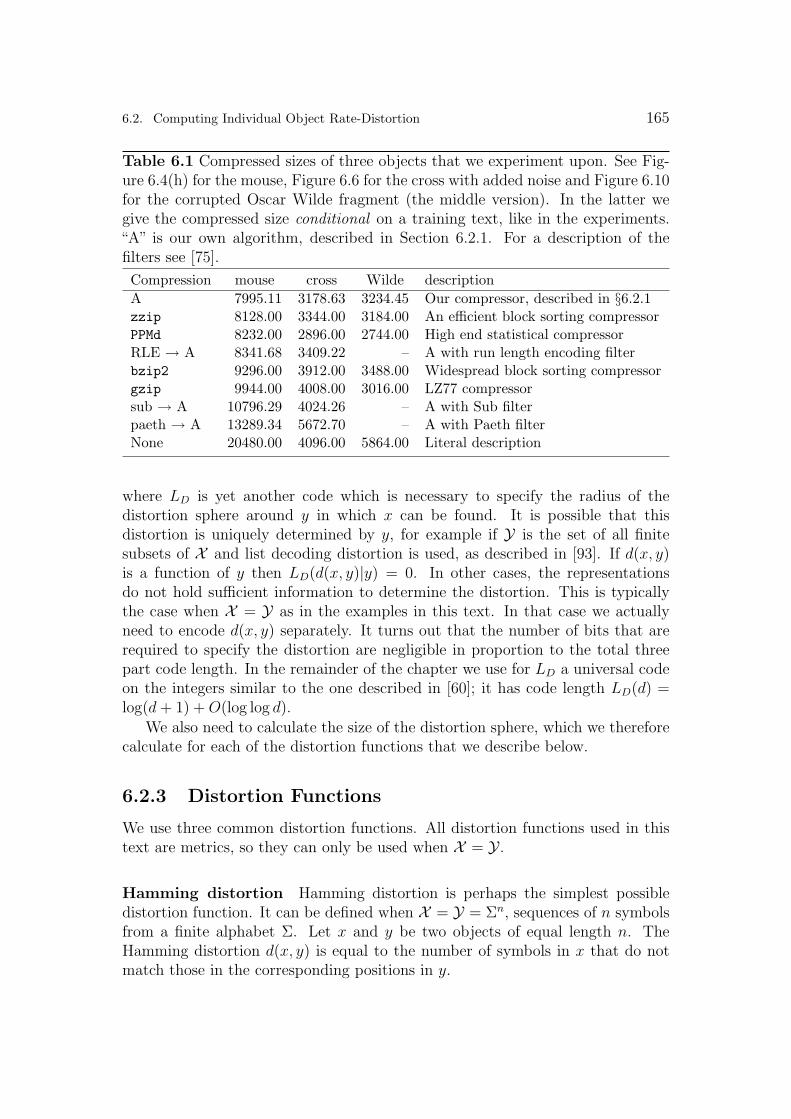
6.2. Computing Individual Object Rate-Distortion 165
Table 6.1 Compressed sizes of three objects that we experiment upon. See Fig-ure 6.4(h) for the mouse, Figure 6.6 for the cross with added noise and Figure 6.10for the corrupted Oscar Wilde fragment (the middle version). In the latter wegive the compressed size conditional on a training text, like in the experiments.“A” is our own algorithm, described in Section 6.2.1. For a description of thefilters see [75].
Compression mouse cross Wilde description
A 7995.11 3178.63 3234.45 Our compressor, described in §6.2.1zzip 8128.00 3344.00 3184.00 An efficient block sorting compressorPPMd 8232.00 2896.00 2744.00 High end statistical compressorRLE → A 8341.68 3409.22 – A with run length encoding filterbzip2 9296.00 3912.00 3488.00 Widespread block sorting compressorgzip 9944.00 4008.00 3016.00 LZ77 compressorsub → A 10796.29 4024.26 – A with Sub filterpaeth → A 13289.34 5672.70 – A with Paeth filterNone 20480.00 4096.00 5864.00 Literal description
where LD is yet another code which is necessary to specify the radius of thedistortion sphere around y in which x can be found. It is possible that thisdistortion is uniquely determined by y, for example if Y is the set of all finitesubsets of X and list decoding distortion is used, as described in [93]. If d(x, y)is a function of y then LD(d(x, y)|y) = 0. In other cases, the representationsdo not hold sufficient information to determine the distortion. This is typicallythe case when X = Y as in the examples in this text. In that case we actuallyneed to encode d(x, y) separately. It turns out that the number of bits that arerequired to specify the distortion are negligible in proportion to the total threepart code length. In the remainder of the chapter we use for LD a universal codeon the integers similar to the one described in [60]; it has code length LD(d) =log(d + 1) + O(log log d).
We also need to calculate the size of the distortion sphere, which we thereforecalculate for each of the distortion functions that we describe below.
6.2.3 Distortion Functions
We use three common distortion functions. All distortion functions used in thistext are metrics, so they can only be used when X = Y .
Hamming distortion Hamming distortion is perhaps the simplest possibledistortion function. It can be defined when X = Y = Σn, sequences of n symbolsfrom a finite alphabet Σ. Let x and y be two objects of equal length n. TheHamming distortion d(x, y) is equal to the number of symbols in x that do notmatch those in the corresponding positions in y.

166 Chapter 6. Individual Sequence Rate Distortion
A Hamming-distortion sphere Sy(a) contains all objects of length n that can beconstructed by replacing a symbols in y with different symbols from the alphabetΣ. Thus the size of the sphere is
(na
)(|Σ| − 1)a.
Euclidean distortion As before, let x = x1 . . . xn and y = y1 . . . yn be twoobjects of equal length, but the symbols now have a numerical interpretation.Euclidean distortion is d(x, y) =
√∑ni=1(xi − yi)2: the distance between x and y
when they are interpreted as vectors in an n-dimensional Euclidean space. Notethat this definition of Euclidean distortion differs from the one in [92].
Our variety of Euclidean distortion requires that X = Y = Zn, the set of n-
dimensional vectors of integers. The size of a Euclidean distortion sphere aroundsome y ∈ Y of length n is hard to compute analytically. We use an upper boundthat is reasonably tight and can be computed efficiently. One may want to skipthis calculation on first reading.
First we define d(v) := d(v,0) =√∑n
i=1 v2i and S(n, a) as the set v : |v| =
n, d(v) = a. We have x ∈ Sy(a) ⇔ x − y ∈ S(n, a), so it suffices to bound thesize of S(n, a). We define:
p(δ|n, a) := ce−δ2n/2a2
where c = 1/∑
δ∈Z
e−δ2n/2a2
P (v) :=n∏
i=1
p(vi|n, d(v));
p(·|n, d(v)) can be interpreted as a probability mass function on the individualentries of v (which in our application always lie between -255 and 255, so inpractice we used a reduced range in the definition of the normalising constantc). Therefore P (v) defines a valid probability mass function on outcomes v inS(n, a). Thus,
1 >∑
v∈S(n,a)
P (v) =∑
v∈S(n,a)
cne−(P
δ2i )n/2a2
=∑
v∈S(n,a)
cne−n/2 = cne−n/2|S(n, a)|.
This yields a bound on the size of S(n, a), which is reasonably tight unless thedistortion a is very low. In that case, we can improve the bound by observingthat v must have at least z = n− d(v)2 zero entries. Let v′ be a vector of lengthn − z that is obtained by removing z zero entries from v. Every v in S(n, a)can be constructed by inserting z zeroes into v′, so we have |Sy(a)| = |S(n, a)| ≤(
nz
)|S(n − z, a)|. The size of S(n − z, a) can be bounded by using the method
described before recursively.
Edit distortion The edit distortion of two strings x and y, of possibly differ-ent lengths, is the minimum number of symbols that have to be deleted from,

6.2. Computing Individual Object Rate-Distortion 167
inserted into, or changed in x in order to obtain y (or vice versa) [54]. It is alsoknown as Levenshtein distortion. It is a well-known measure that is often used inapplications that require approximate string matching.
Edit distortion can be defined for spaces X = Y = Σ∗ for a finite alphabet Σ.We develop an upper bound on the size of the edit distortion sphere, again thecalculation may be skipped on first reading.
We can identify any object in Sy(a) by a program p that operates on y, andwhich is defined by a list of instructions to copy, replace or delete the next symbolfrom y, or to insert a new symbol. We interpret a deletion as a replacement withan empty symbol; so the replacement operations henceforth include deletions. Letd(p) denote the number of insertions and replacements in p, in other words d(p) isthe length of the program minus the number of copies. Clearly for all x ∈ Sy(a),there must be a p such that p(y) = x and d(p) = d(x, y) = a. Therefore the size ofSy(a) can be upper bounded by counting the number of programs with d(p) = a.Let n be the length of y. Any program that contains i insertions and that processesy completely, must be of length n + i. The i insertions, a − i replacements andn−a+ i copies can be distributed over the program in
(n+i
i,a−i,n+a−i
)different ways.
For each insertion and replacement, the number of possibilities is equal to thealphabet size. Therefore,
|Sy(a)| ≤ |p : d(p) = a| ≤ |Σ|aa∑
i=max0,a−n
(n + i
i, n− a + i, a− i
)
.
The sphere can be extremely large, so to facilitate calculation of the log of thesphere size, as is required in our application, it is convenient to relax the boundsome more and replace every term in the sum by the largest one. Calculationreveals that the largest term has
i =
⌊1
4
(
2(a− n) + 1 +√
4(n2 + n + a2 + a) + 1)⌋
.
6.2.4 Searching for the Rate-Distortion Function
The search problem that we propose to address has two properties that make itvery hard. Firstly, the search space is enormous: at rate r there are 2r candidaterepresentations to consider, and for the kinds of objects that are typically sub-jected to lossy compression useful representations are often millions or billionsof bits long. Secondly, we want to avoid making too many assumptions aboutthe two objective functions, so that we can later freely change the compressionalgorithm and the distortion function. Under such circumstances the two mostobvious search methods are not practical:
• An exhaustive search is infeasible for search spaces of such large size, unlessmore specific properties of the objective functions are used in the design

168 Chapter 6. Individual Sequence Rate Distortion
of the algorithm. To investigate how far we could take such an approach,we have implemented an exhaustive algorithm under the requirement that,given a prefix of a representation y, we can compute reasonable lower boundson the values of both objective functions g1 and g2. This allows for relativelyefficient enumeration of all representations of which the objective functionsdo not exceed specific maxima: it is never necessary to consider objectswhich have a prefix for which the lower bounds exceed the constraints,which allows for significant pruning. In this fashion we were able to find therate-distortion function under Hamming distortion for objects of which thecompressed size is about 25 bits or less within a few hours on a desk-topcomputer.
• A greedy search starts with a poor solution and iteratively makes modifi-cations that constitute strict improvements. We found that this proceduretends to terminate quickly in some local optimum that is very bad globally.
Since the structure of the search landscape is at present poorly understood andwe do not want to make any unjustifiable assumptions, we use a genetic searchalgorithm which performs well enough that interesting results can be obtained.
6.2.5 Genetic Algorithm
The used algorithm is an almost completely generic procedure to simultaneouslyoptimise two separate objective functions for objects that are represented as bytesequences. To emphasise this we will consider the abstract objective function gwherever possible, rather than the more concrete rate and distortion functions.
A finite subset of Y is called a pool. The search algorithm initialises a poolP0 with the representation y that has d(x, y) = 0, which means y = x in oursetup, and possibly some “blank” representation that has minimal compressedcode length but high distortion. The pool is then subjected to a process ofselection through survival of the fittest. The weakness wP(y) of an object y ∈ Pis the number of elements of the pool that are smaller according to 4. The(transitive) reduction trd(P) of a pool P is the subset of all elements with zeroweakness. The elements of the reduction of a pool P are called models.
The pool is iteratively updated by replacing elements with high weakness (thefitness function is specified below) by new ones, which are created through eithermutation (random modifications of elements) or crossover (“genetic” recombina-tion of pairs of other candidates). We write Pi to denote the pool after i iterations.When the algorithm terminates after n iterations it outputs the reduction of Pn.
In the next sections we describe our choices for the important components ofthe algorithm: the mechanics of crossover and mutation, the fitness function andthe selection function which specifies the probability that a candidate is removedfrom the pool. In the interest of reproducibility we faithfully describe all our

6.2. Computing Individual Object Rate-Distortion 169
important design choices, even though some of them are somewhat arbitrary. Acasual reader may want to skip such details and move on to Section 6.3.
Crossover
Crossover (also called recombination) is effected by the following algorithm. Giventwo objects x and y we first split them both in three parts: x = x1x2x3 andy = y1y2y3, such that the length of x1 is chosen uniformly at random between 0and the length of x and the length of x2 is chosen from a geometric distributionwith mean 5; the lengths of the yi are proportional to the lengths of the xi. Wethen construct a new object by concatenating x1y2x3.
Mutation
The introduction of a mutation operation is necessary to ensure that the searchspace is connected, since the closure of the gene pool under crossover alone mightnot cover the entire search space. While we could have used any generic mu-tation function that meets this requirement, for reasons of efficiency we havedecided to design a different mutation function for every objective function thatwe implemented. This is helpful because some distortion functions (here, the editdistortion) can compare objects of different sizes while others cannot: mutationis the means by which introduction of objects of different size to the pool can bebrought about when desirable, or avoided when undesirable.
The mutation algorithm we use can make two kinds of change. With proba-bility 1/4 we make a small random modification using an algorithm that dependson the distortion function. Below is a table of the distortion functions and a shortdescription of the associated mutation algorithms:
Distortion Mutation algorithm
Hamming Sets a random byte to a uniformly random valueEuclidean Adds an N [0;σ = 10] value to a random byteEdit A random byte is changed, inserted or deleted
With probability 3/4 we use the following mutation algorithm instead. Itsplits the object x into three parts x = x1x2x3 where the length of x1 is chosenuniformly at random between 0 and the length of x and the length of x2 is chosenfrom a geometric distribution with mean 5. The mutation is effected by traininga (simplified version of) a third order PPM model [24] on x1 and then replacingx2 with an equally long sequence that is sampled from the model. The advantageof this scheme is that every replacement for x2 gets positive probability, butreplacements which have low code length and distortion tend to be much morelikely than under a uniform distribution.

170 Chapter 6. Individual Sequence Rate Distortion
Fitness Function
In theory, the set of representations that witness the rate-distortion function doesnot change under monotonic transformation of either objective function g1 org2. We have tried to maintain this property throughout the search algorithmincluding the fitness function, by never using either objective function directlybut only the ordering relation 4. Under such a regime, a very natural definitionof fitness is minus the weakness of the objects with respect to pool P .
It has been an interesting mini-puzzle to come up with an efficient algorithmto compute the weakness of all objects in the pool efficiently. Our solution is thefollowing very simple algorithm, which has an O(n log n) average case runningtime. It first sorts all elements of the pool by their value under g1 and then insertsthem in order into a binary search tree in which the elements are ordered by theirvalue under g2. As an object is inserted into the tree, we can efficiently counthow many elements with lower values for g2 the tree already contained. Theseelements are precisely the objects that have both lower values on g1 (otherwisethey would not appear in the tree yet) and on g2; as such their number is thedesired weakness.
Selection Function
Figure 6.2 Drop probability
0
0.1
0.2
0.3
0.4
0.5
0.6
0.7
0.8
0.9
1
0 0.2 0.4 0.6 0.8 1
Dro
p pr
obab
ility
(i-1/2)/n
alpha=0alpha=1alpha=2alpha=3alpha=4
A pool P induces a tradeoff profile p(P) := g(y) : y′ 4 y for some y′ in P.It is not hard to see that we have p(P) = p(trd(P)) and p(P) ⊆ p(P ∪ P ′) forall P ′ ⊆ Y . Therefore monotonic improvement of the pool under modification isensured as long as candidates with weakness 0 are never dropped.
We drop other candidates with positive probability as follows. Let y1, . . . , yn
be the elements of P with nonzero weakness, ordered such that for 1 ≤ i < j ≤ n

6.3. Experiments 171
we have wP(yi) < wP(yj) or g1(yi) < g1(yj) if yi and yj have the same weakness.We drop candidate yi from the pool with probability 1/(1 + ( n
i−1/2− 1)α), which
is a modified sigmoid function where α ∈ (1,∞) specifies the sharpness of thetransition from probability zero to one. This function is plotted for differentvalues of α in Figure 6.2. We used α = 4 in our experiments.
6.3 Experiments
We have subjected four objects to our program. The following considerationshave influenced our choice of objects:
• Objects should not be too complex, allowing our program to find a goodapproximation of the distortion-rate curve. We found that the runningtime of the program seems to depend mostly on the complexity of the inputobject; a compressed size of 20,000 bits seemed to be about the maximumour program could handle within a reasonable amount of time, requiring arunning time of the order of weeks on a desk-top computer.
• To check that our method really is general, objects should be quite dif-ferent from each other: they should come from different object domains,for which different distortion functions are appropriate, and they shouldcontain structure at different levels of complexity.
• Objects should contain primary structure and regularities that are distin-guishable and compressible by a block sorting compressor such as the onewe use. Otherwise, we may no longer hope that the compressor implementsa reasonable approximation of the Kolmogorov complexity. For instance,we would not expect our program to do well on a sequence of digits fromthe binary expansion of the number π.
With this in mind, we have selected the objects listed in Figure 6.3.
In each experiment, as time progressed the program found less and less improve-ments per iteration, but the pool never stabilized completely. Therefore we in-terrupted each experiment when (a) after at least one night of computation, thepool did not improve a lot, and (b) for all intuitively good models y ∈ Y that wecould conceive of a priori, the algorithm had found an y′ in the pool with y′ 4 yaccording to (6.4). For example, in each denoising experiment, this test includedthe original, noiseless object. In the experiment on the mouse without addednoise, we also included the images that can be obtained by reducing the numberof grey levels in the original with an image manipulation program. Finally forthe greyscale images we included a number of objects that can be obtained bysubjecting the original object to JPEG2000 compression at various quality levels.

172 Chapter 6. Individual Sequence Rate Distortion
Figure 6.3 The four objects that are subjected to rate-distortion analysis.
A picture of a mouseof 64 × 40 pixels.The picture is anal-ysed with respect toEuclidean distortion.
A noisy monochrome imageof 64 × 64 pixels that de-picts a cross. 377 pixelshave been inverted. Ham-ming distortion is used.
The same picture ofa mouse, but nowzero mean Gaussiannoise with σ = 8 hasbeen added to eachpixel. Euclidean dis-tortion is used; thedistortion to the orig-inal mouse is 391.1.
Beauty, real beauty,ends2wheresan in-tellectual expressoonbegins. IntellHctisg in itself a mMdeofSexggeration, an\destroys theLharmonyof n face. [. . . ]
(See Figure 6.10)
A corrupted quotation fromChapter 1 of The Pictureof Dorian Gray, by OscarWilde. The 733 byte longfragment was created byperforming 68 random in-sertions, deletions and re-placements of characters inthe original text. Edit dis-tortion is used. The rest ofchapters one and two of thenovel are given to the pro-gram as side information.
The first experiment illustrates how algorithmic rate-distortion theory maybe applied to lossy compression problems, and it illustrates how for a given rate,some features of the image are preserved while others can no longer be retained.We compare the performance of our method to the performance of JPEG andJPEG2000 at various quality levels. Standard JPEG images were encoded usingthe ImageMagick version 6.2.2; profile information was stripped. JPEG2000 im-ages were encoded to jpc format with three quality levels using NetPBM version10.33.0; all other options are default. For more information about these softwarepackages refer to [83].
The other three experiments are concerned with denoising. Any model thatis output by the program can be interpreted as a denoised version of the inputobject. We measure the denoising success of a model y as d(x′, y), where x′ is theoriginal version of the input object x, before noise was added. We also comparethe denoising results to those of other denoising algorithms:
1. BayesShrink denoising [18]. BayesShrink is a popular wavelet-based denois-ing method that is considered to work well for images.
2. Blurring (convolution with a Gaussian kernel). Blurring works like a low-pass filter, eliminating high frequency information such as noise. Unfortu-nately other high frequency features of the image, such as sharp contours,are also discarded.
3. Naive denoising. We applied a naive denoising algorithm to the noisy cross,in which each pixel was inverted if five or more out of the eight neighbouring

6.4. Results and Discussion 173
pixels were of different colour.
4. Denoising based on JPEG2000. Here we subjected the noisy input imageto JPEG2000 compression at different quality levels. We then selected theresult for which the distortion to the original image was lowest.
6.3.1 Names of Objects
To facilitate description and discussion of the experiments we will adopt the fol-lowing naming convention. Objects related to the experiments with the mouse,the noisy cross, the noisy mouse and the Wilde fragment, are denoted by thesymbols M, C, N and W respectively. A number of important objects in eachexperiment are identified by a subscript as follows. For O ∈ M, C, N, W, theinput object, for which the rate-distortion function is approximated by the pro-gram, is called Oin. In the denoising experiments, the input object is alwaysconstructed by adding noise to an original object. The original objects and thenoise are called Oorig and Onoise respectively. If Hamming distortion is used,addition is carried out modulo 2, so that the input object is in effect a pixelwiseexclusive OR of the original and the noise. In particular, Cin equals Corig XORCnoise. The program outputs the reduction of the gene pool, which is the setof considered models. Two important models are also given special names: themodel within the gene pool that minimises the distortion to Oorig constitutesthe best denoising of the input object and is therefore called Obest, and the min-imal sufficient statistic as described in Section 6.1.1 is called Omss. Finally, inthe denoising experiments we also give names to the results of the alternative de-noising algorithms. Namely, Cnaive is the result of the naive denoising algorithmapplied to the noisy cross, Nblur is the convolution of N with a Gaussian kernelwith σ = 0.458, Nbs is the denoising result of the BayesShrink algorithm, andNjpeg2000 is the image produced by subjecting N to JPEG2000 compression atthe quality level for which the distortion to Norig is minimised.
6.4 Results and Discussion
After running for some time on each input object, our program outputs thereduction of a pool P , which is interpreted as a set of models. For each ex-periment, we report a number of different properties of these sets. Since weare interested in the rate-distortion properties of the input object x = Oin,we plot the approximation of the distortion-rate function of each input object:dx(r) = mind(x, y) : y ∈ Y , K(y) ≤ r ≈ mind(x, y) : y ∈ trd(P), K(y) ≤ r.Such approximations of the distortion-rate function are provided for all four exper-iments. For the greyscale images we also plot the distortion-rate approximationthat is achieved by JPEG2000 (and in Figure 6.5 also ordinary JPEG) at differentquality levels. Here, the rate is the code length achieved by JPEG(2000), and the

174 Chapter 6. Individual Sequence Rate Distortion
distortion is the Euclidean distortion to Oin. We also plot the code length func-tion as described in Section 6.1.1. Minimal sufficient statistics can be identifiedby locating the minimum of this graph.
6.4.1 Lossy Compression
Experiment 1: Mouse (Euclidean distortion)
Our first experiment involved the lossy compression of M, a greyscale image ofa mouse. A number of elements of the gene pool are shown in Figure 6.4. Thepictures show how at low rates, the models capture the most important globalstructure of the image; at higher rates more subtle properties of the image can berepresented. Image (a) shows a rough rendering of the distribution of bright anddark areas in Min. These shapes are rectangular, which is probably an artifactof the compression algorithm we used: it is better able to compress images withrectangular structure than with oval structure. There is no real reason why anoval should be in any way more complex than a rectangle, but most generalpurpose data compression software is similarly biased. In (b), the rate is highenough that the oval shape of the mouse can be accommodated, and two areasof different overall brightness are identified. After the number of grey shades hasbeen increased a little further in (c), the first hint of the mouse’s eyes becomesvisible. The eyes are improved and the mouse is given paws in (d). At higherrates, the image becomes more and more refined, but the improvements are subtleand seem of a less qualitative nature.
The code length function (Figure 6.5) shows that the only sufficient statistic inthe set of models is Min itself, indicating that the image hardly contains any noise.It also shows the rates that correspond to the models that are shown in Figure 6.4.By comparing these figures it can be clearly seen that the image quality onlydeteriorates significantly if more than half of the information in Min is discarded.Note that this is not a statement about the compression ratio, where the lossilycompressed size is related to the size of the uncompressed object rather than itscomplexity. For example, Min has an uncompressed size of 64 ·40 ·8 = 20480 bits,and the representation in Figure 6.4(g) has a compressed size of 3190.6 bits. Thisrepresentation therefore constitutes compression by a factor of 20480/3190.6 =6.42, which is substantial for an image of such small size. At the same time theamount of information is reduced by a factor of 7995.0/3190.6 = 2.51.

6.4. Results and Discussion 175
Figure 6.4 Lossy image compression results for the mouse (h). The numbers be-low each image denote its compressed size K(·), total code length K(·)+L(·)(Min)and Euclidean distortion d(·, Min), respectively.
(a) 163.0 /19920.9 / 2210.0 (b) 437.8 / 17013.6 / 1080
(c) 976.6 / 15779.7 / 668.9 (d) 1242.9 / 15297.9 / 546.4
(e) 1676.6 / 14641.9 / 406.9 (f) 2324.5 / 14150.1 / 298.9
(g) 3190.6 / 13601.4 / 203.9 (h) 7995.1 / 7996.1 / 0

176 Chapter 6. Individual Sequence Rate Distortion
Figure 6.5 Approximate distortion-rate and code length functions for the mouse.
0
200
400
600
800
1000
1200
0 1000 2000 3000 4000 5000 6000 7000 8000
dist
ortio
n (e
uclid
ean)
rate (compressed size in bits)
Our methodJPEG 2000
JPEGExamples
0
5000
10000
15000
20000
25000
0 1000 2000 3000 4000 5000 6000 7000 8000
code
leng
th (
bits
)
rate (compressed size in bits)
Our methodExamples

6.4. Results and Discussion 177
6.4.2 Denoising
For each denoising experiment, we report a number of important objects, a graphthat shows the approximate distortion-rate function and a graph that shows theapproximate code length function. In the distortion-rate graph we plot not onlythe distortion to Oin but also the distortion to Oorig, to visualise the denoisingsuccess at each rate.
In interpreting these results, it is important to realise that only the reportedminimal sufficient statistic and the results of the BayesShrink and naive denoisingmethods can be obtained without knowledge of the original object – the otherobjects Obest, Ojpeg2000 and Oblur require selecting between a number of al-ternatives in order to optimise the distortion to Oorig, which can only be donein a controlled experiment. Their performance may be better than what can beachieved in practical situations where Oorig is not known.
Experiment 2: Noisy Cross (Hamming distortion)
In the first denoising experiment we approximated the distortion-rate functionof a monochrome cross Corig of very low complexity, to which artificial noisewas added to obtain Cin (the rightmost image in Figure 6.6); the distortion tothe noiseless cross is displayed in the same graph. The best denoising Cbest
(leftmost image) has a distortion of only 3 to the original Corig, which showsthat the distortion-rate function indeed separates structure and noise extremelywell in this example. The bottom graph shows the code length function for thenoisy cross; the minimum on this graph is the minimal sufficient statistic Cmss.In this low complexity example, we have Cmss = Cbest, so the best denoising isnot only very good in this simple example, but it can also be identified.
We did not subject Cin to BayesShrink or blurring because those methods arenot suitable for monochrome images. Therefore we used the extremely simple,“naive” denoising method that is described in Section 6.3 on this specific imageinstead. The middle image shows the result Cnaive; while it does remove most ofthe noise, 40 errors remain, a lot more than the number of errors incurred by theminimal sufficient statistic. All errors except one are close to the contours of thecross. This illustrates how the naive algorithm is limited by its property that ittakes only the local neighbourhood of each pixel into account, it cannot representlarger structures such as straight lines.

178 Chapter 6. Individual Sequence Rate Distortion
Figure 6.6 Denoising a noisy cross. Highlighted objects, from left to right:Cbest, Cnaive and Cin. Exact values are in the bottom table.
rate (compressed size in bits)
0
200
400
600
800
1000
1200
1400
0 500 1000 1500 2000 2500 3000
Distortion to noisy crossDistortion to original
dist
ortio
n (h
amm
ing)
0
500
1000
1500
2000
3000
4000
500 1000 1500 3000rate (compressed size in bits)
3500
2500
0 2000 2500
two
part
cod
e le
ngth
(bi
ts)
Cbest=Cmss Cnaive Cin
K(·) 260.4 669.2 3178.6
K(·) + L(·)(Cin) 2081.9 2533.3 3179.6d(·, Cin) 376 389 0
d(·, Corig) 3 40 377

6.4. Results and Discussion 179
Experiment 3: Noisy mouse (Euclidean distortion)
The noisy mouse poses a significantly harder denoising problem, where the totalcomplexity of the input Nin is more than five times that of the noisy cross. Fig-ure 6.7 shows the denoising results for various denoising methods, and Figure 6.8shows the rate-distortion curve and, as for the noisy cross, the distortion to theoriginal object Norig.
Figure 6.7(a) shows the input object Nin; it was constructed by adding noise(centre image) to the original noiseless image Norig (top-right). We display threedifferent denoising results. Image (h) shows Nbest, the best denoised object fromthe gene pool. Visually it appears to resemble Norig quite well, but there mightbe structure in Norig that was lost in the denoising process. Because humanperception is perhaps the most sensitive detector of structure in image data,we show the difference between Nbest and Norig in (i). We would expect anysignificant structure in the original image that is lost in the denoising process,as well as structure that is not present in the original image, but is somehowintroduced as an artifact of the denoising procedure, to become visible in thisresidual. In the case of Nbest we cannot make out any particular features.
The minimal sufficient statistic, image (d), also appears to be a reasonablysuccessful denoising, albeit clearly of lower complexity than the best one. Inthe residual, darker and lighter patches are definitely discernible. Apparently Nin
does contain some structure beyond what is captured by Nmss, but this cannot beexploited by the compression algorithm. We think that the fact that the minimalsufficient statistic is of lower complexity than the best possible denoising resultshould therefore again be attributed to inefficiencies of the compressor.
For comparison, we have also denoised Nin using the alternative denoisingmethod BayesShrink and the methods based on blurring and JPEG2000 as de-scribed in Section 6.3. We found that BayesShrink does not work well for imagesof such small size: the distortion between Nbs and Nin is only 72.9, which meansthat the input image is hardly affected at all. Also, Nbs has a distortion of 383.8to Norig, which is hardly less than the distortion of 392.1 achieved by Nin itself.
Blurring-based denoising yields much better results: Nblur (j) is the resultafter optimisation of the size of the Gaussian kernel. Its distortion to Norig liesin-between the distortions achieved by Nmss and Nbest, but it is different fromthose objects in two important respects. Firstly, Nblur remains much closer toNin, at a distortion of 260.4 instead of more than 470, and secondly, Nblur ismuch less compressible by K. (To obtain the reported size of 14117 bits we had toswitch on the averaging filter, as described in Section 6.2.1.) These observationsare at present not well understood. Image (k) shows that the contours of themouse are somewhat distorted in Nblur; this can be explained by the fact thatcontours contain high frequency information which is discarded by the blurringoperation as we remarked in Section 6.3.
The last denoising method we compared our results to is the one based on the

180 Chapter 6. Individual Sequence Rate Distortion
JPEG2000 algorithm. Its performance is clearly inferior to our method visuallyas well as in terms of rate and distortion. The result seems to have undergonea smoothing process similar to blurring which introduces similar artifacts in thebackground noise, as is clearly visible in the residual image. As before, the com-parison may be somewhat unfair because JPEG2000 was not designed for thepurpose of denoising, might optimise a different distortion measure and is muchfaster.

6.4. Results and Discussion 181
Figure 6.7 Denoising results for the noisy mouse (a). The numbers below eachimage denote its compressed size K(·), total code length K(·) + L(·)(Nin), distor-tion to Nin and distortion to Norig, respectively.
(a) Nin16699.7 / 16700.7 / 0 / 392.1
(b) Norig(=Min)7995.1 / 26247.8 / 392.1 / 0
(c) Nnoise=Nin-Norig
(d) Nmss1969.8 / 15504.9 / 474.7 / 337.0
(e) Nmss − Norig
(f) Njpeg20003104 / 16395.4 / 444.4 / 379.8
(g) Njpeg2000 − Norig
(h) Nbest3354.5 / 15952.8 / 368.4 / 272.2
(i) Nbest − Norig
(j) Nblur (σ = 0.458)14117.0 / 25732.4 / 260.4 / 291.2
(k) Nblur − Norig

182 Chapter 6. Individual Sequence Rate Distortion
Figure 6.8 Approximate distortion-rate and code length functions for the noisymouse.
0
200
400
600
800
1000
1200
1400
0 2000 4000 6000 8000 10000 12000 14000 16000 18000
dist
ortio
n (e
uclid
ean)
rate (compressed size in bits)
Our methodJPEG 2000
Our distortion to originalJPEG 2000 distortion to original
0
5000
10000
15000
20000
25000
0 2000 4000 6000 8000 10000 12000 14000 16000 18000
code
leng
th (
bits
)
rate (compressed size in bits)

6.4. Results and Discussion 183
Experiment 4: Oscar Wilde fragment (edit distortion)
The fourth experiment, in which we analyse Win, a corrupted quotation fromOscar Wilde, shows that our method is a general approach to denoising thatdoes not require many domain specific assumptions. Worig, Win and Wmss
are depicted in Figure 6.10, the distortion-rate approximation, the distortion toWorig and the three part code length function are shown in Figure 6.11. We havetrained the compression algorithm by supplying it with the rest of Chapters 1 and2 of the same novel as side information, to make it more efficient at compressingfragments of English text. We make the following observations regarding theminimal sufficient statistic:
• In this experiment, Wmss = Wbest so the minimal sufficient statistic sepa-rates structure from noise extremely well here.
• The distortion is reduced from 68 errors to only 46 errors. 26 errors are cor-rected (N), 4 are introduced (H), 20 are unchanged (•) and 22 are changedincorrectly (⋆).
• The errors that are newly introduced (H) and the incorrect changes (⋆)typically simplify the fragment a lot, so that the compressed size may beexpected to drop significantly. Not surprisingly therefore, many of the sym-bols marked H or ⋆ are deletions, or modifications that create a word whichis different from the original, but still correct English. The following tablelists examples of the last category:
Line Worig Win Wmss3 or Nor of
4 the Ghe he
4 any anL an
4 learned JeaFned yearned
5 course corze core
5 then ehen when
8 he fhe the
Since it would be hard for any general-purpose mechanical method (thatdoes not incorporate a sophisticated English language model) to determinethat these changes are incorrect, we should not be surprised to find a numberof errors of this kind.
Side Information
Figure 6.9 shows that the compression performance is significantly improved ifwe provide side information to the compression algorithm, and the improvementis typically larger if (1) the amount of side information is larger, or (2) if the

184 Chapter 6. Individual Sequence Rate Distortion
compressed object is more similar to the side information. Thus, by giving sideinformation, correct English prose is recognised as “structure” sooner and a betterseparation between structure and noise is to be expected. The table also showsthat if the compressed object is in some way different from the side information,then adding more side information will at some point become counter-productive,presumably because the compression algorithm will then use the side informationto build up false expectations about the object to be compressed, which can becostly.
While denoising performance would probably improve if the amount of sideinformation was increased further, it was infeasible to do so in this implementa-tion. Recall from Section 6.2 that he conditional Kolmogorov complexity K(y|z)is approximated by K(y|z) = K(zy)− K(z). The time required to compute thisis dominated by the length of z if the amount of side information is much largerthan the size of the object to be compressed. This can be remedied by using acompression algorithm that processes its input sequentially, because the state ofsuch an algorithm can be cached after processing the side information z; comput-ing K(zy) would then be a simple matter of recalling the state that was reachedafter processing z and then processing y starting from that state. Many com-pression algorithms, among which Lempel-Ziv compressors and most statisticalcompressors, have this property; our approach could thus be made to work withlarge quantities of side information by switching to a sequential compressor butwe have not done this.
Figure 6.9 Compressed size of models for different amounts of side information.Worig is never included in the side information. We do not let Wmss vary withside information but keep it fixed at the object reported in Figure 6.10(c).
Side information z K(Worig|z) K(Wmss|z) K(Win|z)None 3344.1 3333.7 3834.8Chapters 1,2 (57 kB) 1745.7 1901.9 3234.5Whole novel (421 kB) 1513.6 1876.5 3365.9

6.4. Results and Discussion 185
Figure 6.10 A fragment of The Picture of Dorian Gray, by Oscar Wilde.Beauty, real beauty, ends where an intellectual expression begins. Intellect
is in itself a mode of exaggeration, and destroys the harmony of any face.The moment one sits down to think, one becomes all nose, or all forehead, orsomething horrid. Look at the successful men in any of the learned professions.How perfectly hideous they are! Except, of course, in the Church. But then in theChurch they don’t think. A bishop keeps on saying at the age of eighty what hewas told to say when he was a boy of eighteen, and as a natural consequencehe always looks absolutely delightful. Your mysterious young friend, whosename you have never told me, but whose picture really fascinates me, neverthinks. I feel quite sure of that.
(a) Worig, the original text
Beauty, real beauty, ends2wheresan intellectual expressoon begins. IntellHctisg in itself a mMde ofSexggeration, an\ destroys theLharmony of n face. :Them1ment one sits down to ahink@ one becomes jll noeˆ Nor all forehbead, orsomething hNrrid. Look a Ghe successf\l men in anL of te JeaFned professions.How perectly tideous 4they re6 Except, of corze, in7 the Ch4rch. BuP ehen in theChurch they dol’t bthink. =A bishop keeps on saying at the age of eighty whathe was told to say wh”n he was aJb4y of eighten, and sja natural cnsequencefhe a(ways looks ab8olstely de[ightfu). Your mysterious youngL friend, wPosename you h\vo never tld me, mut whose picture really fa?scinates Lme,PneverthinCs. I feel quite surS of that9
(b) Win, the corrupted version of the fragment. At 68 randomly selected positionscharacters have been inserted, deleted or modified. New and replacement charactersare drawn uniformly from ASCII symbols 32–126.
Beauty, real beauty, ends⋆
-whereN
an intellectual express•oon begins. Intell
N
ect isN
⊡
in itself a mN
ode ofN
ex•⊡ggeration, an
N
d destroys theN
harmony of•⊡n
•⊡ face.
⋆
⊡The
mN
oment one sits down toN
think⋆
⊡ one becomes⋆
⊡ll no•⊡e
⋆
⊡
N
⊡oH
f all fore⋆
beH
⊡d, or
something h⋆
irrid. Look a•⊡
⋆
⊡he successf⋆
⊡l men in an⋆
⊡ of t•⊡e
⋆
yeaN
rned proH
vessions.
How perN
fectly•tideous
N
⊡they•⊡re
•6 Except, of co
•⊡r
⋆
⊡e, inN
⊡ the Ch⋆
arch. BuN
t⋆
when in
the Church they do•l’t
N
⊡think.⋆
⊡AH
⊡bishop keeps on saying at the age of eighty what
he was told to say wh⋆
⊡n he was a⋆
⊡b⋆
sy of eight•⊡en, and
•⊡s
•ja natural c
•⊡nsequence
⋆
the a⋆
⊡ways looks abN
solN
utely de⋆
⊡ightfuN
l. Your mysterious youngN
⊡ friend, wN
hose
name you hN
avN
e never t•⊡ld me,
•mut whose picture really fa
N
⊡scinatesN
⊡me,N
never
thin•Cs. I feel quite sur
⋆
⊡ of that•9
(c) Wbest = Wmss; it has edit distortion 46 to the original fragment. Marksindicate the error type: N=correction; H=new error; •=old error; ⋆=changed butstill wrong. Deletions are represented as ⊡.

186 Chapter 6. Individual Sequence Rate Distortion
Figure 6.11 Results for a fragment of The Picture of Dorian Gray by OscarWilde (also see Figure 6.10).
0
100
200
300
400
500
600
700
0 500 1000 1500 2000 2500 3000 3500
dist
ortio
n (e
dit)
rate (compressed size in bits)
Distortion to corrupted fragmentDistortion to original
0
1000
2000
3000
4000
5000
6000
0 500 1000 1500 2000 2500 3000 3500
code
leng
th (
bits
)
rate (compressed size in bits)

6.5. Quality of the Approximation 187
6.5 Quality of the Approximation
It is easy to see from its definition that the distortion-rate function must bea non-increasing function of the rate. The implementation guarantees that ourapproximation is non-increasing as well. In [92] it is assumed that for every x ∈ Xthere exists a representation y ∈ Y such that d(x, y) = 0; in the context of thischapter this is certainly true because we have X = Y and a distortion functionwhich is a metric. The gene pool is initialised with Oin, which always has zeroweakness and must therefore remain in the pool. Therefore at a rate that is highenough to specify x, the distortion-rate function reaches zero.
The shape of the code length function for an object x is more complicated. Lety be the representation for which d(x, y) = 0. In theory, the code length can neverbecome less than the complexity of y, and the minimal sufficient statistic witnessesthe code length function at the lowest rate at which the code length is equal tothe complexity of y. Practically, we found in all denoising experiments that thetotal code length using the minimal sufficient statistic, K(Omss) + LOmss(Oin),
is lower than the code length K(Oin) that is obtained by compressing the inputobject directly. This can be observed in Figures 6.6, 6.8 and 6.11. The effect ismost pronounced in Figure 6.6, where the separation between structure and noiseis most pronounced.
Our hypothesis is that this departure from the theoretical shape of the codelength function must be explained by inefficiency of the compression algorithmin dealing with noise. This is evidenced by the fact that it needs 2735.7 bits toencode Cnoise, while only log2
(4096377
)≈ 1810 bits would suffice if the noise were
specified with a uniform code on the set of indices of all binary sequences withexactly 377 ones out of 64 · 64 (see Section 6.2.3). Similarly, K(Nnoise) = 14093,whereas a literal encoding requires at most 12829 bits (using the bound fromSection 6.2.3).
Another strange effect occurs in Figure 6.8, where the code length functiondisplays a strange “bump”: as the rate is increased beyond the level required tospecify the minimal sufficient statistic, the code length goes up as before, buthere at very high rates the code length starts dropping again.
It is theoretically possible that the code length function should exhibit suchbehaviour to a limited extent. It can be seen in [92] that a temporary increasein the code length function can occur up to a number of bits that depends onthe so-called covering coefficient. Loosely speaking this is the density of smalldistortion balls that is required in order to completely cover a larger distortionball. The covering coefficient in turn depends on the used distortion function andthe number of dimensions. It is quite hard to analyse in the case of Euclideandistortion, so we cannot at present say if theory admits such a large increasein the code length function. However, we believe that the explanation is moremundane in this case. Since the noisy mouse is the most complex object of thefour we experimented on, we fear that this bump may simply indicate that we

188 Chapter 6. Individual Sequence Rate Distortion
interrupted our search procedure too soon. Quite possibly, after a few years ofprocessing on more expensive hardware, the code length function would have runstraight in between Nmss and Nin.
Figure 6.5 shows that our approximation of the distortion-rate function issomewhat better than the approximation provided by either JPEG or JPEG2000,although the difference is not extremely large for higher rates. The probable rea-son is twofold: on the one hand, we do not know for which distortion functionJPEG(2000) is optimised, but it is probably not Euclidean distortion. Thereforeour comparison is somewhat unfair, since our method might well perform worseon JPEG(2000)’s own distortion measure. On the other hand, JPEG(2000) isvery time-efficient, it took only a matter of seconds to compute models at var-ious different quality levels, while it took our own algorithm days or weeks tocompute its distortion-rate approximation. Two conclusions can be drawn fromour result. Namely, if the performance of existing image compression softwarehad been better than the performance of our own method in our experiments,this would have been evidence to suggest that our algorithm does not computea good approximation to the rate-distortion function. The fact that this is notthe case is thus reassuring. Vice versa, if we assume that we have computed agood approximation to the algorithmic rate-distortion function, then our resultsgive a measure of how close JPEG(2000) comes to the theoretical optimum; ourprogram can thus be used to provide a basis for the evaluation of the performanceof lossy compressors.
6.6 An MDL Perspective
So far we have described algorithmic rate-distortion theory in terms of the uncom-putable notion of Kolmogorov complexity, and we developed a practical versionof the method using a data compression algorithm. In the context of this the-sis, it is natural to ask how the practical method we described above fits withinestablished MDL theory. After all, Minimum Description Length was originallydeveloped to obtain a practical version of universal learning based on Kolmogorovcomplexity, which can even be interpreted as a special case (“ideal MDL”, Sec-tion 1.1.3). For example, a major theme in the MDL literature is the motivationof the used codes; some codes are considered acceptable, others are not. To whatcategory belongs the data compression algorithm we used?
First we compare the code length function used in MDL to that we used foralgorithmic rate-distortion in this chapter. In the considered practical version ofalgorithmic rate distortion, by (6.2) and (6.7), the total code length of the sourceobject x ∈ X using a representation y ∈ Y equals
K(y) + LD(d(x, y)|y) + log |Sy(d(x, y))|. (6.8)
In this three part code, the first term counts the number of bits required to

6.6. An MDL Perspective 189
specify the representation, or hypothesis, for the data and the last term countsthe number of bits required to specify the noise. Whether the distortion levelof the source object given a representation should be interpreted as part of thehypothesis or as noise is debatable; in this chapter we found it convenient totreat the distortion level as part of the hypothesis, as in (6.2). But to matchalgorithmic rate-distortion to MDL it is better to think of the distortion level aspart of the noise and identify Y with the available hypotheses.
In our description of MDL in the introductory chapter, the total code lengthof the data x ∈ X with the help of a hypothesis y ∈ Y is
L(y) + Ly(x). (6.9)
Algorithmic rate-distortion theory can be understood as a generalisation of MDLas described in the introduction by making (6.8) and (6.9) match. Suppose thatwe start with an instance of MDL model selection, specified by the code lengthfunctions L(y) and Ly(x), and let Py(x) = 2−Ly(x) be the mass function corre-sponding to Ly(x). We will show that the model selected by MDL is equal toa sufficient statistic in the rate-distortion problem that is obtained by settingK(y) = L(y), d(x, y) = Ly(x) and LD(d|y) = Py(Ly(X) = d). We have
Py(x) = Py(X = x, Ly(X) = Ly(x))
= Py(X = x|Ly(X) = Ly(x))Py(Ly(X) = Ly(x))
=Py(Ly(X) = Ly(x))
|x′ : Ly(x′) = Ly(x)| =2−LD(d(x,y)|y)
|Sy(d(x, y))| ,
so that the code length function that is minimised by sufficient statistics in thisrate-distortion problem is exactly the same code length function that is minimisedin the original MDL problem. Note that to make this work we only really needthe condition that the distortion function has the property that for all y ∈ Yand all x ∈ X , x′ ∈ X we have d(x, y) = d(x′, y) iff Ly(x) = Ly(x′). We chosed(x, y) = Ly(x) because it is a simple function with that property, and because itallows an interpretation of the distortion as the incurred logarithmic loss.
This correspondence actually works both ways: starting with a rate-distortionproblem specified by some K, code LD and distortion function d, we can alsoconstruct an MDL problem that identifies a sufficient statistic by defining L(y) =K(y) and Ly(x) = LD(d(x, y)|y) + log |Sy(d(x, y))|.
Note that in the introductory chapter we were somewhat unspecific as towhich hypothesis should be selected if more than one of them minimises the codelength; the issue becomes much clearer in a rate-distortion analysis because itallows us to easily express a preference for the minimal sufficient statistic as thebest hypothesis for the data. If a thorough analysis of the data is required, italso seems sensible to look at the whole rate-distortion function rather than justat the minimal sufficient statistic, since it provides additional information aboutthe structure that is present in the data at each level of complexity.

190 Chapter 6. Individual Sequence Rate Distortion
When we introduced MDL, we stressed that a suitable code L for the spec-ification of hypotheses must have two properties: (a) it has small regret in theworst case over all considered input objects, and (b) it may be a luckiness codethat does especially well on some inputs (see Section 1.1). In the experiments inthis chapter we used L = K, where K is a general purpose data compression al-gorithm. We need to check that it achieves small regret in the worst case. We willdo this for the experiment on the noisy mouse Nin. In that experiment we onlyconsidered finitely many hypotheses, so as in Example 2, the best possible worst-case regret is achieved by the uniform code. This code requires 64 · 40 · 8 = 20480bits for all representations in Y . The encoding produced by the data compressionalgorithm should never be much longer. We did not prove any bounds for ourcompressor, but we did try to compress ten files of 64 · 40 random bytes each,to see whether or not the compressed representation would be much larger; theworst result was a compressed size of 20812 bytes. This blowup of 332 bits doesseem larger than necessary, but similar or worse overheads are incurred by othercompression software such as Lempel-Ziv based compressors and PPM compres-sors, unless as a built-in feature it checks whether or not it actually manages tocompress the input object, reverting to a literal encoding when this fails. All inall, the worst-case performance of the compressor appears to lie within reasonablebounds, although admittedly we did not check this very thoroughly.
The fact that we subject the source object to a rate-distortion analysis in thefirst place suggests that we believe that reasonable hypotheses can be formulatedat different levels of complexity, which means that we should certainly use aluckiness code to differentiate between simple and more complex representations.This is what data compression software is designed to do really well, and whatallows for an interesting analysis in the case of our example. Another way toconstruct a suitable luckiness code L, which is more in the spirit of the standardMDL approach, is the following. We start out with a countable set of models ofdifferent complexity M1, M2, . . . , and take its union Y = ∪nMn as the set ofrepresentations. We can then encode y by first specifying its model index i usingsome worst-case efficient code, and then specifying y within model i using a secondworst-case efficient code. The details of such an approach to rate-distortion havenot yet been investigated.
6.7 Conclusion
Algorithmic rate-distortion provides a good framework for analysis of large andstructured objects. It is based on Kolmogorov complexity, which is not com-putable. We nevertheless attempted to put this theory into practice by approxi-mating the Kolmogorov complexity of an object by its compressed size. We alsogeneralised the theory in order to enable it to cope with side information, which isinterpreted as being available to both the sender and the receiver in a transmission

6.7. Conclusion 191
over a rate restricted channel. We also describe how algorithmic rate-distortiontheory may be applied to lossy compression and denoising problems.
Finding the approximate rate-distortion function of an individual object is adifficult search problem. We describe a genetic algorithm that is very slow, buthas the important advantage that it requires only few assumptions about theproblem at hand. Judging from our experimental results, our algorithm providesa good approximation, as long as its input object is of reasonably low complexityand is compressible by the used data compressor. The shape of the approximaterate-distortion function, and especially that of the associated three part codelength function, is reasonably similar to the shape that we would expect on thebasis of theory, but there is a striking difference as well: at rates higher than thecomplexity of the minimal sufficient statistic, the three part code length tendsto increase with the rate, where theory suggests it should remain constant. Weexpect that this effect can be attributed to inefficiencies in the compressor.
We find that the algorithm performs quite well in lossy compression, withapparently somewhat better image quality than that achieved by JPEG2000,although the comparison may not be altogether fair. When applied to denoising,the minimal sufficient statistic tends to be a slight underestimate of the complexityof the best possible denoising (an example of underfitting). This is presumablyagain due to inefficiencies in the used compression algorithm.
Beside an approximation of algorithmic rate-distortion theory, the computableversion of the theory can also be interpreted as a generalisation of MDL modelselection. We concluded this chapter with a discussion of this relationship.


Bibliography
[1] P. Adriaans and J. van Benthem (editors). Handbook of the Philosophy ofInformation. Elsevier, 2008.
[2] H. Akaike. A new look at statistical model identification. IEEETransactions on Automatic Control, 19(6):716–723, 1974.
[3] V. Balasubramanian. Statistical inference, Occam’s Razor, and statisticalmechanics on the space of probability distributions. Neural Computation,9:349–368, 1997.
[4] A. Barron, J. Rissanen, and B. Yu. The Minimum Description Lengthprinciple in coding and modeling. IEEE Transactions on InformationTheory, 44(6):2743–2760, 1998.
[5] A.R. Barron. Logically Smooth Density Estimation. PhD thesis, Dept. ofElectrical Engineering, Stanford University, Stanford, CA, 1985.
[6] A.R. Barron. Information-theoretic characterization of Bayes performanceand the choice of priors in parametric and nonparametric problems. InBayesian Statistics 6, pages 27–52. Oxford University Press, 1998.
[7] A.R. Barron. Personal communication, 2008.
[8] A.R. Barron and T.M. Cover. Minimum complexity density estimation.IEEE Transactions on Information Theory, 37(4):1034–1054, 1991.
[9] A.R. Barron and C. Sheu. Approximation of density functions bysequences of exponential families. Annals of Statistics, 19(3):1347–1369,1991.
[10] A.R. Barron, Y. Yang, and B. Yu. Asymptotically optimal functionestimation by minimum complexity criteria. In Proceedings of the 1994International Symposium on Information Theory, page 38, Trondheim,Norway, 1994.
193

194 Bibliography
[11] J. Berger. Personal communication, 2004.
[12] J.O. Berger. Statistical Decision Theory and Bayesian Analysis. SpringerSeries in Statistics. Springer-Verlag, New York, revised and expandedsecond edition, 1985.
[13] J.O. Berger and L.R. Pericchi. Objective Bayesian methods for modelselection: introduction and comparison. Institute of MathematicalStatistics Lecture Notes, (Monograph series) 38:135–207, 1997.
[14] J. Bernardo and A.F.M. Smith. Bayesian Theory. Wiley, 1994.
[15] O. Bousquet. A note on parameter tuning for on-line shifting algorithms.Technical report, Max Planck Institute for Biological Cybernetics, 2003.
[16] O. Bousquet and M.K. Warmuth. Tracking a small set of experts bymixing past posteriors. Journal of Machine Learning Research, 3:363–396,2002.
[17] M. Burrows and D.J. Wheeler. A block-sorting lossless data compressionalgorithm. Technical Report 124, Digital Equipment Corporation, SystemsResearch Center, May 1994.
[18] G. Chang, B. Yu, and M. Vetterli. Adaptive wavelet thresholding forimage denoising and compression. IEEE Transactions on ImageProcessing, 9:1532–1546, 2000.
[19] N. Chomsky. Three models for the description of language. IEEETransactions on Information Theory, 2(3), September 1956.
[20] R. Cilibrasi and P. Vitanyi. Algorithmic clustering of music based onstring compression. Computer Music Journal, 28:49–67, 2004.
[21] B. Clarke. Online forecasting proposal. Technical report, University ofDortmund, 1997. Sonderforschungsbereich 475.
[22] B. Clarke and A. Barron. Jeffreys’ prior is asymptotically least favourableunder entropy risk. The Journal of Statistical Planning and Inference,41:37–60, 1994.
[23] B.S. Clarke and A.R. Barron. Information-theoretic asymptotics of Bayesmethods. IEEE Transactions on Information Theory, IT-36(3):453–471,1990.
[24] J.G. Cleary and I.H. Witten. Data compression using adaptive coding andpartial string matching. IEEE Transactions on Communications,COM-32(4):396–402, April 1984.

Bibliography 195
[25] T.M. Cover and J.A. Thomas. Elements of Information Theory. Series intelecommunications. John Wiley, 1991.
[26] A.P. Dawid. Present position and potential developments: Some personalviews, statistical theory, the prequential approach. Journal of the RoyalStatistical Society, Series A, 147(2):278–292, 1984.
[27] A.P. Dawid. Statistical theory: The prequential approach. Journal of theRoyal Statistical Society B, 147, Part 2:278–292, 1984.
[28] A.P. Dawid. Prequential analysis, stochastic complexity and Bayesianinference. In J.M. Bernardo, J.O. Berger, A.P. Dawid, and A.F.M. Smith,editors, Bayesian Statistics 4, pages 109–125. Oxford University Press,1992.
[29] A.P. Dawid. Prequential data analysis. In M. Ghosh and P.K. Pathak,editors, Current Issues in Statistical Inference: Essays in Honor of D.Basu, Lecture Notes-Monograph Series, pages 113–126. Institute ofMathematical Statistics, 1992.
[30] X. De Luna and K. Skouras. Choosing a model selection strategy.Scandinavian Journal of Statistics, 30:113–128, 2003.
[31] P. Diaconis and D. Freedman. On the consistency of Bayes estimates. TheAnnals of Statistics, 14(1):1–26, 1986.
[32] P. Elias. Universal codeword sets and representations of the integers.IEEE Transactions on Information Theory, 21(2):194–203, 1975.
[33] M.R. Forster. The new science of simplicity. In A. Zellner,H. Keuzenkamp, and M. McAleer, editors, Simplicity, Inference andModelling, pages 83–117. Cambridge University Press, Cambridge, 2001.
[34] D. Foster and E. George. The risk inflation criterion for multipleregression. Annals of Statistics, 22:1947–1975, 1994.
[35] L. Gerensce’r. Order estimation of stationary Gaussian ARMA processesusing Rissanen’s complexity. Technical report, Computer and AutomationInstitute of the Hungarian Academy of Sciences, 1987.
[36] P. Grunwald and S. de Rooij. Asymptotic log-loss of prequential maximumlikelihood codes. In Proceedings of the Eighteenth Annual Conference onLearning Theory (COLT 2005), pages 652–667. Springer, 2005.
[37] P. Grunwald and P. Vitanyi. Shannon information and Kolmogorovcomplexity. Submitted to IEEE Transactions on Information Theory,available at www.cwi.nl/˜paulv/publications.html, 2005.

196 Bibliography
[38] P.D. Grunwald. MDL tutorial. In P.D. Grunwald, I.J. Myung, and M.A.Pitt, editors, Advances in Minimum Description Length: Theory andApplication s. MIT Press, 2005.
[39] P.D. Grunwald. The Minimum Description Length Principle. MIT Press,June 2007.
[40] M. Hansen and B. Yu. Minimum Description Length model selectioncriteria for generalized linear models. In Science and Statistics: Festschriftfor Terry Speed, volume 40 of IMS Lecture Notes – Monograph Series.Institute for Mathematical Statistics, Hayward, CA, 2002.
[41] M.H. Hansen and B. Yu. Model selection and the principle of MinimumDescription Length. Journal of the American Statistical Association,96(454):746–774, 2001.
[42] J.A. Hartigan. Bayes Theory. Springer-Verlag, New York, 1983.
[43] D. Helmbold and M. Warmuth. On weak learning. Journal of Computerand System Sciences, 50:551–573, 1995.
[44] E.M. Hemerly and M.H.A. Davis. Strong consistency of the PLS criterionfor order determination of autoregressive processes. Ann. Statist.,17(2):941–946, 1989.
[45] M. Herbster and M.K. Warmuth. Tracking the best expert. In LearningTheory: 12th Annual Conference on Learning Theory (COLT 1995), pages286–294, 1995.
[46] M. Herbster and M.K. Warmuth. Tracking the best expert. MachineLearning, 32:151–178, 1998.
[47] H. Jeffreys. Theory of Probability. Oxford University Press, London, thirdedition, 1961.
[48] R. Kass and P. Vos. Geometric Foundations of Asymptotic Inference.Wiley, 1997.
[49] R.E. Kass and A.E. Raftery. Bayes factors. Journal of the AmericanStatistical Association, 90(430):773–795, 1995.
[50] P. Kontkanen and P. Myllymaki. A linear-time algorithm for computingthe multinomial stochastic complexity. Information Processing Letters,103:227–233, September 2007.
[51] P. Kontkanen, P. Myllymaki, T. Silander, H. Tirri, and P.D. Grunwald.On predictive distributions and Bayesian networks. Journal of Statisticsand Computing, 10:39–54, 2000.

Bibliography 197
[52] P. Kontkanen, P. Myllymaki, and H. Tirri. Comparing prequential modelselection criteria in supervised learning of mixture models. In T. Jaakkolaand T. Richardson, editors, Proceedings of the Eighth InternationalConference on Articial Intelligence and Statistics, pages 233–238. MorganKaufman, 2001.
[53] A.D. Lanterman. Hypothesis testing for Poisson versus geometricdistributions using stochastic complexity. In Peter D. Grunwald, In JaeMyung, and Mark A. Pitt, editors, Advances in Minimum DescriptionLength: Theory and Applications. MIT Press, 2005.
[54] V.I. Levenshtein. Binary codes capable of correcting deletions, insertions,and reversals. Soviet Physics Doklady, 10(8):707–710, 1966.
[55] J.Q. Li and A.R. Barron. Mixture density estimation. In NIPS, pages279–285, 1999.
[56] K.C. Li. Asymptotic optimality of cp , cl, cross-validation and generalizedcross-validation: Discrete index set. Annals of Statistics, 15:958–975, 1987.
[57] L. Li and B. Yu. Iterated logarithmic expansions of the pathwise codelengths for exponential families. IEEE Transactions on InformationTheory, 46(7):2683–2689, 2000.
[58] F. Liang and A. Barron. Exact minimax predictive density estimation andMDL. In Peter D. Grunwald, In Jae Myung, and Mark A. Pitt, editors,Advances in Minimum Description Length: Theory and Applications. MITPress, 2005.
[59] G. McLachlan and D. Peel. Finite Mixture Models. Wiley Series inProbability and Statistics, 2000.
[60] M.Li and P. Vitanyi. An Introduction to Kolmogorov Complexity and itsApplications. Springer-Verlag, New York, 2nd edition, 1997.
[61] D.S. Modha and E. Masry. Prequential and cross-validated regressionestimation. Machine Learning, 33(1), 1998.
[62] A. Moffat. Compression and Coding Algorithms. Kluwer AcademicPublishers, 2002.
[63] C. Monteleoni and T. Jaakkola. Online learning of non-stationarysequences. In Advances in Neural Information Processing Systems,volume 16, Cambridge, MA, 2004. MIT Press.
[64] K.R. Parthasarathy. Probability Measures on Metric Spaces. Probabilityand Mathematical Statistics. Academic Press, 1967.

198 Bibliography
[65] J. Poland and M. Hutter. Asymptotics of discrete MDL for onlineprediction. IEEE Transactions on Information Theory, 51(11):3780–3795,2005.
[66] L.R. Rabiner. A tutorial on hidden Markov models and selectedapplications in speech recognition. In Proceedings of the IEEE, volume77-2, pages 257–285, 1989.
[67] J. Rissanen. Modeling by the shortest data description. Automatica,14:465–471, 1978.
[68] J. Rissanen. A universal prior for integers and estimation by MinimumDescription Length. Annals of Statistics, 11:416–431, 1983.
[69] J. Rissanen. Universal coding, information, prediction, and estimation.IEEE Transactions on Information Theory, IT-30(4):629–636, 1984.
[70] J. Rissanen. A predictive least squares principle. IMA Journal ofMathematical Control and Information, 3:211–222, 1986.
[71] J. Rissanen. Stochastic Complexity in Statistical Inquiry, volume 15 ofSeries in Computer Science. World Scientific, 1989.
[72] J. Rissanen. Fisher information and stochastic complexity. IEEETransactions on Information Theory, 42(1):40–47, 1996.
[73] J. Rissanen. MDL denoising. IEEE Transactions on Information Theory,46(7):2537–2543, 2000.
[74] J. Rissanen, T.P. Speed, and B. Yu. Density estimation by stochasticcomplexity. IEEE Transactions on Information Theory, 38(2):315–323,1992.
[75] G. Roelofs. PNG – The Definitive Guide. O’Reilly, 1999. Also available atwww.faqs.org/docs/png.
[76] L.J. Savage. The Foundations of Statistics. Dover Publications, 1954.
[77] E.D. Scheirer. Structured audio, Kolmogorov complexity, and generalizedaudio coding. IEEE Transactions on Speech and Audio Processing, 9(8),november 2001.
[78] G. Schwarz. Estimating the dimension of a model. Annals of Statistics,6(2):461–464, 1978.
[79] C.E. Shannon. A mathematical theory of communication. Bell SystemsTechnical Journal, 27:379–423, 623–656, 1948.

Bibliography 199
[80] R. Shibata. Asymptotic mean efficiency of a selection of regressionvariables. Annals of the Institute of Statistical Mathematics, 35:415–423,1983.
[81] E. Sober. The contest between parsimony and likelihood. SystematicBiology, 4:644–653, 2004.
[82] bzip2 and zzip. www.bzip2.org, debin.net/zzip. Lossless compressionsoftware.
[83] ImageMagick and NetPBM. www.imagemagick.org,www.netpbm.sourceforge.net. Open source packages of graphics software.
[84] R.J. Solomonoff. A formal theory of inductive inference, part 1 and part 2.Information and Control, 7:1–22, 224–254, 1964.
[85] T. Speed and B. Yu. Model selection and prediction: Normal regression.Annals of the Institute of Statistical Mathematics, 45(1):35–54, 1993.
[86] M. Stone. An asymptotic equivalence of choice of model bycross-validation and Akaike’s criterion. Journal of the Royal StatisticalSociety B, 39:44–47, 1977.
[87] J. Takeuchi. On minimax regret with respect to families of stationarystochastic processes (in Japanese). In Proceedings of IBIS 2000, pages63–68, 2000.
[88] J. Takeuchi and A. Barron. Asymptotically minimax regret forexponential families. In Proceedings of SITA 1997, pages 665–668, 1997.
[89] J. Takeuchi and A.R. Barron. Asymptotically minimax regret by Bayesmixtures. In Proceedings of the 1998 International Symposium onInformation Theory (ISIT 98), 1998.
[90] R. Tibshirani. Regression shrinkage and selection via the lasso. Journal ofthe Royal Statistical Society, Series B, 58:267–288, 1996.
[91] J. Tromp. Binary lambda calculus and combinatory logic.www.cwi.nl/ tromp/cl/cl.html, 2007.
[92] N. Vereshchagin and P. Vitanyi. Algorithmic rate-distortion theory.arxiv.org/abs/cs.IT/0411014, 2005.
[93] N.K. Vereshchagin and P.M.B. Vitanyi. Kolmogorov’s structure functionsand model selection. IEEE Transactions on Information Theory,50(12):3265–3290, 2004.

200 Bibliography
[94] P.A.J. Volf and F.M.J. Willems. Switching between two universal sourcecoding algorithms. In Proceedings of the Data Compression Conference,Snowbird, Utah, pages 491–500, 1998.
[95] V. Vovk. Derandomizing stochastic prediction strategies. MachineLearning, 35:247–282, 1999.
[96] E.J. Wagenmakers, P.D. Grunwald, and M. Steyvers. Accumulativeprediction error and the selection of time series models. Journal ofMathematical Psychology, 2006. (this issue).
[97] C.Z. Wei. On predictive least squares principles. Annals of Statistics,20(1):1–42, 1990.
[98] P. Whittle. Bounds for the moments of linear and quadratic forms inindependent variables. Theory of Probability and its Applications, V(3),1960.
[99] H. Wong and B. Clarke. Improvement over Bayes prediction in smallsamples in the presence of model uncertainty. The Canadian Journal ofStatistics, 32(3):269–283, 2004.
[100] Q. Xie and A. Barron. Asymptotic minimax regret for data compression,gambling and prediction. IEEE Transactions on Information Theory,46(2):431–445, 2000.
[101] Y. Yang. Model selection for nonparametric regression. Statistica Sinica,9:475–499, 1999.
[102] Y. Yang. Mixing strategies for density estimation. Annals of Statistics,28(1):75–87, 2000.
[103] Y. Yang. Can the strengths of AIC and BIC be shared? Biometrica,92(4):937–950, 2005.
[104] Y. Yang. Consistency of cross-validation for comparing regressionprocedures. Submitted, 2005.
[105] Y. Yang and A.R. Barron. An asymptotic property of model selectioncriteria. IEEE Transactions on Information Theory, 44:117–133, 1998.
[106] Y. Yang and A.R. Barron. Information-theoretic determination ofminimax rates of convergence. Annals of Statistics, 27:1564–1599, 1999.
[107] B. Yu. Lower bounds on expected redundancy for nonparametric classes.IEEE Transactions on Information Theory, 42(1):272–275, 1996.

Notation
Numbers⌊x⌋ The value of x, rounded down to the nearest integer⌈x⌉ The value of x, rounded up to the nearest integerlog x The binary logarithm of xln x The natural logarithm of x1A(x) The indicator function, which equals 1 if x ∈ A and 0 otherwise
SetsB Binary numbers 0 and 1N Natural numbers 0, 1, 2, . . .
(Note: in Chapter 6, theblackboard symbols are usedfor something else)Z Integers . . . ,−2,−1, 0, 1, 2, . . .
Z+ Positive integers 1, 2, . . .|X | The size of a finite set X[n] Abbreviation for 1, 2, . . . , n, with [0] = ∅ and [∞] = Z
+
Sequences. Let n ∈ N and let X be a countable set.X n The set of all length n sequences of elements from XX ∗ The set of all finite sequences of elements from X : X ∗ := ∪n∈NX n
X∞ The set of all infinite sequences of elements from Xxn EITHER exponentiation, OR the sequence x1, x2, . . . , xn for n ∈ N
x0 / ǫ The empty sequence
Asymptotics. Let a, c, x0, x ∈ R.f → a limx→∞ f(x) = af = O(g) ∃x0, c > 0 : ∀x ≥ x0 : |f(x)| ≤ c|g(x)|f = Ω(g) ∃x0, c > 0 : ∀x ≥ x0 : |f(x)| ≥ c|g(x)| (Not the complement of o!)f = Θ(g) f = O(g) and f = Ω(g)f ≍ g The same as f = Θ(g)f = o(g) f(x)/g(x)→ 0
201


Abstract
Model selection is a strange and wonderful topic in learning theory and statistics.At first glance the question seems very clear-cut: how should we decide which setof probability distributions matches the observations at hand best. This questioncomes up time and again in many different contexts, ranging from testing sci-entific hypotheses in general (which among these psychological models describesbest how people behave?) to more concrete applications (what order polynomialshould we use to fit the data in this regression problem? What lossy repre-sentation of this image best captures the structural properties of the original?).Thus, model selection is ubiquitous, and the one-size-fits-all criteria based on theMinimum Description Length (MDL) principle and the closely related Bayesianstatistics are appreciated by many.
Upon closer inspection, many applications of model selection are not as similaras they may first appear. They can be distinguished by technical properties (arethe models nested? Parametric? Countable?), but also by a priori assumptions (isthe process generating the data believed to be an element of any of the consideredmodels?), as well as the motivation for performing model selection in the firstplace (do we want to identify which model contains the data generating process,or do we want to identify which model we may expect to predict future databest?). The best choice of methodology in any situation often depends on suchparticulars, and is further determined by practical considerations such as whetheror not the relevant quantities can be evaluated analytically, and whether efficientalgorithms exist for their calculation. MDL/Bayesian model selection has beenshown to perform quite well in many different contexts and applications; in thisthesis we treat some of the puzzling problems and limitations that have alsobecome apparent over time. We also extend the idea by linking it to other topicsin machine learning and statistical inference.
To apply MDL, universal codes or distributions have to be associated witheach of the considered models. The preferred code is the Normalised MaximumLikelihood (NML) or Shtarkov code. However, this code yields infinite code word
203

204 Abstract
lengths for many models. This first issue with MDL model selection is investigatedin Chapter 2, in which we perform computer experiments to test the performanceof some of the available alternatives. One result is that the model selection crite-rion based on the so-called prequential plug-in code displays inferior performance.This observation seems important because the prequential plug-in code is oftenthought of as a convenient alternative to other universal codes such as the NMLcode, as it is much easier to calculate. It was thought to result in code lengthssimilar to those obtained for other universal codes (such as NML, 2-part codesor Bayesian mixtures), but we discovered that this is only the case if the datagenerating process is in the model. We show in Chapter 3 that the redundancyof the prequential plug-in code is fundamentally different from the standard setby other universal codes if the data generating process is not an element of themodel, so that caution should be exercised when it is applied to model selection.
The third problem treated in this thesis is that MDL/Bayesian model selectionnormally does not take into account that, even in the ideal case where one of theconsidered models is “true” (contains the data generating process), and even ifthe data generating process is stationary ergodic, then still the index of the modelwhose associated universal code issues the best predictions of future data oftenchanges with the sample size. Roughly put, at small sample sizes simple modelsoften issue better predictions of future data than the more complex “true” model,i.e. the smallest model that contains the data generating distribution. When froma certain sample size onward the true model predicts best, the simpler model hasalready built up a lot of evidence in its favour, and a lot of additional data haveto be gathered before the true model “catches up” and is finally identified byBayesian/MDL model selection. This phenomenon is described in Chapter 5, inwhich we also introduce a novel model selection procedure that selects the truemodel almost as soon as enough data have been gathered for it to be able to issuethe best predictions. The criterion is consistent: under mild conditions, the truemodel is selected with probability one for sufficiently large sample sizes. We alsoshow that a prediction strategy based on this model selection criterion achieves anoptimal rate of convergence: its cumulative KL-risk is as low as that of any othermodel selection criterion. The method is based on the switch distribution, whichcan be evaluated using an efficient expert tracking algorithm. More properties ofthis switch distribution are treated in Chapter 4, which also contains a survey ofthis and other expert tracking algorithms and shows how such algorithms can beformulated in terms of Hidden Markov Models.
Finally, in Chapter 6 we evaluate the new theory of algorithmic rate-distortionexperimentally. This theory was recently proposed by Vitanyi and Vereshchaginas an alternative to classical rate-distortion theory. It allows analysis of thestructural properties of individual objects and does not require the specificationof a probability distribution on source objects. Instead it is defined in terms ofKolmogorov complexity, which is uncomputable. To be able to test this theoryin practice we have approximated the Kolmogorov complexity by the compressed

Abstract 205
size of a general purpose data compression algorithm. This practical frameworkis in fact a generalisation of MDL model selection.
The perspectives offered in this thesis on many aspects of MDL/Bayesianmodel selection, contribute to a better understanding of the relationships betweenmodel selection and such diverse topics as universal learning, prediction withexpert advice, rate distortion theory and Kolmogorov complexity.


Samenvatting
Modelselectie is een ongrijpbaar onderwerp in de leertheorie en statistiek. Op heteerste gezicht lijkt het probleem duidelijk: hoe moeten we beslissen welke verza-meling van kansverdelingen het best overeen komt met de beschikbare observaties.Deze vraag duikt telkens weer op in allerlei verschillende contexten, waaronder hettoetsen van hypothesen in het algemeen (welke van deze psychologische modellenbeschrijft het best hoe mensen zich gedragen?) tot meer concrete toepassingen(een polynoom van welke graad moeten we kiezen om de trend in deze gegevens tebeschrijven? Welke “lossy” representatie van dit plaatje beschrijft de structureleeigenschappen van het origineel het best?). Kortom, modelselectie is een sleutel-probleem in vele verschillende toepassingen. De one-size-fits-all-oplossingen diegebaseerd zijn op het Minimum Description Length (MDL) principe en de nauwverwante Bayesiaanse statistiek worden daarom veel gebruikt.
Bij nadere beschouwing blijkt dat de vele toepassingen van modelselectie opessentiele punten verschillen. Ze kunnen worden onderscheiden op basis van tech-nische eigenschappen (zijn de modellen in elkaar bevat? Parametrisch? Telbaar?),maar ook op basis van a priori aannames (nemen we aan dat het proces dat degegevens genereert een element is van een van onze modellen of niet?), alsmede deoorspronkelijke motivatie voor het doen van modelselectie (willen we het modelidentificeren dat het proces bevat dat de gegevens genereert, of willen we eenmodel selecteren waarvan we mogen hopen dat het toekomstige uitkomsten goedzal voorspellen?). De meest wenselijke methodologie hangt in de praktijk vaak afvan dergelijke kwesties, nog los van praktische afwegingen zoals of de relevantegrootheden al dan niet efficient kunnen worden uitgerekend.
Op allerlei manieren is aangetoond dat het gebruik van MDL/Bayesiaansemodelselectie leidt tot goede prestaties in vele contexten; in dit proefschrift wordteen aantal van de raadselachtige problemen en beperkingen van de methodologieonderzocht, die niettemin in de loop van de tijd aan het licht zijn gekomen.Ook wordt het toepassingsdomein van MDL/Bayesiaanse modelselectie uitgebreiddoor het te koppelen aan andere onderwerpen in de machine learning en statistiek.
Om MDL toe te kunnen passen moeten zogenaamde universele codes of uni-
207

208 Samenvatting
versele kansverdelingen worden toegewezen aan alle modellen die worden over-wogen. De code die daarbij volgens sommige literatuur de voorkeur heeft is deNormalised Maximum Likelihood (NML) of Shtarkov code. Het blijkt echterdat deze code voor vele modellen leidt tot oneindige codelengtes, waardoor deprestaties van de verschillende modellen niet meer met elkaar vergeleken kunnenworden. Dit eerste probleem met MDL modelselectie wordt onderzocht in hoofd-stuk 2, waarin we computerexperimenten uitvoeren om de prestaties te meten vanenkele van de beschikbare alternatieven voor de NML code. Een van de meestinteressante resultaten is dat de zogenaamde prequentiele plug-in code leidt totinferieure modelselectieprestaties. De prequentiele plug-in code wordt vaak gezienals een handig alternatief voor andere codes zoals de NML code, omdat het vaakveel makkelijker is uit te rekenen. Het werd vrij algemeen aangenomen dat deresulterende codelengtes vergelijkbaar waren met die van andere universele codeszoals NML of 2-part codes, maar uit onze experimenten blijkt dus dat dit nietonder alle omstandigheden het geval is. In hoofdstuk 3 wordt aangetoond dat deredundantie van de prequentiele plug-in code fundamenteel verschilt van die vanandere universele codes in het geval dat het proces dat de gegevens produceertgeen element is van het model. Dit betekent dat prequentiele plug-in codes metbeleid moeten worden toegepast in modelselectie.
Het derde probleem dat wordt behandeld in dit proefschrift is dat MDL enBayesiaanse modelselectie normaal gesproken geen rekening houden met het vol-gende: zelfs in het ideale geval waarin een van de beschikbare modellen “waar”is (het proces dat de gegevens produceert bevat), en zelfs als het gegevens pro-ducerende proces stationair en ergodisch is, dan nog hangt het af van de hoeveel-heid beschikbare gegevens welk van de beschikbare modellen de beste voorspellin-gen van toekomstige uitkomsten levert. Ruwweg kan worden gesteld dat, alsde hoeveelheid beschikbare gegevens klein is, dat dan eenvoudige modellen vaakbetere voorspellingen leveren dan het complexere “ware” model (i.e., het klein-ste model dat het gegevens producerende proces bevat). Als vervolgens op eengegeven moment de hoeveelheid beschikbare gegevens zo groot is geworden dathet ware model het beste begint te voorspellen, dan heeft het eenvoudigere modelal zo lang zoveel beter gepresteerd dat het soms zeer lang kan duren voordat hetdoor de MDL/Bayesiaanse modelselectieprocedure wordt verworpen. Hoofdstuk5 beschrijft dit verschijnsel, alsmede een nieuwe modelselectieprocedure die hetware model prefereert vrijwel zodra er voldoende gegevens beschikbaar zijn datdat model de beste voorspellingen begint te leveren. Deze nieuwe procedure isconsistent, wat betekent dat (onder milde condities) het ware model wordt ge-selecteerd met kans 1 mits er voldoende gegevens beschikbaar zijn. We tonenook aan dat voorspellen op basis van deze modelselectieprocedure leidt tot op-timaal snelle convergentie: de cumulatieve KL-risk is bewijsbaar zo laag als dievan willekeurig welke andere modelselectieprocedure. De methode is gebaseerdop de switch-verdeling, die kan worden uitgerekend met behulp van een efficientalgoritme voor expert tracking. Meer eigenschappen van deze switch-verdeling

Samenvatting 209
worden behandeld in hoofdstuk 4, waarin we een overzicht geven van deze en an-dere algoritmes voor expert tracking, en waarin we laten zien hoe zulke algoritmeshandig kunnen worden geformuleerd in termen van Hidden Markov Models.
In hoofdstuk 6 tenslotte evalueren we de nieuwe theorie van algoritmischerate-distortion experimenteel. Deze theorie werd recentelijk voorgesteld doorVitanyi en Vereshchagin als een alternatief voor klassieke rate-distortiontheorie.Ze maakt analyse mogelijk van de structurele eigenschappen van individuele ob-jecten, en vereist niet dat er een objectbron wordt gespecificeerd in de vormvan een kansverdeling. In plaats daarvan wordt algoritmische rate-distortiongedefinieerd in termen van Kolmogorovcomplexiteit, die niet berekenbaar is. Omdeze theorie toch in de praktijk te kunnen toetsen benaderen we de Kolmogorov-complexiteit met de gecomprimeerde grootte van een algemeen toepasbaar data-compressiealgoritme. De zo verkregen praktische aanpak is in feite een generali-satie van MDL modelselectie.
De perspectieven die in dit proefschrift worden geboden op vele aspecten vanMDL/Bayesiaanse modelselectie dragen bij tot een dieper begrip van de ver-banden tussen modelselectie en diverse onderwerpen als universal learning, voor-spellen met advies van experts, rate-distortiontheorie en Kolmogorovcomplexiteit.

Titles in the ILLC Dissertation Series:
ILLC DS-2001-01: Maria AloniQuantification under Conceptual Covers
ILLC DS-2001-02: Alexander van den BoschRationality in Discovery - a study of Logic, Cognition, Computation and Neu-ropharmacology
ILLC DS-2001-03: Erik de HaasLogics For OO Information Systems: a Semantic Study of Object Orientationfrom a Categorial Substructural Perspective
ILLC DS-2001-04: Rosalie IemhoffProvability Logic and Admissible Rules
ILLC DS-2001-05: Eva HooglandDefinability and Interpolation: Model-theoretic investigations
ILLC DS-2001-06: Ronald de WolfQuantum Computing and Communication Complexity
ILLC DS-2001-07: Katsumi SasakiLogics and Provability
ILLC DS-2001-08: Allard TammingaBelief Dynamics. (Epistemo)logical Investigations
ILLC DS-2001-09: Gwen KerdilesSaying It with Pictures: a Logical Landscape of Conceptual Graphs
ILLC DS-2001-10: Marc PaulyLogic for Social Software
ILLC DS-2002-01: Nikos MassiosDecision-Theoretic Robotic Surveillance
ILLC DS-2002-02: Marco AielloSpatial Reasoning: Theory and Practice
ILLC DS-2002-03: Yuri EngelhardtThe Language of Graphics
ILLC DS-2002-04: Willem Klaas van DamOn Quantum Computation Theory
ILLC DS-2002-05: Rosella GennariMapping Inferences: Constraint Propagation and Diamond Satisfaction
ILLC DS-2002-06: Ivar VermeulenA Logical Approach to Competition in Industries

ILLC DS-2003-01: Barteld KooiKnowledge, chance, and change
ILLC DS-2003-02: Elisabeth Catherine BrouwerImagining Metaphors: Cognitive Representation in Interpretation and Under-standing
ILLC DS-2003-03: Juan HeguiabehereBuilding Logic Toolboxes
ILLC DS-2003-04: Christof MonzFrom Document Retrieval to Question Answering
ILLC DS-2004-01: Hein Philipp RohrigQuantum Query Complexity and Distributed Computing
ILLC DS-2004-02: Sebastian BrandRule-based Constraint Propagation: Theory and Applications
ILLC DS-2004-03: Boudewijn de BruinExplaining Games. On the Logic of Game Theoretic Explanations
ILLC DS-2005-01: Balder David ten CateModel theory for extended modal languages
ILLC DS-2005-02: Willem-Jan van HoeveOperations Research Techniques in Constraint Programming
ILLC DS-2005-03: Rosja MastopWhat can you do? Imperative mood in Semantic Theory
ILLC DS-2005-04: Anna PilatovaA User’s Guide to Proper names: Their Pragmatics and Semanics
ILLC DS-2005-05: Sieuwert van OtterlooA Strategic Analysis of Multi-agent Protocols
ILLC DS-2006-01: Troy LeeKolmogorov complexity and formula size lower bounds
ILLC DS-2006-02: Nick BezhanishviliLattices of intermediate and cylindric modal logics
ILLC DS-2006-03: Clemens KupkeFinitary coalgebraic logics
ILLC DS-2006-04: Robert SpalekQuantum Algorithms, Lower Bounds, and Time-Space Tradeoffs

ILLC DS-2006-05: Aline HoninghThe Origin and Well-Formedness of Tonal Pitch Structures
ILLC DS-2006-06: Merlijn SevensterBranches of imperfect information: logic, games, and computation
ILLC DS-2006-07: Marie NilsenovaRises and Falls. Studies in the Semantics and Pragmatics of Intonation
ILLC DS-2006-08: Darko SarenacProducts of Topological Modal Logics
ILLC DS-2007-01: Rudi CilibrasiStatistical Inference Through Data Compression
ILLC DS-2007-02: Neta SpiroWhat contributes to the perception of musical phrases in western classicalmusic?
ILLC DS-2007-03: Darrin HindsillIt’s a Process and an Event: Perspectives in Event Semantics
ILLC DS-2007-04: Katrin SchulzMinimal Models in Semantics and Pragmatics: Free Choice, Exhaustivity, andConditionals
ILLC DS-2007-05: Yoav SeginerLearning Syntactic Structure
ILLC DS-2008-01: Stephanie WehnerCryptography in a Quantum World
ILLC DS-2008-02: Fenrong LiuChanging for the Better: Preference Dynamics and Agent Diversity
ILLC DS-2008-03: Olivier RoyThinking before Acting: Intentions, Logic, Rational Choice
ILLC DS-2008-04: Patrick GirardModal Logic for Belief and Preference Change
ILLC DS-2008-05: Erik RietveldUnreflective Action: A Philosophical Contribution to Integrative Neuroscience
ILLC DS-2008-06: Falk UngerNoise in Quantum and Classical Computation and Non-locality
ILLC DS-2008-07: Steven de RooijMinimum Description Length Model Selection: Problems and Extensions


