Embed Size (px)
Citation preview
University of Kentucky University of Kentucky
UKnowledge UKnowledge
Theses and Dissertations--Computer Science Computer Science
2012
IMPROVING TRACEABILITY RECOVERY TECHNIQUES THROUGH IMPROVING TRACEABILITY RECOVERY TECHNIQUES THROUGH
THE STUDY OF TRACING METHODS AND ANALYST BEHAVIOR THE STUDY OF TRACING METHODS AND ANALYST BEHAVIOR
Wei-Keat Kong University of Kentucky, [email protected]
Right click to open a feedback form in a new tab to let us know how this document benefits you. Right click to open a feedback form in a new tab to let us know how this document benefits you.
Recommended Citation Recommended Citation Kong, Wei-Keat, "IMPROVING TRACEABILITY RECOVERY TECHNIQUES THROUGH THE STUDY OF TRACING METHODS AND ANALYST BEHAVIOR" (2012). Theses and Dissertations--Computer Science. 5. https://uknowledge.uky.edu/cs_etds/5
This Doctoral Dissertation is brought to you for free and open access by the Computer Science at UKnowledge. It has been accepted for inclusion in Theses and Dissertations--Computer Science by an authorized administrator of UKnowledge. For more information, please contact [email protected].

STUDENT AGREEMENT: STUDENT AGREEMENT:
I represent that my thesis or dissertation and abstract are my original work. Proper attribution
has been given to all outside sources. I understand that I am solely responsible for obtaining
any needed copyright permissions. I have obtained and attached hereto needed written
permission statements(s) from the owner(s) of each third-party copyrighted matter to be
included in my work, allowing electronic distribution (if such use is not permitted by the fair use
doctrine).
I hereby grant to The University of Kentucky and its agents the non-exclusive license to archive
and make accessible my work in whole or in part in all forms of media, now or hereafter known.
I agree that the document mentioned above may be made available immediately for worldwide
access unless a preapproved embargo applies.
I retain all other ownership rights to the copyright of my work. I also retain the right to use in
future works (such as articles or books) all or part of my work. I understand that I am free to
register the copyright to my work.
REVIEW, APPROVAL AND ACCEPTANCE REVIEW, APPROVAL AND ACCEPTANCE
The document mentioned above has been reviewed and accepted by the student’s advisor, on
behalf of the advisory committee, and by the Director of Graduate Studies (DGS), on behalf of
the program; we verify that this is the final, approved version of the student’s dissertation
including all changes required by the advisory committee. The undersigned agree to abide by
the statements above.
Wei-Keat Kong, Student
Dr. Jane Huffman Hayes, Major Professor
Dr. Raphael Finkel, Director of Graduate Studies
IMPROVING TRACEABILITY RECOVERY TECHNIQUES THROUGH THE STUDY OF TRACING METHODS
AND ANALYST BEHAVIOR
______________________________________________
DISSERTATION ______________________________________________
A dissertation submitted in partial fulfillment of the requirements
for the degree of Doctor of Philosophy in the College of Engineering at the University of Kentucky
By Wei-Keat Kong
Lexington, Kentucky
Director: Dr. Jane Huffman Hayes, Professor of Computer Science
Lexington, Kentucky
2012
Copyright © Wei-Keat Kong 2012
ABSTRACT OF DISSERTATION
IMPROVING TRACEABILITY RECOVERY TECHNIQUES THROUGH THE STUDY OF TRACING METHODS AND ANALYST BEHAVIOR
Developing complex software systems often involves multiple stakeholder interactions,
coupled with frequent requirements changes while operating under time constraints and budget pressures. Such conditions can lead to hidden problems, manifesting when software modifications lead to unexpected software component interactions that can cause catastrophic or fatal situations. A critical step in ensuring the success of software systems is to verify that all requirements can be traced to the design, source code, test cases, and any other software artifacts generated during the software development process. The focus of this research is to improve on the trace matrix generation process and study how human analysts create the final trace matrix using traceability information generated from automated methods.
This dissertation presents new results in the automated generation of traceability matrices and in the analysis of analyst actions during a tracing task. The key contributions of this dissertation are as follows: (1) Development of a Proximity-based Vector Space Model for automated generation of TMs. (2) Use of Mean Average Precision (a ranked retrieval-based measure) and 21-point interpolated precision-recall graph (a set-based measure) for statistical evaluation of automated methods. (3) Logging and visualization of analyst actions during a tracing task. (4) Study of human analyst tracing behavior with consideration of decisions made during the tracing task and analyst tracing strategies. (5) Use of potential recall, sensitivity, and effort distribution as analyst performance measures.
Results show that using both a ranked retrieval-based and a set-based measure with statistical rigor provides a framework for evaluating automated methods. Studying the human analyst provides insight into how analysts use traceability information to create the final trace matrix and identifies areas for improvement in the traceability process. Analyst performance measures can be used to identify analysts that perform the tracing task well and use effective tracing strategies to generate a high quality final trace matrix.
KEYWORDS: Traceability, Process Improvement, Traceability Matrix, Study of Methods, Study of the Analyst

Wei-Keat Kong . Student’s Signature
April 11, 2012 . Date
IMPROVING TRACEABILITY RECOVERY TECHNIQUES THROUGH THE STUDY OF TRACING METHODS
AND ANALYST BEHAVIOR
By
Wei-Keat Kong
Dr. Jane Huffman Hayes . Director of Dissertation
Dr. Raphael Finkel . Director of Graduate Studies
April 11, 2012 .

This dissertation is dedicated to my beloved wife Sin Yee,
for her support in seeing this work through its completion.

iii
Acknowledgments
I would like to thank Dr. Jane Hayes for her guidance and advice through my doctoral
studies. She has been my inspiration to push through the completion of this work while advancing
my career at the same time. Her presence at the University of Kentucky has seen many people
from industry following in her footsteps, pursuing their doctoral degrees while working full-time.
Thanks to my committee members, Dr. Judy Goldsmith, Dr. Jinze Liu, and Dr. Robert
Lorch for their support in making this dissertation a success. I would like to thank Dr. Arne
Bathke as well for his feedback on the statistical sections of the dissertation. My thanks to Dr.
Alex Dekhtyar, Olga Dekhtyar, Dr. Jane Cleland-Huang, Dr. Maureen Doyle, Jeff Holden,
Wenbin Li, Hakim Sultanov, Mark Hays, Bill Kidwell, Jesse Yanneli, and Marcus McAllister for
their assistance during the various phases of the dissertation.
Last but not least, I am deeply grateful for the support my parents and parents-in-law
provided during the last phase of this dissertation. The time they gave of their own personal lives
to come here from across the world was a big help in my effort to complete the dissertation.
iv
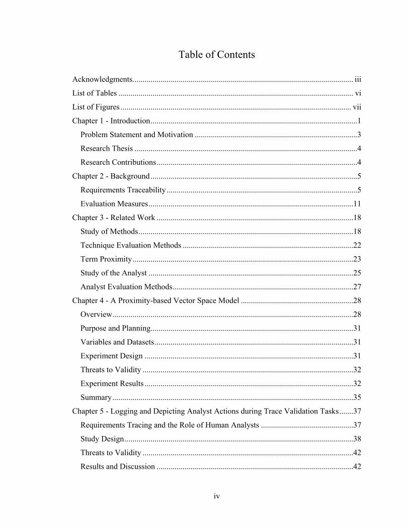
Table of Contents
Acknowledgments.............................................................................................................. iii
List of Tables ..................................................................................................................... vi
List of Figures ................................................................................................................... vii
Chapter 1 - Introduction .......................................................................................................1
Problem Statement and Motivation .................................................................................3
Research Thesis ...............................................................................................................4
Research Contributions ....................................................................................................4
Chapter 2 - Background .......................................................................................................5
Requirements Traceability ...............................................................................................5
Evaluation Measures ......................................................................................................11
Chapter 3 - Related Work ..................................................................................................18
Study of Methods ...........................................................................................................18
Technique Evaluation Methods .....................................................................................22
Term Proximity ..............................................................................................................23
Study of the Analyst ......................................................................................................25
Analyst Evaluation Methods ..........................................................................................27
Chapter 4 - A Proximity-based Vector Space Model ........................................................28
Overview ........................................................................................................................28
Purpose and Planning .....................................................................................................31
Variables and Datasets ...................................................................................................31
Experiment Design ........................................................................................................31
Threats to Validity .........................................................................................................32
Experiment Results ........................................................................................................32
Summary ........................................................................................................................35
Chapter 5 - Logging and Depicting Analyst Actions during Trace Validation Tasks .......37
Requirements Tracing and the Role of Human Analysts ..............................................37
Study Design ..................................................................................................................38
Threats to Validity .........................................................................................................42
Results and Discussion ..................................................................................................42
v
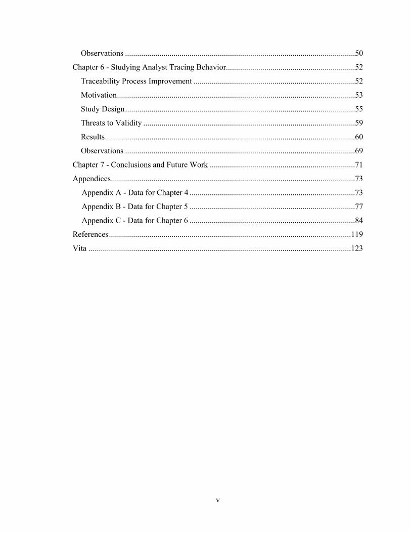
Observations ..................................................................................................................50
Chapter 6 - Studying Analyst Tracing Behavior................................................................52
Traceability Process Improvement ................................................................................52
Motivation ......................................................................................................................53
Study Design ..................................................................................................................55
Threats to Validity .........................................................................................................59
Results ............................................................................................................................60
Observations ..................................................................................................................69
Chapter 7 - Conclusions and Future Work ........................................................................71
Appendices .........................................................................................................................73
Appendix A - Data for Chapter 4 ..................................................................................73
Appendix B - Data for Chapter 5 ..................................................................................77
Appendix C - Data for Chapter 6 ..................................................................................84
References ........................................................................................................................119
Vita ..................................................................................................................................123
vi
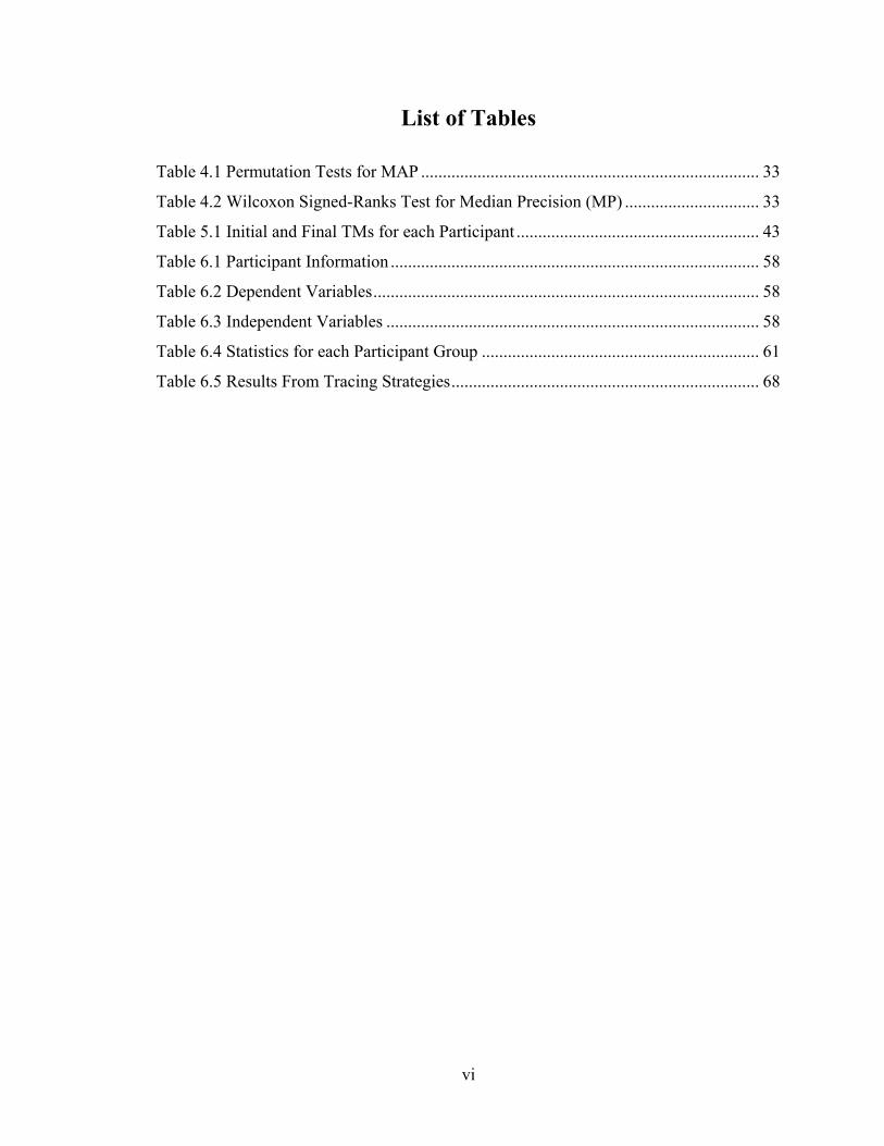
List of Tables
Table 4.1 Permutation Tests for MAP .............................................................................. 33
Table 4.2 Wilcoxon Signed-Ranks Test for Median Precision (MP) ............................... 33
Table 5.1 Initial and Final TMs for each Participant ........................................................ 43
Table 6.1 Participant Information ..................................................................................... 58
Table 6.2 Dependent Variables ......................................................................................... 58
Table 6.3 Independent Variables ...................................................................................... 58
Table 6.4 Statistics for each Participant Group ................................................................ 61
Table 6.5 Results From Tracing Strategies ....................................................................... 68
vii
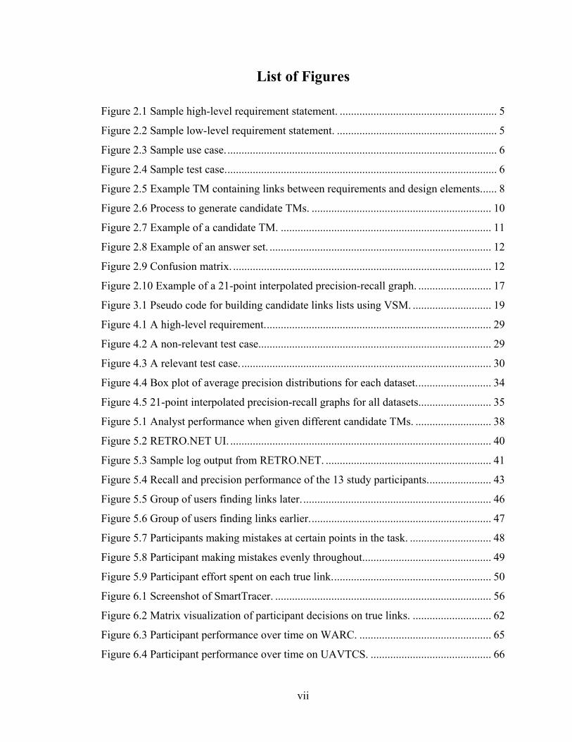
List of Figures
Figure 2.1 Sample high-level requirement statement. ........................................................ 5
Figure 2.2 Sample low-level requirement statement. ......................................................... 5
Figure 2.3 Sample use case. ................................................................................................ 6
Figure 2.4 Sample test case. ................................................................................................ 6
Figure 2.5 Example TM containing links between requirements and design elements. ..... 8
Figure 2.6 Process to generate candidate TMs. ................................................................ 10
Figure 2.7 Example of a candidate TM. ........................................................................... 11
Figure 2.8 Example of an answer set. ............................................................................... 12
Figure 2.9 Confusion matrix. ............................................................................................ 12
Figure 2.10 Example of a 21-point interpolated precision-recall graph. .......................... 17
Figure 3.1 Pseudo code for building candidate links lists using VSM. ............................ 19
Figure 4.1 A high-level requirement. ................................................................................ 29
Figure 4.2 A non-relevant test case. .................................................................................. 29
Figure 4.3 A relevant test case. ......................................................................................... 30
Figure 4.4 Box plot of average precision distributions for each dataset. .......................... 34
Figure 4.5 21-point interpolated precision-recall graphs for all datasets. ......................... 35
Figure 5.1 Analyst performance when given different candidate TMs. ........................... 38
Figure 5.2 RETRO.NET UI. ............................................................................................. 40
Figure 5.3 Sample log output from RETRO.NET. ........................................................... 41
Figure 5.4 Recall and precision performance of the 13 study participants. ...................... 43
Figure 5.5 Group of users finding links later. ................................................................... 46
Figure 5.6 Group of users finding links earlier. ................................................................ 47
Figure 5.7 Participants making mistakes at certain points in the task. ............................. 48
Figure 5.8 Participant making mistakes evenly throughout. ............................................. 49
Figure 5.9 Participant effort spent on each true link. ........................................................ 50
Figure 6.1 Screenshot of SmartTracer. ............................................................................. 56
Figure 6.2 Matrix visualization of participant decisions on true links. ............................ 62
Figure 6.3 Participant performance over time on WARC. ............................................... 65
Figure 6.4 Participant performance over time on UAVTCS. ........................................... 66
1
Chapter 1 - Introduction
Developing complex software systems often involves multiple stakeholder interactions,
coupled with frequent requirements changes while operating under time constraints and budget
pressures. Such conditions can lead to hidden problems, manifesting when software modifications
lead to unexpected software component interactions that can cause catastrophic or fatal situations.
Reports on the Therac-25 radiation accidents [1], Arianne 5 rocket explosion [2], and Mars
Climate Orbiter crash [3] highlight the importance of verifying the safety and reliability of
mission- and safety-critical systems. Failure in software systems that deliver high business value
could mean losing market share to competitors. Rapid changes in marketplace trends can often
leave rigid sequence-based software processes crippled in the wake of requirements changes.
Even in agile software projects, managing traceability from user stories to finished software
product requires that developers understand how components interact within a software system.
A critical step in ensuring the success of software systems is to verify that all
requirements have been met by the design, code, test cases, and other software artifacts generated
in the software development process. Requirements traceability can be defined as the “ability to
follow the life of a requirement in a forward and backward direction [4].” Verification and
Validation (V&V) analysts or Independent V&V (IV&V) analysts achieve this goal by using a
Requirements Traceability Matrix (RTM), more generically called a Traceability Matrix (TM). A
TM consists of links between pairs of software artifacts being traced, e.g., a set of high-level
requirements to a set of low-level requirements. TMs are used to support software engineering
activities such as change impact analysis and regression test identification [5]. Software changes
can be traced to affected components, providing analysts with information on how those changes
affect the entire software system and helping analysts determine the appropriate type and amount
of testing required for the change.
Formal software development processes and software development standards such as the
IEEE/EIA 12207 [6] mandate traceability as part of the software development process. TMs,
however, are commonly created after the fact, where traceability information is recovered from
existing software artifacts. Building such TMs is often error prone and requires intensive effort
[7]. Agile software development processes, however, eschew the traditional TM for alternate
forms of traceability, where the focus on traceability involves driving the development process
2
towards meeting customer requirements through user stories [8]. Even so, maintaining
traceability information using either process involves human interaction, and humans by nature
are not perfect.
Requirements traceability users can be categorized based on how they use traceability in
practice. Low-end traceability users typically use TMs because it is mandated by regulations or
their organization, while high-end traceability users use TMs as an integral part of the
development process and to capture rationale for requirements decisions [9]. A survey of
organizations in various domains on requirements traceability finds that requirements traceability
is seldom used and traces are rarely kept up-to-date [9]. Increasing the use of requirements
traceability requires tracing tools that make life easier for the analyst by producing accurate and
useful results, allowing the analyst to easily discern relevant links from irrelevant links, and
reducing the time spent performing the tracing task [10].
Information Retrieval (IR) techniques greatly reduce the search space for an analyst
tasked with creating a final TM [11]. For example, a TM generated using an IR technique for a
software project with one hundred high-level requirements and two hundred low-level
requirements could contain less than half of the 20,000 possible candidate links for an analyst to
accept or reject. Even then, only a small percentage of these candidate links would be relevant. IR
techniques, in general, are effective in retrieving almost all relevant links (or true links) between
two artifacts (measured by “recall” which is defined in Chapter 2.) In fact, simply returning all
possible links retrieves all relevant links. The number of irrelevant links (or false links) returned
along with true links in the candidate TM1 (measured by “precision” which is defined in Chapter
2) measures a technique’s effectiveness. Another measure that is of interest to the analyst is the
number of false links that are discarded by the technique. This represents the amount of work that
the analyst saves by not having to review all possible links (measured by “selectivity”, which is
defined in Chapter 2.) Tracing technique performance comparisons among researchers present a
challenge due differences in how results are reported and the availability of datasets.
While much effort has been put into improving the performance of automated traceability
techniques, a separate effort focuses on how analysts work with TMs and how their decisions
affect the quality of the final TMs [10, 11, 12, 13]. Researchers have looked at different ways of
evaluating the effort spent by analysts working on TMs [14, 15, 16, 17, 18, 19]. Analysts often
1 A TM is called a “candidate” until an analyst vets them.
3
end up with final TMs that are worse than the candidate TMs [13, 17, 18]. Despite the fact that
analysts introduce subjectivity into the “traceability process loop,” it is not possible to “do away
with” the analyst in the tracing process [13, 17, 18, 19]. These initial studies indicate that there is
still much to study about how analysts work with TMs, and that studying the analyst is a critical
step in traceability process improvement.
Problem Statement and Motivation TM usage continues to be lacking in software engineering. TMs are perceived to be
burdensome to create and maintain, and are further perceived to provide little value. Automating
the TM generation process and quantifying the potential savings when using automated methods
reduces analyst burden. TM usage provides value when tracing techniques provide accurate
results and reduces the effort required to complete the tracing task. One way to improve existing
tracing techniques is to challenge its underlying assumptions. IR techniques often assume that
elements within artifacts are independent of each other, disregarding relationships between
elements within each artifact. One possible improvement would be to consider element proximity
(the number of elements in between two related elements in an artifact) when generating the
candidate TM.
Important information about how analysts work with TMs has not been thoroughly
studied and empirically validated. For example, how accurately do analysts perform tracing
tasks? How often do analysts make correct decisions? How often and why do they make incorrect
decisions? How do analysts spend their time during the tracing task and are they making the best
use of their time? Answering these questions provides new insight as to how to improve
automated tools to encourage beneficial and discourage ineffectual tracing activities.
Automated methods are capable of achieving high recall but have low precision. One
research goal is to improve the quality of candidate TMs generated from unstructured natural
language textual software engineering artifacts. The quality of a candidate TM generated from an
automated tracing technique can be measured by the number of false links that an analyst reviews
before finding true links. An analyst accepts and rejects links in the candidate TM in order to
create the final TM. Another research goal is to identify characteristics of analyst performance
that can lead to higher quality final TMs. The quality of an analyst can be measured by the
decisions they make and effort spent on true and false links in the candidate TMs. Barriers to TM
usage can be overcome once analysts have confidence in automated tools for generating TMs and
when analyst performance can be quantified and targeted for improvement.
4
Research Thesis The dissertation thesis can be stated as follows: Adapting IR techniques that have not
previously been used in requirements tracing improves the quality of candidate TMs generated
using current automated traceability techniques. Studying analyst tracing behavior and identifying
analyst performance characteristics that lead to higher quality final TMs provides targets for
improving analyst performance.
Research Contributions This dissertation makes several contributions. The quality of candidate TMs is improved
through the development of a term proximity-based tracing technique. This technique is validated
against a baseline tracing technique (vector space), showing that the quality of candidate TMs can
be effectively measured through the use of Mean Average Precision MAP (defined in Chapter 2)
as a measure of internal quality and 21-point interpolated precision-recall graph (defined in
Chapter 2) as a measure of overall quality. Different visualization techniques depict how analysts
performed during the tracing task through the logging of analyst actions. This dissertation
introduces potential recall, sensitivity, and effort distribution (defined in Chapter 2) as analyst
performance measures. Analyst decisions on candidate links are visualized and studied to
determine when and why they made incorrect decisions on true links. Tracing strategies derived
from trace logs are used to understand how analysts work with TMs and how tracing strategies
affect tracing results.
The remainder of the dissertation is organized as follows. Chapter 2 presents an overview
of requirements traceability and evaluation measures. Chapter 3 discusses related work. Chapter 4
presents the Proximity-based Vector Space Model (PVSM), an enhancement of the Vector Space
Model (VSM). Chapter 5 reports on the study of analyst behavior through logging and log
depiction. Chapter 6 presents a study of analyst performance and tracing strategies. Chapter 7
concludes the dissertation and outlines future work.
Copyright © Wei-Keat Kong 2012
5
Chapter 2 - Background
This chapter provides an overview of requirements traceability and evaluation measures
used in traceability research.
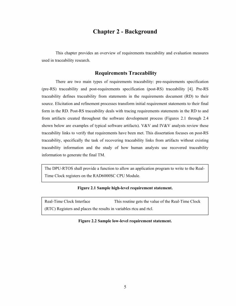
Requirements Traceability There are two main types of requirements traceability: pre-requirements specification
(pre-RS) traceability and post-requirements specification (post-RS) traceability [4]. Pre-RS
traceability defines traceability from statements in the requirements document (RD) to their
source. Elicitation and refinement processes transform initial requirement statements to their final
form in the RD. Post-RS traceability deals with tracing requirements statements in the RD to and
from artifacts created throughout the software development process (Figures 2.1 through 2.4
shown below are examples of typical software artifacts). V&V and IV&V analysts review these
traceability links to verify that requirements have been met. This dissertation focuses on post-RS
traceability, specifically the task of recovering traceability links from artifacts without existing
traceability information and the study of how human analysts use recovered traceability
information to generate the final TM.
Figure 2.1 Sample high-level requirement statement.
Figure 2.2 Sample low-level requirement statement.
The DPU-RTOS shall provide a function to allow an application program to write to the Real-
Time Clock registers on the RAD6000SC CPU Module.
Real-Time Clock Interface This routine gets the value of the Real-Time Clock
(RTC) Registers and places the results in variables rtcu and rtcl.
6
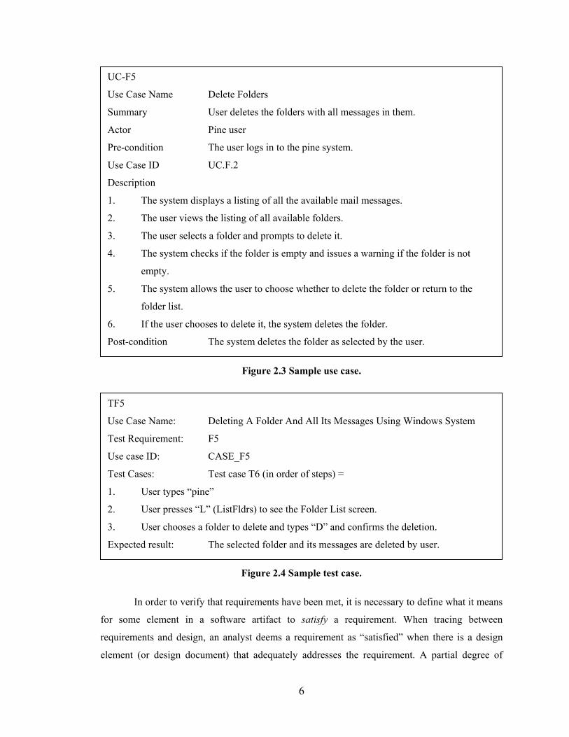
Figure 2.3 Sample use case.
Figure 2.4 Sample test case.
In order to verify that requirements have been met, it is necessary to define what it means
for some element in a software artifact to satisfy a requirement. When tracing between
requirements and design, an analyst deems a requirement as “satisfied” when there is a design
element (or design document) that adequately addresses the requirement. A partial degree of
UC-F5
Use Case Name Delete Folders
Summary User deletes the folders with all messages in them.
Actor Pine user
Pre-condition The user logs in to the pine system.
Use Case ID UC.F.2
Description
1. The system displays a listing of all the available mail messages.
2. The user views the listing of all available folders.
3. The user selects a folder and prompts to delete it.
4. The system checks if the folder is empty and issues a warning if the folder is not
empty.
5. The system allows the user to choose whether to delete the folder or return to the
folder list.
6. If the user chooses to delete it, the system deletes the folder.
Post-condition The system deletes the folder as selected by the user.
TF5
Use Case Name: Deleting A Folder And All Its Messages Using Windows System
Test Requirement: F5
Use case ID: CASE_F5
Test Cases: Test case T6 (in order of steps) =
1. User types “pine”
2. User presses “L” (ListFldrs) to see the Folder List screen.
3. User chooses a folder to delete and types “D” and confirms the deletion.
Expected result: The selected folder and its messages are deleted by user.

7
satisfaction may exist between a requirement and a design element due to the unstructured nature
of language. Satisfaction assessment [20] is another area of research that is emerging in
requirements traceability, where specific parts of a requirements document are mapped to specific
parts of a design element to determine the degree of requirements satisfaction. In this dissertation,
a TM captures satisfaction in the form of links between documents. A link indicates relevance
between two documents. An automated traceability technique generates a candidate TM, which is
a collection of links that an analyst accepts or rejects. The collection of accepted links for a
particular requirement can be treated as the satisfaction of that requirement. The final TM only
contains links that the analyst accepted.
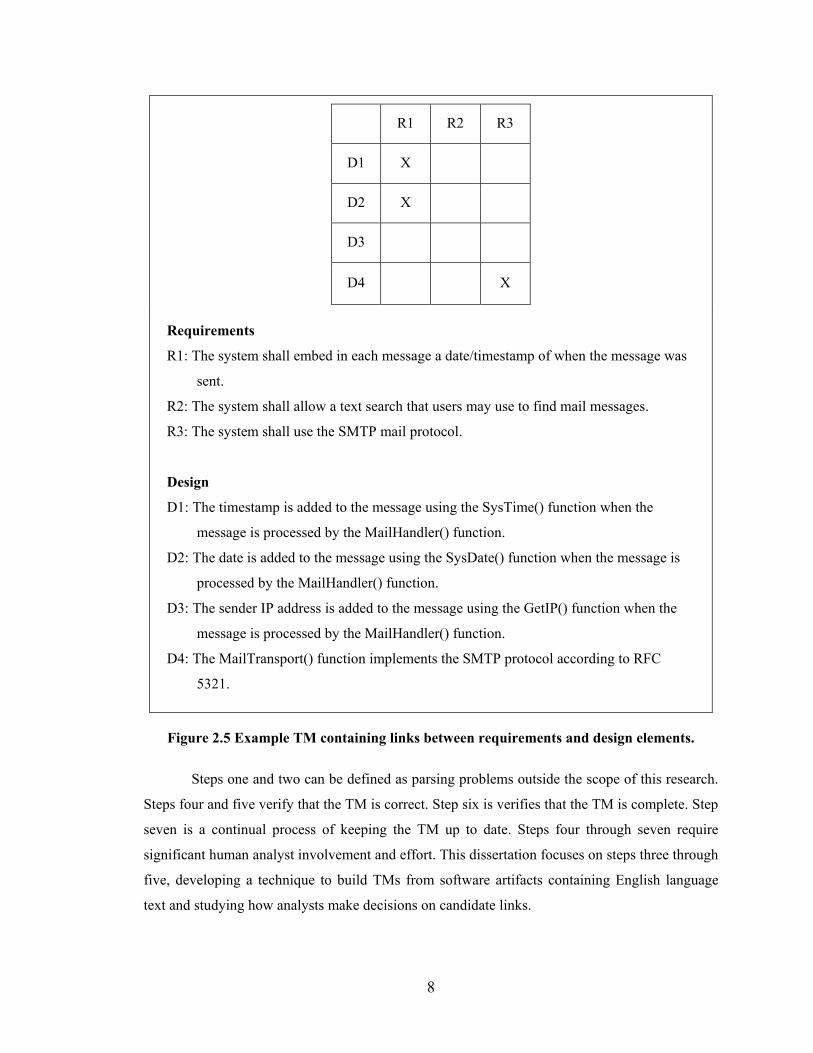
Figure 2.5 depicts a trivial example of a TM that traces between three requirements and
four design elements. R1 and R3 have links to some design elements, but it can be seen that R2
does not have any design element links. This indicates that a requirement possibly has not been
satisfied. Design element D3, in addition, does not have any links to any requirements. This
indicates that there is possibly a design element that was not specified by the requirements. In this
example, tracing from requirements to design is called forward tracing, which verifies that all
requirements are met by some lower-level design element. In this example, R2 is not satisfied by
any design element. Backward tracing verifies that all design elements map to some high-level
requirement ensuring that the design only specifies what is required. In this example, D3 specifies
a design element that is not part of the requirements.
The requirements tracing process between a single requirements document and a single
design document (or any pair of software artifacts) can be broken down into the following steps:
1. Identify individual requirement elements and separate each into individual
documents.
2. Identify individual design elements and separate each into individual documents.
3. Build the TM using software or by hand.
4. Find links to all design documents that satisfy that each requirement document in the
TM.
5. Find links to all requirement documents that are satisfied by each design element in
the TM.
6. Look for missing requirements documents or extraneous design documents.
7. Maintain the TM as changes are made during the software development process.
8
R1 R2 R3
D1 X
D2 X
D3
D4 X
Figure 2.5 Example TM containing links between requirements and design elements.
Steps one and two can be defined as parsing problems outside the scope of this research.
Steps four and five verify that the TM is correct. Step six is verifies that the TM is complete. Step
seven is a continual process of keeping the TM up to date. Steps four through seven require
significant human analyst involvement and effort. This dissertation focuses on steps three through
five, developing a technique to build TMs from software artifacts containing English language
text and studying how analysts make decisions on candidate links.
Requirements
R1: The system shall embed in each message a date/timestamp of when the message was
sent.
R2: The system shall allow a text search that users may use to find mail messages.
R3: The system shall use the SMTP mail protocol.
Design
D1: The timestamp is added to the message using the SysTime() function when the
message is processed by the MailHandler() function.
D2: The date is added to the message using the SysDate() function when the message is
processed by the MailHandler() function.
D3: The sender IP address is added to the message using the GetIP() function when the
message is processed by the MailHandler() function.
D4: The MailTransport() function implements the SMTP protocol according to RFC
5321.
9
In order to prepare software artifacts for traceability link recovery, artifacts are separated
into individual documents, i.e., each containing a single requirement, use case, or test case. The
text in these documents is assumed to be intelligible and may contain minor grammatical and
spelling errors. Documents can vary in internal structure, with no specific formatting or
grammatical style. A corpus represents a collection of documents. Documents are broken down
further into a collection of words or terms, forming a vocabulary for the corpus. In addition, there
is a need to search the document collection for any and all documents that are related to a specific
document. Documents that are used to trace to other documents in the corpus are called queries.
A query consists of terms selected from a document and is used to find other documents that
match or are related to those terms. Document collections are often pre-processed. Pre-processing
of the document collection removes punctuation, line feeds, and special characters in each
document, then separates each document into contiguous strings of alphanumeric characters
(linearizing/tokenizing) called terms. A stop word list containing commonly used terms such as
“a”, “the”, “as” excludes those terms from the corpus. In addition, Porter’s stemming algorithm is
a fast heuristic process that is used to reduce terms to a base form [21]. For example, “includes,”
“including,” and “included” are stemmed to a single token “includ.” This heuristic is imperfect,
and in some cases, two unrelated terms can end up stemmed to the same base form. Even so,
stemming significantly reduces the number of distinct terms in the vocabulary. Stemming,
however, is language-sensitive and performs poorly on languages with complex grammar i.e.,
Italian [22]. Stemmed terms are then indexed into the corpus which maintains statistics about
those terms and the document collection.
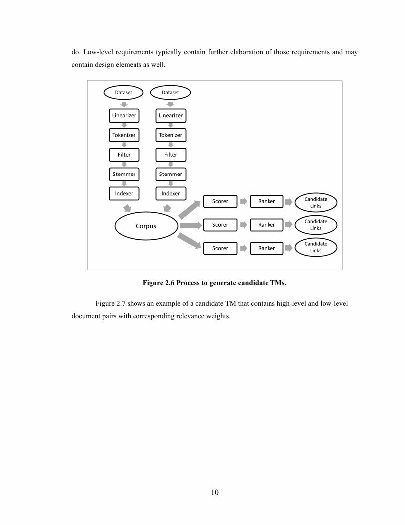
Tracing methods are used to trace between two sets of documents in the corpus to
generate candidate TMs. Candidate TMs are scored using some weighting method to indicate
relevance, and ranked by the relevance weight between the high-level document and the low-level
document. An analyst validates the candidate TM by accepting, rejecting, and possibly adding
links before certifying the final TM. Figure 2.6 shows an example of how links in candidate TMs
are generated.
In software engineering, tracing is typically performed on artifact pairs, e.g., tracing from
a design document to a test description document. In this case, the document collection would
contain a document for each test case from the test description document and a document for each
design element from the design document. Each design element would be used to query the test
case document collection to search for similar test case documents. High-level requirements are
typically represented as a collection of sentences describing in general what the software “shall”
10
do. Low-level requirements typically contain further elaboration of those requirements and may
contain design elements as well.
Figure 2.6 Process to generate candidate TMs.
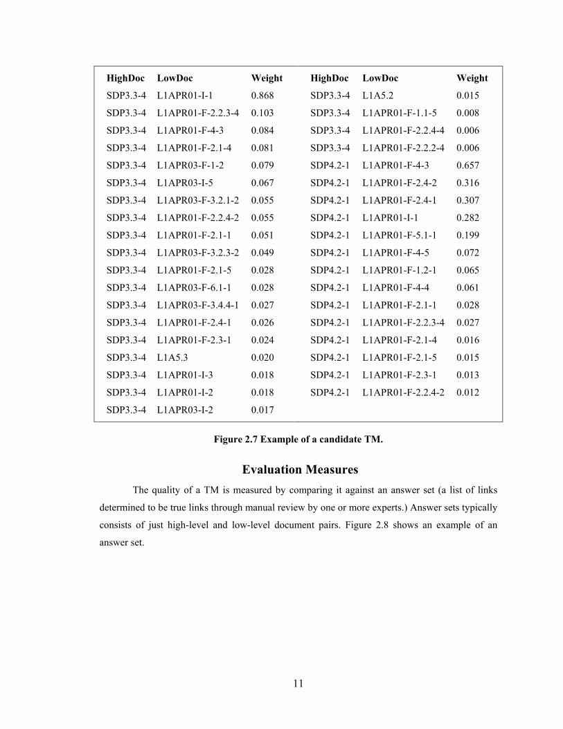
Figure 2.7 shows an example of a candidate TM that contains high-level and low-level
document pairs with corresponding relevance weights.
Linearizer
Tokenizer
Filter
Stemmer
IndexerScorer Ranker
Dataset
Linearizer
Tokenizer
Filter
Stemmer
Indexer
Dataset
Corpus Scorer Ranker
Scorer Ranker
Candidate Links
Candidate Links
Candidate Links
11
HighDoc LowDoc Weight
SDP3.3-4 L1APR01-I-1 0.868
SDP3.3-4 L1APR01-F-2.2.3-4 0.103
SDP3.3-4 L1APR01-F-4-3 0.084
SDP3.3-4 L1APR01-F-2.1-4 0.081
SDP3.3-4 L1APR03-F-1-2 0.079
SDP3.3-4 L1APR03-I-5 0.067
SDP3.3-4 L1APR03-F-3.2.1-2 0.055
SDP3.3-4 L1APR01-F-2.2.4-2 0.055
SDP3.3-4 L1APR01-F-2.1-1 0.051
SDP3.3-4 L1APR03-F-3.2.3-2 0.049
SDP3.3-4 L1APR01-F-2.1-5 0.028
SDP3.3-4 L1APR03-F-6.1-1 0.028
SDP3.3-4 L1APR03-F-3.4.4-1 0.027
SDP3.3-4 L1APR01-F-2.4-1 0.026
SDP3.3-4 L1APR01-F-2.3-1 0.024
SDP3.3-4 L1A5.3 0.020
SDP3.3-4 L1APR01-I-3 0.018
SDP3.3-4 L1APR01-I-2 0.018
SDP3.3-4 L1APR03-I-2 0.017
HighDoc LowDoc Weight
SDP3.3-4 L1A5.2 0.015
SDP3.3-4 L1APR01-F-1.1-5 0.008
SDP3.3-4 L1APR01-F-2.2.4-4 0.006
SDP3.3-4 L1APR01-F-2.2.2-4 0.006
SDP4.2-1 L1APR01-F-4-3 0.657
SDP4.2-1 L1APR01-F-2.4-2 0.316
SDP4.2-1 L1APR01-F-2.4-1 0.307
SDP4.2-1 L1APR01-I-1 0.282
SDP4.2-1 L1APR01-F-5.1-1 0.199
SDP4.2-1 L1APR01-F-4-5 0.072
SDP4.2-1 L1APR01-F-1.2-1 0.065
SDP4.2-1 L1APR01-F-4-4 0.061
SDP4.2-1 L1APR01-F-2.1-1 0.028
SDP4.2-1 L1APR01-F-2.2.3-4 0.027
SDP4.2-1 L1APR01-F-2.1-4 0.016
SDP4.2-1 L1APR01-F-2.1-5 0.015
SDP4.2-1 L1APR01-F-2.3-1 0.013
SDP4.2-1 L1APR01-F-2.2.4-2 0.012
Figure 2.7 Example of a candidate TM.
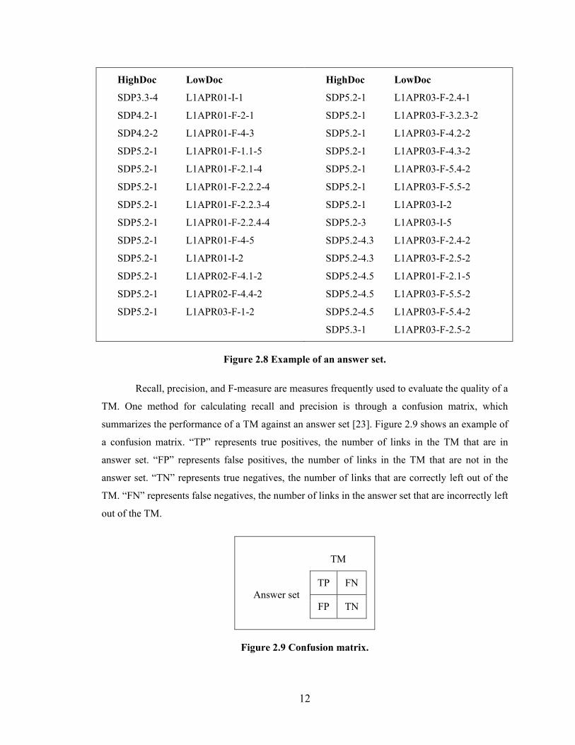
Evaluation Measures The quality of a TM is measured by comparing it against an answer set (a list of links
determined to be true links through manual review by one or more experts.) Answer sets typically
consists of just high-level and low-level document pairs. Figure 2.8 shows an example of an
answer set.
12
HighDoc LowDoc
SDP3.3-4 L1APR01-I-1
SDP4.2-1 L1APR01-F-2-1
SDP4.2-2 L1APR01-F-4-3
SDP5.2-1 L1APR01-F-1.1-5
SDP5.2-1 L1APR01-F-2.1-4
SDP5.2-1 L1APR01-F-2.2.2-4
SDP5.2-1 L1APR01-F-2.2.3-4
SDP5.2-1 L1APR01-F-2.2.4-4
SDP5.2-1 L1APR01-F-4-5
SDP5.2-1 L1APR01-I-2
SDP5.2-1 L1APR02-F-4.1-2
SDP5.2-1 L1APR02-F-4.4-2
SDP5.2-1 L1APR03-F-1-2
HighDoc LowDoc
SDP5.2-1 L1APR03-F-2.4-1
SDP5.2-1 L1APR03-F-3.2.3-2
SDP5.2-1 L1APR03-F-4.2-2
SDP5.2-1 L1APR03-F-4.3-2
SDP5.2-1 L1APR03-F-5.4-2
SDP5.2-1 L1APR03-F-5.5-2
SDP5.2-1 L1APR03-I-2
SDP5.2-3 L1APR03-I-5
SDP5.2-4.3 L1APR03-F-2.4-2
SDP5.2-4.3 L1APR03-F-2.5-2
SDP5.2-4.5 L1APR01-F-2.1-5
SDP5.2-4.5 L1APR03-F-5.5-2
SDP5.2-4.5 L1APR03-F-5.4-2
SDP5.3-1 L1APR03-F-2.5-2
Figure 2.8 Example of an answer set.
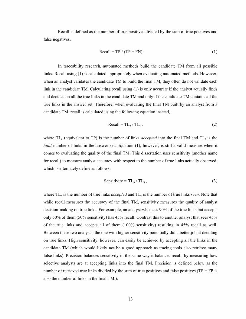
Recall, precision, and F-measure are measures frequently used to evaluate the quality of a
TM. One method for calculating recall and precision is through a confusion matrix, which
summarizes the performance of a TM against an answer set [23]. Figure 2.9 shows an example of
a confusion matrix. “TP” represents true positives, the number of links in the TM that are in
answer set. “FP” represents false positives, the number of links in the TM that are not in the
answer set. “TN” represents true negatives, the number of links that are correctly left out of the
TM. “FN” represents false negatives, the number of links in the answer set that are incorrectly left
out of the TM.
TM
Answer set TP FN
FP TN
Figure 2.9 Confusion matrix.
13
Recall is defined as the number of true positives divided by the sum of true positives and
false negatives,
Recall = TP / (TP + FN) . (1)
In traceability research, automated methods build the candidate TM from all possible
links. Recall using (1) is calculated appropriately when evaluating automated methods. However,
when an analyst validates the candidate TM to build the final TM, they often do not validate each
link in the candidate TM. Calculating recall using (1) is only accurate if the analyst actually finds
and decides on all the true links in the candidate TM and only if the candidate TM contains all the
true links in the answer set. Therefore, when evaluating the final TM built by an analyst from a
candidate TM, recall is calculated using the following equation instead,
Recall = TLa / TLt . (2)
where TLa (equivalent to TP) is the number of links accepted into the final TM and TLt is the
total number of links in the answer set. Equation (1), however, is still a valid measure when it
comes to evaluating the quality of the final TM. This dissertation uses sensitivity (another name
for recall) to measure analyst accuracy with respect to the number of true links actually observed,
which is alternately define as follows:
Sensitivity = TLa / TLs , (3)
where TLa is the number of true links accepted and TLs is the number of true links seen. Note that
while recall measures the accuracy of the final TM, sensitivity measures the quality of analyst
decision-making on true links. For example, an analyst who sees 90% of the true links but accepts
only 50% of them (50% sensitivity) has 45% recall. Contrast this to another analyst that sees 45%
of the true links and accepts all of them (100% sensitivity) resulting in 45% recall as well.
Between these two analysts, the one with higher sensitivity potentially did a better job at deciding
on true links. High sensitivity, however, can easily be achieved by accepting all the links in the
candidate TM (which would likely not be a good approach as tracing tools also retrieve many
false links). Precision balances sensitivity in the same way it balances recall, by measuring how
selective analysts are at accepting links into the final TM. Precision is defined below as the
number of retrieved true links divided by the sum of true positives and false positives (TP + FP is
also the number of links in the final TM.):
14
Precision = TP / (TP + FP) . (4)
Fβ measure combines recall and precision into a single value by taking the harmonic
mean of both measures. Fβ measure can be adjusted to emphasize either precision or recall. In
Equation (5), when β is set to one, precision and recall are weighted equally and the measure is
called the F1 measure. When β is set to two, recall is weighted twice as much as precision and is
called the F2 measure. Similarly, precision is weighted twice as much as recall when β is set to
0.5.
Fβ measure = (1 + β2) * Precision * Recall / ((β2 * Precision) + Recall) . (5)
It should be noted that in requirements tracing research, emphasis has been on recall over
precision. It is often easier for an analyst to determine the relevance of a link in the candidate TM
than to seek out relevant links outside of the candidate TM [12]. The F2 measure is one measure
that traceability researchers have used to emphasize the importance of recall [20]. Note, however,
when evaluating analyst performance on the final TM, the emphasis on recall over precision may
not be appropriate depending on how the final TM is used. Regardless of whether software is
critical or non-critical, TM usage differs depending on the expected “downstream” (successor)
actions. For example, criticality analysis uses the TM to identify “critical” requirements.
Elements that trace to these critical requirements will be subject to additional analysis, review,
and/or testing. A missed link (error of omission) in the TM may mean that an element that really
is tied to a critical requirement is not identified and hence is not subject to the additional rigor. In
this scenario, recall is preferred over precision. Contrast this to tasks such as satisfaction
assessment, consistency checking, and coverage analysis; each of these trigger additional
activities when links are not found in the TM. For example, a requirement marked as “not
satisfied” will be the subject of additional analysis and repair, while marking a requirement as
“satisfied” when it is not (error of commission) leads to the possible “corruption” of successor
activities. Here, precision is preferred over recall.
One other measure that can be obtained from a confusion matrix but is seldom used to
evaluate TMs is “specificity”, defined as the number of true negatives divided by the sum of true
negatives and false positives.
Specificity = TN / (TN + FP) . (6)
15
Specificity as a measure is seldom used in traceability research since the final TM does
not contain links that an automated method or an analyst rejected. Specificity could be considered
as a measure of analyst performance, as it measures how well an analyst rejects false links. TN,
however, heavily influences specificity, which can lead to an inaccurate representation of analyst
performance due to the disproportionate number of false links vs. true links in a candidate TM.
FP is a measure of interest for analyst performance, indicating the number of false links accepted
by the analyst into the final TM. Precision as defined in (4) is a suitable measure for analyst
performance compared to specificity, as TP is bounded by the number of true links in the answer
set. This dissertation uses sensitivity, precision, and additional measures described in Chapter 6 to
measure analyst performance.
Selectivity is a secondary measure used in traceability research that measures the
percentage reduction of all possible links that are presented to the analyst for review after a
candidate TM is generated using an automated method [24]. This measure is also used to indicate
the amount of effort reduced for the analyst building the final TM. This measure is calculated by
dividing the number of candidate links by the total number of possible links for a candidate TM.
Selectivity = (TP + FP) / (TP + FP + TN + FN) . (7)
Measures derived from the confusion matrix are considered set-based measures, as the
position of true links within the TM does not influence those measures. From the perspective of
an analyst vetting links, a candidate TM with true links near the top is more desirable than a
candidate TM with true links further down the list [25]. A ranked-retrieval-based measure,
however, considers the position of true links in the TM. “Lag” is a ranked-retrieval-based
measure [24] that counts the average number of false links above each relevant link in a candidate
TM. This measure indicates the analyst effort needed to review false links that are in the
candidate TM above (before) true links. Lag is an ordinal measure compared to the other earlier
measures which are bounded between zero and one. A limitation of this measure is that it does
not factor in true links that are not in the candidate TM. For example, Lag for a candidate TM that
has one true link at the top of the list but is missing three other true links is zero since there are no
false links above the single true link. MAP is a ranked retrieval-based measure used in the IR
community that is similar to Lag but does not have this limitation. MAP is calculated based on
the position of relevant links in the candidate TM [26]. Using MAP, links near the top of the
candidate TM are considered more important than links further down the list.
16
For example, assume that a query has four true links but the candidate TM only returned
three, ranking them at position 1, 3, and 5. The precision for the first true link is 1. The precision
for the second true link is 2/3 and the precision for the third true link is 3/5. Since the fourth true
link is not in the candidate TM, the precision for that link is 0. The average precision for the
query is (1 + 2/3 + 3/5 + 0) / 4 = 0.57. MAP is the arithmetic mean of precision scores for each
query with at least one true link. The IR community frequently uses MAP to characterize results
of ranked-retrieval IR techniques and it has been shown to be a stable performance measure [27].
Average precision per query allows for per-query performance comparison between
techniques, which is also the base for statistical testing of technique performance using MAP as
the test statistic. This dissertation introduces the use of MAP in traceability research with the
additional rigor of statistical testing to test the difference in MAP between tracing techniques.
Using MAP in traceability experiments will provide more accurate performance comparisons of
traceability techniques.
In prior traceability research that uses recall and precision measures [7, 13, 14, 15, 25,
28], the candidate TM includes queries that do not have any true links for that query in the answer
set. This in effect lowers precision of the candidate TM since all links returned for such queries
will be false links when using a set-based measure. When evaluating automated traceability
techniques using MAP, this measure indicates how well a technique returns a candidate TM with
true links near the top for each query, which naturally excludes queries without any true links. On
the other hand, the 21-point interpolated precision-recall graph (described next) is based on set-
based measures and includes queries without true links, providing “apples to apples” comparison
to prior work while augmenting the comparison with statistical testing.
Weight threshold filtering and document cut point filtering are techniques that are used to
increase precision at the cost of decreasing recall [7, 15, 28]. Threshold filtering sets a lower limit
for an acceptable candidate link. Links with similarity scores lower than the threshold are
excluded from the candidate TM. Document cut point filtering limits the number of candidate
links returned per query. For example, Top 5 filtering returns the top 5 links for each query. The
tradeoff in precision and recall is often visualized using variants of the precision-recall graph,
showing the overall performance of the technique at various recall levels. By varying the weight
threshold or document cut point, precision-recall points are obtained and plotted on the precision-
recall graph.
17
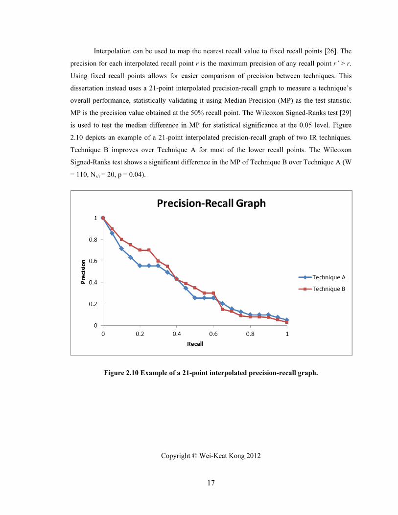
Interpolation can be used to map the nearest recall value to fixed recall points [26]. The
precision for each interpolated recall point r is the maximum precision of any recall point r’ > r.
Using fixed recall points allows for easier comparison of precision between techniques. This
dissertation instead uses a 21-point interpolated precision-recall graph to measure a technique’s
overall performance, statistically validating it using Median Precision (MP) as the test statistic.
MP is the precision value obtained at the 50% recall point. The Wilcoxon Signed-Ranks test [29]
is used to test the median difference in MP for statistical significance at the 0.05 level. Figure
2.10 depicts an example of a 21-point interpolated precision-recall graph of two IR techniques.
Technique B improves over Technique A for most of the lower recall points. The Wilcoxon
Signed-Ranks test shows a significant difference in the MP of Technique B over Technique A (W
= 110, Ns/r = 20, p = 0.04).
Figure 2.10 Example of a 21-point interpolated precision-recall graph.
Copyright © Wei-Keat Kong 2012
18
Chapter 3 - Related Work
This chapter provides an overview of related work and is divided into the study of
methods, technique evaluation methods, term proximity, study of the analyst, and analyst
evaluation methods. Though the dissertation does not build on some of these method studies, they
are provided as additional background information.
Study of Methods The study of methods investigates techniques that recover traceability link information
for analysts to vet. These studies typically apply one or more techniques to retrieve links and
compare them against a baseline technique using some performance measure. This dissertation
contributes to the study of methods by developing a term proximity-based augmentation of the
VSM, validating the work using a ranked-retrieval based measure that has not been previously
used in requirements tracing.
Vector Space Model The VSM [30] is a popular and effective IR technique, considered one of the baseline
techniques in requirements tracing experiments [7, 11, 10, 14, 15, 20, 24, 25, 31, 32, 33]. A
vector represents each document in the corpus where each cell of the vector indicates the
presence or absence of a term in the document, generally using some weighting factor (with term
frequency-inverse document frequency (tf-idf) being the most common). The query is similarly
represented. A similarity value between zero and one is then computed using the cosine angle of
the vectors to represent the relevance of a given document element to the query. Values that are
close to one indicate a document that is highly relevant to the query; values close to zero are not
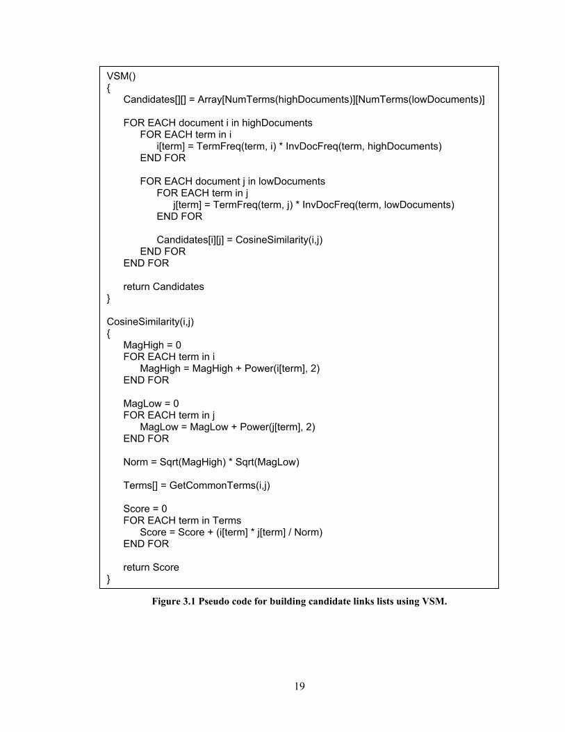
relevant. Candidate TMs are ranked in order of relevance weights. Figure 3.1 shows pseudo code
for generating candidate TMs using VSM. The TermFreq function simply returns the number of
terms in a given document and the InvDocFreq function returns the number of documents
containing the given term.
19
Figure 3.1 Pseudo code for building candidate links lists using VSM.
VSM() { Candidates[][] = Array[NumTerms(highDocuments)][NumTerms(lowDocuments)]
FOR EACH document i in highDocuments FOR EACH term in i
i[term] = TermFreq(term, i) * InvDocFreq(term, highDocuments) END FOR FOR EACH document j in lowDocuments FOR EACH term in j
j[term] = TermFreq(term, j) * InvDocFreq(term, lowDocuments) END FOR Candidates[i][j] = CosineSimilarity(i,j) END FOR
END FOR
return Candidates } CosineSimilarity(i,j) { MagHigh = 0 FOR EACH term in i MagHigh = MagHigh + Power(i[term], 2) END FOR MagLow = 0 FOR EACH term in j MagLow = MagLow + Power(j[term], 2) END FOR Norm = Sqrt(MagHigh) * Sqrt(MagLow) Terms[] = GetCommonTerms(i,j) Score = 0 FOR EACH term in Terms Score = Score + (i[term] * j[term] / Norm) END FOR return Score }
20
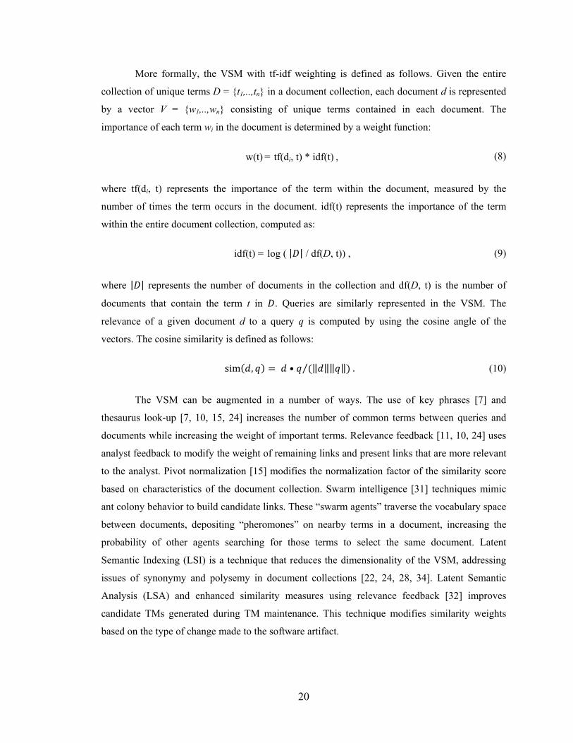
More formally, the VSM with tf-idf weighting is defined as follows. Given the entire
collection of unique terms D = {t1,..,tn} in a document collection, each document d is represented
by a vector V = {w1,..,wn} consisting of unique terms contained in each document. The
importance of each term wi in the document is determined by a weight function:
w(t) = tf(di, t) * idf(t) , (8)
where tf(di, t) represents the importance of the term within the document, measured by the
number of times the term occurs in the document. idf(t) represents the importance of the term
within the entire document collection, computed as:
idf(t) = log ( |𝐷| / df(D, t)) , (9)
where |𝐷| represents the number of documents in the collection and df(D, t) is the number of
documents that contain the term t in 𝐷. Queries are similarly represented in the VSM. The
relevance of a given document d to a query q is computed by using the cosine angle of the
vectors. The cosine similarity is defined as follows:
sim(𝑑, 𝑞) = 𝑑 • 𝑞 (‖𝑑‖‖𝑞‖) .⁄ (10)
The VSM can be augmented in a number of ways. The use of key phrases [7] and
thesaurus look-up [7, 10, 15, 24] increases the number of common terms between queries and
documents while increasing the weight of important terms. Relevance feedback [11, 10, 24] uses
analyst feedback to modify the weight of remaining links and present links that are more relevant
to the analyst. Pivot normalization [15] modifies the normalization factor of the similarity score
based on characteristics of the document collection. Swarm intelligence [31] techniques mimic
ant colony behavior to build candidate links. These “swarm agents” traverse the vocabulary space
between documents, depositing “pheromones” on nearby terms in a document, increasing the
probability of other agents searching for those terms to select the same document. Latent
Semantic Indexing (LSI) is a technique that reduces the dimensionality of the VSM, addressing
issues of synonymy and polysemy in document collections [22, 24, 28, 34]. Latent Semantic
Analysis (LSA) and enhanced similarity measures using relevance feedback [32] improves
candidate TMs generated during TM maintenance. This technique modifies similarity weights
based on the type of change made to the software artifact.
21
All the VSM augmentations mentioned above modify the weights assigned to each
document by modeling some feature of the document collection in order to more accurately rank
the links returned in the candidate TM. Some features are derived from the collection itself (key
phrases, pivot normalization, swarm, LSI/LSA), while others are combined with external
information (thesaurus, relevance feedback). The VSM augmentation introduced in this
dissertation uses term proximity [33], considering the distance between terms in both a query and
document as a measure of document relevance in addition to the tf-idf weighting.
Probabilistic Model The probabilistic model is another popular baseline technique used in requirements
tracing experiments [14, 35, 36, 37, 38, 39]. Most studies use a naïve Bayesian model, where
documents are ranked based on the probability that the document is related to the query. The
probability of a document being related to a query is the sum of probabilities for all terms
occurring in both the query and document over the sum of probabilities for all terms occurring in
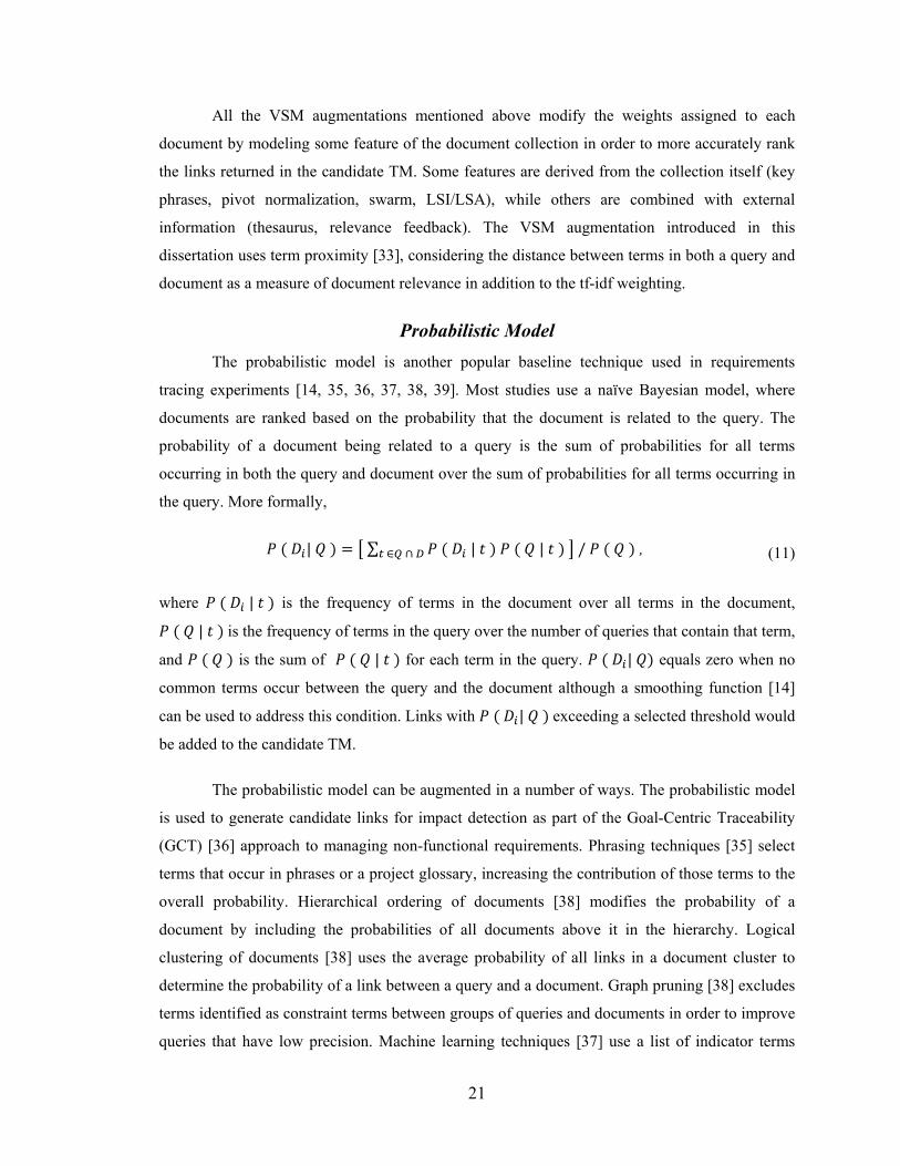
the query. More formally,
𝑃 ( 𝐷𝑖| 𝑄 ) = � ∑ 𝑃 ( 𝐷𝑖 | 𝑡 ) 𝑃 ( 𝑄 | 𝑡 ) 𝑡 ∈𝑄 ∩ 𝐷 � / 𝑃 ( 𝑄 ) , (11)
where 𝑃 ( 𝐷𝑖 | 𝑡 ) is the frequency of terms in the document over all terms in the document,
𝑃 ( 𝑄 | 𝑡 ) is the frequency of terms in the query over the number of queries that contain that term,
and 𝑃 ( 𝑄 ) is the sum of 𝑃 ( 𝑄 | 𝑡 ) for each term in the query. 𝑃 ( 𝐷𝑖| 𝑄) equals zero when no
common terms occur between the query and the document although a smoothing function [14]
can be used to address this condition. Links with 𝑃 ( 𝐷𝑖| 𝑄 ) exceeding a selected threshold would
be added to the candidate TM.
The probabilistic model can be augmented in a number of ways. The probabilistic model
is used to generate candidate links for impact detection as part of the Goal-Centric Traceability
(GCT) [36] approach to managing non-functional requirements. Phrasing techniques [35] select
terms that occur in phrases or a project glossary, increasing the contribution of those terms to the
overall probability. Hierarchical ordering of documents [38] modifies the probability of a
document by including the probabilities of all documents above it in the hierarchy. Logical
clustering of documents [38] uses the average probability of all links in a document cluster to
determine the probability of a link between a query and a document. Graph pruning [38] excludes
terms identified as constraint terms between groups of queries and documents in order to improve
queries that have low precision. Machine learning techniques [37] use a list of indicator terms
22
identified from a subset of documents, increasing the weights of indicator terms that occur in
subsequent documents. Web searches [37, 39] are used to gather collections of web documents,
from which domain concepts are extracted and used to query for candidate links.
The probabilistic model is similar to the VSM in that term frequencies in queries and
documents are used as the basis for calculating similarity scores. Performance comparisons
between these two models have produced mixed results, with no model consistently
outperforming the other under different conditions [14, 40, 41].
Rule-based Model Rule-based models involve building object models between software artifacts, then using
rules to query the model for candidate links. Parts-of-speech patterns can be used to generate
rules for generating candidate TMs [42]. Candidate TMs can also be generated using a
combination of LSI with structural analysis [43], a technique where Traceability Link Graphs
(TLGs) visualize links between source code and documentation elements, which are then used to
generate rules for building the candidate TM. These rule-based methods are highly precise but
require additional analyst effort to configure appropriate rule sets.
Event-based traceability Event-based traceability maintains traceability links in software artifact change
management systems using the probabilistic model [44] and LSI [22]. Under such systems,
software artifacts are monitored for changes, triggering updates for other linked artifacts as
needed. In addition, the dependencies between software artifacts and their states are clearly
visible in the system, providing a high-level view that aids in project management and trace
analysis. While event-based traceability is beneficial for maintaining TMs (step seven of the
requirements tracing process in the previous chapter), these methods are outside the scope of this
dissertation.
Technique Evaluation Methods Results from the study of methods show that IR techniques are able to retrieve most of
the true links (high recall), but usually at the expense of retrieving many false links as well (low
precision). Filtering techniques can be used to measure the performance of a tracing technique
from an overall perspective. Document cut and threshold weight filtering techniques trim the
candidate TM to improve precision while possibly lowering recall, and are visualized using
variants of the precision-recall graph to determine technique effectiveness [7, 14, 15, 24, 28, 35,
23
43]. Precision at each recall point for a given tracing technique, however, may not line up with
values obtained from another technique, which presents a challenge when trying to determine if
one technique outperforms the other. Note, however, filtering does not actually make a difference
in the performance of the tracing technique, i.e., the position of the true links in the candidate TM
does not change with filtering. Filtering techniques are not suitable for measuring per-query
performance of tracing techniques which is important to the analyst who values true links ranked
near the top of the candidate links for each query.
Lag has some shortcomings as a ranked-retrieval based measure in that it can be
misleading when candidate TMs have few links. DiffAR [25] is a measure that indicates the
average weight difference between true links and false links in a candidate TM. Candidate TMs
with high DiffAR clearly distinguish true links from false links. Selectivity is another measure
that provides quantifiable savings from the use of automated methods [11, 24], indicating the
effectiveness of an automated method. An automated method that isn’t very effective returns a
majority of the possible links (has very low precision), which does not provide any reduction in
effort for the analyst and might be perceived as providing little value.
Some probabilistic models require supervised learning before performing the trace
recovery. Evaluation of such methods requires cross validation in order to reduce selection bias
[37]. Unsupervised learning methods, however, can be evaluated using the same evaluation
techniques that are used for evaluating VSM.
The use of different comparison techniques in the traceability community highlights the
need for standardized measurement techniques among researchers. This dissertation introduces
MAP as a measure of the internal quality of candidate TMs and the 21-point interpolated
precision-recall graph as a measure of the overall quality of candidate TMs. Technique
performance can be validated by using statistical testing of both measures.
Term Proximity The IR community has studied a number of term proximity techniques, but so far none of
these techniques has been applied to requirements tracing. This dissertation tailors a term
proximity technique for requirements tracing from the term proximity techniques described
below.
Document relevance can be calculated using the distance between terms in a proximity
relation instance called Z-mode [45]. As a baseline, a set of terms representing important

24
concepts (referred to as a proximity relationship) is selected from each query and used with the
NEAR operator within 200 characters to retrieve relevant documents. Using Z-mode, a span is
defined as the largest number of words between terms in a proximity relationship. Document
relevance is calculated based on the span of each proximity relationship in a document. The
overall document relevance is a function of the manually assigned proximity relationship weight
and the document relevance due to the proximity relationship. The term proximity technique in
this dissertation differs in that all terms from the query are used to find relevant documents, using
terms in close proximity to increase the similarity weight.
Another way to calculate term weights based on term proximity is to use keyword pairs.
A baseline probabilistic model is enhanced with term proximity using all possible term-pairs in a
query within four words of each other [46]. Queries with only one keyword are removed since
term-pairs could not be formed with just a single keyword. The weight of each term pair weight is
calculated using the inverse square of the word distance between term-pairs. The term proximity
technique in this dissertation differs in that weight calculations are not limited to keyword pairs
and that the proximity weight is a component of the overall similarity weight, which does not
exclude queries and documents with single keywords.
A comparison study of two span-based and three distance aggregation measures uses the
distance between terms in the document instead of how often they occur in the document to
determine document relevance [47]. Span-based measures are based on the shortest segment of
text that either covers all query terms including repeated terms, or that covers all query terms at
least once (minimum coverage). Aggregation-based measures look at pair-wise distances between
query terms, considering the minimum distance, average distance, and maximum distance
between each pair of query terms in the document. Documents that only have one query term
return the length of the document as the measure, heavily penalizing documents that only have
one term in common with the query (which may not be fair if that common term is an important
term). Results showed that the minimum distance measure performed the best among the
measures compared. The technique in this dissertation uses a similar distance aggregation
technique in that only terms within a maximum word distance from each other are considered in
the proximity weight calculations.
Another term proximity technique uses term positions to vary the relevance contribution
of a term to the weight of the document [48]. Query terms are grouped into non-overlapping
phrases and the relevance contribution of each phrase is calculated by the number of terms within
25
the phrase and the distance between them. The sum of each relevance contribution replaces the
term frequency in the Okapi BM25 (a probabilistic) model. The technique in this dissertation is
similar in that groups of terms in close proximity to each other in both the query and the
document are aggregated. Instead of replacing a component of the similarity measure, the
proximity measure complements the similarity measure.
This dissertation introduces the idea of calculating document relevance by considering
important terms occurring within close proximity to each other in both the query and the
document. Instead of short ad hoc queries frequently used in the IR domain, queries that are used
in requirements tracing consist of terms from an entire document. This model considers term
proximity of both the query and the documents being traced, ensuring that terms close together in
the query are also close together in the document. Most studies in the IR domain use probabilistic
models, while VSM is a common baseline model in requirements tracing. This dissertation uses
VSM as the underlying model for integrating the term proximity measure. The term proximity
weight is combined with the cosine similarity weight such that links with low cosine similarity
weights increase more than links with high cosine similarity weights.
Study of the Analyst On another front, progress has been made in studying the human analyst in the tracing
process. The study of the analyst refers to examining ways to best use the human analyst’s time in
the tracing process (such as vetting candidate links) in order to generate the best possible final
TM.
Prior to human studies, analyst simulations provided a means to test tracing strategies.
Studies using relevance feedback with multiple iterations and filtering to validate candidate TMs
showed that precision improved substantially when perfect feedback is given by simulated
analysts (always accepts a true link, always rejects a false link). Relevance feedback, however,
still did not outperform a thesaurus retrieval-based technique [10, 24] (results included links used
for feedback).
Simulations of the perfect analyst studied how link ordering and analyst feedback
affected results, measuring the effort required to achieve either a fixed recall level or to measure
the recall achieved using a fixed amount of effort [11]. A number of possible analyst strategies
that decrease analyst effort were studied. Results showed that local ordering with feedback
performed the best. Additional observations found that determining the stopping point is crucial,
26
using feedback helps, and a systematic approach helps. Simulations of relevance feedback for
maintaining software artifacts looked at how prior feedback given by analysts could be used to
reduce the effort of future “retracing” or “delta tracing” tasks. Results showed that prior correct
feedback improved results but results worsened when earlier decisions were wrong [32]. This
dissertation builds on the lessons learned from these simulations, using a study to identify actual
analyst strategies.
Incremental approaches using document cut or threshold weight filtering with various
feedback strategies showed that a significant amount of effort is required to retrieve all true links
in the TM [49] (results excluded links that were used for feedback, and in some cases use of
feedback made results worse). The ADAMS Re-Trace tool [22] uses a similar technique, enabling
analysts to set decreasing threshold values and control the size of the candidate TM presented to
them. The tool also groups relevant links together and alerts analysts to potential feedback
mistakes in the vetting process.
Analysts typically spend most of the time vetting false links, considering that the scarcity
of true links in a candidate TM increases significantly as the matrix of possible links grows.
Humans get tired, which means that they probably have a period of time where they do their best
work. While the simulation studies described above assumed that analysts made perfect decisions,
studies of actual human analysts showed that analysts were fallible in predictable ways [17].
Given small candidate TMs (high precision, low recall), analysts added more links, improving
recall at the cost of precision. Given large candidate TMs (low precision, high recall), analysts
threw links out, improving precision at the cost of some recall. Given higher accuracy candidate
TMs, analysts produced slightly lower accuracy final TMs. Given lower accuracy candidate TMs,
analysts produced significantly higher accuracy final TMs [13, 17, 18]. Analysts tended to
produce final TMs that were near the precision = recall line, meaning they had final TMs that
were about the size of the true TM [13].
Analysts were better at validating links as opposed to searching for missing links [4] and
their accuracy did not depend on whether they had industrial experience or not (while
experienced analysts were more correct on true links than those with less experience, both
achieved less than 50% precision) [18]. Decisions were more likely to be correct when made
quickly and most decisions were made on false links [4, 18]. Effort spent validating links did not
correlate with trace accuracy [2, 18].
27
This dissertation builds on previous analyst studies, focusing on how analysts work with
TMs when given the same starting candidate TM. Analyst actions are logged to provide a step-
by-step account of the decisions made during the tracing task. These logs provide a significant
amount of information that can be mined for trends, analyzed for tracing strategies, and visualized
to show areas where analysts have difficulty during the tracing task.
Analyst Evaluation Methods A number of measures have been used to evaluate the analyst working with TMs. Most of
these measures relate to the effort spent on tracing tasks. In one study, the Recovery Effort Index
(REI) measures the benefit of using an automated tracing technique by using the ratio of retrieved
links over all possible links. This measure is equivalent to selectivity, which is defined in chapter
2. The effort spent on techniques that use the probabilistic model and VSM was compared to the
effort spent using UNIX grep utility that simulated a manual trace. Results from grep were not
ranked and were much worse compared to both IR methods [14]. Another study used a similar
measure, called reduction (which is the same as 1 – selectivity), to gauge the expected effort to
vet links when evaluating precision/recall levels [15]. Effort can also be considered as the amount
of time spent on the tracing task [16, 18]. Post-study surveys asked participants about the amount
of effort spent validating links vs. finding missing links, providing anecdotal evidence that higher
effort spent validating links results in lower final TM accuracy [18].
In this dissertation, effort is considered as a ratio between false links seen and true links
seen, indicating the amount of effort disproportionately allocated to review false links. In
addition, measures that look at how well the analyst decides on true links in the candidate TM
provide a better indicator of analyst performance that could not be obtained from looking at the
final TM. This dissertation also considers the decisions that analysts make during the tracing task,
visualizing how well they do at accepting true links and rejecting false links.
Copyright © Wei-Keat Kong 2012
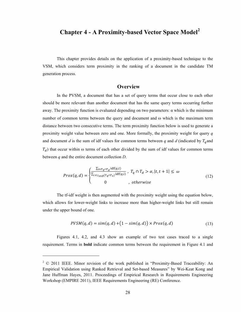
28
Chapter 4 - A Proximity-based Vector Space Model2
This chapter provides details on the application of a proximity-based technique to the
VSM, which considers term proximity in the ranking of a document in the candidate TM
generation process.
Overview In the PVSM, a document that has a set of query terms that occur close to each other
should be more relevant than another document that has the same query terms occurring further
away. The proximity function is evaluated depending on two parameters: α which is the minimum
number of common terms between the query and document and ω which is the maximum term
distance between two consecutive terms. The term proximity function below is used to generate a
proximity weight value between zero and one. More formally, the proximity weight for query q
and document d is the sum of idf values for common terms between q and d (indicated by 𝑇𝑞and
𝑇𝑑) that occur within ω terms of each other divided by the sum of idf values for common terms
between q and the entire document collection D.
𝑃𝑟𝑜𝑥(𝑞,𝑑) = �
∑ idf(𝑞,𝑡)𝑡∈𝑇𝑞∩𝑇𝑑∑ idf(𝑞,𝑖)𝑖 ∈⋃ �𝑇𝑞∩𝑇𝑥�𝑥∈𝐷
, 𝑇𝑞 ∩ 𝑇𝑑 > 𝛼, |𝑡, 𝑡 + 1| ≤ 𝜔
0 , 𝑜𝑡ℎ𝑒𝑟𝑤𝑖𝑠𝑒 (12)
The tf-idf weight is then augmented with the proximity weight using the equation below,
which allows for lower-weight links to increase more than higher-weight links but still remain
under the upper bound of one.
𝑃𝑉𝑆𝑀(𝑞,𝑑) = 𝑠𝑖𝑚(𝑞,𝑑) +�1 − 𝑠𝑖𝑚(𝑞,𝑑)� × 𝑃𝑟𝑜𝑥(𝑞,𝑑) (13)
Figures 4.1, 4.2, and 4.3 show an example of two test cases traced to a single
requirement. Terms in bold indicate common terms between the requirement in Figure 4.1 and
2 © 2011 IEEE. Minor revision of the work published in “Proximity-Based Traceability: An Empirical Validation using Ranked Retrieval and Set-based Measures” by Wei-Keat Kong and Jane Huffman Hayes, 2011. Proceedings of Empirical Research in Requirements Engineering Workshop (EMPIRE 2011), IEEE Requirements Engineering (RE) Conference.
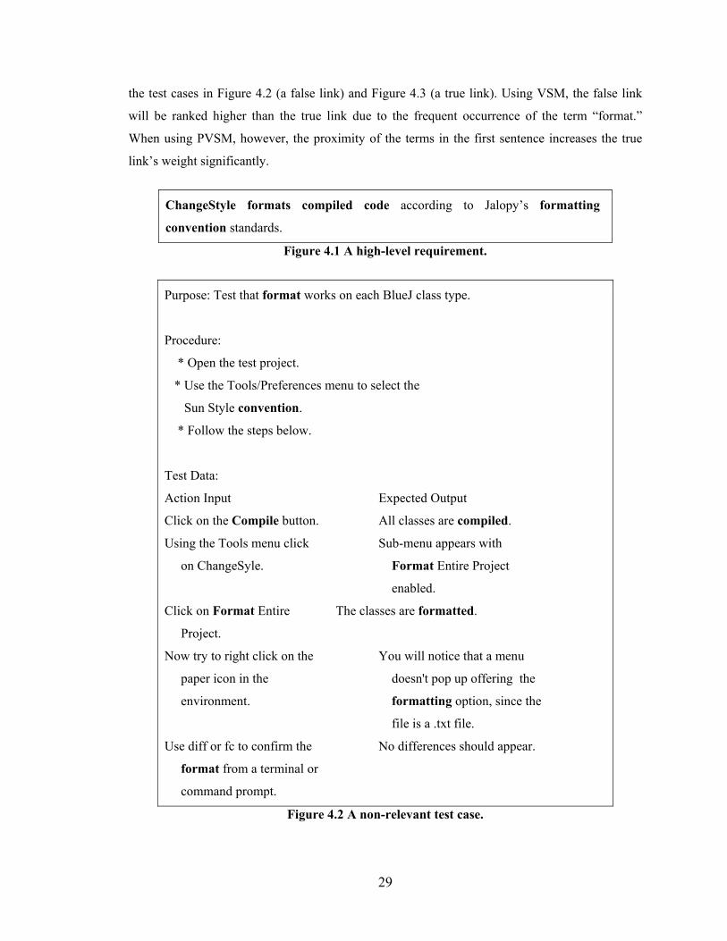
29
the test cases in Figure 4.2 (a false link) and Figure 4.3 (a true link). Using VSM, the false link
will be ranked higher than the true link due to the frequent occurrence of the term “format.”
When using PVSM, however, the proximity of the terms in the first sentence increases the true
link’s weight significantly.
ChangeStyle formats compiled code according to Jalopy’s formatting
convention standards.
Figure 4.1 A high-level requirement.
Purpose: Test that format works on each BlueJ class type.
Procedure:
* Open the test project.
* Use the Tools/Preferences menu to select the
Sun Style convention.
* Follow the steps below.
Test Data:
Action Input Expected Output
Click on the Compile button. All classes are compiled.
Using the Tools menu click Sub-menu appears with
on ChangeSyle. Format Entire Project
enabled.
Click on Format Entire The classes are formatted.
Project.
Now try to right click on the You will notice that a menu
paper icon in the doesn't pop up offering the
environment. formatting option, since the
file is a .txt file.
Use diff or fc to confirm the No differences should appear.
format from a terminal or
command prompt.
Figure 4.2 A non-relevant test case.
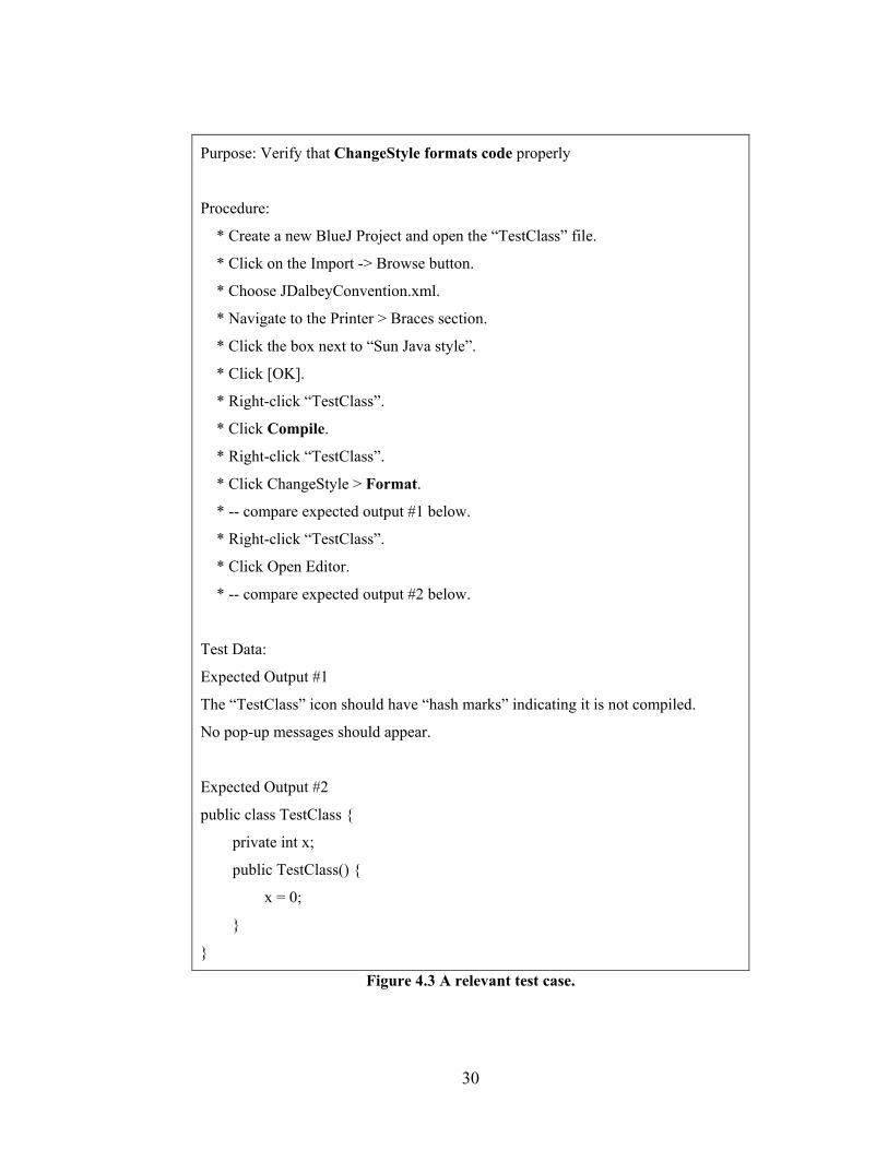
30
Purpose: Verify that ChangeStyle formats code properly
Procedure:
* Create a new BlueJ Project and open the “TestClass” file.
* Click on the Import -> Browse button.
* Choose JDalbeyConvention.xml.
* Navigate to the Printer > Braces section.
* Click the box next to “Sun Java style”.
* Click [OK].
* Right-click “TestClass”.
* Click Compile.
* Right-click “TestClass”.
* Click ChangeStyle > Format.
* -- compare expected output #1 below.
* Right-click “TestClass”.
* Click Open Editor.
* -- compare expected output #2 below.
Test Data:
Expected Output #1
The “TestClass” icon should have “hash marks” indicating it is not compiled.
No pop-up messages should appear.
Expected Output #2
public class TestClass {
private int x;
public TestClass() {
x = 0;
}
}
Figure 4.3 A relevant test case.
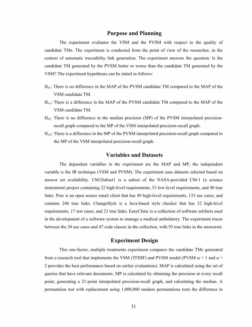
31
Purpose and Planning The experiment evaluates the VSM and the PVSM with respect to the quality of
candidate TMs. The experiment is conducted from the point of view of the researcher, in the
context of automatic traceability link generation. The experiment answers the question: Is the
candidate TM generated by the PVSM better or worse than the candidate TM generated by the
VSM? The experiment hypotheses can be stated as follows:
H01: There is no difference in the MAP of the PVSM candidate TM compared to the MAP of the
VSM candidate TM.
HA1: There is a difference in the MAP of the PVSM candidate TM compared to the MAP of the
VSM candidate TM.
H02: There is no difference in the median precision (MP) of the PVSM interpolated precision-
recall graph compared to the MP of the VSM interpolated precision-recall graph.
HA2: There is a difference in the MP of the PVSM interpolated precision-recall graph compared to
the MP of the VSM interpolated precision-recall graph.
Variables and Datasets The dependent variables in the experiment are the MAP and MP, the independent
variable is the IR technique (VSM and PVSM). The experiment uses datasets selected based on
answer set availability. CM1Subset1 is a subset of the NASA-provided CM-1 (a science
instrument) project containing 22 high-level requirements, 53 low-level requirements, and 40 true
links. Pine is an open source email client that has 49 high-level requirements, 133 use cases, and
contains 246 true links. ChangeStyle is a Java-based style checker that has 32 high-level
requirements, 17 test cases, and 23 true links. EasyClinic is a collection of software artifacts used
in the development of a software system to manage a medical ambulatory. The experiment traces
between the 30 use cases and 47 code classes in the collection, with 93 true links in the answerset.
Experiment Design This one-factor, multiple treatments experiment compares the candidate TMs generated
from a research tool that implements the VSM (TFIDF) and PVSM model (PVSM ω = 1 and α =
2 provides the best performance based on earlier evaluations). MAP is calculated using the set of
queries that have relevant documents. MP is calculated by obtaining the precision at every recall
point, generating a 21-point interpolated precision-recall graph, and calculating the median. A
permutation test with replacement using 1,000,000 random permutations tests the difference in
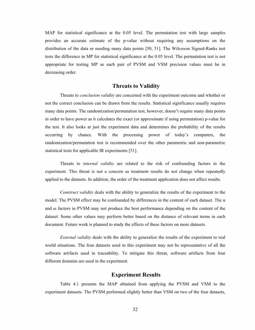
32
MAP for statistical significance at the 0.05 level. The permutation test with large samples
provides an accurate estimate of the p-value without requiring any assumptions on the
distribution of the data or needing many data points [50, 51]. The Wilcoxon Signed-Ranks test
tests the difference in MP for statistical significance at the 0.05 level. The permutation test is not
appropriate for testing MP as each pair of PVSM and VSM precision values must be in
decreasing order.
Threats to Validity Threats to conclusion validity are concerned with the experiment outcome and whether or
not the correct conclusion can be drawn from the results. Statistical significance usually requires
many data points. The randomization/permutation test, however, doesn’t require many data points
in order to have power as it calculates the exact (or approximate if using permutation) p-value for
the test. It also looks at just the experiment data and determines the probability of the results
occurring by chance. With the processing power of today’s computers, the
randomization/permutation test is recommended over the other parametric and non-parametric
statistical tests for applicable IR experiments [51].
Threats to internal validity are related to the risk of confounding factors in the
experiment. This threat is not a concern as treatment results do not change when repeatedly
applied to the datasets. In addition, the order of the treatment application does not affect results.
Construct validity deals with the ability to generalize the results of the experiment to the
model. The PVSM effect may be confounded by differences in the content of each dataset. The α
and ω factors in PVSM may not produce the best performance depending on the content of the
dataset. Some other values may perform better based on the distance of relevant terms in each
document. Future work is planned to study the effects of these factors on more datasets.
External validity deals with the ability to generalize the results of the experiment to real
world situations. The four datasets used in this experiment may not be representative of all the
software artifacts used in traceability. To mitigate this threat, software artifacts from four
different domains are used in the experiment.
Experiment Results Table 4.1 presents the MAP obtained from applying the PVSM and VSM to the
experiment datasets. The PVSM performed slightly better than VSM on two of the four datasets,
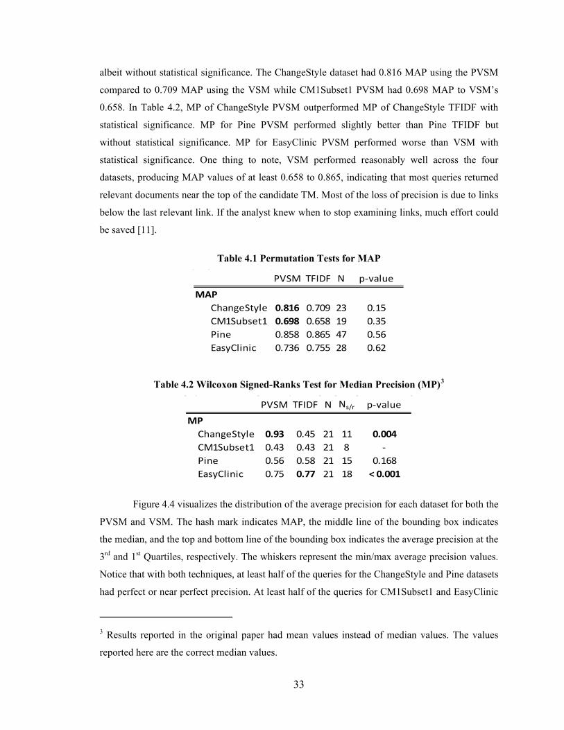
33
albeit without statistical significance. The ChangeStyle dataset had 0.816 MAP using the PVSM
compared to 0.709 MAP using the VSM while CM1Subset1 PVSM had 0.698 MAP to VSM’s
0.658. In Table 4.2, MP of ChangeStyle PVSM outperformed MP of ChangeStyle TFIDF with
statistical significance. MP for Pine PVSM performed slightly better than Pine TFIDF but
without statistical significance. MP for EasyClinic PVSM performed worse than VSM with
statistical significance. One thing to note, VSM performed reasonably well across the four
datasets, producing MAP values of at least 0.658 to 0.865, indicating that most queries returned
relevant documents near the top of the candidate TM. Most of the loss of precision is due to links
below the last relevant link. If the analyst knew when to stop examining links, much effort could
be saved [11].
Table 4.1 Permutation Tests for MAP
PVSM TFIDF N p-value
MAPChangeStyle 0.816 0.709 23 0.15CM1Subset1 0.698 0.658 19 0.35Pine 0.858 0.865 47 0.56EasyClinic 0.736 0.755 28 0.62
Table 4.2 Wilcoxon Signed-Ranks Test for Median Precision (MP)3
PVSM TFIDF N Ns/r p-value
MPChangeStyle 0.93 0.45 21 11 0.004CM1Subset1 0.43 0.43 21 8 -Pine 0.56 0.58 21 15 0.168EasyClinic 0.75 0.77 21 18 < 0.001
Figure 4.4 visualizes the distribution of the average precision for each dataset for both the
PVSM and VSM. The hash mark indicates MAP, the middle line of the bounding box indicates
the median, and the top and bottom line of the bounding box indicates the average precision at the
3rd and 1st Quartiles, respectively. The whiskers represent the min/max average precision values.
Notice that with both techniques, at least half of the queries for the ChangeStyle and Pine datasets
had perfect or near perfect precision. At least half of the queries for CM1Subset1 and EasyClinic
3 Results reported in the original paper had mean values instead of median values. The values
reported here are the correct median values.
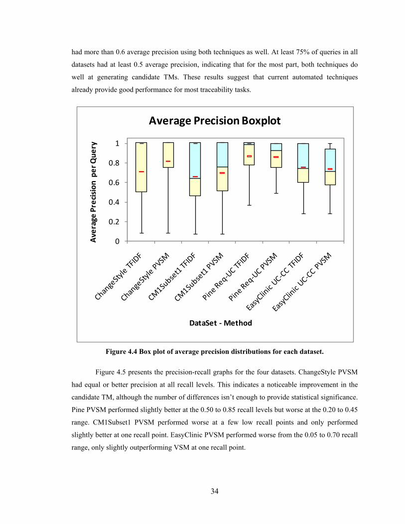
34
had more than 0.6 average precision using both techniques as well. At least 75% of queries in all
datasets had at least 0.5 average precision, indicating that for the most part, both techniques do
well at generating candidate TMs. These results suggest that current automated techniques
already provide good performance for most traceability tasks.
Figure 4.4 Box plot of average precision distributions for each dataset.
Figure 4.5 presents the precision-recall graphs for the four datasets. ChangeStyle PVSM
had equal or better precision at all recall levels. This indicates a noticeable improvement in the
candidate TM, although the number of differences isn’t enough to provide statistical significance.
Pine PVSM performed slightly better at the 0.50 to 0.85 recall levels but worse at the 0.20 to 0.45
range. CM1Subset1 PVSM performed worse at a few low recall points and only performed
slightly better at one recall point. EasyClinic PVSM performed worse from the 0.05 to 0.70 recall
range, only slightly outperforming VSM at one recall point.
0
0.2
0.4
0.6
0.8
1
Aver
age
Prec
ision
per
Que
ry
DataSet - Method
Average Precision Boxplot
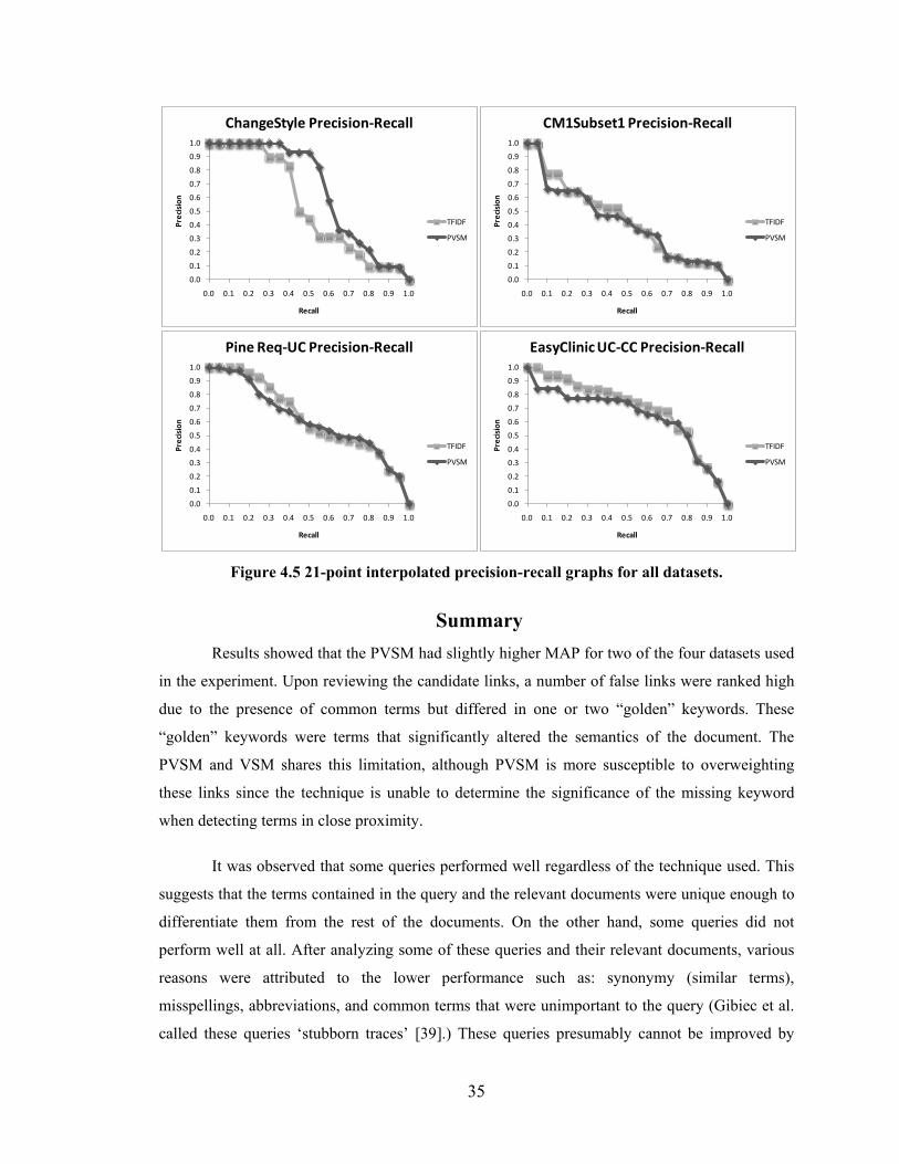
35
Figure 4.5 21-point interpolated precision-recall graphs for all datasets.
Summary Results showed that the PVSM had slightly higher MAP for two of the four datasets used
in the experiment. Upon reviewing the candidate links, a number of false links were ranked high
due to the presence of common terms but differed in one or two “golden” keywords. These
“golden” keywords were terms that significantly altered the semantics of the document. The
PVSM and VSM shares this limitation, although PVSM is more susceptible to overweighting
these links since the technique is unable to determine the significance of the missing keyword
when detecting terms in close proximity.
It was observed that some queries performed well regardless of the technique used. This
suggests that the terms contained in the query and the relevant documents were unique enough to
differentiate them from the rest of the documents. On the other hand, some queries did not
perform well at all. After analyzing some of these queries and their relevant documents, various
reasons were attributed to the lower performance such as: synonymy (similar terms),
misspellings, abbreviations, and common terms that were unimportant to the query (Gibiec et al.
called these queries ‘stubborn traces’ [39].) These queries presumably cannot be improved by
0.0
0.1
0.2
0.3
0.4
0.5
0.6
0.7
0.8
0.9
1.0
0.0 0.1 0.2 0.3 0.4 0.5 0.6 0.7 0.8 0.9 1.0
Prec
ision
Recall
EasyClinic UC-CC Precision-Recall
TFIDF
PVSM
0.0
0.1
0.2
0.3
0.4
0.5
0.6
0.7
0.8
0.9
1.0
0.0 0.1 0.2 0.3 0.4 0.5 0.6 0.7 0.8 0.9 1.0
Prec
ision
Recall
Pine Req-UC Precision-Recall
TFIDF
PVSM
0.0
0.1
0.2
0.3
0.4
0.5
0.6
0.7
0.8
0.9
1.0
0.0 0.1 0.2 0.3 0.4 0.5 0.6 0.7 0.8 0.9 1.0
Prec
ision
Recall
ChangeStyle Precision-Recall
TFIDF
PVSM
0.0
0.1
0.2
0.3
0.4
0.5
0.6
0.7
0.8
0.9
1.0
0.0 0.1 0.2 0.3 0.4 0.5 0.6 0.7 0.8 0.9 1.0
Prec
ision
Recall
CM1Subset1 Precision-Recall
TFIDF
PVSM
36
using frequency-based information alone and could benefit from techniques that are not based on
term frequency such as LSI or use of a thesaurus.
Results suggest that average precision can be used to categorize the difficulty level of
datasets. Datasets that have high MAP with basic IR techniques presumably would not benefit
much from the application of more advanced techniques. Identifying queries that have low
average precision allows a researcher to focus on improving such queries or to detect erroneous
links in the answer set. In this study, Pine had a large proportion of queries that returned many
relevant documents near the top of the candidate link list, resulting in high MAP. Differences in
MAP were influenced by a small number of queries in that dataset. CM1Subset1 and EasyClinic
were comparatively harder datasets with a lower MAP, although they both had MAP over 0.65.
More datasets, however, need to be analyzed in order to validate this idea.
This work in the dissertation introduces a new tracing technique called the PVSM and
validates it using MAP as a measure of the internal quality of a candidate TM. Results show that
PVSM outperforms VSM on two datasets although without statistical significance. The 21-point
interpolated precision-recall graph can be used to visualize the overall performance between two
techniques and test for significant difference in MP. In this study, PVSM outperformed VSM on
MP for ChangeStyle but not for EasyClinic.
Copyright © Wei-Keat Kong 2012

37
Chapter 5 - Logging and Depicting Analyst Actions during
Trace Validation Tasks4
This chapter presents the contribution of an initial study of analyst tracing behavior in the
context of trace validation tasks.
Requirements Tracing and the Role of Human Analysts Research has shown that automated traceability techniques retrieve traceability links
faster than manual techniques [7, 14] and are capable of retrieving most of the true links but at the
cost of retrieving many false links [7, 14, 52, 53].
The key reason for studying automated methods for tracing is to replace menial analyst
effort. In some settings where tracing occurs, e.g., post-deployment activities such as reverse
engineering, fully automated tracing is a feasible alternative to the manual tracing procedures of
today. However, trace recovery and trace validation tasks for mission- or safety-critical projects
must include a human analyst who validates and updates, as necessary, any automatically
generated traces. In such settings, automated tracing tools are still appropriate, as they can “cover
more ground” much faster and present a reduced search space for an analyst to search for links in
a matter of minutes. But it is the accuracy of the final TM, delivered and certified by the analyst,
that serves as the final judgment of success or failure of the tracing process.
Figure 5.1 depicts the results from a study of how well analysts performed when given
candidate TMs with difference accuracies [13]. Each participant's performance is represented by a
vector with the tail indicating the accuracy of the candidate TM and the head (arrow) indicating
the accuracy of the final TM. The results of the study confirmed initial observations: human
analysts that get more accurate candidate TMs do not always produce more accurate final TMs. In
fact, one of the most important observations from the study was that the analysts who were
4 © 2011 ACM. Revision of the work published in “How Do We Trace Requirements? An Initial Study of Analyst Behavior in Trace Validation Tasks” by Wei-Keat Kong, Jane Huffman Hayes, Alex Dekhtyar, Jeff Holden, 2011. Proceedings of the 4th International Workshop on Cooperative and Human Aspects of Software Engineering (CHASE 2011), International Conference on Software Engineering (ICSE Conference).
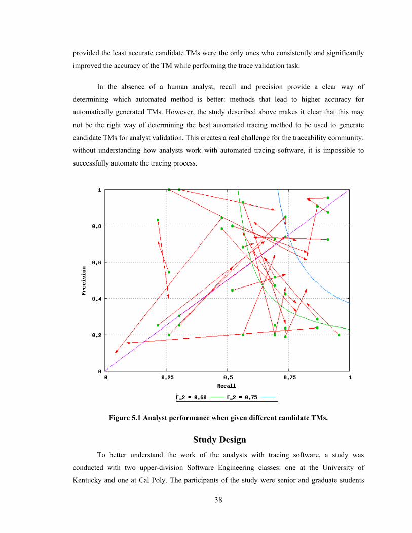
38
provided the least accurate candidate TMs were the only ones who consistently and significantly
improved the accuracy of the TM while performing the trace validation task.
In the absence of a human analyst, recall and precision provide a clear way of
determining which automated method is better: methods that lead to higher accuracy for
automatically generated TMs. However, the study described above makes it clear that this may
not be the right way of determining the best automated tracing method to be used to generate
candidate TMs for analyst validation. This creates a real challenge for the traceability community:
without understanding how analysts work with automated tracing software, it is impossible to
successfully automate the tracing process.
Figure 5.1 Analyst performance when given different candidate TMs.
Study Design To better understand the work of the analysts with tracing software, a study was
conducted with two upper-division Software Engineering classes: one at the University of
Kentucky and one at Cal Poly. The participants of the study were senior and graduate students
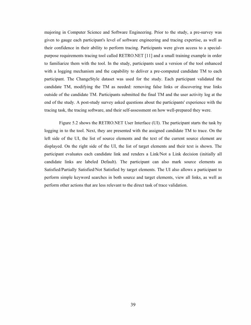
39
majoring in Computer Science and Software Engineering. Prior to the study, a pre-survey was
given to gauge each participant's level of software engineering and tracing expertise, as well as
their confidence in their ability to perform tracing. Participants were given access to a special-
purpose requirements tracing tool called RETRO.NET [11] and a small training example in order
to familiarize them with the tool. In the study, participants used a version of the tool enhanced
with a logging mechanism and the capability to deliver a pre-computed candidate TM to each
participant. The ChangeStyle dataset was used for the study. Each participant validated the
candidate TM, modifying the TM as needed: removing false links or discovering true links
outside of the candidate TM. Participants submitted the final TM and the user activity log at the
end of the study. A post-study survey asked questions about the participants' experience with the
tracing task, the tracing software, and their self-assessment on how well-prepared they were.
Figure 5.2 shows the RETRO.NET User Interface (UI). The participant starts the task by
logging in to the tool. Next, they are presented with the assigned candidate TM to trace. On the
left side of the UI, the list of source elements and the text of the current source element are
displayed. On the right side of the UI, the list of target elements and their text is shown. The
participant evaluates each candidate link and renders a Link/Not a Link decision (initially all
candidate links are labeled Default). The participant can also mark source elements as
Satisfied/Partially Satisfied/Not Satisfied by target elements. The UI also allows a participant to
perform simple keyword searches in both source and target elements, view all links, as well as
perform other actions that are less relevant to the direct task of trace validation.
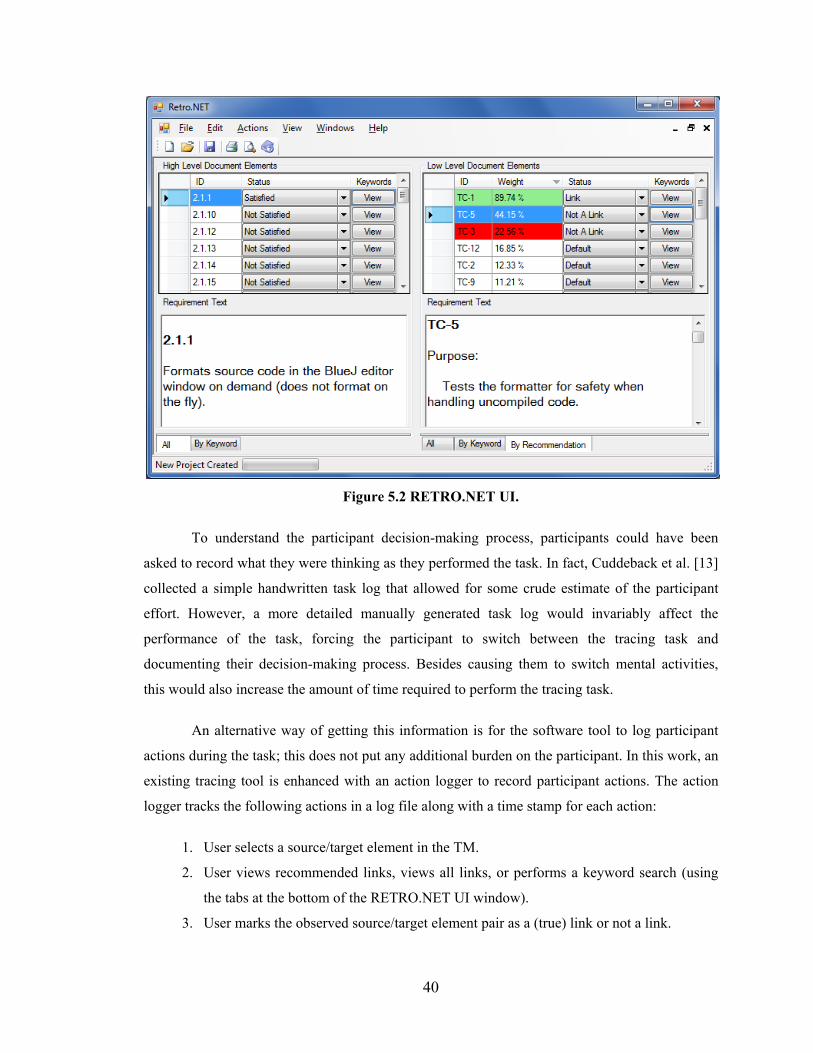
40
Figure 5.2 RETRO.NET UI.
To understand the participant decision-making process, participants could have been
asked to record what they were thinking as they performed the task. In fact, Cuddeback et al. [13]
collected a simple handwritten task log that allowed for some crude estimate of the participant
effort. However, a more detailed manually generated task log would invariably affect the
performance of the task, forcing the participant to switch between the tracing task and
documenting their decision-making process. Besides causing them to switch mental activities,
this would also increase the amount of time required to perform the tracing task.
An alternative way of getting this information is for the software tool to log participant
actions during the task; this does not put any additional burden on the participant. In this work, an
existing tracing tool is enhanced with an action logger to record participant actions. The action
logger tracks the following actions in a log file along with a time stamp for each action:
1. User selects a source/target element in the TM.
2. User views recommended links, views all links, or performs a keyword search (using
the tabs at the bottom of the RETRO.NET UI window).
3. User marks the observed source/target element pair as a (true) link or not a link.
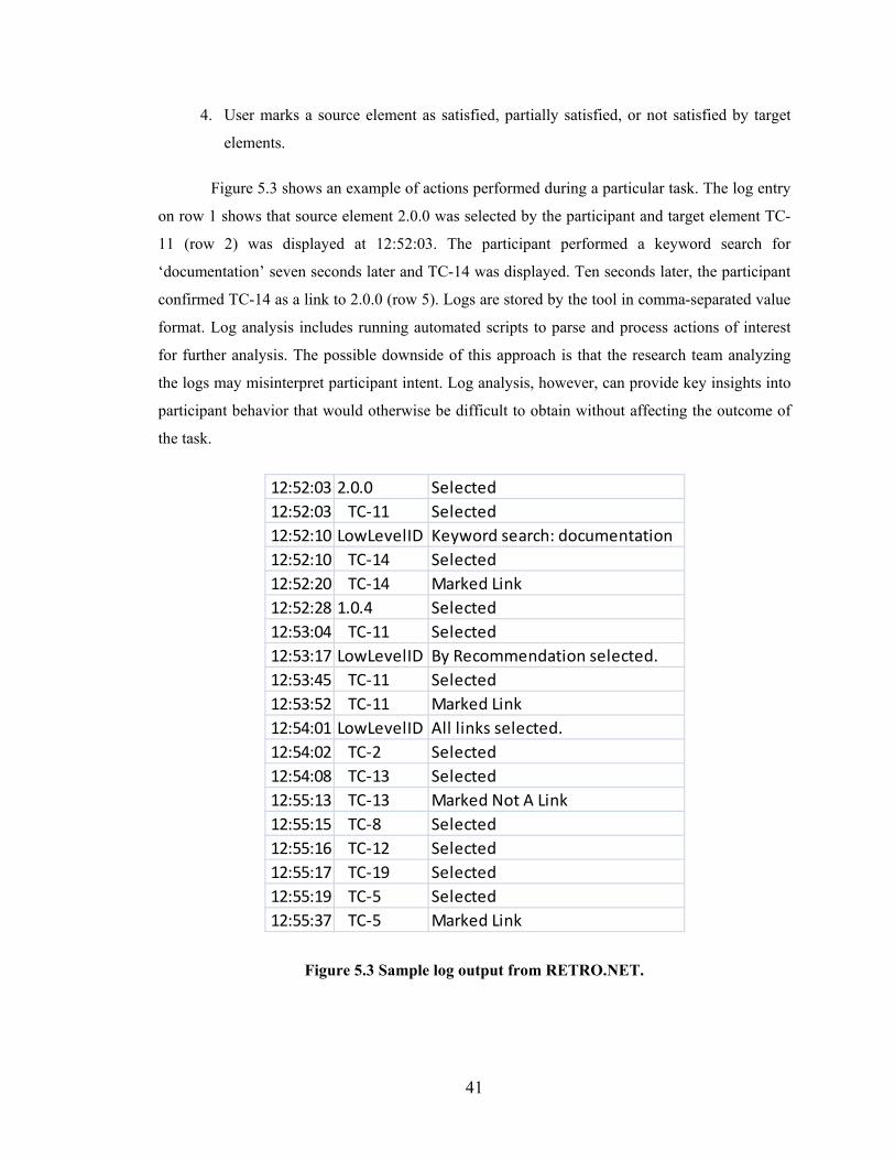
41
4. User marks a source element as satisfied, partially satisfied, or not satisfied by target
elements.
Figure 5.3 shows an example of actions performed during a particular task. The log entry
on row 1 shows that source element 2.0.0 was selected by the participant and target element TC-
11 (row 2) was displayed at 12:52:03. The participant performed a keyword search for
‘documentation’ seven seconds later and TC-14 was displayed. Ten seconds later, the participant
confirmed TC-14 as a link to 2.0.0 (row 5). Logs are stored by the tool in comma-separated value
format. Log analysis includes running automated scripts to parse and process actions of interest
for further analysis. The possible downside of this approach is that the research team analyzing
the logs may misinterpret participant intent. Log analysis, however, can provide key insights into
participant behavior that would otherwise be difficult to obtain without affecting the outcome of
the task.
Figure 5.3 Sample log output from RETRO.NET.
12:52:03 2.0.0 Selected12:52:03 TC-11 Selected12:52:10 LowLevelID Keyword search: documentation12:52:10 TC-14 Selected12:52:20 TC-14 Marked Link12:52:28 1.0.4 Selected12:53:04 TC-11 Selected12:53:17 LowLevelID By Recommendation selected.12:53:45 TC-11 Selected12:53:52 TC-11 Marked Link12:54:01 LowLevelID All links selected.12:54:02 TC-2 Selected12:54:08 TC-13 Selected12:55:13 TC-13 Marked Not A Link12:55:15 TC-8 Selected12:55:16 TC-12 Selected12:55:17 TC-19 Selected12:55:19 TC-5 Selected12:55:37 TC-5 Marked Link
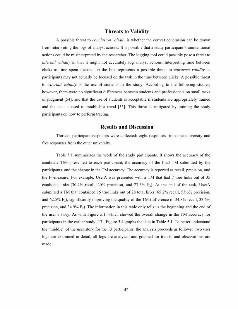
42
Threats to Validity A possible threat to conclusion validity is whether the correct conclusion can be drawn
from interpreting the logs of analyst actions. It is possible that a study participant’s unintentional
actions could be misinterpreted by the researcher. The logging tool could possibly pose a threat to
internal validity in that it might not accurately log analyst actions. Interpreting time between
clicks as time spent focused on the link represents a possible threat to construct validity as
participants may not actually be focused on the task in the time between clicks. A possible threat
to external validity is the use of students in the study. According to the following studies,
however, there were no significant differences between students and professionals on small tasks
of judgment [54], and that the use of students is acceptable if students are appropriately trained
and the data is used to establish a trend [55]. This threat is mitigated by training the study
participants on how to perform tracing.
Results and Discussion Thirteen participant responses were collected: eight responses from one university and
five responses from the other university.
Table 5.1 summarizes the work of the study participants. It shows the accuracy of the
candidate TMs presented to each participant, the accuracy of the final TM submitted by the
participants, and the change in the TM accuracy. The accuracy is reported as recall, precision, and
the F2-measure. For example, UserA was presented with a TM that had 7 true links out of 35
candidate links (30.4% recall, 20% precision, and 27.6% F2). At the end of the task, UserA
submitted a TM that contained 15 true links out of 28 total links (65.2% recall, 53.6% precision,
and 62.5% F2), significantly improving the quality of the TM (difference of 34.8% recall, 33.6%
precision, and 34.9% F2). The information in this table only tells us the beginning and the end of
the user’s story. As with Figure 5.1, which showed the overall change in the TM accuracy for
participants in the earlier study [13], Figure 5.4 graphs the data in Table 5.1. To better understand
the “middle” of the user story for the 13 participants, the analysis proceeds as follows: two user
logs are examined in detail, all logs are analyzed and graphed for trends, and observations are
made.
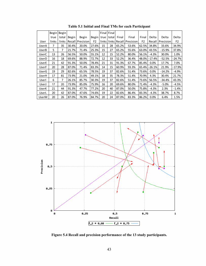
43
Table 5.1 Initial and Final TMs for each Participant
Figure 5.4 Recall and precision performance of the 13 study participants.
User
Begin true links
Begin total links
Begin Recall
Begin Precision
Begin F2
Final true links
Final total links
Final Recall
Final Precision
Final F2
Delta Recall
Delta Precision
Delta F2
UserA 7 35 30.4% 20.0% 27.6% 15 28 65.2% 53.6% 62.5% 34.8% 33.6% 34.9%UserB 5 7 21.7% 71.4% 25.3% 15 27 65.2% 55.6% 63.0% 43.5% -15.9% 37.8%UserC 13 26 56.5% 50.0% 55.1% 12 15 52.2% 80.0% 56.1% -4.3% 30.0% 1.0%UserD 16 18 69.6% 88.9% 72.7% 12 33 52.2% 36.4% 48.0% -17.4% -52.5% -24.7%UserE 21 42 91.3% 50.0% 78.4% 21 31 91.3% 67.7% 85.4% 0.0% 17.7% 7.0%UserF 20 28 87.0% 71.4% 83.3% 14 15 60.9% 93.3% 65.4% -26.1% 21.9% -17.9%UserG 19 29 82.6% 65.5% 78.5% 19 37 82.6% 51.4% 73.6% 0.0% -14.2% -4.9%UserH 17 81 73.9% 21.0% 49.1% 18 35 78.3% 51.4% 70.9% 4.3% 30.4% 21.7%UserI 6 7 26.1% 85.7% 30.3% 19 37 82.6% 51.4% 73.6% 56.5% -34.4% 43.3%UserJ 17 20 73.9% 85.0% 75.9% 16 20 69.6% 80.0% 71.4% -4.3% -5.0% -4.5%UserK 21 44 91.3% 47.7% 77.2% 20 40 87.0% 50.0% 75.8% -4.3% 2.3% -1.4%UserL 20 42 87.0% 47.6% 74.6% 19 22 82.6% 86.4% 83.3% -4.3% 38.7% 8.7%UserM 20 26 87.0% 76.9% 84.7% 20 24 87.0% 83.3% 86.2% 0.0% 6.4% 1.5%
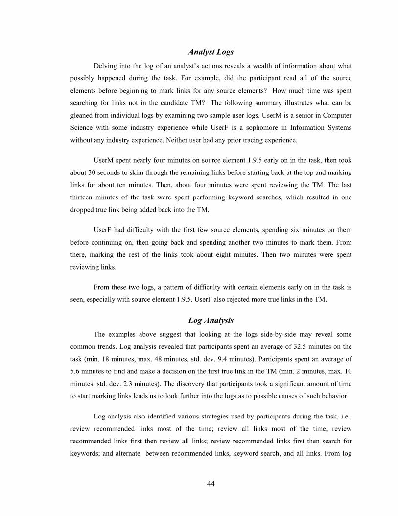
44
Analyst Logs Delving into the log of an analyst’s actions reveals a wealth of information about what
possibly happened during the task. For example, did the participant read all of the source
elements before beginning to mark links for any source elements? How much time was spent
searching for links not in the candidate TM? The following summary illustrates what can be
gleaned from individual logs by examining two sample user logs. UserM is a senior in Computer
Science with some industry experience while UserF is a sophomore in Information Systems
without any industry experience. Neither user had any prior tracing experience.
UserM spent nearly four minutes on source element 1.9.5 early on in the task, then took
about 30 seconds to skim through the remaining links before starting back at the top and marking
links for about ten minutes. Then, about four minutes were spent reviewing the TM. The last
thirteen minutes of the task were spent performing keyword searches, which resulted in one
dropped true link being added back into the TM.
UserF had difficulty with the first few source elements, spending six minutes on them
before continuing on, then going back and spending another two minutes to mark them. From
there, marking the rest of the links took about eight minutes. Then two minutes were spent
reviewing links.
From these two logs, a pattern of difficulty with certain elements early on in the task is
seen, especially with source element 1.9.5. UserF also rejected more true links in the TM.
Log Analysis The examples above suggest that looking at the logs side-by-side may reveal some
common trends. Log analysis revealed that participants spent an average of 32.5 minutes on the
task (min. 18 minutes, max. 48 minutes, std. dev. 9.4 minutes). Participants spent an average of
5.6 minutes to find and make a decision on the first true link in the TM (min. 2 minutes, max. 10
minutes, std. dev. 2.3 minutes). The discovery that participants took a significant amount of time
to start marking links leads us to look further into the logs as to possible causes of such behavior.
Log analysis also identified various strategies used by participants during the task, i.e.,
review recommended links most of the time; review all links most of the time; review
recommended links first then review all links; review recommended links first then search for
keywords; and alternate between recommended links, keyword search, and all links. From log
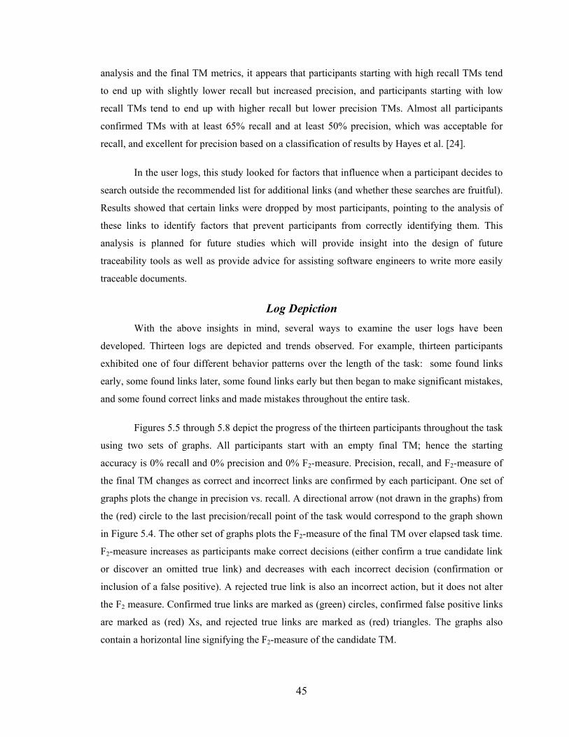
45
analysis and the final TM metrics, it appears that participants starting with high recall TMs tend
to end up with slightly lower recall but increased precision, and participants starting with low
recall TMs tend to end up with higher recall but lower precision TMs. Almost all participants
confirmed TMs with at least 65% recall and at least 50% precision, which was acceptable for
recall, and excellent for precision based on a classification of results by Hayes et al. [24].
In the user logs, this study looked for factors that influence when a participant decides to
search outside the recommended list for additional links (and whether these searches are fruitful).
Results showed that certain links were dropped by most participants, pointing to the analysis of
these links to identify factors that prevent participants from correctly identifying them. This
analysis is planned for future studies which will provide insight into the design of future
traceability tools as well as provide advice for assisting software engineers to write more easily
traceable documents.
Log Depiction With the above insights in mind, several ways to examine the user logs have been
developed. Thirteen logs are depicted and trends observed. For example, thirteen participants
exhibited one of four different behavior patterns over the length of the task: some found links
early, some found links later, some found links early but then began to make significant mistakes,
and some found correct links and made mistakes throughout the entire task.
Figures 5.5 through 5.8 depict the progress of the thirteen participants throughout the task
using two sets of graphs. All participants start with an empty final TM; hence the starting
accuracy is 0% recall and 0% precision and 0% F2-measure. Precision, recall, and F2-measure of
the final TM changes as correct and incorrect links are confirmed by each participant. One set of
graphs plots the change in precision vs. recall. A directional arrow (not drawn in the graphs) from
the (red) circle to the last precision/recall point of the task would correspond to the graph shown
in Figure 5.4. The other set of graphs plots the F2-measure of the final TM over elapsed task time.
F2-measure increases as participants make correct decisions (either confirm a true candidate link
or discover an omitted true link) and decreases with each incorrect decision (confirmation or
inclusion of a false positive). A rejected true link is also an incorrect action, but it does not alter
the F2 measure. Confirmed true links are marked as (green) circles, confirmed false positive links
are marked as (red) Xs, and rejected true links are marked as (red) triangles. The graphs also
contain a horizontal line signifying the F2-measure of the candidate TM.
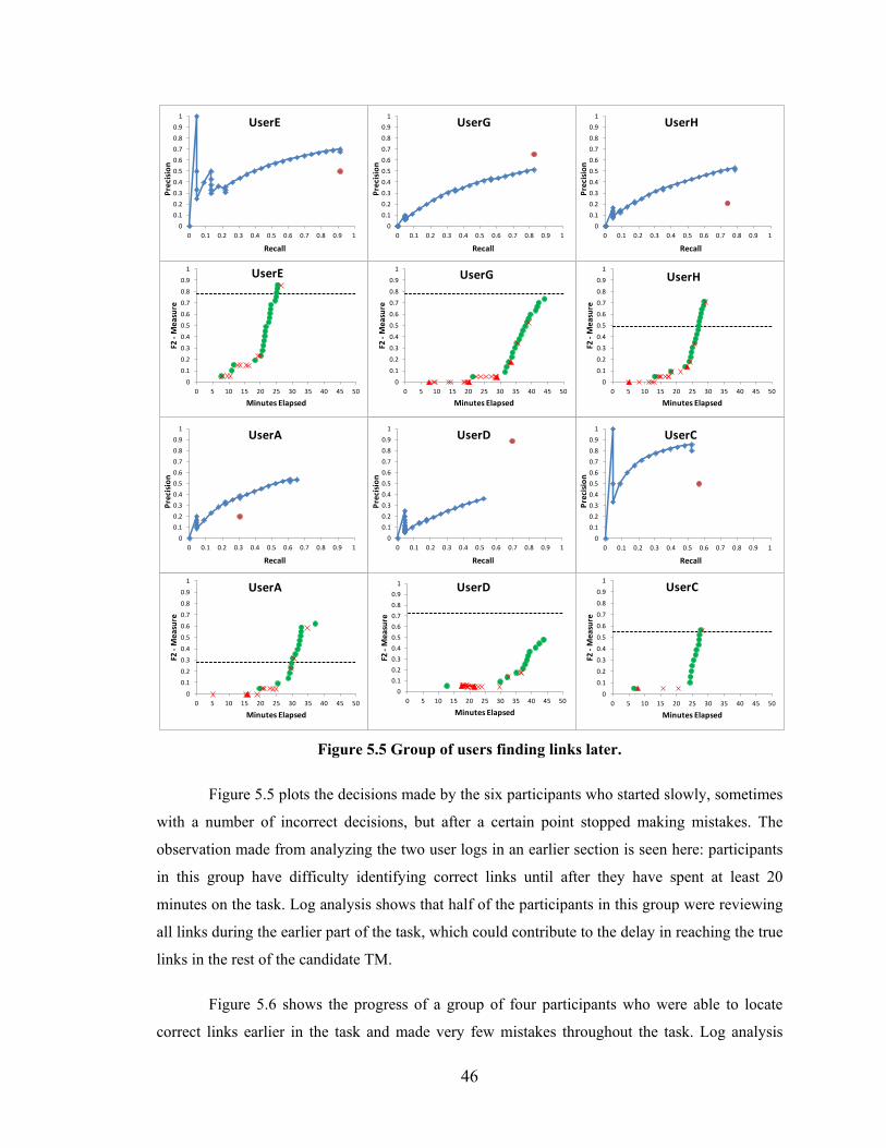
46
Figure 5.5 Group of users finding links later.
Figure 5.5 plots the decisions made by the six participants who started slowly, sometimes
with a number of incorrect decisions, but after a certain point stopped making mistakes. The
observation made from analyzing the two user logs in an earlier section is seen here: participants
in this group have difficulty identifying correct links until after they have spent at least 20
minutes on the task. Log analysis shows that half of the participants in this group were reviewing
all links during the earlier part of the task, which could contribute to the delay in reaching the true
links in the rest of the candidate TM.
Figure 5.6 shows the progress of a group of four participants who were able to locate
correct links earlier in the task and made very few mistakes throughout the task. Log analysis
0
0.1
0.2
0.3
0.4
0.5
0.6
0.7
0.8
0.9
1
0 5 10 15 20 25 30 35 40 45 50
F2 -
Mea
sure
Minutes Elapsed
UserH
0
0.1
0.2
0.3
0.4
0.5
0.6
0.7
0.8
0.9
1
0 5 10 15 20 25 30 35 40 45 50F2
-M
easu
re
Minutes Elapsed
UserG
00.10.20.30.40.50.60.70.80.9
1
0 5 10 15 20 25 30 35 40 45 50
F2 -
Mea
sure
Minutes Elapsed
UserD
0
0.1
0.2
0.3
0.4
0.5
0.6
0.7
0.8
0.9
1
0 5 10 15 20 25 30 35 40 45 50
F2 -
Mea
sure
Minutes Elapsed
UserC
00.10.20.30.40.50.60.70.80.9
1
0 0.1 0.2 0.3 0.4 0.5 0.6 0.7 0.8 0.9 1
Prec
ision
Recall
UserA
00.10.20.30.40.50.60.70.80.9
1
0 0.1 0.2 0.3 0.4 0.5 0.6 0.7 0.8 0.9 1
Prec
ision
Recall
UserC
00.10.20.30.40.50.60.70.80.9
1
0 0.1 0.2 0.3 0.4 0.5 0.6 0.7 0.8 0.9 1
Prec
ision
Recall
UserD
00.10.20.30.40.50.60.70.80.9
1
0 0.1 0.2 0.3 0.4 0.5 0.6 0.7 0.8 0.9 1
Prec
ision
Recall
UserG
00.10.20.30.40.50.60.70.80.9
1
0 0.1 0.2 0.3 0.4 0.5 0.6 0.7 0.8 0.9 1
Prec
ision
Recall
UserH
0
0.1
0.2
0.3
0.4
0.5
0.6
0.7
0.8
0.9
1
0 5 10 15 20 25 30 35 40 45 50
F2 -
Mea
sure
Minutes Elapsed
UserA
0
0.1
0.2
0.3
0.4
0.5
0.6
0.7
0.8
0.9
1
0 5 10 15 20 25 30 35 40 45 50
F2 -
Mea
sure
Minutes Elapsed
UserE
00.10.20.30.40.50.60.70.80.9
1
0 0.1 0.2 0.3 0.4 0.5 0.6 0.7 0.8 0.9 1
Prec
ision
Recall
UserE
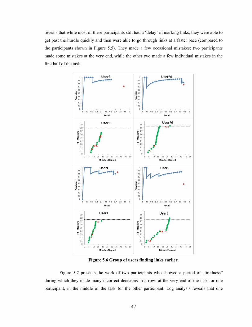
47
reveals that while most of these participants still had a ‘delay’ in marking links, they were able to
get past the hurdle quickly and then were able to go through links at a faster pace (compared to
the participants shown in Figure 5.5). They made a few occasional mistakes: two participants
made some mistakes at the very end, while the other two made a few individual mistakes in the
first half of the task.
Figure 5.6 Group of users finding links earlier.
Figure 5.7 presents the work of two participants who showed a period of “tiredness”
during which they made many incorrect decisions in a row: at the very end of the task for one
participant, in the middle of the task for the other participant. Log analysis reveals that one
0
0.1
0.2
0.3
0.4
0.5
0.6
0.7
0.8
0.9
1
0 5 10 15 20 25 30 35 40 45 50
F2 -
Mea
sure
Minutes Elapsed
UserM
0
0.1
0.2
0.3
0.4
0.5
0.6
0.7
0.8
0.9
1
0 5 10 15 20 25 30 35 40 45 50
F2 -
Mea
sure
Minutes Elapsed
UserJ
0
0.1
0.2
0.3
0.4
0.5
0.6
0.7
0.8
0.9
1
0 5 10 15 20 25 30 35 40 45 50
F2 -
Mea
sure
Minutes Elapsed
UserF
00.10.20.30.40.50.60.70.80.9
1
0 0.1 0.2 0.3 0.4 0.5 0.6 0.7 0.8 0.9 1
Prec
ision
Recall
UserM
00.10.20.30.40.50.60.70.80.9
1
0 0.1 0.2 0.3 0.4 0.5 0.6 0.7 0.8 0.9 1
Prec
ision
Recall
UserF
00.10.20.30.40.50.60.70.80.9
1
0 0.1 0.2 0.3 0.4 0.5 0.6 0.7 0.8 0.9 1
Prec
ision
Recall
UserJ
00.10.20.30.40.50.60.70.80.9
1
0 0.1 0.2 0.3 0.4 0.5 0.6 0.7 0.8 0.9 1
Prec
ision
Recall
UserL
0
0.1
0.2
0.3
0.4
0.5
0.6
0.7
0.8
0.9
1
0 5 10 15 20 25 30 35 40 45 50
F2 -
Mea
sure
Minute Elapsed
UserL
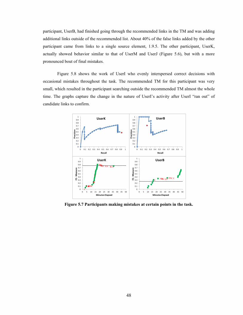
48
participant, UserB, had finished going through the recommended links in the TM and was adding
additional links outside of the recommended list. About 40% of the false links added by the other
participant came from links to a single source element, 1.9.5. The other participant, UserK,
actually showed behavior similar to that of UserM and UserJ (Figure 5.6), but with a more
pronounced bout of final mistakes.
Figure 5.8 shows the work of UserI who evenly interspersed correct decisions with
occasional mistakes throughout the task. The recommended TM for this participant was very
small, which resulted in the participant searching outside the recommended TM almost the whole
time. The graphs capture the change in the nature of UserI’s activity after UserI “ran out” of
candidate links to confirm.
Figure 5.7 Participants making mistakes at certain points in the task.
0
0.1
0.2
0.3
0.4
0.5
0.6
0.7
0.8
0.9
1
0 5 10 15 20 25 30 35 40 45 50
F2 -
Mea
sure
Minutes Elapsed
UserK
00.10.20.30.40.50.60.70.80.9
1
0 0.1 0.2 0.3 0.4 0.5 0.6 0.7 0.8 0.9 1
Prec
ision
Recall
UserB
00.10.20.30.40.50.60.70.80.9
1
0 0.1 0.2 0.3 0.4 0.5 0.6 0.7 0.8 0.9 1
Prec
ision
Recall
UserK
0
0.1
0.2
0.3
0.4
0.5
0.6
0.7
0.8
0.9
1
0 5 10 15 20 25 30 35 40 45 50
F2 -
Mea
sure
Minutes Elapsed
UserB
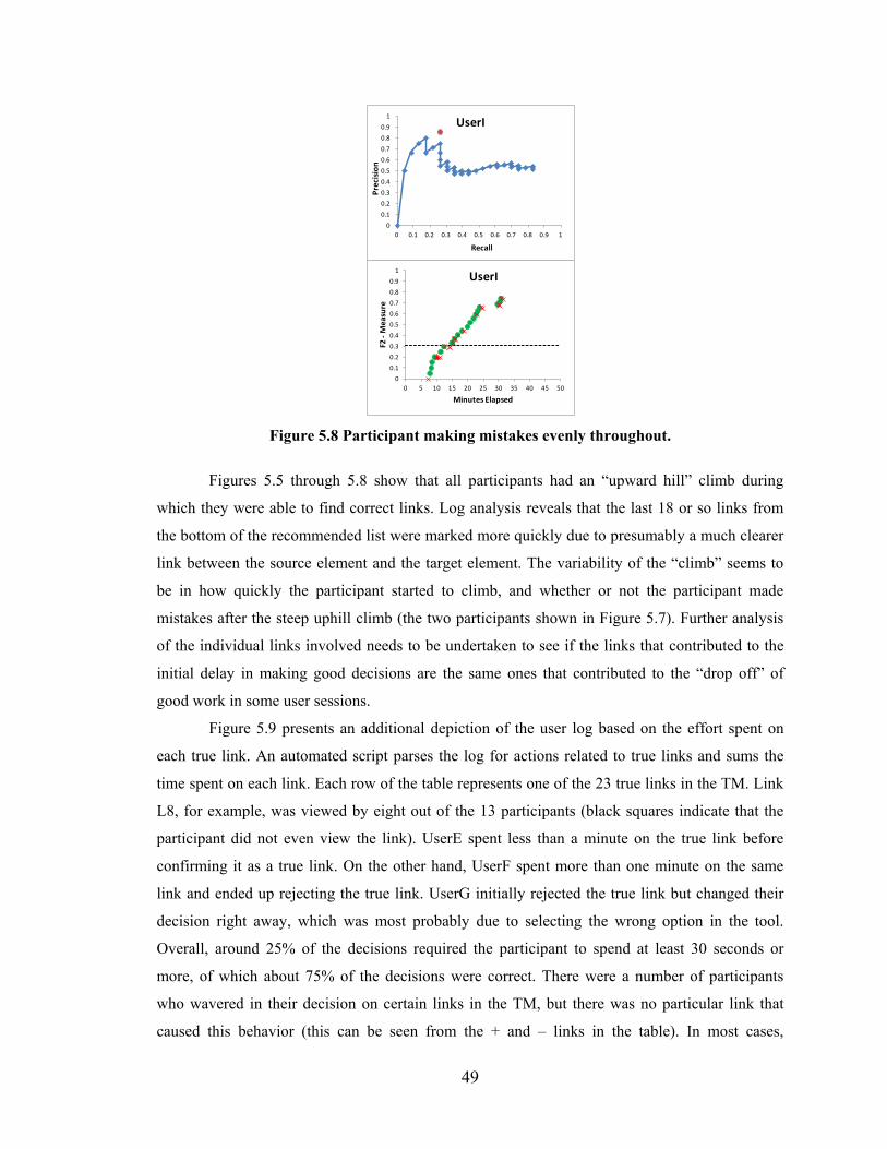
49
Figure 5.8 Participant making mistakes evenly throughout.
Figures 5.5 through 5.8 show that all participants had an “upward hill” climb during
which they were able to find correct links. Log analysis reveals that the last 18 or so links from
the bottom of the recommended list were marked more quickly due to presumably a much clearer
link between the source element and the target element. The variability of the “climb” seems to
be in how quickly the participant started to climb, and whether or not the participant made
mistakes after the steep uphill climb (the two participants shown in Figure 5.7). Further analysis
of the individual links involved needs to be undertaken to see if the links that contributed to the
initial delay in making good decisions are the same ones that contributed to the “drop off” of
good work in some user sessions.
Figure 5.9 presents an additional depiction of the user log based on the effort spent on
each true link. An automated script parses the log for actions related to true links and sums the
time spent on each link. Each row of the table represents one of the 23 true links in the TM. Link
L8, for example, was viewed by eight out of the 13 participants (black squares indicate that the
participant did not even view the link). UserE spent less than a minute on the true link before
confirming it as a true link. On the other hand, UserF spent more than one minute on the same
link and ended up rejecting the true link. UserG initially rejected the true link but changed their
decision right away, which was most probably due to selecting the wrong option in the tool.
Overall, around 25% of the decisions required the participant to spend at least 30 seconds or
more, of which about 75% of the decisions were correct. There were a number of participants
who wavered in their decision on certain links in the TM, but there was no particular link that
caused this behavior (this can be seen from the + and – links in the table). In most cases,
00.10.20.30.40.50.60.70.80.9
1
0 5 10 15 20 25 30 35 40 45 50F2
-M
easu
re
Minutes Elapsed
UserI
00.10.20.30.40.50.60.70.80.9
1
0 0.1 0.2 0.3 0.4 0.5 0.6 0.7 0.8 0.9 1
Prec
ision
Recall
UserI
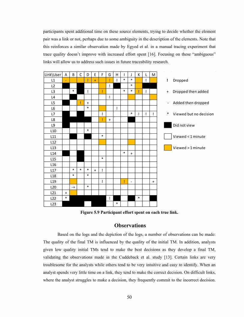
50
participants spent additional time on these source elements, trying to decide whether the element
pair was a link or not, perhaps due to some ambiguity in the description of the elements. Note that
this reinforces a similar observation made by Egyed et al. in a manual tracing experiment that
trace quality doesn’t improve with increased effort spent [16]. Focusing on these “ambiguous”
links will allow us to address such issues in future traceability research.
Figure 5.9 Participant effort spent on each true link.
Observations Based on the logs and the depiction of the logs, a number of observations can be made:
The quality of the final TM is influenced by the quality of the initial TM. In addition, analysts
given low quality initial TMs tend to make the best decisions as they develop a final TM,
validating the observations made in the Cuddeback et al. study [13]. Certain links are very
troublesome for the analysts while others tend to be very intuitive and easy to identify. When an
analyst spends very little time on a link, they tend to make the correct decision. On difficult links,
where the analyst struggles to make a decision, they frequently commit to the incorrect decision.
Link\User A B C D E F G H I J K L ML1 - ! + ! ! * * ! ! Dropped L2 ! *L3 * ! ! * * ! ! + Dropped then addedL4 !L5 ! + - Added then dropped L6 * !L7 ! * ! ! ! * Viewed but no decision L8 ! +L9 Did not viewL10 *L11 * Viewed < 1 minuteL12L13 Viewed > 1 minuteL14 * +L15 *L16L17 * * * + !L18 * *L19 ! ! - +L20 -+ *L21 +L22 * ! *L23 *
51
One key observation discovered through log depictions was that all analysts eventually settle into
a pattern where they make multiple correct decisions in a row. In several of the cases, this
behavior lasts a short time, leading to a second “incorrect link” trend. This “incorrect streak”
often occurred when their final TM recall approached the candidate TM recall. This seems to
occur when analysts did not search outside their candidate TM to locate missing links; instead
they focused on rejecting incorrect links. In most cases these decisions were confirming links
rather than rejecting incorrect links or searching for a missing link. This adds additional support
to the notion that validating a link is a simpler task than discovering a new link [24].
An additional key observation was that analysts tend to cause more errors after the nature
of the task changes. This can be seen when an analyst was presented with an initial TM with low
recall and high precision: such candidate TMs are small. In this study, only two participants,
UserB and UserI, were assigned such TMs. Both participants quickly ran out of candidate links,
appeared to conclude that more links needed to be discovered and, thus, were forced to search for
omitted links. Both participants confirmed many false links past the point where the nature of
their task changed. While anecdotal at this point, if this is confirmed in later studies, this
information can be used as an essential requirement for future tracing tools: the tool should not
produce results with too few links for the analyst to validate, because the switch from link
confirmation to link discovery causes errors of judgment to be introduced.
A final key observation is that, for the most part, analysts were able to use RETRO.NET
effectively with minimal training and guidance. The analysts tended to use the tool as intended,
explored a range of functionality available to them in the tool, and were able to successfully
perform the tracing task.
This work represents an initial study of analyst actions through the logs of their actions.
Analyst actions are visualized to study how they work with candidate TMs to produce the final
TM. These visualizations provide insight into difficulties that analysts encounter when working
with TMs and points to possible improvements to how they can produce better final TMs.
Copyright © Wei-Keat Kong 2012
52
Chapter 6 - Studying Analyst Tracing Behavior5
This chapter provides results from a study of how analysts work with TMs, through
analyzing trace logs and visualizing their progress towards the final TM.
Traceability Process Improvement To move toward improvement of tracing as a practice, it is necessary to consider the
tracing "process improvement feedback loop." Do trends indicating a need for process change
exist and can they be observed? Automated tracing methods do not retrieve perfect TMs [13].
Analysts are not perfect either, and can often make a high quality TM worse [13, 18]. To improve
the practice of traceability, however, analysts need to properly validate TMs and improve their
accuracy. For analysts to do so, this work "drills down" and studies exactly how analysts work
with TMs.
The traceability process improvement goal for this work is to develop procedures and
software that facilitate accurate assisted tracing6 [17]. To that end, there is a need to identify
things that analysts do well and things with which they struggle. Based on this knowledge,
improvements can be made (better tracing methods, better user interfaces, better procedures that
capitalize on analyst strengths) or situations that challenge analysts can be handled or avoided.
While recall and precision address the accuracy of the final tracing product, new
measures are needed to capture information about analyst “behavior.” These measures will enable
researchers to properly understand how analysts perform tracing tasks and to evaluate analyst
work quality. This dissertation posits that recall may not always be preferred over precision when
evaluating analyst quality. Recall only indicates how many true links an analyst added to the final
TM and not how many they did not find or incorrectly rejected. Analysts’ performance should
reflect all their decisions on true and false links. An analyst that rarely rejects a true link, rarely
accepts a false link, and spends less effort on false links produces a high quality final TM.
5 © 2012 Wei-Keat Kong. Revision of the work published in “Process Improvement for
Traceability: A Study of Human Fallibility,” by W.-K. Kong, J. H. Hayes, A. Dekhtyar, and O.
Dekhtyar. University of Kentucky Technical Report TR 520-12, March 5, 2012. 6 Assisted tracing refers to an analyst working with the output of an automated tracing tool.
53
Analysts also need to be put in the situation where they are likely to observe all the true links in
the candidate TM.
This dissertation introduces three new measures that target the study of the tracing
process in addition to the accuracy of the final TM: potential recall, sensitivity, and effort
distribution. These measures are studied in a multi-site and multi-dataset study of assisted
requirements tracing. The study focuses on when and why analysts make correct and incorrect
decisions by logging analyst actions during a tracing task. This work also introduces a matrix
visualization that provides an at-a-glance view of analyst decisions on true links. To support trend
analysis, analyst logs are visualized using a lattice chart that tracks the state of the TM and
analyst measures over time. Participant tracing strategies are identified based on log analysis and
survey data.
Motivation The assisted tracing process is best described as follows: an analyst uses an automated
method to generate a candidate TM, reviews it, makes any desired changes, and “certifies” the
final TM. Human analysts are not perfect and cannot possibly review every link in the candidate
TM without investing significant time and effort. The analyst has to decide how to best spend
their time in order to produce a high quality final TM. The quality of the final TM is measured
against an answer set TM using recall and precision. The quality of analyst decision making on
true links is measured using sensitivity and the following measures.
Since the analyst is not expected to examine every link, some true links may be among
the candidate links not seen by the analyst. Thus, when it comes to validating true links, analyst
accuracy is limited by the percentage of the true links seen. This percentage, dubbed potential
recall, represents the upper bound on recall. It is defined as follows:
Potential recall = TLs / TLt , (14)
where TLs is the number of true links seen (accepted, rejected, or left undecided), and TLt is the
total number of true links in the collection.
Additionally, there is a need to measure analyst effort and how it is spent throughout the
tracing process. In order for analysts to make the best use of their time, the effort spent reviewing
false links should be balanced by the effort spent reviewing true links. The following measure can
54
be used to indicate how analysts spend their time during a tracing task in terms of the number of
links seen:
Effort distribution = FLs / TLs , (15)
where FLs is the number of false links seen and the TLs is the number of true links seen. An
analyst that sees an equal number of true links and false links has an effort distribution of one
(1). This dissertation posits that analysts who view many false links are more likely to accept
some of those links into the final TM, decreasing precision. Note, however, that an analyst may
not go through the trouble of rejecting false links if they know that only accepted links are
included in the final TM, which could result in higher effort distribution if they are skimming
through links looking for specific keywords.
Each analyst, without specific traceability training or guidance, approaches tracing in
their own way. Often, an analyst uses some sort of strategy, either consciously or unconsciously,
to complete the tracing task. Capturing these strategies (without detracting from the actual tracing
task) provides insight as to which strategies produce the best results in terms of potential recall,
sensitivity, and effort distribution. These strategies could also indicate the threshold that an
analyst applies to what they consider to be a true link, which influences the precision of the final
TM.
In order to design reliable and accurate assisted tracing processes, this study investigates
what factors contribute to analyst performance in tracing tasks. In prior studies [13, 17, 18], the
accuracy of the starting candidate TM varied for the tracing task and results showed that the
accuracy of the starting candidate TM strongly influenced the accuracy of the final TM.
Meanwhile, almost no other factors related to individual analyst qualities, their environment, and
their approach to tracing had any significant influence.
The focus of this work is on the link validation task and to “drill down” into analyst
actions using logs of their tracing activity. By having participants work with the same starting
candidate TM, any variability in responses can be attributable to other factors. Three categories of
factors that can influence analyst performance are identified as follows: (i) personal
characteristics, (ii) environmental characteristics, and (iii) tracing behavior. Although these sets
of characteristics are measured in different ways, they are not independent. In particular, the
55
tracing behavior of analysts can be motivated by both their personal characteristics and
environmental factors.
Among the personal characteristics of the participants, this study looks at their grade
level, software engineering experience, tracing experience, and confidence in tracing.
Environmental characteristics are essentially the study dataset and the location/group. Logs and
post-study surveys allow the extraction of information about the tracing behavior of the
participants. This study considers four tracing behaviors: time to complete the tracing task, link
selection strategy, use of feedback, and average number of links viewed per high-level element.
These motivations lead to the following questions:
RQ1: How accurate are analysts at creating the final TM?
RQ2: Do better-performing analysts exhibit certain trends during the tracing task?
RQ3: How do tracing strategies affect the accuracy of the analyst and the final TM?
RQ4: What are statistically significant factors that affect analyst performance?
Study Design This section describes instrumentation, datasets, participants, study design, and data
collection for the study.
Instrumentation To address the research questions in the previous section, an experimental tool called
SmartTracer was created to log participant actions while performing a tracing task. SmartTracer
presents a set of high-level documents (HDs) and a set of low-level documents (LDs) to the
participant, allowing them to make decisions on each retrieved pair of documents. SmartTracer
also allows the participant to make a decision on whether an HD is satisfied by the linked LDs.
The simple user interface is designed to allow the participant to concentrate on the task of making
decisions on trace links. Figure 6.1 shows a screenshot of SmartTracer.
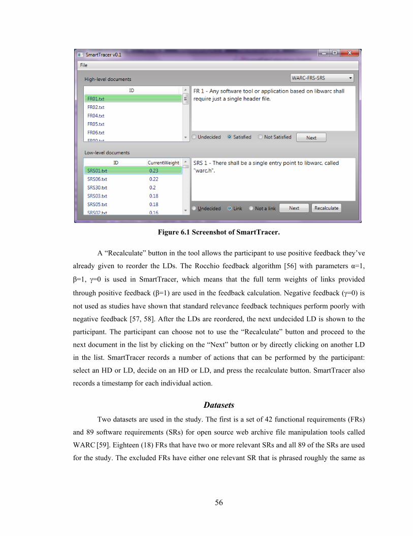
56
Figure 6.1 Screenshot of SmartTracer.
A “Recalculate” button in the tool allows the participant to use positive feedback they’ve
already given to reorder the LDs. The Rocchio feedback algorithm [56] with parameters α=1,
β=1, γ=0 is used in SmartTracer, which means that the full term weights of links provided
through positive feedback (β=1) are used in the feedback calculation. Negative feedback (γ=0) is
not used as studies have shown that standard relevance feedback techniques perform poorly with
negative feedback [57, 58]. After the LDs are reordered, the next undecided LD is shown to the
participant. The participant can choose not to use the “Recalculate” button and proceed to the
next document in the list by clicking on the “Next” button or by directly clicking on another LD
in the list. SmartTracer records a number of actions that can be performed by the participant:
select an HD or LD, decide on an HD or LD, and press the recalculate button. SmartTracer also
records a timestamp for each individual action.
Datasets Two datasets are used in the study. The first is a set of 42 functional requirements (FRs)
and 89 software requirements (SRs) for open source web archive file manipulation tools called
WARC [59]. Eighteen (18) FRs that have two or more relevant SRs and all 89 of the SRs are used
for the study. The excluded FRs have either one relevant SR that is phrased roughly the same as
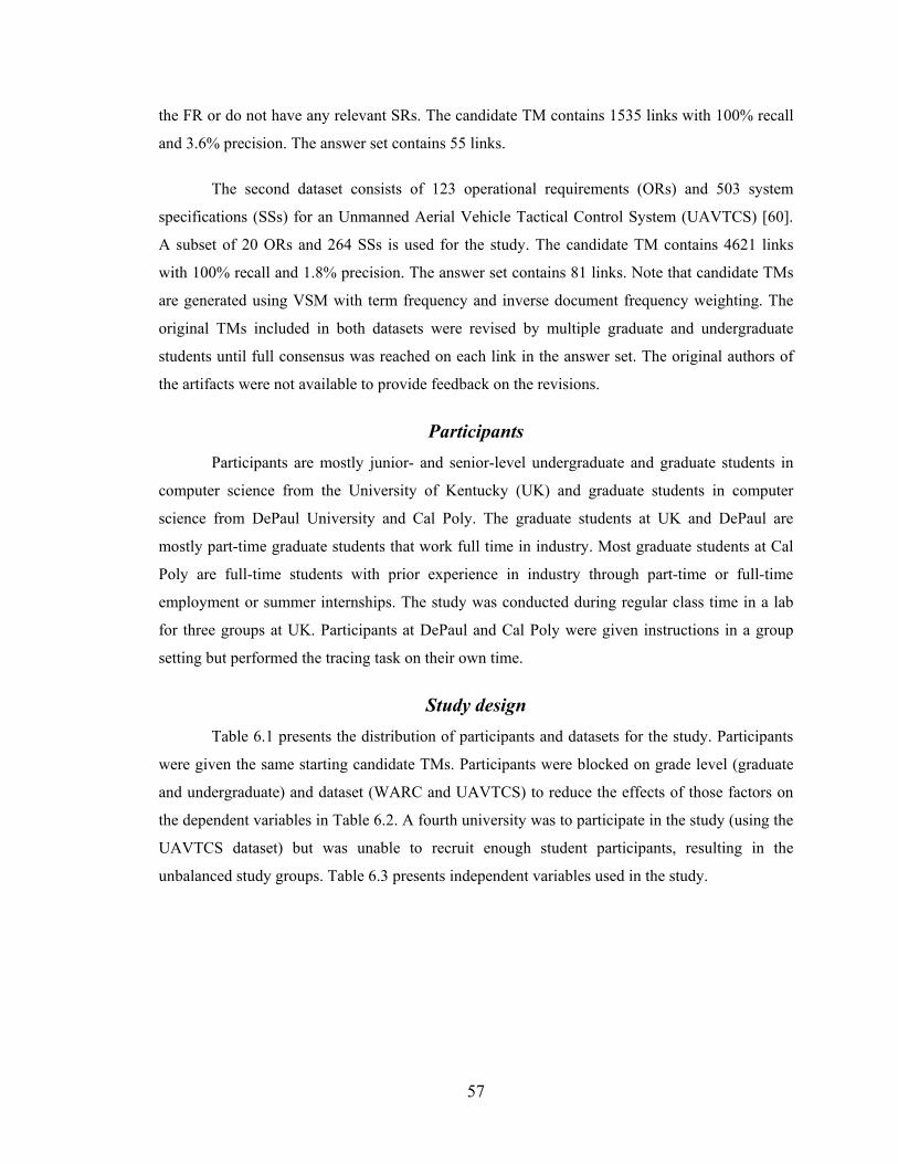
57
the FR or do not have any relevant SRs. The candidate TM contains 1535 links with 100% recall
and 3.6% precision. The answer set contains 55 links.
The second dataset consists of 123 operational requirements (ORs) and 503 system
specifications (SSs) for an Unmanned Aerial Vehicle Tactical Control System (UAVTCS) [60].
A subset of 20 ORs and 264 SSs is used for the study. The candidate TM contains 4621 links
with 100% recall and 1.8% precision. The answer set contains 81 links. Note that candidate TMs
are generated using VSM with term frequency and inverse document frequency weighting. The
original TMs included in both datasets were revised by multiple graduate and undergraduate
students until full consensus was reached on each link in the answer set. The original authors of
the artifacts were not available to provide feedback on the revisions.
Participants Participants are mostly junior- and senior-level undergraduate and graduate students in
computer science from the University of Kentucky (UK) and graduate students in computer
science from DePaul University and Cal Poly. The graduate students at UK and DePaul are
mostly part-time graduate students that work full time in industry. Most graduate students at Cal
Poly are full-time students with prior experience in industry through part-time or full-time
employment or summer internships. The study was conducted during regular class time in a lab
for three groups at UK. Participants at DePaul and Cal Poly were given instructions in a group
setting but performed the tracing task on their own time.
Study design Table 6.1 presents the distribution of participants and datasets for the study. Participants
were given the same starting candidate TMs. Participants were blocked on grade level (graduate
and undergraduate) and dataset (WARC and UAVTCS) to reduce the effects of those factors on
the dependent variables in Table 6.2. A fourth university was to participate in the study (using the
UAVTCS dataset) but was unable to recruit enough student participants, resulting in the
unbalanced study groups. Table 6.3 presents independent variables used in the study.
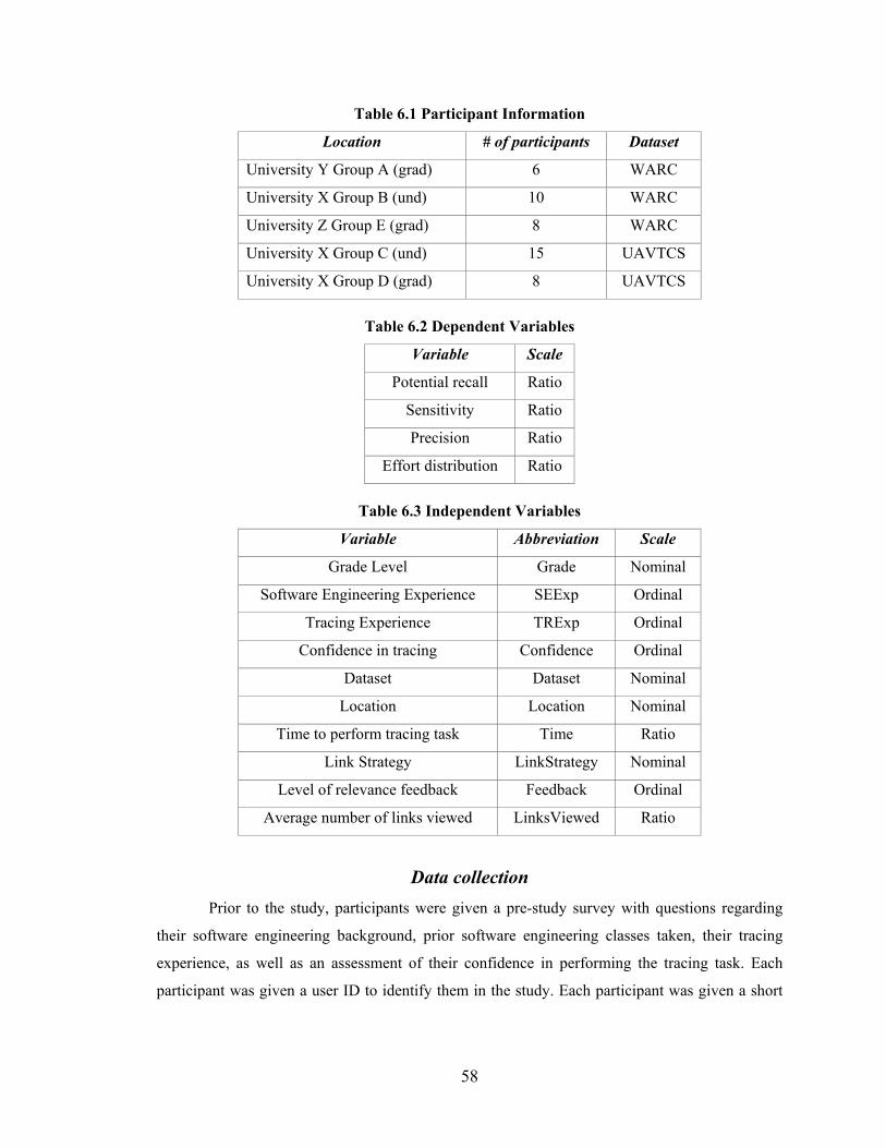
58
Table 6.1 Participant Information
Location # of participants Dataset
University Y Group A (grad) 6 WARC
University X Group B (und) 10 WARC
University Z Group E (grad) 8 WARC
University X Group C (und) 15 UAVTCS
University X Group D (grad) 8 UAVTCS
Table 6.2 Dependent Variables
Variable Scale
Potential recall Ratio
Sensitivity Ratio
Precision Ratio
Effort distribution Ratio
Table 6.3 Independent Variables
Variable Abbreviation Scale
Grade Level Grade Nominal
Software Engineering Experience SEExp Ordinal
Tracing Experience TRExp Ordinal
Confidence in tracing Confidence Ordinal
Dataset Dataset Nominal
Location Location Nominal
Time to perform tracing task Time Ratio
Link Strategy LinkStrategy Nominal
Level of relevance feedback Feedback Ordinal
Average number of links viewed LinksViewed Ratio
Data collection Prior to the study, participants were given a pre-study survey with questions regarding
their software engineering background, prior software engineering classes taken, their tracing
experience, as well as an assessment of their confidence in performing the tracing task. Each
participant was given a user ID to identify them in the study. Each participant was given a short
59
training session on how to use the tracing tool. The overall goal of the study was explained and
instructions were given for them to be mindful of how they perform the task.
After completing the training, participants were given 45 to 60 minutes to complete the
tracing task. Upon completing the tracing task, participants submitted the final TM and trace logs.
The logs track the time spent on each action and record the number of feedback recalculations per
HD.
A post-study survey was given after completing the task, asking each participant to
record: their overall tracing strategy, when they decided to stop looking for additional links,
feedback on what additional tool features might be useful, and their confidence in performing
tracing after performing the task.
Data collection for RQ1 and RQ2: Potential recall, sensitivity, recall, precision, effort
distribution, and final TM size are calculated at each participant’s decision point. Snapshots of
participant decisions are captured at the nearest five-minute mark with the time of the last
decision rounded down to the nearest five-minute mark to plot the charts in Figures 6.3 and 6.4.
Data collection for RQ3: Trace logs and post-study surveys are analyzed to identify
strategies used by participants and compared with data collected for RQ1.
Data collection for RQ4: Pre-study surveys are reviewed and coded into the scales in
Table 6.3. The level of relevance feedback is coded into three levels based on the number of
times participants used the “Recalculate” button.
Threats to Validity Threats to conclusion validity are issues that affect the credibility of the conclusions
reached from the results. The study environment varied due to the multiple locations and
availability of the participants to perform the study at the same time. A possible Hawthorne effect
was introduced when participants were told that their actions were being recorded and that they
were to be mindful of how they performed the tracing task.
Threats to internal validity relate to whether the trends seen are indeed causal. The
somewhat limited amount of time given to participants to complete the tracing task (especially
studies undertaken during class time) could influence results. This was mitigated by having two
of the participant groups perform the study on their own time.
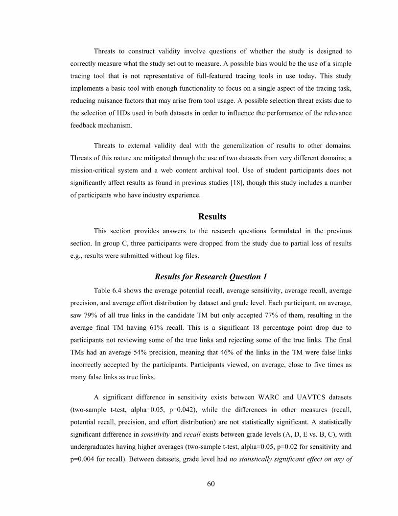
60
Threats to construct validity involve questions of whether the study is designed to
correctly measure what the study set out to measure. A possible bias would be the use of a simple
tracing tool that is not representative of full-featured tracing tools in use today. This study
implements a basic tool with enough functionality to focus on a single aspect of the tracing task,
reducing nuisance factors that may arise from tool usage. A possible selection threat exists due to
the selection of HDs used in both datasets in order to influence the performance of the relevance
feedback mechanism.
Threats to external validity deal with the generalization of results to other domains.
Threats of this nature are mitigated through the use of two datasets from very different domains; a
mission-critical system and a web content archival tool. Use of student participants does not
significantly affect results as found in previous studies [18], though this study includes a number
of participants who have industry experience.
Results This section provides answers to the research questions formulated in the previous
section. In group C, three participants were dropped from the study due to partial loss of results
e.g., results were submitted without log files.
Results for Research Question 1 Table 6.4 shows the average potential recall, average sensitivity, average recall, average
precision, and average effort distribution by dataset and grade level. Each participant, on average,
saw 79% of all true links in the candidate TM but only accepted 77% of them, resulting in the
average final TM having 61% recall. This is a significant 18 percentage point drop due to
participants not reviewing some of the true links and rejecting some of the true links. The final
TMs had an average 54% precision, meaning that 46% of the links in the TM were false links
incorrectly accepted by the participants. Participants viewed, on average, close to five times as
many false links as true links.
A significant difference in sensitivity exists between WARC and UAVTCS datasets
(two-sample t-test, alpha=0.05, p=0.042), while the differences in other measures (recall,
potential recall, precision, and effort distribution) are not statistically significant. A statistically
significant difference in sensitivity and recall exists between grade levels (A, D, E vs. B, C), with
undergraduates having higher averages (two-sample t-test, alpha=0.05, p=0.02 for sensitivity and
p=0.004 for recall). Between datasets, grade level had no statistically significant effect on any of
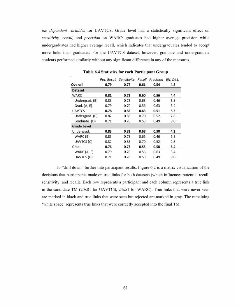
61
the dependent variables for UAVTCS. Grade level had a statistically significant effect on
sensitivity, recall, and precision on WARC: graduates had higher average precision while
undergraduates had higher average recall, which indicates that undergraduates tended to accept
more links than graduates. For the UAVTCS dataset, however, graduate and undergraduate
students performed similarly without any significant difference in any of the measures.
Table 6.4 Statistics for each Participant Group
To “drill down” further into participant results, Figure 6.2 is a matrix visualization of the
decisions that participants made on true links for both datasets (which influences potential recall,
sensitivity, and recall). Each row represents a participant and each column represents a true link
in the candidate TM (20x81 for UAVTCS, 24x51 for WARC). True links that were never seen
are marked in black and true links that were seen but rejected are marked in gray. The remaining
‘white space’ represents true links that were correctly accepted into the final TM.
Pot. Recall Sensitivity Recall Precision Eff. Dist.Overall 0.79 0.77 0.61 0.54 4.8DatasetWARC 0.81 0.73 0.60 0.56 4.4 Undergrad. (B) 0.83 0.78 0.65 0.46 5.8 Grad. (A, E) 0.79 0.70 0.56 0.63 3.4UAVTCS 0.78 0.82 0.63 0.51 5.3 Undergrad. (C) 0.82 0.85 0.70 0.52 2.8 Graduate. (D) 0.71 0.78 0.53 0.49 9.0Grade LevelUndergrad. 0.83 0.82 0.68 0.50 4.2 WARC (B) 0.83 0.78 0.65 0.46 5.8 UAVTCS (C) 0.82 0.85 0.70 0.52 2.8Grad. 0.76 0.73 0.55 0.58 5.4 WARC (A, E) 0.79 0.70 0.56 0.63 3.4 UAVTCS (D) 0.71 0.78 0.53 0.49 9.0
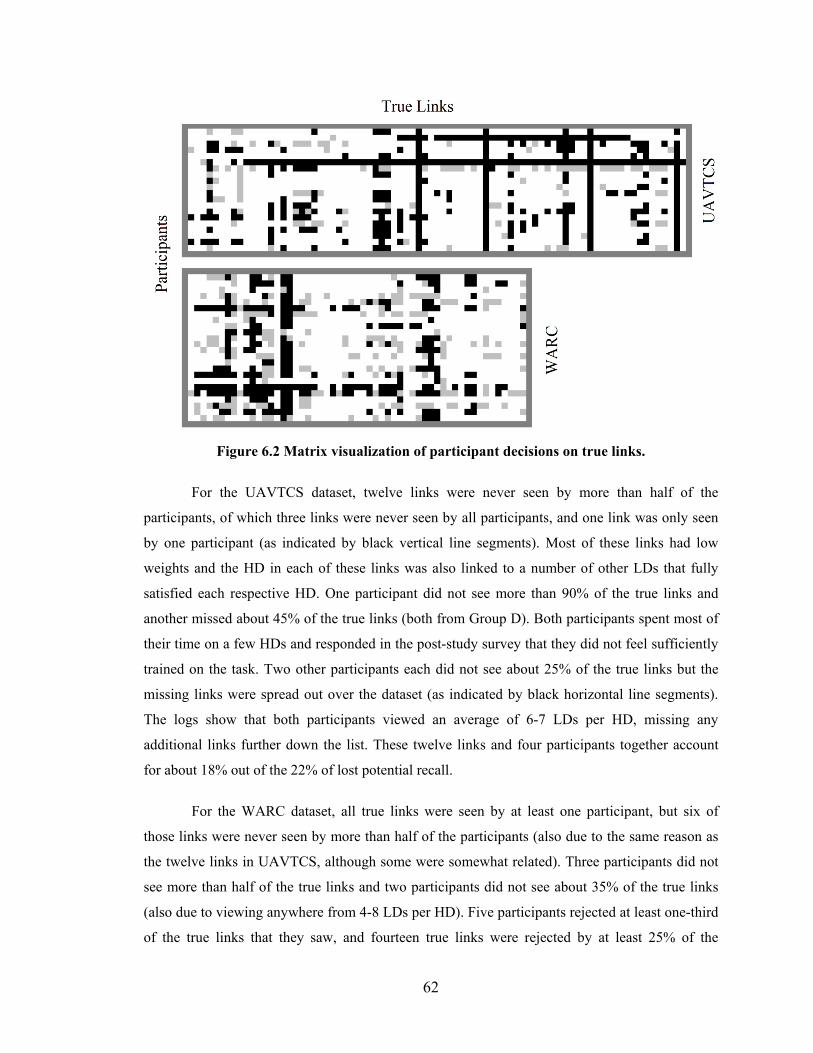
62
Figure 6.2 Matrix visualization of participant decisions on true links.
For the UAVTCS dataset, twelve links were never seen by more than half of the
participants, of which three links were never seen by all participants, and one link was only seen
by one participant (as indicated by black vertical line segments). Most of these links had low
weights and the HD in each of these links was also linked to a number of other LDs that fully
satisfied each respective HD. One participant did not see more than 90% of the true links and
another missed about 45% of the true links (both from Group D). Both participants spent most of
their time on a few HDs and responded in the post-study survey that they did not feel sufficiently
trained on the task. Two other participants each did not see about 25% of the true links but the
missing links were spread out over the dataset (as indicated by black horizontal line segments).
The logs show that both participants viewed an average of 6-7 LDs per HD, missing any
additional links further down the list. These twelve links and four participants together account
for about 18% out of the 22% of lost potential recall.
For the WARC dataset, all true links were seen by at least one participant, but six of
those links were never seen by more than half of the participants (also due to the same reason as
the twelve links in UAVTCS, although some were somewhat related). Three participants did not
see more than half of the true links and two participants did not see about 35% of the true links
(also due to viewing anywhere from 4-8 LDs per HD). Five participants rejected at least one-third
of the true links that they saw, and fourteen true links were rejected by at least 25% of the
63
participants. Most of these rejections were because the LDs in each link were only somewhat
relevant to their respective HDs, causing some participants to waver in their decision.
Results for Research Question 2 Figure 6.3 shows participant performance on the WARC dataset by group on a lattice
chart, tracking potential recall, distribution and TM size (on secondary vertical axis) on the lower
cell at five-minute intervals. The number of links in the answer set is represented as a line
intersecting each bar representing TM size at each time interval. Participant results are sorted by
increasing TM size.
For example, participant B4 had about 5% recall and 65% precision five minutes into the
tracing task and correctly identified all the true links seen up to that point. Thirty minutes into the
task, recall went up to about 30% while precision dropped to about 30% as well. At about 50
minutes (at the end of the task), recall went up to 60%, precision increased to about 40%, but
potential recall was about 90%, i.e., the participant missed about 30% of the true links they saw
(66% sensitivity). Effort distribution steadily increased but leveled off half way through the
tracing task, coinciding with the increased recall and decreased sensitivity (seeing more true links
but rejecting some of them as well).
Similarly, Figure 6.4 shows participant performance on the UAVTCS dataset. Participant
D8 achieved about 5% recall and 60% precision five minutes into the task with 100% sensitivity.
After 30 minutes, precision and sensitivity plunged to about 20% and 30%, respectively.
Additional log analysis revealed that the participant spent about ten minutes on the first two HDs
looking through many LDs, as indicated by the spike in effort distribution. The participant then
started skimming through the remaining HDs, as indicated by the plunge in sensitivity, adding
false links into the final TM, as indicated by the plunge in precision, before spending another 20
minutes on the first two HDs, as indicated by the stagnant recall. The second half of the time saw
a sharp increase in recall as the participant went through the remaining HDs much faster,
accepting many of the true links seen earlier but continuing to accept many false links, as
indicated by increasing recall and sensitivity while lowering precision. The participant ended the
task with a final TM containing 246 links with about 80% recall, 94% sensitivity, and 30%
precision. A number of participants showed similar trends where significant differences between
potential recall and recall early in the tracing task (B1, E2, D4, D8) can be attributed to
participant actions of reading through each HD first before starting to mark links. This can be
64
seen mostly when sensitivity starts low or drops suddenly before increasing steadily as the task
progresses.
WARC participants who performed well (A4, B3, E2) averaged about 75% recall, 59%
precision, and 83% sensitivity while UAVTCS participants who performed well (D1, C1, C2)
also averaged about 76% recall, 58% precision, and 84% sensitivity. These participants increased
recall at a consistent pace, while keeping other measures stable.
In Figure 6.4, participants D2 and D6 did not complete the tracing task as they spent most
of their time on the first few HDs, as indicated by the rapid increase in effort distribution.
Participant D2 changed strategies about 35 minutes into the task (effort distribution peaked and
started coming down) and managed to achieve about 50% recall at the end of the task. Participant
D6, however, spent almost all of their time reviewing false links. Both participants had low
precision from adding many false links into the final TM.
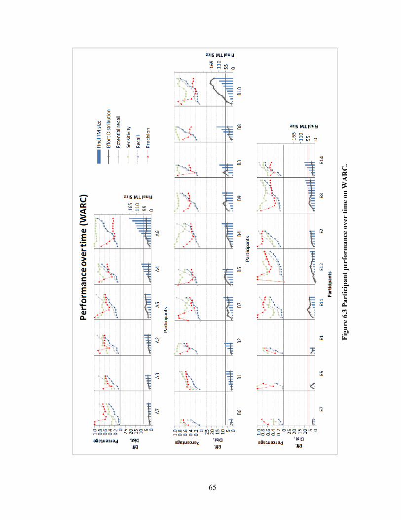
65
Figu
re 6
.3 P
artic
ipan
t per
form
ance
ove
r tim
e on
WA
RC
.
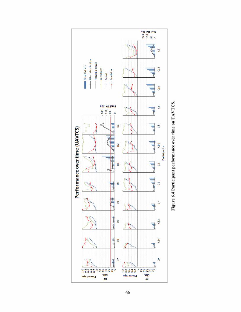
66
Figu
re 6
.4 P
artic
ipan
t per
form
ance
ove
r tim
e on
UA
VT
CS.
67
Results for Research Question 3 SmartTracer directs its users to consider candidate links by HD, consistent with other
tracing software used in similar studies [19, 24, 61]. Analysis of participant logs points to a
number of different strategies used to select links. These strategies are classified based on a single
researcher’s perspective and are briefly outlined below.
First good link. Participants looked through the list of candidate links associated with a single
HD only until they discovered the first good link (one that they think satisfies the HD). They
switched to the next HD immediately after that.
Accept-focused. Participants tended to only submit accept decisions for candidate links, not
bothering to reject links in SmartTracer. These participants understood well that only explicitly
accepted links will be put in the final TM, so not accepting a link is essentially equivalent to
rejecting it.
Preview. Participants previewed their task by reading through the list of HDs and some LDs
before starting to make any decisions on links.
Iterative. Participants revisited most of the HDs more than once to review or change their
decisions.
Some participants used multiple strategies. For some, a distinct strategy could not be
established (Unknown). This study also looked at whether participants used feedback
(“Recalculate” button) during their work. Participants were divided into three categories based on
the average number of links per HD they considered: less than 10, 10 to 20, and more than 20.
Table 6.5 presents the results of the study broken down by participant strategy. For
example, two participants using the “First good link” strategy achieved, on average, 40%
potential recall, 22% recall, 81% precision, and 1.9 effort distribution. This strategy led to fast
task completion (average 15 minutes) but at the cost of not observing a significant number of true
links. On the other hand, participants who used multiple strategies were able to achieve high
potential recall (87% on average) with moderate (4.4. on average) effort distribution.
A significant difference in potential recall and recall exists between those that used
feedback and those who didn’t, but most of the difference can be attributed to the two participants
who used the “first good link” strategy and the participant who only observed two HDs (neither
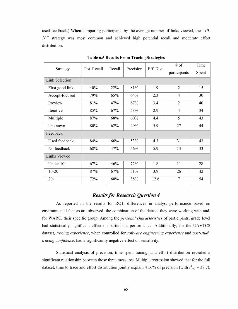
68
used feedback.) When comparing participants by the average number of links viewed, the “10-
20” strategy was most common and achieved high potential recall and moderate effort
distribution.
Table 6.5 Results From Tracing Strategies
Strategy Pot. Recall Recall Precision Eff. Dist. # of
participants
Time
Spent
Link Selection
First good link 40% 22% 81% 1.9 2 15
Accept-focused 79% 65% 64% 2.3 4 30
Preview 81% 47% 67% 3.4 2 40
Iterative 85% 67% 53% 2.9 4 34
Multiple 87% 68% 60% 4.4 5 43
Unknown 80% 62% 49% 5.9 27 44
Feedback
Used feedback 84% 66% 53% 4.3 31 43
No feedback 68% 47% 56% 5.9 13 33
Links Viewed
Under 10 67% 46% 72% 1.8 11 28
10-20 87% 67% 51% 3.9 26 42
20+ 72% 60% 38% 12.6 7 54
Results for Research Question 4 As reported in the results for RQ1, differences in analyst performance based on
environmental factors are observed: the combination of the dataset they were working with and,
for WARC, their specific group. Among the personal characteristics of participants, grade level
had statistically significant effect on participant performance. Additionally, for the UAVTCS
dataset, tracing experience, when controlled for software engineering experience and post-study
tracing confidence, had a significantly negative effect on sensitivity.
Statistical analysis of precision, time spent tracing, and effort distribution revealed a
significant relationship between those three measures. Multiple regression showed that for the full
dataset, time to trace and effort distribution jointly explain 41.6% of precision (with r2adj = 38.7),
69
which is statistically significant. A significant negative correlation with precision exists between
both time to trace (-0.52) and effort distribution (-0.57).
Looking at individual datasets, however, provided some additional insight. For the
WARC dataset, multiple regression showed effort distribution to be significant for precision (r2 =
36.7, r2adj = 30.6) when controlling for time. At the same time, when controlling for effort
distribution, time spent tracing is not a significant influence on precision. For UAVTCS, the
situation is reversed. Controlling for time, multiple regression showed effort distribution to be not
significant for precision, while controlling for effort distribution, time spent tracing is a
significant influence. A similar discrepancy between graduates and undergraduates exists as
well. For graduates, multiple regression showed effort distribution to influence precision
significantly when controlling for time (r2 = 58.1, r2adj = 52.9), while time is not a significant
influence on precision. For undergraduates, the opposite holds.
To summarize, for the WARC dataset, the increase in the number of observed links and
thus the decrease in precision primarily came from participants who viewed more false candidate
links, but it was not affected by how long the participants worked on the tracing task. On the
other hand, for the UAVTCS dataset, increase in the number of links viewed and decrease in
precision primarily came from participants electing to spend more time viewing links, but not
necessarily viewing more false candidate links percentage-wise. Similarly, graduates decreased
their precision whenever they wound up viewing more false candidate links, but not when they
worked longer. Undergraduates decreased their precision with time spent tracing, but not with
how many more false candidate links they saw.
Observations From the results of the previous research questions, results showed that links are more
likely to be missed when there are multiple LDs for an HD and when some of those LDs fully
satisfy the HD. This possibly causes participants to decide at some point that they have enough
LDs to mark the HD “satisfied.” This is especially characteristic of those who never investigate
links that are far down the ranked candidate link list.
Without proper training and direction, some analysts may spend too much time on parts
of the TM where they are more likely to add false links to the TM, decreasing precision.
Participants varied in how selective they are in determining what constitutes a link, possibly
because they did not really know how the TM was to be used.
70
From our observation of the results, participant decisions fall into three categories:
obvious true links, obvious false links, and troublesome gray links, i.e., links that seem to cause
significant amount of deliberation for the analysts. The issue of gray links is also a concern for
researchers when building answer sets (Does the answer set include gray links or not?). These
gray links, nevertheless, represent areas of concern from the viewpoint of the analyst, and should
be investigated further. With knowledge of how the final TM is going to be used, analysts would
then reject or accept all gray links to trigger the appropriate successor activities to resolve those
concerns. Another consideration would be to have a third decision option that separates these
links from the “Yes it’s a link” and “No it’s not a link” decisions. This way, the accuracy of the
analyst at making decisions on links that they think are obvious versus links they think are
“suspect” can be measured.
One of the things that can be done about the analyst other than “embrace” them is to
“change” them [17]. When TM usage is defined, analysts can be “trained” to produce final TMs
that fit the desired final TM characteristic based partially on the final TM size. A final TM size
that is close to the true TM size will have nearly equal precision and recall. Given an estimate of
the true TM size (based on historical data or a starting estimate), analysts are able to be more
aware of their selectiveness when adding links into the final TM, adjusting the thresholds they
apply to links as they proceed through the tracing task and improving their precision. Learning
and applying tracing strategies to tracing tasks is another way to “change” the analyst. Once
studies are undertaken to determine how tracing strategies affect results, analysts will be able to
apply appropriate strategies for the desired tracing task outcomes.
The research contributions of this work are the introduction of analyst-specific measures,
visualization of analyst decisions on true links, and the identification of analyst tracing strategies
through studying the logs of analyst actions. These measures provide a more accurate description
of analyst actions and the visualization of their decisions provides an at-a-glance view of links
that are problematic to analysts. Tracing strategies classified from the analyst logs provide insight
to how analysts approach the task of validating a candidate TM.
Copyright © Wei-Keat Kong 2012
71
Chapter 7 - Conclusions and Future Work
Traceability links recovered after-the-fact from existing software artifacts continue to
present challenges to analysts working with TMs. Although much has been done in the study of
methods to improve the quality of recovered traceability links, the study of the analyst has only
just begun. Even though the analyst introduces subjectivity into the traceability process, it is not
possible to leave the analyst “out of the loop.” Analysts need to have confidence in traceability
tools and in themselves in order to effectively perform tracing tasks. Although studies of new
automated traceability methods will still continue, this work emphasizes the greater need to
understand how analysts work with TMs and how to help them be more effective in tracing tasks.
The following represent the contributions of this dissertation toward the goal of
improving automated traceability techniques and studying how analysts work with TMs:
1. A new proximity-based tracing technique called PVSM was developed, considering the
relevance of documents based on distance between terms in addition to the cosine
similarity weight. Results showed that PVSM performed better than the baseline VSM on
one dataset using the 21-point interpolated precision recall graph and slightly better on
two datasets using MAP.
2. MAP and the 21-point interpolated precision recall graph were introduced and shown to
be effective in evaluating the performance of techniques with statistical rigor in terms of
internal quality and overall quality.
3. Analyst decisions during a tracing task were tracked and saved in the form of trace
activity logs, which were then visualized to show how analysts work with TMs and
analyzed to show how they spent their time during the tracing task.
4. The measures of potential recall, sensitivity, and effort distribution were introduced to
evaluate analyst performance. Logs of analyst actions were visualized to show where
they make correct and incorrect decisions on true links, and investigated to determine the
cause for true links that were never seen and true links that were rejected.
5. Analyst tracing strategies were examined from trace logs and analyzed to determine how
they affect tracing results.
A number of conclusions can be reached based on the results of this dissertation. The
more time analysts spend on links, the more likely they are to make an incorrect decision. The
72
more false links that analysts see, the more likely they are to add those links into the final TM.
This was seen anecdotally in the initial study of the analyst when participants ran out of links and
started searching for additional links, adding many false links into the final TM. In the second
study where participants were only tasked with validating links, a significant association with
precision was found between time spent tracing and effort distribution. This suggests that
participants add more false links into the final TM when they either spend more time on the
tracing task or view more false links. Future work in this area will investigate ways to reduce the
number of false links that analysts view while improving the chances of observing as many true
links as possible. In addition, future work will investigate why true links are rejected by analysts
and identify factors that prevent analysts from correctly identifying these links.
Analysts that employ multiple tracing strategies and use relevance feedback tend to
perform better than other analysts. Future work will include employing multiple reviewers to
classify tracing strategies from the 44 logs and obtain the level of agreement between reviewers
on perceived tracing strategies. Future work will also investigate the influence that tracing
strategies have on the final TM. Prior analyst simulations often assume that analysts provide
perfect feedback. This dissertation reports on a study of actual analysts performing a tracing task
and provides an initial measure of the “imperfect” analyst that misses roughly one out of every
four true links they observe (77% sensitivity). Future studies using relevance feedback will
measure how simulated techniques fare using the tracing strategies mined from trace logs along
with imperfect feedback to validate technique effectiveness.
TMs that have multiple relevant links per high-level element are more likely to have
some links missed by analysts, especially if there are other links that fully satisfy the high-level
element. Future studies will focus on ways to encourage the analyst to continue looking for these
additional links. How a TM will be used in successor activities determines the importance of
recall vs. precision. Future studies will include the investigation of a “gray link” decision as a
possible decision during the tracing task where the analyst is given guidance on final TM usage.
Copyright © Wei-Keat Kong 2012
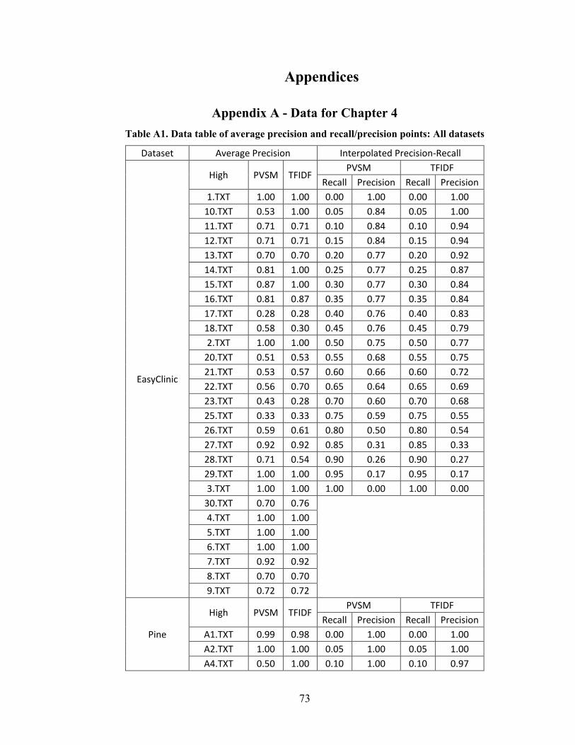
73
Appendices
Appendix A - Data for Chapter 4 Table A1. Data table of average precision and recall/precision points: All datasets
Dataset Average Precision Interpolated Precision-Recall
EasyClinic
High PVSM TFIDF PVSM TFIDF
Recall Precision Recall Precision 1.TXT 1.00 1.00 0.00 1.00 0.00 1.00
10.TXT 0.53 1.00 0.05 0.84 0.05 1.00 11.TXT 0.71 0.71 0.10 0.84 0.10 0.94 12.TXT 0.71 0.71 0.15 0.84 0.15 0.94 13.TXT 0.70 0.70 0.20 0.77 0.20 0.92 14.TXT 0.81 1.00 0.25 0.77 0.25 0.87 15.TXT 0.87 1.00 0.30 0.77 0.30 0.84 16.TXT 0.81 0.87 0.35 0.77 0.35 0.84 17.TXT 0.28 0.28 0.40 0.76 0.40 0.83 18.TXT 0.58 0.30 0.45 0.76 0.45 0.79 2.TXT 1.00 1.00 0.50 0.75 0.50 0.77
20.TXT 0.51 0.53 0.55 0.68 0.55 0.75 21.TXT 0.53 0.57 0.60 0.66 0.60 0.72 22.TXT 0.56 0.70 0.65 0.64 0.65 0.69 23.TXT 0.43 0.28 0.70 0.60 0.70 0.68 25.TXT 0.33 0.33 0.75 0.59 0.75 0.55 26.TXT 0.59 0.61 0.80 0.50 0.80 0.54 27.TXT 0.92 0.92 0.85 0.31 0.85 0.33 28.TXT 0.71 0.54 0.90 0.26 0.90 0.27 29.TXT 1.00 1.00 0.95 0.17 0.95 0.17 3.TXT 1.00 1.00 1.00 0.00 1.00 0.00
30.TXT 0.70 0.76 4.TXT 1.00 1.00 5.TXT 1.00 1.00 6.TXT 1.00 1.00 7.TXT 0.92 0.92 8.TXT 0.70 0.70 9.TXT 0.72 0.72
Pine
High PVSM TFIDF PVSM TFIDF
Recall Precision Recall Precision A1.TXT 0.99 0.98 0.00 1.00 0.00 1.00 A2.TXT 1.00 1.00 0.05 1.00 0.05 1.00 A4.TXT 0.50 1.00 0.10 1.00 0.10 0.97
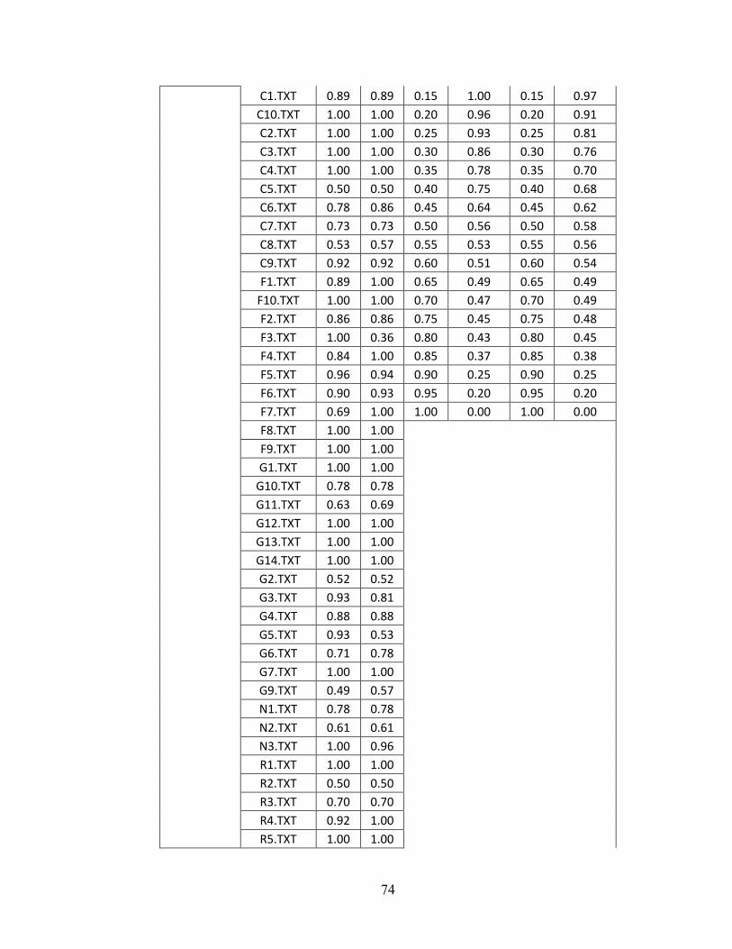
74
C1.TXT 0.89 0.89 0.15 1.00 0.15 0.97 C10.TXT 1.00 1.00 0.20 0.96 0.20 0.91 C2.TXT 1.00 1.00 0.25 0.93 0.25 0.81 C3.TXT 1.00 1.00 0.30 0.86 0.30 0.76 C4.TXT 1.00 1.00 0.35 0.78 0.35 0.70 C5.TXT 0.50 0.50 0.40 0.75 0.40 0.68 C6.TXT 0.78 0.86 0.45 0.64 0.45 0.62 C7.TXT 0.73 0.73 0.50 0.56 0.50 0.58 C8.TXT 0.53 0.57 0.55 0.53 0.55 0.56 C9.TXT 0.92 0.92 0.60 0.51 0.60 0.54 F1.TXT 0.89 1.00 0.65 0.49 0.65 0.49
F10.TXT 1.00 1.00 0.70 0.47 0.70 0.49 F2.TXT 0.86 0.86 0.75 0.45 0.75 0.48 F3.TXT 1.00 0.36 0.80 0.43 0.80 0.45 F4.TXT 0.84 1.00 0.85 0.37 0.85 0.38 F5.TXT 0.96 0.94 0.90 0.25 0.90 0.25 F6.TXT 0.90 0.93 0.95 0.20 0.95 0.20 F7.TXT 0.69 1.00 1.00 0.00 1.00 0.00 F8.TXT 1.00 1.00 F9.TXT 1.00 1.00 G1.TXT 1.00 1.00
G10.TXT 0.78 0.78 G11.TXT 0.63 0.69 G12.TXT 1.00 1.00 G13.TXT 1.00 1.00 G14.TXT 1.00 1.00 G2.TXT 0.52 0.52 G3.TXT 0.93 0.81 G4.TXT 0.88 0.88 G5.TXT 0.93 0.53 G6.TXT 0.71 0.78 G7.TXT 1.00 1.00 G9.TXT 0.49 0.57 N1.TXT 0.78 0.78 N2.TXT 0.61 0.61 N3.TXT 1.00 0.96 R1.TXT 1.00 1.00 R2.TXT 0.50 0.50 R3.TXT 0.70 0.70 R4.TXT 0.92 1.00 R5.TXT 1.00 1.00
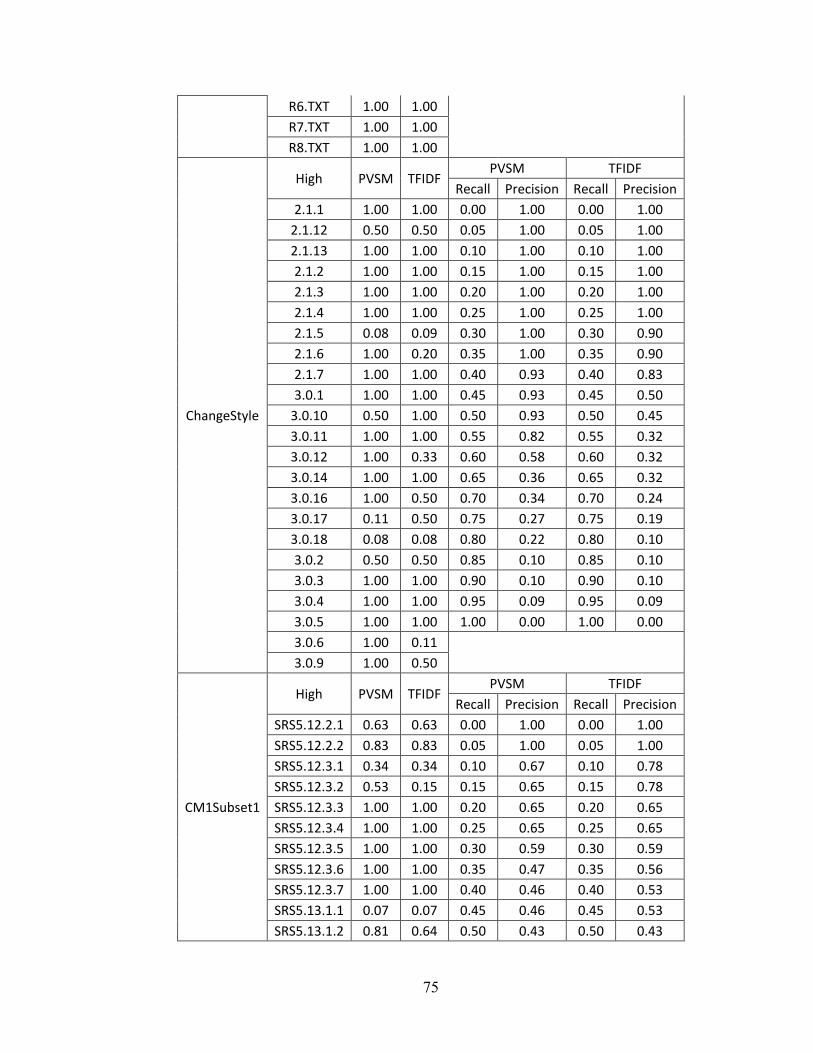
75
R6.TXT 1.00 1.00 R7.TXT 1.00 1.00 R8.TXT 1.00 1.00
ChangeStyle
High PVSM TFIDF PVSM TFIDF
Recall Precision Recall Precision 2.1.1 1.00 1.00 0.00 1.00 0.00 1.00
2.1.12 0.50 0.50 0.05 1.00 0.05 1.00 2.1.13 1.00 1.00 0.10 1.00 0.10 1.00 2.1.2 1.00 1.00 0.15 1.00 0.15 1.00 2.1.3 1.00 1.00 0.20 1.00 0.20 1.00 2.1.4 1.00 1.00 0.25 1.00 0.25 1.00 2.1.5 0.08 0.09 0.30 1.00 0.30 0.90 2.1.6 1.00 0.20 0.35 1.00 0.35 0.90 2.1.7 1.00 1.00 0.40 0.93 0.40 0.83 3.0.1 1.00 1.00 0.45 0.93 0.45 0.50
3.0.10 0.50 1.00 0.50 0.93 0.50 0.45 3.0.11 1.00 1.00 0.55 0.82 0.55 0.32 3.0.12 1.00 0.33 0.60 0.58 0.60 0.32 3.0.14 1.00 1.00 0.65 0.36 0.65 0.32 3.0.16 1.00 0.50 0.70 0.34 0.70 0.24 3.0.17 0.11 0.50 0.75 0.27 0.75 0.19 3.0.18 0.08 0.08 0.80 0.22 0.80 0.10 3.0.2 0.50 0.50 0.85 0.10 0.85 0.10 3.0.3 1.00 1.00 0.90 0.10 0.90 0.10 3.0.4 1.00 1.00 0.95 0.09 0.95 0.09 3.0.5 1.00 1.00 1.00 0.00 1.00 0.00 3.0.6 1.00 0.11 3.0.9 1.00 0.50
CM1Subset1
High PVSM TFIDF PVSM TFIDF
Recall Precision Recall Precision SRS5.12.2.1 0.63 0.63 0.00 1.00 0.00 1.00 SRS5.12.2.2 0.83 0.83 0.05 1.00 0.05 1.00 SRS5.12.3.1 0.34 0.34 0.10 0.67 0.10 0.78 SRS5.12.3.2 0.53 0.15 0.15 0.65 0.15 0.78 SRS5.12.3.3 1.00 1.00 0.20 0.65 0.20 0.65 SRS5.12.3.4 1.00 1.00 0.25 0.65 0.25 0.65 SRS5.12.3.5 1.00 1.00 0.30 0.59 0.30 0.59 SRS5.12.3.6 1.00 1.00 0.35 0.47 0.35 0.56 SRS5.12.3.7 1.00 1.00 0.40 0.46 0.40 0.53 SRS5.13.1.1 0.07 0.07 0.45 0.46 0.45 0.53 SRS5.13.1.2 0.81 0.64 0.50 0.43 0.50 0.43
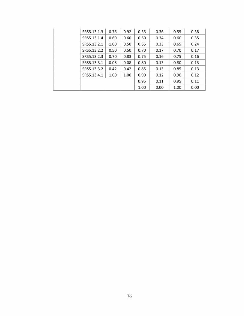
76
SRS5.13.1.3 0.76 0.92 0.55 0.36 0.55 0.38 SRS5.13.1.4 0.60 0.60 0.60 0.34 0.60 0.35 SRS5.13.2.1 1.00 0.50 0.65 0.33 0.65 0.24 SRS5.13.2.2 0.50 0.50 0.70 0.17 0.70 0.17 SRS5.13.2.3 0.70 0.83 0.75 0.16 0.75 0.16 SRS5.13.3.1 0.08 0.08 0.80 0.13 0.80 0.13 SRS5.13.3.2 0.42 0.42 0.85 0.13 0.85 0.13 SRS5.13.4.1 1.00 1.00 0.90 0.12 0.90 0.12
0.95 0.11 0.95 0.11 1.00 0.00 1.00 0.00
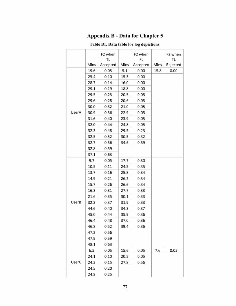
77
Appendix B - Data for Chapter 5 Table B1. Data table for log depictions.
Mins
F2 when TL
Accepted Mins
F2 when FL
Accepted Mins
F2 when TL
Rejected
UserA
19.6 0.05 5.1 0.00 15.8 0.00 25.4 0.10 15.3 0.00 28.7 0.14 16.0 0.00 29.1 0.19 18.8 0.00 29.5 0.23 20.5 0.05 29.6 0.28 20.6 0.05 30.0 0.32 21.0 0.05 30.9 0.36 22.9 0.05 31.6 0.40 23.9 0.05 32.0 0.44 24.8 0.05 32.3 0.48 29.5 0.23 32.5 0.52 30.5 0.32 32.7 0.56 34.6 0.59 32.8 0.59 37.1 0.63
UserB
9.7 0.05 17.7 0.30 10.5 0.11 24.5 0.35 13.7 0.16 25.8 0.34 14.9 0.21 26.2 0.34 15.7 0.26 26.6 0.34 16.3 0.31 27.7 0.33 21.6 0.35 30.1 0.33 32.3 0.37 31.9 0.33 44.6 0.40 34.3 0.37 45.0 0.44 35.9 0.36 46.4 0.48 37.0 0.36 46.8 0.52 39.4 0.36 47.2 0.56 47.9 0.59 48.1 0.63
UserC
6.5 0.05 15.6 0.05 7.6 0.05 24.1 0.10 20.5 0.05 24.3 0.15 27.8 0.56 24.5 0.20 24.8 0.25
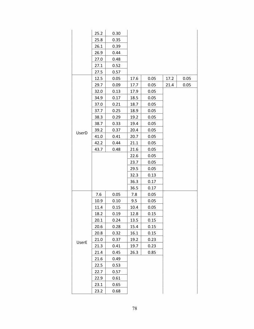
78
25.2 0.30 25.8 0.35 26.1 0.39 26.9 0.44 27.0 0.48 27.1 0.52 27.5 0.57
UserD
12.5 0.05 17.6 0.05 17.2 0.05 29.7 0.09 17.7 0.05 21.4 0.05 32.0 0.13 17.9 0.05 34.9 0.17 18.5 0.05 37.0 0.21 18.7 0.05 37.7 0.25 18.9 0.05 38.3 0.29 19.2 0.05 38.7 0.33 19.4 0.05 39.2 0.37 20.4 0.05 41.0 0.41 20.7 0.05 42.2 0.44 21.1 0.05 43.7 0.48 21.6 0.05
22.6 0.05 23.7 0.05 29.5 0.05 32.3 0.13 36.3 0.17 36.5 0.17
UserE
7.6 0.05 7.8 0.05 10.9 0.10 9.5 0.05 11.4 0.15 10.4 0.05 18.2 0.19 12.8 0.15 20.1 0.24 13.5 0.15 20.6 0.28 15.4 0.15 20.8 0.32 16.1 0.15 21.0 0.37 19.2 0.23 21.3 0.41 19.7 0.23 21.4 0.45 26.3 0.85 21.6 0.49 22.5 0.53 22.7 0.57 22.9 0.61 23.1 0.65 23.2 0.68
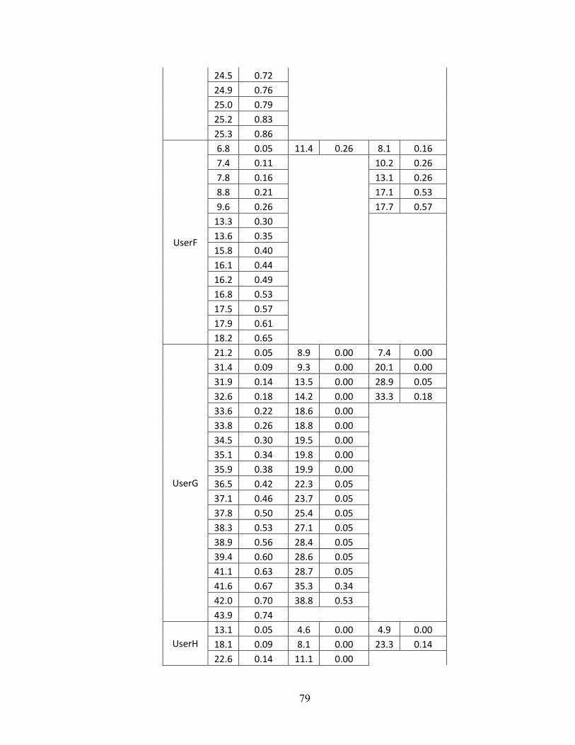
79
24.5 0.72 24.9 0.76 25.0 0.79 25.2 0.83 25.3 0.86
UserF
6.8 0.05 11.4 0.26 8.1 0.16 7.4 0.11 10.2 0.26 7.8 0.16 13.1 0.26 8.8 0.21 17.1 0.53 9.6 0.26 17.7 0.57
13.3 0.30 13.6 0.35 15.8 0.40 16.1 0.44 16.2 0.49 16.8 0.53 17.5 0.57 17.9 0.61 18.2 0.65
UserG
21.2 0.05 8.9 0.00 7.4 0.00 31.4 0.09 9.3 0.00 20.1 0.00 31.9 0.14 13.5 0.00 28.9 0.05 32.6 0.18 14.2 0.00 33.3 0.18 33.6 0.22 18.6 0.00 33.8 0.26 18.8 0.00 34.5 0.30 19.5 0.00 35.1 0.34 19.8 0.00 35.9 0.38 19.9 0.00 36.5 0.42 22.3 0.05 37.1 0.46 23.7 0.05 37.8 0.50 25.4 0.05 38.3 0.53 27.1 0.05 38.9 0.56 28.4 0.05 39.4 0.60 28.6 0.05 41.1 0.63 28.7 0.05 41.6 0.67 35.3 0.34 42.0 0.70 38.8 0.53 43.9 0.74
UserH 13.1 0.05 4.6 0.00 4.9 0.00 18.1 0.09 8.1 0.00 23.3 0.14 22.6 0.14 11.1 0.00
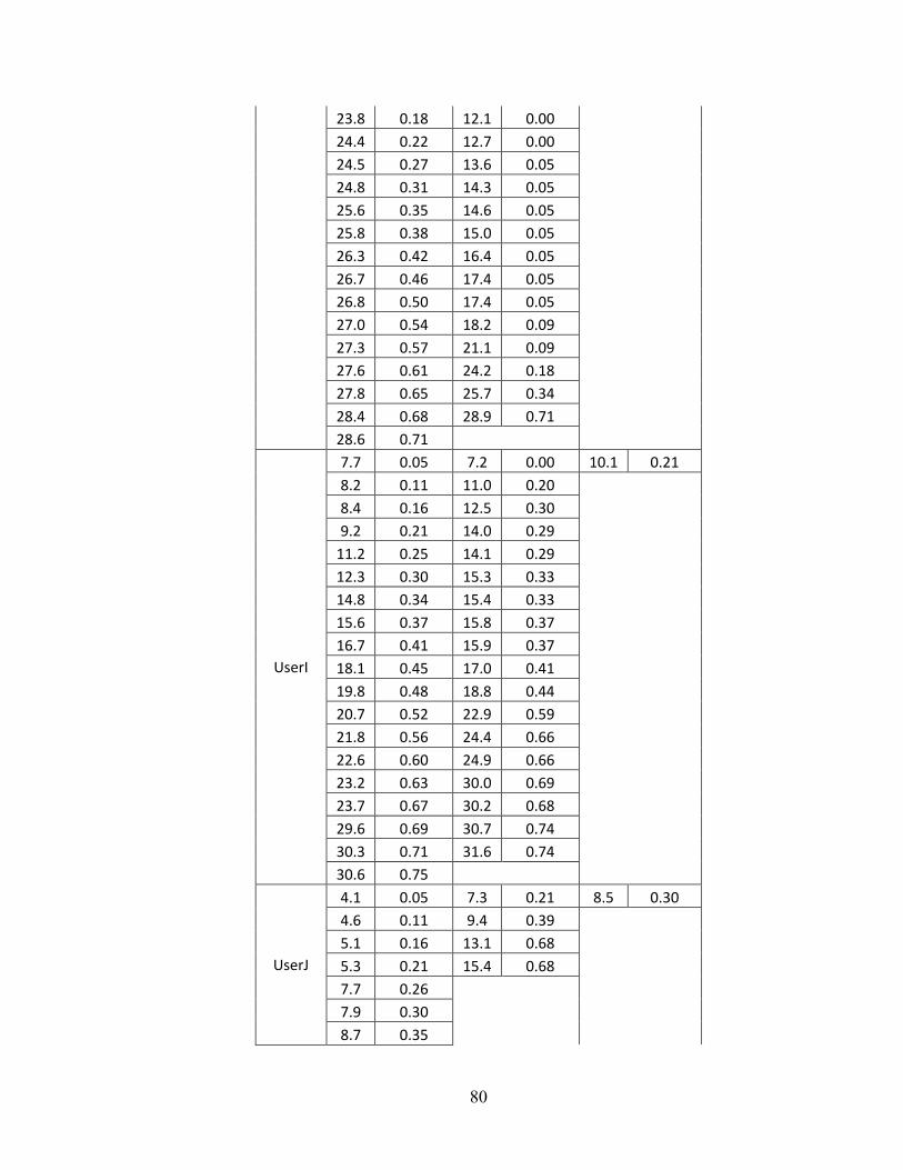
80
23.8 0.18 12.1 0.00 24.4 0.22 12.7 0.00 24.5 0.27 13.6 0.05 24.8 0.31 14.3 0.05 25.6 0.35 14.6 0.05 25.8 0.38 15.0 0.05 26.3 0.42 16.4 0.05 26.7 0.46 17.4 0.05 26.8 0.50 17.4 0.05 27.0 0.54 18.2 0.09 27.3 0.57 21.1 0.09 27.6 0.61 24.2 0.18 27.8 0.65 25.7 0.34 28.4 0.68 28.9 0.71 28.6 0.71
UserI
7.7 0.05 7.2 0.00 10.1 0.21 8.2 0.11 11.0 0.20 8.4 0.16 12.5 0.30 9.2 0.21 14.0 0.29
11.2 0.25 14.1 0.29 12.3 0.30 15.3 0.33 14.8 0.34 15.4 0.33 15.6 0.37 15.8 0.37 16.7 0.41 15.9 0.37 18.1 0.45 17.0 0.41 19.8 0.48 18.8 0.44 20.7 0.52 22.9 0.59 21.8 0.56 24.4 0.66 22.6 0.60 24.9 0.66 23.2 0.63 30.0 0.69 23.7 0.67 30.2 0.68 29.6 0.69 30.7 0.74 30.3 0.71 31.6 0.74 30.6 0.75
UserJ
4.1 0.05 7.3 0.21 8.5 0.30 4.6 0.11 9.4 0.39 5.1 0.16 13.1 0.68 5.3 0.21 15.4 0.68 7.7 0.26 7.9 0.30 8.7 0.35
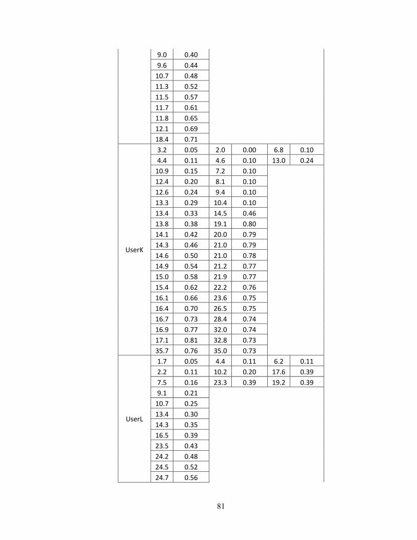
81
9.0 0.40 9.6 0.44
10.7 0.48 11.3 0.52 11.5 0.57 11.7 0.61 11.8 0.65 12.1 0.69 18.4 0.71
UserK
3.2 0.05 2.0 0.00 6.8 0.10 4.4 0.11 4.6 0.10 13.0 0.24
10.9 0.15 7.2 0.10 12.4 0.20 8.1 0.10 12.6 0.24 9.4 0.10 13.3 0.29 10.4 0.10 13.4 0.33 14.5 0.46 13.8 0.38 19.1 0.80 14.1 0.42 20.0 0.79 14.3 0.46 21.0 0.79 14.6 0.50 21.0 0.78 14.9 0.54 21.2 0.77 15.0 0.58 21.9 0.77 15.4 0.62 22.2 0.76 16.1 0.66 23.6 0.75 16.4 0.70 26.5 0.75 16.7 0.73 28.4 0.74 16.9 0.77 32.0 0.74 17.1 0.81 32.8 0.73 35.7 0.76 35.0 0.73
UserL
1.7 0.05 4.4 0.11 6.2 0.11 2.2 0.11 10.2 0.20 17.6 0.39 7.5 0.16 23.3 0.39 19.2 0.39 9.1 0.21
10.7 0.25 13.4 0.30 14.3 0.35 16.5 0.39 23.5 0.43 24.2 0.48 24.5 0.52 24.7 0.56
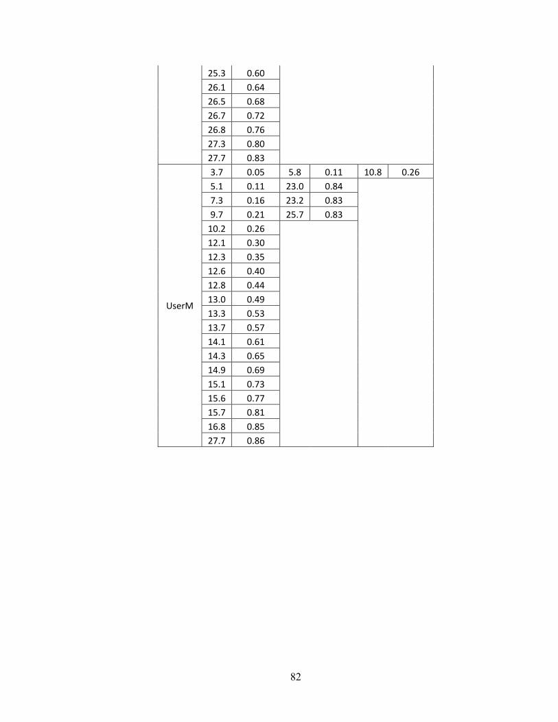
82
25.3 0.60 26.1 0.64 26.5 0.68 26.7 0.72 26.8 0.76 27.3 0.80 27.7 0.83
UserM
3.7 0.05 5.8 0.11 10.8 0.26 5.1 0.11 23.0 0.84 7.3 0.16 23.2 0.83 9.7 0.21 25.7 0.83
10.2 0.26 12.1 0.30 12.3 0.35 12.6 0.40 12.8 0.44 13.0 0.49 13.3 0.53 13.7 0.57 14.1 0.61 14.3 0.65 14.9 0.69 15.1 0.73 15.6 0.77 15.7 0.81 16.8 0.85 27.7 0.86
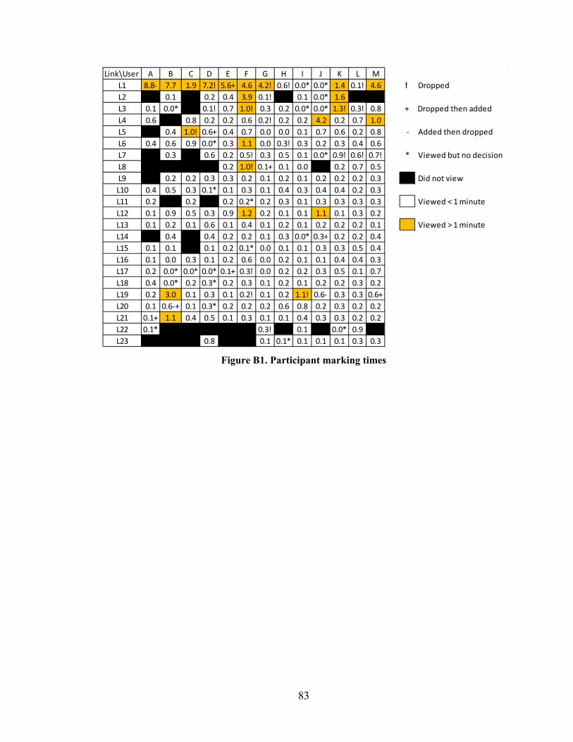
83
Figure B1. Participant marking times
Link\User A B C D E F G H I J K L ML1 8.8- 7.7 1.9 7.2! 5.6+ 4.6 4.2! 0.6! 0.0* 0.0* 1.4 0.1! 4.6 ! Dropped L2 0.1 0.2 0.4 3.9 0.1! 0.1 0.0* 1.6L3 0.1 0.0* 0.1! 0.7 1.0! 0.3 0.2 0.0* 0.0* 1.3! 0.3! 0.8 + Dropped then addedL4 0.6 0.8 0.2 0.2 0.6 0.2! 0.2 0.2 4.2 0.2 0.7 1.0L5 0.4 1.0! 0.6+ 0.4 0.7 0.0 0.0 0.1 0.7 0.6 0.2 0.8 - Added then dropped L6 0.4 0.6 0.9 0.0* 0.3 1.1 0.0 0.3! 0.3 0.2 0.3 0.4 0.6L7 0.3 0.6 0.2 0.5! 0.3 0.5 0.1 0.0* 0.9! 0.6! 0.7! * Viewed but no decision L8 0.2 1.0! 0.1+ 0.1 0.0 0.2 0.7 0.5L9 0.2 0.2 0.3 0.3 0.2 0.1 0.2 0.1 0.2 0.2 0.2 0.3 Did not viewL10 0.4 0.5 0.3 0.1* 0.1 0.3 0.1 0.4 0.3 0.4 0.4 0.2 0.3L11 0.2 0.2 0.2 0.2* 0.2 0.3 0.1 0.3 0.3 0.3 0.3 Viewed < 1 minuteL12 0.1 0.9 0.5 0.3 0.9 1.2 0.2 0.1 0.1 1.1 0.1 0.3 0.2L13 0.1 0.2 0.1 0.6 0.1 0.4 0.1 0.2 0.1 0.2 0.2 0.2 0.1 Viewed > 1 minuteL14 0.4 0.4 0.2 0.2 0.1 0.3 0.0* 0.3+ 0.2 0.2 0.4L15 0.1 0.1 0.1 0.2 0.1* 0.0 0.1 0.1 0.3 0.3 0.5 0.4L16 0.1 0.0 0.3 0.1 0.2 0.6 0.0 0.2 0.1 0.1 0.4 0.4 0.3L17 0.2 0.0* 0.0* 0.0* 0.1+ 0.3! 0.0 0.2 0.2 0.3 0.5 0.1 0.7L18 0.4 0.0* 0.2 0.3* 0.2 0.3 0.1 0.2 0.1 0.2 0.2 0.3 0.2L19 0.2 3.0 0.1 0.3 0.1 0.2! 0.1 0.2 1.1! 0.6- 0.3 0.3 0.6+L20 0.1 0.6-+ 0.1 0.3* 0.2 0.2 0.2 0.6 0.8 0.2 0.3 0.2 0.2L21 0.1+ 1.1 0.4 0.5 0.1 0.3 0.1 0.1 0.4 0.3 0.3 0.2 0.2L22 0.1* 0.3! 0.1 0.0* 0.9L23 0.8 0.1 0.1* 0.1 0.1 0.1 0.3 0.3
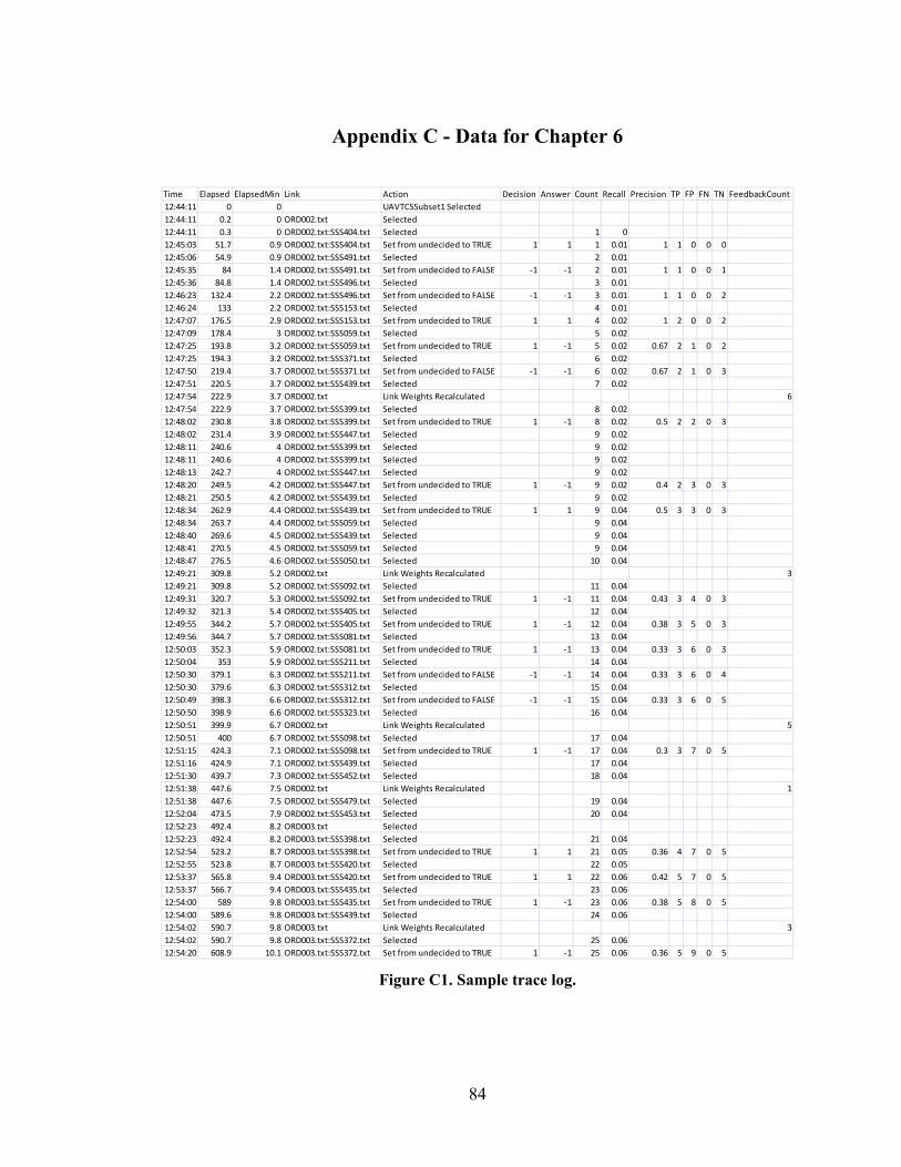
84
Appendix C - Data for Chapter 6
Figure C1. Sample trace log.
Time Elapsed ElapsedMin Link Action Decision Answer Count Recall Precision TP FP FN TN FeedbackCount12:44:11 0 0 UAVTCSSubset1 Selected12:44:11 0.2 0 ORD002.txt Selected12:44:11 0.3 0 ORD002.txt:SSS404.txt Selected 1 012:45:03 51.7 0.9 ORD002.txt:SSS404.txt Set from undecided to TRUE 1 1 1 0.01 1 1 0 0 012:45:06 54.9 0.9 ORD002.txt:SSS491.txt Selected 2 0.0112:45:35 84 1.4 ORD002.txt:SSS491.txt Set from undecided to FALSE -1 -1 2 0.01 1 1 0 0 112:45:36 84.8 1.4 ORD002.txt:SSS496.txt Selected 3 0.0112:46:23 132.4 2.2 ORD002.txt:SSS496.txt Set from undecided to FALSE -1 -1 3 0.01 1 1 0 0 212:46:24 133 2.2 ORD002.txt:SSS153.txt Selected 4 0.0112:47:07 176.5 2.9 ORD002.txt:SSS153.txt Set from undecided to TRUE 1 1 4 0.02 1 2 0 0 212:47:09 178.4 3 ORD002.txt:SSS059.txt Selected 5 0.0212:47:25 193.8 3.2 ORD002.txt:SSS059.txt Set from undecided to TRUE 1 -1 5 0.02 0.67 2 1 0 212:47:25 194.3 3.2 ORD002.txt:SSS371.txt Selected 6 0.0212:47:50 219.4 3.7 ORD002.txt:SSS371.txt Set from undecided to FALSE -1 -1 6 0.02 0.67 2 1 0 312:47:51 220.5 3.7 ORD002.txt:SSS439.txt Selected 7 0.0212:47:54 222.9 3.7 ORD002.txt Link Weights Recalculated 612:47:54 222.9 3.7 ORD002.txt:SSS399.txt Selected 8 0.0212:48:02 230.8 3.8 ORD002.txt:SSS399.txt Set from undecided to TRUE 1 -1 8 0.02 0.5 2 2 0 312:48:02 231.4 3.9 ORD002.txt:SSS447.txt Selected 9 0.0212:48:11 240.6 4 ORD002.txt:SSS399.txt Selected 9 0.0212:48:11 240.6 4 ORD002.txt:SSS399.txt Selected 9 0.0212:48:13 242.7 4 ORD002.txt:SSS447.txt Selected 9 0.0212:48:20 249.5 4.2 ORD002.txt:SSS447.txt Set from undecided to TRUE 1 -1 9 0.02 0.4 2 3 0 312:48:21 250.5 4.2 ORD002.txt:SSS439.txt Selected 9 0.0212:48:34 262.9 4.4 ORD002.txt:SSS439.txt Set from undecided to TRUE 1 1 9 0.04 0.5 3 3 0 312:48:34 263.7 4.4 ORD002.txt:SSS059.txt Selected 9 0.0412:48:40 269.6 4.5 ORD002.txt:SSS439.txt Selected 9 0.0412:48:41 270.5 4.5 ORD002.txt:SSS059.txt Selected 9 0.0412:48:47 276.5 4.6 ORD002.txt:SSS050.txt Selected 10 0.0412:49:21 309.8 5.2 ORD002.txt Link Weights Recalculated 312:49:21 309.8 5.2 ORD002.txt:SSS092.txt Selected 11 0.0412:49:31 320.7 5.3 ORD002.txt:SSS092.txt Set from undecided to TRUE 1 -1 11 0.04 0.43 3 4 0 312:49:32 321.3 5.4 ORD002.txt:SSS405.txt Selected 12 0.0412:49:55 344.2 5.7 ORD002.txt:SSS405.txt Set from undecided to TRUE 1 -1 12 0.04 0.38 3 5 0 312:49:56 344.7 5.7 ORD002.txt:SSS081.txt Selected 13 0.0412:50:03 352.3 5.9 ORD002.txt:SSS081.txt Set from undecided to TRUE 1 -1 13 0.04 0.33 3 6 0 312:50:04 353 5.9 ORD002.txt:SSS211.txt Selected 14 0.0412:50:30 379.1 6.3 ORD002.txt:SSS211.txt Set from undecided to FALSE -1 -1 14 0.04 0.33 3 6 0 412:50:30 379.6 6.3 ORD002.txt:SSS312.txt Selected 15 0.0412:50:49 398.3 6.6 ORD002.txt:SSS312.txt Set from undecided to FALSE -1 -1 15 0.04 0.33 3 6 0 512:50:50 398.9 6.6 ORD002.txt:SSS323.txt Selected 16 0.0412:50:51 399.9 6.7 ORD002.txt Link Weights Recalculated 512:50:51 400 6.7 ORD002.txt:SSS098.txt Selected 17 0.0412:51:15 424.3 7.1 ORD002.txt:SSS098.txt Set from undecided to TRUE 1 -1 17 0.04 0.3 3 7 0 512:51:16 424.9 7.1 ORD002.txt:SSS439.txt Selected 17 0.0412:51:30 439.7 7.3 ORD002.txt:SSS452.txt Selected 18 0.0412:51:38 447.6 7.5 ORD002.txt Link Weights Recalculated 112:51:38 447.6 7.5 ORD002.txt:SSS479.txt Selected 19 0.0412:52:04 473.5 7.9 ORD002.txt:SSS453.txt Selected 20 0.0412:52:23 492.4 8.2 ORD003.txt Selected12:52:23 492.4 8.2 ORD003.txt:SSS398.txt Selected 21 0.0412:52:54 523.2 8.7 ORD003.txt:SSS398.txt Set from undecided to TRUE 1 1 21 0.05 0.36 4 7 0 512:52:55 523.8 8.7 ORD003.txt:SSS420.txt Selected 22 0.0512:53:37 565.8 9.4 ORD003.txt:SSS420.txt Set from undecided to TRUE 1 1 22 0.06 0.42 5 7 0 512:53:37 566.7 9.4 ORD003.txt:SSS435.txt Selected 23 0.0612:54:00 589 9.8 ORD003.txt:SSS435.txt Set from undecided to TRUE 1 -1 23 0.06 0.38 5 8 0 512:54:00 589.6 9.8 ORD003.txt:SSS439.txt Selected 24 0.0612:54:02 590.7 9.8 ORD003.txt Link Weights Recalculated 312:54:02 590.7 9.8 ORD003.txt:SSS372.txt Selected 25 0.0612:54:20 608.9 10.1 ORD003.txt:SSS372.txt Set from undecided to TRUE 1 -1 25 0.06 0.36 5 9 0 5
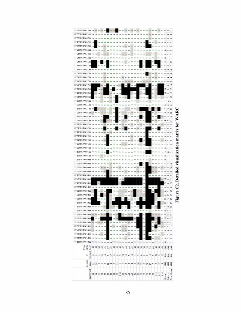
85
User
ID/L
ink
# ne
ver
seen
# re
ject
ed
# Tr
ue
Link
s Se
en
FR01.txt:SRS01.txt
FR01.txt:SRS02.txt
FR01.txt:SRS03.txt
FR01.txt:SRS04.txt
FR01.txt:SRS05.txt
FR01.txt:SRS07.txt
FR02.txt:SRS04.txt
FR02.txt:SRS05.txt
FR02.txt:SRS06.txt
FR02.txt:SRS11.txt
FR02.txt:SRS21.txt
FR02.txt:SRS68.txt
FR04.txt:SRS08.txt
FR04.txt:SRS09.txt
FR04.txt:SRS10.txt
FR05.txt:SRS11.txt
FR05.txt:SRS14.txt
FR06.txt:SRS11.txt
FR06.txt:SRS12.txt
FR06.txt:SRS14.txt
FR09.txt:SRS16.txt
FR09.txt:SRS18.txt
FR14.txt:SRS21.txt
FR14.txt:SRS22.txt
FR14.txt:SRS23.txt
FR14.txt:SRS24.txt
FR14.txt:SRS25.txt
FR14.txt:SRS26.txt
FR16.txt:SRS21.txt
FR16.txt:SRS22.txt
FR16.txt:SRS23.txt
FR16.txt:SRS24.txt
FR16.txt:SRS25.txt
FR16.txt:SRS26.txt
FR17.txt:SRS27.txt
FR17.txt:SRS28.txt
FR18.txt:SRS29.txt
FR18.txt:SRS30.txt
FR20.txt:SRS31.txt
FR20.txt:SRS32.txt
FR21.txt:SRS34.txt
FR21.txt:SRS36.txt
FR24.txt:SRS39.txt
FR24.txt:SRS40.txt
FR25.txt:SRS41.txt
FR25.txt:SRS42.txt
FR25.txt:SRS43.txt
FR27.txt:SRS45.txt
FR27.txt:SRS46.txt
FR35.txt:SRS55.txt
FR35.txt:SRS56.txt
FR39.txt:SRS51.txt
FR39.txt:SRS60.txt
FR42.txt:SRS63.txt
FR42.txt:SRS64.txt
B111
642
22
21
11
01
22
00
21
20
02
22
22
22
22
22
22
22
21
22
20
00
02
22
20
02
22
22
22
2B2
133
402
22
22
22
12
20
00
02
00
22
22
22
22
22
22
22
22
20
22
21
00
22
22
00
22
20
02
21
B33
450
22
22
21
22
22
02
22
21
02
22
22
22
22
22
22
22
22
12
22
22
02
22
22
22
12
22
22
2B4
515
482
21
22
10
12
22
20
12
00
22
12
21
22
22
22
22
12
11
21
11
11
22
22
20
22
22
22
21
B58
1645
22
22
22
01
21
22
12
20
02
11
22
22
22
12
10
10
01
12
22
00
21
11
22
22
11
12
22
2B6
263
272
00
00
00
01
00
00
02
00
00
22
22
02
00
02
22
10
22
22
20
00
22
22
00
21
22
22
20
B74
1749
22
22
22
01
21
11
10
20
01
11
12
22
22
22
12
21
21
12
11
12
22
22
22
22
22
22
22
1B8
43
492
22
21
22
22
10
22
22
00
22
22
22
22
22
22
22
22
22
22
22
02
22
22
22
22
22
22
21
B911
241
22
22
22
11
22
00
22
20
02
22
22
22
22
22
20
20
00
02
00
22
22
22
22
22
22
22
22
0B1
05
548
22
22
22
00
20
00
11
21
22
21
22
22
22
22
22
22
22
22
22
22
12
22
22
22
22
22
22
2A2
613
472
22
11
20
12
20
21
12
01
22
22
22
22
12
22
11
12
12
22
20
00
21
22
22
21
22
22
22
A39
1544
21
21
12
02
22
00
21
20
02
12
22
22
21
22
20
21
01
12
21
00
21
22
22
12
12
12
22
1A4
95
442
21
22
10
12
00
22
22
00
22
22
22
22
22
22
22
22
21
22
00
00
12
22
22
22
22
22
22
A54
1449
22
22
22
01
22
21
11
20
02
22
22
22
22
11
22
12
21
22
22
10
21
22
22
22
11
12
22
1A6
51
482
22
22
21
22
22
20
02
00
22
22
22
22
22
22
22
22
22
22
22
02
22
22
22
22
22
22
22
A710
943
22
22
00
02
22
02
11
20
02
11
22
22
22
22
21
21
22
12
10
00
02
22
22
22
22
22
22
1E1
196
352
00
00
00
02
00
01
12
00
22
20
22
22
10
22
21
20
10
22
21
20
22
22
00
22
22
22
22
E23
250
22
22
22
22
22
02
12
22
22
22
22
22
22
22
22
22
22
02
22
22
01
22
22
22
22
22
22
2E5
362
182
00
00
00
02
00
00
00
00
00
00
22
02
00
00
02
00
00
22
20
02
12
02
00
21
20
02
22
E729
1525
10
20
00
00
10
00
00
20
02
00
11
20
10
02
20
10
00
12
10
00
01
11
20
02
12
02
11
1E8
73
462
22
22
20
12
20
00
22
00
21
12
22
22
22
22
22
22
20
22
22
22
22
22
22
22
22
22
22
E11
521
482
12
10
11
12
12
11
02
00
21
12
22
22
22
22
22
12
11
22
11
12
21
12
20
11
22
12
22
E12
173
362
12
22
00
12
00
20
00
00
22
22
22
22
22
22
02
20
20
22
20
00
22
22
00
22
22
22
21
E14
412
492
21
21
12
22
21
21
12
01
22
12
22
22
21
22
21
21
22
22
10
00
22
22
22
22
22
22
22
Mis
sed
#NA
#NA
#NA
04
34
66
165
07
1710
88
221
202
32
20
03
03
42
16
04
83
70
15
1115
120
01
07
90
00
32
00
2Re
ject
ed#N
A#N
A#N
A1
33
45
63
122
42
310
90
22
16
82
11
01
33
12
26
71
99
04
56
22
74
30
01
19
23
11
19
Tota
l Mis
sed
#NA
#NA
#NA
17
68
1112
1917
211
1913
1817
223
223
910
41
13
16
73
38
611
912
160
510
1717
147
44
07
101
92
63
11
11
Figu
re C
2. D
etai
led
visu
aliz
atio
n m
atri
x fo
r W
AR
C
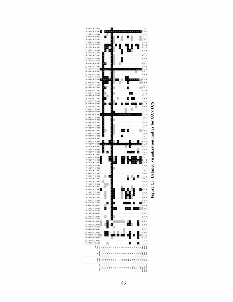
86
User
ID/L
ink
# N
ever
Se
en#
Reje
cted
# Tr
ue
Link
s Se
en
ORD002.txt:SSS153.txt
ORD002.txt:SSS404.txt
ORD002.txt:SSS439.txt
ORD003.txt:SSS323.txt
ORD003.txt:SSS395.txt
ORD003.txt:SSS398.txt
ORD003.txt:SSS420.txt
ORD003.txt:SSS438.txt
ORD003.txt:SSS439.txt
ORD004.txt:SSS209.txt
ORD004.txt:SSS393.txt
ORD004.txt:SSS417.txt
ORD008.txt:SSS376.txt
ORD008.txt:SSS383.txt
ORD008.txt:SSS440.txt
ORD011.txt:SSS009.txt
ORD011.txt:SSS010.txt
ORD011.txt:SSS011.txt
ORD011.txt:SSS012.txt
ORD011.txt:SSS396.txt
ORD012.txt:SSS009.txt
ORD012.txt:SSS010.txt
ORD012.txt:SSS011.txt
ORD012.txt:SSS012.txt
ORD013.txt:SSS011.txt
ORD013.txt:SSS323.txt
ORD013.txt:SSS396.txt
ORD013.txt:SSS425.txt
ORD015.txt:SSS021.txt
ORD015.txt:SSS022.txt
ORD015.txt:SSS023.txt
ORD015.txt:SSS038.txt
ORD015.txt:SSS040.txt
ORD015.txt:SSS403.txt
ORD016.txt:SSS050.txt
ORD016.txt:SSS053.txt
ORD016.txt:SSS055.txt
ORD016.txt:SSS210.txt
ORD016.txt:SSS286.txt
ORD016.txt:SSS397.txt
ORD017.txt:SSS323.txt
ORD017.txt:SSS395.txt
ORD017.txt:SSS396.txt
ORD017.txt:SSS425.txt
ORD017.txt:SSS439.txt
ORD018.txt:SSS393.txt
ORD018.txt:SSS394.txt
ORD020.txt:SSS446.txt
ORD020.txt:SSS459.txt
ORD021.txt:SSS399.txt
ORD021.txt:SSS405.txt
ORD021.txt:SSS447.txt
ORD022.txt:SSS288.txt
ORD022.txt:SSS314.txt
ORD022.txt:SSS317.txt
ORD022.txt:SSS337.txt
ORD022.txt:SSS341.txt
ORD022.txt:SSS378.txt
ORD023.txt:SSS323.txt
ORD023.txt:SSS395.txt
ORD023.txt:SSS396.txt
ORD023.txt:SSS418.txt
ORD023.txt:SSS439.txt
ORD024.txt:SSS108.txt
ORD024.txt:SSS125.txt
ORD024.txt:SSS147.txt
ORD024.txt:SSS149.txt
ORD024.txt:SSS158.txt
ORD025.txt:SSS009.txt
ORD025.txt:SSS010.txt
ORD025.txt:SSS011.txt
ORD025.txt:SSS012.txt
ORD025.txt:SSS396.txt
ORD026.txt:SSS013.txt
ORD026.txt:SSS537.txt
ORD028.txt:SSS280.txt
ORD028.txt:SSS318.txt
ORD028.txt:SSS340.txt
ORD028.txt:SSS384.txt
ORD029.txt:SSS281.txt
ORD029.txt:SSS555.txt
D19
372
22
21
22
21
12
22
22
22
22
22
02
22
22
22
22
00
02
22
20
22
22
22
22
22
02
22
22
22
22
22
20
22
20
22
22
22
22
22
22
20
2D2
371
442
22
22
22
22
22
22
22
22
22
22
22
12
22
22
22
22
20
00
00
20
00
00
00
00
00
00
00
00
00
00
00
00
00
00
00
02
22
22
22
22
D318
1163
22
20
02
21
22
12
20
12
21
11
21
12
21
22
22
22
22
22
20
22
22
12
22
22
02
22
02
02
12
02
00
02
20
20
22
22
00
02
20
20
2D4
164
651
22
00
20
00
22
22
22
02
22
22
21
22
22
22
22
22
20
22
02
22
22
22
22
20
22
22
22
12
22
20
00
22
02
22
22
22
00
22
21
02
D512
069
22
22
22
22
22
22
22
22
22
22
22
22
20
22
22
20
02
22
20
02
22
22
22
22
02
22
02
22
22
22
20
22
20
22
22
22
02
02
22
20
2D6
741
72
21
02
22
02
00
00
00
00
00
00
00
00
00
00
00
00
00
00
00
00
00
00
00
00
00
00
00
00
00
00
00
00
00
00
00
00
00
00
00
00
D713
3168
22
20
12
12
12
12
20
20
20
00
02
22
22
22
12
01
12
22
20
12
21
11
12
12
00
22
11
22
12
12
11
11
10
21
11
12
11
21
11
20
2D8
112
702
22
12
22
21
22
22
02
22
22
22
22
22
22
22
20
00
22
22
02
22
22
22
22
20
22
20
22
22
22
22
02
22
02
22
22
22
20
22
22
02
C18
373
22
20
12
22
12
22
22
22
22
22
22
22
22
22
22
22
22
22
20
02
22
22
22
22
02
22
22
12
22
22
20
22
20
22
22
22
22
22
20
20
2C2
64
752
22
12
22
21
22
22
22
22
22
22
22
22
22
22
22
22
22
22
02
22
22
22
22
20
22
22
22
22
22
21
22
22
02
12
22
22
00
22
22
02
C316
865
22
20
22
22
12
22
22
22
21
11
01
22
22
22
22
00
02
22
20
22
02
02
22
22
02
22
02
22
22
22
21
22
20
22
00
20
02
22
11
20
2C5
113
702
22
01
12
21
22
22
22
02
22
20
22
22
22
22
20
00
22
22
02
22
20
22
22
20
22
22
22
22
22
22
22
22
02
22
22
22
22
22
22
02
C613
468
22
22
22
22
22
22
20
20
20
00
22
22
22
22
22
22
12
22
10
22
22
22
22
22
01
12
02
22
22
22
20
02
20
22
22
22
22
02
22
20
2C7
264
552
22
02
22
01
22
22
02
02
10
10
22
20
12
22
20
00
20
22
02
22
20
22
22
20
22
20
20
22
20
20
00
22
02
22
22
20
00
22
02
02
C922
059
02
00
02
20
02
22
20
20
20
00
22
22
22
22
22
20
22
02
00
02
22
22
22
22
02
22
22
22
02
22
20
22
20
22
22
22
02
22
22
20
2C1
014
1067
22
22
22
21
22
22
22
22
21
12
11
22
21
22
22
00
02
02
20
22
22
22
22
22
02
12
02
02
02
22
20
22
20
22
22
22
10
02
11
20
2C1
218
063
22
20
22
22
22
22
20
20
22
00
02
22
02
22
22
00
02
02
20
22
22
22
22
22
02
22
02
02
22
22
20
22
20
22
22
22
22
22
22
20
2C1
311
270
22
22
22
22
22
22
20
22
22
22
22
22
22
22
22
00
02
22
20
22
22
22
22
22
02
21
02
22
22
22
20
22
10
22
22
22
22
02
22
20
2C1
418
163
02
00
02
20
02
22
20
22
22
22
22
22
20
22
22
20
22
01
20
02
22
22
22
22
02
22
22
22
22
22
20
22
20
22
22
22
20
02
22
20
2C1
510
871
22
21
22
22
22
22
21
20
22
22
02
22
22
22
22
00
02
22
20
22
22
12
22
22
02
22
02
22
22
12
11
22
20
22
22
22
22
22
11
20
2M
isse
d#N
A#N
A#N
A2
02
114
01
53
11
11
101
91
46
58
11
13
31
11
111
1311
18
23
206
13
25
22
22
220
32
212
26
24
24
25
156
22
202
33
32
36
711
11
41
191
Reje
cted
#NA
#NA
#NA
10
14
31
13
80
20
01
10
04
33
13
21
03
00
10
01
20
01
10
10
01
31
10
10
01
21
11
11
20
20
33
11
20
02
11
10
21
01
44
10
0To
tal M
isse
d#N
A#N
A#N
A3
03
157
12
811
13
11
112
91
89
89
43
23
61
12
111
1413
18
34
207
13
38
33
23
220
44
313
37
36
26
28
187
34
202
54
43
38
811
25
82
191
Figu
re C
3. D
etai
led
visu
aliz
atio
n m
atri
x fo
r U
AV
TC
S
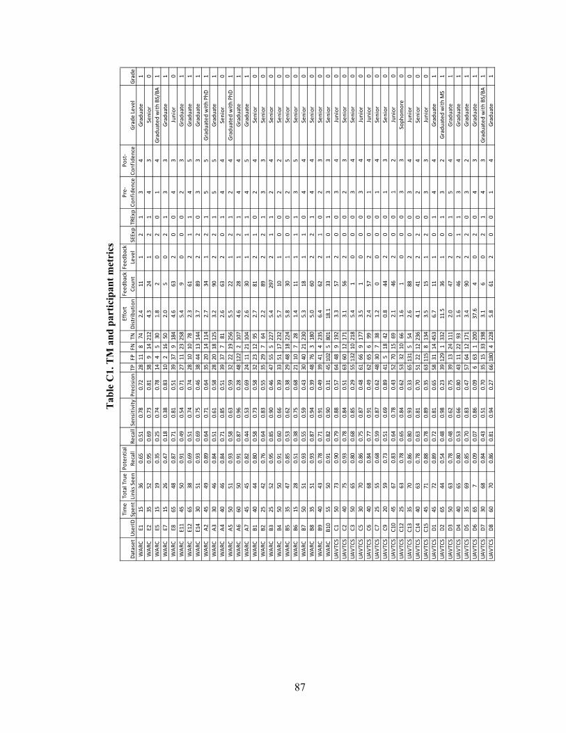
87
Data
set
User
IDTi
me
Spen
tTo
tal T
rue
Link
s See
nPo
tent
ial
Reca
llRe
call
Sens
itivi
tyPr
ecis
ion
TPFP
FNTN
Effo
rt
Dist
ribut
ion
Feed
back
Co
unt
Feed
back
Le
vel
SEEx
pTR
Exp
Pre-
Co
nfid
ence
Post
- Co
nfid
ence
Grad
e Le
vel
Grad
eW
ARC
E115
360.
650.
510.
780.
7228
118
742.
411
12
13
4Gr
adua
te1
WAR
CE2
3552
0.95
0.69
0.73
0.81
389
1421
24.
324
12
14
3Se
nior
0W
ARC
E515
190.
350.
250.
740.
7814
45
301.
82
02
01
4Gr
adua
ted
with
BS/
BA1
WAR
CE7
1526
0.47
0.18
0.38
0.83
102
1650
2.0
50
21
33
Grad
uate
1W
ARC
E865
480.
870.
710.
810.
5139
379
184
4.6
632
00
43
Juni
or0
WAR
CE1
145
500.
910.
490.
540.
7127
1123
258
5.4
90
00
23
Grad
uate
1W
ARC
E12
6538
0.69
0.51
0.74
0.74
2810
1078
2.3
612
11
45
Grad
uate
1W
ARC
E14
3051
0.93
0.69
0.75
0.46
3844
1314
43.
789
22
03
3Gr
adua
te1
WAR
CA2
4549
0.89
0.64
0.71
0.64
3520
1411
42.
734
12
15
5Gr
adua
ted
with
PhD
1W
ARC
A330
460.
840.
510.
610.
5828
2018
125
3.2
902
21
55
Grad
uate
1W
ARC
A440
460.
840.
710.
850.
5139
377
812.
663
20
14
4Se
nior
0W
ARC
A550
510.
930.
580.
630.
5932
2219
256
5.5
221
21
24
Grad
uate
d w
ith P
hD1
WAR
CA6
6050
0.91
0.87
0.96
0.28
4812
22
107
4.6
281
21
44
Grad
uate
1W
ARC
A745
450.
820.
440.
530.
6924
1121
104
2.6
301
11
45
Grad
uate
1W
ARC
B140
440.
800.
580.
730.
5832
2312
952.
781
21
02
4Se
nior
0W
ARC
B225
420.
760.
640.
830.
5535
297
642.
289
22
13
3Se
nior
0W
ARC
B325
520.
950.
850.
900.
4647
555
227
5.4
297
21
12
4Se
nior
0W
ARC
B450
500.
910.
600.
660.
3933
5117
232
5.7
101
00
22
Seni
or0
WAR
CB5
3547
0.85
0.53
0.62
0.38
2948
1822
45.
830
10
02
5Se
nior
0W
ARC
B615
280.
510.
380.
750.
6821
107
281.
411
11
13
5Se
nior
0W
ARC
B750
510.
930.
550.
590.
4330
4021
230
5.3
181
10
44
Seni
or0
WAR
CB8
3551
0.93
0.87
0.94
0.39
4876
318
05.
060
22
14
4Se
nior
0W
ARC
B940
430.
780.
710.
910.
4939
414
235
6.4
622
10
23
Seni
or0
WAR
CB1
055
500.
910.
820.
900.
3145
102
580
118
.133
10
13
3Se
nior
0UA
VTCS
C150
730.
900.
790.
880.
5764
489
192
3.3
572
00
34
Juni
or0
UAVT
CSC2
4075
0.93
0.78
0.84
0.51
6360
1217
13.
156
20
02
3Se
nior
0UA
VTCS
C350
650.
800.
680.
850.
2955
132
1021
85.
41
00
03
4Se
nior
0UA
VTCS
C530
700.
860.
750.
870.
4861
669
177
3.5
10
00
34
Juni
or0
UAVT
CSC6
4068
0.84
0.77
0.91
0.49
6265
699
2.4
572
00
14
Juni
or0
UAVT
CSC7
2555
0.68
0.59
0.87
0.62
4830
738
1.2
00
00
14
Seni
or0
UAVT
CSC9
2059
0.73
0.51
0.69
0.89
415
1842
0.8
442
00
13
Seni
or0
UAVT
CSC1
045
670.
830.
640.
780.
4352
7015
692.
146
20
01
2Ju
nior
0UA
VTCS
C12
2563
0.78
0.65
0.84
0.62
5332
1066
1.6
10
00
33
Soph
omor
e0
UAVT
CSC1
335
700.
860.
800.
930.
3365
131
554
2.6
882
00
34
Juni
or0
UAVT
CSC1
440
630.
780.
630.
810.
7051
2212
236
4.1
412
20
24
Seni
or0
UAVT
CSC1
545
710.
880.
780.
890.
3563
115
813
43.
515
12
03
3Ju
nior
0UA
VTCS
D145
720.
890.
720.
810.
6558
3114
453
6.7
111
01
44
Grad
uate
1UA
VTCS
D265
440.
540.
480.
980.
2339
129
133
211
.536
10
13
2Gr
adua
ted
with
MS
1UA
VTCS
D350
630.
780.
480.
620.
7539
1324
111
2.0
472
01
54
Grad
uate
1UA
VTCS
D440
650.
800.
530.
660.
8043
1122
931.
646
21
13
4Gr
adua
te1
UAVT
CSD5
3569
0.85
0.70
0.83
0.47
5764
1217
13.
490
22
03
2Gr
adua
te1
UAVT
CSD6
657
0.09
0.07
0.86
0.09
663
120
037
.64
02
04
3Gr
adua
te1
UAVT
CSD7
3068
0.84
0.43
0.51
0.70
3515
3319
83.
16
02
14
3Gr
adua
ted
with
BS/
BA1
UAVT
CSD8
6070
0.86
0.81
0.94
0.27
6618
04
228
5.8
612
00
14
Grad
uate
1
Tab
le C
1. T
M a
nd p
artic
ipan
t met
rics
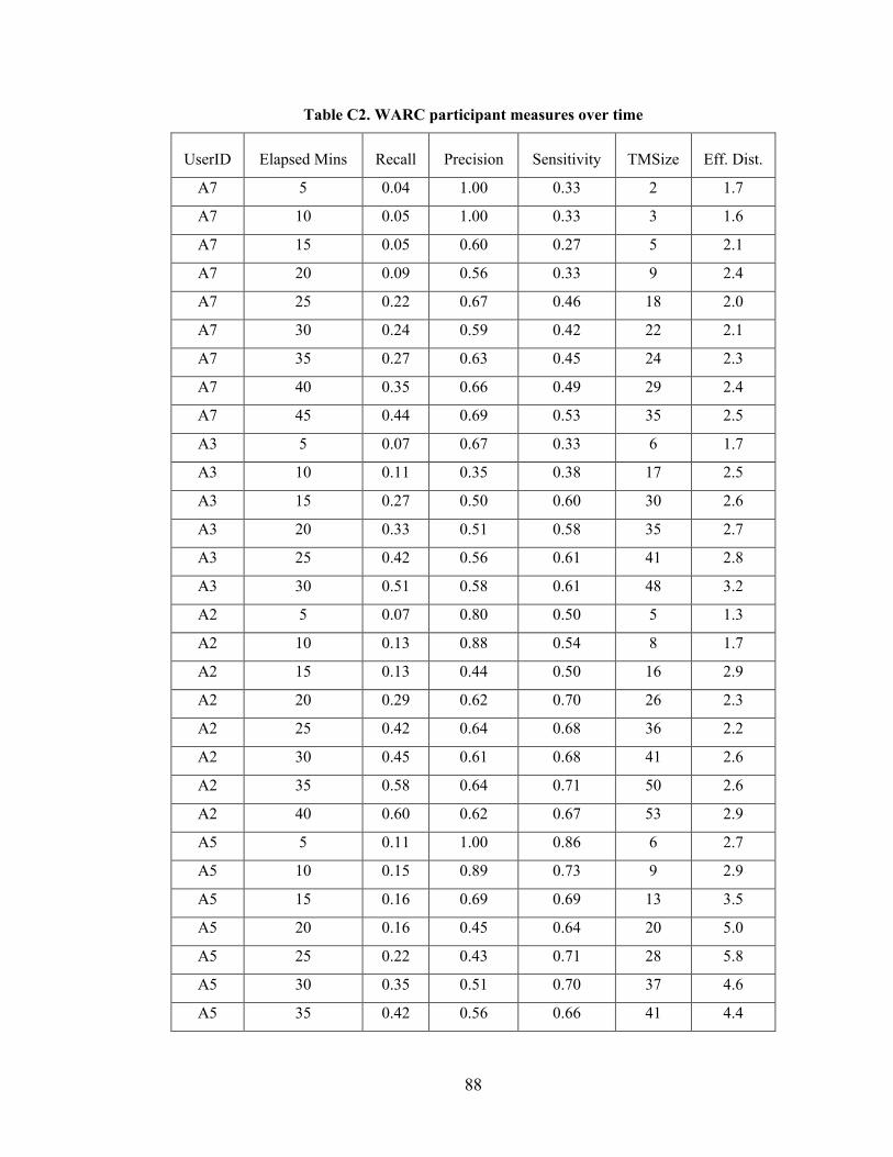
88
Table C2. WARC participant measures over time
UserID Elapsed Mins Recall Precision Sensitivity TMSize Eff. Dist.
A7 5 0.04 1.00 0.33 2 1.7
A7 10 0.05 1.00 0.33 3 1.6
A7 15 0.05 0.60 0.27 5 2.1
A7 20 0.09 0.56 0.33 9 2.4
A7 25 0.22 0.67 0.46 18 2.0
A7 30 0.24 0.59 0.42 22 2.1
A7 35 0.27 0.63 0.45 24 2.3
A7 40 0.35 0.66 0.49 29 2.4
A7 45 0.44 0.69 0.53 35 2.5
A3 5 0.07 0.67 0.33 6 1.7
A3 10 0.11 0.35 0.38 17 2.5
A3 15 0.27 0.50 0.60 30 2.6
A3 20 0.33 0.51 0.58 35 2.7
A3 25 0.42 0.56 0.61 41 2.8
A3 30 0.51 0.58 0.61 48 3.2
A2 5 0.07 0.80 0.50 5 1.3
A2 10 0.13 0.88 0.54 8 1.7
A2 15 0.13 0.44 0.50 16 2.9
A2 20 0.29 0.62 0.70 26 2.3
A2 25 0.42 0.64 0.68 36 2.2
A2 30 0.45 0.61 0.68 41 2.6
A2 35 0.58 0.64 0.71 50 2.6
A2 40 0.60 0.62 0.67 53 2.9
A5 5 0.11 1.00 0.86 6 2.7
A5 10 0.15 0.89 0.73 9 2.9
A5 15 0.16 0.69 0.69 13 3.5
A5 20 0.16 0.45 0.64 20 5.0
A5 25 0.22 0.43 0.71 28 5.8
A5 30 0.35 0.51 0.70 37 4.6
A5 35 0.42 0.56 0.66 41 4.4
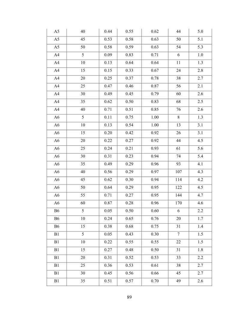
89
A5 40 0.44 0.55 0.62 44 5.0
A5 45 0.53 0.58 0.63 50 5.1
A5 50 0.58 0.59 0.63 54 5.3
A4 5 0.09 0.83 0.71 6 1.0
A4 10 0.13 0.64 0.64 11 1.3
A4 15 0.15 0.33 0.67 24 2.8
A4 20 0.25 0.37 0.78 38 2.7
A4 25 0.47 0.46 0.87 56 2.1
A4 30 0.49 0.45 0.79 60 2.6
A4 35 0.62 0.50 0.83 68 2.5
A4 40 0.71 0.51 0.85 76 2.6
A6 5 0.11 0.75 1.00 8 1.3
A6 10 0.13 0.54 1.00 13 3.1
A6 15 0.20 0.42 0.92 26 3.1
A6 20 0.22 0.27 0.92 44 4.5
A6 25 0.24 0.21 0.93 61 5.6
A6 30 0.31 0.23 0.94 74 5.4
A6 35 0.49 0.29 0.96 93 4.1
A6 40 0.56 0.29 0.97 107 4.3
A6 45 0.62 0.30 0.94 114 4.2
A6 50 0.64 0.29 0.95 122 4.5
A6 55 0.71 0.27 0.95 144 4.7
A6 60 0.87 0.28 0.96 170 4.6
B6 5 0.05 0.50 0.60 6 2.2
B6 10 0.24 0.65 0.76 20 1.7
B6 15 0.38 0.68 0.75 31 1.4
B1 5 0.05 0.43 0.30 7 1.5
B1 10 0.22 0.55 0.55 22 1.5
B1 15 0.27 0.48 0.50 31 1.8
B1 20 0.31 0.52 0.53 33 2.2
B1 25 0.36 0.53 0.61 38 2.7
B1 30 0.45 0.56 0.66 45 2.7
B1 35 0.51 0.57 0.70 49 2.6
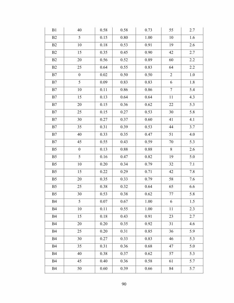
90
B1 40 0.58 0.58 0.73 55 2.7
B2 5 0.15 0.80 1.00 10 1.6
B2 10 0.18 0.53 0.91 19 2.6
B2 15 0.35 0.45 0.90 42 2.7
B2 20 0.56 0.52 0.89 60 2.2
B2 25 0.64 0.55 0.83 64 2.2
B7 0 0.02 0.50 0.50 2 1.0
B7 5 0.09 0.83 0.83 6 1.8
B7 10 0.11 0.86 0.86 7 5.4
B7 15 0.13 0.64 0.64 11 4.3
B7 20 0.15 0.36 0.62 22 5.3
B7 25 0.15 0.27 0.53 30 5.8
B7 30 0.27 0.37 0.60 41 4.1
B7 35 0.31 0.39 0.53 44 3.7
B7 40 0.33 0.35 0.47 51 4.0
B7 45 0.55 0.43 0.59 70 5.3
B5 0 0.13 0.88 0.88 8 2.6
B5 5 0.16 0.47 0.82 19 5.0
B5 10 0.20 0.34 0.79 32 7.1
B5 15 0.22 0.29 0.71 42 7.8
B5 20 0.35 0.33 0.79 58 7.6
B5 25 0.38 0.32 0.64 65 6.6
B5 30 0.53 0.38 0.62 77 5.8
B4 5 0.07 0.67 1.00 6 1.5
B4 10 0.11 0.55 1.00 11 2.3
B4 15 0.18 0.43 0.91 23 2.7
B4 20 0.20 0.35 0.92 31 4.6
B4 25 0.20 0.31 0.85 36 5.9
B4 30 0.27 0.33 0.83 46 5.3
B4 35 0.31 0.36 0.68 47 5.0
B4 40 0.38 0.37 0.62 57 5.3
B4 45 0.40 0.36 0.58 61 5.7
B4 50 0.60 0.39 0.66 84 5.7
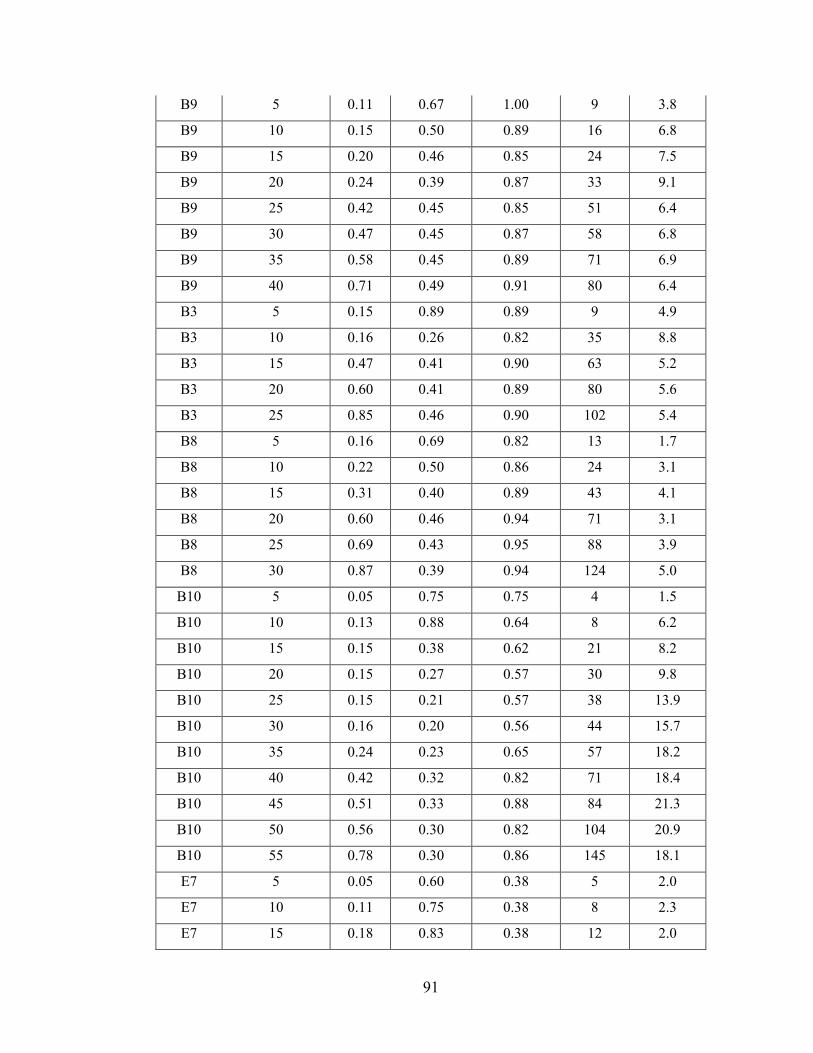
91
B9 5 0.11 0.67 1.00 9 3.8
B9 10 0.15 0.50 0.89 16 6.8
B9 15 0.20 0.46 0.85 24 7.5
B9 20 0.24 0.39 0.87 33 9.1
B9 25 0.42 0.45 0.85 51 6.4
B9 30 0.47 0.45 0.87 58 6.8
B9 35 0.58 0.45 0.89 71 6.9
B9 40 0.71 0.49 0.91 80 6.4
B3 5 0.15 0.89 0.89 9 4.9
B3 10 0.16 0.26 0.82 35 8.8
B3 15 0.47 0.41 0.90 63 5.2
B3 20 0.60 0.41 0.89 80 5.6
B3 25 0.85 0.46 0.90 102 5.4
B8 5 0.16 0.69 0.82 13 1.7
B8 10 0.22 0.50 0.86 24 3.1
B8 15 0.31 0.40 0.89 43 4.1
B8 20 0.60 0.46 0.94 71 3.1
B8 25 0.69 0.43 0.95 88 3.9
B8 30 0.87 0.39 0.94 124 5.0
B10 5 0.05 0.75 0.75 4 1.5
B10 10 0.13 0.88 0.64 8 6.2
B10 15 0.15 0.38 0.62 21 8.2
B10 20 0.15 0.27 0.57 30 9.8
B10 25 0.15 0.21 0.57 38 13.9
B10 30 0.16 0.20 0.56 44 15.7
B10 35 0.24 0.23 0.65 57 18.2
B10 40 0.42 0.32 0.82 71 18.4
B10 45 0.51 0.33 0.88 84 21.3
B10 50 0.56 0.30 0.82 104 20.9
B10 55 0.78 0.30 0.86 145 18.1
E7 5 0.05 0.60 0.38 5 2.0
E7 10 0.11 0.75 0.38 8 2.3
E7 15 0.18 0.83 0.38 12 2.0
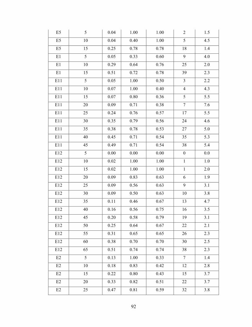
92
E5 5 0.04 1.00 1.00 2 1.5
E5 10 0.04 0.40 1.00 5 4.5
E5 15 0.25 0.78 0.78 18 1.4
E1 5 0.05 0.33 0.60 9 4.0
E1 10 0.29 0.64 0.76 25 2.0
E1 15 0.51 0.72 0.78 39 2.3
E11 5 0.05 1.00 0.50 3 2.2
E11 10 0.07 1.00 0.40 4 4.3
E11 15 0.07 0.80 0.36 5 5.5
E11 20 0.09 0.71 0.38 7 7.6
E11 25 0.24 0.76 0.57 17 5.5
E11 30 0.35 0.79 0.56 24 4.6
E11 35 0.38 0.78 0.53 27 5.0
E11 40 0.45 0.71 0.54 35 5.3
E11 45 0.49 0.71 0.54 38 5.4
E12 5 0.00 0.00 0.00 0 0.0
E12 10 0.02 1.00 1.00 1 1.0
E12 15 0.02 1.00 1.00 1 2.0
E12 20 0.09 0.83 0.63 6 1.9
E12 25 0.09 0.56 0.63 9 3.1
E12 30 0.09 0.50 0.63 10 3.8
E12 35 0.11 0.46 0.67 13 4.7
E12 40 0.16 0.56 0.75 16 3.5
E12 45 0.20 0.58 0.79 19 3.1
E12 50 0.25 0.64 0.67 22 2.1
E12 55 0.31 0.65 0.65 26 2.3
E12 60 0.38 0.70 0.70 30 2.5
E12 65 0.51 0.74 0.74 38 2.3
E2 5 0.13 1.00 0.33 7 1.4
E2 10 0.18 0.83 0.42 12 2.8
E2 15 0.22 0.80 0.43 15 3.7
E2 20 0.33 0.82 0.51 22 3.7
E2 25 0.47 0.81 0.59 32 3.8
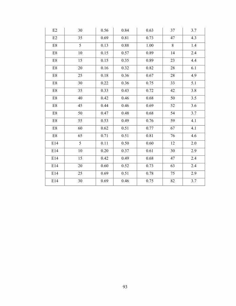
93
E2 30 0.56 0.84 0.63 37 3.7
E2 35 0.69 0.81 0.73 47 4.3
E8 5 0.13 0.88 1.00 8 1.4
E8 10 0.15 0.57 0.89 14 2.4
E8 15 0.15 0.35 0.89 23 4.4
E8 20 0.16 0.32 0.82 28 6.1
E8 25 0.18 0.36 0.67 28 4.9
E8 30 0.22 0.36 0.75 33 5.1
E8 35 0.33 0.43 0.72 42 3.8
E8 40 0.42 0.46 0.68 50 3.5
E8 45 0.44 0.46 0.69 52 3.6
E8 50 0.47 0.48 0.68 54 3.7
E8 55 0.53 0.49 0.76 59 4.1
E8 60 0.62 0.51 0.77 67 4.1
E8 65 0.71 0.51 0.81 76 4.6
E14 5 0.11 0.50 0.60 12 2.0
E14 10 0.20 0.37 0.61 30 2.9
E14 15 0.42 0.49 0.68 47 2.4
E14 20 0.60 0.52 0.73 63 2.4
E14 25 0.69 0.51 0.78 75 2.9
E14 30 0.69 0.46 0.75 82 3.7
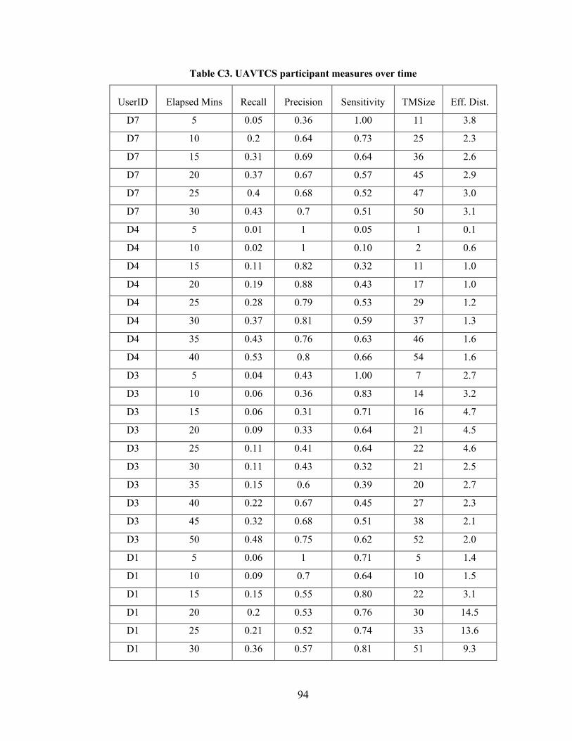
94
Table C3. UAVTCS participant measures over time
UserID Elapsed Mins Recall Precision Sensitivity TMSize Eff. Dist.
D7 5 0.05 0.36 1.00 11 3.8
D7 10 0.2 0.64 0.73 25 2.3
D7 15 0.31 0.69 0.64 36 2.6
D7 20 0.37 0.67 0.57 45 2.9
D7 25 0.4 0.68 0.52 47 3.0
D7 30 0.43 0.7 0.51 50 3.1
D4 5 0.01 1 0.05 1 0.1
D4 10 0.02 1 0.10 2 0.6
D4 15 0.11 0.82 0.32 11 1.0
D4 20 0.19 0.88 0.43 17 1.0
D4 25 0.28 0.79 0.53 29 1.2
D4 30 0.37 0.81 0.59 37 1.3
D4 35 0.43 0.76 0.63 46 1.6
D4 40 0.53 0.8 0.66 54 1.6
D3 5 0.04 0.43 1.00 7 2.7
D3 10 0.06 0.36 0.83 14 3.2
D3 15 0.06 0.31 0.71 16 4.7
D3 20 0.09 0.33 0.64 21 4.5
D3 25 0.11 0.41 0.64 22 4.6
D3 30 0.11 0.43 0.32 21 2.5
D3 35 0.15 0.6 0.39 20 2.7
D3 40 0.22 0.67 0.45 27 2.3
D3 45 0.32 0.68 0.51 38 2.1
D3 50 0.48 0.75 0.62 52 2.0
D1 5 0.06 1 0.71 5 1.4
D1 10 0.09 0.7 0.64 10 1.5
D1 15 0.15 0.55 0.80 22 3.1
D1 20 0.2 0.53 0.76 30 14.5
D1 25 0.21 0.52 0.74 33 13.6
D1 30 0.36 0.57 0.81 51 9.3
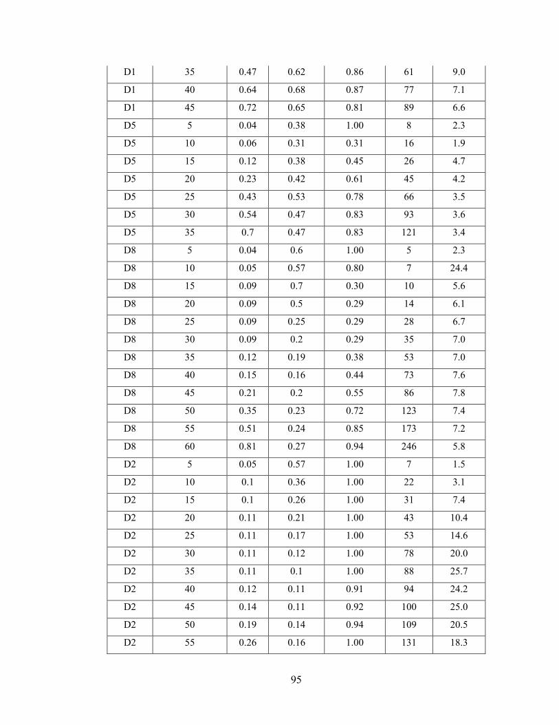
95
D1 35 0.47 0.62 0.86 61 9.0
D1 40 0.64 0.68 0.87 77 7.1
D1 45 0.72 0.65 0.81 89 6.6
D5 5 0.04 0.38 1.00 8 2.3
D5 10 0.06 0.31 0.31 16 1.9
D5 15 0.12 0.38 0.45 26 4.7
D5 20 0.23 0.42 0.61 45 4.2
D5 25 0.43 0.53 0.78 66 3.5
D5 30 0.54 0.47 0.83 93 3.6
D5 35 0.7 0.47 0.83 121 3.4
D8 5 0.04 0.6 1.00 5 2.3
D8 10 0.05 0.57 0.80 7 24.4
D8 15 0.09 0.7 0.30 10 5.6
D8 20 0.09 0.5 0.29 14 6.1
D8 25 0.09 0.25 0.29 28 6.7
D8 30 0.09 0.2 0.29 35 7.0
D8 35 0.12 0.19 0.38 53 7.0
D8 40 0.15 0.16 0.44 73 7.6
D8 45 0.21 0.2 0.55 86 7.8
D8 50 0.35 0.23 0.72 123 7.4
D8 55 0.51 0.24 0.85 173 7.2
D8 60 0.81 0.27 0.94 246 5.8
D2 5 0.05 0.57 1.00 7 1.5
D2 10 0.1 0.36 1.00 22 3.1
D2 15 0.1 0.26 1.00 31 7.4
D2 20 0.11 0.21 1.00 43 10.4
D2 25 0.11 0.17 1.00 53 14.6
D2 30 0.11 0.12 1.00 78 20.0
D2 35 0.11 0.1 1.00 88 25.7
D2 40 0.12 0.11 0.91 94 24.2
D2 45 0.14 0.11 0.92 100 25.0
D2 50 0.19 0.14 0.94 109 20.5
D2 55 0.26 0.16 1.00 131 18.3
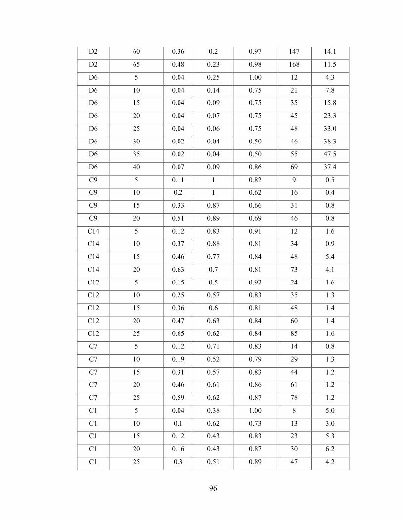
96
D2 60 0.36 0.2 0.97 147 14.1
D2 65 0.48 0.23 0.98 168 11.5
D6 5 0.04 0.25 1.00 12 4.3
D6 10 0.04 0.14 0.75 21 7.8
D6 15 0.04 0.09 0.75 35 15.8
D6 20 0.04 0.07 0.75 45 23.3
D6 25 0.04 0.06 0.75 48 33.0
D6 30 0.02 0.04 0.50 46 38.3
D6 35 0.02 0.04 0.50 55 47.5
D6 40 0.07 0.09 0.86 69 37.4
C9 5 0.11 1 0.82 9 0.5
C9 10 0.2 1 0.62 16 0.4
C9 15 0.33 0.87 0.66 31 0.8
C9 20 0.51 0.89 0.69 46 0.8
C14 5 0.12 0.83 0.91 12 1.6
C14 10 0.37 0.88 0.81 34 0.9
C14 15 0.46 0.77 0.84 48 5.4
C14 20 0.63 0.7 0.81 73 4.1
C12 5 0.15 0.5 0.92 24 1.6
C12 10 0.25 0.57 0.83 35 1.3
C12 15 0.36 0.6 0.81 48 1.4
C12 20 0.47 0.63 0.84 60 1.4
C12 25 0.65 0.62 0.84 85 1.6
C7 5 0.12 0.71 0.83 14 0.8
C7 10 0.19 0.52 0.79 29 1.3
C7 15 0.31 0.57 0.83 44 1.2
C7 20 0.46 0.61 0.86 61 1.2
C7 25 0.59 0.62 0.87 78 1.2
C1 5 0.04 0.38 1.00 8 5.0
C1 10 0.1 0.62 0.73 13 3.0
C1 15 0.12 0.43 0.83 23 5.3
C1 20 0.16 0.43 0.87 30 6.2
C1 25 0.3 0.51 0.89 47 4.2
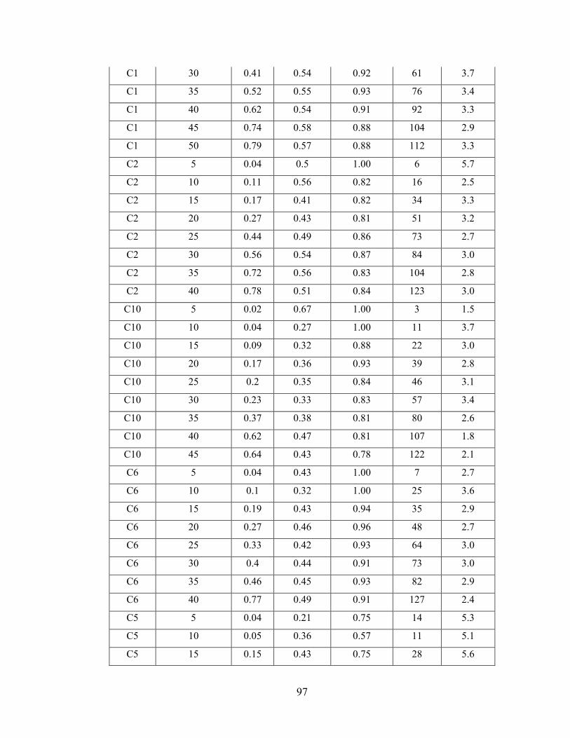
97
C1 30 0.41 0.54 0.92 61 3.7
C1 35 0.52 0.55 0.93 76 3.4
C1 40 0.62 0.54 0.91 92 3.3
C1 45 0.74 0.58 0.88 104 2.9
C1 50 0.79 0.57 0.88 112 3.3
C2 5 0.04 0.5 1.00 6 5.7
C2 10 0.11 0.56 0.82 16 2.5
C2 15 0.17 0.41 0.82 34 3.3
C2 20 0.27 0.43 0.81 51 3.2
C2 25 0.44 0.49 0.86 73 2.7
C2 30 0.56 0.54 0.87 84 3.0
C2 35 0.72 0.56 0.83 104 2.8
C2 40 0.78 0.51 0.84 123 3.0
C10 5 0.02 0.67 1.00 3 1.5
C10 10 0.04 0.27 1.00 11 3.7
C10 15 0.09 0.32 0.88 22 3.0
C10 20 0.17 0.36 0.93 39 2.8
C10 25 0.2 0.35 0.84 46 3.1
C10 30 0.23 0.33 0.83 57 3.4
C10 35 0.37 0.38 0.81 80 2.6
C10 40 0.62 0.47 0.81 107 1.8
C10 45 0.64 0.43 0.78 122 2.1
C6 5 0.04 0.43 1.00 7 2.7
C6 10 0.1 0.32 1.00 25 3.6
C6 15 0.19 0.43 0.94 35 2.9
C6 20 0.27 0.46 0.96 48 2.7
C6 25 0.33 0.42 0.93 64 3.0
C6 30 0.4 0.44 0.91 73 3.0
C6 35 0.46 0.45 0.93 82 2.9
C6 40 0.77 0.49 0.91 127 2.4
C5 5 0.04 0.21 0.75 14 5.3
C5 10 0.05 0.36 0.57 11 5.1
C5 15 0.15 0.43 0.75 28 5.6
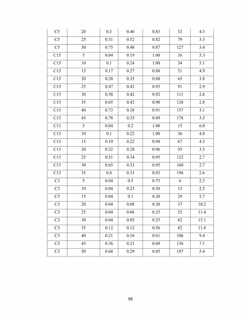
98
C5 20 0.3 0.46 0.83 52 4.3
C5 25 0.51 0.52 0.82 79 3.3
C5 30 0.75 0.48 0.87 127 3.4
C15 5 0.04 0.19 1.00 16 5.3
C15 10 0.1 0.24 1.00 34 5.1
C15 15 0.17 0.27 0.88 51 4.9
C15 20 0.28 0.35 0.88 65 3.8
C15 25 0.47 0.42 0.93 91 2.9
C15 30 0.58 0.42 0.92 111 2.8
C15 35 0.65 0.42 0.90 126 2.8
C15 40 0.73 0.38 0.91 157 3.1
C15 45 0.78 0.35 0.89 178 3.5
C13 5 0.04 0.2 1.00 15 6.0
C13 10 0.1 0.22 1.00 36 4.8
C13 15 0.19 0.22 0.94 67 4.3
C13 20 0.32 0.28 0.96 93 3.5
C13 25 0.51 0.34 0.95 122 2.7
C13 30 0.65 0.33 0.95 160 2.7
C13 35 0.8 0.33 0.93 196 2.6
C3 5 0.04 0.5 0.75 6 2.3
C3 10 0.04 0.23 0.30 13 2.5
C3 15 0.04 0.1 0.30 29 5.7
C3 20 0.04 0.08 0.30 37 10.2
C3 25 0.04 0.06 0.25 52 11.4
C3 30 0.04 0.05 0.25 62 15.1
C3 35 0.12 0.12 0.56 82 11.8
C3 40 0.21 0.16 0.61 106 9.4
C3 45 0.36 0.21 0.69 136 7.1
C3 50 0.68 0.29 0.85 187 5.4
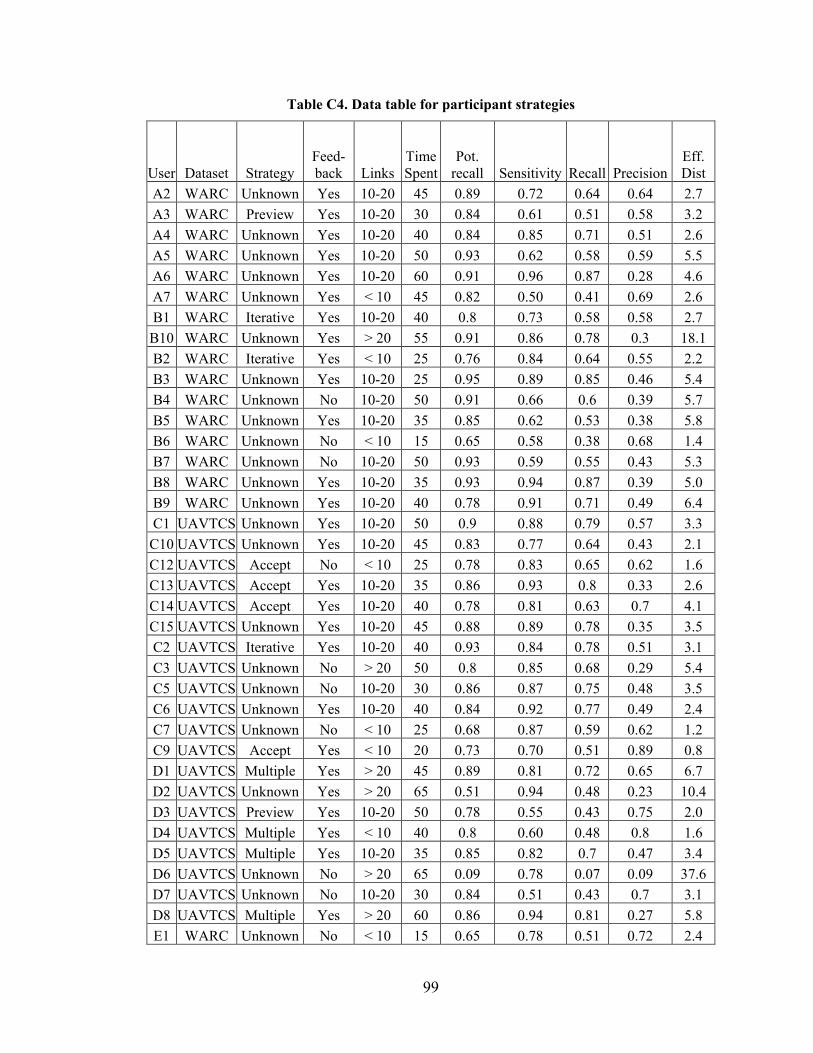
99
Table C4. Data table for participant strategies
User Dataset Strategy Feed-back Links
Time Spent
Pot. recall Sensitivity Recall Precision
Eff. Dist
A2 WARC Unknown Yes 10-20 45 0.89 0.72 0.64 0.64 2.7 A3 WARC Preview Yes 10-20 30 0.84 0.61 0.51 0.58 3.2 A4 WARC Unknown Yes 10-20 40 0.84 0.85 0.71 0.51 2.6 A5 WARC Unknown Yes 10-20 50 0.93 0.62 0.58 0.59 5.5 A6 WARC Unknown Yes 10-20 60 0.91 0.96 0.87 0.28 4.6 A7 WARC Unknown Yes < 10 45 0.82 0.50 0.41 0.69 2.6 B1 WARC Iterative Yes 10-20 40 0.8 0.73 0.58 0.58 2.7
B10 WARC Unknown Yes > 20 55 0.91 0.86 0.78 0.3 18.1 B2 WARC Iterative Yes < 10 25 0.76 0.84 0.64 0.55 2.2 B3 WARC Unknown Yes 10-20 25 0.95 0.89 0.85 0.46 5.4 B4 WARC Unknown No 10-20 50 0.91 0.66 0.6 0.39 5.7 B5 WARC Unknown Yes 10-20 35 0.85 0.62 0.53 0.38 5.8 B6 WARC Unknown No < 10 15 0.65 0.58 0.38 0.68 1.4 B7 WARC Unknown No 10-20 50 0.93 0.59 0.55 0.43 5.3 B8 WARC Unknown Yes 10-20 35 0.93 0.94 0.87 0.39 5.0 B9 WARC Unknown Yes 10-20 40 0.78 0.91 0.71 0.49 6.4 C1 UAVTCS Unknown Yes 10-20 50 0.9 0.88 0.79 0.57 3.3
C10 UAVTCS Unknown Yes 10-20 45 0.83 0.77 0.64 0.43 2.1 C12 UAVTCS Accept No < 10 25 0.78 0.83 0.65 0.62 1.6 C13 UAVTCS Accept Yes 10-20 35 0.86 0.93 0.8 0.33 2.6 C14 UAVTCS Accept Yes 10-20 40 0.78 0.81 0.63 0.7 4.1 C15 UAVTCS Unknown Yes 10-20 45 0.88 0.89 0.78 0.35 3.5 C2 UAVTCS Iterative Yes 10-20 40 0.93 0.84 0.78 0.51 3.1 C3 UAVTCS Unknown No > 20 50 0.8 0.85 0.68 0.29 5.4 C5 UAVTCS Unknown No 10-20 30 0.86 0.87 0.75 0.48 3.5 C6 UAVTCS Unknown Yes 10-20 40 0.84 0.92 0.77 0.49 2.4 C7 UAVTCS Unknown No < 10 25 0.68 0.87 0.59 0.62 1.2 C9 UAVTCS Accept Yes < 10 20 0.73 0.70 0.51 0.89 0.8 D1 UAVTCS Multiple Yes > 20 45 0.89 0.81 0.72 0.65 6.7 D2 UAVTCS Unknown Yes > 20 65 0.51 0.94 0.48 0.23 10.4 D3 UAVTCS Preview Yes 10-20 50 0.78 0.55 0.43 0.75 2.0 D4 UAVTCS Multiple Yes < 10 40 0.8 0.60 0.48 0.8 1.6 D5 UAVTCS Multiple Yes 10-20 35 0.85 0.82 0.7 0.47 3.4 D6 UAVTCS Unknown No > 20 65 0.09 0.78 0.07 0.09 37.6 D7 UAVTCS Unknown No 10-20 30 0.84 0.51 0.43 0.7 3.1 D8 UAVTCS Multiple Yes > 20 60 0.86 0.94 0.81 0.27 5.8 E1 WARC Unknown No < 10 15 0.65 0.78 0.51 0.72 2.4
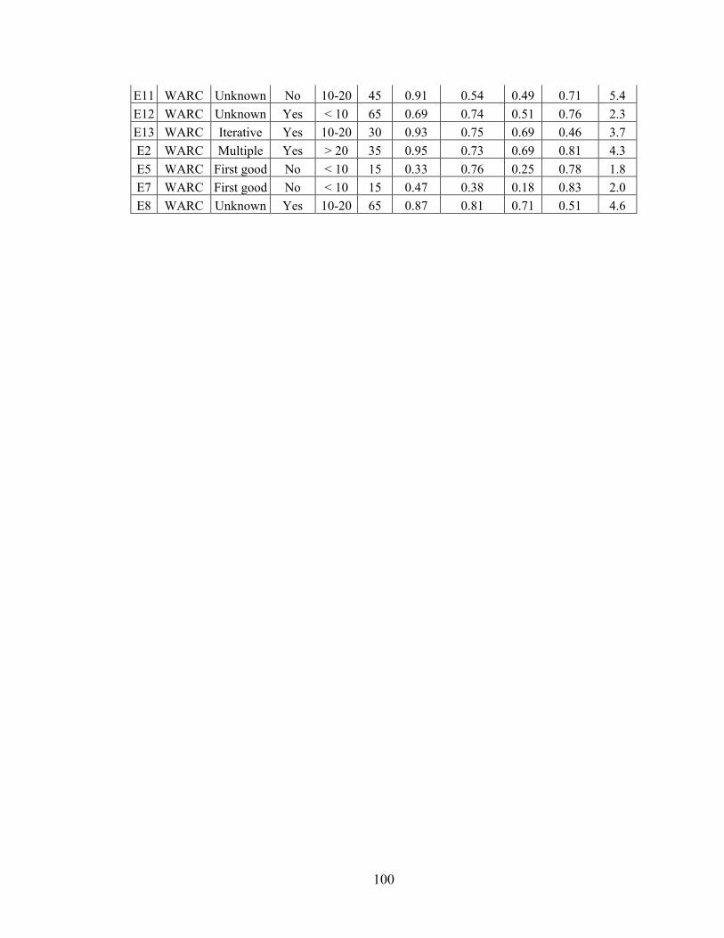
100
E11 WARC Unknown No 10-20 45 0.91 0.54 0.49 0.71 5.4 E12 WARC Unknown Yes < 10 65 0.69 0.74 0.51 0.76 2.3 E13 WARC Iterative Yes 10-20 30 0.93 0.75 0.69 0.46 3.7 E2 WARC Multiple Yes > 20 35 0.95 0.73 0.69 0.81 4.3 E5 WARC First good No < 10 15 0.33 0.76 0.25 0.78 1.8 E7 WARC First good No < 10 15 0.47 0.38 0.18 0.83 2.0 E8 WARC Unknown Yes 10-20 65 0.87 0.81 0.71 0.51 4.6
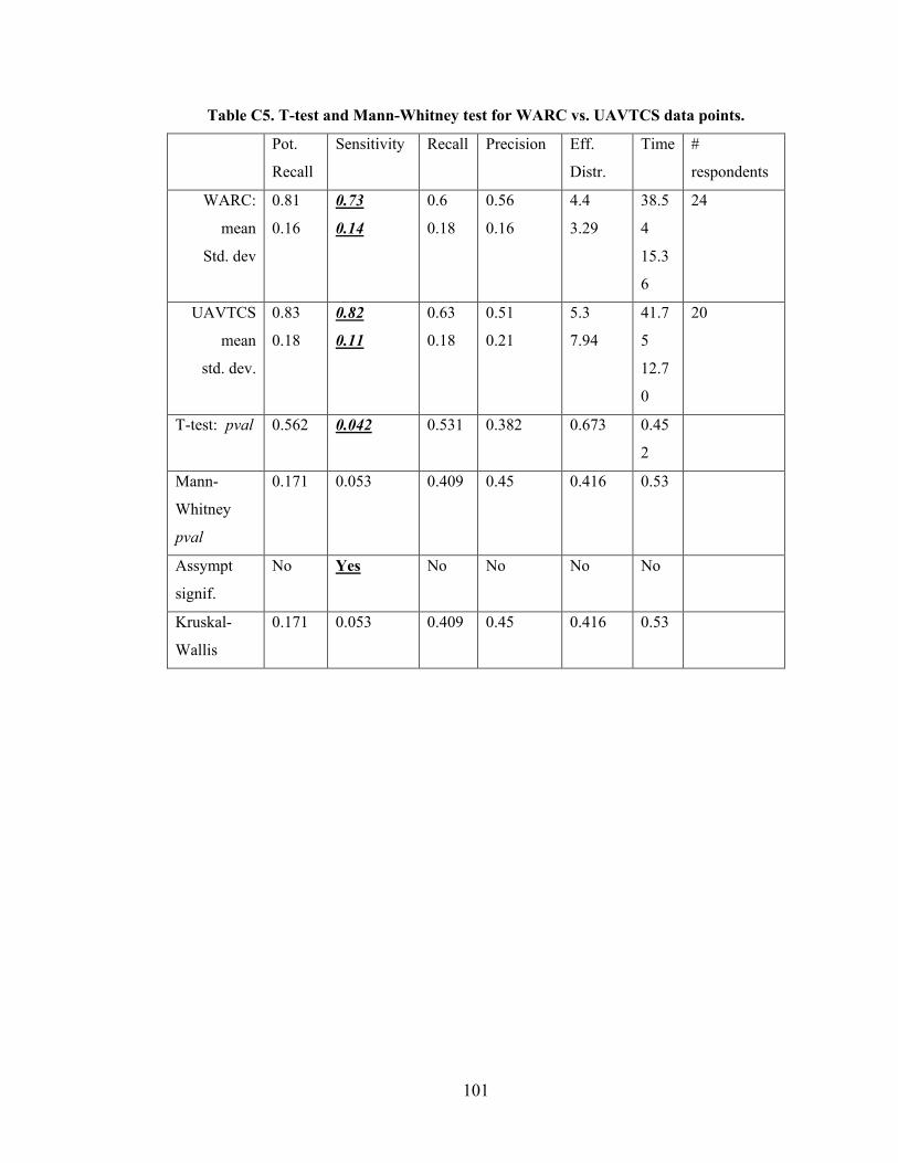
101
Table C5. T-test and Mann-Whitney test for WARC vs. UAVTCS data points.
Pot.
Recall
Sensitivity Recall Precision Eff.
Distr.
Time #
respondents
WARC:
mean
Std. dev
0.81
0.16
0.73
0.14
0.6
0.18
0.56
0.16
4.4
3.29
38.5
4
15.3
6
24
UAVTCS
mean
std. dev.
0.83
0.18
0.82
0.11
0.63
0.18
0.51
0.21
5.3
7.94
41.7
5
12.7
0
20
T-test: pval 0.562 0.042 0.531 0.382 0.673 0.45
2
Mann-
Whitney
pval
0.171 0.053 0.409 0.45 0.416 0.53
Assympt
signif.
No Yes No No No No
Kruskal-
Wallis
0.171 0.053 0.409 0.45 0.416 0.53
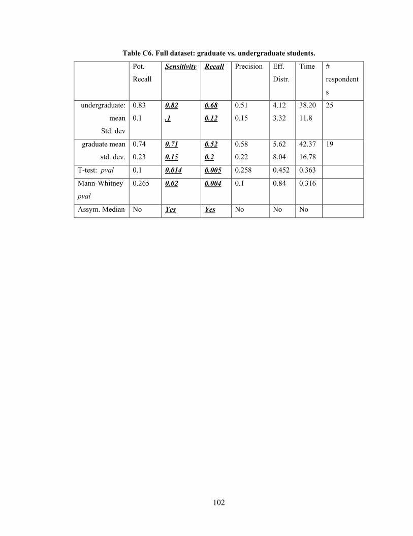
102
Table C6. Full dataset: graduate vs. undergraduate students.
Pot.
Recall
Sensitivity Recall Precision Eff.
Distr.
Time #
respondent
s
undergraduate:
mean
Std. dev
0.83
0.1
0.82
.1
0.68
0.12
0.51
0.15
4.12
3.32
38.20
11.8
25
graduate mean
std. dev.
0.74
0.23
0.71
0.15
0.52
0.2
0.58
0.22
5.62
8.04
42.37
16.78
19
T-test: pval 0.1 0.014 0.005 0.258 0.452 0.363
Mann-Whitney
pval
0.265 0.02 0.004 0.1 0.84 0.316
Assym. Median No Yes Yes No No No
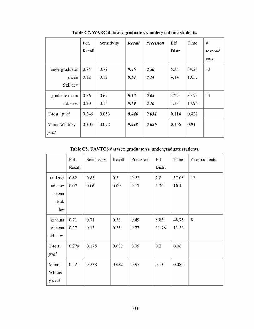
103
Table C7. WARC dataset: graduate vs. undergraduate students.
Pot.
Recall
Sensitivity Recall Precision Eff.
Distr.
Time #
respond
ents
undergraduate:
mean
Std. dev
0.84
0.12
0.79
0.12
0.66
0.14
0.50
0.14
5.34
4.14
39.23
13.52
13
graduate mean
std. dev.
0.76
0.20
0.67
0.15
0.52
0.19
0.64
0.16
3.29
1.33
37.73
17.94
11
T-test: pval 0.245 0.053 0.046 0.031 0.114 0.822
Mann-Whitney
pval
0.303 0.072 0.018 0.026 0.106 0.91
Table C8. UAVTCS dataset: graduate vs. undergraduate students.
Pot.
Recall
Sensitivity Recall Precision Eff.
Distr.
Time # respondents
undergr
aduate:
mean
Std.
dev
0.82
0.07
0.85
0.06
0.7
0.09
0.52
0.17
2.8
1.30
37.08
10.1
12
graduat
e mean
std. dev.
0.71
0.27
0.71
0.15
0.53
0.23
0.49
0.27
8.83
11.98
48.75
13.56
8
T-test:
pval
0.279 0.175 0.082 0.79 0.2 0.06
Mann-
Whitne
y pval
0.521 0.238 0.082 0.97 0.13 0.082
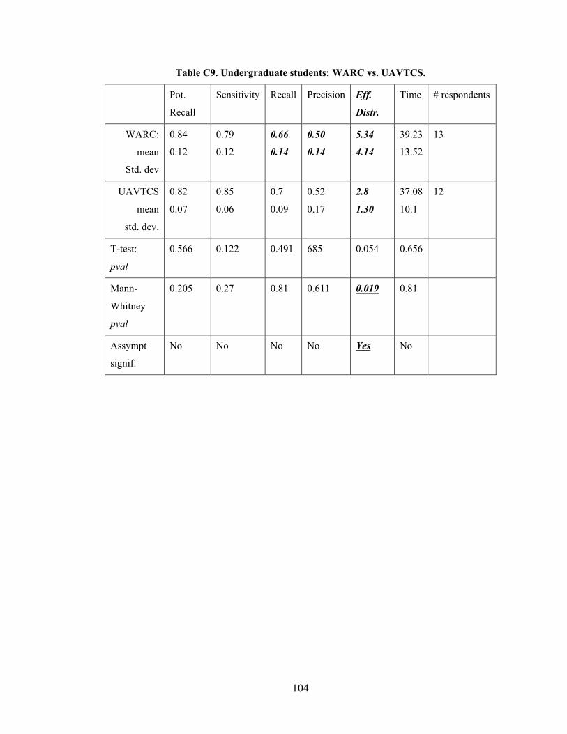
104
Table C9. Undergraduate students: WARC vs. UAVTCS.
Pot.
Recall
Sensitivity Recall Precision Eff.
Distr.
Time # respondents
WARC:
mean
Std. dev
0.84
0.12
0.79
0.12
0.66
0.14
0.50
0.14
5.34
4.14
39.23
13.52
13
UAVTCS
mean
std. dev.
0.82
0.07
0.85
0.06
0.7
0.09
0.52
0.17
2.8
1.30
37.08
10.1
12
T-test:
pval
0.566 0.122 0.491 685 0.054 0.656
Mann-
Whitney
pval
0.205 0.27 0.81 0.611 0.019 0.81
Assympt
signif.
No No No No Yes No
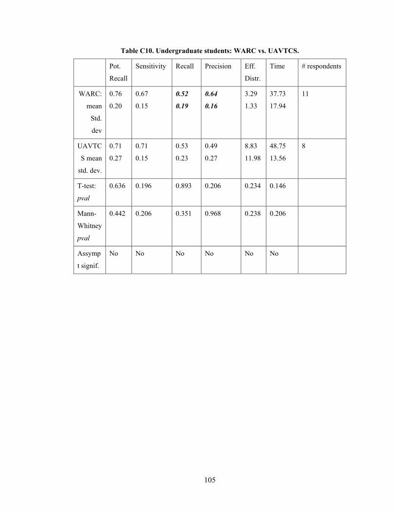
105
Table C10. Undergraduate students: WARC vs. UAVTCS.
Pot.
Recall
Sensitivity Recall Precision Eff.
Distr.
Time # respondents
WARC:
mean
Std.
dev
0.76
0.20
0.67
0.15
0.52
0.19
0.64
0.16
3.29
1.33
37.73
17.94
11
UAVTC
S mean
std. dev.
0.71
0.27
0.71
0.15
0.53
0.23
0.49
0.27
8.83
11.98
48.75
13.56
8
T-test:
pval
0.636 0.196 0.893 0.206 0.234 0.146
Mann-
Whitney
pval
0.442 0.206 0.351 0.968 0.238 0.206
Assymp
t signif.
No No No No No No
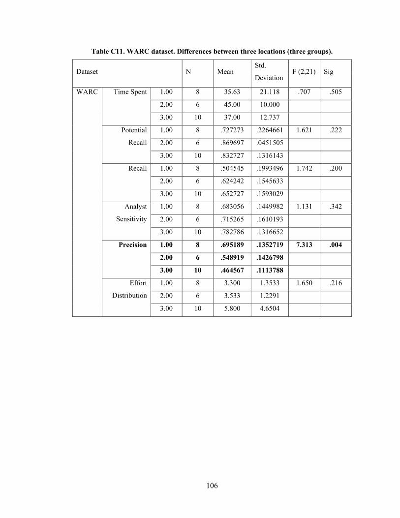
106
Table C11. WARC dataset. Differences between three locations (three groups).
Dataset N Mean Std.
Deviation F (2,21) Sig
WARC Time Spent 1.00 8 35.63 21.118 .707 .505
2.00 6 45.00 10.000
3.00 10 37.00 12.737
Potential
Recall
1.00 8 .727273 .2264661 1.621 .222
2.00 6 .869697 .0451505
3.00 10 .832727 .1316143
Recall 1.00 8 .504545 .1993496 1.742 .200
2.00 6 .624242 .1545633
3.00 10 .652727 .1593029
Analyst
Sensitivity
1.00 8 .683056 .1449982 1.131 .342
2.00 6 .715265 .1610193
3.00 10 .782786 .1316652
Precision 1.00 8 .695189 .1352719 7.313 .004
2.00 6 .548919 .1426798
3.00 10 .464567 .1113788
Effort
Distribution
1.00 8 3.300 1.3533 1.650 .216
2.00 6 3.533 1.2291
3.00 10 5.800 4.6504
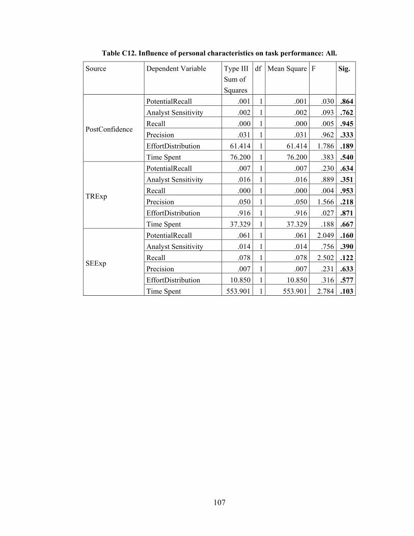
107
Table C12. Influence of personal characteristics on task performance: All.
Source Dependent Variable Type III Sum of Squares
df Mean Square F Sig.
PostConfidence
PotentialRecall .001 1 .001 .030 .864 Analyst Sensitivity .002 1 .002 .093 .762 Recall .000 1 .000 .005 .945 Precision .031 1 .031 .962 .333 EffortDistribution 61.414 1 61.414 1.786 .189 Time Spent 76.200 1 76.200 .383 .540
TRExp
PotentialRecall .007 1 .007 .230 .634 Analyst Sensitivity .016 1 .016 .889 .351 Recall .000 1 .000 .004 .953 Precision .050 1 .050 1.566 .218 EffortDistribution .916 1 .916 .027 .871 Time Spent 37.329 1 37.329 .188 .667
SEExp
PotentialRecall .061 1 .061 2.049 .160 Analyst Sensitivity .014 1 .014 .756 .390 Recall .078 1 .078 2.502 .122 Precision .007 1 .007 .231 .633 EffortDistribution 10.850 1 10.850 .316 .577 Time Spent 553.901 1 553.901 2.784 .103
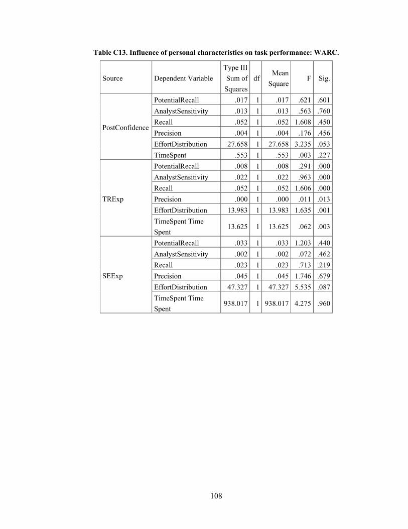
108
Table C13. Influence of personal characteristics on task performance: WARC.
Source Dependent Variable Type III Sum of
Squares df
Mean Square
F Sig.
PostConfidence
PotentialRecall .017 1 .017 .621 .601 AnalystSensitivity .013 1 .013 .563 .760 Recall .052 1 .052 1.608 .450 Precision .004 1 .004 .176 .456 EffortDistribution 27.658 1 27.658 3.235 .053 TimeSpent .553 1 .553 .003 .227
TRExp
PotentialRecall .008 1 .008 .291 .000 AnalystSensitivity .022 1 .022 .963 .000 Recall .052 1 .052 1.606 .000 Precision .000 1 .000 .011 .013 EffortDistribution 13.983 1 13.983 1.635 .001 TimeSpent Time Spent
13.625 1 13.625 .062 .003
SEExp
PotentialRecall .033 1 .033 1.203 .440 AnalystSensitivity .002 1 .002 .072 .462 Recall .023 1 .023 .713 .219 Precision .045 1 .045 1.746 .679 EffortDistribution 47.327 1 47.327 5.535 .087 TimeSpent Time Spent
938.017 1 938.017 4.275 .960
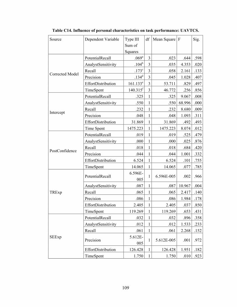
109
Table C14. Influence of personal characteristics on task performance: UAVTCS.
Source Dependent Variable Type III Sum of Squares
df Mean Square F Sig.
Corrected Model
PotentialRecall .069a 3 .023 .644 .598 AnalystSensitivity .104b 3 .035 4.353 .020 Recall .173c 3 .058 2.161 .133 Precision .134d 3 .045 1.028 .407 EffortDistribution 161.133e 3 53.711 .829 .497 TimeSpent 140.315f 3 46.772 .256 .856
Intercept
PotentialRecall .325 1 .325 9.067 .008 AnalystSensitivity .550 1 .550 68.996 .000 Recall .232 1 .232 8.680 .009 Precision .048 1 .048 1.093 .311 EffortDistribution 31.869 1 31.869 .492 .493 Time Spent 1475.223 1 1475.223 8.074 .012
PostConfidence
PotentialRecall .019 1 .019 .525 .479 AnalystSensitivity .000 1 .000 .025 .876 Recall .018 1 .018 .684 .420 Precision .044 1 .044 1.001 .332 EffortDistribution 6.524 1 6.524 .101 .755 TimeSpent 14.065 1 14.065 .077 .785
TRExp
PotentialRecall 6.596E-
005 1 6.596E-005 .002 .966
AnalystSensitivity .087 1 .087 10.967 .004 Recall .065 1 .065 2.417 .140 Precision .086 1 .086 1.984 .178 EffortDistribution 2.405 1 2.405 .037 .850 TimeSpent 119.269 1 119.269 .653 .431
SEExp
PotentialRecall .032 1 .032 .896 .358 AnalystSensitivity .012 1 .012 1.533 .233 Recall .061 1 .061 2.268 .152
Precision 5.612E-
005 1 5.612E-005 .001 .972
EffortDistribution 126.428 1 126.428 1.951 .182 TimeSpent 1.750 1 1.750 .010 .923
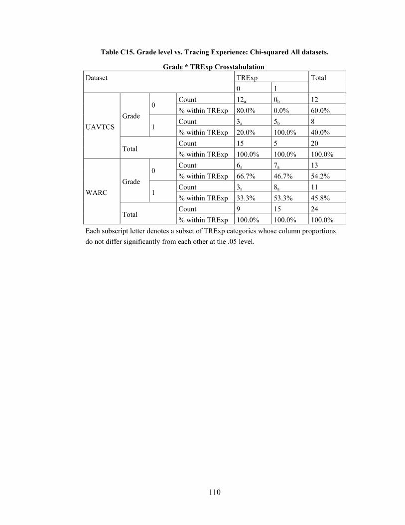
110
Table C15. Grade level vs. Tracing Experience: Chi-squared All datasets.
Grade * TRExp Crosstabulation Dataset TRExp Total
0 1
UAVTCS Grade
0 Count 12a 0b 12 % within TRExp 80.0% 0.0% 60.0%
1 Count 3a 5b 8 % within TRExp 20.0% 100.0% 40.0%
Total Count 15 5 20 % within TRExp 100.0% 100.0% 100.0%
WARC Grade
0 Count 6a 7a 13 % within TRExp 66.7% 46.7% 54.2%
1 Count 3a 8a 11 % within TRExp 33.3% 53.3% 45.8%
Total Count 9 15 24 % within TRExp 100.0% 100.0% 100.0%
Each subscript letter denotes a subset of TRExp categories whose column proportions do not differ significantly from each other at the .05 level.
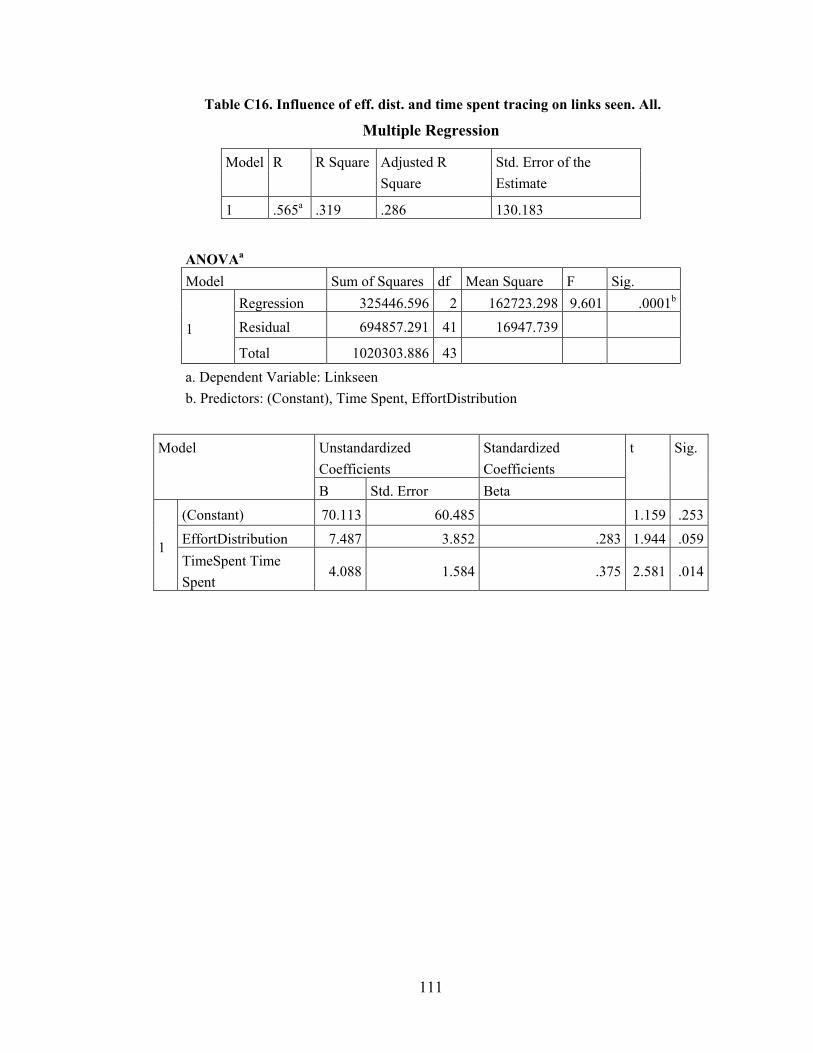
111
Table C16. Influence of eff. dist. and time spent tracing on links seen. All.
Multiple Regression
Model R R Square Adjusted R Square
Std. Error of the Estimate
1 .565a .319 .286 130.183
ANOVAa Model Sum of Squares df Mean Square F Sig.
1
Regression 325446.596 2 162723.298 9.601 .0001b Residual 694857.291 41 16947.739
Total 1020303.886 43
a. Dependent Variable: Linkseen b. Predictors: (Constant), Time Spent, EffortDistribution
Model Unstandardized Coefficients
Standardized Coefficients
t Sig.
B Std. Error Beta
1
(Constant) 70.113 60.485 1.159 .253 EffortDistribution 7.487 3.852 .283 1.944 .059 TimeSpent Time Spent
4.088 1.584 .375 2.581 .014
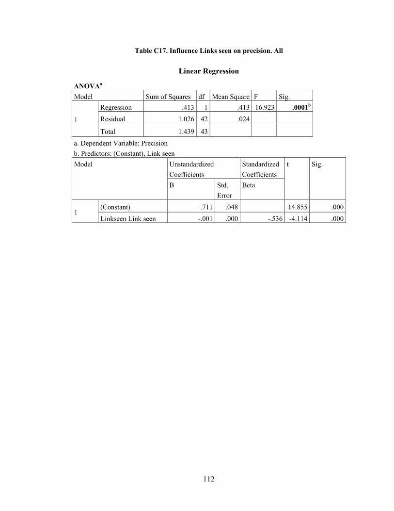
112
Table C17. Influence Links seen on precision. All
Linear Regression
ANOVAa Model Sum of Squares df Mean Square F Sig.
1
Regression .413 1 .413 16.923 .0001b Residual 1.026 42 .024
Total 1.439 43
a. Dependent Variable: Precision b. Predictors: (Constant), Link seen Model Unstandardized
Coefficients Standardized Coefficients
t Sig.
B Std. Error
Beta
1 (Constant) .711 .048 14.855 .000 Linkseen Link seen -.001 .000 -.536 -4.114 .000
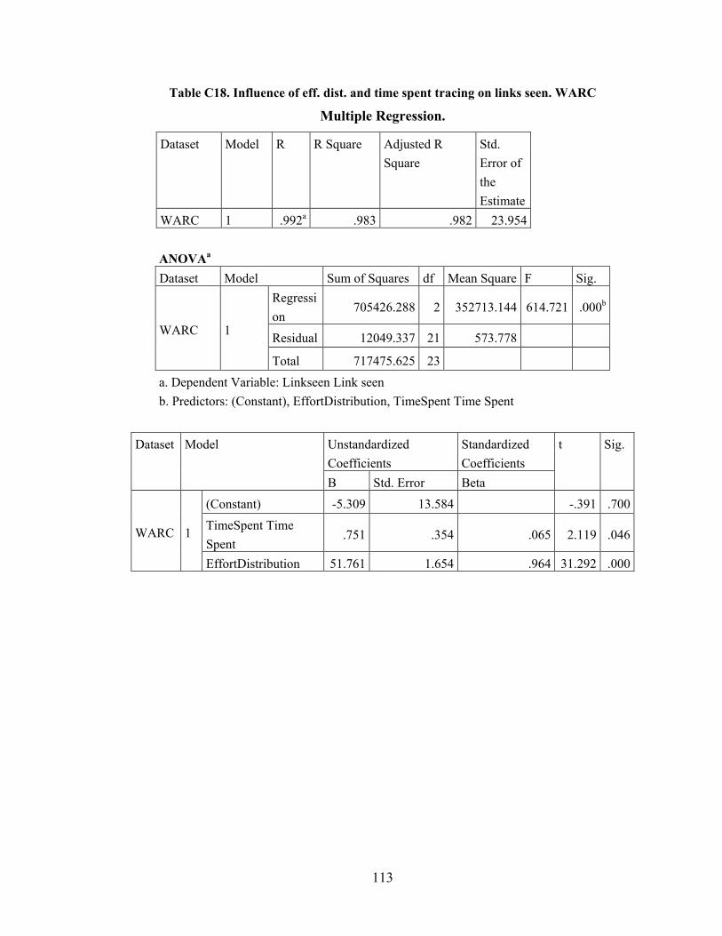
113
Table C18. Influence of eff. dist. and time spent tracing on links seen. WARC
Multiple Regression.
Dataset Model R R Square Adjusted R Square
Std. Error of the Estimate
WARC 1 .992a .983 .982 23.954 ANOVAa Dataset Model Sum of Squares df Mean Square F Sig.
WARC 1
Regression
705426.288 2 352713.144 614.721 .000b
Residual 12049.337 21 573.778
Total 717475.625 23
a. Dependent Variable: Linkseen Link seen b. Predictors: (Constant), EffortDistribution, TimeSpent Time Spent
Dataset Model Unstandardized
Coefficients Standardized Coefficients
t Sig.
B Std. Error Beta
WARC 1
(Constant) -5.309 13.584 -.391 .700 TimeSpent Time Spent
.751 .354 .065 2.119 .046
EffortDistribution 51.761 1.654 .964 31.292 .000
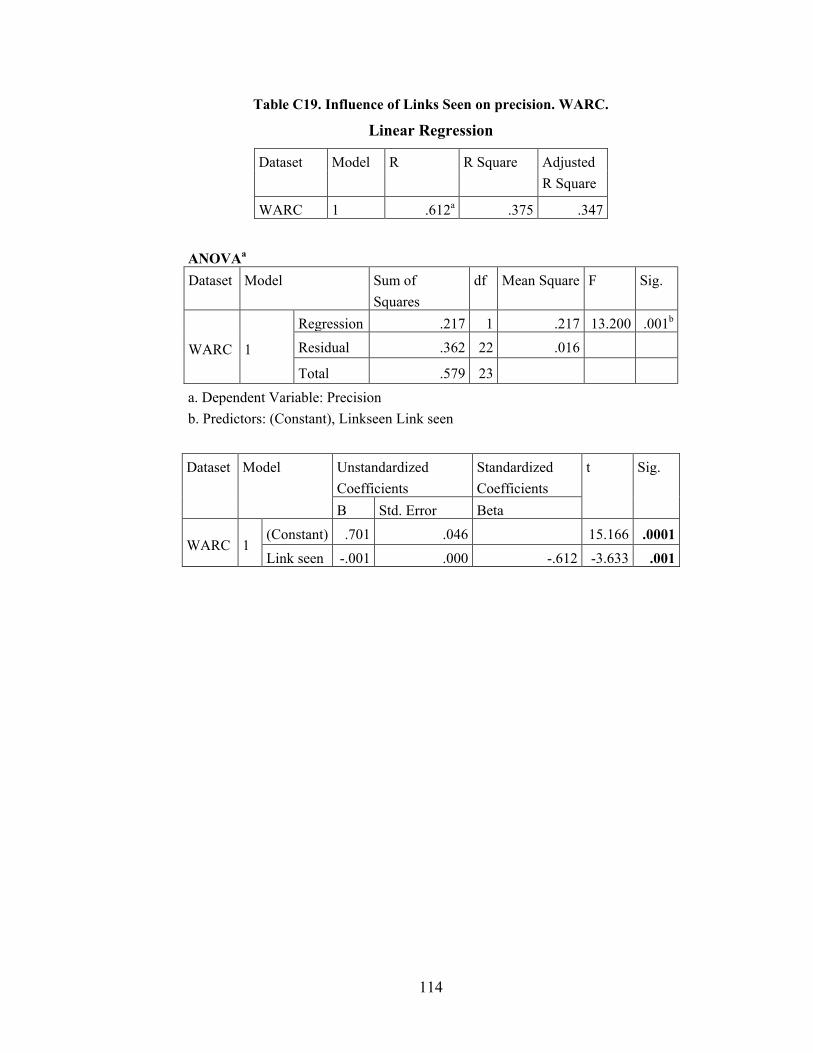
114
Table C19. Influence of Links Seen on precision. WARC.
Linear Regression
Dataset Model R R Square Adjusted R Square
WARC 1 .612a .375 .347
ANOVAa Dataset Model Sum of
Squares df Mean Square F Sig.
WARC 1
Regression .217 1 .217 13.200 .001b Residual .362 22 .016
Total .579 23
a. Dependent Variable: Precision b. Predictors: (Constant), Linkseen Link seen
Dataset Model Unstandardized Coefficients
Standardized Coefficients
t Sig.
B Std. Error Beta
WARC 1 (Constant) .701 .046 15.166 .0001 Link seen -.001 .000 -.612 -3.633 .001
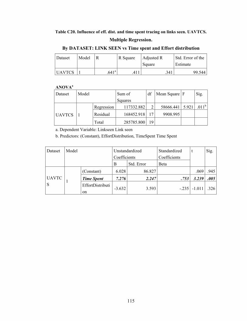
115
Table C20. Influence of eff. dist. and time spent tracing on links seen. UAVTCS.
Multiple Regression.
By DATASET: LINK SEEN vs Time spent and Effort distribution
Dataset Model R R Square Adjusted R Square
Std. Error of the Estimate
UAVTCS 1 .641a .411 .341 99.544
ANOVAa Dataset Model Sum of
Squares df Mean Square F Sig.
UAVTCS 1
Regression 117332.882 2 58666.441 5.921 .011b Residual 168452.918 17 9908.995
Total 285785.800 19
a. Dependent Variable: Linkseen Link seen b. Predictors: (Constant), EffortDistribution, TimeSpent Time Spent
Dataset Model Unstandardized
Coefficients Standardized Coefficients
t Sig.
B Std. Error Beta
UAVTCS
1
(Constant) 6.028 86.827 .069 .945
Time Spent 7.276 2.247 .753 3.239 .005 EffortDistribution
-3.632 3.593 -.235 -1.011 .326
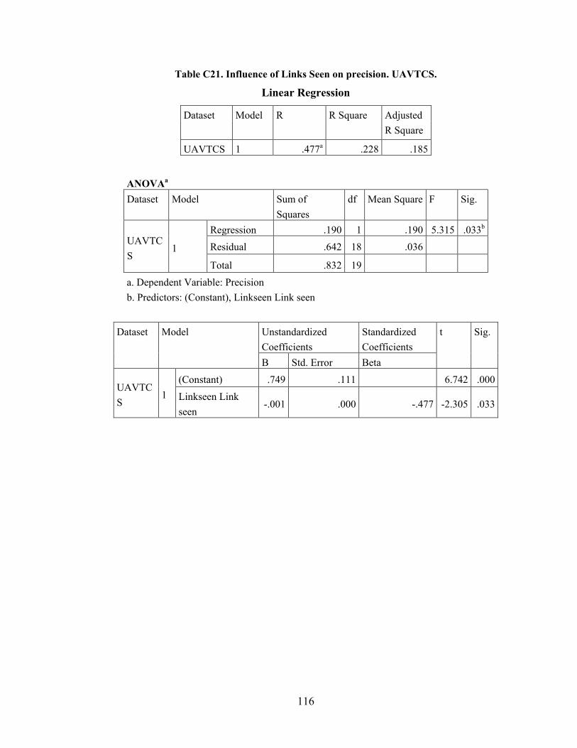
116
Table C21. Influence of Links Seen on precision. UAVTCS.
Linear Regression
Dataset Model R R Square Adjusted R Square
UAVTCS 1 .477a .228 .185
ANOVAa Dataset Model Sum of
Squares df Mean Square F Sig.
UAVTCS
1
Regression .190 1 .190 5.315 .033b Residual .642 18 .036
Total .832 19
a. Dependent Variable: Precision b. Predictors: (Constant), Linkseen Link seen
Dataset Model Unstandardized Coefficients
Standardized Coefficients
t Sig.
B Std. Error Beta
UAVTCS
1 (Constant) .749 .111 6.742 .000 Linkseen Link seen
-.001 .000 -.477 -2.305 .033
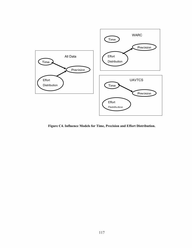
117
Figure C4. Influence Models for Time, Precision and Effort Distribution.
Precision
Time
Effort
Distribution
Precision
Time
Effort
Distribution
Precision
Time
Effort
Distribution
All Data
WARC
UAVTCS
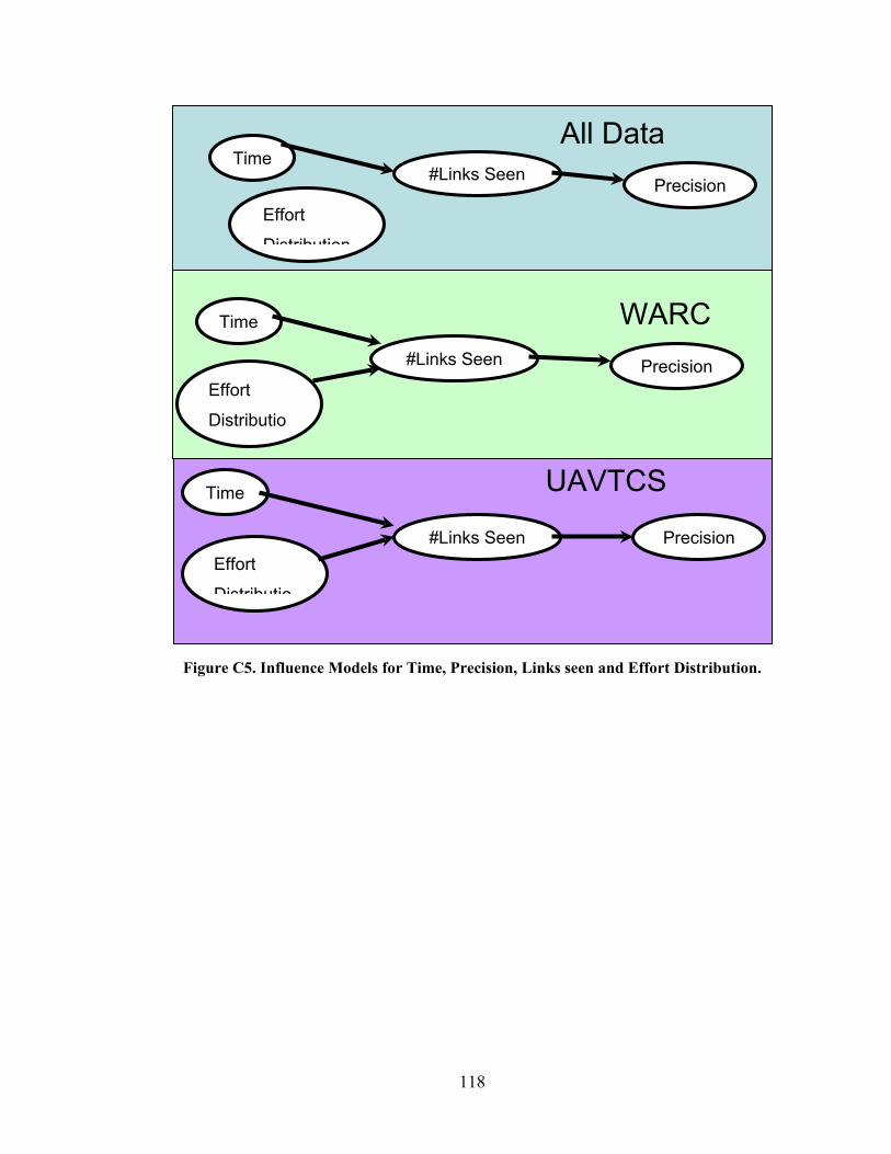
118
Figure C5. Influence Models for Time, Precision, Links seen and Effort Distribution.
Precision Time
Effort
Distribution
Precision
Time
Effort
Distributio
Precision
Time
Effort
Distributio
All Data
WARC
UAVTCS
#Links Seen
#Links Seen
#Links Seen
119
References
[1] N. Leveson and C. Turner, “An Investigation of the Therac-25 Accidents,” Computer, vol. 26, no. 7, pp. 18 –41, Jul. 1993.
[2] G. Le Lann, “An Analysis of the Ariane 5 Flight 501 Failure - A System Engineering Perspective,” in Engineering of Computer-Based Systems, 1997. Proceedings., International Conference and Workshop on, Mar. 1997, pp. 339 –346.
[3] D. Isbell and D. Savage, “Mars Climate Orbiter Failure Board Releases Report, Numerous NASA Actions Underway in Response,” NASA Press Release 99-134, Nov. 1999. [Online]. Available: http://nssdc.gsfc.nasa.gov/planetary/text/-mco_pr_19991110.txt
[4] O. Gotel and C. Finkelstein, “An Analysis of the Requirements Traceability Problem,” in Requirements Engineering, 1994., Proceedings of the First International Conference on, Apr. 1994, pp. 94 –101.
[5] J. Cleland-Huang, “Just Enough Requirements Traceability,” in Computer Software and Applications Conference, 2006. COMPSAC ’06. 30th Annual International, vol. 1, Sept. 2006, pp. 41 –42.
[6] “IEEE/EIA Standard Industry Implementation of International Standard ISO/IEC 12207: 1995 (ISO/IEC 12207) Standard for Information Technology Software Life Cycle Processes,” IEEE/EIA 12207.0-1996, pp. 1 –75, 1998.
[7] J. H. Hayes, A. Dekhtyar, and J. Osborne, “Improving Requirements Tracing via Information Retrieval,” in Requirements Engineering Conference, 2003. Proceedings. 11th IEEE International, Sept. 2003, pp. 138 – 147.
[8] S. Ratanotayanon, S. Sim, and R. Gallardo-Valencia, “Supporting Program Comprehension in Agile with Links to User Stories,” in Agile Conference, 2009. AGILE ’09., Aug. 2009, pp. 26 –32.
[9] B. Ramesh and M. Jarke, “Toward Reference Models for Requirements Traceability,” Software Engineering, IEEE Transactions on, vol. 27, no. 1, pp. 58 –93, Jan. 2001.
[10] J. H. Hayes, A. Dekhtyar, S. Sundaram, and S. Howard, “Helping Analysts Trace Requirements: An Objective Look,” in Requirements Engineering Conference, 2004. Proceedings. 12th IEEE International, Sept. 2004, pp. 249 – 259.
[11] A. Dekhtyar, J. H. Hayes, and J. Larsen, “Make the Most of Your Time: How Should the Analyst Work with Automated Traceability Tools?” in Predictor Models in Software Engineering, 2007. PROMISE’07: ICSE Workshops 2007. International Workshop on, May 2007, p. 4.
[12] J. H. Hayes and A. Dekhtyar, “Humans in the Traceability Loop: Can’t Live with ’em, Can’t Live without ’em,” in Proceedings of the 3rd international workshop on Traceability in emerging forms of software engineering, ser. TEFSE ’05. New York, NY, USA: ACM, 2005, pp. 20–23.
[13] D. Cuddeback, A. Dekhtyar, and J. H. Hayes, “Automated Requirements Traceability: The Study of Human Analysts,” in Requirements Engineering Conference (RE), 2010 18th IEEE International, Oct. 2010, pp. 231 –240.
[14] G. Antoniol, G. Canfora, G. Casazza, A. De Lucia, and E. Merlo, “Recovering Traceability Links Between Code and Documentation,” IEEE Trans. Softw. Eng., vol. 28, no. 10, pp. 970 – 983, Sept. 2002.
[15] R. Settimi, J. Cleland-Huang, O. Ben Khadra, J. Mody, W. Lukasik, and C. DePalma, “Supporting Software Evolution through Dynamically Retrieving Traces to UML Artifacts,” in Software Evolution, 2004. Proceedings. 7th International Workshop on Principles of, Sept. 2004, pp. 49 – 54.
120
[16] A. Egyed, F. Graf, and P. Grünbacher, “Effort and Quality of Recovering Requirements-to-Code Traces: Two Exploratory Experiments,” in Requirements Engineering Conference (RE), 2010 18th IEEE International, Oct. 2010, pp. 221 –230.
[17] D. Cuddeback, A. Dekhtyar, J. H. Hayes, J. Holden, and W.-K. Kong, “Towards Overcoming Human Analyst Fallibility in the Requirements Tracing Process (NIER Track),” in Proceedings of the 33rd International Conference on Software Engineering. New York, NY, USA: ACM, 2011, pp. 860–863.
[18] A. Dekhtyar, O. Dekhtyar, J. Holden, J. H. Hayes, D. Cuddeback, and W.-K. Kong, “On Human Analyst Performance in Assisted Requirements Tracing: Statistical Analysis,” in Requirements Engineering Conference (RE), 2011 19th IEEE International, Sept. 2011, pp. 111 –120.
[19] W.-K. Kong, J. H. Hayes, A. Dekhtyar, and J. Holden, “How Do We Trace Requirements: An Initial Study of Analyst Behavior in Trace Validation Tasks,” in Proceedings of the 4th International Workshop on Cooperative and Human Aspects of Software Engineering, ser. CHASE ’11. New York, NY, USA: ACM, 2011, pp. 32–39.
[20] E. A. Holbrook, J. H. Hayes, and A. Dekhtyar, “Toward Automating Requirements Satisfaction Assessment,” in Requirements Engineering Conference, 2009. RE ’09. 17th IEEE International, Sept. 2009, pp. 149 –158.
[21] M. F. Porter, “Readings in Information Retrieval,” K. Sparck Jones and P. Willett, Eds. San Francisco, CA, USA: Morgan Kaufmann Publishers Inc., 1997, ch. An algorithm for suffix stripping, pp. 313–316.
[22] A. De Lucia, R. Oliveto, and G. Tortora, “ADAMS Re-Trace: Traceability Link Recovery via Latent Semantic Indexing,” in Proceedings of the 30th international conference on Software engineering, ser. ICSE ’08. New York, NY, USA: ACM, 2008, pp. 839–842.
[23] “Glossary of Terms,” Machine Learning, vol. 30, pp. 271–274, 1998. [24] J. H. Hayes, A. Dekhtyar, and S. Sundaram, “Advancing Candidate Link Generation for
Requirements Tracing: the Study of Methods,” Software Engineering, IEEE Transactions on, vol. 32, no. 1, pp. 4 – 19, Jan. 2006.
[25] S. Sundaram, J. H. Hayes, A. Dekhtyar, and E. A. Holbrook, “Assessing Traceability of Software Engineering Artifacts,” Requirements Engineering, vol. 15, pp. 313–335, 2010.
[26] C. D. Manning, P. Raghavan, and H. Schütze, Introduction to Information Retrieval. New York, NY, USA: Cambridge University Press, 2008.
[27] C. Buckley and E. M. Voorhees, “Evaluating Evaluation Measure Stability,” in Proceedings of the 23rd annual international ACM SIGIR conference on Research and development in information retrieval, ser. SIGIR ’00. New York, NY, USA: ACM, 2000, pp. 33–40.
[28] A. Marcus, J. I. Maletic, and A. Sergeyev, “Recovery of Traceability Links between Software Documentation and Source Code,” International Journal of Software Engineering & Knowledge Engineering, vol. 15, no. 5, pp. 811 – 836, 2005.
[29] S. Siegel, Nonparametric Statistics for the Behavioral Sciences, ser. McGraw-Hill series in psychology. McGraw-Hill, 1956.
[30] G. Salton, A. Wong, and C. S. Yang, “A Vector Space Model for Automatic Indexing,” Commun. ACM, vol. 18, pp. 613–620, November 1975.
[31] H. Sultanov, J. H. Hayes, and W.-K. Kong, “Application of Swarm Techniques to Requirements Tracing,” Requirements Engineering, vol. 16, pp. 209–226, 2011.
[32] S. Winkler, “Trace Retrieval for Evolving Artifacts,” in Traceability in Emerging Forms of Software Engineering, 2009. TEFSE ’09. ICSE Workshop on, May 2009, pp. 49 –56.
[33] W.-K. Kong and J. H. Hayes, “Proximity-based Traceability: An Empirical Validation using Ranked Retrieval and Set-based Measures,” in Empirical Requirements Engineering (EmpiRE), 2011 First International Workshop on, Aug. 2011, pp. 45 –52.
121
[34] A. De Lucia, F. Fasano, R. Oliveto, and G. Tortora, “ADAMS Re-Trace: A Traceability Recovery Tool,” in Software Maintenance and Reengineering, 2005. CSMR 2005. Ninth European Conference on, Mar. 2005, pp. 32 – 41.
[35] X. Zou, R. Settimi, and J. Cleland-Huang, “Phrasing in Dynamic Requirements Trace Retrieval,” in Computer Software and Applications Conference, 2006. COMPSAC ’06. 30th Annual International, vol. 1, Sept. 2006, pp. 265 –272.
[36] J. Cleland-Huang, R. Settimi, O. BenKhadra, E. Berezhanskaya, and S. Christina, “Goal-Centric Traceability for Managing Non-Functional Requirements,” in Software Engineering, 2005. ICSE 2005. Proceedings. 27th International Conference on, May. 2005, pp. 362 – 371.
[37] J. Cleland-Huang, A. Czauderna, M. Gibiec, and J. Emenecker, “A Machine Learning Approach for Tracing Regulatory Codes to Product Specific Requirements,” in Software Engineering, 2010 ACM/IEEE 32nd International Conference on, vol. 1, May 2010, pp. 155 –164.
[38] J. Cleland-Huang, R. Settimi, C. Duan, and X. Zou, “Utilizing Supporting Evidence to Improve Dynamic Requirements Traceability,” in Requirements Engineering, 2005. Proceedings. 13th IEEE International Conference on, Aug. 2005, pp. 135 – 144.
[39] M. Gibiec, A. Czauderna, and J. Cleland-Huang, “Towards Mining Replacement Queries for Hard-to-Retrieve Traces,” in Proceedings of the IEEE/ACM international conference on Automated software engineering, ser. ASE ’10. New York, NY, USA: ACM, 2010, pp. 245–254.
[40] C. Marton, “Salton and Buckley’s Landmark Research in Experimental Text Information Retrieval,” Evidence Based Library and Information Practice, vol. 6, no. 4, 2011.
[41] M. O. Nassar, G. Kanaan, and H. A. Awad, “Comparison between Different Global Weighting Schemes,” International Multi Conference of Engineers and Computer Scientists, Hong Kong, 2010.
[42] G. Spanoudakis, A. Zisman, E. Pérez-Miñana, and P. Krause, “Rule-based Generation of Requirements Traceability Relations,” Journal of Systems and Software, vol. 72, no. 2, pp. 105 – 127, 2004.
[43] C. McMillan, D. Poshyvanyk, and M. Revelle, “Combining Textual and Structural Analysis of Software Artifacts for Traceability Link Recovery,” in Traceability in Emerging Forms of Software Engineering, 2009. TEFSE ’09. ICSE Workshop on, May 2009, pp. 41 –48.
[44] J. Cleland-Huang, C. Chang, and M. Christensen, “Event-based Traceability for Managing Evolutionary Change,” Software Engineering, IEEE Transactions on, vol. 29, no. 9, pp. 796 – 810, Sept. 2003.
[45] D. Hawking and P. Thistlewaite, “Proximity Operators - So Near and Yet So Far,” in Proceedings of TREC-4, Nov. 1995, pp. 131–143, nIST special publication 500-236.
[46] Y. Rasolofo and J. Savoy, “Term Proximity Scoring for Keyword-based Retrieval Systems,” in Proceedings of the 25th European conference on IR research, ser. ECIR’03. Berlin, Heidelberg: Springer-Verlag, 2003, pp. 207–218.
[47] T. Tao and C. Zhai, “An Exploration of Proximity Measures in Information Retrieval,” in Proceedings of the 30th annual international ACM SIGIR conference on Research and development in information retrieval, ser. SIGIR ’07. New York, NY, USA: ACM, 2007, pp. 295–302.
[48] R. Song, M. J. Taylor, J.-R. Wen, H.-W. Hon, and Y. Yu, “Viewing Term Proximity from a Different Perspective,” in Proceedings of the IR research, 30th European conference on Advances in information retrieval, ser. ECIR’08. Berlin, Heidelberg: Springer-Verlag, 2008, pp. 346–357.
[49] A. De Lucia, R. Oliveto, and P. Sgueglia, “Incremental Approach and User Feedbacks: a Silver Bullet for Traceability Recovery,” in Proceedings of the 22nd IEEE International
122
Conference on Software Maintenance. Washington, DC, USA: IEEE Computer Society, 2006, pp. 299–309.
[50] H. Ninness, R. Newton, J. Saxon, R. Rumph, A. Bradfield, C. Harrison, E. Vasquez, and S. Ninness, “Small Group Statistics: A Monte Carlo Comparison of Parametric and Randomization Tests,” Behavior and Social Issues, vol. 12, pp. 53–63., 2002.
[51] M. D. Smucker, J. Allan, and B. Carterette, “A Comparison of Statistical Significance Tests for Information Retrieval Evaluation,” in Proceedings of the sixteenth ACM conference on Conference on information and knowledge management, ser. CIKM ’07. New York, NY, USA: ACM, 2007, pp. 623–632.
[52] J. Cleland-Huang, C. Chang, G. Sethi, K. Javvaji, H. Hu, and J. Xia, “Automating Speculative Queries through Event-based Requirements Traceability,” in Requirements Engineering, 2002. Proceedings. IEEE Joint International Conference on, 2002, pp. 289 – 296.
[53] A. Marcus and J. Maletic, “Recovering Documentation-to-source-code Traceability Links using Latent Semantic Indexing,” in Software Engineering, 2003. Proceedings. 25th International Conference on, May 2003, pp. 125 – 135.
[54] M. Höst, B. Regnell, and C. Wohlin, “Using Students as SubjectsA Comparative Study ofStudents and Professionals in Lead-Time Impact Assessment,” Empirical Softw. Engg., vol. 5, no. 3, pp. 201–214, Nov. 2000.
[55] W. F. Tichy, “Hints for Reviewing Empirical Work in Software Engineering,” Empirical Softw. Engg., vol. 5, pp. 309–312, Dec. 2000.
[56] J. Rocchio, Relevance Feedback in Information Retrieval. Prentice-Hall Inc., 1971, ch. 14, pp. 313–323.
[57] M. D. Dunlop, “The Effect of Accessing Nonmatching Documents on Relevance Feedback,” ACM Trans. Inf. Syst., vol. 15, pp. 137–153, Apr. 1997.
[58] X. Wang, H. Fang, and C. Zhai, “A Study of Methods for Negative Relevance Feedback,” in Proceedings of the 31st annual international ACM SIGIR conference on research and development in information retrieval, ser. SIGIR ’08. New York, NY, USA: ACM, 2008, pp. 219–226.
[59] “Specifications for WARC Tools,” Retrieved May 31, 2010. [Online]. Available: http://-code.google.com/p/warc-tools/downloads/list
[60] “UAV Tactical Control System,” Retrieved May 31, 2010. [Online]. Available: http://-www.fas.org/irp/program/collect/uav_tcs.htm
[61] J. Lin, C. C. Lin, J. Huang, R. Settimi, J. Amaya, G. Bedford, B. Berenbach, O. Khadra, C. Duan, and X. Zou, “Poirot: A Distributed Tool Supporting Enterprise-Wide Automated Traceability,” in Requirements Engineering, 14th IEEE International Conference, Sept. 2006, pp. 363 –364.
123
Vita
Date and Place of Birth: August 29, 1976 in Kuala Lumpur, Malaysia Education: University of Kentucky Bachelor of Science in Computer Science, December 1997 University of Kentucky Master of Science in Computer Science, May 2005 Professional Positions Held: Lexmark International, Software Engineer September 2005 – Present Analysts International, Quality Assurance Software Tester February 1998 – September 2005 UK Laboratory for Advanced Networking, College of Engineering Software Verification and Validation Research Lab, Graduate Student Researcher May 2010 – May 2012 Professional Publications: W.-K. Kong and J. H. Hayes, “Proximity-based Traceability: An Empirical Validation using Ranked Retrieval and Set-based Measures,” in Empirical Requirements Engineering (EmpiRE), 2011 First International Workshop on, Aug. 2011, pp. 45 –52. W.-K. Kong, J. H. Hayes, A. Dekhtyar, and J. Holden, “How Do We Trace Requirements: An Initial Study of Analyst Behavior in Trace Validation Tasks,” in Proceedings of the 4th International Workshop on Cooperative and Human Aspects of Software Engineering, ser. CHASE ’11. New York, NY, USA: ACM, 2011, pp. 32–39. D. Cuddeback, A. Dekhtyar, J. H. Hayes, J. Holden, and W.-K. Kong, “Towards Overcoming Human Analyst Fallibility in the Requirements Tracing Process (NIER Track),” in Proceedings of the 33rd International Conference on Software Engineering. New York, NY, USA: ACM, 2011, pp. 860–863. H. Sultanov, J. H. Hayes, and W.-K. Kong, “Application of Swarm Techniques to Requirements Tracing,” Requirements Engineering, vol. 16, pp. 209–226, 2011. J. H. Hayes, H. Sultanov, W.-K. Kong, and W. Li, “Software Verification and Validation Research Laboratory (SVVRL) of the University of Kentucky: Traceability Challenge 2011: Language Translation,” in Proceedings of the 6th International Workshop on Traceability in

124
Emerging Forms of Software Engineering, ser. TEFSE ’11. New York, NY, USA: ACM, 2011, pp. 50–53. J. H. Hayes, W.-K. Kong, W. Li, H. Sultanov, S. A. Wilson, S. Taha, J. Larsen, S. Sundaram., "Software Verification and Validation Research Laboratory (SVVRL) of the University of Kentucky: Traceability Challenge," (2009). Conference paper, held at 2009 Workshop on Traceability in Emerging Forms of Software Engineering (May 18 - 18, 2009), an International Conference on Software Engineering workshop, TEFSE 2009.