Geosci. Model Dev., 5, 1259–1271, 2012www.geosci-model-dev.net/5/1259/2012/doi:10.5194/gmd-5-1259-2012© Author(s) 2012. CC Attribution 3.0 License.

GeoscientificModel Development

A semi-analytical solution to accelerate spin-up of a coupled carbonand nitrogen land model to steady state

J. Y. Xia1, Y. Q. Luo1, Y.-P. Wang2, E. S. Weng3, and O. Hararuk1

1Department of Microbiology and Plant Biology, University of Oklahoma, OK, USA2CSIRO Marine and Atmospheric Research, Centre for Australian Weather and Climate Research,Aspendale, Victoria, Australia3Department of Ecology and Evolutionary Biology, Princeton University, NJ, USA

Correspondence to:J. Y. Xia (jxia@ou.edu)

Received: 14 March 2012 – Published in Geosci. Model Dev. Discuss.: 17 April 2012Revised: 15 August 2012 – Accepted: 5 September 2012 – Published: 11 October 2012

Abstract. The spin-up of land models to steady state of cou-pled carbon–nitrogen processes is computationally so costlythat it becomes a bottleneck issue for global analysis. In thisstudy, we introduced a semi-analytical solution (SAS) forthe spin-up issue. SAS is fundamentally based on the ana-lytic solution to a set of equations that describe carbon trans-fers within ecosystems over time. SAS is implemented bythree steps: (1) having an initial spin-up with prior pool-sizevalues until net primary productivity (NPP) reaches stabi-lization, (2) calculating quasi-steady-state pool sizes by let-ting fluxes of the equations equal zero, and (3) having afinal spin-up to meet the criterion of steady state. Step 2is enabled by averaged time-varying variables over one pe-riod of repeated driving forcings. SAS was applied to bothsite-level and global scale spin-up of the Australian Com-munity Atmosphere Biosphere Land Exchange (CABLE)model. For the carbon-cycle-only simulations, SAS saved95.7 % and 92.4 % of computational time for site-level andglobal spin-up, respectively, in comparison with the tradi-tional method (a long-term iterative simulation to achieve thesteady states of variables). For the carbon–nitrogen coupledsimulations, SAS reduced computational cost by 84.5 % and86.6 % for site-level and global spin-up, respectively. The es-timated steady-state pool sizes represent the ecosystem car-bon storage capacity, which was 12.1 kg C m−2 with the cou-pled carbon–nitrogen global model, 14.6 % lower than thatwith the carbon-only model. The nitrogen down-regulationin modeled carbon storage is partly due to the 4.6 % decreasein carbon influx (i.e., net primary productivity) and partly dueto the 10.5 % reduction in residence times. This steady-state

analysis accelerated by the SAS method can facilitate com-parative studies of structural differences in determining theecosystem carbon storage capacity among biogeochemicalmodels. Overall, the computational efficiency of SAS poten-tially permits many global analyses that are impossible withthe traditional spin-up methods, such as ensemble analysis ofland models against parameter variations.

1 Introduction

Modeling ecosystem biogeochemical cycles is highly de-pendent on initial values because of long-term persistenceof ecosystem state properties. It requires setting up initialvalues of all state variables (e.g., carbon and nitrogen poolsizes) in any biogeochemical models before scientists canuse the models for any analysis. The initial values are ei-ther estimated from observations (D’Odorico et al., 2004;Luo and Reynolds, 1999) or assumed to be at steady state.The latter is usually achieved by traditional spin-up meth-ods that perform long model simulations until no trend ofchange in pool sizes over many periods of the repeated cli-mate forcing, even though the pool sizes vary seasonallyand inter-annually within one period of the repeated forc-ing (Johns et al., 1997; McGuire et al., 1997; Thornton et al.,2002; Yang et al., 1995). Spinning biogeochemical models tosteady state is computationally expensive, especially so whensimulations are performed with global biogeochemical mod-els of coupled C and N cycles (Thornton and Rosenbloom,2005). In general, a fully coupled earth system model with

Published by Copernicus Publications on behalf of the European Geosciences Union.

1260 J. Y. Xia et al.: Spin-up of biogeochemical models

biogeochemical cycles needs to be spun up in several se-quential steps, and each step can take several thousands ofsimulation years (Doney et al., 2006). Spin-up of a fully cou-pled earth system model with a relatively coarse resolution(≈ 3.75◦) atmospheric model is estimated to take hundredsof real-world days of computation using the present NationalCenter for Atmosphere Research (NCAR) supercomputers(Jochum et al., 2010). As a consequence, spin-up has becomea serious constraint on global modeling analysis of biogeo-chemical cycles.

Thornton and Rosenbloom (2005) have explored a fewspin-up methods for achieving steady states of a coupledcarbon–nitrogen ecosystem model. The spin-up of theirmodel begins with initial values of no soil organic matter(SOM) and very small plant pools (Thornton et al., 2002).During the spin-up, the accumulation rate of SOM stronglydepends on the nitrogen addition rate in their model. Theyperiodically increase the mineral nitrogen supply during theearly stage of the spin-up to acclerate the spin-up. Each ni-trogen addition period is followed by a period with reduc-ing nitrogen input linearly to the normal level (Thornton andRosenbloom, 2005; Thornton et al., 2002). The efficiency ofthis punctuated nitrogen addition method is low without anoptimal combination of the nitrogen addition and reductionperiods. A prior analysis for searching such optimal com-binations is needed when this method is applied to a newmodel. An accelerated decomposition method is based onan assumption of linear scaling between decomposition ratesand litter/soil pool sizes. A linearity test between decom-position rates and pool sizes is needed before performingthis method for each new model (Thornton and Rosenbloom,2005). The accelerated decomposition method can distort in-teractions between carbon and nitrogen cycles in the a globalbiogeochemical model of terrestrial carbon, nitrogen, andphosphorus (CASACNP) (Y.-P. Wang, unpublished data) andocean physics for spinning up an ocean model (Bryan andLewis, 1979; Danabasoglu et al., 1996). Although the abovemethods have been used in some modeling studies (Rander-son et al., 2009), most models still use the traditional spin-upmethod with long-term iterative simulations to achieve thesteady states of variables.

Carbon processes in terrestrial ecosystems can be repre-sented by first-order, linear differential equations (Bolker etal., 1998; Luo and Weng, 2011; Luo et al., 2012). This prop-erty renders a possibility to obtain an analytical solution ofsteady states for terrestrial carbon cycle models (Bolker et al.,1998; Comins, 1994; Govind et al., 2011; King, 1995; Luoet al., 2001). Ludwig et al. (1978), for example, have useda two-step approximation. They first calculated the steady-state pool sizes of the fast variables by holding the slow vari-ables fixed, and then analyzed the slow variables with thefast variables held at corresponding steady-state pool sizes.Most of the analytical solutions (Comins, 1994; Govind etal., 2011; King, 1995; Luo et al., 2001) are obtained by usingconstant net primary productivity (NPP). However, temporal

climate fluctuations and seasonal plant growth make it dif-ficult to get an analytical solution for state variables in themodels. Some studies (Lardy et al., 2011; Martin et al., 2007)have attempted to obtain the analytical solution of steady-state pool sizes via managing the climate fluctuations. Thesemethods have used matrix-based analysis but still need tosolve several relatively complicated equations. For these rea-sons, no effective analytical method has been developed tosave the spin-up time for global land models.

An analytical solution is still possible to obtain steady-state pool sizes if we can overcome two obstacles. First,we need to get time-averaged approximations of the time-varying variables, such as environmental scalars and NPP.Since most spin-up uses repeated climate forcing variablesto estimate steady states of pool sizes, we can estimate av-erages of those time-varying variables within one period ofthe repeated forcing variables. Second, for most carbon–nitrogen coupled models, nitrogen regulates carbon cycle viaits influences on photosynthesis and decomposition. Nitro-gen pool sizes are usually related with carbon cycle via car-bon/nitrogen (C/N) ratios (Gerber et al., 2010; Wang et al.,2010). Nitrogen influences on photosynthesis are fast pro-cesses and can be accounted for by short, initial spin-up toreach a stabilization of NPP. The C/N ratios in the end loop ofinitial spin-up for stable NPP can be used to estimate steady-state nitrogen pool sizes. Using the above approximations ofthose time-varying variables will generate errors for estimat-ing steady states of carbon and nitrogen pools. Thus, someadditional spin-up may be necessary to achieve steady statesof all pools.

This study was intended to develop a semi-analytical solu-tion (SAS) to accelerate spin-up of global carbon–nitrogencoupled models. We first discussed biogeochemical prin-ciples underlying SAS. SAS becomes permissible becausea set of first-order ordinary differential equations can ad-equately describe carbon transfers within ecosystems overtime and be analytically solved to obtain steady-state poolsizes. We applied SAS to the Australian Community Atmo-sphere Biosphere Land Exchange (CABLE) model and de-veloped a general procedure of SAS for spin-up. There arethree key steps of SAS. The first step is a short spin-upto obtain steady-state NPP, averaged environmental factorswithin one period of repeated forcing variables, and C/N ra-tios. The second step is to analytically solve the differentialequation to calculate steady-state carbon and nitrogen poolsizes. The last step is to make an additional spin-up to meetthe steady-state criterion for all pools. We evaluated the com-putational efficiency of SAS for the carbon-only and the cou-pled carbon–nitrogen models against the traditional spin-up,applications of SAS to other biogeochemical models, andpossible model analyses enabled by SAS.

Geosci. Model Dev., 5, 1259–1271, 2012 www.geosci-model-dev.net/5/1259/2012/

J. Y. Xia et al.: Spin-up of biogeochemical models 1261

32

709

Figure 1. 710

711

Leaf(X1)

Root(X2)

Woody(X3)

Metabolic Litter (X4)

Structural Litter (X5)

Fast SOM(X7)

Slow SOM(X8)

Passive SOM(X9)

CO2

CO2

CO2

CO2

CO2

CO2

Canopy Photosynthesis

CWD(X6)

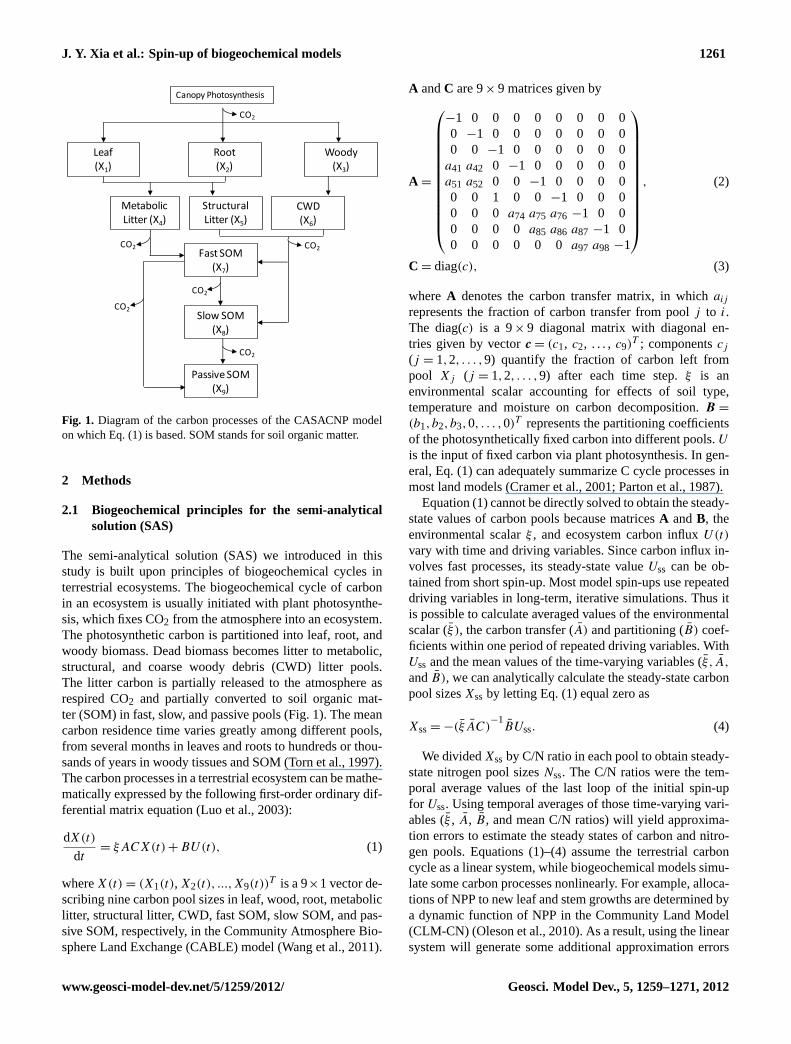
Fig. 1. Diagram of the carbon processes of the CASACNP modelon which Eq. (1) is based. SOM stands for soil organic matter.

2 Methods

2.1 Biogeochemical principles for the semi-analyticalsolution (SAS)

The semi-analytical solution (SAS) we introduced in thisstudy is built upon principles of biogeochemical cycles interrestrial ecosystems. The biogeochemical cycle of carbonin an ecosystem is usually initiated with plant photosynthe-sis, which fixes CO2 from the atmosphere into an ecosystem.The photosynthetic carbon is partitioned into leaf, root, andwoody biomass. Dead biomass becomes litter to metabolic,structural, and coarse woody debris (CWD) litter pools.The litter carbon is partially released to the atmosphere asrespired CO2 and partially converted to soil organic mat-ter (SOM) in fast, slow, and passive pools (Fig. 1). The meancarbon residence time varies greatly among different pools,from several months in leaves and roots to hundreds or thou-sands of years in woody tissues and SOM (Torn et al., 1997).The carbon processes in a terrestrial ecosystem can be mathe-matically expressed by the following first-order ordinary dif-ferential matrix equation (Luo et al., 2003):

dX(t)

dt= ξACX(t) + BU(t), (1)

whereX(t) = (X1(t), X2(t), ...,X9(t))T is a 9×1 vector de-

scribing nine carbon pool sizes in leaf, wood, root, metaboliclitter, structural litter, CWD, fast SOM, slow SOM, and pas-sive SOM, respectively, in the Community Atmosphere Bio-sphere Land Exchange (CABLE) model (Wang et al., 2011).

A andC are 9× 9 matrices given by

A =

−1 0 0 0 0 0 0 0 00 −1 0 0 0 0 0 0 00 0 −1 0 0 0 0 0 0

a41 a42 0 −1 0 0 0 0 0a51 a52 0 0 −1 0 0 0 00 0 1 0 0 −1 0 0 00 0 0 a74 a75 a76 −1 0 00 0 0 0 a85 a86 a87 −1 00 0 0 0 0 0 a97 a98 −1

, (2)

C = diag(c), (3)

whereA denotes the carbon transfer matrix, in whichaij

represents the fraction of carbon transfer from poolj to i.The diag(c) is a 9× 9 diagonal matrix with diagonal en-tries given by vectorc = (c1, c2, . . . , c9)

T ; componentscj

(j = 1,2, . . . ,9) quantify the fraction of carbon left frompool Xj (j = 1,2, . . . ,9) after each time step.ξ is anenvironmental scalar accounting for effects of soil type,temperature and moisture on carbon decomposition.B =

(b1,b2,b3,0, . . . ,0)T represents the partitioning coefficientsof the photosynthetically fixed carbon into different pools.U

is the input of fixed carbon via plant photosynthesis. In gen-eral, Eq. (1) can adequately summarize C cycle processes inmost land models (Cramer et al., 2001; Parton et al., 1987).

Equation (1) cannot be directly solved to obtain the steady-state values of carbon pools because matricesA andB, theenvironmental scalarξ , and ecosystem carbon influxU(t)

vary with time and driving variables. Since carbon influx in-volves fast processes, its steady-state valueUss can be ob-tained from short spin-up. Most model spin-ups use repeateddriving variables in long-term, iterative simulations. Thus itis possible to calculate averaged values of the environmentalscalar (ξ), the carbon transfer (A) and partitioning (B) coef-ficients within one period of repeated driving variables. WithUss and the mean values of the time-varying variables (ξ , A,

andB), we can analytically calculate the steady-state carbonpool sizesXss by letting Eq. (1) equal zero as

Xss= −(ξ AC)−1

BUss. (4)

We dividedXssby C/N ratio in each pool to obtain steady-state nitrogen pool sizesNss. The C/N ratios were the tem-poral average values of the last loop of the initial spin-upfor Uss. Using temporal averages of those time-varying vari-ables (ξ , A, B, and mean C/N ratios) will yield approxima-tion errors to estimate the steady states of carbon and nitro-gen pools. Equations (1)–(4) assume the terrestrial carboncycle as a linear system, while biogeochemical models simu-late some carbon processes nonlinearly. For example, alloca-tions of NPP to new leaf and stem growths are determined bya dynamic function of NPP in the Community Land Model(CLM-CN) (Oleson et al., 2010). As a result, using the linearsystem will generate some additional approximation errors

www.geosci-model-dev.net/5/1259/2012/ Geosci. Model Dev., 5, 1259–1271, 2012

1262 J. Y. Xia et al.: Spin-up of biogeochemical models

to estimate the steady states of carbon and nitrogen pools.Thus, the steady-state carbon and nitrogen pool sizes that areanalytically calculated by Eq. (4) need to be further adjustedwith additional spin-up to meet the criterion of steady statesfor all carbon and nitrogen processes.

Overall, our semi-analytic solution of spin-up consists ofthree steps: (1) an initial spin-up to obtain steady-state carboninflux Uss, temporally averaged values of the time-varyingvariables in Eq. (3) (ξ , A, andB), and C/N values; (2) calcu-lation of the steady-state carbon pool sizesXss using Eq. (3)and the steady-state N pool sizesNss from dividing Xss byC/N ratios; and (3) additional spin-up to meet the steady-state criteria for all carbon and nitrogen processes.

2.2 Model description

We applied the semi-analytic solution of spin-up to the CA-BLE model, which is one of the land surface models forsimulation of biophysical and biochemical processes. Kowal-czyk (2006) and Wang et al. (2011) have described the CA-BLE model in detail. The model includes 5 submodels: radi-ation, canopy micrometeorology, surface flux, soil and snow,and biogeochemical cycles. The CABLE model calls the ra-diation submodel first to compute absorption and transmis-sion of both diffuse and direct beam radiation in the two-big-leaf canopy and at soil surface (see the details in Wang andLeuning, 1998). The canopy micrometeorology submodel es-timates the canopy roughness length, zero-plane displace-ment height and aerodynamic transfer resistance based on thetheory developed by Raupach (Raupach, 1989a, b, 1994) andRaupach et al. (1997). The surface flux submodel uses the ab-sorbed radiation to estimate the water extraction and groundheat flux, which are required in the soil and snow submodel.The biogeochemical-cycles submodel is called last to com-pute the respiration of non-leaf plant tissues, the soil respira-tion, and the net ecosystem CO2 exchange.

The biogeochemical submodel of CABLE evolves fromthe CASACNP model, which was developed by Wang etal. (2010). It adopted the model structure of carbon pro-cesses from the CASA’ model (Randerson et al., 1997) andcontains coupled carbon, nitrogen, and phosphorus cycles.In this study, phosphorus cycle and its coupling with car-bon and nitrogen cycles were not activated. The CASACNPmodel has 9 pools, which include three plant pools (leaf,wood, and root), three litter pools (metabolic litter, struc-tural litter, and coarse woody debris), and three soil pools(microbial biomass, slow and passive soil organic matter)(Fig. 1). There is an additional pool of inorganic nitrogen(NO−

3 + NH+

4 ) when nitrogen cycle is coupled with carboncycle. The equations that describe changes in pool size withtime have been presented by Wang et al. (2010) and can berepresented by Eq. (1). In Eq. (1), parameterC is set to be aconstant in the CABLE model, while matricesA andB, theenvironmental scalarξ , and ecosystem carbon influxU(t)

vary with time and driving variables. In theA matrix, the

carbon transfer coefficients are determined by lignin/nitrogenratio from plant to litter pools, lignin fraction from litter tosoil pools, and soil texture among soil pools. In theB matrix,the carbon partitioning coefficients of the photosyntheticallyfixed carbon into plant pools are determined by availabilitiesof light, water and nitrogen as the carbon allocation schemedescribed by Friedlingstein et al. (1999). The environmen-tal scalar (ξ) regulates the leaf turnover rates by cold anddrought stresses on leaf senescence rate, the turnover rates oflitter carbon pools via limitations of soil temperature, mois-ture, and nitrogen availability, and SOM turnover rates bysoil temperature, moisture, and texture. The soil texture isspatially fixed in the CABLE model. The soil nitrogen willlimit litter decomposition if the gross mineralization is lessthan the immobilization (Wang et al., 2010). We spun up themodel for about one hundred of simulation years to obtainthe steady-state carbon influxUss.

In the CABLE model, the optimal carbon decay rates (theC matrix in Eq. 1) are preset and vary with vegetation types.The vegetation types for each 1◦

× 1◦ grid cell in the modelwere derived from the 0.5◦ × 0.5◦ International Geosphere-Biosphere Programme (IGBP) classification (Loveland et al.,2000). During the spin-up of the coupled carbon–nitrogenmodel, the carbon influx (U) and litter decomposition rateare regulated by the soil nitrogen availability (Wang et al.,2010). The nitrogen regulation may periodically occur untilall the nitrogen processes of the model reach steady states.In the CABLE model, the nitrogen inputs of deposition,fertilizer application and fixation are explicitly estimated.The nitrogen deposition in 1990 was estimated from Den-tener (2006) and nitrogen fixation from Wang and Houl-ton (2009). The global fertilizer application of nitrogen istaken as 0.86 Gt N yr−1 from Galloway et al. (2004) and isdistributed uniformly within the cropland biome (Wang etal., 2010).

The forcing variables required for the CABLE model in-clude incoming short- and long-wave radiation, air temper-ature, specific humidity, air pressure, wind speed, precipita-tion and ambient CO2 concentration. The CABLE model firstgenerated daily meteorological forcing (surface air tempera-ture, soil temperature and moisture). Then the daily forcingswere used to integrate the full model with a time step of oneday. In this study, the meteorological forcings of 1990 wereused to run the global version of the CABLE model to steadystates. A site version of CABLE (v2.01), which has been cal-ibrated by datasets from Harvard Forest, was used for thesite-level analysis in this study. We used forcing data of Har-vard Forest from 1992 to 1999 with the time step of half anhour for the site-level simulation. A detailed description ofthe data sources was provided by Urbanski et al. (2007).

2.3 The procedure of semi-analytic solution to spin-up

For modeling analyses of biogeochemical responses toglobal change, models often have to be first spun up to steady

Geosci. Model Dev., 5, 1259–1271, 2012 www.geosci-model-dev.net/5/1259/2012/

J. Y. Xia et al.: Spin-up of biogeochemical models 1263

33

712 713

Figure 2. 714

715

1.Develop a flow diagram as Fig. 1.

6. Calculate the analytical

solution of the steady-state

pool sizes.

2. Organize the linkage between

fluxes and pools into matrix A, C,

and vector B.

4. Re-code the model (see Text S1).• Set up NPP criterion for the initial spin-up

• Create new variables to store mean values of

the time-varying variables

• Add equations to calculate the analytical

solutions of pools

• Set up a criterion for the slowest pool for the

final spin-up

3. Figure out the determinants of

each element of the time-varying

variables (A, B, and ξ in equation

1) in the model.

5. Initial spin-up.• Read in the initial parameters and

spin-up NPP (or plant carbon pools)

to steady state

• Meanwhile, save all the values of the

variables in the equations in step 4

7. Final spin-up.• Read in the analytical solved carbon

and nitrogen pools, and spin up all

pools to steady states

Fig. 2. The spin-up strategies of the spin-up method with the semi-analytical solution (SAS) used in this study.

state for all pools and fluxes. Traditionally, the biogeochem-ical models first read in all meteorological input parametervalues and initial pool sizes. Then the models continuouslyrun with recycled meteorological forcing variables for thou-sands of simulation years until steady states are reached forall pools and fluxes.

To implement SAS with the CABLE model, we did thefollowing things (Fig. 2):

1. Developing a flow diagram to link carbon pools andfluxes within ecosystems as in Fig. 1.

2. Organizing the linkage between carbon pools and fluxesinto carbon transfer matricesA andC, and plant carbonpartitioning coefficients into vectorB. The preset valuesof the optimal carbon decay rates were organized intotheC matrix.

3. Figuring out how each element of the time-varying vari-ables (A, B andξ) in the Eq. (1) was determined in themodel.

4. Recoding a section in the model (e.g., the biogeochem-ical cycle submodel in the CABLE). The recoding ofthe model includes 4 steps: (1) setting up a criterion forthe stable NPP for the initial spin-up; (2) creating newvariables to store the mean values of the time-varyingparameters; (3) creating equations to calculate the ana-lytical solutions of each pool according to the structuresof matrix A, C and vectorB; and (4) setting up a crite-rion for the steady state of the slowest pool for the finalspin-up. More details about the recoding can be foundin Text S1.

5. Making an initial spin-up by running the model usingrepeated meteorological forcing until NPP (or all plantpools) reached stabilization (Uss). In this study, we ran

the model until the mean change in NPP over each loop(8 yr) of site simulation at Harvard Forest was smallerthan 10−4 g C m−2. For the global simulation, we ranthe model until the mean changes in plant carbon poolsover each loop (1 yr) were smaller than 0.01 % per yearcompared to the previous cycle. Meanwhile, the meanvalues of all the time-varying parameters in Eq. (3) werewritten to those newly created variables. Those param-eters are the stable NPP (Uss), the mean environmentalscalar (ξ ) and matrices of carbon transfer (A) and par-titioning (B) coefficients within one period of repeatedforcing variables, as well as C/N ratios at the end of theinitial spin-up.

6. Calculating the analytical solution of the steady statesof carbon and nitrogen pools. The steady-state carbonpools were solved by letting carbon influx equal effluxfor each pool (Eq. 4). Nitrogen pools are obtained bydividing the steady-state carbon pools by the mean C/Nratios of the end loop of the initial spin-up.

7. Making the final spin-up by using the analyticallysolved carbon and nitrogen pools as initial values untilthe steady-state criterion for the soil carbon pools wasmet. The steady-state criterion set in this study was thatthe change in any soil carbon pool (1Csoil) within eachsimulation cycle was smaller than 0.5 g C m−2 yr−1 (asone criterion in Thornton and Rosenbloom, 2005). Ac-cording to the difference in turnover rate, a slower poolneeds a longer time to reach steady state during the spin-up. The final spin-up is determined by the dynamic ofthe slowest carbon pool when the criterion of steady-state soil carbon pools is small enough.

3 Results

3.1 Performances of SAS at Harvard Forest

For Harvard Forest, the traditional spin-up method took 9768and 6768 yr (1220 and 846 loops, respectively) to get thesteady states of the carbon-only and coupled carbon–nitrogensimulations (1Csoil < 0.5 g C m−2 yr−1), respectively. Thefirst step of the SAS was to spin up the model to reach stableNPP. It took 64 and 336 yr (8 and 42 loops, respectively) forthe carbon-only and coupled carbon–nitrogen simulations,respectively (Fig. 3). After the semi-analytical solution ofsteady-state values was obtained for all carbon and nitrogenpools, it took another 45 and 89 loops of the carbon-onlyand coupled carbon–nitrogen simulations, respectively, forthe change in any soil carbon pool in each loop of simula-tion (1Csoil) less than 0.5 g C m−2 yr−1. In comparison withthe traditional spin-up method, the SAS method saved about95.7 % and 84.5 % of computational time for getting steadystates of the carbon-only and coupled carbon–nitrogen sim-ulations, respectively. The differences in steady-state carbon

www.geosci-model-dev.net/5/1259/2012/ Geosci. Model Dev., 5, 1259–1271, 2012

1264 J. Y. Xia et al.: Spin-up of biogeochemical models

34

716

Figure 3. 717

718

0.8

1.0

1.2

1.4

1.6

1.8

2.0

2.130

2.132

2.134

2.136

2.138

2.140

0 20 40 60 80 100

NP

PC

-N (g

C m

-2d

-1)

NP

PC

-on

ly (

g C

m-2

d-1

)

Time (loops)

C-only

C-N

Fig. 3. Dynamics of NPP in the carbon-only (C-only; NPPC-only)

and coupled carbon–nitrogen (C-N; NPPC-N) simulations with Har-vard Forest data.

pools between the SAS and traditional spin-up methods weresmall, being 0.85 % and 0.24 % of total ecosystem carboncontent for carbon-only and coupled carbon–nitrogen simu-lations, respectively (Table 1).

The stable NPP in the coupled carbon–nitrogen simulation(1.45 g C m−2 d−1) was 32.24 % less than that in the carbon-only simulation (2.14 g C m−2 d−1). The steady-state valueof the total ecosystem carbon pool, which represents theecosystem carbon storage capacity, in the coupled carbon–nitrogen simulation (28.83 kg C m−2) was 31.44 % lowerthan that in the carbon-only simulation (42.05 kg C m−2; Ta-ble 1). Although the passive SOM pool determined the spin-up time of CABLE, the slow SOM pool had the largest poolsize (Figs. 4 and 5) because the steady-state pool size (i.e.,carbon storage capacity) is jointly determined by carbon in-flux and residence time.

3.2 Application of SAS to global simulations

The traditional spin-up method spent 2780 and 5099 sim-ulation years for carbon-only and coupled carbon–nitrogensimulation, respectively, before the change in the slow-est carbon pool met the steady-state criterion (1Csoil <

0.5 g C m−2 yr−1; Fig. 6). For SAS, the initial spin-up took200 simulation years for obtaining steady states of plantcarbon pools in the global carbon-only model and 201 yrfor the coupled carbon–nitrogen model. With the SAS spin-up method, all carbon pools in the carbon-only modelreached steady states (1Csoil < 0.5 g C m−2 yr−1) after an-alytical calculation without any final spin-up (as shown inthe black arrow in Fig. 6). In the coupled carbon–nitrogenmodel, the SAS needed another 483 simulation years to ob-tain the steady states of all pools (as shown in the gray arrowin Fig. 6) after the analytical calculation. The SAS method

35

719

Figure 4. 720

0.140

0.142

0 20 40 60 80 100

Leaf (k

g C

m-2

)

(a)

6

8

10

12

0 20 40 60 80 100

Wo

od

y (kg

C m

-2) (b)

3.6

3.8

4.0

4.2

0 20 40 60 80 100

Ro

ot (k

g C

m-2

)

(c)

0.12

0.13

0.13

0.14

0.14

0.15

0.15

0 20 40 60 80 100

Mlitt

er

(kg

C m

-2)

(d)

0.8

0.9

1.0

0 20 40 60 80 100

Slitt

er

(kg

C m

-2)

(e)

1.5

2.0

2.5

0 20 40 60 80 100

CW

D (kg

C m

-2)

(f)

0.7

0.8

0.9

1.0

0 20 40 60 80 100

Fast S

OM

(kg

C m

-2) (g)

10

15

20

0 20 40 60 80 100

Slo

w S

OM

(kg

C m

-2)

Number of loops

(h)

2

6

10

14

0 500 1000 1500 2000 2500

Pass S

OM

(kg

C m

-2) (i)

Fig. 4. Carbon-only simulations: carbon state trajectories for allcarbon pools at Harvard Forest site with different spin-up meth-ods from traditional procedure (dotted gray lines) and with the SAS(straight black lines).

36

721

Figure 5. 722

0.00

0.04

0.08

0.12

0.16

0 60 120 180 240 300

Leaf (k

g C

m-2

)

(a)

0

3

6

9

12

0 60 120 180 240 300

Wo

od

y (kg

C m

-2) (b)

0

1

2

3

4

5

0 60 120 180 240 300

Ro

ot (k

g C

m-2

)

(c)

0.0

0.1

0.2

0 60 120 180 240 300

Mlitt

er

(kg

C m

-2)

(d)

0.0

0.5

1.0

0 60 120 180 240 300

Slitt

er

(kg

C m

-2)

(e)

0

1

2

3

0 60 120 180 240 300

CW

D (kg

C m

-2)

(f)

0.0

0.2

0.4

0.6

0.8

0 60 120 180 240 300

Fast S

OM

(kg

C m

-2) (g)

4

6

8

10

12

14

16

0 100 200 300 400 500

Slo

w S

OM

(kg

C m

-2)

Number of loops

(h)

4

6

8

0 500 1000 1500 2000 2500

Pass S

OM

(kg

C m

-2) (i)

Fig. 5. Coupled carbon–nitrogen simulations: carbon state trajecto-ries for all carbon pools at Harvard Forest site with different spin-upmethods from traditional procedure (dotted gray lines) and with theSAS (straight black lines).

saves about 92.4 % and 86.6 % of the computational timefor spin-up of the global carbon-only and coupled carbon–nitrogen models to steady states, respectively (Fig. 6).

With the traditional spin-up method, the SOM pool con-tinued to decrease after it reached the steady-state criterion(1Csoil < 0.5 g C m−2 yr−1) (Fig. 6). Additional thousands

Geosci. Model Dev., 5, 1259–1271, 2012 www.geosci-model-dev.net/5/1259/2012/

J. Y. Xia et al.: Spin-up of biogeochemical models 1265

Table 1. Mean steady-state values (kg C m−2) of all pools and their total value (Ctot) from spin-up with traditional and the SAS methods,and the corresponding relative differences (1C; %) for multiple carbon pools. M-litter, metabolic litter pool; S-litter, structural litter pool;FSOM, fast SOM; SSOM, slow SOM; PSOM, passive SOM.

Leaf Woody Root M-litter S-litter CWD FSOM SSOM PSOM Ctot

Carbon-only

Traditional 0.14 8.61 3.85 0.13 0.91 1.78 0.83 16.28 9.53 42.05SAS 0.14 8.61 3.85 0.13 0.91 1.78 0.83 16.28 9.88 42.411C (%) 0.00 0.00 0.00 0.00 0.00 0.00 0.00 0.00 3.67 0.85

Coupled carbon–nitrogen

Traditional 0.10 5.90 2.60 0.10 0.59 1.24 0.57 11.21 6.52 28.83SAS 0.10 5.90 2.60 0.10 0.59 1.24 0.57 11.20 6.68 28.961C (%) 0.00 0.00 0.00 0.00 0.00 0.00 0.00−0.09 2.45 0.24

37

723

Figure 6. 724

1.5

2.0

2.5

3.0

3.5

4.0

4.5

0 5000 10000 15000

Passiv

e S

OM

( k

g m

-2)

Time (loops)

Fig. 6.Dynamics of global mean passive soil carbon pool in carbon-only (filled black diamonds) and coupled carbon–nitrogen (filledgray circles) simulations with traditional method and the SASframework (dotted lines). The arrows and blank symbols show thetimes and values estimated with the SAS framework for carbon-only(black) and coupled carbon–nitrogen (gray) simulations.

of simulation years were needed for the traditional methodto reach steady states of all SOM pools, which were analyti-cally obtained by the SAS with no time (Fig. 6).

3.3 Steady-state pools and fluxes as regulated by N

The capacity of an ecosystem to store carbon is determinedby ecosystem carbon influx and residence times of differ-ent pools (Luo et al., 2003). The global mean steady-stateNPP was greater in the carbon-only (0.37 kg C m−2 yr−1)

than the coupled carbon–nitrogen (0.35 kg C m−2 yr−1) sim-ulation (Fig. 7a and b). A larger proportion of photosyn-thetically fixed carbon was partitioned to pools with longresidence time (e.g., plant wood, slow and passive SOM;Figure 7). The global mean of the ecosystem carbon pool

sizes at steady state decreased from 14.1 in the carbon-only model to 12.1 kg C m−2 in the coupled carbon–nitrogenmodel (Fig. 7). The mean residence time (as dividing steady-state ecosystem carbon pool size by NPP) of the ecosystemcarbon pool at steady state in the coupled carbon–nitrogenmodel (34.0 yr) was 10.5 % shorter than that in the carbon-only model (38.0 yr). In the CABLE model, large fractionsof photosynthate went to plant pools, the CWD pool, andthe slow SOM pool, but a very small fraction (∼ 0.1 %) tothe passive SOM pool (Fig. 7). Globally, nitrogen processesdown-regulated soil carbon storage much more substantiallyat the high (e.g., temperate conifer and mixed forests) thanthe low latitudes (e.g., arid and semi-arid deserts and tropicalforest) (Fig. 8).

4 Discussion

4.1 Computational efficiency

The SAS method saved 92.4 % of computational time forspin-up of the global carbon-only model and 86.6 % for theglobal coupled carbon–nitrogen model in comparison withthe traditional spin-up method. At the site level in Har-vard Forest, SAS saved 95.7 % and 84.5 % of computationaltime for the carbon-only model and coupled carbon–nitrogenmodel, respectively. That means the spin-up with the SASmethod can be up to 20 times as fast as the traditionalmethod. The computational efficiency with the SAS methodis higher than the best method (the accelerated decomposi-tion method) explored by Thornton and Rosenbloom (2005)for site-level spin-up in an evergreen needle-leaf forest.Lardy et al. (2011) have recently developed an iterative ma-trix method to accelerate spin-up with the Pasture SimulationModel (PaSim). They reported that their method speeds upthe spin-up by up to 20 times as well.

The SAS method can be easily implemented for biogeo-chemical models at site, regional, and global scales. As de-scribed in the Methods section, implementation of the SAS

www.geosci-model-dev.net/5/1259/2012/ Geosci. Model Dev., 5, 1259–1271, 2012

1266 J. Y. Xia et al.: Spin-up of biogeochemical models

38

725

Figure 7a 726

727

Leaf(X1) 0.07

Root(X2) 1.27

Woody(X3) 2.92

Metabolic Litter (X4) 0.07

Structural Litter (X5) 0.39

Fast SOM(X7) 0.48

Slow SOM(X8) 5.56

Passive SOM(X9) 2.81

CO2

CO2

CO2

CO2

CO2

CWD(X6) 0.54

52.6

8.7 9.629.1

5.5 3.2 9.618.9 10.3

10.913.4

5.2

1.4

6.9

2.3

2.7

4.6

8.8

0.1

9.5

0.012.9

CO2

0.1

Canopy Photosynthesis 0.78

39

728

Figure 7b 729

CO2

0.1

Leaf(X1) 0.06

Root(X2) 1.22

Woody(X3) 2.81

Metabolic Litter (X4) 0.06

Structural Litter (X5) 0.35

Fast SOM(X7) 0.37

Slow SOM(X8) 4.43

Passive SOM(X9) 2.23

CO2

CO2

CO2

CO2

CO2

Canopy Photosynthesis 0.78

CWD(X6) 0.52

54.7

8.3 9.227.8

5.4 3.0 9.219.2 8.6

11.113.5

4.4

1.2

5.9

2.2

2.6

4.4

8.4

0.1

9.2

0.012.2

(a) (b)

Fig. 7. Structure of CASACNP model for(a) carbon-only and(b) coupled carbon–nitrogen simulations on which Eq. (1) is based. Thefraction of carbon that flows through differential pathways (the numbers near the arrows) is partitioned to the 9 pools. The numbers in theboxes are steady states of ecosystem carbon influx (kg C m−2 yr−1) and pool size (kg C m−2). The fraction to plant pools is determined bypartitioning coefficients in the vectorB in Eq. (1). The fractions to litter and soil pools are determined by the transfer coefficient matrixAin Eq. (1). The values ofB andA are the global mean values at steady states. SOM stands for soil organic matter. Upper and bottom valuesnear the arrows represent fractions from structural litter and coarse wood detritus (CWD), respectively.

40

730

Figure 8. 731

732 Fig. 8. Global distributions of soil carbon density (kg C m−2) atsteady state simulated by the carbon-only (upper panel) or coupledcarbon–nitrogen (bottom panel) models.

method involves some light recoding of original modelsto enable analytical calculation of steady states of carbonand nitrogen pools together with initial and final spin-ups(Text S1). The accelerated decomposition method examinedby Thornton and Rosenbloom (2005) has been found difficultto be applied to an age-structured model (Lardy et al., 2011)and requires re-parameterization with a linear scaling factorfor each new model. The SAS method described in this studyis easily programmed into an existing model, for example inless than 150 lines for the CABLE model.

The computational cost for spinning up models stronglydepends on the criterion used for steady state. The more pre-cise the criterion (i.e., the smaller value), the longer time thespin-up needs for a model to reach the steady state. With thecriterion in this study (1Csoil < 0.5 g C m−2 yr−1), the CA-BLE model was spun up for thousands of simulation yearswith the traditional method. Additional thousands of simu-lation years were needed beyond the traditional spin-up toreach a steady state of any SOM pool, which was analyticallysolved by the SAS (Fig. 6). This suggests the SAS method ismore efficient to estimate the steady states with high preci-sion than the traditional spin-up method.

Geosci. Model Dev., 5, 1259–1271, 2012 www.geosci-model-dev.net/5/1259/2012/

J. Y. Xia et al.: Spin-up of biogeochemical models 1267

4.2 Applications of SAS to various types ofbiogeochemical models

The developed SAS is generally applicable to most of theterrestrial biogeochemical models that share a similar struc-ture with the CABLE model in this study (Fig. 1). TheCENTURY model (Parton et al., 1993), for example, has4 plant pools for grassland/crop (shoot, root, grain, stand-ing dead) and 8 for forests (leaf, fine roots, fine branches,dead branches, large wood, dead large wood, coarse roots,dead coarse roots). The dead plant materials go into 4 lit-ter pools (surface structure and metabolic litter, soil structureand metabolic litter) and then 4 soil organic matter (SOM)pools (surface microbes, soil microbes, slow SOM, and pas-sive SOM). Similar to the CABLE model, the decompositionrate of each carbon pool (C matrix in Eq. 1) in the CEN-TURY model is preset with an optimal value and modified bysoil texture, soil temperature and moisture. The transfer coef-ficients (A matrix in Eq. 1) in the CENTURY model are de-termined by lignin to nitrogen ratio from plant to litter pools,lignin fraction from litter to soil pools, and soil texture fromsoil to soil pools (Bolker et al., 1998; Parton et al., 1987).If SAS is applied to CENTURY, a flow diagram as in Fig. 1would be needed separately for grassland/crop and forest sys-tems due to different numbers of plant pools. The rest of theSAS procedure as described in Fig. 2 can be exactly appliedto CENTURY for spin-up. The Rothamsted carbon (RothC)model has four active SOM pools (decomposable plant mate-rial, resistant plant material, microbial biomass, and humifiedorganic matter) and one inert organic matter pool (Colemanand Jenkinson, 1999). Although the biogeochemical modelsdiffer on the mechanisms of ecological feedbacks (Hurtt etal., 1998), carbon transfers among these models all followfirst-order decay equations as in Eq. (1). Thus, the SAS pro-cedure can be applied to spin-up of the RachC model.

An application of SAS to spin up other coupled carbon–nitrogen models may require additional steps, as differentmodels couple the nitrogen cycle to the carbon cycle in dif-ferent ways. For example, the Princeton Geophysical FluidDynamics Laboratory (GFDL) LM3V model uses one arbi-trary nitrogen storage (or buffering) pool in plants to avoidshort-term switches between N sufficiency and limitation inplants (Gerber et al., 2010). The optimum size of the nitro-gen buffering pool equals the total nitrogen losses from livingpools (leaf, root, and sapwood) over one year. The rest of themodel structure of LM3V for carbon and nitrogen transferswithin the ecosystem is similar to CABLE. Thus, the SAScan be applied to the LM3V model with one additional stepto calculate the steady state of the optimal nitrogen bufferingpool from the analytically solved steady-state live biomasscarbon pools. Similarly, the CLM-CN and O-CN modelshave nitrogen buffering pools (Thornton and Zimmermann,2007; Zaehle et al., 2010). Therefore, it is necessary to de-termine how each model couples the nitrogen cycle with the

carbon cycle before we apply the SAS procedure to spin-upof the coupled carbon–nitrogen models.

One assumption of the SAS method is the linearity of ter-restrial carbon cycle (Eqs. 1–4). However, most biogeochem-ical models simulate some processes in nonlinear ways. Forexample, allocation of NPP to different plant pools is a non-linear function of NPP in the CLM-CN model (Oleson et al.,2010). The more nonlinear processes a model includes, thelarger the approximation errors that will be generated by theanalytical solution, and a longer time is needed for the fi-nal spin-up step to adjust all variables to steady states. An-other assumption of the SAS method is NPP stabilizes fasterthan soil carbon pool size. However, some models have verycomplex vegetation submodels and their NPP cannot stabi-lize quickly. For example, the CLM-CN model has 20 and19 pools for vegetation carbon and nitrogen, respectively(Oleson et al., 2010). Thus, the SAS method cannot savespin-up time of these models as much as the CABLE modelin this study. NPP of some other models, e.g., the PnETmodel (Aber and Federer, 1992), is a function of plant nitro-gen, and therefore NPP will be different between the initialand final spin-up steps. For these models, an iteration of theanalytical solution at the end of each recycle of meteorolog-ical forcing would be needed. That means in the fifth step ofthe SAS method (Fig. 1), the values of all variables in Eq. (4)will be saved at the end of each recycling of meteorologicalforcing instead of after NPP reaches stabilization. Then thesteps 5–7 would be iterated until all pools reach steady states.Such an iterative procedure has been successfully applied tothe Pasim model (Lardy et al., 2011).

In principle, The SAS method can be applicable to spinup ocean biogeochemical models. Most of the ocean biogeo-chemical models use the traditional method for spin-up formore than 10 000 yr to reach steady state (Schmittner et al.,2008). A key issue of applying the SAS method to spin upocean biogeochemical models is whether or not the oceancarbon and nitrogen cycles can be mathematically describedby a matrix form similarly as in Eq. (1). If yes, this SASmethod can facilitate high resolution analysis of or ensemblesimulations with ocean models in the future.

4.3 SAS-facilitated model analyses

Land models have been developed by the modeling commu-nity in the past two decades to predict future states of ecosys-tems and climate. Model intercomparison has recently be-come a popular method to improve our understanding of theland model performances (Friedlingstein et al., 2006; Johnset al., 2011). A common protocol for many of the model in-tercomparison projects is to spin up all the involved modelsto steady states before global change scenarios are appliedto project future changes (Schwalm et al., 2010). Presently,individual models use their own methods for spin-up, oftenwith different criteria of steady states. Standardized spin-up with a fast, easily implemented method can help reduce

www.geosci-model-dev.net/5/1259/2012/ Geosci. Model Dev., 5, 1259–1271, 2012

1268 J. Y. Xia et al.: Spin-up of biogeochemical models

uncertainties in model–model and model–data intercompari-son studies. The SAS method has the potential to serve thoseprojects in such a capacity.

Accelerated spin-up reduces computational overhead formodeling analyses and makes some computationally costlyanalyses feasible. For example, model parameters usuallyrepresent the average physiological properties of plant func-tional types or mean soil attributes. Most of these parametersin the model are assigned values based on relatively few fieldand/or laboratory observations (Stockli et al., 2008). Moreand more databases have been developed to indicate that keyplant physiological properties, such as leaf traits (GLOP-NET; Reich et al., 2007), carboxylation capacity (Vcmax;Kattge et al., 2009), and biomass allocation (Poorter et al.,2012), greatly vary among plants of different species at dif-ferent locations. Similarly, properties of soil processes, suchas temperature sensitivity of soil respiration (Peng et al.,2009), also greatly vary over time and space. The naturalvariations in key plant and soil properties can be adequatelyrepresented only by probability distributions of parameters,which would propagate in the land models to generate un-certainties in model projections (Weng and Luo, 2011; Xu etal., 2006). The model projection uncertainties can be quan-tified through ensemble analysis. However, such ensembleanalysis of land models against parameter variations is com-putationally not feasible, because each ensemble element re-quires spin-up at least once up to a thousand and even milliontimes for one ensemble analysis. Without the ensemble anal-ysis against parameter variations at regional or global scales,uncertainties in model projections cannot be fully assessed.Fast spin-up methods, including SAS, could reduce compu-tational cost and enable the ensemble analysis that is impos-sible with traditional methods.

The SAS method not only accelerates spin-up with highcomputational efficiency but also possibly offers an analyt-ical framework for comparative study of structural differ-ences in modeled ecosystem carbon storage capacity. Thesum of steady-state carbon pool sizes within one ecosystemobtained from an analytical solution of Eq. (4) representsthe ecosystem carbon storage capacity (Luo et al., 2003).At the site of Harvard Forest, the carbon storage capacitywas simulated to be 42.05 kg C m−2 with the carbon-onlymodel. The capacity was down-regulated by nitrogen pro-cesses to be 28.83 kg C m−2 in the coupled carbon–nitrogenmodel. As indicated by Eq. (4), the carbon storage ca-pacity is determined by carbon influx (Uss) and residence

time [(ξ AC)−1

B]. The 45.86 % decrease in carbon stor-age largely resulted from the NPP decrease in the coupledcarbon–nitrogen model NPP (1.45 g C m−2 d−1) in compar-ison with that in the carbon-only model (2.14 g C m−2 d−1).Indeed, the steady-state solution of Eq. (4) can be used toanalyze the determinants of ecosystem carbon storage ca-pacity. Such a linear analytical solution has been success-fully used to estimate the steady-state soil organic carbon

pools of the CENTURY model (Bolker et al., 1998). Thesteady-state carbon pool in the biogeochemical model is de-termined by the carbon influx and residence times (reversesof turnover times). The temporal and spatial variations ofthe residence times are controlled by environmental scalarsto describe effects of temperature, moisture, and soil typeson carbon transfer processes. The environmental scalars usu-ally are substantially different among models. For example,the temperature scalar on carbon decay rates is a general-ized Poisson function in the CENTURY model (Parton et al.,1994) while it is a simple exponential equation in the Terres-trial Ecosystem Model (TEM) (McGuire et al., 1997). Anal-yses of carbon cycles in an analytical framework, such asEq. (4), can help compare structural differences in determin-ing ecosystem carbon storage capacity among biogeochemi-cal models.

5 Conclusions

We developed a new method – the semi-analytical solution(SAS) – to accelerate the spin-up of a process-oriented bio-geochemical model to steady states. The SAS described inthis study mainly contains 3 steps: (1) making an initial spin-up to get steady-state values of photosynthetic carbon inputand plant pools; (2) calculating the semi-analytical solutionof the steady-state pool sizes; (3) having a final spin-up tomeet the criterion of steady states for slowest pools (Fig. 2).For spin-up of the carbon-only model, the SAS method cansave about 95.7 % and 92.4 % computational time for site-level and global simulations, respectively. The efficiency ofthe SAS method decreased for coupled carbon–nitrogen sim-ulations, but it still resulted in 84.5 % and 86.6 % reductionin computational cost for site-level and global simulation,respectively. For those models with complex vegetation dy-namics, iterations of the SAS method would be needed. Wesuggest that the SAS described in this study would be a can-didate for solving the “spin-up problem” in global models.This method enables many modeling analyses, such as en-semble analysis with regard to parameter variability, whichotherwise are impossible with computationally costly spin-up methods.

Supplementary material related to this article isavailable online at:http://www.geosci-model-dev.net/5/1259/2012/gmd-5-1259-2012-supplement.pdf.

Acknowledgements.We thank D. Lawrence, C. Koven, R. Lardy,X. Zhou and S. Niu for their helpful suggestions on the manuscript,and Jing M. Chen and Ajit Govind for the valuable discussionabout the method. This research was financially supported by USNational Science Foundation (NSF) grants DBI 0850290, EPS

Geosci. Model Dev., 5, 1259–1271, 2012 www.geosci-model-dev.net/5/1259/2012/

J. Y. Xia et al.: Spin-up of biogeochemical models 1269

0919466, DEB 0743778, DEB 0840964, and EF 1137293. Parts ofthe model runs were performed at the Supercomputing Center forEducation & Research (OSCER), University of Oklahoma.

Edited by: D. Lawrence

References

Aber, J. D. and Federer, C. A.: A generalized, lumped-parametermodel of photosynthsis, evapotranspiration and net primary pro-duction in temperatre and boreal forest ecosystems, Oecologia,92, 463–474, 1992.

Bolker, B. M., Pacala, S. W., and Parton, W. J.: Linear analysisof soil decomposition: Insights from the century model, Ecol.Appl., 8, 425–439, 1998.

Bryan, K. and Lewis, L.: A water mass model of the world ocean,J. Geophys. Res., 84, 2503–2517, 1979.

Coleman, K. and Jenkinson D.: ROTHC-26.3, A model for theturnover of carbon in soil: Model description and User’s guide,Herts, Rothamsted Research, Harpenden, Hertfordshire, UK,1999.

Comins, H. N.: Equilibrium-analysis of integrated plant-soil mod-els for prediction of the nutrient limited growth-response to CO2Enrichment, J. Theor. Biol., 171, 369–385, 1994.

Cramer, W., Bondeau, A., Woodward, F. I., Prentice, I. C., Betts, R.A., Brovkin, V., Cox, P. M., Fisher, V., Foley, J. A., Friend, A. D.,Kucharik, C., Lomas, M., Ramankutty, N., Sitch, S., Smith, B.,White, A., and Yong-Molling, C.: Global response of terrestrialecosystem structure and function to CO2 and climate change: re-sults from six dynamic global vegetation models, Global ChangeBiol., 7, 357–373, 2001.

D’Odorico, P., Porporato, A., Laio, F., Ridolfi, L., and Rodriguez-Iturbe, I.: Probabilistic modeling of nitrogen and carbon dynam-ics in water-limited ecosystems, Ecol. Model, 179, 205–219,2004.

Danabasoglu, G., McWilliams, J. C., and Large, W. G.: Approachto equilibrium in accelerated global oceanic models, J. Climate,9, 1092–1110, 1996.

Dentener, F.: Global maps of atmospheric nitrogen deposition,1860, 1993, and 2050, Data set, available at:http://daac.ornl.gov(last access: 1 September 2009), from Oak Ridge National Labo-ratory Distributed Active Archive Center, Oak Ridge, TN, USA,2006.

Doney, S. C., Lindsay, K., Fung, I., and John, J.: Natural variabilityin a stable, 1000-yr global coupled climate-carbon cycle simula-tion, J. Climate, 19, 3033–3054, 2006.

Friedlingstein, P., Joel, G., Field, C. B., and Fungm I. Y.: Towardan allocation scheme for global terrestrial carbon models, GlobalChange Biol., 5, 755–770, 1999.

Friedlingstein, P., Cox, P., Betts, R., Bopp, L., Von Bloh, W.,Brovkin, V., Cadule, P., Doney, S., Eby, M., and Fung,I.: Climate-carbon cycle feedback analysis: Results from theC4MIP model intercomparison, J. Climate, 19, 3337–3353,2006.

Galloway, J. N., Dentener, F. J., Capone, D. G., Boyer, E. W.,Howarth, R. W., Seitzinger, S. P., Asner, G. P., Cleveland, C. C.,Green, P. A., Holland, E. A., Karl, D. M., Michaels, A. F., Porter,

J. H., Townsend, A. R., Voosmarty, C. J.: Nitrogen cycles: past,present, and future, Biogeochemistry, 70, 153–226, 2004.

Gerber, S., Hedin, L. O., Oppenheimer, M., Pacala, S. W., andShevliakova, E.: Nitrogen cycling and feedbacks in a globaldynamic land model, Global Biogeochem. Cy., 24, GB1001,doi:1010.1029/2008GB003336, 2010.

Govind, A., Chen, J. M., Bernier, P., Margolis, H., Guindon, L.,and Beaudoin, A.: Spatially distributed modeling of the long-term carbon balance of a boreal landscape, Ecol. Model., 222,2780–2795, 2011.

Hurtt, G. C., Moorcroft P. R., Pacala S. W., and Levin S. A.: Terres-trial models and global change: challenges for the future, GlobalChange Biol., 4, 581–590, 1998.

Jochum, M., Peacock, S., Moore, K., and Lindsay, K.: Response ofair-sea carbon fluxes and climate to orbital forcing changes inthe Community Climate System Model, Paleoceanography, 25,PA3201, doi:3210.1029/2009PA001856, 2010.

Johns, T. C., Carnell, R. E., Crossley, J. F., Gregory, J. M., Mitchell,J. F. B., Senior, C. A., Tett, S. F. B., and Wood, R. A.: The secondHadley Centre coupled ocean-atmosphere GCM: Model descrip-tion, spinup and validation, Clim. Dynam., 13, 103–134, 1997.

Johns, T. C., Royer, J.-F., Hoschel, I., Huebener, H., Roeckner, E.,Manzini, E., May, W., Dufresne, J.-L., Ottera, O. H., van Vuuren,D. P., Salas y Melia, D., Giorgetta, M. A., Denvil, S., Yang, S.,Fogli, P. G., Korper, J., Tjiputra, J. F., Stehfest, E., and Hewitt,C. D.: Climate change under aggressive mitigation: the ENSEM-BLES multi-model experiment, Clim. Dynam., 37, 1975–2003,2011.

Kattge, J., Knorr, W., Raddatz, T., and Wirth, C.: Quantifying photo-synthetic capacity and its relationship to leaf nitrogen content forglobal-scale terrestrial biosphere models, Global Change Biol.,15, 976–991, 2009.

King, D. A.: Equilibrium-analysis of a decomposition and yieldmodel applied to pinus-radiata plantations on sites of contrast-ing fertility, Ecol. Model., 83, 349–358, 1995.

Kowalczyk, E. A.: The CSIRO Atmosphere Biosphere Land Ex-change (CABLE) model for use in climate models and as an of-fline model, CSIRO Marine and Atmospheric Research, 2006.

Lardy, R., Bellocchi G., and Soussana J. F.: A new method to deter-mine soil organic carbon equilibrium, Environ. Modell. Softw.,26, 1759–1763, 2011.

Loveland, T. R., Reed B. C., Brown J. F., Ohlen D. O., Zhu Z.,Yang L., and Merchant J. W.: Development of a global land covercharacteristics database and IGBP DISCover from 1 km AVHRRdata, Int. J. Remote Sens., 21, 1303–1330, 2000.

Ludwig, D., Jones, D. D., and Holling, C. S.: Qualitative analysisof insect outbreak systems: the spruce budworm and forest, J.Anim. Ecol., 47, 315–332, 1978.

Luo, Y. and Reynolds, J. F.: Validity of extrapolating field CO2 ex-periments to predict carbon sequestration in natural ecosystems,Ecology, 80, 1568–1583, 1999.

Luo, Y. and Weng E.: Dynamic disequilibrium of the terrestrial car-bon cycle under global change, Trends Ecol. Evol., 26, 96–104,2011.

Luo, Y., Weng, E., and Yang, Y.: Ecosystem ecology, in: Source-book in Theoretical Ecology, edited by: Hastings, A. and Gross,L., The University of California Press, 2012.

Luo, Y. Q., Wu, L. H., Andrews, J. A., White, L., Matamala, R.,Schafer, K. V. R., and Schlesinger, W. H.: Elevated CO2 differ-

www.geosci-model-dev.net/5/1259/2012/ Geosci. Model Dev., 5, 1259–1271, 2012

1270 J. Y. Xia et al.: Spin-up of biogeochemical models

entiates ecosystem carbon processes: Deconvolution analysis ofDuke Forest FACE data, Ecol. Monogr., 71(3), 357–376, 2001.

Luo, Y. Q., White, L. W., Canadell, J. G., DeLucia, E. H., Ellsworth,D. S., Finzi, A. C., Lichter, J., and Schlesinger, W. H.: Sustain-ability of terrestrial carbon sequestration: A case study in DukeForest with inversion approach, Global Biogeochem. Cy., 17,1021, doi:1010.1029/2002GB001923, 2003.

Martin, M. P., Cordier, S., Balesdent, J., and Arrouays, D.: Peri-odic solutions for soil carbon dynamics equilibriums with time-varying forcing variables, Ecol. Model., 204, 523–530, 2007.

McGuire, A. D., Melillo J. M., Kicklighter D. W., Pan Y. D., XiaoX. M., Helfrich J., Moore B., Vorosmarty C. J., and Schloss A.L.: Equilibrium responses of global net primary production andcarbon storage to doubled atmospheric carbon dioxide: Sensitiv-ity to changes in vegetation nitrogen concentration, Global Bio-geochem. Cy., 11, 173–189, 1997.

Oleson, K. W., Lawrence, D. M., Bonan, G. B., Flanner, M. G.,Kluzek, E., Lawrence, P. J., Levis, S., Swenson, S. C., Thornton,P. E., Dai, A., Decker, M., Dickinson, R., Feddema, J., Heald,C. L., Hoffman, F., Lamarque, J.-F., Mahowald, N., Niu, G.-Y.,Qian, T., Randerson, J., Running, S., Sakaguchi, K., Slater, A.,Stockli, R., Wang, A., Yang, Z. L., Zeng, X., and Zeng, X: Tech-nical description of version 4.0 of the Community Land Model(CLM), 2010.

Parton, W. J., Schimel, D. S., Cole, C. V., and Ojima, D. S.: Analysisof factors controlling soil organic-matter levels in Great-Plainsgrasslands, Soil Sci. Soc. Am. J., 51, 1173–1179, 1987.

Parton, W. J., Scurlock, J. M. O., Ojima, D. S., Gilmanov, T. G., Sc-holes, R. J., Schimel, D. S., Kirchner, T., Menaut, J.-C., Seastedt,T., Garcia Moya, E., Kamnalrut, A., and Kinyamario, J. I.’: Ob-servations and modeling of biomass and soil organic-matter dy-namics for the grassland biome worldwide, Global Biogeochem.Cy., 7, 785–809, 1993.

Parton, W. J., Ojima, D. S., Cole, C. V., and Schimel, D. S.: A gen-eral model for soil organic matter dynamics: sensitivity to litterchemistry, texture and management, in: Quantitative modeling ofsoil farming processes, edited by: Bryant, R. B. and Arnold, R.W., SSSA Special Publication 39, ASA, CSSA, and SSA, Madi-son, Wisconsin, USA, 147–167, 1994.

Peng, S. S., Piao, S. L., Wang, T., Sun, J. Y., and Shen, Z. H.: Tem-perature sensitivity of soil respiration in different ecosystems inChina, Soil Biol. Biochem., 41(5), 1008–1014, 2009.

Poorter, H., Niklas, K. J., Reich, P. B., Oleksyn, J., Poot, P., andMommer, L.: Biomass allocation to leaves, stems and roots:meta-analyses of interspecific variation and environmental con-trol, New Phytol., 193, 30–50, 2012.

Randerson, J. T., Thompson, M. V., Conway, T. J., Fung, I. Y., andField, C. B.: The contribution of terrestrial sources and sinksto trends in the seasonal cycle of atmospheric carbon dioxide,Global Biogeochem. Cy., 11, 535–560, 1997.

Randerson, J. T., Hoffman, F. M., Thornton, P. E., Mahowald, N.M., Lindsay, K., Lee, Y.-H., Nevison, C. D., Doney, S. C., Bo-nan, G., Stockli, R., Covey, C., Running, S. W., and Fung, I. Y.:Systematic assessment of terrestrial biogeochemistry in coupledclimate-carbon models, Global Change Biol., 15, 2462–2484,2009.

Raupach, M. R.: Applying Lagrangian fluid-mechanics to inferscalar source distributions from concentration profiles in plantcanopies, Agr. Forest. Meteorol., 47, 85–108, 1989a.

Raupach, M. R.: A practical Lagrangian method for relating scalarconcentrations to source distributions in vegetation canopies, Q.J. Roy. Meteor. Soc., 115, 609–632, 1989b.

Raupach, M. R.: Simplified expressions for vegetation roughnesslength and zero-plane displacement as functions of canopy heightand area index, Bound-Lay. Meteorol., 71, 211–216, 1994.

Raupach, M. R., Finkele, K., and Zhang, L.: A soil-canopy atmo-sphere model (SCAM): Description and comparisons with fielddata, CSIRO Cent. for Environ. Mech., Canberra, ACT, Aus-tralia, 1997.

Reich, P. B., Wright, I. J., and Lusk, C. H.: Predicting leaf physi-ology from simple plant and climate attributes: A global GLOP-NET analysis, Ecol. Appl., 17, 1982–1988, 2007.

Schmittner, A., Oschlies, A., Matthews, H. D., and Galbraith, E.D.: Future changes in climate, ocean circulation, ecosystems, andbiogeochemical cycling simulated for a business-as-usual CO2emission scenario until year 4000 AD, Global Biogeochem. Cy.,22, GB1013, doi:1010.1029/2007GB002953, 2008.

Schwalm, C. R., Williams, C. A., Schaefer, K., Anderson, R.,Arain, M. A., Baker, I., Barr, A., Black, T. A., Chen, G., andChen, J. M.: A model-data intercomparison of CO2 exchangeacross North America: results from the North American Car-bon Program site synthesis, J. Geophys. Res., 115, G00H05,doi:10.1029/2009JG001229, 2010.

Stockli, R., Lawrence, D. M., Niu, G. Y., Oleson, K. W.,Thornton, P. E., Yang, Z. L., Bonan, G. B., Denning, A.S., and Running, S. W.: Use of FLUXNET in the commu-nity land model development, J. Geophys. Res., 113, G01025,doi:01010.01029/02007JG000562, 2008.

Thornton, P. E. and Rosenbloom, N. A.: Ecosystem model spin-up:Estimating steady state conditions in a coupled terrestrial carbonand nitrogen cycle model, Ecol. Model., 189, 25–48, 2005.

Thornton, P. E. and Zimmermann, N. E.: An improved canopy inte-gration scheme for a land surface model with prognostic canopystructure, J. Climate, 20, 3902–3923, 2007.

Thornton, P. E., Law, B. E., Gholz, H. L., Clark, K. L., Falge, E.,Ellsworth, D. S., Goldstein, A. H., Monson, R. K., Hollinger, D.,Falk, M., Chen, J., and Sparks, J. P.: Modeling and measuring theeffects of disturbance history and climate on carbon and waterbudgets in evergreen needleleaf forests, Agr. Forest. Meteorol.,113, 185–222, 2002.

Torn, M. S., Trumbore, S. E., Chadwick, O. A., Vitousek, P. M., andHendricks, D. M.: Mineral control of soil organic carbon storageand turnover, Nature, 389, 170–173, 1997.

Urbanski, S., Barford, C., Wofsy, S., Kucharik, C., Pyle, E., Bud-ney, J., McKain, K., Fitzjarrald, D., Czikowsky, M., and Munger,J.: Factors controlling CO2 exchange on timescales from hourlyto decadal at Harvard Forest, J. Geophys. Res., 112, G02020,doi:02010.01029/02006JG000293, 2007.

Wang, Y. P. and Houlton, B. Z.: Nitrogen constraints onterrestrial carbon uptake: Implications for the globalcarbon-climate feedback, Geophys. Res. Lett., 36, L24403,doi:24410.21029/22009GL041009, 2009.

Wang, Y. P. and Leuning, R.: A two-leaf model for canopy con-ductance, photosynthesis and partitioning of available energy I:Model description and comparison with a multi-layered model,Agr. Forest. Meteorol., 91, 89–111, 1998.

Wang, Y. P., Law, R. M., and Pak, B.: A global model of carbon,nitrogen and phosphorus cycles for the terrestrial biosphere, Bio-

Geosci. Model Dev., 5, 1259–1271, 2012 www.geosci-model-dev.net/5/1259/2012/

J. Y. Xia et al.: Spin-up of biogeochemical models 1271

geosciences, 7, 2261–2282,doi:10.5194/bg-7-2261-2010, 2010.Wang, Y. P., Kowalczyk, E., Leuning, R., Abramowitz, G., Rau-

pach, M. R., Pak, B., van Gorsel, E., and Luhar, A.: Di-agnosing errors in a land surface model (CABLE) in thetime and frequency domains, J. Geophys. Res., 116, G01034,doi:10.01029/02010JG001385, 2011.

Weng, E. S. and Luo, Y. Q.: Relative information contributions ofmodel vs. data to short- and long-term forecasts of forest carbondynamics, Ecol. Appl., 21(5), 1490–1505, 2011.

Xu, T., White, L., Hui, D. F., and Luo, Y. Q.: Probabilistic inver-sion of a terrestrial ecosystem model: Analysis of uncertainty inparameter estimation and model prediction, Global Biogeochem.Cy., 20, GB2007,doi:10.1029/2005GB002468, 2006.

Yang, Z. L., Dickinson, R. E., Henderson-Sellers, A., and Pitman,A. J.: Preliminary-study of spin-up processes in land-surfacemodels with the first stage data of Project for Intercomparison ofLand-Surface Parameterization Schemes Phase 1(a), J. Geophys.Res-Atmos., 100, 16553–16578, 1995.

Zaehle, S., Friend, A. D., Friedlingstein, P., Dentener, F., Peylin, P.,and Schulz, M.: Carbon and nitrogen cycle dynamics in the O-CN land surface model: 2. Role of the nitrogen cycle in the his-torical terrestrial carbon balance, Global Biogeochem. Cy., 24,GB1006,doi:10.1029/2009GB003522, 2010.

www.geosci-model-dev.net/5/1259/2012/ Geosci. Model Dev., 5, 1259–1271, 2012