Embed Size (px)
Citation preview
Product Traceability and Uncertainty for the GNSS IPW Product
Version 1.0
GAIA-CLIM Gap Analysis for Integrated
Atmospheric ECV Climate Monitoring Mar 2015 - Feb 2018
A Horizon 2020 project; Grant agreement: 640276
Date: 02 February 2017
Dissemination level: PU
Work Package 2; Complied by Kalev Rannat & Jonathan Jones
Table of Contents 1 Product overview ............................................................................................................................................... 5
1.1 Guidance notes .......................................................................................................................................... 5
2 Introduction ......................................................................................................................................................... 9
2.1 Instruments ................................................................................................................................................ 9
2.1.1 Instruments for GNSS data acquisition .................................................................................. 9
2.1.2 Instruments for surface meteorological data acquisition ............................................11
2.2 Methods ......................................................................................................................................................12
2.2.1 Network solution (DD) ...............................................................................................................12
2.2.2 Precise Point Positioning (PPP) ..............................................................................................12
2.2.3 PPP or DD? .......................................................................................................................................12
2.3 Software .....................................................................................................................................................12
2.3.1 Software for GNSS data processing .......................................................................................12
2.3.2 Software for GNSS IPW derivation.........................................................................................13
3 Product Traceability Chain...........................................................................................................................15
4 Element contributions ...................................................................................................................................16
4.1 Satellite orbits (1) ..................................................................................................................................16
4.2 Satellite clocks (2) ..................................................................................................................................18
4.3 GNSS observations (3) ..........................................................................................................................19
4.3.1 Additional uncertainty sources (3a) .....................................................................................20
4.4 Forward Model (GNSS-data processing) (4) ...............................................................................27
4.5 Model and software-specific constraints set by data analyst (4a) .....................................29
4.6 Atmospheric load (4b) .........................................................................................................................30
4.7 Ocean tidal load (4c) .............................................................................................................................31
4.8 Mapping functions (4d) .......................................................................................................................32
4.9 Zenith Total Delay (5) ...........................................................................................................................33
4.10 Site Ts (Surface temperature) (6) ....................................................................................................34
4.11 Site Surface Pressure Ps (7) ...............................................................................................................35
4.12 Mean temperature of the atmosphere Tm (8) ............................................................................36
4.13 Site latitude and height above the mean sea level (9) .............................................................37
4.14 Physical constants (10) ........................................................................................................................38
4.15 GNSS-IPW Processor and Uncertainty Estimator (11)............................................................39
5 Uncertainty Summary ....................................................................................................................................43
6 Traceability uncertainty analysis ..............................................................................................................46
6.1 Summary ....................................................................................................................................................47
6.2 Recommendations .................................................................................................................................47
7 Conclusion ...........................................................................................................................................................48

References ....................................................................................................................................................................49
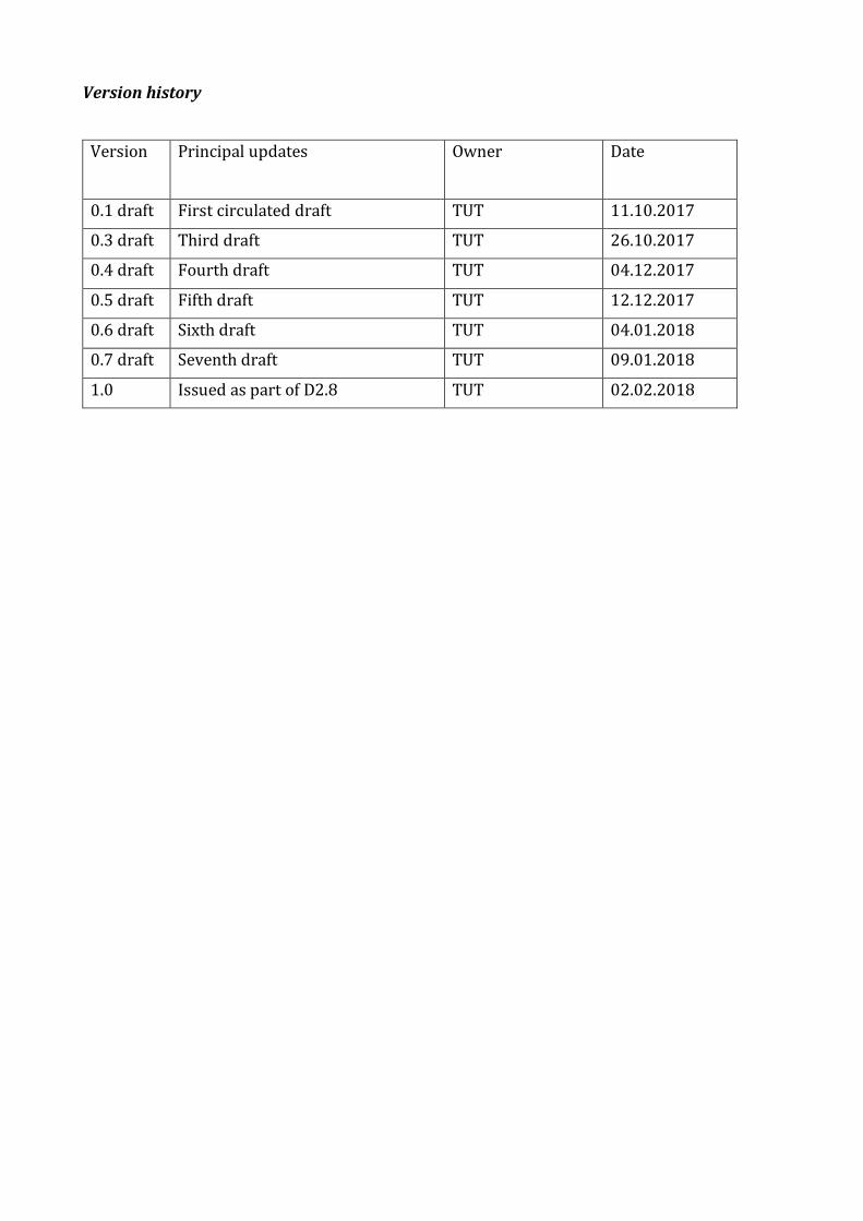
Version history
Version
Principal updates Owner Date
0.1 draft First circulated draft TUT 11.10.2017
0.3 draft Third draft TUT 26.10.2017
0.4 draft Fourth draft TUT 04.12.2017
0.5 draft Fifth draft TUT 12.12.2017
0.6 draft Sixth draft TUT 04.01.2018
0.7 draft Seventh draft TUT 09.01.2018
1.0 Issued as part of D2.8 TUT 02.02.2018
1 Product overview Product name: GNSS IPW (Global Navigation Satellite System Integrated Precipitable Water)
Product technique: Total Column Water Vapour (also known and hereafter named as Integrated
Precipitable Water) derived from GNSS signal delays and ground-based meteorological data
Product measurand: IPW in [kg/m2]
Product form/range: IPW time series
Product dataset: E-GVAP
Site/Sites
• GRUAN https://www.gruan.org/network/sites/
Other networks having sites with high-quality GNSS-data, but not (yet) implementing GRUAN-like
uncertainty analysis which could be included in future:
• IGS Network (http://www.igs.org/)
• EUREF Network (http://www.epncb.oma.be/)
• Various National Geodetic Agencies (e.g. Ordnance Survey GB,
https://www.ordnancesurvey.co.uk/)
• Various National Meteorological and Hydrological Agencies (e.g. Met Office,
https://www.metoffice.gov.uk/)
• Various Commercial Agencies (e.g. Leica, http://www.smartnet-eu.com/)
Product time period: Depends on site and available in delayed-mode for GRUAN GNSS-product
public access.
Data provider: GRUAN
Instrument provider: not identified, but the instrumentation and installations must follow the
Current IGS Site Guidelines (https://kb.igs.org/hc/en-us/articles/202011433-Current-IGS-Site-
Guidelines , sections 2.1.9 and 2.1.11).
Product assessor (for GRUAN): Kalev Rannat & Galina Dick
Assessor contact email (for GRUAN): [email protected] or [email protected]
1.1 Guidance notes
For general guidance see the Guide to Uncertainty in Measurement & its Nomenclature, published
as part of the GAIA-CLIM project.
This document is a measurement product technical document which should be stand-alone i.e. intelligible in isolation. Reference to external sources (preferably peer-reviewed) and documentation from previous studies is clearly expected and welcomed, but with sufficient explanatory content in the GAIA-CLIM document not to necessitate the reading of all these reference documents to gain a clear understanding of the GAIA-CLIM product and associated uncertainties entered into the Virtual Observatory (VO).
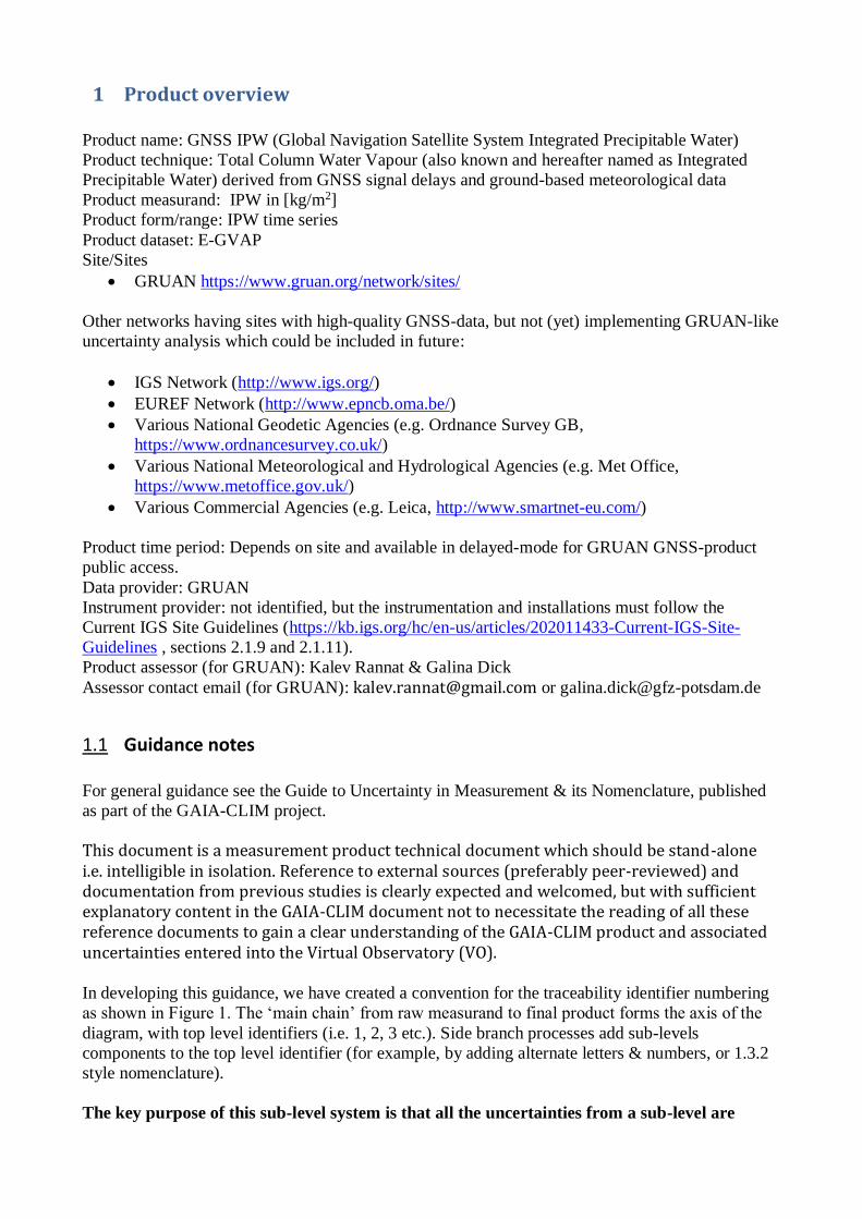
In developing this guidance, we have created a convention for the traceability identifier numbering
as shown in Figure 1. The ‘main chain’ from raw measurand to final product forms the axis of the
diagram, with top level identifiers (i.e. 1, 2, 3 etc.). Side branch processes add sub-levels
components to the top level identifier (for example, by adding alternate letters & numbers, or 1.3.2
style nomenclature).
The key purpose of this sub-level system is that all the uncertainties from a sub-level are
summed in the next level up.
For instance, using Figure 1, contributors 2a1, 2a2 and 2a3 are all assessed as separate components
to the overall traceability chain (have a contribution table). The contribution table for (and
uncertainty associated with) 2a, should combine all the sub-level uncertainties (and any additional
uncertainty intrinsic to step 2a). In turn, the contribution table for contributor 2, should include all
uncertainties in its sub-levels.
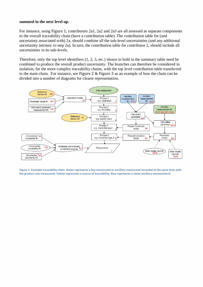
Therefore, only the top level identifiers (1, 2, 3, etc.) shown in bold in the summary table need be
combined to produce the overall product uncertainty. The branches can therefore be considered in
isolation, for the more complex traceability chains, with the top level contribution table transferred
to the main chain. For instance, see Figure 2 & Figure 3 as an example of how the chain can be
divided into a number of diagrams for clearer representation.
Figure 1. Example traceability chain. Green represents a key measurand or ancillary measurand recorded at the same time with the product raw measurand. Yellow represents a source of traceability. Blue represents a static ancillary measurement
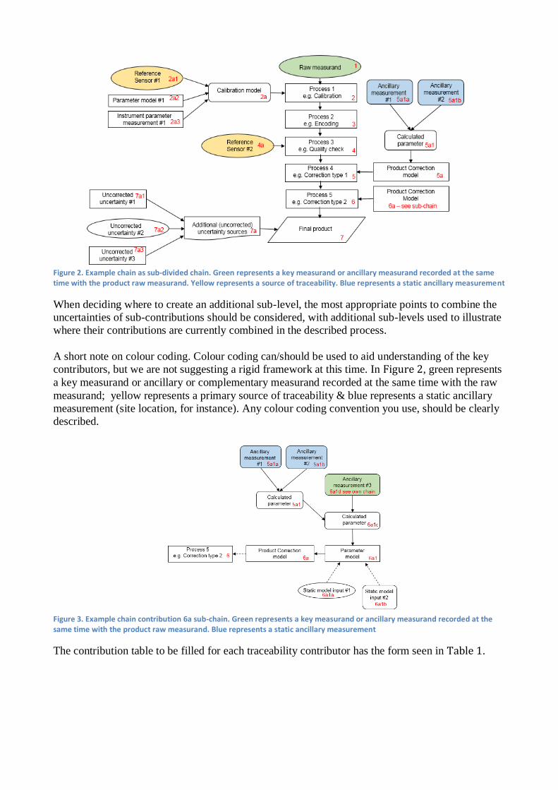
Figure 2. Example chain as sub-divided chain. Green represents a key measurand or ancillary measurand recorded at the same time with the product raw measurand. Yellow represents a source of traceability. Blue represents a static ancillary measurement
When deciding where to create an additional sub-level, the most appropriate points to combine the
uncertainties of sub-contributions should be considered, with additional sub-levels used to illustrate
where their contributions are currently combined in the described process.
A short note on colour coding. Colour coding can/should be used to aid understanding of the key
contributors, but we are not suggesting a rigid framework at this time. In Figure 2, green represents
a key measurand or ancillary or complementary measurand recorded at the same time with the raw
measurand; yellow represents a primary source of traceability & blue represents a static ancillary
measurement (site location, for instance). Any colour coding convention you use, should be clearly
described.
Figure 3. Example chain contribution 6a sub-chain. Green represents a key measurand or ancillary measurand recorded at the same time with the product raw measurand. Blue represents a static ancillary measurement
The contribution table to be filled for each traceability contributor has the form seen in Table 1.
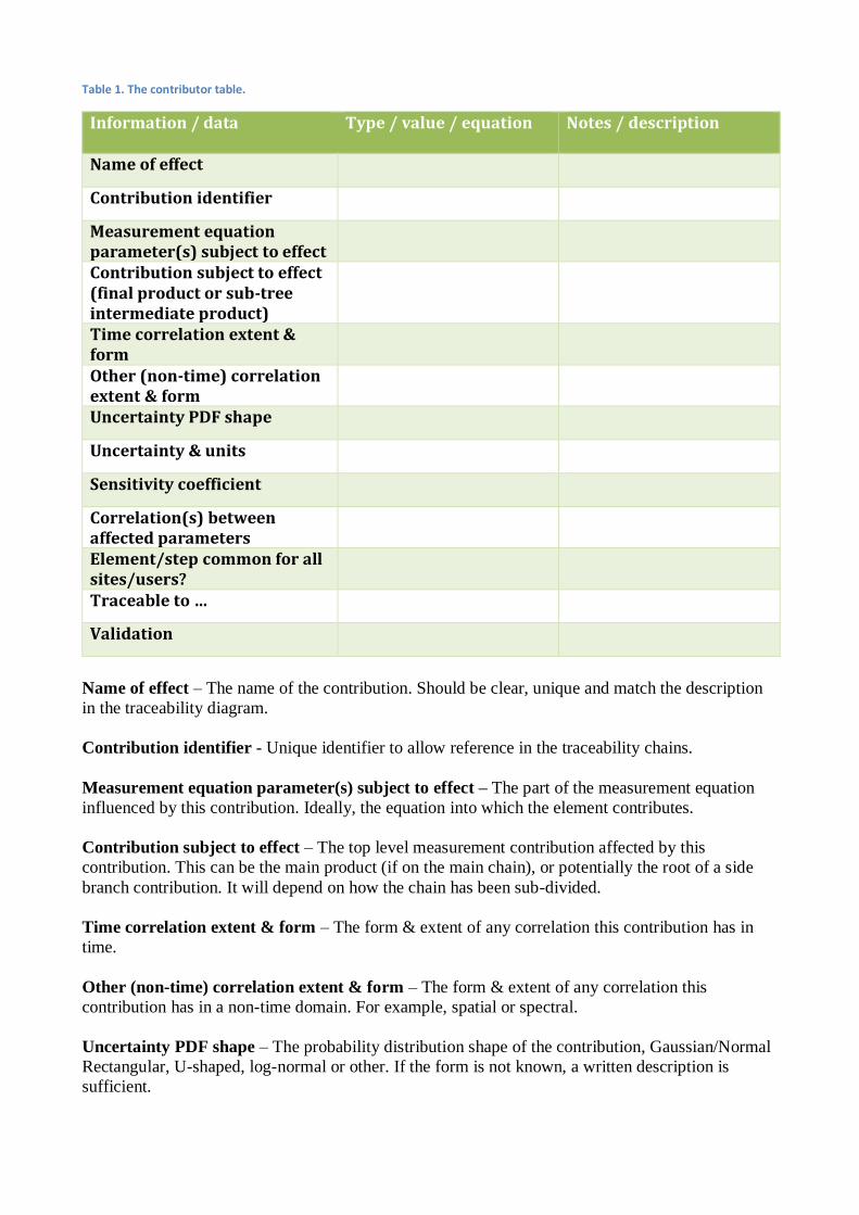
Table 1. The contributor table.
Information / data Type / value / equation Notes / description
Name of effect
Contribution identifier
Measurement equation parameter(s) subject to effect
Contribution subject to effect (final product or sub-tree intermediate product)
Time correlation extent & form
Other (non-time) correlation extent & form
Uncertainty PDF shape
Uncertainty & units
Sensitivity coefficient
Correlation(s) between affected parameters
Element/step common for all sites/users?
Traceable to …
Validation
Name of effect – The name of the contribution. Should be clear, unique and match the description
in the traceability diagram.
Contribution identifier - Unique identifier to allow reference in the traceability chains.
Measurement equation parameter(s) subject to effect – The part of the measurement equation
influenced by this contribution. Ideally, the equation into which the element contributes.
Contribution subject to effect – The top level measurement contribution affected by this
contribution. This can be the main product (if on the main chain), or potentially the root of a side
branch contribution. It will depend on how the chain has been sub-divided.
Time correlation extent & form – The form & extent of any correlation this contribution has in
time.
Other (non-time) correlation extent & form – The form & extent of any correlation this
contribution has in a non-time domain. For example, spatial or spectral.
Uncertainty PDF shape – The probability distribution shape of the contribution, Gaussian/Normal
Rectangular, U-shaped, log-normal or other. If the form is not known, a written description is
sufficient.
Uncertainty & units – The uncertainty value, including units and confidence interval. This can be
a simple equation, but should contain typical values.
Sensitivity coefficient – Coefficient multiplied by the uncertainty when applied to the measurement
equation.
Correlation(s) between affected parameters – Any correlation between the parameters affected
by this specific contribution. If this element links to the main chain by multiple paths within the
traceability chain, it should be described here. For instance, SZA or surface pressure may be used
separately in a number of models & correction terms that are applied to the product at different
points in the processing. Figure 1, contribution 5a1, for an example.
Element/step common for all sites/users – Is there any site-to-site/user-to-user variation in the
application of this contribution?
Traceable to – Describe any traceability back towards a primary/community reference.
Validation – Any validation activities that have been performed for this element?
The summary table, explanatory notes and referenced material in the traceability chain should
occupy <= 1 page for each element entry. Once the summary tables have been completed for the
full end-to-end process, the uncertainties can be combined, allowing assessment of the combined
uncertainty, relative importance of the contributors and correlation scales both temporally and
spatially. The unified form of this technical document should then allow easy comparison of
techniques and methods.
2 Introduction This document presents the Product Traceabililty and Uncertainty (PTU) information for the GNSS
IPW product. The aim of this document is to provide supporting information for the users of this
product within the GAIA-CLIM VO.
2.1 Instruments
2.1.1 Instruments for GNSS data acquisition
Unique receivers and antennas are not encouraged at stations. Only previously known brands and models as described in the IGS rcvr_ant.tab and IGS08.atx file are accepted with full standing within the IGS network ftp://igs.org/pub/station/general/.
2.1.1.1 Receivers
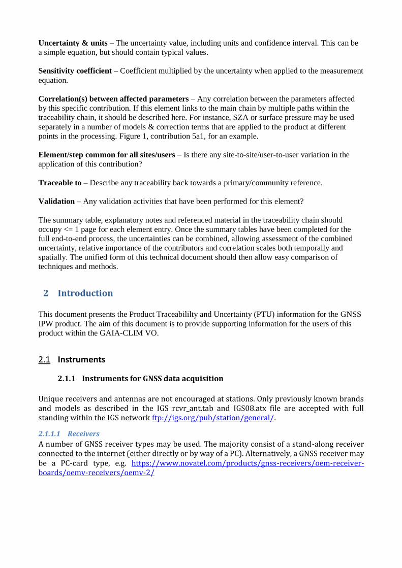
A number of GNSS receiver types may be used. The majority consist of a stand-along receiver connected to the internet (either directly or by way of a PC). Alternatively, a GNSS receiver may be a PC-card type, e.g. https://www.novatel.com/products/gnss-receivers/oem-receiver-boards/oemv-receivers/oemv-2/
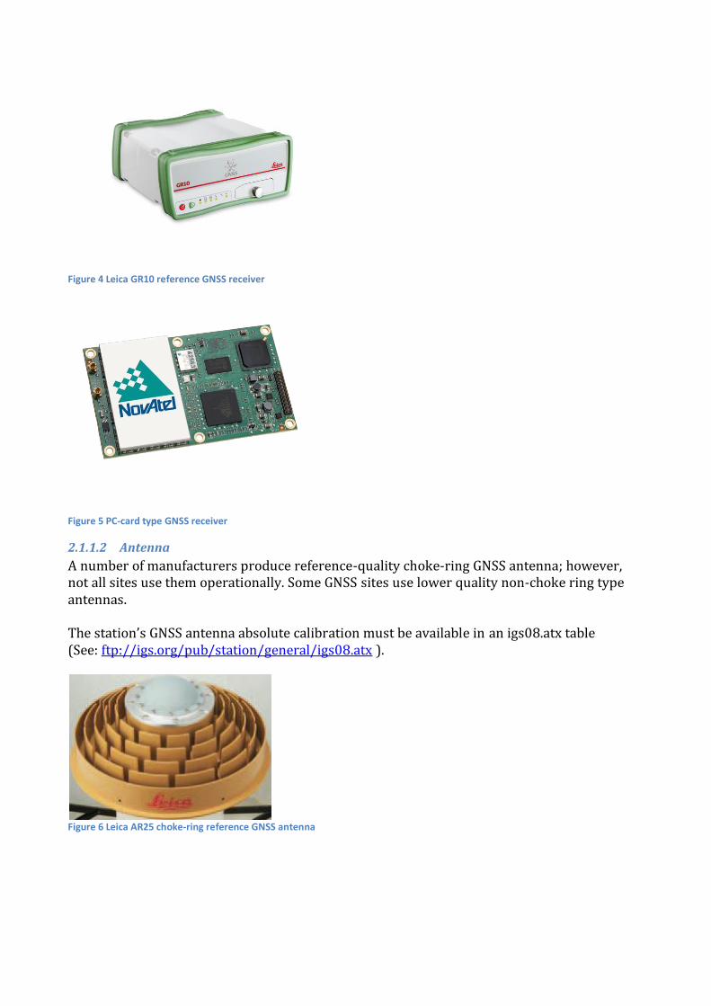
Figure 4 Leica GR10 reference GNSS receiver
Figure 5 PC-card type GNSS receiver
2.1.1.2 Antenna
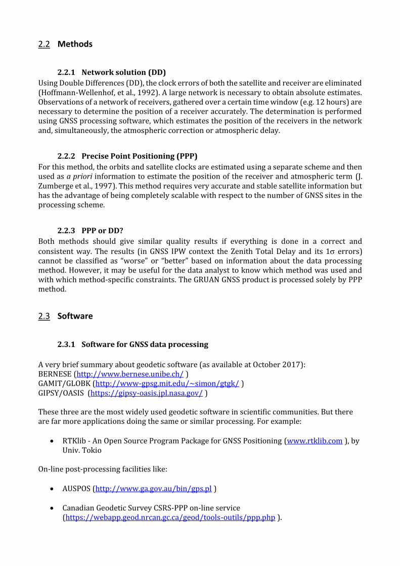
A number of manufacturers produce reference-quality choke-ring GNSS antenna; however, not all sites use them operationally. Some GNSS sites use lower quality non-choke ring type antennas. The station’s GNSS antenna absolute calibration must be available in an igs08.atx table (See: ftp://igs.org/pub/station/general/igs08.atx ).
Figure 6 Leica AR25 choke-ring reference GNSS antenna
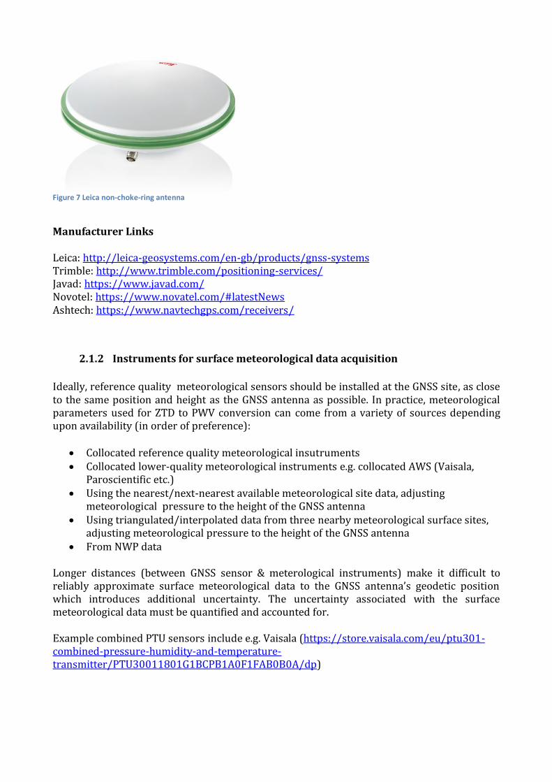
Figure 7 Leica non-choke-ring antenna
Manufacturer Links Leica: http://leica-geosystems.com/en-gb/products/gnss-systems Trimble: http://www.trimble.com/positioning-services/ Javad: https://www.javad.com/ Novotel: https://www.novatel.com/#latestNews Ashtech: https://www.navtechgps.com/receivers/
2.1.2 Instruments for surface meteorological data acquisition
Ideally, reference quality meteorological sensors should be installed at the GNSS site, as close to the same position and height as the GNSS antenna as possible. In practice, meteorological parameters used for ZTD to PWV conversion can come from a variety of sources depending upon availability (in order of preference):
• Collocated reference quality meteorological insutruments • Collocated lower-quality meteorological instruments e.g. collocated AWS (Vaisala,
Paroscientific etc.) • Using the nearest/next-nearest available meteorological site data, adjusting
meteorological pressure to the height of the GNSS antenna • Using triangulated/interpolated data from three nearby meteorological surface sites,
adjusting meteorological pressure to the height of the GNSS antenna • From NWP data
Longer distances (between GNSS sensor & meterological instruments) make it difficult to reliably approximate surface meteorological data to the GNSS antenna’s geodetic position which introduces additional uncertainty. The uncertainty associated with the surface meteorological data must be quantified and accounted for. Example combined PTU sensors include e.g. Vaisala (https://store.vaisala.com/eu/ptu301-combined-pressure-humidity-and-temperature-transmitter/PTU30011801G1BCPB1A0F1FAB0B0A/dp)
2.2 Methods
2.2.1 Network solution (DD)
Using Double Differences (DD), the clock errors of both the satellite and receiver are eliminated (Hoffmann-Wellenhof, et al., 1992). A large network is necessary to obtain absolute estimates. Observations of a network of receivers, gathered over a certain time window (e.g. 12 hours) are necessary to determine the position of a receiver accurately. The determination is performed using GNSS processing software, which estimates the position of the receivers in the network and, simultaneously, the atmospheric correction or atmospheric delay.
2.2.2 Precise Point Positioning (PPP)
For this method, the orbits and satellite clocks are estimated using a separate scheme and then used as a priori information to estimate the position of the receiver and atmospheric term (J. Zumberge et al., 1997). This method requires very accurate and stable satellite information but has the advantage of being completely scalable with respect to the number of GNSS sites in the processing scheme.
2.2.3 PPP or DD?
Both methods should give similar quality results if everything is done in a correct and consistent way. The results (in GNSS IPW context the Zenith Total Delay and its 1 errors) cannot be classified as “worse” or “better” based on information about the data processing method. However, it may be useful for the data analyst to know which method was used and with which method-specific constraints. The GRUAN GNSS product is processed solely by PPP method.
2.3 Software
2.3.1 Software for GNSS data processing
A very brief summary about geodetic software (as available at October 2017): BERNESE (http://www.bernese.unibe.ch/ ) GAMIT/GLOBK (http://www-gpsg.mit.edu/~simon/gtgk/ ) GIPSY/OASIS (https://gipsy-oasis.jpl.nasa.gov/ ) These three are the most widely used geodetic software in scientific communities. But there are far more applications doing the same or similar processing. For example:
• RTKlib - An Open Source Program Package for GNSS Positioning (www.rtklib.com ), by Univ. Tokio
On-line post-processing facilities like:
• AUSPOS (http://www.ga.gov.au/bin/gps.pl )
• Canadian Geodetic Survey CSRS-PPP on-line service (https://webapp.geod.nrcan.gc.ca/geod/tools-outils/ppp.php ).
Or, in-house developed solutions, non-commercial, but not open, for example:
• EPOS (http://www.gfz-potsdam.de/en/section/global-geomonitoring-and-gravity-field/topics/earth-system-parameters-and-orbit-dynamics/epos/ ) used by Helmholtz-Zentrum Potsdam Deutsches GeoForschungsZentrum GFZ.
GRUAN processing:
GRUAN GNSS data processing at the GFZ is based on GFZ EPOS8 software which is based on least
squares adjustment using a sliding window approach and makes use of the IERS standards.
Operational GPS data processing at the GFZ is performed in PPP mode and provides all tropospheric
products: the zenith total delays (ZTD), the integrated water vapour (IWV), the slant total delays
(STD) and tropospheric gradients in near-real time and in post-processing.
Using PPP strategy:
The main idea of the PPP strategy is the processing of each site separately, fixing the high quality
GPS orbits and clocks. Thus the Near Real Time (NRT) processing is split into two steps:
1) "Base cluster" analysis: estimation of high quality GPS orbits and clocks from a global network
(using about 100 IGS sites), where an orbit relaxation starting with the Ultra Rapid GFZ
predictions is performed. Among the estimated parameters for the "base cluster" step are (1) GPS
orbits with predicted Ultra Rapid orbits from GFZ used as initials, (2) Satellite clocks, and (3)
ZTDs for 4-hour intervals.
2) PPP analysis: estimation of ZTDs/IWV/STDs using parallel processing of stations in clusters
with PPP based on fixed orbits and clocks from the first step, adjusting for (1) the ZTDs with
resolution of 15 minutes, and (2) tropospheric east and north gradients with hourly resolution.
The main characteristics of GFZ EPOS8 software processing include:
1) Use of a sliding 24-hour data window
2) Elevation cut-off angle: 7 degrees
3) Sampling rate of GPS data 2.5 minutes
4) Reference frame:
• Earth rotation parameters: GFZ GPS solution/prediction
• The station coordinates are held fixed, once determined with sufficient accuracy within
ITRF
2.3.2 Software for GNSS IPW derivation
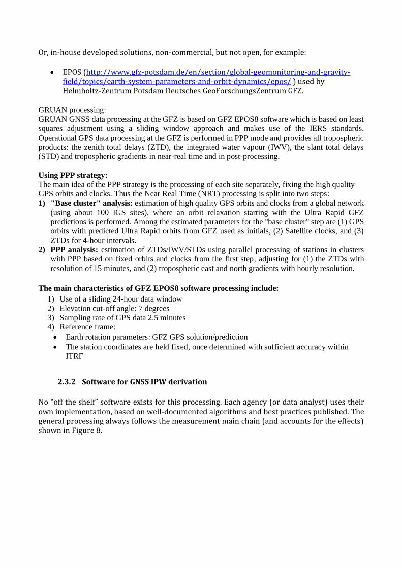
No “off the shelf” software exists for this processing. Each agency (or data analyst) uses their own implementation, based on well-documented algorithms and best practices published. The general processing always follows the measurement main chain (and accounts for the effects) shown in Figure 8.
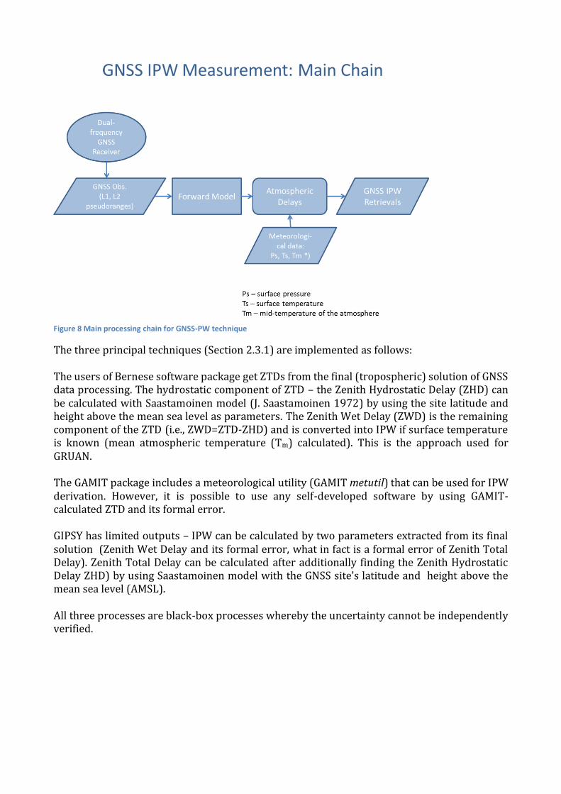
Figure 8 Main processing chain for GNSS-PW technique
The three principal techniques (Section 2.3.1) are implemented as follows: The users of Bernese software package get ZTDs from the final (tropospheric) solution of GNSS data processing. The hydrostatic component of ZTD – the Zenith Hydrostatic Delay (ZHD) can be calculated with Saastamoinen model (J. Saastamoinen 1972) by using the site latitude and height above the mean sea level as parameters. The Zenith Wet Delay (ZWD) is the remaining component of the ZTD (i.e., ZWD=ZTD-ZHD) and is converted into IPW if surface temperature is known (mean atmospheric temperature (Tm) calculated). This is the approach used for GRUAN. The GAMIT package includes a meteorological utility (GAMIT metutil) that can be used for IPW derivation. However, it is possible to use any self-developed software by using GAMIT-calculated ZTD and its formal error. GIPSY has limited outputs – IPW can be calculated by two parameters extracted from its final solution (Zenith Wet Delay and its formal error, what in fact is a formal error of Zenith Total Delay). Zenith Total Delay can be calculated after additionally finding the Zenith Hydrostatic Delay ZHD) by using Saastamoinen model with the GNSS site’s latitude and height above the mean sea level (AMSL). All three processes are black-box processes whereby the uncertainty cannot be independently verified.
3 Product Traceability Chain
Figure 9 Product traceability chain for GNSS-IPW technique
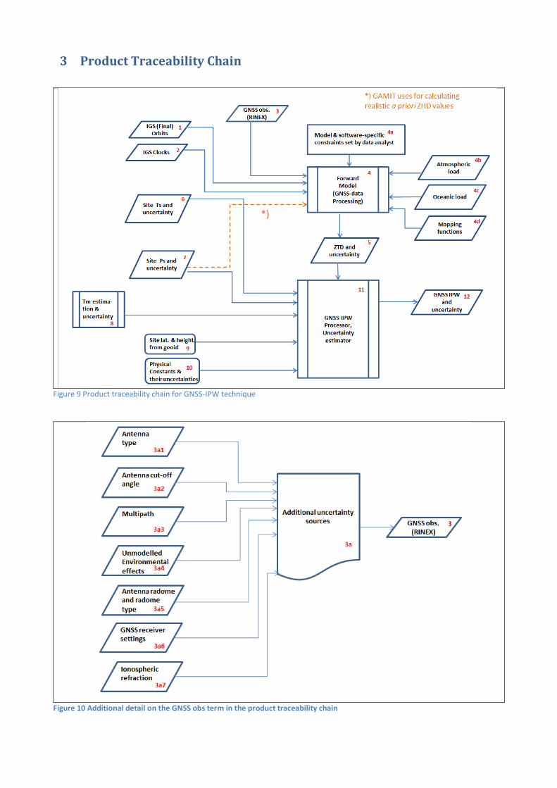
Figure 10 Additional detail on the GNSS obs term in the product traceability chain
As shown in Figure 9, ZTD and its uncertainty are products of the Forward Model (GNSS-data processing software). All uncertainties contributing to the ZTD and its formal uncertainty have their own specific contributions. At the GNSS-data processing phase, many of these effects can be either corrected or ignored (for example, by using or not using the oceanic and atmospheric load). For GNSS-IPW uncertainty quantification it is possible to use analytics given by Ning et al., (2016) to quantify all effects except for ZTD and its uncertainty (term 5 in Figure 9). We have combined effects of all contributors, analysed, weighted and scaled by the GNSS-processing software. There can be made only numeric experiments to quantify some effects for each site or a site in the fixed network of sites, meaning that the results cannot necessarilly be generalised and applied more broadly. For GRUAN GNSS data processing by GFZ (and EPOS8 software) the Figure 9 would look a little different. For the Forward Model, the items 1 (IGS orbits) and 2 (IGS clocks) can be considered as EPOS8 own products, not external (GFZ is one of the IGS data analysis centres). This serves to reduce, to a small degree to which the GRUAN processing contains black-box processes.
4 Element contributions
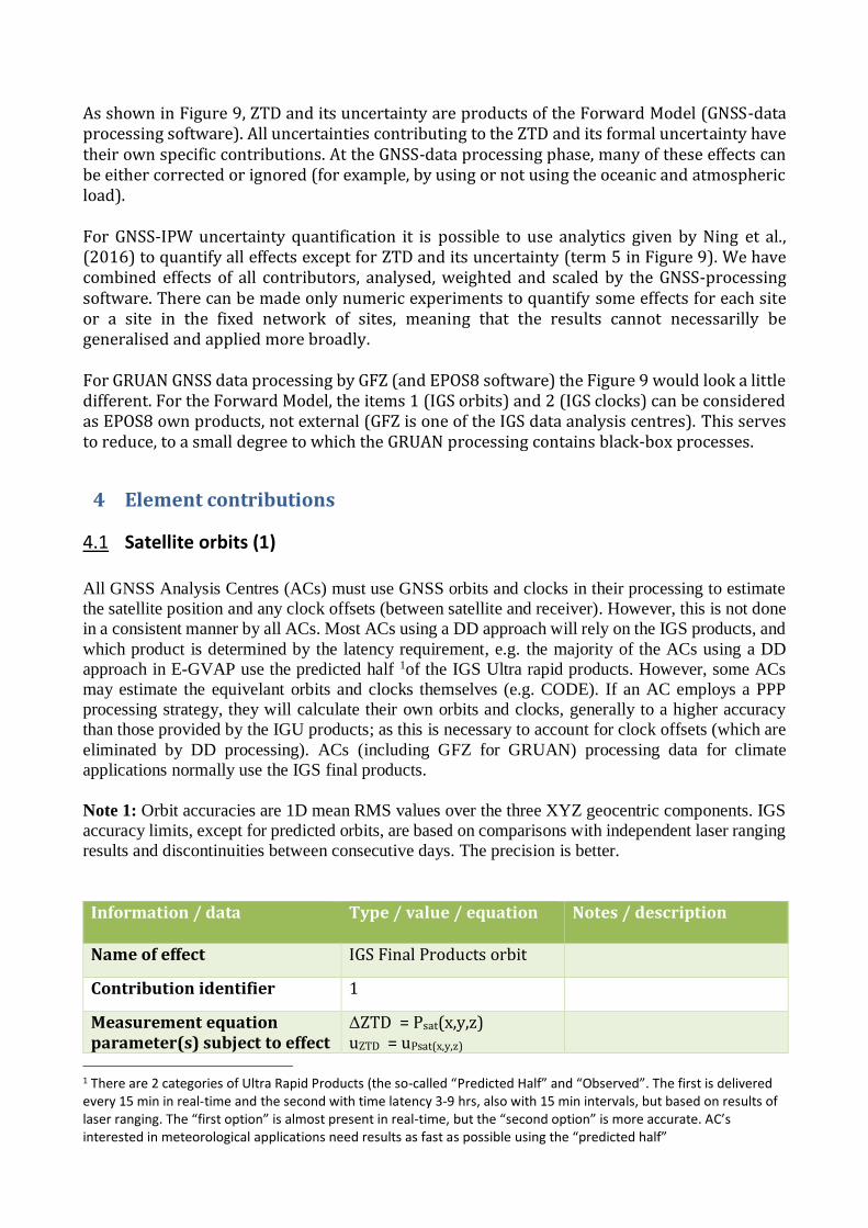
4.1 Satellite orbits (1)
All GNSS Analysis Centres (ACs) must use GNSS orbits and clocks in their processing to estimate
the satellite position and any clock offsets (between satellite and receiver). However, this is not done
in a consistent manner by all ACs. Most ACs using a DD approach will rely on the IGS products, and
which product is determined by the latency requirement, e.g. the majority of the ACs using a DD
approach in E-GVAP use the predicted half 1of the IGS Ultra rapid products. However, some ACs
may estimate the equivelant orbits and clocks themselves (e.g. CODE). If an AC employs a PPP
processing strategy, they will calculate their own orbits and clocks, generally to a higher accuracy
than those provided by the IGU products; as this is necessary to account for clock offsets (which are
eliminated by DD processing). ACs (including GFZ for GRUAN) processing data for climate
applications normally use the IGS final products.
Note 1: Orbit accuracies are 1D mean RMS values over the three XYZ geocentric components. IGS
accuracy limits, except for predicted orbits, are based on comparisons with independent laser ranging
results and discontinuities between consecutive days. The precision is better.
Information / data Type / value / equation Notes / description
Name of effect IGS Final Products orbit
Contribution identifier 1
Measurement equation parameter(s) subject to effect
ΔZTD = Psat(x,y,z) uZTD = uPsat(x,y,z)
1 There are 2 categories of Ultra Rapid Products (the so-called “Predicted Half” and “Observed”. The first is delivered every 15 min in real-time and the second with time latency 3-9 hrs, also with 15 min intervals, but based on results of laser ranging. The “first option” is almost present in real-time, but the “second option” is more accurate. AC’s interested in meteorological applications need results as fast as possible using the “predicted half”
Contribution subject to effect (final product or sub-tree intermediate product)
ZTD
Time correlation extent & form
Between 15 mins & 1 day depending on application
Other (non-time) correlation extent & form
orbital timescales GPS satellite to satellite
Uncertainty PDF shape Normal
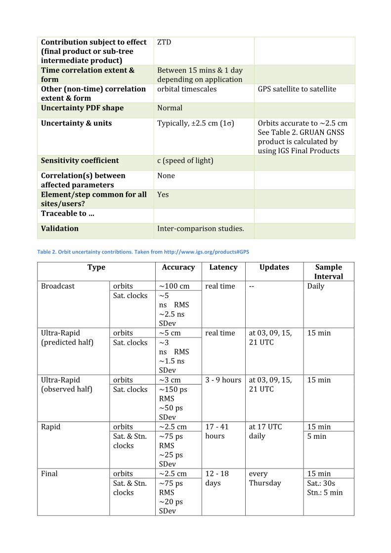
Uncertainty & units Typically, ±2.5 cm (1σ) Orbits accurate to ~2.5 cm See Table 2. GRUAN GNSS product is calculated by using IGS Final Products
Sensitivity coefficient c (speed of light)
Correlation(s) between affected parameters
None
Element/step common for all sites/users?
Yes
Traceable to …
Validation Inter-comparison studies.
Table 2. Orbit uncertainty contribtions. Taken from http://www.igs.org/products#GPS
Type Accuracy Latency Updates Sample Interval
Broadcast orbits ~100 cm real time -- Daily Sat. clocks ~5
ns RMS ~2.5 ns SDev
Ultra-Rapid (predicted half)
orbits ~5 cm real time at 03, 09, 15, 21 UTC
15 min Sat. clocks ~3
ns RMS ~1.5 ns SDev
Ultra-Rapid (observed half)
orbits ~3 cm 3 - 9 hours at 03, 09, 15, 21 UTC
15 min Sat. clocks ~150 ps
RMS ~50 ps SDev
Rapid orbits ~2.5 cm 17 - 41 hours
at 17 UTC daily
15 min Sat. & Stn. clocks
~75 ps RMS ~25 ps SDev
5 min
Final orbits ~2.5 cm 12 - 18 days
every Thursday
15 min Sat. & Stn. clocks
~75 ps RMS ~20 ps SDev
Sat.: 30s Stn.: 5 min
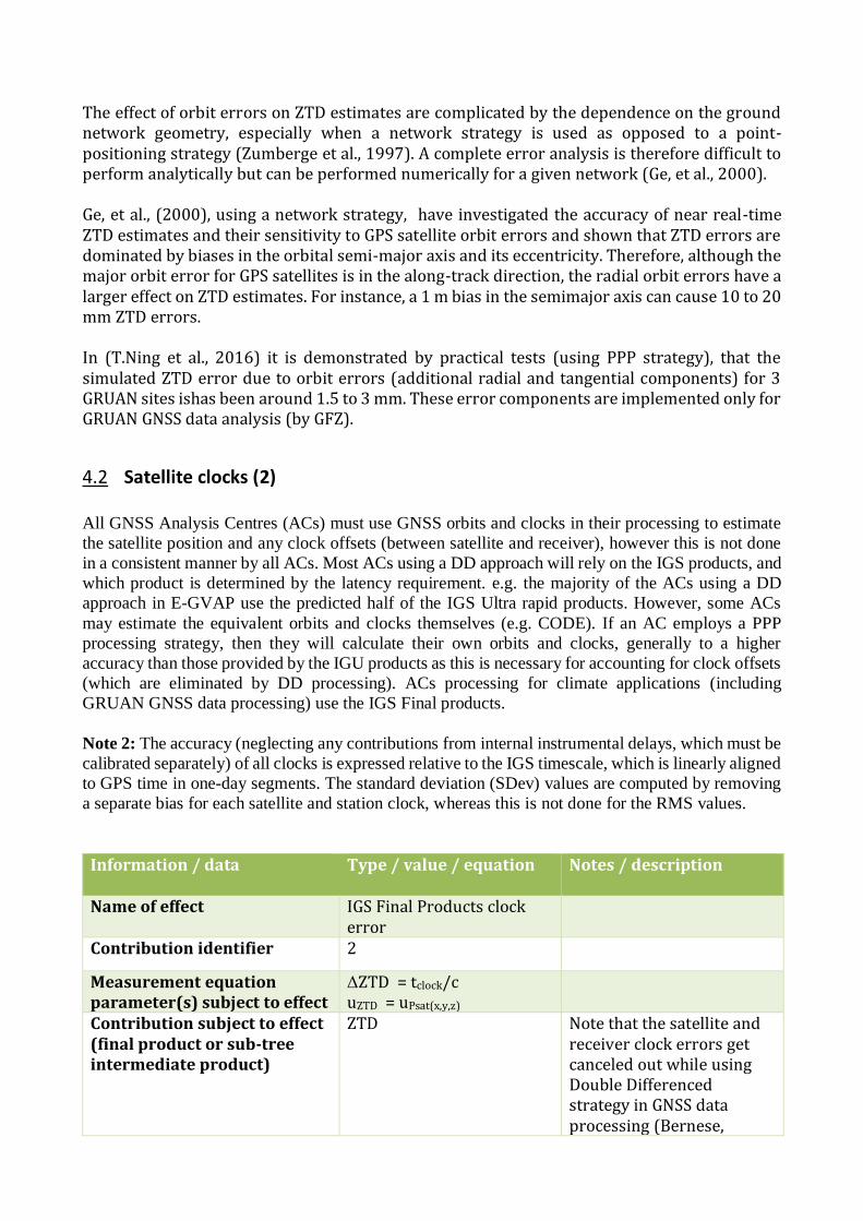
The effect of orbit errors on ZTD estimates are complicated by the dependence on the ground network geometry, especially when a network strategy is used as opposed to a point-positioning strategy (Zumberge et al., 1997). A complete error analysis is therefore difficult to perform analytically but can be performed numerically for a given network (Ge, et al., 2000). Ge, et al., (2000), using a network strategy, have investigated the accuracy of near real-time ZTD estimates and their sensitivity to GPS satellite orbit errors and shown that ZTD errors are dominated by biases in the orbital semi-major axis and its eccentricity. Therefore, although the major orbit error for GPS satellites is in the along-track direction, the radial orbit errors have a larger effect on ZTD estimates. For instance, a 1 m bias in the semimajor axis can cause 10 to 20 mm ZTD errors. In (T.Ning et al., 2016) it is demonstrated by practical tests (using PPP strategy), that the simulated ZTD error due to orbit errors (additional radial and tangential components) for 3 GRUAN sites ishas been around 1.5 to 3 mm. These error components are implemented only for GRUAN GNSS data analysis (by GFZ).
4.2 Satellite clocks (2)
All GNSS Analysis Centres (ACs) must use GNSS orbits and clocks in their processing to estimate
the satellite position and any clock offsets (between satellite and receiver), however this is not done
in a consistent manner by all ACs. Most ACs using a DD approach will rely on the IGS products, and
which product is determined by the latency requirement. e.g. the majority of the ACs using a DD
approach in E-GVAP use the predicted half of the IGS Ultra rapid products. However, some ACs
may estimate the equivalent orbits and clocks themselves (e.g. CODE). If an AC employs a PPP
processing strategy, then they will calculate their own orbits and clocks, generally to a higher
accuracy than those provided by the IGU products as this is necessary for accounting for clock offsets
(which are eliminated by DD processing). ACs processing for climate applications (including
GRUAN GNSS data processing) use the IGS Final products.
Note 2: The accuracy (neglecting any contributions from internal instrumental delays, which must be
calibrated separately) of all clocks is expressed relative to the IGS timescale, which is linearly aligned
to GPS time in one-day segments. The standard deviation (SDev) values are computed by removing
a separate bias for each satellite and station clock, whereas this is not done for the RMS values.
Information / data Type / value / equation Notes / description
Name of effect IGS Final Products clock error
Contribution identifier 2
Measurement equation parameter(s) subject to effect
ΔZTD = tclock/c uZTD = uPsat(x,y,z)
Contribution subject to effect (final product or sub-tree intermediate product)
ZTD Note that the satellite and receiver clock errors get canceled out while using Double Differenced strategy in GNSS data processing (Bernese,
GAMIT).
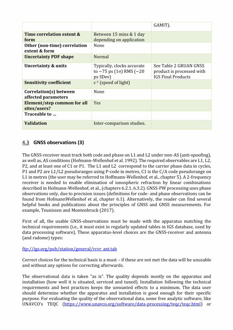
Time correlation extent & form
Between 15 mins & 1 day depending on application
Other (non-time) correlation extent & form
None
Uncertainty PDF shape Normal
Uncertainty & units Typically, clocks accurate to ~75 ps (1σ) RMS (~20 ps SDev)
See Table 2 GRUAN GNSS product is processed with IGS Final Products
Sensitivity coefficient c-1 (speed of light)
Correlation(s) between affected parameters
None
Element/step common for all sites/users?
Yes
Traceable to …
Validation Inter-comparison studies.
4.3 GNSS observations (3)
The GNSS-receiver must track both code and phase on L1 and L2 under non-AS (anti-spoofing), as well as, AS conditions (Hofmann-Wellenhof et al. 1992). The required observables are L1, L2, P2, and at least one of C1 or P1. The L1 and L2 correspond to the carrier phase data in cycles, P1 and P2 are L1/L2 pseudoranges using P-code in metres, C1 is the C/A code pseudorange on L1 in metres (the user may be referred to Hoffmann-Wellenhof, et al., chapter 5). A 2-frequency receiver is needed to enable elimination of ionospheric refraction by linear combinations described in Hofmann-Wellenhof, et al., (chapters 6.2.1, 6.3.2). GNSS-PW processing uses phase observations only, due to precision issues (definitions for code- and phase observations can be found from HofmannWellenhof et al, chapter 6.1). Alternatively, the reader can find several helpful books and publications about the principles of GNSS and GNSS measurements. For example, Teunissen and Montenbruck (2017). First of all, the usable GNSS-observations must be made with the apparatus matching the technical requirements (i.e., it must exist in regularly updated tables in IGS database, used by data processing software). These apparatus-level choices are the GNSS-receiver and antenna (and radome) types: ftp://igs.org/pub/station/general/rcvr_ant.tab Correct choices for the technical basis is a must – if these are not met the data will be unusable and without any options for correcting afterwards. The observational data is taken “as is”. The quality depends mostly on the apparatus and installation (how well it is situated, serviced and tuned). Installation following the technical requirements and best practices keeps the unwanted effects to a minimum. The data user should determine whether the apparatus and installation is good enough for their specific purpose. For evaluating the quality of the observational data, some free analytic software, like UNAVCO’s TEQC (https://www.unavco.org/software/data-processing/teqc/teqc.html) or
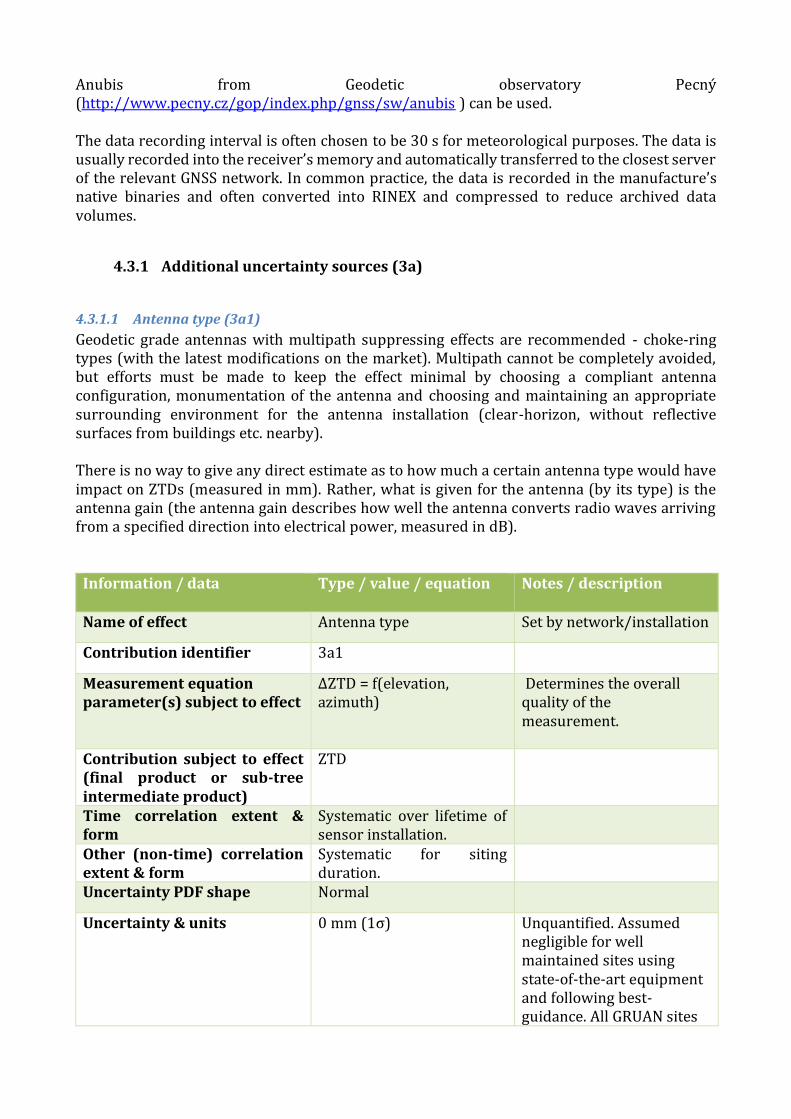
Anubis from Geodetic observatory Pecný (http://www.pecny.cz/gop/index.php/gnss/sw/anubis ) can be used. The data recording interval is often chosen to be 30 s for meteorological purposes. The data is usually recorded into the receiver’s memory and automatically transferred to the closest server of the relevant GNSS network. In common practice, the data is recorded in the manufacture’s native binaries and often converted into RINEX and compressed to reduce archived data volumes.
4.3.1 Additional uncertainty sources (3a)
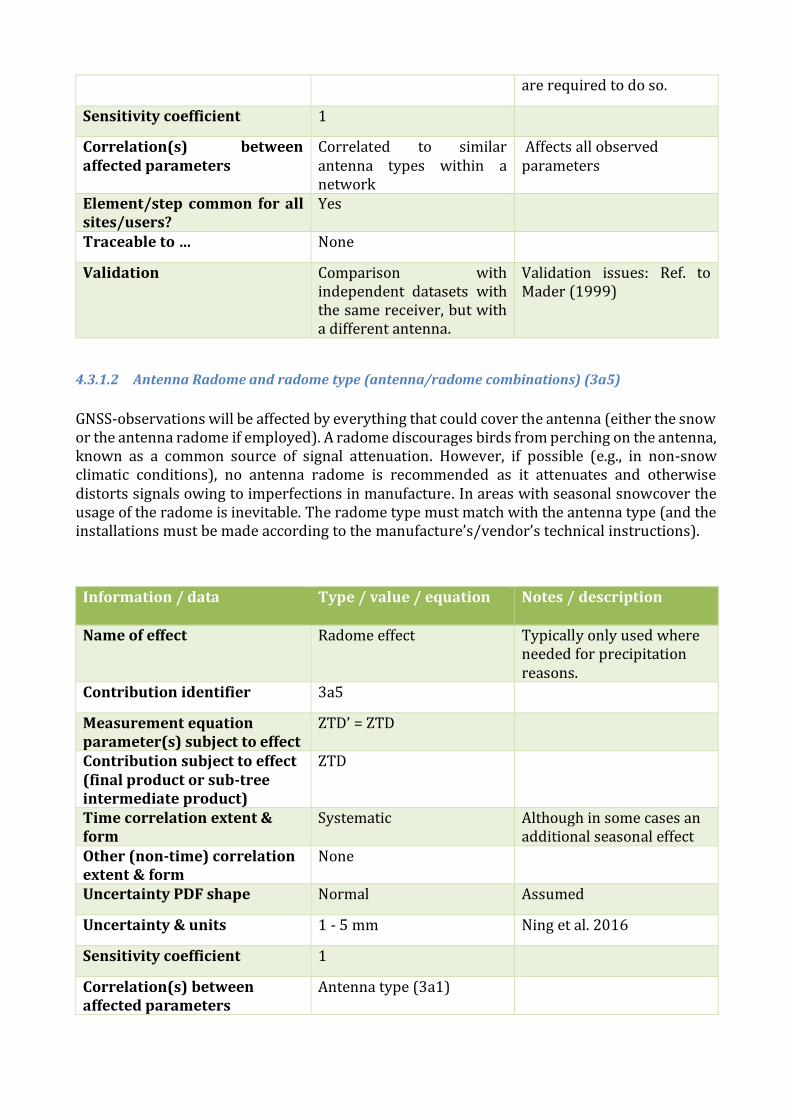
4.3.1.1 Antenna type (3a1)
Geodetic grade antennas with multipath suppressing effects are recommended - choke-ring types (with the latest modifications on the market). Multipath cannot be completely avoided, but efforts must be made to keep the effect minimal by choosing a compliant antenna configuration, monumentation of the antenna and choosing and maintaining an appropriate surrounding environment for the antenna installation (clear-horizon, without reflective surfaces from buildings etc. nearby). There is no way to give any direct estimate as to how much a certain antenna type would have impact on ZTDs (measured in mm). Rather, what is given for the antenna (by its type) is the antenna gain (the antenna gain describes how well the antenna converts radio waves arriving from a specified direction into electrical power, measured in dB).
Information / data Type / value / equation Notes / description
Name of effect Antenna type Set by network/installation
Contribution identifier 3a1
Measurement equation parameter(s) subject to effect
ΔZTD = f(elevation, azimuth)
Determines the overall quality of the measurement.
Contribution subject to effect (final product or sub-tree intermediate product)
ZTD
Time correlation extent & form
Systematic over lifetime of sensor installation.
Other (non-time) correlation extent & form
Systematic for siting duration.
Uncertainty PDF shape Normal
Uncertainty & units 0 mm (1σ) Unquantified. Assumed negligible for well maintained sites using state-of-the-art equipment and following best-guidance. All GRUAN sites
are required to do so.
Sensitivity coefficient 1
Correlation(s) between affected parameters
Correlated to similar antenna types within a network
Affects all observed parameters
Element/step common for all sites/users?
Yes
Traceable to … None
Validation Comparison with independent datasets with the same receiver, but with a different antenna.
Validation issues: Ref. to Mader (1999)
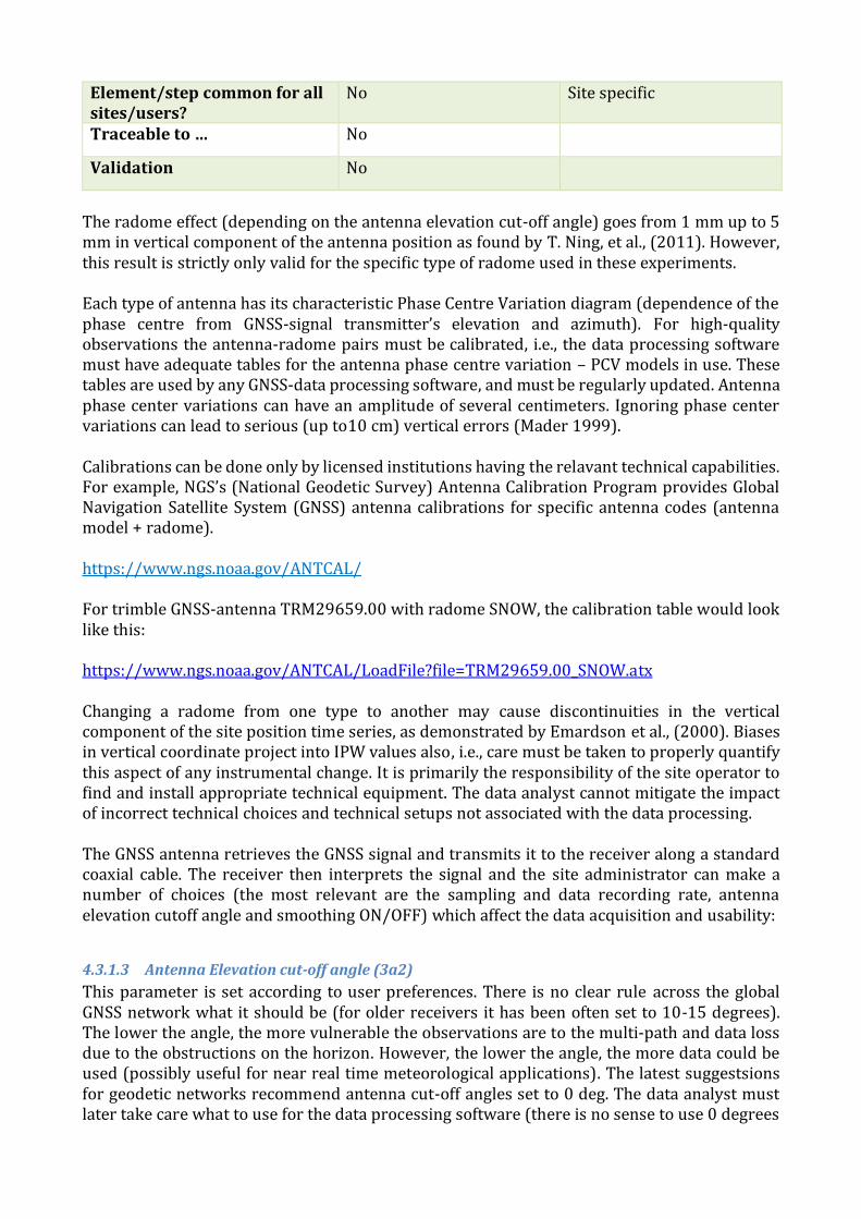
4.3.1.2 Antenna Radome and radome type (antenna/radome combinations) (3a5)
GNSS-observations will be affected by everything that could cover the antenna (either the snow or the antenna radome if employed). A radome discourages birds from perching on the antenna, known as a common source of signal attenuation. However, if possible (e.g., in non-snow climatic conditions), no antenna radome is recommended as it attenuates and otherwise distorts signals owing to imperfections in manufacture. In areas with seasonal snowcover the usage of the radome is inevitable. The radome type must match with the antenna type (and the installations must be made according to the manufacture’s/vendor’s technical instructions).
Information / data Type / value / equation Notes / description
Name of effect Radome effect Typically only used where needed for precipitation reasons.
Contribution identifier 3a5
Measurement equation parameter(s) subject to effect
ZTD’ = ZTD
Contribution subject to effect (final product or sub-tree intermediate product)
ZTD
Time correlation extent & form
Systematic Although in some cases an additional seasonal effect
Other (non-time) correlation extent & form
None
Uncertainty PDF shape Normal Assumed
Uncertainty & units 1 - 5 mm Ning et al. 2016
Sensitivity coefficient 1
Correlation(s) between affected parameters
Antenna type (3a1)
Element/step common for all sites/users?
No Site specific
Traceable to … No
Validation No
The radome effect (depending on the antenna elevation cut-off angle) goes from 1 mm up to 5 mm in vertical component of the antenna position as found by T. Ning, et al., (2011). However, this result is strictly only valid for the specific type of radome used in these experiments. Each type of antenna has its characteristic Phase Centre Variation diagram (dependence of the phase centre from GNSS-signal transmitter’s elevation and azimuth). For high-quality observations the antenna-radome pairs must be calibrated, i.e., the data processing software must have adequate tables for the antenna phase centre variation – PCV models in use. These tables are used by any GNSS-data processing software, and must be regularly updated. Antenna phase center variations can have an amplitude of several centimeters. Ignoring phase center variations can lead to serious (up to10 cm) vertical errors (Mader 1999). Calibrations can be done only by licensed institutions having the relavant technical capabilities. For example, NGS’s (National Geodetic Survey) Antenna Calibration Program provides Global Navigation Satellite System (GNSS) antenna calibrations for specific antenna codes (antenna model + radome). https://www.ngs.noaa.gov/ANTCAL/ For trimble GNSS-antenna TRM29659.00 with radome SNOW, the calibration table would look like this: https://www.ngs.noaa.gov/ANTCAL/LoadFile?file=TRM29659.00_SNOW.atx Changing a radome from one type to another may cause discontinuities in the vertical component of the site position time series, as demonstrated by Emardson et al., (2000). Biases in vertical coordinate project into IPW values also, i.e., care must be taken to properly quantify this aspect of any instrumental change. It is primarily the responsibility of the site operator to find and install appropriate technical equipment. The data analyst cannot mitigate the impact of incorrect technical choices and technical setups not associated with the data processing. The GNSS antenna retrieves the GNSS signal and transmits it to the receiver along a standard coaxial cable. The receiver then interprets the signal and the site administrator can make a number of choices (the most relevant are the sampling and data recording rate, antenna elevation cutoff angle and smoothing ON/OFF) which affect the data acquisition and usability:
4.3.1.3 Antenna Elevation cut-off angle (3a2)
This parameter is set according to user preferences. There is no clear rule across the global GNSS network what it should be (for older receivers it has been often set to 10-15 degrees). The lower the angle, the more vulnerable the observations are to the multi-path and data loss due to the obstructions on the horizon. However, the lower the angle, the more data could be used (possibly useful for near real time meteorological applications). The latest suggestsions for geodetic networks recommend antenna cut-off angles set to 0 deg. The data analyst must later take care what to use for the data processing software (there is no sense to use 0 degrees
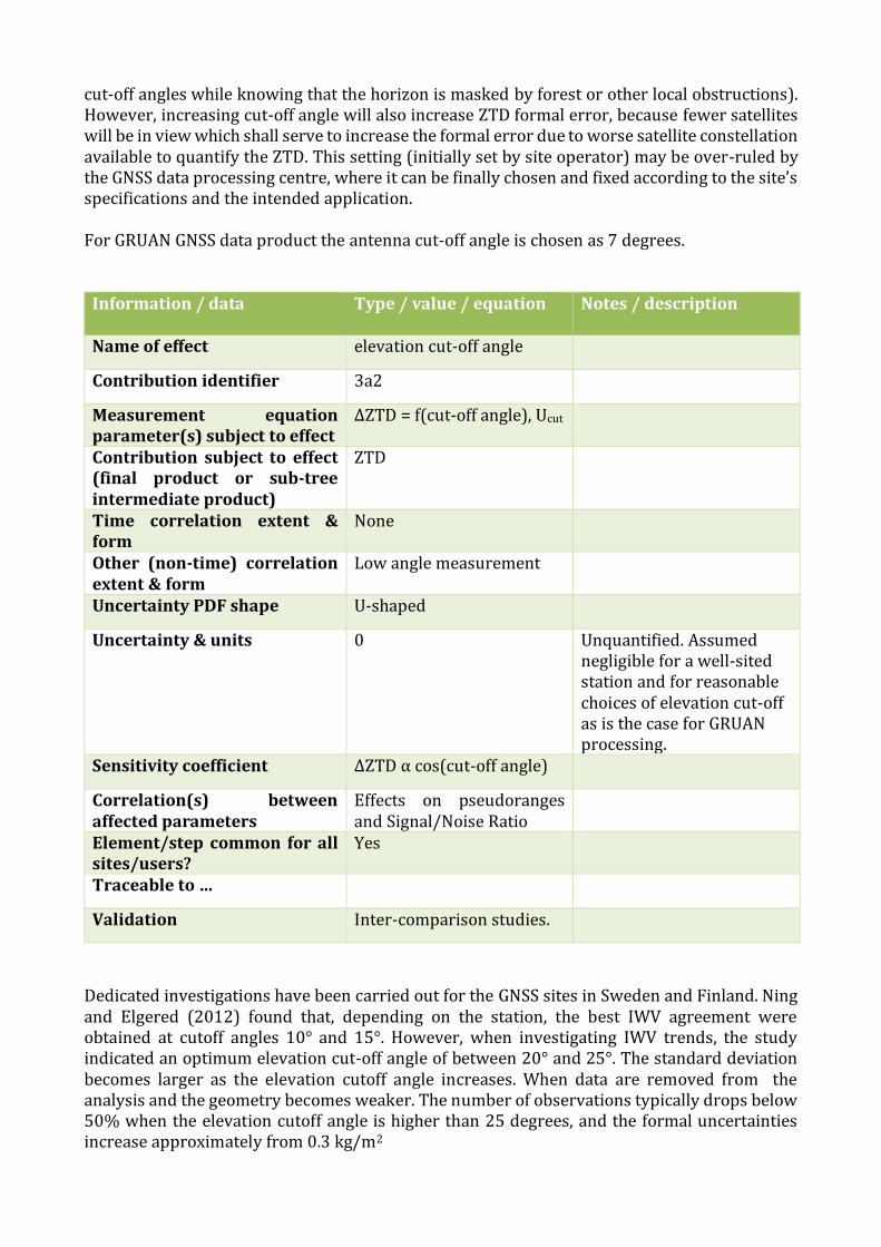
cut-off angles while knowing that the horizon is masked by forest or other local obstructions). However, increasing cut-off angle will also increase ZTD formal error, because fewer satellites will be in view which shall serve to increase the formal error due to worse satellite constellation available to quantify the ZTD. This setting (initially set by site operator) may be over-ruled by the GNSS data processing centre, where it can be finally chosen and fixed according to the site’s specifications and the intended application. For GRUAN GNSS data product the antenna cut-off angle is chosen as 7 degrees.
Information / data Type / value / equation Notes / description
Name of effect elevation cut-off angle
Contribution identifier 3a2
Measurement equation parameter(s) subject to effect
ΔZTD = f(cut-off angle), Ucut
Contribution subject to effect (final product or sub-tree intermediate product)
ZTD
Time correlation extent & form
None
Other (non-time) correlation extent & form
Low angle measurement
Uncertainty PDF shape U-shaped
Uncertainty & units 0 Unquantified. Assumed negligible for a well-sited station and for reasonable choices of elevation cut-off as is the case for GRUAN processing.
Sensitivity coefficient ΔZTD α cos(cut-off angle)
Correlation(s) between affected parameters
Effects on pseudoranges and Signal/Noise Ratio
Element/step common for all sites/users?
Yes
Traceable to …
Validation Inter-comparison studies.
Dedicated investigations have been carried out for the GNSS sites in Sweden and Finland. Ning and Elgered (2012) found that, depending on the station, the best IWV agreement were obtained at cutoff angles 10° and 15°. However, when investigating IWV trends, the study indicated an optimum elevation cut-off angle of between 20° and 25°. The standard deviation becomes larger as the elevation cutoff angle increases. When data are removed from the analysis and the geometry becomes weaker. The number of observations typically drops below 50% when the elevation cutoff angle is higher than 25 degrees, and the formal uncertainties increase approximately from 0.3 kg/m2
for the 5° solution up to 5 kg/m2 for the 40° solution (Ning, T and Elgered, G., 2012). Similar investigations have been made for a broader area, covering the latitudes between 35N-67N by Keernik and Rannat (2016) and the results agree well with that presented by Ning and Elgered (2012). The smallest IWV formal uncertainty as well as RMSD values (from 1.0 to 2.1 mm) between GNSS and comparison techniques were obtained at 10°. The correlation between IWV trends derived from GNSS and comparison techniques were the highest in case of 20°.
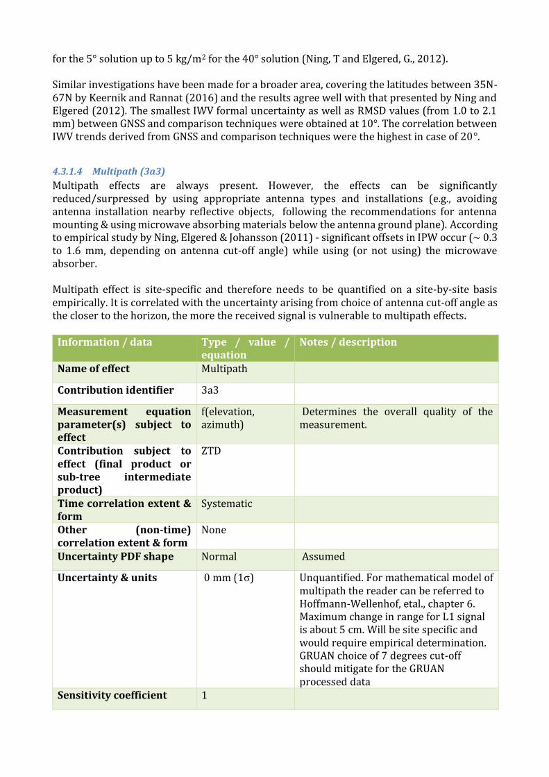
4.3.1.4 Multipath (3a3)
Multipath effects are always present. However, the effects can be significantly reduced/surpressed by using appropriate antenna types and installations (e.g., avoiding antenna installation nearby reflective objects, following the recommendations for antenna mounting & using microwave absorbing materials below the antenna ground plane). According to empirical study by Ning, Elgered & Johansson (2011) - significant offsets in IPW occur (~ 0.3 to 1.6 mm, depending on antenna cut-off angle) while using (or not using) the microwave absorber. Multipath effect is site-specific and therefore needs to be quantified on a site-by-site basis empirically. It is correlated with the uncertainty arising from choice of antenna cut-off angle as the closer to the horizon, the more the received signal is vulnerable to multipath effects.
Information / data Type / value / equation
Notes / description
Name of effect Multipath
Contribution identifier 3a3
Measurement equation parameter(s) subject to effect
f(elevation, azimuth)
Determines the overall quality of the measurement.
Contribution subject to effect (final product or sub-tree intermediate product)
ZTD
Time correlation extent & form
Systematic
Other (non-time) correlation extent & form
None
Uncertainty PDF shape Normal Assumed
Uncertainty & units 0 mm (1σ) Unquantified. For mathematical model of multipath the reader can be referred to Hoffmann-Wellenhof, etal., chapter 6. Maximum change in range for L1 signal is about 5 cm. Will be site specific and would require empirical determination. GRUAN choice of 7 degrees cut-off should mitigate for the GRUAN processed data
Sensitivity coefficient 1
Correlation(s) between affected parameters
Correlated to the site co-ordinates and ZTD
Element/step common for all sites/users?
Yes Site-specific, cannot be generalized
Traceable to … None
Validation Multipath analysis, for example with Anubis from Geodetic observatory Pecný (http://www.pecny.cz/gop/index.php/gnss/sw/anubis )
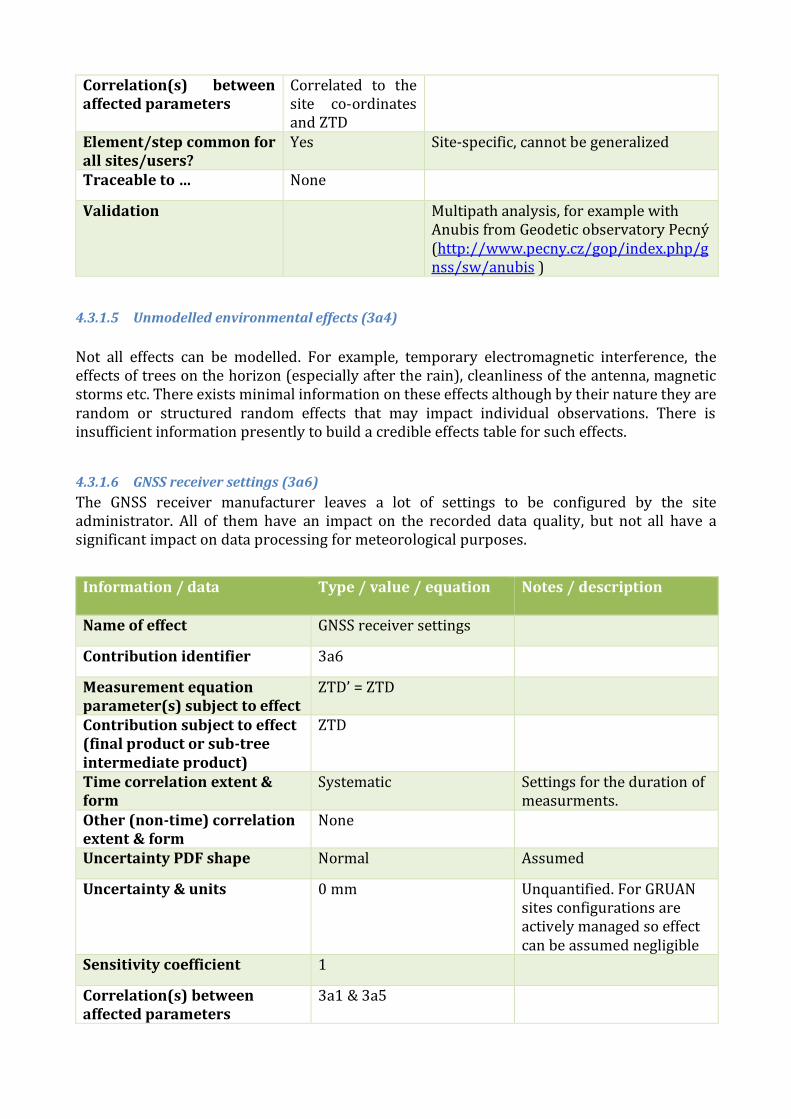
4.3.1.5 Unmodelled environmental effects (3a4)
Not all effects can be modelled. For example, temporary electromagnetic interference, the effects of trees on the horizon (especially after the rain), cleanliness of the antenna, magnetic storms etc. There exists minimal information on these effects although by their nature they are random or structured random effects that may impact individual observations. There is insufficient information presently to build a credible effects table for such effects.
4.3.1.6 GNSS receiver settings (3a6)
The GNSS receiver manufacturer leaves a lot of settings to be configured by the site administrator. All of them have an impact on the recorded data quality, but not all have a significant impact on data processing for meteorological purposes.
Information / data Type / value / equation Notes / description
Name of effect GNSS receiver settings
Contribution identifier 3a6
Measurement equation parameter(s) subject to effect
ZTD’ = ZTD
Contribution subject to effect (final product or sub-tree intermediate product)
ZTD
Time correlation extent & form
Systematic Settings for the duration of measurments.
Other (non-time) correlation extent & form
None
Uncertainty PDF shape Normal Assumed
Uncertainty & units 0 mm Unquantified. For GRUAN sites configurations are actively managed so effect can be assumed negligible
Sensitivity coefficient 1
Correlation(s) between affected parameters
3a1 & 3a5
Element/step common for all sites/users?
No Site settings may change for according to local conditions.
Traceable to … No
Validation No Optimised at setup
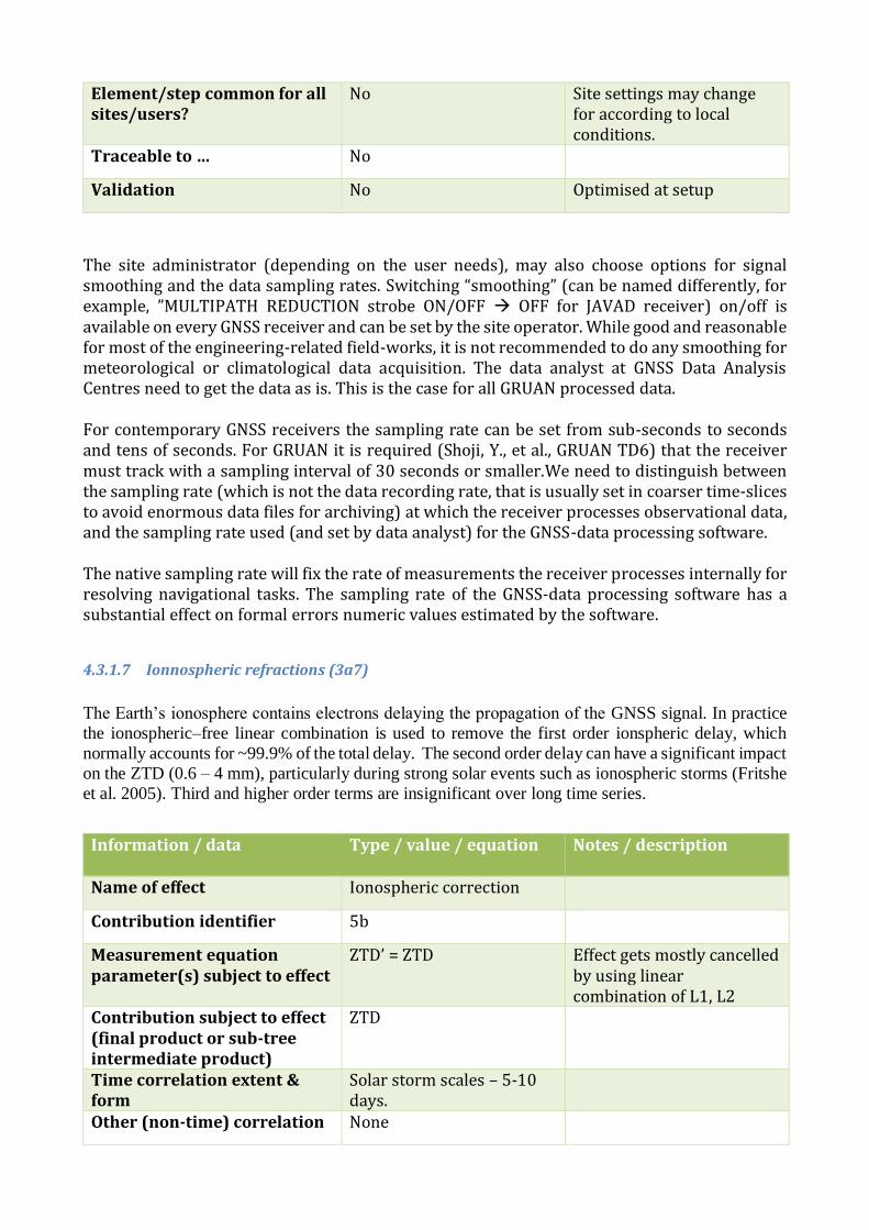
The site administrator (depending on the user needs), may also choose options for signal smoothing and the data sampling rates. Switching “smoothing” (can be named differently, for example, ”MULTIPATH REDUCTION strobe ON/OFF OFF for JAVAD receiver) on/off is available on every GNSS receiver and can be set by the site operator. While good and reasonable for most of the engineering-related field-works, it is not recommended to do any smoothing for meteorological or climatological data acquisition. The data analyst at GNSS Data Analysis Centres need to get the data as is. This is the case for all GRUAN processed data. For contemporary GNSS receivers the sampling rate can be set from sub-seconds to seconds and tens of seconds. For GRUAN it is required (Shoji, Y., et al., GRUAN TD6) that the receiver must track with a sampling interval of 30 seconds or smaller.We need to distinguish between the sampling rate (which is not the data recording rate, that is usually set in coarser time-slices to avoid enormous data files for archiving) at which the receiver processes observational data, and the sampling rate used (and set by data analyst) for the GNSS-data processing software. The native sampling rate will fix the rate of measurements the receiver processes internally for resolving navigational tasks. The sampling rate of the GNSS-data processing software has a substantial effect on formal errors numeric values estimated by the software.
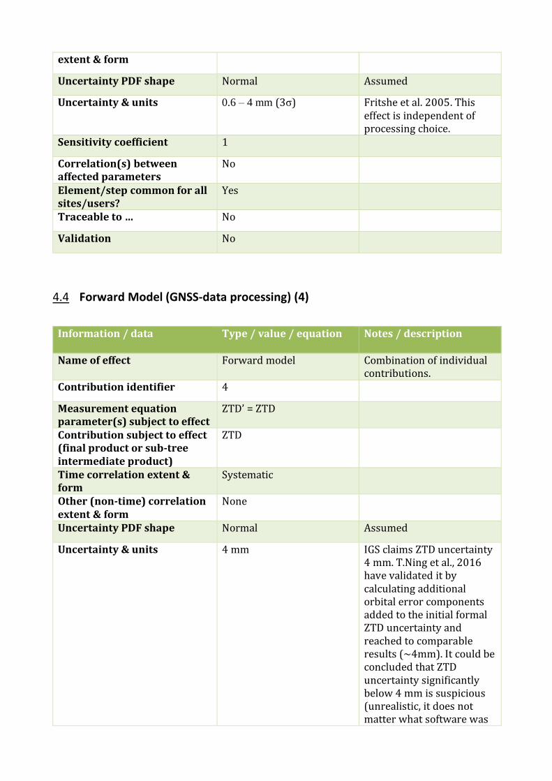
4.3.1.7 Ionnospheric refractions (3a7)
The Earth’s ionosphere contains electrons delaying the propagation of the GNSS signal. In practice
the ionospheric–free linear combination is used to remove the first order ionspheric delay, which
normally accounts for ~99.9% of the total delay. The second order delay can have a significant impact
on the ZTD (0.6 – 4 mm), particularly during strong solar events such as ionospheric storms (Fritshe
et al. 2005). Third and higher order terms are insignificant over long time series.
Information / data Type / value / equation Notes / description
Name of effect Ionospheric correction
Contribution identifier 5b
Measurement equation parameter(s) subject to effect
ZTD’ = ZTD Effect gets mostly cancelled by using linear combination of L1, L2
Contribution subject to effect (final product or sub-tree intermediate product)
ZTD
Time correlation extent & form
Solar storm scales – 5-10 days.
Other (non-time) correlation None
extent & form
Uncertainty PDF shape Normal Assumed
Uncertainty & units 0.6 – 4 mm (3σ) Fritshe et al. 2005. This effect is independent of processing choice.
Sensitivity coefficient 1
Correlation(s) between affected parameters
No
Element/step common for all sites/users?
Yes
Traceable to … No
Validation No
4.4 Forward Model (GNSS-data processing) (4)
Information / data Type / value / equation Notes / description
Name of effect Forward model Combination of individual contributions.
Contribution identifier 4
Measurement equation parameter(s) subject to effect
ZTD’ = ZTD
Contribution subject to effect (final product or sub-tree intermediate product)
ZTD
Time correlation extent & form
Systematic
Other (non-time) correlation extent & form
None
Uncertainty PDF shape Normal Assumed
Uncertainty & units 4 mm IGS claims ZTD uncertainty 4 mm. T.Ning et al., 2016 have validated it by calculating additional orbital error components added to the initial formal ZTD uncertainty and reached to comparable results (~4mm). It could be concluded that ZTD uncertainty significantly below 4 mm is suspicious (unrealistic, it does not matter what software was
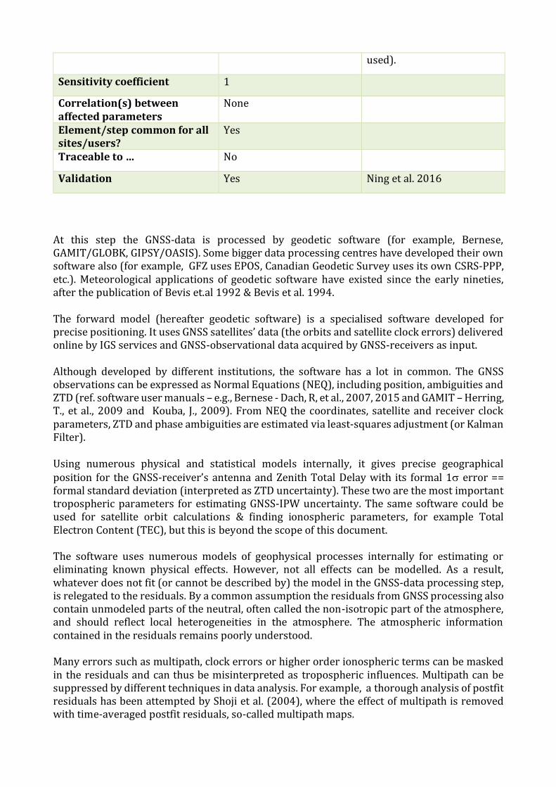
used).
Sensitivity coefficient 1
Correlation(s) between affected parameters
None
Element/step common for all sites/users?
Yes
Traceable to … No
Validation Yes Ning et al. 2016
At this step the GNSS-data is processed by geodetic software (for example, Bernese, GAMIT/GLOBK, GIPSY/OASIS). Some bigger data processing centres have developed their own software also (for example, GFZ uses EPOS, Canadian Geodetic Survey uses its own CSRS-PPP, etc.). Meteorological applications of geodetic software have existed since the early nineties, after the publication of Bevis et.al 1992 & Bevis et al. 1994. The forward model (hereafter geodetic software) is a specialised software developed for precise positioning. It uses GNSS satellites’ data (the orbits and satellite clock errors) delivered online by IGS services and GNSS-observational data acquired by GNSS-receivers as input. Although developed by different institutions, the software has a lot in common. The GNSS observations can be expressed as Normal Equations (NEQ), including position, ambiguities and ZTD (ref. software user manuals – e.g., Bernese - Dach, R, et al., 2007, 2015 and GAMIT – Herring, T., et al., 2009 and Kouba, J., 2009). From NEQ the coordinates, satellite and receiver clock parameters, ZTD and phase ambiguities are estimated via least-squares adjustment (or Kalman Filter). Using numerous physical and statistical models internally, it gives precise geographical position for the GNSS-receiver’s antenna and Zenith Total Delay with its formal 1 error == formal standard deviation (interpreted as ZTD uncertainty). These two are the most important tropospheric parameters for estimating GNSS-IPW uncertainty. The same software could be used for satellite orbit calculations & finding ionospheric parameters, for example Total Electron Content (TEC), but this is beyond the scope of this document. The software uses numerous models of geophysical processes internally for estimating or eliminating known physical effects. However, not all effects can be modelled. As a result, whatever does not fit (or cannot be described by) the model in the GNSS-data processing step, is relegated to the residuals. By a common assumption the residuals from GNSS processing also contain unmodeled parts of the neutral, often called the non-isotropic part of the atmosphere, and should reflect local heterogeneities in the atmosphere. The atmospheric information contained in the residuals remains poorly understood. Many errors such as multipath, clock errors or higher order ionospheric terms can be masked in the residuals and can thus be misinterpreted as tropospheric influences. Multipath can be suppressed by different techniques in data analysis. For example, a thorough analysis of postfit residuals has been attempted by Shoji et al. (2004), where the effect of multipath is removed with time-averaged postfit residuals, so-called multipath maps.
Some software does not offer ZTD directly. For example GIPSY, where Zenith Wet Delay (ZWD) is the final tropospheric product and ZTD must be calculated as a sum of ZWD and Zenith Hydrostatic Delay (ZHD). The ZHD is usually calculated via the Saastamoinen model from the site’s geographical latitude and height above the mean sea level.
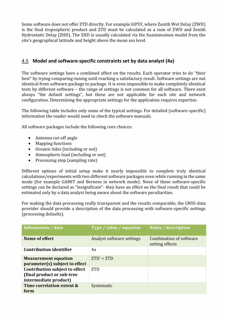
4.5 Model and software-specific constraints set by data analyst (4a) The software settings have a combined effect on the results. Each operator tries to do “their best” by trying-comparing-tuning until reaching a satisfactory result. Software settings are not identical from software package to package. It is even impossible to make completely identical tests by different software – the range of settings is not common for all software. There exist always “the default settings”, but these are not applicable for each site and network configuration. Determining the appropriate settings for the application requires expertise. The following table includes only some of the typical settings. For detailed (software-specific) information the reader would need to check the software manuals. All software packages include the following core choices:
• Antenna cut-off angle • Mapping functions • Oceanic tides (including or not) • Atmospheric load (including or not) • Processing step (sampling rate)
Different options of initial setup make it nearly impossible to complete truly identical calculations/experiments with two different software packages even while running in the same mode (for example GAMIT and Bernese in network mode). None of these software-specific settings can be declared as “insignificant”- they have an effect on the final result that could be estimated only by a data analyst being aware about the software peculiarities. For making the data processing really transparent and the results comparable, the GNSS-data provider should provide a description of the data processing with software-specific settings (processing defaults).
Information / data Type / value / equation Notes / description
Name of effect Analyst software settings Combination of software setting effects
Contribution identifier 4a
Measurement equation parameter(s) subject to effect
ZTD’ = ZTD
Contribution subject to effect (final product or sub-tree intermediate product)
ZTD
Time correlation extent & form
Systematic
Other (non-time) correlation extent & form
None
Uncertainty PDF shape Normal Assumed
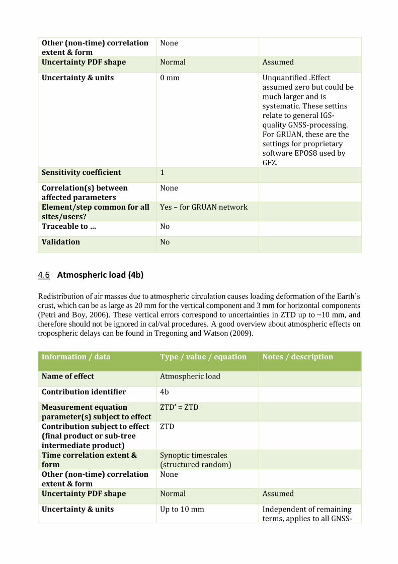
Uncertainty & units 0 mm Unquantified .Effect assumed zero but could be much larger and is systematic. These settins relate to general IGS-quality GNSS-processing. For GRUAN, these are the settings for proprietary software EPOS8 used by GFZ.
Sensitivity coefficient 1
Correlation(s) between affected parameters
None
Element/step common for all sites/users?
Yes – for GRUAN network
Traceable to … No
Validation No
4.6 Atmospheric load (4b) Redistribution of air masses due to atmospheric circulation causes loading deformation of the Earth’s
crust, which can be as large as 20 mm for the vertical component and 3 mm for horizontal components
(Petri and Boy, 2006). These vertical errors correspond to uncertainties in ZTD up to ~10 mm, and
therefore should not be ignored in cal/val procedures. A good overview about atmospheric effects on
tropospheric delays can be found in Tregoning and Watson (2009).
Information / data Type / value / equation Notes / description
Name of effect Atmospheric load
Contribution identifier 4b
Measurement equation parameter(s) subject to effect
ZTD’ = ZTD
Contribution subject to effect (final product or sub-tree intermediate product)
ZTD
Time correlation extent & form
Synoptic timescales (structured random)
Other (non-time) correlation extent & form
None
Uncertainty PDF shape Normal Assumed
Uncertainty & units Up to 10 mm Independent of remaining terms, applies to all GNSS-
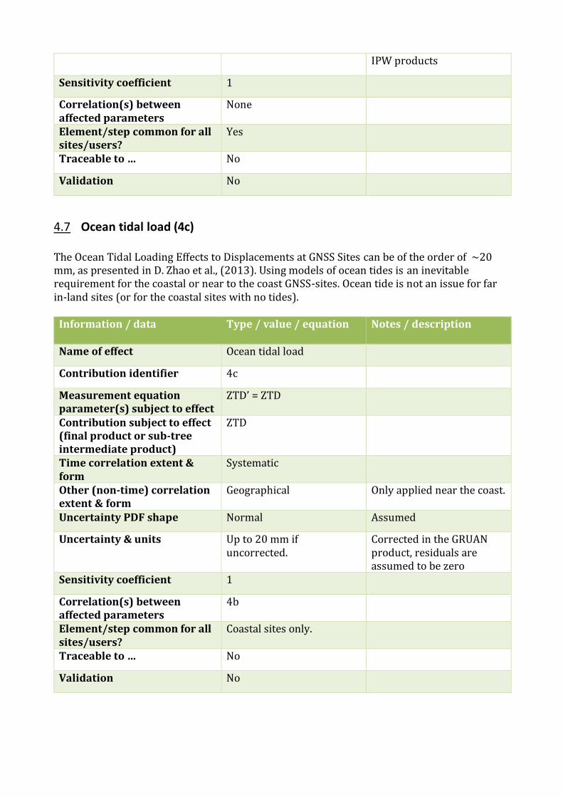
IPW products
Sensitivity coefficient 1
Correlation(s) between affected parameters
None
Element/step common for all sites/users?
Yes
Traceable to … No
Validation No
4.7 Ocean tidal load (4c) The Ocean Tidal Loading Effects to Displacements at GNSS Sites can be of the order of ~20 mm, as presented in D. Zhao et al., (2013). Using models of ocean tides is an inevitable requirement for the coastal or near to the coast GNSS-sites. Ocean tide is not an issue for far in-land sites (or for the coastal sites with no tides).
Information / data Type / value / equation Notes / description
Name of effect Ocean tidal load
Contribution identifier 4c
Measurement equation parameter(s) subject to effect
ZTD’ = ZTD
Contribution subject to effect (final product or sub-tree intermediate product)
ZTD
Time correlation extent & form
Systematic
Other (non-time) correlation extent & form
Geographical Only applied near the coast.
Uncertainty PDF shape Normal Assumed
Uncertainty & units Up to 20 mm if uncorrected.
Corrected in the GRUAN product, residuals are assumed to be zero
Sensitivity coefficient 1
Correlation(s) between affected parameters
4b
Element/step common for all sites/users?
Coastal sites only.
Traceable to … No
Validation No
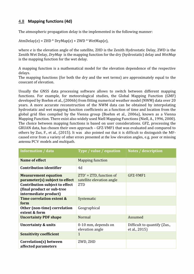
4.8 Mapping functions (4d) The atmospheric propagation delay is the implemented in the following manner: AtmDelay(e) = ZHD * DryMap(e) + ZWD * WetMap(e), where e is the elevation angle of the satellite, ZHD is the Zenith Hydrostatic Delay, ZWD is the Zenith Wet Delay, DryMap is the mapping function for the dry (hydrostatic) delay and WetMap is the mapping function for the wet delay. A mapping function is a mathematical model for the elevation dependence of the respective delays. The mapping functions (for both the dry and the wet terms) are approximately equal to the cosecant of elevation. Usually the GNSS data processing software allows to switch between different mapping functions. For example, for meteorological studies, the Global Mapping Function (GMF) developed by Boehm et al., (2006b) from fitting numerical weather model (NWM) data over 20 years. A more accurate reconstruction of the NWM data can be obtained by interpolating hydrostatic and wet mapping function coefficients as a function of time and location from the global grid files compiled by the Vienna group (Boehm et al., 2006a), known as a Vienna Mapping Function. There exist also widely used Niell Mapping Functions (Niell, A., 1996, 2000). The choice between mapping functions is based on user considerations. GFZ, processing the GRUAN data, has chosen their own approach – GFZ-VMF1 that was evaluated and compared to others by Zus, F., et al., (2015). It was also pointed out that it is difficult to distinguish the MF-
caused error from a variety of other errors presented at the low elevation angles, e.g. poor or missing
antenna PCV models and multipath.
Information / data Type / value / equation Notes / description
Name of effect Mapping function
Contribution identifier 4d
Measurement equation parameter(s) subject to effect
ZTD’ = ZTD, function of satellite elevation angle
GFZ-VMF1
Contribution subject to effect (final product or sub-tree intermediate product)
ZTD
Time correlation extent & form
Systematic
Other (non-time) correlation extent & form
Geographical
Uncertainty PDF shape Normal Assumed
Uncertainty & units 0-10 mm, depends on elevation angle
Difficult to quantify (Zus., et al., 2015)
Sensitivity coefficient 1
Correlation(s) between affected parameters
ZWD, ZHD
Element/step common for all sites/users?
Yes
Traceable to … No
Validation No
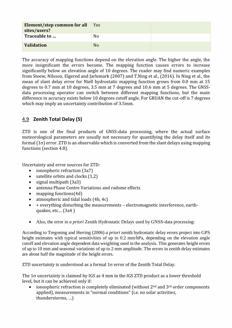
The accuracy of mapping functions depend on the elevation angle. The higher the angle, the more insignificant the errors become. The mapping function causes errors to increase significantly below an elevation angle of 10 degrees. The reader may find numeric examples from Stoew, Nilsson, Elgered and Jarlemark (2007) and T.Ning et al., (2016). In Ning et al., the mean of slant delay error for Niell hydrostatic mapping function grows from 0.0 mm at 15 degrees to 0.7 mm at 10 degrees, 3.5 mm at 7 degrees and 10.6 mm at 5 degrees. The GNSS-data processing operator can switch between different mapping functions, but the main difference in accuracy exists below 10 degrees cutoff angle. For GRUAN the cut-off is 7 degrees which may imply an uncertainty contribution of 3.5mm.
4.9 Zenith Total Delay (5) ZTD is one of the final products of GNSS-data processing, where the actual surface meteorological parameters are usually not necessary for quantifying the delay itself and its formal (1) error. ZTD is an observable which is converted from the slant delays using mapping functions (section 4.8). Uncertainty and error sources for ZTD:
• ionospheric refraction (3a7) • satellite orbits and clocks (1,2) • signal multipath (3a3) • antenna Phase Centre Variations and radome effects • mapping functions(4d) • atmospheric and tidal loads (4b, 4c) • + everything disturbing the measurements – electromagnetic interference, earth-
quakes, etc… (3a4 )
• Also, the error in a priori Zenith Hydrostatic Delays used by GNSS-data processing:
According to Tregoning and Herring (2006) a priori zenith hydrostatic delay errors project into GPS
height estimates with typical sensitivities of up to 0.2 mm/hPa, depending on the elevation angle
cutoff and elevation angle dependent data weighting used in the analysis. This generates height errors
of up to 10 mm and seasonal variations of up to 2 mm amplitude. The errors in zenith delay estimates
are about half the magnitude of the height errors.
ZTD uncertainty is understood as a formal 1 error of the Zenith Total Delay.
The 1 uncertainty is claimed by IGS as 4 mm in the IGS ZTD product as a lower threshold level, but it can be achieved only if:
• ionospheric refraction is completely eliminated (without 2nd and 3rd order components applied), measurements in “normal conditions” (i.e. no solar activities, thunderstorms, …)
• IGS final products used for satellite orbits • Both antenna Phase Centre Variation and radome calibrations implemented (it is
suggested not to use a radome whenever possible) • Signal multipath minimized by using microwave absorber below antenna or
locating/installing with “free horizon” (usually not installed) • Antenna elevation cut-off >= 10 deg. (often not the case)
Uncertainty of ZTD, calculated by PPP method (and EPOS8 software) for GRUAN sites, is the main contributor (ca 75%) to GNSS-IPW uncertainty (ref. table 4 in T.Ning etal., 2016).
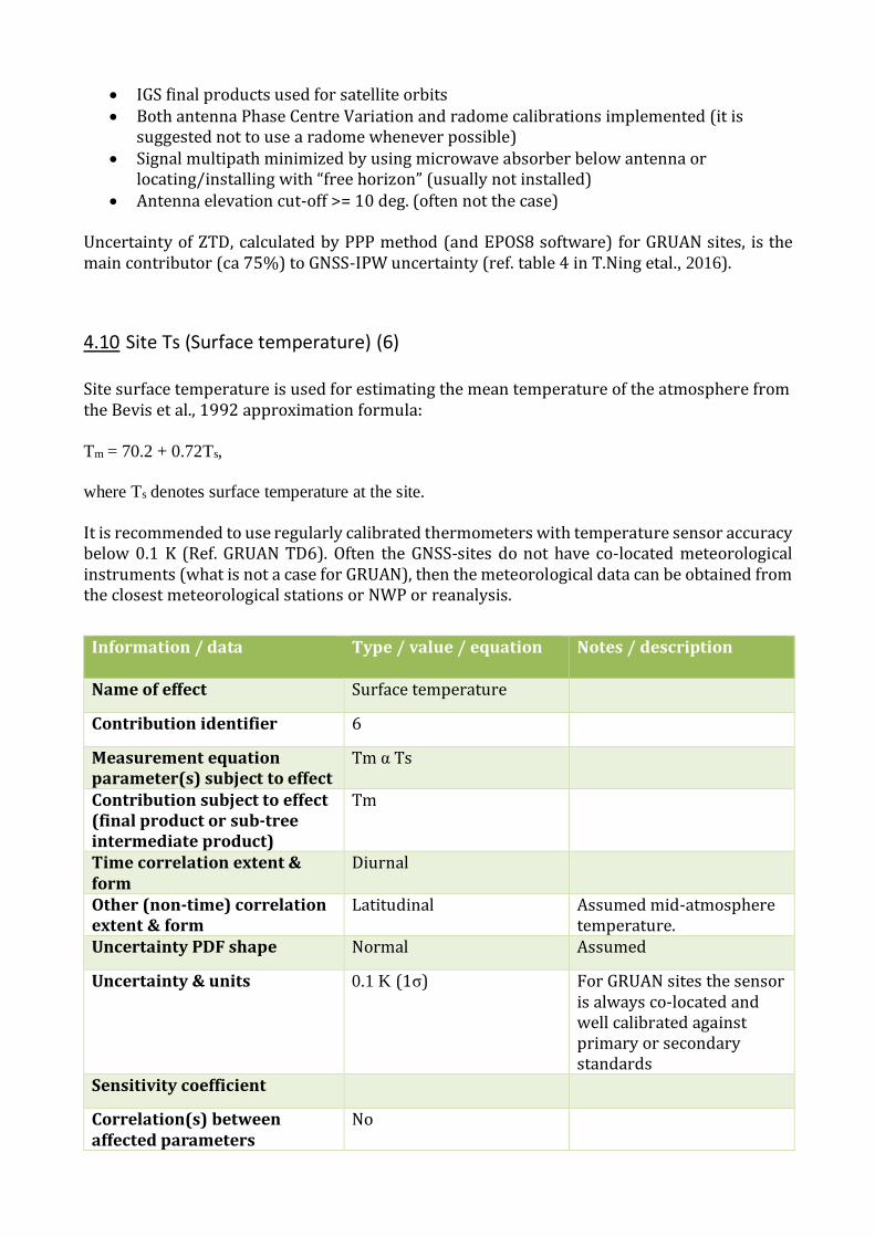
4.10 Site Ts (Surface temperature) (6) Site surface temperature is used for estimating the mean temperature of the atmosphere from the Bevis et al., 1992 approximation formula: Tm = 70.2 + 0.72Ts,
where Ts denotes surface temperature at the site.
It is recommended to use regularly calibrated thermometers with temperature sensor accuracy below 0.1 K (Ref. GRUAN TD6). Often the GNSS-sites do not have co-located meteorological instruments (what is not a case for GRUAN), then the meteorological data can be obtained from the closest meteorological stations or NWP or reanalysis.
Information / data Type / value / equation Notes / description
Name of effect Surface temperature
Contribution identifier 6
Measurement equation parameter(s) subject to effect
Tm α Ts
Contribution subject to effect (final product or sub-tree intermediate product)
Tm
Time correlation extent & form
Diurnal
Other (non-time) correlation extent & form
Latitudinal Assumed mid-atmosphere temperature.
Uncertainty PDF shape Normal Assumed
Uncertainty & units 0.1 K (1σ) For GRUAN sites the sensor is always co-located and well calibrated against primary or secondary standards
Sensitivity coefficient
Correlation(s) between affected parameters
No
Element/step common for all sites/users?
Yes
Traceable to … No
Validation No
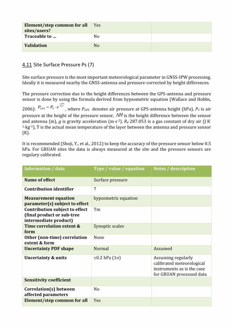
4.11 Site Surface Pressure Ps (7) Site surface pressure is the most important meteorological parameter in GNSS-IPW processing. Ideally it is measured nearby the GNSS-antenna and pressure-corrected by height differences. The pressure correction due to the height differences between the GPS-antenna and pressure sensor is done by using the formula derived from hypsometric equation (Wallace and Hobbs,
2006): TdR
Hg
ePP SGPS
, where PGPS denotes air pressure at GPS-antenna height (hPa), PS is air
pressure at the height of the pressure sensor, H is the height difference between the sensor and antenna (m), g is gravity acceleration (ms-2). Rd 287.053 is a gas constant of dry air (JK-
1kg-1), T is the actual mean temperature of the layer between the antenna and pressure sensor (K). It is recommended (Shoji, Y., et al., 2012) to keep the accuracy of the pressure sensor below 0.5 hPa. For GRUAN sites the data is always measured at the site and the pressure sensors are regulary calibrated.
Information / data Type / value / equation Notes / description
Name of effect Surface pressure
Contribution identifier 7
Measurement equation parameter(s) subject to effect
hypsometric equation
Contribution subject to effect (final product or sub-tree intermediate product)
Tm
Time correlation extent & form
Synoptic scales
Other (non-time) correlation extent & form
None
Uncertainty PDF shape Normal Assumed
Uncertainty & units ±0.2 hPa (1σ) Assuming regularly calibrated meteorological instruments as is the case for GRUAN processed data
Sensitivity coefficient
Correlation(s) between affected parameters
No
Element/step common for all Yes
sites/users?
Traceable to … Site pressure instrumentation
Validation Yes Local meteorological measurments.
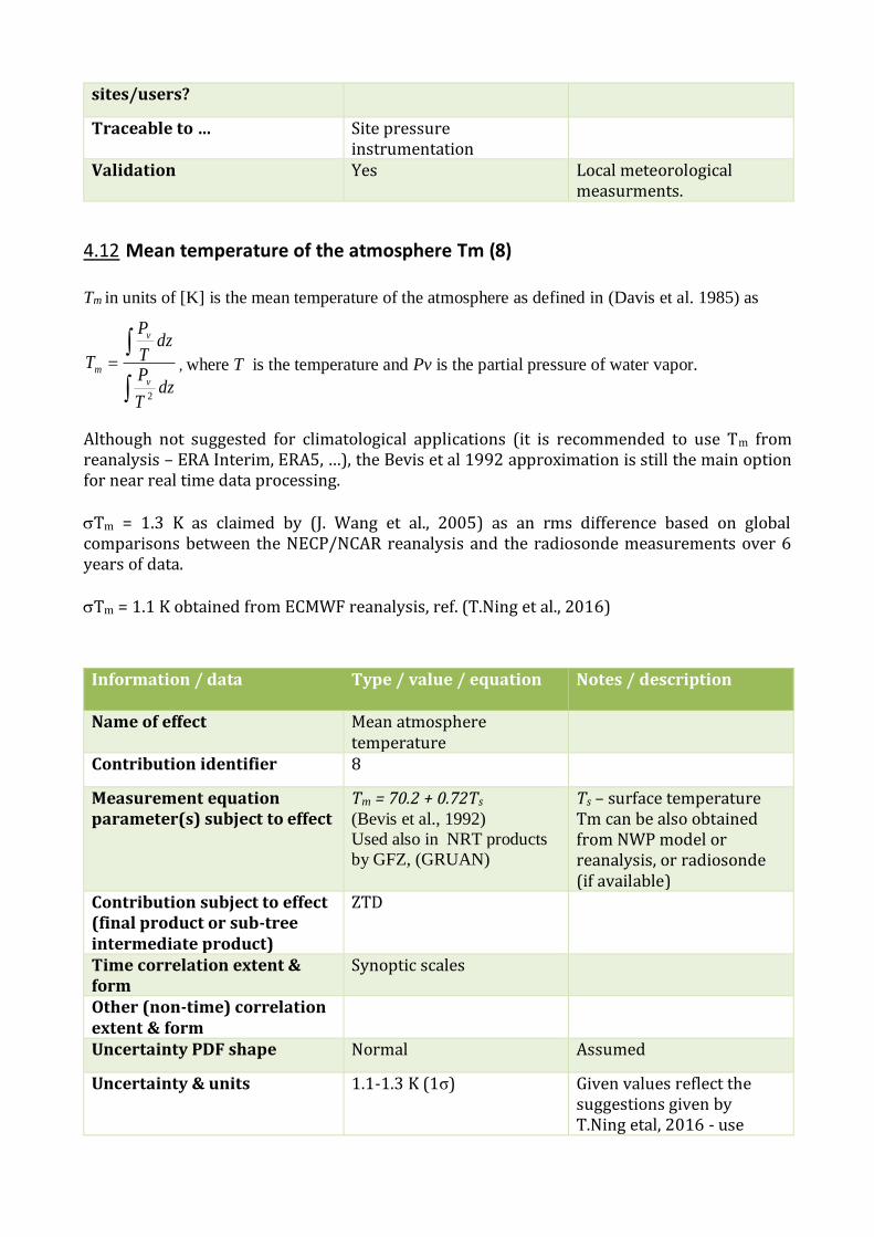
4.12 Mean temperature of the atmosphere Tm (8) Tm in units of [K] is the mean temperature of the atmosphere as defined in (Davis et al. 1985) as
dzT
P
dzT
P
Tv
v
m
2
, where T is the temperature and Pv is the partial pressure of water vapor.
Although not suggested for climatological applications (it is recommended to use Tm from reanalysis – ERA Interim, ERA5, …), the Bevis et al 1992 approximation is still the main option for near real time data processing. Tm = 1.3 K as claimed by (J. Wang et al., 2005) as an rms difference based on global comparisons between the NECP/NCAR reanalysis and the radiosonde measurements over 6 years of data. Tm = 1.1 K obtained from ECMWF reanalysis, ref. (T.Ning et al., 2016)
Information / data Type / value / equation Notes / description
Name of effect Mean atmosphere temperature
Contribution identifier 8
Measurement equation parameter(s) subject to effect
Tm = 70.2 + 0.72Ts (Bevis et al., 1992)
Used also in NRT products
by GFZ, (GRUAN)
Ts – surface temperature Tm can be also obtained from NWP model or reanalysis, or radiosonde (if available)
Contribution subject to effect (final product or sub-tree intermediate product)
ZTD
Time correlation extent & form
Synoptic scales
Other (non-time) correlation extent & form
Uncertainty PDF shape Normal Assumed
Uncertainty & units 1.1-1.3 K (1σ) Given values reflect the suggestions given by T.Ning etal, 2016 - use
reanalysis.
Sensitivity coefficient
Correlation(s) between affected parameters
No
Element/step common for all sites/users?
Yes
Traceable to … No
Validation No
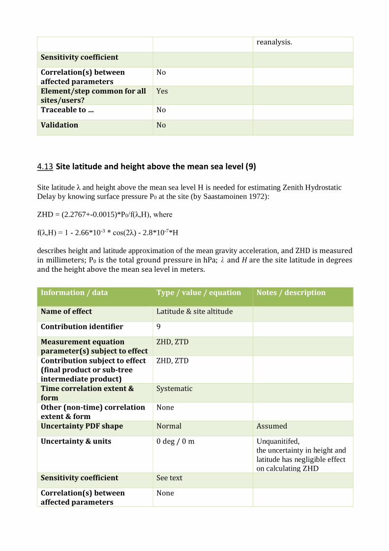
4.13 Site latitude and height above the mean sea level (9) Site latitude λ and height above the mean sea level H is needed for estimating Zenith Hydrostatic
Delay by knowing surface pressure P0 at the site (by Saastamoinen 1972):
ZHD = (2.2767+-0.0015)*P0/f(λ,H), where
f(λ,H) = 1 - 2.66*10-3 * cos(2λ) - 2.8*10-7*H
describes height and latitude approximation of the mean gravity acceleration, and ZHD is measured in millimeters; P0 is the total ground pressure in hPa; and H are the site latitude in degrees and the height above the mean sea level in meters.
Information / data Type / value / equation Notes / description
Name of effect Latitude & site altitude
Contribution identifier 9
Measurement equation parameter(s) subject to effect
ZHD, ZTD
Contribution subject to effect (final product or sub-tree intermediate product)
ZHD, ZTD
Time correlation extent & form
Systematic
Other (non-time) correlation extent & form
None
Uncertainty PDF shape Normal Assumed
Uncertainty & units 0 deg / 0 m Unquanitifed,
the uncertainty in height and
latitude has negligible effect
on calculating ZHD Sensitivity coefficient See text
Correlation(s) between affected parameters
None
Element/step common for all sites/users?
Yes
Traceable to … No
Validation No
Site altitude should be known within 1 m for allowing acceptable accuracy of pressure corrections to the GNSS receiver’s antenna height. By GRUAN requirements (Shoji, Y., et al., GRUAN TD6) the height difference between the surface pressure sensor and the GPS antenna must be measured with an accuracy of 1 m or better.
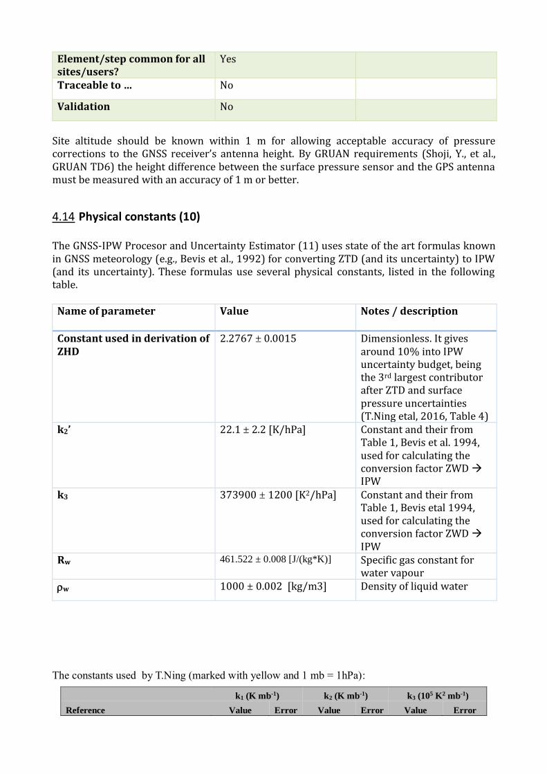
4.14 Physical constants (10) The GNSS-IPW Procesor and Uncertainty Estimator (11) uses state of the art formulas known in GNSS meteorology (e.g., Bevis et al., 1992) for converting ZTD (and its uncertainty) to IPW (and its uncertainty). These formulas use several physical constants, listed in the following table.
Name of parameter Value Notes / description
Constant used in derivation of ZHD
2.2767 ± 0.0015 Dimensionless. It gives around 10% into IPW uncertainty budget, being the 3rd largest contributor after ZTD and surface pressure uncertainties (T.Ning etal, 2016, Table 4)
k2’ 22.1 ± 2.2 [K/hPa] Constant and their from Table 1, Bevis et al. 1994, used for calculating the conversion factor ZWD IPW
k3 373900 ± 1200 [K2/hPa] Constant and their from Table 1, Bevis etal 1994, used for calculating the conversion factor ZWD IPW
Rw 461.522 ± 0.008 [J/(kg*K)] Specific gas constant for water vapour
w 1000 ± 0.002 [kg/m3] Density of liquid water
The constants used by T.Ning (marked with yellow and 1 mb = 1hPa):
k1 (K mb-1) k2 (K mb-1) k3 (105 K2 mb-1)
Reference Value Error Value Error Value Error
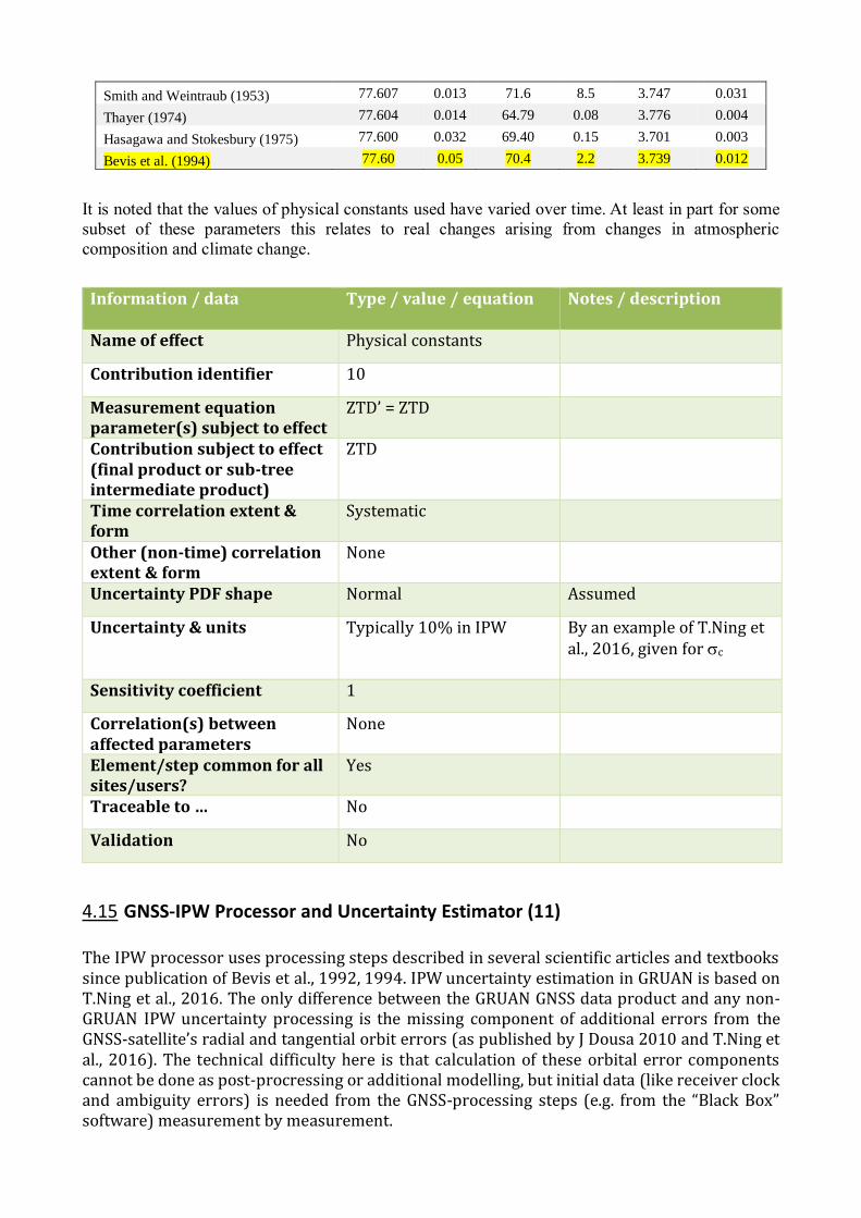
Smith and Weintraub (1953) 77.607 0.013 71.6 8.5 3.747 0.031
Thayer (1974) 77.604 0.014 64.79 0.08 3.776 0.004
Hasagawa and Stokesbury (1975) 77.600 0.032 69.40 0.15 3.701 0.003
Bevis et al. (1994) 77.60 0.05 70.4 2.2 3.739 0.012
It is noted that the values of physical constants used have varied over time. At least in part for some
subset of these parameters this relates to real changes arising from changes in atmospheric
composition and climate change.
Information / data Type / value / equation Notes / description
Name of effect Physical constants
Contribution identifier 10
Measurement equation parameter(s) subject to effect
ZTD’ = ZTD
Contribution subject to effect (final product or sub-tree intermediate product)
ZTD
Time correlation extent & form
Systematic
Other (non-time) correlation extent & form
None
Uncertainty PDF shape Normal Assumed
Uncertainty & units Typically 10% in IPW By an example of T.Ning et al., 2016, given for c
Sensitivity coefficient 1
Correlation(s) between affected parameters
None
Element/step common for all sites/users?
Yes
Traceable to … No
Validation No
4.15 GNSS-IPW Processor and Uncertainty Estimator (11)
The IPW processor uses processing steps described in several scientific articles and textbooks since publication of Bevis et al., 1992, 1994. IPW uncertainty estimation in GRUAN is based on T.Ning et al., 2016. The only difference between the GRUAN GNSS data product and any non-GRUAN IPW uncertainty processing is the missing component of additional errors from the GNSS-satellite’s radial and tangential orbit errors (as published by J Dousa 2010 and T.Ning et al., 2016). The technical difficulty here is that calculation of these orbital error components cannot be done as post-procressing or additional modelling, but initial data (like receiver clock and ambiguity errors) is needed from the GNSS-processing steps (e.g. from the “Black Box” software) measurement by measurement.
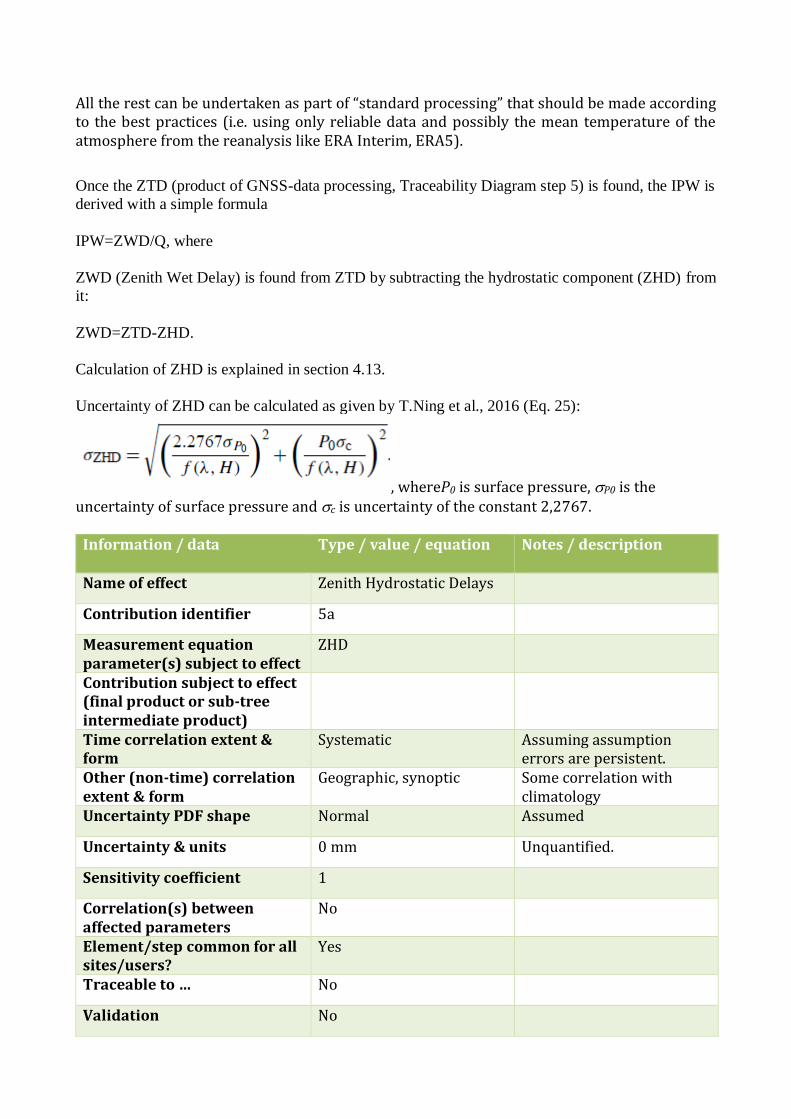
All the rest can be undertaken as part of “standard processing” that should be made according to the best practices (i.e. using only reliable data and possibly the mean temperature of the atmosphere from the reanalysis like ERA Interim, ERA5).
Once the ZTD (product of GNSS-data processing, Traceability Diagram step 5) is found, the IPW is
derived with a simple formula
IPW=ZWD/Q, where
ZWD (Zenith Wet Delay) is found from ZTD by subtracting the hydrostatic component (ZHD) from
it:
ZWD=ZTD-ZHD.
Calculation of ZHD is explained in section 4.13.
Uncertainty of ZHD can be calculated as given by T.Ning et al., 2016 (Eq. 25):
, whereP0 is surface pressure, P0 is the uncertainty of surface pressure and c is uncertainty of the constant 2,2767.
Information / data Type / value / equation Notes / description
Name of effect Zenith Hydrostatic Delays
Contribution identifier 5a
Measurement equation parameter(s) subject to effect
ZHD
Contribution subject to effect (final product or sub-tree intermediate product)
Time correlation extent & form
Systematic Assuming assumption errors are persistent.
Other (non-time) correlation extent & form
Geographic, synoptic Some correlation with climatology
Uncertainty PDF shape Normal Assumed
Uncertainty & units 0 mm Unquantified.
Sensitivity coefficient 1
Correlation(s) between affected parameters
No
Element/step common for all sites/users?
Yes
Traceable to … No
Validation No
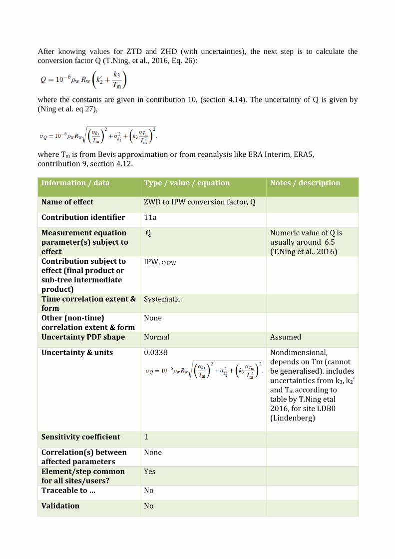
After knowing values for ZTD and ZHD (with uncertainties), the next step is to calculate the
conversion factor Q (T.Ning, et al., 2016, Eq. 26):
where the constants are given in contribution 10, (section 4.14). The uncertainty of Q is given by
(Ning et al. eq 27),
where Tm is from Bevis approximation or from reanalysis like ERA Interim, ERA5, contribution 9, section 4.12.
Information / data Type / value / equation Notes / description
Name of effect ZWD to IPW conversion factor, Q
Contribution identifier 11a
Measurement equation parameter(s) subject to effect
Q Numeric value of Q is usually around 6.5 (T.Ning et al., 2016)
Contribution subject to effect (final product or sub-tree intermediate product)
IPW, IPW
Time correlation extent & form
Systematic
Other (non-time) correlation extent & form
None
Uncertainty PDF shape Normal Assumed
Uncertainty & units 0.0338
Nondimensional, depends on Tm (cannot be generalised). includes uncertainties from k3, k2’ and Tm according to table by T.Ning etal 2016, for site LDB0 (Lindenberg)
Sensitivity coefficient 1
Correlation(s) between affected parameters
None
Element/step common for all sites/users?
Yes
Traceable to … No
Validation No
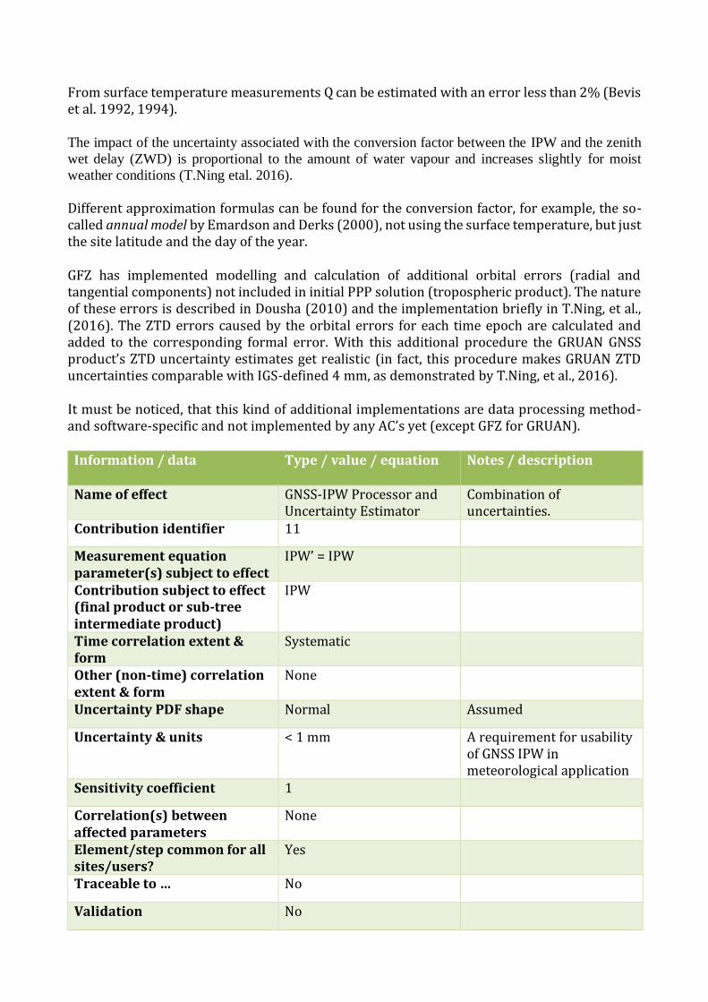
From surface temperature measurements Q can be estimated with an error less than 2% (Bevis et al. 1992, 1994).
The impact of the uncertainty associated with the conversion factor between the IPW and the zenith
wet delay (ZWD) is proportional to the amount of water vapour and increases slightly for moist
weather conditions (T.Ning etal. 2016).
Different approximation formulas can be found for the conversion factor, for example, the so-called annual model by Emardson and Derks (2000), not using the surface temperature, but just the site latitude and the day of the year. GFZ has implemented modelling and calculation of additional orbital errors (radial and tangential components) not included in initial PPP solution (tropospheric product). The nature of these errors is described in Dousha (2010) and the implementation briefly in T.Ning, et al., (2016). The ZTD errors caused by the orbital errors for each time epoch are calculated and added to the corresponding formal error. With this additional procedure the GRUAN GNSS product’s ZTD uncertainty estimates get realistic (in fact, this procedure makes GRUAN ZTD uncertainties comparable with IGS-defined 4 mm, as demonstrated by T.Ning, et al., 2016). It must be noticed, that this kind of additional implementations are data processing method- and software-specific and not implemented by any AC’s yet (except GFZ for GRUAN).
Information / data Type / value / equation Notes / description
Name of effect GNSS-IPW Processor and Uncertainty Estimator
Combination of uncertainties.
Contribution identifier 11
Measurement equation parameter(s) subject to effect
IPW’ = IPW
Contribution subject to effect (final product or sub-tree intermediate product)
IPW
Time correlation extent & form
Systematic
Other (non-time) correlation extent & form
None
Uncertainty PDF shape Normal Assumed
Uncertainty & units < 1 mm A requirement for usability of GNSS IPW in meteorological application
Sensitivity coefficient 1
Correlation(s) between affected parameters
None
Element/step common for all sites/users?
Yes
Traceable to … No
Validation No
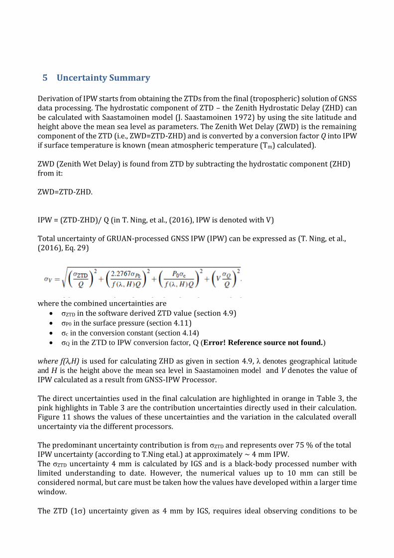
5 Uncertainty Summary Derivation of IPW starts from obtaining the ZTDs from the final (tropospheric) solution of GNSS data processing. The hydrostatic component of ZTD – the Zenith Hydrostatic Delay (ZHD) can be calculated with Saastamoinen model (J. Saastamoinen 1972) by using the site latitude and height above the mean sea level as parameters. The Zenith Wet Delay (ZWD) is the remaining component of the ZTD (i.e., ZWD=ZTD-ZHD) and is converted by a conversion factor Q into IPW if surface temperature is known (mean atmospheric temperature (Tm) calculated). ZWD (Zenith Wet Delay) is found from ZTD by subtracting the hydrostatic component (ZHD) from it: ZWD=ZTD-ZHD. IPW = (ZTD-ZHD)/ Q (in T. Ning, et al., (2016), IPW is denoted with V) Total uncertainty of GRUAN-processed GNSS IPW (IPW) can be expressed as (T. Ning, et al., (2016), Eq. 29)
where the combined uncertainties are
• σZTD in the software derived ZTD value (section 4.9) • σP0 in the surface pressure (section 4.11) • σc in the conversion constant (section 4.14) • σQ in the ZTD to IPW conversion factor, Q (Error! Reference source not found.)
where f(λ,H) is used for calculating ZHD as given in section 4.9, λ denotes geographical latitude
and H is the height above the mean sea level in Saastamoinen model and V denotes the value of IPW calculated as a result from GNSS-IPW Processor. The direct uncertainties used in the final calculation are highlighted in orange in Table 3, the pink highlights in Table 3 are the contribution uncertainties directly used in their calculation. Figure 11 shows the values of these uncertainties and the variation in the calculated overall uncertainty via the different processors. The predominant uncertainty contribution is from σZTD and represents over 75 % of the total IPW uncertainty (according to T.Ning etal.) at approximately ~ 4 mm IPW. The σZTD uncertainty 4 mm is calculated by IGS and is a black-body processed number with limited understanding to date. However, the numerical values up to 10 mm can still be considered normal, but care must be taken how the values have developed within a larger time window. The ZTD (1) uncertainty given as 4 mm by IGS, requires ideal observing conditions to be
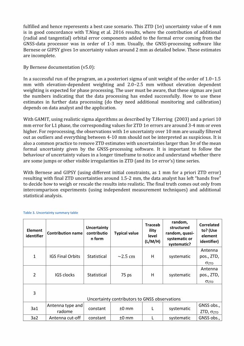
fulfilled and hence reperesents a best case scenario. This ZTD (1) uncertainty value of 4 mm is in good concordance with T.Ning et al. 2016 results, where the contribution of additional (radial and tangential) orbital error components added to the formal error coming from the GNSS-data processor was in order of 1-3 mm. Usually, the GNSS-processing software like Bernese or GIPSY gives 1 uncertainty values around 2 mm as detailed below. These estimates are incomplete. By Bernese documentation (v5.0): In a successful run of the program, an a posteriori sigma of unit weight of the order of 1.0−1.5 mm with elevation-dependent weighting and 2.0−2.5 mm without elevation dependent weighting is expected for phase processing. The user must be aware, that these sigmas are just the numbers indicating that the data processing has ended successfully. How to use these estimates in further data processing (do they need additional monitoring and calibration) depends on data analyst and the application. With GAMIT, using realistic sigma algorithms as described by T.Herring (2003) and a priori 10
mm error for L1 phase, the corresponding values for ZTD 1 errors are around 3-4 mm or even higher. For reprocessing, the observations with 1 uncertainty over 10 mm are usually filtered out as outliers and everything between 4-10 mm should not be interpreted as suspicious. It is also a common practice to remove ZTD estimates with uncertainties larger than 3 of the mean formal uncertainty given by the GNSS-processing software. It is important to follow the behaviour of uncertainty values in a longer timeframe to notice and understand whether there are some jumps or other visible irregularities in ZTD (and its 1 error’s) time series. With Bernese and GIPSY (using different initial constraints, as 1 mm for a priori ZTD error) resulting with final ZTD uncertainties around 1.5-2 mm, the data analyst has left “hands free” to decide how to weigh or rescale the results into realistic. The final truth comes out only from intercomparison experiments (using independent measurement techniques) and additional statistical analysis.
Table 3. Uncertainty summary table
Element identifier
Contribution name Uncertainty contributio
n form Typical value
Traceability level
(L/M/H)
random, structured
random, quasi-systematic or systematic?
Correlated to? (Use element
identifier)
1 IGS Final Orbits Statistical ~2.5 cm H systematic
Antenna pos., ZTD,
ZTD
2 IGS clocks Statistical 75 ps H systematic Antenna
pos., ZTD,
ZTD
3
Uncertainty contributors to GNSS observations
3a1 Antenna type and
radome constant ±0 mm L systematic
GNSS obs.,
ZTD, ZTD
3a2 Antenna cut-off constant ±0 mm L systematic GNSS obs.,
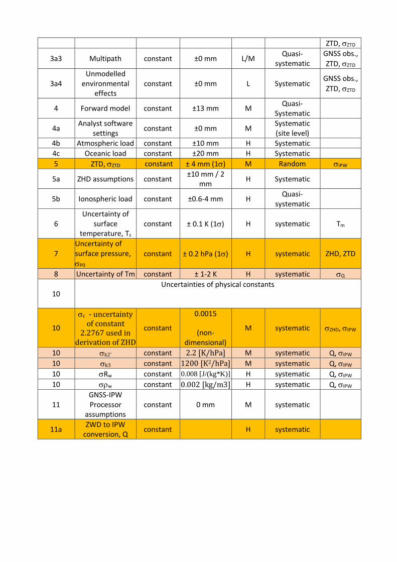
ZTD, ZTD
3a3 Multipath constant ±0 mm L/M Quasi-
systematic GNSS obs.,
ZTD, ZTD
3a4 Unmodelled
environmental effects
constant ±0 mm L Systematic GNSS obs.,
ZTD, ZTD
4 Forward model constant ±13 mm M Quasi-
Systematic
4a Analyst software
settings constant ±0 mm M
Systematic (site level)
4b Atmospheric load constant ±10 mm H Systematic
4c Oceanic load constant ±20 mm H Systematic
5 ZTD, ZTD constant ± 4 mm (1) M Random IPW
5a ZHD assumptions constant ±10 mm / 2
mm H Systematic
5b Ionospheric load constant ±0.6-4 mm H Quasi-
systematic
6 Uncertainty of
surface temperature, Ts
constant ± 0.1 K (1) H systematic Tm
7
Uncertainty of surface pressure,
P0 constant ± 0.2 hPa (1) H systematic ZHD, ZTD
8 Uncertainty of Tm constant ± 1-2 K H systematic Q
10 Uncertainties of physical constants
10
c - uncertainty of constant
2.2767 used in derivation of ZHD
constant
0.0015
(non-dimensional)
M systematic ZHD, IPW
10 k2’ constant 2.2 [K/hPa] M systematic Q, IPW
10 k3 constant 1200 [K2/hPa] M systematic Q, IPW
10 Rw constant 0.008 [J/(kg*K)] H systematic Q, IPW
10 w constant 0.002 [kg/m3] H systematic Q, IPW
11 GNSS-IPW Processor
assumptions constant 0 mm M systematic
11a ZWD to IPW
conversion, Q constant H systematic
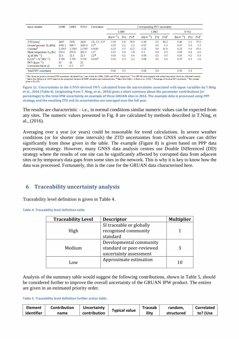
Figure 11. Uncertainties in the GNSS-derived IWV calculated from the uncertainties associated with input variables by T.Ning et al., 2016 (Table 4). (originating from T. Ning, et al., 2016) gives a short summary about the parameter contributions (in percentage) to the total IPW uncertainty on example of three GRUAN sites in 2014. The example data is processed using PPP strategy and the resulting ZTD and its uncertainties are averaged over the full year.
The results are characteristic – i.e., in normal conditions similar numeric values can be expected from
any sites. The numeric values presented in Fig. 8 are calculated by methods described in T.Ning, et
al., (2016).
Averaging over a year (or years) could be reasonable for trend calculations. In severe weather
conditions (or for shorter time intervals) the ZTD uncertainties from GNSS software can differ
significantly from those given in the table. The example (Figure 8) is given based on PPP data
processing strategy. However, many GNSS data analysis centres use Double Differenced (DD)
strategy where the results of one site can be significantly affected by corrupted data from adjacent
sites or by temporary data gaps from some sites in the network. This is why it is key to know how the
data was processed. Fortunately, this is the case for the GRUAN data characterised here.
6 Traceability uncertainty analysis
Traceability level definition is given in Table 4.
Table 4. Traceability level definition table
Traceability Level Descriptor Multiplier
High SI traceable or globally recognised community standard
1
Medium Developmental community standard or peer-reviewed uncertainty assessment
3
Low Approximate estimation
10
Analysis of the summary table would suggest the following contributions, shown in Table 5, should
be considered further to improve the overall uncertainty of the GRUAN IPW product. The entires
are given in an estimated priority order.
Table 5. Traceability level definition further action table.
Element identifier
Contribution name
Uncertainty contribution
Typical value Traceab
ility random,
structured Correlated
to? (Use
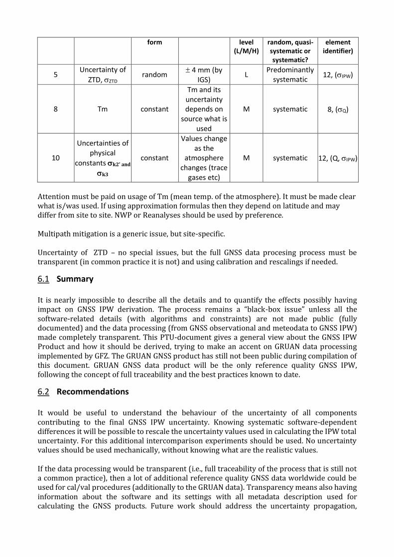
form level (L/M/H)
random, quasi-systematic or systematic?
element identifier)
5 Uncertainty of
ZTD, ZTD random
4 mm (by IGS)
L Predominantly
systematic 12, (IPW)
8 Tm constant
Tm and its uncertainty depends on
source what is used
M systematic 8, (Q)
10
Uncertainties of physical
constants k2’ and
k3
constant
Values change as the
atmosphere changes (trace
gases etc)
M systematic 12, (Q, IPW)
Attention must be paid on usage of Tm (mean temp. of the atmosphere). It must be made clear what is/was used. If using approximation formulas then they depend on latitude and may differ from site to site. NWP or Reanalyses should be used by preference. Multipath mitigation is a generic issue, but site-specific. Uncertainty of ZTD – no special issues, but the full GNSS data procesing process must be transparent (in common practice it is not) and using calibration and rescalings if needed.
6.1 Summary It is nearly impossible to describe all the details and to quantify the effects possibly having impact on GNSS IPW derivation. The process remains a “black-box issue” unless all the software-related details (with algorithms and constraints) are not made public (fully documented) and the data processing (from GNSS observational and meteodata to GNSS IPW) made completely transparent. This PTU-document gives a general view about the GNSS IPW Product and how it should be derived, trying to make an accent on GRUAN data processing implemented by GFZ. The GRUAN GNSS product has still not been public during compilation of this document. GRUAN GNSS data product will be the only reference quality GNSS IPW, following the concept of full traceability and the best practices known to date.
6.2 Recommendations It would be useful to understand the behaviour of the uncertainty of all components contributing to the final GNSS IPW uncertainty. Knowing systematic software-dependent differences it will be possible to rescale the uncertainty values used in calculating the IPW total uncertainty. For this additional intercomparison experiments should be used. No uncertainty values should be used mechanically, without knowing what are the realistic values. If the data processing would be transparent (i.e., full traceability of the process that is still not a common practice), then a lot of additional reference quality GNSS data worldwide could be used for cal/val procedures (additionally to the GRUAN data). Transparency means also having information about the software and its settings with all metadata description used for calculating the GNSS products. Future work should address the uncertainty propagation,
specificially through the ZTD generating software. In Table 3 all the contributions numbered 1-4 are combined into the ZTD uncertainty, but should be individually assessed and combined in accordance with the conditions of measurement.
7 Conclusion
There exists a lot of high-quality GNSS data from global or national geodetic networks that could be used as data with reference quality, but it needs additional information about the data processing and evaluation whether the processing is fully traceable or not. The GRUAN GNSS product should be taken as an example (using uncertainty analysis as described by T.Ning et al 2016) and is the specific processing choices whgich have been highlighted herein. It is currently unavoidable that a subset of current GNSS-data processing software is a „black box“, but the data processing procedures must be (or should be made) transparent (i.e. how exactly a certain „black box“ was used). If everything is done by the best practices, the results can be trusted and taken as reliable. For example, while using ZTD 1 errors processed by Bernese (or GIPSY) do not include additional orbital error components, which contribute an additional 1-3 mm to the ZTD as demonstrated in T. Ning etal 2016. Unfortunately, calculation of these additional orbital error components (J. Dousha 2010, T.Ning etal 2016) is not implemented in any distributable GNSS-processing software yet. The first implementation is done by GFZ (Deutsches GeoForschungsZentrum GFZ) for GRUAN-data processing with their in-house EPOS software and for GRUAN sites only. It is necessary to assign ZTD 1 uncertainty a value of 4 mm (a value claimed by IGS) for estimating the total GNSS IPW uncertainty if using results from Bernese or GIPSY and the ZTD errors‘ time series looks stable (around 2 mm) and does not include obvious outliers. The 1 uncertainties from GAMIT don’t need upscaling for making them „more realistic“. However, care must be taken with uncertainty values exceeding 10 mm – in common practice they are considered as outliers and the corresponding measurements should be excluded from further analysis (regardless of choice of GNSS data processing software). Whatever software is used (either available today or developed in the future) – the ZTD uncertainty cannot be used without additional information/analysis how it was derived (the process transparency is a must). It is key to understand its temporal behaviour within the time window of certain investigations and how well the numeric values match with those obtained from independent techniques (i.e., how realistic they are). Before responsible usage of ZTD in cal/val processes, the observables must be calibrated according to the results from independent techniques. The data analyst must take care on these software-based differences, by not using the formal uncertainty values mechanically and doing necessary scaling of these uncertainties according to intercomparison experiments (for example, GNSS versus VLBI, MWR or radiosonde).
References
Blewitt, G., Basics of the GPS technique, published by the Swedish Land Survey, 1997
Boehm, J. B. Werl, and H. Schuh, Troposphere mapping functions for GPS and very long baseline
interferometry from European Centre for Medium-Range Weather Forecasts operational analysis
data, J. Geophys. Res., 111, B02406, doi:10.1029/2005JB003629, 2006a.
Boehm J, A Niell, P Tregoning, H Schuh (2006b) The Global Mapping Function (GMF): A new empirical
mapping function based on data from numerical weather model data. Geophysical Research Letters
33 L07304 DOI:10.129/2005GL025546
COST Action 716: Exploitation of Ground-Based GPS for Climate and NumericalWeather Prediction
Applications, Final Report, Edited by G. Elgered, H.-P. Plag, H. van der Marel, S. Barlag, and J.
Nash
Dach, R., Hugentobler, U., Fridez, P., Meindl, M. (Editors), User manual of the Bernese GPS Software Version 5.0, AIUB, 2007
Dach, R., Lutz, S., Walser, P., Fridez, P. (Editors), User manual of the Bernese GPS Software Version 5.2, AIUB, 2015
Douša, J.: The impact of errors in predicted GPS orbits on zenith troposphere delay estimation, GPS Solut.,
14, 229–239, doi:10.1007/s10291-009-0138-z, 2010.
Emardson, T.R. and Derks, H.J.P., On the relation between the wet delay and the integrated precipitable
water vapour in the European atmosphere, Meteorol. Appl. 7, 61–68 (2000)
Emardson, T.R., Johansson, J. and Elgered, G., The Systematic Behavior of Water Vapor Estimates Using
Four Years of GPS Observations, IEEE TRANSACTIONS ON GEOSCIENCE AND REMOTE
SENSING, VOL. 38, NO. 1, JANUARY 2000
Herring, T., GPS Solutions (2003) 7: 194. https://doi.org/10.1007/s10291-003-0068-0
Herring, T.A., King, R.W., McClusky, S.C., GAMIT Reference Guide, Rel. 10.3, Department of Earth, Atmospheric, and Planetary Sciences, Massachusetts Institute of Technology
Keernik, H., Rannat, K., An analysis of 16-year long datasets of GNSS measurements: IWV trends and
diurnal cycle in Europe, 4th GNSS4SWEC Workshop and WG/MC, 8th-10th of March, 2016,
Reykjavík
Kouba, J. (2009) A Guide to Using International GNSS Service (IGS) Products.
https://kb.igs.org/hc/en-us/articles/201271873-A-Guide-to-Using-the-IGS-Products (last checked 15.
January 2018)
Mader, G.L., GPS antenna calibration at the National Geodetic Survey, GPS Solutions 3(1):50–58, doi:
10.1007/PL00012780, 1999
Niell, A., Global mapping functions for the atmosphere delay at radio wavelengths, J. Geophys. Res., 101,
3227–3246, 1996.
Niell, A., Improved atmospheric mapping functions for VLBI and GPS, Earth Planets Space, 52, 699–702,
doi:10.1029/95JB03048, 2000.
Ning, T., Elgered, G., and Johansson, J. M.: The impact of microwave absorber and radome geometries on
GNSS measurements of station coordinates and atmospheric water vapour, Adv. Space. Res., 47,
186–196, doi:10.1016/j.asr.2010.06.023, 2011.
Ning, T., Elgered, G., Trends in the Atmospheric Water Vapor Content From Ground-Based GPS: The
Impact of the Elevation Cutoff Angle, IEEE JOURNAL OF SELECTED TOPICS IN APPLIED
EARTH OBSERVATIONS AND REMOTE SENSING, VOL. 5, NO. 3, JUNE 2012
Petrie E. J., M. A. King, P. Moore, D. A. Lavallée, Higher-order ionospheric effects on the GPS reference
frame and velocities. J Geophys Res 115, B03417. doi:10.1029/2009jb006677, 2010.
Petrov, L., and J.-P. Boy (2004), Study of the atmospheric pressure loading signal in very long baseline
interferometry observations, J. Geophys. Res., 109, B03405, doi:10.1029/2003JB002500.
Saastamoinen, J., Atmospheric correction for the troposphere and stratosphere in radio ranging of satellites,
in The Use of Artifical Satellites for Geodesy, Geophys. Monogr. Ser, vol. 15, edited by S. W.
Henriksen et al., pp. 247–251, AGU, Washington, D. C., 1972.
Shoji, Y., Nakamura, H., Iwabuchi, T., Aonashi, K., Seko, H., Mishima, K., Itagaki, A., Ichikawa, R., and
Ohtani, R.: Tsukuba GPS Dense Net Campaign Observation: Improvement in GPS Analysis of Slant
Path Delay by Stacking One-way Postfit Phase Residuals, J. Meteor. Soc. Japan, 82, 301–314, 2004.
Shoji, Y, Braun, J., Wang, J., Rannat, K., Dick, G., Elgered, G., Gutman, S. and Wickert, J., GRUAN
Ground-based GNSS Site Guidelines, https://www.gruan.org/documentation/gruan/td/gruan-td-6/
Stoew, B., Nilsson, T., Elgered, G. And Jarlemark P.O.J, Temporal Correlations of Atmospheric Mapping
Function Errors in GPS Estimation, Journal of Geodesy, Vol. 81, pp. 311-323, 2007
Teunissen, P. and Montenbruck (editors), Springer Handbook of Global Navigation Satellite Systems
(Springer Handbooks), Springer, 2017.
Tregoning, P., and T. A. Herring (2006), Impact of a priori zenith hydrostatic delay errors on GPS estimates
of station heights and zenith total delays, Geophys. Res. Lett., 33, L23303,
doi:10.1029/2006GL027706.
Tregoning, P. and Watson, C., Atmospheric effects and spurious signals in GPS analyses, JOURNAL OF
GEOPHYSICAL RESEARCH, VOL. 114, B09403, doi:10.1029/2009JB006344, 2009
Wallace, J. M., and P. V. Hobbs, 2006: Atmospheric Science: An Introductory Survey. 2nd edition, Academic
Press, 69-72.
Zhao, D., Xu, X., Li, J., Duan, J., Yu, L., Ocean Tidal Loading Effects to Displacements at GNSS Sites, in J.
Sun et al. (eds.), China Satellite Navigation Conference (CSNC) 2013 Proceedings, Lecture Notes in
Electrical Engineering 245, DOI: 10.1007/978-3-642-37407-4_2, _ Springer-Verlag Berlin
Heidelberg 2013
Zumberge, J. F., M. B. Heflin, D. C. Jefferson, M. M. Watkins, F. H. Webb, Precise point positioning for the efficient and robust analysis of GPS data from large networks, J. Geophys. Res., 102 (B3), 5005-5017, doi:10.1029/96JB03860, 1997
Zus, F., Dick, G., Dousa, J., and Wickert, J.: Systematic errors of mapping functions which are based on the VMF1 concept, GPS Solut., 19, 277–286, doi:10.1007/s10291-014-0386-4, 2015.