Forecasting inflation in Malaysia

Copyright © 2009 John Wiley & Sons, Ltd.

Forecasting Inflation in Malaysia

JARITA DUASA,1* NURSILAH AHMAD,2 MANSOR H. IBRAHIM3 AND MOHD PISAL ZAINAL4

1 Department of Economics, Kuliyyah of Economics and Management Sciences, International Islamic University Malaysia, Kuala Lumpur, Malaysia2 Fakulti Ekonomi and Muamalat, University Sains Islam Malaysia, Negeri Sembilan, Malaysia3 Department of Economics, Faculty of Economics and Management, Universiti Putra Malaysia, Selangor Darul Ehsan, Malaysia4 International Centre for Education in Islamic Finance (INCEIF), Kuala Lumpur, Malaysia

ABSTRACTThis paper aims to identify the best indicator in forecasting inflation in Malaysia. In methodology, the study constructs a simple forecasting model that incorporates the indicator/variable using the vector error correction (VECM) model of quasi-tradable inflation index and selected indicators: commodity prices, financial indicators and economic activities. For each indicator, the forecasting horizon used is 24 months and the VECM model is applied for seven sample windows over sample periods starting with the first month of 1980 and ending with the 12th month of every 2 years from 1992 to 2004. The degree of independence of each indicator from inflation is tested by analyzing the variance decomposition of each indicator and Granger causality between each indicator and inflation. We propose that a simple model using an aggrega-tion of indices improves the accuracy of inflation forecasts. The results support our hypothesis. Copyright © 2009 John Wiley & Sons, Ltd.

key words inflation forecaster; VECM model; Malaysian economy

INTRODUCTION

Controlling inflation requires a high degree of foresight. Since policy actions to curb inflation usually take effect only after long lags, the central bank of Malaysia, Bank Negara Malaysia (BNM), needs to know in advance when inflation is likely to rise. Policy makers need to forecast inflation in design-ing appropriate policy measures. A period often used in forecasting inflation for policy discussion is a 24-month horizon. There is always a debate on what variable should be used to better forecast inflation. The issue now is to identify the best indicator in forecasting inflation. The literature

Journal of ForecastingJ. Forecast. (2009)Published online in Wiley InterScience(www.interscience.wiley.com) DOI: 10.1002/for.1154

* Correspondence to: Jarita Duasa, Department of Economics, Kuliyyah of Economics and Management Sciences, Interna-tional Islamic University Malaysia, Jalan Gombak, 53100 Kuala Lumpur, Malaysia. E-mail: [email protected] Y1

J. Duasa et al.

Copyright © 2009 John Wiley & Sons, Ltd. J. Forecast. (2009) DOI: 10.1002/for

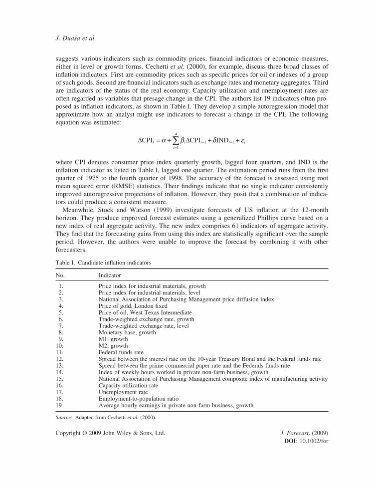
suggests various indicators such as commodity prices, financial indicators or economic measures, either in level or growth forms. Cechetti et al. (2000), for example, discuss three broad classes of inflation indicators. First are commodity prices such as specific prices for oil or indexes of a group of such goods. Second are financial indicators such as exchange rates and monetary aggregates. Third are indicators of the status of the real economy. Capacity utilization and unemployment rates are often regarded as variables that presage change in the CPI. The authors list 19 indicators often pro-posed as inflation indicators, as shown in Table I. They develop a simple autoregression model that approximate how an analyst might use indicators to forecast a change in the CPI. The following equation was estimated:

∆ ∆CPI CPI INDt i t t t

i

= + + +- -=∑α β δ ε1 1

1

4

where CPI denotes consumer price index quarterly growth, lagged four quarters, and IND is the inflation indicator as listed in Table I, lagged one quarter. The estimation period runs from the first quarter of 1975 to the fourth quarter of 1998. The accuracy of the forecast is assessed using root mean squared error (RMSE) statistics. Their findings indicate that no single indicator consistently improved autoregressive projections of inflation. However, they posit that a combination of indica-tors could produce a consistent measure.

Meanwhile, Stock and Watson (1999) investigate forecasts of US inflation at the 12-month horizon. They produce improved forecast estimates using a generalized Phillips curve based on a new index of real aggregate activity. The new index comprises 61 indicators of aggregate activity. They find that the forecasting gains from using this index are statistically significant over the sample period. However, the authors were unable to improve the forecast by combining it with other forecasters.

Table I. Candidate inflation indicators

No. Indicator

1. Price index for industrial materials, growth 2. Price index for industrial materials, level 3. National Association of Purchasing Management price diffusion index 4. Price of gold, London fixed 5. Price of oil, West Texas Intermediate 6. Trade-weighted exchange rate, growth 7. Trade-weighted exchange rate, level 8. Monetary base, growth 9. M1, growth10. M2, growth11. Federal funds rate12. Spread between the interest rate on the 10-year Treasury Bond and the Federal funds rate13. Spread between the prime commercial paper rate and the Federals funds rate14. Index of weekly hours worked in private non-farm business, growth15. National Association of Purchasing Management composite index of manufacturing activity16. Capacity utilization rate17. Unemployment rate18. Employment-to-population ratio19. Average hourly earnings in private non-farm business, growth

Source: Adapted from Cechetti et al. (2000).Y1



In this study, we again attempt to investigate which inflation indicators best predict future inflation, particularly for Malaysia, using a refined method. Specifically, we raise the following two questions. First, what are the inflation indicators that are consistent, reliable and accurate for Malaysia? The second question is: which indicator acts as an equilibrium attractor in the long run? For this purpose, the vector error correction (VECM) model is applied to both the inflation index and selected indicators using monthly data covering the period 1980:01 to 2006:12. The cointegra-tion between variables is tested and the short-run and long-run relationships are identified. We alternate between the following inflation indicators: commodity prices, financial indicators and eco-nomic activities in our analysis. For each indicator, the forecasting horizon used is 24 months. The VECM model is applied to seven subsample windows over the period 1980–2006. The forecasting period is every 2 years starting from 1992 onwards. Each model is evaluated using an out-of-sample forecast based on RMSE statistics.

Since it is also important to have an indicator whose future values can be predicted independently of inflation, we also look at the degree of independence of each indicator from the inflation index. This is done by analyzing the variance decomposition (VDC) of each indicator and Granger causality between each indicator and the inflation index.

This paper is organized as follows. The next section gives an overview of the inflation trend in Malaysia. In the third section we outline statistical properties of the data and model specifications. The fourth section discusses the results and the fifth section concludes.

INFLATION TREND IN MALAYSIA

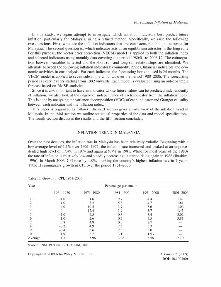
Over the past decades, the inflation rate in Malaysia has been relatively volatile. Beginning with a low average level of 1.1% over 1961–1971, the inflation rate increased and peaked at an unprece-dented high level of 17.4% in 1974 and again at 9.7% in 1981. While for most years of the 1980s the rate of inflation is relatively low and steadily decreasing, it started rising again in 1988 (Ibrahim, 1996). In March 2006, CPI rose by 4.8%, marking the country’s highest inflation rate in 7 years. Table II summarizes growth in CPI over the period 1961–2006.

Table II. Growth in CPI, 1961–2006

Year Percentage per annum

1961–1970 1971–1980 1981–1990 1991–2000 2001–2006

1 -1.0 1.6 9.7 4.4 1.42 2 1.0 3.2 5.8 4.7 1.81 3 4.0 10.5 3.7 3.6 1.06 4 0 17.4 3.9 3.7 1.45 5 -1.0 4.5 0.3 3.4 3.02 6 1.0 2.6 0.7 3.5 3.81 7 5.8 4.8 0.3 2.7 — 8 -0.2 4.9 2.5 5.3 — 9 -0.4 3.6 2.8 3.0 —10 1.9 6.7 3.1 1.53 —Average 1.1 5.98 3.28 3.58 2.10

Source: BNM, 1999 and IFS CD ROM, 2006. Y1

J. Duasa et al.


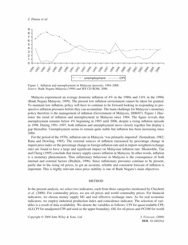
Malaysia experienced an average domestic inflation of 4% in the 1980s and 3.6% in the 1990s (Bank Negara Malaysia, 1999). The present low inflation environment cannot be taken for granted. To maintain low inflation, policy will have to continue to be forward-looking in responding to pro-spective inflation pressures before they can accumulate. The main challenge for Malaysia’s monetary policy therefore is the management of inflation (Government of Malaysia, 2006/07). Figure 1 illus-trates the trend of inflation and unemployment in Malaysia since 1984. The figure reveals that unemployment remains below 4% beginning in 1993 until 2006, despite a rising inflation episode in 1998. During 1991–1997, both inflation and unemployment move closely together but display a gap thereafter. Unemployment seems to remain quite stable but inflation has been increasing since 2004.

For the period of the 1970s, inflation rate in Malaysia ‘was primarily imported’ (Semudram, 1982; Rana and Dowling, 1985). The external sources of inflation (measured by percentage change in import price index or the percentage change in foreign inflation rate and in import-weighted exchange rate) are found to have a large and significant impact on Malaysian inflation rate. Meanwhile, Tan and Cheng (1995) conclude that money supply causes inflation in Malaysia. In other words, inflation is a monetary phenomenon. Thus inflationary behaviour in Malaysia is the consequence of both internal and external factors (Ibrahim, 1996). Since inflationary pressures continue to be present, partly due to the rising oil prices, to get an accurate, reliable and consistent forecast of inflation is important. This is highly relevant since price stability is one of Bank Negara’s main objectives.

METHOD

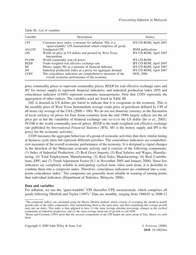
In the present analysis, we select two indicators, each from three categories mentioned by Chechetti et al. (2000). For commodity prices, we use oil prices and world commodity prices. For financial indicators, we choose money supply M1 and real effective exchange rates. As for real economic indicators, we employ industrial production index and coincidence indicator. The selection of vari-ables is a result of data availability. We denote the variables as follows: CPI for quasi-tradable CPI; ALLCPI for unadjusted CPI and used as the upper boundary; OIL for oil prices and PCOM for world

0123456789

1984

1985

1986

1987

1988

1989

1990

1991

1992

1993

1994

1995

1996

1997

1998

1999

2000

2001

2002

2003

2004

2005

2006

unemployment CPI

Figure 1. Inflation and unemployment in Malaysia (percent), 1984–2006 Source: Bank Negara Malaysia (1999) and IFS CD ROM, 2006.

Y1



price commodity prices to represent commodity prices; REER for real effective exchange rates and M1 for money supply to represent financial indicators; and industrial production index (IPI) and coincidence indicator (COIN) represent economic measurements. Note that COIN represents the aggregation of other indices. The variables used are listed in Table III.

OIL is denoted in US dollars per barrel to indicate that it is exogenous to the economy. This is the monthly price of West Texas Intermediate average crude price of petroleum deflated by CPI of all items city-average of the USA (2000 = 100). We do not use domestic currency as the fluctuation of local currency oil prices for East Asian countries from the mid 1990s largely reflects not the oil price per se but the variability of bilateral exchange rate vis-à-vis the US dollar (Ito et al., 2005). PCOM is the world commodity non-oil prices. REER is the trade-weighted real effective exchange rate published by International Financial Statistics (IFS). M1 is the money supply and IPI is the proxy for the economic activities.

COIN measures the aggregate behaviour of a group of economic activities that show similar timing at business cycle turns but represent different activities. The coincidence indicators are comprehen-sive measures of the overall economic performance of the economy. It is designed to signal changes in the direction of the Malaysian economic activity and it consists of the following components: (1) Index of Industrial Production; (2) Real Gross Imports; (3) Real Salaries and Wages, Manufac-turing; (4) Total Employment, Manufacturing; (5) Real Sales, Manufacturing; (6) Real Contribu-tions, EPF; and (7) Trend Adjustment Factor (0.1 in November 2005 and January 2006). Since few indicators are completely reliable in anticipating cyclical turns when used alone, it is desirable to combine them into a composite index. Therefore, coincidence indicators are combined into a com-posite coincidence index.1 The composites are generally more reliable in warning of turning points than individual indicators (Department of Statistics, Malaysia, 2008).

Data and variablesFor inflation, we use the ‘quasi-tradable’ CPI (hereafter CPI) measurement, which comprises all goods following Obstfeld and Taylor (1997).2 Data are monthly, ranging from 1980:01 to 2006:12

Table III. List of variables

Variable Description Source

CPI Consumer price index, a measure for inflation. This is a ‘quasi-tradable’ CPI measurement which comprises all goods

IFS CD-ROM, April 2007

ALLCPI Unadjusted CPI BNM publicationsOIL World oil price in US dollars and proxied by West Texas

IntermediateIFS CD-ROM, April 2007

PCOM World commodity non-oil prices IFS CD-ROMREER Trade-weighted real effective exchange rate IFS CD-ROM, April 2007MI Money supply M1 as a measure of financial indicator IFS CD-ROM, April 2007IPI Industrial production index as a proxy for aggregate demand IFS CD-ROM, April 2007COIN The coincidence indicators are comprehensive measures of the

overall economic performance of the economyDOS, 2006

1 The composite indices are calculated using the Moore–Shiskin method, which consists of averaging the month-to-month growth rates of the index components, after standardizing them to the same units, and then cumulating this average growth rates into an index. This index is then adjusted to have (1) the same average absolute percentage changes as the cyclical component of industrial production; and (2) the same average trend rate of growth as real GDP.2 Bryan and Cecchetti (1993) posit that the services components in the CPI basket are more prone to bias. Hence we omit them. Y1

J. Duasa et al.


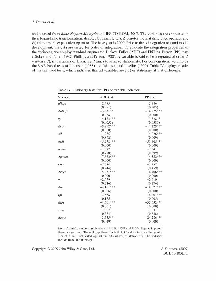
and sourced from Bank Negara Malaysia and IFS CD-ROM, 2007. The variables are expressed in their logarithmic transformation, denoted by small letters. ∆ denotes the first difference operator and E(∙) denotes the expectation operator. The base year is 2000. Prior to the cointegration test and model development, the data are tested for order of integration. To evaluate the integration properties of the variables, we employ standard augmented Dickey–Fuller (ADF) and Phillips–Perron (PP) tests (Dickey and Fuller, 1987; Phillips and Perron, 1988). A variable is said to be integrated of order d, written I(d), if it requires differencing d times to achieve stationarity. For cointegration, we employ the VAR-based tests of Johansen (1988) and Johansen and Juselius (1990). Table IV displays results of the unit root tests, which indicates that all variables are I(1) or stationary at first difference.

Table IV. Stationary tests for CPI and variable indicators

Variable ADF test PP test

allcpi -2.455 -2.546(0.351) (0.305)

∆allcpi -3.631** -14.875***(0.028) (0.000)

cpi -4.183*** -3.528**(0.0053) (0.0381)

∆cpi -9.252*** -17.129***(0.000) (0.000)

oil -1.275 -4.026***(0.892) (0.009)

∆oil -5.972*** -55.405***(0.000) (0.000)

pcom -1.697 -1.241(0.750) (0.899)

∆pcom -7.662*** -14.552***(0.000) (0.000)

reer -2.684 -2.252(0.244) (0.459)

∆reer -5.271*** -14.706***(0.000) (0.000)

m -2.679 -2.610(0.246) (0.276)

∆m -4.161*** -18.527***(0.006) (0.000)

Ipi -2.868 -4.207***(0.175) (0.005)

∆ipi -4.561*** -33.632***(0.001) (0.000)

coin -1.307 -1.831(0.884) (0.688)

∆coin -3.635** -24.286***(0.029) (0.000)

Note: Asterisks denote significance at ***1%, **5% and *10%. Figures in paren-theses are p-values. The null hypotheses for both ADF and PP tests are the hypoth-eses of a unit root tested against the alternatives of stationarity. The statistics include trend and intercept.Y1



The modelIn the vector autoregressive (VAR) model, we use a set of p = 2 endogenous variables, y = [cpi, ind]′, where cpi and ind refer to the logarithm of CPI and a specific indicator variable, respectively. We write a p-dimensional vector error correction model (VECM) as follows:

∆ Γ ∆ Πy y y t Tt i t i t t

i

k

= + + + =- -

-

∑ 1

1

1µ ε , , . . . ,

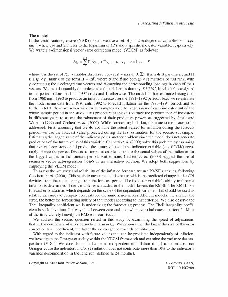
where yt is the set of I(1) variables discussed above; εt ∼ n.i.i.d.(0, ∑); µ is a drift parameter, and Π is a (p × p) matrix of the form Π = αβ′, where α and β are both (p × r) matrices of full rank, with β containing the r cointegrating vectors and α carrying the corresponding loadings in each of the r vectors. We include monthly dummies and a financial crisis dummy, DUM01, in which 0 is assigned to the period before the June 1997 crisis and 1, otherwise. The model is then estimated using data from 1980 until 1990 to produce an inflation forecast for the 1991–1992 period. Next, we re-estimate the model using data from 1980 until 1992 to forecast inflation for the 1993–1994 period, and so forth. In total, there are seven window subsamples used for regression of each indicator out of the whole sample period in the study. This procedure enables us to track the performance of indicators in different years to assess the robustness of their predictive power, as suggested by Stock and Watson (1999) and Cechetti et al. (2000). While forecasting inflation, there are some issues to be addressed. First, assuming that we do not have the actual values for inflation during the forecast period, we use the forecast value projected during the first estimation for the second subsample. Estimating the lagged value of the indicator poses another problem since the model does not generate predictions of the future value of this variable. Cechetti et al. (2000) solve this problem by assuming that expert forecasters could predict the future values of the indicator variable (say PCOM) accu-rately. Hence the perfect forecast assumption enables us to use the actual values of the indicator for the lagged values in the forecast period. Furthermore, Cechetti et al. (2000) suggest the use of recursive vector autoregression (VAR) as an alternative solution. We adopt both suggestions by employing the VECM model.

To assess the accuracy and reliability of the inflation forecast, we use RMSE statistics, following Cecchetti et al. (2000). This statistic measures the degree to which the predicted change in the CPI deviates from the actual change from the forecast period. The indicator variable’s ability to forecast inflation is determined if the variable, when added to the model, lowers the RMSE. The RMSE is a forecast error statistic which depends on the scale of the dependent variable. This should be used as relative measures to compare forecasts for the same series across different models; the smaller the error, the better the forecasting ability of that model according to that criterion. We also observe the Theil inequality coefficient while undertaking the forecasting process. The Theil inequality coeffi-cient is scale invariant. It always lies between zero and one, where zero indicates a perfect fit. Most of the time we rely heavily on RMSE in our study.

We address the second question raised in this study by examining the speed of adjustment, that is, the coefficient of error correction term ectt-1. We propose that the larger the size of the error correction term coefficient, the faster the convergence towards equilibrium.

With regard to the indicator with future values that can be predicted independently of inflation, we investigate the Granger causality within the VECM framework and examine the variance decom-position (VDC). We consider an indicator as independent of inflation if: (1) inflation does not Granger-cause the indicator; and/or (2) inflation does not contribute more than 10% to the indicator’s variance decomposition in the long run (defined as 24 months). Y1

J. Duasa et al.


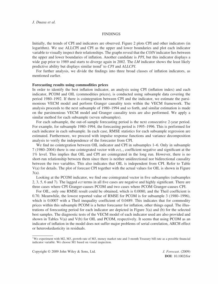
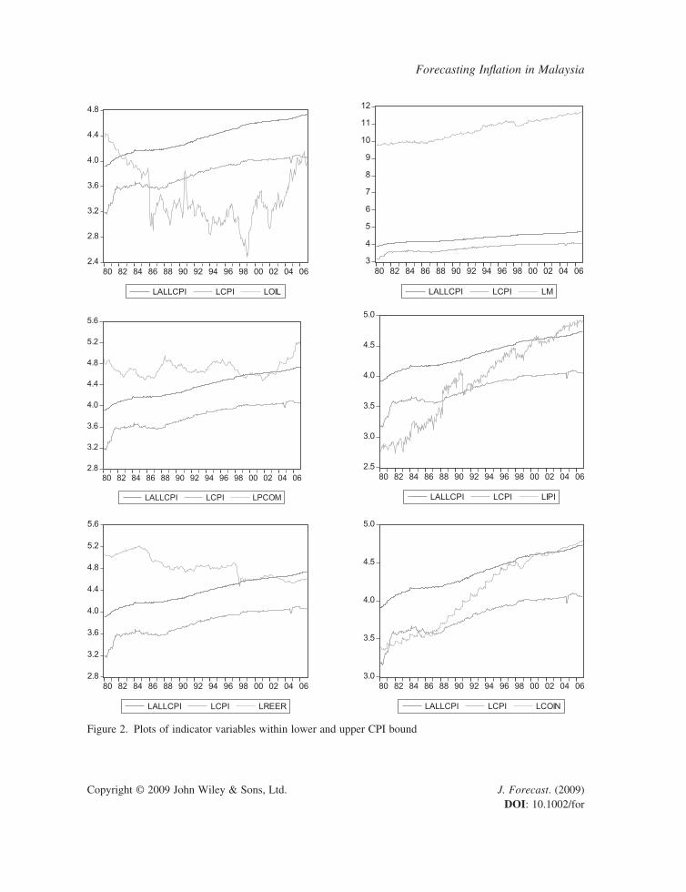
FINDINGS

Initially, the trends of CPI and indicators are observed. Figure 2 plots CPI and other indicators (in logarithm). We use ALLCPI and CPI as the upper and lower boundaries and plot each indicator variable to visually inspect their relationships. The graphs reveal that the COIN indicator lies between the upper and lower boundaries of inflation. Another candidate is PPI, but this indicator displays a wide gap prior to 1989 and starts to diverge again in 2002. The LM indicator shows the least likely predictive ability but displays similar trend3 to CPI and ALLCPI.

For further analysis, we divide the findings into three broad classes of inflation indicators, as mentioned earlier.

Forecasting results using commodities pricesIn order to identify the best inflation indicator, an analysis using CPI (inflation index) and each indicator, PCOM and OIL (commodities prices), is conducted using subsample data covering the period 1980–1992. If there is cointegration between CPI and the indicator, we estimate the parsi-monious VECM model and perform Granger causality tests within the VECM framework. The analysis proceeds to the next subsample of 1980–1994 and so forth, and similar estimation is made on the parsimonious VECM model and Granger causality tests are also performed. We apply a similar method for each subsample (seven subsamples).

For each subsample, the out-of-sample forecasting period is the next consecutive 2-year period. For example, for subsample 1980–1994, the forecasting period is 1995–1996. This is performed for each indicator in each subsample. In each case, RMSE statistics for each subsample regression are estimated. Furthermore, we proceed with impulse response functions and variance decomposition analysis to verify the independence of the forecaster from CPI.

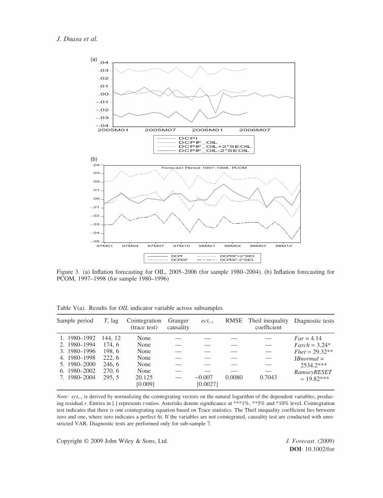
We find no cointegration between OIL indicator and CPI in subsamples 1–6. Only in subsample 7 (1980–2004) there is one cointegrated vector with ectt-1 coefficient negative and significant at the 1% level. This implies that OIL and CPI are cointegrated in the long run. However, there is no short-run relationship between them since there is neither unidirectional nor bidirectional causality between the two variables. This also indicates that OIL is independent from CPI. Refer to Table V(a) for details. The plot of forecast CPI together with the actual values for OIL is shown in Figure 3(a).

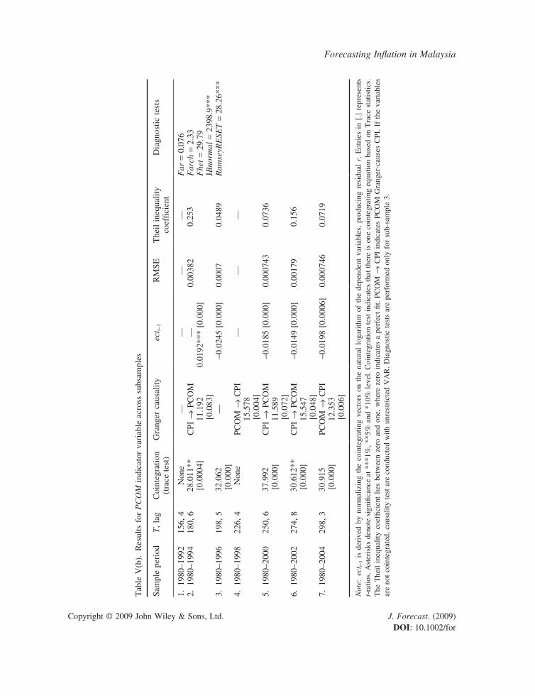
Looking at the PCOM indicator, we find one cointegrated vector in five subsamples (subsamples 2, 3, 5, 6 and 7). The lagged ect terms in all five cases are negative and highly significant. There are three cases where CPI Granger-causes PCOM and two cases where PCOM Granger-causes CPI.

For OIL, only one RMSE result could be obtained, which is 0.0080, and the Theil coefficient is 0.70. Meanwhile, the lowest reported value of RMSE for PCOM is for subsample 3 (1980–1996), which is 0.0007 with a Theil inequality coefficient of 0.0489. This indicates that for commodity prices within this subsample PCOM is a better forecaster for inflation, other things equal. The illus-trations of forecasting period for each indicator are depicted in Figure 3(a) and (b) for the selected best samples. The diagnostic tests of the VECM model of each indicator used are also provided and shown in Tables V(a) and V(b) for OIL and PCOM, respectively. It seems that using PCOM as an indicator of inflation in the model does not suffer major problems of serial correlation, ARCH effect or heteroskedasticity in residuals.

3 We experiment with M2, M3, growth rate of M3, money market rate and 3-month Treasury bill rate as a possible financial indicator variable. We choose M1 based on visual inspection.Y1



2.4

2.8

3.2

3.6

4.0

4.4

4.8

80 82 84 86 88 90 92 94 96 98 00 02 04 06

LALLCPI LCPI LOIL

2.8

3.2

3.6

4.0

4.4

4.8

5.2

5.6

80 82 84 86 88 90 92 94 96 98 00 02 04 06

LALLCPI LCPI LPCOM

2.8

3.2

3.6

4.0

4.4

4.8

5.2

5.6

80 82 84 86 88 90 92 94 96 98 00 02 04 06

LALLCPI LCPI LREER

3

4

5

6

7

8

9

10

11

12

80 82 84 86 88 90 92 94 96 98 00 02 04 06

LALLCPI LCPI LM

2.5

3.0

3.5

4.0

4.5

5.0

80 82 84 86 88 90 92 94 96 98 00 02 04 06

LALLCPI LCPI LIPI

3.0

3.5

4.0

4.5

5.0

80 82 84 86 88 90 92 94 96 98 00 02 04 06

LALLCPI LCPI LCOIN

Figure 2. Plots of indicator variables within lower and upper CPI bound

Y1

J. Duasa et al.


-.04

-.03

-.02

-.01

.00

.01

.02

.03

.04

2005M01 2005M07 2006M01 2006M07

DCPIDCPIF_OILDCPIF_OIL+2*SEOILDCPIF_OIL-2*SEOIL

-.05

-.04

-.03

-.02

-.01

.00

.01

.02

.03

.04

(b)

(a)

97M01 97M04 97M07 97M10 98M01 98M04 98M07 98M10

DCPIDCPI3F

DCPI3F+2*SE3DCPI3F-2*SE3

Forecast Period 1997-1998, PCOM

Table V(a). Results for OIL indicator variable across subsamples

Sample period T, lag Cointegration (trace test)

Granger causality

ectt-1 RMSE Theil inequality coefficient

Diagnostic tests

1. 1980–1992 144, 12 None — — — — Far = 4.14Farch = 3.24*Fhet = 29.32**JBnormal =

2534.2***RamseyRESET

= 19.82***

2. 1980–1994 174, 6 None — — — — 3. 1980–1996 198, 6 None — — — — 4. 1980–1998 222, 6 None — — — — 5. 1980–2000 246, 6 None — — — — 6. 1980–2002 270, 6 None — — — — 7. 1980–2004 295, 5 20.125

[0.009]— -0.007

[0.0027]0.0080 0.7043

Note: ectt-1 is derived by normalizing the cointegrating vectors on the natural logarithm of the dependent variables, produc-ing residual r. Entries in [.] represents t-ratios. Asterisks denote significance at ***1%, **5% and *10% level. Cointegration test indicates that there is one cointegrating equation based on Trace statistics. The Theil inequality coefficient lies between zero and one, where zero indicates a perfect fit. If the variables are not cointegrated, causality test are conducted with unre-stricted VAR. Diagnostic tests are performed only for sub-sample 7.

Figure 3. (a) Inflation forecasting for OIL, 2005–2006 (for sample 1980–2004). (b) Inflation forecasting for PCOM, 1997–1998 (for sample 1980–1996)

Y1



Tab

le V

(b).

Res

ults

for

PC

OM

ind

icat

or v

aria

ble

acro

ss s

ubsa

mpl

es

Sam

ple

peri

odT

, lag

Coi

nteg

ratio

n (t

race

tes

t)G

rang

er c

ausa

lity

ect t-

1R

MSE

The

il in

equa

lity

coef

ficie

ntD

iagn

ostic

tes

ts

1. 1

980–

1992

156,

4N

one

——

——

Far

= 0

.076

Far

ch =

2.3

3F

het

= 29

.79

JBno

rmal

= 2

398.

9***

Ram

seyR

ESE

T =

28.

26**

*

2. 1

980–

1994

180,

628

.011

**[0

.000

4]C

PI →

PC

OM

11.1

92[0

.083

]

—0.

0192

***

[0.0

00]

0.00

382

0.25

3

3. 1

980–

1996

198,

532

.062

[0.0

00]

—-0

.024

5 [0

.000

]0.

0007

0.04

89

4. 1

980–

1998

226,

4N

one

PCO

M →

CPI

15.5

78[0

.004

]

——

—

5. 1

980–

2000

250,

637

.992

[0.0

00]

CPI

→ P

CO

M11

.589

[0.0

72]

-0.0

185

[0.0

00]

0.00

0743

0.07

36

6. 1

980–

2002

274,

830

.612

**[0

.000

]C

PI →

PC

OM

15.5

47[0

.048

]

-0.0

149

[0.0

00]

0.00

179

0.15

6

7. 1

980–

2004

298,

330

.915

[0.0

00]

PCO

M →

CPI

12.3

53[0

.006

]

-0.0

198

[0.0

006]

0.00

0746

0.07

19

Not

e: e

ctt-

1 is

der

ived

by

norm

aliz

ing

the

coin

tegr

atin

g ve

ctor

s on

the

nat

ural

log

arith

m o

f th

e de

pend

ent

vari

able

s, p

rodu

cing

res

idua

l r.

Ent

ries

in

[.]

repr

esen

ts

t-ra

tios.

Ast

eris

ks d

enot

e si

gnifi

canc

e at

***

1%, *

*5%

and

*10

% le

vel.

Coi

nteg

ratio

n te

st in

dica

tes

that

ther

e is

one

coi

nteg

ratin

g eq

uatio

n ba

sed

on T

race

sta

tistic

s.

The

The

il in

equa

lity

coef

ficie

nt l

ies

betw

een

zero

and

one

, w

here

zer

o in

dica

tes

a pe

rfec

t fit

. PC

OM

→ C

PI i

ndic

ates

PC

OM

Gra

nger

-cau

ses

CPI

. If

the

var

iabl

es

are

not

coin

tegr

ated

, cau

salit

y te

st a

re c

ondu

cted

with

unr

estr

icte

d V

AR

. Dia

gnos

tic t

ests

are

per

form

ed o

nly

for

sub-

sam

ple

3.

Y1

J. Duasa et al.


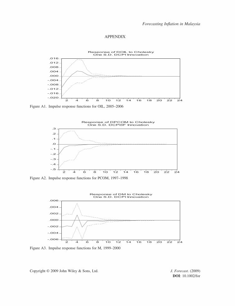
As for impulse response functions (IRFs) and variance decomposition for both indicators, the results reveal that IRFs are not significant and die off within less than a year (the illustrations of IRFs are available in the Appendix). This is verified by VDC analysis, in which for OIL and PCOM the contribution of CPI on the variation of error in the indicators is less than 10% for each sample throughout the sample period. This implies that OIL and PCOM are quite independent from CPI. Refer to Table V(c) for the VDC of each indicator used.

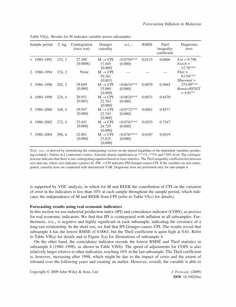
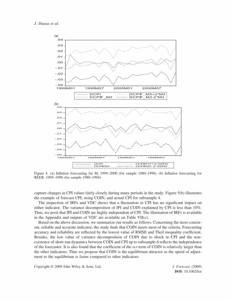
Forecasting results using financial indicatorsThe second analysis uses financial indicators, which are represented by money supply (M) and real effective exchange rate (REER). While using M as inflation indicator, we find six out of seven sub-samples show that there is one cointegration between M and CPI. In all six cases, the ectt-1 terms are negative and significant, indicating the existence of a long-run relationship between them. Within these six subsamples, subsample 4 (1980–1988) shows the lowest RMSE of 0.0071, with a Theil inequality coefficient of 0.65. It is also found that in all subsamples, there exists a short-run relation-ship and the causality runs from M to CPI at 1% significance level. However, the Theil coefficient is quite large, which reflects that M is not a highly accurate forecaster of CPI. Results are presented in Table VI(a). A graphical illustration is displayed in Figure 4(a) for the best subsample, namely subsample 4.

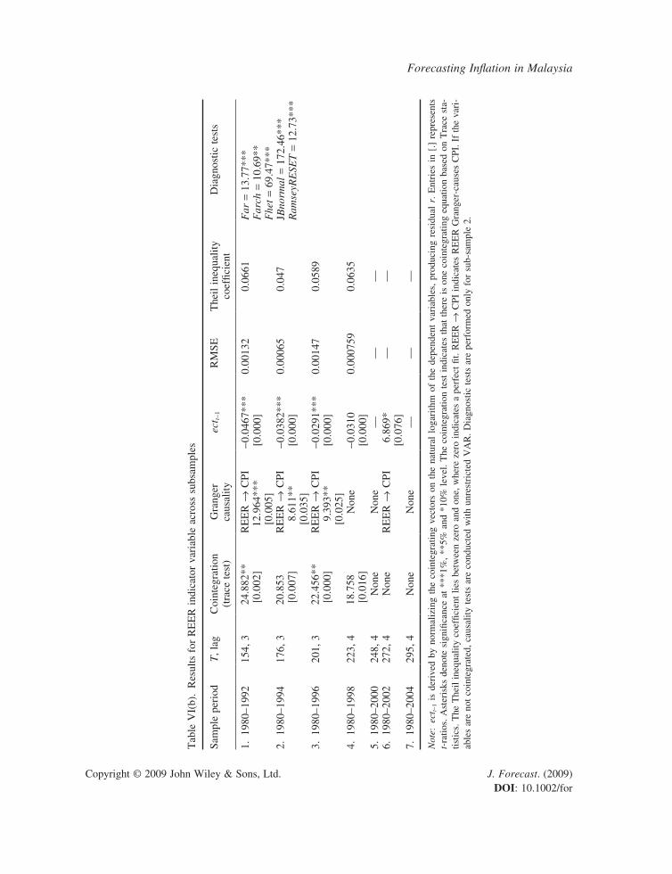
As regards REER, the indicator Granger-causes CPI in samples 1, 2, 3 and 6. One cointegration existed in subsamples 1–4. REER reports low RMSE and Theil inequality coefficient for the first four windows in which subsample 2 marks the lowest RMSE of 0.00065, with a Theil coefficient of 0.047. At a later period the variables are not cointegrated. Therefore, it could be concluded that no long-run relationship existed between them. This might be due to the adoption of a fixed regime one year after the financial crisis and the introduction of capital control in Malaysia in the period.

As for the prediction ability, sample 1 misses the upturn of CPI in 1993 as well as the sudden peak of CPI in 1999. For the rest of forecasting period, REER predicts inflation reasonably well. Results are presented in Table VI(b) and Figure 4(b) depicts the forecasting results for the best sub-sample, i.e. subsample 2. The diagnostic tests of the VECM model of each indicator used are also provided and included in Tables VI(a) and VI(b) for M and REER, respectively. The results show that the model using m as an indicator of inflation does not suffer a problem of autocorrelation as compared to REER, which suffers most problems of residuals.

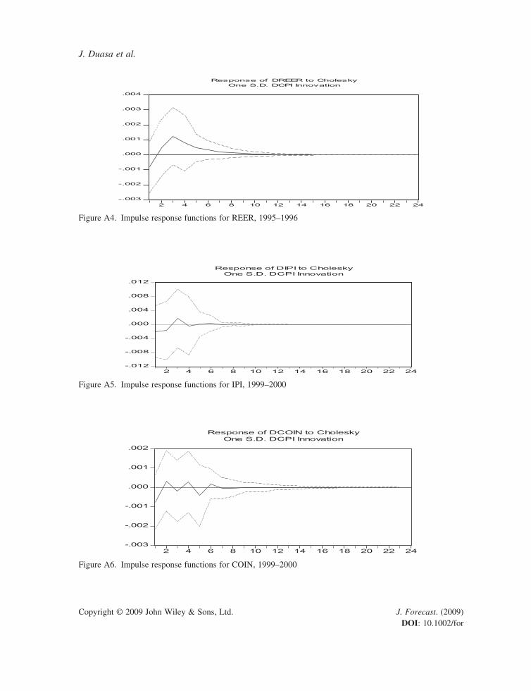
Looking at the IRFs of the best subsample (shown in the Appendix), the results show that IRFs are not significant and die off in less than a year for M and in almost a year for REER. This

Table V(c). Variance decomposition of OIL and PCOM explained by CPI

Month Sample 1 Sample 2 Sample 3 Sample 4 Sample 5 Sample 6 Sample 7

For OIL 6 1.821 3.623 3.009 3.445 2.814 2.553 2.80312 1.857 3.649 3.038 3.842 3.059 2.705 2.80724 1.858 3.650 3.039 3.848 3.062 2.707 2.807

For PCOM 6 3.545 3.102 2.453 2.453 2.029 2.243 0.93012 3.545 3.101 2.455 2.455 2.029 2.242 0.93024 3.545 3.101 2.455 2.455 2.029 2.242 0.930

Y1



Table VI(a). Results for M indicator variable across subsamples


Granger causality


Diagnostic tests

1. 1980–1992 153, 3 27.169[0.0006]

M → CPI11.445[0.009]

-0.0754***[0.000]

0.0115 0.6804 Far = 0.796Farch =

12.78***Fhet =

63.54***JBnormal =


= 4.81**

2. 1980–1994 174, 2 None M → CPI10.261[0.001]

— — —

3. 1980–1996 202, 2 28.649[0.000]

M → CPI15.089[0.000]

-0.0634***[0.000]

0.0079 0.5665

4. 1980–1998 224, 4 26.951[0.001]

M → CPI22.743[0.000]

-0.0824***[0.000]

0.0071 0.6470

5. 1980–2000 248, 4 29.947[0.000]

M → CPI22.743[0.000]

-0.0772***[0.000]

0.0081 0.8577

6. 1980–2002 272, 4 32.441[0.000]

M → CPI24.729[0.000]

-0.0743***[0.000]

0.0255 0.7547

7. 1980–2004 296, 4 32.861[0.000]

M → CPI23.625[0.000]

-0.0787***[0.000]

0.0107 0.6919

Note: ectt-1 is derived by normalizing the cointegrating vectors on the natural logarithm of the dependent variables, produc-ing residual r. Entries in [.] represents t-ratios. Asterisks denote significance at ***1%, **5% and *10% level. The cointegra-tion test indicates that there is one cointegrating equation based on trace statistics. The Theil inequality coefficient lies between zero and one, where zero indicates a perfect fit. PM → CPI indicates PM Granger-causes CPI. If the variables are not cointe-grated, causality tests are conducted with unrestricted VAR. Diagnostic tests are performed only for sub-sample 4.

is supported by VDC analysis, in which for M and REER the contribution of CPI on the variation of error in the indicators is less than 10% at each sample throughout the sample period, which indi-cates the independence of M and REER from CPI (refer to Table VI(c) for details).

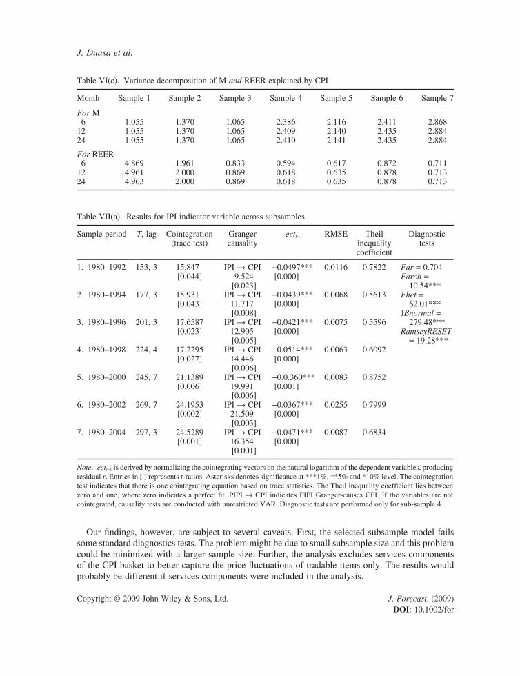
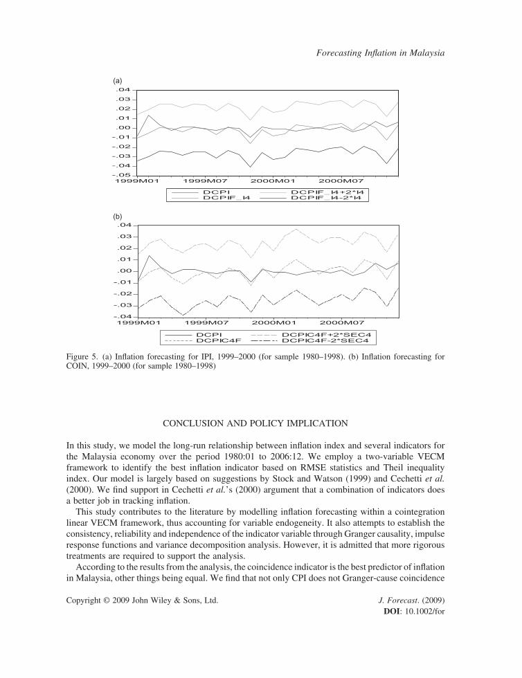
Forecasting results using real economic indicatorsIn this section we use industrial production index (IPI) and coincidence indicator (COIN), as proxies for real economic indicators. We find that IPI is cointegrated with inflation in all subsamples. Fur-thermore, ectt-1 is negative and highly significant in each subsample, indicating the existence of a long-run relationship. In the short run, we find that IPI Granger-causes CPI. The results reveal that subsample 4 has the lowest RMSE of 0.0063, but the Theil coefficient is quite high at 0.61. Refer to Table VII(a) for details and to Figure 5(a) for illustrations of subsample 4.

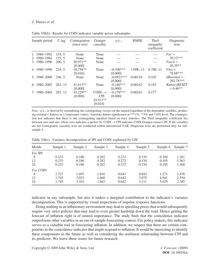
On the other hand, the coincidence indicator records the lowest RMSE and Theil statistics in subsample 4 (1980–1998), as shown in Table VII(b). The speed of adjustments for COIN is also relatively larger relative to other indicators, reaching 16% in the last subsample. The Theil coefficient is, however, increasing after 1998, which might be due to the impact of crisis and the extent of rebound over the following years and creating an outlier. However, overall, the variable is able to Y1

J. Duasa et al.


capture changes in CPI values fairly closely during many periods in the study. Figure 5(b) illustrates the example of forecast CPI, using COIN, and actual CPI for subsample 4.

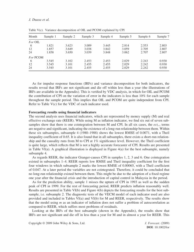
The inspection of IRFs and VDC shows that a fluctuation in CPI has no significant impact on either indicator. The variance decomposition of IPI and COIN explained by CPI is less than 10%. Thus, we posit that IPI and COIN are highly independent of CPI. The illustration of IRFs is available in the Appendix and outputs of VDC are available on Table VII(c).

Based on the above discussion, we summarize our results as follows. Concerning the most consist-ent, reliable and accurate indicator, the study finds that COIN meets most of the criteria. Forecasting accuracy and reliability are reflected by the lowest value of RMSE and Theil inequality coefficient. Besides, the low value of variance decomposition of COIN due to shock in CPI and the non- existence of short-run dynamics between COIN and CPI up to subsample 6 reflects the independence of the forecaster. It is also found that the coefficient of the ect term of COIN is relatively larger than the other indicators. Thus we propose that COIN is the equilibrium attractor as the speed of adjust-ment to the equilibrium is faster compared to other indicators.

(b)

(a)

-.04

-.03

-.02

-.01

.00

.01

.02

.03

.04

1999M01 1999M07 2000M01 2000M07

DCPIDCPIF_M3

DCPIF_M3+2*M3DCPIF_M3-2*M3

-.05

-.04

-.03

-.02

-.01

.00

.01

.02

.03

.04

1995M01 1995M07 1996M01 1996M07

DCPIDCPIR2F

DCPIR1F+2*SER2DCPIR2F-2*SER2

Figure 4. (a) Inflation forecasting for M, 1999–2000 (for sample 1980–1998). (b) Inflation forecasting for REER, 1995–1996 (for sample 1980–1994)

Y1



Tab

le V

I(b)

. R

esul

ts f

or R

EE

R i

ndic

ator

var

iabl

e ac

ross

sub

sam

ples

Sam

ple

peri

odT

, lag

Coi

nteg

ratio

n (t

race

tes

t)G

rang

er

caus

ality

ect t-

1R

MSE

The

il in

equa

lity

coef

ficie

ntD

iagn

ostic

tes

ts

1. 1

980–

1992

154,

324

.882

**[0

.002

]R

EE

R →

CPI

12.9

64**

*[0

.005

]

-0.0

467*

**[0

.000

]0.

0013

20.

0661

Far

= 1

3.77

***

Far

ch =

10.

69**

Fhe

t =

69.4

7***

JBno

rmal

= 1

72.4

6***

Ram

seyR

ESE

T =

12.

73**

*2.

198

0–19

9417

6, 3

20.8

53[0

.007

]R

EE

R →

CPI

8.61

1**

[0.0

35]

-0.0

382*

**[0

.000

]0.

0006

50.

047

3. 1

980–

1996

201,

322

.456

**[0

.000

]R

EE

R →

CPI

9.39

3**

[0.0

25]

-0.0

291*

**[0

.000

]0.

0014

70.

0589

4. 1

980–

1998

223,

418

.758

[0.0

16]

Non

e-0

.031

0[0

.000

]0.

0007

590.

0635

5. 1

980–

2000

248,

4N

one

Non

e—

——

6. 1

980–

2002

272,

4N

one

RE

ER

→ C

PI6.

869*

[0.0

76]

——

7. 1

980–

2004

295,

4N

one

Non

e—

——

Not

e: e

ctt-

1 is

der

ived

by

norm

aliz

ing

the

coin

tegr

atin

g ve

ctor

s on

the

nat

ural

log

arith

m o

f th

e de

pend

ent

vari

able

s, p

rodu

cing

res

idua

l r.

Ent

ries

in

[.]

repr

esen

ts

t-ra

tios.

Ast

eris

ks d

enot

e si

gnifi

canc

e at

***

1%, *

*5%

and

*10

% l

evel

. The

coi

nteg

ratio

n te

st i

ndic

ates

tha

t th

ere

is o

ne c

oint

egra

ting

equa

tion

base

d on

Tra

ce s

ta-

tistic

s. T

he T

heil

ineq

ualit

y co

effic

ient

lie

s be

twee

n ze

ro a

nd o

ne, w

here

zer

o in

dica

tes

a pe

rfec

t fit

. RE

ER

→ C

PI i

ndic

ates

RE

ER

Gra

nger

-cau

ses

CPI

. If

the

vari

-ab

les

are

not

coin

tegr

ated

, cau

salit

y te

sts

are

cond

ucte

d w

ith u

nres

tric

ted

VA

R. D

iagn

ostic

tes

ts a

re p

erfo

rmed

onl

y fo

r su

b-sa

mpl

e 2.

Y1

J. Duasa et al.


Table VII(a). Results for IPI indicator variable across subsamples


Granger causality


Diagnostic tests

1. 1980–1992 153, 3 15.847[0.044]

IPI → CPI9.524

[0.023]

-0.0497***[0.000]

0.0116 0.7822 Far = 0.704Farch =

10.54***Fhet =

62.01***JBnormal =


= 19.28***

2. 1980–1994 177, 3 15.931[0.043]

IPI → CPI11.717[0.008]

-0.0439***[0.000]

0.0068 0.5613

3. 1980–1996 201, 3 17.6587[0.023]

IPI → CPI12.905[0.005]

-0.0421***[0.000]

0.0075 0.5596

4. 1980–1998 224, 4 17.2295[0.027]

IPI → CPI14.446[0.006]

-0.0514***[0.000]

0.0063 0.6092

5. 1980–2000 245, 7 21.1389[0.006]

IPI → CPI19.991[0.006]

-0.0.360***[0.001]

0.0083 0.8752

6. 1980–2002 269, 7 24.1953[0.002]

IPI → CPI21.509[0.003]

-0.0367***[0.000]

0.0255 0.7999

7. 1980–2004 297, 3 24.5289[0.001]

IPI → CPI16.354[0.001]

-0.0471***[0.000]

0.0087 0.6834

Note: ectt-1 is derived by normalizing the cointegrating vectors on the natural logarithm of the dependent variables, producing residual r. Entries in [.] represents t-ratios. Asterisks denotes significance at ***1%, **5% and *10% level. The cointegration test indicates that there is one cointegrating equation based on trace statistics. The Theil inequality coefficient lies between zero and one, where zero indicates a perfect fit. PIPI → CPI indicates PIPI Granger-causes CPI. If the variables are not cointegrated, causality tests are conducted with unrestricted VAR. Diagnostic tests are performed only for sub-sample 4.

Table VI(c). Variance decomposition of M and REER explained by CPI


For M 6 1.055 1.370 1.065 2.386 2.116 2.411 2.86812 1.055 1.370 1.065 2.409 2.140 2.435 2.88424 1.055 1.370 1.065 2.410 2.141 2.435 2.884

For REER 6 4.869 1.961 0.833 0.594 0.617 0.872 0.71112 4.961 2.000 0.869 0.618 0.635 0.878 0.71324 4.963 2.000 0.869 0.618 0.635 0.878 0.713

Our findings, however, are subject to several caveats. First, the selected subsample model fails some standard diagnostics tests. The problem might be due to small subsample size and this problem could be minimized with a larger sample size. Further, the analysis excludes services components of the CPI basket to better capture the price fluctuations of tradable items only. The results would probably be different if services components were included in the analysis.Y1



CONCLUSION AND POLICY IMPLICATION

In this study, we model the long-run relationship between inflation index and several indicators for the Malaysia economy over the period 1980:01 to 2006:12. We employ a two-variable VECM framework to identify the best inflation indicator based on RMSE statistics and Theil inequality index. Our model is largely based on suggestions by Stock and Watson (1999) and Cechetti et al. (2000). We find support in Cechetti et al.’s (2000) argument that a combination of indicators does a better job in tracking inflation.

This study contributes to the literature by modelling inflation forecasting within a cointegration linear VECM framework, thus accounting for variable endogeneity. It also attempts to establish the consistency, reliability and independence of the indicator variable through Granger causality, impulse response functions and variance decomposition analysis. However, it is admitted that more rigorous treatments are required to support the analysis.

According to the results from the analysis, the coincidence indicator is the best predictor of inflation in Malaysia, other things being equal. We find that not only CPI does not Granger-cause coincidence

(b)

(a)

-.05

-.04

-.03

-.02

-.01

.00

.01

.02

.03

.04

1999M01 1999M07 2000M01 2000M07

DCPIDCPIF_I4

DCPIF_I4+2*I4DCPIF_I4-2*I4

-.04

-.03

-.02

-.01

.00

.01

.02

.03

.04

1999M01 1999M07 2000M01 2000M07

DCPIDCPIC4F

DCPIC4F+2*SEC4DCPIC4F-2*SEC4

Figure 5. (a) Inflation forecasting for IPI, 1999–2000 (for sample 1980–1998). (b) Inflation forecasting for COIN, 1999–2000 (for sample 1980–1998)

Y1

J. Duasa et al.


Table VII(b). Results for COIN indicator variable across subsamples


Granger causality


Diagnostic tests

1. 1980–1992 154, 5 None None — — — Far = 30.12***

Farch = 26.39**

Fhet = 78.68***

JBnormal = 292.78***

RamseyRESET = 6.46**

2. 1980–1994 175, 5 None None — — —3. 1980–1996 200, 5 50.971**

[0.000]None — — —

4. 1980–1998 224, 5 18.758**[0.016]

None -0.100***[0.000]

1.09E–12 8.78E–11

5. 1980–2000 246, 5 None None -0.0921***[0.000]

0.00116 0.102

6. 1980–2002 263, 13 41.613**[0.000]

None -0.160***[0.000]

0.00242 0.183

7. 1980–2004 287, 13 43.229**[0.000]

COIN → CPI

24.911**[0.024]

-0.179***[0.000]

0.00243 0.177

Note: ectt-1 is derived by normalizing the cointegrating vectors on the natural logarithm of the dependent variables, produc-ing residual r. Entries in [.] represents t-ratios. Asterisks denote significance at ***1%, **5% and *10% level. The cointegra-tion test indicates that there is one cointegrating equation based on trace statistics. The Theil inequality coefficient lies between zero and one, where zero indicates a perfect fit. COIN → CPI indicates COIN Granger-causes CPI. If the variables are not cointegrated, causality tests are conducted within unrestricted VAR. Diagnostic tests are performed only for sub-sample 4.

Table VII(c). Variance decomposition of IPI and COIN explained by CPI


For IPI 6 0.233 0.186 0.282 0.272 0.154 0.104 1.16112 0.233 0.186 0.282 0.272 0.154 0.105 1.36324 0.233 0.186 0.282 0.272 0.154 0.105 1.368

For COIN 6 1.727 1.497 1.616 0.641 0.842 1.271 1.47612 1.745 3.023 1.660 0.642 3.075 4.941 2.55424 1.745 3.101 1.662 0.642 3.111 5.029 2.385

indicator in any subsample, but also it makes a marginal contribution to the indicator’s variance decomposition. This is supported by visual inspections of impulse response functions.

Doing nothing in an inflationary environment may lead to spiralling prices that would subsequently require very strict policies that may lead to even greater hardship down the road. Hence getting the forecast of inflation right is of utmost importance. The study finds that the coincidence indicator outperforms other variables in an out-of-sample forecasting contest. For policy makers, this indicator serves as a valuable tool in forecasting inflation. In addition, we suspect that there are certain com-ponents in the coincidence indicator that might respond to inflation. It would be interesting to identify these components in the future as well as considering the nonlinear relationship between CPI and its predictor. We leave these issues for future research.Y1



APPENDIX

-.020

-.016

-.012

-.008

-.004

.000

.004

.008

.012

.016

2 4 6 8 10 12 14 16 18 20 22 24

Response of DOIL to CholeskyOne S.D. DCPI Innovation

-.5

-.4

-.3

-.2

-.1

.0

.1

.2

.3

2 4 6 8 10 12 14 16 18 20 22 24

Response of DPCOM to CholeskyOne S.D. DCPI3F Innovation

-.006

-.004

-.002

.000

.002

.004

.006

2 4 6 8 10 12 14 16 18 20 22 24

Response of DM to CholeskyOne S.D. DCPI Innovation

Figure A1. Impulse response functions for OIL, 2005–2006

Figure A2. Impulse response functions for PCOM, 1997–1998

Figure A3. Impulse response functions for M, 1999–2000

Y1

J. Duasa et al.


-.012

-.008

-.004

.000

.004

.008

.012

2 4 6 8 10 12 14 16 18 20 22 24

Response of DIPI to CholeskyOne S.D. DCPI Innovation

-.003

-.002

-.001

.000

.001

.002

2 4 6 8 10 12 14 16 18 20 22 24

Response of DCOIN to CholeskyOne S.D. DCPI Innovation

Figure A5. Impulse response functions for IPI, 1999–2000

Figure A6. Impulse response functions for COIN, 1999–2000

-.003

-.002

-.001

.000

.001

.002

.003

.004

2 4 6 8 10 12 14 16 18 20 22 24

Response of DREER to CholeskyOne S.D. DCPI Innovation

Figure A4. Impulse response functions for REER, 1995–1996

Y1



REFERENCES

Bank Negara Malaysia (BNM). BNM Monthly Bulletin (various issues).Bryan MF, Cecchetti SG. 1993. The consumer price index as a measure of inflation. Economic Review 29(3):

15–24.Cecchetti SG, Chu RS, Steindel C. 2000. The unreliability of inflation indicators. Current Issues in Economic and

Finance 6(4): 1–6.Department of Statistics, Malaysia. 2008. http://www.statistics.gov.my/ [17 April 2008].Dickey DA, Fuller WA. 1987. The likelihood ratio statistics for autoregressive time series with a unit root.

Econometrica 49(4): 251–276.Government of Malaysia. 2006/07. Economic Report.Ibrahim MH. 1996. Inflationary behavior in Malaysia: an empirical re-evaluation of its determinants. Paper pre-

sented at 4th Malaysian Econometric Conference, Kuala Lumpur, 9–10 October 1996, organized by MIER.Ito T, Sasaki Y, Sato K. 2005. Pass-through of exchange rate changes and macroeconomic shocks to domestic

inflation in East Asian countries. Discussion paper series 05-E-020, Research Institute of Economy, Trade and Industry (RIETI), Japan.

Johansen S. 1988. Statistical analysis of cointegrating vectors. Journal of Economic Dynamics and Control 12: 231–254.

Johansen S, Juselius K. 1990. Maximum likelihood estimation and inference on cointegration with applications to the demand for money. Oxford Bulletin of Economics and Statistics 52(2): 169–210.

Obstfeld M, Taylor AM. 1997. Nonlinear aspects of good-market arbitrage and adjustment Heckscher’s commod-ity points revisited. Journal of Japanese and International Economics 11: 441–479.

Phillips PCB, Perron P. 1988. Testing for a unit root in time series regression. Biometrika 75(2): 335–346.Rana P, Dowling J. 1985. Inflationary effects of small but continuous changes in effective exchanges rates: nine

Asian LDCs. Review of Economics and Statistics 67: 496–500.Semudram M. 1982. A Macro-model of the Malaysian economy, 1957–1977. The Developing Economies 20:

154–172.Stock JH, Watson MW. 1999. Forecasting inflation. NBER working paper no. 7023.Tan KG, Cheng CS. 1995. The causal nexus of money, output and price in Malaysia. Applied Economics 27(12):

1245–1251.

Authors’ biographies:Jarita Duasa is an Associate Professor at the Department of Economics at Faculty of Economics and Management Sciences, International Islamic University Malaysia. Her research niche areas are International Economics, Inter-national Finance and Applied Economics.

Nursilah Ahmad is a lecturer in the Faculty of Economics and Muamalat, Islamic Science University of Malaysia (USIM). Currently she holds the post of Post-Graduate Coordinator, Faculty of Economics and Muamalat, USIM. Her areas of specialization include international macroeconomics, social economics and applied economics.

Mansor H Ibrahim is currently a Professor at the Department of Economics at Faculty of Economics and Man-agement, University Putra Malaysia. His research niche areas are monetary economics, financial economics and economic development.

Molid-Pisal Zainal is currently the Joint Director of Research, International Center for Education in Islamic Finance (INCEIF), Kuala Lumpur. His research interests are in the areas of international finance, international trade, macro-econometrics, monetary economics & Islamic financial markets and institutions.

Authors’ addresses:Jarita Duasa, Department of Economics, Kuliyyah of Economics and Management Sciences, International Islamic University Malaysia, Jalan Gombak, 53100 Kuala Lumpur, Malaysia. Y1

J. Duasa et al.


Nursilah Ahmad, Fakulti Ekonomi and Muamalat, University Sains Islam Malaysia, Bandar Baru Nilai, 71800 Nilai, Negeri Sembilan, Malaysia.

Mansor H. Ibrahim, Department of Economics, Faculty of Economics and Management, Universiti Putra Malaysia, 43400 UPM Serdang, Selangor Darul Ehsan, Malaysia.

Mohd Pisal Zainal, The International Centre for Education in Islamic Finance (INCEIF), Second Floor, Annexe Block, Menara Tun Razak (Menara Tradewinds), Jalan Raja Laut, 50350 Kuala Lumpur, Malaysia.

Y1

Documents

Forecasting inflation in Malaysia