1

REVIEW OF THE AER’S INFLATION FORECASTING METHODOLOGY

Dr Martin Lally

Capital Financial Consultants Ltd

8 July 2020

2

CONTENTS

Executive Summary 3

1. Introduction 4

2. Implications of the NPV = 0 Principle for the Treatment of Inflation 4

3. Approaches to Estimating the Expected Inflation Rate 9

3.1 Bond Yields 9

3.2 Inflation Swaps 14

3.3 RBA Inflation Target 16

3.4 Model Based Estimates 18

3.5 Survey Evidence 19

3.6 Survey Evidence Coupled with the Inflation Target 19

4. Empirical Tests 19

4.1 Previous Analysis 19

4.2 Further Tests 21

5. Review of Submissions 27

6. Conclusions 31

References 33

3

EXECUTIVE SUMMARY

The AER currently estimates expected inflation in Australia over a ten-year period using the

RBA’s forecasts for the first two years, the midpoint of the RBA’s target range (2.5%) for the

remaining eight years, and a geometric mean of these values. This paper seeks to assess the

best method for estimating expected future inflation, with particular reference to recent

empirical evidence. The primary conclusions are as follows.

Firstly, given that the AER’s regulatory cycle is five years, the NPV = 0 principle implies

that the AER ought to be estimating expected inflation over each of the next five years rather

than over the next ten years. Secondly, market prices (comprising the break-even rates and

swap prices) are likely to be biased estimators of expected future inflation, and to a degree

that varies over time. Thirdly, using standard RMSE tests of forecasting accuracy, the RBA’s

Target is far superior to the use of market prices for forecasting inflation over 5-10 years, and

therefore market prices can be rejected. Fourthly, across the range of other approaches

considered (comprising forecasts by the RBA, forecasts from Consensus Economics, the

RBA’s Target rate, a Random Walk model, a mean reversion model, and the model of Finlay

and Wende), the lowest RMSE of the forecast errors comes from the RBA’s forecasts for the

first and second years ahead, and the RBA’s Target for all other future years, which

corresponds to the AER’s current approach.

Fifthly, this RMSE analysis uses a long time series of data, and therefore assumes stability in

the underlying process (which involves mean reversion to or close to the RBA’s Target of

2.5%). If the underlying situation has changed, these tests would not be useful. Thus, it is

necessary to assess whether the underlying situation has changed, especially since inflation

has fallen below the Target for the past several years. The best information on this question

comes from Consensus Economics, who (as of April 2020) forecast reversion to that Target

over the next few years. Lastly, and because reversion back to the RBA’s Target is currently

expected to be unusually slow, there is a case for the AER adopting a slow glide path from

the RBA’s forecasts to the Target providing that scenarios in which reversion back from a

low figure is unusually slow (to the disadvantage of the businesses) are not likely to be

matched by scenarios in which reversion back from a high figure is unusually slow (to the

advantage of the businesses).

4

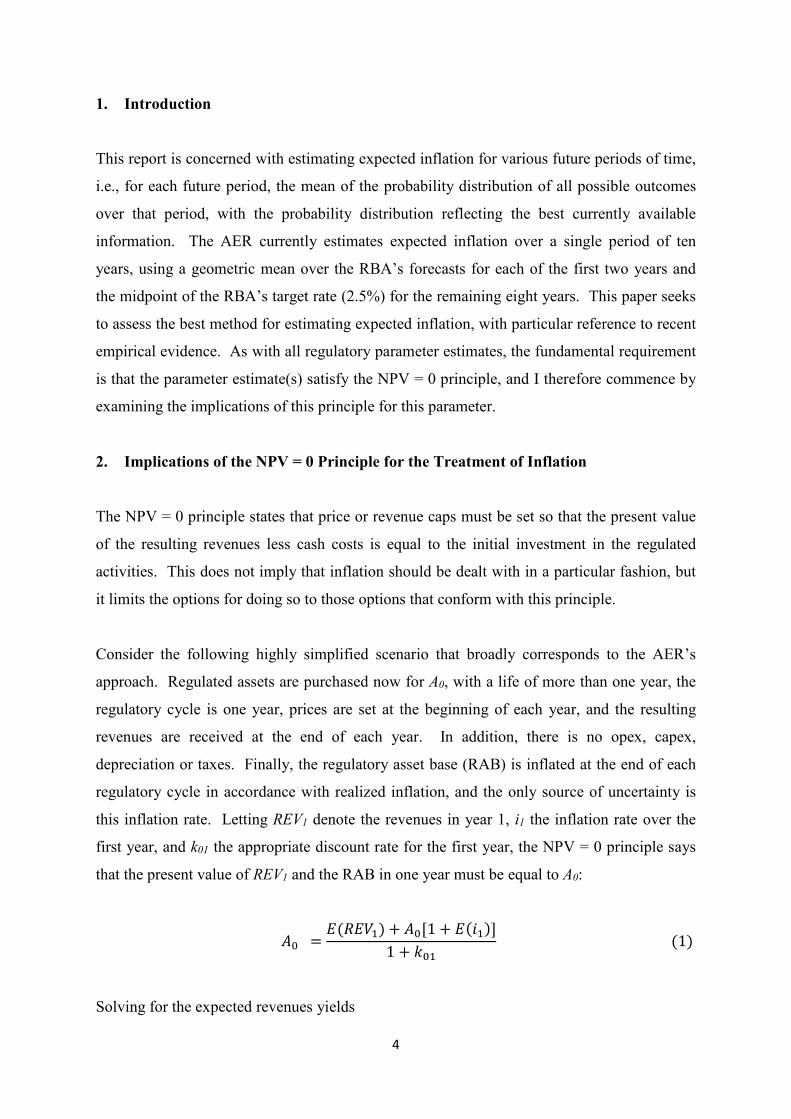
1. Introduction

This report is concerned with estimating expected inflation for various future periods of time,

i.e., for each future period, the mean of the probability distribution of all possible outcomes

over that period, with the probability distribution reflecting the best currently available

information. The AER currently estimates expected inflation over a single period of ten

years, using a geometric mean over the RBA’s forecasts for each of the first two years and

the midpoint of the RBA’s target rate (2.5%) for the remaining eight years. This paper seeks

to assess the best method for estimating expected inflation, with particular reference to recent

empirical evidence. As with all regulatory parameter estimates, the fundamental requirement

is that the parameter estimate(s) satisfy the NPV = 0 principle, and I therefore commence by

examining the implications of this principle for this parameter.

2. Implications of the NPV = 0 Principle for the Treatment of Inflation

The NPV = 0 principle states that price or revenue caps must be set so that the present value

of the resulting revenues less cash costs is equal to the initial investment in the regulated

activities. This does not imply that inflation should be dealt with in a particular fashion, but

it limits the options for doing so to those options that conform with this principle.

Consider the following highly simplified scenario that broadly corresponds to the AER’s

approach. Regulated assets are purchased now for A0, with a life of more than one year, the

regulatory cycle is one year, prices are set at the beginning of each year, and the resulting

revenues are received at the end of each year. In addition, there is no opex, capex,

depreciation or taxes. Finally, the regulatory asset base (RAB) is inflated at the end of each

regulatory cycle in accordance with realized inflation, and the only source of uncertainty is

this inflation rate. Letting REV1 denote the revenues in year 1, i1 the inflation rate over the

first year, and k01 the appropriate discount rate for the first year, the NPV = 0 principle says

that the present value of REV1 and the RAB in one year must be equal to A0:

𝐴𝐴0 =𝐸𝐸(𝑅𝑅𝐸𝐸𝑅𝑅1) + 𝐴𝐴0[1 + 𝐸𝐸(𝑖𝑖1)]

1 + 𝑘𝑘01 (1)

Solving for the expected revenues yields

5

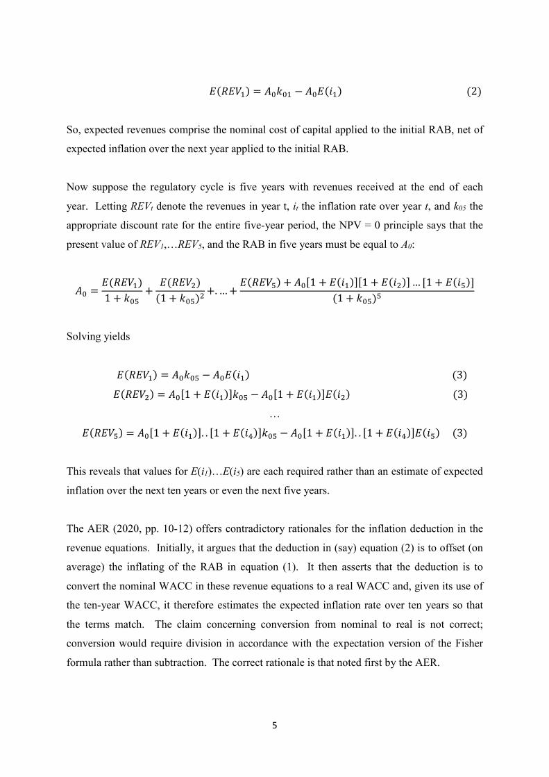
𝐸𝐸(𝑅𝑅𝐸𝐸𝑅𝑅1) = 𝐴𝐴0𝑘𝑘01 − 𝐴𝐴0𝐸𝐸(𝑖𝑖1) (2)

So, expected revenues comprise the nominal cost of capital applied to the initial RAB, net of

expected inflation over the next year applied to the initial RAB.

Now suppose the regulatory cycle is five years with revenues received at the end of each

year. Letting REVt denote the revenues in year t, it the inflation rate over year t, and k05 the

appropriate discount rate for the entire five-year period, the NPV = 0 principle says that the

present value of REV1,…REV5, and the RAB in five years must be equal to A0:

𝐴𝐴0 =𝐸𝐸(𝑅𝑅𝐸𝐸𝑅𝑅1)1 + 𝑘𝑘05

+𝐸𝐸(𝑅𝑅𝐸𝐸𝑅𝑅2)

(1 + 𝑘𝑘05)2+. … +

𝐸𝐸(𝑅𝑅𝐸𝐸𝑅𝑅5) + 𝐴𝐴0[1 + 𝐸𝐸(𝑖𝑖1)][1 + 𝐸𝐸(𝑖𝑖2)] … [1 + 𝐸𝐸(𝑖𝑖5)](1 + 𝑘𝑘05)5

Solving yields

𝐸𝐸(𝑅𝑅𝐸𝐸𝑅𝑅1) = 𝐴𝐴0𝑘𝑘05 − 𝐴𝐴0𝐸𝐸(𝑖𝑖1) (3)

𝐸𝐸(𝑅𝑅𝐸𝐸𝑅𝑅2) = 𝐴𝐴0[1 + 𝐸𝐸(𝑖𝑖1)]𝑘𝑘05 − 𝐴𝐴0[1 + 𝐸𝐸(𝑖𝑖1)]𝐸𝐸(𝑖𝑖2) (3)

…

𝐸𝐸(𝑅𝑅𝐸𝐸𝑅𝑅5) = 𝐴𝐴0[1 + 𝐸𝐸(𝑖𝑖1)]. . [1 + 𝐸𝐸(𝑖𝑖4)]𝑘𝑘05 − 𝐴𝐴0[1 + 𝐸𝐸(𝑖𝑖1)]. . [1 + 𝐸𝐸(𝑖𝑖4)]𝐸𝐸(𝑖𝑖5) (3)

This reveals that values for E(i1)…E(i5) are each required rather than an estimate of expected

inflation over the next ten years or even the next five years.

The AER (2020, pp. 10-12) offers contradictory rationales for the inflation deduction in the

revenue equations. Initially, it argues that the deduction in (say) equation (2) is to offset (on

average) the inflating of the RAB in equation (1). It then asserts that the deduction is to

convert the nominal WACC in these revenue equations to a real WACC and, given its use of

the ten-year WACC, it therefore estimates the expected inflation rate over ten years so that

the terms match. The claim concerning conversion from nominal to real is not correct;

conversion would require division in accordance with the expectation version of the Fisher

formula rather than subtraction. The correct rationale is that noted first by the AER.

6

Furthermore, for a five year regulatory cycle and within these revenue equations, the discount

rate is for a term matching the regulatory cycle (five years) and the expected inflation rates

are for each of the next five years. However, in its revenue setting for regulatory situations

(that involve five year terms), the AER (2020, pp. 11-12) uses a discount rate with a ten-year

term and consistent with this uses an estimate of expected inflation over the same term. This

violates the NPV = 0 requirement.

Furthermore, even if the AER used the ten-year WACC, it does not follow that it should

estimate expected inflation over the same period. If the term structure for WACC were

upward sloping, and that for expected inflation were likewise, using an estimate for expected

inflation for ten years rather than for years 1…5 would likely mitigate the error from using a

ten rather than a five-year WACC. However, the term structure for WACC is generally

upward sloping whilst that for expected inflation is as likely to be downwards as upwards

sloping. So, the use of a ten-year WACC does not warrant use of ten-year expected inflation.

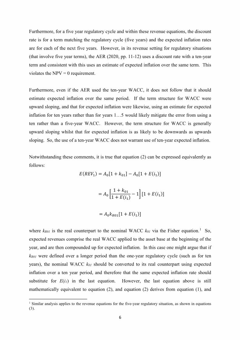
Notwithstanding these comments, it is true that equation (2) can be expressed equivalently as

follows:

𝐸𝐸(𝑅𝑅𝐸𝐸𝑅𝑅1) = 𝐴𝐴0[1 + 𝑘𝑘01] − 𝐴𝐴0[1 + 𝐸𝐸(𝑖𝑖1)]

= 𝐴𝐴0 �1 + 𝑘𝑘01

1 + 𝐸𝐸(𝑖𝑖1)− 1� [1 + 𝐸𝐸(𝑖𝑖1)]

= 𝐴𝐴0𝑘𝑘𝑅𝑅01[1 + 𝐸𝐸(𝑖𝑖1)]

where kR01 is the real counterpart to the nominal WACC k01 via the Fisher equation.1 So,

expected revenues comprise the real WACC applied to the asset base at the beginning of the

year, and are then compounded up for expected inflation. In this case one might argue that if

kR01 were defined over a longer period than the one-year regulatory cycle (such as for ten

years), the nominal WACC k01 should be converted to its real counterpart using expected

inflation over a ten year period, and therefore that the same expected inflation rate should

substitute for E(i1) in the last equation. However, the last equation above is still

mathematically equivalent to equation (2), and equation (2) derives from equation (1), and

1 Similar analysis applies to the revenue equations for the five-year regulatory situation, as shown in equations (3).

7

equation (1) unambiguously requires E(i1)to be the expected inflation rate over one year

rather than ten years. The preceding comments therefore still apply: the error in using a

WACC for longer than the regulatory cycle is not ameliorated by doing the same for the

expected inflation rate.

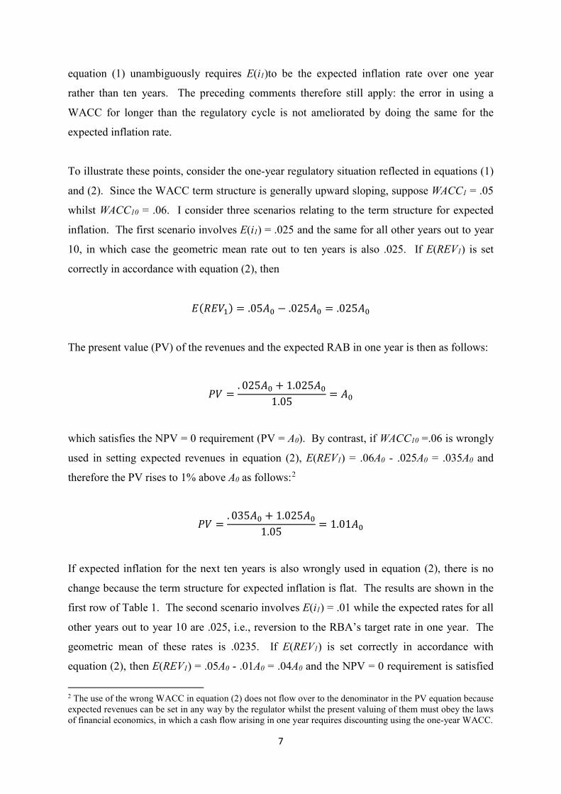
To illustrate these points, consider the one-year regulatory situation reflected in equations (1)

and (2). Since the WACC term structure is generally upward sloping, suppose WACC1 = .05

whilst WACC10 = .06. I consider three scenarios relating to the term structure for expected

inflation. The first scenario involves E(i1) = .025 and the same for all other years out to year

10, in which case the geometric mean rate out to ten years is also .025. If E(REV1) is set

correctly in accordance with equation (2), then

𝐸𝐸(𝑅𝑅𝐸𝐸𝑅𝑅1) = .05𝐴𝐴0 − .025𝐴𝐴0 = .025𝐴𝐴0

The present value (PV) of the revenues and the expected RAB in one year is then as follows:

𝑃𝑃𝑅𝑅 =. 025𝐴𝐴0 + 1.025𝐴𝐴0

1.05= 𝐴𝐴0

which satisfies the NPV = 0 requirement (PV = A0). By contrast, if WACC10 =.06 is wrongly

used in setting expected revenues in equation (2), E(REV1) = .06A0 - .025A0 = .035A0 and

therefore the PV rises to 1% above A0 as follows:2

𝑃𝑃𝑅𝑅 =. 035𝐴𝐴0 + 1.025𝐴𝐴0

1.05= 1.01𝐴𝐴0

If expected inflation for the next ten years is also wrongly used in equation (2), there is no

change because the term structure for expected inflation is flat. The results are shown in the

first row of Table 1. The second scenario involves E(i1) = .01 while the expected rates for all

other years out to year 10 are .025, i.e., reversion to the RBA’s target rate in one year. The

geometric mean of these rates is .0235. If E(REV1) is set correctly in accordance with

equation (2), then E(REV1) = .05A0 - .01A0 = .04A0 and the NPV = 0 requirement is satisfied

2 The use of the wrong WACC in equation (2) does not flow over to the denominator in the PV equation because expected revenues can be set in any way by the regulator whilst the present valuing of them must obey the laws of financial economics, in which a cash flow arising in one year requires discounting using the one-year WACC.

8

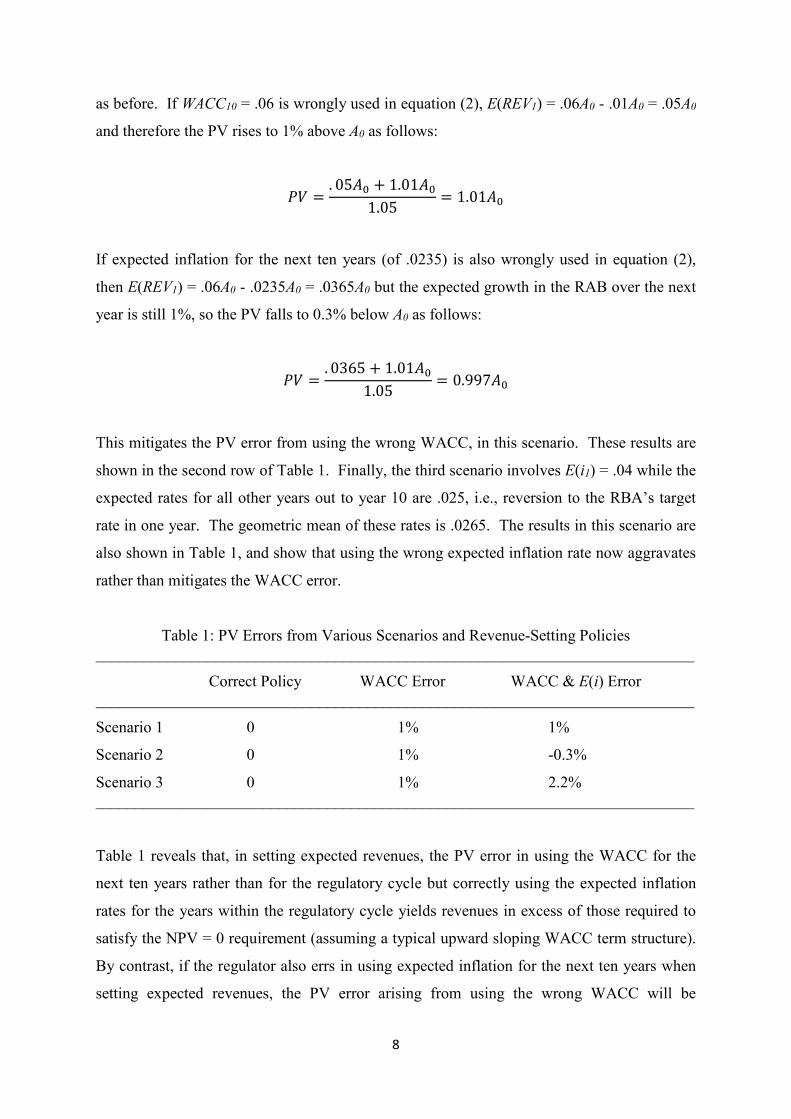
as before. If WACC10 = .06 is wrongly used in equation (2), E(REV1) = .06A0 - .01A0 = .05A0

and therefore the PV rises to 1% above A0 as follows:

𝑃𝑃𝑅𝑅 =. 05𝐴𝐴0 + 1.01𝐴𝐴0

1.05= 1.01𝐴𝐴0

If expected inflation for the next ten years (of .0235) is also wrongly used in equation (2),

then E(REV1) = .06A0 - .0235A0 = .0365A0 but the expected growth in the RAB over the next

year is still 1%, so the PV falls to 0.3% below A0 as follows:

𝑃𝑃𝑅𝑅 =. 0365 + 1.01𝐴𝐴0

1.05= 0.997𝐴𝐴0

This mitigates the PV error from using the wrong WACC, in this scenario. These results are

shown in the second row of Table 1. Finally, the third scenario involves E(i1) = .04 while the

expected rates for all other years out to year 10 are .025, i.e., reversion to the RBA’s target

rate in one year. The geometric mean of these rates is .0265. The results in this scenario are

also shown in Table 1, and show that using the wrong expected inflation rate now aggravates

rather than mitigates the WACC error.

Table 1: PV Errors from Various Scenarios and Revenue-Setting Policies ___________________________________________________________________________

Correct Policy WACC Error WACC & E(i) Error ___________________________________________________________________________

Scenario 1 0 1% 1%

Scenario 2 0 1% -0.3%

Scenario 3 0 1% 2.2% ___________________________________________________________________________

Table 1 reveals that, in setting expected revenues, the PV error in using the WACC for the

next ten years rather than for the regulatory cycle but correctly using the expected inflation

rates for the years within the regulatory cycle yields revenues in excess of those required to

satisfy the NPV = 0 requirement (assuming a typical upward sloping WACC term structure).

By contrast, if the regulator also errs in using expected inflation for the next ten years when

setting expected revenues, the PV error arising from using the wrong WACC will be

9

unaffected if the term structure for expected inflation over the next ten years is flat, mitigated

if the term structure for expected inflation over the next ten years is upward sloping, and

aggravated if the term structure for expected inflation over the next ten years is downward

sloping. Thus, across the three scenarios overall, using the wrong expected inflation rate

does not mitigate the WACC error.

3. Approaches to Estimating the Expected Inflation Rate

3.1 Bond Yields

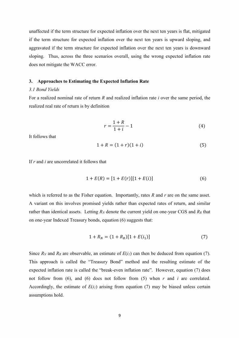
For a realized nominal rate of return R and realized inflation rate i over the same period, the

realized real rate of return is by definition

𝑟𝑟 =1 + 𝑅𝑅1 + 𝑖𝑖

− 1 (4)

It follows that

1 + 𝑅𝑅 = (1 + 𝑟𝑟)(1 + 𝑖𝑖) (5)

If r and i are uncorrelated it follows that

1 + 𝐸𝐸(𝑅𝑅) = [1 + 𝐸𝐸(𝑟𝑟)][1 + 𝐸𝐸(𝑖𝑖)] (6)

which is referred to as the Fisher equation. Importantly, rates R and r are on the same asset.

A variant on this involves promised yields rather than expected rates of return, and similar

rather than identical assets. Letting RN denote the current yield on one-year CGS and RR that

on one-year Indexed Treasury bonds, equation (6) suggests that:

1 + 𝑅𝑅𝑁𝑁 = (1 + 𝑅𝑅𝑅𝑅)[1 + 𝐸𝐸(𝑖𝑖1)] (7)

Since RN and RR are observable, an estimate of E(i1) can then be deduced from equation (7).

This approach is called the “Treasury Bond” method and the resulting estimate of the

expected inflation rate is called the “break-even inflation rate”. However, equation (7) does

not follow from (6), and (6) does not follow from (5) when r and i are correlated.

Accordingly, the estimate of E(i1) arising from equation (7) may be biased unless certain

assumptions hold.

10

Firstly, it is assumed that nominal and indexed bonds are available with the same maturity

dates. However, as noted by Finlay and Olivan (2012, page 50), there do not typically exist

nominal and indexed bonds with the same maturity date, and therefore interpolation would be

required to generate yields over the same period.3 Furthermore, even if the maturity dates

matched, the set of maturity dates for indexed bonds is so limited that interpolation would be

required to generate break-even inflation rates for the desired terms of 1, 2,…5 years. This

interpolation will induce errors in the estimate of expected inflation, because the term

structure of interest rates is not in general linear whilst interpolation typically assumes

linearity. The errors are unlikely to be substantial but the need to do this introduces a highly

undesirable degree of subjectivity into the exercise.

Secondly, it is assumed that the indexed bonds compensate for inflation over the period from

the current moment in time until their maturity. However, inflation-indexed bonds are

subject to lags in correcting for inflation. This too will induce errors in the estimate for

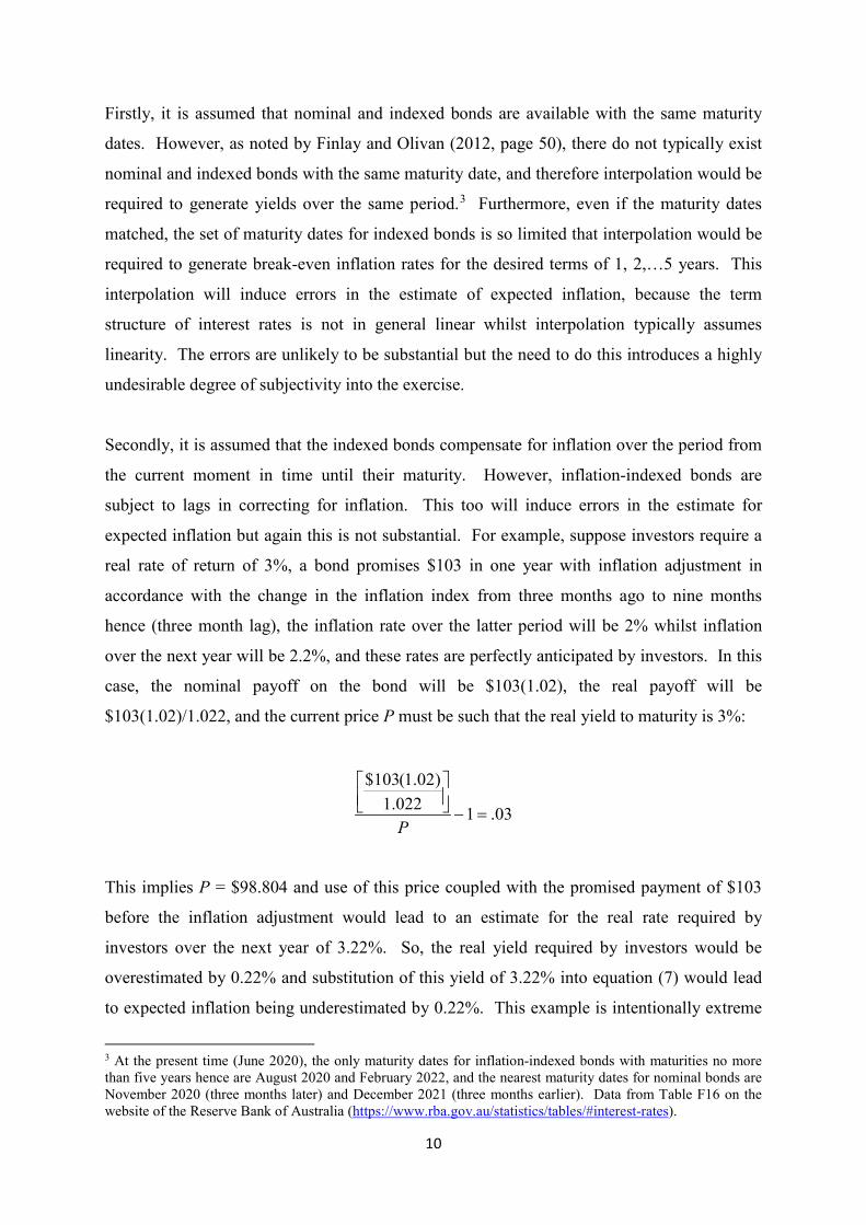
expected inflation but again this is not substantial. For example, suppose investors require a

real rate of return of 3%, a bond promises $103 in one year with inflation adjustment in

accordance with the change in the inflation index from three months ago to nine months

hence (three month lag), the inflation rate over the latter period will be 2% whilst inflation

over the next year will be 2.2%, and these rates are perfectly anticipated by investors. In this

case, the nominal payoff on the bond will be $103(1.02), the real payoff will be

$103(1.02)/1.022, and the current price P must be such that the real yield to maturity is 3%:

03.1022.1)02.1(103$

=−

P

This implies P = $98.804 and use of this price coupled with the promised payment of $103

before the inflation adjustment would lead to an estimate for the real rate required by

investors over the next year of 3.22%. So, the real yield required by investors would be

overestimated by 0.22% and substitution of this yield of 3.22% into equation (7) would lead

to expected inflation being underestimated by 0.22%. This example is intentionally extreme

3 At the present time (June 2020), the only maturity dates for inflation-indexed bonds with maturities no more than five years hence are August 2020 and February 2022, and the nearest maturity dates for nominal bonds are November 2020 (three months later) and December 2021 (three months earlier). Data from Table F16 on the website of the Reserve Bank of Australia (https://www.rba.gov.au/statistics/tables/#interest-rates).

11

in order to dramatise the point. However, empirical estimates (Grishchenko and Huang,

2012, Table 2) reveal that the effect is no more than 0.04%.

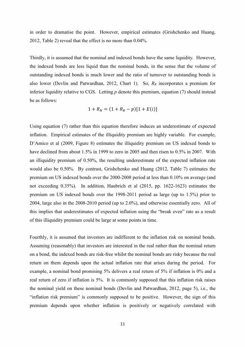
Thirdly, it is assumed that the nominal and indexed bonds have the same liquidity. However,

the indexed bonds are less liquid than the nominal bonds, in the sense that the volume of

outstanding indexed bonds is much lower and the ratio of turnover to outstanding bonds is

also lower (Devlin and Patwardhan, 2012, Chart 1). So, RR incorporates a premium for

inferior liquidity relative to CGS. Letting p denote this premium, equation (7) should instead

be as follows:

1 + 𝑅𝑅𝑁𝑁 = (1 + 𝑅𝑅𝑅𝑅 − 𝑝𝑝)[1 + 𝐸𝐸(𝑖𝑖)]

Using equation (7) rather than this equation therefore induces an underestimate of expected

inflation. Empirical estimates of the illiquidity premium are highly variable. For example,

D’Amico et al (2009, Figure 8) estimates the illiquidity premium on US indexed bonds to

have declined from about 1.5% in 1999 to zero in 2005 and then risen to 0.5% in 2007. With

an illiquidity premium of 0.50%, the resulting underestimate of the expected inflation rate

would also be 0.50%. By contrast, Grishchenko and Huang (2012, Table 7) estimates the

premium on US indexed bonds over the 2000-2008 period at less than 0.10% on average (and

not exceeding 0.35%). In addition, Haubrich et al (2015, pp. 1622-1623) estimates the

premium on US indexed bonds over the 1998-2011 period as large (up to 1.5%) prior to

2004, large also in the 2008-2010 period (up to 2.0%), and otherwise essentially zero. All of

this implies that underestimates of expected inflation using the “break even” rate as a result

of this illiquidity premium could be large at some points in time.

Fourthly, it is assumed that investors are indifferent to the inflation risk on nominal bonds.

Assuming (reasonably) that investors are interested in the real rather than the nominal return

on a bond, the indexed bonds are risk-free whilst the nominal bonds are risky because the real

return on them depends upon the actual inflation rate that arises during the period. For

example, a nominal bond promising 5% delivers a real return of 5% if inflation is 0% and a

real return of zero if inflation is 5%. It is commonly supposed that this inflation risk raises

the nominal yield on these nominal bonds (Devlin and Patwardhan, 2012, page 5), i.e., the

“inflation risk premium” is commonly supposed to be positive. However, the sign of this

premium depends upon whether inflation is positively or negatively correlated with

12

favourable economic states, and this is a contentious question (Bekaert and Wang, 2009, pp,

779-780; Grishchenko and Huang, 2012, pp. 5-6).

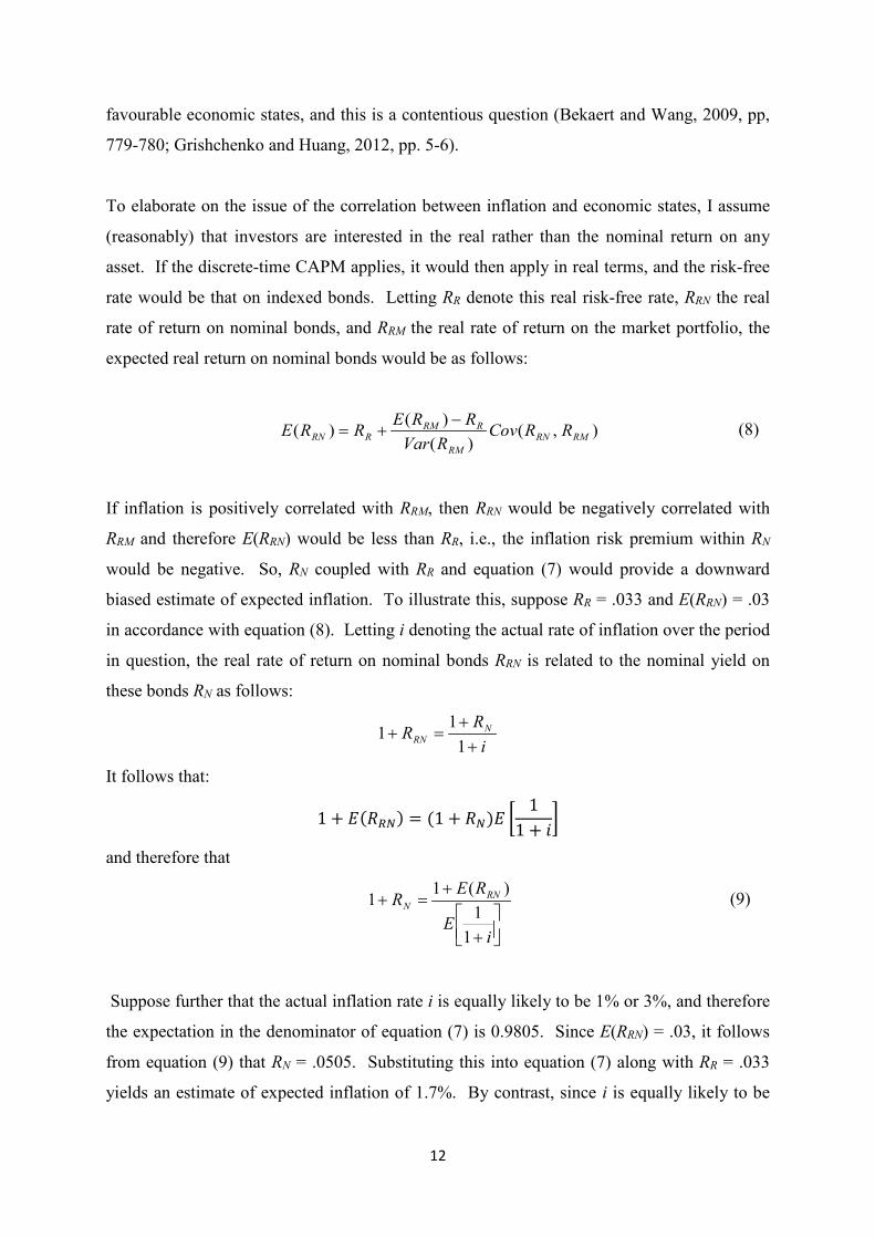
To elaborate on the issue of the correlation between inflation and economic states, I assume

(reasonably) that investors are interested in the real rather than the nominal return on any

asset. If the discrete-time CAPM applies, it would then apply in real terms, and the risk-free

rate would be that on indexed bonds. Letting RR denote this real risk-free rate, RRN the real

rate of return on nominal bonds, and RRM the real rate of return on the market portfolio, the

expected real return on nominal bonds would be as follows:

),()(

)()( RMRNRM

RRMRRN RRCov

RVarRRERRE −

+= (8)

If inflation is positively correlated with RRM, then RRN would be negatively correlated with

RRM and therefore E(RRN) would be less than RR, i.e., the inflation risk premium within RN

would be negative. So, RN coupled with RR and equation (7) would provide a downward

biased estimate of expected inflation. To illustrate this, suppose RR = .033 and E(RRN) = .03

in accordance with equation (8). Letting i denoting the actual rate of inflation over the period

in question, the real rate of return on nominal bonds RRN is related to the nominal yield on

these bonds RN as follows:

iRR N

RN ++

=+1

11

It follows that:

1 + 𝐸𝐸(𝑅𝑅𝑅𝑅𝑁𝑁) = (1 + 𝑅𝑅𝑁𝑁)𝐸𝐸 �1

1 + 𝑖𝑖�

and therefore that

+

+=+

iE

RER RNN

11

)(11 (9)

Suppose further that the actual inflation rate i is equally likely to be 1% or 3%, and therefore

the expectation in the denominator of equation (7) is 0.9805. Since E(RRN) = .03, it follows

from equation (9) that RN = .0505. Substituting this into equation (7) along with RR = .033

yields an estimate of expected inflation of 1.7%. By contrast, since i is equally likely to be

13

1% or 3% in this example, the expected rate of inflation is 2%. So, the use of equation (7)

would lead to an underestimate of the expected inflation rate of 0.30%.

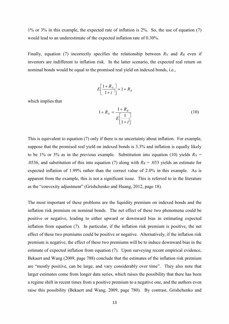
Finally, equation (7) incorrectly specifies the relationship between RN and RR even if

investors are indifferent to inflation risk. In the latter scenario, the expected real return on

nominal bonds would be equal to the promised real yield on indexed bonds, i.e.,

RN Ri

RE +=

++ 11

1

which implies that

+

+=+

iE

RR RN

11

11 (10)

This is equivalent to equation (7) only if there is no uncertainty about inflation. For example,

suppose that the promised real yield on indexed bonds is 3.3% and inflation is equally likely

to be 1% or 3% as in the previous example. Substitution into equation (10) yields RN =

.0536, and substitution of this into equation (7) along with RR = .033 yields an estimate for

expected inflation of 1.99% rather than the correct value of 2.0% in this example. As is

apparent from the example, this is not a significant issue. This is referred to in the literature

as the “convexity adjustment” (Grishchenko and Huang, 2012, page 18).

The most important of these problems are the liquidity premium on indexed bonds and the

inflation risk premium on nominal bonds. The net effect of these two phenomena could be

positive or negative, leading to either upward or downward bias in estimating expected

inflation from equation (7). In particular, if the inflation risk premium is positive, the net

effect of these two premiums could be positive or negative. Alternatively, if the inflation risk

premium is negative, the effect of these two premiums will be to induce downward bias in the

estimate of expected inflation from equation (7). Upon surveying recent empirical evidence,

Bekaert and Wang (2009, page 788) conclude that the estimates of the inflation risk premium

are “mostly positive, can be large, and vary considerably over time”. They also note that

larger estimates come from longer data series, which raises the possibility that there has been

a regime shift in recent times from a positive premium to a negative one, and the authors even

raise this possibility (Bekaert and Wang, 2009, page 780). By contrast, Grishchenko and

14

Huang (2012, page 6) conclude that “..there appears no consensus so far in the (empirical)

literature as to not only the magnitude of the inflation risk premium but also its sign.”

More recently, using Australian data over the period 1992-2010, Finlay and Wende (2012,

Figure 3) estimate the net effect of these two phenomena at from 2.5% to -1.0% over both

five and ten year periods. In addition, using US data over the shorter and more stable

inflationary period from 2000 to 2008, Grishchenko and Huang (2012, Table 6) estimate the

net effect to be negative, statistically significant, and up to 0.50% depending upon the term of

the bonds used and the method for estimating expected inflation. Grishchenko and Huang

(2012, section 5.3) also conclude that the net premium changed from negative to

approximately zero in 2004. In addition, Fleckenstein et al (2014) find that there are large

discrepancies between the price of nominal bonds and a package of indexed bonds and

derivative contracts (inflation swaps) with the same payoffs. They conclude that the cause of

this is mispricing in the bond markets, and the mispricing in terms of interest rates has been

up to 1.8% (ibid, Figure 2). All of this suggests that the “break-even inflation rate” is liable

to be a poor estimator of the expected inflation rate.

Attempting to correct it for the effect of risk and illiquidity would also yield a poor estimator

because the appropriate corrections for these two effects are very unclear. Furthermore, any

such correction could be worse than no such correction. For example, if the net effect of

these two issues is an overestimate of expected inflation of 0.20%, but is mistakenly

estimated to be an overestimate of 0.50% with the result that the break-even rate is reduced

by 0.50%, the error is then an underestimate of 0.30%, which is worse than the 0.20%

overestimate resulting from making no adjustment.

If these problems tended to net out over successive regulatory cycles, they would be less

concerning. However there is no reason to suppose that this would occur, i.e., the method is

likely to be biased over the life of the assets. Thus, significant violations of the NPV = 0

principle are possible from the use of the “break-even” inflation rate.

3.2 Inflation Swaps

An estimate of expected inflation can also be obtained from the fixed rate in zero-coupon

inflation swaps, which involves one party (the Inflation Receiver) paying at the maturity of

the contract a rate set at the commencement of the contract (P) and receiving at contract

15

maturity the realized rate of inflation over the term of the contract, whilst the other party (the

Inflation Payer) is in the opposite position. This fixed rate P is treated as an estimate of

expected inflation.

As with the break-even rate, the two principal problems are premiums for inflation risk and

illiquidity. Consider inflation risk. Letting Pc denote the present value of P, the nominal rate

of return to an Inflation Receiver would then be (i/Pc) - 1, the real rate of return would then

be [i/Pc(1+i)] – 1. Following equation (8), the expected real rate of return on this asset in

accordance with the CAPM (in real terms) would be as follows:

+

−+=−

+ RM

cRM

RRMR

c

RiP

iCovRVar

RRERiP

iE ,)1()(

)(1)1(

(11)

Since the payment P at the maturity date of the contract is fixed in nominal terms, its present

value Pc is P discounted at the nominal risk-free rate RN, and therefore

+

−++=

++

RMcRM

RRMR

N

RiP

iCovRVar

RRERi

RP

iE ,)1()(

)(1)1(

)1(

To a close approximation this is

𝐸𝐸(𝑖𝑖)𝑃𝑃

𝐸𝐸 �1 + 𝑅𝑅𝑁𝑁1 + 𝑖𝑖

� = 1 + 𝑅𝑅𝑅𝑅 + �𝐸𝐸(𝑅𝑅𝑅𝑅𝑅𝑅) − 𝑅𝑅𝑅𝑅𝑅𝑅𝑉𝑉𝑟𝑟(𝑅𝑅𝑅𝑅𝑅𝑅)

� 𝐶𝐶𝐶𝐶𝐶𝐶 �𝑖𝑖

𝑃𝑃𝐶𝐶(1 + 𝑖𝑖),𝑅𝑅𝑅𝑅𝑅𝑅�

i.e.,

𝐸𝐸(𝑖𝑖)𝑃𝑃

[1 + 𝐸𝐸(𝑅𝑅𝑅𝑅𝑁𝑁)] = 1 + 𝑅𝑅𝑅𝑅 + �𝐸𝐸(𝑅𝑅𝑅𝑅𝑅𝑅) − 𝑅𝑅𝑅𝑅𝑅𝑅𝑉𝑉𝑟𝑟(𝑅𝑅𝑅𝑅𝑅𝑅)

� 𝐶𝐶𝐶𝐶𝐶𝐶 �𝑖𝑖

𝑃𝑃𝐶𝐶(1 + 𝑖𝑖),𝑅𝑅𝑅𝑅𝑅𝑅�

So

)(1

,)1()(

)(1)(

RN

RMcRM

RRMR

RE

RiP

iCovRVar

RRER

PiE

+

+

−++

=

16

Invoking the CAPM (in real terms) again, following equation (8), this is as follows:

),()(

(1

,)1()(

)(1)(

RMRNRM

RRMR

RMcRM

RRMR

RRCovRVar

RRER

RiP

iCovRVar

RRER

PiE

−++

+

−++

=

++

−++

+

−++

=

RMN

RM

RRMR

RMcRM

RRMR

Ri

RCovRVar

RRER

RiP

iCovRVar

RRER

,1

1)(

(1

,)1()(

)(1 (12)

If the inflation rate i is positively correlated with the real market return RRM, then the

covariance term in the numerator of equation (12) will be positive and that in the

denominator will be negative. So the inflation swap price P will be less than E(i), and

therefore P will be a downward biased estimator of expected inflation. Letting RP denote

this risk premium

𝑃𝑃 = 𝐸𝐸(𝑖𝑖) + 𝑅𝑅𝑃𝑃

So, if E(i) = .03 and P = .02, using P to estimate E(i) yields an underestimate of E(i) of .01.

Turning now to the issue of illiquidity, Devlin and Patwardhan (2012, page 6) note that these

contracts have poor liquidity in the event of one party seeking an early exit, and suggest that

this would affect the swap price P. This would require parties on one side (buyers or sellers)

to compensate parties on the other side, which is possible if the former group were hedgers.

This would raise or lower P depending upon whether buyers or sellers provided the

compensation to the other group, and therefore would cause P to underestimate or

overestimate expected inflation.

As with the break-even rate, the net effect of these premiums for risk and illiquidity is

unclear. So, the swap price is likely to be a poor estimator of expected inflation, as would the

swap price subject to any attempted correction for these effects.

3.3 RBA Inflation Target

17

Another approach to forecasting inflation is use of the midpoint of the RBA’s target band for

inflation (2.5%). Inflation targeting commenced in Australia in early 1993. For the calendar

years 1994 – 2019, the arithmetic average of the annual inflation rates was 2.49% per year.4

This demonstrates that the RBA has been extremely successful (on average). However, there

has been considerable variation around this, with an estimated standard deviation of 1.2%.

Furthermore, there has been noticeable clustering in outcomes both above and below the

average. In particular, the annual rates were below 2.5% in every quarter from September

1996 to December 1999, and in every quarter since September 2014, whilst they exceeded

2.5% in every quarter from March 2000 to December 2003. Expressed more formally, the

annual rates appear to be a mean-reverting process. So, if the rate is above (below) 2.5%, it is

expected to remain so for some period. Regressing calendar year rates (in percentage terms)

on the preceding year’s value yields the following result:

𝑖𝑖𝑡𝑡 = 1.962 + 0.21𝑖𝑖𝑡𝑡−1 (13)

This is a mean-reverting model, and expressing it in the following equivalent form reveals

that rates revert to a mean of 2.48% (which is almost identical to the RBA’s Target):

𝑖𝑖𝑡𝑡 = 𝑖𝑖𝑡𝑡−1 + 0.79(2.48 − 𝑖𝑖𝑡𝑡−1)

So, given the latest inflation rate, this model predicts the rate for the next year, which is fed

back into the model to predict the rate one year later, and so on. For example, if the latest

rate is 4%, the prediction for next year is 2.8%, and for the year after is 2.6%. Similarly, if

the latest rate is 1%, the prediction for next year is 2.2%, and for the year after is 2.4%. So,

this model implies that reversion to the mean is largely achieved within two years. However,

the p value on the second coefficient in equation (13) is high (0.31), and therefore the

resulting predictions are not statistically compelling (i.e., wide confidence intervals). This

may be due to the limited set of annual observations. Using quarterly data instead yields

𝑖𝑖𝑡𝑡 = 0.509 + 0.175𝑖𝑖𝑡𝑡−1 (14)

4 Data from column C of Table G1 on the website of the Reserve Bank of Australia (http://www.rba.gov.au/statistics/tables/#inflation-expectations).

18

with a p value on the second coefficient of 0.07. This is statistically much more compelling.

Equation (14) is equivalent to the following mean-reverting model, in which (quarterly) rates

revert to a mean of 0.617% (equivalent to 2.49% per year):

𝑖𝑖𝑡𝑡 = 𝑖𝑖𝑡𝑡−1 + 0.825(0.617 − 𝑖𝑖𝑡𝑡−1)

For example, if the latest rate is 1% for the quarter, equivalent to 4% per year, the prediction

for next quarter is year is 0.68%, followed by 0.63% and then 0.62%. Similarly, if the latest

rate is 0.25% for the quarter, equivalent to 1% per year, the prediction for the next quarter is

0.55%, followed by 0.60%, 0.61% and then 0.62%. So, this model implies that reversion to

the mean is largely achieved within a year.

Consistent with this statistical evidence of mean reversion, credible short-term forecasts of

inflation have differed from 2.5%. For example, the RBA’s survey of market economists’

one-year ahead inflation expectations have ranged from 1.8% to 5.5% over the period for

which this survey has been conducted, whilst those for two years ahead have ranged from

1.8% to 4.9%.5 Thus, even if there has been no regime change, for the purposes of estimating

expected inflation over the next year and possibly longer, the RBA’s inflation target would be

unsatisfactory because it implicitly predicts immediate reversion to 2.5%.

3.4 Model Based Forecasts

Econometric models can also be used to forecast inflation. The simplest such models use

only past data. One such example is a random walk, i.e., using the latest observation as the

forecast. A more sophisticated approach using only past data is the mean reverting model, as

described in the previous section. An even more sophisticated approach is that of Finlay and

Wende (2012), based upon Australian data over the 1992-2010 period, using yields on

nominal and inflation-indexed bonds along with economists’ forecasts of inflation, and

requiring 20 parameters to be estimated. A similarly sophisticated approach is that of

Grishchenko and Huang (2012), using US data over the period 2000-2008. A drawback from

such sophisticated approaches is the unlimited number of potential models. So, if the AER

5 Data from Table G3 on the website of the Reserve Bank of Australia (http://www.rba.gov.au/statistics/tables/#inflation-expectations).

19

chose one such model, it would invite regulated businesses and consumer groups to provide

their preferred models.

3.5 Survey Evidence

Another approach is to use survey evidence from credible forecasters. For example, the RBA

reports its survey of market economists’ one-year and two-year ahead inflation expectations.

These subjective forecasts could be expected to outperform more mechanical approaches (the

approaches described above) because any merit in such mechanical approaches could be

expected to be incorporated into the subjective forecasts. As a former central banker, Vahey

(2017, page 7) affirms this point, with explicit reference to central banks monitoring of the

break-even inflation rate. However, no such forecasts are publicly available for more than

two years ahead.

3.6 Survey Evidence Coupled with the Inflation Target

Another approach to forecasting inflation would be to use the RBA’s forecasts and/or survey

evidence for the years for which they are available in conjunction with the RBA’s Target for

the remaining years. This is the AER’s current approach, in which it uses the RBA’s

forecasts for the first two years (the period for which they are available) coupled with the

RBA’s Target of 2.5% for the remaining years of the ten-year forecasting period. So long as

the RBA’s one-year and two-year ahead forecasts are superior to the RBA’s Target, this

estimator will be superior to exclusive use of the Target.

4. Empirical Analysis

4.1 Previous Analysis

Tulip and Wallace (2012, Table 1) use data from 1993 – 2011 to assess the forecast accuracy

of a range of inflation forecasting methods for one year ahead and for the second year ahead.

For one year ahead, the root mean squared error (RMSE) for the RBA’s forecasts is 0.89%,

1.41% for the RBA’s Target, and 1.90% for the Random Walk. For the second year ahead,

the results are 1.27%, 1.36% and 2.19% respectively. All of these differences are statistically

significant except for that between the RBA forecasts and the Target for the second year

ahead. In respect of the RBA’s forecasts, Tulip and Wallace (2012, Table 4) also report that

the biases are immaterial and are not statistically significant. Tulip and Wallace (2012, Table

2) also report that the RMSE of the RBA’s forecasts are only marginally superior to those

provided by other private sector forecasters and the differences are not statistically

20

significant. The superiority of these judgmental forecasts over the mechanical forecasts

(Target and Random walk) is unsurprising because the merits of any forecasts that are

mechanical could be expected to be impounded into the judgmental forecasts.

Finlay and Wende (2012, Figure 2) present forecasts of inflation for 1992-2000, based on a

combination of break-even inflation rates and surveys of forecasters. However they do not

present any formal test of the forecast accuracy of this predictor, and this will be done in the

next section.

Mathysen (2017, Figure 3) presents three different time-series of estimates of the ten-year

break-even inflation rate in Australia, over the period 2000-2016. For all three series, the

results oscillate around the average realized inflation rate of 2.6% since March 2000 (which

in turn is close to the RBA’s Target of 2.5%) but the results in each series are extremely

variable over time, even within the course of a few months (with the most extreme change

being a drop from 3.8% to 1.5% in early 2008). By contrast, since March 2000, the average

realized inflation rate over a ten-year period has not changed by more than 0.3% over the

course of six months.6 This suggests that the premiums for risk and illiquidity within the

break-even rates fluctuated substantially over time and/or investors overreacted to short-term

changes in inflation when estimating the long-term future rate; in either case, the break-even

rate would seem to be a poor estimator for expected inflation. Mathysen does not present any

formal test of the forecast accuracy of these break-even rates, and this will be done in the next

section.

Mathysen (2017, Figure 15) also presents a time-series of ten-year swap prices and the ten-

year break-even rate, over the period October 2009 – June 2016. The swap prices were much

less volatile over time than the break-even inflation rate (and almost entirely within the

RBA’s inflation band). However the time series of swap prices was above the average

realized inflation rate throughout the entire period analysed, and by about 1% for the first half

of the time series, which suggests that they are significantly biased up as predictors. The

swap price also generally exceeded the contemporaneous break-even rate (by about 0.30% in

the last half of the time series). Since both purport to reflect market expectations of future

6 Data from column C of Table G1 on the website of the Reserve Bank of Australia (http://www.rba.gov.au/statistics/tables/#inflation-expectations).

21

inflation embedded in market prices, this persistent discrepancy undercuts the credibility of

both of them. Again, Mathysen does not present any formal test of the forecast accuracy of

the swap rate, and this will be done in the next section.

4.2 Additional Tests

I commence by extending the work of Tulip and Wallace (2012) to include data to 2019, and

to present forecasts for future years beyond the second year where possible. The RBA

provides the RBA forecasts used by these authors, up to 2011, which arise from the RBA’s

Statements of Monetary Policy (SMP) and earlier counterparts.7 I have checked these

reported forecasts against the SMPs, and a number of discrepancies are apparent, most

particularly that for the year ended December 2012, for which the November 2011 SMP

(page 66) gives 3.25% whilst the RBA’s excel file (at CK101) gives 2.56%.8 Accordingly, I

source the RBA’s forecasts from the SMPs as far back as they provide them (November

2007), and earlier from the RBA’s excel file. For the SMPs from November 2007, the RBA

provides a forecast for the following calendar year and the next calendar year. By contrast,

prior to that, the RBA’s excel file only presents forecasts for the next calendar year and the

year ending six months later.

By definition, a forecast must be provided prior to the commencement of the period for which

the variable is forecasted, and it should be as close as possible to the commencement of that

period. Since the SMP forecasts presented from November 2007 are for years ended

December and June, I elect to use calendar years as the period to be forecast and source the

forecasts from the relevant November SMP. So, for example, the SMP forecast for the 2019

calendar year is drawn from the November 2018 SMP. For the period 2000-2006, the

forecasts are taken from the RBA’s excel file for November of that year. For the period

1993-1999, they are taken from the RBA’s excel file for December of that year.

Furthermore, for this total period 1993-2006, the RBA’s annual forecasts in their excel file

extend only as far as the first half of the second calendar year following the forecast. So, the

forecasts presented in November or December of a year that are used here are for the

following calendar year, and for the year ending six months later (which are forecasts for one

7 These are provided in the fourth tab (“CPI – 4 Quarter Change”) of the excel file named “Forecast Data by Event Date” on the Bank’s website: https://www.rba.gov.au/publications/rdp/2012/2012-07-data.html. 8 The SMPs are available at https://www.rba.gov.au/publications/smp/2019/nov/.

22

year ahead and 1.5 years ahead). The actual inflation rates for the relevant years are drawn

from the RBA data noted in footnote 5.

To illustrate, the first forecasts used are those presented in December 1993, for calendar 1994

(3.0%) and the year ended June 1995 (2.8%), with the former being a forecast for one year

ahead and the latter being a forecast for 1.5 years ahead. The actual inflation rate for

calendar 1994 was 2.6% and that for the year ended June 1995 was 4.5%. So, in respect of

these forecasts presented in December 1993, the one year ahead forecast error (for calendar

1994) was 2.6% - 3.0% whilst the 1.5-year ahead forecast error (for the year ended June

1995) was 4.5% - 2.8%. The last forecasts used are that in the November 2017 SMP for the

second year ahead (calendar 2019: 2.25%) and that in the November 2018 SMP for one year

ahead (calendar 2019: 2.25%); the actual inflation rate for 2019 was 1.8%, yielding forecast

errors of 1.8% - 2.25% for both the one and two-year ahead forecasts.

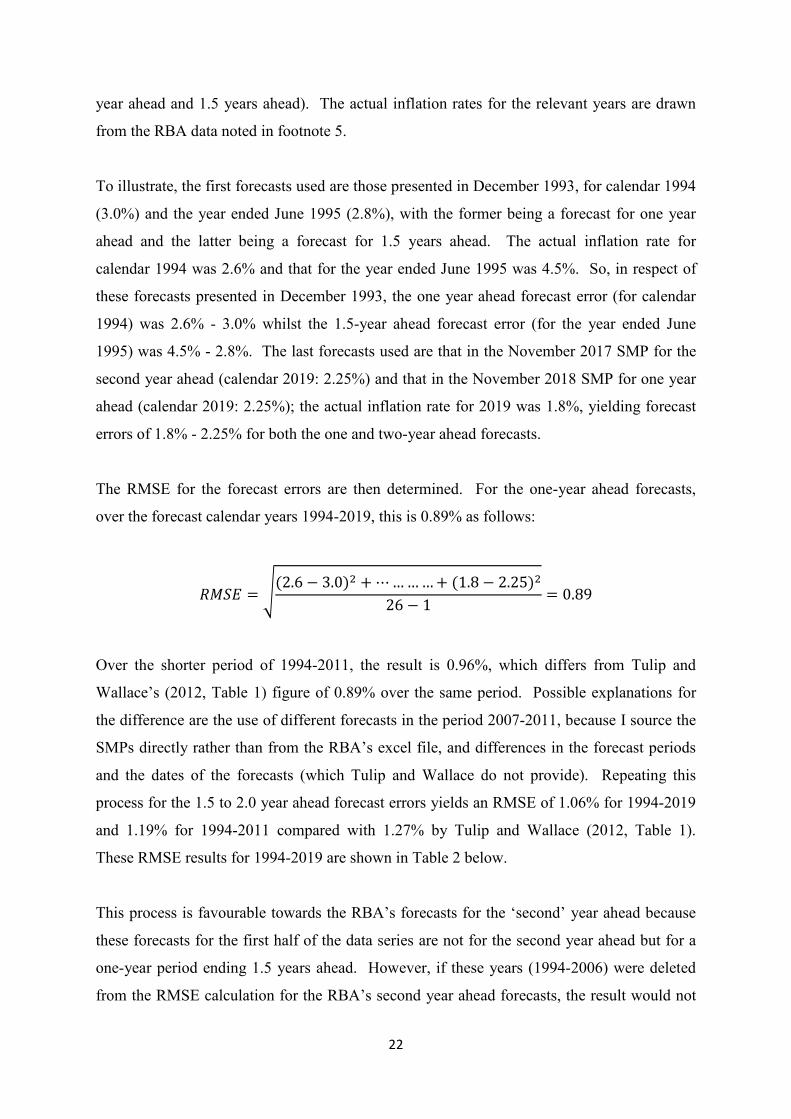
The RMSE for the forecast errors are then determined. For the one-year ahead forecasts,

over the forecast calendar years 1994-2019, this is 0.89% as follows:

𝑅𝑅𝑅𝑅𝑅𝑅𝐸𝐸 = �(2.6 − 3.0)2 + ⋯… … … + (1.8 − 2.25)2

26 − 1= 0.89

Over the shorter period of 1994-2011, the result is 0.96%, which differs from Tulip and

Wallace’s (2012, Table 1) figure of 0.89% over the same period. Possible explanations for

the difference are the use of different forecasts in the period 2007-2011, because I source the

SMPs directly rather than from the RBA’s excel file, and differences in the forecast periods

and the dates of the forecasts (which Tulip and Wallace do not provide). Repeating this

process for the 1.5 to 2.0 year ahead forecast errors yields an RMSE of 1.06% for 1994-2019

and 1.19% for 1994-2011 compared with 1.27% by Tulip and Wallace (2012, Table 1).

These RMSE results for 1994-2019 are shown in Table 2 below.

This process is favourable towards the RBA’s forecasts for the ‘second’ year ahead because

these forecasts for the first half of the data series are not for the second year ahead but for a

one-year period ending 1.5 years ahead. However, if these years (1994-2006) were deleted

from the RMSE calculation for the RBA’s second year ahead forecasts, the result would not

23

be comparable with all other forecasts. Alternatively, if all such years were deleted from the

analysis, then valuable information would be lost. I therefore retain these 1.5 year ahead

RBA forecasts.

A second possible forecasting method is use of the RBA’s target inflation rate of 2.5%. So,

for the one-year ahead forecasts, the forecasts are all 2.5% and the actual outcomes are those

for 1994 (2.6%), …….2019 (1.8%). The resulting RMSE is 1.18%. For the second year

ahead, the process is the same except that the forecasts commence at the beginning of 1994

with a forecast then of the actual rate for 1995. The resulting RMSE is 1.21%. For forecasts

for the third, fourth, fifth and tenth years ahead, using the same approach, the RMSE results

are 1.11%, 1.11%, 0.96% and 0.64%. The difference in results is purely an artefact of

deleting progressively more observations at the beginning of the time series coupled with the

fact that these rates were unusually variable. All of these results are shown in Table 2 below.

A third possibility is use of the Random Walk approach: the one-year ahead forecast for

inflation in a particular year (t) is the outcome in the previous year, the second year ahead

forecast for inflation in year t is the outcome in the penultimate year, and so on. The RMSE

results are shown In Table 2 below.

A fourth possibility is the forecasts by Consensus Economics, which provides forecasts for

calendar years out to ten years ahead and has done so over the 1994-2019 period. For most

of this period, forecasts were generated bi-annually in early October and early April. Since

forecasts should precede the period forecasted, and to the least possible extent, I therefore

utilize the Consensus forecasts in October to forecast the outcomes in the following calendar

years. For example, the forecasts in October 1993 for 1994 and 1995 were 3.3% and 3.9%

respectively. The actual outcomes were 2.6% and 5.1% respectively, yielding forecast errors

of 2.6% - 3.3% for one year ahead and 5.1% - 3.9% for the second year ahead. The RMSE

results are shown in Table 2 below.

A fifth possibility is the Mean Reversion model in equation (14), in which the quarterly

inflation in the December quarter is used to forecast the next quarter’s inflation, which is then

used to forecast the next quarter’s inflation, and so on for the next two quarters; these four

quarterly forecasts are then summed to yield the forecast for the calendar year. Following

this process, the quarterly inflation of 0.2% for Dec 1993 yields a forecast for 1994 of 2.38%.

24

Since inflation for 1994 was 2.6%, the resulting forecast error was 0.22%. The RMSE of

these one-year ahead forecast errors over the 1994-2019 period is 1.17, as shown in Table 2.

Since reversion to the target is forecast to occur by essentially the end of the first year, this

approach would yield essentially the same results as use of the Target for forecast years

beyond the first, and therefore these results need not be calculated. This process is prejudiced

in favour of the Mean Reversion model because the data used to test the forecasts is also used

to estimate the parameters in the model; the model then has knowledge of the data that is

being forecasted. Despite this advantage, it is still outperformed by the RBA’s forecasts,

which reinforces the conclusion that the latter are superior.

A sixth possibility is the model of Finlay and Wende (2012), who present forecasts of

inflation for 1992-2010, based on a combination of break-even inflation rates and surveys of

forecasters (ibid, Figure 2). I couple their estimates for the one-year ahead inflation rate as at

mid 1993, mid 1994, ….mid 2010 with the realized inflation rate for the following year (year

ending June 1994,….year ending June 2011). The bias in the forecasts (0.1%) is immaterial

(and statistically insignificant) whilst the RMSE of the forecast errors is 1.35%.9 The time

period examined is similar to that by Tulip and Wallace (2012), whose RMSE for the RBA’s

forecasts for one-year ahead is 0.89%, and therefore the RBA’s forecasts are significantly

superior. Furthermore, since Finlay and Wende’s forecasts are based on a combination of

break-even inflation rates and survey estimates from Consensus Economics, and the latter are

comparable in forecast accuracy to the RBA’s forecasts (see Tulip and Wallace, 2012, Table

2), it follows that the RBA’s forecasts are significantly superior to break-even rates. This is

unsurprising because the break-even rate is a poor forecaster (due to illiquidity and risk

components) and any merits from this approach could be expected to be impounded into the

RBA’s forecasts.

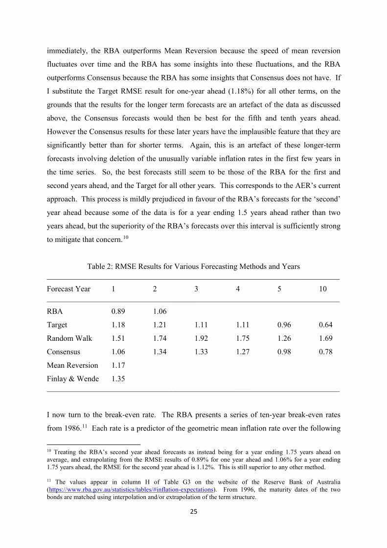
As shown in Table 2, for the first and second years ahead, the lowest RMSE is from the RBA

forecasts. For all other forecast years, the lowest RMSE is from use of the Target. The result

for the first and second years ahead are unsurprising; the RBA outperforms the Random Walk

because the latter fails to recognize that inflation rates are mean reverting, the RBA

outperforms the Target because the latter implicitly assumes that mean reversion occurs

9 Since the results from attempting to read off the data from Finlay and Wende (2012, Figure 2) are too imprecise I sought the data from the RBA and it was kindly supplied.

25

immediately, the RBA outperforms Mean Reversion because the speed of mean reversion

fluctuates over time and the RBA has some insights into these fluctuations, and the RBA

outperforms Consensus because the RBA has some insights that Consensus does not have. If

I substitute the Target RMSE result for one-year ahead (1.18%) for all other terms, on the

grounds that the results for the longer term forecasts are an artefact of the data as discussed

above, the Consensus forecasts would then be best for the fifth and tenth years ahead.

However the Consensus results for these later years have the implausible feature that they are

significantly better than for shorter terms. Again, this is an artefact of these longer-term

forecasts involving deletion of the unusually variable inflation rates in the first few years in

the time series. So, the best forecasts still seem to be those of the RBA for the first and

second years ahead, and the Target for all other years. This corresponds to the AER’s current

approach. This process is mildly prejudiced in favour of the RBA’s forecasts for the ‘second’

year ahead because some of the data is for a year ending 1.5 years ahead rather than two

years ahead, but the superiority of the RBA’s forecasts over this interval is sufficiently strong

to mitigate that concern.10

Table 2: RMSE Results for Various Forecasting Methods and Years ___________________________________________________________________________

Forecast Year 1 2 3 4 5 10 ___________________________________________________________________________

RBA 0.89 1.06

Target 1.18 1.21 1.11 1.11 0.96 0.64

Random Walk 1.51 1.74 1.92 1.75 1.26 1.69

Consensus 1.06 1.34 1.33 1.27 0.98 0.78

Mean Reversion 1.17

Finlay & Wende 1.35 ___________________________________________________________________________

I now turn to the break-even rate. The RBA presents a series of ten-year break-even rates

from 1986.11 Each rate is a predictor of the geometric mean inflation rate over the following

10 Treating the RBA’s second year ahead forecasts as instead being for a year ending 1.75 years ahead on average, and extrapolating from the RMSE results of 0.89% for one year ahead and 1.06% for a year ending 1.75 years ahead, the RMSE for the second year ahead is 1.12%. This is still superior to any other method. 11 The values appear in column H of Table G3 on the website of the Reserve Bank of Australia (https://www.rba.gov.au/statistics/tables/#inflation-expectations). From 1996, the maturity dates of the two bonds are matched using interpolation and/or extrapolation of the term structure.

26

ten years, and these rates can be compared to the actual geometric mean over each such ten

year period. For example, the break-even rate in December 1993 (of 3.0%) is a predictor of

the geometric mean inflation rate over the period 1994-2003 inclusive (which was 2.64%).

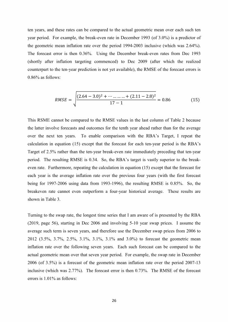
The forecast error is then 0.36%. Using the December break-even rates from Dec 1993

(shortly after inflation targeting commenced) to Dec 2009 (after which the realized

counterpart to the ten-year prediction is not yet available), the RMSE of the forecast errors is

0.86% as follows:

𝑅𝑅𝑅𝑅𝑅𝑅𝐸𝐸 = �(2.64 − 3.0)2 + ⋯… … … + (2.11 − 2.8)2

17 − 1= 0.86 (15)

This RSME cannot be compared to the RMSE values in the last column of Table 2 because

the latter involve forecasts and outcomes for the tenth year ahead rather than for the average

over the next ten years. To enable comparison with the RBA’s Target, I repeat the

calculation in equation (15) except that the forecast for each ten-year period is the RBA’s

Target of 2.5% rather than the ten-year break-even rate immediately preceding that ten-year

period. The resulting RMSE is 0.34. So, the RBA’s target is vastly superior to the break-

even rate. Furthermore, repeating the calculation in equation (15) except that the forecast for

each year is the average inflation rate over the previous four years (with the first forecast

being for 1997-2006 using data from 1993-1996), the resulting RMSE is 0.85%. So, the

breakeven rate cannot even outperform a four-year historical average. These results are

shown in Table 3.

Turning to the swap rate, the longest time series that I am aware of is presented by the RBA

(2019, page 56), starting in Dec 2006 and involving 5-10 year swap prices. I assume the

average such term is seven years, and therefore use the December swap prices from 2006 to

2012 (3.5%, 3.7%, 2.5%, 3.1%, 3.1%, 3.1% and 3.0%) to forecast the geometric mean

inflation rate over the following seven years. Each such forecast can be compared to the

actual geometric mean over that seven year period. For example, the swap rate in December

2006 (of 3.5%) is a forecast of the geometric mean inflation rate over the period 2007-13

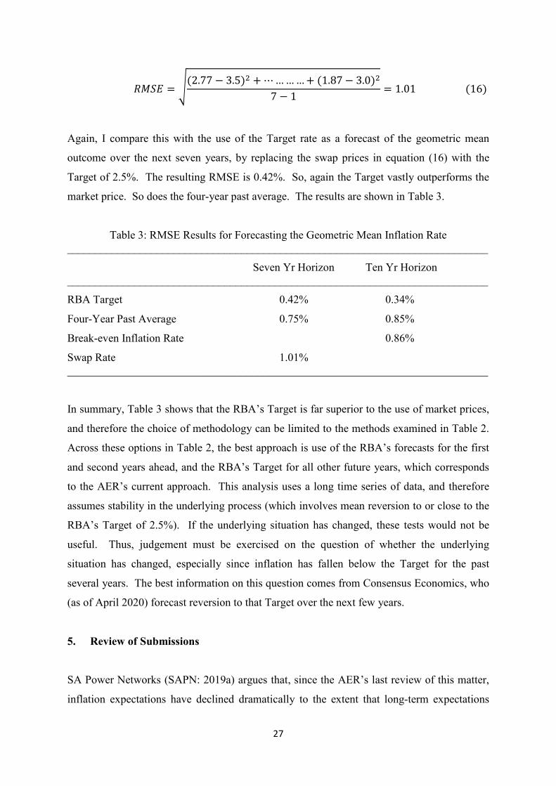
inclusive (which was 2.77%). The forecast error is then 0.73%. The RMSE of the forecast

errors is 1.01% as follows:

27

𝑅𝑅𝑅𝑅𝑅𝑅𝐸𝐸 = �(2.77 − 3.5)2 + ⋯… … … + (1.87 − 3.0)2

7 − 1= 1.01 (16)

Again, I compare this with the use of the Target rate as a forecast of the geometric mean

outcome over the next seven years, by replacing the swap prices in equation (16) with the

Target of 2.5%. The resulting RMSE is 0.42%. So, again the Target vastly outperforms the

market price. So does the four-year past average. The results are shown in Table 3.

Table 3: RMSE Results for Forecasting the Geometric Mean Inflation Rate ___________________________________________________________________________

Seven Yr Horizon Ten Yr Horizon ___________________________________________________________________________

RBA Target 0.42% 0.34%

Four-Year Past Average 0.75% 0.85%

Break-even Inflation Rate 0.86%

Swap Rate 1.01% ___________________________________________________________________________

In summary, Table 3 shows that the RBA’s Target is far superior to the use of market prices,

and therefore the choice of methodology can be limited to the methods examined in Table 2.

Across these options in Table 2, the best approach is use of the RBA’s forecasts for the first

and second years ahead, and the RBA’s Target for all other future years, which corresponds

to the AER’s current approach. This analysis uses a long time series of data, and therefore

assumes stability in the underlying process (which involves mean reversion to or close to the

RBA’s Target of 2.5%). If the underlying situation has changed, these tests would not be

useful. Thus, judgement must be exercised on the question of whether the underlying

situation has changed, especially since inflation has fallen below the Target for the past

several years. The best information on this question comes from Consensus Economics, who

(as of April 2020) forecast reversion to that Target over the next few years.

5. Review of Submissions

SA Power Networks (SAPN: 2019a) argues that, since the AER’s last review of this matter,

inflation expectations have declined dramatically to the extent that long-term expectations

28

have de-anchored from the RBA’s target rate, and therefore that the AER’s current reliance

upon the RBA’s inflation target of 2.5% is no longer justified. In support of this claim,

SAPN (2019a, page 5) notes that the ten-year break-even inflation rate and five to ten year

inflation swap prices are both at historical lows (of 1.4% and 2.0% respectively), as shown in

their figures. However, as discussed previously, these estimators are likely to be biased to an

extent that fluctuates through time, and the empirical evidence is that they are vastly inferior

to use of the RBA’s Target. Furthermore, since SAPN focuses upon their current low values,

it is also useful to examine the predictive success of earlier extreme values for these prices.

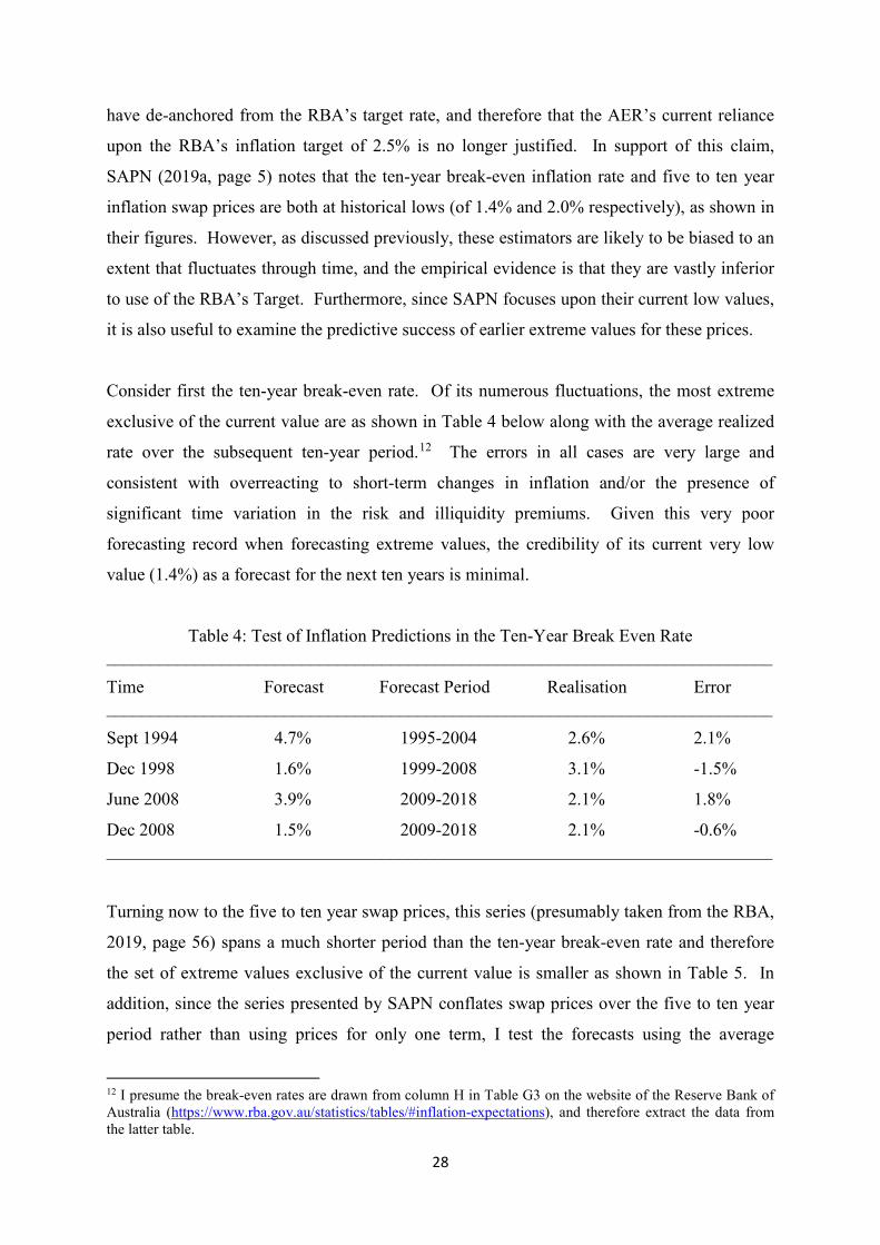
Consider first the ten-year break-even rate. Of its numerous fluctuations, the most extreme

exclusive of the current value are as shown in Table 4 below along with the average realized

rate over the subsequent ten-year period.12 The errors in all cases are very large and

consistent with overreacting to short-term changes in inflation and/or the presence of

significant time variation in the risk and illiquidity premiums. Given this very poor

forecasting record when forecasting extreme values, the credibility of its current very low

value (1.4%) as a forecast for the next ten years is minimal.

Table 4: Test of Inflation Predictions in the Ten-Year Break Even Rate ___________________________________________________________________________

Time Forecast Forecast Period Realisation Error ___________________________________________________________________________

Sept 1994 4.7% 1995-2004 2.6% 2.1%

Dec 1998 1.6% 1999-2008 3.1% -1.5%

June 2008 3.9% 2009-2018 2.1% 1.8%

Dec 2008 1.5% 2009-2018 2.1% -0.6% ___________________________________________________________________________

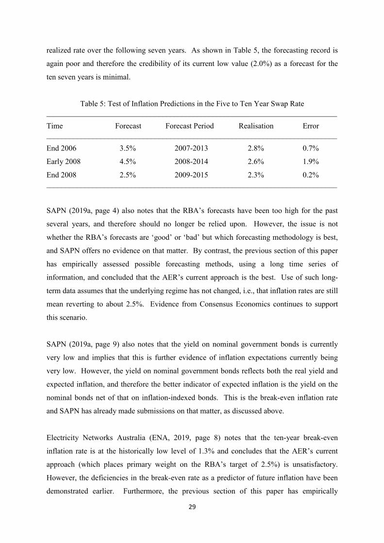
Turning now to the five to ten year swap prices, this series (presumably taken from the RBA,

2019, page 56) spans a much shorter period than the ten-year break-even rate and therefore

the set of extreme values exclusive of the current value is smaller as shown in Table 5. In

addition, since the series presented by SAPN conflates swap prices over the five to ten year

period rather than using prices for only one term, I test the forecasts using the average

12 I presume the break-even rates are drawn from column H in Table G3 on the website of the Reserve Bank of Australia (https://www.rba.gov.au/statistics/tables/#inflation-expectations), and therefore extract the data from the latter table.

29

realized rate over the following seven years. As shown in Table 5, the forecasting record is

again poor and therefore the credibility of its current low value (2.0%) as a forecast for the

ten seven years is minimal.

Table 5: Test of Inflation Predictions in the Five to Ten Year Swap Rate ___________________________________________________________________________

Time Forecast Forecast Period Realisation Error ___________________________________________________________________________

End 2006 3.5% 2007-2013 2.8% 0.7%

Early 2008 4.5% 2008-2014 2.6% 1.9%

End 2008 2.5% 2009-2015 2.3% 0.2% ___________________________________________________________________________

SAPN (2019a, page 4) also notes that the RBA’s forecasts have been too high for the past

several years, and therefore should no longer be relied upon. However, the issue is not

whether the RBA’s forecasts are ‘good’ or ‘bad’ but which forecasting methodology is best,

and SAPN offers no evidence on that matter. By contrast, the previous section of this paper

has empirically assessed possible forecasting methods, using a long time series of

information, and concluded that the AER’s current approach is the best. Use of such long-

term data assumes that the underlying regime has not changed, i.e., that inflation rates are still

mean reverting to about 2.5%. Evidence from Consensus Economics continues to support

this scenario.

SAPN (2019a, page 9) also notes that the yield on nominal government bonds is currently

very low and implies that this is further evidence of inflation expectations currently being

very low. However, the yield on nominal government bonds reflects both the real yield and

expected inflation, and therefore the better indicator of expected inflation is the yield on the

nominal bonds net of that on inflation-indexed bonds. This is the break-even inflation rate

and SAPN has already made submissions on that matter, as discussed above.

Electricity Networks Australia (ENA, 2019, page 8) notes that the ten-year break-even

inflation rate is at the historically low level of 1.3% and concludes that the AER’s current

approach (which places primary weight on the RBA’s target of 2.5%) is unsatisfactory.

However, the deficiencies in the break-even rate as a predictor of future inflation have been

demonstrated earlier. Furthermore, the previous section of this paper has empirically

30

assessed possible forecasting methods, using a long time series of information, and concluded

that the AER’s current approach is the best. Use of such long-term data assumes that the

underlying regime has not changed, i.e., that inflation rates are still mean reverting to about

2.5%. Evidence from Consensus Economics continues to support this scenario.

ENA (2019, page 10) also lists a series of short-term forecasts of inflation reported by the

RBA, claims that all are at or close to their lowest levels ever, and therefore implies that the

AER’s current approach is unwarranted. However the contemporaneous RBA forecasts

(from the November 2019 SMP) are also unusually low: the one-year forecast of 1.75% is the

lowest in a November SMP over the entire 1993-2019 period. Since the AER uses the

RBA’s forecasts for the next two years, the ENA are not citing any information that the AER

is not already effectively using.

ENA (2019, pp. 12-13) also notes that the annual inflation rate has been under the 2.5%

Target for the last 20 quarters, and that this is the longest such occasion since Inflation

Targeting began. It then argues that reversion back to 2.5% will not then occur within two

years, and therefore that the AER’s current methodology is deficient. More compelling

information on this matter comes from Consensus Economics, who forecast (as of April

2020) that reversion to 2.5% will not occur until 2026. The issue then is whether the AER

should change its current methodology to reflect this unusually slow reversion. An

apparently simple means of doing so would be to adopt a glide-path from the RBA’s two-

year ahead forecast to the Target rate of 2.5%. However, this gives rise to two problems:

over what period should the AER glide back to 2.5%, and under what conditions should the

AER do so if it does not do so always. Both are extremely subjective. The AER’s current

approach avoids this subjectivity, and it will satisfy the NPV = 0 requirement so long as these

situations in which reversion to the Target is unusually slow are symmetric, i.e., scenarios in

which reversion back from a low figure is unusually slow (to the disadvantage of the

businesses) are matched by scenarios in which reversion back from a high figure is unusually

slow (to the advantage of the businesses). I do not hold a view on whether such symmetry

exists. If the AER believes symmetry exists, it should retain its current approach. Otherwise,

there is a case for the AER’s adopting a longer glide-path back to the Target.

QTC (2019) favours the ten-year break-even rate as a predictor of future inflation, leading to

a significantly lower estimate of expected inflation than the AER. However, as argued

31

earlier, this estimator is very poor in part because it is biased by the presence of an inflation

risk premium within the yield on nominal CGS. Remarkably and perversely, QTC

recognizes this particular problem despite promoting this break-even methodology.

QTC (2019) goes on to present estimates of NPAT for Ergon Energy and Energex over the

2021-2025 period, which are negative for both firms for all years. These estimates are all

based on the AER’s estimate for expected inflation over the next ten years of 2.45%. As

argued in section 2 above, the appropriate estimates for expected inflation should be specific

to each year and, in the presence of RBA forecasts over the next two years that are

significantly below the Target, the AER’s estimate is too high for each of these years

examined by the QTC.

Jemena (2020) proposes that the AER use a “more market-based approach” or an average of

this and its current approach, to ensure that it delivers positive cash dividends to equity

holders. Jemena’s reference to market-based approaches is presumably a reference to the

break-even rate and/or swap prices, but Jemena presents no evidence on why these models

should be favoured. Furthermore, the evidence presented above is that they are vastly

inferior to the AER’s current approach. Jemena’s also appears to be suggesting that a

methodology for estimating expected inflation should be chosen according to its impact on

the allowed cost of equity. These are separate issues.

6. Conclusions

This paper has assessed the best method for estimating expected future inflation in Australia,

with particular reference to recent empirical evidence, and the principal conclusions are as

follows.

Firstly, given that the AER’s regulatory cycle is five years, the NPV = 0 principle implies

that the AER ought to be estimating expected inflation over each of the next five years rather

than over the next ten years. Secondly, market prices (comprising the break-even rates and

swap prices) are likely to be biased estimators of expected future inflation, and to a degree

that varies over time. Thirdly, using standard RMSE tests of forecasting accuracy, the RBA’s

Target is far superior to the use of market prices for forecasting inflation over 5-10 years, and

therefore market prices can be rejected. Fourthly, across the range of other approaches

32

considered (comprising forecasts by the RBA, forecasts from Consensus Economics, the

RBA’s Target rate, a Random Walk model, a mean reversion model, and the model of Finlay

and Wende), the lowest RMSE of the forecast errors comes from the RBA’s forecasts for the

first and second years ahead, and the RBA’s Target for all other future years, which

corresponds to the AER’s current approach.

Fifthly, this RMSE analysis uses a long time series of data, and therefore assumes stability in

the underlying process (which involves mean reversion to or close to the RBA’s Target of

2.5%). If the underlying situation has changed, these tests would not be useful. Thus, it is

necessary to assess whether the underlying situation has changed, especially since inflation

has fallen below the Target for the past several years. The best information on this question

comes from Consensus Economics, who (as of April 2020) forecast reversion to that Target

over the next few years. Lastly, and because reversion back to the RBA’s Target is currently

expected to be unusually slow, there is a case for the AER adopting a slow glide path from

the RBA’s forecasts to the Target providing that scenarios in which reversion back from a

low figure is unusually slow (to the disadvantage of the businesses) are not likely to be

matched by scenarios in which reversion back from a high figure is unusually slow (to the

advantage of the businesses).

33

REFERENCES AER, 2020. Discussion Paper Regulatory Treatment of Inflation May 2020 (https://www.aer.gov.au/system/files/AER%20-%20Discussion%20paper%20-%20Review%20of%20expected%20inflation%202020%20-%20May%202020.pdf) Bekaert, G., and Wang, X., 2009. “Inflation and the Inflation Risk Premium”, Columbia University working paper (https://www0.gsb.columbia.edu/faculty/gbekaert/papers/inflation_risk.pdf). D’Amico, S., Kim, D., and Wei, M., 2009. ‘Tips from TIPS: the information content of Treasury inflation-protected security prices’, Finance and Economics Discussion Series Working Paper 2010-19, Federal Reserve Board (https://www.federalreserve.gov/pubs/feds/2010/201019/201019pap.pdf). Devlin, W., and Patwardhan, D. 2012. Measuring Market Inflation Expectations (http://www.treasury.gov.au/PublicationsAndMedia/Publications/2012/Economic-Roundup-Issue-2/Report/Measuring-market-inflation-expectations). Electricity Networks Australia, 2019. Estimation of Expected Inflation (https://www.aer.gov.au/system/files/ENA%20–%20Estimation%20of%20expected%20inflation%20–%20Requirement%20for%20a%20review%20-%207%20November%202019.pdf). Fleckenstein, M., Longstaff, F., and Lustig, H., 2014. “The TIPS-Treasury Bond Puzzle”, The Journal of Finance, Vol. 69, pp. 2151-2197. Finlay, R., and Wende, S., 2012. “Estimating Inflation Expectations with a Limited Number of Inflation-Indexed Bonds”, International Journal of Central Banking, Vol. 8, No. 2, pp. 111-142 (http://www.ijcb.org/journal/ijcb12q2a4.pdf). _______ and Olivan, D., 2012. “Extracting Information from Financial Market Instruments”, Reserve Bank Bulletin, March (http://www.rba.gov.au/publications/bulletin/2012/mar/pdf/bu-0312-6.pdf). Grishchenko, O., and Huang, J., 2012. “Inflation Risk Premium: Evidence from the TIPS Market”, Finance and Economics Discussion Series Working Paper 2012-16, Federal Reserve Board (https://www.federalreserve.gov/pubs/feds/2012/201206/201206pap.pdf). Haubrich, J., Pennachi, G., and Ritchken, P., 2015. “Inflation Expectations, Real Rates, and Risk Premia: Evidence from Inflation Swaps”, The Review of Financial Studies, Vol. 25, pp. 1588-1629. Jemena, 2020. Submission Regarding Extremely low Return on Equity from Short-Term Market Fluctuations (https://www.aer.gov.au/networks-pipelines/guidelines-schemes-models-reviews/review-of-expected-inflation-2017/updates). Mathysen, H., 2017. Best Estimates of Expected Inflation: A Comparative Assessment of Four Methods, ACCC/AER Working Paper Series

34

(https://www.accc.gov.au/system/files/Working%20Paper%20no.%2011%20-%20Best%20estimates%20of%20expected%20inflation%20-%20v3.pdf). QTC, 2019. Issues Raised by QTC at the Inflation Working Troup Meeting (https://www.aer.gov.au/networks-pipelines/guidelines-schemes-models-reviews/review-of-expected-inflation-2017/updates). RBA, 2019, Statement of Monetary Policy, November 2019, https://www.rba.gov.au/publications/smp/2019/aug/pdf/statement-on-monetary-policy-2019-08.pdf. SA Power Networks, 2019a. Regulatory Treatment of Inflation-Request for Review (https://www.aer.gov.au/networks-pipelines/guidelines-schemes-models-reviews/review-of-expected-inflation-2017/updates). Tulip, P., and Wallace, S., 2012. “Estimates of Uncertainty around the RBA’s Forecasts”, Research Discussion Paper 2012-07 (http://www.rba.gov.au/publications/rdp/2012/pdf/rdp2012-07.pdf). Vahey, S., 2017. Report to the AER on Estimating Expected Inflation (https://www.aer.gov.au/system/files/Prof%20Shaun%20P%20Vahey%20-%20Report%20to%20the%20AER%20on%20estimating%20expected%20inflation%20-%2015%20September%202017.PDF )