Ch04 - Forecasting

© 2004 by Prentice Hall, Inc., Upper Saddle River, N.J. 07458

4-1

Operations ManagementForecastingChapter 4


4-2

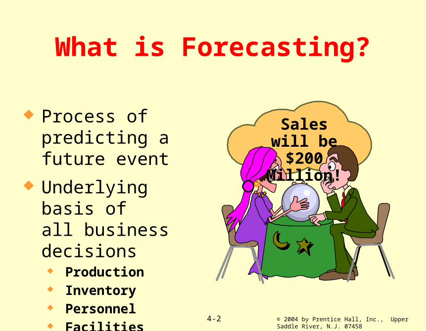
What is Forecasting?

¨ Process of predicting a future event

¨ Underlying basis of all business decisions¨ Production¨ Inventory¨ Personnel¨ Facilities

Sales will be $200

Million!


4-3

Types of Forecasts¨ Economic forecasts

¨ Address business cycle, e.g., inflation rate, money supply etc.

¨ Technological forecasts¨ Predict rate of technological progress

¨ Predict acceptance of new product

¨ Demand forecasts¨ Predict sales of existing product


4-4

¨ Short-range forecast¨ Up to 1 year; usually less than 3 months

¨ Job scheduling, worker assignments¨ Medium-range forecast

¨ 3 months to 3 years¨ Sales & production planning, purchasing, budgeting

¨ Long-range forecast¨ 3+ years¨ New product planning, facility location

Types of Forecasts by Time Horizon


4-5

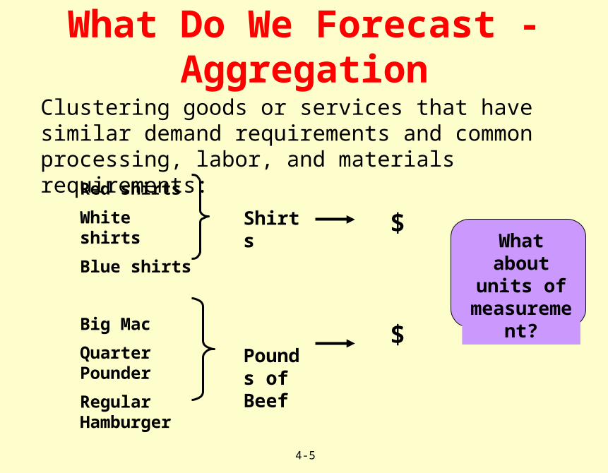
What Do We Forecast - Aggregation

Clustering goods or services that have similar demand requirements and common processing, labor, and materials requirements:Red shirts

White shirtsBlue shirts

Big MacQuarter PounderRegular Hamburger

Shirts

Pounds of Beef

$

$

Why do we aggregate

?

What about

units of measureme

nt?


4-6

Realities of Forecasting

¨ Forecasts are seldom perfect¨ Most forecasting methods assume that there is some underlying stability in the system

¨ Both product family and aggregated product forecasts are more accurate than individual product forecasts


4-7

¨ Persistent, overall upward or downward pattern

¨ Due to population, technology etc.

¨ Several years duration

Trend Component

Time

Response


4-8

¨ Regular pattern of up & down fluctuations

¨ Due to weather, customs etc.

Time

Response

Seasonal Component

Summer


4-9

¨ Repeating up & down movements¨ Due to interactions of factors influencing economy

¨ Usually 2-10 years duration

Time

Response

Cyclical Component

Cycle


4-10

Product Demand

Year1

Year2

Year3

Year4

Actual demand line

Demand for product or service

Seasonal peaks Trend component

Average demand over four yearsRandom

variation


4-11

Forecasting Approaches

¨ Used when situation is ‘stable’ & historical data exist¨ Existing products

¨ Current technology

¨ Involves mathematical techniques¨ e.g., forecasting sales of color televisions

Quantitative Methods¨ Used when situation is vague & little data exist¨ New products¨ New technology

¨ Involves intuition, experience¨ e.g., forecasting sales on Internet

Qualitative Methods


4-12

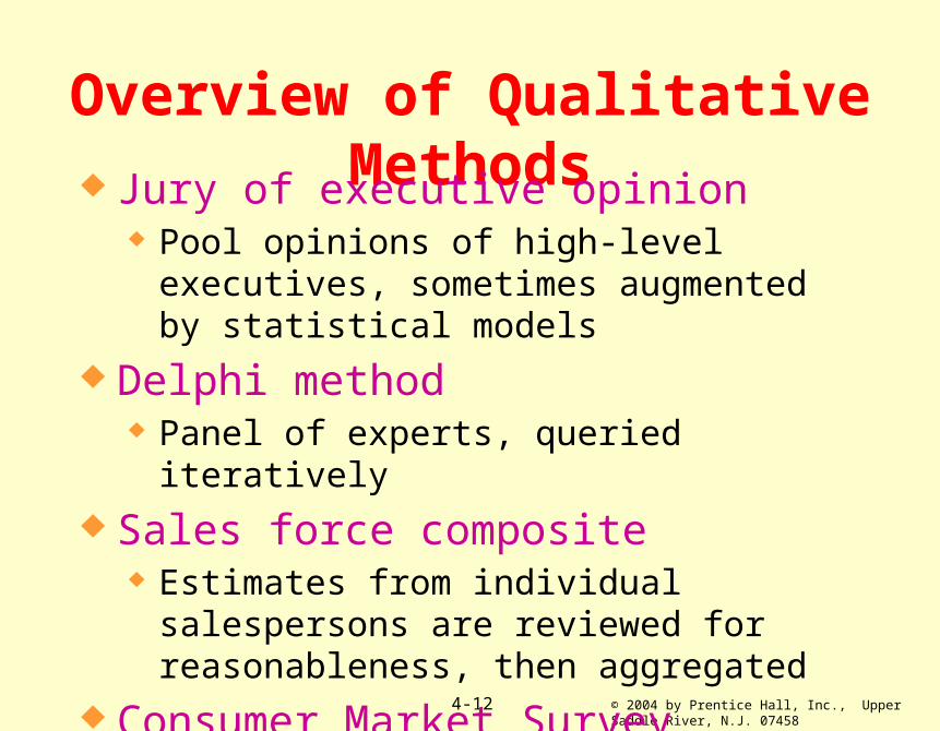
Overview of Qualitative Methods¨ Jury of executive opinion

¨ Pool opinions of high-level executives, sometimes augmented by statistical models

¨ Delphi method¨ Panel of experts, queried iteratively

¨ Sales force composite¨ Estimates from individual salespersons are reviewed for reasonableness, then aggregated

¨ Consumer Market Survey¨ Ask the customer


4-13

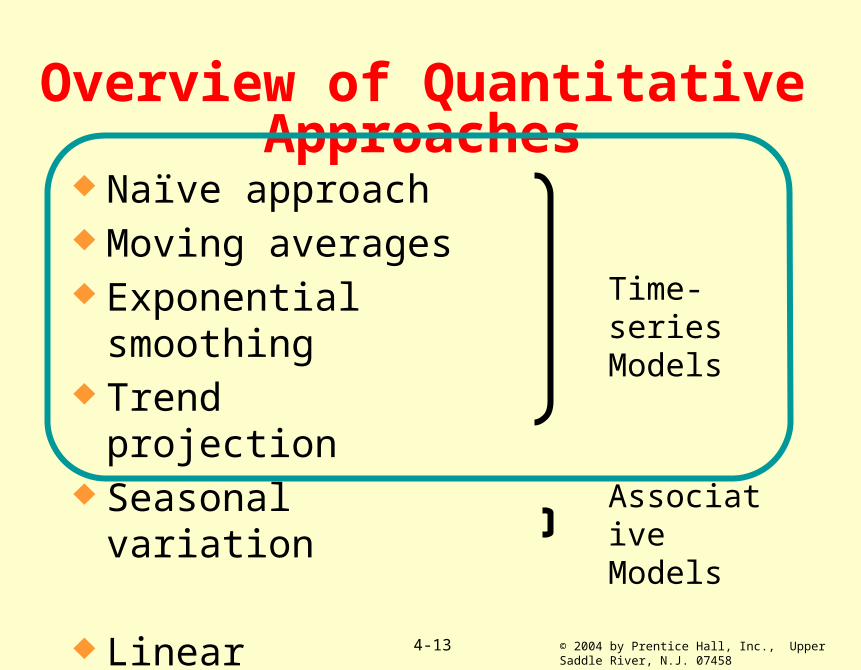
Overview of Quantitative Approaches

¨ Naïve approach¨ Moving averages¨ Exponential smoothing

¨ Trend projection

¨ Seasonal variation

¨ Linear regression

Time-series Models

Associative Models


4-14

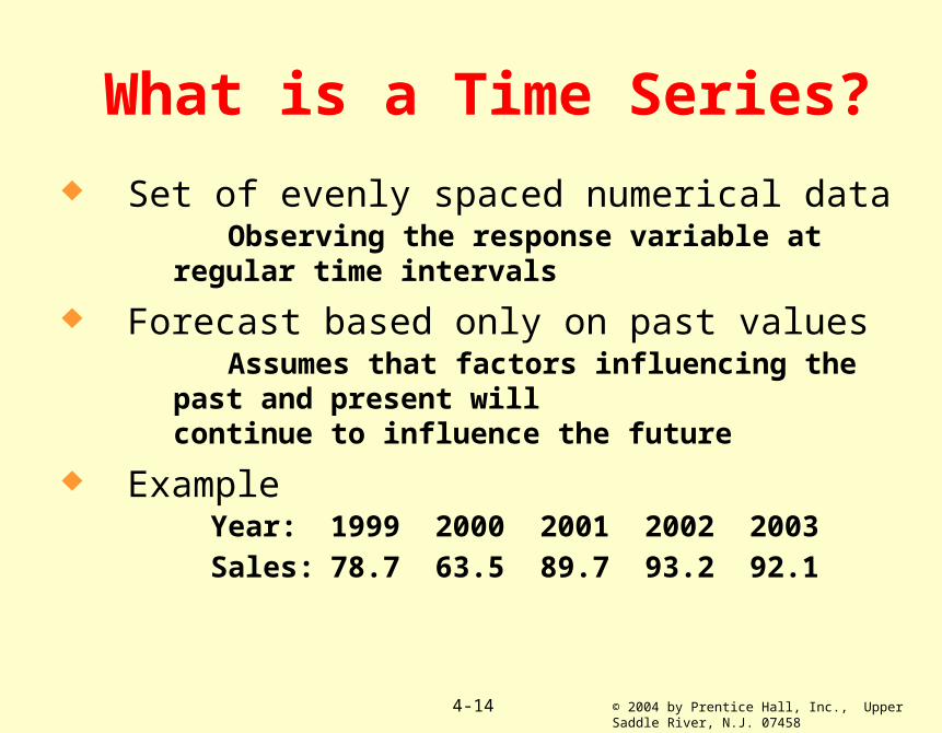
¨ Set of evenly spaced numerical data Observing the response variable at regular time intervals

¨ Forecast based only on past values Assumes that factors influencing the past and present will continue to influence the future

¨ Example Year: 1999 2000 2001 2002 2003 Sales: 78.7 63.5 89.7 93.2 92.1

What is a Time Series?


4-15

Naive Approach

¨ Assumes demand in next period is the same as demand in most recent period¨ e.g., If May sales were 48, then June sales will be 48

¨ Sometimes cost effective & efficient © 1995 Corel Corp.


4-16

Forecast nn

Demand in Previous Periods

Simple Moving Average

F = A + A + A + A

F = A + A + A

t t–1 t–2 t–3 t–4

t t–1 t–2 t–3

4

3


4-17

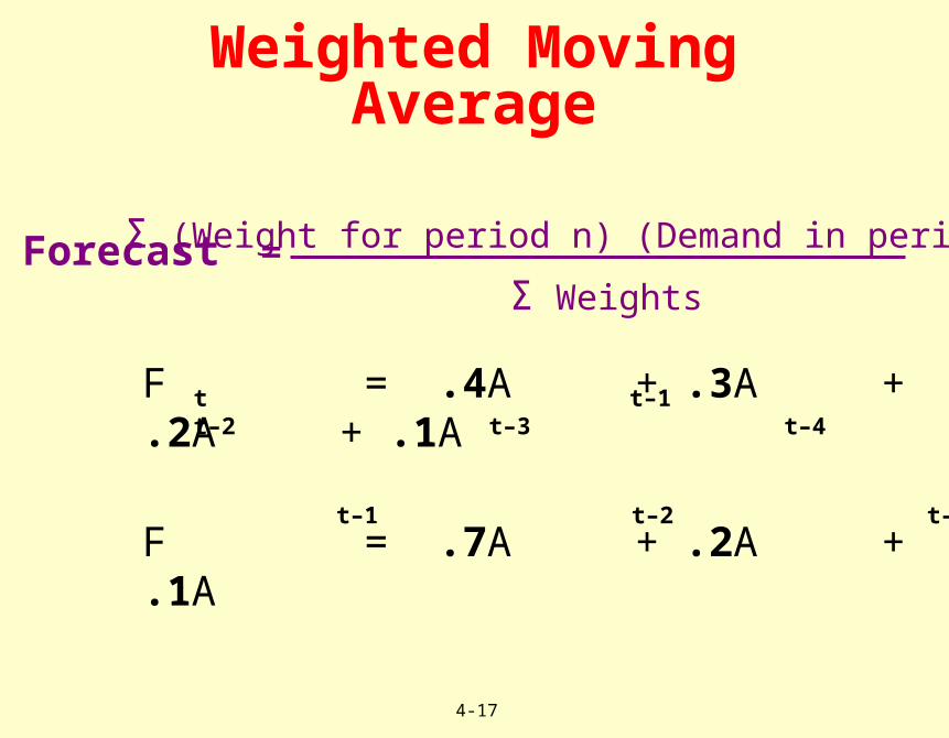
Forecast =Σ (Weight for period n) (Demand in period n) Σ Weights

Weighted Moving Average

F = .4A + .3A + .2A + .1A

F = .7A + .2A + .1A

t t–1 t–2 t–3 t–4

t t–1 t–2 t–3


4-18

¨ Form of weighted moving average¨ Weights decline exponentially¨ Most recent data weighted most

¨ Requires smoothing constant ()¨ Ranges from 0 to 1¨ Subjectively chosen

¨ Involves little record keeping of past data

Exponential Smoothing Method


4-19

Exponential Smoothing

F = A + (1 – ) (F ) = A + F – F = F + (A – F )

t t–1 t–1

t–1 t–1 t–1

t–1 t–1 t–1

Forecast = (Demand last period) + (1 – ) ( Last forecast)

Forecast = Last forecast + (Last demand – Last forecast)


4-20

Tt = (Forecast this period – Forecast last period) + (1- ) (Trend estimate last period) = (Ft - Ft-1) + (1- )Tt-1

Exponential Smoothing with Trend Adjustment

Forecast = Exponentially smoothed forecast (F ) + Exponentially smoothed trend (T )

tt


4-21

Seasonal Variation

Quarter Year 1 Year 2 Year 3 Year 41 45 70 100 1002 335 370 585 7253 520 590 830 11604 100 170 285 215

Total 1000 1200 18002200

Average 250 300 450550

Seasonal Index = Actual DemandAverage Demand = = 0.1845

250Forecast for Year 5 = 2600


4-22

Quarter Year 1 Year 2 Year 3 Year 4

1 45/250 = 0.18 70/300 = 0.23100/450 = 0.22100/550 = 0.18

2335/250 = 1.34370/300 = 1.23585/450 = 1.30725/550 = 1.32

3520/250 = 2.08590/300 = 1.97830/450 = 1.841160/550 = 2.11

4100/250 = 0.40170/300 = 0.57285/450 = 0.63215/550 = 0.39

Quarter Average Seasonal Index

1(0.18 + 0.23 + 0.22 + 0.18)/4 = 0.20

2(1.34 + 1.23 + 1.30 + 1.32)/4 = 1.30

3(2.08 + 1.97 + 1.84 + 2.11)/4 = 2.00

4(0.40 + 0.57 + 0.63 + 0.39)/4 = 0.50

Seasonal Variation

Forecast

650(0.20) = 130650(1.30) = 845650(2.00) = 1300650(0.50) = 325


4-23

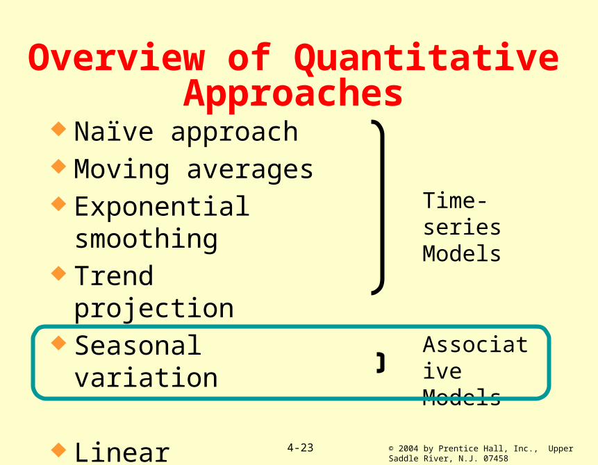
Overview of Quantitative Approaches

¨ Naïve approach¨ Moving averages¨ Exponential smoothing

¨ Trend projection

¨ Seasonal variation

¨ Linear regression

Time-series Models

Associative Models


4-24

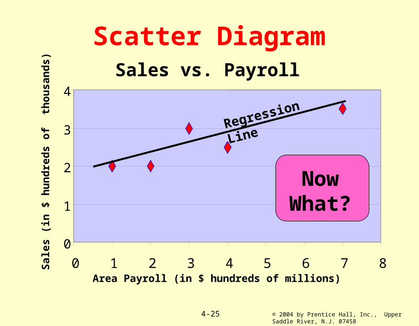
Linear Regression

Independent Dependent Variables Variable

Factors Associated with Our Sales• Advertising• Pricing• Competitors • Economy• Weather

Sales


4-25

Scatter DiagramSales vs. Payroll

0

1

2

3

4

0 1 2 3 4 5 6 7 8Area Payroll (in $ hundreds of millions)

Sale

s (i

n $

hund

reds

of

tho

usan

ds)

Regression

Line

Now What?


4-26

¨ Short-range forecast¨ Up to 1 year; usually less than 3 months

¨ Job scheduling, worker assignments

¨ Medium-range forecast¨ 3 months to 3 years¨ Sales & production planning, budgeting

¨ Long-range forecast¨ 3+ years¨ New product planning, facility location

Types of Forecasts by Time Horizon

Time Series

Associative

Qualitative


4-27

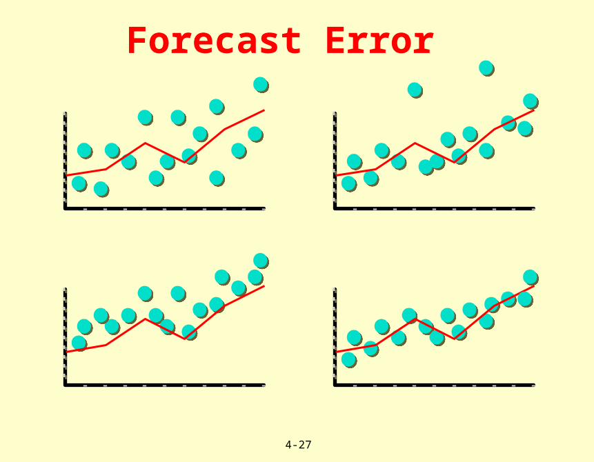
Forecast Error


4-28

Forecast Error

+ 5– 3

E = A – F

t t t


4-29

Forecast Error - CFE

CFE = Et

CFE – Cumulative sum of Forecast Errors

• Positive errors offset negative errors

• Useful in assessing bias in a forecast


4-30

Forecast Error - MSE

MSE – Mean Squared Error

Accentuates large deviations

MSE = Etn

2


4-31

Forecast Error - MAD

|Et |nMAD =

MAD – Mean Absolute Deviation

Widely used, well understood measurement of forecast error


4-32

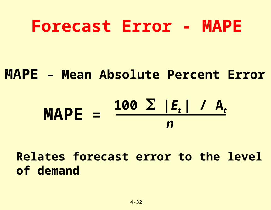
Forecast Error - MAPE

MAPE = 100 |Et | / At

n

MAPE – Mean Absolute Percent Error

Relates forecast error to the level of demand


4-33

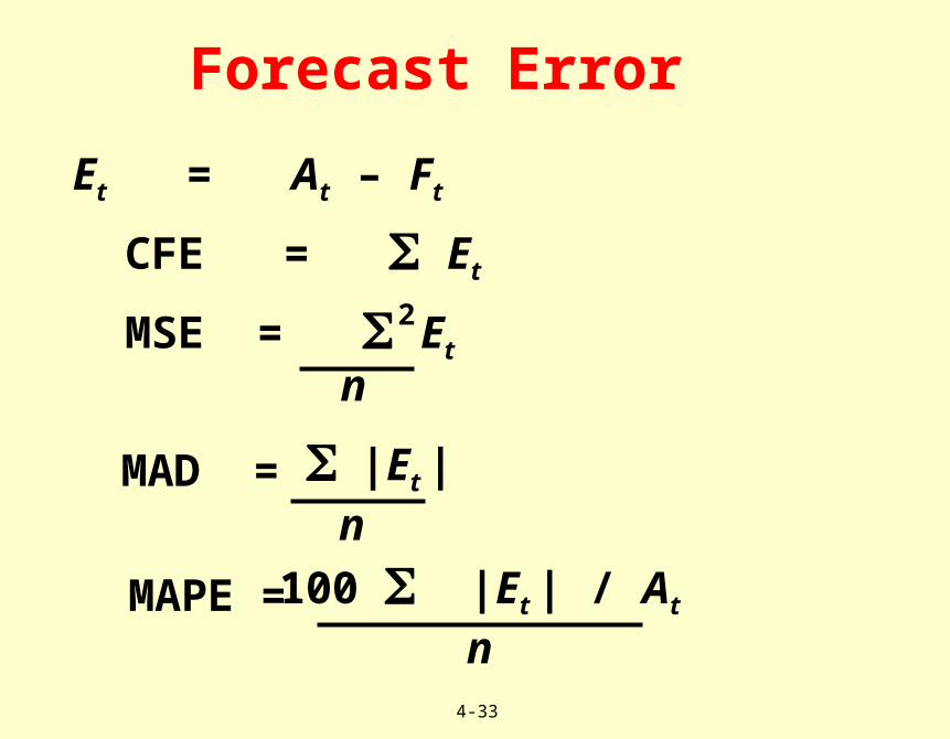
Forecast ErrorEt = At – Ft

CFE = Et

100 |Et | / At

nMAPE =

|Et | n

MAD =

MSE = Et n

2


4-34

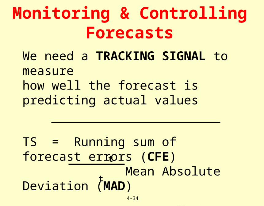
Monitoring & Controlling Forecasts

We need a TRACKING SIGNAL to measure how well the forecast is predicting actual values

TS = Running sum of forecast errors (CFE) Mean Absolute Deviation (MAD) = E | E | / n

t

t


4-35

Plot of a Tracking Signal

Time

Lower control limit

Upper control limit

Signal exceeded limit Tracking

signal CFE / MADAcceptable range

+

0

-


4-36

Forecasting in the Service Sector

Presents unusual challenges¨ special need for short term records

¨ needs differ greatly as function of industry and product

¨ issues of holidays and calendar¨ unusual events


4-37

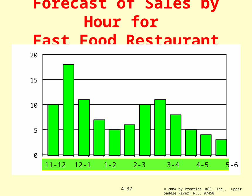
Forecast of Sales by Hour for

Fast Food Restaurant

0

5

10

15

20

+11-12 +1-2 +3-4 +5-6 +7-8 +9-1011-12 12-1 1-2 2-3 3-4 4-5 5-6 6-7 7-8 8-9 9-10 10-11


4-38

Summary¨ Demand forecasts drive a firm’s plans - Production

- Capacity- Scheduling

¨ Need to find the forecasting method(s) that best fit our pattern of demand – no one right tool

- Qualitative methods e.g. customer surveys

- Time series methods (quantitative) rely on historical

demand to predict future demand - Associative models (quantitative) use historical data on

independent variables to predict demand

e.g. promotional campaign¨ Track forecast error to determine if forecasting model requires change

Documents

Ch04 - Forecasting