Embed Size (px)
Citation preview

Department of Computer Science
Per Hurtig
Fast retransmit inhibitions for TCP
Master’s Thesis
2006:xx


Fast retransmit inhibitions for TCP
Per Hurtig
c© 2006 The author and Karlstad University

This thesis is submitted in partial fulfillment of the requirements
for the Masters degree in Computer Science. All material in this
thesis which is not my own work has been identified and no mate-
rial is included for which a degree has previously been conferred.
Per Hurtig
Approved, 2006-02-07
Opponent: Stefan Lindberg
Opponent: Fredrik Strandberg
Advisor: Johan Garcia
Examiner: Tim Heyer
iii


Abstract
The Transmission Control Protocol (TCP) has been the dominant transport protocol in the
Internet for many years. One of the reasons to this is that TCP employs congestion control
mechanisms which prevent the Internet from being overloaded. Although TCP’s congestion
control has evolved during almost twenty years, the area is still an active research area since
the environments where TCP are employed keep on changing. One of the congestion control
mechanisms that TCP uses is fast retransmit, which allows for fast retransmission of data
that has been lost in the network. Although this mechanism provides the most effective
way of retransmitting lost data, it can not always be employed by TCP due to restrictions
in the TCP specification.
The primary goal of this work was to investigate when fast retransmit inhibitions occur,
and how much they affect the performance of a TCP flow. In order to achieve this goal a
large series of practical experiments were conducted on a real TCP implementation.
The result showed that fast retransmit inhibitions existed, in the end of TCP flows, and
that the increase in total transmission time could be as much as 301% when a loss were
introduced at a fast retransmit inhibited position in the flow. Even though this increase was
large for all of the experiments, ranging from 16−301%, the average performance loss, due
to an arbitrary placed loss, was not that severe. Because fast retransmit was inhibited in
fewer positions of a TCP flow than it was employed, the average increase of the transmission
time due to these inhibitions was relatively small, ranging from 0, 3− 20, 4%.
v


Contents
1 Introduction 1
1.1 Scope of work . . . . . . . . . . . . . . . . . . . . . . . . . . . . . . . . . . 2
1.2 Disposition . . . . . . . . . . . . . . . . . . . . . . . . . . . . . . . . . . . 3
2 Background 5
2.1 TCP - Transmission Control Protocol . . . . . . . . . . . . . . . . . . . . . 5
2.1.1 TCP Areas . . . . . . . . . . . . . . . . . . . . . . . . . . . . . . . 6
2.1.2 Data Transfer . . . . . . . . . . . . . . . . . . . . . . . . . . . . . . 7
2.1.3 Reliability . . . . . . . . . . . . . . . . . . . . . . . . . . . . . . . . 7
2.1.4 Flow Control . . . . . . . . . . . . . . . . . . . . . . . . . . . . . . 9
2.1.5 Multiplexing . . . . . . . . . . . . . . . . . . . . . . . . . . . . . . . 10
2.1.6 Connection Management . . . . . . . . . . . . . . . . . . . . . . . . 10
2.1.7 TCP Segments . . . . . . . . . . . . . . . . . . . . . . . . . . . . . 12
2.2 Congestion Control Detail . . . . . . . . . . . . . . . . . . . . . . . . . . . 15
2.2.1 Slow Start . . . . . . . . . . . . . . . . . . . . . . . . . . . . . . . . 16
2.2.2 Congestion Avoidance . . . . . . . . . . . . . . . . . . . . . . . . . 17
2.2.3 Fast Retransmit . . . . . . . . . . . . . . . . . . . . . . . . . . . . . 18
2.2.4 Fast Recovery . . . . . . . . . . . . . . . . . . . . . . . . . . . . . . 18
2.2.5 Congestion Control Summary . . . . . . . . . . . . . . . . . . . . . 20
2.3 Network Emulation . . . . . . . . . . . . . . . . . . . . . . . . . . . . . . . 21
vii

2.3.1 Dummynet . . . . . . . . . . . . . . . . . . . . . . . . . . . . . . . 22
2.4 Related Work . . . . . . . . . . . . . . . . . . . . . . . . . . . . . . . . . . 23
2.5 Summary . . . . . . . . . . . . . . . . . . . . . . . . . . . . . . . . . . . . 26
3 Experimental Design & Environment 29
3.1 Problem Description . . . . . . . . . . . . . . . . . . . . . . . . . . . . . . 29
3.2 Method . . . . . . . . . . . . . . . . . . . . . . . . . . . . . . . . . . . . . 31
3.2.1 Overview . . . . . . . . . . . . . . . . . . . . . . . . . . . . . . . . 31
3.2.2 Details . . . . . . . . . . . . . . . . . . . . . . . . . . . . . . . . . . 33
3.2.3 Parameters . . . . . . . . . . . . . . . . . . . . . . . . . . . . . . . 34
3.3 Environment Overview . . . . . . . . . . . . . . . . . . . . . . . . . . . . . 38
3.4 Environment Details . . . . . . . . . . . . . . . . . . . . . . . . . . . . . . 39
3.4.1 FreeBSD 6.0B3 . . . . . . . . . . . . . . . . . . . . . . . . . . . . . 40
3.4.2 FreeBSD 6.0B5 . . . . . . . . . . . . . . . . . . . . . . . . . . . . . 41
3.4.3 Client & Server applications . . . . . . . . . . . . . . . . . . . . . . 41
3.4.4 Dummynet & Loss patterns . . . . . . . . . . . . . . . . . . . . . . 41
3.4.5 Tcpdump . . . . . . . . . . . . . . . . . . . . . . . . . . . . . . . . 43
3.4.6 Script . . . . . . . . . . . . . . . . . . . . . . . . . . . . . . . . . . 43
3.5 Summary . . . . . . . . . . . . . . . . . . . . . . . . . . . . . . . . . . . . 44
4 Results and Analysis 45
4.1 Short flows . . . . . . . . . . . . . . . . . . . . . . . . . . . . . . . . . . . . 45
4.1.1 General performance loss . . . . . . . . . . . . . . . . . . . . . . . . 45
4.1.2 Positional dependencies . . . . . . . . . . . . . . . . . . . . . . . . 48
4.1.3 Bad RTO Estimation . . . . . . . . . . . . . . . . . . . . . . . . . . 51
4.1.4 Link utilization implications . . . . . . . . . . . . . . . . . . . . . . 55
4.1.5 Receive buffer fluctuations . . . . . . . . . . . . . . . . . . . . . . . 57
4.1.6 TCP packet bursts and their implications . . . . . . . . . . . . . . . 58
viii

4.2 Long flows . . . . . . . . . . . . . . . . . . . . . . . . . . . . . . . . . . . . 60
4.2.1 General performance loss . . . . . . . . . . . . . . . . . . . . . . . . 60
4.2.2 Positional dependencies . . . . . . . . . . . . . . . . . . . . . . . . 62
4.2.3 TCP implementation issues . . . . . . . . . . . . . . . . . . . . . . 64
4.2.4 Irregularity analysis . . . . . . . . . . . . . . . . . . . . . . . . . . . 68
4.3 Results related to earlier work . . . . . . . . . . . . . . . . . . . . . . . . . 71
4.4 Summary . . . . . . . . . . . . . . . . . . . . . . . . . . . . . . . . . . . . 72
5 Future work 73
5.1 Other approaches . . . . . . . . . . . . . . . . . . . . . . . . . . . . . . . . 73
5.2 SCTP . . . . . . . . . . . . . . . . . . . . . . . . . . . . . . . . . . . . . . 74
5.3 Dummynet . . . . . . . . . . . . . . . . . . . . . . . . . . . . . . . . . . . 74
5.4 FreeBSD Initial window size . . . . . . . . . . . . . . . . . . . . . . . . . . 74
5.5 FreeBSD Slow Start issue . . . . . . . . . . . . . . . . . . . . . . . . . . . 75
5.6 FreeBSD recovery issue . . . . . . . . . . . . . . . . . . . . . . . . . . . . . 75
5.7 Performance gain with buffer tuning . . . . . . . . . . . . . . . . . . . . . 76
5.8 Lowering the fast retransmit threshold . . . . . . . . . . . . . . . . . . . . 76
6 Conclusions 77
References 79
A List of Abbreviations 83
B Additional Software 85
B.1 Tcptrace . . . . . . . . . . . . . . . . . . . . . . . . . . . . . . . . . . . . . 85
C FreeBSD Kernel details & modifications 89
C.1 TCP Implementation . . . . . . . . . . . . . . . . . . . . . . . . . . . . . . 89
C.1.1 Initial RTO Calculation . . . . . . . . . . . . . . . . . . . . . . . . 96
ix
C.2 Deactivating the TCP host cache . . . . . . . . . . . . . . . . . . . . . . . 97
D Source code & Scripts 99
D.1 Loss pattern generator . . . . . . . . . . . . . . . . . . . . . . . . . . . . . 99
D.1.1 Usage . . . . . . . . . . . . . . . . . . . . . . . . . . . . . . . . . . 99
D.1.2 Source code . . . . . . . . . . . . . . . . . . . . . . . . . . . . . . . 100
D.2 Experiment script . . . . . . . . . . . . . . . . . . . . . . . . . . . . . . . . 106
D.2.1 Source code . . . . . . . . . . . . . . . . . . . . . . . . . . . . . . . 107
D.3 Client & Server applications . . . . . . . . . . . . . . . . . . . . . . . . . . 113
D.3.1 Client source code . . . . . . . . . . . . . . . . . . . . . . . . . . . 114
D.3.2 Server source code . . . . . . . . . . . . . . . . . . . . . . . . . . . 117
x

List of Figures
2.1 TCP Communication . . . . . . . . . . . . . . . . . . . . . . . . . . . . . . 6
2.2 Acknowledgment . . . . . . . . . . . . . . . . . . . . . . . . . . . . . . . . 8
2.3 Sliding window . . . . . . . . . . . . . . . . . . . . . . . . . . . . . . . . . 9
2.4 Three Way Handshake . . . . . . . . . . . . . . . . . . . . . . . . . . . . . 11
2.5 TCP Connection Termination . . . . . . . . . . . . . . . . . . . . . . . . . 12
2.6 TCP Header . . . . . . . . . . . . . . . . . . . . . . . . . . . . . . . . . . . 14
2.7 TCP Congestion Control . . . . . . . . . . . . . . . . . . . . . . . . . . . . 20
2.8 Real operational network . . . . . . . . . . . . . . . . . . . . . . . . . . . . 21
2.9 Network emulator . . . . . . . . . . . . . . . . . . . . . . . . . . . . . . . . 22
2.10 Dummynet pipes . . . . . . . . . . . . . . . . . . . . . . . . . . . . . . . . 23
3.1 Fast Retransmit inhibitions . . . . . . . . . . . . . . . . . . . . . . . . . . 31
3.2 Experiment overview . . . . . . . . . . . . . . . . . . . . . . . . . . . . . . 32
3.3 Environment overview . . . . . . . . . . . . . . . . . . . . . . . . . . . . . 39
3.4 Environment detailed . . . . . . . . . . . . . . . . . . . . . . . . . . . . . . 39
3.5 Dummynet Configuration . . . . . . . . . . . . . . . . . . . . . . . . . . . 42
3.6 Loss pattern . . . . . . . . . . . . . . . . . . . . . . . . . . . . . . . . . . . 42
3.7 Tcpdump . . . . . . . . . . . . . . . . . . . . . . . . . . . . . . . . . . . . 44
4.1 Performance loss for the short flows . . . . . . . . . . . . . . . . . . . . . . 46
4.2 Average performance loss for the short flows . . . . . . . . . . . . . . . . . 47
xi
4.3 Transmission time graph 40 Kbit/s . . . . . . . . . . . . . . . . . . . . . . 48
4.4 Transmission time graph 80 Kbit/s . . . . . . . . . . . . . . . . . . . . . . 49
4.5 Transmission time graph 160 Kbit/s . . . . . . . . . . . . . . . . . . . . . . 50
4.6 Transmission time graph 320 Kbit/s . . . . . . . . . . . . . . . . . . . . . . 51
4.7 Transmission time graph 500, 1000, 2000, 4000, 8000, and 10000 Kbit/s . . 52
4.8 Transmission time graph 1000 Kbit/s, low delays . . . . . . . . . . . . . . 53
4.9 Bad RTO estimation . . . . . . . . . . . . . . . . . . . . . . . . . . . . . . 54
4.10 Acknowledgment misinterpretation . . . . . . . . . . . . . . . . . . . . . . 56
4.11 Server with 320 Kbit/s, 300ms delay, no losses . . . . . . . . . . . . . . . . 59
4.12 Server with 320 Kbit/s, 300ms delay, loss on position eight . . . . . . . . . 59
4.13 Server with 320 Kbit/s, 300ms delay, loss on position nine . . . . . . . . . 59
4.14 Server with 320 Kbit/s, 300ms delay, loss on position ten . . . . . . . . . . 60
4.15 Performance loss for the long flows . . . . . . . . . . . . . . . . . . . . . . 60
4.16 Average performance loss for the long flows . . . . . . . . . . . . . . . . . . 61
4.17 Transmission time graph 40, 80, and 160 Kbit/s . . . . . . . . . . . . . . . 63
4.18 Transmission time graph 500 Kbit/s . . . . . . . . . . . . . . . . . . . . . . 64
4.19 Transmission time graph 1000, 4000, and 10000kbps . . . . . . . . . . . . . 65
4.20 Server with 80 Kbit/s, 300ms delay, loss on position 12 . . . . . . . . . . . 68
4.21 Server with 80 Kbit/s, 300ms delay, loss on position 50 . . . . . . . . . . . 68
4.22 Server with 80 Kbit/s, 300ms delay, loss on position 84 . . . . . . . . . . . 69
4.23 Server with 500 Kbit/s, 300ms delay, loss on position 41 . . . . . . . . . . 70
4.24 Server with 500 Kbit/s, 300ms delay, loss on position 50 . . . . . . . . . . 70
4.25 One controlled loss, 10 ms . . . . . . . . . . . . . . . . . . . . . . . . . . . 71
B.1 Tcptrace Symbols . . . . . . . . . . . . . . . . . . . . . . . . . . . . . . . . 85
B.2 Tcptrace Example . . . . . . . . . . . . . . . . . . . . . . . . . . . . . . . 88
xii

List of Tables
2.1 TCP Flags . . . . . . . . . . . . . . . . . . . . . . . . . . . . . . . . . . . . 15
3.1 Test case parameters . . . . . . . . . . . . . . . . . . . . . . . . . . . . . . 35
B.1 Tcptrace symbol explanation . . . . . . . . . . . . . . . . . . . . . . . . . . 87
C.1 TCP parameters . . . . . . . . . . . . . . . . . . . . . . . . . . . . . . . . 94
C.2 Default values of TCP parameters . . . . . . . . . . . . . . . . . . . . . . . 95
C.3 TCP constants . . . . . . . . . . . . . . . . . . . . . . . . . . . . . . . . . 98
xiii


Listings
3.1 Experiment detailed . . . . . . . . . . . . . . . . . . . . . . . . . . . . . . 33
4.1 sys/net/inet/tcp input.c, lines 1983–1999 . . . . . . . . . . . . . . . . . . . 66
C.1 sys/net/inet/tcp input.c, lines 2744-2746 . . . . . . . . . . . . . . . . . . . 96
C.2 sys/net/inet/tcp input.c, lines 2762-2763 . . . . . . . . . . . . . . . . . . . 96
C.3 sys/net/inet/tcp timer.h, lines 129-135 . . . . . . . . . . . . . . . . . . . . 97
C.4 sys/net/inet/tcp var.h, lines 341-344 . . . . . . . . . . . . . . . . . . . . . 97
C.5 sys/net/inet/tcp hostcache.c, lines 130-134 . . . . . . . . . . . . . . . . . . 98
C.6 sys/net/inet/tcp hostcache.c, lines 130-134, modified . . . . . . . . . . . . 98
D.1 Loss pattern generator . . . . . . . . . . . . . . . . . . . . . . . . . . . . . 100
D.2 Configuration script . . . . . . . . . . . . . . . . . . . . . . . . . . . . . . . 107
D.3 Experiment execution script . . . . . . . . . . . . . . . . . . . . . . . . . . 113
D.4 Client application source code . . . . . . . . . . . . . . . . . . . . . . . . . 114
D.5 Server application source code . . . . . . . . . . . . . . . . . . . . . . . . . 117
xv


Chapter 1
Introduction
For many years TCP [29] has been the most commonly used transport protocol in the
Internet. TCP is currently used by a large set of network applications like web browsers,
FTP clients, and online computer games.
Because of recent years’ network evolution, including the mobile communication revo-
lution, the performance improvements of networking hardware, and the continuing growth
of the Internet, the demands that a transport protocol is facing have become more and
more complex. In order to meet these demands a lot of research and refinements have been
done on TCP, making it one of the most complex transport protocols of today.
One of the reasons to why TCP is so popular is that it guarantees reliable data transfer
to the applications using it. Other transport protocols, like UDP [28], do not provide this
guarantee and are therefore unsuitable for applications that require that data arrives safely
at the receiver.
Another reason to the popularity of TCP is that it contains mechanisms that automat-
ically try to prevent networks from being congested. As computer networks, especially the
Internet, began to grow large in the late 80’s the problem of network congestion was discov-
ered. Basically this problem, congestion, occurs when parts of the network infrastructure
becomes over-utilized by large amounts of traffic and, therefore, are unable to deliver any
1
2 CHAPTER 1. INTRODUCTION
data.
Since the incorporation of congestion control in TCP, the reliability mechanisms have
been combined with some of the mechanisms that provide the congestion control. This is
done because of the fact that possible unreliability of a network in most cases is due to
congestion, and therefore it is natural that some of these mechanisms are combined. The
exact behavior and interaction between various TCP mechanisms can potentially have a
large impact on performance. In this work we focus on the examination of one mechanism,
fast retransmit.
Fast retransmit is both a reliability mechanism as well as a congestion control mech-
anism. Its primary purpose is to resend data that has been lost in the network, but it
also gives TCP a hint about the current congestion status in the network. As the name
indicates fast retransmit is a fast way of retransmitting data, much faster than the other
reliability mechanism, i.e. timeout, that TCP uses. But one of the problems regarding
the fast retransmit mechanism is that it can not be employed under certain circumstances,
due to factors that have to do with the TCP specification. This phenomenon is called
fast retransmit inhibitions, and the primary goal of this thesis is to investigate when these
inhibitions occur, and how much they affect the performance of a TCP session.
1.1 Scope of work
This thesis presents an experimental evaluation of fast retransmit inhibitions in an emu-
lated network environment, using the FreeBSD 6 TCP implementation. The congestion
control mechanisms in this TCP implementation are based on NewReno [9]. Furthermore,
this TCP version employs a bandwidth limiting feature called “Bandwidth Delay Product
Window Limiting” which was disabled for the experiments.
We consider a simple model of a single TCP flow between a client and a server. By
controlling the existence and placement of data loss, within this flow, our goal is to in-

1.2. DISPOSITION 3
vestigate where fast retransmit inhibitions occur, in a flow, and how much they affect the
performance of the TCP session.
For the experiments we have used a large set of network parameters, such as different
bandwidths, end-to-end delays, and flow sizes. In order to conduct this evaluation a real-
time network emulator was used to represent the network that the client and the server
communicate over. Furthermore, a number of existing applications & scripts was modified
and some new developed to automate the experimental process, in terms of configuring
the network emulator according to desired network parameters, and executing the actual
experiments.
Although the main intention of this work was to examine the existence and impact of
fast retransmit inhibitions, other, interesting, results that are related to the behavior and
performance of TCP are also presented in the thesis.
1.2 Disposition
The rest of the thesis is structured as follows. Chapter 2 presents background information
on TCP, network emulation, and other work that in some ways are related to the work
presented in this thesis. The first two sections in the chapter give an overview of how TCP
manages connections between different hosts, transfers data, and how the reliability and
the congestion control mechanisms are designed. The following two sections give a quick
overview of the concept of network emulation and how it can be used, and a summary of
some related work that have been conducted in this area.
In Chapter 3 the problem of fast retransmit inhibitions is discussed in more detail.
In addition to this, the experiment design, environment, and the tools needed to do the
experiments are presented. In the first part of this chapter some theoretical background on
the fast retransmit inhibitions are provided along with an extended problem description
and the method that was used for the experiments. The rest of this chapter contains more
4 CHAPTER 1. INTRODUCTION
detailed information about the parameters of the experiments, and the environment that
the experiments were conducted in.
Chapter 4 presents the results of the experiments. This chapter is divided into two
separate parts; one for short TCP flows, and one for long ones. Each of these parts begins
with an overview of how much the performance suffers in the presence of fast retransmit
inhibitions. The parts then continue with a more detailed view of how the positioning of
data loss affects the total transmission time of a TCP flow. This is followed by a number of
sections that analyzes particularly interesting results, and finally, in the end of this chapter
some of the results are compared to results that have been published in a related study.
In Chapter 5, further work that might be conducted are presented. This chapter con-
tains ideas on how to use different evaluation techniques to investigate fast retransmit
inhibitions. It also contains suggestions of work that might be done given the results in
this thesis.
Finally, in Chapter 6, the work that is described in this thesis is summarized. This
chapter provides a quick resume over the work, a summary of the most important results,
and mentions some interesting phenomena that were discovered during the work.
To aid the reader of this thesis, a list of abbreviations is provided in Appendix A.

Chapter 2
Background
This chapter provides background information relevant to this project’s area. The focus of
this chapter is on TCP details, but an introduction to network emulation is also provided,
as well as a section with related work.
2.1 TCP - Transmission Control Protocol
The Transmission Control Protocol [3, 29] (TCP) is the most used transport protocol in
the Internet today. It is a part of the TCP/IP protocol suite which allows computers,
regardless of operating system and hardware, to communicate with each other. One of the
major properties of TCP is that it is able to provide a connection-oriented data transfer
service that is reliable to applications who require that no data is lost and/or damaged in
the communication process.
TCP is used in conjunction with the Internet Protocol [28] (IP) which only provides an
unreliable conectionless data transfer service between different hosts. To be able to provide
conection-oriented reliable communication, TCP needs to implement mechanisms on top
of IP. Figure 2.1 shows how two different processes, P and Q, located on two different
hosts use TCP to communicate with each other.
5

6 CHAPTER 2. BACKGROUND
Process P
TCP
IP
Process Q
TCP
IP
Host BHost A
reliable
TCP communication
unreliable
IP communication
Figure 2.1: TCP Communication
2.1.1 TCP Areas
As mentioned before, the primary purpose of TCP is to provide a connection-oriented
reliable data transfer service between different applications. To be able to provide this
service on top of an unreliable communication systems TCP needs to consider the following
areas [3, 29]:
• Data Transfer
• Reliability
• Flow Control
• Multiplexing
• Connection Management
• TCP Segments
• Congestion Control
These areas are discussed below, with special attention given to congestion control.
2.1. TCP - TRANSMISSION CONTROL PROTOCOL 7
2.1.2 Data Transfer
TCP is able to transmit a continuous byte stream in each direction between its users.
To achieve this TCP packages the data that is about to be sent into segments and then
transmits them to the other end.
The sending TCP is permitted to send data that is submitted by the user at its own
convenience, but in some cases the user wants to make sure that all data submitted to the
TCP have been transfered to the receiver. For this purpose a push operation is available.
When this operation is used, the sending TCP sends all the remaining data to the receiver,
which in turn must pass the data immediately to the receiving process. To make it possible
for the receiving TCP to know if the data received is to be delivered immediately TCP
specifies a PUSH flag.1
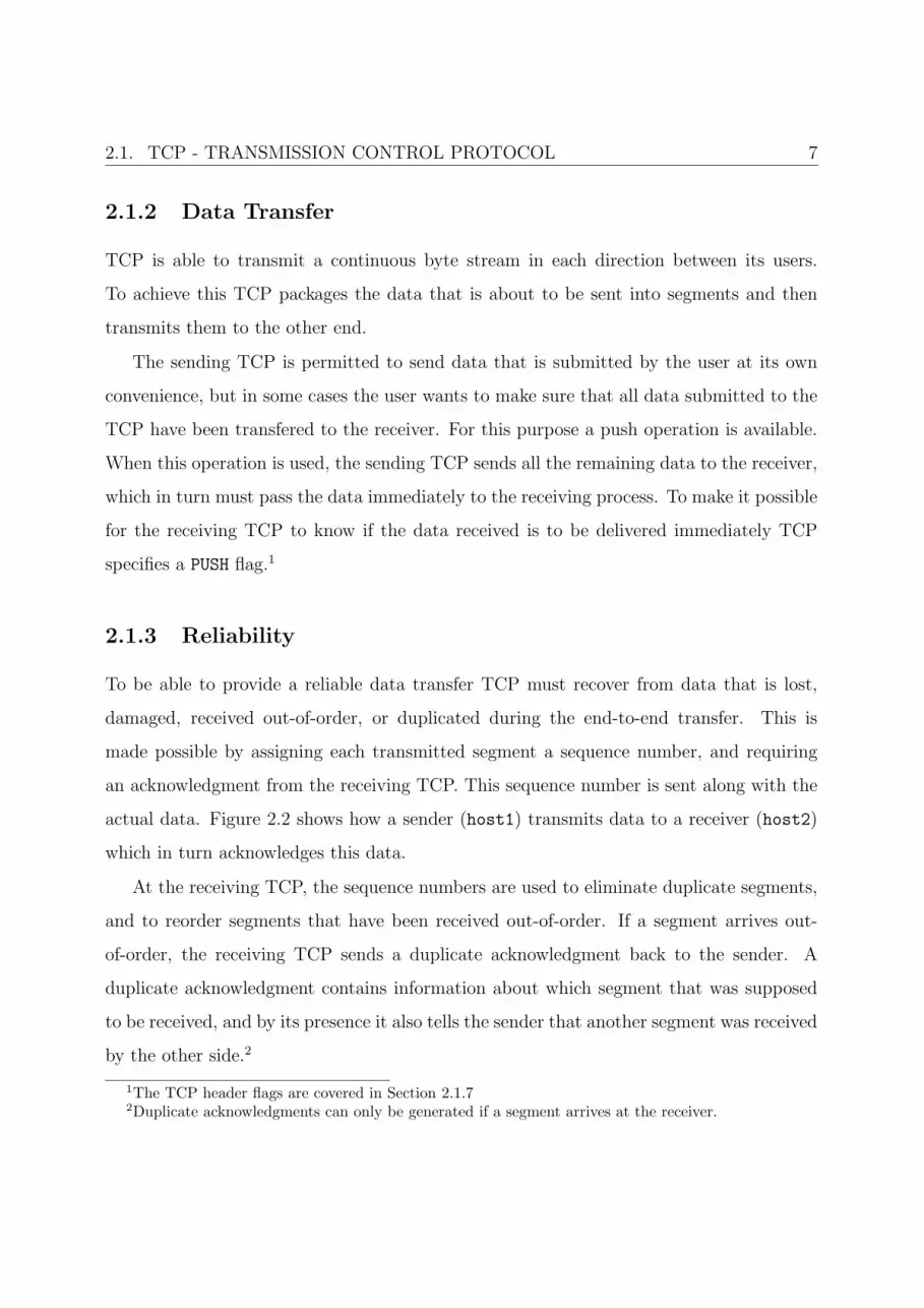
2.1.3 Reliability
To be able to provide a reliable data transfer TCP must recover from data that is lost,
damaged, received out-of-order, or duplicated during the end-to-end transfer. This is
made possible by assigning each transmitted segment a sequence number, and requiring
an acknowledgment from the receiving TCP. This sequence number is sent along with the
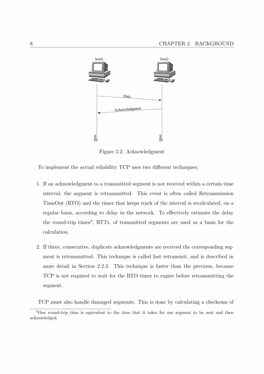
actual data. Figure 2.2 shows how a sender (host1) transmits data to a receiver (host2)
which in turn acknowledges this data.
At the receiving TCP, the sequence numbers are used to eliminate duplicate segments,
and to reorder segments that have been received out-of-order. If a segment arrives out-
of-order, the receiving TCP sends a duplicate acknowledgment back to the sender. A
duplicate acknowledgment contains information about which segment that was supposed
to be received, and by its presence it also tells the sender that another segment was received
by the other side.2
1The TCP header flags are covered in Section 2.1.72Duplicate acknowledgments can only be generated if a segment arrives at the receiver.
8 CHAPTER 2. BACKGROUND
host1 host2
time
time
Data
Acknowledgment
������
������
���������������������������������������������������������������� ������������������������
Figure 2.2: Acknowledgment
To implement the actual reliability TCP uses two different techniques;
1. If an acknowledgment to a transmitted segment is not received within a certain time
interval, the segment is retransmitted. This event is often called Retransmission
TimeOut (RTO) and the timer that keeps track of the interval is recalculated, on a
regular basis, according to delay in the network. To effectively estimate the delay
the round-trip times3, RTTs, of transmitted segments are used as a basis for the
calculation.
2. If three, consecutive, duplicate acknowledgments are received the corresponding seg-
ment is retransmitted. This technique is called fast retransmit, and is described in
more detail in Section 2.2.3. This technique is faster than the previous, because
TCP is not required to wait for the RTO timer to expire before retransmitting the
segment.
TCP must also handle damaged segments. This is done by calculating a checksum of
3One round-trip time is equivalent to the time that it takes for one segment to be sent and thenacknowledged.

2.1. TCP - TRANSMISSION CONTROL PROTOCOL 9
each transmitted segment which the receiver must verify. Damaged data is discarded by
the receiver and the recovery relies on the two retransmission techniques mentioned earlier.
2.1.4 Flow Control
In some situations data is received faster than it is consumed by the application using
TCP. When this happens TCP buffers the incoming data so that the application can read
the data when it needs it. To avoid that the buffer runs out of space TCP has a flow
control mechanism. This mechanism provides means for the receiving TCP to control
the amount of data that is sent by the sending TCP by including a “window” with every
acknowledgment. This window, called the receiver window, contains an acceptable range of
sequence numbers (beyond the last successfully received segment) that may be sent by the
sender. Figure 2.3 shows how the sender uses this window in the sending process. Outside
the window, on the left, we can see three segments that have been sent and acknowledged
by the receiver. In the first part of the window there are three segments that have been
sent but not yet acknowledged. The second part of the window contains segments that
can be sent right away, and outside the window, on the right hand, we have segments that
can not be sent before the window slides. As long as the window offered by the receiver is
constant the receipt of an acknowledgment will make the window slide one position to the
right for each acknowledged segment.
window moves
2 3 4 5 6 7 8 9 10 11 ...
offered window
(advertised by receiver)
usable window
sent andacknowledged
sent, not ACKedcan send ASAP
can’t send until
1
Figure 2.3: Sliding window
There are situations when the TCP receiver has nothing to acknowledge but still needs
to send an update of the receiver window. If the last advertised receiver window had zero

10 CHAPTER 2. BACKGROUND
size, i.e. the receiver’s buffer is full, and the buffer space is beginning to be freed the
receiver must have some way of reporting this to the sender (to prevent deadlock). This is
solved by the use of window updates. A window update is simply an acknowledgment that
does not acknowledge the receipt of any new data, only advertises a new receiver window,
and is sent when the buffer opens up.
2.1.5 Multiplexing
To allow more than one application per computer to use TCP simultaneously TCP uses
a multiplexing service. This service enables TCP to demultiplex incoming data so that
every application using TCP receives its’ “own” data. To accomplish this TCP specifies
that every process using TCP must be assigned a port. This port concatenated with the
network address of the host forms a socket. A socket may simultaneously form pairs with
a number of different sockets but every pair of sockets uniquely identifies a connection
between two processes. The binding of ports to processes is handled independently by
each host machine, but some ports are often bound to a specific type of process. Examples
of this is FTP client-/server processes which often use a port number of 21.
2.1.6 Connection Management
As described above the unique identifier of a connection is a pair of sockets, but there
is more to it. Although sockets can be used to identify a connection, a connection also
consists of certain status information. TCP is required to initialize and maintain this
information, including sockets, sequence numbers, and window sizes. This information is
used by the reliability, flow control, and congestion control mechanisms.
To realize the communication between two processes, their TCP’s must establish a
connection. The connection establishment is the initialization of the status information
(on each side). Later, when the communication is complete, their TCP’s must close the
connection, freeing the resources for other use.

2.1. TCP - TRANSMISSION CONTROL PROTOCOL 11
Because of the fact that the connection establishment is undertaken over a potentially
unreliable communication system, a certain form of handshake must be conducted between
the two TCP’s. This handshake, called a three way handshake, synchronizes the status
information that needs to be shared between the two TCP’s (including window sizes,
sequence numbers). An example of a connection establishment is shown in Figure 2.4.
SYN
ACK
SYN, ACK
host1 host2
time
time
�������
������
���������������������������������������������������� ���������� ������
������������������ ����������
Figure 2.4: Three Way Handshake
1. host1 sends a segment with the SYN flag set. This flag tells host2 that the sender
wants to initiate a connection (synchronize connection information).
2. host2 accepts the connection invitation by also sending a segment with the SYN flag
set. It also acknowledges the SYN from host1.
3. host1 acknowledges the response.
After these three segments have been correctly received, a “full duplex”4 connection
between the two is established.
To terminate a TCP connection, both sides must issue a termination request to the
other. This is illustrated in Figure 2.5.
4Full duplex means that data can flow in both directions simultaneously.

12 CHAPTER 2. BACKGROUND
host1 host2
time
time
FIN
ACK
ACK
FIN
������
������
���������������������������������������������������������������� ������
������������������������������
Figure 2.5: TCP Connection Termination
1. host1 sends a segment with the FIN flag set. This flag tells host2 that the sender
wants to terminate the connection.
2. host2 acknowledges the FIN and sends a segment with FIN flag set. This tells host1
that host2 is also ready to terminate the connection.
3. host1 acknowledges the FIN.
2.1.7 TCP Segments
Each TCP segment that is transmitted contains a header and, in most cases, data. Figure
2.6 shows the format of a TCP segment. The first two fields (source and destination ports)
are used in order to determine which process that should receive/has transmitted the data
(see Section 2.1.5). The third and fourth field contain the sequence number information
that is used by the reliability mechanism of TCP (see Section 2.1.3). The 4-bit Data Offset
field is used to indicate where the actual data is located in the segment. This is necessary
because the Options field in TCP segments can be of different lengths. The Reserved field

2.1. TCP - TRANSMISSION CONTROL PROTOCOL 13
has a length of 6-bits and is not currently used as it is intended for future use. The small
fields, occupying one bit each, are called flags and are summarized in Table 2.1. The 16-bit
window field is the receiver window that was described in Section 2.1.4. The next field, the
16-bit checksum field, contains checksum information that can be used to determine if the
segment has been damaged (see Section 2.1.3). The 16-bit urgent pointer field contains a
pointer to data that is urgent. This field is only used if the URG flag is set. The Options
field can, for example, contain time stamps, and/or information about window scaling [12].
Because the Options and Data fields are not necessarily used, the minimum size of a
TCP segment can be 20 bytes. The maximum segment size (MSS), however, is determined
in the connection establishment by a negotiation between the different hosts. This nego-
tiation is normally based on the maximum transfer unit of the underlying IP protocol at
both hosts. The maximum transfer unit, or MTU, is the maximum size of a IP datagram,
and if a TCP segment is larger than this value it will be fragmented into multiple IP data-
grams. To avoid fragmentation issues5 hosts normally calculate their maximum segment
size based on the MTU, and the smallest segment size that one of the hosts wants to use,
to avoid fragmentation, will be used as the maximum segment size (MSS) throughout the
connection (by both hosts).6
5One issue that comes with fragmentation is the re-assembly of fragmented datagrams which can betime consuming.
6The negotiation is conducted by the use of the Options field.

14 CHAPTER 2. BACKGROUND
0 15 16 31
16-bit source port 16-bit destination port
32-bit sequence number
32-bit acknowledgment number
4-bitoffset
Reserved(6-bits)
U
R
G
A
C
K
P
S
H
R
S
T
S
Y
N
F
I
N16-bit window
16-bit checksum 16-bit urgent pointer
20 bytes
Options (if any)
Data (if any)
hh
hh
hh
hh
hh
hh
hh
hh
hh
hh
hh
hh
hh
hh
hhh
hh
hh
hh
hh
hh
hh
hh
hh
hh
hh
hh
hh
hh
hh
hhh
Figure 2.6: TCP Header

2.2. CONGESTION CONTROL DETAIL 15
Name Description
URG Urgent pointer. Indicates that the segment contains urgent datawhich is pointed at by the urgent pointer.
ACK Acknowledgment. Indicates that the acknowledgment number fieldcontains the sequence number of the next expected segment.
PSH Push. Indicates that the data should be delivered immediately tothe receiving process.
RST Reset. Resets the connection.SYN Synchronize. Synchronize sequence numbers.FIN Finish. No more data from sender.
Table 2.1: TCP Flags
2.2 Congestion Control Detail
When a router in a network can not distribute packets as fast as it receives them, it starts
filling up its internal buffers. If the arrival rate continues to be higher than the sending rate,
the router will eventually start to drop packets. This is called congestion. The network
itself has no means of telling the hosts on the network that congestion has occurred, so
the TCP protocol must rely on other information to detect congestion. TCP solves this
by interpreting packet loss as a sign of network congestion,7 and as already mentioned (in
Section 2.1.3) TCP uses two different mechanisms for detecting packet loss. One mechanism
is timeout, which occurs when sent data is not acknowledged by the receiver in time. The
other mechanism is the reception of three duplicate acknowledgments.
In order to deal with the problem of congestion TCP uses two different mechanisms;
Slow Start which is described in the next section, and Congestion Avoidance introduced
in the section thereafter.
7Packet loss could also be due to damage, but normally only a small amount of packet losses are dueto damage, so the assumption of congestion is considered to be safe.

16 CHAPTER 2. BACKGROUND
2.2.1 Slow Start
In early TCP implementations, a sender was allowed to send multiple segments (up to the
advertised receiver window size) in the start of a connection in order to quickly reach the
capacity of the link. The situation is similar to the situation of pouring water, fast, through
a regular pipe. No one would consider the idea of pouring a small fraction of the water and
wait and then pour a little more, and so on. The approach that most people would choose
is to simply pour the water as fast as possible through the pipe. For computer networking,
this approach may work very well if the two hosts share a LAN, or if the links and routers
between them are underutilized. If, on the other hand, it exists slower links or routers
which are under high utilization between them, this approach can lead to congestion.
To avoid this TCP uses an algorithm called slow start. Slow start is conducted in the
beginning of every TCP connection and its main purpose is to find the maximum available
bandwidth at which it can send data without causing the network to be congested. To
realize this, slow start forces the TCP sender to transmit at a slow sending rate and then
rapidly increasing it until the available bandwidth between the hosts is believed to be
found.
The slow start mechanism introduces a new window to the sender’s TCP: the congestion
window (often referred to as cwnd). When a new connection is established the cwnd is
initialized to 0 < cwnd ≤ min(4 ∗ MSS, max(2 ∗ MSS, 4380 bytes)) [5].
Each time an acknowledgment is received the size of cwnd is increased by one segment,
allowing the sender to transmit two new segments. This approach will lead to an almost
exponential growth of the cwnd. Even though this strategy causes the cwnd to grow large
very quickly the sender is never allowed to transmit more data than the receiver advertised
window allows (see Section 2.1.4), even if the cwnd is larger.
Eventually some intermediate router will not be able to handle this growing traffic flow,
without dropping packets. When this happens TCP will interpret the lost packets as a
sign of congestion and enter congestion avoidance.
2.2. CONGESTION CONTROL DETAIL 17
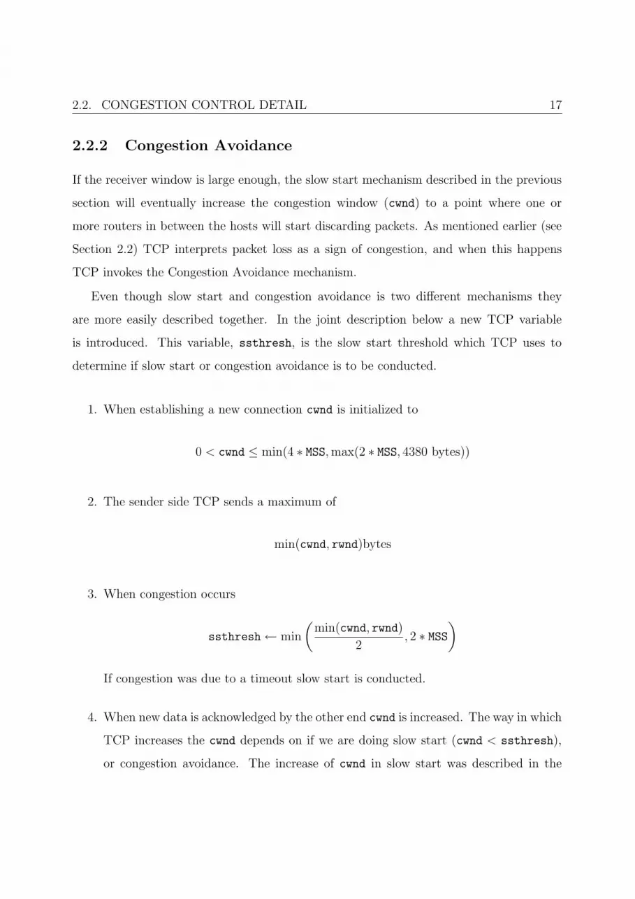
2.2.2 Congestion Avoidance
If the receiver window is large enough, the slow start mechanism described in the previous
section will eventually increase the congestion window (cwnd) to a point where one or
more routers in between the hosts will start discarding packets. As mentioned earlier (see
Section 2.2) TCP interprets packet loss as a sign of congestion, and when this happens
TCP invokes the Congestion Avoidance mechanism.
Even though slow start and congestion avoidance is two different mechanisms they
are more easily described together. In the joint description below a new TCP variable
is introduced. This variable, ssthresh, is the slow start threshold which TCP uses to
determine if slow start or congestion avoidance is to be conducted.
1. When establishing a new connection cwnd is initialized to
0 < cwnd ≤ min(4 ∗ MSS, max(2 ∗ MSS, 4380 bytes))
2. The sender side TCP sends a maximum of
min(cwnd, rwnd)bytes
3. When congestion occurs
ssthresh← min
(min(cwnd, rwnd)
2, 2 ∗ MSS
)
If congestion was due to a timeout slow start is conducted.
4. When new data is acknowledged by the other end cwnd is increased. The way in which
TCP increases the cwnd depends on if we are doing slow start (cwnd < ssthresh),
or congestion avoidance. The increase of cwnd in slow start was described in the
18 CHAPTER 2. BACKGROUND
previous section, and if we are doing congestion avoidance then cwnd← cwnd+ 1
cwnd,
which results in a linear increase of the cwnd.
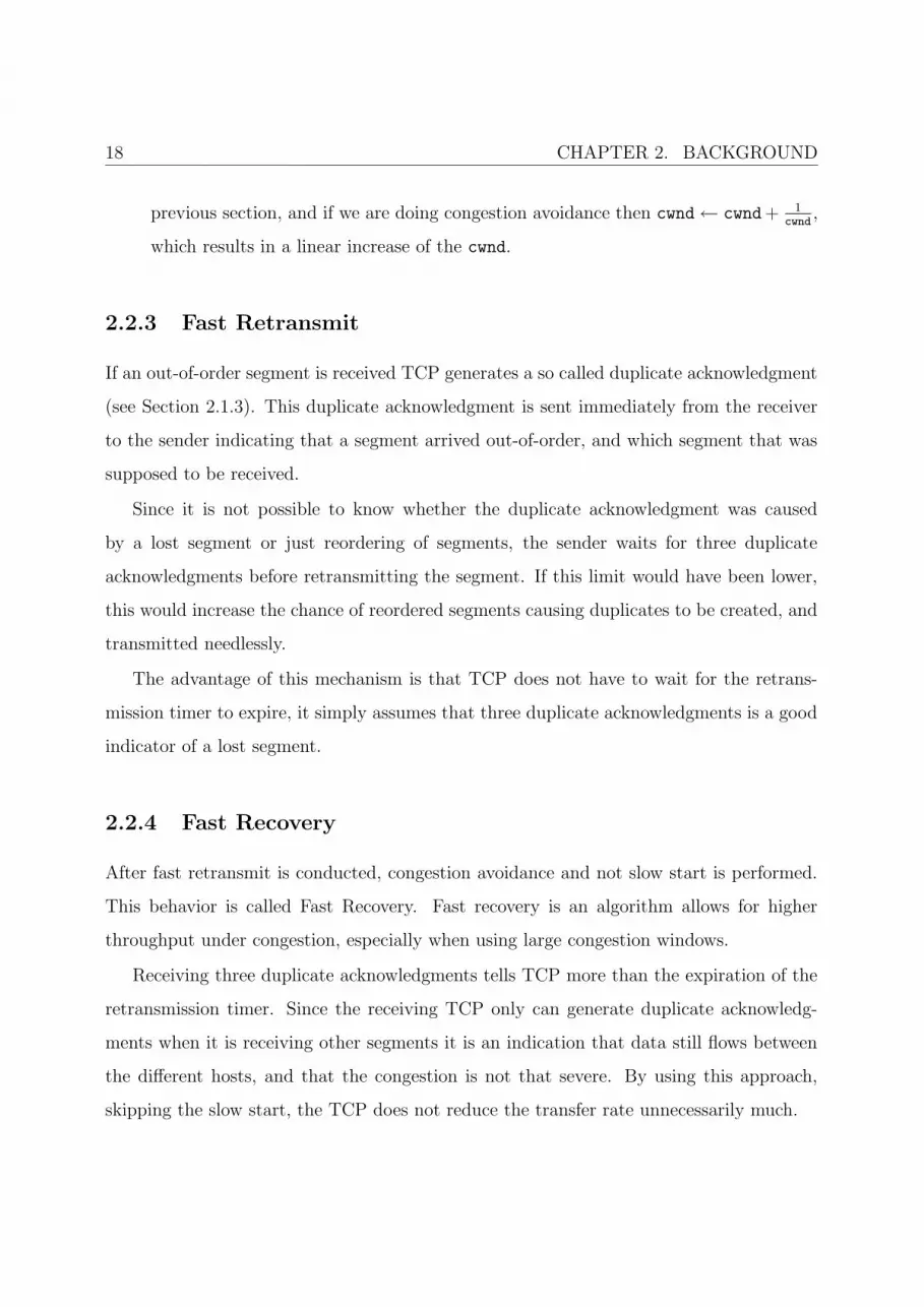
2.2.3 Fast Retransmit
If an out-of-order segment is received TCP generates a so called duplicate acknowledgment
(see Section 2.1.3). This duplicate acknowledgment is sent immediately from the receiver
to the sender indicating that a segment arrived out-of-order, and which segment that was
supposed to be received.
Since it is not possible to know whether the duplicate acknowledgment was caused
by a lost segment or just reordering of segments, the sender waits for three duplicate
acknowledgments before retransmitting the segment. If this limit would have been lower,
this would increase the chance of reordered segments causing duplicates to be created, and
transmitted needlessly.
The advantage of this mechanism is that TCP does not have to wait for the retrans-
mission timer to expire, it simply assumes that three duplicate acknowledgments is a good
indicator of a lost segment.
2.2.4 Fast Recovery
After fast retransmit is conducted, congestion avoidance and not slow start is performed.
This behavior is called Fast Recovery. Fast recovery is an algorithm allows for higher
throughput under congestion, especially when using large congestion windows.
Receiving three duplicate acknowledgments tells TCP more than the expiration of the
retransmission timer. Since the receiving TCP only can generate duplicate acknowledg-
ments when it is receiving other segments it is an indication that data still flows between
the different hosts, and that the congestion is not that severe. By using this approach,
skipping the slow start, the TCP does not reduce the transfer rate unnecessarily much.
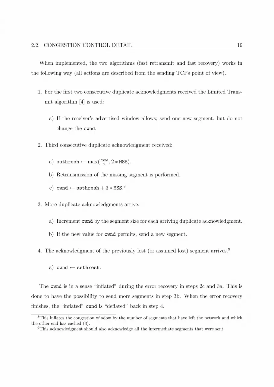
2.2. CONGESTION CONTROL DETAIL 19
When implemented, the two algorithms (fast retransmit and fast recovery) works in
the following way (all actions are described from the sending TCPs point of view).
1. For the first two consecutive duplicate acknowledgments received the Limited Trans-
mit algorithm [4] is used:
a) If the receiver’s advertised window allows; send one new segment, but do not
change the cwnd.
2. Third consecutive duplicate acknowledgment received:
a) ssthresh← max( cwnd2
, 2 ∗ MSS).
b) Retransmission of the missing segment is performed.
c) cwnd← ssthresh + 3 ∗ MSS.8
3. More duplicate acknowledgments arrive:
a) Increment cwnd by the segment size for each arriving duplicate acknowledgment.
b) If the new value for cwnd permits, send a new segment.
4. The acknowledgment of the previously lost (or assumed lost) segment arrives.9
a) cwnd ← ssthresh.
The cwnd is in a sense “inflated” during the error recovery in steps 2c and 3a. This is
done to have the possibility to send more segments in step 3b. When the error recovery
finishes, the “inflated” cwnd is “deflated” back in step 4.
8This inflates the congestion window by the number of segments that have left the network and whichthe other end has cached (3).
9This acknowledgment should also acknowledge all the intermediate segments that were sent.
20 CHAPTER 2. BACKGROUND
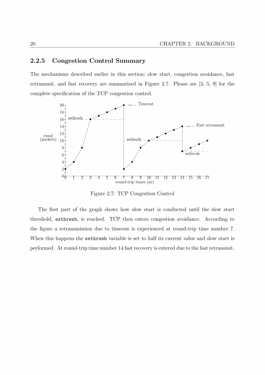
2.2.5 Congestion Control Summary
The mechanisms described earlier in this section; slow start, congestion avoidance, fast
retransmit, and fast recovery are summarized in Figure 2.7. Please see [3, 5, 9] for the
complete specification of the TCP congestion control.
0 1 2 3 4 5 6 7 8 9 10 11 12 13 14 15 16 170
2
4
6
8
10
12
14
16
18
20
cwnd(packets)
round-trip times (nr)
ssthresh
ssthresh
ssthresh
Timeout
Fast retransmit
Figure 2.7: TCP Congestion Control
The first part of the graph shows how slow start is conducted until the slow start
threshold, ssthresh, is reached. TCP then enters congestion avoidance. According to
the figure a retransmission due to timeout is experienced at round-trip time number 7.
When this happens the ssthresh variable is set to half its current value and slow start is
performed. At round-trip time number 14 fast recovery is entered due to the fast retransmit.

2.3. NETWORK EMULATION 21
2.3 Network Emulation
Because of the complexity of todays networks, especially the Internet, transport proto-
cols have become more and more complex. Because of the increase in complexity it is
nowadays hard, if possible at all, to fully grasp the behavior and performance issues of
a protocol without evaluating it under controlled conditions. Luckily, there are several
methods of evaluating transport protocols. These methods include analysis, simulation
and experiments with real protocol implementations. Even though analysis and simu-
lation can be used with advantage, experiments with real protocol implementations are
attractive because they more accurately reflect how transport protocols that are used in
real operational networks behave. Experiments with real protocol implementations can be
done in two different ways, using a real operational network or using network emulation.
Network
ServerClient
���������������
���������������
�������������������������
���������������
Figure 2.8: Real operational network
In a real operational network, illustrated in Figure 2.8, it is often hard (if possible at all)
to monitor and control the network parameters that can have impact on the experiments.
These parameters include delays, bandwidths, queue sizes, packet losses and external traffic
sources. If the relationship between an experimental result and a collection of network
parameters is to be investigated, there can be problems if one, or more, of these parameters
are unknown or uncontrollable. It is much easier to investigate such a relationship if the
parameters are available. In addition to this it is also very hard to control and reproduce
experiments if no control over the network parameters are provided.
22 CHAPTER 2. BACKGROUND
Client ServerNetwork emulator
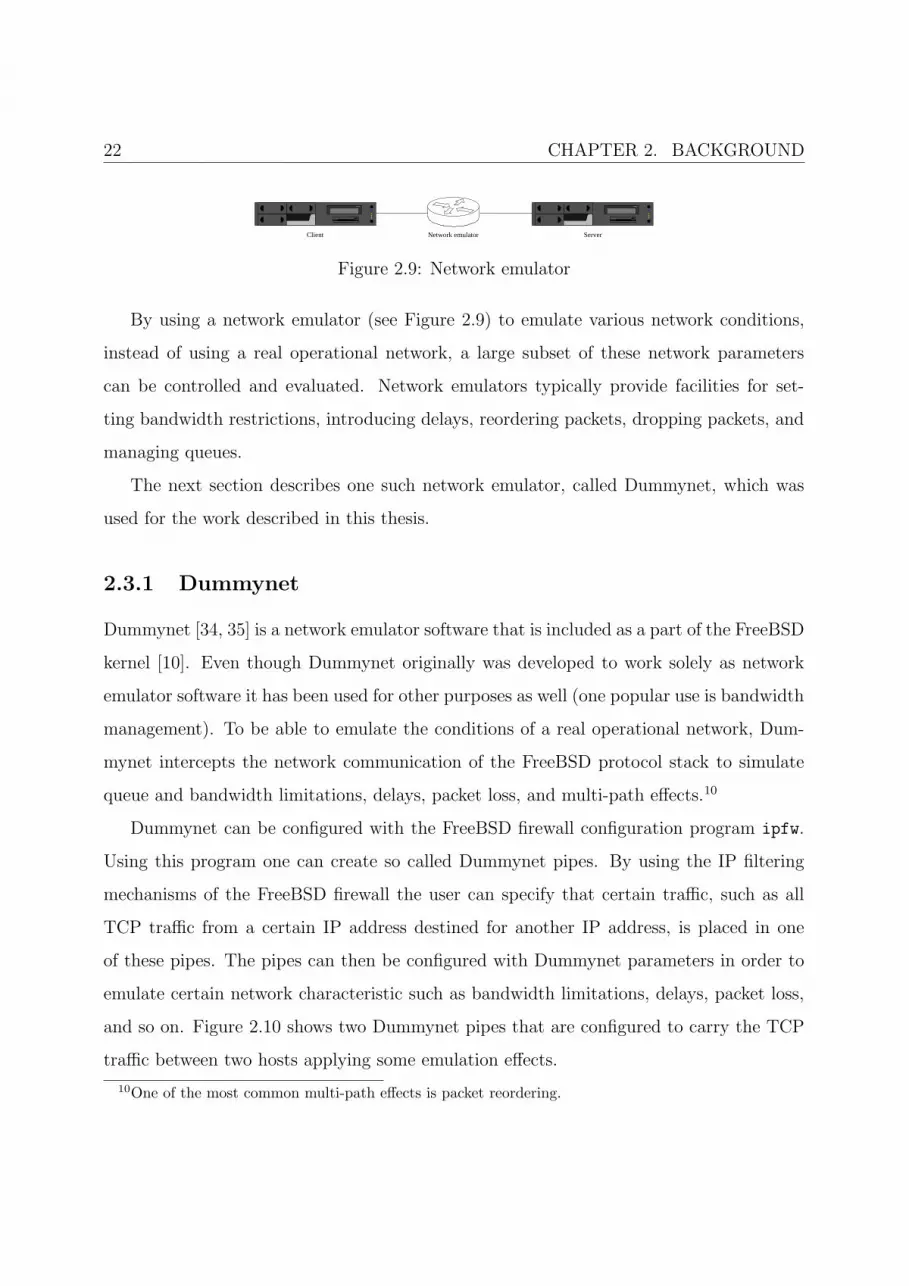
Figure 2.9: Network emulator
By using a network emulator (see Figure 2.9) to emulate various network conditions,
instead of using a real operational network, a large subset of these network parameters
can be controlled and evaluated. Network emulators typically provide facilities for set-
ting bandwidth restrictions, introducing delays, reordering packets, dropping packets, and
managing queues.
The next section describes one such network emulator, called Dummynet, which was
used for the work described in this thesis.
2.3.1 Dummynet
Dummynet [34, 35] is a network emulator software that is included as a part of the FreeBSD
kernel [10]. Even though Dummynet originally was developed to work solely as network
emulator software it has been used for other purposes as well (one popular use is bandwidth
management). To be able to emulate the conditions of a real operational network, Dum-
mynet intercepts the network communication of the FreeBSD protocol stack to simulate
queue and bandwidth limitations, delays, packet loss, and multi-path effects.10
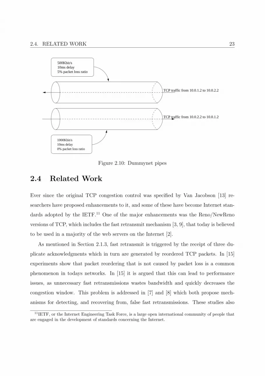
Dummynet can be configured with the FreeBSD firewall configuration program ipfw.
Using this program one can create so called Dummynet pipes. By using the IP filtering
mechanisms of the FreeBSD firewall the user can specify that certain traffic, such as all
TCP traffic from a certain IP address destined for another IP address, is placed in one
of these pipes. The pipes can then be configured with Dummynet parameters in order to
emulate certain network characteristic such as bandwidth limitations, delays, packet loss,
and so on. Figure 2.10 shows two Dummynet pipes that are configured to carry the TCP
traffic between two hosts applying some emulation effects.
10One of the most common multi-path effects is packet reordering.
2.4. RELATED WORK 23
500Kbit/s10ms delay5% packet loss ratio
1000Kbit/s10ms delay0% packet loss ratio
TCP traffic from 10.0.1.2 to 10.0.2.2
TCP traffic from 10.0.2.2 to 10.0.1.2
Figure 2.10: Dummynet pipes
2.4 Related Work
Ever since the original TCP congestion control was specified by Van Jacobson [13] re-
searchers have proposed enhancements to it, and some of these have become Internet stan-
dards adopted by the IETF.11 One of the major enhancements was the Reno/NewReno
versions of TCP, which includes the fast retransmit mechanism [3, 9], that today is believed
to be used in a majority of the web servers on the Internet [2].
As mentioned in Section 2.1.3, fast retransmit is triggered by the receipt of three du-
plicate acknowledgments which in turn are generated by reordered TCP packets. In [15]
experiments show that packet reordering that is not caused by packet loss is a common
phenomenon in todays networks. In [15] it is argued that this can lead to performance
issues, as unnecessary fast retransmissions wastes bandwidth and quickly decreases the
congestion window. This problem is addressed in [7] and [8] which both propose mech-
anisms for detecting, and recovering from, false fast retransmissions. These studies also
11IETF, or the Internet Engineering Task Force, is a large open international community of people thatare engaged in the development of standards concerning the Internet.
24 CHAPTER 2. BACKGROUND
propose mechanisms for increasing the duplicate acknowledgment threshold dynamically if
reordering of segments is detected. Other work that has been conducted in the same area
[27] argues that even though packet reordering is a common phenomenon the effects of it
is not that severe and therefore the duplicate acknowledgment threshold could be lowered
to two in order to gain more fast retransmit opportunities. A lowering of the duplicate
acknowledgment threshold is also proposed in [19], but in this case the lowering is dynamic
and happens in two different scenarios; when the amount of data in flight is not enough to
enable the fast retransmit mechanism12, or when the sender is idle.13
Other work related to increase the fast retransmit opportunities is done in [20, 21] which
specifies a TCP segmentation mechanism called TCP-SF. By fragmenting the packets so
that at least three packets always are in flight, TCP-SF aims to enable fast retransmit even
when the congestion window is too small to normally allow this.
Even though fast retransmit is the preferred way of retransmitting lost data, retrans-
missions due to timeout are still common. To gain performance a large number of TCP
hosts [2] uses TCP implementations which allow a minimum RTO that is less than the
specified standard of one second [26]. This is a potential problem, especially for TCP hosts
that operate over low bandwidth links and have large initial windows [5], as it can result
in spurious retransmissions which considerably lower the performance of the connection.
Even if the minimum RTO is set according to the standard, spurious retransmissions can
occur due to different path characteristics. To avoid that these, unnecessary, retransmis-
sions lower the performance, changes to the TCP protocol have been proposed in [6, 32][25].
In [6, 32] the Eifel Algorithm is presented. This algorithm aims to improve TCP perfor-
mance by restoring the TCP congestion state after a spurious retransmission is detected. It
also adapts the RTO timer in order to prevent further spurious retransmissions. F-RTO,
described in [25], is a proposed sender side modification which is similar to the limited
12To generate three duplicate acknowledgments at least three packets must be on the way to the receiverso that three duplicate acknowledgments can be generated.
13Due to receiver window limitations or that no unsent data is ready for transmission.
2.4. RELATED WORK 25
transmit algorithm, but instead applied to the recovery from timeouts.
Besides the work on avoiding timeouts, in favor of fast retransmit, and recovering
from spurious retransmissions, a lot of research has been conducted due to the increase of
network paths with high bandwidth and delay. One of the major problems with TCP is
that it performs poorly when both the bandwidth and the delay increases. To solve this
problem different techniques have been proposed; Adaptive start (Astart) [33] which is a
proposed modification of the TCP slow start phase to better utilize the link with the help
of bandwidth estimation techniques, and Scalable TCP [16] which is a modification to the
congestion control of TCP that allows for better link utilization by allowing a faster growth
of the congestion window.
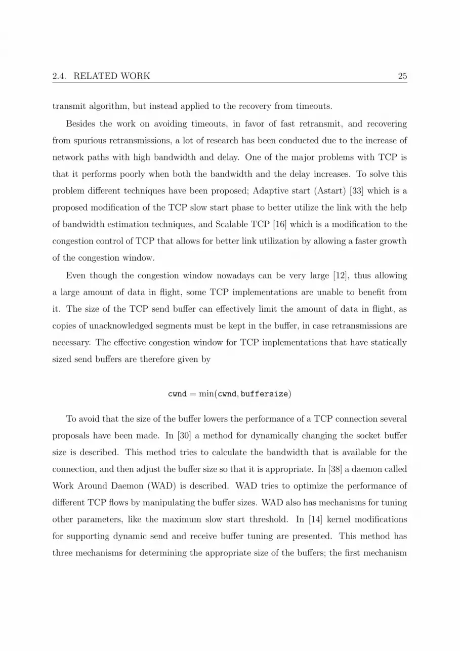
Even though the congestion window nowadays can be very large [12], thus allowing
a large amount of data in flight, some TCP implementations are unable to benefit from
it. The size of the TCP send buffer can effectively limit the amount of data in flight, as
copies of unacknowledged segments must be kept in the buffer, in case retransmissions are
necessary. The effective congestion window for TCP implementations that have statically
sized send buffers are therefore given by
cwnd = min(cwnd, buffersize)
To avoid that the size of the buffer lowers the performance of a TCP connection several
proposals have been made. In [30] a method for dynamically changing the socket buffer
size is described. This method tries to calculate the bandwidth that is available for the
connection, and then adjust the buffer size so that it is appropriate. In [38] a daemon called
Work Around Daemon (WAD) is described. WAD tries to optimize the performance of
different TCP flows by manipulating the buffer sizes. WAD also has mechanisms for tuning
other parameters, like the maximum slow start threshold. In [14] kernel modifications
for supporting dynamic send and receive buffer tuning are presented. This method has
three mechanisms for determining the appropriate size of the buffers; the first mechanism
26 CHAPTER 2. BACKGROUND
determines the buffer size according to the current network conditions, the second takes
the memory management into account14, and the third asserts a memory usage limit to
prevent that too much memory is used. One operating system that includes dynamic buffer
sizing is Linux [39] which automatically increases the send buffers when there is need for
it.
Although a lot of research has been conducted on TCP, little has been done with a
deterministic emulation approach. Common network emulators, like Dummynet, usually
provide means for generating packet losses, but only in non-deterministic ways like ran-
domly induced losses and overflow of emulated buffers.
According to [11] non-determinstic evaluation is not enough to cover all aspects of
transport protocol behavior, especially for short-lived flows the position of the loss within
the flow has an impact on the throughput. This statement is proved by experiments done
with an extended, deterministic, version of the Dummynet network emulator. This version
allows for position based losses, and the results presented clearly show that the position of
a loss has impact on the total transmission time.
Another feature of the deterministic emulation approach is, according to [11], that ex-
perimental results are reproducible. Using a typical network emulator it is not possible
to place losses at the exact same location as in previous experiments, but with this deter-
ministic approach losses can be placed in the exact same location every time. This makes
results easier to reproduce and the variance in the results is less.
2.5 Summary
In this chapter the basic behavior of TCP has been described, in terms of data transmission,
reliability mechanisms, and the congestion control mechanisms that are used. We have seen
that TCP is a reliable transport protocol, which also tries to prevent over-utilization of the
14So that the memory is fairly shared between different TCP flows.

2.5. SUMMARY 27
network it operates in. The chapter also included a short introduction to the concept of
network emulation, and explained the basics of the Dummynet network emulation software.
Finally, in the last part of the chapter, some work that is related to this thesis was presented.
In the next chapter the experiment design is defined, and the environment in which the
experiments were conducted is described.


Chapter 3
Experimental Design & Environment
In this chapter detailed descriptions of the experimental design, and the environment in
which the experiments were conducted, are provided. The chapter starts with a description
of the fast retransmit inhibition problem, and continues with details on how the experi-
ments were designed. In the last part of this chapter the different parts of the experimental
environment are described.
3.1 Problem Description
As described in Section 2.2, TCP congestion control consists of a number of different, and
interrelated, mechanisms. One of these mechanisms is the fast retransmit. The purpose of
the fast retransmit mechanism is to allow a sender to retransmit lost packets before they are
regarded as lost by the TCP retransmission timer. Fast retransmit uses the receipt of three
duplicate acknowledgments as an indicator of packet loss. Duplicate acknowledgments can
be generated by the receiver for two different reasons; packet reordering in the network, or
packet loss. Which of these reasons that causes the duplicate acknowledgment is hard for
the sender to decide. To ensure that the fast retransmit mechanism does not mistakenly
assume that a packet that has been reordered in the network was lost, and makes an
29

30 CHAPTER 3. EXPERIMENTAL DESIGN & ENVIRONMENT
unnecessary retransmission of it, a duplicate acknowledgment threshold is used. For TCP
this threshold is set to three.
While the use of the duplicate acknowledgment threshold helps TCP to avoid retrans-
mitting packets that have been mildly reordered in the network it also has negative con-
sequences. One of these negative consequences is evident at the end of a connection when
the application has written all its data to the transport layer. Since the fast retransmit
mechanism requires the receipt of three duplicate acknowledgments as an indication of
packet loss, it cannot work if there are less than three packets to send after the packet
that has been lost. Thus, at the end of connections when there are not enough packets
to send to generate three duplicate acknowledgments, the lost packet must be recovered
using a retransmission due to timeout. A similar problem is also evident at the beginning
of a connection when the three-way-handshake is conducted (see Section 2.1.6). If one of
the first packets in this procedure is lost it is not possible to perform a fast retransmit
because packets needed for duplicate acknowledgment generation simply does not exist.
Allthough this problem can cause performance problems as well, it is not considered as a
fast retransmit inhibition. This because it is not an effect of the duplicate acknowledgment
threshold. An illustration of a client and a server that experience these problems is shown
in Figure 3.1.
A timeout is intended to occur only if the network suffers from heavy congestion,
therefore the recovery from such a timeout includes a considerable reduction of the sending
rate1 in order to reduce the (over)utilization of the network. Fast retransmit, on the other
hand, uses a recovery mechanism that lowers the sending rate less compared to the timeout
recovery. The reason why the sending rate is lowered less is that the receipt of the three
duplicate acknowledgments indicates that packets in fact have left the network, indicating
that the congestion is not that severe.
So, even if fast retransmit is suitable for the current network conditions, it is not possible
1By employing the slow start mechanism.
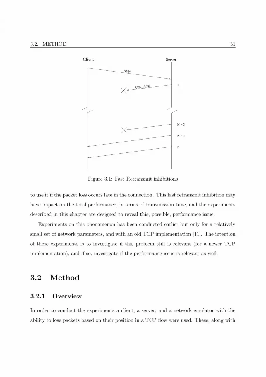
3.2. METHOD 31
1
SYN
SYN, ACK
N − 2
N − 1
N
Client Server
Figure 3.1: Fast Retransmit inhibitions
to use it if the packet loss occurs late in the connection. This fast retransmit inhibition may
have impact on the total performance, in terms of transmission time, and the experiments
described in this chapter are designed to reveal this, possible, performance issue.
Experiments on this phenomenon has been conducted earlier but only for a relatively
small set of network parameters, and with an old TCP implementation [11]. The intention
of these experiments is to investigate if this problem still is relevant (for a newer TCP
implementation), and if so, investigate if the performance issue is relevant as well.
3.2 Method
3.2.1 Overview
In order to conduct the experiments a client, a server, and a network emulator with the
ability to lose packets based on their position in a TCP flow were used. These, along with
32 CHAPTER 3. EXPERIMENTAL DESIGN & ENVIRONMENT
other components that were used for building the experimental environment are described
in the next two sections.
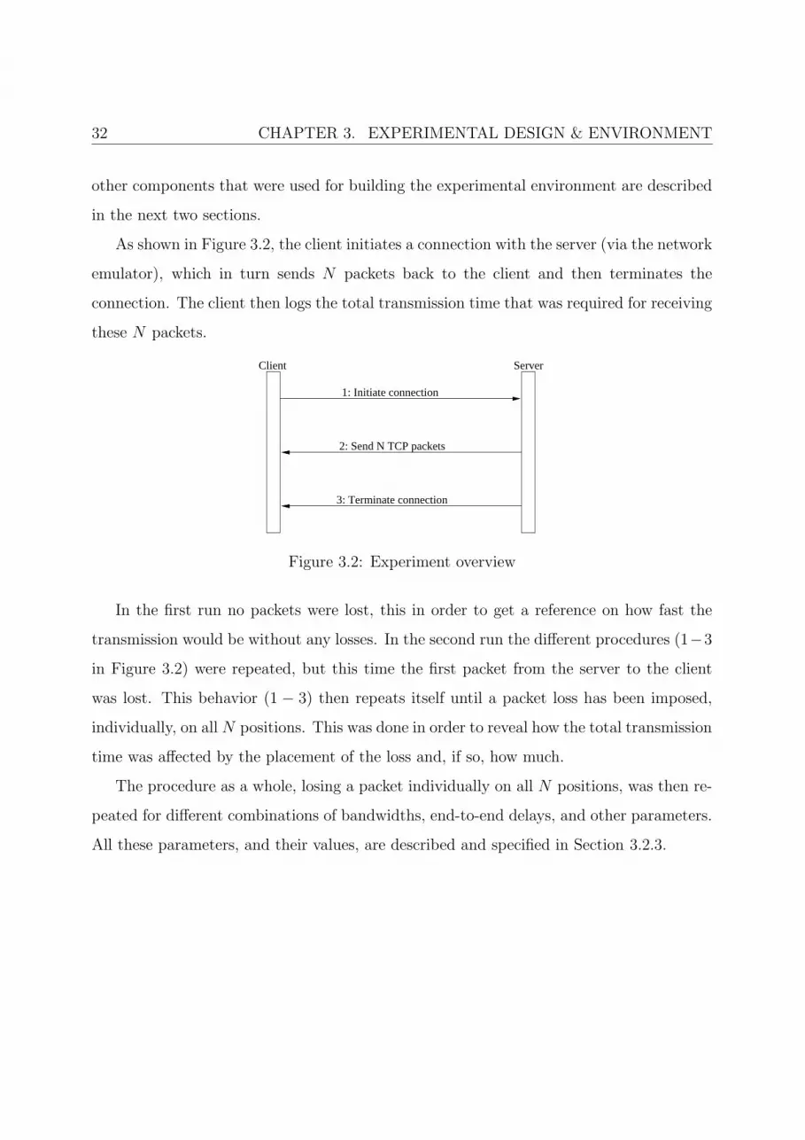
As shown in Figure 3.2, the client initiates a connection with the server (via the network
emulator), which in turn sends N packets back to the client and then terminates the
connection. The client then logs the total transmission time that was required for receiving
these N packets.
2: Send N TCP packets
1: Initiate connection
3: Terminate connection
Client Server
Figure 3.2: Experiment overview
In the first run no packets were lost, this in order to get a reference on how fast the
transmission would be without any losses. In the second run the different procedures (1−3
in Figure 3.2) were repeated, but this time the first packet from the server to the client
was lost. This behavior (1 − 3) then repeats itself until a packet loss has been imposed,
individually, on all N positions. This was done in order to reveal how the total transmission
time was affected by the placement of the loss and, if so, how much.
The procedure as a whole, losing a packet individually on all N positions, was then re-
peated for different combinations of bandwidths, end-to-end delays, and other parameters.
All these parameters, and their values, are described and specified in Section 3.2.3.
3.2. METHOD 33
3.2.2 Details
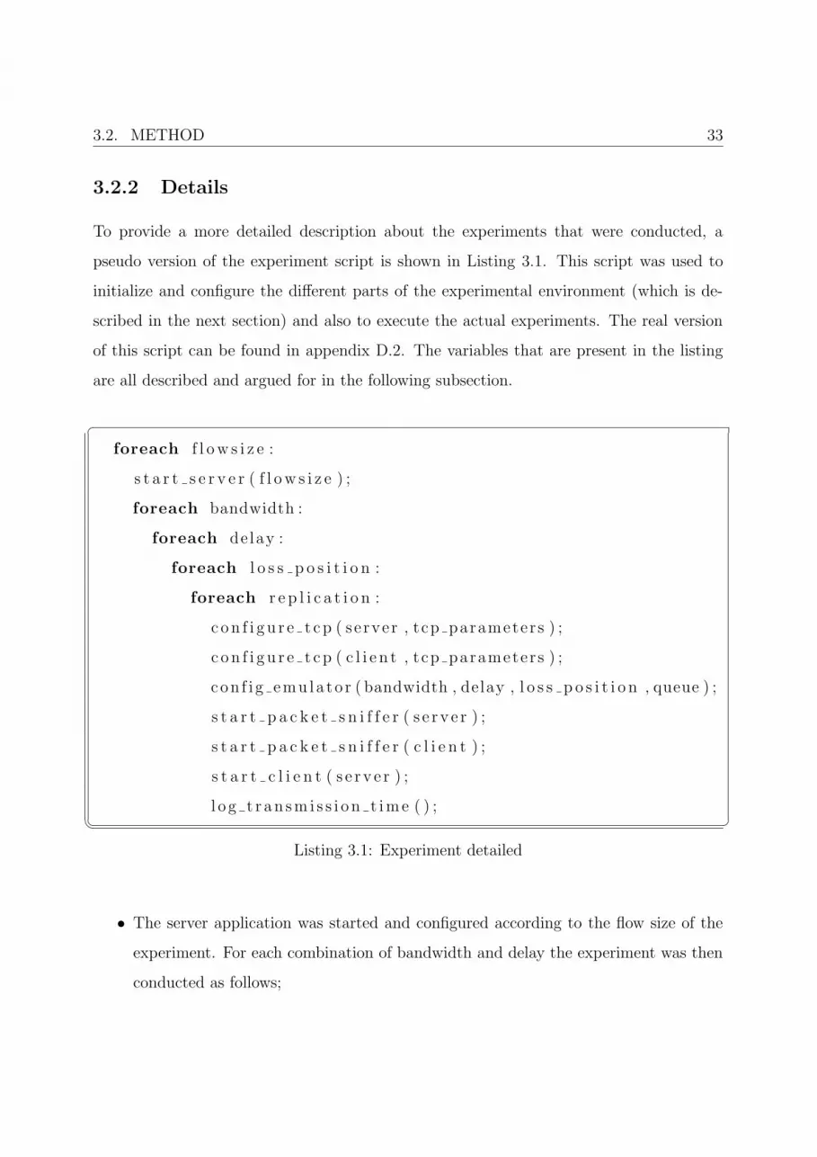
To provide a more detailed description about the experiments that were conducted, a
pseudo version of the experiment script is shown in Listing 3.1. This script was used to
initialize and configure the different parts of the experimental environment (which is de-
scribed in the next section) and also to execute the actual experiments. The real version
of this script can be found in appendix D.2. The variables that are present in the listing
are all described and argued for in the following subsection.
�
foreach f l ow s i z e :
s t a r t s e r v e r ( f l ow s i z e ) ;
foreach bandwidth :
foreach delay :
foreach l o s s p o s i t i o n :
foreach r e p l i c a t i o n :
c on f i g u r e t c p ( se rver , tcp parameters ) ;
c on f i g u r e t c p ( c l i e n t , tcp parameters ) ;
c on f i g emu la to r ( bandwidth , delay , l o s s p o s i t i o n , queue ) ;
s t a r t p a c k e t s n i f f e r ( s e r v e r ) ;
s t a r t p a c k e t s n i f f e r ( c l i e n t ) ;
s t a r t c l i e n t ( s e r v e r ) ;
l o g t r an sm i s s i on t ime ( ) ;� �
Listing 3.1: Experiment detailed
• The server application was started and configured according to the flow size of the
experiment. For each combination of bandwidth and delay the experiment was then
conducted as follows;

34 CHAPTER 3. EXPERIMENTAL DESIGN & ENVIRONMENT
• For every position within the TCP flow (loss position) the following was done (with
replication repetitions);
1. The client and server machines were configured with TCP parameters.
2. The network emulator was configured with bandwidth, delay, position of packet
loss, and queue size parameters.
3. Traffic loggers on the client and server machines were started.
4. The client application was started (starting the experiment).
5. The total transmission time of the experiment was logged.
3.2.3 Parameters
TCP parameters
As mentioned earlier, in Section 2.2, TCP makes use of two different phases during a
connection; slow start and congestion avoidance. In both these phases the congestion
window is steadily increasing until a packet loss is detected, then the congestion window
is decreased and the procedure repeats itself. Instead of letting TCP cause congestion
when probing for available bandwidth some TCP versions implement bandwidth limiting
functionality that is supposed to decrease the sending rate when the available bandwidth
is believed to be reached.
To determine the available bandwidth different TCP implementations use different
techniques. The TCP implementation of FreeBSD 6 [10] (which was used for the exper-
iments) has such a feature, called TCP bandwidth-delay product window limiting, which
is enabled by default. The implementation of this bandwidth limiting functionality is
similar to TCP/Vegas [17], which also tries to prevent congestion losses by adapting the
throughput to the network conditions.
Even though such features may be useful to prevent network congestion from occurring,
the primary goal of this work was to study what actually happens, in terms of performance
3.2. METHOD 35
and behavior, when packet loss do occur. Furthermore, this bandwidth limitinh feature is
not a proposed TCP standard which results in that different TCP implementations that
incorporates this kind of feature, almost certainly, will have a unique way of implementing
it. Thus, having it enabled would make the experiments lack in generality.
For these reasons the bandwidth limiting feature of FreeBSD was disabled. This was
done by changing the value of the sysctl2 parameter net.inet.tcp.inflight.enable
from its original value of 1 to 0.
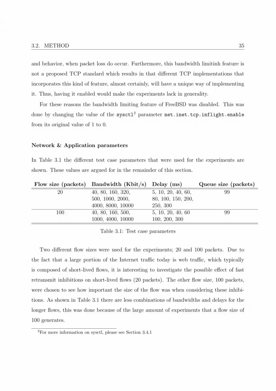
Network & Application parameters
In Table 3.1 the different test case parameters that were used for the experiments are
shown. These values are argued for in the remainder of this section.
Flow size (packets) Bandwidth (Kbit/s) Delay (ms) Queue size (packets)
20 40, 80, 160, 320, 5, 10, 20, 40, 60, 99500, 1000, 2000, 80, 100, 150, 200,4000, 8000, 10000 250, 300
100 40, 80, 160, 500, 5, 10, 20, 40, 60 991000, 4000, 10000 100, 200, 300
Table 3.1: Test case parameters
Two different flow sizes were used for the experiments; 20 and 100 packets. Due to
the fact that a large portion of the Internet traffic today is web traffic, which typically
is composed of short-lived flows, it is interesting to investigate the possible effect of fast
retransmit inhibitions on short-lived flows (20 packets). The other flow size, 100 packets,
were chosen to see how important the size of the flow was when considering these inhibi-
tions. As shown in Table 3.1 there are less combinations of bandwidths and delays for the
longer flows, this was done because of the large amount of experiments that a flow size of
100 generates.
2For more information on sysctl, please see Section 3.4.1
36 CHAPTER 3. EXPERIMENTAL DESIGN & ENVIRONMENT
The server application that were used for the experiments, described in Section 3.4.3, is
designed to send N buffers containing 2500 bytes of data to the client. To be able to send
exactly 20 packets we were forced to take several things into account. The MTU of the IP
packets in the experimental environment was set to 1500 bytes which yields a maximum
TCP packet size of 1500 − 20 − 20 − 12 = 1448 bytes, where the IP and TCP header is
consuming 20 bytes each, and the TCP options used by the FreeBSD TCP implementation
require 12 bytes of data. Due to the nature of TCP the server application also needs to
send 2 packets that do not contain any data; one of these packet is the SYN-ACK packet
that is used in the three-way-handshake, and the other one is the final acknowledgment
sent in the connection termination process. By solving difference 3.1, we can conclude that
10 buffers (x) of data must be sent in order to get the additional 18 packets.
17 <x× 2500
1448≤ 18, x ∈ Z
+ (3.1)
By the same argumentation we concluded that 56 buffers of data was required to gen-
erate a flow of 100 packets.
The bandwidths at which the experiments were conducted, 40−10000 Kbit/s, is believed
to be a range of bandwidths that frequently exists within real networks. The lower limit, 40
Kbit/s, may not be a common bandwidth in todays high-speed networks, but it is included
as some people still use modems to connect to the Internet. The upper limit, 10000 Kbit/s,
is quite low but we were restrained to use it as it was the theoretical maximum for the
network emulation software that we used.
In todays networks a wide range of delays exist. In a local area network, LAN, the
physical distance between different hosts is, typically, small and they are often intercon-
nected using few, if any, routers. The short distance and the limited processing of the
traffic3 lead to small end-to-end delays between the hosts. A wide area network, or WAN,
3In terms of routing.

3.2. METHOD 37
can be defined as a set of interconnected LANs. Depending on the size of the WAN, and
where the different hosts are located, in terms of physical distance and number of routers
in between, the delays can vary considerably. While two hosts that both share WAN and
LAN have a small end-to-end delay, two hosts that are separated by thousands of miles
and numerous intermediate routers have a considerably longer delay. To cover most of
these scenarios delays between 5− 300 ms were used.
Another reason for choosing the bandwidths and delays in the way that was done was
to create bandwidth-delay products, or BDPs, that are equal (or almost equal). BDP is a
measurement of the maximum link capacity that can be utilized by TCP, and it is therefore
interesting to see if any similar effects, between different experiments, occur when the BDP
is equal.
BDP (bytes) = Bandwidth (Kbytes/s) ∗Delay (ms) (3.2)
Worth to note is that the delay in Equation 3.2 is not the end-to-end delay, but the
round-trip time.4
For example; using equation 3.2, the BDP for a connection with a bandwidth of 40
Kbit/s and an round-trip time of 20 ms is exactly the same as for the case of 80 Kbit/s
and 10 ms.5
The queue size was set to 99 packets for both of the different flows sizes. This number is
sufficiently high to avoid buffer overflows. Normally, as mentioned in Section 2.2, congestion
occurs when a router in a network has a full buffer and the incoming rate of the traffic
keeps exceeding the outgoing, thus making the router start discarding incoming packets.
Due to the fact that we want do decide exactly when to loose packets in the flow that
behavior, losing packets due to buffer overflows, is not preferred.
4The time required for a segment to be sent and acknowledged.5 40∗10
3
8∗ 20 = 80∗10
3
8∗ 10 = 100 Kbytes. Where the division with 8 is done to go from bits to bytes.

38 CHAPTER 3. EXPERIMENTAL DESIGN & ENVIRONMENT
Other parameters
The number of replications was set to three, this in order to account for possible variance
in the results.
3.3 Environment Overview
To be able to conduct the experiments that were described in the previous section, an
experimental environment was constructed.
There were two major requirements for the experimental environment. The first re-
quirement was that the TCP communication between a client and a server (located in the
environment) should not differ much from TCP communication between a client and a
server over a real network. This requirement was fulfilled by using a network emulator
that could emulate network parameters that are common in real operational networks.
The other requirement was that the environment should be able to produce position based
losses within a TCP communication flow. With position based losses it would be possible
to make positional dependencies of the losses visible and it would also be easier to repro-
duce results with small variance. To deal with this requirement the network emulator was
equipped with a network emulation software that was able to produce losses according to
given positions.
In Figure 3.3 the setup of the experimental environment is illustrated. The solid lines
show the links that carry the experiment traffic, i.e. the traffic between the client and the
server (via the network emulator). The dashed lines show the separate control network
that the three computers were connected in. This control network was created in order
to let the computers to be automatically configured with experiment parameters without
interfering with the experiment traffic.
The computers used for building this environment were Dell Optiplex GX260 with
3Com 100Mbit/s network cards. The client and the server was running FreeBSD 6.0B3,
3.4. ENVIRONMENT DETAILS 39
Switch
Client ServerNetwork emulator
Control Traffic
TCP experiment traffic
Figure 3.3: Environment overview
and the network emulator FreeBSD 6.0B5.
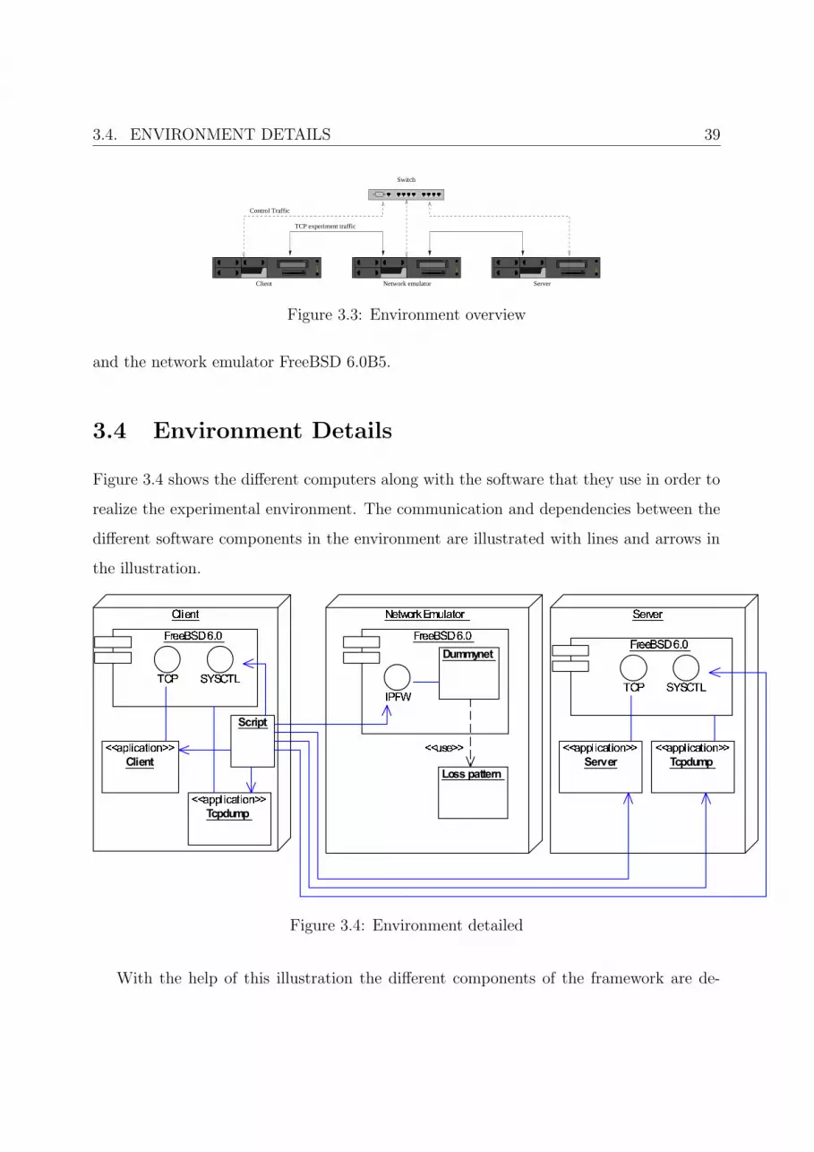
3.4 Environment Details
Figure 3.4 shows the different computers along with the software that they use in order to
realize the experimental environment. The communication and dependencies between the
different software components in the environment are illustrated with lines and arrows in
the illustration.
Figure 3.4: Environment detailed
With the help of this illustration the different components of the framework are de-
40 CHAPTER 3. EXPERIMENTAL DESIGN & ENVIRONMENT
scribed in the following subsections.
3.4.1 FreeBSD 6.0B3
The client and the server were both configured to run FreeBSD 6.0B3, this to make sure
that the TCP implementations of the client and the server were the same. If different
implementations of TCP is used in an experiment there can be a problem determining if
the result depends on one of the implementations, or on the other, or on the combination of
the two. The easiest way to eliminate this risk is simply to run identical implementations
on the different hosts.
FreeBSD 6.0B3 has a feature that is called host caching. This feature, TCP host
caching, caches host observations from TCP. This allows the TCP to reuse round-trip
times, congestion window size, slow start threshold, and bandwidth estimates from previous
connections in order to optimize new TCP connections to the same host. This was not
acceptable for the experimental environment because every experiment was, of course,
required to be independent from previous experiments. To disable this feature a slight
modification to the kernel was required. Details about this kernel modification can be
found in Section C.2 of the appendix.
FreeBSD has a command that is called sysctl. This command acts as an interface to
the kernel and can be used to list and modify a large number of kernel parameters. Some
of these parameters can be used in order to configure the TCP implementation. Two of
these parameters, net.inet.tcp.slowstart_local_flightsize, and
net.inet.tcp.slowstart_flightsize, are used to control the allowed amount of out-
standing TCP packets during the slow start phase. Because network communication be-
tween computers on a local network (same subnet) are more likely to have a large amount
of available bandwidth, the values of these two parameters differed.6 The machines that
were used as client and server in the environment were on the same subnet, so we were
6Allowing a larger amount of outstanding data in a local network.
3.4. ENVIRONMENT DETAILS 41
required to change the value of net.inet.tcp.slowstart_local_flightsize, in order to
treat the traffic in the network as “non-local”.
For more information on the FreeBSD TCP implementation see appendix C.1.
3.4.2 FreeBSD 6.0B5
The operating system on the network emulator computer was FreeBSD 6.0B5. The kernel
of this operating system was configured to run a modified version of Dummynet. More
information about Dummynet and the modified Dummynet can be found in Section 3.4.4.
3.4.3 Client & Server applications
The client and server applications in this environment work like a sink and a source. When
the server is started it takes as argument the port number to listen for connections at and
how much data to transmit to connecting clients. The client is started by passing the
server host name and port number. When a successful connection is established between
the two applications, the server application sends the specified amount of data to the client
and closes the connection. When the client has received all the data sent by the server,
indicated by a close from the server, the client tries to close the connection and returns
the elapsed time from connection to the receipt of the final data.
The sources to these applications are provided in Appendix D.3.
3.4.4 Dummynet & Loss patterns
As described in Section 2.3.1 Dummynet is a network emulator software. The Dummynet
version that was used for this environment is the extended version mentioned in Section
2.4. To be able to use the extended version we were required to port it from FreeBSD
4.6.x to FreeBSD 6.0B5.7 By using this version we could generate positional losses in TCP
7Unfortunately this porting is too extensive to be included/described within the thesis.

42 CHAPTER 3. EXPERIMENTAL DESIGN & ENVIRONMENT
data flows by simply specifying which packets that should be lost. A Dummynet example
configuration is shown in Figure 3.5.
ipfw add 1 pipe 100 tcp from <server> <server-port> to <client> in
ipfw add 2 pipe 200 tcp from <client> to <server> <server-port> out
ipfw add 3 pipe 300 tcp from <server> <server-port> to <client> out
ipfw pipe 100 config packlfile <pattern>
ipfw pipe 200 config bw <bw> delay <delay> queue <queue>
ipfw pipe 300 config bw <bw> delay <delay> queue <queue>
Figure 3.5: Dummynet Configuration
In Figure 3.5 we can see that three Dummynet pipes are created and configured.8 One
pipe for traffic that is coming into the network emulator (from the server), and two pipes for
the outgoing traffic (traffic from both client and server).9 The two pipes that is configured
for outgoing traffic is configured to emulate bandwidth limitations, delays, and queue-size
limitations. The pipe for the incoming server traffic is configured with a “loss pattern”.
This loss pattern is a file that contains a binary pattern that tells Dummynet exactly which
packets in the TCP data flow that should be lost.
Let us say that we want to lose the fourth packet in a TCP data stream, then the loss
pattern simply looks like in Figure 3.6 where N is the period of the loss pattern, i.e. after
Dummynet processed N packets it will start over from the beginning of the pattern again.
0 0 0 1 0 0 . . . 0︸ ︷︷ ︸
N positions
Figure 3.6: Loss pattern
8This is done by the help of the program ipfw, that was mentioned in Section 2.3.19No pipe is created for incoming traffic from the client, which is perfectly legal if no emulation effects
is to be applied on that traffic.
3.4. ENVIRONMENT DETAILS 43
To simplify the creation of such patterns, a pattern generation application was con-
structed. This application is described in appendix D.1.
3.4.5 Tcpdump
To be able to log and analyze TCP traffic flowing between the client and the server Tcp-
dump [37] was used. This tool, Tcpdump, can be used to capture traffic on a network
interface according to a given expression. An example usage of Tcpdump is;
tcpdump -i eth0 -w log.pcap tcp port 80
where we instruct Tcpdump to capture all TCP traffic, with a source or destination port
of 80, on the network interface eth0. The -w switch tells Tcpdump to store the captured
data to a file (log.pcap in this example).
Applications like Tcpdump are often called packet sniffers. These sniffers are usually
made up of two major components; a packet analyzer and a packet capture. The packet
capture component is responsible for the actual traffic capturing, which takes place in
kernel space. Here the packet capture component receives copies of all the link frames that
are sent and/or received (in our case Ethernet frames). The other component, the packet
analyzer, is an application executing in user space. This application is able to interpret the
captured frames in terms of higher-level protocols and to perform various actions on the
captured traffic. In Figure 3.7 we can see that Tcpdump, which actually is just a packet
analyzer, uses the BSD Packet Filter (BPF) [23], with the help of the pcap library [18], in
order to capture network traffic. These components, together, form a packet sniffer.
3.4.6 Script
The script is the “brain” of the experimental environment. As illustrated in Figure 3.4, and
described in Section 3.2.2, this script was used to start the client and the server application,

44 CHAPTER 3. EXPERIMENTAL DESIGN & ENVIRONMENT
Physical
Ethernet
IP
TCP
Client/Serverapplication
Kernel space
User space
Packet sniffer
Tcpdump
BPF
pcap library
Figure 3.7: Tcpdump
and to configure all parts of the environment according to the desired parameters of the
experiment at hand. The source code to this script can be found in Appendix D.2.
3.5 Summary
In this chapter we have presented the problem with fast retransmit inhibitions, the ex-
perimental design that was required to reveal these inhibitions were presented, and the
environment in which the experiments were conducted was described in detail. In the next
chapter the results of the experiments are presented and, in some cases, analyzed.

Chapter 4
Results and Analysis
This chapter presents the results and the analysis of the experiments. The chapter is
divided into two different parts; one for the short flows (20 packets), and one for the long
flows (100 packets). Each part begins with a section where the performance loss due to
the fast retransmit inhibitions are presented. In the following section a more detailed view
is presented. Here we can see how losses on all different positions in the flows affects the
total transmission time. All interesting phenomena and anomalies that are present in this
section are then discussed and analyzed in the subsequent sections, where the flows that
contain these interesting results are studied on packet level.
4.1 Short flows
4.1.1 General performance loss
Figure 4.1 shows how much additional time that was required in order to complete a
transmission if the introduced packet loss was placed in the end of the flow, where fast
retransmit should be inhibited, as opposed to a loss where fast retransmit was used. The
y-axis of the graph show the additional time, in percent, that was required for a flow
with a delay according to the x-axis (ms). The figure shows that for combinations of high
45

46 CHAPTER 4. RESULTS AND ANALYSIS
0
50
100
150
200
250
300
350
0 20 40 60 80 100 120 140 160 180 200 220 240 260 280 300
Add
ition
al T
ime
(%)
Delay (ms)
Performance loss
40Kbps80Kbps
160Kbps320Kbps500Kbps
1000Kbps2000Kbps4000Kbps8000Kbps
10000Kbps
Figure 4.1: Performance loss for the short flows
bandwidth and low delay the performance consequences of a late loss are dramatic. For a
bandwidth of 10000 Kbit/s and a delay of 5 ms 301% of additional time is required. This
can be compared with a bandwidth of 80 Kbit/s and a delay of 5 ms where “only” 117%
of additional time is required. Another interesting thing to note is that the additional
time seems to decrease more rapidly for higher bandwidths, as the delay increases, than
for the lower bandwidths. For lower bandwidths the performance impact seems to be more
stable. In the case of 80 Kbit/s the additional time required ranges from 117% to 47%
for the different delays, whereas a bandwidth of 10000 Kbit/s ranges from 301% to 31%.
The reason why this graph does not contain any results for the three lowest delays (5, 10,
and 20 ms) of 40 Kbit/s has to do with a defect in the FreeBSD TCP implementation.
This defect causes the transmission time of flows with low bandwidth and delay to increase
dramatically. To be certain of that these results are not mistakenly associated with the
problem of fast retransmit inhibitions they were not included in the graph. The defect in
the FreeBSD implementation is discussed more throurghly in the next two sections.
In Figure 4.2 the average additional time that was required due to fast retransmit
inhibitions is shown. In the previous figure, Figure 4.1, it was assumed that the packet
loss occurred at a position where fast retransmit was inhibited. In this figure, however, the
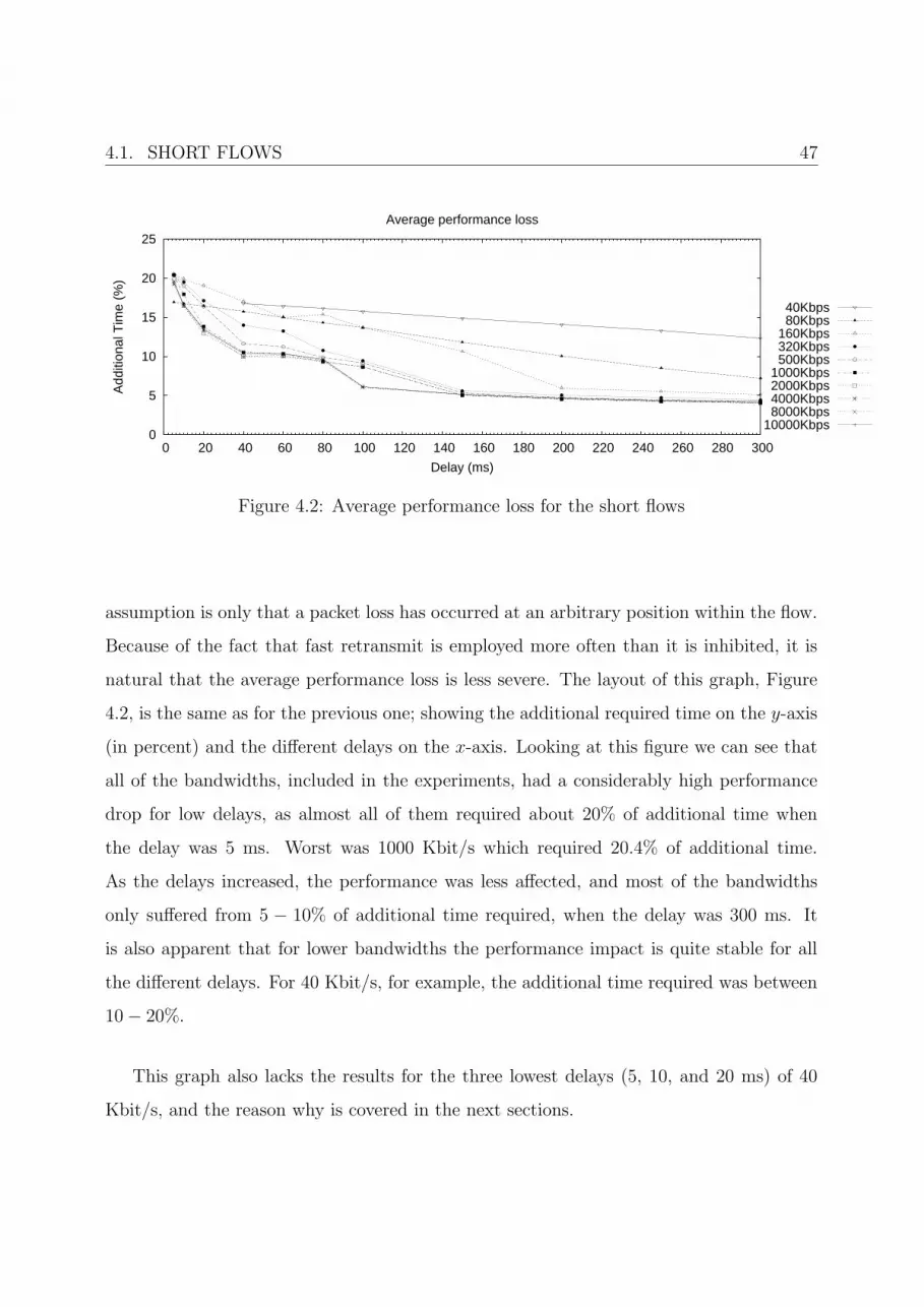
4.1. SHORT FLOWS 47
0
5
10
15
20
25
0 20 40 60 80 100 120 140 160 180 200 220 240 260 280 300
Add
ition
al T
ime
(%)
Delay (ms)
Average performance loss
40Kbps80Kbps
160Kbps320Kbps500Kbps
1000Kbps2000Kbps4000Kbps8000Kbps
10000Kbps
Figure 4.2: Average performance loss for the short flows
assumption is only that a packet loss has occurred at an arbitrary position within the flow.
Because of the fact that fast retransmit is employed more often than it is inhibited, it is
natural that the average performance loss is less severe. The layout of this graph, Figure
4.2, is the same as for the previous one; showing the additional required time on the y-axis
(in percent) and the different delays on the x-axis. Looking at this figure we can see that
all of the bandwidths, included in the experiments, had a considerably high performance
drop for low delays, as almost all of them required about 20% of additional time when
the delay was 5 ms. Worst was 1000 Kbit/s which required 20.4% of additional time.
As the delays increased, the performance was less affected, and most of the bandwidths
only suffered from 5 − 10% of additional time required, when the delay was 300 ms. It
is also apparent that for lower bandwidths the performance impact is quite stable for all
the different delays. For 40 Kbit/s, for example, the additional time required was between
10− 20%.
This graph also lacks the results for the three lowest delays (5, 10, and 20 ms) of 40
Kbit/s, and the reason why is covered in the next sections.

48 CHAPTER 4. RESULTS AND ANALYSIS
0
2000
4000
6000
8000
10000
12000
14000
0 2 4 6 8 10 12 14 16 18 20
Tim
e (m
s)
Loss position
40Kbps
5 ms10 ms20 ms40 ms60 ms80 ms
100 ms150 ms200 ms250 ms300 ms
Figure 4.3: Transmission time graph 40 Kbit/s
4.1.2 Positional dependencies
Figure 4.3 shows, for a bandwidth of 40 Kbit/s, the total transmission time of the whole
flow when a packet loss is introduced at a certain position in the flow. The y-axis of
the graph shows the total transmission time, in milliseconds, that was required for a flow
with packet loss at a certain position (x-axis). Position 0 on the x-axis corresponds to no
loss. As we can see in this figure the expected positional dependencies among the losses
exists. When the first packet was lost, the SYN-ACK packet in the three way handshake (see
Section 2.1.6), the transmission time was increased by approximately three seconds which
corresponds to the initial value of the TCP retransmission timer [26]. When the loss was
positioned in the middle of the flow the results indicate that the fast retransmit algorithm
was used. For losses placed at the end of the flow the transmission time shows that fast
retransmit was not conducted.1
However, some of the results, shown this figure, are strange and unexpected. For the
three lowest delays (5, 10, and 20 ms) the average transmission time is higher than for
1The 20th packet is an acknowledgment to the connection termination packet from the client to theserver. When this packet is sent the total transmission time is already calculated by the client, whichimplies that a loss of this packet does not affect the total transmission time.

4.1. SHORT FLOWS 49
0
1000
2000
3000
4000
5000
6000
7000
8000
0 2 4 6 8 10 12 14 16 18 20
Tim
e (m
s)
Loss position
80Kbps
5 ms10 ms20 ms40 ms60 ms80 ms
100 ms150 ms200 ms250 ms300 ms
Figure 4.4: Transmission time graph 80 Kbit/s
larger delays, and these three delays also contains two strange peaks for losses at positions
14 and 20. This strange peak result is analyzed in Section 4.1.3.
If we continue with the results for the higher bandwidths we can see that the strange
peaks that existed in the case of 40 Kbit/s, Figure 4.3, are gone. The results for 80 Kbit/s,
Figure 4.4, confirms the expected positional dependencies among the losses. For the lowest
delays we can clearly see that there exist three separate regions in the graph; the beginning
where the first packet (the SYN-ACK) is lost, the middle section where the fast retransmit
algorithm is used, and the end where fast retransmit is inhibited. For higher delays,
however, the middle section of the graph becomes smaller, making the total transmission
time considerably longer for a loss early in the flow than in the middle. This phenomenon
is even more visible in the case of 160 Kbit/s, Figure 4.5, where the total transmission
time when a loss occurs at position four in the flow is greater than the transmission time
when one of the last packets in the flow is lost, even though fast retransmit is possible at
the fourth position. This is analyzed in Section 4.1.4.
Another interesting phenomenon is that the end section starts to expand for low delays.
For 160 Kbit/s with low delay, Figure 4.5, the results indicate that the fast recovery
algorithm is not used when losses are placed at positions 16, 17, 18, and 19 in the flow.

50 CHAPTER 4. RESULTS AND ANALYSIS
0
1000
2000
3000
4000
5000
6000
7000
0 2 4 6 8 10 12 14 16 18 20
Tim
e (m
s)
Loss position
160Kbps
5 ms10 ms20 ms40 ms60 ms80 ms
100 ms150 ms200 ms250 ms300 ms
Figure 4.5: Transmission time graph 160 Kbit/s
In the previous results this only applied to positions 17, 18, and 19. This is analyzed in
Section 4.1.5.
Moving up to a bandwidth of 320 Kbit/s, Figure 4.6, we can tell by the results that
all the previous phenomena and dependencies are visible. A new and interesting thing is
that a “dip” in the transmission time is visible when a packet loss is introduced at position
nine in the flow. For 320 Kbit/s with a delay of 300 ms the required transmission time is
about 14% less for a loss at position nine than for losses at positions eight and ten. This
is analyzed in Section 4.1.6.
In Figure 4.7 the results for the bandwidths 500, 1000, 2000, 4000, 8000, and 10000
Kbit/s are shown. These results do not contain any new interesting phenomena, even
though some of the previously analyzed phenomena, such as the impact of an early loss,
seem to have a greater impact on the total transmission time as the bandwidth and delay
increase. In Figure 4.8 the results for 1000 Kbit/s with delays ranging from 5− 100 ms are
shown, to better give a view of the results for the lower delays. In this figure we can see
most of the previously mentioned dependencies and phenomena.
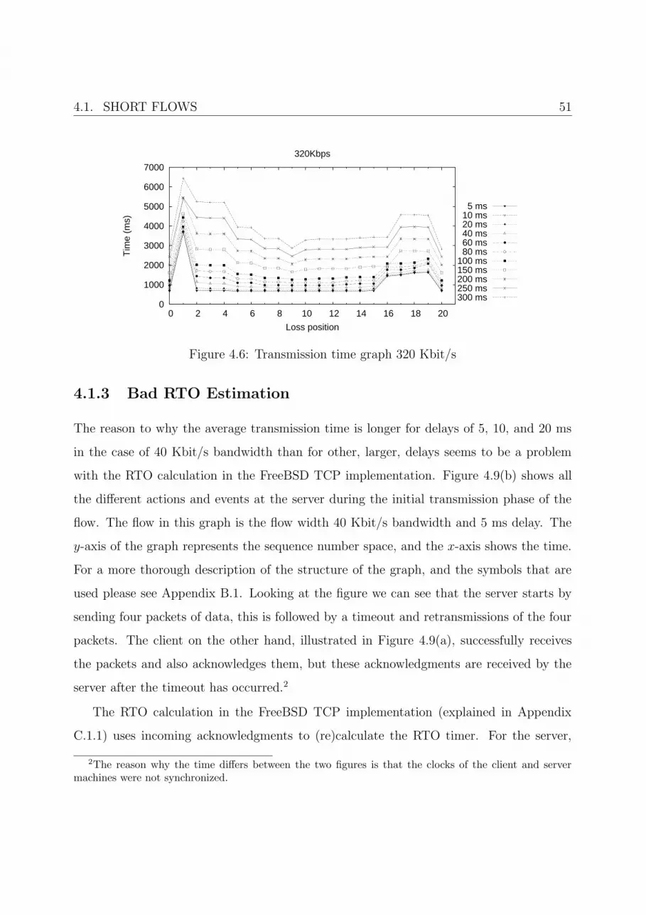
4.1. SHORT FLOWS 51
0
1000
2000
3000
4000
5000
6000
7000
0 2 4 6 8 10 12 14 16 18 20
Tim
e (m
s)
Loss position
320Kbps
5 ms10 ms20 ms40 ms60 ms80 ms
100 ms150 ms200 ms250 ms300 ms
Figure 4.6: Transmission time graph 320 Kbit/s
4.1.3 Bad RTO Estimation
The reason to why the average transmission time is longer for delays of 5, 10, and 20 ms
in the case of 40 Kbit/s bandwidth than for other, larger, delays seems to be a problem
with the RTO calculation in the FreeBSD TCP implementation. Figure 4.9(b) shows all
the different actions and events at the server during the initial transmission phase of the
flow. The flow in this graph is the flow width 40 Kbit/s bandwidth and 5 ms delay. The
y-axis of the graph represents the sequence number space, and the x-axis shows the time.
For a more thorough description of the structure of the graph, and the symbols that are
used please see Appendix B.1. Looking at the figure we can see that the server starts by
sending four packets of data, this is followed by a timeout and retransmissions of the four
packets. The client on the other hand, illustrated in Figure 4.9(a), successfully receives
the packets and also acknowledges them, but these acknowledgments are received by the
server after the timeout has occurred.2
The RTO calculation in the FreeBSD TCP implementation (explained in Appendix
C.1.1) uses incoming acknowledgments to (re)calculate the RTO timer. For the server,
2The reason why the time differs between the two figures is that the clocks of the client and servermachines were not synchronized.

52 CHAPTER 4. RESULTS AND ANALYSIS
0
1000
2000
3000
4000
5000
6000
7000
0 2 4 6 8 10 12 14 16 18 20
Tim
e (m
s)
Loss position
500Kbps
5 ms10 ms20 ms40 ms60 ms80 ms
100 ms150 ms200 ms250 ms300 ms
0
1000
2000
3000
4000
5000
6000
7000
0 2 4 6 8 10 12 14 16 18 20
Tim
e (m
s)
Loss position
1000Kbps
5 ms10 ms20 ms40 ms60 ms80 ms
100 ms150 ms200 ms250 ms300 ms
0
1000
2000
3000
4000
5000
6000
7000
0 2 4 6 8 10 12 14 16 18 20
Tim
e (m
s)
Loss position
2000Kbps
5 ms10 ms20 ms40 ms60 ms80 ms
100 ms150 ms200 ms250 ms300 ms
0
1000
2000
3000
4000
5000
6000
7000
0 2 4 6 8 10 12 14 16 18 20
Tim
e (m
s)
Loss position
4000Kbps
5 ms10 ms20 ms40 ms60 ms80 ms
100 ms150 ms200 ms250 ms300 ms
0
1000
2000
3000
4000
5000
6000
7000
0 2 4 6 8 10 12 14 16 18 20
Tim
e (m
s)
Loss position
8000Kbps
5 ms10 ms20 ms40 ms60 ms80 ms
100 ms150 ms200 ms250 ms300 ms
0
1000
2000
3000
4000
5000
6000
7000
0 2 4 6 8 10 12 14 16 18 20
Tim
e (m
s)
Loss position
10000Kbps
5 ms10 ms20 ms40 ms60 ms80 ms
100 ms150 ms200 ms250 ms300 ms
Figure 4.7: Transmission time graph 500, 1000, 2000, 4000, 8000, and 10000 Kbit/s

4.1. SHORT FLOWS 53
0
500
1000
1500
2000
0 2 4 6 8 10 12 14 16 18 20
Tim
e (m
s)
Loss position
1000Kbps
5 ms10 ms20 ms40 ms60 ms80 ms
100 ms
Figure 4.8: Transmission time graph 1000 Kbit/s, low delays
Figure 4.9(b), the only acknowledgment that was used as a base for the RTO timer cal-
culation (before the retransmissions started) was the acknowledgement to the SYN-ACK
packet in the three-way handshake (see Section 2.1.6). These packets had the sizes 78 and
66 bytes which gives a round-trip time, without considering the delay, of approximately
78∗8
40∗103 + 66∗8
40∗103 = 0, 0156 + 0, 0132 = 0, 0288 seconds. This sets, if we follow the steps in
C.1.1, the RTO timer to 287 milliseconds. If we consider a full-sized packet, 1500 bytes,
with an acknowledgment of 66 bytes the round-trip time, without considering the delay,
becomes 1500∗8
40∗103 + 66∗8
40∗103 = 0, 3132 seconds. Thus, when the first full-sized packet is sent the
round-trip time will be greater than the RTO timer which will result in a retransmission.
Even though no delay was included in this example, our results show that this problem
seems to exist for delays that are ≤ 20 ms.
The strange peaks located at positions 14 and 20 in Figure 4.3 are related to the
inaccurate RTO calculations. In Figure 4.10(a) we can see another strange behavior that is
conducted by the FreeBSD TCP implementation. When acknowledgments for new packets,
packets sent after the retransmissions, are received by the server they3 are regarded as
3The acknowledgments.
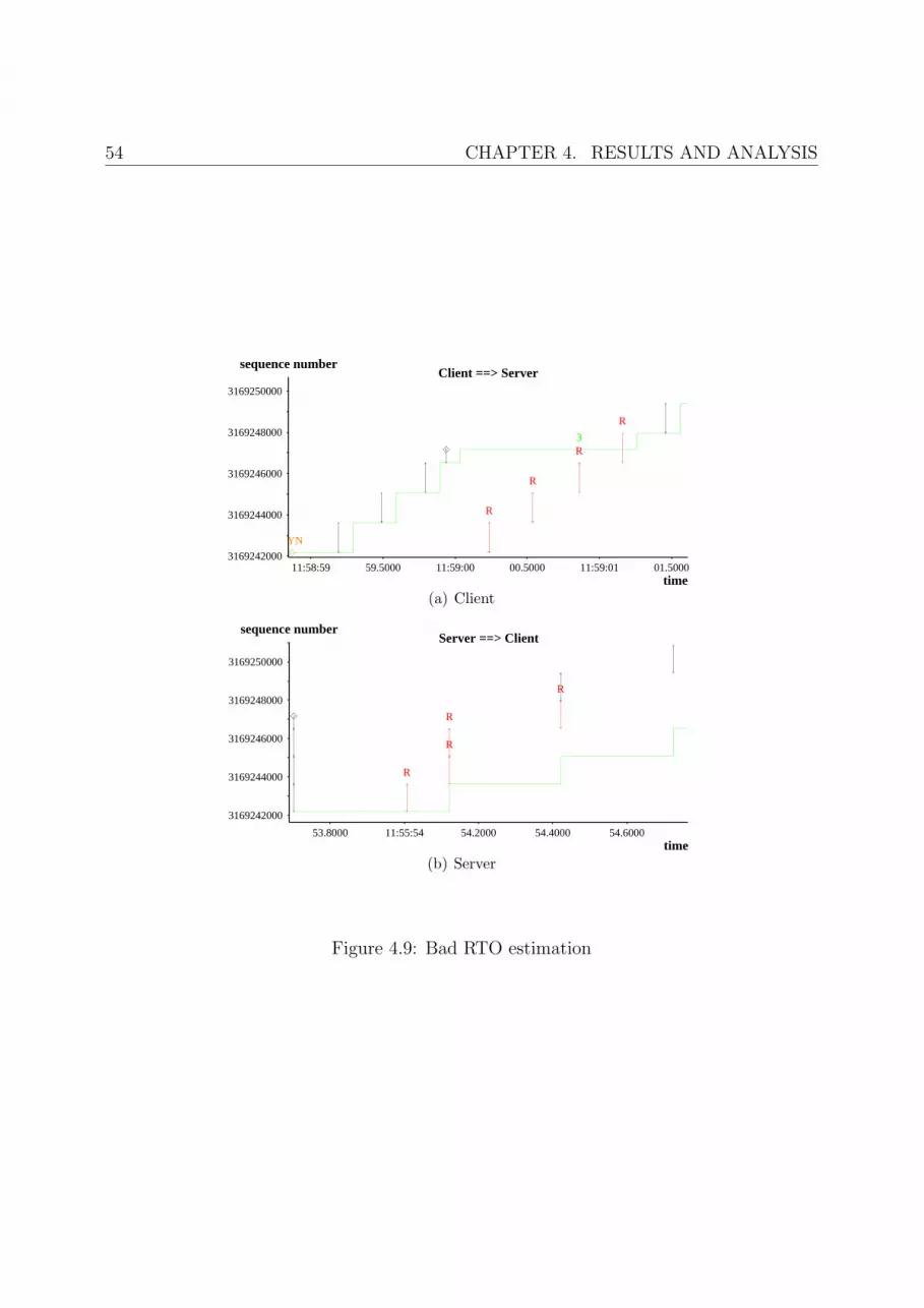
54 CHAPTER 4. RESULTS AND ANALYSIS
3169250000
3169248000
3169246000
3169244000
316924200001.5000 11:59:01 00.5000 11:59:00 59.5000 11:58:59
sequence number
time
Client ==> Server
R
3R
R
R
�
SYN
(a) Client
3169250000
3169248000
3169246000
3169244000
3169242000
54.600054.400054.2000 11:55:54 53.8000
sequence number
time
Server ==> Client
R
R
R
R
�
(b) Server
Figure 4.9: Bad RTO estimation

4.1. SHORT FLOWS 55
already received and duplicate acknowledgments is sent to the client in response.4 Because
of this (mis)behavior there are not enough packets in flight to trigger the fast retransmit
mechanism, instead the server waits for the retransmission timer to expire (because of the
four initial losses the retransmission timer is set very high) and then resends packet number
14. For a loss at position 20 the problem is the same.
The reason why these peaks do not exist for losses at other positions in the flow is
illustrated in Figures 4.10(b) and 4.10(c), which shows how losses on position 13 and 15
are treated by the server. In 4.10(b) we can see that packet 14 triggers a retransmission of
the lost packet. This behavior indicates that the server believes that it still recovers from
the four initial losses, otherwise it would have taken three duplicate acknowledgments to
trigger a retransmission. In Figure 4.10(c) the 15’th packet is lost, but this packet is one of
the strange duplicate acknowledgments that was sent from the server to the client, so no
harm seems to be done. The reason why the server behaves in this way is, unfortunately,
unclear.
4.1.4 Link utilization implications
The reason why losses at early positions causes the transmission time to increase signifi-
cant as the bandwidth and the delay increases, as in Figure 4.5, is due to the fact that the
bandwidth-delay product increases. The bandwidth-delay product, or BDP, is a measure-
ment of how much data that can be in flight at the same time. Earlier, in Section 2.2.1, the
transfer of data was compared with pouring water through a pipe. The fastest way to do
this is to pour all the water into the pipe at once, making the pipe completely filled. The
same argument holds for data transfer. The BDP, which can be compared to the volume
of a pipe, is calculated according to Equation 3.2 in Section 3.2.3, which is repeated here
for convenience.
4Indicated by the small x’s in the figure.
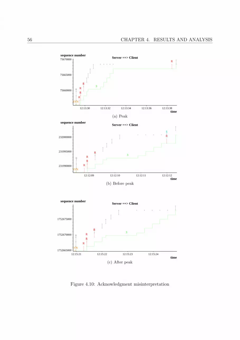
56 CHAPTER 4. RESULTS AND ANALYSIS
75670000
75665000
75660000
12:13:38 12:13:36 12:13:34 12:13:32 12:13:30
sequence number
time
Server ==> ClientR
3R
R
R
R
�
SYN�
(a) Peak
232000000
231995000
231990000
12:12:12 12:12:11 12:12:10 12:12:09
sequence number
time
Server ==> Client
R
S
3R
R
R
R
�
SYN�
(b) Before peak
1752675000
1752670000
1752665000 12:15:24 12:15:23 12:15:22 12:15:21
sequence number
time
Server ==> Client
3R
R
R
R
�
SYN�
(c) After peak
Figure 4.10: Acknowledgment misinterpretation

4.1. SHORT FLOWS 57
BDP (bytes) = Bandwidth (Kbytes/s) ∗Delay (ms)
Because of the possible problem with network congestion TCP does not send all data
that is submitted for transmission right away, to utilize the full capacity of the link without
considering concurrent traffic, but uses the slow start mechanism (see Section 2.2.1) to
rapidly increase the utilization of the link to an acceptable level.
At the beginning of a TCP connection, the slow start mechanism has not had the
chance to increase sending rate to fully utilize the link, so if a loss occurs early the con-
gestion avoidance phase, which increases the sending rate very slow, is entered earlier. For
connections with high BDP an early loss can be a problem, as the utilization of the link
will be lower.
4.1.5 Receive buffer fluctuations
In Figure 4.5, 160 Kbit/s, we can see that the “end section” of the graph, the section
where fast retransmit is not possible to perform, grows larger for low delays. The reason
to why the section where fast retransmit is no longer possible grows is related to the use
of window updates. As mentioned in Section 2.1.4 a TCP receiver (the client in our case)
uses window updates to inform the sender (server) when the receiver window opens up.
Unfortunately a TCP sender has no way of determining if a duplicate acknowledgment
with an updated receiver window is an “ordinary” duplicate acknowledgment or if it is a
window update. Therefore all duplicate acknowledgments with an updated receiver window
are treated as window updates and not duplicate acknowledgments. This behavior seems
to have consequences on the fast retransmit mechanism, especially for connections with
low delay.
For connections with a low end-to-end delay the TCP client is forced to buffer data,
due to the fast delivery. The buffering makes the advertised receiver window to shrink, and

58 CHAPTER 4. RESULTS AND ANALYSIS
when a duplicate acknowledgment is sent in response to our introduced loss this duplicate
acknowledgment also contains an updated receiver window size and is therefore treated as
a window update. The reason why this phenomenon is not visible for lower bandwidths
and/or higher delays is that the client, in most cases, does not receive data faster than it
reads it, therefore it does not buffer any data which leads to an unchanged receiver window.
4.1.6 TCP packet bursts and their implications
The reason why a dip in the total transmission time can be seen when a loss is introduced
at position nine in flows with high delay is a consequence of the data transmission behavior
of TCP in combination with the length of the flow. The transmission behavior of TCP is,
basically, to send a number of packets, wait for them to be acknowledged, and then send
more packets. Figure 4.11 shows the communication from the servers point of view when
the bandwidth was 320 Kbit/s, the delay 300 ms, and no losses were introduced. As we
can see the packet sending was partitioned into three distinct groups (or bursts); the initial
group that was sent upon connection establishment, and then two groups that were sent
in response to the acknowledgments of the previous. Looking at Figure 4.12 we can see
that the loss that was at position eight in the flow caused the server to send all the data
in four groups, instead of three, which adds approximately one extra round-trip time to
the total transmission time. A loss on position nine, Figure 4.13, did not cause an extra
group of packet sending as the congestion window had opened up slightly more than in
the previous case, and therefore both the retransmission and the final packet were sent in
the same group. In Figure 4.14 we can see that a loss on position ten also caused an extra
group of packet sending, but in that case it was due to the fact that the packet loss was
not detected until the acknowledgments of the packets in the final group arrived.
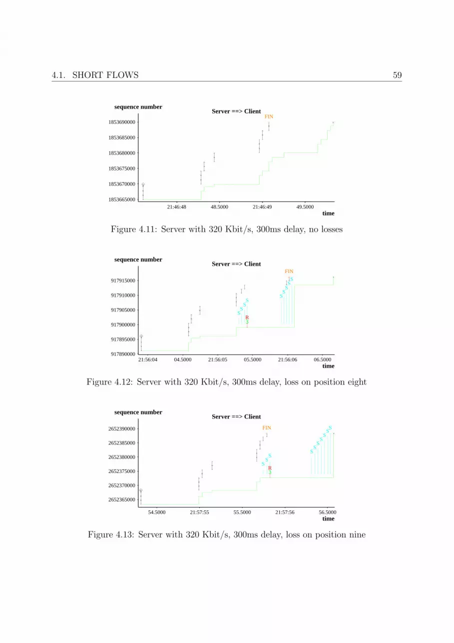
4.1. SHORT FLOWS 59
1853690000
1853685000
1853680000
1853675000
1853670000
185366500049.5000 21:46:49 48.5000 21:46:48
sequence number
time
Server ==> ClientFIN
�
Figure 4.11: Server with 320 Kbit/s, 300ms delay, no losses
917915000
917910000
917905000
917900000
917895000
91789000006.5000 21:56:06 05.5000 21:56:05 04.5000 21:56:04
sequence number
time
Server ==> Client
S
FIN
SS
SS
R
S
3
SS
S
�
Figure 4.12: Server with 320 Kbit/s, 300ms delay, loss on position eight
2652390000
2652385000
2652380000
2652375000
2652370000
2652365000
56.5000 21:57:56 55.5000 21:57:55 54.5000
sequence number
time
Server ==> Client
SS
SS
SS
S
R
S
3
FIN
SS
�
Figure 4.13: Server with 320 Kbit/s, 300ms delay, loss on position nine
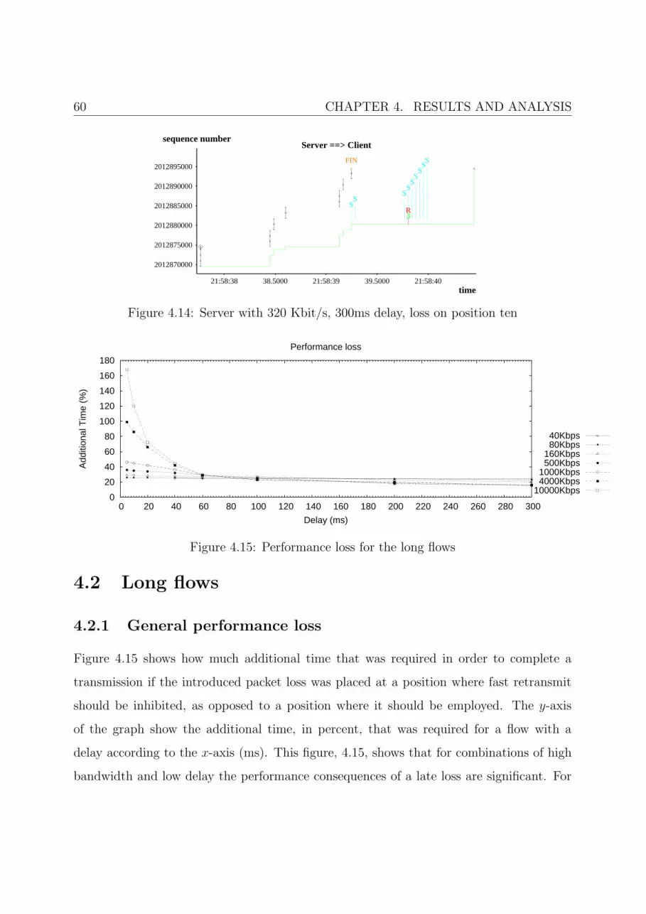
60 CHAPTER 4. RESULTS AND ANALYSIS
2012895000
2012890000
2012885000
2012880000
2012875000
2012870000
21:58:40 39.5000 21:58:39 38.5000 21:58:38
sequence number
time
Server ==> Client
SS
SS
S
R
S
3
SS
FIN
S
�
Figure 4.14: Server with 320 Kbit/s, 300ms delay, loss on position ten
0
20
40
60
80
100
120
140
160
180
0 20 40 60 80 100 120 140 160 180 200 220 240 260 280 300
Add
ition
al T
ime
(%)
Delay (ms)
Performance loss
40Kbps80Kbps
160Kbps500Kbps
1000Kbps4000Kbps
10000Kbps
Figure 4.15: Performance loss for the long flows
4.2 Long flows
4.2.1 General performance loss
Figure 4.15 shows how much additional time that was required in order to complete a
transmission if the introduced packet loss was placed at a position where fast retransmit
should be inhibited, as opposed to a position where it should be employed. The y-axis
of the graph show the additional time, in percent, that was required for a flow with a
delay according to the x-axis (ms). This figure, 4.15, shows that for combinations of high
bandwidth and low delay the performance consequences of a late loss are significant. For

4.2. LONG FLOWS 61
0
0.5
1
1.5
2
2.5
3
3.5
4
4.5
0 20 40 60 80 100 120 140 160 180 200 220 240 260 280 300
Add
ition
al T
ime
(%)
Delay (ms)
Average performance loss
40Kbps80Kbps
160Kbps500Kbps
1000Kbps4000Kbps
10000Kbps
Figure 4.16: Average performance loss for the long flows
a bandwidth of 10000 Kbit/s and a delay of 5 ms 168% of additional time is required.
Compared to the results of the short flows, where all the bandwidths that had a delay of 5
ms had over 100% of additional time required, these longer flows seem to generally suffer
less from a late loss. As we can see in the figure the results converge fast, and from 60 ms
of delay all of the bandwidths require less than 40% of additional time.
In Figure 4.16 the average additional time that was required due to fast retransmit
inhibitions is shown. In the previous figure, Figure 4.15, it was assumed that the packet
loss occured at a position where fast retransmit was inhibited. In this figure, however,
the assumption is only that a packet loss has occurred at an arbitrary position within the
flow. The layout of this graph is the same as for the previous one; showing the additional
required time on the y-axis (in percent) and the different delays on the x-axis. The reason
to why the average performance loss for these longer flows are so insignificant (compared
to the short flows discussed in Section 4.1.1) is partly due to the fact that the number of
occasions when fast retransmit is inhibited is very small compared to the number of times
when it is employed. Another reason to why the effects of the fast retransmit inhibitions
are so small has to do with an implementation issue in FreeBSD which causes the average
transmission time to be relatively high, even if fast retransmit is conducted. This problem

62 CHAPTER 4. RESULTS AND ANALYSIS
is identified in the next section, and is more deeply analyzed in Section 4.2.3. If we take a
look at Figure 4.16 we can see that the additional time that is required is 4% or less for
all different combinations of bandwidths and delays. For the largest delay, 300 ms, all of
the bandwidths require an additional time that is less than one percent.
The reason why these graphs, Figures 4.15 and 4.16, do not contain any results for the
three lowest delays (5, 10, and 20 ms) of 40 Kbit/s has to do with a defect in the FreeBSD
TCP implementation (discussed in Section 4.1.3). This defect causes the transmission time
of flows with low bandwidth and delay to increase dramatically. To be certain of that these
results are not mistakenly associated with the problem of fast retransmit inhibitions they
were not included in the graphs.
4.2.2 Positional dependencies
Figure 4.17 shows, for the bandwidths of 40, 80, and 160 Kbit/s, the total transmission
time of the whole flow when a packet loss is introtuced at a certain position in the flow. The
y-axis of the graph shows the total transmission time, in milliseconds, that was required for
a flow with packet loss at a certain position (x-axis). Position 0 on the x-axis corresponds
to no loss. Looking at the top of this figure (40 Kbit/s), we can see that positional
dependencies among the losses are clearly visible in the results. The three lowest delays
(5, 10, and 20 ms) have the same strange peaks, and high average transmission time, as
the corresponding short flows had. This is due to the same problems that were discussed
in Section 4.1.3.
Compared to the short flows the results for these, longer flows, seem to contain a section
in the middle where the total transmission time is unexpectedly high. For 80 Kbit/s, in the
middle of Figure 4.17, this middle section becomes more visible and for 160 Kbit/s with a
delay of 300 ms, bottom of Figure 4.17, 30% of additional transmission time is required for
a loss at position 50 compared to a loss at position 80, even though fast retransmit should
have been used in both cases. This is analyzed in Section 4.2.3.
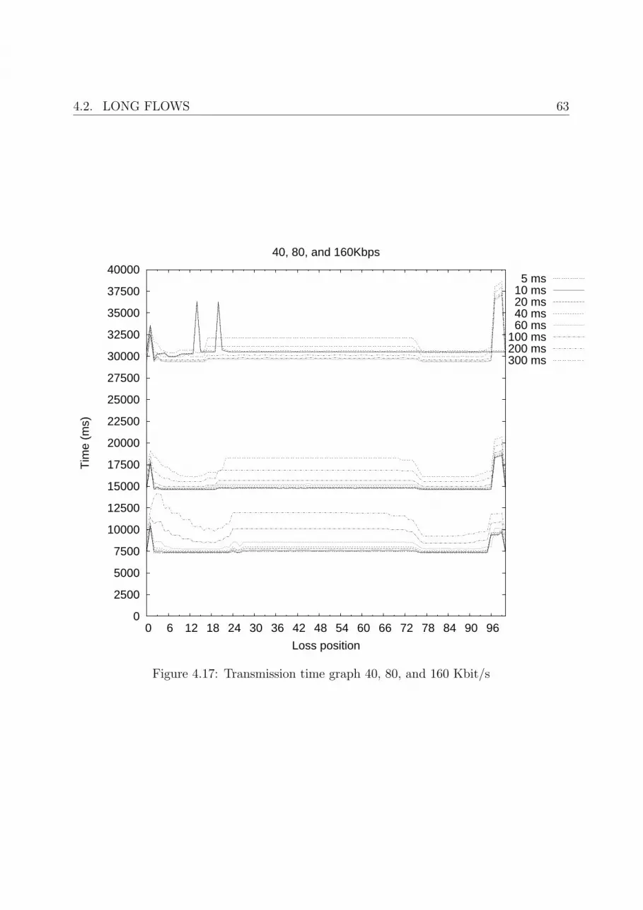
4.2. LONG FLOWS 63
0
2500
5000
7500
10000
12500
15000
17500
20000
22500
25000
27500
30000
32500
35000
37500
40000
0 6 12 18 24 30 36 42 48 54 60 66 72 78 84 90 96
Tim
e (m
s)
Loss position
40, 80, and 160Kbps
5 ms10 ms20 ms40 ms60 ms
100 ms200 ms300 ms
Figure 4.17: Transmission time graph 40, 80, and 160 Kbit/s

64 CHAPTER 4. RESULTS AND ANALYSIS
0
2000
4000
6000
8000
10000
12000
14000
0 6 12 18 24 30 36 42 48 54 60 66 72 78 84 90 96
Tim
e (m
s)
Loss position
500Kbps
5 ms10 ms20 ms40 ms60 ms
100 ms200 ms300 ms
Figure 4.18: Transmission time graph 500 Kbit/s
Another interesting thing that is visible in the 160 Kbit/s results, shown in the bottom
of Figure 4.17, is that the total transmission time becomes very high, for flows with high
delay, if a loss is introduced at an early position. This behavior was also found for the
shorter flows, and was analyzed in Section 4.1.4.
For a bandwidth of 500 Kbit/s, Figure 4.18, we can see that the first section of the
graph continue to grow, as the bandwidth and the delay increases. Another interesting
observations is that the middle section of the graph becomes more and more irregular as
the delay increases. This behavior is discussed in Section 4.2.4.
The rest of the results, shown in Figure 4.19, do not contain any new interesting aspects.
The only difference from the previous results is that the impacts of an early loss seem to
increase as the bandwidth and the delay increase.
4.2.3 TCP implementation issues
For a loss at an early position (≈ 2− 20) in the case of 80 Kbit/s, and with a delay of 300
ms, Figure 4.17, fast retransmit seems to work. This is also confirmed by Figure 4.20. This
figure shows all the different actions and events at the server when a loss was introduced
at position 12 in the flow. The y-axis of the graph represents the sequence number space,

4.2. LONG FLOWS 65
0
2000
4000
6000
8000
10000
12000
0 6 12 18 24 30 36 42 48 54 60 66 72 78 84 90 96
Tim
e (m
s)
Loss position
1000Kbps
5 ms10 ms20 ms40 ms60 ms
100 ms200 ms300 ms
0
2000
4000
6000
8000
10000
12000
0 6 12 18 24 30 36 42 48 54 60 66 72 78 84 90 96
Tim
e (m
s)
Loss position
4000Kbps
5 ms10 ms20 ms40 ms60 ms
100 ms200 ms300 ms
0
2000
4000
6000
8000
10000
12000
0 6 12 18 24 30 36 42 48 54 60 66 72 78 84 90 96
Tim
e (m
s)
Loss position
10000Kbps
5 ms10 ms20 ms40 ms60 ms
100 ms200 ms300 ms
Figure 4.19: Transmission time graph 1000, 4000, and 10000kbps

66 CHAPTER 4. RESULTS AND ANALYSIS
and the x-axis shows the time. For a more thorough description of the structure of the
graph, and the symbols that are used please see Appendix B.1. In this figure, 4.20, we
can see that the server was retransmitting the lost segment after receiving three duplicate
acknowledgments, and that limited transmit and window inflation was performed in the
recovery phase. However, for a loss positioned in the middle section of the flow, position
50, the server acted suspiciously. As mentioned before, in Section 2.2.4, fast retransmission
is followed by congestion avoidance which slowly increases the congestion window. But in
this case, Figure 4.21, we can see that slow start is conducted, as the server rapidly injects
packets into the network (sending two packets for every incoming acknowledgment).
The reason to why this is done has to do with an implementation detail in the FreeBSD
kernel.
/∗
∗ Out o f f a s t recovery .
∗ Window i n f l a t i o n shou ld have l e f t us
∗ with approx imate ly snd s s t h r e s h
∗ ou t s tand ing data .
∗ But in case we would be i n c l i n e d to
∗ send a burs t , b e t t e r to do i t v i a
∗ the s low s t a r t mechanism .
∗/
i f (SEQ GT( th−>th ack +
tp−>snd s s thre sh ,
tp−>snd max ) )
tp−>snd cwnd = tp−>snd max −
th−>th ack +
tp−>t maxseg ;
else

4.2. LONG FLOWS 67
tp−>snd cwnd = tp−>snd s s th r e sh ;
Listing 4.1: sys/net/inet/tcp input.c, lines 1983–1999
Listing 4.1 shows an extract of the kernel source code. In the listing th_ack is the
number of the received acknowledgment, snd_ssthresh is the slow start threshold variable,
t_maxseg is the MSS, and snd_cwnd is the congestion window. This piece of code actually
suggests that slow start should be used, instead of congestion avoidance, under certain
circumstances. To verify that it was this piece of code that actually caused this behavior,
it was modified to print out the value of the acknowledgment number, in order to compare
it with the traffic log.
Another thing that TCP implementations also should do is to perform slow start until
a packet loss has occurred.5 Looking at Figure 4.21 again we can see that this is not done
either, as the packet transmission rate prior to the loss is linear.6 In addition to this, the
server did not use limited transmit or window inflation when the duplicate acknowledg-
ments arrived.
The explanation to this behavior is related to the size of the TCP send buffer. To
ensure reliability TCP must buffer copies of transmitted segments, in case that some of
them are lost and must be retransmitted. The size of this buffer has a considerable effect
on the performance, as the maximum number of packets that can be in flight is implicitly
limited by it. In FreeBSD the default size of this buffer is set to 32 Kbytes (please see
Appendix C.1), which limits the amount of data that can be in flight to exactly 32 Kbytes.
When the congestion window has grown equal to (or greater than) this number, the send
buffer is full and for every segment that is acknowledged, TCP is only able to send one
new segment.7 The reason why this phenomenon is not visible in Figure 4.20 is that the
5The slow start phase is also to be abandoned when the ssthresh variable is reached. However, for thisversion of FreeBSD, ssthresh has the same default size as the maximum allowed congestion window, andtherefore the slow start phase is not abandoned until the congestion window is at its maximum value, ora packet loss is detected.
6If slow start had been conducted, the transmission rate would have increased considerably more.7When transmitted segments are acknowledged they are removed from the buffer.
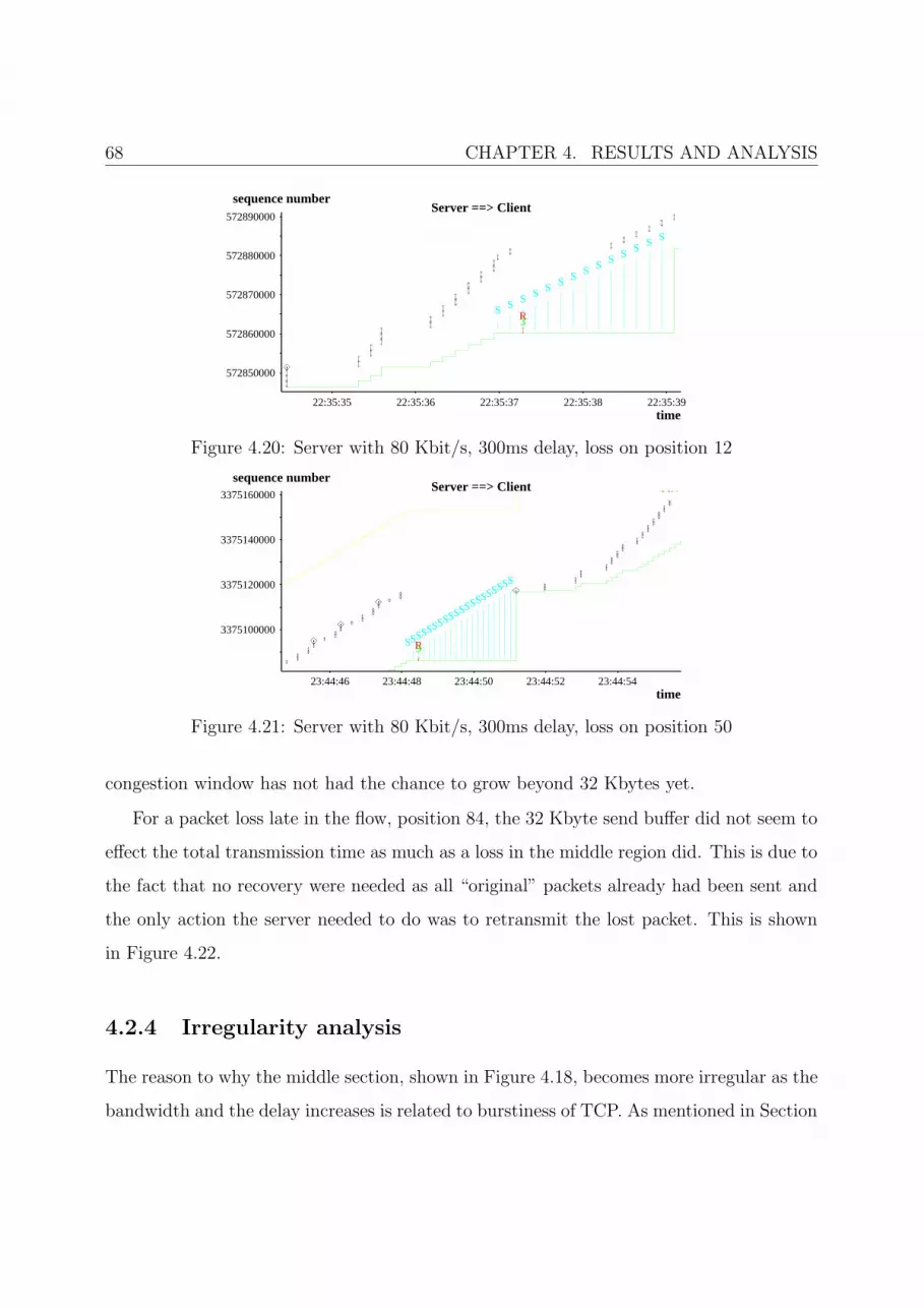
68 CHAPTER 4. RESULTS AND ANALYSIS
572890000
572880000
572870000
572860000
572850000
22:35:39 22:35:38 22:35:37 22:35:36 22:35:35
sequence number
time
Server ==> Client
SSSSSSSSSSS
R
S
3
SS
�
Figure 4.20: Server with 80 Kbit/s, 300ms delay, loss on position 12
3375160000
3375140000
3375120000
3375100000
23:44:54 23:44:52 23:44:50 23:44:48 23:44:46
sequence number
time
Server ==> Client FIN
�
SSSSSSSSSSSSSSSSSRS3
SS
�
�
�
Figure 4.21: Server with 80 Kbit/s, 300ms delay, loss on position 50
congestion window has not had the chance to grow beyond 32 Kbytes yet.
For a packet loss late in the flow, position 84, the 32 Kbyte send buffer did not seem to
effect the total transmission time as much as a loss in the middle region did. This is due to
the fact that no recovery were needed as all “original” packets already had been sent and
the only action the server needed to do was to retransmit the lost packet. This is shown
in Figure 4.22.
4.2.4 Irregularity analysis
The reason to why the middle section, shown in Figure 4.18, becomes more irregular as the
bandwidth and the delay increases is related to burstiness of TCP. As mentioned in Section

4.2. LONG FLOWS 69
4121700000
4121680000
4121660000
4121640000
4121620000
00:46:32 00:46:31 00:46:30 00:46:29 00:46:28
sequence number
time
Server ==> Client
SSSSSSSSSSSSRS3
SS
FIN�
�
�
Figure 4.22: Server with 80 Kbit/s, 300ms delay, loss on position 84
4.1.6 the data transfer behavior of TCP makes the sender send packets in partitions, or
bursts, and depending on where the loss is introduced the number of such bursts can vary.
If we take a look at Figure 4.23, which is the flow with 500 Kbit/s and 300 ms delay, we can
see the server when a packet loss was introduced at the 41’th position of the flow (where
an irregularity clearly is visible in Figure 4.18). If we, in this figure, count the number
of distinct partitions, or bursts, we get the number 12. If we, on the other hand, take a
look at Figure 4.24 which shows the same flow, but with a loss on position 50, we can see
that there are only 11 bursts. As we can see in Figure 4.18 the difference in the number
of bursts, clearly affects the total transmission time (making a slight bump in the graph
where the extra burst is). For flows with low delay, an extra burst (which approximately
corresponds to an extra round-trip time) is not as significant, in terms of additional time,
as for flows with higher delays. That is the reason why the irregularities are not visible,
though they exist, for lower delays.

70 CHAPTER 4. RESULTS AND ANALYSIS
1643050000
1643000000
1642950000
1642900000
21:09:52 21:09:50 21:09:48 21:09:46 21:09:44
sequence number
time
Server ==> Client
FIN
�
SSSSSSSSSSSSSSSSRS3SSS
�
�
SYN�
Figure 4.23: Server with 500 Kbit/s, 300ms delay, loss on position 41
2719150000
2719100000
2719050000
2719000000
21:22:54 21:22:52 21:22:50 21:22:48
sequence number
time
Server ==> Client
FIN
�
SSSSSSSSSSSSSSSSRS3SSS
�
�
�
SYN�
Figure 4.24: Server with 500 Kbit/s, 300ms delay, loss on position 50

4.3. RESULTS RELATED TO EARLIER WORK 71
4.3 Results related to earlier work
As mentioned earlier, in Section 2.4, other work that has been conducted [11] has also
revealed the existence, and to some extent the implications, of fast retransmit inhibitions.
One of the results of that work, shown in Figure 4.25, clearly shows that the position of a
loss has impact on the total transmission time.
0
500
1000
1500
2000
2500
3000
3500
0 2 4 6 8 10 12 14 16 18 20
Tim
e (m
s)
Loss position
1000Kbps - 10ms
2 initial win4 initial win
Figure 4.25: One controlled loss, 10 ms
Figure 4.25 shows that the total transmission time for a short-lived flow (20 packets)
were considerably longer when the loss was positioned in the beginning or the end of a
flow. If we take a look at Figure 4.8 in Section 4.1.2, which contains the result of an
experiment with corresponding network parameters8 (1000 Kbit/s, and 10 ms delay) we
can clearly see some differences. First of all we can see that the end section, where fast
retransmit is inhibited, of the graph shown in Figure 4.25 is considerably higher than the
one shown in Figure 4.8. This is due to the fact that newer versions of FreeBSD break the
proposed standard of 1 second minimum RTO [26], thus allowing a much faster timeout to
occur. While this behavior seems to work very well in this case, it can also have negative
consequences. In Section 4.1.3 we could see that combinations of low bandwidth and low
8For our experiment an initial window size that approximately corresponds to 4 was used.

72 CHAPTER 4. RESULTS AND ANALYSIS
end-to-end delay could cause the RTO timer to expire prematurely, thus causing spurious
retransmissions. This could have been avoided if the standard of 1 second minimum RTO
had been used.
Another interesting thing worth to note is that the results shown in Figure 4.25 do
not contain the enlarged end section that is visible in Figure 4.8 and analyzed in Section
4.1.5. Why this difference exists is not clear, but it may be due to differences in the TCP
implemenations.
4.4 Summary
In this chapter we have seen the results of the experiments, and some analysis regarding
them. We have seen that fast retransmit inhibitions are present, and that they in most
cases affect the performance very much. The problem of fast retransmit inhibitions showed
to be greater for short flows, as the risk of experiencing a late loss is much higher.
In addition to this, many interesting and unexpected phenomena have been discovered
and discussed. To some of these phenomena we were able to give a complete analysis, but
in some cases more work is needed in order to gain a complete understanding.
The next chapter presents some interesting ideas of what can be done in the future.

Chapter 5
Future work
The results that were achieved by the experiments did not only reveal the existence and
implications of fast retransmit inhibitions. Several, other, interesting phenomena were
discovered and analyzed in the previous chapter. However, some of these phenomena, like
the strange peaks that were discussed in Section 4.1.3, were somewhat out of scope for
this thesis, and were therefore not fully analyzed. The following sections provide some
interesting ideas on future work that is possible.
5.1 Other approaches
The fast retransmit inhibitions could also be investigated using other evaluation techniques,
such as
• Mathematical analysis. This approach uses models that describe TCP behavior in
mathematical terms. An initial effort will have to be made to classify the differ-
ent models and select the most appropriate. The model must capture the startup
behavior of TCP and the effects of timeouts.
• Simulations. This approach uses the TCP implementation in the ns2 network simula-
tor [1]. The use of simulation allows a large parameter space to be explored, and since
73
74 CHAPTER 5. FUTURE WORK
the TCP implementation in ns2 is much used in the network research community the
results are easy to relate and compare to other simulation studies.
• Implementation examination. When insights into the behavior of the fast retransmit
inhibitions have been obtained through one or more of the above approaches, an
implementation examination study can also be performed. The purpose of this study
would be to examine to what extent current implementations of TCP are sensitive
to the inhibitions, and how large the differences between different implementations
are.
5.2 SCTP
The same experiments could be conducted for the Stream Control Transmission Protocol
[31] (SCTP). SCTP is in many ways similar to TCP, in terms of reliability and congestion
control, and it would be nice to investigate if fast retransmit inhibitions exist here as well.
5.3 Dummynet
The extended version of the Dummynet network emulation software, that was used for this
work, could be developed further. This in order to support dynamically varying delays and
bandwidths.
5.4 FreeBSD Initial window size
Even though the sysctl parameter that controls the initial slow start size was manipulated
(see Section 3.4.1), and the host caching feature that FreeBSD uses was effectively disabled,
the TCP implementation allowed more data to be transmitted, initially, than the TCP
standard proposes [5]. In fact, the TCP implementation allowed us to send 4 full-sized

5.5. FREEBSD SLOW START ISSUE 75
segments upon connection establishment, where the TCP standard only allows about 3. It
is unclear why the current implementation does this, but it might be possible to find out
why using some different approaches.
• By inspecting the source code of the FreeBSD TCP/IP implementation.
• By doing experiments with computers that do not reside on the same subnet, we
might get a different behavior.
5.5 FreeBSD Slow Start issue
In Section 4.2.3 it was found that the FreeBSD TCP implementation, under certain cirum-
stances, chooses to employ the slow start mechanism instead of congestion avoidance. The
reason for this, according to the comments in the source code, is that it is better to send
a “burst” via the slow start mechanism than the congestion avoidance mechanism. Fur-
ther experiments could be conducted in order to investigate if this behavior improves the
performance, or if the TCP standard way is more efficient.
5.6 FreeBSD recovery issue
In Section 4.1.3 it was observed that the TCP implementation was unable to exit the re-
covery phase correctly. Due to a bad RTO estimation the server retransmitted a number
of segments prematurely. When the server started to send new segments, the acknowledg-
ments to these (sent by the client) triggered the server to send duplicate acknowledgments
back, instead of leaving the recovery phase and continue with regular transmission. The
reason why the server behaved in that way is unclear, and it would be interesting to
investigate this strange behavior further.

76 CHAPTER 5. FUTURE WORK
5.7 Performance gain with buffer tuning
As the results for the long flows showed, Section 4.2, the performance was affected by the
small default size of the TCP send buffer. For servers conducting large file transfers over
network paths with high delays, a 32 Kbyte send buffer size is totally unacceptable, as it
will limit the link utilization considerably. Some interesting work that could be done is
• Measuring the performance gain as the buffer size increases. This would be relatively
easy, and straightforward, as the size of the send buffer in FreeBSD can be controlled
with a sysctl variable.
• Implement buffer auto-tuning as it is done in the Linux kernel [39]. This would, of
course, be a much more complex task to perform, but definitely interesting.
5.8 Lowering the fast retransmit threshold
In the TCP implementation that was studied, the duplicate acknowledgment threshold that
fast retransmit uses was three (according to TCP standards). By lowering this threshold
fast retransmit opportunities would be gained. However, as mentioned in 2.4, studies show
that this could, possibly, make TCP vulnerable to network reordering. Work that could
be done here is to investigate if a good estimation technique of network reordering could
be developed and used for dynamically lowering the threshold.
Chapter 6
Conclusions
In this thesis the existence of and performance loss due to fast retransmit inhibitions, which
usually are evident in the end of TCP connections, have been investigated.
By setting up an experimental environment consisting of a client, a server, and a net-
work emulator which had the ability to lose packets according to their position in a flow,
we were able to design and execute experiments that concluded that these inhibitions exist
in modern TCP implementations and that they, considerably, can reduce the performance
of a TCP connection, especially for short-lived flows.
The experiments that were conducted covered a large number of combinations of net-
work parameters, such as different bandwidths, end-to-end delays, and flow sizes. All
together, over 20.000 experiments were performed in order to gain the results. In order to
perform this large number of experiments, in an efficient manner, scripts that automated
the configuration and execution of the experiments were used. Furthermore, we have ported
network emulation software in order to run it on newer versions of FreeBSD, and developed
a number of scripts and applications that aided us in the experimental process.
It was shown that the increase in total transmission time, of a short-lived TCP flow,
could be as much as 300% when a loss was introduced at a fast retransmit inhibited
position in the flow. For larger flows, the worst case scenario resulted in an increase of
77
78 CHAPTER 6. CONCLUSIONS
transmission time with about 170%. Even though the increase of the total transmission
time, in precense of a loss where fast retransmit was inhibited, were considerably large in
all of the experiments, ranging from 16 − 301%, the average performance loss, due to an
arbitrarily positioned loss, was not that severe. Because of the fact that fast retransmit
is inhibited in fewer positions of a TCP flow than it is employed, the average increase of
the transmission time due to these inhibitions was not that large. For the short flows the
average increase was at most 20.4%, and for the longer flows, where the risk of having a
loss at a fast retransmit inhibited position is less likely, the maximum increase was only
4% at the most.
Not only the fast retransmit inhibitions of TCP affected the results of the conducted
experiments. One reason to why the average increase, in terms of additional transmission
time, of the long flows was so small had to do with the default buffering capabilities of the
TCP implementation that was used. This buffering issue caused the total transmission time
to be large, even when fast retransmit was possible to perform, and therefore the difference
in performance was smaller. In addition to the buffering issues, some other implementation
details, that were related to the behavior and performance of TCP were discovered. One
example of this was the management of the RTO timer, which allowed a RTO that is
smaller than the standard of 1 second to be used. While this lead to positive performance
effects in some cases, it was also shown that it could cause spurious retransmissions, which
considerably lowered the performance. We also found a number of other interesting things
during the work. Some of them were described and analyzed within the thesis, while others
were out of the scope and therefore suggested as future work.

References
[1] The network simulator - ns-2. http://www.isi.edu/nsnam/ns.
[2] Sally Floyd Alberto Medina, Mark Allman. Measuring the evolution of transportprotocols in the internet. ACM SIGCOMM Computer Communication Review, 35(2),April 2005.
[3] M. Allman. RFC 2581: TCP congestion control. Technical report, April 1999.
[4] M. Allman. RFC 3042: Enhancing TCP’s loss recovery using limited transmit. Tech-nical report, January 2001.
[5] M. Allman. RFC 3390: Increasing TCP’s initial window. Technical report, October2002.
[6] Reiner Ludwig Andrei Gurtov. Responding to spurious timeouts in TCP. In Proc.IEEE INFOCOM, pages 2312–2322, March 2003.
[7] Ka-Cheong Leung Changming Ma. Improving TCP robustness under reordering net-work environment. In Proc. IEEE GLOBECOM,2004, page 2072, December 2004.
[8] Mark Allman Ethan Blanton. On making TCP more robust to packet reordering.ACM SIGCOMM Computer Communication Review, 32(1), January 2002.
[9] S. Floyd. RFC 3782: The newreno modification to TCP’s fast recovery algorithm.Technical report, April 2004.
[10] FreeBSD 6.0. http://www.freebsd.org.
[11] Johan Garcia. Improving Performance in Heterogeneous Networks: A Transport LayerCentered Approach. PhD thesis, Karlstad University, 2005.
[12] V. Jacobson. RFC 1323: TCP extensions for high performance. Technical report,May 1992.
[13] Van Jacobson. Congestion avoidance and control. In ACM SIGCOMM ’88, volume 18,pages 314–329, August 1988.
79

80 REFERENCES
[14] Matthew Mathis Jeffrey Semke, Jamshid Mahdavi. Automatic TCP buffer tuning. InACM SIGCOMM, volume 28, pages 315–323, October 1998.
[15] Nicholas Shectman Jon C. R. Bennett, Craig Partridge. Packet reordering is notpathological network behavior. IEEE/ACM Transactions on Networking (TON), 7(6),December 1999.
[16] Tom Kelly. Scalable TCP: improving performance in highspeed wide area networks.ACM SIGCOMM Computer Communication Review, 33(2), April 2003.
[17] Larry Peterson Lawrence Brakmo, Sean O’Malley. TCP vegas: New techniques forcongestion detection and avoidance. In SIGCOMM, volume 24, pages 24–35, October1994.
[18] Libpcap. http://www.tcpdump.org.
[19] U. Ayesta J. Blanton M. Allman, K. Avrachenkov. Early retransmit for TCP andSCTP. IETF,Draft,work in progress, August 2003.
[20] Claudio Casetti Marco Mellia, Michela Meo. TCP Smart-Framing: using smart seg-ments to enhance the performance of TCP. In Proceedings of IEEE GLOBECOM2001, pages 1708–1712, April 2001.
[21] Claudio Casetti Marco Mellia, Michela Meo. TCP smart framing: a segmentationalgorithm to reduce TCP latency. IEEE/ACM Transactions on Networking (TON),13(2):316–329, April 2005.
[22] M. Mathis. RFC 2018: TCP selective acknowledgment options. Technical report,October 1996.
[23] S. McCanne and V. Jacobson. The bsd packet filter: a new architecture for user-level packet capture. In Proceedings of the Winter 1993 USENIX Conference, pages259–269, San Diego, California, USA, January 1993.
[24] Shawn Ostermann. Tcptrace. http://www.tcptrace.org.
[25] Kimmo Raatikainen Pasi Sarolahti, Markku Kojo. F-RTO: an enhanced recovery algo-rithm for TCP retransmission timeouts. ACM SIGCOMM Computer CommunicationReview, 33(2):51–63, April 2003.
[26] V. Paxson. RFC 2988: Computing TCP’s retransmission timer. Technical report,November 2000.
[27] Vern Paxson. End-to-end internet packet dynamics. IEEE/ACM Transactions onNetworking (TON), 7(3), June 1999.
REFERENCES 81
[28] J. Postel. RFC 791: Internet protocol. Technical report, September 1981.
[29] J. Postel. RFC 793: Transmission control protocol. Technical report, September 1981.
[30] R. Prasad, M. Jain, and C. Dovrolis. Socket buffer auto-sizing for high-performancedata transfers. Journal of Grid Computing, 1(4):361–376, 2004.
[31] et al. R. Stewart. RFC 2960: Stream control transmission protocol. Technical report,October 2000.
[32] Randy H. Katz Reiner Ludwig. The eifel algorithm: making TCP robust againstspurious retransmissions. ACM SIGCOMM Computer Communication Review, 30(1),January 2000.
[33] Kenshin Yamada M. Y. Sanadidi Mario Gerla Ren Wang, Giovanni Pau. TCP startupperformance in large bandwidth delay networks. In Proc. IEEE INFOCOM, pages795–804, March 2004.
[34] Luigi Rizzo. Dummynet: a simple approach to the evaluation of network protocols.ACM Computer Communication Review, 27(1):31–41, 1997.
[35] Luigi Rizzo. Dummynet and forward error correction. In Freenix 98, New Orleans,June 1998.
[36] Tim Shepard. Xplot. http://www.xplot.org.
[37] Tcpdump. http://www.tcpdump.org.
[38] Brian Tierney Tom Dunigan, Matt Mathis. A TCP tuning deamon. In Proceedings ofthe 2002 ACM/IEEE conference on Supercomputing, November 2002.
[39] Linus Torvalds and The Free Software Community. The Linux Kernel.http://www.kernel.org, September 1991.


Appendix A
List of Abbreviations
ACK Acknowledgment
cwnd Congestion Window
BDP Bandwidth-delay Product
FIN Finish
FTP File Transfer Protocol
IP Internet Protocol
MSS Maximum Segment Size
MTU Maximum Transfer Unit
RTO Retransmission TimeOut
RTT Round-Trip Time
rwnd Receiver window
ssthresh Slow start threshold
SCTP Stream Control Transmission Protocol
SYN Synchronize
TCP Transmission Control Protocol
83


Appendix B
Additional Software
B.1 Tcptrace
Tcptrace [24] is a piece of software that can produce graphs based on traffic logs generated
by Tcpdump (see Section 3.4.5). These time sequence graphs can then be viewed by Xplot
[36] to show all the actions and events that occur during a lifetime of a TCP connection.
The y-axis in these graphs represents the sequence number space, and the x-axis shows the
time. The symbols that appears in the graphs are presented in Figure B.1, and described
in table B.1.
R
Acknowledgment level Transmission Retransmission Zero sized packet PushS
3
SYN
FIN
Sack information Three duplicate acks Syn Fin
Figure B.1: Tcptrace Symbols
In Figure B.2 an example of a time sequence graph is shown. In this example a con-
nection between a client and a server is shown from the servers point of view. If we start
85
86 APPENDIX B. ADDITIONAL SOFTWARE
from the beginning of the connection (at time 16:29:12) and walk forwards we can see the
following events:
1. A packet with the SYN flag has been received by the server, thus a TCP connection
has been established.
2. The server sends four TCP segments to the client. The last of these packets has the
PUSH flag set.
3. When the acknowledgment to the first segment arrives at the server (indicated by
the growing acknowledgment level) it transmits two new segments.
4. The behavior continues; acknowledgments ⇒ more segments sent.
5. Duplicate acknowledgments with SACK information arrives at the server. When
three of these are received (indicated by the symbol “3” in the graph) a retransmis-
sion is conducted by the server (indicated by the symbol “R”). Apparantly the fifth
segment that was sent from the server was lost on its’ way to the client.1
6. The arrival of duplicate acknowledgments continues until the retransmission is ac-
knowledged.
7. The server tries to close the connection by sending a segment with the FIN flag set.
8. Acknowledgments to transmitted segments arrive.
9. The connection is terminated.
1This can be concluded by comparing the arrowheads of the retransmitted segment and segment numberfive.

B.1. TCPTRACE 87
Symbol Description
Acknowledgment level This line keeps track of the acknowledgments re-ceived from the other end. If a graph contains twoof these lines the upper one represents the adver-tised receiver window.
Transmission Represents sent packets. The down arrow repre-sents the sequence number of the first byte of thepacket, and the up arrow represents the last.
Retransmission Represents retransmitted packets. The up anddown arrows has the same meaning as for regu-lar transmissions.
Zero sized packet Packet without data sent.Push Packet with the PUSH flag set.Sack information Duplicate acknowledgment with SACK [22] infor-
mation received. The line shows the sequencerange for the SACK blocks.
Three duplicate acks Indicates that three duplicate acknowledgmentshas been received.
Syn A packet with the SYN flag has been sent.Fin A packet with the FIN flag has been sent.
Table B.1: Tcptrace symbol explanation

88A
PP
EN
DIX
B.
AD
DIT
ION
AL
SO
FT
WA
RE
713510000
713505000
713500000
713495000
713490000
713485000
16:29:16 16:29:14 16:29:12
sequence number
time
Time sequence graphFIN
SS
SS
SS
R
S
3
SS
�
SYN
�
Fig
ure
B.2
:T
cptr
ace
Exam
ple

Appendix C
FreeBSD Kernel details &
modifications
In this appendix some relevant information about the FreeBSD 6 TCP implementation is
provided. This information includes a subset of the different parameters that the TCP im-
plementation uses, along with descriptions of them and their default values. The appendix
also provides information on how the initial RTO timer is calculated, and how the TCP
implementation was modified in order to disable the host caching feature.
C.1 TCP Implementation
The TCP implementation of FreeBSD 6 is a modern TCP implementation which supports
a wide range of the proposed RFC TCP standards. The implementation is based on the
NewReno congestion control, and it also supports a modern technique, bandwidth-delay
product limiting, for preventing network congestion.
A large amount of parameters that controls the behavior of the FreeBSD TCP imple-
mentation is available via the sysctl command. sysctl is a command that is used to
modify, and inspect, kernel parameters during runtime. In table C.1 a subset of these
89

90 APPENDIX C. FREEBSD KERNEL DETAILS & MODIFICATIONS
parameters is shown and described.1 The default values of the parameters listed in these
tables are presented in table C.2.
Parameter (net.inet.tcp.) Description
rfc1323 Implement the window scaling and timestamp options
of RFC 1323.
rfc3042 Enable the Limited Transmit algorithm as described in
RFC 3042. It helps avoid timeouts on lossy links and
also when the congestion window is small, as happens
on short transfers.
rfc3390 Enable support for RFC 3390, which allows for a
variable-sized starting congestion window on new con-
nections, depending on the maximum segment size. This
helps throughput in general, but particularly affects
short transfers and high-bandwidth large propagation-
delay connections. When this feature is enabled, the
slowstart flightsize and local slowstart flightsize settings
are not observed for new connection slow starts, but they
are still used for slow starts that occur when the con-
nection has been idle and starts sending again.
sack.enable Enable support for RFC 2018, TCP Selective Acknowl-
edgment option, which allows the receiver to inform the
sender about all successfully arrived segments, allowing
the sender to retransmit the missing segments only.
sendspace Maximum TCP send window.
recvspace Maximum TCP receive window.
1The table is extracted from the FreeBSD TCP manual pages.
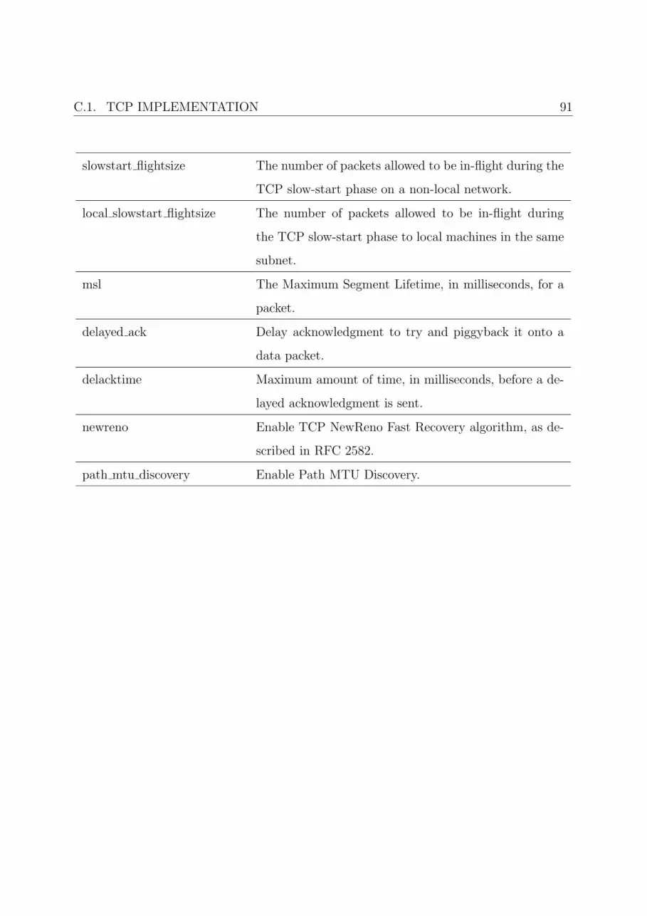
C.1. TCP IMPLEMENTATION 91
slowstart flightsize The number of packets allowed to be in-flight during the
TCP slow-start phase on a non-local network.
local slowstart flightsize The number of packets allowed to be in-flight during
the TCP slow-start phase to local machines in the same
subnet.
msl The Maximum Segment Lifetime, in milliseconds, for a
packet.
delayed ack Delay acknowledgment to try and piggyback it onto a
data packet.
delacktime Maximum amount of time, in milliseconds, before a de-
layed acknowledgment is sent.
newreno Enable TCP NewReno Fast Recovery algorithm, as de-
scribed in RFC 2582.
path mtu discovery Enable Path MTU Discovery.

92 APPENDIX C. FREEBSD KERNEL DETAILS & MODIFICATIONS
rexmit min, rexmit slop Adjust the retransmit timer calculation for TCP. The
slop is typically added to the raw calculation to take into
account occasional variances that the SRTT (smoothed
round-trip time) is unable to accommodate, while the
minimum specifies an absolute minimum. While a num-
ber of TCP RFCs suggest a 1 second minimum, these
RFCs tend to focus on streaming behavior, and fail to
deal with the fact that a 1 second minimum has se-
vere detrimental effects over lossy interactive connec-
tions, such as a 802.11b wireless link, and over very fast
but lossy connections for those cases not covered by the
fast retransmit code. For this reason, we use 200ms of
slop and a near-0 minimum, which gives us an effective
minimum of 200ms (similar to Linux).

C.1. TCP IMPLEMENTATION 93
inflight.enable Enable TCP bandwidth-delay product limiting. An at-
tempt will be made to calculate the bandwidth-delay
product for each individual TCP connection, and limit
the amount of inflight data being transmitted, to avoid
building up unnecessary packets in the network. This
option is recommended if you are serving a lot of data
over connections with high bandwidth-delay products,
such as modems, GigE links, and fast long-haul WANs,
and/or you have configured your machine to accommo-
date large TCP windows. In such situations, without
this option, you may experience high interactive laten-
cies or packet loss due to the overloading of interme-
diate routers and switches. Note that bandwidth-delay
product limiting only effects the transmit side of a TCP
connection.
inflight.debug Enable debugging for the bandwidth-delay product al-
gorithm.
inflight.min This puts a lower bound on the bandwidth-delay prod-
uct window, in bytes. A value of 1024 is typically used
for debugging. 6000-16000 is more typical in a produc-
tion installation. Setting this value too low may result
in slow ramp-up times for bursty connections. Setting
this value too high effectively disables the algorithm.
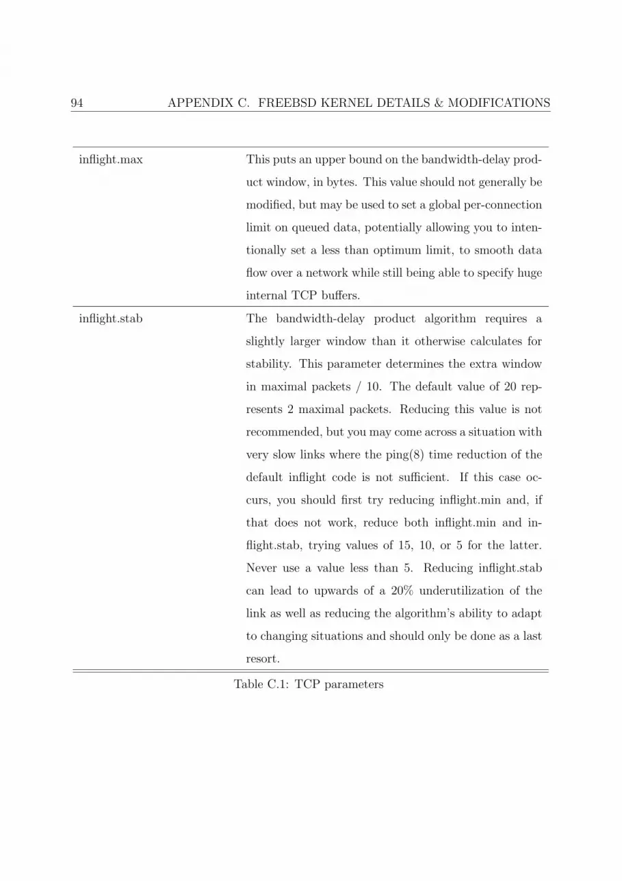
94 APPENDIX C. FREEBSD KERNEL DETAILS & MODIFICATIONS
inflight.max This puts an upper bound on the bandwidth-delay prod-
uct window, in bytes. This value should not generally be
modified, but may be used to set a global per-connection
limit on queued data, potentially allowing you to inten-
tionally set a less than optimum limit, to smooth data
flow over a network while still being able to specify huge
internal TCP buffers.
inflight.stab The bandwidth-delay product algorithm requires a
slightly larger window than it otherwise calculates for
stability. This parameter determines the extra window
in maximal packets / 10. The default value of 20 rep-
resents 2 maximal packets. Reducing this value is not
recommended, but you may come across a situation with
very slow links where the ping(8) time reduction of the
default inflight code is not sufficient. If this case oc-
curs, you should first try reducing inflight.min and, if
that does not work, reduce both inflight.min and in-
flight.stab, trying values of 15, 10, or 5 for the latter.
Never use a value less than 5. Reducing inflight.stab
can lead to upwards of a 20% underutilization of the
link as well as reducing the algorithm’s ability to adapt
to changing situations and should only be done as a last
resort.
Table C.1: TCP parameters

C.1. TCP IMPLEMENTATION 95
Parameter (net.inet.tcp.) Default value
rfc1323 Enabledrfc3042 Enabledrfc339 Enabledsack.enable Enabledsendspace 32768 bytesrecvspace 65536 bytesslowstart flightsize 1 packetlocal slowstart flightsize 4 packetsmsl 30000 millisecondsdelayed ack Enableddelacktime 100 millisecondsnewreno Enabledpath mtu discovery Enabledrexmit min 3 millisecondsrexmit slop 200 millisecondsinflight.enable Enabledinflight.debug Disabledinflight.min 6144 bytesinflight.max 1073725440 bytesinflight.stab 20
Table C.2: Default values of TCP parameters

96 APPENDIX C. FREEBSD KERNEL DETAILS & MODIFICATIONS
C.1.1 Initial RTO Calculation
In FreeBSD 6 the RTO timer is (re)calculated each time an acknowledgment arrives. The
calculation is triggered on lines 1188 − 1199 in the sys/net/inet/tcp_input.c file. A
function named tcp_xmit_timer is called with the difference between the current time
(measured in ticks) and the time when the packet that triggered the acknowledgment was
sent (also in ticks) plus one tick.2 This is the actual round-trip time of the packet that the
acknowledgment acknowledges.3
For the listings in this section there are some variable who’s values do not show. These
values are listed in Table C.3.
The function tcp_xmit_timer starts by determining whether a smoothed round-trip
time has been previously calculated or not, if this is not the case the function calculates
the smoothed rtt (t_srtt), the rtt variance (t_rttvar) and the best rtt (rttbest) with
the help of the given round-trip time (rtt);
tp−>t s r t t = r t t < < TCP RTT SHIFT ;
tp−>t r t t v a r = r t t < < (TCP RTTVAR SHIFT − 1 ) ;
tp−>t r t t b e s t = tp−>t s r t t + tp−>t r t t v a r ;
Listing C.1: sys/net/inet/tcp input.c, lines 2744-2746
After these steps have been conducted the retransmission timer (t_rxtcur) is set;
TCPT RANGESET( tp−>t rx t cu r , TCP REXMTVAL( tp ) ,
max( tp−>t r t tmin , r t t + 2) , TCPTVREXMTMAX) ;
2If the timestamp option (RFC 1323 [12]) is turned off the RTO calculation is not called from here,and not with the same parameters.
3On most architectures one tick corresponds to one millisecond

C.2. DEACTIVATING THE TCP HOST CACHE 97
Listing C.2: sys/net/inet/tcp input.c, lines 2762-2763
where the macro TCPT_RANGESET is defined as
#define TCPT RANGESET( tv , value , tvmin , tvmax ) do { \
( tv ) = ( value ) + t cp r exm i t s l op ; \
i f ( ( u long ) ( tv ) < ( u long ) ( tvmin ) ) \
( tv ) = ( tvmin ) ; \
else i f ( ( u long ) ( tv ) > ( u long ) ( tvmax ) ) \
( tv ) = ( tvmax ) ; \
} while (0 )
Listing C.3: sys/net/inet/tcp timer.h, lines 129-135
and the macro TCP_REXMTVAL as
#define TCP REXMTVAL( tp ) \
max( ( tp)−>t r t tmin , ( ( ( tp)−> t s r t t >> (TCP RTT SHIFT − \
TCP DELTA SHIFT) ) + ( tp)−> t r t t v a r ) >> TCP DELTA SHIFT)
Listing C.4: sys/net/inet/tcp var.h, lines 341-344
C.2 Deactivating the TCP host cache
In order to disable the host caching feature of the FreeBSD TCP implementation, the source
code shown in Listing C.5, was changed to look like the code in Listing C.6. When this
change was performed the only thing that was required to be done for the host cache to be
emptied, was to change the value of the sysctl variable net.inet.tcp.hostcache.purge
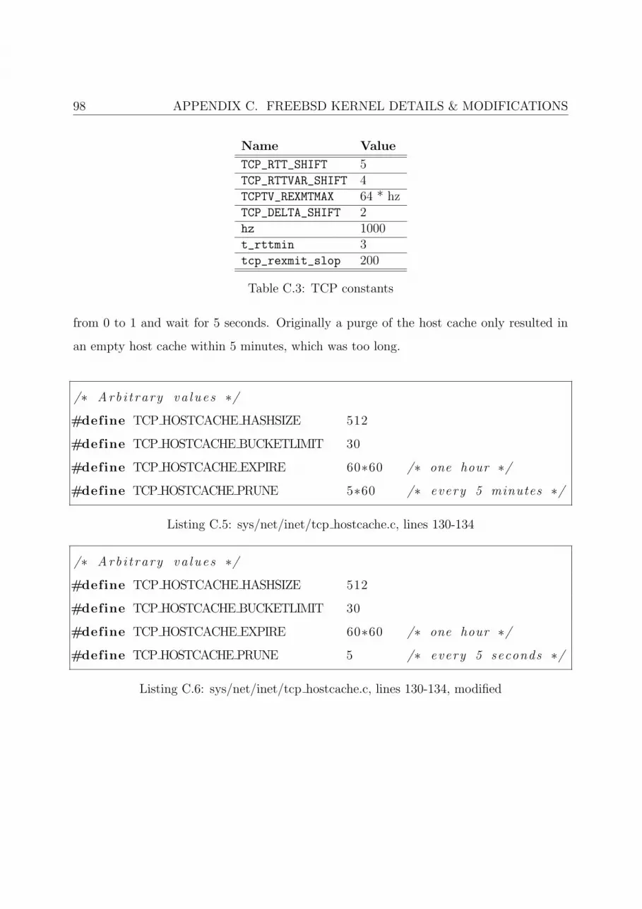
98 APPENDIX C. FREEBSD KERNEL DETAILS & MODIFICATIONS
Name Value
TCP_RTT_SHIFT 5TCP_RTTVAR_SHIFT 4TCPTV_REXMTMAX 64 * hzTCP_DELTA_SHIFT 2hz 1000t_rttmin 3tcp_rexmit_slop 200
Table C.3: TCP constants
from 0 to 1 and wait for 5 seconds. Originally a purge of the host cache only resulted in
an empty host cache within 5 minutes, which was too long.
/∗ Arb i t rary va l u e s ∗/
#define TCP HOSTCACHE HASHSIZE 512
#define TCP HOSTCACHE BUCKETLIMIT 30
#define TCP HOSTCACHE EXPIRE 60∗60 /∗ one hour ∗/
#define TCP HOSTCACHE PRUNE 5∗60 /∗ every 5 minutes ∗/
Listing C.5: sys/net/inet/tcp hostcache.c, lines 130-134
/∗ Arb i t rary va l u e s ∗/
#define TCP HOSTCACHE HASHSIZE 512
#define TCP HOSTCACHE BUCKETLIMIT 30
#define TCP HOSTCACHE EXPIRE 60∗60 /∗ one hour ∗/
#define TCP HOSTCACHE PRUNE 5 /∗ every 5 seconds ∗/
Listing C.6: sys/net/inet/tcp hostcache.c, lines 130-134, modified

Appendix D
Source code & Scripts
This appendix provides the source codes to some of the applications and scripts that were
used in this work. The first section in the appendix presents the loss pattern generator
mentioned in Section 3.4.4, the second section describes the experiment script that was
used in order to automatically configure the environment and run the experiments, and,
finally, the third section in this appendix describes the client & server applications that
were used for the experiments.
D.1 Loss pattern generator
This application was developed in order to simplify the creation of the loss patterns that
were used by the Dummynet network emulator. In the two following subsections the usage
of the application, and its source code are provided.
D.1.1 Usage
The usage of the loss pattern generator is as follows;
loss_pos <sequence factor> <positions> <filename> <mode> [<start value>]
99

100 APPENDIX D. SOURCE CODE & SCRIPTS
where the argument <sequence factor> specifies the length of the pattern. Let us say
that a sequence factor of 2 is entered, then the length of the pattern is 2 ∗ 16 = 32, which
means that after 32 processed packets Dummynet will start over from the beginning of the
pattern again. The argument <positions> is a comma separated list of positions where
losses should occur in the flow. A list of 1,4, would make Dummynet to lose the first and
the fourth packet. The <filename> argument is simply the filename of the pattern that
should be created. This is the file that should be loaded into Dummynet. The argument
<mode> is used to control how the comma separated list, that was mentioned earlier, is
interpreted. If <mode> == time then the numbers in the list specifies when to switch from
non-loss to loss. For example, if <positions> == 4,8 and <mode> == time, then there
will be no losses on positions 0− 3, losses on positions 4− 7, and no losses from position
8 and on. If <mode> == time then the optional argument <start value> can be used.
By default <start value> == 0. If we change this value to 1, however, then the previous
example would result in a pattern that specifies; losses on positions 0 − 3, no losses on
positions 4− 7, and losses from position 8 and on.
D.1.2 Source code
#include <s t d i o . h>
#include <s t d l i b . h>
#include <s t r i n g s . h>
#include <s t r i n g . h>
#define SEQUENCE LENGTH ARG 1
#define LOSS POSITIONS ARG 2
#define LOSS PATTERN NAME 3
#define LOSS MODE 4
#define TIME DRIVEN START 5
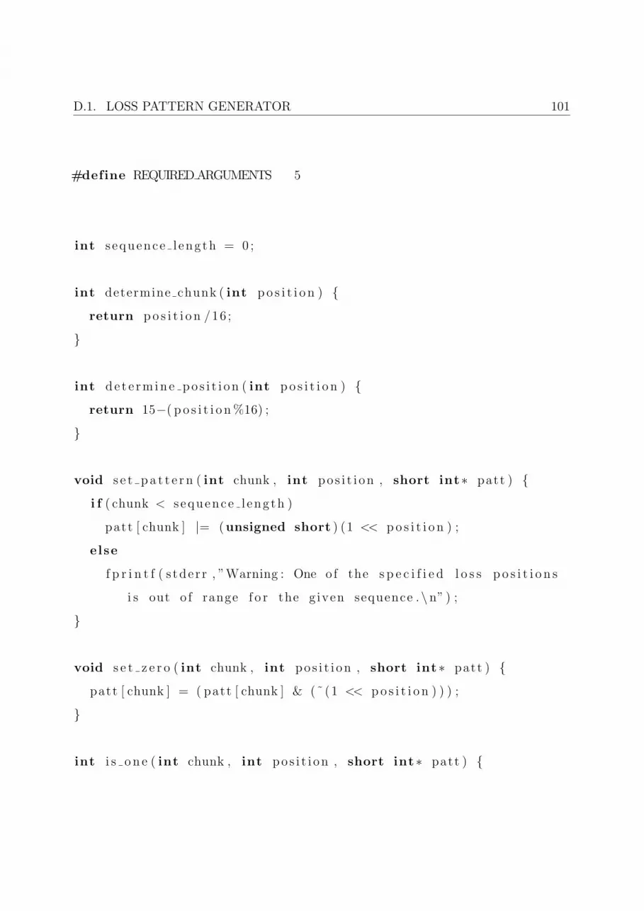
D.1. LOSS PATTERN GENERATOR 101
#define REQUIRED ARGUMENTS 5
int s equence l ength = 0 ;
int determine chunk ( int po s i t i o n ) {
return po s i t i o n /16 ;
}
int de t e rm ine po s i t i on ( int po s i t i o n ) {
return 15−( p o s i t i o n %16) ;
}
void s e t p a t t e r n ( int chunk , int pos i t i on , short int∗ patt ) {
i f ( chunk < s equence l ength )
patt [ chunk ] |= (unsigned short ) (1 << po s i t i o n ) ;
else
f p r i n t f ( s tde r r , ”Warning : One o f the s p e c i f i e d l o s s p o s i t i o n s
i s out o f range f o r the g iven sequence .\n” ) ;
}
void s e t z e r o ( int chunk , int pos i t i on , short int∗ patt ) {
patt [ chunk ] = ( patt [ chunk ] & (˜(1 << po s i t i o n ) ) ) ;
}
int i s o n e ( int chunk , int pos i t i on , short int∗ patt ) {

102 APPENDIX D. SOURCE CODE & SCRIPTS
return patt [ chunk ] & (1 << po s i t i o n ) ;
}
int i s d i g i t (char arg ) {
return ( arg >= ’ 0 ’ && arg <= ’ 9 ’ ) ;
}
int i s i n t e g e r ( const char∗ arg ) {
int r e s u l t = 1 ;
int i ;
for ( i =0; i < s t r l e n ( arg ) ; i++) {
r e s u l t &= i s d i g i t ( arg [ i ] ) ;
}
return r e s u l t ;
}
int s e t l o s s e s ( const char∗ l o s s l i s t , short int∗ pat t e rns ) {
i f ( i s i n t e g e r ( l o s s l i s t ) ) {
int tmp = a to i ( l o s s l i s t ) ;
s e t p a t t e r n ( determine chunk (tmp) , d e t e rm ine po s i t i on (tmp) ,
pa t t e rn s ) ;
return 1 ;
} else {
const char∗ l i s t e l em en t = s t r t ok ( l o s s l i s t , ” , ” ) ;

D.1. LOSS PATTERN GENERATOR 103
i f ( l i s t e l em en t != NULL && i s i n t e g e r ( l i s t e l em en t ) ) {
int tmp = a to i ( l i s t e l em en t ) ;
s e t p a t t e r n ( determine chunk (tmp) , d e t e rm ine po s i t i on (tmp) ,
pa t t e rn s ) ;
return 1 &
s e t l o s s e s ( l o s s l i s t+s t r l e n ( l i s t e l em en t )+1, pat t e rn s ) ;
}
}
return 0 ;
}
int g e t l i s t e l em e n t (char∗ l i s t ) {
const char∗ l i s t e l em en t = s t r t ok ( l i s t , ” , ” ) ;
l i s t = l i s t + s t r l e n ( l i s t e l em en t ) + 1 ;
p r i n t f ( ” l i s t : %s\n” , l i s t ) ;
i f ( l i s t e l em en t != NULL)
return a t o i ( l i s t e l em en t ) ;
return −1;
}
int main ( int argc , char∗∗ argv ) {
/∗ Val ida t e command l i n e arguments (START) ∗/
i f ( argc < REQUIRED ARGUMENTS | |
! i s i n t e g e r ( argv [SEQUENCE LENGTH ARG] ) ) {
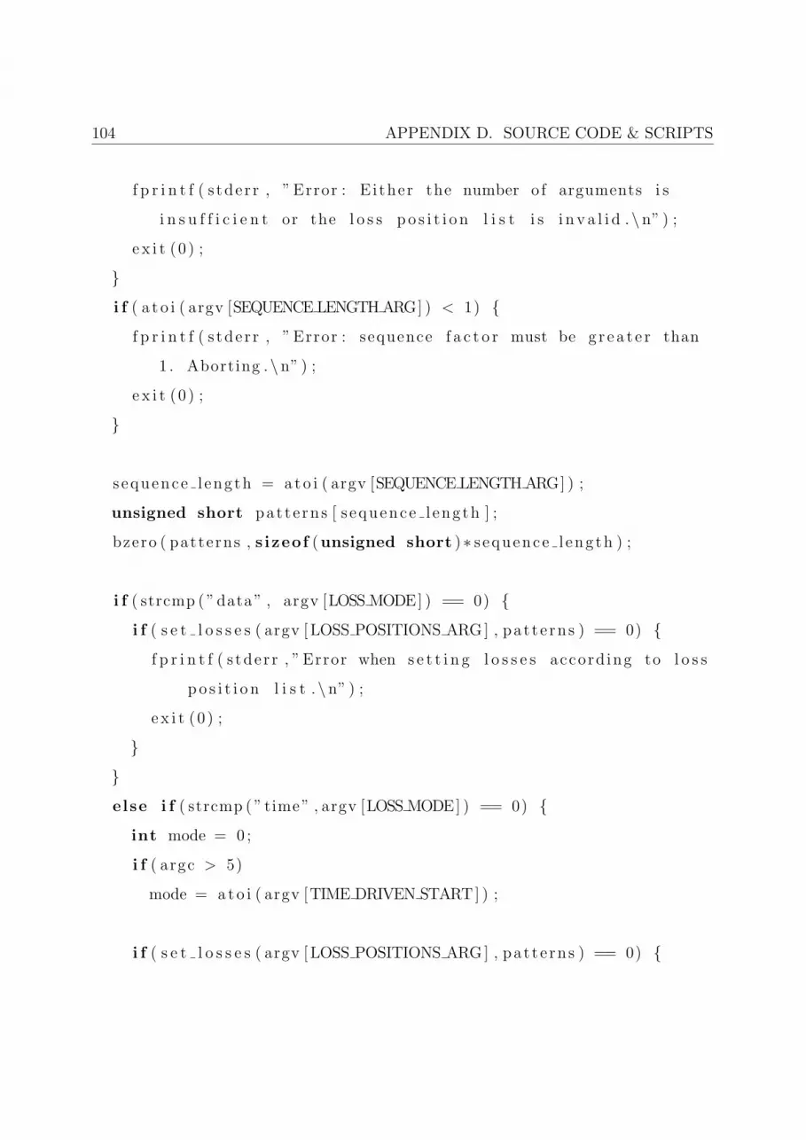
104 APPENDIX D. SOURCE CODE & SCRIPTS
f p r i n t f ( s tde r r , ”Error : E i ther the number o f arguments i s
i n s u f f i c i e n t or the l o s s p o s i t i o n l i s t i s i n v a l i d .\n” ) ;
e x i t (0 ) ;
}
i f ( a t o i ( argv [SEQUENCE LENGTH ARG] ) < 1) {
f p r i n t f ( s tde r r , ”Error : sequence f a c t o r must be g r e a t e r than
1 . Aborting .\n” ) ;
e x i t (0 ) ;
}
s equence l ength = a t o i ( argv [SEQUENCE LENGTH ARG] ) ;
unsigned short pat t e rns [ s equence l ength ] ;
bzero ( patterns , s izeof (unsigned short )∗ s equence l ength ) ;
i f ( strcmp ( ”data” , argv [LOSS MODE] ) == 0) {
i f ( s e t l o s s e s ( argv [LOSS POSITIONS ARG] , pa t t e rn s ) == 0) {
f p r i n t f ( s tde r r , ”Error when s e t t i n g l o s s e s accord ing to l o s s
p o s i t i o n l i s t .\n” ) ;
e x i t (0 ) ;
}
}
else i f ( strcmp ( ” time” , argv [LOSS MODE] ) == 0) {
int mode = 0 ;
i f ( argc > 5)
mode = a t o i ( argv [TIME DRIVEN START] ) ;
i f ( s e t l o s s e s ( argv [LOSS POSITIONS ARG] , pa t t e rn s ) == 0) {

D.1. LOSS PATTERN GENERATOR 105
f p r i n t f ( s tde r r , ”Error when s e t t i n g l o s s e s accord ing to l o s s
p o s i t i o n l i s t .\n” ) ;
e x i t (0 ) ;
}
i f (mode == 0 | | mode == 1) {
int i , j ;
for ( i =0; i < s equence l ength ; i++) {
for ( j =15; j >= 0 ; j−−) {
i f ( i s o n e ( i , j , pa t t e rn s ) ) {
mode = ( mode ? 0 : 1 ) ;
}
i f (mode) {
s e t p a t t e r n ( i , j , pa t t e rn s ) ;
}
else {
s e t z e r o ( i , j , pa t t e rn s ) ;
}
}
}
}
else {
f p r i n t f ( s tde r r , ”Error : S ta r t va lue i n c c o r e c t .\n” ) ;
e x i t (0 ) ;
}
}

106 APPENDIX D. SOURCE CODE & SCRIPTS
else {
f p r i n t f ( s tde r r , ”Error : Mode does not e x i s t .\n” ) ;
e x i t (0 ) ;
}
/∗ Write pa t t e rn to f i l e ∗/
FILE ∗ o u t f i l e ;
o u t f i l e = fopen ( argv [LOSS PATTERN NAME] , ”w” ) ;
i f ( o u t f i l e == NULL) {
f p r i n t f ( s tde r r , ”Error : Could not open %s f o r wr i t i ng .
Aborting . ” , argv [LOSS PATTERN NAME] ) ;
e x i t (0 ) ;
}
i f ( fw r i t e (&patterns , s izeof ( pa t t e rn s ) ,1 , o u t f i l e ) == 0) {
f p r i n t f ( s tde r r , ”Error : Could not wr i t e to f i l e %s . Aborting” ,
argv [LOSS PATTERN NAME] ) ;
e x i t (0 ) ;
}
f c l o s e ( o u t f i l e ) ;
return 0 ;
}
Listing D.1: Loss pattern generator
D.2 Experiment script
In this section the script that was used to configure the environment and to execute the
experiments is described. In fact, it is two scripts; one script, written in Perl, that takes

D.2. EXPERIMENT SCRIPT 107
care of the environment configuration, and one shell script that executes the actual exper-
iment. The shell script is called by the configuration script when the configuration of the
environment is completed.
The scripts provided in this appendix are designed for the experiments with the short
flows, but comments are provided within the code to show how the experiments with the
longer flows were conducted as well.
These scripts are modified versions of the scripts that were used for the experiments in
[11].
D.2.1 Source code
Configuration script
#!/ usr / b in / p e r l
# Define genera l op t i ons
# 041105 Johan Garcia
# Modif ied 050830 Per Hurt ig
#−−−−−−−−−−−−−−−−−−−−−−−
$ r e p l i k a t =3;
# name temp la te f o r the output f i l e s
$outf i lnamn=”/home/per / experiment / t e s t ” ;
# Machine i d e n t i t i e s
# This s c r i p t i s des i gned to be run on the c l i e n t
$ s e rv e r = ” 1 0 . 0 . 2 . 1 ” ;
$ c l i e n t = ” 1 0 . 0 . 1 . 1 ” ;
$ r c t r l = ” root \@3g . c a r l . kau . se ” ;

108 APPENDIX D. SOURCE CODE & SCRIPTS
$ s c t r l = ”per\@3b . c a r l . kau . se ” ;
$portnr = ”1234” ;
# Network Parameter
#−−−−−−−−−−−−−−−−−−−−−−−−−
# Define the t e s t case parameters
@bwdown =
(”40Kbit/ s ” , ”80Kbit/ s ” , ”160Kbit/ s ” , ”320Kbit/ s ” , ”500Kbit/ s ” , ”1000Kbit/ s ” , ”2000Kbit/ s ” , ”4000Kbit/ s ” , ”8000Kbit/ s ” , ”10000Kbit/ s ” ) ;
@bwup =
( ”40Kbit/ s ” , ”80Kbit/ s ” , ”160Kbit/ s ” , ”320Kbit/ s ” , ”500Kbit/ s ” , ”1000Kbit/ s ” , ”2000Kbit/ s ” , ”4000Kbit/ s ” , ”8000Kbit/ s ” , ”10000Kbit/ s ” ) ;
@delay = (5 ,10 ,20 ,40 ,60 ,80 ,100 ,150 ,200 ,250 ,300) ;
@queue = (99) ;
# Set the f i l e s i z e s to be r e t r i e v e d ∗ 2500
@size = (10) ;
$pat te rns =20;
$pa t t e r np r e f i x=” pat t e rns / pattern ” ;
# For f l ows wi th l e n g t h 100
#@bwdown =
(”40 Kbit / s ” ,”80 Kbit / s ” ,”160 Kbit / s ” ,”500 Kbit / s ” ,”1000 Kbit / s ” ,”4000 Kbit / s ” ,”10000 Kbit / s ”) ;
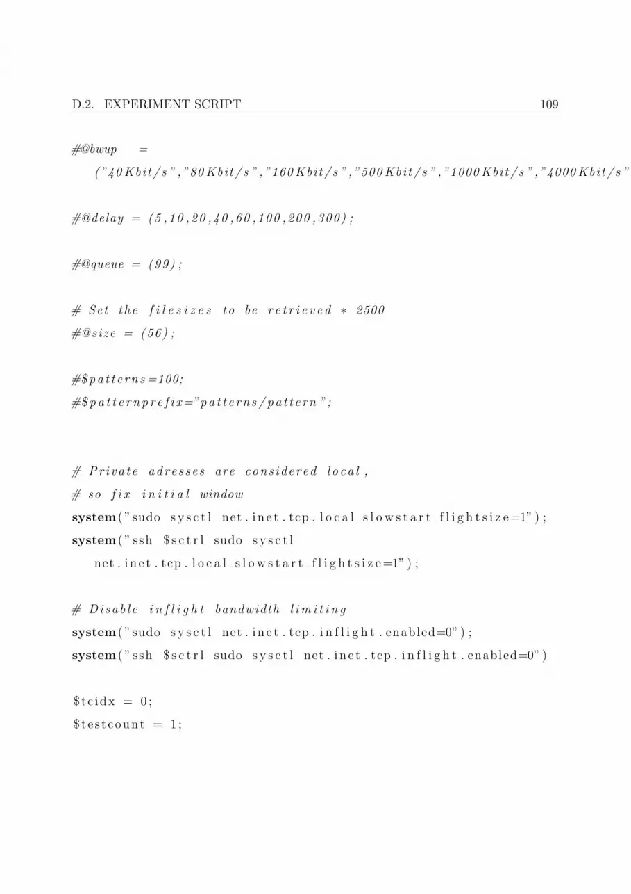
D.2. EXPERIMENT SCRIPT 109
#@bwup =
(”40 Kbit / s ” ,”80 Kbit / s ” ,”160 Kbit / s ” ,”500 Kbit / s ” ,”1000 Kbit / s ” ,”4000 Kbit / s ” ,”10000 Kbit / s ”) ;
#@delay = (5 ,10 ,20 ,40 ,60 ,100 ,200 ,300) ;
#@queue = (99) ;
# Set the f i l e s i z e s to be r e t r i e v e d ∗ 2500
#@size = (56) ;
#$pa t t e rn s =100;
#$ p a t t e r n p r e f i x=”pa t t e rn s / pa t t e rn ” ;
# Pr iva te adre s s e s are cons idered l o c a l ,
# so f i x i n i t i a l window
system ( ” sudo s y s c t l net . i n e t . tcp . l o c a l s l o w s t a r t f l i g h t s i z e=1” ) ;
system ( ” ssh $ s c t r l sudo s y s c t l
net . i n e t . tcp . l o c a l s l o w s t a r t f l i g h t s i z e=1” ) ;
# Disab l e i n f l i g h t bandwidth l im i t i n g
system ( ” sudo s y s c t l net . i n e t . tcp . i n f l i g h t . enabled=0” ) ;
system ( ” ssh $ s c t r l sudo s y s c t l net . i n e t . tcp . i n f l i g h t . enabled=0” )
$tc idx = 0 ;
$ t e s t count = 1 ;
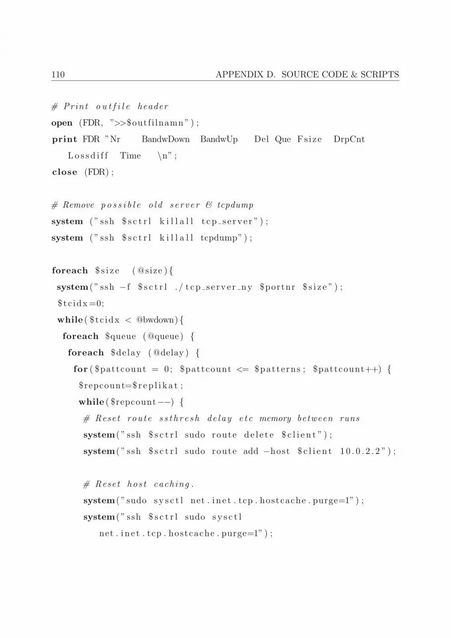
110 APPENDIX D. SOURCE CODE & SCRIPTS
# Print o u t f i l e header
open (FDR, ”>>$outf i lnamn ” ) ;
print FDR ”Nr BandwDown BandwUp Del Que Fs i z e DrpCnt
L o s s d i f f Time \n” ;
close (FDR) ;
# Remove p o s s i b l e o l d s e r v e r & tcpdump
system ( ” ssh $ s c t r l k i l l a l l t c p s e r v e r ” ) ;
system ( ” ssh $ s c t r l k i l l a l l tcpdump” ) ;
foreach $ s i z e ( @size ){
system ( ” ssh −f $ s c t r l . / t cp s e r v e r ny $portnr $ s i z e ” ) ;
$ t c idx =0;
while ( $ t c idx < @bwdown){
foreach $queue (@queue ) {
foreach $delay ( @delay ) {
for ( $pattcount = 0 ; $pattcount <= $patte rns ; $pattcount++) {
$repcount=$ r e p l i k a t ;
while ( $repcount−−) {
# Reset route s s t h r e s h de lay e t c memory between runs
system ( ” ssh $ s c t r l sudo route d e l e t e $ c l i e n t ” ) ;
system ( ” ssh $ s c t r l sudo route add −host $ c l i e n t 1 0 . 0 . 2 . 2 ” ) ;
# Reset hos t caching .
system ( ” sudo s y s c t l net . i n e t . tcp . hostcache . purge=1” ) ;
system ( ” ssh $ s c t r l sudo s y s c t l
net . i n e t . tcp . hostcache . purge=1” ) ;
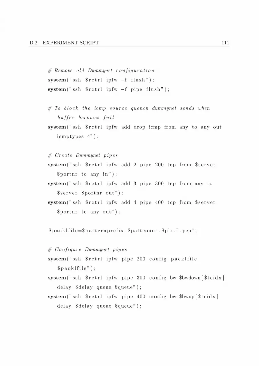
D.2. EXPERIMENT SCRIPT 111
# Remove o ld Dummynet c on f i g u r a t i on
system ( ” ssh $ r c t r l ipfw −f f l u s h ” ) ;
system ( ” ssh $ r c t r l ipfw −f p ipe f l u s h ” ) ;
# To b l o c k the icmp source quench dummynet sends when
b u f f e r becomes f u l l
system ( ” ssh $ r c t r l ipfw add drop icmp from any to any out
icmptypes 4” ) ;
# Create Dummynet p ipe s
system ( ” ssh $ r c t r l ipfw add 2 pipe 200 tcp from $s e rv e r
$portnr to any in ” ) ;
system ( ” ssh $ r c t r l ipfw add 3 pipe 300 tcp from any to
$ s e rv e r $portnr out” ) ;
system ( ” ssh $ r c t r l ipfw add 4 pipe 400 tcp from $s e rv e r
$portnr to any out” ) ;
$ p a c k l f i l e=$pa t t e r np r e f i x . $pattcount . $p l r . ” . pep” ;
# Configure Dummynet p ipe s
system ( ” ssh $ r c t r l ipfw pipe 200 con f i g p a c k l f i l e
$ p a c k l f i l e ” ) ;
system ( ” ssh $ r c t r l ipfw pipe 300 con f i g bw $bwdown [ $ tc idx ]
de lay $delay queue $queue” ) ;
system ( ” ssh $ r c t r l ipfw pipe 400 con f i g bw $bwup [ $ tc idx ]
de lay $delay queue $queue” ) ;

112 APPENDIX D. SOURCE CODE & SCRIPTS
open(FDR, ”>>$outf i lnamn ” ) ;
printf FDR(”%4i %10s %10s %3d %3d %3d
%s” , $testcount , $bwdown [ $ tc idx ] , $bwup [ $ tc idx ] , $delay , $queue , $ s i z e , $pattcount ) ;
close (FDR) ;
# Serve r s i d e l o g g i n g
system ( ” ssh −f $ s c t r l sudo tcpdump − i x l0 −w /tmp/temp . pcap
tcp port $portnr &” ) ;
system ( ” s l e e p 5” ) ;
# Execute t e s t
system ( ” . / runt e s t . sh $ s e rv e r $portnr >> $outf i lnamn ” ) ;
system ( ” sudo gz ip −f /tmp/temp . pcap” ) ;
system ( ”cp /tmp/temp . pcap . gz
” . $outf i lnamn . $ te s t count . ” . pcap . gz” ) ;
system ( ” ssh $ s c t r l sudo k i l l a l l tcpdump” ) ;
system ( ” ssh −f $ s c t r l sudo gz ip −f /tmp/temp . pcap” ) ;
system ( ” ssh −f $ s c t r l cp /tmp/temp . pcap . gz
” . $outf i lnamn . ” srv ” . $ t e s t count . ” . pcap . gz” ) ;
$ t e s t count++;
}
}
}
}
D.3. CLIENT & SERVER APPLICATIONS 113
++$tc idx ;
}
}
Listing D.2: Configuration script
Execution script
#!/ usr / l o c a l / b in / bash
# Usage : r un t e s t . sh s e r v e r s e r v e r po r t
# C l i e n t s i d e l o g g i n g
sudo tcpdump −w /tmp/temp . pcap − i x l0 tcp port $2 &
s l e ep 1
# Sta r t c l i e n t
. / t c p c l i e n t $1 $2 100 100 unused > tmp . tmp
s l e ep 2
sudo k i l l a l l tcpdump
# Return e l ap s ed time
cat tmp . tmp
Listing D.3: Experiment execution script
D.3 Client & Server applications
This section contains the source codes of the client & server applications. These applica-
tions are modified versions of the applications used in [11].

114 APPENDIX D. SOURCE CODE & SCRIPTS
D.3.1 Client source code
#include <uni s td . h>
#include <s t r i n g . h>
#include <s t d l i b . h>
#include <s t d i o . h>
#include <sys / types . h>
#include <sys / socke t . h>
#include <ne t i n e t / in . h>
#include <ne t i n e t / tcp . h>
#include <netdb . h>
#include <sys / time . h>
#include <uni s td . h>
#include <sys / s t a t . h>
#include < f c n t l . h>
int main ( int argc , char ∗∗ argv ) {
char ∗ remhost ;
char r ead buf [ 5 0 000 ] , c ;
u sho r t remport ;
int sock , nread , fd ;
int l en ;
int bu f f e r ;
long sum = 0 ;
long t i d ;
struct sockaddr in remote ;
struct hostent ∗h ;

D.3. CLIENT & SERVER APPLICATIONS 115
struct t imeva l tv1 , tv2 ;
i f ( argc != 3) {
f p r i n t f ( s tde r r , ” usage : t c p c l i e n t <host> <port>\n” ) ;
e x i t (1 ) ;
}
remhost = argv [ 1 ] ;
remport = a t o i ( argv [ 2 ] ) ;
/∗ Create TCP socke t ∗/
i f ( ( sock = socket (AF INET , SOCK STREAM, 0) ) < 0) {
per ro r ( ” t e s t c l i e n t : socke t ” ) ;
e x i t (1 ) ;
}
/∗ I n i t i a l i z e sockaddr in s t r u c t u r e f o r remote hos t ∗/
bzero ( ( char ∗)&remote , s izeof ( remote ) ) ;
remote . s i n f am i l y = AF INET ;
i f ( ( h = gethostbyname ( remhost ) ) == NULL) {
per ro r ( ” t e s t c l i e n t : gethostbyname” ) ;
e x i t (1 ) ;
}

116 APPENDIX D. SOURCE CODE & SCRIPTS
bcopy ( ( char ∗)h−>h addr , (char ∗)&remote . s in addr ,
h−>h l ength ) ;
remote . s i n p o r t = htons ( remport ) ;
/∗ S ta r t the t imer b e f o r e connect ing to remote hos t ∗/
gett imeofday(&tv1 , NULL) ;
i f ( connect ( sock , ( struct sockaddr ∗) & remote ,
s izeof ( remote ) ) < 0) {
per ro r ( ” t e s t c l i e n t : connect ” ) ;
e x i t (1 ) ;
}
/∗
∗ Read data from socke t . Count number o f b y t e s r e c e i v ed and
measure
∗ the time
∗/
while ( ( nread = read ( sock , read buf , s izeof ( r ead buf ) ) ) > 0) {
sum += nread ;
}
gett imeofday(&tv2 , NULL) ;
t i d = ( ( tv2 . t v s e c − tv1 . t v s e c ) ∗ 1000 + ( tv2 . tv u s e c −
tv1 . tv u s e c ) / 1000) ;
c l o s e ( sock ) ;
D.3. CLIENT & SERVER APPLICATIONS 117
p r i n t f ( ”%7ld \n” , t i d ) ;
}
Listing D.4: Client application source code
D.3.2 Server source code
#include <uni s td . h>
#include <s t r i n g . h>
#include <s t d l i b . h>
#include <s t d i o . h>
#include <sys / types . h>
#include <sys / socke t . h>
#include <sys / time . h>
#include <ne t i n e t / in . h>
#include <ne t i n e t / tcp . h>
#include <netdb . h>
char send buf [ 2 5 0 0 0 ] ;
int main ( int argc , char ∗∗ argv ) {
int l i s t e n e r , i , l oops ;
u shor t myport ;
int conn ;
struct sockaddr in s1 , s2 ;
int l ength ;
char ch , tecken ;

118 APPENDIX D. SOURCE CODE & SCRIPTS
struct t imeva l tv1 , tv2 ;
long t i d ;
long bytes ;
tecken = ’ 0 ’ ;
for ( i = 0 ; i < s izeof ( send buf ) ; i++) {
send buf [ i ] = tecken ;
i f ( tecken == ’ 9 ’ )
tecken = ’ 0 ’ ;
else
tecken++;
}
i f ( argc != 3) {
f p r i n t f ( s tde r r , ” usage : t c p s e r v e r <port> <nmb loops>\n” ) ;
e x i t (1 ) ;
}
i f ( ( l i s t e n e r = socket (AF INET , SOCK STREAM, 0) ) < 0) {
per ro r ( ” t e s t s e r v e r : socke t ” ) ;
e x i t (1 ) ;
}
myport = a t o i ( argv [ 1 ] ) ;
bzero ( ( char ∗)&s1 , s izeof ( s1 ) ) ;
s1 . s i n f am i l y = AF INET ;
s1 . s i n addr . s addr = INADDR ANY;
s1 . s i n p o r t = htons (myport ) ;
D.3. CLIENT & SERVER APPLICATIONS 119
i f ( bind ( l i s t e n e r , ( struct sockaddr ∗) & s1 , s izeof ( s1 ) ) < 0) {
per ro r ( ” i n e t r s t r e am : bind” ) ;
e x i t (1 ) ;
}
l ength = s izeof ( s1 ) ;
i f ( getsockname ( l i s t e n e r , ( struct sockaddr ∗) & s1 , &length ) <
0) {
per ro r ( ” t e s t s e r v e r : getsockname” ) ;
e x i t (1 ) ;
}
l i s t e n ( l i s t e n e r , 1) ;
l ength = s izeof ( s2 ) ;
while (1 ) {
i f ( ( conn = accept ( l i s t e n e r , ( struct sockaddr ∗) & s2 ,
&length ) ) < 0) {
per ro r ( ” t e s t s e r v e r : accept ” ) ;
e x i t (1 ) ;
}
p r i n t f ( ”\nConnection e s t ab l i s h ed , sending data” ) ;
l oops = a t o i ( argv [ 2 ] ) ;
gett imeofday(&tv1 , NULL) ;
i f ( l oops > 1) {
wr i t e ( conn , send buf , 5000) ;
l oops −=2;
}

120 APPENDIX D. SOURCE CODE & SCRIPTS
for ( i = 0 ; i < l oops ; i++)
wr i t e ( conn , send buf , 2500) ;
gett imeofday(&tv2 , NULL) ;
t i d = ( ( tv2 . t v s e c − tv1 . t v s e c ) ∗ 1000 + ( tv2 . tv u s e c −
tv1 . tv u s e c ) / 1000) ;
p r i n t f ( ”\nBytes sent : %ld \n” , bytes = ( loops ∗
( s izeof ( send buf ) ) ) ) ;
p r i n t f ( ”Elapsed time : %ld ms\n” , t i d ) ;
p r i n t f ( ”Send ra t e : %l f bps\n” , ( bytes ∗ 8 ∗ 1000 .0 ) / t i d ) ;
f f l u s h ( stdout ) ;
c l o s e ( conn ) ;
}
}
Listing D.5: Server application source code