Embed Size (px)
Citation preview
sustainability
Article
Electricity Consumption Forecasting Based on a BidirectionalLong-Short-Term Memory Artificial Neural Network
Dana-Mihaela Petros, anu 1,* and Alexandru Pîrjan 2
�����������������
Citation: Petros, anu, D.-M.; Pîrjan, A.
Electricity Consumption Forecasting
Based on a Bidirectional Long-Short-
Term Memory Artificial Neural
Network. Sustainability 2021, 13, 104.
https://dx.doi.org/10.3390/su130101
04
Received: 15 November 2020
Accepted: 22 December 2020
Published: 24 December 2020
Publisher’s Note: MDPI stays neu-
tral with regard to jurisdictional claims
in published maps and institutional
affiliations.
Copyright: © 2020 by the authors. Li-
censee MDPI, Basel, Switzerland. This
article is an open access article distributed
under the terms and conditions of the
Creative Commons Attribution (CC BY)
license (https://creativecommons.org/
licenses/by/4.0/).
1 Department of Mathematics-Informatics, Faculty of Applied Sciences, University Politehnica of Bucharest,060042 Bucharest, Romania
2 Department of Informatics, Statistics and Mathematics, Romanian-American University, 012101 Bucharest,Romania; [email protected]
* Correspondence: [email protected]; Tel.: +40-761-086-656
Abstract: The accurate forecasting of the hourly month-ahead electricity consumption representsa very important aspect for non-household electricity consumers and system operators, and atthe same time represents a key factor in what regards energy efficiency and achieving sustainableeconomic, business, and management operations. In this context, we have devised, developed, andvalidated within the paper an hourly month ahead electricity consumption forecasting method. Thismethod is based on a bidirectional long-short-term memory (BiLSTM) artificial neural network (ANN)enhanced with a multiple simultaneously decreasing delays approach coupled with function fittingneural networks (FITNETs). The developed method targets the hourly month-ahead total electricityconsumption at the level of a commercial center-type consumer and for the hourly month aheadconsumption of its refrigerator storage room. The developed approach offers excellent forecastingresults, highlighted by the validation stage’s results along with the registered performance metrics,namely 0.0495 for the root mean square error (RMSE) performance metric for the total hourly month-ahead electricity consumption and 0.0284 for the refrigerator storage room. We aimed for andmanaged to attain an hourly month-ahead consumed electricity prediction without experiencinga significant drop in the forecasting accuracy that usually tends to occur after the first two weeks,therefore achieving a reliable method that satisfies the contractor’s needs, being able to enhancehis/her activity from the economic, business, and management perspectives. Even if the devised,developed, and validated forecasting solution for the hourly consumption targets a commercialcenter-type consumer, based on its accuracy, this solution can also represent a useful tool for othernon-household electricity consumers due to its generalization capability.
Keywords: long term electricity consumption forecasting; artificial neural networks (ANNs); bidi-rectional long-short-term memory (BiLSTM) networks; function fitting neural networks (FITNETs);large commercial center-type consumers
1. Introduction1.1. Motivation
According to the International Energy Agency, between 1971 and 2018, the world totalfinal energy consumption multiplied by 2.3, growing from 4243 “millions of tons of oilequivalent (Mtoe)” in 1971 to 9938 Mtoe in 2018 [1]. While the share of energy consumptionhas been almost constant over the years in most sectors, energy consumption in non-residential sectors has increased over the course of time, from 76% in 1971 to 79% in 2018.The non-residential sector, comprising the consumption arising from industry, transport,commercial activities, services rendered in the public interest, agricultural activities, forest-related activities and unspecified other sectors, represents the largest sector, which accountsfor the largest percentage within the world total final energy consumption. Consideringthe mentioned indicators, one is able to deduce that attaining efficiency with regard to
Sustainability 2021, 13, 104. https://dx.doi.org/10.3390/su13010104 https://www.mdpi.com/journal/sustainability

Sustainability 2021, 13, 104 2 of 31
energy within non-household sectors impacts in a considerable manner the worldwideefforts to save fuel, to reduce pollutants, to achieve sustainable economic, business, andmanagement operations, and to enhance the quality of life.
Consequently, in order to attain worldwide energy efficiency, a factor of major impor-tance consists in providing an accurate prediction of the consumers’ electricity consumptionbelonging to the large non-household category. Moreover, such an accurate forecast helpsin optimizing the electricity consumption and influencing the consumption strategy, andfacilitates the efforts made in view of attaining an appropriate environment and naturalresource management. In this context, the accurate forecasting of the hourly month aheadelectricity consumption is a very important aspect for non-household electricity consumersand system operators, and at the same time represents an essential factor in what regardsenergy efficiency.
In our country, Romania, the total energy consumption increased at a pace of 1.3%per year between 2014 and 2019, year in which it reached the value of 34 Mtoe. The non-household final consumers represent the largest sector, representing an amount of 74% ofthe total electricity consumption in 2019 (45% of the total electricity consumption is due tothe industry, while 17% is represented by the services) [2].
Lately, in the scientific literature, the interest regarding the accurate forecast of the con-sumed electricity has been growing at an ever-accelerating pace, the researchers developinga wide range of applications, methods, and techniques in order to obtain forecasts of timeseries related to energy datasets. In this paper, we have devised, developed, and validatedan electricity consumption forecasting method based on a bidirectional long-short-termmemory (BiLSTM) artificial neural network (ANN) enhanced with a multiple simultane-ously decreasing delays approach coupled with function fitting neural networks (FITNETs)for the hourly month-ahead total electricity consumption at the level of a commercialcenter-type consumer and for the hourly month-ahead consumption of its refrigeratorstorage room.
In order to emphasize the results related to the approached subject reported withinthe scientific literature and to contextualize the research developed within this paper, aliterature review is performed in the following subsection, having as a main purpose thenecessity to pinpoint an exact deficiency, an unsolved problem, and a gap that still exists inthe current body of knowledge that is being addressed by the research presented withinthis paper.
Afterwards, the “Materials and Methods” section depicts the most important notionsthat have been applied in the development of the prediction method along with details con-cerning the stages and steps that represent the building blocks for our proposed approach.
Afterwards, the following section, “Results”, presents the results obtained over thecourse of the stages and steps of the prediction method developed based on a BiLSTMANN enhanced with a multiple simultaneously decreasing delays approach coupled withFITNETs, for the month-ahead total electricity consumption at the level of the commercialcenter type-consumer and the month-ahead consumption of the refrigerator storage room.Firstly, we present the results regarding the developed BiLSTM ANN total hourly electricityconsumption forecasting solution with multiple delays support, based on the adaptive mo-ment estimation (ADAM), stochastic gradient descent with momentum (SGDM), and rootmean square propagation (RMSProp) training algorithms. Secondly, we depict the resultswith regard to the FITNET ANN prediction approach for the refrigerator storage room,based on the Levenberg–Marquardt (LM), Bayesian regularization (BR), and scaled conju-gate gradient (SCG) training algorithms. Lastly, we present the results registered during thevalidation process of the developed method, by analyzing the registered forecasting results.
Subsequently, in the fourth section, the “Discussion”, we analyze and interpret theforecasting results obtained through the developed approach, in contrast with other ex-isting studies and approaches from the body of knowledge targeting resembling issues,highlighting also future research directions and limitations of our proposed approach.
Sustainability 2021, 13, 104 3 of 31
In the “Conclusions” section, we emphasize the most important outcomes and findingsof the paper, by interpreting our findings at a higher level of abstraction than in the“Discussion” section. We highlight and justify the fact that we have managed to addressthe target proposed within the “Introduction” section.
1.2. Literature Review
In the research paper [3], Moradzadeh et al. devised a hybrid method comprising ofan adjusted support vector regression (SVR) and long short-term memory (LSTM) ANN,entitled SVR-LSTM, with a view to obtaining a short-term forecast of the electricity con-sumption of a microgrid located in Sub-Saharan Africa. For the input variables, the authorstook into account different factors that have an effect on the microgrid’s load; factorslike the commercial establishments, different family units consisting of houses and theiroccupants, while for the outputs they used electricity load profiles. The hybrid approachwas benchmarked against its single constituent parts and similar approaches from the sci-entific literature, providing superior results in terms of the correlation coefficient (R), meansquared error (MSE), RMSE, mean absolute error (MAE), and mean absolute percentageerror (MAPE) performance metrics.
Kim et al. propose in [4] a hybrid approach, entitled “(c, l)-LSTM + convolutionalneural network (CNN)”, used for predicting the electricity demand in view of assuringan efficient management and appropriate operational activities for a smart grid. Theauthors’ proposed method involves two variates sequences, comprising pairs of key values,associated with contextual information, that are inserted into LSTM ANNs to obtain sets offeatures that are afterwards used by a CNN to obtain a forecast of the electricity demand.After assessing the performance of their method by comparing it with the autoregressiveintegrated moving average (ARIMA), the (c, l)-LSTM, and with a sequence-to-sequence(S2S) LSTM in terms of the MAPE and relative RMSE (RRMSE) performance metrics, theauthors state that their method yielded better results in terms of accuracy.
Within the scientific article [5], Yaprakdal et al. propose a forecasting method basedon deep recurrent neural networks (DRNNs), consisting of a BiLSTM ANN, entitled“DRNN Bi-LSTM”, in order to obtain an accurate estimation for the day-ahead electricitydemand and the total photovoltaic electricity production for a microgrid equipped withboth photovoltaic panels and diesel generators. The authors applied their method on a realproduction dataset. They compared their proposed method with other approaches fromthe literature, namely with a deep CNN (D-CNN) [6], a Copula model deep belief network(Copula-DBN) [7], a DRNN-LSTM [8], and with parallel convolutional recurrent neuralnetworks (CNN-RNN) [9]. Finally, the authors concluded that their devised method offerssuperior results as depicted by the MAPE performance metric.
Recognizing the importance of attaining an accurate prediction of the day-aheadhourly electricity consumption in order to optimize and appropriately manage the energyrelated resources, in [10], Santra et al. propose an approach consisting of LSTM ANNs forsolving the problems related to long-term data dependencies and genetic algorithm (GA) toget the most appropriate parameters for the LSTM ANNs. The authors trained the networkusing real electricity load and meteorological datasets, and afterwards, they tested theirproposed method and compared it with the results provided by a LSTM ANN that doesnot have its parameters tuned by means of a GA, and concluded the superiority of theirapproach based on the MAPE performance metric that highlighted a higher accuracy level.
Acknowledging the importance that an accurate monthly electricity demand forecastexerts at both local and countrywide levels, along with the numerous challenges that mustbe overcome in attaining these goals when referring to the residential segment, in thescientific article [11], Son et al. put forward a prediction method based on LSTM ANNs.The authors explain this choice as being driven by the robustness and efficiency that LSTMANNs exhibited during the course of time when it came to predicting time series. Intraining the model, the authors used a dataset comprising of 22 years of monthly electricityconsumption from South Korea, while for evaluating the performance, the MAE, RMSE,
Sustainability 2021, 13, 104 4 of 31
MAPE, post-error ratio (C), mean bias error (MBE), and the unpaired peak accuracy (UPA)performance metrics were computed and analyzed. After having benchmarked the pro-posed method against the SVR, the backpropagation ANN, the ARIMA, and the multiplelinear regression (MLR), the authors state that they registered very good results, the LSTMapproach having proved to be superior in all of the analyzed cases.
Considering the increase in the number of smart metering equipment and infrastruc-ture throughout the world, an increase that has led to huge volumes of useful data relatedto electricity consumption and disaggregated loads, in [12], Alonso et al. introduce a pro-cessing and forecasting methodology for multiple time series datasets recorded by meansof smart-metering devices. In contrast to classical and univariate methods, the authorsput forward a RNN model with LSTM for the purpose of identifying different patternsof electricity consumption stemming from different individual electricity consumers andhouseholds, with the goal of achieving day-ahead accurate predictions while consumingvery low computational resources. After benchmarking and computing the MSE along withthe MAE performance metrics, the authors conclude the efficiency of their devised LSTMmodel in forecasting electricity consumption time series. In future work, the authors aim toachieve a larger prediction time frame, namely a week-ahead forecast, to experiment withvarious LSTM architectures and different experimental conditions, from diverse datasets todissimilar geographic regions.
In the scientific article [13], taking into account that attaining a long-term forecast ofthe electricity consumption is of paramount importance from both the monetary and timeresources perspectives, Almazrouee et al. perform a comparative analysis between theProphet and Holt–Winters long-term forecasting models in terms of prediction accuracyand efficiency. When conducting their study, the authors used real electricity consumptiondatasets ranging between the years 2010 and 2020 from the powerplants located in Kuwaitin order to predict the electricity consumption for the following 10 years, up to the year2030. After benchmarking their method, the authors observed that the Prophet modelyielded forecasts with a higher level of accuracy, as highlighted by the RMSE, the MAPE,coefficient of determination (R2), MAE, and coefficient of variation of RMSE (CVRMSE)performance indicators. In addition, the authors inserted Gaussian white noise of differentintensities in order to assess the robustness of the two analyzed models and concluded thatthe Prophet model is more resilient to noise than the Holt–Winters one.
In their paper [14], Shao et al. put forward a hybrid model in order to provide“multiple forecasts by combining CNNs and LSTM” ANNs. The hybrid model was devel-oped in order to parallelly process the dataset, therefore improving the robustness of theconventional CNN–LSTM approach. Afterwards, the features extracted using the above-mentioned methods were used along with six statistical variables, namely “mean, max,min, standard deviation (Sd), skewness (Skew), and kurtosis (Kurt)”, and the developedmodel was validated using three real datasets coming from three American companies.The authors compare their model with others, based on deep learning (DL), such asDNN-LSTM [15], nonpooling convolutional neural network LSTM (NPCNN-LSTM) [16],LSTM-LSTM [17], CNN-LSTM [18] and conclude that their developed approach has provenits robustness and efficiency when forecasting the electricity consumption for different timehorizons, ranging from very short term to long term.
In the context of the worldwide ever-increasing electricity demand, Mir et al. presentan insight of the forecasting approaches designed in the scientific literature in order toestimate future electricity demands in the cases of countries having low and middleincomes [19]. The devised study takes into account different prediction methodologiesfrom the body of knowledge, targeting various time horizons, and remark that in thecases when forecasting for long [20] or medium time [21] intervals, the models based ontime series have been mainly used, while for short term intervals [22], the techniqueshave made use of artificial intelligence (AI). The authors remark that in each country theelectricity demand is influenced by a series of determinants, such as the population of therespective country, the gross domestic product (GDP), the local weather conditions, and the
Sustainability 2021, 13, 104 5 of 31
consumption for different moments and intervals of time (as local consumption habits). Inthis paper, the authors also present a comparative analysis of the results retrieved from thescientific literature with the ones from their country, Pakistan. The authors conclude theirdeveloped analysis of the scientific literature by identifying a series of research gaps in thecase of Pakistan that will be worth narrowing in the future, such as the limited number ofstudies regarding short-term load forecasting (STLF) and the lack of medium-term loadforecasting (MTLF) studies.
In the article [23], Marulanda et al. develop a method with a view to obtaining long-term scenarios with regard to the forecasting of the produced wind energy, consideringspatial and temporal dependencies between energy markets from different areas. Afterhaving assessed the dependencies using a bottom-up strategy and real production datasetsfrom France, Spain, and Portugal, the authors concluded that the ordered quantile transfor-mation provided the most appropriate normalization of the time series when comparedto the logit Yeo–Johnson and Box–Cox ones. In what concerns the data division process,the authors remarked that segmenting the datasets monthly led to better results, while thecomparison with the pinball loss function and with the Winkler score metrics highlightedthe superiority of their approach.
Being aware of the importance of electricity load forecasting in view of planningefficient operation of supply networks, within the scientific article [24], Sloyali implementeda series of machine learning methods, namely ANN, MLR, adaptive neuro-fuzzy inferencesystem (ANFIS), and support vector machine (SVM) with the purpose of estimating energydemand, and discussed criteria related to its generation in Cyprus. The author remarkedthat the electricity load depends on external parameters such as weather, humidity, andsolar irradiation, but also on national factors, obtaining therefore the parameters used asinputs for the machine learning algorithms. Afterwards, based on datasets representingthe electricity usage in the years 2016 and 2017, the author developed simulations in thepurpose of evaluating the algorithms’ performance and analyzing the short- and long-termforecasting. The study concludes that in both cases the implemented approaches offer abetter performance than the rest of the analyzed ML-based ones, due to the fact that theyprovide more accurate forecasting results.
In light of the extreme importance and numerous benefits that a long-term accurateforecast of the electricity consumption can bring to energy providers and dispatchers,Elkamel et al. propose in [25] a model based on the MLR along with three CNNs forpredicting electricity consumption for the state of Florida. The authors developed andcompared the performance of univariant, multichannel, and multihead ANNs along withthe MLR. The MSE, RMSE, MAE, and MAPE performance metrics revealed the superiorityof the multichannel and multihead CNNs in contrast to the model based on the MLR, theaccuracy of the CNN approach having increased along with the size of the dataset. Theauthors concluded that the multichannel CNN provided the best results, being the mostsuitable option of the analyzed ones for fulfilling the objective of attaining a long-termelectricity forecast in the case of Florida.
Within the research paper [26], Son et al. bring forward an electricity consumptionprediction method developed based on deep neural network (DNN) and LSTM ANNscovering the medium- and long-term forecasting time frame. The performance metrics,consisting of the MAE, RMSE, MAPE, R2, and the CVRMSE computed according to thedefinition from [27], convey the superiority of the DNN approach in contrast to the longshort-term one. The authors stated that in their future work they intend to address theexisting limitations pertaining to the lack of weather data and seasonality.
In a recent paper, Ribeiro et al. started their research by highlighting the importanceof benefitting from accurate energy consumption forecasts in the case of companies thatare energy intensive consumers [28]. In addition, the authors highlight the importance ofimplementing DL techniques in energy demand forecasting. In this purpose, the authorscompare two benchmarks, namely the ARIMA and a technique that exists on site, againstthree DL approaches, namely RNN, LSTM, and gated recurrent unit (GRU), and two
Sustainability 2021, 13, 104 6 of 31
approaches based on the SVR and random forest models. The comparison was conductedusing a short-term time horizon for the obtained forecasts, within which a dataset retrievedfrom a Brazilian company was used. The developed comparison showed that the approachalready implemented at the case site provided the worst results, while the ones providedby the GRU model surpassed all the other approaches that were tested within this study.
Considering from both the integration and operational costs point of views howbeneficial is for power grid operators to be able to obtain their own power generationforecasts, in [29], Kim et al. develop a photovoltaic electricity production forecastingmethod for a one-hour-ahead, an approach that combines a BiLSTM in two steps with anANN that uses the exponential moving average (EMA) for pre-processing the datasets.After benchmarking and computing the RMSE, MAPE, and the R2, the authors concludedthat the combined method is superior to others.
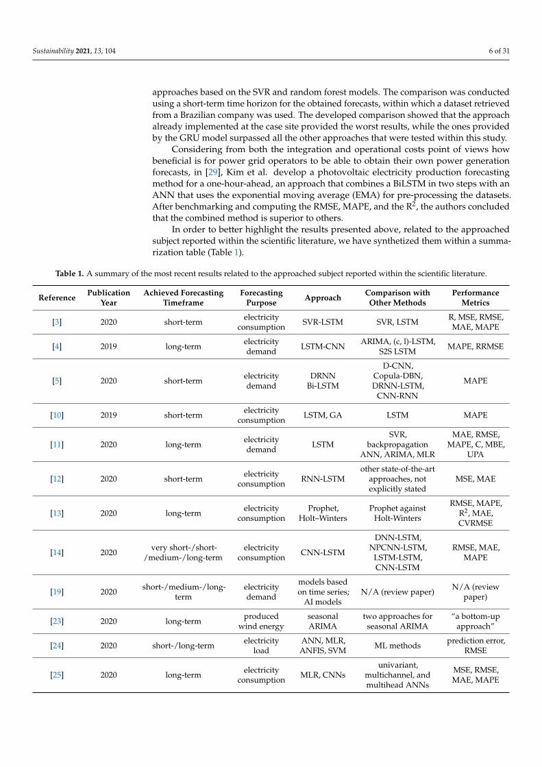
In order to better highlight the results presented above, related to the approachedsubject reported within the scientific literature, we have synthetized them within a summa-rization table (Table 1).
Table 1. A summary of the most recent results related to the approached subject reported within the scientific literature.
Reference PublicationYear
Achieved ForecastingTimeframe
ForecastingPurpose Approach Comparison with
Other MethodsPerformance
Metrics
[3] 2020 short-term electricityconsumption SVR-LSTM SVR, LSTM R, MSE, RMSE,
MAE, MAPE
[4] 2019 long-term electricitydemand LSTM-CNN ARIMA, (c, l)-LSTM,
S2S LSTM MAPE, RRMSE
[5] 2020 short-term electricitydemand
DRNNBi-LSTM
D-CNN,Copula-DBN,DRNN-LSTM,
CNN-RNN
MAPE
[10] 2019 short-term electricityconsumption LSTM, GA LSTM MAPE
[11] 2020 long-term electricitydemand LSTM
SVR,backpropagation
ANN, ARIMA, MLR
MAE, RMSE,MAPE, C, MBE,
UPA
[12] 2020 short-term electricityconsumption RNN-LSTM
other state-of-the-artapproaches, notexplicitly stated
MSE, MAE
[13] 2020 long-term electricityconsumption
Prophet,Holt–Winters
Prophet againstHolt-Winters
RMSE, MAPE,R2, MAE,CVRMSE
[14] 2020 very short-/short-/medium-/long-term
electricityconsumption CNN-LSTM
DNN-LSTM,NPCNN-LSTM,
LSTM-LSTM,CNN-LSTM
RMSE, MAE,MAPE
[19] 2020 short-/medium-/long-term
electricitydemand
models basedon time series;
AI modelsN/A (review paper) N/A (review
paper)
[23] 2020 long-term producedwind energy
seasonalARIMA
two approaches forseasonal ARIMA
“a bottom-upapproach”
[24] 2020 short-/long-term electricityload
ANN, MLR,ANFIS, SVM ML methods prediction error,
RMSE
[25] 2020 long-term electricityconsumption MLR, CNNs
univariant,multichannel, andmultihead ANNs
MSE, RMSE,MAE, MAPE
Sustainability 2021, 13, 104 7 of 31
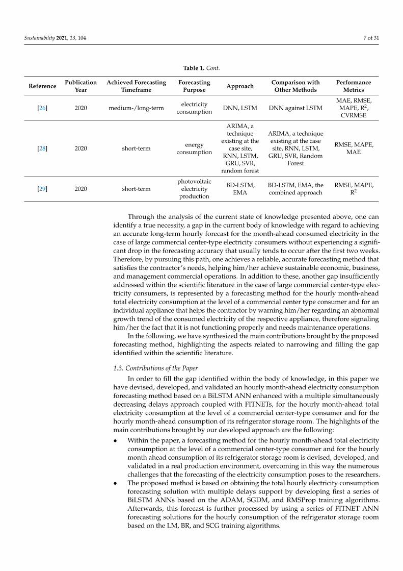
Table 1. Cont.
Reference PublicationYear
Achieved ForecastingTimeframe
ForecastingPurpose Approach Comparison with
Other MethodsPerformance
Metrics
[26] 2020 medium-/long-term electricityconsumption DNN, LSTM DNN against LSTM
MAE, RMSE,MAPE, R2,CVRMSE
[28] 2020 short-term energyconsumption
ARIMA, atechnique
existing at thecase site,
RNN, LSTM,GRU, SVR,
random forest
ARIMA, a techniqueexisting at the casesite, RNN, LSTM,
GRU, SVR, RandomForest
RMSE, MAPE,MAE
[29] 2020 short-termphotovoltaic
electricityproduction
BD-LSTM,EMA
BD-LSTM, EMA, thecombined approach
RMSE, MAPE,R2
Through the analysis of the current state of knowledge presented above, one canidentify a true necessity, a gap in the current body of knowledge with regard to achievingan accurate long-term hourly forecast for the month-ahead consumed electricity in thecase of large commercial center-type electricity consumers without experiencing a signifi-cant drop in the forecasting accuracy that usually tends to occur after the first two weeks.Therefore, by pursuing this path, one achieves a reliable, accurate forecasting method thatsatisfies the contractor’s needs, helping him/her achieve sustainable economic, business,and management commercial operations. In addition to these, another gap insufficientlyaddressed within the scientific literature in the case of large commercial center-type elec-tricity consumers, is represented by a forecasting method for the hourly month-aheadtotal electricity consumption at the level of a commercial center type consumer and for anindividual appliance that helps the contractor by warning him/her regarding an abnormalgrowth trend of the consumed electricity of the respective appliance, therefore signalinghim/her the fact that it is not functioning properly and needs maintenance operations.
In the following, we have synthesized the main contributions brought by the proposedforecasting method, highlighting the aspects related to narrowing and filling the gapidentified within the scientific literature.
1.3. Contributions of the Paper
In order to fill the gap identified within the body of knowledge, in this paper wehave devised, developed, and validated an hourly month-ahead electricity consumptionforecasting method based on a BiLSTM ANN enhanced with a multiple simultaneouslydecreasing delays approach coupled with FITNETs, for the hourly month-ahead totalelectricity consumption at the level of a commercial center-type consumer and for thehourly month-ahead consumption of its refrigerator storage room. The highlights of themain contributions brought by our developed approach are the following:
• Within the paper, a forecasting method for the hourly month-ahead total electricityconsumption at the level of a commercial center-type consumer and for the hourlymonth ahead consumption of its refrigerator storage room is devised, developed, andvalidated in a real production environment, overcoming in this way the numerouschallenges that the forecasting of the electricity consumption poses to the researchers.
• The proposed method is based on obtaining the total hourly electricity consumptionforecasting solution with multiple delays support by developing first a series ofBiLSTM ANNs based on the ADAM, SGDM, and RMSProp training algorithms.Afterwards, this forecast is further processed by using a series of FITNET ANNforecasting solutions for the hourly consumption of the refrigerator storage roombased on the LM, BR, and SCG training algorithms.
Sustainability 2021, 13, 104 8 of 31
• The developed forecasting method encompasses the advantages of BiLSTM ANNsenhanced with a multiple simultaneously decreasing delays approach coupled withFITNETs, the main advantage of the BiLSTM approach being their capacity to learnlong-term dependencies in both directions, by passing through data twice: backwardand forward; while the main advantage of the FITNETs consists in their capacity toforecast accurately in the context of a fast-training process. The developed approachoffers excellent forecasting results, highlighted by the validation stage’s results alongwith the registered performance metrics. For example, in the case of the BiLSTMANNs, the best registered values for RMSE are: 0.0307 during the training process,0.0327 for the integral set, and 0.0495 during the testing process. When forecastingthe month ahead electricity consumption of the refrigerator storage room using thebest of the developed FITNET ANNs, we obtained an excellent value of the RMSEperformance metric during the forecasting process, namely 0.0284.
• One of the most important aspects related to the forecasting accuracy is representedby the fact that we managed to attain an hourly month-ahead consumed electricityprediction without experiencing a significant drop in the forecasting accuracy thatusually tends to occur after the first two weeks, therefore achieving a reliable methodthat satisfies the contractor’s needs, being able to help him/her attain energy efficiencyand achieve sustainable economic, business, and management operations.
• In all the analyzed cases, the training times registered very good values (namely, inthe case of the ANNs that provided the best forecasting accuracy, 1462.415 s for theFITNET ANN and 0.64699 s for the BiLSTM ANN), without requiring investments inan expensive hardware configuration. This represents a very important advantagefor the moment when the devised solution is put into operation and the ANNsneed subsequent re-training steps, because over the course of time new datasets areregistered and provided to the developed neural networks as inputs.
In the “Discussion” and “Conclusions” sections of the paper, we present more detailsregarding the added value of this research. In the following, the “Materials and Methods”section is presented.
2. Materials and Methods
The main purpose behind our devised research methodology has been the needto design, develop, and validate an efficient forecasting method that is able to providelarge commercial center-type electricity consumers with as accurate as possible month-ahead hourly electricity consumption projections. We have acknowledged from the verybeginning the fact that the provided forecasts must cover the whole hourly month-aheadtime frame and at the same time be as reliable as possible in what concerns the predictionaccuracy for tackling the contractor’s real needs and therefore to be able to improve theoverall economic, management, and business aspects of his/her activity.
Considering that we have tackled previous challenges related to electricity forecastingover the course of our previous studies and research grants, the first logical step was totry and tap into our already devised materials and methods in this field and assess theirsuitability for the current purpose. Therefore, as in one of our research group’s previousstudies [30], the profile of the electricity consumer was of commercial center-type andthe forecasting horizon consisted of hourly month-ahead predictions, we first tried toinvestigate if the employed methods from that study, namely an ANNs approach based onthe non-linear autoregressive (NAR) and the non-linear autoregressive with exogenousinputs (NARX) models could provide satisfactory results for our current situation.
The method based on the NAR model yielded results with insufficient accuracy,especially considering that in our current situation the contractor needed not only anhourly forecast for the overall activity, but an accurate forecast for the refrigerator storageroom as well. When trying to apply the NARX approach from the previous work, wewere hindered by the unavailable outdoor temperature forecasts that the contractor wasnot inclined to purchase in the long run, making this choice for a temperature exogenous
Sustainability 2021, 13, 104 9 of 31
dataset unfeasible. However, building a time stamp dataset and using it as an exogenousvariable for the NARX approach improved the accuracy in contrast with the NAR modelwhen it came to hourly forecasts for the week-ahead, but was unsatisfactory for the hourlymonth-ahead. At this point, we decided to explore other approaches that yielded improvedresults while preserving the findings regarding the potential benefits of an exogenoustimestamp dataset.
Another previous work of one of the authors of the current paper targeted the fore-casting of the consumed electricity for a whole month on an hourly resolution, in thecase of an industrial consumer [31]. Even if the profiles of the two electricity consumersdiffer, we investigated the approach consisting of using the ANNs based on the NARXmodel for obtaining first a forecast of the total daily aggregated electricity consumptionthat is being processed further using LSTM ANNs for refining the forecasted aggregateddaily electricity consumption for a whole month on an hourly resolution. The obtainedresults were superior when compared to [30], and if an hourly two-weeks ahead forecasthad sufficed for the contractor, the approach would have been an acceptable solution. Inaddition, the refrigerator storage room had to undergo the same method applied separatelyall over again leading to exceedingly high training times for the ANNs. These findings,although not satisfactory for our purpose, led us to the decision of investigating furtherthe potential benefits that LSTM ANNs could bring in devising our forecasting method,considering their ability to learn dependencies in the long-term.
As we wanted to attain a high degree of accuracy for all of the weeks comprising thehourly month-ahead forecasts, after having experimented with regular LSTM ANNs thatprovided very good results for the first two weeks, only to register a drop afterwards inthe forecasting accuracy, especially for the last week of the month-ahead forecast horizon,we decided to traverse the input data in both directions. Therefore, we developed andimplemented within the second stage of the forecasting method a BiLSTM ANN enhancedwith multiple simultaneously decreasing delays, as depicted below when presenting indetail the stages and steps of the proposed forecasting method. As we wanted to saveconsiderable processing time without affecting the forecasting accuracy, we tried to avoidre-applying the whole process once again for the refrigerator storage room and triedto disaggregate its hourly month-ahead electricity consumption from the total hourlymonth-ahead electricity consumption forecasted by the BiLSTM enhanced with multiplesimultaneously decreasing delays.
We considered the fact that in a previous work, along with a part of our research group,we managed to achieve an electricity disaggregation method based on FITNETs, a methodthat has provided a high degree of accuracy when it came to forecasting the disaggregatedelectricity loads [32]. This led us to the decision of coupling the BiLSTM enhanced withmultiple simultaneously decreasing delays approach with a FITNETs one used in the pur-pose of disaggregating the hourly month-ahead electricity consumption of the refrigeratorstorage room out of the total hourly month-ahead forecasted electricity consumption.
The devised forecasting method was developed using the following software config-uration: the Windows 10 Education operating system, version 1803, OS build 17134.523(produced by Microsoft Corporation from Redmond town, Washington, United States ofAmerica); the MATLAB development environment software version R2020(a) (producedby MathWorks, Inc. from Natick town, MA, USA) and an entry to mid-level hardwareconfiguration from the computational point of view. The advantage of developing theforecasting method using an inexpensive hardware configuration consists of reduced costsfor the current operator and other potential ones that will not have to buy expensivehardware equipment for the frequent retraining operations of the ANNs. The researchdeveloped and presented within this paper emerged as a consequence of the request ofour contractor, a commercial center-type consumer from Romania. The electricity datasetsregistered and given by the contractor comprise the total hourly consumption at the com-mercial center-type level and the hourly consumption of the refrigerator storage room forthe period January–December 2019.
Sustainability 2021, 13, 104 10 of 31
Cold-Rite, one of the most renowned companies in the refrigeration industry fromSydney, Australia that provides “commercial and industrial refrigeration solutions, in-cluding walk in fridges, commercial water chillers, humidity-controlled rooms and more”,published a list of the most important symptoms signaling the fact that a cool room doesnot function properly and it needs maintenance, otherwise risking serious side effects suchas a skyrocket in the electricity consumption and even a potential spoilage of the coolingsystem [33].
According to the specialists in refrigeration systems from this company, the mostimportant five signs that a cool room needs maintenance are: condensation (consistingin “droplets of water on the inside of the cool room”), ice (representing “spot ice formingon the freezer door”), buzzing sounds (when refrigeration units are “excessively noisy”),spoiling food (in the case when perishable items in the fridge spoil before their expirationdate), and most of all, higher energy bills. This final sign usually reflects the fact thatsome of the used appliances are inefficient and might need servicing. Therefore, at therequest of the contractor, in order to be able to warn him/her regarding an abnormalgrowth trend of the consumed electricity of the refrigerator storage room, we targeted inour study obtaining an as accurate as possible forecasting approach for the month-aheadhourly consumption of the refrigerator storage room along with the main purpose of thestudy, the month-ahead hourly total electricity consumption at the level of the commercialcenter-type consumer, based on which the contractor can choose his/her most suitablebilling plan.
In the following, there are presented details concerning the stages and steps thatrepresent the constructing elements of our developed forecasting method, along with aseries of details regarding the main concepts used in developing our forecasting approach,such as BiLSTM neural networks and FITNETs.
2.1. Stage I: Acquiring and Preprocessing the Datasets
The first stage of the forecasting method has five steps over the course of which thedatasets were acquired and preprocessed. Throughout the first step of this stage, twodatasets for the whole year were acquired from the commercial center-type consumer: afirst dataset comprising the previously recorded total consumed electricity per hour (THED)and a second dataset representing the previously recorded electricity consumption per hourof the refrigerator storage room (RHED), each of the datasets consisting in 8760 recordsrepresenting the hourly consumption for the year 2019, measured in MWh. The datasetswere provided by the contractor who retrieved them from his own metering system.
We designed the first stage’s second step to search for abnormal or missing values thatmight occur within the two above-mentioned datasets (due to the malfunctioning of themetering device or due to recording errors) for obtaining the final preprocessed previouslyrecorded consumed electricity per hour datasets (entitled PTHED for the historical totalhourly consumed electricity and PRHED for the refrigerator storage room). However, evenif when we devised our forecasting approach, we remarked that in this particular case, thetwo datasets given by the contractor did not contain such type of values, we designed thisstep to make sure that the devised forecasting method can be applied for a wider rangeof commercial center-type consumer cases, similar to the one for which we conducted thecurrent study and therefore to be able to generalize the devised forecasting approach. Inorder to solve the issues regarding the potential missing or abnormal values, we designedthis step to apply a gap-filling approach that has proven its effectiveness when applied inprevious studies, some of them being conducted within our research team [30–32,34], themethod being based on a linear interpolation approach.
Over the course of the first stage’s third step of the method, each of the two pre-processed datasets obtained during the previous step was divided into two hourly datasubsets. Therefore, the PTHED dataset was divided into a training subset (PTHEDT) and avalidation subset (PTHEDV), while the PRHED dataset was divided into a training subset(PRHEDT) and a validation subset (PRHEDV). Both of the PTHEDT and PRHEDT subsets
Sustainability 2021, 13, 104 11 of 31
consisted of 8016 samples corresponding to the first 11 months of the year 2019, whileeach of the PTHEDV and PRHEDV subsets consisted of 744 samples corresponding to thelast month of the year 2019. The PTHEDT and PRHEDT subsets were used to develop,train, and validate the prediction method, while the PTHEDV and PRHEDV subsets wereused in the purpose of validating the forecasting approach, through a comparison of thereal values for the last month of the year, stored in the validation subsets PTHEDV andPRHEDV, with the forecasted ones for the total hourly consumed electricity and for therefrigerator storage room.
The Supplementary Materials file contains detailed information about the datasets.
2.2. Stage II: Developing the BiLSTM ANN Total Hourly Electricity Consumption ForecastingSolution with Multiple Delays Support
One of the main research directions when dealing with the analysis of time seriesconsists in forecasting the behavior of the respective series in the future, with various timehorizons ranging from short- to medium- and long-term ones, depending on the specificityof the analyzed problem and on the implemented forecasting approach.
Over the course of time, in order to obtain an accurate forecasting in time series prob-lems, researchers have developed various techniques, within which the DL and machine-based algorithms represent useful and efficient approaches. Comparing these methodsto the ones based on regression techniques, one can remark their irrefutable advantageshighlighted by the accuracy of the obtained results. For example, the LSTM models, partic-ular cases of recurrent neural networks (RNNs), also entitled feedback-based models [35],provide improved prediction results compared to the ones obtained when using ARIMAmodels, due to the fact that LSTM models benefit from an enhanced memory, capable oflearning a larger amount of input data due to specific gates that they incorporate for thispurpose [31,34].
The LSTM ANNs have been implemented by many scientists within their stud-ies [36–41], due to their main advantage that they offer when compared to the feed forwardANNs, consisting in the LSTM’s architecture that comprises a sequence input layer allow-ing the input of the time series or sequences in the ANN, along with a certain LSTM layer,conceived in order to store and be able to retrieve patterns over long time periods. TheLSTMs incorporate certain loops enabling the prolonged existence of information that ispassed inside the LSTM ANN from one step to another. In this type of ANN, the inputdata are crossed only once (from the input to the output) and the network computes theforecasting based on the past and current data.
With the purpose of obtaining an additional improvement of the forecasting accuracy,an enhanced architecture of LSTMs was proposed, namely the BiLSTM one, which enablesadditional training steps through which the input data are used for training in bothdirections, by passing through data twice: backward and forward [35,42,43]. In fact, theBiLSTMs models are based on the aggregation of input information coming from theprevious and upcoming steps related to a certain time step in LSTM models and therefore,in this kind of model, in any moment of time the information from past and future ispreserved [44].
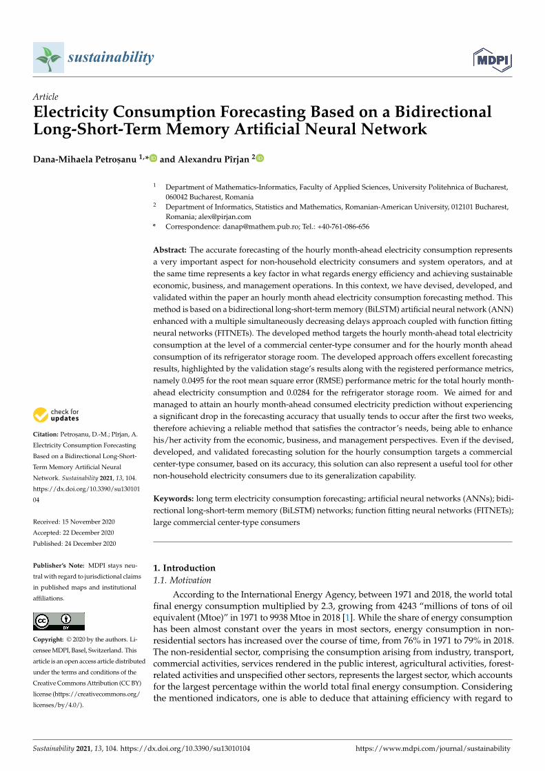
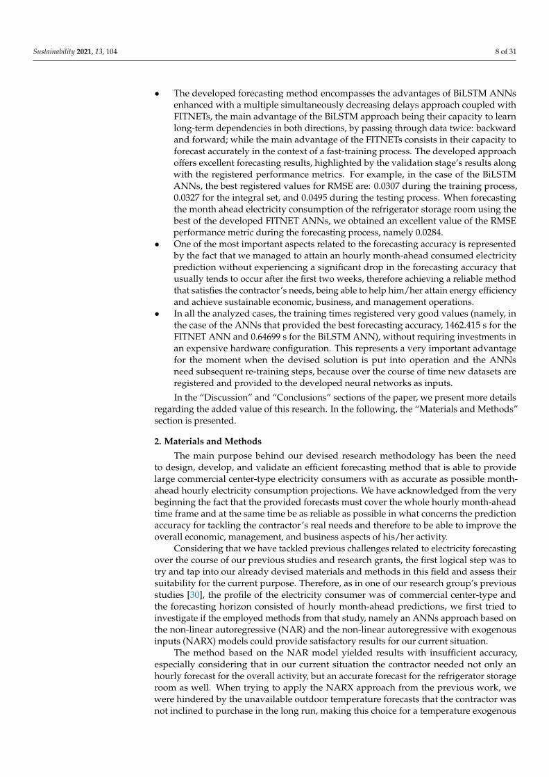
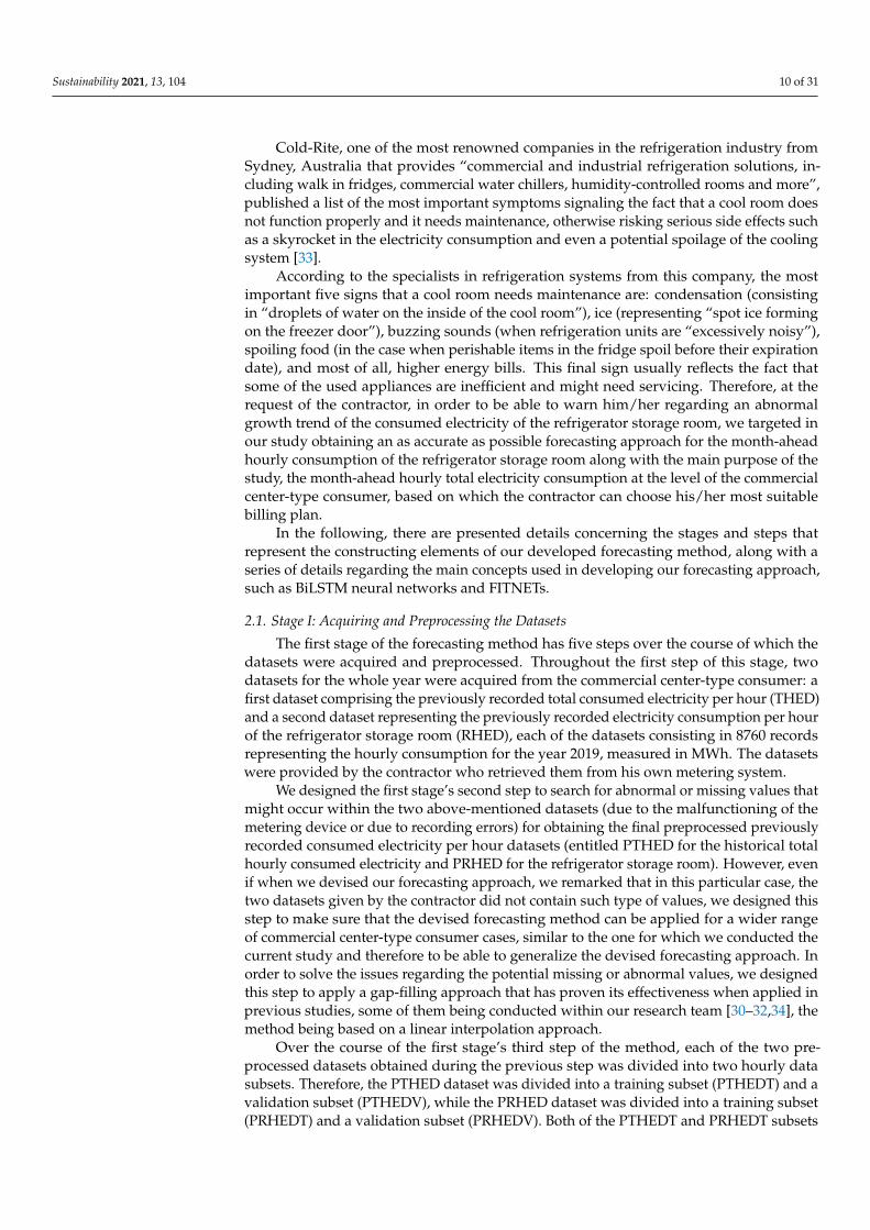
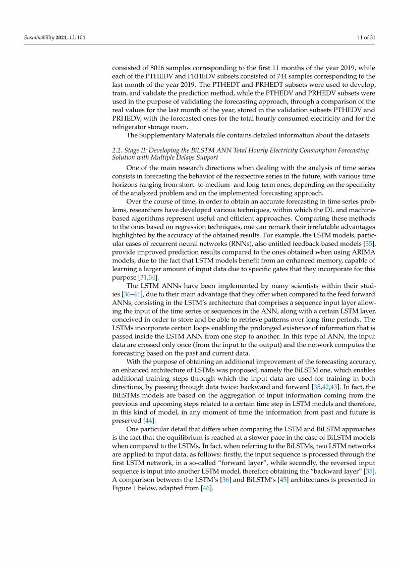
One particular detail that differs when comparing the LSTM and BiLSTM approachesis the fact that the equilibrium is reached at a slower pace in the case of BiLSTM modelswhen compared to the LSTMs. In fact, when referring to the BiLSTMs, two LSTM networksare applied to input data, as follows: firstly, the input sequence is processed through thefirst LSTM network, in a so-called “forward layer”, while secondly, the reversed inputsequence is input into another LSTM model, therefore obtaining the “backward layer” [35].A comparison between the LSTM’s [36] and BiLSTM’s [45] architectures is presented inFigure 1 below, adapted from [46].
Sustainability 2021, 13, 104 12 of 31Sustainability 2021, 13, x FOR PEER REVIEW 12 of 32
(a) The LSTM Architecture (b) The BiLSTM Architecture
Figure 1. A comparison between the long-short-term memory (LSTM)’s and bidirectional long-short-term memory (BiLSTM)’s architectures.
The BiLSTM ties the two hidden layers having reverse directions in order to compute the same output, which takes into account both the past and future states at the same time. In many situations, the simultaneous access to these two states helps improve the model’s per-formance. The main principle on which the architecture of a BiLSTM is based, consists in split-ting each neuron into two directions: one corresponds to the future and reflects the forward states, while the second corresponds to the past, highlighting the backward states [42].
In what concerns the training process of the BiLSTMs, this is achieved by using sim-ilar algorithms to the ones used in the case of regular LSTMs, for example the ADAM, SGDM, and RMSProp training algorithms [32]. Nevertheless, when the training process is based on the back-propagation technique, a series of supplementary processes are re-quired due to the fact that the input and output layers updates cannot take place simulta-neously. In the BiLSTM’s case, the training steps consist in [42]: • Within the forward pass, both the forward and backward states are passed first and
afterwards, the output neurons are passed. • Within the backward pass, firstly the output neurons are passed, while the forward
and backward states are passed subsequently. • Afterwards, when the two passes into the two opposite directions have been per-
formed, the network updates the weights. Over the course of time, researchers have developed various applications of the
BiLSTM models, such as: dependency parsing [47], protein structure prediction [43,48], translations [49], entity extraction [50], handwritten recognition [51], and speech recogni-tion [52,53].
In order to take advantage of the numerous benefits of the BilSTM ANNs, we decided to make them an integral part of developing the second stage of our forecasting approach, consisting in six steps. Over the course of the second stage’s first step, the training subset PTHEDT was retrieved and normalized by processing it as to have a mean of 0 and a variance of 1, corresponding to a standard normal distribution [54].
Subsequently, we constructed, in the second stage’s second step, an array of delays 𝐷 = {𝑥 , … , 𝑥 } and the BiLSTM inputs based on the number and values of the delays, therefore obtaining a set of d training inputs (BiLSTMI) for the BiLSTM ANN total hourly electricity consumption month-ahead forecasting solution enhanced with a multiple sim-ultaneously decreasing delays approach. According to our devised approach, when con-
Figure 1. A comparison between the long-short-term memory (LSTM)’s and bidirectional long-short-term memory(BiLSTM)’s architectures.
The BiLSTM ties the two hidden layers having reverse directions in order to computethe same output, which takes into account both the past and future states at the same time.In many situations, the simultaneous access to these two states helps improve the model’sperformance. The main principle on which the architecture of a BiLSTM is based, consistsin splitting each neuron into two directions: one corresponds to the future and reflectsthe forward states, while the second corresponds to the past, highlighting the backwardstates [42].
In what concerns the training process of the BiLSTMs, this is achieved by using similaralgorithms to the ones used in the case of regular LSTMs, for example the ADAM, SGDM,and RMSProp training algorithms [32]. Nevertheless, when the training process is basedon the back-propagation technique, a series of supplementary processes are required dueto the fact that the input and output layers updates cannot take place simultaneously. Inthe BiLSTM’s case, the training steps consist in [42]:
• Within the forward pass, both the forward and backward states are passed first andafterwards, the output neurons are passed.
• Within the backward pass, firstly the output neurons are passed, while the forwardand backward states are passed subsequently.
• Afterwards, when the two passes into the two opposite directions have been per-formed, the network updates the weights.
Over the course of time, researchers have developed various applications of theBiLSTM models, such as: dependency parsing [47], protein structure prediction [43,48],translations [49], entity extraction [50], handwritten recognition [51], and speech recogni-tion [52,53].
In order to take advantage of the numerous benefits of the BilSTM ANNs, we decidedto make them an integral part of developing the second stage of our forecasting approach,consisting in six steps. Over the course of the second stage’s first step, the training subsetPTHEDT was retrieved and normalized by processing it as to have a mean of 0 and avariance of 1, corresponding to a standard normal distribution [54].
Subsequently, we constructed, in the second stage’s second step, an array of delaysD = {x1, . . . , xd} and the BiLSTM inputs based on the number and values of the delays,therefore obtaining a set of d training inputs (BiLSTMI) for the BiLSTM ANN total hourlyelectricity consumption month-ahead forecasting solution enhanced with a multiple si-multaneously decreasing delays approach. According to our devised approach, whenconsidering a certain xk ∈ D, k ∈ {1, . . . , d} as a delay, the developed method takes into
Sustainability 2021, 13, 104 13 of 31
consideration as delays all the values within the set {xk, xk − 1, . . . , 2, 1} and uses themas simultaneous input sequences.
Throughout the course of the steps 3, 4, and 5, using the set of delays D and theBiLSTMI inputs, a set of BiLSTM ANNs was developed, trained using the ADAM, SGDM,and RMSProp algorithms. In the case of each training algorithm, we developed 50 BiLSTMANNs with the purpose of obtaining the most accurate forecast of the electricity consump-tion per hour, covering a timeframe of an entire month, by developing networks withvarious architectures comprising a number of hidden units n ∈ {100, 200, . . . , 1000}, thedelays varying within the set D = {1, 6, 12, 18, 24}. In addition to the values containedin the set D, we also tested supplementary intermediate values of the delays, but we savedonly the most eloquent ones in order to highlight the variation and especially the impact ofthe values of the delays. Following the experimental tests, a noticeable improvement inperformance accuracy was found when increasing the delay value with a minimum of 6units. However, in order to depict the impact that the delay has on the forecasting accuracy,we also studied, for benchmarking purposes, the case where the delay has the minimumvalue, namely when d = 1.
When developing an ANN-based forecasting solution, and particularly in the cases ofour developed BiLSTM and FITNET neural networks, one has to take into considerationthe fact that when the devised solution is implemented in a real production environment,the ANNs need follow-up steps for retraining, because as time passes, the volume of dataincreases and has to be submitted to the developed neural networks as inputs. In thiscontext, the training time is of great importance in assessing the performance of a certainforecasting solution based on ANNs and therefore, for both types of developed ANNs(BiLSTM and FITNET), we registered and compared the training times.
2.3. Stage III. Elaborating the FITNET ANN Prediction Approach for the Electricity Consumptionof the Refrigerator Storage Room
The ANNs were developed starting from the natural, biological networks existingin the brains of human beings or animals, with the purpose of learning how to performcertain activities starting from pre-existing examples, such as pattern classification, socialnetwork, image recognition, speech recognition, and medical diagnosis [55,56].
Being modeled as to resemble the biological neurons of a natural brain, an ANNcomprises a group of interconnected nodes (the neurons) that are working in parallel andare connected through weights, having the purpose of transmitting the signal from oneneuron to another. After receiving a signal, each artificial neuron processes and passes it toan interconnected node. In most of the ANN models, the neurons compute the outputsthrough a function that depends on the input data and is nonlinear. These neurons arecharacterized by their weights that get adjusted over the course of a learning process. Theartificial neurons are positioned on different layers defined as to correspond to specifictasks that the neurons have to execute on the received inputs. All the signals pass throughthe ANN’s layers, starting with the input layer and going further to the output one.
The first developed ANN model is represented by the feed-forward neural networks,case in which the information flows forward, in a unidirectional way. In the scientificliterature, one of the most frequently used feed-forward neural networks model consistsin function fitting ANNs (FITNET ANNs), useful in the cases when one needs to fit arelationship that connects the inputs and the outputs [57].
The learning process of the ANNs is based on different training algorithms selectedby taking into consideration the specific tasks that should be performed within each prob-lem. When dealing with the training algorithms, one of the most frequently approachedproblems within the scientific community concerns the determination of the best trainingalgorithm for a certain ANN. The accuracy and the training time represent the most fre-quently used criteria based on which the classification of the algorithms is done, while thebest training algorithm is different from case to case, depending on the specificity of theproblem and of the training set [34]. In the forecasting method’s third stage, we elaborated
Sustainability 2021, 13, 104 14 of 31
a series of FITNETs based on the most frequently used training techniques: the LM [58,59],the BR [60,61], and the SCG [62,63] algorithms.
After we developed and analyzed numerous possible options to devise an accurateforecasting solution for the month-ahead hourly refrigerator storage room consumption,by testing different types of ANNs architectures, we noticed that this type of networkscan accurately predict, in the context of a fast training process, the month-ahead hourlyrefrigerator storage room consumption when they are provided as inputs the trainingsubset PTHEDT with their associated timestamps and as an output the PRHEDT dataset.
Consequently, the third stage of the devised approach targets within its seven steps themonth-ahead forecasting of the refrigerator storage room consumption. In the third stage’sfirst step, we associated a timestamp dataset (TSJN) to the PTHEDT dataset. Each of the8016 entries of the timestamp dataset contains a number ranging from 1 to 24 representingthe current hour; a number ranging from 1 to 7 representing the current day of the week(the first day of the week is considered to be Monday); a number between 1 and themaximum number of days of the current month (which can be 28, 30, or 31); and a numberranging from 1 to 11 representing the current month, namely one of the first eleven ones ofthe year 2019. Over the course of steps 2, 3, and 4, we elaborated a sequence of FITNETforecasting ANNs for the hourly consumption of the refrigerator storage room trainedusing the LM, BR, and SCG algorithms. In elaborating the ANNs, we used as inputs theTSJN and PTHEDT datasets and as output the PRHEDT dataset. In view of identifyingthe FITNET ANN that offers the highest performance level, we benchmarked differentvalues for the hidden layer’s size N, by choosing N ∈ {10, 20, . . . , 100, 200, . . . , 1000}.Consequently, we obtained 57 ANNs, consisting in 19 networks per training algorithm.The dimension of the involved datasets, PTHEDT, TSJN and PRHEDT, was of 744 samples,corresponding to the hourly measurements during the 31 days of the month of December.
When developing the FITNETs trained using the LM or SCG algorithms, the PTHEDTdataset was divided into three subsets by using the 70%-15%-15% approach for the training,validation, and testing processes, composing each of these percentages by randomlychosen samples.
In the case of the BR algorithm, the input dataset was also divided into three subsets,but their allocation was slightly different from the cases of the other two training algorithms,because the BR training algorithm does not imply a validation step. Therefore, evenif for this training algorithm the PTHEDT dataset was divided according to the same70%-15%-15% approach, the subset that would have been allocated to the validation stepremained unused but kept separately. This allocation strategy has the main advantage thatit provides the same data volumes in the testing and training processes for the LM, BR, andSCG algorithms, and therefore creates the premise of attaining an appropriate comparisonbetween the results obtained using the three different training algorithms. We ran a numberof 10 training iterations for each of the analyzed cases, and selected the best network basedon execution time and MSE performance metric for identifying and storing the networkthat provided the most accurate forecasting results. Finally, after the steps 2, 3, and 4, weobtained a total number of 57 FITNET ANNs for the hourly consumption of the refrigeratorstorage room, whose forecasting accuracy was compared afterwards, in the third stage’sfifth step. By analyzing the MSE, the values of R, and the training times, we saved theFITNET ANN that offered the most accurate prediction for the hourly consumption of therefrigerator storage room (BestFITNET), while discarding the remaining networks.
2.4. Stage IV: Forecasting with an Hourly Resolution the Total Electricity Consumption and theConsumption of the Refrigerator Storage Room, and Validating the Results
Stage four of the devised prediction method had four steps. During the second stage’slast step, we obtained a BiLSTM ANNs total hourly electricity consumption forecastingsolution with multiple delays support.
Over the course of the fourth stage’s first step, for each of the analyzed cases, with thepurpose of identifying and saving the network that provided the most accurate forecasting,we ran a number of 10 training iterations and selected the best network based on execution

Sustainability 2021, 13, 104 15 of 31
time and RMSE performance metric. In this way, for each of the three training algorithms,we saved 15 BiLSTM ANNs with a multiple simultaneously decreasing delays approach,therefore obtaining 45 neural networks. Subsequently, we forecasted the total hourlyelectricity consumption for the month of December (obtaining the FHD dataset) for each ofthe 45 ANNs and denormalized these datasets (obtaining a new dataset, FHDDN) in orderto compare them with the PTHEDV validation subset by computing the RMSE performancemetric. Therefore, we saved the BiLSTM ANN that offered the most accurate prediction(BestBiLSTM) based on the RMSE performance metric and the registered training times,while discarding the remaining networks.
Afterwards, over the course of the fourth stage’s second step of our devised approach,we associated a timestamp dataset (TSD) to the FHDDN dataset. Each entry of the times-tamp dataset contains: a number ranging from 1 to 24 representing the current hour; anumber ranging from 1 to 7 representing the current day of the week (the first day ofthe week is considered to be Monday); a number between 1 and 31 representing the dayof the month; and the number 12 representing the current month, namely the month ofDecember of the year 2019. Subsequently, during the fourth stage’s third step, by usingthe BestFITNET ANN, the denormalized FHDDN dataset, and the TSD timestamp dataset,we forecasted the hourly electricity consumption of the refrigerator storage room for themonth of December (FHDR).
Over the course of the fourth stage’s last step, in order to obtain a validation of theforecasting results of the refrigerator storage room’s electricity consumption, we comparedthe FHDR and PRHEDV datasets and computed the RMSE performance metric.
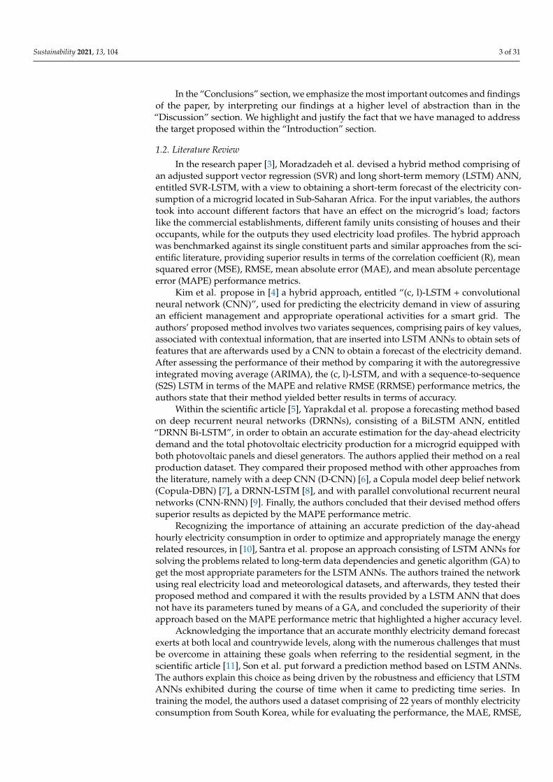
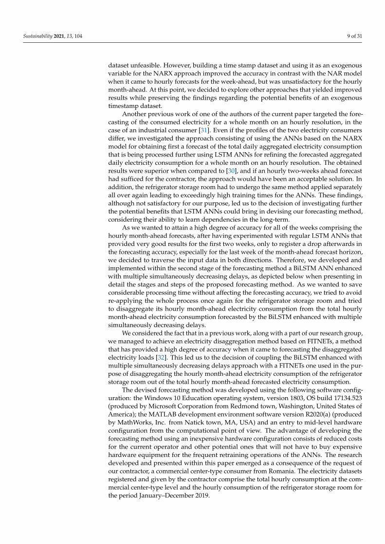
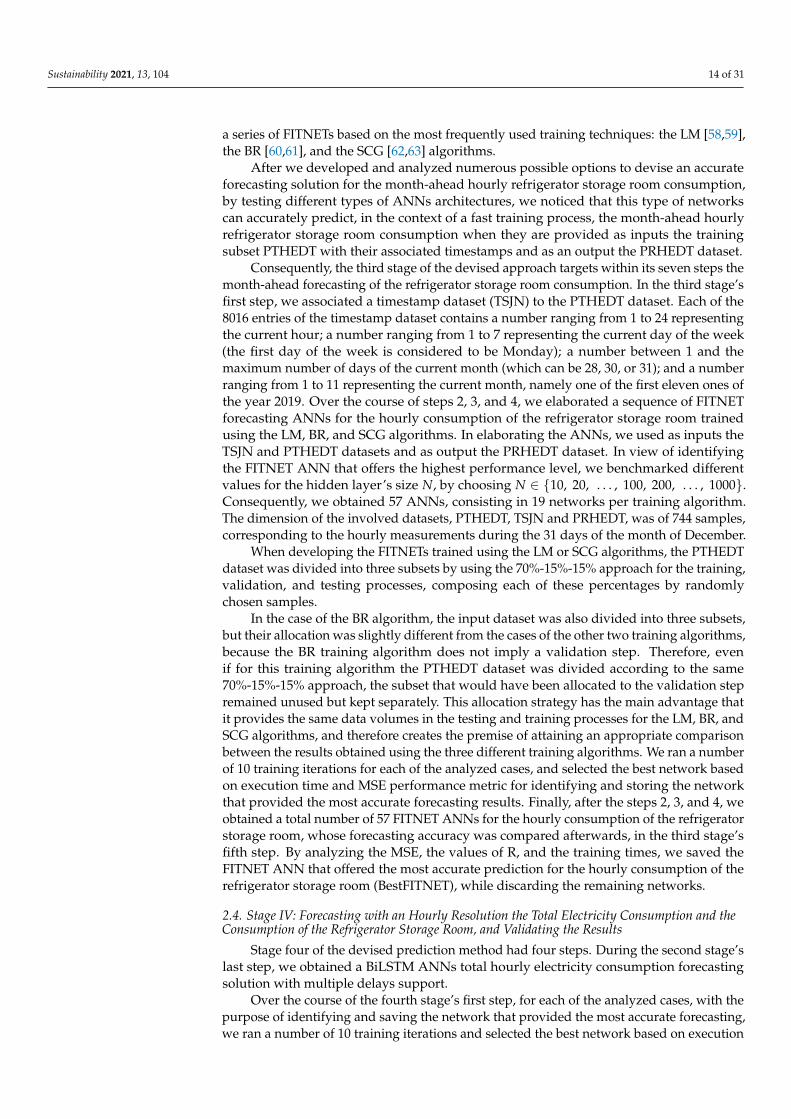
The forecasting method designed, developed, validated, and presented in Section 2.1,Section 2.2, Section 2.3, Section 2.4 is synthesized in the following flowchart (Figure 2).
In the following, we provide the results recorded during the development of theexperimental tests and their implications.
Sustainability 2021, 13, 104 16 of 31Sustainability 2021, 13, x FOR PEER REVIEW 16 of 32
Figure 2. The flow diagram of the proposed approach.
In the following, we provide the results recorded during the development of the ex-perimental tests and their implications.
Figure 2. The flow diagram of the proposed approach.
Sustainability 2021, 13, 104 17 of 31
3. Results
In the following, we present the main experimental results registered during the stagesand steps of the prediction method.
3.1. Results Regarding the Developed BiLSTM ANN Total Hourly Electricity ConsumptionForecasting Solution with Multiple Delays Support
As we have mentioned before, within steps 3, 4, and 5 of the second stage of ourforecasting approach, we developed the BiLSTM ANN forecasting solution with multipledelays support, a solution that was used afterwards, during the fourth stage’s first step, inorder to forecast the total consumed electricity per hour for the last month of the year andto identify the best BiLSTM ANN total hourly electricity consumption forecasting solutionwith multiple decreasing delays support (BestBiLSTM) based on the RMSE performancemetric and on the registered training times. Analyzing the developed BiLSTM ANNs,we remarked that regarding the number of hidden units, starting with n = 300, andconsidering the dimension of the minibatchsize as 128, the performance reached a plateauso that any further increase in the number of neurons no longer brought a noticeableincrease in the performance accuracy, but only a significant increase in the execution time(e.g., 2713.504 s = 45.23 min when considering the ADAM training algorithm withn = 1000 and d = 1, compared to 1259.877 s = 20.99 min registered in the case whenconsidering the ADAM training algorithm with n = 300 and d = 1). Consequently, thedeveloped method tests various values for the parameters of the BiLSTM ANNs and savesthe network that provides the best results.
Concerning the number of hidden layers, we considered firstly a single layer andafterwards two layers, concluding that an increase in the number of layers did not bringfurther improvements to the forecasting accuracy, but a considerable penalty in the exe-cution time (e.g., 12, 249.532 s = 204.158 min = 3.402 h when considering the ADAMtraining algorithm, with 300 hidden units in each of the two layers and a delay d = 24,compared to 1259.877 s = 20.99 min registered in the case when considering the ADAMtraining algorithm with n = 300, d = 1 and a single hidden layer).
We synthetized the obtained results in Table 2, which contains the RMSE performancemetric along with the times t (measured in seconds) representing the duration of thetraining process, registered during the various experimental tests, making use of eachtraining algorithms, considering the number of hidden units n = 300 and the delayparameter varying within the set D = {1, 6, 12, 18, 24}. Regarding the maximum valueof the delay parameter, when we tried to increase it further, we noticed that the forecastingaccuracy did not register significant improvements, while the training times increased to agreat extent (for example, for all the training algorithms, when considering the maximumvalue of the delay parameter equal to 30, the training time doubled its value, while thevalue of the RMSE performance metric barely improved). We recall the fact that, accordingto the second step of the second stage of our devised methodology, when choosing a certainvalue within the set D, all the integers obtained by decreasing the initial value up to 1 aretaken into consideration by the devised approach as delays and used as simultaneous inputsequences, therefore achieving a multiple simultaneously decreasing delays approach.
Analyzing Table 2, we observed that the vast majority of the BiLSTM networks fromthis table offer an accurate forecast as depicted by the RMSE values and consequently aresuitable to be used by the contractor in actual daily activities. Nevertheless, one also has totake into consideration the running times that significantly increase the higher the size of thehidden layer is, whereas the forecasting accuracy remains almost the same. Regarding thevariation of the delay parameters, according to the results obtained during the experimentaltests, the best results were the ones obtained when considering the maximum value of thedelay equal to 24, meaning that, according to our developed approach, in the context ofthe decreasing delays support, the network took into consideration as delays all the valueswithin the set {24, 23, . . . , 2, 1} and used them as inputs.
Sustainability 2021, 13, 104 18 of 31
Table 2. An overview of the results obtained when developing the BiLSTM artificial neural network(ANN) total hourly electricity consumption forecasting solution with multiple simultaneously delayssupport (t is measured in seconds).
ADAM Training Algorithm
n/d 1 6 . . . 1 12 . . . 1 18 . . . 1 24 . . . 1
300RMSE 0.0865 0.0595 0.0579 0.0583 0.0495
t 1259.877 1419.438 1445.786 1454.187 1462.415
RMSPROP Training Algorithm
n/d 1 6 . . . 1 12 . . . 1 18 . . . 1 24 . . . 1
300RMSE 0.0789 0.0692 0.0558 0.0597 0.0504
t 1291.090 1291.941 1292.111 1337.825 1358.041
SGDM Training Algorithm
n/d 1 6 . . . 1 12 . . . 1 18 . . . 1 24 . . . 1
300RMSE 0.0787 0.0686 0.0545 0.0609 0.0526
t 965.800 966.605 992.054 1015.9377 1294.2159
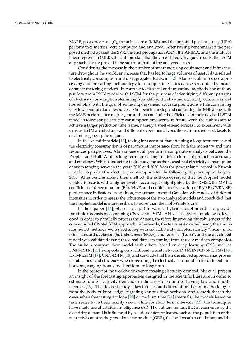
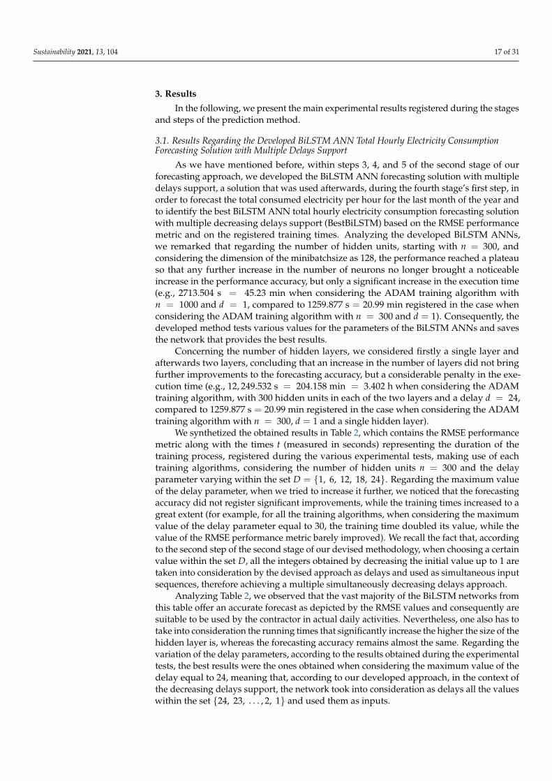
Analyzing the obtained results synthetized above in Table 2, registered by the 15 BiL-STM networks trained with the ADAM, SGDM, and RMSProp algorithms, it can be ob-served that the ANN trained based on the ADAM training algorithm provides the mostaccurate forecast as depicted by the RMSE value (0.0495) and the computational time of1462.415 s = 24.373 min. According to the devised approach, we entitled this total hourlyelectricity consumption forecasting solution with multiple delays support, as BestBiLSTM,a network whose architecture is depicted in Figure 3.
Sustainability 2021, 13, x FOR PEER REVIEW 18 of 32
300 RMSE 0.0789 0.0692 0.0558 0.0597 0.0504 t 1291.090 1291.941 1292.111 1337.825 1358.041
SGDM Training Algorithm n/d 1 6…1 12…1 18…1 24…1
300 RMSE 0.0787 0.0686 0.0545 0.0609 0.0526 t 965.800 966.605 992.054 1015.9377 1294.2159
Analyzing Table 2, we observed that the vast majority of the BiLSTM networks from this table offer an accurate forecast as depicted by the RMSE values and consequently are suitable to be used by the contractor in actual daily activities. Nevertheless, one also has to take into consideration the running times that significantly increase the higher the size of the hidden layer is, whereas the forecasting accuracy remains almost the same. Regard-ing the variation of the delay parameters, according to the results obtained during the experimental tests, the best results were the ones obtained when considering the maxi-mum value of the delay equal to 24, meaning that, according to our developed approach, in the context of the decreasing delays support, the network took into consideration as delays all the values within the set {24, 23, … ,2, 1} and used them as inputs.
Analyzing the obtained results synthetized above in Table 2, registered by the 15 BiLSTM networks trained with the ADAM, SGDM, and RMSProp algorithms, it can be observed that the ANN trained based on the ADAM training algorithm provides the most accurate forecast as depicted by the RMSE value (0.0495) and the computational time of 1462.415 𝑠𝑒𝑐𝑜𝑛𝑑𝑠 = 24.373 𝑚𝑖𝑛𝑢𝑡𝑒𝑠. According to the devised approach, we entitled this total hourly electricity consumption forecasting solution with multiple delays support, as BestBiLSTM, a network whose architecture is depicted in Figure 3.
Figure 3. The architecture of the BestBiLSTM network.
One can find the obtained BestBiLSTM network within the Supplementary Materials.
3.2. The Obtained Results in the Case of the FITNET ANNs Provided Forecasts for the Refrigerator Storage Room
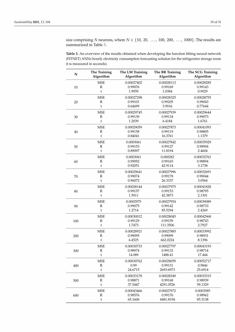
Over the course of the third stage’s second, third, and fourth steps, we registered for each of the developed function fitting ANNs, the running time along with MSE and R computed for the training dataset. As we mentioned before, we used a hidden layer’s size comprising 𝑁 neurons, where 𝑁 ∈ {10, 20, … , 100, 200, … , 1000}. The results are summa-rized in Table 3.
Figure 3. The architecture of the BestBiLSTM network.
One can find the obtained BestBiLSTM network within the Supplementary Materials.
3.2. The Obtained Results in the Case of the FITNET ANNs Provided Forecasts for the RefrigeratorStorage Room
Over the course of the third stage’s second, third, and fourth steps, we registeredfor each of the developed function fitting ANNs, the running time along with MSE andR computed for the training dataset. As we mentioned before, we used a hidden layer’s
Sustainability 2021, 13, 104 19 of 31
size comprising N neurons, where N ∈ {10, 20, . . . , 100, 200, . . . , 1000}. The results aresummarized in Table 3.
Table 3. An overview of the results obtained when developing the function fitting neural network(FITNET) ANNs hourly electricity consumption forecasting solution for the refrigerator storage room(t is measured in seconds).
N The TrainingAlgorithm
The LM TrainingAlgorithm
The BR TrainingAlgorithm
The SCG TrainingAlgorithm
10MSE 0.00027402 0.00028113 0.00028285
R 0.99076 0.99169 0.99143t 1.9959 1.0384 0.9029
20MSE 0.00027298 0.00028325 0.00028755
R 0.99101 0.99205 0.99043t 0.64699 3.9916 0.77644
30MSE 0.00029745 0.00027939 0.00029644
R 0.99139 0.99118 0.99073t 1.2039 6.4184 1.6761
40MSE 0.00029059 0.00027873 0.00041093
R 0.99158 0.99119 0.98805t 0.84041 16.3761 1.1379
50MSE 0.0003061 0.00027842 0.00035929
R 0.99153 0.99127 0.98904t 0.89097 11.8194 2.4604
60MSE 0.0003061 0.000282 0.00032761
R 0.99092 0.99165 0.98894t 0.92051 42.9114 3.1738
70MSE 0.00029641 0.00027996 0.00032691
R 0.99074 0.99178 0.99044t 0.96072 26.3337 3.0564
80MSE 0.00028144 0.00027975 0.00041828
R 0.99157 0.99153 0.98795t 1.5911 42.3873 2.1301
90MSE 0.0002975 0.00027954 0.00039089
R 0.99075 0.99142 0.98733t 1.2714 85.5294 2.4269
100MSE 0.00030012 0.00028045 0.00042968
R 0.99129 0.99159 0.98743t 1.7473 111.3506 2.7927
200MSE 0.00028921 0.00027885 0.00033992
R 0.99095 0.99099 0.98931t 6.4525 662.0224 8.1396
300MSE 0.00030733 0.00027797 0.00043193
R 0.98974 0.99132 0.98714t 14.089 1488.41 17.444
400MSE 0.00030762 0.00028059 0.00052717
R 0.99 0.99131 0.9846t 24.6715 2693.6973 25.6914
500MSE 0.00033178 0.00028349 0.00033315
R 0.98871 0.99168 0.98939t 37.5447 4291.0526 59.1329
600MSE 0.00043466 0.00027972 0.0003585
R 0.98576 0.99176 0.98962t 65.1606 4481.8194 85.3138

Sustainability 2021, 13, 104 20 of 31
Table 3. Cont.
N The TrainingAlgorithm
The LM TrainingAlgorithm
The BR TrainingAlgorithm
The SCG TrainingAlgorithm
700MSE 0.00043285 0.00028053 0.00058308
R 0.98621 0.99126 0.98229t 93.8144 6084.2019 68.2735
800MSE 0.00042612 0.00027583 0.00053732
R 0.98746 0.99076 0.98389t 121.1446 8205.7725 106.8163
900MSE 0.00045703 0.00027928 0.0005471
R 0.98545 0.99136 0.98346t 156.5832 10453.9573 132.4432
1000MSE 0.00069004 0.00027433 0.00073457
R 0.98107 0.99139 0.98049t 214.5622 13230.2844 145.866
The registered results emphasize the fact that the developed FITNET ANNs provideda very good forecasting accuracy in all the cases, highlighted by the MSE values thatwere very small, ranging between 0.00027298 (registered for N = 20 and the LM trainingalgorithm) and 0.00073457 (registered for N = 1000 and the SCG training algorithm); andthe values of R that were around 1, ranging between 0.98049 (registered for N = 1000and the SCG training algorithm) and 0.99205 (registered for N = 20 and the BR trainingalgorithm). As regards the execution times, their values varied from 0.64699 s (registeredfor N = 20 and the LM training algorithm) and a maximum of 13, 230.2844 s (registered forN = 1000 and the BR training algorithm).
The most accurate prediction results (as highlighted by the MSE and R performancemetrics) were registered when the FITNET ANNs were trained using the LM and BRalgorithms. However, even if when the FITNET ANNs were trained using the SCGtraining algorithm, the performance metrics were lower than in the other two cases, for thisalgorithm, the training process was the fastest. Consequently, if new datasets appear oftenand the FITNET ANN requires frequent retraining steps, the SCG represents a suitablesolution due to its high computational speed and reduced memory requirements.
According to the devised methodology, in the third stage’s final step, by comparingthe performance metrics of the 57 developed FITNETs for the hourly consumption of therefrigerator storage room synthetized in Table 3, we determined the network that offeredthe most accurate prediction hourly (BestFITNET), while discarding the remaining ones.The BestFITNET ANN was the one with a hidden layer’s size comprising N = 20 neurons,trained using the LM algorithm, case in which the values of the performance metrics wereMSE = 0.00027298, R = 0.99101. One can find within the Supplementary Materials theBestFITNET network.
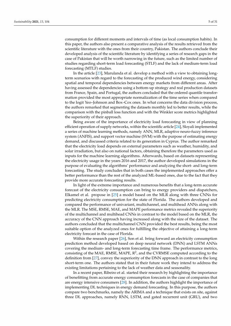
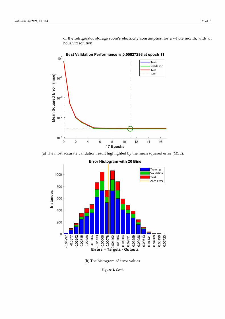
For the purpose of highlighting the accuracy provided by the BestFITNET ANN, wepresent and analyze in the following the performance plots of this network. Firstly, wecomputed and represented the three curves corresponding to the training, validation andtesting processes (Figure 4a). Analyzing this plot, one can remark that the performancepeak was attained at the 11th epoch, when the MSE had the value 0.00027298. Figure 4ahighlights the fact that none of the three curves increased significantly before the others,they are almost overlapping. This remark confirms that we obtained an accurate predictionand that an overfitting process does not occur. Another important conclusion that canbe drawn from the analysis of Figure 4a is the efficiency of the training process and theconfirmation that the dataset was divided in an appropriate way. Analyzing the plots,one can remark that for any of the curves there is no increase after the convergence hastaken place, which represents a strong argument in stating that the FITNET ANN approachrepresents a robust solution, providing an increased level of accuracy in the prediction
Sustainability 2021, 13, 104 21 of 31
of the refrigerator storage room’s electricity consumption for a whole month, with anhourly resolution.
Sustainability 2021, 13, x FOR PEER REVIEW 21 of 32
(a) The most accurate validation result highlighted by the mean squared error (MSE).
(b) The histogram of error values.
Figure 4. Cont.
Sustainability 2021, 13, 104 22 of 31Sustainability 2021, 13, x FOR PEER REVIEW 22 of 32
(c) The regression plots between the targets and outputs.
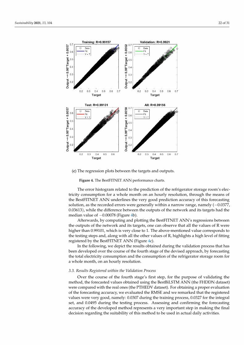
Figure 4. The BestFITNET ANN performance charts.
The error histogram related to the prediction of the refrigerator storage room’s elec-tricity consumption for a whole month on an hourly resolution, through the means of the BestFITNET ANN underlines the very good prediction accuracy of this forecasting solu-tion, as the recorded errors were generally within a narrow range, namely (−0.0377, 0.03613), while the difference between the outputs of the network and its targets had the median value of −0.00078 (Figure 4b).
Afterwards, by computing and plotting the BestFITNET ANN’s regressions between the outputs of the network and its targets, one can observe that all the values of R were higher than 0.99101, which is very close to 1. The above-mentioned value corresponds to the testing steps and, along with all the other values of R, highlights a high level of fitting registered by the BestFITNET ANN (Figure 4c).
In the following, we depict the results obtained during the validation process that has been developed over the course of the fourth stage of the devised approach, by fore-casting the total electricity consumption and the consumption of the refrigerator storage room for a whole month, on an hourly resolution.
3.3. Results Registered within the Validation Process Over the course of the fourth stage’s first step, for the purpose of validating the
method, the forecasted values obtained using the BestBiLSTM ANN (the FHDDN dataset) were compared with the real ones (the PTHEDV dataset). For obtaining a proper evalua-tion of the forecasting accuracy, we evaluated the RMSE and we remarked that the regis-tered values were very good, namely: 0.0307 during the training process, 0.0327 for the
Figure 4. The BestFITNET ANN performance charts.
The error histogram related to the prediction of the refrigerator storage room’s elec-tricity consumption for a whole month on an hourly resolution, through the means ofthe BestFITNET ANN underlines the very good prediction accuracy of this forecastingsolution, as the recorded errors were generally within a narrow range, namely (−0.0377,0.03613), while the difference between the outputs of the network and its targets had themedian value of −0.00078 (Figure 4b).
Afterwards, by computing and plotting the BestFITNET ANN’s regressions betweenthe outputs of the network and its targets, one can observe that all the values of R werehigher than 0.99101, which is very close to 1. The above-mentioned value corresponds tothe testing steps and, along with all the other values of R, highlights a high level of fittingregistered by the BestFITNET ANN (Figure 4c).
In the following, we depict the results obtained during the validation process that hasbeen developed over the course of the fourth stage of the devised approach, by forecastingthe total electricity consumption and the consumption of the refrigerator storage room fora whole month, on an hourly resolution.
3.3. Results Registered within the Validation Process
Over the course of the fourth stage’s first step, for the purpose of validating themethod, the forecasted values obtained using the BestBiLSTM ANN (the FHDDN dataset)were compared with the real ones (the PTHEDV dataset). For obtaining a proper evaluationof the forecasting accuracy, we evaluated the RMSE and we remarked that the registeredvalues were very good, namely: 0.0307 during the training process, 0.0327 for the integralset, and 0.0495 during the testing process. Assessing and confirming the forecastingaccuracy of the developed method represents a very important step in making the finaldecision regarding the suitability of this method to be used in actual daily activities.
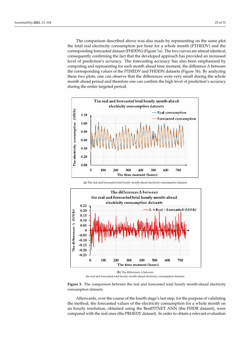
Sustainability 2021, 13, 104 23 of 31
The comparison described above was also made by representing on the same plotthe total real electricity consumption per hour for a whole month (PTHEDV) and thecorresponding forecasted dataset (FHDDN) (Figure 5a). The two curves are almost identical,consequently confirming the fact that the developed approach has provided an increasedlevel of prediction’s accuracy. The forecasting accuracy has also been emphasized bycomputing and representing for each month ahead time moment, the difference ∆ betweenthe corresponding values of the PTHEDV and FHDDN datasets (Figure 5b). By analyzingthese two plots, one can observe that the differences were very small during the wholemonth ahead period and therefore one can confirm the high level of prediction’s accuracyduring the entire targeted period.
1
(a) The real and forecasted total hourly month-ahead electricity consumption datasets
(b) The differences Δ between
the real and forecasted total hourly month-ahead electricity consumption datasets 555555555555
Figure 5. The comparison between the real and forecasted total hourly month-ahead electricityconsumption datasets.
Afterwards, over the course of the fourth stage’s last step, for the purpose of validatingthe method, the forecasted values of the electricity consumption for a whole month onan hourly resolution, obtained using the BestFITNET ANN (the FHDR dataset), werecompared with the real ones (the PRHEDV dataset). In order to obtain a relevant evaluation
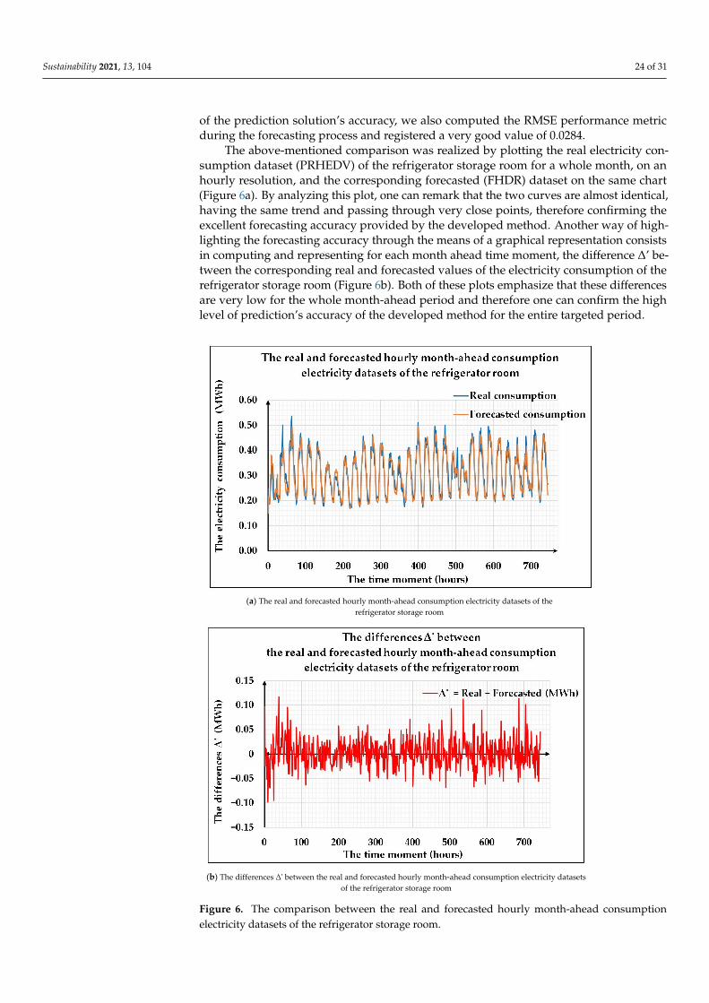
Sustainability 2021, 13, 104 24 of 31
of the prediction solution’s accuracy, we also computed the RMSE performance metricduring the forecasting process and registered a very good value of 0.0284.
The above-mentioned comparison was realized by plotting the real electricity con-sumption dataset (PRHEDV) of the refrigerator storage room for a whole month, on anhourly resolution, and the corresponding forecasted (FHDR) dataset on the same chart(Figure 6a). By analyzing this plot, one can remark that the two curves are almost identical,having the same trend and passing through very close points, therefore confirming theexcellent forecasting accuracy provided by the developed method. Another way of high-lighting the forecasting accuracy through the means of a graphical representation consistsin computing and representing for each month ahead time moment, the difference ∆’ be-tween the corresponding real and forecasted values of the electricity consumption of therefrigerator storage room (Figure 6b). Both of these plots emphasize that these differencesare very low for the whole month-ahead period and therefore one can confirm the highlevel of prediction’s accuracy of the developed method for the entire targeted period.
2
(a) The real and forecasted hourly month-ahead consumption electricity datasets of the
refrigerator storage room
(b) The differences Δ' between the real and forecasted hourly month-ahead consumption electricity datasets
of the refrigerator storage room 666666666666
2
(a) The real and forecasted hourly month-ahead consumption electricity datasets of the
refrigerator storage room
(b) The differences Δ' between the real and forecasted hourly month-ahead consumption electricity datasets
of the refrigerator storage room 666666666666 Figure 6. The comparison between the real and forecasted hourly month-ahead consumptionelectricity datasets of the refrigerator storage room.
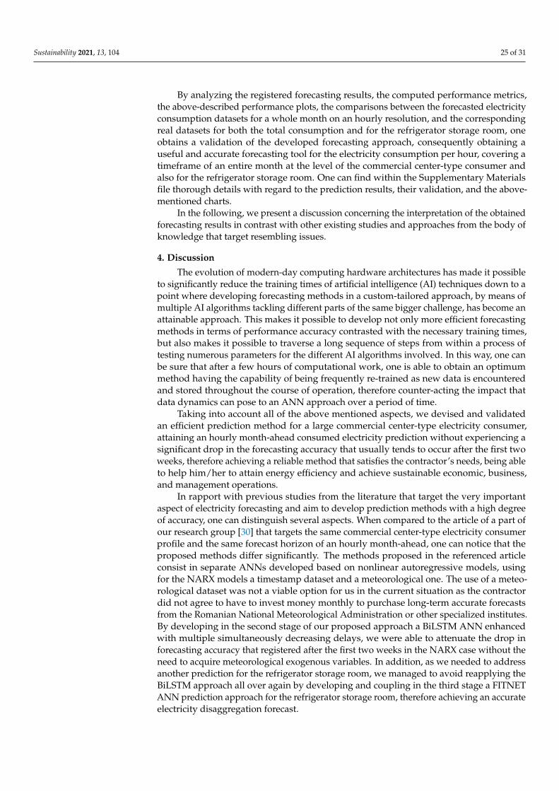
Sustainability 2021, 13, 104 25 of 31
By analyzing the registered forecasting results, the computed performance metrics,the above-described performance plots, the comparisons between the forecasted electricityconsumption datasets for a whole month on an hourly resolution, and the correspondingreal datasets for both the total consumption and for the refrigerator storage room, oneobtains a validation of the developed forecasting approach, consequently obtaining auseful and accurate forecasting tool for the electricity consumption per hour, covering atimeframe of an entire month at the level of the commercial center-type consumer andalso for the refrigerator storage room. One can find within the Supplementary Materialsfile thorough details with regard to the prediction results, their validation, and the above-mentioned charts.
In the following, we present a discussion concerning the interpretation of the obtainedforecasting results in contrast with other existing studies and approaches from the body ofknowledge that target resembling issues.
4. Discussion
The evolution of modern-day computing hardware architectures has made it possibleto significantly reduce the training times of artificial intelligence (AI) techniques down to apoint where developing forecasting methods in a custom-tailored approach, by means ofmultiple AI algorithms tackling different parts of the same bigger challenge, has become anattainable approach. This makes it possible to develop not only more efficient forecastingmethods in terms of performance accuracy contrasted with the necessary training times,but also makes it possible to traverse a long sequence of steps from within a process oftesting numerous parameters for the different AI algorithms involved. In this way, one canbe sure that after a few hours of computational work, one is able to obtain an optimummethod having the capability of being frequently re-trained as new data is encounteredand stored throughout the course of operation, therefore counter-acting the impact thatdata dynamics can pose to an ANN approach over a period of time.
Taking into account all of the above mentioned aspects, we devised and validatedan efficient prediction method for a large commercial center-type electricity consumer,attaining an hourly month-ahead consumed electricity prediction without experiencing asignificant drop in the forecasting accuracy that usually tends to occur after the first twoweeks, therefore achieving a reliable method that satisfies the contractor’s needs, being ableto help him/her to attain energy efficiency and achieve sustainable economic, business,and management operations.
In rapport with previous studies from the literature that target the very importantaspect of electricity forecasting and aim to develop prediction methods with a high degreeof accuracy, one can distinguish several aspects. When compared to the article of a part ofour research group [30] that targets the same commercial center-type electricity consumerprofile and the same forecast horizon of an hourly month-ahead, one can notice that theproposed methods differ significantly. The methods proposed in the referenced articleconsist in separate ANNs developed based on nonlinear autoregressive models, usingfor the NARX models a timestamp dataset and a meteorological one. The use of a meteo-rological dataset was not a viable option for us in the current situation as the contractordid not agree to have to invest money monthly to purchase long-term accurate forecastsfrom the Romanian National Meteorological Administration or other specialized institutes.By developing in the second stage of our proposed approach a BiLSTM ANN enhancedwith multiple simultaneously decreasing delays, we were able to attenuate the drop inforecasting accuracy that registered after the first two weeks in the NARX case without theneed to acquire meteorological exogenous variables. In addition, as we needed to addressanother prediction for the refrigerator storage room, we managed to avoid reapplying theBiLSTM approach all over again by developing and coupling in the third stage a FITNETANN prediction approach for the refrigerator storage room, therefore achieving an accurateelectricity disaggregation forecast.
Sustainability 2021, 13, 104 26 of 31
In the paper [30], together with a member of our group of researchers, we managed tosuccessfully develop and implement a hybrid LSTM-FITNET approach. The LSTM ANNsproved very useful in refining a weather forecast corresponding to a certain region at thelevel of individual wind turbines so as to obtain accurate input values for subsequentFITNET ANNs that provided an accurate forecast for the hourly day-ahead production andconsumption of electricity in the case of a wind farm located on a hilly terrain. In the caseof the large hypermarket chain consumer, when an hourly month-ahead time horizon wasneeded, a BiLSTM ANN enhanced with multiple simultaneously decreasing delays provedto be more useful than a LSTM approach for avoiding a steeper decline of the forecastingaccuracy towards the end of the month. In contrast to the previous study, the FITNETANNs proved useful for electricity disaggregation purposes, while being unsuitable for aninitial forecasting of the total consumption per hour for a whole month.
Within the scientific article [35], Siami et al. performed a comparative analysis betweena BiLSTM approach and a LSTM one, along with analyzing the implications that a largertraining data volume related to financial stocks has in terms of forecasting accuracy whendevising forecasting methods based on BiLSTMs models compared with LSTM ones.Instead of financial stock data, we used in our study data related to the consumption ofelectricity in the commerce sector. In addition, as we needed a higher degree of forecastingaccuracy in order to cover the hourly month-ahead timeframe, we devised the BiLSTMANN with multiple simultaneously decreasing delays support in contrast with the analyzedapproach. The registered results of the authors are in accordance with our findings, namelythat, when provided with sufficient training data, a BiLSTM ANN provides a more accurateforecast in contrast to unidirectional LSTM ANNs, benefitting from the fact that longterm dependencies are learned and stored by passing through data twice, both backwardand forward.
The goal of achieving an as accurate as possible electricity consumption or productionforecasting is of extreme importance to all the involved parties, starting from electricityproducers, dispatchers, policy regulators, up to the different types of electricity consumers.Therefore, in the scientific literature, one can find a great variety of papers that focus onachieving accurate electricity forecasts from the production and consumption perspectives,proposing different forecasting methods developed based on the electricity profiles of theinvolved beneficiaries and on the durations of the forecasting windows.
In order to attain these goals, scientists have used different methods and carried out nu-merous performance improvement techniques, such as: SVR [3,11,28], LSTMANNs [3,4,10,11,26,28], RNN [5,28], BiLSTM ANN [5], Copula-DBN [7], DRNN-LSTM [8],CNN-RNN [9], the Prophet and Holt–Winters long-term forecasting models [13],CNNs [4,6,14,25], MLR [24,25], SVM [24], and ANFIS [24]. In contrast with these, withinour article, we devised and developed a forecasting method for the hourly month-aheadelectricity consumption based on a BiLSTM ANN enhanced with a multiple simultaneouslydecreasing delays approach coupled with FITNETs.
Analyzing the scientific literature, one can remark that when forecasting the electricityconsumption, different forecasting time horizons are of interest, encompassing short-[3,14,19,22,24,26,28], medium- [19,21,26], and long-term timeframes [10,13,14,20,23–25,64],each of them bringing their own particular advantages in line with the actual requirementsand business needs of the contractors. We targeted the hourly month-ahead electricityprediction, considering the numerous benefits that such a forecast brings to the large-electricity commercial center-type consumer, ranging from the negotiation and choosingof the most appropriate hourly billing tariffs and correct estimations for the month-aheadelectricity consumption submitted to the dispatcher to proper decisional support in whatconcerns the return on investment in more energy efficient equipment and assessingexpanding options.
In what concerns the registered results, it is clear that every method was customizedin view of the particular situations it had to address and the different targeted purposes,therefore making use of distinctive datasets covering certain scenarios with their particular
Sustainability 2021, 13, 104 27 of 31
characteristics. Consequently, one cannot attain an entirely eloquent comparison betweenthe forecasting methods from the scientific literature. Nevertheless, it can be noticed thatthe forecasting methods yielded results with a high degree of accuracy which meets thecontractors’ real needs, attaining the objectives of the respective studies.
Although the final form of our proposed forecasting method that we reached afterhaving applied the described research methodology within which we tried to progressivelyimprove the steps and methods with a view to reaching the final goal registered verygood results in term of prediction accuracy, as the performance metrics, the analysis of thegraphical performance plots, and the direct comparison between the real recorded and theforecasted datasets depict, our proposed method nonetheless has certain limits.
One of the most protruding limits comes from the need to have an initial sufficientamount of recorded data to facilitate the proper training of ANNs so as to obtain reliable,accurate prediction results. Consequently, as we are targeting a long-term forecast, the ini-tial necessary historical amount of data needs to be of a minimum of 11 months, otherwisewe have to accept an initial lower degree of forecasting accuracy that will increase as newdata accumulate over time and the re-training process has access to them.
By analyzing the existing body of knowledge, one can observe that many studies havefocused on developing a variety of forecasting methods targeting particular situationsand case studies regarding the consumption of electricity in the case of large commercialcenter-type consumers. Achieving a comprehensive, all-encompassing comparison witha view to the particularities and the most important characteristics of the multitude ofproposed methods is an extremely difficult endeavor, even an unreachable one, taking intoaccount the vast number of records of studies and processes that have been carried out fordifferent scenarios, targeting distinctive objectives, using different datasets.
Even so, when several case studies share similar features, a certain method can beadapted and applied from a specific case to another by means of a generalization procedure.In this regard, the large hypermarket chain for which we devised the approach constitutesa non-limitative case where our proposed method can be successfully applied. Thisstatement is justified by the fact that the large hypermarket chain can be regarded as arepresentative example with regard to other similar electricity consumers, which are placedby the European Regulations within the same electricity consumption band, namely thecategory “Band-ID”, characterized by an annual electricity consumption which varieswithin the range [2000; 20,000] MWh [65].
Consequently, the proposed electricity forecasting method, consisting in a BiLSTMANN enhanced with a multiple simultaneously decreasing delays approach coupled withFITNETs, a method designed, developed, and validated in accordance to the devisedmethodology detailed in the second section of the paper, can be put into practice efficiently,having a generalizing capability, being able to cover a wide range of scenarios that exhibitsimilar features to the studied one.
Moreover, we designed, developed, validated, and compiled the hourly month-aheadforecasting method using a state of the art programming platform, aimed precisely atscientists, in order to assure the possibility of putting it into operation in a large varietyof situations that require efficient long term electricity forecasting tools, ensuring in viewof the software quality perspective its functional suitability, reliability, usability, main-tainability, and performance efficiency with respect to the processing time and necessarycomputational resources. All of these characteristics reinforce the potential of our proposedmethod of being widely applicable, also from the hardware and software point of views, asa result emphasizing once more that the proposed approach has the ability to meet bothexpressed and implicit requirements of diverse beneficiaries, therefore being able to deliverbona fide business value.
Currently, worldwide, in 2020, humanity has to deal with disruptive circumstancescaused by the rapid spread of the SARS-CoV-2 pandemic and its terrifying side effects, afact that highlights the intricate connection between people, companies, countries, andgovernments. This unprecedented situation in the contemporary history of humanity
Sustainability 2021, 13, 104 28 of 31
has generated unexpected consequences at personal, local, and global levels, raising infront of the human beings questions about the vulnerability of individuals, companies,and local and global economies, in the context of job losses, lack of trust in authorities,and concerns regarding a general sense of uncertainty. Consequently, it is natural for anyresearch tackling issues regarding future projections to discuss the impact of disruptivecircumstances such as economic crises [66] or the one mentioned above.
In Romania, the virus was detected for the first time on 26 February 2020 [67] andin the time period that has elapsed since then, more and more effects have cascaded.A detailed analysis of the particular situation approached in our research showed thatin the context of the pandemic, our contractor did not have to close or restructure hisbusiness (except for the implementation of social distancing measures and other measuresto prevent or limit the effects of the pandemic). Even during the lockdown period, thelarge hypermarket chain for which we have designed, developed, and implemented theforecasting method has continued its daily activity according to its usual schedule.
The developed prediction method allows retraining with new datasets, related to theperiod after the outbreak of the coronavirus pandemic. Therefore, in order to be able toanalyze the impact of this situation on the input datasets and on the forecasting results, weintend as future research to retrain the developed networks and revalidate the obtainedresults as soon as we have the new datasets corresponding to the disruptive circumstances.A first approach that we plan to experiment with in further research includes narrowing theretraining timeframe window, from once a month to twice a month, or, if deemed necessary,even once a week. In addition, we also intend to explore the usage of exogenous variablesrelated to the disturbing pandemic event when developing the BiLSTM with multiplesimultaneously decreasing delays support, if the retraining of the network will haveproved to be insufficient, or even consider developing a separate AI stage that forecasts thenecessary adjustments and apply them in subsequent processing stages.
Another future research direction consists in the assessment of the economic operators’intentions towards using alternative solar energy resources using analytical tools [68],as government subsidies have become more prevalent during the pandemic in order tosustain economic operators in reducing their electricity expenditures, and the electricityproduced by the commercial operators’ own renewable installations must be forecastedas well.
5. Conclusions
The aim of this paper, namely, to design and develop an electricity consumptionprediction method for the consumed electricity per hour, for a whole month, in the case ofan industrial consumer and for its refrigerator storage room, is a very important aspect forthe non-household electricity consumers and for the system operators and at the same timerepresents a key-factor in what regards energy efficiency, achieving sustainable economic,business, and management operations.
In addition to this, an accurate forecast offers benefits in what regards the electricityconsumption optimization, influencing the consumption strategy and facilitating the effortsin view of attaining an appropriate natural resource and environmental management. Inaddition, an accurate prediction method for the consumed electricity per hour, for a wholemonth, at the level of the large hypermarket chain helps the contractor in choosing themost suitable billing plan, offering him/her also the opportunity to negotiate in advancewith the dispatch operator the most appropriate billing tariff.
Using the designed, developed, and validated electricity consumption forecastingmethod based on a BiLSTM ANN enhanced with a multiple simultaneously decreasingdelays approach coupled with FITNETs, we managed to predict the consumed electricityper hour for a whole month in the case of a large hypermarket chain consumer and forits refrigerator storage room. The analysis of the registered forecasting results and theperformance plots, along with the comparison of the real values for the last month ofthe year, with the forecasted ones for both the total consumption and for the refrigerator
Sustainability 2021, 13, 104 29 of 31
storage room, the analysis of the devised approach in contrast to other existing studies andapproaches from the scientific literature body of knowledge targeting resembling issues,all emphasize the advantages of our proposed method and its capacity to narrow the gapidentified after having analyzed the current state of knowledge.
Although the devised, developed, and validated forecasting solution for the hourlyconsumption focuses on a commercial center-type consumer, this solution also represents auseful, accurate tool for other non-household electricity consumers, due to its generaliza-tion capability.
Supplementary Materials: The following are available online at https://www.mdpi.com/2071-1050/13/1/104/s1: the Sheet “12-month dataset” of the “Dataset.xlsx” Excel file that comprises detailed in-formation about the datasets; the BestBiLSTM ANN (ADAM_300_BILSTM_1_STRAT_24_DELAYS.matfile); the BestFITNET ANN (FITNET_TRAINLM_20_NEURONI.mat file); the Sheet “BiLSTM” of the“Dataset.xlsx” Excel file that comprises the forecasted results for the last month of the year for thetotal electricity consumption and the validation of the forecasting results; the Sheet “FITNET” of the“Dataset.xlsx” Excel file that comprises the forecasted results for the last month of the year for therefrigerator storage room and the validation of the forecasting results.
Author Contributions: Conceptualization, D.-M.P. and A.P.; methodology, D.-M.P. and A.P.; software,D.-M.P. and A.P.; validation, D.-M.P. and A.P.; formal analysis, D.-M.P. and A.P.; investigation,D.-M.P. and A.P.; resources, D.-M.P. and A.P.; data curation, D.-M.P. and A.P.; writing—original draftpreparation, D.-M.P. and A.P.; writing—review and editing, D.-M.P. and A.P.; visualization, D.-M.P.and A.P.; supervision, D.-M.P.; project administration, D.-M.P. and A.P.; funding acquisition, D.-M.P.All authors have read and agreed to the published version of the manuscript.
Funding: The article processing charge (APC) was discounted integrally by the MultidisciplinaryDigital Publishing Institute (MDPI).
Acknowledgments: The authors would like to express their gratitude for the logistics supportreceived from the Center of Research, Consultancy and Training in Economic Informatics andInformation Technology RAU-INFORTIS of the Romanian-American University.
Conflicts of Interest: The authors declare no conflict of interest.
References1. World Energy Balances Overview (2020 edition). Available online: https://webstore.iea.org/world-energy-balances-overview-
2020-edition (accessed on 14 November 2020).2. Romania Energy Market Report. Available online: https://www.enerdata.net/estore/country-profiles/romania.html
(accessed on 14 November 2020).3. Moradzadeh, A.; Zakeri, S.; Shoaran, M.; Mohammadi-Ivatloo, B.; Mohammadi, F. Short-Term Load Forecasting of Microgrid via
Hybrid Support Vector Regression and Long Short-Term Memory Algorithms. Sustainability 2020, 12, 7076. [CrossRef]4. Kim, M.; Choi, W.; Jeon, Y.; Liu, L. A hybrid neural network model for power demand forecasting. Energies 2019, 12, 931.
[CrossRef]5. Yaprakdal, F.; Yilmaz, M.B.; Baysal, M.; Anvari-Moghaddam, A. A deep neural network-assisted approach to enhance short-term
optimal operational scheduling of a microgrid. Sustainability 2020, 12, 1653. [CrossRef]6. Khan, S.; Javaid, N.; Chand, A.; Khan, A.B.M.; Rashid, F.; Afridi, I.U. Electricity Load Forecasting for Each Day of Week Using
Deep CNN. In Web, Artificial Intelligence and Network Applications; Barolli, L., Takizawa, M., Xhafa, F., Enokido, T., Eds.; SpringerInternational Publishing: Cham, Switzerland, 2019; pp. 1107–1119.
7. Ouyang, T.; He, Y.; Li, H.; Sun, Z.; Baek, S. Modeling and Forecasting Short-Term Power Load With Copula Model and DeepBelief Network. IEEE Trans. Emerg. Top. Comput. Intell. 2019, 3, 127–136. [CrossRef]
8. Wen, L.; Zhou, K.; Yang, S.; Lu, X. Optimal load dispatch of community microgrid with deep learning based solar power andload forecasting. Energy 2019, 171, 1053–1065. [CrossRef]
9. He, W. Load Forecasting via Deep Neural Networks. In Procedia Computer Science; Elsevier: Amsterdam, The Netherlands, 2017;pp. 308–314.
10. Santra, A.S.; Lin, J.L. Integrating long short-term memory and genetic algorithm for short-term load forecasting. Energies 2019, 12,2040. [CrossRef]
11. Son, H.; Kim, C. A deep learning approach to forecasting monthly demand for residential-sector electricity. Sustainability 2020, 12,3103. [CrossRef]
12. Alonso, A.M.; Nogales, F.J.; Ruiz, C. A single scalable LSTM model for short-term forecasting of massive electricity time series.Energies 2020, 13, 5328. [CrossRef]
Sustainability 2021, 13, 104 30 of 31
13. Almazrouee, A.I.; Almeshal, A.M.; Almutairi, A.S.; Alenezi, M.R.; Alhajeri, S.N. Long-term forecasting of electrical loads inKuwait using prophet and holt-winters models. Appl. Sci. 2020, 10, 5627. [CrossRef]
14. Shao, X.; Kim, C.S.; Sontakke, P. Accurate deep model for electricity consumption forecasting using multi-channel and multi-scalefeature fusion CNN-LSTM. Energies 2020, 13, 1881. [CrossRef]
15. Hu, Q.; Zhang, R.; Zhou, Y. Transfer learning for short-term wind speed prediction with deep neural networks. Renew. Energy2016, 85, 83–95. [CrossRef]
16. Liu, S.; Ji, H.; Wang, M.C. Nonpooling convolutional neural network forecasting for seasonal time series with trends. IEEE Trans.Neural Netw. Learn. Syst. 2020, 31, 2879–2888. [CrossRef] [PubMed]
17. Kong, W.; Dong, Z.Y.; Jia, Y.; Hill, D.J.; Xu, Y.; Zhang, Y. Short-Term Residential Load Forecasting Based on LSTM RecurrentNeural Network. IEEE Trans. Smart Grid 2019, 10, 841–851. [CrossRef]
18. Kim, T.Y.; Cho, S.B. Predicting residential energy consumption using CNN-LSTM neural networks. Energy 2019, 182, 72–81.[CrossRef]
19. Mir, A.A.; Alghassab, M.; Ullah, K.; Khan, Z.A.; Lu, Y.; Imran, M. A review of electricity demand forecasting in low and middleincome countries: The demand determinants and horizons. Sustainability 2020, 12, 5931. [CrossRef]
20. Perwez, U.; Sohail, A.; Hassan, S.F.; Zia, U. The long-term forecast of Pakistan’s electricity supply and demand: An application oflong range energy alternatives planning. Energy 2015, 93, 2423–2435. [CrossRef]
21. Sigauke, C. Forecasting medium-term electricity demand in a South African electric power supply system. J. Energy S. Afr. 2017,28, 54–67. [CrossRef]
22. Potapov, V.; Khamitov, R.; Makarov, V.; Gritsay, A.; Tyunkov, D.; Chervenchuk, I. Short-Term Forecast of Electricity Load for LLCOmsk Energy Retail Company Using Neural Network. In Proceedings of the 12th International Scientific and Technical Conference“Dynamics of Systems, Mechanisms and Machines”, Dynamics 2018, Omsk, Russia, 13–15 November 2018; IEEE Publisher:Piscataway, NJ, USA, 2019.
23. Marulanda, G.; Bello, A.; Cifuentes, J.; Reneses, J. Wind power long-term scenario generation considering spatial-temporaldependencies in coupled electricity markets. Energies 2020, 13, 3427. [CrossRef]
24. Solyali, D. A Comparative Analysis of Machine Learning Approaches for Short-/Long-Term Electricity Load Forecasting inCyprus. Sustainability 2020, 12, 3612. [CrossRef]
25. Elkamel, M.; Schleider, L.; Pasiliao, E.L.; Diabat, A.; Zheng, Q.P. Long-term electricity demand prediction via socioeconomicfactors-a machine learning approach with Florida as a case study. Energies 2020, 13, 3996. [CrossRef]
26. Son, N.; Yang, S.; Na, J. Deep Neural Network and Long Short-Term Memory for Electric Power Load Forecasting. Appl. Sci. 2020,10, 6489. [CrossRef]
27. Hong, T.; Kim, J.; Koo, C. LCC and LCCO 2 analysis of green roofs in elementary schools with energy saving measures.Energy Build. 2012, 45, 229–239. [CrossRef]
28. Ribeiro, A.M.N.C.; do Carmo, P.R.X.; Rodrigues, I.R.; Sadok, D.; Lynn, T.; Endo, P.T. Short-Term Firm-Level Energy-ConsumptionForecasting for Energy-Intensive Manufacturing: A Comparison of Machine Learning and Deep Learning Models. Algorithms2020, 13, 274. [CrossRef]
29. Kim, Y.; Seo, K.; Harrington, R.J.; Lee, Y.; Kim, H.; Kim, S. High accuracy modeling for solar PV power generation using NobleBD-LSTM-based neural networks with EMA. Appl. Sci. 2020, 10, 7339. [CrossRef]
30. Pîrjan, A.; Oprea, S.V.; Carutasu, G.; Petros, anu, D.M.; Bâra, A.; Coculescu, C. Devising hourly forecasting solutions regardingelectricity consumption in the case of commercial center type consumers. Energies 2017, 10, 1727. [CrossRef]
31. Petros, anu, D.M. Designing, developing and validating a forecasting method for the month ahead hourly electricity consumptionin the case of medium industrial consumers. Processes 2019, 7, 310. [CrossRef]
32. Oprea, S.-V.; Pîrjan, A.; Cărut,as, u, G.; Petros, anu, D.-M.; Bâra, A.; Stănică, J.-L.; Coculescu, C. Developing a Mixed Neural NetworkApproach to Forecast the Residential Electricity Consumption Based on Sensor Recorded Data. Sensors 2018, 18, 1443. [CrossRef]
33. Signs that Your Cool Room Needs Maintenance. Available online: https://www.cold-rite.com.au/post/signs-your-cool-room-needs-maintenance (accessed on 14 November 2020).
34. Pîrjan, A.; Cărut,as, u, G.; Petros, anu, D.-M. Designing, Developing, and Implementing a Forecasting Method for the Producedand Consumed Electricity in the Case of Small Wind Farms Situated on Quite Complex Hilly Terrain. Energies 2018, 11, 2623.[CrossRef]
35. Siami-Namini, S.; Tavakoli, N.; Namin, A.S. The Performance of LSTM and BiLSTM in Forecasting Time Series. In Proceedings ofthe —2019 IEEE International Conference on Big Data, Big Data 2019, Los Angeles, CA, USA, 9–12 December 2019; IEEE Publisher:Piscataway, NJ, USA, 2019; pp. 3285–3292.
36. Hochreiter, S.; Schmidhuber, J. Long Short-Term Memory. Neural Comput. 1997, 9, 1735–1780. [CrossRef]37. Murad, A.; Pyun, J.-Y. Deep Recurrent Neural Networks for Human Activity Recognition. Sensors 2017, 17, 2556. [CrossRef]38. Zheng, H.; Yuan, J.; Chen, L. Short-Term Load Forecasting Using EMD-LSTM Neural Networks with a Xgboost Algorithm for
Feature Importance Evaluation. Energies 2017, 10, 1168. [CrossRef]39. Bouktif, S.; Fiaz, A.; Ouni, A.; Serhani, M. Optimal Deep Learning LSTM Model for Electric Load Forecasting using Feature
Selection and Genetic Algorithm: Comparison with Machine Learning Approaches. Energies 2018, 11, 1636. [CrossRef]40. Huang, C.-J.; Kuo, P.-H. A Deep CNN-LSTM Model for Particulate Matter (PM2.5) Forecasting in Smart Cities. Sensors 2018, 18,
2220. [CrossRef] [PubMed]
Sustainability 2021, 13, 104 31 of 31
41. Nguyen, M.-T.; Nguyen, V.-H.; Yun, S.-J.; Kim, Y.-H. Recurrent Neural Network for Partial Discharge Diagnosis in Gas-InsulatedSwitchgear. Energies 2018, 11, 1202. [CrossRef]
42. Schuster, M.; Paliwal, K.K. Bidirectional recurrent neural networks. IEEE Trans. Signal Process. 1997, 45, 2673–2681. [CrossRef]43. Baldi, P.; Brunak, S.; Frasconi, P.; Soda, G.; Pollastri, G. Exploiting the past and the future in protein secondary structure prediction.
In Bioinformatics; Oxford University Press: Oxford, UK, 1999; pp. 937–946.44. Rasifaghihi, N. Predictive Analytics: Regression Analysis with LSTM, GRU and BiLSTM in TensorFlow. Available online: https:
//towardsdatascience.com/predictive-analysis-rnn-lstm-and-gru-to-predict-water-consumption-e6bb3c2b4b02 (accessed on14 November 2020).
45. Graves, A.; Schmidhuber, J. Framewise phoneme classification with bidirectional LSTM and other neural network architectures.In Neural Networks; Elsevier: Amsterdam, The Netherlands, 2005; Volume 18, pp. 602–610.
46. Mohan, A.T.; Gaitonde, D.V. A deep learning based approach to reduced order modeling for turbulent flow control using LSTMneural networks. arXiv 2018, arXiv:1804.09269.
47. Kiperwasser, E.; Goldberg, Y. Simple and Accurate Dependency Parsing Using Bidirectional LSTM Feature Representations.Trans. Assoc. Comput. Linguist. 2016, 4, 313–327. [CrossRef]
48. Pollastri, G.; McLysaght, A. Porter: A new, accurate server for protein secondary structure prediction. Bioinformatics 2005, 21,1719–1720. [CrossRef]
49. Sundermeyer, M.; Alkhouli, T.; Wuebker, J.; Ney, H. Translation modeling with bidirectional recurrent neural networks. InProceedings of the EMNLP 2014—2014 Conference on Empirical Methods in Natural Language Processing, Doha, Qatar, 25–29October 2014; pp. 14–25.
50. Dernoncourt, F.; Lee, J.Y.; Szolovits, P. Neuroner: An easy-to-use program for named-entity recognition based on neural networks.In Proceedings of the EMNLP 2017—Conference on Empirical Methods in Natural Language Processing: System Demonstrations,Copenhagen, Denmark, 9–11 September 2017; pp. 97–102.
51. Liwicki, M.; Graves, A.; Bunke, H.; Schmidhuber, J. A Novel Approach to On-Line Handwriting Recognition Based on Bidi-rectional Long Short-Term Memory Networks. In Proceedings of the 9th International Conference on Document Analysis andRecognition (ICDAR 2007), Parana, Brazil, 23–26 September 2007; pp. 367–371.
52. Graves, A.; Jaitly, N.; Mohamed, A.R. Hybrid speech recognition with Deep Bidirectional LSTM. In Proceedings of the 2013IEEE Workshop on Automatic Speech Recognition and Understanding, ASRU 2013, Piscataway, NJ, USA, 8–13 December 2013;pp. 273–278.
53. Graves, A.; Fernández, S.; Schmidhuber, J. Bidirectional LSTM networks for improved phoneme classification and recognition.In Lecture Notes in Computer Science (Including Subseries Lecture Notes in Artificial Intelligence and Lecture Notes in Bioinformatics);Springer International Publishing: Cham, Switzerland, 2005; pp. 799–804.
54. MathWorks Documentation. Time Series Forecasting Using Deep Learning. Available online: https://www.mathworks.com/help/deeplearning/ (accessed on 14 November 2020).
55. Ibrahim, N.K.; Abdullah, R.S.A.R.; Saripan, M.I. Artificial Neural Network Approach in Radar Target Classification. J. Comput. Sci.2009, 5, 23–32. [CrossRef]
56. Lippmann, R.P. An Introduction to Computing with Neural Nets. IEEE ASSP Mag. 1987, 4, 4–22. [CrossRef]57. Schmidhuber, J. Deep Learning in neural networks: An overview. Neural Netw. 2015, 61, 85–117. [CrossRef] [PubMed]58. Levenberg, K. A method for the solution of certain non-linear problems in least squares. Q. J. Appl. Math. 1944, 2, 164–168.
[CrossRef]59. Hagan, M.T.; Menhaj, M.B. Training Feedforward Networks with the Marquardt Algorithm. IEEE Trans. Neural Networks 1994, 5,
989–993. [CrossRef] [PubMed]60. MacKay, D.J.C. Bayesian Interpolation. Neural Comput. 1992, 4, 415–447. [CrossRef]61. Foresee, F.D.; Hagan, M.T. Gauss-Newton approximation to bayesian learning. In Proceedings of the International Conference on
Neural Networks, Houston, TX, USA, 12 June 1997; pp. 1930–1935.62. Møller, M.F. A scaled conjugate gradient algorithm for fast supervised learning. Neural Netw. 1993, 6, 525–533. [CrossRef]63. Huang, Y. Advances in Artificial Neural Networks—Methodological Development and Application. Algorithms 2009, 2, 973–1007.
[CrossRef]64. Petros, anu, D.-M.; Cărut,as, u, G.; Cărut,as, u, N.L.; Pîrjan, A. A Review of the Recent Developments in Integrating Machine Learning
Models with Sensor Devices in the Smart Buildings Sector with a View to Attaining Enhanced Sensing, Energy Efficiency, andOptimal Building Management. Energies 2019, 12, 4745. [CrossRef]
65. Eurostat. Energy Statistics—Electricity Prices for Domestic and Industrial Consumers, Price Components. Available online:https://ec.europa.eu/eurostat/cache/metadata/en/nrg_pc_204_esms.htm (accessed on 14 November 2020).
66. Zirra, D. Investments in the context of the actual economic crises. Rom. Econ. Bus. Rev. 2011, 6, 145.67. Romanian Government. Covid-19 Official News. Available online: https://stirioficiale.ro/informatii (accessed on 14 November 2020).68. Perju-Mitran, A.; Mitran, R.-A. Assessing Public Opinion on Solar Energy Topics Using Google Trends. J. Inf. Syst. Oper. Manag.
2018, 12, 153–162.