Embed Size (px)
Citation preview
$t'-V*ï*^£Sï*;K;i'"*
DISCHARGE MEASUREMENT STRUCTURES
Working Group on Small Hydraulic Structures
Editor: M. G. BOS
I CENTRALE LANDBOUWCATALOGUS
0000 0006 9092
INTERNATIONAL INSTITUTE FOR LAND RECLAMATION AND IMPROVEMENT/ILRI P.O. BOX 45 WAGENINGEN THE NETHERLANDS 1976
1 * CC& ^ ? K ' <.J i - ! . I •'/•'» '
Manuscript of the Working Group on Small Hydraulic Structures. Represented in this Group are the following institutions
INTERNATIONAL INSTITUTE FOR LAND RECLAMATION AND I M P R O V E M E N T / I L R I , WAGENINGEN
DELFT HYDRAULICS LABORATORY, DELFT
AGRICULTURAL UNIVERSITY. DEPARTMENTS OF HYDRAULICS AND IRRIGATION, WAGENINGEN
This publication will appear as Publication No. 161, Delft Hydraulics Laboratory. Delft Publication No. 20, ILRI, Wageningen Report No. 4, Laboratory of Hydraulics and Catchment Hydrology, Wageningen.
i() International Institute for Land Reclamation and Improvement/ILRI, Wageningen, 1976 The Netherlands
This book or any part thereof must not be reproduced in any form without the written permission of ILRI.
Printed in The Netherlands
Preface The Working Group on Small Hydraulic Structures was formed in September 1971 and
charged with the tasks of surveying current literature on small structures in
open channels and of conducting additional research as considered necessary.
The members of the Working Group are all engaged in irrigation engineering, hydro
logy, or hydraulics, and are employed by the Delft Hydraulics Laboratory (DHL),
the University of Agriculture (LH) at Wageningen, or the International Institute
for Land Reclamation and Improvement (ILRI) at Wageningen.
The names of those participating in the Group are:
Ing. W.Boiten (DHL)
Ir. M.G.Bos (ILRI)
Prof.Ir. D.A.Kraijenhoff van de Leur (LH)
Ir. H.Oostinga (DHL) during 1975
Ir. R.H.Pitlo (LH)
Ir. A.H.de Vries (DHL)
Ir. J.Wijdieks (DHL)
The Group lost one of its initiators and most expert members in the person of
Professor Ir. J.Nugteren (LH), who died on April 20, 1974.
The manuscripts for this publication were written by various group members.
Ing. W.Boiten prepared the Sections 4.3, 4.4, and 7.3; Ir. R.H.Pitlo prepared
Section 7.5; Ir. A.H.de Vries prepared the Sections 7.2, 7.3, 9.2, and 9.7,
and the Appendices II and III. The remaining manuscripts were written by Ir.
M.G.Bos. All sections were critically reviewed by all working group members,
after which Ir. M.G.Bos prepared the manuscripts for publication.
Special thanks are due to Ir. E.Stamhuis and Ir. T.Meijer for their critical
review of Chapter 3, to Dr P.T.Stol for his constructive comments on Appendix II
and to Dr.M.J.Hall of the Imperial College of Science and Technology, London, for
proof-reading the entire manuscript.
This book presents instructions, standards, and procedures for the selection,
design, and use of structures, which measure or regulate the flow rate in open
channels. It is intended to serve as a guide to good practice for engineers
concerned with the design and operation of such structures. It is hoped that
the book will serve this purpose in three ways: (i) by giving the hydraulic
theory related to discharge measurement structures; (ii) by indicating the major
demands made upon the structures; and (iii) by providing specialized and tech
nical knowledge on the more common types of structures now being used throughout
the world.
The text is addressed to the designer and operator of the structure and gives
the hydraulic dimensions of the structure. Construction methods are only given
if they influence the hydraulic performance of the structure. Otherwise, no
methods of construction nor specifications of materials are given since they
vary greatly from country to country and their selection will be influenced
by such factors as the availability of materials, the quality of workmanship,
and by the number of structures that need to be built.
The efficient management of water supplies, particularly in the arid regions
of the world, is becoming more and more important as the demand for water grows
even greater with the world's increasing population and as new sources of water
become harder to find. Water resources are one of our most vital commodities and
they must be conserved by reducing the amounts of water lost through inefficient
management. An essential part of water conservation is the accurate measurement
and regulation of discharges.
We hope that this book will find its way, not only to irrigation engineers and
hydrologists, but also to all others who are actively engaged in the management
of water resources. Any comments which may lead to improved future editions
of this book will be welcomed.
Wageningen, October 1975 M.G.Bos
editor
VI
Contents LIST OF PRINCIPAL SYMBOLS XIII
1 Basic principles of fluid flow as applied to measuring structures l
1.1 General 1 1.2 Continuity 2 1.3 Equation of motion in the s-direction 3 1.4 Piezometric gradient in the n-direction 4 1.5 Hydrostatic pressure distribution in the m-direction 8 1.6 The total energy head of an open channel cross-section 8 1.7 Recapitulation 11 1.8 Specific energy 11 1.9 The broad-crested weir 15 1.9.1 Broad-crested weir with rectangular control section 16 1.9.2 Broad-crested weir with parabolic control section 19 1.9.3 Broad-crested weir with triangular control section 20 1.9.4 Broad-crested weir with truncated triangular control section 20 1.9.5 Broad-crested weir with trapezoidal control section 22 1.9.6 Broad-crested weir with circular control section 24 1.10 Short-crested weir 27 1.11 Critical depth flumes 29 1.12 Orifices 30 1.13 Sharp-crested weirs 34 1.13.1 Sharp-crested weirs with rectangular control section 36 1.13.2 Sharp-crested weirs with a parabolic control section 37 1.13.3 Sharp-crested weirs with triangular control section 38 1.13.4 Sharp-crested weirs with truncated triangular control section 38 1.13.5 Sharp-crested weirs with trapezoidal control section 39 1.13.6 Sharp-crested weirs with circular control section 39 1.13.7 Sharp-crested proportional weir 42 1.14 The aeration demand of weirs 45 1.15 Channel expansions 49 1.15.1 General 49 1.15.2 Influence of tapering the side walls 50 1.15.3 Calculation of modular limit for downstream transitions 53 1.16 Selected list of literature 56
2 Auxiliary equipment for measuring structures 57 2.1 Introduction 57 2.2 Head measurement station 58 2.3 The approach channel 59 2.4 Tailwater level 60 2.5 Staff gauge 61 2.6 Stilling well 62 2.7 Maximum stage gauge 68 2.8 Recording gauge 70 2.9 Diameter of float 71 2.10 Instrument shelter 73 2.11 Protection against freezing 75 2.12 Differential head meters 75 2.13 Selected list of references 81
3 The selection of structures 83 3.1 Introduction 83 3.2 Demands made upon a structure 83 3.2.1 Function of the structure 83
VII
3.2.2 Required fall of energy head to obtain modular flow 85 3.2.3 Range of discharges to be measured 89 3.2.4 Sensitiveness 92 3.2.5 Flexibility 94 3.2.6 'Sediment discharge capability 96 3.2.7 Passing of floating and suspended debris 100 3.2.8 Undesirable change in discharge 100 3.2.9 Minimum of water level in upstream channel 101 3.2.10 Required accuracy of measurement 102 3.2.11 Standardization of structures in an area 102 3.3 Properties and limits of application of structures 103 3.3.1 General 103 3.3.2 Tabulation of data 103 3.4 Selecting the structure 111 3.5 Selected list of references 120
4 Broad-crested weirs 121 4.1 Round-nosed horizontal broad-crested weir 121 4.1.1 Description 121 4.1.2 Evaluation of discharge 123 4.1.3 Modular limit 124 4.1.4 Limits of application 124 4.2 The Romijn movable measuring/regulating weir 125 4.2.1 Description 125 4.2.2 Evaluation of discharge 128 4.2.3 Modular limit 130 4.2.4 Commonly used weir dimensions 131 4.2.5 Limits of application 135 4.3 Triangular broad-crested weir 137 4.3.1 Description 137 4.3.2 Evaluation of discharge 140 4.3.3 Modular limit 142 4.3.4 Limits of application 143 4.4 Broad-crested rectangular profile weir 143 4.4.1 Description 143 4.4.2 Evaluation of discharge 146 4.4.3 Limits of application 148 4.5 Faiyum weir 149 4.5.1 Description 149 4.5.2 Modular limit 151 4.5.3 Evaluation of discharge 152 4.5.4 Limits of application 152 4.6 Selected list of references 153
5 Sharp-crested weirs 155 5.1 Rectangular sharp-crested weirs 156 5.1.1 Description 156 5.1.2 Evaluation of discharge 158 5.1.3 Limits of application 161 5.2 V-notch sharp-crested weirs 161 5.2.1 Description 161 5.2.2 Evaluation of discharge 164 5.2.3 Limits of application 168 5.2.4 Rating tables 168 5.3 Cipoletti weir 169 5.3.1 Description 169
VIII
5.3.2 Evaluation of discharge 171 5.3.3 Limits of application 171 5.4 Circular weir 173 5.4.1 Description 173 5.4.2 Determination of discharge 175 5.4.3 Limits of application 176 5.5 Proportional weir 176 5.5.1 Description 176 5.5.2 Evaluation of discharge 179 5.5.3 Limits of application 180 5.6 Selected list of references 181
6 Short-crested weirs 183 6.1 Weir sill with rectangular control section 183 6.1.1 Description 183 6.1.2 Evaluation of discharge 184 6.1.3 Limits of application 185 6.2 V-notch weir sill 185 6.2.1 Description 185 6.2.2 Evaluation of discharge 187 6.2.3 Limits of application 187 6.3 Triangular profile two-dimensional weir 191 6.3.1 Description 191 6.3.2 Evaluation of discharge 193 6.3.3 Modular limit 195 6.3.4 Limits of application 196 6.4 Triangular profile flat-vee weir 197 6.4.1 Description 197 6.4.2 Evaluation of discharge 198 6.4.3 Modular limit and non-modular discharge 200 6.4.4 Limits of application 203 6.5 Butcher's movable standing wave weir 203 6.5.1 Description 203 6.5.2 Evaluation of discharge 207 6.5.3 Limits of application 208 6.6 WES-Standard spillway 209 6.6.1 Description 209 6.6.2 Evaluation of discharge 213 6.6.3 Limits of application 216 6.7 Cylindrical crested weir 216 6.7.1 Description 216 6.7.2 Evaluation of discharge 218 6.7.3 Limits of application 221 6.8 Selected list of references 223
7 Flumes 225 7.1 Long-throated flumes 225 7.1.1 Description 225 7.1.2 Evaluation of discharge 227 7.1.3 Modular limit 232 7.1.4 Limits of application 235 7.2 Throatless flumes with rounded transition 236 7.2.1 Description 236 7.2.2 Evaluation of discharge 238 7.2.3 Modular limit 239
IX
7.2.4 Limits of application 240 7.3 Throatless flumes with broken plane transition 241 7.3.1 Description 241 7.4 Parshall flumes 243 7.4.1 Description 243 7.4.2 Evaluation of discharge 247 7.4.3 Submerged flow 262 7.4.4 Accuracy of discharge measurement 265 7.4.5 Loss of head through the flume 265 7.4.6 Limits of application 269 7.5 H-f lûmes 270 7.5.1 Description 270 7.5.2 Evaluation of discharge 272 7.5.3 Modular limit 273 7.5.4 Limits of application 274 7.6 Selected list of references 289
8 Or i f ices 293 8.1 Circular sharp-edged orifice 293 8.1.1 Description 293 8.1.2 Determination of discharge 295 8.1.3 Limits of application 296 8.2 Rectangular sharp-edged orifice 296 8.2.1 Description 296 8.2.2 Determination of discharge 298 8.2.3 Modular limit 302 8.2.4 Limits of application . 302 8.3 Constant-head-orifice . 304 8.3.1 Description 304 8.3.2 Determination of discharge 307 8.3.3 Limits of application 308 8.4 Radial or tainter gate 309 8.4.1 Description 309 8.4.2 Evaluation of discharge 311 8.4.3 Modular limit 313 8.4.4 Limits of application 313 8.5 Crump-De Gruyter adjustable orifice 314 8.5.1 Description 314 8.5.2 Evaluation of discharge 320 8.5.3 Limits of application 320 8.6 Metergate 321 8.6.1 Description 321 8.6.2 Evaluation of discharge 324 8.6.3 Metergate installation 326 8.6.4 Limits of application 329 8.7 Neyrpic module 330 8.7.1 Description 330 8.7.2 Discharge characteristics 334 8.7.3 Limits of application 338 8.8 Danaïdean tub 338 8.8.1 Description 338 8.8.2 Evaluation of discharge 339 8.8.3 Limits of application 342 8.9 Selected list of references 343
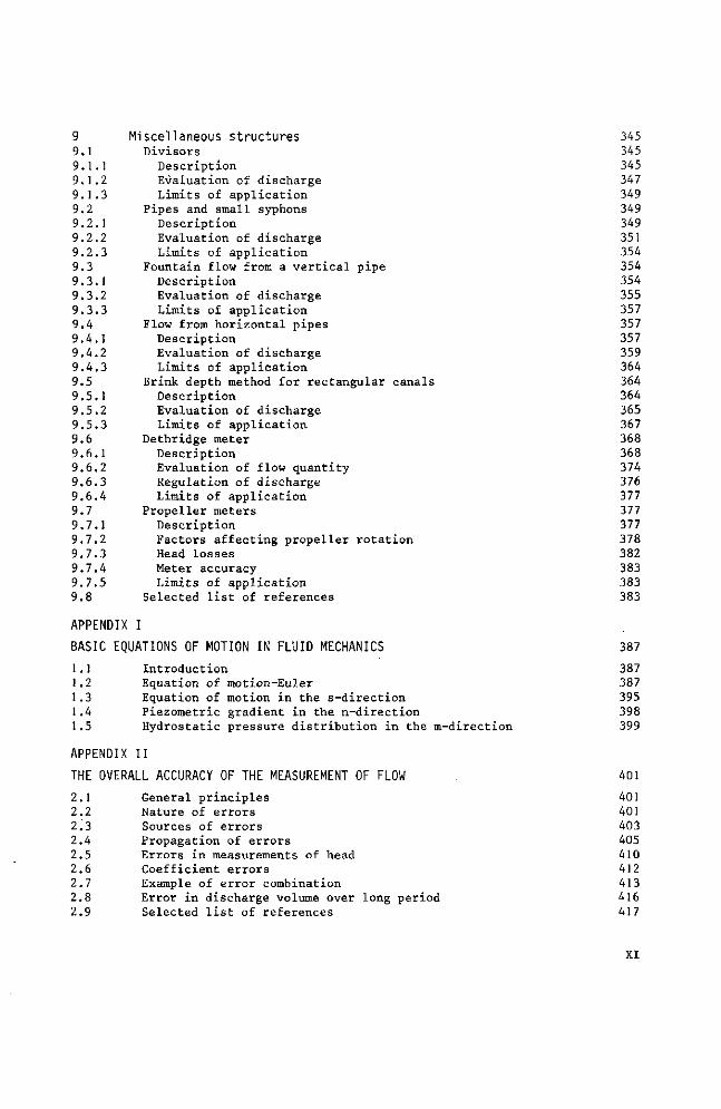
9 Miscellaneous structures 345 9.1 Divisors 345 9.1.1 Description 345 9.1.2 Evaluation of discharge 347 9.1.3 Limits of application 349 9.2 Pipes and small syphons 349 9.2.1 Description 349 9.2.2 Evaluation of discharge 351 9.2.3 Limits of application 354 9.3 Fountain flow from a vertical pipe 354 9.3.1 Description 354 9.3.2 Evaluation of discharge 355 9.3.3 Limits of application 357 9.4 Flow from horizontal pipes 357 9.4.1 Description 357 9.4.2 Evaluation of discharge 359 9.4.3 Limits of application 364 9.5 Brink depth method for rectangular canals 364 9.5.1 Description 364 9.5.2 Evaluation of discharge 365 9.5.3 Limits of application 367 9.6 Dethridge meter 368 9.6.1 Description 368 9.6.2 Evaluation of flow quantity 374 9.6.3 Regulation of discharge 376 9.6.4 Limits of application 377 9.7 Propeller meters 377 9.7.1 Description 377 9.7.2 Factors affecting propeller rotation 378 9.7.3 Head losses 382 9.7.4 Meter accuracy 383 9.7.5 Limits of application 383 9.8 Selected list of references 383
APPENDIX I
BASIC EQUATIONS OF MOTION IN FLUID MECHANICS 387
1.1 Introduction 387
1.2 Equation of motion-Euler 387 1.3 Equation of motion in the s-direction 395 1.4 Piezometric gradient in the n-direction 398 1.5 Hydrostatic pressure distribution in the m-direction 399
APPENDIX II
THE OVERALL ACCURACY OF THE MEASUREMENT OF FLOW 401
2.1 General principles 401
2.2 Nature of errors 401 2.3 Sources of errors 403 2.4 Propagation of errors 405 2.5 Errors in measurements of head 410 2.6 Coefficient errors 412 2.7 Example of error combination 413 2.8 Error in discharge volume over long period 416 2.9 Selected list of references 417
XI
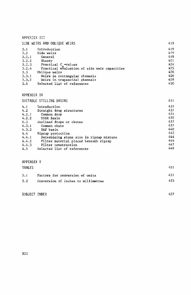
APPENDIX III
SIDE WEIRS AND OBLIQUE WEIRS 419
3.1 Introduction 419 3.2 Side weirs 419 3.2.1 General 419 3.2.2 Theory 421 3.2.3 Practical C -values 424 3.2.4 Practical evaluation of side weir capacities 425 3.3 Oblique weirs 426 3.3.1 Weirs in rectangular channels 426 3.3.2 Weirs in trapezoidal channels 428 3.4 Selected list of references 430
APPENDIX IV
SUITABLE STILLING BASINS 431
4.1 Introduction 431 4.2 Straight drop structures 431 4.2.1 Common drop 431 4.2.2 USBR Basin 435 4.3 Inclined drops or chutes 437 4.3.1 Common chute 437 4.3.2 SAF basin 440 4.4 Riprap protection 442 4.4.1 Determining stone size in riprap mixture 444 4.4.2 Filter material placed beneath riprap 444 4.4.3 Filter construction 447 4.5 Selected list of references 449
APPENDIX V
TABLES 451
5.1 Factors for conversion of units 451
5.2 Conversion of inches to millimetres 455
SUBJECT INDEX 457
XII
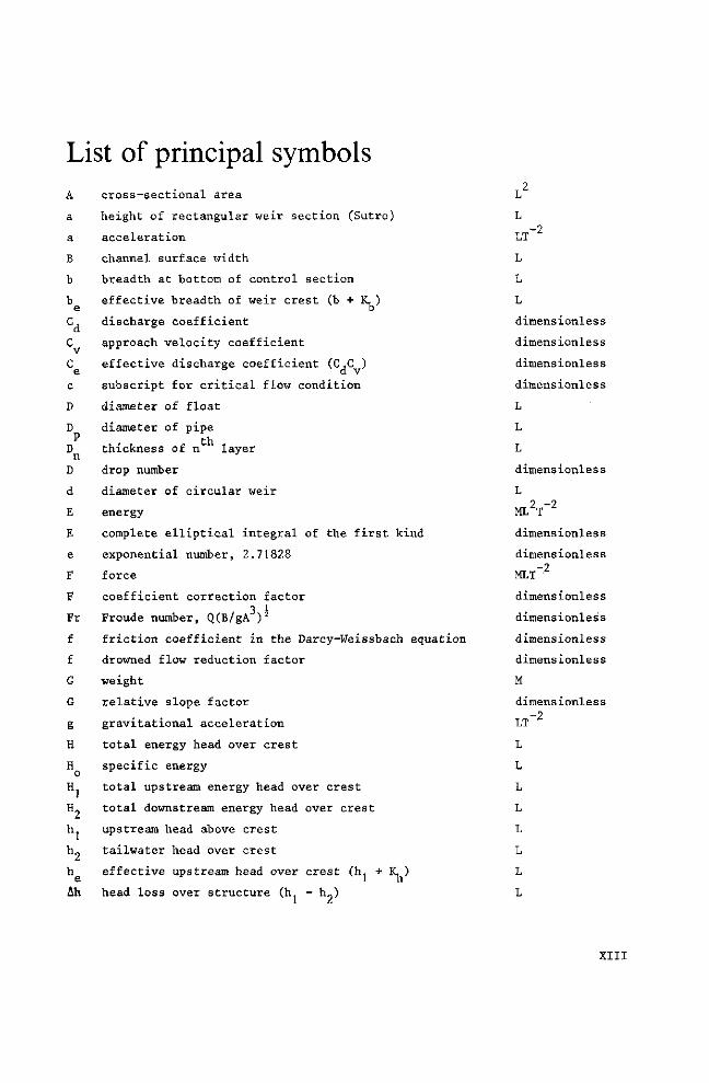
List of principal symbols A
a
a
B
b
b
c
D
D P
D il
D
d
E
E
e
F
F
Fr
f
f
G
G
g
H
H
2 h
e Ah
cross-sectional area
height of rectangular weir section (Sutro)
acceleration
channel surface width
breadth at bottom of control section
effective breadth of weir crest (b + K, )
discharge coefficient
approach velocity coefficient
effective discharge coefficient (C.C )
subscript for critical flow condition
diameter of float
diameter of pipe
thickness of n layer
drop number
diameter of circular weir
energy
complete elliptical integral of the first kind
exponential number, 2.71828
force
coefficient correction factor 3 l
Froude number, Q(B/gA ) 2
friction coefficient in the Darcy-Weissbach equation
drowned flow reduction factor
weight
relative slope factor
gravitational acceleration
total energy head over crest
specific energy
total upstream energy head over crest
total downstream energy head over crest
upstream head above crest
tailwater head over crest
effective upstream head over crest (h( + K, )
head loss over structure (h - h„)
L
L
LT"2
L
L
L
dimensionless
dimensionless
dimensionless
dimensionless
L
L
L
dimensionless
L 2 -2
ML T
dimensionless
dimensionless
MLT-2
dimensionless
dimensionless
dimensionless
dimensionless
M
dimensionless
LT"2
L
L
L
L
L
L
L
L
XIII
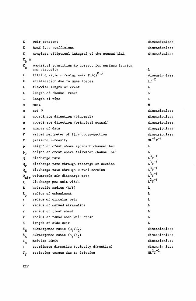
K weir constant
K head loss coefficient
K complete elliptical integral of the second kind
\ &
K empirical quantities to correct for surface tension and viscosity
k filling ratio circular weir (h/d)
k acceleration due to mass forces
L flowwise length of crest
L length of channel reach
1 length of pipe
m mass
m cot 8
m coordinate direction (binormal)
n coordinate direction (principal normal)
n number of data
P wetted perimeter of flow cross-section
P pressure intensity
p height of crest above approach channel bed
p. height of crest above tailwater channel bed
Q discharge rate
Q discharge rate through rectangular section
Q discharge rate through curved section
Q . volumetric air discharge rate air °
discharge per unit width
hydraulic radius (A/P)
radius of embankment
radius of circular weir
radius of curved streamline
radius of float-wheel
radius of round-nose weir crest
length of side weir
submergence ratio (H /H»)
submergence ratio (h./h.)
modular limit
coordinate direction (velocity direction)
resisting torque due to friction
q R
h r
r
r
r
S
S„
dimensionless
dimensionless
dimensionless
dimensionless
LT"2
L
L
L
M
dimensionless
dimensionless
dimensionless
dimensionless
dimensionless
ML-'T"2
L
L
LV LV LV LV LV L
L
L
L
L
L
L
dimensionless
dimensionless
dimensionless
dimensionless 2 -2
ML T
XIV
TW tailwater level
t time
V volume of fluid
v fluid velocity
v average fluid velocity (Q/A)
W friction force
w acceleration due to friction
w underflow gate opening
X relative error
X horizontal distance
x breadth of weir throat at height y above crest
x factor due to boundary roughness
x cartesian coordinate direction
Y vertical distance
y vertical depth of flow
y coordinate direction
z coordinate direction
z coordinate direction
Az drop height
a velocity distribution coefficient
a angle of circular section
a diversion angle
ß half angle of circular section (J a)
' Tnax Tnin
6 error
A small increment of
A (p - p)/p : relative density
8 weir notch angle
ïï circular circumference-diameter ratio; 3.1416
p mass density of water p . mass density of air "air J
p mass density of bed material
w circular section factor
Ç friction loss coefficient
T standard deviation
T estimate of standard deviation
T relative standard deviation
L
T
L3
LT"
LT -1
MLT
LT"2
L
dimensionless
L
L
dimensionless
dimensionless
L
L
dimensionless
dimensionless
dimensionless
L
dimensionless
degrees
degrees
degrees
dimensionless
dimensionless
dimensionless
dimensionless
degrees
dimensionless
ML - 3
-3 ML
-3
ML
dimensionless
dimensionless
dimensionless
dimensionless
dimensionless
XV
1 Basic principles of fluid flow as applied to measuring structures
1.1 General The purpose of this chapter is to explain the fundamental principles involved
in evaluating the flow pattern in weirs, flumes, orifices and other measuring
structures, since it is the flow pattern that determines the head-discharge re
lationship in such structures.
Since the variation of density is negligible in the context of these studies,
we shall regard the mass density (p) of water as a constant. Nor shall we con
sider any flow except time invariant or steady flow, so that a streamline indi
cates the path followed by a fluid particle.
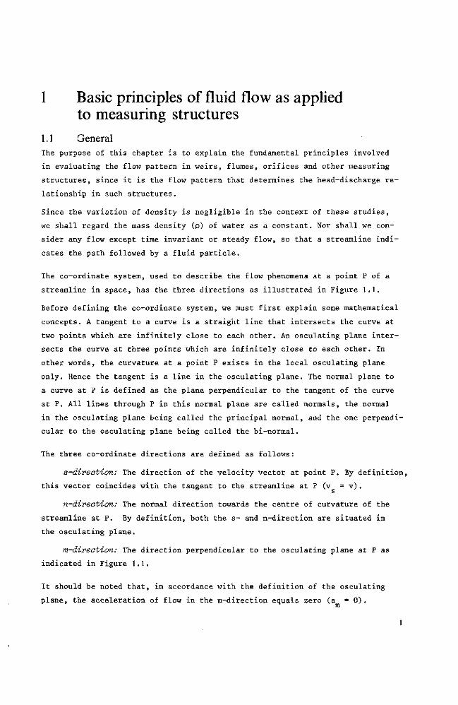
The co-ordinate system, used to describe the flow phenomena at a point P of a
streamline in space, has the three directions as illustrated in Figure 1.1.
Before defining the co-ordinate system, we must first explain some mathematical
concepts. A tangent to a curve is a straight line that intersects the curve at
two points which are infinitely close to each other. An osculating plane inter
sects the curve at three points which are infinitely close to each other. In
other words, the curvature at a point P exists in the local osculating plane
only. Hence the tangent is a line in the osculating plane. The normal plane to
a curve at P is defined as the plane perpendicular to the tangent of the curve
at P. All lines through P in this normal plane are called normals, the normal
in the osculating plane being called the principal normal, and the one perpendi
cular to the osculating plane being called the bi-normal.
The three co-ordinate directions are defined as follows :
a-direotion: The direction of the velocity vector at point P. By definition,
this vector coincides with the tangent to the streamline at P (v = v ) .
n-direotion: The normal direction towards the centre of curvature of the
streamline at P. By definition, both the s- and n-direction are situated in
the osculating plane.
m-direotion: The direction perpendicular to the osculating plane at P as
indicated in Figure 1.1.
It should be noted that, in accordance with the definition of the osculating
plane, the acceleration of flow in the m-direction equals zero (a = 0 ) . m
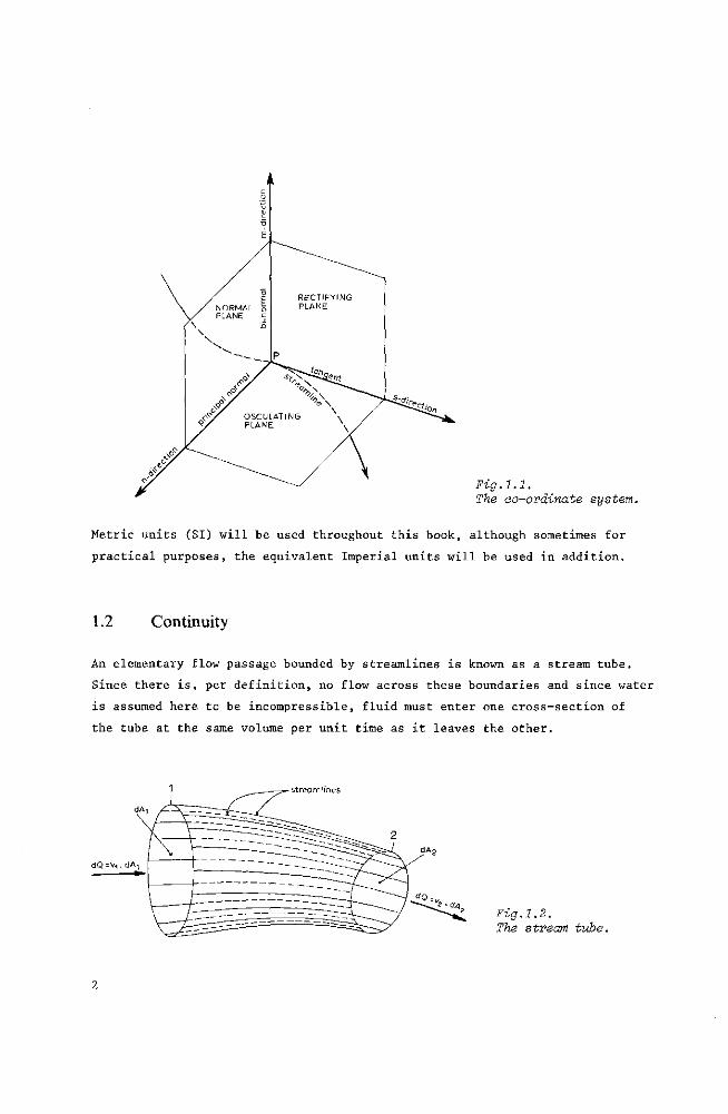
Fig.1.1. The co-ordinate system.
Metric units (SI) will be used throughout this book, although sometimes for
practical purposes, the equivalent Imperial units will be used in addition.
1.2 Continuity
An elementary flow passage bounded by streamlines is known as a stream tube.
Since there is, per definition, no flow across these boundaries and since water
is assumed here to be incompressible, fluid must enter one cross-section of
the tube at the same volume per unit time as it leaves the other.
streamlines
Fig.1.2. The stream tube.
From the assumption of steady flow, it follows that the shape and position of
the stream tube do not change with time. Thus the rate at which water is flowing ,
across a section equals the product of the velocity component perpendicular to
the section and the area of this section. If the subscripts 1 and 2 are applied
to the two ends of the elementary stream tube, we can write:
Discharge = dQ = vidAi = V2dA2 (1-1)
This continuity equation is valid for incompressible fluid flow through any
stream tube. If Equation 1.1 is applied to a stream tube with finite cross-
sectional area, as in an open channel with steady flow (the channel bottom,
side slopes, and water surface being the boundaries of the stream tube), the
continuity equation reads:
A -Q = ƒ vdA = vA = constant
viAi = v2A2 (1-2)
where v is the average velocity component perpendicular to the cross-section
of the open channel.
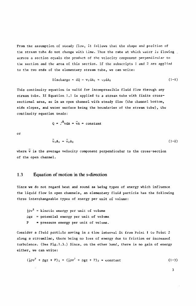
1.3 Equation of motion in the s-direction
Since we do not regard heat and sound as being types of energy which influence
the liquid flow in open channels, an elementary fluid particle has the following
three interchangeable types of energy per unit of volume:
jpv = kinetic energy per unit of volume
pgz = potential energy per unit of volume
P = pressure energy per unit of volume.
Consider a fluid particle moving in a time interval At from Point 1 to Point 2
along a streamline, there being no loss of energy due to friction or increased
turbulence. (See Fig.1.3.) Since, on the other hand, there is no gain of energy
either, we can write:
G p v 2 + pgz + P)i = (sPv2 + pgz + P ) 2 = constant (1-3)
This equation is valid for points along a streamline only if the energy losses
are negligible and the mass density (p) is a constant. According to Equation 1-3:
£pv + pgz + P = constant (1-4)
v2/2g + P/pg + z constant (1-5)
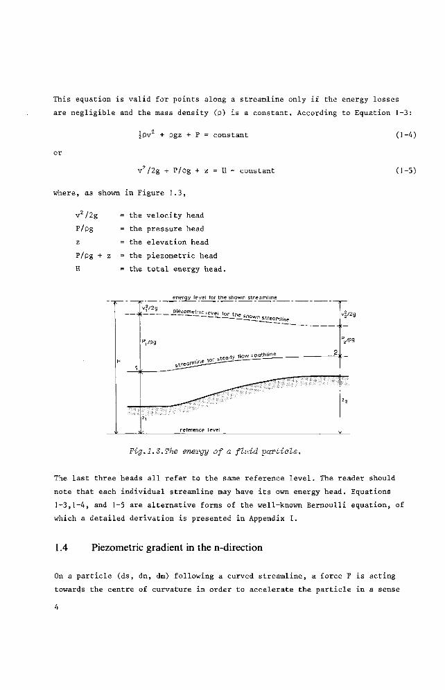
where, as shown in Figure 1.3,
v2/2g = the velocity head
P/pg = the pressure head
z = the elevation head
P/pg + z the piezometric head
H = the total energy head.
^2 P i«ometr icjevel fo
energy level for the shown streamline
',2/2g
- i i s a h e ^ o ^ ^ ^ if
p , /pg
reference level
v^/2g
,/pg
Fig.1.3.The energy of a fluid partiale.
The last three heads all refer to the same reference level. The reader should
note that each individual streamline may have its own energy head. Equations
1-3,1-4, and 1-5 are alternative forms of the well-known Bernoulli equation, of
which a detailed derivation is presented in Appendix I.
1.4 Piezometric gradient in the n-direction
On a particle (ds, dn, dm) following a curved streamline, a force F is acting
towards the centre of curvature in order to accelerate the particle in a sense
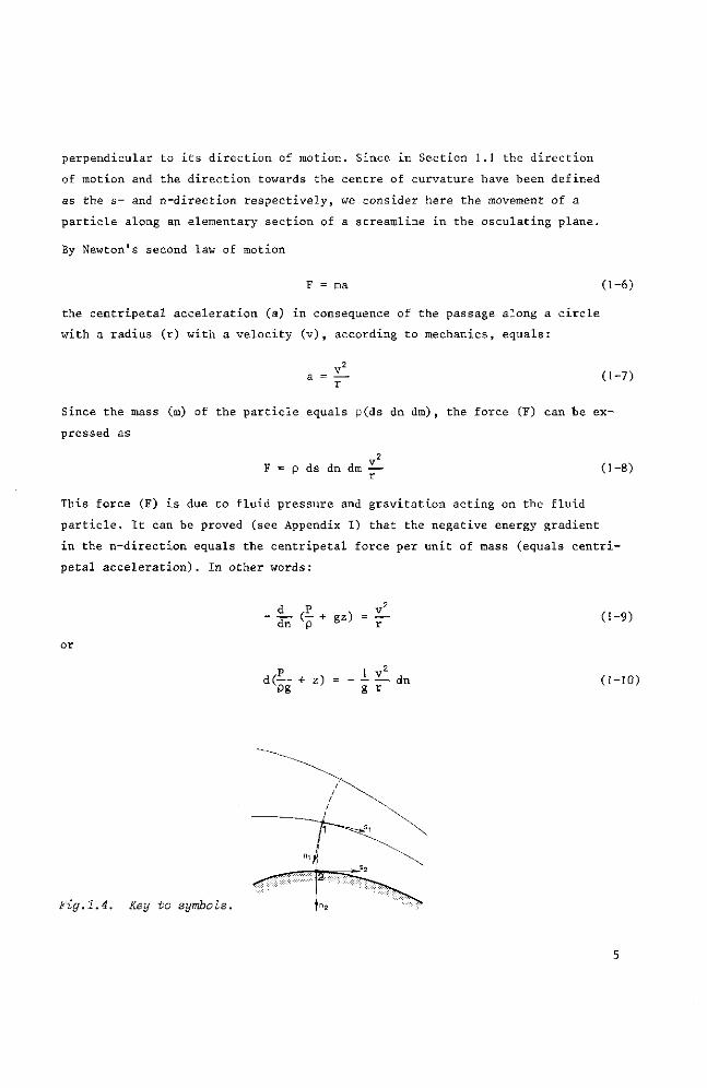
perpendicular to its direction of motion. Since in Section 1.1 the direction
of motion and the direction towards the centre of curvature have been defined
as the s- and n-direction respectively, we consider here the movement of a
particle along an elementary section of a streamline in the osculating plane.
By Newton's second law of motion
(1-6)
the centripetal acceleration (a) in consequence of the passage along a circle
with a radius (r) with a velocity (v), according to mechanics, equals:
(1-7)
Since the mass (m) of the particle equals p(ds dn dm), the force (F) can be ex
pressed as
2 F = p ds dn dm (1-8)
This force (F) is due to fluid pressure and gravitation acting on the fluid
particle. It can be proved (see Appendix I) that the negative energy gradient
in the n-direction equals the centripetal force per unit of mass (equals centri
petal acceleration). In other words:
drT ( p + gz) = F (1-9)
d ( — + z) = Pg
i ^ d n g r
(1-10)
Fig.1.4. Key to symbols.
After integration of this equation from Point 1 to Point 2 in the n-direction
we obtain the following equation for the fall of piezometric head in the
n-direction (see Fig.1.4)
Pg Pg + z
1 ƒ ^ d n (1-11)
In this equation
Pg + z the piezometric head at Point 1
+ z Pg
2 2 7 ^ d n 1 gr
the piezometric head at Point 2
the difference between the piezometric heads at Points 1 and 2 due to the curvature of the streamlines
From this equation it appears that, if the streamlines are straight (r = °°), the
integral has zero value, and thus the piezometric head at Point 1 equals that
at Point 2, so that
Pg + z constant (1-12)
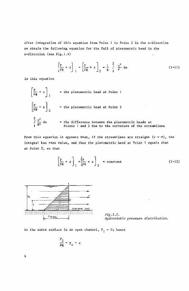
Fig.1.5. Hydrostatic pressure distribution.
At the water surface in an open channel, V = 0; hence
P 2
__ = y - Z
Pg o
pg(y - z) (1-13)
Thus, if r = °° there is what is known as a hydrostatic pressure distribution.
If the streamlines are curved, however, and there is a significant flow velocity,
the integral may reach a considerable value.
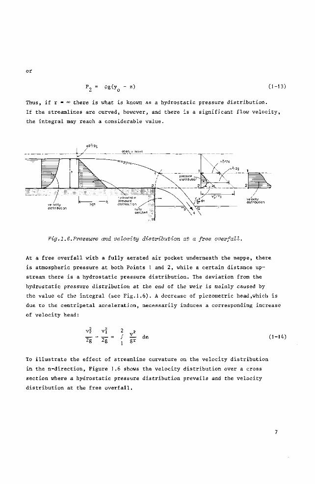
nvV2g
velocity distribution
Fig.1.6.Pressure and velocity distribution at a free overfall.
At a free overfall with a fully aerated air pocket underneath the nappe, there
is atmospheric pressure at both Points 1 and 2, while a certain distance up
stream there is a hydrostatic pressure distribution. The deviation from the
hydrostatic pressure distribution at the end of the weir is mainly caused by
the value of the integral (see Fig.1.6). A decrease of piezometric head,which is
due to the centripetal acceleration, necessarily induces a corresponding increase
of velocity head:
vi Vi 2 2 T. 75— = ƒ — dn 2g 2g ] gr
(1-14)
To illustrate the effect of streamline curvature on the velocity distribution
in the n-direction, Figure 1.6 shows the velocity distribution over a cross
section where a hydrostatic pressure distribution prevails and the velocity
distribution at the free overfall.
1.5 Hydrostatic pressure distribution in the m-direction
As mentioned in Section 1.1, in the direction perpendicular to the osculating
plane, not only v = 0 , but also
dv a = TT- = ° m dt
Consequently, there is no net force acting in the m-direction, and therefore
the pressure distribution is hydrostatic.
Consequently, in the m-direction
P + pgz = constant (1-15)
p — + z = constant (1-16) Pg
1.6 The total energy head of an open channel cross-section
According to Equation 1.4, the total energy per unit of volume of a fluid particle
can be expressed as the sum of the three types of energy:
i pv2 + pgz + P (1-17)
We now want to apply this expression to the total energy which passes through
the entire cross-section of a channel. We therefore need to express the total
kinetic energy of the discharge in terms of the average flow velocity of the
cross-section.
In this context, the reader should note that this average flow velocity is not a
directly measurable quantity but a derived one, defined by
v = £ (1-18)
Due to the presence of a free water surface and the friction along the solid
channel boundary, the velocities in the channel are not uniformly distributed
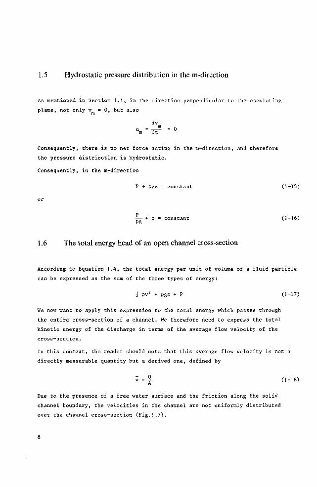
over the channel cross-section (Fig.1.7).
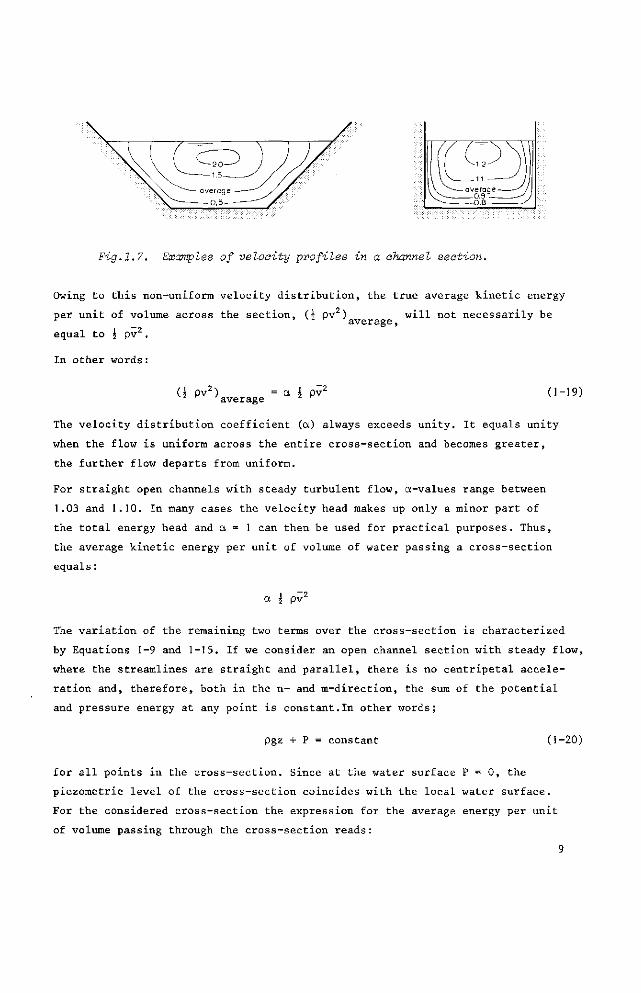
Fig.1.7. Examples of velocity profiles in a channel section.
Owing to this non-uniform velocity distribution, the true average kinetic energy
per unit of volume across the section, (S pv ) will not necessarily be ^ _ average, J
equal to 5 pv2.
In other words :
(I pv2) = a I pv2
average (1-19)
The velocity distribution coefficient (a) always exceeds unity. It equals unity
when the flow is uniform across the entire cross-section and becomes greater,
the further flow departs from uniform.
For straight open channels with steady turbulent flow, a-values range between
1.03 and 1.10. In many cases the velocity head makes up only a minor part of
the total energy head and a = 1 can then be used for practical purposes. Thus,
the average kinetic energy per unit of volume of water passing a cross-section
equals :
a I pv2
The variation of the remaining two terms over the cross-section is characterized
by Equations 1-9 and 1-15. If we consider an open channel section with steady flow,
where the streamlines are straight and parallel, there is no centripetal accele
ration and, therefore, both in the n- and m-direction, the sum of the potential
and pressure energy at any point is constant.In other words;
pgz + P = constant (1-20)
for all points in the cross-section. Since at the water surface P = 0, the
piezometric level of the cross-section coincides with the local water surface.
For the considered cross-section the expression for the average energy per unit
of volume passing through the cross-section reads:
E = a J pv + P + pgz
or if expressed in terms of head
(1-21)
v P
2g Pg (1-22)
where H is the total energy head of a cross-sectional area of flow. We have now
reached the stage that we are able to express this total energy head in the ele
vation of the water surface (P/pg + z) plus the velocity head av2/2g.
head measurement section
control section
..........,.!,........ i ;::;.ï.;m:^;::ï:ïïSiS:-;::f.:-,. 1
i 1
1
' f l o w 1 1 1 1
~^t|Ä:S::. .S,:! m ^^~ 1
! - * - 1
1 1
avf/2g
av'/2g
*2
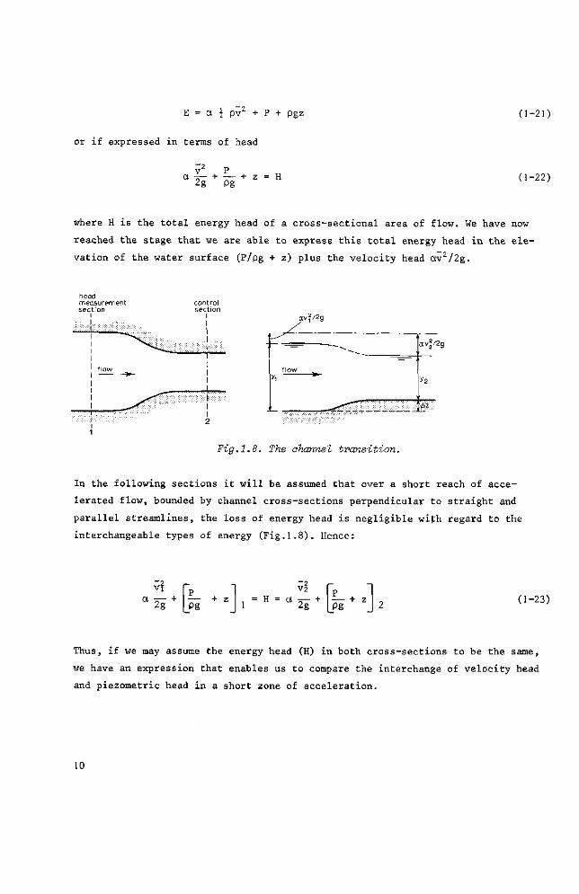
Fig.1.8. The channel transition.
In the following sections it will be assumed that over a short reach of acce
lerated flow, bounded by channel cross-sections perpendicular to straight and
parallel streamlines, the loss of energy head is negligible with regard to the
interchangeable types of energy (Fig.1.8). Hence:
vî a 2 T + z 1 = H = a
vi
2g +
pg + z (1-23)
Thus, if we may assume the energy head (H) in both cross-sections to be the same,
we have an expression that enables us to compare the interchange of velocity head
and piezometric head in a short zone of acceleration.
1.7 Recapitulation
For a short zone of acceleration bounded by cross-sections perpendicular to
straight and parallel streamlines, the following two equations are valid:
Continuity equation (1-2)
Q = ViAi = v2A2
Bernoulli's equation (1-23)
Vl H = a 75- +
2g
P — + z Pg
vi , = a 75— + 1 2g
P — + z Pg
In both cross-sections the piezometric level coincides with the water surface
and the latter determines the area A of the cross-section. We may therefore
conclude that if the shapes of the two cross-sections are known, the two un
knowns vi and V2 can be determined from the two corresponding water levels by
means of the above equations.
It is evident, however, that collecting and handling two sets of data per measur
ing structure is an expensive and time-consuming enterprise which should be
avoided if possible. It will be shown that under critical flow conditions one
water level only is sufficient to determine the discharge. In order to explain
this critical condition, the concept of specific energy will first be defined.
1.8 Specific energy
The concept of specific energy was first introduced by Bakhmeteff in 1912,
and is defined as the average energy per unit weight of water at a channel
section as expressed with respect to the channel bottom. Since the piezometric
level coincides with the water surface, the piezometric head with respect to
the channel bottom is:
p
— + z = y, the water depth (1-24)
so that the specific energy head can be expressed as :
H = y + av2/2g (1-25)
11
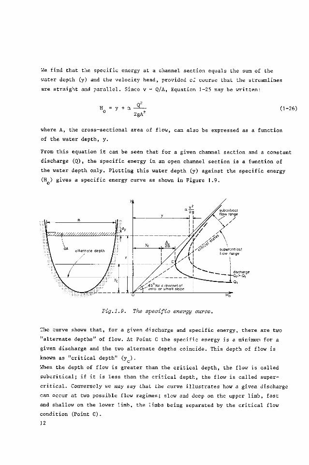
We find that the specific energy at a channel section equals the sum of the
water depth (y) and the velocity head, provided of course that the streamlines
are straight and parallel. Since v = Q/A, Equation 1-25 may be written:
y + a 2gAz
(1-26)
where A, the cross-sectional area of flow, can also be expressed as a function
of the water depth, y.
From this equation it can be seen that for a given channel section and a constant
discharge (Q), the specific energy in an open channel section is a function of
the water depth only. Plotting this water depth (y) against the specific energy
(H ) gives a specific energy curve as shown in Figure 1.9.
Fig.1.9. The specific energy curve.
The curve shows that, for a given discharge and specific energy, there are two
"alternate depths" of flow. At Point C the specific energy is a minimum for a
given discharge and the two alternate depths coincide. This depth of flow is
known as "critical depth" (y ) .
When the depth of flow is greater than the critical depth, the flow is called
subcritical; if it is less than the critical depth, the flow is called super
critical. Conversely we may say that the curve illustrates how a given discharge
can occur at two possible flow regimes; slow and deep on the upper limb, fast
and shallow on the lower limb, the limbs being separated by the critical flow
condition (Point C ) .
12
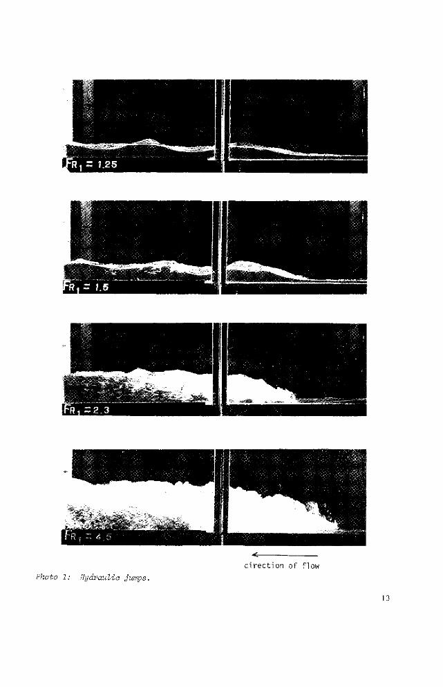
direct ion of flow Photo 1: Hydraulic jumps.
13
When there is a rapid change in depth of flow from a high to a low stage, a
steep depression will occur in the water surface; this is called a "hydraulic
drop". On the other hand, when there is a rapid change from a low to a high
stage, the water surface will rise abruptly; this phenomenon is called a "hydrau
lic jump" or "standing wave". The standing wave shows itself by its turbulence
(white water), whereas the hydraulic drop is less apparent. However, if in a
standing wave the change in depth is small, the water surface will not rise
abruptly but will pass from a low to a high level through a series of undulations
(undular jump), and detection becomes more difficult. The normal procedure to
ascertain whether critical flow occurs in a channel contraction - there being
subcritical flow upstream and downstream of the contraction - is to look for
a hydraulic jump immediately downstream of the contraction.
From Figure 1.9 it is possible to see that if the state of flow is critical,i.e.
if the specific energy is a minimum for a given discharge, there is one value
for the depth of flow only. The relationship between this minimum specific
energy and the critical depth is found by differentiating Equation 1-26 to y,
while Q remains constant.
dHo Q2 dA , v2 dA ,. _,,. -,— = 1 - a — -j- = 1 - a —T- j— (1-27) dy gA3 dy gA dy
Since dA = B dy, this equation becomes:
dH -2„ -=— = 1 - a — T - (1-28) dy g A
If the specific energy is a minimum dH /dy = 0, we may write:
v2 A
« 2 f = 2 f - (,"29)
Equation 1-29 is valid only for steady flow with parallel streamlines in a channel
of small slope. If the velocity distribution coefficient, a, is assumed to be
unity, the criterion for critical flow becomes:
v2/2g = j A / B or v = v = (g A /B )°,5° (1-30) c ° * c c c ° c c
14
Provided that the tailwater level of the measuring structure is low enough to
enable the depth of flow at the channel contraction to reach critical depth,
Equations 1-2, 1-23, and 1-30 allow the development of a discharge equation for
each measuring device, in which the upstream total energy head (H.) is the only in
dependent variable.
Equation 1-30 states that at critical flow the average flow velocity
vc - (g Ac/Bc)°-5° (1-31)
It can be proved that this flow velocity equals the velocity with which the
smallest disturbance moves in an open channel, as measured relative to the flow.
Because of this feature, a disturbance or change in a downstream level cannot
influence an upstream water level if critical flow occurs in between the two
cross-sections considered. The "control section" of a measuring structure is lo
cated where critical flow occurs and subcritical, tranquil, or streaming
flow passes into supercritical, rapid, or shooting flow.
Thus, if critical flow occurs at the control section of a measuring structure,
the upstream water level is independent of the tailwater level; the flow over
the structure is then called "modular".
1.9 The broad-crested weir
A broad-crested weir is an overflow structure with a horizontal crest above which
the deviation from a hydrostatic pressure distribution because of centripetal
acceleration may be neglected. In other words, the streamlines are practically
straight and parallel.To obtain this situation the length of the weir crest in
the direction of flow (L) should be related to the total energy head over the weir
crest as 0.08 s? H /L < 0.50. H./L 5- 0.08 because otherwise the energy losses above
the weir crest cannot be neglected, and undulations may occur on the crest;
H /L -S 0.50, so that only slight curvature of streamlines occurs above the crest
and a hydrostatic pressure distribution may be assumed.
If the measuring structure is so designed that there are no significant energy
losses in the zone of acceleration upstream of the control section, according
to Bernoulli's equation (1-23):
Hj = hj + a vf/2g = H = y + a v2/2g
15
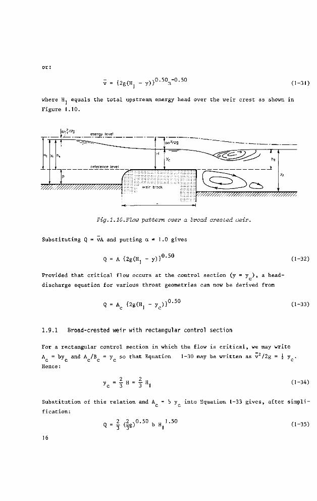
r„ ,„ ,-,0.50 -0.50 v = {2g(H] - y)} a (1-31)
where H1 equals the total upstream energy head over the weir crest as shown in
Figure 1.10.
Tmmmmmzm?/ V/////////////////////////////////?///////,
Fig.1.10.Flaw pattern over a broad crested weir.
Substituting Q = vA and putting a = 1.0 gives
Q = A {2g(H, - y)}0'5 0 (1-32)
Provided that critical flow occurs at the control section (y = y ) , a head-
discharge equation for various throat geometries can now be derived from
Q = Ac {2g(H, - yc)}0,5° (1-33)
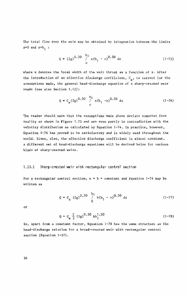
1.9.1 Broad-crested weir with rectangular control section
For a rectangular control section in which the flow is critical, we may write
A = by and A /B = y so that Equation 1-30 may be written as v2/2g = 5 y . c c
Hence c c c
2 2 yc - 3 H - 3 H .
(1-34)
Substitution of this relation and A = b y into Equation 1-33 gives, after simpli
fication:
_. 2 ,2 ,0.50 , „ 1.50 Q = 3 (3g) b H, (1-35)
16
*- B^Bc
—=—
' Vc
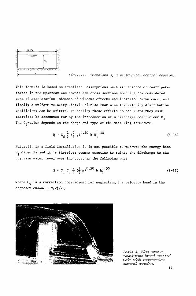
\, » Fig.1.11. Dimensions of a rectangular control section.
This formula is based on idealized assumptions such as: absence of centripetal
forces in the upstream and downstream cross-sections bounding the considered
zone of acceleration, absence of viscous effects and increased turbulence, and
finally a uniform velocity distribution so that also the velocity distribution
coefficient can be omitted. In reality these effects do occur and they must
therefore be accounted for by the introduction of a discharge coefficient C ,.
The C,-value depends on the shape and type of the measuring structure.
- _ _ 2 2 .0.50 , „1.50 Q = Cd 3 (3 S ) b Hl (1-36)
Naturally in a field installation it is not possible to measure the energy head
H1 directly and it is therefore common practice to relate the discharge to the
upstream water level over the crest in the following way:
Q « c. „ 2 .2 0.50 , ,1.50 Cv 3 (- g) b h, (1-37)
where C is a correction coefficient for neglecting the velocity head in the
approach channel, aivf/2g.
Photo 2. Flow over a round-nose broad-crested weir with rectangular control section.
17
Generally, the approach velocity coefficient
u
C = v
(1-38)
where u equals the power of h in the head-discharge equation, being u = 1.50
for a rectangular control section.
Thus C is greater than unity and is related to the shape of the approach channel
section and to the power of h in the head-discharge equation.
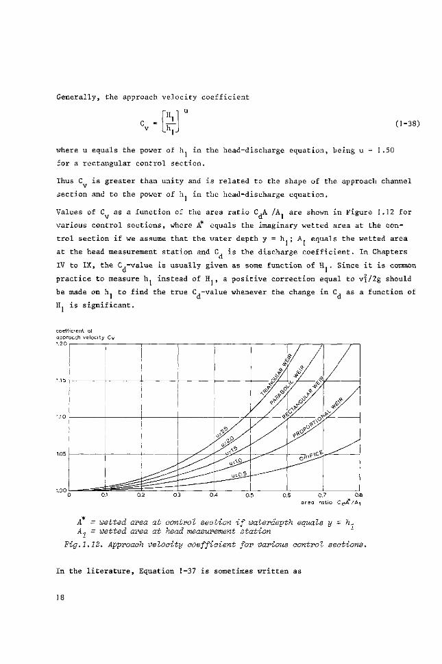
Values of C as a function of the area ratio C .A /A, are shown in Figure 1.12 for v d 1 6
various control sections, where A* equals the imaginary wetted area at the con
trol section if we assume that the water depth y = h. ; A, equals the wetted area
at the head measurement station and C is the discharge coefficient. In Chapters
IV to IX, the C,-value is usually given as some function of H.. Since it is common
practice to measure h. instead of H., a positive correction equal to v?/2g should
be made on h, to find the true C.-value whenever the change in C, as a function of 1 d a
H, is significant.
coefficient of approach velocity C 1.20
0.S 0.7 0.8 area ratio C d ^ / A i
A = wetted area at control section if waterdepth equals y - h1 A1 - Wetted area at head measurement station
Fig.1.12. Approach velocity coefficient for various control sections.
In the literature, Equation 1-37 is sometimes written as
18
C',' C b h. d v 1
1 .50 (1-39)
It should be noted that in this equation the coefficient C" has the dimension
r - -ll • L2 T I. To avoid mistakes and to facilitate easy comparison of discharge coef
ficients in both the metric and the Imperial systems, the use of Equation 1-37 is
recommended.
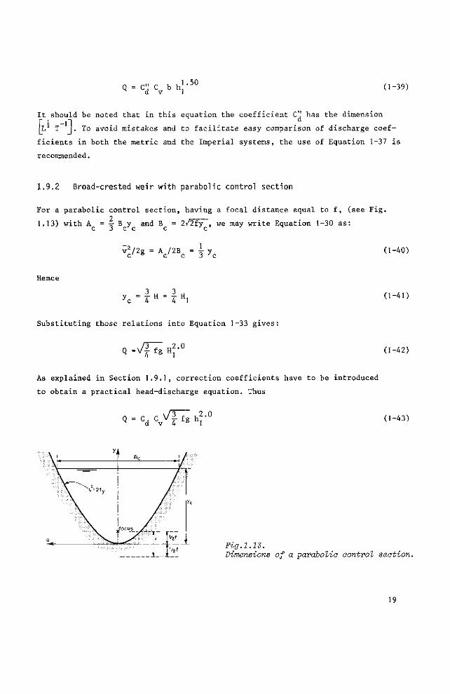
1.9.2 Broad-crested weir with parabolic control section
For a parabolic control section, having a focal distance equal to f, (see Fig.
1.13) with A = -x- B y and B = 2/2fy , we may write Equation 1-30 as:
v2/2g = A /2B c' 5 c c 3 y c
(1-40)
Hence
3 3 y = Y H = f H, •'c 4 4 1
(1-41)
Substituting those relations into Equation 1-33 gives:
Q = 4 ^ H;-° (1-42)
As explained in Section 1.9.1, correction coefficients have to be introduced
to obtain a practical head-discharge equation. Thus
\fï Q = c d C v V i f g h 2 - ° (1-43)
Fig.1.13. Dimensions of a parabolic control section.
19
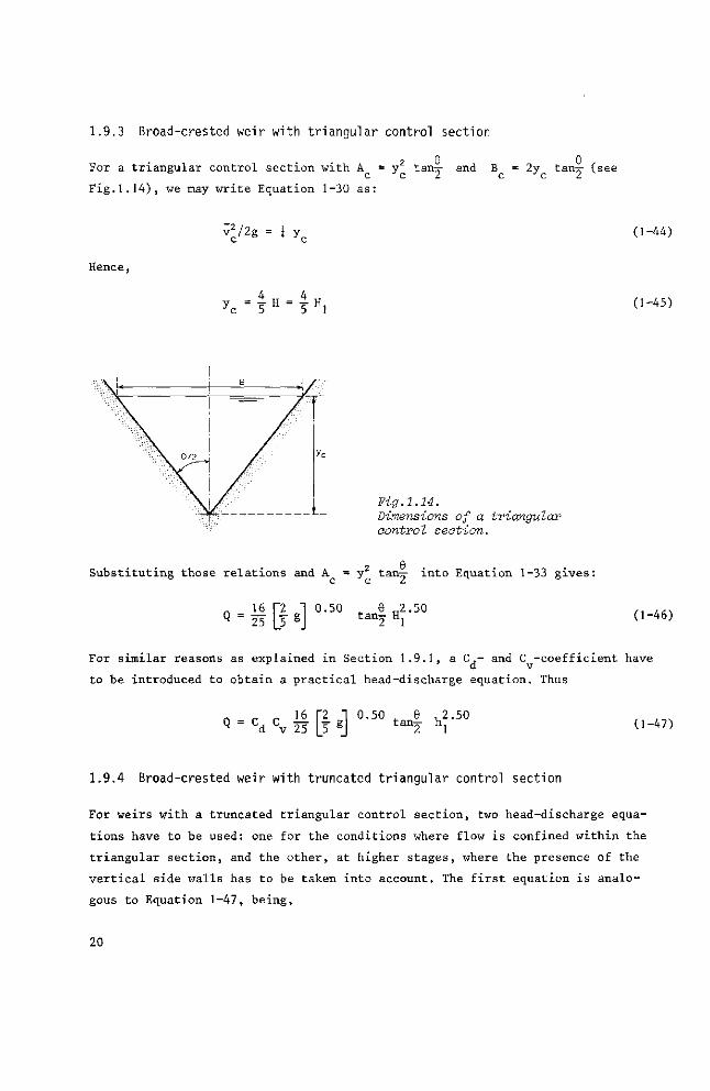
1.9.3 Broad-crested weir with triangular control section
ft R
For a t r i a ngu l a r con t ro l s e c t i on with A = y2 tan-rr and B = 2y tan-^- (see c c 2 c c z
F i g . 1 . 1 4 ) , we may w r i t e Equation 1-30 a s :
Hence,
< / 2 g * y„
4 4 y c = 5 H • s H i
(1-44)
(1-45)
Fig.1.14. Dimensions of a triangular control section.
Substituting those relations and A = y tan-=- into Equation 1-33 gives:
n 16 T2 "1 0.50 _ 6 2.50 ,. .,. Q = 25L5SJ t a n2Hl °"4 6 )
For similar reasons as explained in Section 1.9.1, a C,- and C -coefficient have
to be introduced to obtain a practical head-discharge equation. Thus
2.50 _. „ „ 16 [2 I 0.50 _ e , 2 Q = Cd Cv 25 ]J gJ t a n 2 h l (1-47)
1.9.4 Broad-crested weir with truncated triangular control section
For weirs with a truncated triangular control section, two head-discharge equa
tions have to be used: one for the conditions where flow is confined within the
triangular section, and the other, at higher stages, where the presence of the
vertical side walls has to be taken into account. The first equation is analo
gous to Equation 1-47, being,
20
Q = cd cv ë 0.50 e ,2.50
t a n 2 hl (1-48)
which is valid if Hj < 1.25 H,.
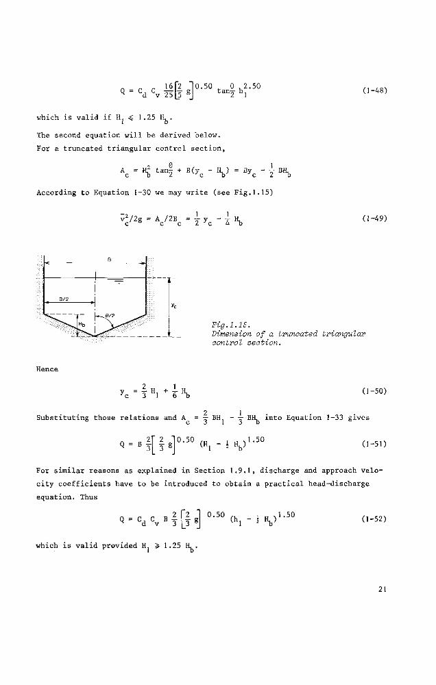
The second equation will be derived below.
For a truncated triangular control section,
Ac = H£ tan^ + B(yc " V = Byc ~ 2 BHb
According to Equation 1-30 we may write (see Fig. 1.15)
v2/2g = A/2B 4 ? - T \ c c c 2 c 4 D (1-49)
• <
_-
B/2
_ ':
B
—
-^9/2
Hb Fig.1.15. Dimension of a truncated triangular control section.
Hence
yc = ! Hi + I \ (1-50)
2 1 . Substituting those relations and A = •=• BH - •=• BH, into Equation 1-33 gives
Q = B T ^ ( H , - I V 1 - 5 0 (1-51)
For similar reasons as explained in Section 1.9.1, discharge and approach velo
city coefficients have to be introduced to obtain a practical head-discharge
equation. Thus
Q = C, C B T ^ d v 3 0.50
(h V 1.50 (1-52)
which is valid provided H. 1.25 H, .
21
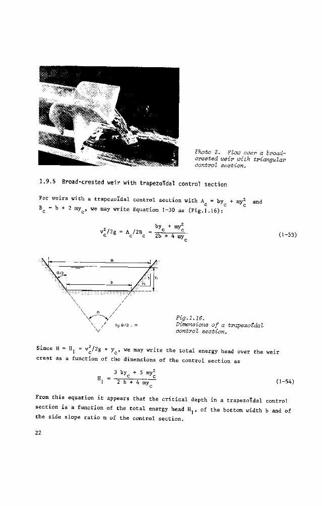
Photo 3. Flow over a broad-crested weir with triangular control seetion.
1.9.5 Broad-crested weir with trapezoidal control secti on
For weirs with a trapezoidal control section with A = by + my and
B = b + 2 my , we may write Equation 1-30 as (Fig.1.16):
2, , byc + myr v2/2g = A„/2B„ - C C V c 2b + 4 myo
(1-53)
tg 9/2 : m
Fig.1.16. Dimensions of a trapézoïdal control section.
Since H = H = v /2g + y , we may write the total energy head over the weir
crest as a function of the dimensions of the control section as
H, = 3 by + 5 my2
1 2 b + 4 myr (1-54)
From this equation it appears that the critical depth in a trapézoïdal control
section is a function of the total energy head fL , of the bottom width b and of
the side slope ratio m of the control section.
22
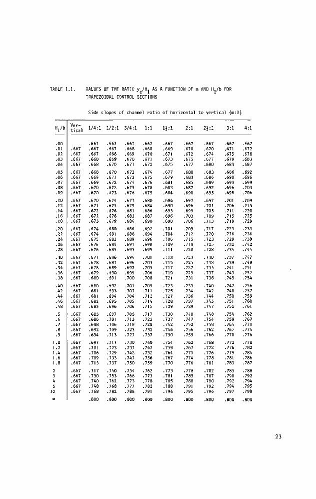
TABLE 1.1. VALUES OF THE RATIO y /Hj AS A FUNCTION OF m AND Hj/b FOR
TRAPEZOIDAL CONTROL SECTIONS
Side slopes of channel ratio of horizontal to vertical (m:l)
H:/b
.00
.01
.02
.03
.04
.05
.06
.07
.08
.09
.10
.12
.14
.16
.18
.20
.22
.24
.26
.28
.30
.32
.34
.36
.38
.40
.42
.44
.46
.48
.5
.6
.7
.8
.9
1.0 1.2 1.4 1.6 1.8
2 3 4 5 0
œ
Vertical
.667
.667
.667
.667
.667
.667
.667
.667
.667
.667
.667
.667
.667
.667
.667
.667
.667
.667
.667
.667
.667
.667
.667
.667
.667
.667
.667
.667
.667
.667
.667
.667
.667
.667
.667
.667
.667
.667
.667
.667
.667
.667
.667
.667
1/4:1
.667
.667
.667
.668
.668
.668
.669
.669
.670
.670
.670
.671
.672
.672
.673
.674
.674
.675
.676
.676
.677
.678
.678
.679
.680
.680
.681
.681
.682
.683
.683
.686
.688
.692
.694
.697
.701
.706
.709
.713
.717
.730
.740
.748
.768
.800
1/2:1
.667
.667
.668
.669
.670
.670
.671
.672
.672
.673
.674
.675
.676
.678
.679
.680
.681
.683
.684
.685
.686
.687
.689
.690
.691
.692
.693
.694
.695
.696
.697
.701
.706
.709
.713
.717
.723
.729
.733
.737
.740
.753
.762
.768
.782
.800
3/4 :1
.667
.668
.669
.670
.671
.672
.673
.674
.675
.676
.677
.679
.681
.683
.684
.686
.688
.689
.691
.693
.694
.696
.697
.699
.700
.701
.703
.704
.705
.706
.708
.713
.718
.723
.727
.730
.737
.742
.747
.750
.754
.766
.773
.777
.788
.800
1:1
.667
.668
.670
.671
.672
.674
.675
.676
.678
.679
.680
.684
.686
.687
.690
.692
.694
.696
.698
.699
.701
.703
.705
.706
.708
.709
.711
.712
.714
.715
.717
.723
.728
.732
.737
.740
.747
.752
.756
.759
.762
.773
.778
.782
.791
.800
1J :1
.667
.669
.671
.673
.675
.677
.679
.681
.683
.684
.686
.690
.693
.696
.698
.701
.704
.706
.709
.711
.713
.715
.717
.719
.721
.723
.725
.727
.728
.729
.730
.737
.742
.746
.750
.754
.759
.764
.767
.770
.773
.781
.785
.788
.794
.800
2:1
.667
.670
.672
.675
.677
.680
.683
.685
.687
.690
.692
.696
.699
.703
.706
.709
.712
.715
.718
.720
.723
.725
.727
.729
.731
.733
.734
.736
.737
.739
.740
.747
.752
.756
.759
.762
.767
.771
.774
.776
.778
.785
.788
.791
.795
.800
2 J : 1
.667
.670
.674
.677
.680
.683
.686
.689
.692
.695
.697
.701
.705
.709
.713
.717
.720
.723
.725
.728
.730
.733
.735
.737
.738
.740
.742
.744
.745
.747
.748
.754
.758
.762
.766
.768
.772
.776
.778
.781
.782
.787
.790
.792
.796
.800
3:1
.667
.671
.675
.679
.683
.686
.690
.693
.696
.698
.701
.706
.711
.715
.719
.723
.726
.729
.732
.734
.737
.739
.741
.743
.745
.747
.748
.750
.751
.752'
.754
.759
.764
.767
.770
.773
.776
.779
.781
.783
.785
.790
.792
.794
.797
.800
4:1
.667
.672
.678
.683
.687
.692
.696
.699
.703
.706
.709
.715
.720
.725
.729
.733
.736
.739
.742
.744
.747
.749
.751
.752
.754
.756
.757
.759
.760
.761
.762
.767
.771
.774
.776
.778
.782
.784
.786
.787
.788
.792
.794
.795
.798
.800
23
It also shows that, if both b and m are known, the ratio y /H is a function of
H . Values of y /H as a function of m and the ratio H /b are shown in Table 1.1.
Substitution of A = by + my into Equation 1-33 and introduction of a dis-c c c
charge coefficient gives as a head-discharge equation
Q = Cd {byc + my2} {2g(H] - y ^ } 0 " 5 0 (1-55)
Since for each combination of b, m, and H /b, the ratio y /H is given in Table
1.1, the discharge Q can be computed because the discharge coefficient has a
predictable value. In this way a Q-H1 curve can be obtained. If the approach 2 . .
velocity head v^/2% is negligible, this curve may be used for gauging purposes. . 2
If the approach velocity has a significant value, v /2g should be estimated and 2 .
h1 = Hj - v1/2g may be obtained in one or two steps.
In the literature the trapezoidal control section is sometimes described as the sum
of a rectangular and a triangular control section. Hence, along similar lines as
will be shown in Section 1.13 for sharp-crested weirs, a head-discharge equation
is obtained by superposing the head-discharge equations valid for a rectangular
and a triangular control section. For broad-crested weirs, however, this pro
cedure results in a strongly variable C,-value, since for a given H the critical 2 4
depth in the two superposed equations equals -^ H. for a rectangular and -=• H. for
a triangular control section. This difference of simultaneous y -values is one
of the reasons why superposition of various head-discharge equations is not
allowed. A second reason is the significant difference in mean flow velocities
through the rectangular and triangular portions of the control section.
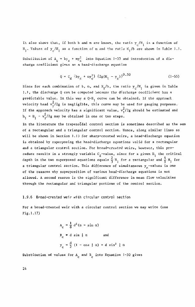
1.9.6 Broad-crested weir with circular control section
For a broad-crested weir with a circular control section we may write (see
Fig.1.17)
1 ? A = -pr d (a - sin a)
c a
B = d sin 5 a and c
y = j (1 - cos 5 a) = d sin2 \ a
Substitution of values for A and B into Equation 1-30 gives c c
24
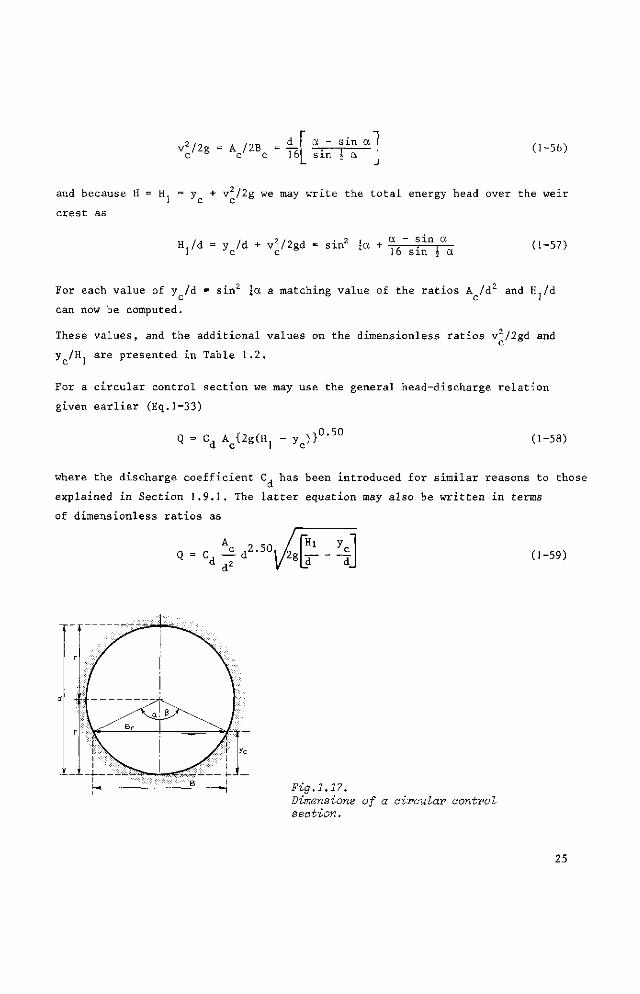
v2/2g = A /2 d a - sin a c c 16 I sin
(1-56)
and because H = H = y + v /2g we may write the total energy head over the weir
crest as
H /j / j . 2/ij • 2 i a - sin a H,/d = yc/d + vc/2gd - sin Ja + ]6 s i n , a (1-57)
For each value of y /d = sin2 |a a matching value of the ratios A /d2 and H,/d c c 1
can now be computed.
These values, and the additional values on the dimensionless ratios v2/2gd and
y /H are presented in Table 1.2.
For a circular control section we may use the general head-discharge relation
given earlier (Eq.1-33)
Q = C d A c { 2 g ( H 1 - y c ) } 0.50
(1-58)
where the discharge coefficient C, has been introduced for similar reasons to those
explained in Section 1.9.1. The latter equation may also be written in terms
of dimensionless ratios as
^ , ^ 2 > d d (1-59)
Fig.1.17. Dimensions of a circular control section.
25
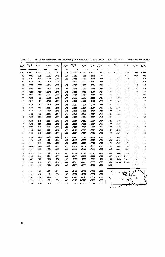
RATIOS FOR DETERMINING THE DISCHARGE Q OF A BROAD-CRESTED WEIR AND LONG-THROATED FLUME WITH CIRCULAR CONTROL SECTION
yc/d
O.OI
.02
.03
.04
.05
.06
.07
.08
.09
.10
.11
.12
.13
.14
.15
.16
.17
.18
.19
.20
.21
.22
.23
.24
.25
.26
.27
.28
.29
.30
.31
.32
.33
.34
.35
y|^
0.0033
.0067
.0101
.0134
.0168
.0203
.0237
.0271
.0306
.0341
.0376
.0411
.0446
.0482
.0517
.0553
.0589
.0626
.0662
.0699
.0736
.0773
.0811
.0848
.0887
.0925
.0963
.1002
.1042
.1081
.1121
.1161
.1202
.1243
.1284
Hj/d
0.0133
.0267
.0401
.0534
.0668
.0803
.0937
.1071
.1206
.1341
.1476
.1611
.1746
.1882
.2017
.2153
.2289
.2426
.2562
.2699
.2836
.2973
.3111
.3248
.3387
.3525
.3663
.3802
.3942
.4081
.4221
.4361
.4502
.4643
.4784
Ac/d2
0.0013
.0037
.0069
.0105
.0147
.0192
.0242
.0294
.0350
.0409
.0470
.0534
.0600
.0688
.0739
.0811
.0885
.0961
.1039
.1118
.1199
.1281
.1365
.1449
.1535
.1623
.1711
.1800
.1890
.1982
.2074
.2167
.2260
.2355
.2450
VH1
0.752
.749
.749
.749
.748
.748
.747
.747
.746
.746
.745
.745
.745
.744
.744
.743
.743
.742
.742
.741
.740
.740
.739
.739
.738
.738
.737
.736
.736
.735
.734
.734
.733
.732
.732
yc/d
0.36
.37
.38
.39
.40
.41
.42
.43
.44
.45
.46
.47
.48
.49
.50
.51
.52
.53
.54
.55
.56
.57
.58
.59
.60
.61
.62
.63
.64
.65
.66
.67
.68
.69
.70
y j ^
0.1326
.1368
.1411
.1454
.1497
.1541
.1586
.1631
.1676
.1723
.1769
.1817
.1865
.1914
.1964
.2014
.2065
.2117
.2170
.2224
.2279
.2335
.2393
.2451
.2511
.2572
.2635
.2699
.2765
.2833
.2902
.2974
.3048
.3125
.3204
Hj/d
0.4926
.5068
.5211
.5354
.5497
.5641
.5786
.5931
.6076
.6223
.6369
.6517
.6665
.6814
.6964
.7114
.7265
.7417
.7570
.7724
.7879
.8035
.8193
.8351
.8511
.8672
.8835
.8999
.9165
.9333
.9502
.9674
.9848
1.0025
1.0204
Vd2
0.2546
.2642
.2739
.2836
.2934
.3032
.3130
.3229
.3328
.3428
.3527
.3627
.3727
.3827
.3927
.4027
.4127
.4227
.4327
.4426
.4526
.4625
.4724
.4822
.4920
.5018
.5115
.5212
.5308
.5404
.5499
.5594
.5687
.5780
.5872
VH1
0.731
.730
.729
.728
.728
.727
.726
.725
.724
.723
.722
.721
.720
.719
.718
.717
.716
.715
.713
.712
.711
.709
.708
.707
.705
.703
.702
.700
.698
.696
.695
.693
.691
.688
.686
yc/d
0.71
.72
.73
.74
.75
.76
.77
.78
.79
.80
.81
.82
.83
.84
.85
.86
.87
.88
.89
.90
.91
.92
.93
.94
.95
.96
.97
.98
.99
1.00
H,
vj£i
0.3286
.3371
.3459
.3552
.3648
.3749
.3855
.3967
.4085
.4210
.4343
.4485
.4638
.4803
.4982
.5177
.5392
.5632
.5900
.6204
.6555
.6966
.7459
.8065
.8841
.9885
1.1410
1.3958
1.9700
-
Hj/d A c /d 2
1.0386 0.5964
1.0571 .6054
1.0759 .6143
1.0952 .6231
1.1148 .6319
1.1349 .6405
1.1555 .6489
1.1767 .6573
1.1985 .6655
1.2210 .6735
1.2443 .6815
1.2685 .6893
1.2938 .6969
1.3203 .7043
1.3482 .7115
1.3777 .7186
1.4092 .7254
1.4432 .7320
1.4800 .7384
1.5204 .7445
1.5655 .7504
1.6166 .7560
1.6759 .7612
1.7465 .7662
1.8341 .7707
1.9485 .7749
2.1110 .7785
2.3758 ' .7817
2.9600 .7841
.7854
i*2£i
" 2ü_l
>t Ac
1 -\V__
VH i
0.684
.681
.679
.676
.673
.670
.666
.663
.659
.655
.651
.646
.641
.636
.630
.624
.617
.610
.601
.592
.581
.569
.555
.538
.518
.493
.460
.412
.334
-
_— -—
m
26
Provided that the diameter of the control section is known and H is measured
(H, - h if the approach velocity is low), values for the ratios A /d2 and y là
can be read from Table 1.2. Substitution of this information and a common C,-
value gives a value for Q, so that Equation 1-59 may be used as a general head-
discharge equation for broad-crested weirs with circular control section.
2 If the approach velocity head Vj/2g cannot be neglected, v, should be estimated
2 . and h. = H, - Vj/2g calculated in one or two steps.
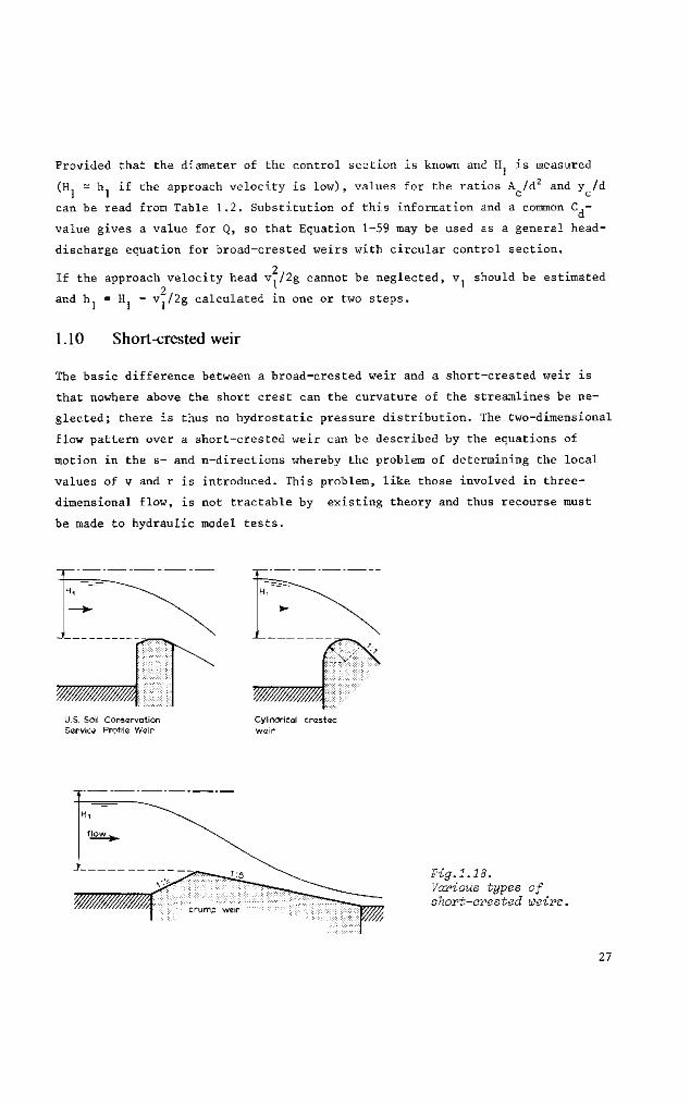
1.10 Short-crested weir
The basic difference between a broad-crested weir and a short-crested weir is
that nowhere above the short crest can the curvature of the streamlines be ne
glected; there is thus no hydrostatic pressure distribution. The two-dimensional
flow pattern over a short-crested weir can be described by the equations of
motion in the s- and n-directions whereby the problem of determining the local
values of v and r is introduced. This problem, like those involved in three-
dimensional flow, is not tractable by existing theory and thus recourse must
be made to hydraulic model tests.
U.S. Soil Conservation Service Profile Weir
Cylindrical crested weir
Fig.1.18. Various types of short-crested weirs.
27
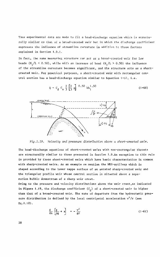
Thus experimental data are made to fit a head-discharge equation which is structu
rally similar to that of a broad-crested weir but in which the discharge coefficient
expresses the influence of streamline curvature in addition to those factors
explained in Section 1.9.1.
In fact, the same measuring structure can act as a broad-crested weir for low
heads (H;/L < 0.50), while with an increase of head (H /L > 0.50) the influence
of the streamline curvature becomes significant, and the structure acts as a short-
crested weir. For practical purposes, a short-crested weir with rectangular con
trol section has a head-discharge equation similar to Equation 1-37, i.e.
2 [2 I 0, Q • Cd Cv 3 U 4
50 bh]' 5 0 (1-60)
energy level
Fig.1.19. Velocity and pressure distribution above a short-orested weir.
The head-discharge equations of short-crested weirs with non-rectangular throats
are structurally similar to those presented in Section 1.9.An exception to this rule
is provided by those short-crested weirs which have basic characteristics in common
with sharp-crested weirs. As an example we mention the WES-spillway which is
shaped according to the lower nappe surface of an aerated sharp-crested weir and
the triangular profile weir whose control section is situated above a sepa
ration bubble downstream of a sharp weir crest.
Owing to the pressure and velocity distributions above the weir crest,as indicated
in Figure 1.19, the discharge coefficient (C.) of a short-crested weir is higher d
than that of a broad-crested weir. The rate of departure from the hydrostatic pres
sure distribution is defined by the local centripetal acceleration v2/r (see
Eq.1.10). .2 d_
dn Pg + z v
gr (1-61)
28
Depending on the degree of curvature in the overflowing nappe, an underpressure
may develop near the weir crest, while under certain circumstances even vapour
pressure can be reached (see also Appendix 1). If the overfailing nappe is not
in contact with the body of the weir, the air pocket beneath the nappe should be
aerated to avoid an underpressure, which increases the streamline curvature at
the control section. For more details on this aeration demand the reader is
referred to Section 1.14.
1.11 Critical depth flumes
A free flowing critical depth or standing wave flume is essentially a streamlined
constriction built in an open channel where a sufficient fall is available so
that critical flow occurs in the throat of the flume. The channel constriction
may be formed by side contractions only, by a bottom contraction or hump only,
or by both side and bottom contractions.
The hydraulic behaviour of a flume is essentially the same as that of a broad-
crested weir. Consequently, stage-discharge equations for critical depth flumes
are derived in exactly the same way as was illustrated in Section 1.9.
In this context it is noted that the stage-discharge relationships of several
critical depth flumes have the following empirical shape:
Q = C'hu (1-62)
where C' is a coefficient depending on the breadth (b) of the throat, on the 2
velocity head v /2g at the head measurement station, and on those factors which
influence the discharge coefficient; h is not the water level but the piezometric
level over the flume crest at a specified point in the converging approach
channel, and u is a factor usually varying between 1.5 and 2.5 depending on
the geometry of the control section.
Examples of critical depth flumes that have such a head-discharge relationship
are the Parshall flume, Cut-throat flume, and H-flume.
Empirical stage-discharge equations of this type (Eq.1-62) have always been
derived for one particular structure, and are valid for that structure only.
If such a structure is installed in the field, care should be taken to copy
the dimensions of the tested original as accurately as possible.
29
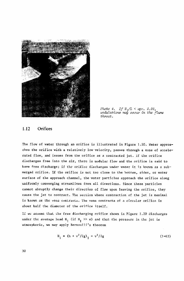
Photo 4. If HjL < apr. 0.08, undulations may oaour in the flume throat.
1.12 Orifices
The flow of water through an orifice is illustrated in Figure 1.20. Water approa
ches the orifice with a relatively low velocity, passes through a zone of accele
rated flow, and issues from the orifice as a contracted jet. If the orifice
discharges free into the air, there is modular flow and the orifice is said to
have free discharge; if the orifice discharges under water it is known as a sub
merged orifice. If the orifice is not too close to the bottom, sides, or water
surface of the approach channel, the water particles approach the orifice along
uniformly converging streamlines from all directions. Since these particles
cannot abruptly change their direction of flow upon leaving the orifice, they
cause the jet to contract. The section where contraction of the jet is maximal
is known as the vena contracta. The vena contracta of a circular orifice is
about half the diameter of the orifice itself.
If we assume that the free discharging orifice shown in Figure 1.20 discharges
under the average head H (if H » w) and that the pressure in the jet is
atmospheric, we may apply Bernoulli's theorem
Hj = (h + v 2 /2g) ] = v2/2g (1-63)
30
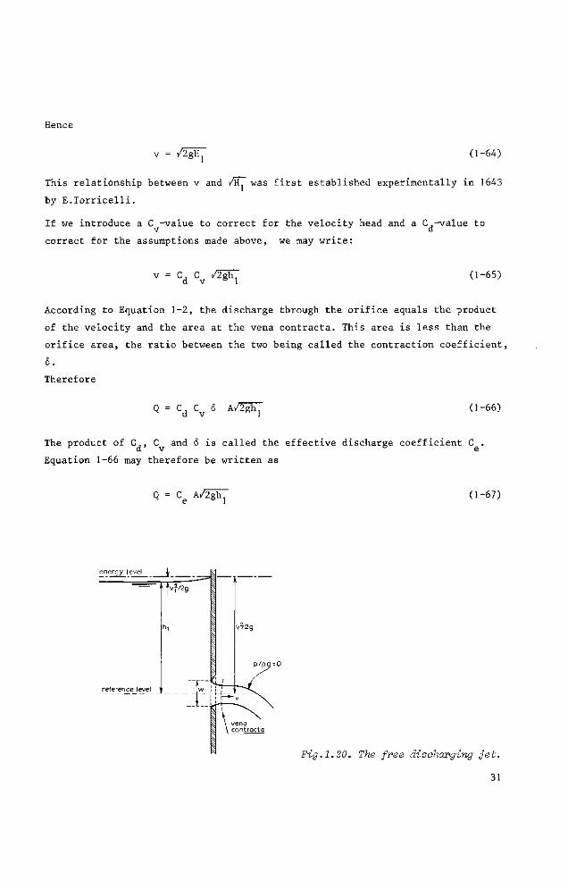
Hence
v = /2gH (1-64)
This relationship between v and /HT was first established experimentally in 1643
by E.Torricelli.
If we introduce a C -value to correct for the velocity head and a C.-value to
v J d co r rec t for the assumptions made above, we may w r i t e :
CdCv /2ih7 (1-65)
According to Equation 1-2, the discharge through the orifice equals the product
of the velocity and the area at the vena contracta. This area is less than the
orifice area, the ratio between the two being called the contraction coefficient,
6.
Therefore
Q = C, C 6 A/2gh, d v 1
(1-66)
The product of C,, C and 6 is called the effective discharge coefficient C .
Equation 1-66 may therefore be written as
Q = Ce A/2ihy (1-67)
energy level
p /pg=0
reteren£e_leyel_ J
Fig.1.20. The free discharging get.
31
Proximity of a bounding surface of the approach channel on one side of the ori
fice prevents the free approach of water and the contraction is partially sup
pressed on that side. If the orifice edge is flush with the sides or bottom of
the approach channel, the contraction along this edge is fully suppressed. The
contraction coefficient, however, does not vary greatly with the length of ori
fice perimeter that has suppressed contraction. If there is suppression of
contraction on one or more edges of the orifice and full contraction on at
least one remaining edge, more water will approach the orifice with a flow
parallel to the face of the orifice plate on the remaining edge(s) and cause
an increased contraction, which will compensate for the effect of partially
or fully suppressed contraction.
Of significant influence on the contraction, however, is the roughness of the
face of the orifice plate. If, for example, lack of maintenance has caused algae
to grow on the orifice plate, the velocity parallel to the face will decrease,
causing a decreased contraction and an increased contraction coefficient. Thus,
unlike broad-crested weirs, an increase of boundary roughness of the structure
will cause the discharge to increase if the head h remains constant. This is
also true for sharp-crested weirs.
Equation 1-67 is valid provided that the discharge occurs under the average
head. For low heads, however, there is a significant difference between the
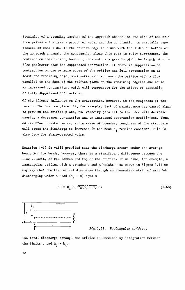
flow velocity at the bottom and top of the orifice. If we take, for example, a
rectangular orifice with a breadth b and a height w as shown in Figure 1.21 we
may say that the theoretical discharge through an elementary strip of area bdz,
discharging under a head (h, - z) equals
dQ C b /2 e *<\ z) dz (1-68)
1 L
•//»/W////»Wm///W///WI/»/l/W///77777.
Fig.1.21. Rectangular orifice.
The total discharge through the orifice is obtained by integration between
the limits o and h, - h .
32
h,-h b t
Q = C b ƒ /2 g(h -z) dz o
(1-69)
n . , 2 nr- ,,1.50 ,1 .50, Q = Ce b g /2i (hb - ht ) (1-70)
If h = 0, the latter equation expresses the discharge across a rectangular
sharp-crested weir (see also Section 1.13). In practice Equation 1-67 is used for
all orifices, including those discharging under low heads, all deviations from the
theoretical equation being corrected for in the effective discharge coefficient.
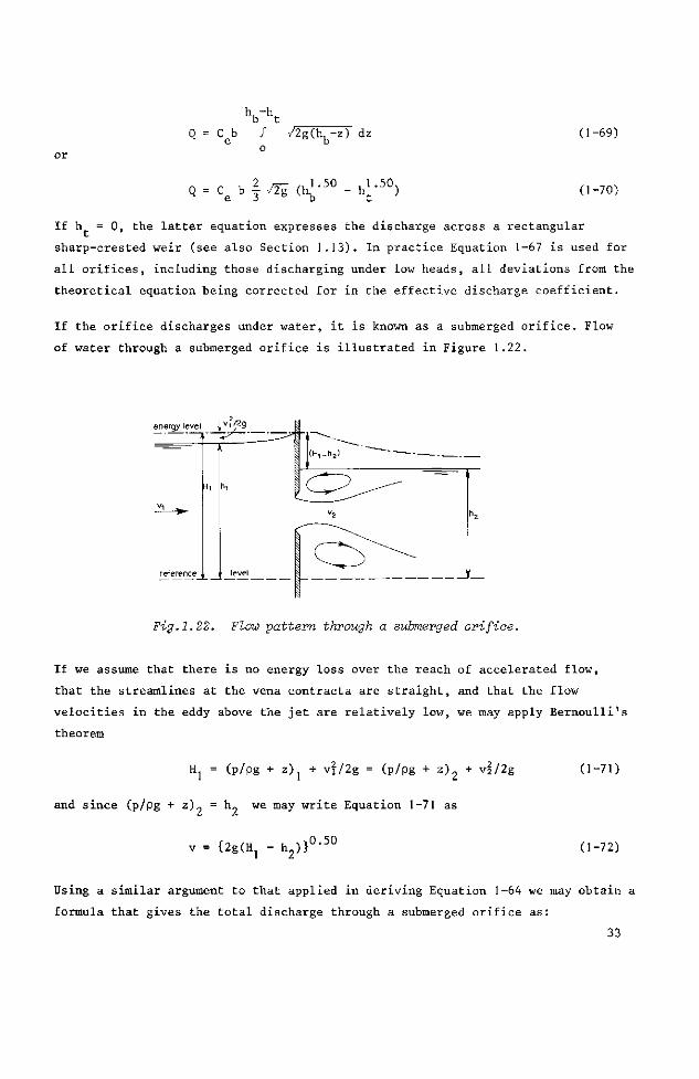
If the orifice discharges under water, it is known as a submerged orifice. Flow
of water through a submerged orifice is illustrated in Figure 1.22.
Fig.1.22. Flow •pattern through a submerged orifice.
If we assume that there is no energy loss over the reach of accelerated flow,
that the streamlines at the vena contracta are straight, and that the flow
velocities in the eddy above the jet are relatively low, we may apply Bernoulli's
theorem
Hj = (p/pg + z)j + v?/2g = (p/pg + z ) 2 + vl/2g
and since (p/pg + z)„ = h» we may write Equation 1-71 as
v = {2g(H] - h2)} 0.50
(1-71)
(1-72)
Using a similar argument to that applied in deriving Equation 1-64 we may obtain a
formula that gives the total discharge through a submerged orifice as:
33
Q = Ce A{2g(h] - h 2 ) } ° - 5 0 (1-73)
1.13 Sharp-crested weirs
If the crest length in the direction of flow of a weir is short enough not to influ
ence the head-discharge relationship of this weir (H /L greater than about 15) the
weir is called sharp-crested. In practice, the crest in the direction of flow is ge
nerally equal to or less than 0.002 m so that even at a minimum head of 0.03 m the
nappe is completely free from the weir body after passing the weir and no adhered
nappe can occur. If the flow springs clear from the downstream face of the weir, an
air pocket forms beneath the nappe from which a quantity of air is removed continu
ously by the overfailing jet. Precautions are therefore required to ensure that the
pressure in the air pocket is not reduced, otherwise the performance of the weir
will be subject to the following undesirable effects:
a) Owing to the increase of underpressure, the curvature of the overfalling
jet will increase, causing an increase of the discharge coefficient (C,).
b) An irregular supply of air to the air pocket will cause vibration of the
jet resulting in an unsteady flow.
If the frequency of the overfalling jet, air pocket, and weir approximate each
other there will be resonance, which may be disastrous for the structure as a
whole.
To prevent these undesirable effects, a sufficient supply of air should be main
tained to the air pocket beneath the nappe. This supply of air is especially
important for sharp-crested weirs, since this type is used frequently for
discharge measurements where a high degree of accuracy is required (laboratory,
pilot scheme, etc.).
Figure 1.23 shows the profile of a fully aerated nappe over a rectangular sharp-
crested weir without side contractions as measured by Bazin and Scimini. This
figure shows that for a sharp-crested weir the concept of critical flow is not
applicable. For the derivation of the head-discharge equations it is assumed
that sharp-crested weirs behave like orifices with a free water surface,
and the following assumptions are made:
34
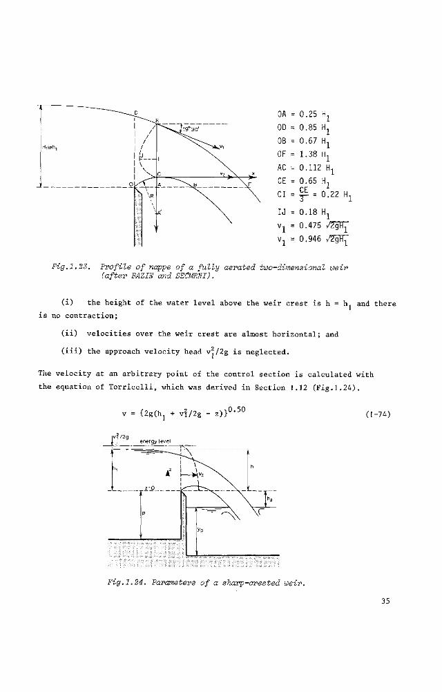
OA = 0.25 H
OD = 0.85 H
OB = 0.67 H
OF = 1.38 H
AC = 0.112 H,
CE = 0.65 H1
CI = C£ = 0.22 Hj
IJ = 0.18 H
M1 = 0.475 /2~gTq"
vx = 0.946 /2gRY
Fig.1.23. Profile of nappe of a fully aerated two-dimensional weir (after BAZIN and SEGMENT).
(i) the height of the water level above the weir crest is h = h. and there
is no contraction;
(ii) velocities over the weir crest are almost horizontal; and
(iii) the approach velocity head v^/2g is neglected.
The velocity at an arbitrary point of the control section is calculated with
the equation of Torricelli, which was derived in Section 1.12 (Fig.1.24).
0.50 (1-74)
Fig.1.24. Parameters of a sharp-crested weir.
35
The total flow over the weir may be obtained by integration between the limits
z=0 and z=h :
. ,„ .0.50 ^ ,, .0.50 , ,. „,. Q = (2g) ƒ x(hj - z) dz (1-75)
o
where x denotes the local width of the weir throat as a function of z. After
the introduction of an effective discharge coefficient, C , to correct for the
assumptions made, the general head-discharge equation of a sharp-crested weir
reads (see also Section 1.12):
_ „ t0 s0.50 kl n 5 0
Q = Ce(2g) ƒ x(h -z) dz (1-76) o
The reader should note that the assumptions made above deviate somewhat from
reality as shown in Figure 1.23 and are even partly in contradiction with the
velocity distribution as calculated by Equation 1-74. In practice, however,
Equation 1-76 has proved to be satisfactory and is widely used throughout the
world. Since, also, the effective discharge coefficient is almost constant,
a different set of head-discharge equations will be derived below for various
kinds of sharp-crested weirs.
1.13.1 Sharp-crested weir with rectangular control section
For a rectangular control section, x = b = constant and Equation 1-76 may be
written as
Q = C (2g)0-50 / b(h - z ) 0 - 5 0 dz (1-77) 0
Q = C e f (2g)°-50bh;-50 (.-78)
So, apart from a constant factor, Equation 1-78 has the same structure as the
head-discharge relation for a broad-crested weir with rectangular control
section (Equation 1-37).
36
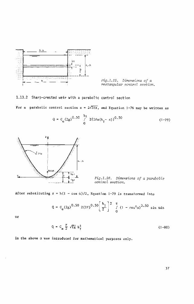
Fig.1.25. Dimensions of a rectangular control section.
1.13.2 Sharp-crested weir with a parabolic control section
For a parabolic control section x = 2/2fz, and Equation 1-76 may be written as
Q = C (2g)°-50 / 2{2fz(h,- z)}0-50
0 ' (1-79)
h 1 = h
Fig.1.26. Dimensions of a •parabolic control section.
After substituting z = h(l - cos a)/2, Equation 1-79 is transformed into
Q - Ce(2g)°-50 2(2f)0-5 0 2 IT
ƒ (1 - cos2a)u"JU sin ada 0
or
Q = ce \ /a hj2 (1-80)
In the above a was introduced for mathematical purposes only.
37
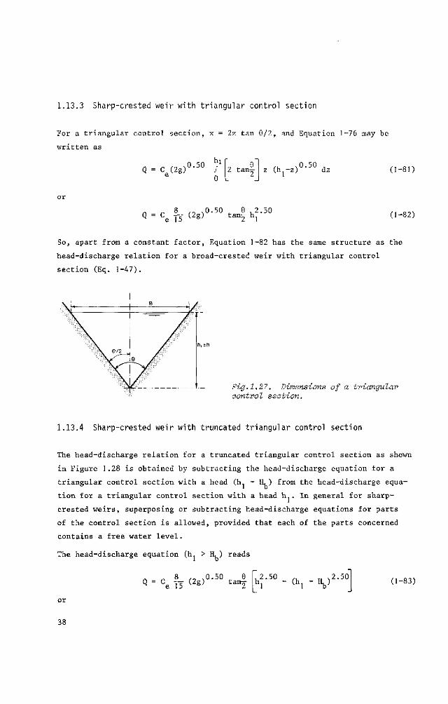
1.13.3 Sharp-crested weir with triangular control section
For a triangular control section, x = 2z tan 8/2, and Equation 1-76 may be
written as
Q = ce(2g) 0.50 ^
2 tan^ z (.h -z; dz (1-81)
. r 8 ,0 ,0.50 ,. e ,2.50 Q = C£ y j (2g) tanj hj (1-82)
So, apart from a constant factor, Equation 1-82 has the same structure as the
head-discharge relation for a broad-crested weir with triangular control
section (Eq. 1-47).
h, = h
Fig.1.27. Dimensions of a triangular control section.
1.13.4 Sharp-crested weir with truncated triangular control section
The head-discharge relation for a truncated triangular control section as shown
in Figure 1.28 is obtained by subtracting the head-discharge equation for a
triangular control section with a head (hj - H, ) from the head-discharge equa
tion for a triangular control section with a head h . In general for sharp-
crested weirs, superposing or subtracting head-discharge equations for parts
of the control section is allowed, provided that each of the parts concerned
contains a free water level.
The head-discharge equation (hj > H, ) reads
_ 8 ,„ ,0.50 „ 6 Ce ^ (2g) tan^
2.50 (h, V 2.50
(1-83)
38
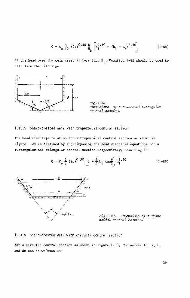
. r 4 ,„ .0.50 B Q = Ce 15 (2g) ÎÇ
2.50 (hi - V 2.50
(1-84)
If the head over the weir crest is less than H, , Equation 1-82 should be used to
calculate the discharge.
B
1 i
B/2
v 1— k-^S/2 ^ Fig.1.28. Dimensions of a truncated triangular control section.
1.13.5 Sharp-crested weir with trapezoidal control section
The head-discharge relation for a trapezoidal control section as shown in
Figure 1.29 is obtained by superimposing the head-discharge equations for a
rectangular and triangular control section respectively, resulting in
Q = ce f ( 2 g ) 0 - 5 0 b + •=• hr tany
1.50 (1-85)
tg9/2 = m Fig.1.29. Dimensions of a trapezoidal control section.
1.13.6 Sharp-crested weir with circular control section
For a circular control section as shown in Figure 1.30, the values for x, z,
and dz can be written as
39
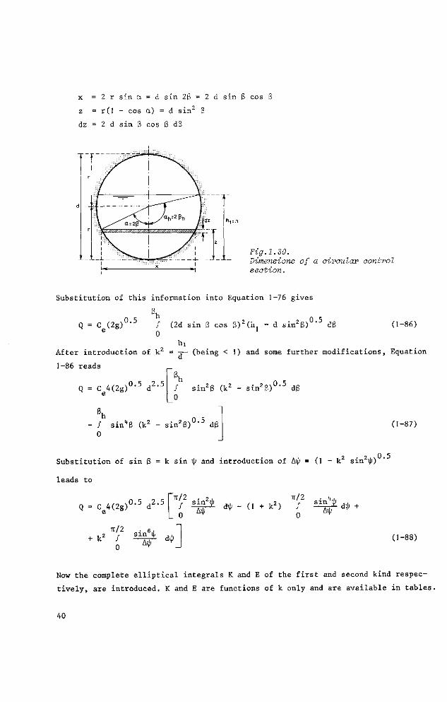
x = 2 r sin a = d sin 2ß = 2 d sin ß cos
z = r(l - cos a) = d sin2 ß
dz = 2 d sin 3 cos ß dß
h1 = h
Dimensions of a circular control section.
Substitution of this information into Equation 1-76 gives
ß h
Q = C ( 2 g ) 0 - 5 ƒ (2d sin ß cos ß)2(h - d sin2ß)°'5 dß (1-86) e 0
After introduction of k2 = -3— (being < 1) and some further modifications, Equation
1-86 reads
Q = Ce4(2g)°-5 d2 , 5 ƒ sin2ß (k2 - s i n 2 ß ) 0 - 5 dß 0
ƒ sin^ß (k2 - s i n 2 ß r - J dß 0
(1-87)
Substitution of sin ß = k sin if and introduction of Ai() = (1 - k2 sin2i|j)
leads to
„ , ,„ vO.5 ,2.5 Q = Ce4(2g) d 'ïï/2 . 2, TT/2 . i, ,
; - 1 d*-(. + k 2 ) / ^ d ^ +
fr/2 . 6 , di[) (1-88)
Now the complete elliptical integrals K and E of the first and second kind respec
tively, are introduced. K and E are functions of k only and are available in tables.
40
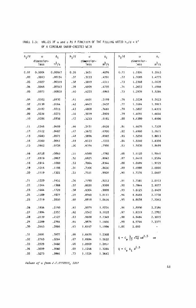
TABLE 1.3: VALUES OF u and $ AS A FUNCTION OF THE FILLING RATIO hj/d = k2
OF A CIRCULAR SHARP-CRESTED WEIR
y d
O.Ol
.02
.03
.04
.05
.06
.07
.08
.09
.10
.11
.12
.13
.14
.15
.16
.17
.18
.19
.20
.21
.22
.23
.24
.25
.26
.27
.28
.29
.30
.31
.32
.33
.34
.35
u dimension-
less
0.0004
.0013
.0027
.0046
.0071
.0102
.0139
.0182
.0231
.0286
.0346
.0412
.0483
.0560
.0642
.0728
.0819
.0914
.1014
.1119
.1229
.1344
.1464
.1589
.1719
.1854
.1994
.2139
.2289
.2443
.2601
.2763
.2929
.3099
.3273
*i
mJ/s
0.00047
.00154
.00319
.00543
.00839
.0120
.0164
.0215
.0273
.0338
.0409
.0487
.0571
.0661
.0758
.0860
.0967
.1080
.1198
.1322
.1452
.1588
.1729
.1877
.2030
.2190
.2355
.2527
.2704
.2886
.3072
.3264
.3460
.3660
.3866
h1/d
0.36
.37
.38
.39
.40
.41
.42
.43
.44
.45
.46
.47
.48
.49
.50
.51
.52
.53
.54
.55
.56
.57
.58
.59
.60
.61
.62
.63
.64
.65
.66
.67
.68
.69
.70
(j)
dimension-less
.3451
.3633
.3819
.4009
.4203
.4401
.4603
.4809
.5019
.5233
.5451
.5672
.5896
.6123
.6354
.6588
.6825
.7064
.7306
.7551
.7799
.8050
.8304
.8560
.8818
.9079
.9342
.9608
.9876
1.0147
1.0420
1.0694
1.0969
1.1246
1.1524
*i
mJ/s
.4076
.4291
.4511
.4735
.4965
.5199
.5437
.5681
.5929
.6182
.6439
.6700
.6965
.7233
.7506
.7782
.8062
.8344
.8630
.8920
.9212
.9509
.9809
1.0111
1.0416
1.0724
1.1035
1.1349
1.1666
1.1986
1.2308
1.2632
1.2957
1.3284
1.3612
hj/d
0.71
.72
.73
.74
.75
.76
.77
.78
.79
.80
.81
.82
.83
.84
.85
.86
.87
.88
.89
.90
.91
.92
.93
.94
.95
.96
.97
.98
.99
1.00
Q = c e
Q = Ce
CO
dimension-less
1.1804
1.2085
1.2368
1.2653
1.2939
1.3226
1.3514
1.3802
1.4091
1.4380
1.4670
1.4960
1.5250
1.5540
1.5830
1.6120
1.6410
1.6699
1.6988
1.7276
1.7561
1.7844
1.8125
1.8403
1.8678
1.8950
1.9219
1.9484
1.9744
2.000
4 *r- ,2.5 -pr- /2g cod
A J2-5
•i
ra'/s
1.3943
1.4275
1.4609
1.4946
1.5284
1.5623
1.5963
1.6303
1.6644
1.6986
1.7328
1.7671
1.8013
1.8356
1.8699
1.9041
1 .9384
1.9725
2.0066
2.0407
2.0743
2.1077
2.1409
2.1738
2.2063
2.2384
2.2702
2.3015
2.3322
-
or
Values of to from J.C.STEVENS, 1957 41
îr/2 = ƒ
0
TT/2
= ƒ 0
dij; AIJJ
AIJJ dii
(1-89)
(1-90)
For the separate integrals of Equation 1-88 the following general reduction
formula can be derived (n being an arbitrary even number):
TT/2 . n, „ 2 TT/2 . n-2, . , TT/2 . n-4. ƒ "n! = 2l2Ü*_ ƒ Ü B * # _ El3 i_ ƒ ! i * 4 d (,-91) 0 A * n H k2 0 A * n H k2 0 A *
Combinations of Equations 1-88, 1-89, 1-90, and 1-91 gives
Q = Ce Ï5 ( 2 S ) 0 ' 5 d 2 ' 5 { 2 ( ' - k2 + k"*) E - (2 - 3k2 + k") K> (1-92)
Q - Ce }5(2g)°-5 d2-5 U - ce *. d2-5 ^
Equation 1-93 was first obtained by A.Staus and K.von Sanden in 1926.
Values of ÙJ = {2(1 - k2 + k"*) E - (2 - 3k2 + k"*) K} and of <f>. = jy(2g)°-5 0)
are presented in Table 1.3.
1.13.7 Sharp-crested proportional weir
A proportional weir is defined as a weir in which the discharge is linearly pro
portional to the head over the weir crest. In other words, the control section
over a proportional weir is shaped in such a way that the sensitivity of the
weir
f^=,.0 (1-94)
In order to satisfy this identity the curved portion of the weir profile must sa
tisfy the relation x = cz ' (c is a constant), so that the theoretical head-
discharge equation, according to Equation 1-76, reads
42
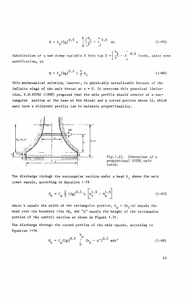
Q = C (2g)0-5 c ƒ O
0.5 dz
Substitution of a new dummy variable f3 into tan
modification, to 4' - ï
0.5
(1-95)
leads . after some
Q = Ce(2g)°-5 c f h , (1-96)
This mathematical solution, however, is physically unrealizable because of the
infinite wings of the weir throat at z = 0. To overcome this practical limita
tion, H.H.SUTRO (1908) proposed that the weir profile should consist of a rec
tangular portion at the base of the throat and a curved portion above it, which
must have a different profile law to maintain proportionality.
h,=h
Fig.1.31. Dimensions of a proportional SUTRO weir notch.
The discharge through the rectangular section under a head hr above the weir
crest equals, according to Equation 1-78
? 0 5 Q r = C e f (2g)°-5b h 1
, - 5 - h 1 - 5
1 o (1-97)
where b equals the width of the rectangular portion, h = (h.-a) equals the
head over the boundary line CD, and "a" equals the height of the rectangular
portion of the control section as shown in Figure 1.31.
The discharge through the curved portion of the weir equals, according to
Equation 1-76
Q = C (2g)0-5 ƒ (h - z ' ) 0 , 5 xdz' c e 0 °
(1-98)
43
Thus the total discharge through the weir equals
Q = Qr + Qc = ce(2g)0-5
h 0 0 5
+ ƒ (h - z') ' xdz' 0 °
2 , /,1.5 , 1 .5 \ 3 b l h l " h o )
(1-99)
The discharge through the weir must be proportional to the head above an arbitra
rily chosen reference level situated in the rectangular portion of the weir. The
reference level AB is selected at a distance of one-third of the rectangular
portion above the weir crest to facilitate further calculations. So the total
discharge through the weir also reads
Q = KChj - a/3) (1-100)
where K is a weir constant.
Since proportionality is valid for heads equal to or above the boundary line CD,
must hold also if
99 and 1-100 gives
it must hold also if h = 0 . Substitution of h = 0 and h, = a into Equations o o 1
Q = Ce I (2g)0-5 ba1-5 and
Q = | Ka
Consequently the weir constant equals
K = C b (2ga)°-5 (1-101)
Substitution of the latter equation into Equation 1-100 gives
Q = Ce (2ga)°-5 b(h, - a/3) (1-102)
as a head-discharge equation.
The relationship between x and z' for the curved position of the weir can be
obtained from the condition that Equations 1-99 and 1-102 should be equal to
each other, thus
44
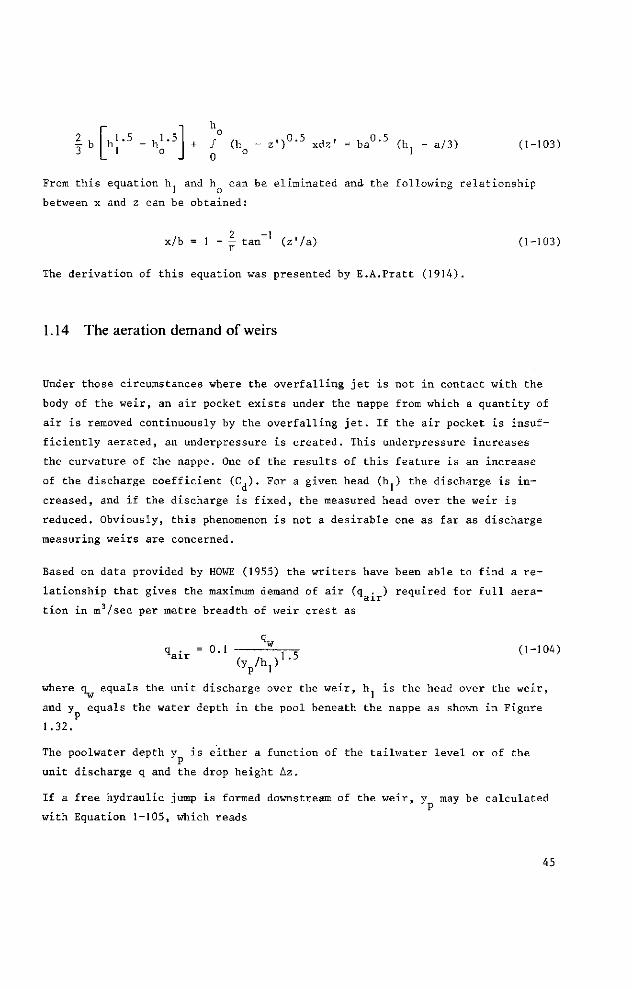
f ' J - 5 J - 5
h, - h 1 o
h
+ ƒ (h - z')°-5 xdz' = ba0-5 (h - a/3) (1-103) 0 °
From this equation h and h can be eliminated and the following relationship
between x and z can be obtained:
x/b = 1 - tan"1 (z'/a) (1-103)
The derivation of this equation was presented by E.A.Pratt (1914).
1.14 The aeration demand of weirs
Under those circumstances where the overfailing jet is not in contact with the
body of the weir, an air pocket exists under the nappe from which a quantity of
air is removed continuously by the overfailing jet. If the air pocket is insuf
ficiently aerated, an underpressure is created. This underpressure increases
the curvature of the nappe. One of the results of this feature is an increase
of the discharge coefficient (C,). For a given head (h ) the discharge is in
creased, and if the discharge is fixed, the measured head over the weir is
reduced. Obviously, this phenomenon is not a desirable one as far as discharge
measuring weirs are concerned.
Based on data provided by HOWE (1955) the writers have been able to find a re
lationship that gives the maximum demand of air (q . ) required for full aera
tion in m3/sec per metre breadth of weir crest as
l a i r 0 0 " 1 ^ T T ( 1-, 0 4 )
where q equals the unit discharge over the weir, h is the head over the weir,
and y equals the water depth in the pool beneath the nappe as shown in Figure
1.32.
The poolwater depth y is either a function of the tailwater level or of the
unit discharge q and the drop height Az.
If a free hydraulic jump is forme
with Equation 1-105, which reads
If a free hydraulic jump is formed downstream of the weir, y may be calculated
45
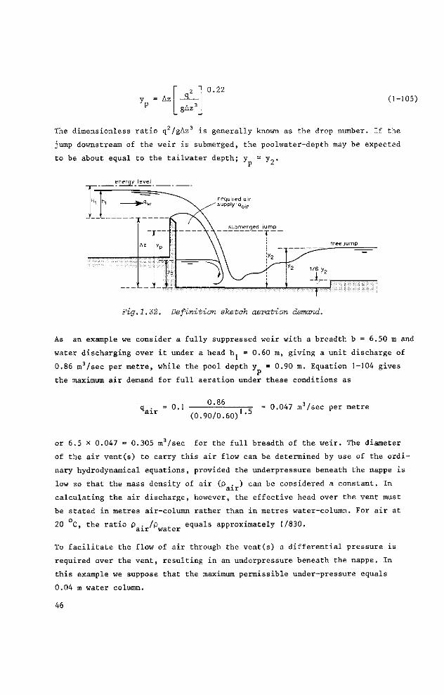
y = Az P gAz'
0.22 (1-105)
The dimensionless ratio q2/gAz3 is generally known as the drop number. If the
jump downstream of the weir is submerged, the poolwater-depth may be expected
to be about equal to the tailwater depth; y ~ y„.
energy teve)
Fig.1.32. Definition sketch aeration demand.
As an example we consider a fully suppressed weir with a breadth b = 6.50 m and
water discharging over it under a head h, = 0.60 m, giving a unit discharge of
0.86 m3/sec per metre, while the pool depth y = 0.90 m. Equation 1-104 gives
the maximum air demand for full aeration under these conditions as
0.86
(0.90/0.60) 1.5 = 0.047 m3/sec per metre
or 6.5 x 0.047 = 0.305 m3/sec for the full breadth of the weir. The diameter
of the air vent(s) to carry this air flow can be determined by use of the ordi
nary hydrodynamical equations, provided the underpressure beneath the nappe is
low so that the mass density of air (p . ) can be considered a constant. In air
calculating the air discharge, however, the effective head over the vent must be stated in metres air-column rather than in metres water-column. For air at
20 C, the ratio p . /p ,_ equals approximately 1/830. ' rair Kwater M r r J
To facilitate the flow of air through the vent(s) a differential pressure is
required over the vent, resulting in an underpressure beneath the nappe. In
this example we suppose that the maximum permissible under-pressure equals
0.04 m water column.
46
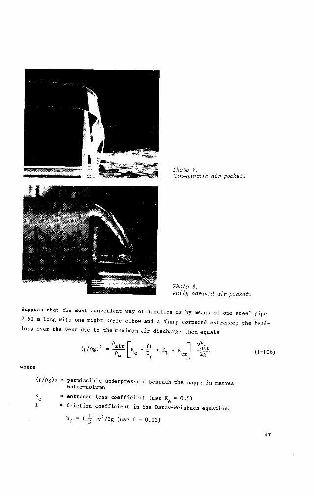
Photo S. Non-aerated air pocket.
Photo 6. Fully aerated air pocket.
Suppose that the most convenient way of aeration is by means of one steel pipe
2.50 m long with one-right angle elbow and a sharp cornered entrance; the head-
loss over the vent due to the maximum air discharge then equals
2
(P/Pg)2 = W _
K + |t + K, + K e D TJ ex
air 2g
where
(p/pgh - permissible underpressure beneath the nappe in metres water-column
K - entrance loss coefficient (use K = 0.5)
= friction coefficient in the Darcy-Weisbach equation;
f jj vz/2g (use f 0.02)
(1-106)
47
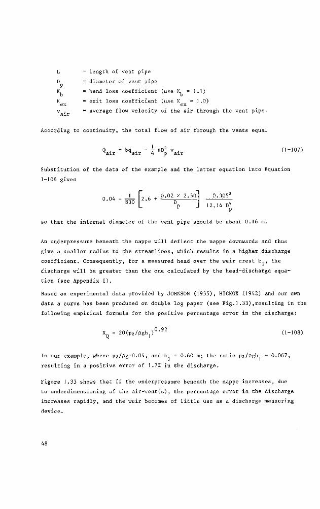
L = length of vent pipe
D = diameter of vent pipe P
]L = bend loss coefficient (use K, = 1.1)
K = exit loss coefficient (use K = 1 .0) ex ex
v . = average flow velocity of the air through the vent pipe, air
According to continuity, the total flow of air through the vents equal
Q . = bq . = j- TTD2 v . (1-107) air ^air 4 p air
Substitution of the data of the example and the latter equation into Equation
1-106 gives
0.04=4 „ , 0.02 x 2.50 z. b + D
P P
so that the internal diameter of the vent pipe should be about 0.16 m.
An underpressure beneath the nappe will deflect the nappe downwards and thus
give a smaller radius to the streamlines, which results in a higher discharge
coefficient. Consequently, for a measured head over the weir crest h , the
discharge will be greater than the one calculated by the head-discharge equa
tion (see Appendix I).
Based on experimental data provided by JOHNSON (1935), HICKOX (1942) and our own
data a curve has been produced on double log paper (see Fig.1.33)»resulting in the
following empirical formula for the positive percentage error in the discharge:
XQ = 20(p2/pgh1)°-92 (1-108)
In our example, where p2/pg=0.04, and h = 0.60 m; the ratio p2/pgh = 0.067,
resulting in a positive error of 1.1% in the discharge.
Figure 1.33 shows that if the underpressure beneath the nappe increases, due
to underdimensioning of the air-vent(s), the percentage error in the discharge
increases rapidly, and the weir becomes of little use as a discharge measuring
device.
48
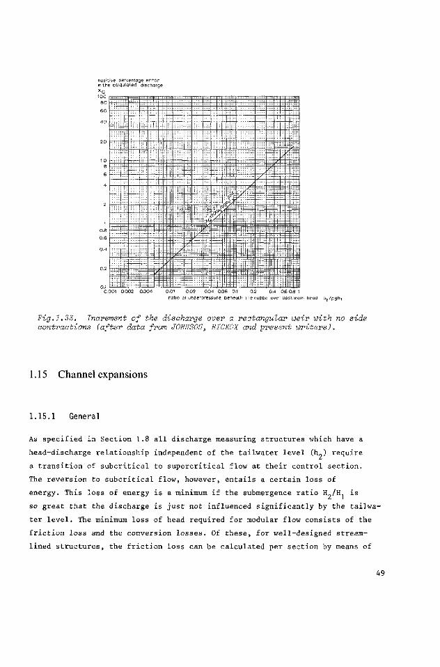
positive percentage e r r o r in the calqulQted discharge
0.8
0.6
...=î
-•• : äf
"H: Fl"
: : : : M l
::::!:! i i i iÜ i !;::!::
t-^ü-
ÜHp
j . i i r i f j ^ ^ : ± T
. { ; ] 1 !
^^=
l i l i i
• - • -
: : i : :
= — 4-:::
—
—
Uü
::::
— :::-.
.__
r f ; 1 ;.
i . : r
Ë —
= i:
zi^m . . ... :.:: . ,|....
: 1 Mi:
-Tr . . .
l ; . . : :
h l i i j
i l ! i i : i i i i f i
- - i - O i i
. , .~.
! • • [
!:i|
I üf pit
f i -
v ^ H * ^ r z r r r j : : : :
==i=nüË= : T : M . — —
i i : i
fill
|*-J
=^4-
-— ==
— •
. ,
!':; il
"Ü dJ
TH-
te — ; i ~
ipi
~
/: : ^ T i ( i-^-
— — T
ir*|
-•tl
j •
.., ....1.
: r --j>f-
IEJ -TÄ
i ' l i r r t o
1-^"" 1"
r^H t 'M* k&W ih-^Tti
_../.. zzrl.l'-':
- -:: ; E "; ï~
i-i-44
+-MI
*t-jr ttl 4# HI
-/-
:!.-
^ ^,-1-
•k
Iff1
P
; : L
: :-
----- • !___ _ . t _ : _ " fËffi
- • :
— - • - -
ff I I _ - . _ Z
J Î Ï
• • — r
=F_±
~ i . .
1 i - i ii-i n
- t r
• -J
z¥ : : ; •
—
:-. ~~zi
:z
l~l
rll ï|[ T + t - ü
4 0.001 0.002 0.004 0.01 0.02 0.04 0.06 0.1 0.2 0.4 0.6 0.8 1 ratio of underpressure Deneath the nappe over upstream bead p . / ngh .
Fig.1.S3. Increment of the discharge over a rectangular weir with no side contractions (after data from JOHNSON, HICKOX and present writers).
1.15 Channel expansions
1.15.1 General
As specified in Section 1.8 all discharge measuring structures which have a
head-discharge relationship independent of the tailwater level (h„) require
a transition of subcritical to supercritical flow at their control section.
The reversion to subcritical flow, however, entails a certain loss of
energy. This loss of energy is a minimum if the submergence ratio H /H is
so great that the discharge is just not influenced significantly by the tailwa
ter level. The minimum loss of head required for modular flow consists of the
friction loss and the conversion losses. Of these, for well-designed stream
lined structures, the friction loss can be calculated per section by means of
49
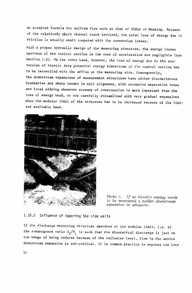
an accepted formula for uniform flow such as that of Chézy or Manning. Because
of the relatively short channel reach involved, the total loss of energy due to
friction is usually small compared with the conversion losses.
With a proper hydraulic design of the measuring structure, the energy losses
upstream of the control section in the zone of acceleration are negligible (see
Section 1.6). On the other hand, however, the loss of energy due to the con
version of kinetic into potential energy downstream of the control section has
to be reconciled with the afflux at the measuring site. Consequently,
the downstream expansions of measurement structures have either discontinuous
boundaries and sharp breaks in wall alignment, with extensive separation zones
and local eddying whenever economy of construction is more important than the
loss of energy head, or are carefully streamlined with very gradual expansions
when the modular limit of the structure has to be increased because of the limi
ted available head.
Photo 7. If no kinetic energy needs to be recovered a sudden downstream expansion is adequate.
1.15.2 Influence of tapering the side walls
If the discharge measuring structure operates at its modular limit, i.e. if
the submergence ratio I^/Hj is such that the theoretical discharge is just on
the verge of being reduced because of the tailwater level, flow in the entire
downstream expansion is sub-critical. It is common practice to express the los
50
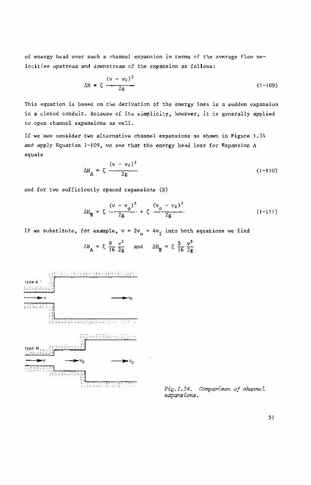
of energy head over such a channel expansion in terms of the average flow ve
locities upstream and downstream of the expansion as follows:
(v - v 2 ) 2
AH = £ 2g
(1-109)
This equation is based on the derivation of the energy loss in a sudden expansion
in a closed conduit. Because of its simplicity, however, it is generally applied
to open channel expansions as well.
If we now consider two alternative channel expansions as shown in Figure 1.34
and apply Equation 1-109, we see that the energy head loss for Expansion A
equals
(v - v2)< A H A = Ç
2g (1-110)
and for two sufficiently spaced expansions (B)
(v - v ) 2 (v - v 2 ) 2
(1 -111)
If we substitute, for example, v = 2v = 4v„ into both equations we find
AH. 16 2g
and AH. B
5_ vj_ 16 2g
type A
-v2
type B
->-v,
Fig.1.34. Comparison of channel expansions.
51
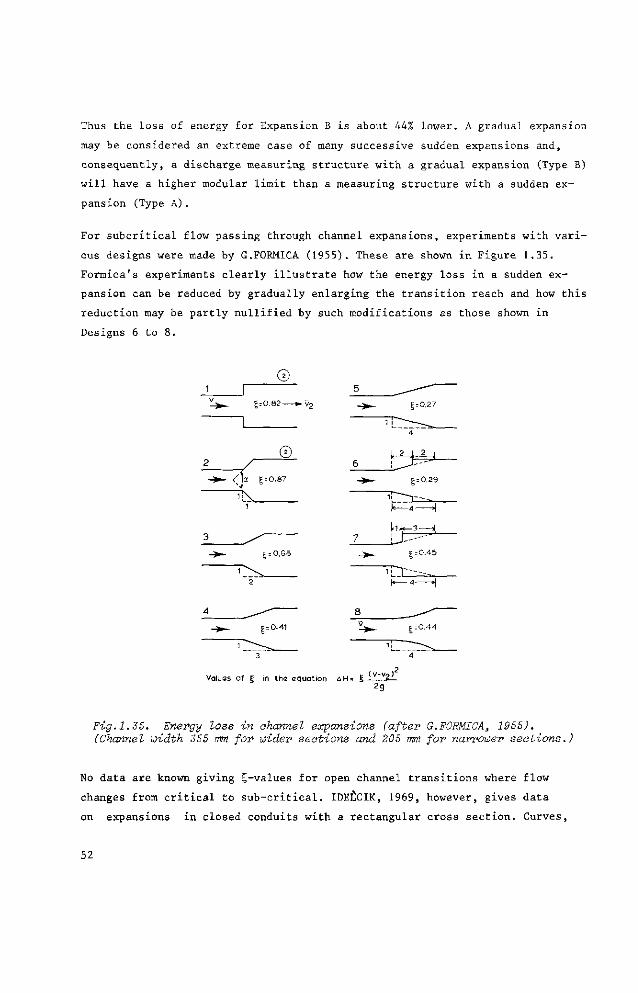
Thus the loss of energy for Expansion B is about 44% lower. A gradual expansion
may be considered an extreme case of many successive sudden expansions and,
consequently, a discharge measuring structure with a gradual expansion (Type B)
will have a higher modular limit than a measuring structure with a sudden ex
pansion (Type A ) .
For subcritical flow passing through channel expansions, experiments with vari
ous designs were made by G.FORMICA (1955). These are shown in Figure 1.35.
Formica's experiments clearly illustrate how the energy loss in a sudden ex
pansion can be reduced by gradually enlarging the transition reach and how this
reduction may be partly nullified by such modifications as those shown in
Designs 6 to 8.
© 1 r~
l_
^ 1N_
1
3 ^
Vï> 2
4 .
1 [""•-•
= 0.82
© g = 0.87
g r. 0.68
|=0.41
•v2
5
6
7
8
| = 0.27
1 I _ 4
I, 2 I 2 j
5 = 0.29
11 —t - - ^
h J ^ 3 — * |
iJ---" g =0.45
T Ï - T - - -
g = 0.44
li " \
Values of g in the equation ûH= I (v-v2)
2g
Fig.1.35. Energy loss in channel expansions (after G.FORMICA, 1955). (Channel width. 355 mm for wider sections and 205 mm for narrower sections.)
No data are known giving Ç-values for open channel transitions where flow
changes from critical to sub-critical. IDEÈCIK, 1969, however, gives data
on expansions in closed conduits with a rectangular cross section. Curves,
52
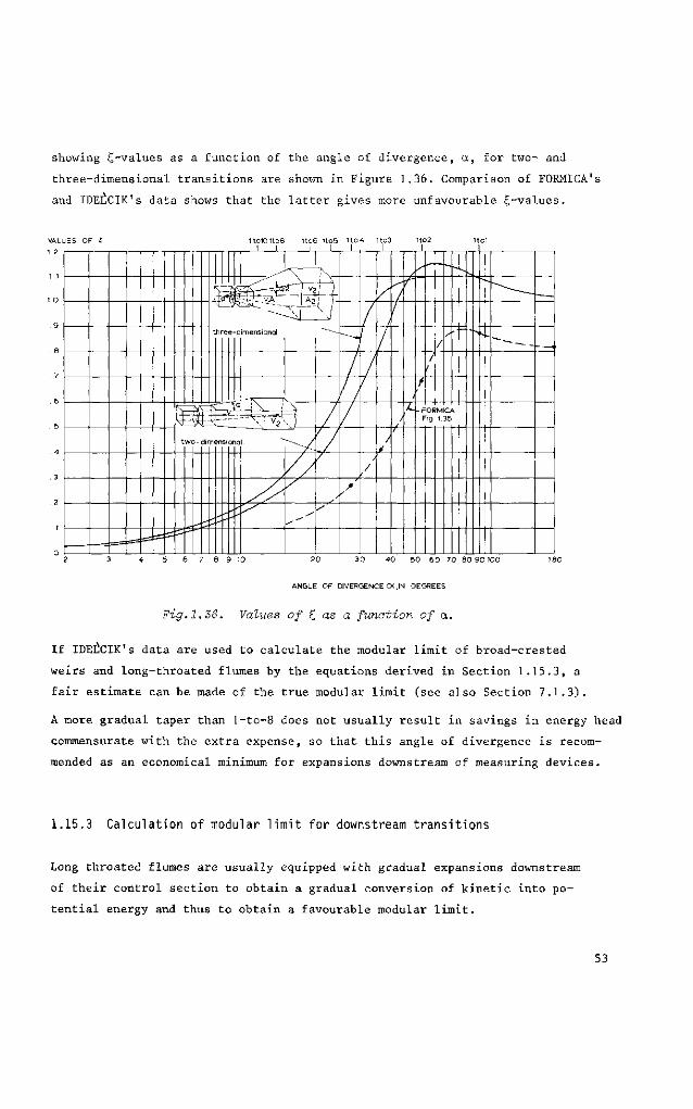
showing Ç-values as a function of the angle of divergence, a, for two- and
three-dimensional transitions are shown in Figure 1.36. Comparison of FORMICA's
and IDELCIK's data shows that the latter gives more unfavourable Ç-values.
VALUES OF S
.
3
1to101to8 I I
1toE
" ] \
"^^|~^2
« 0 5 I
N
ft "-^~--^s£y th
^ IN
30 t w i-dia en
ee dimensional
" ~ 4 a ' \ «' • Y _ . _ _ j ; _ .
sior
: v2V)
al ~~~^~~--~~Y
/ /
^ ,
y
1to4 I
/
/ u 7 y
/
to3 I
/
/
/ \
/
, L
ito2 I
/ 1
/ / /•
-FORMICA Fig 1.35
n Ol
------ _ _
4 5 6 7 8 9 10 3 0 4 0 5 0 6 0 70 8 0 9 0 100
ANGLE OF DIVERGENCE CX,IN DEGREES
Fig.1.26. Values of Ç as a function of a.
If IDEÜCIK's data are used to calculate the modular limit of broad-crested
weirs and long-throated flumes by the equations derived in Section 1.15.3, a
fair estimate can be made of the true modular limit (see also Section 7.1.3).
A more gradual taper than l-to-8 does not usually result in savings in energy head
commensurate with the extra expense, so that this angle of divergence is recom
mended as an economical minimum for expansions downstream of measuring devices.
1.15.3 Calculation of modular limit for downstream transitions
Long throated flumes are usually equipped with gradual expansions downstream
of their control section to obtain a gradual conversion of kinetic into po
tential energy and thus to obtain a favourable modular limit.
53
As shown in Section 1.9 the head discharge relationship of a long-throated flume
can be written as
Q = constant C, bu" (1-112)
In this equation C, is a coefficient which corrects for deviations from the
assumptions that the upstream energy head U] would be equal to the energy head,
H, at the control section and that the streamlines at the control are straight
and parallel. For heads which are low with resjSect to the throat length
(0.10 -S H./L •£ 0.33) we may safely assume, however, that the C -value is mainly
influenced by the first assumption so that replacement of H by H in Equation
1-112 results in
Q = constant bHU (1-113)
Combination of the Equations 1-112 and 1-113 gives
H , ^ " = H or, (1-114)
H. - H = H.(l - c'/u) (1-115) 1 1 d
being an approximate expression for the loss of energy head between the head
measurement station and the control section.
Downstream of the control section the loss of energy head may be expressed by
(v - v 2 ) 2
H - H 2 = £ ^ + AH (1-116)
where AH denotes the loss of energy head over the downstream transition due to
friction.
Substitution of Equation 1-114 into Equation 1-116 gives after some transforma
tion
H 2 , (v - v 2 ) 2 AH
Ê7 - Cd - 5 -2gHi -Hf" (1-,,7)
Equation 1-117 is an expression for the modular limit of a long-throated flume
or broad-crested weir (C, < 1). To obtain modular flow obviously
54
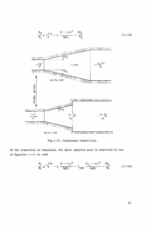
? « cl'" - E (v - v 2 ) 2 AH,
2gH, ( 1 -118)
* . A
use Eq 1-118
use Eq ,1-119
V2 .A2
H 2
Fig.1.37. Downstream transitions.
If the transition is truncated, the above equation must be rewritten by use
of Equation 1-111 to read
H, l/u « d
<v - V ' 2gHi
(v - v 2 )' o
'180 2gHi
AH (1-119)
55
1.16 Selected list of literature
1. BASIN, H.E.: Experiments nouvelles sur l'écoulement en déversoir.
Annales des Ponts et Chaussées. Vol.7, 1896, pp.249-357.
2. CARLIER, M.: Hydraulique générale et appliquée.
Collection du Centre de recherches et d'essais de Chatou. Eyrolles, Paris, 1972.
3. FORMICA, G.: Esperienze preliminari sulle perdite di carico nei canali,
dovute a cambiamenti di sezione.
L'Energia elettrica. Milano, Vol.32, No.7. pp.554-568. July 1955.
4. HENDERSON, F.M.: Open channel flow. The Macmillan Company, New York,1966.
5. HICKOX, G.H.: Aeration of spillways. Transactions of the American
Society of Civil Engineers. Vol.109, pp.537-556. 1944.
6. HOWE, J.W., SHIEH, G.C. and OBADIA, A.O.: Aeration demand of a weir
calculated. Civil Engineering Vol.25, No.5, p.289. 1955. Easton, Pa. & Personal
Communication, 1972 (HOWE).
7. IDELCIK, I.E.: Memento des pertes de charge. Coll.du Centre de re
cherche et d'essais de Chatou. Eyrolles, Paris, 1969. (Transi.from Russian.)
8. KING, H.W. and BRATER, E.F.: Handbook of hydiaulics. 5° Edition.
McGraw-Hill Book Comp :
9. KNAPP, F.H.: Ausfluss, Überfall und Durchfluss im Wasserbau.
Verl.G.Braun, Karlsruhe, 1960.
10. PRATT, E.A.: Another proportional-flow weir; Sutro weir.
Engineering News, Vol.72, No.9, p.462. August 1914.
11. ROUSE, H.: Fluid Mechanics for hydraulic engineers.
Dover Publications, Inc. New York, 1938. Reprint 1961.
12. ROUSE, H.: Engineering Hydraulics. John Wiley & Sons, Inc., New York,
1950, Fourth printing 1964.
13. SCIMINI, E.: Sulla forme delle vene tracimani. L'Energia elettrica,
Milano, Vol.7, No.4, pp.293-305. April 1930.
14. STEVENS, J.C.: Flow through circular weirs. J.of the Hydraulics Division
of the American Society of Civil Engineers, Vol.83,No.HY 6, Dec.1957, Paper 1455.
15. VEN TE CHOW:Open-channel hydraulics.Mcgraw-Hill Book Comp.New York,1959.
56
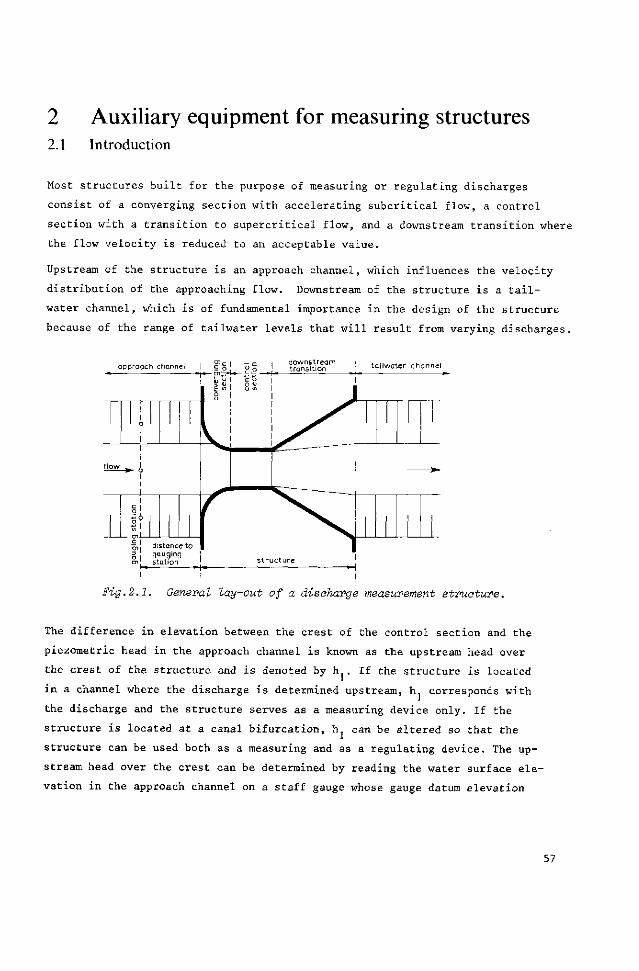
2 Auxiliary equipment for measuring structures 2.1 Introduction
Most structures built for the purpose of measuring or regulating discharges
consist of a converging section with accelerating subcritical flow, a control
section with a transition to supercritical flow, and a downstream transition where
the flow velocity is reduced to an acceptable value.
Upstream of the structure is an approach channel, which influences the velocity
distribution of the approaching flow. Downstream of the structure is a tail-
water channel, which is of fundamental importance in the design of the structure
because of the range of tailwater levels that will result from varying discharges.
approach channel j ç g I Ä Y c f r T ! f ^ e r chanhel
Fig.2.1. General lay-out of a discharge measurement structure.
The difference in elevation between the crest of the control section and the
piezometric head in the approach channel is known as the upstream head over
the crest of the structure and is denoted by h1. If the structure is located
in a channel where the discharge is determined upstream, h, corresponds with
the discharge and the structure serves as a measuring device only. If the
structure is located at a canal bifurcation, h. can be altered so that the
structure can be used both as a measuring and as a regulating device. The up
stream head over the crest can be determined by reading the water surface ele
vation in the approach channel on a staff gauge whose gauge datum elevation
57
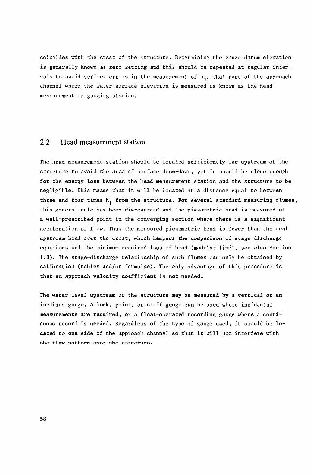
coincides with the crest of the structure. Determining the gauge datum elevation
is generally known as zero-setting and this should be repeated at regular inter
vals to avoid serious errors in the measurement of h . That part of the approach
channel where the water surface elevation is measured is known as the head
measurement or gauging station.
2.2 Head measurement station
The head measurement station should be located sufficiently far upstream of the
structure to avoid the area of surface draw-down, yet it should be close enough
for the energy loss between the head measurement station and the structure to be
negligible. This means that it will be located at a distance equal to between
three and four times h from the structure. For several standard measuring flumes,
this general rule has been disregarded and the piezometric head is measured at
a well-prescribed point in the converging section where there is a significant
acceleration of flow. Thus the measured piezometric head is lower than the real
upstream head over the crest, which hampers the comparison of stage-discharge
equations and the minimum required loss of head (modular limit, see also Section
1.8). The stage-discharge relationship of such flumes can only be obtained by
calibration (tables and/or formulae). The only advantage of this procedure is
that an approach velocity coefficient is not needed.
The water level upstream of the structure may be measured by a vertical or an
inclined gauge. A hook, point, or staff gauge can be used where incidental
measurements are required, or a float-operated recording gauge where a conti
nuous record is needed. Regardless of the type of gauge used, it should be lo
cated to one side of the approach channel so that it will not interfere with
the flow pattern over the structure.
58
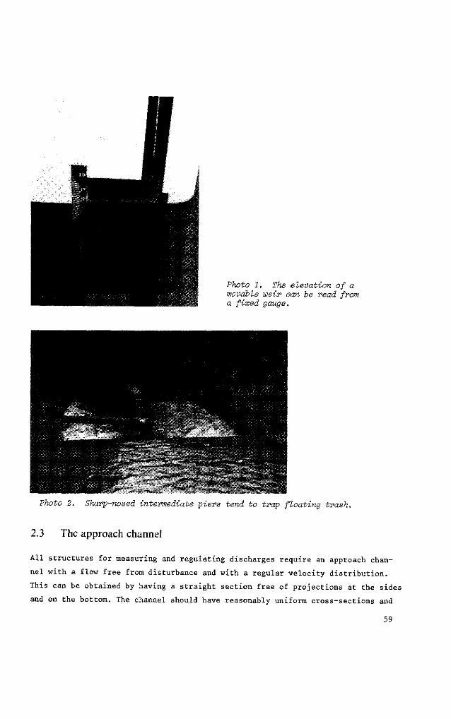
Photo 1. The elevation of a movable weir can be read from a fixed gauge.
&£&&•& - •"•--"• ".' "•-• y~-Photo 2. Sharp-nosed intermediate piers tend to trap floating trash.
2.3 The approach channel
All structures for measuring and regulating discharges require an approach chan
nel with a flow free from disturbance and with a regular velocity distribution.
This can be obtained by having a straight section free of projections at the sides
and on the bottom. The channel should have reasonably uniform cross-sections and
59
be straight for a length equal to approximately 10 times its average width,
provided that the breadth of the control section is equal to or greater than half
the width of the approach channel. If the breadth of the control section is less
than this, the length of the approach channel, should be at least 20 times the
breadth of the control section. In canals that carry no debris, the
desired flow conditions can be provided by suitably placed baffles formed by
vertical vanes or laths. These baffles should not be located nearer to the head
measurement station than 10 times h .
If super-critical flow occurs upstream of the structure, a hydraulic jump should
be introduced to ensure a regular velocity distribution at the head measurement
station. This jump should be located at a distance of not less than 30 times
h from the structure.
In cases where the entry to the converging section is through a bend, where the
approach channel is too short, or where a hydraulic jump occurs within the dis
tance mentioned above, either the approach channel must be modified or the struc
ture must be calibrated in situ, for example by use of the velocity-area method
or salt dilution method.
2.4 Tailwater level
The difference between the water level immediately below the downstream transi
tion (tailwater level) and the elevation of the crest of the structure is known
as the downstream head over the crest and is denoted by h„. Tailwater level,
and thus the submergence ratio h„/h , is affected by the hydraulic properties
of the tailwater channel and by the occurrence of transitions in that channel.
The measuring structure should be so designed that modular flow is maintained
under all operating conditions. If there is only a limited head loss available,
both the elevation of the crest in relation to the downstream energy level and
the length and shape of the downstream transition should be selected in such a
way that modular flow is ensured (see also Section 1.15).
If the tailwater channel is relatively wide or if the tailwater level is
affected by a downstream structure, it may occur that the measuring structure
is modular at its maximum design capacity, but non-modular with lesser discharges.
Under such circumstances a decrease in the upstream head means an increase in
the submergence ratio h„/h . The crest of the control section should then be
60
raised so that h„, and thus the ratio h./h , decreases to below the modular limit.
If the measuring structure is modular over its entire operating range, it is not
necessary to make tailwater measurements (see Section 1.8). If the flow conditions
are non-modular, however, both h and h„ must be recorded to allow the discharge
to be calculated. The tailwater level should be measured immediately downstream
of the deceleration transiLion where normal channel velocities occur. The equip
ment to be used for this purpose may be the same as that used for measuring the
upstream water level or it may be of a lower accuracy, and thus more simple,
depending on the frequency with which submerged flow occurs (see also Section
2.12).
It is evident that collecting and handling two sets of data per measuring structure
is an expensive and time-consuming enterprise, which should be avoided as much as
possible. Other even more important reasons for applying a modular structure are
that in an irrigation canal system a water user with his own canal inlet cannot
increase the discharge by lowering the tailwater level while, on the other hand,
all persons concerned have a simple way of checking whether they receive their
proper share of the available water.
2.5 Staff gauge
Where no detailed information on the discharge is needed or in stream channels
where the flow fluctuation is gradual, periodic readings on a calibrated staff
gauge may provide adequate data. A staff gauge should also be provided if the
head is registered by a float-operated recorder as it will enable comparison
of the outside water level with the head in the float well.
Supports for the staff gauge should not interfere with the flow pattern in the
structure, and should be independent of the stilling well. Most permanent gauges
are plates of enamelled steel, cast aluminium, or polyester, bolted or screwed
in sections to a timber or steel pole. A typical gauge is shown in Figure 2.2.
The gauge should be placed in such a manner that the water level can be read from
the canal bank. Care should be taken that the staff gauge is firmly secured.The
following type of support has proved satisfactory for permanent installations: a
section of 180 mm channel iron is embedded about 0.50 m in a concrete block and
extended above the block to the maximum height required. The concrete block should
extend well below the maximum expected frost penetration and at least 0.60 m
61
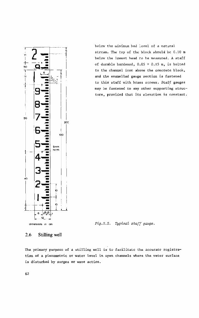
below the minimum bed level of a natural
stream. The top of the block should be 0.10 m
below the lowest head to be measured. A staff
of durable hardwood, 0.05 x 0.15 m, is bolted
to the channel iron above the concrete block,
and the enamelled gauge section is fastened
to this staff with brass screws. Staff gauges
may be fastened to any other supporting struc
ture, provided that its elevation is constant.
dimensions in cm Fig.2.2. Typical staff gauge.
2.6 Stilling well
The primary purpose of a stilling well is to facilitate the accurate registra
tion of a piezometric or water level in open channels where the water surface
is disturbed by surges or wave action.
62
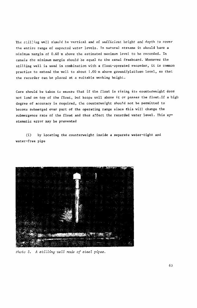
The stilling well should be vertical and of sufficient height and depth to cover
the entire range of expected water levels. In natural streams it should have a
minimum margin of 0.60 m above the estimated maximum level to be recorded. In
canals the minimum margin should be equal to the canal freeboard. Whenever the
stilling well is used in combination with a float-operated recorder, it is common
practice to extend the well to about 1.00 m above ground/platform level, so that
the recorder can be placed at a suitable working height.
Care should be taken to ensure that if the float is rising its counterweight does
not land on top of the float, but keeps well above it or passes the float.If a high
degree of accuracy is required, the counterweight should not be permitted to
become submerged over part of the operating range since this will change the
submergence rate of the float and thus affect the recorded water level. This sy
stematic error may be prevented
(i) by locating the counterweight inside a separate water-tight and
water-free pipe
Photo 3. A stilling well made of steel pipes.
63
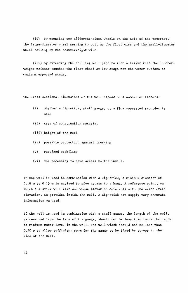
(ii) by mounting two different-sized wheels on the axle of the recorder,
the large-diameter wheel serving to coil up the float wire and the small-diameter
wheel coiling up the counterweight wire
(iii) by extending the stilling well pipe to such a height that the counter
weight neither touches the float wheel at low stage nor the water surface at
maximum expected stage.
The cross-sectional dimensions of the well depend on a number of factors:
(i) whether a dip-stick, staff gauge, or a float-operated recorder is
used
(ii) type of construction material
(iii) height of the well
(iv) possible protection against freezing
(v) required stability
(vi) the necessity to have access to the inside.
If the well is used in combination with a dip-stick, a minimum diameter of
0.10 m to 0.15 m is advised to give access to a hand. A reference point, on
which the stick will rest and whose elevation coincides with the exact crest
elevation, is provided inside the well. A dip-stick can supply very accurate
information on head.
If the well is used in combination with a staff gauge, the length of the well,
as measured from the face of the gauge, should not be less than twice the depth
to minimum water level in the well. The well width should not be less than
0.20 m to allow sufficient room for the gauge to be fixed by screws to the
side of the well.
64
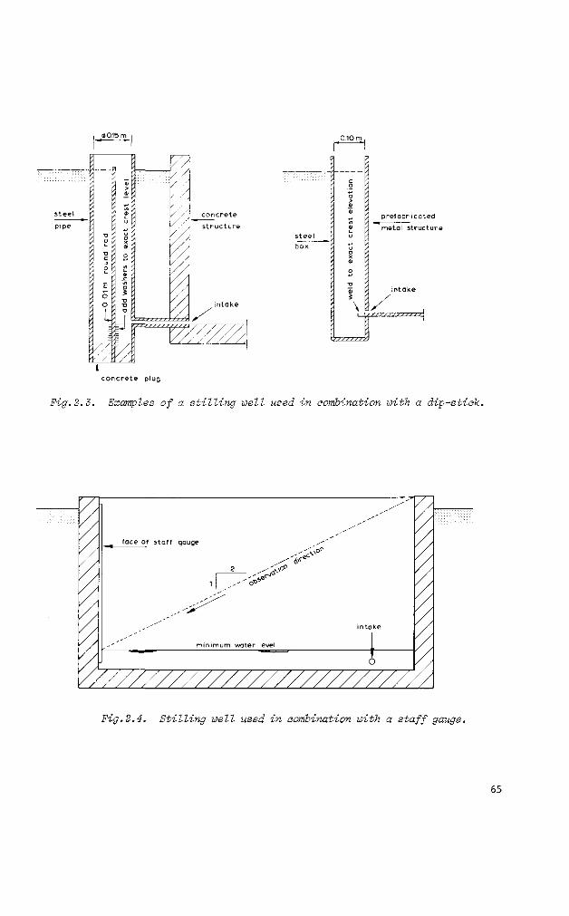
4015 m
steel pipe V
£ V s
u .=--i-v-7-7j / / / /?•
s t ructure
concrete plug
steel box
prefabr icated metal structure
rryrssv/////\
Fig.2.3. Examples of a stilling well used in combination with a dip-stick.
Fig.2.4, Stilling well used in combination with a staff gauge.
65
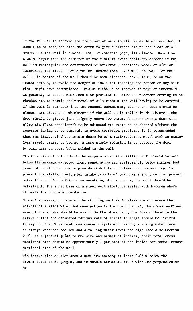
If the well is to accommodate the float of an automatic water level recorder, it
should be of adequate size and depth to give clearance around the float at all
stages. If the well is a metal, PVC, or concrete pipe, its diameter should be
0.06 m larger than the diameter of the float to avoid capillary effect; if the
well is rectangular and constructed of brickwork, concrete, wood, or similar
materials, the float should not be nearer than 0.08 m to the wall of the
well. The bottom of the well should be some distance, say 0.15 m, below the
lowest intake, to avoid the danger of the float touching the bottom or any silt
that might have accumulated. This silt should be removed at regular intervals.
In general, an access door should be provided to allow the recorder setting to be
checked and to permit the removal of silt without the well having to be entered.
If the well is set back into the channel embankment, the access door should be
placed just above the embankment; if the well is installed in the channel, the
door should be placed just slightly above low water. A second access door will
allow the float tape length to be adjusted and gears to be changed without the
recorder having to be removed. To avoid corrosion problems, it is recommended
that the hinges of these access doors be of a rust-resistant metal such as stain
less steel, brass, or bronze. A more simple solution is to support the door
by wing nuts on short bolts welded to the well.
The foundation level of both the structure and the stilling well should be well
below the maximum expected frost penetration and sufficiently below minimum bed
level of canal or stream to provide stability and eliminate undercutting. To
prevent the stilling well plus intake from functioning as a short-cut for ground
water flow and to facilitate zero-setting of a recorder, the well should be
watertight. The inner base of a steel well should be sealed with bitumen where
it meets the concrete foundation.
Since the primary purpose of the stilling well is to eliminate or reduce the
effects of surging water and wave action in the open channel, the cross-sectional
area of the intake should be small. On the other hand, the loss of head in the
intake during the estimated maximum rate of change in stage should be limited
to say 0.005 m. This head loss causes a systematic error; a rising water level
is always recorded too low and a falling water level too high (see also Section
2.9). As a general guide to the size and number of intakes, their total cross-
sectional area should be approximately 1 per cent of the inside horizontal cross-
sectional area of the well.
The intake pipe or slot should have its opening at least 0.05 m below the
lowest level to be gauged, and it should terminate flush with and perpendicular
66
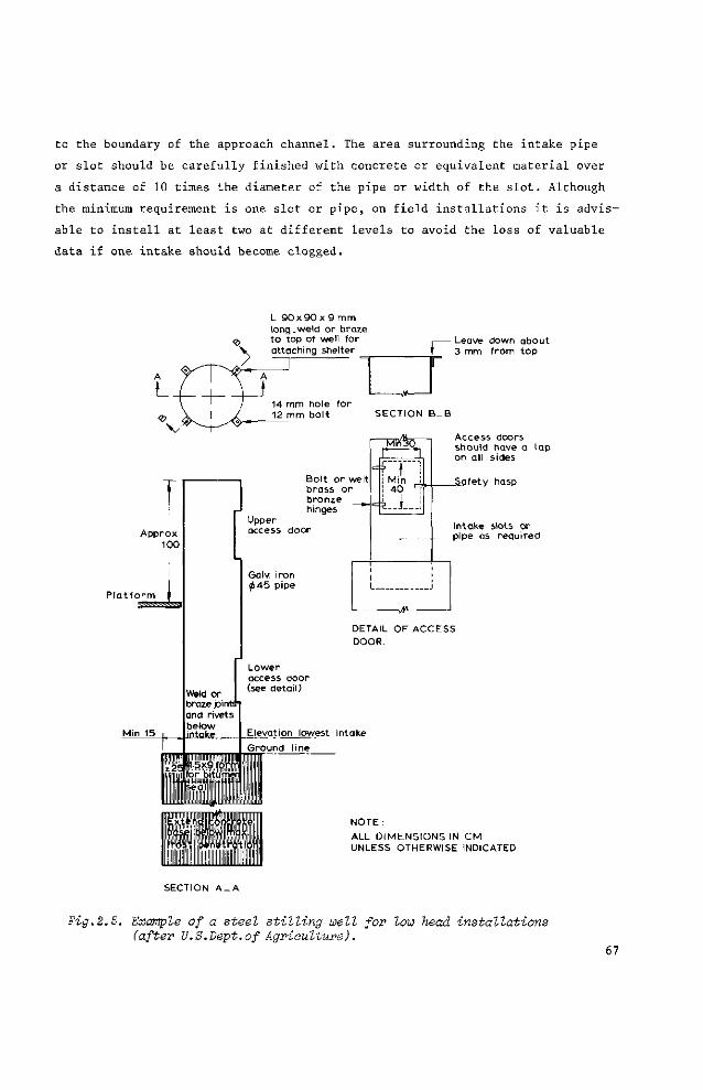
to the boundary of the approach channel. The area surrounding the intake pipe
or slot should be carefully finished with concrete or equivalent material over
a distance of 10 times the diameter of the pipe or width of the slot. Although
the minimum requirement is one slot or pipe, on field installations it is advis
able to install at least two at different levels to avoid the loss of valuable
data if one intake should become clogged.
L 9 0 x 9 0 x 9 mm long.weld or braze to top of well for attaching shelter
"T r - Leave down about 3 mm from top
14 mm hole for 12 mm bolt
Bolt or welt brass or bronze _^_ hinges "~
SECTION B_B
Upper access door
r—i Min 40
Access doors should have a on all sides
_S_afety hasp
Intake slots or pipe as required
-^~ DETAIL OF ACCESS DOOR.
Elevation lowest intake
NOTE: ALL DIMENSIONS IN CM UNLESS OTHERWISE INDICATED
SECTION A - A
Fig.2.5. Example of a steel stilling well for low head installations (after U.S.Dept.of Agriculture).
67
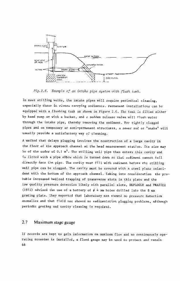
stream bed-
0.60 m.min.
Fig.2.6. Example of an intake pipe system with flush tank.
In most stilling wells, the intake pipes will require periodical cleaning,
especially those in rivers carrying sediments. Permanent installations can be
equipped with a flushing tank as shown in Figure 2.6. The tank is filled either
by hand pump or with a bucket, and a sudden release valve will flush water
through the intake pipe, thereby removing the sediment. For tightly clogged
pipes and on temporary or semi-permanent structures, a sewer rod or "snake" will
usually provide a satisfactory way of cleaning.
A method that delays plugging involves the construction of a large cavity in
the floor of the approach channel at the head measurement station. Its size may
be of the order of 0.1 m3. The stilling well pipe then enters this cavity and
is fitted with a pipe elbow which is turned down so that sediment cannot fall
directly into the pipe. The cavity must fill with sediment before the stilling
well pipe can be clogged. The cavity must be covered with a steel plate coinci
dent with the bottom of the approach channel. Taking into consideration the pro
bable increased bedload trapping of transverse slots in this plate and the
low quality pressure detection likely with parallel slots, REPLOGLE and FRAZIER
(1973) advised the use of a battery of 4 4 mm holes drilled into the 8 mm
grating plate. They reported that laboratory use showed no pressure detection
anomalies and that field use showed no sedimentation plugging problems, although
periodic grating and cavity cleaning is required.
2.7 Maximum stage gauge
If records are kept to gain information on maximum flow and no continuously ope
rating recorder is installed, a flood gauge may be used to protect and retain
68
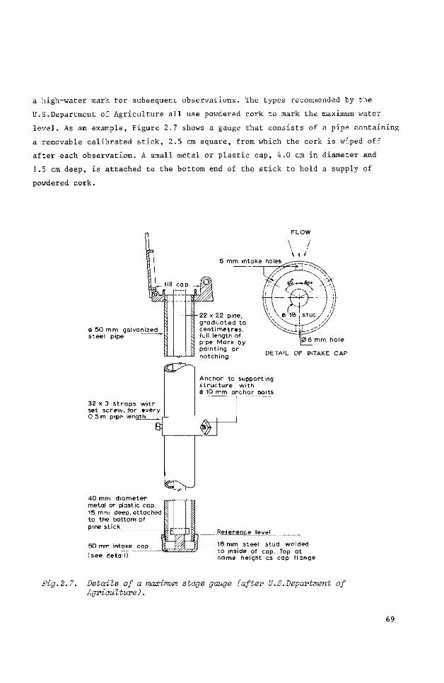
a high-water mark for subsequent observations. The types recommended by the
U.S.Department of Agriculture all use powdered cork to mark the maximum water
level. As an example, Figure 2.7 shows a gauge that consists of a pipe containing
a removable calibrated stick, 2.5 cm square, from which the cork is wiped off
after each observation. A small metal or plastic cap, 4.0 cm in diameter and
1.5 cm deep, is attached to the bottom end of the stick to hold a supply of
powdered cork.
<J 50 mm galvanized steel pipe
32 x 3 s t raps w i th set screw, for every 0.5 m pipe length
e
40 mm diameter metal or plastic cap, 15 mm deep, attached to the bottom of pine st ick
6 mm intake holes
FLOW
\ i / \ w
50 mm intake cap
(see detail)
-22 x 22 pine, g raduated to cent imetres, full length of pipe Mark by painting or notching
0 6 mm hole
DETAIL OF INTAKE CAP
Anchor to supporting s t ruc tu re w i th * 10 mm anchor bolts
Reference level
18 mm steel stud welded to inside of cap. Top at same height as cap f lange
Fig.2. 7. Details of a maximum stage gauge (after U.S.Department of Agriculture).
69
The 50 mm galvanized pipe is equipped with a perforated cap (4 perforations of
^ 6 mm) at the bottom and another cap at the top. The top cap should be easily
removable to allow observations but should have provisions for a padlock to
prevent vandalism. The pipe should be securely anchored in an upright position
as described in Section 2.5 for a staff gauge. The top of the pipe should be ac
cessible, also at flood stages, to facilitate observations. Since the flood gauge
is intended to register high water marks, the pipe should be long enough to ex
tend from the moderate high water mark, which is expected on an average of say
twice per year, to a point above the maximum stage expected.
2.8 Recording gauge
Automatic water stage recorders are instruments that produce graphical or punched
paper tape records of water surface elevation in relation to time. The usual
accessories to a recorder and its clock are a float, a counterweight, a calibrated
float tape, two tape clamps with rings, a box of charts or paper tapes, and the
manufacturer's instructions.
The use of such a recorder, in combination with a float well, has the following
advantages over an ordinary attendant-read staff gauge:
(i) In rivers with daily fluctuations, continuous records provide the
most accurate means of determining the daily average
(ii) The entire hydrograph is recorded with the maximum and minimum
stages as a function of time
(iii) Observations can be made at remote places where observers are not
available or in locations that are not accessible under all weather conditions.
Various meteorological instrument manufacturers produce a variety of commercial
ly available recorders. Most recorders operate on the principle of a reducing
mechanism that permits the accurate registration of a wide range in stage on
a scale which can be read easily.
Most recorders have several time- and stage-scale ratios available, and may
run as long as 60 days before the clock has to be rewound or the chart or tape
replaced.
Some recorders are driven by clocks operated either by spring or weight; the
70
digital recorder is an electrically operated device. No further details of re
corders are given here, since the manufacturer's description and instructions
are both detailed and complete, while technical progress soon makes any descrip
tion obsolete.
Regardless of the type of water level recorder selected, it should be equipped
with a calibrated float tape that passes over the float wheel. The float and
counterweight should be attached to the ends of the tape by ring connectors. If
the recorder is not equipped with a tape index pointer, one should be attached
either to the shelterhouse floor or to the instrument case. The purpose of the
calibrated tape and the index pointer is to enable the observer to check the
registered water level against the actual water level in the float well and that
shown on the independently placed staff gauge. As such,they provide an immediate
check on whether recorder, float, and inlet pipe or slots are functioning pro
perly.
2.9 Diameter of float
All water level recorders operate only if a certain initial resistance is over
come. This resistance, which is due to friction in the recorder and on the
axle, can be expressed as a resisting torque, Tf, on the shaft of the float
wheel.
If the counterweight exerts a tensile force, F, on the float-tape, this force
must increase or decrease by AF before the recorder will operate so that:
AF r > T (2-1)
where
AF = change in tensile force on float-tape between float and float wheel
r = radius of the float wheel
T. = resisting torque due to friction on the float wheel axle.
When we have, for example, a continuously rising water level in the well, a
decrease in the tensile force, AF, is required, which is possible only if the
upward force acting on the submerged part of the float increases. Consequently,
71
the float has to lag behind the rising water table by a distance Ah, so that
the volume of the submerged float section will increase by
AV = j DzAh (2-2)
where D equals the diameter of the float. According to Archimedes' law, the
upward force will increase linearly with the weight of the displaced volume of
water, hence
AF = j D2Ahpg (2-3)
Substitution of Equation 2-3 into Equation 2-1 shows that the friction in the
recorder and on the axle causes a registration error of the water level
4T Ah > - (2-4)
pgTTD2r
This lagging behind of the float causes a systematic error; a rising water level
is always registered too low and a falling water level too high.
Accepting the recorder's internal friction moment, T., as a basic datum, this
systematic error can only be reduced by enlarging either the float diameter, D,
or the radius of the float-wheel, r.
Submergence of the counterweight and an increase of weight of the float tape or
cable on one side of the float wheel (and consequently a decreasing weight on
the other side) cause a known change in tape force at the float. This change in
force, AF, results in a systematic registration error, Ah, which can be calcu
lated by Equation 2-3. These systematic errors can also be reduced by enlarging
the float diameter.
The reader should note that the phenomena just described produce a systematic
error that adds to the one mentioned in Section 2.6, i.e. that due to the head
loss in the intakes.
72
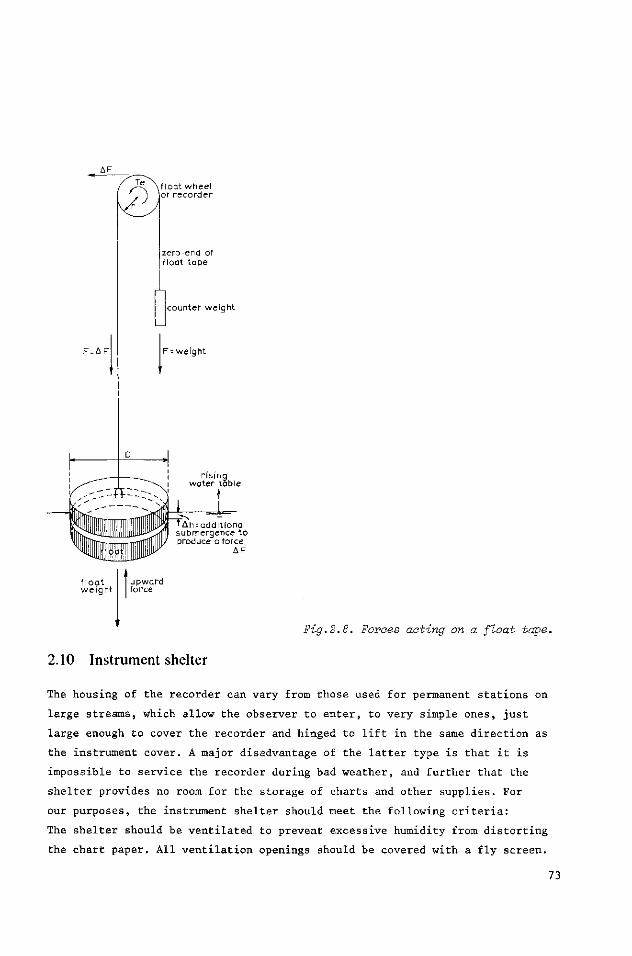
AF
/ > 5 \ f l o a t wheel v j of recorder
zero-end of float tape
F .ÄF
counter weight
F = weight
rising water table
Ah^additional submergence to produce a force
AF
upward force
2.10 Instrument shelter
Fig.2.8. Forces acting on a float tape.
The housing of the recorder can vary from those used for permanent stations on
large streams, which allow the observer to enter, to very simple ones, just
large enough to cover the recorder and hinged to lift in the same direction as
the instrument cover. A major disadvantage of the latter type is that it is
impossible to service the recorder during bad weather, and further that the
shelter provides no room for the storage of charts and other supplies. For
our purposes, the instrument shelter should meet the following criteria:
The shelter should be ventilated to prevent excessive humidity from distorting
the chart paper. All ventilation openings should be covered with a fly screen.
73
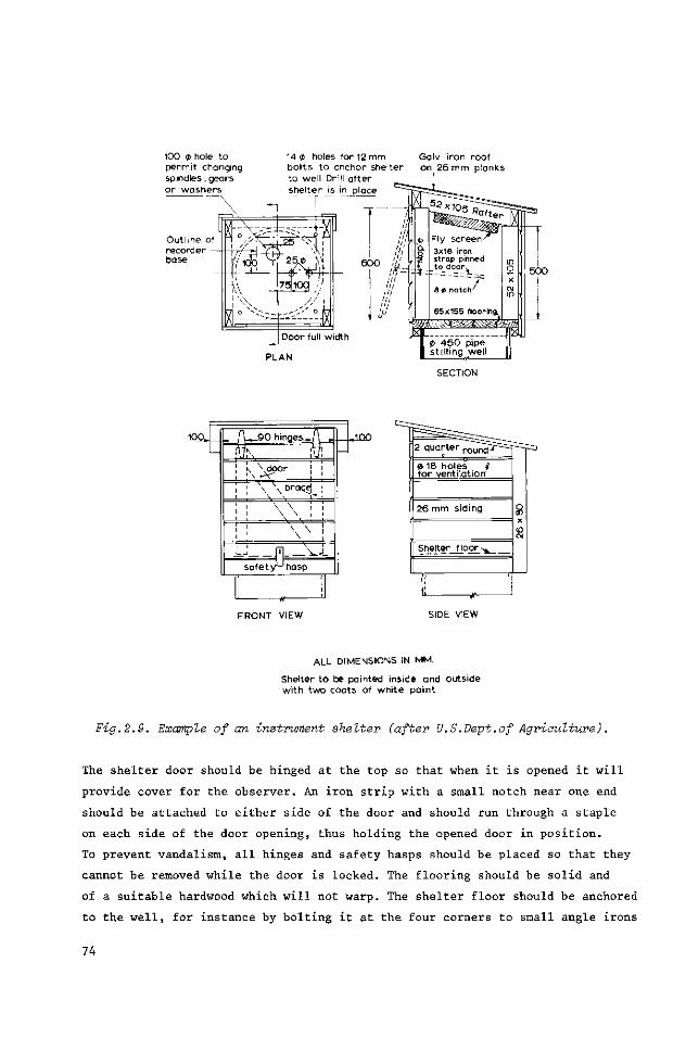
100 0 hole t o pe rmi t changing spindles, gears o r washe rs
14 0 holes for 12 mm b o l t s t o anchor shel ter t o wel l . Dril l a f t e r s h e l t e r j s in place
Galv i ron roof on 26 m m p lanks
Door full w idth
PLAN
6 0 0 5 0 0
SECTION
1 0 0 . . — J Û 0
FRONT VIEW
2 quar te r r o u n c H
© 18 ho les I f o r vent i la t ion
26 mm s id ing
Shelter f l oo r s
SIDE VIEW
ALL DIMENSIONS IN MM.
Shelter t o be painted inside and outs ide w i t h two coa ts of w h i t e pa in t
Fig.2.9. Example of an instrument shelter (after U.S.Dept.of Agriculture).
The shelter door should be hinged at the top so that when it is opened it will
provide cover for the observer. An iron strip with a small notch near one end
should be attached to either side of the door and should run through a staple
on each side of the door opening, thus holding the opened door in position.
To prevent vandalism, all hinges and safety hasps should be placed so that they
cannot be removed while the door is locked. The flooring should be solid and
of a suitable hardwood which will not warp. The shelter floor should be anchored
to the well, for instance by bolting it at the four corners to small angle irons
74
welded to the top of the float well. Condensation can be reduced by gluing or
spraying a 3 mm layer of cork to the inside of both the metal shelter and the
recorder cover. Silica gel can be utilized as a desiccant, but the moisture
should be removed from the gel at regular intervals by heating it in an oven to
about 150 °C (300 °F).
2.11 Protection against freezing
During winter it may be necessary to protect the stagnant water in the float
well against freezing. This can be done by employing one or more of the following
methods, depending on location and climate. If the well is set into the bank, an
isolating subfloor can be placed inside the well just below ground level. Care
should be taken, however, that both the float and counterweight can still move
freely over the range of water levels expected during winter. If the well is
heated with an electric heater or cluster of lights, or when a lantern or oil
heater is suspended just above the water level, the subfloor will reduce the
loss of heat. A reflector to concentrate the light or heat energy on the water
surface will increase the heating efficiency.
A layer of low-freezing-point oil, such as fuel oil, around the float can be
used as protection. The thickness of the oil layer required equals the greatest
thickness of ice expected, plus some allowance for water-stage fluctuations.
To prevent leakage of oil and erroneous records, a watertight float well will be
necessary. Since the mass density of oil is less than that of water, the oil
will stand higher in the float well than the water surface in the open channel.
Consequently, the recorder must be adjusted to give the true water stage. If
the stilling well is large compared with the float, it is advisable to accom
modate the float in an inner pipe and to place the oil in this pipe to avoid the
danger of oil being spilled into the open channel. The inner pipe should be open
at the bottom so that water may pass freely in and out of it.
2.12 Differential head meters
The differential head meter is an important device in structures where the
difference between two piezometric heads or water levels has to be known. Examp
les of such structures are the constant head orifice and other submerged orifices.
75
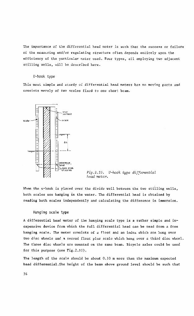
The importance of the differential head meter is such that the success or failure
of the measuring and/or regulating structure often depends entirely upon the
efficiency of the particular meter used. Four types, all employing two adjacent
stilling wells, will be described here.
U-hook type
This most simple and sturdy of differential head meters has no moving parts and
consists merely of two scales fixed to one short beam.
£eference_ T level
zero ends of scales
Fig.2.10. U-hook type differential head meter.
When the u-hook is placed over the divide wall between the two stilling wells,
both scales are hanging in the water. The differential head is obtained by
reading both scales independently and calculating the difference in immersion.
Hanging scale type
A differential head meter of the hanging scale type is a rather simple and in
expensive device from which the full differential head can be read from a free
hanging scale. The meter consists of a float and an index which are hung over
two disc wheels and a second float plus scale which hang over a third disc wheel.
The three disc wheels are mounted on the same beam. Bicycle axles could be used
for this purpose (see Fig.2.11).
The length of the scale should be about 0.10 m more than the maximum expected
head differential.The height of the beam above ground level should be such that
76
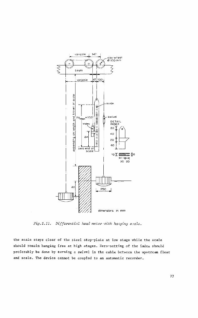
dimensions in mm
Fig.2.11. Differential head meter with hanging scale.
the scale stays clear of the steel stop-plate at low stage while the scale
should remain hanging free at high stages. Zero-setting of the index should
preferably be done by turning a swivel in the cable between the upstream float
and scale. The device cannot be coupled to an automatic recorder.
77
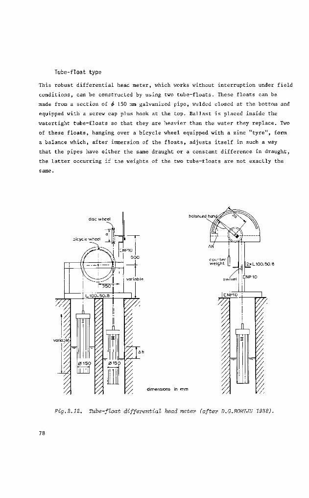
Tube-float type
This robust differential head meter, which works without interruption under field
conditions, can be constructed by using two tube-floats. These floats can be
made from a section of $ 150 mm galvanized pipe, welded closed at the bottom and
equipped with a screw cap plus hook at the top. Ballast is placed inside the
watertight tube-floats so that they are heavier than the water they replace. Two
of these floats, hanging over a bicycle wheel equipped with a zinc "tyre", form
a balance which, after immersion of the floats, adjusts itself in such a way
that the pipes have either the same draught or a constant difference in draught,
the latter occurring if the weights of the two tube-floats are not exactly the
same.
disc wheel
bicycle wheel
balanced hani
dimensions in mm
Fig.2.12. Tube-float differential head meter» (after D.G.ROMIJN 1938).
78
When the head between the two stilling wells is changing, each of the floats will
move over half the change in head. By transmitting the movement of the floats,
as illustrated in Figure 2.12, a differential head meter is obtained, which shows
the difference in head on a real or enlarged scale depending on the diameter
of the disc-wheel and the length of the balanced hand. The diameter of the disc
wheel should be such that half its circumference is equal to or slightly larger
than half the maximum difference in head to be measured. In this case the scale
only fills half a circle, which facilitates observations.
A change of head will cause a point on the circumference of the disc-wheel to
move over half that dimension. Provided the hand is twice as long as the radius
of the wheel, its point moves over a distance twice as far as the movement of one
float. Hence, it shows the real change in head. The length of the tube-floats
should be such that, at both maximum and minimum stages, the floats are neither
submerged nor hanging free above the water surface.
Index-setting of the hand should preferably be done by turning a swivel in the
cable between the downstream float (II) and the disc-wheel. If required, the
differential head can be recorded by an automatic recorder.
Suction lift type
A portable differential head meter which facilitates accurate observation is
the suction lift type. This instrument consists of two glass tubes which are
joined at the top by a tee that is connected to a transparent conduit in which
a partial vacuum can be created by means of a simple hand-operated pump.
The lower ends of the glass tubes are connected with the stilling wells for
the upstream and downstream heads. The meter is operated as follows. The stop
cock valve is opened and a partial vacuum is created by means of the hand
pump so that water flows into the container and all air is removed from the con
duits. Then the stopcock valve is closed. Subsequently, by operating the valve,
some air is admitted so that the two liquid levels become visible in the glass
tubes. The difference in head can now be obtained by reading the elevation of
each liquid level independently on a scale placed behind the tubes.
A device developed by the Iowa Institute simplifies this process by the use
of a continuous tape over pulleys mounted at the top and bottom of the gauge.
The zero end of the tape is set at one liquid level and a sliding indicator
moved to the other level. Subsequently, the difference in head is given as a di
rect reading on the tape.
79
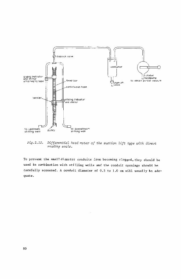
sliding indicator J_|_ and mirror K j attached to tape
stopcock valve
to upstream stilling well
D = ^ „ M ^ Q
,fixed bar
.continuous tape
r j i sliding indicator -++1 and mirror
to downstream st(Iiing well
Y^drain-otf [jvalve
suitable Jhandpump
to obtain partial vacuum
Fig.2.13. Differential head meter of the suction lift type with direct reading scale.
To prevent the small diameter conduits from becoming clogged, they should be
used in combination with stilling wells and the conduit openings should be
carefully screened. A conduit diameter of 0.5 to 1.0 cm will usually be ade
quate.
80
2.13 Selected list of references
1. BRITISH STANDARDS INSTITUTION: Methods of Measurement of Liquid Flow
in Open Channels. B.S.3680: Part 4A: Thin plate weirs and venturi flumes.
Part 4B: Long base weirs. British Standards House, London W.1. 1965, 1969.
2. REPLOGLE, J.A. and G.FRAZIER: Depth detection in critical depth flumes.
Annual Report 1973. U.S.Water Conservation Laboratory, USDA, Phoenix, AZ.
3. ROMIJN, D.G.: Meetsluizen ten behoeve van Irrigatiewerken. Vereniging
van Waterstaats Ingenieurs in Nederlandsch-Indië. Bandung 1938.
4. ROUSE, H.: Engineering Hydraulics. John Wiley & Sons, Inc., New York,
London. 4th printing 1964.
5. TROSKOLANSKI, A.T.: Hydrometry. Theory and practice of hydraulic measure
ments. Pergamon Press, Oxford, London, New York, Paris. 1960.
6. U.S.DEPARTMENT OF AGRICULTURE: Field manual for research in Agricultural
Hydrology. Agriculture Handbook No.224. Washington, D.C. 1962.
7. U.S.DEPARTMENT OF THE INTERIOR. Water Measurement Manual. U.S.Bureau
of Reclamation. 2nd Ed. Denver, Colorado. 1967. Repr.1971.
3 The selection of structures
3.1 Introduction
In selecting a suitable structure to measure or regulate the flow rate in open
channels, all demands that will be made upon the structure should be listed. For
discharge measuring and regulating structures, hydraulic performance is funda
mental to the selection, although other criteria such as construction cost
and standardization of structures may tip the balance in favour of another device.
The hydraulic dimensions of the discharge measuring or regulating structures
described in the following chapters are standardized. The material from which the
device is constructed, however, can vary from wood to brick-work, concrete,
polyester, metal, or any other suitable material. The selection of the material
depends on such criteria as the availability and cost of local material and la
bour, the life-time of the structure, pre-fabrication etc. Constructional details
are not given in this book except for those steel parts whose construction can
influence the hydraulic performance of the structure.
Although the cost of construction and maintenance is an important criterion in
the selection of structures, the ease with which a discharge can be measured or
regulated is frequently more important since this will reduce the cost of opera
tion. This factor can be of particular significance in irrigation schemes, where
one ditchrider or gatesman has to control and adjust 10 to 20 or more structures
daily. Here, ease of operation is labour saving and ensures a more efficient di
stribution of water over the irrigated area.
Although other criteria will come into play in the final selection of a discharge
measuring or regulating structure, the remarks in this chapter will be limited to
a selection based solely on hydraulic criteria.
3.2 Demands made upon a structure
3.2.1 Function of the structure
Broadly speaking, there are four different types of structures, each with its
own particular function:
83
- discharge measuring structure
- discharge regulating structure
- flow divider
- flow totalizer
Discharge measuring structure
The function of such a structure is to enable the flow rate through the channel
in which it is placed to be determined. If the structure is not required to ful
fil any other function, such as water-level control, it will have no movable
parts. Discharge measurement structures can be found in natural streams and drainage
canals, and also in hydraulic laboratories or in industries where flow rates need
to be measured. All flumes and fixed weirs are typical examples of discharge
measurement structures.
Discharge regulating structure
These structures are frequently found in irrigation canals where, as well as
having a discharge measuring function, they also serve to regulate the flow and
so distribute the water over the irrigated area. Discharge regulating structures
can be used when water is drawn from a reservoir or when a canal is to be split
up into two or more branches. A discharge regulating structure is equipped with
movable parts. If the structure is a weir, its crest will be movable in a verti
cal direction; if an orifice (gate) is utilized, the area of the opening will be
variable. Almost all weirs and orifices can be used as discharge regulating
structures. In this context it is curious to note that in many irrigation canal
systems, the discharge is regulated and measured by two structures placed in line
in the same canal. The first structure is usually a discharge regulating gate
and, the second downstream of the first, is a discharge measuring flume. It would
seem to be a waste of money to build two such structures, when one would suffice.
Moreover,the use of two structures requires a larger loss of head to operate within
the modular flow range than if only one is used. Another even more serious
disadvantage is that setting the required discharge with two structures is a
more time consuming and complicated procedure than if a single regulating struc
ture is used. Obviously, such procedures do not contribute to the efficient manage
ment of the available water.
84
Flow d iv ider
It may happen that in an irrigated area we are only interested in the percentage
distribution of the incoming flow into two or more branch canals. This percentage
distribution can be achieved by constructing a group of weirs all having the same
crest level but with different control widths. If the percentage distribution has
to vary with the flow rate in the undivided canal, the crest level of the weirs
may differ or the control sections may have different shapes. Sometimes the
required percentage distribution of flow over two canals has to vary while the
incoming flow remains constant. This problem can be solved by using a movable
partition (or divisor) board which is adjusted and locked in place above a fixed
weir crest (see Section 9.1).
Although a flow divider needs no head measurement device to fulfil its function,
a staff gauge placed in the undivided canal can give additional information on
the flow rate, if this is required by the project management.
Flow totalizer.
If we want to know the volume of water passing a particular section in a given
period, we can find this by using a flow totalizer. Such information will be
required, for instance, if a farmer is charged for the volume of water he diverts
from the irrigation canal system, or if an industry is charged for the volume of
effluent it discharges into a stream. The two flow totalizers treated in this book
both have a rotating part and a revolution counter which can be fitted with an
additional counter or hand to indicate the instantaneous flow rate.
3.2.2 Required fall of energy head to obtain modular flow
Flumes and weirs
The available head and the required head at the discharge measuring site influence
both the type and the shape of the structure that will be selected. For weirs and
flumes, the minimum required head AH to operate in the modular flow range can be
expressed as a fraction of the upstream energy head H, or as (IL - H„)/ïL. This
ratio can also be written as 1 - H„/H., the last term of which describes the limit
of the modular flow range, i.e., the modular limit (see also Section 1.6).
The modular, limit is defined as the value of submergence ratio H_/FL at which the
real discharge deviates by 1% from the discharge calculated by the head-discharge
85
equation. We can compare the required fall over weirs of equal width by consider
ing their respective modular limits. The modular limit of weirs and flumes depends
basically on the degree of streamline curvature at the control section and on the
reduction of losses of kinetic energy if any, in the downstream expansion. Broad-
crested weirs and long-throated flumes, which have straight and parallel stream
lines at their control section and where part of the kinetic energy is recovered,
can obtain a modular limit as high as fU/H. = 0.95. As mentioned in Chapter I,
the discharge coefficient of a weir increases if the streamline curvature at the
control section increases. At the same time, however, a rising tailwater level
tends to reduce the degree of streamline curvature, and thus reduces the discharge.
Consequently we can state that the modular limit of a weir or flume will be lower
as the streamlines are more strongly curved under normal operation. The extreme
examples are the rectangular sharp-crested weir and the Cipoletti weir, where
the tailwater level must remain at least 0.05 m below crest level, so that stream
line curvature at the control section will not be affected. Modular limits are gi
ven for each structure and are summarized in Section 3.3.
The available head and the required head over a structure are determining factors
for the crest elevation, width and shape of the control section, and for the shape
of the downstream expansion of a discharge measurement structure. This can be
shown by the following example.
Suppose a 0.457 m (1.5 ft) wide Parshall flume is to be placed in a trapezoidal
concrete-lined farm ditch with l-to-1.5 side slopes, a bottom width of 0.50 m, and
its crest at ditch bottom level. In the ditch the depth-discharge relationship is
controlled by its roughness, geometry, and slope.
1 2/3 -If we use the Manning equation, v = — R s2, with a value of n = 0.014 and
s = 0.002, we obtain a satisfactory idea of the tailwater depth in the ditch.
Tailwater depth data are shown in Figure 3.1, together with the head-discharge
curve of the Parshall flume and its 70% submergence line (modular limit).
An examination of the 70% submergence curve and the stage-discharge curve shows
that submerged flow will occur at all discharges below 0.325 m /s, when the flume
crest coincides with the ditch bottom. Figure 3.1 clearly shows that if a design
engineer only checks the modularity of a device at maximum stage, he may unknow
ingly introduce submerged flow conditions at lower stages.
The reason for this phenomenon is to be found in the depth-discharge relationship
of ditch and control section. In the given example, a measuring structure with a
rectangular control section and a discharge proportional to about the 1.5 power of
86
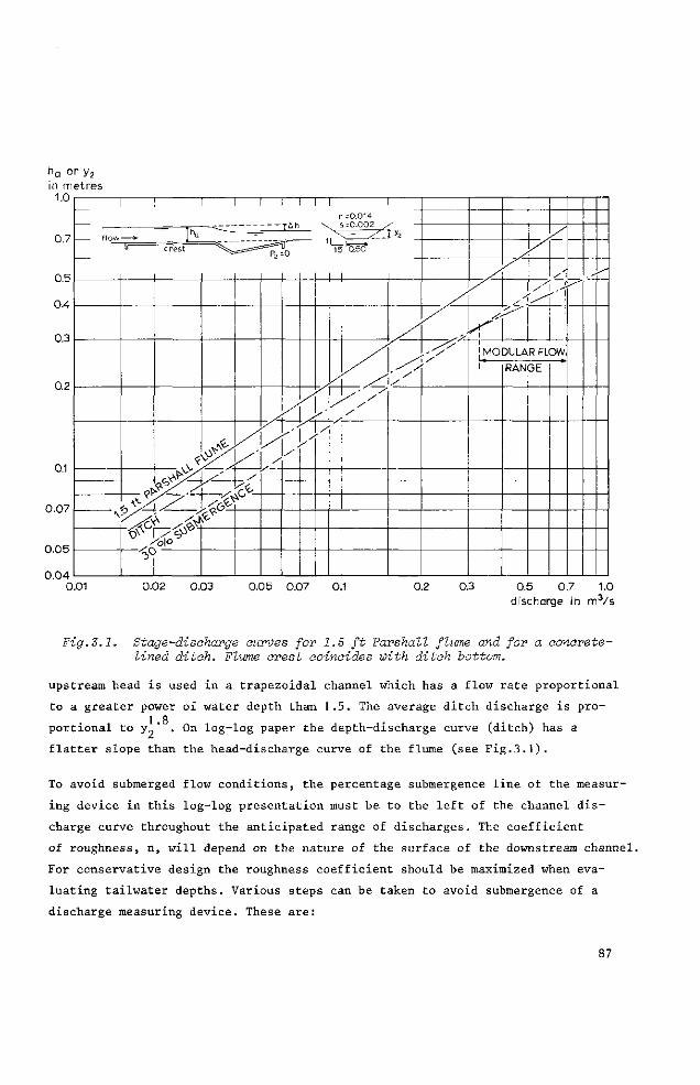
h Q o in m 1.0
0.7
0.5
0.4
0.3
0.2
r y 2
et res
0.1
0.07
0.05
0.04 0.
flow—» l ° u crest v < ï ; ^=^^^^ r '
\
"P
' ° v .
,<
Wï & .
/ '
V UcP x '® "o\o
\
V
/ '& V-"
'
\ n =0.014
^è lqzS* \ 15 0.50
Î V
's y
- /
—
y I
i MODULAR FLOW]
I RAN 3E
^
.01 0.02 0.03 0.05 0.07 0.1 0.2 0.3 0.5 0.7 1.0 discharge in m3/s
Fig.3.1. Stage-discharge curves for 1.5 ft Parahall flume and for a concrete-lined ditch. Flume crest coincides with ditch bottom.
upstream head is used in a trapezoidal channel which has a flow rate proportional
to a greater power of water depth than 1.5. The average ditch discharge is pro-1 R
portional to y„' . On log-log paper the depth-discharge curve (ditch) has a
flatter slope than the head-discharge curve of the flume (see Fig.3.1).
To avoid submerged flow conditions, the percentage submergence line of the measur
ing device in this log-log presentation must be to the left of the channel dis
charge curve throughout the anticipated range of discharges. The coefficient
of roughness, n, will depend on the nature of the surface of the downstream channel.
For conservative design the roughness coefficient should be maximized when eva
luating tailwater depths. Various steps can be taken to avoid submergence of a
discharge measuring device. These are:
87
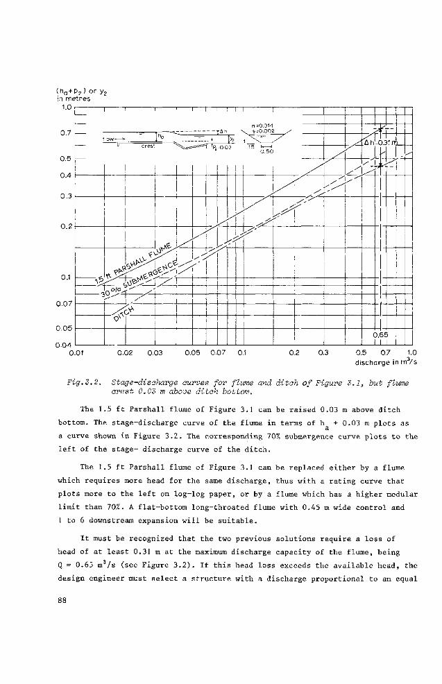
(ha + p2) or y2
in metres 1.0
0.7
0.5
0.4
0.3
0.2
0.1
0.07
0.05
0.04
f
^
. ^ yAh I O W ^ I1 '0 -=- i Jy-
r ~ crest % & = = = = = î l 'p2=o.03
1
J
1 ^
o^°-r ^ ^ ,
^
^
^
• ^ s
y
^ / 1
S& 1 __ ov
[
1
^' y^
n =0.014 x 5=0.002 /
1:"XT~ / 15 1-—J
0.50
S
\ ]
-£ •> '
/*
^
I
l l . . . i .
^ h
/'
I i
M n -y
I i i
—
—
0.65 I I I
-
0.01 0.02 0.03 0.05 0.07 0.1 0.2 0.3 0.5 0.7 1.0 discharge in m /s
Fig.S.2. Stage-discharge curves for flume and ditch of Figure 3.1, but flume crest 0.03 m above ditch bottom.
The 1.5 ft Parshall flume of Figure 3.1 can be raised 0.03 m above ditch
bottom. The stage-discharge curve of the flume in terms of h + 0.03 m plots as
a curve shown in Figure 3.2. The corresponding 70% submergence curve plots to the
left of the stage- discharge curve of the ditch.
The 1.5 ft Parshall flume of Figure 3.1 can be replaced either by a flume
which requires more head for the same discharge, thus with a rating curve that
plots more to the left on log-log paper, or by a flume which has a higher modular
limit than 70%. A flat-bottom long-throated flume with 0.45 m wide control and
1 to 6 downstream expansion will be suitable.
It must be recognized that the two previous solutions require a loss of
head of at least 0.31 m at the maximum discharge capacity of the flume, being
Q = 0.65 m3/s (see Figure 3.2). If this head loss exceeds the available head, the
design engineer must select a structure with a discharge proportional to an equal
of greater power of head than the power of the depth y. of the ditch. For example,
he may select a flat-bottom, long-throated flume with a trapezoidal control section
and a gradual downstream expansion. Such a flume can be designed in such a way
that at Q = 0.65 m3/s an upstream head h1 = 0.53 m and a modular limit of about
0.85 occur resulting in a required head loss of only 0.08 m. He could also use a
flume with a (truncated) triangular, parabolic, or semi-circular control section.
Orifices
At the upstream side of free flowing orifices or undershot gates, the upper edge
of the opening must be submerged to a depth which is at least equal to the height
of the opening. At the downstream side the water level should be sufficiently low
so as not to submerge the jet (see Chapter 8).For this reason free flowing orifices,
especially at low flows, require high head losses and are less commonly used than
submerged orifices. The accuracy of a discharge measurement obtained with a sub
merged orifice depends on the accuracy with which the differential head over the
orifice can be measured. Depending on the method by which this is done and the
required accuracy of the discharge measurement, a minimum fall can be calculated
with the aid of Appendix II. In general, we do not recommend the use of differen
tial heads of less than 0.10 m.
3.2.3 Range of discharges to be measured
The flow rate in an open channel tends to vary with time. The range between
Q . and Q through which the flow should be measured strongly depends on the
nature of the channel in which the structure is placed. Irrigation canals, for
example, have a considerably narrower range of discharges than do natural streams.
The anticipated range of discharges to be measured may be classified by the ratio
max min
From the limits of application of several weirs, a maximum attainable y_value can
be calculated. Taking the example of the round-nosed horizontal broad-crested
weir (Section 4.1), the limits of application indicate that H]/L can range between
0.05 m and 0.50. As a result we obtain a maximum value of y which is
Q C .max ,- _n. 1 .5 Y = J2ÏÏL = _i (°-5°) * 35 (3_2) ' Q . C.min fn „,1.5 v '
Tnin d (0.05)
This illustrates that whenever the ratio Y = Q /Q . exceeds about 35 the round-inax Turn
nosed horizontal broad-crested weir described in Section 4.1 cannot be used. Weirs
or flumes that utilize a larger range of head, or which have a head-discharge re
lationship proportional to a power of head greater than 1.5, or both, can be used
in channels where Y = Q /Q-,- exceeds 35. The following example shows how the
Y_value, in combination with the available upstream channel water depth y , in
fluences the choice of a control section. The process of selection is as follows:
Find a suitable flume and weir for
Q ^ = 0.015 m3/s
Q = 3.00 m3/s -> y = 200 max '
yj = hj + p < 0.80 m
The flume is to be placed in an existing trapezoidal channel with a 4-m wide bot
tom and l-to-2 side slopes. At maximum water depth y, = 0.80 m, the Froude number
in the approach channel is Fr = v./(gA /B ) 2 = 0.18. For Fr < 0.50 the water
surface will be sufficiently stable.
From the relatively high Y~value of 200 we can conclude that the control section
of the structure should be narrower at minimum stage than at maximum stage. Meet
ing the requirements of this example are control sections with a narrow bottomed
trapezium, or a triangular or truncated triangular shape. Because of the limited
available width we select a truncated triangular control section of which two
solutions are illustrated below.
Triangular profile flat-V weir (Fig.3.3)
According to Section 6.4.2 the basic head-discharge equation of this weir reads
4 ,„,.0.5 B CdCv Ï5 ( 2 g ) H^
2.5 „_ TT s2.5 e
h- - (he" V (3-3)
2 .5 in which the term (h - H, ) should be deleted if h is less than H, . If we use
e b e b
the l-to-2/l-to-5 weir profile and a l-to-10 cross slope, the minimum channel
discharge can be measured at the minimum required head, since Q at 0.06 m head is
Q 0 > 0 6 = 0.66 x 1 x Ï- (2g)°-5 x i | (0.06 - 0.0008)2-5
90
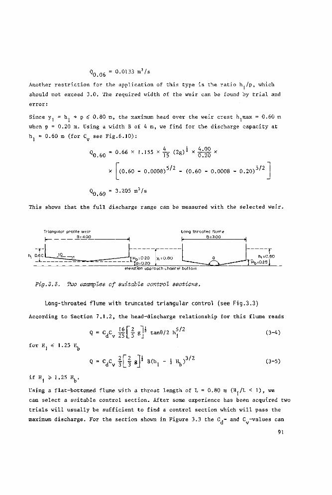
Q0_06 = 0.0133 m3/s
Another restriction for the application of this type is the ratio lu/p, which
should not exceed 3.0. The required width of the weir can be found by trial and
error:
Since y. = h. + p 0.80 m, the maximum head over the weir crest h max = 0.60 m
when p = 0.20 m. Using a width B of 4 m, we find for the discharge capacity at
h = 0.60 m (for C see Fig.6.10):
0 = 0 66 x 1 155 x ~ (2s)5 x iLi2£ x ^0.60 • 15 y %> 0.20
(0.60 - 0.0008)5/2 - (0.60 - 0.0008 - 0.20)5/2
% . 6 0 = 3 - 2 0 5 * 3 / s
This shows that the full discharge range can be measured with the selected weir.
Triangular profi le wei r B = 4.00
Long throated f lume , B = 3.00
•£Hb = 0.20 |y, =0.80 TP = 0.2Q
elevation approach channel bot tom
"~~T h,=0.80
|Hb=0.S5[
Fig.2.3. Two examples of suitable control sections.
Long-throated flume with truncated triangular control (see Fig.3.3)
According to Section 7.1.2, the head-discharge relationship for this flume reads
for Hj < 1 .25 IL
* = CdCv M
d v 3
tanO/2 h' 5/2 1
B(h, - i i y 3/2
(3-4)
(3-5)
if H » 1.25 H,.
Using a flat-bottomed flume with a throat length of L = 0.80 m (H./L < 1), we
can select a suitable control section. After some experience has been acquired two
trials will usually be sufficient to find a control section which will pass the
maximum discharge. For the section shown in Figure 3.3 the C,- and C -values can
91
be found as follows:
For h, = 0.80 m, H,/L - 1, Figure 7.3 shows that C, = 1.0
The area ratio
Cd À^ = 0.80 x 5.60 = ° - 4 5
and we find in Figure 1.12 that the related C -value is about 1.06 (1.5 < u < 2.0)
Substitution of these values into Equation 3-5 yields a discharge capacity at
h. = 0.80 m equal to
Q0 80 = 1-° X K 0 6 X f ( f 9-8 1 ) 5 x 3 (°- 8 0 - 0.125)3/2
Vso = 3-01 m3/s
At minimum applicable head of h. =0.1 L = 0.08 m (see Section 7.1.4) C, = 0.88 1 a
and C -1.0. v
Using Equation 3-4 we find that at h = 0.08 m the discharge capacity is
QO.08 = ° - 8 8 X l-0xi|(f 9 . 8 . ) ^ x o . 0 8 5 / 2
Q0_08 = 0.0121 m3/s
This shows that both minimum and maximum discharges can be measured with the
selected structure.
These structures are only two of the many which meet the demands set on the
discharge range and upstream water depth.
3.2.4 Sensitivity
The accuracy to which a discharge can be measured will depend not only on the
errors inherent to the structure but also on the variation of upstream head
during the period between two head readings and the rate of change of diverted
discharge because of this change of head.
In various countries, the accuracy of discharge measuring structure is expressed
in the sensitivity, S, of the structure. This is defined as the fractional
change of discharge of the structure that is caused by the unit rise, usually
Ah = 0.01 m, of the upstream water level. For modular flow (dQ/dh,)Ahl
S _ _ _ (3-6)
92
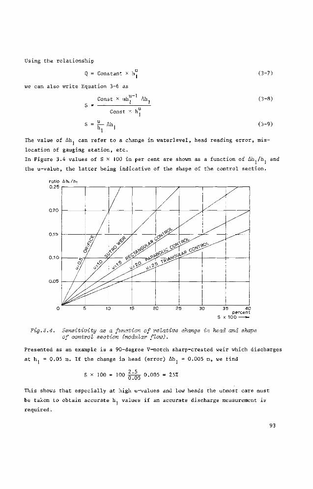
Using the relationship
Q = Constant x h"
we can also write Equation 3-6 as
Const x uh"~ Ah
Const x h
S = TT Ahi hl '
(3-7)
(3-8)
(3-9)
The value of Ah, can refer to a change in waterlevel, head reading error, mis-
location of gauging station, etc.
In Figure 3.4 values of S x 100 in per cent are shown as a function of Ah /ht and
the u-value, the latter being indicative of the shape of the control section.
ratio Ah,/hi
0.25
0.20
0.15
0.10
0.05
35 40 percent
S x 100 —
Fig.3.4. Sensitivity as a function of relative change in head and shave of control section (modular flow).
Presented as an example is a 90-degree V-notch sharp-crested weir which discharges
at h. = 0.05 m. If the change in head (error) Ah. = 0.005 m, we find
S x 100 = 100 2.5 0.05
0.005 = 25%
This shows that especially at high u-values and low heads the utmost care must
be taken to obtain accurate h, values if an accurate discharge measurement is
required.
93
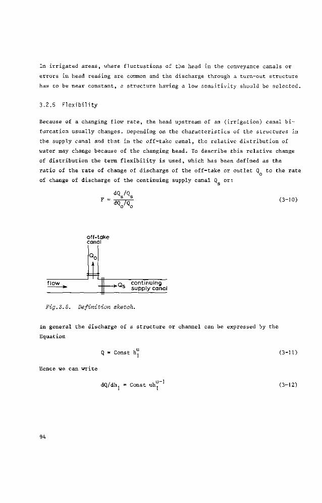
In irrigated areas, where fluctuations of the head in the conveyance canals or
errors in head reading are common and the discharge through a turn-out structure
has to be near constant, a structure having a low sensitivity should be selected.
3.2.5 Flexibility
Because of a changing flow rate, the head upstream of an (irrigation) canal bi
furcation usually changes. Depending on the characteristics of the structures in
the supply canal and that in the off-take canal, the relative distribution of
water may change because of the changing head. To describe this relative change
of distribution the term flexibility is used, which has been defined as the
ratio of the rate of change of discharge of the off-take or outlet Q to the rate
of change of discharge of the continuing supply canal Q or:
(3-10)
flow
off-take canal
a,
Q continuing s supply canal
Fig.3.5. Definition sketch.
In general the discharge of a structure or channel can be expressed by the
Equation
Q = Const h (3-11)
Hence we can write
dQ/dh = Const uh" ' (3-12)
94
Division by Q and by Const h gives
dQ/Q = u dh /h (3-13)
Subs t i t u t i on of Equation 3-13 i n to Equation 3-10 for both Q and Q r e s u l t s in
u dh h, F = ^ lo£_L£ (3-,4)
u dh . n , s 1,s 1 ,o
Since a change in water level in the upstream reach of the supply canal causes an
exactly equal change in h, and h, , the quotient dh, /dh = 1, and thus
u h, F = ° l ' s (3-15)
u h, s 1 ,o
The proportional distribution of water over two or more canals may be classified
according to the flexibility as follows:
F = 1
For F = 1 we may write
u h.
^r = h ^ <3"I6> s 1 ,s
To meet this requirement for various heads, the structures on the off-take and
supply canal must be of the same type and their crest or sills must be at the
same level.
F < 1
If less variation is allowed in the off-take discharge than in the supply canal
discharge, the flexibility of the bifurcation has to be less than unity and is
said to be sub-proportional.
The easiest way to obtain F < 1 is to select two different types of structures,
for example :
an orifice as off-take; u = 0.5
a weir with rectangular (or other) control in the supply canal: u = 1.5 (or more).
95
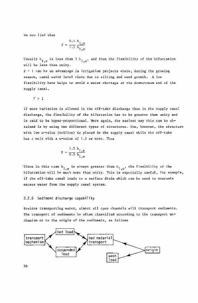
We now find that
0.5 h l,s
1 .5 h l,o
Usually h, is less than 3 h, , and then the flexibility of the bifurcation 1 ,s 1 ,o J
will be less than unity.
F < 1 can be an advantage in irrigation projects where, during the growing
season, canal water level rises due to silting and weed growth. A low
flexibility here helps to avoid a water shortage at the downstream end of the
supply canal.
F > 1
If more variation is allowed in the off-take discharge than in the supply canal
discharge, the flexibility of the bifurcation has to be greater than unity and
is said to be hyper-proportional. Here again, the easiest way this can be ob
tained is by using two different types of structures. Now, however, the structure
with low u-value (orifice) is placed in the supply canal while the off-take
has a weir with a u-value of 1.5 or more. Thus
1 .5 h l,s
0.5 h.
'Since in this case h1 is always greater than h1 , the flexibility of the
bifurcation will be much more than unity. This is especially useful, for example,
if the off-take canal leads to a surface drain which can be used to evacuate
excess water from the supply canal system.
3.2.6 Sediment discharge capability
Besides transporting water, almost all open channels will transport sediments.
The transport of sediments is often classified according to the transport me
chanism or to the origin of the sediments, as follows
transport mechanism
96
bed load
suspended load
bed material transport
wash load
origin
The expressions used in this diagram are defined as follows:
Bed-load
Bed-load is the transport of sediment particles sliding, rolling, or jumping over
and near the channel-bed, generally in the form of moving bed forms such as dunes
and ripples. Many formulae have been developed to describe the mechanism of the
bed-load, some being completely based upon experiment, while others are founded upon
a model of the transport mechanism. Most of these equations, however, have in
common that they contain a number of "constants" which have to be modified ac
cording to the field data collected for a certain river. In fact, all the devi
ations in bed-load from the theoretical results are counteracted by selecting the
right "constants".
Most of the available bed-load functions can be written as a relation between the
transport parameter
X = T/\AgD3
and the flow parameter
Y = JJys/AD
where
T = transport in solid volume per unit width (sometimes expressed in terms of the transport including voids, S, according to T = S(l - e ) , where e is the porosity
y = depth of flow (often y is replaced by the hydraulic radius R)
D = grain diameter
A = relative density = (p - p)/p
s = hydraulic gradient
y = so-called ripple factor, in reality a factor of ignorance, used to obtain agreement between measured and computed values of T.
As an example of such an X versus Y relation the well known MEYER-PETER/MÜLLER
bed-load function may be given;
X = A(Y - 0.047)3 / 2 (3-17)
with A = 8.
Typical bed-load equations like the Meyer-Peter/Müller equation do not include
suspended-load. Equation (3-17) differs from the total-load equation given below,
although the construction of both equations will appear to be similar.
97
Suspended-load
Suspended-load is the transport of bed particles when the gravity force is counter
balanced by upward forces due to the turbulence of the flowing water. This means
that the particles make larger or smaller jumps, but return eventually to the
river-bed. By that time, however, other particles from the bed will be in suspen
sion and, consequently, the concentration of particles transported as suspended-
load does not change rapidly in the various layers.
A strict division between bed-load and suspended-load is r.ot possible; in fact,
the mechanisms are related. It is therefore not surprising that the so-called
total-load (bed-load and suspended-load together) equations have a similar construc
tion to that of the bed-load equations.
An example of a total-load equation is the equation of ENGELUND and HANSEN (1967),
which reads
X = 0.05 Y 5 / 2 (3-18)
with
r r2-] 2/5
C = roughness coefficient of Chézy
D = D50
Wash-load
Wash-load is the transport of small particles finer (generally < 50 ym) than the
bulk of the bed material and rarely found in the bed. Transport quantitites found
from bed-load, suspended-load, and total-load formulae do not include wash-load
quantities.
Whereas for a certain cross-section quantities of suspended-load and bed-load
can be calculated with the use of the locally valid hydraulic conditions, this is
not the case for wash-load. The rate of wash-load is mainly determined by clima-
tological characteristics and the erosion features of the whole catchment area.
Since there is normally no interchange with bed particles, wash-load is not important
for local scour or silting. Owing to the very low fall velocity of the wash-load
particles, wash-load only contributes to sedimentation in areas with low current
velocities (reservoirs, dead river branches, on the fields). Owing to the small
fall velocity, in turbulent water the concentration of the particles over a vertical
98
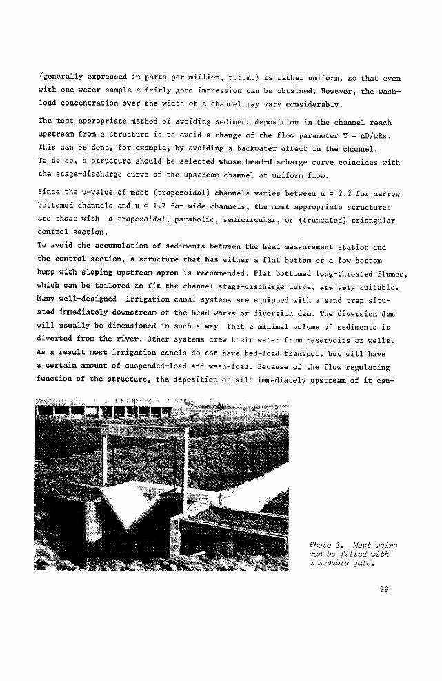
(generally expressed in parts per million, p.p.m.) is rather uniform, so that even
with one water sample a fairly good impression can be obtained. However, the wash-
load concentration over the width of a channel may vary considerably.
The most appropriate method of avoiding sediment deposition in the channel reach
upstream from a structure is to avoid a change of the flow parameter Y = AD/yRs.
This can be done, for example, by avoiding a backwater effect in the channel.
To do so, a structure should be selected whose head-discharge curve coincides with
the stage-discharge curve of the upstream channel at uniform flow.
Since the u-value of most (trapezoidal) channels varies between u - 2.2 for narrow
bottomed channels and u - 1.7 for wide channels, the most appropriate structures
are those with a trapezoidal, parabolic, semicircular, or (truncated) triangular
control section.
To avoid the accumulation of sediments between the head measurement station and
the control section, a structure that has either a flat bottom or a low bottom
hump with sloping upstream apron is recommended. Flat bottomed long-throated flumes,
which can be tailored to fit the channel stage-discharge curve, are very suitable.
Many well-designed irrigation canal systems are equipped with a sand trap situ
ated immediately downstream of the head works or diversion dam. The diversion dam
will usually be dimensioned in such a way that a minimal volume of sediments is
diverted from the river. Other systems draw their water from reservoirs or wells.
As a result most irrigation canals do not have bed-load transport but will have
a certain amount of suspended-load and wash-load. Because of the flow regulating
function of the structure, the deposition of silt immediately upstream of it can-
«M*T-;iBWWj •"V»*** * ; « • « ;
W ^ I * - . . - .* - • *. f *• * l V ^** ^ 4b -
Photo 1. Moet weirs aan be fitted with a movable gate.
99
not always be avoided even if uniform flow is maintained upstream of the head
measurement station.
If an adjustable orifice is used as a discharge regulating structure, it is recom
mended that a bottom sill be avoided. If a movable weir is used, it should be
fitted with a movable bottom gate that can be lifted to wash out sediments. This
gate arrangement is described in Section 4.2. Its use is not restricted solely
to the Romijn weir; it can be used in combination with all weirs described in
Chapters 4, 5, and 6.
3.2.7 Passing of floating and suspended debris
All open channels, and especially those which pass through forested or populated
areas, transport all kinds of floating and suspended debris. If this debris is
trapped by the discharge measuring structure, the approach channel and control
section become clogged and the structure ceases to act as a discharge measuring
device.
In irrigation canals it may be practical to install a trash rack at strategic
points to alleviate the problem of frequently clogged structures. This applies
especially if narrow openings, V-notches, or orifices are used. In drainage
channels, however, because of their larger dimensions, the installation of
trash-racks would not be practical. For drainage canals therefore one
should select structures that are not vulnerable to clogging. All sharp-
crested weirs and orifices are easily clogged and are thus not recommended if
floating debris has to be passed. Weirs with a sloping upstream face or weirs
with a rounded nose or crest and all flumes will pass debris relatively easily.
Piers which have no rounded nose or are less than 0.30 m wide, which thus
includes sharp-edged movable partition boards, tend to trap the bulkier debris.
3.2.8 Undesirable change in discharge
Structures may be damaged through vandalism or by persons who stand to benefit
from a faulty or non-operating structure. To prevent such damage, the design engi
neer should keep structures as simple as possible and any movable parts should be
as sturdy as is economically justified. It may also happen that attempts will be
made to alter the discharge of a structure by changing the hydraulic conditions
under which the structure should operate.
100
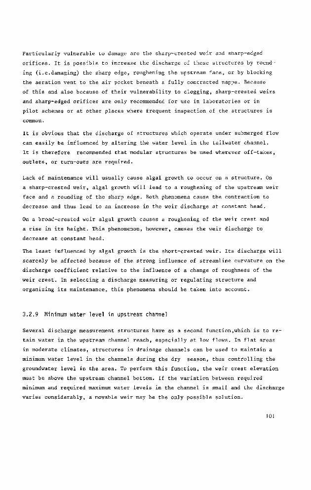
Particularly vulnerable to damage are the sharp-crested weir and sharp-edged
orifices. It is possible to increase the discharge of these structures by round
ing (i.e.damaging) the sharp edge, roughening the upstream face, or by blocking
the aeration vent to the air pocket beneath a fully contracted nappe. Because
of this and also because of their vulnerability to clogging, sharp-crested weirs
and sharp-edged orifices are only recommended for use in laboratories or in
pilot schemes or at other places where frequent inspection of the structures is
common.
It is obvious that the discharge of structures which operate under submerged flow
can easily be influenced by altering the water level in the tailwater channel.
It is therefore recommended that modular structures be used wherever off-takes,
outlets, or turn-outs are required.
Lack of maintenance will usually cause algal growth to occur on a structure. On
a sharp-crested weir, algal growth will lead to a roughening of the upstream weir
face and a rounding of the sharp edge. Both phenomena cause the contraction to
decrease and thus lead to an increase in the weir discharge at constant head.
On a broad-crested weir algal growth causes a roughening of the weir crest and
a rise in its height. This phenomenon, however, causes the weir discharge to
decrease at constant head.
The least influenced by algal growth is the short-crested weir. Its discharge will
scarcely be affected because of the strong influence of streamline curvature on the
discharge coefficient relative to the influence of a change of roughness of the
weir crest. In selecting a discharge measuring or regulating structure and
organizing its maintenance, this phenomena should be taken into account.
3.2.9 Minimum water level in upstream channel
Several discharge measurement structures have as a second function,which is to re
tain water in the upstream channel reach, especially at low flows. In flat areas
in moderate climates, structures in drainage channels can be used to maintain a
minimum water level in the channels during the dry season, thus controlling the
groundwater level in the area. To perform this function, the weir crest elevation
must be above the upstream channel bottom. If the variation between required
minimum and required maximum water levels in the channel is small and the discharge
varies considerably, a movable weir may be the only possible solution.
101
On the other hand, in hot climates it may be desirable to design discharge measure
ment structures so that the channels in which they are placed will go dry if no
flow occurs. This may be a necessary precaution to prevent the spread of serious
diseases like malaria and bilharzia. It may also be convenient to have irrigation
canals go dry by gravity flow so that maintenance work can be performed. This
will require that all structures in supply canals and drainage channels have
zero crest elevation. If a raised weir crest is needed during other periods, a mo
vable weir will provide the answer.
3.2.10 Required accuracy of measurement
In the head-discharge equation of each structure there is a discharge coefficient
and an approach velocity coefficient, or a combination of these coefficients. The
accuracy with which a discharge can be measured with a particular structure depends
to a great extent on the variation of these coefficients determined under similar
hydraulic conditions.
For all of the structures described, an expected error in the product C.C or in
the combined coefficient is given in the relevant section on the evaluation of
discharge. These errors are also listed in Section 3.3. Often, the error in C.C ' d v
is not constant but decreases if the C,-value increases, which usually occurs if
the head over a crest increases.
Besides the error in the coefficients, the most important error in a discharge
measurement is the error inherent to the determination of a head or head differen
tial.
The error in head mainly depends on the method and accuracy of zero setting and the
method used to measure the head. It can be expressed in a unit of length indepen
dently of the value of head to be measured. As a result enormous errors often
occur in a discharge measurement if the structure operates under minimal applica
ble head or head differential (see also Sensitivity, Section 3.2.5).
3.2.11 Standardization of structures in an area
It may happen that in a certain area, several structures will be considered suit
able for use, each being able to meet all the demands made of discharge measuring or
regulating structures. It may also happen that one of these suitable structures
is already in common use in the area. If so, we would recommend the continued use
of the familiar device, especially if one person or one organization is charged
102
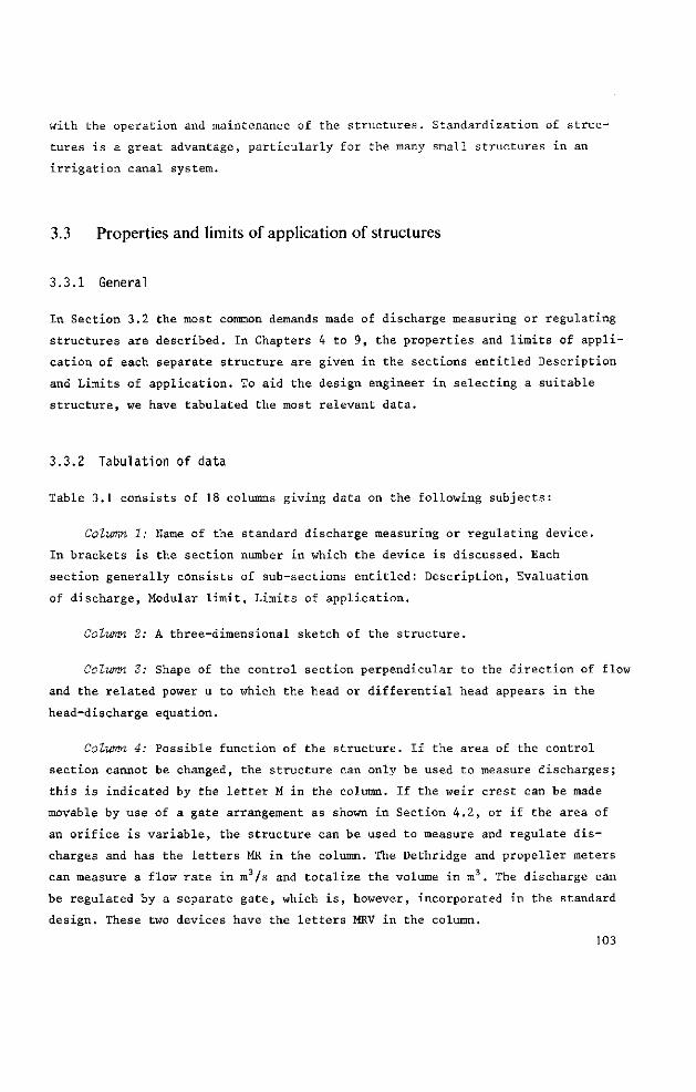
with the operation and maintenance of the structures. Standardization of struc
tures is a great advantage, particularly for the many small structures in an
irrigation canal system.
3.3 Properties and limits of application of structures
3.3.1 General
In Section 3.2 the most common demands made of discharge measuring or regulating
structures are described. In Chapters 4 to 9, the properties and limits of appli
cation of each separate structure are given in the sections entitled Description
and Limits of application. To aid the design engineer in selecting a suitable
structure, we have tabulated the most relevant data.
3.3.2 Tabulation of data
Table 3.1 consists of 18 columns giving data on the following subjects:
Column 1: Name of the standard discharge measuring or regulating device.
In brackets is the section number in which the device is discussed. Each
section generally consists of sub-sections entitled: Description, Evaluation
of discharge, Modular limit, Limits of application.
Column 2: A three-dimensional sketch of the structure.
Column 3: Shape of the control section perpendicular to the direction of flow
and the related power u to which the head or differential head appears in the
head-discharge equation.
Column 4: Possible function of the structure. If the area of the control
section cannot be changed, the structure can only be used to measure discharges;
this is indicated by the letter M in the column. If the weir crest can be made
movable by use of a gate arrangement as shown in Section 4.2, or if the area of
an orifice is variable, the structure can be used to measure and regulate dis
charges and has the letters MR in the column. The Dethridge and propeller meters
can measure a flow rate in m3/s and totalize the volume in m3. The discharge can
be regulated by a separate gate, which is, however, incorporated in the standard
design. These two devices have the letters MRV in the column.
103
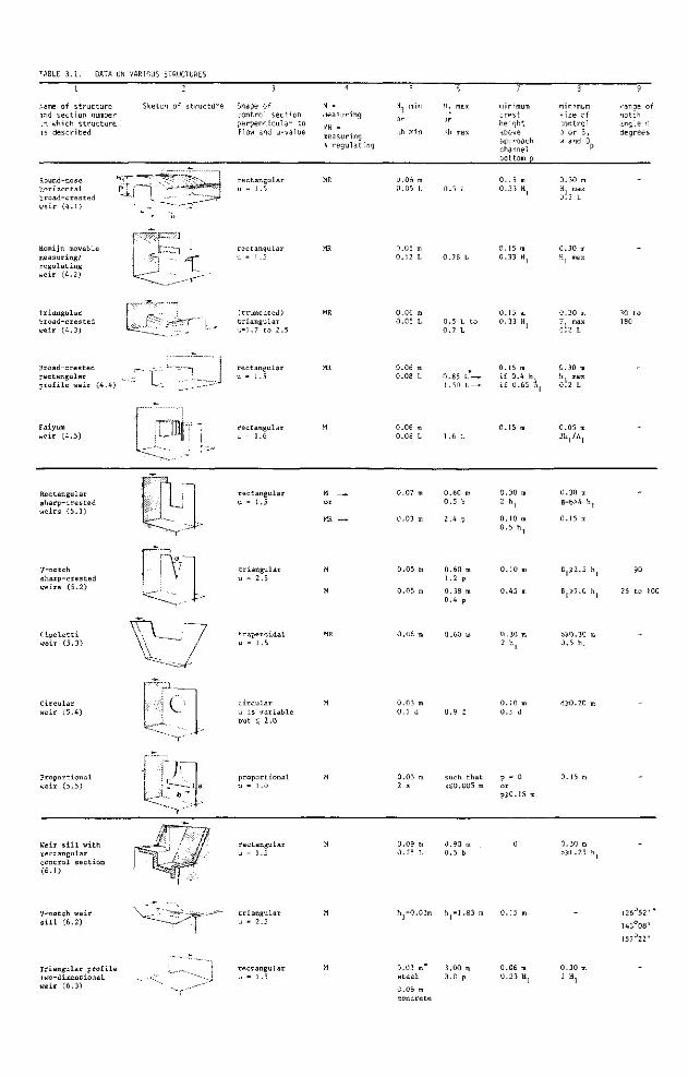
DATA ON VARIOUS STRUCTURES
1
Name o f s t r u c t u r e and sec t ion number in which s t r u c t u r e is descr ibed
Sketch of s t ructun Shape o f con t ro l sec t ion perpend icu la r t o f low and u-value
•A = measuring
m = measuring *i r e gu l a t i ng
5
H. max minimum crest height above aoproach channel bottom p
mi m m um size of control o or B, w and D
<-ange of notch angle 0 degrees
Round-nose horizontal broad-crested weir (4.1)
^* •£&£#& 0.06 i 0.05
0.30 m H max 0 .2 L
Romijn movable measuring/ regulating weir (4.2)
J-' *-)
*-^
-ri J
T • \r- '
rectangular u = 1 .5
0.30 m H max
Triangular broad-crested weir (4.3)
(truncated) triangular u-1.7 to 2.5
0.06 m 0.05 L 0.5 L to
0.7 L
0.15 m 0.33 H
0.30 m H max o!2 L
Broad-crested rectangular profile weir (4.4)
~, rectangular u - 1.5
0.06 m +
0.08 L 0.85 L — 1.50 L — -
if 0.4 h if 0.65 h,
Faiyum weir (4.5) i L m etangular
= 1.6 0.06 m 0.08 L 1.6 L
0.05 m 3h,/A,
Rectangular sharp-crested weirs (5,1)
rectangular 0.60 m 0.5 b
0.30 m 2 h,
0.10 m 0.5 h,
0.30 m B-b>4 h,
V-notch sharp-crested weirs (5.2)
triangular u = 2.5
0.60 m 1.2 p
0.38 m 0.4 p
0.10
0.45
Bjï2.5 h 90
B.Ï5.0 h 25 to 100
CipoLetti weir (5.3)
0.30 1 2 h.
bï0.30 m 0.5 h,
Circular weir (5.4) e circular
u is variable but ^ 2 . 0
0.03 m 0.1 à
0.10 m 0.5 d
Proportional weir (5.5)
_1 " b "
I
proportional u = 1.0
such that p = 0 x$0.005 m or
p^O.15 m
Weir sill with rectangular control section (6-1)
rectangular 0.09 m 0.90 i 0.75 L 0.5 b
0.30 m b^l.25 b.
V-notch weir sill (6.2)
Triangular profile two-dimensional weir (6.3)
T triangular u = 2.5
rectangular
h -0.03m
0.03 m* steel
0.06 m concrete
h =1.83 m
3.00 m 3.0 p
0.15 m
0.06 m 0.33 H
0.30 m 2H.
126 52
143°08
157°22
^
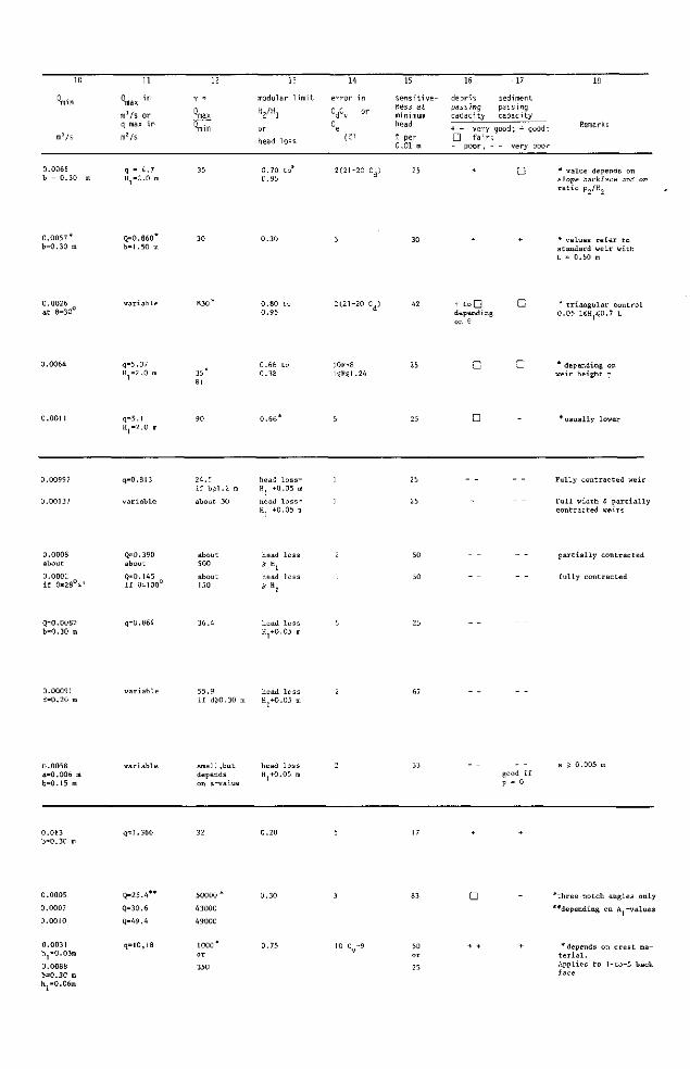
15
tn3/s or q max i n
m2/s
modular 1 i m i t
H,/H.
error in sensitiveness at minimum head
% per 0.01 m
debris sediment passing passing capacity capacity
+ + very good; + good; a fair; - poor; - - very poor
0.0066 b = 0.30 m
0.70 to 0.95
* value depends on slope backface and on ratio p„/H0
0.0057" b=0.30 m
Q=0.860 b-1.50 m
* values refer to standard weir with L = 0.60 m
0.0026 at 9=30°
0.80 to 0.95
2(21-20 C ) 42 + t o n depending
triangular control 0.05 L^H,$0.7 L
q=5.07 H,=2.0 i
0.66 to 0.38
10F-8 UF^l .24
depending on weir height p
q=5.1 H,=2.0 IT
* usually lower
0.00997
0.00137
q=0.8I3
variable
24.5 if b^l .2 m
about 30
head loss= K +0.05 m
head loss = H, +0.05 n:
Fully contracted weir
Full width 8 partially contracted weirs
0.0008 about
0.0002 if 6-28°4'
Q=0.390 about
Q«0.145 if 6=100°
about 500
about 150
head » H ,
head * H,
loss
loss
partially contracted
fully contracted
0=0.0082 b=0.30 in
q=Q.864 head loss H.+0.05 m
0.00091 d=0.20 m
head loss H.+0.05 m
0.0058 a=0.006 m b-0.15 m
variable small,but depends on a-value
head le Hj+O.O; good if
p - 0
q=1.366
0.0005
0.0007
0.0010
0.0031 hj-0.0301
0.0088 b=0.30 m h,=0.06m
q-25.4**
Q=30.6
Q-49.4
q=10,38
50000 *
43000
49000
1000* or
350
three notch angles only
**depending on A -values
* depends on crest material . Applies to l-to-5 back face
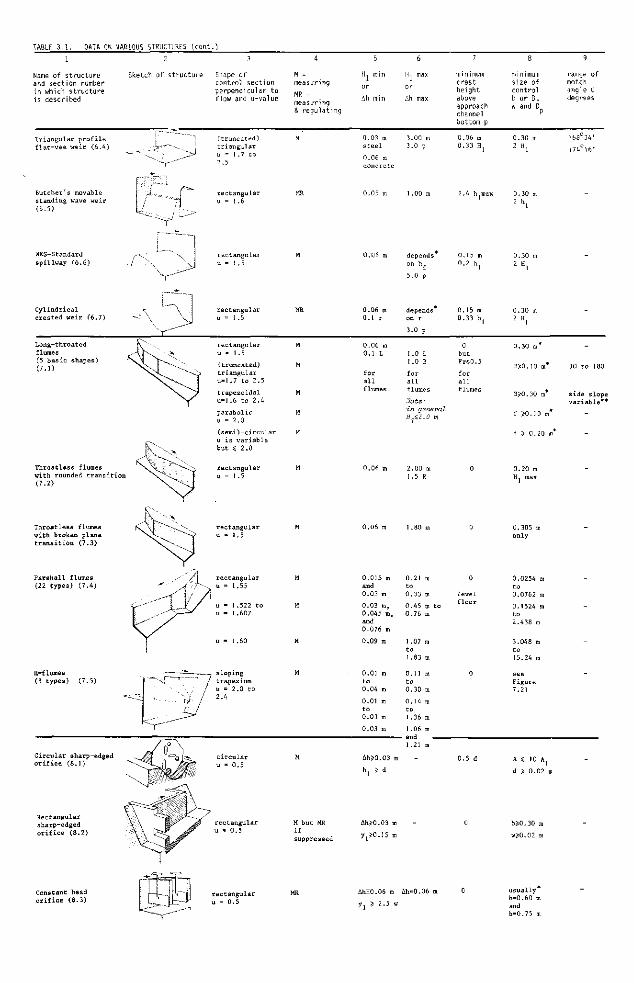
TABLE 3.1. DATA ON VARIOUS STRUCTURES (cont.)
1
Name of structure and section number in which structure is described
Triangular profile flat-vee weir (6.4)
Sketch of structure Shape of M = control section measuring perpendicular to „R
flow and u-value m e a~u r i r l g
& regulating
Ah min Ah max
(truncated) triangular u = I.7 to 2.5
0.03 m steel
0.06 m concrete
3.00 3.0 p
minimum crest height above approach channel bottom p
0.06 m 0.33 H,
mi m mum size of control b or B, w and 0
0.30 m 2 H,
range of notch angle 0 degrees
»68 34'
174°16'
Butcher's movable standing wave weir (6.5)
rectangular u = I .6
0.30 i 2 h,
WES-Standard spillway (6.6)
^> V"
depends on h.
0.30 i 2 H.
Cylindrical crested weir (6.7)
depends 0.15 m 0.33 h,
0.30 i 2 H,
Long-throated flumes (5 basic shapes) (7.1)
rectangular u = 1.5
(truncated) triangular u-1.7 to 2.5
trapezoidal u=l.6 to 2.4
parabolic u = 2.0
(semi)-circular u is variable but $ 2.0
0.06 m 0.1 L
for all flumes
1.0 L 1.0 B
for all flumes
'Jote .•
in aeneral H £3.0 m
but Fr$0..
0.30 m*
BS0.10 m*
BSO.30 m*
f SO.10 m'
d S 0.20 t
side slope variable**
Throatless flumes with rounded transition (7.2)
rectangular u = 1.5
0.20 m H, max
Throatless flumes with broken plane transition (7.3)
Parshall flumes (22 types) (7.4)
rectangular u - 1.5
H-flûmes (3 types) (7.5)
0.305 i only
Circular sharp-edged orifice (8.1)
Rectangular sharp-edged orifice (8.2)
Constant head orifice (8.3)
rectangular u = 0.5
M but MR if suppressed
0.015 m and 0.03 m
0.03 m, 0.045 m, and 0.076 m
0.09 m
0.21 to 0.33
0.45 0.76
1 .07 to 1.83
m
m
m to m
m
m
0
level floor
0.0254 m to 0.0762 m
0.1524 m to 2.438 m
3.048 m to 15.24 m
0.04 m
0.01 m to 0.03 m
0.03 m
Ah?0.03 m
h, i d
0.30 m
0.14 m to 1.36 m
1.06 m and 1.21 m
-
AhS0.03 m
y,S0.]5 m
Ah=0.06 m Ah=0.06 m
y, ï 2.5 w
Figure 7.21
A ^ 10 A
d S 0.02 i
bS0.30 m
w^0.02 m
usually b=0.60 m and b=0.75 m
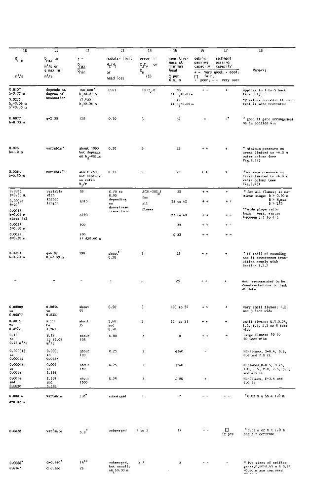
15
^max
m3/s or q max in
m*/s
"max
modular 1imit
H,/H,
(%)
sensitiveness at minimum head
% per 0.01 m
debris passing capacity
sediment passing capacity
+ + very good; + good;
- poor; - - very poor
0.0137 h=0.03 m
0.0275 h =0.06 m b =0.30 m
depends on degree of truncation
100,000* h,^0.03 m
17,500 h,JO.06 m
if h =0.03 IT
42 if h,=0.06n
Applies to l-to-5 back face only.
*y-values decrease if control is more truncated
0.0077 b=0.3Q m
good if gate arrangement in Section 4.2
0.025 b=1.0 i
about 1000 0.30 but depends on h -value
minimum pressure on crest limited to -4.0 m water column (see Fig.6.17)
0.0064 b=0.30 m
about 750, but depends on ratio Hj/r
. pressure on crest limited to -4,0 m water column (see Fig.6.23)
0.0066 b=0.30 m
0.00098 6=90°
0.0036 b=0.08 m slope 1:2
0.0027 f=0.10 m
0.0026 d=0.20 m
variable with throat length
35
100 if d?0.60 m
0.70 to 0.95 depending on downstream transition
2(21-20C )
f o r
a l l
flumes
25
28 to 42
27 to 40
* for all flumes; at maximum stage: B > 0.30 m
B > H max B > L75
**side slope ratio horz : vert, varies between \: I to 4 :1
0.0050 b=0.20 m
q=4.82 H,=2.00 l
about 0.50
* if radii of rounding and if downstream transition comply with Section 7.2.2
not recommended to be constructed due to lack of data
0.00009 t o 0.00077
0.0015 t o 0.0972
0.16 t o 0.75 m3/s
0.000012 t o 0.00034
0.000031 t o 0.0014
0.0018 and 0.0020
0.00014
d=0.02 m
0.0054 t o 0.0321
0.111 t o 3,949
8.28 to 93.04 m V s
0.0003 t o 0.0223
0.009 t o 2.336
2.369 and 3.326
variable
about 55
about 75
about 105
about 100
about 750
about 1500
5.8*
0.50
0.60 and 0.70
0.80
0.25
0.25
0.25
submerged
very small flumes; 1,2, and 3 inch wide
small flumes; 0.5,0.75, I.0, 1.5, 2,3 to 8 feet wide
large flumes; 10 to 50 feet wide
HS-flumes, D=0.4, 0.6, 0.8 and 1.0 ft
H-flumes,D=0.5, 0.75, 1.0, 1.5, 2.0, 2.5, 3.0, and 4.5 ft
HL-flumes, D=3.5 and 4.0 ft
* 0.03 m $ Ah < 1.0 m
D if p=i
* 0.03 m «A h 1.0 m and A = constant
0.0086
0.0107
Q=0.140
Q=0.280
submerged, but usually AH £0.30 m
* Two sizes of orifice gates,0.60x0.45 m & 0.75 X0.60 m are com.used
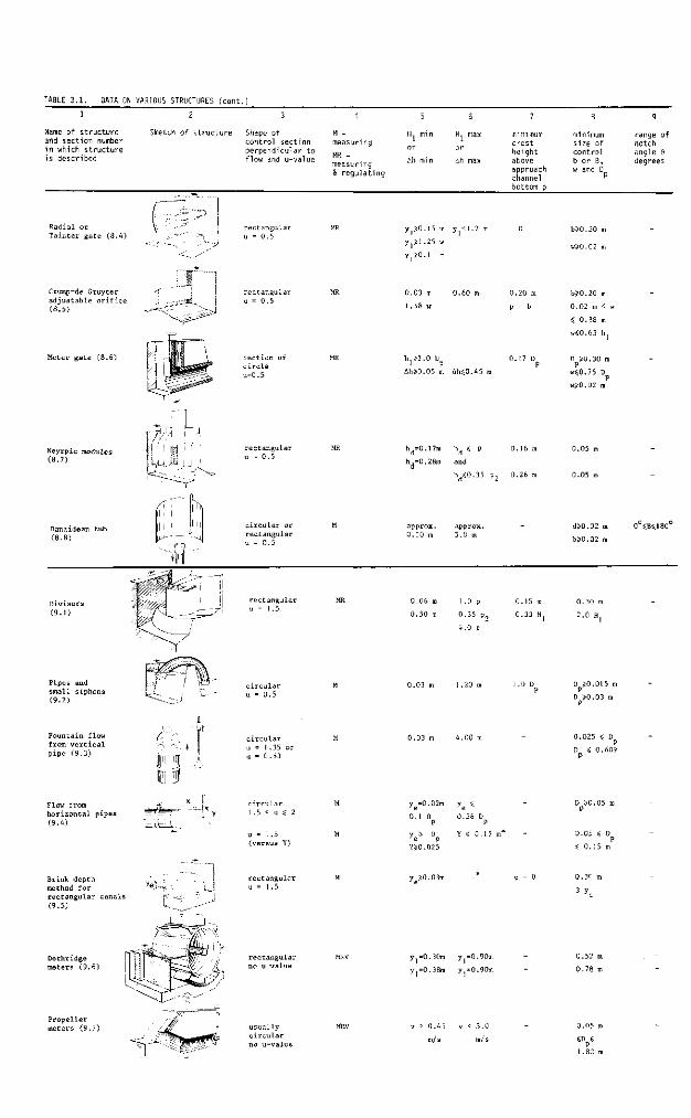
TABLE 3.1. DATA ON VARIOUS STRUCTURES (cont.)
1
Name of structure and section number in which structure is described
Sketch of structure Shape of control section perpendicular to flow and u-value
measuring
MR = measuring & regulating
minimum crest height above approach channel bottom p
minimum size of control b or B, w and D
P
range of notch angle G degrees
Radial or Tainter gate (8.4)
rectangular u = 0.5
y >0.15 m y <].2 r
y.^0.1 r
b>0.30 m
w»0.02 m
Crump-de Gruyter adjustable orifice (8.5)
Meter gate (8.6)
Neyrpic modules (8.7)
Danaidean tub (8.8)
rectangular u = 0.5
Section of circle u=0.5
rectangular u = 0.5
circular or rectangular u - 0.5
0.03 m
1.58 w
h,J].0 D ] p
Ah?0.0 5 m
0
Ah
60
$0
m
45 m
0.20 m
p = b
0.17 D P
b?0.20 m
0.02 m <
5 0.38 m
w^0.63 h
D £0.30 m P
ws=0.75 D P
w^0.02 m
h,=0.17m h, « P
h $0.35 p 2 0.26 :
approx. approx. 0.10 m 5.0 m
dj0.02 m
b?0.02 m
Divisors (9.1)
Pipes and small siphons (9.2)
rectangular u = 1 .5
circular u = 0.5
0.06 m !.0 p 0.15 m
0.50 r 0.35 p,, 0.33 H
4.0 r
0.30 m
2.0 H,
D S0.015 i P
D ^0.03 m
Fountain flow from vertical pipe (9.3)
circular u = 1.35 or u = 0.53
0.025 D P
D $ 0.609
Flow from horizontal pipes (9.4)
* 3 - ^ ^ . ircular .5 < u $ 2
y =0.02m y ^
y -> D Y « 0. 15 m e P
Y^O.025
0.05 S D P
$ 0.15 m
Brink depth "'( -method for e.t--y rectangular canals |-(9.5)
Dethridge meters (9,6)
Propeller meters (9.7)
rectangular
rectangular /'/ no upvalue
usually circular no u-value
y ?0.03m
y =0.30m y =0.90m
y =0.38m y =0.90m
0.45
m/s
0.30 •
3 y .
0.52 m
0.78 m
0.05 m
P 1 .82 m
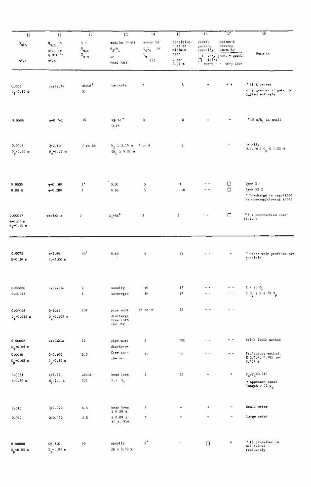
mVs
g in max
m3/s or q max in
m2/s
tnax
13
modular 1imit
head loss
14
zrror in
CdCv
Ce (Ï)
or
15
sensitiveness at ni ni mum head
•Ó per
0.01 m
debris passing capacity
sediment passing capacity
+ + very good; + good;
Q fair; - poor; - - very poor
0.005
y.=0.15 m
* If A varies
Y is greater if gate is lifted entirely
q=0.742 up to
0.25
0.0076
D =0.30 m
Q=2.10 Usually 0.20 m $ D
0.0005
0.0010
q=0.100
q=0.200
0.60
0.60
G Type X 1
G Type XX 2
* Discharge is regulated by opening/closing gates
d=0.02 m h,=0.10 i
h,+6d* *Ô = contraction coefficient
0.0075
b=0.30 i
q=5.69
H,=2.00 m
* Other weir profiles are possible
0.00006
0.00037
usually
submerged
L > 20 D P
6 D $ L 20 Ü
0.00048
D =0.025 m discharge free into
0.00062
D =0.05 m P
0.0020
D =0.05 m P
0.0081
b=0.30 m
variable
Q=0.100
D =0.15 m P
q=4.82
H-2 .0 m
42
2 . 5
about
175
pipe musl dischargt
free inti
the a i r
head los:
2.1 H
Brink depth method
Trajectory method; X=0.152, 0.Î05 and 0.457 m
* Approach canal length J 12 y
0.015
0.040
Q*=0.070
Q=0.140
4.6
3.5
head loss J 0.08 m
? 0.09 m at y min.
Small meter
Large meter
0.00088
D =0.05 i
Q=13.0
D =1.82 m
usually
Ah $ 0.50 m
* If propeller is maintained frequently
Column 5: Minimum value of H or Ah in metres or in terms of structural
dimensions.
Column 6: As Column 5, but giving maximum values.
Column 7: Minimum height of weir crest or invert of orifice above approach
channel bottom; in metres or in terms of structural dimensions.
Column 8: Minimum dimensions of control section; b, B, w, and D .
Column 9: Range of notch angle 8 for triangular control sections.
Column 10: Minimum discharge (Q . ) in m3/s x 10 or 1/s of the smallest
possible structure of the relevant type, being determined by the minima given in
Columns 5, 8, and 9.
Column 11: Maximum discharge: q in m 2 /s, being the discharge per metre crest
width if this width is not limited to a maximum value, or Q in m3/s if both the head
(differential) and control section dimensions are limited to a maximum. No maximum
discharge value is shown if neither the head (differential) nor the control di
mensions are limited by a theoretical maximum. Obviously, in such cases, the
discharge is limited because of various practical and constructional reasons.
Column 12: Value of Y = 0 /O . of the structure. If Q cannot be calcu-Tiiax Tnrn Tmax
lated directly, the Y ~ v a l u e c a n usually be determined by substituting the limi
tations on head (differential) in the head-discharge equation, as shown in Section
3.2.3.
Column IS: Modular limit H./H or required total head loss over the structure.
The modular limit is defined as that submergence ratio H„/H whereby the modular
discharge is reduced by 1% due to an increasing tailwater level.
Column 14: Error in the product C ,C or in the coefficient C .
d v e
Column IS: Maximum value of the sensitivity of the structure times 100,
being
100 S = £- Ah, 100 h, 1
where the minimum absolute value of h is used with the assumption Ah, = 0.01. The
figures shown give a percentage error in the minimum discharge if an error in the
determination of h, equal to 0.01 m is made. The actual error Ah, obviously depends
on the method by which the head is determined.
Column 16: Classifies the structures as to the ease with which they pass
floating and suspended debris.
110
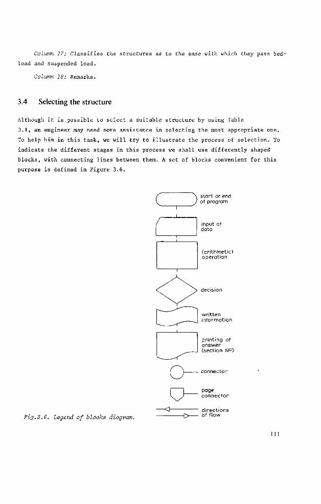
Colwran 17: Classifies the structures as to the ease with which they pass bed-
load and suspended load.
Column 18: Remarks.
3.4 Selecting the structure
Although it is possible to select a suitable structure by using Table
3.1, an engineer may need some assistance in selecting the most appropriate one.
To help him in this task, we will try to illustrate the process of selection. To
indicate the different stages in this process we shall use differently shaped
blocks, with connecting lines between them. A set of blocks convenient for this
purpose is defined in Figure 3.6.
start or end of program
input of data
(arithmetic) operation
decision
written nformation
printing of answer (section N°)
connector
page connector
Fig.3.6. Legend of blocks diagram. directions of flow
111
All blocks except the terminal block, which has no exit, and logical deci
sion blocks, which have two or more exits, may have any number of entry
paths but only one exit path. A test for a logical decision is usually framed
as a question to which the answer is "Yes" or "No", each exit from the Lozenge
block being marked by the appropriate answer.
A block diagram showing the selection process is shown in Figure 3.7.
The most important parts of this process are:
The weighing of the hydraulic properties of the structure against the actual
situation or environment in which the structure should function (boundary condi
tions) ;
The period of reflection, being the period during which the engineer tests
the type of structure and decides whether it is acceptable.
Both parts of the selection process should preferably be passed through several
times to obtain a better understanding of the problem.
To assist the engineer to find the most appropriate type of structure, and thus
the relevant section number in the next chapters of this book, we have included
Figure 3.8, which treats approximately that part of the selection process enclosed
by the dotted line in Figure 3.7. In constructing the diagram of Figure 3.8 we
have only used the most important criteria. The use of more criteria would make
the diagram longer and more complex.
After one or more suitable structures (sections) are found we recommend that
Table 3.1 be consulted for a first comparative study, after which the appropriate
section should be studied. During the latter study one takes the secondary boundary
conditions into account and continues through the "reflection branch" of Figure
3.7 until the proper structure has been selected.
It is stressed again that in this chapter the selection of structures is based
purely upon the best hydraulic performance. In reality it is not always desirable
to alter the existing situation so that all limits of application of a standard
structure are fulfilled. If, however, a structure is to be used to measure dis
charges and its head-discharge relationship is not known accurately, the structure
must either be calibrated in a hydraulic laboratory or calibrated in situ. Cali
bration in situ can be performed by using the area-velocity method or the salt
dilution method.
112
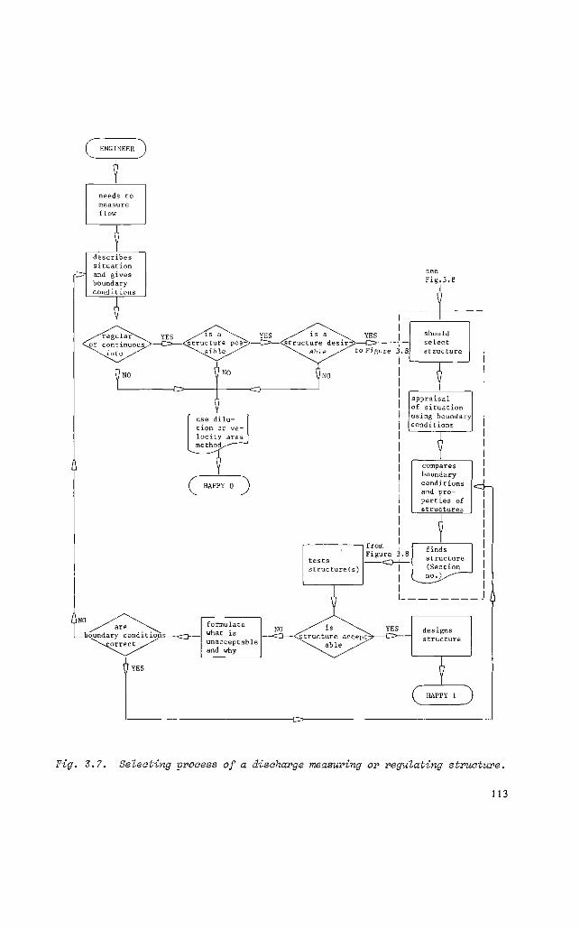
see Fig.3.8
to Figure 3
use dilution or velocity area method.
are -boundary conditions-
correct
formulate what is unacceptable and why
"~l
should select structure
appraisal of situation using boundary conditions
Fig. 3.7. Selecting process of a discharge measuring or regulating structure.
113
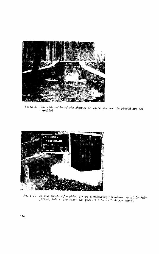
Photo 2. The side walls of the channel in which the weir is placed are not parallel.
WWBJI
Photo 3. If the limits of application of a measuring structure cannot be fulfilled, laboratory tests can provide a head-discharge curve.
114
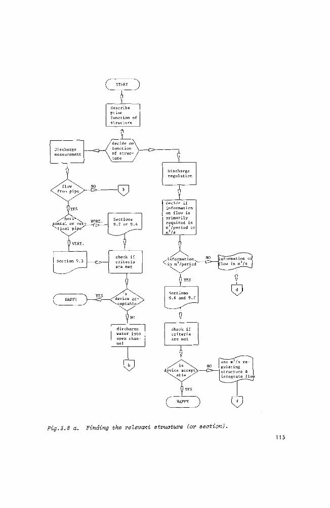
describe prime function of structure
Discharge measurement
/decide on\ _/ function
\ of struc-\ ture /
discharge water into open channel
Discharge regulation
decide if information on flow is primarily required in m3/period or
( HAPPY j
Fig.3.8 a. Finding the relevant structure (or section).
115
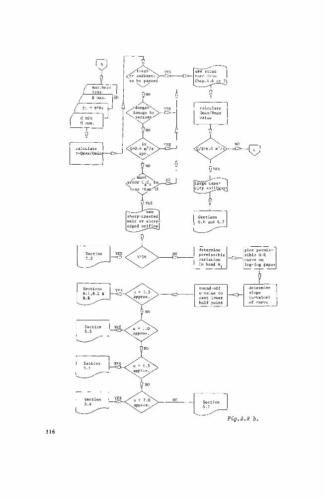
/ 1
îiax.head loss 1
/ B max.
/»-/ Q min
Q max
p+H
-
ÄH
J
calculate Y=Qmax/Qmin
plot sib le curve log-l
permis-
Q-H on
og paper
Fzg.3.
116
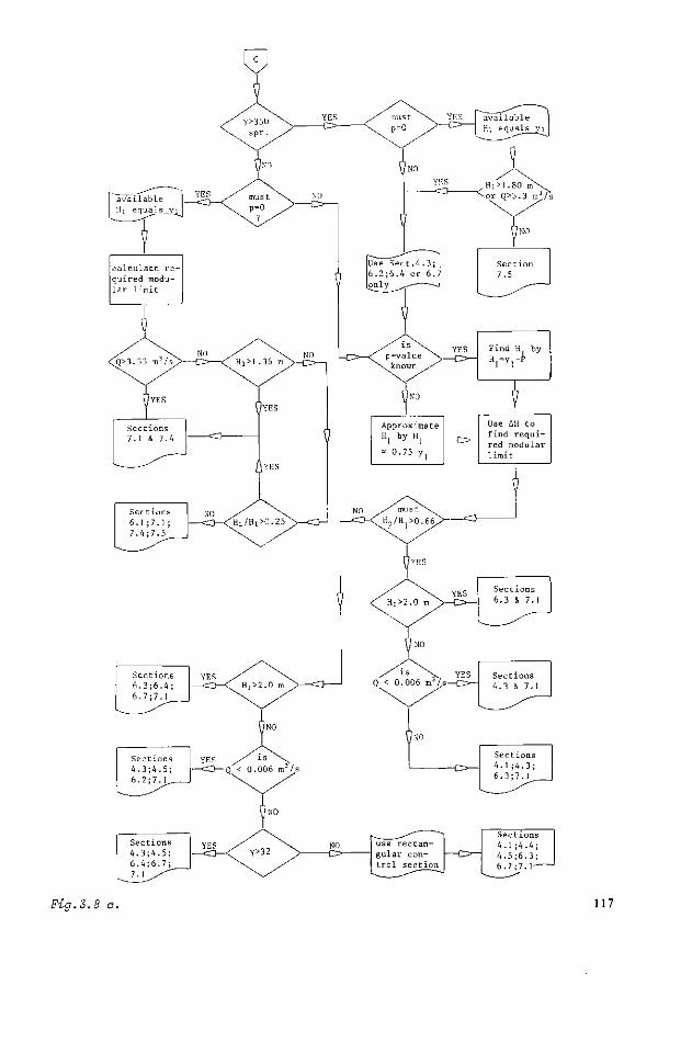
O—'
Sections 4.1 ; 4 .4 ; 4 . 5 ; 6 . 3 ; 6 .7 ;7 . 1- '
Hg.Z.B o. 117
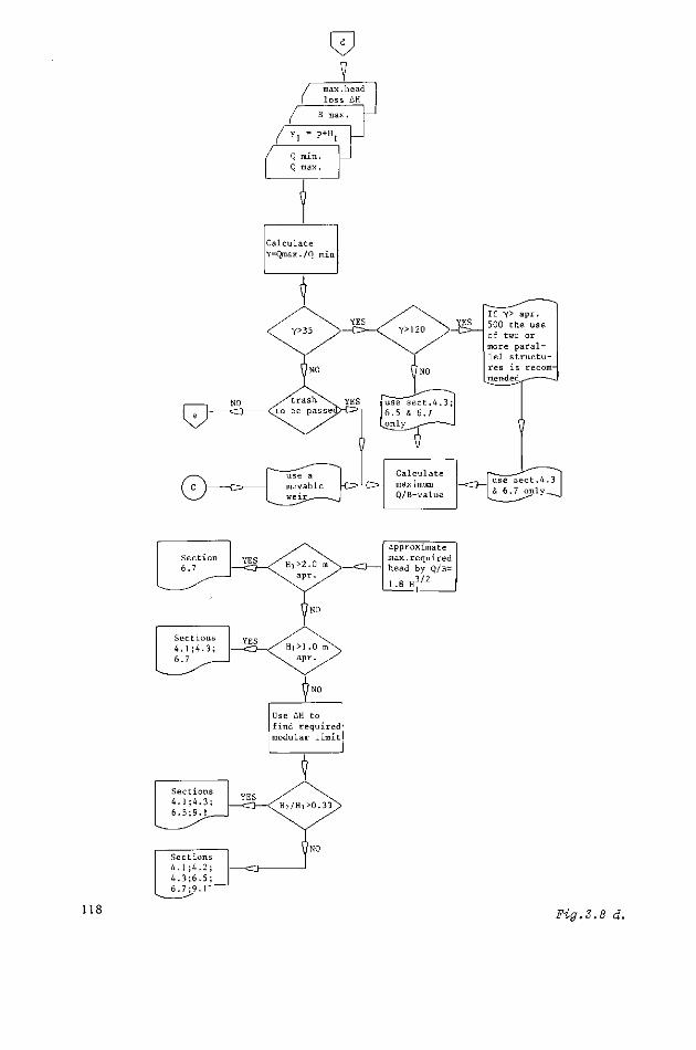
/ max. heao [ loss AH
/ B max.
( yi = P + H i
/ Q min. Q max.
-J
Calculate Y=Qmax./0 min
If y> apr. 500 the use of two or more parallel structu
r e AH to find required modular limit
Sections 4 4 6
1 3 7
4 6 9
2; 5;
r 118 Fig.3.8 d.
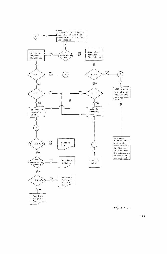
Fig.3.8 e.
119
3.5 Selected list of references
1. BERKHOUT, F.M.C.: Lecture notes on irrigation engineering. F 18.
University of Technology, Delft. 1965.
2. ENGELUND, F. and HANSEN, E.: A monograph on sediment transport in al
luvial streams. Teknisk Forlag, Copenhagen. 1967.
3. MAHBUB, S.I., and GULHATI, N.D.: Irrigation outlets. Atma Ram & Sons,
India, 1951 . 184 pp.
4. MEIJER-PETER, E. and MÜLLER, R.: Formulas for bed-load transport.
Proc.Second meeting of the International Association for Hydraulic Structures Res.,
Stockholm 1948. Vol.2, Paper 2.
5. NETHERLANDS ENGINEERING CONSULTANTS (NEDECO): Rio Magdalena and Canal
del dique survey project. The Hague 1973.
6. REPLOGLE, J.A.: Discussion of Rectangular cutthroat flow measuring
flumes (Proc.Paper 5628). J.of the Irrigation and Drainage Division of the ASCE.
Vol.94. No.IR3. Sept. 1968, pp.359-362.
120
4 Broad-crested weirs
Classified under the term "broad-crested weirs" are those structures over which
the streamlines run parallel to each other at least for a short distance, so
that a hydrostatic pressure distribution may be assumed at the control section.
To obtain this condition, the length in the direction of flow of the weir crest
(L) is restricted to the total upstream energy head over the crest (H ) . In the
following sections the limitation on the ratio H /L will be specified for the fol
lowing types of broad-crested weirs;
4.1 Round-nose horizontal broad-crested weir; 4.2 The Romijn movable measuring/
regulating weir; 4.3 Triangular broad-crested weir; 4.4 Broad-crested rectangu
lar profile weir; 4.5 Faiyum weir.
4.1 Round-nosed horizontal broad-crested weir
4.1.1 Description
This weir is in use as a standard discharge measuring device and, as such, is
described in the British Standard 3680, 1969, which is partly quoted below. The
weir comprises a truly level and horizontal crest between vertical abutments.
The upstream corner is rounded in such a manner that flow separation does not
occur. Downstream of the horizontal crest there may be
(i) a vertical face
(ii) a downward slope or
(iii) a rounded corner, depending on the submergence ratio under which the
weir should operate at modular flow.
The weir structure should be rigid and watertight and be at right angles to
the direction of flow.
121
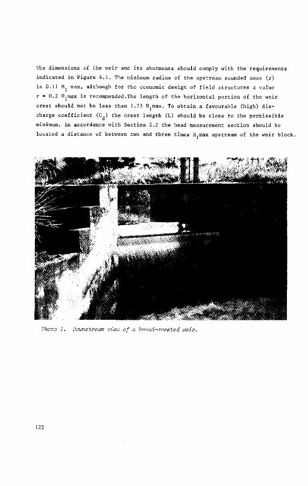
The dimensions of the weir and its abutments should comply with the requirements
indicated in Figure 4.1. The minimum radius of the upstream rounded nose (r)
is 0.11 H max, although for the economic design of field structures a value
r = 0.2 H max is recommended.The length of the horizontal portion of the weir
crest should not be less than 1.75 H.max. To obtain a favourable (high) dis
charge coefficient (C,) the crest length (L) should be close to the permissible
minimum. In accordance with Section 2.2 the head measurement section should be
located a distance of between two and three times H max upstream of the weir block.
I ***** < i
<-" .„ . , •/ft»-.«.
Photo 1. Downstream view of a broad-crested weir.
122
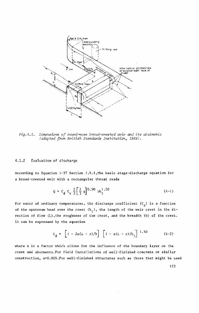
^Rad S 2 Hjmax
e geometr ies ream face of
Fig.4.1. Dimensions of round-nose broad-crested weir and its abutments (adapted from British Standards Institution, 1969).
4.1.2 Evaluation of discharge
According to Equation 1-37 Section 1.9.1,the basic stage-discharge equation for
a broad-crested weir with a rectangular throat reads
C, C d
2 V 2 ~|0. v 3 L ï 8J
50 ,, 1.50 b hl
(4-1)
For water of ordinary temperatures, the discharge coefficient (C,) is a function
of the upstream head over the crest (h ) , the length of the weir crest in the di
rection of flow (L),the roughness of the crest, and the breadth (b) of the crest.
It can be expressed by the equation
Cd = [l - 2x(L - r)/b] [l - x(L - r)/hj 1.50
(4-2)
where x is a factor which allows for the influence of the boundary layer on the
crest and abutments.For field installations of well-finished concrete or similar
construction, x^O.OOS.For well-finished structures such as those that might be used
123
in laboratories for gauging clean water, x - 0.003.
The appropriate value of the approach velocity coefficient (C ) can be read from
Figure 1.12 (Chapt.1).
The error in the product C.C of a well maintained round-nose broad-crested weir, d v '
which has been constructed with reasonable care and skill, can be deduced from
the equation
X = + 2(21 - 20 C ) per cent (4-3)
The method by which this error is to be combined with other sources of error is
shown in Appendix II.
4.1.3 Modular limit
The flow over a weir is modular when it is independent of variations in tail-
water level. For this to occur, assuming subcritical conditions in the tail-water
channel, the tailwater level (h„) must not rise beyond a certain percentage of
the upstream head over the weir crest (H ) . Hence, the height of the weir above
the bottom of the tailwater channel (p9) should be such that the weir operates
at modular flow at all discharges. The modular limit can be read from Figure 4.2
as a function of H./p„ and the slope of the back face of the weir. The design
value of p. should be established by a trial and error method.
4.1.4 Limits of application
a) The practical lower limit of h. is related to the magnitude of the in
fluence of fluid properties, to the boundary roughness, and to the accuracy
with which h. can be determined. The recommended lower limit is 0.06 m or 0.05
times L, whichever is greater.
b) The limitations on Hj/p arise from difficulties experienced when the
Froude number Fr = v./(gA)/B) ' in the approach channel exceeds 0.5, coupled
with inadequate experimental confirmation at high values of H./p. The recom
mended upper limit is H /p = 1.5, while p should be greater than or equal to
0.15 m.
124
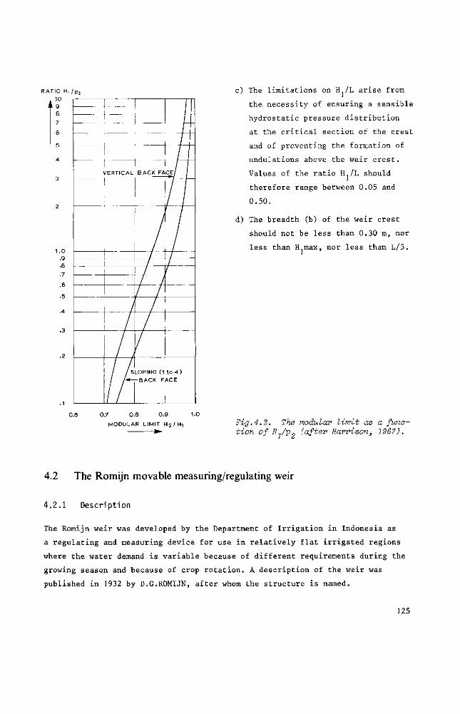
RATIO H, /p2
10 * 9
1.0
.9
.8
.7
.6
.5
• - • -
VERTICAL
I !
BACK FA / I
CE/ /
XL
/ / s
/
LOPING (1 -BACK F
to 4 ) ACE
c) The limitations on H./L arise from
the necessity of ensuring a sensible
hydrostatic pressure distribution
at the critical section of the crest
and of preventing the formation of
undulations above the weir crest.
Values of the ratio H /L should
therefore range between 0.05 and
0.50.
d) The breadth (b) of the weir crest
should not be less than 0.30 m, nor
less than H max, nor less than L/5.
0.7 0.8 0.9 1.0
MODULAR LIMIT H 2 / Hi Fig.4.2. The modular limit as a function of H-j/Pn (after Harrison, 1967).
4.2 The Romijn movable measuring/regulating weir
4.2.1 Description
The Romijn weir was developed by the Department of Irrigation in Indonesia as
a regulating and measuring device for use in relatively flat irrigated regions
where the water demand is variable because of different requirements during the
growing season and because of crop rotation. A description of the weir was
published in 1932 by D.G.ROMIJN, after whom the structure is named.
125
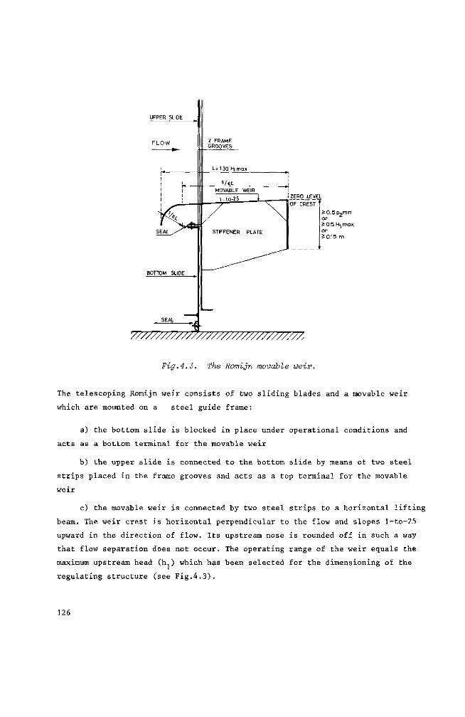
"7777777777777777777777777777777777;
Fig.4.3. The Romijn movable weir.
The telescoping Romijn weir consists of two sliding blades and a movable weir
which are mounted on a steel guide frame:
a) the bottom slide is blocked in place under operational conditions and
acts as a bottom terminal for the movable weir
b) the upper slide is connected to the bottom slide by means of two steel
strips placed in the frame grooves and acts as a top terminal for the movable
weir
c) the movable weir is connected by two steel strips to a horizontal lifting
beam. The weir crest is horizontal perpendicular to the flow and slopes l-to-25
upward in the direction of flow. Its upstream nose is rounded off in such a way
that flow separation does not occur. The operating range of the weir equals the
maximum upstream head (h ) which has been selected for the dimensioning of the
regulating structure (see Fig.4.3).
126
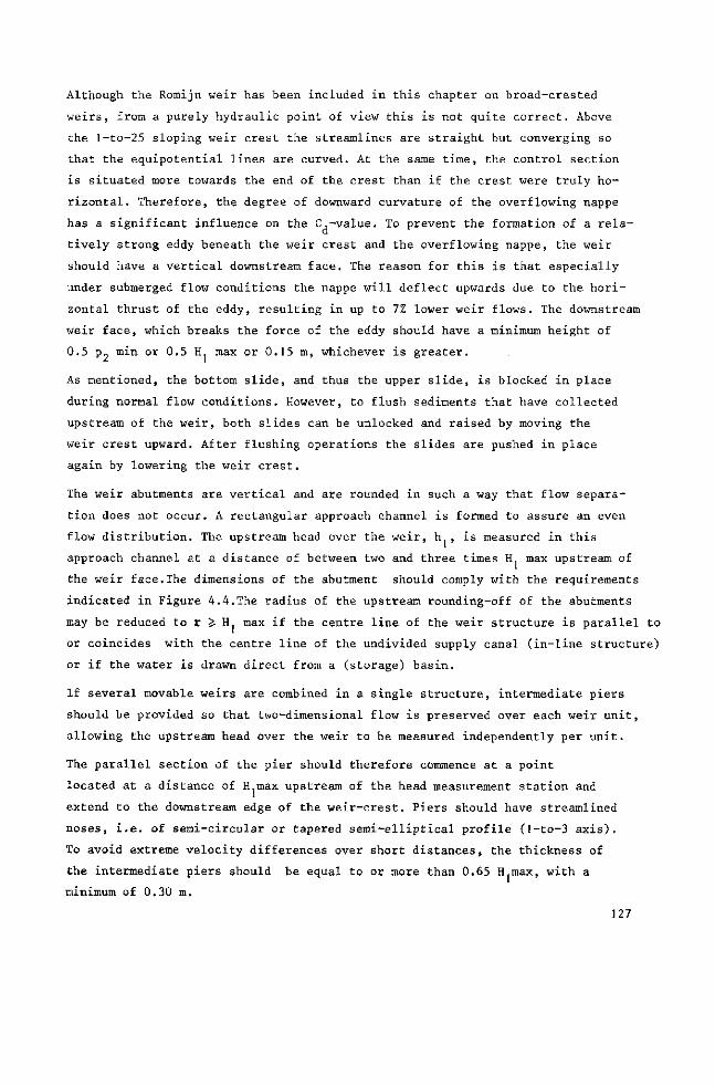
Although the Romijn weir has been included in this chapter on broad-crested
weirs, from a purely hydraulic point of view this is not quite correct. Above
the l-to-25 sloping weir crest the streamlines are straight but converging so
that the equipotential lines are curved. At the same time, the control section
is situated more towards the end of the crest than if the crest were truly ho
rizontal. Therefore, the degree of downward curvature of the overflowing nappe
has a significant influence on the C,-value. To prevent the formation of a rela
tively strong eddy beneath the weir crest and the overflowing nappe, the weir
should have a vertical downstream face. The reason for this is that especially
under submerged flow conditions the nappe will deflect upwards due to the hori
zontal thrust of the eddy, resulting in up to 7% lower weir flows. The downstream
weir face, which breaks the force of the eddy should have a minimum height of
0.5 p„ min or 0.5 H max or 0.15 m, whichever is greater.
As mentioned, the bottom slide, and thus the upper slide, is blocked in place
during normal flow conditions. However, to flush sediments that have collected
upstream of the weir, both slides can be unlocked and raised by moving the
weir crest upward. After flushing operations the slides are pushed in place
again by lowering the weir crest.
The weir abutments are vertical and are rounded in such a way that flow separa
tion does not occur. A rectangular approach channel is formed to assure an even
flow distribution. The upstream head over the weir, h , is measured in this
approach channel at a distance of between two and three times H max upstream of
the weir face.The dimensions of the abutment should comply with the requirements
indicated in Figure 4.4.The radius of the upstream rounding-off of the abutments
may be reduced to I J H max if the centre line of the weir structure is parallel to
or coincides with the centre line of the undivided supply canal (in-line structure)
or if the water is drawn direct from a (storage) basin.
If several movable weirs are combined in a single structure, intermediate piers
should be provided so that two-dimensional flow is preserved over each weir unit,
allowing the upstream head over the weir to be measured independently per unit.
The parallel section of the pier should therefore commence at a point
located at a distance of H max upstream of the head measurement station and
extend to the downstream edge of the weir-crest. Piers should have streamlined
noses, i.e. of semi-circular or tapered semi-elliptical profile (l-to-3 axis).
To avoid extreme velocity differences over short distances, the thickness of
the intermediate piers should be equal to or more than 0.65 I^max, with a
minimum of 0.30 m.
127
ï2Himax TRANSITION
side slope of canal
^ 5H,max 1.3H-|max aerat ion g roove
DIVERTED FLOW ^ >
»Himax, _ 2 toSH, max
I .intake pipe -it .
GAUGE OR STILLING WELL* |
movable 2l gauge
al ternat ive a r rangement
5> 2 t imes maximum depth t o
water surface in well
Fig.4.4. Hydraulic dimensions of weir abutments.
Since the weir crest moves up and down, a fixed staff gauge at the head measure
ment station does not provide a value for the upstream head over the crest unless
the weir crest elevation is registered separately in terms of gauged head. To
avoid this procedure, the weir is equipped with a gauge that moves up and down
with the weir crest (see Fig.4.4). Zero level of this gauge coincides with the
downstream edge of the weir crest, so that the upstream head over the crest equals
the immersed depth of the gauge and can he read without time lag. The movable
gauge is attached to the extended lifting beam as shown in Figure 4.6.
4.2.2 Evaluation of discharge
According to Equation 1-37, Section 1.9.1, the basic head discharge equation for
a broad-crested weir with a rectangular control section reads
d v 3 [M 0.50 ,,1.50 bh. (4-4)
128
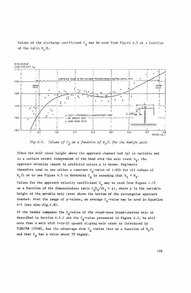
Values of the discharge coefficient C, may be read from Figure 4.5 as a function
of the ratio H./L.
DISCHARGE COEFFICIENT Cd 1.10
07 o.e RATIO H,/L
Fig. 4. 5. Values of C, as a function of B.JL for the Romijn weir.
Since the weir crest height above the approach channel bed (p) is variable and
to a certain extent independent of the head over the weir crest h , the
approach velocity cannot be predicted unless p is known. Engineers
therefore tend to use either a constant C.-value of 1.055 for all values of d
hj/L or to use Figure 4.5 to determine C by assuming that h. - H .
Values for the approach velocity coefficient C may be read from Figure 1.12
as a function of the dimensionless ratio C h /(h. + p ) , where p is the variable
height of the movable weir crest above the bottom of the rectangular approach
channel. Over the range of p-values, an average C -value may be used in Equation
4-4 (see also Fig.4.8).
If the reader compares the C,-value of the round-nose broad-crested weir as
described in Section 4.1.2 and the C,-value presented in Figure 4.5, he will
note that a weir with l-to-25 upward sloping weir crest as introduced by
VLUGTER (1940), has the advantage that C varies less as a function of H /L
and that C, has a value about 7% higher.
129
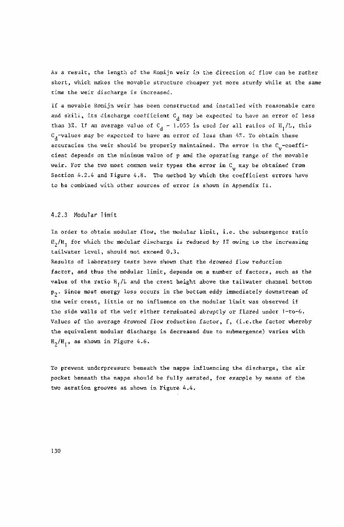
As a result, the length of the Romijn weir in the direction of flow can be rather
short, which makes the movable structure cheaper yet more sturdy while at the same
time the weir discharge is increased.
If a movable Romijn weir has been constructed and installed with reasonable care
and skill, its discharge coefficient C, may be expected to have an error of less
than 3%. If an average value of C = 1.055 is used for all ratios of H,/L, this
Cj-values may be expected to have an error of less than 4%. To obtain these
accuracies the weir should be properly maintained. The error in the C -coeffi
cient depends on the minimum value of p and the operating range of the movable
weir. For the two most common weir types the error in C may be obtained from
Section 4.2.4 and Figure 4.8. The method by which the coefficient errors have
to be combined with other sources of error is shown in Appendix II.
4.2.3 Modular l imit
In order to obtain modular flow, the modular limit, i.e. the submergence ratio
H„/H for which the modular discharge is reduced by 1% owing to the increasing
tailwater level, should not exceed 0.3.
Results of laboratory tests have shown that the drowned flow reduction
factor, and thus the modular limit, depends on a number of factors, such as the
value of the ratio H./L and the crest height above the tailwater channel bottom
p„ . Since most energy loss occurs in the bottom eddy immediately downstream of
the weir crest, little or no influence on the modular limit was observed if
the side walls of the weir either terminated abruptly or flared under l-to-6.
Values of the average drowned flow reduction factor, f, (i.e.the factor whereby
the equivalent modular discharge is decreased due to submergence) varies with
H./H,, as shown in Figure 4.6.
To prevent underpressure beneath the nappe influencing the discharge, the air
pocket beneath the nappe should be fully aerated, for example by means of the
two aeration grooves as shown in Figure 4.4.
130
SUBMERGENCE RATIO H2/H, 1.0
0.9
0.8
0.7
0.6
0.5
0.4
0.3
0.2
0.1
- V r - - andP l o AA + o - s i i T f l ^ ,
» 0.16 m /sec • 0.12 Ä 0.08 ., i n n? • 0.01
b=0.40m L= 0.475 m
••••up
? =042n-,
? ^ -
^Tîr- + 4»4 .~
s
\ \
modular lin H2 /H1 =03
\ \
\ \ i nit \ ,V, 3 m °VÄ1_
1 1
0.6 0.7 0.8 0.9 1.0 DROWNED FLOW REDUCTION FACTOR f
Fig.4.6. Drowned flow reduction factor for Bomijn weir.
4.2.4 Commonly used weir dimensions
The reader will have noted that all dimensions of both the weir and its abut
ments are related to the maximum value selected for the total energy head over
the weir crest (îLmax). The loss of head required for modular flow is also re
lated to the total energy head as Ah = h - h ^ 0.70 tLmax.
Since the limiting factor in most relatively flat irrigated areas is the avail
able head for open canal and weir flow, the maximum value of h is limited to
a certain practical value which approximates 0.45 m. The length of the weir crest
in the direction of flow consequently equals L=0.60 m, of which 0.50 m is straight and
sloping 1:25 upward in the direction of flow and the remaining 0.10 m forms the
rounded nose, its radius also being 0.10 m.
131
Theoretically any weir breadth greater or equal to 0.30 m may be used, but to
obtain a degree of standardization in the structures of an irrigation project a
limited number of breadths should be employed. It is often practicable to use a
breadth not greater than b = 1.50 m, since a central handwheel can then be used
to move the weir while the groove arrangement can be a relatively simple one
consisting of steel blades sliding in narrow (0.01 m) grooves. If the breadth
b exceeds 1.50 m, a groove arrangement as shown in Section 6.5.1 may be used.
Examples of constructional drawings are shown in Figure 4.7.
If the Romijn weir is installed in accordance with Figure 4.6, which is the
normal method of installation, the values for hr and p vary in such a way that
0.05 m 4: h <S 0.45 m
0.55 m ^ p 5$ 0.95 m
0.60 m •$ h + p ^ 1.00 m
Due to the variation of both ht and p, the approach velocity coefficient is not
a function of hj alone, but ranges between the broken lines shown in Figure 4.8.
In irrigation practice it is confusing to work with several C -values for the
same upstream head. Therefore the use of an average C -value, as a function of
the upstream head h only, is advised. It follows from Figure 4.8 that this
average C -value may be expected to have an error of less than 1%. The discharge
in m3/s per metre width of weir crest can be calculated from Equation 4-4 and
Figures 4.5 and 4.8. Values of q for each 0.01 m of head are presented in Table
4.1, Column 2.
An alternative method of installing the weir is to use no bottom slide. The
movable weir is then lowered behind a drop in the channel bottom, this drop
acting as a bottom terminal. With this method, the height of the weir crest
above the bottom of approach channel is less than with the normal method of in
stallation. Consequently, the approach velocity and thus the C -value is signi
ficantly higher.For a standard weir with a length of the weir crest in the direction
of flow L = 0.60 m, values of p and h1 range in such a way that:
0.05 m £ h ^ 0.45 m
0.15 m p < 0.55 m
0.20 m ^ h + p <: 0.60 m
132
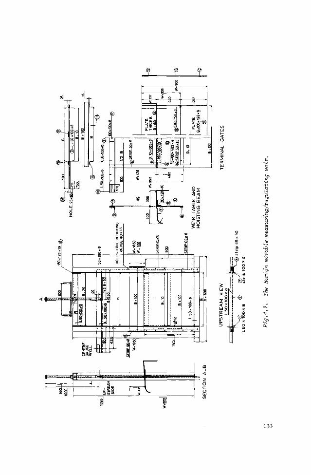
3
<3> S
(3
S <35
<s
s • ^ > Sn S 03 O <a E
O S s
T i
O
ft;
133
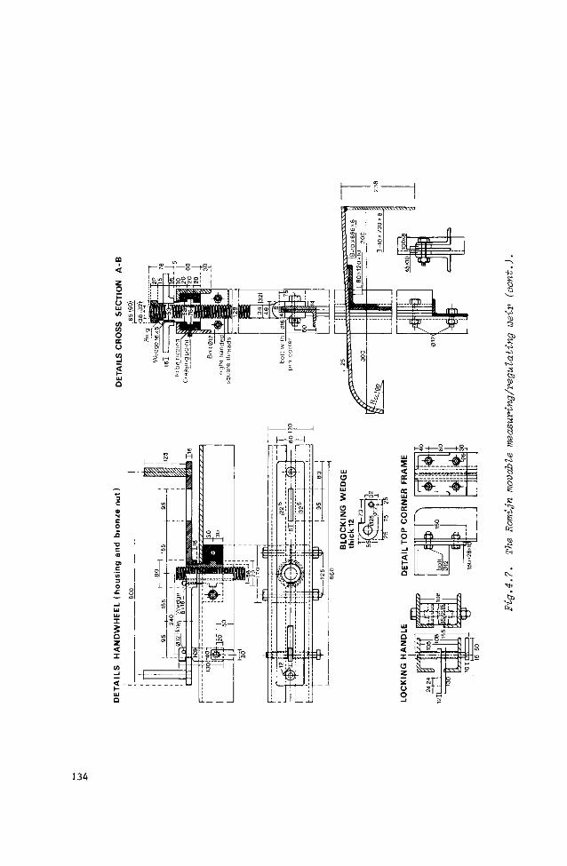
s o
Si
(S 3
S
S Co
Öl S Si 3 03 Ö <S E
S
'Ci S o te;
ta
134
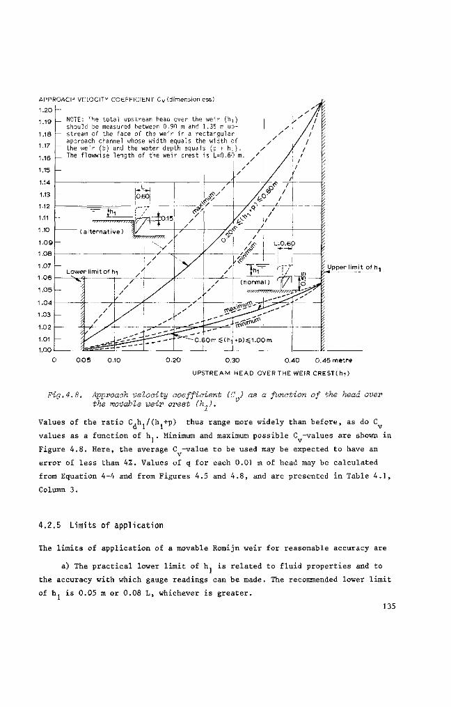
APPROACH VELOCITY COEFFICIENT Cv (dimensionless)
1.20 — _ NOTE: The t o ta l upstream head over the
0.05 0.10 0.20 0.30 0.40 0.45 metre
UPSTREAM HEAD OVER THE WEIR CREST( hi )
Fig.4. 8. Approach velocity coefficient (C ) as a function of the head over the movable weir crest (h1).
Values of the ratio C,h-/(h1+p) thus range more widely than before, as do C
values as a function of h,. Minimum and maximum possible C -values are shown in l r v
Figure 4.8. Here, the average C -value to be used may be expected to have an
error of less than 4%. Values of q for each O.Ol m of head may be calculated
from Equation 4-4 and from Figures 4.5 and 4.8, and are presented in Table 4.1,
Column 3.
4.2.5 Limits of application
The limits of application of a movable Romijn weir for reasonable accuracy are
a) The practical lower limit of hj is related to fluid properties and to
the accuracy with which gauge readings can be made. The recommended lower limit
of h. is 0.05 m or 0.08 L, whichever is greater.
135
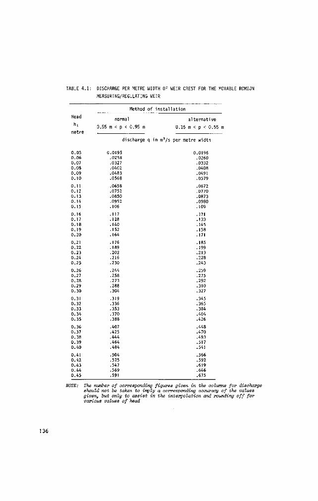
TABLE 4.1: DISCHARGE PER METRE WIDTH OF WEIR CREST FOR THE MOVABLE ROMIJN
MEASURING/REGULATING WEIR
Head
hi
metre
Method of installation
normal alternative
0.55 m < p < 0.95 m 0.15 m < p < 0.55 m
0.05 0.06 0.07 0.08 0.09 0.10
0.11 0.12 0.13 0.14 0.15
0.16 0.17 0.18 0.19 0.20
0.21 0.22 0.23 0.24 0.25
0.26 0.27 0.28 0.29 0.30
0.31 0.32 0.33 0.34 0.35
0.36 0.37 0.38 0.39 0.40
0.41 0.42 0.43 0.44 0.45
0.0195 .0258 .0327 .0402 .0483 .0568
.0658
.0752
.0850
.0952
.106
.117
.128
.140
.152
.164
.176
.189
.202
.216
.230
.244
.258
.273
.288
.304
.319
.336
.353
.370
.388
.407
.425
.444
.464
.484
.504
.525
.547
.569
.591
discharge q in m3/s per metre width
0.0196 .0260 .0332 .0408 .0491 .0579
.0672
.0770
.0873
.0980
.109
.121
.133
.145
.158
.171
.185
.199
.213
.228
.243
.259
.275
.292
.310
.327
.345
.365
.384
.404
.426
.448
.470
.493
.517
.541
.566
.592
.619
.646
.675
NOTE: The number of corresponding figures given in the columns for discharge should not be taken to imply a corresponding accuracy of the values given, but only to assist in the interpolation and rounding off for various values of head
136
b) To reduce the influence of boundary layer effects at the sides of the
weir, the weir breadth b should not be less than 0.30m nor less than the maximum
value of Hj.
c) The height of the weir crest above the bottom of the approach channel
should not be less than 0.15 m nor less than 0.33 H.max.
d) To obtain a sensibly constant discharge coefficient, the ratio IL/L should
not exceed 0.75.
e) The submergence ratio H„/H. should not exceed 0.30 to obtain modular
flow.
4.3 Triangular broad-crested weir
4.3.1 Description
On natural streams and irrigation canals where it is necessary to measure a wide
range of discharges, a triangular control has several advantages. Firstly it
provides a large breadth at high flows so that the backwater effect is not ex
cessive. Secondly, at low flows the breadth is reduced so that the sensitivity
of the weir remains acceptable. These advantages, combined with the fact that
a triangular control section has a critical depth equal to 0.8 H. so that the
weir can take a high submergence before its capacity is affected, makes this
weir type an interesting flow measuring device. A description of the weir,
although slightly different in shape, was published in 1963 by R.J.BOS1.
The weir profile in the direction of flow shows an upstream rounded nose with a mi
nimum radius r equal to 0.11 H.max to prevent flow separation.For the economic
design of field structures, however, a value r=0.20 ELmax is recommended. To obtain
1 Bos tested a weir type with l-to-25 sloping crest similar to that of the Bomij'n weir. Since sufficient data are not available, however, no further details on this Weir type will be given.
137
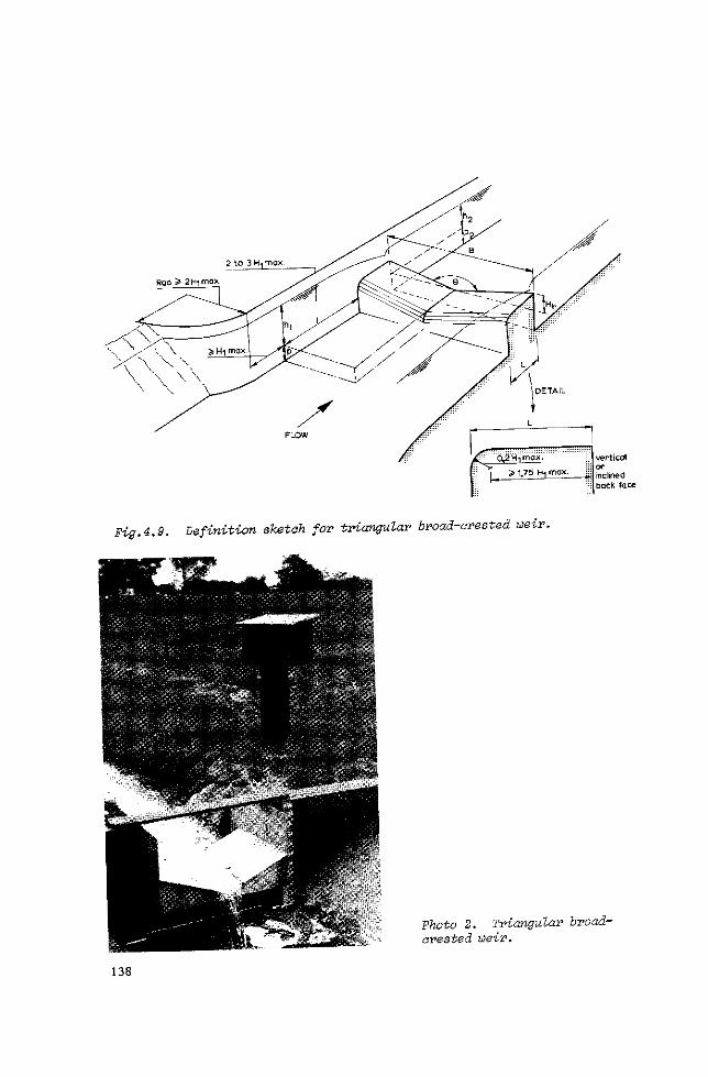
Rad 5 2 Hi max
Fig.4.9. Definition sketch for triangular broad-created weir.
S^Ti^AS .* V "''" tfc-'s *•'
Photo 2. Triangular broad-crested weir.
138
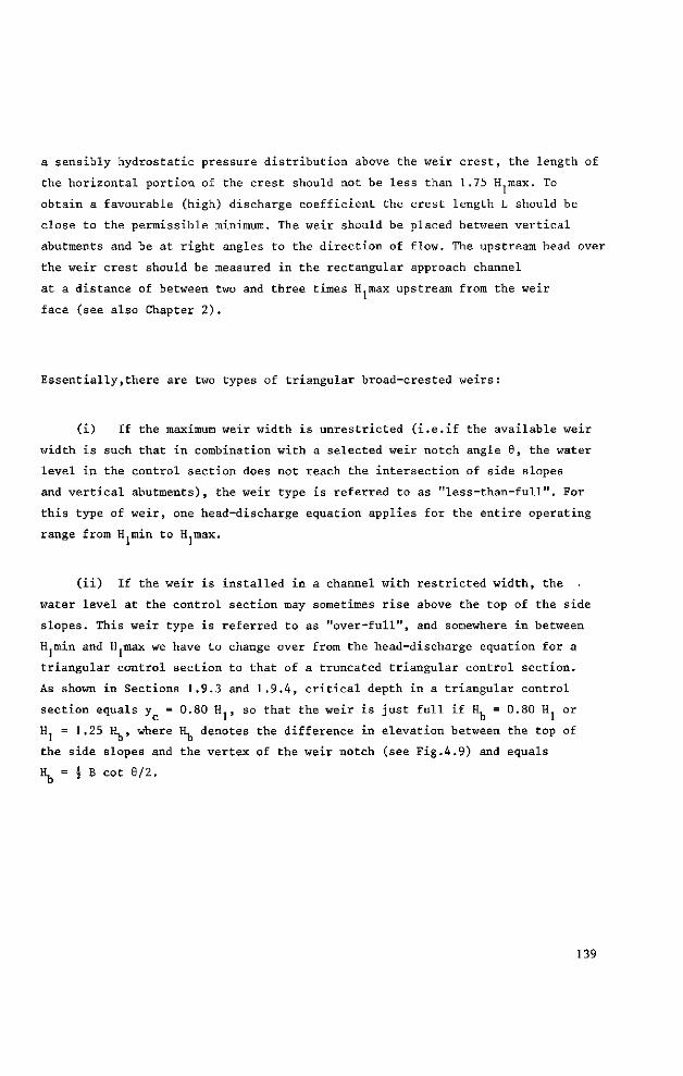
a sensibly hydrostatic pressure distribution above the weir crest, the length of
the horizontal portion of the crest should not be less than 1 .75 ILmax. To
obtain a favourable (high) discharge coefficient the crest length L should be
close to the permissible minimum. The weir should be placed between vertical
abutments and be at right angles to the direction of flow. The upstream head over
the weir crest should be measured in the rectangular approach channel
at a distance of between two and three times ILmax upstream from the weir
face (see also Chapter 2 ) .
Essentially,there are two types of triangular broad-crested weirs:
(i) If the maximum weir width is unrestricted (i.e.if the available weir
width is such that in combination with a selected weir notch angle 6, the water
level in the control section does not reach the intersection of side slopes
and vertical abutments), the weir type is referred to as "less-than-full". For
this type of weir, one head-discharge equation applies for the entire operating
range from ILmin to Hjinax.
(ii) If the weir is installed in a channel with restricted width, the
water level at the control section may sometimes rise above the top of the side
slopes. This weir type is referred to as "over-full", and somewhere in between
Hjinin and H.max we have to change over from the head-discharge equation for a
triangular control section to that of a truncated triangular control section.
As shown in Sections 1.9.3 and 1.9.4, critical depth in a triangular control
section equals y = 0.80 H., so that the weir is just full if H, = 0.80 H. or
H1 = 1.25 H, , where H, denotes the difference in elevation between the top of
the side slopes and the vertex of the weir notch (see Fig.4.9) and equals
H. = J B cot 8/2.
139
4.3.2 Evaluation of discharge
As discussed already in Section 4.3.1 we can distinguish between two different
cases of head-discharge relationships, as follows
"Less-Than-Full" (H1 « 1.25 Hb)
In this case the basic-head-discharge equation for a triangular control section
is applicable, which, according to Section 1.9.3, reads
. _ _ 16 Yl "10.50 _ O ,2.50 ,. ., Q = CdCv 25 |_5 gJ t a n 2 hl (4~5)
where the discharge coefficient may be read as a function of the ratio H./L from
Figure 4.10. The approach velocity coefficient may be read from Figure 1.12 as
a function of the dimensionless ratio
CdA*/A, = (Cdhj tan| )/B(hj + p)
"Over-Full" (Hj » 1.25 Hfa)
In this case the basic head-discharge equation for a truncated triangular control
section applies (see Section 1.9.4)
Q - c d c v t [ ! 8 ] ° - 5 0 ^ . - i v , - 5 ° «-«>
where values of C, again may be read from Figure 4.10 as a function of the
ratio H./L. It should be noted that if H./L exceeds 0.50 the weir cannot be
termed broad-crested. If ratios Hj/L > 0.50 are used, the overfalling nappe
should be fully aerated, and it should be noted that the modular limits given
in Section 4.3.2 will decrease significantly with increasing H./L-values. C -
values may be obtained from Figure 1.12 as a function of the dimensionless
ratio CdA*/Aj = (^(hj - iHb)/(h] + p ) .
140
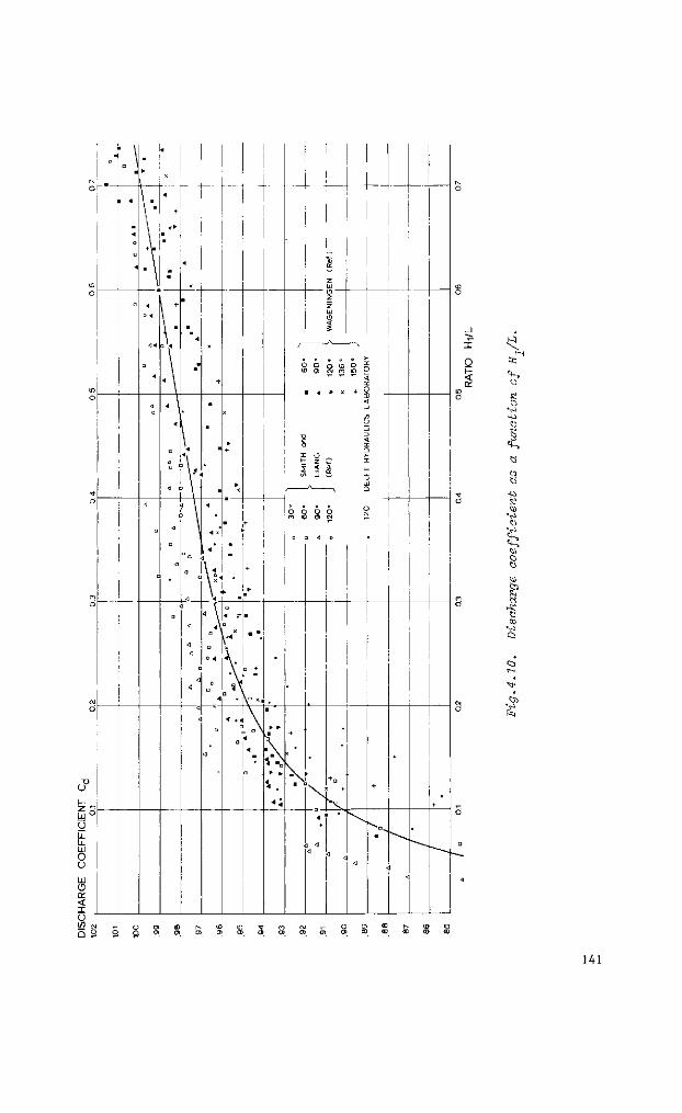
s
•
3
3
"i
3
t
t
3
vj
>
' \ • 1
• 4
. 4
°
«
4
|
\ "B
" i +-4
"i \ i ' • \ •
ir ; a \
4
O 4
« 4
' <3
°
< a
\ +
\ \ \ \ • \
• 4 l
\ \ \ A \
< \ ) 4
D <J
4
• ]
I
* 4
* i
\ ï 4
4 .
D 1 \ 4
*
+
.
•
* 1 *
* \ ' ï \ 1
? \ n \ n \
<a
<i
4
4 x
|
x
+
*
.4 L-1
i i
! cr
Z UI O z z
i LU O
< | s A
O o o O
O O o ID t o O i o j n
• 4 • X
i
• .+
i "D C
i I o ! 1- Z C
S 2 * ' *—^
a s u s
1 O O O O ' C l (O 0> (M
•
, 4 i D = i 1 •
- 1\ -s ' °\<1 "
4 3
a
< < <
l 1 \ 4 -
4 1 •
\ \° " \« *
> G
O 41
a
<1 4
4
\f
+
•
•
• •
\ a +
* \ + • 3\i
4
* 4
D
4
+
i
-
* rC * • •
4 '4 \ + n N 4
4
•
•
• ••
B\ <"\ * • •
• »
< < .
*<
+
*
.
^ v •
•
„ N 4
« < « <d
<1
-U j
| 1
v i
o >
i n O
*" <
< —i
L/l
o
3 < o: Û
X l _ Li .
i
l
LÜ : Û '
C\i j
j
j i
! ;
<
+
^
!
>
< <
+ "
I
o < cc
O
K O
K
«e. co ö
+i S <ä>
O
o «
1? ö
f «
CO • ^ > Q
l i j
141
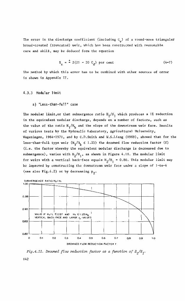
The error in the discharge coefficient (including C ) of a round-nose triangular
broad-crested (truncated) weir, which has been constructed with reasonable
care and skill, may be deduced form the equation
X = - 2(21 - 20 C,) per cent c d
(4-7)
The method by which this error has to be combined with other sources of error
is shown in Appendix II.
4.3.3 Modular limit
a) "Less-than-full" case
The modular limit,or that submergence ratio H„/H1 which produces a 1% reduction
in the equivalent modular discharge, depends on a number of factors, such as
the value of the ratio H./H, and the slope of the downstream weir face. Results
of various tests by the Hydraulic Laboratory, Agricultural University,
Wageningen, 1964-1971, and by C.D.Smith and W.S.Liang (1969), showed that for the
less-than-full type weir (H./R <: 1.25) the drowned flow reduction factor (f)
(i.e. the factor whereby the equivalent modular discharge is decreased due to
submergence), varies with H„/H , as shown in Figure 4.11. The modular limit
for weirs with a vertical back-face equals H /H = 0.80. This modular limit may
be improved by constructing the downstream weir face under a slope of l-to-4
(see also Fig.4.2) or by decreasing p..
SUBMERGENCE RATIO H 2 / H 1.00
0 £ 5
0.80
VALID VERTI
IF H i / L : A L BACK
$ 0 . 5 7 A -FACE AN
MD H-i $ 3 LARGE
1 .25H b
32 -VALUES
0.1 0.2 0.3 0.4 0.5 0.6 0.7
DROWNED FLOW REDUCTION FACTOR f
0.8
Fig.4.11. Drowned flow reduction factor as a function of H9/H1.
142
b) "Over-full-case"
No systematic research has been done on the evaluation of the modular limit of
"over-full" type weirs. It may be expected, however, that the modular limit will
change gradually to that of a broad-crested weir as described in Section 4.1.1
if the ratio H /H increases significantly above 1.25.
4.3.4 Limits of application
The limits of application of the triangular broad-crested weir and truncated
weir for reasonable accuracy are:
a) The practical lower limit of h is related to the magnitude of the
influence of fluid properties, boundary roughness, and the accuracy with which
hj can be determined,
whichever is greater.
hj can be determined. The recommended lower limit is 0.06 m or 0.05 times L,
b) The weir notch angle 8 should not be less than 30 .
c) The recommended upper limit of the ratio H./p = 3.0, while p should not
be less than 0.15 m.
d) The limitation on H /L arises from the necessity of ensuring a sensible
hydrostatic pressure distribution at the control section. Values of the ratio
h /L should therefore not exceed 0.50 (0.70 if sufficient head is available).
e) The breadth B of a truncated triangular broad-crested weir should not be
less than 0.30 m, nor less than H max, nor less than L/5.
4.4 Broad-crested rectangular profile weir
4.4.1 Description
From a constructional point of view the broad-crested rectangular profile weir
is a rather simple measuring device. The weir block shown in Figure 4.12 has
a truly flat and horizontal crest. Both the upstream and downstream weir faces
should be smooth vertical planes. The weir block should be placed in a rectan
gular approach channel perpendicular to the direction of flow. Special care
should be taken that the crest surface makes a straight and sharp 90-degree
intersection with the upstream weir face.
143
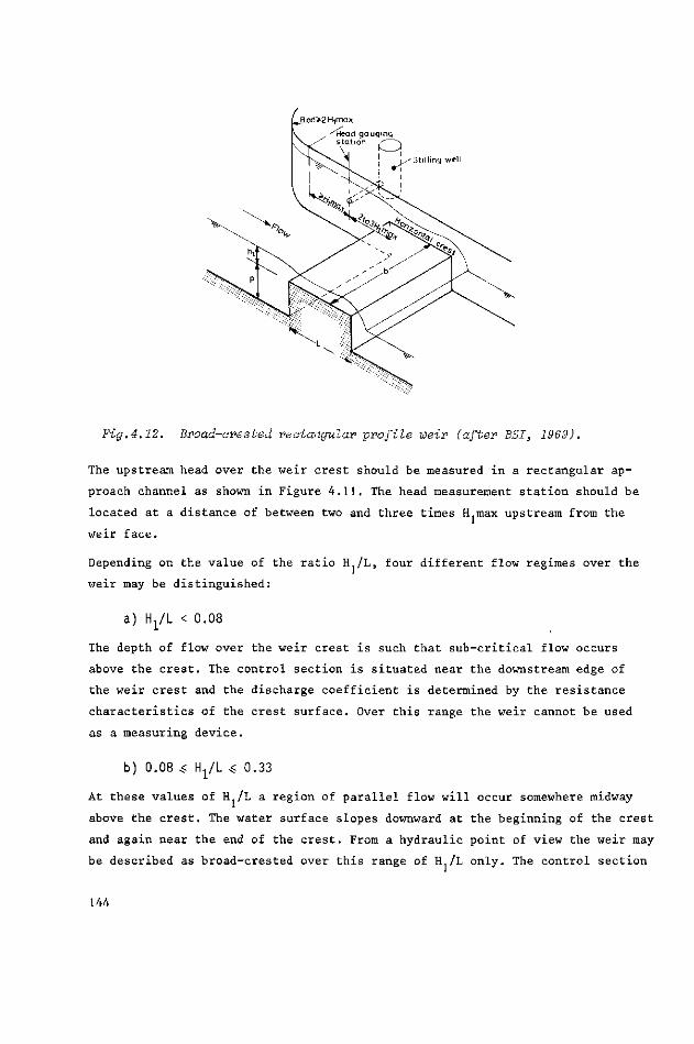
^Rgd?2 H-,max
-""Head gauging station £ - > ,
. 1 J j / S t i l l i n g well
Fig.4.12. Broad-crested rectangular profile weir (after BSI, 1969).
The upstream head over the weir crest should be measured in a rectangular ap
proach channel as shown in Figure 4.11. The head measurement station should be
located at a distance of between two and three times H max upstream from the
weir face.
Depending on the value of the ratio H /L, four different flow regimes over the
weir may be distinguished:
a) Hj/L < 0.08
The depth of flow over the weir crest is such that sub-critical flow occurs
above the crest. The control section is situated near the downstream edge of
the weir crest and the discharge coefficient is determined by the resistance
characteristics of the crest surface. Over this range the weir cannot be used
as a measuring device.
b) 0.08 H^L « 0.33
At these values of H./L a region of parallel flow will occur somewhere midway
above the crest. The water surface slopes downward at the beginning of the crest
and again near the end of the crest. From a hydraulic point of view the weir may
be described as broad-crested over this range of H /L only. The control section
144
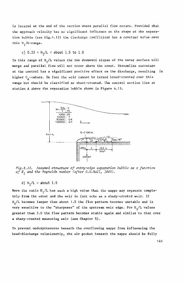
is located at the end of the section where parallel flow occurs. Provided that
the approach velocity has no significant influence on the shape of the separa
tion bubble (see Fig.4.12) the discharge coefficient has a constant value over
this H,/L-range.
c) 0.33 < Hj/L < about 1.5 to 1.8
In this range of H./L values the two downward slopes of the water surface will
merge and parallel flow will not occur above the crest. Streamline curvature
at the control has a significant positive effect on the discharge, resulting in
higher C,-values. In fact the weir cannot be termed broad-crested over this
range but should be classified as short-crested. The control section lies at
station A above the separation bubble shown in Figure 4.13.
Fig.4.13. Assumed structure of entry-edge separation bubble as a function of H, and the Reynolds number (after G.W.Hall, 1982).
d) H^L > about 1.5
Here the ratio H./L has such a high value that the nappe may separate comple
tely from the crest and the weir in fact acts as a sharp-crested weir. If
H./L becomes larger than about 1.5 the flow pattern becomes unstable and is
very sensitive to the "sharpness" of the upstream weir edge. For H./L values
greater than 3.0 the flow pattern becomes stable again and similar to that over
a sharp-crested measuring weir (see Chapter 5 ) .
To prevent underpressures beneath the overflowing nappe from influencing the
head-discharge relationship, the air pocket beneath the nappe should be fully
145
aerated whenever H./L exceeds 0.33. Dimensions of the aeration duct should be
determined as shown in Section 1.14.
The modular limit, or that submergence ratio H„/H which produces a 1% reduction
from the equivalent modular discharge, depends on the ratio H /L. If
0.08 ^ H /L 0.33, the modular limit may be expected to be 0.66. If H /L = 1.5,
however, the modular limit is about 0.38 and over the range 0.33 < H /L < 1.5
the modular limit may be obtained by linear interpolation between the given va
lues. Provided that the ratio h /(h + p) •$ 0.35, Figure 4.18, too, can be used
to obtain information on the reduction of modular flow due to submergence.
4.4.2 Evaluation of discharge
The basic head-discharge equation derived in Section 1.9.1 can be used to
evaluate the flow over the weir. This equation reads
. _ _ 2 [2 10.50 ,,1.50 ,. „, Q = C d C v 3 L 3 g J bhl (4"8)
where the approach velocity coefficient C may be read from Figure 1.12 as a
function of the dimensionless ratio C,A /A. = C,h./(h + p ) . Experimental
results have shown that under normal field conditions the discharge coefficient
is a function of the two ratios h./L and h./(h + p ) . As mentioned in the pre
vious section, the discharge coefficient remains constant if there is parallel
flow at the control section and if the approach velocity does not influence the
shape of the separation pocket. Hence C, remains fairly constant if both
0.08 < hj/L «: 0.33 and
hj/Chj + p) $ 0.35
The average value of C, within these limits is 0.848 and is referred to as the
basic discharge coefficient. If one of the limits is not fulfilled the basic
coefficient should be multiplied by a coefficient correction factor F which
is always greater than unity since both streamline curvature at the control
section and a depression of the separation bubble have a positive influence
on weir flow. Values of F as a function of h./L and h1/(h1 + p) can be read
from Figure 4.14.
146
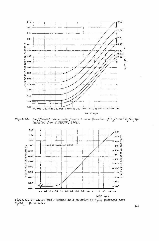
0.60
0.10 0.15 0.20 0-25 0.30 035 0.40 0.45 0.50 0.55 0.60 0.65 0.70 0.75 0.80 0.85
RATIO h«/ L
Fig.4.14. Coefficient correction factor F as a function of hjL and h1/(hl+p) (adapted from J.SINGER, 1964).
1.06
1.04
1.02
0.96
0 .96
0.94
0 92
0 90
0.86
0.84
I
i
r ! --
VALID IF h i / ( h i » D ) «0.35
i —
I
0.8 4 8
0.1
--y
I-- •--!
z._
\- -
0.2 0.3 0.4 0.5 0.6 0.7
—
i i
-
0 .8 0 . 9
-7
7
| i :
. _
-
1.0 1.1 1.2 13 1
RA T I O h-, / L
r -
~
~
-
~
_ -
4 1
1.24
1.22
1.20
1.18
1.16
1.14
1.12
1.10
1.06
1.06
1.04
1.02
1.00
1.5
Fig.4.IB. C -.-values and F-values as a function of h1/L, provided that h1/(h1 + p) $ 0.35. l
147
There are not enough experimental data available to give the relation between
C, and the ratios h./L and hr/(h + p) with satisfactory accuracy over the entire
range. If, however, the influence of the approach velocity on C, is negligible,
(i.e. if h /(h + p) 4 0.35), C.-values can be read as a function of h /L from
Figure 4.15.
The error in the discharge coefficient (including C ) of a rectangular profile
weir, constructed with reasonable care and skill, may be obtained from the
equation
X = + (10F - 8) per cent (4-9)
To obtain this accuracy the structure should be properly maintained. The method
by which this error should be combined with other sources of error is shown
in Appendix II.
4.4.3 Limits of appl icat ion
The limits of application of the rectangular profile weir essential for reaso
nable accuracy are:
a) The practical lower limit of h1 is related to the magnitude of the in
fluence of fluid properties, to boundary roughness, and to the accuracy with
which h1 can be determined. The recommended lower limit of h is 0.06 m or 0.08
times L, whichever is greater.
b) The recommended upper limit of the ratio hl/(h1 + p) = 0.60, while p
should not be less than 0.15 m.
c) The ratio h /L should not be less than 0.08 and should not exceed 1.50.
If, however, the influence of the approach velocity on C, is significant
(i.e. if h /(h + p) > 0.35), C,-values are only available provided that the
ratio h./L 4 0.85.
d) The breadth b of the weir should not be less than 0.30 m nor less than
hjmax, nor less than L/5.
e) The air pocket beneath the nappe should be fully aerated whenever the
ratio h,/L exceeds 0.33.
148
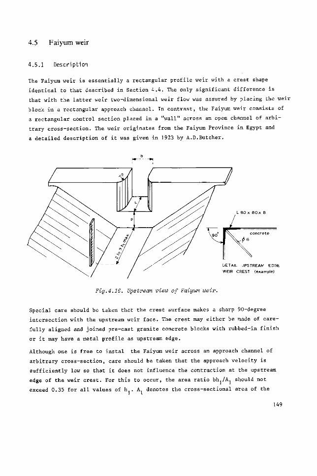
4.5 Faiyum weir
4.5.1 Description
The Faiyum weir is essentially a rectangular profile weir with a crest shape
identical to that described in Section 4.4. The only significant difference is
that with the latter weir two-dimensional weir flow was assured by placing the weir
block in a rectangular approach channel. In contrast, the Faiyum weir consists of
a rectangular control section placed in a "wall" across an open channel of arbi
trary cross-section. The weir originates from the Faiyum Province in Egypt and
a detailed description of it was given in 1923 by A.D.Butcher.
DETAIL UPSTREAM EDGE
WEIR CREST (example)
Fig.4.16. Upstream view of Faiyum weir.
Special care should be taken that the crest surface makes a sharp 90-degree
intersection with the upstream weir face. The crest may either be made of care
fully aligned and joined pre-cast granite concrete blocks with rubbed-in finish
or it may have a metal profile as upstream edge.
Although one is free to instal the Faiyum weir across an approach channel of
arbitrary cross-section, care should be taken that the approach velocity is
sufficiently low so that it does not influence the contraction at the upstream
edge of the weir crest. For this to occur, the area ratio bh /A. should not
exceed 0.35 for all values of h.. A denotes the cross-sectional area of the
149
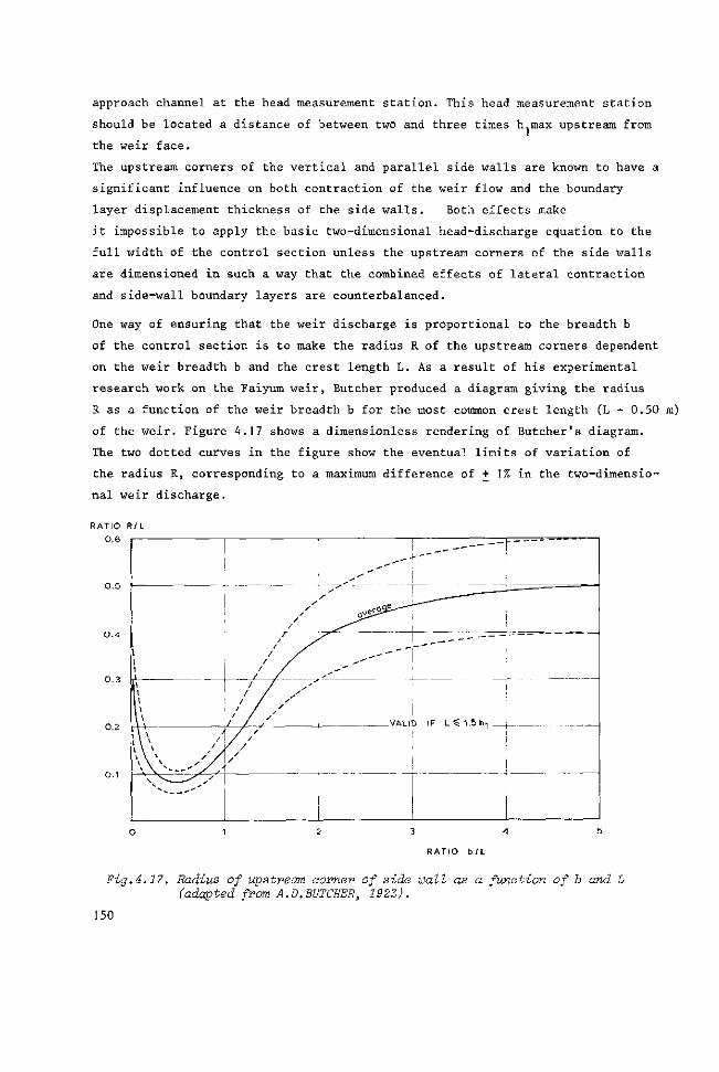
approach channel at the head measurement station. This head measurement station
should be located a distance of between two and three times h max upstream from
the weir face.
The upstream corners of the vertical and parallel side walls are known to have a
significant influence on both contraction of the weir flow and the boundary
layer displacement thickness of the side walls. Both effects make
it impossible to apply the basic two-dimensional head-discharge equation to the
full width of the control section unless the upstream corners of the side walls
are dimensioned in such a way that the combined effects of lateral contraction
and side-wall boundary layers are counterbalanced.
One way of ensuring that the weir discharge is proportional to the breadth b
of the control section is to make the radius R of the upstream corners dependent
on the weir breadth b and the crest length L. As a result of his experimental
research work on the Faiyum weir, Butcher produced a diagram giving the radius
R as a function of the weir breadth b for the most common crest length (L = 0.50 m)
of the weir. Figure 4.17 shows a dimensionless rendering of Butcher's diagram.
The two dotted curves in the figure show the eventual limits of variation of
the radius R, corresponding to a maximum difference of + 1% in the two-dimensio
nal weir discharge.
RATIO R/L
0.6
Fig.4.17. Radius of upstream corner of side wall as a function of b and L (adapted from A.D.BUTCHER, 1923).
150
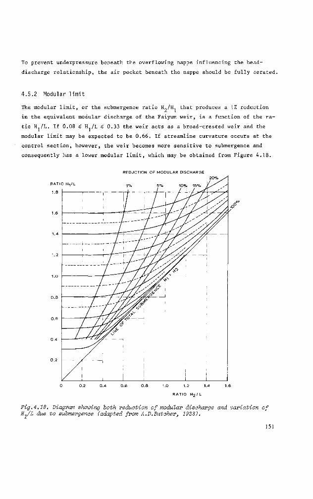
To prevent underpressure beneath the overflowing nappe influencing the head-
discharge relationship, the air pocket beneath the nappe should be fully aerated.
4.5.2 Modular limit
The modular limit, or the submergence ratio H„/H1 that produces a 1% reduction
in the equivalent modular discharge of the Faiyum weir, is a function of the ra
tio H./L. If 0.08 •£ H /L •£ 0.33 the weir acts as a broad-crested weir and the
modular limit may be expected to be 0.66. If streamline curvature occurs at the
control section, however, the weir becomes more sensitive to submergence and
consequently has a lower modular limit, which may be obtained from Figure 4.18.
RATK
1.8
1.6
1.4
1.2
0 .8
0.6
0.4
0.2
3 H-|/L
REDUCTION OF MODULAR DISCHARGE
1°/. 5°/= 10-/(. 15% ƒ / / I / ^ 7
I / / I / L A /
i~-----4''''lS^:7^y
i
- _ i .
/
/ / —7 / ^-y s' s >
4^---~T~'~f^J^/'/^' 1}^J^//,V'/^//
/ _ - i - - / " " " " ~ / LS7 ',''//
1 -^J-^f^/'y^^ / L--J'/i/yy^
1 / /'7/ytfr
7 //f^/s'P
<S , '
//Jys'
\ ' ! i 1 ! i i i
0.2 0.4 0.6 0.8 1.0 1.2 1.4 1.6
RATIO H,/L
Fig.4.18. Diagram showing both reduction of modular discharge and variation of H^/L due to submergence (adapted from A.D.Butcher, 1923).
151
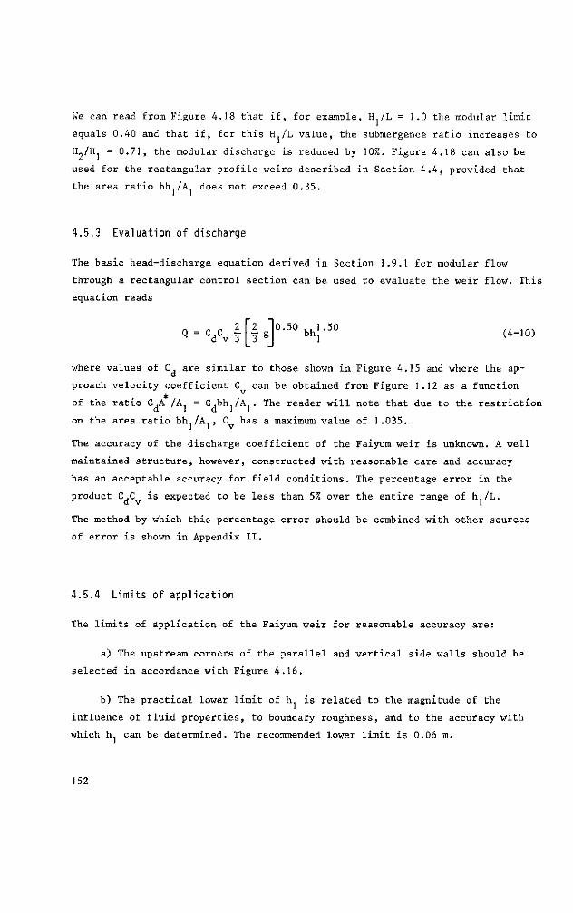
We can read from Figure 4.18 that if, for example, H./L = 1.0 the modular limit
equals 0.40 and that if, for this H./L value, the submergence ratio increases to
H„/H = 0.71, the modular discharge is reduced by 10%. Figure 4.18 can also be
used for the rectangular profile weirs described in Section 4.4, provided that
the area ratio bb^/A, does not exceed 0.35.
4.5.3 Evaluation of discharge
The basic head-discharge equation derived in Section 1.9.1 for modular flow
through a rectangular control section can be used to evaluate the weir flow. This
equation reads
^ d v 3 0 - 5 0 b h [ - 5 0 (4-10)
where values of C, are similar to those shown in Figure 4.15 and where the ap
proach velocity coefficient C can be obtained from Figure 1.12 as a function
of the ratio C.A /A. = C.bh./A,. The reader will note that due to the restriction d 1 d 1 1
on the area ratio bh,/A,, C has a maximum value of 1.035. 1 1 v
The accuracy of the discharge coefficient of the Faiyum weir is unknown. A well
maintained structure, however, constructed with reasonable care and accuracy
has an acceptable accuracy for field conditions. The percentage error in the
product C,C is expected to be less than 5% over the entire range of h /L.
The method by which this percentage error should be combined with other sources
of error is shown in Appendix II.
4.5.4 Limits of application
The limits of application of the Faiyum weir for reasonable accuracy are:
a) The upstream corners of the parallel and vertical side walls should be
selected in accordance with Figure 4.16.
b) The practical lower limit of h is related to the magnitude of the
influence of fluid properties, to boundary roughness, and to the accuracy with
which hj can be determined. The recommended lower limit is 0.06 m.
152
c) The area ratio bh /A should not exceed 0.35.
d) The breadth of the control section should not be less than 0.05 m.
e) The ratio h /L should not be less than 0.08 and should not exceed 1.6.
f) The airpocket beneath the nappe should be fully aerated whenever h /L
exceeds 0.33.
4.6 Selected list of references
1. AGRICULTURAL UNIVERSITY WAGENINGEN: Various laboratory reports on the
V-notch broad-crested weir. Hydraulic Laboratory Agric.Univ.,Wageningen.
2. BOS, M.G.: The Romijn movable measuring/regulating weir. Publ.in joint
FAO-ICID publication on small hydraulic structures in irrigation distribution
systems. Irrigation and Drainage Paper, No.26.
3. BOS, R.J.: De lange meetoverlaat met V-vormige kruin. Polytechnisch
Tijdschrift No.7B, 1964 pp.254-259; N0.8B, pp.301-310.
4. BRITISH STANDARDS INSTITUTION: Methods of measurement of liquid flow
in open channels. British Standard 3680, Part 4B, Long base weirs. London 1969.
5. BUTCHER, A.D.: Submerged weirs and standing wave weirs. Government
Press, Cairo, 1923. 17 pp.
6. DELFT HYDRAULICS LABORATORY: Invloed van stromingsvorm van een Romijn
meetoverlaat op de afvoer-coefficient. Report Hydraulics Laboratory, Delft, 1953.
7. HALL, G.W.: Analytic determination of the discharge characteristics of
broad-crested weirs using boundary layer theory. Proceedings of the Inst.of
Civil Engineers, 1967. Vol.22, June, Paper 6607. pp.177-190.
8. HARRISON, A.J.M.: The streamlined broad-crested weir. Proceedings of
the Inst.of Civil Engineers, 1967. Dec. Vol.38, pp.657-678.
9. HORTON, R.E.: Weir experiments, Coefficients and Formulas. Water Supply
Paper 200, Geological Survey, U.S.Department of the Interior, Washington D.C. 1907.
10. ISO, TC 113-WG 2, THE NETHERLANDS: A reference document on the round-nose
broad-crested weir. Wageningen, Agric.Univ.Hydraul.Laboratory, May 1967, unpubl.
153
11. KEUTNER, C : Strömungsvorgänge an breitkronigen Wehrkörpern Einlaufbau
werken. Der Bauingenieur, Vol.15, 1934, p.366.
12. LELIAVSKY, S.: Irrigation Engineering: Siphons, Weirs and Locks.
Design textbook in Civil Engineering, Vol.II, Chapman and Hall Ltd., London 1965.
13. PITLO, R.H., and SMIT, M.: Discussion to reference 17. Proc.of the Am.
Soc.of Civil Engineers, Irrigation and Drainage Division,R3, Sept.1970, pp.
364-369.
14. ROMIJN, D.G.• Een regelbare meetoverlaat als tertiaire aftapsluis.
De Waterstaatsingenieur, Bandung, 1932, Nr.9.
15. ROMIJN, D.G.: Meetsluizen ten behoeve van irrigatiewerken. Handleiding
door "De Vereniging van Waterstaats Ingenieurs in Nederlandsch Indië, 1938,
pp.58.
16. SINGER, J.: Square-edged broad-crested weir as a flow measuring device.
Water and Water Engineering, June 1964, Vol.68, Nr.820, pp.229-235.
17. SMITH, C D . , and LIANG, W.S.: Triangular broad-crested weir. Proc.of
the Am.Soc.of Civil Engineers, Irrigation and Drainage Division, IR 4, Dec.
1969, Paper 6954. pp.493-502 and closure in IR 4, Dec.1971, pp.637-640.
18. VLUGTER, H.: De regelbare meetoverlaat. De Waterstaatsingenieur,
Bandung, 1940, Nr.10.
19. WOODBURN, J.G.: Tests of broad-crested weirs. Proc.of the Am.Soc.of Civil
Engineers, Vol.56, 1930, Sept.,No.7,pp.1583-1612.Also:Trans.ASCE,Vol.96,1932,
Paper 1797, pp.387-408.
154
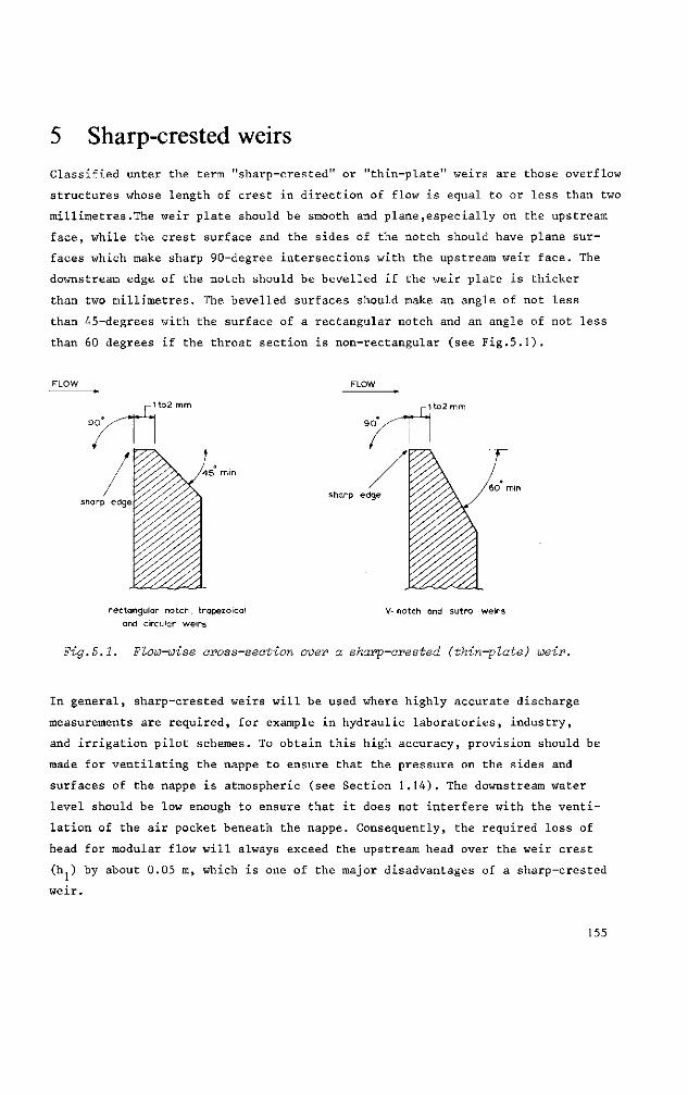
5 Sharp-crested weirs Classified unter the term "sharp-crested" or "thin-plate" weirs are those overflow
structures whose length of crest in direction of flow is equal to or less than two
millimetres.The weir plate should be smooth and plane,especially on the upstream
face, while the crest surface and the sides of the notch should have plane sur
faces which make sharp 90-degree intersections with the upstream weir face. The
downstream edge of the notch should be bevelled if the weir plate is thicker
than two millimetres. The bevelled surfaces should make an angle of not less
than 45-degrees with the surface of a rectangular notch and an angle of not less
than 60 degrees if the throat section is non-rectangular (see Fig.5.1).
sharp edge
rectangular notch, trapezoidal
and circular weirs
V- notch and sutro weirs
Fig.5.1. Flow-wise cross-section over a sharp-crested (thin-plate) weir.
In general, sharp-crested weirs will be used where highly accurate discharge
measurements are required, for example in hydraulic laboratories, industry,
and irrigation pilot schemes. To obtain this high accuracy, provision should be
made for ventilating the nappe to ensure that the pressure on the sides and
surfaces of the nappe is atmospheric (see Section 1.14). The downstream water
level should be low enough to ensure that it does not interfere with the venti
lation of the air pocket beneath the nappe. Consequently, the required loss of
head for modular flow will always exceed the upstream head over the weir crest
(hj) by about 0.05 m, which is one of the major disadvantages of a sharp-crested
weir.
155
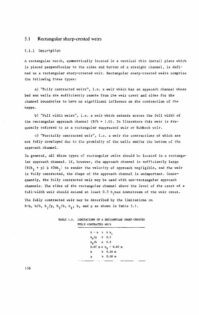
5.1 Rectangular sharp-crested weirs
5.1.1 Description
A rectangular notch, symmetrically located in a vertical thin (metal) plate which
is placed perpendicular to the sides and bottom of a straight channel, is defi
ned as a rectangular sharp-crested weir. Rectangular sharp-crested weirs comprise
the following three types:
a) "Fully contracted weirs", i.e. a weir which has an approach channel whose
bed and walls are sufficiently remote from the weir crest and sides for the
channel boundaries to have no significant influence on the contraction of the
nappe.
b) "Full width weirs", i.e. a weir which extends across the full width of
the rectangular approach channel (B/b = 1.0). In literature this weir is fre
quently referred to as a rectangular suppressed weir or Rehbock weir.
c) "Partially contracted weir", i.e. a weir the contractions of which are
not fully developed due to the proximity of the walls and/or the bottom of the
approach channel.
In general, all three types of rectangular weirs should be located in a rectangu
lar approach channel. If, however, the approach channel is sufficiently large
{B(h. + p) ~Z- lObhj} to render the velocity of approach negligible, and the weir
is fully contracted, the shape of the approach channel is unimportant. Conse
quently, the fully contracted weir may be used with non-rectangular approach
channels. The sides of the rectangular channel above the level of the crest of a
full-width weir should extend at least 0.3 h.max downstream of the weir crest.
The fully contracted weir may be described by the limitations on
B-b, b/B, h./p, hj/b, h , b, and p as shown in Table 5.1.
TABLE 5.1. LIMITATIONS OF A RECTANGULAR SHARP-CRESTED
FULLY CONTRACTED WEIR
B
h, h, 0,
- b
l'P , /b
.07 m
* ^ 4
.£
4
0
0
h.
h! .5
.5
< 0, .60 m
b > 0.30 m
p > 0.30 u
156
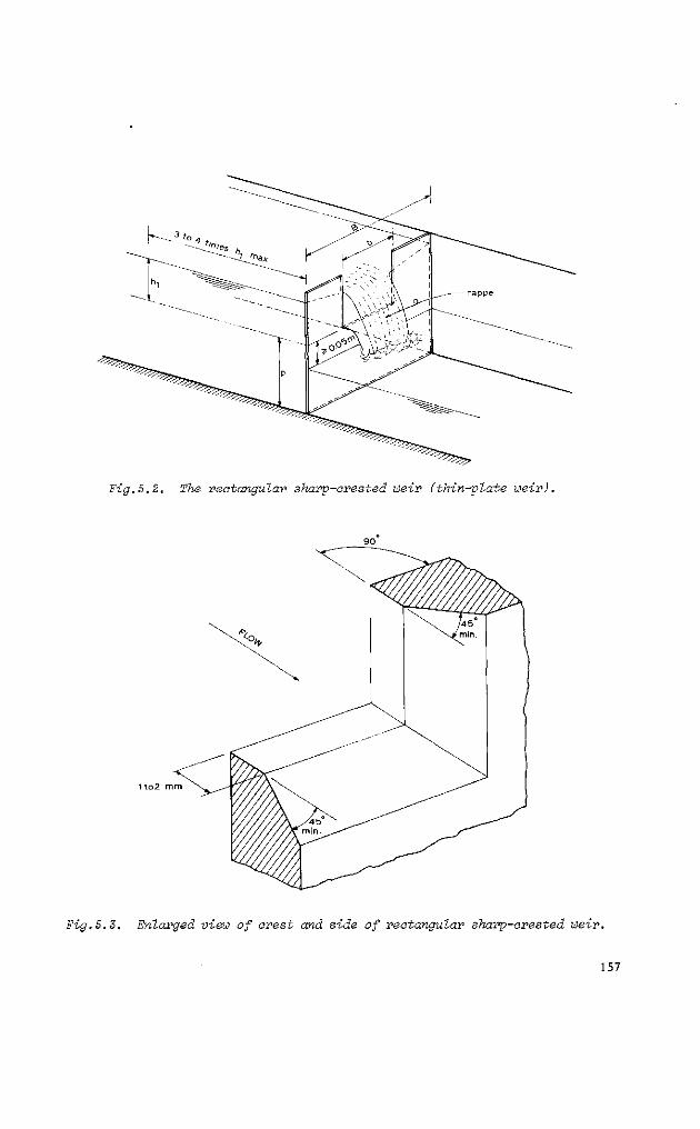
Fig.5.2. The rectangular sharp-crested weir (thin-plate weir).
Fig.5.3. Enlarged view of arest and side of rectangular sharp-crested weir.
157
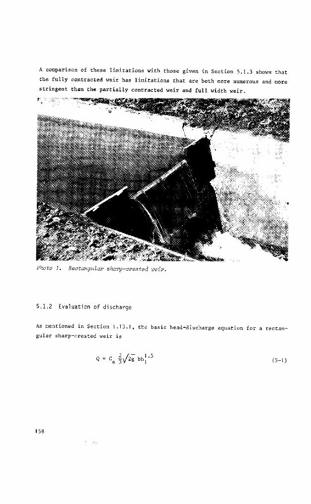
A comparison of these limitations with those given in Section 5.1.3 shows that
the fully contracted weir has limitations that are both more numerous and more
stringent than the partially contracted weir and full width weir.
Photo 1. Rectangular sharp-orested weir.
5.1.2 Evaluation of discharge
As mentioned in Section 1.13.1, the basic head-discharge equation for a rectc
gular sharp-crested weir is
Q = ce § y ü bh 1.5
(5-1)
158
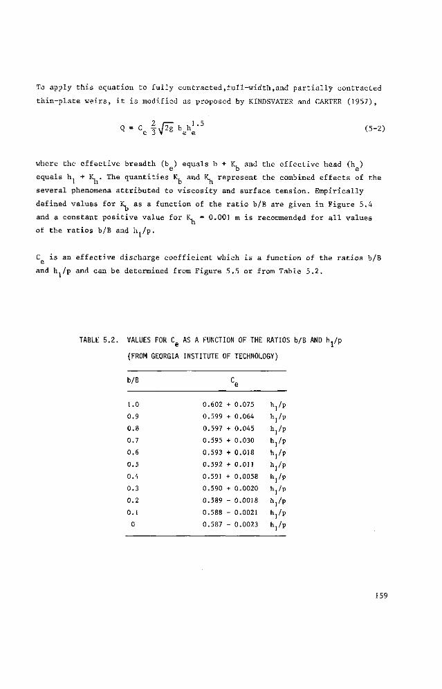
To apply t h i s equation to f u l ly con t r ac t ed , fu l l -w id th , and p a r t i a l l y cont rac ted
t h i n - p l a t e we i r s , i t i s modified as proposed by KINDSVATER and CARTER (1957),
C e 3 \ / ^ b e h 1.5 e
(5-2)
where the effective breadth (b ) equals b + K, and the effective head (h )
equals h. + K, . The quantities K, and K, represent the combined effects of the
several phenomena attributed to viscosity and surface tension. Empirically
defined values for L as a function of the ratio b/B are given in Figure 5.4
and a constant positive value for IC = 0.001 m is recommended for all values
of the ratios b/B and h /p.
C is an effective discharge coefficient which is a function of the ratios b/B
and h./p and can be determined from Figure 5.5 or from Table 5.2.
TABLE 5.2. VALUES FOR Cg AS A FUNCTION OF THE RATIOS b/B AND h^p
(FROM GEORGIA INSTITUTE OF TECHNOLOGY)
b/B
1.0
0.9
0.8
0.7
0.6
0.5
0.4
0.3
0.2
0.1
0
0.602 +
0.599 +
0.597 +
0.595 +
0.593 +
0.592 +
0.591 +
0.590 +
0.589 -
0.588 -
0.587 -
0.075
0.064
0.045
0.030
0.018
0.011
0.0058
0.0020
0.0018
0.0021
0.0023
,/p
l/p
,/P
,/P
,/P
,/P
,/P
,/P
,/P
,/P
,/P
159
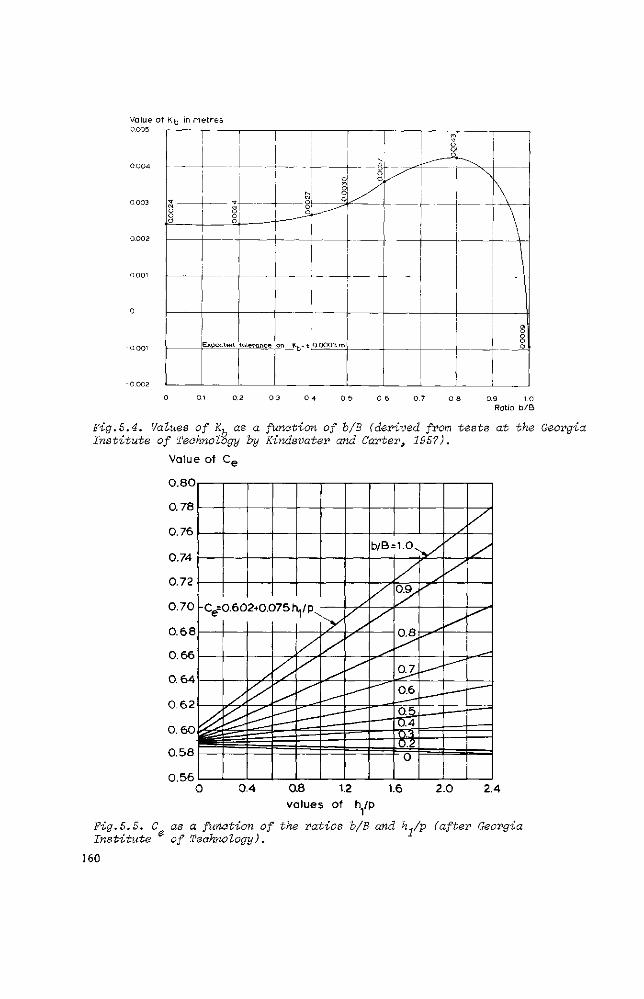
Value of Kb in metres 0.OO5
! L i OJ O O ö
o o o
Expected tolerance
D27
O m O O Ö
O ^-^* ö*-^"""^
!
on K b - 0.00O3 m
1 1 5 o o o
^ --
\o.o
c
60000
0.9 10 Ratio b/B
Fig.5.4. Values of K-, as a function of b/B (derived from tests at the Georgia Institute of Technology by Kindsvater and Carter, 1957).
Value of C€
0.80
0.78
0.76
0.74
0.72
0.70
0.68
0.66
0.64
0.62
0.60
0.58
0.56
"ce= 0.60 2«0.C )75f-ypv.
b/B: 1 0 ^ /
/ 0.9H
0.8
Q7.
0.6
0 5 , TX4
0
'
0.4 0.8 1.2 1.6 2.0 2.4
values of h/p
Fig.5.5. C as a function of the ratios b/B and h1/p (after Georgia Institute of Technology).
160
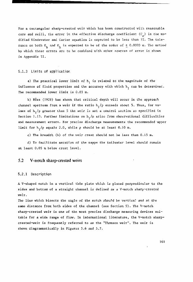
For a rectangular sharp-crested weir which has been constructed with reasonable
care and skill, the error in the effective discharge coefficient (C ) in the mo
dified Kindsvater and Carter equation is expected to be less than 1%. The tole
rance on both K, and K, is expected to be of the order of + 0.0003 m. The method
by which these errors are to be combined with other sources of error is shown
in Appendix II.
5.1.3 Limits of application
a) The practical lower limit of h1 is related to the magnitude of the
influence of fluid properties and the accuracy with which h1 can be determined.
The recommended lower limit is 0.03 m.
b) Boss (1929) has shown that critical depth will occur in the approach
channel upstream from a weir if the ratio ht/p exceeds about 5. Thus, for va
lues of h /p greater than 5 the weir is not a control section as specified in
Section 1.13. Further limitations on h /p arise from observational difficulties
and measurement errors. For precise discharge measurements the recommended upper
limit for h /p equals 2.0, while p should be at least 0.10 m.
c) The breadth (b) of the weir crest should not be less than 0.15 m.
d) To facilitate aeration of the nappe the tailwater level should remain
at least 0.05 m below crest level.
5.2 V-notch sharp-crested weirs
5.2.1 Description
A V-shaped notch in a vertical thin plate which is placed perpendicular to the
sides and bottom of a straight channel is defined as a V-notch sharp-crested
weir.
The line which bisects the angle of the notch should be vertical and at the
same distance from both sides of the channel (see Section 5 ) . The V-notch
sharp-crested weir is one of the most precise discharge measuring devices sui
table for a wide range of flow. In international literature, the V-notch sharp-
crested-weir is frequently referred to as the "Thomson weir". The weir is
shown diagrammatically in Figures 5.6 and 5.7.
161
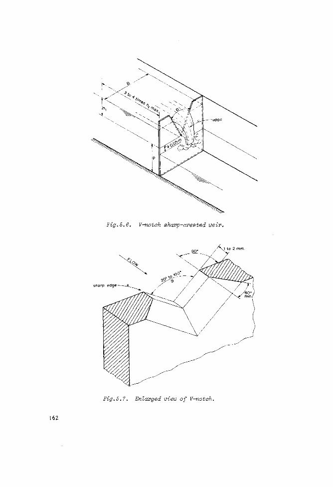
Fig. S. 6. V-notßh sharp-orested weir.
1 to 2 mm.
sharp edge
Fig. 5. 7. Enlarged view of V-^notoh.
162
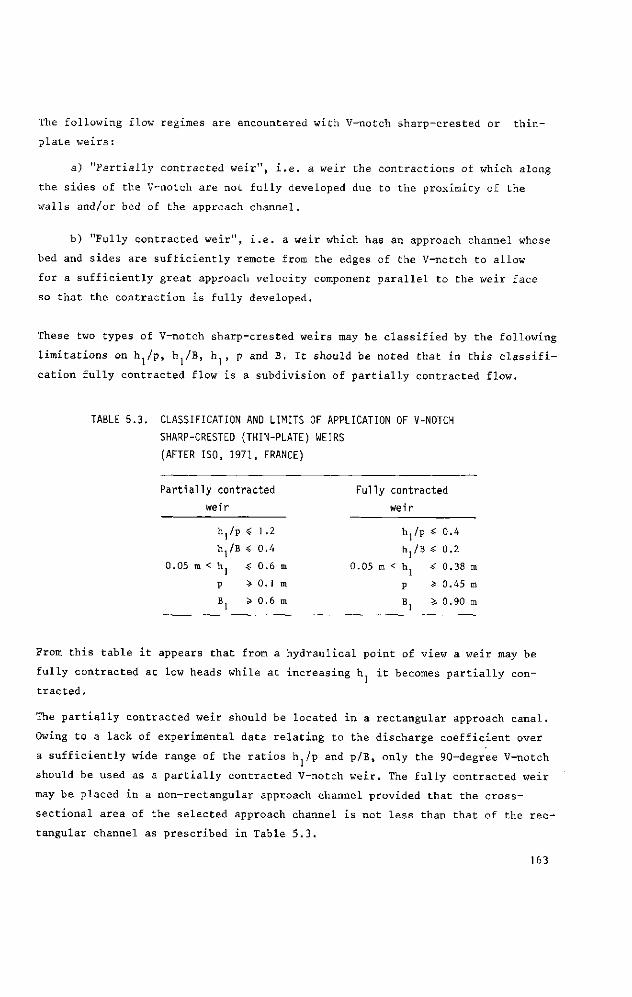
The following flow regimes are encountered with V-notch sharp-crested or thin-
plate weirs :
a) "Partially contracted weir", i.e. a weir the contractions of which along
the sides of the V-notch are not fully developed due to the proximity of the
walls and/or bed of the approach channel.
b) "Fully contracted weir", i.e. a weir which has an approach channel whose
bed and sides are sufficiently remote from the edges of the V-notch to allow
for a sufficiently great approach velocity component parallel to the weir face
so that the contraction is fully developed.
These two types of V-notch sharp-crested weirs may be classified by the following
limitations on h /p, h./B, h , p and B. It should be noted that in this classifi
cation fully contracted flow is a subdivision of partially contracted flow.
TABLE 5.3. CLASSIFICATION AND LIMITS OF APPLICATION OF V-NOTCH
SHARP-CRESTED (THIN-PLATE) WEIRS
(AFTER ISO, 1971, FRANCE)
Partially contracted
0.05
weir
h,
h m < h
P
B,
/P
/B
« « ^
> >
1
0,
0,
0.
0,
.2
.4
.6
.1
.6
m
m
m
Fully contracted
weir
hj/p £ 0.4
hj/B « 0.2
0.05 m < h *: 0.38 m
p > 0.45 m
B ï- 0.90 m
From this table it appears that from a hydraulical point of view a weir may be
fully contracted at low heads while at increasing h it becomes partially con
tracted.
The partially contracted weir should be located in a rectangular approach canal.
Owing to a lack of experimental data relating to the discharge coefficient over
a sufficiently wide range of the ratios h./p and p/B, only the 90-degree V-notch
should be used as a partially contracted V-notch weir. The fully contracted weir
may be placed in a non-rectangular approach channel provided that the cross-
sectional area of the selected approach channel is not less than that of the rec
tangular channel as prescribed in Table 5.3.
163
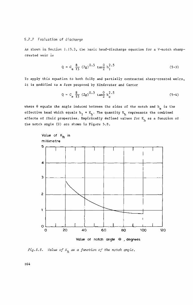
5.2.2 Evaluation of discharge
As shown in Section 1.13.3, the basic head-discharge equation for a V-notch sharp-
crested weir is
. _ 8 ., ,0.5 _ 0 ,2.5 Q = Ce — (2g) tany h] (5-3)
To apply this equation to both fully and partially contracted sharp-crested weirs,
it is modified to a form proposed by Kindsvater and Carter
_ „ 8 ., .0.5 _ 9 ,2.5 Q = Ce IT ( 2 g ) tan2 he
(5-4)
where 9 equals the angle induced between the sides of the notch and h is the
effective head which equals h. + K. . The quantity K, represents the combined
effects of fluid properties. Empirically defined values for t as a function of
the notch angle (9) are shown in Figure 5.8.
Value of Kh in
millimetre
4
•?
1
o
I
I
I
I
I
I
I
I
'
I
I
I 0 20 40 60 80 100
Value of notch angle © , degrees
Fig.5.8. Value of K, as a function of the notch angle.
120
164
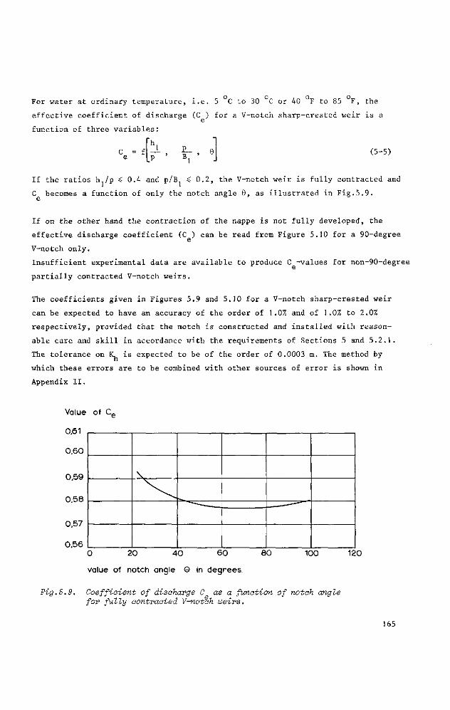
For water at ordinary temperature, i.e. 5 C to 30 C or 40 F to 85 F, the
effective coefficient of discharge (C ) for a V-notch sharp-crested weir is a
function of three variables:
"h C = f
e (5-5)
If the ratios h,/p *: 0.4 and p/B ^ 0.2, the V-notch weir is fully contracted and
C becomes a function of only the notch angle 9, as illustrated in Fig.5.9.
If on the other hand the contraction of the nappe is not fully developed, the
effective discharge coefficient (C ) can be read from Figure 5.10 for a 90-degree
V-notch only.
Insufficient experimental data are available to produce C -values for non-90-degree
partially contracted V-notch weirs.
The coefficients given in Figures 5.9 and 5.10 for a V-notch sharp-crested weir
can be expected to have an accuracy of the order of 1.0% and of 1.0% to 2.0%
respectively, provided that the notch is constructed and installed with reason
able care and skill in accordance with the requirements of Sections 5 and 5.2.1.
The tolerance on 1C is expected to be of the order of 0.0003 m. The method by
which these errors are to be combined with other sources of error is shown in
Appendix II.
Value of C_
0,60
0,59
0,58
0,57
0,56
""—'-'•*-. , , ———-"""
0 20 40 60
value of notch angle 0 in degrees
80 100 120
Fig.5.9. Coefficient of discharge C as a function of notch angle for fully contracted V-notch weirs.
165
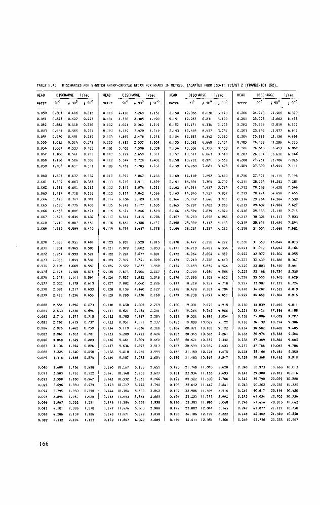
DISCHARGES FOR V-NOTCH SHARP-CRESTED WEIRS FOR HEADS IN METRES. (ADAPTED FROM ISO/TC 113/GT 2 (FRANCE-10) 152).
HEAD
met re
0 .050
0.051
0 .052
0 .053
0 .054
0 .055
0 .056
0 .057
0 .058
0 .059
0 .060
0.061
0 .062
0 .063
0 .064
0 .065
0 .066
0 .067
0 .068
0 .069
0 .070
0.071
0 .072
0 .073
0 .074
0 .075
0 .076
0 .077
0 .078
0 .079
0 .080
0.081
0 .082
0 .083
0 .084
0 .085
0 .086
0 .087
0 .088
0 .089
0 .090
0.091
0 .092
0 .093
0 .094
0 .095
0 .096
0 .097
0 .098
0 .099
DISCHARGE
90°
0 .803
0 .843
0 .884
0 .926
0 .970
1.015
1.061
1.108
1.156
1.206
1.257
1.309
1.362
1.417
1.473
1.530
1.588
1.648
1.710
1.772
1.836
1.901
1.967
2 .035
2 .105
2 .176
2 .248
2 .322
2.397
2 .473
2 .551
2 .630
2 .710
2.792
2 .876
2.961
3 .048
3.136
3 .225
3 .316
3.409
3 .503
3 .598
3 .696
3.795
3 .895
3.997
4 .101
4 .206
4 .312
i 90°
0.406
0.427
0.448
0.469
0.491
0.514
0.537
0.561
0.586
0.611
0.637
0.663
0.691
0.718
0.747
0.776
0.806
0.836
0.867
0.899
0.932
0.965
0.999
1.033
1.069
1.105
1.141
1 .179
1.217
1.256
1.296
1.336
1.377
1.419
1.462
1.505
1.549
1.594
1.640
1.686
1.734
1.782
1.830
1.880
1.930
1.981
2.033
2.086
2.139
2.194
/sec
1 90°
0 .215
0 .225
0 .236
0 .247
0.259
0.271
0 .283
0 .295
0 .308
0.321
0 .334
0 .348
0 .362
0 .376
0.391
0 .406
0.421
0 .437
0 .453
0 .470
0 .486
0 .503
0.521
0 .539
0.557
0 .575
0 .594
0 .613
0 .633
0 .653
0 .673
0 .694
0 .715
0 .737
0 .759
0.781
0 .803
0 .826
0 .850
0 .874
0 .898
0 .922
0 .947
0 .973
0 .998
1.025
1.051
1.078
1.106
1.133
HEAD
metre
0 .100
0.101
0 .102
0 .103
0 .104
0 .105
0 .106
0 .107
0 .108
0 .109
0 .110
0.111
0 .112
0 .113
0 .114
0 .115
0 .116
0.1 17
0 .118
0 .119
0 .120
0.121
0 .122
0 .123
0 .124
0 .125
0 .126
0 .127
0 .128
0 .129
0 .130
0.131
0 .132
0 .133
0 .134
0 .135
0 .136
0 .137
0 .138
0 .139
0 .140
0.141
0 .142
0 .143
0 .144
0 .145
0 .146
0 .147
0 .148
0 .149
DISCHARGE
90°
4 .420
4 .530
4 .641
4 .754
4 .869
4 .985
5 .103
5.222
5 .344
5.467
5.592
5.719
5 .847
5.977
6 .108
6 .242
6 .377
6 .514
6 .653
6 .793
6 .935
7 .079
7 .224
7 .372
7 .522
7 .673
7 .827
7.982
8.139
8.298
8 .458
8.621
8 .785
8.951
9 .119
9 .289
9.461
9 .634
9 .810
9 .987
10.167
10.348
10.532
10.717
10.904
11.093
11.284
11.476
11.671
11.867
i 90°
2 .249
2 .305
2 .362
2 .420
2 .478
2 .537
2 .598
2 .659
2 .720
2 .783
2 .847
2.911
2 .976
3.042
3.109
3 .177
3 .246
3 .315
3 .386
3 .457
3 .529
3 .602
3.677
3.751
3.827
3 .904
3 .982
4 .060
4 .140
4 .220
4 .302
4 .384
4 .467
4 .551
4 .636
4 .722
4 .809
4 .897
4 .986
5 .075
5.166
5 .258
5.351
5.444
5.539
5 .635
5.732
5 .830
5.929
6 .029
/ s e c
J 90°
1.161
1.190
1.219
1.249
1.278
1.309
1.339
1.371
1.402
1.434
1.466
1.499
1.533
1.566
1.601
1.635
1.670
1.706
1.742
1.778
1.815
1.853
1 .891
1.929
1.968
2.007
2 .046
2 .086
2 .127
2 .168
2 .209
2.251
2 .294
2 .337
2 .380
2 .424
2 .468
2 .513
2 .559
2 .604
2.651
2 .697
2 .744
2 .792
2 .840
2 .889
2 .938
2 .988
3 .038
3 .089
HEAD
metre
0 .150
0.151
0 .152
0 .153
0 .154
0 .155
0 .156
0 .157
0 .158
0 .159
0 .160
0.161
0 .162
0 .163
0 .164
0 .165
0 .166
0 .167
0 .168
0 .169
0 .170
0.171
0 .172
0 .173
0 .174
0 .175
0 .176
0 .177
0 .178
0 .179
0 .180
0.181
0 .182
0 .183
0 .184
0 .185
0 .186
0 .187
0 .188
0 .189
0 .190
0.191
0 .192
0 .193
0 .194
0 .195
0 .196
0 .197
0 .198
0 .199
DISCHARGE
90°
12.066
12.267
12.471
12.676
12.883
13.093
13.304
13.517
13.732
13.950
14.169
14.391
14.614
14.840
15.067
15.297
15.529
15.763
15.999
16.237
16.477
16.719
16.964
17.210
17.459
17.709
17.963
18.219
18.478
18.738
19.001
19.265
19.531
19.800
20.071
20 .345
20.621
20.899
21.180
21 .463
21 .748
22.034
22.322
22.612
22.906
23 .203
23.501
23.802
24.106
14.411
I 90°
6 .130
6.231
6.334
6 .437
6 .542
6 .648
6 .755
6 .863
6.971
7.081
7.192
7.304
7.417
7.531
7.646
7.762
7 .879
7.998
8.117
8.237
8.358
8.481
8.604
8.728
8.854
8 .980
9 .108
9 .237
9.367
9 .497
9 .629
9 .762
9 .896
10.032
10.168
10.305
10.444
10.584
10.726
10.867
I I . 0 1 0
11.155
11.300
11.447
11.595
11.743
11.893
12.044
12.197
12.351
/ s e c
J 90°
3 .140
3.192
3.245
3.297
3 .350
3.404
3 .458
3 ,513
3 .568
3.624
3 .680
3 .737
3.794
3.852
3.911
3 .969
4 .029
4 .089
4 .149
4 .210
4 .272
4 .334
4 .397
4 .460
4 .524
4 .588
4 .653
4 .718
4 .784
4 .851
4 .918
4 .986
5.054
5.122
5.192
5.261
5.332
5 .403
5 .475
5.547
5 .620
5 .693
5.766
5.841
5.916
5.992
6 .068
6 .145
6 .222
6.300
HEAD
metre
0 .200
0.201
0 .202
0 .203
0 .204
0 .205
0 .206
0 .207
0 .208
0 .209
0 .210
0.211
0 .212
0 .213
0 .214
0 .215
0 .216
0 .217
0 .218
0 .219
0 .220
0.221
0 .222
0 .223
0 .224
0 .225
0 .226
0 .227
0 .228
0 .229
0 .230
0.231
0 .232
0 .233
0 .234
0 .235
0 .236
0 .237
0 .238
0 .239
0 .240
0.241
0 .242
0 .243
0 .244
0 .245
0 .246
0 .247
0 .248
0 .249
DISCHARGE
90°
24.719
25 .028
25.339
25.652
25.969
26 .288
26 .610
26.934
27 .261
27 .590
27.921
28.254
28 .588
28.924
29.264
29 .607
29 .953
30.301
30.651
31 .004
31 .359
31.717
32.077
32.439
32 .803
33 .168
33 .535
33.907
34.282
34.659
35/039
35.421
35.806
36.139
36.582
36.974
37.369
37.766
38 .166
38 .568
38 .973
39.380
39 .790
40 .202
40.617
41 .034
41.454
41.877
42 .302
42 .730
J 90°
12.506
12.662
12.819
12.977
13.136
13.296
13.457
13.620
13.784
13.949
14.115
14.282
14.450
14.620
14.264
14.964
15.138
15.313
15.489
15.666
15.844
16.024
16.204
16.386
16.570
16.754
16.940
17.127
17.315
17.504
17.695
17.886
18.079
18.274
18.469
18.666
18.864
19.063
19.263
19.465
19.668
19.872
20.079
20.287
20.496
20.705
20.916
21.127
21.340
21.555
/sec
i 90°
6.379
6.458
6.537
6.617
6.698
6.780
6.862
6.944'
7.028
7.111
7.196
7.281
7.366
7.453
7.539
7.627
7.715
7.803
7.893
7.982
8.073
8.164
8.255
8.347
8.441
8.535
8.629
8.724
8.819
8.915
9.011
9.108
9.207
9.306
9.405
9.504
9.605
9.706
9.808
9.910
10.013
10.116
10.220
10.325
10.430
10.536
10.642
10.750
10.858
10.967
166
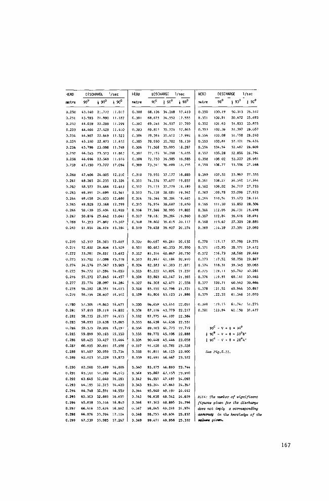
HEAD
metre
0.250
0.251
0.252
0.253
0.254
0.255
0.256
0.257
0.258
0.259
0.260
0.261
0.262
0.263
0.264
0.265
0.266
0.267
0.268
0.269
0.270
0.271
0.272
0.273
0.274
0.275
0.276
0.277
0.278
0.279
0.280
0.281
0.282
0.283
0.284
0.285
0.286
0.287
0.288
0.289
0.290
0.291
0.292
0.293
0.294
0.295
0.296
0.297
0.298
0.299
DISCHARGE 1/sec
90°
43.160
43.593
44.028
44.466
44.907
45.350
45.796
46.245
46.696
47.150
47.606
48.065
48.527
48.991
49.458
49.928
50.400
50.876
51.353
51.834
52.317
52.802
53.291
53.782
54.276
54.772
55.272
55.774
56.282
56.794
57.306
57.819
58.335
58.853
59.375
59.899
60.425
60.955
61.487
62.023
62.560
63.101
63.645
64.195
64.748
65.303
65.858
66.416
66.976
67.539
} 90°
21.772
21.990
22.209
22.429
22.649
22.873
23.098
23.323
23.549
23.777
24.005
24.235
24.466
24.699
24.933
25.168
25.404
25.642
25.881
26.121
26.363
26.606
26.851
27.098
27.347
27.596
27.845
28.097
28.351
28.607
28.863
29.119
29.377
29.638
29.901
30.163
30.427
30.691
30.959
31.229
31.499
31.769
32.040
32.315
32.591
32.869
33.146
33.424
33.704
33.985
} 90°
11.077
11.187
11.299
11.410
11.523
11.635
11.749
11.863
11.978
12.094
12.210
12.326
12.443
12.561
12.680
12.799
12.920
13.041
13.162
13.284
13.407
13.529
13.653
13.778
13.903
14.030
14.157
14.284
14.413
14.542
14.671
14.802
14.933
15.065
15.197
15.330
15.464
15.598
15.734
15.870
16.006
16.143
16.281
16.420
16.559
16.699
16.840
16.982
17.124
17.267
HEAD
metre
0.300
0,301
0.302
0.303
0.304
0.305
0.306
0.307
0.308
0.309
0.310
0.311
0.312
0.313
0.314
0.315
0.316
0.317
0.318
0.319
0.320
0.321
0.322
0.323
0.324
0.325
0.326
0.327
0.328
0.329
0.330
0.331
0.332
0.333
0.334
0.335
0.336
0.337
0.338
0.339
0.340
0.341
0.342
0.343
0.344
0.345
0.346
0.347
0.348
0.349
DISCHARGE 1/sec
90°
68.106
68.675
69.246
69.821
70.398
70.980
71.568
72.159
72.750
73.341
73.936
74.534
75.135
75.738
76.344
76.954
77.566
78.181
78.802
79.428
80.057
80.685
81.314
81.947
82.583
83.222
83.863
84.508
85.155
85.806
86.459
87.116
87.775
88.438
89.103
89.772
90.448
91.128
91.811
92.491
93.175
93.862
94.551
95.244
95.940
96.638
97.340
98.045
98.753
99.471
i 90°
34.268
34.552
34.837
35.124
35.412
35.702
35.995
36.290
36.585
36.880
37.177
37.477
37.779
38.081
38.384
38.687
38.995
39.304
39.615
39.927
40.241
40.553
40.867
41.184
41.503
41.824
42.147
42.471
42.796
43.123
43.451
43.779
44.107
44.438
44.773
45.108
45.446
45.785
46.125
46.467
46.810
47.153
47.497
47.842
48.191
48.542
48.895
49.249
49.604
49.958
i 90°
17.410
17.555
17.700
17.845
17.992
18.139
18.287
18.435
18.585
18.735
18.885
19.037
19.189
19.342
19.495
19.650
19.805
19.960
20.117
20.274
20.432
20.590
20.750
20.910
21.071
21.232
21.395
21.558
21.721
21.886
22.051
22.217
22.384
22.551
22.719
22.888
23.058
23.228
23.400
23.572
23.744
23.910
24.092
24.267
24.442
24.619
24.796
24.974
25.152
25.332
HEAD
metre
0.350
0.351
0.352
0.353
0.354
0.355
0.356
0.357
0.358
0.359
0.360
0.361
0.362
0.363
0.364
0.365
0.366
0.367
0.368
0.369
0.370
0.371
0.372
0.373
0.374
0.375
0.376
0.377
0.378
0.379
0.380
0.381
! 1
DISCHARGE 1/sec
90°
100.19
100.91
101.63
102.36
103.08
103.81
104.54
105.28
106.02
106.77
107.52
108.27
109.02
109.78
110.54
11 1.30
112.06
112.84
113.62
114.39
115.17
115.95
116.73
117.52
118.31
119.11
119.91
120.71
121.52
122.32
123.13
123.94
90° - V *
90° - V »
90° - V *
See Fig. 5.11
IIOTE:
figure
The number
i 90°
50.313
50.672
51.033
51.397
51.758
52.121
52.487
52.856
53.227
53.596
53.967
54.340
54.717
55.096
55.473
55.852
56.231
56.616
57.003
57.391
57.780
58.171
58.560
58.950
59.345
59.742
60.141
60.542
60.944
61.346
61.747
62.150
8 - 90°
6 - 53°8
6 - 28°4
1 90°
25.512
25.693
25.875
26.057
26.240
26.424
26.609
26.794
26.981
27.168
27.355
27.544
27.733
27.923
28.114
28.306
28.498
28.691
28.885
29.080
29.275
29.472
29.669
29.867
30.065
30.264
30.465
30.666
30.867
31.070
31.273
31.477
'
of significant
e given for the discharge
does not imply
cusauraay in the
« l u « given.
a oowesponding
knowledge of t)
167
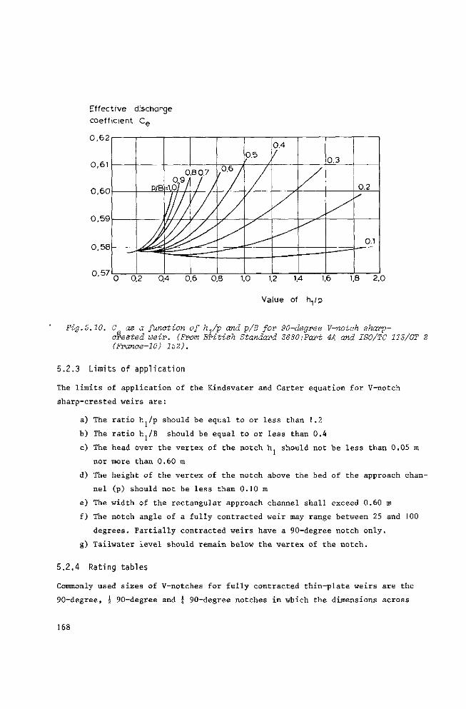
Effective discharge coefficient Ce
0,62
0,61
0,60
0,59
0,58
0,57
P/B
0 0,9/
=10 /
II/ %£•
8 07
/ /
0.6 À 1 /
0.5 0.4 / 0.3
0.2
0.1
O 0,2 Q4 0,6 0,8 1,0 1,2 1,4 1,6 1,8 2,0
Value of t ^ /p
Fig.S.10. C as a function of h1/p and p/B for 90-degree V-notoh sharp-arested weir. (From British Standard 3680:Part 4A and ISO/TC 113/GT 2 (Franae-10) 152).
5.2.3 Limits of application
The limits of application of the Kindsvater and Carter equation for V-notch
sharp-crested weirs are:
a) The ratio lu/p should be equal to or less than 1.2
b) The ratio h./B should be equal to or less than 0.4
c) The head over the vertex of the notch h should not be less than 0.05 m
nor more than 0.60 m
d) The height of the vertex of the notch above the bed of the approach chan
nel (p) should not be less than 0.10 m
e) The width of the rectangular approach channel shall exceed 0.60 m
f) The notch angle of a fully contracted weir may range between 25 and 100
degrees. Partially contracted weirs have a 90-degree notch only.
g) Tailwater level should remain below the vertex of the notch.
5.2.4 Rating tables
Commonly used sizes of V-notches for fully contracted thin-plate weirs are the
90-degree, \ 90-degree and \ 90-degree notches in which the dimensions across
168
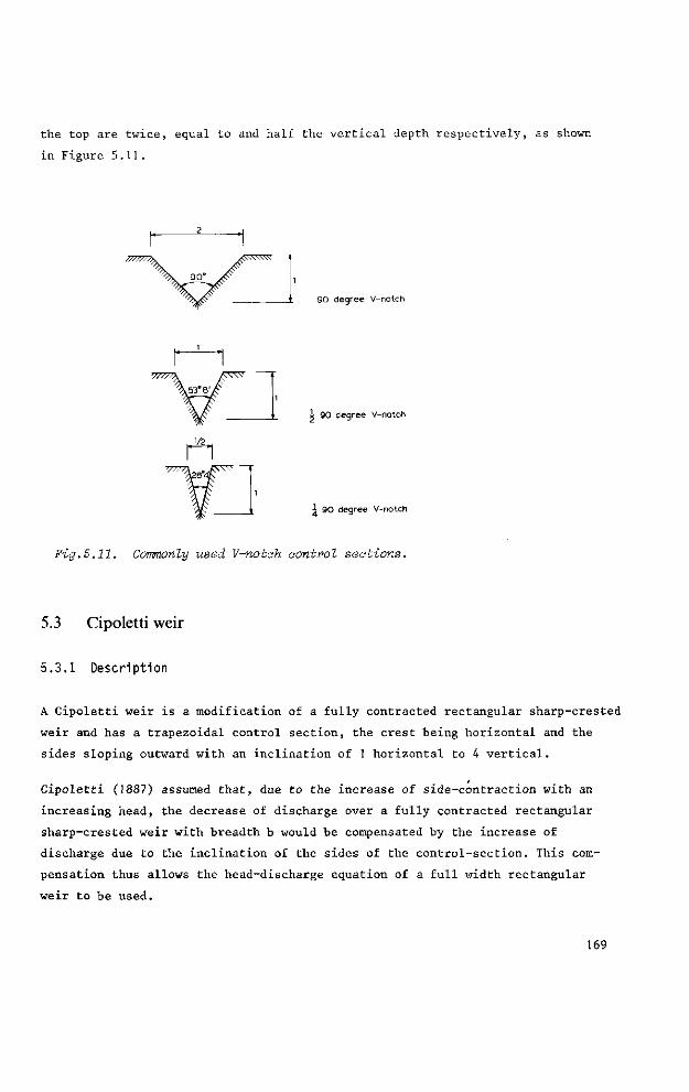
the top are twice, equal to and half the vertical depth respectively, as shown
in Figure 5.11.
90 degree V-notch
1 90 degree V-notch
\ 90 degree V-notch
Fig.5.11. Commonly used V-notch control sections.
5.3 Cipoletti weir
5.3.1 Description
A Cipoletti weir is a modification of a fully contracted rectangular sharp-crested
weir and has a trapezoidal control section, the crest being horizontal and the
sides sloping outward with an inclination of 1 horizontal to 4 vertical.
Cipoletti (1887) assumed that, due to the increase of side-contraction with an
increasing head, the decrease of discharge over a fully contracted rectangular
sharp-crested weir with breadth b would be compensated by the increase of
discharge due to the inclination of the sides of the control-section. This com
pensation thus allows the head-discharge equation of a full width rectangular
weir to be used.
169
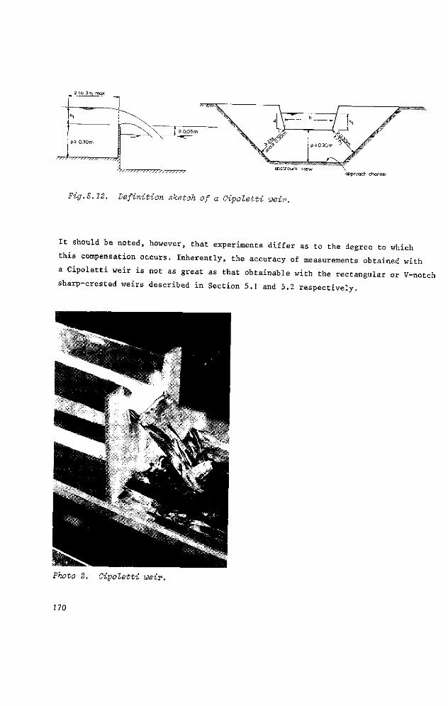
2 to 3 hi max
• p>< 0.30 m
w ~
J?
upstream vie
i / S
1 % w \
app
V
roach channel
J®^/;M±X$^
4F
Fig.S.12. Definition sketch of a Cipoletti uezr.
It should be noted, however, that experiments differ as to the degree to which
this compensation occurs. Inherently, the accuracy of measurements obtained with
a Cipoletti weir is not as great as that obtainable with the rectangular or V-notch
sharp-crested weirs described in Section 5.1 and 5.2 respectively.
Photo 2. Cipoletti weir.
170
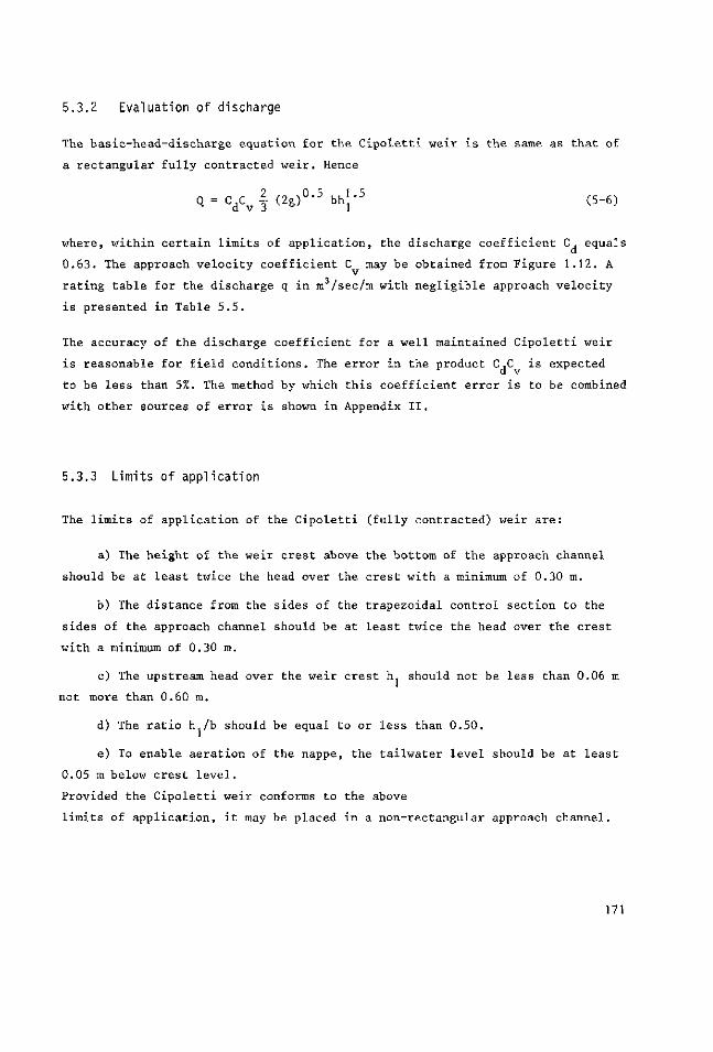
5.3.2 Evaluation of discharge
The basic-head-discharge equation for the Cipoletti weir is the same as that of
a rectangular fully contracted weir. Hence
Q = C d C y | (2g)0-5 bhj-5 (5-6)
where, within certain limits of application, the discharge coefficient C, equals
0.63. The approach velocity coefficient C may be obtained from Figure 1.12. A
rating table for the discharge q in m /sec/m with negligible approach velocity
is presented in Table 5.5.
The accuracy of the discharge coefficient for a well maintained Cipoletti weir
is reasonable for field conditions. The error in the product C ,C is expected r d v
to be less than 5%. The method by which this coefficient error is to be combined
with other sources of error is shown in Appendix II.
5.3.3 Limits of application
The limits of application of the Cipoletti (fully contracted) weir are:
a) The height of the weir crest above the bottom of the approach channel
should be at least twice the head over the crest with a minimum of 0.30 m.
b) The distance from the sides of the trapezoidal control section to the
sides of the approach channel should be at least twice the head over the crest
with a minimum of 0.30 m.
c) The upstream head over the weir crest h should not be less than 0.06 m
not more than 0.60 m.
d) The ratio h./b should be equal to or less than 0.50.
e) To enable aeration of the nappe, the tailwater level should be at least
0.05 m below crest level.
Provided the Cipoletti weir conforms to the above
limits of application, it may be placed in a non-rectangular approach channel.
171
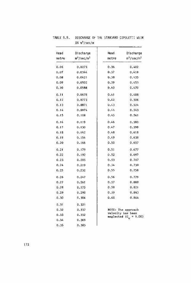
TABLE 5.5. DISCHARGE OF THE STANDARD CIPOLETTI WEIR
IN m3/sec/m
Head
metre
0.06
0.07
0.08
0.09
0.10
0.11
0.12
0.13
0.14
0.15
0.16
0.17
0.18
0.19
0.20
0.21
0.22
0.23
0.24
0.25
0.26
0.27
0.28
0.29
0.30
0.31
0.32
0.33
0.34
0.35
Discharge
mVsec/m1
0.0273
0.0344
0.0421
0.0502
0.0588
0.0678
0.0773
0.0871
0.0974
0.108
0.119
0.130
0.142
0.154
0.166
0.179
0.192
0.205
0.219
0.232
0.247
0.261
0.275
0.290
0.306
0.321
0.337
0.352
0.369
0.385
Head
metre
0.36
0.37
0.38
0.39
0.40
0.41
0.42
0.43
0.44
0.45
0.46
0.47
0.48
0.49
0.50
0.51
0.52
0.53
0.54
0.55
0.56
0.57
0.58
0.59
0.60
NOTE: The
Discharge
mVsec/m1
0.402
0.418
0.435
0.453
0.470
0.488
0.506
0.524
0.543
0.561
0.580
0.599
0.618
0.638
0.657
0.677
0.697
0.717
0.738
0.758
0.779
0.800
0.821
0.843
0.864
approach v e l o c i t y has been neg lec ted (C = 1.00)
172
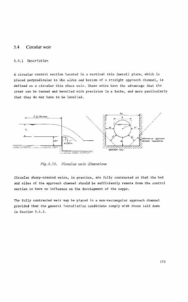
5.4 Circular weir
5.4.1 Description
A circular control section located in a vertical thin (metal) plate, which is
placed perpendicular to the sides and bottom of a straight approach channel, is
defined as a circular thin plate weir. These weirs have the advantage that the
crest can be turned and bevelled with precision in a lathe, and more particularly
that they do not have to be levelled.
2 to 3h, max
alternative approach •channel boundaries
Fig.5.13. Circular weir dimensions
Circular sharp-crested weirs, in practice, are fully contracted so that the bed
and sides of the approach channel should be sufficiently remote from the control
section to have no influence on the development of the nappe.
The fully contracted weir may be placed in a non-rectangular approach channel
provided that the general installation conditions comply with those laid down
in Section 5.4.3.
173
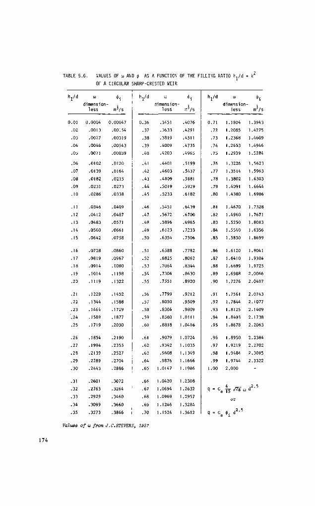
TABLE 5.6. VALUES OF a AND $ AS A FUNCTION OF THE FILLING RATIO hj/d = kc
OF A CIRCULAR SHARP-CRESTED WEIR
yd
0.01
.02
.03
.04
.05
.06
.07
.08
.09
.10
.11
.12
.13
.14
.15
.16
.17
.18
.19
.20
.21
.22
.23
.24
.25
.26
.27
.28
.29
.30
.31
.32
.33
.34
.35
til
dimension less
0.0004
.0013
.0027
.0046
.0071
.0102
.0139
.0182
.0231
.0286
.0346
.0412
.0483
.0560
.0642
.0728
.0819
.0914
.1014
.1119
.1229
.1344
.1464
.1589
.1719
.1854
.1994
.2139
.2289
.2443
.2601
.2763
.2929
.3099
.3273
•l
mJ/s
0.00047
.00154
.00319
.00543
.00839
.0120
.0164
.0215
.0273
.0338
.0409
.0487
.0571
.0661
.0758
.0860
.0967
.1080
.1198
.1322
.1452
.1588
.1729
.1877
.2030
.2190
.2355
.2527
.2704
.2886
.3072
.3264
.3460
.3660
.3866
hj/d
0.36
.37
.38
.39
.40
.41
.42
.43
.44
.45
.46
.47
.48
.49
.50
.51
.52
.53
.54
.55
.56
.57
.58
.59
.60
.61
.62
.63
.64
.65
.66
.67
.68
.69
.70
ÙJ
dimension-less
.3451
.3633
.3819
.4009
.4203
.4401
.4603
.4809
.5019
.5233
.5451
.5672
.5896
.6123
.6354
.6588
.6825
.7064
.7306
.7551
.7799
.8050
.8304
.8560
.8818
.9079
.9342
.9608
.9876
1.0147
1.0420
1.0694
1.0969
1.1246
1.1524
•i
mJ/s
.4076
.4291
.4511
.4735
.4965
.5199
.5437
.5681
.5929
.6182
.6439
.6700
.6965
.7233
.7506
.7782
.8062
.8344
.8630
.8920
.9212
.9509
.9809
1.0111
1.0416
1.0724
1.1035
1.1349
1.1666
1.1986
1.2308
1.2632
1.2957
1.3284
1.3612
hj/d
0.71
.72
.73
.74
.75
.76
.77
.78
.79
.80
.81
.82
.83
.84
.85
.86
.87
.88
.89
.90
.91
.92
.93
.94
.95
.96
.97
.98
.99
1.00
Q = c e
Q = c e
ÜJ
dimension less
1.1804
1.2085
1.2368
1.2653
1.2939
1.3226
1.3514
1.3802
1.4091
1.4380
1.4670
1.4960
1.5250
1.5540
1.5830
1.6120
1.6410
1.6699
1.6988
1.7276
1.7561
1.7844
1.8125
1.8403
1.8678
1.8950
1.9219
1.9484
1.9744
2.000
4 Y5 /Zgf io
or
1
+1
m^/s
1.3943
1.4275
1.4609
1.4946
1.5284
1.5623
1.5963
1.6303
1.6644
1.6986
1.7328
1.7671
1.8013
1.8356
1.8699
1.9041
1.9384
1.9725
2.0066
2.0407
2.0743
2.1077
2.1409
2.1738
2.2063
2.2384
2.2702
2.3015
2.3322
-
d2'5
Values of o> from J.C.STEVENS, 1957
174
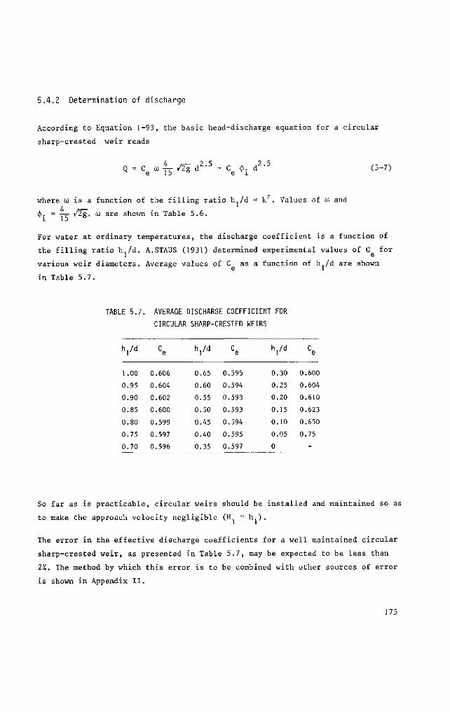
5.4.2 Determination of discharge
According to Equation 1-93, the basic head-discharge equation for a circular
sharp-crested weir reads
Q = C a) ~ /2i d 2 - 5 = C <(>. d 2 , 5 s e 15 ö e ri
(5-7)
where u is a function of the filling ratio h,/d = k2 . Values of 0) and
»i 15 /2g. üj are shown in Table 5.6.
For water at ordinary temperatures, the discharge coefficient is a function of
the filling ratio h /d. A.STAUS (1931) determined experimental values of C for
various weir diameters. Average values of C as a function of h /d are shown
in Table 5.7.
TABLE 5.7. AVERAGE DISCHARGE COEFFICIENT FOR
CIRCULAR SHARP-CRESTED WEIRS
yd
1.00
0.95
0.90
0.85
0.80
0.75
0.70
Ce
0.606
0.604
0.602
0.600
0.599
0.597
0.596
h,/d
0.65
0.60
0.55
0.50
0.45
0.40
0.35
Ce
0.595
0.594
0.593
0.593
0.594
0.595
0.597
yd
0.30
0.25
0.20
0.15
0.10
0.05
0
Ce
0.600
0.604
0.610
0.623
0.650
0.75
-
So far as is practicable, circular weirs should be installed and maintained so as
to make the approach velocity negligible (H - lu).
The error in the effective discharge coefficients for a well maintained circular
sharp-crested weir, as presented in Table 5.7, may be expected to be less than
2%. The method by which this error is to be combined with other sources of error
is shown in Appendix II.
175
The lower quarter of a circular weir is sometimes described as a parabola of
which the focal distance equals the radius of the circle. According to Equation
1-80, the head-discharge relationship then reads
Q = Ce I \A"^ hl'° (5_8)
where the effective discharge coefficient approximates those presented in Table
5.7, provided that h /d about 0.25.
5.4.3 Limits of application
The limits of application of the circular sharp-crested weir are:
a) The height of the crest above the bed of the approach channel should
not be less than the radius of the control section with a minimum of 0.10 m.
b) The sides (boundary of the rectangular, trapézoïdal, or circular approach
channel should not be nearer than r to the weir notch.
c) The ratio H./d should be equal to or more than 0.10.
d) The practical lower limit of H is 0.03 m.
e) To enable aeration of the nappe the tailwater level should be at least
0.05 m below crest level.
If the lower half only of the circular control section is used, the same limits
of application should be observed.
5.5 Proportional weir
5.5.1 Description
The proportional or Sutro weir is defined as a weir in which the discharge is
linearly proportional to the head over an arbitrary reference level which, for
176
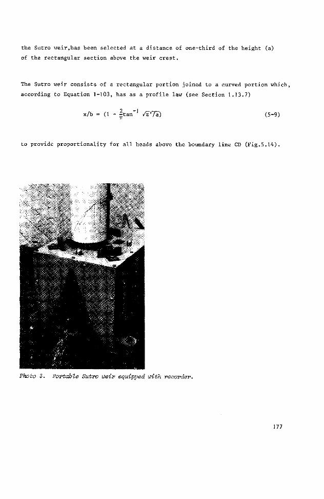
the Sutro weir,has been selected at a distance of one-third of the height (a)
of the rectangular section above the weir crest.
The Sutro weir consists of a rectangular portion joined to a curved portion which,
according to Equation 1-103, has as a profile law (see Section 1.13.7)
x/b = (1 - -tan ' /E"'7a) (5-9)
to provide proportionality for all heads above the boundary line CD (Fig.5.14).
Photo 3. Portable Sutro weir equipped with reaorder.
177
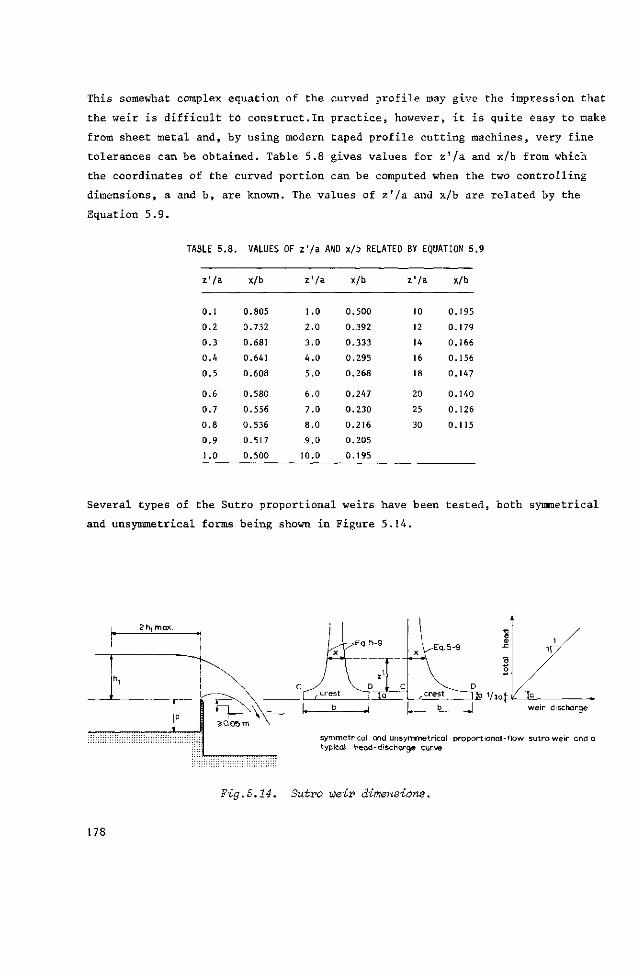
This somewhat complex equation of the curved profile may give the impression that
the weir is difficult to construct.In practice, however, it is quite easy to make
from sheet metal and, by using modern taped profile cutting machines, very fine
tolerances can be obtained. Table 5.8 gives values for z'/a and x/b from which
the coordinates of the curved portion can be computed when the two controlling
dimensions, a and b, are known. The values of z'/a and x/b are related by the
Equation 5.9.
TABLE 5.8. VALUES OF z'/a AND x/b RELATED BY EQUATION 5.9
z'/a
0.1
0.2
0.3
0.4
0.5
0.6
0.7
0.8
0.9
1.0
X/b
0.805
0.732
0.681
0.641
0.608
0.580
0.556
0.536
0.517
0.500
z'/a
1.0
2.0
3.0
4.0
5.0
6.0
7.0
8.0
9.0
10.0
X/b
0.500
0.392
0.333
0.295
0.268
0.247
0.230
0.216
0.205
0.195
z'/a
10
12
14
16
18
20
25
30
x/b
0.195
0.179
0.166
0.156
0.147
0.140
0.126
0.115
Several types of the Sutro proportional weirs have been tested, both symmetrical
and unsymmetrical forms being shown in Figure 5.14.
2 h, max
V— l—-—J crest 1ya i / 3 a ^
weir discharge
symmetrical and unsymmetrical proportional-f low sutro weir and a typical head-discharge curve.
Fig.5.14. Sutro weir dimensions.
178
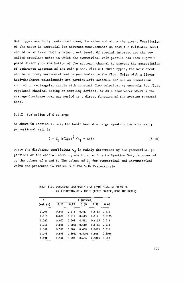
Both types are fully contracted along the sides and along the crest. Ventilation
of the nappe is essential for accurate measurements so that the tailwater level
should be at least 0.05 m below crest level. Of special interest are the so-
called crestless weirs in which the symmetrical weir profile has been superim
posed directly on the bottom of the approach channel to prevent the accumulation
of sediments upstream of the weir plate. With all three types, the weir crest
should be truly horizontal and perpendicular to the flow. Weirs with a linear
head-discharge relationship are particularly suitable for use as downstream
control on rectangular canals with constant flow velocity, as controls for float
regulated chemical dosing or sampling devices, or as a flow meter whereby the
average discharge over any period is a direct function of the average recorded
head.
5.5.2 Evaluation of discharge
As shown in Section 1.13.7, the basic head-discharge equation for a linearly
proportional weir is
Q = Cd b(2ga)* (h, - a/3) (5-10)
where the d ischarge coe f f i c i en t C, i s mainly determined by the geometr ical po-
por t ions of the con t ro l s e c t i on , which, according to Equation 5-9, i s governed
by the values of a and b . The va lues of C, for symmetrical and unsymmetrical
weirs a re p resented in Tables 5.9 and 5.10 r e s p e c t i v e l y .
TABLE 5 . 9 . DISCHARGE COEFFICIENTS OF SYMMETRICAL SUTRO WEIRS
AS A FUNCTION OF a AND b (AFTER SOUCEK, HOWE AND MAVIS)
a
(metres)
0.006
0.015
0.030
0.046
0.061
0.076
0.091
0.15
0.608
0.606
0.603
0.601
0.599
0.598
0.597
0.23
0.613
0.611
0.608
0.6055
0.604
0.6025
0.602
b (metres)
0.30
0.617
0.615
0.612
0.610
0.608
0.6065
0.606
0.38
0.6185
0.617
0.6135
0.6115
0.6095
0.608
0.6075
0.46
0.619
0.6175
0.614
0.612
0.610
0.6085
0.608
179
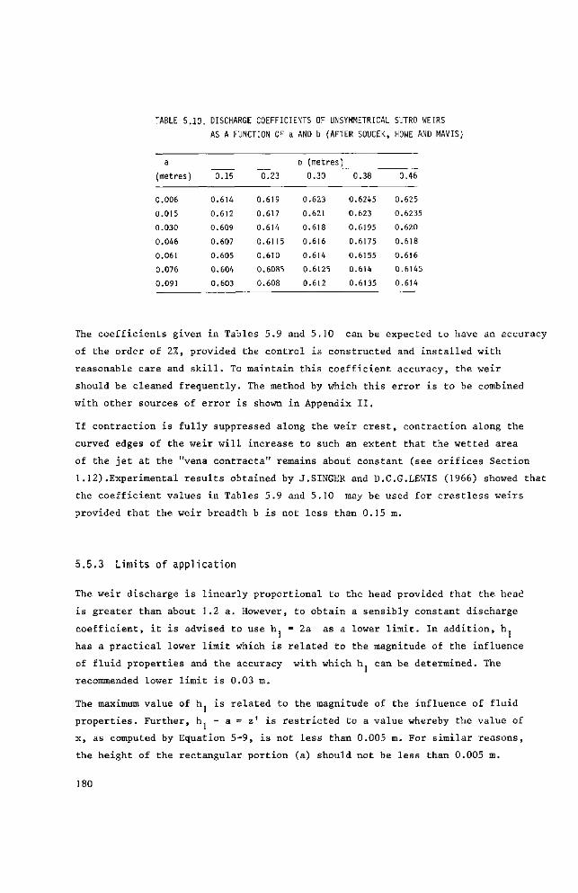
TABLE 5.10. DISCHARGE COEFFICIENTS OF ASYMMETRICAL SUTRO WEIRS
AS A FUNCTION OF a AND b (AFTER SOUCEK, HOWE AND MAVIS)
a (metres)
0.006
0.015
0.030
0.046
0.061
0.076
0.091
0.15
0.614
0.612
0.609
0.607
0.605
0.604
0.603
0 .23
0.619
0.617
0.614
0.6115
0.610
0.6085
0.608
b (metres) 0.30
0.623
0.621
0.618
0.616
0.614
0.6125
0.612
0 .38
0.6245
0.623
0.6195
0.6175
0.6155
0.614
0.6135
0.46
0.625
0.6235
0.620
0.618
0.616
0.6145
0.614
The coefficients given in Tables 5.9 and 5.10 can be expected to have an accuracy
of the order of 2%, provided the control is constructed and installed with
reasonable care and skill. To maintain this coefficient accuracy, the weir
should be cleaned frequently. The method by which this error is to be combined
with other sources of error is shown in Appendix II.
If contraction is fully suppressed along the weir crest, contraction along the
curved edges of the weir will increase to such an extent that the wetted area
of the jet at the "vena contracta" remains about constant (see orifices Section
1.12).Experimental results obtained by J.SINGER and D.C.G.LEWIS (1966) showed that
the coefficient values in Tables 5.9 and 5.10 may be used for crestless weirs
provided that the weir breadth b is not less than 0.15 m.
5.5.3 Limits of application
The weir discharge is linearly proportional to the head provided that the head
is greater than about 1.2 a. However, to obtain a sensibly constant discharge
coefficient, it is advised to use h. = 2a as a lower limit. In addition, h
has a practical lower limit which is related to the magnitude of the influence
of fluid properties and the accuracy with which ht can be determined. The
recommended lower limit is 0.03 m.
The maximum value of h. is related to the magnitude of the influence of fluid
properties. Further, h. - a = z' is restricted to a value whereby the value of
x, as computed by Equation 5-9, is not less than 0.005 m. For similar reasons,
the height of the rectangular portion (a) should not be less than 0.005 m.
180
The breadth (b) of the weir crest should not be less than 0.15 m to allow the
use of the standard discharge coefficient.
To achieve a fully contracted weir, the ratio b/p should be equal to or greater
than 1.0 and the ratio B/b not less than 3.0.
Linearly proportional weirs that do not comply with the limits on the breadth
of the crest can be employed satisfactorily provided that such weirs are first
calibrated to obtain the proper coefficient value. Due to lack of experimental
data, no standard C-values are yet available if b < 0.15 m.
To allow sufficient aeration of the nappe, tailwater-level should be at least
0.05 m below crest level.
5.6 Selected list of references
1. BANKS, W.H.H., BURCH, CR. and SHAW, T.L.: The design of proportional
and logarithmic thin-plate weirs. J.of Hydraulic Research, Vol.6, 1968, No.2,
pp.75-106, Delft.
2. BOSS, P.: Berechnung der Abflussmengen und der Wasserspiegellage bei
Abstürzen und Schwellen unter besonderer Berücksichtigung der dabei auftretenden
Zusatzspannungen. Wasserkraft U.Wasserwirtschaft, Vol.22,1929, pp.13-33.
3. BRITISH STANDARDS INSTITUTION. Methods of measurement of liquid flow in
open channels. BS 3680, Part 4A: Thin-plate weirs and venturi flûmes.1965.London.
4. CIPOLETTI, C : Modulo per la dispensa delle acque atramazzo libero di
forma trapezia e coefficiente di contrazione constante. Esperimenti e formole
per grandi stramazzi a soglia inclinata e orizontale. Milano, Hocpli, 1886,88 p.
5. FRANKE, P.G.: Messüberfälle. Das Gas- und Wasserfläche, 103 Jahrg.,
1962, Nr.40, pp.1072-1075. Nr.42, pp.1137-1140 and Nr.44, pp.1178-1181.
6. KINDSVATER, C E . and R.W.C.CARTER: Discharge characteristics of rec
tangular thin-plate weirs. Journal of the Hydraulics Division of the ASCE, Vol.83,
No.HY 6, Dec.1957, Paper 1453.
7. L'ASSOCIATION FRANÇAISE DE NORMALISATION: Mesure de débit de l'eau
dans les chenaux au moyen de déversoire en mince paroi. X 10-311, Dec.1971,
IS0/TC 113/GT 2 (France-10), 152.
181
8. PRATT, E.A.: Another proportional-flow weir. Sutro weir. Engineering
News, Vol.72, No.9, p.462, Aug.27, 1914.
9. REHBOCK, Th.: Die Ausbildung der Überfälle beim Abfluss von Wasser über
Wehre nebst Beschreibung der Anlage zur Beobachtung von Überfällen im Flusslabo
ratorium zu Karlsruhe, Karlsruhe 1909. Festschrift der Grossherzoglichen Tech
nischen Hochschule Fridericiana.
10. REHBOCK, Th.: Wassermessung mit scharfkantigen Uberfallwehren. Z.des
Vereines deutscher Ingenieure. 73 (1929), No.24, pp.817-823, Berlin.
11. SINGER, J. and LEWIS, D.C.G.: Proportional-flow weirs for automatic
sampling or dosing. Water & Water Engineering.March 1966,V.70, No.841 ,pp. 105-111 .
12. SOUCEK, J., HOWE, H.E., and MAVIS, F.T.: Sutro weir investigations
furnish discharge coefficients. Engineering New-Record, November 12, 1936.
13. STAUS, A.: Der Beiwert kreisrunder Überfälle. Wasserkraft U.Wasser
wirtschaft, 1931, p.42, No.4.
14. STEVENS, J.C.: Flow through circular weirs. J.of the Hydraulics Div.
of the ASCE, Vol.83, No.HY 6, Dec.1957, Paper 1455.
15. THIJSSE, J.Th.: Discharge meters. Waterloopkundig Laboratorium, Delft.
16. THOMSON, J.: On experiments on the measurement of water by triangular
notches in weir-boards. Report of the 28th meeting British Ass.for Advancement
of Science, held at Leeds, Sept.1858, pp.181-185, London 1859.
17. UNITED STATES BUREAU OF RECLAMATION: Water measurement manual. Second
edition, Denver, Col., 1971.
18. WELLS, J.R.: Discharge characteristics of rectangular notch weirs in
rectangular channels. MSc.Thesis presented to the Georgia Institute of Technol.,
Atlanta, Ga., 1954.
182
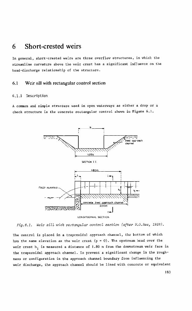
6 Short-crested weirs
In general, short-crested weirs are those overflow structures, in which the
streamline curvature above the weir crest has a significant influence on the
head-discharge relationship of the structure.
6.1 Weir sill with rectangular control section
6.1.1 Description
A common and simple structure used in open waterways as either a drop or a
check structure is the concrete rectangular control shown in Figure 6.1.
lined approach channel
SECTION I-I
FULLY AERATED
Fig. I
tmmmmmm LONGITUDINAL SECTION
Weir sill with rectangular control section (after W.O.Ree, 1928).
The control is placed in a trapezoidal approach channel, the bottom of which
has the same elevation as the weir crest (p = 0 ) . The upstream head over the
weir crest h. is measured a distance of 1.80 m from the downstream weir face in
the trapezoidal approach channel. To prevent a significant change in the rough
ness or configuration in the approach channel boundary from influencing the
weir discharge, the approach channel should be lined with concrete or equivalent
183
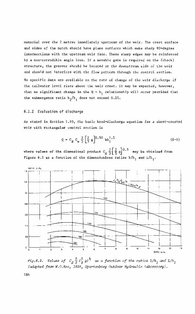
material over the 2 metres immediately upstream of the weir. The crest surface
and sides of the notch should have plane surfaces which make sharp 90-degree
intersections with the upstream weir face. These sharp edges may be reinforced
by a non-corrodible angle iron. If a movable gate is required on the (check)
structure, the grooves should be located at the downstream side of the weir
and should not interfere with the flow pattern through the control section.
No specific data are available on the rate of change of the weir discharge if
the tailwater level rises above the weir crest. It may be expected, however,
that no significant change in the Q - h relationship will occur provided that
the submergence ratio h„/h does not exceed 0.20.
6.1.2 Evaluation of discharge
As stated in Section 1.10, the basic head-discharge equation for a short-crested
weir with rectangular control section is
Q = C, C d v
2 [2 10.
3 La sj 5 0 b h [ - 5
(6-1)
2 r 2 "1 0.5 where values of the dimensional product C -^ \ -^ g ' may be obtained fr
Figure 6.2 as a function of the dimensionless ratios b/h. and L/h1.
~^~Z
|
i
__
-_!£s
- — _ _ t
' •*>
^ - l ^
55
Mïf ?
s"'
-\^^
10 11 12 13 14
RATIO b /h .
9 9 p
Fig. 6. 2. Values of C-, •=• (-=• g) 2 as a function of the ratios b/h- and L/h-
(adapted from W.O.Ree, 1938, Spartanborg Outdoor Hydraulic Laboratory).
184
Values of the approach velocity coefficient C can be read as a function of
C, A /A in Chapter I, Figure 1.12, where A = bh .
For a weir which has been constructed and maintained with reasonable care and
skill the error in the product C.C in Equation 6.1, may be expected to be less
than 5%. The method by which the coefficient error is to be combined with other
sources of error is shown in Appendix II.
6.1.3 Limits of application
For reasonable accuracy, the limits of application of a weir sill with rectangu
lar control section are:
a) The practical lower limit of h is related to the magnitude of the
influence of fluid properties, to the boundary roughness in the approach section,
and to the accuracy with which lu can be determined. The recommended lower
limit is 0.09 m.
b) The crest surface and sides of the control section should have plane
surfaces which make sharp 90-degree intersections with the upstream weir face.
c) The bottom width of the trapezoidal approach channel should be 1.25 b.
d) The upstream head hj should be measured 1.80 m above the downstream
weir face. Consequently, h1 should not exceed half of this distance, i.e. 0.90 m.
e) To obtain modular flow the submergence ratio h„/h should not exceed
0.20.
6.2 V-notch weir sill
6.2.1 Description
In natural streams, where it is necessary to measure a wide range of discharge,
a triangular control section has the advantage of providing a wide opening at
high flows so that it causes no excessive backwater effects, whereas at low
flows its opening is reduced so that the sensitivity of the structure remains
acceptable.
The U.S. Soil Conservation Service developed a V-notch weir sill with 2-to-l,
185
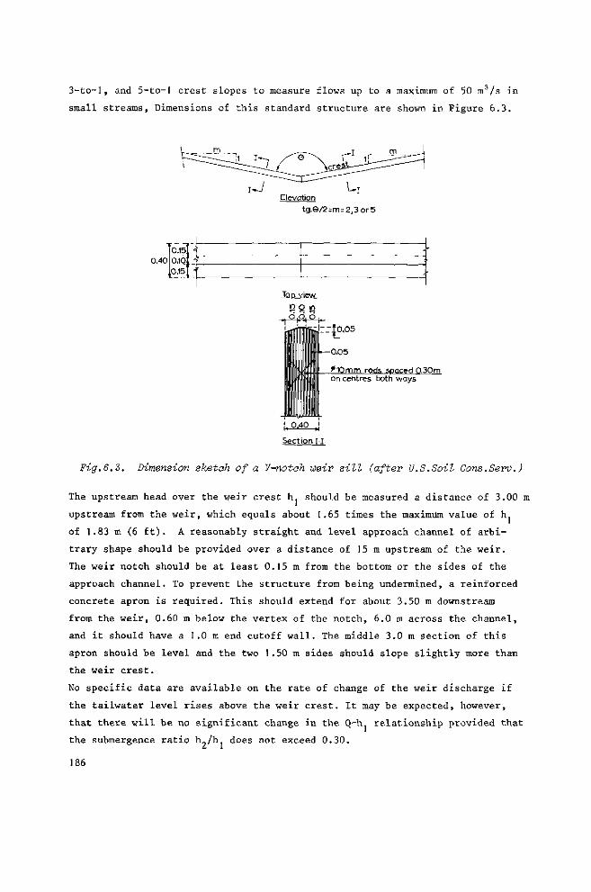
3-to-l, and 5-to-l crest slopes to measure flows up to a maximum of 50 m3/s in
small streams, Dimensions of this standard structure are shown in Figure 6.3.
Elevation tg .e /2 :m=2,3or5
0.40 0.15 0.1Q ,0.15
Top view
in o in
Section I-I
Fig.6.3. Dimension sketch of a V-notoh weir sill (after U.S.Soil Cons.Serv.)
The upstream head over the weir crest h. should be measured a distance of 3.00 m
upstream from the weir, which equals about 1.65 times the maximum value of h
of 1.83 m (6 ft). A reasonably straight and level approach channel of arbi
trary shape should be provided over a distance of 15 m upstream of the weir.
The weir notch should be at least 0.15 m from the bottom or the sides of the
approach channel. To prevent the structure from being undermined, a reinforced
concrete apron is required. This should extend for about 3.50 m downstream
from the weir, 0.60 m below the vertex of the notch, 6.0 m across the channel,
and it should have a I.0 m end cutoff wall. The middle 3.0 m section of this
apron should be level and the two 1.50 m sides should slope slightly more than
the weir crest.
No specific data are available on the rate of change of the weir discharge if
the tailwater level rises above the weir crest. It may be expected, however,
that there will be no significant change in the Q-h relationship provided that
the submergence ratio h„/h does not exceed 0.30.
186
6.2.2 Evaluation of discharge
The basic head-discharge equation for a short-crested weir with a triangular
control section is as shown in Section 1.9.3:
Q = CdCv ! | [ ! g]°,5tan 6/2 h ^ 5 (6-2)
where tan 6/2 equals m.
Based on hydraulic laboratory tests conducted by the U.S.Soil Conservation Ser
vice at Cornell University, Ithaca, N.Y., rating tables have been developed
giving the discharge in m3/s at each 0.3048 m (1 foot) of head for a number of
wetted areas, A,, at the head measurement station. These are presented in
Table 6.1.
From this table, it is possible to read, for example, that the discharge over a
5-to-l V-notch weir under a head h, = 0.915 m and a wetted area of the approach
channel of A = 6.50 m2 equals 7.70 m3/s. For a wetted area of At = 15.0 m ,and there
fore with a lower approach velocity, the weir discharge equals 6.56 m3/s under
the same head. The head-discharge relationship for these weirs can be obtained
by plotting the discharge for each 0.3048 m (1 foot) of head and the correspond
ing wetted area of the approach channel.
Discharges for heads up to 0.20 m can be obtained from Table 6.2. A smooth
line is drawn through the plotted points and a rating table for each 0.01 m
of head is produced from this curve.It should be understood that any significant
change in the approach cross-section, due either to cutting or filling, requires
a revision of the Q - h curve.
It can be expected that for a well-maintained V-notch weir which has been con
structed with reasonable care and skill the error in the discharges shown in
Tables 6.1 and 6.2 will be less than 3%. The method by which this error is to be
combined with other sources of error is shown in Appendix II.
6.2.3 Limits of application
For reasonable accuracy, the limits of application of the V-notch weir sill are:
a) The head over the weir crest should be at least 0.03 m and should be
measured a distance of 3.00 m upstream from the weir.
187
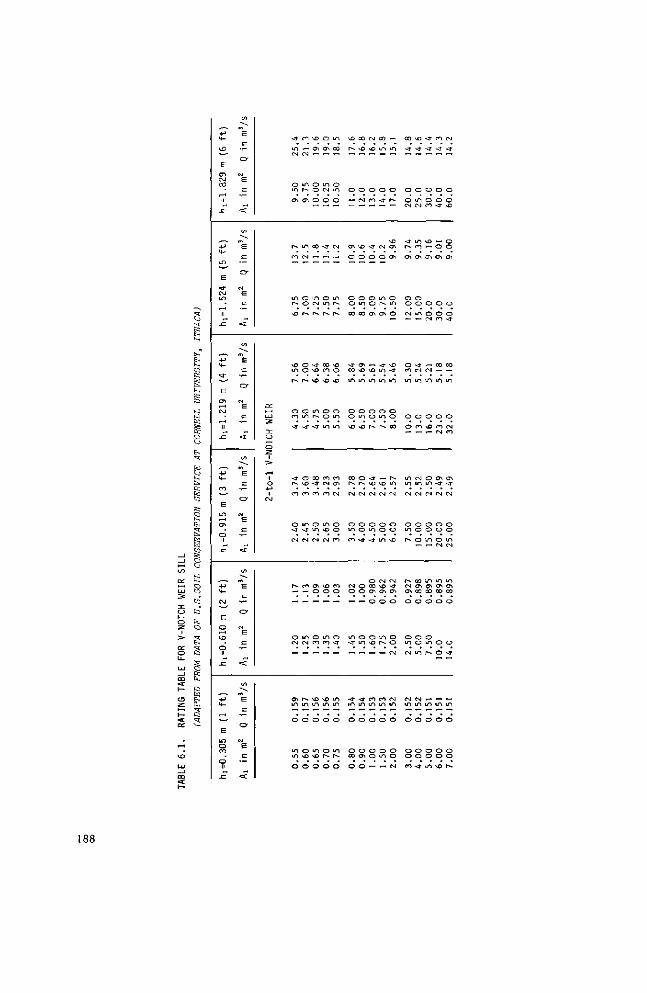
E«
to , - f
E« 1
y. a rt
4-> <4~
KO
E
en O-J c o
II
sz
•*->
4 -
LT)
E *3-C\J i r )
ii
-C
- p 4 -
« " E
en
C\J
il
- C
+-> t i
r o
"—' E
\n
en
o
- C
^. +-> 4 -
OJ
*—' E
O
KO
O II
J Z
-t-> 4 -
"—* E
LD O r o
o i i
- C
t/l - v .
E
c • ' -
C r
CM E
£=
• <
to
*- E
c
o -
CM E
c :
• <
tn
\ E
c
o -
CM E
c
•a :
u i
\ E
e
C r
CM
E
c
<c
(ƒ)
T" E
EZ
C r
CM
E
c :
«C
i/>
\ E
EZ
o -
CM
E
c
«<
c c
U I 3
z e C_3 1 — O
2 »
1 o
•4-> 1
CvJ
<r
in CM
O m
CTi
r -
m
m r-*
v£)
^o m
r-*
O co
-*
• < *
r-.
en
o
-* CM
r^ —
O CN
o\ m
o
m m
o
m v£>
— Ov
iA O r» O <?\ o
m oo
Ol —
O u-i O CM
r * r »
O - * O ^o
r-* £>
o m i n r-*
-d- -<r
o co vO < f
oo OO
m o -d - m
CM CM
oo a \ — o
u~i O CM OO
r--. KO m m
o o
o m KO VO
o o
o m
en CO
m o OM u-l
o o
•<r CM
o m m r-*
r » r -
CO KO r o o
\0 KD
O O o m
m m
OO co CM CT\
00 CM
m o \0 o
CM CO
v O CO O o
m o CO <J
KO m m m
o o
o m r-. r -
o o
vO CO OM CO —
r - vo KO m m
o o o o o
— CM oo -3- r »
KO CTi KD <ï CM Cn
O O o o en
o o o m o o m o r - m
00 CO CTi CTi o
- t f CT. — -3" MD CO KD vD i n s t
m m m m m
o o o o o o m o m o
KD ^o r - r-* co
C O O v J - S r-* r-* KD \D i n
CM 0M CM CM CM
O O O O O m o m o o
co -<t -d- m KD
O CM OM OM O 00 \ 0 -3-O O C ^ O \ o^
m o o m o -J- m \ d r^ o
-d- < r oo r o CM i n i n i n i n i n
o o o o o
o o o o o oo f ^ o m o
O O — —' CM
CO KD
<t <t
O o
o i n CM CM
•<r m r-. oo
en en
o o o o
CM m
O sf CO CM
m m
o o
o CO
m CM m m CM CM
o o m o
r-> O
r- oo CM en 0\ CO
o o
o o m o
CM i n
CM CM m m
o o
o o o o
co v r
< r co CM
•<r -<r - *
O O O
O O O 0O -3- vD
KD —• O * - o o
o o o
o o o CM oo -a-
— C0 00 fs | — —
m m m
o o o
^D CO CM — CM CO
O 0*i CT\ m - t f s r
CM CM CM
O O O o o o
m o i n —• CM CM
m m m
00 00 00
o o o
o m o o
r^ o * *
m m m
o o o
o o o o o o
i m o s
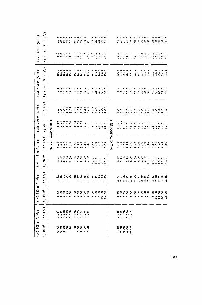
•M 4 -
l £ >
' E
a^ C\J C O
. - H 11
- C
s~.
+ J
4-LT)
' E
« 3 -CXI L D
,—( I I
- C
- P 4 -
«3-
' E
cr>
C M
M
.c
- M 4 -
0 0
*— E
L f i
CT*
O II
- C
,—* -l-> 4 -
( X I
-— E
O
i £ >
O 11
.c
+ J 4 -
. - H
*— E
i n o ro o it
JZ
(/) "k c
O '
CM
E c
< 1/1
^T"-E tz
o -
<s E c
• <
t / 1 - V .
E S I
O *
£M
E c
< C
c/i
\ E c:
O *
(M
E c
et
V )
<^"" c:
O *
CM
E c
<c
1/1 " v .
E c
C D -
CM
E C
,_, <c
o£
UJ
3 rc C_J
o
r=-
i
o
m
v D
O
en
o m
CN
CTi
m o
o CN
~
o m M J
- d -CN
m
LTl
r-m
C N v O
L O 0 0
—
r-en CN
O
m r-O
0 0
0 0 CN
i n
LT\
o
0 0
o
^
C 0
o
~
m rv
vO
en CO
-d-
o o - j
SD i n
o o C N
<r m CN
O
O 0 0
o
v D
r
O v D
CO
^
O
CN
m o
~
o o r -v
en -d-- d
o i n
•<r
- d -- d -
o m CN
CN
en CM
o
o en o
o r-CM
m v O
o
\ Û
o en
O i v O
CJ\
o in
r-
in CN
-*
O O
m
CN - d -
i n
r-CN
o en CN
o
o O
—
i n
v O CM
o r -
m
m
o - d
en o\
o o
co
-d-
"" <r
o m m
o -d-
o o m
0 0
CN
O
o CN
-
a> m
o 0 0
„
u-1
O
m
CN
o O",
o m
co
vo o
-d-
o o \D
C 0
en
o m en
v O CN CN
O
O
m
-
CT>
- d "
O
en
CT>
-d-
O \o
co 0 0
o o
en
CN O
- d
o i n
^o
r~ en
o o •< r
m C M
CN
o
o o CN
<r - d -C M
o o
r -
<r
o r-.
r-. \ û
0 0
O in O".
0 0
en
en
o o r-.
>sO
en
o m - d -
- d -CN CN
O
O O
en
v O
m CM
m CN CN
i n
-d-
o co
m m co
o
o
en
m
o o 0 0
i n
en
o o m
- d -CN CN
O
O o m
— en CN
o m
< î
- d -
o o CN
r-en CO
o
CO C 0
en
o o o\
in en
o i n
m
- d -
CN
O
O
m r-
co CM CM
m r-
CN
- d -
m CM CM
m CN
CO
O
CM
m 0 0
en
O O
<f en
O O \£>
m CM
o
t> en
o
-*
o i n CN
en o 0 0
o
m
Cn r-.
en
m CM
- d -
en
o o r-
o CM CM
O
O - d -
o i
en
O
O
m
o en r»
O
O CN
r-r~-
en
O
m
en m
O O
0 0
co
_
o o m
0 0
m
o o ~ j
o 0 0
r-.
O
O
en
in r»
en
O O CN
en en
o o o
r~-„
o o •X)
r-
m
O
m m
en r-~ r-.
O
m -< f
-* r-
en
O
m CN
en en
O O
<r
a:
LU
3 in C J h -O
1
1
o 1
L O
-d-cr> ^r
o CN
o
o en
o v£)
—
- d
v O
o
\o
^ co
o \n m
r»
CN
O 0 0
CM
v D 0 0
en o
o m
-
en \£>
<r
o en CM
CO
CN
O
c -
—
— v O
m CM
cr> - d -
0 0
m r-m
h »
CN
O O en
CN 0 0
en o
o o CN
- ï
en <r
o i n CN
cr>
CN
m 0 0
-~
0 0
m
m
r» — CO
o o \D
0 0
CN
CN
en
co r» en O
O O
en
— __ < T
m r-CM
O
\D
O
O CM
m m
o CM
r-0 0
r
m CM
vu
CN m
CN
O
m en
v O
en o
o o v ©
0 0
C7\
en
o o m
o
i n CM
i n
CN CM
CN
in
m CN
O r-.
r-
O m \ £>
CTv
CN
m r-en
v D
r en O
O O
O
— CTi
en
m CN
m
m
•<r
o m CN
O
m
o
en
- d -
r-
O O r-.
in
CN
o o - 3 -
i n
co en
O
m
_ CM
m r-C N
\ D
-*
O
<f
•X> CN
r-
o m r--
C N
CM
O
m •<r
o CO
m r~-m
0 0
en
o o en
•<r
< j -
o m
o
~ r -
O O
0 0
o~> en
CN
O O
m
v O
r . en
O O - 3 -
i v .
e n CN
i n
CN
en
CN
-d-
O \ D
<7\ CJ\
v O
O
o en
m en
CN
o o v D
— r-en
o m -d-
\ D
CN
o m en
O
- d -
m
r-
-d-0 0
\D
O
O
m en
CM
O
o r-
V D
VD
m
o O i n
-d-
en CN
O
O ~ d -
0 0
en
O
O CN
r» vJD
v D
O
CM
CM en
cN
O i n
0 0
- d -
-o en
o m m
en
en CM
o o m
m m
o
m CN
\£>
m v D
o m
o en
CN
o o o
CN
\ D
en
O
O \D
CN
en
O
o \ D
< T
en
o
o en
0 0
-d-\D
o o CN
en CN
o o m
o VJD
en
o m r—
o
en CM
o m r»
en en
o
o - d -
CN - d -
v D
O
O
en
0 0 CM
CM
o o o CN
o VD
en
o O a i
co
CN CM
O
o CTv
CM
en
o
m \ Û
o
-tf \o
o m - d -
ao
CM
O O
m CM
189
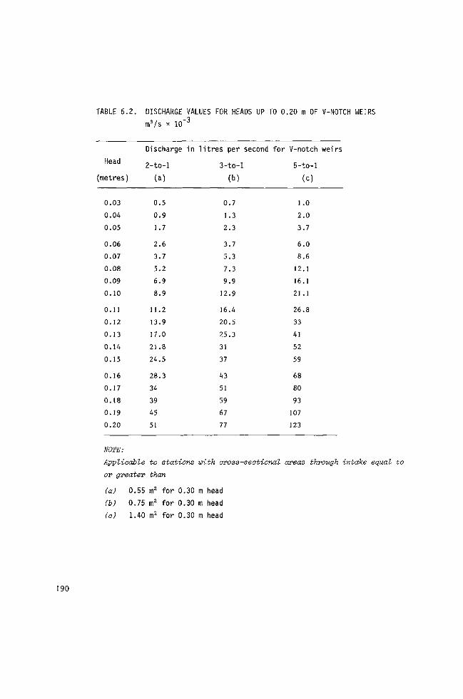
TABLE 6.2. DISCHARGE VALUES FOR HEADS UP TO 0.20 m OF V-NOTCH WEIRS
m3/s x 10"3
Discharge in litres per second for V-notch weirs
5-to-l
(c)
ncttu
(metres)
0.03
0.04
0.05
0.06
0.07
0.08
0.09
0.10
0.11
0.12
0.13
0.14
0.15
0.16
0.17
0.18
0.19
0.20
2-tO-l
(a)
0.5
0.9
1.7
2.6
3.7
5.2
6.9
8.9
11.2
13.9
17.0
21.8
24.5
28.3
34
39
45
51
3-tO-
(b
0.7
1.3
2.3
3.7
5.3
7.3
9.9
12.9
16.4
20.5
25.3
31
37
43
51
59
67
77
1 .
2.
3.
6.
8.
12.
16.
21.
26.
33
41
52
59
68
80
93
107
123
,0
,0
,7
.0
,6
,1
,1
,1
,8
NOTE:
Applicable to stations with cross-sectional areas through intake equal to
or greater than
(a) 0.55 m2 for 0.30 m head
(b) 0.75 m2 f o r 0.30 m head
(o) 1.40 m2 f o r 0.30 m head
190
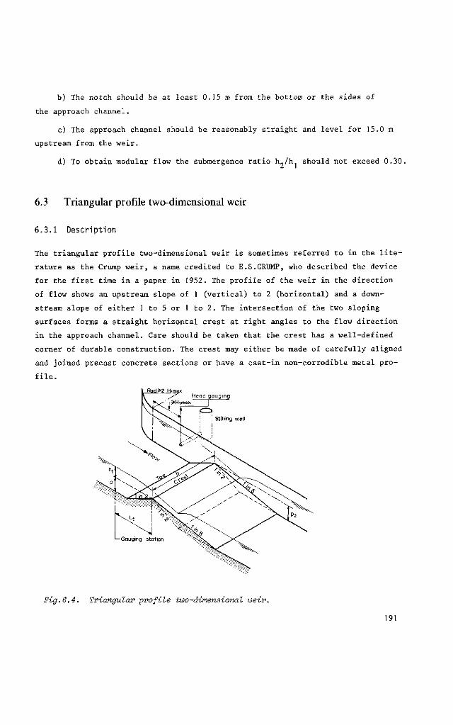
b) The notch should be at least 0.15 m from the bottom or the sides of
the approach channel.
c) The approach channel should be reasonably straight and level for 15.0 m
upstream from the weir.
d) To obtain modular flow the submergence ratio h„/h1 should not exceed 0.30.
6.3 Triangular profile two-dimensional weir
6.3.1 Description
The triangular profile two-dimensional weir is sometimes referred to in the lite
rature as the Crump weir, a name credited to E.S.CRUMP, who described the device
for the first time in a paper in 1952. The profile of the weir in the direction
of flow shows an upstream slope of 1 (vertical) to 2 (horizontal) and a down
stream slope of either 1 to 5 or 1 to 2. The intersection of the two sloping
surfaces forms a straight horizontal crest at right angles to the flow direction
in the approach channel. Care should be taken that the crest has a well-defined
corner of durable construction. The crest may either be made of carefully aligned
and joined precast concrete sections or have a cast-in non-corrodible metal pro
file.
Rqd£2 HIITIQX ^ Head gauging r>Himax I
Fig.6.4. Triangular profile two-dimensional weir.
191
Tests were carried out at the Hydraulics Research Station at Wallingford (U.K.) to
determine the maximum permissible truncation of the weir block in the direction of
flow whereby the discharge coefficient was to be within 0.5% of its constant value.
It was found that for a l-to-2 / l-to-5 weir the minimum horizontal distance from
the weir crest to point of truncation of the weir block equals 1.0 H max for
the l-to-2 slope and 2.0 H max for the l-to-5 slope. For a l-to-2 / l-to-2
weir, these minimum distances equal 0.8 H max for the upstream slope and
1.2 H max for the downstream slope.
The upstream head over the weir crest ht should be measured in a rectangular
approach channel at a sufficient distance upstream from the crest to avoid the
area of surface draw-down,but close enough to the crest for the energy loss
between the head measurement station and the control section to be negligible.
For this to occur, the head measurement station should be at a distance t = 6 p
upstream from the weir crest for a l-to-2 / l-to-5 weir and at 1. = 4 p for a
l-to-2 / l-to-2 weir. If no particularly high degree of accuracy is required
in the maximum discharges to be measured, savings can be made in the construction
cost of the structure by reducing the distance from the crest to head measure
ment station to 2p + 0.5 H. max. The additional error introduced will be of
the order of 0.25% at an H./p value of 1, of 0.5% at an IL/p value of 2, and of
1% at an H,/p value of 3.
If the weir is to be used for discharge measuring beyond the modular range,
crest tappings should be provided to measure the piezometric level in the sepa
ration pocket formed immediately downstream of the crest. The crest tapping
should consist of a sufficient number (usually 4 to 12) of </> 0.01 m holes dril
led in the weir crest block on 0.10 m centres 0.019 m downstream from the weir
crest as shown in Figure 6.5. The edges of the holes should not be rounded or
burred.
Preferably, the crest tapping should be located at the centre of the weir, but
may be off-centre provided that the side walls do not interfere with the pres
sure distribution in the separation pocket. A distance of about 1.20 m from
the side walls should be sufficient. Weirs with a breadth b of less than 2.5 m
should have the crest tapping in the centre.
192
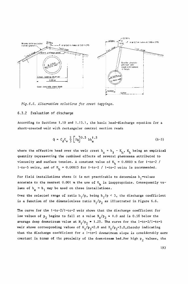
Bronze plate seated on rubber gasket -
0-Ofc, £ of sf 0.01 m holes at 0.10 m CRS
r- 0.019 rr,
^l~Jjs- -£ of 0 0.01 m tubes at 0.10 m CF?S
Granite concrete pre-cast weir
ƒ block with rubbed : - finish
Fig.6.5. Alternative solutions for crest tappings.
6.3.2 Evaluation of discharge
According to Sections 1.10 and 1.13.1, the basic head-discharge equation for a
short-crested weir with rectangular control section reads
Q = CdC vfH°' e (6-3)
where the effective head over the weir crest h = h. - K, , K, being an empirical
quantity representing the combined effects of several phenomena attributed to
viscosity and surface tension. A constant value of K, = 0.0003 m for l-to-2 /
l-to-5 weirs, and of K, = 0.00025 for l-to-2 / l-to-2 weirs is recommended.
For field installations where it is not practicable to determine h.-values
accurate to the nearest 0.001 m the use of K, is inappropriate. Consequently va
lues of h - h may be used on these installations.
Over the selected range of ratio h,/p, being h,/p < 3, the discharge coefficient
is a function of the dimensionless ratio Hj/p. as illustrated in Figure 6.6.
The curve for the l-to-2/l-to-2 weir shows that the discharge coefficient for
low values of p. begins to fall at a value H./p„ = 1.0 and is 0.5% below the
average deep downstream value at HT/p„ = 1.25. The curve for the l-to-2/l-to-5
weir shows corresponding values of H./p =2.0 and H /p =3.0,thereby indicating
that the discharge coefficient for a l-to-5 downstream slope is considerably more
constant in terms of the proximity of the downstream bed.For high p„ values, the
193
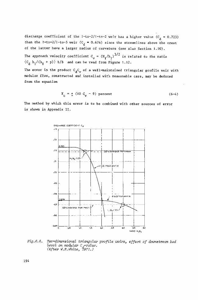
discharge coefficient of the l-to-2/I-to-2 weir has a higher value (C, = 0.723)
than the l-to-2/]-to-5 weir (C, = 0.674) since the streamlines above the crest
of the latter have a larger radius of curvature (see also Section 1.10).
3/2 The approach velocity coefficient C = (H./h ) is related to the ratio
{Cd hj/(hj + p)} b/B and can be read from Figure 1.12.
The error in the product C,C of a well-maintained triangular profile weir with
modular flow, constructed and installed with reasonable care, may be deduced
from the equation
X = + (10 C - 9) percent c - v v (6-4)
The method by which this error is to be combined with other sources of error
is shown in Appendix II.
DISCHARGE COEFFICIENT Cd
Fig.6.6. Two-dimensional triangular profile weirs, effect of downstream bed level on modular C-rvalue. (After W.R.White, 1971.)
194
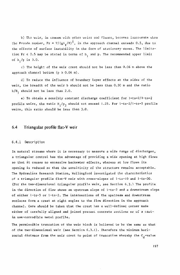
b) The weir, in common with other weirs and flumes, becomes inaccurate when I
the Froude number, Fr = V/(gA / B ) 2 , in the approach channel exceeds 0.5, due to
the effects of surface instability in the form of stationary waves. The limita
tion Fr < 0.5 may be stated in terms of h and p. The recommended upper limit
of h /p is 3.0.
c) The height of the weir crest should not be less than 0.06 m above the
approach channel bottom (p 5- 0.06 m) .
d) To reduce the influence of boundary layer effects at the sides of the
weir, the breadth of the weir b should not be less than 0.30 m and the ratio
b/H1 should not be less than 2.0.
e) To obtain a sensibly constant discharge coefficient for l-to-2/l-to-2
profile weirs, the ratio H /p„ should not exceed 1.25. For 1-to-2/1-to-5 profile
weirs, this ratio should be less than 3.0.
6.4 Triangular profile flat-V weir
6.4.1 Description
In natural streams where it is necessary to measure a wide range of discharges,
a triangular control has the advantage of providing a wide opening at high flows
so that it causes no excessive backwater effects, whereas at low flows its
opening is reduced so that the sensitivity of the structure remains acceptable.
The Hydraulics Research Station, Wallingford investigated the characteristics
of a triangular profile flat-V weir with cross-slopes of l-to-10 and l-to-20.
(For the two-dimensional triangular profile weir, see Section 6.3.) The profile
in the direction of flow shows an upstream slope of l-to-2 and a downstream slope
of either l-to-5 or l-to-2. The intersections of the upstream and downstream
surfaces form a crest at right angles to the flow direction in the approach
channel. Care should be taken that the crest has a well-defined corner made
either of carefully aligned and joined precast concrete sections or of a cast-
in non-corrodible metal profile.
The permissible truncation of the weir block is believed to be the same as that
of the two-dimensional weir (see Section 6.3.1). Therefore the minimum hori
zontal distance from the weir crest to point of truncation whereby the C,-value
197
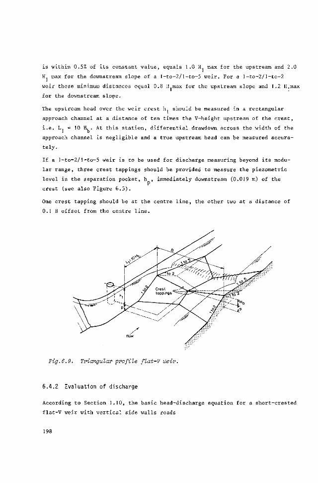
is within 0.5% of its constant value, equals 1.0 H max for the upstream and 2.0
H max for the downstream slope of a l-to~2/l-to-5 weir. For a 1-to-2/l-to-2
weir these minimum distances equal 0.8 H max for the upstream slope and 1.2 H max
for the downstream slope.
The upstream head over the weir crest h should be measured in a rectangular
approach channel at a distance of ten times the V-height upstream of the crest,
i.e. L = 10 H, . At this station, differential drawdown across the width of the
approach channel is negligible and a true upstream head can be measured accura
tely.
If a l-to-2/1-to-5 weir is to be used for discharge measuring beyond its modu
lar range, three crest tappings should be provided to measure the piezometric
level in the separation pocket, h , immediately downstream (0.019 m) of the
crest (see also Figure 6.5).
One crest tapping should be at the centre line, the other two at a distance of
0.1 B offset from the centre line.
Fig. 6.9. Triangular profile flat-V weir.
6.4.2 Evaluation of discharge
According to Section 1.10, the basic head-discharge equation for a short-crested
flat-V weir with vertical side walls reads
198
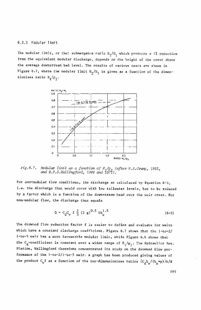
6.3.3 Modular limit
The modular limit, or that submergence ratio H./H which produces a 1% reduction
from the equivalent modular discharge, depends on the height of the crest above
the average downstream bed level. The results of various tests are shown in
Figure 6.7, where the modular limit H /H is given as a function of the dimen-
sionless ratio H /p„.
RATIO H2/H 0.9
0.6
0.5
0.4
0.3
0.2
0.1
4
1 to 2/1 JO 5WÇU. •*
- 4^ Sf-
- -
^- —
^
1.5 2.0 RATIO H,/p2
Fig.6. 7. Modular limit as a function of R J-ç (after E.S.Crump, 1952, and H.R.S.Wallingford, 1966 and 1971).
For non-modular flow conditions, the discharge as calculated by Equation 6-3,
i.e. the discharge that would occur with low tailwater levels, has to be reduced
by a factor which is a function of the downstream head over the weir crest. For
non-modular flow, the discharge thus equals
CdCv f f (2 g ) 0 " 5 bbj- (6-5)
The drowned flow reduction factor f is easier to define and evaluate for weirs
which have a constant discharge coefficient. Figure 6.7 shows that the l-to-2/
l-to-5 weir has a more favourable modular limit, while Figure 6.6 shows that
the C^-coefficient is constant over a wider range of H /p . The Hydraulics Res.
Station, Wallingford therefore concentrated its study on the drowned flow per
formance of the l-to-2/l-to-5 weir. A graph has been produced giving values of
the product C f as a function of the two-dimensionless ratios {C.h /(h +p)}b/B v d e e
195
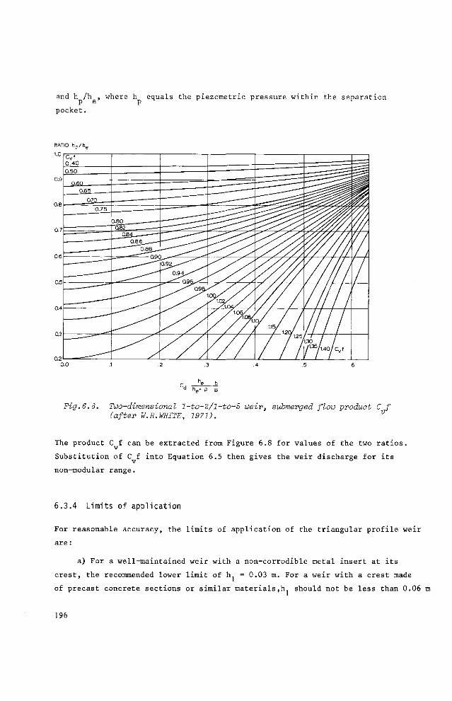
and h /h , where h equals the piezometric pressure within the separation p e p n r r F
pocket .
RATIO hp/h,
1.0
e b P B
Fig.6. 8. Two-dimensional l-to-2/l-to-5 weir, submerged flow product C f (after W.R.WHITE, 1971). V
The product C f can be extracted from Figure 6.8 for values of the two ratios.
Substitution of C f into Equation 6.5 then gives the weir discharge for its
non-modular range.
6.3.4 Limits of application
For reasonable accuracy, the limits of application of the triangular profile weir
are :
a) For a well-maintained weir with a non-corrodible metal insert at its
crest, the recommended lower limit of h = 0.03 m. For a weir with a crest made
of precast concrete sections or similar materials,h should not be less than 0.06 m
196
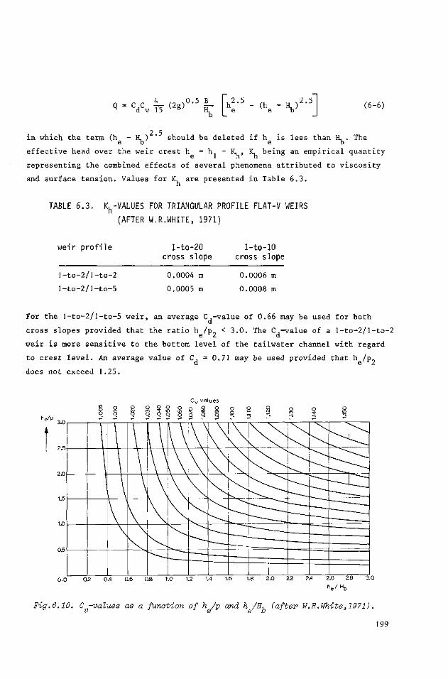
» - v» h <«0-5 k 2.5 (he - V 2.5
(6-6)
2 5 m which the term (h - IL ) should he deleted if h is less than H, . The
effective head over the weir crest h = h - K, , K, being an empirical quantity
representing the combined effects of several phenomena attributed to viscosity
and surface tension. Values for K, are presented in Table 6.3.
TABLE 6.3. ^-VALUES FOR TRIANGULAR PROFILE FLAT-V WEIRS
(AFTER W.R.WHITE, 1971)
weir profile l-to-20 cross slope
l-to-10 cross slope
l-to-2/l-to-2
l-to-2/l-to-5
0.0004 m
0.0005 m
0.0006 m
0.0008 m
For the l-to-2/l-to-5 weir, an average C,-value of 0.66 may be used for both
cross slopes provided that the ratio h /p < 3.0. The C,-value of a l-to-2/l-to-2
weir is more sensitive to the bottom level of the tailwater channel with regard
to crest level. An average value of C, = 0.71 may be used provided that h /p„
does not exceed 1.25.
he/p
O O O o o Q O
o o o o q q q
05
0.0 0.2 0.4 0.6 OB 1.0 1.2 1.4 1.6 1.8 2.0 22 2A 2.6 2.B 3.0
Fig. 6.10. C -values as a function of h /p and h /E-, (after W.R.White,1971).
199
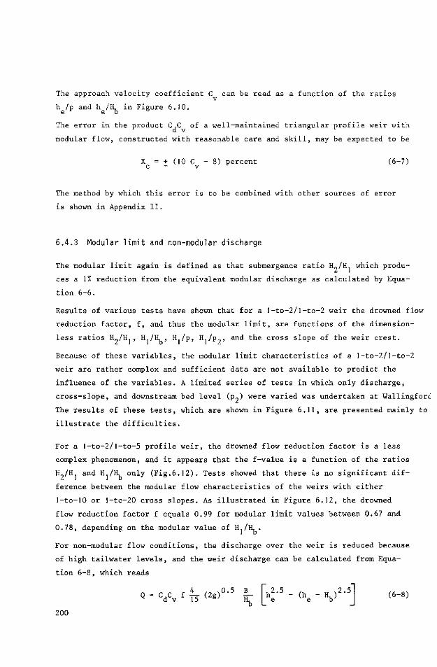
The approach velocity coefficient C can be read as a function of the ratios
h /p and h /H, in Figure 6.10.
The error in the product C.C of a well-maintained triangular profile weir with
modular flow, constructed with reasonable care and skill, may be expected to be
X = + (10 C - 8) percent (6-7) c - v
The method by which this error is to be combined with other sources of error
is shown in Appendix II.
6.4.3 Modular limit and non-modular discharge
The modular limit again is defined as that submergence ratio H„/H1 which produ
ces a 1% reduction from the equivalent modular discharge as calculated by Equa
tion 6-6.
Results of various tests have shown that for a l-to-2/l-to-2 weir the drowned flow
reduction factor, f, and thus the modular limit, are functions of the dimension-
less ratios H„/Hr, H /ïL, H./p, H /p , and the cross slope of the weir crest.
Because of these variables, the modular limit characteristics of a l-to-2/l-to-2
weir are rather complex and sufficient data are not available to predict the
influence of the variables. A limited series of tests in which only discharge,
cross-slope, and downstream bed level (p9) were varied was undertaken at Wallingforc
The results of these tests, which are shown in Figure 6.11, are presented mainly to
illustrate the difficulties.
For a l-to-2/l-to-5 profile weir, the drowned flow reduction factor is a less
complex phenomenon, and it appears that the f-value is a function of the ratios
H„/H and Hj/H, only (Fig.6.12). Tests showed that there is no significant dif
ference between the modular flow characteristics of the weirs with either
l-to-10 or l-to-20 cross slopes. As illustrated in Figure 6.12, the drowned
flow reduction factor f equals 0.99 for modular limit values between 0.67 and
0.78, depending on the modular value of H /iL .
For non-modular flow conditions, the discharge over the weir is reduced because
of high tailwater levels, and the weir discharge can be calculated from Equa
tion 6-8, which reads
«•'A'î iW'' ' iç -;-5 - o. - v 2 - 5 (6-8)
200
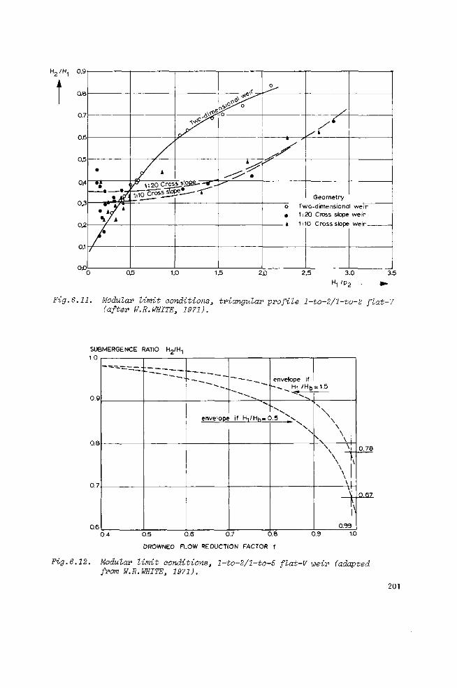
0.8
Fig.6.11. Modular limit conditions, triangular profile l-to-2/l-to-2 flat-V (after W.R.WHITE, 1971).
1.0
0.9
0.8
0.7
0.6
envelope if - ^ Hi /Hb = 15
envelope if H i /Hh«0.5 ^ v
^ \ \ 't N \ \ \ \ I \ i V
X 0.99
0.78
0£7_
0.4 0.5 0.6 0.7 0.8
DROWNED FLOW REDUCTION FACTOR f
0.9 1.0
Fig.6.12. Modular limit conditions, l-to-2/l-to-5 flat-V weir (adapted from W.R.WHITE, 1971).
201
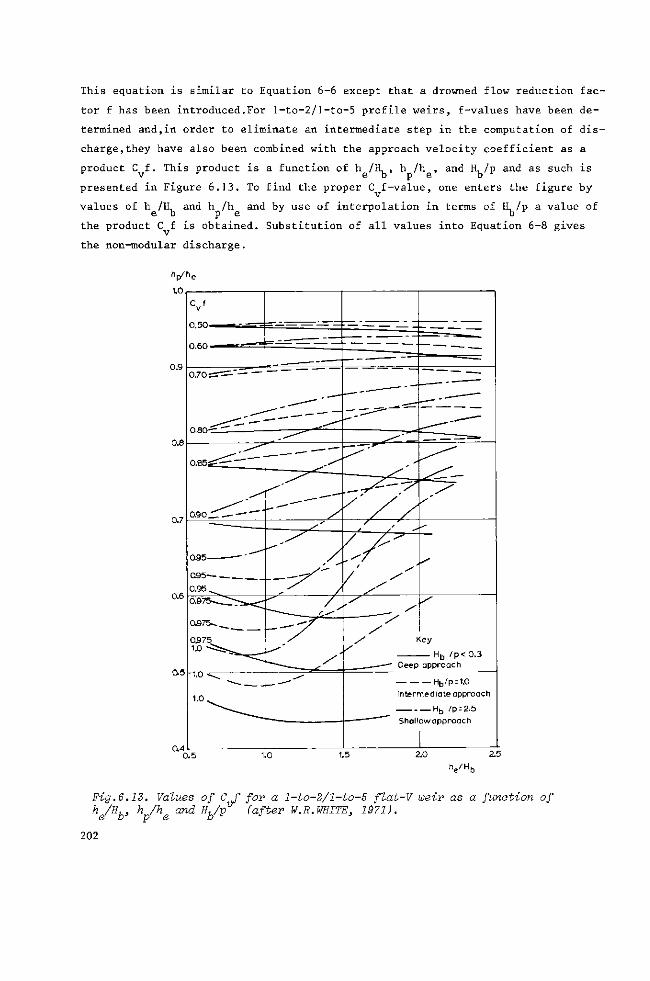
This equation is similar to Equation 6-6 except that a drowned flow reduction fac
tor f has been introduced.For l-to-2/I-to-5 profile weirs, f-values have been de
termined and,in order to eliminate an intermediate step in the computation of dis
charge, they have also been combined with the approach velocity coefficient as a
product C f. This product is a function of h /H, , h /h , and H, /p and as such is
presented in Figure 6.13. To find the proper C f-value, one enters the figure by
values of h /H, and h /h and by use of interpolation in terms of H, /p a value of
the product C f is obtained. Substitution of all values into Equation 6-8 gives
the non-modular discharge.
Fig.6.13. Values of C f for a l-to-2/l-to-5 flat-V weir as a function of h /H-,, h /h and Ujv (after W.R.WHITE, 1971). e b' y e Ve J '
202
6.4.4 Limits of application
For reasonable accuracy, the limits of application of a triangular profile flat-V
weir are:
a) For a well-maintained weir with a non-corrodible metal insert at its
crest, the recommended lower limit of h = 0.03 m. For a crest made of pre-cast
concrete sections or similar materials, h should not be less than 0.06 m.
b) To prevent water surface instability in the approach channel in the form
of stationary waves, the ratio h /p should not exceed 3.0.
c) The height of the vertex of the weir crest should not be less than 0.06 m
above the approach channel bottom.
d) To reduce the influence of boundary layer effects at the sides of the
weir, the width of the weir B should not be less than 0.30 m and the ratio B/H.
should not be less than 2.0.
e) To obtain a sensibly constant discharge coefficient for l-to-2/l-to-2
profile weirs, the ratio H /p„ should not exceed 1.25. For l-to-2/1-to-5 profile
weirs, this ratio should be less than 3.0.
f) The upstream head over the weir crest should be measured a distance of
10 H, upstream from the weir crest in a rectangular approach channel.
g) To obtain modular weir flow, the submergence ratio H„/H should not
exceed 0.30 for l-to-2/l-to-2 profile weirs and should be less than 0.67 for
l-to-2/1-to-5 profile weirs. For the latter weir profile, however, non-modular
flows may be calculated by using Equation 6-8 and Figure 6.13.
6.5 Butcher's movable standing wave weir
6.5.1 Description
Butcher's weir was developed to meet the particular irrigation requirements
in the Sudan, where the water supplied to the fields varies because of diffe
rent requirements during the growing season and because of crop rotation. A
description of the weir was published for the first time in 1922 by A.D.BUTCHER,
after whom the structure has been named.1
1 Nowadays the structure is manufactured eommeroially by Newton Chambers Engineering Ltd., Thornoliff, Sheffield, England.
203
The weir consists of a round-crested movable gate with guiding grooves and a
self-sustaining hand gear for raising and lowering it. The cylindrical crest is
horizontal perpendicular to the flow direction. The profile in the direction of
flow shows a vertical upstream face connected to a l-to-5 downward sloping face
by a 0.25 h max radius circle, where h max is the upper limit of the range of
heads to be expected at the gauge located at a distance 0.75 h max upstream from
the weir face.
The side walls are vertical and are rounded at the upstream end in such a way
that flow separation does not occur. Thus a rectangular approach channel is
formed to assure two-dimensional weir flow. The upstream water depth over the
weir crest tu is measured in this approach channel by a movable gauge mounted
on two supports. The lower support is connected to the movable gate and the upper
support is bolted to the hoisting beam. The gauge must be adjusted so that its
zero corresponds exactly with the weir crest. Because of their liability to dama
ge the supports have been kept rather short; a disadvantage of this shortness is
that the water surface elevation is measured in the area of surface drawdown
so that the hydraulic dimensions of both the approach channel and weir cannot
be altered without introducing an unknown change in the product of C C . The
centre line of the gauge should be 0.75 h max upstream from the weir face.
The weir can be raised high enough to cut off the flow at full supply level
in the feeder canal and, when raised, leakage is negligible. In practice it has
been found advantageous to replace the lower fixed weir, behind which the weir
moves, with a concrete or masonry sill whose top width is about 0.10 m and whose
upstream face is not flatter than 2-to-l.
The maximum water depth over the weir crest, and thus the maximum permissible dis
charge per metre weir crest,influences the weir dimensions. Used in the Sudan are
two standard types with maximum values of h = 0.50 m and h = 0.80 m respectively.
It is recommended that 1.00 m be the upper limit for h . The breadth of the weir
varies from 0.30 m to as much as 4.00 m, the larger breadths used in conjunction
with high htmax-values. As shown in Figure 6.14, p = 1.4 h max, which results in
low approach velocities.
The modular limit is defined as the submergence ratio h„/h which produces a
1% reduction from the equivalent modular discharge. Results of various tests
showed that the modular limit is h„/h = 0.70. The average rate of reduction
from the equivalent modular discharge is shown in percentages in Figure 6.15.
204
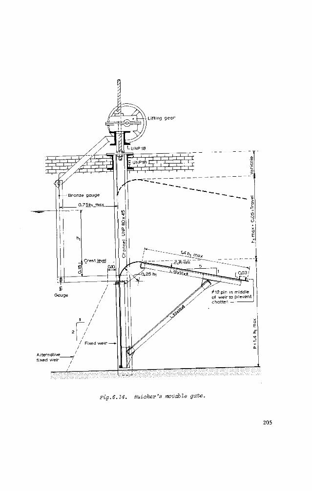
Fig. 6.14. Butcher's movable gate.
205
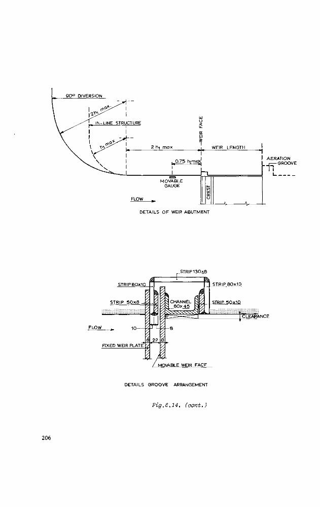
9 0 ° DIVERSION
AERATION I _| GROOVE
DETAILS OF WEIR ABUTMENT
STRIP 1 3 0 x 6
FLOW ^
CLEARANCE
Jfl- A4-/ MOVABLE WEIR FACE
DETAILS GROOVE ARRANGEMENT
Fig.6.14. (aont.)
206
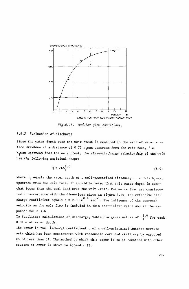
Q85
0.80
0.75
070
/•
' 1 1
•yS
1 1 1 ! 1 1 0 1 2 3 4 5 6 7 8 9 10 11 12
PERCENT ••
"/.REDUCTION FROM EQUIVALENT MODULAR FLOW
Fig.6.15. Modular flow conditions.
6.5.2 Evaluation of discharge
Since the water depth over the weir crest is measured in the area of water sur
face drawdown at a distance of 0.75 h max upstream from the weir face, i.e.
hjmax upstream from the weir crest, the stage-discharge relationship of the weir
has the following empirical shape:
cbh 1.6
(6-9)
where hj equals the water depth at a well-prescribed distance, 1 = 0.75 h max,
upstream from the weir face. It should be noted that this water depth is some
what lower than the real head over the weir crest. For weirs that are construc
ted in accordance with the dimensions shown in Figure 6.14, the effective dis
charge coefficient equals c = 2.30 m sec . The influence of the approach
velocity on the weir flow is included in this coefficient value and in the ex
ponent value 1.6.
To facilitate calculations of discharge, Table 6.4 gives values of h] for each
0.01 m of water depth.
The error in the discharge coefficient c of a well-maintained Butcher movable
weir which has been constructed with reasonable care and skill may be expected
to be less than 3%. The method by which this error is to be combined with other
sources of error is shown in Appendix II.
207
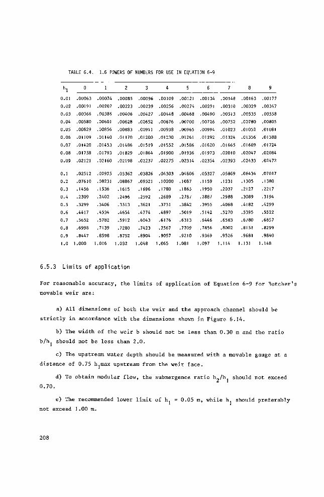
TABLE 6.4. 1.6 POWERS OF NUMBERS FOR USE IN EQUATION 6-9
h l
0.01
0.02
0.03
0.04
0.05
0.06
0.07
0.08
0.09
0.1
0.2
0.3
0.4
0.5
0.6
0.7
0.8
0.9
1.0
0
.00063
.00191
.00366
.00580
.00829
.01109
.01420
.01758
.02121
.02512
.07610
.1456
.2309
.3299
.4417
.5652
.6998
.8447
1.000
1
.00074
.00207
.00386
.00601
.00856
.01140
.01453
.01793
.02160
.02925
.08231
.1536
.2402
.3406
.4534
.5782
.7139
.8598
1.016
2
.00085
.00223
.00406
.00628
.00883
.01170
.01486
.01829
.02198
.03362
.08867
.1615
.2496
.3513
.4654
.5912
.7280
.8752
1.032
3
.00096
.00239
.00427
.00652
.00911
.01200
.01519
.01864
.02237
.03826
.09521
.1696
.2592
.3621
.4774
.6043
.7423
.8904
1.048
4
.00109
.00256
.00448
.00676
.00938
.01230
.01552
.01900
.02275
.04303
.10200
.1780
.2689
.3731
.4897
.6176
.7567
.9057
1.065
5
.00121
.00274
.00468
.00700
.00965
.01261
.01586
.01936
.02314
.04806
.1087
.1865
.2787
.3842
.5019
.6313
.7709
.9210
1.081
6
.00134
.00291
.00490
.00726
.00994
.01292
.01620
.01973
.02354
.05327
.1159
.1950
.2887
.3955
.5142
.6446
.7856
.9369
1.097
7
.00148
.00310
.00513
.00752
.01023
.01324
.01665
.02010
.02393
.05869
.1231
.2037
.2988
.4068
.5270
.6583
.8002
.9526
1 .114
8
.00163
.00329
.00535
.00780
.01052
.01356
.01689
.02047
.02433
.06434
.1305
.2127
.3089
.4182
.5395
.6780
.8151
.9681
1.131
9
.00177
.00347
.00558
.00805
.01081
.01388
.01724
.02084
.02472
.07017
.1380
.2217
.3194
.4299
.5522
.6857
.8299
.9840
1.148
6.5.3 Limits of application
For reasonable accuracy, the limits of application of Equation 6-9 for Butcher's
movable weir are:
a) All dimensions of both the weir and the approach channel should be
strictly in accordance with the dimensions shown in Figure 6.1 A.
b) The width of the weir b should not be less than 0.30 m and the ratio
b/h should not be less than 2.0.
c) The upstream water depth should be measured with a movable gauge at a
distance of 0.75 h.max upstream from the weir face.
d) To obtain modular flow, the submergence ratio h„/h should not exceed
0.70.
e) The recommended lower limit of h. = 0.05 m, while h. should preferably
not exceed 1.00 m.
208
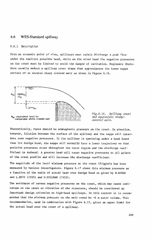
6.6 WES-Standard spillway
6.6.1 Description
From an economic point of view, spillways must safely discharge a peak flow
under the smallest possible head, while on the other hand the negative pressures
on the crest must be limited to avoid the danger of cavitation. Engineers there
fore usually select a spillway crest shape that approximates the lower nappe
surface of an aerated sharp crested weir as shown in Figure 6.16.
hsc ^equivalent head for comparable sharp-crested weir
Fig.6.16. Spillway erest and equivalent sharp-arested weir.
Theoretically, there should be atmospheric pressure on the crest. In practice,
however, friction between the surface of the spillway and the nappe will intro
duce some negative pressures. If the spillway is operating under a head lower
than its design head, the nappe will normally have a lower trajectory so that
positive pressures occur throughout the crest region and the discharge coef
ficient is reduced. A greater head will cause negative pressures at all points
of the crest profile and will increase the discharge coefficient.
The magnitude of the local minimum pressure at the crest (P/pg)min has been
measured by various investigators. Figure 6.17 shows this minimum pressure as
a function of the ratio of actual head over design head as given by H.ROUSE
and L.REID (1935) and O.DILLMAN (1933).
The avoidance of severe negative pressures on the crest, which may cause cavi
tation on the crest or vibration of the structure, should be considered an
important design criterion on high-head spillways. In this context it is recom
mended that the minimum pressure on the weir crest be -4 m water column. This
recommendation, used in combination with Figure 6.17, gives an upper limit for
the actual head over the crest of a spillway.
209
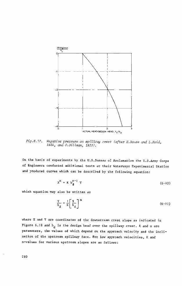
(P/Pglmin
\ \
I \ i \j
Fig.6.17. Negative pressure on spillway crest (after H.Rouse and L.Reid, 1935, and O.Dillman, 1933).
On the basis of experiments by the U.S.Bureau of Reclamation the U.S.Army Corps
of Engineers conducted additional tests at their Waterways Experimental Station
and produced curves which can be described by the following equation:
X n = K h""1 Y d
which equation may also be written as
Y_ = l[~X_ hd ~ K L V
(6-10)
(6-11)
where X and Y are coordinates of the downstream crest slope as indicated in
Figure 6.18 and hd is the design head over the spillway crest. K and n are
parameters, the values of which depend on the approach velocity and the incli
nation of the upstream spillway face. For low approach velocities, K and
n-values for various upstream slopes are as follows:
210
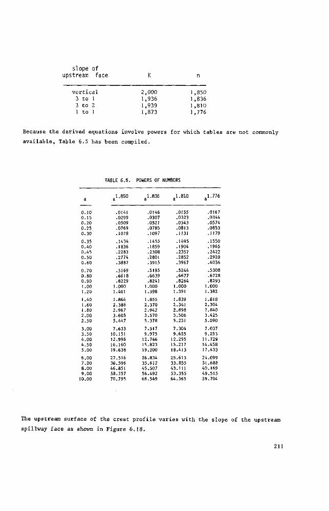
slope of upstream face
vertical
3 to 1
3 to 2
1 to 1
2 ,000 1,936 1,939 1,873
1,850 1 ,836 1,810 1,776
Because the derived equations involve powers for which tables are not commonly
available, Table 6.5 has been compiled.
TABLE 6.5. POWERS OF NUMBERS
0.10 0.15 0.20 0.25 0.30
0.35 0.40 0.45 0.50 0.60
0.70 0.80 0.90 1,00 1.20
1.40 1.60 1.80 2.00 2.50
3.00 3.50 4.00 4.50 5.00
6.00 7.00 8.00 9.00
10.00
1.850 1.836 1.810 .1.776
.0141
.0299
.0509
.0769
.1078
.1434
.1836
.2283
.2774
.3887
.5169
.6618
.8229 1.000 1.401
1.864 2.386 2.967 3.605 5.447
7.633 10.151 12.996 16.160 19.638
27.516 36.596 46.851 58.257 70.795
.0146
.0307
.0521
.0785
.1097
.1455
.1859
.2308
.2801
.3915
.5195
.6639
.8241 1.000 1.398
1.855 2.370 2.942 3.570 5.378
7.517 9.975
12.746 15.823 19.200
26.834 35.612 45.507 56.492 68.549
.0155
.0323
.0543
.0813
.1131
.1495
.1904
.2357
.2852
.3967
.5244
.6677
.8264 1.000 1.391
1.839 2.341 2.898 3.506 5.251
7.304 9.655
12.295 15.217 18.413
25.613 33.855 43.111 53.355 64.565
.0167
.0344
.0574
.0853
.1179
.1550
.1965
.2422
.2920
.4036
.5308
.6728
.8293 1.000 1.382
1.818 2.304 2.840 3.425 5.090
7.037 9.253
11.729 14.458 17.433
24.099 31.688 40.169 49.515 59.704
The upstream surface of the crest profile varies with the slope of the upstream
spillway face as shown in Figure 6.18.
211
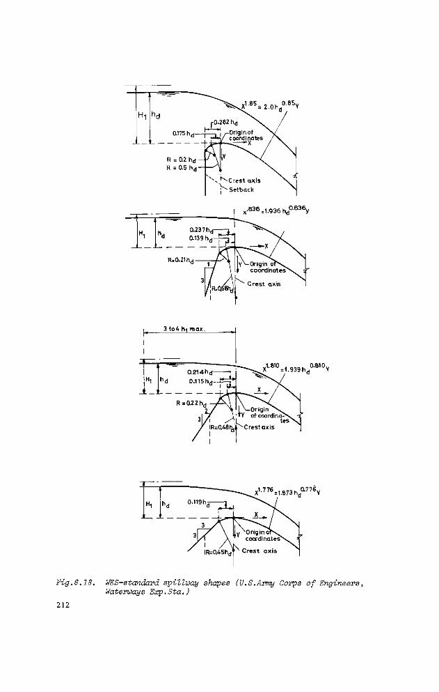
^ ^ X 1 6 5 = 2 . 0 h ° B 5 Y
3 to& hi max
X1-810 = 1.939hd°-810Y
X1-776=1.873hda776Y
ly OriginOT" coordinates^
I / \K IR=0.45hd' Crest axis
Fig.6.18. WES-standard spillway shapes (U.S.Army Corps of Engineers, Waterways Exp. Sta. )
212
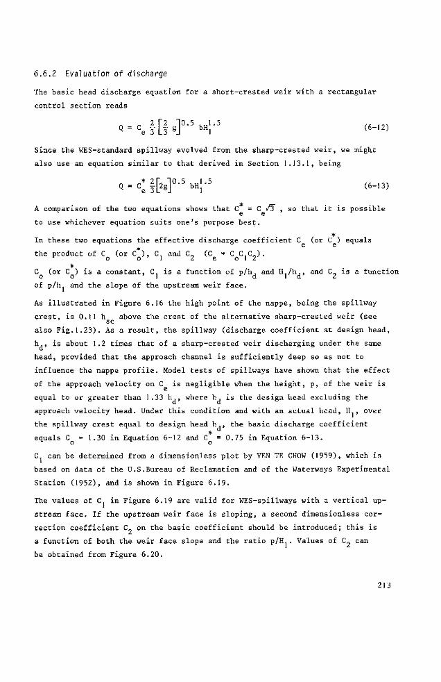
6.6.2 Evaluation of discharge
The basic head discharge equation for a short-crested weir with a rectangular
control section reads
« . -« .Kl«] 0 - 5 »! - 5
Since the WES-standard spillway evolved from the sharp-crested weir, we might
also use an equation similar to that derived in Section 1.13.1, being
Q = < f [ 2 g ] ° - 5 b H ; - 5 (6-13)
A comparison of the two equations shows that C = C /3~ , so that it is possible -,* Je
to use whichever equation suits one's purpose best.
* In these two equations the effective discharge coefficient C (or C ) equals
the product of C (or C ) , C. and C„ (C = C C.C.). o o l z e o 1 z
* C (or C ) is a constant, C] is a function of p/h, and Hj/h,, and C„ is a function
of p/hj and the slope of the upstream weir face.
As illustrated in Figure 6.16 the high point of the nappe, being the spillway
crest, is 0.11 h above the crest of the alternative sharp-crested weir (see sc
also Fig.1.23). As a result, the spillway (discharge coefficient at design head,
h,, is about 1.2 times that of a sharp-crested weir discharging under the same
head, provided that the approach channel is sufficiently deep so as not to
influence the nappe profile. Model tests of spillways have shown that the effect
of the approach velocity on C is negligible when the height, p, of the weir is
equal to or greater than 1.33 h,, where h, is the design head excluding the
approach velocity head. Under this condition and with an actual head, H , over
the spillway crest equal to design head h,, the basic discharge coefficient
equals C = 1.30 in Equation 6-12 and C = 0.75 in Equation 6-13.
Ct can be determined from a dimensionless plot by VEN TE CHOW (1959), which is
based on data of the U.S.Bureau of Reclamation and of the Waterways Experimental
Station (1952), and is shown in Figure 6.19.
The values of Cj in Figure 6.19 are valid for WES-spillways with a vertical up
stream face. If the upstream weir face is sloping, a second dimensionless cor
rection coefficient C„ on the basic coefficient should be introduced; this is
a function of both the weir face slope and the ratio p/fL . Values of C- can
be obtained from Figure 6.20.
213
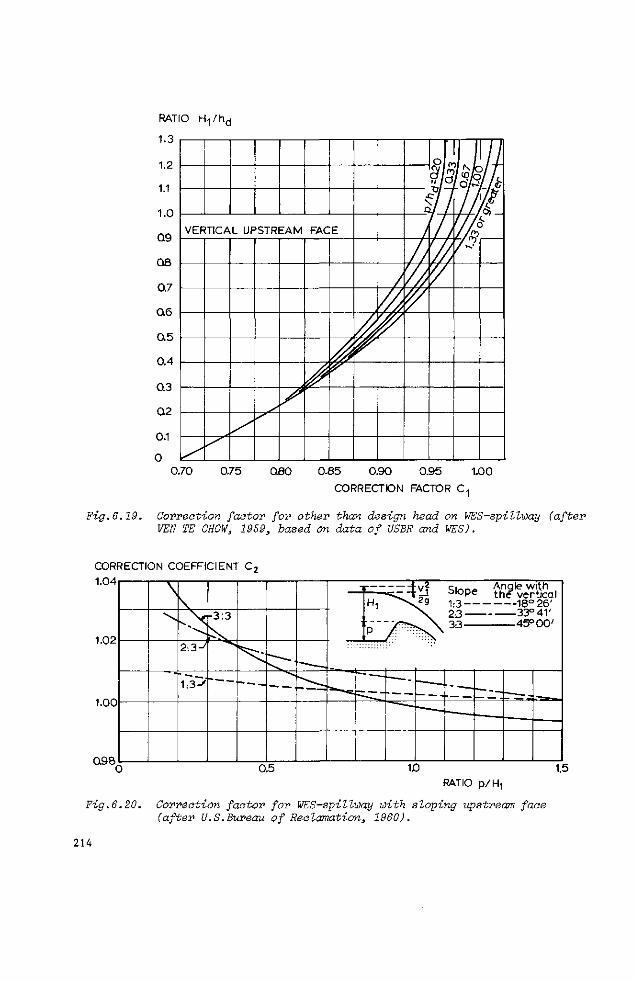
RATIO t ^ / h g
1.3
1.2
1.1
1.0
Q9
08
0.7
0.6
0.5
0.4
0.3
Q2
0.1
0 0.70
VERTICAL UPSTREAM FACE
oL
•d^Ldw /b • c / / ^/ / Q.1 / i
Ol U7è / ***'
0.75 O80 0.85 0.90 0.95 1.00
CORRECTION FACTOR C,
Fig.6.19. Correction factor for other than design head on WES-spillway (after VEN TE CHOW, 1959, based on data of USBR and WES).
CORRECTION COEFFICIENT C2
1.04
1.02
1.00
0.98
2 : 3 ^
1.3^
-3:3
< 5 : ^
f — Hi
— T V? ^ " \ 2 g
P / : • ••:
Slope t h | vertical 1:3 18° 26' 23 33° 41 ' 33 45° 0 0 '
,
0.5 10 1.5 RATIO p /H,
Fig.6.20. Correction factor for WES-spillway with sloping upstream face (after V.S.Bureau of Reclamation, 1960).
214
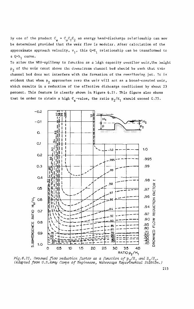
By use of the product C = C C C„ an energy head-discharge relationship can now
be determined provided that the weir flow is modular. After calculation of the
approximate approach velocity, v , this Q_H relationship can be transformed to
a Q-h curve.
To allow the WES-spillway to function as a high capacity overflow weir,the height
p7 of the weir crest above the downstream channel bed should be such that this
channel bed does not interfere with the formation of the overflowing jet. It is
evident that when p« approaches zero the weir will act as a broad-crested weir,
which results in a reduction of the effective dishcarge coefficient by about 23
percent. This feature is clearly shown in Figure 6.21. This figure also shows
that in order to obtain a high C -value, the ratio P7/H. should exceed 0.75.
-0.2
-0.1
0.
0.1
0.2
0.3
0.4
05
x 0.6
I
O
CE
UJ (J z UJ o cc UJ
m I/)
0.7
0.8
0.9
1.0
M o , g;
iii -l'
! "
»J i ' u
'III' >i !
W
i l
i ^ ~
v70r*
V
/
y
- 1.0
,..995
.99
.98
,•97
=.96
,_,.94 -
92
_ 4-.90
85 J 80
"" •=—..70r
1.0
.995
.99
.98 ^ cc O
O .97
.96 O
.94 y Q UJ CC .92
.90
.85
.80
.70
.60
5 O
0 0.5 1D 1.5 2.0 25
û ui
2
Q 3.0 3.5 40
RATIO Pj/H,
Fig.6,21. Drowned flow reduction factor as a function of pjE1 and EjE . (Adapted from U.S.Army Corps of Engineers, Waterways Experimental Station.)
215
Figure 6.21 also shows that, provided P9/H. 0.75, the modular discharge as
calculated by Equation 6-12 is decreased to about 99% of its theoretical value
if the submergence ratio H-/H equals 0.3. Values of the drowned flow reduction
factor f, by which the theoretical discharge is reduced under the influence of
both P9/H. and H„/H , can be read from Figure 6.21.
The accuracy of the discharge coefficient C = CnC1C„ of a WES-spillway which
has been constructed with care and skill and is regularly maintained will be
sufficient for field conditions. The error of C may be expected to be less than
5%. The method by which this error is to be combined with other sources of error
is shown in Appendix II.
6.6.3 Limits of application
For reasonable accuracy, the limits of application of a weir with a WES-spillway
crest are:
a) The upstream head over the weir crest h. should be measured a distance
of 2 to 3 times lumax upstream from the weir face. The recommended lower limit
of h is 0.06 m.
b) To prevent water surface instability in the approach channel, the ratio
p/h1 should not be less than 0.20.
c) To reduce the influence of boundary layer effects at the side walls of
the weir, the ratio b/Hj should not be less than 2.0.
d) To obtain a high C -value, the ratio p9/H should not be less than about
0.75.
e) The modular limit H./H = 0.3, provided that the tailwater channel bot
tom does not interfere with the flow pattern over the weir (p„/H ~i- 0.75).
f) The minimum allowable pressure at the weir crest equals - 4.00 m water
column (P/pg ^ - 4.0 m ) .
6.7 Cylindrical crested weir
6.7.1 Description
A cylindrical crested weir is an overflow structure with a rather high discharge
216
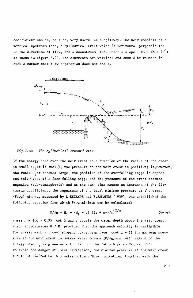
coefficient and is, as such, very useful as a spillway. The weir consists of a
vertical upstream face, a cylindrical crest which is horizontal perpendicular
to the direction of flow, and a downstream face under a slope 1-to-l (a = 45 )
as shown in Figure 6.22. The abutments are vertical and should be rounded in
such a manner that flow separation does not occur.
2 to 3 Ht max
Fig.6.22. The cylindrical crested weir.
If the energy head over the weir crest as a function of the radius of the crest
is small (ïL/r is small), the pressure on the weir crest is positive; if,however,
the ratio H /r becomes large, the position of the overfalling nappe is depres
sed below that of a free falling nappe and the pressure of the crest becomes
negative (sub-atmospheric) and at the same time causes an increase of the dis
charge coefficient, the magnitude of the local minimum pressure at the crest
(P/pg) min was measured by L.ESCANDE and F.SANANES (1959), who established the
following equation from which P/pg minimum can be calculated:
P/pg = Hj - (Hj - y) {(r + ny)/r} 2/n
(6-14)
where n = 1.6 + 0.35 cot a and y equals the water depth above the weir crest,
which approximates 0.7 Hj provided that the approach velocity is negligible.
For a weir with a 1-to-l sloping downstream face (cot a = 1) the minimum pres
sure at the weir crest in metres water column (P/pg)min with regard to the
energy head H. is given as a function of the ratio lu/r in Figure 6.23.
To avoid the danger of local cavitation, the minimum pressure at the weir crest
should be limited to -4 m water column. This limitation, together with the
217
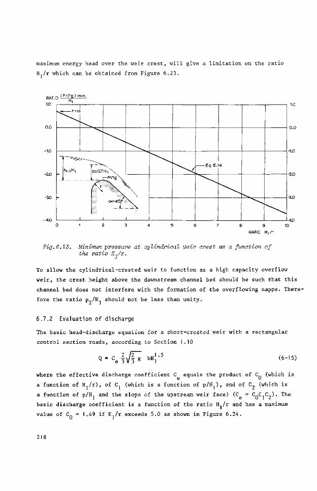
maximum energy head over the weir crest, will give a limitation on the ratio
KL/r which can be obtained from Figure 6.23.
RATIO ( P / p 9 ) m m ' 1.0 H'
0.0
-30 |-
Fig.6.23. Minimum pressure at cylindrical weir crest as a function of the ratio U1/r.
To allow the cylindrical-crested weir to function as a high capacity overflow
weir, the crest height above the downstream channel bed should be such that this
channel bed does not interfere with the formation of the overflowing nappe. There
fore the ratio p9/H, should not be less than unity.
6.7.2 Evaluation of discharge
The basic head-discharge equation for a short-crested weir with a rectangular
control section reads, according to Section 1.10
Q = c e | y | 7 bH;-5 (6-15)
where the effective discharge coefficient C equals the product of Cn (which is
a function of H./r), of C. (which is a function of p/H.), and of C„ (which is
a function of p/ïL and the slope of the upstream weir face) (C = C.CLC.). The
basic discharge coefficient is a function of the ratio H /r and has a maximum
value of C. = 1.49 if IL/r exceeds 5.0 as shown in Figure 6.24.
218
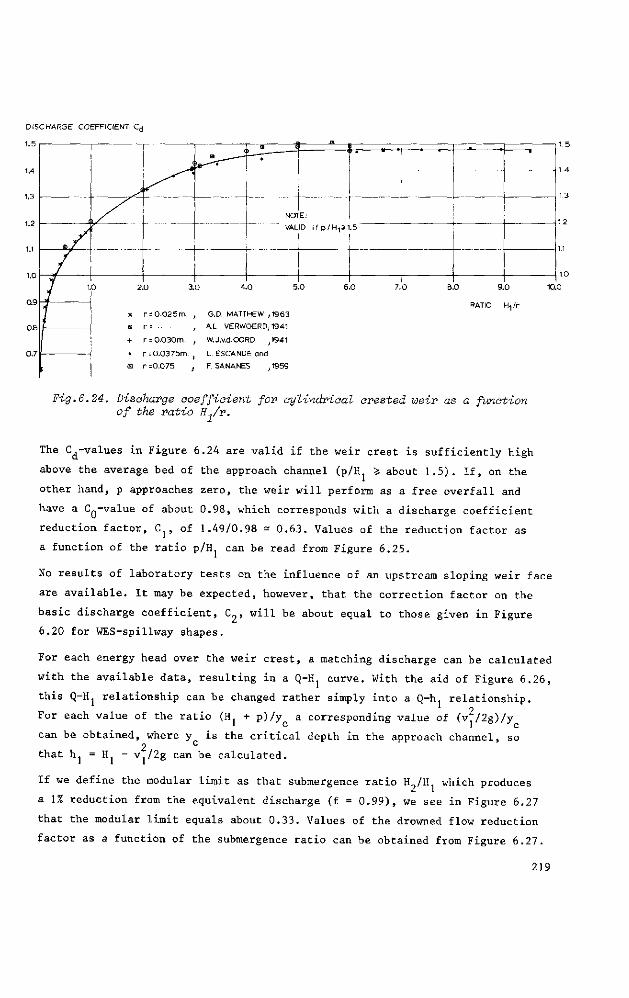
DISCHARGE COEFFICIENT Cd
1.5
r = O.030m.
r= 0.03 75m.
r =0.075
G.D. MATTHEW ,1963
AL. VERWOERD, 1941
W.J.v.d.OORD ,1941
L.ESCANDE and
F. SA NA NES ,1959
8.0 9.0 10.0
RATIO H, /r
Fig.6.24. Discharge coefficient for cylindrical crested weir as a function of the ratio H1/r.
The C,-values in Figure 6.24 are valid if the weir crest is sufficiently high
above the average bed of the approach channel (p/H 5- about 1.5). If, on the
other hand, p approaches zero, the weir will perform as a free overfall and
have a C^-value of about 0.98, which corresponds with a discharge coefficient
reduction factor, C , of 1.49/0.98 - 0.63. Values of the reduction factor as
a function of the ratio p/H can be read from Figure 6.25.
No results of laboratory tests on the influence of an upstream sloping weir face
are available. It may be expected, however, that the correction factor on the
basic discharge coefficient, C , will be about equal to those given in Figure
6.20 for WES-spillway shapes.
For each energy head over the weir crest, a matching discharge can be calculated
with the available data, resulting in a Q-H curve. With the aid of Figure 6.26,
this Q-Hj relationship can be changed rather simply into a Q-h. relationship.
For each value of the ratio (Hj + p)/y a corresponding value of (v /2g)/y
can be obtained, where y is the critical depth in the approach channel, so 2 c
that h. = H. - Vj/2g can be calculated.
If we define the modular limit as that submergence ratio H /H which produces
a 1% reduction from the equivalent discharge (f = 0.99), we see in Figure 6.27
that the modular limit equals about 0.33. Values of the drowned flow reduction
factor as a function of the submergence ratio can be obtained from Figure 6.27.
219
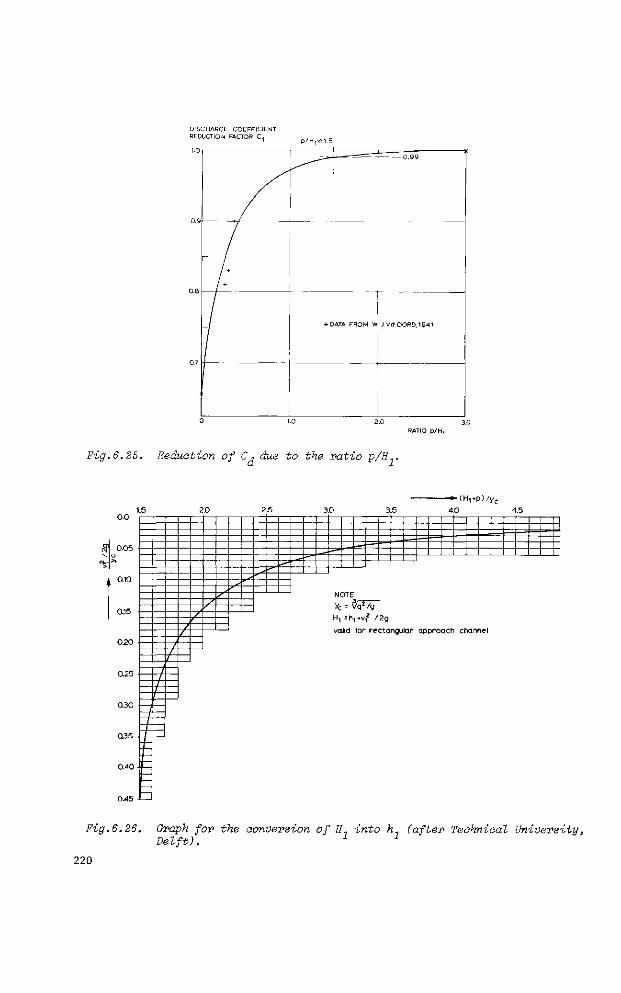
DISCHARGE COEFFICIENT REDUCTION FACTOR C.
1 ^ i —
- / \
1 +
-/
~
+ DATA FROM W
0.99
J.vcJ OORD.1941
Fig. 6. 25. Reduction of C-, due to the ratio p/H1.
- " • ( H , . p ) / y c
4.0 4.5
NOTE-
H, =h,.v,2 / 2g
valid for rectangular approach channel
Fig.6.26. Graph for the conversion of ff7 into hn (after Technical University, delft). Â 1
220
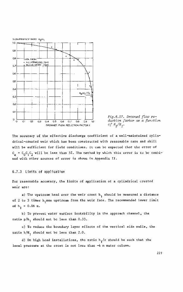
SUBMERGENCE RATIO Hg/H.
1.0
0.4
0.3
H
DATA F
h A.L.V W.J.v
- ^
ROM
ERWOERD,1941 d. OORD ,1941
, ^ , \
Ha/H,
A --'/3 f
Q2 0.3 0 . 4 0 .5 0.6 0 . 7 0.8 0.9 1.0
DROWNED FLOW REDUCTION FACTOR f
Fig.6.27. Drowned flow reduction factor as a function of H2/Er
The accuracy of the effective discharge coefficient of a well-maintained cylin
drical-crested weir which has been constructed with reasonable care and skill
will be sufficient for field conditions. It can be expected that the error of
C = C„C,C„ will be less than 5%. The method by which this error is to be combi-e 0 1 2
ned with other sources of error is shown in Appendix II.
6.7.3 Limits of application
For reasonable accuracy, the limits of application of a cylindrical crested
weir are:
a) The upstream head over the weir crest h. should be measured a distance
of 2 to 3 times h,max upstream from the weir face. The recommended lower limit
of h = 0.06 m.
b) To prevent water surface instability in the approach channel, the
ratio p/h. should not be less than 0.33.
c) To reduce the boundary layer effects of the vertical side walls, the
ratio b/H. should not be less than 2.0.
d) On high head installations, the ratio h./r should be such that the
local pressure at the crest is not less than -4 m water column.
221
e) To prevent the tailwater channel bottom from influencing the flow
pattern over the weir, the ratio P9/Hj should not be less than unity.
f) The modular limit H /H = 0.33.
222
6.8 Selected list of references
1. BAZIN, H.E.: Expériences nouvelles sur l'écoulement en déversoir.
Annales des Ponts et Chaussées. Vol.7, 1896, pp.249-357.
2. BRITISH STANDARDS INSTITUTION: Methods of measurement of Liquid flow
in open channels. British Standard 3680, Part 4B, Long base weirs. 1969. 39 pp.
3. BUTCHER, A.D.: Submerged weirs and standing wave weirs. Min.of Public
Works, Cairo 1923. 17 pp.
4. BUTCHER, A.D.: Clear overfall weirs. Res.Work Delta Barrage. Min.of
Public Works, Cairo 1921/22.
5. CHOW, VEN TE: Open-Channel Hydraulics. McGraw-Hill Book Company Inc.,
New York, 1959. 680 pp.
6. CRUMP, E.S.: A new method of gauging stream flow with little afflux
by means of a submerged weir of triangular profile. Proc.Inst.Civil Engrs.,
Part 1, Vol.1 (March), 1952. pp.223-242.
7. DILLMAN, 0.: Untersuchungen an Überfällen. Mitt.des Hydr.Inst.der
Tech.Hochschule München. 1933. No.7. pp.26-52.
8. ESCANDE, L. and SANANES, F.: Etude des seuils déversants à fente
aspiratrice. La Houklle Blanche, 14 (1959), No.B, Dec. Grenoble, pp.892-902.
9. LELIAVSKY, S.: Irrigation Engineering: Syphons, Weirs and Locks.
Vol.11. Chapman & Hall Ltd., London 1965. 296 pp.
10. MATTHEW, G.D.: On the influence of curvature, surface tension and
viscosity on flow over round-crested weirs. Proc.Inst.Civil Engrs., Vol.25
(Aug.), 1962. pp.511-524.
11. OORD, W.J., van der: Stuw met cirkelvormige kruin. MSc Thesis. Techn.
University Delft 1941.
12. ROUSE, H. and REID, L.: Model research on spillway crests. Civil Eng.
Vol.5, 1935. January, p.10.
13. U.S.ARMY CORPS OF ENGINEERS: Corps of Engineers Hydraulic Design Cri
teria. Prepared for Office of the Chief of Engineers. Waterways Experimental
Station Vicksburg, Miss. 1952. Revised in subsequent years.
14. U.S.BUREAU OF RECLAMATION: Design of small dams. USBR Denver 1960.
611 pp.
223
15. U.S.BUREAU OF RECLAMATION: Studies of crests for overfall dams. Boulder
Canyon Project Final Reports. Part VI. USBR Denver, Hydraulic Investigations,
Bull.3, 1948.
16. U.S.DEPARTMENT OF AGRICULTURE: Field manual for research in agricultural
hydrology. Agric.Handbook No.224, Washington 1962. 215 pp.
17. VERWOERD, A.L.: Capaciteitsbepaling van volkomen en onvolkomen overlaten
met afgeronde kruinen. Waterstaatsingenieur in Nederlandsch-Indië, 1941, Juli,
No.7. pp.65-78 (II).
18. VLUGTER, H.: De volkomen overlaat. (Modular weirs.) De Waterstaats
Ingenieur, No.4, Bandung 1932.
19. WALLINGFORD HYDRAULIC RESEARCH STATION: The triangular profile Crump
weir. Effects of a bend in the approach channel. Report EX 518, 1970. W.HRS,
England.
20. WATER RESOURCES BOARD: Crump Weir Design. Reading Bridge House, England,
1970 TN 8 (rev.), 92 pp.
21. WHITE, W.R. and BURGESS, J.S.: Triangular profile weir with 1:2 up
stream and downstream slopes. Hydr.Res.Sta.Wallingford, England, Oct. 1967.
Rep.No.INT 64, pp.41-47.
22. WHITE, W.R.: The flat vee weir. Water & Water Eng., Jan. 1968, V 72
No.863, pp.13-19.
23. WHITE, W.R.: The performance of two-dimensional and flat-V triangular
profile weirs. Proc.Inst.Civil Engrs. 1971. Suppl. (ii), Paper 7350 S. 48 pp.
224
7 Flumes A critical depth-flume is essentially a geometrically specified constriction built
in an open channel where sufficient fall is available for critical flow to occur
in the throat of the flume. Flumes are "in-line" structures, i.e. their centre
line coincides with the centre line of the undivided channel in which the flow
is to be measured. The flume cannot be used in structures like turnouts,
controls and other regulating devices.
In this chapter the following types of critical-depth flumes will be described:
Long-throated flumes (7.1), Throatless flumes with rounded transition (7.2),
Throatless flumes with broken plane transition (7.3), Parshall flumes (7.4),
H-flumes (7.5). The name "Venturi flume" is not used in this chapter, since
this term is reserved for flumes in which flow in the constriction is sub-criti
cal. The discharge through such a constriction can be calculated by use of the
equations presented in Section 1.7.
7.1 Long-throated flumes
7.1.1 Description
Classified under the term "long-throated flumes" are those structures which have
a throat section in which the streamlines run parallel to each other at least
over a short distance. Because of this, hydrostatic pressure distribution can
be assumed at the control section. This assumption allowed the various head-
discharge equations to be derived, but the reader should note that discharge
coefficients are also presented for high H./L ratios when the streamlines at
the control are curved.
The flume comprises a throat of which the bottom (invert) is truly horizontal
in the direction of flow. The crest level of the throat should not be lower than
the dead water level in the channel, i.e. the water level downstream at zero flow.
The throat section is prismatic but the shape of the flume cross-section is
rather arbitrary, provided that no horizontal planes, or planes that are nearly
so, occur in the throat above crest (invert) level, since this will cause a dis
continuity in the head-discharge relationship. Treated in this section will be
the most common flumes, i.e. those with a rectangular, V-shaped, trapezoidal,
truncated V, parabolic, or circular throat cross-section.
225
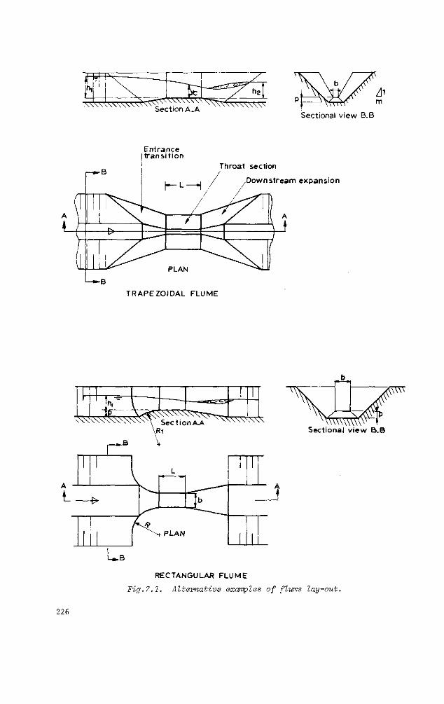
Section A .A Sectional v iew B.B
Entrance I t rans i t ion
Throat section
Downstream expansion
TRAPEZOIDAL FLUME
RECTANGULAR FLUME
Fig.7.1. Alternative examples of flume lay-out.
226
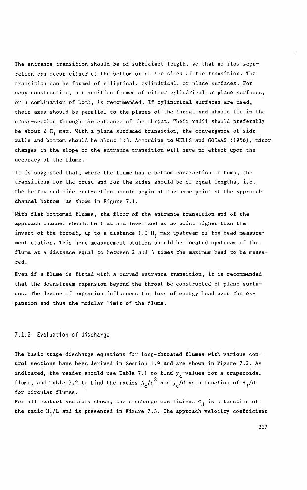
The entrance transition should be of sufficient length, so that no flow sepa
ration can occur either at the bottom or at the sides of the transition. The
transition can be formed of elliptical, cylindrical, or plane surfaces. For
easy construction, a transition formed of either cylindrical or plane surfaces,
or a combination of both, is recommended. If cylindrical surfaces are used,
their axes should be parallel to the planes of the throat and should lie in the
cross-section through the entrance of the throat. Their radii should preferably
be about 2 H max. With a plane surfaced transition, the convergence of side
walls and bottom should be about 1:3. According to WELLS and GOTAAS (1956), minor
changes in the slope of the entrance transition will have no effect upon the
accuracy of the flume.
It is suggested that, where the flume has a bottom contraction or hump, the
transitions for the crest and for the sides should be of equal lengths, i.e.
the bottom and side contraction should begin at the same point at the approach
channel bottom as shown in Figure 7.1.
With flat bottomed flumes, the floor of the entrance transition and of the
approach channel should be flat and level and at no point higher than the
invert of the throat, up to a distance 1.0 H max upstream of the head measure
ment station. This head measurement station should be located upstream of the
flume at a distance equal to between 2 and 3 times the maximum head to be measu
red.
Even if a flume is fitted with a curved entrance transition, it is recommended
that the downstream expansion beyond the throat be constructed of plane surfa
ces. The degree of expansion influences the loss of energy head over the ex
pansion and thus the modular limit of the flume.
7.1.2 Evaluation of discharge
The basic stage-discharge equations for long-throated flumes with various con
trol sections have been derived in Section 1.9 and are shown in Figure 7.2. As
indicated, the reader should use Table 7.1 to find y -values for a trapezoidal 2 C
flume, and Table 7.2 to find the ratios A /d and y /d as a function of H,/d c c 1
for circular flumes.
For all control sections shown, the discharge coefficient C, is a function of
the ratio U./L and is presented in Figure 7.3. The approach velocity coefficient
227
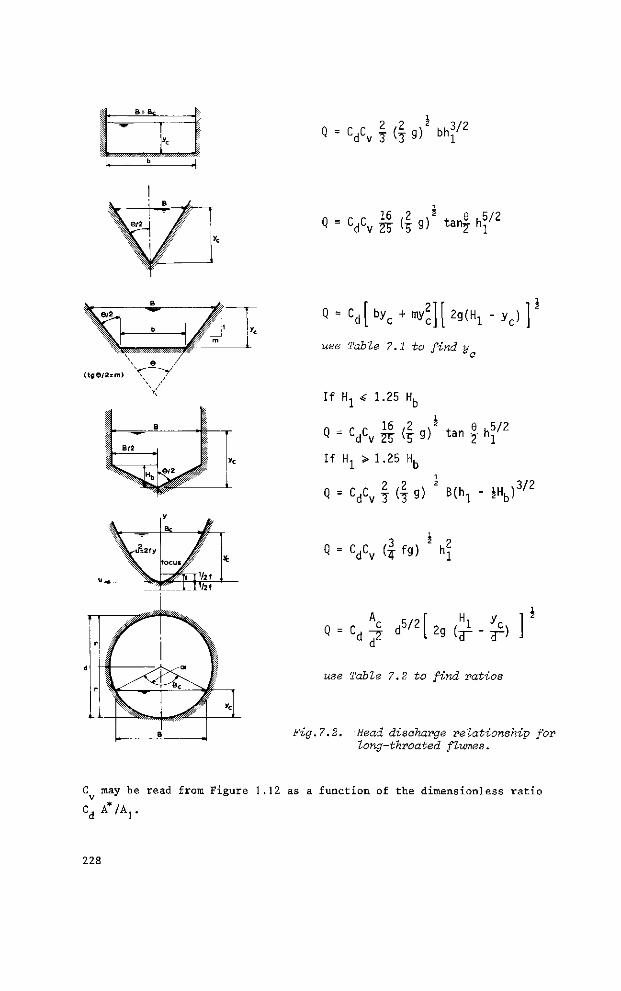
j | . B = B t
1 V ü >|
Q = C d C v § ( | g ) 2 b h 3 / 2
n r r 16 ,2 , 2 . e . 5 / 2 Q = CdCv SF (5" 9) t a n ? h l
%&%%MMf0?0ï00&%A
[byc + my2][2g(H1 - yc) ] Q = C d | b y c + myc
use Table 7.1 to find y
(tae/2=m)
BI 2
90ß
If H1 « 1.25 Hfa
« = CdCv £ (! 9)1 tan f h 5 / 2
If Hx > 1.25 Hb
i
Q = CdCv | (| 9) ß(hl - iV3/2
^s.
£z2,y
^ 5
Bc
ifocusy!
#'
-T'/2f V?(
X: Q = CdCv $ f9) 2 h?
0 - C c d5 / 2
g - cd -j d
Hi y c 29 (<r - r )
use Table 7.2 to find ratios
Fig. 7.2. Head discharge relationship for long-throated f lianes.
C may be read from Figure 1.12 as a function of the dimensionless ratio
<£A*/A,.
228
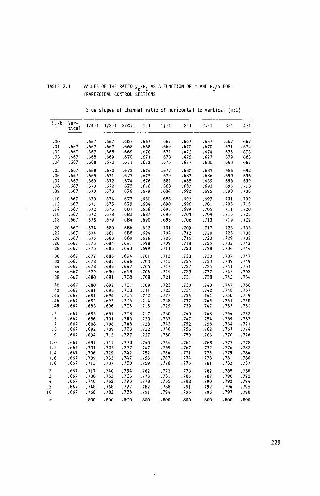
TABLE 7.1. VALUES OF THE RATIO y /Hj AS A FUNCTION OF m AND Hj/b FOR
TRAPEZOIDAL CONTROL SECTIONS
Side slopes of channel ratio of horizontal to vertical (m:l)
H1/b
.00
.01
.02
.03
.04
.05
.06
.07
.08
.09
.10
.12
.14
.16
.18
.20
.22
.24 .26 .28
.30
.32
.34
.36
.38
.40
.42
.44
.46
.48
.5
.6
.7
.8
.9
1.0 1.2 1.4 1.6 1.8
2 3 4 5
10
Vertical
.667
.667
.667
.667
.667
.667
.667
.667
.667
.667
.667
.667
.667
.667
.667
.667
.667
.667
.667
.667
.667
.667
.667
.667
.667
.667
.667
.667
.667
.667
.667
.667
.667
.667
.667
.667
.667
.667
.667
.667
.667
.667
.667
.667
1/4:1
.667
.667
.667
.668
.668
.668
.669
.669
.670
.670
.670
.671
.672
.672
.673
.674
.674
.675
.676
.676
.677
.678
.678
.679
.680
.680
.681
.681
.682
.683
.683
.686
.688
.692
.694
.697
.701
.706
.709
.713
.717
.730
.740
.748
.768
1/2:1
.667
.667
.668
.669
.670
.670
.671
.672
.672
.673
.674
.675
.676
.678
.679
.680
.681
.683
.684
.685
.686
.687
.689
.690
.691
.692
.693
.694
.695
.696
.697
.701
.706
.709
.713
.717
.723
.729
.733
.737
.740
.753
.762
.768
.782
3 /4 :1
.667
.668
.669
.670
.671
.672
.673
.674
.675
.676
.677
.679
.681
.683
.684
.686
.688
.689
.691
.693
.694
.696
.697
.699
.700
.701
.703
.704
.705
.706
.708
.713
.718
.723
.727
.730
.737
.742
.747
.750
.754
.766
.773
.777
.788
1:1
.667
.668
.670
.671
.672
.674
.675
.676
.678
.679
.680
.684
.686
.687
.690
.692
.694
.696
.698
.699
.701
.703
.705
.706
.708
.709
.711
.712
.714
.715
.717
.723
.728
.732
.737
.740
.747
.752
.756
.759
.762
.773
.778
.782
.791
1 | :1
.667
.669
.671
.673
.675
.677
.679
.681
.683
.684
.686
.690
.693
.696
.698
.701
.704
.706
.709
.711
.713
.715
.717
.719
.721
.723
.725
.727
.728
.729
.730
.737
.742
.746
.750
.754
.759
.764
.767
.770
.773
.781
.785
.788
.794
2:1
.667
.670
.672
.675
.677
.680
.683
.685
.687
.690
.692
.696
.699
.703
.706
.709
.712
.715
.718
.720
.723
.725
.727
.729
.731
.733
.734
.736
.737
.739
.740
.747
.752
.756
.759
.762
.767
.771
.774
.776
.778
.785
.788
.791
.795
2\:\
.667
.670
.674
.677
.680
.683
.686
.689
.692
.695
.697
.701
.705
.709
.713
.717
.720
.723
.725
.728
.730
.733
.735
.737
.738
.740
.742
.744
.745
.747
.748
.754
.758
.762
.766
.768
.772
.776
.778
.781
.782
.787
.790
.792
.796
3:1
.667
.671
.675
.679
.683
.686
.690
.693
.696
.698
.701
.706
.711
.715
.719
.723
.726
.729
.732
.734
.737
.739
.741
.743
.745
.747
.748 .750 .751 .752
.754
.759
.764
.767
.770
.773
.776
.779
.781
.783
.785
.790
.792
.794
.797
4:1
.667
.672
.678
.683
.687
.692
.696
.699 .703 .706
.709
.715
.720
.725
.729
.733
.736
.739
.742
.744
.747
.749
.751
.752
.754
.756
.757 .759 .760 .761
.762
.767
.771
.774
.776
.778
.782
.784
.786
.787
.788
.792
.794
.795
.798
.800 .800 .800 .800 .800 .800 .800 .800 .800
229
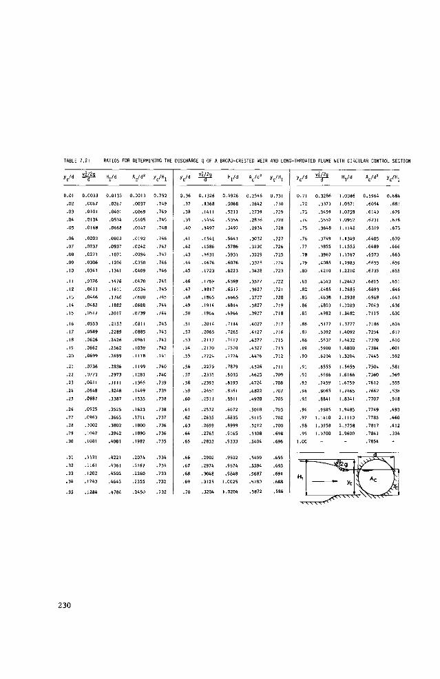
TABLE 7.2: RATIOS FOR DETERMINING THE DISCHARGE Q OF A BROAD-CRESTED HEIR AND LONG-THROATED FLUME WITH CIRCULAR CONTROL SECTION
yc/d
O.Ol
.02
.03
.04
.05
.06
.07
.08
.09
.10
.11
.12
.13
.14
.15
.16
.17
.18
.19
.20
.21
.22
.23
.24
.25
.26
.27
.28
.29
.30
.31
.32
.33
.34
.35
&P
0.0033
.0067
.0101
.0134
.0168
.0203
.0237
.0271
.0306
.0341
.0376
.0411
.0446
.0482
.0517
.0553
.0589
.0626
.0662
.0699
.0736
.0773
.0811
.0848
.0887
.0925
.0963
.1002
.1042
.1081
.1121
.1161
.1202
.1243
.1284
Hj/d
0.0133
.0267
.0401
.0534
.0668
.0803
.0937
.1071
.1206
.1341
.1476
.1611
.1746
.1882
.2017
.2153
.2289
.2426
.2562
.2699
.2836
.2973
.3111
.3248
.3387
.3525
.3663
.3802
.3942
.4081
.4221
.4361
.4502
.4643
.4784
Ac/dz
0.0013
.0037
.0069
.0105
.0147
.0192
.0242
.0294
.0350
.0409
.0470
.0534
.0600
.0688
.0739
.0811
.0885
.0961
.1039
.1118
.1199
.1281
.1365
.1449
.1535
.1623
.1711
.1800
.1890
.1982
.2074
.2167
.2260
.2355
.2450
VHi
0.752
.749
.749
.749
.748
.748
.747
.747
.746
.746
.745
.745
.745
.744
.744
.743
.743
.742
.742
.741
.740
.740
.739
.739
.738
.738
.737
.736
.736
.735
.734
.734
.733
.732
.732
yc/d
0.36
.37
.38
.39
.40
.41
.42
.43
.44
.45
.46
.47
.48
.49
.50
.51
.52
.53
.54
.55
.56
.57
.58
.59
.60
.61
.62
.63
.64
.65
.66
.67
.68
.69
.70
vi^
0.1326
.1368
.1411
.1454
.1497
.1541.
.1586
.1631
.1676
.1723
.1769
.1817
.1865
.1914
.1964
.2014
.2065
.2117
.2170
.2224
.2279
.2335
.2393
.2451
.2511
.2572
.2635
.2699
.2765
.2833
.2902
.2974
.3048
.3125
.3204
Hj/d
0.4926
.5068
.5211
.5354
.5497
.5641
.5786
.5931
.6076
.6223
.6369
.6517
.6665
.6814
.6964
.7114
.7265
.7417
.7570
.7724
.7879
.8035
.8193
.8351
.8511
.8672
.8835
.8999
.9165
.9333
.9502
.9674
.9848
1 .0025
1.0204
Vd!
0.2546
.2642
.2739
.2836
.2934
.3032
.3130
.3229
.3328
.3428
.3527
.3627
.3727
.3827
.3927
.4027
.4127
.4227
.4327
.4426
.4526
.4625
.4724
.4822
.4920
.5018
.5115
.5212
.5308
.5404
.5499
.5594
.5687
.5780
.5872
VH1
0.731
.730
.729
.728
.728
.727
.726
.725
.724
.723
.722
.721
.720
.719
.718
.717
.716
.715
.713
.712
.71!
.709
.708
.707
.705
.703
.702
.700
.698
.696
.695
.693
.691
.688
.686
yc/c
0.7
.7
.7
vl^
0.3286
.3371
.3459
.74 .3552
.7
.7<
.7"
.3648
.3749
.3855
.78 .3967
.T-
.8C
.8
.8,
.8.
.84
.8;
.8«
.8"
.86
.85
.9C
.9
.9!
.93
.94
.95
.96
.97
.96
.95
l.OC
H,
.4085
.4210
.4343
.4485
.4638
.4803
.4982
.5177
.5392
.5632
.5900
.6204
.6555
.6966
.7459
.8065
.8841
.9885
1.1410
1.3958
1.9700
-
Hj/d Ac/d!
1.0386 0.5964
1.0571 .6054
1.0759 .6143
1.0952 .6231
1.1148 .6319
I.1349 .6405
1.1555 .6489
1.1767 .6573
1.1985 .6655
1.2210 .6735
1.2443 .6815
1.2685 .6893
1.2938 .6969
1.3203 .7043
1.3482 .7115
1.3777 .7186
1.4092 .7254
1.4432 .7320
1.4800 .7384
1.5204 .7445
1.5655 .7504
1.6166 .7560
1.6759 .7612
1.7465 .7662
1.8341 .7707
1.9485 .7749
2.1110 .7785
2.3758 .7817
2.9600 .7841
.7854
^ g
re
v< -TN\\\
d
i Ac
v 'Vx
VH1
0.684
.681
.679
.676
.673
.670
.666
.663
.659
.655
.651
.646
.64!
.636
.630
.624
.617
.610
.601
.592
.581
.569
.555
.538
.518
.493
.460
.412
.334
-
A
230
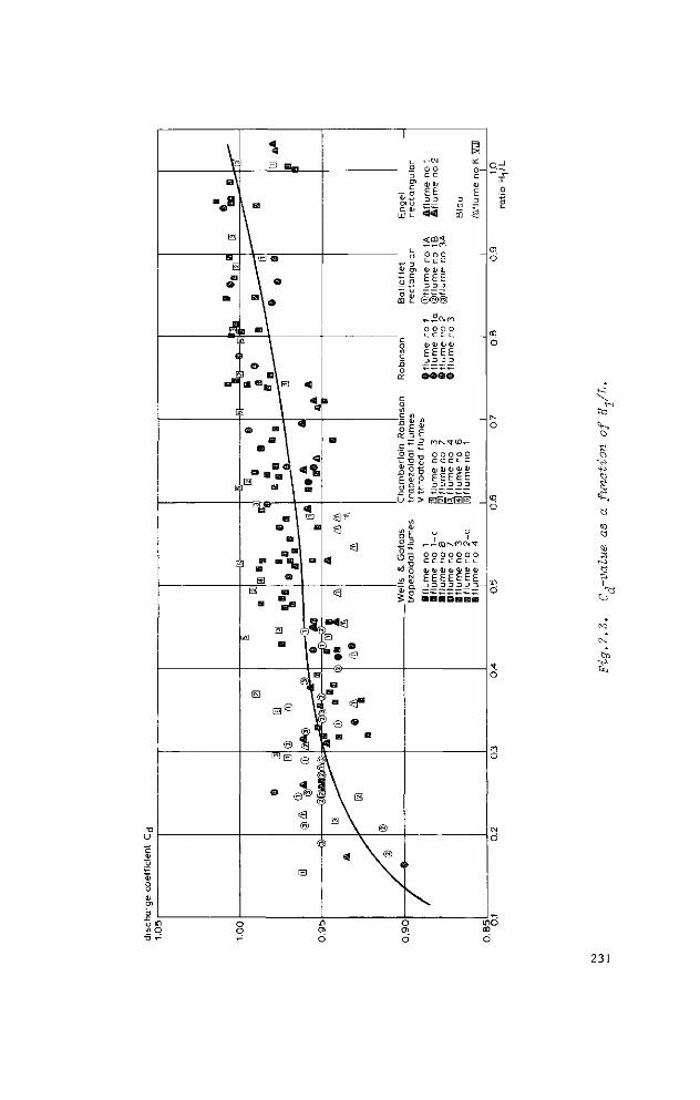
ö D Ol
UJ (_
<U Dl
O O
ffl ï
m
—
o o c c <U <D
E£
<^
< t û «
O o O
<L> 4 J <b
£ £ £ D D 3
e@© ,-^wn 0 O 0 o c c c c (Li flJ 1> QJ
£ £ £ £ D D 3 D
ffl 3
C t/l 3 "" IC o £ £
^ : _?. nr^^j-iÛT-
dj dj <u OJ <u £ £ £ £ £
.2 ^ J - coNnc^ r o o o o o o o a a c c a c a d ; 4> <lj Hl 1> 1» OJ
E E £ £ E E £ =J 3 3 3 3 3 3 -
1-5 \
co
I
03
231
The error in the product C ,C of a well maintained lone-throated flume which has d v °
been constructed with reasonable care and skill may be deduced from the equation
Xc = + 2 (21 - 20 C ) per cent (7-1)
The method by which this coefficient error is to be combined with other sources
of error is shown in Appendix II.
7.1.3 Modular limit
Although the available evidence is insufficient to define the relation between
the modular limit and the angle of expansion, some information can be obtained
from Section 1.15. Practice varies between very gentle and costly expansions of
about l-to-15, to ensure a high modular limit, and short expansions of l-to-4.
It is recommended that the divergences of each plane surface be not more abrupt
than l-to-4. If in some circumstances it is desirable to construct a short down
stream expansion, it is better to truncate the transition rather than to enlarge
the angle of divergence (see also Fig.1.35). At one extreme if no velocity head
needs to be recovered, the downstream transition can be fully truncated. It will
be clear from Section 1.15 that no expanding section will be needed if the
tailwater level is always less than y above the invert of the flume throat.
At the other extreme, when almost all velocity head needs to be recovered, a
transition with a very gradual expansion of sides and bed is required. The
modular limit of long-throated flumes with various control cross sections and
downstream expansions can be estimated with the aid of Section 1.15.3. As an
illustration, we shall estimate the modular limit of the flume shown in Figure
7.4, flowing under an upstream energy head H = 0.20 m. As can be read from
Figure 7.3, the C,-value for H /L = 0.33 equals 0.952. Hence for this flume
3 V 3 0 . 952 $• \lïr 9 .81 0 . 30 0 . 2 0 3 / 2 = 0 .0436 m 3 / s
2 Since we know that the water depth at the control is y = -5- H = 0.133 m,
we can calculate v with the equation
v = - 2 - = 1.09 m/s c y b J c
232
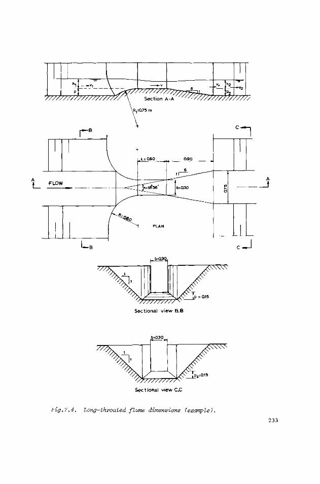
'y////////////////////\ Sec
R,=Q75 m
^ZZPmnhMsÀ, v. Th2
777777777T
Sectional v iew B.B
£=030
p2=Q15
Sec t ional view CC
Fig.7.4. Long-throated flume dimensions (example).
233
To find the modular limit we now have to equalize by trial and error the Equation
1-119, which was presented in Section 1.15.3. This equation, which is valid for
a truncated expansion reads
H„ . , (v - v ) 2 (v - v„)2 AH, _ i < C l / u - f ° F —2 L. I (7-2) Hj d ^19 2gH ^180 2gH H w ;
In the above equation u = 1.5, the Ç-values can be taken from Figure 1.36, and
AH may be estimated by using the Chëzy or Manning equation. For a three-dimen
sional expansion Ç q = 0.42 and Ç.on = 1.10. Energy losses over the downstream
expansion are estimated to be AH = 0.005 m, resulting in a AHf/H value of 0.025.
It should be noted that for low values of H and relatively long expansions
(small angles of divergence a), the ratio AH /H becomes significantly more
important.
Substitution of the already known values into Equation 7-2 yields
H ? r -i T T ^ T T ^ 0.943 - 0.255 0.42 (1.09 - v ) 2 - 1.10 (v - v„) 2 (7-3) 0.20 L- o o 2 -J
This relationship must now be equalized by using different H„ values.
Step 1
H„ = 0.16 m and thus v - 0.19 m/s, v„ - 0.13 m/s
and Equation 7-3 becomes
0.80 0.943 - 0.255 {0.340 - 0.004}
0.80 << 0.857
Step 2
H„ = 0.17 m and thus v =0.18 m/s, v„ = 0.13 m/s I o 2
and Equation 7-3 becomes
0.85 « 0.943 - 0.255 {0.348 - 0.003}
0.85 0.855
which fits to the second decimal so that we may state that the modular limit
of the shown flume at H. = 0.20 m is H./H. - 0.85. Since in the example both
234
velocities v. and v„ are low (both values of v2/2g < 0.001 m) we can state,
that the minimum loss of head over the flume to obtain modular flow is
H - H 2 = 0.03 m.
The same procedure can be followed to predict the modular limit for other heads
and other flumes. Modular limits as high as 0.96 can be achieved in gentle
transitions.
Flumes whose throat is shorter than 2 H do not have straight and parallel stream
lines at the control section; streamlines become increasingly curved as H in
creases. The available data are insufficient to define the relation of the mo
dular limit and the degree of streamline curvature. It can be stated that, in
general, the modular limit, however, decreases with an increasing value of
Hj/L. As a conservative rule we may assume that if the ratio H./L increases from
0.5 to 1.0, the modular limit H„/H decreases linearly from the value calculated
when using Section 1.15.3 to a value of about 0.5 y /H , where y is the critical
depth at the control.
7.1.4 Limits of application
The limits of application of a long-throated flume for reasonably accurate flow
measurements are:
a) The practical lower limit of ht is related to the magnitude of the
influence of fluid properties, boundary roughness, and the accuracy with which
hj can be determined. The recommended lower limit is 0.06 m or 0.1 L, whichever
is greater.
b) To prevent water surface instability in the approach channel the Froude i
number F = Vj/(gA / B ) 2 should not exceed 0.5.
c) The lower limitation on the ratio H /L arises from the necessity to
prevent undulations in the flume throat. Values of the ratio Hj/L should range
between 0.1 and 1.0.
d) The width B of the water surface in the throat at maximum stage should
not be less than 0.30 m, nor less than H max, nor less than L/5.
e) The width at the water surface in a triangular throat at minimum stage
should not be less than 0.20 m.
235
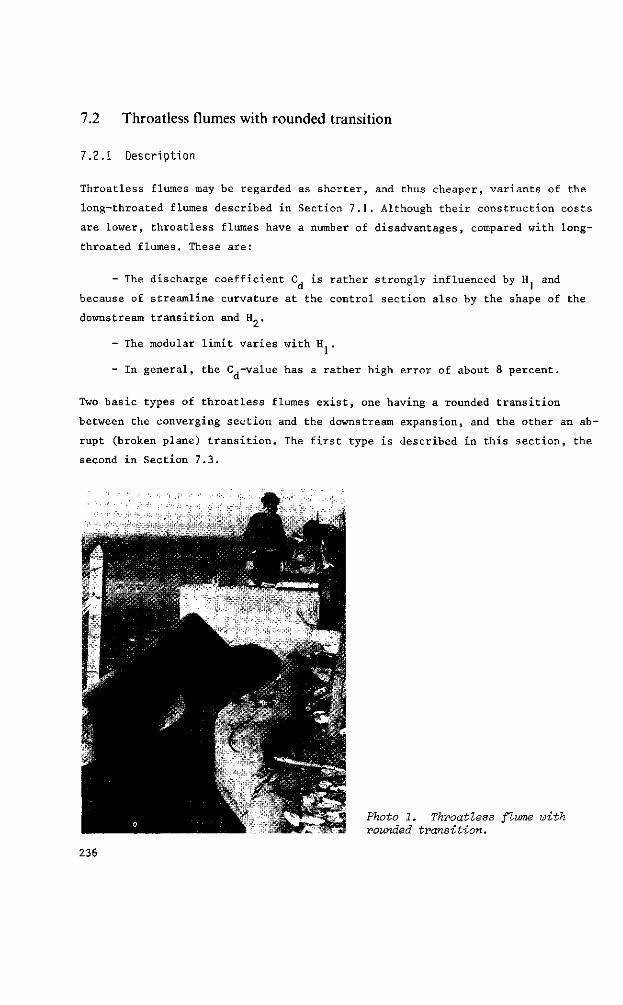
7.2 Throatless flumes with rounded transition
7.2.1 Description
Throatless flumes may be regarded as shorter, and thus cheaper, variants of the
long-throated flumes described in Section 7.1. Although their construction costs
are lower, throatless flumes have a number of disadvantages, compared with long-
throated flumes. These are:
- The discharge coefficient C is rather strongly influenced by H and
because of streamline curvature at the control section also by the shape of the
downstream transition and H..
- The modular limit varies with H .
- In general, the C,-value has a rather high error of about 8 percent.
Two basic types of throatless flumes exist, one having a rounded transition
between the converging section and the downstream expansion, and the other an ab
rupt (broken plane) transition. The first type is described in this section, the
second in Section 7.3.
*? Photo 1. Throatless flume with rounded transition.
236
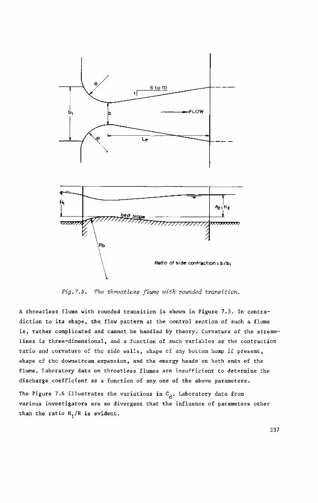
VTTTTT^^^
h2=H2
XWUWOWUO
Ratio of side contraction ; b/b.
Fig.7.5. The throatless flume with rounded transition.
A throatless flume with rounded transition is shown in Figure 7.5. In contra
diction to its shape, the flow pattern at the control section of such a flume
is, rather complicated and cannot be handled by theory. Curvature of the stream
lines is three-dimensional, and a function of such variables as the contraction
ratio and curvature of the side walls, shape of any bottom hump if present,
shape of the downstream expansion, and the energy heads on both ends of the
flume. Laboratory data on throatless flumes are insufficient to determine the
discharge coefficient as a function of any one of the above parameters.
The Figure 7.6 illustrates the variations in C,. Laboratory data from
various investigators are so divergent that the influence of parameters other
than the ratio H /R is evident.
237
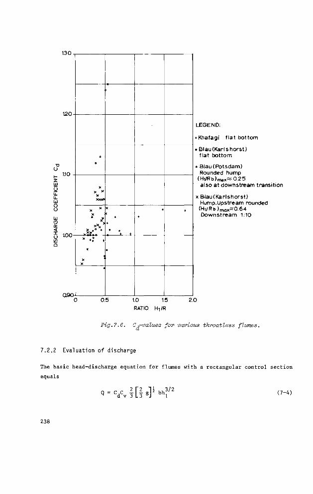
T3 U I -2 W y tiu o u LU <D CE < I U a
120-
110 -
OQ("L
0
0
X
X
xxxx
X X
X ° X»
V *
3** * * •? •
* 1
x
4
)
X
<
+
•
• '
+
+
• +
+
+
+
LEGEND:
• Khafagi f lat bottom
• Blau(Karlshorst) f lat bottom
• Blau (Potsdam) Rounded hump
(Hi/Rb)max- 0.25 also at downstream transition
x Blau(Karlshorst) Hump.Upstream rounded (Hi/Rb)max:=0.64 Downstream 1:10
0.5 1.0 1.5
RATIO H-i /R
2.0
Fig. 7.6. C-.-values for various throatless flumes.
7.2.2 Evaluation of discharge
The basic head-discharge equation for flumes with a rectangular control section
equals
*- d c v f[§gP * bh?/ 2 (7-4)
238
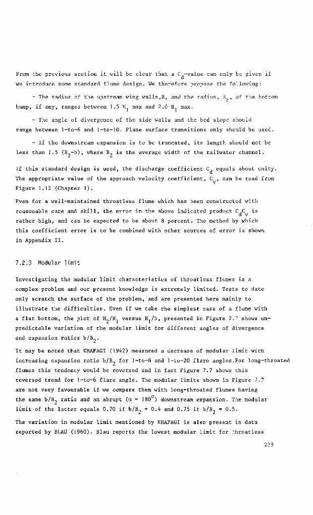
From the previous section it will be clear that a C -value can only be given if
we introduce some standard flume design. We therefore propose the following:
Th e radius of the upstream wing walls,R, and the radius, R, , of the bottom
hump, if any, ranges between 1.5 H max and 2.0 Hf max.
- The angle of divergence of the side walls and the bed slope should
range between l-to-6 and l-to-10. Plane surface transitions only should be used.
- If the downstream expansion is to be truncated, its length should not be
less than 1.5 (B„-b), where B. is the average width of the tailwater channel.
If this standard design is used, the discharge coefficient C equals about unity.
The appropriate value of the approach velocity coefficient, C , can be read from
Figure 1.12 (Chapter 1).
Even for a well-maintained throatless flume which has been constructed with
reasonable care and skill, the error in the above indicated product C ,C is r d v
rather high, and can be expected to be about 8 percent. The method by which
this coefficient error is to be combined with other sources of error is shown
in Appendix II.
7.2.3 Modular limit
Investigating the modular limit characteristics of throatless flumes is a
complex problem and our present knowledge is extremely limited. Tests to date
only scratch the surface of the problem, and are presented here mainly to
illustrate the difficulties. Even if we take the simplest case of a flume with
a flat bottom, the plot of H./Hj versus H /b, presented in Figure 7.7 shows un
predictable variation of the modular limit for different angles of divergence
and expansion ratios b/B..
It may be noted that KHAFAGI (1942) measured a decrease of modular limit with
increasing expansion ratio b/B„ for l-to-8 and l-to-20 flare angles.For long-throated
flumes this tendency would be reversed and in fact Figure 7.7 shows this
reversed trend for l-to-6 flare angle. The modular limits shown in Figure 7.7
are not very favourable if we compare them with long-throated flumes having
the same b/B„ ratio and an abrupt (a. = 180 ) downstream expansion. The modular
limit of the latter equals 0.70 if b/B = 0.4 and 0.75 if b/B = 0.5.
The variation in modular limit mentioned by KHAFAGI is also present in data
reported by BLAU (1960). Blau reports the lowest modular limit for throatless
239
flumes, which equals 0.5; for H /b = 0.41, A/A = 0.21, b/B = 0.49, wingwall
divergence and bed slope both l-to-10.
There seems little correlation between the available data, which would indicate
that the throatless flume is not a suitable modular discharge measurement
structure if the ratio H /H exceeds about 0.5.
MODULAR LIMIT H2IH-]
1
0.9
0.8
0.7
1:20 tV&2=05
1:6 bife2=Q5~=*==
0 0.5 1.0 1.5 2.0 2.5 RATIO H^b
Fig.7. 7. Modular limit conditions of flat bottomed throatless flumes (after Khafagi, 1942).
7.2.4 Limits of application
The limits of application of a throatless flume with rounded transition for
reasonably accurate flow measurements are:
a) Flume design should be in accordance with the standards presented in
Section 7.2.2.
b) The practical lower limit of h. depends on the influence of fluid
properties, boundary roughness, and the accuracy with which h can be determined.
The recommended lower limit is 0.06 m.
c) To prevent water surface instability in the approach channel the Froude l
number Fr = v./(gA./B ) 2 should not exceed 0.5.
d) The width b of the flume throat should not be less than 0.20 m nor
less than H1 max.
240
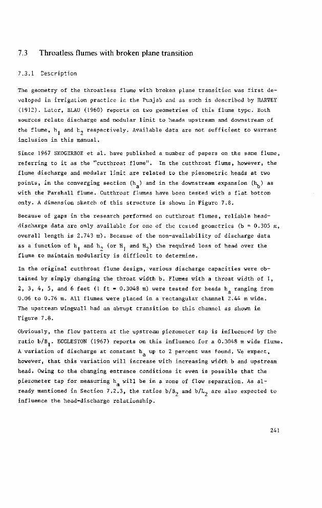
7.3 Throatless flumes with broken plane transition
7.3.1 Description
The geometry of the throatless flume with broken plane transition was first de
veloped in irrigation practice in the Punjab and as such is described by HARVEY
(1912). Later, BLAU (1960) reports on two geometries of this flume type. Both
sources relate discharge and modular limit to heads upstream and downstream of
the flume, h and h„ respectively. Available data are not sufficient to warrant
inclusion in this manual.
Since 1967 SKOGERBOE et al. have published a number of papers on the same flume,
referring to it as the "cutthroat flume". In the cutthroat flume, however, the
flume discharge and modular limit are related to the piezometric heads at two
points, in the converging section (h ) and in the downstream expansion (h, ) as
with the Parshall flume. Cutthroat flumes have been tested with a flat bottom
only. A dimension sketch of this structure is shown in Figure 7.8.
Because of gaps in the research performed on cutthroat flumes, reliable head-
discharge data are only available for one of the tested geometries (b = 0.305 m,
overall length is 2.743 m ) . Because of the non-availability of discharge data
as a function of hj and h. (or H and H.) the required loss of head over the
flume to maintain modularity is difficult to determine.
In the original cutthroat flume design, various discharge capacities were ob
tained by simply changing the throat width b. Flumes with a throat width of 1,
2, 3, 4, 5, and 6 feet (1 ft = 0.3048 m) were tested for heads h ranging from
0.06 to 0.76 m. All flumes were placed in a rectangular channel 2.44 m wide.
The upstream wingwall had an abrupt transition to this channel as shown in
Figure 7.8.
Obviously, the flow pattern at the upstream piezometer tap is influenced by the
ratio b/B . EGGLESTON (1967) reports on this influence for a 0.3048 m wide flume.
A variation of discharge at constant h up to 2 percent was found. We expect,
however, that this variation will increase with increasing width b and upstream
head. Owing to the changing entrance conditions it even is possible that the
piezometer tap for measuring h will be in a zone of flow separation. As al
ready mentioned in Section 7.2.3, the ratios b/B„ and b/L_ are also expected to
influence the head-discharge relationship.
241
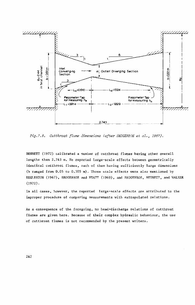
' / / / / / / / / / ' / / / / / • .
Fig.7.8. Cutthroat flume dimensions (after SKOGERBOE et al., 1967).
BENNETT (1972) calibrated a number of cutthroat flumes having other overall
lengths than 2.743 m. He reported large-scale effects between geometrically
identical cutthroat flumes, each of them having sufficiently large dimensions
(b ranged from 0.05 to 0.305 m ) . Those scale effects were also mentioned by
EGGLESTON (1967), SKOGERBOE and HYATT (1969), and SKOGERBOE, BENNETT, and WALKER
(1972).
In all cases, however, the reported large-scale effects are attributed to the
improper procedure of comparing measurements with extrapolated relations.
As a consequence of the foregoing, no head-discharge relations of cutthroat
flumes are given here. Because of their complex hydraulic behaviour, the use
of cutthroat flumes is not recommended by the present writers.
242
7.4 Parshall flumes
7.4.1 Description
Parshall flumes are calibrated devices for the measurement of water in open
channels. They were developed by R.PARSHALL (1922) after whom the device was
named.
The flume consists of a converging section with a level floor, a throat section
with a downward sloping floor, and a diverging section with an upward sloping
floor.
Because of this unconventional design, the control section of the flume is not
situated in the throat but near the end of the level "crest" in the converging
section. The modular limit of the Parshall flume is lower than that of the
other long-throated flumes described in Section 7.1.
In deviation from the general rule for long-throated flumes where the upstream
head must be measured in the approach channel, Parshall flumes are calibrated
against a piezometric head, h , measured at a prescribed location in the conver
ging section. The "downstream" piezometric head h, is measured in the throat.
This typical American practice is also used in the cutthroat and H flumes.
Parshall flumes were developed in various sizes, the dimensions of which are
given in Table 7.3. Care must be taken to construct the flumes exactly in accor
dance with the structural dimensions given for each of the 22 flumes, because
the flumes are not hydraulic scale models of each other. Since throat length
and throat bottom slope remain constant for series of flumes while other di
mensions are varied, each of the 22 flumes is an entirely different device.
For example, it cannot be assumed that a dimension in the 12-ft flume will
be three times the corresponding dimension in the 4-ft flume.
On the basis of throat width, Parshall flumes have been somewhat arbitrarily
classified into three main groups for the convenience of discussing them, select
ing sizes, and determining discharges.
These groups are "very small" for 1-, 2-, and 3-in flumes, "small" for 6-in
through 8-ft flumes and "large" for 10-ft up to 50-ft flumes (USBR, 1971).
243
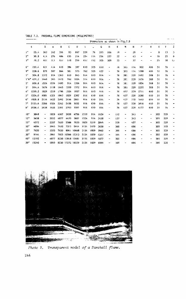
TABLE 7.3. PARSHALL FLUME DIMENSIONS (MILLIMETRES)
1"
2"
3"
6"
9"
1'
1'6
2'
3'
4'
5'
6'
7'
8'
10'
12'
15'
20'
25'
30'
40'
50'
b
25.4
50.8
76.2
152.4
228.6
304.8
" 457.2
609.6
914.4
1219.2
1524.0
1828.8
2133.6
2438.4
3048
3658
4572
6096
7620
9144
12192
15240
A
363
414
467
621
879
1372
1448
1524
1676
1829
1981
2134
2286
2438
--------
a
242
276
311
414
587
914
965
1016
1118
1219
1321
1422
1524
1626
1829
2032
2337
2845
3353
3861
4877
5893
B
356
406
457
610
864
1343
1419
1495
1645
1794
1943
2092
2242
2391
4267
4877
7620
7620
7620
7925
8230
8230
C
93
135
178
394
381
610
762
914
1219
1524
1829
2134
2438
2743
3658
4470
5588
7315
8941
10566
13818
17272
D
167
214
259
397
575
845
1026
1206
1572
1937
2302
2667
3032
3397
4756
5607
7620
9144
10668
12313
15481
18529
E
229
254
457
610
762
914
914
914
914
914
914
914
914
914
1219
1524
1829
2134
2134
2134
2134
2134
Dimensions
L
76
114
152
305
305
610
610
610
610
610
610
610
610
610
914
914
1219
1829
1829
1829
1829
1829
G
203
254
305
610
457
914
914
914
914
914
914
914
914
914
1829
2438
3048
3658
3962
4267
4877
6096
as shown in F
H
206
257
309
-----------
--------
K
19
22
25
76
76
76
76
76
76
76
76
76
76
76
152
152
229
305
305
305
305
305
ig.7.9
M
---
305
305
381
381
381
381
457
457
457
457
457
--------
N
29
43
57
114
114
229
229
229
229
229
229
229
229
229
343
343
457
686
686
686
686
686
P
---
902
1080
1492
1676
1854
2222
2711
3080
3442
3810
4172
--------
R
---
406
406
508
508
508
508
610
610
610
610
610
--------
X
8
16
25
51
51
51
51
51
51
51
51
51
51
51
305
305
305
305
305
305
305
305
Y
13
25
38
76
76
76
76
76
76
76
76
76
76
76
229
229
229
229
229
229
229
229
Z
3
6
13
-----------
--------
Photo 2. Transparent model of a Parshall flume.
244
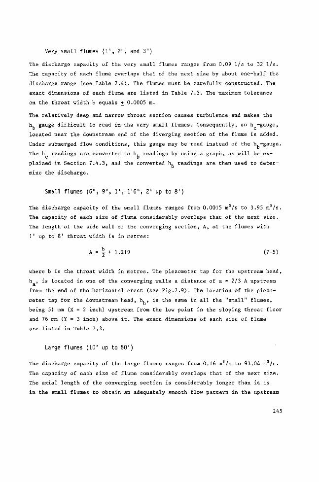
Very small flumes (1", 2", and 3")
The discharge capacity of the very small flumes ranges from 0.09 l/s to 32 l/s.
The capacity of each flume overlaps that of the next size by about one-half the
discharge range (see Table 7.4). The flumes must be carefully constructed. The
exact dimensions of each flume are listed in Table 7.3. The maximum tolerance
on the throat width b equals + 0.0005 m.
The relatively deep and narrow throat section causes turbulence and makes the
h, gauge difficult to read in the very small flumes. Consequently, an h -gauge,
located near the downstream end of the diverging section of the flume is added.
Under submerged flow conditions, this gauge may be read instead of the h, -gauge.
The h readings are converted to h, readings by using a graph, as will be ex
plained in Section 7.4.3, and the converted h, readings are then used to deter
mine the discharge.
Small flumes (6", 9", 1', 1'6", 2' up to 8')
The discharge capacity of the small flumes ranges from 0.0015 m3/s to 3.95 m /s.
The capacity of each size of flume considerably overlaps that of the next size.
The length of the side wall of the converging section, A, of the flumes with
1' up to 8' throat width is in metres:
A = | + 1.219 (7-5)
where b is the throat width in metres. The piezometer tap for the upstream head,
h , is located in one of the converging walls a distance of a = 2/3 A upstream
from the end of the horizontal crest (see Fig.7.9). The location of the piezo
meter tap for the downstream head, h , is the same in all the "small" flumes,
being 51 mm (X = 2 inch) upstream from the low point in the sloping throat floor
and 76 mm (Y = 3 inch) above it. The exact dimensions of each size of flume
are listed in Table 7.3.
Large flumes (10' up to 50')
The discharge capacity of the large flumes ranges from 0.16 m3/s to 93.04 m3/s.
The capacity of each size of flume considerably overlaps that of the next size.
The axial length of the converging section is considerably longer than it is
in the small flumes to obtain an adequately smooth flow pattern in the upstream
245
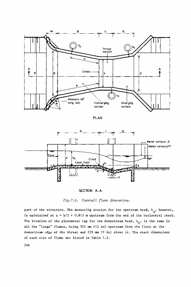
PLAN
Water surface , S
Water surface.FF
SECTION A-A
Fig.7.9. Parshall flume dimensions.
part of the structure. The measuring station for the upstream head, h , however,
is maintained at a = b/3 + 0.813 m upstream from the end of the horizontal crest.
The location of the piezometer tap for the downstream head, h, , is the same in b
all the "large" flumes, being 305 mm (12 in) upstream from the floor at the
downstream edge of the throat and 229 mm (9 in) above it. The exact dimensions
of each size o£ flume are listed in Table 7.3.
246
All flumes must be carefully constructed to the dimensions listed, and careful
levelling is necessary in both longitudinal and transverse directions if standard
discharge table is to be used. When gauge zeros are established, they should
be set so that the h -, h -, and h -gauges give the depth of water above the
level crest - not the depths above pressure taps.
If the Parshall flume is never to be operated above the 0.60 submergence limit,
there is no need to construct the portion downstream of the throat. The trunca
ted Parshall flume (without diverging section) has the same modular flow charac
teristics as the standard flume. The truncated flume is sometimes referred to
as the "Montana flume".
7.4.2 Evaluation of discharge
The upstream head-discharge (h -Q) relationship of Parshall flume of various
sizes, as calibrated empirically, is represented by an equation, having the
form:
Q = Khu (7-6) a
where K denotes a dimensional factor which is a function of the throat width.
The power u varies between 1.522 and 1.60. Values of K and u for each size of
flume are given in Table 7.4. In the listed equations Q is the modular discharge
in m /s, and h is the upstream gauge reading in metres.
The flumes cover a range of discharges from 0.09 1/s to 93.04 m3/s and have
overlapping capacities to facilitate the selection of a suitable size. Each
of the flumes listed in Table 7.4 is a standard device and has been calibrated
for the range of discharges shown in the table. Detailed information on the
modular discharge for each size of flume as a function of h are presented in
the Tables 7.5 to 7.11.
247
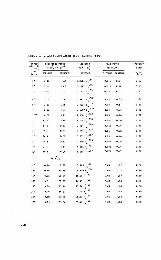
TABLE 7.4. DISCHARGE CHARACTERISTICS OF PARSHALL FLUMES
Throat width b in f e e t
o r inches
1"
2"
3"
6"
9"
1'
1 '6"
2 '
3 '
4 '
5 '
6 '
7 '
8 '
10'
12'
15'
20 '
25 '
30 '
40 '
50 '
Discharge 3 , in m / s :
minimum
0.09
0.18
0.77
1.50
2.50
3.32
4.80
12.1
17.6
35.8
44.1
74.1
85.8
97.2
in m
0.16
0.19
0.23
0.31
0.38
0.46
0.60
0.75
range
x 10~3
maximum
5.4
13.2
32.1
111
251
457
695
937
1427
1923
2424
2929
3438
3949
/S
8.28
14.68
25.04
37.97
47.14
56.33
74.70
93.04
Equation
Q = Kh^
(met r ic )
0.0604 h 1 , 5 5
a
0.1207 h ' ' 5 5
a 0.1771 h 1 * 5 5
a
0.3812 h 1 ' 5 8
a 1 53
0.5354 h ' * J J
a 1 522
0.6909 h * a
1 . 0 5 6 h 1 ' 5 3 8
a
1 . 4 2 8 h K 5 5 0
a
2 . 1 8 4 h 1 - 5 6 6
a
2 . 9 5 3 h 1 - 5 7 8
a
3.732 h 1 " 5 8 7
a
4 . 5 . 9 h 1 - 5 9 5
a
5.312 h 1 " 6 0 1
a
6 . 1 1 2 h 1 - 6 0 7
a
i ,ci J - 6 0 7.463 h a
8 . 8 5 9 h 1 - 6 0
a
1 0 . 9 6 h ' - 6 0
a 1/ /R J - 6 0
14.45 h a 1 7 . 9 4 h 1 ' 6 0
a Ol / / J - 6 0 21.44 h a
2 8 . 4 3 h 1 - 6 0
a
35.41 h 1 " 6 0
Head range
in metres
minimum
0.015
0.015
0.03
0 .03
0.03
0.03
0.03
0.046
0.046
0.06
0.06
0.076
0.076
0.076
0.09
0.09
0.09
0.09
0.09
0.09
0.09
0.09
maximum
0.21
0.24
0 .33
0.45
0.61
0.76
0.76
0.76
0.76
0.76
0.76
0.76
0.76
0.76
1.07
1.37
1.67
1 .83
1.83
1.83
1 .83
1.83
Modular
l im i t
Vha
0.50
0.50
0.50
0.60
0.60
0.70
0.70
0.70
0.70
0.70
0.70
0.70
0.70
0.70
0.80
0.80
0.80
0.80
0.80
0.80
0.80
0.80
248
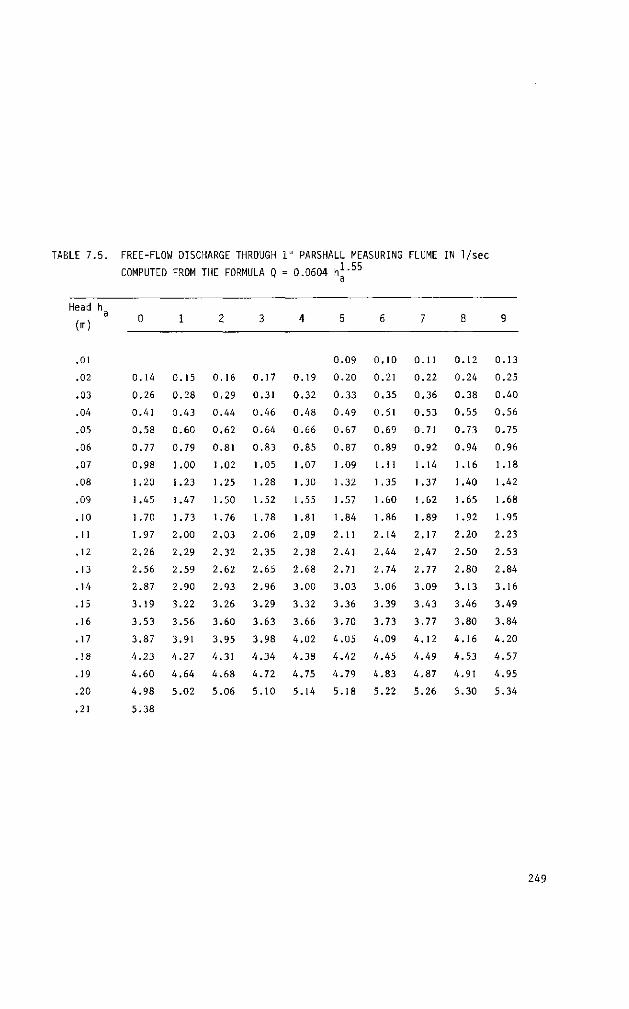
TABLE 7.5. FREE-FLOW DISCHARGE THROUGH 1" PARSHALL MEASURING FLUME IN 1/sec
COMPUTED FROM THE FORMULA Q = 0.0604 h ^ 5 5
a
Head h a
(m)
.01
.02
.03
.04
.05
.06
.07
.08
.09
.10
.11
.12
.13
.14
.15
.16
.17
.18
.19
.20
.21
0
0.14
0.26
0.41
0.58
0.77
0.98
1.20
1.45
1.70
1.97
2.26
2.56
2.87
3.19
3.53
3.87
4 .23
4.60
4.98
5.38
1
0.15
0.28
0.43
0.60
0.79
1.00
1.23
1.47
1.73
2.00
2.29
2.59
2.90
3.22
3.56
3.91
4.27
4.64
5.02
2
0.16
0.29
0.44
0.62
0.81
1 .02
1.25
1.50
1.76
2.03
2.32
2.62
2.93
3.26
3.60
3.95
4.31
4.68
5.06
3
0.17
0.31
0.46
0.64
0.83
1.05
1.28
1.52
1 .78
2.06
2.35
2.65
2.96
3.29
3.63
3.98
4.34
4.72
5.10
4
0.19
0.32
0.48
0.66
0.85
1.07
1.30
1 .55
1.8!
2.09
2.38
2.68
3.00
3.32
3.66
4.02
4.38
4.75
5.14
5
0.09
0.20
0.33
0.49
0.67
0.87
1 .09
1 .32
1.57
I .84
2.11
2.41
2.71
3.03
3.36
3.70
4.05
4.42
4.79
5.18
6
0.10
0.21
0.35
0.51
0.69
0.89
1.11
1.35
1.60
1.86
2.14
2.44
2.74
3.06
3.39
3.73
4.09
4.45
4.83
5.22
7
0.11
0.22
0.36
0.53
0.71
0.92
1.14
1.37
1.62
1.89
2.17
2.47
2.77
3.09
3.43
3.77
4.12
4.49
4.87
5.26
8
0.12
0.24
0.38
0.55
0.73
0.94
1.16
1.40
1.65
1.92
2.20
2.50
2.80
3.13
3.46
3.80
4.16
4.53
4.91
5.30
9
0.13
0.25
0.40
0.56
0.75
0.96
1.18
1.42
1.68
1 .95
2 .23
2.53
2.84
3.16
3.49
3.84
4.20
4.57
4.95
5.34
249
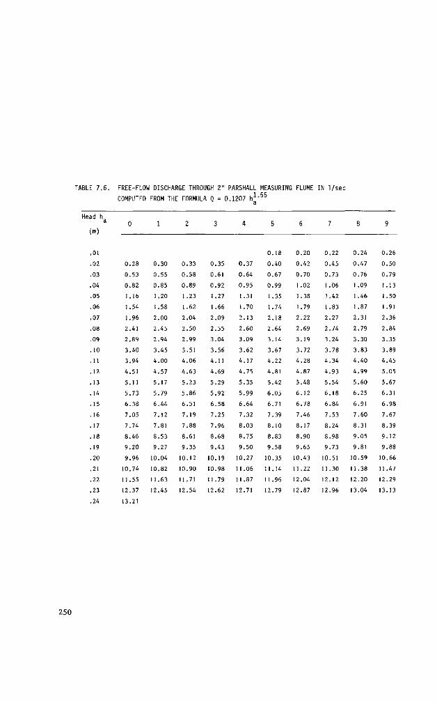
TABLE 7.6. FREE-FLOW DISCHARGE THROUGH 2" PARSHALL MEASURING FLUME IN 1/sec
COMPUTED FROM THE FORMULA Q = 0.1207 h*'55
a
Head h a
(m)
.01
.02
.03
.04
.05
.06
.07
.08
.09
.10
.11
.12
.13
.14
.15
.16
.17
.18
.19
.20
.21
.22
.23
.24
0
0 .28
0 .53
0.82
1.16
1.54
1.96
2.41
2.89
3.40
3.94
4.51
5.11
5.73
6.38
7.05
7.74
8.46
9.20
9.96
10.74
11.55
12.37
13.21
1
0.30
0.55
0.85
1 .20
1.58
2.00
2 .45
2.94
3.45
4 .00
4.57
5.17
5.79
6.44
7.12
7.81
8.53
9.27
10.04
10.82
11.63
12.45
2
0.33
0.58
0.89
1.23
1.62
2.04
2.50
2.99
3.51
4.06
4 .63
5.23
5.86
6.51
7.19
7.88
8.61
9 .35
10.12
10.90
11.71
12.54
3
0.35
0.61
0.92
1.27
1.66
2.09
2.55
3.04
3.56
4.11
4.69
5.29
5.92
6.58
7.25
7.96
8.68
9.43
10.19
10.98
11.79
12.62
4
0.37
0.64
0.95
1.31
1.70
2.13
2.60
3.09
3.62
4.17
4.75
5.35
5.99
6.64
7.32
8.03
8.75
9.50
10.27
11.06
11.87
12.71
5
0.18
0.40
0.67
0.99
1.35
1.74
2.18
2.64
3.14
3.67
4.22
4.81
5.42
6.05
6.71
7.39
8.10
8.83
9 .58
10.35
11.14
11.96
12.79
6
0.20
0.42
0.70
1 .02
1 .38
1.79
2.22
2.69
3.19
3.72
4 .28
4.87
5.48
6.12
6.78
7.46
8.17
8.90
9.65
10.43
11.22
12.04
12.87
7
0.22
0.45
0 .73
1.06
1 .42
1.83
2.27
2.74
3.24
3.78
4.34
4 .93
5.54
6.18
6.84
7.53
8.24
8.98
9 .73
10.51
11.30
12.12
12.96
8
0.24
0.47
0.76
1.09
1.46
1.87
2.31
2.79
3.30
3.83
4.40
4.99
5.60
6.25
6.91
7.60
8.31
9.05
9.81
10.59
11.38
12.20
13.04
9
0.26
0.50
0.79
1.13
1 .50
1.91
2.36
2.84
3.35
3.89
4.45
5.05
5.67
6.31
6.98
7.67
8.39
9.12
9.88
10.66
11.47
12.29
13.13
250
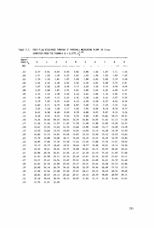
TABLE 7.7. FREE-FLOW DISCHARGE THROUGH 3" PARSHALL MEASURING FLUME IN 1/sec
COMPUTED FROM THE FORMULA Q = 0.1771 h* - 5 5
Upper-head h
(m)
.03
.04
.05
.06
.07
.08
.09
.10
.11
.12
.13
.14
.15
.16
.17
.18
.19
.20
.21
.22
.23
.24
.25
.26
.27
.28
.29
.30
.31
.32
.33
0
0.77
1.21
1.70
2.26
2.87
3.53
4.24
4.99
5.79
6.62
7.50
8.41
9.36
10.34
11.36
12.41
13.50
14.62
15.76
16.94
18.15
19.39
20.66
21.95
23.27
24.62
26.00
27.40
28.83
30.28
31.76
1
0.81
1.25
1.76
2.32
2.94
3.60
4.31
5.07
5.87
6.71
7.59
8.50
9.45
10.44
11.46
12.52
13.61
14.73
15.88
17.06
18.27
19.51
20.78
22.08
23.41
24.76
26.14
27.54
28.97
30.43
31.91
2
0.85
1.30
1.81
2.38
3.00
3.67
4.39
5.15
5.95
6.79
7.68
8.60
9.55
10.54
11.57
12.63
13.72
14.84
16.00
17.18
18.40
19.64
20.91
22.21
23.54
24.89
26.28
27.68
29.12
30.58
32.06
3
0.90
1.35
1.87
2.44
3.06
3.74
4.46
5.23
6.03
6.88
7.77
8.69
9.65
10.64
11.67
12.74
13.83
14.96
16.11
17.30
18.52
19.77
21.04
22.34
23.67
25.03
26.42
27.83
29.26
30.72
4
0.94
1.40
1 .92
2.50
3.13
3.81
4 .53
5.30
6.12
6.97
7.80
8.78
9.75
10.75
11.78
12.84
13.94
15.07
16.23
17.42
18.64
19.89
21.17
22.48
23.81
25.17
26.56
27.97
29.41
30.87
5
0.98
1.45
1.98
2.56
3.20
3.88
4.61
5.38
6.20
7.05
7.95
8.88
9.85
10.85
11.88
12.95
14.05
15.19
16.35
17.54
18.77
20.02
21 .30
22.61
23.94
25.31
26.70
28.11
29.55
31 .02
6
1.02
1.50
2.03
2.62
3.26
3.95
4.69
5.46
6.28
7.14
8.04
8.97
9.94
10.95
11.99
13.06
14.16
15.30
16.47
17.66
18.89
20.15
21.43
22.74
24.08
25.44
26.84
28.25
29.70
31.17
7
1.07
1.55
2.09
2 .68
3.33
4.02
4.76
5.54
6.37
7.23
8.13
9.07
10.04
11 .05
12.09
13.17
14.28
15.42
16.59
17.79
19.01
20.27
21.56
22.87
24.21
25.58
26 .98
28.40
29.84
31 .32
8
1.11
1.60
2.15
2 .75
3.40
4.09
4.84
5.62
6.45
7.32
8.22
9.16
10.14
11.15
12.20
13.28
14.39
15.53
16.70
17.91
19.14
20.40
21.69
23.01
24.35
25.72
27.12
28.54
29.99
31.46
9
1.16
1.65
2.20
2.81
3.46
4.17
4.91
5.70
6.54
7.41
8.32
9.26
10.24
11.26
12.31
13.39
14.50
15.65
16.82
18.03
19.26
20.53
21.82
23.14
24.49
25.86
27.26
28.68
30.14
31.61
251
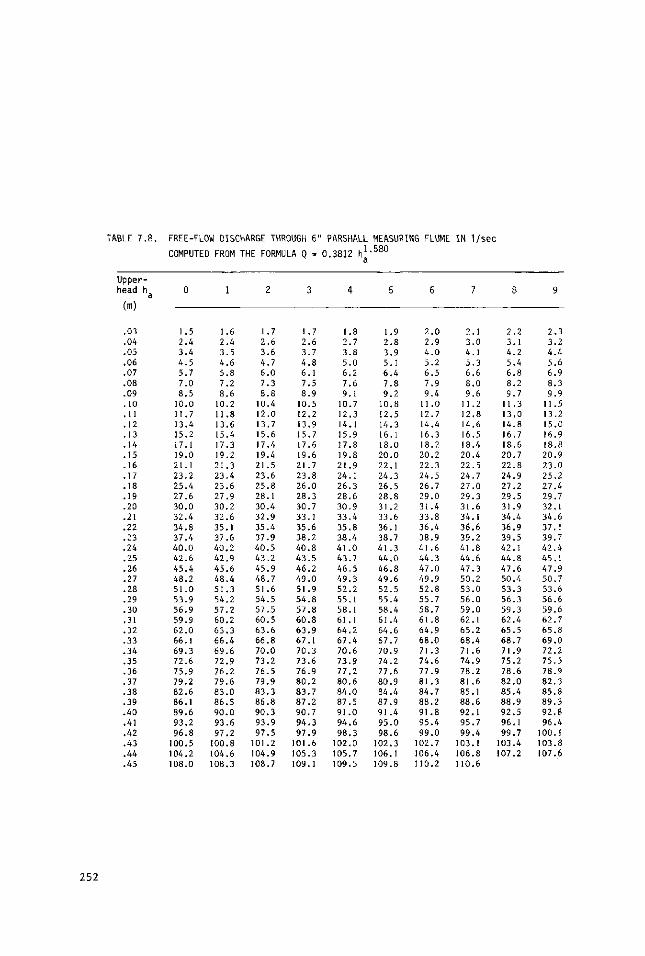
TABLE 7.8.
Upper-head h
(m)
.03
.04
.05
.06
.07
.08
.09
.10
.11
.12
.13
.14
.15
.16
.17
.18
.19
.20
.21
.22
.23
.24
.25
.26
.27
.28
.29
.30
.31
.32
.33
.34
.35
.36
.37
.38
.39
.40
.41
.42
.43
.44
.45
FREE-FLOW DISCHARGE THROUGH 6"
COMPUTED FROM
0
1.5 2.4 3.4 4.5 5.7 7.0 8.5
10.0 11.7 13.4 15.2
17.1 19.0
21.1 23.2
25.4 27.6 30.0 32.4
34.8 37.4
40.0 42.6
45.4 48.2
51.0
53.9 56.9 59.9 62.0 66.1
69.3 72.6
75.9 79.2 82.6 86.1 89.6 93.2
96.8
100.5 104.2
108.0
1
1.6 2.4 3.5 4.6 5.8 7.2 8.6
10.2 11.8 13.6 15.4
17.3 19.2
21 .3 23.4 25.6 27.9 30.2
32.6 35.1 37.6
40.2
42.9 45.6 48.4
51.3 54.2 57.2 60.2
63.3 66.4 69.6
72.9 76.2
79.6 83.0 86.5 90.0 93.6 97.2
100.8
104.6 108.3
THE FORMULA Q =
2
1.7 2.6 3.6 4.7 6.0 7.3 8.8
10.4 12.0 13.7 15.6 17.4 19.4
21.5 23.6 25.8 28.1
30.4
32.9 35.4
37.9
40.5 43.2
45.9 48.7 51.6
54.5 57.5 60.5 63.6 66.8
70.0 73.2
76.5 79.9 83.3 86.8
90.3 93.9
97.5 101.2
104.9 108.7
3
1.7 2.6 3.7 4.8 6.1 7.5 8.9
10.5 12.2
13.9 15.7 17.6 19.6
21.7 23.8 26.0
28.3 30.7
33.1 35.6 38.2
40.8 43.5 46.2
49.0 51.9 54.8 57.8 60.8
63.9 67.1 70.3 73.6
76.9 80.2
83.7 87.2
90.7
94.3 97.9
101.6
105.3
109.1
PARSHALL
0.3812 h] a
4
1.8 2.7 3.8 5.0 6.2 7.6 9.1
10.7 12.3 14.1
15.9 17.8
19.8 21.9 24.1
26.3 28.6
30.9 33.4
35.8 38.4
41.0 43.7
46.5 49.3 52.2
55.1 58.1 61.1 64.2 67.4
70.6
73.9 77.2 80.6 84.0 87.5
91.0 94.6
98.3 102.0 105.7
109.5
MEASURING FLUME
.580
5
1.9 2.8 3.9 5.1 6.4 7.8 9.2
10.8 12.5 14.3 16.1 18.0 20.0 22.1
24.3 26.5 28.8
31 .2 33.6 36.1
38.7
41.3 44.0
46.8 49.6
52.5 55.4 58.4 61.4
64.6 67.7
70.9 74.2 77.6
80.9 84.4 87.9 91.4 95.0 98.6
102.3 106.1 109.8
6
2.0 2.9 4.0 5.2 6.5 7.9 9.4
11.0 12.7 14.4
16.3 18.2 20.2
22.3 24.5
26.7 29.0
31.4 33.8
36.4 38.9 41.6
44.3 47.0 49.9 52.8
55.7 58.7 61.8
64.9 68.0
71.3 74.6
77.9 81.3 84.7 88.2
91.8 95.4
99.0 102.7 106.4 110.2
IN 1/sec
7
2.1 3.0 4.1 5.3 6.6 8.0 9.6
11.2 12.8 14.6 16.5 18.4 20.4
22.5
24.7 27.0 29.3 31.6 34.1
36.6 39.2
41.8 44.6
47.3 50.2
53.0 56.0 59.0 62.1 65.2 68.4 71.6
74.9 78.2
81.6 85.1 88.6 92.1 95.7
99.4
103.1 106.8 110.6
8
2.2 3.1 4.2 5.4 6.8 8.2 9.7
11.3 13.0 14.8 16.7 18.6 20.7
22.8
24.9 27.2
29.5 31.9 34.4
36.9 39.5 42.1
44.8 47.6 50.4
53.3 56.3 59.3 62.4 65.5 68.7
71.9 75.2 78.6
82.0 85.4 88.9 92.5 96.1
99.7 103.4 107.2
9
2.3 3.2 4.4 5.6 6.9 8.3 9.9
11.5 13.2 15.0
16.9 18.8
20.9 23.0 25.2 27.4
29.7 32.1 34.6
37.1 39.7 42.4
45.1
47.9 50.7 53.6 56.6 59.6
62.7 65.8 69.0 72.2 75.5
78.9 82.3 85.8 89.3 92.8 96.4
100.1 103.8 107.6
252
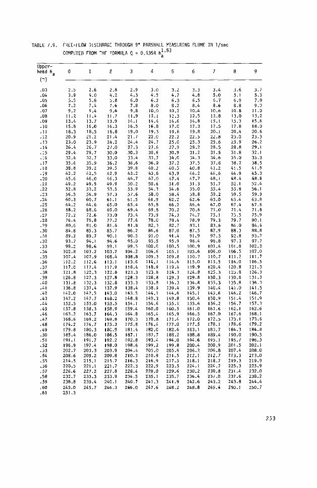
TABLE 7 . 9 .
Upper-head h
(m)
.03
.04
.05
.06
.07
.08
.09
.10
.11
.12
.13
.14
.15
.16
.17
.18
.19
.20
.21
.22
.23
.24
.25
.26
.27
.28
.29
.30
.31
.32
.33
.34
.35
.36
.37
.38
.39
.40
.41
.42
.43
.44
.45
.46
.47
.48
.49
.50
.51
.52
.53
.54
.55
.56
.57
.58
.59
.60
.61
FREE-FLOW DISCHARGE THROUGH 9"
COMPUTED FROM THE FORMULA Q =
0
2.5 3.9 5.5 7.2 9.2
11.2 13.4 15.8 18.3 20.9 23.0 26.4 29.4 32.4 35.6 38.8 42.2 45.6 49.2 52.8 56.5 60.3 64.2 68.2 72.2 76.4 80.6 84.8 89.2 93.7 98.2
102.8 107.4 112.2 117.0 121.8 126.8 131.8 136.8 142.0 147.2 152.5 157.8 163.2 168.6 174.2 179.8 185.4 191.1 196.9 202.7 208.6 214.5 220.5 226.6 232.7 238.8 245.0 251.3
1
2.6 4.0 5.6 7.4 9.4
11.4 13.7 16.0 18.5 21.2 23.9 26.7 29.7 32.7 35.9 39.2 42.5 46.0 49 .5 53.2 56.9 60.7 64.6 68.6 72.6 76.8 81.0 85.3 89.7 94.1 98.6
103.2 107.9 112.6 117.4 122.3 127.3 132.3 137.4 142.5 147.7 153.0 158.3 163.7 169.2 174.7 180.3 186.0 191.7 197.4 203.3 209.2 215.1 221.1 227.2 233.3 239.4 245.7
2
2 .8 4 .2 5 .8 7.6 9.6
11.7 13.9 16.3 18.8 21.4 24.2 27.0 30.0 33.0 36.2 39.5 42.9 46.3 49.9 53.5 57.3 61.1 65.0 69.0 73.0 77.2 81.4 85.7 90.1 94.6 99.1
103.7 108.4 113.1 117.9 122.8 127.8 132.8 137.9 143.0 148.2 153.5 158.9 164.3 169.8 175.3 180.9 186.5 192.2 198.0 203.9 209.8 215.7 221.7 227.8 233.9 240.1 246.3
3
2 .9 4 .3 6.0 7.8 9.8
11.9 14.1 16.5 19.0 21.7 24.4 27.3 30.3 33.4 36.6 39.8 43.2 46.7 50.2 53.9 57.6 61.5 65.4 69.4 73.4 77.6 81.8 86.2 90.5 95.0 99.5
104.2 108.8 113.6 118.4 123.3 128.3 133.3 138.4 143.5 148.8 154.1 159.4 164.8 170.3 175.8 181.4 187.1 192.8 198.6 204.4 210.3 216.3 222.3 228.4 234.5 240.7 246.0
PARSHALL
0.5354 h\ a
4
3.0 4.5 6.2 8.0
10.0 12.1 14.4 16.8 19.3 22.0 24.7 27.6 30.6 33.7 36.9 40.2 43.6 47.0 50.6 54.3 58.0 61.9 65.8 69.8 73.9 78.0 82.3 86.6 91.0 95.5
100.0 104.6 109.3 114.1 118.9 123.8 128.8 133.8 138.9 144.1 149.3 154.6 160.0 165.4 170.8 176.4 182.0 187.7 193.4 199.2 205.0 210.9 216.9 222.9 229.0 235.1 241.3 247.6
MEASURING FLUME
.53
5
3.2 4 .7 6 .3 8.2
10.2 12.3 14.6 17.0 19.6 22.2 25.0 27.9 30.9 34.0 37.2 40 .5 43.9 47.4 51.0 54.6 58.4 62.2 66.2 70.2 74.3 78.4 82.7 87.0 91.4 95.9
100.5 105.1 109.8 114.6 119.4 124.3 129.3 134.3 139.4 144.6 149.8 155.1 160.5 165.9 171.4 177.0 182.6 188.2 194.0 199.8 205.6 211.5 217.5 223.5 229.6 235.7 241.9 248.2
6
3.3 4 .8 6 .5 8.4
10.4 12.5 14.8 17.3 19.8 22.5 25 .3 28.2 31.2 34 .3 37.5 40 .8 44.2 47.7 51.3 55.0 58.8 62.6 66.6 70.6 74.7 78.9 83.1 87.5 91.9 96.4
100.9 105.6 110.2 115.0 119.9 124.8 129.8 134.8 139.9 145.1 150.4 155.6 161.0 166.5 172.0 177.5 183.1 188.8 194.6 200.4 206.2 212.1 218.1 224.1 230.2 236.4 242.6 248.8
IN 1/sec
7
3.4 5.0 6.7 8.6
10.6 12.8 15.1 17.5 20.1 22.8 25.6 28.5 31.5 34.6 37.8 41.2 44.6 48.1 51.7 55.4 59.2 63.0 67.0 71.0 75.1 79.3 83.6 87.9 92.3 96.8
101.4 106.0 110.7 115.5 120.4 125.3 130.3 135.3 140.4 145.6 150.9 156.2 161 .6 167.0 172.5 178.1 183.7 189.4 195.1 200.9 206.8 212.7 218.7 224.7 230.8 237.0 243.2 249.4
8
3.6 5.1 6.9 8.8
10.8 13.0 15.3 17.8 20.4 23.0 25.9 28.8 31.8 35.0 38.2 41 .5 44.9 48.4 52.1 55.8 59.5 63.4 67.4 71.4 75.5 79.7 84.0 88 .3 92.8 97 .3
101.8 106.5 111.2 116.0 120.8 125.8 130.8 135.8 141.0 146.2 151.4 156.7 162.1 167.6 173.1 178.6 184.3 190.0 195.7 201.5 207.4 213.3 219.3 225.3 231.4 237.6 243.8 250.1
9
3.7 5.3 7.0 9.0
11.0 13.2 15.6 18.0 20.6 23.3 26.2 29.1 32.1 35.3 38.5 41.8 45 .3 48.8 52.4 56.1 59.9 63.8 67.8 71.8 75.9 80.1 84.4 88.8 93.2 97.7
102.3 107.0 111.7 116.5 121.3 126.3 131 .3 136.3 141.5 146.7 151.9 157.3 162.6 168.1 173.6 179.2 184.8 190.5 196.3 202.1 208.0 213.0 219.9 225.9 232.0 238.2 244.4 250.7
253
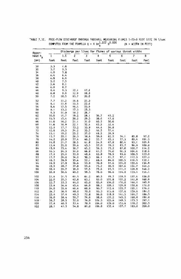
,ELE 7.10.
Upper-head h
(mm)
30 32 34 36 38 40 42 44 46 48 50
52 54 56 58 60 62 64 66 68 70 72 74 76 78 80 82 84 86 88 90 92 94 96 98
100
102 104 106 108 110 112 114 116 118-120 122
FREE-I FLOW DISCHARGE THROUGH PARSHALL MEASURING
COMPUTED FROM
1
feet
3.3 3.7 4.0 4.4 4.8 5.2 5.6 6.0 6.4 6.8 7.2
7.7 8.1 8.6 9.1 9.5
10.0 10.5 11.0
11.6 12.1 12.6
13.1 13.7 14.2
14.8 15.4
15.9 16.5
17.1 17.7 18.3 18.9 19.5
20.1 20.8
21.4 22.0 22.7 23.4 24.0
24.7
25.4 26.0
26.7 27.4 28.1
THE FORMULA Q =
Discharge per
1.5
feet
4.8 5.3 5.8 6.4 6.9 7.5 8.1 8.7 9.3 9.9
10.5
11.2
11.9 12.5 13.2
14.0 14.7 15.4 16.2
16.9 17.7 18.5 19.2
20.1 20.9
21.7 22.0 23.4
24.3 25.1
26.0
26.9 27.8 28.7
29.7 30.6
31.5 32.5 33.5
34.4 35.4
36.4 37.4
38.4 39.5 40.5 41.5
2
feet
12.1
12.9
13.7
14.6 15.5 16.4
17.3 18.2 19.2 20.2 21.1 22.1
23.2 24.2 25.2
26.3 27.4
28.5 29.6 30.7
31 .9 33.0 34.2
35.4 36.6 37.8
39.0 40.2
41.5 42.8 44.0
45.4 46.6
48.0 49.3
50.7 52.0 53.4 54.8
4 b h 1 " 5 2 2 b 0 - 0 2 6
3
1/sec for flumes
3
feet
17.6 18.8
20.0
21.3 22.6
23.9 25.3 26.7 28.1
29.5 3!.0 32.4
33.9 35.5 37.0 38.6 40.2
41.8 43.5 45.2
46.8 48.6 50.3 52.1 53.8 55.6
57.5
59.3
61.2 63.1 65.0
66.9
68.9 70.8 72.8 74.8
76.9 78.9 81.0
4
feet
36.7 38.6 40.5
42.5 44.4 46.5 48.5 50.6
52.7 54.9 57.0
59.3 61.5 63.8
66.1 68.4 70.8 73.2
75.6 78.0
80.5 83.0 85.6
88.1 90.7
93.3 96.0
98.6 101.3 104.0 106.8
FLUMES
(b
1-TO-S FOOT SIZ
= WIDTH IN FEET
of various throat widths
5
feet
45.2 47.6
50.0 52.4 54.8 57.4
59.9 62.5 65.1 67.8
70.5 73.2 76.0 78.9 81.7 84.6 87.6
90.5 93.5 96.6
99.7 102.8 106.0
109.1 112.4 115.6
118.9 122.2 125.6 129.0 132.4
6
feet
74.1 77.3 80.4
83.7 87.0
90.3 93.6 97.1
100.5 104.0 107.6 111.2
114.8
118.5 122.2 126.0 129.8
133.7 137.6
141.5 145.5 149.5 153.6 157.7
7
feet
85.8 89.4
93.1 96.9
100.7 104.6
108.5 112.5
116.5 120.6 124.7
128.9 133.1
137.4 141.8
146.1 150.6
155.1 159.6
164.2 168.8
173.5 178.2 183.0
8
feet
97.2
101.3 105.6
109.8 114.2 118.6 123.0 127.5
132.1 136.8
141.5 146.2
151.1
156.0 160.9 165.9 171.0
176.1 181.2 186.5
191 .8 197.1 202.5 208.0
254
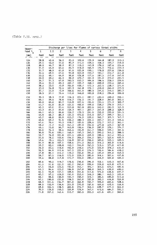
(Table 7.10. cont.)
Upper-head h
(mm)
124 126 128 130 132 134 136 138 140 142 144 146 148 150
152 154 156 158 160 162 164 166 168 170 172 174 176 178 180 182 184 186 188 190 192 194 196 198 200
202 204 206 208 210 212 214 216 218 220 222 224 226
1
feet
28.8
29.5 30.2
31.0
31.7 32.4 33.2
33.9 34.7 35.4 36.2
37.0
37.7 38.5
39.3 40.1
40.9 41.7 42.5 43.3 44.1
44.9 45.7 46.6 47.4 48.2 49.1
50.0 50.8
51.7
52.5 53.4 54.3
55.2
56.0
56,9 57.8
58.7 59.6
60.6 61.5 62.4
63.3 64.2 65.2
66.1
67.1
68.0 69.0
69.9 70.9 71.8
Discharge per
1.5
feet
42.6 43.6
44.7 45.8
46.9
48.0
49.1 50.2
51.3 52.5
53.6
54.8
55.9 57.1
58.3
59.4 60.6
61.8 63.0 64.2
65.5
66.7 68.0 69.2
70.4 71.7 73.0
74.3 75.6 76.8 78.2
79.5
80.8 82.!
83.4 84.8 86.1
87.5
88.8
90.2
91.6 93.0 94.4
95.8 97.2
98.6 100.0
101.4 102.9 104.3 105.8 107.2
2
feet
56.2
57.6
59.0 60.4
61.9
63.4 64.8 66.3 67.8 69.3 70.8
72.4
73.9 75.4
77.0
78.6 80.2 81.8 83.4
85.0
86.6
88.3 89.9
91 .6 93.3 95.0 96.7
98.4
100.1 101.8
103.6 105.3
107.1
108.8 110.6
112.4 114.2
116.0 117.8
119.7
121.5 123.4 125.2
127.1 129.0
130.9 132.8
134.7 136.6 138.5
140.5 142.4
1/sec for flumes
3
feet
83.1 85.2
87.3 89.5
91.6
93.8 96.0 98.2
100.5
102.7 105.0
107.3 109.6
112.0
114.3 116.7 119.0
121.4 123.8 126.3
128.7 131.2
133.7 136.2
138.7 141.2 143.8
146.4
148.9
151.5 154.2
156.8
159.4
162.1 164.8
167.5 170.2
172.9 175.7
178.4 181.2
184.0 186.8 189.6 192.4
195.3 198.2
201.0
203.9 206.8 209.8
212.7
4 feet
109.6 112.4 115.2
118.0
120.9
123.8 126.8
129.7 132.7
135.7 138.7
141.8
144.9 148.0
151.1
154.2 157.4 160.6 163.8
167.1 170.3 173.6
176.9 180.3 183.6
187.0 190.4 193.8
197.3
200.8 204.2
207.8
211.3
214.8 218.4
222.0 225.6
229.3 233.0
236.6
240.4 244.1 247.8 251.6
255.4 259.2
263.0
266.9 270.8 274.7 278.6
282.3
; of various throat width
5
feet
135.9 139.4
142.9
146.5 150.1
153.7 157.4 161.0 164.8
168.5
172.3 176.1
180.0 183.8
187.7
191.7 195.6
199.6 203.6
207.7 211.8
215.9 220.0 224.2
228.4 232.6 236.9 241.2
245.5
249.8 254.2 258.6
263.0
267.5 272.0
276.5 281.0 285.6
290.2
294.8
299.4 304.1 308.8 313.6
318.3
323.1 327.9 332.7 337.6
342.5 347.4
352.3
6
feet
161.8 166.0
170.2
174.5 178.8
183.1 187.5
191.9 196.4
200.9 205.4
210.0
214.6 219.2
223.9 228.6 233.4 238.2
243.0
247.9 252.8
257.7 262.7
267.7
272.7 277.8 282.9
288.0 293.2
298.4 303.7
309.0 314.3
319.6 325.0
330.4 335.9
341.4
346.9
352.4
358.0 363.6
369.3 375.0 380.7 386.4 392.2
398.0 403.8
409.7 415.6 421.6
7
feet
187.9 192.7
197.6
202.6 207.6
212.7 217.8 223.0 228.1
233.4
238.7 244.0 249.4
254.8
260.2
265.8
271.3 276.9 282.5 288.2
293.9 299.7 305.5
311.3 317.2
223.1 329.1 335.1 341.2
347.2
353.4
359.5 365.8
372.0
378.3 384.6 391.0
397.4 403.8
410.3 416.8 423.4 430.0 436.6
443.3 450.0 456.8
463.6 470.4
477.3 484.2
491.1
is
8
feet
213.5 219.0
224.6
230.3 236.0
241.8 247.6 253.5
259.4
265.4 271.4
277.5 283.7
289.8
296.1
302.4 308.7 315.1
321.5
328.0 334.5 341.1 347.7
354.4 361 .1
367.9 374.7 381.6 388.5
395.5
402.5 409.5 416.6
423.8 431.0 438.2
445.5 452.8
460.2
467.6
475.1 482.6 490.1 497.7
505.4 513.0 520.8
528.6 536.4 544.2 552.1
560.1
255
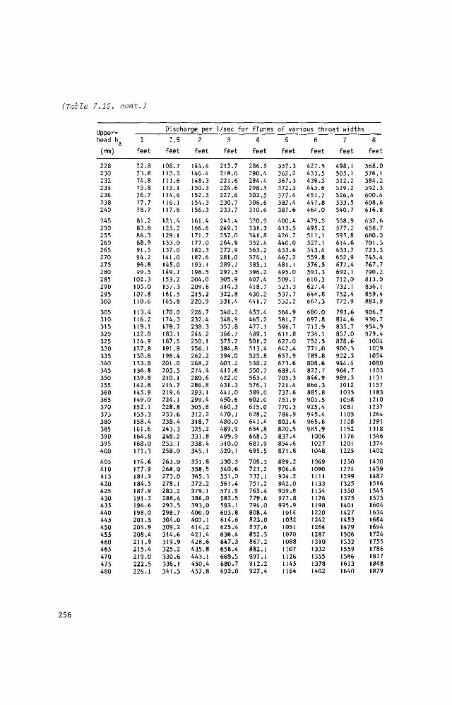
(Table 7.10.
Upper-head h
(mm)
228 230 232 234 236 238 240
245 250 255 260 265 270 275 280 285 290 295 300
305 310 315 320 325 330 335 340 345 350 355 360 365 370 375 380 385 390 395 400
405 410 415 420 425 430 435 440 445 450 455 460 465 470 475 480
aont.)
a 1 feet
72.8 73.8 74.8 75.8 76.7 77.7 78.7
81.2 83.8 86.3 88.9 91.5 94.2 96.8 99.5
102.3 105.0 107.8 110.6
113.4 116.2 119.1 122.0 124.9 127.8 130.8 133.8 136.8 139.8 142.8 145.9 149.0 152.1 155.3 158.4 161.6 164.8 168.0 171.3
174.6 177.9 181.2 184.5 187.9 191.2 194.6 198.0 201.5 204.9 208.4 211.9 215.4 219.0 222.5 226.1
Discharge per
1.5
feet
108.7 110.2 111.6 113.1 114.6 116.1 117.6
121.4 125.2 129.1 133.0 137.0 141.0 145.0 149.1 153.2 157.3 161.5 165.8
170.0 174.3 178.7 183.1 187.5 191.9 196.4 201.0 205.5 210.1 214.7 219.4 224.1 228.8 233.6 238.4 243.3 248.2 253.1 258.0
263.0 268.0 273.0 278.1 283.2 288.4 293.5 298.7 304.0 309.2 314.6 319.9 325.2 330.6 336.1 341.5
2
feet
144.4 146.4 148.3 150.3 152.3 154.3 156.3
161.4 166.6 171.7 177.0 182.3 187.6 193.1 198.5 204.0 209.6 215.2 220.9
226.7 232.4 238.3 244.2 250.1 256.1 262.2 268.2 274.4 280.6 286.8 293.1 299.4 305.8 312.2 318.7 325.2 331 .8 338.4 345.1
351.8 358.5 365.3 372.2 379.1 386.0 393.0 400.0 407.1 414.2 421.4 428.6 435.8 443.1 450.4 457.8
1/sec fa
3
feet
215.7 218.6 221.6 224.6 227.6 230.7 233.7
241.4 249.1 257.0 264.9 272.9 281.0 289.2 297.5 305.9 314.3 322.8 331.4
340.2 348.9 357.8 366.7 375.7 384.8 394.0 403.2 412.6 422.0 431.3 441.0 450.6 460.3 470.1 480.0 489.9 499.9 510.0 520.1
530.3 540.6 551.0 561.4 571.9 582.5 593.1 603.8 614.6 625.4 636.4 647.3 658.4 669.5 680.7 692.0
r flumes
4 feet
286.5 290.4 294.4 298.5 302.5 306.6 310.6
320.9 331.3 341.8 352.4 363.2 374.1 385.1 396.2 407.4 418.7 430.2 441.7
453.4 465.2 477.1 489.1 501.2 513.4 525.8 538.2 550.7 563.4 576.1 589.0 602.0 615.0 628.2 641.4 654.8 668.3 681.9 695.5
709.3 723.2 737.1 751.2 765.4 779.6 794.0 808.4 823.0 837.6 852.3 867.2 882.1 897.1 912.2 927.4
of various throat width
5
feet
357.3 362.2 367.3 372.3 377.4 382.4 387.6
400.4 413.5 426.7 440.0 453.6 467.2 481.1 495.0 509.1 523.3 537.7 552.2
566.9 581.7 596.7 611.8 627.0 642.4 657.9 673.6 689.4 705.3 721.4 737.6 753.9 770.3 786.9 803.6 820.5 837.4 854.6 871.8
889.2 906.6 924.2 942.0 959.8 977.8 995.9
1014 1032 1051 1070 1088 1107 1126 1145 1164
6
feet
427.5 433.5 439.5 445.6 451.7 447.8 464.0
479.5 495.2 511.1 527.1 543.4 559.8 576.5 593.3 610.3 627.4 644.8 662.3
680.0 697.8 715.9 734.1 752.5 771.0 789.8 808.6 827.7 846.9 866.3 885.8 905.5 925.4 945.4 965.6 985.9
1006 1027 1048
1069 1090 1111 1133 1154 1176 1198 1220 1242 1264 1287 1310 1332 1355 1378 1402
7
feet
498.1 505.1 512.2 519.2 526.4 533.5 540.7
558.9 577.2 595.8 614.6 633.7 652.9 672.4 692.1 712.0 732.1 752.4 772.9
793.6 814.6 835.7 857.0 878.6 900.3 922.3 944.4 966.7 989.3
1012 1035 1058 1081 1105 1128 1152 1176 1201 1225
1250 1274 1299 1325 1350 1375 1401 1427 1453 1479 1506 1532 1559 1586 1613 1640
s
8
feet
568.0 576.1 584.2 592.3 600.4 608.6 616.8
637.6 658.7 680.0 701.5 723.3 745.4 767.7 790.2 813.0 836.1 859.4 882.9
906.7 930.7 954.9 979.4
1004 1029 1054 1080 1105 1131 1157 1183 1210 1237 1264 1291 1318 1346 1374 1402
1430 1459 1487 1516 1545 1575 1604 1634 1664 1694 1724 1755 1786 1817 1848 1879
256
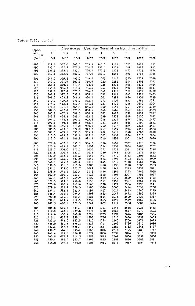
(Table 7.10. aont.)
Upper-
head h
(mm)
485 490 495 500
505 510 515 520 525 530 535 540 545 550 555 560 565 570 575 580 585 590 595 600
605 610 615 620 625 630 635 640 645 650 655 660 665 670 675 680 685 690 695 .700
705 710 715 720 725 730 735 740 745 750 755 760
1
feet
229.7 233.3
236.9 240.6
244.2
247.9 251.6
255.4
259.1 262.9 266.7 270.5
274.3 278.1
282.0
285.9 289.8 293.7
297.6 301.6 305.5 309.5 313.5
317.5
321.6
325.6 329.7
333.8 337.9
342.0 346.1
350.3 354.5 358.6
362.9 367.1 371.3 375.6
379.8 384.1
388.4
392.8 397.1
401.5
405.8 410.2
414.6
419.1
423.5 428.0 432.4
436.9
441.4
445.9 450.4
455.0
Dischi
1.5
feet
347.0 352.5 358.1
363.6
369.2
374.9 380.6
386.3 392.0
397.7 403.5 409.3 415.2 421.1
427.0
432.9 438.8 444.8 450.8
456.9 463.0 469.1 475.2
481.4
487.5
493.7 500.0 506.2
512.5
518.9 525.2
531.6
538.0 544.4
550.9 557.3 563.8 570.4
576.9
583.5
599.1 596.8 603.4
610.1
616.8 623.6
630.4 637.2
644.0 650.8
657.7 664.6
671.5
678.4 685.4
692.4
ïrge per
2
feet
465.2 472.6
480.1 487.7
495.3
502.9 510.5 518.2 526.0
533.8 541.6
549.5 557.4
565.3 573.3
581.3 589.4 597.5
605.6 613.8 622.0 630.3 638.6
646.9
655.3 663.7 672.2
680.7 689.2
697.8 706.4
715.0 723.7
732.4 741.1
749.9 758.8
767.6 776.5
785.4 794.4
803.4 812.5
821.5
839.7 839.8
849.0 858.2
867.5 876.8
886.1
895.4
904.8
914.3 923.7
933.2
1/sec fo
3
feet
703.3 714.7 726.1 737.6
749.2
760.9 772.6 784.4
796.2
808.1 820.1 832.1 844.2
856.4
868.6
880.9 893.2
905.6
918.1 930.6 943.2
955.9 968.6
981.4
994.2
1007 1020
1033 1046
1059 1072
1086
1099 1112 1126
1139 1153 1166
1180 1194 1208
1221
1235
1249
1263 1277
1292
1306 1320
1334 1349
1363 1377
1392
1406
1421
r flumes
4
feet
942.7 958.1
973.5 989.1
1005 1020 1036
1052 1068
1084 1101
1117 1133 1150
1166
1183
1199 1216
1233 1250 1267 1284 1302
1319
1336
1354
1371 1389 1407
1424 1442
1460 1478 1496
1515
1533 1551 1570 1588
1607 1625
1644 1663 1682
1701 1720
1739 1758 1778
1797 1817
1836
1856
1875 1895
1915
of various throat widths
5
feet
1184 1203
1223 1242
1262 1282
1302 1322
1342
1363 1383 1404 1424
1445 1466
1487
1508
1529 1551 1572
1594 1615 1637
1659
1681
1703 1725 1748
1770
1793 1815 1838
1861 1884 1907
1930
1953 1977 2000 2024 2047
2071 2095
2119
2143 2167
2191 2216 2240 2265
2289 2314
2339 2364
2389
2414
6
feet
1425 1448 1472 1496
1520 1544
1568 1592
1617 1642 1666
1691 1716
1741 1767 1792
1818
1844 1869
1895 1922 1948 1974
2001
2027 2054 2081
2108 2135
2163 2190
2218 2245
2273 2301
2529 2357 2386 2414
2443 2472
2500
2529 2558
2588 2617 2646
2676 2706
2736
2765 2796
2826 2856
2886
2917
7
feet
1668 1695
1723 1751
1779
1808 1836 1865
1893 1922 1951 1981
2010
2040
2070 2099
2130 2160 2190 2221 2252 2282
2313
2345
2376 2408
2439 2471
2503 2535
2567 2600 2632
2665 2698
2731 2764
2798 2831
2865
2899 2933
2967
3001
3035 3070
3105
3139 3174 3210 3245
3280
3316
3351
3387
3423
8
feet
1911 1942 1974 2006
2039 2071 2104
2137 2170
2203 2239
2271 2304
2339 2373 2407
2442
2477 2512
2547 2582
2618 2654
2690
2726 2762
2798
2835 2872
2909 2946
2983 3021
3059 3097
3135 3173 3211 3250
3289 3328
3367 3406
3446
3485 3525
3565 3605 3645 3686
3727 3767
3808
3850
3891
3932
257
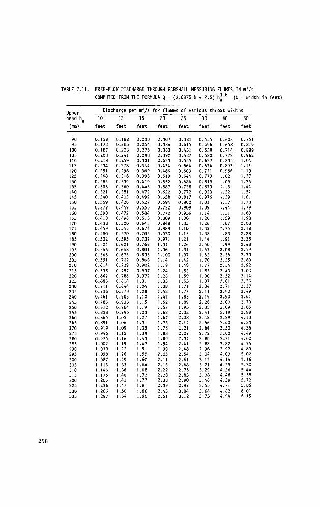
TABLE 7.11. FREE-FLOW DISCHARGE THROUGH PARSHALL MEASURING FLUMES IN m 3 /s.
COMPUTED FROM THE FORMULA Q = (3.6875 b + 2.5) h 1 - 6 (b = width in feet)
Upper-head h
(mm)
90 95
100 105
110
115 120 125 130 135
140 145 150
155 160 165
170 175 180 185
190 195
200 205
210 215 220 225
230 235 240 245
250 255
260 265 270 275 280 285
290 295
300 305 310 315 320
325 330 335
Di s
10 feet
0.158 0.173
0.187 0.203
0.218 0.234
0.251 0.268 0.285 0.303 0.321 0.340
0.359 0.378
0.398 0.418
0.438 0.459 0.480 0.502
0.524 0.546
0.568
0.591 0.614 0.638 0.662 0.686
0.711 0.736 0.761 0.786 0.812
0.838 0.865 0.891
0.919 0.946
0.974 1.002
1.030 1.058 1.087 1.116 1.146 1.175 1.205
1.236 1.266
1.297
charge pe
12 feet
0.188 0.205
0.223 0.241
0.259 0.278 0.298
0.318 0.339 0.360 0.381 0.403
0.426
0.449 0.472 0.496
0.520 0.545 0.570
0.595 0.621 0.648
0.675 0.702
0.739 0.757 0.786 0.814
0.844 0.873
0.903 0.933 0.964
0.995 1.03 1.06 1.09 1.12
1.16
1.19 1.22 1.26
1.29 1.33 1.36 1.40 1.43
1.47 1.50 1.54
r m3/s
15 feet
0.233 0.254
0.275 0.298 0.321
0.344
0.369 0.393
0.419 0.445 0.472
0.499 0.527 0.555
0.584 0.613
0.643 0.674 0.705
0.737 0.769 0.801
0.835 0.868 0.902
0.937 0.972
1.01 1.04 1.08 1.12 1.15
1.19 1.23 1.27
1.31 1.35 1.39 1.43 1.47
1.51 1.55 1.60 1.64
1.68 1.73 1.77 1.8!
1.86 1.90
for flumes of various throat widths
20 feet
0.307 0.334
0.363 0.392
0.423 0.454
0.486
0.519 0.552
0.587 0.622
0.658
0.694 0.732
0.770 0.809 0.848
0.889 0.930 0.971
1.01 1.06
1.100 1.14
1.19 1.24 1.28 1.33 1.38 1.42
1.47 1.52
1.57 1.62
1.67 1.73 1.78
1.83 1.89 1.94
1.99 2.05 2.11
2.16 2.22 2.28
2.33 2.39
2.45 2.51
25 feet
0.381 0.415
0.451 0.487 0.525 0.564
0.603 0.644
0.686 0.728 0.772
0.817 0.862
0.909 0.956 1.00 1.05 1.10
1.15 1.21
1.26
1.31
1.37 1.42
1.48
1.53 1.59 1.65 1.71 1.77
1.83 1.89 1.95 2.02
2.08 2.14 2.21 2.27
2.34 2.41
2.48 2.54 2.61 2.68 2.75 2.83 2.90
2.97
3.04 3.12
30 feet
0.455 0.496
0.539 0.582
0.627 0.674
0.721 0.770
0.819 0.870
0.923 0.976
1.03 1.09 1.14 1.20 1.26 1.32
1.38 1.44
1.50 1.57
1.63 1.70
1.77 1 .83 1 .90 1.97
2.04 2.11 2.19 2.26 2.33 2.41
2.48 2.56
2.64 2.72
2.80
2.88 2.96 3.04
3.12 3.21
3.29 3.38
3.46
3.55 3.64 3.73
40 feet
0.603 0.658
0.714 0.772
0.832 0.893 0.956
1.02
1 .09 1.15 1.22
1 .29
1.37 1.44 1.51 1.59 1.67 1.75
1.83 1.91
1.99 2.08
2.16
2.25 2.34 2.43 2.52 2.61
2.71 2.80 2.90 3.00 3.09 3.19
3.29 3.40
3.50 3.60 3.71 3.82
3.92 4.03 4.14 4.25 4.36 4.48
4.59 4.71
4.82 4.94
50 feet
0.751
0.819
0.889 0.962
1.04 1.11
1.19 1.27 1.35 1.44
1.52 1.61
1.70
1.79 1.89 1.98 2.08
2.18 2.28 2.38
2.48 2.59
2.70 2.80 2.92
3.03 3.14 3.26
3.37 3.49 3.61 3.73 3.85 3.98 4.10
4.23 4.36
4.49 4.62
4.75
4.89 5.02 5.16
5.30 5.44 5.58 5.72
5.86 6.01 6.15
258
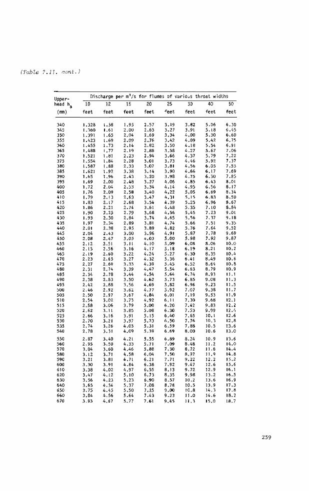
(Table 7.11. aont.
Upper-head h
(mm)
340 345 350 355 360 365 370 375 380 385 390 395 400 405 410 415 420 425 430 435 440 445 450 455 460 465 470 475 480 485 490 495 500 505 510 515 520 525 530 535 540
550 560 570 580 590 600 610 620 630 640 650 660 670
)
Dis
10
f e e t
1.328 1.360 1 .391 1.423 1.455 1.488 1.521 1.554 1.587 1.621 1.65 1.69 1.72 1.76 1.79 1.83 1.86 1.90 1.93 1.97 2.01 2.04 2 .08 2.12 2.15 2.19 2 .23 2.27 2.31 2.34 2 .38 2.42 2.46 2.50 2.54 2 .58 2.62 2.66 2.70 2.74 2 .78
2.87 2.95 3.04 3.12 3.21 3.30 3.38 3.47 3.56 3.65 3.75 3.84 3.93
charge
12
f e e t
1.58 1.61 1.65 1.69 1.73 1.77 1.81 1.84 1.88 1.92 1.96 2.00 2.04 2.09 2.13 2.17 2.21 2.25 2.30 2.34 2 .38 2.43 2.47 2.51 2.56 2.60 2.65 2.69 2.74 2.78 2.83 2.88 2.92 2.97 3.02 3.06 3.11 3.16 3.21 3.26 3.31
3.40 3.50 3.60 3.71 3.81 3.91 4.02 4.12 4.23 4.34 4.45 4.56 4.67
per m3 /s
15
f e e t
1.95 2.00 2.04 2.09 2.14 2.19 2 .23 2 .28 2.33 3.38 2.43 2 .48 2.53 2 .58 2.63 2.68 2.74 2.79 2.84 2.89 2.95 3.00 3.05 3.11 3.16 3.22 3.27 3.33 3.39 3.44 3.50 3.56 3.62 3.67 3.73 3.79 3.85 3.91 3.97 4 .03 4.09
4.21 4.33 4.46 4 .58 4.71 4 .84 4.97 5.10 5.23 5.37 5.50 5.64 5.77
for flumes of various throat wi
20
f e e t
2.57 2.63 2.69 2.76 2.82 2.88 2.94 3.01 3.07 3.14 3.20 3.27 3.34 3.40 3.47 3.54 3.61 3.68 3.74 3.81 3.89 3.96 <t.03 4.10 4.17 4.24 4.32 4.39 4.47 4.54 4.62 4.69 4.77 4.84 4.92 5.00 5.08 5.15 5.23 5.31 5.39
5.55 5.71 5.88 6.04 6.21 6.38 6.55 6.73 6.90 7.08 7.25 7.43 7.61
25
f e e t
3.19 3.27 3.34 3.42 3.50 3.58 3.66 3.73 3.81 3.90 3.98 4.06 4.14 4.22 4.31 4.39 4 .48 4 .56 4.65 4.74 4.82 4 . 9 ! 5.00 5.09 5.18 5.27 5.36 5.45 5.54 5.64 5.73 5.82 5.92 6.01 6.11 6.20 6.30 6.40 6.50 6.59 6.69
6.89 7.09 7.30 7.50 7.71 7.92 8.13 8.35 8.57 8.78 9.00 9.23 9.45
30
f e e t
3.82 3.91 4.00 4.09 4 .18 4.27 4.37 4.46 4.56 4.66 4 .75 4 .85 4.95 5.05 5.15 5.25 5.35 5.45 5.56 5.66 5.76 5.87 5.98 6.08 6.19 6.30 6.41 6.52 6.63 6.74 6.85 6.96 7.07 7.19 7.30 7.42 7.53 7.65 7.76 7.88 8.00
8.24 8.48 8.72 8.97 9.22 9.47 9.72 9 .98 10.2 10.5 10.8 11 .0 11 .3
40
f e e t
5.06 5.18 5.30 5.42 5.54 5.67 5.79 5.92 6.05 6.17 6.30 6.43 6.56 6.69 6.83 6.96 7.10 7 .23 7.37 7.51 7.64 7.78 7.92 8.06 8.21 8.35 8.49 8.64 8.79 8.93 9.08 9.23 9.38 9.53 9.68 9.83 9.99 10.1 10.3 10.5 10.6
10.9 11.2 11.6 11.9 12.2 12.6 12.9 13.2 13.6 13.9 14.3 14.6 15.0
d ths
50
f e e t
6.30 6.45 6.60 6.75 6.91 7.06 7.22 7.37 7.53 7.69 7.85 8.01 8.17 8.34 8.50 8.67 8.84 9.01 9.18 9.35 9.52 9.69 9.87 10.0 10.2 10.4 10.6 10.8 10.9 11.1 11.3 11.5 11 .7 11.9 12.1 12.2 12.4 12.6 12.8 13.6 13.0
13.6 14.0 14.4 14.8 15.2 15.6 16.1 16.5 16.9 17.3 17.8 18.2 18.7
259
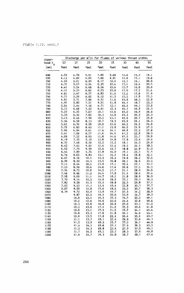
(Table 7.11. cont.)
Upper-head h
(mm)
680 690 700 710 720 730 740 750 760 770 780 790 800 810 820 830 840 850 860 870 880 890 900 910 920 930 940 950 960 970 980 990
1000 1010
1020 1030 1040 1050 1060 1070 1080
1090 1100 1110 1120
1130 1140 1150
1160 1170
1180
1190 1200
Di 10
feet
4.03 4.12 4.22
4.31 4.41
4.51 4.61
4.7! 4.81
4.91 5.01 5.12 5.22
5.33
5.43 5.54
5.65 5.75 5.86 5.97 6.08
6.19 6.31 6.42
6.53 6.64 6.76
6.87 6.99 7.11
7.23 7.34 7.46 7.58
7.70 7.82
7.95 8.07 8.19
scharge per m3/s
12 feet
4.78 4.89 5.01 5.12
5.24
5.35
5.47 5.59 5.71 5.83 5.95 6.08
6.20 6.32
6.45 6.58
6.70
6.83 6.96
7.09 7.22
7.35 7.48 7.62
7.75
7.89 8.02 8.16
8.30 8.44 8.58 8.72
8.86 9.00
9.14 9.29 9.43 9.58 9.72
9.87 10.0 10.2
10.3 10.5 10.6 10.8
10.9 11.1 11.2
11.4 11.5 11.7
11.9
15 feet
5.91 6.05
6.19 6.34
6.48 6.62
6.77 6.92 7.06 7.21
7.36 7.52
7.67 7.82
7.98
8.13
8.29 8.45 8.61
8.77 8.93 9.10 9.26 9.42
9.59 9.76
9.93 10.1
10.3 10.4 10.6
10.8 11 .0
11.1
11.3 11.5 11 .7 11.8 12.0 12.2
12.4 12.6
12.8 13.0
13.1 13.3 13.5 13.7
13.9 14.1
14.3 14.5
14.7
for flumes of various th
20 feet
7.80 7.98
8.17 8.35 8.54 8.73
8.93 9.12
9.31 9.51
9.71 9.91 10.1
10.3 10.5
10.7
10.9 11.1 11.4 11.6
11.8 12.0 12.2
12.4 12.6
12.9 13.1 13.3 13.5 13.8
14.0 14.2
14.4 14.7
14.9 15.1 15.4 15.6
15.9 16.1
16.3 16.6 16.8 17.1
17.3 17.6 17.8 18.1
18.3 18.6 18.8
19.1 19.3
25
feet
9.68 9.91 10.1 10.4 10.6 10.8
11.1 11.3 11.6 11.8 12.1
12.3 12.6 12.8
13.1 13.3
13.6 13.8 14.1 14.4 14.6
14.9 15.2
15.4
15.7 16.0 16.2 16.5
16.8 17.1 17.4 17.7
17.9 18.2
18.5 18.8
19.1 19.4 19.7 20.0
20.3 20.6
20.9 21.2
21.5 21.8 22.1
22.4 22.7 23.1
23.4 23.7 24.0
30 feet
11.6 11.8 12.1 12.4
12.7 13.0 13.2
13.5 13.8 14.1 14.4 14.7
15.0
15.3 15.6
15.9
16.2 16.5 16.8 17.2
17.5 17.8
18.1 18.4
18.8 19.1 19.4 19.8
20.1 20.4 20.8 21.1
21.4 21.8 22.1
22.5 22.8 23.2
23.5 23.9 24.2
24.6
25.0 25.3 25.7 26.1
26.4 26.8 27.2 27.6
27.9 28.3 28.7
roat wi
40 feet
15.3 15.7
16.1 16.4
16.8 17.2
17.6 17.9 18.3 18.7
19.1 19.5
19.9 20.3 20.7
21.1 21.5
21 .9 22.3 22.8 23.2
23.6 24.0
24.4
24.9 25.3 25.8 26.2
26.6
27.1 27.5 28.0
28.4
28.9 29.3 29.8
30.3 30.7 31.2
31.7 32.2 32.6
33.1 33.6
34.1 34.6
35.1 35.6
36.1 36.5
37.0 37.6
38.1
dths
50 feet
19.1 19.6 20.0
20.5 20.9 21.4
21.9 22.3 22.8 23.3 23.8
24.3 24.8 25.3 25.8
26.3
26.8
27.3 27.8 28.3
28.9 29.4
29.9 30.5 31.0 31.5 32.1 32.6 33.2
33.7 34.3 34.8 35.4
36.0
36.5 37.1 37.7
38.3 38.9 39.5 40.1 40.6 41.2 41.8
42.4 43.1
43.7 44.3 44.9 45.5 46.1 46.8
47.4
260
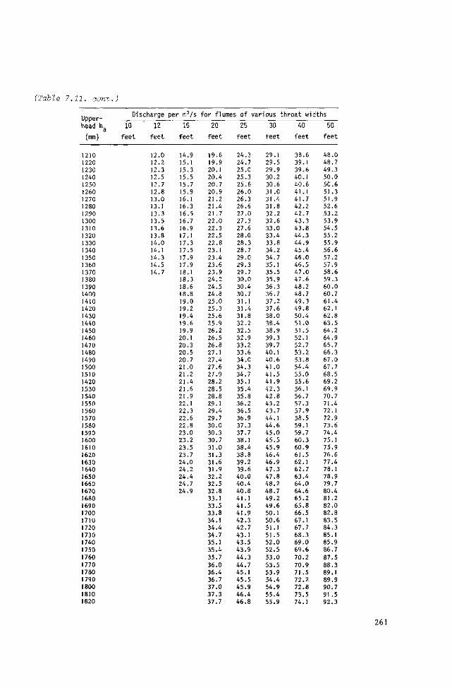
'Table ', 7.11. aont.
Upper-head h
(mm)
1210 1220
1230 1240
1250 1260
1270 1280 1290 1300
1310 1320
1330
1340 1350 1360
1370 1380
1390 1400 1410 1420
1430
1440 1450 1460
1470 1480
1490 1500
1510 1420
1530 1540 1550
1560 1570
1580
1590 1600
1610
1620
1630 1640
1650 1660
1670 1680
1690 1700
1710 1720
1730 1740
1750
1760
1770
1780 1790 1800
1810 1820
J Discharge
10 12
feet feet
12, 12, 12, 12. 12, 12. 13, 13, 13, 13, 13, 13. 14. 14, 14. 14. 14.
.0
.2
.3
.5
.7
.8
.0
.1
.3
.5
.6
.8
.0
.1 ,3 .5 ,7
per m3/s
15 feet
14.9
15.1 15.3 15.5
15.7
15.9 16.1 16.3 16.5
16.7 16.9
17.1 17.3 17.5
17.9
17.9 18.1 18.3 18.6 18.8
19.0 19.2
19.4 19.6
19.9
20.1 20.3 20.5 20.7 21 .0 21.2
21.4 21.6
21.9 22.1 22.3 22.6 22.8
23.0 23.2
23.5
23.7
24.0 24.2
24.4 24.7
24.9
for flumes of various throat wi
20 feet
19.6
19.9
20.1 20.4
20.7
20.9 21 .2 21.4 21.7 22.0
22.3 22.5
22.8
23.1 23.4 23.6
23.9 24.2
24.5 24.8
25.0 25.3 25.6
25.9 26.2
26.5 26.8
27.1 27.4 27.6
27.9 28.2
28.5 28.8
29.1 29.4
29.7
30.0 30.3 30.7
31.0
31.3 31.6
31 .9 32.2 32.5
32.8
33.1 33.5 33.8
34.1 34.4 34.7
35.1 35.4
35.7
36.0
36.4 36.7 37.0
37.3 37.7
25 feet
24.3 24.7
25.0 25.3
25.6 26.0
26.3 26.6
27.0
27.3 27.6 28.0
28.3 28.7
29.0
29.3 29.7 30.0
30.4 30.7
31.1 31.4 31.8 32.2
32.5
32.9 33.2
33.6 34.0 34.3
34.7
35.1 35.4 35.8 36.2 36.5
36.9
37.3 37.7
38.1 38.4
38.8 39.2 39.6 40.0 40.4 40.8
41.1 41.5
41.9
42.3 42.7
43.1 43.5
43.9
44.3
44.7 45.1
45.5 45.9
46.4 46.8
30 feet
29.1
29.5
29.9 30.2
30.6 31.0 31.4
31 .8 32.2
32.6
33.0 33.4 33.8 34.2
34.7 35.1 35.5
35.9 36.3 36.7 37.2
37.6 38.0
38.4
38.9 39.3 39.7
40.1 40.6 41.0
41.5 41.9
42.3 42.8 43.2 43.7 44.1
44.6
45.0 45.5
45.9 46.4
46.9 47.3 47.8 48.2
48.7 49.2
49.6
50.1 50.6
51.1 51.5 52.0
52.5
53.0
53.5
53.9 54.4
54.9 55.4
55.9
40 feet
38.6
39.1 39.6
40.1 40.6
41.1 41.7 42.2
42.7 43.3 43.8
44.3
44.9 45.4
46.0 46.5 47.0 47.6 48.2
48.7
49.3 49.8 50.4 51.0
51.5 52.1
52.7 53.2
53.8 54.4
55.0
55.6 56.1
56.7 57.3 57.9
58.5
59.1 59.7 60.3
60.9 61.5
62.1 62.7 63.4
64.0 64.6 65.2
65.8 66.5
67.1 67.7
68.3 69.0
69.6
70.2
70.9
71.5 72.2
72.8
73.5
74.1
dths
50 feet
48.0 48.7
49.3 50.0
50.6
51.3 51.9 52.6 53.2
53.9 54.5 55.2
55.9 56.6 57.2
57.9 58.6 59.3 60.0
60.7 61.4 62.1
62.8 63.5
64.2
64.9 65.7 66.3
67.0 67.7 68.5 69.2
69.9 70.7 71.4 72.1
72.9 73.6 74.4
75.1
75.9 76.6 77.4 78.1
78.9 79.7 80.4
81 .2 82.0 82.8
83.5 84.3
85.1 85.9
86.7
87.5
88.3
89.1 89.9 90.7
91.5
92.3
261
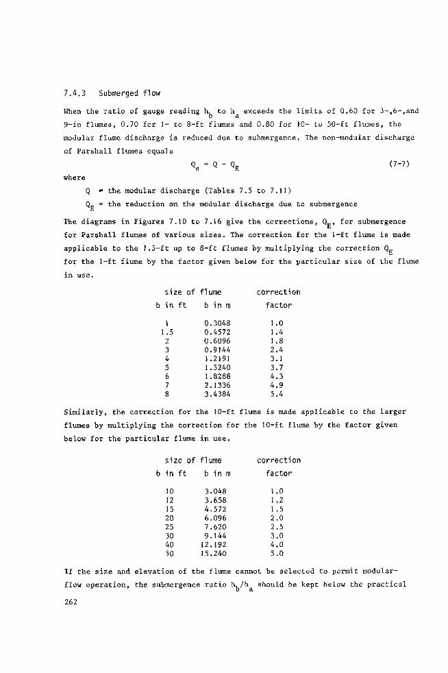
7.4.3 Submerged flow
When the ratio of gauge reading h, to h exceeds the limits of 0.60 for 3-,6-,and
9-in flumes, 0.70 for 1- to 8-ft flumes and 0.80 for 10- to 50-ft flumes, the
modular flume discharge is reduced due to submergence. The non-modular discharge
of Parshall flumes equals
where
QS = Q
the modular discharge (Tables 7.5 to 7.11)
the reduction on the modular discharge due to submergence
(7-7)
The diagrams in Figures 7.10 to 7.16 give the corrections, Q , for submergence
for Parshall flumes of various sizes. The correction for the 1-ft flume is made
applicable to the 1.5—ft up to 8-ft flumes by multiplying the correction Q
for the 1-ft flume by the factor given below for the particular size of the flume
in use.
size of
b in
1 1.5 2 3 4 5 6 7 8
ft flume
b in m
0.3048 0.4572 0.6096 0.9144 1.2191 1.5240 1.8288 2.1336 3.4384
correction
factor
1.0 1.4 1.8 2.4 3.1 3.7 4.3 4.9 5.4
Similarly, the correction for the 10-ft flume is made applicable to the larger
flumes by multiplying the correction for the 10-ft flume by the factor given
below for the particular flume in use.
size of
b in ft
10 12 15 20 25 30 40 50
flume
b in m
3.048 3.658 4.572 6.096 7.620 9.144
12.192 15.240
correction
factor
1.0 1.2 1.5 2.0 2.5 3.0 4.0 5.0
If the size and elevation of the flume cannot be selected to permit modular-
flow operation, the submergence ratio h, /h should be kept below the practical
262
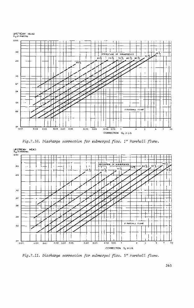
UPSTREAM HEAD h a in metres
s
y
s
S
y
y
s
y
s
s
y
y
'
y
y
s
*
*
.
>
•*
y
y
y .'
y
*
**
s
'
s
'
s
M
6 0
y' J
S*
'' , y
y„
y
y
>
s* /
y
y < y
6
s
s
5?
* X
PERCENTAGE OF SUBMERGENCE
^ 7
^
o°/
y s f
5 7a 80 % B 5 %
1" PARSHALL FLUME
9 0
s ' /
0 . 0 1 0 . 0 2 0 . 0 3 0 . 0 5 0 . 0 7 0 . 1 0 0 . 2 0 0 . 3 0 0 . 5 0 0 7 0 1 2 3 5 7 1 0
CORRECTION QE in L/s
Fig.7.10. Discharge correction for submerged flow. 1" Parshall flume.
UPSTREAM HEAD h a in metres O.SO
/
/
y
s
s
y
•
' y
/
y
y ,
>
s
y
'
s
,
y
A
s »
s
*
s
, 4
/
' y
y
y
y y
y y
y
y * *
y
y s
s S
°%
y
y
À
y
y] *
s
,
J
^
PERCENTAGE OF SUBMERGENCE
y
*
l0
y
y
y
y'
y
*
y
y
7 0 ?
' S
y [*% 0)
' 1
2" PARSHALL FLUME
1 5 "
9
1
1
o% ^
0.01 0.02 0.03 0.05 0.07 0.10 0.20 0.30 O.SO 0.70 1 2 3 S 7 10
CORRECTION QE in L/s
Fig.?.11. Discharge correction for submerged flow. 2" Parshall flume.
263
UPSTREAM HEAD h n in m e t r e s
4
J S
'
'
y
'
s
s s
s'
y
y
'
s
y
*
'
\s
<
'
S
'
s
*
s
''
y
• S
so
ri
y
y
x-
'
y
'
s
<*
*
'
PERCENTAGE OF SUBMERGENCE
6 5 %
y
/ s
S
y
Si
S
y'
^ >'
>%
-J .'
75 % 8 0 % 8 5 % 9 0 %
3" PARSHALL FLUME
95 °
0 . 2 0 .3
CORRECTION QE in L/s
SO 7 0 1 0 0
Fig.7.12. Discharge correction for submerged flow. 3" Parshall flume.
limit of 0.95, since the flume ceases to be a measuring device if submergence
exceeds this limit.
As mentioned, turbulence in the relatively deep and narrow throat of the "very
small" flumes makes the h,-gauge difficult to read. If an h -gauge is used under
submerged flow conditions, the h -readings should be converted to h, -readings
with the aid of Figure 7.17, and the converted h, -values are then used to de
termine the submerged discharge with the aid of Figures 7.10 to 7.14.
264
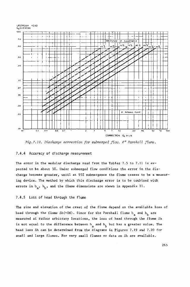
UPSTREAM HEAD h a in metres
é
s
y*
k
S\
'" •
'
'
^
• Y
'
•
*
S
m
>
^ / s
*'
s
' s
'
y
>
/
'
•
/
' y y
, / J
. • "
• y
x"
>
*' ^
• '"
S
S
y
s
* y
'' y
0
PERCENTAGE OF SUBMERGENCE
y
y y
•
y
y
•"' y
6 5 %
y
y
y
y
*
7 0 % 7 5 %
•'1 - ^ L^ •
e o %
6" PARSHALL FLUME
8 5 % 5 5 / 0
0 .5 0 7 SO 7 0
CORRECTION QE in L/s
Fig.7.13. Discharge correction for submerged flow. 6" Parshall flume.
7.4.4 Accuracy of discharge measurement
The error in the modular discharge read from the Tables 7.5 to 7.11 is ex
pected to be about 3%. Under submerged flow conditions the error in the dis
charge becomes greater, until at 95% submergence the flume ceases to be a measur
ing device. The method by which this discharge error is to be combined with
errors in h , h, , and the flume dimensions are shown in Appendix II.
7.4.5 Loss of head through the flume
The size and elevation of the crest of the flume depend on the available loss of
head through the flume Ah(-AH). Since for the Parshall flume h and h, are a b
measured at rather arbitrary locations, the loss of head through the flume Ah
is not equal to the difference between h and h, but has a greater value. The
head loss Ah can be determined from the diagrams in Figures 7.19 and 7.20 for
small and large flumes. For very small flumes no data on Ah are available.
265
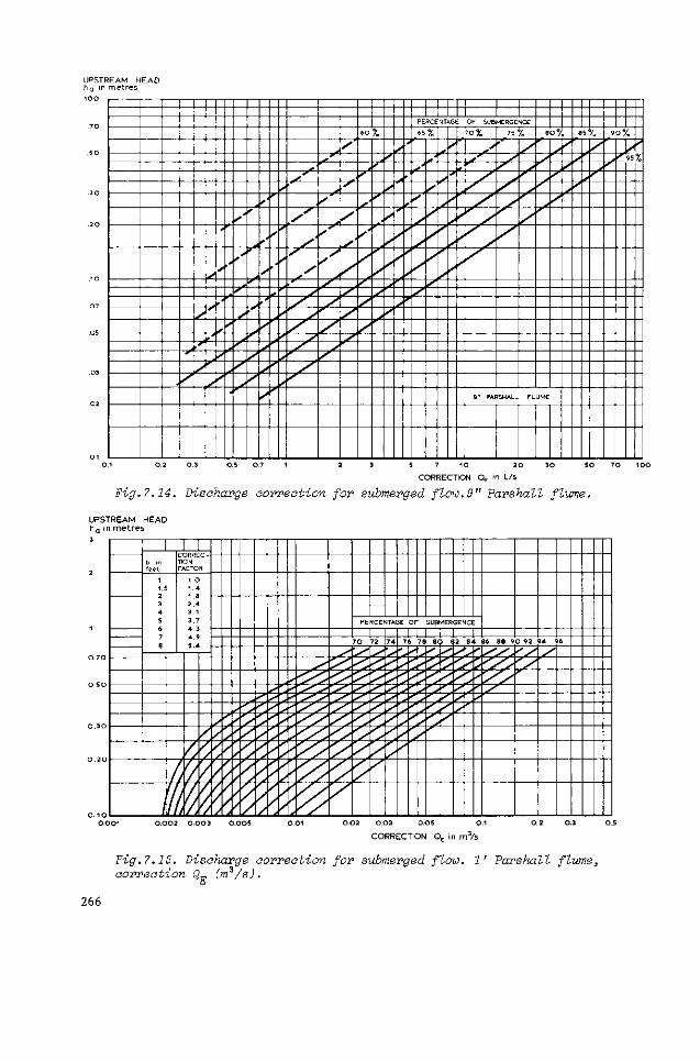
UPSTREAM HEAD h a in m e t r e s
/
•
4
'
4
S
y
'
J
A
' M
s
s
'
'
y
**
' 1 y
•
y
r
'
*
S
s
*
\ j S
•
y\
/*
s
s
>
y
. s
y
4
àO%
s"
4
4
'
' .
s
>
^
/
J
J
'
PERCENTAGE OF SUBMERGENCE
6 5 %
^ y
y
> 70% 7 5 %
y 8'0%
9" PARSHALL FLUME
85 / o 9 0 %
95 X
0.2 0.3 0.5 0.7 1 5 7 10 2 0 30 SO 70 100
CORRECTION QE in L/s
Fig.7.14. Discharge correction for submerged flow.9" Parshall flume.
UPSTREAM HEAD h a in m e t r e s
1 i 1 b in feet
1 1.5 2 3 4 5 6 7 8
I
CORRECTION FACTOR
1.0 1.4 1 .8 2.4 3 .1 3.7 4,3 4.9 5.4
k
PERCENTAGE OF SUBMERGENCE
| 7 0 72 7 4 I . . .
76 78 8C > 82 84 86 86 9 O 92 94 96
0 .002 0.OO3 0.005 0.02 0.03 0.O5 O.
CORRECTION QF in m 3 / s
0.2 0.3
Fig.7.IS. Discharge correction for submerged flow. 1T Parshall flume, correction Q^ (m/s).
266
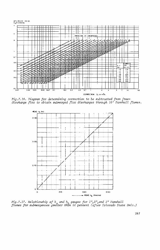
UPSTREAM HEAD h a i n metres
0.02 0 03 0 05 0.07 O.I 0.2 0.3 OS 0.7
CORRECTION QE in m3/s
Fig.7.16. Diagram for determining correction to be subtracted from free-discharge flow to obtain submerged flow discharges through 10' Parshall flumes.
HEAD
0. 30
0 20
0.10
hc <m)
/
''
/
! " "T ^
—
/
/
/ /
/
-
/
i
! ! : . ,
/
V / •
/
j - i
/
i ; !
!
j ! : ' i
!
• -
!
! 1
! 1
|
i ! J
i ! 0.20 0 30
-»• HEAD h (metres)
Fig. 7.17. Relationship of h and h-, gauges for l",2"1and 3" Parshall flumes for submergences greater than 50 percent (after Colorado State Univ.)
267
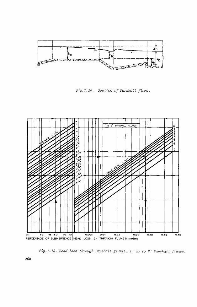
Fig.7.18. Section of Parehalt flume.
95 90 85 SO 70 60 PERCENTAGE OF SUBMERGENCE
0 .005 O.Ol 0 .02 0 .05 O.I O 0 . 20 0 .40
HEAD LOSS AH THROUGH FLUME in metres
Fig.7.19. Head-loss through Parshall flumes. 1' up to 8' Parshall flumes.
268
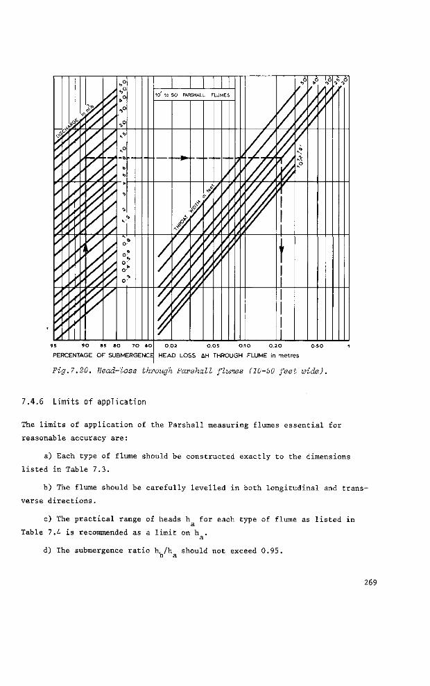
95 90 85 SO 70 60
PERCENTAGE OF SUBMERGENCE 0.02 0 .05 0.10 0 . 20 0-50
HEAD LOSS AH THROUGH FLUME in metres
Fig.7.20. Head-loss through Parshall flumes (10-50 feet wide).
7.4.6 Limits of application
The limits of application of the Parshall measuring flumes essential for
reasonable accuracy are:
a) Each type of flume should be constructed exactly to the dimensions
listed in Table 7.3.
b) The flume should be carefully levelled in both longitudinal and trans
verse directions.
c) The practical range of heads h for each type of flume as listed in
Table 7.4 is recommended as a limit on h . a
d) The submergence ratio h, /h should not exceed 0.95. b a
269
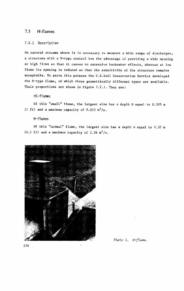
7.5 H-flumes
7.5.1 Description
On natural streams where it is necessary to measure a wide range of discharges,
a structure with a V-type control has the advantage of providing a wide opening
at high flows so that it causes no excessive backwater effects, whereas at low
flows its opening is reduced so that the sensitivity of the structure remains
acceptable. To serve this purpose the U.S.Soil Conservation Service developed
the H-type flume, of which three geometrically different types are available.
Their proportions are shown in Figure 7.2.1. They are:
HS-flûmes
Of this "small" flume, the largest size has a depth D equal to 0.305 m
(1 ft) and a maximum capacity of 0.022 m3/s.
H-flûmes
Of this "normal" flume, the largest size has a depth D equal to 1.37 m
(4.5 ft) and a maximum capacity of 2.36 m3/s.
Photo 1. H-flwne.
270
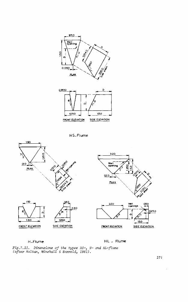
r-**^ \ Well . / \ open ing /
a
O.C
A // \ Ir \ r \
5D 1
PLAN
i/7 \ ô
/ /
ft
0.383 D
FRONT ELEVATION SIDE ELEVATION
HS-Flume
L ™* -i FRONT ELEVATION
/ J A* i
/ 3 1 / l
| 135D _
0.3 D
3.2D
\WI 05D openings
Q25D 'TT—
SIDE ELEVATION FRONT ELEVATION SIDE ELEVATION
H-Flume HL _ Flume
Fig. 7. 21. Dimensions of the types HS-, H- and HL-flume (after Holton, Minshall & Harrold, 1961).
271
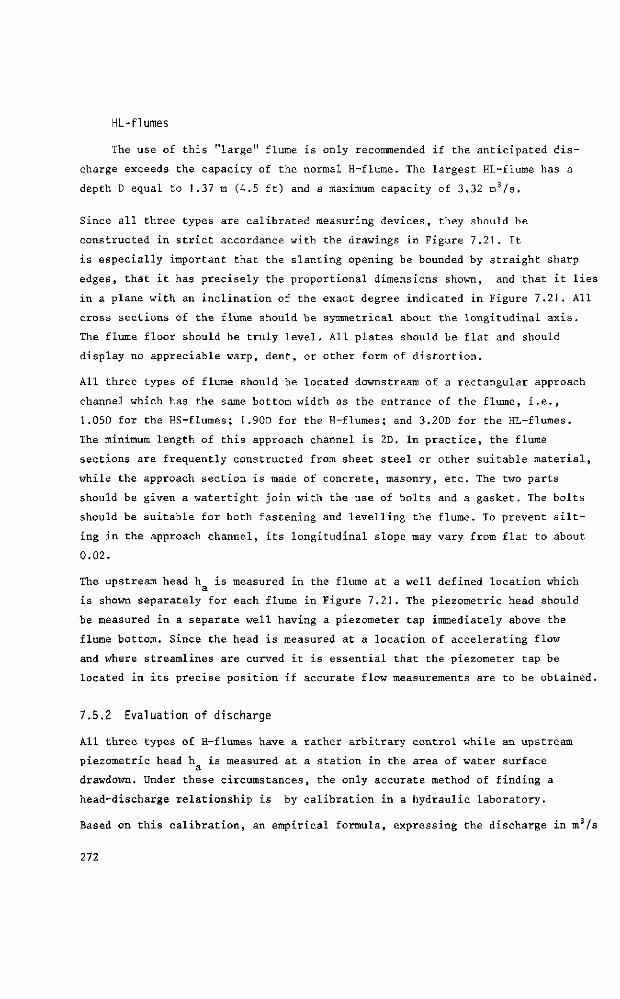
HL-fl unies
The use of this "large" flume is only recommended if the anticipated dis
charge exceeds the capacity of the normal H-flume. The largest HL-flume has a
depth D equal to 1.37 m (4.5 ft) and a maximum capacity of 3.32 m3/s.
Since all three types are calibrated measuring devices, they should be
constructed in strict accordance with the drawings in Figure 7.21. It
is especially important that the slanting opening be bounded by straight sharp
edges, that it has precisely the proportional dimensions shown, and that it lies
in a plane with an inclination of the exact degree indicated in Figure 7.21. All
cross sections of the flume should be symmetrical about the longitudinal axis.
The flume floor should be truly level. All plates should be flat and should
display no appreciable warp, dent, or other form of distortion.
All three types of flume should be located downstream of a rectangular approach
channel which has the same bottom width as the entrance of the flume, i.e.,
1.05D for the HS-flûmes; I.90D for the H-flûmes; and 3.20D for the HL-flûmes.
The minimum length of this approach channel is 2D. In practice, the flume
sections are frequently constructed from sheet steel or other suitable material,
while the approach section is made of concrete, masonry, etc. The two parts
should be given a watertight join with the use of bolts and a gasket. The bolts
should be suitable for both fastening and levelling the flume. To prevent silt
ing in the approach channel, its longitudinal slope may vary from flat to about
0.02.
The upstream head h is measured in the flume at a well defined location which a
is shown separately for each flume in Figure 7.21. The piezometric head should
be measured in a separate well having a piezometer tap immediately above the
flume bottom. Since the head is measured at a location of accelerating flow
and where streamlines are curved it is essential that the piezometer tap be
located in its precise position if accurate flow measurements are to be obtained.
7.5.2 Evaluation of discharge
All three types of H-flumes have a rather arbitrary control while an upstream
piezometric head h is measured at a station in the area of water surface r a
drawdown. Under these circumstances, the only accurate method of finding a
head-discharge relationship is by calibration in a hydraulic laboratory.
Based on this calibration, an empirical formula, expressing the discharge in m /s
272
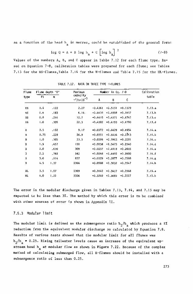
as a function of the head h in metres, could be established of the general form: a
log Q = A + B log h + C [ log h 1 (7-8)
Value s of t h e numbers A, B, and C a ppe a r i n T ab l e 7 .12 f o r e ach f lume t y p e . Ba
sed on E q u a t i o n 7 - 8 , c a l i b r a t i o n t a b l e s were p r e p a r e d f o r e ach f l ume ; s e e T a b l e s
7 . 13 f o r t h e HS - f l ûmes .Tab l e 7 .14 f o r t h e H-f lumes and T ab l e 7 .15 f o r t h e HL- f lûmes .
TABLE 7.12. DATA ON THREE TYPE H-FLUMES
Flume Flume depth "D" Maximum Number in Eq. 7-8 Cal ibrat ion
type " f t m~~ capacity t a b l e
mVsxlO
HS 0.4 .122 2.27 -0.4361 +2.5151 +0.1379 7 .13 .a
HS 0.6 .183 6.14 -0 .4430 +2.4908 +0.1657 7 .13.b
HS 0 .8 .244 12.7 -0 .4410 +2.4571 +0.1762 7.13.C
HS 1.0 . 305 22.3 -0.4382 +2.4193 +0.1790 7 .13.d
H 0.5 .152 9.17 +0.0372 +2.6629 +0.1954 7 .14 . a
H 0.75 .229 26.9 +0.0351 +2.6434 +0.2Î43 7 .14 .b
H 1.0 .305 53.5 +0.0206 +2.5902 +0.2281 7.14.C
H 1.5 .457 150 +0.0238 +2.5473 +0.2540 7 .14.d
H 2.0 .610 309 +0.0237 +2.4918 +0.2605 7 .14 .e
H 2 .5 .762 542 +0.0268 +2.4402 +0.2600 7 .14 . f
H 3.0 .914 857 +0.0329 +2.3977 +0.2588 7 .14 .g
H 4 .5 ! .37 2366 +0.0588 +2.3032 +0.2547 7 .14 .h
HL 3.5 1.07 2369 +0.3142 +2.3417 +0.2568 7 .15 .a
HL 4 .0 1.22 3326 +0.3240 +2.3083 +0.2527 7 .15.b
T h e e r r o r i n t h e m o d u l a r d i s c h a r g e g i v e n i n T a b l e s 7 . 1 3 , 7 . 1 4 , a n d 7 . 1 5 may b e
e x p e c t e d t o b e l e s s t h a n 3 % . The m e t h o d b y w h i c h t h i s e r r o r i s t o b e c o m b i n e d
w i t h o t h e r s o u r c e s o f e r r o r i s s h o w n i n A p p e n d i x I I .
7.5.3 Modular l imi t
The modular limit is defined as the submergence ratio h„/h which produces a 1%
reduction from the equivalent modular discharge as calculated by Equation 7.8.
Results of various tests showed that the modular limit for all flumes was
h„/h = 0.25. Rising tailwater levels cause an increase of the equivalent up
stream head h at modular flow as shown in Figure 7.22. Because of the complex
method of calculating submerged flow, all H-flumes should be installed with a
submergence ratio of less than 0.25.
273
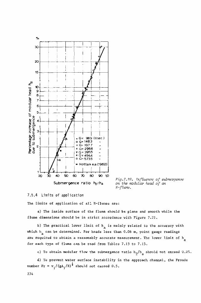
"O
ra
30
20
15
10 9 8
J5 7
O 6
E = u 0;
* C 4
pp I E 3 jS ^ c o
S I 2
Q.TJ
•
•
.
'
1 ;
.. -i
1
!
..—.—
, j
/ x
O
fA
j
&
— i —
. .
!
,
J k
. o =
>
. /
f-
98.S
J 0 ^
r i
/ ! i
I
, 4 — - —
i
. 1 —
i
1 1 > (l/sec.) o 0 - 148.3
x Q= 197 7 + O 296.6 ! Q = 395.5 A o = 494.4 ° O 573.5 « Hottan e.a.(1962)
, I , I , I , 20 30 40 50 60 70 80 90 1,0
Fig.7.22. Influenae of submergence Submergence ratio l^/ha ow the modular' head of an
H-flume.
7.5.4 Limits of application
The limits of application of all H-flûmes are:
a) The inside surface of the flume should be plane and smooth while the
flume dimensions should be in strict accordance with Figure 7.21.
b) The practical lower limit of h is mainly related to the accuracy with
which h can be determined. For heads less than 0.06 m, point gauge readings
are required to obtain a reasonably accurate measurement. The lower limit of h
for each type of flume can be read from Tables 7.13 to 7.15.
c) To obtain modular flow the submergence ratio h„/h should not exceed 0.25.
d) To prevent water surface instability in the approach channel, the Froude l
number Fr = v./(gA./B)2 should not exceed 0.5.
274
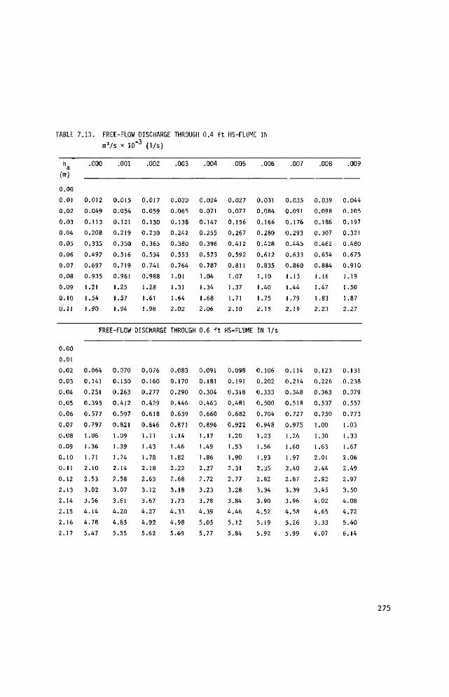
TABLE
(m)
0.00
0.01
0.02
0 .03
0.04
0.05
0.06
0.07
0 .08
0.09
0.10
0.11
0.00
0.01
0.02
0 .03
0.04
0.05
0.06
0.07
0.08
0.09
0.10
0.11
0.12
2 .13
2.14
2.15
2 .16
2.17
7 .13 . FREE-FLOW
m
.000
0.012
0.049
0.113
0.208
0.335
0.497
0.697
0.935
1.21
1.54
1.90
3 / s x 10
.001
0.015
0.054
0.121
0.219
0.350
0.516
0.719
0.961
1.25
1.57
1.94
FREE-FLOW 1
0.064
0.141
0.251
0.395
0.577
0.797
1.06
1.36
1.71
2.10
2.53
3.02
3.56
4.14
4 .78
5.47
0.070
0.150
0.263
0.412
0.597
0.821
1.09
1.39
1.74
2.14
2 .58
3.07
3.61
4.20
4 .85
5.55
DISCHARGE THROUGH 0.4 ft
" J ( 1 / s )
.002
0.017
0.059
0.130
0.230
0.365
0.534
0.741
0.988
1.28
1.61
1.98
.003
0.020
0.065
0.138
0.242
0.380
0 .553
0.764
1.01
1.31
1.64
2.02
DISCHARGE THROUGH
0.076
0.160
0.277
0.429
0.618
0.846
1.11
1.43
1.78
2 .18
2 .63
3.12
3.67
4.27
4 .92
5.62
0.083
0.170
0.290
0.446
0.639
0.871
1.14
1.46
1.82
2.22
2.68
3.18
3.73
4 .33
4 .98
5.69
.004
0.024
0.071
0.147
0.255
0.396
0.573
0.787
1.04
1.34
1.68
2.06
0.6 f t
0.091
0.181
0.304
0.463
0.660
0.896
1.17
1.49
1.86
2.27
2.72
3.23
3.78
4.39
5 .05
5.77
; HS-FLUME IN
.005
0.027
0.077
0.156
0.267
0.412
0.592
0.811
1.07
1.37
1.71
2.10
HS-FLUME
0.098
0.191
0.318
0.481
0.682
0.922
1.20
1.53
1.90
2.31
2.77
3.28
3.84
4.46
5.12
5.84
.006
0.031
0.084
0.166
0.280
0.428
0.612
0.835
1.10
1.40
1.75
2 .15
IN 1/S
0.106
0.202
0.333
0.500
0.704
0.948
1.23
1.56
1.93
2.35
2.82
3.34
3.90
4.52
5.19
5.92
.007
0.035
0.091
0.176
0.293
0.445
0.633
0.860
1.13
1.44
1.79
2 .19
0.114
0.214
0.348
0.518
0.727
0.975
1.26
1.60
1.97
2.40
2.87
3.39
3.96
4 .58
5.26
5.99
.008
0.039
0.098
0.186
0.307
0.462
0.654
0.884
1.16
1.47
1.83
2 .23
0.123
0.226
0.363
0.537
0.750
1.00
1.30
1.63
2.01
2.44
2.92
3.45
4.02
4 .65
5.33
6.07
.009
0.044
0.105
0.197
0.321
0.480
0.675
0.910
1.19
1.50
1.87
2.27
0.131
0.238
0.379
0.557
0.773
1.03
1.33
1.67
2.06
2.49
2.97
3.50
4 .08
4.72
5.40
6.14
275
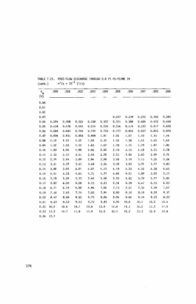
TABLE
(cont.
ha (m)
0.00
O.Ol
0 .02
0 .03
0.04
0 .05
0.06
0 .07
0 .08
0.09
0 .10
0.11
0.12
0 .13
0.14
0 .15
0.16
0.17
0 .18
0.19
0.20
0.21
0.22
0 .23
0.24
7 . 13 . FREE-FLOW
) m
.000
0.294
0.458
0.660
0.904
1.19
1.52
1.90
2.32
2.79
3.31
3.89
4.51
5.19
5.92
6.71
7.56
8.47
9 .43
10.5
11.5
12.7
7 s x 10'
.001
0.308
0.476
0.683
0.931
1.22
1.56
1.94
2.37
2.84
3.37
3.95
4 .58
5.26
6.00
6.79
7.65
8.56
9.53
10.6
11.7
DISCHARGE THROUI
' J ( V S )
.002
0.324
0.495
0.706
0.958
1.25
1.59
1.98
2.41
2.89
3.42
4.01
4.64
5.33
6.08
6.88
7.74
8.65
9.63
10.7
11.8
.003
0.339
0.514
0.729
0.986
1.29
1.63
2.02
2.46
2.94
3.48
4.07
4.71
5.40
6.15
6.96
7.82
8.75
9.73
10.8
11.9
3H 0 .8 f t
.004
0.355
0.534
0.753
1.01
1.32
1.67
2.06
2.50
2.99
3.54
4 .13
4.77
5.48
6.23
7.04
7.91
8.84
9.83
10.9
12.0
HS-FLUME IN
.005
0.227
0.371
0.554
0.777
1.04
1.35
1.70
2 .10
2.55
3.05
3.59
4.19
4.84
5.55
6.31
7.13
8.00
8.94
9.94
11.0
12.1
.006
0.239
0.388
0.574
0.802
1.07
1.38
1.74
2 .15
2.60
3.10
3.65
4 .25
4.91
5.62
6.39
7.21
8.10
9.04
10.0
11.1
12.2
.007
0.252
0.404
0.595
0.827
1.10
1.42
1.78
2 .19
2.65
3.15
3.71
4.32
4 .98
5.70
6.47
7.30
8.19
9.14
10.1
11.2
12.3
.008
0.266
0.422
0.617
0.852
1.13
1.45
1.82
2.23
2.69
3.20
3.77
4 .38
5.05
5.77
6.55
7.39
8.28
9.23
10.2
11.3
12.5
.009
0.280
0.440
0.638
0.878
1.16
1.49
1.86
2 .28
2.74
3.26
3.83
4 .45
5.12
5.85
6.63
7.47
8.37
9.33
10.4
11.4
12.6
276
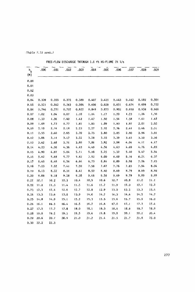
(Table 7.13 aont.)
FREE-FLOW DISCHARGE THROUGH 1.0 f t HS-FLUME IN 1/s
\ (m)
0.00
0.01
0.02
0 .03
0.04
0.05
0.06
0.07
0 .08
0.09
0.10
0.11
0.12
0 .13
0.14
0.15
0 .16
0.17
0 .18
0.19
0.20
0.21
0.22
0 .23
0.24
0.25
0.26
0.27
0 .28
0.29
0.30
.000
0.339
0.521
0.746
1.02
1.33
1.69
2.10
2.55
3.06
3.62
4 .23
4.90
5.62
6.40
7 .23
8.13
9.08
10.1
11.2
12.3
13.5
14.8
16.1
17.5
19.0
20.6
22.2
.001
0.355
0.542
0.771
1.04
1.36
1.73
2.14
2.60
3.11
3.68
4.30
4.97
5.69
6.48
7.32
8.22
9 .18
10.2
11.3
12.4
13.6
14.9
16.3
17.7
19.2
20.7
22.3
.002
0.372
0.563
0.797
1.07
1.40
1.77
2 .18
2.65
3.17
3.74
4.36
5.04
5.77
6.56
7.41
8.31
9.28
10.3
11.4
12.6
13.8
15.1
16.4
17.8
19.3
20.9
.003
0.389
0.584
0.822
1.10
1.43
1.81
2 .23
2.70
3.22
3.80
4 .43
5.11
5 .85
6.64
7.50
8.41
9.38
10.4
11.5
12.7
13.9
15.2
16.5
18.0
19.5
21 .0
.004
0.407
0.606
0.849
1.14
1.47
1.85
2.27
2.75
3.28
3.86
4.49
5.18
5.92
6.73
7.58
8.50
9.48
10.5
11.6
12.8
14.0
15.3
16.7
18.1
19.6
21.2
.005
0.425
0.629
0.875
1.17
1.50
1.89
2.32
2.80
3.33
3.92
4.56
5.25
6.00
6.81
7.67
8.60
9.58
10.6
11.7
12.9
14.2
15.5
16.8
18.3
19.8
21.4
.006
0.443
0.651
0.902
1.20
1.54
1.93
2.36
2.85
3.39
3.98
4 .63
5.32
6.08
6.89
7.76
8.69
9.69
10.7
11.9
13.0
14.3
15.6
17.0
18.4
19.9
21 .5
.007
0.462
0.674
0.930
1.23
1.58
1.97
2.41
2.90
3.45
4 .04
4.69
5.40
6.16
6.98
7.85
8.79
9.79
10.8
12.0
13.2
14.4
15.7
17.1
18.6
20.1
21.7
.008
0.482
0.698
0.958
1.26
1.61
2.01
2.46
2.96
3.50
4.11
4.76
5.47
6.24
7.06
7.94
8.89
9.89
11.0
12.1
13.3
14.5
15.9
17.3
18.7
20.2
21.8
.009
0.501
0.722
0.986
1.30
1.65
2.05
2.51
3.01
3.56
4 .17
4 .83
5.54
6.32
7.15
8.04
8.98
9.99
11.1
12.2
13.4
14.7
16.0
17.4
18.9
20.4
22 .0
277
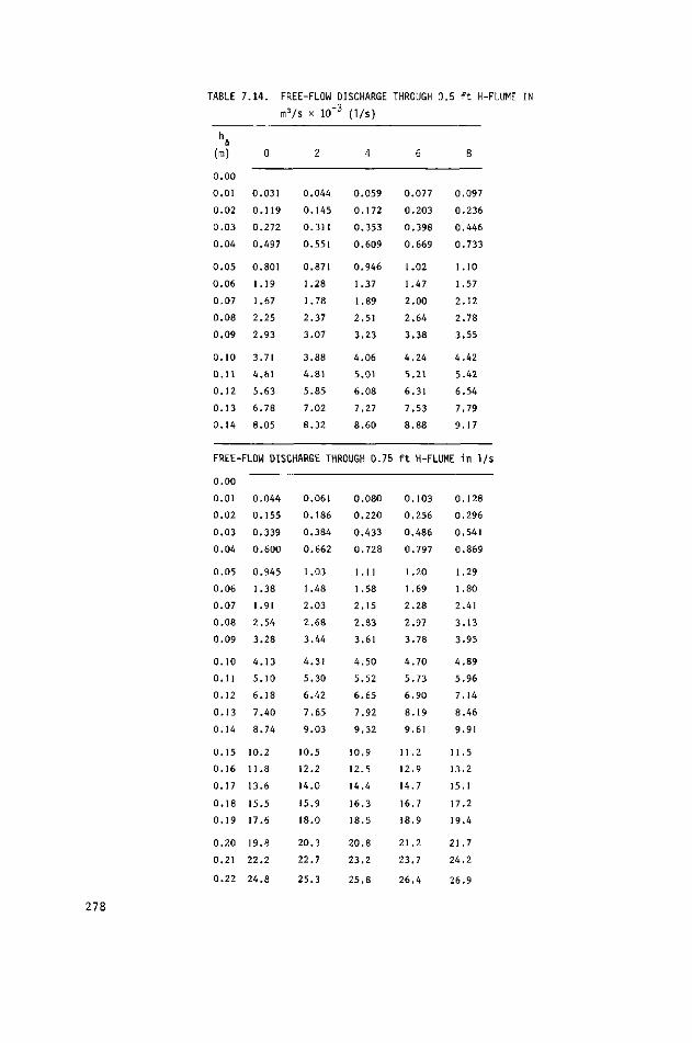
TABLE 7 . 1 4 . FREE-FLOW DISCHARGE THROUGH 0 .5 f t H-FLUME IN
h a
(m)
0.00
0.01
0.02
0 .03
0.04
0 .05
0.06
0.07
0 .08
0.09
0.10
0.11
0.12
0 .13
0.14
FREE-
0.00
0.01
0.02
0 .03
0.04
0 .05
0.06
0.07
0 .08
0.09
0.10
0.11
0.12
0 .13
0.14
0.15
0.16
0.17
0.18
0.19
0.20
0.21
0.22
m
0
0.031
0.119
0.272
0.497
0.801
1.19
1.67
2.25
2 .93
3.71
4.61
5.63
6.78
8.05
3 / s x 10" 3
2
0.044
0.145
0.311
0.551
0.871
1.28
1.78
2.37
3.07
3.88
4.81
5.85
7.02
8.32
(Vs)
4
0.059
0.172
0.353
0.609
0.946
1.37
1.89
2.51
3.23
4.06
5.01
6.08
7.27
8.60
FLOW DISCHARGE THROUGH 0.75
0.044
0.155
0.339
0.600
0.945
1.38
1.91
2 .54
3.28
4 .13
5.10
6.18
7.40
8.74
10.2
11.8
13.6
15.5
17.6
19.8
22.2
24.8
0.061
0.186
0.384
0.662
1.03
1.48
2.03
2 .68
3.44
4.31
5.30
6.42
7.65
9.03
10.5
12.2
14.0
15.9
18.0
20.3
22.7
25.3
0.080
0.220
0.433
0.728
1.11
1.58
2.15
2 .83
3.61
4.50
5.52
6.65
7.92
9.32
10.9
12.5
14.4
16.3
18.5
20.8
23.2
25.8
6
0.077
0.203
0.398
0.669
1.02
1.47
2.00
2.64
3.38
4.24
5.21
6.31
7 .53
8.88
8
0.097
0.236
0.446
0.733
1.10
1.57
2.12
2.78
3.55
4.42
5.42
6.54
7.79
9.17
f t H-FLUME in 1/s
0 .103
0.256
0.486
0.797
1.20
1.69
2 .28
2.97
3.78
4.70
5.73
6.90
8.19
9.61
11.2
12.9
14.7
16.7
18.9
21 .2
23.7
26.4
0.128
0.296
0.541
0.869
1.29
1.80
2.41
3 .13
3.95
4.89
5.96
7.14
8.46
9.91
11.5
13.2
15.1
17.2
19.4
21.7
24.2
26.9
278
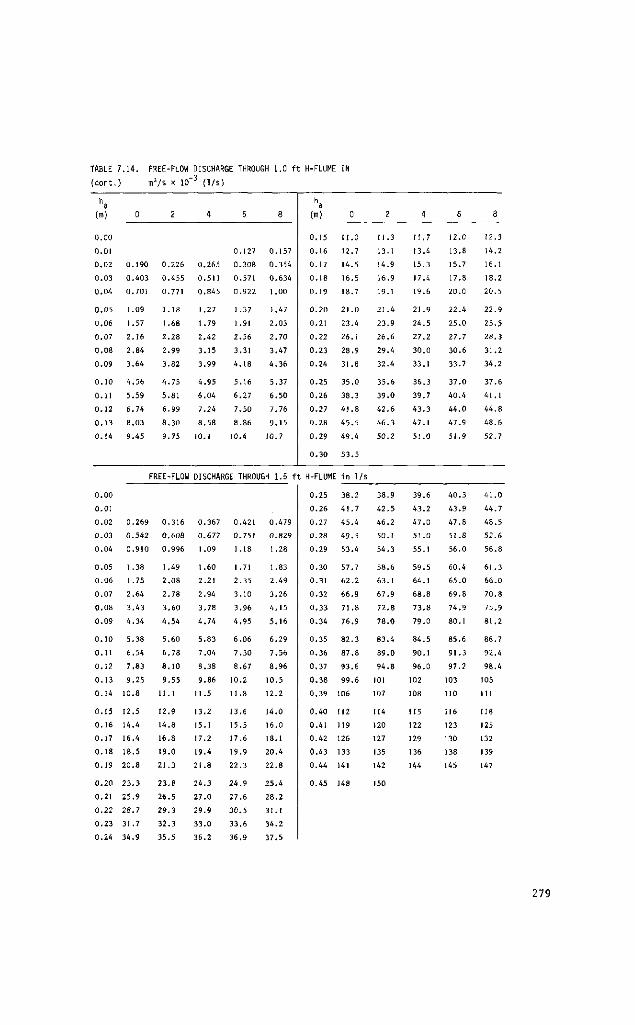
TABLE 7.14. FREE-FLOW DISCHARGE THROUGH 1.0 ft H-FLUME IN
(cont.)
ha (m)
0.00
0.01
0.02
0.03
0.04
0.05
0.06
0.07
0.08
0.09
0.10
0.11
0.12
0.13
0.14
m
0
0.190
0.403
0.701
1.09
1.57
2.16
2.84
3.64
4.56
5.59
6.74
8.03
9.45
3/s x 10"
2
0.226
0.455
0.771
1.18
1.68
2.28
2.99
3.82
4.75
5.81
6.99
8.30
9.75
(1/s)
4
0.265
0.511
0.845
1.27
1.79
2.42
3.15
3.99
4.95
6.04
7.24
8.58
10.1
6
0.127
0.308
0.571
0.922
1.37
1.91
2.56
3.31
4.18
5.16
6.27
7.50
8.86
10.4
8
0.157
0.354
0.634
1.00
1 .47
2.03
2.70
3.47
4.36
5.37
6.50
7.76
9.15
10.7
ha (m)
0.15
0.16
0.17
0.18
0.19
0.20
0.21
0.22
0.23
0.24
0.25
0.26
0.27
0.28
0.29
0.30
0
11.0
12.7
14.5
16.5
18.7
21.0
23.4
26.1
28.9
31.8
35.0
38.3
41.8
45.5
49.4
53.5
2
11.3
13.1
14.9
16.9
19.1
21.4
23.9
26.6
29.4
32.4
35.6
39.0
42.6
46.3
50.2
4
11.7
13.4
15.3
17.4
19.6
21.9
24.5
27.2
30.0
33.1
36.3
39.7
43.3
47.1
51.0
6
12.0
13.8
15.7
17.8
20.0
22.4
25.0
27.7
30.6
33.7
37.0
40.4
44.0
47.9
51.9
8
12.3
14.2
16.1
18.2
20.5
22.9
25.5
28.3
31.2
34.2
37.6
41.1
44.8
48.6
52.7
FREE-FLOW DISCHARGE THROUGH 1.5 ft H-FLUME in 1/s
0.00
0.01
0.02
0.03
0.04
0.05
0.06
0.07
0.08
0.09
0.10
0.11
0.12
0.13
0.14
0.15
0.16
0.17
0.18
0.19
0.20
0.21
0.22
0.23
0.24
0.269
0.542
0.910
1.38
1.75
2.64
3.43
4.34
5.38
6.54
7.83
9.25
10.8
12.5
14.4
16.4
18.5
20.8
23.3
25.9
28.7
31.7
34.9
0.316
0.608
0.996
1.49
2.08
2.78
3.60
4.54
5.60
6.78
8.10
9.55
11.1
12.9
14.8
16.8
19.0
21.3
23.8
26.5
29.3
32.3
35.5
0.367
0.677
1.09
1.60
2.21
2.94
3.78
4.74
5.83
7.04
8.38
9.86
11.5
13.2
15.1
17.2
19.4
21.8
24.3
27.0
29.9
33.0
36.2
0.421
0.751
1.18
1.71
2.35
3.10
3.96
4.95
6.06
7.30
8.67
10.2
11.8
13.6
15.5
17.6
19.9
22.3
24.9
27.6
30.5
33.6
36.9
0.479
0.829
1.28
1.83
2.49
3.26
4.15
5.16
6.29
7.56
8.96
10.5
12.2
14.0
16.0
18.1
20.4
22.8
25.4
28.2
31.1
34.2
37.5
0.25
0.26
0.27
0.28
0.29
0.30
0.31
0.32
0.33
0.34
0.35
0.36
0.37
0.38
0.39
0.40
0.41
0.42
0.43
0.44
0.45
38.2
41.7
45.4
49.3
53.4
57.7
62.2
66.9
71.8
76.9
82.3
87.8
93.6
99.6
106
112
119
126
133
141
148
38.9
42.5
46.2
50.1
54.3
58.6
63.1
67.9
72.8
78.0
83.4
89.0
94.8
101
107
114
120
127
135
142
150
39.6
43.2
47.0
51.0
55.1
59.5
64.1
68.8
73.8
79.0
84.5
90.1
96.0
102
108
115
122
129
136
144
40.3
43.9
47.8
51.8
56.0
60.4
65.0
69.8
74.9
80.1
85.6
91.3
97.2
103
110
116
123
130
138
145
41.0
44.7
48.5
52.6
56.8
61 .3
66.0
70.8
75.9
81.2
86.7
92.4
98.4
105
111
118
125
132
139
147
279
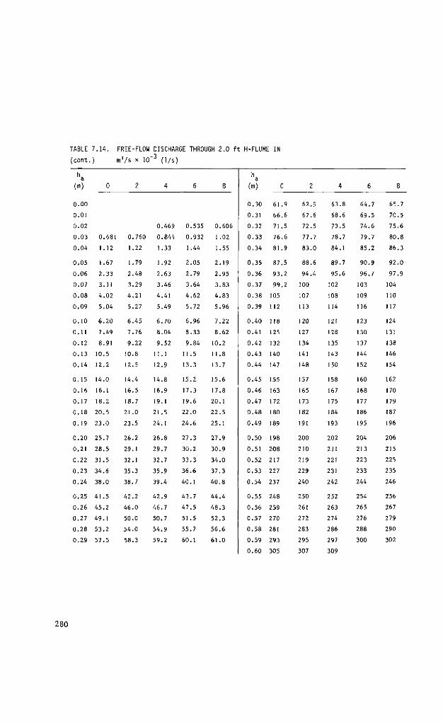
TABLE 7 .14
( c o n t . ) m3 /s x 10
FREE-FLOW DISCHARGE THROUGH 2 . 0 f t H-FLUME IN -3
( 1 / s )
ha (m)
0.00
O.Ol
0.02
0.03
0.04
0.05
0.06
0.07
0.08
0.09
0.10
0.11
0.12
0.13
0.14
0.15
0.16
0.17
0.18
0.19
0.20
0.21
0.22
0.23
0.24
0.25
0.26
0.27
0.28
0.29
0
0.681
1.12
1.67
2.33
3.11
4.02
5.04
6.20
7.49
8.91
10.5
12.2
14.0
16.1
18.2
20.5
23.0
25.7
28.5
31.5
34.6
38.0
41.5
45.2
49.1
53.2
57.5
2
0.760
1.22
1.79
2.48
3.29
4.21
5.27
6.45
7.76
9.22
10.8
12.5
14.4
16.5
18.7
21.0
23.5
26.2
29.1
32.1
35.3
38.7
42.2
46.0
50.0
54.0
58.3
4
0.469
0.844
1.33
1.92
2.63
3.46
4.41
5.49
6.70
8.04
9.52
11.1
12.9
14.8
16.9
19.1
21.5
24.1
26.8
29.7
32.7
35.9
39.4
42.9
46.7
50.7
54.9
59.2
6
0.535
0.932
1.44
2.05
2.79
3.64
4.62
5.72
6.96
8.33
9.84
11.5
13.3
15.2
17.3
19.6
22.0
24.6
27.3
30.2
33.3
36.6
40.1
43.7
47.5
51.5
55.7
60.1
8
0.606
1 .02
1.55
2.19
2.95
3.83
4.83
5.96
7.22
8.62
10.2
11.8
13.7
15.6
17.8
20.1
22.5
25.1
27.9
30.9
34.0
37.3
40.8
44.4
48.3
52.3
56.6
61.0
h a
(m)
0.30
0.31
0.32
0.33
0.34
0.35
0.36
0.37
0.38
0.39
0.40
0.41
0.42
0.43
0.44
0.45
0.46
0.47
0.48
0.49
0.50
0.51
0.52
0.53
0.54
0.55
0.56
0.57
0.58
0.59
0.60
0
61
66
71
76
81
87
93
99
105
112
118
125
132
140
147
155
163
172
180
189
198
208
217
227
237
248
259
270
281
293
305
9
6
5
6
9
5
2
2
62
67
72
77
83
88
94
100
107
113
120
127
134
141
148
157
165
173
182
191
200
210
219
229
240
250
261
272
283
295
307
9
6
5
7
0
6
4
4
63.8
68.6
73.5
78.7
84.1
89.7
95.6
102
108
114
121
128
135
143
150
158
167
175
184
193
202
211
221
231
242
252
263
274
286
297
309
t
64
69
74
79
85
90
96
103
109
116
123
130
137
144
152
160
168
177
186
195
204
213
223
233
244
254
265
276
288
300
7
5
6
7
2
9
7
8
65.7
70.5
75.6
80.8
86.3
92.0
97.9
104
110
117
124
131
138
146
154
162
170
179
187
196
206
215
225
235
246
256
267
279
290
302
280
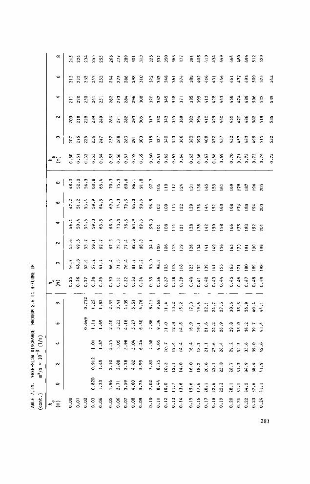
t/î —•
Q CO
C O
U 3
*a-
C M
o
m.—-
co
<x>
^ J -
CsJ
o
co
<x>
<3-
O J
o
i n
CM
CM
CM
CTi O CM
O e g
O
m
o
o
0 0 - 3 "
CM
- 3 -
- 3 -
m s i
en
sr
m CM
o
o o
o
- 3 -CM
CM CM
O
CO
CM
m
o
o
CM
m
CM
u-1
s r
O i n
cn s i -
co
0 0
sr
CM
o
o
o
sr
co CM
O co CM
0 0 CM CM
CM CM
CM
m o
co
m
s j -
m m
s t
m
r-
CO
m
en
CM
m
CM
O
CM CO
O
CT* - 3 -
O
CM
O o
m - 3 -CM
CO sr CM
sr CM
cn CO CM
CO CM
CO
m
o
0 0
o
cn
Os m
o
en m
0 0
m
CM
r--m
co CM
o
CM CM
~
-~
O
~ CM
cn
O
o CM oo
o
co o o
i n m CM
CO
m
m CM
OS
-3"
-3-
sr m
o
s i -
i n
i n
- 3 -
m
co
r-.
en
O
CM 0 0
~
cn
~~
m
~
m sr
—
CO
co
— s t -O
o
CM
-3-
CM
CM SO CM
O
CM
i n CM
i n i n
o
co
o
co
cn ^ 3
CO
co
CO
sr
O CO
o
m m CM
O sr
CM
m CM
CM
o
CM
x> cn
—
O
o
r-r-. CM
r-CM
CO r-CM
CM
oo
CM
m
o
co
i n
co
-3-
co
co
co
CM
r—
co
co
o
- 3 -
co
ro CM
CO
m o
co
0 0 0 0
CM
r-
CM
o o
cn 0 0 CM
0 0 CM
- 3 -0 0
CM
CM CO CM
O CO CM
m
o
O 0 0
m
0 0
• s r
r^
s T
M3
CM c o
O
C n CO
- 3 "
0 0
sr
OO
CO
0 0
co
CJ\
m co
o o
o CO
0 0 C n
v u cn CM
c o cn CM
as CM
co m
o
•x> co
o
m 0 0
as
CO
co
0 0
CM 0 0
r—
co
CO
co
o
m
m
CM
m
-3" O
m
CM 0 0
sr
o
<t
0 0
o
o
CO
co
o CO
0 0 o CO
m o CO
CO o co
CTl
m
o
co
en
o as
m
a\ 0 0
co
0 0
co
CM
co
s f CO
O
X >
VO
O m \D
sr CM
v O
as Os m
m
m
as O o
m
CO
CM CM CO
O CM CO
co
m
co
o
o
r—
as
m
os
co
m en
sr en
o CO CTi
m CO
o
i n
0 0
KD
0 0
r-N
0 0
m r-N
O CO
r^
CM O
r v
O
O
co co
i n co CO
CM CO CO
O CO CO
CM CO
•X !
O
- 3 " O
CM O
O
o o
as
00 as
CO
o
co
en
co
Os
m o
en
m
0 0
0 0
o
o m CO
co
CO
m - 3 " CO
CO
CO
o
CO
CM
O
O
en o
0 0
o
o
o
co
O
-3-
"*
O
~
P ^
O
CO
o
o o
CM
o
co \£> CO
\D CO
0 0 m CO
m m co
co m CO
co
o
r»
m
- 3 "
CO
CM
0 0 CO
O
CM
CO
0 0
CM
- 3 "
CM
CM
r-
— CO
o
co
CO
co
en
co
co
- 3 -
O
* 3 -CM
CM CM
CM
cn
0 0
en co O
CM
i n
0 0
- 3 -
- 3 "
-*
O
- 3 "
\D
CO
O
en co
co 00 co
m co co
CM CO CO
o co CO
m
o
CO
en CM
0 0 CM
CM
m CM
O -3"
O
CO
r^
en
\o
<r
v£>
O
\ D
V O
m
m
o
m o - 3 "
CM o •-3-
en Os co
as CO
CO en CO
O
CO CO
CO
m co
-3-CO
CM CO
- 3 -
O
\D
Os
Os
r^
co
CM
co
\D
r-
o
OS
- 3 "
CO
o
oo o -3-
o
m - 3 "
CM - 3 -
s i
en CO
CM
-3-O
CM CM
>£>
CM
„
CM
v D
O CM
_ O CM
O
CO ~3-
CO - 3 "
0 0 CM - 3 "
m CM
CM CM - 3 "
0 0
O
CO
m
CM
m
o m
en -3-
co -3-
O
r^
CM
CM
- 3 " CM
\D
CO CM
CO CM
\D
CM CM
0 0
O
o\
-3-
s T
CO - 3 " - 3 -
O - 3 "
co
en -X)
o
\ D
o
0 0
m
m
m m
-3" -3-
O
m
CM
en
M 3 CM
- 3 "
CM
0 0
•n CM
CM
m CM
Os
O
- 3 -
- 3 "
- 3 "
0 0 m <3-
m m - 3 "
i n - 3 -
o
o
en
CO
KD «X>
m
co
m o-o
m
o CO
0 0
en CM
CM
en CM
r^
co CM
0 0 CM
O CM
O
O 0 0 < f
r-.
- 3 -
- 3 "
O
- 3 -
- 3 -
O
0 0
in r-.
co
n-
M 3
O
X )
CO
co
o
CO
co
CO
CM CO
r-
co
co
CM
o
Os - 3 "
co en s i
en co s f
0 0 s t
CO 0 0 -3"
CM
o
0 0
m 0 0
CO 0 0
CO
o co
s t -
o
en
CO
CM
M 3 CO
•x>
m CO
en
-eten
CM
- 3 -CO
CM CM
O
CM
i n
en O
\0 o i n
CM o i n
en en - 3 -
CO
O
x> en
-3" cn
CM
cn
O cn
en 0 0
0 0
- 3 "
O
sr
o s f
r^
cn co
O
cn
- 3 -
0 0 CO
^o
P-.
co
CO CM
O
cn CM m
m
m
CM CM
m
m
m
m
O
m o
CO o CM
O CM
cn cn
0 0
cn
cn s *
o
- 3 " - 3 "
~3 -
CO - 3 "
v D
CM S T
cn
s i
s t
sr CM
o
CM - 3 "
m
CO
m
m co i n
CM CO
m
m
o
281
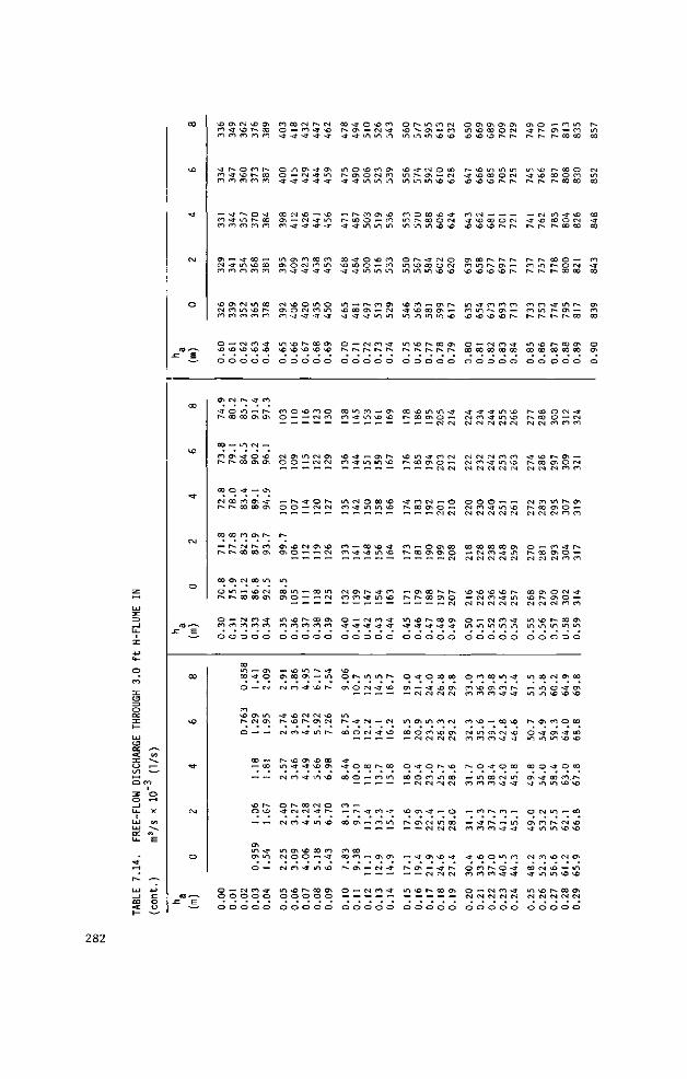
Ü3 Q£ - - v <: u) :n \ o i— i/ i — o m 3 o o I-H _ i ü_ X
r
CO
U3
vt-
OJ
o
(O — *
-e E
co
MO
~
C\J
o
rO ^-v
-e E
CO
« 3
tt
C\J
O
e« --v -C E
MD m en
st
en en
en m
er. CM en
MD CM en
o MD
o
Os
st r-
OO
m pv
00
CM
oo
pv
00
O
^ o en
O
o o o
Os st en
pv st en
st st en
st en
o\ en en
MD
o
CM
O co
„
o\ pv
O
OO pv
00
pv pv.
os
un pv
^ m o
— o o
CM MO en
o MD en
pv. m en
St un m
CM m en
CM MD
O
p-
in 00
m st 00
st
en OO
en
CM 00
CM
OO
eg en
o
CO
m 00
o
en MD ps
o
CM O
O
MD pv en
en r-m
O pv en
OO MD en
m MD en
en MD
o
st
CT.
CM
o Os
_ CT 00
er.
pv 00
00
\o 00
en en
o
st
™
CT. CN
—
00
— —.
MD
o " CT.
m CT.
o
m o o
CT 00 en
pv 00 en
st 00 en
OO en
00 r» en
st MD
o
en
pv CT
MD OS
Os
•vT Os
r-v
en Os
m CM Os
st en
o
Os
o CM
m CT
~
„
00
—
pv MD
*"•
st in
-st
o o
en o st
O O st
00 Os en
m Os en
CM Os en
m MD
O
en o
CM
o
o
pv.
Os Os
m 00 Os
m m o
o\ CM
st pv
CM
rv.
m CM
o st
CM
m CM
CM
m o o
00
st
m
sr
CM
st
C7S O st
vD O st
MD MD
O
O
Os O
pv O
MD O
m o
MD en
o
MD OO
en
MD MD
en
MD st
en
pv CM
m
Os
o en
MD
o o
CM en
-*
o-. CM -J-
MD CM va-
en CM st
o CM st
pv MD
o
MD
m
st
CM
pv.
en
o
m Os
st
CM pv.
st
Os va
st
00 CM
st
MO
o St
pv.
o o
pv. vast
st vast
st st
00 en va-
in en sa-
co MD
o
en CM
CM CM
O CM
CT.
00
00 en
o
— MO
CM Os
m
M0 MO
tn
CM sa-
in
00
" m
00
o o
CM MO va-
os m sr
M0
m <t
en m va-
o m sj
Os MO
O
o en
Os CM
pv. CM
MD CN
m CM
Os en
o
va-in
r-.
M0 CM
Pv.
co Os
MO
O Pv.
MO
en st
MO
Os O
O
00 Pv va-
in Pv. sr
Pv st
00 M0 sa-
in MO st
o Pv
o
00 en
MO en
m en
en en
CM en
o st
o
MO
o Os
m Pv.
00
•vt st
00
en
— 00
en 00
Pv
o
o
st Os st
o Os st
^ 00 va
st 00 sr
00 sf
Pv
O
m va
st st
CM va
st
Os en
— st
o
Pv
o ~~ st
O
—,
O
o ~ _
Pv
CT.
00 en
Os
„
o
o
m
M0
o m
en o m
o o m
Os st
CM Pv
O
en m
m
o un
00 st
Pv. st
CM st
O
m CM
—
CM
CM —
00
„
^-
st
™
— " CM
O
MO CM in
en CM un
CT.
m
MO
un
m
m
en Pv
o
MO
CT in
00 un
MO
m
vain
en sr
o
un
va-
™
— st —
Pv.
en
"
en
en
Os
CM
en
o
m st
m
CT. en m
MO en un
en en un
CT. CM un
st Pv.
O
OS MO
Pv, MO
MO MO
st MO
en MO
st st
o
Pv
MO ™
CM
MO
""
00
m —
-a-
>n
Os
st
st
O
O MO un
MO un un
en un un
o m m
MO St un
un Pv
o
00 Pv
MO Pv
st Pv
en Pv.
Pv
m st
O
O
CT.
""
m 00
~"
o 00
~"
MO
Pv.
— Pv
un
o
Pv Pv. un
st Pv un
o r-v un
Pv MO un
en MO
m
MO Pv
O
MO CO
in 00
en 00
00
CT. Pv
MO St
O
sr „ CM
Os
O CM
st
O CM
CT.
Os
st
Os
MO
O
m Os un
CM Os un
00 00
m
va-co un
00 m
Pv Pv
O
m OS
va-os
CM Os
O Os
00 00
r^ st
O
O
st CM
un
en CM
o C^i CM
st
CM CM
Os
CM
Pv
O
en
MO
O
MO
MO O MO
CM O MO
Os Os m
00 Pv
o
m o CM
en o CM
O
Os Os
Pv Os
CO st
O
00
MO CM
en
MO CM
l-~
in CM
— un CM
MO
va-CM
00
O
CM en MO
00 CM MO
va-CM MO
O CM MO
MO
Os P--
O
st
CM
CM
CM
O
CM
CO O CM
Pv. O CM
o\ va-
o
OO
Os CM
CM
OS CM
MO
CO CM
O
00 CM
<t
Pv CM
Os
o
o un MO
P~ va-MO
en va-M0
os en MO
MO
O 00
o
sT CM CM
CM CM CM
O CM CM
00
CM
MO
CM
O un
O
O
m en
en
CM en
Pv
_ en
— en
st
o en
o CM
o
CT. MO MO
MO MO MO
CN MO MO
00
m MO
vain MO
00
O
va-en
CM en CM
O en CM
00 C M CM
MO CM CM
„
un
o
en
MO en
MO
m en
o un en
en va-en
MO
en en
—. CM
O
Os OO MO
m 00 MO
00 MO
Pv Pv MO
en Pv MO
CM 00
O
st st CM
CM st CM
O st
00 en CM
MO en CM
CM un
o
00
Os en
— Os en
va-
00
m
Pv
Pv.
en
o Pv.
en
CM CM
o
Os
o Pv
un o Pv
o Pv
Os MO
en Os MO
en CO
o
un un CM
en un CM
un CM
00 st CM
MO st CM
en un
o
m en st
00
CM st
o CM st
en
st
un
o st
en CM
o
Os CM Pv
m CM Pv
CM Pv
Pv
Pv
en
Pv
va-00
o
MO MO CM
en MO CM
MO
Os
CM
Pv un CM
va-un
o
st
Pv vj-
MO
MO st
00
un st
—' m va-
en
sî st
st CM
O
CT. va-r
un st Pv
vf Pv
Pv en Pv
en en •"*•
un 00
o
Pv Pv CM
va-
CM
CM Pv CM
O Pv CM
CO MO CM
in un
o
un
_ un
Pv
o in
0O
Os st
O
CT. vt
CM
00 va
in CM
O
O Pv Pv
MO MO Pv
CM MO Pv
Pv un Pv
en un Pv
MO 00
o
CO 00 CM
MO CO CM
en 00 CM
co CM
Os r-v CM
MO un
o
00
un in
Os
vt un
o st un
CM
en un
en
CM
m MO CM
O
CT> Pv
Pv OO Pv
en co Pv
00 Pv Pv
sr
Pv
P-00
O
o o en
Os CM
un Os CM
en Os CM
o Os CM
Pv un
o
CM
O MO
en
CT. un
sr
00 un
un
Pv.
m
MO
MO
un
Pv. CM
o
en
00
co o 00
st
o CO
o o CO
un Os r-v
00 00
o
CM
en
Os
o en
Pv
o en
vt o en
o en
00 un
o
Os
st MO
O
st MO
O
en MO
— CM MO
CM
MO
00 CM
O
un pv en u-i 00 co
O CM m un co co
MO 00 CM St 00 00
— m CM vt 00 00
Pv CT. —. en CO 00
Os O 00 Os
o o
vt CM
en
CM
en
Os
en
Pv
en
st
en
Os un
o
00
Os MO
00
co MO
00
Pv MO
00
MO MO
Cjs
in MO
Os CM
O
282
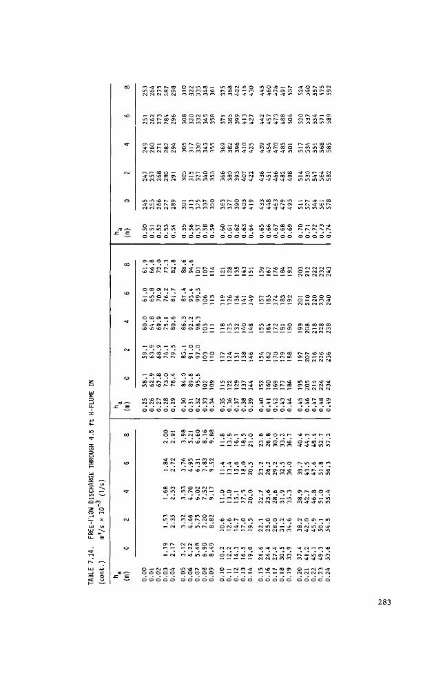
CO
V£)
*r
<XJ
o
(Ü s
J= E
co
UD
<d"
Od
o
(O '—^
-e E
co
VO
**
OJ
o
ro *-~-JZ E
m m CM
m CN
Cn •<r CM
r-»
-tf CM
m -d-CM
o m
o
CT\
MD
O
^o
O
o MO
„
Ol m
CO m
m CM
o
o o
o
-J-M3 CM
CM MD CM
O \o CM
r» m CM
LO m CM
m
o
CO
MD MD
CO
m MD
co
-d-MD
cn
m \£>
Oi
CM MO
\D CM
o
_t o
o
m p-CM
CO
CM
r-* CM
00 •*D CM
MD MD CM
CM in
o
o
CM 1-
0\
O r-
cn
os MO
Cn
CO \ß
CO
p^ ^O
p» CM
O
CM
o O
^ co CM
-tf 00 CM
CM 00 CM
O 00 CM
r- p-CM
CO m
o
co
p* p-
CM
MD r^
m p^
„
sj-
" o
CO p*
00 CM
O
O O
CM
-tf 00
_
00 MD
„
co m
~"
Cn CO
~ rO O
o
co cn CM
\D o\
"
•vT O-i CM
cn CM
cn co CM
<r m
o
00
co
r-
00
v£>
O 00
m
cn r-*
•<f
co r-~
Oi CM
O
Os
CM
CM r^
CM
CO m
CM
m CO
CM
p^
— CM
-d" O
O
O
CO
co o CO
m o CO
CO o co
O CO
m m
o
MD
co 00
-d-
p^ co
co
MD CO
— m 00
o
<3-00
O CO
o
CO os CO
MD p^
co
co m
CO
CM CO
CO
CM
~" CO
m o
o
CM CM CO
o
CO
f-
co
m
CO
CO
CO
^ m
o
\o
•<T
CT\
-d-
CO Cn
CM
CM 0\
O
cn
00
0"\ 00
^ co
o
CM
m
m cn
<t
o p^
-d-
^o -d-
-d-
CM CM
<t
MD O
o
m CO CO
CM CO
m
o CO CO
r-CM CO
m CM co
p»
m
o
o
m
cn cn
CO
00 cn
o
p* cn
co
in Cn
CM CO
O
o MD
MD
_ CO
MD
CM O
MD
m p^
m
00 <r
m
p* o
o
00 -3" CO
m -d-CO
co -d-CO
o -d-CO
r» co co
co m
o
r-~ O
MS o
m o
co o
CM O
CO CO
o
MD
— CO
CO 00
r-*
CM m
r^
O CM
r^
O Oi
\D
00
o O
^ MD CO
CO m co
m m CO
CO m co
O m CO
cn m
o
-d-
CO
o
cn O
r CO
o
00 00
cn
CM m
o\
r»
~ cn
CM co
co
Cn
-tf co
cn O
O
m r-. co
p-co
cn \D CO
MD M3 CO
CO ^D CO
O MD
O
CM
cn
00
p^
in
m CO
o
00
_» ""
-d-
„
~"
o
^ ~
\ü
o
CM
O
o
o
00 co CO
m CO CO
00 CO
o CO CO
r^ p^ co
MD
O
co CM
MD CM
m CM
<t CM
CM CM
\D CO
O
co
CO
"~
-d-
eo —
O
co
"
MD
CM
CM
CM
„
O
CM O -d-
o~> cn co
^D cn co
co cn co
o cn co
CM vO
O
m CO
<r co
CM CO
CO
cn CM
r^ CO
o
— MD
~
MD
in
—
" m
^-
r-»
<r
CO
<t
CM
O
VD
<r
CO
-j
o
-j-
r^ O -d-
m o <r
CO MD
O
CO -3-
-d-
O
<*
00 co
r- co
00 co
O
in
00
" o
00
"
in
r^
"—
o
r-
in
M5
CO
O
O co -d"
r^ CM -d"
m CM
-tf
CM
'J-
cn
-3-
vr ^o
o
m
cn
-*
co <r
MD
<*
<J •d-
cn co
o
o „ CM
m
o CM
O
O CM
m
cn
o
cn
<r
o
m <j ~3-
CM <T -J
cn co <f
v£> CO -r
CO CO <r
m MÏ
o
cn m
r^ m
m m
<t m
CM m
o
-* o
co
CO CM
CM
CO CM
r^
CM CM
~ CM CM
« CM
m
o
o £>
<r
r-m •<r
-d-m <f
m •<3-
00
-* -*
MD v£>
O
r^ ^D
m ^o
<r \o
CM MO
O MD
„ <r
o
00
MD CM
CM
\£> CM
VO
m CM
O
m CM
<r <3-CM
MD
o
MD r-. <f
co r .
-*
O p^ sr
MD MD ST
CO MD
-*
r» MD
O
MO r^
sj-i^
CM r^
O r
cn MD
CM *j-
O
o
o co
CM
Cn CM
MD
00 CM
O
00 CM
*3-
CM
r^
o
„ cn ~3-
CO 00 -d-
m co
-*
CM 00 ~d-
cn r^ •<r
co MD
O
-* 00
co 00
00
Cn r^
p-. r^
co <3-
O
CM
CO CO
m
CM CO
cn
_ CO
CM
CO
m
o co
00
o
r» O m
-3-o m
o m
co cn -d-
m <y\ <t
cn vD
O
CO cn
cn
O cn
CO 00
MD O0
<f -3"
O
f*
MO CO
O
MD CO
co
m co
MD
CO
Cn
co co
cn
O
•<r CM m
o CM m
r-
m
-d-
in
m
o
o
co o CM
O CM
cn cn
cn
m cn
m <r
o
<r
o -a-
r^
cn co
cn
00 co
CM
co co
** co
o CM
o
o •<r m
r» co m
•<r CO m
o co m
p» CM m
p-
o
CM
CM
O
CM
00 O CM
P» O
m o CM
MD
<fr O
CO
*d--d-
m
CO
-*
r^
CM <r
o
CM
CM
-* „ CM
O
P-m m
-* m m
m m
r-
-* m
•j-<t m
CM P^
O
CM CM
O
CM
00
CM
\D
CM
-4"
CM
P^ <J
O
-Î
00 <t
MD
r-r
co
M0 -d-
<J\
m
— m
CM CM
o
in p^ m
r-m
CO \£> m
-d-^O in
\D m
ro p~
O
CM CO CM
O CO CM
00 CM CM
Mï CM CM
<r CM CM
00 <r
o
f*
CM m
00
„
m
o
^ m
— o m
co
cn
co CM
O
CM cn in
cn 00 m
m CO m
CM 00 m
co p-m
<j-p^
o
co -d-CM
o -d-CM
00 CO CM
v£> CO CM
-d-CO CM
en -d-
O
CM
r- m
co
M) m
-d-
m m
m
m
MD
CO in
d-CM
O
283
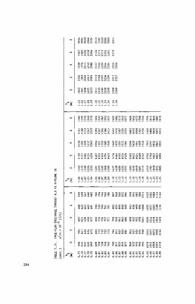
CO
MD
*d-
C\J
O
fÖ -—-
.e e
CO
MD
*d"
C\J
O
<d '—--£Z E
CO
UD
«d-
CvJ
o
fÖ '
J= E .—-
-d-
m CA
p» -d-
CA
CA
CA
CM ro CA
CA
Ol
MD MD
MD
MD m
o in
m -d-
o o
o
MD
MD o MD
m o MD
CA CA un
MD CA m
m p^
o
„ CA CA
ro CO CA
MD p-
CA
CA
MD CA
MD CA
MD
co CA
CO CO
CM CO
r-r-
r-
O
CO (N MD
m rs| MD
CN MD
^ MD
-d-
MD
MD r*~ O
CO
o
CM
O
CN O CN
co
O
Cs|
MD
O O CM
CO CA CA
CM
O
CM
m
CM
CA o CM
-d" O CM
CO CA
CM O
r*. -d-MD
cn -d-MD
CA CO MD
MD ro \D
CM ro MD
p» p*
O
MD MD
o
CM
CO
m o CM
o m o CM
en -4" o CM
m CO
o
CO CM
CO -d-CM
CM -d-CM
p» co CM
en CM
MD CM
CO o
MD MD MD
CN MD MD
00 m \D
-d-m MD
o m MD
00 p^
O
-d-O
CM
MD CA
o
CM
00
00 O
CO O CM
CO r-. o
CM
CA
CM
MD r» CM
o p^ CM
m vO CM
CA m
-
CO m CM
-d-o
m CO MD
CO MD
r^ r^ MD
ro p^ MD
CA MD MD
CA p^
O
CM
CM
ST CO
CM
Csl
CA
s
CM
o CO
-J-o CO
CA CA CM
CS, CA CM
p-CO
-
CO CM
m o
-d-o p»
o o p^
MD CA MD
CO CA MD
CA 00 MD
O CO
o
_ CO
CO
m MD
CM
CO m CM
o m CM
CO
CO CO CO
p» CM CO
CM CO
MD
CO
O
CO
MD O
-d-CN r-
O CM P*
MD
P»
CM
P^
CO o p»
_ CO
o
o
CM CM
CN
CM CN
m O CM CM
P* OA
CN
CA 00
CM
CM CO
CM MD ro
MD m co
o m CO
LO •d-
co
CA CO co
p~ o
-d--d-t-
O -d-p^
MD CO p^
CM ro r-*
co CM P^
CM 00
O
o MD CM
m CM
-d-CM CM
MD CO
CM
co CM CM CM
CO CO
CM CA CO
MD 00 CO
O CO CO
<r p^ CO
CO MD CO
00 o
m MD P v
MD p»
r^ m r^
CM in r-*
CO -d-p^
CO CO
o
o o CO CM
CN CA CM CM
-d-C0 CM CM
MD P-CM CM
CO MD CM CM
-d-CO
CM -d-
m
-d-
CA o -d-
CO o -d-
CO CA CO
CA O
MD 00 r-N
CO
"
p^ p> r-.
CO r-. p-
CA MD P-
-d-CO
O
— -d-
co
CO CO CO CM
m CO
CO CM
CO
o CO
m CO
CM m -d-
MD •<r - j -
o -d-sj-
~d-CO -d-
p-
•d-
O
r-O 00
CM O 00
CO CA p^
-d-CA p-
o CA r-*
m CO
o
MD MD CO
P»
m CO CM
OA -d-CO CM
MD CO
CO ~d-
MD r» <r
o p^ -d-
•<r MD •<r
00 m -d-
co CM 00
-d-CM CO
o CM CO
in
00
CO
MD CO
O
CO
in
p-o m
o m
m CA -d-
CA 00 ~d-
CM
o m co
MD ~d-00
<r 00
r-* co 00
CO CO co
r-* co
o
•d-in
CA CO m
CN co m
MD CM m
o CM m
CO
CM P^ 00
co MD 00
CO MD CO
CA m 00
m m 00
00 00
o
p» p» m
o p -
m
-d-MD m
00 in in
m m
-d-
-d-CA CO
o CA co
MD co CO
CO CO
r--p^ 00
CA 00
o
CA O MD
CO O MD
MD CA m
o CA m
CO CO m
in
00
CA
CO
CA
CA o CA
-d-O CA
CA CA CO
o CA
O
~d-MD
m CO MD
CA CM MD
CN CN \D
MD
MD
MD
-d-CA
MD CO CA
CM CO CA
P-v
CA
CM CM CA
„ CA
O
m p-MD
00 MD MD
MD \o
m m MD
CO -d-MD
P-.
m MD CA
O MD CA
m m CA
O m CA
MD -d-CA
CM CA
O
CO O P»
o r-
m CA MD
CO CO MD
CO MD
CO
CO 00 CA
-d-00 CA
CA p-CA
-d-r^ CA
CA MD CA
CO CA
O
CM •<r
r
m CO r^
00 CM P»
CM CM P^
in
r-.
CA
CO
O
CO o o
CO o o
CO CA CA
CO CA CA
-d-CA
o
MD p» P-.
CA MD P~
CO MD P-
MD m p^
CA -d-p-
O CM
CO O
CM CO O
CO CM O
CO CM O
CO
o
m CA
O
CO
-d-o CO
P--CA p*
o CA p^
CO CO p^
CN
CN MD O
r-N
m o
CM m o
p^ -d-o
CM <J O
MD CA
O
MD -d-CO
CA CO 00
CM CO CO
m CM CO
CO
CO
CM CM
CO 00 o
CO CO o
CO p-o
CO
o
CO MD o
P-. CA
o
CM 00 00
m p^ CO
r». MD CO
O MD 00
CO m 00
CO CM
~d-
CO o
CO o
00 CA o
CO CA o
CO CA
o
CO
CA
o
CA
CO o CA
^D CA CO
CA CO 00
'd-CM
o -d-
-d-CO
CA CM
<r CM
CA
~~ CA CA
O
284
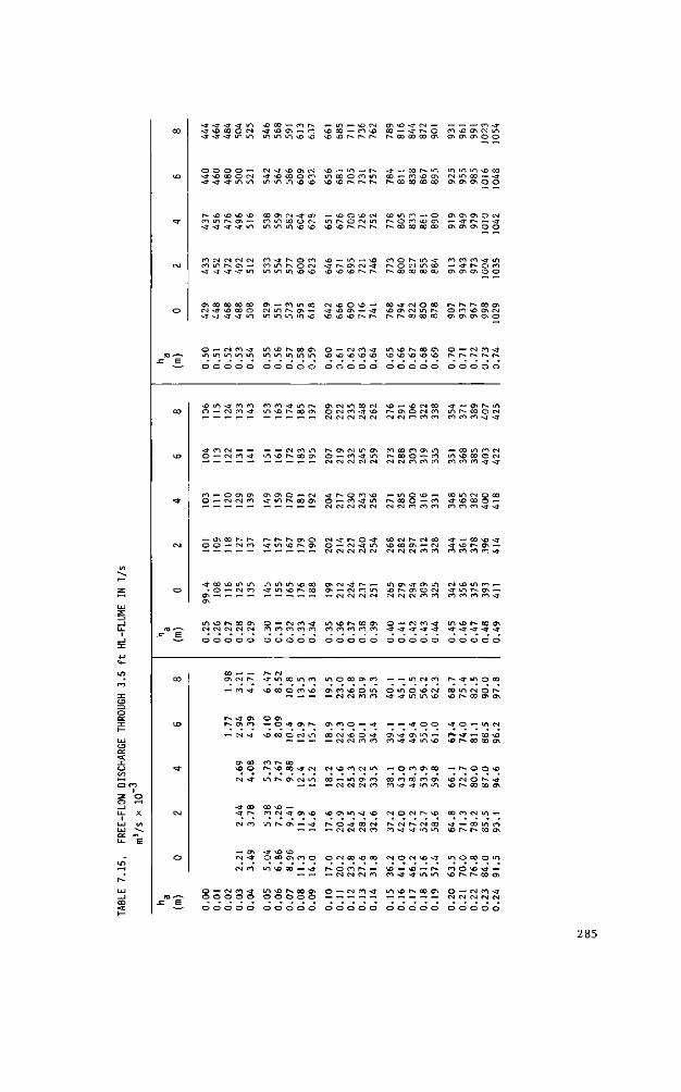
•d- -d- -d- -<r m
-d- -a- -d- m m
o o o o — * t i o e o O N -<r <j- -<r m m
N \D ifl >û vD on m N en — •d- -d- -3- -d- m
On CM CN CM CN en m N O I --d- -d- -d- -d- m
a\ oo co 00 00
-3- -d- - * <r m
vu oo — co N — m ^ - v o o v i -d" *£> 0 \ ™ CO vO 00 ~ - CO MD un un un »e \o \o ".o N N N
a i vD -d- CN — 00 - s j N O N co co oo o\
— — — m -d -
00 VD cri csj m 01 0*i CJi O O
CN -d" vO CTl CN <j vo to o n un >n in so ^D
CO on CN -d - 00 oo m co o OM i / l 1/1 IT| \ û \ D
oo -d- N o co oo un p-. o ON un i n i n ^o vo
on — oo un oo M I A N 0 \ -un m un un vo
V£) ,— LTl — N
un co o oo m
\D vß N N N
— vO O >£> CN un r - o CM un vo ^o N N N
un m un so oo CM m oo ~ - j -
Oi CF< Ol O O
oo m oo — o t— o oo ^o en r-- oo oo oo oo
ON vJD O M3 — >J M) CA — - ï ^û vo *£> N N
m o M n < r N O M m co N C O C O C O C O
00 -4- ON O 00 \ D O l M m N N N C O C O C0
O l On CT\ O OM - •vT N - - J on On 0~i O O
oo co co s t un — -d- N o oo CA O CT» O O
PN N N CO O-i O r n \ D CTi CM C\ C \ C> Cf\ o
o o o o o o o o o o o o o o o o o o o o o o o o o
v o u n < t c o o o co oo <r m N oncNunoocN MD ~ - MO CN oo ^ • - o> N m O — CN CO <T lH\0 rv CO Ol O CN CO <t M3 N Oi O CN CO m M » O l N „ ^_ „ „ „ _- ^_ „ — ^ 0MCNCNCNCN CNCNCOCOCO CO CO CO -d- <t
-d- oo CN ~- — — — OM oo m N o> CM in oi co ao co oi m ~- co un co CM O " CM tn vt ui T rs co o> o — oo d- in M O o - n m ^o oo o CM ^ - „ „ „ _ - ^ _ ^ - _ „ „ C N C N C N 0 M 0 N CN CN 0O CO CO CO OO CO -d" -d"
C O ^ - O O C T i CTi O l O " CN s j IS- O fO ^D ~ - un O M3 ~ - o o u n c N O c o O ^ - C N C N C O <r m rv co e. o ~- oo <j- in N oo o ~- oo -j- MO co o — ^ ^ ^ - „ „ ^ - ^ - „ ^ — CNONONCNCN cNoMcocooo oo co co -d- -d-
— O \ C 0 N N N N N O l O C N s t N O - d - CO N N CM CO -d" — 00 M3 <T o o — c N c o < f m vß N e i o — CM < r m MO co o i ~ - CM < r > O N O -„ „ „ _ — ^_ ^ - „ „ „ C N C N C M e M O M OMCMCNOOCO CO CO OO CO <fr
• ^ co VÛ m m m i n i n MD oo on CM -d- N ~ i n o x r o i m CM oo un m — • O — CM r o -d - i n >£> N co en ~ CM oo un vo N o i o CM - j - m N cn -
cn — « « ^ - ^ - — ™ „ _ - ^ - C M C M O N O N c N C M C N o o o o co co co oo < t o \
m *o N co cn o — O N C O S T m ^ o N co o> o — CM co <j- in vß N oo oi C N C N O N O M C N CO CO CO CO CO 0 O 0 O 0 O C O O O • * - Ï < r < ' J -d - -d1 -d" v f <fr
o o o o o o o o o o o o o o o o o o o o o o o o o
CO ~ - — N CM
cri cN N »d- m oo in oo m o oo o i co - - m c g co N 4 in o co
~ - co -d- \ o o o o t o v o o \ r o MO o m o m o * N oo i n ON o N ~ — ~- - es (N n fl -d- <a- i n m vo MO N oo on o i
N <* o i O o i
N oi co — o <r oi N o> n o - <t ^ - ^ - s j o o -d- o — in CM
— CM -d- vC co o es m c o c u o o * J o i <ï a i un ~ - r ^ - * ~ co \o —, ^ - — — 0N CM CO CO OO <J -d" m M3 * N C O CO O l
Ol OO OO Ni OO \ D O N MD OO -d" CN C N v O O O C N m « O CO O l CO ~ - N O O vO
CM < t m N O l CM m CO — m O CO 0 0 0 0 0 0 0 0 0 1 vO OM O î*- *d"
^ - — — C M C N C N I O O co < r < r m m > D N C O co o<
-d- 00 00 MD •—
• d - N CO CN > ï C M D \ D 0> m • * i O CM O CM N VO CO CO M i n -CM CO U0 N O l — < ï N O - Î 0 0 N N CM N CN CO -d" — CO m CO
~ - — - CM CM CM c o c o - j - j m m MO N N oo 01
^ - 0 1 -d- \o \Q c M - d - o c o c h n o o c M c o v o co c N O e N v o < t m o c o o m
c N c o un \ o 00 — < r N O C O N ^ - \ © — \ © —. N 1 0 0 * 0 4 « — ^ - - CM CM CM CO CO •Cf - T m m « N N C O a
O — CN 00 -d- m v C N Q O C A O ™ CN CO -vT lO 'C N 00 Cl O — CM co <t
O O O O O O O O O O — _ ^ - « ^ - « „ „ ^ - _ CM CM CM CM CM
O O O O O o o o o o O O O O O O O O O O O O O O O
285
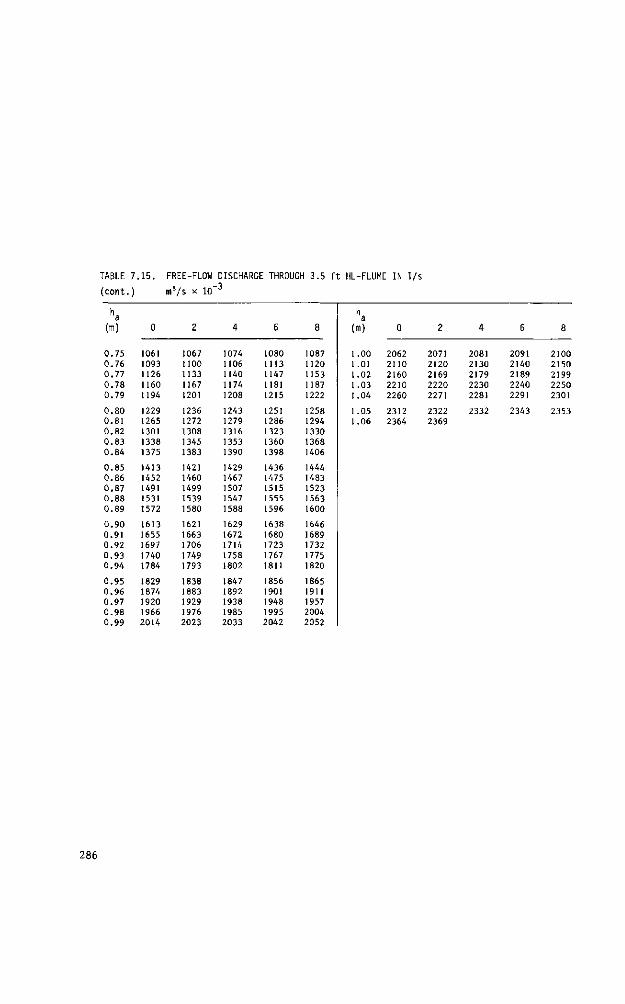
TABLE 7.15. FREE-FLOW DISCHARGE THROUGH 3.5 f t HL-FLUME IN 1/s
(cont . ) m3/s x 10 -3
ha (m)
0.75 0.76
0.77 0.78
0.79
0.80 0.81 0.82
0.83 0.84
0.85 0.86
0.87 0.88
0.89
0.90
0.91 0.92
0.93 0.94
0.95 0.96 0.97 0.98
0.99
0
1061
1093 1126
1160
1194
1229 1265 1301 1338
1375
1413 1452
1491 1531 1572
1613 1655 1697
1740 1784
1829 1874 1920 1966
2014
2
1067
1100 1133
1167
1201
1236 1272
1308
1345
1383
1421
1460
1499 1539 1580
1621
1663 1706
1749 1793
1838 1883
1929 1976
2023
4
1074
1106 1140
1174
1208
1243 1279 1316
1353 1390
1429 1467 1507 1547
1588
1629 1672
1714 1758 1802
1847 1892
1938 1985
2033
6
1080
1113
1147 1181
1215
1251 1286
1323 1360 1398
1436
1475 1515 1555
1596
1638 1680
1723 1767
1811
1856
1901 1948 1995 2042
8
1087
1120
1153 1187 1222
1258 1294 1330 1368
1406
1444
1483 1523 1563
1600
1646
1689 1732
1775 1820
1865 1911
1957 2004 2052
ha (m)
1 .00
1.01 1.02
1.03
1.04
1.05 1.06
0
2062
2110 2160
2210
2260
2312 2364
2
2071 2120 2169
2220
2271
2322
2369
4
2081 2130
2179
2230 2281
2332
6
2091 2140
2189 2240
2291
2343
8
2100 2150
2199 2250 2301
2353
286
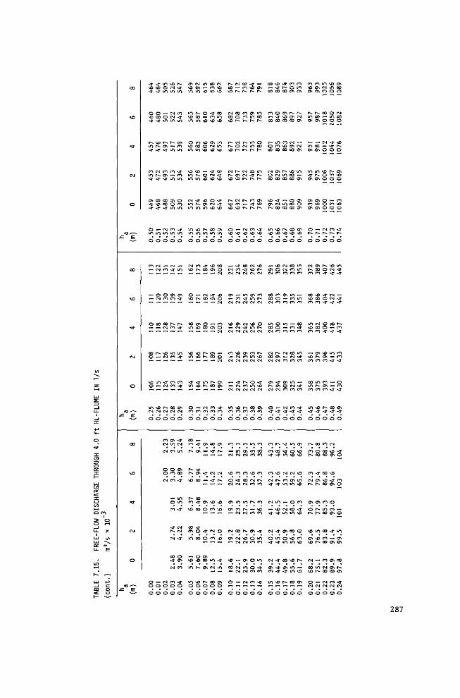
• J - J i T i ^ N O l CM m CO CM r - CM CO -J - ~ -v û C C O N - J \D O l *— CO v£> 00 *— CO O l s j - 4 m i A m i / i 10 vo ^ D vo \ 0 r - r— r^ r~-
o o — CM co I ^ N O - Î K CM co co 01 m ^o co o CM < r VD oo — en i n co o co m co - j - -d - m m m L o i n ^ D v o ^ ^ o r - * r * r — r -
p*. v£> r - r- o i o m m o i o r-~ CM r-* co o I A F N C .-1 en v£) CO O CM u~l r-~ o CM m co < - î < r i n m m i r i v o m vo \ 0 r - r - r^ r -
n N e n n ^ t v o œ - < - co CM P - CM co m u~i r- o \ — co m s o N s t p^ o i CM <3- r-*
o i c o co O i o N ^ \ 0 O > T p^ CM r-* en o i - JvDCO O o i IT) S 0\ CM - J M) Ol ~ <T vD •^r<j--^fiT)u-i m m m *o MÏ m ^ N s N
C O M J - Î n c o co en m vX) a i — -<r r^ o co MD o i CM i n co CO CO CO O l O l O l O l O O O
co o o \ r^ r-* P-. r~* co o CM - - j \ ß o i M in co - in co CO CO COCO O l O i O l O O O
N i n t n i N - ' — —« CM < î vß o co *£> o i CM i n c o — -a- r-» COCO CO CO O l O i O l O O O
c M c i r * . \ û m i r i m m N O i O CM u~i CO ~ -<r P^ O CO v£> CO CO CO CO O l O i O l O O O
l û - j " o o i o i o i o - n o i c M i n c o o n m o w v o N CO CO CO O l O i O l O O O
O O O O O O O O O O O O O O O O O O O O O O O O O
CO CM — ™ — CN fO < t vO CO p - - J C O N ^ O — \ O C M C O m CM O l P^ VO m ~ CM co N Ï m V O N C O d o CM co < j ^ P~ en O N t n m N C O O N - J _» _ ^ - „ _-, ^ _ _ ^ ^_ çsj CMCMCNOMCM CM CO CO CO CO CO m »cf v j - J
— o o o i o i o — CM < t vo o i — m en co c o r o o i m — co o •<ƒ CM ^~ — cMcoco-4- \o N C O O I O — co <r m r^ M O ~ c i m v o * O N - J ™ _ ^ - „ „ ^ „ ^ ^ ( ^ CM CM CM CM CM CM CO CO CO CO CO CO <T t <t
o c o c o r ^ r ^ co o i o — co »o o i es *o o i o o i n - c o i n c N O c o r ^ — — CM n - j m i o c o o i o - CM » j m Is» co o — co <r l o c o o - n — ^ - ^ - — - ^ - — — ^ - ^ - CM C M C M C M C M C M CM co cn co co co co < r <ƒ < r
co r-. ^ o u i m \ 0 >,o p^. o i — co i ß o i en P-^ M h . CM c o m — o i ^ o m c o o — CM co < î m \ 0 p» co o — c N c n m v o co o i - CM <T >xi N o i - co — — — " - — ^ - ^ - ^ - ^ c M CM CS CM CM CM C M C M C O C O C O CO CO CO <J <J
\ o m - d - c o c o - 3 - v j - m i ^ - o i •— <± p^ o -a- o i -3- o i m — co m co — o o — CM co ^ r m I Û r N co en — CM eo m m r ^ o i o c M ^ t m r^ o i — co ~ - — — — — ^ - ^ - _ ^ - ^ - CM CM CM CM I N CM CM CO CO CO CO CO CO - J -NT
m i o PN co en o — CM en < t m \ o N C C O I o ~ - CM co - ? m i o r ^ c o o i CM CM CM CM CM CO CO CO CO CO CO CO CO CO «O -<f <ƒ ^ f - ï <T <T <T < î - t f < t
O O O O O O O O O O O O O O O O O O O O O O O O O
co O l <T 00 ~ -cM i n CM — < • o i co o i co - - - m co c o r ^ ^ t m o i i ^ co co CM
CM c o m r ^ o i — < t r - — m o i co co co co ^ o i ß c o o c o ^ o < r _ ^ - , - CM CM CM CO CO • T ' * i n o o p-. co co o i o
o o oi r^ ^r o r o c o r ^ o i < r c M c M v£> co co v£> co c o v o CM CM m co < * co vo
CM CO • * VO 00 ~ - <T p - 0 < T 00 C M I N CM N CO O l m CM O l v£> <T CO — — — CM CM CM r o co < f < t i n m m r ^ r - c o o i O
— m N co o m e o < r o i ^ o ^ o o i m m P-» co C M I O - O C O o i o i c o o
c n * * * x o c o m en n N - - i o - vo CM co • * o M n c o -^ - — __ p - CM CM co co < r • * m m \ o p ^ r - c o o i o
< t CM CO < •
NCM 0 1 0 - * C M O CM CO px Ol <r CM • * Ol CO O \D m 00 « j m
C M - * m c o o c o i û o i c M I O o m o m o ^ o c o O l vu CO " O l
— — — p- M CM co co < t < f m m v f j I D s oo o i o i
00 o — O Ol
-4-01 > C i D ( O i O < t v O - O l O i O CM <r co ^o p - CM •— CO Ol 00
CM co m h - o i CM m co CM m o < t 01 «s- 0 1 m > - co m CM 0 1 r^ _ - „ ^ c s j f s j c o e o co • * < r m vC vo M » oo 0 1
o — CM co • * t n ^ o r - o o o i o — CM co *a- m v o r ^ c o o i o - CM c o - t o o o o o o o o o o — —i — — « ^ - ^ - ^ - ^ - , - CMCMCMCMCM
o o o o o o o o o o o o o o o o o o o o o o o o o
287
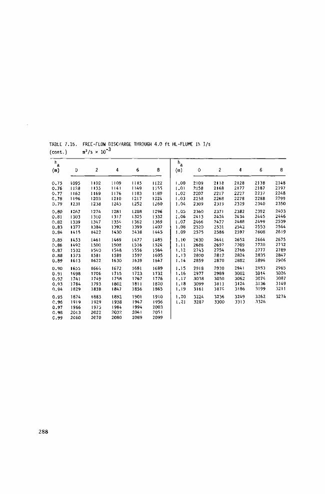
TABLE 7.15.
( cont . ) m3/s
FREE-FLOW DISCHARGE THROUGH 4.0 f t HL-FLUME IN ] / s 3
x 10
ha (m)
0.75 0.76
0.77 0.78
0.79
0.80 0.81 0.82
0.83 0.84
0.85
0.86 0.87
0.88 0.89
0.90 0.91 0.92
0.93 0.94
0.95
0.96
0.97 0.98
0.99
0
1095 1128 1 162
1196
1231
1267 1303
1339 1377 1415
1453 1492 1532
1573 1613
1655
1698 1741
1784 1829
1874
1919
1966 2013 2060
2
1102
1135
1169 1203
1238
1274 1310
1347 1384 1422
1461
1500 1540
1581 1622
1664 1706
1749
1793 1838
1883
1929
1975 2022
2070
4
1109 1141 1176
1210
1245
1281 1317 1354 1392
1430
1469
1508 1548
1589 1630
1672
1715 1758
1802 1847
1892
1938
1984 2032 2080
6
1115 1149 1183
1217 1252
1288 1325 1362
1399 1438
1477 1516
1556 1597
1639
1681
1723 1767 1811 1856
1901
1947 1994 2041
2089
8
1122 1155
1189 1224
1260
1296 1332
1369 1407 1445
1485
1524 1564
1605 1647
1689 1732
1776 1820 1865
1910
1956
2003 2051
2099
ha (m)
1.00 1.01 1.02
1.03
1.04
1.05 1.06
1.07 1.08 1.09
1.10
1.11 1.12
1.13 1.14
1.15 1.16 1.17
1.18
1.19
1.20 1.21
0
2109 2158 2207
2258
2309
2360 2413 2466 2520
2575
2630 2686
2743 2800
2859
2918
2977 3038
3099 3161
3224
3287
2
2118
2168 2217
2268
2319
2371 2424
2477 2531 2586
2641
2697 2754
2812 2870
2930
2989 3050 3111 3174
3236
3300
4
2128 2177
2227 2278
2329
2382 2434 2488 2542
2597
2652
2709 2766 2824 2882
2941 3002 3062
3124 3186
3249 3313
6
2138
2187 2237
2288 2340
2392 2445
2499 2553 2608
2664 2720
2777
2835 2894
2953 3014 3074
3136
3199
3262 3326
8
2148 2197
2248
2299 2350
2403 2446
2509 2564
2619
2675 2732
2789
2847 2906
2965 3026 3087
3149 3211
3274
288
7.6 Selected list of references
1. ACKERS, P., and HARRISON, A.J.M.: Critical-depth flumes for flow measure
ment in open channels. Dept.of Sci.& Industrial Research. Hydraulic Res.Sta.,
Hydr.Research Paper No.5. London. 1963.
2. BALLOFFET, A.: Critical flowmeters (Venturi flumes). Proc.ASCE. 81
(1951), Paper 743.
3. BENNET, R.S.: Cutthroat flume discharge relations. Thesis presented
to Colorado State University, Fort Collins, Col., in partial fulfillment of
requirements for the degree of Master of Science. 1972.
4. BLAU, E.: Die modelmässige Untersuchung von Venturikanälen verschiede
ner Grösse und Form. Veröffentlichungen der Forschungsanstalt für Schiffahrt,
Wasser- und Grundbau.Nr.8. Akademie Verlag, Berlin. 1960.
5. BRITISH STANDARDS INSTITUTION: Methods of measurement of liquid flow in
open channels. BS3680. Part 4. Weirs and flumes. 4A: Thin plate weirs and venturi
flumes. 1965.
6. CAPLAN, F.: Nomograph for Free Flow Discharge through a Parshall Flume.
Water & Sewage Works. May 1963.
7. EGGLESTON, K.O.: Effects of boundary geometry on critical and subcri-
tical flow through measuring flumes. Utah Water Research Laboratory. College
of Engineering, Utah State University. Logan, Utah. 1967.
8. ENGEL, F.V.A.E.: The venturi flume. Tne Engineer. 158 (1934). Aug.3,
pp.104-107. Aug.10, pp.131-133. London.
9. FANE, A.C.: Report on flume experiments on Sirhind Canal. Punjab Irriga
tion Branch. Paper No.110, Punjab Eng.Congress. 1927.
10. HARVEY, W.B.: Harvey's Irrigation Outlet. Punjab Irrigation Branch.
Paper. 1912.
11. HOLTAN, H.N., MINCHAL, N.E., and HARROLD, L.L.: Field manual for
research in agricultural hydrology. Soils & Water Conservation Research Div.,
Agricultural Research Service, Agricultural Handbook No.224. Washington D.C.1962.
289
12. IDELCIK, I.E.: Memento des pertes de charge. Collection du Centre
de recherche et d'essais de Chatou. Eyrolles. Paris, 1969.
13. INGLIS, G.C.: Notes on standing wave flumes and flume meter falls.Public
Works Dept., Technical Paper No.15. Bombay. 1929.
14. JAMESON, A.H.: The development of the venturi flume. Water & Water Engi
neering. March 20. 1930. pp.105-107.
15. KHAFAGI, A.: Der Venturikanal. Theorie und Anwendung. Diss.-Drückerei AG.
Gebr.Leemann & Co., Zürich. 1942.
16. PARSHALL, R.L.: Improving the Distribution of Water to Farmers by Use of
the Parshall Measuring Flume. Soil Conservation Service. Bull.488. U.S.Dept.
of Agriculture and Colorado Agricultural Experiment Station. Colorado A and M
College. Fort Collins, Colorado. May 1945.
17. PARSHALL, R.L.: Measuring Water in Irrigation Channels with Parshall
Flumes and Small Weirs. Soil Conservation Circular No.843. U.S.Dept. of Agri
culture, May 1950.
18. PARSHALL, R.L.: Parshall Flumes of Large Size. Bull.426-A (Reprint of
Bull.386). Colorado Agric.Experiment Sta., Colorado State University, Fort
Collins, Colorado, March 1953.
19. PETERKA, A.J.: Water Measurement Procedures. Irrigation Operators'
Workshop - 1965. Hydraulics Laboratory Report No.Hyd.-552. Bureau of Reclamation,
November 15, 1965 (unpublished).
20. ROBINSON, A.R.: Parshall Measuring Flumes of Small Sizes. Technical
Bulletin No.61. Agricultural Experiment Station. Colorado State University.
Fort Collins, Colorado. 1957.
21. ROBINSON, A.R., and CHAMBERLAIN, A.R.: Trapezoidal flumes for open-
channel flow measurement. Trans.Amer.Soc.Agri.Engnrs. 1960. 3. Nr.2, pp.120-128.
22. ROBINSON, A.R.: Simplified Flow Corrections for Parshall Flumes under
Submerged Conditions. Civil Engineering ASCE. September 1965.
290
23. ROBINSON, A.R.: Trapezoidal flumes for measuring flow in irrigation
channels. Agr.Res.Service ARS 41-140. March 1968. U.S.Dept.of Agriculture,p.15.
24. SCHUSTER, J.C.(Ed.): Water measurement procedures. Irrigation operators'
workshop. Report on REC-OCE-70-38. U.S.Bureau of Reclamation, Denver, Colorado,
pp.49. 1970.
25. SKOGERBOE, G.V., HYATT, M.L., ANDERSON, R.K., and EGGLESTON, K.O.:
Design and calibration of submerged open channel flow measurement structures.
Part 3: Cutthroat flumes. Report WG31-4. Utah Water Res.Laboratory. College
of Engineering. Utah State Unviersity. Logan, Utah. April 1957.
26. SKOGERBOE, G.V. and HYATT, M.L.: Analysis of submergence in flow
measuring flumes. J.of the Hydraulics Div., ASCE. Vol.93, No.HY4, Proc.Paper
5348. July 1967. pp.183-200.
27. SKOGERBOE G.V., HYATT M.L., ENGLAND, J.D. and JOHNSON, J.R.: Design
and Calibration of submerged open channel flow measurement structures. Part 2.
Parshall flumes. Report WG 3/-3. Utah Water Research Laboratory. College of
Eng. Utah St.University. Logan, Utah. March 1967.
28. SKOGERBOE, G.V., and HYATT, M.L.: Rectangular cutthroat flow measur
ing flumes. J.of the Irrigation and Drainage Div.ASCE, Vol.93, No.IR4. Dec.
1967, pp.1-33.
29. SKOGERBOE, G.V., BENNETT, R.S., and WALKER, W.R.: Generalized dis
charge relations for cutthroat flumes. J.of the Irrig.and Drainage Div.ASCE,
Vol.98. No.IR4. Dec.1972, pp.569-583.
30. U.S.DEPARTMENT OF THE INTERIOR, U.S.BUREAU OF RECLAMATION: Water
measurement manual. Second Ed. 1967. Denver, Colorado, 327 pp.
31. VEN TE CHOW: Open channel hydraulics. McGraw-Hill Book Comp., New
York, 1959, pp.680.
32. WELLS, E.A., and GOTAAS, H.B.: Design of Venturi flumes in circular
conduits. J.Sanit.Engng.Div.,ASCE. Paper No.2937. 1956. pp.749-771.
291
8 Orifices A well defined opening in a plate or bulkhead, the top of which is placed well
below the upstream water level, is classified here as an orifice.
8.1 Circular sharp-edged orifice
8.1.1 Description
A circular sharp-edged orifice, used as a measuring device, is a well-defined
opening in a (metal) plate or bulkhead, which is placed perpendicular to the
sides and bottom of a straight approach channel. For true orifice flow to occur,
the upstream water level must always be well above the top of the opening,such
that vortex-flow with air entrainment is not evident.
If the upstream water level drops below the top of the opening, it no longer
performs as an orifice but as a weir (see Section 5.4).
This orifice is one of the older devices used for measuring water and formerly
it was set up to discharge freely into the air,resulting in a considerable loss of
head. To overcome this excessive head loss, the orifice is now arranged with the
tailwater above the top of the opening. This "submerged orifice" conserves head
and can be used where there is insufficient fall for a sharp-crested weir or where
the head difference is too small to produce modular flow with a broad-crested weir
or flume. Circular orifices have the advantage that the opening can be turned and
its edges bevelled with precision on a lathe.Another advantage is that during in
stallation no levelling is required.
In practice, circular sharp-edged orifices are fully contracted so that the bed
and sides of the approach channel and the free water surface should be suf
ficiently remote from the control section to have no influence on the contraction
of the discharging jet. The fully contracted orifice may be placed in a non-
rectangular approach channel, provided that the general installation conditions
comply with those explained in Section 8.1.3.
A general disadvantage of submerged orifices is that debris, weeds and sediment
can accumulate upstream of the orifice, and may prevent accurate measurements.
In sediment-laden water, it is especially difficult for maintenance personnel to
determine whether the orifice is obstructed or completely open to flow. To
prevent the overtopping of the embankments in the case of a blocked orifice,
the top of the orifice wall should only be to the maximum expected upstream
water level so it can act as an overflow weir.
293
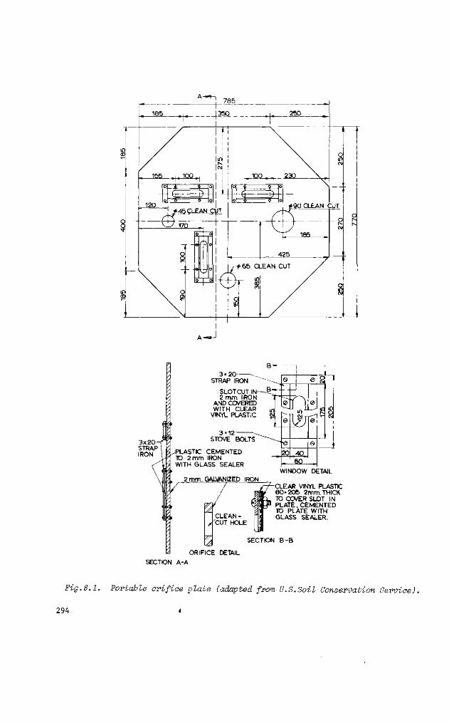
. -J
3 «20 STRAP IRON
SLOT CUT IN-2 mm IRON
AND COVERED WITH CLEAR
VINYL PLASTIC
3 "12 STOVE BOLTS
L- TD PLASTIC CEMENTED
2 mm IRON WITH GLASS SEALER
2 mm GAIVANIZED IRON
CLEAN-'CUT HOLE
WINDOW DETAIL
CLEAR VINYL PLASTIC 80« 205 2mm. THICK TO COVER SLOT IN PLATE. CEMENTED TO PLATE WITH GLASS SEALER.
ORIFICE DETAIL
SECTION B-B
SECTION A-A
Fig.8.1. Portable orifice plate (adapted from U.S.Soil Conservation Service).
294 <
Orifice plates are simple, inexpensive and easy to install, which makes them
suitable as a portable device to measure very low discharges such as furrow
streamflow. An example of a portable orifice plate with three ranges of measure
ment is shown in Figure 8.1. The orifice plate shown contains three slots covered
with clear vinyl plastic to permit the reading of the differential head from
the downstream side of the plate. Since flow through this orifice must be sub
merged it may be necessary to restrict the downstream channel in order to raise
the tailwater level above the top of the orifice.
8.1.2 Determination of discharge
The basic head-discharge equations for orifice flow, according to Section 1.12,
are
Q = CdCv Av^gCh, - h2) (8-1)
for submerged flow conditions, and
Q = C C A/2gAh (8-2)
if the orifice discharges freely into the air. In these two equations, h -h_
equals the head differential across the orifice and Ah equals the upstream head
above the centre of the orifice (see Figs.1.8 and 1.19). A is the area of the
orifice and equals ; TTd2, where d is the orifice diameter.
Orifices should be installed and maintained so that the approach velocity is
negligible, thus ensuring that C approaches unity.
Calibration studies performed by various research workers have produced the
average C,-values shown in Table 8.1.
The error in the discharge coefficient for a well-maintained circular sharp-
crested orifice, constructed with reasonable care and skill, is expected to
be of the order of 1%.
The method by which the coefficient error is to be combined with other sources
of error is shown in Appendix II.
295
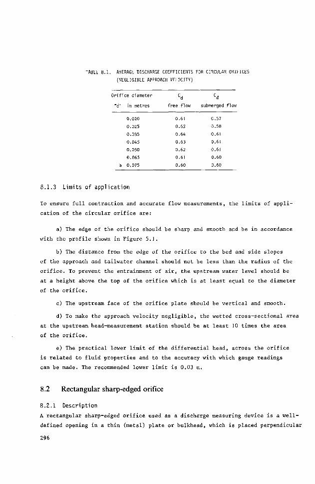
TABLE 8.1. AVERAGE DISCHARGE COEFFICIENTS FOR CIRCULAR ORIFICES
(NEGLIGIBLE APPROACH VELOCITY)
Or i f i ce diameter
"d " in metres
0.020
0.025
0.035
0.045
0.050
0.065
* 0.075
Cd
f ree flow
0.61
0.62
0.64
0.63
0.62
0.61
0.60
Cd
submerged flow
0.57
0.58
0.61
0.61
0.61
0.60
0.60
8.1.3 Limits of application
To ensure full contraction and accurate flow measurements, the limits of appli
cation of the circular orifice are:
a) The edge of the orifice should be sharp and smooth and be in accordance
with the profile shown in Figure 5.1.
b) The distance from the edge of the orifice to the bed and side slopes
of the approach and tailwater channel should not be less than the radius of the
orifice. To prevent the entrainment of air, the upstream water level should be
at a height above the top of the orifice which is at least equal to the diameter
of the orifice.
c) The upstream face of the orifice plate should be vertical and smooth.
d) To make the approach velocity negligible, the wetted cross-sectional area
at the upstream head-measurement station should be at least 10 times the area
of the orifice.
e) The practical lower limit of the differential head, across the orifice
is related to fluid properties and to the accuracy with which gauge readings
can be made. The recommended lower limit is 0.03 m.
8.2 Rectangular sharp-edged orifice
8.2.1 Description
A rectangular sharp-edged orifice used as a discharge measuring device is a well-
defined opening in a thin (metal) plate or bulkhead, which is placed perpendicular
296
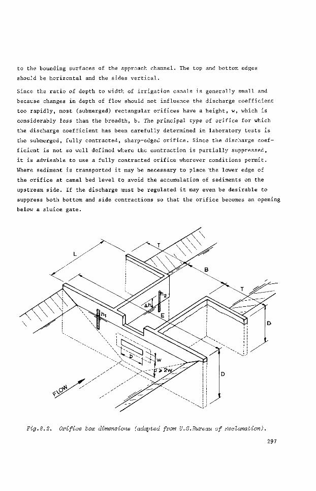
to the bounding surfaces of the approach channel. The top and bottom edges
should be horizontal and the sides vertical.
Since the ratio of depth to width of irrigation canals is generally small and
because changes in depth of flow should not influence the discharge coefficient
too rapidly, most (submerged) rectangular orifices have a height, w, which is
considerably less than the breadth, b. The principal type of orifice for which
the discharge coefficient has been carefully determined in laboratory tests is
the submerged, fully contracted, sharp-edged orifice. Since the discharge coef
ficient is not so well defined where the contraction is partially suppressed,
it is advisable to use a fully contracted orifice wherever conditions permit.
Where sediment is transported it may be necessary to place 'the lower edge of
the orifice at canal bed level to avoid the accumulation of sediments on the
upstream side. If the discharge must be regulated it may even be desirable to
suppress both bottom and side contractions so that the orifice becomes an opening
below a sluice gate.
Fig.8.2. Orifice box dimensions (adapted from U.S.Bureau of Reclamation),
297
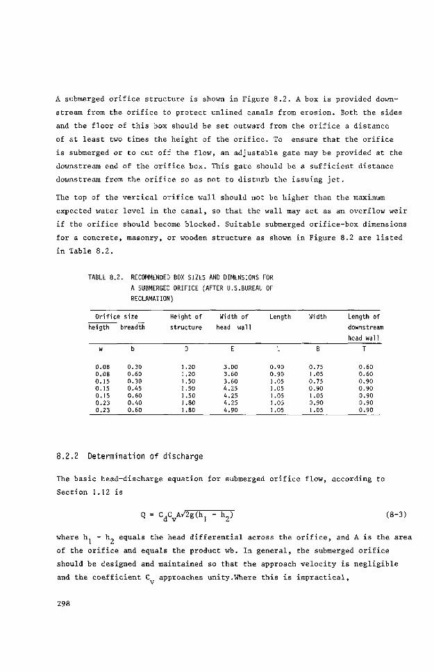
A submerged orifice structure is shown in Figure 8.2. A box is provided down
stream from the orifice to protect unlined canals from erosion. Both the sides
and the floor of this box should be set outward from the orifice a distance
of at least two times the height of the orifice. To ensure that the orifice
is submerged or to cut off the flow, an adjustable gate may be provided at the
downstream end of the orifice box. This gate should be a sufficient distance
downstream from the orifice so as not to disturb the issuing jet.
The top of the vertical orifice wall should not be higher than the maximum
expected water level in the canal, so that the wall may act as an overflow weir
if the orifice should become blocked. Suitable submerged orifice-box dimensions
for a concrete, masonry, or wooden structure as shown in Figure 8.2 are listed
in Table 8.2.
TABLE 8.2. RECOMMENDED BOX SIZES AND DIMENSIONS FOR
A SUBMERGED ORIFICE (AFTER U.S.BUREAU OF
RECLAMATION)
Orifi
heigth
w
0.08 0.08 0.15 0.15 0.15 0.23 0.23
ce size
breadth
b
0.30 0.60 0.30 0.45 0.60 0.40 0.60
He
St
ght of
"ucture
D
1.20 1 1 1 1 1 1
20 50 50 50 80 80
Width of
head wall
E
3.00 3.60 3.60 4.25 4.25 4.25 4.90
Length
L
0.90 0.90 1.05 1.05 1.05 1.05 1.05
Width
B
0.75 1.05 0.75 0.90 1.05 0.90 1.05
Length of
downstream
head wall
T
0.60 0.60 0.90 0.90 0.90 0.90 0.90
8.2.2 Determination of discharge
The basic head-discharge equation for submerged orifice flow, according to
Section 1.12 is
Q = CdCvA/2g(h] - h2) (8-3)
where h. - h„ equals the head differential across the orifice, and A is the area
of the orifice and equals the product wb. In general, the submerged orifice
should be designed and maintained so that the approach velocity is negligible
and the coefficient C approaches unity.Where this is impractical,
298
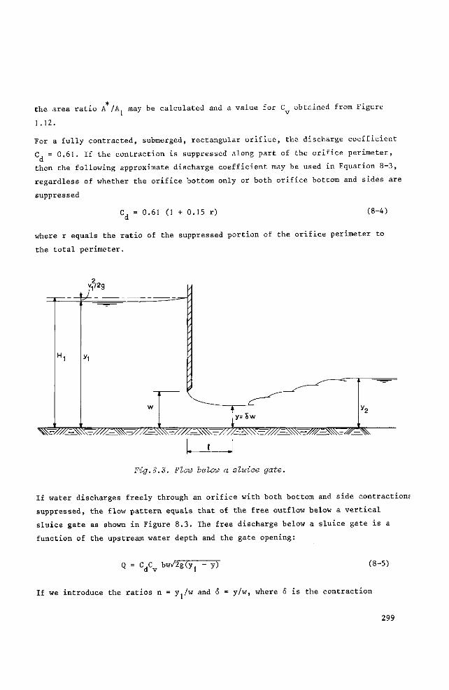
the area ratio A /A may be calculated and a value for C^ obtained from Figure
1.12.
For a fully contracted, submerged, rectangular orifice, the discharge coefficient
C. = 0.61. If the contraction is suppressed along part of the orifice perimeter, d
then the following approximate discharge coefficient may be used in Equation 8-3,
regardless of whether the orifice bottom only or both orifice bottom and sides are
suppressed
C, = 0.61 (1 + 0.15 r) d
(8-4)
where r equals the ratio of the suppressed portion of the orifice perimeter to
the total perimeter.
I , • ,1 Fig.8.3. Flow below a sluiae gate.
If water discharges freely through an orifice with both bottom and side contractions
suppressed, the flow pattern equals that of the free outflow below a vertical
sluice gate as shown in Figure 8.3. The free discharge below a sluice gate is a
function of the upstream water depth and the gate opening:
Q = CdCv bw/2g(y] - y) (8-5)
If we introduce the ratios n = y./w and 6 = y/w, where <5 is the contraction
299
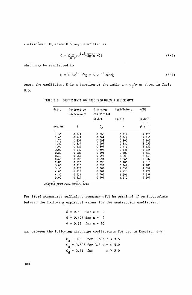
coefficient, Equation 8-5 may be written as
1 .5 Q = CX bw /2g(n -o)
d v
which may be simplified to
Q = K bw 1 - 5 /2g = A w 0 - 5 K/2É
(8-6)
(8-7)
where the coefficient K is a function of the ratio n = y./w as shown in Table
8.3.
TABLE 8.3. COEFFICIENTS FOR FREE FLOW BELOW A SLUICE GATE
Ratio
n=yj/w
1.50 1.60 1.70 1.80 1.90 2.00 2.20 2.40 2.60 2.80 3.00 3.50 4.00 4.50 5.00
Contraction
coefficient
5
0.648 0.642 0.637 0.634 0.632 0.630 0.628 0.626 0.626 0.625 0.625 0.625 0.624 0.624 0.624
Discharge
coefficient
Eq.8-6
Cd
0.600 0.599 0.598 0.597 0.597 0.596 0.596 0.596 0.597 0.598 0.599 0.602 0.604 0.605 0.607
Coefficient
Eq.8-7
K
0.614 0.641 0.665 0.689 0.713 0.735 0.780 0.823 0.865 0.905 0.944 1.038 1.124 1.204 1.279
K/Zg
Eq.8-7
^ S " 1
2.720 2.838 2.946 3.052 3.159 3.255 3.453 3.643 3.832 4.010 4.183 4.597 4.977 5.331 5.664
Adapted from P.G.Franke, 1968
For field structures sufficient accuracy will be obtained if we interpolate
between the following empirical values for the contraction coefficient:
6 = 0.63 for n = 2
6 = 0.625 for n = 3
o = 0.62 for n = 10
and between the following discharge coefficients for use in Equation 8-6:
C, = 0.60 for 1.5 < n < 3.5 d
C, = 0.605 for 3.5 < n < 5.0 d
C, = 0.61 for n > 5.0 d
300
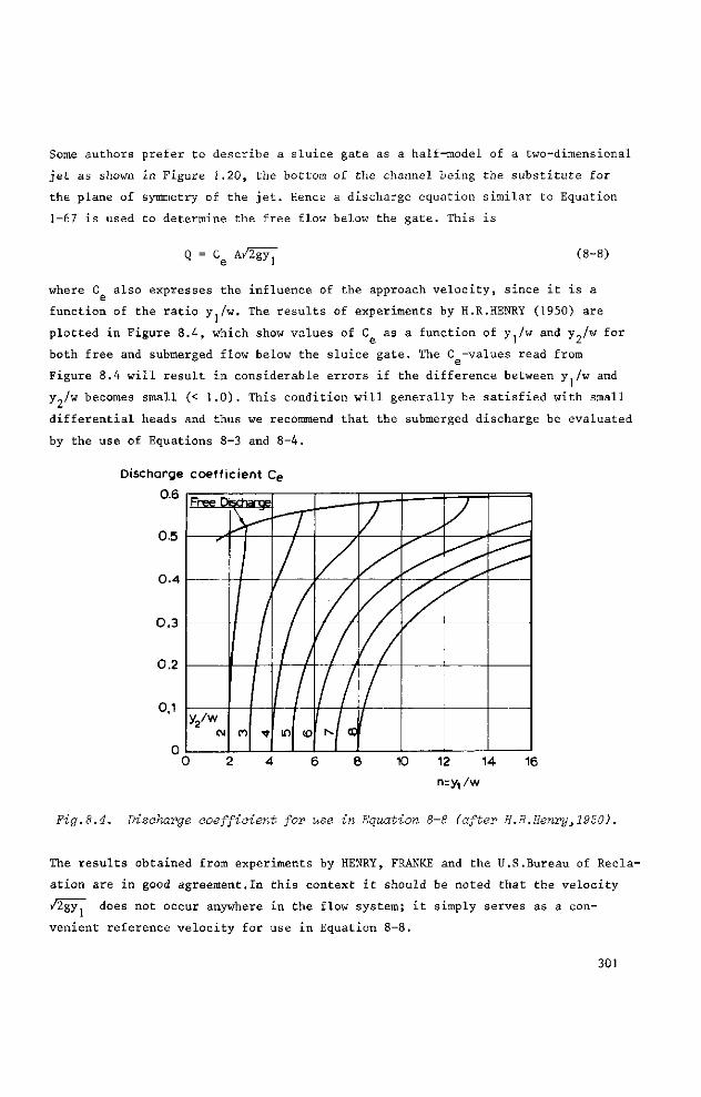
Some authors prefer to describe a sluice gate as a half-model of a two-dimensional
jet as shown in Figure 1.20, the bottom of the channel being the substitute for
the plane of symmetry of the jet. Hence a discharge equation similar to Equation
1-67 is used to determine the free flow below the gate. This is
Q = Ce A/2iyy (8-8)
where C also expresses the influence of the approach velocity, since it is a
function of the ratio y./w. The results of experiments by H.R.HENRY (1950) are
plotted in Figure 8.4, which show values of C as a function of y./w and y„/w for
both free and submerged flow below the sluice gate. The C -values read from
Figure 8.4 will result in considerable errors if the difference between y./w and
y„/w becomes small (< 1.0). This condition will generally be satisfied with small
differential heads and thus we recommend that the submerged discharge be evaluated
by the use of Equations 8-3 and 8-4.
Discharge coefficient C e
0.6
0.5
0.4
0.3
0.2
0.1
0 2 4 6 8 10 12 14 16 nr^/w
Fig.8.4. Discharge coefficient for use in Equation 8-8 (after Ü.R.Henry,1950).
The results obtained from experiments by HENRY, FRANKE and the U.S.Bureau of Recla-
ation are in good agreement.In this context it should be noted that the velocity
Free Discharae
X"
y2/w CM
/ /
CO ^ 101 (0
1 r*./ ©
S y
/2gyT does not occur anywhere in the flow system; it simply serves as a con
venient reference velocity for use in Equation 8-8.
301
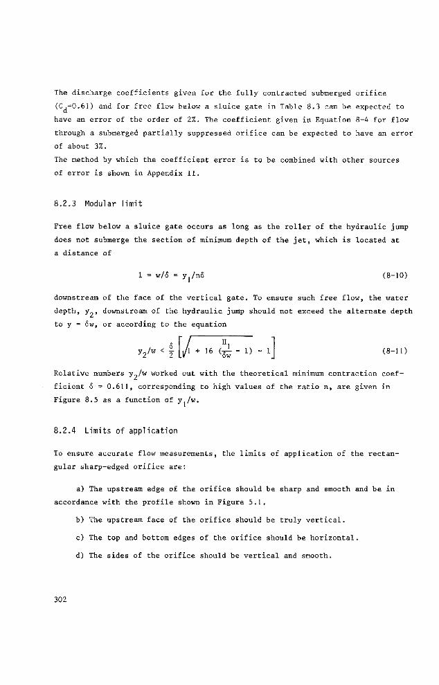
The discharge coefficients given for the fully contracted submerged orifice
(C =0.61) and for free flow below a sluice gate in Table 8.3 can be expected to
have an error of the order of 2%. The coefficient given in Equation 8-4 for flow
through a submerged partially suppressed orifice can be expected to have an error
of about 3%.
The method by which the coefficient error is to be combined with other sources
of error is shown in Appendix II.
8.2.3 Modular l i m i t
Free flow below a sluice gate occurs as long as the roller of the hydraulic jump
does not submerge the section of minimum depth of the jet, which is located at
a distance of
1 = w/<5 = y]/ni5 (8-10)
downstream of the face of the vertical gate. To ensure such free flow, the water
depth, y„, downstream of the hydraulic jump should not exceed the alternate depth
to y = 6w, or according to the equation
y2/w < j Hl
1 + 16 (-J- - 1) ow
(8-11)
Relative numbers y-/w worked out with the theoretical minimum contraction coef
ficient ô = 0.611, corresponding to high values of the ratio n, are given in
Figure 8.5 as a function of y./w.
8.2.4 Limits of application
To ensure accurate flow measurements, the limits of application of the rectan
gular sharp-edged orifice are:
a) The upstream edge of the orifice should be sharp and smooth and be in
accordance with the profile shown in Figure 5.1.
b) The upstream face of the orifice should be truly vertical.
c) The top and bottom edges of the orifice should be horizontal.
d) The sides of the orifice should be vertical and smooth.
302
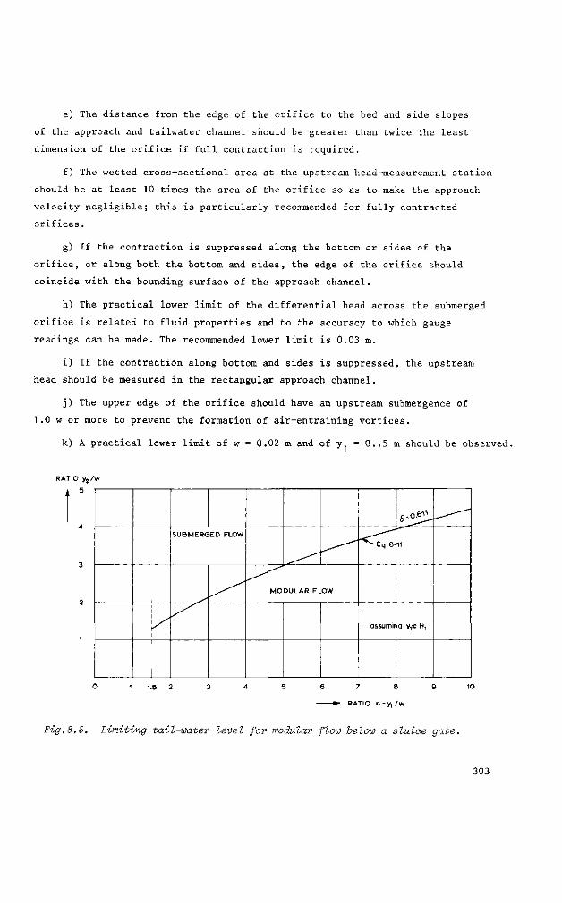
e) The distance from the edge of the orifice to the bed and side slopes
of the approach and tailwater channel should be greater than twice the least
dimension of the orifice if full contraction is required.
f) The wetted cross-sectional area at the upstream head-measurement station
should be at least 10 times the area of the orifice so as to make the approach
velocity negligible; this is particularly recommended for fully contracted
orifices.
g) If the contraction is suppressed along the bottom or sides of the
orifice, or along both the bottom and sides, the edge of the orifice should
coincide with the bounding surface of the approach channel.
h) The practical lower limit of the differential head across the submerged
orifice is related to fluid properties and to the accuracy to which gauge
readings can be made. The recommended lower limit is 0.03 m.
i) If the contraction along bottom and sides is suppressed, the upstream
head should be measured in the rectangular approach channel.
j) The upper edge of the orifice should have an upstream submergence of
1.0 w or more to prevent the formation of air-entraining vortices.
k) A practical lower limit of w = 0.02 m and of y = 0.15 m should be observed.
RATIO y 2 / w
5
[
1 .
l 1
l
SUBMERGED FLOW
MODULAR FLOW
6 ^
" ^ E q . 8 - 1 1
assuming y ^ H1
0 1 1.5 2 3 4 5 6 7 8 9 10
»• RATIO n = y , / w
Fig. 8.5. Limiting tail-water level for modular flow below a sluice gate.
303
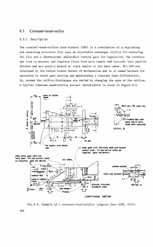
8.3 Constant-head-orifice
8.3.1 Description
The constant-head-orifice farm turnout (CHO) is a combination of a regulating
and measuring structure that uses an adjustable submerged orifice for measuring
the flow and a (downstream) adjustable turnout gate for regulation. The turnouts
are used to measure and regulate flows from main canals and laterals into smaller
ditches and are usually placed at right angles to the main canal. The CHO was
developed by the United States Bureau of Reclamation and is so named because its
operation is based upon setting and maintaining a constant head differential,
Ah, across the orifice.Discharges are varied by changing the area of the orifice.
A typical constant head-orifice turnout installation is shown in Figure 8.6.
b/_ canal or lateral - - '*—( slope
, Vent dia = TO pipe dia
-1:1
0 0.08 bend into wall place top of bars flush with concrete
DETAIL B
for typical joint detail, see
PLAN
c i . slide gate with flat back seat and square / bottom slide, lift and anchor bolts as
required, gate not shown. steel slide gate with flat back seat, l i ft and anchor bolts as required, gate not shown. —--
\ .M___ I ™ * top. hol es
mm
dia. holes.
canal or lateral-slope ---_•
>-£lA--.
r(max)-'
o.3o]"N.w:s.y^ Y ° J ° _ T T
control WS."' o y
cement mortar . ^ 0 i 5 » .
reinf. not shown- t
1 . 1 ^
0.20
IT: 0.101
Î 0.25 i ] T
0 6 0 I . _. precast concrete
A pressure pipe. 0.20
LONGITUDINAL SECTION
0.01 DETAIL A
Fig.8.6. Example of a aonstant-head-orifioe (adapted from USBR, 1970).
304
To set a given flow, the orifice opening A required to pass the given discharge
is determined, and the orifice gate is set at this opening. The downstream turnout
gate is then adjusted until the head differential as measured over the orifice
gate equals the required constant-head, which usually equals 0.06 m. The dis
charge will then be at the required value. The rather small differential head
used is one of the factors contributing to the inaccuracy of discharge measure
ments made by the CHO. For instance, errors of the order of 0.005 m in reading
each staff gauge may cause a maximum cumulative error of 0.01 m or about 16% in
Ah, which is equivalent to 8% error in the discharge. Introducing a larger dif
ferential head would reduce this type of error, but larger flow disturbances
would be created in the stilling basin between the two gates. Furthermore, it is
usually desirable to keep head losses in an irrigation system as low as possible.
Since the downstream gate merely serves the purpose of setting a constant head
differential across the orifice gate, its shape is rather arbitrary. In fact,
the turnout gate shown in Figure 8.5 may be replaced by a movable weir or
flap-gate if desired. If the CHO is connected to a culvert pipe that is flowing
full, the air pocket immediately downstream of the turnout gate should be aerated
by means of a ventilation pipe. The diameter of this pipe should be 1/6 of the
culvert diameter to provide a stable flow pattern below the turnout gate. If
the flow through the downstream gate is submerged, a change of tailwater level
of the order of a few centimetres will cause an equivalent change of water level
in the basin between the two gates. Under field conditions, the discharge in the
main canal is likely to be large compared with the discharge through the turnout.
Hence the head differential over the orifice gate will change with any change
in tailwater level, resulting in a considerable error in the diverted flow.
The reader will note that if reasonable accuracy is required in discharge
measurement, the flow below the turnout gate should be supercritical at all
tailwater levels. For this to occur, the turnout gate requires a minimum loss
of head which may be calculated as explained in Section 8.2.2 and with the
aid of Figure 8.5. The combined loss of head over the orifice gate (usually
0.06 m) and over the turnout gate (variable) to produce modular flow is consi
derable.
Usually the CHO is placed at an angle of 90 from the centre line of the main
canal, and no approach channel is provided to the orifice gate. As a result,
the flow in the main canal will cause an eddy and other flow disturbances
immediately upstream of the orifice gate opening, thus affecting the flow below
the orifice gate. Such detrimental effects increase as the flow velocity in the
305
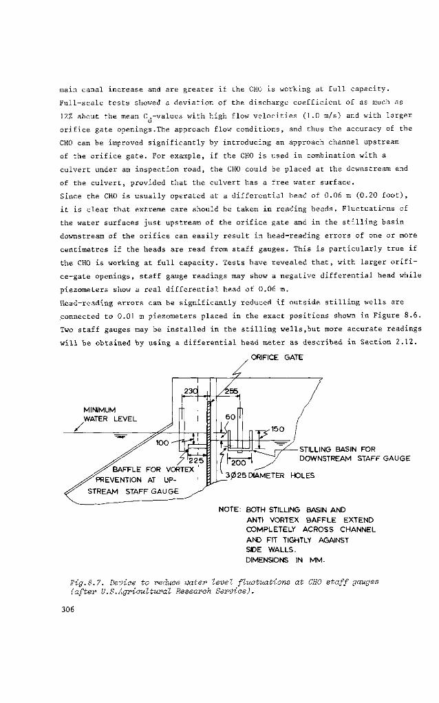
main canal increase and are greater if the CHO is working at full capacity.
Full-scale tests showed a deviation of the discharge coefficient of as much as
12% about the mean C,-values with high flow velocities (1.0 m/s) and with larger
orifice gate openings.The approach flow conditions, and thus the accuracy of the
CHO can be improved significantly by introducing an approach channel upstream
of the orifice gate. For example, if the CHO is used in combination with a
culvert under an inspection road, the CHO could be placed at the downstream end
of the culvert, provided that the culvert has a free water surface.
Since the CHO is usually operated at a differential head of 0.06 m (0.20 foot),
it is clear that extreme care should be taken in reading heads. Fluctuations of
the water surfaces just upstream of the orifice gate and in the stilling basin
downstream of the orifice can easily result in head-reading errors of one or more
centimetres if the heads are read from staff gauges. This is particularly true if
the CHO is working at full capacity. Tests have revealed that, with larger orifi
ce-gate openings, staff gauge readings may show a negative differential head while
piezometers show a real differential head of 0.06 m.
Head-reading errors can be significantly reduced if outside stilling wells are
connected to 0.01 m piezometers placed in the exact positions shown in Figure 8.6.
Two staff gauges may be installed in the stilling wells,but more accurate readings
will be obtained by using a differential head meter as described in Section 2.12.
ORIFICE GATE
MINIMUM WATER LEVEL
100
'225' BAFFLE FOR VORTEX
'PREVENTION AT UPSTREAM STAFF GAUGE
STILLING BASIN FOR DOWNSTREAM STAFF GAUGE
200
3 0 2 5 DIAMETER HOLES
NOTE: BOTH STILLING BASIN AND ANTI VORTEX BAFFLE EXTEND COMPLETELY ACROSS CHANNEL AND FIT TIGHTLY AGAINST SIDE WALLS. DIMENSIONS IN MM.
Fig. 8.7. Device to reduce water level fluctuations at CHO staff gauges (after U.S.Agricultural Research Service).
306
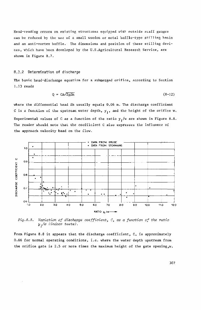
Head-reading errors on existing structures equipped with outside staff gauges
can be reduced by the use of a small wooden or metal baffle-type stilling basin
and an anti-vortex baffle. The dimensions and position of these stilling devi
ces, which have been developed by the U.S.Agricultural Research Service, are
shown in Figure 8.7.
8.3.2 Determination of discharge
The basic head-discharge equation for a submerged orifice, according to Section
1.13 reads
Q = CA/2gAh (8-12)
where the differential head Ah usually equals 0.06 m. The discharge coefficient
C is a function of the upstream water depth, y , and the height of the orifice w.
Experimental values of C as a function of the ratio y./w are shown in Figure 8.8.
The reader should note that the coefficient C also expresses the influence of
the approach velocity head on the flow.
m
0 9
ns
0 7
Ofi
.
, •
• •
«* « * , • • o * *
o
° ° '„*• °
| o DATA FROM • DATA FROM
' o •
KRUSE 1 STOKMANS
' o
*
°
•
*
1-0 2.0 3.0 40 5.0 6.0 70 8.0 9 0 10.0 11.0 12
RATIO y, /w —
Fig.8.8. Variation of discharge coefficient, C, as a function of the ratio y-,/w (indoor tests).
From Figure 8.8 it appears that the discharge coefficient, C, is approximately
0.66 for normal operating conditions, i.e. where the water depth upstream from
the orifice gate is 2.5 or more times the maximum height of the gate opening,w.
307
Substitution of the values C, = 0.66, Ah - 0.06 m, and g = 9.81 m/s into Equation
8.1 gives the following simple area-discharge relationship for the CHO:
Q = 0.716 A = 0.716 bw (8-13)
If the breadth of the orifice is known, a straight-line relationship between the
orifice gate opening and the flow may be plotted for field use.
The error in the discharge coefficient given for the Constant-Head-Orifice
(C = 0.66) can be expected to be of the order of 7%. This coefficient error
applies for structures that have an even velocity distribution in the approach
section. If an eddy is formed upstream of the orifice gate, however, an additi
onal error of up to 12% may occur (see also Section 8.3.1).
The method by which the coefficient error is to be combined with other sources
of error, which have a considerable magnitude, is shown in Appendix II. In this
context, the reader should note that if the upstream gate is constructed with
uninterrupted bottom and side walls and a sharp-edged gate, Equations 8-3 and
8-4 can be used to determine the discharge through the orifice with an accuracy
of about 3%.
8.3.3 Limits of application
The limits of application of the Constant-Head-Orifice turnout are:
a) The upstream edge of the orifice gate should be sharp and smooth and
be in accordance with the profile shown in Figure 8.6.
b) The sides of the orifice should have a groove arrangement as shown in
Figure 8.6.
c) The bottom of the approach section upstream of the orifice gate should
be horizontal over a distance of at least four times the upstream water depth.
d) To obtain a somewhat constant value for the discharge coefficient, C,
the ratio y./w should be greater than 2.5.
e) The approach section should be such that no velocity concentrations
are visible upstream of the orifice gate.
308
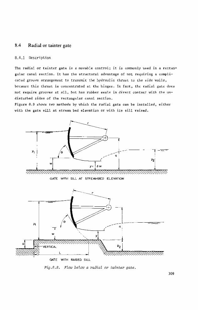
8.4 Radial or tainter gate
8.4.1 Description
The radial or tainter gate is a movable control; it is commonly used in a rectan
gular canal section. It has the structural advantage of not requiring a compli
cated groove arrangement to transmit the hydraulic thrust to the side walls,
because this thrust is concentrated at the hinges. In fact, the radial gate does
not require grooves at all, but has rubber seals in direct contact with the un
disturbed sides of the rectangular canal section.
Figure 8.9 shows two methods by which the radial gate can be installed, either
with the gate sill at stream bed elevation or with its sill raised.
*1
—
w
Ie m^
y=
•'-Pi
5 W
a r *2
GATE WITH SILL AT STREAMBED ELEVATION
^ ^ ^ ^ 5 ^ ^ ^ ^ ^ "VERTICAL
^ ^ ^ ^ ^ ^ ^ 'A GATE WITH RAISED SILL
Fig.8.9. Flow below a radial or tainter gate.
309
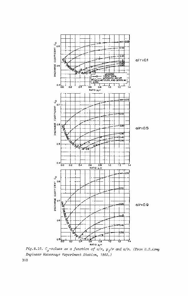
So.
4
X /
"I X '
%< uv
s
S
¥t o *~
"RA -^rî^KS
*T<
- —
w/r=
0.10
0.20
0.40 nfsc
005
- O TOCH DATA INTERPOLATED*
XH.METZLER.AND GENTILINI ATA
1 1 1 I 0 6 0.8 RATIO y,/r
y
1 1
^ /
^ %,
*
y
s
1
v: •<
^ •
/
k
^ "
^
o?
x^o
^ oè
' > H —
w/r=
û.to
0.20
0.30
0.4O
Q50
0.05
0.0 0.2 0,4 0.6 0.8 1.0 1.2 1.4 RATIO y , / r
u
z
G
u. LxJ O
u UJ
ce °'
< a
0.5
m|
h 1
/ '
\ •
i "*\ <
/ '
/ / '
0 / c
/
/
k. 1 °
/
/
/ '
S
S
/
""
^
^ r"
^s
1
0.10
0.20
mfl
0.40
0.50
a/r=0.1
a/r=0.5
a/rzO.9
Fig. 8.10. Co-values as a funotion of a/r, y Jr and w/r. (From U.S.Army
Engineer Waterways Experiment Station, 1960.)
310
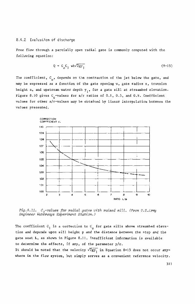
8.4.2 Evaluation of discharge
Free flow through a partially open radial gate is commonly computed with the
following equation:
Q = CoCj wb/2g7j (8-15)
The coefficient, C , depends on the contraction of the jet below the gate, and
may be expressed as a function of the gate opening w, gate radius r, trunnion
height a, and upstream water depth y , for a gate sill at streambed elevation.
Figure 8.10 gives C -values for a/r ratios of 0.1, 0.5, and 0.9. Coefficient
values for other a/r-values may be obtained by linear interpolation between the
values presented.
CORRECTION COEFFICIENT C,
110
1.09
1.08
1.07
1.06
1.05
1.04
1.03
1.02
101
1.00
\ \ ^
^ ^ . • • —
7 8
RATIO L /p
Fig. 8.11. C^-values for radial gates with raised sill. (From U.S.Army Engineer Waterways Experiment Station.)
The coefficient C, is a correction to C for gate sills above streambed eleva-1 o °
tion and depends upon sill height p and the distance between the step and the
gate seat L, as shown in Figure 8.11. Insufficient information is available
to determine the effects, if any, of the parameter p/r. It should be noted that the velocity /2gy in Equation 8-15 does not occur any
where in the flow system, but simply serves as a convenient reference velocity.
311
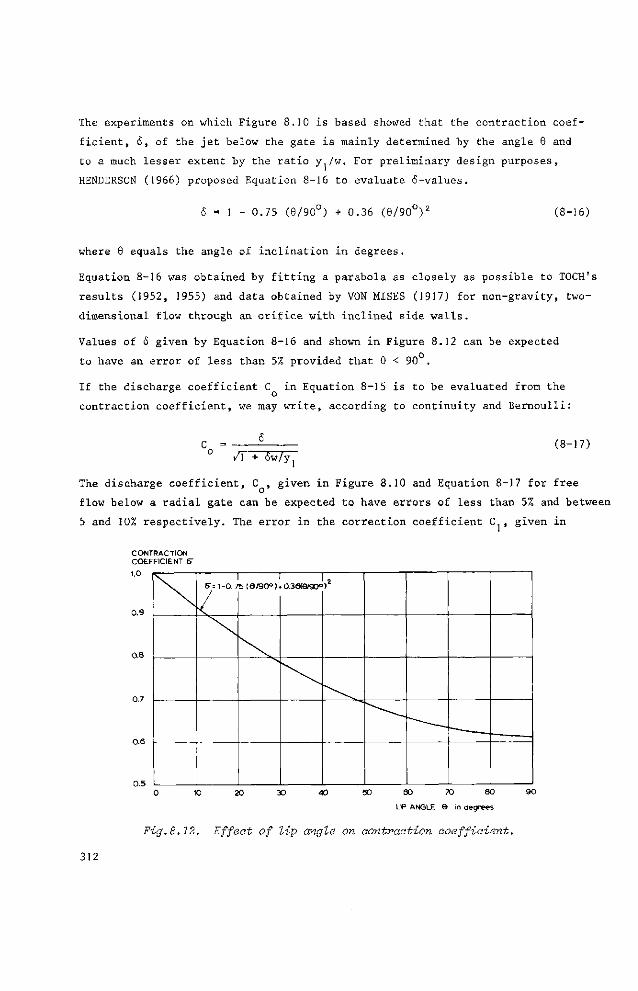
The experiments on which Figure 8.10 is based showed that the contraction coef
ficient, <5, of the jet below the gate is mainly determined by the angle 6 and
to a much lesser extent by the ratio y./w. For preliminary design purposes,
HENDERSON (1966) proposed Equation 8-16 to evaluate 6-values.
1 - 0.75 (6/90u) + 0.36 (9/90 ) °\2 (8-16)
where 6 equals the angle of inclination in degrees.
Equation 8-16 was obtained by fitting a parabola as closely as possible to TOCH's
results (1952, 1955) and data obtained by VON MISES (1917) for non-gravity, two-
dimensional flow through an orifice with inclined side walls.
Values of 5 given by Equation 8-16 and shown in Figure 8.12 can be expected
to have an error of less than 5% provided that 6 < 90 .
If the discharge coefficient C in Equation 8-15 is to be evaluated from the
contraction coefficient, we may write, according to continuity and Bernoulli:
C = o
V\ + ów/y (8-17)
The discharge coefficient, C , given in Figure 8.10 and Equation 8-17 for free
flow below a radial gate can be expected to have errors of less than 5% and between
5 and 10% respectively. The error in the correction coefficient C , given in
CONTRACTION COEFFICIENT 5"
0.9
0.8
5": 1-0. 7 •5(6/90°) 0.36©/90° )2
50 60 70 80 90
LIP ANGLE e in degrees
Fig.8.12. Effect of lip angle on contraction coefficient.
312
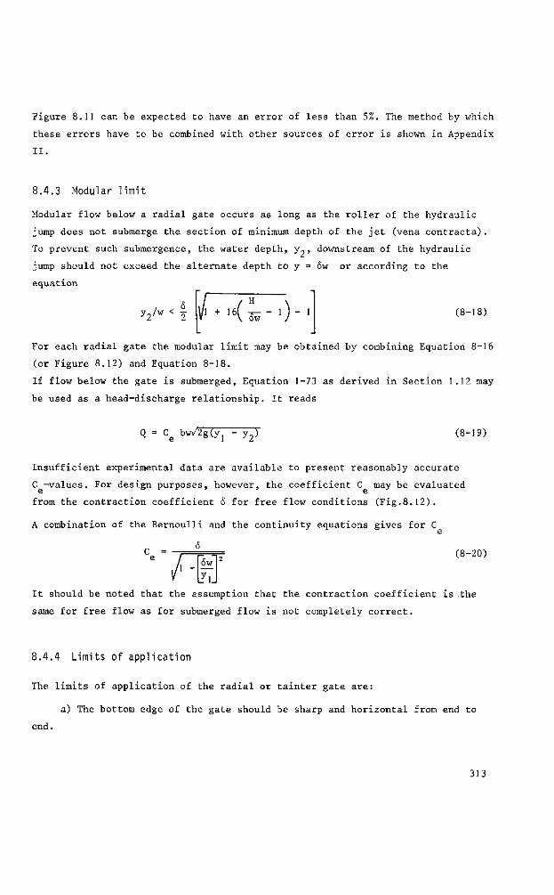
Figure 8.11 can be expected to have an error of less than 5%. The method by which
these errors have to be combined with other sources of error is shown in Appendix
II.
8.4.3 Modular limit
Modular flow below a radial gate occurs as long as the roller of the hydraulic
jump does not submerge the section of minimum depth of the jet (vena contracta).
To prevent such submergence, the water depth, y„, downstream of the hydraulic
jump should not exceed the alternate depth to y = 6w or according to the
equation
y2/w < 2 V' + 1 6 (^-0 (8-18)
For each radial gate the modular limit may be obtained by combining Equation 8-16
(or Figure 8.12) and Equation 8-18.
If flow below the gate is submerged, Equation 1-73 as derived in Section 1.12 may
be used as a head-discharge relationship. It reads
Q = C e bw/2g~(y~[ *2>
(8-19)
Insufficient experimental data are available to present reasonably accurate
C -values. For design purposes, however, the coefficient C may be evaluated
from the contraction coefficient S for free flow conditions (Fig.8.12).
A combination of the Bernoulli and the continuity equations gives for C
C = e
ôw
iFïj
(8-20)
It should be noted that the assumption that the contraction coefficient is the
same for free flow as for submerged flow is not completely correct.
8.4.4 Limits of application
The limits of application of the radial or tainter gate are:
a) The bottom edge of the gate should be sharp and horizontal from end to
end.
313
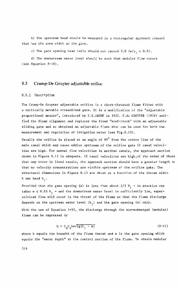
b) The upstream head should be measured in a rectangular approach channel
that has the same width as the gate.
c) The gate opening head ratio should not exceed 0.8 (w/y ^ 0.8).
d) The downstream water level should be such that modular flow occurs
(see Equation 8-18).
8.5 Crump-De Gruyter adjustable orifice
8.5.1 Description
The Crump-De Gruyter adjustable orifice is a short-throated flume fitted with
a vertically movable streamlined gate. It is a modification of the "adjustable
proportional module", introduced by E.S.CRUMP in 1922. P.de GRUYTER (1926) modi
fied the flume alignment and replaced the fixed "roof-block" with an adjustable
sliding gate and so obtained an adjustable flume that can be used for both the
measurement and regulation of irrigation water (see Fig.8.13).
Usually the orifice is placed at an angle of 90 from the centre line of the
main canal which may cause eddies upstream of the orifice gate if canal veloci
ties are high. For normal flow velocities in earthen canals, the approach section
shown in Figure 8.13 is adequate. If canal velocities are high,of the order of those
that may occur in lined canals, the approach section should have a greater length sc
that no velocity concentrations are visible upstream of the orifice gate. The
structural dimensions in Figure 8.13 are shown as a function of the throat width
b and head h .
Provided that the gate opening (w) is less than about 2/3 H - in practice one
takes w ^ 0.63 h. - and the downstream water level is sufficiently low, super
critical flow will occur in the throat of the flume so that the flume discharge
depends on the upstream water level (h ) and the gate opening (w) only.
With the use of Equation 1-33, the discharge through the non-submerged (modular)
flume can be expressed by
Q = C C bw/2g(h - w) (8-21)
where b equals the breadth of the flume throat and w is the gate opening which
equals the "water depth" at the control section of the flume. To obtain modular
314
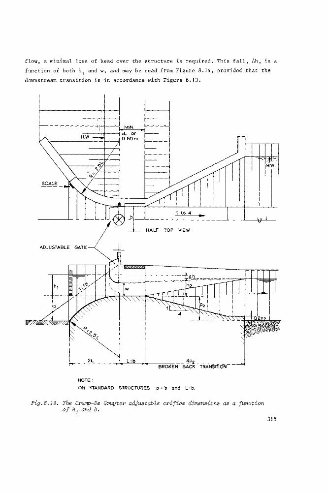
flow, a minimal loss of head over the structure is required. This fall, Ah, is a
function of both h and w, and may be read from Figure 8.14, provided that the
downstream transition is in accordance with Figure 8.13.
BROKEN BACK TRANSITION
NOTE :
ON STANDARD STRUCTURES p = b and L = b.
Fig.8.13. The Cmmp-De Gruyter adjustable orifice dimensions as a function of h1 and b.
315
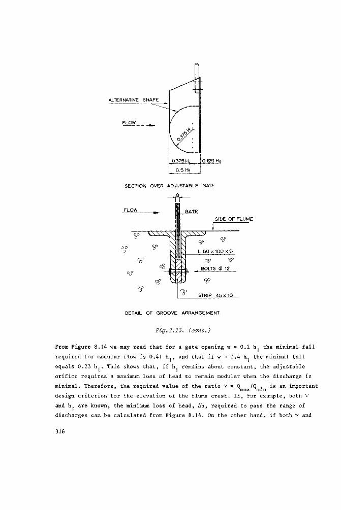
SECTION OVER ADJUSTABLE GATE
-A.
FLOW
SIDE OF FLUME
DETAIL OF GROOVE ARRANGEMENT.
Fig.8.13. (aont.)
From Figure 8.14 we may read that for a gate opening w = 0.2 h the minimal fall
required for modular flow is 0.41 h1, and that if w = 0,4 h1 the minimal fall
equals 0.23 hj. This shows that, if h remains about constant, the adjustable
orifice requires a maximum loss of head to remain modular when the discharge is
minimal. Therefore, the required value of the ratio y = Q /Q . is an important max m m
design criterion for the elevation of the flume crest. If, for example, both y
and h. are known, the minimum loss of head, Ah, required to pass the range of
discharges can be calculated from Figure 8.14. On the other hand, if both Y an<i
316
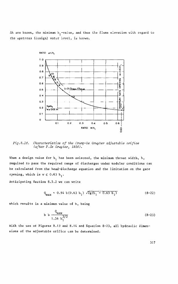
Ah are known, the minimum h -value, and thus the flume elevation with regard to
the upstream (design) water level, is known.
RATIO Ah/h.,
1.0
0.9
0.8
0.7
0.6
0.5
0.4
0.3
0.2
0.1
Y10 9 \ a
X\
H^h, w>0.02 n
< 4 \ \ Y =3=Qmtix/°rr
i
ax
<0 Ö -Î
O z z UJ
& UJ 1 -<
1 1 1
— 1 -
0.3 0.4
RATIO w/h,
Fig.8.14. Characteristics of the Crump-De Gruyter adjustable orifice (after P.de Gruyter, 1926).
When a design value for h. has been selected, the minimum throat width, b,
required to pass the required range of discharges under modular conditions can
be calculated from the head-discharge equation and the limitation on the gate
opening, which is w 0.63 lu .
Anticipating Section 8.5.2 we can write
Qmax = °'94 b < : ° - 6 3 V / 2 g ( h , - °-63 h,) (8-22)
which results in a minimum value of b, being
Q„„„ b >
1.56 h 3/2 1
(8-23)
With the use of Figures 8.13 and 8.14 and Equation 8-23, all hydraulic dimen
sions of the adjustable orifice can be determined.
317
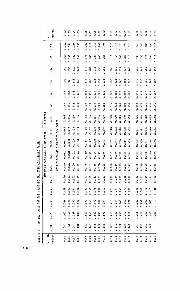
<u i -
-t-> ÜJ E
c - r -
C (/t • ( - <u
s_ + J CU
3 e
C D U D
O
O D L D
O
U D m
o
*d" L f l
O
CSJ LT>
O
o L f i
O
c o *d-
o
z n
4-> t o CU i . o
<u E 3
t S -( D
> O
" O rtJ CU
. e
E fO CU S -
- p
(/) O . = D
MD * 3 -
O
• * ^ T
O
C M <3"
O
O • 3 -
o
cXl m
o
MD m
o
^ i -c o
o
C M C O
O
O C O
O
C UI i~ CU
s_ - p CU
3 E
O ) i-
4-> <u E
s -<u o .
t / l
\ E
£=
c r
<u en S -
o V )
-o +-> c 3
CM O
O
CN MD O
O
_, MD O
O
O MD O
O
CT» m o
o
0 0 LO
o
o
r -m O
O
MD i n o
o
L O m o
o
-* m o
o
CM
m o
o
o m o
o
en - d -O
o
cc -d-o
o
MD - d -o
o
m -d-o o
•4--d" O
O
o
o
r o o
o
- d "
CT» O
O
CM
CT. O
O
O
CT» O
O
0 0 CO
o
o
r » C 0 o
o
i n 0 0 O
O
- d -0 0 o
o
CM CO o
o
o co o
o
0 0 r-. o
o
MD r- O
o
- d -r- O
O
CM r-. o
O
O r » o
o
0 0 MD O
O
- d -MD O
O
O") O
o
- d -o
o
< t CM
~ O
CM
— O
O CM
-— O
0 0
— o
MD
" O
CO
— o
o
o
C O o
o
m o
*— o
CM O
r" o
o o
o
r-.
CT» o
o
-d"
CT» O
o
o en o
o
0 0 0 0 o
o
- d -0 0 o
o
- d -O
o
m o
o
•<r m
— o
CM m
— o
CT» - d -
— o
MD -d-
— o
co - d -
— O
O - d "
— O
MD CO
o
co co
o
o CO
— o
MD CM
""" O
CM CM
O
CT» -' O
MD
— o
CM
— O
0 0 o
"-o
-d-o
— o
m o
o
v O o
o
CM co
"" o
co r-.
" o
- d -r -
" O
_ r - .
~ o
0 0 MD
~ o
m MD
~ o
CM \ D
O
CO m
o
- d -m
— o
o m
-" o
MD - d
O
CM •<r
~ o
r-. co
~ O
CM CO
— O
r -CM
O
CM
O
MD O
O
r - . O
O
CM
CM
O
CO o CM
O
- d -o CM
O
o o CM
O
m
CT» ™
o
o
CT» — o
\ D 0 0
O
CM 0 0
O
r -r-.
— O
r -
" O
r^ \ o
O
CM \ D
"-O
\D m
— o
o m
— o
m •<r
o
o < r
o
r--O
O
CO o
o
_ - d -CM
o
VD r o CM
O
_ CO CM
O
v D CM CM
O
„ CM CM
O
^ CM
O
_ CM
O
v£> O
O
O O CM
O
- d " CT\
" O
CO CO
o
CM 0 0
'" O
v£)
• ~
o
o r-*
~ o
CO \ o
o
v D i n
o
0 0 o
o
( T i O
o
CO \ £ ) CM
O
CO \o CM
O
co m CM
O
CM m CM
o
viD •<r CM
O
o - J -CM
O
- d -r o
O
CO CM CM
O
CN
O
UO
CM
O
CO o CM
O
O CM
O
- d -CT.
" o
r » 0 0
— o
o 0 0
o
CM r »
O
CTi O
o
o
o
- d -CTi CM
O
0 0 0 0 CM
O
CM CO CM
O
\ D I-» CM
O
o r-. CM
O
CO \ o CM
o
VJD m CM
o
cr> -d-CM
O
CM -<r CM
o
m CO CM
O
0 0 CM CM
O
O CM CM
O
CM
CM
O
- d -o CM
O
m CT\
o
\ D co
o
o
o
o
o
co
o
- d -
CO
o
CO o CO
o
o o CO
o
CM o> CM
o
m 0 0 CM
o
0 0 r -CM
o
o r-. CM
o
CM \D CM
o
CO m
^ o
v D - d -CM
o
r-~ CO CM
o
CO CM CM
o
o>
CM
o
o
CM
o
o o CM
o
o
CM
o
^o
<* CO
o
0 0 co r o
o
o r o CO
o
co CM CO
o
•x>
CO
o
co o CO
o
o o r o
O
CM
CT. CM
O
r O CO CM
O
- d -r-. CM
o
- d -\ D CM
O
<* u 0 CM
O
•<r <r CM
O
- d -CO CM
O
CO CM CM
O
CM
CM
O
CM
O
CO
o
o r -co
O
CM <n r o
O
- d -m r o
O
^ O - J -CO
O
r--co CO
o
CO CM CO
O
o->
CO
O
O
CO
o
o o CO
o
o
CT. CM
O
O CO
O
O r » CM
O
CX. m CM
o
co
<* CM
O
\ D r o CM
O
- d -CM
CM
O
CO
O
- d -
O
m
CT» CO
o
M5 0 0 CO
o
r -p -co
o
0 0 v O CO
o
CT» m CO
o
o m CO
o
o -d-r o
O
O CO CO
o
CT\
CO
o
co o CO
o
r -cr.
o
v O 0 0 CM
O
r o r -CM
O
O
^ CM
O
r^ < r CM
O
- d -co CM
O
- d -
O
m
o
o
- d -
o
o
- d -
O
O O ~d-
O
O
CT» CO
O
o 0 0 r o
O
O r^ co
O
CO m CO
o
v O -<r CO
o
m CO CO
o
•<r
r o
o
CM
r o
o
CT» CT» CM
O
\D CO CM
O
CM r -CM
O
r » i n CM
O
CM • d -CM
O
m
o
^D
O
O -d-<r
o
o CO - d -
o
o
- d -
O
O
- d -
O
CT» CT» CO
O
CO CO r o
O
^D r -r o
O
~ d vo r o
O
i n co
O
CT. co co
O
v£> CM CO
o
CM
CO
o
CO
CT» CM
O
CM 0 0 CM
O
v £ i v O CM
O
O m CM
O
\D
O
r -
O
•<r MD <r
o
r o m - d -
o
CM - d -•<r
o
o r o - d -
o
0 0
- d -
O
M5 O <r
o
-<r
CT. CO
O
CO CO
o
0 0 ^o CO
o
<r i n co
o
CT» co co
o
- d -CM CO
O
CO O CO
O
CM
CT» CM
O
- d -r-* CM
O
O m CM
O
P ^
O
CO
o
v O CO - d -
o
-d-t - . •<r
o
CM v£J - d -
O
O m - d -
o
r^ r o < f
O
<r CM - d -
O
O
-<r
o
U J er» co
o
co co
o
MD M3 r o
o
o m CO
o
- d -CO CO
o
0 0
CO
o
CT\ CT. CM
O
O CO CM
o
o v O CM
O
CO
O
CT. O
•<r o m
o
CM
CT» - d -
o
o 0 0 - d -
o
0 0 MD ~d-
o
-d-m •< r
o
o - d -- d -
O
m CM -d-
o
o
- d -
O
ȣ>
CT. r o
O
O 0 0 CO
o
CM MD CO
O
- d -- d -r o
o
m CM r o
O
m o CO
o
-d-0 0 CM
O
CM MD CM
O
CT» O
O CM
O
m CM m
o
CM
m
o
CO
CT» ~d-
o
MD 0 0 -d-
o
CM r». - d -
O
MD m -<r
o
o -d-- d -
O
~d-CM - d -
O
co o •<r
o
o
CT» CO
O
CM r » co
O
CM m CO
o
_ CO CO
o
o
CO
o
0 0 0 0 CM
o
o CM
o
318
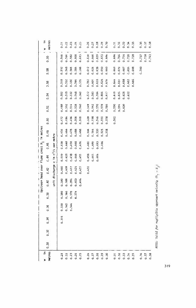
(/) <1J ï -
4-> QJ E
c
*""
n t/i r - QJ
S -4 - ) QJ
3 E
O MO
O
C O L O
0
U D L O
O
*3" L O
O
C\J i n
O
O LO
0
CO «sT
O
= c
4-> t / 1 a i s~ o
a i E 13
<4-
S-O)
> o
-o CÖ a i
sz
£ (O OJ s-
4 0
l / l C
= 3
UD *d"
O
^ r «d-
O
CM «3-
O
O
"* O
C O 0 0
0
U D OO
O
«a-00
0
CM C O
0
0
co
0 JZ l / l < - O )
s_ +-> QJ
3 E
QJ i -
+ J QJ E
s» QJ C L
(/) \ "E
c:
c r
0) e n i . «3
SZ O to
• 0
4 0
c 3
CM
0
MD - J -m
0
CM CO i n
O
CO
"">. O
CM
O i n
O
co co -d-
O
CN r-. -d"
O
-J-m -d-
0
0 0 co -d-
0
CTi
-d-
0
0 0 -d-
0
0 co co
0
0 MD CO
O
CO CO CO
0
MD
CO
O
O
CM
O
- J MD u~\
O
CO - d -m
0
C-J
L n
0
co
L A
O
CM O m
0
-d-00 -d-
0
MD MD -d"
O
00 -d--d"
O
CO CN <r
O
co O < r
0
co co co
0
MD MD CO
0
Cs] - d " CO
0
Cv! <M
O
O
CM CO m
0
MD MD m
0
0 L A m
0
CM CO m
0
-d-
m
0
MD er. -d-
0
co r --d-
O
co UO - j -
O
0 0 co < r
0
p -
- j -
0
•<r cr> CO
0
0 p -CO
0
<r <r CO
0
co CN
O
-d-
O
O O UD
O
< r CO m
0
MD \ D i n
0
co -d-m
0
co CM m
0
00 0 m
0
00 co -d-
O
0 0 MD -d-
O
MD -d--d-
O
-d-
-d-
O
O O -d"
O
-d* p -co
0
-d-CN
O
i n CN
0
i n
UD
0
MD en U~l
0
co r -i n
O
O UD m
0
0 -d-i n
0
en
i n
O
co en -d-
0
MD p -- d -
0
CM UO
-d-
0
p -CN
- d -
O
-d-O ~d
0
m CN
0
MD
0
__ MD
O
CN
MD
O
Csl
CT\ m
O
CM p -m
0
en < r m
0
co CM m
0
UD 0 i n
0
CN CO ~d-
O
co i n < r
0
CM CO - d -
O
MD CN
O
r-* CN
O
MD - 3 -UD
O
<r CN MD
O
- d -0 UO
O
CO co i n
0
CN MD i n
0
0 0 CO i n
O
-d-
m
0
ON co - d -
0
CM MD •<r
0
r -CN
O
CO
O
O m MD
0
0 0 co MD
0
\0
MD
O
-d-CTN
m
0
0 p » m
0
MD - d -i n
0
0 CN i n
0
co o> < r
0
-tf MD <T
O
CO CM
O
C7N CN
O
CN r -•^D
O
O m MD
0
co
MD
O
•<r 0 MD
O
co
i n
0
CM m LO
0
CM m
0
MD 0-1 - j -
0
a\ CN
O
O CO
0
- 3 -0 0 MD
0
0 MD \£>
0
MD CO MD
O
CM
MD
O
MD 0 0 m
0
co m i n
0
co CN m
0
0 CO
0
co
0
-<r o> MD
0
0 MD MD
O
- d -- d -MD
0
0 0
MD
0
0 0-1 m
0
CM MD m
0
co
0
CM CO
0
- d -0 p -
0
0 1 p -MD
0
_ m ••V
0
- d -CM MD
0
• d -CT. m
0
co
0
co co
0
- d -
p -
0
p -0 0 MD
O
CO i n MD
0
co
MD
O
O O MD
O
CO CO
O
<* CO
O
O CN P -
O
-d-0-1 MD
O
CN MD MD
O
CN CO MD
O
-d-CO
0
uO CO
O
0 0 CM P~-
O
CO CT. MD
O
MD MD MD
O
m CO
O
MD CO
O
CN CO P -
O
O O r~-
0
MD co
O
P» co CO CO
0 0
0 0 CN co -<r p - p »
O O
h » 0 0 CO CO
0 0
31<
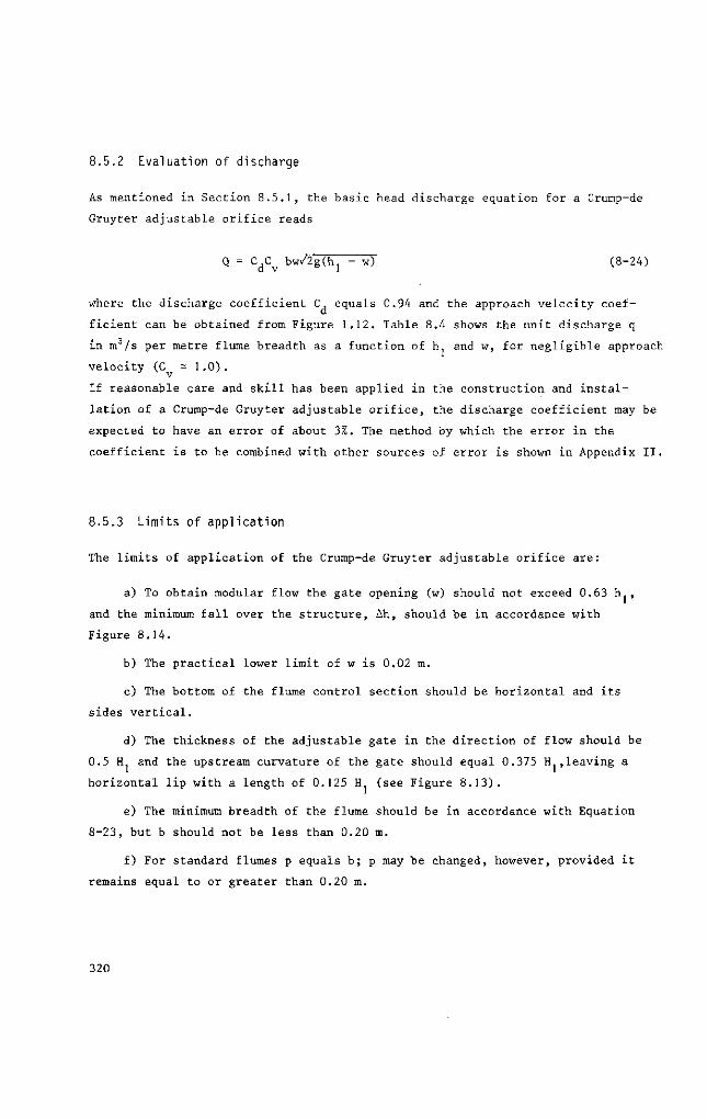
8.5.2 Evaluation of discharge
As mentioned in Section 8.5.1, the basic head discharge equation for a Crump-de
Gruyter adjustable orifice reads
Q = C C bw/2g(h - w) (8-24)
where the discharge coefficient C equals 0.94 and the approach velocity coef
ficient can be obtained from Figure 1.12. Table 8.4 shows the unit discharge q
in m /s per metre flume breadth as a function of h1 and w, for negligible approach
velocity (C = 1.0).
If reasonable care and skill has been applied in the construction and instal
lation of a Crump-de Gruyter adjustable orifice, the discharge coefficient may be
expected to have an error of about 3%. The method by which the error in the
coefficient is to be combined with other sources of error is shown in Appendix II.
8.5.3 Limits of application
The limits of application of the Crump-de Gruyter adjustable orifice are:
a) To obtain modular flow the gate opening (w) should not exceed 0.63 lu ,
and the minimum fall over the structure, Ah, should be in accordance with
Figure 8.14.
b) The practical lower limit of w is 0.02 m.
c) The bottom of the flume control section should be horizontal and its
sides vertical.
d) The thickness of the adjustable gate in the direction of flow should be
0.5 H. and the upstream curvature of the gate should equal 0.375 H.,leaving a
horizontal lip with a length of 0.125 H (see Figure 8.13).
e) The minimum breadth of the flume should be in accordance with Equation
8-23, but b should not be less than 0.20 m.
f) For standard flumes p equals b; p may be changed, however, provided it
remains equal to or greater than 0.20 m.
320
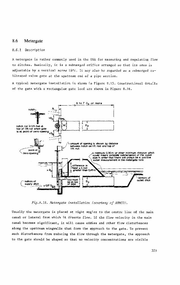
8.6 Metergate
8.6.1 Description
A metergate is rather commonly used in the USA for measuring and regulating flow
to ditches. Basically, it is a submerged orifice arranged so that its area is
adjustable by a vertical screw lift. It may also be regarded as a submerged ca
librated valve gate at the upstream end of a pipe section.
A typical metergate installation is shown in Figure 8.15. Constructional details
of the gate with a rectangular gate leaf are shown in Figure 8.16.
6 to 7 DD or more
notch cut in lift nod at top of I if t nut when gate is at point of zero opening T~'
_J1~£ -amount of opening is shown by distance
between notch on lift rod and top of l i f t nut
a minimum 0.30m or other minimum distance which would insure complete submergence of the outlet pipe in order that there will always be a positive water measurement in the metergate tank
Fig.8.15. Metergate installation (courtesy of ARMCO).
Usually the metergate is placed at right angles to the centre line of the main
canal or lateral from which it diverts flow. If the flow velocity in the main
canal becomes significant, it will cause eddies and other flow disturbances
along the upstream wingwalls that form the approach to the gate. To prevent
such disturbances from reducing the flow through the metergate, the approach
to the gate should be shaped so that no velocity concentrations are visible
321
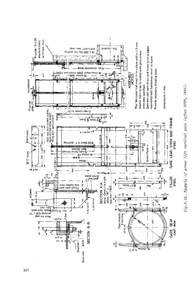
3
ÜJ
> < ce
t o V < UI
(O
si - J
1 UJ
t r LÜ
LU UJ f -(/)
LO M i O } r-i
ft; CQ co C ï
?H
« +i <K ö ~ co
ö ia
T - i
3
co
O
ca
£
322
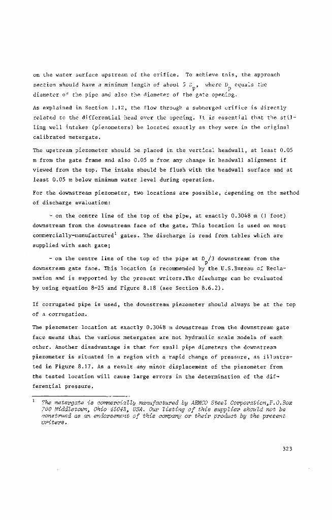
on the water surface upstream of the orifice. To achieve this, the approach
section should have a minimum length of about 5 D , where D equals the P _P
diameter of the pipe and also the diameter of the gate opening.
As explained in Section 1.12, the flow through a submerged orifice is directly
related to the differential head over the opening. It is essential that the stil
ling well intakes (piezometers) be located exactly as they were in the original
calibrated metergate.
The upstream piezometer should be placed in the vertical headwall, at least 0.05
m from the gate frame and also 0.05 m from any change in headwall alignment if
viewed from the top. The intake should be flush with the headwall surface and at
least 0.05 m below minimum water level during operation.
For the downstream piezometer, two locations are possible, depending on the method
of discharge evaluation:
- on the centre line of the top of the pipe, at exactly 0.3048 m (1 foot)
downstream from the downstream face of the gate. This location is used on most
commercially-manufactured1 gates. The discharge is read from tables which are
supplied with each gate;
- on the centre line of the top of the pipe at D /3 downstream from the p
downstream gate face. This location is recommended by the U.S.Bureau of Recla
mation and is supported by the present writers.The discharge can be evaluated
by using equation 8-25 and Figure 8.18 (see Section 8.6.2).
If corrugated pipe is used, the downstream piezometer should always be at the top
of a corrugation.
The piezometer location at exactly 0.3048 m downstream from the downstream gate
face means that the various metergates are not hydraulic scale models of each
other. Another disadvantage is that for small pipe diameters the downstream
piezometer is situated in a region with a rapid change of pressure, as illustra
ted in Figure 8.17. As a result any minor displacement of the piezometer from
the tested location will cause large errors in the determination of the dif
ferential pressure.
1 The metergate is commercially manufactured by ARMCO Steel Corporation^ .0 .Box 700 Middletown, Ohio 45042, USA. Our listing of this supplier should not he construed as an endorsement of this company or their product by the present writers.
323
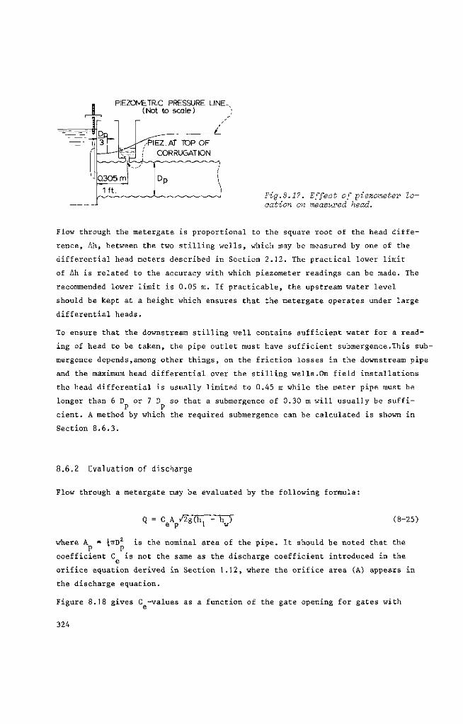
PIEZOMETRIC PRESSURE LINE. (Not to scale)
/PIEZ. AT TOP O F
CORRUGATION
Fig.8.17. Effect of piezometer location on measured head.
Flow through the metergate is proportional to the square root of the head diffe
rence, Ah, between the two stilling wells, which may be measured by one of the
differential head meters described in Section 2.12. The practical lower limit
of Ah is related to the accuracy with which piezometer readings can be made. The
recommended lower limit is 0.05 m. If practicable, the upstream water level
should be kept at a height which ensures that the metergate operates under large
differential heads.
To ensure that the downstream stilling well contains sufficient water for a read
ing of head to be taken, the pipe outlet must have sufficient submergence.This sub
mergence depends,among other things, on the friction losses in the downstream pipe
and the maximum head differential over the stilling wells.On field installations
the head differential is usually limited to 0.45 m while the meter pipe must be
longer than 6 D or 7 D so that a submergence of 0.30 m will usually be suffi
cient. A method by which the required submergence can be calculated is shown in
Section 8.6.3.
8.6.2 Evaluation of discharge
Flow through a metergate may be evaluated by the following formula:
Q = CeAp/2g(h, - hw) (8-25)
where A = |TTD2 is the nominal area of the pipe. It should be noted that the p p.
coefficient C is not the same as the discharge coefficient introduced in the
orifice equation derived in Section 1.12, where the orifice area (A) appears in
the discharge equation.
Figure 8.18 gives C -values as a function of the gate opening for gates with
324
either a rectangular or a circular gate leaf, and with their downstream pressure
tap at D /3 downstream from the downstream face of the gate. The curve for
circular leaves was derived from tables published by ARMCO; that for rectangular
leaves was taken from the U.S.Bureau of Reclamation, 1961.
Although the curves in Figure 8.18 were obtained for particular approach condi
tions, all approach sections that comply with the conditions outlined in Section
8.6.4 may be used in combination with the C -curves shown. This was demonstrated
by tests, conducted by the U.S.Bureau of Reclamation (1961), which showed that
C -values are not influenced by approach conditions if the gate opening remains
less than 50%; in the range from 50% to 75%, the C -value may increase
slightly. Gate openings greater than 75% are not recommended for discharge regu
lation since, in this range, the C -value shows considerable variation (see
also Figure 8.20).
The discharge coefficient shown in Figure 8.18 may be expected to have an error
of less than 3% for gate openings up to 50%, and an error of less than 6% for
gate openings up to 75%. The method by which this error is to be combined with
COEFFICIENT Cg
7
Fig.8.18. C -values for pressure tap located at D/3.
325
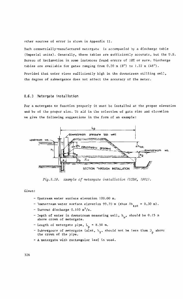
other sources of error is shown in Appendix II.
Each commercially-manufactured metergate is accompanied by a discharge table
(Imperial units). Generally, these tables are sufficiently accurate, but the U.S.
Bureau of Reclamation in some instances found errors of 18% or more. Discharge
tables are available for gates ranging from 0.20 m (8") to 1.22 m (48").
Provided that water rises sufficiently high in the downstream stilling well,
the degree of submergence does not affect the accuracy of the meter.
8.6.3 Metergate installation
For a metergate to function properly it must be installed at the proper elevation
and be of the proper size. To aid in the selection of gate size and elevation
we give the following suggestions in the form of an example:
upstream ws
downstream ws.
^ \ \ \ W / ^ \ ^ | j J SECTION THROUGH INSTALLATDN %sMèm!
M Fig.8.19. Example of metergate installation (USBR, 1961).
Given :
tot 0.30 m ) .
Upstream water surface elevation 100.00 m.
Downstream water surface elevation 99.70 m (thus Ah
Turnout discharge 0.140 m3/s.
Depth of water in downstream measuring well, h , should be 0.15 m above crown of metergate.
Length of metergate pipe, L = 8.50 m.
Submergence of metergate inlet, h1, should not be less than D above the crown of the pipe.
A metergate with rectangular leaf is used.
326
Find:
1. Metergate size.
2. Elevation at which metergate should be placed.
1: Metergate size
a) When downstream scour is a problem, an exit velocity has to be selected
that will not cause objectionable erosion, say v -£ 0.90 m/s. From A = Q/v we
find A ^ 0.140/0.90 = 0.156 m2 or D î> 0.445 m. P P
An 18-inch (D = 0.457 m) metergate is required.
b) When downstream scour is not a problem, we select a metergate that
operates at gate openings not exceeding 75% (see Section 8.6.2). For 75%
gate opening the coefficient C - 0.51 (Fig.8.18) and the maximum differential
head Ah - 1.8 Ah (Fig.8.20). Taking into account some losses due to friction
in the pipe, we assume Ah = 1.60 Air = 1.60 x 0.30 = 0.48 m. From Equation 0.5 t 0 t . 2
8-25: Q = C A (2gAh) we obtain the minimum area of the pipe: A >- 0.0895 m and thus D S- 0.34 m. Our initial estimate is a 14-inch metergate (D = 0.356 m) .
c) Check capacity of selected gate. It is common practice to express the loss
of hydraulic head as a function of the velocity head, v /2g.
For a metergate the velocity head in the pipe can be found by substituting the
continuity equation Q/A = v into Equation 8-25, which leads to
v = C /2iÄh (8-26)
~ = C2 Ah (8-27) ig e
The total (available) loss of head over the structure, Ah , equals the sum of
the energy loss over the gate, the friction losses in the meterpipe, and the
exit losses, so that:
Ahtot - Ahgate + h v 2 / 2S + Çex (8~28)
If we assume that no recovery of kinetic energy occurs at the pipe exit (Ç =1.0),
we can write
Ahtot = A hr + Çf v'/ 2 g ( 8 _ 2 9 )
327
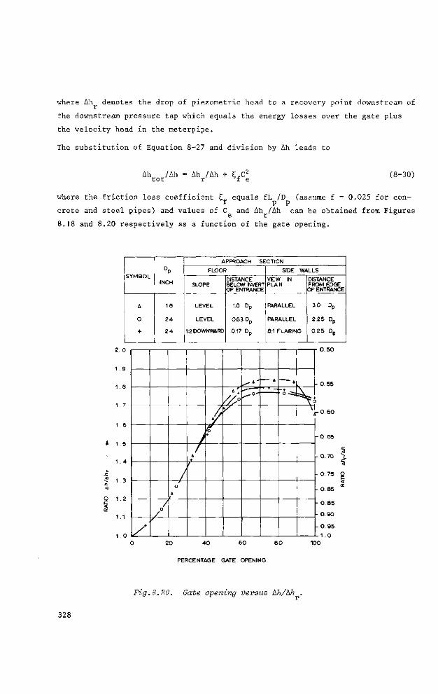
where Ah denotes the drop of piezometric head to a recovery point downstream of
the downstream pressure tap which equals the energy losses over the gate plus
the velocity head in the meterpipe.
The substitution of Equation 8-27 and division by Ah leads to
Ah /Ah tot
Ah /Ah + E,CC2
r f e (8-30)
where the friction loss coefficient E_ equals fL /D (assume f = 0.025 for con-f P P
crete and steel pipes) and values of C and Ah /Ah can be obtained from Figures 8.18 and 8.20 respectively as a function of the gate opening.
SYMBOL
A
O
+
DP
INCH
18
24
2 4
APPROACH SECTION
FLOOR
SLOPE
LEVEL
LEVEL
1:2 DOWNWARD
DISTANCE BELOW NVERT OF ENTRANCE
10 Dp
0.63 Dp
0.17 Dp
SIDE WALLS
VEW IN PLAN
PARALLEL
PARALLEL
8:1 FLARING
DISTANCE FROM EDGE
OF ENTRANCE
3.0 Dp
2.25 Dp
0.25 Dp
1.0 IZ
Y -/-
-I
y ! ; •
&
20 4 0 60 8 0
PERCENTAGE GATE OPENING
-0 60
0.75 2 Ü
0.85
- 0.85
- O 90
0 95 1 .0
100
Fig.8.20. Gate opening versus Ah/ah .
328
In our example Ah = 0.30 m and ǣ = fL /D = 0.025 x 8.50/0.356 = 0.60. For 75% tot f P P
gate opening C ~ 0.51 and the ratio Ah/Ah - 1.80, so that according to Equation
8-30 the maximum value of Ah = 0.42 m. Using this adjusted value of Ah, turnout
capacity at 75% gate opening equals
i
Q ~ 0.51 x i TT x 0.3562 (2g x 0.42)2 = 0.146 m3/s
A 14-in metergate is adequate.
2: Elevation at which metergate should be placed
If the differential head over the metergate structure is a constant, in our example
Ah = 0.30 m, the head difference Ah measured between the two wells is at its tot
maximum with gate openings of around 50%. Using Equation 8-30 the following Ah-
values can be computed:
gate opening 35% 40% 50% 55% 60% 75%
Ah (m) 0.399 0.437 0.452 0.458 0.454 0.422
- To meet the requirement of water surface 0.15 m above the crown of the
pipe (0.05 m above bottom of well) in the downstream well, elevation of crown
entrance would be set at
EL = 100.00 - Ah - h = 100.00 - 0.46 - 0.15 = 99.39 m max w
- To meet the upstream submergence requirement, h , of 1.0 D , the crown of
the pipe entrance should be set at EL = 100.00 - D - 99.64 m. p
The depth requirement for a measurable water surface in the downstream well is
the governing factor and the metergate should be set with its crown of entrance
not higher than EL = 99.39 m.
8.6.4 Limits of applications
The limits of application of the metergate are:
a) The crown of the pipe entrance should have an upstream submergence of
1.0 D or more. P
b) Submergence of the pipe outlet should be such that the water surface in
the downstream well is not less than 0.15 m above the crown of the pipe. 329
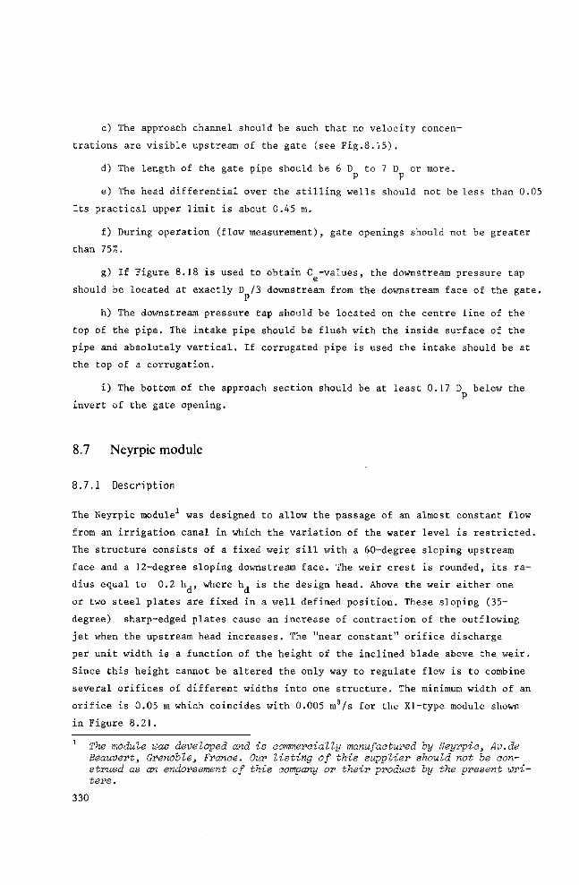
c) The approach channel should be such that no velocity concen
trations are visible upstream of the gate (see Fig.8.15).
d) The length of the gate pipe should be 6 D to 7 D or more.
e) The head differential over the stilling wells should not be less than 0.05
Its practical upper limit is about 0.45 m.
f) During operation (flow measurement), gate openings should not be greater
than 75%.
g) If Figure 8.18 is used to obtain C -values, the downstream pressure tap
should be located at exactly D /3 downstream from the downstream face of the gate.
h) The downstream pressure tap should be located on the centre line of the
top of the pipe. The intake pipe should be flush with the inside surface of the
pipe and absolutely vertical. If corrugated pipe is used the intake should be at
the top of a corrugation.
i) The bottom of the approach section should be at least 0.17 D below the
invert of the gate opening.
8.7 Neyrpic module
8.7.1 Description
The Neyrpic module1 was designed to allow the passage of an almost constant flow
from an irrigation canal in which the variation of the water level is restricted.
The structure consists of a fixed weir sill with a 60-degree sloping upstream
face and a 12-degree sloping downstream face. The weir crest is rounded, its ra
dius equal to 0.2 h,, where h, is the design head. Above the weir either one
or two steel plates are fixed in a well defined position. These sloping (35-
degree) sharp-edged plates cause an increase of contraction of the outflowing
jet when the upstream head increases. The "near constant" orifice discharge
per unit width is a function of the height of the inclined blade above the weir.
Since this height cannot be altered the only way to regulate flow is to combine
several orifices of different widths into one structure. The minimum width of an
orifice is 0.05 m which coincides with 0.005 m3/s for the Xl-type module shown
in Figure 8.21 .
1 The module was developed and is commercially manufactured by Neyrpic, Av.de Beauvert, Grenoble, France. Our listing of this supplier should not be construed as an endorsement of this company or their product by the present writers.
330
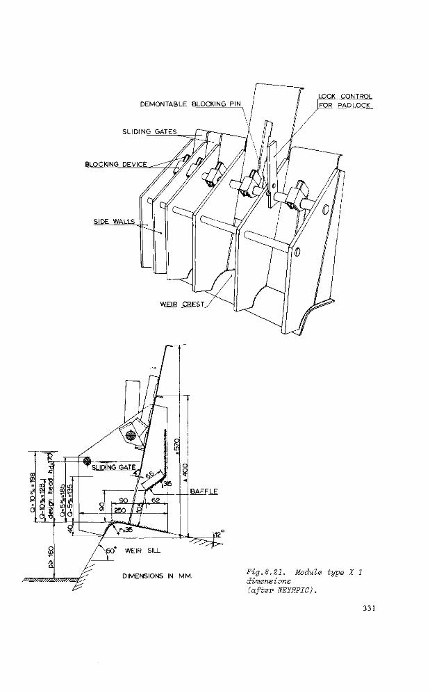
DEMONTABLE BLOCKING PIN LOCK CONTROL FOR PADLOCK
WEIR CREST
/a*T»s!w=* , / î DIMENSIONS IN MM.
Fig.8.21. Module type X 1
dimensions
(after NEÏRPIC).
331
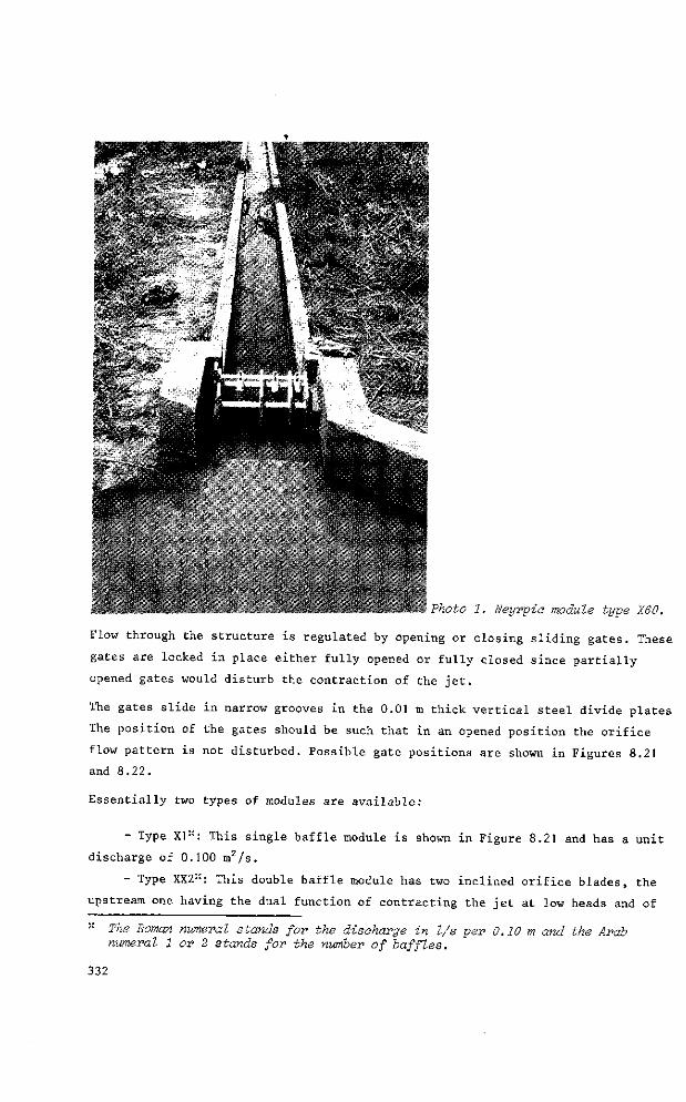
4"
* " frS**
Photo 1. Neyrpio module type X60.
Flow through the structure is regulated by opening or closing sliding gates. These
gates are locked in place either fully opened or fully closed since partially
opened gates would disturb the contraction of the jet.
The gates slide in narrow grooves in the 0.01 m thick vertical steel divide plates
The position of the gates should be such that in an opened position the orifice
flow pattern is not disturbed. Possible gate positions are shown in Figures 8.21
and 8.22.
Essentially two types of modules are available:
- Type XI::: This single baffle module is shown in Figure 8.21 and has a unit
discharge of 0.100 m2/s.
- Type XX2": This double baffle module has two inclined orifice blades, the
upstream one having the dual function of contracting the jet at low heads and of
" The Roman numeral stands for the discharge in l/s per 0.10 m and the Arab numeral 1 or 2 stands for the number of baffles.
332
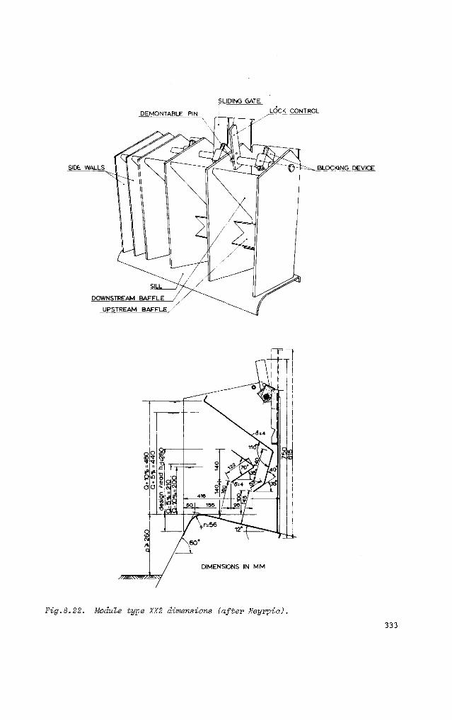
SLIDING GATE
DEMONTABLE PIN
SIDE WALLS
DOWNSTREAM BAFFLE
UPSTREAM BAFFLE
LOCK CONTROL
BLOCKING DEVICE
DIMENSIONS IN M M
Fig.8.22. Module type XX2 dimensions (after Neyrpia).
333
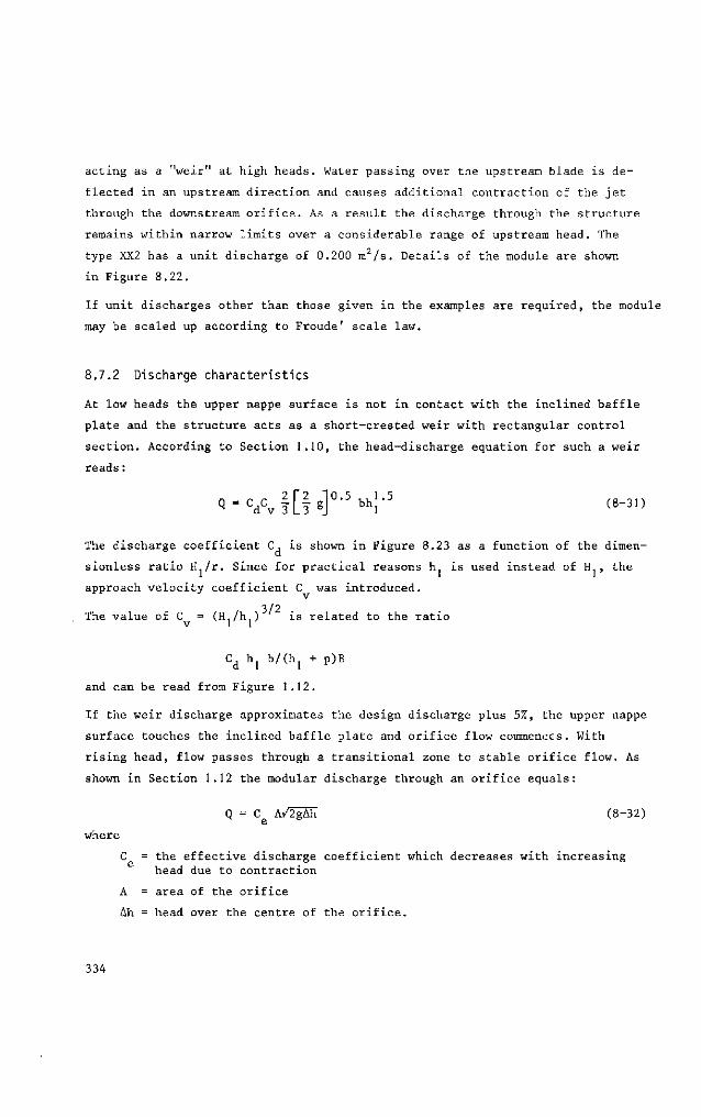
acting as a "weir" at high heads. Water passing over the upstream blade is de
flected in an upstream direction and causes additional contraction of the jet
through the downstream orifice. As a result the discharge through the structure
remains within narrow limits over a considerable range of upstream head. The
type XX2 has a unit discharge of 0.200 m /s. Details of the module are shown
in Figure 8.22.
If unit discharges other than those given in the examples are required, the module
may be scaled up according to Froude' scale law.
8.7.2 Discharge characteristics
At low heads the upper nappe surface is not in contact with the inclined baffle
plate and the structure acts as a short-crested weir with rectangular control
section. According to Section 1.10, the head-discharge equation for such a weir
reads :
«-v.![!.]°-5»'!-5 <-«> The discharge coefficient C, is shown in Figure 8.23 as a function of the dimen-
sionless ratio IL/r. Since for practical reasons h. is used instead of H , the
approach velocity coefficient C was introduced.
3/2 The value of C = (H /h ) is related to the ratio
Cd hj b/(hj + p)B
and can be read from Figure 1.12.
If the weir discharge approximates the design discharge plus 5%, the upper nappe
surface touches the inclined baffle plate and orifice flow commences. With
rising head, flow passes through a transitional zone to stable orifice flow. As
shown in Section 1.12 the modular discharge through an orifice equals:
where
Q = C A/2gÄh (8-32)
C = the effective discharge coefficient which decreases with increasing head due to contraction
A = area of the orifice
Ah = head over the centre of the orifice.
334
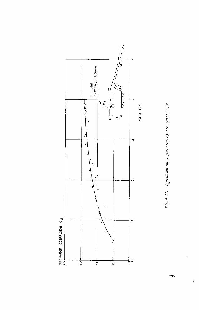
I
o < ce
«
O
K O
K
C?
N2 CK]
335
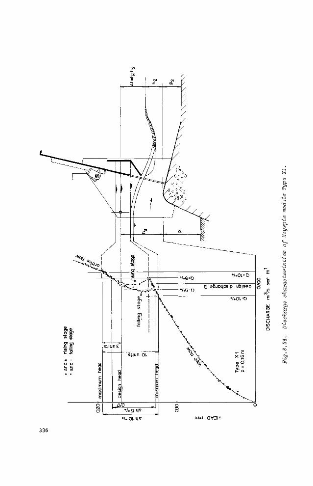
»/. omv UJtu Q V 3 H
336
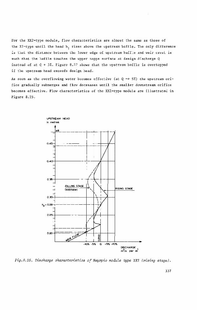
For the XX2-type module, flow characteristics are almost the same as those of
the XI-type until the head h rises above the upstream baffle. The only difference
is that the distance between the lower edge of upstream baffle and weir crest is
such that the baffle touches the upper nappe surface at design discharge Q
instead of at Q + 5%. Figure 8.22 shows that the upstream baffle is overtopped
if the upstream head exceeds design head.
As soon as the overflowing water becomes effective (at Q =+ 5%) the upstream ori
fice gradually submerges and flow decreases until the smaller downstream orifice
becomes effective. Flow characteristics of the XX2-type module are illustrated in
Figure 8.25.
-10% -5% Q «5% «10V. DISCHARGE m ;s per m
Fig.8.25. Discharge characteristics of Neyrpic module type XX2 (rising stage).
337
The discharge through a module constructed with reasonable care and skill and
in accordance with the dimensions shown in Figures 8.21 and 8.22 will vary some
10% around the design discharge provided that the upstream head is kept between
given limits.
Sometimes the upstream head is maintained between narrower limits, so that the
discharge deviates no more than 5% from the design value. Due to the difference
in the module's behaviour with either rising or falling stage, however, the 5%
range is not well defined.
Tö keep the module functioning properly, frequent maintenance is required.
8.7.3 Limits of application
The limits of application of the Neyrpic module are:
a) The upstream water level should be kept between the limits shown in Fi
gures 8.21 and 8.22.
b) To reduce the influence of the approach velocity on the flow pattern
through the module, the ratio h /p should not exceed unity.
c) To prevent the tailwater channel bottom from influencing the flow pattern
through the orifice, the ratio p„/h. should not be less than 0.35. 1 d
d) To obtain modular flow, the ratio h./h. should not exceed 0.60. z a
8.8 Danai'dean tub
8.8.1 Description
The Danaidean tub is a vessel which receives a flow of water from above and dischai
ges it through a (circular) orifice or a (rectangular) slot in its bottom. After
some time the water surface in the Danaidean tub stabilizes to a head lu , being
the head that makes the orifice discharge at the same rate as water flows into
the tub (Q = Q. = Q ) . The head h, can be read by means of a piezometer as in out 1 J v
shown in Figure 8.26. If the area A of the orifice is known, the discharge can be
calculated (see Section 8.8.2). If the head-discharge equations are to be appli
cable, however, the contraction of the jet must not be hindered. Therefore, the
338
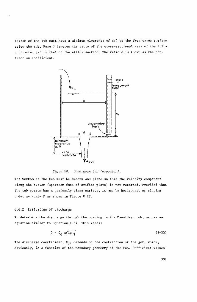
bottom of the tub must have a minimum clearance of d/ô to the free water surface
below the tub. Here 6 denotes the ratio of the cross-sectional area of the fully
contracted jet to that of the efflux section. The ratio 6 is known as the con
traction coefficient.
minimum clearance d/5
vena contracta
piezometer tap'
tü scale
transparant tube
TQout
Fig.8.26, Danaidean tub (circular).
The bottom of the tub must be smooth and plane so that the velocity component
along the bottom (upstream face of orifice plate) is not retarded. Provided that
the tub bottom has a perfectly plane surface, it may be horizontal or sloping
under an angle (3 as shown in Figure 8.27.
8.8.2 Evaluation of discharge
To determine the discharge through the opening in the Danaidean tub, we use an
equation similar to Equation 1-67. This reads:
Q = Cd A/2ghj (8-33)
The discharge coefficient, C , depends on the contraction of the jet, which,
obviously, is a function of the boundary geometry of the tub. Sufficient values
339
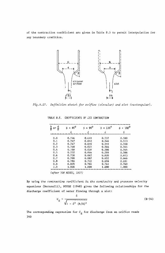
of the contraction coefficient are given in Table 8.5 to permit interpolation for
any boundary condition.
Fig. 8.27. definition sketch for orifice (circular) and slot (rectangular).
TABLE 8.5. COEFFICIENTS OF JET CONTRACTION
b d B-°rïï
0.0 0.1 0.2 0 .3 0.4 0 .5 0.6 0.7 0 .8 0.9 1.0
ß = 45°
6
0.746 0.747 0.747 0.748 0.749 0.752 0.758 0.768 0.789 0.829 1.000
ß = 90°
S
0.611 0.612 0.616 0.622 0.631 0.644 0.662 0.687 0.722 0.781 1.000
ß = 135°
&
0.537 0.546 0.555 0.566 0.580 0.599 0.620 0.652 0.698 0.761 1.000
ß = 180°
6
0.500 0.513 0.528 0.544 0.564 0.586 0.613 0.646 0.691 0.760 1.000
(after VON MISES, 1917)
By using the contraction coefficient in the continuity and pressure velocity
equations (Bernoulli), ROUSE (1948) gives the following relationships for the
discharge coefficient of water flowing through a slot:
/
(8-34)
1 - <52 (b/B):
The corresponding expression for C, for discharge from an orifice reads
340
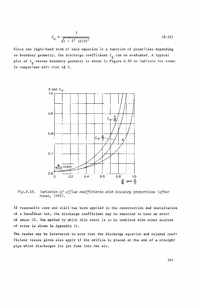
(d/D)1 (8-35)
Since the right-hand term of each equation is a function of quantities depending
on boundary geometry, the discharge coefficient C, can be evaluated. A typical
plot of C, versus boundary geometry is shown in Figure 8.28 to indicate its trend
in comparison with that of 6.
5 and C^ 1.0
0.9
0.8
0.7
0.6
n f g ^ l 1 ^ -
cd.
cc
i /
b 1
/ f
-y
I 1 7
I ƒ
/
0.2 0.4 0.6 0.8 1.0
Fig. 8. 28. Variation of efflux coefficients with, boundary proportions (after Rouse, 1949).
If reasonable care and skill has been applied in the construction and installation
of a Danaïdean tub, the discharge coefficient may be expected to have an error
of about 2%. The method by which this error is to be combined with other sources
of error is shown in Appendix II.
The reader may be interested to note that the discharge equation and related coef
ficient values given also apply if the orifice is placed at the end of a straight
pipe which discharges its jet free into the air.
341
8.8.3 Limits of application
The limits of application of the Danaïdean tub are:
a) The edge of the opening should be sharp and be in accordance with the
profile shown in Figure 5.1.
b) The ratios b/B and d/D should not exceed 0.8.
c) The contraction of the jet must not be hampered. To ensure this, the botton
of the tub must have a minimum clearance of d/<$ (or b/<$) above the downstream
water level.
342
8.9 Selected list of references
1. AL-KHOUDARI, N.:The module à masque type-X. Agric.Univ.Wageningen.
M.Sc.Thesis 1973. 39 pp.
2. ARMCO DRAINAGE & METAL PRODUCTS INC.: Water measurement tables. Portland,
Oregon 1951.
3. FRANKE, P.G., and VALENTIN, F.: The determination of discharge below
gates in case of variable tailwater conditions. J.of Hydraulics Res. 7 (1969),
No.4, pp.433-447.
4. GENTILINI, B.:Flow under inclined or radial sluice gate. Technical and
experimental results. La Houille Blanche 1947, Vol.2.
5. GRUYTER, P.de: Een nieuw type aftap - tevens meetsluis. De Waterstaats
ingenieur. 1926 (No.12) and 1927 (No.1). Batavia, Java.
6. HENDERSON, F.M. Open channel flow. The MacMillan Comp., New York 1966.
522 pp.
7. HENRY, H: Discussion to Diffusion of submerged jets. Transitions of
the American Society of Civil Engineers. 115 (1950)., pp.687-697.
8. KRUSE, E.A.:The constant-head orifice farm turnout. U.S.Dept.of Agric.
Report ARS 41-93, Fort Collins, Col. 1965. 24 pp.
9. METZLER, D.E.: A Model Study of Tainter Gate Operation. State Univ.of
Iowa Master's Thesis. August 1948.
10. MISES, R.von: Berechnung von Ausfluss und Überfällzahlen. Z.des Vereines
deutscher Ingenieure 61 (1917). No.21, pp.447-452; No.22, pp.469-474; No.23,
pp.493-498. Berlin.
ll.NEYRPIC: Irrigation canal equipment. Ets Neyrpic, Grenoble, France. 1955.
32 pp.
12. ROMIJN, D.G.: Meetsluizen ten behoeve van irrigatiewerken. Handleiding
uitgegeven door de "Vereniging van Waterstaat-ingenieur in Nederlandsch-Indië."
Bandung 1938. 58 pp.
13. SCHUSTER, J.C.: Water measurement procedures. Irrigation operators'
workshop. U.S.Bureau of Reclamation, Denver, Col.1970. Report REC-OCE-70-38. 49 pp.
14. STOKMANS, J.A.: Metingen aan de constant-head-orifice-turnout. Agric.
Uniy., Wageningen. M.Sc.Thesis not published. (1970)
343
15. TOCH, A.: The Effect of a Lip Angle Upon Flow Under a Tainter Gate.
State Univ.of Iowa Master's Thesis, February 1952.
16. U.S.ARMY ENGINEER WATERWAYS EXPERIMENT STATION: Model Study of the
spillway for New Lock and Dam No.1. St.Lucie Canal, Florida. Technical Memorandum
No.153-1, Vicksburg, Miss., June 1939.
17. U.S.ARMY ENGINEER WATERWAYS EXPERIMENT STATION: Spillway for New Cum
berland Dam, Ohio River, West Virginia. Technical Memorandum No.2-386, Vicksburg,
Miss.,July 1954.
18. U.S.ARMY ENGINEER WATERWAYS EXPERIMENT STATION: Stilling Basin for
Warrior Dam, Ohio River, West Virginia. Technical Report No.2-485, Vicksburg,
Miss., July 1958.
19. U.S.ARMY ENGINEER WATERWAYS EXPERIMENT STATION: Spillways and Stilling
Basins, Jackson Dam, Tombigbee River, Alabama. Technical Report No.2-531, Vicks
burg, Miss., January 1960.
20. U.S.ARMY ENGINEER WATERWAYS EXPERIMENT STATION: Hydraulic design cri
teria. Sheets 320-4 to 320-7. Vicksburg, Miss. 1960.
21. U.S.BUREAU OF RECLAMATION: Water measurement manual. U.S.Gov.printing
office, Washington. Second Ed. 1967. 326 pp.
22. U.S.SOIL CONSERVATION SERVICE: National Engineering Handbook. Chap.9,
Section 15: Measurement of irrigation water. U.S.Government printing office,
Washington. 1962. 70 pp.
344
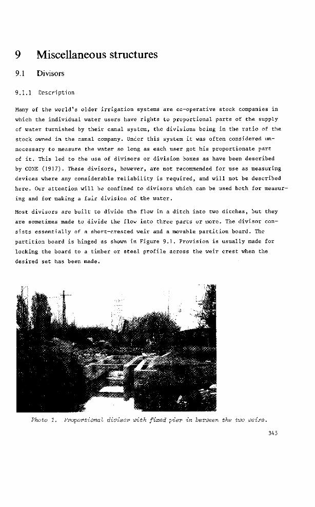
9 Miscellaneous structures 9.1 Divisors
9.1.1 Description
Many of the world's older irrigation systems are co-operative stock companies in
which the individual water users have rights to proportional parts of the supply
of water furnished by their canal system, the divisions being in the ratio of the
stock owned in the canal company. Under this system it was often considered un
necessary to measure the water so long as each user got his proportionate part
of it. This led to the use of divisors or division boxes as have been described
by CONE (1917). These divisors, however, are not recommended for use as measuring
devices where any considerable reliability is required, and will not be described
here. Our attention will be confined to divisors which can be used both for measur
ing and for making a fair division of the water.
Most divisors are built to divide the flow in a ditch into two ditches, but they
are sometimes made to divide the flow into three parts or more. The divisor con
sists essentially of a short-crested weir and a movable partition board. The
partition board is hinged as shown in Figure 9.1. Provision is usually made for
locking the board to a timber or steel profile across the weir crest when the
desired set has been made.
Photo 1. Proportional divisor with fixed pier in between the two weirs.
345
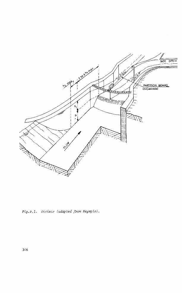
Fig.9.1. Divisor (adapted from Neyrpia).
346
The structure shown in Figure 9.1 was designed by Neyrpic and consists of a
slightly curved weir sill with a 60-degree sloping upstream face and a 12-degree
sloping downstream face. The weir crest is rounded, its radius being equal to r =
0.2 h.max, where h max is the maximum upstream head. Viewed from above, the weir
crest is curved with a minimum radius of 1.75 b; the crest width b should not be
less than 2 tLmax.
The upstream head, h 1 , is to be measured in a rectangular approach channel at a
distance of between 2 h max and 3 h max upstream from the weir crest.
The upstream edge of the partition board should be sharp (•$ 0.005 m thick) and
should be located immediately downstream of the weir crest, in the area where
flow is super-critical.
A disadvantage of sharp-edged partition boards is that trash and floating debris are
caught, so that frequent maintenance is required to obtain a proportional divi
sion of water.
The flow-wise weir profile is not a determining factor in the proportional divi
sion of water. In principle, any short-crested weir is suitable, especially the
triangular profile two-dimensional weir (Section 6.3) and the cylindrical crested
weir (Section 6.7).
9.1.2 Evaluation of discharge
According to Section 1.10, the basic head-discharge equation for a short-crested
weir with a rectangular control section reads
Q = c d c v ! [ ! ^ 2 b h ! ' 5 (9- , }
where the approach velocity coefficient C may be read from Figure 1.12 as a
function of the area ratio C ,A /k,. The discharge coefficient of the Neyrpic weir
profile is a function of the ratio Hj/r as shown in Figure 9.2.
The modular C,-values shown in Figure 9.2 are valid if the weir crest is suffi
ciently high above the average bed of both the approach and tailwater channel so
as not to influence the streamline curvature above the weir crest. To ensure
this, the ratio p/H should not be less than 0.33 and the ratio P9/H should not
be less than 0.35. To obtain modular flow, the ratio H./H should not exceed 0.60.
It should be noted that the weir width b is measured along the curved weir crest.
347
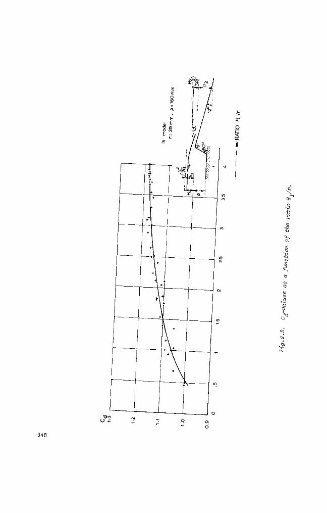
c I" O
et
5Ä i «
O
K O
O K
co
s ö
I
os
ft.
348
The accuracy of the discharge coefficient of a well maintained divisor which has
been constructed with reasonable care and skill will be sufficient for field con
ditions. The error in the product C C may be expected to be less than 5 per cent.
The method by which this error is to be combined with other sources of error is
shown in Appendix II.
9.1.3 Limits of application
The limits of application of a divisor equipped with a Neyrpic weir crest are:
a) The upstream head over the weir crest h should be measured at a distance
of 2 to 3 times hjinax upstream from the weir crest. The recommended lower limit
of hj = 0.06 m.
b) To prevent water surface instability in the approach channel, the ratio
p/H should not be less than 0.33.
c) To prevent the tailwater channel bottom from influencing the flow pattern
over the weir crest, the ratio p./h. should not be less than 0.35.
d) To reduce boundary layer effects of the vertical side walls, the ratio
b/H should not be less than 2.0.
e) To obtain sensibly two-dimensional flow over the weir crest, the hori
zontal radius of curvature of the weir crest should not be less than 1.75 b.
f) The ratio H /r should not be less than 0.20.
g) To obtain modular flow, the ratio H„/H1 should not exceed 0.60.
9.2 Pipes and small syphons
9.2.1 Description
On irrigated farms, short sections of pipe are frequently used to distribute water
over the fields. Commonly used for this purpose are plastic, aluminium, or galva
nized steel pipes and siphons. Some examples are shown in Figure 9.3.
349
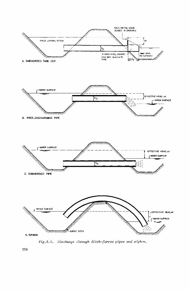
GALV. METAL DOOR w w w w w v ^ . SLIDES IN GROOVES
7777777777777^
A. SUBMERGED TAKE OUT
V777777777777/
B. FREE-DISCHARGING PIPE
J EFFECTIVE HEAD, Ah
WATER SURFACE
'7777777777777.
C. SUBMERGED PIPE
EFFECTIVE HEAD, Ah
r-WATER SURFACE
'''///////////$-
" ^ E F F E C T I V E HEAD, Ah
WATER SURFACE
D. SIPHON >?W/////////S^
Fig.9.3. Discharge through ditch-furrow pipes and siphon.
350
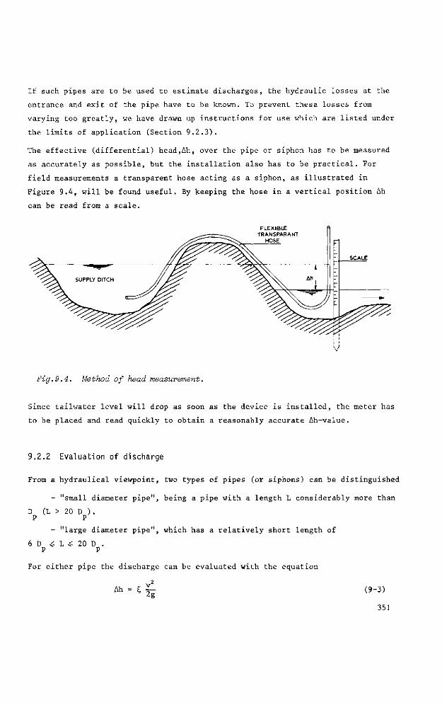
If such pipes are to be used to estimate discharges, the hydraulic losses at the
entrance and exit of the pipe have to be known. To prevent these losses from
varying too greatly, we have drawn up instructions for use which are listed under
the limits of application (Section 9.2.3).
The. effective (differential) head,Ah, over the pipe or siphon has to be measured
as accurately as possible, but the installation also has to be practical. For
field measurements a transparent hose acting as a siphon, as illustrated in
Figure 9.4, will be found useful. By keeping the hose in a vertical position Ah
can be read from a scale.
Fig.9.4. Method of head measurement.
Since tailwater level will drop as soon as the device is installed, the meter has
to be placed and read quickly to obtain a reasonably accurate Ah-value.
9.2.2 Evaluation of discharge
From a hydraulical viewpoint, two types of pipes (or siphons) can be distinguished
- "small diameter pipe", being a pipe with a length L considerably more than
D (L > 20 D ) . P P
- "large diameter pipe", which has a relatively short length of
6 D v< L * 20 D . P P
For either pipe the discharge can be evaluated with the equation
„2 Ah = Ç
2g (9-3)
351
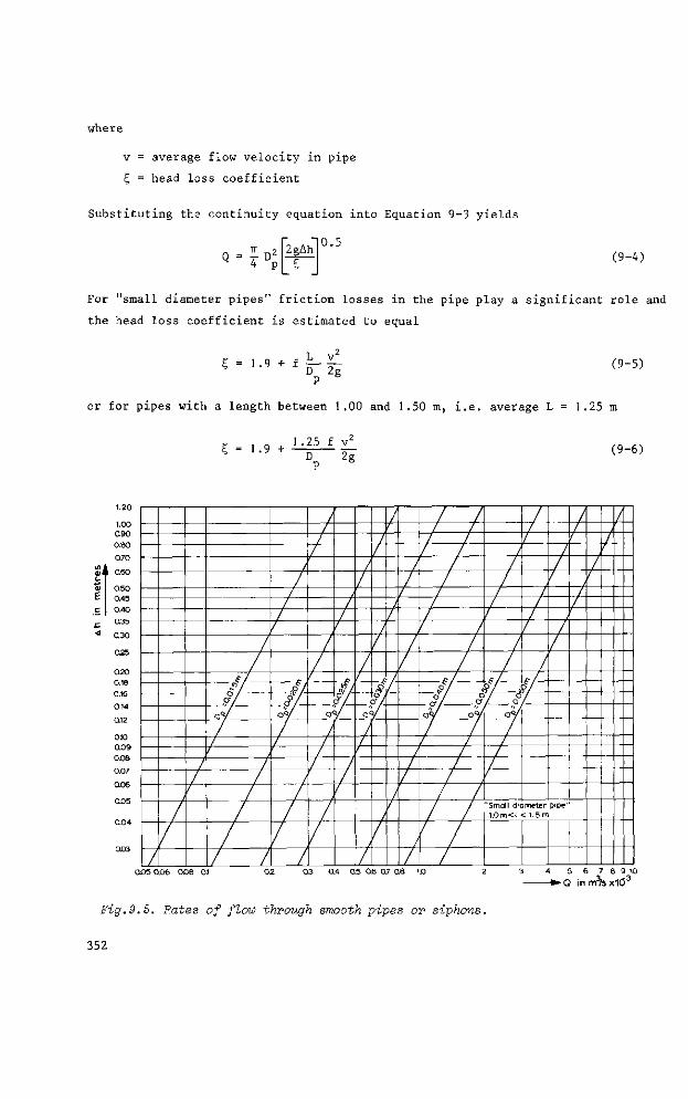
where
v = average flow velocity in pipe
Ç = head loss coefficient
Substituting the continuity equation into Equation 9-3 yields
0.5
4 p 2aAh
S (9-4)
For "small diameter pipes" friction losses in the pipe play a significant role and
the head loss coefficient is estimated to equal
' - " " E r f c (9-5)
or for pipes with a length between 1.00 and 1.50 m, i.e. average L = 1.25 m
Ç = 1 . 9 + 1 .25 f vj_
Dp 2g (9-6)
1.20
1.00
0.90
0.80
0.70
o î i i Q60
Q50
0.45
0.40
0.35
0.30
Q25
0.20
0.18
0.16
0.14
0.12
010
0.09
0.08
0.07
0.06
0.05
/
I /
/
I /
/
f / • ? /
C f /
°y
/ /
/ /
/
/
/ /
p / &
oy
- • - — - /
/
1
/
/
/ /
o<
t
1 /
'
i
1
y
/ / 1
/ /
/ /
~4 TO / o* A
Qc
/ /
/ /
/ '
/ /
/ / /
/ /
/ /
v°/ ' ° / t?
? 7 — * / o Q V O V O V
/ / /
?7
/ /
f
/ / i
t
/ / "Small diameter pipe" / / l .0m<L< 1.5m
/ i
4
/ 1
l
/
0.05 0.06 0Û8 0.1 0 2 0 3 0.4 0.5 0.6 0.7 Q8 1j0 3 4 5 6 7 8 9 10
-Q in m3/sx1Ö3
Fig.9.5. Rates of flow through smooth pipes or siphons.
352
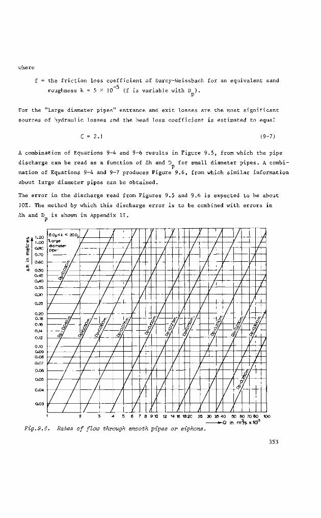
where
f = the friction loss coefficient of Darcy-Weissbach for an equivalent sand
roughness k = 5 x 10 (f is variable with D ) .
For the "large diameter pipes" entrance and exit losses are the most significant
sources of hydraulic losses and the head loss coefficient is estimated to equal
S = 2.1 (9-7)
A combination of Equations 9-4 and 9-6 results in Figure 9.5, from which the pipe
discharge can be read as a function of Ah and D for small diameter pipes. A combi
nation of Equations 9-4 and 9-7 produces Figure 9.6, from which similar information
about large diameter pipes can be obtained.
The error in the discharge read from Figures 9.5 and 9.6 is expected to be about
10%. The method by which this discharge error is to be combined with errors in
Ah and D is shown in Appendix II.
1.20
1.00
0.80
0.70
0.60
0.50 0.45 0.40 0.35 (XX 0.25
0.20 0.18 0.16 0.14 0.12
0.10
0.09
0.08
0.07
0.06
0.05
6 Dp< L < 20 Dp
"Large diameter j pipe" /
/ o /
y
/
/ / a-—,
o/ >>/
v c
/ / / /
/ / /
oV
/ /
/ /
/
oV 'S $ f <f
/
/
/ /
'
/ /
/
/ / /
c
<?/
1
/ '
/ /
/
/ / '
M y
/ /
/ /
/ / /
/ /
/ / t
/ f^
/ /
/ /
— ( o
é/ /
/ ^
/ i
/ I
i
'
/ L
.y
—
/ . /
6 ~Sfl— VI
éy
/ / i
/
/ /
/ i
/ /
c
/ /
1 /
/ 1
/
/
- / /
/
/ /
/ /
& Si
/ / /
i /
i
i
/
/
/ /
/ / /
»
/
c
/
'
/ /
/ 1
^ y
tf
/ /
/ /
M oV
è
i
/
/
/ / J
c
4
/ /
/ 1
J /
/ 1
1/-o7
/ /
i/ il
J 1
/ /
7 8 9 10 12 14 16 18 20 25 30 35 40 50 60 70 80 100
Fig.9.6. Rates of flow through smooth pipes or siphons. -•-Q in m^s X1Ö3
353
9.2.3 Limits of appl icat ion
To produce a reasonably accurate estimate of the discharge through a pipe or
siphon, the following limits of application are considered essential.
a) Pipes should have clear cut edges (no rounding-off) and a constant dia
meter from entrance to end. The pipe entrance should protrude from the ditch
embankment and the flow velocity in the ditch should be less than one third of
the average velocity in the pipe.
b) The pipe should be made of "technically smooth material". For
D ^ 0.05 m, PVC or aluminium are suitable, while if D > 0.05 m galvanized steel _P P is also suitable.
c) To prevent air-bubbles from collecting at the top of a siphon, it is re
commended that v > 1.3 (g D sin a) ' , where a denotes the angle of the down
stream siphon limb from the horizontal.
d) To eliminate bend-losses, the radius of bends should not be less than
8 D . P
e) No air-entraining vortex should be visible at the pipe entrance.
f) The exit cross-section of the pipe has to flow entirely full. For a free
discharging horizontal pipe, this occurs if Q ^ 1.18 g D m3/s. (See also
Sections 9.4 and 9.5.)
g) The recommended lower limit of Ah is 0.03 m. The recommended lower limit
of D is 0.015 m for "small diameter pipes" and 0.03 m for "large diameter pipes",
9.3 Fountain flow from a vertical pipe
9.3.1 Description
Fountain flow from a vertical pipe into the air can occur during pumping tests,
or when there is flow from pressure conduits or from artesian wells. Such flow
can occur either as weir flow or as jet flow.
Weir flow. Water discharges from the pipe with sub-critical flow and is si
milar to flow over a curved sharp-crested weir. Weir flow occurs if the height
to which the water rises above the pipe is equal to or less than 0.37 D .
Jet flow. Water discharges from the pipe with supercritical flow. Jet flow
occurs if the height of the jet exceeds 1.4 D , as determined by sighting over
the jet to obtain the average rise.
354
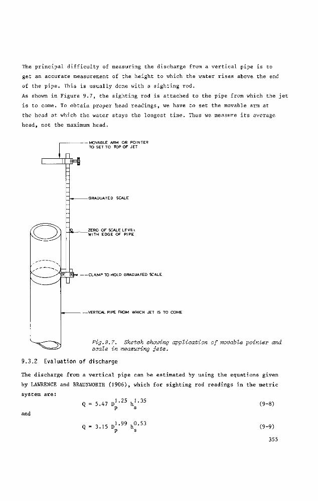
The principal difficulty of measuring the discharge from a vertical pipe is to
get an accurate measurement of the height to which the water rises above the end
of the pipe. This is usually done with a sighting rod.
As shown in Figure 9.7, the sighting rod is attached to the pipe from which the jet
is to come. To obtain proper head readings, we have to set the movable arm at
the head at which the water stays the longest time. Thus we measure its average
head, not the maximum head.
-MOVABLE ARM OR POINTER TO SET TO TOP OF JET
• n 54-
-GRADUATED SCALE
-ä— ZERO OF SCALE LEVEL WITH EDGE OF PIPE
-CLAMP TO HOLD GRADUATED SCALE
-VERTICAL PIPE FROM WHICH JET IS TO COME
Fig.9.7. Sketch showing application of movable pointer and scale in measuring jets.
9.3.2 Evaluation of discharge
The discharge from a vertical pipe can be estimated by using the equations given
by LAWRENCE and BRAUNWORTH (1906), which for sighting rod readings in the metric
system are: 1 25 1 35
Q = 5.47 D h (9-8) p s
and
3.15 D1-99!.0-53
P s (9-9)
355
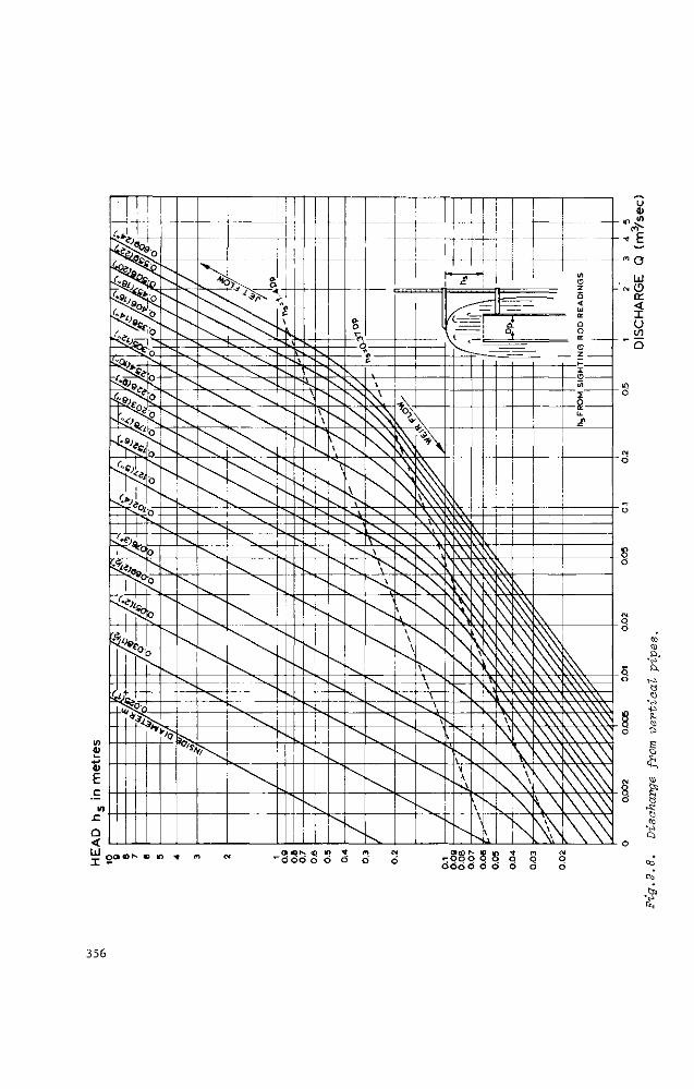
" o d d d d rOOO ö 6 d d d d d d
CD
C i
Ö l
356
Equation 9-8 is valid for weir flow (h < 0.37 D ) and Equation 9-9 is valid for n s p iet flow (h ^ 1.4 D ) . For iet heights between 0.37 D and 1.4 D , the flow is J s p J 6 p p
somewhat less than given by either of these equations. Figure 9.8, prepared from
LAWRENCE and BRAUNWORTH data, shows flow rates in m3/s for standard pipes and for
jet heights up to 4.0 m.
The accuracy with which the jet flow can be evaluated may be expected to be about
15% for sighting rod readings. For weir flow these accuracies are about 20%.
9.3.3 Limits of application
The limits of application that enable a reasonable estimate of the discharge from
a vertical pipe are:
a) Pipes should have clear cut edges and a constant diameter over at least
a length of 6 D .
b) Pipes should be vertical for at least a length of 6 D from the top of
the pipe.
c) The practical range of pipe diameters is 0.025 m -S D <: 0.609 m.
d) The practical range of heads is 0.03 m < h 4.0 m.
9.4 Flow from horizontal pipes
9.4.1 Description
Flow from a horizontal pipe can be estimated by using either the California pipe
method1 developed by VAN LEER (1922) or the trajectory method developed at Purdue
University by GREEVE (1928). The California pipe method applies only to pipes
flowing less than half full, whereas the more general trajectory method applies
equally well to both partially and completely filled pipes.
1 The California pipe method is identical to the brink depth method for circular canals.
357
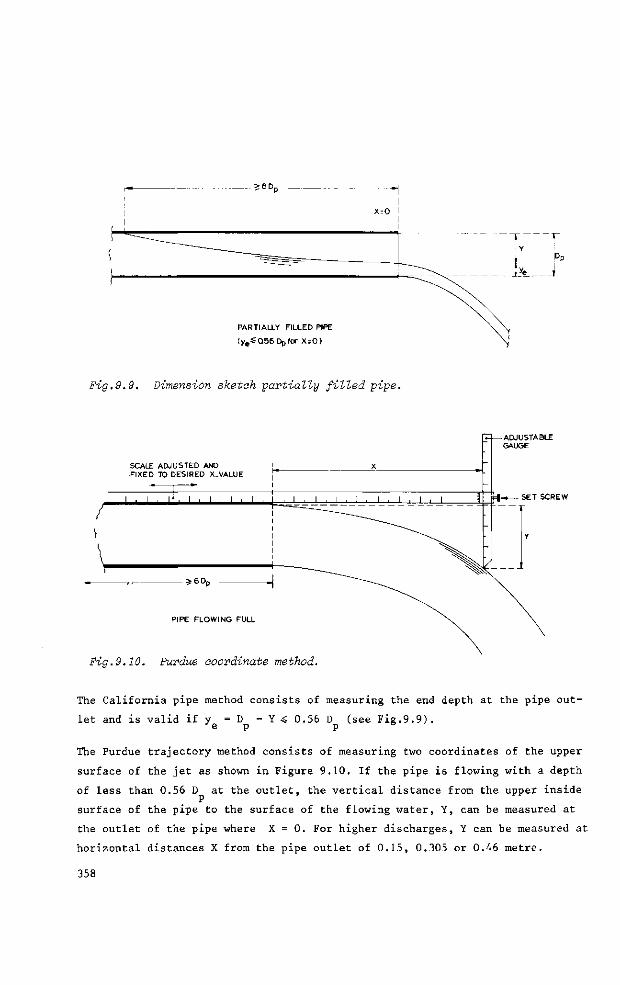
X = 0 I
PARTIALLY FILLED PIPE
(y eSQ56Dplor X = 0 )
Fig.9.9. Dimension sketch partially filled pipe.
SCALE ADJUSTED AND FIXED TO DESIRED X.VALUE
PIPE FLOWING FULL
Fig.9.10. Purdue coordinate method.
SET SCREW
The California pipe method consists of measuring the end depth at the pipe outlet and is valid if y = D - Y 4 0.56 D (see Fig.9.9).
e p p
The Purdue trajectory method consists of measuring two coordinates of the upper
surface of the jet as shown in Figure 9.10. If the pipe is flowing with a depth
of less than 0.56 D at the outlet, the vertical distance from the upper inside p
surface of the pipe to the surface of the flowing water, Y, can be measured at
the outlet of the pipe where X = 0. For higher discharges, Y can be measured at
horizontal distances X from the pipe outlet of 0.15, 0.305 or 0.46 metre.
358
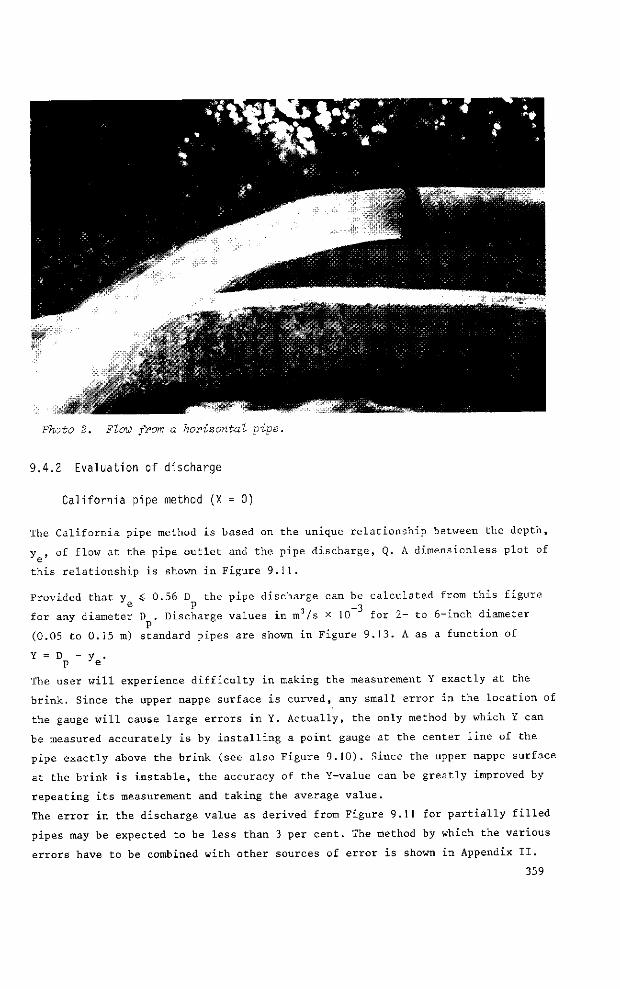
Photo 2. Flow from a horizontal pipe.
9.4.2 Evaluation of discharge
California pipe method (X = 0)
The California pipe method is based on the unique relationship between the depth,
y , of flow at the pipe outlet and the pipe discharge, Q. A dimensionless plot of
this relationship is shown in Figure 9.11.
Provided that y ^ 0.56 D the pipe discharge can be calculated from this figure e P , -3
for any diameter D . Discharge values in m / s x 10 for 2- to 6-inch diameter
(0.05 to 0.15 m) standard pipes are shown in Figure 9.13. A as a function of
Y = D - y . p 'e
The user will experience difficulty in making the measurement Y exactly at the
brink. Since the upper nappe surface is curved, any small error in the location of
the gauge will cause large errors in Y. Actually, the only method by which Y can
be measured accurately is by installing a point gauge at the center line of the
pipe exactly above the brink (see also Figure 9.10). Since the upper nappe surface
at the brink is instable, the accuracy of the Y-value can be greatly improved by
repeating its measurement and taking the average value.
The error in the discharge value as derived from Figure 9.11 for partially filled
pipes may be expected to be less than 3 per cent. The method by which the various
errors have to be combined with other sources of error is shown in Appendix II.
359
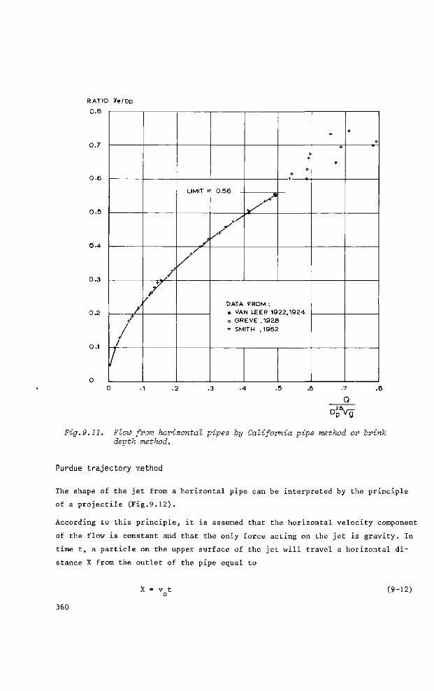
RATIO ye/Dp
0.8
0 . 7
0 . 6
0 . 5
0 . 4
0 . 3
0 . 2
0.1
/
/ /
/ 1
.s
/ /
1 IMIT »" n.Sfi
y
/
y
+ +
O o
DATA FROM : • VAN LEER 1922,1924 o GREVE ,1928 + SMITH ,1962
+
0
•
o
o
.1 .2 .3 .4 .5 .6 .7
Q
. 8
DpVg
Fig.9.11. Flow from horizontal pipes by California pipe method or brink depth method.
Purdue trajectory method
The shape of the jet from a horizontal pipe can be interpreted by the principle
of a projectile (Fig.9.12).
According to this principle, it is assumed that the horizontal velocity component
of the flow is constant and that the only force acting on the jet is gravity. In
time t, a particle on the upper surface of the jet will travel a horizontal di
stance X from the outlet of the pipe equal to
X = v t o
(9-12)
360
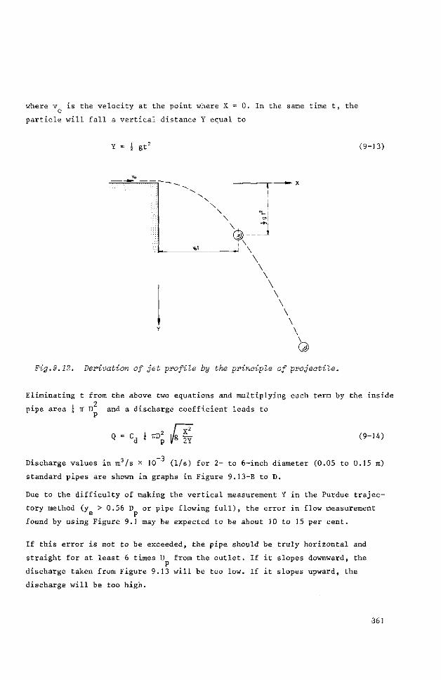
where v is the velocity at the point where X = 0. In the same time t, the o
particle will fall a vertical distance Y equal to
Y = gt' (9-13)
C4>
Fig.9.12. Derivation of get profile by the principle of projectile.
Eliminating t from the above two equations and multiplying each term by the inside 2
pipe area \ TT D and a discharge coefficient leads to
Q = cd * ™ p |/s I Y (9-14)
Discharge values in m 3 /s x 10 (1/s) for 2- to 6-inch diameter (0.05 to 0.15 m)
standard pipes are shown in graphs in Figure 9.13-B to D.
Due to the difficulty of making the vertical measurement Y in the Purdue trajec
tory method (y > 0.56 D or pipe flowing full), the error in flow measurement
found by using Figure 9.1 may be expected to be about 10 to 15 per cent.
If this error is not to be exceeded, the pipe should be truly horizontal and
straight for at least 6 times D from the outlet. If it slopes downward, the
discharge taken from Figure 9.13 will be too low. If it slopes upward, the
discharge will be too high.
-361
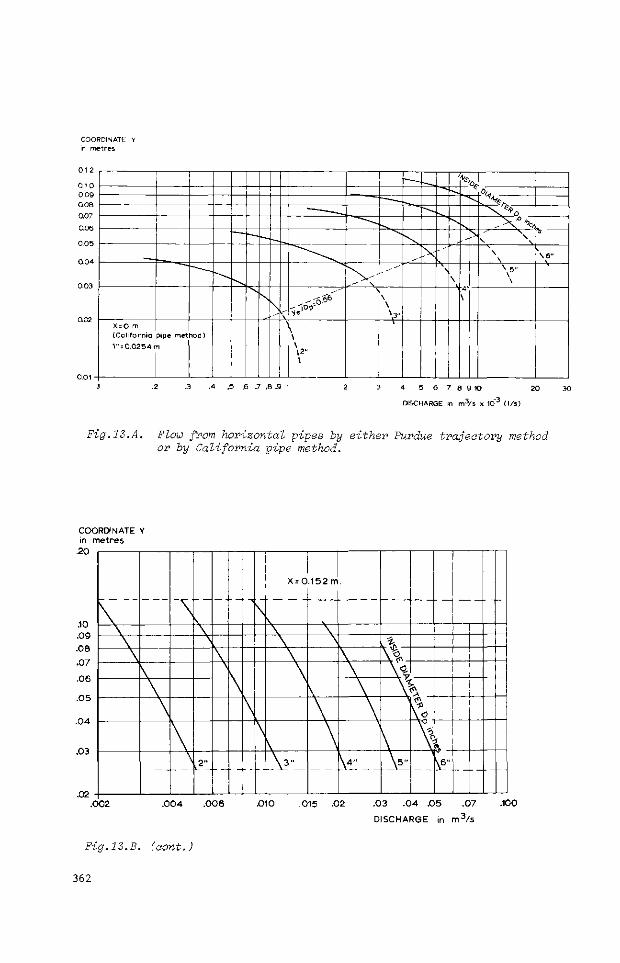
COORDINATE Y in met res
0 1 2
0.10
0.09
0.08
0.07
0.06
0.05
Q 0 4
0.03
X = 0 m
(Ca l i fo rn ia
1 " = 0 . 0 2 5 4 r
pipe met
n.
hod)
N k \ \ • \ \ \ \
-~~ s
---^ \ \ \ \ 3 "
\
N \ 4' \
Of
°'l
. V v% .v%. \ \
V" \ 6 "
.3 .4 .5 .6 .7 .8 .9 1 3 4 5 6 7 8 9 10 20 30
DISCHARGE in m 3 / s x 10"3 ( l / s )
Fig.12.A. Flow from horizontal pipes by either Purdue trajectory method or by California pipe method.
COORDINATE Y in metres
.20
.10 .09 .08 .07 .06 .05
.04
.03
.02
A
\ \ ,2"
- -
\
\
X = 0
\
V
.152rr
.
\ 4 "
\% \ ^
\ <g.
\ \
V"
<" $
\ \
- —
I
% \6" --
.002 .004 .006 .010 .015 .02 .03 .04 .05 .07 .100 DISCHARGE in m3 /s
Fig. 13. B. (oont.)
362
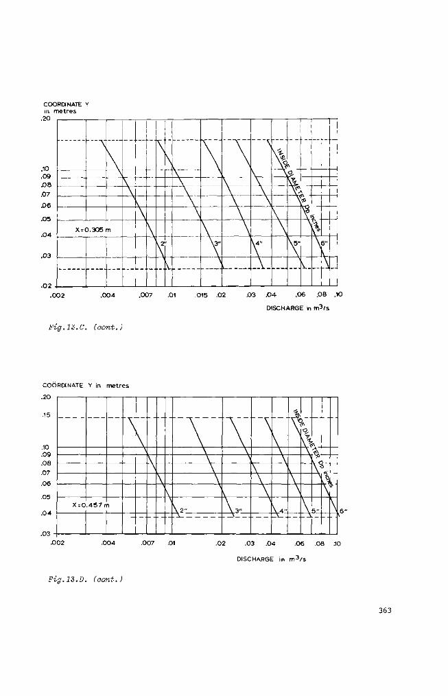
COORDINATE Y in metres
.20
.10
.09
.08
.07 J06
.05
.04
.03
.02
X;0.305m
s, \
K y
ft \
;
—V
i i
—
\ 3 "
\
\4"
1 ' i
t\ .
i i ' i ;
°' v V-
\ 5 '
^ -
V" \
i
]
.002 .004 .007 .01 .015 .02 .03 .04 .06 .08 .10
DISCHARGE in m3 /s
Fig.13.C. (oont.)
COORDINATE Y in metres
.20
.15
.10
.09
.08
.07
.06
.05
.04
.03
X = 0 . 4 5 7 r n
" \
\ \ \ \
f" S \ \ \
V"
- - * - -
\
\ ,
~ ~ \
\ \ \ \
\ « "
1 V
\ \
o '
\ «\ VC
\ * 1 V
\
\ , .
---
V
\
.002 .004 .007 .01 .02 .03 .04 .06 .08 .10
DISCHARGE in m 3 / s
Fig.13.D. (oont.)
363
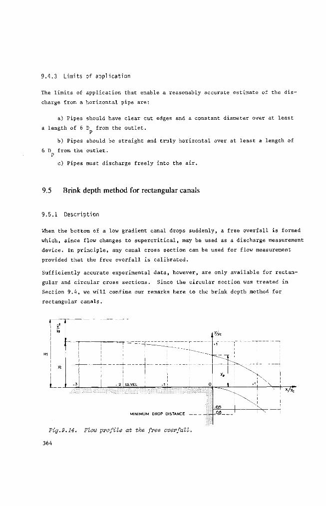
9.4.3 Limits of application
The limits of application that enable a reasonably accurate estimate of the dis
charge from a horizontal pipe are:
a) Pipes should have clear cut edges and a constant diameter over at least
gth of 6 D from the outlet.
b) Pipes should be straight and truly horizontal over at least a length of
from the outlet.
c) Pipes must discharge freely into the air.
9.5 Brink depth method for rectangular canals
9.5.1 Description
When the bottom of a low gradient canal drops suddenly, a free overfall is formed
which, since flow changes to supercritical, may be used as a discharge measurement
device. In principle, any canal cross section can be used for flow measurement
provided that the free overfall is calibrated.
Sufficiently accurate experimental data, however, are only available for rectan
gular and circular cross sections. Since the circular section was treated in
Section 9.4, we will confine our remarks here to the brink depth method for
rectangular canals.
Fig.9.14. Flow profile at the free overfall.
364
i " i 1
i
f
1
i j
• - 3
; ; ! 1 j
1 ! i - 2 | LEVEL , -1 j
MINIMUM DROP DISTANCE
/
i /
L_
J_
__
i- ,
*e
-0.5 -0ß__ -- \
— j
V x/yc
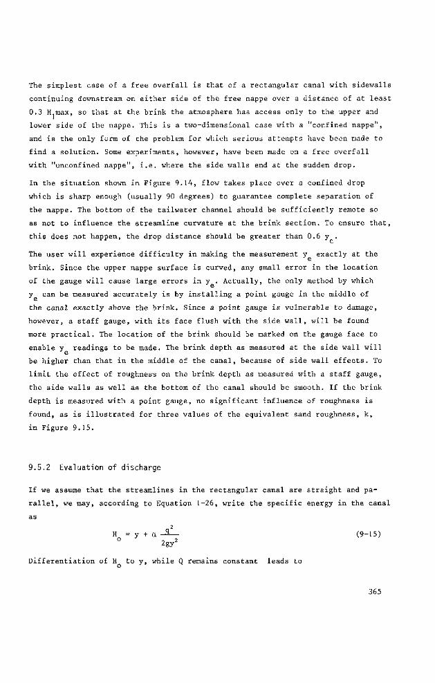
The simplest case of a free overfall is that of a rectangular canal with sidewalls
continuing downstream on either side of the free nappe over a distance of at least
0.3 ïLmax, so that at the brink the atmosphere has access only to the upper and
lower side of the nappe. This is a two-dimensional case with a "confined nappe",
and is the only form of the problem for which serious attempts have been made to
find a solution. Some experiments, however, have been made on a free overfall
with "unconfined nappe", i.e. where the side walls end at the sudden drop.
In the situation shown in Figure 9.14, flow takes place over a confined drop
which is sharp enough (usually 90 degrees) to guarantee complete separation of
the nappe. The bottom of the tailwater channel should be sufficiently remote so
as not to influence the streamline curvature at the brink section. To ensure that,
this does not happen, the drop distance should be greater than 0.6 y .
The user will experience difficulty in making the measurement y exactly at the
brink. Since the upper nappe surface is curved, any small error in the location
of the gauge will cause large errors in y . Actually, the only method by which
y can be measured accurately is by installing a point gauge in the middle of
the canal exactly above the brink. Since a point gauge is vulnerable to damage,
however, a staff gauge, with its face flush with the side wall, will be found
more practical. The location of the brink should be marked on the gauge face to
enable y readings to be made. The brink depth as measured at the side wall will
be higher than that in the middle of the canal, because of side wall effects. To
limit the effect of roughness on the brink depth as measured with a staff gauge,
the side walls as well as the bottom of the canal should be smooth. If the brink
depth is measured with a point gauge, no significant influence of roughness is
found, as is illustrated for three values of the equivalent sand roughness, k,
in Figure 9.15.
9.5.2 Evaluation of discharge
If we assume that the streamlines in the rectangular canal are straight and pa
rallel, we may, according to Equation 1-26, write the specific energy in the canal
as
2
H = y + a - 3 — (9-15) 2gy
Differentiation of H to y, while Q remains constant leads to
365
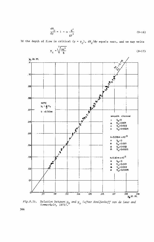
dH 2 -.— = 1 - a — — dy 3
gy (9-16)
If the depth of flow is critical (y = y ), dH /dy equals zero, and we may write
qq g
(9-17)
yc in m. .11
.10
.09
- V O
,r
4
.08
.07
.06
.05
.04
.03
.02
.01
NOTE
V c = | H l
b =0.50m
À d1
•f tf
tf
f «/
cfr
tf
ƒ /
y
^
smooth channel
• So=0 A So=0.001 + S =0.002
k=0.08m x 1 0 ° o So = 0 * S„=0.001
A
k=0.30m x10~ Sn=0
.01 02 .03 .04 .05 .06 .07 .08 .09
Fig.9.IS. Relation between y, and y (after Kraijenhoff van de Leur and Dommerholt, 1972). a
366
Assuming a = 1 and substituting Q = bq leads to
Q = b/i y3J2 (9-18)
The experiments of ROUSE (1936), and further experiments by various authors,
showed that for a confined nappe the brink section has a flow depth equal to
y = 0.715 y (9-19) e c
resulting in the discharge equation
3/2
Q = b/i ye
0.715 (9-20)
As shown in Figure 9.15, slight variations in the roughness of the canal bounda
ries and in the canal bottom slope are of little significance on the ratio y /y .
If the free overfall has an unconfined nappe, however, the ratio y /y is somewhat
less than in the two-dimensional case, being equal to 0.705.
For a free overfall which is constructed and maintained with reasonable care and
skill, the coefficients 0.715 and 0.705 can be expected to have an error of the
order of 2% and 3% respectively, provided y is measured in the middle of the
channel. If y is measured at the side walls an additional error in y occurs due J c J e
to boundary roughness (see Section 9.4.2 for other possible errors). The method
by which these errors are to be combined with other sources of error is shown
in Appendix II.
9.5.3 Limits of application
The limits of application of the brink depth method for rectangular canals are:
a) Perpendicular to the flow, the brink should be truly horizontal and the
side walls of the rectangular approach canal should be parallel from end to end.
b) To obtain a uniform velocity distribution, the length of the approach
channel should not be less than 12 y . c
c) The longitudinal slope of this approach channel should preferably be zero
but not more than s = 0.0025.
d) The practical lower limit of y is related to the magnitude of the influ
ence of fluid properties and the accuracy with which y can be measured. The
367
recommended lower limit is 0.03 m.
e) The y -value should be measured in the middle of the canal, preferably
by means of a point gauge.
f) The width of the canal should not be less than 3 y nor less than 0.30 m.
g) To obtain free flow, the drop height should not be less than 0.6 y .
9.6 Dethridge meter
9.6.1 Description
The Dethridge meter is a rather commonly used device for measuring the volume
of irrigation water supplied to farms from main and lateral canals in Australia.
The meter was designed by J.S.Dethridge of the State Rivers and Water Supply Com
mission, Victoria, in 1910. This Commission provided the present information on
the standard device, of which today about 20,000 are in operation in irrigation
areas throughout Australia.
The meter consists of an undershot water wheel turned by the discharging water pas
sing through its emplacement, which is a short concrete outlet specially formed
to provide only the minimum practicable clearance of the lower half of the
wheel at its sides and round the lowest 70 degrees of its circumference.
Two standard sizes of the meter are used: the 1.524 m (5 ft) diameter "large"
meter which is suitable for discharges from 0.040 m3/s to 0.140 m 3 /s, and the
"small", 1.219 m (4 ft) diameter meter for discharges from 0.015 m3/s to 0.070 m3/s
The main dimensions of both meters, which are similar in general form, are shown
in Figure 9.16.
The wheel is made up of a cylinder of 2 mm thick mild steel sheet, bearing eight
external vanes of the same material, each welded against the surface of the cy
linder on a widely distended "V", with the root of the "V" leading in the di
rection of the wheel's rotation. At the root of each vane is a small air vent
so that compartments between the vanes can fill completely with water while
being submerged by rotation of the wheel. The outer corners of the vanes are
chamferred.
The internal bracing used to consist of three crossed pairs of timber spokes
(+ 0.10 x 0.05 m) placed at the middle and both ends of the cylinder. Today they
have given way to ^ 16 mm steel rods in parallel pairs, welded on either side
of the 25 mm internal diameter pipe-axle of the wheel (see Fig.9.17).
368
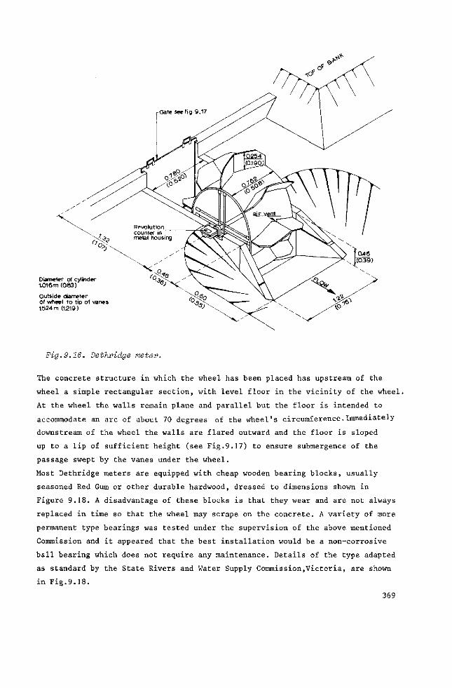
Diameter of cylinder 1.016 m (0.83)
Outside diameter of wheel to t ip of vanes 1.524 m (1.219)
rGate see f ig 9.17
Fig.9.16. Vethridge meter.
The concrete structure in which the wheel has been placed has upstream of the
wheel a simple rectangular section, with level floor in the vicinity of the wheel.
At the wheel the walls remain plane and parallel but the floor is intended to
accommodate an arc of about 70 degrees' of the wheel's circumference.Immediately
downstream of the wheel the walls are flared outward and the floor is sloped
up to a lip of sufficient height (see Fig.9.17) to ensure submergence of the
passage swept by the vanes under the wheel.
Most Dethridge meters are equipped with cheap wooden bearing blocks, usually
seasoned Red Gum or other durable hardwood, dressed to dimensions shown in
Figure 9.18. A disadvantage of these blocks is that they wear and are not always
replaced in time so that the wheel may scrape on the concrete. A variety of more
permanent type bearings was tested under the supervision of the above mentioned
Commission and it appeared that the best installation would be a non-corrosive
ball bearing which does not require any maintenance. Details of the type adapted
as standard by the State Rivers and Water Supply Commission,Victoria, are shown
in Fig.9.18.
369
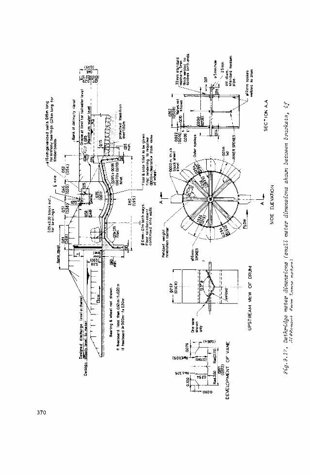
370
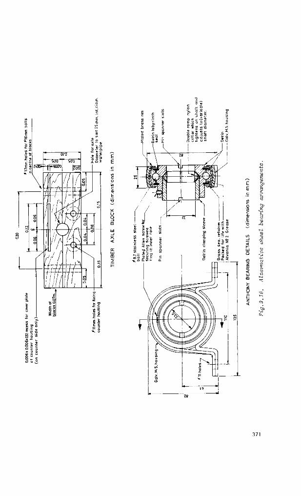
o 'ui c il E •a
U
3 m LU _ i X
< cc LÜ m 2
LÜ Q
O Z ce <
O I z <
to
K
E CD Öi K ö
ö
K
ö 'S
rei
TO
ö
<32
tu
371
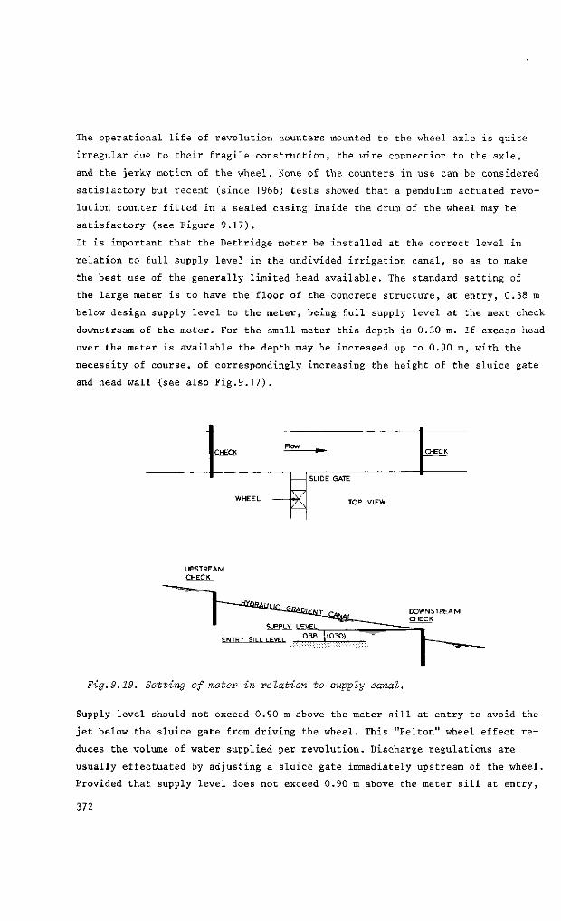
The operational life of revolution counters mounted to the wheel axle is quite
irregular due to their fragile construction, the wire connection to the axle,
and the jerky motion of the wheel. None of the counters in use can be considered
satisfactory but recent (since 1966) tests showed that a pendulum actuated revo
lution counter fitted in a sealed casing inside the drum of the wheel may be
satisfactory (see Figure 9.17).
It is important that the Dethridge meter be installed at the correct level in
relation to full supply level in the undivided irrigation canal, so as to make
the best use of the generally limited head available. The standard setting of
the large meter is to have the floor of the concrete structure, at entry, 0.38 m
below design supply level to the meter, being full supply level at the next check
downstream of the meter. For the small meter this depth is 0.30 m. If excess head
over the meter is available the depth may be increased up to 0.90 m, with the
necessity of course, of correspondingly increasing the height of the sluice gate
and head wall (see also Fig.9.17).
E SUDE GATE
UPSTREAM CHECK
DOWNSTREAM CHECK
ENTRY SILL LEVEL
Fig.9.19. Setting of meter in relation to supply canal.
Supply level should not exceed 0.90 m above the meter sill at entry to avoid the
jet below the sluice gate from driving the wheel. This "Pelton" wheel effect re
duces the volume of water supplied per revolution. Discharge regulations are
usually effectuated by adjusting a sluice gate immediately upstream of the wheel.
Provided that supply level does not exceed 0.90 m above the meter sill at entry,
372
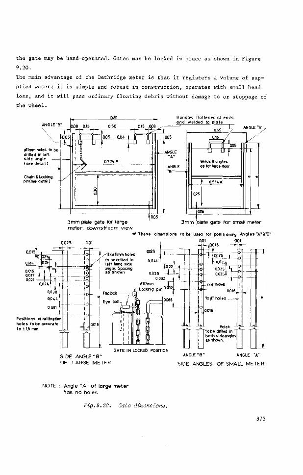
the gate may be hand-operated. Gates may be locked in place as shown in Figure
9.20.
The main advantage of the Dethridge meter is that it registers a volume of sup
plied water; it is simple and robust in construction, operates with small head
loss, and it will pass ordinary floating debris without damage to or stoppage of
the wheel.
AN G LE "B'
^llmm holes to be drilled In left side angle (see detail )
Chain & Locking pintsee detail)
Handles f l a t tened at ends and welded to pla te
3mm plate gate for large meter, downstream view
3mm plate gate for small meter
0.025 0.01
* These dimensions t o b e used for posit ioning Angles "A"8."B"
0.01 Q01 —J-U-iO.016
1.0 22, »
0.025 1 — ' . i 0.032 j !
010mm J~T
Locking p in°* 2 [
0.086
Positions of calibration holes to be accurate to 11,5 mm
l<>
HUM
4t, f^]^ -Jlr-HF
aM4-i-|i'l-0.025~f"
GATE IN LOCKED POSITION
r._7x9l1 holes
7x 011 holes -
0.016
Holes -to be drilled in both sideangles as shown.
0.016, M , _
rt
S I D E A N G L E " B "
O F L A R G E M E T E R
ANGLE " 8 " ANGLE "A"
SIDE ANGLES OF SMALL METER
NOTE : Angle " A " o f large meter has no holes
Fig.9.20. Gate dimensions.
373
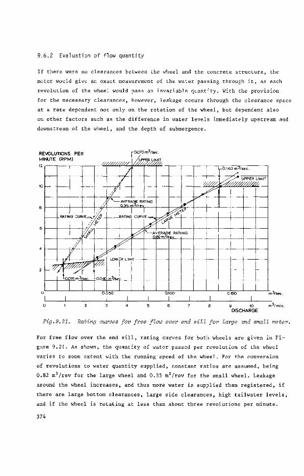
9.6.2 Evaluation of flow quantity
If there were no clearances between the wheel and the concrete structure, the
meter would give an exact measurement of the water passing through it, as each
revolution of the wheel would pass an invariable quantity. With the provision
for the necessary clearances, however, leakage occurs through the clearance space
at a rate dependent not only on the rotation of the wheel, but dependent also
on other factors such as the difference in water levels immediately upstream and
downstream of the wheel, and the depth of submergence.
REVOLUTIONS PER MINUTE (RPM)
10
8
6
2
0
C
RATIN
//
G CUR VF-^ 1
-y/
*/\ — •0.015 m3/sec.
////////////
'V
/ffi.
-0.040
/
/ /
- 0.070 m3/sec.
/UPPER LIMIT
' ^ AVERAGE RATING |0.35 m 3 / rev
1 1 1 RATING CURVE .
\S LOW
m3/se
S :R L I M
^ß i# r
^—AVERAGE RAT 0.82 m3/rev
V
NG
0.050 0.100
I I ! I I I I 1 2 4 5 t 7
1
|
8
r 0 . 1 4 0 m3/sec.
/ / " UPPER LIMIT
i^//////////////
0.150
s DISO
10 ^ R G E
m3/sec.
m /min
Fig.9.21. Rating curves for free flow over end sill for large and small meter.
For free flow over the end sill, rating curves for both wheels are given in Fi
gure 9.21. As shown, the quantity of water passed per revolution of the wheel
varies to some extent with the running speed of the wheel. For the conversion
of revolutions to water quantity supplied, constant ratios are assumed, being
0.82 m3/rev for the large wheel and 0.35 m3/rev for the small wheel. Leakage
around the wheel increases, and thus more water is supplied than registered, if
there are large bottom clearances, large side clearances, high tailwater levels,
and if the wheel is rotating at less than about three revolutions per minute.
374
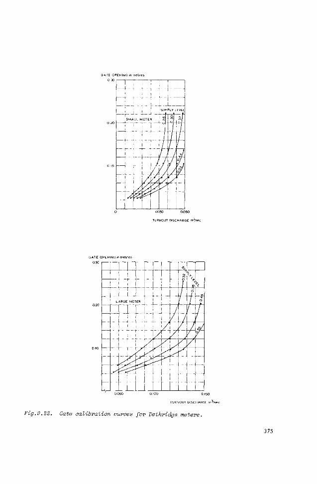
GATE OPENING in metres 0 30 r r — r—
M- - î - - r -
'SUPPLY LEVEL
0.050 0.060
TURNOUT DISCHARGE m3/sec.
GATE OPENING in metres
0.30
—
—
—
1
_L__L J . LARGE METER
- — T r - f 4 -i i
! ' - t - J 1 - -
; " i - f -f
i j
•^
r- T r r
. !. ! . i l l
|
~ - , !
- - t - j - —
i /
A 1 / / 1 X
yT~
- i !_ .
- !- - i -1
r r
! LAJ_ «4U
eo V O' ƒ
/ 1 v
/ 1 o
- -
--
— .....
1 fi/ °y
0.150
TURNOUT DISCHARGE m3/sec
Fig.9,22. Gate calibration curves for Dethridge meters.
375
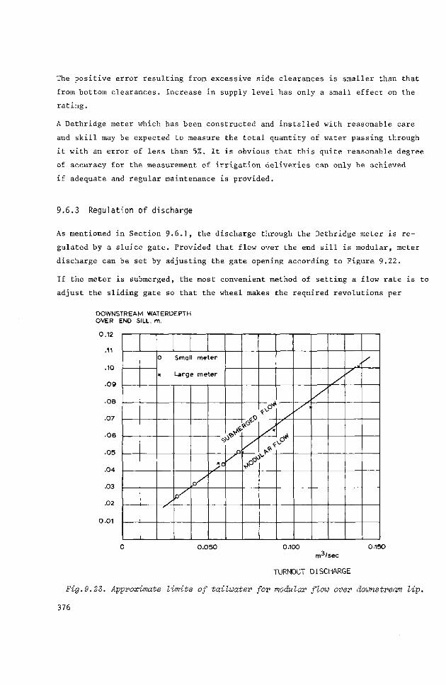
The positive error resulting from excessive side clearances is smaller than that
from bottom clearances. Increase in supply level has only a small effect on the
rating.
A Dethridge meter which has been constructed and installed with reasonable care
and skill may be expected to measure the total quantity of water passing through
it with an error of less than 5%. It is obvious that this quite reasonable degree
of accuracy for the measurement of irrigation deliveries can only be achieved
if adequate and regular maintenance is provided.
9.6.3 Regulation of discharge
As mentioned in Section 9.6.1, the discharge through the Dethridge meter is re
gulated by a sluice gate. Provided that flow over the end sill is modular, meter
discharge can be set by adjusting the gate opening according to Figure 9.22.
If the meter is submerged, the most convenient method of setting a flow rate is to
adjust the sliding gate so that the wheel makes the required revolutions per
DOWNSTREAM WATERDEPTH OVER END SILL. m.
0.12
.11
.10
.09
.08
.07
.06
.05
.04
.03
.02
0.01
0 Small meter
» Large meter
/ S FT
<b
»a
n
/
* < * -
\y s
S*
l°*
jr t
/
0.050 0.100 0-15O m3'sec
TURNOUT DISCHARGE
Fig.9.23. Approximate limits of tailwater for modular flow over downstream lip.
376
minute to pass this flow. Figure 9.21 may be used for this purpose, provided that
tailwater levels remain less than 0.17 m over the end sill to avoid excessive
leakage through the clearances of the large wheel. For the small wheel this value
is 0.13 m.
Approximate limits of tailwater level to obtain modular flow through the Dethridge
meter are shown in Figure 9.23 for both meters.
9.6.4 Limits of application
The limits of application of the Dethridge meter are:
a) The practical lower limit for the supply level over the entry sill is
0.38 m for the large meter and 0.30 m for the small meter. The upper limit for
this supply level is 0.90 m for both meters.
b) Tailwater level should not be more than 0.17 m over the end sill of the
large meter. This value is 0.13 m for the small meter.
c) The wheel should neither make less than about 3 r.p.m.nor more than about
10 to 12 r.p.m. Consequently, the discharge capacity ranges between 0.040 m /s and
0.140 m3/s for the large meter and between 0.015 m3/s and 0.070 m3/s for the small
meter (see also Fig.9.21).
d) Clearance between the floor and side fillets of the structure and the
wheel should not exceed 0.006 m for both meters. Clearance between the side walls
and the wheel should not exceed 0.009 m for the large meter and 0.006 m for the
small meter.
9.7 Propeller meters
9.7.1 Description1
Propeller meters are commercial flow measuring devices used near the end of pipes
or conduits flowing full, or as "in-line" meters in pressurized pipe systems. The
meters have been in use since about 1913 and are of many shapes, kinds, and sizes.
The material presented in this section applies to all makes and models of meters,
in general, and serves to provide a better understanding of propeller operation.
1 The information presented in this section is for the major part an abstract from an excellent review on propeller meters by SCHUSTER and USBR (1970 and 1967).
377
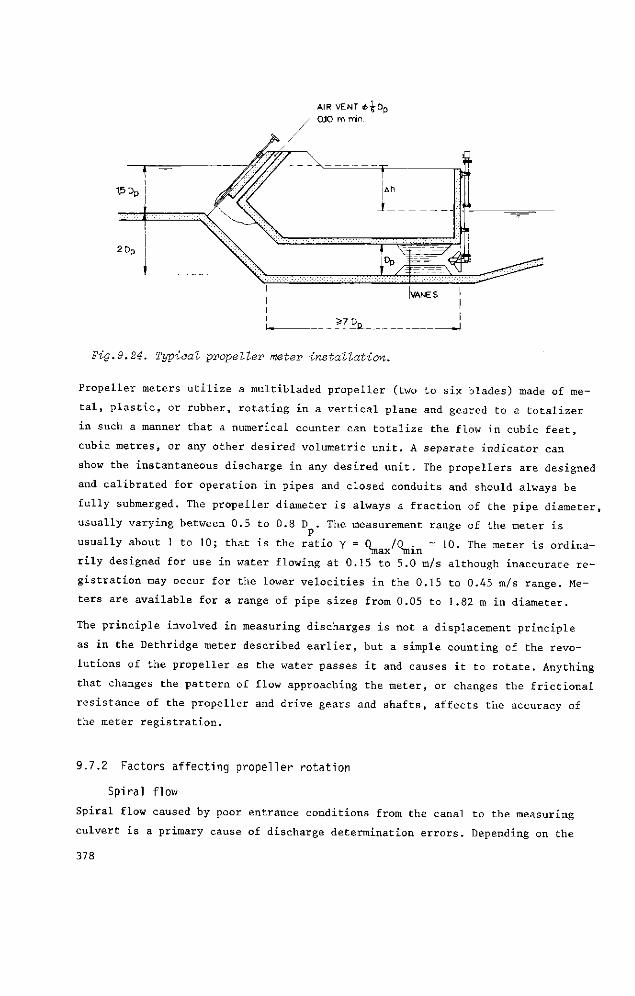
AIR VENT é | D p
0.10 m min
Fig.9.24. Typical propeller meter installation.
Propeller meters utilize a multibladed propeller (two to six blades) made of me
tal, plastic, or rubber, rotating in a vertical plane and geared to a totalizer
in such a manner that a numerical counter can totalize the flow in cubic feet,
cubic metres, or any other desired volumetric unit. A separate indicator can
show the instantaneous discharge in any desired unit. The propellers are designed
and calibrated for operation in pipes and closed conduits and should always be
fully submerged. The propeller diameter is always a fraction of the pipe diameter,
usually varying between 0.5 to 0.8 D . The measurement range of the meter is
P
usually about 1 to 10; that is the ratio Y = Q m ^ / Q ^ n ~ 10- T h e meter is ordina
rily designed for use in water flowing at 0.15 to 5.0 m/s although inaccurate re
gistration may occur for the lower velocities in the 0.15 to 0.45 m/s range. Me
ters are available for a range of pipe sizes from 0.05 to 1.82 m in diameter.
The principle involved in measuring discharges is not a displacement principle
as in the Dethridge meter described earlier, but a simple counting of the revo
lutions of the propeller as the water passes it and causes it to rotate. Anything
that changes the pattern of flow approaching the meter, or changes the frictional
resistance of the propeller and drive gears and shafts, affects the accuracy of
the meter registration.
9.7.2 Factors affecting propeller rotation
Spiral flow
Spiral flow caused by poor entrance conditions from the canal to the measuring
culvert is a primary cause of discharge determination errors. Depending on the
378
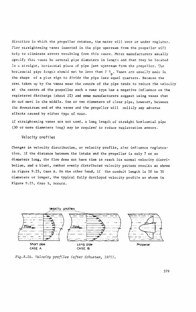
direction in which the propeller rotates, the meter will over or under register.
Flow straightening vanes inserted in the pipe upstream from the propeller will
help to eliminate errors resulting from this cause. Meter manufacturers usually
specify that vanes be several pipe diameters in length and that they be located
in a straight, horizontal piece of pipe just upstream from the propeller. The
horizontal pipe length should not be less than 7 D . Vanes are usually made in
the shape of a plus sign to divide the pipe into equal quarters. Because the
area taken up by the vanes near the centre of the pipe tends to reduce the velocity
at the centre of the propeller such a vane type has a negative influence on the
registered discharge (about 2%) and some manufacturers suggest using vanes that
do not meet in the middle. One or two diameters of clear pipe, however, between
the downstream end of the vanes and the propeller will nullify any adverse
effects caused by either type of vane.
If straightening vanes are not used, a long length of straight horizontal pipe
(30 or more diameters long) may be required to reduce registration errors.
Velocity profiles
Changes in velocity distribution, or velocity profile, also influence registra
tion. If the distance between the intake and the propeller is only 7 or so
diameters long, the flow does not have time to reach its normal velocity distri
bution, and a blunt, rather evenly distributed velocity pattern results as shown
in Figure 9.25, Case A. On the other hand, if the conduit length is 20 to 30
diameters or longer, the typical fully developed velocity profile as shown in
Figure 9.25, Case B, occurs.
Velocity profi les
?:-~_ / / F l0W f c
-*4. ^ ^
/ _ / ^ ^ { ^
= § ^ ^ i / *"] /
\ >^i.
J~~~ / Jy / */ /
^ ^ •-• - " - A
Short pipe
CASE A Long pipe CASE B
Propeller
Fig.9.25. Velocity profiles (after Schuster, 1970).
379
Here, the velocity of flow near the centre of the pipe is high compared with the
velocity near the walls. A meter whose propeller diameter is only one-half the
pipe diameter would read 3 to 4 per cent higher than it would in the flat velo
city profile. A larger propeller could therefore be expected to produce a more
accurate meter because it is driven by more of the total flow in the line. Labo
ratory tests show this to be true. When the propeller diameter exceeds 75 per
cent of the pipe diameter, the changes in registration due to variations of the
velocity profile are minor.
Propeller motion
Since the meter, in effect, counts the number of revolutions of the propeller to
indicate the discharge, any factor that influences the rate of propeller turning
affects the meter registration. Practically all propeller effects reduce the
number of propeller revolutions which would otherwise occur, and thus result in
under-registration. Propeller shafts are usually designed to rotate in one or more
bearings. The bearing is contained in a hub and is protected from direct contact
with objects in the flow. However, water often can and does enter the bearing.
Some hubs trap sediment, silt, or other foreign particles, and after these work
into the bearing a definite added resistance to turning becomes apparent. Some
propellers are therefore designed for flow through cleaning action so that parti
cles do not permanently lodge in the bearings. Care should be taken in lubricating
meter bearings. Use of the wrong lubricant (perhaps none should be used) can in
crease the resistance to propeller motion, particularly in cold water. It should
also be established that the lubricant is reaching the desired bearing or other
surfaces after it is injected. For some meters, the manufacturers do not recommend
lubrication of the bearings.
Floating moss or weeds can foul a propeller unless it is protected by screens.
Heavy objects can break the propeller. With larger amounts, or certain kinds, of
foreign material in the water, even screens may not solve the problem.
The propeller meter will require continuous maintenance. Experience has shown that
maintenance costs can be reduced by establishing a regular maintenance programme,
which includes lubrication and repair of meters, screen cleaning, replacement about
every 2 years, and general maintenance of the turnout and its approaches. In a
regular programme many low-cost preventive measures can be made routine and there
by reduce the number of higher cost curative measures to be faced at a later time.
Maintenance costs may be excessive if meters are used in sediment-laden water.
380
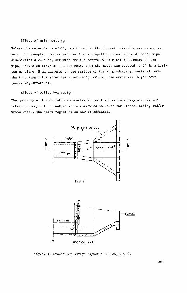
Effect of meter setting
Unless the meter is carefully positioned in the turnout, sizeable errors may re
sult. For example, a meter with an 0.30 m propeller in an 0.60 m diameter pipe
discharging 0.22 m3/s, set with the hub centre 0.025 m off the centre of the
pipe, showed an error of 1.2 per cent. When the meter was rotated 11.5 in a hori
zontal plane (8 mm measured on the surface of the 76 mm-diameter vertical meter
shaft housing), the error was 4 per cent; for 23 , the error was 16 per cent
(under-registration).
Effect of outlet box design
The geometry of the outlet box downstream from the flow meter may also affect
meter accuracy. If the outlet is so narrow as to cause turbulence, boils, and/or
white water, the meter registration may be affected.
Warp from vertical to 1.5 :1 ,
PLAN
-KD.W.S.
SECTION A -A
Fig.9.26. Outlet box design (after SCHUSTER, 1970).
381
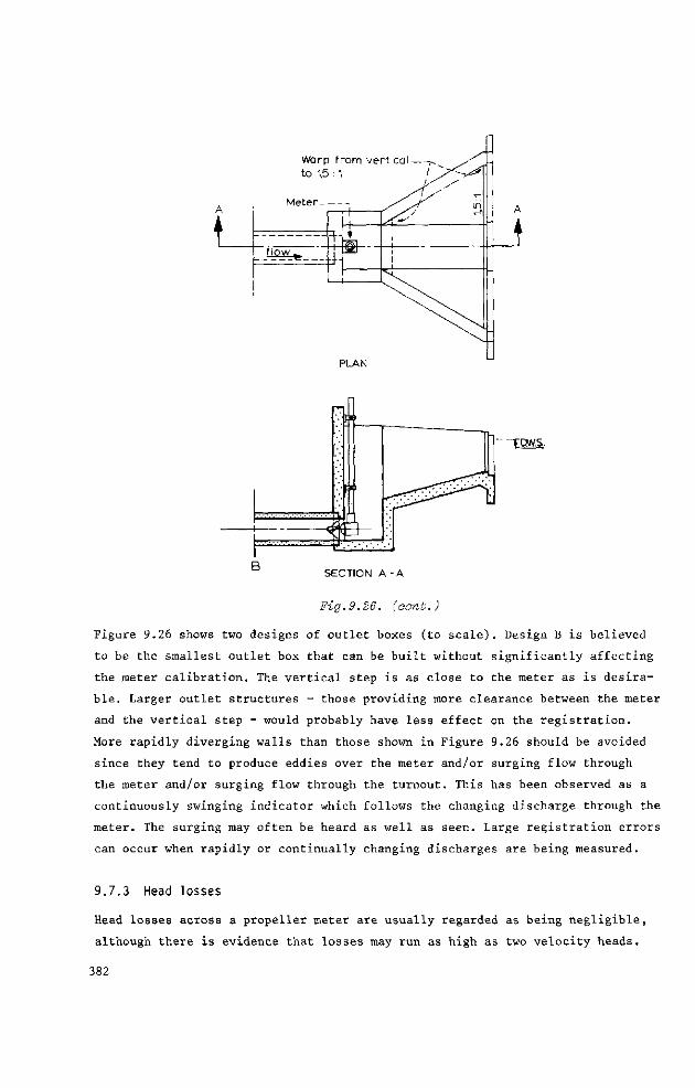
Warp from ver to 1.5 : 1
PLAN
~TCW.S.
SECTION A - A
Fig.9.26. (aont.)
Figure 9.26 shows two designs of outlet boxes (to s c a l e ) . Design B is believed
to be the smallest outlet box that can be built without significantly affecting
the meter calibration. The vertical step is as close to the meter as is desira
ble. Larger outlet structures - those providing more clearance between the meter
and the vertical step - would probably have less effect on the registration.
More rapidly diverging walls than those shown in Figure 9.26 should be avoided
since they tend to produce eddies over the meter and/or surging flow through
the meter and/or surging flow through the turnout. This has been observed as a
continuously swinging indicator which follows the changing discharge through the
meter. The surging may often be heard as well as seen. Large registration errors
can occur when rapidly or continually changing discharges are being measured.
9.7.3 Head losses
Head losses across a propeller meter are usually regarded as being negligible,
although there is evidence that losses may run as high as two velocity heads.
382
In many cases turnout losses including losses through the pipe entrance, screens,
sand trap, pipe, etc., are large enough to make the losses at the meter seem
negligible. Some allowance for meter losses should be made during turnout design,
however, and the meter manufacturer can usually supply the necessary information.
Table 9.1 may serve to give an impression of the head losses that occur over a
typical propeller meter installation as shown in Figures 9.24, and in which the
horizontal pipe length is 7 D .
TABLE 9.1. HEAD LOSSES OVER PROPELLER METER INSTALLATION
(AFTER USBR, 1967)
Q, m3/s D , m Ah, m
0 .085 0 . 140 0 . 280
0 . 30 0 . 36 0 .46
0 . 50 0 .54 0 .66
9.7.4 Meter accuracy
The accuracy of most propeller meters, stated in broad terms, is within 5 per cent
of the actual flow. Greater accuracy is sometimes claimed for certain meters and
this may at times be justified, although it is difficult to repeat calibration
tests, even under controlled conditions in a laboratory, to within 2 per cent.
A change in lubricating practice or lubricant, along with a change in water tem
perature, can cause errors of this magnitude. A change in line pressure (the head
on the turnout entrance) can cause errors of from 1 to 2 per cent.
9.7.5 Limits of application
The limits of application of the propeller meter for reasonable accuracy are:
a) The propeller should be installed under the conditions it was calibrated
for.
b) To reduce errors due to always existing differences in velocity profiles
between calibration and field structure, the propeller diameter should be as large
as practicable. For a circular pipe a propeller diameter of 0.75 D or more is re
commended .
c) The minimum length of the straight and horizontal conduit upstream from the
propeller is 7 D , provided flow straightening vanes are used.
d) If no flow straightening vanes are used, a straight horizontal pipe with-
ny flow disturbances ;
stream from the propeller.
out any flow disturbances and with a minimum length of 30 D should be used up
383
e) The flow velocity in the pipe should be above 0.45 m/s for best performance
In sediment-laden water the velocity should be even higher to minimize the added
friction effect produced by worn bearings.
384
9.8 Selected list of references
1. CONE, V.M.: Divisors. The Agric.Exp.Sta. Fort Collins, Col., Bulletin 228.
1917. 52 pp.
2. DELLEUR, J.W., DOOGE, J.C.I., and GENT, K.W.: Influence of slope and
roughness on the free overfall. Proc.of the American Society of Civil Engineers,
Vol.82, 1956. No.HY 4, Paper No.1o38.
3. DETHRIDGE, J.S.: An Australian water meter for irrigation supplies.
Engineering News, 7 (1913), No.26, Dec.25, p.1283, New York.
4. DISKIN, M.H.: End depth at a drop in trapezoidal channels. Proc.of the
American Society of Civil Engineers, Vol.87, July 1961, No.HY 4, Paper No.2851.
5. GREEVE, F.W.: Measurement of pipe flow by the coordinate method. Purdue
Engineering Exp.Sta., Bulletin 32, 1928.
6. ISO: Second Draft proposal for an ISO Recommendation on liquid flow
measurement in open channels by weirs and flumes. Brink depth method for measure
ment of flow at a free overfall. ISO/TC 113/WG 2 (secretariat 26)95, December 1967.
7. KRAIJENHOFF VAN DE LEUR, D.A., and DOMMERHOLT, A.: Brink depth method for
flow measurements. Supplementary data from The Netherlands to ISO/TC 113/WG2
(secretariat-26)95, December 1972.
8. LAWRENCE, F.E., and BRAUNWORTH, P.L.: Fountain flow of water in vertical
pipes. American Society of Civil Engineers. Transactions vol.57, pp.256-306. 1906.
9. LEER, B.R.van: The California pipe method of water measurement. Engineer
ing News-Record, Aug.3, 1922, Aug.21, 1924.
10. MEACHAM, I.: Water measurement in Victorian irrigation districts. The
Dethridge meter. Ann.Bulletin, International Commission on Irrigation and Drainage,
New Delhi, 1956, pp.14-16.
11. MURLEY, K.: Dethridge meter investigations. Aqua. Vol.17, May 1966,
No.9, pp.202-211. Off.J.State Rivers and Water Supply Commission. Victoria, Austr.
12. NEOGY, B.N.: Brink Depth for trapezoidal broad-crested weir. Proc.of
the Am.Society of Civil Engineers. December 1972, No.HY 12, Paper No.9427. 1972.
13. NEYRPIC: Irrigation canal equipment. Neyrpic, Grenoble, 1955. 32 pp.
14. ROHWER, C : Discharge of pipes flowing partly full. Civil Engineering,
Oct.1943.
385
15. ROUSE, H.: Discharge Characteristics of the free overfall. Civil Engineer
ing, April 1936, Vol.6, No.4.
16. SCHUSTER, J.C.: Water measurement procedures. Irrigation operators'
workshop. Div.of general research, Engineering and Research Centre, Bureau of
Reclamation, Denver Col. Report REC-OCE-70-38, Sept.1970, 49 pp.
17. SCOTT, V.E., and HOUSTON, C E . : Measuring irrigation water. Circular
473. California Agricultural Exp.Sta., Univ. of California. January 1959.
18. SMITH, C D . : Brink Depth for a circular channel. Proc.Am.Soc.Civ.Engnrs.
November 1962, N0.HY6, Paper No.3327. 1962.
19. UNITED STATES BUREAU OF RECLAMATION. Water Measurement Manual. Denver,
Colorado, 1967. 327 pp.
386
Appendix I Basic equations of motion in fluid mechanics
1.1 Introduction
It is assumed that the reader of this book is familiar with the basic laws of
fluid mechanics. Nevertheless, some of these laws will be discussed in this
appendix to summarise material and to emphasize certain subjects which are
important in the context of discharge measurement structures in open channels.
1.2 Equation of motion-Euler
In fluid mechanics we consider the motion of a fluid under the influence of
forces acting upon it. Since these forces produce an unsteady motion, their study
is essentially one of dynamics and must be based on Newton's second law of
motion:
F = ma (1)
where F is the force required to accelerate a certain mass (m) at a certain
rate (a). If we consider the motion of an elementary fluid volume (dx dy dz)
with a constant mass-density (p), its mass (m) equals
m = p dx dy dz (2)
The following forces may act on this particle:
a) The normal pressures (p) exerted on the lateral faces of the elementary
volume by the bordering fluid particles.
b) The mass forces, which include in the first place the gravitational force
and in the second the power of attraction of the moon and the sun and the Co-
riolis force. These forces, acting on the mass (p dx dy dz) of the fluid particle,
are represented together by their components in the X-, Y-, and Z-direction. It is
common practice to express these components per unit of mass, and therefore as
accelerations; for example, the gravitational force is expressed as the downward
acceleration g.
c) Friction. There are forces in a fluid which, due to friction, act as
shear forces on the lateral faces of the elementary particle (dx dy dz).
387
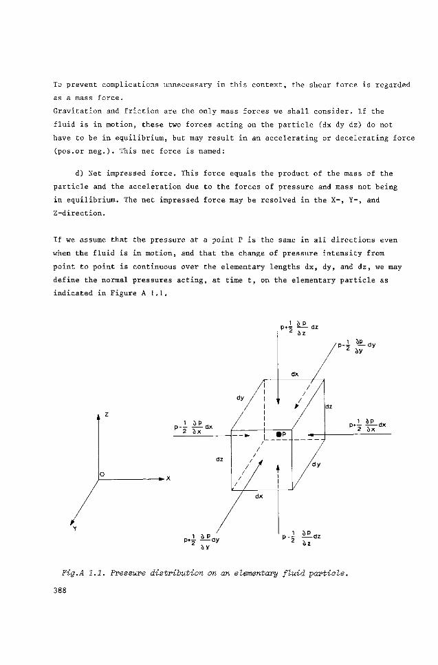
To prevent complications unnecessary in this context, the shear force is regarded
as a mass force.
Gravitation and friction are the only mass forces we shall consider. If the
fluid is in motion, these two forces acting on the particle (dx dy dz) do not
have to be in equilibrium, but may result in an accelerating or decelerating force
(pos.or neg.). This net force is named:
d) Net impressed force. This force equals the product of the mass of the
particle and the acceleration due to the forces of pressure and mass not being
in equilibrium. The net impressed force may be resolved in the X-, Y-, and
Z-direction.
If we assume that the pressure at a point P is the same in all directions even
when the fluid is in motion, and that the change of pressure intensity from
point to point is continuous over the elementary lengths dx, dy, and dz, we may
define the normal pressures acting, at time t, on the elementary particle as
indicated in Figure A 1.1.
l ÄP
Fig.A 1.1. Fressure distribution on an elementary fluid partiele.
388
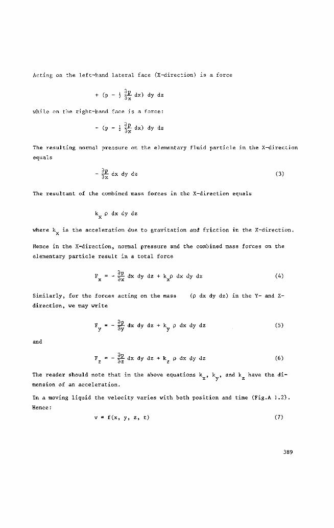
Acting on the left-hand lateral face (X-direction) is a force
+ (P _ 2 5" dx) dy dz
while on the right-hand face is a force:
~ (p - 5 ä" dx) dy dz Sx
The resulting normal pressure on the elementary fluid particle in the X-direction
equals
- | | dx dy dz (3)
The resultant of the combined mass forces in the X-direction equals
k p dx dy dz
x J
where k is the acceleration due to gravitation and friction in the X-direction. x
Hence in the X-direction, normal pressure and the combined mass forces on the
elementary particle result in a total force
F = - T ^ dx dy dz + k p dx dy dz (4)
Similarly, for the forces acting on the mass (p dx dy dz) in the Y- and Z-
direction, we may write
F = - T~ dx dy dz + k p dx dy dz (5) y 3y •> y ^ •>
and
F = - -—• dx dy dz + k p dx dy dz (6) z 3z J z ^ J
The reader should note that in the above equations k , k , and k have the di-x y z
mension of an acceleration.
In a moving liquid the velocity varies with both position and time (Fig.A 1.2).
Hence :
v = f(x, y, z, t) (7)
389
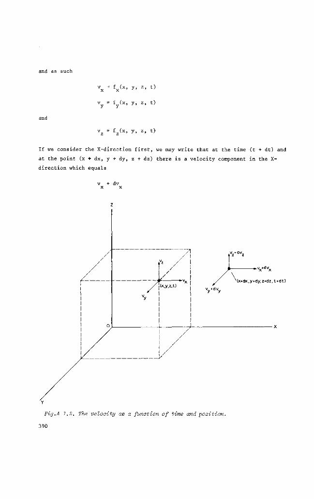
and as such
and
Vx = f x ( x ' y ' Z' l )
v = f (x, y, z, t)
V z = f z ( x ' y ' Z ' fc)
If we consider the X-direction first, we may write that at the time (t + dt) and
at the point (x + dx, y + dy, z + dz) there is a velocity component in the X-
direction which equals
v + dv x x
(x»dx,y»dy. z*dz, t»dt)
Fig.A 1.2. The velocity as a function of time and •position.
390
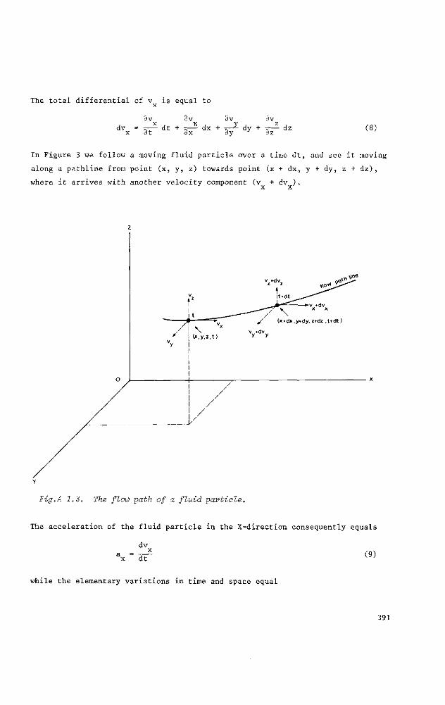
The total differential of v is equal to x
3v 3v dv 8v dv = ~ dt + 7; dx + TT—— dy + T T — dz
x dt dx oy y dz (8)
In Figure 3 we follow a moving fluid particle over a time dt, and see it moving
along a pathline from point (x, y, z) towards point (x + dx, y + dy, z + dz),
where it arrives with another velocity component (v + dv ) .
Fig.A 1.3. The flow path of a fluid partiale.
The acceleration of the fluid particle in the X-direction consequently equals
dv
a x _ dt (9)
while the elementary variations in time and space equal
391
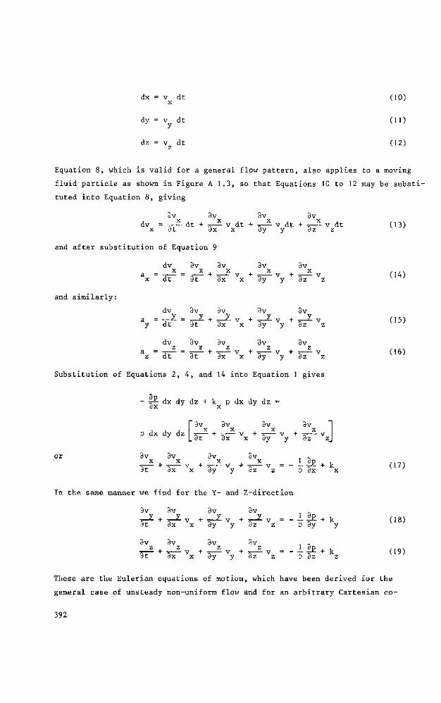
dx = v dt x
dy = v dt y
dz = v dt z
(10)
(11)
(12)
Equation 8, which is valid for a general flow pattern, also applies to a moving
fluid particle as shown in Figure A 1.3, so that Equations 10 to 12 may be substi
tuted into Equation 8, giving
3v dv dV dv 3v dv = -2. dt + ~ v dt + ~ v dt + v ^ v dt
x dt dx x dy y dz z
and after substitution of Equation 9
dv
a dt
3v 3v 3v 3v x , x x , x
TTT— + T T — V + ^ — V + » V dt dx X dy y dz z
and similarly:
dv ay = dF
dv _ z
az ~ d T
3v 3v 3v 3v irr- + -^ v + -£ v + -2- v dt dx x dy y dz z
3v 3v 3v 3v z z z z
rr— + T T — V + •* V + ir V dt dx x 3y y dz z
Substitution of Equations 2, 4, and 14 into Equation 1 gives
_ 3P 3x
dx dy dz + k p dx dy dz
(13)
(14)
(15)
(16)
p dx dy dz 3v 3v 3v 3v
X , X X X
TT- + -K— v + — v + — v
dt dx x dy y dz z 3v 3v 3v 3v
X X X X TyT— + TT— V + TT— V + •» V dt dx x dy y dz z p dx x
(17)
In the same manner we find for the Y- and Z-direction
3v 3v 3v 3v „ ÏL. + 4- y + iL y + i- -y — — £_ + J
dt 3x x 3y y 3z z p 3y y
3v 3v 3v 3v z z z , z
•~T— + K — v + T V + ^ v
dt dx x dy y dz z
p dz z
(18)
(19)
These are the Eulerian equations of motion, which have been derived for the
general case of unsteady non-uniform flow and for an arbitrary Cartesian co-
392
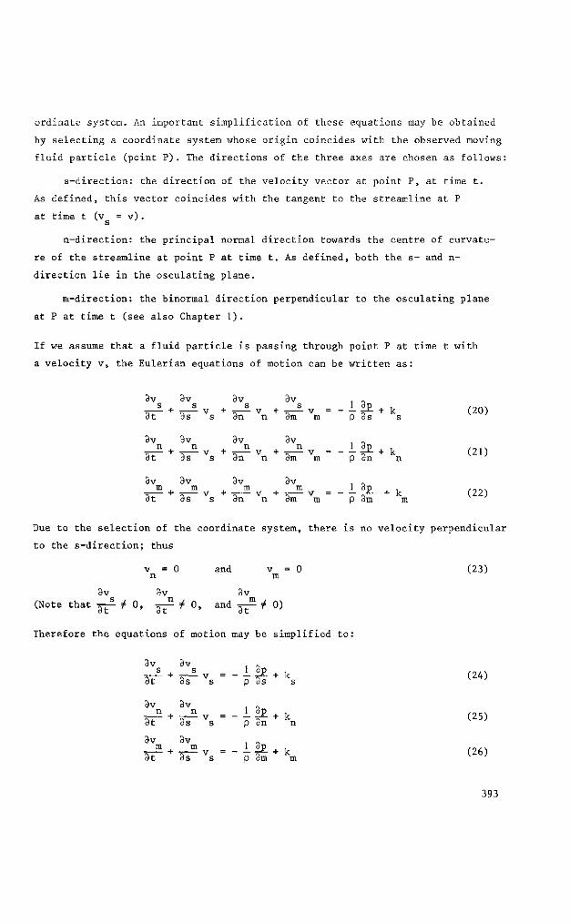
ordinate system. An important simplification of these equations may be obtained
by selecting a coordinate system whose origin coincides with the observed moving
fluid particle (point P ) . The directions of the three axes are chosen as follows:
s-direction: the direction of the velocity vector at point P, at time t.
As defined, this vector coincides with the tangent to the streamline at P
at time t (v = v ) . s
n-direction: the principal normal direction towards the centre of curvatu
re of the streamline at point P at time t. As defined, both the s- and in
direction lie in the osculating plane.
m-direction: the binormal direction perpendicular to the osculating plane
at P at time t (see also Chapter 1).
If we assume that a fluid particle is passing through point P at time t with
a velocity v, the Eulerian equations of motion can be written as:
3v 3v 3v 3 s , s s s 1 3p L i
v + •=— v + •*— v = - — •— + k av • + a"2" v + ^ v + ^ v = - X ^ + k (20) dt ds s dn n dm m p ds s
3v 9v 3v 3v , » n n n n 1 dp ,_,.
• 5 — + » v + ir— v + 3 — v = ^ + k (21) dt ds s dn n dm m p dn n
3v 3v 3v 3v , . m m m m 1 dp , /<>.>•>
•5T— + x v + •=— v + 7c— v = - — £- + k (22) d t d s s d n n d m m p d m m
Due to the selection of the coordinate system, there is no velocity perpendicular
to the s-direction; thus
v = 0 and v = 0 (23) n m
3v 3v 3v (Note t ha t TT-^- î 0 , ^ j 0 , and T - S / 0) dt dt dt
Therefore the equat ions of motion may be s impl i f ied t o :
3v 3v s , s £u 5— + 3-2-V = - 7 - - ^ + k (24)
3t 3s s p ds s
3v 3v . „ n n 1 dp , ,nr\
•5— + K — v = - - ^ + k (25) dt 3s s p 3n n 3v 3v , »
m m 1 d p , / 0 / - S TT— + TC V = TT*- + k (26) d t d s s p d m m
393
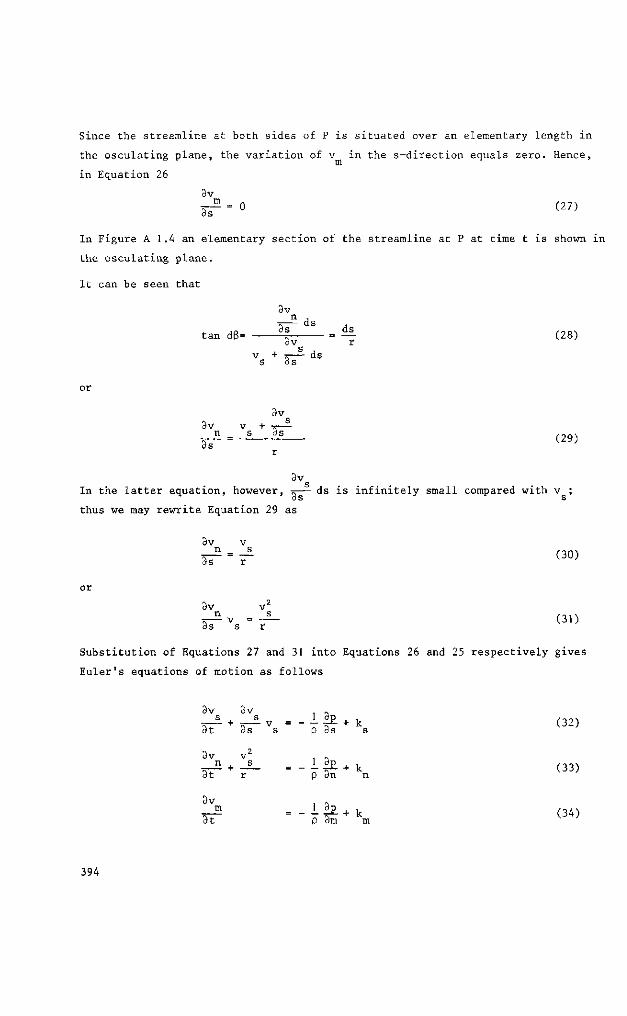
Since the streamline at both sides of P is situated over an elementary length in
the osculating
in Equation 26
the osculating plane, the variation of v in the s-direction equals zero. Hence, 6 f m -i
3v ~ = 0 (27) ds
In Figure A 1.4 an elementary section of the streamline at P at time t is shown in
the osculating plane.
It can be seen that
tan dß= ^ = — (28)
v s
3v ~ ds 3s
3v + 3 -^- ds
ds
ds r
3v 3v v + •*—
« = _5 *1 (29) ds
r 3v
s . . In the latter equation, however, -r— ds is infinitely small compared with v ;
thus we may rewrite Equation 29 as
3v v ^ = — (30) 3s r
3v v2
n s n n ~ — v = (31) 3s s r
Substitution of Equations 27 and 31 into Equations 26 and 25 respectively gives
Euler's equations of motion as follows
3V 3V , ~
s + s v = _ I | £ + k (32) dt 3s s p ds s 3v v2 . ~
3t r p 3n n
— - = - - ^2- + k (34) 3t p 3m km U ^ ;
394
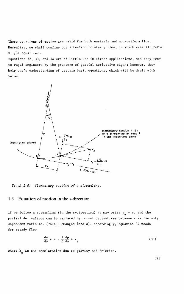
These equations of motion are valid for both unsteady and non-uniform flow.
Hereafter, we shall confine our attention to steady flow, in which case all terms
8../3t equal zero.
Equations 32, 33, and 34 are of little use in direct applications, and they tend
to repel engineers by the presence of partial derivative signs; however, they
help one's understanding of certain basic equations, which will be dealt with
below.
(osculating plane)
elementary section (1-2) of a streamline at t ime t in the osculating plane
Fig.A 1.4. Elementary section of a streamline.
1.3 Equation of motion in the s-direction
If we follow a streamline (in the s-direction) we may write v = v, and the
partial derivatives can be replaced by normal derivatives because s is the only
dependent variable. (Thus 8 changes into d ) . Accordingly, Equation 32 reads
for steady flow
dv ds p ds s
(35)
where k is the acceleration due to gravity and friction.
395
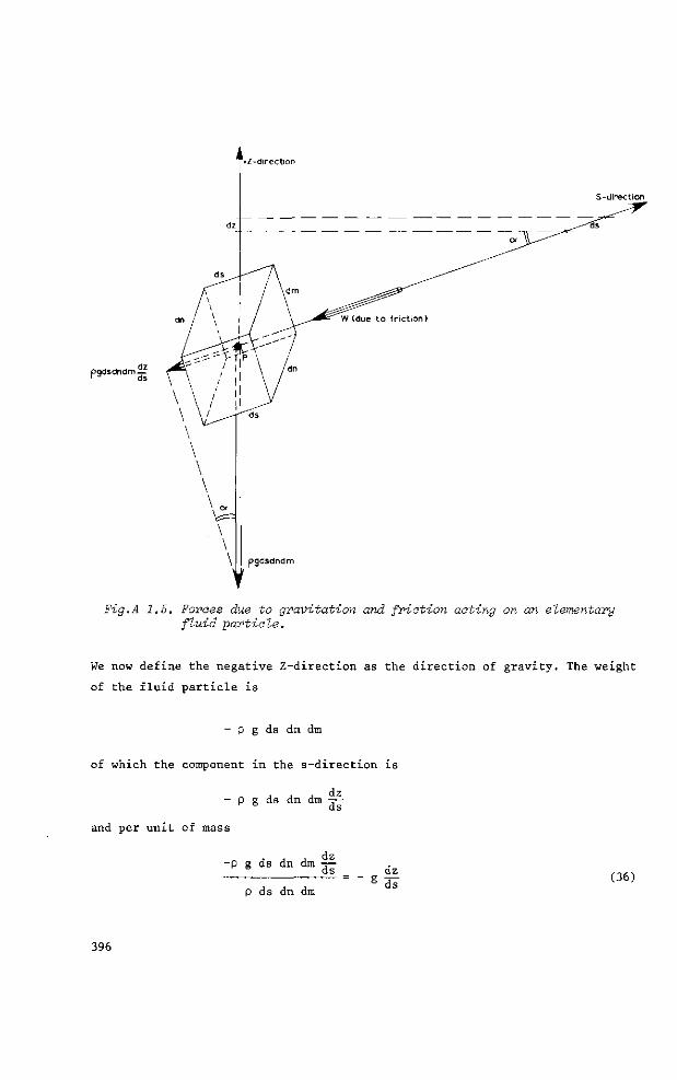
pgdsdndm —
Fig.A 1.5. Forces due to gravitation and friction acting on an elementary fluid particle.
We now define the negative Z-direction as the direction of gravity. The weight
of the fluid particle is
- p g ds dn dm
of which the component in the s-direction is
> , j dz p e ds dn dm -r- ds
and per unit of mass
, , , dz -p g ds dn dm -r— ,
ds dz
p ds dn dm ds
(36)
396
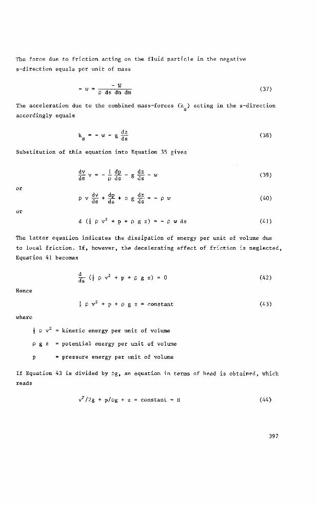
The force due to friction acting on the fluid particle in the negative
s-direction equals per unit of mass
" W (37) p ds dn dm
The acceleration due to the combined mass-forces (k ) acting in the s-direction
accordingly equals
ks - - w - g g (38)
Substitution of this equation into Equation 35 gives
dv 1 dp dz . n. -3— v = -~- - g -j w (39) ds p ds 6 ds
or dv , dp dz ....
p v d 7 + d f + p S d ¥ = - p w ( 4 0 )
or
d 0 p v 2 + p + p g z ) = - p w d s (41)
The latter equation indicates the dissipation of energy per unit of volume due
to local friction. If, however, the decelerating effect of friction is neglected,
Equation 41 becomes
~ (i P v2 + p + p g z) = 0 (42)
Hence
j p v 2 + p + p g z = constant (43)
where
5 p v = kinetic energy per unit of volume
p g z = potential energy per unit of volume
p = pressure energy per unit of volume
If Equation 43 is divided by pg, an equation in terms of head is obtained, which
reads
v2/2g + p/pg + z = constant = H (44)
397
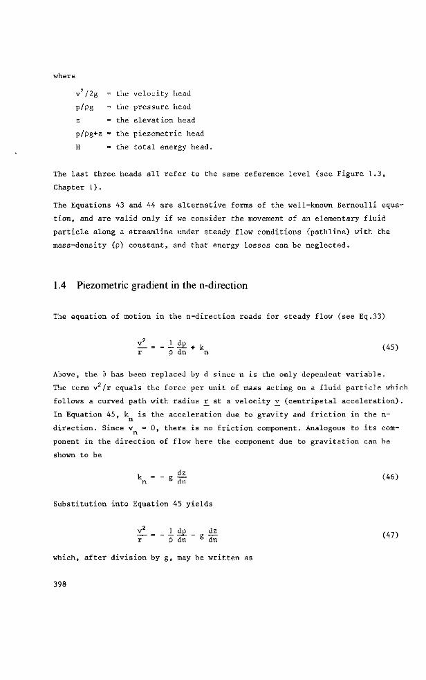
where
v2/2g = the velocity head
p/pg = the pressure head
z = the elevation head
p/pg+z = the piezometric head
H = the total energy head.
The last three heads all refer to the same reference level (see Figure 1.3,
Chapter 1).
The Equations 43 and 44 are alternative forms of the well-known Bernoulli equa
tion, and are valid only if we consider the movement of an elementary fluid
particle along a streamline under steady flow conditions (pathline) with the
mass-density (p) constant, and that energy losses can be neglected.
1.4 Piezometric gradient in the n-direction
The equation of motion in the n-direction reads for steady flow (see Eq.33)
^ = - i ^ + k (45) r p dn n
Above, the 3 has been replaced by d since n is the only dependent variable.
The term vz/r equals the force per unit of mass acting on a fluid particle which
follows a curved path with radius r at a velocity v (centripetal acceleration).
In Equation 45, k is the acceleration due to gravity and friction in the n-
direction. Since v = 0 , there is no friction component. Analogous to its com
ponent in the direction of flow here the component due to gravitation can be
shown to be
k = - g (46) n dn
Substitution into Equation 45 yields
vf_ _ l_ dp dz r p dn g dn
which, after division by g, may be written as
p d n - d n ( 4 7 )
398
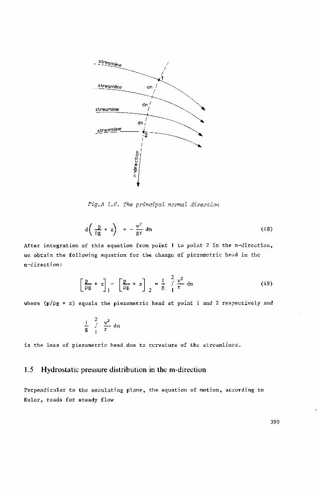
Fig.A 1.6. The principal normal direction
d( -P + z) = - x l dn \ Pg / gr
(48)
After integration of this equation from point 1 to point 2 in the n-direction,
we obtain the following equation for the change of piezometric head in the
n-direction:
Pg P-+ z Pg
2 2 ƒ ^ - d n 1 r
(49)
where (p/pg + z) equals the piezometric head at point 1 and 2 respectively and
— ƒ — dn g 1 r
is the loss of piezometric head due to curvature of the streamlines.
1.5 Hydrostatic pressure distribution in the m-direction
Perpendicular to the osculating plane, the equation of motion, according to
Euler, reads for steady flow
399
- IfJR + k = 0 (50) p dm m
Since there is no velocity component perpendicular to the osculating plane
(v = 0 ) , there is no friction either. The component of the acceleration due
to gravity in the m-direction is obtained as before, so that
Substitution of this acceleration in the equation of motion (Eq.50) gives
which may be written as
i- 2 - + z = 0 (53) dm pg
It follows from this equation that the piezometric head in the m-direction is
•s— + z = constant (54) Pg
irrespective of the curvature of the streamlines.
In other words, perpendicular to the osculating plane, there is a hydrostatic
pressure distribution.
400
Appendix II The overall accuracy of the measurement of flow 2.1 General principles
Whenever a flow rate or discharge is measured, the value obtained is simply
the best estimate of the true flow rate which can be obtained from the data
collected; the true flow rate may be slightly greater or less than this value.
This appendix describes the calculations required to arrive at a statistical
estimate of the range which is expected to cover the true flow rate.
The usefulness of the flow rate measurement is greatly enhanced if a statement
of possible error accompanies the result. The error may be defined as the dif
ference between the true flow rate and the flow rate which is calculated from
the measured water level (upstream head) with the aid of the appropriate
head-discharge equations.
It is not relevant to give an absolute upper bound to the value of error. Due
to chance, such bounds can be exceeded. Taking this into account, it is better
to give a range which is expected to cover the true value of the measured
quantity with a high degree of probability.
This range is termed the uncertainty of measurement, and the confidence level
associated with it indicates the probability that the range quoted will include
the true value of the quantity being measured. In this appendix a probability
of 95% is adopted as the confidence level for all errors.
2.2 Nature of errors
Basically there are three types of error which must be considered (see Fig.1)
a) Spurious errors (human mistakes and instrument malfunctions)
b) Random errors (experimental and reading errors)
c) Systematic errors (which may be either constant or variable)
NOTE: Seations 1 and 2 of this appendix ave based on a draft proposal of an ISO standard prepared by KINGHORN
401
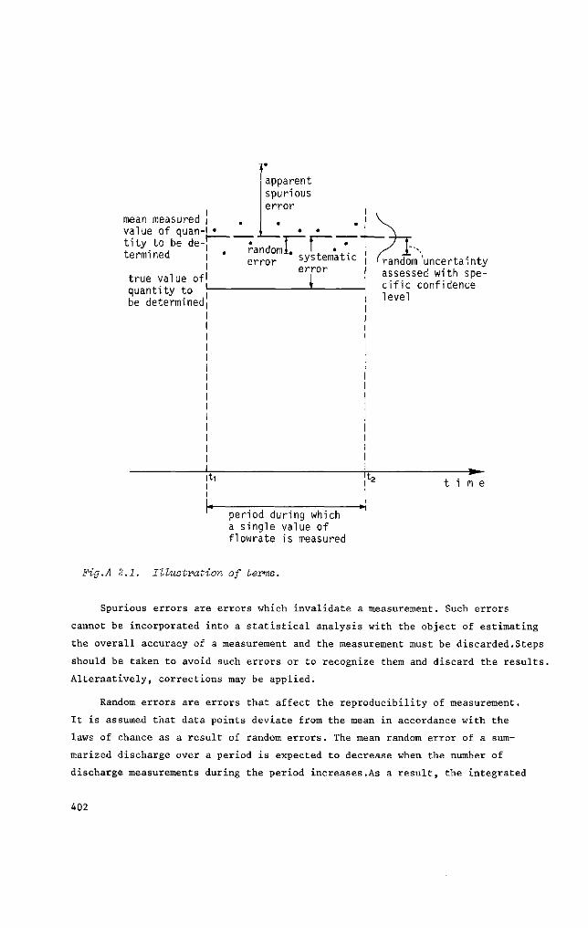
mean measured value of quantity to be determined
true value of! quantity to be determined!
apparent spurious error
random!. ' • * error systematic
error random uncertainty assessed with specific confidence level
t i m e
period during which a single value of flowrate is measured
Fig.A 2.1. Illustration of terms.
Spurious errors are errors which invalidate a measurement. Such errors
cannot be incorporated into a statistical analysis with the object of estimating
the overall accuracy of a measurement and the measurement must be discarded.Steps
should be taken to avoid such errors or to recognize them and discard the results.
Alternatively, corrections may be applied.
Random errors are errors that affect the reproducibility of measurement.
It is assumed that data points deviate from the mean in accordance with the
laws of chance as a result of random errors. The mean random error of a sum
marized discharge over a period is expected to decrease when the number of
discharge measurements during the period increases.As a result, the integrated
402
flow over a long period of observation will have a mean random error that
approaches zero. It is emphasized that this refers to time-dependent errors
only, and that the length of time over which observations should be made has
to be several times the period of fluctuations of flow.
Systematic errors are errors which cannot be reduced by increasing the
number of measurements so long as equipment and conditions remain unchanged.
Whenever there is evidence of a systematic error of a known sign, the mean
error should be added to (or subtracted from) the measurement results. A re
sidual systematic error should be assessed as half the range of possible va
riation that is due to this systematic error.
A strict separation of random and systematic errors has to be made because
of their different sources and the different influence they have on the total
error. This influence will depend on whether the error in a single measurement
is concerned, or that in the sum of a series of measurements.
2.3 Sources of errors
For discharge measurement structures, the sources of error may be identified
by considering a generalized form of head-discharge equation:
Q = w Cd C v f/g"b h" (1)
where w and u are numerical constants which are not subject to error. The
acceleration due to gravity, g, varies from place to place, but the variation
is small enough to be neglected in flow measurement.
So the following errors remain to be considered:
6C = error in product C, C
óf = error in drowned flow reduction factor f
ôb = error in dimensional measurement of weir; e.g. the width of the weir b or the weir notch angle 8
ôh = error in h and/or Ah
403
The error <$C of each of the standard structures described in Chapters 4 to
9 is given in the relevant sections on evaluation of discharge. These errors
are considered to be constant and systematic. This classification is not entirely
correct because C. and C are functions of h,. However, the variations in C, and d v 1 ' d
C as a function of h, are sufficiently small to be neglected.
v 1 J b
When flow is modular, the drowned flow reduction factor f is constant (f=1.0)
and is not subject to error. As a result, for modular flow of = 0. When flow
is non-modular (submerged) the error of consists of a systematic error,of ,
being the error in the numerical value of f,and of systematic and random errors
caused by the fact that f is a function of the submergence ratio S =H./H =H„/h .
The error 6b depends on the accuracy with which the structure as constructed
can be measured, and is also a systematic error. In practice this error may
prove to be insignificant in comparison with other errors. The error oh, has
to be split into a random error ôh and a systematic error 6h . Those errors R b
may contain many contributory errors. Possible sources of contributory errors
are:
(i) internal friction of the recording system
(ii) inertia of the indication mechanism
(iii) instrument errors
(iv) zero setting
(v) settling or tilting sideways of the structure with time
(vi) the crest not being level, or other construction faults not included in 6b
(vii) improper maintenance of the structure (this also may cause an extra error ÓC)
(viii) reading errors
We have to be careful in recognizing whether an error is random or systematic.
Some sources can cause either systematic or random errors, depending on circum
stances. Internal friction of the recorder, for example, causes a systematic
error of a single measurement or a number of measurements in a period when
either rising or falling stage is being considered, but a random error if the
total discharge through an irrigation canal per season is being considered.
On natural streams, however, falling stage may occur over a much longer period
than rising stage and here the internal friction of the recorder once again
results in a systematic error. Also zero setting may cause either a systematic
or a random error. If a single measurement or measurements within the period
404
between two zero settings are considered,the error will be systematic; it will
be random if one is considering the total discharge over a period which is
long in comparison with the interval between zero settings. The errors due
to (iii), (v), and (vi) are considered to be systematic, that due to (viii) being
random.
In the following sections the term relative error will frequently
be found. By this we mean the error in a quantity divided by this quantity. For
example, the relative error in h1 equals X, = óh /h .
2.4 Propagation of errors
The overall error in the flow Q is the resultant of various contributory errors,
which themselves can be composite errors. The propagation of errors is to be
based upon the standard deviation of the errors. The standard deviation a out of
a set of measurements on Y may be estimated by the equation
n - 2 Z (Y. - Y)
a 2 = i ^ X — (2)
n - 1
where
Y = the arithmetic mean of the n-measurements of the variable Y
Y. = the value obtained by the i measurement of the variable Y
n = the total number of measurements of Y.
The relative standard deviation o' equals a divided by the observed mean. Hence
n
Y
Z ( Y . - Y ) 2
i=l X
(n - 1) (3)
The relative standard deviation of the mean a', of n-measurements is given by
a' = — (4) Y &
If Equations 2 to 4 cannot be used to estimate the relative standard de
viation, it may be estimated by using the relative error of the mean for a 95%
confidence level, X.. The value of X. is either given (X ) , or must be estimated. 1 l c
405
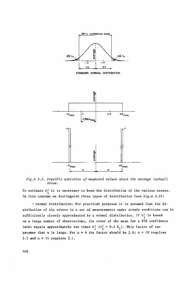
95"/o confidence band
STANDARD NORMAL DISTRIBUTION
CT
0,58X_
+ X „
Fig.A 2.2. Possible variation of measured values about the average (actual) value.
To estimate a.' it is necessary to know the distribution of the various errors.
In this context we distinguish three types of distribution (see Fig.A 2.2):
- normal distribution: For practical purposes it is assumed that the di
stribution of the errors in a set of measurements under steady conditions can be
sufficiently closely approximated by a normal distribution. If a', is based
on a large number of observations, the error of the mean for a 95% confidence
level equals approximately two times cr! (a! = 0.5 X . ) . This factor of two
assumes that n is large. For n = 6 the factor should be 2.6; n = 10 requires
2.3 and n = 15 requires 2.1.
406
- uniform distribution: For errors X. having their extreme values at either
+X or -X with an equal probability for every error size in this range, a.' TT13X HI 3 X -L
equals 0.58 X (a! = 0.58 X ) . max l max
- point binomial distribution: For errors X. which always have an extreme
value of either +X or -X , with an equal probability for each of these max max
values, a', equals 1.0 X (a! = X ) . l max l max
To determine the magnitude of composite errors the standard deviation has to be
used. The composite standard deviation can be calculated with the following
equation
CTT
k E G. a!
i-1 L x
(5)
in which
where
a' = relative standard deviation of the composite factor T
a! = relative standard deviation of the factor F. l l
F. = relevant factor influencing Q; the error of this factor is uncorrelated with the errors in other contributory factors of Equations 5 and 6; F. may itself be a composite factor
It is emphasized that only factors with uncorrelated errors can be introduced
in Equation 5. This means that it is incorrect to determine a' by substituting
a', a', a', and a' into Equation 5 because the errors in f and hi are correla
ted. One must start from relevant ^contributing to 5C, 6b, of and 6hi) errors
or standard deviations which are mutually independent. For weirs and flumes,
those independent errors are generally ÔC, 6b, of , 6h (containing 6h and n \ IK
äh._) and ÔH„ (containing <5H_ and 6H„ ) . The first three errors are systematic 1 o Z ZK Zo
errors. The last two errors are often composite errors themselves, and their
magnitude has to be determined with the use of Equations 5 and 6.
+ óf is the error in the numerical value of f and has no relation to ôh,. n I
Systematic and random errors in f caused by its relation to h and H„ are
not independent and cannot be substituted into Equation 5.
407
Substitution into Equation 6 of the independent factors contributing to the
overall error in Q and their relative standard deviations yields the first two
terms of the following equations.
Gc - 3C Q '
G. 3Q b
b 8b Q
G - S_I= 1 Gf - 3f Q ' n n
r - 9Q_ — = „ il. S hi 3hi Q 3Sh f
= 9 Q _ ^ . = 3f Sh H2 3H2 Q 3S, f
The righthand side of these equations is found by partial differentiation of
Equation 1 to C, b, f , h,, and H„ respectively. In doing so we have to take
into account that f is a function of S - H„/h1. Putting
3SU f AS. f G ( 7 )
h h
and substituting the above information into Equation 5 gives
a! = f"a'2 + a;2 + a'2 + (u-G)2 a'2 + G2 a'2 1 (8) Q L c b fn hi H2 J
As has been mentioned in the section on sources of error, we have to distinguish
between systematic and random errors because of their different influences on
the accuracy of measured volumes over long periods. Using the given information
on the character of various errors, we can divide Equation 8 into two equations;
one for random errors and the other for systematic errors, as follows:
°QR = [<U"G>2 < R + G 2 aH2R? W
*QS = [ a c 2 + ü b 2 + 0 f n + ^ 2 < S + G 2 ü H 22 s ] ^ <>°>
For most discharge measuring structures, the error 5f is unknown. We know,
408
however, that if f does not deviate much from unity (near modular flow), the
error of is negligible. For low values of f (f < appr.0.8), the error in the
numerical value of f, of , becomes large, but then the absolute value of G
becomes so large that the structure ceases to be an accurate measuring device.
As mentioned, Sf is usually unknown and therefore it is often assumed that n J
of - 0 and thus also 0' - 0. n f
n
To determine G we need a relationship between the drowned flow reduction
factor and the submergence ratio. If we have, for example, a triangular broad-
crested weir operating at a submergence ratio H„/H = 0.925, we can determine
G (being a measure for the "slope" of the S,-f-curve) from Figure 4.9 as
Af/f = (0.775 - 0.825)/0.80 _ , As, /S, (0.932 - 0.918)/0.925
h h
It should be noted that G always has a negative value.
From Equations 9 and 10, it may be noted that a increases sharply if |G| in-
creases, i.e. if the slope of the H./lL-f-curve in Figure 4.9 becomes flat.
If flow is modular, the drowned flow reduction factor f is constant and is not
subject to error (f=1.0).
Thus, a' = 0 and G = 0, and as a consequence Equations 9 and 10 reduce to n
a G R = U O h l R ( , , )
and
a:„ = ("a'2 + a'2 + u2 a ; 2 l * (12) L c b his J
It is noted again that Equations 11 and 12 are only valid if flow is modular.
It can be proved that the combination of a sufficiently large number of errors
not having a normal distribution tends to a composite error having a normal
distribution. So we may assume that the overall error of the flow rate measure
ment has a normal distribution even if the overall error is the result of the
combination of a few errors not having a normal distribution. Thus, the overall
relative error of the flow rate for a single discharge measurement approximates
XQ
2 2 a' + a'
OR QS (13)
409
It should be realized that the relative error X is not a single value for a
given device, but will vary with discharge. It is therefore necessary to con
sider the error at several discharges covering the required range of measurement.
In error analysis, estimates of certain errors (or standard deviations) will
often be used. There is a general tendency to underestimate errors. In some
cases they may even be overlooked.
2.5 Errors in measurements of head
When errors are quoted, the reader should be aware that the general tendency is
for them to be underestimated. He should also realize that errors having a
95 per cent confidence level must be estimated by the user.
Chapter 2.2 indicates that the head measurement station should be located suf
ficiently far upstream of the structure to avoid the area of surface drawdown,
yet it should be close enough for the energy loss between the head measurement
station and structure to be negligible. For each of the standard structures
described in Chapters 4 to 9, the location of the head measurement station has
been prescribed. In practice, however, it very often happens that this station
is located incorrectly, resulting in very serious errors in head.
Insufficient depth of the foundation of the structure or the head measurement de
vice, or both, can cause errors in the zero-setting since ground-frost and
changes in soil-moisture may move the structure and device. To limit errors in
zero setting it is recommended that the setting be repeated at least twice a
year; for example, after a period of frost, after a rainy season, or during
summer or a dry season. The reading error of a staff-gauge is strongly influ
enced by the reading angle and the distance between the gauge and the observer,
the turbulence of the water, and the graduation unit of the gauge.
For example, a staff gauge with centimeter graduation placed in standing water
can be read with a negligible systematic error and a random reading error of
0.003 m. If the same gauge is placed in an approach channel with a smooth water
surface, the gauge becomes more difficult to read and a systematic reading error
of 0.005 m and a random reading error of 0.005 m may be expected. Little research
410
has been done on this subject, although ROBERTSON (1966) reports on the reading
error of a gauge with graduation in feet and tenths of a foot located in reason
ably still water in a river. He recorded a systematic reading error of 0.007 m
and a random reading error of 0.007 m. The graduation unit of the reported gauge
equaled 0.03 m.If the water surface is not smooth or the position of the ob
server is not optimal, or both, reading errors exceeding one or more graduation
units must be expected.
It is obvious that a dirty gauge face hinders readings and will cause serious
reading errors. Staff gauges should therefore be installed in locations where
it is possible for the observer to clean them.
Since reading a gauge in standing water causes a smaller reading error than
one read in streaming water, the use of a stilling well must be considered
whenever the accuracy of head readings has to be improved. The stilling well
should be designed according to the instructions given in Chapter 2.6.
When a float-operated automatic water level recorder is used great care should
be given to the selection of the cable, although it is recommended that a cali
brated float tape be used instead. The cable or tape should not stretch and
should be made of corrosion-resistant material.
Several errors are introduced when a float-operated recorder is used in combi
nation with a stilling well. These are:
- Lag error due to imperfections in the stilling well. This error, caused
by head losses in the pipe connecting the stilling well with the approach chan
nel during rising or falling discharges or head losses caused by a leaking stil
ling well, has also been considered in Chapter 2.6.
- Instrument errors, due to imperfections in the recorder. This error
depends on contributory errors due to internal friction of the recorder, faulty
zero setting, and back-lash in the mechanism, etc.
The magnitude of internal friction should be given by the manufacturer of the
recorder. The reader should realize, however, that manufacturers are sometimes
rather optimistic and that their data are valid for factory-new recorders only.
Regular maintenance will be required to minimize internal friction. The error due
to internal friction and those caused by a change in cable weight hanging on
one side of the float wheel or submergence of the counter weight are considered
411
in Chapter 2.9. The magnitude of all these errors is inversely proportional to
the square of the float diameter (d 2 ).
To give an idea of the order of magnitude of errors that may occur in automatic
recorders we cite three examples:
- STEVENS (1919) reports on a recorder equipped with a <t> 0.25 m float, a
steel cable, and a 4 kg counter weight. The following errors were observed:
Error due to submergence of counterweight 0.0015 m. Difference in readings
between falling and rising stage due to internal friction 0.002 m. An increasing
total weight of cable plus counter weight hanging on one side of the cable wheel
caused a registration error of 0.06%.
- ROBERTSON (1966) reports on the reading error of recorder charts. When
a writing mechanism with 1:1 reduction (full scale) was used, the systematic
reading error was negligible and the random error was 0.010 m. For a writing
mechanism with 10:1 reduction, however, a systematic error of 0.010 m and a ran
dom error of 0.016 m was reported. No float diameter was mentioned.
- AGRICULTURAL UNIVERSITY (1966) at Wageningen reports on laboratory tests
conducted under ideal conditions with a digital recorder giving a signal for a
0.003 m head interval. Equipped with a <b 0.20 m float the digital reading showed
a negligible systematic error and a random error of 0.002 m. In addition, a dif
ference of 0.002 m was found between readings for falling and rising stage. The
errors found in the Wageningen tests must be regarded an absolute minimum.
It should be noted that if waves are dampened in the approach channel by means of
a stilling well a systematic error may be introduced. This is a result of the
non-linear relationship between the head and the discharge.
2.6 Coefficient errors
The coefficient errors presented in Chapters 4 to 9 are valid for well-maintained
clean structures. To obtain the accuracies listed, sediment, debris, and algal
growth must be removed regularly. To keep the structure free of weed, fungicides
can be used. The best method is probably to add, say, 0.5 per cent by weight
of cement copper oxide to facing concrete during mixing. Copper sulphate or
another appropriate fungicide can be applied to existing concrete but frequent
treatment will be required. Algal growth on non-concrete structural parts can
412
be prevented by regular treatment with an anti-fouling paint such as that used
on yachts.
It must be realized that algal growth on broad-crested weirs and flumes increases
friction and "raises" the crest. Consequently algal growth has a negative in
fluence on C,-values. On sharp-crested weirs or sharp-edged orifices, algal
growth reduces the velocity component along the weir face, causing an increase
of C.-values, d
NAGLER (1929) investigated this type of influence on a sharp-crested weir whose
upstream weir face was roughened with coarse sand. He found that, compared with
the coefficient value of a smooth-faced weir the discharge coefficient increased
by as much as 5 per cent when h = 0.15 m and by 7 per cent when h = 0.06 m.
Algal growth on the upstream face of sharp-crested weirs may cause a "rounding-
off" of the edge which, in addition to reducing the velocity component along
the weir face, causes a decrease of contraction and consequently results in an
increase of the discharge coefficient. For a head of 0.15 m, THOMAS (1957) repor
ted an increase of some 2, 3, 5.5, 11, and 13.5 per cent due solely to the ef
fect of rounding-off by radii of a mere 1, 3, 6, 12, and 19 mm respectively.
Another factor that will cause the discharge coefficient to increase is insuf
ficient aeration of the air pocket beneath the overfalling nappe of a sharp-
or short-crested weir (see also Chap.1.14).
2.7 Example of error combination
In this example all errors mentioned are expected to have a 95 per cent confi
dence level. We shall consider a triangular broad-crested weir as described in
Chapter 4.3, flowing less-than-full, with a vertical back face, a crest length
L = 0.60 m, a weir notch angle 8 = 120 , and a crest height p = 0.30 m. Accord
ing to Chapter 4.3, the following head-discharge equation applies
Q = C d C v H \ / F f tanfhf-5 (14)
Both upstream and downstream heads were measured by identical digital recorders
giving a signal for every 0.003 m head difference (thus maximum reading error
is 0.0015 m ) . The random error due to internal friction of the recorder was
0.002 m. The systematic error in zero setting was estimated to be 0.002 m due
413
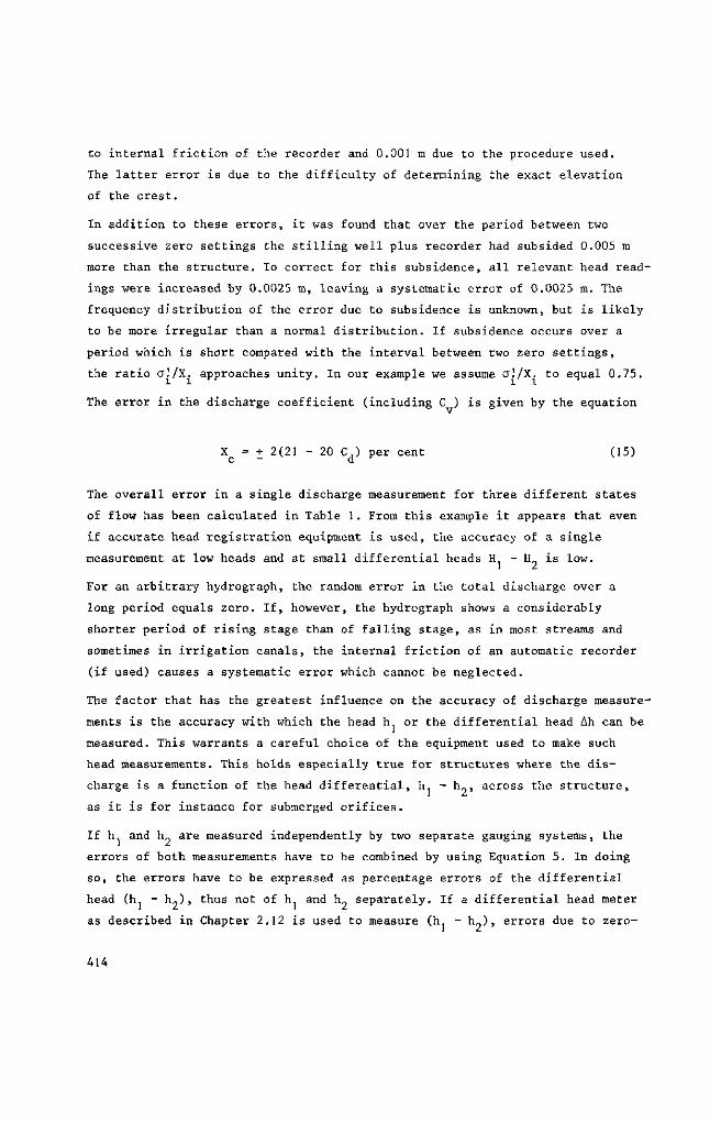
to internal friction of the recorder and 0.001 m due to the procedure used.
The latter error is due to the difficulty of determining the exact elevation
of the crest.
In addition to these errors, it was found that over the period between two
successive zero settings the stilling well plus recorder had subsided 0.005 m
more than the structure. To correct for this subsidence, all relevant head read
ings were increased by 0.0025 m, leaving a systematic error of 0.0025 m. The
frequency distribution of the error due to subsidence is unknown, but is likely
to be more irregular than a normal distribution. If subsidence occurs over a
period which is short compared with the interval between two zero settings,
the ratio a'./X. approaches unity. In our example we assume ol/X. to equal 0.75.
The error in the discharge coefficient (including C ) is given by the equation
X = + 2(21 - 20 C.) per cent (15) c - d
The overall error in a single discharge measurement for three different states
of flow has been calculated in Table 1. From this example it appears that even
if accurate head registration equipment is used, the accuracy of a single
measurement at low heads and at small differential heads H. - H„ is low.
For an arbitrary hydrograph, the random error in the total discharge over a
long period equals zero. If, however, the hydrograph shows a considerably
shorter period of rising stage than of falling stage, as in most streams and
sometimes in irrigation canals, the internal friction of an automatic recorder
(if used) causes a systematic error which cannot be neglected.
The factor that has the greatest influence on the accuracy of discharge measure
ments is the accuracy with which the head h or the differential head Ah can be
measured. This warrants a careful choice of the equipment used to make such
head measurements. This holds especially true for structures where the dis
charge is a function of the head differential, h. - h„, across the structure,
as it is for instance for submerged orifices.
If hj and h„ are measured independently by two separate gauging systems, the
errors of both measurements have to be combined by using Equation 5. In doing
so, the errors have to be expressed as percentage errors of the differential
head (h1 - h„), thus not of h and h_ separately. If a differential head meter
as described in Chapter 2.12 is used to measure (h - h„), errors due to zero-
414
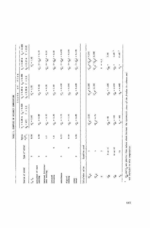
415
settings and in some cases due to reading of one head are avoided, thereby
providing more accurate measurements.
2.8 Error in discharge volume over long period
If during a "long" period a great number of single discharge measurements
(n > 15) are made and these measurements are used in combination with head
readings, to calculate the discharge volume over an irrigation season or hy-
drological year, the percentage random error X . _ tends to zero and can be e & vol.R neglected.
The systematic percentage error X , „ of a volume of water measured at a r vol.S
particular station is a function of the systematic percentage error of the
discharge (head) at which the volume was measured. Since the systematic per
centage error of a single measurement decreases if the head increases, a
volume measured over a long period of low discharges will be less accurate
than the same volume measured over a (shorter) period of higher discharge. As
a consequence we have to calculate X .. as a weighted error by use of the
equation
fQo' dt xvoi.s = 2 - r o i - (]6>
which may also be written as
.*, Q i 0QS A t
Xvol.S = 2 ¥ <17> I Q. At
i=l L
where
At = period between two successive discharge measurements
By using Equations 16 and 17 the reader will note that the value of X 1 =
X . will be significantly lower than the single value X and will be
reasonably small, provided that a sufficient number of measurements are made
over the period considered.
416
2.9 Selected list of references
1. AGRICULTURAL UNIVERSITY, Wageningen: Voortgezet onderzoek van registre
rende waterstands meters. Hydraulica Laboratorium. Nota No.4, 15 pp. 1966.
2. BRITISH STANDARD INSTITUTION: Measurement of liquid flow in open chan
nels. Part 4: Weirs and flumes. 4B: Long base weirs. BS 3680. London 1969.BSI.
39 pp.
3. KINGHORN, F.C.: Draft proposal for an ISO standard on the calculation
of the uncertainty of a measurement of flowrate. Doc.No.ISO/TC 30/WG 14:24 E.
1975.
4. NAGLER, F.A.: Discussion of precise weir measurements. Transaction ASCE.
Vol.93. 1929. p.115.
5. ROBERTSON, A.I.G.S.: The magnitude of probable errors in water level
determination at a gauging station. Water Resources Board. TN 7, Reading,
England. 1966. Reprinted 1970.
6. STEVENS, J.C.: The accuracy of water-level recorders and indicators of
the float type. Transactions ASCE. Vol.83. 1919.
7. THOMAS, C.W.: Common errors in measurement of irrigation water. Journal
Irrigation and Drainage Div.Proc.Am.Soc.of Civ.Eng. Vol.83, No.IR 2 2, Sept.1957.
Paper 1361 , pp.1-24.
417

Appendix III Side weirs and oblique weirs
3.1 Introduction
Most of the weirs described in this book serve mainly to measure discharges.
Some, however, such as those described in Chapters 4 and 6, can also be used
to control upstream water levels. To perform this dual function, the weirs have
to be installed according to the requirements given in the relevant chapters.
Since these weirs are usually relatively wide with respect to the upstream head,
the accuracy of their flow measurements is not very high. Sometimes the dis
charge measuring function of the weir is entirely superseded by its water level
control function, resulting in a contravention in their installation rules. The
following weirs are typical examples of water level control structures.
Side Weir: This weir is part of the channel embankment, its crest being
parallel to the flow direction in the channel. Its function is to drain water
from the channel whenever the water surface rises above a predetermined level
so that the channel water surface downstream of the weir remains below a maximum
permissible level.
Oblique weir: The most striking difference between an oblique weir and
other weirs is that the crest of the oblique weir makes an angle with the flow
direction in the channel. The reason for this is that the width (b) of the weir
crest must be greater than the width of the channel so that with a change in
discharge the water surface upstream of the weir remains between narrow limits.
Some other weir types which can maintain such an almost constant upstream water
level will also be described.
3.2 Side weirs
3.2.1 General
In practice, sub-critical flow will occur in almost all rivers and irrigation
or drainage canals in which side weirs are constructed. Therefore, we shall
restrict our attention to side weirs in canals where the flow remains subcritical.
419
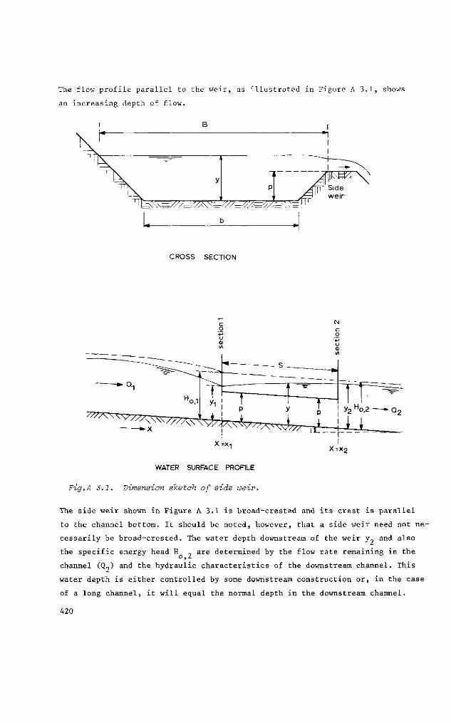
The flow profile parallel to the weir, as illustrated in Figure A 3.1, shows
an increasing depth of flow.
CROSS SECTION
X=x2
WATER SURFACE PROFILE
Fig.A 3.1. Dimension sketch of side weir.
The side weir shown in Figure A 3.1 is broad-crested and its crest is parallel
to the channel bottom. It should be noted, however, that a side weir need not ne
cessarily be broad-crested. The water depth downstream of the weir y. and also
the specific energy head H are determined by the flow rate remaining in the o, Z
channel (Q„) and the hydraulic characteristics of the downstream channel. This
water depth is either controlled by some downstream construction or, in the case
of a long channel, it will equal the normal depth in the downstream channel. 420
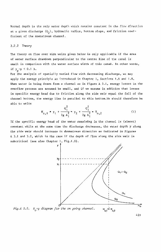
Normal depth is the only water depth which remains constant in the flow direction
at a given discharge (CO, hydraulic radius, bottom slope, and friction coef
ficient of the downstream channel.
3.2.2 Theory
The theory on flow over side weirs given below is only applicable if the area
of water surface drawdown perpendicular to the centre line of the canal is
small in comparison with the water surface width of this canal. In other words,
if y -p < 0.1 B. P
For the analysis of spatially varied flow with decreasing discharge, we may
apply the energy principle as introduced in Chapter 1, Sections 1.6 and 1.8.
When water is being drawn from a channel as in Figure A 3.1, energy losses in the
overflow process are assumed be small, and if we assume in addition that losses
in specific energy head due to friction along the side weir equal the fall of the
channel bottom, the energy line is parallel to this bottom.We should therefore be
able to write
H , = y, + o,l J 1
!1 = y-,
• i H
9 A 2 " ° > 2
2g A,
(1) 2g A,
If the specific energy head of the water remaining in the channel is (almost)
constant while at the same time the discharge decreases, the water depth y along
the side weir should increase in downstream direction as indicated in Figures
A 3.1 and 3.2, which is the case if the depth of flow along the side weir is
subcritical (see also Chapter 1, Fig. 1.9).
y
Fig.A 3.2. H -y diagram for the on going channel. H „^H „ o,1 o,2
421
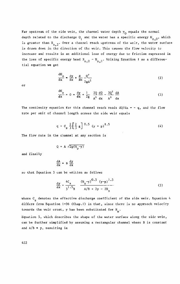
Far upstream of the side weir, the channel water depth y equals the normal
depth related to the discharge Q and the water has a specific energy H _, which
is greater than H „. Over a channel reach upstream of the weir, the water surface
is drawn down in the direction of the weir. This causes the flow velocity to
increase and results in an additional loss of energy due to friction expressed in
the loss of specific energy head H _ - H „. Writing Equation 1 as a differen
tial equation we get
(2) o dy + d_ Jf dx dx dx „ .2
2gA
^2.= 0 = ^ + i - ^ S ^ - ^ ^ (3) d x d x 2 g A2 dx A3 dx
The continuity equation for this channel reach reads dQ/dx = - q, and the flow
rate per unit of channel length across the side weir equals
_ 2 \ 2 1 0.5 , .1.5 ,.s q = cs 3 La 8J ( y _ p ) (4)
The flow rate in the channel at any section is
and finally
Q = A /2g(HQ-y)
M . B dy dx dx
so that Equation 3 can be written as follows
dy _ 4 Cs ( y y ) ° - 5 (y-P)'-5 (5)
d x 31-5B A/B + 2y - 2H
where C denotes the effective discharge coefficient of the side weir. Equation 4
differs from Equation 1-36 (Chap.1) in that, since there is no approach velocity
towards the weir crest, y has been substituted for H .
J o
Equation 5, which describes the shape of the water surface along the side weir,
can be further simplified by assuming a rectangular channel where B is constant
and A/B = y, resulting in
422
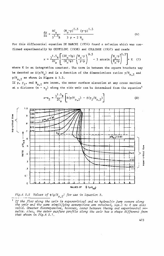
dy dx
4C
,1.5,.
,„ ,0.5 , .1.5 (HQ-y) (y-p)
3 y - 2 H (6)
For this differential equation DE MARCHI (1934) found a solution which was con
firmed experimentally by GENTILINI (1938) and COLLINGE (1957) and reads
2C
(2Ho-3p) /Ho-y
(H -p) y-p
0.5
3 arcsin
i0.5-
+ K (7)
where K is an integration constant. The term in between the square brackets may
be denoted as <}>(y/H ) and is a function of the dimensionless ratios y/H and
p/H . as shown in Figure A 3.3.
If p, y„, and H . are known, the water surface elevation at any cross section
at a distance (x - x„) along the side weir can be determined from the equation1
3'-5B 2C >(*/Ho.2> ' ^ o ^
(8)
r"
<
7
.6
M
.3
2
1
n
095
0.90
085
0.80
0.75
0.70
-1
ol
0 -9 - !
A01~
> -
0.8°
-<
2/3
i - ' - • • - ;
' /
r\ \
-
7
\ \
-1
7h
l \-^ \ \
(
- *s
^
)
^
2 i 4
p/HojïO.SO
5 5 '
0.60
0.50
040
0.30
020
i 9
VALUES OF {> (y/HQ^)
Fig.A 3.3 Values of <p(y/H ) for use in Equation 8.
If the flow along the weir is supercritical and no hydraulic jump occurs along the weir and the same simplifying assumptions are retained, Eqs.1 to 8 are also valid. Greater discrepancies, however, occur between theory and experimental results. Also, the water surface profile along the weir has a shape different from that shown in Fig.A 3.1.
423
If the simplifying assumptions made to write Equation 1 cannot be retained, or,
in other words, if the statement
ƒ C2R
S tan i « y - y (9)
is not correct, the water surface elevation parallel to the weir can only be
obtained by making a numerical calculation starting at the downstream end of
the side weir (at x = x«). This calculation also has to be made if the cross
section of the channel is not rectangular.
For this procedure the following two equations can be used
y u - yd =
( W (vu"Vd)
2g cV Ax
A A r 2 \2 I0-5 r J-5 A vuAu - VdAd = Cs 3 La gJ ( yd'p ) Ax
(10)
(11)
where
Ax = length of the considered channel section
u = subscript denoting upstream end of section
d = subscript denoting downstream end of section
C = coefficient of Chézy
R = hydraulic radius of channel
It should be noted that before one can use Equations 10 and 11 sufficient infor
mation must be available on both A and R along the weir. The accuracy of the
water surface elevation computation will depend on the length and the chosen
number of elementary reaches Ax.
3.2.3 Practical C -value s
The reader will have noted that in Equations 3 to 9 an effective discharge coef
ficient C is used. For practical purposes, a value
C = 0.95 C, s d
(12)
may be used, where C, equals the discharge coefficient of a standard weir of
similar crest shape to those described in Chapters 4 and 6.
424
If Equations A to II are used for a sharp-crested side weir, the reader
should be aware of a difference of v3 in the numerical constant between the head-
discharge equations of broad-crested and sharp-crested weirs with rectangular
control section. In addition it is proposed that the discharge coefficient
(C ) of a sharp-crested weir be reduced by about 10% if it is used as a side weir.
This leads to the following C -value to be used in the equations for sharp-
crested side weirs
C = 0.90 /3 C ~ 1.55 C (13) s e e
3.2.4 Practical evaluation of side weir capacity
Various authors proposed simplified equations describing the behaviour of
sharp-crested side weirs along rectangular channels. However, discrepancies
exist between the experimental results and the equations proposed, and it
follows that each equation has only a restricted validity.
In this Appendix we shall only give the equations as proposed by FORCHHEIMER (1930),
which give an approximate solution to the Equations 3 and 4 assuming that the
water surface profile along the side weir is a straight line. The Forchheimer
equations read:
AQ = cs | ,/fT s [ ^ l y2
p
1.5 (14)
and
yi - yi 5, - (15)
v?/2g - v|/2g - AHo
where
AH = the loss of specific energy head along the side weir due to friction.
AH can be estimated from o
AH = {(vi - v2)/2}2 S/C2R - iS (16) o
The most common problem is how to calculate the side weir length S, if
AQ = Qi - 0.2, y2 and p are known. To find S an initial value of yi has to be
estimated, which is then substituted into the Equations 14 and 15. By trial and
error yi (and thus S) should be determined in such a way that Ci = 1.0.
425
The equations 14 and 15 a re app l icab le i f
F r , = v ^ / g T T < 0.75 (17)
and
y, - V > 0 (18)
If the above limits do not apply, the water depth y at the entrance of the side
weir and the side weir length S required to discharge a flow 0. - Q„ should be
calculated by the use of Equation 1, which reads
2 2 Q, 0.2
Ho) 2=>, + 7-2 = 2 + 7-2 (19)
2gAj 2gA2
In combination with the equation
1 - x 2 = 2-73|-[^y,/Ho)2) -*<VHo,2>] (20) -S = x ' ' Ld
The latter equation is a result of substituting Equation 12 into Equation 8. In
using Equation 20 the reader should be aware that the term xT - x„ is negative
since ~/.. < x„. As mentioned before, values of cj>(y/H 7 ) can be read from Fig.A 3.3
as a function of the ratios p/H „ and y/H „.
o,2 J o,2
3.3 Oblique weirs
3.3.1 Weirs in rectangular channels
According to AICHEL (1953), the discharge q per unit width of crest across
oblique weirs placed in a rectangular canal as shown in Figure A 3.4 can be calcu
lated by the equation q =
where
• -ÏL ! K (2° q = the discharge over a weir per unit width if the same type of weir
had been placed perpendicular to the canal axis (e = 90 ) .
3 = a dimensionless empirical function of the angle of the weir crest
(in degrees) with the canal axis.
426
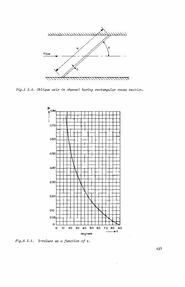
\\\\\\\\\\\\\\\\\\\\\\\\\\\\\\vw Fig.A 3.4. Oblique weir in channel having rectangular cross section.
0.60
0 50
0.40
020
0
l
\ \
i
\ \ \
• ; \ \
\ \
V \
0 10 20 30 40 50 60 70 80 90
Fig.A 3.5.
degrees
-Values as a function of e.
-•e
427
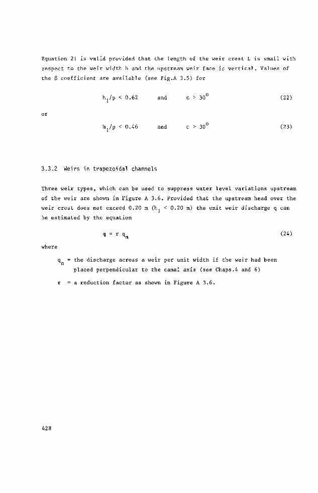
Equation 21 is valid provided that the length of the weir crest L is small with
respect to the weir width b and the upstream weir face is vertical. Values of
the 3 coefficient are available (see Fig.A 3.5) for
h /p < 0.62 and c > 30° (22)
h /p < 0.46 and £ > 30° (23)
3.3.2 Weirs in trapezoidal channels
Three weir types, which can be used to suppress water level variations upstream
of the weir are shown in Figure A 3.6. Provided that the upstream head over the
weir crest does not exceed 0.20 m (h < 0.20 m) the unit weir discharge q can
be estimated by the equation
q = r qn (24)
where
q = the discharge across a weir per unit width if the weir had been
placed perpendicular to the canal axis (see Chaps.4 and 6)
r = a reduction factor as shown in Figure A 3.6.
428
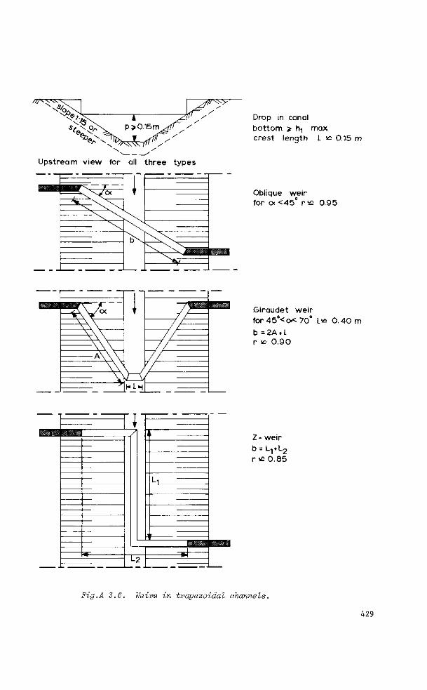
Upstream view for all three types
T
Drop in canal bottom > fy max crest length L «= 0.15 m
Oblique weir for ex <45° r ^ 0.95
Giraudet weir for45°<o«< 70° L* 0.40 m b = 2A • L r v 0.90
.d
1 /
L2
1
1-1
\l ESQ
-J
Z- weir b = L1 + L2
r ^ 0.85
Fig.A 3.6. Weirs in trapezoidal channels.
429
3.4 Selected list of references
1. AICHEL, O.G.: Abflusszahlen für schiefe Wehre. (Discharge ratios for
oblique weirs.) Z.VDI 95 (1953). No.1, Jan.1, pp.26-27.
2. COLLINGE, V.K.: The discharge capacity of side weirs. Proc.of the Inst,
of Civil Engineers, Vol.6, 1957. Febr., pp.288-304.
3. ENGELS, H.: Versuche über Streichwehre. Mitt.aus dem Dresdener Fluss
bau-Laboratorium. Forschungsarbeiten auf dem Gebiete des Ingenieurwesens No.
200. Berlin 1917.
4. ENGELS, H.: Weitere Versuche über Streichwehre. Mitt. aus dem Dresde
ner Flussbau-Laboratorium. Forschungsarbeiten auf dem Gebiete des Ingenieur
wesens no.201. 55 pp. Berlin 1920.
5. FORCHHEIMER, Ph.: Hydraulik. 3.Aufl., 1930, pp.406-408.
6. FRAZER, W.: The behaviour of side weirs in prismatic rectangular
channels. Proc.of the Inst.of Civil Eng., Vol.6, 1957. Febr., pp.305-328.
7. GENTILINI, B.: Richerche sperimentali sugli sfioratori longitudinali
(prima serie di prove). L'Energie Elettrica, 15 (1938), Sept. No.9, pp.583-
595. Milano.
8. HENDERSON, F.M.: Open Channel Flow. MacMillan Comp. New York. 1966,
521 pp.
9. DE MARCHI, G.: Saggio di teoria de funzionamente degli stramazzi
laterali. L'Energie Elettrica, 11 (1934), Nov., pp.849-860. Milano.
10. SCHAFFERNAK, F.: Streichwehrberechnung, österreichische Wochenschrift
f.d.öffentl.Baudienst. Heft 36, 1918.
11. SCHMIDT, M.: Zur Frage des Abflusses über Streichwehre. Mitt.Nr.41.
Inst.für Wasserbau der Tech.Universität Berlin-Charlottenburg, 1954.
12. SCHMIDT, M.: Die Berechnung von Streichwehren. Die Wasserwirtschaft,
1954-1955, pp.96-100.
13. VEN TE CHOW: Open channel hydraulics. McGraw-Hill, New York, 680 pp.
430
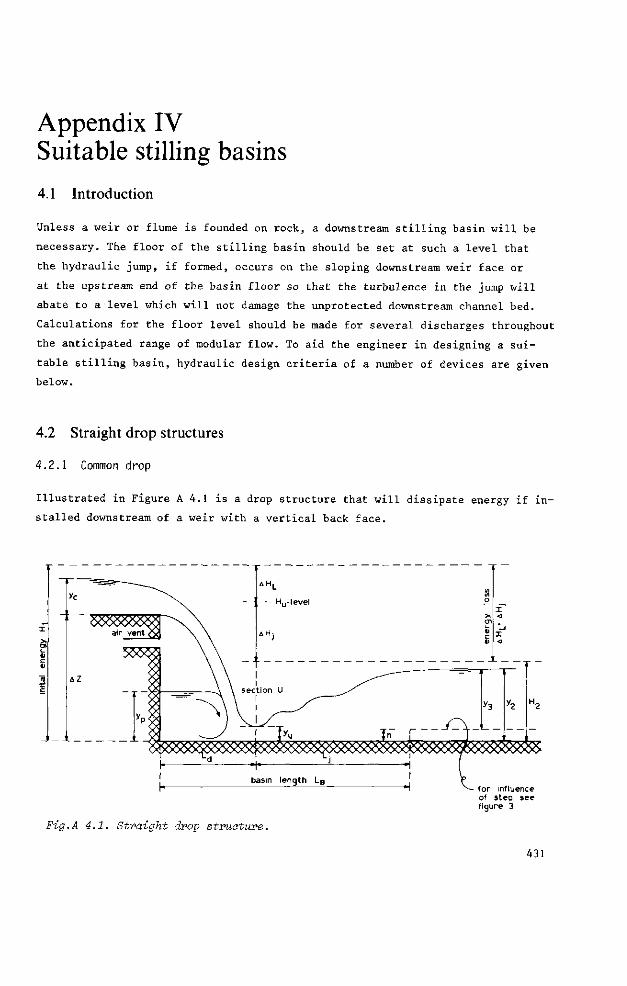
Appendix IV Suitable stilling basins 4.1 Introduction
Unless a weir or flume is founded on rock, a downstream stilling basin will be
necessary. The floor of the stilling basin should be set at such a level that
the hydraulic jump, if formed, occurs on the sloping downstream weir face or
at the upstream end of the basin floor so that the turbulence in the jump will
abate to a level which will not damage the unprotected downstream channel bed.
Calculations for the floor level should be made for several discharges throughout
the anticipated range of modular flow. To aid the engineer in designing a sui
table stilling basin, hydraulic design criteria of a number of devices are given
below.
4.2 Straight drop structures
4.2.1 Common drop
Illustrated in Figure A 4.1 is a drop structure that will dissipate energy if in
stalled downstream of a weir with a vertical back face.
x "
>
4f
'
.
1
yc
A Z
L
air vent Q )
J
1
\ \ \ \
- - Hu- level
t ion U
Tn" r ~y
o
en V c D
<
<
L
*3 y2 H 2
- h • basin length L B
Fig.A 4.1. Straight drop structure.
f o r influence of s tep see f igure 3
431
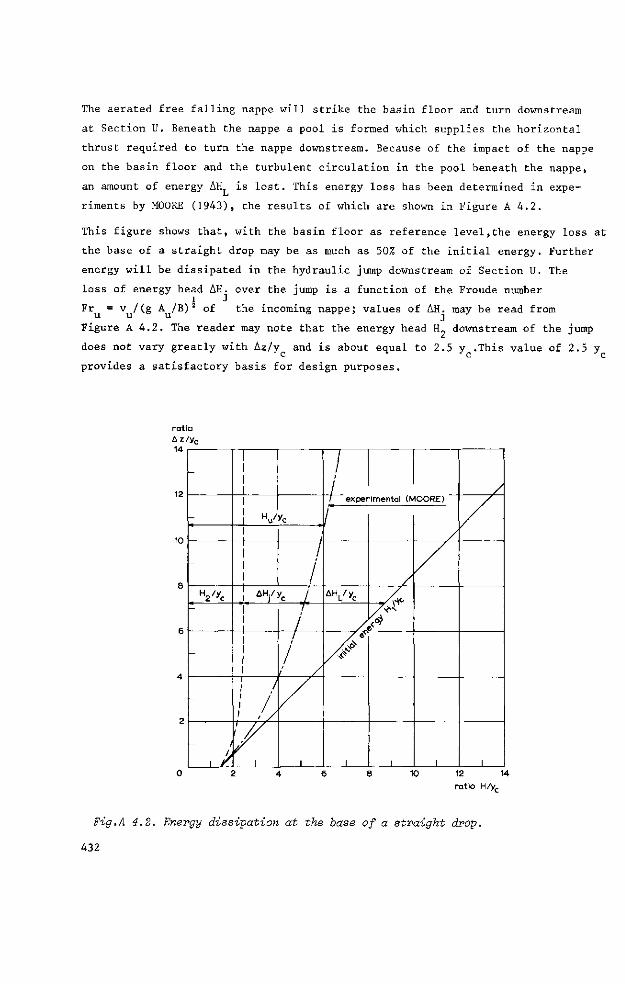
The aerated free falling nappe will strike the basin floor and turn downstream
at Section U. Beneath the nappe a pool is formed which supplies the horizontal
thrust required to turn the nappe downstream. Because of the impact of the nappe
on the basin floor and the turbulent circulation in the pool beneath the nappe,
an amount of energy AH is lost. This energy loss has been determined in expe
riments by MOORE (1943), the results of which are shown in Figure A 4.2.
This figure shows that, with the basin floor as reference level,the energy loss at
the base of a straight drop may be as much as 50% of the initial energy. Further
energy will be dissipated in the hydraulic jump downstream of Section U. The
loss of energy head AH. over the jump is a function of the Froude number I J
Fr = v /(g A / B ) 2 of the incoming nappe; values of AH. may be read from
Figure A 4.2. The reader may note that the energy head H„ downstream of the jump
does not vary greatly with Az/y and is about equal to 2.5 y .This value of 2.5 y c J c c
provides a satisfactory basis for design purposes.
ratio Az/y c
14
12
10
-
_
-
H2/yc
-
-
/ n
i r
I
! v *C
/
L I AH/yc 1
\ I
'i h
1
/ /
/
1
/
/ / ex per
»* /
û V * c
/, / ê
i
imental (MOORE)
— n / ^
1 1 1 10 12 14
ratio H/y
Fig.A 4.2. Energy dissipation at the hase of a straight drop.
432
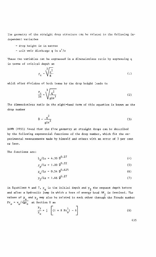
The geometry of the straight drop structure can be related to the following in
dependent variables
- drop height Az in metres
- unit weir discharge q in m /s
These two variables can be expressed in a dimensionless ratio by expressing q
in terms of critical depth as
3 ' z
(1)
which after division of both terms by the drop height leads to
3
Az (2)
The dimensionless ratio in the right-hand term of this equation is known as the
drop number
D gAz"
(3)
RAND (1955) found that the flow geometry at straight drops can be described
by the following exponential functions of the drop number, which fit the ex
perimental measurements made by himself and others with an error of 5 per cent
or less.
The functions are:
L,/Az = 4.30 D d
y /Az = 1 .00 D' P
y /Az = 0.54 D' u
y2/Az = 1.66 D1
,0.27
0.22
,0.425
0.27
(4)
(5)
(6)
(7)
In Equations 6 and 7, y is the initial depth and y. the sequent depth before
and after a hydraulic jump in which a loss of energy head AH. is involved. The
values of y and y„ may also be related to each other through the Froude number
Fr = v //gy at Section U as u u b u
( 1 + 8 Fr ) - 1 u (8)
433
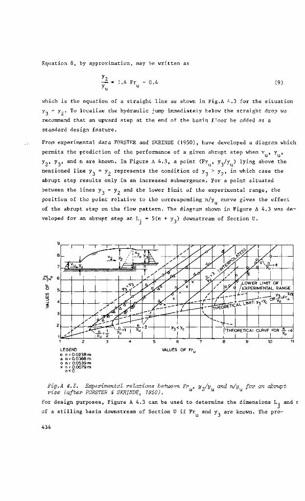
Equation 8, by approximation, may be written as
— = 1.4 Fr - 0.4 y,, u
(9)
which is the equation of a straight line as shown in Fig.A 4.3 for the situation
y, = y„. To localize the hydraulic jump immediately below the straight drop we
recommend that an upward step at the end of the basin floor be added as a
standard design feature.
From experimental data FORSTER and SKRINDE (1950), have developed a diagram which
permits the prediction of the performance of a given abrupt step when v , y ,
y„, y_, and n are known. In Figure A 4.3, a point (Fr , y,/y ) lying above the
mentioned line y = y represents the condition of y_ > y , in which case the
abrupt step results only in an increased submergence. For a point situated
between the lines y, = y„ and the lower limit of the experimental range, the
position of the point relative to the corresponding n/y curve gives the effect
of the abrupt step on the flow pattern. The diagram shown in Figure A 4.3 was de
veloped for an abrupt step at L. = 5(n + y,) downstream of Section U.
LEGEND a n = 0.0238 m A n = 0.0366 m o n = 0.0539 m x n = 0.0079 m
n<0
5 6 7
VALUES OF Fr,,
Fig.A 4.3. Experimental relations between Fr , yJy and n/y for an abrupt rise (after FORSTER & SKRINDE, 1950). u ó u u
For design purposes, Figure A 4.3 can be used to determine the dimensions L. and r
of a stilling basin downstream of Section U if Fr and y, are known. The pro-
434
cedure to find the largest required value of n if Fr , y , and y. are known is u u 3
as follows :
Define for the flow condition at or near maximum discharge the situation of the
point (Fr , y,/y ) and by interpolation that of the corresponding value of the
ratio n/y . Repeat this exercise for other discharges within the anticipated
range of discharge and use the highest n-value for the design. A minimum tail-
water level y_ to prevent the jump from being washed out can thus also be deter
mined .
The straight drop spillway will still be effective if the tailwater level does
not reach critical depth above the weir crest, i.e. as long as the weir flow
is modular.
4.2.2 USBR basin
The USBR has developed an alternative basin which is especially suitable if
tailwater level is greater than the sequent depth and varies independently of
the flow rate.
This impact block type basin was developed for low heads, and gives a good
energy dissipation over a wide range of tailwater levels. The energy dissipa
tion is principally by turbulence induced by the impingement of the incoming
jet upon the impact blocks. The required tailwater level, therefore, is more
or less independent of the drop distance Az.
The linear hydraulic dimensions of the structure as shown in Figure A 4.4 are:
total basin length (for L,-values see Fig.A4.5) L_ = L, + 2.55 y a B a c
basin length to upstream face of impact block L, + 0.8 y
minimum tailwater depth required y„ ^ 2.15 y
optimum impact block height 0.8 y c
width and spacing of impact blocks (0.40 + 0.15) y
optimum end sill height 0.4 y
minimum side wall height y„ + 0.85 y
435
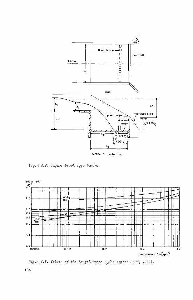
section of center line
Fig.A 4.4. Impact block type basin.
length ratio L d /Az 4 .0
1 .0 0.8
0.6
0.4
5.0 _ OO"
Ah/h, 0.6
10
2.0
2 3 drop number D=q /gAz
Fig.A 4.5. Values of the length ratio Ljhz (after- USER, 1960).
436
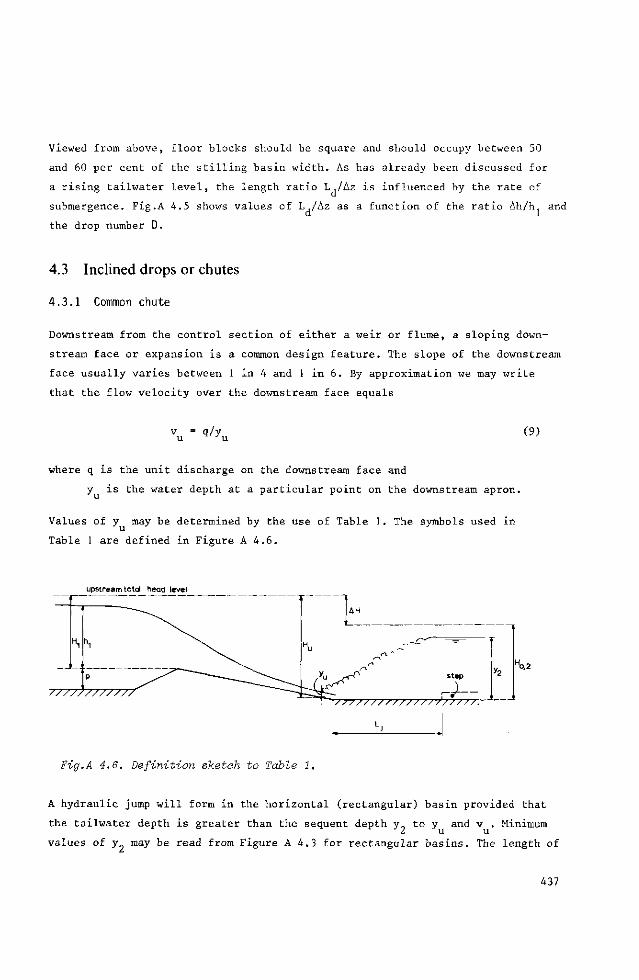
Viewed from above, floor blocks should be square and should occupy between 50
and 60 per cent of the stilling basin width. As has already been discussed for
a rising tailwater level, the length ratio L,/Az is influenced by the rate of
submergence. Fig.A 4.5 shows values of L,/Az as a function of the ratio Ah/h, and
the drop number D.
4.3 Inclined drops or chutes
4.3.1 Common chute
Downstream from the control section of either a weir or flume, a sloping down
stream face or expansion is a common design feature. The slope of the downstream
face usually varies between 1 in 4 and 1 in 6. By approximation we may write
that the flow velocity over the downstream face equals
v„ = 4/y„ (9)
where q is the unit discharge on the downstream face and
y is the water depth at a particular point on the downstream apron.
Values of y may be determined by the use of Table 1. The symbols used in
Table 1 are defined in Figure A 4.6.
upstream to td head level
Fig.A 4.6. Definition sketch to Table 1.
A hydraulic jump will form in the horizontal (rectangular) basin provided that
the tailwater depth is greater than the sequent depth y to y and v . Minimum
values of y may be read from Figure A 4.3 for rectangular basins. The length of
437
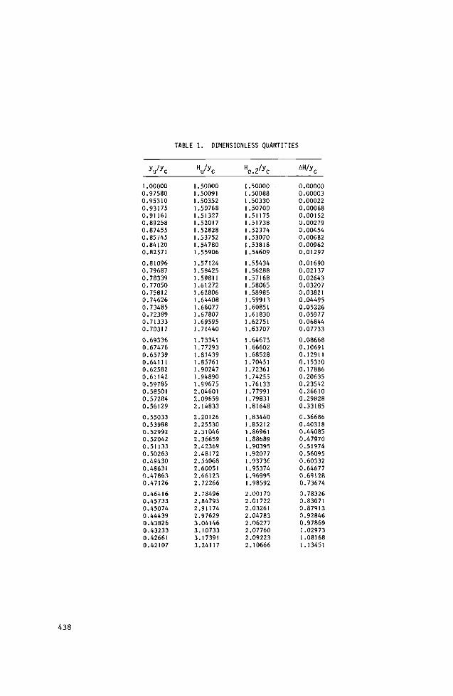
TABLE 1. DIMENSIONLESS QUANTITIES
Vyc 1.00000 0.97580 0.95310 0.93175 0.91161 0.89258 0.87455 0.85745 0.84120 0.82571
0.81096 0.79687 0.78339 0.77050 0.75812 0.74626 0.73485 0.72389 0.71333 0.70317
0.69336 0.67476 0.65739 0.64111 0.62582 0.61142 0.59785 0.58501 0.57284 0.56129
0.55033 0.53988 0.52992 0.52042 0.51133 0.50263 0.49430 0.48631 0.47863 0.47126
0.46416 0.45733 0.45074 0.44439 0.43826 0.43233 0.42661 0.42107
V*c 1.50000 1.50091 1.50352 1.50768 1.51327 1.52017 1.52828 1.53752 1.54780 1.55906
1.57124 1.58425 1.59811 1.61272 1.62806 1.64408 1.66077 1.67807 1.69595 1.71440
1.73341 1.77293 1.81439 1.85761 1.90247 1.94890 1.99675 2.04601 2.09659 2.14833
2.20126 2.25530 2.31046 2.36659 2.42369 2.48172 2.54068 2.60051 2.66123 2.72266
2.78496 2.84793 2.91174 2.97629 3.04146 3.10733 3.17391 3.24117
Ho.2^c
1.50000 1.50088 1.50330 1.50700 1.51175 1.51738 1.52374 1.53070 1.53818 1.54609
1.55434 1.56288 1.57168 1.58065 1.58985 1.59913 1.60851 1.61830 1.62751 1.63707
1.64673 1.66602 1.68528 1.70451 1.72361 1.74255 1.76133 1.77991 1.79831 1.81648
1.83440 1.85212 1.86961 1.88689 1.90395 1.92077 1.93736 1.95374 1.96995 1.98592
2.00170 2.01722 2.03261 2.04783 2.06277 2.07760 2.09223 2.10666
AH/yc
0.00000 0.00003 0.00022 0.00068 0.00152 0.00279 0.00454 0.00682 0.00962 0.01297
0.01690 0.02137 0.02643 0.03207 0.03821 0.04495 0.05226 0.05977 0.06844 0.07733
0.08668 0.10691 0.12911 0.15310 0.17886 0.20635 0.23542 0.26610 0.29828 0.33185
0.36686 0.40318 0.44085 0.47970 0.51974 0.56095 0.60332 0.64677 0.69128 0.73674
0.78326 0.83071 0.87913 0.92846 0.97869 1.02973 1.08168 1.13451
438
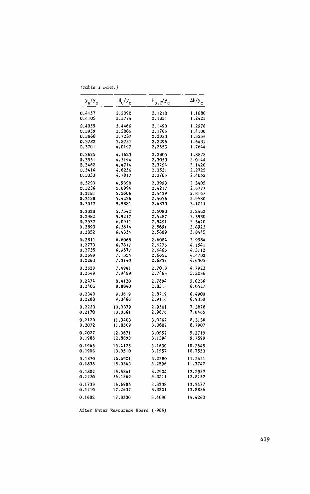
(Table 1 oont.)
V*c 0.4157 0.4105
0.4055 0.3959 0.3868 0.3782 0.3701
0.3625 0.3551 0.3482 0.3416 0.3353
0.3293 0.3236 0.3181 0.3128 0.3077
0.3028 0.2982 0.2937 0.2893 0.2852
0.2811 0.2773 0.2735 0.2699 0.2263
0.2629 0.2549
0.2474 0.2405
0.2340 0.2280
0.2223 0.2170
0.2120 0.2072
0.2027 0.1985
0.1945 0.1906
0.1870 0.1835
0.1802 0.1770
0.1739 0.1710
0.1682
V*c 3.3090 3.3774
3.4466 3.5865 3.7287 3.8731 4.0197
4.1683 4.3194 4.4714 4.6256 4.7817
4.9398 5.0994 5.2606 5.4236 5.5881
5.7542 5.9217 6.0911 6.2614 6.4334
6.6068 6.7817 6.9577 7.1354 7.3140
7.4941 7.9499
8.4130 8.8840
9.3619 9.8466
10.3379 10.8361
11.3403 11.8509
12.3671 12.8893
13.4175 13.9510
14.4901 15.0343
15.5841 16.1362
16.6985 17.2637
17.8330
» 0 . 2 ^
2.1210 2.1351
2.1490 2.1765 2.2033 2.2296 2.2553
2.2805 2.3050 2.3294 2.3531 2.3765
2.3993 2.4217 2.4439 2.4656 2.4870
2.5080 2.5287 2.5491 2.5691 2.5889
2.6084 2.6276 2.6465 2.6652 2.6837
2.7018 2.7463
2.7894 2.8313
2.8719 2.9116
2.9501 2.9876
3.0267 3.0602
3.0952 3.1294
3.1630 3.1957
3.2280 3.2596
3.2904 3.3211
3.3508 3.3801
3.4090
AH/yc
1.1880 1.2423
1.2976 1.4100 1.5254 1.6435 1.7644
1.8878 2.0144 2.1420 2.2725 2.4052
2.5405 2.6777 2.8167 2.9580 3.1011
3.2462 3.3930 3.5420 3.6923 3.8445
3.9984 4.1541 4.3112 4.4702 4.6303
4.7923 5.2036
5.6236 6.0527
6.4900 6.9350
7.3878 7.8485
8.3136 8.7907
9.2719 9.7599
10.2545 10.7553
11.2621 11.7747
12.2937 12.8157
13.3477 13.8836
14.4240
After Water Resources Board (1966)
439
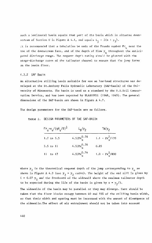
such a horizontal basin equals that part of the basin which is situated down
stream of Section U in Figure A 4.1, and equals L. = 5(n + y ) .
It is recommended that a tabulation be made of the Froude number Fr near the u
toe of the downstream face, and of the depth of flow y throughout the antici
pated discharge range. The sequent depth rating should be plotted with the
stage-discharge curve of the tailwater channel to ensure that the jump forms
on the basin floor.
4.3.2 SAF Basin
An alternative stilling basin suitable for use on low-head structures was de
veloped at the St.Anthony Falls Hydraulic Laboratory (SAF-basin) of the Uni
versity of Minnesota. The basin is used as a standard by the U.S.Soil Conser
vation Service, and has been reported by BLAISDELL (1948, 1949). The general
dimensions of the SAF-basin are shown in Figure A 4.7.
The design parameters for the SAF-basin are as follows.
TABLE 2. DESIGN PARAMETERS OF THE SAF-BASIN
Fru=vu/(gAu/B)^ Lß/y2 TW/y2
1.7 to 5.5 4.5/Fr0'76 1.1 - Fr2/120 u u
5.5 to 11 4.5/Fr0-76 0.85 u
11 to 17 4.5/Fr0,76 1 .0 - Fr2/800 u u
where y„ is the theoretical sequent depth of the jump corresponding to y as
shown in Figure A 4.3 (use y_ = y„ curve). The height of the end sill is given by
C = 0.07 y„ and the freeboard of the sidewall above the maximum tailwater depth
to be expected during the life of the basin is given by z = y„/3.
The sidewalls of the basin may be parallel or they may diverge. Care should be
taken that the floor blocks occupy between 40 and 55% of the stilling basin width,
so that their width and spacing must be increased with the amount of divergence of
the sidewalls.The effect of air entrainment should not be taken into account
440
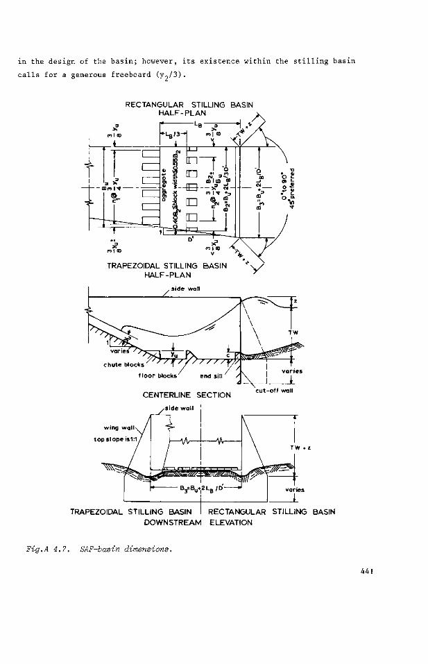
in the design of the b a s in ; however, i t s ex i s tence wi th in the s t i l l i n g bas in
c a l l s for a generous freeboard ( y „ /3 ) .
RECTANGULAR STILLING BASIN HALF-PLAN
a — I « o tl f O «i- =. •S * — O — »? « i l
o n—i © ffl
D'
TRAPEZOIDAL STILLING BASIN HALF-PLAN
varies ' ^
chute blocks
floor blocks
CENTERLINE SECTION
,side wall
cut-oft wall
^ wing wall
top slope is 1:1 T W . z
TRAPEZOIDAL STILLING BASIN I RECTANGULAR STILLING BASIN DOWNSTREAM ELEVATION
Fig.A 4.7. SAF-basin dimensions.
441
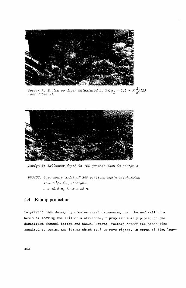
Design A: Tailwater depth calculated by TW/y = 1.1 - Fr /120 (see Table 2). u
Design B: Tailwater depth is 15% greater than in Design A.
PHOTOS: 1:20 saale model of SAF stilling basin discharging
1200 mz/s in prototype,
b = 40.0 m, AH - 3.50 m.
4.4 Riprap protection
To prevent bank damage by erosive currents passing over the end sill of a
basis or leaving the tail of a structure, riprap is usually placed on the
downstream channel bottom and banks. Several factors affect the stone size
required to resist the forces which tend to move riprap. In terms of flow leav-
442
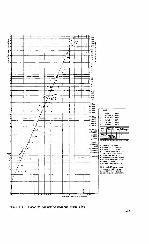
1000 8 0 0 6 0 0
DUBUAT
BOUNICEAU
BLACKWELL
SAINJON
SUCHIER GILBERT
1 7 8 6
1 8 4 5
1 8 5 7
1871
1874 1914
TESTS BY
HO HU
GILBERT
COMPETENT VELOCITY ELEVAT
SCHAFFERNAK $$£&
| _£_ IHG AT ING
SCHAFFERNAK K E p T w M O T ^
+
* +
• i S POINTS ARE SATISFACTORY INSTALLATIONS
. F O R E I G N , PROTO ( 1 )
• BONNEVILLE FLUME ( 2 )
• BONNEVILLE CLOSURE ( 2 )
if COLUMBIA RIVER, PROTO ( 2 )
LOS ANGELES DlST, PROTO ( 2)
0 2UIDER 2EE, PROTO ( 2 )
» PASSAMAQUODY, MODEL ( 2 )
a STILLING B A S I N , M O D E L ( 3 )
| CHANNEL, M O D E L (3 )
* Mc NARY D A M , M O D E L ( 4 )
(1) E H HOOKER,ASCE,VOL 36
(2) C I.GRIMM 8, N .LEUPOLD.1939
(3) WATERWAYS EXP STATION
(4) B O N N E V I L L E LABORATORY
2 3 4 5 6 7 8 9 1 0
bottom velocity in m/sec
Fig.A 4.8. Curve to determine maximum stone size.
443
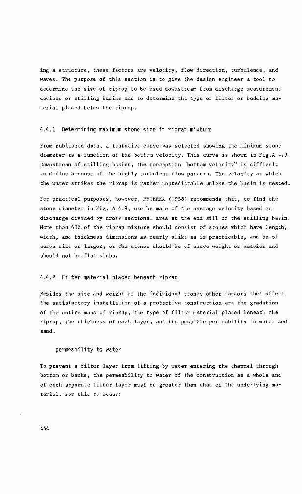
ing a structure, these factors are velocity, flow direction, turbulence, and
waves. The purpose of this section is to give the design engineer a tool to
determine the size of riprap to be used downstream from discharge measurement
devices or stilling basins and to determine the type of filter or bedding ma
terial placed below the riprap.
4.4.1 Determining maximum stone size in riprap mixture
From published data, a tentative curve was selected showing the minimum stone
diameter as a function of the bottom velocity. This curve is shown in Fig.A 4.9.
Downstream of stilling basins, the conception "bottom velocity" is difficult
to define because of the highly turbulent flow pattern. The velocity at which
the water strikes the riprap is rather unpredictable unless the basin is tested.
For practical purposes, however, PETERKA (1958) recommends that, to find the
stone diameter in Fig. A 4.9, use be made of the average velocity based on
discharge divided by cross-sectional area at the end sill of the stilling basin.
More than 60% of the riprap mixture should consist of stones which have length,
width, and thickness dimensions as nearly alike as is practicable, and be of
curve size or larger; or the stones should be of curve weight or heavier and
should not be flat slabs.
4.4.2 Filter material placed beneath riprap
Besides the size and weight of the individual stones other factors that affect
the satisfactory installation of a protective construction are the gradation
of the entire mass of riprap, the type of filter material placed beneath the
riprap, the thickness of each layer, and its possible permeability to water and
sand.
permeability to water
To prevent a filter layer from lifting by water entering the channel through
bottom or banks, the permeability to water of the construction as a whole and
of each separate filter layer must be greater than that of the underlying ma
terial. For this to occur:
444
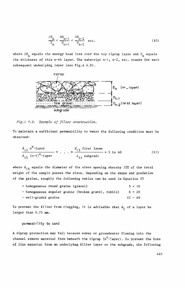
AH AH n-1
Dn-1
AH n-2
n-2 etc. (10)
where AH equals the energy head loss over the top riprap layer and D equals
the thickness of this n-th layer. The subscript n-1, n-2, etc. stands for each
subsequent underlying layer (see Fig.A 4.9).
r iprap
mSsMsmm fine gravel
subgrade
Dn (n°
Jn-1
layer)
D n 2 ( f i r s t layer)
Fig.A 4.9. Example of filter construction.
To maintain a sufficient permeability to water the following condition must be
observed:
d. _ n -layer
d ,. (n-1 ) -layer
d _ first layer
d _ subgrade 5 to 40 (11)
where d^. equals the diameter of the sieve opening whereby 15% of the total
weight of the sample passes the sieve. Depending on the shape and gradation
of the grains, roughly the following ratios can be used in Equation 15
- homogeneous round grains (gravel) 5 - 1 0
- homogeneous angular grains (broken gravel, rubble) 6 - 2 0
- well-graded grains 1 2 - 4 0
To prevent the filter from clogging, it is advisable that d,. of a layer be
larger than 0.75 mm.
permeability to sand
A riprap protection may fail because waves or groundwater flowing into the
channel remove material from beneath the riprap (n -layer). To prevent the loss
of fine material from an underlying filter layer or the subgrade, the following
445
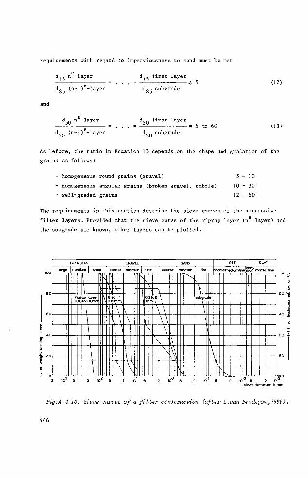
requirements with regard to imperviousness to sand must be met
d ,. n -layer
dg 5 (n-1) -layer
d . first layer
d0_ subgrade ö j
« 5 (12)
and
d5o n _ l a y e r
d5Q (n-1) -layer
d_n first layer
d_n subgrade 5 to 60 (13)
As before, the ratio in Equation 13 depends on the shape and gradation of the
grains as follows:
- homogeneous round grains (gravel) 5 - 1 0
- homogeneous angular grains (broken gravel, rubble) 1 0 - 3 0
- well-graded grains 1 2 - 6 0
The requirements in this section describe the sieve curves of the successive
filter layers. Provided that the sieve curve of the riprap layer (n layer) and
the subgrade are known, other layers can be plotted.
8 0
2 0
BOULDERS
l a rge medium small
r 1
p r DO
\
> ap layer to30Omrr
i
+
GRAVEL
coarse medium fine
\
--* 4
> 8 '
\
\
-* 0
'
V
4
\
\ \ \ \ \
\ \ \
-
\ \ \ _\,
! \ I \ i \ i
À-V
V
0.3t I m m
1
1
\
— o 8
\ \
\
SAND
coarse medium
k \ \ \ \
\ \ -A >..-
V v
\
f-^ J
fine
'V subgrad«
\ i
\ \\
SLT
coarse^nedium|fine
\
V > N
v e r y f ine
CLAY
cocrse|f ine
40 S
2 10 5 2 10 5 2 10 5 2 10 5 2 1 0 5 2 10 : diameter in mm
Fig.A 4.10. Sieve curves of a filter construction (after L.van Bendegom,1969).
446
In practice one should use materials that have a grain size distribution which
is locally available, since it is uneconomical to compose a special mixture.
To provide a stable and effectively functioning filter, the sieve curves for
subgrade and filter layers should run about parallel for the small-diameter
grains.
An example of plotting sieve curves of the various layers of a riprap protection
is shown in Figure A 4.10.
4.4.3 Filter construction
To obtain a fair grain size distribution throughout a filter layer, each layer
should be sufficiently thick.The following thicknesses must be regarded as a
minimum for a filter construction made in the dry
- sand, fine gravel 0.05 to 0.10 m
- gravel 0.10 to 0.20 m
- stones 1.5 to 2 times the largest stone diameter
With filters constructed under water, these thicknesses have to be increased
considerably to compensate for irregularities in the subgrade and because it
is more difficult to apply an even layer under water.
Many variations can be made on the basic filter construction. One or more of
the layers can be replaced with other materials. With some protective linings,
only the riprap layer (n layer) is maintained, while the underlying layers are
replaced by one single layer. For example
- concrete blocks on a nylon filter
- stones on braided azobé slabs on plastic filter
- gabions on fine gravel
- nylon-sand mattresses
The usual difficulty with these variants is their perviousness to underlying
sand.The openings in each layer should not be greater than 0.5 x dRC.
of the underlying material. If openings are greater, one should not replace
all underlying layers but maintain as many layers (usually one) as are needed
to prevent the subgrade from being washed through the combined layer.
447
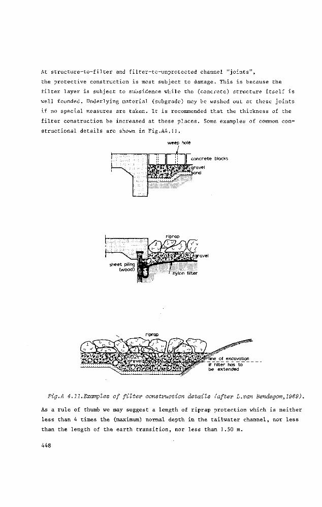
At structure-to-filter and filter-to-unprotected channel "joints",
the protective construction is most subject to damage. This is because the
filter layer is subject to subsidence while the (concrete) structure itself is
well founded. Underlying material (subgrade) may be washed out at these joints
if no special measures are taken. It is recommended that the thickness of the
filter construction be increased at these places. Some examples of common con
structional details are shown in Fig.A4.ll.
concrete blocks
riprap
of excavation filter has to
extended
Fig.A 4.11.Examples of filter construction details (after L.van Bendegom,1969).
As a rule of thumb we may suggest a length of riprap protection which is neither
less than 4 times the (maximum) normal depth in the tailwater channel, nor less
than the length of the earth transition, nor less than 1.50 m.
448
4.5 Selected list of references
1. VAN BENDEGOM, L. et al.: Principles governing the design and construc
tion of economic revetments for protecting the banks of rivers and canals for
ocean and inland navigation. 20th Intern.navigation Congr.Paris, 43 pp. 1969.
2. BERRY, N.K.: The start of bed load movement. Thesis. Univ.of Colorado,
USA, 1948.
3. BLAISDELL, F.W.: The SAF stilling basin. U.S.Dept.of Agric.Soil Con
servation Service. St.Anthony Falls Hydraulic Laboratory, Minneapolis, Minn.,
Dec.1943.
4. BLAISDELL, F.W.: The SAF stilling basin. A structure to dissipate the
destructive energy in high-velocity flow from spillways. U.S.Dept.of Agric.
Service in cooperation with the Minnesota Agric.Exp.Sta. & St.Anthony Falls
Hydraulic Laboratory. Agric.Handbook 156. Washington D.C. U.S.Gov.Printing
Office, 1959.
5. CANALS AND RELATED STRUCTURES. Commissioner's office, Denver (Col.).
U.S.Dept.of the Interior, Bureau of Reel.Design Standards 3. 1961.
6. DESIGN OF SMALL DAMS. U.S.Dept.of the Interior. Bureau of Reel.,
Washington D.C. U.S.Gov.Printing Office. 1960. 611 pp.
7. DORT, J.A.van, BOS, M.G.: Drainage principles and applications.
Chapt.29: Main drainage systems. Int.Institute for Land Recl.& Improvement.
Publication 16. Vol.IV. Wageningen 1974. pp.124-224.
8. FORSTER, J.W., SKRINDE, R.A.: Control of the hydraulic jump by sills.
Transactions, American Society of Civil Engineers. Vol.115, 1950. pp.973-987.
9. HENDERSON, F.M.: Open Channel Flow. MacMillan Co., New York 1966.522 pp.
10. MAVIS, F.T., LAUSHEY, L.M.: A reappraisal of the beginnings of bed
movement-competent velocity. Proc.of the Int.Assoc.for Hydraulic Research. March
1948. Stockholm, pp.213-218.
11. MOORE, W.L.: Energy loss at the base of a free overfall. Trans.of the
Amer.Soc.of Civ.Engineers. 1943. Vol.108, pp.1343-1392. Paper No.2204.
12. PETERKA, A.J.: Hydraulic design of stilling basins and energy dissi-
pators. U.S.Dept.of the Interior. Bureau of Reel.Water Resources Techn.Publ.
Engineering Monograph No.25, 1964. 223 pp.
449
13. RAND, W.: Flow geometry at straight drop spillways. Proc.Amer.Soc.of
Civil Engineers. Vol.8. Sept.1955. No.791.
14. VLUGTER, H.: 12j Jaar hydrodynamische research aan waterloopkundige
modellen in Nederlandsch Indië. De Ingenieur in Ned.Indië. No.9. 1941.
450
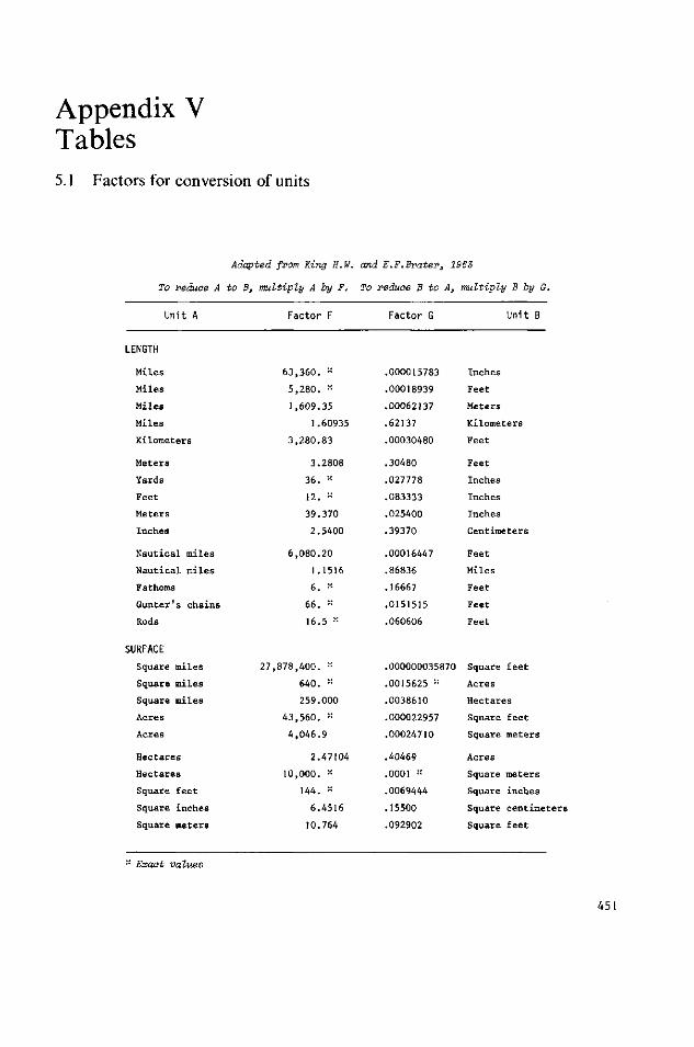
Appendix V Tables 5.1 Factors for conversion of units
Adapted from King H.W. and E.F.Brater, 1963
To reduce A to B, multiply A by F. To reduce B to A, multiply B by G.
Unit A
LENGTH
Miles
Miles
Miles
Miles
Kilometers
Meters
Yards
Feet
Meters
Inches
Nautical miles
Nautical miles
Fathoms
Gunter's chains
Rods
SURFACE
Square miles
Square miles
Square miles
Acres
Acres
Hectares
Hectares
Square feet
Square inches
Square meters
Factor F
63,360. ::
5,280. -
1,609.35
1.60935
3,280.83
3.2808
36. ::
12. "
39.370
2.5400
6,080.20
1.1516
6. "
66. "
16.5 "
27,878,400. ::
640. "
259.000
43,560. ::
4,046.9
2.47104
10,000. ::
144. «
6.4516
10.764
Factor G
.000015783
.00018939
.00062137
.62137
.00030480
.30480
.027778
.083333
.025400
.39370
.00016447
.86836
.16667
.0151515
.060606
.000000035870
.0015625 "
.0038610
.000022957
.00024710
.40469
.0001 ;:
.0069444
.15500
.092902
Unit B
Inches
Feet
Meters
Kilometers
Feet
Feet
Inches
Inches
Inches
Centimeters
Feet
Miles
Feet
Feet
Feet
Square feet
Acres
Hectares
Square feet
Square meters
Acres
Square meters
Square inches
Square centimeter!
Square feet
:: Exaot Values
451
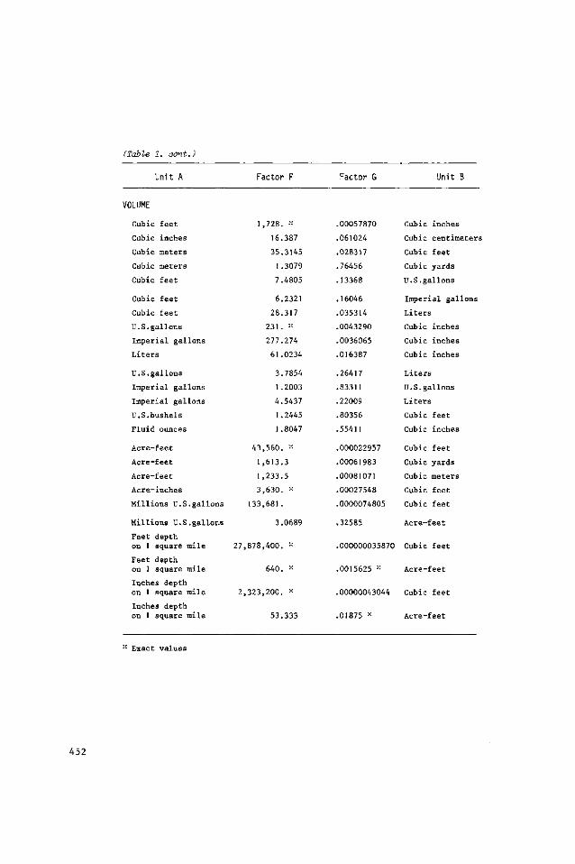
(Table 1. aûnt.)
Unit A Factor F Factor G Unit B
VOLUME
Cubic feet
Cubic inches
Cubic meters
Cubic meters
Cubic feet
Cubic feet
Cubic feet
U.S.gallons
Imperial gall
Liters
U.S.gallons
Imperial gal]
.ons
.ons
Imperial gallons
U.S.bushels
Fluid ounces
Acre-feet
Acre-feet
Acre-feet
Acre-inches
Millions U.S.
Millions U.S.
gallons
.gallons
Feet depth on 1 square mile
Feet depth on 1 square mile
Inches depth on 1 square mile
Inches depth on I square mile
1
43
1
1
3
133
27,878
2,323
,728. »
16.387
35.3145
1.3079
7.4805
6.2321
28.317
231. »
277.274
61.0234
3.7854
1.2003
4.5437
1.2445
1.8047
,560. ::
,613.3
,233.5
,630. ::
,681.
3.0689
,400. "
640. •-
,200. "
53.333
.00057870
.061024
.028317
.76456
.13368
.16046
.035314
.0043290
.0036065
.016387
.26417
.83311
.22009
.80356
.55411
.000022957
.00061983
.00081071
.00027548
.0000074805
.32585
.000000035870
.0015625 ::
.00000043044
.01875 ::
Cubic inches
Cubic centimeters
Cubic feet
Cubic yards
U.S.gallons
Imperial gallons
Liters
Cubic inches
Cubic inches
Cubic inches
Liters
U.S.gallons
Liters
Cubic feet
Cubic inches
Cubic feet
Cubic yards
Cubic meters
Cubic feet
Cubic feet
Acre-feet
Cubic feet
Acre-feet
Cubic feet
Acre-feet
" Exact values
452
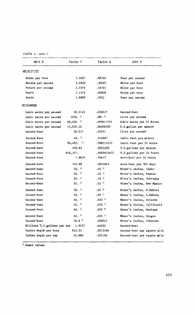
(Table 1. oont.)
Unit A Factor F Factor G Unit B
VELOCITIES
Miles per hour
Meters per second
Meters per second
Knots
Knots
1
3
2
1
1
.4667
2808
2369
1516
6889
.68182
.30480
.44704
.86836
.5921
Feet per second
Miles per hour
Miles per hour
Miles per hour
Feet per second
DISCHARGE
Cubic metre
Cubic metre
Cubic metre
Cubic metre
Second-feet
Second-feet
Second-feet
Second-feet
Second-feet
Second-feet
Second-feet
Second-feet
Second-feet
Second-feet
Second-feet
Second-feet
Second-feet
Second-feet
Second-feet
Second-feet
Second-feet
Second-feet
Millions U.S
Inches depth
Inches depth
per
per
per
per
second
second
second
second
.gallons per
per
per
hour
day
86
15
86
646
day
35.3145
000. "
400. "
850.20
28.317
60. ::
,400. "
448.83
,317.
1.9835
723.98
50. ::
50. "
50. "
50. "
50. ::
50. ::
40. "
40. -
40. "
40. "
38.4 "
1.5472
645.33
26.889
028317
001 "
000011574
00006309
03531
016667
000011574
0022280
0000015472
50417
0013813
02 "
02 ::
02 ::
02 "
02 -
02 -
025 ::
025 -
025 "
025 "
026042
64632
0015496
037190
Second-feet
Litre per second
Cubic metre per
U.S.gallon per
24 hours
minute
Litre per second
Cubic feet per
Cubic feet per
U.S.gallons per
U.S.gallons per
minute
24 hours
minute
24 hours
Acre-feet per 24 hours
Acre-feet per 365 days
Miner's inches,
Miner's inches,
Miner's inches,
Miner's inches,
Miner's inches,
Miner's inches,
Miner's inches,
Miner's inches,
Miner's inches,
Miner's inches,
Miner's inches,
Second-feet
Second-feet per
Second-feet per
Idaho
Kansas
Nebraska
New Mexico
N.Dakota
S.Dakota
Arizona
California
Montana
Oregon
Colorado
square mil
square mil
:: Exact values
453
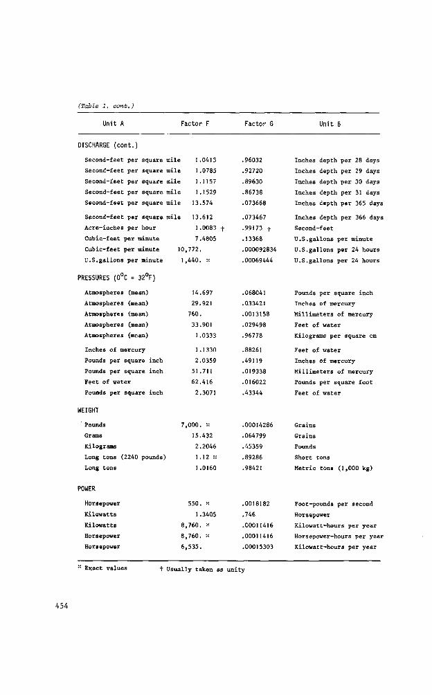
(Table 1. sont.)
Unit A Factor F Factor G Unit B
DISCHARGE (cont.)
Second-feet per square mile 1.0413 .96032
Second-feet per square mile 1.0785 .92720
Second-feet per square mile 1.1157 .89630
Second-feet per square mile 1.1529 .86738
Second-feet per square mile 13.574 .073668
Second-feet per square mile 13.612 .073467
Acre-inches per hour 1.0083 f .99173 +
Cubic-feet per minute 7.4805 .13368
Cubic-feet per minute 10,772. .000092834
U.S.gallons per minute 1,440. :c .00069444
PRESSURES (0°C = 32°F)
Atmospheres (mean)
Atmospheres (mean)
Atmospheres (mean)
Atmospheres (mean)
Atmospheres (mean)
Inches of mercury
Pounds per square
Founds per square
Feet of water
Pounds per square
inch
inch
inch
14.697
29.921
760.
33.901
1.0333
1.1330
2.0359
51.711
62.416
2.3071
.068041
.033421
.0013158
.029498
.96778
.88261
.49119
.019338
.016022
.43344
Inches depth per 28 days
Inches depth per 29 days
Inches depth per 30 days
Inches depth per 31 days
Inches depth per 365 days
Inches depth per 366 days
Second-feet
U.S.gallons per minute
U.S.gallons per 24 hours
U.S.gallons per 24 hours
Pounds per square inch
Inches of mercury
Millimeters of mercury
Feet of water
Kilograms per square cm
Feet of water
Inches of mercury
Millimeters of mercury
Pounds per square foot
Feet of water
WEIGHT
Pounds 7,000. ::
Grams 15.432
Kilograms 2.2046
Long tons (2240 pounds) 1.12 ::
Long tons I.0160
00014286
064799
45359
89286
98421
Grains
Grains
Pounds
Short tons
Metric tons (1,000 kg)
POWER
Horsepower
Kilowatts
Kilowatts
Horsepower
Horsepower
550. ::
1.3405
8,760. "
8,760. -
6,535.
.0018182
.746
.00011416
.00011416
.00015303
Foot-pounds per second
Horsepower
Kilowatt-hours per year
Horsepower-hours per year
Kilowatt-hours per year
Exact values t Usually taken as unity
454
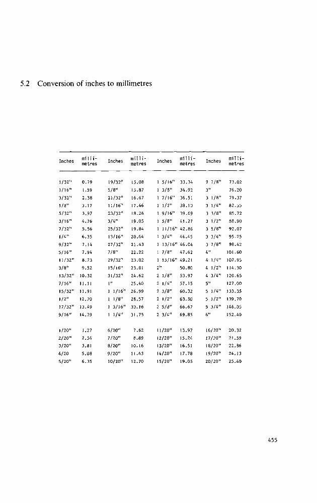
5.2 Conversion of inches to millimetres
Inches milli-metres Inches mi 11i -
metres Inches milli-metres Inches
millimetres
1/32"
1/16"
3/32"
1/8"
5/32"
3/16"
7/32"
1/4"
9/32"
5/16"
11/32"
3/8"
13/32"
7/16"
15/32"
1/2"
17/32"
9/16"
1/20"
2/20"
3/20"
4/20
5/20"
0.79
1.59
2.38
3.17
3.97
4.76
5.56
6.35
7.14
7.94
8.73
9.52
10.32
11.11
11.91
12.70
13.49
14.29
1.27
2.54
3.81
5.08
6.35
19/32"
5/8"
21/32"
11/16"
23/32"
3/4"
25/32"
13/16"
27/32"
7/8"
29/32"
15/16"
31/32"
1"
1 1/16"
1 1/8"
1 3/16"
1 1/4"
6/20"
7/20"
8/20"
9/20"
10/20"
15.08
15.87
16.67
17.46
18.26
19.05
19.84
20.64
21.43
22.22
23.02
23.81
24.62
25.40
26.99
28.57
30.16
31.75
7.62
8.89
10.16
11.43
12.70
1 5/16"
1 3/8"
1 7/16"
1 1/2"
1 9/16"
1 5/8"
1 11/16"
1 3/4"
1 13/16"
1 7/8"
1 15/16"
2"
2 1/8"
2 1/4"
2 3/8"
2 1/2"
2 5/8"
2 3/4"
11/20"
12/20"
13/20"
14/20"
15/20"
33.34
34.92
36.51
38.10
39.69
41.27 1 42.86
44.45
' 46.04
47.62
49.21
50.80
53.97
57.15
60.32
63.50
66.67
69.85
13.97
15.24
16.51
17.78
19.05
2 7/8"
3"
3 1/8"
3 1/4"
3 3/8"
3 1/2"
3 5/8"
3 3/4"
3 7/8"
4"
4 1/4"
4 1/2"
4 3/4"
5"
5 1/4"
5 1/2"
5 3/4"
6"
16/20"
17/20"
18/20"
19/20"
20/20"
73.02
76.20
79.37
82.55
85.72
88.90
92.07
95.25
98.42
101.60
107.95
114.30
120.65
127.00
133.35
139.70
146.05
152.40
20.32
21.59
22.86
24.13
25.40
455
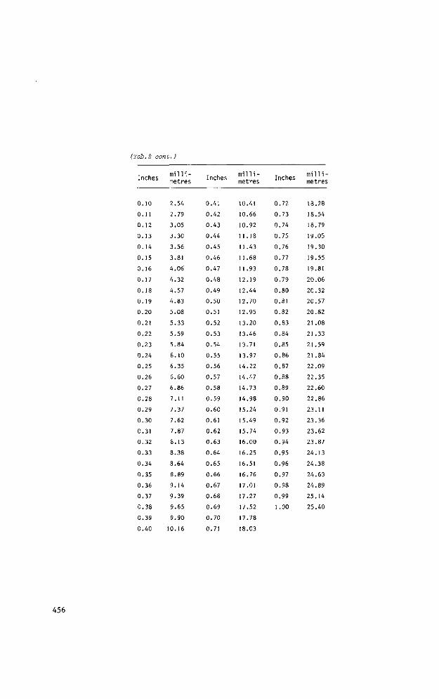
(Tab.2 cont.)
Inches
0.10
0.11
0.12
0.13
0.14
0.15
0.16
0.17
0.18
0.19
0.20
0.21
0.22
0.23
0.24
0.25
0.26
0.27
0.28
0.29
0.30
0.31
0.32
0.33
0.34
0.35
0.36
0.37
0.38
0.39
0.40
millimetres
2.54
2.79
3.05
3.30
3.56
3.81
4.06
4.32
4.57
4.83
5.08
5.33
5.59
5.84
6.10
6.35
6.60
6.86
7.11
7.37
7.62
7.87
8.13
8.38
8.64
8.89
9.14
9.39
9.65
9.90
10.16
Inches
0.41
0.42
0.43
0.44
0.45
0.46
0.47
0.48
0.49
0.50
0.51
0.52
0.53
0.54
0.55
0.56
0.57
0.58
0.59
0.60
0.61
0.62
0.63
0.64
0.65
0.66
0.67
0.68
0.69
0.70
0.71
mill i-metres
10.41
10.66
10.92
11.18
11.43
11.68
11.93
12.19
12.44
12.70
12.95
13.20
13.46
13.71
13.97
14.22
14.47
14.73
14.98
15.24
15.49
15.74
16.00
16.25
16.51
16.76
17.01
17.27
17.52
17.78
18.03
Inches
0.72
0.73
0.74
0.75
0.76
0.77
0.78
0.79
0.80
0.81
0.82
0.83
0.84
0.85
0.86
0.87
0.88
0.89
0.90
0.91
0.92
0.93
0.94
0.95
0.96
0.97
0.98
0.99
1.00
mi 11i -metres
18.28
18.54
18.79
19.05
19.30
19.55
19.81
20.06
20.32
20.57
20.82
21.08
21.33
21.59
21.84
22.09
22.35
22.60
22.86
23.11
23.36
23.62
23.87
24.13
24.38
24.63
24.89
25.14
25.40
456
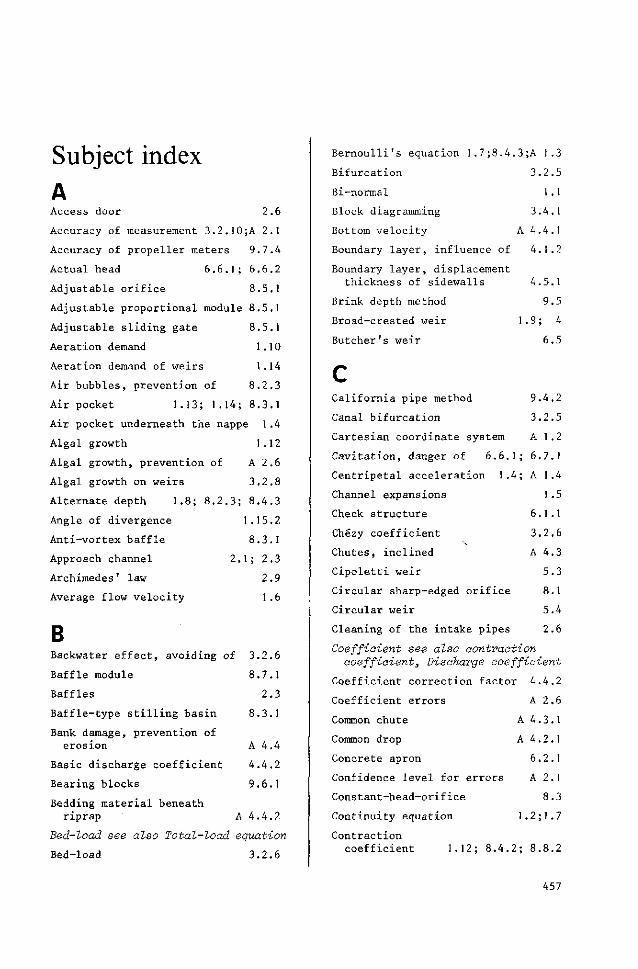
Subject index
Access door 2.6
Accuracy of measurement 3.2.10;A 2.1
Accuracy of propeller meters 9.7.4
Actual head 6.6.1; 6.6.2
Adjustable orifice 8.5.1
Adjustable proportional module 8.5.1
Adjustable sliding gate 8.5.1
Aeration demand 1.10
Aeration demand of weirs 1.14
Air bubbles, prevention of 8.2.3
Air pocket 1.13; 1.14; 8.3.1
Air pocket underneath the nappe 1.4
Algal growth 1.12
Algal growth, prevention of A 2.6
Algal growth on weirs
Alternate depth 1.8
Angle of divergence
Anti-vortex baffle
Approach channel
Archimedes' law
Average flow velocity
3.2.8
5.2.3; 8.4.3
1 .15.2
8.3.1
2.1 ; 2.3
2.9
1.6
B Backwater effect, avoiding of 3.2.6
Baffle module 8.7.1
Baffles 2.3
Baffle-type stilling basin 8.3.1
Bank damage, prevention of
erosion A 4.4
Basic discharge coefficient 4.4.2
Bearing blocks 9.6.1
Bedding material beneath
riprap A 4.4.2
Bed-load see also Total-load equation
Bed-load 3.2.6
Bernoulli's equation 1.7;8.4.3;A 1.3
Bifurcation 3.2.5
Bi-normal 1 . 1
Block diagramming 3.4.1
Bottom velocity A 4.4.1
Boundary layer, influence of 4.1.2
Boundary layer, displacement
thickness of sidewalls 4.5.1
Brink depth method 9.5
Broad-crested weir 1-9; 4
Butcher's weir 6.5
California pipe method 9.4.2
Canal bifurcation 3.2.5
Cartesian coordinate system A 1.2
Cavitation, danger of 6.6.1; 6.7.1
Centripetal acceleration 1.4; A 1.4
Channel expansions 1.5
Check structure 6.1.1
Chézy coefficient 3.2.6
Chutes, inclined A 4.3
Cipoletti weir 5.3
Circular sharp-edged orifice 8.1
Circular weir 5.4
Cleaning of the intake pipes 2.6
Coefficient see also contraction coefficient, Discharge coefficient
Coefficient correction factor 4.4.2
Coefficient errors A 2.6
Common chute A 4.3.1
Common drop A 4.2.1
Concrete apron 6.2.1
Confidence level for errors A 2.1
Constant-head-orifice 8.3
Continuity equation 1.2; 1.7
Contraction coefficient 1.12; 8.4.2; 8.8.2
457
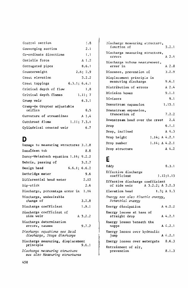
Control section
Converging section
Co-ordinate directions
Coriolis force
Corrugated pipes
Counterweight
Crest elevation
Crest tappings 6.3
Critical depth of flow
Critical depth flumes
Crump weir
Crump-de Gruyter adjustable orifice
Curvature of streamlines
1
2
1
A 1
8.6
2.6; 2
3.2
1; 6.4
1
1.11;
6.3
8
A 1
8
1
1
2
1
9
2
1
8
7
1
5
4
Cutthroat flume 1.11; 7.3.1
Cylindrical crested weir 6.7
Damage to measuring structures 3.2.8
Danaïdean tub 8.8
Darcy-Weissbach equation 1.14; 9.2.2
3.2.7
.1; 6.6.2
9.6
2.12
2.6
Debris, passing of
Design head
Dethridge meter
Differential head meter
Dip-stick
Discharge, percentage error in 1.14
Discharge, undesirable
change of 3.2.8
Discharge coefficient 1.9.1
Discharge coefficient of side weir A 3.2.2
Discharge determination errors, causes 9.7.2
Discharge equations see Head discharge, Stage discharge
Discharge measuring, displacement principle 9.6.1
Discharge measuring structure see also Measuring structures
Discharge measuring structure, function of 3.2.1
Discharge measuring structure, errors A 2.4
Discharge volume measurement,
error in A 2.8
Diseases, prevention of 3.2.9
Displacement principle in
measuring discharge 9.6.1
Distribution of errors A 2.4
Division boxes 9.1.1
Divisors 9.1
Downstream expansion 1.15.1
Downstream expansion,
truncation of 7.2.2
Downstream head over the crest 2.4
Drop 6.1.1
Drop, inclined A 4.3
Drop height 1.14; A 4.2.1
Drop number 1.14; A 4.2.1
Drop structure A 4.2
Eddy 8.3.1
Effective discharge coefficient 1.12; 1.13
Effective discharge coefficient of side weir A 3.2.2; A 3.2.3
Elevation head 1.3; A 1.3
Energy see also Kinetic energy, Potential energy
Energy dissipation A 4.2.2
Energy losses at base of straight drop A 4.2.1
A 4.2.1 Energy losses beneath the
nappe
Energy losses over hydraulic
j ump A 4.2.1
Energy losses over metergate 8.6.3
Entrainment of air, prevention 8.1.3
458
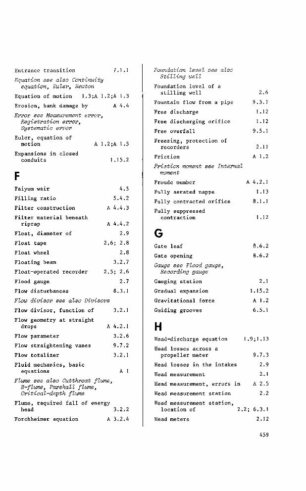
Entrance transition 7.1.1
Equation see also Continuity equation, Euter, Newton
Equation of motion 1.3;A 1.2;A 1.3
Erosion, bank damage by A 4.4
Error see Measurement error, Registration error, Systematic error
Euler, equation of motion
Expansions in closed conduits
A 1.2;A 1.5
1.15.2
Faiyum weir
Filling ratio
Filter construction
Filter material beneath riprap
Float, diameter of
Float tape
Float wheel
Floating beam
Float-operated recorder
Flood gauge
Flow disturbances
5
A 4
A 4
2.6;
3
2.5;
8
Flow divisor see also Divisors
Flow divisor, function of
Flow geometry at straight drops
Flow parameter
Flow straightening vanes
Flow totalizer
3
A 4
3
9
3
4
4
.4
.4
2
2
2
.2
2
2
.3
.2
.2
.2
.7
.2
5
2
3
2
9
8
8
7
6
7
1
1
1
6
2
1
Fluid mechanics, basic equations A 1
Flume see also Cutthroat flume, H-flume, Farshall flume, Critical-depth flume
Flume, required fall of energy head 3,
Forchheimer equation A 3
2.2
2.4
Foundation level see also Stilling well
Foundation level of a stilling well
Fountain flow from a pipe
Free discharge
Free discharging orifice
Free overfall
Freezing, protection of recorders
Friction
Friction moment see Internal moment
Froude number
Fully aerated nappe
Fully contracted orifice
2.6
9.3.1
1.12
1 .12
9.5.1
2.11
A 1 .2
A 4.2.1
1.13
8.1.1
Fully suppressed contraction
Gate leaf
Gate opening
Gauge see Flood gauge, Recording gauge
Gauging station
Gradual expansion
Gravitational force
Guiding grooves
H Head-discharge equation
Head losses across a propeller meter
Head losses in the intakes
Head measurement
Head measurement, errors in
Head measurement station
Head measurement station, location of
Head meters
1 .12
8.6.2
8.6.2
2.1
1.15.2
A 1 .2
6.5.1
1.9;1.13
9.7.3
2.9
2.1
A 2.5
2.2
.2; 6.3.1
2.12
459
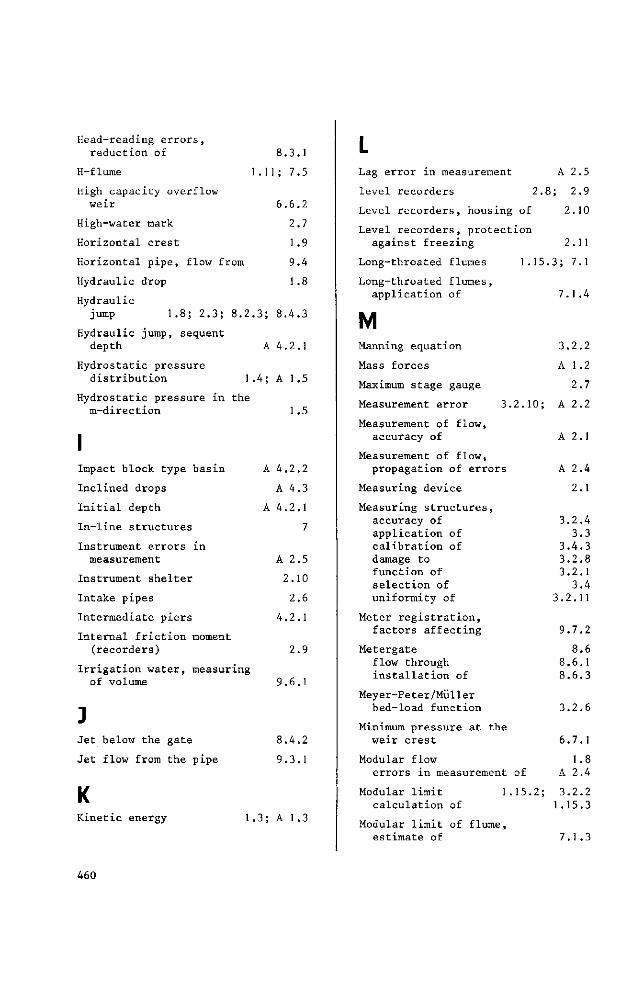
Head-reading errors,
reduction of 8.3.1
H-flume 1.11; 7.5
High capacity overflow
weir 6.6.2
High-water mark 2.7
Horizontal crest 1.9
Horizontal pipe, flow from 9.4
Hydraulic drop 1 .8
Hydraulic jump
Hydraulic jump, sequent depth
Hydrostatic pressure distribution
Hydrostatic pressure in the m-direction
1.8; 2.3; 8.2.3; 8.4.3
A 4.2.1
1.4; A 1.5
1.5
Impact block type basin
Inclined drops
Initial depth
In-line structures
Instrument errors in measurement
Instrument shelter
Intake pipes
Intermediate piers
Internal friction moment (recorders)
Irrigation water, measuring of volume
A
A
4
A
4
A
2
4
2
2
2.
4
9
2
2
2
6
2
3
1
7
5
0
6
1
9
1
J Jet below the gate
Jet flow from the pipe
K Kinetic energy
8.4.2
9.3.1
1.3; A 1.3
Lag error in measurement
level recorders 2.
Level recorders, housing of
Level recorders, protection against freezing
Long-throated flumes
Long-throated flumes, application of
1 .15
M Manning equation
Mass forces
Maximum stage gauge
Measurement error
Measurement of flow, accuracy of
Measurement of flow,
3.2.10;
A 2.5
i; 2.9
2.10
2.11
,3; 7.1
7.1.4
3.2.2
A 1.2
2.7
A 2.2
A 2.1
propagation of
Measuring device
errors
Measuring structures, accuracy of application of calibration of damage to function of selection of uniformity of
A 2.4
2.1
3.2.4 3.3
3.4.3 3.2.8 3.2.1
3.4 3.2.11
Meter registration, factors affecting
Metergate flow through installation of
Meyer-Peter/Müller bed-load function
Minimum pressure at the weir crest
Modular flow errors in measurement of
Modular limit 1.15.2; calculation of
Modular limit of flume, estimate of
9.7.2
8.6 8.6.1 8.6.3
3.2.6
6.7.1
1.8 A 2.4
3.2.2 1.15.3
7.1.3
460
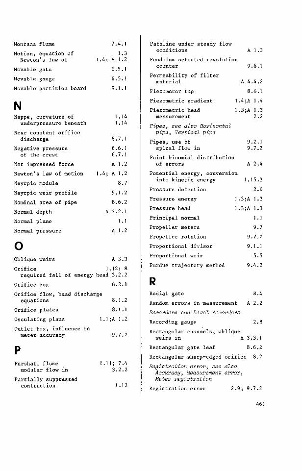
Montana flume 7.4.1
Motion, equation of Newton's law of
Movable gate
Movable gauge
Movable partition board
1.4; 1 .3
A 1.2
6.5.1
6.5.1
9.1.1
N Nappe, curvature of
underpressure beneath
Near constant orifice discharge
1.14 1.14
8.7.1
Negative pressure of the crest
Net impressed force
Newton's law of motion
Neyrpic module
Neyrpic weir profile
Nominal area of pipe
Normal depth
Normal plane
Normal pressure
6.6 6.7
A 1
1.4; A 1
8
9.1
8.6
A 3.2
1
A 1
I 1
2
2
7
2
2
1
1
2
Oblique weirs A 3.3
Orifice 1.12; 8
required fall of energy head 3.2.2
Orifice box 8.2.1
Orifice flow, head discharge
equations 8.1.2
Orifice plates 8.1.1
Osculating plane 1.1;A 1.2
Outlet box, influence on meter accuracy 9.7.2
Parshall flume 1.11; 7.4 modular flow in 3.2.2
Partially suppressed contraction 1.12
Pathline under steady flow conditions A 1.3
Pendulum actuated revolution counter 9.6.1
Permeability of filter material
Piezometer tap
Piezometric gradient
Piezometric head measurement
A
1.4
1 .3
4
8
,A
.A
4
6
1
1 2
2
1
4
3 2
Pipes, see also Horizontal pipe, Vertical pipe
Pipes, use of 9.2.1 spiral flow in 9.7.2
Point binomial distribution of errors A 2.4
Potential energy, conversion into kinetic energy
Pressure detection
Pressure energy
Pressure head
Principal normal
Propeller meters
Propeller rotation
Proportional divisor
Proportional weir
Purdue trajectory method
1 .3
1.3
1.15
2
;A 1
;A 1
1
9
9.7
9.1
5
9.4
.3
.6
.3
.3
.1
.7
.2
.1
5
.2
Radial gate 8.4
Random errors in measurement A 2.2
Reaorders see Level recorders
Recording gauge 2.8
Rectangular channels, oblique
weirs in A 3.3.1
Rectangular gate leaf 8.6.2
Rectangular sharp-edged orifice 8.2
Registration error, see also Aoeuraey', Measurement error, Meter registration
Registration error 2.9; 9.7.2
461
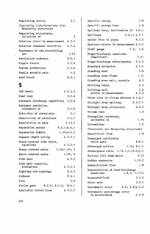
Regulating device 2.1
Regulating structures see also Measuring structures
Regulating structures,
selection of 3
Relative error in measurement A 2.3
Relative standard deviation A 2.4
Resonance of the overfalling jet
Revolution counters
Ripple factor
Riprap protection
Romijn movable weir.
Roof-block
1.13
9.6.1
3.2.6
A 4.4
4.2
8.5.1
SAF basin A 4.3.2
Sand trap 3.2.6
Sediment discharge capability 3.2.6
Sediment particles,
transport of 3.2.6
Selection of structures 3.1
Sensitivity of structure 3.2.4
Sensitivity of weir 1.13.7
Separation pocket 6.3.1 ;6.4.1
Separation bubble 1.10;4.4.1
Sequent depth rating A 4.3.1
Sharp-crested side weirs,
equations A 3.2.4
Sharp-crested weirs 1.10;1.13; 5
Short-crested weirs 1.10; 6
Side weir A 3.2 Side weir capacity,
evaluation
Sighting rod readings
Siphons
Slot
A 3.2.4
9.3.2
9.2.1
2.6
Sluice gate 8.2.1; 8.2.2; 9.6.1
Spatially varied flow A 3.2.2
Specific energy 1.8
Specific energy head 1.8
Spillway face, inclination of 6.6.1
Spillways 6.6.1; 6.7.1
Spiral flow in pipes 9.7.2
Spurious errors in measurement A 2.2
Staff gauge 2.5; 2.6
Stage-discharge equations
(empirical) 1.11
Stage-discharge relationship 6.5.2
Standard deviation A 2.4
Standing wave 1 .8
Standing wave flume 1.11
Standing wave weir, movable 6.5
Stilling basin A 4 Stilling well
errors in measurement 2.6
A 2.5
Stone size in riprap mixture A 4.4.1
Straight drop spillway A 4.2.1
Straight drop structures A 4.2
Stream tube 1.2
Streamline curvature,
influence of 1.10
Streamlines 1.2
Structures see Measuring structures
Subcritical flow 1.8
Submerged calibrated
valve gate 8.6.1
Submerged orifice 1.12; 8.1.1
Submergence ratio 1 .15.1 ; 1.15.2;2.4
Suction lift head meter 2.12
Sudden expansion 1.15.2
Supercritical flow 1.8
Superposition of head-discharge
equations 1.9.5; 1.13.4
Suspended-load 3.2.6
Sutro weir 5.5.1
Systematic error 2.6; 2.9;A 2.2
Systematic percentage error in measurement A 2.8
462
Tailwater channel 2.1; 2.4
Tailwater level 2.1; 2.4
Tailwater measurement 2.4
Tainter gate 8.4
Tape index pointer 2.8
Thomson weir 5.2.1
Throat of the flume 1.11
Throatless flumes 7.2; 7.3
Torricelli's equation 1.13
Total energy head 1.3; A 1.3
Total energy head of an open channel
Total-load equation
Trajectory method
Transition reach
Transport parameter
1.6
3.2.6
9.4.2
1.15.2
3.2.6
Trapezoidal channels, oblique
weirs in A 3.3.2
Trash rack 3.2.7
Triangular broad-crested weir 4.3 Triangular profile flat-V
weir
Triangular profile weir
Truncated Parshall flume
Truncated transition
Truncation, point of
Truncation of downstream expansion
Tube-float differential head meter
Turnout gate
u Undershot gates 3.2.2
Undershot water wheel 9.6.1
Undular jump 1.8
Uniform distribution of errors A 2.4
Upstream channel, minimum water level in 3.2.9
Upstream energy head over the crest 1.9; 2.1
Upstream rounded nose, minimum radius of 4.1.1
Upstream spillway face, inclination of 6.6.1
Upstream water level (over the crest) 1.9.1
USBR basin A 4.2.2
Valve gate 8.6.1
Vapour pressure 1.10
Velocity above the weir crest 1.10
Velocity coefficient 1.6; 1.9.1
Velocity distribution 1-4; 1.6
Velocity head 1.3; A 1.3
Velocity profile, influence on registration
Vena contracta
Ventilation pipe
Venturi flume
9.7.2
1.12; 5.5.2
8.3.1
7
6.4
6.3
7.4.1
.15.3
6.3.1
7.2.2
2.12
8.3.1
o o o
Vertical pipe, flow from
V-notch sharp-crested weir
V-notch weir sill
Volume of irrigation water, measuring
w Wash-load
Water level, registration error
Water surface along side weir
Water wheel
9
3
A 3
9
9
5
6
.6
.2
2
2
6
3
2
2
1
6
9
2
1
Weir see also Broad-orested weir, Short-crested weir, Sharp-orested weir
463
Weir, aeration demand 1.14 required fall of energy head 3.2.2 sensitivity 1.13.7
Weir block, truncation of permissible truncation
Weir constant
Weir face, inclination of
Weir flow from vertical pipe 9.3.1
6 . 3 . 6 .4 .
1.13.
6 .6 .
1 1
7
1
Weir notch angle
Weir sill
WES-spillway
4.3.1 ; 4.3.4
6.1
1.10; 6.6
Zero-setting 2.1
464 * it * , -v . • •••*


