I

Centre for Geo-Information

Thesis Report GIRS-2008-20

Application of continuum removal technique to the water absorption features in the NIR region to estimate canopy water content

Taeibah Abdi

DE

CE

MB

ER

200

8

II

III

Application of the continuum removal technique to the water absorption features in the NIR region to estimate canopy water content

Taeibah Abdi

Registration number 800827-003-080

Supervisors:

dr. ir. J. Clevers

dr. ir. L. Kooistra

A thesis submitted in partial fulfilment of the degree of Master of Science

at Wageningen University and Research Centre,

The Netherlands.

December 2008

Wageningen, the Netherlands

Thesis code number: GRS-80439 Thesis Report: GIRS-2008-20 Wageningen University and Research Centre Laboratory of Geo-information Science and Remote Sensing

IV

V

Foreword This Report is my MSc thesis done as part of the Master of Science in Geo-Information Science (MGI) at the Wageningen University. The report is about application of the continuum removal technique to the water absorption features in NIR. My deep appreciation goes to my supervisors Dr. Jan Clevers and Dr. Lammert Kooistra for their invaluable encouragements, ideas, suggestions and patience during my research work. Without their advice and support this thesis would never have become feasible. I would like to extend my special thanks to my husband Hadi and daughter Mozhdeh for their courage and support during the entire period of my thesis work. Taeibah Abdi, December 2008

VI

Table of content: ABSTRACT............................................................................................................................... 1

1 INTRODUCTION.............................................................................................................. 2

1.1 Background ................................................................................................................... 2

1.2 Problem definition........................................................................................................ 3

1.3 Research objective........................................................................................................ 4

1.4 Research questions ....................................................................................................... 4

1.5 Report outline................................................................................................................ 4

2 LITERATURE REVIEW.................................................................................................... 5

2.1 Overview – CWC estimation ...................................................................................... 5

2.2 Spectral indices ........................................................................................................... 5

2.4 First derivative of spectra............................................................................................ 6

2.5 Continuum removal..................................................................................................... 7

3 MATERIALS AND METHOD ......................................................................................... 9

3.1 Study area.................................................................................................................... 9

3.2 DATA........................................................................................................................ 10

3.2.1 Field spectroradiometer measurements.............................................................. 10

3.2.2 Biomass .............................................................................................................. 15

3.2.3 Airborne image................................................................................................... 15

3.3 Conceptual model...................................................................................................... 16

3.4 Statistical evaluation of results....................................................................................... 17

4 RESULT................................................................................................................................ 19

4.1 FW, DW and CWC estimation using Continuum removal indicators ........................... 19

4.1.1 Continuum Removal Indices of FieldSpec Measurement....................................... 20

4.1.2 Continuum Removal Indices of HyMap image in 2004 ......................................... 28

4.2 Water Band Index........................................................................................................... 30

4.3 Water Band Index across spectrum (WBIxxx) .............................................................. 31

4.4 Normalized difference water index ................................................................................ 32

4.5 First derivative of spectra............................................................................................... 32

5 DISCUSSION ....................................................................................................................... 34

6 CONCLUSION AND RECOMMENDATION.................................................................... 38

6.1 Conclusion...................................................................................................................... 38

6.2 Recommendation............................................................................................................ 38

VII

List of figures Figure 1: Example of two spectral signatures of Millingerwaard plots measured with the ASD

FieldSpec Pro. .................................................................................................................... 3 Figure 2. Example spectrum of grassland:(a) reflectance spectrum with continuum lines (b)

continuum removed reflectance spectrum.......................................................................... 7 Figure 3.1: Location and current land use for the floodplain Millingerwaard along the river

Rhine in the Netherlands. ................................................................................................... 9 Figure 3.2: Location of Achterhoek in the Netherlands........................................................... 10 Figure 3.4: Experimental set-up of sampling plot according to VALERI-protocol................. 11 Figure 3.5: Ground based measurements for radiometric corrections and spectral

characterization of vegetation within the Millingerwaard floodplain. ............................. 12 Figure 3.7: Example of first 20 FieldSpec measurements in the vegetation plots at site in 2008 .............................................................................................................................. 14 Figure 3.8: Example of second 20 FieldSpec measurements in the vegetation plots at

Korenburgerveen site in 2008 .......................................................................................... 14 Figure 3.9: Example of 21 spectral signatures as derived from HyMap image for the

Millingerwaard test area in 2004...................................................................................... 16 Figure 3.10: Conceptual model indicates connection in research strategies for CWC

estimation ......................................................................................................................... 17 Figure 4.1 Comparison of coefficient of determination between dry weight and continuum

removal indices based on FieldSpec measurements in 2004 in Millingerwaard site, considering different intervals.......................................................................................... 20

Figure 4.2 Coefficient of determination between biomass and continuum removal indices in different intervals at water absorption feature 970nm in Millingerwaard in 2005. a) FW, b) DW and c) CWC.......................................................................................................... 22

Figure 4.3 Coefficient of determination between biomass and continuum removal indices in different intervals at water absorption feature 1200nm in Millingerwaard in 2005. a) FW, b) DW and c) CWC.......................................................................................................... 23

Figure 4.4 Coefficient of determination between biomass and continuum removal indices in different intervals at water absorption feature 970nm in Korenburgerveen in 2008. a) FW, b) DW and c) CWC.................................................................................................. 25

Figure 4.5 Coefficient of determination between biomass and continuum removal indices in different intervals at water absorption feature 1200nm in Korenburgerveen in 2008. (a) FW, (b) DW, (c) CWC..................................................................................................... 26

Figure 4.6 Coefficient of Determinations between DW and continuum removal indices in two different intervals around 970 nm for HyMap image in 2004. ........................................ 28

Figure 4.7 Coefficient of Determinations between DW and continuum removal indices in two different intervals around 1200 nm for HyMap image in 2004. ...................................... 29

Figure 4.8 Coefficient of determination between biomass and WIxxx.................................... 31 Figure4.9 Coefficient of determination between canopy biophysical variables and first

derivative of canopy reflectance. .................................................................................... 33 Figure 5.1 Frequency of DW in three data sets........................................................................ 34 Figure 5.2 Fresh weights as a function of NDVI in a) Millingerwaard in 2005, b)

Korenburgerven in 2008................................................................................................... 35 Figure 5.3 Canopy water content as a function of MBD at water absorption feature 970 nm.

a) Millingerwaard in 2005, b) Korenburgerveen in 2008....................................................... 38

VIII

List of tables: Table4.1 Continuum start and end point definition for the water absorption feature at 970 nm

and 1200 nm in the reflectance spectra of vegetation in Millingerwaard 2005. .............. 19 Table4.2 Correlation coefficient of DW and continuum removal indices at water absorption

feature 970 nm on FieldSpec measurements in 2004 in Millingerwaard site. ................. 21 Table4.3 Correlation coefficient of DW and continuum removal indices at water absorption

feature 1200 nm on FieldSpec measurements in 2004 in Millingerwaard site. ............... 21 Table4.4 Correlation coefficient of CWC and continuum removal indices at water absorption

feature 970 nm on FieldSpec measurements in 2005 in Millingerwaard site .................. 24 Table4.5 Correlation coefficient of CWC and continuum removal indices at water absorption

feature 1200 nm on FieldSpec measurements in 2005 in Millingerwaard site ................ 24 Table4.6 Correlation coefficients of CWC and continuum removal indices at water absorption

feature 970 nm on FieldSpec measurements in 2008 in Korenburgerven site................. 27 Table4.7 Correlation coefficients of CWC and continuum removal indices at water absorption

feature 1200 nm on FieldSpec measurements in 2008 in Korenburgerven site............... 27 Table4.8 Correlation coefficient of DW and continuum removal indices at water absorption

feature 970 nm and 1200 nm on HyMap image considering only one pixel in Millingerwaard site in 2004. ............................................................................................ 30

Table4.9 Correlation coefficient of DW and continuum removal indices at water absorption features 970 nm and 1200 nm on HyMap image considering 3 by 3 pixels in Millingerwaard site in 2004. ........................................................................................... 30

Table 4.10 Correlation coefficient of biomass and WBI in three FieldSpec measurements and HyMap dataset.................................................................................................................. 30

Table 4.11 Maximum Correlation coefficient of biomass and WBIxxx in three FieldSpec measurements ................................................................................................................... 31

Table 4.12 coefficient of Correlation between biomass and NDWI in each dataset. .............. 32 Table5.1 results for the indices tested in estimating canopy water content (site2 and 3) or just

dry weight (site1) as shown by the coefficient of determination (R2). ............................ 36

IX

ABBREVIATIONS: CWC Canopy water content

WBI Water band index

NDWI Normalized difference water index

NDVI Normalized difference vegetation index

NDII Normalized Difference Infrared Index

MSI Moisture Stress Index

EWT Equivalent water thickness

FW Fresh weight

DW Dry weight

BD Band depth

Dc Band center

NBD Normalized band depth

MBD Maximum band depth

AUC Area under continuum

NIR Near infrared

VALERI Validation of Land European Remote sensing Instruments Df Degrees of freedom

1

ABSTRACT

Biogeochemical processes in plants, such as photosynthesis, evaporation and net primary production, are directly related to foliar water. Therefore, the canopy water content (CWC) is important for understanding of the terrestrial ecosystem functioning. Spectral information related to the water absorption features at 970 nm and 1200 nm offers possibilities for deriving information on CWC. The objective of this study was to find which interval around the water absorption features at 970 nm and 1200 nm should be selected to apply the continuum removal technique for estimating CWC and biomass, and which index or indices based on the continuum removal technique are stronger on estimation canopy biophysical variables and finally compare the results of the continuum removal to those based on spectral indices and derivative spectra. The feasibility of using information from the water absorption features in the near-infrared (NIR) region of the spectrum was tested by estimating canopy water content for two test sites with different canopy structure. The first site is a heterogeneous natural area in the floodplain Millingerwaard along the river Waal in the Netherlands. The other site is an extensively managed grasslands which is located as a buffer zone around a central rewetted bog ecosystem in the Achterhoek near Winterswijk. Spectral information at both test sites was obtained with an ASD FieldSpec spectrometer, whereas at the first site HyMap airborne imaging spectrometer data were also acquired. Based on these datasets the best interval to apply the continuum removal technique at these water absorption features is the broader one which includes the whole absorption feature at 970 and 1200 nm. Results yielded that maximum band depth (MBD) and area under the curve (AUC) have clearly stronger correlation with biophysical variables than other continuum removal indicators at both water absorption features in the NIR region in a homogeneous area, while MBD/AUC and AUC/MBD at 970 nm have higher correlation with canopy biophysical variables in a heterogeneous area. Result also showed that the first derivative of spectra is better than indices derived from the continuum removal and WBI and NDWI on estimation of canopy biophysical variables in a heterogeneous area and MBD and AUC based on the continuum removal technique in a homogeneous area yielded a stronger effect on estimation of canopy biophysical variables. Key words: Canopy water content, fresh weight, dry weight, Field spectrometer, Continuum removal technique, Derivative spectra, Spectral indices, Remote sensing

2

1 INTRODUCTION

1.1 Background Currently one of the main scientific issues is to understand and quantify the impact of global climate change on the Earth system. One of the challenges of the coming decades is the understanding of the role of terrestrial ecosystems and the changes they may undergo. The water cycle is one of its most important characteristics (ESA, 2006). In this respect, the canopy water content is of interest in many applications. Estimates of vegetation water content are of interest for assessing vegetation water status in agriculture and forestry (Gao, 1996; Gao & Goetz, 1995; Penuelas et al., 1997; Ustin et al., 2004a,b, 1998; Zarco-Tejada et al., 2003), and have been used for drought assessment (Penuelas et al., 1993) and prediction of susceptibility to wildfire (Chuvieco et al., 2004; Riano et al., 2005; Ustin et al., 1998). Thus, canopy water content is important for the understanding of the functioning of the terrestrial ecosystem (Running & Coughlan, 1988).

Water absorption features as a result of absorption by O-H bonds in water can be found at approximately 970, 1200, 1450 and 1950 nm (Curran, 1989). The features at 1450 and 1950 nm are most pronounced. However, in those spectral bands atmospheric absorption by water vapor is that strong that hardly any radiation is reaching the Earth surface. As a result, those bands will result in very noisy measurements and should not be used for remote sensing. The features at 970 and 1200 nm are not that pronounced, but still clearly observable (Danson et al., 1992; Sims & Gamon, 2003). Therefore, these offer interesting possibilities for deriving information on leaf and canopy water content. However, in these regions also minor absorption features due to atmospheric water vapor occur at 940 and 1140 nm (lqbal, 1983). These are shifted somewhat to shorter wavelengths in comparison to the liquid water bands caused by water in the canopy. Figure 1 illustrates water absorption features in the infrared region for some spectral measurements on natural vegetation plots. The position of the liquid water absorption features at 970 nm and 1200 nm are indicated.

3

ASD Fieldspec Pro

0

0.1

0.2

0.3

0.4

0.5

0.6

0 500 1000 1500 2000 2500 3000

Wavelength (nm)

Ref

lect

ance

Figure 1: Example of two spectral signatures of Millingerwaard plots measured with the ASD FieldSpec Pro.

1.2 Problem definition For quantifying the water content, at the canopy level the canopy water content (CWC) can be defined as the quantity of water per unit area of ground surface and thus can be given in g m-2 (Ceccato et al., 2002) or in kgm-2 by converting EWT to the appropriate units:

CWC = EWTLAI × (1)

Where EWT is the equivalent water thickness and defined as the quantity of water per unit leaf area in g cm-2 (Danson et al., 1992).

Another way of calculating CWC is by taking the difference between fresh weight (FW in kg m-2) and dry weight (DW in kg m-2): CWC = FW – DW (2)

Various approaches have been developed for estimation of water content in plants. These can be divided broadly into spectral indices and techniques based on the inversion of radiative transfer models. Water content sensitive spectral indices are typically combinations between reflectance at wavelengths where water absorbs energy at different magnitudes. Spectral indices that have been developed using these water bands are: Water Band Index (WBI), Water Band Index normalized with NDVI (WBI/NDVI), and Normalized Difference Water Index (NDWI). Also the first derivative of the spectral signature has been used in the NIR region. Most of these indices are similar to those which have been applied in the red-edge spectral region to estimate chlorophyll content such as Simple Ratio and the Normalized Difference Vegetation Index (Rouse et al., 1973; Tucker 1979; Sellers 1985). Continuum removal techniques also have been applied in the red-edge spectral region. However, there have been surprisingly few studies that have applied this technique to the water absorption features in the NIR region and examined the relationships between canopy water content and indicators derived from the continuum removal technique.

4

1.3 Research objective The aim of this thesis is to apply the continuum removal technique to the water absorption features in the NIR region to estimate canopy water content and biomass. Aim is also to compare the results of the continuum removal to those based on other approaches such as WBI, NDWI and first derivative spectra.

1.4 Research questions 1) Which spectral interval should be used to apply the continuum removal technique to the

water absorption features at 970 nm and 1200 nm?

2) Which index based on the continuum removal technique (maximum band depth, area under the curve or MBD/ Area) is best for estimating canopy water content?

3) Are these results more accurate than WBI, NDWI, and first derivative of spectra?

1.5 Report outline The general background information of the research was introduced in chapter one. This includes the problem definition, research objectives, research questions, and report outline. Chapter two reviews available methods for CWC estimation. Chapter three includes study area and data which have been available. The implementation of the continuum removal technique and previous methods is discussed in Chapter four. Chapter five presents the results of the application of the new method, continuum removal, and other methods on the Millingerwaard and Achterhoek areas. Chapter five discusses the results with regard to the research questions. Finally, chapter 6 lists the conclusions and recommendations raised from the study. The appendices are given at the end of the report.

5

2 LITERATURE REVIEW

2.1 Overview – CWC estimation Because water has several absorption maxima throughout the infrared region of the spectrum (Palmer & Williams, 1974), quite a number of different spectral indices based on a ratio, or some other simple mathematical formula of reflectance at two or more wavelengths (Ceccato et al., 2002; Gao & Goetz, 1995; Gao, 1996; Penuelas et al., 1993; Serrano et al., 2000; Ustin et al., 1998).), first derivative of spectral reflectance (Clevers & Kooistra, 2006), and continuum removal techniques (Tian et al., 2001) have been developed for estimation of water content.

2.2 Spectral indices 2.3.1 Water Band Index

The simplest water index is a ratio between reflectance at a reference wavelength where water does not absorb and a wavelength where water does absorb. One example of this is the water band index (WBI). The Water Band Index is a reflectance measurement that is sensitive to changes in canopy water status. As the water content of vegetation canopies increases, the strength of the absorption around 970 nm increases relative to that of 900 nm (Penuelas et al. 1993; Champagne et al. 2001). WBI is defined by the following equation:

970

900

ρρ=WBI (3)

Where ρ 900 and ρ 970 are the spectral reflectance at 900 and 970 nm, respectively. The common rang for green vegetation is 0.8 to 1.2.

Sims and Gamon (2003) generalized WBIxxx, which is defined by the equation (4). This water band index tests the effect of variation in the strength of light absorption by water across the spectrum:

xxxWBIxxx

ρρ900= (4)

Where the reference wavelength is held constant at 900 nm but the index wavelength (xxx) is varied.

2.3.3 Normalized Difference Water Index

The Normalized Difference Water Index (NDWI) is sensitive to changes in vegetation canopy water content because reflectance at 860 nm and 1240 nm has similar but slightly different liquid water absorption properties. The scattering of light by vegetation canopies enhances the weak liquid water absorption at 1240 nm. Applications include forest canopy stress analysis, leaf area index studies in densely foliated vegetation, plant productivity modeling, and fire susceptibility studies (Gao, 1996). NDWI is defined by the following equation:

1240860

1240860

ρρρρ

+−=NDWI (5)

6

Where 860ρ and 1240ρ are the spectral reflectance at 860 and 1240 nm, respectively. The value of this index ranges from -1 to 1. The common range for green vegetation is -0.1 to 0.4.

2.3.4 Moisture Stress Index

The Moisture Stress Index (MSI) is a reflectance measurement that is sensitive to increasing leaf water content. As the water content of leaves in vegetation canopies increases, the strength of the absorption around 1599 nm increases. Absorption at 819 nm is nearly unaffected by changing water content, so it is used as the reference. Applications include canopy stress analysis, productivity prediction and modeling, fire hazard condition analysis, and studies of ecosystem physiology. The MSI is inverted relative to the other water VIs; higher values indicate greater water stress and less water content (Hunt et al. 1989; Ceccato et al. 2002). MSI is defined by the following equation:

819

1599

ρρ=MSI (6)

The value of this index ranges from 0 to more than 3. The common range for green vegetation is 0.4 to 2.

2.3.5 Normalized Difference Infrared Index

The Normalized Difference Infrared Index (NDII) is a reflectance measurement that is sensitive to changes in water content of plant canopies. The NDII uses a normalized difference formulation instead of a simple ratio, and the index values increase with increasing water content. Applications include crop agricultural management, forest canopy monitoring, and vegetation stress detection (Hardisky et al., 1983; Jackson et al. 2004). NDII is defined by the following equation:

NDII = 1649819

1649819

ρρρρ

+−

(7)

The value of this index ranges from -1 to 1. The common range for green vegetation is 0.02 to 0.6.

2.4 First derivative of spectra First derivative of the reflectance spectrum corresponds to the slopes of the absorption features. It’s defined by the following equation:

First derivative of spectra at (λ +0.5) = λλρρ λλ

−+−+

1

1 (8)

Where λ refers to channels in the absorption feature. It provides better correlation with leaf water content than those obtained from the direct correlation with reflectance (Clevers & Kooistra, 2006).

7

2.5 Continuum removal The continuum is an estimate of the other absorptions present in the spectrum, not including the one of interest (figure 2a). Once the continuum line is established, continuum-removed spectra for the absorption features are calculated by dividing the original reflectance spectrum by the corresponding reflectance of the continuum line (Figure 2b).

Reflectance Spectra

0

0.1

0.2

0.3

0.4

0.5

0.6

0.7

400 900 1400 1900 2400

Wavelength (nm)

Ref

lect

ance

a)

Continuum Removal Spectra

0.8

0.85

0.9

0.95

1

1.05

400 900 1400 1900 2400

Wavelength (nm)

Co

nti

nu

um

Rem

ove

d

Ref

lect

ance

b) Figure 2. Example spectrum of grassland:

(a) Reflectance spectrum with continuum lines

(b) Continuum removed reflectance spectrum

8

From the continuum-removed reflectance, the band depth (D) for each channel in the absorption feature was computed by:

'1 RD −= (9) Where 'R is the continuum-removed reflectance (Clark & Roush, 1984). After computing band depth, maximum band depth, area under the curve, maximum band depth normalized to the area under the curve and area under the curve normalized to the maximum band depth will be calculated according to following formulas:

}max{ λDMBD = (10)

∑= λDAUC (11)

Whereλ refers to channels in the absorption feature. Reflectance spectra of vegetation canopies vary with changing leaf water but remote sensing measurements are also affected by atmospheric absorption, the size of leaf cells, the abundance of other absorbers in the leaf (such as biochemistry), and the fractional area coverage of leaves in heterogeneous landscapes. Therefore, analytical methods for estimation of plant water must overcome any sensitivity to these extraneous factors. Normalization of continuum-removed reflectance spectra minimizes these influences. The normalized band-depth (Dn) at all wavelengths within the continuum-removed absorption feature is calculated by dividing the band-depth of each channel by the band-depth at the band center (Dc):

Dc

DDn = (12)

Where the band center is the minimum of the continuum-removed absorption feature. Variations of Dn with wavelength describe the shape of the absorption feature. Resulting differences in the shapes of absorption features between samples are correlated to foliar water.

9

3 MATERIALS AND METHOD

3.1 Study area The first study site is a heterogeneous natural area in the floodplain Millingerwaard along the river Waal in the Netherlands. The floodplain Millingerwaard is part of the Gelderse Poort nature reserve (Figure 3). This is a nature rehabilitation area, meaning that individual floodplains are taken out of agricultural production and are allowed to undergo natural succession. This has resulted in a heterogeneous landscape with river dunes along the river, a large softwood forest in the eastern part along the winter dike and in the intermediate area a mosaic pattern of different succession stages (pioneer, grassland, shrubs). To stimulate the development of a heterogeneous landscape, a low grazing density of 1 animal (e.g., Galloway, Koniks) per 2-4 ha has been chosen. This density allows grazing whole year round and also development of forest is possible. The surface area of water changes over the year. During high floods, the whole floodplain except for the higher parts of the river dunes is flooded. Due to the variability in elevation, some lower areas will be flooded for a relatively long period.

Figure 3.1: Location and current land use for the floodplain Millingerwaard along the river Rhine in the Netherlands.

10

The second study site is a managed grassland in the Achterhoek in the Netherlands. In the Netherlands several Natura2000 sites have been identified, amongst these is the Korenburgerveen in the Achterhoek near Winterswijk. The Korenburgerveen is a rewetted bog ecosystem with an area of 509 ha consisting of the following habitat types: raised bog, swamp forest, heath land, and extensively used grasslands. In this thesis focus will be on the structure and functioning of the extensively managed grasslands which are located as a buffer zone around the central rewetted bog ecosystem. The grasslands have been gradually taken out of agricultural production and are grazed extensively. Nature managers are interested in the development of the quality of the grasslands over time as under the right conditions valuable habitat types like ‘blauwgraslanden’ could develop.

Figure 3.2: Location of the Achterhoek in the Netherlands.

3.2 DATA

3.2.1 Field spectroradiometer measurements On July 28th, 2004, a field campaign with an ASD FieldSpec Pro FR spectroradiometer was performed at site 1 (Millingerwaard). Within 21 square areas of 5 m by 5m centered at each plot 10 spectral measurements were performed, whereby each measurement was the average of 50 readings at the same spot. The area for the spectral measurements (5 m by 5 m) was larger than the one for the destructive sampling (2 m by 2 m). Measurement height was about 1.5 m. Since vegetation height varied for the different plant functional types, the distance between instrument aperture and canopy also varied. A spectralon white reference panel was used for calibration.

11

For one location only sand was erroneously measured, not the vegetation. Preliminary analysis of the data for this test site showed that four plots, which were influenced by heavy grazing and as a result had a very low but dense grass sward, had a deviating relationship between spectral indices and biomass (Kooistra et al., 2006; Schaepman et al., 2007). These were grouped as a distinct plant functional type and omitted from this study. As a result, 16 plots remained for further analysis. Figure 3.3 gives an overview of all measurements performed on 28 July 2004 over the vegetation plots.

16

18

0

0.1

0.2

0.3

0.4

0.5

0.6

0.7

400

800

1200

1600

2000

2400

wavelength (nm)

Ref

lect

ance

2

3

4

5

6

7

8

9

10

11

12

13

14

15

16

17

18

19

20

21

22

Figure 3.3: Example of 21 FieldSpec measurements in the vegetation plots at Millingerwaard site in 2004 On June 19th, 2005, another field campaign with an ASD FieldSpec Pro FR spectroradiometer was performed at site 1 (Millingerwaard). Within a square area of 20m-20m centered at each plot 12 measurements were performed according to the VALERI sampling scheme (figure 3.4). Every point has a letter associated to it. Each measurement was the average of 15 readings at the same spot. Measurement height was about 1 m above the vegetation.

Figure 3.4: Experimental set-up of a sampling plot according to the VALERI-protocol

(www.avignon.inra.fr/valeri/).

12

A description of the vegetation was made for 14 vegetation plots (20 x 20 m) that were also radiometrically characterized. Locations of the plots are shown in Figure 3.5.

Figure 3.5: Ground based measurements for radiometric corrections and spectral characterization of vegetation within the Millingerwaard floodplain (2005).

After calculating average spectra per plot in 2004 and 2005, the resulting spectra were smoothed using a 15 nm wide moving Savitsky-Golay filter (applying a second order polynomial fit within the window) to reduce instrument noise. Figure 3.6 gives an overview of the measurements performed on 19 June 2005 over the vegetation plots in the Millingerwaard.

13

0

0.1

0.2

0.3

0.4

0.5

0.6

0.7

400 900 1400 1900 2400

Wavelength (nm)

Ref

lect

ance

1

2

3

4

5

6

7

8

9

10

11

12

13

14

Figure 3.6: Example of 14 FieldSpec measurements in the vegetation plots at the Millingerwaard site in 2005

On June 8th and 9th, 2008, a field campaign with an ASD FieldSpec Pro FR spectroradiometer was performed at test site 2 (Korenburgerveen). Within a square area of 3m by 3m centered at each plot 12 measurements were performed. So, the area for the spectral measurements (3 m by 3 m) was larger than the one for the destructive sampling (2m by 2 m). Measurement height was about 1 m. Since vegetation height varied for the different plant functional types, the distance between instrument aperture and canopy also varied. Figure 3.7 and 3.8 give an overview of the measurements performed on 8 and 9 June 2008 over the vegetation plots. Preliminary analysis of the data for this test site showed that plot 25, which was influenced by heavy grazing and as a result had a very low but dense grass sward, had a deviating relationship between spectral indices and biomass. This was omitted from this study. As a result, 39 plots remained for further analysis. In these three data sets a spectralon white reference panel was used for calibration.

14

0

0.1

0.2

0.3

0.4

0.5

0.6

0.7

0.8

0 500 1000 1500 2000 2500

Wavelength (nm)

Ref

lect

ance

1234567891011121314151617181920

Figure 3.7: Example of first 20 FieldSpec measurements in the vegetation plots at the Korenburgerveen site in 2008.

25

0

0.1

0.2

0.3

0.4

0.5

0.6

0 500 1000 1500 2000 2500 3000

Wavelength (nm)

Ref

lect

ance

21

22

23

24

25

26

27

28

29

30

31

32

33

34

35

36

37

38

39

40

Figure 3.8: Example of second 20 FieldSpec measurements in the vegetation plots at the Korenburgerveen site in 2008.

15

3.2.2 Biomass Vegetation biomass was sampled in three subplots with a relatively homogeneous vegetation cover measuring 0.5 x 0.5 m, located within the VALERI-plots. Biomass was clipped at 0.5 cm above the ground level and stored in paper bags. The collected material was weighted for fresh biomass. Subsequently, the average fresh biomass per plot was calculated, and then it was dried for 24 h at 70ºC, After drying for 24 hours at 70°C, vegetation dry matter weight was determined. Subsequently, the average dry biomass per plot was calculated. Unfortunately, no fresh weight was measured in 2004, so canopy water content could not be determined. In order to make comparisons with data set in 2005, we assumed a dry matter content of 30% for all plots based on measurements done in 2005. Values for the measured fresh and dry weight per sample in 2005 are presented in appendix 3 and average values per plot are presented in appendix 4. Plot 11 and 13 were not harvested in 2005 due to the presence of large shrubs of Sambucus nigra. Values for the measured dry weight per plot in 2004 are presented in appendix 5. Values for the measured fresh and dry weight per sample and per plot in the Korenburgerveen in 2008 are presented in appendix 6 and 7.

3.2.3 Airborne image On July 28th, 2004, airborne imaging spectrometry data were collected from an altitude of 2300 m (a.s.l.) using the HyMap sensor (Integrated Spectronics, Australia) onboard a Dornier DO-228 aircraft operated by the German Aerospace Centre DLR for test site 1 (Millingerwaard). Complete spectra over the range of 450–2480 nm were recorded with a bandwidth of 15–20 nm by 4 spectrographic modules. Each module provided 32 spectral channels giving a total of 128 spectral measurements for each pixel. However, the delivered data contained 126 bands because the first and last bands of the first spectrometer were deleted during pre-processing. Ground resolution of the images was 5 m. The flight line was oriented close to the solar principal plane to minimize directional effects. The HyMap images were geo-atmospherically processed with the modules PARGE and ATCOR4 to obtain geocoded surface reflectance data (Richter & Schlapfer, 2002; Schlapfer & Richter, 2002), approximating hemispherical directional reflectance factors (HDRF) (Schaepman-Strub et al., 2006). Visibility was estimated by combining sun photometer measurements with Modtran4 radiative transfer simulation following the approach of Keller (2001). Finally, spectral signatures were derived for the pixels matching the locations of the 21 plots defined in the field. Again, the four plots with the distinct plant functional type, being influenced by heavy grazing, showed a deviating relationship between spectral indices and biomass. The plot measured as sand with the FieldSpec could be analyzed correctly in the HyMap image. As a result, 17 plots remained for further analysis. Figure 3.9 gives an overview of the 21 spectral signatures using the HyMap image.

16

0

0.1

0.2

0.3

0.4

0.5

0.6

0.7

400 800 1200 1600 2000 2400

wavelength (nm)

Ref

lect

ance

2345678910111213141516171819202122

Figure 3.9: Example of 21 spectral signatures as derived from the HyMap image for the Millingerwaard test area in 2004.

3.3 Conceptual model Several literature sources have published different methods to estimate CWC (Hardisky et al., 1983; Hunt et al. 1989; Penuelas et al. 1993; Gao, 1996; Champagne et al. 2001; Jackson et al. 2004). The thesis aims to adapt the continuum removal technique in the estimation of CWC and compare results based on this technique to those based on WI, NDWI and first derivative of the spectral signature. Figure 3.10 summarizes the approach used for applying the continuum removal technique to the water absorption features in the NIR region to estimate CWC. This conceptual model also included the comparison of derived results with results based on WI, NDWI and first derivative of the spectral signature.

17

Figure 3.10: Conceptual model indicates connection in research strategies for CWC estimation

3.4 Statistical evaluation of results The quantity r, called the linear correlation coefficient, measures the strength and the direction of a linear relationship between two variables. In this thesis the correlation coefficient between biomass and continuum removal indices over several intervals, WBI, WBIxxx, NDWI and first derivative is calculated. The mathematical formula for computing r is:

(13) Where n is the number of pairs of data

The value of r is such that -1 < r < +1. The + and – signs are used for positive linear correlations and negative linear correlations, respectively.

The coefficient of determination, r2, is useful because it gives the proportion of the variance (fluctuation) of one variable (FW, DW and CWC) that is predictable from the

18

indices. It is a measure that allows us to determine how certain one can be in making predictions from a certain model/graph. The coefficient of determination is the ratio of the explained variation to the total variation.

In the next step, it should be checked whether the correlation coefficient is significant. We have set the α level at 0.05. In order to determine if the r value we found with our sample meets that requirement, it will be used a critical value table for Pearson’s Correlation Coefficient (see appendix 9). First degrees of freedom (df) must be determined. For a correlation study, the degree of freedom is equal to 2 less than the number of subjects. By using the critical value table it would be found the intersection of α .05 and related degrees of freedom. Then it should be discovered whether there is a statistically significant difference between coefficient of the correlation values between biomass and indices based on the continuum removal technique over different intervals. To reach this purpose the following steps have been followed:

- Make a model for biophysical variables based on each continuum removal index. - Calculate the estimated biophysical variable based on that model. - Calculate the difference between the measured and estimated value for biophysical

variable per interval (e1, e2, e3 ... e9 at water absorption feature 970 nm and e1, e2, e3… e15 at water absorption 1200 nm).

- Calculate the difference between error of the first interval and the other intervals (e1-e2, e1-e3, e1-e4…).

- Use T-test with α 0.05.

This procedure is used to answer questions such as: is the effect of MBD stronger than AUC for the estimation of biomass? This is used to check the difference between two dependent correlations, thus, from a single sample. This procedure allows seeing if two correlations in a triangle are statistically significantly different. We have to put three correlations in the r1, r2, r3 boxes, respectively. These three correlations have to form a triangle: they must be rxy, rzy and rxz. Give the sample size in the bottom (N2) box. Finally a number of confidence intervals around the difference between the two correlations and p-values are produced (see appendix 10).

19

4 RESULT Since the main component of living green vegetation is water, in general fresh weight, dry weight and water content will show a strong association (Rollin and Milton, 1998). So in this thesis the relationship between these three variables and indices was computed and analyzed.

4.1 FW, DW and CWC estimation using Continuum remov al indicators To investigate which interval is suitable for applying the continuum removal technique to the water absorption features in the NIR region it is reasonable to start with broad intervals which include the whole absorption features around 970 nm (920 nm – 1080 nm) and 1200 nm (1080 nm-1280nm). Once the continuum lines around 970 nm and 1200 nm were established separately, continuum-removed spectra were calculated by dividing the original reflectance spectrum by the corresponding reflectance of the continuum line in these two water absorption features. From the continuum-removed reflectance, the band depth (BD) for each channel in the absorption feature and the band center, the minimum of the continuum-removed absorption feature, were computed.Then it was easy to find the maximum band depth (MBD) and also the area under the continuum (AUC) which is the sum of the band depth in all channels in the absorption feature. Subsequently, maximum band depth was normalized to the area under the continuum and also the area under the continuum was normalized to the maximum band depth. In the further steps, intervals around those water absorption features were decreased by 5 nm at both left and right side, and all the procedures were repeated. Table 4.1 shows one example of all intervals which were considered to apply the continuum removal technique to the water absorption features in the NIR region. Table 4.1 Continuum start and end point definition for the water absorption feature at 970 nm and 1200 nm in the reflectance spectra of vegetation in Millingerwaard 2005.

970 nm 1200 nm Step Continuum

Line Start (nm) Continuum Line End (nm)

Continuum Line Start (nm)

Continuum Line End (nm)

1 920 1080 1080 1280 2 925 1075 1085 1275 3 930 1070 1090 1270 4 935 1065 1095 1265 5 940 1060 1100 1260 6 945 1055 1105 1255 7 950 1050 1110 1250 8 955 1045 1115 1245 9 960 1040 1120 1240 10 1125 1235 11 1130 1230 12 1135 1225 13 1140 1220 14 1145 1215 15 1150 1210

20

4.1.1 Continuum Removal Indices of FieldSpec Measurement

Since fresh weight, dry weight and canopy water content are associated, it makes sense to relate indices based on the water absorption features also with dry weight for the FieldSpec measurements in 2004 (fresh weight and water content were not measured). Figure 4.1 shows the results of the coefficient of determination between dry weight and indices based on the continuum removal technique (MBD, AUC, MBD/AUC and AUC/MBD) over different intervals at water absorption features 970 nm and 1200 nm of vegetation plots measured with the ASD FieldSpec pro in Millingerwaard site in 2004. Figure 4.1 (a) shows a linear pattern. The maximum value of the coefficient of determination for MBD and AUC/MBD is 0.1, for AUC it is 0.08 and for MBD/AUC it is 0.16. All are located in the interval 960 nm to 1040 nm of the spectral signature. The minimum value of the coefficient of determination for MBD/AUC and AUC/MBD is 0.0 and for MBD it is 0.05 and for AUC it is 0.04. These are located in the interval 920 nm to 1080 nm of the spectral signature. This graph also shows some fluctuations in the coefficient of determination between DW and MAB/AUC and AUC/MBD over different intervals. Figure 4.2 (b) shows that the coefficient of determination between dry weight and MBD/AUC and AUC/MBD is zero over all intervals, The coefficient of determination between dry weight and MBD and AUC is 0.065 and is constant till interval 1125 nm to 1235 nm, then it increases to 0.09.

0

0.02

0.04

0.06

0.08

0.1

0.12

0.14

0.16

0.18

920-1080

925-1075

930-1070

935--1065

940-1060

945-1055

950-1050

955-1045

960-1040

Intervals (nm)

Coe

ffic

ient

of

Det

erm

inat

ion

MBD

AUC

MBD/AUC

AUC/MBD

0

0.02

0.04

0.06

0.08

0.1

0.12

0.14

0.16

0.18

1080-1280

1085-1275

1090-1270

1095-1265

1100-1260

1105-1255

1110-1250

1115-1245

1120-1240

1125-1235

1130-1230

1135-1225

1140-1220

1145-1215

1150-1210

Intervals (nm)

Coe

ffic

ient

of

Det

erm

inat

ion

MBD

AUC

MBD/AUC

AUC/MBD

(a) (b) Figure 4.1 Comparison of coefficient of determination between dry weight and continuum removal indices based on FieldSpec measurements in 2004 in Millingerwaard site, considering different intervals

(a) At water absorption feature 970 nm.

(b) At water absorption feature 1200 nm

Now it should be checked whether the correlation coefficient of DW and these indices over different intervals is significant. In this data set for 2004 degrees of freedom would be 14. By using the critical value table (see appendix 9) it would be found the intersection of α .05 and 14 degrees of freedom. The value found at the intersection (.497) is the minimum correlation coefficient r that we would need to confidently state 95 times out of a hundred that the relationship we found with my 16 pairs exists in the population from which they were drawn.

21

Table 4.2 and 4.3 show that all absolute values of the correlation coefficient are less than 0.497. So, we fail to reject the null hypotheses. There is not a statistically significant relationship between DW and indices based on the continuum removal technique at the water absorption features in the NIR region on the FieldSpec measurements in the Millingerwaard site in 2004.

Table 4.2 Correlation coefficient of DW and continuum removal indices at the water absorption feature 970 nm based on FieldSpec measurements in 2004 in Millingerwaard site.

Interval (nm) r(DW, MBD) r(DW,AUC) r(DW,MBD/AUC) r(DW,AUC/MBD) 920-1080 0.220 0.202 -0.007 -0.007 925-1075 0.233 0.219 -0.138 0.118 930-1070 0.245 0.224 -0.183 0.156 935-1065 0.254 0.228 -0.294 0.251 940-1060 0.261 0.226 -0.236 0.190 945-1055 0.268 0.231 -0.247 0.196 950-1050 0.289 0.252 -0.291 0.235 955-1045 0.313 0.275 -0.388 0.319 960-1040 0.328 0.283 -0.404 0.319

Table 4.3 Correlation coefficient of DW and continuum removal indices at the water absorption feature 1200 nm based on FieldSpec measurements in 2004 in Millingerwaard site.

Interval (nm) r(DW,MBD) r(DW,AUC) r(DW,MBD/AUC) r(DW,AUC/MBD) 1080-1280 0.259 0.257 -0.048 0.043 1085-1275 0.258 0.253 -0.005 -0.001 1090-1270 0.257 0.251 0.029 -0.034 1095-1265 0.256 0.250 0.052 -0.057 1100-1260 0.257 0.252 0.045 -0.049 1105-1255 0.257 0.254 0.022 -0.026 1110-1250 0.258 0.256 -0.007 0.004 1115-1245 0.256 0.256 -0.023 0.021 1120-1240 0.255 0.255 -0.020 0.018 1125-1235 0.257 0.259 -0.013 0.011 1130-1230 0.264 0.268 -0.018 0.017 1135-1225 0.275 0.281 -0.008 0.008 1140-1220 0.285 0.294 -0.017 0.017 1145-1215 0.290 0.299 -0.031 0.031 1150-1210 0.292 0.297 0.001 -0.002

22

Figure 4.2 shows the results of the coefficient of determination between biomass and indices based on the continuum removal technique over several intervals at the water absorption feature 970 nm of vegetation plots measured with the ASD FieldSpec pro at the Millingerwaard site in 2005. Graphs in figure 4.2a, b and c, which are related to fresh weight, dry weight and canopy water content, follow exactly the same pattern. These three graphs show that biomass (FW, DW, and CWC) has the highest correlation with MBD and AUC in the first interval (920 nm – 1080 nm) and with MBD/AUC and AUC/MBD in the second interval (925 nm to 1075 nm). Also they show that the biomass and indices based on the continuum removal technique have the lowest correlation in the last interval around the water absorption feature at 970 nm (960 nm – 1040 nm). In this way it is visible through these graphs that CWC has the highest value in all intervals around the water absorption feature at 970 nm in comparison with FW and DW. DW has the lowest r2.

0

0.1

0.2

0.3

0.4

0.5

0.6

0.7

920-1080

925-1075

930-1070

935-1065

940-1060

945-1055

950-1050

955-1045

960-1040

Intervals (nm)

Coe

ffic

ient

of

Det

erm

inat

ion MBD

AUC

MBD/AUC

AUC/MBD

0

0.1

0.2

0.3

0.4

0.5

0.6

0.7

920-1080

925-1075

930-1070

935-1065

940-1060

945-1055

950-1050

955-1045

960-1040

Intervals (nm)

Coe

ffic

ient

of

Det

erm

inat

ion

MBD

AUC

MBD/AUC

AUC/MBD

(a) (b)

0

0.1

0.2

0.3

0.4

0.5

0.6

0.7

920-1080

925-1075

930-1070

935-1065

940-1060

945-1055

950-1050

955-1045

960-1040

Intervals (nm)

Coe

ffic

ient

of

Det

erm

inat

ion

MBD

AUC

MBD/AUC

AUC/MBD

(c)

Figure 4.2 Coefficient of determination between biomass and continuum removal indices in different intervals at the water absorption feature 970nm in Millingerwaard in 2005.

a) Fresh weight

b) Dry weight

c) Canopy water content

23

Figure 4.3 shows results of the coefficient of determination between biomass and indices based on the continuum removal technique over several intervals at the water absorption feature 1200 nm of vegetation plots measured with the ASD FieldSpec pro in the Millingerwaard site in 2005.

In general, graphs in figure 4.3a, b and c, which are related to fresh weight, dry weight and canopy water content, show that the coefficient of determination between CWC and indices is almost the same as the coefficient of determination between FW and those indices are higher than those for DW. The MBD and AUC in these three graphs have a constant value for the coefficient of determination in initial intervals and then follow a decreasing pattern. The other two follow a more cosinusoidal pattern.

0

0.1

0.2

0.3

0.4

1080-12801085-12751090-12701095-12651100-12601105-12551110-12501115-12451120-12401125-12351130-12301135-12251140-12201145-12151150-1210

Intervals (nm)

Coe

ffic

ient

of

Det

erm

iona

tion

MBD

AUC

MBD/AUC

AUC/MBD

0

0.1

0.2

0.3

0.4

1080-12801085-12751090-12701095-12651100-12601105-12551110-12501115-12451120-12401125-12351130-12301135-12251140-12201145-12151150-1210

Intervals (nm)

Coe

ffic

ient

of

Det

erm

inat

ion MBD

AUC

MBD/AUC

AUC/MBD

(a) (b)

0

0.1

0.2

0.3

0.4

1080-1280

1085-1275

1090-1270

1095-1265

1100-1260

1105-1255

1110-1250

1115-1245

1120-1240

1125-1235

1130-1230

1135-1225

1140-1220

1145-1215

1150-1210

Intervals (nm)

Coe

ffic

ient

of

Det

erm

inat

ion

MBD

AUC

MBD/AUC

AUC/MBD

(c)

Figure 4.3 Coefficient of determination between biomass and continuum removal indices in different intervals at the water absorption feature 1200nm in Millingerwaard in 2005.

a) Fresh weight

b) Dry weight

c) Canopy water content

24

Since in this data set 12 samples are available, so the degrees of freedom would be 10. By using the critical value table a value is 0.576 at the intersection of α 0.05 and 10 degrees of freedom. Table 4.5 shows that all absolute values of the correlation coefficient of CWC with MBD are less than 0.576. So, we fail to reject the null hypotheses. There is not a statistically significant relationship between CWC and MBD at the water absorption feature 970 nm based on FieldSpec measurements in the Millingerwaard site in 2005. However, the absolute values for the correlation coefficient of CWC with AUC in the three first intervals which have been highlighted are more than 0.576 and also for MBD/AUC and AUC/MBD in seven intervals they are more than 0.567. Therefore in these intervals we reject the null hypothesis which means there is a statistically significant relationship between CWC and AUC, MBD/AUC and AUC/MBD, respectively, in water absorption feature 970 nm on FieldSpec measurement in this data set.

Table 4.4 shows that the correlation coefficient of CWC with MBD and AUC is statistically not significant in any of the intervals. The correlation coefficient of CWC with MBD/AUC and also AUC/MBD is statistically significant in only two intervals.

Table 4.4 Correlation coefficient of CWC and continuum removal indices at the water absorption feature 970 nm based on FieldSpec measurements in 2005 in Millingerwaard site

Interval r(CWC,MBD) r(CWC, AUC) r(CWC, MBD/AUC) r(CWC,AUC/MBD) 920-1080 0.559 0.611 -0.727 0.735 925-1075 0.550 0.600 -0.788 0.795 930-1070 0.527 0.569 -0.730 0.740 935-1065 0.503 0.536 -0.634 0.645 940-1060 0.479 0.509 -0.584 0.593 945-1055 0.461 0.498 -0.580 0.589 950-1050 0.446 0.493 -0.595 0.606 955-1045 0.413 0.464 -0.546 0.555 960-1040 0.384 0.443 -0.518 0.527

Table 4.5 Correlation coefficient of CWC and continuum removal indices at the water absorption feature 1200 nm based on FieldSpec measurements in 2005 in Millingerwaard site

Interval(nm) r(CWC,MBD) r(CWC, AUC) r(CWC, MBD/AUC) r(CWC,AUC/MBD) 1080-1280 0.543 0.556 -0.484 0.486 1085-1275 0.542 0.553 -0.434 0.436 1090-1270 0.540 0.548 -0.352 0.352 1095-1265 0.537 0.543 -0.234 0.232 1100-1260 0.533 0.536 -0.081 0.078 1105-1255 0.529 0.529 0.072 -0.074 1110-1250 0.523 0.520 0.222 -0.221 1115-1245 0.515 0.507 0.327 -0.324 1120-1240 0.503 0.491 0.405 -0.402 1125-1235 0.487 0.472 0.482 -0.479 1130-1230 0.472 0.456 0.547 -0.544 1135-1225 0.463 0.447 0.592 -0.589 1140-1220 0.453 0.438 0.604 -0.600 1145-1215 0.432 0.420 0.564 -0.559 1150-1210 0.351 0.365 -0.012 -0.008

25

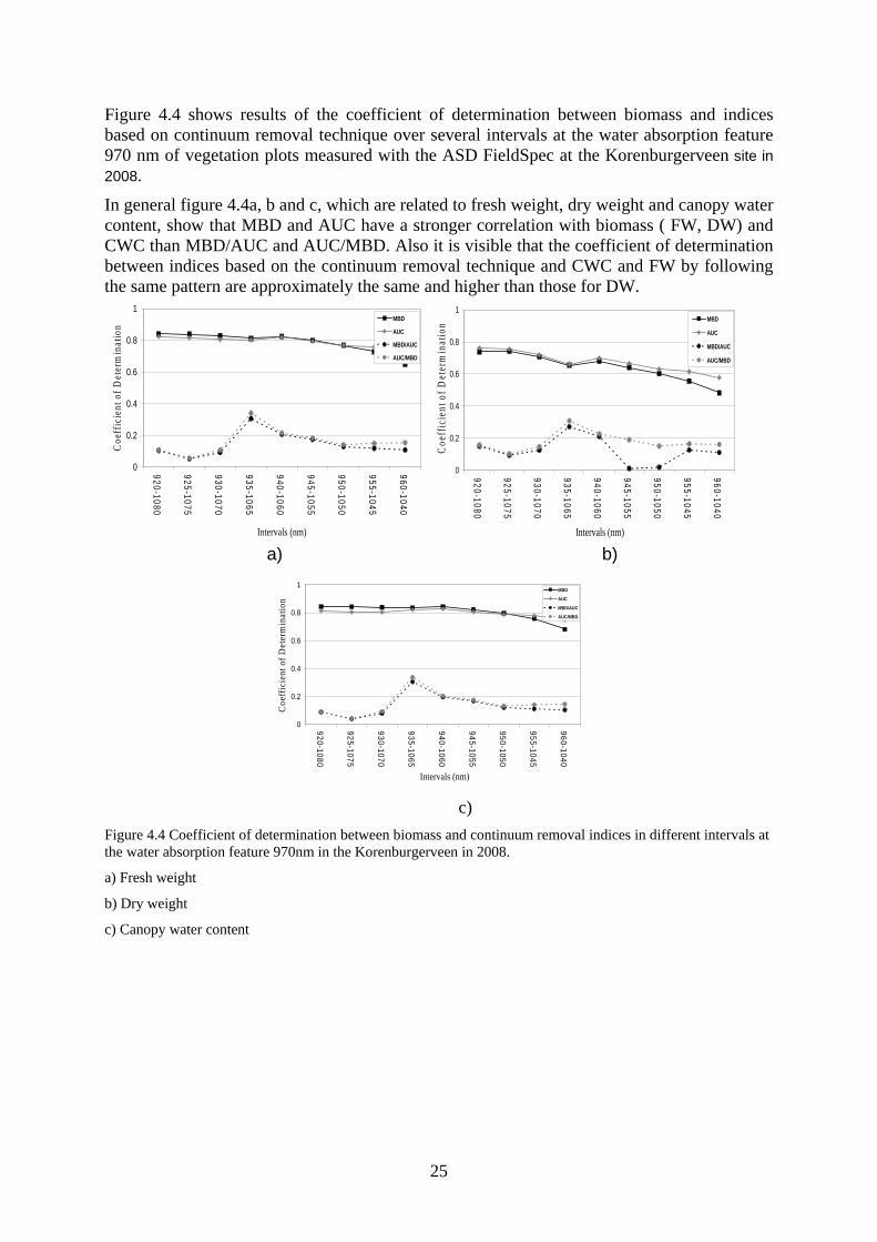
Figure 4.4 shows results of the coefficient of determination between biomass and indices based on continuum removal technique over several intervals at the water absorption feature 970 nm of vegetation plots measured with the ASD FieldSpec at the Korenburgerveen site in 2008.

In general figure 4.4a, b and c, which are related to fresh weight, dry weight and canopy water content, show that MBD and AUC have a stronger correlation with biomass ( FW, DW) and CWC than MBD/AUC and AUC/MBD. Also it is visible that the coefficient of determination between indices based on the continuum removal technique and CWC and FW by following the same pattern are approximately the same and higher than those for DW.

0

0.2

0.4

0.6

0.8

1

920-1080

925-1075

930-1070

935-1065

940-1060

945-1055

950-1050

955-1045

960-1040

Intervals (nm)

Coe

ffic

ient

of

Det

erm

inat

ion MBD

AUC

MBD/AUC

AUC/MBD

0

0.2

0.4

0.6

0.8

1

920-1080

925-1075

930-1070

935-1065

940-1060

945-1055

950-1050

955-1045

960-1040

Intervals (nm)

Coe

ffic

ient

of

Det

erm

inat

ion MBD

AUC

MBD/AUC

AUC/MBD

a) b)

0

0.2

0.4

0.6

0.8

1

920-1080

925-1075

930-1070

935-1065

940-1060

945-1055

950-1050

955-1045

960-1040

Intervals (nm)

Coe

ffic

ient

of

Det

erm

inat

ion

MBD

AUC

MBD/AUC

AUC/MBD

c)

Figure 4.4 Coefficient of determination between biomass and continuum removal indices in different intervals at the water absorption feature 970nm in the Korenburgerveen in 2008.

a) Fresh weight

b) Dry weight

c) Canopy water content

26

Figure 4.5 shows results of the coefficient of determination between biomass and indices based on the continuum removal technique over several intervals at the water absorption feature 1200 nm of vegetation plots measured with the ASD FieldSpec at the Korenburgerveen site in 2008. In general it shows that the coefficient of determination between biomass and MBD and AUC are almost constant over different intervals of the spectral signature. This figure also shows that the correlation between biomass and MBD/AUC and AUC/MBD is increasing in most of the intervals except in the last few intervals. It is visible through these graphs that the coefficient of determination between FW and indices follows the same value as the coefficient of determination between CWC and the indices.

0

0.2

0.4

0.6

0.8

1

1080-1280

1085-1275

1090-1270

1095-1265

1100-1260

1105-1255

1110-1250

1115-1245

1120-1240

1125-1235

1130-1230

1135-1225

1140-1220

1145-1215

1150-1210

Intervals (nm)

Coe

ffic

ient

of

Det

erm

inat

ion

MBD

AUC

MBD/AUC

AUC/MBD

0

0.2

0.4

0.6

0.8

1

1080-1280

1085-1275

1090-1270

1095-1265

1100-1260

1105-1255

1110-1250

1115-1245

1120-1240

1125-1235

1130-1230

1135-1225

1140-1220

1145-1215

1150-1210

Intervals (nm)

Coe

ffic

ient

of

Det

erm

inat

ion

MBD

AUC

MBD/AUC

AUC/MBD

(a) (b)

0

0.2

0.4

0.6

0.8

1

1080-1280

1085-1275

1090-1270

1095-1265

1100-1260

1105-1255

1110-1250

1115-1245

1120-1240

1125-1235

1130-1230

1135-1225

1140-1220

1145-1215

1150-1210

Intervals (nm)

Coe

ffic

ient

of

Det

erm

inat

ion

MBD

AUC

MBD/AUC

AUC/MBD

(c)

Figure 4.5 Coefficient of determination between biomass and continuum removal indices in different intervals at the water absorption feature 1200nm in the Korenburgerveen in 2008.

a) Fresh weight

b) Dry weight

c) Canopy water content

27

Since in this data set 39 samples are available, the degrees of freedom would be 37. By using the critical value table a value is found of 0.325 at the intersection of α .05 and 37 degrees of freedom. Table 4.6 shows that all absolute values of the correlation coefficient of CWC with MBD and AUC are more than 0.325. The absolute values for the correlation coefficient of CWC with MBD/AUC and AUC/MBD only in some intervals which have been highlighted is more than 0.325. Therefore in these intervals we reject the null hypothesis which means there is a statistically significant relationship between CWC and AUC and MBD/AUC and AUC/MBD at the water absorption feature 970 nm based on FieldSpec measurements in this data set. Table 4.7 shows that the correlation coefficient of CWC with MBD and AUC is statistically significant in all intervals and the correlation coefficient of CWC with MBD/AUC and also AUC/MBD in only three intervals is statistically not significant.

Table 4.6 Correlation coefficients of CWC and continuum removal indices at the water absorption feature 970 nm based on FieldSpec measurements in 2008 in the Korenburgerveen site.

Interval (nm) r(CWC,MBD) r(CWC, AUC) r(CWC, MBD/AUC) r(CWC,AUC/MBD) 920-1080 0.918 0.903 -0.297 0.301 925-1075 0.918 0.898 -0.198 0.207 930-1070 0.916 0.897 -0.281 0.306 935-1065 0.914 0.906 -0.554 0.582 940-1060 0.918 0.910 -0.443 0.452 945-1055 0.908 0.899 -0.409 0.418 950-1050 0.892 0.887 -0.349 0.364 955-1045 0.871 0.883 -0.334 0.376 960-1040 0.825 0.863 -0.322 0.381 Table 4.7 Correlation coefficients of CWC and continuum removal indices at the water absorption feature 1200 nm based on FieldSpec measurements in 2008 in the Korenburgerveen site.

Interval (nm) r(CWC,MBD) r(CWC, AUC) r(CWC, MBD/AUC) r(CWC,AUC/MBD) 1080-1280 0.857 0.850 -0.375 0.384 1085-1275 0.857 0.851 -0.378 0.383 1090-1270 0.856 0.852 -0.398 0.403 1095-1265 0.856 0.852 -0.419 0.420 1100-1260 0.855 0.852 -0.434 0.436 1105-1255 0.855 0.853 -0.438 0.439 1110-1250 0.855 0.852 -0.447 0.459 1115-1245 0.855 0.854 -0.460 0.461 1120-1240 0.857 0.857 -0.446 0.444 1125-1235 0.861 0.861 -0.381 0.379 1130-1230 0.863 0.864 -0.278 0.271 1135-1225 0.861 0.865 -0.164 0.155 1140-1220 0.846 0.852 0.044 -0.051 1145-1215 0.851 0.846 0.344 -0.346 1150-1210 0.875 0.874 0.408 -0.394

28

4.1.2 Continuum Removal Indices of HyMap image in 2004 Figure 4.6 shows the coefficient of determination between DW and indices based on the continuum removal technique in two different intervals (928.25nm-1084.05nm and 958.95nm – 1038.45nm) around the water absorption feature at 970 nm of the HyMap image in 2004. Since some sample plots had been located exactly at the border of two pixels of the images. I extracted spectral signature one time by only considering one pixel (a) and next time by considering 3 by 3 pixels (b). Figure 4.6a and b indicate that DW has a higher correlation with MBD and AUC when the whole absorption feature has been included to apply the continuum removal technique than when only some part of the water absorption feature has been included. On the other hand they show DW has higher correlation with MBD/AUC and AUC/MBD in narrower interval around the water absorption feature at 970 nm. Figure 4.6b shows that the coefficient of determination between DW and MBD/AUC and AUC/MBD is much higher than those in figure 4.6a.

0

0.1

0.2

0.3

0.4

0.5

MBD AUC MBD/AUC AUC/MBD

Indices

Coeffi

cient

of D

ete

rmin

atio

n

928.25 nm - 1084.05 nm

958.95 nm - 1038.45 nm

(a)

0

0.1

0.2

0.3

0.4

0.5

MBD AUC MBD/AUC AUC/MBDIndices

Coe

ffici

ent o

f Dete

rmin

atio

n

928.04 nm-1084.85 nm

959.95 nm-1038.45 nm

(b)

Figure 4.6 Coefficient of Determination between DW and continuum removal indices for two different intervals around 970 nm for the HyMap image in 2004.

(a) Considering only 1 pixel

(b) Considering 3 by 3 pixels

29

Figure 4.7 shows the coefficient of determination between DW and indices based on the continuum removal technique in two different intervals (1084.05nm-1286.95nm and 1158.05nm – 1230.25nm) around the water absorption feature at 1200 nm of the HyMap image in 2004 by extracting the spectral signature of one pixel (a) and 3 by 3 pixels (b). Figure 4.7a shows that the coefficient of determination between DW and MBD and AUC are almost the same in both intervals and are about 0.1. The values for MBD/AUC and AUC/MBD are higher for the broader interval. The maximum value is 0.13 for the AUC in the narrower interval and MBD/AUC and AUC/MBD in the broader interval. Figure 4.7b shows that in general the correlation between DW and continuum removal indices in broader intervals is higher than in narrower intervals when 3 by 3 pixels are considered to extract the spectral signature and the maximum value is 0.13 which is related to MBD/AUC and AUC/MBD.

0

0.1

0.2

0.3

0.4

0.5

MBD AUC MBD/AUC AUC/MBD

Indices

Coe

ffici

ent o

f Det

erm

inat

ion

1084.05 nm-1286.95 nm

1158.05 nm-1230.25 nm

(a)

0

0.1

0.2

0.3

0.4

0.5

MBD AUC MBD/AUC AUC/MBD

Indices

Coeffi

cient of D

ete

rmin

atio

n

1084.25 nm- 1286.95nm

1158.08 nm-1230.25 nm

(b)

Figure 4.7 Coefficient of Determination between DW and continuum removal indices in two different intervals around 1200 nm for the HyMap image in 2004.

(a) Considering only 1 pixel

(b) Considering 3 by 3 pixels

30

In this data set, the degrees of freedom would be 15. So a value of 0.482 is found at the intersection of α 0.05 and 15 degrees of freedom. Table 4.9 and 4.10 show the correlation coefficients of DW with continuum removal indices around water absorption features 970 nm and 1200 nm. All values in table 4.8 are less than 0.482. We would fail to reject our null hypotheses: There is not a statistically significant relationship between DW and indices based on the continuum removal technique at the water absorption features 970 nm and 1200 nm in the HyMap image of the Millingerwaard site in 2004 when only one pixel has been considered to extract the spectral signature. Table 4.9 shows there is a statistically significant relationship between DW and MBD/AUC and AUC/MBD at water absorption feature 970 nm in the interval 958.95 nm to 1038.45 nm when using 3 by 3 pixels per plot.

Table 4.8 Correlation coefficient of DW and continuum removal indices at water absorption feature 970 nm and 1200 nm based on the HyMap image considering only one pixel in Millingerwaard site in 2004.

Interval (nm) r(DW,MBD) r(DW, AUC) r(DW, MBD/AUC) r(DW,AUC/MBD) 928.25-1084.05 0.419 0.391 -0.320 0.093 958.95-1038.45 0.361 0.246 0.391 -0.382 1084.05-1286.95 0.320 0.302 0.355 -0.356 1158.05-1230.25 0.332 0.349 -0.222 0.232 Table 4.9 Correlation coefficient of DW and continuum removal indices at water absorption features 970 nm and 1200 nm based on the HyMap image considering 3 by 3 pixels in Millingerwaard site in 2004.

Interval (nm) r(DW,MBD) r(DW, AUC) r(DW, MBD/AUC) r(DW,AUC/MBD) 928.25-1084.05 0.444 0.403 -0.086 0.316 958.95-1038.45 0.354 0.242 0.670 -0.644 1084.05-1286.95 0.291 0.274 0.355 -0.358 1158.05-1230.25 0.214 0.243 -0.341 0.342

4.2 Water Band Index Table 4.10 shows the correlation coefficient and the coefficient of determination between WBI and biophysical variables in each dataset. This relationship in the 2004 datasets for both FieldSpec and HyMap (1pixel and 3*3 pixels) is not statistically significant with α 0.05 and 14 degrees of freedom in the FieldSpec data set and 15 degrees of freedom in the HyMap dataset. Results in 2005 show that the relationship between WBI and both FW and CWC are significant with α .05 and 10 degrees of freedom. For the 2008 FieldSpec data, the correlation coefficient between WBI and these three biophysical variables are statistically significant with α .05 and 37 degrees of freedom. Table 4.10 Correlation coefficient of biomass and WBI in three FieldSpec and one HyMap dataset.

Data set in: df p-value Biomass r(WI , biomass) R2(WI , biomass) 2004 (FieldSpec.) 14 0.497 DW 0.406 0.165 (HyMap-1pixel) 15 0.482 DW 0.401 0.161 (HyMap-3*3pixels) 0.423 0.179 2005 (FieldSpec.) 10 0.576 FW 0.607 0.368 DW 0.478 0.228 CWC 0.630 0.397 2008 (FieldSpec.) 37 0.325 FW 0.888 0.789 DW 0.811 0.658 CWC 0.896 0.803

31

4.3 Water Band Index across spectrum (WBIxxx) WBIxxx tests the effect of variation in the strength of light absorption by water across the spectrum. Figure 4.8 illustrates the coefficient of determination between WBIxxx and available canopy biophysical variables in the FieldSpec measurements in Milingerwaard in 2004 and 2005 and the Korenburgerveen in 2008. Table 4.11 provides an overview of the maximum values in terms of R2 with respect to all tested combinations of WBI in Eq. (4).

0

0.1

0.2

0.3

0.4

0.5

900 925 950 975 1000 1025 1050 1075

Wavelength (nm)

Coefficient of Determination

DW

a)

0

0.2

0.4

0.6

0.8

1

900 925 950 975 1000 1025 1050 1075

Wavelength (nm)

Coe

ffic

ient

of

De

term

ina

tion

FWDW

CWC

0

0.2

0.4

0.6

0.8

1

900 925 950 975 1000 1025 1050 1075

Wavelength (nm)

Co

effic

ien

t of D

eter

min

atio

n

FW

DW

CWC

b) c) Figure 4.8 Coefficient of determination between biomass and WBIxxx in a) fieldSpec measurements in Milingerwaard in 2004 b) FieldSpec measurements in Millingerwaard in 2005 c) FieldSpec measurements in Korenburgerveen in 2008. Table 4.11 Maximum Correlation coefficient of biomass and WBIxxx in three FieldSpec measurements

Data set in: Biomass Max R2(WBI, biomass) Absorption feature 2004 (FieldSpec.) DW 0.250 1048 2005 (FieldSpec.) FW 0.654 914 DW 0.572 914 CWC 0.649 915 2008 (FieldSpec.) FW 0.789 977 DW 0.686 958 CWC 0.804 977

32

4.4 Normalized difference water index Table 4.12 shows the correlation coefficient and coefficient of determination between NDWI and biophysical variables in each dataset. Both datasets in 2004 show that there is not a statistically significant relationship between NDWI and DW with α 0.05 and 14 degrees of freedom in the FieldSpec data set and 15 degrees of freedom in the HyMap dataset. Results in 2005 show that the relationship between NDWI and both FW and CWC are significant with α 0.05 and 10 degrees of freedom. For the 2008 FieldSpec data, the correlation coefficient between NDWI and these three biophysical variables are statistically significant with α 0.05 and 37 degrees of freedom. Table 4.12 Coefficient of Correlation between biomass and NDWI in each dataset.

Data set in: df p-value Biomass r(NDWI , biomass) R2(NDWI , biomass) 2004 (FieldSpec.) 14 0.497 DW 0.494 0.245 (HyMap-1pixel) 15 0.482 DW 0.379 0.144 (HyMap-3*3pixels) 0.431 0.186 2005 (FieldSpec.) 10 0.576 FW 0.590 0.348 DW 0.503 0.253 CWC 0.601 0.361 2008 (FieldSpec.) 37 0.325 FW 0.737 0.543 DW 0.692 0.478 CWC 0.738 0.544

4.5 First derivative of spectra Figure 4.9 illustrates the R2 between the first derivative and biophysical variables (FW, DW and CWC) in different data sets. In order to facilitate interpreting the wavelength positions in this figure, an example of one spectrum is added for illustration. This figure clearly shows that correlations depend on the spectral position. Region A in Figure 4.9 relates to the left slope of the absorption feature at about 970 nm. Region B relates to the right slope. Region C refers to the left slope of the absorption feature at about 1200 nm. Region D refers to the right slope of the later absorption feature. In general figure 4.9 shows that for many spectral positions beyond 900 nm the relationship between the first derivative and CWC, FW and DW are statistically significant at α 0.05. Figure 4.9a illustrates the relationship between DW and first derivative of spectra in the FieldSpec of Millingerwaard in 2004. The most significant coefficient of determination of 0.510 is found in region C at 1193.5 (meaning the difference between 1193 nm and 1194 nm). Figure 4.9b that refers to the HyMap considering one pixel for each sample plot. The most significant coefficient of determination (R2) of 0.451 is found in region B at 1000.6 nm. The most significant coefficient of determination of 0.628 is found in region D in figure 4.9c, which shows the relationship between first derivative of spectra in the HyMap image considering 3 by 3 pixels and DW. Figure 4.9d refers to the FieldSpec of Millingerwaard in 2005. It shows that the relationship between the first derivative and both FW and DW is statistically significant in all regions, whereas for CWC in region C it is only significant with a coefficient of determination of 0.446 at 1163.5 nm. Figure 4.9e illustrates that the relationship between the first derivatives of FieldSpec measurements of the Korenburgerveen and all three biophysical variables are statistically significant in each region. The most significant coefficient of determination between first derivatives and CWC of 0.408, which is found in region A at 966.5 nm.

33

0

0.1

0.2

0.3

0.4

0.5

0.6

900 950 1000 1050 1100 1150 1200 1250 1300 1350

Wavelength (nm)

Co

effic

ien

t o

f D

eter

min

atio

n

0

0.1

0.2

0.3

0.4

0.5

0.6

Ref

lect

ance

R2

Signature

a)

0

0.1

0.2

0.3

0.4

0.5

0.6

900 950 1000 1050 1100 1150 1200 1250 1300 1350

Wavelength (nm)

Co

effic

ien

t o

f D

eter

min

atio

n

0

0.1

0.2

0.3

0.4

0.5

0.6

Ref

lect

ance

R2

signature

0

0.1

0.2

0.3

0.4

0.5

0.6

0.7

900 950 1000 1050 1100 1150 1200 1250 1300 1350

Wavelength (nm)

Coe

ffic

ient

of

De

term

ina

tion

0.0

0.1

0.2

0.3

0.4

0.5

0.6

Ref

lect

ance

R2

Signature

b) c)

0

0.1

0.2

0.3

0.4

0.5

0.6

0.7

900 950 1000 1050 1100 1150 1200 1250 1300 1350

Wavelength (nm)

Coe

ffic

ient

of

De

term

ina

tion

0

0.1

0.2

0.3

0.4

0.5

0.6

Ref

lect

ance

FW

DW

CWC

signature

0

0.1

0.2

0.3

0.4

0.5

0.6

900 950 1000 1050 1100 1150 1200 1250 1300 1350

Wavelength (nm)

Co

effic

ien

t o

f D

eter

min

atio

n

0

0.1

0.2

0.3

0.4

0.5

0.6

0.7

Ref

lect

ance

FWDWCWCsignature

d) e)

Figure 4.9 Coefficient of determination between canopy biophysical variables and first derivative of canopy reflectance. a) FieldSpec derivatives with DW at the Millingerwaard test site in 2004. b) HyMap derivative with DW at the Millingerwaard test site (1pixel) in 2004. c) HyMap derivative with DW at the Millingerwaard test site (3*3pixels) in 2004. d) FieldSpec derivative with FW, DW and CWC at the Millingerwaard test site in 2005. e) FieldSpec derivative with FW, DW and CWC at the Korenburgerveen site in 2008.

34

5 DISCUSSION In the first part of this thesis the continuum removal technique was applied to different intervals around the water absorption features at 970 nm and 1200 nm for estimating canopy water content, fresh weight and dry weight . Analyzing three datasets indicated different results. Test site 1 (FieldSpec measurements of Millingerwaard in 2004) shows that when a narrower interval is applied to the continuum removal technique the correlation between DW and indices based on the continuum removal technique is higher. Test site 2 (FieldSpec measurements of Millingerwaard in 2005) shows that while the interval is going to be narrower the correlation between canopy water content and MBD and AUC based on the continuum removal technique around water absorption feature will decrease (figure 4.2, 4.3 and 4.4). Test site 3 (Korenburgerveen in 2008) shows the constant coefficient of correlation between canopy water content and indices over several intervals. As shown data sets in Millingerwaard in 2004 and 2005 (figure 5.1a and 5.1b) have normal distribution. Figure 5.1b also shows that dry weight of sample plots was distributed in different ranges between minimum and maximum value. Whereas figure 5.1a shows that most of sample plots are located around the mean value for dry weight. Figure 5.1c shows that data set in the Korenburgerveen has skewed to the right. Thus, how to select the sample plots cause the difference in our results.

DW

12.5

11.5

10.5

9.5

8.5

7.5

6.5

5.5

4.5

3.5

2.5

1.5

.5

DW

Fre

quen

cy

6

5

4

3

2

1

0

Std. Dev = 2.09

Mean = 6.0

N = 17.00

a)

DW

9.58.57.56.55.54.53.52.51.5.5

DW

Fre

quen

cy

2.5

2.0

1.5

1.0

.5

0.0

Std. Dev = 2.72

Mean = 4.4

N = 12.00

DW

5.504.503.502.501.50.50

DW

Fre

quen

cy

14

12

10

8

6

4

2

0

Std. Dev = 1.24

Mean = 1.81

N = 40.00

b) c) Figure 5.1 Frequency of DW in three data sets:

a) FieldSpec measurements of Millingerwaard in 2004

b) FieldSpec measurements of Millingerwaard in 2005

35

c) FieldSpec measurements of Korenburgerveen in 2008

Another difference between the datasets in the Millingerwaard and Korenburgerveen is related to the values of the correlation coefficient between biophysical variables (CWC, FW and DW) and indices. FieldSpec measurements of Korenburgerveen in 2008 show much higher correlation than FieldSpec measurements of Millingerwaard in 2004 and 2005. To investigate why there is such a difference between these two data sets looking at vegetation indices such as NDVI can be useful. Figure 5.2 illustrates the scatter plot for fresh weight as a function of NDVI in FieldSpec measurements in Millingerwaard in 2005 and Korenburgerveen in 2008. Figure 5.2a shows that most of the sample plots have the same value of NDVI (around 0.9) in Milingerwaard. Figure 5.2b illustrates a broader range for NDVI in Korenburgerven than for Millingerwaard. Since NDVI is directly related to the photosynthetic capacity and hence energy absorption of plant canopies, the difference in correlation can be affected by species type. Also it was already mentioned that the Korenburgerveen site is a homogeneous and Millingerwaard is a heterogeneous area, therefore the probability of having several species types in one sample plot in Milingerwaard is much larger than in Korenburgerveen. So, this variety in species types can cause less correlation between biophysical variables (CWC, FW and DW) and indices.

0

10

20

30

40

50

0.6 0.65 0.7 0.75 0.8 0.85 0.9 0.95 1

NDVI

FW

(to

n/h

a)

a)

0

5

10

15

20

25

0.6 0.65 0.7 0.75 0.8 0.85 0.9 0.95 1

NDVI

FW

(to

n/h

a)

Figure 5.2 Fresh weights as a function of NDVI in a) Millingerwaard in 2005, b) Korenburgerveen in 2008

36

Results show that there is not a statistically significant difference between the coefficient of determination between biophysical variables (FW, DW and CWC) and the continuum removal indices over different intervals. In the second part of this thesis the continuum removal technique has been applied for the HyMap image to find out which index has the highest relationship with DW (just DW was available). Results show that in the water absorption feature at 970 nm MBD and AUC for broader intervals and MBD/AUC and AUC/MBD for narrower intervals have a higher coefficient of correlation with DW. But at the water absorption features at 1200 nm both intervals show nearly the same coefficient of correlation. By looking at the table in appendix 9 we discovered that the correlation between DW and continuum removal indicators is not statistically significantly different from there being no correlation. Whereas the objective of this part was to investigate the effect of which index based on the continuum removal technique is better for estimation of DW. In each step the effect of two indices with α of 0.05 was compared (see examples 1 and 2 in appendix 10). Result shows there is not a statistically significant difference between indices based on the continuum removal technique. Finally, in last part of this thesis a comparison is made between indices mentioned in the literature review on estimation of CWC for test site 2 and 3 and estimation of DW for test site 1. Table 5.1 provides an overview of all results in terms of R2 values. Table 5.1 Rresults for the indices tested in estimating canopy water content (site2 and 3) or just dry weight (site1) as shown by the coefficient of determination (R2).

Site1 FieldSpec

Site1 HyMap (1pixel)

Site1 HyMap (3*3pixels)

Site2 FieldSpec

Site3 FieldSpec

Best derivative 0.51@1193.5 0.628@1265.75 0.487@983.6 0.446@1163.5 0.408@966.5 WBI 0.165 0.161 0.179 0.397 0.803 NDWI 0.245 0.144 0.186 0.361 0.544 970 nm feature MBD 0.048 0.176 0.197 0.312 0.843 AUC 0.041 0.153 0.162 0.373 0.815 MBD/AUC 0.000 0.102 0.007 0.529 0.088 AUC/MBD 0.000 0.009 0.100 0.540 0.091 1200nm feature MBD 0.067 0.102 0.085 0.295 0.734 AUC 0.066 0.091 0.075 0.309 0.723 MBD/AUC 0.002 0.126 0.126 0.234 0.141 AUC/MBD 0.002 0.127 0.128 0.236 0.147 Site1: FieldSpec measurements in Millingerwaard in 2004 Site2: FieldSpec measurements in Millingerwaard in 2005 Site3: FieldSpec measurements in Korenburgerveen in 2008 The WBI performed better than the NDWI in the estimation of the canopy water content in terms of significance. Results for the continuum removal methods (applied to either of the water absorption features) were clearly worse for the heterogenous area (site 1 and 2) and clearly better for the homogeneous area (site 3). Also the scatter plot of canopy water content as a function of MBD in Figure 5.3 shows that canopy water content is highly correlated to the MBD at water absorption feature 970 nm in a homogeneous area (Korenburgerveen).

37

Whereas there is not a clear relationship between canopy water content and the maximum band depth in a heterogeneous area (Millingerwaard). The MBD and AUC for the water absorption feature at 1200 nm performed worse than for the water absorption feature at 970 nm, whereas MBD/AUC and AUC/MBD for the water absorption feature at 1200 nm performed better than at 970 nm on the estimation of canopy water content in terms of significance.

y = 15508x - 598.76R2 = 0.8436

0

500

1000

1500

2000

0 0.05 0.1 0.15

MBD arund 970 nm

CW

C (

g/m

2)

a)

y = 25386x - 1242R2 = 0.3121

0

500

1000

1500

2000

2500

3000

3500

4000

0 0.05 0.1 0.15 0.2

MBD around 970 nm

CW

C (

g/m

2)

b)

Figure 5.3 Canopy water content as a function of MBD at water absorption feature 970 nm.

a) Korenburgerveen in 2008

b) Millingerwaard in 2005

38

6 CONCLUSION AND RECOMMENDATION

6.1 Conclusion The objective of this thesis was to apply the continuum removal technique to the water absorption features in the NIR region to estimate canopy water content and biomass. Objective was also to compare the results of the continuum removal method to WI, NDWI and first derivative of spectra. Result presented in this report show that for the FieldSpec measurements, indices based on the continuum removal method (MBD, AUC, MBD/AUC and AUC/MBD) have higher correlation with canopy biophysical variables for broader intervals at the water absorption features 970 nm and 1200 nm. Results yielded that MBD and AUC have clearly a stronger correlation with biophysical variables than other continuum removal indicators at both water absorption features in the NIR region in a homogenous area. For a heterogeneous area MBD/AUC and AUC/MBD at 970 nm and MBD and AUC at 1200 nm have higher correlation with canopy biophysical variables. Results for the HyMap data set (both considering one pixel and 3 by 3 pixels for each plot) yielded that the MBD and AUC for broader intervals and MBD/AUC and AUC/MBD for narrower intervals have a higher correlation with canopy biophysical variables at the water absorption features 970 nm and shows that canopy biophysical variables have the same correlation with continuum removal indicators for broader and narrower intervals at the water absorption feature 1200 nm. For both water absorption features of HyMap, MBD/AUC and AUC/MBD have the best effect on estimating dry weight. The last part of this thesis focused on the effect of different indices on the estimation of canopy biophysical variables. Result showed that the first derivative of the spectra is much better than continuum removal indices and clearly better than WBI and NDWI in the estimation of canopy biophysical variables in a heterogeneous area. Whereas in a homogeneous area (site 3) continuum removal indices (only MBD and AUC) yielded stronger effects on estimation of canopy biophysical variables and the first derivative yielded the worst results. Derivatives provide better results for heterogeneous area and MBD and AUC provide better results in this study than reflectance or indices as used in literature (Sims and Gamon, 2003; Clevers & Kooistra, 2006). An advantage of derivative spectra is their insensitivity to variations in soil background and atmospheric effects (Clevers et al., 2001). As a result, derivative spectra also will be insensitive to the presence of yellow, dry vegetation and litter, making them attractive as estimator for canopy water content.

6.2 Recommendations Further analyzing is required to focus on the dependency of the result on plant functional type. To get a better conclusion for the first part of this thesis it would be better to have different datasets of FieldSpec measurements for each type of area (homogonous and heterogeneous) with the same size and same numbers of sample plots and the same sampling method.

39

The maximum band depth and the area under the curve have the higher correlation with canopy water content in homogeneous area than in heterogeneous area, so we wish to test on more than these two test sites to be sure about this result.

40

Reference: Ceccato P. N., Gobron S., Flasse B., Pinty, & S. Tarantola, 2002, "Designing a spectral index

to estimate vegetation water content from remote sensing data" Remote sensing of environment 82 188-197.

Champagne, C., Pattey, E., Bannari, A., and Stratchan, I.B., 2001. "Mapping Crop Water Status: Issues of Scale in the Detection of Crop Water Stress Using Hyperspectral Indices". Proceedings of the 8th International Symposium on Physical Measurements and Signatures in Remote Sensing, Aussois, France, 79-84.

Chuvieco E., Cocero D., Riono D., Martin P., Martinez J., Perez F., et al., 2004, "Combining NDVI and surface temperature for the estimation of live fuel moisture content in forest fire danger rating" Remote sensing of environment 92 322-331

Clark R. N. & Roush T. L., 1984, "Reflectance spectroscopy: quantitative analysis techniques for remote sensing applications" Journal of geophysical research 89 6329-6340.

Clevers, J.G.P.W., de Jong, S.M., Epema, G.F., van der Meer, F., Bakker, W.H., Skidmore, A.K., Addink, E.A., 2001. "MERIS and the red-edge position". International Journal of Applied Earth Observation and Geoinformation 3 (4), 313–320

Clevers, J.G.P.W., Kooistra L., 2006. "Using spectral information at the NIR water absorption features to estimate canopy water content and biomass". ISPRS mid-term symposium remote sensing: from pixels to processes, 8-11 May, Enschede, The Netherlands, pp. 6.

Curran, P. J., 1989. "Remote sensing of foliar chemistry". Remote Sensing of Environment, 30 271-278.

Danson F. M., Steven M. D., Malthus T. J., & Clark J. A., 1992, "High-spectral resolution data for determining leaf water content" International journal of remote sensing 13 461-470.

ESA, 2006. "The Changing Earth". SP-1304, 83 pp.

Gao B. C., Goetz A. F., 1995, "Retrieval of equivalent water thickness and information related to biochemical components of vegetation canopies from AVIRIS data". Remote Sensing of Environment 52 155–162.

Gao B.C., 1996, "NDWI - A normalized difference water index for remote sensing of vegetation liquid water from space". Remote sensing of environment 58 257-266.

Hardisky M.A., Klemas V., and Smart R.M., 1983. "The Influences of Soil Salinity, Growth Form, and Leaf Moisture on the Spectral Reflectance of Spartina Alterniflora Canopies". Photogrammetric Engineering and Remote Sensing 49 77-83.

Hunt Jr. E.R., & Rock, B.N., 1989. "Detection of Changes in Leaf Water Content Using Near- And Middle-Infrared Reflectances". Remote Sensing of Environment 30 43-54.

Iqbal, M., 1983. "An introduction to solar radiation". Academic Press, Ontario, 390 pp. Jackson T.L., Chen D., Cosh M.,. Anderson F. Li, M, Walthall C., Doriaswamy P., and Hunt

E.R., 2004. "Vegetation Water Content Mapping Using Landsat Data Derived Normalized Difference Water Index for Corn and Soybeans". Remote Sensing of Environment 92 475-482.

Keller, P.A., 2001. "Imaging spectroscopy of lake water quality parameters". Ph.D. Thesis. Remote Sensing Series 36, RSL, University of Zurich, 161.

41

Kokaly R. F., Clark R. N. 1999, "Spectroscopic determination of leaf biochemistry using band-depth analysis of absorption features and stepwise multiple linear regression" Remote sensing of environment 67 267-287.

Kooistra, L., Suarez Barranco M.D., Van Dobben H., E Schaepman M.E., 2006. "Regional scale monitoring of vegetation biomass in river floodplains using imaging spectroscopy and ecological modeling". Proceedings IGARRS '06 Symposium, Denver, Colorado, 124-127.

Kooistra, L., Sterkx, S., , Liras laita, E., Mengesha, T., Verbeiren, B., Batelaan, O., Vandobben, H., Schaepman, M.E., Schaepman-Strub, G., And Struiver, J. 2005 HyEco04: An airborne imaging spectroscopy campaign in the floodplain the Millingerwaard, the Netherlands. CGI-report, Wageningen UR, Wageningen.

Palmer k.f., Williams D., 1974 "optical properties of water in the near infrared". Optical Society 64 1107-1110.

Penuelas J., Filella I., Biel C., Serrano L., & Save R., 1993, "The reflectance at the 950-970 nm region as an indicator of plant water status" International journal of remote sensing 14 1887-1905.

Penuelas J., Pinol J., Ogaya R., & Filella I. 1997, "Estimation of plant water concentration by the reflectance Water Index WI (R900/R970)" International journal of remote sensing 18 2869-2875.

Richter, R. & Schlapfer, D. 2002, "Geo-atmospheric processing of airborne imaging spectrometry data. Part 2: atmospheric/topographic correction". International Journal of Remote Sensing, 23 2631-2649.

Riano, D., Vaughan, P., Zarco-Tejada, E., & Ustin, P. J., 2005. "Estimation of fuel moisture content by inversion of radiative transfer models to simulate equivalent water thickness and dry matter content. Analysis at leaf and canopy level". IEEE Transactions on Geoscience and Remote Sensing, 43 819−826.

Rollin, E. M., and Milton, E. J., 1998. "Processing of high spectral resolution reflectance data for the retrival of vanopy water content information". Remote Sensing of Environment, 65 86-92

Rouse, J.W., Haas, R.H., Schell, J.A. and Deering, D.W., 1973. "Monitoring Vegetation Systems in the Great Plains with ERTS". Third ERTS Symposium, NASA SP-351 I 309-317.

Running, S.W. & Coughlan, J.C. 1988. "A general-model of forest ecosystem processes for regional applications .1. Hydrologic balance, canopy gas-exchange and primary production Processes". Ecological Modelling, 42 125- 154.

Schaepman-Strub, G, Schaepman, M.E., Painter, T.H., Dangel S. & Martonchik, J.V., 2006. "Reflectance quantities in optical remote sensing-definitions and case studies". Remote Sensing of Environment, 103 27-42.

Schaepman, M.E., Wamelink, G.W.W., Van Dobben, H.F., Gloor, M., Schaepman-Strub, G., Kooistra, L., Clevers, J.G.P.W., Schmidt, A., Berendse, F., 2007. "River floodplain vegetation scenario development using imaging spectroscopy derived products as input variables in a dynamic vegetation model". Photogrammetric Engineering and Remote Sensing 73 1179–1188.

42

Schlapfer D., Richter R., 2002. "Geo-atmospheric processing of airborne imaging spectrometry data. Part 1: parametric orthorectification". International Journal of Remote Sensing 23, 2609–2630.

Sellers, P.J., 1985. "Canopy Reflectance, Photosynthesis and Transpiration". International Journal of Remote Sensing 6 1335-1372.

Serrano L., Ustin S. L., Roberts D. A., Gamon J. A., & Penuelas J., 2000. "Deriving water content of chaparral vegetation from AVIRIS data". Remote Sensing of Environment, 74 570– 581.

Sims D.A., & Gamon, J.A. 2003, " Estimation of vegetation water content and photosynthetic tissue area from spectral reflectance: a comparison of indices based on liquid water and chlorophyll absorption features" Remote Sensing of Environment 84, 526–537

Tian Q., Tong Q., Pu R., Guo, X., & Zhao C., 2001. "Spectroscopic determinations of wheat water status using 1650 – 1850 nm spectral absorption features". International Journal of Remote Sensing, 22 2329– 2338.

Tucker, C.J., 1979. "Red and Photographic Infrared Linear Combinations for Monitoring Vegetation". Remote Sensing of the Environment 8 127-150.

Ustin S.L., Roberts D.A., Pinzon J., Jacquemoud S., Gardner M., Scheer G., 1998, "Estimating canopy water content of chaparral shrubs using optical methods" Remote sensing of environment 65 280-291

Ustin, S.L., Darling, D., Kefauver, S., Greenberg, J., Cheng, Y.B., &Whiting, M. L. 2004a. "Remotely sensed estimates of crop water demand". S.P.I.E. the international symposium on optical science and technology. 49th annual meeting, Denver, CO, 2–6 August.

Ustin, S. L., Jacquemoud, S., Zarco-Tejada, P. J., and Asner, G., 2004b. "Remote Sensing of Environmental Processes, State of the Science and New Directions. in Manual of Remote Sensing Vol. 4. Remote Sensing for Natural Resource Management and Environmental Monitoring. ASPRS. John Wiley and Sons, New York 768p. +cd. ASPRS. John Wiley and Sons, New York, pages 679-730

Zarco-Tejada, P.J., Rueda, C.A., & Ustin, S. L. 2003. "Water content estimation in vegetation with MODIS reflectance data and model inversion methods". Remote Sensing of Environment, 85 109−124.

43

Appendix 1- Vegetation description

Vegetation descriptions were made according to the method of Braun-Blanquet(1951). Abundance per species was estimated optically as percentage soil covered by living biomass in vertical projection, and scored in a nine-point scale. All bryophytes and lichens, and also vascular species that were not readily recognisable in the field, were collected for later identification. Taraxacum species were taken together as T. vulgare, and Rubus species were taken together as R. fruticosus, except R. caesius. No subspecific taxa were used. Nomenclature follows van der Meijden et al. (1990), Touw & Rubers (1989), and Brand et al. (1988) for vascular species, mosses and lichens, respectively. No distinction in layers (e.g. by using pseudo-species) was made. Syntaxonomic nomenclature follows Schaminée et al. (1995, 1996, and 1998). In total, 79 species were found in the plots in the Millingerwaard. The number of occurrences in the total of 20 plots is listed below. Code Number of

occurrences Full name

Achilmil 5 Achillea millefolium L.

Agrossto 5 Agrostis stolonifera L.

Arctilap 9 Arctium lappa L.

Arrheela 2 Arrhenatherum elatius (L.) J.& C.Presl

Atrippat 2 Atriplex patula L.

Brassnig 7 Brassica nigra (L.) Koch

Bromuine 3 Bromus inermis Leysser

Calamepi 10 Calamagrostis epigejos (L.) Roth

Calyssep 2 Calystegia sepium (L.) R.Br.

Cardunut 2 Carduus nutans L.

Carexhir 6 Carex hirta L.

Cerasfon 3 Cerastium fontanum Baumgarten

Cirsiarv 15 Cirsium arvense (L.) Scopoli

Cirsivul 2 Cirsium vulgare (Savi) Tenore

Cratamon 1 Crataegus monogyna Jacquin

Cynoddac 2 Cynodon dactylon (L.) Persoon

Dactyglo 5 Dactylis glomerata L.

Dipsaful 1 Dipsacus fullonum L.

Elymurep 9 Elymus repens (L.) Gould

Epilohir 3 Epilobium hirsutum L.

Epilotet 3 Epilobium tetragonum L.

Equisarv 1 Equisetum arvense L.

Erigecan 5 Erigeron canadensis L.

Eryngcam 6 Eryngium campestre L.

Euphocyp 1 Euphorbia cyparissias L.

Euphoesu 4 Euphorbia esula L.

Festurub 7 Festuca rubra L.

44

Galeotet 2 Galeopsis tetrahit L.

Galiuapa 4 Galium aparine L.

Galiumol 2 Galium mollugo L.

Geranpus 1 Geranium pusillum L.

Glechhed 10 Glechoma hederacea L.

Hernigla 5 Herniaria glabra L.

Hyperper 2 Hypericum perforatum L.

Iris pse 1 Iris pseudacorus L.

Linarvul 1 Linaria vulgaris Miller

Loliuper 2 Lolium perenne L.

Lycopeur 2 Lycopus europaeus L.

Lythrsal 2 Lythrum salicaria L.

Matrimar 3 Matricaria maritima L.

Mediclup 1 Medicago lupulina L.

Melilalt 2 Melilotus altissima Thuillier

Menthaqu 2 Mentha aquatica L.

Myosoarv 1 Myosotis arvensis (L.) Hill

Myosol-c 1 Myosotis laxa (subsp. cespitosa) (Schultz) Nordh.

Odontver 3 Odontites vernus (Bellardi) Dumortier

Oenotbie 2 Oenothera biennis L.

Pastisat 1 Pastinaca sativa L.

Phalaaru 1 Phalaris arundinacea L.

Phleupra 2 Phleum pratense L.

Plantlan 2 Plantago lanceolata L.

Plantmaj 1 Plantago major L.

Poa ann 2 Poa annua L.

Poa pra 3 Poa pratensis L.

Poa tri 11 Poa trivialis L.

Polynper 3 Polygonum persicaria L.

Potenans 5 Potentilla anserina L.

Potenrep 11 Potentilla reptans L.

Prunevul 1 Prunella vulgaris L.

Ranunrep 3 Ranunculus repens L.

Roripaus 1 Rorippa austriaca (Crantz) Besser

Rubuscae 8 Rubus caesius L.

Rumexace 3 Rumex acetosa L.

Rumexcri 2 Rumex crispus L.

Rumexobt 1 Rumex obtusifolius L.

45

Saponoff 2 Saponaria officinalis L.

Seneceru 1 Senecio erucifolius L.

Senecina 5 Senecio inaequidens DC.

Senecjac 4 Senecio jacobaea L.

Solandul 1 Solanum dulcamara L.

Solidcan 3 Solidago canadensis L.

Stellaqu 2 Stellaria aquatica (L.) Scopoli

Tanacvul 2 Tanacetum vulgare L.

Taraxoff 4 Taraxacum officinale s.s. Wiggers

Trifofra 1 Trifolium fragiferum L.

Triforep 5 Trifolium repens L.

Urticdio 10 Urtica dioica L.

Verbanig 2 Verbascum nigrum L.

Refrence: L. Kooistra, S. Sterkx, E. Liras Laita, T. Mengesha, B. Verbeiren, O. Batelaan, H. van Dobben, M. Schaepman, G. Schaepman&Strub and J. Stuiver "HyEco’04: an airborne imaging spectroscopy campaign in the floodplain Millingerwaard, the Netherlands.Quality assessment of field and airborne data" CGI Report 2005&07.

46

Appendix 2- Measured weight for the individual samples in Millingerwaard in 2005.

Plot VALERI

Fresh Weight

Dry Weight

PFT Nr. Location g/m2 g/m2 shrub 1 A 4737.56 923.84 Shrub 1 C 3525.2 433.08 shrub 1 E 4999.48 1027.24 herb 2 A 555.68 113.6 herb 2 C 1613.88 380.24 herb 2 E 2106 528.12 herb 3 A 497.88 1011.6 herb 3 C 679 194.84 herb 3 E 1561.4 296.44 herb 4 A 2114.48 456.6 herb 4 C 957.92 196.88 herb 4 E 2538.88 562.84 shrub 5 A 2050.56 540.88 Shrub 5 C 2312.92 684.16 shrub 5 E 3661.72 1170.96 herb 6 A 881.76 141 herb 6 C 635.12 133.56 herb 6 E 682.16 143 herb 7 A 2687.2 680.4 herb 7 C 1767.12 589.84 herb 7 E 1866.28 357.84 herb 8 A 1518.84 487.36 herb 8 C 1331.72 286.48 herb 8 E 1105.84 242.4 shrub 9 A 4570.12 1155.44 Shrub 9 C 4107.4 1155.72 shrub 9 E 1247.4 333.48 shrub 10 A 2747.88 485.32 Shrub 10 C 1998.04 641.8 shrub 10 E 2967.2 597.4 herb 12 A 429.12 84.04 herb 12 C 271 31.6 herb 12 E 489.84 115.64 herb 14 A 803.08 151.04 herb 14 C 1505.12 314.24

47

Appendix 3- Measured weight for the individual plots in the Millingerwaard in 2005. Plot

fresh weight

dry weight

water weight

Nr. g/m2 g/m2 g/m2 1 4420.75 794.72 3626.03 2 1425.19 340.65 1084.53 3 912.76 197.63 715.13 4 1870.43 405.44 1464.99 5 2675.07 798.67 1876.40 6 733.01 139.19 593.83 7 2106.87 542.69 1564.17 8 1318.80 338.75 980.05 9 3308.31 868.21 2440.09 10 2571.04 574.84 1996.20 12 396.65 77.09 319.56 14 1154.10 232.64 921.46

48

Appendix 4- Measured dry weight for the individual plots in the Millingerwaard in 2004. Plot

dry weight

Nr. g/m2 2 142.88 3 623.08 4 715.68 5 142.08 6 580.8 7 602.36 8 709.72 9 714.48 10 736.56 11 1164.64 12 741.24 13 127.32 14 572.44 15 395.96 16 368.24 17 646.08 18 241.88 19 489.64 20 508.52 21 258.68 22 371

49

Appendix 5- Measured weight for the individual samples in the Korenburgerveen in 2008. Plot

VALERI

Fresh Weight

Dry Weight

Nr. Location g/m2 g/m2 1 A 760 177 1 C 1496 298 1 E 1200 226 2 A 1848 425 2 C 880 215 2 E 1288 289 3 A 920 205 3 C 904 179 3 E 840 201 4 A 304 75 4 C 640 136 4 E 344 76 5 A 1008 235 5 C 1136 251 5 E 1104 255 6 A 760 164 6 C 680 146 6 E 464 142 7 A 880 234 7 C 2176 402 7 E 2632 499 8 A 1616 343 8 C 3192 635 8 E 1640 340 9 A 792 169 9 C 848 226 9 E 1400 302 10 A 808 211 10 C 424 119 10 E 816 208 11 A 248 53 11 C 288 54 11 E 544 119 12 A 944 208 12 C 896 182 12 E 1104 238 13 A 2352 900 13 C 1008 249 13 E 1008 257 14 A 424 88 14 C 656 137 14 E 456 86

50

Plot

VALERI

Fresh Weight

Dry Weight

Nr. Location g/m2 g/m2 15 A 672 134 15 C 664 149 15 E 344 89 16 A 1544 344 16 C 1136 277 16 E 760 182 17 A 1624 419 17 C 848 221 17 E 1056 282 18 A 136 32 18 C 192 43 18 E 96 23 19 A 1224 240 19 C 1912 426 19 E 1072 226 20 A 656 157 20 C 880 215 20 E 1304 291 21 A 268 89 21 C 280 89 21 E 144 46 22 A 336 93 22 C 320 82 22 E 248 63 23 A 680 184 23 C 296 94 23 E 120 41 24 A 512 166 24 C 416 114 24 E 232 65 25 A 32 13 25 C 24 8 25 E 16 5 26 A 216 63 26 C 120 33 26 E 64 21 27 A 152 40 27 C 136 50 27 E 216 60 28 A 328 92 28 C 192 79 28 E 288 58

51

Plot

VALERI

Fresh Weight

Dry Weight

Nr. Location g/m2 g/m2 29 A 384 98 29 C 616 172 29 E 624 153 30 A 416 87 30 C 360 66 30 E 208 47 31 A 168 39 31 C 704 163 31 E 704 136 32 A 1208 355 32 C 2960 951 32 E 936 243 33 A 288 72 33 C 232 59 33 E 280 61 34 A 1448 336 34 C 1024 236 34 E 240 68 35 A 224 70 35 C 296 76 35 E 56 17 36 A 1016 251 36 C 1032 271 36 E 712 176 37 A 664 169 37 C 544 156 37 E 480 132 38 A 1780 481 38 C 584 161 38 E 200 58 39 A 392 95 39 C 368 122 39 E 208 66 40 A 600 166 40 C 712 216 40 E 1152 352

52

Appendix 6- Measured weight for the individual plots in the Korenburgerveen in 2008 Plot

fresh weight

dry weight

water weight

Nr. g/m2 g/m2 g/m2 1 1152 233.56 918.44 2 1338.67 309.76 1028.91 3 888 195.07 692.93 4 429.33 95.83 333.51 5 1082.67 246.92 835.75 6 634.67 150.51 484.16 7 1896 378.32 1517.68 8 2149.33 439.57 1709.76 9 1013.33 232.56 780.77 10 682.67 179.25 503.41 11 360 75.48 284.52 12 981.33 209.36 771.97 13 1456 468.87 987.13 14 512 103.63 408.37 15 560 123.61 436.39 16 1146.67 267.63 879.04 17 1176 307.33 868.67 18 141.33 32.64 108.69 19 1402.67 297.01 1105.65 20 946.67 220.84 725.83 21 230.67 74.53 156.13 22 301.33 79.49 221.84 23 365.33 106.37 258.96 24 386.67 114.80 271.87 25 24 8.57 15.43 26 133.33 38.96 94.37 27 168 50.03 117.97 28 269.33 76.61 192.72 29 541.33 140.75 400.59 30 328 66.76 261.24 31 525.33 112.24 413.09 32 1701.33 516.47 1184.87 33 266.67 64.16 202.51 34 904 213.31 690.69 35 192 54.12 137.88 36 920 232.56 687.44 37 562.67 152.64 410.03 38 854.67 233.27 621.40 39 322.67 94.37 228.29 40 821.33 244.67 576.67

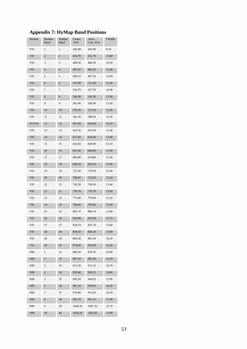
53

Appendix 7: HyMap Band Positions Module Module

Band HyMap Band

Center Wvl

Atmo. Corr. Wvl.

FWHM

VIS 1 1 445.00 442.00 8.10

VIS 2 2 454.70 451.70 13.60

VIS 3 3 469.30 466.30 16.50

VIS 4 4 485.20 482.20 15.60

VIS 5 5 500.10 497.10 15.60

VIS 6 6 515.00 512.00 15.40

VIS 7 7 530.70 527.70 16.40

VIS 8 8 546.30 543.30 15.90

VIS 9 9 561.40 558.40 15.20

VIS 10 10 576.30 573.30 15.30

VIS 11 11 591.50 588.50 15.50

631VIS 12 12 607.00 604.00 16.10

VIS 13 13 622.50 619.50 15.30

VIS 14 14 637.60 634.60 15.40

VIS 15 15 652.60 649.60 15.10

VIS 16 16 667.60 664.60 15.30

VIS 17 17 682.80 679.80 15.50

VIS 18 18 698.20 695.20 15.90

VIS 19 19 713.50 710.50 15.30

VIS 20 20 728.50 725.50 15.20

VIS 21 21 743.50 740.50 15.40

VIS 22 22 758.70 755.70 15.60

VIS 23 23 773.80 770.80 15.10

VIS 24 24 788.60 785.60 15.30

VIS 25 25 803.70 800.70 15.60

VIS 26 26 818.90 815.90 15.70

VIS 27 27 834.10 831.10 15.60

VIS 28 28 849.20 846.20 15.90

VIS 29 29 864.50 861.50 16.20

VIS 30 30 879.60 876.60 16.20

NIR 1 31 880.50 879.35 16.90

NIR 2 32 897.10 895.95 16.10

NIR 3 33 913.30 912.15 16.70

NIR 4 34 929.40 928.25 16.00

NIR 5 35 945.20 944.05 15.90

NIR 6 36 961.10 959.95 16.20

NIR 7 37 976.80 975.65 16.10

NIR 8 38 992.70 991.55 15.90

NIR 9 39 1008.50 1007.35 15.70

NIR 10 40 1024.10 1022.95 15.90

54

NIR 11 41 1039.60 1038.45 15.50

NIR 12 42 1055.00 1053.85 15.30

NIR 13 43 1070.10 1068.95 15.50

NIR 14 44 1085.20 1084.05 15.40

NIR 15 45 1100.30 1099.15 15.20

NIR 16 46 1115.10 1113.95 15.10

NIR 17 47 1130.00 1128.85 15.30

NIR 18 48 1144.70 1143.55 15.10

NIR 19 49 1159.20 1158.05 14.80

NIR 20 50 1173.80 1172.65 15.20

NIR 21 51 1188.50 1187.35 15.20

NIR 22 52 1202.80 1201.65 14.80

NIR 23 53 1217.00 1215.85 14.90

NIR 24 54 1231.40 1230.25 15.20

NIR 25 55 1245.80 1244.65 15.00

NIR 26 56 1259.90 1258.75 14.80

NIR 27 57 1273.90 1272.75 14.80

NIR 28 58 1288.00 1286.85 14.90

NIR 29 59 1301.90 1300.75 14.80

NIR 30 60 1315.90 1314.75 14.90

NIR 31 61 1329.90 1328.75 14.80

NIR 32 62 1343.30 1342.15 14.50

SWIR1 1 63 1403.90 1404.40 15.50

SWIR1 2 64 1418.40 1418.90 15.60

SWIR1 3 65 1432.50 1433.00 15.50

SWIR1 4 66 1446.80 1447.30 15.50

SWIR1 5 67 1460.80 1461.30 14.90

SWIR1 6 68 1474.70 1475.20 15.10

SWIR1 7 69 1488.60 1489.10 15.10

SWIR1 8 70 1502.40 1502.90 14.80

SWIR1 9 71 1515.90 1516.40 14.70

SWIR1 10 72 1529.10 1529.60 14.90

SWIR1 11 73 1542.70 1543.20 15.20

SWIR1 12 74 1556.20 1556.70 14.80

SWIR1 13 75 1569.30 1569.80 14.50

SWIR1 14 76 1582.30 1582.80 14.70

SWIR1 15 77 1595.20 1595.70 14.90

SWIR1 16 78 1608.30 1608.80 14.50

SWIR1 17 79 1621.10 1621.60 14.40

SWIR1 18 80 1633.90 1634.40 14.70

SWIR1 19 81 1646.70 1647.20 14.60

SWIR1 20 82 1659.40 1659.90 14.30

SWIR1 21 83 1671.70 1672.20 14.10

55

SWIR1 22 84 1684.10 1684.60 14.40

SWIR1 23 85 1696.70 1697.20 14.40

SWIR1 24 86 1709.00 1709.50 13.90

SWIR1 25 87 1721.20 1721.70 13.70

SWIR1 26 88 1733.30 1733.80 14.00

SWIR1 27 89 1745.50 1746.00 14.00

SWIR1 28 90 1757.50 1758.00 13.50

SWIR1 29 91 1769.40 1769.90 13.60

SWIR1 30 92 1781.20 1781.70 13.60

SWIR1 31 93 1793.10 1793.60 13.50

SWIR1 32 94 1804.90 1805.40 13.10

SWIR2 1 95 1951.10 1953.20 21.00

SWIR2 2 96 1969.90 1972.00 20.90

SWIR2 3 97 1988.60 1990.70 20.90

SWIR2 4 98 2007.30 2009.40 21.20

SWIR2 5 99 2026.00 2028.10 21.10

SWIR2 6 100 2044.70 2046.80 21.30

SWIR2 7 101 2063.20 2065.30 21.00

SWIR2 8 102 2081.20 2083.30 20.20

SWIR2 9 103 2098.80 2100.90 20.10

SWIR2 10 104 2116.50 2118.60 20.10

SWIR2 11 105 2134.20 2136.30 20.30

SWIR2 12 106 2151.90 2154.00 20.50

SWIR2 13 107 2169.50 2171.60 19.90

SWIR2 14 108 2186.20 2188.30 19.00

SWIR2 15 109 2203.10 2205.20 20.40

SWIR2 16 110 2221.30 2223.40 19.50

SWIR2 17 111 2238.00 2240.10 19.70

SWIR2 18 112 2255.50 2257.60 20.40

SWIR2 19 113 2272.30 2274.40 19.80

SWIR2 20 114 2289.00 2291.10 19.50

SWIR2 21 115 2305.40 2307.50 19.20

SWIR2 22 116 2321.50 2323.60 19.20

SWIR2 23 117 2337.70 2339.80 19.40

SWIR2 24 118 2354.20 2356.30 19.60

SWIR2 25 119 2370.40 2372.50 19.40

SWIR2 26 120 2386.40 2388.50 19.00

SWIR2 27 121 2402.20 2404.30 18.60

SWIR2 28 122 2417.80 2419.90 18.50

SWIR2 29 123 2433.30 2435.40 18.60

SWIR2 30 124 2448.80 2450.90 18.90

SWIR2 31 125 2464.50 2466.60 18.60

SWIR2 32 126 2479.90 2482.00 18.30

56

Appendix 8: HyMap QuickLooks

HyMap Quicklook ‘Millingerwaard’, 28. July 2004, Strip 1 (RGB = 15/10/5 (652.6 nm, 576.3 nm, 500.1 nm)) (left = Raw DLR quicklook, right = Geocoded and calibrated VITO quicklook).

57

Appedix 9: Critical values of the pearson product-moment correlation coefficient

df = n -2

Level of Significance (p) for Two-Tailed Test

.10 .05 .02 .01

df

1

2

3

4

5

6

7

8

9

10

11

12

13

14

15

16

17

18

.988

.900

.805

.729

.669

.622

.582

.549

.521

.497

.476

.458

.441

.426

.412

.400

.389

.378

.997

.950

.878

.811

.754

.707

.666

.632

.602

.576

.553

.532

.514

.497

.482

.468

.456

.444

.9995

.980

.934

.882

.833

.789

.750

.716

.685

.658

.634

.612

.592

.574

.558

.542

.528

.516

.9999

.990

.959

.917

.874

.834

.798

.765

.735

.708

.684

.661

.641

.623

.606

.590

.575

.561

58

19

20

21

22

23

24

25

26

27

28

29

30

35

40

45

50

60

70

80

90

100

.369

.360

.352

.344

.337

.330

.323

.317

.311

.306

.301

.296

.275

.257

.243

.231

.211

.195

.183

.173

.164

.433

.423

.413

.404

.396

.388

.381

.374

.367

.361

.355

.349

.325

.304

.288

.273

.250

.232

.217

.205

.195

.503

.492

.482

.472

.462

.453

.445

.437

.430

.423

.416

.409

.381

.358

.338

.322

.295

.274

.256

.242

.230

.549

.537

.526

.515

.505

.496

.487

.479

.471

.463

.456

.449

.418

.393

.372

.354

.325

.303

.283

.267

.254

http://www.gifted.uconn.edu/siegle/research/Correlation/corrchrt.htm

59

Appendex 10: Difference between two dependent correlations, thus, from a single sample.

60

Example 1: checking the effect of MBD and AUC on estimation of DW at water absorption feature 970 nm in HyMap image considering only one pixel for each sample plot. dependent (single sample) differences the correlations must be: rxy, rxz & ryz t-values for all differences: r1-r2= -0.57464; t= -7.33661 (p=0; 1-p=1) r1-r3= 0.02726; t= 0.98979 (p=0.83046; 1-p=0.1695) r2-r3= 0.6019; t= 8.33402 (p=1; 1-p=0) all with 14 degrees of freedom (multiply p-values with 2 for double sided testing) Confidence Intervals for the difference between r1 and r2 C.I. lower d(r) upper --------------------------------------- Confidence intervals only if the number of cases is larger than 20 R1 is the correlation between Y and X R2 is the correlation between Y and Z R3 is the correlation between X and Z correlation between Y and X Simple (r(yx)): 0.41856 Partial (r(yx.z)): 0.2793 correlation between Y and Z Simple (r(yz)): 0.9932 Partial (r(yz.x)): 0.9924 correlation between X and Z Simple (r(xz)): 0.3913 Partial (r(xz.y)): -0.2309 ANOVA table (variance explained in Y by x & z): ------------------------------------------ Total = expl. + added * not expl. in Y = by X + by Z * by X ------------------------------------------ R-sq: |0.9875 =0.1752 +0.9848 *0.8248 F: |553.2 |3 |910 df: |7 |14 |14 p-val: |0 |0.1066 |0 --------------------------------------more Confidence Intervals for R (Y.xz) (Optimistic C.I. for correlation for Y on x&z) C.I. lower Ry.xz upper --------------------------------------- 80% 0.986906 < 0.9937 < 0.997005 90% 0.983877 < 0.9937 < 0.997571 95% 0.980692 < 0.9937 < 0.997974 99% 0.972575 < 0.9937 < 0.998579

61

Example 2: checking the effect of MBD and MBD/AUC on estimation of DW at water absorption feature 970 nm in HyMap image considering only one pixel for each sample plot. Dependent (single sample) differences the correlations must be: rxy, rxz & ryz t-values for all differences: r1-r2= 0.44996; t= 1.12058 (p=0.85934; 1-p=0.1407) r1-r3= 0.73846; t= 2.2489 (p=0.97943; 1-p=0.0206) r2-r3= 0.2885; t= 1.06219 (p=0.84693; 1-p=0.1531) all with 14 degrees of freedom (multiply p-values with 2 for double sided testing) Confidence Intervals for the difference between r1 and r2 C.I. lower d(r) upper --------------------------------------- Confidence intervals only if the number of cases is larger than 20 R1 is the correlation between Y and X R2 is the correlation between Y and Z R3 is the correlation between X and Z correlation between Y and X Simple (r(yx)): 0.41856 Partial (r(yx.z)): 0.4314 correlation between Y and Z Simple (r(yz)): -0.0314 Partial (r(yz.x)): 0.1191 correlation between X and Z Simple (r(xz)): -0.3199 Partial (r(xz.y)): -0.3379 ANOVA table (variance explained in Y by x & z): ------------------------------------------ Total = expl. + added * not expl. in Y = by X + by Z * by X ------------------------------------------ R-sq: |0.1869 =0.1752 +0.0142 *0.8248 F: |1.6 |3 |0.2 df: |7 |14 |14 p-val: |0.2661 |0.1066 |0.6604 --------------------------------------more Confidence Intervals for R (Y.xz) (Optimistic C.I. for correlation for Y on x&z) C.I. lower Ry.xz upper --------------------------------------- 80% 0.092394 < 0.4323 < 0.681988 90% -0.01213 < 0.4323 < 0.734122 95% -0.1027 < 0.4323 < 0.773323 99% -0.273459 < 0.4323 < 0.835499 http://www.quantitativeskills.com/sisa/statistics/correl.htm