Revitalization of the Gemenc-area, Baja, Hungary

I A study on hydrological possibilities to revitalise the ecosystem in the Keselyüs-area

II Towards the restoration of the Gyürüsalj floodplain

Twan Rosmalen Istvân Zsuffa Loek Stalpers

RAPPORT 46 April 1994

Vakgroep Waterhuishouding Nieuwe Kanaal 11 , 6709 PA Wageningen

ISSN 0926-230X

>9°pf

FOREWORD

In the last years integrated water resources management took the headlines both in

The Netherlands and abroad. Water resources planning and other water related

activities started to reflect the new concept i.e. to seek the solution of hydraulic

engineering problems within the context of the environment, social aspirations and

sustainability considerations next to the explicitly required integration of quantity

and quality aspects of both surface and groundwater and the coordination with

other sectoral plans.

In spite of considerable achievements there is still lack of knowledge concerning

the integration of these elements. The need to conceive an adequate decision

making setup is particularly felt.

The Department of Water Resources of the Wageningen Agricultural University

has therefore decided to concentrate a part of its research efforts on the

development of decision support techniques designed to assist the derivation of

satisfactory compromise solutions in integrated water resources management. In

order to ensure practical relevance, the development of this methodology is linked

with its application to the decision making inherent in the revitalization of the

floodplains of (large) rivers. By focusing on the problem of the sustainable water

resources management of this unique transitional zone between aquatic and

terrestrial ecosystems the Department clearly follows the research mandate of the

Wageningen Agricultural University as formulated in the Strategic Plan of 1992.

While the results of this publication are not yet definitive, the present report,

combining the excellent thesis co-authored by Ir. T. Rosmalen en Ir. L. Stalpers

and the study report by the PhD candidate of Dipl.Ing. I. Zsuffa Jr. can be

regarded as the first applications along the envisaged research line.

However this report does not only document the involvement of the Department of

Water Resources in the ongoing research activities towards the renaturalization of

the floodplains. It is also the proof of a thriving international educational

cooperation within the framework of the TEMPUS Programme of the European

Union. The generous funding of student exchange within the framework of the

Joint European Project Nr. 2150 East-West Cooperation Forum in the Area of

Environment-Water-Agricultural Soils (EWA-Ring) made it possible that students

of the Wageningen Agricultural University could learn and work in Hungary,

visiting the world-famous Gemene Floodplains of the Danube in Southern Hungary

and using parts of it as case studies.

It is my pleasant duty as Chairman of the Department of Water Resources and

Coordinator of EWA-Ring to express my thanks to our partners at the Technical

University of Budapest and at the 'Pollack Mihaly' Technical College Baja.

Furthermore my thanks are also extended to colleagues of the Lower Danube

Valley Water Authority Baja as well to the experts of the Hungarian state

authorities on environmental protection and forestry. Their contribution was

essential to ensure the proper integration of ideas.

My particular thanks are due to Prof. Dr. techn. I. Zsuffa Sr., Chairman of the

Department of Water Resources Management of the TU Budapest for his

enthusiastic support and advice he bestowed upon our students from Wageningen.

The Gemene Floodplain studies do not constitute an exotic or accidental

application. This university cooperation lies rather in line with the ongoing bilateral

cooperation between Rijkswaterstaat and the Hungarian water resources authorities

OVF and VITUKI. The renaturalization of the floodplains along the Waal, the

Rhine and the Meuse would certainly benefit from the experience gained at the

semi-natural floodplains of Gemene.

Prof.Dr.-Ing. Janos J. Bogardi

Chairman of the Department of Water Resources

Wageningen, April 1994

CONTENTS

Introduction 1 Summary 3

REVITALISATION OF THE GEMENC-AREA, BAJA, HUNGARY 4

Revitalisation of the Gemenc-area 5 Summary 6 Acknowledgments 8

1 Introduction 9 1.1 Location of the study-area 9 1.2 Description of the problems and background

of the research 9 1.3 Goal of this study 11 1.4 Method of research 11 1.5 Organising the report 12

2 Description of the Gemenc-area 13 2.1 Introduction 13 2.2 History of the Gemenc-area 13 2.3 Topography 14 2.4 Geology and soil 14 2.5 Hydrology 16

2.5.1 Regime of the Danube 17 2.5.2 Precipitation and evaporation 19 2.5.3 Groundwater 19

2.6 Ecology 19 2.6.1 Flora 20 2.6.2 Fauna 20

2.7 Cultural aspects 21 2.8 Other interests in the area 21

3 Analysis of the hydrological regime of the Danube 22 3.1 Introduction 22 3.2 Methods and backgrounds 22

3.2.1 Homogeneity of high waters 22 3.2.2 Analysis of high water periods 25

3.3 Results and conclusions 27 3.3.1 Homogeneity of high waters 28 3.3.2 Analysis of high water periods 34

3.3.2.1 Maximum length of floods 35 3.3.2.2 Sums of lengths of flood periods 35 3.3.2.3 Numbers of flood periods 36

4 A general proposition to rewet the Keselys-area 41 4.1 Introduction 41 4.2 Description of a general proposition to rewet

the Keselys-area 41

4.2.1 Placing of weirs into the "foks" 42 4.2.2 Connecting the Kis-Holt-Duna and the

Grebec ^ 42 4.2.3 The intake of Si water 42

4.3 Discussion of the proposition 43 4.3.1 Placing of weirs into the "foks" 43 4.3.2 Connecting the Kis-Holt-Duna and the

Grebec 44 4.3.3 The intake of Si water 44

5 Description and application of a model for channel flow for the Keselys-area 45 5.1 Introduction 45 5.2 Description of the model for channel flow 46

5.2.1 Assumptions and constraints 47 5.2.2 Initial and boundary conditions 47

5.3 Applying the "F0K5"-model to the Keselys-area 47 5.3.1 Assumptions and constraints 47

5.3.1.1 Lay-out of the system 48 5.3.1.2 Influence of precipitation and

evaporation 48 5.3.1.3 Influence of groundwater 48 5.3.1.4 Other assumptions 49

5.3.3 Setting up the model 49 5.3.3.1 Lay-out of the system 49 5.3.3.2 Input data and sources 49

5.3.4 Calculations with the "F0K5"-model 51 5.3.4.1 Calculations 51 5.3.4.2 Estimation of inaccuracies 51

5.3.4.2.1 Effect of precipitation excess 54

5.3.4.2.2 Effect of groundwater 54 5.3.4.2.3 Effect of the lay-out 55 5.3.4.2.4 Sensitivity analysis 55

5.4 Conclusions and recommendations 57 5.4.1 Conclusions 57

5.4.1.1 Applications of "F0K5" 57 5.4.1.2 Hydrological characteristics of

the calculated system 58 5.4.2 Recommendations 59

5.4.2.1 Recommendations concerning the current model 59

5.4.2.2 Application of the "F0K5"-model to other systems 59

6 Elaboration of placing a weir into the "Nagy-Kis-fok" 60 6.1 Introduction 60 6.2 Description of the "Reservoir Sizing Model" 60 6.3 Application of the "Reservoir Sizing Model"

to the Kis-Holt-Duna 61 6.3.1 Input data and sources 62 6.3.2 Limitations of the model calculations 63 6.3.3 Results 64

6.3.3.1 Actual situation 64 6.3.3.2 Forecast 64

6.4 Designing a weir 70 6.4.1 "River barrage" 70 6.4.2 "Valve weir" 72 6.4.3 "Lockers" 73 6.4.4 Conclusions and recommendations concerning

the weir 74 6.5 Conclusions and recommendations 75

7 Conclusions and recommendations 77 7.1 Introduction 77 7.2 Analysis of the hydrological regime of the

Danube 77 7.3 A general proposition to rewet the Keselyüs-area 77 7.4 Application of a simulation model for channel

flow 78 7.4.1 Conclusions 78 7.4.2 Recommendations 79

7.5 Placing a movable weir into the "Nagy-Kis-fok" 80 7.6 General conclusion and recommendation 81

References 82

Appendices 83 I Location of the Keselyüs-area in the Gemene-area 84 II Revitalisation-propositions in the Gemenc-area 85 III Geographical map of the Keselyüs-area 86 IV Gemene protected landscape area 87 V Location of the refuge-centres and the Göga-area 88 VI Topographical map of the Keselyüs-area 89 VII Location of the piezometers and borings 90 VIII Boring in the Keselyüs-area 91 IX Location of the gauging stations 93 X Monthly precipitation excess for the period

1984-1987 94 XI.1 Groundwater time series (paralell to Danube) 95 XI.2 Groundwater time series (perpendicular to Danube) 96 XII Hydraulic gradient of Danube 97 XIII The theory of Kolmogorov-Smirnov 99 XIV General proposition to rewet the Keselyüs-area 103 XV Physical backgrounds of the "F0K5"-model 104 XVI Surface-height relations for the Kis-Holt-Duna

and the Decsi-Nagy-Holt-Duna 107 XVII Cross-sections of the "Veranka-Nagy-fok" and

the "Nagy-Kis-fok" 111 XVIII Longitudinal sections of the "Veranka-Nagy-fok"

and the "Nagy-Kis-fok" 130 XIX Estimation of the bottom height of the

"Nagy-Malom-fok" 132 XX Application of the Moran's model: Basic

assumptions and relationships 133 XXI Calculating the volume-height relation for

the Kis-Holt-Duna 135

XXII Forecast 137 XXIII Visual impression of the Keselyüs-area 140

TOWARDS THE RESTORATION OF THE GYÜRÜSALJ FLOODPLAIN 145

1 Description of the Gyürüsalj floodplain 146

2 Problem survey 148

3 The principles of restoration of the Gyürüsalj floodplain 151

4 Hydrological simulation of the restoration alternatives 152 4.1 Calibration of the simulation model FOK 152 4.2 The proposed alternatives and their model

layouts 155 4.2.1 Alternative 1 4.2.2 Alternative 2. 4.2.3 Alternative 3. 4.2.4 Alternative 4.

the "Side Channel" 155 the "Polder" 156 the "Semi-Polder" 159 the "Super Polder" 159

5 Evaluation of the alternatives 162 5.1 Water exchange between the Bâta branch and

the Danube 162 5.2 Reproduction conditions of fish in the Bâta

branch 164 5.3 Humidity status of the Gyürüsalj floodplain 166 5.4 Investment and maintenance costs 168

6 Selecting the alternatives according to preferences of the decision makers 170

7 Conclusions and recommendations for further research 172 7.1 Conclusions and recommendations concerning the

application of the FOK model 172 7.2 Conclusions and recommendations concerning the

evaluation of alternatives 172

References 174

Appendix I.: FOK: A computer model for simulating the water regime of a floodplain water system 175

Appendix II.: Input files and results of the alternatives 187

INTRODUCTION

This publication is the result of two studies made in the framework of TEMPUS (Trans European Mobility Scheme for Univer­sity Studies) and is adopted by the Council of the European Communities.

The first study, which is called "Revitalisation of the Gemenc-area, Baja, Hungary", is made by A.F.M. Rosmalen and L.J. Stal­pers and is a thesis report for the study "Cultuurtechniek" at the Agricultural University Wageningen. This thesis study has been carried out at the Technical University of Budapest, Hungary and the Technical College "Pollack Mihâly", Institute of Water Management, Baja, Hungary. The second study, which is called "Towards the restoration of the Gyürüsalj floodplain region" is made by Ir. I. Zsuffa Jr. as part of his PhD-study at the Agricultural University of Wageningen, The Netherlands.

Both studies concern the same subject: the Gemenc-area. The Gemenc-area is a floodplain of the Danube near the town of Baja in the South of Hungary. The water regime of the Danube has a main influence on the abiotic conditions of this area and therefore also a very important influence on its ecological development. Nowadays, the Gemene is exposed to serious degredations mainly due to changes in the water regime of the Danube. The most harmful change is the lowering of the water levels of the river, caused by the regulation works. This process has resulted in desiccation in the area and degradation of the forest.

Common goal of both studies is to find methods for restoration of the water regime on the floodplain for the benefit of the ecosys­tem. The framework of these studies is the following:

1. to prove the strucural lowering of Danube levels, 2. to make a general proposition to restore the water regime in

the Gemenc-area, 3. to set up and elaborate several alternatives, 4. to evaluate the alternatives according to hydro-ecological

criterions.

There is a slight difference in both studies. In the first study the structural lowering of the Danube is demonstrated. After that a general propostion to rewet the Northern part Gemenc-area has been made. A hydraulic simulation model ("F0K5") has been applied to get a broad insight into the hydrology of the floodplain. Further, one alternative has been elaborated in more detail with help of the Reservoir Sizing Model. This elaboration deals only with one criterion: the

increase of the water levels of the lake systems within the Northern part of the Gemene-area. An evaluation of the alter­natives has not been made. The second study deals with the setting up, elaboration and (hydro-ecological) evaluation of several alternatives. The hydro-ecological evaluation has been made according to three criterions: - the increase of the water levels of the lake systems, - the increase of water exchange, - more optimal conditions for the fish population.

Finally common conclusions and recommendations have been made.

SUMMARY

Common conclusions for revitalisation of the Gemene area are mentioned in this chapter. More detailed conclusions are given in the two reports seperately.

1. Structural changes in the water regime of the Danube. The principal problem of the Gemene area has been caused by structural changes in the water regime of the Danube. These are the lowering of the river levels and the acceleration of the flood wave propagation. The lowered river levels resulted in dessication of the floodplain and the accelerated flood propagation has worsened the reproduction conditions of fish.

2. Restoration of the water regime. It is concluded that restoration of the water regime of the Danube, with help of the existing channel system and new hydraulic structures, is needed.

3. Planning of the restoration of the Gemene area. It is concluded that restoration of the Gemene area can be done in the following way.

- Application of hydraulic structures and excavation works are needed.

- The hydraulic structures (and their different operation policies) and excavation works constitute the basis of several restoration alternatives.

- Simulation of the alternatives with help of an appropriate hydraulic simulation model (like F0K5 or FOK10). This model can give insight into the consequences of the restoration alternatives on the water regime of the floodplain.

- Evaluation of the alternatives with help of known relations between water regime and ecology.

Revitalisation of the Gemenc-area, Baj a, Hungary

A study on hydrological possibilities to revitalise the ecosystem in the Keselyüs-area

Twan Rosmalen Loek Stalpers

Technical University Budapest, Hungary

Technical College "Pollack Mihâly" Institute of Water Management, Baja, Hungary

Agricultural University Wageningen, the Netherlands

REVITALISATION OF THE GEMENC AREA

This report was made under the auspices of TEMPUS Joint European Project (JEP) No. 2150-92/2. TEMPUS is the acronym for the Trans-European Mobility Scheme for University Studies, adopted by the Council of the European Communities. TEMPUS forms part of the overall programme of Community aid for the economic restructuring of the countries of Central/Eastern Europe. Within this framework, training has been identified as one of the priority areas for cooperation. Targeted to meet the specific needs of Central/Eastern Europe, the main goals of the TEMPUS Scheme are:

- to promote the quality and support the development of the higher education systems in the countries of Central/Eastern Europe,

- to encourage their growing interaction with partners in the European Community, through joint activities and relevant mobility.

The TEMPUS JEP No. 2150 is the Joint European Project coordinated by Prof. Dr. Ing. J.J. Bogardi of the Wageningen Agricultural University. This Joint European Project is an interuniversity forum for (east-west) cooperation in the area of Environment, Water and Agricultural Soils (EWA-Ring).

Twan Rosmalen Loek Stalpers April 1993

Technical University Budapest, Hungary

Technical College "Pollack Mihâly" Institute of Water Management, Baja, Hungary

Agricultural University Wageningen, the Netherlands

SUMMARY

The Gemenc-area is situated in the south of Hungary near the town of Baja and is a floodplain forest in the valley of the Danube. The hydrology of the Keselyüs-area, which is the northern part of the Gemenc-area, has been dealt with in this study. Floods of the Danube have (and had) a main influence on the abiotic conditions of this area and therefore also a very impor­tant influence on its ecological development.

The first objective of this study has been to show that a struc­tural lowering of the number and length of floods of the Danube occurred in this century. Using the computer program "Technical Hydrology", probability functions of lenghts, sums of lengths and number of floods have been constructed for the period 1901 to 1920 and for the period of 1967 to 1990. These functions show that lengths, sums of lengths and number of floods have decreased during this century. As a result of this, the richness and the chances of development of the ecosystem have been diminished.

The second objective of this study has been to make a general proposition to increase the water quantity in the Keselyüs-area. Because no quantitative hydrological demands for optimal ecological conditions are defined yet, the proposition only concerns an increase of the water quantities of the lakes in the area (this means an increase of the water levels of the lakes). The general proposition encloses three options: the placing of weirs to capture Danube water during a high water period, connec­ting the Kis-Holt-Duna to the Grebec to establish water flow into this lake and the intake of Sió water into the lake system. These three options can also be combined.

The third objective of this study has been to apply a simulation model for channel flow to get a broad insight in the surfacial hydrology of the floodplain lake system related to the Danube. To study the hydrological behaviour of this lake system, a one-dimensional unsteady surface water flow model ("FOK5"-model) has been used to describe the hydrological features of these channels and lakes. The model calculates water level time series for the lakes and velocity, discharge and water depth time series for the channels.

From the calculations it can be concluded that the water levels in the lakes follow very closely the water levels in the Danube when longer periods (more than several weeks) are regarded. It can be concluded that resistance to waterflow of the channels is very little because of very large cross sectional dimensions.

From the estimation of inaccuracies it can be concluded that the influence of the estimation of the Manning-Strickler coefficient

is of a minor importance. The influence of precipitation excess seems to be of more impor­tance, especially for Kis-Holt-Duna (which is situated at a higher level than the Decsi-Nagy-Holt-Duna) and shows periods of several months in which neither Danube water is flowing in nor out. In these periods precipitation excess is an important water balance factor. The influence of possible interaction between lakes (channels) and groundwater remains unclear.

Calculations with the "F0K5"-model have been used to elaborate the option which concerns the placing of a movable weir in the "Nagy-Kis-fok". With help of the "Reservoir Sizing Model", which is incorporated in "Technical Hydrology", probability functions of the reservoir (Kis-Holt-Duna) being filled at different volumes have been constructed. Evaporation has been regarded as the water demand. The main starting point is that calculated discharges in the actual situation (1967 to 1990) are also valid for a situation in which water is stored in the Kis-Holt-Duna by means of a movable weir. Also a forecast for 50 years has been made. From the calculations with the "Reservoir Sizing Model" it can be concluded that in the growing season the probability of the reservoir being totally filled is relatively high. The calculated probabilities of the reservoir being totally filled in the year 2040 are much lower than in the actual situation. It is recommended that "lockers" (a type of weir) are used to increase the water quantity of the lake system.

In general it can be concluded that rewetting the Keselyüs-area by placing movable weirs in the connecting channels between the lakes can be a good solution as a first step within a larger framework of hydrological activities. It is recommended to collect more hydrological data and study hydrological demands for an optimal ecological situation. After this a repetition of the calculations should be made to reduce the effects of different assumptions made in this study.

ACKNOWLEDGMENTS

Staying three months in Budapest has been a very interesting and pleasant experience for us. Our stay would not have been so successful without the help and support we got in Budapest, Baja and Wageningen.

We want to thank Prof. Dr. Ing. J.J. Bogardi of the Agricultural Univesity Wageningen to make it possible for us to go to Hungary. We also want to thank Ir. Ewa Wietsma of the same university for the arrangements she made for us. Concerning our arrival in Budapest we want to thank Steve and Dr. Ferenc Kiss Guba to make us feel at home very quickly. With regard to the project we want to thank Ir. Istvan Zsuffa Jr. of the Agricultural University Wageningen for his help at dis­tance, Gâbor Molnâr for his supervising activities, Dr. J. Reimann of the Department of Mathematics for statistical in­sights, Ir. Rózsa Csoma of the Department of Hydraulic En­gineering for her help related to hydraulic structures and Dr. Istvân Kontur and other staff members of the Department of Water Resources Engineering of the Technical University of Budapest. We also like to thank the staff members of the Technical College "Pollack Mihâly" Institute of Water Management, Baja for their help. The time we spent in Baja will be unforgettable, thanks to the staff members of the Gemene Protected Landscape Area. Last but certainly not least we want to thank Prof. I. Zsuffa Sr. for his great support and enthusiasm, his always having time and the things he taught us about Hungary.

We hope that this study will be a useful step in the efforts to revitalise the Gemenc-area.

Twan Rosmalen Loek Stalpers April 1993

1 INTRODUCTION

1.1 Location of the study-area

The Gemenc-area is situated in the south of Hungary-/ about 190 kilometers south of Budapest, near the town of Baja (40,000 inhabitants) and is a floodplain forest in the valley of the Danube (see fig. 1.1). The area is about 17,800 ha. In this study the study-area does not concern the total Gemenc-area, but the northern part of it, which is called Keselyüs-area. The Keselyüs-area is limited by the Sió-river in the north, the Danube in the east, the Veranka-branch in the south and the winterdike in the west (see appendix I). The Keselyüs-area is about 3,400 ha.

o » oo»*

Fig. 1.1: Location of the Gemenc-area in Hungary in the Danube-basin [Source: Fruget et al., 1992]

1.2 Description of the problems and background of the research

Floods of the Danube have (and certainly had in the past) a main influence on the abiotic conditions of this area and therefore also a very important influence on its ecological development.

It can be shown that a structural lowering of the number and

9

length of floods of the Danube has occurred in this century. As a result of this, the richness and the chances of development of the ecosystem have been diminished.

River training works have been carried out along the Danube near the Gemenc-area into the two following stages.

1. River bed regulation. River bed regulations have started in 1804. This means that river bends have been cut. As a result ofincreasing water velocities local river bed erosion occurs. This means a local lowering of the river bed bottom and also a lowering of the minimum, maximum and average water levels in the Danube [Fruget et al., 1992].

2. Standardization. Standardization works have been carried out since 1912. In practice it has seemed hard to control the water velocities in the meandering river. It has been decided to lead the river into a more sinusoid shape, in order to get a better control of the water velocities. In this way more optimal conditions for the economically important navigation at the Danube have been obtained. These standardization works have started slowly, but after a disastrous ice jamming in 1956 these works were accelerated and finished in 1965. Rock fills have been placed into the Danube in such a way that the river bends into the desired direction [Pers. Comm. Zsuffa Sr., 1993] . These measures have the same consequences as mentioned at 1.

The river training works have led to an improvement of the possibilities of navigation on the Danube as well as to a protec­tion against floods. There is no doubt that the two advantages mentioned are of extreme importance for the national economy and for the safety of the population as well. Now that the river training works have been completed it is time to pay attention to another main issue of importance, viz. the protection and development of rare natural areas. The Gemenc-area is such an area. It is necessary to take measures so that the Gemenc-area is rewetted while the advantages for navigation and protection against floods remain unchanged. A number of measures has been suggested to revitalise the Gemenc-area (see appendix II).

1. Revitalisation of old Danube-branches : increase the dis­charge of old Danube-branches to refresh them and to stop silting up. This has been done with the Veranka-branch: rock fills were placed in such a way that an increase of water from the Danube into the Veranka-branch has been es­tablished.

2. Filtration of water into parallel arms of the Danube: filtration of water through sandy banks along the Danube in the south of the Gemenc-area.

10

3. Placing of weirs near the lakes to capture more water after a high water period or flood.

4. Water intake from the Sió-river: periodically intake of clean Sió water.

The four measures mentioned above have as a common objective to enlarge the quantity of water in the Gemenc-area. When studying these measures, the following aspects have to be taken into consideration :

1. silting up of lakes, channels and old branches, 2. throughflow, in order to obtain sufficient refreshing, 3. dynamics of the hydrological situation, 4. waterquality aspects.

1.3 Goal of this study

The goal of this study is fourfold.

1. To demonstrate that in this century a structural lowering of the water levels of the Danube (and therefore a structural decrease of the numbers and lengths of floods) has occurred.

2. To make a general proposition to increase the water quantity in the Keselyüs-area.

3. To apply a simulation model for channel flow to get a broad insight in the surfacial hydrology of the floodplain lake system related to the Danube (see appendix III).

4. To elaborate one proposition for rewetting the Keselyüs-area.

1.4 Method of research

The first goal of the study (prove the structural decrease of numbers and lengths of Danube levels) has been achieved with help of the computer program "Technical Hydrology". This program deals with statistical analyses of hydrological data.

The second goal has been achieved by insights gained during the research period.

The third goal has been achieved by means of a computer program, called "F0K5" that deals with channel flow.

The fourth goal, the elaboration of a proposition has been achieved using the "Reservoir Sizing Model", which is incor­porated in "Technical Hydrology".

11

1.5 Organising the report

In the second chapter a description of the area has been made. This description has been subdivided into eight sections. These sections concern history of the Gemenc-area, topography, geology and soil, hydrology, ecology, cultural aspects and other interests in the area. The third chapter deals with the statistical analysis of time series data from the Danube and conclusions from this analysis have been made. In the fourth chapter a general proposition has been made to increase the surfacial water storage in the Keselyüs-area. The fifth chapter describes the model for channel flow as well as the application of this model for the Keselyüs-area. Conclusions concerning this model are mentioned. In the sixth chapter a part of this general proposition has been elaborated in more detail. Conclusions have been drawn concerning this elaboration. The seventh and last chapter has been reserved for conclusions and recommendations.

12

2 DESCRIPTION OF THE GEMENC-AREA

2.1 Introduction

The Gemenc-area is a "Protected Landscape Area". This means that the area has important pedological and ecological values, which makes it unique within Hungary, and should therefore be protected. In the "Gemene Protected Landscape Area" (GPLA) two zones are marked down, each with a different degree of protection. The zones of the first degree, with the most important ecological features, form the heart of the forest reserve. The zones of the second degree are used as buffers for protection. These zones of the second degree are also a forest reserve (see appendix IV). The GPLA is nowadays on the short-list to become a "National Park". If the GPLA would become a "National Park" a more active policy can be carried out in the Gemenc-area [Pers. Comm. Zsuffa Sr., 1993].

2.2 History of the Gemenc-area

Until the end of the 18th century the Gemene - f loodplain is not occupied by man. The floodplain consists of a large unified area and serves as a biotope for i.a. breeding birds, deer and wild boars. In case of a Danube flood the water reaches as far as the hills in the east, establishing a waterlevel of about 0.2 m., but animals are still able to find a refuge. About 1790 people are establishing in the Gemenc-area, especially on little mounds. Their foodsupply consists of locally found food like eggs and fish. Since the occupation has started, life in the biotope has been disturbed.

After the river bed régularisation of the Danube in the beginning of the 19th century, the winterdike has been constructed. Since more and more people are settling in the area outside the winter-dike, the area between the Danube and the winterdike becomes the most important biotope for the animals. In case of a flood, however, the water now reaches up to the winterdike, establishing a waterlevel of about 3 m. In this case animals are unable to find a refuge. Therefore refuges are constructed (see appendix V) . These refuges consist of summerdikes isolating an area. In case a flood lasts for more than two weeks, water infiltrates under the summerdikes into the refuge centres, establishing a waterlevel in the refuge centres. Therefore also refuge hills are constructed between the Danube and the winterdike as another refuge option [Pers. Comm. Zsuffa Sr., 1993].

13

2.3 Topography

In this study only the topography of the Keselyüs-area has been investigated. The topography of this area shows no variation on macro relief scale. On meso relief scale however there is much more variation, the heights differ from 84,5 to 91,0 m above zero-level (the zerolevel is situated 8100 cm. above Baltic Sea-level). This large vertical variation in heights is caused by former beds of the meandering Danube. This variation is visible in the whole area, but is most obvious in the north of the Keselyüs-area, where former river bends of the Danube can be seen. In the northern part of the Keselyüs-area the heights are slightly larger than those of the southern part. At this location heights differ from 88,0 to 91,0 m. The lowest heights can obviously be found near the lakes and old river branches, situated in the south of the Keselyüs-area, where the heights differ from 84,5 to 88,5m. (see appendix VI).

2.4 Geology and soil

As has been stated before, the Gemenc-area is a floodplain and was formed by the meandering of the Danube. In times of floods, the river overflows its banks, depositing alluvium sediments along the banks [Whitten et al., 1972]. The fluvial forms of the alluvial plain which are still visible today are (see figure 2.1):

- the old meanders partly connected to the Danube : Grébeci Duna, Veranka-branch, Ven Duna and Kadar Duna,

- the old meanders with no direct connection with the Danube: Kis-Holt-Duna and Nyeki Duna,

- the parallel arms of the Danube, situated in the south of the Gemenc-area, caused by an increase of the concave form of the Danube. A very clear example of the meandering of the Danube is the Veranka-branch. Figure 2.2 shows a reconstruction of the evolution of this branch [Fruget et al., 1992] .

Sedimentation has had a main influence on the soil which can be found today. The soil has been matured by biological influences of the forest. The maturing of the soils is still continuing. In the northern part of the Keselyüs-area ten borings to a depth of 10 m. were made to analyse the soil. Also nine piezometers were installed (piezometer 10 is out of action) (see appendix VII) . From the borings it can be concluded that the sub soil exists of fine, greyish sand (with a K-value between 0.5 and 1.2 m./day) . On top of this sub soil a layer of loam and silt is deposited (with a K-value between 0.04 and 11.3 m./day). This layer varies in thickness from about 1,3 to 5,3 m. (see appendix VIII) [Zsuffa Sr. et al., 1992].

14

v^

>> :0

•O _ _

==^jC

/ *J

4g/

I ï • / ^ / }</

/ c /^ / // : J 1 K \ V ff

( A ^—j/f \ / ^m * v ( o /

Jr^ I V 13/

"S

•••' Jy^\lJ^ / /»/

fy^M, ^5^^^^ V *~ J V °

y * \ . " " * " ^ Ä . ^ — ^ ^ K

ap

os

zt

as

Du

na

V

én

Du

na

C

se

rt

ai

Du

na

N

yé

ki

Ho

lt

Du

na

K

op

pâ

ny

t6

S

ze

re

ml

ei

Du

na

K

ad

ar

Du

na

O H M n ^ m

c 3 Q

De

cs

i-

Na

gy

-H

ol

t-

Ki

s-

Ho

lt

-D

un

a

Gr

eb

ec

(n

or

th

)

Gr

eb

ec

(s

ou

th

)

Ke

se

ly

Us

M

al

om

-l

ak

e

Ve

ra

nk

a

Ki

s R

ez

et

i D

un

a

H es n V u) <o r» (0

\ \ -^

rvi^i / r* ' \ y A M Ç = = * \ / ^ ~ ~ ^ ^ i q^»-<r >^

' l\J« T " 2 - ^ ^ 1 •#? ^ " I f ' JI*^**^

irUi

* !1U 1

1 It/ "* JsmM

A / /J}r»—_^3-=—" y1**" lu / > / / / ^ ' o> / / r i ^^^ **

Fig. 2 . 1 : Hydrological features in the Geraenc-area

15

Fig. 2.2: Reconstruction of the geomorphological evolution of the Veranka-branch [Source: Fruget et al., 1992]

2.5 Hydrology

The Keselyüs-area is bounded by the river Sió in the north, the Danube in the east and the Veranka-branch in the south. Important hydrological features in the Keselyüs-area are listed in table 2.1 (including some characteristics) and visualised in appendix III.

16

Name

Grebec

Veranka

Decsi-Nagy-Holt-Duna

Kis-Holt-Duna

Forgo-lake

"Sand-Bank"-lake

"Veranka-Nagy-fok"

"Nagy-Kis-fok"

"Grebec-Forgo-fok"

Keselyüs

Length (m.)

6800

14700

-

-

-

-

824

1070

1720

7820

Sort

old meander

old meander

oxbow lake

oxbow lake

lake

lake

channel

channel

channel

channel Table 2.1: Important hydrological features in the Keselyüs-area

To get a clear picture of the hydrology of the Gemenc-area it is necessary to look at three important aspects, viz.:

1. regime of the Danube, As a result of the regime of the Danube, two situations can occur: 1. channel flow from the Danube to the lakes and old

branches, 2. overland flow (direct inundation) of the floodplain.

2. precipitation and evaporation in the area, 3. groundwatermovement.

In the following paragraphs these three aspects will be treated.

2.5.1 Regime of the Danube

In the section near the town of Baja the Danube has a mean annual discharge of 2400 m3sec"1 (a mean flood of 5100 m3sec~x, a mean low water flow of 1000 m3sec_1, an absolute maximum of 7800 m3sec"1, an absolute minimum of 600 m3sec_1) [Fruget et al., 1992] . The yearly fluctuation of the water is 8 m. High water periods are generally from April until July, but periods of flood can also occur in

17

low water medium water high water

< 420 420 - 700

> 700

winter. Danube water levels are measured at the gauging stations of Baja and Szekszârd-Gemenc (see appendix IX) . In this study water level data from Baja are used because of the fact that from 1901 up to now a complete data set of daily levels is available. It can be seen that in this century (1901-1990) the maximum stage of 1009 cm. above zero-level was reached in 1956 . The minimum level was 67 cm. and the average level 416 cm. Taking the measured water levels into consideration it is convenient to make the following hydrological distinction1 :

cm. above zero-level cm. above zero-level cm. above zero-level

When Danube levels are rising above a level of 420 cm., the lakes in the Keselyüs-area are filled with Danube water via an existing system of channels. When Danube water levels exceed 700 cm. inundation starts. The borders of the lakes are overtopped and the adjacent lower parts of the lakes are inundated. At Danube water levels over 900 cm. waterflow directly across the Danube-bank occurs and the largest part of the Keselyüs-area is inundated.

In case of filling of the southern part of the system, Danube water is flowing via the Veranka-branch to the "fok" (a "fok" is a channel, see also section 2.7) connecting the Veranka-branch and the Decsi-Nagy-Holt-Duna. In this way the Decsi-Nagy-Holt-Duna is filled. Via connections from Decsi-Nagy-Holt-Duna to Kis-Holt-Duna, and from Kis-Holt-Duna to the "Sand-Bank"-lake these other two lakes are filled. From the Decsi-Nagy-Holt-Duna a connection to the Malom-lake and the Hanis-lake in the south exists. In the northern part of the area the Forgó-lake is filled via the Grebec and the "Grebec-Forgó-fok". When Danube water levels exceed 700 cm. inundation starts. The borders of the lakes are overtopped and the adjacent lower parts of the lakes are inundated. At Danube water levels over 900 cm. waterflow directly across the Danube-bank occurs and the largest part of the Keselyüs-area is inundated.

1These values represent the water levels at the location of the Keselyüs-area. The water levels at the gauging station of Baja are about 55 cm. lower (see appendix XII).

18

2.5.2 Precipitation and evaporation

In appendix X the average, monthly precipitation excess for the Keselyüs-area is shown for the period of 1984-1987. The as­sumption is made that those four years give a good approximation for the average actual situation. The data are collected from the "Yearbook of the Hydrological Service of Hungary" of the four years respectively. Precepitation data have been calculated by taking the average values of the stations Bata and Decs. The evaporation for the Keselyüs-area has been assumed to be the evaporation measured at the gauging station of Pecs (see appendix IX). The collected data in the "Yearbook of the Hydrological Service of Hungary" have been corrected to get the open water evaporation. It can be concluded that the average yearly precipitation excess has a negative value.

2.5.3 Groundwater

From 17-05-1992 until 25-10-1992 phreatic groundwater levels were measured in 9 piezometers with an interval of 6 days. Obviously these data are neither sufficient to get insight in the yearly behaviour of the groundwater nor do they contain information about waterflow in the vertical plane. The available piezometer data have been collected in appendix XI. In this appendix also the Danube levels (Baja levels modified for the Keselyüs-area, see appendix XII) are shown. Appendix XI. 1 depicts a parallel section along the Danube, appendix XI. 2 is perpendicular to the Danube. From appendix XI. 1 it can be concluded that phreatic groundwater is globally flowing in a southern direction for the regarded time period and area. From the perpendicular section it can be concluded that the Danube acts as a drain, the groundwater flow is from west to east. Piezometer 7 shows groundwater levels which are highly influenced by the Danube levels. This piezometer is situated near the bank of the Danube. Piezometers 1, 4, 5 and 6 follow the decreasing trend of the Danube but are not reacting on fluctuations of the Danube in a shorter period (days to weeks) . This may be caused by the low hydraulic permeability of the first ten meters in this area.

2.6 Ecology

For centuries, the river Danube has defined the flora and fauna along its course. The regular floods, which inundated the area, created an unique vegetation. The Danube is the most important factor for the Gemenc-ecosystem.

19

2.6.1 Flora

In the Gemenc-area the so called "gallery forests" are to be found. In these forests old natural trees are present as well as new planted ones. The traditional trees in the area are oaks, poplars and willows. Among the planted trees are maples and plane trees. From the 17,800 ha. of the Gemenc-area 15,200 ha. are covered by forest. Vegetation in the Gemenc-area is dominated by regular floods. An ecological distinction in heights can be made. The lowest part of the area, below a level of 86,2 m. , is called the "low flood area". It can be inundated for several months. In this area there are no trees, only little vegetation. The area above the level of 88,2 m. is called the "high flood area", and exists of elevations made by the Danube or made by man. In this area there is a more varied vegetation than in the "low flood area". In the whole area there are about 250 species of vegetation. In between there are very rare species [Aller et al., 1991] .

2.6.2 Fauna

The Gemenc-area is an important area for wild animals, especially for deer and wild boars. In the days of the ancient regime, the Gemenc-area has become a favourite hunting place, and a big game population was desirable. Even nowadays the population of big game is very large, especially the deer population. It exists of about 5000 deer while for an area with the size of Gemene a population of 1000 would be suitable. As a result of this large population there is a lot of damage to the young vegetation. Therefore hunting is necessary to balance the wildlife [Pers. Comm. Zsuffa Sr., 1993]. In the last ten years over 200 different bird species have been detected in the Gemenc-area i.a. black storks, aigrettes, gray and red herons, spoonbills, eagles, falcons, owls, etc. Some of them are very rare and they need the silent, protected conditions of this area to survive. The presence of black storks and sea eagles indicates that the Gemenc-area is very valuable [Aller et al, 1991]. The spoonbill visits this area because of the richness of fish. However, it can not settle permanently because there is no large, united water area. Plans have been made to create such an area at Göga, in the north of the Gemenc-area (see appendix V) [Pers. Comm. Zsuffa Sr., 1993]. The fishlife is also an important aspect of the Gemenc-ecosystem. Because of the river training works the population has been diminished since the twenties and thirties of this century. Nowadays about fifty fish species are living in the area [Aller et al, 1991].

20

2.7 Cultural aspects

In former times fishing was an important way of food supply for the people near the Gemenc-area. The local, classical method of catching fish on a large scale was the so called "fok"-fishing method ("fok" is the Hungarian word for rivermouth). Before the rising of the Danube artificial channels ("foks") are made. At the rising of the river, water will flow into these channels. In the breeding season, when it is time for the fish to spawn, they swim upstream of these "foks". Afterwards the fish can easily be caught by sifting the rivermouth with fishing nets [Aller et al., 1991].

2.8 Other interests in the area

The Gemenc-area is an interesting area for having a second house and for tourism. It may be evident that these activities disturb the peace and chances of natural development in the area. Finally it has to be mentioned that the occurrence of valuable wood species has led to the use of the Gemene-forests for woodproduction.

To get a visual impression of the Keselyüs-area see appendix XXIII.

21

3 ANALYSIS OF THE HYDROLOGICAL REGIME OF THE DANUBE

3.1 Introduction

As defined in the goals of this study an analysis of the Danube levels of this century has been made to prove a decrease of the number and lengths of flood periods. This has been done by use of the computer program "Technical Hydrology" (TH). The TH-computer program is a program for the statistic processing of hydrological data and is a product of the Technical College "Pollack Mihâly" Institute of Water Management, Baja, Hungary. In the beginning of the seventies the idea for this program was launched and the first Hungarian version (called "Muszaki Hydrologiai") was ready in 1975. After several improvements the first PC-version was presented in 1986 [Aller et. al., 1991] . Nowadays also an English version of the program is available called "Technical Hydrology". This has been used in this study.

3.2 Methods and backgrounds

The methods applied in "Technical Hydrology" are mainly based on hydrological statistics and other methods of the theory of probabilities. These methods are collected into three groups (considering three practical areas) as follows:

- computation of high waters, - water resources estimation, - reservoir computation.

Commonly used methods on the three mentioned areas are available also in a separate menu, called "hydrological statistics" (see fig. 3.1). In the description of the methods and backgrounds, only the options that are used in this study are described. These are "homogeneity of high waters" and "analysis of high water periods".

3.2.1 Homogeneity of high waters

The purpose of a test of homogeneity is to check if a series of data can statistically be described as homogeneous or not. Homogeneity of a series of data means that these series have the same distribution function [Reimann, 1989]. In the TH-program the homogeneity of a series of data is checked

22

*** SPECIAL APPLICATIONS *** Hydrological Statistics

Time Series Analysis Data Maintenance

* Computation of HIGH WATERS * * WATER RESOURCES estimation * * RESERVOIR computation

Homogeneity of h igh waters Prob, d i s t r i b u t i o n of h igh waters Analys is of h igh water pe r iods

Fig. 3.1 Menu of the TH-Model

with the Kolmogorov-Smirnov-Test (for an explanation about the Koltnogorov-Srairnov-Test see appendix XIII) .

The input data for the homogeneity t e s t are shown in f i g . 3 .2 . The bold p r in ted words are the data or options t ha t can be changed in the model.

Homogeneity Test

Data file (.THD): XXXX

Gauging station : XXXX

Start y.:XXXX

Period: Annual Monthly Interval

- Smirnoff - Kolmogoroff Test

water level data

Last y.:XXXX

Method : Halving Stepping Given year Combined

Characteristic : Maximum Minimum Mean

XX

XX XX

Significance levels: lower limit : XX% upper limit : XX%

Fig. 3.2 Input data for homogeneity t e s t

In the TH-model four options are incorporated to apply the Kolmogorov-Smirnov-Test.

23

- Halving: a series of data is cut in the middle and the halves are compared to each other for homogeneity.

- Given year: a series of data is cut at a certain year and both parts are compared to each other for homogeneity.

- Stepping: a series of data is checked by steps. A step part (which has to be entered) is checked for homogeneity to the rest of the sample. After this, one year is added from the sample to the step part and both samples are checked for homogeneity again. This will continue until the end of the series. The year with the worst result for homogeneity is the result of the test.

- Combined: a series of data is checked for homogeneity by the stepping method. After this, the first data point of the series is substracted and the series is checked again by the stepping method. In this way the largest homogeneous series at the end of the time series is found. The first number that has to be entered is the same as for the stepping method, the second number that has to be entered indicates the smallest sample from where the cal­culation has to be stopped. The year, from where a series of data is seperated into two parts is called the cut point.

In the TH-model also two significance levels have to be entered. When the probability of homogeneity is lower than the lower significance level, the series of data are considered to be not homogeneous. If the probability for homogeneity is between the lower and the upper significance level (a so called grey domain), it is uncertain that the series of data are homogeneous. If the probability of homogeneity exceeds the upper significance level, the series of data are considered to be homogeneous. In the THmodel these significance levels are set at 30% (or 0.3) and 70% (or 0.7), according to J. Bernier (University of Sorbonne, France) [Pers. Comm. Zsuffa Sr., 1993]. After entering all the needed information the model starts the homogeneity test. After finishing the computation the results can be represented numerically or graphically (see fig. 3.3).

The results show the non exceeding probability l-L(z) (= P ) . This is given for the year with the worst result, the so called cut point. When the stepping method is applied a summary graph is the graphical result. This shows the non exceeding probability (1-L(z)) at all cut points for a certain period.

24

Homogeneity Test

(Smirnoff - Kolmogoroff two sample test)

Station: XXXX Processed period : XXXX-XXXX Data type : water level maximum ( cm ) Analysed interval : year Method: stepping the cut point; worst result is at cut

Results :

Max. difference between the two frequence curves, Dmax= The probability indicating the homogeneity, P Considering the XX & XX %, as significance limits, the homogeneity of the time series is uncertain.

point: XXXX

= .XXX = .XXX

Fig. 3.3 Numerical results of the homogeneity test

3.2.2 Analysis of high water periods

"Analysis of high water periods" supplies the possibility to

create probability functions. With the "crossing method" probability functions can be constructed. The "crossing method" implies that for each crossing level the number of observations above this level is counted. Herewith the probability function is obtained. These probability functions can be constructed for five different characteristics :

- maximum lengths of flood periods: analysis of the largest length of flood periods of each year,

- sums of lengths of flood periods: analysis of the total length of flood in a year,

- maximum values of "flood load": analysis of the maximal amount of water of a flood,

- numbers of flood periods: analysis of the numbers of floods in a year,

- average numbers of flood periods: analysis of the average number of flood periods.

The input data of "analysis of high water periods" are shown in fig. 3.4. A computation can be made for one or more crossing levels. These can be set automatically or optionally.

25

Data file (.THD) Gauging station Start y.:XXXX Extremes : min.

Analysis of Stochastic Time series (Crossing Method)

Daily water levels xxxx xxxx

Last y.:XXXX XX cm

Period: mean : XXX

first m:XX cm max.

Time series parameters :

Maximum lengths of flood periods Sums of lengths of flood periods Maximum values of "flood load" Numbers of flood periods Average numbers of flood periods

Computation for

Crossing levels

last m:XX : XX

More levels One level

Automatic Optional

Fig. 3.4 The input data of the analysis of stochastic time series

The five possibilities mentioned above concern the given period. When a flood occurs at the end of a period and finishes in the beginning of the following period, the model considers this flood as two separate floods (see fig. 3.5).

After the calculation for each crossing level the results can be compared to four different types of distribution functions.

- Theoretical distribution function: the results are compared to the theoretical distribution function. For the "maximum lengths of floods" this is the Gumbel distribution, for the "sums of lengths of floods" the Gauss distribution, for the "maximum values of flood loads" the Gumbel distribution and for the "numbers of flood periods" the Poisson distribution.

- Empirical distribution function: the results are compared to the empirical distribution function.

- Dominant distribution function: the results are compared to the best fitting distribution function. The best fitting distribution function is applied to the whole series of data.

- Mixed distribution function: this is the same method as described for the dominant distribution function, but now the best fitting distribution function is not applied to the whole series. In this way it is possible that for one level an emperical distribution function is used and for another level a theoretical distribution function.

The results of analysis of high water periods can be represented numerically or graphically.

26

900

BÜO

7 D 0

^ 600

^_J

> (U — 400

Da

nu

be

-

o

• D

n

1 0 0

F

-

-

e t i v e D a n u b e - l e v e w i t h c r o s s i n g - I eve I a t 478 cm

*__ \ L \ f ^ M i A. l\ / w v /\

year

S

Fig. 3.5 Determination of the number of floods in a year

3.3 Results and conclusions

To analyse the Danube levels of this century a period at the beginning of this century is compared to a period at the end of this century. However, before an analysis of a series of data can be made, the series have to be tested for homogeneity. The decision whether a series of data is homogeneous or not is rather arbitrary. In this study the following demands are put to the test for homogeneity.

1. If the probability for homogeneity of series of data exceeds the significance level of 70% at all cut points, the largest series of data will be used to analyse.

2. If for a cut point of a series of data the probability of homogeneity is lower than the significance level of 3 0%, the series of data can not be used to analyse.

3. Series of data are compared for all common years. The series with the highest cumulative probability of homogeneity will be used to analyse.

In paragraph 3.3.1 the results of the tests for homogeneity are mentioned and discussed. Only the floods are analysed in this study, because these are the main feature, determining the hydrology of the floodplain. The results of the analysis of floods are mentioned and discussed in paragraph 3.3.2.

27

3.3.1 Homogeneity of high waters

When testing for homogeneity, it is required that there is at least a sample of 20, so periods of at least 2 0 years have been investigated [Pers. Comm. Reimann, 1993]. The stepping method has been applied with steps of 5. This is also valid for the combined method. The second option for the combined method is set at 20, so a series of data has at least 20 samples.

First the period of 1901-1990 has been tested for homogeneity of high waters. Table 3.1 shows the result and the cut point of this test. Figure 3.6 shows the summary graph.

Time period l-L(z) Cut point

1901 - 1990 0.004 1967 Table 3.1 Test for homogeneity of the period 1901-1990

The value of l-L(z) for the cut point does not exceed the 0.3 significance level, so homogeneity of this period can not be true. The summary graph shows that the results are also poor for other years. The values hardly exceed the significance level of 0.3 and only a very few exceed the significance level of 0.7. It can be concluded that homogeneity of the period of 1901-1990 can not be true. This means that the series of data of 1901-1990 can not be compared with one distribution graph.

To make an analysis of the Danube levels in this century, it is necessary to find two periods at the beginning and at the end of this century that are homogeneous. First an analysis of a period at the beginning of this century has been made. This period is from 1901-1920 until 1901-1930. Table 3.2 shows the results of this test.

The time period of 1901-1920 shows the best result. The worst result of this period is found in 1914 with a l-L(z) -value of 0.425. Because this value exceeds the significance level of 0.3, it is uncertain whether the time period of 1901-1920 is homogeneous. The summary graph however shows good results for the other cut points (see fig 3.7). Three cut points show a l-L(z)-value between the significance levels of 0.3 and 0.7 (homogeneity is uncertain) . The other cut points all show a result above the level of 0.7 (homogeneity is certain) . This result can be con­sidered as satisfying. Therefore the time period of 1901-1920 will be used for analysing the high water periods at the beginning of this century.

28

Time period

1901 - 1920

1901 - 1921

1901 - 1922

1901 - 1923

1901 - 1924

1901 - 1925

1901 - 1926

1901 - 1927

1901 - 1928

1901 - 1929

1901 - 1930

l-L(z)

0.425

0.199

0.095

0.187

0.308

0.351

0.178

0.170

0.210

0.091

0.103

Cut point

1914

1914

1914

1914

1914

1914

1921

1922

1920

1920

1914

Table 3.2 Results of the test for homogeneity for periods at the beginning of this century-

Testing a period at the end of this century, the stepping method and the combined method have been used. First the combined method for testing homogeneity has been applied. This test indicates that the period of 1961-1990 is totally above the lower level of 0.3 (so homogeneity is uncer­tain) with the cut point at 1982. There is no series of data which totally exceeds the significance level of 0.7. The summary graph is shown in fig 3.8.

Next, the periods from 1961-1990 until 1971-1990 have been tested for homogeneity, using the stepping method. The results of this test are shown in table 3.3. The periods of 1967-1990 (with a value of 0.675) and 1971-1990 (with a value of 0.660) both show good results. Both cut points are in 1982 and the probability for homogeneity of these periods exceed the significance level of 0.3 by far.

For both periods of 1967-1990 and 1971-1990 the summary graphs are shown in fig. 3.9 and fig. 3.10. The 1-L (z)-values of these summary graphs are shown in table 3.4.

29

Time period

1961 - 1990

1962 - 1990

1963 - 1990

1964 - 1990

1965 - 1990

1966 - 1990

1967 - 1990

1968 - 1990

1969 - 1990

1970 - 1990

1971 - 1990

l-L(z)

0.311

0.351

0.398

0.452

0.517

0.591

0.675

0.410

0.605

0.593

0.660

Cut point

1982

1982

1982

1982

1982

1982

1982

1973

1973

1982

1982

Table 3.3. Results of the test for homogeneity for periods at the end of this century

30

Cut point

1971

1972

1973

1974

1975

1976

1977

1978

1979

1980

1981

1982

1983

1984

1985

cumulative probability for common years

1967 - 1990

0.726

0.878

0.755

0.992

0.978

0.995

0.967

0.996

0.984

0.988

0.890

0.675

0.911

1.000

0.928

10.312

1971 - 1990

-

-

-

-

0.952

0.971

0.953

0.985

0.999

0.988

0.884

0.660

0.882

1.000

0.952

10.226

Table 3.4 Probability values of 1967-1990 and 1971-1990

Only the cut point of 1982 shows for both periods a result below the significance level of 0.7. Both periods exceed the sig­nificance level of 0.7 at all the other cut points. The cumulative probability for the common years shows that the series of 1967-1990 have a slightly better result than the series of 1971-1990. Therefore the period of 1967-1990 is used for analysing the high water periods.

31

l-L(z)

SHirnoff-KolKogoroff HoMogeneity Test (SuMMary figure)

DU NA - BA JA Annual period water level Maxi HUH

0.60ft:

0.40ft:

0.20ft:

0.00a |l|MifT.T-M-,.|l|H | l i W i a i i W • • • . ^ I l l l l l l l l ,, 1910' 1920' 1939' 1940' 1950' I960' 1970' 1980'. 1990'

CUT points Fig 3.6 Summary graph of the period 1901-1990 (stepping method)

Snirnoff-KolHogoroff HoMogeneity Test (SuMMary figure)

l-L(z) DUNA - BAJA Annual period water level Maxi MUM

1910' 1920' Cut points

Fig 3.7 Summary graph of the period 1901-1920 (stepping method)

32

l-L(z) DU NA - BA JA Annual period water level Maxi MUM

0.S00J

0.408_

0.30ft.

Q.90ßl, , , , , i .^imif^iWlllUtT 191ff 1920' 193« 1948 19S0' i960' "MJT I960' 1990'

F i g 3 . 8 Summary g r a ph of t h e p e r i o d 1901-1990 (combined method)

l-L(z)

0.80Q-

0.60£

8.40a:

0.20a:

0.00a: 19 701

SMirnoff-KolMogoroff Howogeneity Test (SuMHary figure)

D U N A - B A J A Annual period water level Maxi MUM

1 ill II llllllllllll ffllllllllll l||mNm|

Cut poin 19901

t5

Fig 3.9 Summary graph of t h e p e r i od 1967-1990 ( s tepping method)

33

SMirnoff-KolMogoroff Honogeneity Test (SuMMary figure)

l-L(z) DU NA -Annual period

BA JA water level Maxi HUM

1980' im Cut points

Fig 3.10 Summary graph of the period 1971-1990 (stepping method)

3.3.2 Analysis of high water periods

To prove the diminishing of number and lengths of floods the next three characteristics have been taken into consideration:

1. maximum length of floods, 2. sums of lengths of flood periods, 3. numbers of flood periods.

Using the crossing method the probability functions have been constructed for the characteristics mentioned. This has been done for the period 1901-1920 as well as the period 1967-1990. The crossing levels in the TH-model are set at 356, 406,456, 506, 556, 606, 656, 706, 756 and 806 cm. This means that the crossing levels in the Keselyüs-area are 400, 450, 500, 550, 600, 650, 700, 750, 800 and 850 cm. (see appendix XII). The results of the analysis of the "maximum length of floods", "sums of lengths of flood periods" and the "numbers of flood periods" are discussed respectively in the paragraphs 3.3.2.1, 3.3.2.2 and 3.3.2.3.

34

3.3.2.1 Maximum lenght of floods

The crossing method has been applied to the theoretical distribution function. In the case of "maximum length of floods" this is a Gumbel distribution. For the "maximum length of floods" the analysis has been made for length of floods of 0, 1, 2, 3, 5, 10, 20, 40, 60 and 100 days. The result of the analysis of the period of 1901-1920 is shown in fig. 3.9, the result of the period of 1967-1990 is shown in fig. 3.10. At a Keselys level of 700 cm. inundation in the Gemenc-area starts. Therefore it is interesting to look at this level. This means that in this case the Baja level is 656 cm.

The non exceeding frequency at level 656 cm. of both periods is listed in table 3.5. It is clear that during this century the non exceeding frequency has increased. This is valid for all crossing levels and for all lengths. This means that less floods of less lengths have occurred in the period of 1967-1990 compared to the period of 1901-1920.

Length of flood

0 days

1 day

2 days

3 days

5 days

10 days

2 0 days

40 days

60 days

100 days

1901 - 1920

0.140

0.155

0.165

0.180

0.215

0.300

0.465

0.740

0.890

0.975

1967 - 1990

0.250

0.300

0.345

0.395

0.495

0.795

0.905

0.985

1.000

1.000 Table 3.5 Non exceeding frequency for the "maximum length of

flood periods" (at 656 cm.)

3.3.2.2 Sums of lengths of flood periods

For the "sums of lengths of flood periods" the analysis has been made for lengths of flood of 0, 1, 2, 3, 5, 10, 20, 40, 60 and 100 days.

35

The theoretical distribution of "sums of lengths of flood periods" is a Gauss distribution. The result of the analysis of the period of 1901-1920 is shown in fig. 3.13, the result of the period of 1967-1990 is shown in fig. 3.14.

Lengths of flood

0 days

1 day

2 days

3 days

5 days

10 days

2 0 days

4 0 days

6 0 days

100 days Table 3.6: Non exceed

1901 - 1920

0.060

0.065

0.070

0.075

0.080

0.105

0.195

0.405

0.665

0.960 ling frequency for the

1967 - 1990

0.240

0.255

0.270

0.295

0.330

0.430

0.635

0.920

0.950

1.000 "sums of lengths of

flood periods" (at 656 cm.)

The non exceeding frequency at level 656 cm. of both periods is listed in table 3.6. The difference between the period of 1901-1920 and the period of 1967-1990 is very obvious. The non exceeding frequency of the period of 1967-1990 is larger at all lenghts. This is also the case at the other crossing levels. It can be concluded that the sums of lengths of floods nowadays are less than those at the beginning of this century.

3.3.2.3 Numbers of flood periods

The theoretical distribution function of "numbers of flood periods" is a Poisson distribution. For the "numbers of flood periods" an analysis has been made for 0, 2, 4, 6, 8 and 10 floods. The result of the analysis of the period of 1901-1920 is shown in fig. 3.15, the result of the period of 1967-1990 is shown in fig. 3.16. The non exceeding frequency at level 656 cm. of both periods is listed in table 3.7.

36

The non exceeding frequency has increased between the periods of 1901-1920 and 1967-1990. This is valid for all numbers of flood periods and at all crossing levels. This means that nowadays less floods have occurred, compared to the situation at the beginning of the century.

Number of floods

0 floods

2 floods

4 floods

6 floods

8 floods

10 floods

Table 3.7: Non exceed

1901 - 1920

0.015

0.205

0.585

0.865

0.970

0.995

ling frequency for the

1967 - 1990

0.195

0.765

0.970

0.995

1.000

1.000

"numbers of flood periods" (at 656 cm.)

37

NaxiMun lengths of flood periods

Base level D U N A " B A J A

( CM ) Flood lengths (day)

~l I I I I-1 I I I | I I I I i i 1 I I " ^ ^ ^ ^ ^ ^ T ~ i i i i i i J I " " T ~ ^ ~ ^ T " " ^ ^ ^ ^ ^ ^ ^ ^ n " * T * T "

8.8 0.1 8.2 0.3 8.4 8.5 8.6 8.7 8.8 8.9 1.8 Non-exceeding probability! P

Fig 3.11: Maximum length of floods for the period 1901-1920

Base level ( CM )

Maximum lengths of flood periods DUNA - BAJA

19G7 - 1990 Annual period GuMbel distrib.

Flood lengths (day! 8

™l~'ï — T I I ™ I I I l i l t I I 1 r "T"T ,"T~Jm' ' l""l I I I"™!" I I I I I I

8.8 8.1 8.2 0.31 8.4 8.5 8.6 8.7 8.8 8.9 1.8 Non-exceeding probability, P

Fig 3.12: Maximum length of floods for the period 1967-1990

38

Suns of lengths of flood periods

Base level » " N A - B A J A ( CM ) Flood lengths (day)

i i i i — i i i i — i i i i i i i i — i i i i — i i i i — i i i i — i i i i — i i i i i i i i

0,0 0.1 0.2 0.3 8.4 0.5 0.6 0.7 0.81 8.9 1.8 Non-exceeding probability» P

Fig 3.13: Sum of lengths of flood periods for the period 1901/20

SUNS of lengths of flood periods

Base level » " N A - B A J A ( CM ) Flood lengths (day)

700:

600:

see:

400:

0.01

1967'- 199Q1

Annual period / Gauss distrib.

A IM

^

Su^

à wrf~p

' ^

a ^

^

s*-

? um

-*y

e.l 0.2 0.3 0.4 0.5 0.6 0.7 0.8 0.9 1.0 Non-exceeding probability» P

Fig 3.14: Sums of lengths of flood periods.for the period 1967/90

39

Base level ( CM )

Numbers of flood periods DUNA - BAJA

Nunber of floods

1901 - 192G Annual period" Poisson distrib.

8.8' 8,1 8.2' 8.3 Non-exceeding probability! P

Fig 3.15: Number of flood periods for the period 1901-1920

Base level ( CM )

NuMbers of flood periods DUNA - BAJA

Nuttber of floods

19G7 - 1990 Annual period Poisson dis

i" i i i 1 i i' i 1 i i i 1 i i i 1 T i i 1 i i i i i i i I i i i 1 i i i ' — n

8.8 0.1 0.2 0.3 0.4 0.5 0.6 0.71 0.8 0.9 1.0 Non-exceeding probability, P

Fig 3.16: Number of flood periods for the period 1967-1990

40

4 A GENERAL PROPOSITION TO REWET THE KESELYUS-AREA

4.1 Introduction

As described in section 1.3 the second goal of this study is to make a general proposition to increase the water quantity in the Keselyüs-area. It has become clear from the previous sections that the water quantity flowing into the Gemenc-area has decreased during this century. From an ecological point of view it is necessary to rewet the Gemenc-area. In this study the Keselyüs-area, the northern part of the Gemenc-area, is used to look at different options to rewet this area. If the proposition has a satisfying result, studies can be made to apply the proposition to the whole Gemenc-area.

4.2 Description of a general proposition to rewet the Keselyüs-area

In this section a general proposition is described to rewet the Keselyüs-area. This proposition is a broad plan only indicating ways to resolve the problem. The starting assumptions of the proposition are mentioned below.

1. The options to rewet the Keselyüs-area should fit in in a "natural" way. This means that they should not be detrimen­tal to the natural scenery of the Keselyüs-area. This starting assumption i.a. implies that the use of electricity should be avoided [Pers. Comm. Zsuffa Sr., 1993] .

2. Implementation of an option may not disturb the Keselyüs-area .

3. The options should be financial manageable [Pers. Comm. Zsuffa Sr., 1993] .

4. The fourth assumption, which is derived from the third, is that the options may be carried out in phases. In this way an option can partly be carried out, dependent on the finances.

Because no quantitative hydrological demands for optimal ecological conditions are defined yet, the proposition only concerns an increase of the water quantities of the lakes (this means an increase of the water levels of the lakes). In the proposition three options can be distinguished (see appendix XIV).

41

1. Placing of movable weirs in the "foks". 2. Connecting the Kis-Holt-Duna to the Grebec-branch for the

intake of Danube water. 3. Intake of Sió water.

The last two options also include the placing of movable weirs. An optimalisâtion of the number and the location of the weirs has not been made in this study. The three options will be described and discussed respectively in the sections 4.2.1, 4.2.2 and 4.2.3.

4.2.1 Placing of weirs into the "foks"

In the actual situation the water levels in the lakes can be increased by placing movable weirs. During an increase of Danube levels the weir can be set low, so Danube water can flow into the lake system in the south of the Keselyüs-area and the Forgó-lake. After a decrease of the Danube levels the weir can be kept high. In this way the water can be stored in the lakes. The weirs can be placed into the "Veranka-Nagy-f ok", into the "Nagy-Kis-fok", in the "Kis-"Sand-Bank"-lake-fok" or into the "Grebec-Forgó-fok" (see appendix XIV).

4.2.2 Connecting the Kis-Holt-Duna and the Grebec

A connection can be made from the Kis-Holt-Duna to the Grebec-branch. In this way water can flow from the Grebec to the Kis-Holt-Duna (see appendix XIV) . Natural dips in the area can be used to make this connection. The bottom height of the "Nagy-Kis-fok" is at a maximum of 86.29 m. [Technical College "Pollack Mihâly" Institute of Water Management, 1992]. When the connection from the Kis-Holt-Duna to the Grebec-branch is constructed below this level of 86.29 m. , water will flow from the Grebec to the lake at an earlier stage. This proposition also demands the placing of weirs, to prevent a water flow back from the Kis-Holt-Duna to the Grebec.

4.2.3 The intake of Sió water

The Danube has old river beds in the Keselyüs-area. These river beds and the Keselyüs can be used to supply the lake system in the south ("Sand-Bank"-lake, Kis-Holt-Duna and Nagy-Decsi-Holt-Duna) and the lake system in the north (Forgó-lake, Peti-lake and Hanis-lake) with Sió water. In this way water intake from the Sió can take place during a low water period or a period of drought. The Sió water can be lead by different ways. The first way is via

42

the Keselyüs to the "Sand-Bank"-lake, from the "Sand-Bank"-lake to the Kis-Holt-Duna and from the Kis-Holt-Duna to the Decsi-Nagy-Holt-Duna. The second way is via old Danube beds to the Forgo-lake, from the Forgo-lake to the Hanis-lake and from the Hanis-lake to the Peti-lake (see appendix XIV). A reservoir has to be made in the north of the Keselyüs-area (the Göga-area may be a possibility, see section 2.6.2) to guarantee water supply at times of demand. If the placing of weirs is not applied to this option the levels of the lakes can only be as high as the bottom height of the "fok", connecting one lake to another. In this case the surplus of water (this means the water above the bottom height of the "fok") will flow to the next lake. If the lake levels should be higher than the bottom height of the "fok", placing of weirs is necessary.

4.3 Discussion of the proposition

The three options which have been mentioned in section 4.2 can also be combined. This will lead to many new options which only differ in small detail (e.g. concerning the location and the number and height of the movable weirs).

The three options achieve an increase of the water quantity in the Keselyüs-area. However no judgement can be made about the following aspects, which also have to be taken into consideration when an option is elaborated:

1. the differences in silting up of lakes, "foks" and old branches,

2. the differences in throughflow, in order to obtain refreshing, 3. the differences in the dynamics of the hydrological situation, 4. the differences in water quality.

Some general remarks are made about the aspects mentioned and they are discussed in the sections 4.3.1, 4.3.2 and 4.3.3. In those sections the options are also discussed referring to the starting assumptions, mentioned in section 4.2.

4.3.1 Placing of weirs into the "foks"

In the option of placing movable weirs it is possible to set the weirs low when a peak of the Danube is expected. The lakes will first be emptied but will be filled again by the expected Danube peak. In this way the water in the lakes will be refreshed and silting up may be prevented. Such a situation may especially occur in spring. No judgment can be given about the chance that this situation will occur and if the expected Danube peak is

43

large enough to fill the lakes to the old level again. Also about the ecological consequences of this option no judgment can be made.

Placing of weirs may be fitted in in the Keselyüs-area in a natural way. If the movable weirs are tended by man power no electricity is necessary. It is possible to implement this option in phases : first one weir can be applied to a lake and if the results are satisfying, more weirs may be placed. This option seems financial manageable.

4.3.2 Connecting the Kis-Holt-Duna and the Grebec

The channel connecting the Kis-Holt-Duna and the Grebec must have a maximum bottom height below a level of 86.29 m. However no judgment can be given about the bottom height which has the most optimal result.

This option can not be executed in phases, because a connection from the Kis-Holt-Duna requires a movable weir. If the natural dips of the area are used to make the connection it may not have a big impact on the natural environment. This option seems financial less feasible than the option discussed in section 4.3.1.

4.3.3 The intake of Sió water

The water quality of the Sió-river is generally higher than the water quality of the Danube [Pers. Comm. Zsuffa Sr., 1993] . The advantage of this option is that only water with a high quality can be used to rewet the area and may therefore be more suitable. In this case it is necessary that the water quality is checked before an intake of Sió water into the reservoir. When there is enough Sió water in the reservoir, the surplus of this water can be used to obtain througflow in the lakes to obtain refreshing. This may also prevent silting up of the lakes, "foks" and old branches.

Because the option of the intake of Sió water is the most expen­sive it is possible that it can not be fully executed, because of a lack of finances. This option can be executed in phases. The option can first be applied to the lake system in the south. If the results are satisfying, it can be applied to the lake system in the north.

44

5 DESCRIPTION AND APPLICATION OF A MODEL FOR CHANNEL FLOW FOR THE KESELYÛS-AREA

5.1 Introduction

To study the hydrological behaviour of the Kis-Holt-Duna, the Decsi-Nagy-Holt-Duna, the "Sand-Bank"-lake, the Veranka and the interconnecting channels in the floodplain of the Keselyûs-area (see figure 5.1), a one dimensional unsteady surface water flow model has been used to describe the hydrological features of these channels and lakes.

"Sand-Bank»-lake *&p • A

Kis-Holt-Duna

Nagy-Kis-fok"

Decsi-Nagy-Holt-Duna

Key: t

,,Kis-"Sand-Bank,,-lake-fok"

"Veranka-Nagy-fok"

Water inf low J L Water outf low

» i i • i 1 1 i i < i equals 1 kilometer

Fig. 5.1: The lake system

45

Constructing and calibrating an appropriate computer simulation of the system suitable for every possible situation, demands a lot of (field)data and a very extensive (complex) computer representation. Because of a lack of both a simple one dimen­sional unsteady surface water flow model has been applied. Using the model, however, can give insight in the behaviour of the system and the kind of effects which can be expected from several measures. The surface water flow model is called "F0K5" and is developed by Istvân Zsuffa of the Agricultural University of Wageningen. The application of the model for the Keselyüs-area has been described in section 5.3. In section 5.4 conclusions have been drawn. In the following section a brief description of the model has been given.

5.2 Description of the model for channel flow

The mathematical hydrological basis of the "F0K5"-model has been described in appendix XV [Pers. Comm. Zsuffa Jr., 1993].

The "F0K5"-model describes the water regime of a floodplain lake system as a function of the river hydrograph. The schematized lake system consists of lakes and prismatic channels which connect the lakes to each other or to the river (see figure 5.2). The model calculates water level time series for the lakes and velocity, discharge and water depth time series for the channels.

2 sió

Kis-Holt-Duna & "Sand-Bank"-lake

Decsi-Nagy-Holt-Duna

"Veranka-Nagy-fok"

"Nagy-Kis-fok"

1 Veranka/Danube

Fig 5.2: Schematized lay-out of the lake system

46

5.2.1 Assumptions and constraints

The main assumptions are that the flow in the channels is gradually variable and there is no water flow in the lakes. A channel is (independent of its length) idealised by a prismatic channel with a horizontal bottom, one bottom width and one bank slope. Furthermore, the model only deals with surface water flow and neglects the other water balance factors like evaporation, precipitation and seepage. The model assumes that the water flow between the river and the lake system is so little that it does not influence the river hydrograph. The constraints of the model are the river, channel and lake bank elevations. In case of overtopping these banks inundation of the area starts. The model is not able to describe this (complex) hydrological situation. As a result of this, calculations for the Keselyüs-area can only be made for low and medium water periods as defined in section 2.5.1.

5.2.2 Initial and boundary conditions

Initial conditions are the lake levels at t=0. The boundary con­ditions are the values of the discretized river hydrograph over the considered time period.

5.3 Applying the "F0K5"-model to the Keselyüs-area

In this section the application of the "F0K5" -model for the Veranka, the Decsi-Nagy-Holt-Duna, the Kis-Holt-Duna (including the "Sand-Bank"-lake) and the interconnecting channels, is treated. Because of a lack of calibration data the calculations have been made for an arbitrary period and serve to show the working of the model, the dynamics of the system and the sen­sitivity for uncertain parameters. In chapter 6 model cal­culations are used in a more practical oriented way.

5.3.1 Assumptions and constraints

In the following, three main assumptions are discussed. The first assumption deals with the lay-out of the system, the second deals with the influence of precipitation and evaporation and the third assumption deals with the influence of groundwater on the surface system. These assumptions cause errors in the calculations. The magnitude of these errors is hard to estimate as yet. In section 5.3.4.2 (Estimation of inaccuracies) the effect of the different assumptions is discussed in more detail.

47

5.3.1.1 Lav-out of the system

Figure 5.1 shows that a connection to the southern part of the Gemenc-area exists (from Decsi-Nagy-Holt-Duna to the Malom-lake). This interconnection is not incorporated in the model-cal­culations because of a lack of data and the assumption that this southern connection has no dominant influence on the water quantities flowing in and out the Decsi-Nagy-Holt-Duna.

5.3.1.2 Influence of precipitation and evaporation

As outlined in section 2.5.2, the yearly precipitation excess (precipitation minus evaporation) is negative in an average situation. Especially in the period June-October negative precipitation excess occurs. From November until February the precipitation excess is generally positive. With the model described in the previous section it is not possible to take precipitation and evaporation into account and is therefore neglected. With the collected data in section 2.5.2 it is possible to give a range within calculated lake water levels can differ from real levels. The difference is not just the rate of the precipitation excess of the calculated time period, but is also influenced by the preceding time period and by the time length of filling of the lake (or the time length of the lake being empty) . The monthly rates of precipitation excess give the maximum difference between calculated and real levels for that month. Appendix X shows that this value is approximately 15 cm. at a maximum. In section 5.3.4.2.1 the effect of precipitation and evaporation on the chosen calculation period has been described in more detail.

5.3.1.3 Influence of groundwater

Also the interaction between lakes (channels) and groundwater may have a dominant influence on the water levels in the lakes (and channels). In section 2.5.3 a brief description of the groundwater behaviour has been given, based on available piezometer data. It can be concluded that these data do not give insight in the quantitative interaction between lakes (channels) and groundwater. Only the expectation that the lakes infiltrate in a low Danube water period and act as drains after a (total) inundation, can be made. The assumption is made that in low and medium water periods, the interaction of a lake with the groundwater is of a minor quan­titative importance [Pers. Comm. Zsuffa Sr. , 1993] . This as­sumption is based on the following:

48

1. the hydraulic conductivity of the first ten meters of the subsurface of the area is generally low (0.04 - 11.3 m./day, see section 2.4 and appendix VIII),

2. the bottom of the lakes are silted up by, 1. clayey and organic deposits of the Danube (low water

velocity in the lakes), 2. local organic deposits.

5.3.1.4 Other assumptions

At last the following assumptions have been made:

1. there is no time lag of waterflow in the channels, 2. the water regime of the Veranka branch is the same as the

regime of the Danube [Pers. Comm. Zsuffa Sr., 1993].

5.3.3 Setting up the model

5.3.3.1 Lav-out of the system

The lay-out of the system is schematized in figure 5.2.

The Kis-Holt-Duna and the "Sand-Bank"-lake have been schematized as one lake because :

1. no data from the connecting fok are available, 2. this connecting fok can hardly be considered as a channel.

The connection from the Kis-Holt-Duna to the Sió-river is not existing. This connection has been incorporated to make it possible to simulate waterflow from the Sió-river to the lakes in the future. The rivers and lakes have been numbered from 1 to 4. The channels are defined with the numbers of the adjacent lakes (or rivers) . Positive flow is defined from the lower to the higher number.

5.3.3.2 Input data and sources

In this section a survey of model input as well as its sources have been given.

Input data :

lakes :

geometry: relation surface waterlevel

49

Source: data from Kis-Holt-Duna and Decsi-Nagy-Holt-Duna of the Technical College "Pollack Mihâly" Institute of Water Management, Baja, Hungary. These data have been completed by use of a topographical map (see appendix VI) . The data are collected in appendix XVI.

channels :

Manning-Strickler coefficient

Source: The Manning roughness coefficient has been estimated by use of a table containing Manning coefficients for different types and conditions of open channels [Starosolzky, 1987] . The Manning coefficient has been set to 0.040 (Manning-Strickler coefficient: 25).

geometry:

- channel length

- bottom width

and

- slope of channel bank - channel bottom elevation Source: data from "Kis-Holt-Duna-fok" and "Decsi-Nagy-Holt-Duna-fok" of the Technical College "Pollack Mihâly" Institute of Water Management, Baja, Hungary. Lateral sections as well as cross sections of these two channels had been drawn. These drawings have been used to determine the average (prismatic) characteris­tics of these channels: bank slope, bottom width and channel length (see appendix XVII). Also the maximum channel bottom elevations have been determined (see appendix XVIII).

boundary conditions:

lakes: water levels (starting levels)

Source: The starting levels have been based on the antecedent hydrological situation before the calculation period (1986) by also calculating the last four months of 1985 (after an overtop­ping) , assuming that the effects of error in the starting levels after the overtopping in 1985 have been decreased to a minimum during that year.

rivers: river hydrograph (Danube)

Source: Danube water level data from the gauging station Baja of the Technical College "Pollack Mihâly" Institute of Water Management, Baja, Hungary. These data have been corrected for the Keselyüs-area for the average Danube slope between the gauging

50

Station Szekszârd-Gemenc and Ba ja and the slope of the Veranka-branch (see appendix XII).

Time period, time interval and starting conditions:

The period January until December of 1986 has been chosen to be the calculation period. In this period only low and medium water periods occur so no overtopping of the lake banks occurs. The time interval of calculation has been set to one hour. This is convenient because in this case the model calculations are convergat ing. The levels of the lakes at the start of the calculation period have been determined by also calculating the last four months of 1985. The starting levels for September 1985 have been set equal to the maximum water level in the lakes (8800 cm. above datum).

5.3.4 Calculations with the "FOK5"-model

This section has been subdivided into two main paragraphs. The first shows the results of the calculations for 1986, the second paragraph deals with the inaccuracies of the model. In section 5.3.4.2.4 (Sensitivity analysis) the effect of estimating the Manning-Strickler coefficient is dealt with.

5.3.4.1 Calculations

In figures 5.3 and 5.4 the model results have been shown graphically. Figures 5.3 and 5.4 depict the water levels in the lakes in 1986 and June 1986 respectively. In figures 5.5 to 5.7 other output characteristics (concerning the channels) of the model have been visualized. These are the discharges, the water velocities and the water depths in the channels.

5.3.4.2 Estimation of inaccuracies

Without further research it is very difficult to estimate the quantitative effects of the assumptions on the calculations. In this section the influence of evaporation and precipitation on the water levels of the Kis-Holt-Duna in a dry period is treated. Furthermore the possible effects as a result of the assumptions concerning groundwater and lay-out have been mentioned. In the last section the sensitivity analysis has been treated.

51

a "ter 986

£ 8 7 0 0 U

3 B 6 0 0

ra "ü

850G

> o (O 8 4 G 0

> O)

8 2 0 0 1 0 -

-

-

o f D a n u b e .

\ V

N a g y D e c s i Ho I t D u n a a no! K s Ho I t

3

l

\

D u n a

D a n u b e I e v e I s

L a k e I e v e I s K i

D 7 - J u I 1 5 - O c t 2 3 - J a n

d a t e

2 L a k e leve Is Nagy D e c s i Ho It D u n a

O 3 - M a y

Ho I t Duns

Fig. 5.3: Calculated lake levels in 1986

r~~\

e u

£ -I-1

(0 TD

<D > O

_Q CO

If]

01 > 0)

8 7 0 0

S B 5 0

8 6 0 0

8 5 5 0 2 3 -

1

3 —

W a t e r - l e v e l s J u n e 1 9 8 6 o f D a n u b e , N a g y D e c s i H o l t D u n a a n d K i s H o l t D u n a

/xy\

1 V \ r - • 1 \ .

1

May 2 8 - M a y G 2 - J u n G 7 - J u n 1 2 - J u n 1 7 - J u n 2 2 - J u n 2 7 - J u n G 2 - J u l D 7 - J u I

d a t e

_ D a n u b e I e v e I s 2 ——— L a k e I e v e I s Nagy D e c s i Ho I t D u n a

— L a k e l e v e l s K i s Ho I t Duna

Fig. 5.4: Calculated lake levels in June 1986

52

c/i

v_/

scharges june o f ' V e r a n k a N a g y " - a n d ' N a g y < i s " - f o k

9 8 6

ij) 0)

i_

JZ u o Ol

23-May 28-May 02-Jun D7-J D2-Ju I D7-JL

d i s c h a r g e s of7 the " Ver a n k a - Nagy " "fok

d i s c h a r g e s of" the "Nagy Kis'' fok

Fig. 5.5: Calculated discharges in June 1986

C/l

E

c/l

- t -1

O O

(1) >

0)

ca s

W a t e r - v e l o c i t i e s June 1986 o f " V e r a n k a N a g y " - a n d " N a g y K ï s " - f o k

0 . 3

0 . 2

D . 1

0

- 0 . 1

'A

/ 2A

w t^/ \r^\ 2 3 - M a y 2 8 - M a y 0 2 - J u n 0 7 - J u n 1 2 - J u n 1 7 - J u n 2 2 - J u n 2 7 - J u n 0 2 - J u l O V - J u l

d a t e

l w a t e r - v e l o c i t i e s o f t h e " V e r a n k a - N a g y ' ' f o k

l w a t e r - v e l o c i t i e s o f t h e " N a g y K i s " f o k

Fig. 5.6: Calculated water velocities in June 1986

53

/-A

e Ol

Q. (U

"O

0)

ra

Water-depths June 986 of 'Veranka Nagy"- and "Nagy Kis"-fok

) water-depths of the "Veranka-Nagy" tok 2 water-depths ot the "Nagy Kis" fok

Fig. 5.7: Calculated water depths in June 1986

5.3.4.2.1 Effect of precipitation excess

It is not possible to make a quantitative evaluation of the effect of precepitation and evaporation. However it is possible to get some idea of the quantitative effect of evaporation in a dry period (when no inflow or outflow occurs) on the lake levels. The Kis-Holt-Duna has been chosen to illustrate this for the period July until December 1986. In this period the lake shows no interaction with the Decsi-Nagy-Holt-Duna. The values of monthly precipitation excess have been added to the water level at the end of the month. From this point to the starting point a linear interpolation has been made. It has been calculated that in the period July 1 th. until December 31 th. a maximum difference of 25 cm. occurs (see fig. 5.8).

5.3.4.2.2 Effect of groundwater

No data are available which give insight in the quantitative interaction between lakes (channels) and groundwater so no judgment can be made about inaccuracies.

54

ater

s= o

v — '

E

- i - 1

"O

0 > O

JD (0

LD

01

0)

S700

BBOG

S5DD

840D

B3DO

B2DO -10-

n 9 8 6

1 5 - O c t 2 3 - J a n

Fig. 5.8: Effect of precipitation excess on lake levels in a period without channel flow (for Kis-Holt-Duna)

5.3.4.2.3 Effect of the lay-out

Because no data are available of the Southern system (Malom-lake) it is impossible to get insight in the quantitave importance of this connection. The estimation is that the maximum height of the fok is about 80 cm. higher than the maximum height of the Decsi-Nagy-Holt-Duna (see appendix XIX). For Danube water levels to 8600 cm. (8520 cm. + 80 cm.) the Southern connection is of no influence.

5.3.4.2.4 Sensitivity analysis

To analyse the influence of the Manning-Strickler (K) coefficient on the model calculations, a sensitivity analysis has been made. The Manning-Strickler coefficient is the only parameter which had to be estimated. Therefore it is the only parameter taken into consideration in this sensitivity analysis. The analysis has been made for the period April 1th. to May 30th. 1992 because this period shows a large variation in calculated water levels of the lakes. In this period filling as well as emptying of the lakes

55

occur. In figure 5.9 the results of the analysis for the Decsi-Nagy-Holt-Duna are shown. In the analysis the Manning-Strickler coefficients have been set to the values listed in table 5.1. Values within a range of 20-30 m1/3/s have been assumed realistic values for the channels in the Gemenc-area (see section 5.3.3.2).

K Manning-S t r i c k l e r [m1 /3/s]

10

20

25

30

40

n= k Manning [s/m1 /3] {n=l/K}

0 . 1

0.050

0 .040

0 .033

0 .025

r ema rk s

u n r e a l i s t i c v a l u e

r e a l i s t i c v a l u e

v a l u e u s ed i n model c a l c u l a t i o n s

r e a l i s t i c v a l u e

u n r e a l i s t i c v a l u e Table 5.1: Manning-Strickler values used in the sensitivity

analysis

_> 4-J

m U

fl) > O to

E

01

(\> > (U

V (0

BB50

BBGD

B 7 5 0

B7G0

BB5G

BBOO

B55G

B50D

B 4 5 0

84GG 1 7

S e n s i t i v i t y - a n a l y s i s CK M a n n i n g - S t r i c k 1 e r ] D e c s î - N a g y - H o I t - D u n a

ar 27-Mar 06-Apr

D a n u b e - levels 3_

K=25 4-

16-Apr 2B-Apr 06-May 16-May 26-Way D5-JL

Date

K=10

K = 3 0

K = 2 0

K = 4D

Fig. 5.9: Calculated water levels in Decsi-Nagy-Holt-Duna for different values of the Manning-Strickler coefficient

56

E rs +-> (O

"O

0 > O

JD (O

en

0) > CD

ra

S e n s i t i v i t y - a n a l y s i s CK M a n n i n g -D e c s i - N a g y - H o I t - D u n a

S t r ï c k I e r J

8 5 2 0 1 6 -

D a n u b e - I e v e I s 3

K = 2 5 4

Fig. 5.10: Partial enlargement of figure 5.9

From the figures 5.9 and 5.10 it can be concluded that the dif­ferences in water levels in the Decsi-Nagy-Holt-Duna, as a result of different realistic values for the Manning-Strickler coef­ficient, never exceed a value of approximately 10 cm. These maximum differences occur in a period of a sudden rise or fall of Danube levels.

5.4 Conclusions and recommendations

5.4.1 Conclusions

5.4.1.1 Application of "F0K5"

The "F0K5" -model is an easy to handle tool to describe the surface hydrology of a floodplain system. The possibility to simulate the effects of weirs gives way to search for solutions to optimize the hydrology of a floodplain.

57

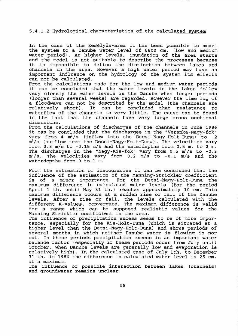
5.4.1.2 Hydroloqical characteristics of the calculated system

In the case of the Keselyüs-area it has been possible to model the system to a Danube water level of 8800 cm. (low and medium water period). At higher levels, inundation of the area starts and the model is not suitable to describe the processes because it is impossible to define the distinction between lakes and channels in the area. However a high water period may have an important influence on the hydrology of the system its effects can not be calculated. From the calculations made for the low and medium water periods it can be concluded that the water levels in the lakes follow very closely the water levels in the Danube when longer periods (longer than several weeks) are regarded. However the time lag of a floodwave can not be described by the model (the channels are relatively short). It can be concluded that resistance to waterflow of the channels is very little. The cause can be found in the fact that the channels have very large cross sectional dimensions. From the calculations of discharges of the channels in June 1986 it can be concluded that the discharges in the "Veranka-Nagy-fok" vary from 4 m3/s (inflow into the Decsi-Nagy-Holt-Duna) to -2 m3/s (outflow from the Decsi-Nagy-Holt-Duna). The velocities vary from 0.3 m/s to -0.15 m/s and the waterdepths from 0.5 m. to 2 m. The discharges in the "Nagy-Kis-fok" vary from 0.5 m3/s to -0.3 m3/s. The velocities vary from 0.2 m/s to -0.1 m/s and the waterdepths from 0 to 1 m.

From the estimation of inaccuracies it can be concluded that the influence of the estimation of the Manning-Strickler coefficient is of a minor importance. For the Decsi-Nagy-Holt-Duna the maximum difference in calculated water levels (for the period April 1 th. until May 31 th.) reaches approximately 10 cm. This maximum difference occurs at a sudden rise or fall of the Danube levels. After a rise or fall, the levels calculated with the different K-values, convergate. The maximum difference is valid for a range which can be supposed realistic values for the Manning-Strickler coefficient in the area. The influence of precipitation excess seems to be of more impor­tance, especially for the Kis-Holt-Duna (which is situated at a higher level than the Decsi-Nagy-Holt-Duna) and shows periods of several months in which neither Danube water is flowing in nor out. In these periods precipitation excess is an important water balance factor (especially if these periods occur from July until October, when Danube levels are generally low and evaporation is relatively high). In the calculated case of July 1th. to December 31 th. in 1986 the difference in calculated water level is 25 cm. at a maximum. The influence of possible interaction between lakes (channels) and groundwater remains unclear.

58

5.4.2 Recommendations

5.4.2.1 Recommendations concerning the current model

To calibrate the model for the actual situation it is necessary to collect field data. This collecting of field data serves two goals :

1. possibility to check basic assumptions on validity, 2. possibility to compare calculated characteristics with

measured characteristics.

ad 1. As already mentioned it is necessary to check the interaction of lakes (channels) and groundwater. It is recommended to study the groundwaterflow at the location of the lakes. It can be suggested that also water quality measurements may give insight in the origin of the water in the lakes. It is also recommended to check the assumption that the water levels and water level fluctuation in the Veranka are similar to those of the Danube. Furthermore the assumption concerning the neglect of the connection from the Decsi-Nagy-Holt-Duna to the Malom-lake can best be avoided by incorporating the southern part of the system in future model calculations. This means that characteristics of lakes and channels of this southern system have to be measured. If the dimensions of the "Kis-"Sand-Bank"-lake-fok" are measured, it may be possible to model the Kis-Holt-Duna and the "Sand-Bank"-lake as two seperate lakes.

ad 2. To calibrate the current model (or a new variant) it is necessary to collect lake level data of the lakes incorporated in the model. It can also be very helpful to have discharge measurements of the connecting channels. It may be evident that these data should cover a range of Danube levels as large as possible.

5.4.2.2 Application of the "F0K5"-model to other systems

When applying the "F0K5"-model to other systems it is recommended to study the behaviour of time lag of floodwaves in long chan­nels. When channels are relatively short this possible time lag may not be of importance, but in case of long channels it may be that the Chezy equation is not adequate to describe the hydrological features of the channel system.

59

6 ELABORATION OF PLACING A WEIR INTO THE "NAGY-KIS-FOK"

6.1 Introduction

In this chapter one of the options mentioned in chapter 4 has been elaborated. The option which has been elaborated concerns the placing of a movable weir into the "Nagy-Kis-fok". The first goal of this elaboration is to study how the storage capacity of the Kis-Holt-Duna and the "Sand-Bank"-lake can be used by cap­turing Danube water during high water periods. Also a forecast for 50 years has been made. This is described in sections 6.2 and 6.3. The second goal is to make a proposition for a type of weir which can be used to store a maximum amount of water in the area. This is described in section 6.4. The first goal has been achieved by means of a computer program called "Reservoir Sizing Model" which is incorporated in the TH-model. The second goal has been achieved by comparing weirs which can be used in the Gemenc-area.

6.2. Description of the "Reservoir Sizing Model"

Water management using storage is an adaption of random processes of water supply. Because of this random character, the unavoidable shortages in water supply during dry seasons are covered by stored waters of wet seasons. A distinction in two different types of water management (with different types of storage reservoir operation) can be made:

1. flood control: storage reservoirs exclusively built for flood control are emptied immediately after the flood has passed in order to enable them to receive the next flood,

2. optimize water use: in reservoirs serving water users the water surplus in wet periods are retained for dry periods.

While a flood retention reservoir is kept empty most of the time, those serving water users are kept as full as necessary and feasible most of the time. Because of these contradicting operation strategies, a complex mode of operation must be ap­plied.

In this study the Kis-Holt-Duna and the "Sand-Bank"-lake are considered as a reservoir which has to meet a certain water demand i.e. the evaporation. Therefore this reservoir is treated as the second type of reservoir mentioned above.

60

In case of a reservoir which serves water users the release function of a reservoir is given as K = f (M) where K stands for the storage capacity to be provided and M for the water demand.

Because the stochastic process of water supplies is transformed by the reservoir, the function which represents this transfor­mation can not be deterministic. In fact, in case of the reser­voir which serves water users, with a capacity K, the problem is to derive the storage yield function given as

K = f(M,P)

Where P is the probability of meeting water demand M [Zsuffa Sr. et al., 1987] . A more detailed describtion of the theory and backgrounds concerning the "Reservoir Sizing Model" is dealt with in appendix XX.

In the TH-model (see also section 3.2) a possibility to study reservoirs is incorporated. This part of the model, which is called "Reservoir Computation" (see fig. 6.1), makes it possible to compute probability functions to describe the storage process of a reservoir.

*** SPECIAL APPLICATIONS *** Hydrological Statistics

Time Series Analysis Data Maintenance

* Computation of HIGH WATERS * * WATER RESOURCES estimation * * RESERVOIR computation

Fig. 6.1 Menu of the TH-Model

The main assumptions underlying the "Reservoir Sizing Model" are (see also appendix XX):

1. inflow water discharges during the successive time intervals are independent stochastic variables,

2. the input discharge into the reservoir within any interval At precedes water release.

6.3 Application of the "Reservoir Sizing Model" to the Kis-Holt-Duna

In this section the application and the results of using the "Reservoir Sizing Model" are discussed. The main question to be

61

answered is whether the storage capacity of the Kis-Holt-Duna (including the "Sand-Bank"-lake) can be used in an optimal way by retention of Danube water entering the area during a high water period. The main starting point is that calculated discharges in the actual situation are also valid for a situation in which water is stored in the Kis-Holt-Duna by means of a movable weir. In these calculations the effect of precipitation and evaporation are taken into account. The precipitation excess has been regarded as a water demand. To meet with the main assumption that inflowing water discharges during the successive time intervals have to be independent stochastic variables, the correlation coefficient has to be less than 0.30 [Pers. Comm. Zsuffa Sr., 1993].

Section 6.3.1 gives a summary of input data and sources. In section 6.3.2 the limitations of the application of the "Rese­rvoir Sizing Model" are discussed. Section 6.3.3 deals with the results for the actual situation and for a possible situation in 50 years.

6.3.1 Input data and sources

The input data for the "Reservoir Sizing Model" consist of the following:

Discharges Positive (incoming) discharges into the Kis-Holt-Duna during the period of 1967 to 1990. These discharges are calculated by the "FOK5"-model (see chapter 5). Because the "Reservoir Sizing Model" requires monthly data, the data have been converted to monthly data.

Control codes for calculation Considering the main assumption that input discharges have to be independent and that the correlation coefficient has to be less than 0.30, the smallest possible time unit to take into con­sideration is 3 months. The considered time units are:

1. September, October, November, 2. December, January, February, 3. March, April, May, 4. June, July, August.

The model transforms input data to unit volumes. Amongst others the magnitude of the unit volume determines the accuracy of the model calculations. The unit volume was set to 0.020 Million m3. It has been calculated that the capacity of the Kis-Holt-Duna including the "Sand-Bank"-lake is 460.000 m3 (see appendix XXI) or 23 times the unit volume.

62

Precipitation and evaporation In the "Reservoir Sizing Model" precipitation excess has been looked at as a (fixed) water demand. Precipitation and evaporation data were used from the stations Pecs (evaporation) and Decs and Bâta (precipitation) (see also appendix X and section 2.5.2). The years 1984 to 1987 have been assumed to give an average idea of the amount of precipitation and evaporation for the period 1967 to 1990. Following the subdivision in periods of three months the precipitation excess has been given for each of these three months (in unit volumes). In case of a period with a positive precipitation excess, the value for water demand was set to zero. Consequently the fol­lowing unit volumes for "precipitation excess" have been used:

1. September, October, November 1 unit volume, 2. December, January, February 0 unit volumes, 3. March, April, May 1 unit volume, 4. June, July, August 5 unit volumes.

6.3.2 Limitations of the model calculations

Obviously all constraints discussed in connection with the ap­plication of the "FOK5"-model (providing the input discharges of the reservoir) also influence the calculations with the "Rese­rvoir Sizing Model". Furthermore it has to be mentioned that independently calculating input discharges and the effect of precipitation and evaporation can not be correct because most of the time these features are mutually influenced. It can also be questioned whether the applied precipitation and evaporation data from 1984 to 1987 give a good approximation for the calculated period 1967 to 1990. The necessity to neglect positive precipitation excess (negative demand) leads to an underrating of the possibility that the reservoir is filled with a certain volume during a certain time period. The main assumption that all input discharges can be stored in the reservoir leads to an overrating of the possibility that the reservoir is full in a certain time period because inflowing discharges in the reservoir will evidently decrease when more water is stored in the reservoir. Finally it has to be mentioned again that in these calculations no inflow is calculated when Danube levels exceed a Keselyüs level of 8800 cm. This may lead to a serious underrating of the possibility that the reservoir is full in a certain time period. The quantitative influence of these limitations on the model calculations are difficult to define as yet. However, it is assumed that the model calculations give a broad indication to answer the question whether it is possible to use the storage capacity of the Kis-Holt-Duna with Danube water from high water periods.

63

6.3.3 Results

In this section a survey of the results with the "Reservoir Sizing Model" has been given. The calculation has not only been made for the actual situation but also for a future situation (the year 2040) . The actual situation is discussed in the fol­lowing section. The forecast for the year 2040 is discussed in section 6.3.3.2.

6.3.3.1 Actual situation

In figures 6.2 to 6.5 the so called "behaviour functions" for the Kis-Holt-Duna are depicted for the different calculation periods. The x-axis represents the non exceeding probability P. This is the probability that a certain water volume (represented by the y-axis) in the reservoir is not exceeded. Two extreme levels can be distinguished: the reservoir is totally full or the reservoir is totally empty.

In table 6.1 the probabilities that the reservoir is totally full or totally empty are listed.

time period

Sept, Oct, Nov

Dec, Jan, Feb

March, April, May

June, July, Aug

probability that reservoir is full

0.17

0.51

0.63

0.83

probability that reservoir is empty

0

0

0

0 Table 6.1: Probabilities for the Kis-Holt-Duna in the

actual situation

It can be concluded that in the growing season (roughly from March until August) the probabilty of the reservoir being totally filled is relatively high. Whether this is sufficient to cover the demands from an ecological point of view remains unclear. This question is beyond the scope of this study.

6.3.3.2 Forecast

As has been discussed in section 3.3.2 it is clear that water levels of the Danube have decreased during this century. In this

64

section an extrapolation of this decreasing trend has been made to construct the "behaviour functions" of the Kis-Holt-Duna for the year 2040. It must be recognized that a period of fifty years is probably far too long to make a proper estimation, because the assumption that the decreasing trend of Danube water levels will continue in the future is very uncertain. However, the year 2040 has been chosen arbitrary to make a prediction of the "behaviour functions" in the future. This has been done by means of linear extrapolation of the maximum Danube water levels. By constructing a Q-h relation for the Danube levels and the discharges flowing into the Kis-Holt-Duna, an estimation has been made of the average decrease of the inflowing discharges (see appendix XXII). It has been calculated that the discharges will decrease with a factor of 0.264. The discharges of the current situation have been multiplied with this factor to construct the "behaviour functions" for the situation in 2040. These are depicted in figures 6.6 to 6.9. The probabilities whether the Kis-Holt-Duna will be totally full or empty in the different periods are listed in table 6.2.

time period

Sept, Oct, Nov

Dec, Jan, Feb

March, April, May

June, July, Aug

probability that reservoir is full

0

0.04

0.18

0.25

probability that reservoir is empty

0

0.02

0.01

0.03 Table 6.2: Probabilities for the Kis-Holt-Duna in the

year 2040

When table 6.1 (actual situation) is compared to table 6.2 (situation in 2040) it can be concluded that a serious decrease of the water volume in the Kis-Holt-Duna will take place.

65

x [DM]

Reservoir Sizingi RSTP Model

"Behavior function" <P = prob(X<x|M=y,K=z)>

kiç decsi

L_Ergodic state ^Period : 1 SefRm - Capacity : Denand

2 3 DV = 1 DM =

.46 H.H3

T T N T

x'= shortage

J2JUÛ.

x = cverflou

x = sï3ï fred u iters

.8 .1 .2 .3 .4 .5 .6 .7 Non-exceeding probability» P

.8 .9 1.8

Fig 6.2: Behaviour function for the actual situation (September, October, November)

x [DV]

Reservoir Sizing« RSTP Model

"Behavior function" <P = prob(X<x|M=y,K=z)}

r

: ki

:

r m •

-

-

; decsi

Ert odic sti

x = c

x = s

ite

verf low

tored w

Period : 2 Dec-Feb Capacity : 23 DV = .4 Denand : Q DM = .8 DV= .628 M . N 3

1 1

iters

s M .M3 3 M . M 3

.8 .1 .3 .4 .5 .6 Non-exceeding probability. P

.7 .8 .9 1.8

Fig 6.3: Behaviour function for the actual situation (December, January, February)

66

x EDV]

Reservoir Sizingi RSTP Model

"Behavior function" {P = prob(X<x|M=y,K=z)}

K :

x' = shortage

x = everf low

x = stored uiters

Ergodic state Period : 3 Har-Hay Capacity : 23 DV = Denand : 1 DV = DV= .020 M . M 3

.46 H.M3

.02 H.M3

.0 .1 """".2 "" .3 .4 .5 .6 .7 Non-exceeding probability) P

.8 .9 1.0

Fig 6.4: Behaviour function for the actual situation (March, April, May)

x [DV]

K

.E

:

: s

\

-

1

ki

X

i decsi

= short

Reservoir Sizingi RSTP Model

"Behavior function" <P = prob(X<x|M=y,K=z)}

age

.1 .2

Erç Per Cap DP«

DV:

odic st< iod acity and

x = c

X = s

kte : 4 Jun-: 23 DV : 5 DV

.020 H.H3

1

verf low

tored w

Aug = .4 = .1

i ters

! H .N3 ) M .M3_

.3 .4 .5 .6 .7 .8 .9 1.8 Non-exceeding probabi l i ty . P

Fig 6.5: Behaviour function for the actual situation (June, July, August)

67

x [DV]

Reservoir Sizing« RSTF Model

"Behavior function" <P = prob(X<x|M=y.K=z)}

ki ; decsi

rgodic state eriod : 1 Sep-Nov

Capacity : 23 DV = Denand : 1 DV = DV= .828 H.H3

.8 .1 .2 .3 .4 .5 .6 .7 .8 .9 1.8 Non-exceeding probability« P

Fig 6.6: Behaviour function for the year 2040 (September, October, November)

Reservoir Sizing» RSTP Model

"Behavior function" x [DV] <P = prob(X<x|M=y.K=z)}

K

: ki -

i decsi

: Ergodic stat ^ P e r i o d :

e 2 Dec-Feb

: Capacity : 23 DV = .46 N.M3 : Denand : 8 DV = .88 H.M3 ' ' i ' • • • '

i i i i

.828 M.M3

.8 .1 .2 .3 .4 .5 .6 .7 Non-exceeding probability» P

x = c

X = s

verf low

tored Ui

.8 .9

, . / iters

1.0

Fig 6.7: Behaviour function for the year 2040 (December, January, February)

68

Reservoir Sizing» RSTP Model

"Behavior function" x EDV] <P = prob(X<x|N=y.K=z)}

K

• * •

: ki ; decsi

: Ergodic stal ^Pe r iod :

e 3 Mar-May

: Capacity : 23 DV = .46 H.H3 : Demand : 1 DV = .62 H.«3 . : DV=

U. jjj

.628

= ahort

H.H3

«ge—-1

x = overflow

tored w iters

.6 .1 .2 .3 .4 .5 .6 .7 .8 .3 1.8 Non-exceeding probability» P

Fig 6.8: Behaviour function for the year 2040 (March, April, May)

Reservoir Sizing» RSTP Model

"Behavior function" x [DV] <P = prob(X<x|M=y.K=z)>

K

.[

: ki "

i decsi

: Ergodic stat ^Per iod :

e _^ 4 Jun-flug

: Capacity : 23 DV = .46 H . M 3 ^ : Deiiand : 5 DV = JB-ttmib : DV=

? *

.626

= short

M . M 3 ^

age

1 .1 .2 .3 .4 .5 .6 .7 Non-exceeding probability» P

x = c - ^

X = £

verflatf ^ > ~ tored u

y iters

.8 .9 1.8

Fig 6.9: Behaviour function for the year 2040 (June, July, August)

69

6.4 Designing a weir

In this section a comparison has been made between different types of weirs which can be applied to the Keselyüs-area, to increase water storage in the Kis-Holt-Duna.

To compare the different weirs, demands are set where the weirs should compy with:

1. the weir should be movable: in this way it is possible to capture Danube water during a rise of Danube levels,

2. the weir must be financially manageable, 3. the weir must fit in in the natural environment of the

Keselyüs-area and can not be detrimental to the area, 4. installation of the weir may not disturb the Keselyüs-area, 5. the use of electricity should be avoided: this implies that

the weir must be tended by manpower.

In the sections 6.4.1, 6.4.2 and 6.4.3 three different types of weirs are described and discussed. In section 6.4.4 conclusions are drawn and a recommendation for a weir has been made.

6.4.1 "River Barrage"

The "river barrage" (see fig. 6.10) is a movable weir which exists of a steel main gate which is hung in a slot. The main structure of the weir consists of concrete walls. The gate can be lifted upwards with help of a hoist by manpower. This may be a disadvantage if this weir is applied to the Keselyüs-area. In this case the weir should be very large as a result of the large dimensions of the "Nagy-Kis-fok". It can be tended by manpower, but it will probably take two men to lift the gate [Pers. Comm. Csoma, 1993] . Another disadvantage is that if the gate is lifted during a high water period, the steel gate is at a height of about 4 metres. This, and the construction of a ladder, lamp and service bridge makes that this weir has a very big impact on the natural scenery.

70

J&-

wamnA saw*^»»

1. fundament plate 2. side wall 3. wing wall 4. slots of main gate 5. slots of provisional gate 6. stone lining 7. precast limig 8. sheet wall 9. cut off 10. sip-nap

11. main gate 12. provisional gate 13. seal 14. hoist 15. service bridge 16. handrail 17. ladder 18. gauge 19. lamp

Fig 6.10: The "river barrage" [Source: Department of Hydraulic Engineering, Technical University of Budapest]

the gate. Therefore it is necessary that a two sided constructed to prevent the gate from damage (see fig. 6. makes the weir very expensive [Pers. Comm. Csoma, 1993].

The main gate has to stand a water pressure from both sides of the gate. Therefore it is necessary that a two sided seal is

'' " n (see fig. 6.11). This

71

frVvWvVAWA^Sl

yerticaJ ü'-fi

\ ar ruw

}

Fig 6.11: One sided seal [Source: Department of Hydraulic Engineering, Technical University of Budapest]

The advantage of the "river barrage" is that it is very secure and that it probably will work adequate.

6.4.2 "Valve Weir"

The "valve weir" consists of a valve, with water pressure from both sides (see fig. 6.12). If the water level from "fok"-side (and as a result of that the water pressure) increases, the valve turns, and water flows into the lake. In case of the "valve weir" the water level in the lake can not be controlled, because Danube water will always flow in when it reaches a level higher than the lake level.

72

Fig 6.12: The "valve weir"

This type of weir is a very simple solution. It is less expensive than a "river barrage" but more expensive than "lockers" (see section 6.4.3) . The advantage of a "valve weir" is that it is not necessary to tend such a weir.

6.4.3 "Lockers"

This is the most simple type of weir. It consists of wooden planks ("lockers"), which can be placed on top of each other (see fig. 6.13). When the Danube levels have risen to the highest level, the lockers can be placed on top of each other, to capture the water.

73

Fig 6.13: "Lockers"

This weir can be made from materials that origin from the area. The weir must be tended manually, however it may be more dif­ficult than for the two other types of weirs. The most important advantage of this type of weir however may be that it is a very cheap solution. It can be used to check whether the placing of weirs has the desired effect on the area. It is also possible to apply this type of weir to other locations without large costs. A disadvantage of "lockers" is that it is relatively labour-intensive to control.

6.4.4 Conclusions and recommendations concerning the weir

No judgment can be made whether the weirs can resist the water pressure. It is recommended that this will be investigated. It may be possible that an extra channel has to be made next to the

74

weir, to transport the water after an inundation.

The "river barrage" seems the less suitable weir for this area. It is very expensive, has a big impact on the natural scenery and it is hard to tend manually. It is recommended that, if weirs are applied to the Keselyüs-area, "lockers" are used. They have the same effect as the other two types of weirs, are cheap and relative easy to tend manually. If the result is satisfying, and the storage capacity of the Kis-Holt-Duna increases, the "lockers" can be replaced by a "valve weir", which is more easy to tend. Another advantage of "lockers" is that they can easily be applied to other locations.

6.5 Conclusions and recommendations

As a result of the rough assumptions (see section 6.3) it is recommended to repeat the calculations with the "Reservoir Sizing Model" with more realistic values for the inflowing discharges in the reservoir. These values can be obtained by incorporating the behaviour of a movable weir in the "F0K5"-model and repeat the calculations. Furthermore refined calculations with the "F0K5"-model (calibration) are necessary to enlarge the reliability of the calculations. Concerning the assumptions about precipitation and evaporation it is recommended to check if the period 1984-1987 is a represen­tative period. It would be more accurate to incorporate the effect of precipitation and evaporation in the "F0K5"-model. In this case the use of the "Reservoir Sizing Model" for this kind of problems may be starting point for further discussion.

From the calculations of the "behaviour functions" it can be concluded that in the growing season (roughly from March until August) the probabilty of the reservoir being totally filled is relatively high. Whether this is sufficient to cover the demands from an ecological point of view remains unclear. This question is beyond the scope of this study. It is recommended that demands to create an optimal hydro-ecological situation are studied and compared with this kind of results. When table 6.1 (actual situation) is compared with table 6.2 (situation in 2 040) it can be concluded that in the future a serious decrease in water contents of the lake system will take place. This conclusion is only valid under the assumption that the linear decrease of Danube levels in this century will con­tinue in the next fifty years. It is recommended to study these assumptions in more detail and to make a forecast for a shorter period. Furthermore it has to be said that the defined Q-h relation (see appendix XXII) is a weak relation. For further research it is recommended to study the expected Danube levels for the future

75

and calculate the effects for different scenarios.

It is recommended that demands to create an optimal hydro-ecological situation are studied.

76

7 CONCLUSIONS AND RECOMMENDATIONS

7.1 Introduction

In this chapter a summary of conclusions which have been drawn in this study has been given. A subdivision has been made according to the four main goals of this study. Section 7.2 deals with the prove that in this century a structural lowering of the water levels of the Danube occured. Section 7.3 deals with the general proposition to rewet the Keselyüs-area. Section 7.4 treats the conclusions and recommendations of the application of a simulation model for channel flow for the Keselyüs-area. Section 7.5 deals with the conclusions and recommendations of the elaborated option to rewet the Keselyüs-area. Section 7.6 con­cerns general conclusions and recommendations.

7.2 Analysis of the hydrological regime of the Danube

In analysis of high water periods it has been proved that the Danube levels of the period 1967 until 1990 have decreased compared to the Danube levels of the period 1901 until 1920. This is indicated by the following features:

1. floods of less lengths have occured in the period of 1967-1990 compared to the period of 1901-1920,

2. the sums of lengths of floods in the period of 1967-1990 is less than those of the period of 1901-1920,

3. less floods have occured during the period of 1967-1990 compared to the period of 1901-1920.

7.3 A general proposition to rewet the Keselvüs-area

Three options have been made which increase the water quantity in the Keselyüs-area.

1. Placing of movable weirs in the "Veranka-Nagy-fok", the "Nagy-Kis-fok", the "Kis-"Sand-Bank"-lake-fok" and/or the "Grebec-Forgó-fok".

2. Connecting the Kis-Holt-Duna to the Grebec-branch for the intake of Danube water.

3. The intake of Sió water into the lake system in the North (Forgó-lake, Hanis-lake and Peti-lake) and/or the lake system in the South ("Sand-Bank"-lake, Kis-Holt-Duna and Decsi-Nagy-Holt-Duna) of the Keselyüs-area.

77

The last two options also include the placing of movable weirs. The options also can be combined.

It is recommended that the following aspects, concerning the three options, are studied in more detail:

1. further elaboration of the options and combinations of the options,

2. the differences between the three options concerning silting up of the lakes, "foks" and old branches,

3. the differences between the three options in throughflow, in order to obtain refreshing,

4. the differences between the three options in the dynamics of the hydrological situation,

5. the differences between the three options concerning the water qualities of the Danube and the Sió.

7.4 Application of a simulation model for channel flow

7.4.1 Conclusions

The "F0K5"-model is an easy to handle tool to describe the surface hydrology of a floodplain system. The possibility to simulate the effects of weirs gives way to search for solutions to optimize the hydrology of a floodplain.

In the case of the Keselyüs-area it has been possible to model the system to a Danube water level of 8800 cm. (low and medium water period) . At higher levels, inundation of the area starts and the model is not suitable to describe the processes because it is impossible to define the distinction between lakes and channels in the area. However a high water period may have an important influence on the hydrology of the system its effects can not be calculated. From the calculations made for the low and medium water periods it can be concluded that the water levels in the lakes follow very closely the water levels in the Danube when longer periods (longer than several weeks) are regarded. However the time lag of a floodwave can not be described by the model (the channels are relatively short). It can be concluded that resistance to waterflow of the channels is very little. The cause can be found in the fact that the channels have very large cross sectional dimensions.

From the estimation of inaccuracies it can be concluded that the influence of the estimation of the Manning-Strickler coefficient is of a minor importance. For the Decsi-Nagy-Holt-Duna the maximum difference in calculated water levels (for the period April 1 th. until May 31 th.) reaches approximately 10 cm. This

78

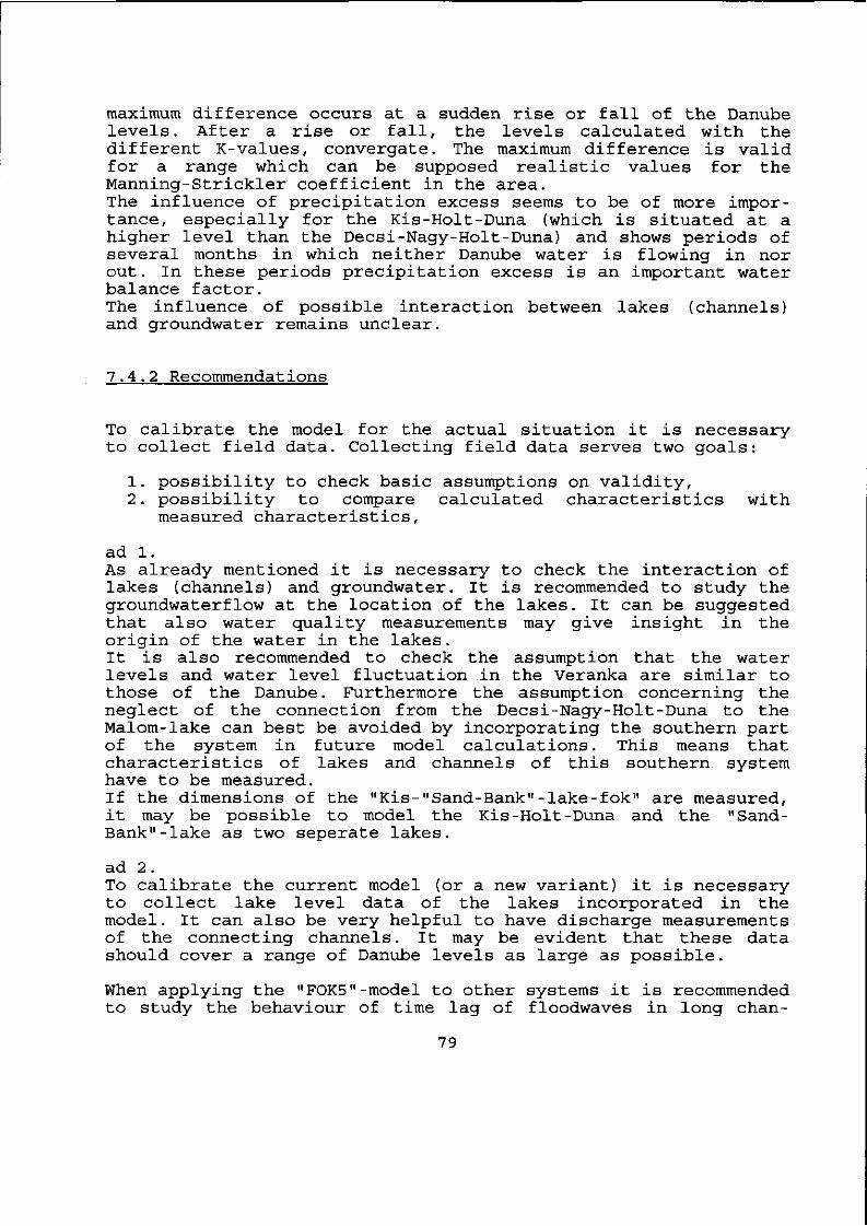
maximum difference occurs at a sudden rise or fall of the Danube levels. After a rise or fall, the levels calculated with the different K-values, convergate. The maximum difference is valid for a range which can be supposed realistic values for the Manning-Strickler coefficient in the area. The influence of precipitation excess seems to be of more impor­tance, especially for the Kis-Holt-Duna (which is situated at a higher level than the Decsi-Nagy-Holt-Duna) and shows periods of several months in which neither Danube water is flowing in nor out. In these periods precipitation excess is an important water balance factor. The influence of possible interaction between lakes (channels) and groundwater remains unclear.

7.4.2 Recommendations

To calibrate the model for the actual situation it is necessary to collect field data. Collecting field data serves two goals:

1. possibility to check basic assumptions on validity, 2. possibility to compare calculated characteristics with

measured characteristics,

ad 1. As already mentioned it is necessary to check the interaction of lakes (channels) and groundwater. It is recommended to study the groundwaterflow at the location of the lakes. It can be suggested that also water quality measurements may give insight in the origin of the water in the lakes. It is also recommended to check the assumption that the water levels and water level fluctuation in the Veranka are similar to those of the Danube. Furthermore the assumption concerning the neglect of the connection from the Decsi-Nagy-Holt-Duna to the Malom-lake can best be avoided by incorporating the southern part of the system in future model calculations. This means that characteristics of lakes and channels of this southern system have to be measured. If the dimensions of the "Kis-"Sand-Bank"-lake-fok" are measured, it may be possible to model the Kis-Holt-Duna and the "Sand-Bank"-lake as two seperate lakes.

ad 2. To calibrate the current model (or a new variant) it is necessary to collect lake level data of the lakes incorporated in the model. It can also be very helpful to have discharge measurements of the connecting channels. It may be evident that these data should cover a range of Danube levels as large as possible.

When applying the "F0K5"-model to other systems it is recommended to study the behaviour of time lag of floodwaves in long chan-

79

nels. When channels are relatively short this possible time lag may not be of importance, but in case of long channels it may be that the Chezy equation is not adequate to describe the hydrological features of the channel system.

7.5 Placing a movable weir into the "Nacrv-Kis-fok"

As a result of the rough assumptions it is recommended to repeat the calculations with the "Reservoir Sizing Model" with more realistic values for the inflowing discharges in the reservoir. These values can be obtained by incorporating the behaviour of a movable weir in the "F0K5"-model and repeat the calculations. Furthermore refined calculations with the "F0K5"-model (calibration) are necessary to enlarge the reliability of the calculations. Concerning the assumptions about precipitation and evaporation it is recommended to check if the period 1984-1987 is a represen­tative period. It would be more accurate to incorporate the effect of precipitation and evaporation in the "F0K5"-model. In this case the use of the "Reservoir Sizing Model" may be starting point for further discussion.

From the calculations of the "behaviour functions" it can be concluded that in the growing season (roughly from March until August) the probabilty of the reservoir being totally filled is relatively high. Whether this is sufficient to cover the demands from an ecological point of view remains unclear. It is recom­mended that demands to create an optimal hydro-ecological situation are studied. It can be concluded that in the year 2040 a serious decrease in water quantity of the Kis-Holt-Duna will take place. It is recom­mended that the assumptions concerning the extrapolation of the decreasing trend of the Danube are studied in more detail. It may be more realistic to make a forecast for a shorter period. Furthermore it has to be said that the defined Q-h relation is not an unambigous relation. For further research it is recom­mended to study the expected Danube levels for the future and calculate the effects for different scenarios.

It is recommended that, if weirs are applied to the Keselyüs-area, "lockers" are used. They have the same effect as a "river barrage" and a "valve weir" and are cheap. If the result is satisfying, and the storage capacity of the Kis-Holt-Duna increases, the "lockers" can be replaced by a "valve weir", which is more easy to tend.

80

7.6 General conclusion and recommendation

In general it can be concluded that rewetting the Keselyüs-area by placing movable weirs into the connecting channels between the lakes can be a good solution as a first step within a larger framework of hydrological activities. It is recommended to collect more hydrological data and study ecological demands. After this a repetition of the calculations should be made to reduce the effects of different assumptions.

81

REFERENCES

Aller, M. v., M. Guinée, L. Hombergen, H. v.d. Weyden, 1991, Revitalisation of the Gemene Floodplain Forest, Delft University of Technology, Faculty of Civil Engineering, 62 p.

Fruget, J.F., Castella, E., Amoros, C , Roux, A.L., 1992, Les Ecosystèmes Aquatiques Danubiens, Etat des Connaissances sur leur Fonctionnement suivi d'un Projet d'Etude du Secteur du Gemene (Hongrie), la Fondation Cousteau, 84 p.

Hydrographical Service of Hungary, 1985, Yearbook of the Hydrographical Service of Hungary 1984, Budapest, 288 p.

Hydrographical Service of Hungary, 1986, Yearbook of the Hydrographical Service of Hungary 1985, Budapest, 284 p.

Hydrographical Service of Hungary, 1987, Yearbook of the Hydrographical Service of Hungary 1986, Budapest, 269 p.

Hydrographical Service of Hungary, 1988, Yearbook of the Hydrographical Service of Hungary 1987, Budapest, 284 p.

Reimann, J., 1989, Mathematical Statistics with Application in Flood Hydrology, Akadémiai Kiadó, Budapest, 330 p.

Starosolszky, Ö., 1987, Applied Surface Hydrology, Water Resour­ces Publications, Colorado, 821 p.

Whitten, D.G.A. Penguin, 516 p.

Brooks, J.R.V., 1972, Dictionary of Geology, The

Zsuffa, I., Gâlai, A., 1987, Reservoir Sizing by Transition Probabilities, Theory, Methodology, Application, Water Resources Publications, Colorado, 186 p.

Zsuffa, I., Buzetzky, G., Eichardt, G., Kalocsa, B., Schnidt, A., Sziebert, J., Vancsura, P., Varga, A., Vas, K., Zellei, L., 1992, Revitalisation du Systeme Hydraulique et de l'Ecosystème de Foret de Gemene, Etude Préliminaire, Ecole Technique Superieur Pollack Mihaly Institut de l'Aménagement en Eau, 32 p.

82

Revitalisation of the Gemenc-area, Baja, Hungary

A study on hydrological possibilities to revitalise the ecosystem in the Keselyüs-area

APPENDICES

Twan Rosmalen Loek Stalpers

Technical University Budapest, Hungary

Technical College "Pollack Mihâly" Institute of Water Management, Baja, Hungary

Agricultural University Wageningen, the Netherlands

83

THE GEMENC-AREA

Appendix: I Title: LOCATION OF THE KESELYÜS-AREA IN THE GEMENC-AREA

Scale: equals 10 kilometre

Key:

Keselyüs-area

84

THE GEMENC-AREA

Appendix: II Title: REVITALISATION-PROPOSITIONS IN THE GEMENC-AREA

equals 10 kilometre

Key:

1. Revitalisation of old branches 2. Filtration of water in old Danube-branches 3. Placing of weirs 4. Water intake from the Sió-riyer

(Source: Aller et. al., 1991 (adapted);

85

THE KESELYÜS-AREA

Appendix:111

S c a l e :

Key:

T i t l e : GEOGRAPHICAL MAP OF THE KESELYÜS-AREA

1«

si

sad

ike

vamp

86

THE GEMENC-AREA

Appendix: IV

Scale: ^ H H =

Key: • Title: GEMENC PROTECTED LANDSCAPE

Protection zone of first degree

Protection zone of second degree

AREA

equals 10 kilometre

87

THE GEMENC-AREA

Appendix: V Title: LOCATION OF .THE REFUGE-CENTRES AND THE GÖGA-AREA

Scale: ^ ^ M n^^, ^mmm — a t^m^ | equals 10 kilometre

Key:

,-x C L_ Góga-area *q

—r i | l l i i

[ S o ur C( E e

Refuge-centres

rs. Coram. Zsuffa Sr., 1993]

88

^â$NSfeià

« Ç l ,

•mr mm > V

»Si1

m.

*^M:

VI

&^>w

>$Mfe^3S« i TOPOGRAPHICAL MAP OF THE KESELYÜS-AREA

' ' • •' '*& ' ' « A V ' 2> • ~ • Ev

90

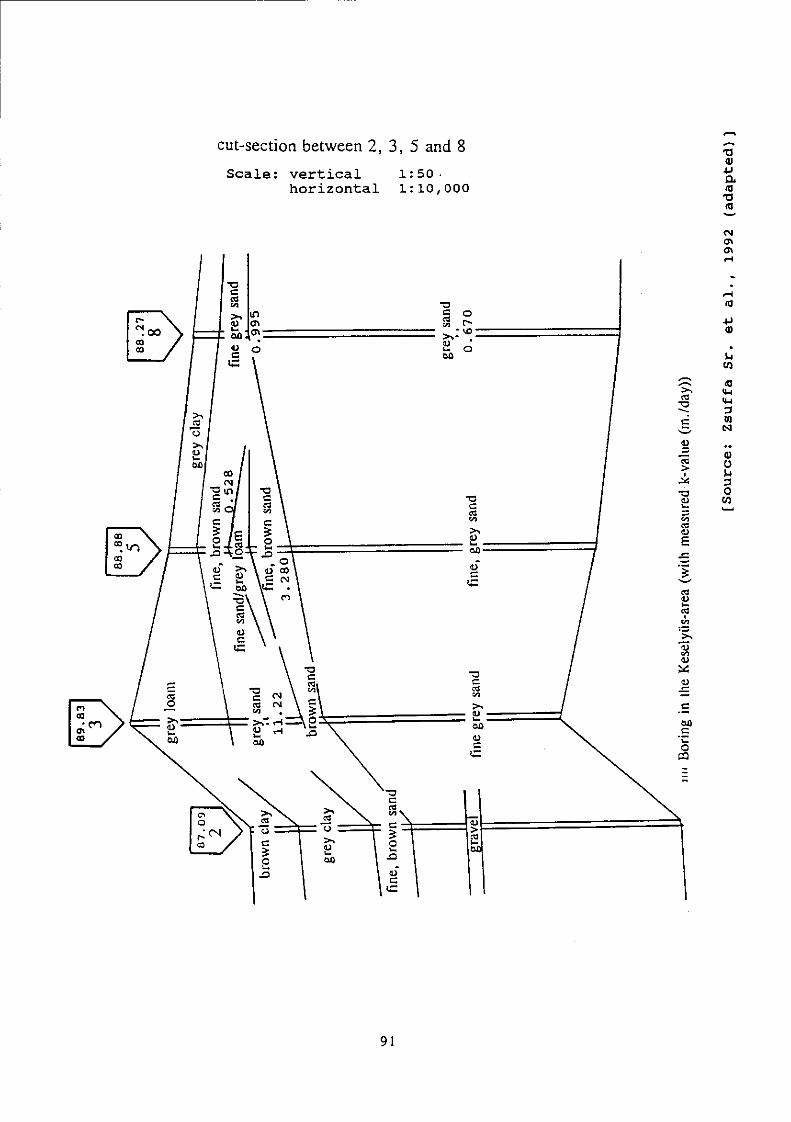
cut-section between 2, 3, 5 and 8

Scale: vertical 1:50-horizontal 1:10,000

-a <u 4J a « •a

s-+^

.-—\ p-% C3

E v—'' O 3

"ëd

> 1 ±s

-a <u w* 60 C3 <U P

-P <u

u W

(0 <M <M 3

##

a> o 3 0 w <_

91

cut-section between 1, 4, 5, 6 and 7 Scale: vertical 1:50

horizontal 1:10,000

a\ \ CO /

2° -J\ at c ƒ 5 / P /

-a c CS </5

c * o

if 1 c /

-O

si" c

>% aj i— -où-

c C

in CT> a\ o

ca O

T3 C rd C/5

>»v <u où-

K <u

c

00 -<N -in

• o

-3

«3 VI

>* i> -u- -ou

•&

CM H

, O

T3 C

>» . (U -• u - -

Où 1) c

c« 1)

(U

o

00

o

1)

aû-

o

- a c ca

<u c

«c

. 0 0

(U •P a «3 •a

(M en

-M (U

<t-l

3

>> c«

• u i=

1)

—-«S > 1

u-Uï c3 (U

(U Ü u 3 0 en

92

THE GEMENC-AREA

Append ix :

S c a l e : ^

Key: i

2

3

4

5

IX T i t l e : LOCATION OF THE GAUGING STATIONS

^ a B ^ a ^ 3 3 B ^ i ^ c = > ^ i ^ K = ] e q u a l s 10 k i l o m e t r e

Ba ja (km. 1 4 7 8 . 8 )

S z e k s z a r d - G e m e n c (km. 1 4 9 6 . 0 )

B â t a

Decs

Pec s

93

o

e

r-00 ON TH

1 m T

VO oo ON T H

1 «O 00 ON rH

i •<+ 00 ON T—l

1 • T

> 00 ON H

• *

00 ON H

P O H rri 0*

w tü H

Pi O l i i

CO

W u X

w F; o H

EH M 0 J M U W tf Pu

>H

.-J K H S ( ) S

X

o O

o o »O

O

! o o o

i n

(min) SS93X3 uojiBjidpajd 94

X>

G

Q

00

N 0)

N

ex

co N (U

N <ü

x

o o 00 00

o o t-> 00

o o VO 00

o o «o 00

o o "3-00

o o co 00

o 00 ^

('UK)) UiniBp 9A0qB S(3A3[J31BMpunOJ§

95

o o 00 00

o o t-> 00

o o VO 00

o o >o 00

o o Tf 00

o o co 00

•O <u

U-i <=> I

00 , _ l

<ü

1 cd Q

N

VO

N • i - i

«o N

O,

N (U

• 1 - 4

O«

N

'EL

w

o En

D u M P w Pd w

co m H

w co w S l-l E-"

W

Q

O

CN

X

('Ulo) UinjBp 9AOqB S[3A3[J3JBMpiinOjS

96

APPENDIX XII HYDRAULIC GRADIENT OF THE DANUBE

The Danube levels which are used in this study have been measured at the gauging station of Baja. Because the Keselyüs-area is situated north of this gauging station, a correction has been made for the Keselyüs-area.

First a correction has been made to the mouth of the Veranka into the Danube which is situated most upstream. This point is situated at river kilometer 1488 (see appendix IX). To compute the hydraulic gradient of the Danube between the gauging stations of Szekszârd-Gemenc (82.52 m. above datum at river kilometer 1496.0) and Baja (81.00 m. above datum at river kilometer 1478.8) (see appendix IX) daily water levels of the Danube of both gauging stations have been compared. This has been done for a low water period of 09-11 until 19-11 of 1987 (see table XII.1).

Date

09-11-1987

10-11-1987

11-11-1987

12-11-1987

13-11-1987

14-11-1987

15-11-1987

16-11-1987

17-11-1987

18-11-1987

19-11-1987

Average hydraulic gradient

Szekszard-Gemenc

8379

8370

8367

8365

8362

8360

8369

8372

8370

8372

8377

Baja

8298

8292

8286

8279

8274

8274

8281

8284

8282

8288

8296

Hydraulic gradient

4.68

4.51

4.68

4.97

5.09

4.97

5.09

5.09

5.09

4.86

4.68

4.83

Table XII.1: Hydraulic gradient (09-11-1987 until 19-11-1987)

The hydraulic difference between the gauging station of Baja and the most upstream river mouth of the Veranka into the Danube is therefore (1488.0-1478.8) * 4.83 = 44,44 cm. This has been rounded to 44 cm.

97

The next correction has been made for the location where the "Veranka-Nagy-fok" flows into the Veranka. The total head loss is 22 cm. From this loss 10 cm. is con­centrated around a bank (spillway) upstream the Veranka-branch [Aller et al., 1991]. The total length of the Veranka is 14.7 km. The hydraulic gradient in the Veranka is therefore (22-10)/14.7 = 0.82 cm./km. The "Veranka-Nagy-fok" is situated 3.4 km. downstream of the beginning of the Veranka. The hydraulic dif­ference between the beginning of the "Veranka-Nagy-fok" and the mouth of the Veranka into the Danube (including the 10 cm. spillway) is therefore (3.4 * 0.82) + 10 = 12.79 cm. (this has been rounded to 13 cm.) The total head loss between the gauging station of Baja and the beginning of the "Veranka-Nagy-fok" is 44 - 13 = 31 cm.

98

APPENDIX XIII; THE THEORY OF KOLMOGOROV-SMIRNOV

XIII.1 Introduction

The Kolmogorov-Smirnov test can be used for testing homogeneity of a series of data. This test can be used to test whether the null hypothesis (a series of data is homogeneous) has to be rejected or not. The Kolmogorov-Smirnov test can also be used for testing the goodness of fit. In this case the test is applied to check the null hypothesis (two distribution functions are equal) has to be rejected or not.

The theory of Kolmogorov-Smirnov is based on the theory of Glivenko. So first the theory of Glivenko will be discussed here and after that the theory of Kolmogorov-Smirnov.

XI11.2 The theory of Glivenko

Suppose there is a sample Xlf X j , . . . , ^ of a random variable X. In the practice of hydrology the distribution function F(x) of a random variable X is mostly unknown. However, a rather good ap­proach of the distribution function F(x) can be found by using the following method (if the number of sample elements is high enough [Oral announcement Reimann, 1993]). First the sample elements are ordered into a sequence of increasing magnitude ;

X\ < X*2 <X*.

A step function Fn(x) can be defined in the following way (see Fig. XIII.1):

0 if x s X\

Pn(x) = k/n

1

Fnlxl

1-

î*V I—1 n

| 1 1 1

x 1 . * 2 * 3

i f X*k < x s X*k+1

i f x > X*n.

i

f

i—1

i i i L ' * X* X

Figure XIII.1: Step function [Source: Reimann, 1989]

99

The function Fn(x) is called an emperical distribution function. The emperical distribution function has all properties of a distribution function:

- the values fall in the range between 0 and 1, - it's monotonically non-decreasing, - it's continuous from the left.

At all abscissa points X*± (i=l, 2,...n) Fn(x) has a jump upwards by l/n. So at a certain point x, the value of Fn(x) is so many times l/n as many sample elements lower than x can be found. In other words the value of Fn(x.) at a point x is equal to the relative frequency of the event {X<x}. The probability of the same event is P(X<x) = F(x).

The frequency has a binomial distribution whose parameters are the number of observations n, and the probability of the event F(x). It can be proved that:

P[Fn(x)=^]=ln)[F(x)]k[l-F(x)]I>-

and:

E[Fn(x)] = F(x)

and:

D[Fn(x)] = FU) [l-F(x)] n

The question is which approximate difference can be expected between the emperical distribution function Fn(x) and the theoretical distribution function F(x), with a fixed n.

According to the Chebysev inequality:

P[\Fn(x)-F(x) \<X •A F(x) [1-FU)] ] > ( 1 _ 1 x

n X2

Since F(x) [l-F(x)] s 1A, the absolute value of difference for any x will be in the order of magnitude n"H. So with an increasing n, the difference will converge to zero. This fact is expressed by the theory of Glivenko: if n is increasing, the emperical distribution function converges uniformely on the whole real line to the theoretical distribution function (Fig. XIII.2).

100

Figure XIII.2: Theoretical distribution function [Source: Reimann, 1989]

So if:

£>n=max \Fn(x) -F(x)

then:

P(liirtDn=0) =1

Dn represents the maximum difference between the emperical distribution function and the theoretical cumulative distribution function.

XI11. 3 The theory of Kolmocrorov-Smirnov

Glivenko has proved that the emperical distribution function will converge to the theoretical cumulative distribution function if n tends to infinity. Kolmogorov has investigated what large ab­solute difference can be expected between the emperical and theoretical distribution function (i.e. how fast this convergence will be). As has been shown already, the order of magnitude of Dn is ap­proximately n~*. Kolmogorov has proved that the random variable DnVn fluctuates around a bounded value. He has obtained the following expression for the distribution of this random variable :

HmP(y/nDn<z) = V (-1) iexp"2i2z2=ü:(z)

Smirnov has invested the one-sided deviations. He has found:

D*=max[Fn(x) -F(x)]

101

££=max[F(x) -Fn(x)] X

Following:

limP(v/ïïD*<z) =l±TC[P(s/nD~<z) =l-exp"2z2=5(z)

In case of a test of homogenity the serie of data is cut into two parts (not necessarily two equal parts) . For both samples an emperical distribution function is constructed. Dn represents the maximum difference between the two emperical distribution functions. The null hypothesis is in this case: the series of data is homogeneous. In case of a fitting test the emperical distribution function is compared with a theoretical distribution function. Dn represents the maximum difference between the emperical distribution function and the theoretical distribution function. The null hypothesis is in this case: the emperical distribution function and the theoretical distribution function are identical.

If the observed value of Dn attains or summounts the value given in a table the hypothesis can be rejected.(See table XIII.1) [Reimann, 1989].

n

8 9

10 11 12 13 14 15

16 17 18 19 20

0.95

0.4543

0.4300

0.4093

0.3912

0.3754

0.3614

0.3489

0.3376

0.3273

0.3180

0.3094

0.3014

0.2941

0.99

0.5419 0.5133

0.4889

0.4677

0.4491

0.4325

0.4176

0.4042

0.3920

0.3809

0.3706

0.3612

0.3524

n

21 22 23 24 25 26 27 28 29 30 35 40 45 50

0.95

0.2827

0.2809

0.2749

0.2693

0.2640

0.2591

0.2544

0.2499

0.2457

0.2417

0.2243

0.2101

0.1984

0.1884

0.99

0.3443

0.3367

0.3295

0.3229

0.3166

0.3106

0.3050

0.2997

0.2947

0.2899

0.2690

0.2521

0.2380

0.2260

Table XIII.1: Kolmogorov one-sample test for two-sided alternative hypothesis [Source: Reimann, 1989]

102

* • « * • .

THE KESELYUS-AREA

Appendix :XIV T i t l e : GENERAL PROPOSITION TO REWET THE KESELYÜS-AREA

Scale: equals 1 kilometre

Key: winterdike wexr

(possible location) '" road

4 ^ lake

" ^ ...."T.. swamp

1. P l a c i n g of we i r s

2 . Connect ing t h e Kis-Holt -Duna and t h e Grebec

3 . I n t ake of S i ó -water

103

APPENDIX XV: PHYSICAL BACKGROUNDS OF THE "FOK5"-MODEL

XV.1 The governing equations

The continuity equation for a lake:

dV=A1(z(t))dz=J^Qcidt

-v^^-fhE^i i=l

Where :

dV : change of the water volume in lake Ai : surface area of the lake z : water level elevation in the lake Qci: discharge of the i. channel entering the lake k : the number of channels entering the lake

XV.2 Discharge equation for a channel

The water flow in a channel can be described by the dynamic de Saint Venant equation:

g dt dx dx c2R

Because of the assumption that the flow varies gradually, the first two inertia terms can be neglected:

ox AZCZR

oz _Q

lx~5

104

The Chézy equation is the result:

2

Q=kAR 3 /S=Ky/S

Where K=l/n is the Manning-Strickler coefficient.

XV.3 Discharge equation for a weir

The model considers broad crested weirs. The water can flow over a weir in two ways: free overflow and submerged flow. The dis­charge equation for free overflow follows:

Qf = cb (zu- zw)^2

if

zd- zw< 2/3 (zu - zw)

For submerged flow the discharge equation equals:

Qa = 2.5907 * cb (zd - zw) sjzu - zd

if

zd - zw * 2/3 (zu - zw)

Where :

zu: upstream water level zd: downstream water level zw: weir crest elevation b: weir width c: discharge coefficient.

105

XV.4 Numerical formulation

After integration of the continuity equation from tn to tn+1:

Analytical integration of the left hand side and numerical integration of the right hand side :

zn+1~zn+Yf — [K(zn,zf) i=l 2 N

Z?~Zn 1

sign(z?-zn) + h A^Z")

n+l „n+1 +K(zn+1,z"

\

„n+l_ n+l

t*E- sign{zT1-zn*1) 1 ]At A,(z"+1)

Where :

l1 : the length of the channel num. i. z1 : The level of the lake which is connected to the

subjected lake by the channel num. i. (this can be the river itself).

Similar equations can be set up for each of the lakes in the system. The solution of such an equation is done by iteration. The steps of the iteration are the followings:

1. zn+1=zn in the right side of the equation 2. solving the equation which results: zn+1* 3. if | zn+1 - zn+1 | < e for each lake, the iteration is

stopped, else zn+1=zn+1. and go back to point 2.

[Pers. Comm. Zsuffa Jr., 1993]

106

XVI SURFACE-HEIGHT RELATIONS FOR THE KIS-HOLT-DUNA AND THE DECSI-NAGY-HOLT-DUNA

0) CS c 3

Q I

I . 1 o e ü o 05 t l Z5

CO

o o

o o

o o «o

o o

C/J

c cd co 3 O

co

e cd 3 cr CA

O o en

t-1 o

cd cd

T3 I

2 «3

o

•e 3 CA

O o CS

o o

o o 00 00

o o r» 00

o o VO 00

o o m 00

o o Tf 00

o o r<"> 00

o o ts 00

(s3Ji9uinu3o) uinjBp 3AoqB jqSpq

107

c o s <D g 1 — 3

Q 't- 1 oä o git C^ ca Ï! <D S O o +—

o o

O O CS

o o o i H

§

o o vO

o o ^-

CA TJ c cö 1 o s

CA

I H

<U

6 CU l - c

CO 3 CT c/3

(U

3 CA

CL ca

e e o

.1-4

cd +-» CO

T3

*ca c .o ]+3 T3 T3 ca

1 1 1

ca • * - »

ca T3 1

2

o o CN

O o 0 \ 00

o o 00 00

o o C--00

o o vO 00

o o >o 00

o o TT 00

o o m 00

o o CS 00

(s3J}3Uii}U3o) uinjBp 9AoqB jqäraq

108

12 CD . . cd

r - c

O)? ® 1 I Vi

a (D Ü CO

CO

o

o oo

o

o

o >n

o

O CO

m TJ ri CO

3 O

<u t - l

R D ca 3 CT vi

CJ CG

< 4 - l t - l 3 Wi

r<1 +-» CS •o 1

2 1 3

o

O o §8

o o r» 00

O O VO 00

O O «o 00

o o s s

co 00

o o CN 00

o o T - l 00

(saJiauiijuao) umjep 3AoqB iqSpq

109

CO CD v_ .+_•

O) 0

i 1 CD Ü CO

TZ

cd

3 Q 1

"o K 1 v>

2

CO

cd

6 e o cd +-* cd

TD

"cd c .o "*3 T3 TD cd

I

cd +-> cd

TD

I TD

13

00 00 00 oo oo 00 s CO

00 oo § 00

(s3jj3tatju3o) amjep SAoqe m^iaq

110

Appendix XVII: Cross-sections of the "Veranka-Nagy-fok" and the "Nagy -Ki s - fok"

O

Q

I

u Q m I—I

Ö 0 •H a M

o u 0

I

> >

Ö

>

N i3 N W (Ü

N W

cvi

..•^.*.r...r..^...1.

. . . J . . . I . . . S - . J . . . J - " ' — <•-- J—.J — i - . ^ . - J — J — J — J — -

- - ^ - - • r - - - < - " V " - - i " - r " ' V - - ^ - " i " - r " - r - * i -

"."If i""f"T"i"öf"ï"T"i"'"i*"f"T"r"r"T"r" • I I I |_J • I • I I I I 1 4 *

8

8

8 8

8

8

8

8 od

8 id

8

8 oi

8 ui

8

8 8 3 8 8 8 8 ^ 8 8 8 8 8 8 8 8 8 8Ö

oicnOTraSraracucO.ÖJDQDQoatórarara

(jgu/jifldBp-fotfpw

1 1 1

O

I—I ra u P

I

U W Q

CO I—I

0

g

o o I

ö >

N

N 7] CD U 0)

N

CO

8

8 Pi

8 3

8

8

8 c5

8 od

8 Id

8 cl

8

8 Ui

8 Hi

8 3 8 8 8 8 8 8 8 8 8 8 8 8 8 8 8 8d

{jauJ)lfl*p-BBS^BUJ

112

o

u Q

03 U W P

i—i

o 0 0)

m m O Ü

>

I—I

N N m

N

8

8

8

8

8 S'

8

8 od

8 Irî

8

8 oi

8

8 HI

8 § | 8 S 8 3 8 3 8 3 8 3 8 3 8 3 8 d

^

(jau))ifldBp-Ba*5puj

113

o

CG U w

I GO U w Q

CO I—I

a O) 7]

m m O

a I >>

Ö

> i—i

N 3 N W (U Sn

N

8

8 0

8

8

8

8 C4

8 od

8 id

8

8 oi

8

8

8 § 8 8 8 8 8 8 8 8 8 8 8 8 8 8 8 8 Ö

S o i o i ß l ä S i a i o i l f f l n i 'a gj 81 5 5 d cd

10 (jgujjifldap-fesrtpuj

114

o

u Q

i i—i

u Q

CG i—i

4J ü

O U ü

I

ö >

I—I <ü N

N W (ü JH <ü

m

8

8

8

8

8 Si

8 55

8 cd

8 irl

8

8 oi

8 cd

8 ri

8 § 3 8 8 8 8 8 3 8 3 8 8 8 8 8 3 8 Ö

S o i c n c Q o a m c o o S o Q O D r a e J S J ä m o Q c d

CO (/guj)ifltëp-fea<puj

115

O

p

I i—i

ra u Q ra I—I

o Ü CU 9]

O

CJ

I

Ö

> p-H

N J3 N W (ü Sn 0)

^

m

8

8

8

8

8

8

8 cd

8 ui

8

8

8 id

8

8 S 8 8 8 8 8 8 8 8 8 8 8 8 8 8 a 8 d

o i c n c n r a r a S r o t a c u ö J c u g i r a S r a D a c ü

IS {/guj)iR*p-BBa(jsuj

116

o

OD u W Q

>=<

i i—i

OD U w Q OD i — i

ü m m m O u o

I

Ö

> . i—i

N i3 N m CU

0)

N W

8

8 (3

8

8

8

8

8 cd

8 ld

8

8 O)

8 id

rt

8 § 1 8 3 8 8 8 3 8 3 8 3 8 3 8 3 8°'

00 (jguj)ifld6p-Baa<iBUi

117

o fr

1—I w u Q

l i—i

u P

i—i

Ü

m 0 ü

Ö

> I — I

03 N

N W CU !H 0)

N' m

8

8 Pi

8

8

8 3'

8 ci

8 od

8 id

8

8 oi

8 cd

8 Hl

8 § 1 8 3 8 3 8 3 8 3 8 3 8 3 8 3 8Ö

03 (jguj)ip*p-BBB^0UJ

118

O

h—I

u Q

i

u Q

W i—i

o "43 o 0]

0 u o

I > >

Ö >

i—i

N iQ N W <D SH 0)

N

8

8 Pi

8 3

8

8

8

8 cd

8 id

8

8 O)

8 id

8

8

o i c n c n D Q o a c a m c û m c a c Q D a c Q c a c Q c a c d

O {/guj)ifldBp-Besrfjpw

119

o

u Q

I i—i

Q

i—i

+J Ü <D

M 0 u o

I > >

Ö

> i—i

N

N m 03

(U

N m

8

8

8 3

8

8

8 c5

8 cd

8 id

8

8 cri

8 uj

8 ri

8 § 8 8 8 8 8 8 3 8 8 8 8 8 8 8 8 8 d

o i c n c n S m r a S c Q D Q ß J ß i g i S l ä S D u c a

(/guflifltëp-festfpw

120

o fa

p

i co u p w i—i

o w KI »1 O

a

I > >

Ö

>

N i3 N m (D U

N

8

8

8 3

&

8

8

8 cd

8 id

8

8

8 id

8 Kl

8 S S 8 3 8 8 8 8 8 8 8 8 8 3 8 8 8 0

S a ï a i r a r a a i r a c t i D Q n l r a a i g i r a r a r a r a

CVÎ

(/guj)i^-fes<pju

1 2 1

o

u

l i—i

E) U W Q ra i—i

o •H

ü 9]

91

O ü

I

ö >

I—I CU N

N UI <U

(U

N w

'" {":'":" \ : S ! i" \ ' : " : : i i i . . . J . . . l . . A . . ^ . . « J . . . l . . A . . J . . . j V . « L . . A . . J — U - A . . J . . .

8 P5

8 ca

8 ui

8 c4

8 oi

8 cd

8 Hl

8 8 | 8 S 8 a 8 S 8 a 8 3 83 .8 S 8Ö

CQ

(/gu/jifltëp-feafaju

122

o fr

t—I w u

Q

Q

-H N W K

d O

ü CU

O

O

I

d

% N

N m eu

N

8

8

8

8

8

8

8 cd

8 ITS

8

8

8 td

8

8 8 | 8 a 8 a 8 S 8 a 8 a 8 S 8 S 8 ö

•jguQifltëp-feateJU

1 2 3

o fa

I—I w u H Q

P

-H N fa

K

Ö O

ü CU

W' KI O u O

I

ö >

i—i

d) N

49 N KI CU

CU

m

§ 3 8 3 8 3 8 3 8 3 8 5 )8383 8° S c n c n S r a S r a t u D u S i r a a s r a r a ä c D r a

yau/)ifffcp-Bea<puj

124

o fr

I—I

Q

P -H N

Ö

o

ü

Öl M O u o I !>>

Ö

> i-H

N i3 N IM (U

N

cd

« • • • • • •

. J . . . ! . . . < . . . . > . . . J . . . L . . . I . . J . . . J . . . I . . . t . . - J . - . l . . . I . . . J .

. J . . . t . . . < . . . . > - . . J . . . I . . . < . . . . I . - - J . . - 1 . . . 1 - - J . - - 1 - - . « . . . - > -

: t L :

8

8

8

8

8 3"

8

8 cd

8 ui

8 c4

8 o»

8 cd

8 ri

8 8 1 8 8 8 3 8 3 8 3 8 3 8 3 8 3 8 Ö

ygu])in*p-fes<pju

125

o

ü Q

o •>-j +j ü <u

w O u o I

!>>

Ö

>

N £ N W (U

CU

N »]

«

8

8

8

8

8

8 Fi

8 cd

8 Id

8

8 cri

8 id

8

8 § § 8 3 8 3 8 3 8 3 8 3 8 3 8 3 8 Ö

ygujjtfffep-feafcuj

126

o

p

Q

-H N

K

O

o W

KI 03 O

a

I

Ö

> i—i <D N

$

N W (ü JH (ü

N W

id

8

8

8

8

8

8

8 cd

8 tri

8

8 oi

8 xü

8

8 8 1 8 8 8 3 8 3 8 3 8 3 8 3 8 3 8 d

jguj)i|]dBp-Baa^uj

1 2 7

o fa

u

Q

Q

I-H -H N

O •H

O <u 7]

O

O

I

ö >

I—I

CU N

^3 m <u

N m

co

. . . • • . . . . . . . i . . . * . . . . . . . . . . . i . . . * . . . . . . . . - - . i . . - . - - . . . . i . . . s . . .

• . . . 1 * . . fc • . . t e « - -1«. . . . . . . . . . - * . . • • « . . . . . . . . . . «te . . « . . . * . . . t e . . « 1 . . m

. . . J . . . L . . . l . . . * . . . . . . . . . . . . l . . . f . . . . . . . . . . . l . . J . . . . . . . I - - . « . . .

• _ . * 1 . . . . . . . t e . « • J * . . . ' . . . . . . . t e . , a « . . . . - . . . * , » a t e * . . . . . . . . . t e . . « I . _ .

• * * "C**-r---r--^* • * ! • - - ? - - - r * * " C - - - î - - - r * * " r - - î - - - r " " " r - - ^ - - -

. . . • * . • • ! . . . *. . . -» . . . J . • . I - . . ^ - . . * . . . J . . . I . . . 1 . . J . . . I . . . 1 . . J . . . .

• • f • * I t ' t t * * - • • f • « t

• • • • • • • • « ULI • • i • i t . . . v . . r . v . . v . . 1 . . . r . . v . . v . . 1 J K . f . . v . . 1 . . . r . . v . . v . .

• • • • • • • • • 1*1 • • f • • I • • • • < • • • • KJ • • * f • •

. - . . > . • . . . . . i * . - * • . . . . . . . . . . i • - . * . . . j r a . t . . . i . . . . . . . . . . < . . . . * . _ .

> . . . 1 . . . . . . . t e . . W . . . . . . . . . . . . . t e . . . ! . . . « • • . . . . . t e . . . . . . . . . . t e . . * t . . . <

. . . j . . . . . . . i . . - > . . . j . . . . . . . i . - . f . . . i . ^ • . . . i . . . . . . . . . . i . . j . . .

• t i « t f • i i T y • i • • • f

. . .^ . . . r . . . r . . , < . . . 1 . . . r . . . r . .^ . . . 1 . . . r . . . r . .^ . . . r «. . r . . n . . . • . a . . . . . . . a . t e . . . t . . . . . • • • • • .te J _ . )_ . . . • • • . • • . te.., L . . . . . .te . . . « . . . .

. - • « • . . . . . . . l - . J . . . . . . . . . . . V ^ « . ^ . . . . . . . . . . . * . . . . * . . . . . . * . . . . * . . .

• - - « C - - - r - - - ï - - - ^ - - • î * - - r - - - î B - - ^ - * * î - r - r - - - r - " J - - - r - - - r - - • » - * - •

- - . . » . . . . . • • l . . J . . . . . . . . . . . 4 . . . J . . . J . . . . . . . I . - & . . . L . . . I . . J . . .

• - . a l . . . . . . . t e . . . 1 . . . . . . . . . . . t e . . . 1 . . . . . . . . . . m^F~ . . . . * . . . t e . . « I . . . ,

• - - ^ - - - r - - - r - - ^ - - - i - " r * " r - * ^ - - - î - y r - - -J»- - ï - - - f - - - } • - -«{ • - - •

- - - -%- - — r — - -ï- - - -Î- - - ^ - - - r - - -3- - ^ - - " - - - r - « 3 - - - i - - - r J -J- - .

• I I I I • I I • I I .1 I I . . . % . . . f . . . ^ . . . ^ . . . . . . . . . . . r . . ^ . . . . . . r . . . r . . . . . . ^ . . . r . . ^ . . .

- . . . « . . . 1 . . . 1 - . J . . . . . . . . . . . l - . J . . . . . . . . . . 1 . . 4 . . . . . . . 4 . . . J . . .

8

8 Pi

8 3

8

8

8 c5

8 cd

8 ui

N

8 oi

8

8 ri

3 8 8 8 8 8 8 8 8 8 8 8 8 3 8 3 8Ö

S o i o i r a r a r a r a ß l i f l n i n l B J o o ä r a r a m

vauj)m*P-fe^Buj

128

w o fc

1—1 w u Q

0 <U Cfl

l/i l/i 0 ü

z

tl

»H N

I

> >

Ö

>

r—I

N iQ N CU U CU

N «

8 8

8

8

8

8

8 cl

8 cd

8 ui

8 Dl

8 oi

8 ui

8

8 g a s a s a s a s a s a s a s a s 0

yaui)ifldBp-Bas^puj

1 2 9

XVIII : LONGITUDINAL SECTIONS OF THE "VERANKA-NAGY-FOK" AND THE "NAGY-KIS-FOK"

o I

05 CA

O

•ö s —f ca

o I

E> <3 O

• A

A

<k

• A

o o ON

o o 00

o o

o

o o i n

o o "3-

o o en

o o <N

o o r H

/•—s, CA l - l

u R u o C ca +-» </3 T3

ca 43

<ts «4-1

o •4-»

43 bO <U

43

A

1 43

1 •c O

43 bO

• ^ u 43

•

•4-*

43 bO

43

e o •4-» +-> O

43

•

1 43 <£ <0

O •4->

43 M

43 a) b l ca i-4

V > cd

43 <4->

43 bC i-<

<4-<

O •4->

•â D

43 <U bO ca i i OJ > 5

r - H

43 bO

43

e o •4->

O 43

B 3

e 3

co

o ON

ON 00

00 00

f -00

vo 00

m 00

T f 0 0

CO 00

<s 00

(sj9i9ui) tunjBp 9AoqB iqSiaq

130

cd

C cd

X I

*•-<

<u <+-< o +-> Ä tan <U

•c

A

(4-1 O

0) JU u bi CO »-. <u > cd

<S

M G cd

X> •4->

bO

S «a

bO

•c

•

•a <D

• G (U bO cd i-i <D

cd

4=1 bO

e o •»-J +-> o x>

bO (U

4=1

e o +-> O

43

e e

en

o ON

o\ 00

00 00

l > 00

VO 00

>o 00

Tt-00

co 00

ra 00

(sj9i3Ui) ainiBp 3AoqB jqSiaq

131

APPENDIX XIX: ESTIMATION OF THE BOTTOM HEIGHT OF THE "NAGY-MALOM FOK"

No data about the "fok" that leads from the Decsi-Nagy-Holt-Duna to the Malom-lake ("Nagy-Malom-fok") are available. During a field trip an estimation of the bottom height of this "fok" has been made. At the time of the surveying the Decsi-Nagy-Holt-Duna was frozen. A number of measurements has been made at the end of the "Veranka-Nagy-fok", indicating that the depth was about 0.5 m. below the ice surface. The bottom height of the "Nagy-Malom-fok" was about 0.3 m. above the ice surface of the Decsi-Nagy-Holt-Duna. The ice surface has been considered to be horizontal. The bottom height of the "Veranka-Nagy-fok" near the lake is at a height of 85.20 m. Therefore it can be concluded that the bottom height of the "Nagy-Malom-fok" is at a level of about 86.00 m. (see fig. XIX.1.)

Because the measurements have been made roughly, no exact height can be computed, but the calculated bottom height of the "Nagy-Malom-fok" gives an indication of the bottom height.

8 6 . 0 0 m.

i c e s u r f ace

"Veranka-Nagy-fok"

8 5 . 2 0 m.

"Nagy-Malom-fok"

0 . 5 m. Decsi-Nagy-Holt-Duna

Fig. XIX.1: Reconstruction of the bottom height of the "Nagy-Malom"-fok

132

APPENDIX XX: APPLICATION OF THE MORAN'S MODEL: BASIC ASSUMPTIONS AND RELATIONSHIPS

The input discharges I(t) which enter the reservoir continuously in time are analyzed by discrete series of time interval At. The probability distribution of water supply volumes I (At) entering during At is estimated by the frequency distribution R(x) derived from observed data. In order to avoid the fit of probability distribution functions, the frequency distribution R(x) is used instead. In summary, the stationary probability distribution F(x) of input discharges of time interval At=l year is approximated by

R(x) = r(Izx) ~ F(x) = p(I<.x) (XX. 1)

while the nonstationary distributions F(x,T) of monthly input discharges, or for time intervals a fraction of the year, with T the sequential number of these intervals within the year, is approximated by

R(x) = r[I(T)<x] ~ F(x,T) = p[I(T)<x] (XX. 2)

The following assumptions are made on input and output dischar­ges:

Assumption 1 Inflow water discharges during the successive time intervals s-l,s,s+l are independent stochastic variables, defined by

p(KsAt) = i\l(s-l) At = j') = p(J(sAt) = i) (XX. 3)

Assumption 2 The input discharge into the reservoir within any interval deltat precedes water release.

Under these assumptions the stored water £(t) in the reservoir at the end of the s-th time interval is given by

£(sAt) = max[min[£ (s-1) At + J(sAt) , K] -M, 0] (XX. 4)

In equation XX.4 the term

min [£,(s-l) A t+J(sAt) , K] =£*(sAt) (XX.5)

133

implies that at the end of the filling period, figuratively by the end of 'spring' in the case of a year, the reservoir impounds either the stored volume at the end of previous year £[(s-l) At] plus the inflow volume I (s At) during the s-th year, or the reservoir is full.

The external term of equation XX.4

maxtr(sAt) -M, )] =£(sAfc) (XX.6)

tells that either the reservoir storage is reduced by the volume M released to meet the water demand during the depletion period, or the reservoir is empty.

The overflow W in the s-th time interval from a reservoir is described by:

W(sAt) = max[J(sAfc) - Ke[ (s-1) A t] , 0] = max[J(sAfc) -(K~l [ (s-1) A t] ) ,0] (XX.1)

with:

K = reservoir capacity Ke = free storage capacity

The water shortage is described by

Sh = min[min[Ç(t-l) + J( t) , K] -M, 0] (XX. 8)

[Zsuffa Sr. et al., 1987]

134

APPENDIX XXI: CALCULATING THE VOLUME-HEIGHT RELATION FOR THE KIS-HOLT PUNA

To determine the capacity of the Kis-Holt-Duna (including the "Sand-Bank-lake") the known surface-height relation has been used to calculate the volume-height relation. Table XXI.1 shows the measured surfaces and calculated volumes for each water level in the lake.

water level

8275

8300

8325

8350

8375

8400

8425

8450

8475

8500

8525

8550

8575

8600

8625

8650

8675

8700

8725

8750

8775

8800

sum

surface (m2 * 1000)

0

0.36

0.48

6

12

13.2

14.4

16.8

19.2

21.6

24

30

36

51.6

67.2

80.4

93.6

108

127.2

211.2

295.2

379.2

volume / m 3 * 1000)

0.045

0.105

0.81

2.25

3.15

3.45

3.9

4.5

5.1

5.7

6.75

8.25

10.95

14.85

18.45

21.75

25.2

29.4

42.3

63.3

84.3

105.6

460110

Table XXI.1 : Calculated volume of the Kis-Holt-Duna and "Sand-Bank"-lake

135

The capacity of the reservoir is 460.110 m3

136

APPENDIX XXII: FORECAST

To make a forecast of the behaviour of the Kis-Holt-Duna as a "reservoir" in 50 years (in 2040) , the decrease of the mean maximum Danube level of the past 90 years has been linear extrapolated. The mean maximum in 1901 is 795 cm. above datum and the mean maximum in 1990 is 718 cm. above datum. This means that the average decrease of the mean maximum Danube level is (795 718)/90 = 0.856 cm./year (see fig. XXII.1).

100

11111111 1910

TTTTTTTTT 192Û

TTTTTTTTT 193d

11111111111111 1940

\ !

I I I I I I I I I I I I I

;d 195 I960 TTTTTTTTT

1970 II11 I I I 11

1980

•4- j . fQP.

100

TTTTTTTTT 1990

Fig. XXII.1 Average Danube levels from 1901-1990 [Source: Fruget et al., 1992]

137

(•mo) s[3A3[-3qniiB(I"

138

After a linear extrapolation the mean maximum Danube level in 2040 will be 50 * 0.856 = 42.800 cm. lower (this has been rounded to 43 cm.).

In the Q-h relation for the Danube levels and the discharges in the "Nagy-Kis-fok" a multipliar has been calculated. Because the Q-h relation does not show one obvious realation, two Q-h relations have been drawn (see fig XXII.2). From these two Q-h relations a multipliar has been derived for both situations. These are listed in the tables XXII.1 and XXII.2.

Because the average multipliar of both situations is almost the same, therefore the average multipliar of both situations (0.264) has been used in the calculations for the situation of 2040.

Danube level 1990 (cm. )

8798

8711

average multipliar

Danube level 2040 (cm. )

8755

8668

Discharge 1990 (m3/sec)

2.00

0.22

Discharge 2040 (m3/sec)

0.57

0.05

Multipliar

0.285

0.227

0.256

Table XXII.1: Derivation of the multipliar for situation A

Danube level 1990 (cm. )

8733

8693

average multipliar

Danube level 2040 (cm. )

8690

8650

Discharge 1990

(m3/sec)

2.00

0.82

Discharge 2040 (m3/sec)

0.77

0.13

Multipliar

0.385

0.159

0.272

Table XXII.2: Derivation of the multipliar for situation B

139

XXIII : Visual impression of the Keselyüs-area

Photo 1: Forgo-lake

Photo 2: Kis-Holt-Duna 140

Photo 3: Kis-"Sand-Bank"-lake fok

Photo 4: Nagy-Kis-fok 141

Photo 5: Veranka-Nagy-fok by sunset

Photo 6 : The mouth of the Veranka-Nagy fok 142

Photo 7: Forgó-Grebec fok

Photo 8 : A family wild boars

143

Photo 9 : Old Danube meander

Photo 10 Deer

144

Towards the Restoration of the Gyürüsalj Floodplain

Ir. Istvan Zsuffa

Agricultural University Wageningen, the Netherlands

145

1 DESCRIPTION OF THE GYURUSALJ FLOODPLAIN

Gyürüsalj is a sub-region of the Gemene forest, a Danube riparian floodplain in the South of Hungary. The area of the Gemene is about 17 800 ha where 2000 ha is the Gyürüsalj. Gyürüsalj is situated in the Southern part of the Gemene on the right bank of the Danube. It is delimited by the main channel, the Bâta branch and two connecting channels. The Bâta branch is a former meander of the Danube, cut off artificially in the last century. Now, it is an oxbow lake. The length of the branch is about 7 km and the mean width of it is 80 m. The branch is connected to the river by the two channels. This kind of floodplain channels is called "fok" in Hungarian and such system of floodplain lakes and channels is called fok-system. The upstream channel is the Cîmer-fok and the downstream one is the Bâta Old Danube (fig. 1.). Both are artificial channels dug by local fishermen about two hundred years ago. Several natural ditches can be found between the Bâta branch and the Danube which run parallel with the branch. These, so called, scrolls are typical results of the former meander development process of the Bâta branch. Natural levee can be found on the bank of the Danube which has been created by the river through depositing sediment during floods. This levee is about one meter higher than the average floodplain level. Gyürüsalj is supplied with water from outside the floodplain as well, by means of the Lajvér brook, which flows into the Bâta branch. Average discharge of the brook is 50 1/s. The natural flora of the Gyürüsalj is very rich like that of any other natural floodplain. Willow bushes can be found at the lowest places followed by white willow trees at higher elevations. Next species in the succession are black and white poplar trees, which are followed by oak-ash-elm forests on the highest areas. This natural composition of the flora has been disturbed at most places by artificial tree plantations for wood production purposes. Nowadays great parts of the Gyürüsalj, as well as that of the whole Gemene, are occupied by these planted forests. The faunal composition of the floodplain is also very rich. Dominant big mammals are deer and wild boar. The most valuable and rare predator mammals are otter and wild cat. Foxes and badgers can be found in high numbers. The bird-world of the forest is also very valuable. The black stork and the white-tailed eagle, these two very sensitive and rare species, are still living and nestling in the Gemene. The Bâta branch and its surroundings are inhabited by herons and water-fowls. The branch and the fok channels are important for the fish population too, especially during the spawning period when they move, by the help of flood, from the river into the branch through the foks and spawn on the inundated, vegetated banks of the branch.

146

3HF~ Bâta "Est

Fig. 1. The Gyürüsalj floodplain and its surroundings,

147

2 PROBLEM SURVEY

Environmental problems of the Gemene are consequences of human activities on the floodplain and changes of the river influence.

The most important human activities in the Gyürüsalj are wood production and hunting. Wood production resulted in cutting of natural forests and planting of artificially developed or imported trees. These new forests are not suitable habitats for the ecosystem any more. For example, the black stork, who likes to nestle in oak forests, will never move into a forest consisting of improved poplars. Other harmful effect of wood production is noise disturbance caused by trucks and other machines. An other source of problems is hunting. Since this is a very good business, the hunted game stock (consisting of deers and wild-boars) have been enlarged by artificial feeding. Nowadays, the number of these animals are much higher than the natural habitat capacity of the floodplain. Consequences of this overload are rather harmful: the many deer eat all young trees, so the forests can hardly renew in a natural way. Even the artificial plantations are endangered by these animals, thus they are defended by fences. Fences cause further problems: they hamper the animals in their migrations and mean deadly traps for them in case of high floods.

Besides human activities, changes of the river influence mean the other main reason of the problems, although they have been resulted by human interferences as well. The most significant interference was the river regulation carried out in the last and at the beginning of this century. The great meanders were cut off (like the Bâta branch) and the bed was fixed, with the help of groynes and embankment protection, in order to ensure navigation, and safe discharge of water, sediment and ice. As a result of it, the water velocities increased which resulted in the deepening of the bed. Fig. 2. shows the trend analysis of the Danube water levels and discharges at Mohâcs, a city 20 km downstream from Gyürüsalj . The mean and minimum water levels have a strong decreasing trend with 1.5m total decrease during the past ninety years, meanwhile the discharges have no trend during this period. This means that water level decreasing in this reach of the Danube has been caused by bed erosion, indeed. This process resulted in the gradual desiccation of the floodplain since the inundation durations and frequencies have decreased at each elevation and the groundwater table has also been lowered. Nowadays, the Gyürüsalj, as well as the entire Gemene, is full of dying willow trees, furthermore several wet plants, such as the bloomy black­berry, the water lily and the water chestnut, have disappeared, due to the desiccation [Richnovszky, 1989] . Regulation works caused changes in the flood wave propagation processes of the Danube as well. Flood waves are snorter, and their propagation celerity and amplitude are higher than before. The rate of water level change has increased. These changes have

148

Fig. 2. Trend analysis of water levels and discharges of the Danube (Keve, 1992) .

negative impacts on the fish population. Sudden decrease of the water level causes trapping of fish into small ponds where they would easily die due to the lack of food and oxygen, or these ponds can even dry up resulting in the total annihilation of its fish stock. Furthermore, sudden decrease of water level would result in the stranding and die of the immobile eggs and larvae of fish during and after the spawning period. For example, one of the most common fish of Hungary, the carp, can hardly reproduce its stock in the Danube in a natural way due to the reasons mentioned above [Pinter, 1992]. Sudden increase of the

149

water level would be detrimental, too, because the deposited eggs can submerge into deep anoxic water being dangerous for them. This is the reason why strong year-classes of fish tend to result from gradually increasing water levels that are accompanied by a high amplitude flood of long duration [Welcomme, 1979]. Besides regulation works, influence of the river on the Gemene floodplain have been altered by the wood production activities, too, because the forestry company has had the beds of the fok channels filled at many places in order to provide cross roads for the trucks. These cross dams close the way of the flooding water and thus contribute to the desiccation problem of the floodplain. In the Gyürüsalj floodplain, the Cimer-fok is closed partly at two places with such cross dams.

150

3 THE PRINCIPLES OF RESTORATION OF THE GYURUSALJ FLOODPLAIN

Solution of environmental problems caused by human activities require first of all appropriate administrative measures. The nature protection authority should order the wood production company to introduce nature friendly forest management where the reforestation will be done by original trees, the present final cutting method will be replaced by the nature friendly cutting out method and the planted trees will not be surrounded by fences. Simultaneously, the hunting association should be forced to decrease the over-sized animal stock to the natural level by shooting out the excess. Finally, the nature protection authority should appoint the most valuable parts as strictly protected areas where any kind of human activities, even the access, would be forbidden. Protective buffer zones should be appointed around the strictly protected areas where only restricted human activities will be allowed.

Restoration of ecologically favourable river influence on the Gyürüsalj floodplain is a more complex task. The emphasize should be laid on enhancement and control of the river influence. For enhancement, the cross dams of the fok channels should be demolished and their beds should be lowered in order to let the water flowing into the floodplain in cases of smaller floods as well. Controlling the river influence can be implemented through strategic decisions like changing the sizes of the existing channels or building new channels, weirs or sluices with appropriate sizes. In case of sluices the water regime in the floodplain can be controlled operationally as well. With the help of such infrastructure, the desiccation problem can be solved by storing the flood waters in the floodplain for a certain time. Furthermore, the flashy river regime can be transformed into slow water level fluctuations being more favourable for the fish population.

The rest of this report concentrates only on the restoration of ecologically favourable river influence on the basis of the principles described above.

151

4 HYDROLOGICAL SIMULATION OF THE RESTORATION ALTERNATIVES

The different planned infrastructures and their operation build up several discrete restoration alternatives. Evaluation of the consequences of these alternatives on the water regime can be done with the help of a simulation model developed by the author. This model has been named FOK in order to refer to the Hungarian name of floodplain water systems. FOK is a one dimensional unsteady surface-water flow model based on the cell-type floodplain model of Cunge [1975]. It simulates the water regime of a floodplain water system. The schematized water system consists of lakes linked to each other, and to the river, by weirs, sluices, or channels. Outputs of the model are water level time series for lakes and discharge time series for links. Strategic decisions of floodplain restoration are incorporated into the model by means of :

- layout of the water system: the way how to interconnect the lakes and the river by the links,

- channel sizes and channel bed elevations, - sluice and weir sizes, and their crest elevations.

Operational decisions are daily sluice openings, which should be given for every simulation day during the running of the program Initial data of the simulation model are lake levels at t = 0. Boundary data are daily river levels during the considered simulation period. More detailed description of the model can be found in Appendix I. .

4.1 Calibration of the simulation model FOK

Calibration means adjustment of the model in such a way that its outputs become similar to the measured real values of the reference period.

The reference period is 15th July - 15th August 1993 during which topographical surveying of the channels as well as discharge measurements in the channels were done. Topographical data mean the basis for deriving geometrical parameters of channels. Discharge measurements mean basis for the calibration. Unfortunately, only two discharge measurements were done and water levels in the Bâta branch were not recorded at all, thus the accuracy of the calibration should be classified as weak. Parameters of the Bâta branch, namely elevation - water surface area data pairs were derived from a 1:10000 map through tracing the contour lines with a digital planimeter, since detailed topographical data from the surroundings of the lake were not available.

First step of the calibration is the schematization, which means setting up the layout of the system. The Gyürüsalj water system consist of one lake (the Bâta branch) which is connected to the river by two links (the fok channels) .

152

The lake has a third link, too, which is in fact the inlet of the Lajvér brook. Now, the task is to determine the types of the links. It is obvious that the Bâta Old Danube is a channel type link, since its bed is rather prismatic with a more or less horizontal bottom. The Cimer-fok is quite an other case. Its bed contains two cross dams, a bigger and a smaller one, which put the question whether it is really a channel type link or rather a weir type one. According to on-field observations, the weir type version approaches better the reality, because most of the energy losses of the flow were concentrated to the section of the bigger cross dam during the entire observation period, while energy losses in the slowly flowing channels upstream and downstream from this weir were not that significant. Furthermore, the flow over the weir was always free, so the water levels in the Bâta branch did not effect the flow in the Cimer-fok, which also supports the concept of weir type flow. The distance between the mouths of the two foks are 6 km on the Danube and so the differences between water levels of these two sections of the river are significant (about 3 8 cm). Thus, these two sections should be represented by two different boundary lakes in the model. Determination of the type of the third link, the inlet of the Lajvér brook, needs different approach. The previous links connect the lake to the river where the boundary conditions are water levels, while this third link connects the lake to a brook where discharges represent the boundary conditions. Since the model takes into consideration only water levels as boundary data, the discharges should be transformed into water levels and an appropriate link type with appropriate sizes should be chosen which reproduce the original discharges. This means that, the type of the link should be weir with high crest elevation, because this is the case when the discharge depends only on the boundary water levels and the lake levels don't have any effect on them.

The next step of the calibration is the adjustment of parameters. Since geometrical and topographical data are given by field measurements and maps, the adjustment subjects first of all the roughness coefficient of the Bâta Old Danube channel and the discharge coefficient of the natural weir in the Cimer-fok. Although, it turned out that adjustment of the geometrical data, especially that of the insufficiently surveyed Bâta Old Danube, is also needed in order to reproduce the measured discharges.

Fig. 3. shows the schematized water system of the Gyürüsalj floodplain, as it is required by the model.

Fig. 4. shows the simulated discharges of the two fok channels resulted by the calibrated model. It can be seen, that the calculated discharge of the Bâta Old Danube on the day of 24.07.93 and that of the Cimer-fok on 26.07.93, are almost identical to the measured values, which were QB = 11.9m3/s in the Bâta Old Danube and Qc = 1.89m3/s in the Cimer-fok. Input files of the model programme with the calibrated parameters can be found in Appendix II.. Simulated water levels of the Bâta branch together with the

153

boundary lakes in the model

weirs in the model

Fig. 3. The schematized water system of the Gyürüsalj

j^-g-g-^-g

j 1G | 12 [ 14 \ 9 11 13 15

15 | 17 | 19 | 21 j 23 | 25 j 27 | 23 | 31 16 18 2D 22 24 2G 28 3D

days * n JuI y and August nr D Laj ver brook Cimer Tok o Bata O Id Danube

Fig. 4. Simulated discharges of the present situation,

Danube water levels can be seen on fig. 5.. This results reflect the reality as well, since the water levels of the branch follow closely that of the Danube at the mouth of the Bâta Old Danube.

154

-15 I 17 I 19 | 2 1 | 23 j 35 | 27 | 2 9 | 31 | 2 | 4 | B j B | ID | 12 j 14 | 16 18 2G 22 24 2S 2B 30 1 3 5 7 9 11 13 15

days in July and August

• Danube at Cimer foK Bata branch

Fig. 5. Simulated water levels of the Bâta branch in the present situation.

4.2 The proposed alternatives and their model layouts

Four basic water regime restoration alternatives have been proposed based on different infrastructural design. During the formulation of them the following two objectives have been taken into account : improving the water supply of the Bâta branch (enhancement) and making the water regime of the branch controllable. In case of those alternatives where sluices are built into the system, operation policies should be defined which divide these basic alternatives into several sub-alternatives. Each alternative have been simulated for the reference period by the FOK model. Outputs of the simulations can be found in Appendix II..

4.2.1 Alternative 1.: the 'Side Channel'

This restoration alternative consists of the most easily executable measures for improving the water supply of the Gyürüsalj floodplain. These measures are concentrated on the improvement of the flow conditions in the Cimer-fok in order to enhance the water supply and exchange of the Bâta branch. For this purpose the two cross dams should be demolished, the tree trunks, deposited by former floods, should be taken out of the bed, and the bottom of the upstream reach of the channel should be lowered by one meter in order to let the water flow in, in case of lower floods. This increased discharge capacity of the

155

Cîmer-fok makes the system similar to a side channel since most of the inflow takes place in this fok-channel while most of the outflow takes place in the Bâta Old Danube during a flood period (see also fig 1. in Appendix II.). These measures require changes in the parameters of the model. First of all, the type of the Cîmer-fok has to be changed from weir to channel, because of the demolished cross dams (fig. 6.). Geometrical parameters of this channel can be derived from the cross-sections and long-section figures of the fok which were made after the field surveying data. Of course, the sections should contain the proposed changes such as the bottom lowering and the cross dam demolishment. The roughness coefficient of such a channel is equal with that of an earth channel in very bad condition, where the bed is curving, the cross sections are irregular and dense vegetation cover the entire bed. The coefficient of such a channel is k=25 m1/3/s [Haszpra, 1987] .

boundary lakes in the model

weirs in the model

Fig. 6. The schematized water system of Alternative 1

4.2.2 Alternative 2 the 'Polder'

The emphasis is on storing flood waters and controlling water level fluctuations in the Bâta branch. For this purpose, a sluice is proposed to be placed into the Bâta Old Danube. In this case, the Cîmer-fok can remain untouched, since its cross dams would help storing the water in the lake. Such a system is similar to a polder where the water regime can highly be controlled by short term operational decisions (sluice operation). The best location of the sluices is about 1.5 km from the mouth

156

of the Bâta Old Danube, where the channel crosses an old railway dike. The sluice would be built into the opening of this dike. The schematized layout of this alternative consists of two weirs, one channel, one sluice and two lakes (fig. 7.). The reason why

boundary lakes in the model

weirs in the model

sluice in the model

Fig. 7. The schematized water system of Alternative 2..

the water system should be represented by two lakes is, that a significant part of the capacity of the Bâta branch (about one-tenth of it) will be found between the Danube and the sluice due to the proposed position of the structure. The FOK model enables the user to put sliding gate type sluice into the layout of the water system. Geometrical parameters of such a sluice should be given by the user. In this case, the following parameters have been used:

- crest elevation : 170 m above datum - width : 3 m .

The weir flow discharge coefficient should be 1.5, since it is an artificial structure. Application of sluices, enables water engineers to make operational decisions too. Operational decisions should be based on well defined sluice management policies. In this case of restoration, the policies are based on the following principles:

- Open the gate completely, when the water levels are rising in the river, in order to let the clean oxygen rich flood water, together with nutrients, fish and other living organisms, flow into the floodplain water system.

- Close the gate after the flood peak for a certain time and then open it gradually, so as to store the flood water and to reduce the rate of fall of water level for the benefit of the desiccating plants and fish respectively. It is important to release the water after a certain time, otherwise the water system of the floodplain would become

157

a network of stagnant lakes being much less beneficial for the ecosystem than floodplains exposed to inundation processes.

- Don't let the water level dropping under a predefined elevation (by closing the gate) in order to counteract the desiccation process in the area.

According to these principles, four policies have been set up for operating the sluice in the Bâta Old Danube:

Policy 1.: - if HD < 200 cm above datum, then keep the water level of

the Bâta branch at 200 cm (HD is the water level in the Danube at the mouth of the Bâta Old Danube),

- if HD > HB then open the gate of the sluice completely (HB

is the water level in the Bâta branch), - close the gate completely on the day of the flood peak and

keep it closed for two days, - open the gate to 3 0 cm on the second day after the peak, - open it to 60 cm on the fourth day after the peak, - open it to 1 m on the sixth day after the peak, - open it completely on the eighth day after the flood peak.

Policy 2.: - if HD < 250 cm then keep the water level of the Bâta branch

at 250 cm, The rest is the same as that of Policy 1..

Policy 3•: - if HD < 200 cm then keep the water level of the Bâta branch

at 200 cm, - if HD > HB then open the gate of the sluice completely, - close the gate completely on the day of the flood peak and

keep it closed for two days, - open the gate to 4 0 cm on the second day after the peak, - open it to 60 cm on the fifth day after the peak, - open it to 1 m on the eighth day after the peak, - open it completely on the eleventh day after the flood

peak.

Policy 4.: - if HD < 250 cm then keep the water level of the Bâta branch

at 250 cm, The rest is the same as that of Policy 3..

Combinations of strategic decisions and the operation decisions give several sub-alternatives. Thus, Alternative 2., which has been built up from the strategic decisions, can be split up into four sub-alternatives according to the four operation policies. These are Alternative 2/1, 2/2, 2/3, 2/4.

158

4.2.3 Alternative 3 the 'Semi-Polder '

This alternative is a combination of the previous two: the Cîmer-fok should be cleaned and excavated, furthermore a weir should be built into the Bâta Old Danube (fig. 8.) . The aim is to combine the positive features of these alternatives, namely the controllable water regime and the high rate of water exchange. This alternative is called Semi-Polder since large amounts of

boundary lakes in the model

weirs in the model

sluice in the model

Fig. 8. The schematized water system of Alternative 3..

water flow through the enlarged Cimer-fok in an uncontrolled way. This alternative can also be split up into four sub-alternatives according to the four operation policies of the sluice in the Bâta old Danube.

4.2.4 Alternative 4.: the 'Super Polder'

This alternative means the largest control over the water regime because a second sluice, beside that one in the Bâta Old Danube, is proposed to add to the system by building it into the Cimer-fok (fig. 9.) . Thus, all inflow and outflow of the lake are controlled, except in case of very high floods when the entire floodplain is inundated. This is the alternative which is able to satisfy the broadest variety of restoration objective requirements due to its full water control ability. Operation policies derived for this double sluice system are based on the same principles as that of Alternative 2. and 3.. Four policies have been established which are the following:

159

boundary lakes in the model

weirs in the model

sluice in the model

Fig. 9. The schematized water system of Alternative 4..

Policy 5.: sluice 1. (sluice in the Bâta Old Danube):

- if HD < 200 cm above datum, then keep the water level of the Bâta branch at 200 cm,

- if HD > HB then open the gate of the sluice completely, - close the gate completely on the day of the flood peak and

keep it closed for four days, - open the gate to 3 0 cm on the fourth day after the peak, - open it to 60 cm on the sixth day after the peak, - open it to 1 m on the eighth day after the peak, - open it completely on the tenth day after the flood peak,

sluice 2. (sluice in the Cimer-fok): - if HD > HB then open the gate of the sluice completely, - close the gate on the day of the flood peak and keep it

closed for two days, then open it completely.

Policy 6.: sluice 1.:

- if HD < 250 cm then keep the water level of the Bâta branch at 250 cm,

The rest is the same as that of Policy 5..

Policy 7.: sluice 1.:

- if HD < 200 cm then keep the water level of the Bâta branch at 200 cm,

- if HD > HB then open the gate of the sluice completely, - close the gate completely on the day of the flood peak and

keep it closed for four days, - open the gate to 4 0 cm on the fourth day after the peak, - open it to 60 cm on the seventh day after the peak,

160

- open it to 1 m on the tenth day after the peak, - open it completely on the thirteenth day after the flood

peak. sluice 2. (sluice in the Cîmer-fok):

- if HD > HB then open the gate of the sluice completely, - close the gate on the day of the flood peak and keep it

closed for two days, then open it completely.

Policy 8.: sluice 1.:

- if HD < 250 cm then keep the water level of the Bâta branch at 250 cm,

The rest is the same as that of Policy ! . .

Of course, these policies divide Alternative 4. into four sub-alternatives which are numbered as 4/5, 4/6, 4/7 and 4/8.

161

5 EVALUATION OF THE ALTERNATIVES

The alternatives have been evaluated on the basis of their hydrological behaviour since this is the dominant abiotic factor of floodplain ecosystems. A proper evaluation would need simulated hydrological statistical data from each alternative, being long enough for deriving meaningful statistical variables. Unfortunately, such long data series were not available because the simulations and the statistical evaluation of the simulated data series, which should be at least 10 years long daily data, would have been extremely great work needing much more time and base data, and better software facilities which were not available at the time of the research. Instead, statistical information calculated from the simulated hydrological data of the reference period (July 15. - August 15. 1993) and supplemented with known statistical information on the regime of the Danube, have been generalized, by using assumptions, in order to derive information on the water regime of the Bâta branch. Statistical information on the Danube have been derived from the results of the statistical analysis of Danube water levels made by Keve [1992].

The alternatives were evaluated according to four criteria: - Water exchange between the Bâta branch and the Danube. - Reproduction conditions of fish in the Bâta branch. - Humidity status of the Gyürüsalj floodplain. - Investment and maintenance costs.

The evaluations and their results are described in the following sections.

5.1 Water exchange between the Bâta branch and the Danube

Intensive and continuous water exchange is beneficial for the ecosystem of the floodplain, as well as for that of the entire river system, because it does not allow the lake water to become anaerobe and eutrophicated, and it ensures the migration of nutrients, organisms and fish in and out of the floodplain which is essential for a well functioning river ecosystem. The rate of water exchange has been estimated from the following two variables :

- Average duration of the Danube water levels above the elevation of the inflow threshold. This gives the annual average number of days during which inflow into the lake could occur. In case of the Present Situation and Alternative 1., this threshold is 177 cm above datum. This is the average lake level when the Danube is lower than the bottom level of the Bâta Old Danube (160 cm). At this level the amount of water flowing out through the Bâta Old Danube is equal to the average inflow of the Lajvér brook plus the average precipitation excess. In case

162

of Alternative 2., 3., 4. the operation policies, applied for the sluice in the Bâta Old Danube, determine the threshold elevations. Consequently, two threshold levels should be taken into consideration: 200 cm and 250 cm. As it can be seen, the Cimer-fok does not have any influence on the thresholds since its bottom elevation is far above the elevations mentioned above, irrespective of the alternative. Tab. 1. shows the average annual durations of the Danube levels above these elevations.

alternatives

Present Situation, Alt. 1.

Alt. 2/1, 2/3, 3/1, 3/3, 4/5, 4/7

Alt. 2/2, 2/4, 3/2, 3/4, 4/6, 4/8

inflow threshold (cm above datum.)

177

200

250

yearly average duration (days)

257

238

194

relative duration

1.0

0.926

0.755

Tab. 1. Durations of the Danube water levels above the thresholds.

- Total amount of water flown into the Bâta branch during that part of the reference period when the water levels are higher than the highest threshold elevation (250 cm) at each alternative. Since the water levels at the beginning (17.7.93) and at the end (11.8.93) of this period are almost the same in case of each alternative (about 250 cm; see water level graphs in Appendix II.), and by presuming that the inflow water get mixed immediately with the water of the Bâta branch, we can conclude that the total inflow volume during this period indicates well the rate of water exchange in case of each alternative during this part of the reference period. The total inflow volume has been calculated by the approximative integration of the output discharge graphs of the alternatives. These graphs can be found in Appendix II. .

Assumption 1. : The proportions of the total inflow volumes during the sub-period, weighted by the relative durations of Danube levels above the inflow thresholds indicate well the rate of water exchanges of the alternatives on long term.

Tab. 3. presents the results of the evaluation of the alternatives on the basis of this criterion. The criterion achievements are derived from the weighted relative inflows by using the classifications of tab. 2..

163

weighted relative inflow class

< 0.60

0.60 - 0.80

0.80- 1.00

> 1.00

criterion achievement

0(bad)

1 (medium)

2 (good)

3 (excellent)

Tab. 2. Criterion achievement classes for water exchange,

alternatives

Present Situation

1

2/1

2/2

2/3

2/4

3/1

3/2

3/3

3/4

4/5

4/6

4/7

4/8

total amount of inflow during

17.7.-11.8.93 (m3d/s)

64

92

45

45

43

43

61

61

61

61

55

55

55

55

relative inflow

1.0

1.438

0.703

0.703

0.672

0.672

0.953

0.953

0.953

0.953

0.859

0.859

0.859

0.859

relative inflow weighted by the relative Danube

water level duration above the threshold

1.0

1.44

0.65

0.53

0.62

0.51

0.88

0.72

0.88

0.72

0.79

0.65

0.79

0.65

criterion achievement

2

3

1

0

1

0

2

1

2

1

1

1

1

1

Tab. 3. Evaluation according to the water exchange criterion.

5.2 Reproduction conditions of fish in the Bâta branch

In general, the reproductions rate of the fish stock of a floodplain lake is determined by two water regime factors :

- height of inundations during the spawning season; the higher the inundation, the greater the inundated areas covered by terrestrial vegetation, which are excellent spawning places,

- rate of fall of the water levels during the spawning season; the higher the rate of fall, the greater the fish-egg and larvae mortality.

164

When comparing the reproduction conditions in the Bâta branch in case of the different alternatives, the first factor can be neglected, because the peaks of the floods in the branch are almost the same in each cases due to the applied operation policies which let the rising flood flowing into the lake (see Appendix II.). For deriving criterion values for the rate of fall of water level, let's consider the carp as indicator species, since this is one of the most common fish in Hungary. The deposited eggs of this fish need 3-3.5 days for hatching. After hatching the larvas stick to the vegetation for 4-5 days more and then start their independent life [Pinter, 1989]. Thus, the carp needs at least one week continuous water cover on the spawning places for successful natural reproduction. This means, that the fall of the water level within the week after the day of spawning indicates well the success of reproduction. Now, let's evaluate the reproduction conditions in the Bâta branch during the reference period in case of each alternatives. This flood period contains two flood peaks. Assuming, that most of the spawning take place on the day before the first and on the 2day of the second flood peak, when all spawning fish could reach the spawning grounds, the success of the fish reproduction depends on the decrease of the water level during the seven days after these two spawning days. Tab. 4. shows the results of the evaluations according to this criterion. The criterion achievement classes are presented by tab. 5., which was created by taking into account the fact that the present situation is definitely bad for fish reproduction.

alternatives

Present Situation

1

2/1, 2/2

2/3, 2/4

3/1, 3/2

3/3, 3/4

4/5, 4/6

4/7, 4/8

fall of the water during the 7 days after the first

spawning day (cm)

107

109

50

49

73

71

55

59

fall after the second spawning day (cm)

232

233

200

165

224

205

147

141

sum of water level falls (cm)

339

342

250

214

297

276

202

200

criterion achievement

0

0

2

3

1

1

3

3

Tab. 4. Evaluation according to the fish reproduction criterion.

Assumption 2. : The criterion achievements of the alternatives presented in tab. 4., indicate the achievements of fish reproduction criterion on a long term.

165

class of sum of water level falls (cm)

306.5 - 342

271 - 306.5

235.5 - 271

200 - 235.5

criterion achievement

0(bad)

1 (medium)

2 (good)

3 (excellent)

Tab. 5. Criterion achievement classes for fish reproduction conditions.

5.3 Humidity status of the Gyürüsali floodplain

Humidity status of the floodplain depends highly on the water levels in the Bâta branch, since the branch surrounds the area and so its water levels influence the groundwater table to a high extent, and it can inundate great parts of the floodplain in case of high water levels. Thus, the humidity status on long term is highly determined by the average water level of the branch. The average levels in case of each alternative, have been estimated according to the following procedure:

a. Calculation of the average water levels during that sub-period of the reference period when the simulated water levels are higher than the highest threshold elevation (tab. 6.).

b. Calculation of the long term average water levels of the Bâta branch when the Danube is above the threshold by using Assumption 3 . .

Assumption 3.: On long term, the proportion between the average Danube level at the mouth of the Bâta Old Danube and the average water level of the Bâta branch, when the Danube water level is above the threshold, is equal to the respective proportion of the considered simulation period in case of each alternative. Average Danube levels above the thresholds are shown by tab. 7. .

c. Calculation of the long term average water levels in the Bâta branch by adding the weighted average water levels of the periods when the Danube is above the threshold to the weighted average water levels of the periods when the Danube is below the threshold. The weights are the exceedence and non-exceedence probabilities of the Danube water level at the threshold elevation. The average water level in the branch, when the Danube is below the threshold, is obviously equal to the threshold elevation.

d. Deriving achievement values for this criterion by using tab. 8. which was created by taking into consideration the fact that the present desiccated situation is bad.

166

Present Situation

a 1 t e r n a t i

V

e s

Danube at the mouth of the Bâta Old Danube

Bâta branch

1

2/1

2/2

2/3

2/4

3/1

3/2

3/3

3/4

4/5

4/6

4/7

4/8

average water level (cm above datum)

406.2

406.1

407.7

441.9

442.1

443.7

443.8

435.1

435.2

435.9

436.0

445.4

445.5

444.8

444.9

relative average water level

1.000

1.000

1.004

1.088

1.088

1.092

1.093

1.071

1.071

1.073

1.073

1.097

1.097

1.095

1.095

Tab. 6. Average water levels during the sub-period of the reference period (17.7.-11.8.93).

alternatives

Present Situation, Alt.l.

Alt. 2/1, 2/3, 3/1, 3/3, 4/5, 4/7

Alt. 2/2, 2/4, 3/2, 3/4, 4/6, 4/8

inflow threshold (cm above datum)

177

200

250

long term averages of Danube levels above threshold (cm above datum)

329

341

371

Tab. 7. Long term averages of Danube water levels above the threshold at the mouth of the Bâta Old Danube.

Results of evaluations of the alternatives according to the criteria of humidity status can be seen on tab. 9..

167

class of relative average water levels in the Bâta branch

< 1.06

1.06- 1.11

1.11 - 1.16

> 1.16

criterion achievement

0(bad)

1 (medium)

2 (good)

3 (excellent)

Tab. 8. Criterion achievement classes for humidity-status .

alternatives

Present Situation

1

2/1

2/2

2/3

2/4

3/1

3/2

3/3

3/4

4/5

4/6

4/7

4/8

estimated long term average of water levels above the

threshold in the Bâta branch

(cm above datum)

329

330

371

404

372

406

365

397

366

398

374

407

373

406

long term average of water levels in the

Bâta branch when the Danube is lower than

the threshold (cm above datum)

177

177

200

250

200

250

200

250

200

250

200

250

200

250

estimated long term average water level in the Bâta branch (cm above datum)

284

285

311

332

312

333

308

328

308

329

313

334

313

333

relative average water level

1.000

1.004

1.095

1.169

1.099

1.172

1.084

1.155

1.084

1.158

1.102

1.176

1.102

1.172

criterion achievement

0

0

1

3

1

3

1

2

1

2

1

3

1

3

Tab. 9. Evaluation according to the humidity status criterion.

5.4 Investment and maintenance costs

When deriving achievement values for this criterion, the Present Situation has to be taken into consideration as the best alternative, since maintaining it does not cost any money. Consequently, this alternative gets "3" as achievement value. The worst alternative from this point of view is Alt. 4. because this requires the most extensive construction works, since two sluices should be built and the Cîmer-fok should be excavated, and also the maintenance of such an infrastructure needs the most money

168

and effort among the alternatives. Thus, the criterion achievement of Alternative 4. is "0". The achievement values of the rest of the alternatives have been derived in the following way: excavating and maintenance of the Cîmer-fok take -0.50 achievement point, while the construction, operation and maintenance of one sluice take -1.25 achievement points. The difference between the two values reflects the fact that the construction, maintenance and especially the continuous operation make a sluice much more expensive than earth excavation in and temporal maintenance of the Cîmer-fok. Tab. 10. presents the achievements of the alternatives in case of the criteria of investment and maintenance costs.

alternatives

Present Situation

1.

2/1, 2/2, 2/3, 2/4

3/1, 3/2, 3/3, 3/4

4/5, 4/6, 4/7, 4/8

criterion achievement

3

2.50

1.75

1.25

0

Tab. 10. Evaluation according to the investment and maintenance costs criterion.

169

6 SELECTING THE ALTERNATIVES ACCORDING TO PREFERENCES OF THE DECISION MAKERS

Results of the evaluation can be aggregated into a Pay-off matrix (tab. 11.). Presentation of such a table to the Decision Makers (DM) is already a great help when they have to choose among the alternatives according to their preferences. Although, if the table is too big, then the DM is not able to choose only by looking at the table. Multiple Criteria Decision Support (MCDS) techniques are needed in such cases.

alternatives

Present Situation

1.

2/1

2/2

2/3

2/4

3/1

3/2

3/3

3/4

4/5

4/6

4/7

4/8

achievement values of the criteria

water exchange between the Bâta branch and the

Danube

2

3

1

0

1

0

2

1

2

1

1

1

1

1

reproduction conditions of fish in

the Bâta branch

0

0

2

2

3

3

1

1

1

1

3

3

3

3

humidity status of the Gyürüsalj

floodplain

0

0

1

3

1

3

1

2

1

2

1

3

1

3

investment and maintenance costs

3

2.50

1.75

1.75

1.75

1.75

1.25

1.25

1.25

1.25

0

0

0

0

Tab. 11. The Pay-off matrix.

One of the simplest MCDS technique is the weighted average method [Goicoechea et al. 1982]. At this method, the preference of the

DM is represented by weights assigned to each criterion. The worth Uj, for the j-th alternative, can be represented as:

m

^•=E wirij

Where vii : the weight of the i-th criterion,

170

r±j : criterion achievement of j-th alternative at i-th criterion (from the Pay-off matrix),

m : number of criteria.

The decision rule is to select the alternative with the greatest worth, that is:

Uoptimal = mf,X t 7j

Thus, the task of the decision makers is to set weights for each criterion according to their preferences. In case of the subjected floodplain restoration project, four possible preference sets, consisting of the criterion weights, have been set up as examples (see tab. 12.).

criteria

water exchange

reproduction conditions of fish

humidity status

costs

preference sets and their criteria weights

1.

1

4

3

2

2.

2

4

3

1

3.

4

2

3

1

4.

4

3

1

2

5.

3

4

1

2

Tab. 12. The preference sets

The establishment of preference sets has been followed by the calculation of worth of each alternative and the selection of alternatives with the greatest worth in case of each preference sets. These are the best alternatives according to the predefined preferences. Tab. 13. shows the results of this selection process.

preference sets

1.

2.

3.

4.

5.

the best alternative(s)

2/4

4/6, 4/8

4/6, 4/8

1

2/3

the worth of the best alternative(s)

24.5

23

19

17

19

Tab. 13. The best alternatives according to the preferences

171

7 CONCLUSIONS AND RECOMMENDATIONS FOR FURTHER RESEARCH

7.1 Conclusions and recommendations concerning the application of the FOK model

Representation of a floodplain channel as a prismatic one is a rather rough simplification. Consequently, the channel should be divided into reaches in the model and the flow should be calculated in a more accurate step by step way between the two lakes. For this purpose, more geometrical data are needed from the channel.

Elevation - water surface data pairs of the Bâta branch should be more accurate, based on detailed topographical surveying of the area.

The model schematization should be more elaborate in order to be able to simulate those high water periods when water flows into the system not only through the given links but also in other ways like river bank overflow or surface flow.

If the seepage in and out of the lake proves to be significant, then it has to be incorporated into the model by means of simplified seepage flow equations.

A good model calibration requires much more measured discharge and water level data.

The calibrated model should be verified, which means to check the model whether its results are similar to the real values in case of other simulation periods, which are independent from that used for the calibration.

7.2 Conclusions and recommendations concerning the evaluation of alternatives

The simulation period must be much longer (at least 10 years), which is sufficient for deriving meaningful statistical variables over the simulated water regime.

The number and range of alternatives and sluice operation policies must be higher in order to be able to satisfy broad range of preferences. Genetic algorithms are recommended for creating new improved alternatives and operation policies out of the existing ones.

More ecological criteria should be taken into consideration, which would necessitate the application of

172

species oriented ecological models.

Application of GIS provides more help during setting up and evaluating the alternatives. It helps to derive input field data for the hydrological and ecological models. Furthermore, GIS can also take part in the data processing phase by determining the location and area of inundated floodplain territories. Finally, it supports the decision making process by presenting the consequences of the alternatives on maps like predicted natural vegetation structure maps.

173

REFERENCES

Cunge, J.A., 1975, Two-dimensional modelling of flood plains, in: Mahmood, K. , Yevjevich, V., 1975, Unsteady flow in open channels, Water Resources Publications, Fort Collins, 705-730.

Goicoechea, A., Hansen, D.R., Duckstein, L. , 1982, Multiobjective decision analysis with engineering and business applications, John Wiley & Sons.

Haszpra, O., 1987, Hidraulika I., (Fluid mechanics I.), Tankönyvk i adó, Budape s t.

Keve, G., 1992, Revitalization of the Gelderse Poort area, diploma work, TEMPUS JEP No. 0266.

Pinter, K., 1992, Magyarorszâg halai, (Fish of Hungary), Akadémiai Kiadó, Budapest.

Richnovszky, A., 1989, Az Alsó-Duna-artéri erdök ökológiaja, (Ecology of the floodplain forests along the Lower-Danube), Eötvös József Tanïtóképzö Föiskola, Baja.

Welcomme, R.L., 1979, Fisheries ecology of floodplain rivers, Longman Ine., New York.

174

APPENDIX I.

FOK: A COMPUTER MODEL FOR SIMULATING THE WATER REGIME OF FLOODPLAIN WATER SYSTEM

Introduction

This paper introduces a one dimensional unsteady surface-water flow model, which is based on the cell-type floodplain model of Cunge (1975). This model simulates the water regime of a floodplain water system as a function of the river regime. The schematized water system consists of system lakes linked to each other, and to the boundary lakes, by links such as weirs, sluices or channels. Boundary lakes represent those sections of the river to which the floodplain water system has been connected. The outputs of the model are water level time series for the system lakes and discharge, velocity, water depth time series for the links.

2. Assumptions and constraints

There are two fundamental hypotheses on which the governing equations are based (Cunge, 1975):

- the volume of water stored in a system lake is directly related to the level in this lake,

- the discharge between two adjacent lakes, through the link, is a function of their water levels only; this amounts to disregard any forces of inertia which might act on the flow between these two lakes.

Beside surface water flow, the model takes into consideration two other water balance factors, the precipitation and the evaporation. On the other hand it neglects the seepage. Finally, the model assumes that the water flow between the river and the lake system is so small that it does not affect the river hydrograph. The constraints of the model are the river, channel and lake bank elevations. It is because, if they were overtopped than large quantities of water would flow out from the system to other parts of the floodplain and the water balance of the model would not be satisfied any more.

175

3. Governing equations

3.1 Continuity equation for system lakes k

dV=A1(z(t) ) dz=Yl Q^t+PA^t-EAj^dt

Where dV Ai

z Qi

k P E

2 = 1

A i ^ f = E Oi+PA1-EA1 dt 2=1

infinite small change of the water volume in the lake surface area of the lake water level elevation in the lake discharge through the i. link (weir, sluice or channel) entering the lake the number of links entering the lake precipitation rate open water evaporation rate

3.2 Flow equations for channels

The water flow in a channel can be described by the dynamic de Saint Venant equation:

g at ox ox c2R

Because of the second fundamental hypotheses, the first two inertia terms can be neglected:

dz + Q2

dx A2C2R =0

This is the diffusive wave equation, where: oz _e

~dx~S

is the slope of the water surface. This two equation results the well known Chézy formula:

Q=knAR2JS=Ks[S

Where km=l/n: Manning-Strickler coefficient K: conveyance of the average flow cross section S: average water surface slope in the channel

Water depth and water velocity in a channel are considered to be identical to the mean depth and velocity of the average flow cross section.

176

3.3 Flow equations for weirs

The model considers broad-crested weirs. The water can flow over a weir in two ways: free overflow and submerged flow. The discharge equation for free overflow (Cunge, 1975):

_3

Öf=c^(zu-zw) 2

if zd-zw<£ (zu-z„) .

For submerged f low (Cunge, 1 9 75 ) :

Qs=2 . 5907 cjDw{zd-zw) sfz^Td

i f zd-zw*^(zu-zw) .

Where zu: upstream water level zd: downstream water level zw: weir crest elevation bw: weir width cw: weir discharge coefficient

In case of free flow, the water depth above the weir is less than the upstream head, due to the flow contraction:

hf=0. 67 (zu-zw)

In case of submerged flow, the water depth is considered to be equal to the downstream head:

hs=zd-zw

Average water velocity at the weir is calculated from the discharge, width and water depth data.

3.4 Flow equations for sluices

The water can flow in four ways through a sliding gate type sluice: free weir flow, submerged weir flow, free orifice flow, submerged orifice flow. If gate opening (op) > 0.67(zu-zw) then the flow is of weir type (Ankum, 1991) , and the flow parameters can be calculated in the ways described above. If op < 0.67(zu-zw) then the flow is of orifice type. The discharge equation for orifice flow is the following (Boiten, 1992) :

0=c0opb^2g(zu-zw)

Where c0: orifice discharge coefficient op : gate opening bw: width of the weir of the sluice.

177

If Zd~ZW

op <0.305[< 26 187 " "-15-1] » then the flow is free and the

op discharge coefficient (for sharp edged sliding gate) (Boiten, 1992) :

0.61 co=-

\ 1+0.61- op

Zu~zw else, the flow is submerged and the coefficient is derived from the following graph:

computed measured

18 20

Fig. 1. Graph for deriving submerged orifice discharge coefficients (Boiten, 1992).

Water depth in case of orifice flow is considered to be equal to the gate opening, since this is the bottle neck of the flow. Orifice water velocity is considered to be identical to the average velocity of the contracted flow cross section right behind the opening. This is the section where the highest velocities occur due to the contraction. Thus:

v= e 0.61opbw

Where 0.61op is the contracted flow depth.

178

Numerical formulation

Let's integrate the continuity equation from tn to tn+1:

dz

Analytical integration of the left hand side:

ƒ ^dt=z(tn+1)-z(tn)=z^-z"

Numerical integration of the right hand side, by taking into consideration that tn+1-tn is small enough and using long term average precipitation and evaporation data:

+ (P-E)] At

In case of channel :

Qi=K{z,zi) z-z±

\ li sign{zL-z)

Where : 1±: the length of the i. link (if it is a channel) z±: the level of the lake which is connected to the subjected

system lake by the i. link. (This can be a boundary lake too. )

sign (z±-z) = (z±-z) / Zi-z : this term gives the right direction of discharge in the channel.

In case of weir or sluice, see discharge equations for them: zu=z± and zd=z if the water flows into the lake, zu=z and zd=z± if the water flows out of the lake. (In this last case, Q± should be taken as a negative number.)

Thus, the integrated continuity equation for a system lake is:

z*+i*za+'£±[Qi{zatz?) ^+Q.(z^1,zT1) p—]Afc+(P-S)At

2=1 ^ A-^ ( Z 1 Aj(Z )

Similar equations can be set up for each system lakes. The solution of such an equation system is done by iteration. We use iteration because the equation system is not of linear type and so, we cannot apply linear solution algorithms. The steps of the iteration are the followings:

1. let zn+1=zn on the right side of the equation system 2. solve the equation system which results: zn+1* on the left

side

179

if |z*+1-zi3+1|<efor each system lake, or the number of iteration steps has reached the predefined limit,then the iteration is stopped (e is the predefined allowable error of the iteration), else zn+1 = zn+1, on the right sides and go back to point 2. .

5. Small depth problem of channels

Let's assume that z > z±. Then the absolute channel discharge is

z-z Q^Kiz^i) -^=^{z,zi)s[z:rz~i

K{z,z±) K(az+(l-a) zj Where (J)(z,zi)= — = — =<|>(az+ (1-a) zi)

is the conveyance of the channel. Initially, alpha is set to 0.5, as we assume that the water level of the average flow cross section is equal to the average of the levels of the two adjacent lakes. Now, let's consider that z is constant while z± is decreasing. In this case the discharge should not be descreasing. This means the following (Cunge, 1975) :

dz± dz^ x 2sfz^z~i

The derivative on the left side can be expressed analytically, and so, this condition can be checked at each calculation step. If the condition has not been satisfied, then the model increases the alpha value gradually, until the condition becomes satisfied. This modification of alpha corresponds to the suppression of downstream influence (Cunge, 1975).

6. Initial and boundary conditions

Initial conditions are water levels in the system lakes at t=0. Boundary conditions are precipitation rates, open water evaporation rates and water levels in the boundary lakes during the considered simulation period. In case of sluices, daily gate openings represent additional boundary conditions.

180

Parameters of the model

The most important parameter is the time step Dt. If we consider too high time step, then the iteration would not converge. On the other hand, if Dt is too small then the calculation time becomes very long or even the memory capacities would be overtopped. This model is suitable for simulating any kind of floodplain lake system. Consequently, it is our task to determine the layout of the subjected system. Layout means the way, how the lakes are interconnected by the links. Later on, we will discuss the exact way of defining the layout. Furthermore, we have to give the parameters of the system lakes and the links. For the system lakes, morphological, elevation - surface area data pairs have to be given. It is convenient, to have 25 cm difference between two adjacent elevation data. The last pair means the bank of the system lake, above which the floodplain is going to be inundated. The channels are supposed to be prismatic and trapezoidal. Channel parameters are the geometrical data and the Manning-Strickler smoothness coefficients. It is important to realize, especially in case of wide and deep channels, that the water is stored in the channels as well. Consequently, we have to incorporate the channel beds into the morphological curves of the adjacent system lakes. Weir and sluice parameters are crest elevations, widths and weir flow discharge coefficients. Finally, we have to give the bank elevations of the boundary lakes, which are in fact river bank elevations.

Calibration of the model

Calibration means the adjustment of parameters in order to get similar results, under similar conditions, as in the reality. The adjustment starts during the setting up of the layout of the subjected system, when we have to define the type of the links. For example, it is not always the case that a non-structural connection is of channel type. For instance, if there is a small crest across the bed of a short channel then this link is rather of weir type then of channel type. The parameters of such a weir (crest elevation, width, discharge coefficient) are initiated by field measurements and adjusted through the calibration. In case of a real channel type link, the adjustment of the geometrical data (length, bottom elevation, average cross section) should be done on the basis of field measurements or maps. During calibration, the smoothness coefficients are adjusted first of all.

181

9. Descriptions of the program

The model program has been written in FORTRAN 77 and it is stored in the FOK10.FOR file. The file contains the main program and four subroutines.

9.1 Input data files

The input data files are: BOUNDARY.DAT, STRUCT.DAT, CHANNELS.DAT, LAKES.DAT. The BOUNDARY.DAT file contains the boundary and initial data for the model. The first twelve rows contain the monthly average precipitation excess (precipitation - open water evaporation) values in cm starting with January and ending with December. If the overland flow into the lakes, resulted by precipitation, is significant, then it should be taken into consideration by means of an increased precipitation excess value. The 13th row shows the initial water levels of the system lakes in cm above datum, starting with the level of the first lake. The first number of the 14th row shows on which day of the year the simulation starts. The second number is an integer indicating the number of the following daily boundary water level data. This must not be higher than 60, in order to avoid memory overtopping. Thus, if we are dealing with a long time series then it should be divided into smaller ones and run them separately. The initial conditions of each running are the final lake levels of the previous running. The third number in the 14th row is the number of boundary lakes incorporated into the system. The rest of the rows of the BOUNDARY.DAT file contains the daily water levels of of the boundary lakes in cm above the datum. The first column contains the water level time series of the first boundary lake while the second column contains that of the second one etc.. Note again, that more than one boundary lake can belong to the same river. Accordingly, we are able to model the situation where the lake system is connected to one river at many points being far away from each other, and so, having considerably different river level time series. The STRUCT.DAT file contains the weir and sluice (structures) parameters in the following way:

(1. row: sluice 1.) 1020.00 1.50 0.80 (2. row: sluice 2.)

(m. row: sluice m.) . (m: number of sluices) (m+1. row: weir 1.) 1030.00 1.50 1.20

Where (see sluice 1.): 1020.00 : crest elevation of the structure above datum (cm)

182

1.50 : weir discharge coefficient (for weir type flow in case of sluice)

0.80 : width (m) Remark: in case of wide sluices or wide artificial broad-crested weirs (bw > 0.5m), the discharge coefficient is always 1.50 (Ankum, 1991) . The LAKES.DAT file contains the morphological information on the lakes as it can be seen on the example below:

bank elevation of the first boundary lake

bank elevation of the second boundary lake

(1. row) (2. row) (3. row) 900.00 100000.00

925.00 105000.00 950.00 110000.00

(18. row) 16

1275.00 300000.00

900.00 100000.00

Num. of t h e d a t a p a i r s .

E l eva t i on (cm) and water s u r f a ce (m2) p a i r s .

f i r s t system l ake

second system l ake

The CHANNELS.DAT con t a i n s t he pa rameters of t he channe ls (see a l s o f i g . 2 . ) :

1. row (channel 1.): 26.40 100.00 1000.00 1030.00 990.00 1000.00 2.60 1.00 0.50 2. row (channel 2.) : 28.40 150.00 1000.00 1020.00 1020.00 990.00 2.60 1.00 1.00

Where (see channel 1.) 26.40 100.00 1000.00 1030.00

990.00

1000.00 2.60 1.00 0.50

km, Manning-Strickler smoothness coef. length (m) average bottom elevation above datum (cm) maximum bottom elevation (cm), which determines the threshold for the channel flow, bottom elevation at the beginning of the channel (cm) bottom elevation at the end of the channel (cm) max. depth (m) bottom width (m) bank slope (ctg of the horizontal slope angle)

183

Fig. 2. Examples for deriving channel bottom elevations

9.2 Output data files

The results of the program are stored in the following files: LLEV.OTP, VELOCT.OTP, DISCH.OTP, DEPTH.OTP. The results are given at every 24th hour in order to avoid long output file. Thus, the time step of the output file is one day and isn't identical to the time step of the calculation! The first column of each files contains the water levels of the first river for comparison purposes. LLEV.OTP contains the resulted daily lake levels. The first column shows the water levels in the first boundary lake and the rest of the columns contain the simulated water levels of the system lakes starting with the levels of the first lake in the second column. DISCH.OTP: this file contains the discharge time series of each link in the following way: 1. column: water levels in the first boundary lake (for comparison). 2. column: discharges through sluice 1.

1+m. column: discharges through sluice m. 1+m+l. column: discharges through weir 1.

(m: number of sluices)

1+m+n. column: discharges through weir n. 1+m+n+l. column: discharges in channel 1.

(n: number of weirs)

1+m+n+l. column: discharges in channel 1. (1: number of channels) VELOCT.OTP, DEPTH.OTP files contain the mean velocities and depths in the links. The structure of these files is the same as that of

184

DISCH.OTP.

9.3 Running of the program

First, the program asks for the time step. After it the layout of the lake system should be entered. For this purpose, one have to relate numbers to the lakes, sluices, weirs and channels like in figure 3.

boundary lake

system lake

sluice

weir

channel

Fig. 3. Example for the layout of a floodplain lake system

The program first asks for the number of sluices, weirs and channels of the subjected system. Then, for each link, the identity numbers of the adjacent two lakes have to be given. Lake number 1. to number 10 should allways be boundary lakes. Lake num. 11. to num. 20. are the system lakes, where lake 11. is the first system lake, lake 12. is the second one etc.. If the system does not contain sluices (or weirs or channels) then 0 must be typed in, when the program asks for the number. This is the way how the system layout should be determined. The sequence how you enter a lake pair determines the positive flow direction in that link. Let's consider the example on fig. 3.: if you enter first 1 and then 11 when the program asks the place of

185

sluice 1., then the positive flow direction in this link will be from the first boundary lake (first river) to lake 11.. Note, that this sequence also determines the beginning and the end of a channel. In our example, if you enter first 11 and then 13 when the program asks for the place of channel 2., then the beginning of the channel is at lake 11. and the end of it is at lake 13.. After it, the program starts the calculations which would take a considerable long time in case of long input time series. If the system contains at least one sluice, then the program stops at the beginning of every day of the simulation period and asks for new gate openings which should be given in meters. This is the way how on-line operation of sluices can be incorporated into the simulation. The calculation stops if the water level overtops one of the river, channel or lake banks. An error message would appear if the input time series is extremely long or the chosen time step is too small. It is because the matrix capacities are not enough for such a mass of data. After running, one have to check the results for convergency. If the system lake levels are oscillating at some places or having impossible values then the convergency has not been achieved. If these errors are too high, then the program should be run with a shorter time step. The lake level data as well as the channel flow data can best be observed on graphs which can be created by the LOTUS software.

REFERENCES

Ankum, P., 1991, Flow control in irrigation systems, IHE Delft.

Boiten, W. , 1992, Vertical gates for distribution of irrigation water, Rapport 30., Vakgroep Waterhuishouding, LU Wageningen.

Cunge, J.A., Two-dimensional modelling of flood plains, in: Mahmood, K., Yevjevich, V., 1975, Unsteady flow in open channels, Water Resources Publications, Fort Collins, 705-73 0.

186

APPENDIX II.

INPUT FILES AND RESULTS OF THE ALTERNATIVES

1. Input files for modelling the Present Situation

BOUNDARY.DAT : 0.0 0.0 0.0 0.0 0.0 0.0 -10.0 -8.0 0.0 0.0 0.0 0.0

153. 195 33 3 190.2 215.2 261. 304. 319. 349. 386. 431. 460. 494. 543. 573. 575.2 546.2 506.4 475.4 463.4 462.2 497. 537. 541.2 521.2 482.4 430.4 379.4 332.4 315.4 308.2 298.2

153. 178. 223. 266. 281. 311. 348. 393. 422. 456. 505. 535. 538. 509. 470. 439. 427. 425. 459. 499. 504. 484. 446. 394. 343. 296. 279. 271. 261.

1013. 1013, 1013, 1013, 1013, 1021, 1013, 1013, 1063, 1013, 1013, 1013, 1013, 1013, 1013, 1013, 1013, 1013, 1013, 1013, 1013, 1013, 1013, 1013, 1013, 1013, 1013, 1013, 1013,

.6

.6

.6

.6

.6

.5

.6

.6

.0

.6

.6

.6

.6

.6

.6

.6

.6

.6

.6

.6

.6

.6

.6

.6

.6

.6

.6

.6

.6

187

283.2 246. 1013.6 267.2 230. 1013.6 253.2 216. 1013.6 252.2 215. 1013.6

CHANNELS.DAT : 30.00 2510.0 160. 160. 160. 160. 5.00 3.50 3.40

STRUCT.DAT : 1000.0 1.0 1.0

482.0 0.7 3.0

LAKES.DAT : 628.0 628.0 1500.0 11

154.0 204.0 254.0 304.0 354.0 404.0 454.0 504.0 554.0 604.0 654.0

50000.0 100000.0 278000.0 418000.0 627000.0 1131000.0 1546000.0 2268000.0 3819000.0 5611000.0 9020000.0

2. Input files and results of Alternative 1,

CHANNELS.DAT : 25.00 1684.3 369.0 374.0 369.0 369.0 5.00 5.00 1.55 30.00 2510.0 160. 160. 160. 160. 5.00 3.50 3.40

STRUCT.DAT : 1000.0 1.0 1.0

BOUNDARY.DAT and LAKES.DAT are the same as that of the Present Situation.

188

days

C 1 mer fok:

27 29 28 3'ü

n July and August

-»- Bata Old Danube

Fig. 1. Simulated discharges of Al ternat ive 1

15 | 17 | 19 21 23 25 20 22 24 2'B

days In July and August

2'7 I 2 9 I 3 1 I 2 T ~ 4 I 6 I S I 1 0 I 1 2 I l'-4 I 2a 30 1 3 5 7 à 11 13 15

D Danube at c I mer fok + Bata branch

Fig. 2. Simulated water l eve ls of Al te rna t ive 1

189

3. Input files and results of Alternative 2

CHANNELS.DAT : 30.00 1590.0 160. 160. 160. 160. 5.00 3.50 3.20

STRUCT.DAT : 170.0 1.5 3.0

1000.0 1.0 1.0 482.0 0.7 3.0

LAKES.DAT : 628.0 628.0 1500.0 12

12

104.0 154.0 204.0 254.0 304.0 354.0 404.0 454.0 504.0 554.0 604.0 654.0

104.0 154.0 204.0 254.0 304.0 354.0 404.0 454.0 504.0 554.0 604.0 654.0

20000.0 49500.0 99000.0 275000.0 395000.0 574000.0 1015500.0 1313500.0 1935500.0 3031500.0 4586000.0 7670000.0

200.0 500.0 1000.0 3000.0 23000.0 53000.0 115500.0 232500.0 332500.0 787500.0 1025000.0 1350000.0

The BOUNDARY.DAT file is the same as that of the Present Situation, except that the initial lake level of the Bâta branch (lake 11.) is equal to the predefined minimum (200 or 250 cm) and the level of the small lake (lake 12.) is 153 cm. Fig. 3. shows the simulated water levels of Alt. 2/1, when the chosen time step was 6 min. The results at the end of the period are quite unrealistic since the water levels in the small lake are considerably higher than that of the Danube and the Bâta branch, which is impossible. The reason is that the iterations have not converged because this time step is too long for simulating a system with such a small lake and such high discharges. Thus, the simulation has been repeated with a shorter time step (dt = 1.8 min) . The results of this simulation are satisfactory from the point of view of convergence (fig. 4., fig. 5.). This time step have been used for simulations of the other sub-alternatives, too.

190

i s I -h I i'9 I a'i I 23 I 25 I 2!7 I 2'g I a'-i I i l 4 I é I 1 6 1 8 20 22 24 26 2 8 3 0 1 3 5 7

d a y s i n J u l y and Augus t

E~| 1'2 | 14 11 13 1'5

• Danube at Cimer fok Bata branch o the smal I lake

Fig. 3. Wrong water l evel s imulation of Al te rna t ive 2/1

I 2'l I 2 3 I 2 5 I 2*7 | 2!9 | 3 1 I i I -4 I é I S I l b I l'2 I 1 4 I !D 22 24 2B 28 3D 1 3 5 7 9 11 13 15

days in July and August

the sluice + Cimer fok o Bata Old Danube

Fig. 4. Simulated discharges of Al ternat ive 2/1

191

5 I <h I 1 9 I a'-t I 2 3 I 2 5 I sh I 2 b I 3'1 I 2 | 4 I é I I l b I l b I 1 4 I IB IS 2Ü 22 24 2B 2G 3D -1 3 5 7 9 11 13 15

days in July and August

• Danube at cimer fok: + Bata branch o the smal I lake

Fig. 5. Simulated water l eve ls of Al ternat ive 2 /1 .

19 i'a 2'Q

23 25 | 27 | 29 22 24 2E 28 3*0

days In JuI y and August MMMMM1'2

• the sluice + C l mer fok o Bata Old Danube

Fig. 6. Simulated discharges of Al ternat ive 2/2

192

5 I i b I V g I a'i I a'a | a s I 2 S I 2 g I 3'i I a I X ! £ I 4 I i b I 1 2 I i U I 16 1B 2D 22 24 26 2S 3D -1 3 5 7 9 11 13 15

days in July and August

Q Danube at Clmer fok + Bata branch o the small lake

Fig. 7. Simulated water l eve ls of Al te rna t ive 2/2

2'1 I 23 I 2^" I 2'7 I 2'g 2*0 22 24 2 G 2 S SU

days in July and August F T ^ 12 I 14 1 13 15

• the s Iuice Clmer fok o Bata Old Danube

Fig. 8. Simulated discharges of Al ternat ive 2/3

193

-lb I -ib I a1-, I a b I 2 b I 2 b I a b I a1-, I a 1 4 I 6 1 4 | n b I V a I , U I 1S 2Ü 22 24 2G 28 3D -1 3 S 7 9 11 13 15

days in July and August

• Danube at Cimer fok: •+- Bata branch o the smal I lake

Fig. 9. Simulated water l eve ls of Al te rna t ive 2/3

-ib I -ib I -ib I a'-i I a b I a b I a b I a b I 3'-i I a I 4 I B I a I -ib I -l'a I -IU I -IB IB 2D 22 24 2B aa 3D 1 3 5 7 9 1-1 -13 1^

days in July and August

the sluice + Cl mer fok o Bata Old Danube

Fig. 10. Simulated discharges of Al ternat ive 2/4

194

15 17 1 b I a'-l I 2 3 I 2 5 I 2 7 I 2 ^ I a'i I 5 T~3 I 5 | Ü I l b | l'2 I l U I 2Û 22 24- 2G 2S 3D 1 3 5 7 9 11 13 15

days in July and August

Danube at Clmer Tok + Bata branch o the smal I lake

Fig. 11. Simulated water levels of Alternative 2/4

4. Input files and results of Alternative 3.

CHANNELS.DAT : 25.00 1684.3 369.0 374.0 369.0 369.0 5.00 5.00 1.55 30.00 1590.0 160. 160. 160. 160. 5.00 3.50 3.20

STRUCT.DAT : 170.0 1.5 3.0

1000.0 1.0 1.0

For the data of LAKES.DAT and BOUNDARY.DAT, see Alternative 2

195

b I a'-l I 2 3 I 2 5 I 2 7 | a b I 3'1 I 2 I 4 I é I 4 I lb I 1 2 I 1 4 2D 22 24 2B 23 30 "1 3 5 7 9 1 1 1 3 1

days in July ancJ August

tne sluice + Cimer fok o Bata Old Danube

Fig. 12. Simulated discharges of Al ternat ive 3/1

b I i'7 I V9 I a'-i I 2b I als ! aS I ab I 3'<i I 2 I i I é I ^ I 1b I 12 I iU I 16 13 2Ü 22 24 2B 28 3D 1 3 5 7 9 11 13 15

days

Danube a t Cimer rok: J u I y and Augus t

-+- Ba ta b r a n c h o t h e sma I I I alee

Fig. 13. Simulated water l eve ls of Al ternat ive 3/1

196

5 I i S I V o I a'-i I 2 3 I 2 5 I 2 7 I 2 9 I 3'l I 2 I 4 I 6 I e I i b I 1 2 I 1 4 I IG 18 20 22 24 2S 2B 3D 1 3 5 7 9 11 13 15

days in July and August

the sluice + Ci mer fok <> Bata Old Danube

Fig. 14. Simulated discharges of Al te rna t ive 3/2

15 1 16 18

7 I 19 I a'l ! 23 I 25 I 27 | 29 | 3'l I 2 I 4 I 6 I 8 I 10 I l'2 | 14 I 18 2Ü 22 24 2G 2S 3Ü 1 3 5 7 9 11 13 15

days in July and August

a Danube at Clmer fok + Bata branch o the sma I I I ake

Fig. 15. Simulated water l eve ls of Al ternat ive 3/2

197

ils I I 1 9 I a'-i I 2 3 I 2 5 I 2 7 I 2 b I a1-. I 2 I 4 I 6 I a -IS -18 2Q 22 24 2B 2B 3Û 1 3 5 7 22

the sluice

24 2'B 2B 3 G days in July and August

Cl mer fok o Bata Old Danube

11 13 15

Fig. 16. Simulated discharges of A l te rna t ive 3/3

15 17 1 b I E'i I 2'B I z b I 2 S I 2'g I a1-, I I I 4 I è I i I i b I V a I V « 2Ü 22 24 2G 23 3D 1 3 5 7 9 11 13 1

days In July and August

Danube at Cimer fok •+- Bata branch o the smaI I Iake

Fig. 17. Simulated water l eve ls of Al te rna t ive 3/3

198

Ï 5 I 1 7 I V g I 2 S I 2 3 I 2 k I 2 7 I 2 b I 3'i I 2 I 4 I 6 I a I i b I 1 2 I i U I IB 18 2Ü 32 24 2G 2B 3D -1 3 5 7 9 11 13 15

days In July and August

the sluice + Cimer fok o Bata Old Danube

Fig. 18. Simulated discharges of Al ternat ive 3/4

5 I 1'7 ! 1 9 I 2'l I 2 3 | 2 5 I 2 7 I 2 9 I 3'l I 2 I 4 I 6 I 8 I lb I 1 2 I 1 4 I 1G 1B 2D 22 24 26 28 3D 1 3 5 7 9 11 13 15

days i n JuI y and August

a Danube at Cimer fok + Bata branch o the smal I lake

Fig. 19. Simulated water l eve ls of Al te rna t ive 3/4

199

5. Input files and results of Alternative 4.

CHANNELS.DAT : 25.00 1684.3 369.0 374.0 369.0 369.0 5.00 5.00 1.55 30.00 1590.0 160. 160. 160. 160. 5.00 3.50 3.20

STRUCT.DAT : 170.0 1.5 3.0 370.0 1.5 3.0

1000.0 1.0 1.0

LAKES.DAT : 628.0 12

12

8

104 154 204 254 304 354 404 454 504 554 604 654

104 154 204 254 304 354 404 454 504 554 604 654

304 354 404 454 504 554 604 654

628.0 1500.0

.0

.0

.0

.0

.0

.0

.0

.0

.0

.0

.0

.0

0 0 0 0 0 0 0 0 0 0 0 0

0 0 0 0 0 0 0 0

20000.0 49500.0 99000.0 275000.0 395000.0 574000.0 1015500.0 1313500.0 1935500.0 3031500.0 4586000.0 7670000.0

200.0 500.0 1000.0 3000.0 23000.0 53000.0 115500.0 232500.0 332500.0 787500.0 1025000.0 1350000.0

0.0 3000.0 11000.0 13000.0 15000.0 16000.0 16000.0 16000.0

The BOUNDARY.DAT file is the same as that of the Present Situation, except that the initial lake level of the Bâta branch (lake 11.) is equal to the predefined minimum (200 or 250 cm), furthermore the level of the small lake in the Bâta Old Danube (lake 12.) is 153 cm and that of the small lake in the Cimer-fok (lake 13.) is 360 cm.

200

'g I a'-i I 2 3 I 2 W I 2 7 I 2 b I B'I I 2 I X I é I d> I 1 b I 1 2 I i U I 2Ü 22 24 2G 2S 30 -1 3 5 7 9 1 1 1 3 15

days in July and August

downstream sluice -t- upstream sluice

Fig. 20. Simulated discharges of Al ternat ive 4/5

1S I l"7 I lb | 21 I 23 I 2*5 I 2^ I 2'9 I 3'1 1E IB 2D 22 24 2B 28 30

days in July and August rTTTTTra^ra~ • Danube at CI mer "fok ata branch o first smal! I ak;e A second small lake

Fig. 21. Simulated water l eve ls of Al te rna t ive 4/5

201

,'5 I - h I 1 9 I ='-. I 2 3 I 2 5 I 2*7 I 2 9 I 3*1 I 2 1 4 I 6 I 8 I l b I 1 2 I l U I IG 18 20 22 24 2G 28 30 1 3 5 7 9 1-1 -13 15

days in July and August

downstream sluice + upstream sluice

Fig. 22. Simulated discharges of Al ternat ive 4/6

s I Ï 7 I 1 9 I a'i I 2 3 I a t I s'y I 2 9 I s'i I i I 4 I e I 8 I i b I 1 2 I i U I -IB 1B 20 22 24 2G 2S 30 -1 3 S 7 9 11 13 -IS

days in July and August

Danube at CI mer fok -+• Bata branch o first smal I lake A second smal I lake

Fig. 23. Simulated water l eve ls of Al te rna t ive 4/6

202

S I V g I a'-i I 2 3 I 2 5 I 2 7 I 2 9 I a'i I 2 I 4 | 6 I s I i b I V 2 I 1 4 I 18 20 22 24 26 2 8 3 0 - 1 3 5 7 9 11 13 IB

days in July and August

downstream sluice -+- upstream sluice

Fig. 24. Simulated discharges of Al ternat ive 4/7,

2 5 I 2*7 ! a'9 I 3'1 I 2 1 5 I 1 7 I 1 9 I 2 1 I 2 3 I 2 5 I 2"? ! 2 9 ! 3'1 I 2 I 4 I é I 8 I lb | 1S 18 2Ü 22 24 2B 2B 3D 1 3 5 7 9 11

days In July and Aucjust

12 14 13 15

a Danube at C l mer fok + Bata branch o first small lake A second small lake

Fig. 25. Simulated water l eve ls of Al te rna t ive 4/7

203

5 I 1*7 I 1 9 I 21-! I 2 3 I 2 5 I 2*7 ! 2 b I a'-i I 2 I 4 I 6 I 9 I -lb I 1 2 I 1 4 | IS IB 2Ü 22 24 2B 2B 30 1 3 5 7 9 11 13 15

days in July and August

downstream sluice + upstream sluice

Fig. 26. Simulated discharges of Al ternat ive 4/8

1 5 I 1*7 I 1 9 I 2'l I 2 3 I 2 5 I 2 ^ I 2*9 I 3'<l I 2 I 4 I é I é I l b | 1 2 I 1 4 I 1G 1S 20 22 24 2B 28 30 1 3 5 7 9 11 13 15

n Danube at Cl mer fok

days In July and August

îata branch o first smal I lake A second smal I lake

Fig. 27. Simulated water l eve ls of Al te rna t ive 4/8

204