Embed Size (px)
Citation preview
HAL Id: tel-03165043https://pastel.archives-ouvertes.fr/tel-03165043
Submitted on 10 Mar 2021
HAL is a multi-disciplinary open accessarchive for the deposit and dissemination of sci-entific research documents, whether they are pub-lished or not. The documents may come fromteaching and research institutions in France orabroad, or from public or private research centers.
L’archive ouverte pluridisciplinaire HAL, estdestinée au dépôt et à la diffusion de documentsscientifiques de niveau recherche, publiés ou non,émanant des établissements d’enseignement et derecherche français ou étrangers, des laboratoirespublics ou privés.
CONTRIBUTION TO PERSONALIZED FINITEELEMENT BASED MUSCULOSKELETAL
MODELING OF THE LOWER LIMBBhrigu Lahkar
To cite this version:Bhrigu Lahkar. CONTRIBUTION TO PERSONALIZED FINITE ELEMENT BASED MUSCU-LOSKELETAL MODELING OF THE LOWER LIMB. Biomechanics [physics.med-ph]. HESAMUniversité, 2020. English. �NNT : 2020HESAE070�. �tel-03165043�
ÉCOLE DOCTORALE SCIENCES DES MÉTIERS DE
L’INGÉNIEUR [Institut de Biomécanique Humaine Georges Charpak – Campus de Paris]
THÈSE
présentée par : Bhrigu Kumar LAHKAR
soutenue le : 14 décembre 2020
pour obtenir le grade de : Docteur d’HESAM Université
préparée à : Arts et Métiers, Sciences et Technologies
Spécialité : Spécialité du diplôme
Contribution à la modélisation
musculosquelettique personnalisée du
membre inférieur par éléments finis
THÈSE dirigée par : Mme SKALLI Wafa
et co-encadrée par : Mme THOREUX Patricia et M. ROHAN Pierre-Yves
Jury
M. Yohan PAYAN, Directeur de Recherche CNRS, Rapporteur
Laboratoire TIMC IMAG, Université Grenoble Alpes et Président
M. Sébastien LUSTIG, Professeur des Universités/Praticien Hospitalier,
Service de Chirurgie Orthopédique, CHU Lyon Croix-Rousse, Hospices Civils de Lyon Rapporteur
Mme Valentina CAMOMILLA, Maître de Conférences,
Département des sciences du mouvement, de l'homme et de la santé,
Université de Rome "Foro Italico" Examinateur
M. Patrick LACOUTURE, Professeur des Université,
Institut Pprime, UPR 3346 CNRS, Université de Poitiers Examinateur
Mme Wafa SKALLI, Professeur des Universités,
Institut de Biomécanique Humaine Georges Charpak,
Arts et Métiers, Sciences et Technologies Examinateur
Mme Patricia THOREUX, Professeur des Universités/Praticienne Hospitalière,
Hôpital Avicenne et Institut de Biomécanique Humaine Georges Charpak,
Arts et Métiers, Sciences et Technologies Examinateur
M. Pierre-Yves ROHAN, Maître de Conférences,
Institut de Biomécanique Humaine Georges Charpak,
Arts et Métiers, Sciences et Technologies Examinateur
T
H
È
S
E

To my parents, my wife Sweta and my sisters Dipshikha and Dibyasree
i

Declaration
I hereby declare that work done in the thesis entitled, “Contribution to personalized finite
element-based musculoskeletal modeling of the lower limb” submitted towards partial ful-
fillment for the award of Doctoral Degree at Institut de Biomécanique Humaine Georges Charpak,
Arts et Métiers ParisTech, Paris, France, is an authentic record of work carried out by me under
the supervision of Prof Wafa Skalli (PhD), Prof Patricia Thoreux (PhD, orthopedic surgeon) and
Pierre-Yves Rohan (PhD).
Date: 14th December, 2020 Bhrigu Kumar Lahkar
ii
Acknowledgement
First and foremost, I would like to express my profound exaltation and gratitude to my
thesis supervisors Prof Wafa Skalli (PhD), Prof Patricia Thoreux (PhD, orthopedic surgeon),
and Pierre-Yves Rohan (PhD) for their candid guidance, constructive propositions, and over-
whelming inspiration in nurturing the research. It has been a blessing for me to spend many
opportune moments under their direction since the inception of the thesis.
In particular, the present work is a testimony of continuous guidance and motivation
from Mme Skalli and Pierre-Yves, which finally led to realize the thesis in its current form.
Apart from professional activities, I learned many personal traits during our discourse face-
to-face or otherwise. Noteworthy to mention their care and concern when I felt sick during
the second year of my thesis. I consider myself fortunate to have worked with such won-
derful human beings.
I would like to offer my sincere thanks to other couple of mentors without whom achiev-
ing the objectives wouldn’t have been possible. Thank you Prof Helene Pillet (PhD), Xavier
Bonnet (PhD) and Ayman Assi (PhD), for providing crucial resources and information in
the successful completion of this work. I would also like to thank Mme Marine Souq and M.
Mohamed Marhoum for their administrative assistance.
I am grateful to Insitut de Biomécanique Humaine Georges Charpak, BiomechAM chair pro-
gram and its investors Fondation ParisTech, Société Générale, COVEA for providing finan-
cial assistance.
Of course, the pandemic (COVID 19) also deserves some credit. Although it has ad-
versely affected the socio-economic and health structure of all nations and economies, it has
taught to remain complacent at a personal level. Thank you for shaping me into a more
mature and resilient person.
Finally, I would like to express my sincere gratitude to all who directly or indirectly
helped me complete my thesis.
iii
Contents
Declaration ii
Acknowledgement iii
Contents iv
Résumé en français 1
General Introduction 21
1 Musculoskeletal Anatomy of the Lower Limb and Clinical Context 23
1.1 Descriptive anatomy . . . . . . . . . . . . . . . . . . . . . . . . . . . . . . . . . . . . 23
1.1.1 Osseosus components . . . . . . . . . . . . . . . . . . . . . . . . . . . . . . 23
1.1.2 Lower limb musculature and connective tissues . . . . . . . . . . . . . . 25
1.2 Biomechanics of the hip and knee joint . . . . . . . . . . . . . . . . . . . . . . . . 27
1.3 Clinical context . . . . . . . . . . . . . . . . . . . . . . . . . . . . . . . . . . . . . . . 29
1.3.1 Lower limb pathology and prevalence . . . . . . . . . . . . . . . . . . . . 29
1.3.2 Assessment methods . . . . . . . . . . . . . . . . . . . . . . . . . . . . . . . 29
1.3.3 Treatments and outcomes . . . . . . . . . . . . . . . . . . . . . . . . . . . . 32
2 Literature Review 35
2.1 FE modeling and analysis of the knee joint . . . . . . . . . . . . . . . . . . . . . . 35
2.1.1 Geometry . . . . . . . . . . . . . . . . . . . . . . . . . . . . . . . . . . . . . . 35
2.1.2 Material properties . . . . . . . . . . . . . . . . . . . . . . . . . . . . . . . . 38
2.1.3 Boundary and loading condition . . . . . . . . . . . . . . . . . . . . . . . . 40
2.1.4 Verification and Validation . . . . . . . . . . . . . . . . . . . . . . . . . . . 40
2.2 Musculoskeletal modeling . . . . . . . . . . . . . . . . . . . . . . . . . . . . . . . . 41
2.3 FE-MSK model . . . . . . . . . . . . . . . . . . . . . . . . . . . . . . . . . . . . . . . 45
2.4 Objectives . . . . . . . . . . . . . . . . . . . . . . . . . . . . . . . . . . . . . . . . . . 47
3 Subject-specific finite element model development and evaluation of the knee
joint 49
3.1 Fast subject-specific FE mesh generation of the knee joint from biplanar X-ray
images . . . . . . . . . . . . . . . . . . . . . . . . . . . . . . . . . . . . . . . . . . . . . 50
3.1.1 Introduction . . . . . . . . . . . . . . . . . . . . . . . . . . . . . . . . . . . . 50
3.1.2 Materials and methods . . . . . . . . . . . . . . . . . . . . . . . . . . . . . . 51
iv
3.1.3 Results and Discussion . . . . . . . . . . . . . . . . . . . . . . . . . . . . . . 54
3.1.4 Conclusions . . . . . . . . . . . . . . . . . . . . . . . . . . . . . . . . . . . . . 55
3.2 Development and evaluation of a new procedure for subject-specific tension-
ing of finite element knee ligaments . . . . . . . . . . . . . . . . . . . . . . . . . . 58
3.2.1 Introduction . . . . . . . . . . . . . . . . . . . . . . . . . . . . . . . . . . . . 58
3.2.2 Materials and methods . . . . . . . . . . . . . . . . . . . . . . . . . . . . . . 59
3.2.3 Results . . . . . . . . . . . . . . . . . . . . . . . . . . . . . . . . . . . . . . . . 64
3.2.4 Discussion . . . . . . . . . . . . . . . . . . . . . . . . . . . . . . . . . . . . . . 67
4 Soft Tissue Artifact correction in motion analysis 71
4.1 Development and evaluation of a new methodology for Soft Tissue Artifact
compensation in the lower limb . . . . . . . . . . . . . . . . . . . . . . . . . . . . . 72
4.1.1 Introduction . . . . . . . . . . . . . . . . . . . . . . . . . . . . . . . . . . . . 72
4.1.2 Materials and methods . . . . . . . . . . . . . . . . . . . . . . . . . . . . . . 73
4.1.3 Results . . . . . . . . . . . . . . . . . . . . . . . . . . . . . . . . . . . . . . . . 79
4.1.4 Discussion . . . . . . . . . . . . . . . . . . . . . . . . . . . . . . . . . . . . . . 82
4.2 Experimental quantification of soft tissue deformation in quasi-static single
leg flexion using biplanar imaging . . . . . . . . . . . . . . . . . . . . . . . . . . . 85
4.2.1 Introduction . . . . . . . . . . . . . . . . . . . . . . . . . . . . . . . . . . . . 85
4.2.2 Materials and methods . . . . . . . . . . . . . . . . . . . . . . . . . . . . . . 86
4.2.3 Results . . . . . . . . . . . . . . . . . . . . . . . . . . . . . . . . . . . . . . . . 89
4.2.4 Discussion . . . . . . . . . . . . . . . . . . . . . . . . . . . . . . . . . . . . . . 92
5 Clinical application: Preliminary investigation 95
5.1 Utility of EOS system in evaluating TKA implant pose . . . . . . . . . . . . . . . 96
5.1.1 Introduction . . . . . . . . . . . . . . . . . . . . . . . . . . . . . . . . . . . . 96
5.1.2 Materials and methods . . . . . . . . . . . . . . . . . . . . . . . . . . . . . . 98
5.1.3 Results . . . . . . . . . . . . . . . . . . . . . . . . . . . . . . . . . . . . . . . . 99
5.1.4 Discussion . . . . . . . . . . . . . . . . . . . . . . . . . . . . . . . . . . . . . . 99
General conclusion and perspectives 103
A Sources of errors in gait analysis 106
B Various TKA alignment state-of-the-art approaches 107
C Soft Tissue Deformation (STD) with both the schemes 110
C.0.1 Scheme1 . . . . . . . . . . . . . . . . . . . . . . . . . . . . . . . . . . . . . . . 110
C.0.2 Scheme2 . . . . . . . . . . . . . . . . . . . . . . . . . . . . . . . . . . . . . . . 111
D Definition of TKA implant coordinate system (CSYS) 112
Bibliography 114
v
Résumé en français
Le système musculo-squelettique (MSK) du membre inférieur travaille en synergie pour
assurer à la fois stabilité et mobilité. Toute perturbation de la synergie due à des troubles du
système MSK peut entraîner des limitations fonctionnelles, ce qui est une cause majeure de
handicap sur tous les continents et dans toutes les économies du monde. L’un des troubles
du système MSK les plus répandus est l’arthrose, qui touchera 303 millions de personnes
dans le monde en 2017 (Stanaway et al., 2019).
L’arthroplastie totale du genou est l’intervention chirurgicale la plus courante pour l’arthrose
en phase terminale afin de restaurer la fonction articulaire. Cependant, les patients ne restent
que partiellement satisfaits en raison de la performance sous-optimale de l’articulation re-
construite. Il existe des facteurs liés aux techniques chirurgicales, à l’état de santé général
des patients et aux caractéristiques de leur appareil MSK individuel qui contribuent au
résultat global d’une intervention chirurgicale. Parmi les nombreux facteurs, le mauvais
alignement des composants de l’implant est un facteur majeur qui contribue à réduire la
survie de l’implant (Schroer et al., 2013).
Pour faciliter l’alignement correct des implants, les chirurgiens s’appuient largement sur
les modalités d’imagerie médicale (par exemple, CT, IRM) pour évaluer les informations
morphologiques des patients, telles que l’alignement 3D des membres, la forme et la taille
des os. Malgré les progrès des techniques d’évaluation, il ne semble pas y avoir de consen-
sus complet sur une procédure particulière qui fonctionne le mieux. Comme la défaillance
d’un implant est associée au relâchement et à l’usure de l’implant en raison des fortes con-
traintes développées à l’interface de l’implant (MacInnes, Gordon et Wilkinson, 2012), il faut
donc, pour éviter la dégradation de l’implant, éviter les fortes contraintes articulaires. C’est
pourquoi il est nécessaire d’avoir une compréhension objective des charges mécaniques in
vivo au niveau de l’articulation.
Il existe des moyens complémentaires pour étudier la mécanique des articulations in vivo
(par exemple, la quantification de la cinématique articulaire, la quantification des charges
mécaniques transmises via les articulations, etc.) L’analyse de la marche est souvent utilisée
pour l’évaluation partielle ou indirecte des altérations du système MSK après une blessure
ou pathologie, et des résultats fonctionnels du traitement. Une telle approche permet une
évaluation quantitative du schéma de mouvement des patients, mais les charges mécaniques
articulaires ne peuvent pas être étudiées directement.
Dans ce contexte, les modèles éléments finis (EF) sont utilisés pour estimer la mécanique
locale de l’articulation. Bien que pertinents, , l’utilisation en milieu clinique de ces modèles
1
Résumé en français
reste un verrou majeur en raison de l’expertise et le temps nécessaire pour le développe-
ment de tels modèles patient-spécifiques et aussi pour la simulation de cas d’usages. Les
principaux défis sont la génération rapide et précis d’un maillage en éléments finis à partir
d’images médicales et la mise en place d’une approche avec un compromis entre simplicité
et pertinence. En outre, les modèles éléments finis représentent, pour la plupart, la réponse
mécanique de sujets humains post-mortem en réponse à des chargements passifs ou des
efforts musculaires génériques. Comme ce comportement de charge ne représenter, que
partiellement, des chargements physiologiques spécifiques à chaque individu, l’intégration
de tels modèles avec des conditions de chargement physiologiques est indispensable.
Pour définir des chargements mécaniques cliniquement pertinents, la plupart des travaux
dans la littérature utilisent des modèles MSK qui incorporent des données issus de l’analyse
quantitative du mouvement à partir d’un système de capture de mouvement basé sur des
marqueurs cutanés. Mais ces techniques présentent d’importantes limites, dont les « arté-
facts de tissus mous » (i.e., le mouvement relatif entre les marqueurs cutanés et les os sous-
jacents)ce qui introduit une erreur lors du calcul de la cinématique des articulations. Par
conséquent, pour estimer avec précision la cinématique des articulations, il est primordial
de compenser ces artefacts.
Pour lever ces verrous, l’objectif de ce travail est de contribuer à développer un cadre
de modélisation MSK complet pour étudier de manière couplée la mécanique locale (par
exemple, la charge de contact de l’articulation) de l’articulation dans des conditions physi-
ologiques limites.. L’objectif général est se compose donc des deux objectifs suivants :
- Développer et évaluer un modèle EF personnalisé de l’articulation du genou en tenant
compte de la géométrie spécifique au sujet et des propriétés des matériaux ligamentaires.
- Compenser l’artefact des tissus mous dans l’analyse du mouvement en adoptant une
nouvelle approche.
Le travail suivant illustre une approche de modélisation et d’évaluation par éléments
finis (EF) de l’articulation du genou pour estimer la cinématique de l’articulation. Dans
une première partie, une méthodologie pour la génération rapide et quasi-automatique de
maillages d’éléments finis personnalisés de l’articulation du genou à partir d’images radio-
graphiques biplanaires est proposée. Ce travail a fait l’objet d’une conférences Internationale
avec acte et comité de Lecture (Lahkar et al., 2018). Dans un deuxième temps, l’évaluation
de la réponse mécanique passive des modèles EF personnalisée sous un chargement externe
en flexion est décrite.Une nouvelle méthodologie pour calibrer les propriétés des matériaux
ligamentaires à partir de données qu’il est possible de collecter en routine clinique est égale-
ment proposée et évaluée. Ce travail a été publié dans la revue à comité de lecture Computer
Methods in Biomechanics and Biomedical Engineering intitulée "Development and evalua-
tion of a new procedure for subject-specific tensioning of EF knee ligaments“ (lahkar et al.,
2020 ) Dans une troisième partie, pour contribuer à la mise en place de protocoles permettant
de collecter des données sur les conditions aux limites in vivo, une nouvelle méthodologie
2
Résumé en français
pour la compensation des artefacts des tissus mous dans l’analyse quantitative du mouve-
ment par la méthode des éléments finis. Enfin, dans le dernier chapitre, une quantification
expérimentale de la déformation des tissus mous lors de la flexion quasi-statique d’une seule
jambe à l’aide de l’imagerie biplanaire.
Partie I : Génération rapide d’un Maillage EF personnalisé de l’articulation du genou à
partir d’images radiographiques biplanaires De nombreux modèles EF de l’articulation
du genou ont été mis au point pour étudier le mécanisme lésionnels du genou (Kiapour et
al., 2014), l’évaluation de la chirurgie (Kang et al., 2018 ; Xie et al., 2017) et la cinématique
de contact dans l’articulation du genou (Donahue et al., 2002 ; Koo, Rylander et Andriac-
chi, 2011 ; Ali et al., 2016). Cependant, en raison des coûts de calcul importants requis
pour développer et personnaliser les modèles à partir de données de tomodensitométrie
ou d’IRM, toutes les études de la littérature ne comprenaient les données que d’un seul in-
dividu. Pourtant, la variabilité inter-individuelle ne peut pas être négligée lorsqu’il s’agit
d’estimer la réponse mécanique d’un patient, qui est évidemment directement liée à la mor-
phologie des os et le comportement mécanique des différents tissus.. Comme alternative
aux données de la tomodensitométrie et de l’IRM, l’utilisation de l’image radiographique
biplanaire est prometteuse pour effectuer des reconstructions 3D des structures osseuses
(Chaibi et al., 2012) en raison de la faible dose de rayonnement, du temps de reconstruction
très court et de la capacité à reproduire facilement des structures osseuses complexes.
La qualité du maillage EF joue un rôle essentiel dans l’obtention de résultats fiables et
précis. Traditionnellement, les maillages tétraédriques sont faciles à générer, mais ils ré-
duisent l’ordre de convergence des déformations et des contraintes (Payen et Bathe, 2011) et
souffrent de problèmes de stabilité numérique associés au verrouillage en cisaillement et au
verrouillage volumétrique (Joldes, Wittek et Miller, 2009 ; Onishi et Amaya, 2014). De plus,
un maillage par éléments finis avec des éléments tétraédriques nécessite plus d’éléments
que les éléments hexaédriques pour obtenir la même précision de solution, ce qui entraîne
un coût de calcul plus élevé (Ramos et Simoes, 2006). Pour éviter ces problèmes, les élé-
ments hexaédriques sont préférés pour la conception de modèles biomédicaux (Gérard et
al., 2006 ; Rohan et al., 2017).
La construction automatique d’un maillage EF avec des éléments hexaédriques est un
processus long et restrictif (Tautges, Blacker, et Mitchell, 1996). La littérature montre que
la majorité des articles traitent de méthodes automatiques rapides et robustes pour générer
des maillages tétraédriques de géométries arbitraires (Löhner et Parikh, 1988 ; Yerry et Shep-
hard, 1984). Bien que plusieurséquipes aient contribué à développer des méthodes permet-
tant la génération automatique de maillages hexaédriques à l’aide de différentes techniques,
l’utilisation de la génération automatique de maillages hexaédriques est encore limitée en
raison de problèmes de robustesse (Rohan et al., 2017).
L’objectif de la présente étude a été motivée par encourageants obtenus pour la modéli-
sation EF personnalisée de la colonne cervicale inférieure (Laville, Laporte et Skalli, 2009).
Dans ce travail, une approche spécifique pour générer automatiquement un maillage EF
3
Résumé en français
personnalisé à partir d’images radiographiques biplanaires est proposée pour la structure
de l’articulation du genou.
Onze spécimens de membre inférieur sain de cadavres frais, âgés de 47 à 79 ans, ont été
utilisés dans ce travail basé sur une étude précédente (Pillet et al., 2016). Chaque spécimen
comprend le fémur, le tibia et la rotule avec des structures articulaires passives intactes.
La méthodologie globale de la présente étude suit les étapes suivantes : (a) acquisition
d’une image radiographique biplanaire pour les spécimens d’intérêt, (b) reconstruction 3D
du fémur, du tibia et de la rotule, (c) génération d’un maillage générique (MG) de toute
l’articulation du genou, (d) déformation du MG pour obtenir un maillage personnalisé (MP),
(e) évaluation de la qualité du maillage du MP et (f) calcul de la précision de la représenta-
tion de la surface.
Tout d’abord, des images radiographiques biplanaires des structures osseuses (fémur,
tibia et rotule) pour l’un des spécimens cadavériques (dénommé générique) ainsi que pour
les 11 spécimens d’intérêt ont été acquises à l’aide du dispositif d’imagerie à faible dose
EOS. Ensuite, à partir des images radiographiques, des modèles numériques 3D de tous
les spécimens ont été obtenus en utilisant un algorithme de reconstruction 3D validé par
des études précédentes avec un temps de reconstruction de 10 min pour chaque spécimen
(Chaibi et al., 2012 ; Quijano et al., 2013). Pour rappel, le processus de reconstruction 3D
commence par l’identification et le marquage de diverses régions anatomiques et de points
de repère sur les images biplanaires. Ensuite, sur la base d’inférences statistiques, un mod-
èle paramétrique personnalisé simplifié (SPPM) est généré. Ensuite, le modèle générique 3D
morpho-réaliste est déformé vers le MPPP pour obtenir un modèle paramétrique personnal-
isé morpho-réaliste (MPPM) en utilisant les moindres carrés mobiles et l’interpolation par
krigeage (Trochu, 1993). Enfin, ce MPPM est ajusté manuellement jusqu’à l’obtention de la
meilleure estimation du modèle spécifique au sujet concerné.
Dans l’étape suivante, la reconstruction 3D générique a été importée dans Geomagic Stu-
dio 12.0 (systèmes 3D, Caroline, États-Unis) pour la construction manuelle de patchs afin
de former des ensembles de cubes déformés dans le modèle. Ensuite, le modèle CAO a été
importé dans une routine Matlab personnalisée pour créer un maillage volumétrique. Ici,
chaque cube déformé a été discrétisé en ensembles de petits blocs. Cela a été fait en discréti-
sant les bords du cube déformé, puis les faces suivies par le cube entier. Ainsi, un maillage
linéaire hexaédrique générique a été généré pour un cube déformé d’abord, puis pour les
autres avec le même procédé.
Enfin, une cartographie (fonction φ) des points sources (génériques) aux points cibles
(spécifiques au sujet) a été évaluée en appliquant une double interpolation de krigeage
(Trochu, 1993). Ensuite, sur la base de la cartographie, le maillage générique de chaque
spécimen a été déformé pour obtenir un maillage spécifique au sujet en utilisant une inter-
polation numérique. La déformation du maillage a été effectuée dans une routine Matlab
personnalisée avec un coût de calcul de près de 30 secondes pour chaque spécimen.
4
Résumé en français
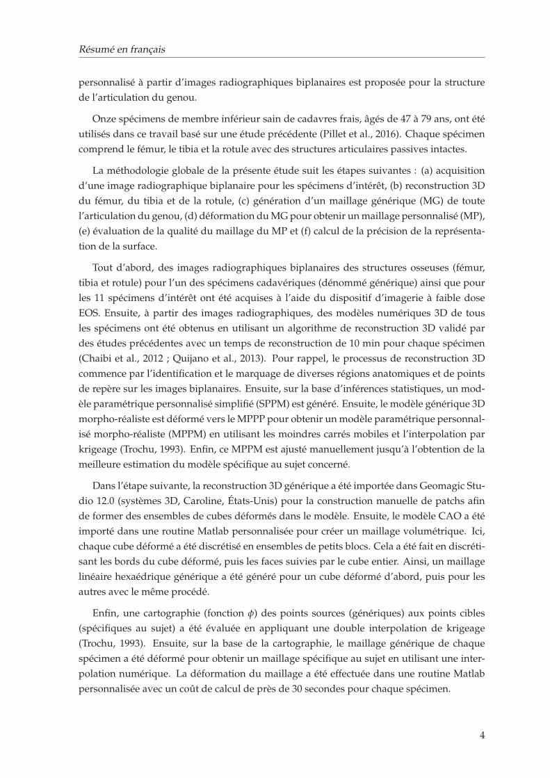
Grâce à la méthodologie entièrement automatisée décrite, un maillage spécifique au su-
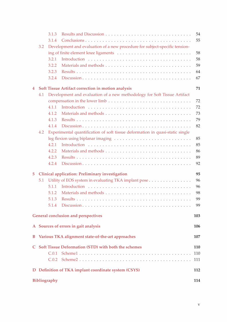
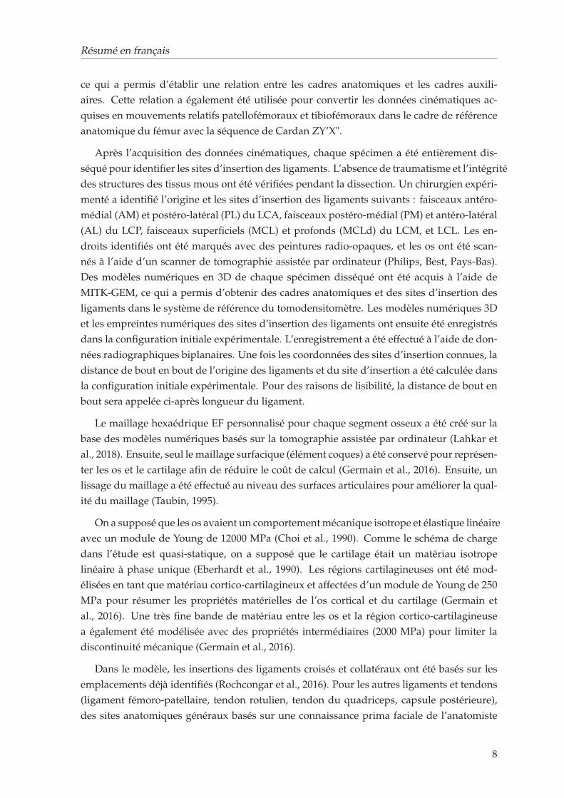
jet a été généré pour les 11 spécimens d’articulation du genou. La figure 1 illustre tous
les maillages générés à l’aide de cette méthodologie. La qualité du maillage individuel de
l’articulation du genou est représentée en termes d’indicateurs de qualité du maillage (%
d’avertissement au-dessus de la valeur seuil). Il n’y a aucune erreur dans aucune maille
et le pourcentage total d’avertissement est très inférieur de manière satisfaisante, avec une
valeur maximale de 0,59% pour le 10e spécimen.
1 2 3
4 5 6 7
8 9 10 11
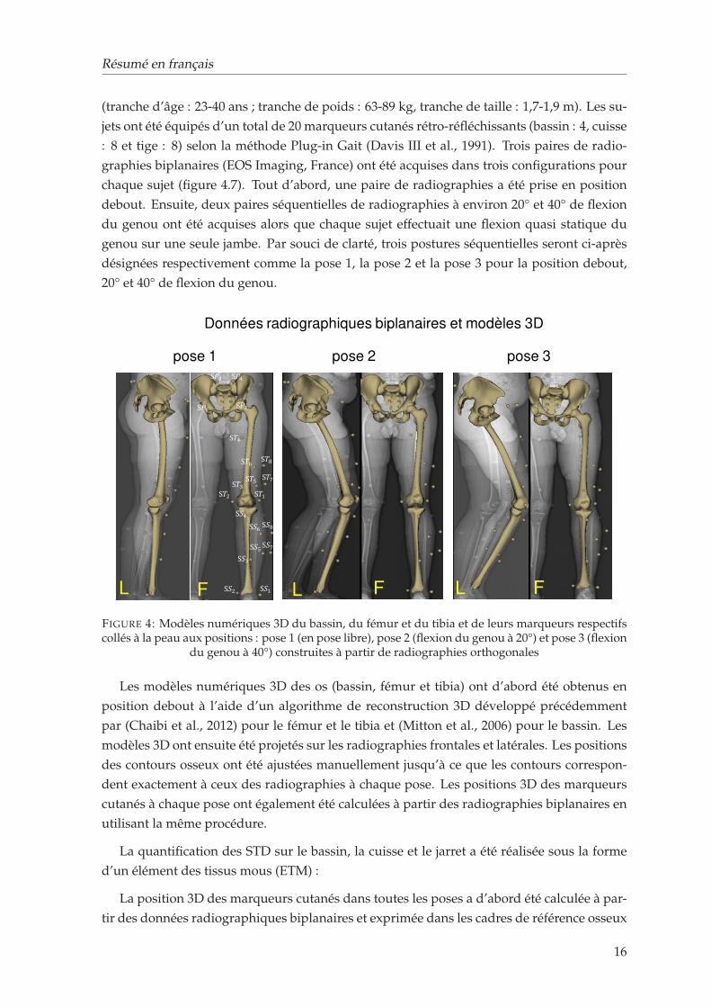
FIGURE 1: Maillage global de l’articulation du genou pour l’ensemble des 11 spécimens. Pour plusde clarté, seule l’épiphyse distale du fémur et l’épiphyse proximale du tibia sont représentées
La méthodologie proposée dans la présente étude repose principalement sur la concep-
tion minutieuse d’un maillage EF générique à partir d’une reconstruction 3D de la structure
cible avec les caractéristiques anatomiques d’intérêt appropriées. La prudence s’impose
5
Résumé en français
dans les zones fonctionnelles : surface de contact et sites d’insertion des ligaments de l’articulation
du genou. Ce travail préliminaire est un effort ponctuel, désormais pour établir la déforma-
tion automatique du maillage, du générique au spécifique.
Dans l’ensemble, ce travail a contribué à la génération rapide, précise et semi-automatique
d’un maillage EF hexaédrique de l’articulation du genou. En raison de la rapidité et de la
spécificité du sujet en termes de géométrie, cette méthodologie a le potentiel d’être mise en
œuvre dans la routine clinique pour étudier les caractéristiques personnalisées de l’articulation
du genou. Toutefois, dans ce but, la validation du modèle est importante. Une évaluation
sera abordée dans la partie suivante.
Partie II: Développement et évaluation d’une nouvelle procédure de mise en tension des
ligaments à éléments finis du genou Les modèles EF sont couramment utilisés comme
un moyen complémentaire fiable aux études expérimentales fournissant des informations
significatives sur la biomécanique de l’articulation du genou. Diverses techniques de mod-
élisation ont été utilisées pour modéliser la structure de l’articulation, en particulier les lig-
aments. Certaines des stratégies sont guidées par la simplicité, tandis que d’autres se con-
centrent sur la capture fidèle de l’anatomie spécifique du spécimen avec différents niveaux
de fidélité de représentation de l’articulation. Par exemple, certains modèles de la littéra-
ture comprenaient des géométries 3D de ligaments ayant un comportement matériau com-
plexe (Kiapour et al., 2014 ; Limbert, Taylor, et Middleton, 2004 ; Orsi et al., 2016 ; Pena
et al., 2006). Une telle approche permet d’étudier le comportement d’enveloppement des
ligaments et d’analyser la réponse biomécanique locale (par exemple, les contraintes et les
déformations 3D à travers les tissus). Néanmoins, les modèles anatomiquement plus com-
plexes nécessitent des informations détaillées basées sur des images des structures des tis-
sus mous considérées. La génération et la simulation de tels modèles nécessitent souvent
un temps beaucoup plus long que celui nécessaire pour des modèles plus simples (Bolcos et
al., 2018). Par conséquent, les modèles plus simples peuvent être bénéfiques pour les études
où un nombre plus élevé de sujets doit être analysé et, en même temps, capable de prédire
la mécanique des articulations.
Dans une tentative de simplification du modèle, d’autres auteurs ont proposé de représen-
ter les ligaments sous forme de faisceaux de ressorts ou de câbles de tension uniquement
(Adouni et Shirazi-Adl, 2009 ; Baldwin et al., 2012 ; Moglo et Shirazi-Adl, 2005). Bien que les
ligaments soient exposés à des états de contrainte en compression et en traction, la contribu-
tion de la contrainte de traction est nettement plus élevée que les autres (Pena et al., 2006 ;
Orsi et al., 2016). Une telle simplification est donc considérée comme raisonnable et recom-
mandée en particulier pour prédire la cinématique des articulations (Beidokhti et al., 2017).
Néanmoins, la personnalisation des propriétés des ligaments (raideur et précontrainte), bien
que cliniquement essentielle pour restaurer la stabilité des articulations, représente un défi
pour la communauté. Par exemple, il existe un consensus sur le fait que la sous-tension des
greffes pourrait entraîner une laxité articulaire, qui est biomécaniquement analogue à celle
d’un genou déficient sur le plan ligamentaire (Sherman et al., 2012). En outre, en raison de
6
Résumé en français
la morphologie variable, différents faisceaux d’un ligament (par exemple, deux faisceaux de
fibres principales du LCA) peuvent présenter une précontrainte variable en devenant actifs
à différents angles de flexion (Girgis, Marshall et JEM, 1975). Du point de vue de la modéli-
sation, il a également été signalé qu’une prétension ligamentaire mal appliquée peut avoir
un effet considérable sur la cinématique du genou (Mesfar et Shirazi-Adl, 2006 ; Rachmat et
al., 2016). Pour s’attaquer à ce problème, certains auteurs ont utilisé des méthodes inverses
pour calibrer le comportement constitutif de certains ligaments. Les auteurs ont utilisé soit
des tests de laxité (Baldwin et al., 2012 ; Beidokhti et al., 2017) soit des charges de distraction
(Zaylor, Stulberg, et Halloran, 2019) pour estimer les propriétés des ligaments en minimisant
les différences entre la cinétique prédite par le modèle et la cinétique expérimentale. Ces cal-
ibrations sont toutefois susceptibles d’être coûteuses sur le plan des calculs.
Pour contribuer à lever ce verrou, nous avons proposé un cadre original pour calibrer la
tension des ligaments du genou EF personnalisé dans les modèles EF, basé sur des données
acquises expérimentalement. L’évaluation du modèle personnalisé a été réalisée en com-
parant, pour chacun des six spécimens cadavériques testés, la cinématique fémoro-tibiale
prédite numériquement en flexion passive avec les données expérimentales de. Nous avons
émis l’hypothèse que la méthodologie proposée avec des pré-tensions personnalisées pou-
vait permettre de prédire la cinématique passive globale de l’articulation du genou.
Nous avons obtenu les réponses cinématiques expérimentales du genou dans une étude
précédente (Rochcongar et al., 2016). La procédure expérimentale est brièvement rappelée
ci-après. Six échantillons de membres inférieurs fraîchement congelés, prélevés sur des su-
jets âgés de 47 à 79 ans, ont été testés en flexion-extension passive sur un banc d’essai ciné-
matique préalablement validé (Azmy et al., 2010 ; Hsich et Draganich, 1997). La peau et
les muscles ont été enlevés, à l’exception de huit centimètres de tendon du quadriceps et
du muscle poplité avant la collecte des données cinématiques. Toutes les autres structures
pertinentes des tissus mous des articulations (comme les ligaments, la capsule articulaire)
ont été conservées intactes pendant l’acquisition des données cinématiques. Le fémur a été
maintenu fixe, et le mouvement de flexion a été introduit dans le tibia par un système de
cordes et de poulies. Pendant la flexion, les positions des trois trépieds marqueurs placés
sur le fémur, le tibia et la rotule ont été enregistrées à l’aide d’un système optoélectronique.
Ces positions enregistrées ont permis d’établir des cadres de référence auxiliaires à partir de
t=0 (avant l’application de la charge de flexion) jusqu’à la fin de la flexion. Les incertitudes
de mesure avec le système optoélectronique ont été évaluées au préalable. Des incertitudes
globales de moins de 0,5 mm en translation et de 1° en rotation ont été obtenues (Azmy et
al., 2010).
De plus, deux radiographies orthogonales de chaque spécimen ont été acquises à l’aide
d’un système de radiographie biplanaire EOS afin d’obtenir des modèles numériques 3D
des os et des marqueurs de trépied. À partir des modèles 3D, des cadres de référence
anatomiques pour le fémur, le tibia et la rotule ont été définis (Schlatterer et al., 2009). Des
cadres de référence auxiliaires ont également été définis à partir des marqueurs de trépied,
7
Résumé en français
ce qui a permis d’établir une relation entre les cadres anatomiques et les cadres auxili-
aires. Cette relation a également été utilisée pour convertir les données cinématiques ac-
quises en mouvements relatifs patellofémoraux et tibiofémoraux dans le cadre de référence
anatomique du fémur avec la séquence de Cardan ZY’X".
Après l’acquisition des données cinématiques, chaque spécimen a été entièrement dis-
séqué pour identifier les sites d’insertion des ligaments. L’absence de traumatisme et l’intégrité
des structures des tissus mous ont été vérifiées pendant la dissection. Un chirurgien expéri-
menté a identifié l’origine et les sites d’insertion des ligaments suivants : faisceaux antéro-
médial (AM) et postéro-latéral (PL) du LCA, faisceaux postéro-médial (PM) et antéro-latéral
(AL) du LCP, faisceaux superficiels (MCL) et profonds (MCLd) du LCM, et LCL. Les en-
droits identifiés ont été marqués avec des peintures radio-opaques, et les os ont été scan-
nés à l’aide d’un scanner de tomographie assistée par ordinateur (Philips, Best, Pays-Bas).
Des modèles numériques en 3D de chaque spécimen disséqué ont été acquis à l’aide de
MITK-GEM, ce qui a permis d’obtenir des cadres anatomiques et des sites d’insertion des
ligaments dans le système de référence du tomodensitomètre. Les modèles numériques 3D
et les empreintes numériques des sites d’insertion des ligaments ont ensuite été enregistrés
dans la configuration initiale expérimentale. L’enregistrement a été effectué à l’aide de don-
nées radiographiques biplanaires. Une fois les coordonnées des sites d’insertion connues, la
distance de bout en bout de l’origine des ligaments et du site d’insertion a été calculée dans
la configuration initiale expérimentale. Pour des raisons de lisibilité, la distance de bout en
bout sera appelée ci-après longueur du ligament.
Le maillage hexaédrique EF personnalisé pour chaque segment osseux a été créé sur la
base des modèles numériques basés sur la tomographie assistée par ordinateur (Lahkar et
al., 2018). Ensuite, seul le maillage surfacique (élément coques) a été conservé pour représen-
ter les os et le cartilage afin de réduire le coût de calcul (Germain et al., 2016). Ensuite, un
lissage du maillage a été effectué au niveau des surfaces articulaires pour améliorer la qual-
ité du maillage (Taubin, 1995).
On a supposé que les os avaient un comportement mécanique isotrope et élastique linéaire
avec un module de Young de 12000 MPa (Choi et al., 1990). Comme le schéma de charge
dans l’étude est quasi-statique, on a supposé que le cartilage était un matériau isotrope
linéaire à phase unique (Eberhardt et al., 1990). Les régions cartilagineuses ont été mod-
élisées en tant que matériau cortico-cartilagineux et affectées d’un module de Young de 250
MPa pour résumer les propriétés matérielles de l’os cortical et du cartilage (Germain et
al., 2016). Une très fine bande de matériau entre les os et la région cortico-cartilagineuse
a également été modélisée avec des propriétés intermédiaires (2000 MPa) pour limiter la
discontinuité mécanique (Germain et al., 2016).
Dans le modèle, les insertions des ligaments croisés et collatéraux ont été basés sur les
emplacements déjà identifiés (Rochcongar et al., 2016). Pour les autres ligaments et tendons
(ligament fémoro-patellaire, tendon rotulien, tendon du quadriceps, capsule postérieure),
des sites anatomiques généraux basés sur une connaissance prima faciale de l’anatomiste
8
Résumé en français
ont été utilisés. Chaque ligament croisé a été représenté par 2 faisceaux (Blankevoort et
Huiskes, 1991) ainsi que le LCM (profond et superficiel) (Smith et al., 2016). La capsule
postérieure et les ligaments fémoro-patellaires étaient représentés par 8 faisceaux chacun
(4 faisceaux dans le côté médial et latéral chacun), tandis que le quadriceps et le tendon
rotulien étaient représentés par 4 faisceaux chacun (Germain et al., 2016)) et le LCL par un
seul faisceau (Meister et al., 2000). Tous les ligaments et tendons ont été représentés comme
des éléments de câble point à point, en tension uniquement, car leur contribution en tension
est beaucoup plus élevée que celle en compression (Baldwin et al., 2009 ; Harris et al., 2016).
Trois paires de contact surface-surface sans frottement ont été considérées : le cartilage tibia-
fémur (médial et latéral) et le cartilage fémur-patella.
Trois cas de valeurs de précontrainte ligamentaire ont été considérés pour les ligaments
croisés et collatéraux. Aucune valeur de précontrainte pour les autres ligaments n’a été prise
en compte et les valeurs de rigidité (k) pour tous les ligaments ont été adoptées ou estimées
à partir de notre étude précédente (Germain et al., 2016). Il est à noter que des valeurs de
rigidité constantes ont été appliquées à tous les spécimens.
Cas 1 : Propriétés génériques des matériaux. Les valeurs de prétension ont été adoptées à
partir d’une étude précédente (Germain et al., 2016).
Cas 2 : Précalcul automatique à partir de données expérimentales. Pour chaque spécimen, les
précontraintes spécifiques des ligaments et des faisceaux ont été automatiquement calculées
à partir des longueurs expérimentales des ligaments.
Cas 3 : Combinaison d’un pré-calcul automatique et d’un ajustement manuel supplémentaire.
Lors de la mise en œuvre des propriétés génériques des ligaments (cas 1), seuls deux
modèles EF sur six ont atteint une convergence complète.
La cinématique prédite a montré un grand écart par rapport à l’expérimentation, tant en
termes d’ampleur que de tendance. En utilisant les propriétés des matériaux ligamentaires
calculées automatiquement, 5 modèles sur 6 ont atteint une convergence sur 60° de flexion.
Grâce aux propriétés des matériaux ligamentaires calculées automatiquement et à l’ajustement
manuel, tous les modèles de genou EF sont restés stables sur toute la plage de flexion. La
durée d’exécution individuelle était d’environ 13 minutes par spécimen.
TABLE 1: Différence moyenne RACINE DE L’ERREUR QUADRATIQUE MOYENNERACINE DEL’ERREUR QUADRATIQUE MOYENNE ± ECART-TYYPE entre la cinématique expérimentale et
celle prédite par le modèle
Flexion Cas A/A(°) I/E(°) P/A(mm) I/S(mm) L/M(mm)
0-60°
1 - - - - -
2 2.4 ± 1.3 6.3 ± 6.2 5.0 ± 3.5 1.9 ± 1.8 1.2 ± 1.1
3 1.5 ± 1.3 5.3 ± 5.1 3.4 ± 2.3 1.2 ± 0.8 2.0 ± 1.9
A/A: Abduction/Adduction, I/E: Interne/Externe, P/A:Postérieur/Antérieur, I/S: Inférieure/Supérieure, L/M: Latéral/Médial
9
Résumé en français
Dans cette étude, nous avons mis en place une nouvelle méthodologie pour la construc-
tion de modèles personnalisés du genou, avec une géométrie basée sur la tomodensitométrie
et évalué une nouvelle procédure de calibrage spécifique au sujet de la prétension des lig-
aments à partir de données radiographiques biplanaires. La cinématique fémoro-tibiale
prédite de chaque modèle a été comparée à la réponse in vitro correspondante pour trois
cas différents de propriétés ligamentaires (prétension). Tout d’abord, nous avons cherché à
savoir si les modèles EF avec des valeurs génériques de prétension peuvent saisir la variabil-
ité inter-individuelle de la cinématique in vitro. Ensuite, des pré-souches obtenues expéri-
mentalement ont été recrutées dans les modèles EF et la cinématique prédite a été observée
(cas 2). Troisièmement, la cinématique du modèle a été observée en ce qui concerne les pro-
priétés calibrées des ligaments basées sur la combinaison de précontraintes pré-calculées et
d’autres ajustements (cas 3).
Bien qu’il soit difficile de comparer directement les prédéformations estimées avec des
études similaires dans la littérature en raison de la variabilité de la géométrie des ligaments
et des propriétés des matériaux, les valeurs des prédéformations ont été trouvées dans la
fourchette confirmée par d’autres (Amiri et al., 2006 ; Wismans et al., 1980 ;). En outre, la
plupart des ligaments ont été trouvés en état de tension en extension complète, à l’exception
du LCP, ce qui est globalement en accord avec la littérature (Blankevoort et Huiskes, 1991 ;
Guess, Razu et Jahandar, 2016 ; Moglo et Shirazi-Adl, 2005). De même, la réponse cinéma-
tique prédite a également montré une bonne correspondance avec les résultats expérimen-
taux pour tous les spécimens. Les différences numériques expérimentales constatées dans
cette étude étaient comparables à celles d’études similaires rapportées dans la littérature
(Beidokhti et al., 2017 ; Harris et al., 2016).
La procédure de calcul de la prétension ligamentaire directement à partir de données
expérimentales (cas 3) a fourni une première estimation satisfaisante, basée sur un mod-
èle dont la cinématique estimée était déjà en bon accord avec les données expérimentales.
Comme cette approche semble être peu coûteuse sur le plan des calculs (15-20 secondes pour
obtenir une prétension ligamentaire spécifique pour un seul modèle de genou) et simple
sur le plan méthodologique, elle peut servir d’alternative fiable pour estimer les valeurs de
prétension ligamentaire spécifiques au sujet. Il convient de noter qu’aucune évaluation di-
recte des tensions ligamentaires n’a été réalisée dans la présente étude. La décision de mettre
en œuvre la technique actuelle comme alternative doit être prise avec prudence. Pour une
mise en œuvre réussie de cette technique dans le cadre clinique, une évaluation exhaustive
du modèle dans diverses conditions de charge est nécessaire, y compris la tension ligamen-
taire et la tension de contact.
En conclusion, comme il s’agissait d’une première étude visant à appliquer directement
des valeurs de précharge sur des modèles directement issus de l’expérience, qui peuvent
trouver des portées dans les études cliniques basées sur des modèles, telles que la planifi-
cation de l’équilibrage ou de la reconstruction des ligaments car elle réduit la complexité
du développement des modèles (en particulier l’étalonnage des ligaments) ainsi que le coût
de calcul, tout en maintenant une bonne correspondance avec les données expérimentales.
10
Résumé en français
Dans ce but, une évaluation plus poussée du modèle serait nécessaire pour les échantillons
de plus grande taille et dans d’autres scénarios cliniquement pertinents.
Dans l’ensemble, cette partie a permis d’aborder deux défis importants dans l’élaboration
de modèles et les approches d’évaluation, comme l’a expliqué la revue de la littérature. La
méthodologie quasi-automatique employée dans la première partie a permis de générer un
maillage EF de l’articulation du genou spécifique au sujet, avec une qualité de maillage et
une précision de représentation de surface satisfaisantes.
Partie III: Développement d’une nouvelle méthodologie pour la Compensation des arte-
facts des tissus mous dans l’analyse quantitative du mouvement par la méthode des élé-
ments finis Une évaluation précise de la cinématique in vivo est essentielle pour obtenir
des informations sur le fonctionnement normal des articulations (Akbarshahi et al., 2010) et
pour étudier la pathologie des articulations des membres inférieurs (Andriacchi et Alexan-
der, 2000). La capture de mouvement basée sur les marqueurs cutanés (SM) est la tech-
nique la plus répandue utilisée pour estimer la cinématique du squelette du membre in-
férieur. Toutefois, la précision de cette technique est affectée par le mouvement relatif des
tissus mous par rapport à l’os sous-jacent, un biais communément appelé "artefact des tis-
sus mous" (STA). S’il n’est pas compensé, le STA peut entraîner des erreurs cinématiques
moyennes allant jusqu’à 16 mm en translation et 13° en rotation pour l’articulation du genou
(Benoit et al., 2006). Ces erreurs peuvent avoir une influence significative sur l’évaluation
de la pathologie ou les effets du traitement dans l’analyse clinique de la marche (Seffinger
et Hruby, 2007).
Différentes méthodes ont été proposées dans la littérature pour réduire l’effet de la STA
sur l’estimation de la pose osseuse. Parmi celles-ci, la MBO, qui s’appuie sur un modèle ciné-
matique prédéfini avec des contraintes articulaires spécifiques, est de plus en plus utilisée.
Au départ, des contraintes cinématiques simples telles que les articulations à charnière ou
sphériques étaient considérées comme représentant l’articulation de la hanche et du genou
(Lu et O’connor, 1999 ; Reinbolt et al., 2005). Plus tard, des contraintes anatomiques sur
les articulations (mécanisme parallèle, courbes de couplage) ont été introduites, ce qui a en-
couragé la cinématique 3D car elles ont permis des déplacements articulaires (Gasparutto
et al., 2015 ; Richard et al., 2016). Cependant, quelles que soient les contraintes articulaires
imposées, les cinématiques génériques (non personnalisées) dérivées de modèles se sont
révélées inexactes (erreur cinématique du genou jusqu’à 17° et 8 mm) car ces modèles ne
pouvaient pas s’adapter à la géométrie spécifique du patient, en particulier dans des condi-
tions pathologiques (Clément et al., 2017).
La simplification conjointe a des conséquences indirectes sur la précision prédictive des
modèles musculo-squelettiques du corps rigide (MSK) et des modèles MSK basés sur la
FE. Les études qui ont utilisé des modèles FE-MSK pour prédire la mécanique locale des
articulations en utilisant la cinématique articulaire in vivo (Shu et al., 2018 ; Xu et al., 2016),
ont supposé que l’articulation du genou avait un DoF de 1. Cela pourrait entraîner une
11
Résumé en français
propagation des incertitudes sur la cinématique prédite et affecter la réaction articulaire
ainsi que les forces musculaires et ligamentaires.
Dans les contextes susmentionnés, l’estimation fiable de la cinématique du squelette à
l’aide de données de mouvement basées sur la SM reste un défi majeur (Richard, Cappozzo
et Dumas, 2017). Dans une étude précédente, un modèle conceptuel EF a été proposé pour la
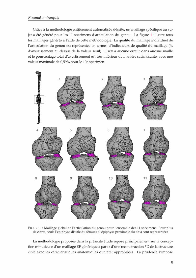
compensation de la STA (Skalli et al., 2018). L’objectif de la présente étude était de dévelop-
per le modèle conceptuel pour le membre inférieur et de le mettre en œuvre sur des volon-
taires sains en tenant compte des modèles spécifiques au sujet.
S𝐹𝑖
HJ
KJ
S𝐹𝑖SC𝐹𝑖
HJ
KJ
SC𝐹𝑖 B𝐹𝑖B𝐹𝑖
B𝑃𝑖
B𝑇𝑖
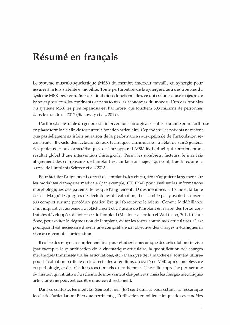
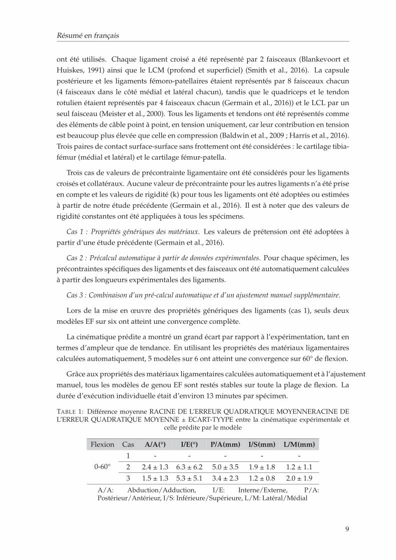
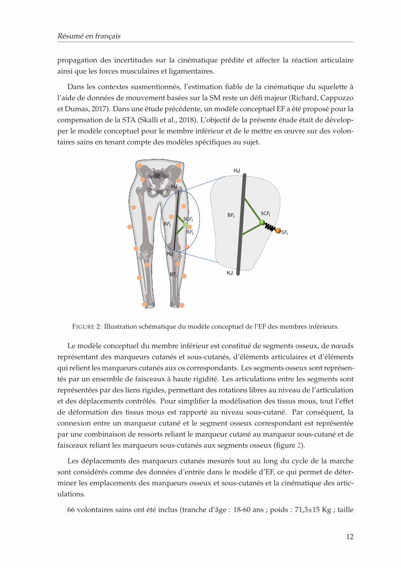
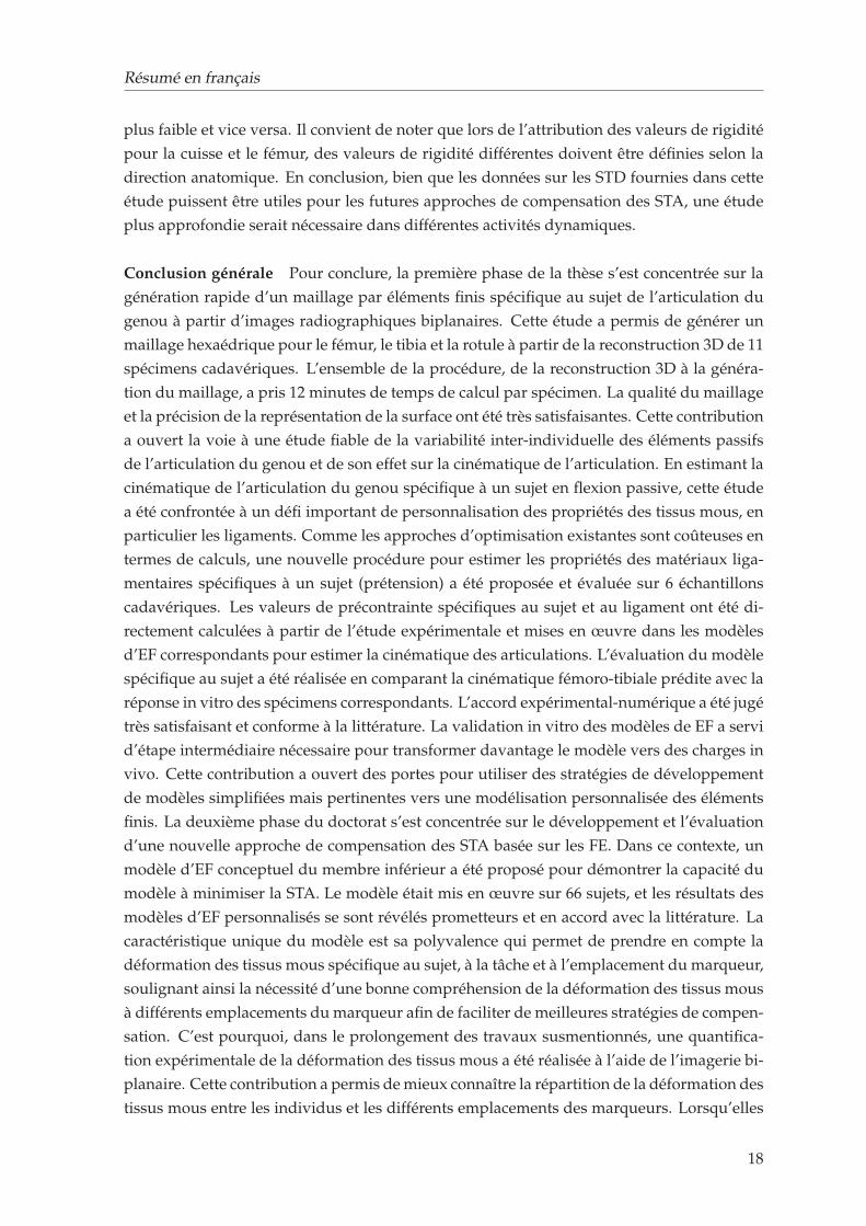
FIGURE 2: Illustration schématique du modèle conceptuel de l’EF des membres inférieurs.
Le modèle conceptuel du membre inférieur est constitué de segments osseux, de nœuds
représentant des marqueurs cutanés et sous-cutanés, d’éléments articulaires et d’éléments
qui relient les marqueurs cutanés aux os correspondants. Les segments osseux sont représen-
tés par un ensemble de faisceaux à haute rigidité. Les articulations entre les segments sont
représentées par des liens rigides, permettant des rotations libres au niveau de l’articulation
et des déplacements contrôlés. Pour simplifier la modélisation des tissus mous, tout l’effet
de déformation des tissus mous est rapporté au niveau sous-cutané. Par conséquent, la
connexion entre un marqueur cutané et le segment osseux correspondant est représentée
par une combinaison de ressorts reliant le marqueur cutané au marqueur sous-cutané et de
faisceaux reliant les marqueurs sous-cutanés aux segments osseux (figure 2).
Les déplacements des marqueurs cutanés mesurés tout au long du cycle de la marche
sont considérés comme des données d’entrée dans le modèle d’EF, ce qui permet de déter-
miner les emplacements des marqueurs osseux et sous-cutanés et la cinématique des artic-
ulations.
66 volontaires sains ont été inclus (tranche d’âge : 18-60 ans ; poids : 71,3±15 Kg ; taille
12
Résumé en français
: 170±10 cm) dans cette étude. Les seuls critères d’exclusion étaient les antécédents de
chirurgie orthopédique des membres inférieurs.
L’analyse quantitative du mouvement a été effectuée sur un système d’analyse optoélec-
tronique comprenant 7 caméras vidéo (Vicon Motion System Ltd., Oxford Metrics, UK).
Les marqueurs optoélectroniques ont été positionnés selon la méthode de la Plug-in Gait
(Davis III et al., 1991), et les participants ont été invités à effectuer une marche en palier à
une vitesse choisie par eux-mêmes. Des radiographies biplanaires ont ensuite été acquises
à l’aide du système EOS (EOS Imaging, France). Des modèles numériques 3D des os ont
été obtenus à l’aide d’un algorithme de reconstruction 3D validé par des études antérieures
(Chaibi et al., 2012). L’emplacement des marqueurs cutanés a également été calculé à partir
de radiographies biplanaires.
À partir des modèles numériques 3D des os, des points de repère anatomiques spéci-
fiques au sujet ont été identifiés, ce qui a permis d’obtenir les coordonnées nodales de
chaque os. La distance entre la peau et les marqueurs sous-cutanés a été arbitrairement
choisie comme étant de 1 mm (c’est-à-dire la longueur du ressort). Sur la base du déplace-
ment moyen en translation de l’articulation du genou trouvé dans notre précédent travail
expérimental in vitro (Germain et al., 2016), la longueur de l’articulation du genou a été fixée
à 20 mm. Pour la hanche, la longueur articulaire a été fixée à 1 mm sur la base de données
non publiées sur le déplacement en translation de la hanche quantifié à l’aide de rayons X
biplanaires.
Les déplacements des marqueurs mesurés à partir de la capture du mouvement ont été
progressivement introduits dans le modèle comme une condition limite prescrite, et les po-
sitions des marqueurs osseux et sous-cutanés résultants tout au long du cycle de marche ont
été calculées à l’aide du logiciel commercial ANSYS.
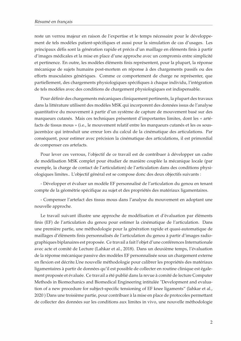
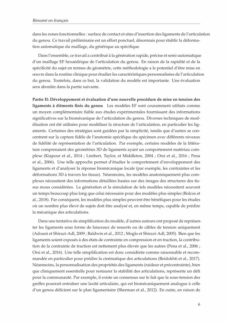
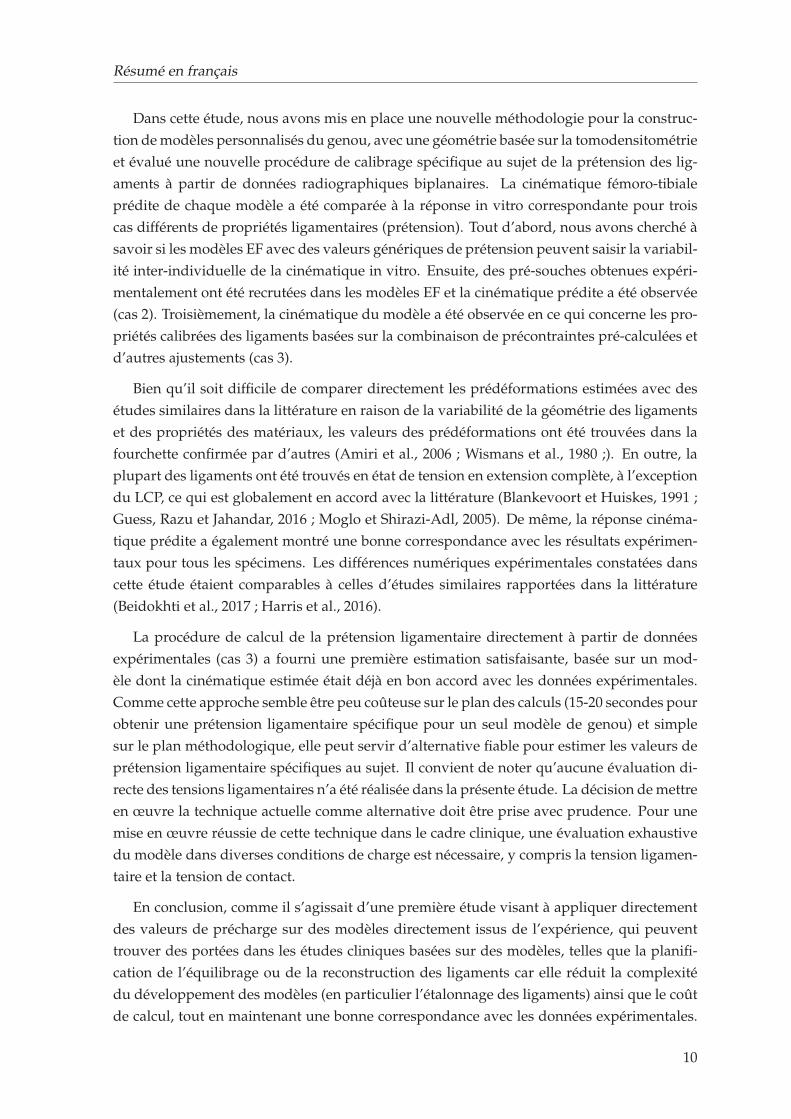
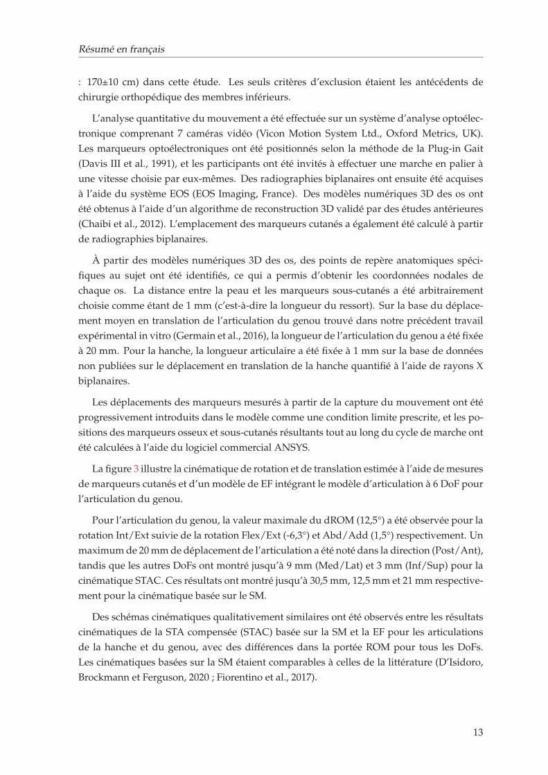
La figure 3 illustre la cinématique de rotation et de translation estimée à l’aide de mesures
de marqueurs cutanés et d’un modèle de EF intégrant le modèle d’articulation à 6 DoF pour
l’articulation du genou.
Pour l’articulation du genou, la valeur maximale du dROM (12,5°) a été observée pour la
rotation Int/Ext suivie de la rotation Flex/Ext (-6,3°) et Abd/Add (1,5°) respectivement. Un
maximum de 20 mm de déplacement de l’articulation a été noté dans la direction (Post/Ant),
tandis que les autres DoFs ont montré jusqu’à 9 mm (Med/Lat) et 3 mm (Inf/Sup) pour la
cinématique STAC. Ces résultats ont montré jusqu’à 30,5 mm, 12,5 mm et 21 mm respective-
ment pour la cinématique basée sur le SM.
Des schémas cinématiques qualitativement similaires ont été observés entre les résultats
cinématiques de la STA compensée (STAC) basée sur la SM et la EF pour les articulations
de la hanche et du genou, avec des différences dans la portée ROM pour tous les DoFs.
Les cinématiques basées sur la SM étaient comparables à celles de la littérature (D’Isidoro,
Brockmann et Ferguson, 2020 ; Fiorentino et al., 2017).
13
Résumé en français
(−in
tern
+
exte
rn )°
(−e
xte
nsio
n +
fle
xio
n )°
(−a
bd
uctio
n +
ad
du
ctio
n )°
(−p
osté
rie
ure
+a
nté
rie
ure
)mm
(−in
féri
eu
r+
su
pé
rie
ur
)mm
(−m
éd
iale
+la
téra
le)m
m
FIGURE 3: La cinématique de l’articulation du genou pendant la marche est présentée commeMean±1SD. Les valeurs moyennes pour les résultats basés sur les marqueurs cutanés (vert) et lesrésultats prévus par le modèle EF (bleu) sont présentées sous forme de lignes continues, tandis que
l’écart-type est présenté dans des tons plus clairs.
L’approche proposée peut servir dans deux grands domaines d’application : i) dans
l’analyse de la marche pour la recherche, où la personnalisation des modèles à l’aide de
l’imagerie médicale (par exemple, CT, IRM, rayons X biplanaires) n’est généralement pas
effectuée. Toutefois, il est possible de compenser l’ATS par des techniques classiques de
mise à l’échelle du modèle, tout en étant capable de différencier les paramètres de rigidité
des tissus mous entre différents sous-groupes. ii) dans l’analyse clinique de la marche, où
la personnalisation du modèle par imagerie médicale pourrait permettre de saisir les détails
anatomiques des articulations saines ou dégénérées.
En conclusion, nous avons présenté un modèle conceptuel de EF du membre inférieur
pour la compensation de la STA et l’avons testé avec succès sur une population de 66 sujets
de morphologies différentes. Le modèle s’est avéré satisfaisant pour la compensation de
l’ATS et polyvalent, facilitant les paramètres nécessaires à la personnalisation du modèle.
La méthodologie développée et évaluée dans cette étude peut améliorer la précision des
prédictions cinématiques, ce qui est essentiel pour les modèles MSK ainsi que pour la prise
de décisions cliniques.
Dans cette partie, nous avons observé que le modèle proposé basé sur l’EF du membre
inférieur pouvait effectivement compenser l’ATS et les résultats observés étaient conformes
à la littérature. Cependant, lors de l’élaboration du modèle, des valeurs de rigidité arbi-
traires ont été attribuées aux ressorts car aucune information sur la déformation des tissus
mous à chaque emplacement de marqueur n’était disponible. Cela a conduit à étudier ex-
périmentalement le modèle de déformation des tissus mous au niveau du membre inférieur
pendant le mouvement. Cette contribution est incluse dans la partie suivante.
14
Résumé en français
Partie IV: Quantification expérimentale de la déformation des tissus mous lors de la flex-
ion quasi-statique d’une seule jambe à l’aide de l’imagerie biplanaire L’analyse du mou-
vement basée sur les marqueurs de peau (SM) est la méthode non invasive la plus courante
pour estimer la position et l’orientation du squelette dans l’espace 3D. La précision de cette
méthode est principalement limitée par le mouvement relatif entre les tissus mous et l’os
sous-jacent, communément appelé artefact des tissus mous (STA). Afin de compenser ce
mouvement et d’estimer avec précision la position du squelette in vivo pendant le mouve-
ment, il est essentiel de connaître le schéma de déformation des tissus mous (STD) pendant
le mouvement (Benoit et al., 2006 ; Stagni et al., 2005).
Plusieurs études invasives et radiologiques ont été proposées pour caractériser les STD
lors de différentes tâches motrices. La plupart de ces études ont conclu que les STD dépen-
dent d’un sujet individuel, du type d’activité exercée, de la configuration des marqueurs
ainsi que des lieux. Par exemple, peu d’études ont constaté que l’erreur cinématique due à
une STD est plus importante à la cuisse qu’à la jambe, ce qui suggère un schéma spécifique
à la localisation et au segment pour compenser l’artefact (Akbarshahi et al., 2010 ; Stagni
et al., 2005 ; Benoit et al., 2006). Néanmoins, ces études se sont principalement concentrées
sur la quantification des erreurs cinématiques causées par les STD plutôt que sur les STD
elles-mêmes.
À la connaissance des auteurs, il n’existe qu’une seule étude dans la littérature traitant
de la quantification des STD à différents emplacements et directions de marqueurs chez 20
volontaires sains (Gao et Zheng, 2008). Mais, en raison de limitations techniques empêchant
l’accès à la position des os, la quantification des STA a été rapportée comme un mouvement
inter-marqueurs au lieu d’un mouvement des marqueurs par rapport à la position réelle des
os. Par conséquent, on manque encore de données de référence sur les STD spécifiques au
sujet, à l’endroit et à la direction, qui pourraient fournir des indications pour des stratégies
efficaces de compensation de la STA pour l’analyse des mouvements basée sur la SM.
Parmi les différentes méthodes mises au point pour compenser la STA, la méthode MBO
(pour Multi-Body Optimisation) est de plus en plus utilisée. Elle attribue généralement une
matrice de poids reflétant la distribution des erreurs STA parmi les marqueurs adhérant
à un segment (Lu et O’connor, 1999). En marge de ces méthodes, une nouvelle approche
basée sur l’EF pour compenser la STA du membre inférieur a été évaluée avec succès dans
une population de 66 sujets. Le modèle EF permet d’incorporer la rigidité de correction de
STA à chaque emplacement de marqueur, et la rigidité peut être calibrée sur la base des
informations sur les STD locales à chaque emplacement de marqueur et le long de chaque
direction anatomique. Toutefois, en raison du manque de données sur les STD, des valeurs
arbitraires ont été attribuées aux paramètres de rigidité.
L’étude actuelle vise donc à quantifier la déformation des tissus mous du bassin, de la
cuisse et de la tige à chaque emplacement de marqueur et dans trois directions anatomiques
lors de la flexion quasi statique d’une jambe du genou à l’aide d’une radiographie biplanaire
à faible dose. Les données rétrospectives incluses dans l’étude ont recruté dix volontaires
15
Résumé en français
(tranche d’âge : 23-40 ans ; tranche de poids : 63-89 kg, tranche de taille : 1,7-1,9 m). Les su-
jets ont été équipés d’un total de 20 marqueurs cutanés rétro-réfléchissants (bassin : 4, cuisse
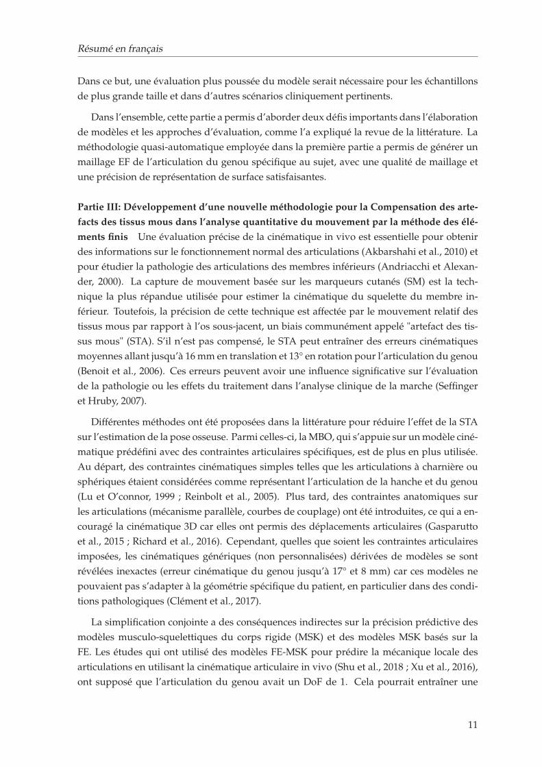
: 8 et tige : 8) selon la méthode Plug-in Gait (Davis III et al., 1991). Trois paires de radio-
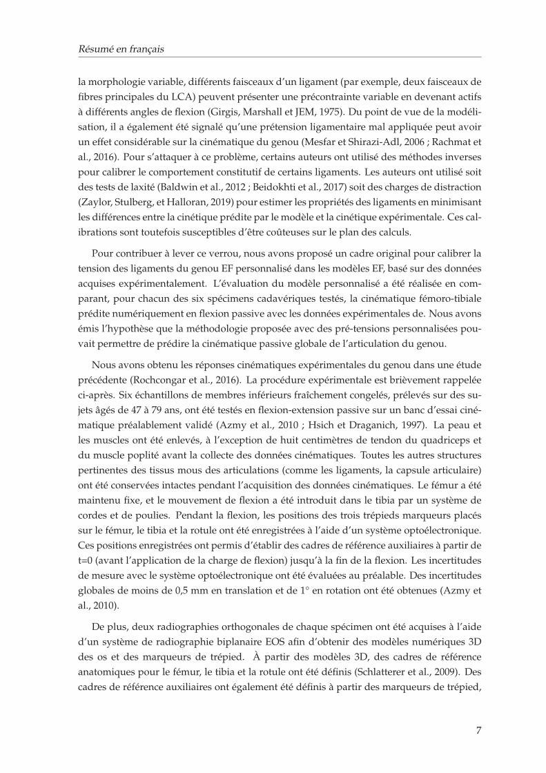
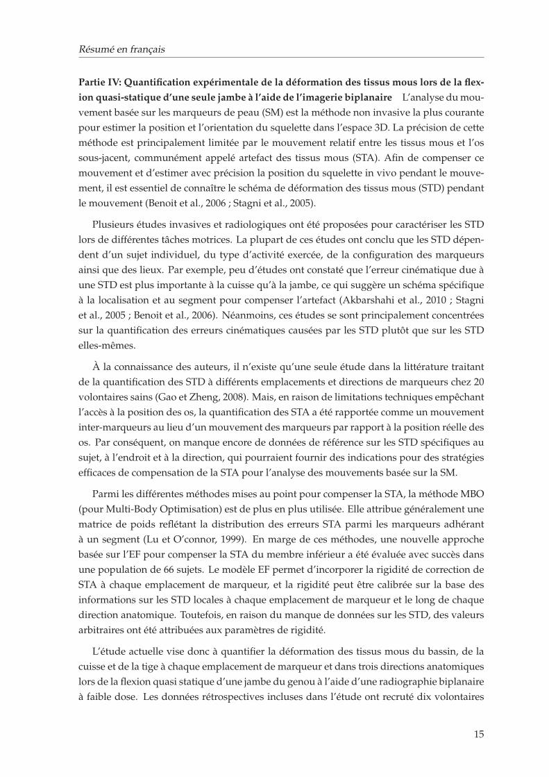
graphies biplanaires (EOS Imaging, France) ont été acquises dans trois configurations pour
chaque sujet (figure 4.7). Tout d’abord, une paire de radiographies a été prise en position
debout. Ensuite, deux paires séquentielles de radiographies à environ 20° et 40° de flexion
du genou ont été acquises alors que chaque sujet effectuait une flexion quasi statique du
genou sur une seule jambe. Par souci de clarté, trois postures séquentielles seront ci-après
désignées respectivement comme la pose 1, la pose 2 et la pose 3 pour la position debout,
20° et 40° de flexion du genou.
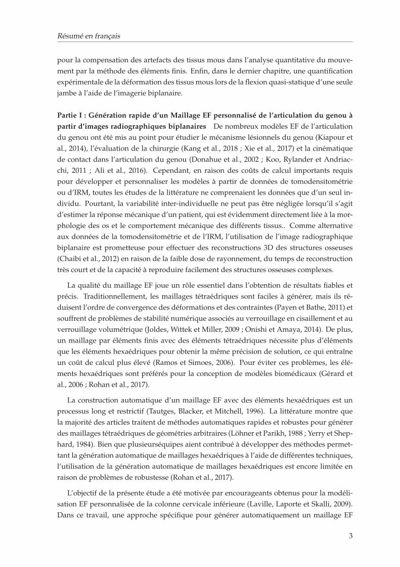
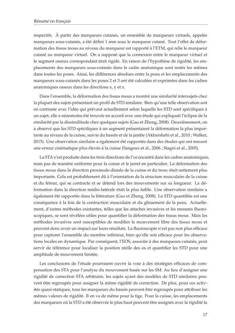
Données radiographiques biplanaires et modèles 3D
pose 1 pose 3pose 2
F F FL L L
S𝑃3S𝑃1 S𝑃2
S𝑃4
S𝑇1S𝑇2 S𝑇3S𝑇4
S𝑇5S𝑇6 S𝑇7S𝑇8
S𝑆1S𝑆2S𝑆3S𝑆4
S𝑆5S𝑆6 S𝑆7S𝑆8
FIGURE 4: Modèles numériques 3D du bassin, du fémur et du tibia et de leurs marqueurs respectifscollés à la peau aux positions : pose 1 (en pose libre), pose 2 (flexion du genou à 20°) et pose 3 (flexion
du genou à 40°) construites à partir de radiographies orthogonales
Les modèles numériques 3D des os (bassin, fémur et tibia) ont d’abord été obtenus en
position debout à l’aide d’un algorithme de reconstruction 3D développé précédemment
par (Chaibi et al., 2012) pour le fémur et le tibia et (Mitton et al., 2006) pour le bassin. Les
modèles 3D ont ensuite été projetés sur les radiographies frontales et latérales. Les positions
des contours osseux ont été ajustées manuellement jusqu’à ce que les contours correspon-
dent exactement à ceux des radiographies à chaque pose. Les positions 3D des marqueurs
cutanés à chaque pose ont également été calculées à partir des radiographies biplanaires en
utilisant la même procédure.
La quantification des STD sur le bassin, la cuisse et le jarret a été réalisée sous la forme
d’un élément des tissus mous (ETM) :
La position 3D des marqueurs cutanés dans toutes les poses a d’abord été calculée à par-
tir des données radiographiques biplanaires et exprimée dans les cadres de référence osseux
16
Résumé en français
respectifs. À partir des marqueurs cutanés, un ensemble de marqueurs virtuels, appelés
marqueurs sous-cutanés, a été défini 1 mm sous le marqueur cutané. Tout l’effet de défor-
mation des tissus mous au niveau du marqueur est rapporté à l’ETM, qui relie le marqueur
cutané au marqueur virtuel. On a supposé que la connexion entre le marqueur virtuel et
le segment osseux correspondant était rigide. En raison de l’hypothèse de rigidité, les em-
placements des marqueurs sous-cutanés dans le cadre anatomique sont restés les mêmes
dans toutes les poses. Ainsi, les différences absolues entre la peau et les emplacements des
marqueurs sous-cutanés dans les poses 2 et 3 ont été calculées et exprimées dans les cadres
anatomiques osseux dans les directions x, y et z.
Dans l’ensemble, la déformation des tissus mous a montré une similarité intersujets chez
la plupart des sujets présentant un profil de STD similaire. Bien qu’une telle observation soit
en contraste avec l’idée qui prévaut actuellement selon laquelle les STD sont spécifiques à
un sujet, elle a néanmoins été trouvée en accord avec une étude qui expliquait l’éclipse de la
similarité par la dissimilitude chez quelques sujets (Gao et Zheng, 2008). Deuxièmement, on
a observé que les STD spécifiques à un segment présentaient la déformation la plus impor-
tante au niveau de la cuisse, suivie du bassin et de la jambe (Akbarshahi et al., 2010 ; Walker,
2015). Une observation similaire a également été rapportée dans des études qui ont mesuré
une erreur cinématique plus élevée à la cuisse (Sangeux et al., 2006 ; Stagni et al., 2005).
La STA s’est produite dans les trois directions de l’os encastré dans les cadres anatomiques,
mais pas de manière uniforme pour la cuisse et le jarret en particulier. La déformation des
tissus mous dans la direction proximale-distale de la cuisse et du tronc était nettement plus
importante. Cela est probablement dû à l’orientation de la structure musculaire de la cuisse
et du fémur, qui se contracte et se détend lors des mouvements sur sa longueur. La dé-
formation dans la direction médio-latérale était la plus faible. Une observation similaire a
également été rapportée dans la littérature (Gao et Zheng, 2008). La STD quantifiée est une
conséquence à la fois de la contraction musculaire et du glissement de la peau. Actuelle-
ment, d’autres méthodes existantes, telles que les attaches invasives et les mesures fluoro-
scopiques, se sont révélées utiles pour quantifier la déformation des tissus mous. Mais les
méthodes invasives sont susceptibles de modifier le mouvement libre des tissus mous et
peuvent donc avoir un impact sur leurs résultats. La fluoroscopie n’est pas non plus efficace
pour capturer l’ensemble du membre inférieur, bien qu’elle soit efficace pour les observa-
tions locales en dynamique. Par conséquent, l’EOS, associée à des marqueurs cutanés, peut
servir de référence pour localiser la position réelle des os et quantifier les STD pour une
amplitude de mouvement limitée.
Les conclusions de l’étude pourraient ouvrir la voie à des stratégies efficaces de com-
pensation des STA pour l’analyse du mouvement basée sur les SM. Au lieu d’assigner une
rigidité de correction STA arbitraire, les sujets ayant des modèles de STD similaires peu-
vent être regroupés pour assigner la même rigidité de correction. De plus, pour ces activ-
ités quasi-statiques, tous les marqueurs du bassin peuvent être regroupés pour attribuer les
mêmes valeurs de rigidité. Il en va de même pour la tige. Pour la cuisse, les emplacements
des marqueurs où la STD a été observée le plus haut peuvent être assignés avec la rigidité la
17
Résumé en français
plus faible et vice versa. Il convient de noter que lors de l’attribution des valeurs de rigidité
pour la cuisse et le fémur, des valeurs de rigidité différentes doivent être définies selon la
direction anatomique. En conclusion, bien que les données sur les STD fournies dans cette
étude puissent être utiles pour les futures approches de compensation des STA, une étude
plus approfondie serait nécessaire dans différentes activités dynamiques.
Conclusion générale Pour conclure, la première phase de la thèse s’est concentrée sur la
génération rapide d’un maillage par éléments finis spécifique au sujet de l’articulation du
genou à partir d’images radiographiques biplanaires. Cette étude a permis de générer un
maillage hexaédrique pour le fémur, le tibia et la rotule à partir de la reconstruction 3D de 11
spécimens cadavériques. L’ensemble de la procédure, de la reconstruction 3D à la généra-
tion du maillage, a pris 12 minutes de temps de calcul par spécimen. La qualité du maillage
et la précision de la représentation de la surface ont été très satisfaisantes. Cette contribution
a ouvert la voie à une étude fiable de la variabilité inter-individuelle des éléments passifs
de l’articulation du genou et de son effet sur la cinématique de l’articulation. En estimant la
cinématique de l’articulation du genou spécifique à un sujet en flexion passive, cette étude
a été confrontée à un défi important de personnalisation des propriétés des tissus mous, en
particulier les ligaments. Comme les approches d’optimisation existantes sont coûteuses en
termes de calculs, une nouvelle procédure pour estimer les propriétés des matériaux liga-
mentaires spécifiques à un sujet (prétension) a été proposée et évaluée sur 6 échantillons
cadavériques. Les valeurs de précontrainte spécifiques au sujet et au ligament ont été di-
rectement calculées à partir de l’étude expérimentale et mises en œuvre dans les modèles
d’EF correspondants pour estimer la cinématique des articulations. L’évaluation du modèle
spécifique au sujet a été réalisée en comparant la cinématique fémoro-tibiale prédite avec la
réponse in vitro des spécimens correspondants. L’accord expérimental-numérique a été jugé
très satisfaisant et conforme à la littérature. La validation in vitro des modèles de EF a servi
d’étape intermédiaire nécessaire pour transformer davantage le modèle vers des charges in
vivo. Cette contribution a ouvert des portes pour utiliser des stratégies de développement
de modèles simplifiées mais pertinentes vers une modélisation personnalisée des éléments
finis. La deuxième phase du doctorat s’est concentrée sur le développement et l’évaluation
d’une nouvelle approche de compensation des STA basée sur les FE. Dans ce contexte, un
modèle d’EF conceptuel du membre inférieur a été proposé pour démontrer la capacité du
modèle à minimiser la STA. Le modèle était mis en œuvre sur 66 sujets, et les résultats des
modèles d’EF personnalisés se sont révélés prometteurs et en accord avec la littérature. La
caractéristique unique du modèle est sa polyvalence qui permet de prendre en compte la
déformation des tissus mous spécifique au sujet, à la tâche et à l’emplacement du marqueur,
soulignant ainsi la nécessité d’une bonne compréhension de la déformation des tissus mous
à différents emplacements du marqueur afin de faciliter de meilleures stratégies de compen-
sation. C’est pourquoi, dans le prolongement des travaux susmentionnés, une quantifica-
tion expérimentale de la déformation des tissus mous a été réalisée à l’aide de l’imagerie bi-
planaire. Cette contribution a permis de mieux connaître la répartition de la déformation des
tissus mous entre les individus et les différents emplacements des marqueurs. Lorsqu’elles
18

Résumé en français
sont intégrées dans le régime d’indemnisation des STA, ces informations perspicaces sur
la déformation des tissus mous peuvent fournir des résultats plus fiables et cliniquement
pertinents.
Dans l’ensemble, les objectifs entrepris pendant le doctorat sont apparus nécessaires
pour développer un cadre complet de modélisation EF-MSK. Néanmoins, pour développer
un modèle EF-MSK à part entière, l’intégration des muscles au modèle existant est essen-
tielle pour piloter le modèle avec des muscles actionnés suivant le pipeline des dynamiques
inverse et directe. Dans cette direction, des travaux futurs seront nécessaires et le cadre
développé pour la modélisation EF-MSK dans l’étude actuelle fournira une base solide.
19

General Introduction
The musculoskeletal (MSK) system of the lower extremity combinedly acts as a pillar and
propulsion system when we stand, walk, or perform an activity. The bones, ligamentous
structure, and muscles all together work in synergy to provide both stability and mobility.
Any disturbance in the synergy due to MSK disorders, may lead to functional limitations,
which is a major cause of disability in all continents and economies. One of the highly
prevalent MSK disorders is osteoarthritis (OA), affecting 303 million people globally in 2017
(Stanaway et al., 2019).
Total Knee Arthroplasty (TKA) is the most common surgical intervention for end-stage
OA to restore joint function. Yet, patients remain partially satisfied due to sub-optimal per-
formance of the reconstructed joint. There are factors related to surgical techniques, patients’
general health condition and characteristics of their individual MSK apparatus that con-
tribute to the overall outcome of a surgical intervention. Out of numerous factors, malalign-
ment of implant components is a major contributor to the reduced implant survival (Schroer
et al., 2013).
To facilitate proper implant alignment, surgeons largely rely on medical imaging modal-
ities (e.g., CT, MRI) to assess patients’ morphological information, such as 3D limb align-
ment1, bone shape and size. Despite the advancement of assessment techniques, there seems
no complete consensus on a particular procedure that works the best. As implant failure is
associated with implant loosening and wear due to high stress developed at the implant in-
terface (MacInnes, Gordon, and Wilkinson, 2012), therefore, to avoid implant degradation,
high joint stresses have to be avoided. This motivates the need for an objective understand-
ing of the in vivo mechanical loads at the joint.
There are complementary means to investigate in vivo joint mechanics (e.g., joint kine-
matics, joint load etc.). Gait analysis is often used for partial or indirect assessment of po-
tential alternations of MSK properties after injury/pathology, and functional outcomes of
treatment. Such approach although allows quantitative assessment of patients’ motion pat-
tern, however, joint mechanical loads cannot be investigated directly.
In the aforementioned context, Finite Element (FE) models are traditionally popular in
estimating local mechanics of the joint. Yet, translating models to clinics remains a major
bottleneck due computational burden associated with model development and simulation.
The key challenges are fast and accurate generation of finite element mesh from images
1three dimensional alignment of bone segments (e.g., femur and tibia) with respect to each other
21
General Introduction
and, adopting a approach with a decent trade-off between simplicity and relevance. More-
over, conventional FE models are mostly representative of the in vitro specimens working
under either passive load or generic muscle loads. As such loading behavior cannot repre-
sent subject-specific physiological loads, integrating FE models with physiological loading
conditions is indispensable.
To define clinically relevant loads, MSK models are widely used that generally incorpo-
rate motion data acquired from skin marker-based motion capture system. Such motion
data inherently constitutes an artifact commonly known as Soft Tissue Artifact (STA), which
directly introduces error while computing joint kinematics. Therefore to accurately estimate
joint kinematics, compensating for STA is paramount.
Based on the aforementioned series of challenges, it appears that there is still a need
for developing a comprehensive MSK modeling framework to understand local mechanics
(e.g., joint contact load) of the joint under physiological boundary conditions.
To explore such possibilities, the BiomecAM chair program on subject-specific MSK mod-
eling was initiated at Institut de Biomécanique Humaine Georges Charpak. The program seeks
to develop computational models for clinical research in order to help diagnosing disease
entities, treatment planning, and monitoring. Experimental facilities such as motion capture
system and in vitro test rig are available that go hand-in-hand with computational modeling
and evaluation framework. Presence of imaging resource like biplanar low dose X-Ray sys-
tem (EOS ®, EOS-imaging, France) works as a focal point in the institute, which facilitates
fast image acquisition of the whole body skeleton. Overall, the entire amenities available at
the institute offer a holistic approach in developing MSK models.
To exploit such facilities available at the institute towards developing clinically relevant
MSK models, the overall aim of the PhD thesis is thus set as “contribution to personalized
finite element based musculoskeletal modeling of the lower limb”. The overall aim is motivated by
the need to understand native knee joint biomechanics in daily activities and eventually to
translate the model in clinical practice for surgery planning and assessment.
The manuscript is organized as follows-
The first chapter includes overview of the general anatomy of the lower limb with a
specific attention to the knee joint, and its clinical contexts. The second chapter contains
review of relevant literature concerning finite element models, gait analysis and associated
MSK models to highlight the current challenges. The third chapter focuses on development
of personalized finite element models dealing with both geometry and material properties
of the ligaments, and validation with experimental results. In the fourth chapter, a novel
approach for soft tissue artifact compensation is proposed and evaluated. The fifth chapter
contains an opening towards clinical application, where utility of the low dose biplanar X-
ray system is briefly explored in evaluating TKA implant alignment.
22
Chapter 1
Musculoskeletal Anatomy of the
Lower Limb and Clinical Context
The lower limb musculoskeletal system consists of connective tissues of the articulated bony
skeleton and the skeletal ligaments and muscles that act across the articulations. It is spe-
cialized to support the body’s weight, locomotion and maintenance of the overall stability
of the body. This chapter briefly overviews the musculoskeletal anatomy of the lower limb
and the clinical context with a specific attention to the knee joint.
1.1 Descriptive anatomy
1.1.1 Osseosus components1
(i) Pelvis The pelvis is large, irregular and constricted centrally. The bony pelvis is com-
posed of 4 bones : the two hip bones, the sacrum and the coccyx. The two hip bones artic-
ulate with each other anteriorly at the symphysis pubis and posteriorly with the sacrum at
the sacro-iliac joints. The hip bones consist of ilium, ischium and pubis bones which fuse
at the deep hemispherical socket forming the acetabulum. The hip joint is the articulation
between the femur head and the acetabulum of the hip bone. Each of pelvic bones has
unique landmarks (i.e. tuberosities and notches), such as anterior/posterior superior iliac
spine (figure1.1(A)). The primary function of the pelvis is to transfer the load of the upper
body onto the lower limb during walking, standing or other motor tasks and to provide a
strong and stable connection between the trunk and the lower extremities.
(ii) Femur The femur is the longest bone in the human body and articulates on its upper
part with the acetabulum (hip joint) and on its lower part with the tibia, fibula and patella
altogether to form the knee joint. Its shaft has a general forward convexity. Proximally, the
femur consists of a head, neck and greater and lesser trochanters. The distal extremity of the
femur is wider and more substantial acting as a bearing surface for transmission of weight
to the tibia. It bears two large condyles (medial and lateral) that articulate with the tibial
plateaus forming the femorotibial joint. The two most prominent points of the condyles
1(Burgess and Lui, 2019; Gray, 2009; Snell, 2010)
23
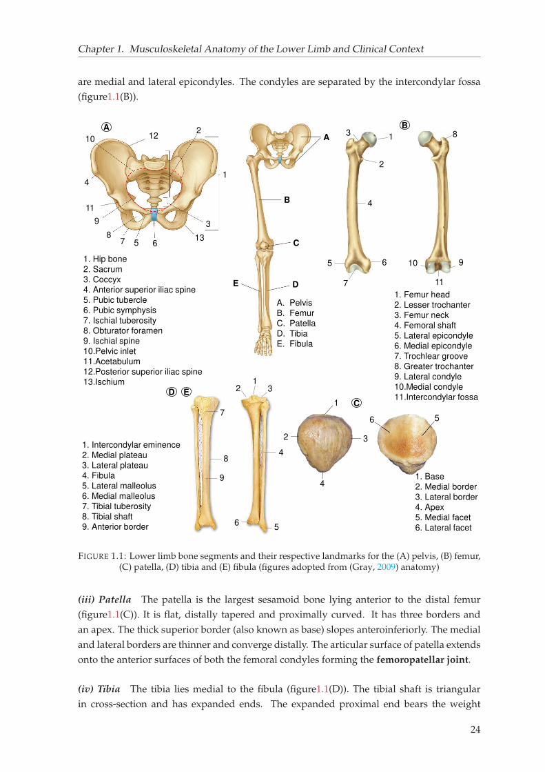
Chapter 1. Musculoskeletal Anatomy of the Lower Limb and Clinical Context
are medial and lateral epicondyles. The condyles are separated by the intercondylar fossa
(figure1.1(B)).
1
2
3
4
6
7
8
910
B
1. Hip bone
2. Sacrum
3. Coccyx
4. Anterior superior iliac spine
5. Pubic tubercle
6. Pubic symphysis
7. Ischial tuberosity
8. Obturator foramen
9. Ischial spine
10.Pelvic inlet
11.Acetabulum
12.Posterior superior iliac spine
13.Ischium
A
B
C
DE
A. Pelvis
B. Femur
C. Patella
D. Tibia
E. Fibula
1. Femur head
2. Lesser trochanter
3. Femur neck
4. Femoral shaft
5. Lateral epicondyle
6. Medial epicondyle
7. Trochlear groove
8. Greater trochanter
9. Lateral condyle
10.Medial condyle
11.Intercondylar fossa
1
2
3
4
5 678
9
10
11
12
13
A
1. Intercondylar eminence
2. Medial plateau
3. Lateral plateau
4. Fibula
5. Lateral malleolus
6. Medial malleolus
7. Tibial tuberosity
8. Tibial shaft
9. Anterior border
5
11
12
7
3
4
56
8
9 1. Base
2. Medial border
3. Lateral border
4. Apex
5. Medial facet
6. Lateral facet
1
2 3
4
56
C
D E
FIGURE 1.1: Lower limb bone segments and their respective landmarks for the (A) pelvis, (B) femur,(C) patella, (D) tibia and (E) fibula (figures adopted from (Gray, 2009) anatomy)
(iii) Patella The patella is the largest sesamoid bone lying anterior to the distal femur
(figure1.1(C)). It is flat, distally tapered and proximally curved. It has three borders and
an apex. The thick superior border (also known as base) slopes anteroinferiorly. The medial
and lateral borders are thinner and converge distally. The articular surface of patella extends
onto the anterior surfaces of both the femoral condyles forming the femoropatellar joint.
(iv) Tibia The tibia lies medial to the fibula (figure1.1(D)). The tibial shaft is triangular
in cross-section and has expanded ends. The expanded proximal end bears the weight
24
Chapter 1. Musculoskeletal Anatomy of the Lower Limb and Clinical Context
transmitted through the femur and has asymmetric articular facets called medial and lat-
eral plateaus. The medial tibial plateau is normally concave, whereas the lateral plateau has
an anteroposterior convexity with large subject-to-subject variations (Hashemi et al., 2008).
The plateaus are separated by intercondylar eminence. The slightly expanded distal end is
laterally rotated compared to the proximal. The tibial tuberosity is the truncated apex of a
triangular area divided into distal rough and proximal smooth region, where the patellar
ligament is attached.
(v) Fibula The fibula is more slander than the tibia and has an irregular shaped head, a
narrow neck, a long shaft and a distal lateral malleolus (figure1.1(E)). The fibular collateral
ligament (FCL) (also known as lateral collateral ligament (LCL)) is attached to the fibular
head.
1.1.2 Lower limb musculature and connective tissues2
(i) Muscles The muscles of the anterior compartment of the thigh include sartorius, rectus
femoris, vasti medialis, intermedius and lateralis (figure1.2(A)). Vasti and rectus femoris ex-
tend towards the knee joint through a common tendon, collectively referred to as quadriceps
tendon and they act as an extensor muscle of the knee.
The muscles of the medial compartment of the thigh include gracilis, pectineus, adductor
longus, adductor brevis and adductor magnus. These muscles primarily act as adductors of
the thigh.
The posterior compartment consists of long and short heads of biceps femoris, semitendi-
nosus and semimembranosus. These are collectively termed as ’hamstrings’ and they act as
hip extensor and knee flexor (figure1.2(B)).
(ii) Menisci and ligamentous structure The menisci (medial and lateral) of the knee joint
are roughly semi-lunar in shape. Their proximal surfaces are concave shaped and articulate
with the cartilage of the femoral condyles. The distal surfaces are generally flat shaped,
resting on the tibial plateaus.
The menisci act as shock absorbers and protect the joint from the considerable forces
generated during motion. They also provide stability by maintaining congruity with the
articular surfaces. Other functions are lubrication, nutrition and proprioception (Cameron
and Macnab, 1972).
The capsular and ligamentous assembly of the knee joint along with articular surfaces
and muscles play a fundamental role in providing stability to the joint. As per general
anatomical sites, the cruciate ligaments, ACL (anterior cruciate ligament) and PCL (poste-
rior cruciate ligament) are inserted into the intercondylar femoral recess on one side, and
respectively on pre-spinal and retro-spinal areas of the tibia on the other side (figure1.2(D))
2(Capkin et al., 2017; Gray, 2009)
25
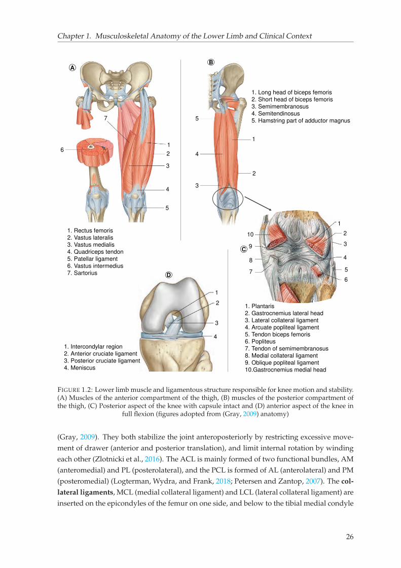
Chapter 1. Musculoskeletal Anatomy of the Lower Limb and Clinical Context
1
2
3
4
5
1
2
1
3
4
5
6
7
1. Rectus femoris
2. Vastus lateralis
3. Vastus medialis
4. Quadriceps tendon
5. Patellar ligament
6. Vastus intermedius
7. Sartorius
1. Long head of biceps femoris
2. Short head of biceps femoris
3. Semimembranosus
4. Semitendinosus
5. Hamstring part of adductor magnus
1. Plantaris
2. Gastrocnemius lateral head
3. Lateral collateral ligament
4. Arcuate popliteal ligament
5. Tendon biceps femoris
6. Popliteus
7. Tendon of semimembranosus
8. Medial collateral ligament9. Oblique popliteal ligament
10.Gastrocnemius medial head
AB
C
1
2
3
4
5
6
7
8
10
9
D
1
2
3
4
1. Intercondylar region
2. Anterior cruciate ligament
3. Posterior cruciate ligament
4. Meniscus
FIGURE 1.2: Lower limb muscle and ligamentous structure responsible for knee motion and stability.(A) Muscles of the anterior compartment of the thigh, (B) muscles of the posterior compartment ofthe thigh, (C) Posterior aspect of the knee with capsule intact and (D) anterior aspect of the knee in
full flexion (figures adopted from (Gray, 2009) anatomy)
(Gray, 2009). They both stabilize the joint anteroposteriorly by restricting excessive move-
ment of drawer (anterior and posterior translation), and limit internal rotation by winding
each other (Zlotnicki et al., 2016). The ACL is mainly formed of two functional bundles, AM
(anteromedial) and PL (posterolateral), and the PCL is formed of AL (anterolateral) and PM
(posteromedial) (Logterman, Wydra, and Frank, 2018; Petersen and Zantop, 2007). The col-
lateral ligaments, MCL (medial collateral ligament) and LCL (lateral collateral ligament) are
inserted on the epicondyles of the femur on one side, and below to the tibial medial condyle
26
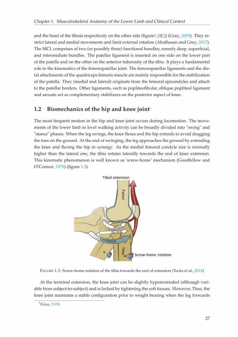
Chapter 1. Musculoskeletal Anatomy of the Lower Limb and Clinical Context
and the head of the fibula respectively on the other side (figure1.2(C)) (Gray, 2009). They re-
strict lateral and medial movements and limit external rotation (Abulhasan and Grey, 2017).
The MCL comprises of two (or possibly three) functional bundles, namely deep, superficial,
and intermediate bundles. The patellar ligament is inserted on one side on the lower part
of the patella and on the other on the anterior tuberosity of the tibia. It plays a fundamental
role in the kinematics of the femoropatellar joint. The femoropatellar ligaments and the dis-
tal attachments of the quadriceps femoris muscle are mainly responsible for the stabilization
of the patella. They (medial and lateral) originate from the femoral epicondyles and attach
to the patellar borders. Other ligaments, such as popliteofibular, oblique popliteal ligament
and arcuate act as complementary stabilizers on the posterior aspect of knee.
1.2 Biomechanics of the hip and knee joint3
The most frequent motion in the hip and knee joint occurs during locomotion. The move-
ments of the lower limb in level walking activity can be broadly divided into "swing" and
"stance" phases. When the leg swings, the knee flexes and the hip extends to avoid dragging
the toes on the ground. At the end of swinging, the leg approaches the ground by extending
the knee and flexing the hip in synergy. As the medial femoral condyle size is normally
higher than the lateral one, the tibia rotates laterally towards the end of knee extension.
This kinematic phenomenon is well known as ‘screw-home’ mechanism (Goodfellow and
O’Connor, 1978) (figure 1.3).
Screw-home rotation
Tibial extension
FIGURE 1.3: Screw-home rotation of the tibia towards the end of extension (Tocks et al., 2018)
At the terminal extension, the knee joint can be slightly hyperextended (although vari-
able from subject-to-subject) and is locked by tightening the soft tissues. However, Thus, the
knee joint maintains a stable configuration prior to weight bearing when the leg forwards
3(Gray, 2009)
27
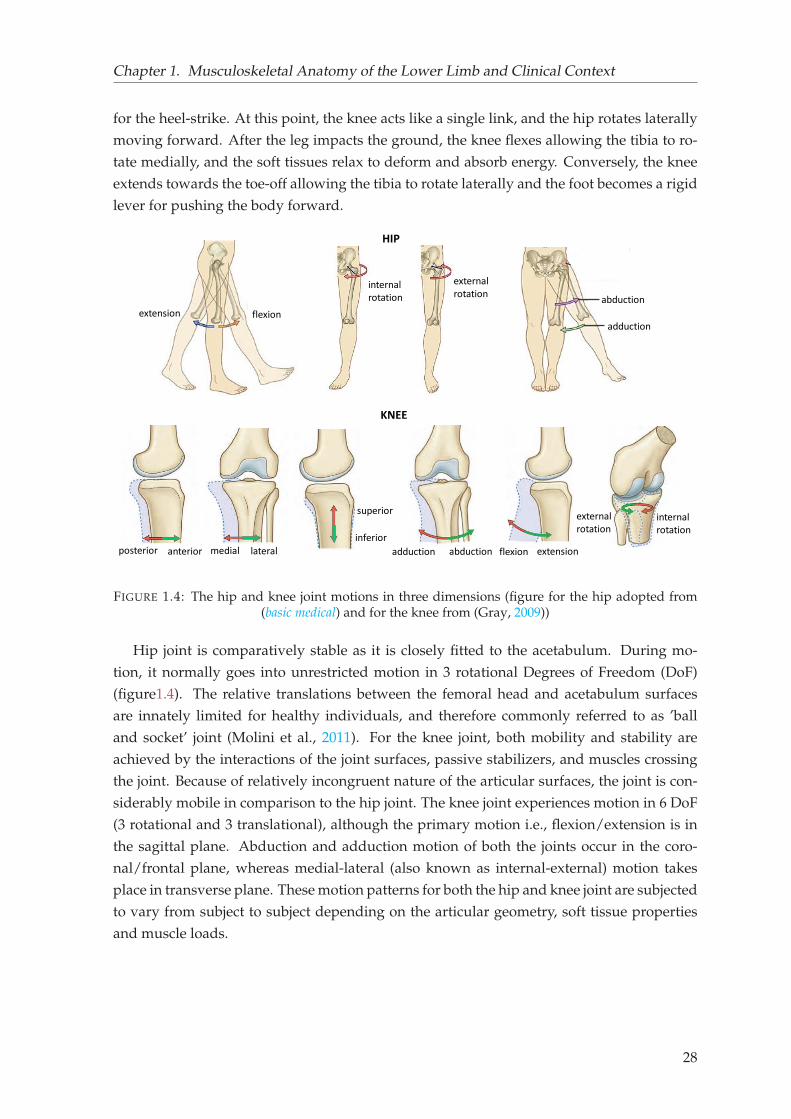
Chapter 1. Musculoskeletal Anatomy of the Lower Limb and Clinical Context
for the heel-strike. At this point, the knee acts like a single link, and the hip rotates laterally
moving forward. After the leg impacts the ground, the knee flexes allowing the tibia to ro-
tate medially, and the soft tissues relax to deform and absorb energy. Conversely, the knee
extends towards the toe-off allowing the tibia to rotate laterally and the foot becomes a rigid
lever for pushing the body forward.
aabduction
adduction
internal
rotation
external
rotation
extension flexion
posterior anterior lateralmedial
superior
inferior
abductionadduction extensionflexion
internal
rotation
external
rotation
HIP
KNEE
FIGURE 1.4: The hip and knee joint motions in three dimensions (figure for the hip adopted from(basic medical) and for the knee from (Gray, 2009))
Hip joint is comparatively stable as it is closely fitted to the acetabulum. During mo-
tion, it normally goes into unrestricted motion in 3 rotational Degrees of Freedom (DoF)
(figure1.4). The relative translations between the femoral head and acetabulum surfaces
are innately limited for healthy individuals, and therefore commonly referred to as ’ball
and socket’ joint (Molini et al., 2011). For the knee joint, both mobility and stability are
achieved by the interactions of the joint surfaces, passive stabilizers, and muscles crossing
the joint. Because of relatively incongruent nature of the articular surfaces, the joint is con-
siderably mobile in comparison to the hip joint. The knee joint experiences motion in 6 DoF
(3 rotational and 3 translational), although the primary motion i.e., flexion/extension is in
the sagittal plane. Abduction and adduction motion of both the joints occur in the coro-
nal/frontal plane, whereas medial-lateral (also known as internal-external) motion takes
place in transverse plane. These motion patterns for both the hip and knee joint are subjected
to vary from subject to subject depending on the articular geometry, soft tissue properties
and muscle loads.
28
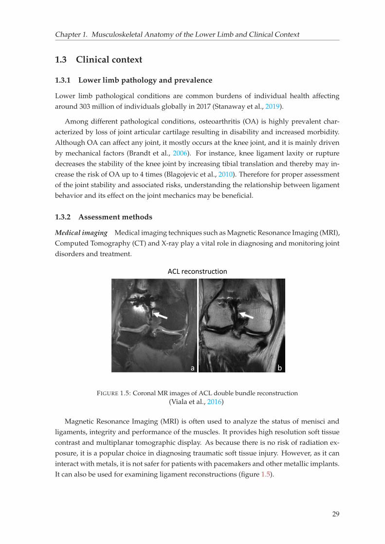
Chapter 1. Musculoskeletal Anatomy of the Lower Limb and Clinical Context
1.3 Clinical context
1.3.1 Lower limb pathology and prevalence
Lower limb pathological conditions are common burdens of individual health affecting
around 303 million of individuals globally in 2017 (Stanaway et al., 2019).
Among different pathological conditions, osteoarthritis (OA) is highly prevalent char-
acterized by loss of joint articular cartilage resulting in disability and increased morbidity.
Although OA can affect any joint, it mostly occurs at the knee joint, and it is mainly driven
by mechanical factors (Brandt et al., 2006). For instance, knee ligament laxity or rupture
decreases the stability of the knee joint by increasing tibial translation and thereby may in-
crease the risk of OA up to 4 times (Blagojevic et al., 2010). Therefore for proper assessment
of the joint stability and associated risks, understanding the relationship between ligament
behavior and its effect on the joint mechanics may be beneficial.
1.3.2 Assessment methods
Medical imaging Medical imaging techniques such as Magnetic Resonance Imaging (MRI),
Computed Tomography (CT) and X-ray play a vital role in diagnosing and monitoring joint
disorders and treatment.
b
ACL reconstruction
a b
FIGURE 1.5: Coronal MR images of ACL double bundle reconstruction(Viala et al., 2016)
Magnetic Resonance Imaging (MRI) is often used to analyze the status of menisci and
ligaments, integrity and performance of the muscles. It provides high resolution soft tissue
contrast and multiplanar tomographic display. As because there is no risk of radiation ex-
posure, it is a popular choice in diagnosing traumatic soft tissue injury. However, as it can
interact with metals, it is not safer for patients with pacemakers and other metallic implants.
It can also be used for examining ligament reconstructions (figure 1.5).
29
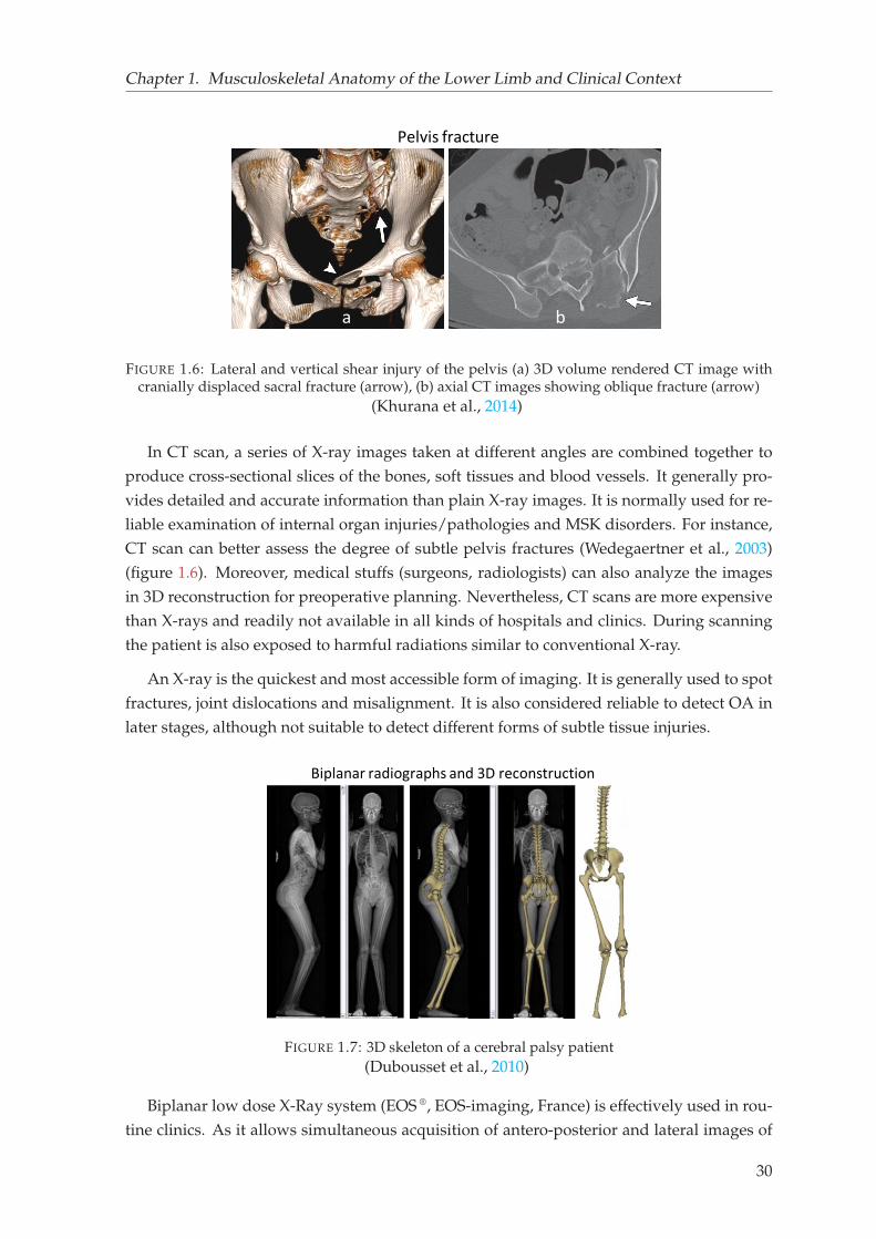
Chapter 1. Musculoskeletal Anatomy of the Lower Limb and Clinical Context
Pelvis fracture
a b
FIGURE 1.6: Lateral and vertical shear injury of the pelvis (a) 3D volume rendered CT image withcranially displaced sacral fracture (arrow), (b) axial CT images showing oblique fracture (arrow)
(Khurana et al., 2014)
In CT scan, a series of X-ray images taken at different angles are combined together to
produce cross-sectional slices of the bones, soft tissues and blood vessels. It generally pro-
vides detailed and accurate information than plain X-ray images. It is normally used for re-
liable examination of internal organ injuries/pathologies and MSK disorders. For instance,
CT scan can better assess the degree of subtle pelvis fractures (Wedegaertner et al., 2003)
(figure 1.6). Moreover, medical stuffs (surgeons, radiologists) can also analyze the images
in 3D reconstruction for preoperative planning. Nevertheless, CT scans are more expensive
than X-rays and readily not available in all kinds of hospitals and clinics. During scanning
the patient is also exposed to harmful radiations similar to conventional X-ray.
An X-ray is the quickest and most accessible form of imaging. It is generally used to spot
fractures, joint dislocations and misalignment. It is also considered reliable to detect OA in
later stages, although not suitable to detect different forms of subtle tissue injuries.
Biplanar radiographs and 3D reconstruction
a b c
FIGURE 1.7: 3D skeleton of a cerebral palsy patient(Dubousset et al., 2010)
Biplanar low dose X-Ray system (EOS ®, EOS-imaging, France) is effectively used in rou-
tine clinics. As it allows simultaneous acquisition of antero-posterior and lateral images of
30
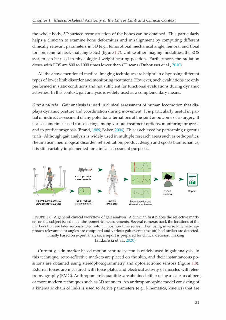
Chapter 1. Musculoskeletal Anatomy of the Lower Limb and Clinical Context
the whole body, 3D surface reconstruction of the bones can be obtained. This particularly
helps a clinician to examine bone deformities and misalignment by computing different
clinically relevant parameters in 3D (e.g., femorotibial mechanical angle, femoral and tibial
torsion, femoral neck shaft angle etc.) (figure 1.7). Unlike other imaging modalities, the EOS
system can be used in physiological weight-bearing position. Furthermore, the radiation
doses with EOS are 800 to 1000 times lower than CT scans (Dubousset et al., 2010).
All the above mentioned medical imaging techniques are helpful in diagnosing different
types of lower limb disorder and monitoring treatment. However, such evaluations are only
performed in static conditions and not sufficient for functional evaluations during dynamic
activities. In this context, gait analysis is widely used as a complementary means.
Gait analysis Gait analysis is used in clinical assessment of human locomotion that dis-
plays dynamic posture and coordination during movement. It is particularly useful in par-
tial or indirect assessment of any potential alternations at the joint or outcome of a surgery. It
is also sometimes used for selecting among various treatment options, monitoring progress
and to predict prognosis (Brand, 1989; Baker, 2006). This is achieved by performing rigorous
trials. Although gait analysis is widely used in multiple research areas such as orthopedics,
rheumatism, neurological disorder, rehabilitation, product design and sports biomechanics,
it is still variably implemented for clinical assessment purposes.
Event detection and kinematics estimation
FIGURE 1.8: A general clinical workflow of gait analysis. A clinician first places the reflective mark-ers on the subject based on anthropometric measurements. Several cameras track the locations of themarkers that are later reconstructed into 3D position time series. Then using inverse kinematic ap-proach relevant joint angles are computed and various gait events (toe-off, heel strike) are detected.
Finally based on expert analysis, a report is prepared for clinical decision. making(Kidzinski et al., 2020)
Currently, skin marker-based motion capture system is widely used in gait analysis. In
this technique, retro-reflective markers are placed on the skin, and their instantaneous po-
sitions are obtained using stereophotogrammetry and optoelectronic sensors (figure 1.8).
External forces are measured with force plates and electrical activity of muscles with elec-
tromyography (EMG). Anthropometric quantities are obtained either using a scale or calipers,
or more modern techniques such as 3D scanners. An anthropomorphic model consisting of
a kinematic chain of links is used to derive parameters (e.g., kinematics, kinetics) that are
31
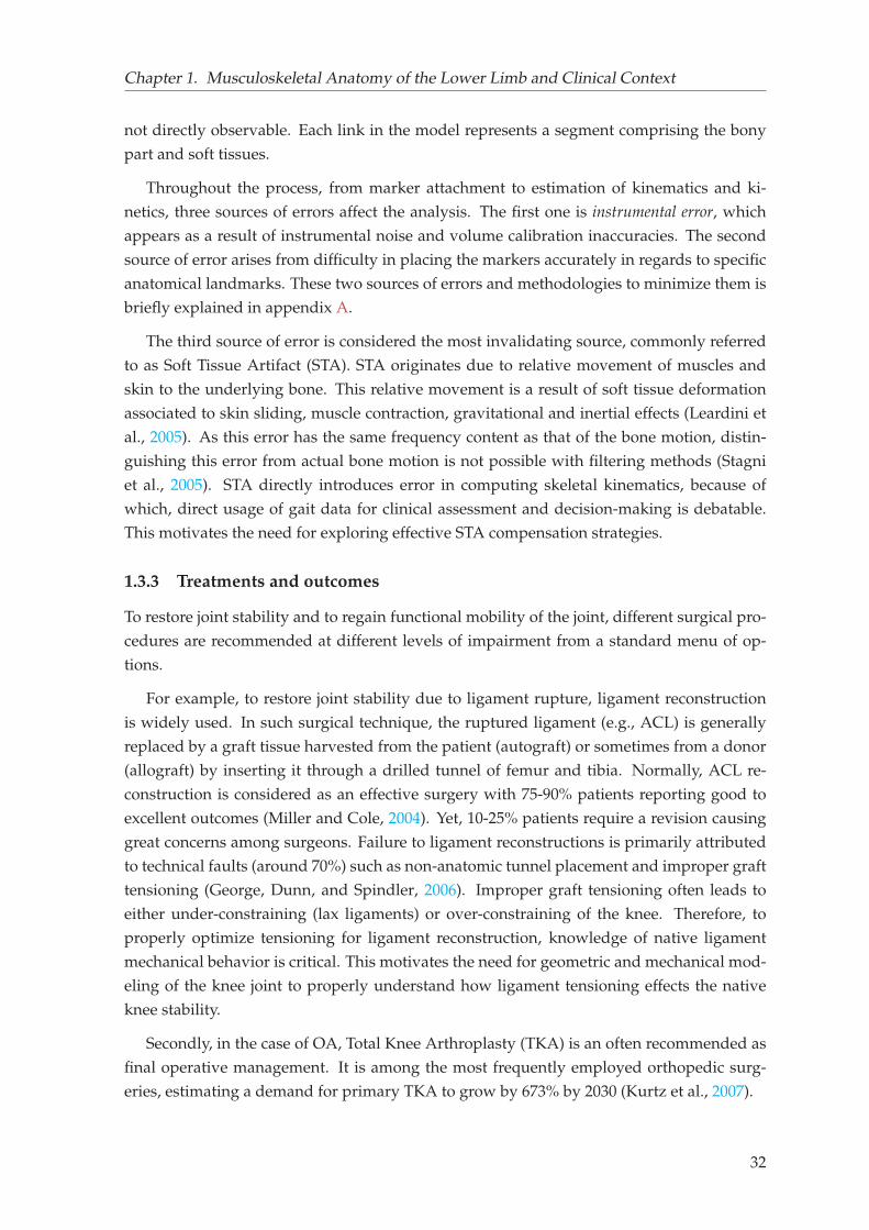
Chapter 1. Musculoskeletal Anatomy of the Lower Limb and Clinical Context
not directly observable. Each link in the model represents a segment comprising the bony
part and soft tissues.
Throughout the process, from marker attachment to estimation of kinematics and ki-
netics, three sources of errors affect the analysis. The first one is instrumental error, which
appears as a result of instrumental noise and volume calibration inaccuracies. The second
source of error arises from difficulty in placing the markers accurately in regards to specific
anatomical landmarks. These two sources of errors and methodologies to minimize them is
briefly explained in appendix A.
The third source of error is considered the most invalidating source, commonly referred
to as Soft Tissue Artifact (STA). STA originates due to relative movement of muscles and
skin to the underlying bone. This relative movement is a result of soft tissue deformation
associated to skin sliding, muscle contraction, gravitational and inertial effects (Leardini et
al., 2005). As this error has the same frequency content as that of the bone motion, distin-
guishing this error from actual bone motion is not possible with filtering methods (Stagni
et al., 2005). STA directly introduces error in computing skeletal kinematics, because of
which, direct usage of gait data for clinical assessment and decision-making is debatable.
This motivates the need for exploring effective STA compensation strategies.
1.3.3 Treatments and outcomes
To restore joint stability and to regain functional mobility of the joint, different surgical pro-
cedures are recommended at different levels of impairment from a standard menu of op-
tions.
For example, to restore joint stability due to ligament rupture, ligament reconstruction
is widely used. In such surgical technique, the ruptured ligament (e.g., ACL) is generally
replaced by a graft tissue harvested from the patient (autograft) or sometimes from a donor
(allograft) by inserting it through a drilled tunnel of femur and tibia. Normally, ACL re-
construction is considered as an effective surgery with 75-90% patients reporting good to
excellent outcomes (Miller and Cole, 2004). Yet, 10-25% patients require a revision causing
great concerns among surgeons. Failure to ligament reconstructions is primarily attributed
to technical faults (around 70%) such as non-anatomic tunnel placement and improper graft
tensioning (George, Dunn, and Spindler, 2006). Improper graft tensioning often leads to
either under-constraining (lax ligaments) or over-constraining of the knee. Therefore, to
properly optimize tensioning for ligament reconstruction, knowledge of native ligament
mechanical behavior is critical. This motivates the need for geometric and mechanical mod-
eling of the knee joint to properly understand how ligament tensioning effects the native
knee stability.
Secondly, in the case of OA, Total Knee Arthroplasty (TKA) is an often recommended as
final operative management. It is among the most frequently employed orthopedic surg-
eries, estimating a demand for primary TKA to grow by 673% by 2030 (Kurtz et al., 2007).
32
Chapter 1. Musculoskeletal Anatomy of the Lower Limb and Clinical Context
While planning for TKA implantation, clinicians preoperatively assess the knee in the
three spatial planes for successful implant positioning. There are several options available
for proper implant positioning (detailed in Appendix B). For instance, one popular princi-
ple is to position the implant components by aligning to the mechanical axis of the knee
joint (Jeffery, Morris, and Denham, 1991). Conversely, others recommend anatomical align-
ment of implants, which reported better implant durability (Kim et al., 2014). Few others
also advocate on kinematic alignment and patient specific instrumentation for longer im-
plant survivorship (up to 10 years) and functional outcomes (Howell et al., 2001; Yaffe et
al., 2014; Zhu et al., 2017). Despite such aforementioned geometric alignment approach
for better functional outcomes, no complete consensus on a particular technique has been
achieved yet, as "one size fits none" for many treatments (Fregly, Boninger, and Reinkens-
meyer, 2012). For better functioning of the implant, along with optimal choice of implant
design and alignment, a precise balancing of the soft tissues is also critical (Vaienti et al.,
2017).
As overall functional stability of the knee joint is achieved by inter-dependent interaction
of various constituents of the joint (e.g., articular surface, capsule, menisci, ligaments and
muscles), it is clinically difficult to differentiate variability of influence on TKA performance.
Therefore, a comprehensive understanding of these elements in a native knee is important
for surgery planning. Personalized computational modeling could be one possible avenue
for objective assessment of subject-specific properties.
Synthesis
This chapter highlighted that
- Personalized computation modeling such as FE modeling could be helpful for un-
derstanding native knee joint mechanics and for surgery planning. Therefore first
part of the next chapter will be focused on salient FE models and their model devel-
opment and evaluation strategies.
- We also observed that for proper assessment of functional outcomes of an inter-
vention, gait analysis is essential as it offers physiological loading conditions. It is
also important for prescribing clinically relevant boundary conditions for computa-
tional models (e.g., musculoskeletal models). However, direct usage of gait data is
error prone because of soft tissue artifact (STA). Therefore the second part of the next
chapter will be focused on different STA compensation strategies. Also different com-
plementary means for assessing joint biomechanical behavior under in vivo loading
conditions will be explored.
33

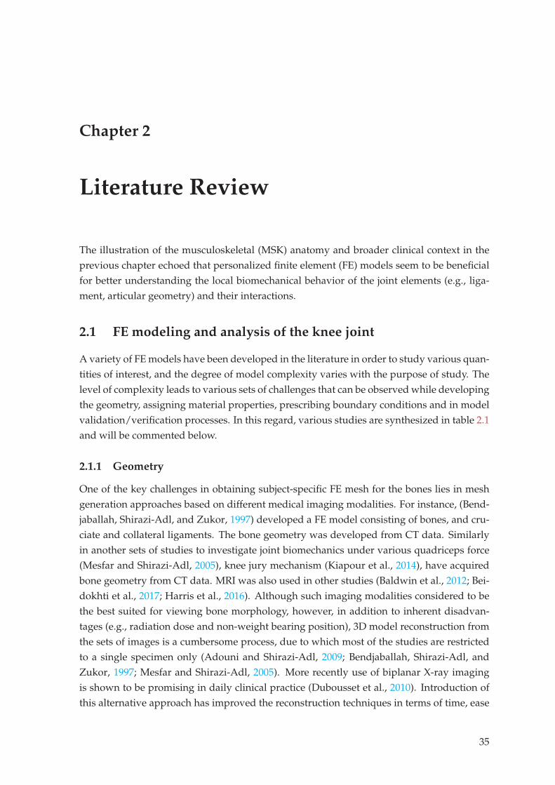
Chapter 2
Literature Review
The illustration of the musculoskeletal (MSK) anatomy and broader clinical context in the
previous chapter echoed that personalized finite element (FE) models seem to be beneficial
for better understanding the local biomechanical behavior of the joint elements (e.g., liga-
ment, articular geometry) and their interactions.
2.1 FE modeling and analysis of the knee joint
A variety of FE models have been developed in the literature in order to study various quan-
tities of interest, and the degree of model complexity varies with the purpose of study. The
level of complexity leads to various sets of challenges that can be observed while developing
the geometry, assigning material properties, prescribing boundary conditions and in model
validation/verification processes. In this regard, various studies are synthesized in table 2.1
and will be commented below.
2.1.1 Geometry
One of the key challenges in obtaining subject-specific FE mesh for the bones lies in mesh
generation approaches based on different medical imaging modalities. For instance, (Bend-
jaballah, Shirazi-Adl, and Zukor, 1997) developed a FE model consisting of bones, and cru-
ciate and collateral ligaments. The bone geometry was developed from CT data. Similarly
in another sets of studies to investigate joint biomechanics under various quadriceps force
(Mesfar and Shirazi-Adl, 2005), knee jury mechanism (Kiapour et al., 2014), have acquired
bone geometry from CT data. MRI was also used in other studies (Baldwin et al., 2012; Bei-
dokhti et al., 2017; Harris et al., 2016). Although such imaging modalities considered to be
the best suited for viewing bone morphology, however, in addition to inherent disadvan-
tages (e.g., radiation dose and non-weight bearing position), 3D model reconstruction from
the sets of images is a cumbersome process, due to which most of the studies are restricted
to a single specimen only (Adouni and Shirazi-Adl, 2009; Bendjaballah, Shirazi-Adl, and
Zukor, 1997; Mesfar and Shirazi-Adl, 2005). More recently use of biplanar X-ray imaging
is shown to be promising in daily clinical practice (Dubousset et al., 2010). Introduction of
this alternative approach has improved the reconstruction techniques in terms of time, ease
35
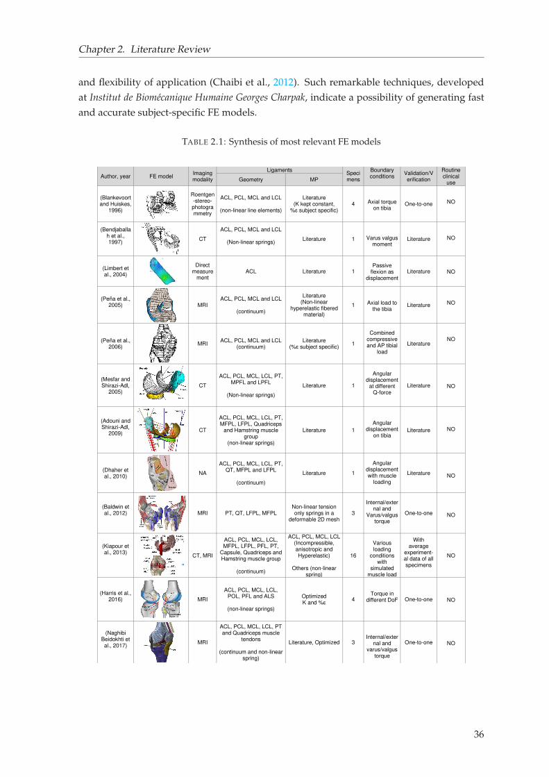
Chapter 2. Literature Review
and flexibility of application (Chaibi et al., 2012). Such remarkable techniques, developed
at Institut de Biomécanique Humaine Georges Charpak, indicate a possibility of generating fast
and accurate subject-specific FE models.
TABLE 2.1: Synthesis of most relevant FE models
Author, year FE model Imaging modality
Ligaments Specimens
Boundary conditions
Validation/Verification
Routine clinical
use Geometry MP
(Blankevoort and Huiskes,
1996)
Roentgen-stereo- photogrammetry
ACL, PCL, MCL and LCL
(non-linear line elements)
Literature (K kept constant,
%ɛ subject specific) 4
Axial torque on tibia
One-to-one
NO
(Bendjaballah et al., 1997)
CT
ACL, PCL, MCL and LCL
(Non-linear springs)
Literature 1
Varus valgus moment
Literature
NO
(Limbert et al., 2004)
Direct measure
ment ACL Literature 1
Passive
flexion as displacement
Literature
NO
(Peña et al., 2005)
MRI ACL, PCL, MCL and LCL
(continuum)
Literature (Non-linear
hyperelastic fibered material)
1
Axial load to the tibia
Literature
NO
(Peña et al., 2006)
MRI ACL, PCL, MCL and LCL
(continuum) Literature
(%ɛ subject specific) 1
Combined
compressive and AP tibial
load
Literature
NO
(Mesfar and Shirazi-Adl,
2005)
CT
ACL, PCL, MCL, LCL, PT, MPFL and LPFL
(Non-linear springs)
Literature 1
Angular
displacement at different
Q-force
Literature
NO
(Adouni and Shirazi-Adl,
2009)
CT
ACL, PCL, MCL, LCL, PT, MFPL, LFPL, Quadriceps
and Hamstring muscle group
(non-linear springs)
Literature 1
Angular displacement
on tibia Literature
NO
(Dhaher et al., 2010)
NA
ACL, PCL, MCL, LCL, PT, QT, MFPL and LFPL
(continuum)
Literature 1
Angular
displacement with muscle
loading
Literature
NO
(Baldwin et al., 2012)
MRI PT, QT, LFPL, MFPL Non-linear tension only springs in a
deformable 2D mesh 3
Internal/exter
nal and Varus/valgus
torque
One-to-one
NO
(Kiapour et al., 2013)
CT, MRI
ACL, PCL, MCL, LCL, MFPL, LFPL, PFL, PT,
Capsule, Quadriceps and Hamstring muscle group
(continuum)
ACL, PCL, MCL, LCL (Incompressible, anisotropic and Hyperelastic)
Others (non-linear
spring)
16
Various loading
conditions with
simulated muscle load
With average
experiment-al data of all specimens
NO
(Harris et al., 2016)
MRI
ACL, PCL, MCL, LCL, POL, PFL and ALS
(non-linear springs)
Optimized K and %ɛ 4
Torque in different DoF One-to-one
NO
(Naghibi Beidokhti et al., 2017)
MRI
ACL, PCL, MCL, LCL, PT and Quadriceps muscle
tendons
(continuum and non-linear spring)
Literature, Optimized 3
Internal/external and
varus/valgus torque
One-to-one
NO
36
Chapter 2. Literature Review
To include ligaments in the models according to their subject-specific anatomical attach-
ment sites, studies either did not explicitly mention the procedure (Pena et al., 2005; Pena
et al., 2006), or used MRI data (Baldwin et al., 2012; Harris et al., 2016; Kiapour et al., 2014).
Few others also attempted to implement personalized insertion sites based on CT data, but
was partially successful because of poor visibility of soft tissues in the images (Adouni and
Shirazi-Adl, 2009; Mesfar and Shirazi-Adl, 2005). Notably, all these studies agreed that im-
plementing accurate subject-specific ligament attachment sites in the models is essential to
avoid undesired influence on ligament loads and eventually in joint kinematics. In this
context, (Rochcongar et al., 2016) at Institut de Biomécanique Humaine Georges Charpak, intro-
duced an original technique to identify ligament attachment sites accurately based on CT
images of dissected knee joint. Such insights could be a strong ground for subject-specific
joint modeling.
b
a
FIGURE 2.1: (a) Schematic representation of the knee ligaments (ACL, PCL, MCL and LCL) as 1D, 2Dand 3D elements adopted from (Galbusera et al., 2014) (b) force(F) - strain(ǫ) behavior of a ligamentadopted from (Blankevoort and Huiskes, 1991). 2ǫl is the threshold strain indicating toe to linear
region
With regards to modeling of the ligaments, traditionally both 1D and higher dimensional-
ity (2D, 3D) elements have been equally used (figure 2.1a). As because the ligaments are not
able to sustain compression load, 1D elements such as cables/springs, trusses are commonly
used either as bundles of elements (Bendjaballah, Shirazi-Adl, and Zukor, 1997; Mesfar and
Shirazi-Adl, 2005) or as a single bundle (Yu, Walker, and Dewar, 2001). Such elements are
advantageous for easy implementation and computationally inexpensive. While detailed
representation (e.g., solid elements) of the ligaments could be interesting for studying force
distribution on the ligaments (Bendjaballah, Shirazi-Adl, and Zukor, 1997), such models re-
quire detailed image-based information resulting in high computational cost in developing
and simulating them. Moreover, neglecting 3D behavior of ligaments does not dramatically
impact other parameters such as joint kinematics (Blankevoort and Huiskes, 1991). In this
aspect, simpler representation may be beneficial for studies where higher number of subjects
need to be analyzed and, at the same time, capable of predicting joint mechanics (Beidokhti
37
Chapter 2. Literature Review
et al., 2017; Galbusera et al., 2014).
To represent other soft tissues (e.g., cartilage, menisci) in the model, wide range of possi-
ble choices can be observed. The level of detailing varies according to research question and
specific application of it. Some models concentrate on faithful capture of specimen-specific
anatomy using CT and MRI imaging to investigate mechanical role of the components in
a tissue. For example, one study included main articular soft tissue structures of the knee
joint, featuring cartilage layers and menisci with complex material behavior (Pena et al.,
2006) to study combined role of ligaments and menisci. Such type of models can potentially
provide new insights into surgery performance such as meniscectomy, and disease progres-
sion such as OA. Conversely, some other strategies are steered by simplicity, where all the
joint soft tissues are not explicitly modeled. For instance, the same group referred earlier ex-
cluded cartilage and meniscal geometry in the model that was aimed to study effect of graft
tensioning in ACL reconstruction (Pena et al., 2005). This study concluded that "influence
of menisci and cartilage with regards to the main objective of the study is not very impor-
tant". These studies underlined the importance of a proper decision-making on inclusion of
relevant joint elements in the model.
Overall, all the above studies and their methodology of representing the joint, particu-
larly the passive structures, highlighted several challenges. These can be broadly tailored
into two categories. First, generation of fast and accurate subject-specific FE mesh and sec-
ond, a proper balance between relevance and simplicity to represent the joint structure.
2.1.2 Material properties
When it comes to assigning material properties of the bones, depending on the scale of
hierarchy and purpose of study, varieties of material modeling are chosen. At mesoscale,
bones are investigated either at osteon level embedded in the cortical bone or at the porous
network in the spongy bone (Sabet et al., 2016). At the macroscale or at the whole bone level,
bones are differentiated between cortical and trabecular/spongy bones. This differentiation
is largely based on distinction of porosity of the bones (Morgan, Unnikrisnan, and Hussein,
2018). Such differentiation helps studies to investigate bone fracture mechanism (Keyak et
al., 2001), to estimate bone strength following treatments of osteoporosis (Burr, 2016). At
this level, anisotropy, inhomogeneity, viscoelasticity and nonlinearity can be introduced.
Even multiscale models are used to understand cascade of mechanisms at different levels
within the bone (Sabet et al., 2016). However, to investigate quasistatic response at the joint,
considering bone as linear elastic is reasonable. Elastic modulus of cortical bone has been
reported roughly in the range 10 GPa to 32 GPa, when measured with different test methods
such as destructive, ultrasound and non-indentation method (Choi et al., 1990; Hunt et al.,
1998). The Poisson’s ratio varies in the range 0.15 to 0.45, however it is classically set to
0.3 (Rupin et al., 2008). Since the elastic modulus of bone is considerably higher than the
surrounding soft tissues, the bones are considered rigid more often (Beidokhti et al., 2017;
Halloran, Petrella, and Rullkoetter, 2005; Pena et al., 2005). The choice of bones as rigid is
also motivated by reduced computational time.
38
Chapter 2. Literature Review
Quantitative estimation of material properties of soft tissues is extremely challenging.
The properties are known to vary with subject, posture, loading condition and time (Zheng
and Mak, 1999). The properties can also be different depending upon whether measured in
vivo, in vitro or in situ. However, in vitro methods are more popular for detailed investigation
of both the physiological and mechanical behaviors of tissue. Therefore, constitutive laws
assigned to soft tissues are conveniently acquired from various in vitro experimental studies
available in the literature.
For representing cartilage, varieties of material representation can be seen in the liter-
ature. To understand cartilage mechanics and influence of cartilage structure on the knee
joint, some authors used depth-dependent cartilage properties with fibril networks (Halo-
nen et al., 2016; Shirazi, Shirazi-Adl, and Hurtig, 2008). A few included multi-scale mod-
eling of cartilage (Tanska, Mononen, and Korhonen, 2015; Halloran et al., 2012). Cartilage
as linear elastic material has been commonly used due to its equivalence between incom-
pressibility and short-time biphasic nature (Ateshian, Ellis, and Weiss, 2007; Kiapour et al.,
2014). One study at Institut de Biomécanique Humaine Georges Charpak also showed the pos-
sibility of defining cartilage and bone together as a homogeneous bone-cartilage material
with equivalent material properties of bone and cartilage (Germain et al., 2016). Although,
such consideration may not be sufficient for estimating cartilage mechanics, yet can be con-
sidered relevant for predicting kinematic behavior of the knee joint. Similar is the case for
the meniscus, where a detailed representation was required to understand role of meniscus
in response to loading and damage progression (Halonen et al., 2014; Kiapour et al., 2014).
Ligaments, based on their representation, different constitutive laws have been tradition-
ally assigned. For 1D type of elements, non-linear force-strain behavior is assigned to the
ligaments with quadratic toe region and linear forward (Blankevoort and Huiskes, 1991)
(figure 2.1b). Bi-linear form of force-strain behavior has also been used by linearizing the
toe region (Shin, Chaudhari, and Andriacchi, 2007). In 3D representation of ligaments, they
are commonly defined as incompressible material behavior (Beidokhti et al., 2017; Dhaher,
Kwon, and Barry, 2010). In either case, whether 1D or 3D, the elements representing the
ligaments can only sustain tension and offer no resistance to compressive load (Galbusera
et al., 2014). Moreover, knee ligaments (particularly ACL, LCL and MCL) are known to be
at strained state, already sustaining tensile load at full extension (Guess, Razu, and Jahan-
dar, 2016; Pena et al., 2006). The PCL normally stays in slack condition at the full extension
(Blankevoort and Huiskes, 1991). This strain at the fully extended position of the knee is
commonly referred to as prestrain or reference strain or initial strain.
Deriving prestrain values confronts numerous hurdles. Challenges are mostly linked to
both measurement and modeling issues. Measurement challenges are related to identifi-
cation of accurate ligament attachment sites and determination of ligament characteristics
during motion (Belvedere et al., 2012; Gardiner, Weiss, and Rosenberg, 2001; Rochcongar et
al., 2016). Owing to such difficulties, FE models generally adopt prestrain values from other
studies (Adouni and Shirazi-Adl, 2009; Bendjaballah, Shirazi-Adl, and Zukor, 1997; Mesfar
39
Chapter 2. Literature Review
and Shirazi-Adl, 2005). However, such approach cannot be considered as subject-specific as
prestrain values do not correspond to the specimen under study.
In an attempt for assigning subject-specific prestrain values, laxity tests on cadaveric
specimens are normally used to indirectly estimate prestrain values based on optimization
methods (Baldwin et al., 2012; Harris et al., 2016; Beidokhti et al., 2017), which aim for mini-
mizing a cost function (experimental-numerical kinetic/kinematic difference) in subsequent
iterations. All these studies concluded that subject-specific prestrain values offer accurate
kinematic and kinetic prediction. Nevertheless, such methods are likely to be computation-
ally expensive up to 400-600h per specimen depending upon complexity of the models as
reported by (Beidokhti et al., 2017). In such context, any alternative approach which can
circumvent high computational cost could be beneficial for clinical translation.
2.1.3 Boundary and loading condition
In FE models representing in vitro specimens, boundary and loading conditions are normally
based on corresponding controlled in vitro studies. Such studies mostly focused on repro-
ducing in vitro experiments. For instance, passive flexion load as displacement was applied
on the tibia in a study to understand the behavior of stressed and stress-free ligament (Lim-
bert, Taylor, and Middleton, 2004). Other studies also attempted to implement in vivo alike
dynamic loads. To observe detailed biomechanics (e.g., joint kinematics, ligament and ex-
tensor muscle forces) of the knee joint in various closed kinematics chain exercises, (Mesfar
and Shirazi-Adl, 2005) introduced flexion load at the tibia under various quadriceps force by
keeping the femur fixed. Based on the results, this study advocated the use of squat exercises
in post-ligament reconstruction period. In a similar fashion, (Baldwin et al., 2012) and their
subsequent works used a whole joint knee simulator (Kansas Knee Simulator) to apply dy-
namic loads on the joint of a cadaveric specimen. Then the experimental loading profile was
implemented to evaluate the FE model of the knee joint. Although such models based on
cadaveric specimens are admirable in increasing knowledge on interaction between passive
stabilizers of the joint, yet debatable for muscular activity in the absence of physiological
loading conditions. Moreover, such implemented loads are largely generic as same loading
pattern were applied for different specimens, whereas the knee joint is subjected to variable
loading conditions during daily life activities such as walking. In vivo based computational
models such as musculoskeletal models seem to be an efficient alternative since such models
can embody physiological loading conditions based on motion analysis data.
2.1.4 Verification and Validation
Traditionally, in vitro models are considered relatively simple to validate with correspond-
ing experimental study in comparison to in vivo models. This is particularly true for val-
idating joint kinematics, where reasonably accurate kinematics can be obtained by rigidly
attaching markers to the bones. In this aspect, a kinematic test bench was developed at
Institut de Biomécanique Humaine Georges Charpak (Azmy et al., 2010). This experimental
set up uses a servo-actuator to place the quadriceps tendon under traction and a rope and
40
Chapter 2. Literature Review
pulley system to continuously mobilize the knee in flexion/extension by introducing pas-
sive load at the tibia, while keeping the femur fixed. Then, with the help of bone-attached
retro-reflective tripod markers and an optoelectronic device, spatial bone positions can be
deduced. Subsequently, this set up has been used in several other studies to acquire joint
kinematics and parallelly served in model validations (Dagneaux et al., 2015; Germain et
al., 2016). However, substantial variabilities can be observed regarding model validation. In
some scenarios, models were validated against average experimental data (Germain et al.,
2016; Kiapour et al., 2014) representing general trends. These studies, although build con-
fidence in the ability of FE models to represent general trends, such evidence may not be
sufficient to capture inter-individuality of knee specimens. Here, direct validation (one-to-
one) of model-predicted response against corresponding cadaveric results could be crucial
for proper model validations before translating the model to in vivo loading conditions.
Synthesis 1
After reviewing various literature on in vitro FE models, it is evident that despite
significant advancements over recent years, translating models to clinics remains a
major challenge. The challenges are mainly linked to-
- Fast and accurate methods for building subject-specific FE models.
- Adopting a modeling approach with decent trade-off between relevance and model
simplification to accelerate computational time.
- Calibration of ligament material properties.
2.2 Musculoskeletal modeling
To noninvasively investigate relationship between locomotion and internal biomechanical
quantities, musculoskeletal (MSK) modeling represents a valuable method in a wide range
of physiological and pathological conditions. Traditionally, such models have been used
to study wide variety of biomechanical investigations such as mechanisms of MSK disor-
der (Eltoukhy et al., 2017; Neptune, Zajac, and Kautz, 2009), effects of surgery (osteotomy
(Brand, 1997; Schmidt et al., 1999), tendon transfer (Fridén and Lieber, 2002; Murray et al.,
2002; Herrmann and Delp, 1999; Delp, Komattu, and Wixson, 1994), tendon lengthening
(Delp, Statler, and Carroll, 1995; Delp and Zajac, 1992), ligament reconstruction (Pena et al.,
2005), total joint replacement (Delp, Komattu, and Wixson, 1994; Delp et al., 1996; Piazza
and Delp, 1996)). Models have also been used to analyze muscular coordination in dynamic
activities to understand normal (Anderson and Pandy, 2003) and pathological movement
(Piazza and Delp, 1996).
The usual pipeline of MSK model development approach are accompanied by inverse
kinematics, inverse dynamics and forward dynamics (figure 2.2). In the inverse kinematics,
skin marker based motion data is usually used as input to estimate joint kinematics. Then,
41
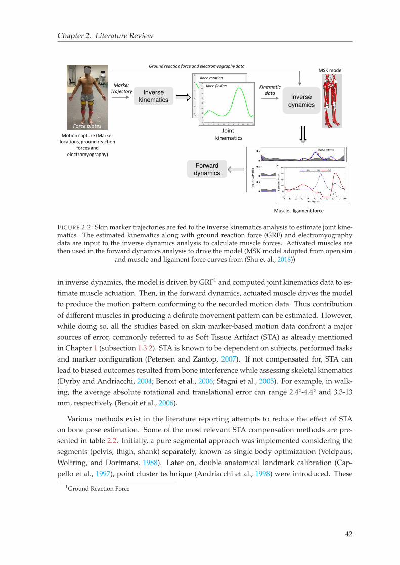
Chapter 2. Literature Review
Inverse
kinematics
Motion capture (Marker
locations, ground reaction
forces and
electromyography)
Inverse
dynamics
Joint
kinematics
Muscle , ligament force
Forward
dynamics
Force plates
Marker
Trajectory
Knee flexion
Knee rotation
Kinematic
data
Ground reaction force and electromyography dataMSK model
FIGURE 2.2: Skin marker trajectories are fed to the inverse kinematics analysis to estimate joint kine-matics. The estimated kinematics along with ground reaction force (GRF) and electromyographydata are input to the inverse dynamics analysis to calculate muscle forces. Activated muscles arethen used in the forward dynamics analysis to drive the model (MSK model adopted from open sim
and muscle and ligament force curves from (Shu et al., 2018))
in inverse dynamics, the model is driven by GRF1 and computed joint kinematics data to es-
timate muscle actuation. Then, in the forward dynamics, actuated muscle drives the model
to produce the motion pattern conforming to the recorded motion data. Thus contribution
of different muscles in producing a definite movement pattern can be estimated. However,
while doing so, all the studies based on skin marker-based motion data confront a major
sources of error, commonly referred to as Soft Tissue Artifact (STA) as already mentioned
in Chapter 1 (subsection 1.3.2). STA is known to be dependent on subjects, performed tasks
and marker configuration (Petersen and Zantop, 2007). If not compensated for, STA can
lead to biased outcomes resulted from bone interference while assessing skeletal kinematics
(Dyrby and Andriacchi, 2004; Benoit et al., 2006; Stagni et al., 2005). For example, in walk-
ing, the average absolute rotational and translational error can range 2.4°-4.4° and 3.3-13
mm, respectively (Benoit et al., 2006).
Various methods exist in the literature reporting attempts to reduce the effect of STA
on bone pose estimation. Some of the most relevant STA compensation methods are pre-
sented in table 2.2. Initially, a pure segmental approach was implemented considering the
segments (pelvis, thigh, shank) separately, known as single-body optimization (Veldpaus,
Woltring, and Dortmans, 1988). Later on, double anatomical landmark calibration (Cap-
pello et al., 1997), point cluster technique (Andriacchi et al., 1998) were introduced. These
1Ground Reaction Force
42
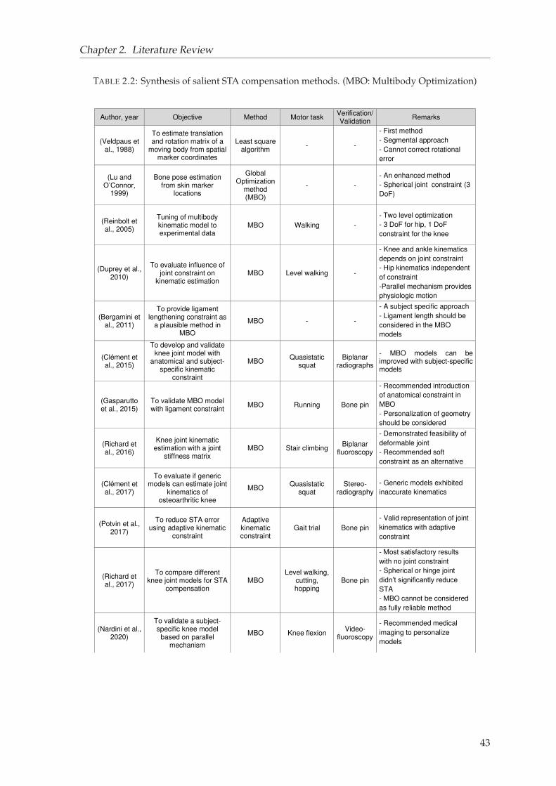
Chapter 2. Literature Review
TABLE 2.2: Synthesis of salient STA compensation methods. (MBO: Multibody Optimization)
Author, year Objective Method Motor task Verification/Validation
Remarks
(Veldpaus et al., 1988)
To estimate translation and rotation matrix of a
moving body from spatial marker coordinates
Least square algorithm
- -
- First method
- Segmental approach
- Cannot correct rotational
error
(Lu and O’Connor,
1999)
Bone pose estimation from skin marker
locations
Global Optimization
method (MBO)
- -
- An enhanced method
- Spherical joint constraint (3
DoF)
(Reinbolt et al., 2005)
Tuning of multibody kinematic model to experimental data
MBO Walking -
- Two level optimization
- 3 DoF for hip, 1 DoF
constraint for the knee
(Duprey et al., 2010)
To evaluate influence of joint constraint on
kinematic estimation MBO Level walking -
- Knee and ankle kinematics
depends on joint constraint
- Hip kinematics independent
of constraint
-Parallel mechanism provides
physiologic motion
(Bergamini et al., 2011)
To provide ligament lengthening constraint as
a plausible method in MBO
MBO - -
- A subject specific approach
- Ligament length should be
considered in the MBO
models
(Clément et al., 2015)
To develop and validate knee joint model with
anatomical and subject-specific kinematic
constraint
MBO Quasistatic
squat Biplanar
radiographs
- MBO models can be improved with subject-specific models
(Gasparutto et al., 2015)
To validate MBO model with ligament constraint
MBO Running Bone pin
- Recommended introduction
of anatomical constraint in
MBO
- Personalization of geometry
should be considered
(Richard et al., 2016)
Knee joint kinematic estimation with a joint
stiffness matrix MBO Stair climbing
Biplanar fluoroscopy
- Demonstrated feasibility of
deformable joint
- Recommended soft
constraint as an alternative
(Clément et al., 2017)
To evaluate if generic models can estimate joint
kinematics of osteoarthritic knee
MBO Quasistatic
squat Stereo-
radiography
- Generic models exhibited
inaccurate kinematics
(Potvin et al., 2017)
To reduce STA error using adaptive kinematic
constraint
Adaptive kinematic constraint
Gait trial Bone pin
- Valid representation of joint
kinematics with adaptive
constraint
(Richard et al., 2017)
To compare different knee joint models for STA
compensation MBO
Level walking, cutting, hopping
Bone pin
- Most satisfactory results
with no joint constraint
- Spherical or hinge joint
didn’t significantly reduce STA
- MBO cannot be considered
as fully reliable method
(Nardini et al., 2020)
To validate a subject-specific knee model
based on parallel mechanism
MBO Knee flexion Video-
fluoroscopy
- Recommended medical
imaging to personalize
models
43
Chapter 2. Literature Review
methods were partially successful in compensating STA by estimating bone position satis-
factorily. But couldn’t estimate the orientation of the bones properly. Consequently, multi-
body optimization (MBO) methods were used as an alternative to compensate for STA (Lu
and O’connor, 1999). This method relies on a predefined kinematic model, which entails
searching for the best possible overall pose by minimizing the distances between the mea-
sured and model estimated marker trajectories in least square sense and respecting joint
constraints. This method considers revolute (Reinbolt et al., 2005) or spherical (Charlton
et al., 2004; Lu and O’connor, 1999; Reinbolt et al., 2005) joint kinematic constraints as the
most common choices to represent hip and knee articulation. Although such approxima-
tion provides a satisfactory balance between complexity of the models and accuracy of the
synthesized motion, yet such constraints do not allow joint displacement and therefore limit
its performance in reducing STA (Stagni et al., 2005). For subjects with lesions at the joint
structure, more anatomical description at the joint level is required.
Later on, different sets of joint anatomical constraints such as parallel mechanism, cou-
pling curves, ligament length variation, elastic joint were implemented particularly in the
knee joint to facilitate joint displacement (Bergamini et al., 2011; Duprey, Cheze, and Du-
mas, 2010; Gasparutto et al., 2015; Richard et al., 2016). These studies showed that anatom-
ical constraints could offer physiological motion, such as limited abduction-adduction with
femoral rollback. However, such constraints were also shown inaccurate (kinematic error
up to 17° and 8 mm) and inadequate for clinical application as these models could not adapt
patient-specific geometry, particularly in the case of OA patients (Clément et al., 2017). In
opposed to the remarks of (Duprey, Cheze, and Dumas, 2010), who observed parallel mech-
anism as a better choice, (Richard, Cappozzo, and Dumas, 2017) obtained accurate result
with no constraint. The later study also concluded that MBO cannot be considered as a
fully reliable method. Recently, use of medical imaging is also recommended to personalize
models (Nardini et al., 2020).
Despite such significant advancement in compensating for STA, MBO methods still lack
the versatility of implementing subject-specific characteristics. In that support, an experi-
mental study on quantification of soft tissue deformation (STD) concluded that for reliable
STA compensation, knowledge of marker location-specific STD is essential (Gao and Zheng,
2008). With such information better STA compensation strategy can be devised. This in-
dicates a need for adaptable modeling approaches that can account for subject-, task-, and
marker location dependent STA.
In light of the aforementioned contexts, the use of FE models appears to be a better strat-
egy as it shows good capacity of implementing subject-specific morphology of the bones ac-
quired from CT or biplanar radiograph data (Lahkar et al., 2018). In that direction, at Institut
de Biomécanique Humaine Georges Charpak, (Skalli et al., 2018) proposed a FE based novel ap-
proach to compensate for STA. The model consists of rigid beam elements to represent bony
structures (pelvis, femur and tibia) and compliant springs to account for soft tissue defor-
mation effect. This simple yet versatile model provides ample scope to further investigate
44
Chapter 2. Literature Review
the soft tissue deformability and represent the joint with more complex and anatomically
relevant model.
Apart from the lacking of a proper approach in compensating for STA, musculoskele-
tal (MSK) models also confront other two critical challenges. Firstly, the MSK multibody
model, comprising of rigid body segments (bones) connected by ligaments and Muscle-
Tendon Units (MTU), can consider the individual characteristics of the subjects for biome-
chanical analysis and simulation (Erdemir et al., 2007; Saraswat, Andersen, and MacWilliams,
2010). Nonetheless, the contribution of muscle and ligament forces at the joint levels and
the effects of prosthesis design on human movement cannot be easily studied using MSK
models owing to the simplification (spherical, revolute joint consideration) of the joint as
elaborated previously (Shu et al., 2018). Moreover, to predict local biomechanical parame-
ters (e.g., contact stress) of the joint, a rigid body MSK model is not suitable. Secondly, a
usual practice for personalizing the MSK models are based on scaling methods (Correa and
Pandy, 2011; Valente et al., 2015). Here a generic model is scaled to fit the dimensions of the
subject using certain anatomical landmarks. This technique considers only overall anthro-
pometry of a subject, ignoring the distinctive features of the joint (e.g., ligament insertion
sites, articular geometry) (Smale et al., 2019). Therefore, the model may not accurately repli-
cate the subject’s anatomy and eventually may impact its kinematic estimations. In this as-
pect, a group in their series of studies showed considerable differences between MRI-based
models and scaled models while estimating muscle tendon length, moment arm and on gait
kinematics (Scheys et al., 2008a; Scheys et al., 2008b; Scheys et al., 2011).
In this context, probably the better strategy would be to use concurrent FE-MSK (finite
element based musculoskeletal) models to overcome the obstacles (computational burden
of FE models and oversimplification of MSK models) of each modeling domain, while im-
proving the quality of the analysis.
Synthesis 2
- STA compensation is paramount for accurate estimation of skin marker-based mo-
tion data.
- Simplified joint constraints are currently incapable of representing detailed knee
joint structure, particularly in joints with lesion.
- Medical image-based model personalization is essential to replicate subject-specific
morphology.
- A versatile approach for STA compensation could be valuable which can take
subject-, task-, and marker location-specific STA into account.
2.3 FE-MSK model
FE-MSK modeling approaches have been recently become popular to study local mechanics
of the joint under in vivo loading conditions (refer to table 2.3). One study reported influence
45
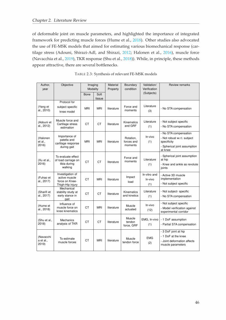
Chapter 2. Literature Review
of deformable joint on muscle parameters, and highlighted the importance of integrated
framework for predicting muscle forces (Hume et al., 2018). Other studies also advocated
the use of FE-MSK models that aimed for estimating various biomechanical response (car-
tilage stress (Adouni, Shirazi-Adl, and Shirazi, 2012; Halonen et al., 2016), muscle force
(Navacchia et al., 2019), TKR response (Shu et al., 2018)). While, in principle, these methods
appear attractive, there are several bottlenecks.
TABLE 2.3: Synthesis of relevant FE-MSK models
Author,
year
Objective Imaging
Modality
Material
Property
Boundary
condition
Validation/
Verification
(Subjects)
Review remarks
Bone Soft
tissue
(Yang et
al., 2010)
Protocol for
subject specific
knee modelMRI MRI literature
Force and
moments
Literature
(3)- No STA compensation
(Adouni et
al., 2012)
Muscle force and
Cartilage stress
estimation
CT CT literatureKinematics
and GRF
Literature
(1)
- Not subject specific
- No STA compensation
(Halonen
et al.,
2016)
Importance of
patella and
cartilage response
during gait
MRI MRI literature
Rotation,
forces and
moments
In-vivo
(1)
- No STA compensation
- Not robust w.r.t. subject
specificity
- Spherical joint assumption
at knee
(Xu et al.,
2016)
To evaluate effect
of load carriage on
tibia during
walking
CT CT literature
Force and
momentsLiterature
(1)
- Spherical joint assumption
at hip
- Knee and ankle as revolute
joints
(Fuhao et
al., 2017)
Investigation of
active muscle
force on Knee-
Thigh-Hip injury
CT MRI literatureImpact
load
In-vitro and
In-vivo
(1)
- Active 3D muscle
implementation
- Not subject specific
(Sharifi et
al., 2017)
Mechanical
stability study at
early stance in
gait
CT CT literatureKinematics
and kinetics
Literature
(1)
- Not subject- specific
- No STA compensation
(Hume et
al., 2018)
Influence of
muscle force on
knee kinematics
CT MRI literatureMuscle
actuated
In-vivo
(12)
- Not subject specific
- Model verification against
experimental corridor
(Shu et al.,
2018)
Mechanics
analysis of TKRCT CT literature
Muscle
tendon
force, GRF
EMG, In-vivo
(1)
- 1 DoF assumption
- Partial STA compensation
(Navacchi
a et al.,
2019)
To estimate
muscle forces CT MRI literature
Muscle
tendon force
EMG
(2)
- 3 DoF joint at hip
- 1 DoF at the knee
- Joint deformation affects
muscle parameters
46
Chapter 2. Literature Review
First, fast and accurate model FE development approaches in terms of subject-specific
morphology and material properties, simplified modeling strategies to foster clinical trans-
lation and model validation/verification approaches.
Second, alike rigid body MSK models, most of the FE-MSK models either neglected
STA (Yang et al., 2010; Adouni, Shirazi-Adl, and Shirazi, 2012; Halonen et al., 2016; Shar-
ifi, Shirazi-Adl, and Marouane, 2017) or partially compensated it by simplifying the joint.
For instance, (Shu et al., 2018) assumed the knee joint as 1 DoF to estimate joint kinematics,
and then estimated kinematic data were used to compute muscle parameters (muscle mo-
ment, muscle length, muscle velocity). Undoubtedly, such consideration will manifest error
propagation in the subsequent steps. A similar methodology was followed in (Xu et al.,
2016) study. Hence, solving the STA problem seems to be a common challenge for both the
model types, rigid body MSK and FE-MSK models.
Based on the systematic review on various computational modeling strategies, it can be
summarized that although a large body of work has been performed in the literature, it
highlights enormous complexities in developing a FE-MSK framework for the lower limb,
in particular the knee joint. Therefore, it appears that there is still a need for a comprehensive
framework of subject-specific FE-MSK modeling by taking the above mentioned challenges
into account.
2.4 Objectives
The overall aim of the PhD thesis was thus set as a ’Contribution to personalized FE-based
musculoskeletal modeling of the lower limb’ with the purpose of bridging the gap be-
tween current state-of-the-art approaches for musculoskeletal modeling and their applica-
bility towards clinics.
Based on the overall aim, manifold sub-objectives were defined as
- To develop and evaluate personalized FE model of the knee joint by taking subject-
specific geometry and ligament material properties into account. This objective will
be addressed in Chapter 3.
- To compensate for Soft Tissue Artifact in motion analysis by adopting a novel ap-
proach. This will be tackled in Chapter 4.
- Finally, a clinical application was briefly explored in the context of utility of the low
dose biplanar X-ray system in evaluating Total Knee Arthroplasty (TKA) implant
alignment. This will be addressed in Chapter 5.
47

Chapter 3
Subject-specific finite element model
development and evaluation of the
knee joint
This chapter illustrates an approach for subject-specific finite element (FE) modeling and
evaluation of the knee joint to estimate joint kinematics. The first section includes a method-
ology for fast and quasi-automatic subject-specific FE mesh generation of the knee joint from
biplanar X-ray images, which has been published in a conference proceedings (CMBBE,
2018) (Lahkar et al., 2018). The second section includes evaluation of the subject-specific
FE models under passive response. Here, a novel approach for calibrating ligament ma-
terial properties has been proposed and evaluated. This work has been submitted to the
peer-reviewed journal Computer Methods in Biomechanics and Biomedical Engineering entitled
"Development and evaluation of a new procedure for subject-specific tensioning of FE knee
ligaments."
49
Chapter 3. Subject-specific finite element model development and evaluation of the knee
joint
3.1 Fast subject-specific FE mesh generation of the knee joint from
biplanar X-ray images
Abstract An accurate and fast computational mesh generation is a prerequisite toperform personalized FE analyses. Traditionally, both triangular/tetrahedral and quadri-lateral/hexahedral FE elements are used for 3D mesh generation. But because of distinctnumerical advantages, hexahedral elements are preferred to avoid numerical instability.Here, we propose a methodology to develop fast and automatic subject-specific mesh for kneejoint from biplanar X-ray images. This methodology first involves building 3D reconstructionfrom biplanar radiographic image and then generating generic linear hexahedral mesh forthe femur, tibia and patella. The generic mesh (GM) for individual bony structure is thendeformed to obtain subject specific mesh (SSM) based on kriging interpolation. Meshing ofboth the meniscus follows a different approach where the surface nodes of the femur andtibia are used to generate linear hexahedral elements mesh. This complete methodology wassuccessfully tested on 11 cadaveric specimens with approximately 12 min computational timefor each out of which 3D reconstruction time was nearly 10 min. Numerical cost involved indeforming mesh for each specimen was 30 sec and generating mesh for both the meniscuswas nearly 1 min. Mesh quality was assessed using standard ANSYS mesh quality indicators(aspect ratio, parallel deviation, maximum angle, Jacobian ratio and warping factor). Foreach specimen the value of total warnings above threshold showed in the range of 0.38-0.59%with no error. Surface mesh accuracy was evaluated as the point-to-surface distance between3D reconstruction and subject-specific mesh and the mean RMS values were reported. Forall specimens, mean (RMS) errors in mm were respectively less than or equal to 0.2 (0.3), 0.3(0.55) and 0.0 (0.1) for femur, tibia and patella which are less than the uncertainties of 3Dreconstruction.
Keywords: FEM, 3D reconstruction, subject specific mesh, knee joint, biplanar X-ray
3.1.1 Introduction
Numerous FE models of the knee joint have been developed to investigate knee injury mech-
anism (Kiapour et al., 2014), surgery assessment (Kang et al., 2018; Xie et al., 2017) and
contact kinematics at knee joint (Haut Donahue et al., 2002; Koo, Rylander, and Andriac-
chi, 2011; Ali et al., 2016). However, because of extensive computational effort required
for preparing subject specific model from CT-scan or MRI data, most of the models in lit-
erature are done only for one or very few subjects. This results in poor validation of the
model while dealing with patient specific estimation of tissue response as well as studying
effect of morphological inter-subject variability. As an alternative to CT scan and MRI data,
use of biplanar X-ray image is promising to perform 3D reconstructions of bony structures
(Chaibi et al., 2012) because of low radiation dose, very little reconstruction time and ability
to replicate complex bony structure with ease.
The quality of FE mesh plays vital role in obtaining reliable and accurate results. Tra-
ditionally, tetrahedral meshes are easy to generate but it reduces order of convergence for
50
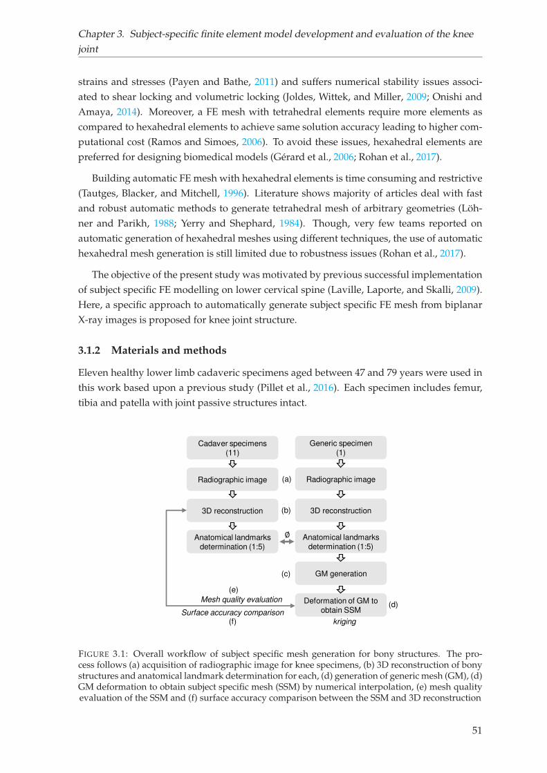
Chapter 3. Subject-specific finite element model development and evaluation of the knee
joint
strains and stresses (Payen and Bathe, 2011) and suffers numerical stability issues associ-
ated to shear locking and volumetric locking (Joldes, Wittek, and Miller, 2009; Onishi and
Amaya, 2014). Moreover, a FE mesh with tetrahedral elements require more elements as
compared to hexahedral elements to achieve same solution accuracy leading to higher com-
putational cost (Ramos and Simoes, 2006). To avoid these issues, hexahedral elements are
preferred for designing biomedical models (Gérard et al., 2006; Rohan et al., 2017).
Building automatic FE mesh with hexahedral elements is time consuming and restrictive
(Tautges, Blacker, and Mitchell, 1996). Literature shows majority of articles deal with fast
and robust automatic methods to generate tetrahedral mesh of arbitrary geometries (Löh-
ner and Parikh, 1988; Yerry and Shephard, 1984). Though, very few teams reported on
automatic generation of hexahedral meshes using different techniques, the use of automatic
hexahedral mesh generation is still limited due to robustness issues (Rohan et al., 2017).
The objective of the present study was motivated by previous successful implementation
of subject specific FE modelling on lower cervical spine (Laville, Laporte, and Skalli, 2009).
Here, a specific approach to automatically generate subject specific FE mesh from biplanar
X-ray images is proposed for knee joint structure.
3.1.2 Materials and methods
Eleven healthy lower limb cadaveric specimens aged between 47 and 79 years were used in
this work based upon a previous study (Pillet et al., 2016). Each specimen includes femur,
tibia and patella with joint passive structures intact.
Anatomical landmarks determination (1:5)
Deformation of GM to obtain SSM
Cadaver specimens (11)
Generic specimen (1)
Radiographic image Radiographic image
3D reconstruction 3D reconstruction
Anatomical landmarks determination (1:5)
GM generation
kriging
Mesh quality evaluation
Surface accuracy comparison
∅(a)
(b)
(c)
(d)
(e)
(f)
FIGURE 3.1: Overall workflow of subject specific mesh generation for bony structures. The pro-cess follows (a) acquisition of radiographic image for knee specimens, (b) 3D reconstruction of bonystructures and anatomical landmark determination for each, (d) generation of generic mesh (GM), (d)GM deformation to obtain subject specific mesh (SSM) by numerical interpolation, (e) mesh qualityevaluation of the SSM and (f) surface accuracy comparison between the SSM and 3D reconstruction
51
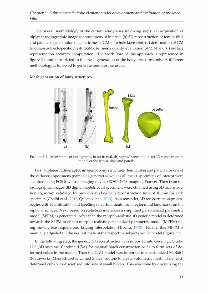
Chapter 3. Subject-specific finite element model development and evaluation of the knee
joint
The overall methodology of the current study uses following steps: (a) acquisition of
biplanar radiographic image for specimens of interest, (b) 3D reconstruction of femur, tibia
and patella, (c) generation of generic mesh (GM) of whole knee joint, (d) deformation of GM
to obtain subject-specific mesh (SSM), (e) mesh quality evaluation of SSM and (f) surface
representation accuracy computation. The work flow of this approach is represented in
figure 3.1 and is restricted to the mesh generation of the bony structures only. A different
methodology is followed to generate mesh for meniscus.
Mesh generation of bony structures
(a) (b) (c)
femur
tibia
patella
FIGURE 3.2: An example of radiographs in (a) frontal, (b) sagittal view and its (c) 3D reconstructionmodel of the femur, tibia and patella
First, biplanar radiographic images of bony structures (femur, tibia and patella) for one of
the cadaveric specimens (named as generic) as well as all the 11 specimens of interest were
acquired using EOS low dose imaging device (EOS ®, EOS-imaging, France). Then from the
radiographic images, 3D digital models of all specimens were obtained using 3D reconstruc-
tion algorithm validated by previous studies with reconstruction time of 10 min for each
specimen (Chaibi et al., 2012; Quijano et al., 2013). As a reminder, 3D reconstruction process
begins with identification and labelling of various anatomical regions and landmarks on the
biplanar images. Next, based on statistical inferences a simplified personalized parametric
model (SPPM) is generated. After that, the morpho-realistic 3D generic model is deformed
towards the SPPM to obtain morpho-realistic personalized parametric model (MPPM) us-
ing moving least square and kriging interpolation (Trochu, 1993). Finally, this MPPM is
manually adjusted till the best estimate of the respective subject specific model (figure 3.2).
In the following step, the generic 3D reconstruction was imported into Geomagic Studio
12.0 (3D systems, Carolina, USA) for manual patch construction so as to form sets of de-
formed cubes in the model. Then the CAD model was imported to a customized Matlab ®
(Mathworks, Massachusetts, United States) routine to create volumetric mesh. Here, each
deformed cube was discretized into sets of small blocks. This was done by discretizing the
52
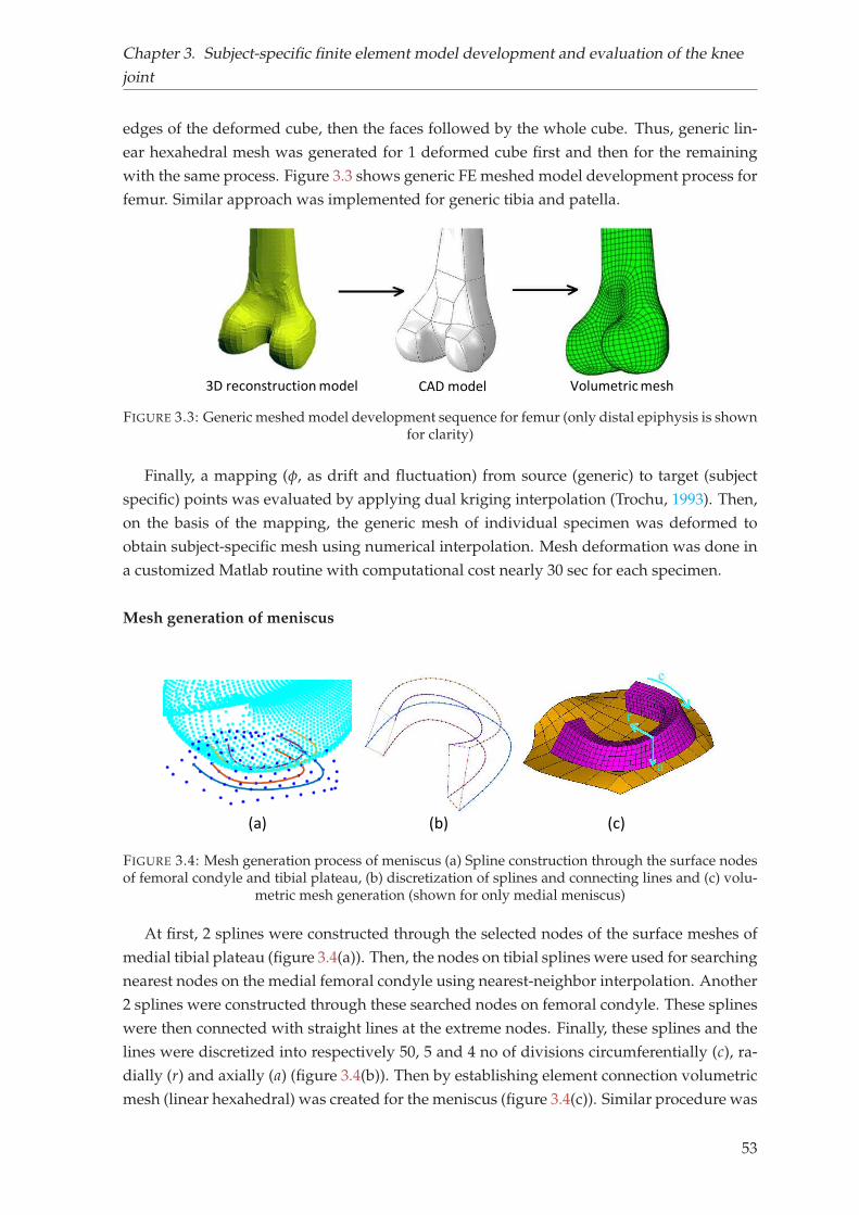
Chapter 3. Subject-specific finite element model development and evaluation of the knee
joint
edges of the deformed cube, then the faces followed by the whole cube. Thus, generic lin-
ear hexahedral mesh was generated for 1 deformed cube first and then for the remaining
with the same process. Figure 3.3 shows generic FE meshed model development process for
femur. Similar approach was implemented for generic tibia and patella.
3D reconstruction model CAD model Volumetric mesh
FIGURE 3.3: Generic meshed model development sequence for femur (only distal epiphysis is shownfor clarity)
Finally, a mapping (φ, as drift and fluctuation) from source (generic) to target (subject
specific) points was evaluated by applying dual kriging interpolation (Trochu, 1993). Then,
on the basis of the mapping, the generic mesh of individual specimen was deformed to
obtain subject-specific mesh using numerical interpolation. Mesh deformation was done in
a customized Matlab routine with computational cost nearly 30 sec for each specimen.
Mesh generation of meniscus
(a) (b) (c)
FIGURE 3.4: Mesh generation process of meniscus (a) Spline construction through the surface nodesof femoral condyle and tibial plateau, (b) discretization of splines and connecting lines and (c) volu-
metric mesh generation (shown for only medial meniscus)
At first, 2 splines were constructed through the selected nodes of the surface meshes of
medial tibial plateau (figure 3.4(a)). Then, the nodes on tibial splines were used for searching
nearest nodes on the medial femoral condyle using nearest-neighbor interpolation. Another
2 splines were constructed through these searched nodes on femoral condyle. These splines
were then connected with straight lines at the extreme nodes. Finally, these splines and the
lines were discretized into respectively 50, 5 and 4 no of divisions circumferentially (c), ra-
dially (r) and axially (a) (figure 3.4(b)). Then by establishing element connection volumetric
mesh (linear hexahedral) was created for the meniscus (figure 3.4(c)). Similar procedure was
53
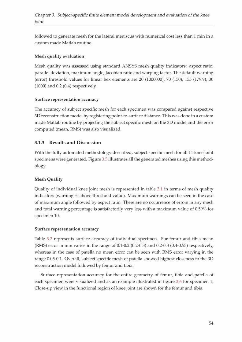
Chapter 3. Subject-specific finite element model development and evaluation of the knee
joint
followed to generate mesh for the lateral meniscus with numerical cost less than 1 min in a
custom made Matlab routine.
Mesh quality evaluation
Mesh quality was assessed using standard ANSYS mesh quality indicators: aspect ratio,
parallel deviation, maximum angle, Jacobian ratio and warping factor. The default warning
(error) threshold values for linear hex elements are 20 (1000000), 70 (150), 155 (179.9), 30
(1000) and 0.2 (0.4) respectively.
Surface representation accuracy
The accuracy of subject specific mesh for each specimen was compared against respective
3D reconstruction model by registering point-to-surface distance. This was done in a custom
made Matlab routine by projecting the subject specific mesh on the 3D model and the error
computed (mean, RMS) was also visualized.
3.1.3 Results and Discussion
With the fully automated methodology described, subject specific mesh for all 11 knee joint
specimens were generated. Figure 3.5 illustrates all the generated meshes using this method-
ology.
Mesh Quality
Quality of individual knee joint mesh is represented in table 3.1 in terms of mesh quality
indicators (warning % above threshold value). Maximum warnings can be seen in the case
of maximum angle followed by aspect ratio. There are no occurrence of errors in any mesh
and total warning percentage is satisfactorily very less with a maximum value of 0.59% for
specimen 10.
Surface representation accuracy
Table 3.2 represents surface accuracy of individual specimen. For femur and tibia mean
(RMS) error in mm varies in the range of 0.1-0.2 (0.2-0.3) and 0.2-0.3 (0.4-0.55) respectively,
whereas in the case of patella no mean error can be seen with RMS error varying in the
range 0.05-0.1. Overall, subject specific mesh of patella showed highest closeness to the 3D
reconstruction model followed by femur and tibia.
Surface representation accuracy for the entire geometry of femur, tibia and patella of
each specimen were visualized and as an example illustrated in figure 3.6 for specimen 1.
Close-up view in the functional region of knee joint are shown for the femur and tibia.
54
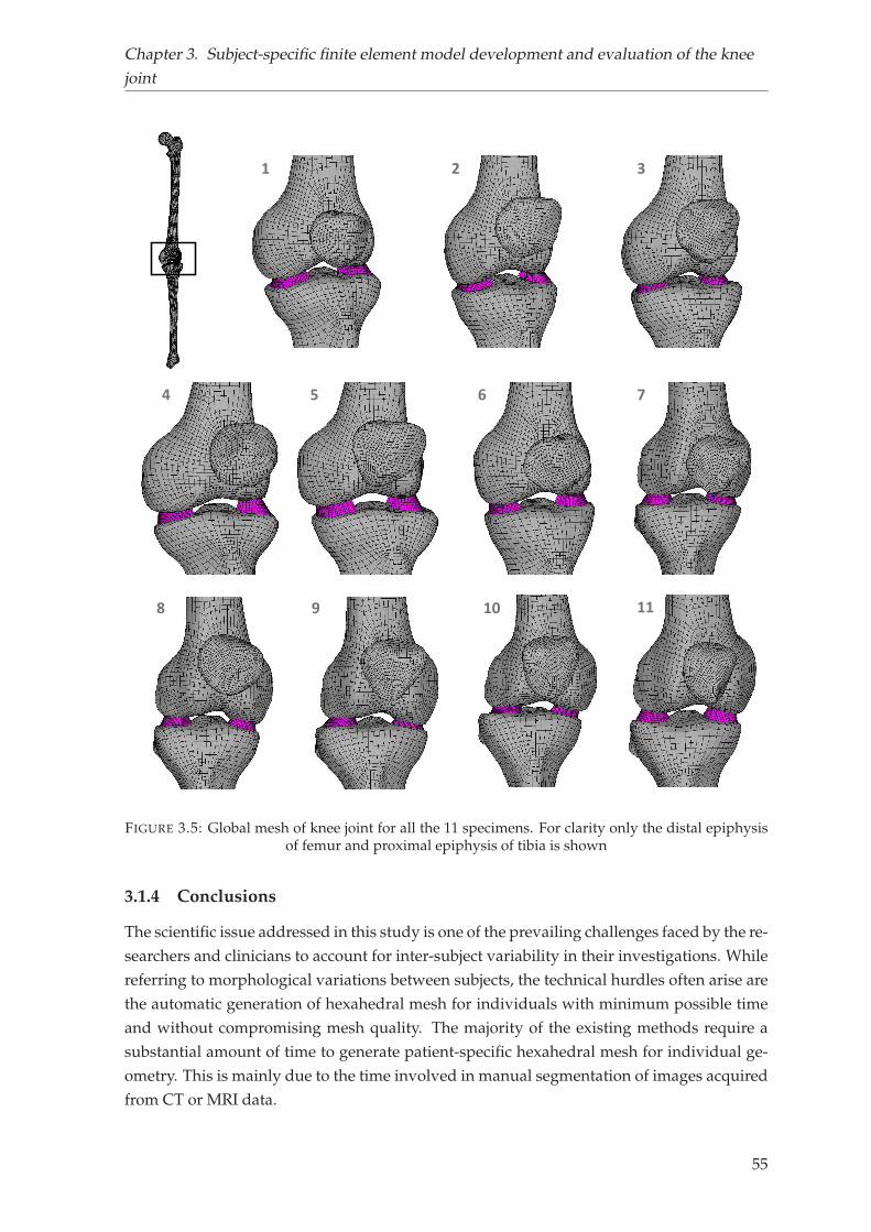
Chapter 3. Subject-specific finite element model development and evaluation of the knee
joint
1 2 3
4 5 6 7
8 9 10 11
FIGURE 3.5: Global mesh of knee joint for all the 11 specimens. For clarity only the distal epiphysisof femur and proximal epiphysis of tibia is shown
3.1.4 Conclusions
The scientific issue addressed in this study is one of the prevailing challenges faced by the re-
searchers and clinicians to account for inter-subject variability in their investigations. While
referring to morphological variations between subjects, the technical hurdles often arise are
the automatic generation of hexahedral mesh for individuals with minimum possible time
and without compromising mesh quality. The majority of the existing methods require a
substantial amount of time to generate patient-specific hexahedral mesh for individual ge-
ometry. This is mainly due to the time involved in manual segmentation of images acquired
from CT or MRI data.
55
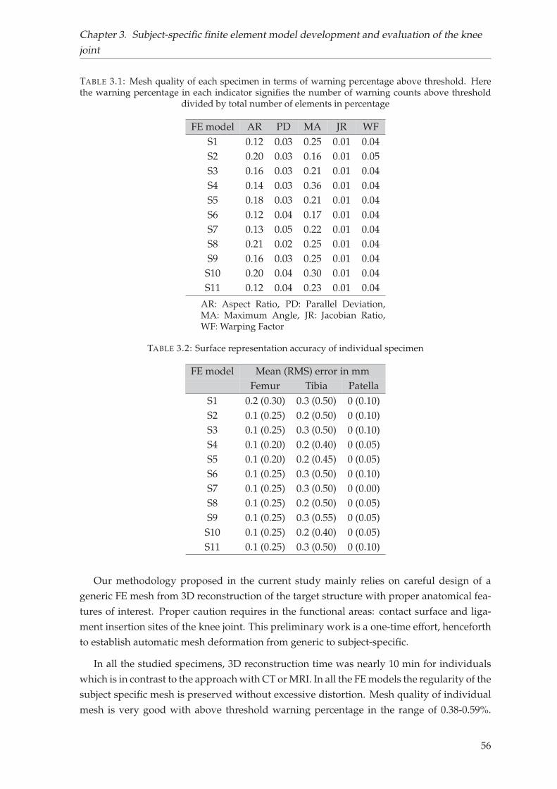
Chapter 3. Subject-specific finite element model development and evaluation of the knee
joint
TABLE 3.1: Mesh quality of each specimen in terms of warning percentage above threshold. Herethe warning percentage in each indicator signifies the number of warning counts above threshold
divided by total number of elements in percentage
FE model AR PD MA JR WFS1 0.12 0.03 0.25 0.01 0.04S2 0.20 0.03 0.16 0.01 0.05S3 0.16 0.03 0.21 0.01 0.04S4 0.14 0.03 0.36 0.01 0.04S5 0.18 0.03 0.21 0.01 0.04S6 0.12 0.04 0.17 0.01 0.04S7 0.13 0.05 0.22 0.01 0.04S8 0.21 0.02 0.25 0.01 0.04S9 0.16 0.03 0.25 0.01 0.04S10 0.20 0.04 0.30 0.01 0.04S11 0.12 0.04 0.23 0.01 0.04
AR: Aspect Ratio, PD: Parallel Deviation,MA: Maximum Angle, JR: Jacobian Ratio,WF: Warping Factor
TABLE 3.2: Surface representation accuracy of individual specimen
FE model Mean (RMS) error in mmFemur Tibia Patella
S1 0.2 (0.30) 0.3 (0.50) 0 (0.10)S2 0.1 (0.25) 0.2 (0.50) 0 (0.10)S3 0.1 (0.25) 0.3 (0.50) 0 (0.10)S4 0.1 (0.20) 0.2 (0.40) 0 (0.05)S5 0.1 (0.20) 0.2 (0.45) 0 (0.05)S6 0.1 (0.25) 0.3 (0.50) 0 (0.10)S7 0.1 (0.25) 0.3 (0.50) 0 (0.00)S8 0.1 (0.25) 0.2 (0.50) 0 (0.05)S9 0.1 (0.25) 0.3 (0.55) 0 (0.05)S10 0.1 (0.25) 0.2 (0.40) 0 (0.05)S11 0.1 (0.25) 0.3 (0.50) 0 (0.10)
Our methodology proposed in the current study mainly relies on careful design of a
generic FE mesh from 3D reconstruction of the target structure with proper anatomical fea-
tures of interest. Proper caution requires in the functional areas: contact surface and liga-
ment insertion sites of the knee joint. This preliminary work is a one-time effort, henceforth
to establish automatic mesh deformation from generic to subject-specific.
In all the studied specimens, 3D reconstruction time was nearly 10 min for individuals
which is in contrast to the approach with CT or MRI. In all the FE models the regularity of the
subject specific mesh is preserved without excessive distortion. Mesh quality of individual
mesh is very good with above threshold warning percentage in the range of 0.38-0.59%.
56
Chapter 3. Subject-specific finite element model development and evaluation of the knee
joint
FIGURE 3.6: Surface representation accuracy as point-to-surface distance for (a) femur, (b) tibia and(c) patella
Again, the algorithm employed in the current methodology was able to closely replicate the
bony structures of individuals maintaining satisfactory surface representation accuracy. To
our best knowledge, no such methodology is developed till now especially for knee joint
which can allow generation of nearly accurate mesh from 3D reconstruction for any number
of specimens.
Overall, this section of the chapter 1 contributed to fast, accurate and semi-automatic
hexahedral FE mesh generation of the knee joint. Because of fastness and subject specificity
in terms of geometry, this methodology has the potential to be implemented in clinical rou-
tine to investigate personalized characteristics of the knee joint. However, in that aim model
validation is important, which will be addressed in the following section.
57
Chapter 3. Subject-specific finite element model development and evaluation of the knee
joint
3.2 Development and evaluation of a new procedure for subject-
specific tensioning of finite element knee ligaments1
Abstract Subject-specific tensioning of ligaments is essential for the stability of the kneejoint and represents a challenging aspect in the development of finite element models. Weaimed to introduce and evaluate a new procedure for the quantification of ligament pre-strains from biplanar X-ray and CT data. Subject-specific model evaluation was performedby comparing predicted femorotibial kinematics with the in vitro response of six cadavericspecimens. The differences obtained using personalized models were comparable to thosereported in similar studies in the literature. This study is the first step towards the use ofsimplified, personalized knee FE models in clinical context such as ligament balancing.
Keywords: Finite Element Analysis, Ligament Prestrain, Subject-Specific Knee Model,Joint Kinematics, Model Evaluation
3.2.1 Introduction
The knee joint is highly susceptible to frequent injury of ligaments. If it remains untreated,
has the probability of limiting joint stability, and can further lead to progression of joint
arthritis (Fleming et al., 2005). In such scenario, early stage clinical intervention e.g., liga-
ment repair or replacement is often recommended. For such therapeutic interventions and
to properly plan surgical procedures, accurate knowledge of the biomechanical behavior of
knee ligaments is fundamental.
Several experiments dealing with main knee ligaments (anterior cruciate ligament (ACL),
posterior cruciate ligament (PCL), lateral collateral ligament (LCL) and medial collateral
ligament (MCL)) have been carried out in the literature (Aunan et al., 2012; Belvedere et al.,
2012; Gardiner, Weiss, and Rosenberg, 2001; Pedersen et al., 2019; Rochcongar et al., 2016).
Although these studies have substantially increased knowledge on joint functions, yet the
complexity of measurements, lesser availability of cadavers, ethical and cost implications
have made data acquisition challenging.
Alternatively, FE models are commonly used as a reliable complementary means to ex-
perimental studies providing significant insight into knee joint biomechanics. A variety of
modeling techniques have been utilized to model the joint structure, particularly ligaments.
Some of the strategies are steered by simplicity, while others concentrate on faithful cap-
ture of specimen-specific anatomy with varying levels of joint representation fidelity. For
example, some models included 3D geometries of ligaments with complex material behav-
ior (Kiapour et al., 2014; Limbert, Taylor, and Middleton, 2004; Orsi et al., 2016; Pena et al.,
2006). Such approach allows to consider ligament wrapping behavior and analysis of local
biomechanical response (e.g., 3D stresses and strains across tissue). Nevertheless, higher
anatomically complex models require detailed image-based information of the soft tissue
1Potential copyright issues with direct reuse of the article including figures and contents
58
Chapter 3. Subject-specific finite element model development and evaluation of the knee
joint
structures under consideration. Generation and simulation of such models often require
manifold higher time than that for simpler models (Bolcos et al., 2018). Therefore, simpler
models may be beneficial for studies where higher number of subjects need to be analyzed
and, at the same time, capable of predicting joint mechanics.
In an attempt for model simplification, other authors have proposed to represent liga-
ments as bundles of springs or tension only cables (Adouni and Shirazi-Adl, 2009; Baldwin
et al., 2012; Moglo and Shirazi-Adl, 2005). Although ligaments are exposed to both compres-
sive and tensile states of stress, yet the contribution of tensile stress is substantially higher
than others (Pena et al., 2006; Orsi et al., 2016). Therefore, such simplification is consid-
ered reasonable and recommended particularly for predicting joint kinematics (Beidokhti
et al., 2017). Nevertheless, personalization of ligament properties (stiffness and prestrain),
although clinically essential to restore joint stability, represents a challenge for the commu-
nity. For example, there is a consensus that graft under-tensioning could lead to joint laxity,
which is biomechanically analogous to a ligament deficient knee (Sherman et al., 2012). In
addition to that, owing to variable morphology, different bundles of a ligament (e.g., two
main fiber bundles of ACL) may exhibit variable prestrain by becoming active at different
flexion angles (Girgis, Marshall, and JEM, 1975). From a modeling perspective, it has also
been reported that incorrectly applied ligament prestrain can have a considerable effect on
the kinematics of the knee (Mesfar and Shirazi-Adl, 2006; Rachmat et al., 2016). To tackle
this issue, some authors made subject-specific adjustment using inverse methods to cali-
brate specific ligament constitutive behavior. Models either used laxity tests (Baldwin et al.,
2012; Beidokhti et al., 2017) or distraction loading (Zaylor, Stulberg, and Halloran, 2019) to
estimate ligament properties by minimizing differences between model-predicted and ex-
perimental kinetics. Such calibrations are, however, likely to be computationally expensive.
In light of the above considerations, we proposed an original framework for calibrat-
ing subject-specific tensioning of FE knee ligaments based on experimentally acquired data.
Subject-specific model evaluation was performed by comparing predicted femorotibial kine-
matics under passive flexion with the experimental data of six cadaveric specimens. We
hypothesized that the employed methodology of building personalized FE models with
experiment-based prestrains could predict overall passive kinematics of the knee joint.
3.2.2 Materials and methods
The overall workflow of generating specimen-specific FE mesh is presented in figure 3.7
Experimental data acquisition
We obtained the experimental knee kinematic responses in a previous study (Rochcongar
et al., 2016). The experimental procedure is recalled briefly hereafter. Six fresh-frozen lower
limb specimens harvested from subjects with age range 47 to 79 years, were tested under
passive flexion-extension on a previously validated kinematic test-bench (Azmy et al., 2010;
Hsich and Draganich, 1997). Skin and muscles were removed except eight centimeters of
59
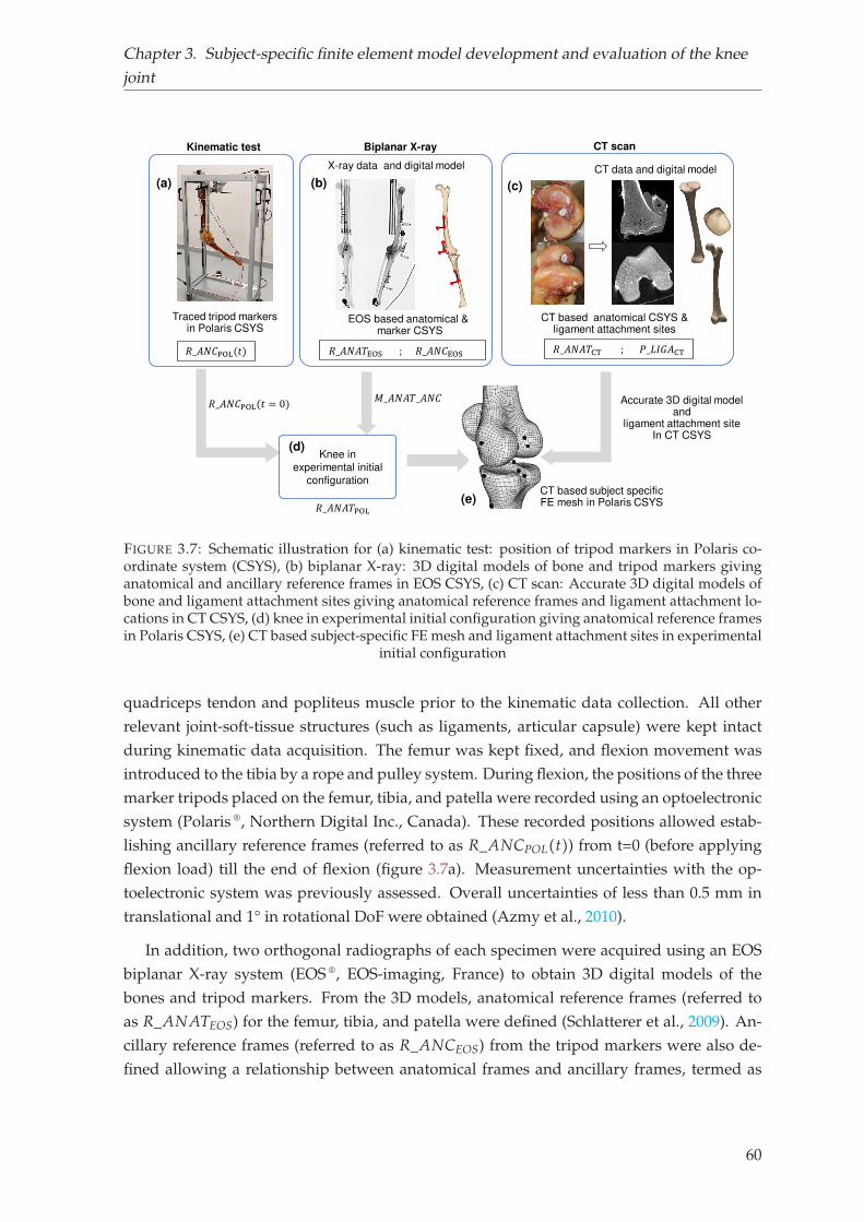
Chapter 3. Subject-specific finite element model development and evaluation of the knee
joint
EOS based anatomical &marker CSYS
(a)
𝑅_𝐴𝑁𝐶POL(𝑡)
Kinematic test
Traced tripod markersin Polaris CSYS
(b)
Biplanar X-ray
X-ray data and digital model
𝑅_𝐴𝑁𝐶POL(𝑡 = 0)
CT scan
(c)
CT based anatomical CSYS &ligament attachment sites
CT data and digital model
CT based subject specific FE mesh in Polaris CSYS
Accurate 3D digital modeland
ligament attachment siteIn CT CSYS
Knee in
experimental initial
configuration
(d)
(e)𝑅_𝐴𝑁𝐴𝑇POL
𝑀_𝐴𝑁𝐴𝑇_𝐴𝑁𝐶𝑅_𝐴𝑁𝐴𝑇EOS ; 𝑅_𝐴𝑁𝐶EOS 𝑅_𝐴𝑁𝐴𝑇CT ; 𝑃_𝐿𝐼𝐺𝐴CT
FIGURE 3.7: Schematic illustration for (a) kinematic test: position of tripod markers in Polaris co-ordinate system (CSYS), (b) biplanar X-ray: 3D digital models of bone and tripod markers givinganatomical and ancillary reference frames in EOS CSYS, (c) CT scan: Accurate 3D digital models ofbone and ligament attachment sites giving anatomical reference frames and ligament attachment lo-cations in CT CSYS, (d) knee in experimental initial configuration giving anatomical reference framesin Polaris CSYS, (e) CT based subject-specific FE mesh and ligament attachment sites in experimental
initial configuration
quadriceps tendon and popliteus muscle prior to the kinematic data collection. All other
relevant joint-soft-tissue structures (such as ligaments, articular capsule) were kept intact
during kinematic data acquisition. The femur was kept fixed, and flexion movement was
introduced to the tibia by a rope and pulley system. During flexion, the positions of the three
marker tripods placed on the femur, tibia, and patella were recorded using an optoelectronic
system (Polaris ®, Northern Digital Inc., Canada). These recorded positions allowed estab-
lishing ancillary reference frames (referred to as R_ANCPOL(t)) from t=0 (before applying
flexion load) till the end of flexion (figure 3.7a). Measurement uncertainties with the op-
toelectronic system was previously assessed. Overall uncertainties of less than 0.5 mm in
translational and 1° in rotational DoF were obtained (Azmy et al., 2010).
In addition, two orthogonal radiographs of each specimen were acquired using an EOS
biplanar X-ray system (EOS ®, EOS-imaging, France) to obtain 3D digital models of the
bones and tripod markers. From the 3D models, anatomical reference frames (referred to
as R_ANATEOS) for the femur, tibia, and patella were defined (Schlatterer et al., 2009). An-
cillary reference frames (referred to as R_ANCEOS) from the tripod markers were also de-
fined allowing a relationship between anatomical frames and ancillary frames, termed as
60
Chapter 3. Subject-specific finite element model development and evaluation of the knee
joint
M_ANAT_ANC (figure 3.7b). This relation was further used for converting acquired kine-
matic data, R_ANCPOL(t) to relative patellofemoral and tibiofemoral motions in the femur
anatomical reference frame with Cardan sequence ZY’X”.
After the kinematic data acquisition, each specimen was fully dissected to identify the
ligament attachment sites. Absence of trauma and integrity of soft tissue structures was
checked during the dissection. An experienced surgeon identified the origin and inser-
tion locations for the following ligaments: anteromedial (AM) and posterolateral (PL) bun-
dles of ACL, posteromedial (PM) and anterolateral (AL) bundles of PCL, superficial (MCLs)
and deep (MCLd) bundles of MCL, and LCL. Identified locations were marked with radio-
opaque paints, and the bones were scanned using a computed tomography (CT) scanner
(Philips, Best, The Netherlands). 3D digital models of each dissected specimen were ac-
quired using MITK-GEM ® (version 5.0) giving anatomical frames (R_ANATCT) and liga-
ment attachment sites (P_LIGACT) in the CT scanner system of reference (figure 3.7c). 3D
Digital models and digital footprints of ligament attachment sites were then registered into
experimental initial configuration. Registration was performed with biplanar X-ray data.
Once the centroidal coordinates of the attachment sites were known, the end-to-end distance
of the ligaments origin and insertion site was computed at experimental initial configura-
tion. For the sake of readability, end-to-end distance will be referred to as ligament length
hereafter.
Initial bone pose estimation
Relative pose (position and orientation) of tibia and patella with respect to the femur at
initial unloaded configuration was obtained using the relation M_ANAT_ANC and exper-
imental kinematic data, R_ANC_POL(t) at time=0 (figure 3.7d)).
Specimen specific FE model
(i) FE mesh First, subject-specific FE hexahedral mesh for each bony segment was created
based on the subject-specific CT based digital models (figure 3.7e) (Lahkar et al., 2018). Then,
only the surface mesh (4-noded shell element) was kept to represent bones and cartilage to
reduce computational cost (Germain et al., 2016). Then, mesh smoothing was performed at
the articular surfaces to improve the mesh quality (Taubin, 1995).
Mesh quality was assessed using standard ANSYS ® mesh quality indicators: aspect ra-
tio, parallel deviation, maximum angle, Jacobian ratio, and warping factor. The surface
accuracy of specimen specific mesh for each specimen was compared against respective 3D
digital model (i.e. segmented 3D geometry from CT data) by registering Hausdorff distance
expressed in mean (2RMS) values.
(ii) Knee joint FE model Bones were assumed to be isotropic linear elastic with Young’s
modulus of 12000 MPa (Choi et al., 1990). As the loading pattern in the study is quasi-static,
61
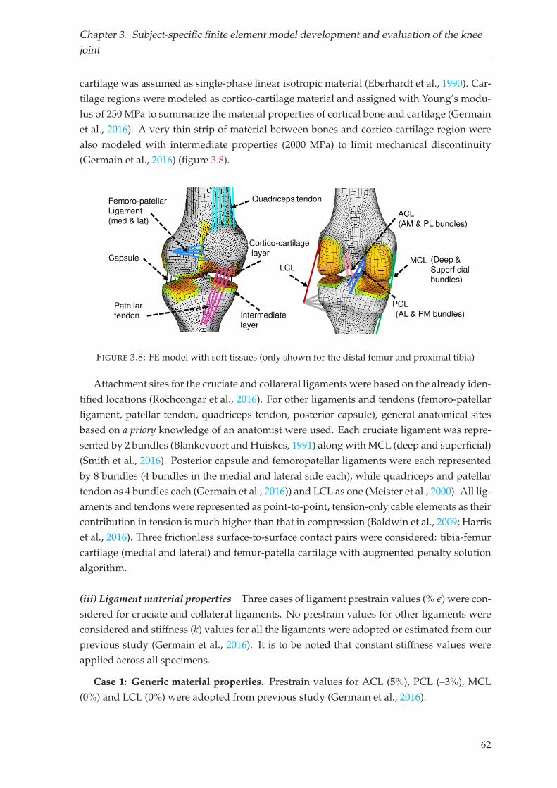
Chapter 3. Subject-specific finite element model development and evaluation of the knee
joint
cartilage was assumed as single-phase linear isotropic material (Eberhardt et al., 1990). Car-
tilage regions were modeled as cortico-cartilage material and assigned with Young’s modu-
lus of 250 MPa to summarize the material properties of cortical bone and cartilage (Germain
et al., 2016). A very thin strip of material between bones and cortico-cartilage region were
also modeled with intermediate properties (2000 MPa) to limit mechanical discontinuity
(Germain et al., 2016) (figure 3.8).
Capsule
Patellar
tendon
Femoro-patellar
Ligament
(med & lat)
Intermediate
layer
Cortico-cartilage
layer
Quadriceps tendon
LCL
PCL
(AL & PM bundles)
ACL
(AM & PL bundles)
MCL (Deep &
Superficial
bundles)
FIGURE 3.8: FE model with soft tissues (only shown for the distal femur and proximal tibia)
Attachment sites for the cruciate and collateral ligaments were based on the already iden-
tified locations (Rochcongar et al., 2016). For other ligaments and tendons (femoro-patellar
ligament, patellar tendon, quadriceps tendon, posterior capsule), general anatomical sites
based on a priory knowledge of an anatomist were used. Each cruciate ligament was repre-
sented by 2 bundles (Blankevoort and Huiskes, 1991) along with MCL (deep and superficial)
(Smith et al., 2016). Posterior capsule and femoropatellar ligaments were each represented
by 8 bundles (4 bundles in the medial and lateral side each), while quadriceps and patellar
tendon as 4 bundles each (Germain et al., 2016)) and LCL as one (Meister et al., 2000). All lig-
aments and tendons were represented as point-to-point, tension-only cable elements as their
contribution in tension is much higher than that in compression (Baldwin et al., 2009; Harris
et al., 2016). Three frictionless surface-to-surface contact pairs were considered: tibia-femur
cartilage (medial and lateral) and femur-patella cartilage with augmented penalty solution
algorithm.
(iii) Ligament material properties Three cases of ligament prestrain values (% ǫ) were con-
sidered for cruciate and collateral ligaments. No prestrain values for other ligaments were
considered and stiffness (k) values for all the ligaments were adopted or estimated from our
previous study (Germain et al., 2016). It is to be noted that constant stiffness values were
applied across all specimens.
Case 1: Generic material properties. Prestrain values for ACL (5%), PCL (–3%), MCL
(0%) and LCL (0%) were adopted from previous study (Germain et al., 2016).
62
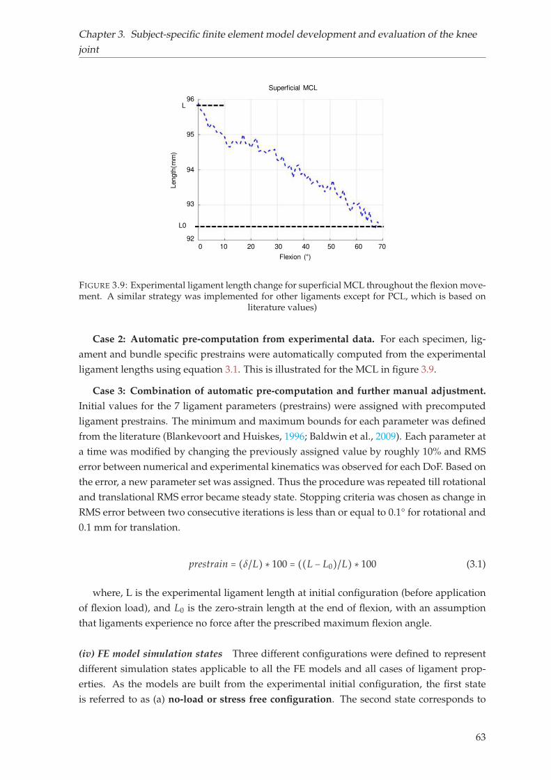
Chapter 3. Subject-specific finite element model development and evaluation of the knee
joint
L
L0
Length
(mm
)
96
95
94
93
92
Superficial MCL
Flexion (°)0 10 20 30 40 50 60 70
FIGURE 3.9: Experimental ligament length change for superficial MCL throughout the flexion move-ment. A similar strategy was implemented for other ligaments except for PCL, which is based on
literature values)
Case 2: Automatic pre-computation from experimental data. For each specimen, lig-
ament and bundle specific prestrains were automatically computed from the experimental
ligament lengths using equation 3.1. This is illustrated for the MCL in figure 3.9.
Case 3: Combination of automatic pre-computation and further manual adjustment.
Initial values for the 7 ligament parameters (prestrains) were assigned with precomputed
ligament prestrains. The minimum and maximum bounds for each parameter was defined
from the literature (Blankevoort and Huiskes, 1996; Baldwin et al., 2009). Each parameter at
a time was modified by changing the previously assigned value by roughly 10% and RMS
error between numerical and experimental kinematics was observed for each DoF. Based on
the error, a new parameter set was assigned. Thus the procedure was repeated till rotational
and translational RMS error became steady state. Stopping criteria was chosen as change in
RMS error between two consecutive iterations is less than or equal to 0.1° for rotational and
0.1 mm for translation.
prestrain = (δ/L) ∗ 100 = ((L − L0)/L) ∗ 100 (3.1)
where, L is the experimental ligament length at initial configuration (before application
of flexion load), and L0 is the zero-strain length at the end of flexion, with an assumption
that ligaments experience no force after the prescribed maximum flexion angle.
(iv) FE model simulation states Three different configurations were defined to represent
different simulation states applicable to all the FE models and all cases of ligament prop-
erties. As the models are built from the experimental initial configuration, the first state
is referred to as (a) no-load or stress free configuration. The second state corresponds to
63
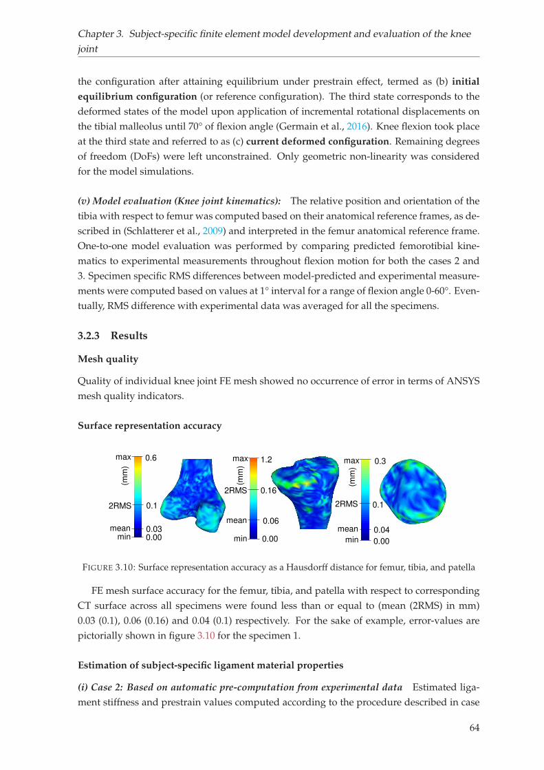
Chapter 3. Subject-specific finite element model development and evaluation of the knee
joint
the configuration after attaining equilibrium under prestrain effect, termed as (b) initial
equilibrium configuration (or reference configuration). The third state corresponds to the
deformed states of the model upon application of incremental rotational displacements on
the tibial malleolus until 70° of flexion angle (Germain et al., 2016). Knee flexion took place
at the third state and referred to as (c) current deformed configuration. Remaining degrees
of freedom (DoFs) were left unconstrained. Only geometric non-linearity was considered
for the model simulations.
(v) Model evaluation (Knee joint kinematics): The relative position and orientation of the
tibia with respect to femur was computed based on their anatomical reference frames, as de-
scribed in (Schlatterer et al., 2009) and interpreted in the femur anatomical reference frame.
One-to-one model evaluation was performed by comparing predicted femorotibial kine-
matics to experimental measurements throughout flexion motion for both the cases 2 and
3. Specimen specific RMS differences between model-predicted and experimental measure-
ments were computed based on values at 1° interval for a range of flexion angle 0-60°. Even-
tually, RMS difference with experimental data was averaged for all the specimens.
3.2.3 Results
Mesh quality
Quality of individual knee joint FE mesh showed no occurrence of error in terms of ANSYS
mesh quality indicators.
Surface representation accuracy
0.00min 0.00min
0.6max
0.00min
2RMS 0.1
mean 0.03
1.2max
2RMS 0.16
mean 0.06
0.3max
2RMS 0.1
mean 0.04
(mm
)
(mm
)
(mm
)
FIGURE 3.10: Surface representation accuracy as a Hausdorff distance for femur, tibia, and patella
FE mesh surface accuracy for the femur, tibia, and patella with respect to corresponding
CT surface across all specimens were found less than or equal to (mean (2RMS) in mm)
0.03 (0.1), 0.06 (0.16) and 0.04 (0.1) respectively. For the sake of example, error-values are
pictorially shown in figure 3.10 for the specimen 1.
Estimation of subject-specific ligament material properties
(i) Case 2: Based on automatic pre-computation from experimental data Estimated liga-
ment stiffness and prestrain values computed according to the procedure described in case
64
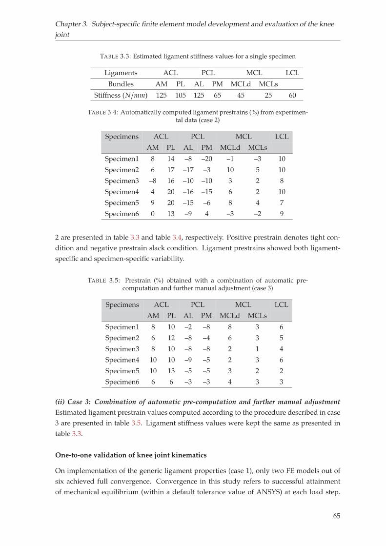
Chapter 3. Subject-specific finite element model development and evaluation of the knee
joint
TABLE 3.3: Estimated ligament stiffness values for a single specimen
Ligaments ACL PCL MCL LCL
Bundles AM PL AL PM MCLd MCLs
Stiffness (N/mm) 125 105 125 65 45 25 60
TABLE 3.4: Automatically computed ligament prestrains (%) from experimen-tal data (case 2)
Specimens ACL PCL MCL LCL
AM PL AL PM MCLd MCLs
Specimen1 8 14 –8 –20 –1 –3 10
Specimen2 6 17 –17 –3 10 5 10
Specimen3 –8 16 –10 –10 3 2 8
Specimen4 4 20 –16 –15 6 2 10
Specimen5 9 20 –15 –6 8 4 7
Specimen6 0 13 –9 4 –3 –2 9
2 are presented in table 3.3 and table 3.4, respectively. Positive prestrain denotes tight con-
dition and negative prestrain slack condition. Ligament prestrains showed both ligament-
specific and specimen-specific variability.
TABLE 3.5: Prestrain (%) obtained with a combination of automatic pre-computation and further manual adjustment (case 3)
Specimens ACL PCL MCL LCL
AM PL AL PM MCLd MCLs
Specimen1 8 10 –2 –8 8 3 6
Specimen2 6 12 –8 –4 6 3 5
Specimen3 8 10 –8 –8 2 1 4
Specimen4 10 10 –9 –5 2 3 6
Specimen5 10 13 –5 –5 3 2 2
Specimen6 6 6 –3 –3 4 3 3
(ii) Case 3: Combination of automatic pre-computation and further manual adjustment
Estimated ligament prestrain values computed according to the procedure described in case
3 are presented in table 3.5. Ligament stiffness values were kept the same as presented in
table 3.3.
One-to-one validation of knee joint kinematics
On implementation of the generic ligament properties (case 1), only two FE models out of
six achieved full convergence. Convergence in this study refers to successful attainment
of mechanical equilibrium (within a default tolerance value of ANSYS) at each load step.
65
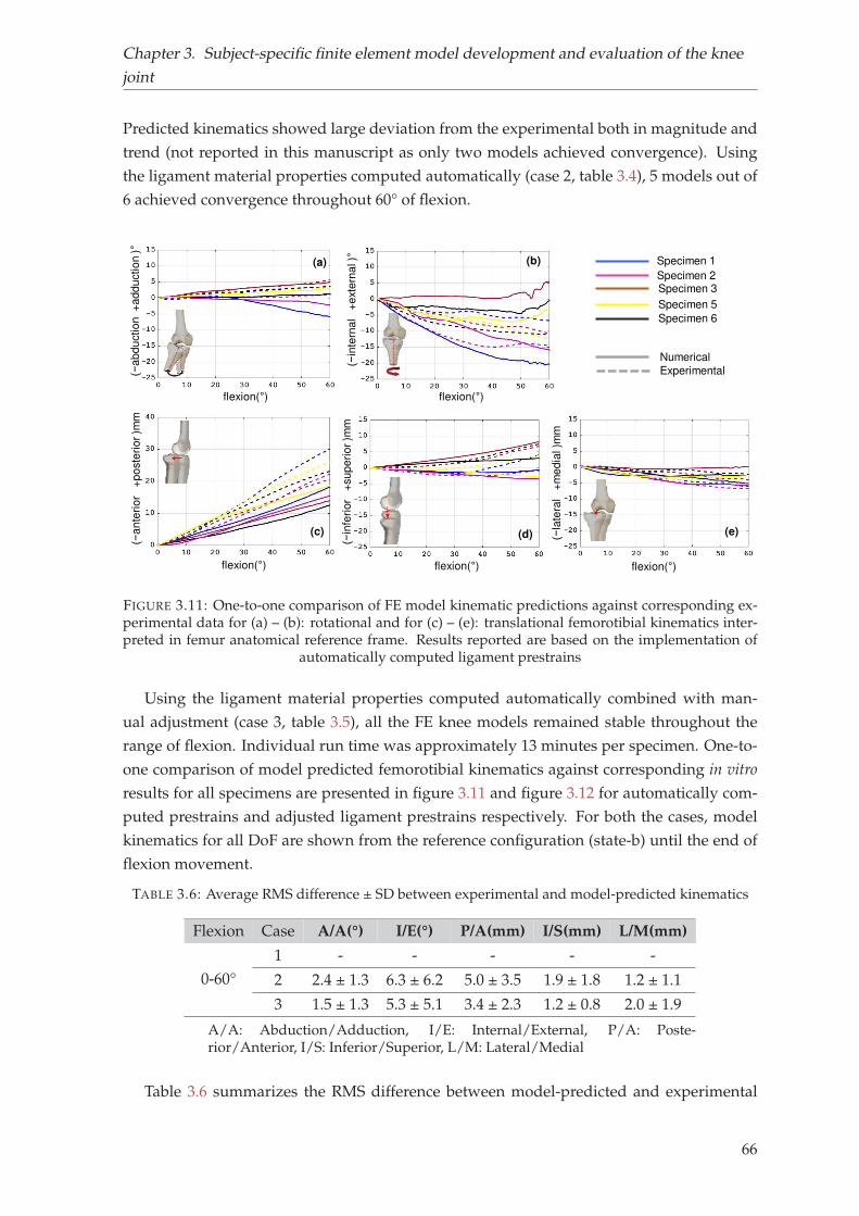
Chapter 3. Subject-specific finite element model development and evaluation of the knee
joint
Predicted kinematics showed large deviation from the experimental both in magnitude and
trend (not reported in this manuscript as only two models achieved convergence). Using
the ligament material properties computed automatically (case 2, table 3.4), 5 models out of
6 achieved convergence throughout 60° of flexion.
Specimen 1
Specimen 3Specimen 2
Specimen 5
Numerical
Experimental(−a
bd
uctio
n +
ad
du
ctio
n )°
flexion(°)
flexion(°) flexion(°) flexion(°)
(−in
tern
al
+e
xte
rna
l )°
(−a
nte
rio
r
+p
oste
rio
r )m
m
(−in
feri
or
+
su
pe
rio
r )m
m
(−la
tera
l +
me
dia
l )m
m
flexion(°)
(b)(a)
(c) (d) (e)
Specimen 6
FIGURE 3.11: One-to-one comparison of FE model kinematic predictions against corresponding ex-perimental data for (a) – (b): rotational and for (c) – (e): translational femorotibial kinematics inter-preted in femur anatomical reference frame. Results reported are based on the implementation of
automatically computed ligament prestrains
Using the ligament material properties computed automatically combined with man-
ual adjustment (case 3, table 3.5), all the FE knee models remained stable throughout the
range of flexion. Individual run time was approximately 13 minutes per specimen. One-to-
one comparison of model predicted femorotibial kinematics against corresponding in vitro
results for all specimens are presented in figure 3.11 and figure 3.12 for automatically com-
puted prestrains and adjusted ligament prestrains respectively. For both the cases, model
kinematics for all DoF are shown from the reference configuration (state-b) until the end of
flexion movement.
TABLE 3.6: Average RMS difference ± SD between experimental and model-predicted kinematics
Flexion Case A/A(°) I/E(°) P/A(mm) I/S(mm) L/M(mm)
0-60°
1 - - - - -
2 2.4 ± 1.3 6.3 ± 6.2 5.0 ± 3.5 1.9 ± 1.8 1.2 ± 1.1
3 1.5 ± 1.3 5.3 ± 5.1 3.4 ± 2.3 1.2 ± 0.8 2.0 ± 1.9
A/A: Abduction/Adduction, I/E: Internal/External, P/A: Poste-rior/Anterior, I/S: Inferior/Superior, L/M: Lateral/Medial
Table 3.6 summarizes the RMS difference between model-predicted and experimental
66
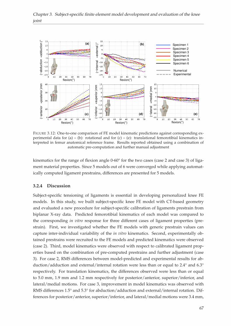
Chapter 3. Subject-specific finite element model development and evaluation of the knee
joint
Specimen 6
Specimen 1
Specimen 3Specimen 2
Specimen 4
Specimen 5
Numerical
Experimental(−a
bd
uctio
n +
ad
du
ctio
n )°
flexion(°)
flexion(°) flexion(°) flexion(°)
(−in
tern
al
+e
xte
rna
l )°
(−a
nte
rio
r
+p
oste
rio
r )m
m
(−in
feri
or
+
su
pe
rio
r )m
m
(−la
tera
l +
me
dia
l )m
m
flexion(°)
(b)(a)
(c) (d) (e)
FIGURE 3.12: One-to-one comparison of FE model kinematic predictions against corresponding ex-perimental data for (a) – (b): rotational and for (c) – (e): translational femorotibial kinematics in-terpreted in femur anatomical reference frame. Results reported obtained using a combination of
automatic pre-computation and further manual adjustment
kinematics for the range of flexion angle 0-60° for the two cases (case 2 and case 3) of liga-
ment material properties. Since 5 models out of 6 were converged while applying automat-
ically computed ligament prestrains, differences are presented for 5 models.
3.2.4 Discussion
Subject-specific tensioning of ligaments is essential in developing personalized knee FE
models. In this study, we built subject-specific knee FE model with CT-based geometry
and evaluated a new procedure for subject-specific calibration of ligaments prestrain from
biplanar X-ray data. Predicted femorotibial kinematics of each model was compared to
the corresponding in vitro response for three different cases of ligament properties (pre-
strain). First, we investigated whether the FE models with generic prestrain values can
capture inter-individual variability of the in vitro kinematics. Second, experimentally ob-
tained prestrains were recruited to the FE models and predicted kinematics were observed
(case 2). Third, model kinematics were observed with respect to calibrated ligament prop-
erties based on the combination of pre-computed prestrains and further adjustment (case
3). For case 2, RMS differences between model-predicted and experimental results for ab-
duction/adduction and external/internal rotation were less than or equal to 2.4° and 6.3°
respectively. For translation kinematics, the differences observed were less than or equal
to 5.0 mm, 1.9 mm and 1.2 mm respectively for posterior/anterior, superior/inferior, and
lateral/medial motions. For case 3, improvement in model kinematics was observed with
RMS differences 1.5° and 5.3° for abduction/adduction and external/internal rotation. Dif-
ferences for posterior/anterior, superior/inferior, and lateral/medial motions were 3.4 mm,
67
Chapter 3. Subject-specific finite element model development and evaluation of the knee
joint
1.2 mm and 2 mm respectively. These results show that the proposed methodology allows
us to obtain a first good approximation of the prestrain values with further manual adjust-
ment to improve the kinematic prediction.
As far as the authors are aware of, there are numerous challenges exist in determining
ligament prestrain. Challenges are linked to both measurement issues and modeling issues.
Measurement challenges are mainly methodological issues related to identification of lig-
ament attachment sites and determination of ligament elongation pattern during motion
(Belvedere et al., 2012; Gardiner, Weiss, and Rosenberg, 2001; Woo et al., 1990). Because
of such difficulties, FE models in general, adopt prestrain values from other studies avail-
able in the literature (Galbusera et al., 2014; Yang et al., 2010). As these values are adopted
from other experimental studies and not corresponding to the specimen under considera-
tion, thereby cannot be considered as subject-specific. Optimization methods have also been
extensively used to calibrate specific ligament constitutive behavior. These approaches par-
ticularly used laxity tests to calibrate their models (Baldwin et al., 2012; Beidokhti et al.,
2017). Such approaches are, although shown effective to attain specimen-specific ligament
properties, yet computationally expensive.
The current study focused on the development and evaluation of a new procedure for
subject-specific tensioning of FE knee ligaments. The proposed procedure builds upon data
previously collected during an experimental investigation conducted to identify ligament
(cruciate and collateral) attachment sites, and to determine the ligament elongation pat-
terns during passive knee flexion (Rochcongar et al., 2016). The FE model replicates the
natural ligament (cruciate and collateral) insertions since these are derived from the radio
opaque paint locations painted on the specimens prior to the CT-scan (figure 3.7). The values
obtained were consistent with those experimental measurements reported in the literature
(Belvedere et al., 2012; Bicer et al., 2010). It is worth mentioning that because of the lack
of experimental data for other ligaments, generic insertion sites were employed. Although,
it is difficult to directly compare the estimated prestrains with similar studies in literature
because of variability in ligament geometry and material property, yet the prestrain values
were found within the range confirmed by others (Amiri et al., 2006; Wismans et al., 1980;
Zaylor, Stulberg, and Halloran, 2019). Also, most of the ligaments were found in tensed state
at full extension except PCL, which is overall in agreement with the literature (Blankevoort
and Huiskes, 1991; Guess, Razu, and Jahandar, 2016; Moglo and Shirazi-Adl, 2005). Simi-
larly, predicted kinematic response also showed good correspondence with the experimen-
tal results for all the specimens. The experimental-numerical differences found in this study
were comparable to similar studies reported in the literature (Beidokhti et al., 2017; Harris
et al., 2016). For instance, (Beidokhti et al., 2017) reported an average RMS difference of
3.5° and 2.8° respectively for abduction/adduction and external/internal rotations. For an-
terior/posterior, superior/inferior and lateral/medial motions the differences were 3 mm,
2.3 mm and 1.6 mm respectively. It is worthwhile to mention that when generic properties
were used, most of the models couldn’t reach convergence. As previously reported by other
research teams (e.g., (Schwartz, Chokhandre, and Erdemir, 2019)) focusing on the medial
68
Chapter 3. Subject-specific finite element model development and evaluation of the knee
joint
collateral ligament), convergence difficulty appeared in this kind of models when material
properties were not personalized.
The procedure to compute ligament prestrain directly from experimental data (Case 3)
provided satisfactory initial guess, based on which model estimated kinematics were al-
ready in good agreement with the experimental data. As this approach appears to be com-
putationally inexpensive (15-20 sec to obtain ligament specific prestrain for a single knee
model) and methodologically simple, it may serve as a reliable alternative for estimating
subject-specific ligament prestrain values. To be noted that no direct evaluation of the liga-
ment tensions was performed in the present study. The decision to implement the current
technique as an alternative has to be conducted with caution. For successful implementation
of this technique towards clinics, exhaustive model evaluation under various loading con-
ditions is required including ligament tension and contact stress. Nevertheless, validating
joint kinematics as a first step could be valuable to show feasibility of the current approach.
This study contains some considerations and limitations worth highlighting. First, while
comparing with experimental kinematics, model-predicted results were shown from ref-
erence configuration (state-b). It is an auto-equilibrated configuration under the prestrain
effect, which is not concurrent with initial experimental configuration and difficult to cali-
brate. This results in absolute offset from the experimental kinematics (Baldwin et al., 2012),
although masked in relative kinematics. Second, we acknowledge that one of the sources of
discrepancies between experimental-numerical kinematics may come from model simplifi-
cations and assumptions. It is also to be noted that predicted kinematics with a combination
of initial guess from experimental data and further manual adjustment displayed closer cor-
respondence to in vitro data. Although the difference is minimal, this may be attributed to
the representation of overall joint soft tissue structure with simple ligamentous structures
without including cartilage layers and menisci. As the proposed methodology is not based
on current state-of-the-art approaches (such as MRI based complex models with detailed
soft tissue structures), there was difficulty to obtain subject-specific geometry of cartilage
and menisci with available imaging modalities (CT and biplanar X-ray) employed in our
study. Such simplification, therefore doesn’t hold if we are interested in more detailed local
insights, e.g., cartilage contact stress. However, for analysis, such as graft tensioning effect
on knee response while reconstructing ACL, such simplification was considered relevant
(Pena et al., 2005). Third, exclusion of meniscus may overestimate the role of the ligaments
in constraining the joint and providing stability (Harris et al., 2016). However, other studies
reported no remarkable influence of meniscus on the assessment of the knee joint kinemat-
ics, especially for the flexion range 0°–90° (Amiri et al., 2006; Guess, Razu, and Jahandar,
2016). Fourth, ligaments and tendons were represented as bundles of 1D elements, which
may not capture actual ligament length variation, as they do not account for material con-
tinuum, fiber twisting or wrapping. Yet, such simplification provides faster solutions and
recommended, particularly for the prediction of knee kinematic parameters (Bolcos et al.,
69
Chapter 3. Subject-specific finite element model development and evaluation of the knee
joint
2018; Beidokhti et al., 2017). Fifth, we chose to personalize only ligament prestrains, al-
though stiffness values vary from subject to subject. This consideration was based on sensi-
tivity analyses found in literature, where model predicted kinematics are proclaimed to be
highly sensitive to strain state at initial configuration rather than stiffness values (Pena et al.,
2005; Wismans et al., 1980). Besides, the models were validated only under passive flexion
load, which may not imitate an in vivo situation of clinical interest, yet could be a first step
of assessing the potential of the models towards complex scenarios. In this contribution, a
maximum flexion angle of 70° was considered to calibrate the model as this range covers
the most common amplitude of in vivo motion under level walking, during which ligaments
offer a substantial contribution to knee stability (Butler et al., 2007). However, perspective
work will focus on calibrating the model up to 120° of knee flexion. We acknowledge that
no influence of experimental uncertainty nor sensitivity of ligament attachment sites on pre-
dicted kinematics was performed. Future study is necessary to asses this issue. Finally, the
study was limited to six specimens due to time and labor associated with CT segmenta-
tion, yet higher in number compared to other similar published studies. This might limit
the model at the current state for clinical translation; however, it was imperative to build
CT-based models to minimize the impact of geometrical uncertainty in model predictions.
In conclusion, as it was a first study to directly implement prestrain values on models di-
rectly from the experiment, which may find scopes in model-based clinical studies, such as
planning of ligament balancing or reconstruction as it reduces complexity in model devel-
opment (especially ligament calibration) as well as computational cost, while maintaining
good correspondence with experimental data. In that aim, further model evaluation would
be necessary for larger specimen size and in other clinically relevant scenarios.
Overall, this chapter allowed to address two prominent challenges exist in model de-
velopment and evaluation approaches as elaborated in the literature review. The quasi-
automatic methodology employed in the first section helped to generate subject-specific FE
mesh of the knee joint with satisfactory mesh quality and surface representation accuracy.
Thanks to the EOS system and fast 3D reconstruction techniques.
The second section focused on validation of the subject-specific in vitro FE models of
the knee joint under passive flexion. A novel methodology to calibrate ligament prestrains
based on experimentally acquired values was attempted and evaluated satisfactorily. The
overall methodology helped to estimate knee kinematics with low computational cost as
no optimization process was involved, and secondly owing to the careful strategy of model
simplification. The model validation against in vitro experiments, although cannot be con-
sidered sufficient (passive loads), however, will serve as an intermediate step prior to trans-
lating the models towards in vivo loading condition.
70
Chapter 4
Soft Tissue Artifact correction in
motion analysis
The contribution elaborated in the previous chapter allowed to assess feasibility and capa-
bility of the FE models to estimate joint kinematics of the knee joint. In order to proceed a
step further, i.e., to estimate in vivo kinematics, integration of subject-specific physiological
boundary conditions to the FE models is paramount. As discussed in the literature review,
the widespread approach to apply in vivo boundary conditions in models is skin marker-
based motion analysis data. Also, it is clearly evident that estimation of joint kinematics
based on skin marker data is error prone because of soft tissue artifact (STA). It is also ap-
parent that existing methods for STA compensation are not adequate to take subject-specific
joint morphology (in particular for patients with joint lesion) and soft tissue properties into
account. This justified the need to propose a different approach for STA compensation which
is elaborated in the first section of this chapter. This work has been submitted to Journal of
Biomechanics entitled "Development and evaluation of a new methodology for Soft Tissue
Artifact compensation in the lower limb" and is currently under review.
The second section pertains to experimental quantification of soft tissue deformation,
which is often considered essential to effectively compensate for STA.
71
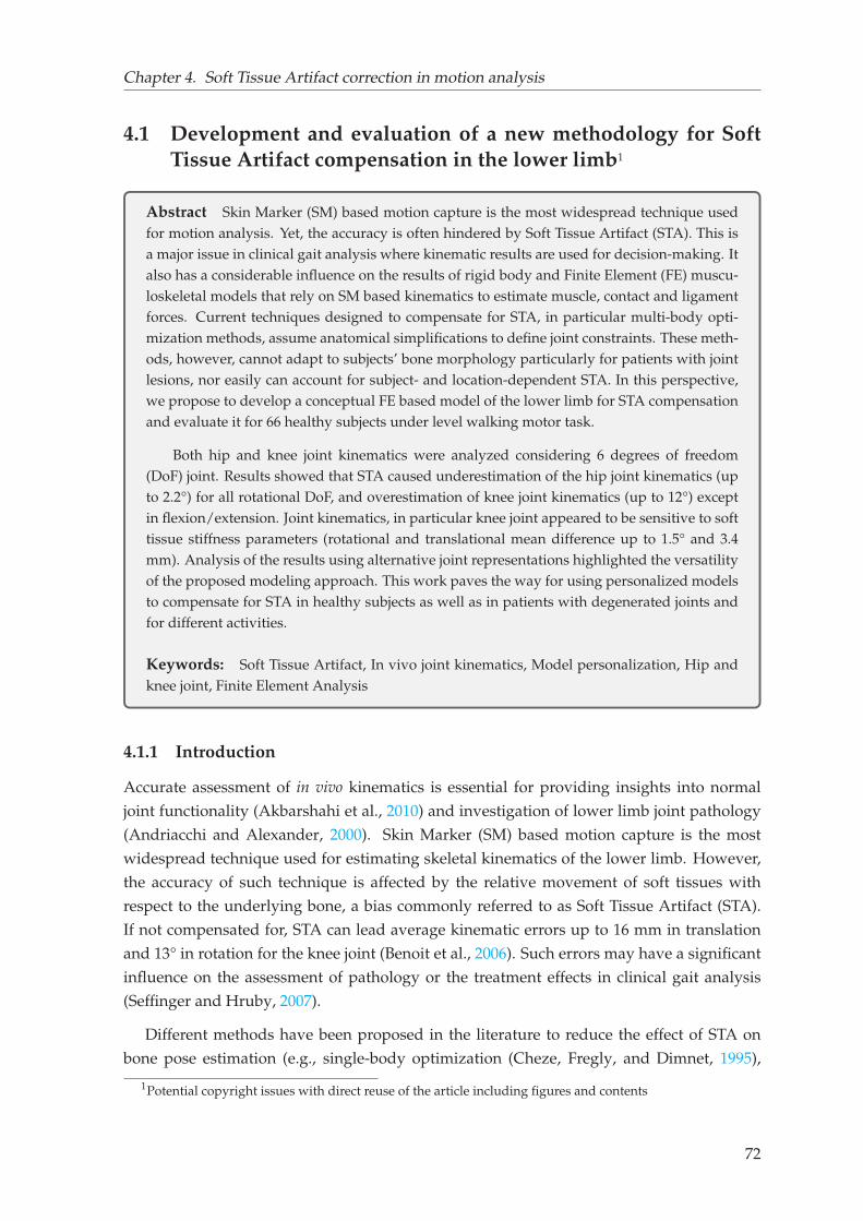
Chapter 4. Soft Tissue Artifact correction in motion analysis
4.1 Development and evaluation of a new methodology for Soft
Tissue Artifact compensation in the lower limb1
Abstract Skin Marker (SM) based motion capture is the most widespread technique usedfor motion analysis. Yet, the accuracy is often hindered by Soft Tissue Artifact (STA). This isa major issue in clinical gait analysis where kinematic results are used for decision-making. Italso has a considerable influence on the results of rigid body and Finite Element (FE) muscu-loskeletal models that rely on SM based kinematics to estimate muscle, contact and ligamentforces. Current techniques designed to compensate for STA, in particular multi-body opti-mization methods, assume anatomical simplifications to define joint constraints. These meth-ods, however, cannot adapt to subjects’ bone morphology particularly for patients with jointlesions, nor easily can account for subject- and location-dependent STA. In this perspective,we propose to develop a conceptual FE based model of the lower limb for STA compensationand evaluate it for 66 healthy subjects under level walking motor task.
Both hip and knee joint kinematics were analyzed considering 6 degrees of freedom(DoF) joint. Results showed that STA caused underestimation of the hip joint kinematics (upto 2.2°) for all rotational DoF, and overestimation of knee joint kinematics (up to 12°) exceptin flexion/extension. Joint kinematics, in particular knee joint appeared to be sensitive to softtissue stiffness parameters (rotational and translational mean difference up to 1.5° and 3.4mm). Analysis of the results using alternative joint representations highlighted the versatilityof the proposed modeling approach. This work paves the way for using personalized modelsto compensate for STA in healthy subjects as well as in patients with degenerated joints andfor different activities.
Keywords: Soft Tissue Artifact, In vivo joint kinematics, Model personalization, Hip andknee joint, Finite Element Analysis
4.1.1 Introduction
Accurate assessment of in vivo kinematics is essential for providing insights into normal
joint functionality (Akbarshahi et al., 2010) and investigation of lower limb joint pathology
(Andriacchi and Alexander, 2000). Skin Marker (SM) based motion capture is the most
widespread technique used for estimating skeletal kinematics of the lower limb. However,
the accuracy of such technique is affected by the relative movement of soft tissues with
respect to the underlying bone, a bias commonly referred to as Soft Tissue Artifact (STA).
If not compensated for, STA can lead average kinematic errors up to 16 mm in translation
and 13° in rotation for the knee joint (Benoit et al., 2006). Such errors may have a significant
influence on the assessment of pathology or the treatment effects in clinical gait analysis
(Seffinger and Hruby, 2007).
Different methods have been proposed in the literature to reduce the effect of STA on
bone pose estimation (e.g., single-body optimization (Cheze, Fregly, and Dimnet, 1995),
1Potential copyright issues with direct reuse of the article including figures and contents
72
Chapter 4. Soft Tissue Artifact correction in motion analysis
double anatomical landmark calibration (Cappello et al., 1997), point cluster technique (An-
driacchi et al., 1998), and Multi-body Optimisation (MBO) (Lu and O’connor, 1999). Amongst
these, MBO, which relies on a predefined kinematic model with specific joint constraints, is
increasingly used.
Initially, simple kinematic constraints such as hinge or spherical joints were considered to
represent hip and knee articulation (Charlton et al., 2004; Lu and O’connor, 1999; Reinbolt et
al., 2005). Later, anatomical joint constraints (parallel mechanism, coupling curves, ligament
length variation, elastic joint etc.) were introduced providing encouraging 3D kinematics as
they allowed joint displacements (Bergamini et al., 2011; Duprey, Cheze, and Dumas, 2010;
Gasparutto et al., 2015; Richard et al., 2016). However, regardless of the joint constraints
imposed, generic (unpersonalized) model-derived kinematics were shown inaccurate (knee
kinematic error up to 17° and 8 mm) as these models could not adapt to patient-specific
geometry, particularly in pathological conditions (Clément et al., 2017). On the other hand,
personalization of model geometry based on medical images were shown promising in im-
proving the accuracy of joint kinematics (Assi et al., 2016; Clément et al., 2015; Nardini et al.,
2020).
Joint simplification has indirect consequences on the predictive accuracy of both rigid
body musculoskeletal (MSK) models and FE based MSK models. Studies that used FE-MSK
models to predict local joint mechanics using in vivo joint kinematics (Shu et al., 2018; Xu
et al., 2016), assumed the knee joint as 1 DoF. This might result in propagation of uncertain-
ties on the predicted kinematics and would affect the joint reaction as well as muscle and
ligament forces.
In light of the aforementioned contexts, reliable estimation of skeletal kinematics with
SM based motion data is still a major challenge (Richard, Cappozzo, and Dumas, 2017).
Furthermore, extensive time and complexity associated with customization of models to
subjects’ geometry prohibit large sample size. In that context, methods for 3D reconstruction
of bony segments from medical imaging modalities, in particular biplanar X-ray imaging is
promising in research and clinical routine (Chaibi et al., 2012). Also, there is a need for
adaptable modeling approaches that can account for subject-, task-, and location-dependent
STA.
In a previous study, a conceptual FE model was proposed for STA compensation (Skalli
et al., 2018). The objective of the current study was to develop the conceptual model for the
lower limb and to implement it on healthy volunteers considering subject-specific models.
4.1.2 Materials and methods
First, the conceptual model is presented. Then implementation of the model is illustrated
within an IRB approved (CEHDF285) study. Finally, the consistency and versatility of the
model were investigated through sensitivity of various parameters, including the joints rep-
resentation.
73
Chapter 4. Soft Tissue Artifact correction in motion analysis
Conceptual FE model of the lower limb
S𝐹𝑖
HJ
KJ
S𝐹𝑖SC𝐹𝑖
HJ
KJ
SC𝐹𝑖 B𝐹𝑖B𝐹𝑖
B𝑃𝑖
B𝑇𝑖
FIGURE 4.1: Schematic illustration of the conceptual lower limb FE model. Detailed illustrationshown only for the femur segment. BPi, BFi and BTi denote pelvis, femur and tibia bone nodes.SFi and SCFi are the skin and subcutaneous markers respectively for the femur segment. HJ and KJ
denote the hip and knee joint respectively.
The conceptual model the lower limb consists of bone segments, nodes representing
skin markers and subcutaneous markers, joint elements, and elements that connect the skin
markers to the corresponding bones. Bone segments are represented by a set of high stiffness
beams. The joints between the segments are represented by rigid links, allowing free rota-
tions at the joint and controlled displacements. To simplify the soft tissue modeling, all the
soft tissue deformation effect is reported to the subcutaneous level. Therefore the connection
between a skin marker and corresponding bone segment is represented by a combination of
spring connecting the skin marker to the subcutaneous marker and beams connecting the
subcutaneous markers to the bone segments (figure 4.1).
The measured skin marker displacements throughout gait cycle are considered as input
to the FE model, yielding bone and subcutaneous marker locations and joints kinematics.
Skin markers are denoted by S, differentiating between those of the pelvis (SP), femur
(SF) and tibia (ST). The number of markers for the pelvis (NMP), femur (NMF) and tibia
(NMT) is variable and depends on the protocol being considered. Each skin marker is there-
fore referred to using the corresponding subscript: SPi, SFi and STi respectively for the pelvis
(SP1 to SPNMP), femur (SF1 to SPNMF) and tibia (ST1 to STNMT). Using the same conven-
tion, subcutaneous markers are denoted SC (SCPi, SCFi and SCTi for the pelvis, femur and
tibia respectively) and the bone points are denoted as B (differentiating between those of
the pelvis (BP), femur (BF) and tibia (BT)). Hip and knee joints are denoted by HJ and KJ
respectively.
74
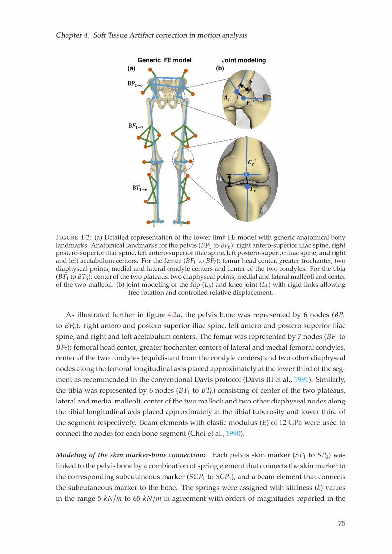
Chapter 4. Soft Tissue Artifact correction in motion analysis
Generic FE model
(a)
𝑨𝒄′ 𝑭𝒄′(b)
𝑪𝒄′𝑻𝒄′
Joint modeling
B𝑃1−6B𝐹1−7
B𝑇1−6 𝐿k
FIGURE 4.2: (a) Detailed representation of the lower limb FE model with generic anatomical bonylandmarks. Anatomical landmarks for the pelvis (BP1 to BP6): right antero-superior iliac spine, rightpostero-superior iliac spine, left antero-superior iliac spine, left postero-superior iliac spine, and rightand left acetabulum centers. For the femur (BF1 to BF7): femur head center, greater trochanter, twodiaphyseal points, medial and lateral condyle centers and center of the two condyles. For the tibia(BT1 to BT6): center of the two plateaus, two diaphyseal points, medial and lateral malleoli and centerof the two malleoli. (b) joint modeling of the hip (Lh) and knee joint (Lk) with rigid links allowing
free rotation and controlled relative displacement.
As illustrated further in figure 4.2a, the pelvis bone was represented by 6 nodes (BP1
to BP6): right antero and postero superior iliac spine, left antero and postero superior iliac
spine, and right and left acetabulum centers. The femur was represented by 7 nodes (BF1 to
BF7): femoral head center, greater trochanter, centers of lateral and medial femoral condyles,
center of the two condyles (equidistant from the condyle centers) and two other diaphyseal
nodes along the femoral longitudinal axis placed approximately at the lower third of the seg-
ment as recommended in the conventional Davis protocol (Davis III et al., 1991). Similarly,
the tibia was represented by 6 nodes (BT1 to BT6) consisting of center of the two plateaus,
lateral and medial malleoli, center of the two malleoli and two other diaphyseal nodes along
the tibial longitudinal axis placed approximately at the tibial tuberosity and lower third of
the segment respectively. Beam elements with elastic modulus (E) of 12 GPa were used to
connect the nodes for each bone segment (Choi et al., 1990).
Modeling of the skin marker-bone connection: Each pelvis skin marker (SP1 to SP4) was
linked to the pelvis bone by a combination of spring element that connects the skin marker to
the corresponding subcutaneous marker (SCP1 to SCP4), and a beam element that connects
the subcutaneous marker to the bone. The springs were assigned with stiffness (k) values
in the range 5 kN/m to 65 kN/m in agreement with orders of magnitudes reported in the
75
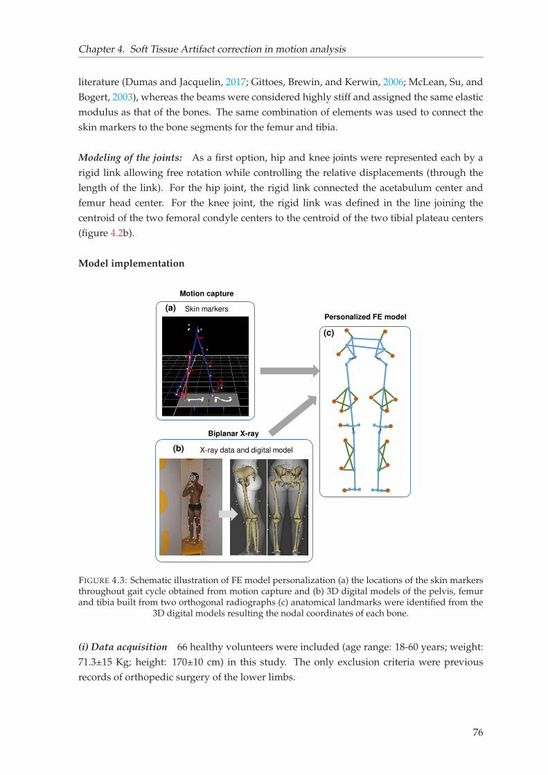
Chapter 4. Soft Tissue Artifact correction in motion analysis
literature (Dumas and Jacquelin, 2017; Gittoes, Brewin, and Kerwin, 2006; McLean, Su, and
Bogert, 2003), whereas the beams were considered highly stiff and assigned the same elastic
modulus as that of the bones. The same combination of elements was used to connect the
skin markers to the bone segments for the femur and tibia.
Modeling of the joints: As a first option, hip and knee joints were represented each by a
rigid link allowing free rotation while controlling the relative displacements (through the
length of the link). For the hip joint, the rigid link connected the acetabulum center and
femur head center. For the knee joint, the rigid link was defined in the line joining the
centroid of the two femoral condyle centers to the centroid of the two tibial plateau centers
(figure 4.2b).
Model implementation
Personalized FE model
(c)
(b) X-ray data and digital model
Biplanar X-ray
(a) Skin markers
Motion capture
FIGURE 4.3: Schematic illustration of FE model personalization (a) the locations of the skin markersthroughout gait cycle obtained from motion capture and (b) 3D digital models of the pelvis, femurand tibia built from two orthogonal radiographs (c) anatomical landmarks were identified from the
3D digital models resulting the nodal coordinates of each bone.
(i) Data acquisition 66 healthy volunteers were included (age range: 18-60 years; weight:
71.3±15 Kg; height: 170±10 cm) in this study. The only exclusion criteria were previous
records of orthopedic surgery of the lower limbs.
76
Chapter 4. Soft Tissue Artifact correction in motion analysis
Quantitative Movement Analysis was performed on an optoelectronic analysis system
comprising 7 video-cameras (Vicon Motion System Ltd., Oxford Metrics, UK). The optoelec-
tronic markers were positioned following the Plug-in Gait ® method (Davis III et al., 1991),
and participants were asked to perform level walking at self-selected speed (figure 4.3a).
Biplanar radiographs were then acquired using the EOS system (EOS Imaging, France). 3D
digital models of bones were obtained using a 3D reconstruction algorithm validated by
previous studies (figure 4.3b) (Chaibi et al., 2012). The location of skin markers was also
computed from biplanar X-Rays.
(ii) Subject-specific FE model development and simulation From the 3D digital models of
the bones, subject-specific anatomical landmarks were identified, resulting in nodal coor-
dinates of each bone, as represented in figure 4.3c. The distance between skin and subcu-
taneous markers were arbitrarily chosen as 1 mm (i.e., spring length). Based on the mean
translational displacement of the knee joint found in our previous in vitro experimental
work (Germain et al., 2016), the joint length for the knee (Lk) was fixed to 20 mm. For the
hip (Lh ), the joint length was fixed to 1 mm based on an unpublished data on the hip trans-
lational displacement quantified using biplanar X-rays. For simplicity, stiffness parameter
of the springs was kept constant across all segments and assigned 50 kN/mm.
The measured marker displacements from the motion capture were incrementally in-
troduced to the model as a prescribed boundary condition, and resulting bone and subcu-
taneous marker positions throughout the gait cycle were computed using commercial FE
package ANSYS ®. The resolution was performed via an implicit scheme and taking into
account geometric non-linearity.
(iii) Kinematic computation The positions of the resulting bone segments and subcuta-
neous markers were used to define a set of virtual markers (figure 4.4). These virtual mark-
ers hereafter will be termed as corrected markers (CFi) and were defined with the same con-
sideration as those of the subcutaneous markers, i.e., rigid links with the bone segment. The
positions of the corrected markers were used to compute STA Compensated (STAC) joint
kinematics. Hip and knee joint rotational kinematics were expressed in the pelvis and femur
anatomical reference frames (EOS-based) respectively, and with Cardan sequence YX′Z′′.
Hip joint translation was defined as the relative displacement between points A′
c and F′
c
expressed in the pelvis anatomical reference frame. Similarly, knee joint translation was de-
fined as a relative displacement between points C′
c and T′
c expressed in the femur anatomical
reference frame. Anatomical reference frames were defined as described in (Schlatterer et
al., 2009) for the femur and tibia, and in (Dubois, 2014) for the pelvis. A customized Matlab ®
(Mathworks, Massachusetts, United States) routine was used for both SM-based and STAC
kinematic processing.
Joint kinematics (mean±1SD) for the hip and knee joint were plotted for all 6 DoF over
time normalized gait cycle. Difference in range of motions (dROM) was also computed
between SM-based and STAC kinematics.
77
Chapter 4. Soft Tissue Artifact correction in motion analysis
A
B
C
S𝐹𝑖SC𝐹𝑖𝐶𝐹𝑖
𝑹𝒇𝒆𝒎S𝑃𝑖
𝐶𝑃𝑖SC𝑃𝑖 S𝑇𝑖SC𝑇𝑖 𝐶𝑇𝑖
𝑹𝒑𝒆𝒍
𝑹𝒕𝒊𝒃
FIGURE 4.4: Illustration of corrected markers (CFi, CPi, CTi) and anatomical reference frames(R f em, Rpel , Rtib) for the (A) femur, (B) pelvis and (C) tibia respectively. Corrected markers are ob-tained from the subcutaneous marker in a direction orthogonal to the bone segment and 1mm awayfrom subcutaneous marker. Anatomical reference frames for the femur and tibia were defined as
described in (Schlatterer et al., 2009) and for pelvis (Dubois, 2014).
Illustration of versatility
(i) Sensitivity of spring stiffness and joint length Two different stiffness values for the sub-
cutaneous springs were implemented (5 kN/m and 65 kN/m) to investigate the influence of
stiffness parameters on joint kinematics. Segment specific stiffness values were also consid-
ered by assigning different stiffness values to pelvis (5 kN/m), femur (10 kN/m) and tibia (55
kN/m).
Furthermore, two different knee joint lengths (Lk = 21 mm and 31 mm) were arbitrarily
considered to investigate the impact of joint lengths on estimated kinematics. Implemented
knee joint lengths were based on the minimum and maximum value found in the popula-
tion. In this case, spring stiffnesses were kept constant with a value 65 kN/m.
Joint kinematics (mean±1SD) for the hip and knee joint were computed for all 6 DoF over
time normalized gait cycle. Differences in range of motions (dROM) were also computed for
the kinematics computed with different stiffness values and different joint lengths.
(ii) Alternative joint representation Two other alternative joint models were considered to
illustrate the versatility of the lower limb FE model. These alternative joint models consid-
ered were:
Parallel Mechanism: Two rigid links connecting the center of the medial and lateral condyles
to the corresponding tibial plateaus were considered to model the knee joint approximating
the femur-tibia contact behavior. The hip joint model was left unaltered (single-link model).
78
Chapter 4. Soft Tissue Artifact correction in motion analysis
Spherical joint: Spherical joint model at the hip and knee joint was considered allowing
free rotations while restricting the displacements. The location of the joint constraint was
placed on the femur head center for the hip joint and the mid-point of the two femoral
condyles for the knee joint.
Joint kinematics (mean±1SD) for the hip and knee joint were compared among the single
link, parallel mechanism and spherical joint model. Spring stiffness value 65 kN/mm were
assigned for all the joint models.
Model comparison with multi-body optimization
As no reference kinematics (artifact-free motion) was available, the FE model results were
compared to a classical STA compensation MBO method with spherical joint modeling for
both the hip and knee joints (Lu and O’connor, 1999). The joint constraints and locations
incorporated in the MBO were in accordance with the FE model. To compare the kinematic
results of the subject-specific FE models with MBO, the same anatomical reference frames
were defined for the MBO bone segments.
Differences between the two methods were also analyzed with a Student’s t-test or Wilcoxon
sign-rank test depending on the outcomes of the Shapiro-Wilk test of normality, using a cus-
tomized Matlab routine. For all the tests, the significance level was set 0.05 a priori.
4.1.3 Results
Each FE model with 6-DoF joints required less than 45 sec of run time on a single processor
desktop PC to simulate a complete gait cycle of approximately 200–300 frames. All results
are synthesized in Table 4.1.
Joint kinematics
Both rotational and translational kinematics estimated with skin marker measurements and
FE model embedding the 6 DoF joint model are illustrated in figures 4.5 and 4.6 for the
hip and knee joints respectively. The joint kinematics are plotted over time-normalized gait
cycle.
Overall, for the hip joint, STAC and SM-based kinematics exhibited qualitatively similar
pattern. However, differences in range of motion (dROM) varied across all DoF, with a max-
imum value of –2.2° for Abduction/Adduction (Abd/Add) followed by –1.6° and –0.3° for
Flexion/Extension (Flex/Ext) and Internal/External (Int/Ext) rotation respectively. Max-
imum joint displacement up to 1 mm was observed for STAC kinematics while showing
up to 41.5 mm for SM-based kinematics in Posterior/Anterior (Post/Ant) direction. In the
Medial/Lateral (Med/Lat) and Inferior/Superior (Inf/Sup) direction, joint displacement ex-
hibited less than 1 mm, whereas SM-based kinematics showed up to 28 mm.
79
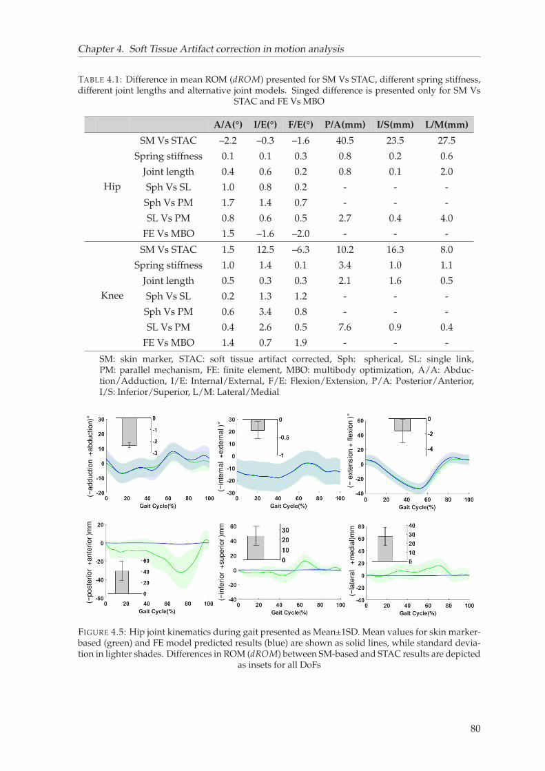
Chapter 4. Soft Tissue Artifact correction in motion analysis
TABLE 4.1: Difference in mean ROM (dROM) presented for SM Vs STAC, different spring stiffness,different joint lengths and alternative joint models. Singed difference is presented only for SM Vs
STAC and FE Vs MBO
A/A(°) I/E(°) F/E(°) P/A(mm) I/S(mm) L/M(mm)
Hip
SM Vs STAC –2.2 –0.3 –1.6 40.5 23.5 27.5
Spring stiffness 0.1 0.1 0.3 0.8 0.2 0.6
Joint length 0.4 0.6 0.2 0.8 0.1 2.0
Sph Vs SL 1.0 0.8 0.2 - - -
Sph Vs PM 1.7 1.4 0.7 - - -
SL Vs PM 0.8 0.6 0.5 2.7 0.4 4.0
FE Vs MBO 1.5 –1.6 –2.0 - - -
Knee
SM Vs STAC 1.5 12.5 –6.3 10.2 16.3 8.0
Spring stiffness 1.0 1.4 0.1 3.4 1.0 1.1
Joint length 0.5 0.3 0.3 2.1 1.6 0.5
Sph Vs SL 0.2 1.3 1.2 - - -
Sph Vs PM 0.6 3.4 0.8 - - -
SL Vs PM 0.4 2.6 0.5 7.6 0.9 0.4
FE Vs MBO 1.4 0.7 1.9 - - -
SM: skin marker, STAC: soft tissue artifact corrected, Sph: spherical, SL: single link,PM: parallel mechanism, FE: finite element, MBO: multibody optimization, A/A: Abduc-tion/Adduction, I/E: Internal/External, F/E: Flexion/Extension, P/A: Posterior/Anterior,I/S: Inferior/Superior, L/M: Lateral/Medial
(−a
dd
uctio
n +
ab
du
ctio
n)°
(−in
tern
al
+e
xte
rna
l )°
(−e
xte
nsio
n +
fle
xio
n )°
(−p
oste
rio
r +
an
teri
or
)mm
(−in
feri
or
+su
pe
rio
r )m
m
(−la
tera
l +
me
dia
l)m
m
FIGURE 4.5: Hip joint kinematics during gait presented as Mean±1SD. Mean values for skin marker-based (green) and FE model predicted results (blue) are shown as solid lines, while standard devia-tion in lighter shades. Differences in ROM (dROM) between SM-based and STAC results are depicted
as insets for all DoFs
80
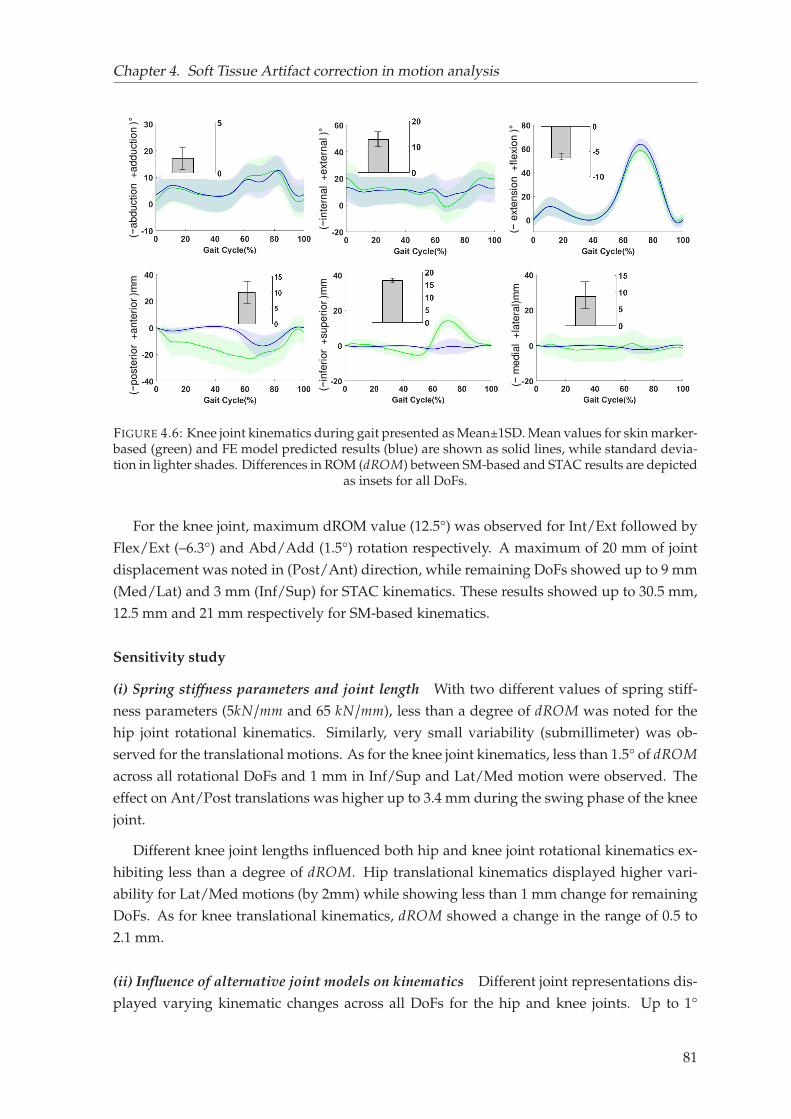
Chapter 4. Soft Tissue Artifact correction in motion analysis
(−in
tern
al
+e
xte
rna
l )°
(−e
xte
nsio
n +
fle
xio
n )°
(−a
bd
uctio
n +
ad
du
ctio
n )°
(−p
oste
rio
r +
an
teri
or
)mm
(−in
feri
or
+su
pe
rio
r )m
m
(−m
ed
ial +
late
ral)
mm
FIGURE 4.6: Knee joint kinematics during gait presented as Mean±1SD. Mean values for skin marker-based (green) and FE model predicted results (blue) are shown as solid lines, while standard devia-tion in lighter shades. Differences in ROM (dROM) between SM-based and STAC results are depicted
as insets for all DoFs.
For the knee joint, maximum dROM value (12.5°) was observed for Int/Ext followed by
Flex/Ext (–6.3°) and Abd/Add (1.5°) rotation respectively. A maximum of 20 mm of joint
displacement was noted in (Post/Ant) direction, while remaining DoFs showed up to 9 mm
(Med/Lat) and 3 mm (Inf/Sup) for STAC kinematics. These results showed up to 30.5 mm,
12.5 mm and 21 mm respectively for SM-based kinematics.
Sensitivity study
(i) Spring stiffness parameters and joint length With two different values of spring stiff-
ness parameters (5kN/mm and 65 kN/mm), less than a degree of dROM was noted for the
hip joint rotational kinematics. Similarly, very small variability (submillimeter) was ob-
served for the translational motions. As for the knee joint kinematics, less than 1.5° of dROM
across all rotational DoFs and 1 mm in Inf/Sup and Lat/Med motion were observed. The
effect on Ant/Post translations was higher up to 3.4 mm during the swing phase of the knee
joint.
Different knee joint lengths influenced both hip and knee joint rotational kinematics ex-
hibiting less than a degree of dROM. Hip translational kinematics displayed higher vari-
ability for Lat/Med motions (by 2mm) while showing less than 1 mm change for remaining
DoFs. As for knee translational kinematics, dROM showed a change in the range of 0.5 to
2.1 mm.
(ii) Influence of alternative joint models on kinematics Different joint representations dis-
played varying kinematic changes across all DoFs for the hip and knee joints. Up to 1°
81
Chapter 4. Soft Tissue Artifact correction in motion analysis
of dROM was observed for hip Add/Abd when the joint model was changed to spherical
from the single-link. This value changed till 1.7° when the joint model was further switched
to parallel mechanism from single-link. Maximum dROM of 4 mm was observed for the
hip Lat/Med motion followed by Post/Ant motion (2.7 mm) and Inf/Sup motion (0.4 mm)
when changing knee joint model from single-link to parallel mechanism. Similarly, knee
joint kinematics exhibited up to 3.4° in dROM for Int/Ext rotation when joint model was
altered, while Add/Abd and Flex/Ext displayed up to 0.6° and 1.2° respectively. Knee
Post/Ant motion displayed up to 7.6 mm of dROM, whereas less than 1 mm of dROM was
noted for the remaining DoFs.
FE Model comparison with MBO
Statistically significant differences between MBO-based and FE-based STA compensation
for the hip and knee joints were found (p<0.05). Those differences, however, were always in
the range of 0.7° to 2°.
4.1.4 Discussion
Soft Tissue Artifact compensation is essential for accurate estimation of in vivo joint kine-
matics in both research and clinical routine; however, personalization and versatility of cur-
rent model-based methods still represents a challenge. The purpose of this study was to
develop and evaluate a conceptual FE model of the lower limb for STA compensation. The
proposed method was successfully tested on a population of 66 subjects. This model is com-
putationally fast (less than 45 sec run time), and its main advantage is versatility allowing a
wide range of parameters and joint representations to be considered.
Qualitatively similar kinematic patterns were observed between SM-based and FE-based
STA compensated (STAC) kinematic results for both the hip and knee joints, with differ-
ences in range ROM across all DoFs. SM-based kinematics were comparable to the litera-
ture (D’Isidoro, Brockmann, and Ferguson, 2020; Fiorentino et al., 2017). Results obtained
showed that overall rotational ROM was underestimated by SM-based results up to 2.2° for
the hip joint, thus confirming similar observations reported in studies that compared SM-
based ROM to dual fluoroscopic measurements (Fiorentino et al., 2020). For the knee joint,
SM-based ROM was smaller by 6.3° for the Flex/Ext only. For the other DoFs, SM-based
ROM was higher up to 12° as compared to STAC kinematics. For translational kinematics
of the knee joint, SM-based results were higher (up to 30.5 mm of ROM) as compared to
STAC kinematics showing up to 20 mm. STAC knee kinematics were comparable to studies
reported in the literature that reported either bone-pin-based or fluoroscopy-based kinemat-
ics (Benoit et al., 2006; Kozanek et al., 2009; Myers et al., 2012). Nevertheless, we observed
overall higher dROM values between SM-based and STAC as compared to the studies that
reported in the range 4.4°–5.3° for rotational kinematics and up to 13mm for translational
kinematics (Benoit et al., 2006; Leardini et al., 2005). These discrepancies may arise from the
experimental protocol such as number of markers, cluster configuration and location.
82
Chapter 4. Soft Tissue Artifact correction in motion analysis
While comparing FE model predicted results to those of MBO-based, statistically signifi-
cant differences were observed. However, mean differences were minor (less than or equal
to 2°).
The distinguished advantage of the current approach as opposed to the MBO is the model
versatility. First, the introduction of springs to account for all soft tissue deformation facili-
tated to compensate for STA by adjusting the stiffness parameters. Sensitivity study showed
that joint kinematics (particularly the knee joint) were sensitive to spring stiffness exhibit-
ing dROM value up to 1.5° for the rotational kinematics and up to 4.5 mm for translational
kinematics. Given the subject-specific nature of the soft tissue deformation, spring param-
eters can be calibrated in the presence of reference kinematics. Moreover, the model allows
to easily tune individual spring parameters, which could be helpful to account for location-
specific soft tissue behavior (Akbarshahi et al., 2010; Gao and Zheng, 2008). Second, the
FE model allows easy implementation of alternatives joint models and joint lengths. Joint
models can be further customized to reproduce specific joint angular and translational dis-
placements quantified in specific sub-groups and for specific motor tasks (Kim et al., 2019).
Although we cannot confirm the accuracy of the results in the absence of a gold standard,
our findings revealed that joint representations have considerable influence on the estimated
kinematics, establishing similar remarks as reported in the literature (Duprey, Cheze, and
Dumas, 2010; Richard, Cappozzo, and Dumas, 2017). Furthermore, the study (Richard,
Cappozzo, and Dumas, 2017) concluded that none of the joint constraints (kinematic or
anatomical) could significantly improve the estimation of joint kinematics, and therefore
image-based (CT, MRI, biplanar X-ray etc.) model personalization was recommended (Clé-
ment et al., 2017; Nardini et al., 2020). In that context, the current FE model has the potential
to implement a wide range of joint models, from the most simplified (with spherical con-
straint) to the anatomically detailed (with articular surfaces).
This study has some limitations. First, there was no reference kinematics to compare
the results to. Therefore, the joint kinematics exhibited by the FE models were compared
to those computed with the MBO method. Nevertheless, as we cannot consider MBO as a
fully reliable solution for STA compensation (Richard, Cappozzo, and Dumas, 2017), such
comparison is only for assessing the qualitative performance of the FE model. Second, STA
parameters implemented in the model were arbitrary as there is lack of data in the litera-
ture. Personalization of such parameters is, however, essential to encompass different range
of subjects (young, adult, patients with cerebral palsy and osteoarthritis). Third, joint repre-
sentation in this model is still simplified, which could be insufficient for investigating local
joint mechanics for healthy or degenerated joints (Adouni, Shirazi-Adl, and Shirazi, 2012;
Lenhart et al., 2015; Shu et al., 2018; Valente et al., 2014). Nevertheless, as a preliminary
step, the current contribution only focused on exploring and facilitating personalization of
the parameters that are important for STA compensation. Moreover, even with simplified
joint representation, the model could limit the effect of STA in joint kinematics. Fourth, al-
though the proposed approach may give the impression that it complicates the process of
STA compensation in gait analysis, the perspectives are numerous, as already highlighted.
83
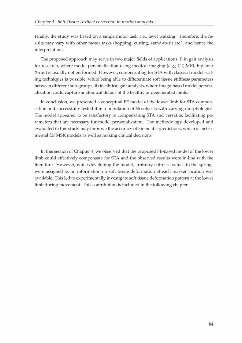
Chapter 4. Soft Tissue Artifact correction in motion analysis
Finally, the study was based on a single motor task, i.e., level walking. Therefore, the re-
sults may vary with other motor tasks (hopping, cutting, stand-to-sit etc.) and hence the
interpretations.
The proposed approach may serve in two major fields of applications: i) in gait analysis
for research, where model personalization using medical imaging (e.g., CT, MRI, biplanar
X-ray) is usually not performed. However, compensating for STA with classical model scal-
ing techniques is possible, while being able to differentiate soft tissue stiffness parameters
between different sub-groups. ii) in clinical gait analysis, where image-based model person-
alization could capture anatomical details of the healthy or degenerated joints.
In conclusion, we presented a conceptual FE model of the lower limb for STA compen-
sation and successfully tested it in a population of 66 subjects with varying morphologies.
The model appeared to be satisfactory in compensating STA and versatile, facilitating pa-
rameters that are necessary for model personalization. The methodology developed and
evaluated in this study may improve the accuracy of kinematic predictions, which is instru-
mental for MSK models as well as making clinical decisions.
In this section of Chapter 4, we observed that the proposed FE-based model of the lower
limb could effectively compensate for STA and the observed results were in-line with the
literature. However, while developing the model, arbitrary stiffness values to the springs
were assigned as no information on soft tissue deformation at each marker location was
available. This led to experimentally investigate soft tissue deformation pattern at the lower
limb during movement. This contribution is included in the following chapter.
84
Chapter 4. Soft Tissue Artifact correction in motion analysis
4.2 Experimental quantification of soft tissue deformation in quasi-
static single leg flexion using biplanar imaging1
Abstract Soft tissue deformation (STD) causes the most prominent source of error in skinmarker (SM) based motion analysis, commonly referred to as Soft Tissue Artifact (STA). Tocompensate for its effect and to accurately assess in vivo joint kinematics, quantification ofSTD in three-dimension (3D) is essential. In the literature, different invasive and radiologicalapproaches have been employed to study how STA propagates in joint kinematics. However,there is limited reference data extensively reporting distribution of the artifact itself in 3D.
The current study was thus aimed at quantifying STD in 10 subjects along three anatomicaldirections. Biplanar X-ray system was used to determine true bone and SM positions whilethe subjects underwent quasi-static single leg flexion.
STD exhibited inter-subject similarity. A non-uniform distribution was observed at thepelvis, thigh and shank displaying maximum at the thigh (up to 18.5 mm) and minimumat the shank (up to 8 mm). STD at the pelvis and thigh displayed inter-marker similarity.STD at the pelvis was found direction independent, showing similar distribution in all the3 directions. However, the thigh and shank exhibited higher STD in the proximal-distaldirection of the bone embedded anatomical reference frame. These findings may providemore insights while interpreting motion analysis data as well to effectively strategize STAcompensation methods.
Keywords: Soft tissue deformation, Skin marker-based motion analysis, Biplanar X-ray
4.2.1 Introduction
Skin Marker (SM) based motion analysis is the most common non-invasive method for esti-
mating skeletal position and orientation in 3D space. Accuracy of such method is mainly
limited by relative movement between soft tissues and the underlying bone, commonly
known as Soft Tissue Artifact (STA). In order to compensate for it and to accurately esti-
mate in vivo skeletal position during motion, knowledge of Soft Tissue Deformation (STD)
pattern during motion is critical (Benoit et al., 2006; Stagni et al., 2005).
Several invasive (e.g., bone pins (Benoit et al., 2006; Reinschmidt et al., 1997)and radio-
logical studies (e.g., fluoroscopy (D’Isidoro, Brockmann, and Ferguson, 2020; Stagni et al.,
2005), biplanar X-ray (Südhoff et al., 2007; Tashman and Anderst, 2002), MRI (Akbarshahi et
al., 2010; Sangeux et al., 2006)) have been proposed to characterize STD during different mo-
tor tasks. Most of the studies concluded that STD is dependent on an individual subject, type
of performed activity, marker configuration as well as locations. For instance, few studies
have found that kinematic error due to STD is greater at the thigh than the shank, suggest-
ing location- and segment- specific scheme to compensate for the artefact(Akbarshahi et al.,
1Potential copyright issues with direct reuse of the article including figures and contents (article under prepa-ration)
85
Chapter 4. Soft Tissue Artifact correction in motion analysis
2010; Stagni et al., 2005; Benoit et al., 2006). Nevertheless, these studies primarily focused
on quantifying the kinematic errors caused by STD rather than STD itself.
As far as the authors are aware of, only one study exists in the literature dealing with
quantification of STD at different marker locations and directions in 20 healthy volunteers
(Gao and Zheng, 2008). But, due to technical limitations preventing access to the bone po-
sition, STA quantification was reported as inter-marker movement instead of marker move-
ment relative to true bone positions. Hence, there is still a lack of reference data on subject-,
location- and direction-specific STD, which may provide insight for effective STA compen-
sation strategies for SM based motion analysis.
Amongst the different methods devised for compensating STA, multi-body optimization
(MBO) method is increasingly used. It generally assigns a weight matrix reflecting the STA
error distribution among the markers adhered to a segment (Lu and O’connor, 1999). More-
over, FE based novel approach to compensate for STA of the lower limb and successfully
evaluated in a population of 66 subjects ( section 4.1). The FE model facilitates to incorpo-
rate STA correction stiffness at each marker location, and stiffness can be calibrated based
on information of local STD at each marker location and along each anatomical direction.
However, owing to lack of STD data, arbitrary values were assigned for the stiffness param-
eters.
The current study was thus aimed at quantifying soft tissue deformation on the pelvis,
thigh and shank at each marker location and in three anatomical directions during single-leg
quasi-static knee flexion using low dose biplanar radiography.
4.2.2 Materials and methods
Data collection
The retrospective data included in the study recruited ten volunteers (age range: 23-40 years;
weight range: 63-89 kg, height range: 1.7-1.9 m), 6 months after ACL reconstruction fol-
lowing approval of a relevant ethical committee. Patients with a large osteochondral de-
fect (>1cm2), operated for a meniscal suture and multi-ligament knee injury, or diagnosed
with a neuromuscular disorder which could impair motion, were excluded from this study.
The mean IKDC (International Knee Documentation Committee) score for the subjects was
79.7±7.2. This score ranges from 0 to 100, with higher scores representing lower levels of
symptoms and higher levels of function and sports activity (Irrgang et al., 2001).
Subjects were equipped with a total of 20 retro-reflective skin markers (pelvis: 4, thigh:
8 and shank: 8) according to the Plug-in Gait ® method (Davis III et al., 1991). Three pairs
of biplanar radiographs (EOS Imaging, France) were acquired in three configurations for
each subject (figure 4.7). First, a pair of radiograph was taken in the free-standing position.
Then, two sequential pairs of radiographs at approximately 20° and 40° of knee flexion were
acquired while each subject performed a quasi-static single-leg knee flexion. For the sake of
86
Chapter 4. Soft Tissue Artifact correction in motion analysis
Biplanar X-ray data and 3D models
pose 1 pose 3pose 2
F F FL L L
S𝑃3S𝑃1 S𝑃2
S𝑃4
S𝑇1S𝑇2 S𝑇3S𝑇4
S𝑇5S𝑇6 S𝑇7S𝑇8
S𝑆1S𝑆2S𝑆3S𝑆4
S𝑆5S𝑆6 S𝑆7S𝑆8
FIGURE 4.7: 3D digital models of the pelvis, femur and tibia and their respective skin adhered mark-ers at positions: pose 1 (free-standing), pose 2 (20° knee flexion) and pose 3 (40° knee flexion) builtfrom orthogonal radiographs. Marker nomenclature is shown at pose 1 for the pelvis: SP1 to SP4, for
the thigh ST1 to ST8 and for the shank: SS1 and SS8. L: lateral and F: frontal view
clarity, three sequential postures will be hereafter termed as respectively pose 1, pose 2 and
pose 3 for free-standing, 20° and 40° of knee flexion.
3D digital models of bones (pelvis, femur and tibia) were first obtained at free-standing
position using a 3D reconstruction algorithm developed previously by (Chaibi et al., 2012)
for the femur and tibia and (Mitton et al., 2006) for the pelvis. The 3D models were then
projected on the frontal and lateral radiographs. The positions of the bony contours were
manually adjusted until the contours exactly matched those of the radiographs at each pose.
3D locations of skin markers at each pose were also computed from biplanar radiographs
using the same procedure. Anatomical reference (Ranat) frames for the femur and tibia was
defined following the definition reported in (Schlatterer et al., 2009), and for the pelvis, in
(Dubois, 2014). x, y and z axes of the Ranat frames are along antero-posterior, proximal-distal
and medial-lateral direction respectively.
Quantification of STD
STD quantification on the pelvis, thigh and shank was performed based on two different
schemes in line with the literature.
First, as a Soft Tissue Element (STE) deformation at each marker location as introduced in
the previous section 4.1. The overall procedure is briefly explained and illustrated in figure
4.8.
87
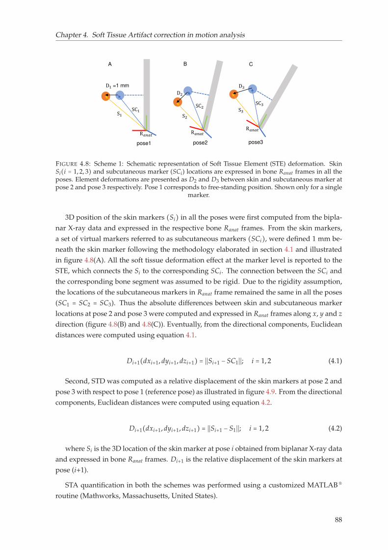
Chapter 4. Soft Tissue Artifact correction in motion analysis
pose1
D1 =1 mm
S1pose2
D2S2
pose3
S3D3
R𝑎𝑛𝑎𝑡 R𝑎𝑛𝑎𝑡 R𝑎𝑛𝑎𝑡
A B C
SC1 SC2 SC3
FIGURE 4.8: Scheme 1: Schematic representation of Soft Tissue Element (STE) deformation. SkinSi(i = 1, 2, 3) and subcutaneous marker (SCi) locations are expressed in bone Ranat frames in all theposes. Element deformations are presented as D2 and D3 between skin and subcutaneous marker atpose 2 and pose 3 respectively. Pose 1 corresponds to free-standing position. Shown only for a single
marker.
3D position of the skin markers (Si) in all the poses were first computed from the bipla-
nar X-ray data and expressed in the respective bone Ranat frames. From the skin markers,
a set of virtual markers referred to as subcutaneous markers (SCi), were defined 1 mm be-
neath the skin marker following the methodology elaborated in section 4.1 and illustrated
in figure 4.8(A). All the soft tissue deformation effect at the marker level is reported to the
STE, which connects the Si to the corresponding SCi. The connection between the SCi and
the corresponding bone segment was assumed to be rigid. Due to the rigidity assumption,
the locations of the subcutaneous markers in Ranat frame remained the same in all the poses
(SC1 = SC2 = SC3). Thus the absolute differences between skin and subcutaneous marker
locations at pose 2 and pose 3 were computed and expressed in Ranat frames along x, y and z
direction (figure 4.8(B) and 4.8(C)). Eventually, from the directional components, Euclidean
distances were computed using equation 4.1.
Di+1(dxi+1, dyi+1, dzi+1) = ∣∣Si+1 − SC1∣∣; i = 1, 2 (4.1)
Second, STD was computed as a relative displacement of the skin markers at pose 2 and
pose 3 with respect to pose 1 (reference pose) as illustrated in figure 4.9. From the directional
components, Euclidean distances were computed using equation 4.2.
Di+1(dxi+1, dyi+1, dzi+1) = ∣∣Si+1 − S1∣∣; i = 1, 2 (4.2)
where Si is the 3D location of the skin marker at pose i obtained from biplanar X-ray data
and expressed in bone Ranat frames. Di+1 is the relative displacement of the skin markers at
pose (i+1).
STA quantification in both the schemes was performed using a customized MATLAB ®
routine (Mathworks, Massachusetts, United States).
88
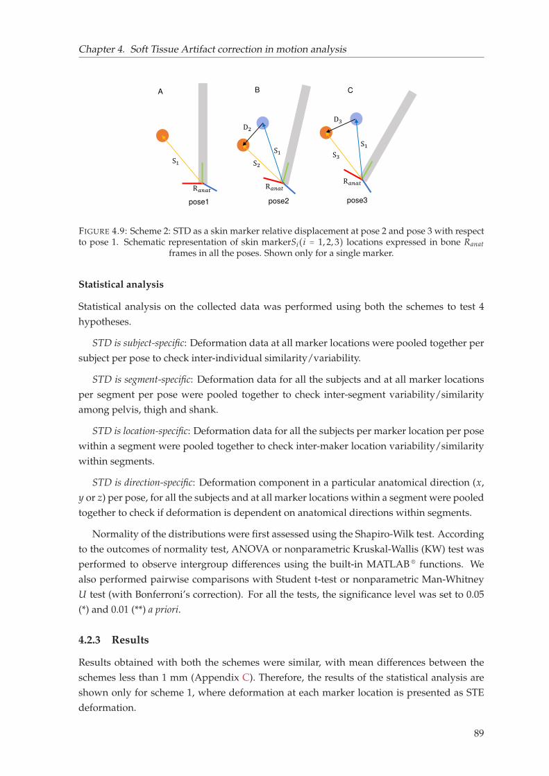
Chapter 4. Soft Tissue Artifact correction in motion analysis
pose1
S1pose2
S2pose3
S3R𝑎𝑛𝑎𝑡 R𝑎𝑛𝑎𝑡 R𝑎𝑛𝑎𝑡
A B C
S1D2 D3
S1
FIGURE 4.9: Scheme 2: STD as a skin marker relative displacement at pose 2 and pose 3 with respectto pose 1. Schematic representation of skin markerSi(i = 1, 2, 3) locations expressed in bone Ranat
frames in all the poses. Shown only for a single marker.
Statistical analysis
Statistical analysis on the collected data was performed using both the schemes to test 4
hypotheses.
STD is subject-specific: Deformation data at all marker locations were pooled together per
subject per pose to check inter-individual similarity/variability.
STD is segment-specific: Deformation data for all the subjects and at all marker locations
per segment per pose were pooled together to check inter-segment variability/similarity
among pelvis, thigh and shank.
STD is location-specific: Deformation data for all the subjects per marker location per pose
within a segment were pooled together to check inter-maker location variability/similarity
within segments.
STD is direction-specific: Deformation component in a particular anatomical direction (x,
y or z) per pose, for all the subjects and at all marker locations within a segment were pooled
together to check if deformation is dependent on anatomical directions within segments.
Normality of the distributions were first assessed using the Shapiro-Wilk test. According
to the outcomes of normality test, ANOVA or nonparametric Kruskal-Wallis (KW) test was
performed to observe intergroup differences using the built-in MATLAB ® functions. We
also performed pairwise comparisons with Student t-test or nonparametric Man-Whitney
U test (with Bonferroni’s correction). For all the tests, the significance level was set to 0.05
(*) and 0.01 (**) a priori.
4.2.3 Results
Results obtained with both the schemes were similar, with mean differences between the
schemes less than 1 mm (Appendix C). Therefore, the results of the statistical analysis are
shown only for scheme 1, where deformation at each marker location is presented as STE
deformation.
89
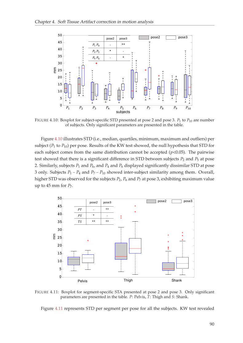
Chapter 4. Soft Tissue Artifact correction in motion analysis
mm
𝑃1 𝑃2 𝑃3 𝑃4 𝑃5 𝑃6 𝑃7 𝑃8 𝑃9 𝑃10subjects
pose2 pose3pose2 pose3𝑃1 𝑃6 - **𝑃2 𝑃5 * -𝑃4 𝑃6 - *
FIGURE 4.10: Boxplot for subject-specific STD presented at pose 2 and pose 3. P1 to P10 are numberof subjects. Only significant parameters are presented in the table.
Figure 4.10 illustrates STD (i.e., median, quartiles, minimum, maximum and outliers) per
subject (P1 to P10) per pose. Results of the KW test showed, the null hypothesis that STD for
each subject comes from the same distribution cannot be accepted (p<0.05). The pairwise
test showed that there is a significant difference in STD between subjects P2 and P5 at pose
2. Similarly, subjects P1 and P6, and P4 and P6 displayed significantly dissimilar STD at pose
3 only. Subjects P1 − P4 and P7 − P10 showed inter-subject similarity among them. Overall,
higher STD was observed for the subjects P2, P6 and P7 at pose 3, exhibiting maximum value
up to 45 mm for P7.
Pelvis Thigh Shank
mm
pose2 pose3𝑃𝑇 - **𝑃𝑆 * -𝑇𝑆 ** **
pose2 pose3
FIGURE 4.11: Boxplot for segment-specific STA presented at pose 2 and pose 3. Only significantparameters are presented in the table. P: Pelvis, T: Thigh and S: Shank.
Figure 4.11 represents STD per segment per pose for all the subjects. KW test revealed
90
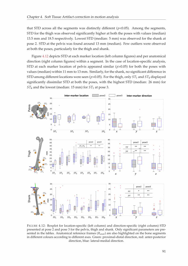
Chapter 4. Soft Tissue Artifact correction in motion analysis
that STD across all the segments was distinctly different (p<0.05). Among the segments,
STD for the thigh was observed significantly higher at both the poses with values (median)
13.5 mm and 18.5 respectively. Lowest STD (median: 5 mm) was observed for the shank at
pose 2. STD at the pelvis was found around 13 mm (median). Few outliers were observed
at both the poses, particularly for the thigh and shank.
Figure 4.12 depicts STD at each marker location (left column figures) and per anatomical
direction (right column figures) within a segment. In the case of location-specific analysis,
STD at each marker location of pelvis appeared similar (p>0.05) for both the poses with
values (median) within 11 mm to 13 mm. Similarly, for the shank, no significant difference in
STD among different locations were seen (p>0.05). For the thigh, only ST1 and ST4 displayed
significantly dissimilar STD at both the poses, with the highest STD (median: 26 mm) for
ST4 and the lowest (median: 15 mm) for ST1 at pose 3.
𝑆𝑃1 𝑆𝑃2 𝑆𝑃3 𝑆𝑃4
𝑆𝑇1 𝑆𝑇2 𝑆𝑇3 𝑆𝑇4 𝑆𝑇5 𝑆𝑇6 𝑆𝑇7 𝑆𝑇8
𝑆𝑆1 𝑆𝑆2 𝑆𝑆3 𝑆𝑆4 𝑆𝑆5 𝑆𝑆6 𝑆𝑆7 𝑆𝑆8
Inter-marker location Inter-marker direction
𝑥 𝑦 𝑧
𝑥 𝑦 𝑧
𝑥 𝑦 𝑧
pose2 pose3
pose2 pose3𝑆𝑇1 𝑆𝑇4 ** **
pose2 pose3𝑥𝑦 ** **𝑦𝑧 ** **
𝑆𝑃1 𝑆𝑃2
𝑆𝑃3 𝑆𝑃4
mm
𝑆𝑇1𝑆𝑇2 𝑆𝑇3
𝑆𝑇4
𝑆𝑇5𝑆𝑇6 𝑆𝑇7
𝑆𝑇8 mm
Thig
h
mm
Shank
𝑆𝑆1𝑆𝑆2𝑆𝑆3
𝑆𝑆4𝑆𝑆5𝑆𝑆6
𝑆𝑆7𝑆𝑆8
pose2 pose3𝑥𝑧 * **𝑦𝑧 ** **
Pelv
is
FIGURE 4.12: Boxplot for location-specific (left column) and direction-specific (right column) STDpresented at pose 2 and pose 3 for the pelvis, thigh and shank. Only significant parameters are pre-sented in the tables. Anatomical reference frames (Ranat) are also highlighted on the bone segmentsin different colours according to different axes. Green: proximal-distal direction, red: anter-posterior
direction, blue: lateral-medial direction.
91
Chapter 4. Soft Tissue Artifact correction in motion analysis
In the case of direction-specific analysis, a similar (p>0.05) STD was observed across the
three anatomical directions of the pelvis Ranat frame. STD along proximal-distal direction
of the thigh was observed distinctly higher in both the poses, while showing similar values
along antero-posterior and lateral-medial direction. STD at the shank was appeared simi-
lar along antero-posetrior and proximal-distal direction, while revealing significantly lower
values along the medial-lateral direction. Overall analysis showed higher STD at pose 3 as
compared to pose 2.
4.2.4 Discussion
In order to compensate for STA and to interpret SM-based motion analysis data, knowledge
of Soft Tissue Deformation (STD) pattern in three dimension (3D) is essential. Yet, there
is a paucity of reference data in the literature comprehensively showing variability of STD
among individuals, segments, marker locations and along the three anatomical directions.
The purpose of this study was to quantify STD in 3D at the pelvis, thigh and shank for 10
subjects. Two schemes were employed to quantity STD, although exhibited similar results.
The rationale behind employing two schemes is that both of them may serve two dif-
ferent communities; first, those particularly deal with compensation methods, and second
those deal with STD quantification. The first scheme intends to address conventional STA
compensation methods (such as MBO) that generally minimizes measured and model deter-
mined marker position. The subcutaneous markers are analogous to the model determined
markers. This approach could also be helpful for FE-based STA compensation method,
where a deformable element connecting the skin and subcutaneous marker accounts for
all soft tissue deformation (as detailed in section 4.1). The second scheme pertains to STD
quantification methods, where soft tissue deformation is considered as a relative displace-
ment of skin markers at different poses with respect to the reference pose.
Overall, soft tissue deformation displayed inter-subject similarity in most of the subjects
showing a similar STD pattern. Although such observation is in contrast to the current
prevailing idea of STD as subject-specific, yet found in accordance with one study which
explained overshadowing of similarity by dissimilarity for few subjects (Gao and Zheng,
2008). Secondly, segment-specific STD was observed exhibiting the highest deformation at
the thigh followed by the pelvis and the shank (Akbarshahi et al., 2010; Walker, 2015). A
similar observation was also reported in studies that measured higher kinematic error at the
thigh (Sangeux et al., 2006; Stagni et al., 2005).
STD at the pelvis and shank exhibited no inter-marker variability. For the thigh, the
marker (ST4) placed towards the hip joint showed significantly higher STD, where muscle
thickness is higher (Rouhandeh and Joslin, 2018). Except ST4, other markers at the displayed
similar STD.
STA occurred in all the three directions of the bone embedded anatomical frames, how-
ever not uniform for the thigh and shank in particular. Soft tissue deformation in proximal-
distal direction of the thigh and shank was distinctly higher. This is probably due to the
92
Chapter 4. Soft Tissue Artifact correction in motion analysis
orientation of the muscular structure of the thigh and shank, which contracts and relaxes
during movement along its length. Deformation in the medial-lateral direction was noticed
the lowest. A similar observation was also reported in the literature (Gao and Zheng, 2008).
This study, to the authors’ knowledge, is the second attempt to use EOS low dose system,
allowing to quantify STD in 3D. Previously, our group used EOS to investigate motion of
lower limb attachment systems with respect to the underlying bone (Südhoff et al., 2007). It
is to be noted that because of the limited acquisition volume within the EOS, markers present
in the radiographs were not consistent throughout the subjects. Few markers couldn’t be lo-
cated in the radiographs of some subjects either in the orthogonal views or in the consecutive
poses. Moreover, both due to limited acquisition volume and ethical reasons, the number
of poses had to be limited. Also, we acknowledge that STD reported in this study doesn’t
include inertial effects, as the movement under consideration was quasi-static. Quantified
STD is a consequence of both muscle contraction and skin sliding. Currently, other existing
methods, such as invasive attachments and fluoroscopic measurements, have been shown
useful to quantify soft tissue deformation. But, invasive methods are prone to alter free soft
tissue movement and therefore, may impact its results. Fluoroscopy is also not effective
for capturing the entire lower limb, although efficient for local observations in dynamics.
Hence, EOS in conjunction with skin markers can serve as a gold standard to locate actual
bone positions as well to quantify STD for a limited range of motion.
The findings in the study may open up effective STA compensation strategies for SM-
based motion analysis. Instead of assigning arbitrary STA correction stiffness, subjects with
similar STD patterns can be grouped together to assign the same correction stiffness. More-
over, for such quasi-static activities, all the markers at the pelvis can be grouped together to
assign the same stiffness values. Similar is the case for the shank. For the thigh, marker lo-
cations where STD was observed highest can be assigned with the lowest stiffness and vice
versa. To be noted that while assigning stiffness values for the thigh and shank, different
stiffness values need to be defined along different anatomical direction. In conclusion, al-
though the STD data provided in this study may be beneficial for future STA compensation
approaches, further study would be required in different dynamic activities.
93

Chapter 5
Clinical application: Preliminary
investigation
The contribution in the previous chapter allowed to develop and evaluate a novel FE-based
approach for soft tissue artifact (STA) compensation of the lower limb (first section). The
STA compensated kinematics revealed that the personalized FE models (geometry and bound-
ary condition) could effectively compensate for STA, although direct validation was not
possible. This work further led to proposing an effective STA compensation strategy that
would allow personalizing soft tissue stiffness properties based on experimentally acquired
soft tissue deformation pattern (second section).
It is noteworthy to mention that the personalization of the FE models was based on the
morphology of healthy population. Given the effectiveness of the model for STA compen-
sation, it is also essential to develop and evaluate models replicating patients’ morphology,
which may eventually lead to investigation of various surgical scenarios and outcomes. In
that direction, this chapter briefly describes a preliminary investigation on the utility of the
biplanar X-ray system in evaluating Total Knee Arthroplasty (TKA) implant alignment.
95
Chapter 5. Clinical application: Preliminary investigation
5.1 Utility of EOS system in evaluating TKA implant pose1
Abstract Total knee Arthroplasty (TKA) is a frequently performed surgical procedure interminal stage osteoarthritis (OA). However, patients still remain dissatisfied because of eitherpatient related factors (e.g., age, health) or surgical factors (e.g., implant design, alignment)leading to a revised TKA. Out of several factors affecting functional outcome of TKA, implantalignment is considered as a major contributor. To preoperatively plan for TKA implantation,surgeons normally use CT-scan images to align the implant components with respect to the3D alignment of femur and tibia. There are several standard alignment options available,from which a surgeon chooses one based on subjective assessment. However, there is nocomplete agreement on a particular procedure that can provide better functional outcome andimplant survivorship. It is now well known that apart from low dose irradiation, biplanarX-ray imaging allows image acquisition in weight-bearing positions unlike CT scans. Thisfacility could be advantageous in the sense that patients’ position may significantly impactlower limb alignment and thereby may affect the implant alignment process. In this regard,biplanar X-ray may ease the process of implant alignment as it is routinely used in clinics.The objective of this study is therefore to evaluate the utility of the biplanar X-ray systemin evaluating TKA implant alignment. In a first step, reproducibility of the TKA implantalignment process is evaluated in the current contribution.
12 patients operated with TKA were included in the study. All subjects underwent bi-planar radiography postoperatively and digital models of the implants were manually posi-tioned on the postoperative radiographs. The process was performed by 3 operators and interoperator reproducibility study was carried out on 3 rotational and 3 translation parametersfollowing the guidelines of the ISO 5725-2 standard.
Reproducibility of manual positioning for translation was less than 1 mm for both the im-plant components. For rotational parameters, less than or equal to 1.5° was observed for thefemoral component while revealing less than 3° for the tibial component. Overall, EOS imag-ing system showed a good reproducibility for evaluating knee prosthesis position. This studymay contribute to further investigation of global alignment of the TKA implant with respectto both lower limb and upper limb skeleton in order to provide an effective surgery planning.
Keywords: Biplanar X-ray, TKA implant alignment, surgery planning
5.1.1 Introduction
To regain functional mobility and relieve pain, Total Knee Arthroplasty (TKA) is often rec-
ommended at the later stage of Osteoarthritis (OA). An increase in 33% (more than 80000)
TKA cases were registered in the period 2008-2013 in France (Colas et al., 2016). In the
United States, it is expected to surpass 3 million TKA cases by the year 2030, with a hospital
cost of more than 2 billion dollars (Kurtz et al., 2007). With such increase in trends, number
of dissatisfied patients have been rising accordingly. Two studies reported that up to 20%
of the patients experienced sub-optimal satisfaction 1 year postoperatively, and 30-34% of
1Potential copyright issues with direct reuse of the article including figures and contents (article under prepa-ration)
96
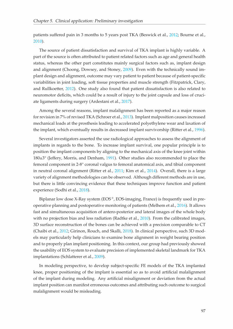
Chapter 5. Clinical application: Preliminary investigation
patients suffered pain in 3 months to 5 years post TKA (Beswick et al., 2012; Bourne et al.,
2010).
The source of patient dissatisfaction and survival of TKA implant is highly variable. A
part of the source is often attributed to patient related factors such as age and general health
status, whereas the other part constitutes mainly surgical factors such as, implant design
and alignment (Choong, Dowsey, and Stoney, 2009). Even with the technically sound im-
plant design and alignment, outcome may vary patient to patient because of patient-specific
variabilities in joint loading, soft tissue properties and muscle strength (Fitzpatrick, Clary,
and Rullkoetter, 2012). One study also found that patient dissatisfaction is also related to
neuromotor deficits, which could be a result of injury to the joint capsule and loss of cruci-
ate ligaments during surgery (Ardestani et al., 2017).
Among the several reasons, implant malalignment has been reported as a major reason
for revision in 7% of revised TKA (Schroer et al., 2013). Implant malposition causes increased
mechanical loads at the prosthesis leading to accelerated polyethylene wear and laxation of
the implant, which eventually results in decreased implant survivorship (Ritter et al., 1996).
Several investigators asserted the use radiological approaches to assess the alignment of
implants in regards to the bone. To increase implant survival, one popular principle is to
position the implant components by aligning to the mechanical axis of the knee joint within
180±3° (Jeffery, Morris, and Denham, 1991). Other studies also recommended to place the
femoral component in 2-8° coronal valgus to femoral anatomical axis, and tibial component
in neutral coronal alignment (Ritter et al., 2011; Kim et al., 2014). Overall, there is a large
variety of alignment methodologies can be observed. Although different methods are in use,
but there is little convincing evidence that these techniques improve function and patient
experience (Sodhi et al., 2018).
Biplanar low dose X-Ray system (EOS ®, EOS-imaging, France) is frequently used in pre-
operative planning and postoperative monitoring of patients (Melhem et al., 2016). It allows
fast and simultaneous acquisition of antero-posterior and lateral images of the whole body
with no projection bias and less radiation (Radtke et al., 2010). From the calibrated images,
3D surface reconstruction of the bones can be achieved with a precision comparable to CT
(Chaibi et al., 2012; Girinon, Rouch, and Skalli, 2018). In clinical perspective, such 3D mod-
els may particularly help clinicians to examine bone alignment in weight bearing position
and to properly plan implant positioning. In this context, our group had previously showed
the usability of EOS system to evaluate precision of implemented skeletal landmark for TKA
implantations (Schlatterer et al., 2009).
In modeling perspective, to develop subject-specific FE models of the TKA implanted
knee, proper positioning of the implant is essential so as to avoid artificial malalignment
of the implant during modeling. Any artificial misalignment or deviation from the actual
implant position can manifest erroneous outcomes and attributing such outcome to surgical
malalignment would be misleading.
97
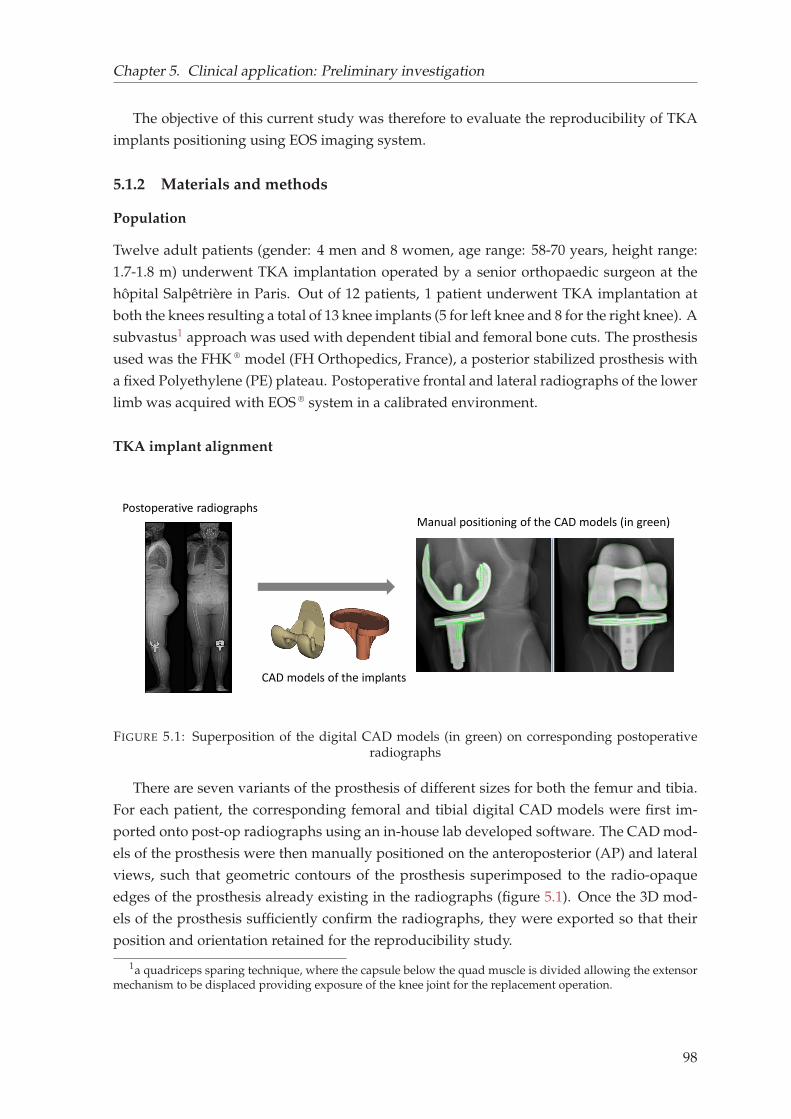
Chapter 5. Clinical application: Preliminary investigation
The objective of this current study was therefore to evaluate the reproducibility of TKA
implants positioning using EOS imaging system.
5.1.2 Materials and methods
Population
Twelve adult patients (gender: 4 men and 8 women, age range: 58-70 years, height range:
1.7-1.8 m) underwent TKA implantation operated by a senior orthopaedic surgeon at the
hôpital Salpêtrière in Paris. Out of 12 patients, 1 patient underwent TKA implantation at
both the knees resulting a total of 13 knee implants (5 for left knee and 8 for the right knee). A
subvastus1 approach was used with dependent tibial and femoral bone cuts. The prosthesis
used was the FHK ® model (FH Orthopedics, France), a posterior stabilized prosthesis with
a fixed Polyethylene (PE) plateau. Postoperative frontal and lateral radiographs of the lower
limb was acquired with EOS ® system in a calibrated environment.
TKA implant alignment
Postoperative radiographs
CAD models of the implants
Manual positioning of the CAD models (in green)
FIGURE 5.1: Superposition of the digital CAD models (in green) on corresponding postoperativeradiographs
There are seven variants of the prosthesis of different sizes for both the femur and tibia.
For each patient, the corresponding femoral and tibial digital CAD models were first im-
ported onto post-op radiographs using an in-house lab developed software. The CAD mod-
els of the prosthesis were then manually positioned on the anteroposterior (AP) and lateral
views, such that geometric contours of the prosthesis superimposed to the radio-opaque
edges of the prosthesis already existing in the radiographs (figure 5.1). Once the 3D mod-
els of the prosthesis sufficiently confirm the radiographs, they were exported so that their
position and orientation retained for the reproducibility study.
1a quadriceps sparing technique, where the capsule below the quad muscle is divided allowing the extensormechanism to be displaced providing exposure of the knee joint for the replacement operation.
98
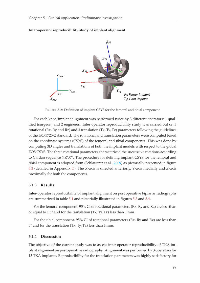
Chapter 5. Clinical application: Preliminary investigation
Inter-operator reproducibility study of implant alignment
𝑍𝐹𝑖
𝑌𝐹𝑖𝑋𝐹𝑖𝑍𝑇𝑖
𝑌𝑇𝑖𝑋𝑇𝑖 𝐹𝑖: Femur implant𝑇𝑖: Tibia Implant
𝑍𝑒𝑜𝑠𝑌𝑒𝑜𝑠𝑋𝑒𝑜𝑠EOS
FIGURE 5.2: Definition of implant CSYS for the femoral and tibial component
For each knee, implant alignment was performed twice by 3 different operators: 1 qual-
ified (surgeon) and 2 engineers. Inter operator reproducibility study was carried out on 3
rotational (Rx, Ry and Rz) and 3 translation (Tx, Ty, Tz) parameters following the guidelines
of the ISO 5725-2 standard. The rotational and translation parameters were computed based
on the coordinate systems (CSYS) of the femoral and tibial components. This was done by
computing 3D angles and translations of both the implant models with respect to the global
EOS CSYS. The three rotational parameters characterized the successive rotations according
to Cardan sequence YZ′X′′. The procedure for defining implant CSYS for the femoral and
tibial component is adopted from (Schlatterer et al., 2009) as pictorially presented in figure
5.2 (detailed in Appendix D). The X-axis is directed anteriorly, Y-axis medially and Z-axis
proximally for both the components.
5.1.3 Results
Inter-operator reproducibility of implant alignment on post operative biplanar radiographs
are summarized in table 5.1 and pictorially illustrated in figures 5.3 and 5.4.
For the femoral component, 95% CI of rotational parameters (Rx, Ry and Rz) are less than
or equal to 1.5° and for the translation (Tx, Ty, Tz) less than 1 mm.
For the tibial component, 95% CI of rotational parameters (Rx, Ry and Rz) are less than
3° and for the translation (Tx, Ty, Tz) less than 1 mm.
5.1.4 Discussion
The objective of the current study was to assess inter-operator reproducibility of TKA im-
plant alignment on postoperative radiographs. Alignment was performed by 3 operators for
13 TKA implants. Reproducibility for the translation parameters was highly satisfactory for
99
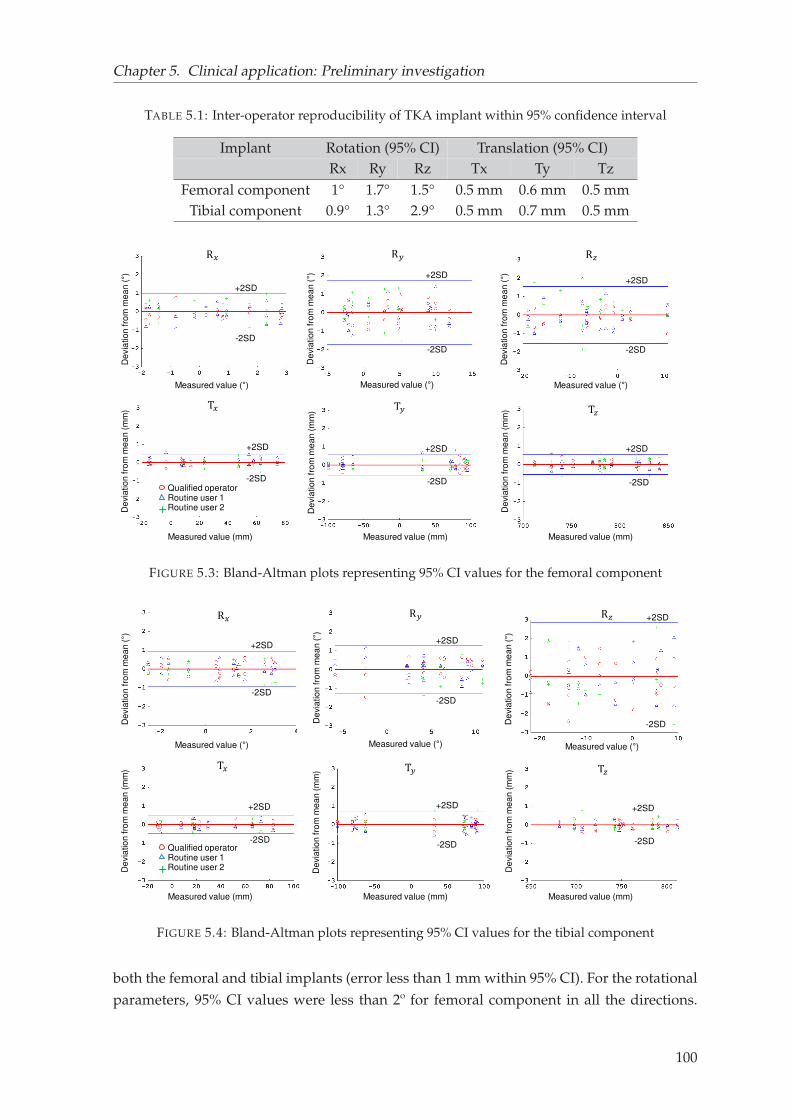
Chapter 5. Clinical application: Preliminary investigation
TABLE 5.1: Inter-operator reproducibility of TKA implant within 95% confidence interval
Implant Rotation (95% CI) Translation (95% CI)Rx Ry Rz Tx Ty Tz
Femoral component 1° 1.7° 1.5° 0.5 mm 0.6 mm 0.5 mmTibial component 0.9° 1.3° 2.9° 0.5 mm 0.7 mm 0.5 mm
T𝑧
De
via
tio
n fro
m m
ea
n (
mm
)
Measured value (mm)
T𝑦
De
via
tio
n fro
m m
ea
n (
mm
)
Measured value (mm)
T𝑥
De
via
tio
n fro
m m
ea
n (
mm
)
Measured value (mm)
R𝑥
De
via
tio
n fro
m m
ea
n (°)
Measured value (°)
R𝑦D
evia
tio
n fro
m m
ea
n (°)
Measured value (°)
R𝑧
De
via
tio
n fro
m m
ea
n (°)
Measured value (°)
Qualified operatorRoutine user 1Routine user 2+
+2SD
+2SD+2SD
+2SD +2SD +2SD
-2SD
-2SD -2SD
-2SD -2SD -2SD
FIGURE 5.3: Bland-Altman plots representing 95% CI values for the femoral component
T𝑧
De
via
tio
n fro
m m
ea
n (
mm
)
Measured value (mm)
T𝑦
De
via
tio
n fro
m m
ea
n (
mm
)
Measured value (mm)
T𝑥
De
via
tio
n fro
m m
ea
n (
mm
)
Measured value (mm)
R𝑥
De
via
tio
n fro
m m
ea
n (°)
Measured value (°)
R𝑦
De
via
tio
n fro
m m
ea
n (°)
Measured value (°)
R𝑧
De
via
tio
n fro
m m
ea
n (°)
Measured value (°)
Qualified operatorRoutine user 1Routine user 2+
+2SD+2SD
+2SD
+2SD +2SD +2SD
-2SD-2SD
-2SD
-2SD-2SD -2SD
FIGURE 5.4: Bland-Altman plots representing 95% CI values for the tibial component
both the femoral and tibial implants (error less than 1 mm within 95% CI). For the rotational
parameters, 95% CI values were less than 2º for femoral component in all the directions.
100
Chapter 5. Clinical application: Preliminary investigation
For the tibial component, more variation can be observed up to 2.9°, particularly about the
Z–axis, which represents rotation in the axial plane.
The reproducibility achieved on the postoperative radiographs are comparable to the
study of (Schlatterer et al., 2009), who performed alignment of the TKA using the bony
landmarks of the preoperative radiographs. The methodology they implemented was ad-
vantageous to select the skeletal landmarks as the preoperative radiographs do not contain
any bone cuts. Nevertheless, the reproducibility obtained in our study is in agreement with
them who reported less than less than 3° (95% CI) for the rotational parameters and less
than 1 mm (95% CI) for the translation parameters. Another study evaluated the reliability
of implant adjustment on the radiographs, which reported mean error less than 1° and a
maximum error of 1.1° (Langlois, 2003). Overall, the EOS system and the in-house lab de-
veloped software for 3D reconstruction and implant readjustment can be considered highly
reliable.
Such high degree of reproducibility will be advantageous for building personalized FE
models representing patients with TKA and to evaluate implant performance post-surgery.
This will open further opportunities to study the effect of different implant alignment method-
ologies on the implant performance by observing passive response. Nevertheless, further
studies will be necessary to correlate implant orientations with those of the bone segments
such as mechanical or anatomical axis of the knee joint.
101

General conclusion and perspectives
The musculoskeletal (MSK) system of the lower limb, the knee joint in particular, is a com-
plex system constituting bony structures, cartilages, ligaments, muscles and other connec-
tive tissues. It has a fundamental role to support the weight of the body and to produce con-
trolled and precise movement by inter-dependently coordinating among the constituents.
Repeated activities of daily life or any high impact exertion can inflict aberrant loads in the
joint, causing injuries to the bones and other soft tissues. Such mechanical burden disturbs
the overall stability of the entire limb and can further introduce joint degeneration (e.g.,
osteoarthritis), leading to partial or complete loss of functional activities.
In the clinical context, we observed that to restore the stability and mobility of the system,
various surgical management methods have been traditionally performed depending on the
degree of severity. One of the widespread surgical procedures for end-stage osteoarthritis
is Total Knee Arthroplasty (TKA). To perform TKA implantation, clinicians mostly prefer
geometric alignment techniques based on radiographic images as a preoperative planning.
Although implant positioning procedure has been improved with advanced surgical tools,
there is no complete unanimity on a particular method that works the best, and the implant
is still likely to fail under abnormal mechanical loads. As the knee joint elements do not
inherently function in isolation, understanding their interaction and their influence at the
joint seems logical for better surgical planning. In this aspect, we observed that personal-
ized FE modeling could be a promising avenue for assessing patient-specific joint mechanics
for different treatment scenarios. It was also apparent that to assess functional outcomes af-
ter surgical intervention, assessing the knee joint under in vivo loading conditions is crucial.
Further, we observed the importance of gait analysis to feed physiological boundary condi-
tions to the models. While prescribing physiological loading conditions in the models based
on skin marker-based motion data, the most prominent source of error in estimating joint
kinematics appeared as soft tissue artifact (STA). Such conclusions on broader clinical con-
text led to study relevant literature on FE modeling strategies, gait analysis and associated
musculoskeletal models, and various STA compensation strategies in the context of current
challenges and opportunities.
In the literature, a large body of work on FE models, FE-MSK models could be seen
to estimate various quantities of interests that cannot be easily obtained with experimental
studies. Nevertheless, numerous challenges appeared in the model development and evalu-
ation approaches. One of the critical challenges we observed was obtaining fast and accurate
103
General conclusion and perspectives
finite element mesh from medical images. Another prominent challenge appeared as adopt-
ing a computationally inexpensive approach for subject-specific FE model development and
validation focusing on personalized geometry and ligament material properties. The third
key challenge was devising a effective STA compensation strategy. Owing to such hurdles,
translating models to clinically relevant tools remains a major bottleneck, and therefore the
existing models could hardly be seen used in routine clinics. This motivated the need for
developing a FE-MSK modeling framework by taking the aforementioned challenges into
account.
Based on the identified challenges, the first phase of the thesis focused on fast subject-
specific finite element mesh generation of the knee joint from biplanar X-ray images. This
study enabled to generate hexahedral mesh for the femur, tibia and patella from the 3D
reconstruction of 11 cadaveric specimens. The whole procedure from 3D reconstruction to
mesh generation took 12 minutes of computational time per specimen. Mesh quality and
surface representation accuracy were highly satisfactory. This contribution paved the way
to reliably investigate inter-individual variability of the knee joint passive elements and its
effect on joint kinematics.
In estimating subject-specific knee joint kinematics under passive flexion, this study con-
fronted a significant challenge of personalizing soft-tissue properties, particularly the lig-
aments. As the existing optimization approaches are computationally expensive, a new
procedure to estimate specimen-specific ligament material property (prestrain) was pro-
posed and evaluated on 6 cadaveric specimens. Subject- and ligament-specific prestrain
values were directly computed from the experimental study and implemented in the cor-
responding FE models to estimate joint kinematics. Subject-specific model evaluation was
performed by comparing predicted femorotibial kinematics with the in vitro response of the
corresponding specimens. The experimental-numerical agreement was found highly sat-
isfactory and in-line with the literature. In vitro validation of the FE models served as an
intermediate step necessary for further transforming the model towards in vivo loads. This
contribution opened up gateways to use simplified yet relevant model development strate-
gies towards personalized FE modeling.
The second phase of the PhD focused on development and evaluation of a novel FE-
based STA compensation approach. In this context, a conceptual FE model of the lower
limb was proposed to showcase the model’s capability to minimize STA. The model was
implemented on 66 subjects, and the results of the personalized FE models revealed promis-
ing and in agreement with the literature. The model’s unique feature was its versatility to
take subject-, task-, and marker location-specific soft tissue deformation into account, thus
emphasizing the need for a proper understanding of soft tissue deformation at different
marker locations so as to facilitate better compensation strategies.
Therefore, in a continuation of the aforementioned work, experimental quantification of
soft tissue deformation was performed using biplanar imaging. This contribution enhanced
104
General conclusion and perspectives
the knowledge of the distribution of soft tissue deformation among individuals and differ-
ent marker locations. When integrated into the STA compensation scheme, such insightful
information on soft tissue deformation may provide more reliable and clinically relevant
results.
The third phase of the thesis was dedicated to clinical application, in which utility of
the biplanar X-ray system in positioning the Total Knee Arthroplasty (TKA) implant was
briefly explored. The implemented methodology, although manual, was found highly re-
producible. This contribution opened ways to develop subject-specific knee joints FE mod-
els with TKA implants and study how implant alignment influences joint mechanics. In a
step forward, the interaction of the implant with other elements of the knee joint during
daily activities can be studied.
In conclusion, the objectives undertaken during the PhD appeared to be necessary for
developing a comprehensive framework of FE-MSK modeling. Nevertheless, to develop a
full-fledged FE-MSK model, integrating muscles to the existing model is essential to drive
the model with actuated muscles following the pipeline of inverse and forward dynamics.
In that direction future work will be necessary and the framework developed for the FE-
MSK modeling in the current study will provide a strong base.
105
Appendix A
Sources of errors in gait analysis
Only the first two sources of errors are described here, as because the third source of error
(STA) is explained in the main text elaborately.
The instrumental error arises as a result of instrumental noise and volume calibration in-
accuracies. Using different filtering methods, number of cameras, and volume calibration
algorithms, contribution of this error to the total error can substantially be decreased and
often considered negligible (Surer and Kose, 2011).
The second source of error arises from difficulty in placing the markers accurately in re-
gards to specific anatomical landmarks. This needs proper expertise, and at many times the
landmarks are not easily palpable for patients with musculoskeletal disorders and even for
healthy subjects with excessive soft tissues. For instance, conventional gait models (CGM)
establish the medial-lateral axis of the knee based on markers placed on medial and lateral
epicondyles, or sometimes from the position of knee alignment devices (KAD) (Davis and
DeLuca, 1996). Any discrepancy between marker position and bony landmarks eventually
leads to erroneous estimation of joint centers and other kinematic parameters. Both func-
tional and predictive methods have been proposed to circumvent this problem. Functional
methods aim at the estimation of subject-specific joint centers/axes by using movement
data of adjacent segments relative to marker cluster motion. Conversely, predictive meth-
ods (regression-based approaches) have been recommended in situations when the range of
motion is restricted, particularly for patients with cerebral palsy (Assi et al., 2016). Never-
theless, accuracy of both the approaches been greatly enhanced by the use biplanar X-ray
system (EOS, EOS imaging, France), as it allows accurate static calibration between bones
and skin markers at patient’s standing position (Assi et al., 2016; Pillet et al., 2014; Sauret
et al., 2016). Using 3D reconstructions acquired from biplanar images, an average accuracy
of 2.9 mm was achieved (Pillet et al., 2014) in comparison to non-image-based methods re-
porting 13 mm to 30 mm of accuracy in locating hip joint center (Sangeux, Peters, and Baker,
2011). With such advancement in techniques and medical imaging facilities, this source of
error has been substantially reduced.
106
Appendix B
Various TKA alignment
state-of-the-art approaches
Table B.1 presents an overview of some of the mostly used state-of-the-art approaches for
TKA implant alignment and current controversies.
Amount of corrections for osteotomy, optimal implant size and type, and alignment of
implant components are important surgical factors that a clinician must determine for a suc-
cessful surgery. Normally, two main types of implants: constrained (or hinged) and uncon-
strained are used (Lemaire and Witvoet, 2002). Constrained implants are used for patients
with damaged ligaments, where the femur and the tibial components are linked together
with a hinge mechanism. Unconstrained implants offer nearly physiological movements
(e.g., varus/valgus and internal/external rotation). Depending on the type and size of the
implant, preoperative assessment of the knee in the three spatial planes is normally per-
formed for successful implant positioning.
One popular principle is to position the implant components by aligning to the mechan-
ical axis of the knee joint within 180±3° (Jeffery, Morris, and Denham, 1991). For mechanical
alignment of the femur, normally intramedullary (IM) guide is used, yet there is controversy
between intramedullary and extramedullary (EM) methods for the tibial alignment (Bansal
et al., 2020). One study found IM guide to be more accurate on 103 primary TKA cases
(Cashman et al., 2011), whereas comparable results were obtained between those two tech-
niques by another study performed on 350 TKA (Zeng et al., 2015). Nevertheless, all these
studies considered mechanical alignment as a gold standard. Conversely, no association be-
tween mechanical alignment and implant survival was observed in a study on 398 primary
TKA cases (Parratte et al., 2010). Another study also recommended anatomical alignment of
implants, which reported better implant durability for 3048 primary cases (Kim et al., 2014).
The concept of mechanical alignment has also been challenged by another study (Howell
et al., 2001). This study observed encouraging implant survivorship (up to 10 years) and
functional outcomes on kinematically aligned knees performed on 220 cases. Moreover,
studies based on kinematic alignment claimed that it can restore native knee alignment by
aligning rotational axes of the implant components to the kinematic axes of the knee joint
(Dossett et al., 2014). Patient specific instrumentation (PSI) has also been recently used as
107
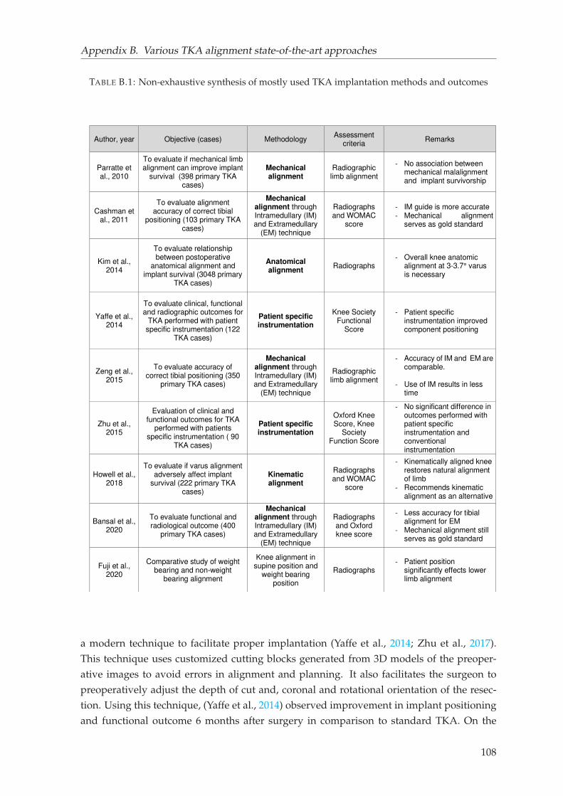
Appendix B. Various TKA alignment state-of-the-art approaches
TABLE B.1: Non-exhaustive synthesis of mostly used TKA implantation methods and outcomes
Author, year Objective (cases) Methodology Assessment
criteria Remarks
Parratte et al., 2010
To evaluate if mechanical limb alignment can improve implant
survival (398 primary TKA cases)
Mechanical alignment
Radiographic limb alignment
- No association between mechanical malalignment and implant survivorship
Cashman et al., 2011
To evaluate alignment accuracy of correct tibial
positioning (103 primary TKA cases)
Mechanical alignment through Intramedullary (IM) and Extramedullary
(EM) technique
Radiographs and WOMAC
score
- IM guide is more accurate - Mechanical alignment
serves as gold standard
Kim et al., 2014
To evaluate relationship between postoperative
anatomical alignment and implant survival (3048 primary
TKA cases)
Anatomical alignment
Radiographs - Overall knee anatomic
alignment at 3-3.7° varus is necessary
Yaffe et al., 2014
To evaluate clinical, functional and radiographic outcomes for
TKA performed with patient specific instrumentation (122
TKA cases)
Patient specific instrumentation
Knee Society Functional
Score
- Patient specific instrumentation improved component positioning
Zeng et al., 2015
To evaluate accuracy of correct tibial positioning (350
primary TKA cases)
Mechanical alignment through Intramedullary (IM) and Extramedullary
(EM) technique
Radiographic limb alignment
- Accuracy of IM and EM are comparable.
- Use of IM results in less
time
Zhu et al., 2015
Evaluation of clinical and functional outcomes for TKA
performed with patients specific instrumentation ( 90
TKA cases)
Patient specific instrumentation
Oxford Knee Score, Knee
Society Function Score
- No significant difference in outcomes performed with patient specific instrumentation and conventional instrumentation
Howell et al., 2018
To evaluate if varus alignment adversely affect implant
survival (222 primary TKA cases)
Kinematic alignment
Radiographs and WOMAC
score
- Kinematically aligned knee restores natural alignment of limb
- Recommends kinematic alignment as an alternative
Bansal et al., 2020
To evaluate functional and radiological outcome (400
primary TKA cases)
Mechanical alignment through Intramedullary (IM) and Extramedullary
(EM) technique
Radiographs and Oxford knee score
- Less accuracy for tibial alignment for EM
- Mechanical alignment still serves as gold standard
Fuji et al., 2020
Comparative study of weight bearing and non-weight
bearing alignment
Knee alignment in supine position and
weight bearing position
Radiographs - Patient position
significantly effects lower limb alignment
a modern technique to facilitate proper implantation (Yaffe et al., 2014; Zhu et al., 2017).
This technique uses customized cutting blocks generated from 3D models of the preoper-
ative images to avoid errors in alignment and planning. It also facilitates the surgeon to
preoperatively adjust the depth of cut and, coronal and rotational orientation of the resec-
tion. Using this technique, (Yaffe et al., 2014) observed improvement in implant positioning
and functional outcome 6 months after surgery in comparison to standard TKA. On the
108

Appendix B. Various TKA alignment state-of-the-art approaches
other hand, no significant improvement in clinical and functional outcome was found be-
tween PSI and standard instrumentation in another study (Zhu et al., 2017). Patient position
was also found to have significant influence on alignment accuracy, reporting differences in
alignment between weight bearing and supine position (Fujii et al., 2020).
109
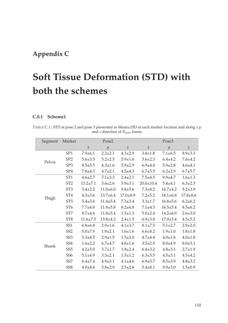
Appendix C
Soft Tissue Deformation (STD) with
both the schemes
C.0.1 Scheme1
TABLE C.1: STD at pose 2 and pose 3 presented as Mean±1SD at each marker location and along x,yand z direction of Ranat frame
Segment Marker Pose2 Pose3x y z x y z
Pelvis
SP1 7.9±6.1 2.2±2.1 4.3±2.9 3.8±1.8 7.1±6.5 8.9±3.3SP2 5.6±3.5 5.2±2.5 5.9±1.6 3.6±2.3 6.4±4.2 7.6±4.2SP3 8.5±5.5 4.3±1.6 5.9±2.9 6.9±4.4 5.9±2.8 4.6±4.1SP4 7.8±4.3 4.7±2.1 4.5±4.3 6.7±5.5 6.2±2.9 6.7±5.7
Thigh
ST1 4.6±2.7 7.1±3.3 2.4±2.1 7.5±4.5 9.9±4.7 1.6±1.3ST2 13.2±7.1 3.6±2.6 5.9±3.1 20.0±10.4 5.4±4.1 6.3±2.3ST3 3.4±2.2 11.0±6.0 9.8±5.6 7.3±8.2 16.7±4.2 5.2±3.9ST4 4.3±3.6 13.7±6.4 17.0±8.9 7.2±5.2 18.1±6.8 17.8±8.6ST5 5.4±3.6 11.4±5.4 7.3±3.4 3.3±1.7 16.8±5.6 6.2±6.2ST6 7.7±4.8 11.9±5.8 8.2±6.8 7.1±4.3 16.5±5.4 8.5±6.2ST7 8.7±4.6 11.8±5.4 1.5±1.3 5.0±2.4 14.2±6.9 2.6±3.0ST8 11.6±7.5 13.8±4.2 2.4±1.5 6.9±3.8 17.0±3.4 4.5±5.2
Shank
SS1 6.8±6.8 2.9±1.6 4.1±3.7 8.1±7.5 5.1±2.7 2.9±2.0SS2 5.0±7.9 1.9±2.1 1.6±1.6 6.6±8.2 1.9±1.0 1.8±1.8SS3 3.3±4.5 2.9±1.5 1.5±2.0 4.7±4.4 4.0±1.6 4.0±1.8SS4 1.6±2.2 6.7±4.7 4.0±1.6 3.5±2.9 8.0±4.9 8.0±5.1SS5 4.2±5.0 3.7±1.7 1.8±2.4 6.4±3.2 4.8±3.1 2.7±1.9SS6 5.1±4.9 3.3±2.1 1.5±1.2 6.3±5.5 4.5±3.1 4.5±4.2SS7 6.4±7.4 4.9±3.1 4.1±4.6 6.9±5.7 8.5±3.9 4.8±3.2SS8 4.0±4.4 5.8±2.9 2.5±2.6 5.4±8.1 9.9±3.0 1.5±0.9
110
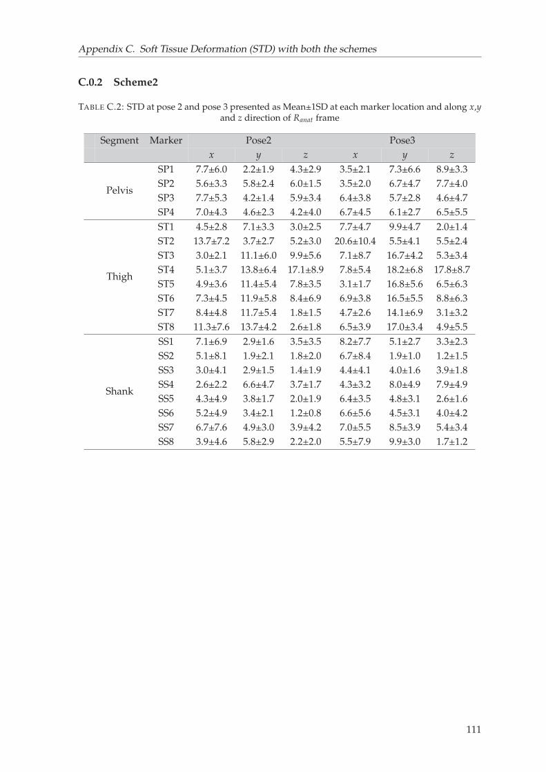
Appendix C. Soft Tissue Deformation (STD) with both the schemes
C.0.2 Scheme2
TABLE C.2: STD at pose 2 and pose 3 presented as Mean±1SD at each marker location and along x,yand z direction of Ranat frame
Segment Marker Pose2 Pose3x y z x y z
Pelvis
SP1 7.7±6.0 2.2±1.9 4.3±2.9 3.5±2.1 7.3±6.6 8.9±3.3SP2 5.6±3.3 5.8±2.4 6.0±1.5 3.5±2.0 6.7±4.7 7.7±4.0SP3 7.7±5.3 4.2±1.4 5.9±3.4 6.4±3.8 5.7±2.8 4.6±4.7SP4 7.0±4.3 4.6±2.3 4.2±4.0 6.7±4.5 6.1±2.7 6.5±5.5
Thigh
ST1 4.5±2.8 7.1±3.3 3.0±2.5 7.7±4.7 9.9±4.7 2.0±1.4ST2 13.7±7.2 3.7±2.7 5.2±3.0 20.6±10.4 5.5±4.1 5.5±2.4ST3 3.0±2.1 11.1±6.0 9.9±5.6 7.1±8.7 16.7±4.2 5.3±3.4ST4 5.1±3.7 13.8±6.4 17.1±8.9 7.8±5.4 18.2±6.8 17.8±8.7ST5 4.9±3.6 11.4±5.4 7.8±3.5 3.1±1.7 16.8±5.6 6.5±6.3ST6 7.3±4.5 11.9±5.8 8.4±6.9 6.9±3.8 16.5±5.5 8.8±6.3ST7 8.4±4.8 11.7±5.4 1.8±1.5 4.7±2.6 14.1±6.9 3.1±3.2ST8 11.3±7.6 13.7±4.2 2.6±1.8 6.5±3.9 17.0±3.4 4.9±5.5
Shank
SS1 7.1±6.9 2.9±1.6 3.5±3.5 8.2±7.7 5.1±2.7 3.3±2.3SS2 5.1±8.1 1.9±2.1 1.8±2.0 6.7±8.4 1.9±1.0 1.2±1.5SS3 3.0±4.1 2.9±1.5 1.4±1.9 4.4±4.1 4.0±1.6 3.9±1.8SS4 2.6±2.2 6.6±4.7 3.7±1.7 4.3±3.2 8.0±4.9 7.9±4.9SS5 4.3±4.9 3.8±1.7 2.0±1.9 6.4±3.5 4.8±3.1 2.6±1.6SS6 5.2±4.9 3.4±2.1 1.2±0.8 6.6±5.6 4.5±3.1 4.0±4.2SS7 6.7±7.6 4.9±3.0 3.9±4.2 7.0±5.5 8.5±3.9 5.4±3.4SS8 3.9±4.6 5.8±2.9 2.2±2.0 5.5±7.9 9.9±3.0 1.7±1.2
111
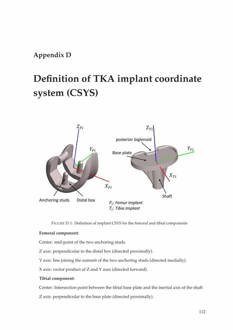
Appendix D
Definition of TKA implant coordinate
system (CSYS)
𝐹𝑖: Femur implant𝑇𝑖: Tibia Implant
𝑍𝑇𝑖𝑌𝑇𝑖
𝑋𝑇𝑖
𝑍𝐹𝑖𝑌𝐹𝑖
𝑋𝐹𝑖Anchoring studs Distal box
Base plate
posterior biglenoid
Shaft
FIGURE D.1: Definition of implant CSYS for the femoral and tibial components
Femoral component:
Center: mid-point of the two anchoring studs.
Z axis: perpendicular to the distal box (directed proximally).
Y axis: line joining the summit of the two anchoring studs (directed medially).
X axis: vector product of Z and Y axes (directed forward).
Tibial component:
Center: Intersection point between the tibial base plate and the inertial axis of the shaft
Z axis: perpendicular to the base plate (directed proximally).
112

Appendix D. Definition of TKA implant coordinate system (CSYS)
Y axis: Parallel to the posterior biglenoid and perpendicular to Z axis (directed medially).
X axis: vector product of Z and Y axes (directed forward).
113
Bibliography
Abulhasan, Jawad F and Michael J Grey (2017). “Anatomy and physiology of knee stability”.
In: Journal of Functional Morphology and kinesiology 2.4, p. 34.
Adouni, M and A Shirazi-Adl (2009). “Knee joint biomechanics in closed-kinetic-chain ex-
ercises”. In: Computer Methods in Biomechanics and Biomedical Engineering 12.6, pp. 661–
670.
Adouni, M, A Shirazi-Adl, and R Shirazi (2012). “Computational biodynamics of human
knee joint in gait: from muscle forces to cartilage stresses”. In: Journal of biomechanics
45.12, pp. 2149–2156.
Akbarshahi, Massoud et al. (2010). “Non-invasive assessment of soft-tissue artifact and its
effect on knee joint kinematics during functional activity”. In: Journal of biomechanics 43.7,
pp. 1292–1301.
Ali, Azhar A et al. (2016). “Validation of predicted patellofemoral mechanics in a finite el-
ement model of the healthy and cruciate-deficient knee”. In: Journal of biomechanics 49.2,
pp. 302–309.
Amiri, Shahram et al. (2006). “Mechanics of the passive knee joint. Part 1: the role of the
tibial articular surfaces in guiding the passive motion”. In: Proceedings of the Institution of
Mechanical Engineers, Part H: Journal of Engineering in Medicine 220.8, pp. 813–822.
Anderson, Frank C and Marcus G Pandy (2003). “Individual muscle contributions to sup-
port in normal walking”. In: Gait & posture 17.2, pp. 159–169.
Andriacchi, Thomas P and Eugene J Alexander (2000). “Studies of human locomotion: past,
present and future”. In: Journal of biomechanics 33.10, pp. 1217–1224.
Andriacchi, TP et al. (1998). “A point cluster method for in vivo motion analysis: applied to
a study of knee kinematics”. In:
Ardestani, Marzieh M et al. (2017). “TKA patients with unsatisfying knee function show
changes in neuromotor synergy pattern but not joint biomechanics”. In: Journal of Elec-
tromyography and Kinesiology 37, pp. 90–100.
Assi, Ayman et al. (2016). “Validation of hip joint center localization methods during gait
analysis using 3D EOS imaging in typically developing and cerebral palsy children”. In:
Gait & Posture 48, pp. 30–35.
Ateshian, Gerard A, Benjamin J Ellis, and Jeffrey A Weiss (2007). “Equivalence between
short-time biphasic and incompressible elastic material responses”. In:
Aunan, Eirik et al. (2012). “A new method to measure ligament balancing in total knee
arthroplasty: laxity measurements in 100 knees”. In: Archives of orthopaedic and trauma
surgery 132.8, pp. 1173–1181.
114
Bibliography
Azmy, C et al. (2010). “EOS® orthopaedic imaging system to study patellofemoral kinemat-
ics: Assessment of uncertainty”. In: Orthopaedics & Traumatology: Surgery & Research 96.1,
pp. 28–36.
Baker, Richard (2006). “Gait analysis methods in rehabilitation”. In: Journal of neuroengineer-
ing and rehabilitation 3.1, p. 4.
Baldwin, Mark A et al. (2009). “Verification of predicted specimen-specific natural and im-
planted patellofemoral kinematics during simulated deep knee bend”. In: Journal of biome-
chanics 42.14, pp. 2341–2348.
Baldwin, Mark A et al. (2012). “Dynamic finite element knee simulation for evaluation of
knee replacement mechanics”. In: Journal of biomechanics 45.3, pp. 474–483.
Bansal, Mohit R et al. (2020). “Tibial alignment technique and its influence on clinical and
functional outcomes following total knee arthroplasty”. In: Journal of Clinical Orthopaedics
and Trauma.
basic medical. URL: https://basicmedicalkey.com/lower-limb-2/.
Beidokhti, Hamid Naghibi et al. (2017). “The influence of ligament modelling strategies on
the predictive capability of finite element models of the human knee joint”. In: Journal of
biomechanics 65, pp. 1–11.
Belvedere, Claudio et al. (2012). “Geometrical changes of knee ligaments and patellar tendon
during passive flexion”. In: Journal of biomechanics 45.11, pp. 1886–1892.
Bendjaballah, MZea, A Shirazi-Adl, and DJ Zukor (1997). “Finite element analysis of human
knee joint in varus-valgus”. In: Clinical biomechanics 12.3, pp. 139–148.
Benoit, Daniel L et al. (2006). “Effect of skin movement artifact on knee kinematics during
gait and cutting motions measured in vivo”. In: Gait & posture 24.2, pp. 152–164.
Bergamini, Elena et al. (2011). “Tibio-femoral joint constraints for bone pose estimation dur-
ing movement using multi-body optimization”. In: Gait & posture 33.4, pp. 706–711.
Beswick, Andrew David et al. (2012). “What proportion of patients report long-term pain
after total hip or knee replacement for osteoarthritis? A systematic review of prospective
studies in unselected patients”. In: BMJ open 2.1.
Bicer, Elcil Kaya et al. (2010). “Current knowledge in the anatomy of the human anterior
cruciate ligament”. In: Knee surgery, sports traumatology, arthroscopy 18.8, pp. 1075–1084.
Blagojevic, M et al. (2010). “Risk factors for onset of osteoarthritis of the knee in older adults:
a systematic review and meta-analysis”. In: Osteoarthritis and cartilage 18.1, pp. 24–33.
Blankevoort, L. and R. Huiskes (1991). “Ligament-Bone Interaction in a Three-Dimensional
Model of the Knee”. In: Journal of Biomechanical Engineering 113.3, pp. 263–269.
Blankevoort, Leendert and Rik Huiskes (1996). “Validation of a three-dimensional model of
the knee”. In: Journal of biomechanics 29.7, pp. 955–961.
Bolcos, Paul O et al. (2018). “Comparison between kinetic and kinetic-kinematic driven knee
joint finite element models”. In: Scientific reports 8.1, pp. 1–11.
Bourne, Robert B et al. (2010). “Patient satisfaction after total knee arthroplasty: who is sat-
isfied and who is not?” In: Clinical Orthopaedics and Related Research® 468.1, pp. 57–63.
Brand, Richard A (1989). “Can biomechanics contribute to clinical orthopaedic assessments?”
In: The Iowa Orthopaedic Journal 9, p. 61.
115
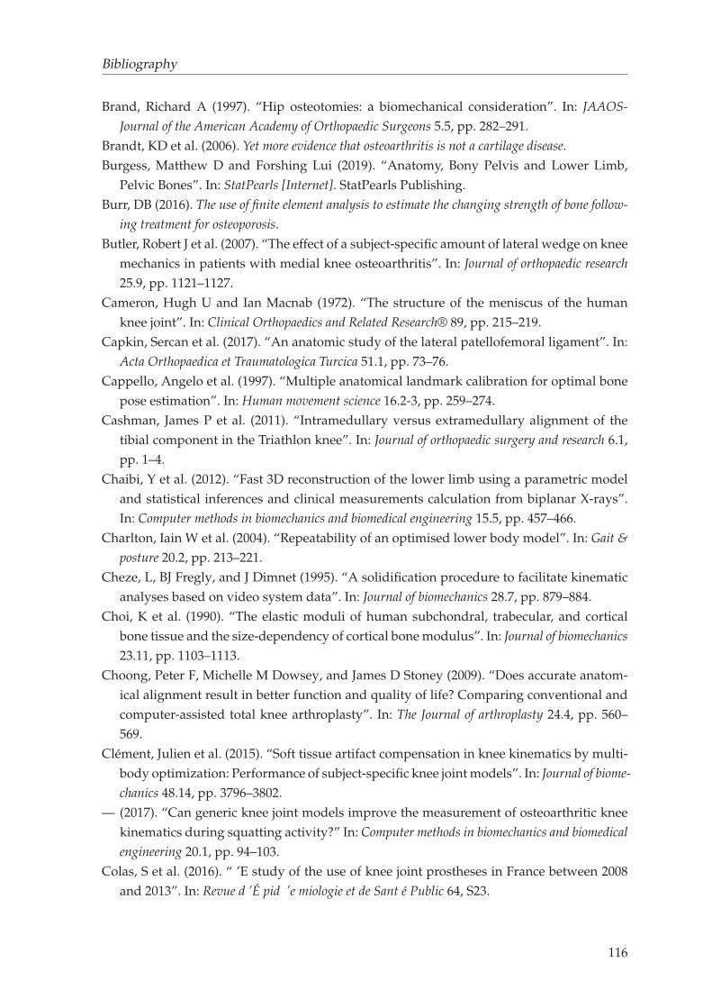
Bibliography
Brand, Richard A (1997). “Hip osteotomies: a biomechanical consideration”. In: JAAOS-
Journal of the American Academy of Orthopaedic Surgeons 5.5, pp. 282–291.
Brandt, KD et al. (2006). Yet more evidence that osteoarthritis is not a cartilage disease.
Burgess, Matthew D and Forshing Lui (2019). “Anatomy, Bony Pelvis and Lower Limb,
Pelvic Bones”. In: StatPearls [Internet]. StatPearls Publishing.
Burr, DB (2016). The use of finite element analysis to estimate the changing strength of bone follow-
ing treatment for osteoporosis.
Butler, Robert J et al. (2007). “The effect of a subject-specific amount of lateral wedge on knee
mechanics in patients with medial knee osteoarthritis”. In: Journal of orthopaedic research
25.9, pp. 1121–1127.
Cameron, Hugh U and Ian Macnab (1972). “The structure of the meniscus of the human
knee joint”. In: Clinical Orthopaedics and Related Research® 89, pp. 215–219.
Capkin, Sercan et al. (2017). “An anatomic study of the lateral patellofemoral ligament”. In:
Acta Orthopaedica et Traumatologica Turcica 51.1, pp. 73–76.
Cappello, Angelo et al. (1997). “Multiple anatomical landmark calibration for optimal bone
pose estimation”. In: Human movement science 16.2-3, pp. 259–274.
Cashman, James P et al. (2011). “Intramedullary versus extramedullary alignment of the
tibial component in the Triathlon knee”. In: Journal of orthopaedic surgery and research 6.1,
pp. 1–4.
Chaibi, Y et al. (2012). “Fast 3D reconstruction of the lower limb using a parametric model
and statistical inferences and clinical measurements calculation from biplanar X-rays”.
In: Computer methods in biomechanics and biomedical engineering 15.5, pp. 457–466.
Charlton, Iain W et al. (2004). “Repeatability of an optimised lower body model”. In: Gait &
posture 20.2, pp. 213–221.
Cheze, L, BJ Fregly, and J Dimnet (1995). “A solidification procedure to facilitate kinematic
analyses based on video system data”. In: Journal of biomechanics 28.7, pp. 879–884.
Choi, K et al. (1990). “The elastic moduli of human subchondral, trabecular, and cortical
bone tissue and the size-dependency of cortical bone modulus”. In: Journal of biomechanics
23.11, pp. 1103–1113.
Choong, Peter F, Michelle M Dowsey, and James D Stoney (2009). “Does accurate anatom-
ical alignment result in better function and quality of life? Comparing conventional and
computer-assisted total knee arthroplasty”. In: The Journal of arthroplasty 24.4, pp. 560–
569.
Clément, Julien et al. (2015). “Soft tissue artifact compensation in knee kinematics by multi-
body optimization: Performance of subject-specific knee joint models”. In: Journal of biome-
chanics 48.14, pp. 3796–3802.
— (2017). “Can generic knee joint models improve the measurement of osteoarthritic knee
kinematics during squatting activity?” In: Computer methods in biomechanics and biomedical
engineering 20.1, pp. 94–103.
Colas, S et al. (2016). “ ’E study of the use of knee joint prostheses in France between 2008
and 2013”. In: Revue d ’É pid ’e miologie et de Sant é Public 64, S23.
116
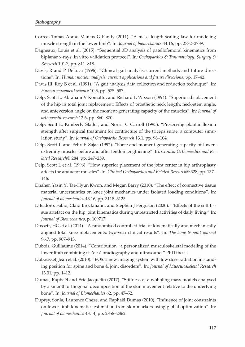
Bibliography
Correa, Tomas A and Marcus G Pandy (2011). “A mass–length scaling law for modeling
muscle strength in the lower limb”. In: Journal of biomechanics 44.16, pp. 2782–2789.
Dagneaux, Louis et al. (2015). “Sequential 3D analysis of patellofemoral kinematics from
biplanar x-rays: In vitro validation protocol”. In: Orthopaedics & Traumatology: Surgery &
Research 101.7, pp. 811–818.
Davis, R and P DeLuca (1996). “Clinical gait analysis: current methods and future direc-
tions”. In: Human motion analysis: current applications and future directions, pp. 17–42.
Davis III, Roy B et al. (1991). “A gait analysis data collection and reduction technique”. In:
Human movement science 10.5, pp. 575–587.
Delp, Scott L, Abraham V Komattu, and Richard L Wixson (1994). “Superior displacement
of the hip in total joint replacement: Effects of prosthetic neck length, neck-stem angle,
and anteversion angle on the moment-generating capacity of the muscles”. In: Journal of
orthopaedic research 12.6, pp. 860–870.
Delp, Scott L, Kimberly Statler, and Norris C Carroll (1995). “Preserving plantar flexion
strength after surgical treatment for contracture of the triceps surae: a computer simu-
lation study”. In: Journal of Orthopaedic Research 13.1, pp. 96–104.
Delp, Scott L and Felix E Zajac (1992). “Force-and moment-generating capacity of lower-
extremity muscles before and after tendon lengthening”. In: Clinical Orthopaedics and Re-
lated Research® 284, pp. 247–259.
Delp, Scott L et al. (1996). “How superior placement of the joint center in hip arthroplasty
affects the abductor muscles”. In: Clinical Orthopaedics and Related Research® 328, pp. 137–
146.
Dhaher, Yasin Y, Tae-Hyun Kwon, and Megan Barry (2010). “The effect of connective tissue
material uncertainties on knee joint mechanics under isolated loading conditions”. In:
Journal of biomechanics 43.16, pp. 3118–3125.
D’Isidoro, Fabio, Clara Brockmann, and Stephen J Ferguson (2020). “‘Effects of the soft tis-
sue artefact on the hip joint kinematics during unrestricted activities of daily living.” In:
Journal of Biomechanics, p. 109717.
Dossett, HG et al. (2014). “A randomised controlled trial of kinematically and mechanically
aligned total knee replacements: two-year clinical results”. In: The bone & joint journal
96.7, pp. 907–913.
Dubois, Guillaume (2014). “Contribution ‘a personalized musculoskeletal modeling of the
lower limb combining st ’e r é oradiography and ultrasound.” PhD thesis.
Dubousset, Jean et al. (2010). “EOS: a new imaging system with low dose radiation in stand-
ing position for spine and bone & joint disorders”. In: Journal of Musculoskeletal Research
13.01, pp. 1–12.
Dumas, Raphaël and Eric Jacquelin (2017). “Stiffness of a wobbling mass models analysed
by a smooth orthogonal decomposition of the skin movement relative to the underlying
bone”. In: Journal of Biomechanics 62, pp. 47–52.
Duprey, Sonia, Laurence Cheze, and Raphaël Dumas (2010). “Influence of joint constraints
on lower limb kinematics estimation from skin markers using global optimization”. In:
Journal of biomechanics 43.14, pp. 2858–2862.
117
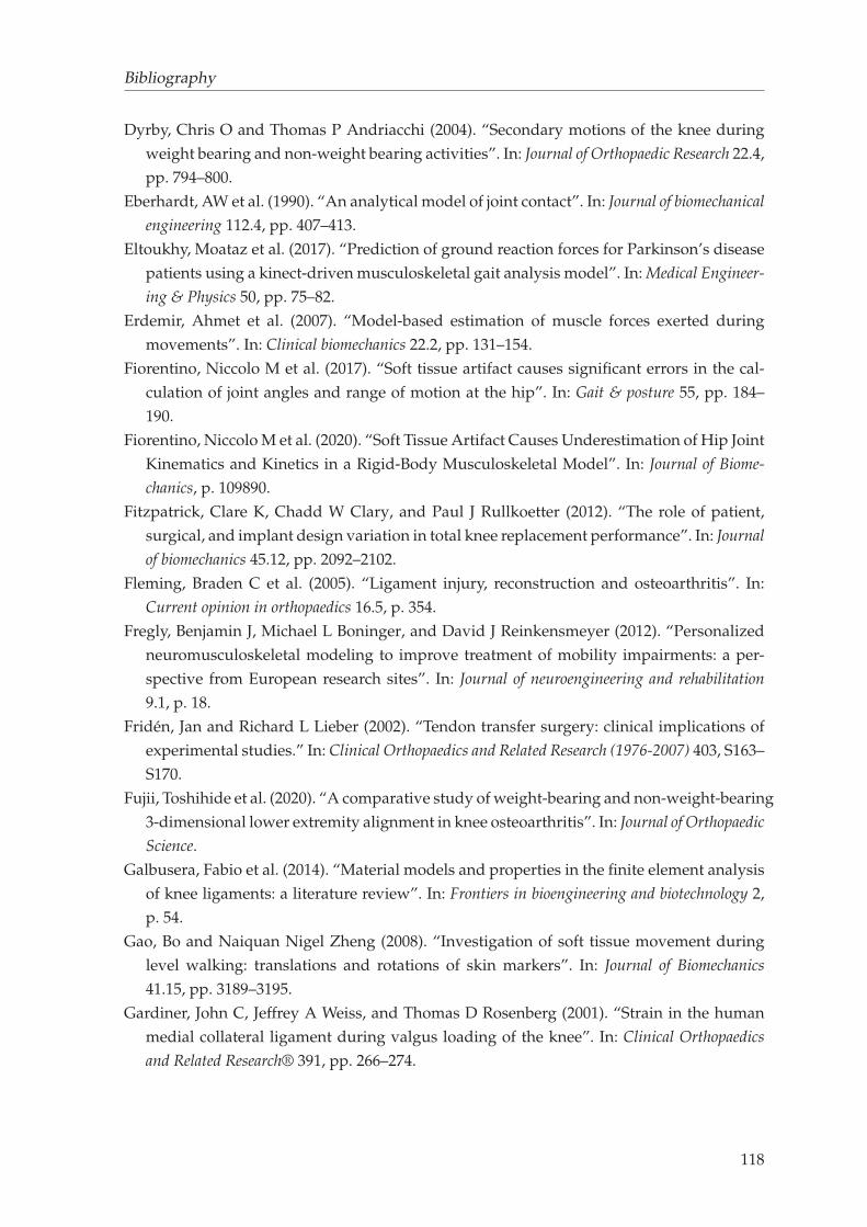
Bibliography
Dyrby, Chris O and Thomas P Andriacchi (2004). “Secondary motions of the knee during
weight bearing and non-weight bearing activities”. In: Journal of Orthopaedic Research 22.4,
pp. 794–800.
Eberhardt, AW et al. (1990). “An analytical model of joint contact”. In: Journal of biomechanical
engineering 112.4, pp. 407–413.
Eltoukhy, Moataz et al. (2017). “Prediction of ground reaction forces for Parkinson’s disease
patients using a kinect-driven musculoskeletal gait analysis model”. In: Medical Engineer-
ing & Physics 50, pp. 75–82.
Erdemir, Ahmet et al. (2007). “Model-based estimation of muscle forces exerted during
movements”. In: Clinical biomechanics 22.2, pp. 131–154.
Fiorentino, Niccolo M et al. (2017). “Soft tissue artifact causes significant errors in the cal-
culation of joint angles and range of motion at the hip”. In: Gait & posture 55, pp. 184–
190.
Fiorentino, Niccolo M et al. (2020). “Soft Tissue Artifact Causes Underestimation of Hip Joint
Kinematics and Kinetics in a Rigid-Body Musculoskeletal Model”. In: Journal of Biome-
chanics, p. 109890.
Fitzpatrick, Clare K, Chadd W Clary, and Paul J Rullkoetter (2012). “The role of patient,
surgical, and implant design variation in total knee replacement performance”. In: Journal
of biomechanics 45.12, pp. 2092–2102.
Fleming, Braden C et al. (2005). “Ligament injury, reconstruction and osteoarthritis”. In:
Current opinion in orthopaedics 16.5, p. 354.
Fregly, Benjamin J, Michael L Boninger, and David J Reinkensmeyer (2012). “Personalized
neuromusculoskeletal modeling to improve treatment of mobility impairments: a per-
spective from European research sites”. In: Journal of neuroengineering and rehabilitation
9.1, p. 18.
Fridén, Jan and Richard L Lieber (2002). “Tendon transfer surgery: clinical implications of
experimental studies.” In: Clinical Orthopaedics and Related Research (1976-2007) 403, S163–
S170.
Fujii, Toshihide et al. (2020). “A comparative study of weight-bearing and non-weight-bearing
3-dimensional lower extremity alignment in knee osteoarthritis”. In: Journal of Orthopaedic
Science.
Galbusera, Fabio et al. (2014). “Material models and properties in the finite element analysis
of knee ligaments: a literature review”. In: Frontiers in bioengineering and biotechnology 2,
p. 54.
Gao, Bo and Naiquan Nigel Zheng (2008). “Investigation of soft tissue movement during
level walking: translations and rotations of skin markers”. In: Journal of Biomechanics
41.15, pp. 3189–3195.
Gardiner, John C, Jeffrey A Weiss, and Thomas D Rosenberg (2001). “Strain in the human
medial collateral ligament during valgus loading of the knee”. In: Clinical Orthopaedics
and Related Research® 391, pp. 266–274.
118
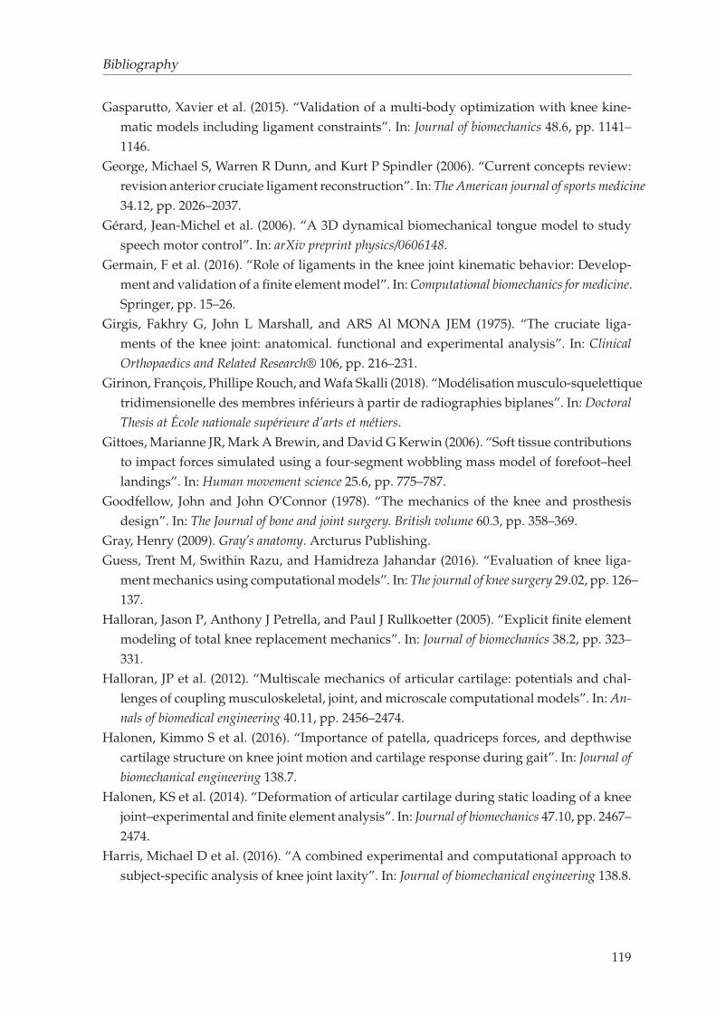
Bibliography
Gasparutto, Xavier et al. (2015). “Validation of a multi-body optimization with knee kine-
matic models including ligament constraints”. In: Journal of biomechanics 48.6, pp. 1141–
1146.
George, Michael S, Warren R Dunn, and Kurt P Spindler (2006). “Current concepts review:
revision anterior cruciate ligament reconstruction”. In: The American journal of sports medicine
34.12, pp. 2026–2037.
Gérard, Jean-Michel et al. (2006). “A 3D dynamical biomechanical tongue model to study
speech motor control”. In: arXiv preprint physics/0606148.
Germain, F et al. (2016). “Role of ligaments in the knee joint kinematic behavior: Develop-
ment and validation of a finite element model”. In: Computational biomechanics for medicine.
Springer, pp. 15–26.
Girgis, Fakhry G, John L Marshall, and ARS Al MONA JEM (1975). “The cruciate liga-
ments of the knee joint: anatomical. functional and experimental analysis”. In: Clinical
Orthopaedics and Related Research® 106, pp. 216–231.
Girinon, François, Phillipe Rouch, and Wafa Skalli (2018). “Modélisation musculo-squelettique
tridimensionelle des membres inférieurs à partir de radiographies biplanes”. In: Doctoral
Thesis at École nationale supérieure d’arts et métiers.
Gittoes, Marianne JR, Mark A Brewin, and David G Kerwin (2006). “Soft tissue contributions
to impact forces simulated using a four-segment wobbling mass model of forefoot–heel
landings”. In: Human movement science 25.6, pp. 775–787.
Goodfellow, John and John O’Connor (1978). “The mechanics of the knee and prosthesis
design”. In: The Journal of bone and joint surgery. British volume 60.3, pp. 358–369.
Gray, Henry (2009). Gray’s anatomy. Arcturus Publishing.
Guess, Trent M, Swithin Razu, and Hamidreza Jahandar (2016). “Evaluation of knee liga-
ment mechanics using computational models”. In: The journal of knee surgery 29.02, pp. 126–
137.
Halloran, Jason P, Anthony J Petrella, and Paul J Rullkoetter (2005). “Explicit finite element
modeling of total knee replacement mechanics”. In: Journal of biomechanics 38.2, pp. 323–
331.
Halloran, JP et al. (2012). “Multiscale mechanics of articular cartilage: potentials and chal-
lenges of coupling musculoskeletal, joint, and microscale computational models”. In: An-
nals of biomedical engineering 40.11, pp. 2456–2474.
Halonen, Kimmo S et al. (2016). “Importance of patella, quadriceps forces, and depthwise
cartilage structure on knee joint motion and cartilage response during gait”. In: Journal of
biomechanical engineering 138.7.
Halonen, KS et al. (2014). “Deformation of articular cartilage during static loading of a knee
joint–experimental and finite element analysis”. In: Journal of biomechanics 47.10, pp. 2467–
2474.
Harris, Michael D et al. (2016). “A combined experimental and computational approach to
subject-specific analysis of knee joint laxity”. In: Journal of biomechanical engineering 138.8.
119
Bibliography
Hashemi, Javad et al. (2008). “The geometry of the tibial plateau and its influence on the
biomechanics of the tibiofemoral joint”. In: The Journal of Bone and Joint Surgery. American
volume. 90.12, p. 2724.
Haut Donahue, Tammy L et al. (2002). “A finite element model of the human knee joint for
the study of tibio-femoral contact”. In: J. Biomech. Eng. 124.3, pp. 273–280.
Herrmann, Ariel M and Scott L Delp (1999). “Moment arm and force-generating capacity
of the extensor carpi ulnaris after transfer to the extensor carpi radialis brevis”. In: The
Journal of hand surgery 24.5, pp. 1083–1090.
Howell, Stephen M et al. (2001). “The relationship between the angle of the tibial tunnel in
the coronal plane and loss of flexion and anterior laxity after anterior cruciate ligament
reconstruction”. In: The American journal of sports medicine 29.5, pp. 567–574.
Hsich, Y-F and LF Draganich (1997). “Knee kinematics and ligament lengths during physio-
logic levels of isometric quadriceps loads”. In: The Knee 4.3, pp. 145–154.
Hume, Donald R et al. (2018). “The interaction of muscle moment arm, knee laxity, and
torque in a multi-scale musculoskeletal model of the lower limb”. In: Journal of biome-
chanics 76, pp. 173–180.
Hunt, KD et al. (1998). “Ultrasonic determination of the elastic modulus of human cortical
bone”. In: Medical and biological engineering and computing 36.1, pp. 51–56.
Irrgang, James J et al. (2001). “Development and validation of the international knee doc-
umentation committee subjective knee form”. In: The American journal of sports medicine
29.5, pp. 600–613.
Jeffery, Robert S, Richard W Morris, and Robin A Denham (1991). “Coronal alignment af-
ter total knee replacement”. In: The Journal of bone and joint surgery. British volume 73.5,
pp. 709–714.
Joldes, Grand Roman, Adam Wittek, and Karol Miller (2009). “Non-locking tetrahedral finite
element for surgical simulation”. In: Communications in Numerical Methods in Engineering
25.7, pp. 827–836.
Kang, KT et al. (2018). “A computational simulation study to determine the biomechani-
cal influence of posterior condylar offset and tibial slope in cruciate retaining total knee
arthroplasty”. In: Bone & joint research 7.1, pp. 69–78.
Keyak, JH et al. (2001). “Prediction of fracture location in the proximal femur using finite
element models”. In: Medical engineering & physics 23.9, pp. 657–664.
Khurana, Bharti et al. (2014). “Pelvic Ring Fractures: What the Orthopedic Surgeon Wants to
Know”. In: Radiographics 34.5, pp. 1317–1333.
Kiapour, Ali et al. (2014). “Finite element model of the knee for investigation of injury mech-
anisms: development and validation”. In: Journal of biomechanical engineering 136.1.
Kidzinski, Łukasz et al. (2020). “Deep neural networks enable quantitative movement anal-
ysis using single-camera videos”. In: Nature communications 11.1, pp. 1–10.
Kim, Young-Hoo et al. (2014). “The relationship between the survival of total knee arthro-
plasty and postoperative coronal, sagittal and rotational alignment of knee prosthesis”.
In: International orthopaedics 38.2, pp. 379–385.
120
Bibliography
Kim, Youngwoo et al. (2019). “Stand-to-Sit Kinematics of the Pelvis Is Not Always as Ex-
pected: Hip and Spine Pathologies Can Have an Impact”. In: The Journal of arthroplasty
34.9, pp. 2118–2123.
Koo, Seungbum, Jonathan H Rylander, and Thomas P Andriacchi (2011). “Knee joint kine-
matics during walking influences the spatial cartilage thickness distribution in the knee”.
In: Journal of biomechanics 44.7, pp. 1405–1409.
Kozanek, Michal et al. (2009). “Tibiofemoral kinematics and condylar motion during the
stance phase of gait”. In: Journal of biomechanics 42.12, pp. 1877–1884.
Kurtz, Steven et al. (2007). “Projections of primary and revision hip and knee arthroplasty
in the United States from 2005 to 2030”. In: Jbjs 89.4, pp. 780–785.
Lahkar, Bhrigu et al. (2018). “Fast Subject Specific Finite Element Mesh Generation of Knee
Joint from Biplanar X-ray Images”. In: 15th International Conference in Computer Methods
in Biomechanics and Biomedical Engineering.
Langlois, Laurent Nod ’e (2003). “Three-dimensional analyzes of angular deviations of the
axes of the lower limb, in pr ’e per and postop é ratory”. PhD thesis. Paris, ENSAM.
Laville, A, S Laporte, and W Skalli (2009). “Parametric and subject-specific finite element
modelling of the lower cervical spine. Influence of geometrical parameters on the motion
patterns”. In: Journal of biomechanics 42.10, pp. 1409–1415.
Leardini, Alberto et al. (2005). “Human movement analysis using stereophotogrammetry:
Part 3. Soft tissue artifact assessment and compensation”. In: Gait & posture 21.2, pp. 212–
225.
Lemaire, Roger and Jacques Witvoet (2002). “Prothèses totales du genou”. In: Cahiers d’enseignement
de la SOFCOT 81.
Lenhart, Rachel L et al. (2015). “Prediction and validation of load-dependent behavior of
the tibiofemoral and patellofemoral joints during movement”. In: Annals of biomedical
engineering 43.11, pp. 2675–2685.
Limbert, G, M Taylor, and J Middleton (2004). “Three-dimensional finite element modelling
of the human ACL: simulation of passive knee flexion with a stressed and stress-free
ACL”. In: Journal of biomechanics 37.11, pp. 1723–1731.
Logterman, Stephanie L, Frank B Wydra, and Rachel M Frank (2018). “Posterior cruciate
ligament: anatomy and biomechanics”. In: Current reviews in musculoskeletal medicine 11.3,
pp. 510–514.
Löhner, Rainald and Paresh Parikh (1988). “Generation of three-dimensional unstructured
grids by the advancing-front method”. In: International Journal for Numerical Methods in
Fluids 8.10, pp. 1135–1149.
Lu, T-W and JJ O’connor (1999). “Bone position estimation from skin marker co-ordinates
using global optimisation with joint constraints”. In: Journal of biomechanics 32.2, pp. 129–
134.
MacInnes, Scott J, Andrew Gordon, and J Mark Wilkinson (2012). “Risk factors for aseptic
loosening following total hip arthroplasty”. In: Recent advances in arthroplasty 10, p. 26975.
121
Bibliography
McLean, Scott G, Anne Su, and Antonie J van den Bogert (2003). “Development and vali-
dation of a 3-D model to predict knee joint loading during dynamic movement”. In: J.
Biomech. Eng. 125.6, pp. 864–874.
Meister, Brad R et al. (2000). “Anatomy and kinematics of the lateral collateral ligament of
the knee”. In: The American journal of sports medicine 28.6, pp. 869–878.
Melhem, Elias et al. (2016). “EOS® biplanar X-ray imaging: concept, developments, benefits,
and limitations”. In: Journal of children’s orthopaedics 10.1, pp. 1–14.
Mesfar, W and A Shirazi-Adl (2005). “Biomechanics of the knee joint in flexion under various
quadriceps forces”. In: The knee 12.6, pp. 424–434.
— (2006). “Biomechanics of changes in ACL and PCL material properties or prestrains in
flexion under muscle force-implications in ligament reconstruction”. In: Computer meth-
ods in biomechanics and biomedical engineering 9.4, pp. 201–209.
Miller, Mark D and Brian J Cole (2004). Textbook of arthroscopy. Vol. 355. Gulf Professional
Publishing.
Mitton, David et al. (2006). “3D reconstruction of the pelvis from bi-planar radiography”. In:
Computer methods in biomechanics and biomedical engineering 9.1, pp. 1–5.
Moglo, KE and A Shirazi-Adl (2005). “Cruciate coupling and screw-home mechanism in
passive knee joint during extension–flexion”. In: Journal of biomechanics 38.5, pp. 1075–
1083.
Molini, L et al. (2011). “Hip: Anatomy and US technique”. In: Journal of ultrasound 14.2,
pp. 99–108.
Morgan, Elise F, Ginu U Unnikrisnan, and Amira I Hussein (2018). “Bone mechanical prop-
erties in healthy and diseased states”. In: Annual review of biomedical engineering 20, pp. 119–
143.
Murray, Wendy M et al. (2002). “The influence of elbow position on the range of motion
of the wrist following transfer of the brachioradialis to the extensor carpi radialis brevis
tendon”. In: JBJS 84.12, pp. 2203–2210.
Myers, Casey A et al. (2012). “In vivo tibiofemoral kinematics during 4 functional tasks of
increasing demand using biplane fluoroscopy”. In: The American journal of sports medicine
40.1, pp. 170–178.
Nardini, Fabrizio et al. (2020). “An Anatomical-Based Subject-Specific Model of In-Vivo
Knee Joint 3D Kinematics From Medical Imaging”. In: Applied Sciences 10.6, p. 2100.
Navacchia, Alessandro et al. (2019). “A computationally efficient strategy to estimate muscle
forces in a finite element musculoskeletal model of the lower limb”. In: Journal of Biome-
chanics 84, pp. 94–102.
Neptune, Richard R, Felix E Zajac, and Steven A Kautz (2009). “Author’s Response to Com-
ment on “Contributions of the individual ankle plantar flexors to support, forward pro-
gression and swing initiation during walking”(Neptune et al., 2001) and “Muscle me-
chanical work requirements during normal walking: The energetic cost of raising the
body’s center-of-mass is significant”()”. In: Journal of biomechanics 42.11, p. 1786.
122
Bibliography
Onishi, Y and K Amaya (2014). “A locking-free selective smoothed finite element method us-
ing tetrahedral and triangular elements with adaptive mesh rezoning for large deforma-
tion problems”. In: International Journal for Numerical Methods in Engineering 99.5, pp. 354–
371.
Orsi, Alexander D et al. (2016). “The effects of knee joint kinematics on anterior cruciate
ligament injury and articular cartilage damage”. In: Computer methods in biomechanics and
biomedical engineering 19.5, pp. 493–506.
Parratte, Sebastien et al. (2010). “Effect of postoperative mechanical axis alignment on the
fifteen-year survival of modern, cemented total knee replacements”. In: JBJS 92.12, pp. 2143–
2149.
Payen, Daniel Jose and Klaus-Jürgen Bathe (2011). “Improved stresses for the 4-node tetra-
hedral element”. In: Computers & structures 89.13-14, pp. 1265–1273.
Pedersen, Dennis et al. (2019). “A novel non-invasive method for measuring knee joint lax-
ity in four dof: In vitro proof-of-concept and validation”. In: Journal of biomechanics 82,
pp. 62–69.
Pena, E et al. (2005). “A finite element simulation of the effect of graft stiffness and graft
tensioning in ACL reconstruction”. In: Clinical Biomechanics 20.6, pp. 636–644.
Pena, E et al. (2006). “A three-dimensional finite element analysis of the combined behavior
of ligaments and menisci in the healthy human knee joint”. In: Journal of biomechanics 39.9,
pp. 1686–1701.
Petersen, Wolf and Thore Zantop (2007). “Anatomy of the anterior cruciate ligament with
regard to its two bundles”. In: Clinical Orthopaedics and Related Research® 454, pp. 35–47.
Piazza, Stephen J and Scott L Delp (1996). “The influence of muscles on knee flexion during
the swing phase of gait”. In: Journal of biomechanics 29.6, pp. 723–733.
Pillet, Hélène et al. (2014). “A reference method for the evaluation of femoral head joint
center location technique based on external markers”. In: Gait & posture 39.1, pp. 655–
658.
Pillet, Hélène et al. (2016). “Femur, tibia and fibula bone templates to estimate subject-
specific knee ligament attachment site locations”. In: Journal of Biomechanics 49.14, pp. 3523–
3528.
Quijano, S et al. (2013). “Three-dimensional reconstruction of the lower limb from biplanar
calibrated radiographs”. In: Medical engineering & physics 35.12, pp. 1703–1712.
Rachmat, HH et al. (2016). “In-situ mechanical behavior and slackness of the anterior cru-
ciate ligament at multiple knee flexion angles”. In: Medical engineering & physics 38.3,
pp. 209–215.
Radtke, Kerstin et al. (2010). “Effect of limb rotation on radiographic alignment in total knee
arthroplasties”. In: Archives of orthopaedic and trauma surgery 130.4, pp. 451–457.
Ramos, A and JA Simoes (2006). “Tetrahedral versus hexahedral finite elements in numerical
modelling of the proximal femur”. In: Medical engineering & physics 28.9, pp. 916–924.
Reinbolt, Jeffrey A et al. (2005). “Determination of patient-specific multi-joint kinematic
models through two-level optimization”. In: Journal of biomechanics 38.3, pp. 621–626.
123
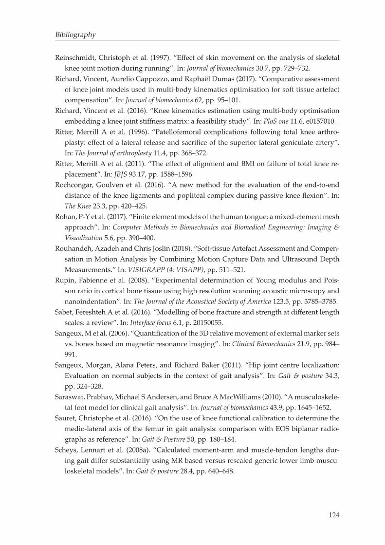
Bibliography
Reinschmidt, Christoph et al. (1997). “Effect of skin movement on the analysis of skeletal
knee joint motion during running”. In: Journal of biomechanics 30.7, pp. 729–732.
Richard, Vincent, Aurelio Cappozzo, and Raphaël Dumas (2017). “Comparative assessment
of knee joint models used in multi-body kinematics optimisation for soft tissue artefact
compensation”. In: Journal of biomechanics 62, pp. 95–101.
Richard, Vincent et al. (2016). “Knee kinematics estimation using multi-body optimisation
embedding a knee joint stiffness matrix: a feasibility study”. In: PloS one 11.6, e0157010.
Ritter, Merrill A et al. (1996). “Patellofemoral complications following total knee arthro-
plasty: effect of a lateral release and sacrifice of the superior lateral geniculate artery”.
In: The Journal of arthroplasty 11.4, pp. 368–372.
Ritter, Merrill A et al. (2011). “The effect of alignment and BMI on failure of total knee re-
placement”. In: JBJS 93.17, pp. 1588–1596.
Rochcongar, Goulven et al. (2016). “A new method for the evaluation of the end-to-end
distance of the knee ligaments and popliteal complex during passive knee flexion”. In:
The Knee 23.3, pp. 420–425.
Rohan, P-Y et al. (2017). “Finite element models of the human tongue: a mixed-element mesh
approach”. In: Computer Methods in Biomechanics and Biomedical Engineering: Imaging &
Visualization 5.6, pp. 390–400.
Rouhandeh, Azadeh and Chris Joslin (2018). “Soft-tissue Artefact Assessment and Compen-
sation in Motion Analysis by Combining Motion Capture Data and Ultrasound Depth
Measurements.” In: VISIGRAPP (4: VISAPP), pp. 511–521.
Rupin, Fabienne et al. (2008). “Experimental determination of Young modulus and Pois-
son ratio in cortical bone tissue using high resolution scanning acoustic microscopy and
nanoindentation”. In: The Journal of the Acoustical Society of America 123.5, pp. 3785–3785.
Sabet, Fereshteh A et al. (2016). “Modelling of bone fracture and strength at different length
scales: a review”. In: Interface focus 6.1, p. 20150055.
Sangeux, M et al. (2006). “Quantification of the 3D relative movement of external marker sets
vs. bones based on magnetic resonance imaging”. In: Clinical Biomechanics 21.9, pp. 984–
991.
Sangeux, Morgan, Alana Peters, and Richard Baker (2011). “Hip joint centre localization:
Evaluation on normal subjects in the context of gait analysis”. In: Gait & posture 34.3,
pp. 324–328.
Saraswat, Prabhav, Michael S Andersen, and Bruce A MacWilliams (2010). “A musculoskele-
tal foot model for clinical gait analysis”. In: Journal of biomechanics 43.9, pp. 1645–1652.
Sauret, Christophe et al. (2016). “On the use of knee functional calibration to determine the
medio-lateral axis of the femur in gait analysis: comparison with EOS biplanar radio-
graphs as reference”. In: Gait & Posture 50, pp. 180–184.
Scheys, Lennart et al. (2008a). “Calculated moment-arm and muscle-tendon lengths dur-
ing gait differ substantially using MR based versus rescaled generic lower-limb muscu-
loskeletal models”. In: Gait & posture 28.4, pp. 640–648.
124
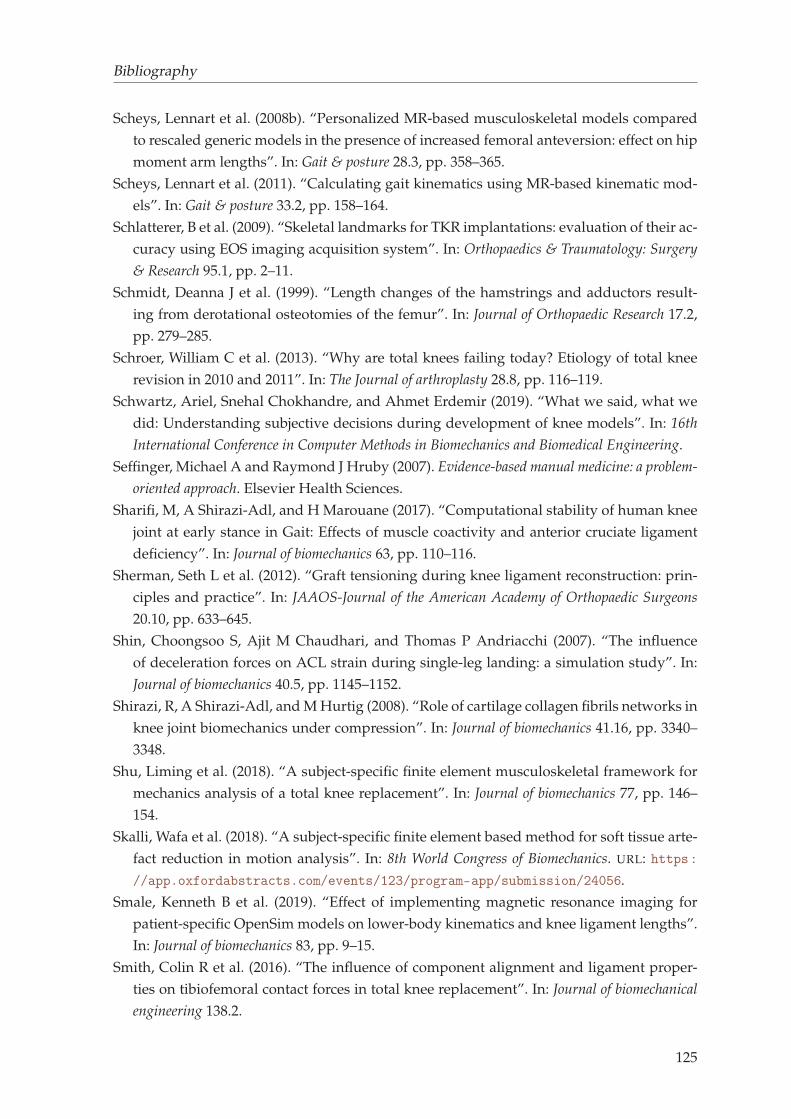
Bibliography
Scheys, Lennart et al. (2008b). “Personalized MR-based musculoskeletal models compared
to rescaled generic models in the presence of increased femoral anteversion: effect on hip
moment arm lengths”. In: Gait & posture 28.3, pp. 358–365.
Scheys, Lennart et al. (2011). “Calculating gait kinematics using MR-based kinematic mod-
els”. In: Gait & posture 33.2, pp. 158–164.
Schlatterer, B et al. (2009). “Skeletal landmarks for TKR implantations: evaluation of their ac-
curacy using EOS imaging acquisition system”. In: Orthopaedics & Traumatology: Surgery
& Research 95.1, pp. 2–11.
Schmidt, Deanna J et al. (1999). “Length changes of the hamstrings and adductors result-
ing from derotational osteotomies of the femur”. In: Journal of Orthopaedic Research 17.2,
pp. 279–285.
Schroer, William C et al. (2013). “Why are total knees failing today? Etiology of total knee
revision in 2010 and 2011”. In: The Journal of arthroplasty 28.8, pp. 116–119.
Schwartz, Ariel, Snehal Chokhandre, and Ahmet Erdemir (2019). “What we said, what we
did: Understanding subjective decisions during development of knee models”. In: 16th
International Conference in Computer Methods in Biomechanics and Biomedical Engineering.
Seffinger, Michael A and Raymond J Hruby (2007). Evidence-based manual medicine: a problem-
oriented approach. Elsevier Health Sciences.
Sharifi, M, A Shirazi-Adl, and H Marouane (2017). “Computational stability of human knee
joint at early stance in Gait: Effects of muscle coactivity and anterior cruciate ligament
deficiency”. In: Journal of biomechanics 63, pp. 110–116.
Sherman, Seth L et al. (2012). “Graft tensioning during knee ligament reconstruction: prin-
ciples and practice”. In: JAAOS-Journal of the American Academy of Orthopaedic Surgeons
20.10, pp. 633–645.
Shin, Choongsoo S, Ajit M Chaudhari, and Thomas P Andriacchi (2007). “The influence
of deceleration forces on ACL strain during single-leg landing: a simulation study”. In:
Journal of biomechanics 40.5, pp. 1145–1152.
Shirazi, R, A Shirazi-Adl, and M Hurtig (2008). “Role of cartilage collagen fibrils networks in
knee joint biomechanics under compression”. In: Journal of biomechanics 41.16, pp. 3340–
3348.
Shu, Liming et al. (2018). “A subject-specific finite element musculoskeletal framework for
mechanics analysis of a total knee replacement”. In: Journal of biomechanics 77, pp. 146–
154.
Skalli, Wafa et al. (2018). “A subject-specific finite element based method for soft tissue arte-
fact reduction in motion analysis”. In: 8th World Congress of Biomechanics. URL: https:
//app.oxfordabstracts.com/events/123/program-app/submission/24056.
Smale, Kenneth B et al. (2019). “Effect of implementing magnetic resonance imaging for
patient-specific OpenSim models on lower-body kinematics and knee ligament lengths”.
In: Journal of biomechanics 83, pp. 9–15.
Smith, Colin R et al. (2016). “The influence of component alignment and ligament proper-
ties on tibiofemoral contact forces in total knee replacement”. In: Journal of biomechanical
engineering 138.2.
125
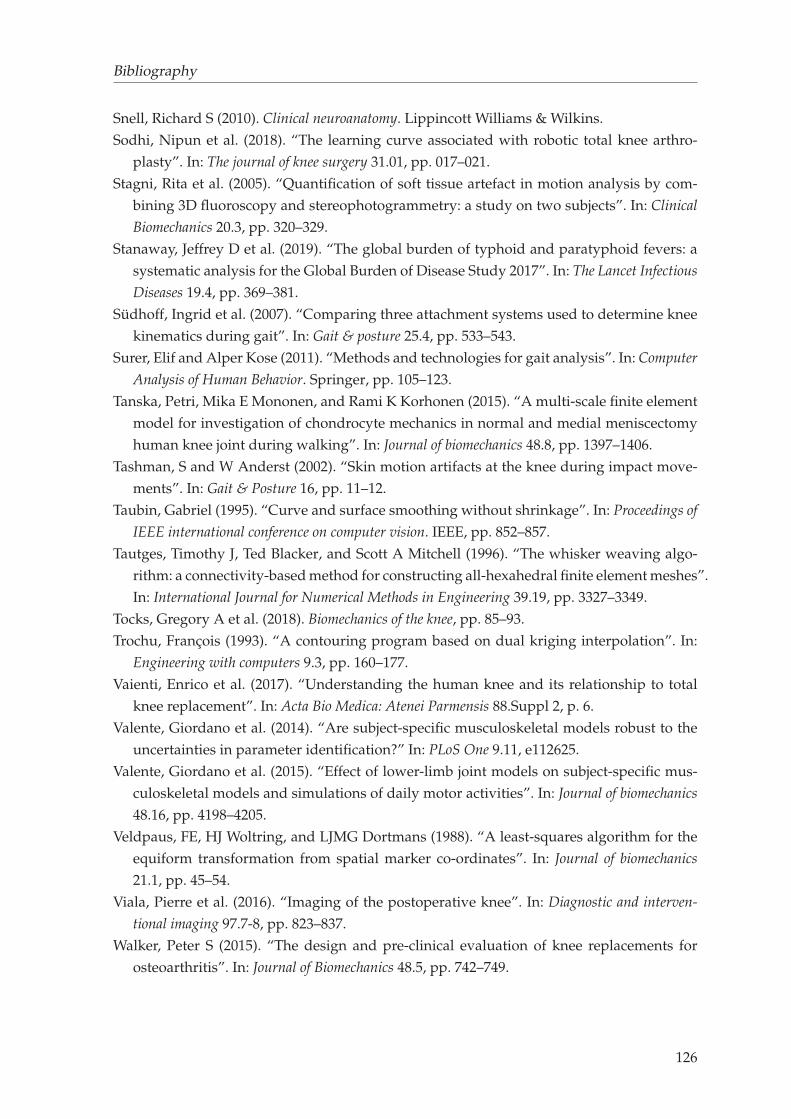
Bibliography
Snell, Richard S (2010). Clinical neuroanatomy. Lippincott Williams & Wilkins.
Sodhi, Nipun et al. (2018). “The learning curve associated with robotic total knee arthro-
plasty”. In: The journal of knee surgery 31.01, pp. 017–021.
Stagni, Rita et al. (2005). “Quantification of soft tissue artefact in motion analysis by com-
bining 3D fluoroscopy and stereophotogrammetry: a study on two subjects”. In: Clinical
Biomechanics 20.3, pp. 320–329.
Stanaway, Jeffrey D et al. (2019). “The global burden of typhoid and paratyphoid fevers: a
systematic analysis for the Global Burden of Disease Study 2017”. In: The Lancet Infectious
Diseases 19.4, pp. 369–381.
Südhoff, Ingrid et al. (2007). “Comparing three attachment systems used to determine knee
kinematics during gait”. In: Gait & posture 25.4, pp. 533–543.
Surer, Elif and Alper Kose (2011). “Methods and technologies for gait analysis”. In: Computer
Analysis of Human Behavior. Springer, pp. 105–123.
Tanska, Petri, Mika E Mononen, and Rami K Korhonen (2015). “A multi-scale finite element
model for investigation of chondrocyte mechanics in normal and medial meniscectomy
human knee joint during walking”. In: Journal of biomechanics 48.8, pp. 1397–1406.
Tashman, S and W Anderst (2002). “Skin motion artifacts at the knee during impact move-
ments”. In: Gait & Posture 16, pp. 11–12.
Taubin, Gabriel (1995). “Curve and surface smoothing without shrinkage”. In: Proceedings of
IEEE international conference on computer vision. IEEE, pp. 852–857.
Tautges, Timothy J, Ted Blacker, and Scott A Mitchell (1996). “The whisker weaving algo-
rithm: a connectivity-based method for constructing all-hexahedral finite element meshes”.
In: International Journal for Numerical Methods in Engineering 39.19, pp. 3327–3349.
Tocks, Gregory A et al. (2018). Biomechanics of the knee, pp. 85–93.
Trochu, François (1993). “A contouring program based on dual kriging interpolation”. In:
Engineering with computers 9.3, pp. 160–177.
Vaienti, Enrico et al. (2017). “Understanding the human knee and its relationship to total
knee replacement”. In: Acta Bio Medica: Atenei Parmensis 88.Suppl 2, p. 6.
Valente, Giordano et al. (2014). “Are subject-specific musculoskeletal models robust to the
uncertainties in parameter identification?” In: PLoS One 9.11, e112625.
Valente, Giordano et al. (2015). “Effect of lower-limb joint models on subject-specific mus-
culoskeletal models and simulations of daily motor activities”. In: Journal of biomechanics
48.16, pp. 4198–4205.
Veldpaus, FE, HJ Woltring, and LJMG Dortmans (1988). “A least-squares algorithm for the
equiform transformation from spatial marker co-ordinates”. In: Journal of biomechanics
21.1, pp. 45–54.
Viala, Pierre et al. (2016). “Imaging of the postoperative knee”. In: Diagnostic and interven-
tional imaging 97.7-8, pp. 823–837.
Walker, Peter S (2015). “The design and pre-clinical evaluation of knee replacements for
osteoarthritis”. In: Journal of Biomechanics 48.5, pp. 742–749.
126
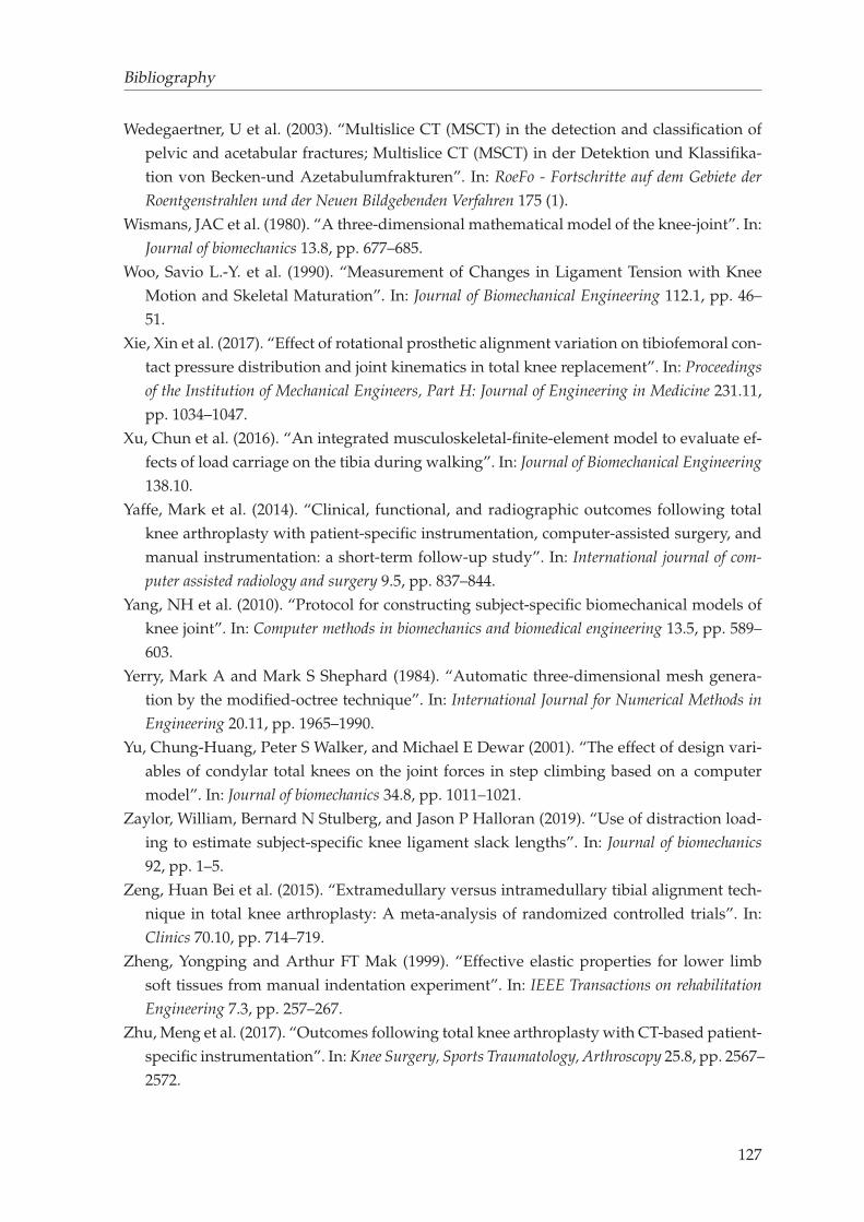
Bibliography
Wedegaertner, U et al. (2003). “Multislice CT (MSCT) in the detection and classification of
pelvic and acetabular fractures; Multislice CT (MSCT) in der Detektion und Klassifika-
tion von Becken-und Azetabulumfrakturen”. In: RoeFo - Fortschritte auf dem Gebiete der
Roentgenstrahlen und der Neuen Bildgebenden Verfahren 175 (1).
Wismans, JAC et al. (1980). “A three-dimensional mathematical model of the knee-joint”. In:
Journal of biomechanics 13.8, pp. 677–685.
Woo, Savio L.-Y. et al. (1990). “Measurement of Changes in Ligament Tension with Knee
Motion and Skeletal Maturation”. In: Journal of Biomechanical Engineering 112.1, pp. 46–
51.
Xie, Xin et al. (2017). “Effect of rotational prosthetic alignment variation on tibiofemoral con-
tact pressure distribution and joint kinematics in total knee replacement”. In: Proceedings
of the Institution of Mechanical Engineers, Part H: Journal of Engineering in Medicine 231.11,
pp. 1034–1047.
Xu, Chun et al. (2016). “An integrated musculoskeletal-finite-element model to evaluate ef-
fects of load carriage on the tibia during walking”. In: Journal of Biomechanical Engineering
138.10.
Yaffe, Mark et al. (2014). “Clinical, functional, and radiographic outcomes following total
knee arthroplasty with patient-specific instrumentation, computer-assisted surgery, and
manual instrumentation: a short-term follow-up study”. In: International journal of com-
puter assisted radiology and surgery 9.5, pp. 837–844.
Yang, NH et al. (2010). “Protocol for constructing subject-specific biomechanical models of
knee joint”. In: Computer methods in biomechanics and biomedical engineering 13.5, pp. 589–
603.
Yerry, Mark A and Mark S Shephard (1984). “Automatic three-dimensional mesh genera-
tion by the modified-octree technique”. In: International Journal for Numerical Methods in
Engineering 20.11, pp. 1965–1990.
Yu, Chung-Huang, Peter S Walker, and Michael E Dewar (2001). “The effect of design vari-
ables of condylar total knees on the joint forces in step climbing based on a computer
model”. In: Journal of biomechanics 34.8, pp. 1011–1021.
Zaylor, William, Bernard N Stulberg, and Jason P Halloran (2019). “Use of distraction load-
ing to estimate subject-specific knee ligament slack lengths”. In: Journal of biomechanics
92, pp. 1–5.
Zeng, Huan Bei et al. (2015). “Extramedullary versus intramedullary tibial alignment tech-
nique in total knee arthroplasty: A meta-analysis of randomized controlled trials”. In:
Clinics 70.10, pp. 714–719.
Zheng, Yongping and Arthur FT Mak (1999). “Effective elastic properties for lower limb
soft tissues from manual indentation experiment”. In: IEEE Transactions on rehabilitation
Engineering 7.3, pp. 257–267.
Zhu, Meng et al. (2017). “Outcomes following total knee arthroplasty with CT-based patient-
specific instrumentation”. In: Knee Surgery, Sports Traumatology, Arthroscopy 25.8, pp. 2567–
2572.
127

Bibliography
Zlotnicki, Jason P et al. (2016). “Basic biomechanic principles of knee instability”. In: Current
reviews in musculoskeletal medicine 9.2, pp. 114–122.
128

CONTRIBUTION À LA MODÉLISATION MUSCULOSQUELETTIQUE PERSONNALISÉE DU
MEMBRE INFÉRIEUR PAR ELEMENTS FINIS
RESUME : Le trouble musculosquelettique du membre inférieur est l'un des fardeaux de
santé les plus courants pouvant entraîner une déficience fonctionnelle chez un individu.
Bien que diverses options de gestion opérationnelle soient disponibles, il ne semble pas y avoir unanimité sur une procédure particulière qui servirait au mieux les intérêts de tous.
Pour évaluer objectivement les troubles et planifier efficacement les interventions
chirurgicales, il est essentiel de comprendre la biomécanique des membres inférieurs dans
des conditions de charge physiologique. Avec cette motivation, ce travail de thèse vise à développer un cadre complet de modélisation musculosquelettique du membre inférieur
basé sur les éléments finis. La première phase du travail de thèse est axée sur le
développement et l'évaluation de modèles personnalisés d'éléments finis en flexion
passive. De nouvelles approches sont proposées et évaluées pour le développement rapide de modèles axés sur la géométrie et les propriétés des ligaments. Dans la deuxième phase,
une nouvelle approche basée sur les éléments finis pour la compensation des artefacts des
tissus mous est proposée et évaluée. Cette contribution a permis de compenser efficacement les artefacts des tissus mous dans l'analyse du mouvement en tenant compte
de la spécificité du sujet. La troisième phase du travail de thèse est consacrée à
l'application clinique, où l'utilité du système radiographique biplan dans l'évaluation de
l'alignement des implants de l'arthroplastie totale du genou est brièvement explorée.
Dans l'ensemble, ce travail de thèse peut aider à estimer et à comprendre avec précision la
biomécanique des membres inférieurs dans des conditions de charge cliniquement
pertinentes, et à rapprocher le modèle de la routine clinique.
Mots clés : Modélisation personnalisée, Eléments finis, Articulation du genou, Artefact
des tissus mous, Biomécanique, Radiographie biplanaire
CONTRIBUTION TO PERSONLIZED FINITE ELEMENT BASED MUSCULOSKELETAL
MODELING OF THE LOWER LIMB
ABSTRACT : Musculoskeletal disorder of the lower limb is one of the most common health
burdens that may lead to functional impairment in an individual. Although various
operative management options are available, there seems no unanimity on a particular
procedure that serves the best. To objectively assess disorders and effectively plan surgeries, it is essential to understand lower limb biomechanics under physiological
loading conditions. With that motivation, this PhD aims to develop a comprehensive finite
element based musculoskeletal modeling framework of the lower limb. The first phase of
the PhD focuses on the development and evaluation of subject-specific finite element models under passive flexion. Novel approaches are proposed and evaluated for fast
model development focusing on geometry and ligament properties. In the second phase, a
novel finite element based approach for soft tissue artifact compensation is proposed and
evaluated. This contribution allowed to effectively compensate for soft tissue artifact in motion analysis by taking subject specificity into account. The third phase of the PhD is
dedicated to clinical application, where the utility of the biplanar X-ray system in
evaluating Total Knee Arthroplasty implant alignment is briefly explored.
Overall, this PhD may help to accurately estimate and understand lower limb
biomechanics under clinically relevant loading conditions, and bring the model a step
closer to clinical routine.
Keywords : Subject-specific modeling, Finite Element analysis, Knee joint, Soft Tissue
Artifact, Biomechanics, Biplanar X-ray


