Embed Size (px)
Citation preview
i
THE KNOWLEDGE REPRESENTATION AND
ALGORITHM FOR PERSONALIZED INFECTIOUS
DISEASE RISK PREDICTION
A thesis submitted to the
Trinity College Dublin, the University of Dublin
for the degree
Doctor of Philosophy
Retno Aulia Vinarti
Knowledge and Data Engineering Group
School of Computer Science and Statistics
Trinity College Dublin, Ireland
2019
Supervised by Prof. Lucy Hederman

ii
DECLARATION
I, the undersigned, declare that this work has not been previously submitted as an exercise
for a degree at this or any other University, and that, unless otherwise stated, it is entirely
my own work.
Retno Aulia Vinarti

iii
PERMISSION TO LEND OR COPY
I, the undersigned, agree that the Trinity College Library may lend or copy this thesis
upon request.
Retno Aulia Vinarti
iv
ACKNOWLEDGMENT
During the PhD journey, I feel blessed to meet people with positive influences on my life
and on this thesis particularly.
First of all, I would like to thank Lucy Hederman for all her time and patience to support
the research written in this thesis. From the beginning, the PhD interview, until the
ending, this thesis submission. She surely becomes one of the most inspiring people that
I have met, as a woman, as a researcher, and as a mother. I am truly thankful that the
destiny brought me to meet you, as my PhD supervisor.
As importantly, I thank my husband, Fajar Annas Susanto, whose unconditional love
to me and our daughter, Rania Annas Ramadhani, led me to finish this thesis. To my
parents and parents-in-law who always pray for my strength when I am at the lowest
points in this journey. Also, to my brother, Lintang Jati Prasojo, who sublet his
apartment to me and my family.
I would like to thank my Indonesian friends, for the delish food they sent to my apartment
when I was busy doing my thesis at my lab, or for their companion to keep my sanity
when I was deeply missing my daughter. To my best friends who patiently listen to my
rantings, Riska Asriana, Junita Purwandari, Rizka Hadiwiyanti. To my supportive
colleague, Hanim Maria Astuti. To my knowledge sources, Fariziyah Dwi Safitri, Nurul
Kodriati, Gumgum Darmawan, Ika Yuni Wulansari.
I would also thank my lab mates, Ramisa Hamed, for her limitless kindness; Gary
Munnelly for the guitar; Harshvardhan Pandit for optimizing the algorithm, Brendan
Spillane, Fahim Salim, Jamie McGann, and other lab mates for their help at KDEG.
Also, for Irish people, chatty grandmas on the bus or streets who are very welcoming to
foreign people, so my family and I can live in peace. This condition truly supports
everyone to make this world as a better place to live. Somehow, their spirits of
independence in all sectors inspire me so much. I promise that I will tell my future
generations to be kind to any foreigners they meet anywhere.
Finally, I would like to thank the Islamic Development Bank for their financial aid for
these three years.

v
“To expect the unexpected shows a thoroughly modern intellect.”
– Oscar Wilde
vi
ABSTRACT
Infectious diseases are a major cause of human morbidity. However, in the EU in 2014
more than 40 thousand deaths caused by infectious diseases were considered preventable.
Information about infection risk based on personal and environmental attributes, as well
as up-to-date infectious disease risk knowledge is expected to make lay people aware of
their infection risks. With the emergence of APIs and GPS technology, surrounding
location features and weather information can be inferred from a person's position. This
offers an opportunity to create a system for personalized infectious disease risk
prediction.
This thesis presents research towards a system that can predict personalized infectious
disease risk (IDR) based on a person's attributes and geo-position by utilizing infectious
disease risk knowledge (entitled PROSPECT-IDR: Personalised Prediction of
Infectious Disease Risk). A knowledge representation was designed to facilitate
epidemiologists to encode infectious disease risk knowledge in a form familiar to them.
The generic IDR ontology represents personal and environmental risk factors for all
human infectious diseases (n=234). Quantifications for the risk factors (e.g. odds ratios)
are encoded using five IDR rule types. This IDR knowledge representation (ontology and
rule types) allows encoding of knowledge about risk of infectious diseases prevalent in a
region.
The IDR ontology can never be complete, as new risk factors for existing diseases, and
new diseases, are constantly discovered. The initial generic ontology contains all risk
factors found in the Atlas of Human Infectious Diseases, and in factsheets from the CDC
and WHO. Each instantiation of knowledge for a specific disease in a region comprises
of a subset of risk factors from the generic ontology plus any new risk factors not found
there, along with a set of risk quantification rules (instantiations of the five rule types).
An algorithm (entitled BN-Builder) converts the knowledge-base into a fully functioning
and consistent risk prediction model, a Bayesian Network, which is the core of the
PROSPECT-IDR prediction system.
The usefulness and completeness of the IDR knowledge representation (initial generic
ontology and five rule types) were evaluated using 22 published case-control studies that
encode infectious disease risk knowledge. Each case-control study was encoded as one
evaluation knowledge-base. With regard to completeness, more than 3/4 of the ontology
vii
objects needed to encode the knowledge in the evaluation case-control studies were found
in the initial generic ontology. With regard to usefulness, more than 3/5 were used to
encode evaluation case-control studies. With regard to completeness and usefulness of
the five rule types, all infectious disease risk knowledge in the 22 evaluation case-control
studies can be encoded with just those five rule types, and all five rule types were used.
To evaluate BN-Builder algorithm, the consistency between the generated BN and the
knowledge-base was measured. Chi-square tests for differences were carried out for two
evaluation knowledge-bases that covered all functions of the algorithm and all data
ranges allowed by the rule types. There was no significant difference between the
resulting infectious disease risk prediction and the encoded knowledge (p > .05).
Evaluation results suggest that the IDR knowledge representation is useful. Further,
statistical findings indicate that the BN-Builder algorithm generates infectious disease
risk predictions that are consistent with the encoded risk knowledge. The PROSPECT-
IDR system that this IDR-KB and BN-Builder algorithm is designed for is expected to
give information about personalized infectious disease risk prediction to lay people. So,
the relevant preventive actions can be tailored based on this personalized information,
and thus, hopefully will reduce the incidence number of infectious diseases in the world.
viii
RESEARCH OUTPUTS
Published
R. A. Vinarti and L. Hederman, “Personalization of Infectious Disease Risk Prediction:
Towards Automatic Generation of a Bayesian Network,” in Proceedings – IEEE
Symposium on Computer-Based Medical Systems, 2017, vol. 2017 - June (see
Appendix 3 for full paper).
R. Vinarti and L. Hederman, A knowledge-base for a personalized infectious disease risk
prediction system, Book Section – Studies in Health Technology and Informatics.
vol. 247. 2018 (see Appendix 4 for full paper).
R. A. Vinarti and L. Hederman, “Introduction of a Bayesian Network Builder Algorithm
- Personalized Infectious Disease Risk Prediction,” Proceedings – 11th
International Joint Conference on Biomedical Engineering Systems and
Technologies, vol. 5, no. Biostec, pp. 115–126, 2018 (see Appendix 5 for full
paper).
The form of Knowledge Representation is available in R. A. Vinarti, “IDR Ontologies”,
https://osf.io/p6qv8/, Open Science Framework, 2018.
The BN-Builder algorithm is available in R. Vinarti, "Thesis Code",
https://github.com/retnor/ThesisCode
Submitted
R. A. Vinarti and L. Hederman, “A Personalized Infectious Disease Risk Prediction
System”, International Journal of Expert Systems with Applications (see
Appendix 6 for full paper).
R. A. Vinarti and L. Hederman, “Infectious Disease Risk knowledge representation for
use in a personalized IDR prediction system”, BMC - Journal of Biomedical
Semantics (see Appendix 7 for full paper).
ix
TABLE OF CONTENTS
1. Introduction ............................................................................................................... 1
1.1 Background ........................................................................................................ 1
1.2 Motivation .......................................................................................................... 4
1.3 Research Questions ............................................................................................ 7
1.4 Objectives and Goals .......................................................................................... 7
1.5 Contribution to the State of the Art .................................................................... 8
1.6 Methodology ...................................................................................................... 9
1.7 Thesis Overview ............................................................................................... 11
2. State of the Art – Infectious Disease Risk Prediction System ............................... 14
2.1 Definition of Personalized Infectious Disease Risk Prediction System ........... 14
2.2 Existing Research on Infectious Disease Risk Prediction and its Predictor
Modelling .................................................................................................................... 17
2.2.1 Previous research related to risk prediction techniques ............................ 21
2.2.2 Previous research related to person and environmental modelling .......... 24
2.3 Conclusion........................................................................................................ 26
3. State of the Art – The domain knowledge and its representation .......................... 28
3.1 The Domain of Knowledge: Human Infection Risk ........................................ 28
3.1.1 Etiology of Infectious Diseases ................................................................ 29
3.1.2 Disease Risk Quantifications .................................................................... 42
3.1.3 Summary ................................................................................................... 47
3.2 Disease Knowledge Representation ................................................................. 48
3.2.1 Ontology ................................................................................................... 54
3.2.2 Fuzzy Cognitive Map ................................................................................ 58
3.2.3 Bayesian Network ..................................................................................... 61
3.2.4 Rules ......................................................................................................... 64
3.2.5 Summary ................................................................................................... 68
3.3 Approaches that combine knowledge representation and risk prediction as a
single model ................................................................................................................ 70
3.3.1 Probabilistic Relational Model ................................................................. 71
3.3.2 Bayesian Knowledge-base ........................................................................ 72
3.3.3 Probabilistic Knowledge-base .................................................................. 74
3.3.4 Probabilistic-OWL (PR-OWL) ................................................................. 75
3.3.5 BayesOWL and BNTab ............................................................................ 77
3.3.6 Summary ................................................................................................... 79
x
3.4 Conclusion ........................................................................................................ 79
4. Design of PROSPECT-IDR System Architecture and the User Interfaces ............ 81
4.1 Introduction ...................................................................................................... 81
4.2 Influences from the State of the Art ................................................................. 81
4.2.1 Data Sources, Reports, APIs ..................................................................... 82
4.2.2 Reused Concepts and Objects ................................................................... 82
4.2.3 Required Tools and Activities ................................................................... 83
4.3 The PROSPECT-IDR system ........................................................................... 86
4.4 The System Components .................................................................................. 89
5. Design and Evaluation of the Infectious Disease Risk (IDR) Knowledge-base (KB)
................................................................................................................................. 93
5.1 Introduction ...................................................................................................... 93
5.2 Influences from the State of the Art ................................................................. 93
5.2.1 What knowledge to represent .................................................................... 94
5.2.2 How to represent the knowledge and yield personalized prediction from it .
................................................................................................................... 96
5.3 Ontology Construction ..................................................................................... 97
5.3.1 Generic ontology ....................................................................................... 99
5.3.2 Disease-specific ontology ....................................................................... 105
5.4 Rule Type Design ........................................................................................... 107
5.5 Knowledge-base Evaluation ........................................................................... 112
5.5.1 Evaluation Plan ....................................................................................... 112
5.5.2 IDR Evaluation Cases ............................................................................. 114
5.5.3 Evaluation Results: IDR Rule Types ...................................................... 117
5.5.4 Evaluation Results: IDR Rules ................................................................ 119
5.5.5 Evaluation Results: IDR Generic Ontology ............................................ 121
5.6 Conclusion ...................................................................................................... 124
6. Design and Test of the BN-Builder Algorithm ..................................................... 126
6.1 Introduction .................................................................................................... 126
6.2 Influences from the State of the Art ............................................................... 126
6.3 The Design of BN-Builder Algorithm ............................................................ 127
6.3.1 Translation from Ontology to Bayesian Network ................................... 128
6.3.2 Intermediate Representation of Network and Rule Structure ................. 130
6.3.3 Network Construction procedure ............................................................ 139
6.3.4 CPT Population procedure ...................................................................... 141
6.3.5 Summary ................................................................................................. 144
6.4 BN-Builder Testing ........................................................................................ 145
xi
6.4.1 Testing Plan and Testing Cases .............................................................. 145
6.4.2 Test Results: BN structure ...................................................................... 152
6.4.3 Test Results: CPT ................................................................................... 155
6.5 Conclusion...................................................................................................... 164
7. Conclusions ........................................................................................................... 166
7.1 Overview ........................................................................................................ 166
7.2 Objectives and Achievements ........................................................................ 166
7.3 Contribution to the State of the Art ................................................................ 169
7.4 Limitations ..................................................................................................... 171
7.4.1 Limitations of the research ..................................................................... 171
7.4.2 Limitations of the proposed solution ...................................................... 173
7.5 Discussion ...................................................................................................... 174
7.6 Future Work ................................................................................................... 175
References ..................................................................................................................... 177
Appendices .................................................................................................................... 191
Appendix 1 – Articles used in Knowledge Representation Design .......................... 191
Appendix 2 – Design of the User Interfaces for Knowledge Encoding ................... 201
Appendix 3 – CBMS Proceeding Publication .......................................................... 205
Appendix 4 – MIE Book Section Publication .......................................................... 212
Appendix 5 – HealthInf Proceeding Publication ...................................................... 217
Appendix 6 – ESWA Journal Submission ................................................................ 230
Appendix 7 – BMC Journal Submission .................................................................. 248
Appendix 8 – A Collation Table ............................................................................... 272
xii
TABLE OF FIGURES
Figure 1.1: Extract of an output of a case-control study for tuberculosis in African
population [21] .................................................................................................................. 5
Figure 1.2: An early version of the knowledge representation ........................................ 5
Figure 2.1: Distribution across subject areas of articles in Scopus containing “risk
prediction” terminology .................................................................................................. 15
Figure 2.2: Distribution across subject areas of Scopus articles matching
“personalization” ............................................................................................................. 16
Figure 3.1: Diagram of chain of infection ...................................................................... 30
Figure 3.2: Infection transmission modes ...................................................................... 31
Figure 3.3: The correlation between environment and infectious diseases (redrawn from
[125]) ............................................................................................................................... 34
Figure 3.4: A sample of peacefulness as an infection driver from AHID [13] .............. 36
Figure 3.5: A sample of Tuberculosis brief explanation from AHID [13] ..................... 37
Figure 3.6: A distribution map of Tuberculosis from AHID [13] .................................. 37
Figure 3.7: A WHO factsheet that explains malaria risk factors [31] ............................ 40
Figure 3.8: A CDC factsheet that explains cholera risk factors [30] ............................. 41
Figure 3.9 Procedure to select documents about knowledge representation for this
review. ............................................................................................................................. 49
Figure 3.10: A tree explaining the relationship between ontologies given in Table 3.6
......................................................................................................................................... 56
Figure 3.11: Fuzzy Cognitive Map to represent the example of Anthrax risk. Blue arrows
indicate positive relationships, whereas brown arrows indicate negative relationships. 59
Figure 3.12: Dummy adjacency matrix that represents anthrax risk .............................. 59
Figure 3.13: Confidence Rating for each link in the FCM ............................................. 60
Figure 3.14: The example of BN representing Anthrax risk .......................................... 63
Figure 3.15: Sample extract of the CPT of the BN that representing anthrax risk ........ 63
Figure 3.16: Probabilistic Relational Model for Anthrax risk knowledge ..................... 72
Figure 3.17: Bayesian Knowledge-base for Anthrax risk knowledge ............................ 73
Figure 3.18: An OWL schema for representing one predicate of Anthrax risk knowledge
......................................................................................................................................... 76
Figure 3.19: A PR-OWL schema for representing the same predicate as Figure 3.17 . 76
Figure 3.20: An ontology to represent the Anthrax risk knowledge .............................. 77
Figure 3.21: The generated binary BN ........................................................................... 78
Figure 4.1: Draft of PROSPECT-IDR system architecture ............................................ 85
Figure 4.2: The design of PROSPECT-IDR system ...................................................... 92
Figure 5.1: An illustration of sample risk factors and their ratios for tuberculosis. ....... 95
xiii
Figure 5.2: The IDR generic ontology (without individuals); the main classes are inside
the polygon ................................................................................................................... 103
Figure 5.3: The disease-specific ontology for cholera risk in India ............................ 106
Figure 5.4: The correlation between IDR generic ontology main classes and the IDR rule
types .............................................................................................................................. 107
Figure 5.5: IDR examples written in SWRL ............................................................... 110
Figure 5.6: COVER anomaly types [226] .................................................................... 113
Figure 6.1: RDF Structure............................................................................................ 130
Figure 6.2: A sample of person risk factor multiple hierarchy .................................... 131
Figure 6.3: An RDF representation of some class and individual of the example given in
Figure 6.2 ...................................................................................................................... 133
Figure 6.4: XPath queries for retrieving node and state names from RDF .................. 133
Figure 6.5: Rule examples and their design ................................................................. 133
Figure 6.6: Rule splitting illustration ........................................................................... 134
Figure 6.7: The SWRL rule RDF representation of the S1 in Figure 6.6 (some
unimportant URL was truncated) ................................................................................. 135
Figure 6.8: XPath queries for retrieving items in the rule intermediate representation from
RDF ............................................................................................................................... 136
Figure 6.9: XPath query for retrieving item in the optional risk factor from RDF ...... 136
Figure 6.10: The generated sample Tuberculosis BN .................................................. 141
Figure 6.11: Sample set of Tuberculosis CPT ............................................................. 142
Figure 6.12: A resource to specify impossible combination ........................................ 143
Figure 6.13: The IDR ontology structure of tuberculosis in Indonesia ....................... 149
Figure 6.14: The IDR rules of tuberculosis in Indonesia ............................................. 150
Figure 6.15: The IDR ontology structure of tuberculosis in China ............................. 150
Figure 6.16: The IDR rules of tuberculosis in China ................................................... 151
Figure 6.17: SPARQL query result for TBINS .............................................................. 153
Figure 6.18: The generated BN for TBINS .................................................................... 153
Figure 6.19: The backend encoding for unknown individual that is shared between
smoking and HIV sub-classes ....................................................................................... 154
Figure 6.20: SPARQL query result for TBCHN ............................................................ 154
Figure 6.21: The generated BN for TBCHN .................................................................. 155
Figure 6.22: Capture from the BN-Builder algorithm console that showing the number
of impossible combinations .......................................................................................... 160
Figure 6.23: 8 of 24 impossible combinations inside the TBCHN CPT ........................ 161
xiv
TABLE OF TABLES
Table 1.1: Top 20 leading causes of DALYs globally in 2015 [1] .................................. 1
Table 1.2: Incidence report of infectious diseases in 2014 per WHO region (in millions)
[2] ...................................................................................................................................... 2
Table 1.3: The number of preventable deaths in EU countries in 2013 (infectious disease
mortality only) ................................................................................................................... 2
Table 2.1: Search aim and keys submitted to the academic repositories, and the resulting
articles ............................................................................................................................. 19
Table 2.2: Search aim and keys submitted to the non-academic repositories, and the
resulting articles .............................................................................................................. 19
Table 2.2: Summary of risk prediction approaches and techniques ............................... 21
Table 2.3: Summary of articles about predictor model of infectious disease risk prediction
......................................................................................................................................... 24
Table 3.1: The infection drivers summarized from [13] ................................................ 37
Table 3.2: Retrieved articles that contain the risk quantifications ................................. 42
Table 3.3: An example of a table for calculating the magnitude of a risk factor (i.e.
contingency table) ........................................................................................................... 46
Table 3.4: Summary of disease-related knowledge representations from articles
published from 2008 until mid-2018. .............................................................................. 50
Table 3.5: A list of the found ontologies ........................................................................ 55
Table 3.6: A CPT example of a generated SSBN........................................................... 77
Table 4.1: The reused concepts from existing ontologies .............................................. 83
Table 5.1: Extract of the collation table (2 of 234 human existing infectious diseases)
....................................................................................................................................... 100
Table 5.2: Ontology encoding of infection drivers into the main classes of IDR generic
ontology [13] ................................................................................................................. 101
Table 5.3: The IDR rule types and their encoding examples ....................................... 109
Table 5.4: Selection of infectious diseases for evaluation ............................................ 115
Table 5.5: The coverage of the infectious diseases selected for the evaluation based on
the reservoir types, transmission modes and the risk factor categories. ....................... 116
Table 5.6: Descriptions of the case-control studies used for evaluation ...................... 116
Table 5.7: The IDR rule types usefulness ..................................................................... 118
Table 5.8: Summary of the number of IDR rules for each knowledge-base. ............... 119
Table 5.9: The used individuals in IDR generic ontology ............................................ 122
Table 5.10: The summary of the completeness evaluation .......................................... 124
Table 6.1: First option of the network intermediate representation ............................. 132
Table 6.2: Second option of the network intermediate representation ......................... 132

xv
Table 6.3: Sample components of intermediate representation of the sample rules in
Figure 6.5 ..................................................................................................................... 135
Table 6.4: Coverage of test cases ................................................................................. 147
Table 6.5: The declarative risk knowledge encoded in TBINS and TBCHN ................... 148
Table 6.6: The coverage of each test case .................................................................... 151
Table 6.7: Explanation Table of IDR rules in TBINS .................................................... 156
Table 6.8: The correctness test of the TBINS ................................................................ 157
Table 6.9: Explanation Table of IDR rules in TBCHN .................................................. 160
Table 6.10: The correctness test of the TBCHN ............................................................. 162
xvi
ABBREVIATIONS
AHID Atlas of Human Infectious Diseases
AIDS Acquired Immunodeficiency Syndrome
ANN Artificial Neural Networks
API Application Programming Interface
ASP Answer Set Programming
BFO Basic Formal Ontology
BKB Bayesian Knowledge-base
BN Bayesian Network
CARRE Cardiorenal Risk Factor Ontology
CDC Centre for Disease Control and Prevention
CPT Conditional Probability Tables
DALY Disability-adjusted life year
FCM Fuzzy Cognitive Maps
GPS Global Positioning System
HIV Human Immunodeficiency Virus
HPV Human Papillomavirus
IDO Infectious Disease Ontology
IDR Infectious Disease Risk
KB Knowledge-base
LR Logistic Regression
OBO Open Biomedical Ontologies
OntoQA Ontological Quality Assessment
OR Odds Ratios
OWL Web Ontology Language (WOL), an honor for William A.
Martin’s knowledge representation project named One World
Language (OWL)
PKB Probabilistic Knowledge-base
PRM Probabilistic Relational Model
PROSPECT-IDR Personalized Prediction of Infectious Disease Risk
PR-OWL Probabilistic – OWL
RDF Resource Description Framework
RR Relative Risk
SARS Severe Acute Respiratory Syndrome
SEIR Susceptible – Exposed – Infected – Recovered
SN Semantic Networks
SIRS Susceptible – Infected – Recovered – Susceptible
SPARQL SPARQL Protocol and RDF Query Language
STI Sexual Transmitted Infections
SWRL Semantic-web Rule Language
TB Tuberculosis
UNSD United Nations Statistics Division
URL Uniform Resource Locator
WHO World Health Organization
XML Extensible Markup Language
XPath XML Path Language
1
1. INTRODUCTION
1.1 Background
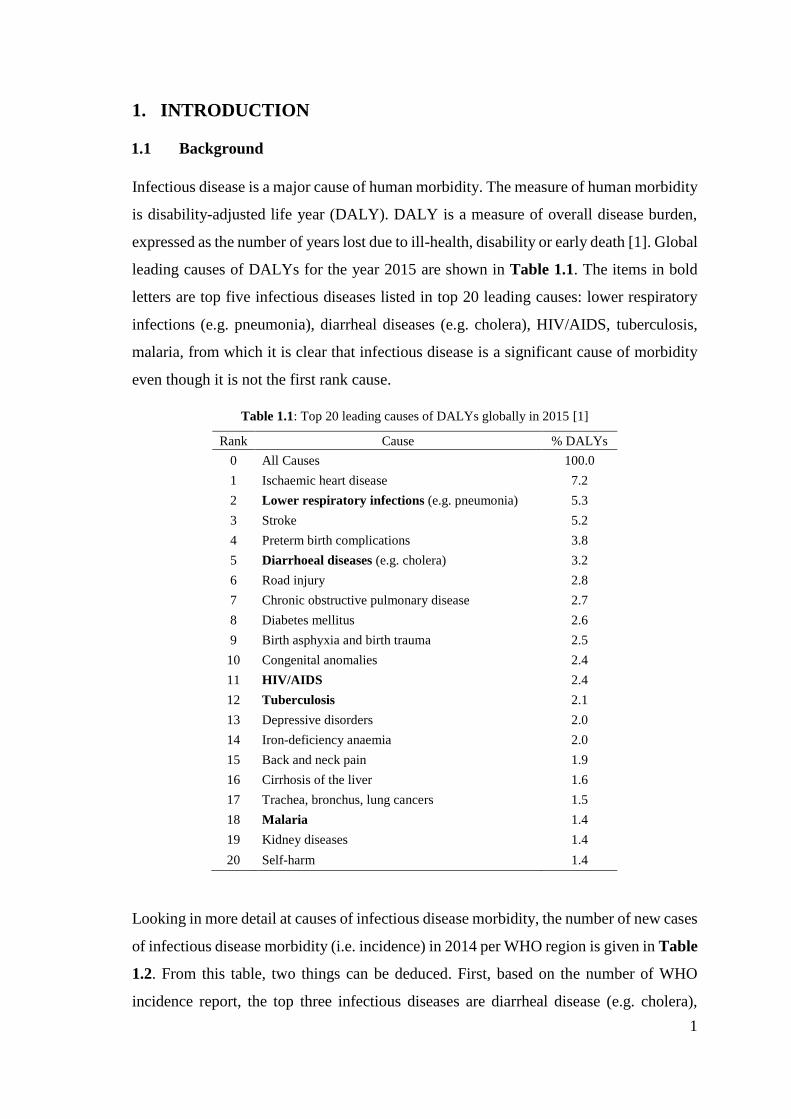
Infectious disease is a major cause of human morbidity. The measure of human morbidity
is disability-adjusted life year (DALY). DALY is a measure of overall disease burden,
expressed as the number of years lost due to ill-health, disability or early death [1]. Global
leading causes of DALYs for the year 2015 are shown in Table 1.1. The items in bold
letters are top five infectious diseases listed in top 20 leading causes: lower respiratory
infections (e.g. pneumonia), diarrheal diseases (e.g. cholera), HIV/AIDS, tuberculosis,
malaria, from which it is clear that infectious disease is a significant cause of morbidity
even though it is not the first rank cause.
Table 1.1: Top 20 leading causes of DALYs globally in 2015 [1]
Rank Cause % DALYs
0 All Causes 100.0
1 Ischaemic heart disease 7.2
2 Lower respiratory infections (e.g. pneumonia) 5.3
3 Stroke 5.2
4 Preterm birth complications 3.8
5 Diarrhoeal diseases (e.g. cholera) 3.2
6 Road injury 2.8
7 Chronic obstructive pulmonary disease 2.7
8 Diabetes mellitus 2.6
9 Birth asphyxia and birth trauma 2.5
10 Congenital anomalies 2.4
11 HIV/AIDS 2.4
12 Tuberculosis 2.1
13 Depressive disorders 2.0
14 Iron-deficiency anaemia 2.0
15 Back and neck pain 1.9
16 Cirrhosis of the liver 1.6
17 Trachea, bronchus, lung cancers 1.5
18 Malaria 1.4
19 Kidney diseases 1.4
20 Self-harm 1.4
Looking in more detail at causes of infectious disease morbidity, the number of new cases
of infectious disease morbidity (i.e. incidence) in 2014 per WHO region is given in Table
1.2. From this table, two things can be deduced. First, based on the number of WHO
incidence report, the top three infectious diseases are diarrheal disease (e.g. cholera),
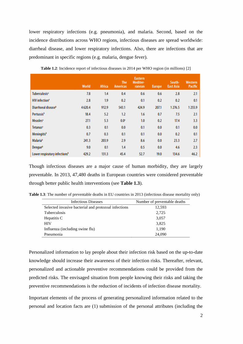
2
lower respiratory infections (e.g. pneumonia), and malaria. Second, based on the
incidence distributions across WHO regions, infectious diseases are spread worldwide:
diarrheal disease, and lower respiratory infections. Also, there are infections that are
predominant in specific regions (e.g. malaria, dengue fever).
Table 1.2: Incidence report of infectious diseases in 2014 per WHO region (in millions) [2]
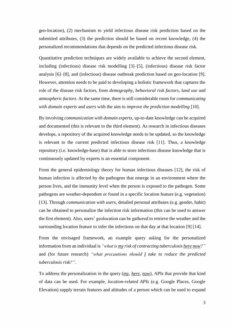
Though infectious diseases are a major cause of human morbidity, they are largely
preventable. In 2013, 47,480 deaths in European countries were considered preventable
through better public health interventions (see Table 1.3).
Table 1.3: The number of preventable deaths in EU countries in 2013 (infectious disease mortality only)
Infectious Diseases Number of preventable deaths
Selected invasive bacterial and protozoal infections 12,593
Tuberculosis 2,725
Hepatitis C 3,057
HIV 3,825
Influenza (including swine flu) 1,190
Pneumonia 24,090
Personalized information to lay people about their infection risk based on the up-to-date
knowledge should increase their awareness of their infection risks. Thereafter, relevant,
personalized and actionable preventive recommendations could be provided from the
predicted risks. The envisaged situation from people knowing their risks and taking the
preventive recommendations is the reduction of incidents of infection disease mortality.
Important elements of the process of generating personalized information related to the
personal and location facts are (1) submission of the personal attributes (including the
3
geo-location), (2) mechanism to yield infectious disease risk prediction based on the
submitted attributes, (3) the prediction should be based on recent knowledge, (4) the
personalized recommendations that depends on the predicted infectious disease risk.
Quantitative prediction techniques are widely available to achieve the second element,
including (infectious) disease risk modelling [3]–[5], (infectious) disease risk factor
analysis [6]–[8], and (infectious) disease outbreak prediction based on geo-location [9].
However, attention needs to be paid to developing a holistic framework that captures the
role of the disease risk factors, from demography, behavioral risk factors, land use and
atmospheric factors. At the same time, there is still considerable room for communicating
with domain experts and users with the aim to improve the prediction modelling [10].
By involving communication with domain experts, up-to-date knowledge can be acquired
and documented (this is relevant to the third element). As research in infectious diseases
develops, a repository of the acquired knowledge needs to be updated, so the knowledge
is relevant to the current predicted infectious disease risk [11]. Thus, a knowledge
repository (i.e. knowledge-base) that is able to store infectious disease knowledge that is
continuously updated by experts is an essential component.
From the general epidemiology theory for human infectious diseases [12], the risk of
human infection is affected by the pathogens that emerge in an environment where the
person lives, and the immunity level when the person is exposed to the pathogen. Some
pathogens are weather-dependent or found in a specific location feature (e.g. vegetation)
[13]. Through communication with users, detailed personal attributes (e.g. gender, habit)
can be obtained to personalize the infection risk information (this can be used to answer
the first element). Also, users’ geolocation can be gathered to retrieve the weather and the
surrounding location feature to infer the infections on that day at that location [9] [14].
From the envisaged framework, an example query asking for the personalized
information from an individual is “what is my risk of contracting tuberculosis here now?”
and (for future research) “what precautions should I take to reduce the predicted
tuberculosis risk?”.
To address the personalization in the query (my, here, now), APIs that provide that kind
of data can be used. For example, location-related APIs (e.g. Google Places, Google
Elevation) supply terrain features and altitudes of a person which can be used to expand
4
on the concept of here [9], [15]. Weather-related APIs (e.g. OpenWeather) provide
atmospheric conditions of a city in a country at a given date and time, this can be used to
expand on now in the query above [16]–[18]. WHO reports can be used to give the latest
tuberculosis incidence in here [19]. The basic personal attributes are required to be
submitted by the users to explain my.
To sum up, the background of this thesis is in public health and epidemiology, and, to be
more specific, is epidemiology of human infectious diseases. Meanwhile, in the context
of computer systems, the thesis background is in knowledge representation, (infectious)
disease risk prediction systems, and personalization systems.
1.2 Motivation
Started by a concern about infectious disease burden in the world, informing lay people
about their personal infection risk is achievable through designing a framework (e.g.
system, service) that allows communication with both experts and the users (whose risk
are being predicted) and capable of predicting the infectious disease risk based on the
weather, location, personal attributes, and recent knowledge.
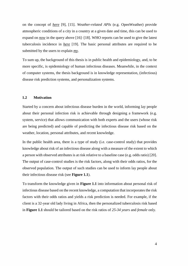
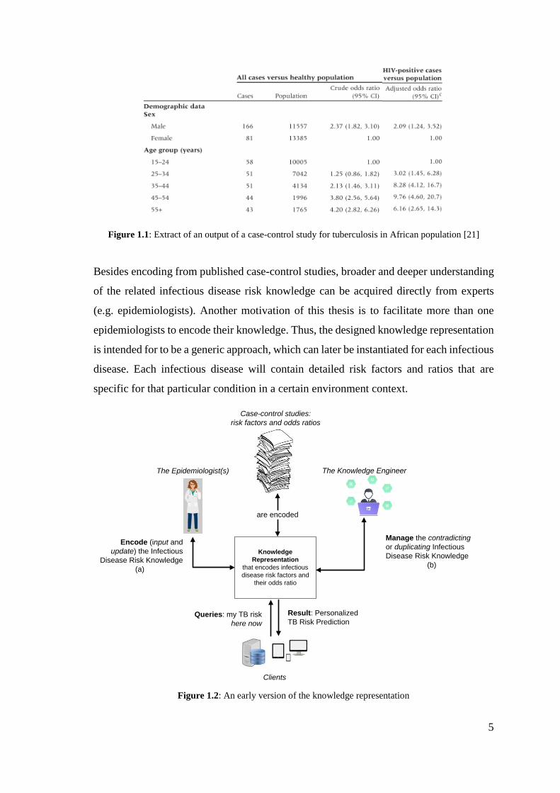
In the public health area, there is a type of study (i.e. case-control study) that provides
knowledge about risk of an infectious disease along with a measure of the extent to which
a person with observed attributes is at risk relative to a baseline case (e.g. odds ratio) [20].
The output of case-control studies is the risk factors, along with their odds ratios, for the
observed population. The output of such studies can be used to inform lay people about
their infectious disease risk (see Figure 1.1).
To transform the knowledge given in Figure 1.1 into information about personal risk of
infectious disease based on the recent knowledge, a computation that incorporates the risk
factors with their odds ratios and yields a risk prediction is needed. For example, if the
client is a 32-year old lady living in Africa, then the personalized tuberculosis risk based
in Figure 1.1 should be tailored based on the risk ratios of 25-34 years and female only.
5
Figure 1.1: Extract of an output of a case-control study for tuberculosis in African population [21]
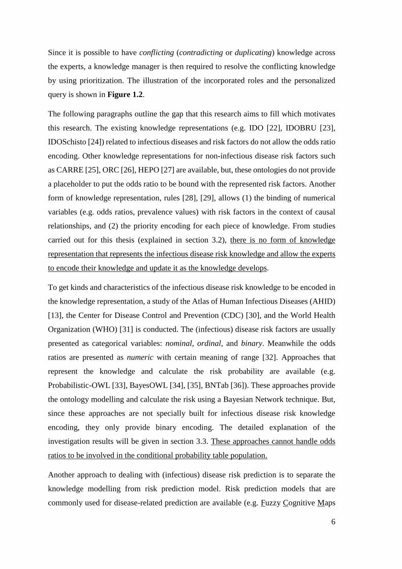
Besides encoding from published case-control studies, broader and deeper understanding
of the related infectious disease risk knowledge can be acquired directly from experts
(e.g. epidemiologists). Another motivation of this thesis is to facilitate more than one
epidemiologists to encode their knowledge. Thus, the designed knowledge representation
is intended for to be a generic approach, which can later be instantiated for each infectious
disease. Each infectious disease will contain detailed risk factors and ratios that are
specific for that particular condition in a certain environment context.
Queries: my TB risk
here now
Result: Personalized
TB Risk Prediction
Clients
The Epidemiologist(s) The Knowledge Engineer
Knowledge
Representation
that encodes infectious
disease risk factors and
their odds ratio
Encode (input and
update) the Infectious
Disease Risk Knowledge
(a)
Manage the contradicting
or duplicating Infectious
Disease Risk Knowledge
(b)
Case-control studies:
risk factors and odds ratios
are encoded
Figure 1.2: An early version of the knowledge representation
6
Since it is possible to have conflicting (contradicting or duplicating) knowledge across
the experts, a knowledge manager is then required to resolve the conflicting knowledge
by using prioritization. The illustration of the incorporated roles and the personalized
query is shown in Figure 1.2.
The following paragraphs outline the gap that this research aims to fill which motivates
this research. The existing knowledge representations (e.g. IDO [22], IDOBRU [23],
IDOSchisto [24]) related to infectious diseases and risk factors do not allow the odds ratio
encoding. Other knowledge representations for non-infectious disease risk factors such
as CARRE [25], ORC [26], HEPO [27] are available, but, these ontologies do not provide
a placeholder to put the odds ratio to be bound with the represented risk factors. Another
form of knowledge representation, rules [28], [29], allows (1) the binding of numerical
variables (e.g. odds ratios, prevalence values) with risk factors in the context of causal
relationships, and (2) the priority encoding for each piece of knowledge. From studies
carried out for this thesis (explained in section 3.2), there is no form of knowledge
representation that represents the infectious disease risk knowledge and allow the experts
to encode their knowledge and update it as the knowledge develops.
To get kinds and characteristics of the infectious disease risk knowledge to be encoded in
the knowledge representation, a study of the Atlas of Human Infectious Diseases (AHID)
[13], the Center for Disease Control and Prevention (CDC) [30], and the World Health
Organization (WHO) [31] is conducted. The (infectious) disease risk factors are usually
presented as categorical variables: nominal, ordinal, and binary. Meanwhile the odds
ratios are presented as numeric with certain meaning of range [32]. Approaches that
represent the knowledge and calculate the risk probability are available (e.g.
Probabilistic-OWL [33], BayesOWL [34], [35], BNTab [36]). These approaches provide
the ontology modelling and calculate the risk using a Bayesian Network technique. But,
since these approaches are not specially built for infectious disease risk knowledge
encoding, they only provide binary encoding. The detailed explanation of the
investigation results will be given in section 3.3. These approaches cannot handle odds
ratios to be involved in the conditional probability table population.
Another approach to dealing with (infectious) disease risk prediction is to separate the
knowledge modelling from risk prediction model. Risk prediction models that are
commonly used for disease-related prediction are available (e.g. Fuzzy Cognitive Maps
7
(FCM) [37], [38], Bayesian Networks (BN) [3], [39], Logistic Regression (LR) [40],
[41]). Knowledge about infectious disease risk factors has characteristics (mix between
nominal, ordinal, binary states) which are compatible with the BN technique. A version
of Bayes chain rule [42], [43] is available to be utilized. However, none of the existing
algorithms populate a CPT by utilizing this version of Bayes chain rule. A detailed
explanation of each risk prediction model will be elaborated in section 2.2.1.
Taking all previous into consideration, a knowledge-base that (1) represents infectious
disease risk knowledge (as in Figure 1.1), (2) allows infectious disease risk prediction,
(3) is usable by the epidemiologists and manageable by knowledge manager continuously
as the knowledge develops (illustrated in Figure 1.2), is the goal of this thesis.
1.3 Research Questions
The research question posed in this thesis is,
‘can a useful knowledge representation be designed to encode infectious disease risk
knowledge, and can this the encoded knowledge be correctly availed of to yield
personalized infectious disease risk prediction?’
1.4 Objectives and Goals
In answering the research question presented in the preceding section, the main goal of
the useful knowledge representation is that it -
G1. allows epidemiologists to encode infectious disease risk knowledge
continuously as the knowledge develops.
G2. can be availed to yield personalized infectious disease risk prediction.
To achieve those main goals, the objectives of this thesis is
O1. to comprehend the characteristics of the infectious disease risk knowledge that
are relevant to predict a person's infectious disease risk from declarative
knowledge sources (e.g. AHID [13], CDC [30], WHO [31]).
O2. to search and review the state of the art in (infectious) disease risk prediction
systems and the used techniques.
8
O3. to search and review the state of the art of knowledge representation specific
for (infectious) disease knowledge.
O4. to design a form of knowledge representation that fits the knowledge
characteristics and meets the goals G1 and G2.
O5. to evaluate the consistency between the resulting personalized infectious disease
risk prediction and the encoded knowledge.
As a placeholder of the knowledge representation and the needed tools, a system is also
designed in this thesis that,
G3. facilitates the clients to submit their personal queries and personalize their
infectious disease risks
G4. facilitates the knowledge manager to resolve the conflicting knowledge (e.g.
contradicting and duplicating)
G5. retrieves relevant contexts from live data sources (e.g. APIs) and disease
morbidity from WHO reports
However, since the main focus of this thesis is the form of the knowledge representation
that is capable of encoding infectious disease risk knowledge which allows risk
prediction, thus, the design of the system that utilizes the knowledge-base and allows
communication to the experts and the clients is adequate. Therefore, the system
development is not included in this thesis.
1.5 Contribution to the State of the Art
This thesis proposes a contribution, a format of knowledge representation that allows
domain experts to continuously encode the knowledge related to a personalized infectious
disease risk prediction. The form of knowledge representation is published in a a
conference proceeding and uploaded to the Open Science Framework repository (see
Appendix 4 for early development and Appendix 7 for the later version). Together with
a tool (as an algorithm) to make sure that the encoded knowledge is consistent with the
risk prediction results. The Java packages of the algorithm are published in a conference
proceeding (see Appendix 5 for early development) and uploaded in a GitHub repository.
This thesis also proposes a minor contribution related to the design of a system
architecture. The system is where the knowledge representation and the tool interact
9
with the other components (e.g. APIs) to serve personalized requests from clients. The
request is to calculate a person’s risk of contracting of an infectious disease at a time at a
certain place. The system also facilitates a knowledge manager to resolve conflicting
knowledge as the epidemiologists continuously update the knowledge-base. We call this
system PROSPECT-IDR (Personalised Prediction of Infectious Disease Risk).
1.6 Methodology
To answer the research question posed in section 1.3 and achieve goals listed in section
1.4, this section explains how this research is conducted. Basically, this section is an
elaboration of the objectives listed in section 1.4.
The contexts of this thesis are infectious diseases, risk prediction, knowledge
representation, and personalization. To retrieve existing research, projects, apps, web
services in these contexts, a search on the peer-reviewed article repository, and app and
web stores is conducted. For the journal repository search, the relevant topics are
infectious disease informatics, public health informatics, global health informatics,
computational epidemiology, and digital epidemiology. The search results are then
analyzed based on two focuses: (1) the risk prediction techniques that they use, and (2)
how they model their risk factors (i.e. predictors). Any related data stores (e.g. APIs,
reports, patient admission records) that may be reused for the system are also investigated
during this search.
The first part of the research question of this thesis is whether a useful knowledge
representation can be designed to encode the infectious disease risk knowledge. This part
has two concentrations, first, on the characteristics of the infectious disease risk
knowledge (e.g. the risk factors, and odds ratios) and second, on the form of knowledge
representation (e.g. ontology, rules) that fits to the (infectious) disease risk knowledge
characteristics (e.g. ordinal (smoking habit), binary (gender), nominal (nationality)). To
find the characteristics of the knowledge, key declarative knowledge sources are
consulted (e.g. AHID, CDC, WHO). From these knowledge sources, all risk factors
mentioned for all human infectious diseases are collated. This collation includes the
personal risk factors and relationships between (infectious) disease risk and the climate
or location features. For the form of (infectious) disease risk knowledge representation, a
10
search in journal and knowledge repositories is conducted with specific key search on
‘disease’. The search aims to find the concepts, objects, or structure of existing knowledge
representation that can be reused partially or wholly.
The next part of the research question is whether the knowledge representation is usable
by the epidemiologists. To make this knowledge representation usable, a user interface
that facilitates inputting knowledge into the knowledge representation is designed. The
characteristics of the epidemiological knowledge are represented as input controls of the
user interface. The process of inputting knowledge details obtained from case-control
studies is then designed as features in the user interfaces.
The last part of the research question is whether the encoded knowledge can be correctly
availed to yield personalized infectious disease risk prediction. This part of the question
adds another focus to the knowledge representation search by investigating a way or a
tool that allows the encoded knowledge to support the infectious disease risk prediction.
The system that serves the personalized queries from clients asking for their infectious
disease risk prediction, PROSPECT-IDR, is then designed. In this system design, the
reusable and relevant data sources that were obtained, the forms of knowledge
representation and the prediction techniques that were reviewed, the facilitations of the
communication to experts, knowledge manager and clients, are all included. At this stage,
a decision of the risk prediction technique that meets all requirements is made. Following
this decision, the form of knowledge representation that is compatible with the risk
prediction technique is chosen. Two involving activities: time to encode knowledge, and
prediction time, are also described at this stage.
After finding the infectious disease risk knowledge characteristics and quantifications, a
form of knowledge representation is designed by taking influences from the existing
concepts, objects, or structures. Besides that, the design of the knowledge representation
is also affected by the prediction technique that allow infectious disease risk prediction
from the encoded knowledge. The usefulness and the completeness of the (initial version)
knowledge representation are evaluated. The evaluation involves selected case-control
studies that discovered knowledge of infectious diseases prevalent in several countries.
The algorithm that makes sure the encoded knowledge is used correctly by the risk
prediction technique is then constructed. The various characteristics and quantifications
11
found in the infectious disease risk knowledge are the main focus of the tool development.
Evaluation cases (in the form of a knowledge-base) are intentionally built (including the
contradicting and duplicating knowledge) with aim to test the consistency of the resulting
infectious disease risk prediction with the encoded knowledge, and the ability to handle
different priority levels that are set by the knowledge manager to resolve the conflicts.
The outcome of the PROSPECT-IDR as a holistic system is the infectious disease risk
prediction that is personalized based on personal attributes (including the inferred
environment condition at a time in a place). The correctness of the resulting personalized
infectious disease risk prediction can be evaluated using reliability testing [43]. However,
the infectious disease risks depend on the quality of the case-control studies’ outputs (risk
factors, and the associated risk ratios). The better the case-control studies were
researched, the more qualified the risk factors and odds ratios that are encoded in the
knowledge-base, thus, the more reliable the infectious disease risk prediction. However,
the tool that is designed in this thesis only makes sure that the resulting risk prediction
results are consistent with the encoded knowledge in the designed form of knowledge
representation. This means that the tool is not responsible for the quality of the encoded
knowledge which can impact the reliability of the end results. Therefore, even though a
reliability evaluation for the risk prediction results is related, this evaluation is not
included in this thesis. An article that evaluates the reliability of the resulting infectious
disease risk prediction for three infectious diseases prevalent in three different countries
has been submitted to a journal. See Appendix 6 to read this submission.
1.7 Thesis Overview
The preceding section described the thesis methodology that covers review of the state-
of-the-art, design and evaluation of the knowledge representation (including the required
tool). The search related to literature, apps, web services, projects, forms of knowledge
representation resulted in two thesis chapters.
Chapter 2 reviews existing projects, web services, systems, proposals, or apps related to
human (infectious) disease risk prediction systems. In this chapter, the information of the
reusable data sources, risk prediction techniques, and predictor modelling of the human
(infectious) disease risk prediction are identified.
12
Chapter 3 describes the domain knowledge that explains how a person is at risk of an
infectious disease based on personal and environment risk factors. This kind of
knowledge is available in epidemiology for infectious diseases provided by CDC.
Thereafter, the reviews of the disease knowledge representations are discussed and
reviewed. Other articles about the risk prediction models that also serve as knowledge-
base, or a knowledge-base that also models probabilistic knowledge are investigated.
Advantages and limitations for each model are outlined in this chapter. An example of
declarative infectious disease risk knowledge is also shown in each model with aim to
give a fair comparison for the discussion.
From the state-of-the-art review chapters above, data sources, forms of knowledge
representation, the way the projects, web services, systems, proposals, or apps model their
predictors and their prediction techniques were gathered. The relevant features or
concepts were taken for inspiration to create the components of PROSPECT-IDR system.
Chapter 4 explains the influences taken from the literature review chapters (chapter 2
and 3) to design the PROSPECT-IDR system. All required data sources and components
are described in this chapter. The system is designed to achieve goals G3 to G5 in section
1.4. In this chapter, the explanation about decisions of the knowledge representation and
the risk prediction technique that fit the system is elaborated. The further details of the
knowledge representation are elaborated in chapter 5.
Taking two decisions made in chapter 4, the design and evaluation of the covered
components are elaborated in chapter 5 and chapter 6 as the main chapters of this thesis.
Chapter 5 describes the design of the form of knowledge representation that encodes the
infectious disease risk knowledge taken from declarative knowledge sources (e.g. AHID,
WHO, CDC). The form of knowledge representation is designed to allow the encoded
knowledge to be used for predicting personalized infectious disease risk using the chosen
risk prediction technique. In the evaluation, knowledge of several infectious diseases
prevalent in several countries is encoded in the designed knowledge representation. This
encoding activity aims to test the usefulness and completeness of the initial design of the
knowledge representation.
Chapter 6 explains the required tool to keep the knowledge consistent between the
encoded knowledge and the resulting personalized infectious disease risk prediction. To

13
make sure the consistency of this algorithm, test cases (i.e. knowledge-bases) that touch
the boundaries of the requirements (including conflicting knowledge) are chosen.
Thereafter, the algorithm is executed to transform the encoded knowledge into a BN. The
resulting BN and the encoded knowledge are then compared and analyzed whether they
are consistent or not.
Chapter 7 concludes the thesis. It summarizes the thesis contributions made to the state-
of-the-art together with the limitations. Some discussion related to long-term vision and
the continuation of research from this thesis is also provided in this chapter.
14
2. STATE OF THE ART –
INFECTIOUS DISEASE RISK PREDICTION SYSTEM
This chapter reviews the state of the art in infectious disease risk prediction systems,
focusing on context-specific and personalized prediction. This chapter describes projects,
apps, ongoing research that is related to infectious disease risk prediction and
personalization. This chapter informs us about the basic definition and typical research in
"personalization", "infectious disease" and "risk prediction" in the context of the areas of
medicine and computer science. The domains that cover this kind of research are
Computational Epidemiology, Public Health Informatics, Infectious Disease Informatics,
Digital Epidemiology, and Global Health Informatics. The review yields the prediction
models that are usually used for (infectious) disease risk prediction, the kind of the inputs
and outputs for each model, and what kind of data in what form is available for person
and environment modelling relevant to (infectious) disease risks.
Together with the following chapter (chapter 3 – the domain knowledge and its
representation), the prediction models and obtainable data found in this chapter will
influence the design decisions (explained in chapters 4, 5, and 6).
2.1 Definition of Personalized Infectious Disease Risk Prediction System
Based on the Merriam-Webster dictionary, prediction is an act to declare or indicate in
advance; foretell on the basis of observation, experience or scientific reason [44].
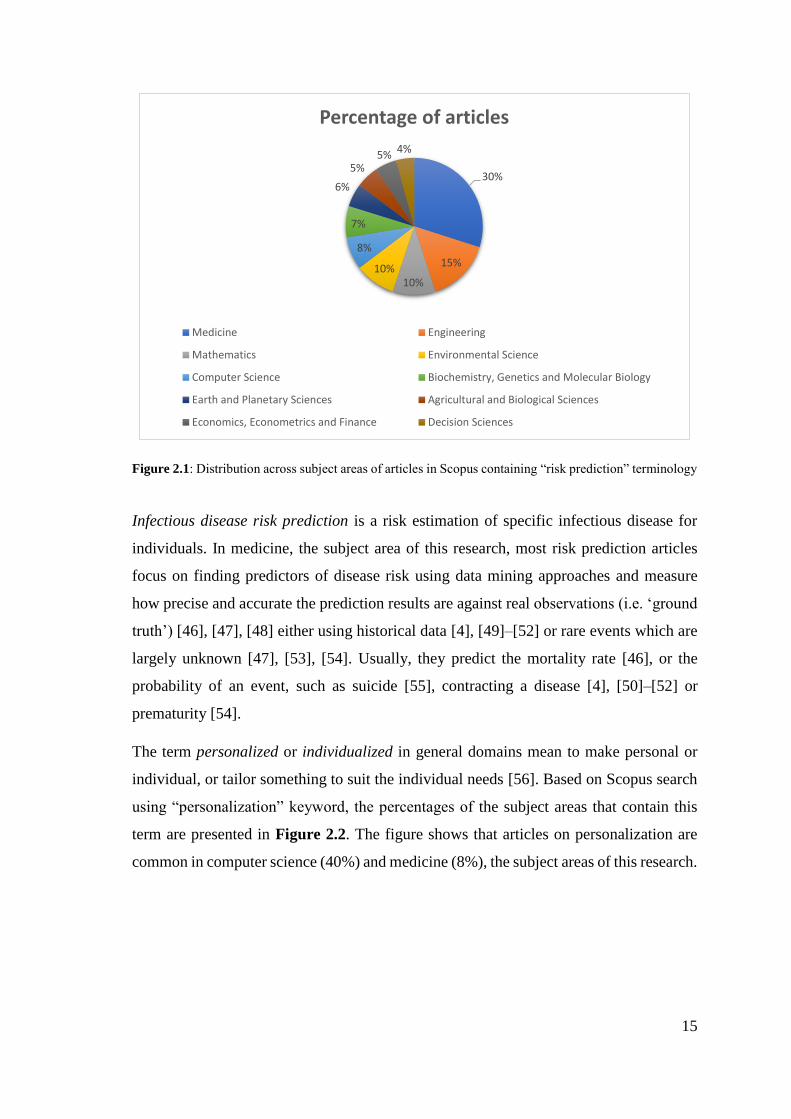
Risk prediction is an estimation of future outcomes for individuals based on one or more
underlying predictors (characteristics) [45]. Risk prediction has application in many
domains. Based on Scopus search using “risk prediction” or “risk estimation” keywords,
the distribution of such articles across subject areas is presented in Figure 2.1. Medicine,
the subject area of this research, is the most common.
15
Figure 2.1: Distribution across subject areas of articles in Scopus containing “risk prediction” terminology
Infectious disease risk prediction is a risk estimation of specific infectious disease for
individuals. In medicine, the subject area of this research, most risk prediction articles
focus on finding predictors of disease risk using data mining approaches and measure
how precise and accurate the prediction results are against real observations (i.e. ‘ground
truth’) [46], [47], [48] either using historical data [4], [49]–[52] or rare events which are
largely unknown [47], [53], [54]. Usually, they predict the mortality rate [46], or the
probability of an event, such as suicide [55], contracting a disease [4], [50]–[52] or
prematurity [54].
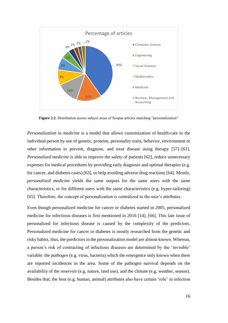
The term personalized or individualized in general domains mean to make personal or
individual, or tailor something to suit the individual needs [56]. Based on Scopus search
using “personalization” keyword, the percentages of the subject areas that contain this
term are presented in Figure 2.2. The figure shows that articles on personalization are
common in computer science (40%) and medicine (8%), the subject areas of this research.
30%
15%
10%10%
8%
7%
6%
5%5% 4%
Percentage of articles
Medicine Engineering
Mathematics Environmental Science
Computer Science Biochemistry, Genetics and Molecular Biology
Earth and Planetary Sciences Agricultural and Biological Sciences
Economics, Econometrics and Finance Decision Sciences
16
Figure 2.2: Distribution across subject areas of Scopus articles matching “personalization”
Personalization in medicine is a model that allows customization of health-care to the
individual person by use of genetic, proteins, personality traits, behavior, environment or
other information to prevent, diagnose, and treat disease using therapy [57]–[61].
Personalized medicine is able to improve the safety of patients [62], reduce unnecessary
expenses for medical procedures by providing early diagnosis and optimal therapies (e.g.
for cancer, and diabetes cases) [63], or help avoiding adverse drug reactions [64]. Mostly,
personalized medicine yields the same outputs for the same users with the same
characteristics, or for different users with the same characteristics (e.g. hyper-tailoring)
[65]. Therefore, the concept of personalization is centralized to the user’s attributes.
Even though personalized medicine for cancer or diabetes started in 2005, personalized
medicine for infectious diseases is first mentioned in 2016 [14], [66]. This late issue of
personalized for infectious disease is caused by the complexity of the predictors.
Personalized medicine for cancer or diabetes is mostly researched from the genetic and
risky habits, thus, the predictors in the personalization model are almost known. Whereas,
a person’s risk of contracting of infectious diseases are determined by the ‘invisible’
variable: the pathogen (e.g. virus, bacteria) which the emergence only known when there
are reported incidences in the area. Some of the pathogen survival depends on the
availability of the reservoir (e.g. nature, land use), and the climate (e.g. weather, season).
Besides that, the host (e.g. human, animal) attributes also have certain ‘role’ in infection
40%
15%
13%
9%
8%
5%
4%2% 2% 2%
Percentage of articles
Computer Science
Engineering
Social Sciences
Mathematics
Medicine
Business, Management andAccounting
17
risk [14]. Host susceptibility is affected by the host’s immunity level which is, in turn,
influenced by weather, genetic factors, demographic factors, behavior, or pre-existing
illness [66], [67].
These personal and environmental risk factors become the definition of an extended
personalization concept. The personalization is not only focused on the user attributes but
also the environment (e.g. weather and location) of the user. This extended
personalization definition was used to search for articles that relate to the PROSPECT-
IDR system developed for this research.
2.2 Existing Research on Infectious Disease Risk Prediction and its Predictor
Modelling
In order to find state of the art in personalized infectious disease risk prediction systems,
the first step was to identify relevant domain topics. These were gathered from the titles
of journals, conferences, and book chapters; the names of laboratories, research centers,
and course disciplines at the intersection between informatics, computer science, public
health, and (infectious) diseases. The following domains recurred in multiple titles:
computational epidemiology, public health informatics, infectious disease informatics,
digital epidemiology, and global health informatics.
Computational epidemiology is a multidisciplinary field that harnesses computer science,
mathematics, geographic information science and public health to understand the spread
of (infectious) diseases, or human behavior patterns that contribute to (infectious) disease
risk [68].
Informatics synthesizes the theory and practices of computer science, information
sciences, and behavioral and management sciences into methods, tools and concepts [69].
An effective informatics application is able to transform raw data into usable information.
In the public health domain, informatics can be used for monitoring and surveillance, to
support improved decision-making, and to improve population health [70]. Public health
informatics empowers disease interventions and prevention – leading to better health of
individuals and the community where they live [71].
18
Infectious disease informatics is a multidisciplinary field of science that is extended from
research on the public health laboratory data to find potential infectious disease vectors
and more robust to surveillance and computational of epidemiological factors. This
domain is intersected with computational epidemiology and public health informatics but
have more focus at vectors of infectious diseases [72].
Digital epidemiology is epidemiology that uses digital data to find the patterns (using
machine learning) which are used to understand and mitigate or preventing the disease.
The source of the data generation can be from inside, or outside the public health system
in a region [73].
Global health informatics is a multidisciplinary field between computer science,
medicine, engineering, public health, policy, and business that aims to improve healthcare
systems and outcomes. Admittedly, the global health informatics focus on specific vector-
borne diseases (e.g. Ebola, zika) in specific region.
Having identified the relevant domains, search queries were submitted to two types of
repository: (1) repository of established mobile or web apps (including the general-
purpose search engines such as Google, app store, and web store). The resulting
information from this kind of research is usually used to find the terminologies, general
concepts, and current technology which may not registered to peer-reviewed publications,
(2) repository of scientific articles (mainly referred from index citation database, such as
Scopus); the results from this repository usually follow a valid research methodology and
thus the information is more credible and qualified as the basis of the state-of-the-art of
this research.
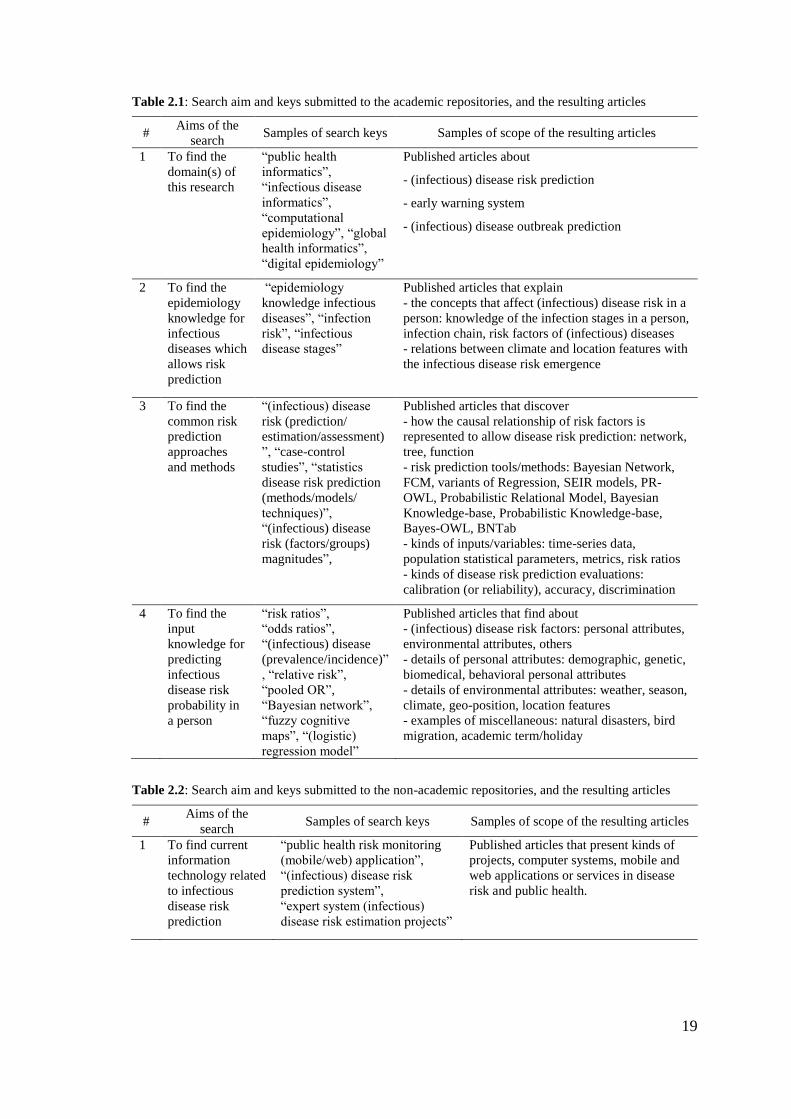
The search keys used to obtain the supporting articles for this chapter are presented in
Table 2.1 and Table 2.2. The keywords of the resulting articles in the upper rows
determine the search keys of the lower rows. Table 2.1 and Table 2.2 list the search
key(s) that is submitted to academic and non-academic type of repository, respectively.
The resulting publication types are news articles, WHO/CDC web pages, thesis books,
articles that are not peer-reviewed, lecture notes, book chapters. The search keys in the
last two rows were submitted to the second, scientific, type of repository related to health
and sciences (e.g. Science Direct, PLOS one, omics online, Nature, Google Scholar,
Academia).
19
Table 2.1: Search aim and keys submitted to the academic repositories, and the resulting articles
# Aims of the
search Samples of search keys Samples of scope of the resulting articles
1 To find the
domain(s) of
this research
“public health
informatics”,
“infectious disease
informatics”,
“computational
epidemiology”, “global
health informatics”,
“digital epidemiology”
Published articles about
- (infectious) disease risk prediction
- early warning system
- (infectious) disease outbreak prediction
2 To find the
epidemiology
knowledge for
infectious
diseases which
allows risk
prediction
“epidemiology
knowledge infectious
diseases”, “infection
risk”, “infectious
disease stages”
Published articles that explain
- the concepts that affect (infectious) disease risk in a
person: knowledge of the infection stages in a person,
infection chain, risk factors of (infectious) diseases
- relations between climate and location features with
the infectious disease risk emergence
3 To find the
common risk
prediction
approaches
and methods
“(infectious) disease
risk (prediction/
estimation/assessment)
”, “case-control
studies”, “statistics
disease risk prediction
(methods/models/
techniques)”,
“(infectious) disease
risk (factors/groups)
magnitudes”,
Published articles that discover
- how the causal relationship of risk factors is
represented to allow disease risk prediction: network,
tree, function
- risk prediction tools/methods: Bayesian Network,
FCM, variants of Regression, SEIR models, PR-
OWL, Probabilistic Relational Model, Bayesian
Knowledge-base, Probabilistic Knowledge-base,
Bayes-OWL, BNTab
- kinds of inputs/variables: time-series data,
population statistical parameters, metrics, risk ratios
- kinds of disease risk prediction evaluations:
calibration (or reliability), accuracy, discrimination
4 To find the
input
knowledge for
predicting
infectious
disease risk
probability in
a person
“risk ratios”,
“odds ratios”,
“(infectious) disease
(prevalence/incidence)”
, “relative risk”,
“pooled OR”,
“Bayesian network”,
“fuzzy cognitive
maps”, “(logistic)
regression model”
Published articles that find about
- (infectious) disease risk factors: personal attributes,
environmental attributes, others
- details of personal attributes: demographic, genetic,
biomedical, behavioral personal attributes
- details of environmental attributes: weather, season,
climate, geo-position, location features
- examples of miscellaneous: natural disasters, bird
migration, academic term/holiday
Table 2.2: Search aim and keys submitted to the non-academic repositories, and the resulting articles
# Aims of the
search Samples of search keys Samples of scope of the resulting articles
1 To find current
information
technology related
to infectious
disease risk
prediction
“public health risk monitoring
(mobile/web) application”,
“(infectious) disease risk
prediction system”,
“expert system (infectious)
disease risk estimation projects”
Published articles that present kinds of
projects, computer systems, mobile and
web applications or services in disease
risk and public health.
20
The search results of the queries listed in Table 2.1 and Table 2.2 are then used in section
2.2.1 and 2.2.2. The results are either scientific articles or web pages that explain certain
web services, apps, or projects that exist or in development or planned. Some of the
projects in Table 2.1 and Table 2.2 are reviewed below.
The VBD-AIR tool [74] enables the user to explore the interrelationships among
distributions of vector-borne infectious diseases (malaria, dengue, yellow fever and
chikungunya) and international air service routes to quantify seasonally changing risks of
vector and vector-borne disease importation and spread by air travel. It uses Climatic
Euclidean Distances (CEDs) to measure similarity in climatic regime between one airport
and another. The incorporated atmospheric attributes are rainfall (r), temperature (t) and
humidity (h) recorded for each airport location for each month. From this tool, the current
research adopted way of retrieving atmospheric attributes from weather API.
HealthMap [75], [76] is an internet-based system designed to collect and display
information about new infectious disease outbreaks according to geo-location, time, and
infectious agents. HealthMap integrates outbreak data from multiple electronic sources
such as UN data, news websites, WHO and CDC websites.
The AIME.Life (Artificial Intelligence in Medical Epidemiology) project [9] aims to
predict dengue outbreak 3 months in advance based on geo-position and date/time, by
incorporating public health data, weather, and geographical data. Both HealthMap and
AIME.Life projects are using Google Map APIs as a geo-position locator; their way of
converting the geo-position into location for other purposes influenced the PROSPECT-
IDR system. Even though this AIME.Life used the same inputs with this thesis to predict
an infectious disease: geo-position, public health data, weather, and geographical data,
AIME.Life does not contain the knowledge-base for infectious diseases. Thus, it cannot
be replicated to other infectious diseases because it might need different knowledge and
lead to different inputs.
CAIDE (Cardiovascular Risk Factors, Aging, and Incidence of Dementia) [77] is an app
based on the Dementia Risk Score that has two aims: (1) allowing users (lay people) to
detect their individual risk, and (2) allowing practitioners to discuss preventive measures
and monitor risk reduction. To achieve the first aim, lay people are asked to enter personal
attributes (e.g. age, educational level, blood pressure, obesity, and physical inactivity)
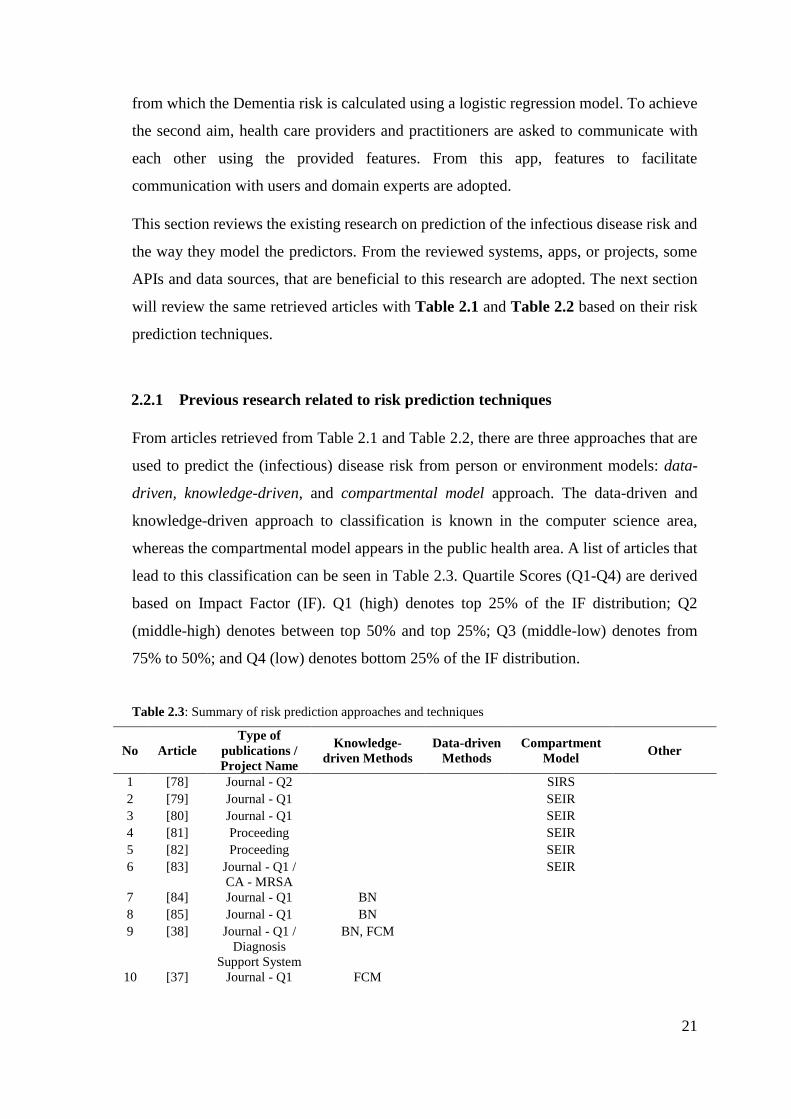
21
from which the Dementia risk is calculated using a logistic regression model. To achieve
the second aim, health care providers and practitioners are asked to communicate with
each other using the provided features. From this app, features to facilitate
communication with users and domain experts are adopted.
This section reviews the existing research on prediction of the infectious disease risk and
the way they model the predictors. From the reviewed systems, apps, or projects, some
APIs and data sources, that are beneficial to this research are adopted. The next section
will review the same retrieved articles with Table 2.1 and Table 2.2 based on their risk
prediction techniques.
2.2.1 Previous research related to risk prediction techniques
From articles retrieved from Table 2.1 and Table 2.2, there are three approaches that are
used to predict the (infectious) disease risk from person or environment models: data-
driven, knowledge-driven, and compartmental model approach. The data-driven and
knowledge-driven approach to classification is known in the computer science area,
whereas the compartmental model appears in the public health area. A list of articles that
lead to this classification can be seen in Table 2.3. Quartile Scores (Q1-Q4) are derived
based on Impact Factor (IF). Q1 (high) denotes top 25% of the IF distribution; Q2
(middle-high) denotes between top 50% and top 25%; Q3 (middle-low) denotes from
75% to 50%; and Q4 (low) denotes bottom 25% of the IF distribution.
Table 2.3: Summary of risk prediction approaches and techniques
No Article
Type of
publications /
Project Name
Knowledge-
driven Methods
Data-driven
Methods
Compartment
Model Other
1 [78] Journal - Q2 SIRS
2 [79] Journal - Q1 SEIR
3 [80] Journal - Q1 SEIR
4 [81] Proceeding SEIR
5 [82] Proceeding SEIR
6 [83] Journal - Q1 /
CA - MRSA
SEIR
7 [84] Journal - Q1 BN
8 [85] Journal - Q1 BN
9 [38] Journal - Q1 /
Diagnosis
Support System
BN, FCM
10 [37] Journal - Q1 FCM
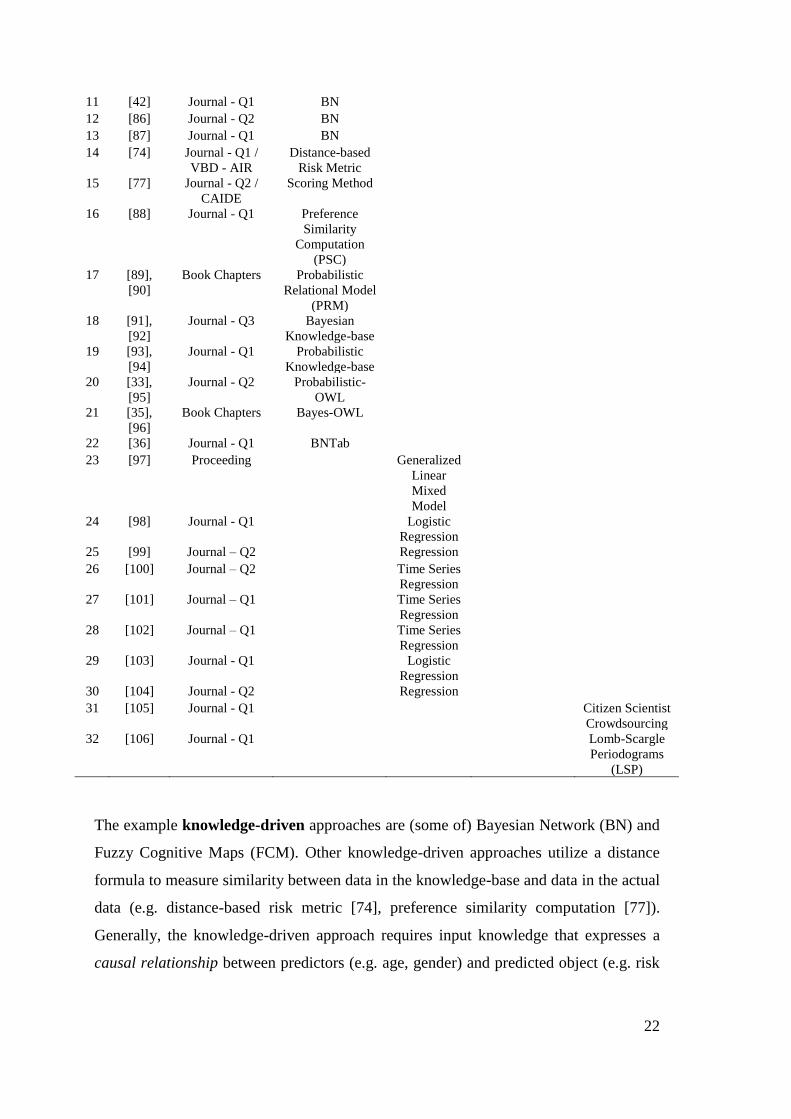
22
11 [42] Journal - Q1 BN
12 [86] Journal - Q2 BN
13 [87] Journal - Q1 BN
14 [74] Journal - Q1 /
VBD - AIR
Distance-based
Risk Metric
15 [77] Journal - Q2 /
CAIDE
Scoring Method
16 [88] Journal - Q1 Preference
Similarity
Computation
(PSC)
17 [89],
[90]
Book Chapters Probabilistic
Relational Model
(PRM)
18 [91],
[92]
Journal - Q3 Bayesian
Knowledge-base
19 [93],
[94]
Journal - Q1 Probabilistic
Knowledge-base
20 [33],
[95]
Journal - Q2 Probabilistic-
OWL
21 [35],
[96]
Book Chapters Bayes-OWL
22 [36] Journal - Q1 BNTab
23 [97] Proceeding Generalized
Linear
Mixed
Model
24 [98] Journal - Q1 Logistic
Regression
25 [99] Journal – Q2 Regression
26 [100] Journal – Q2 Time Series
Regression
27 [101] Journal – Q1 Time Series
Regression
28 [102] Journal – Q1 Time Series
Regression
29 [103] Journal - Q1 Logistic
Regression
30 [104] Journal - Q2 Regression
31 [105] Journal - Q1 Citizen Scientist
Crowdsourcing
32 [106] Journal - Q1 Lomb-Scargle
Periodograms
(LSP)
The example knowledge-driven approaches are (some of) Bayesian Network (BN) and
Fuzzy Cognitive Maps (FCM). Other knowledge-driven approaches utilize a distance
formula to measure similarity between data in the knowledge-base and data in the actual
data (e.g. distance-based risk metric [74], preference similarity computation [77]).
Generally, the knowledge-driven approach requires input knowledge that expresses a
causal relationship between predictors (e.g. age, gender) and predicted object (e.g. risk
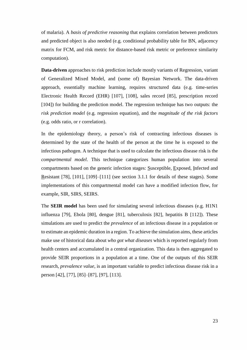
23
of malaria). A basis of predictive reasoning that explains correlation between predictors
and predicted object is also needed (e.g. conditional probability table for BN, adjacency
matrix for FCM, and risk metric for distance-based risk metric or preference similarity
computation).
Data-driven approaches to risk prediction include mostly variants of Regression, variant
of Generalized Mixed Model, and (some of) Bayesian Network. The data-driven
approach, essentially machine learning, requires structured data (e.g. time-series
Electronic Health Record (EHR) [107], [108], sales record [85], prescription record
[104]) for building the prediction model. The regression technique has two outputs: the
risk prediction model (e.g. regression equation), and the magnitude of the risk factors
(e.g. odds ratio, or r correlation).
In the epidemiology theory, a person’s risk of contracting infectious diseases is
determined by the state of the health of the person at the time he is exposed to the
infectious pathogen. A technique that is used to calculate the infectious disease risk is the
compartmental model. This technique categorizes human population into several
compartments based on the generic infection stages: Susceptible, Exposed, Infected and
Resistant [78], [101], [109]–[111] (see section 3.1.1 for details of these stages). Some
implementations of this compartmental model can have a modified infection flow, for
example, SIR, SIRS, SEIRS.
The SEIR model has been used for simulating several infectious diseases (e.g. H1N1
influenza [79], Ebola [80], dengue [81], tuberculosis [82], hepatitis B [112]). These
simulations are used to predict the prevalence of an infectious disease in a population or
to estimate an epidemic duration in a region. To achieve the simulation aims, these articles
make use of historical data about who got what diseases which is reported regularly from
health centers and accumulated in a central organization. This data is then aggregated to
provide SEIR proportions in a population at a time. One of the outputs of this SEIR
research, prevalence value, is an important variable to predict infectious disease risk in a
person [42], [77], [85]–[87], [97], [113].
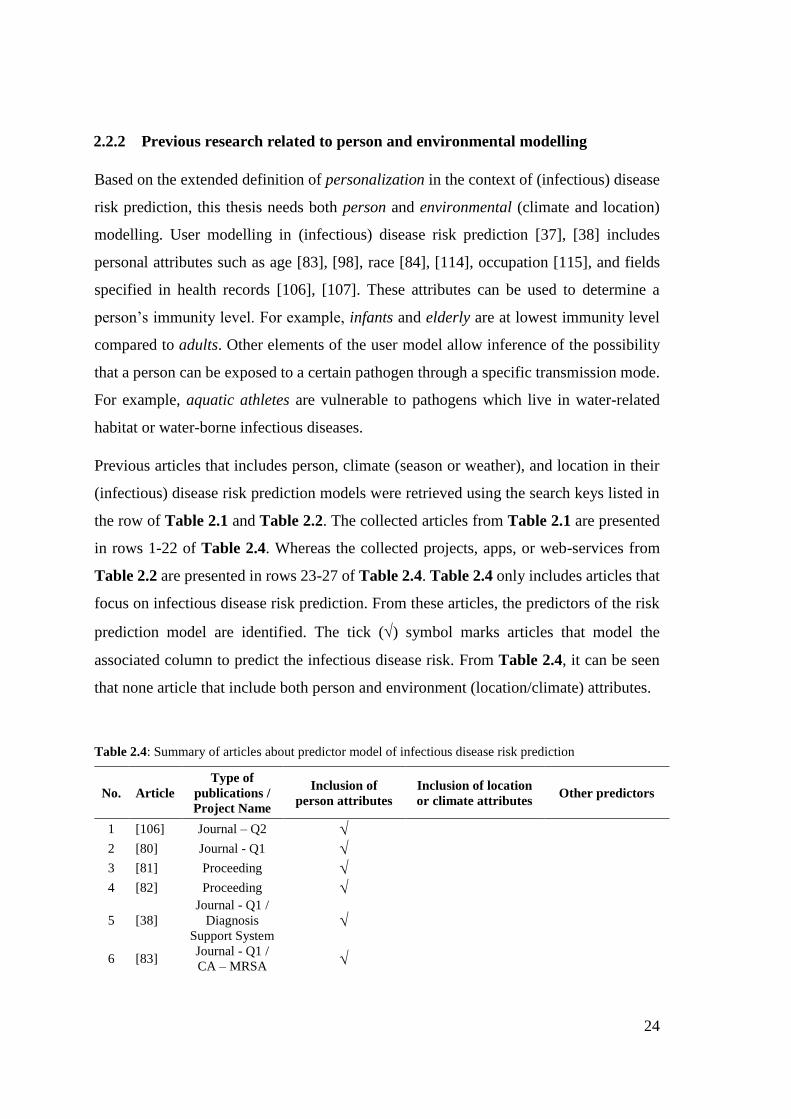
24
2.2.2 Previous research related to person and environmental modelling
Based on the extended definition of personalization in the context of (infectious) disease
risk prediction, this thesis needs both person and environmental (climate and location)
modelling. User modelling in (infectious) disease risk prediction [37], [38] includes
personal attributes such as age [83], [98], race [84], [114], occupation [115], and fields
specified in health records [106], [107]. These attributes can be used to determine a
person’s immunity level. For example, infants and elderly are at lowest immunity level
compared to adults. Other elements of the user model allow inference of the possibility
that a person can be exposed to a certain pathogen through a specific transmission mode.
For example, aquatic athletes are vulnerable to pathogens which live in water-related
habitat or water-borne infectious diseases.
Previous articles that includes person, climate (season or weather), and location in their
(infectious) disease risk prediction models were retrieved using the search keys listed in
the row of Table 2.1 and Table 2.2. The collected articles from Table 2.1 are presented
in rows 1-22 of Table 2.4. Whereas the collected projects, apps, or web-services from
Table 2.2 are presented in rows 23-27 of Table 2.4. Table 2.4 only includes articles that
focus on infectious disease risk prediction. From these articles, the predictors of the risk
prediction model are identified. The tick () symbol marks articles that model the
associated column to predict the infectious disease risk. From Table 2.4, it can be seen
that none article that include both person and environment (location/climate) attributes.
Table 2.4: Summary of articles about predictor model of infectious disease risk prediction
No. Article
Type of
publications /
Project Name
Inclusion of
person attributes
Inclusion of location
or climate attributes Other predictors
1 [106] Journal – Q2
2 [80] Journal - Q1
3 [81] Proceeding
4 [82] Proceeding
5 [38]
Journal - Q1 /
Diagnosis
Support System
6 [83] Journal - Q1 /
CA – MRSA
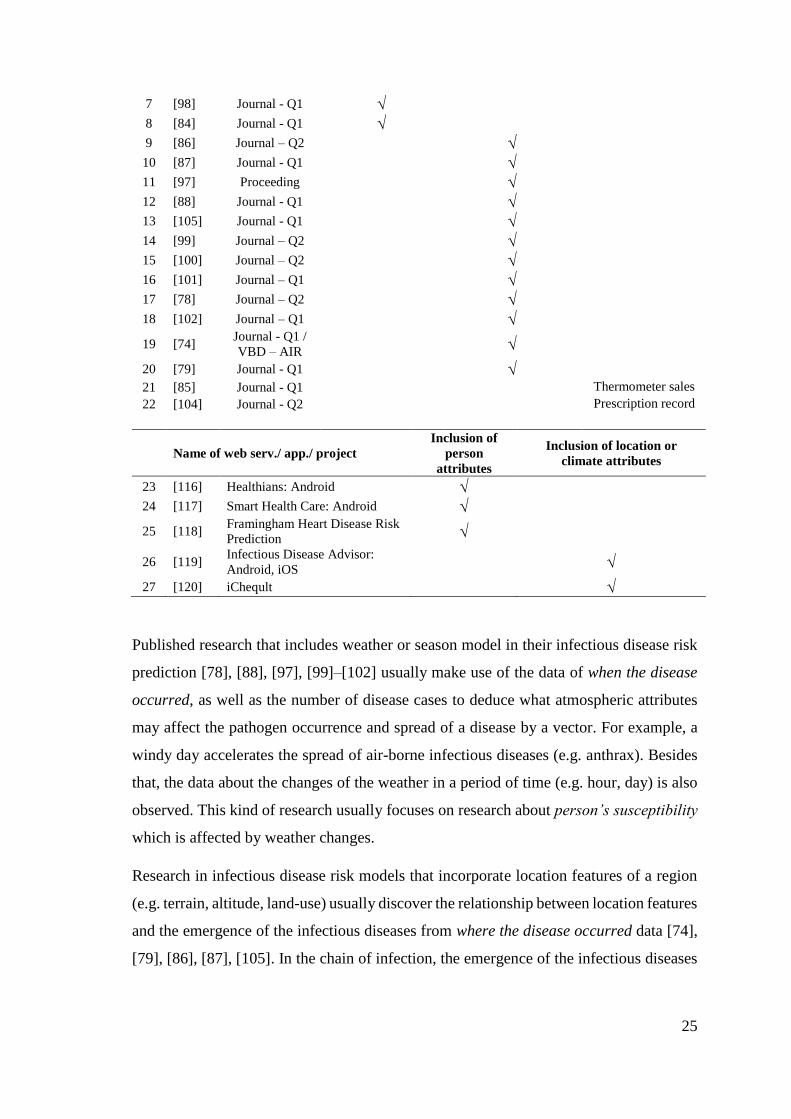
25
7 [98] Journal - Q1
8 [84] Journal - Q1
9 [86] Journal – Q2
10 [87] Journal - Q1
11 [97] Proceeding
12 [88] Journal - Q1
13 [105] Journal - Q1
14 [99] Journal – Q2
15 [100] Journal – Q2
16 [101] Journal – Q1
17 [78] Journal – Q2
18 [102] Journal – Q1
19 [74] Journal - Q1 /
VBD – AIR
20 [79] Journal - Q1
21 [85] Journal - Q1 Thermometer sales
22 [104] Journal - Q2 Prescription record
Name of web serv./ app./ project
Inclusion of
person
attributes
Inclusion of location or
climate attributes
23 [116] Healthians: Android
24 [117] Smart Health Care: Android
25 [118] Framingham Heart Disease Risk
Prediction
26 [119] Infectious Disease Advisor:
Android, iOS
27 [120] iCheqult
Published research that includes weather or season model in their infectious disease risk
prediction [78], [88], [97], [99]–[102] usually make use of the data of when the disease
occurred, as well as the number of disease cases to deduce what atmospheric attributes
may affect the pathogen occurrence and spread of a disease by a vector. For example, a
windy day accelerates the spread of air-borne infectious diseases (e.g. anthrax). Besides
that, the data about the changes of the weather in a period of time (e.g. hour, day) is also
observed. This kind of research usually focuses on research about person’s susceptibility
which is affected by weather changes.
Research in infectious disease risk models that incorporate location features of a region
(e.g. terrain, altitude, land-use) usually discover the relationship between location features
and the emergence of the infectious diseases from where the disease occurred data [74],
[79], [86], [87], [105]. In the chain of infection, the emergence of the infectious diseases
26
is determined by whether a person lives close to the pathogen’s reservoir, or vector’s
natural habitat. For example, the natural habitat of a chikungunya mosquito’s eggs is a
stagnant water pool; thus, the people who are infected are found to live near locations that
contain such water-related features (e.g. lake, basin).
From Table 2.4, it can be seen that no one risk prediction article includes person, climate,
and location attributes for predicting infectious disease risk. However, there are research
articles that include person, climate, and location attributes in disease-related studies but
are not about infectious disease risk personal prediction (e.g. disease outbreak prediction
research, early warning system). Outbreak detection systems [9], [39], [121]–[125] do
include all those attributes in their prediction models. The outputs of these articles can
tell the user when and where the pathogen will be active and cause an outbreak. Some
knowledge can be taken from these outbreak detection articles:
(1) Even though the possibility of contracting of an infectious disease is higher during
an outbreak period, not all people living in the location of the outbreak will have
the same risk of contracting the disease; the risk also depends on the person’s
susceptibility level, and the transmission modes of the infectious diseases.
(2) The exact GPS location of someone yields atmospheric attributes that infer
weather at a location. The weather information can be an indicator whether
pathogens or vectors are active or not in a location.
(3) The sources of infectious disease data, the methods to get odds ratios and
prevalence from the data, the prediction evaluation methods and risk prediction
models that these articles use to predict the location of the outbreak can be reused.
To be more specific, the location features can be used to identify the reservoir of
a particular pathogen.
2.3 Conclusion
In the beginning, this chapter gave the definition of the personalized infectious disease
risk prediction which lies in a multidisciplinary area between medicine and computer
science area. The specific disciplines in the medicine area that are relevant to this research
27
are public health and human infectious diseases. Whereas the relevant disciplines in the
computer science area are knowledge representation and personalization.
Referring back to the aim of this chapter outlined in the methodology (section 1.6), this
chapter focuses on the risk prediction techniques that are common in (infectious) disease
research, and from the way they model the predictors (person and environment). From
queries given in Table 2.1, three categories of prediction techniques are retrieved:
knowledge-driven, data-driven, and compartment model.
From knowledge-driven approach, two important components that appear in most
methods are causal relationship between predictors and predicted object and the basis of
predictive reasoning. From data-driven approach, other two essential elements are the
risk prediction equation and the magnitude of the predictors (i.e. risk ratios). From
compartment model, two concepts used to simulate infection in a person were obtained:
infection stages (susceptible-exposed-infected-recovered) and prevalence value.
From the collected articles on infectious disease risk prediction, no article involves both
person and environment in their risk prediction model. However, from the outbreak
detection articles that include person and environment models, some important and
relevant information are gathered:
(1) To estimate a person's susceptibility level, personal attributes (e.g. age,
occupation) and health records can be used.
(2) To deduce when the disease occurred, atmospheric attributes can be used to infer
weather-dependent pathogen or vector.
(3) To discover where the disease emerges, specific location features that become
reservoir of specific pathogens can be availed.
28
3. STATE OF THE ART –
THE DOMAIN KNOWLEDGE AND ITS REPRESENTATION
The previous chapter reviewed the risk prediction techniques, and predictor modelling
(i.e. person and environment models) from scientific articles and non-academic projects,
services or apps. From chapter 2, information about how to represent the (infectious)
disease risk knowledge and what kind of data that influences the infectious disease risk
prediction were obtained.
This chapter reviews the existing forms of disease knowledge representation. Before
searching for disease knowledge representation, the scope of domain knowledge that is
relevant to explain a person’s risk of contracting infectious diseases is first
comprehended. The domain knowledge is gathered from the epidemiology for human
infectious disease discipline. This knowledge elaborates more the attributes relevant to
the person and environment model, and SEIR compartment model (section 3.1.1).
Thereafter, the kinds of knowledge representation related to the domain knowledge are
searched. Techniques used to encode (infectious) disease risk, and similar knowledge in
computer interpretable form are explored (section 3.2). Besides that, the ability of using
the represented knowledge to predict the infectious disease risk is also investigated. As
none of these techniques meet the needs of the research, section 3.3 presents approaches
that combine risk prediction techniques and knowledge-bases, but not related to disease
or health.
Some information in this chapter will influence the design of the system, and the
knowledge representation in chapters 4 and 5, respectively.
3.1 The Domain of Knowledge: Human Infection Risk
This section describes relevant knowledge to estimate a person’s risk of contracting
infectious diseases in epidemiology domain. The knowledge in this section is the detailed
explanation of the susceptibility of a person, climate-dependent pathogen1 and vector2,
1 an infectious agent that causes illnesses
2 agent that carries and transmits pathogen into another host
29
and pathogen reservoir3 in specific location features. The etiology of infectious diseases
in human is explained in section 3.1.1, whereas, the quantifications that are common in
the epidemiology domain related to risk factor are presented in section 3.1.2. This section
concludes the scope of infectious disease risk knowledge (risk factors and their
quantifications) that relevant to personalized infectious disease risk prediction (section
3.1.3).
3.1.1 Etiology of Infectious Diseases
Three kinds of knowledge are included in this section: chain of infection that explains the
basic cycle of how infections are transmitted and infect humans; infection flow in a person
(SEIR compartment model) that describes stages of infection in a person; and the
knowledge that shows correlation between environment and infectious diseases.
Chain of Infection
Infectious disease is an ailment caused by a pathogen which is transmitted from an
infected person, animal or reservoir to a susceptible human (i.e. host) directly or
indirectly using a vector or vehicle [67], [126].
A pathogen is an agent causing an infectious disease (e.g. bacteria, virus, parasite, prion).
Based on their activity, the pathogens are divided into two: active and dormant pathogen.
Active pathogens multiply in their natural habitat (i.e. reservoir) and are ready to attack
hosts (e.g. human, plant, animal). Some pathogens require specific atmospheric
conditions to survive and multiply in the reservoir (i.e. climatic-dependent pathogen). For
example, Campylobacter spp. was found prefer to live in water surface during winter;
warmer temperature supports other bacteria to out-compete Campylobacter spp. and
ultraviolet light prohibits the survival of this bacteria [127]. Even though pathogens
cannot be seen with the naked eye, some developing projects can be used to estimate the
pathogen emergence in a location (e.g. Pathosphere.org [128]), country-based morbidity
reports can also be an indicator of the activity of pathogens of notifiable diseases [19].
3 person, animal, plant, or substance in which pathogen lives and multiplies
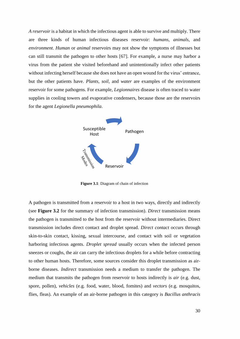
30
A reservoir is a habitat in which the infectious agent is able to survive and multiply. There
are three kinds of human infectious diseases reservoir: humans, animals, and
environment. Human or animal reservoirs may not show the symptoms of illnesses but
can still transmit the pathogen to other hosts [67]. For example, a nurse may harbor a
virus from the patient she visited beforehand and unintentionally infect other patients
without infecting herself because she does not have an open wound for the virus’ entrance,
but the other patients have. Plants, soil, and water are examples of the environment
reservoir for some pathogens. For example, Legionnaires disease is often traced to water
supplies in cooling towers and evaporative condensers, because those are the reservoirs
for the agent Legionella pneumophila.
Figure 3.1: Diagram of chain of infection
A pathogen is transmitted from a reservoir to a host in two ways, directly and indirectly
(see Figure 3.2 for the summary of infection transmission). Direct transmission means
the pathogen is transmitted to the host from the reservoir without intermediaries. Direct
transmission includes direct contact and droplet spread. Direct contact occurs through
skin-to-skin contact, kissing, sexual intercourse, and contact with soil or vegetation
harboring infectious agents. Droplet spread usually occurs when the infected person
sneezes or coughs, the air can carry the infectious droplets for a while before contracting
to other human hosts. Therefore, some sources consider this droplet transmission as air-
borne diseases. Indirect transmission needs a medium to transfer the pathogen. The
medium that transmits the pathogen from reservoir to hosts indirectly is air (e.g. dust,
spore, pollen), vehicles (e.g. food, water, blood, fomites) and vectors (e.g. mosquitos,
flies, fleas). An example of an air-borne pathogen in this category is Bacillus anthracis
Pathogen
Reservoir
Susceptible Host
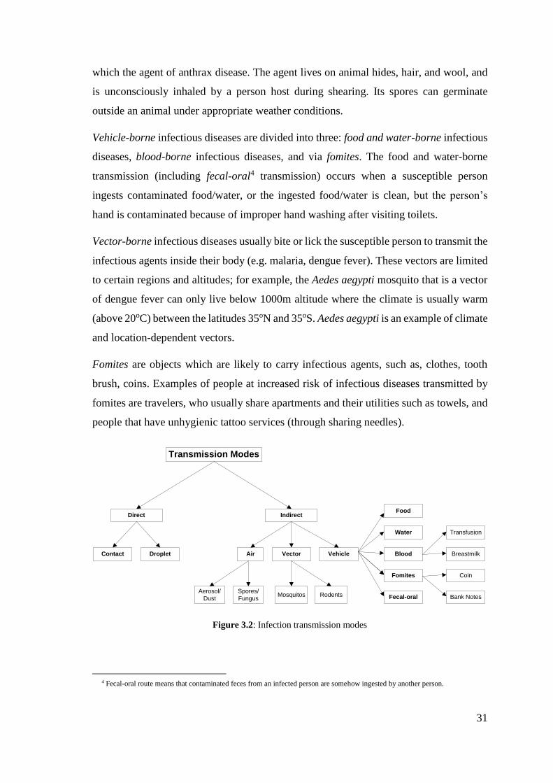
31
which the agent of anthrax disease. The agent lives on animal hides, hair, and wool, and
is unconsciously inhaled by a person host during shearing. Its spores can germinate
outside an animal under appropriate weather conditions.
Vehicle-borne infectious diseases are divided into three: food and water-borne infectious
diseases, blood-borne infectious diseases, and via fomites. The food and water-borne
transmission (including fecal-oral4 transmission) occurs when a susceptible person
ingests contaminated food/water, or the ingested food/water is clean, but the person’s
hand is contaminated because of improper hand washing after visiting toilets.
Vector-borne infectious diseases usually bite or lick the susceptible person to transmit the
infectious agents inside their body (e.g. malaria, dengue fever). These vectors are limited
to certain regions and altitudes; for example, the Aedes aegypti mosquito that is a vector
of dengue fever can only live below 1000m altitude where the climate is usually warm
(above 20oC) between the latitudes 35oN and 35oS. Aedes aegypti is an example of climate
and location-dependent vectors.
Fomites are objects which are likely to carry infectious agents, such as, clothes, tooth
brush, coins. Examples of people at increased risk of infectious diseases transmitted by
fomites are travelers, who usually share apartments and their utilities such as towels, and
people that have unhygienic tattoo services (through sharing needles).
Transmission Modes
Direct Indirect
Contact Droplet Vector VehicleAir
Aerosol/
Dust
Spores/
FungusMosquitos Rodents
Food
Water
Blood
Fomites
Breastmilk
Coin
Bank Notes
Transfusion
Fecal-oral
Figure 3.2: Infection transmission modes
4 Fecal-oral route means that contaminated feces from an infected person are somehow ingested by another person.
32
As described above, infectious diseases result from the interaction between pathogen,
host, and environment. More specifically, transmission occurs when the pathogen leaves
its reservoir using a specific mode of transmission, then enters to a susceptible human
host. From this host, the infection can be transmitted to other human directly, depending
on the disease transmission mode. This sequence is called the chain of infection.
Infection flow in a person
In epidemiology, there is a well-known mathematical modelling of infectious diseases.
This model divides the human population into compartments: Susceptible – Exposed –
Infected – Recovered (SEIR) [109] [129]. This division assumes that individuals
belonging to the same compartment have the same characteristics. The flow of these
compartments reflects the infection stages in a person.
Susceptible is a state of the targeted host (human) with low or declining immunity system.
The human susceptibility is affected by many factors: life stages, genetic, nutrition intake,
pre-existing diseases, tobacco smoking and alcohol consumption, and hygiene [130].
- Life stages refer to ages and developmental stages throughout human life. Early
life development stage from age of 3 – 24 months (infant, toddler) is a critical
period when a human has the lowest immune system. The human immunity then
increases with age. The peak of immunity is at adult development stage.
Thereafter, immunity declines (elderly). Most articles in case-control studies that
explain (infectious) disease risk prediction include age, and development stage
as personal risk factors [4], [131], [132].
- Genetic factors may confer susceptibility or resistance to particular diseases.
Usually in a population, genetic factors are identified through the parents’
medical history, nationality, or ethnicity. For example, infectious diseases that
are transmitted vertically from a pregnant mother to her unborn baby (e.g.
Rubella) [133]–[135].
- Nutrition intake is determined by a person’s consumption habits (e.g. eating and
drinking habits). Improper nutrition intake can result in obesity or malnutrition
both of which are risk factors for any diseases [136], [137].
33
- Those who have pre-existing diseases (such as cardiovascular disease, diabetes,
or renal dysfunction) may be more vulnerable to any infectious disease. For
example, people with positive HIV/AIDS are six-fold more susceptible to
Tuberculosis than people who do not have HIV/AIDS [21], [41], [138]–[140].
- Tobacco smoking and alcohol drinking are associated with numerous infectious
diseases, such as tuberculosis. Despite this, some articles may show no
correlation between these habits and tuberculosis. In fact, these habit increase
dual exposure to arsenic and ethanol which weaken the function of liver, heart,
and kidneys [141]. Thereafter, the weak body organs can result in a susceptible
person to any diseases, including tuberculosis [6], [142]–[144].
- Low hygiene is related with high risk of food and water-borne infectious diseases
(e.g. cholera). Also, low hygiene can be an indicator of a person’s low social
class (poverty); poverty is positively correlated with any infectious disease risks
[145]–[147].
Exposed is a state when a host (human) has been attacked by the infectious pathogen of
a particular disease. The exposure can be traced from the infectious disease transmission
modes. There are four transmission modes: direct contact (person-to-person), air-borne,
vehicle-borne, and vector-borne. From previous section, personal attributes, and the
surrounding environments of a person can determine whether the person is at risk of
certain infectious disease that are transmitted in some way [81], [109].
Infected is a state where a pathogen is already inside a human body. Most articles in
epidemiology and clinical domains identify whether a person is infected or not based on
his reported symptoms. However, the infection may still occur even though the host does
not show any symptoms, but he is still able to carry and transmit the pathogen to other
humans. Therefore, the majority of the case-control studies test serum samples for certain
antibodies to conclude whether a person is infected or not [87], [148], [149].
Recovered is a state where the infected human regains his immunity and health. This state
is related with nutrition intake, exercise habits, tobacco smoking and alcohol
consumption, and current atmospheric condition (e.g. solar exposure).
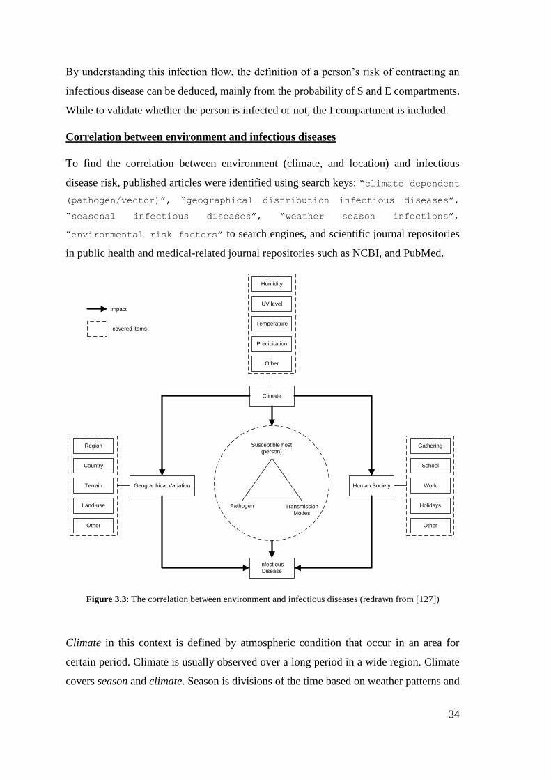
34
By understanding this infection flow, the definition of a person’s risk of contracting an
infectious disease can be deduced, mainly from the probability of S and E compartments.
While to validate whether the person is infected or not, the I compartment is included.
Correlation between environment and infectious diseases
To find the correlation between environment (climate, and location) and infectious
disease risk, published articles were identified using search keys: “climate dependent
(pathogen/vector)”, “geographical distribution infectious diseases”,
“seasonal infectious diseases”, “weather season infections”,
“environmental risk factors” to search engines, and scientific journal repositories
in public health and medical-related journal repositories such as NCBI, and PubMed.
Susceptible host
(person)
Pathogen Transmission
Modes
Climate
Infectious
Disease
Human SocietyGeographical Variation
impact
Temperature
Precipitation
Other
UV level
Humidity
Terrain
Land-use
Other
Country
Region
Work
Holidays
Other
School
Gathering
covered items
Figure 3.3: The correlation between environment and infectious diseases (redrawn from [127])
Climate in this context is defined by atmospheric condition that occur in an area for
certain period. Climate is usually observed over a long period in a wide region. Climate
covers season and climate. Season is divisions of the time based on weather patterns and
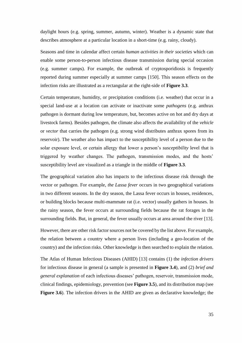
35
daylight hours (e.g. spring, summer, autumn, winter). Weather is a dynamic state that
describes atmosphere at a particular location in a short-time (e.g. rainy, cloudy).
Seasons and time in calendar affect certain human activities in their societies which can
enable some person-to-person infectious disease transmission during special occasion
(e.g. summer camps). For example, the outbreak of cryptosporidiosis is frequently
reported during summer especially at summer camps [150]. This season effects on the
infection risks are illustrated as a rectangular at the right-side of Figure 3.3.
Certain temperature, humidity, or precipitation conditions (i.e. weather) that occur in a
special land-use at a location can activate or inactivate some pathogens (e.g. anthrax
pathogen is dormant during low temperature, but, becomes active on hot and dry days at
livestock farms). Besides pathogen, the climate also affects the availability of the vehicle
or vector that carries the pathogen (e.g. strong wind distributes anthrax spores from its
reservoir). The weather also has impact to the susceptibility level of a person due to the
solar exposure level, or certain allergy that lower a person’s susceptibility level that is
triggered by weather changes. The pathogen, transmission modes, and the hosts’
susceptibility level are visualized as a triangle in the middle of Figure 3.3.
The geographical variation also has impacts to the infectious disease risk through the
vector or pathogen. For example, the Lassa fever occurs in two geographical variations
in two different seasons. In the dry season, the Lassa fever occurs in houses, residences,
or building blocks because multi-mammate rat (i.e. vector) usually gathers in houses. In
the rainy season, the fever occurs at surrounding fields because the rat forages in the
surrounding fields. But, in general, the fever usually occurs at area around the river [13].
However, there are other risk factor sources not be covered by the list above. For example,
the relation between a country where a person lives (including a geo-location of the
country) and the infection risks. Other knowledge is then searched to explain the relation.
The Atlas of Human Infectious Diseases (AHID) [13] contains (1) the infection drivers
for infectious disease in general (a sample is presented in Figure 3.4), and (2) brief and
general explanation of each infectious diseases’ pathogen, reservoir, transmission mode,
clinical findings, epidemiology, prevention (see Figure 3.5), and its distribution map (see
Figure 3.6). The infection drivers in the AHID are given as declarative knowledge; the
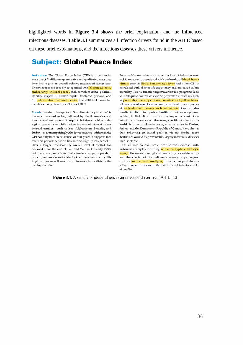
36
highlighted words in Figure 3.4 shows the brief explanation, and the influenced
infectious diseases. Table 3.1 summarizes all infection drivers found in the AHID based
on these brief explanations, and the infectious diseases these drivers influence.
Figure 3.4: A sample of peacefulness as an infection driver from AHID [13]
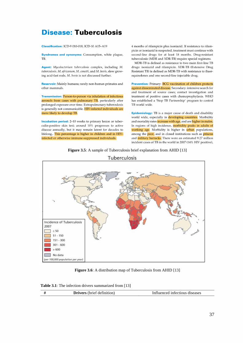
37
Figure 3.5: A sample of Tuberculosis brief explanation from AHID [13]
Figure 3.6: A distribution map of Tuberculosis from AHID [13]
Table 3.1: The infection drivers summarized from [13]
# Drivers (brief definition) Influenced infectious diseases
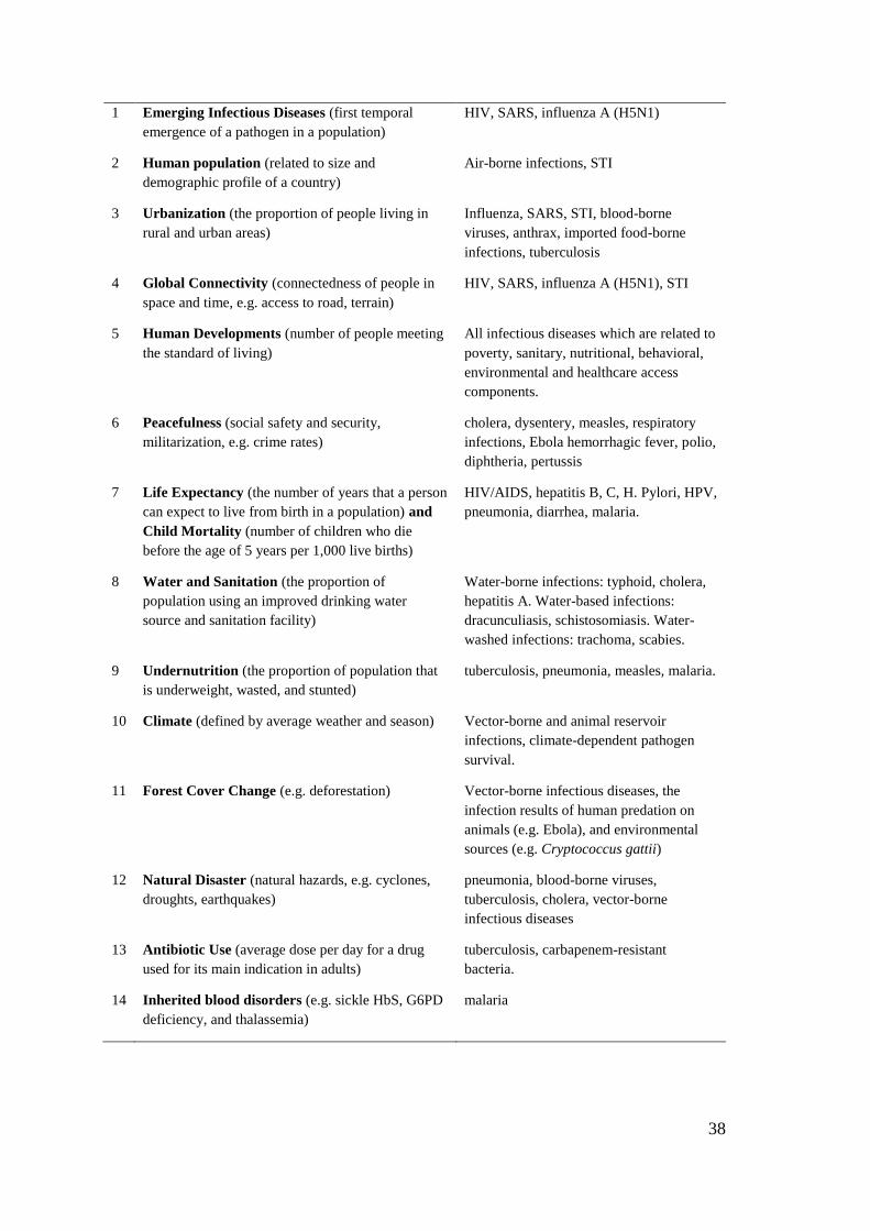
38
1 Emerging Infectious Diseases (first temporal
emergence of a pathogen in a population)
HIV, SARS, influenza A (H5N1)
2 Human population (related to size and
demographic profile of a country)
Air-borne infections, STI
3 Urbanization (the proportion of people living in
rural and urban areas)
Influenza, SARS, STI, blood-borne
viruses, anthrax, imported food-borne
infections, tuberculosis
4 Global Connectivity (connectedness of people in
space and time, e.g. access to road, terrain)
HIV, SARS, influenza A (H5N1), STI
5 Human Developments (number of people meeting
the standard of living)
All infectious diseases which are related to
poverty, sanitary, nutritional, behavioral,
environmental and healthcare access
components.
6 Peacefulness (social safety and security,
militarization, e.g. crime rates)
cholera, dysentery, measles, respiratory
infections, Ebola hemorrhagic fever, polio,
diphtheria, pertussis
7 Life Expectancy (the number of years that a person
can expect to live from birth in a population) and
Child Mortality (number of children who die
before the age of 5 years per 1,000 live births)
HIV/AIDS, hepatitis B, C, H. Pylori, HPV,
pneumonia, diarrhea, malaria.
8 Water and Sanitation (the proportion of
population using an improved drinking water
source and sanitation facility)
Water-borne infections: typhoid, cholera,
hepatitis A. Water-based infections:
dracunculiasis, schistosomiasis. Water-
washed infections: trachoma, scabies.
9 Undernutrition (the proportion of population that
is underweight, wasted, and stunted)
tuberculosis, pneumonia, measles, malaria.
10 Climate (defined by average weather and season) Vector-borne and animal reservoir
infections, climate-dependent pathogen
survival.
11 Forest Cover Change (e.g. deforestation) Vector-borne infectious diseases, the
infection results of human predation on
animals (e.g. Ebola), and environmental
sources (e.g. Cryptococcus gattii)
12 Natural Disaster (natural hazards, e.g. cyclones,
droughts, earthquakes)
pneumonia, blood-borne viruses,
tuberculosis, cholera, vector-borne
infectious diseases
13 Antibiotic Use (average dose per day for a drug
used for its main indication in adults)
tuberculosis, carbapenem-resistant
bacteria.
14 Inherited blood disorders (e.g. sickle HbS, G6PD
deficiency, and thalassemia)
malaria
39
15 Immunization (active or passive vaccines that have
been injected to a person since birth)
Vaccine-preventable infectious diseases
16 Vector Presence (terrain and climatic conditions
that affect vector emergence e.g. Anopheles, P.
vivax)
Vector-borne infectious diseases
17 Bird Migration (seasonal event in which certain
bird species travel between breeding and
overwintering grounds)
influenza A, west nile virus, western
equine encephalitis, St. Louis encephalitis,
Japanese encephalitis, Lyme disease.
18 Livestock Density (the population of cattle,
poultry, sheep and goats per kilometer square)
leptospirosis, fascioliasis, tuberculosis,
brucellosis, African trypanosomiasis, Q
fever, campylobacter, listeria.
From several rows in the infection drivers (in Table 3.1), a deeper understanding of a
country’s infection risks can be comprehended. Rows number 2 (human population), 5
(human developments), 6 (peacefulness), and 7 (life expectance and child mortality),
show the infection driver attributes that can be inferred from a country. This is because
these drivers can be deduced from certain indicators which are usually surveyed for
country scope; for example, the Global Peace Index is a measure of peacefulness.
Whereas, the infection drivers that are related to a specific location in a country (including
terrain and land-use) are in rows numbered 3 (urbanization), 4 (global connectivity), 8
(water and sanitation), 11 (forest cover), 16 (vector presence), 18 (livestock density).
Infection drivers (in Table 3.1) that are related to a person’s health or medical status are
9 (undernutrition), 13 (antibiotic use), 14 (inherited blood disorder), and 15
(immunization). For example, a person who has less body mass index (i.e. undernutrition)
would be likely to have a higher risk to any infections. The climate related infection
disease drivers are 10 (climate) and 16 (vector presence). These two drivers can be used
to explain the effect of climate on the presence of some vectors. But, driver #12 (natural
disaster) and #17 (bird migration) cannot be classified into person, climate or location.
However, the eighteen infection drivers are not enough to get the details of the infection
risk factors. Therefore, to get detailed risk factors, all mentioned risk factors for all human
infectious diseases in those declarative sources (AHID, WHO, CDC) was collated. 105
infectious diseases are mentioned in AHID; another 129 infectious diseases not listed in
AHID but mentioned in WHO and CDC are also gathered (e.g. yersiniosis, trichuriasis).
In total, 234 distinct infectious diseases were collated from three sources (AHID, WHO,
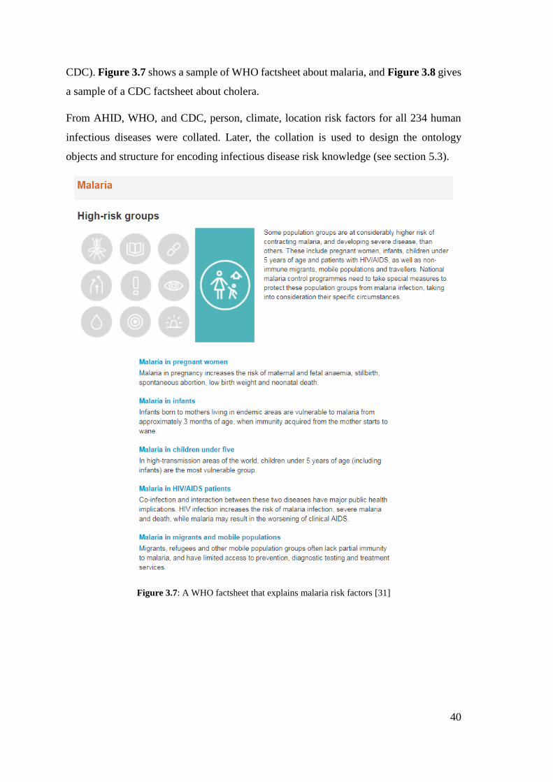
40
CDC). Figure 3.7 shows a sample of WHO factsheet about malaria, and Figure 3.8 gives
a sample of a CDC factsheet about cholera.
From AHID, WHO, and CDC, person, climate, location risk factors for all 234 human
infectious diseases were collated. Later, the collation is used to design the ontology
objects and structure for encoding infectious disease risk knowledge (see section 5.3).
Figure 3.7: A WHO factsheet that explains malaria risk factors [31]
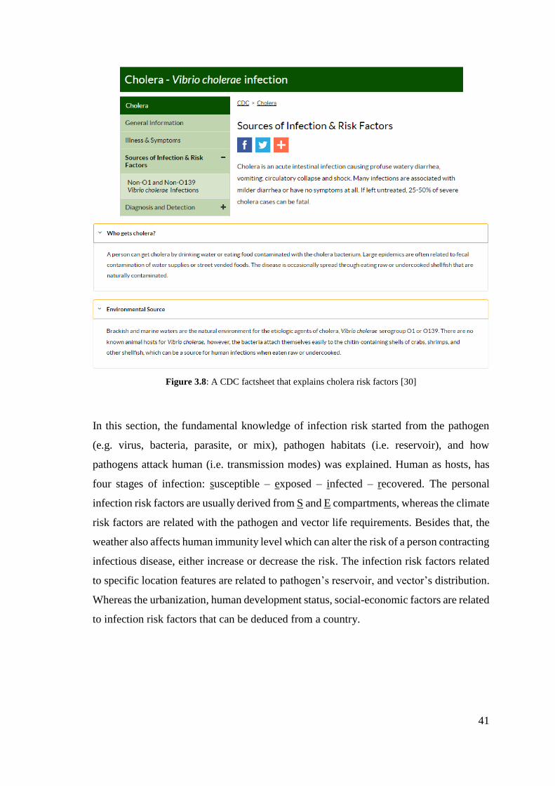
41
Figure 3.8: A CDC factsheet that explains cholera risk factors [30]
In this section, the fundamental knowledge of infection risk started from the pathogen
(e.g. virus, bacteria, parasite, or mix), pathogen habitats (i.e. reservoir), and how
pathogens attack human (i.e. transmission modes) was explained. Human as hosts, has
four stages of infection: susceptible – exposed – infected – recovered. The personal
infection risk factors are usually derived from S and E compartments, whereas the climate
risk factors are related with the pathogen and vector life requirements. Besides that, the
weather also affects human immunity level which can alter the risk of a person contracting
infectious disease, either increase or decrease the risk. The infection risk factors related
to specific location features are related to pathogen’s reservoir, and vector’s distribution.
Whereas the urbanization, human development status, social-economic factors are related
to infection risk factors that can be deduced from a country.
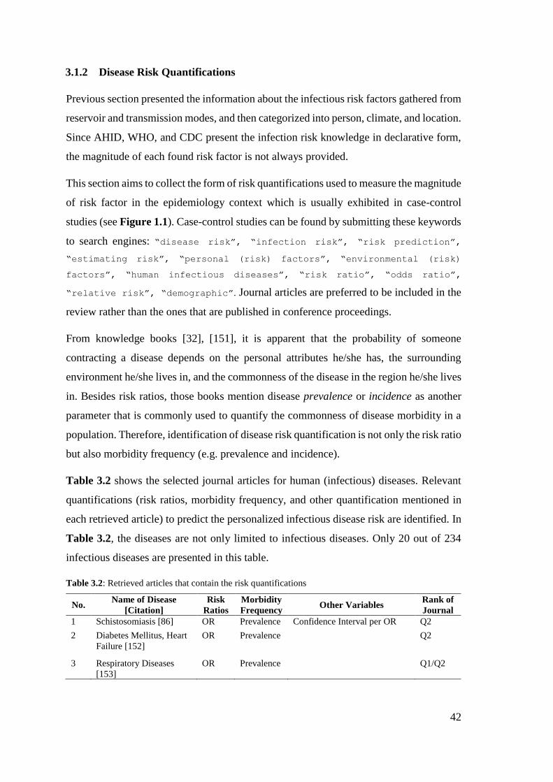
42
3.1.2 Disease Risk Quantifications
Previous section presented the information about the infectious risk factors gathered from
reservoir and transmission modes, and then categorized into person, climate, and location.
Since AHID, WHO, and CDC present the infection risk knowledge in declarative form,
the magnitude of each found risk factor is not always provided.
This section aims to collect the form of risk quantifications used to measure the magnitude
of risk factor in the epidemiology context which is usually exhibited in case-control
studies (see Figure 1.1). Case-control studies can be found by submitting these keywords
to search engines: “disease risk”, “infection risk”, “risk prediction”,
“estimating risk”, “personal (risk) factors”, “environmental (risk)
factors”, “human infectious diseases”, “risk ratio”, “odds ratio”,
“relative risk”, “demographic”. Journal articles are preferred to be included in the
review rather than the ones that are published in conference proceedings.
From knowledge books [32], [151], it is apparent that the probability of someone
contracting a disease depends on the personal attributes he/she has, the surrounding
environment he/she lives in, and the commonness of the disease in the region he/she lives
in. Besides risk ratios, those books mention disease prevalence or incidence as another
parameter that is commonly used to quantify the commonness of disease morbidity in a
population. Therefore, identification of disease risk quantification is not only the risk ratio
but also morbidity frequency (e.g. prevalence and incidence).
Table 3.2 shows the selected journal articles for human (infectious) diseases. Relevant
quantifications (risk ratios, morbidity frequency, and other quantification mentioned in
each retrieved article) to predict the personalized infectious disease risk are identified. In
Table 3.2, the diseases are not only limited to infectious diseases. Only 20 out of 234
infectious diseases are presented in this table.
Table 3.2: Retrieved articles that contain the risk quantifications
No. Name of Disease
[Citation]
Risk
Ratios
Morbidity
Frequency Other Variables
Rank of
Journal
1 Schistosomiasis [86] OR Prevalence Confidence Interval per OR Q2
2 Diabetes Mellitus, Heart
Failure [152]
OR Prevalence
Q2
3 Respiratory Diseases
[153]
OR Prevalence
Q1/Q2
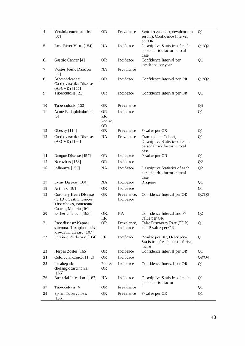
43
4 Yersinia enterocolitica
[87]
OR Prevalence Sero-prevalence (prevalence in
serum), Confidence Interval
per OR
Q1
5 Ross River Virus [154] NA Incidence Descriptive Statistics of each
personal risk factor in total
case
Q1/Q2
6 Gastric Cancer [4] OR Incidence Confidence Interval per
incidence per year
Q1
7 Vector-borne Diseases
[74]
NA Prevalence
8 Atherosclerotic
Cardiovascular Disease
(ASCVD) [155]
OR Incidence Confidence Interval per OR Q1/Q2
9 Tuberculosis [21] OR Incidence Confidence Interval per OR Q1
10 Tuberculosis [132] OR Prevalence
Q3
11 Acute Endophthalmitis
[5]
OR,
RR,
Pooled
OR
Incidence
Q1
12 Obesity [114] OR Prevalence P-value per OR Q1
13 Cardiovascular Disease
(ASCVD) [156]
NA Prevalence Framingham Cohort,
Descriptive Statistics of each
personal risk factor in total
case
Q1
14 Dengue Disease [157] OR Incidence P-value per OR Q1
15 Norovirus [158] OR Incidence
Q2
16 Influenza [159] NA Incidence Descriptive Statistics of each
personal risk factor in total
case
Q2
17 Lyme Disease [160] NA Incidence R square Q1
18 Anthrax [161] OR Incidence
Q1
19 Coronary Heart Disease
(CHD), Gastric Cancer,
Thrombosis, Pancreatic
Cancer, Malaria [162]
OR Prevalence,
Incidence
Confidence Interval per OR Q2/Q3
20 Escherichia coli [163] OR,
RR
NA Confidence Interval and P-
value per OR
Q2
21 Rare disease: Kaposi
sarcoma, Toxoplasmosis,
Kawasaki disease [107]
OR Prevalence,
Incidence
False Discovery Rate (FDR)
and P-value per OR
Q1
22 Parkinson’s disease [164] RR Incidence P-value per RR, Descriptive
Statistics of each personal risk
factor
Q1
23 Herpes Zoster [165] OR Incidence Confidence Interval per OR Q1
24 Colorectal Cancer [142] OR Incidence
Q3/Q4
25 Intrahepatic
cholangiocarcinoma
[166]
Pooled
OR
Incidence Confidence Interval per OR Q1
26 Bacterial Infections [167] NA Incidence Descriptive Statistics of each
personal risk factor
Q1
27 Tuberculosis [6] OR Prevalence
Q1
28 Spinal Tuberculosis
[136]
OR Prevalence P-value per OR Q1
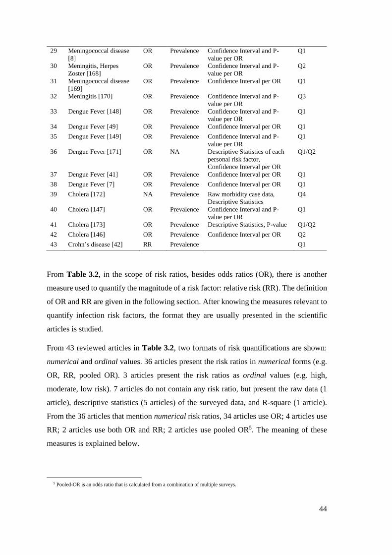
44
29 Meningococcal disease
[8]
OR Prevalence Confidence Interval and P-
value per OR
Q1
30 Meningitis, Herpes
Zoster [168]
OR Prevalence Confidence Interval and P-
value per OR
Q2
31 Meningococcal disease
[169]
OR Prevalence Confidence Interval per OR Q1
32 Meningitis [170] OR Prevalence Confidence Interval and P-
value per OR
Q3
33 Dengue Fever [148] OR Prevalence Confidence Interval and P-
value per OR
Q1
34 Dengue Fever [49] OR Prevalence Confidence Interval per OR Q1
35 Dengue Fever [149] OR Prevalence Confidence Interval and P-
value per OR
Q1
36 Dengue Fever [171] OR NA Descriptive Statistics of each
personal risk factor,
Confidence Interval per OR
Q1/Q2
37 Dengue Fever [41] OR Prevalence Confidence Interval per OR Q1
38 Dengue Fever [7] OR Prevalence Confidence Interval per OR Q1
39 Cholera [172] NA Prevalence Raw morbidity case data,
Descriptive Statistics
Q4
40 Cholera [147] OR Prevalence Confidence Interval and P-
value per OR
Q1
41 Cholera [173] OR Prevalence Descriptive Statistics, P-value Q1/Q2
42 Cholera [146] OR Prevalence Confidence Interval per OR Q2
43 Crohn’s disease [42] RR Prevalence
Q1
From Table 3.2, in the scope of risk ratios, besides odds ratios (OR), there is another
measure used to quantify the magnitude of a risk factor: relative risk (RR). The definition
of OR and RR are given in the following section. After knowing the measures relevant to
quantify infection risk factors, the format they are usually presented in the scientific
articles is studied.
From 43 reviewed articles in Table 3.2, two formats of risk quantifications are shown:
numerical and ordinal values. 36 articles present the risk ratios in numerical forms (e.g.
OR, RR, pooled OR). 3 articles present the risk ratios as ordinal values (e.g. high,
moderate, low risk). 7 articles do not contain any risk ratio, but present the raw data (1
article), descriptive statistics (5 articles) of the surveyed data, and R-square (1 article).
From the 36 articles that mention numerical risk ratios, 34 articles use OR; 4 articles use
RR; 2 articles use both OR and RR; 2 articles use pooled OR5. The meaning of these
measures is explained below.
5 Pooled-OR is an odds ratio that is calculated from a combination of multiple surveys.
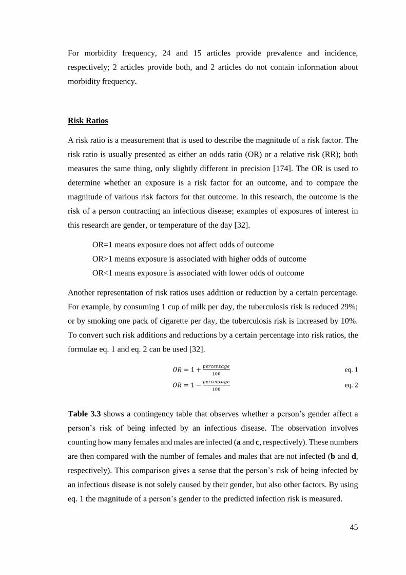
45
For morbidity frequency, 24 and 15 articles provide prevalence and incidence,
respectively; 2 articles provide both, and 2 articles do not contain information about
morbidity frequency.
Risk Ratios
A risk ratio is a measurement that is used to describe the magnitude of a risk factor. The
risk ratio is usually presented as either an odds ratio (OR) or a relative risk (RR); both
measures the same thing, only slightly different in precision [174]. The OR is used to
determine whether an exposure is a risk factor for an outcome, and to compare the
magnitude of various risk factors for that outcome. In this research, the outcome is the
risk of a person contracting an infectious disease; examples of exposures of interest in
this research are gender, or temperature of the day [32].
OR=1 means exposure does not affect odds of outcome
OR>1 means exposure is associated with higher odds of outcome
OR<1 means exposure is associated with lower odds of outcome
Another representation of risk ratios uses addition or reduction by a certain percentage.
For example, by consuming 1 cup of milk per day, the tuberculosis risk is reduced 29%;
or by smoking one pack of cigarette per day, the tuberculosis risk is increased by 10%.
To convert such risk additions and reductions by a certain percentage into risk ratios, the
formulae eq. 1 and eq. 2 can be used [32].
𝑂𝑅 = 1 +𝑝𝑒𝑟𝑐𝑒𝑛𝑡𝑎𝑔𝑒
100 eq. 1
𝑂𝑅 = 1 −𝑝𝑒𝑟𝑐𝑒𝑛𝑡𝑎𝑔𝑒
100 eq. 2
Table 3.3 shows a contingency table that observes whether a person’s gender affect a
person’s risk of being infected by an infectious disease. The observation involves
counting how many females and males are infected (a and c, respectively). These numbers
are then compared with the number of females and males that are not infected (b and d,
respectively). This comparison gives a sense that the person’s risk of being infected by
an infectious disease is not solely caused by their gender, but also other factors. By using
eq. 1 the magnitude of a person’s gender to the predicted infection risk is measured.
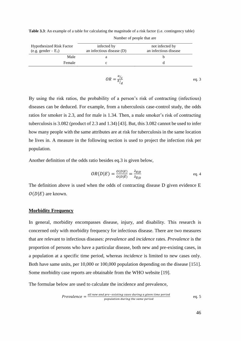
46
Table 3.3: An example of a table for calculating the magnitude of a risk factor (i.e. contingency table)
Number of people that are
Hypothesized Risk Factor
(e.g. gender – E1)
infected by
an infectious disease (D)
not infected by
an infectious disease
Male a b
Female c d
𝑂𝑅 =𝑎
𝑐⁄
𝑏𝑑⁄
eq. 3
By using the risk ratios, the probability of a person’s risk of contracting (infectious)
diseases can be deduced. For example, from a tuberculosis case-control study, the odds
ratios for smoker is 2.3, and for male is 1.34. Then, a male smoker’s risk of contracting
tuberculosis is 3.082 (product of 2.3 and 1.34) [43]. But, this 3.082 cannot be used to infer
how many people with the same attributes are at risk for tuberculosis in the same location
he lives in. A measure in the following section is used to project the infection risk per
population.
Another definition of the odds ratio besides eq.3 is given below,
𝑂𝑅(𝐷|𝐸) =𝑂(𝐷|𝐸)
𝑂(𝐷|�̅�)=
𝜆𝐸|𝐷
𝜆�̅�|𝐷 eq. 4
The definition above is used when the odds of contracting disease D given evidence E
𝑂(𝐷|𝐸) are known.
Morbidity Frequency
In general, morbidity encompasses disease, injury, and disability. This research is
concerned only with morbidity frequency for infectious disease. There are two measures
that are relevant to infectious diseases: prevalence and incidence rates. Prevalence is the
proportion of persons who have a particular disease, both new and pre-existing cases, in
a population at a specific time period, whereas incidence is limited to new cases only.
Both have same units, per 10,000 or 100,000 population depending on the disease [151].
Some morbidity case reports are obtainable from the WHO website [19].
The formulae below are used to calculate the incidence and prevalence,
𝑃𝑟𝑒𝑣𝑎𝑙𝑒𝑛𝑐𝑒 =𝑎𝑙𝑙 𝑛𝑒𝑤 𝑎𝑛𝑑 𝑝𝑟𝑒−𝑒𝑥𝑖𝑠𝑡𝑖𝑛𝑔 𝑐𝑎𝑠𝑒𝑠 𝑑𝑢𝑟𝑖𝑛𝑔 𝑎 𝑔𝑖𝑣𝑒𝑛 𝑡𝑖𝑚𝑒 𝑝𝑒𝑟𝑖𝑜𝑑
𝑝𝑜𝑝𝑢𝑙𝑎𝑡𝑖𝑜𝑛 𝑑𝑢𝑟𝑖𝑛𝑔 𝑡ℎ𝑒 𝑠𝑎𝑚𝑒 𝑝𝑒𝑟𝑖𝑜𝑑 eq. 5
47
𝐼𝑛𝑐𝑖𝑑𝑒𝑛𝑐𝑒 =𝑛𝑒𝑤 𝑐𝑎𝑠𝑒𝑠 𝑑𝑢𝑟𝑖𝑛𝑔 𝑎 𝑔𝑖𝑣𝑒𝑛 𝑡𝑖𝑚𝑒 𝑝𝑒𝑟𝑖𝑜𝑑
𝑝𝑜𝑝𝑢𝑙𝑎𝑡𝑖𝑜𝑛 𝑑𝑢𝑟𝑖𝑛𝑔 𝑡ℎ𝑒 𝑠𝑎𝑚𝑒 𝑝𝑒𝑟𝑖𝑜𝑑 𝑜𝑟 𝑎𝑡 𝑠𝑡𝑎𝑟𝑡 𝑜𝑓 𝑝𝑒𝑟𝑖𝑜𝑑 eq. 6
Since the measure that is usually reported to public health agencies (e.g. WHO, CDC) is
the number of reported cases (the numerator of eq. 4 and eq. 5), the population of a
country where a client lives is used to calculate the prevalence or incidence.
3.1.3 Summary
In summary, three concepts are needed to predict infectious disease risk in a person: (1)
the chain of infection for general human infectious diseases, (2) the SEIR concept of
infection flow in a person, (3) the correlation between environment (climate, location)
and the infectious disease emergence. Chain of infection shows that infectious diseases
are the result of interaction between three elements: pathogen, host, and environment.
Pathogen or vectors of infectious diseases have specific reservoir and transmission modes
where the environmental risk factors can be deduced. By understanding the SEIR model,
the host susceptibility and the possibility to get pathogen exposure can be used to explain
the personal risk factors. Whereas from the correlation between environment and
infection risks, there are three components that are influential: geographical variation (e.g.
terrain, land-use, country), climate (e.g. weather and season), human social interaction
(e.g. gathering, work, school), and human immunity changes affected by certain
atmospheric conditions (e.g. winter-immunosuppression). The characteristics of the
infectious disease risk knowledge can be binary, nominal, and ordinal. Meanwhile the
infectious disease risk quantifications are continuous (e.g. risk ratios, morbidity
frequencies).
The further explanation about country and location features were reviewed from AHID
infection drivers. Human and livestock density population, human developments,
peacefulness are the examples of infection drivers which are usually observed from a
nation. Whereas the urbanization, water and sanitation are the examples of infection
drivers from a specific region of a nation. Furthermore, all mentioned risk factors from
all human infectious diseases that ever existed are collated from declarative knowledge
sources: Atlas of Human Infectious Diseases (AHID), World Health Organization
(WHO), and Centre for Disease Control and Prevention (CDC). The infection risk
48
drivers’ can be categorized into risk factors that related to person, climate (weather or
season), location (country or location features). For accommodating infection risk factors
that cannot be classified into aforementioned categories, a miscellaneous can be used.
Thereafter, the quantifications of the risk factors were reviewed from case-control studies
in epidemiology domain. The common measurements are risk ratios and morbidity
frequency. Risk ratios, either as odds ratios (OR) or relative risk (RR), are used to quantify
the magnitude of the impact of risk factors on a disease. Whereas the commonness of
disease morbidity in a region is usually presented in numeric form with certain population
units, either as prevalence or incidence. By using these two measurements, the person’s
risk of contracting of infectious diseases can be estimated based on her/his risk ratios of
the personal and environmental risk factors and morbidity frequency of the location.
The collected information about risk factor and quantifications will be used to design the
knowledge representation for infectious disease risk knowledge. The design will be
presented in chapter 5.
3.2 Disease Knowledge Representation
In section 1.4, research objectives and goals were explained. A knowledge representation
that encodes the infectious disease risk knowledge and usable by the epidemiologists is
needed. In section 3.1, the infectious disease risk knowledge, risk factors and risk ratios,
was explained. This section investigates the existing knowledge representation for human
(infectious) disease in medical and computer science areas that help the domain experts.
Thereafter, the required efforts and adjustments of the domain experts to encode their
knowledge using the selected knowledge representation are identified.
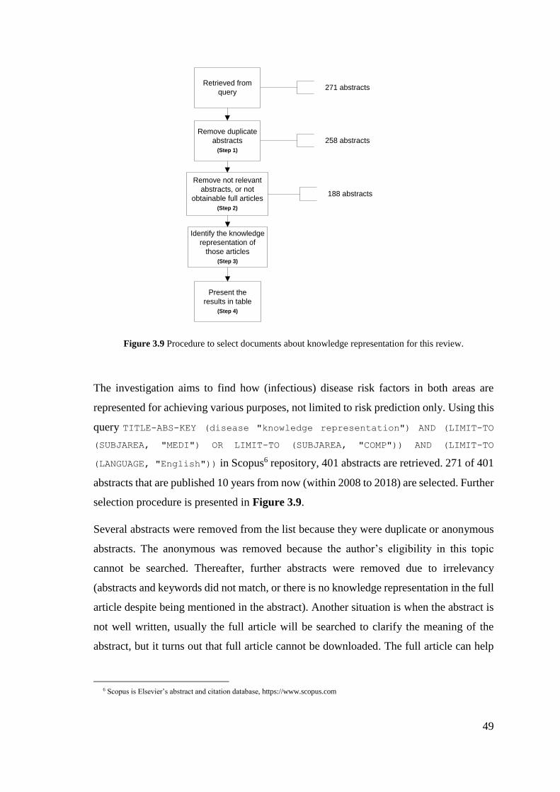
49
Retrieved from
query
Remove duplicate
abstracts
(Step 1)
271 abstracts
258 abstracts
Remove not relevant
abstracts, or not
obtainable full articles
(Step 2)
188 abstracts
Identify the knowledge
representation of
those articles
(Step 3)
Present the
results in table
(Step 4)
Figure 3.9 Procedure to select documents about knowledge representation for this review.
The investigation aims to find how (infectious) disease risk factors in both areas are
represented for achieving various purposes, not limited to risk prediction only. Using this
query TITLE-ABS-KEY (disease "knowledge representation") AND (LIMIT-TO
(SUBJAREA, "MEDI") OR LIMIT-TO (SUBJAREA, "COMP")) AND (LIMIT-TO
(LANGUAGE, "English")) in Scopus6 repository, 401 abstracts are retrieved. 271 of 401
abstracts that are published 10 years from now (within 2008 to 2018) are selected. Further
selection procedure is presented in Figure 3.9.
Several abstracts were removed from the list because they were duplicate or anonymous
abstracts. The anonymous was removed because the author’s eligibility in this topic
cannot be searched. Thereafter, further abstracts were removed due to irrelevancy
(abstracts and keywords did not match, or there is no knowledge representation in the full
article despite being mentioned in the abstract). Another situation is when the abstract is
not well written, usually the full article will be searched to clarify the meaning of the
abstract, but it turns out that full article cannot be downloaded. The full article can help
6 Scopus is Elsevier’s abstract and citation database, https://www.scopus.com
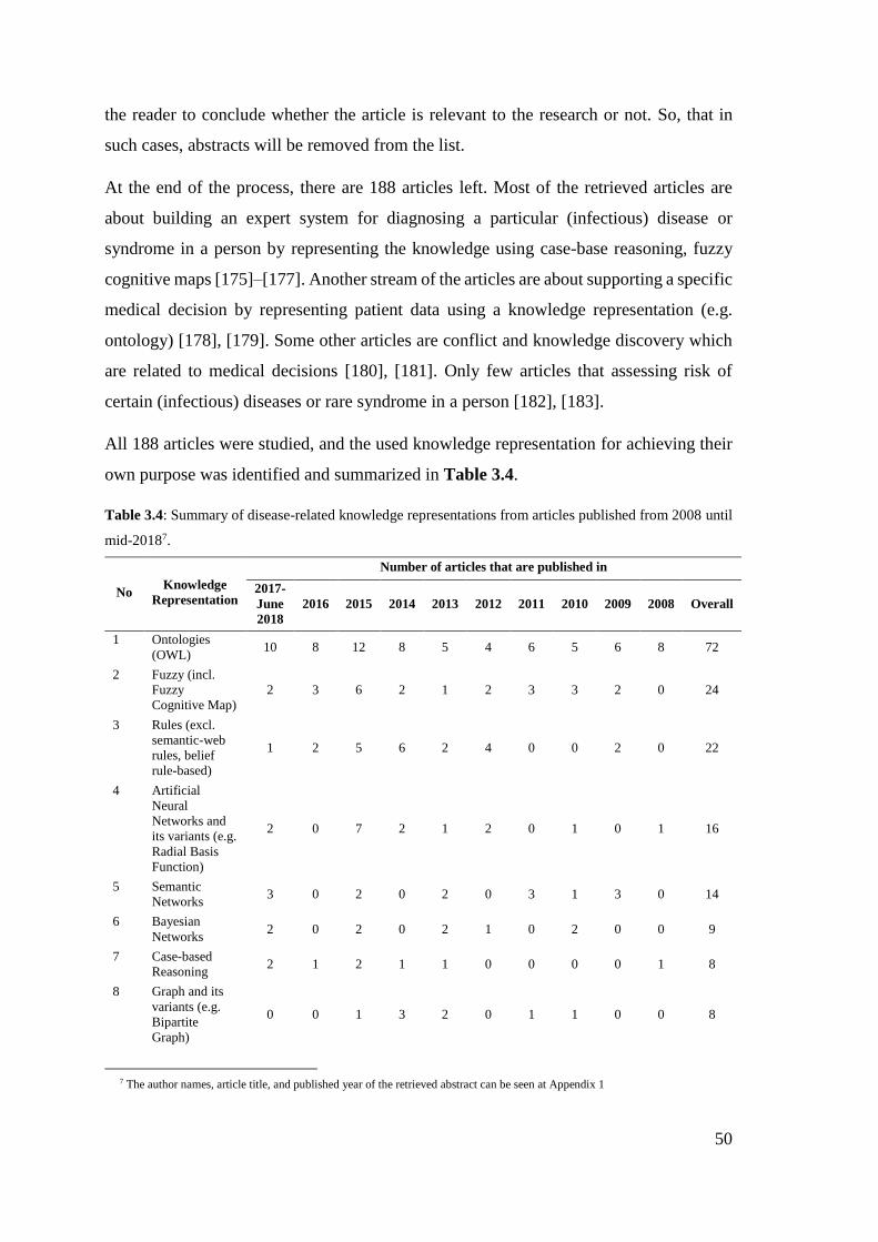
50
the reader to conclude whether the article is relevant to the research or not. So, that in
such cases, abstracts will be removed from the list.
At the end of the process, there are 188 articles left. Most of the retrieved articles are
about building an expert system for diagnosing a particular (infectious) disease or
syndrome in a person by representing the knowledge using case-base reasoning, fuzzy
cognitive maps [175]–[177]. Another stream of the articles are about supporting a specific
medical decision by representing patient data using a knowledge representation (e.g.
ontology) [178], [179]. Some other articles are conflict and knowledge discovery which
are related to medical decisions [180], [181]. Only few articles that assessing risk of
certain (infectious) diseases or rare syndrome in a person [182], [183].
All 188 articles were studied, and the used knowledge representation for achieving their
own purpose was identified and summarized in Table 3.4.
Table 3.4: Summary of disease-related knowledge representations from articles published from 2008 until
mid-20187.
No Knowledge
Representation
Number of articles that are published in
2017-
June
2018
2016 2015 2014 2013 2012 2011 2010 2009 2008 Overall
1 Ontologies
(OWL) 10 8 12 8 5 4 6 5 6 8 72
2 Fuzzy (incl.
Fuzzy
Cognitive Map)
2 3 6 2 1 2 3 3 2 0 24
3 Rules (excl.
semantic-web
rules, belief
rule-based)
1 2 5 6 2 4 0 0 2 0 22
4 Artificial
Neural
Networks and
its variants (e.g.
Radial Basis
Function)
2 0 7 2 1 2 0 1 0 1 16
5 Semantic
Networks 3 0 2 0 2 0 3 1 3 0 14
6 Bayesian
Networks 2 0 2 0 2 1 0 2 0 0 9
7 Case-based
Reasoning 2 1 2 1 1 0 0 0 0 1 8
8 Graph and its
variants (e.g.
Bipartite
Graph)
0 0 1 3 2 0 1 1 0 0 8
7 The author names, article title, and published year of the retrieved abstract can be seen at Appendix 1
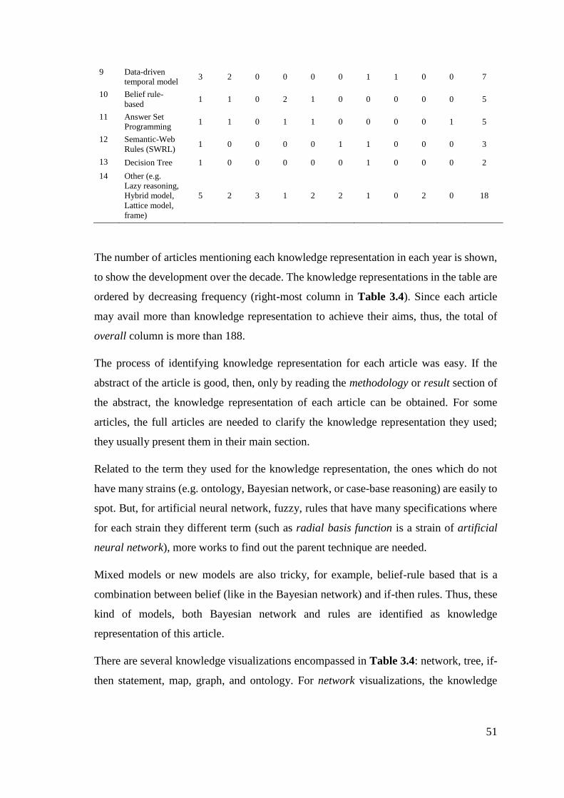
51
9 Data-driven
temporal model 3 2 0 0 0 0 1 1 0 0 7
10 Belief rule-
based 1 1 0 2 1 0 0 0 0 0 5
11 Answer Set
Programming 1 1 0 1 1 0 0 0 0 1 5
12 Semantic-Web
Rules (SWRL) 1 0 0 0 0 1 1 0 0 0 3
13 Decision Tree 1 0 0 0 0 0 1 0 0 0 2
14 Other (e.g.
Lazy reasoning,
Hybrid model,
Lattice model,
frame)
5 2 3 1 2 2 1 0 2 0 18
The number of articles mentioning each knowledge representation in each year is shown,
to show the development over the decade. The knowledge representations in the table are
ordered by decreasing frequency (right-most column in Table 3.4). Since each article
may avail more than knowledge representation to achieve their aims, thus, the total of
overall column is more than 188.
The process of identifying knowledge representation for each article was easy. If the
abstract of the article is good, then, only by reading the methodology or result section of
the abstract, the knowledge representation of each article can be obtained. For some
articles, the full articles are needed to clarify the knowledge representation they used;
they usually present them in their main section.
Related to the term they used for the knowledge representation, the ones which do not
have many strains (e.g. ontology, Bayesian network, or case-base reasoning) are easily to
spot. But, for artificial neural network, fuzzy, rules that have many specifications where
for each strain they different term (such as radial basis function is a strain of artificial
neural network), more works to find out the parent technique are needed.
Mixed models or new models are also tricky, for example, belief-rule based that is a
combination between belief (like in the Bayesian network) and if-then rules. Thus, these
kind of models, both Bayesian network and rules are identified as knowledge
representation of this article.
There are several knowledge visualizations encompassed in Table 3.4: network, tree, if-
then statement, map, graph, and ontology. For network visualizations, the knowledge
52
representation #4 (Artificial Neural Networks), #5 (Semantic Networks), and #6
(Bayesian Networks). Artificial Neural Networks (ANN) is a deep learning technology by
training large data to create an adaptive map that consists of layers of nodes where nodes
between layers are connected by a weighted edge. Bayesian Networks (BN) is a
knowledge model that contains node which represents a random variable, and edges
between the nodes representing probabilistic dependencies among the corresponding
random variables. Semantic Network (SN) is a form of knowledge representation between
concepts, objects, features, events in a network. Unlike the ANN and BN that are
executable approach to yield the numerical prediction, SN is more as a conceptual
approach, hence, need other executable approach to formalize the SN. Some articles
include frame (#14) into SN. However, SN is good at conceptualizing knowledge that
needs clarity on object-to-object relationships, while frame focus on the conceptualization
of object-to-attribute relationships.
An ontology (i.e. knowledge graph) is a representation of formal naming, definition of the
categories, properties, and relations by explicitly conceptualizing the data and entities in
one, many, or all domains. Ontology allows sharing conceptualization (e.g. vocabulary)
which can be used to model a specific knowledge for a particular purpose.
For tree visualizations, decision trees (#13) is a knowledge model learned from
observations about an item which represented as a branch. A tree can be used to represent
if-then rules.
Rules (#3) is a conditional statement that represents causality between antecedent and
consequent, which denoted by p → q. A set of rules is a rule-base which is commonly
used as a knowledge representation. Rules that is implemented in an ontology
environment is called semantic-web rules (#12). Rules that incorporate uncertainty like
BN is called belief rule-based (#10). In Table 3.4, these three types of rules are separated
since they have different feature and environment of implementation. More discussion
about these three kinds of rule will be provided in section 3.2.4.
A set of rules is called as rule-base. The rule-base is commonly used to predict desired
outcome(s). Rule-base is built from historical data or observations, thus, mostly it can
only solve the problem that has already known before. For a new problem that is not
contained in the observations, the case-based reasoning (#7) model can be used. A
53
technique to measure distance between the new problem and the cases is utilized, which
then can be used to infer the estimation of the results.
Besides rules, a knowledge visualization that using a statement is Answer Set
Programming (#11) (ASP). ASP is a form of declarative programming which is
categorized constraint programming languages. Group of logics and AND or OR
operators are used to create the ASP.
For map representation, Fuzzy Cognitive Maps (FCM) (#2) is a combination of fuzzy logic
and cognitive mapping. Fuzzy logic itself is a form of multi-valued logic which the values
may be any real number between 0 and 1. Fuzzy logic are represented by if-then
statement. Cognitive maps (i.e. mental map or mental model) is a representation which
allows the users to look for a cause-effect in the ideas of the mapping. Since there is no
cognitive map appear as standalone knowledge model in the collected articles, thus, FCM
is merged with fuzzy logic knowledge representation.
From the review, it is apparent that there are two approaches to acquiring knowledge in
the context of artificial intelligence systems. First, the knowledge is induced from
observational data; this approach is known as data-driven [106], [184], [185]. The
knowledge representations that are used in data-driven cases are Fuzzy Cognitive Maps,
Artificial Neural Networks, Data-driven temporal models, and Decision Trees.
Second, approach to knowledge acquisition is from domain experts directly or from their
knowledge documentations; this approach is known as knowledge-driven [186], [187].
The knowledge-driven representations that are used for knowledge-driven systems are in
Table 3.4 are Ontologies, (some of) Fuzzy, (some of) Rules, (some of) Bayesian
Network, Semantic Network, etc.
Whereas, based on the characteristic of the knowledge representation, there are two
representation types: (1) using node-link structures, and (2) using antecedent and
consequent. Of the knowledge representation listed in Table 3.4, Ontologies, Semantic
Networks, Bayesian networks, Fuzzy Cognitive Maps, Artificial Neural Networks,
Decision Trees and Graphs are categorized in the first type. The advantage of node-link
structures is they easily represent properties of an object, and illustrate the relationship
between objects [188]. Whereas the second type, antecedent-consequent (if-then rules),
54
comprises of Semantic-web rules, Belief rule-based, Answer Set Programming. This kind
of representation emphasizes the causal relationship between antecedent and the
consequent [189]–[191].
From Table 3.4, it can be seen that the most used knowledge representation in these areas
is ontologies (discussed in section 3.2.1). For node-link structures, the most used data-
driven approach is, Fuzzy Cognitive Map; and, the most used knowledge-driven approach
is, Bayesian Network. These methods are described in section 3.2.2 and 3.2.3,
respectively. Also, all kinds of rules are explained in section 3.2.4.
To answer the research question, two types of approaches can be used. The first type is
approaches that represent knowledge related to diseases mentioned in risk prediction
articles. This type is explained in section 3.2.1 to 3.2.4. Whereas, the following section
presents the second type of approaches that combine both risk prediction and knowledge
representation as a single model but not related to disease or health. This second type will
be described in section 3.3.
3.2.1 Ontology
As described in section 1.6, the knowledge representation for this research is expected to
encode the infectious disease risk knowledge. From section 3.1, the personal attributes
related to infectious disease risk knowledge can be presented as risk factors, and
quantified by risk ratios, whereas some the environmental attributes (e.g. country as a
location) to infectious disease risk knowledge can be quantified by morbidity frequency.
In this section, relevant ontologies are explored with a view to identifying an existing
ontology which can be reused to encode infectious disease risk factors for both personal
and environmental attributes.
An ontology is a formalization of knowledge using classes and properties. From Table
3.4, ontology is the most used knowledge representation for encoding the domain
knowledge in computer science and medical areas. Several of the reviewed articles
provide URLs of ontology repositories. Thus, they lead to further search in repositories
such as BioPortal [192], OBO Foundry [193], or Google Code Archive [194].
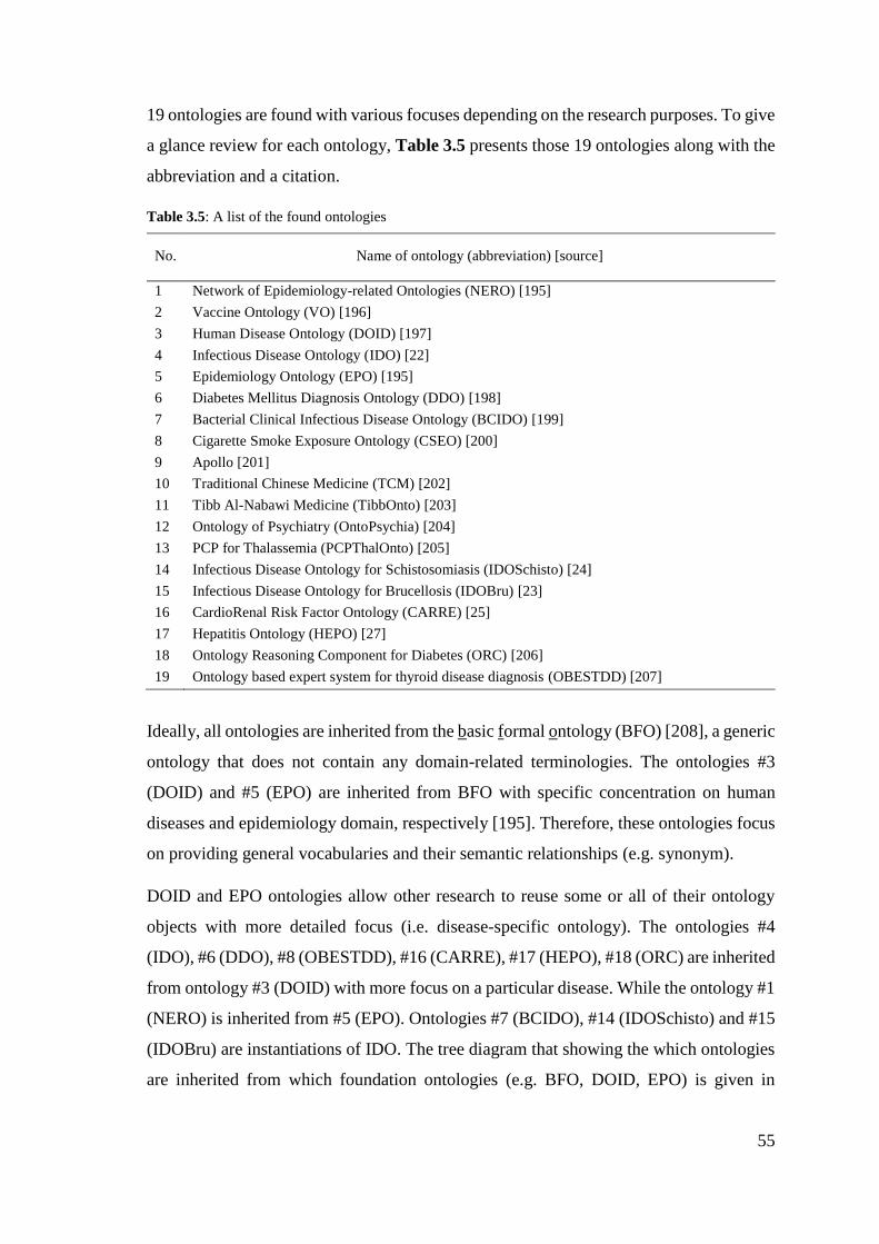
55
19 ontologies are found with various focuses depending on the research purposes. To give
a glance review for each ontology, Table 3.5 presents those 19 ontologies along with the
abbreviation and a citation.
Table 3.5: A list of the found ontologies
No. Name of ontology (abbreviation) [source]
1 Network of Epidemiology-related Ontologies (NERO) [195]
2 Vaccine Ontology (VO) [196]
3 Human Disease Ontology (DOID) [197]
4 Infectious Disease Ontology (IDO) [22]
5 Epidemiology Ontology (EPO) [195]
6 Diabetes Mellitus Diagnosis Ontology (DDO) [198]
7 Bacterial Clinical Infectious Disease Ontology (BCIDO) [199]
8 Cigarette Smoke Exposure Ontology (CSEO) [200]
9 Apollo [201]
10 Traditional Chinese Medicine (TCM) [202]
11 Tibb Al-Nabawi Medicine (TibbOnto) [203]
12 Ontology of Psychiatry (OntoPsychia) [204]
13 PCP for Thalassemia (PCPThalOnto) [205]
14 Infectious Disease Ontology for Schistosomiasis (IDOSchisto) [24]
15 Infectious Disease Ontology for Brucellosis (IDOBru) [23]
16 CardioRenal Risk Factor Ontology (CARRE) [25]
17 Hepatitis Ontology (HEPO) [27]
18 Ontology Reasoning Component for Diabetes (ORC) [206]
19 Ontology based expert system for thyroid disease diagnosis (OBESTDD) [207]
Ideally, all ontologies are inherited from the basic formal ontology (BFO) [208], a generic
ontology that does not contain any domain-related terminologies. The ontologies #3
(DOID) and #5 (EPO) are inherited from BFO with specific concentration on human
diseases and epidemiology domain, respectively [195]. Therefore, these ontologies focus
on providing general vocabularies and their semantic relationships (e.g. synonym).
DOID and EPO ontologies allow other research to reuse some or all of their ontology
objects with more detailed focus (i.e. disease-specific ontology). The ontologies #4
(IDO), #6 (DDO), #8 (OBESTDD), #16 (CARRE), #17 (HEPO), #18 (ORC) are inherited
from ontology #3 (DOID) with more focus on a particular disease. While the ontology #1
(NERO) is inherited from #5 (EPO). Ontologies #7 (BCIDO), #14 (IDOSchisto) and #15
(IDOBru) are instantiations of IDO. The tree diagram that showing the which ontologies
are inherited from which foundation ontologies (e.g. BFO, DOID, EPO) is given in
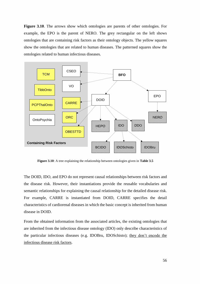
56
Figure 3.10. The arrows show which ontologies are parents of other ontologies. For
example, the EPO is the parent of NERO. The grey rectangular on the left shows
ontologies that are containing risk factors as their ontology objects. The yellow squares
show the ontologies that are related to human diseases. The patterned squares show the
ontologies related to human infectious diseases.
BFO
DOIDEPO
NERO
VO
CSEO
IDOHEPO
ORC
DDO
BCIDO IDOSchisto IDOBru
OBESTTD
CARRE
OntoPsychia
TCM
TibbOnto
PCPThalOnto
Containing Risk Factors
Figure 3.10: A tree explaining the relationship between ontologies given in Table 3.5
The DOID, IDO, and EPO do not represent causal relationships between risk factors and
the disease risk. However, their instantiations provide the reusable vocabularies and
semantic relationships for explaining the causal relationship for the detailed disease risk.
For example, CARRE is instantiated from DOID, CARRE specifies the detail
characteristics of cardiorenal diseases in which the basic concept is inherited from human
disease in DOID.
From the obtained information from the associated articles, the existing ontologies that
are inherited from the infectious disease ontology (IDO) only describe characteristics of
the particular infectious diseases (e.g. IDOBru, IDOSchisto); they don’t encode the
infectious disease risk factors.
57
Therefore, a new investigation to find disease-specific ontologies that inherit objects from
different generic ontology is conducted. Now, the ontologies in Table 3.5, that encode
risk factors, inherited from DOID or from BFO are investigated. This investigation aims
to find reusable terminologies, measures, annotations to encode infectious disease risk
factors. As a result, there are 5 ontologies that represent disease risk factor knowledge in
the context of epidemiology: #2 (VO), #8 (CSEO), #16 (CARRE), #18 (ORC), #19
(OBESTDD). CARRE is built to find the risk prediction of the cardiorenal disease,
therefore, the CARRE contains some personal risk factors. Same with CARRE, ORC is
designed to model domain and operational knowledge for understanding diabetes risk
factor. The OBESTDD focuses on obesity risk factor for thyroid disease only. Whereas,
CSEO defines the cigarette smoking effects to general health, not specific to disease risk.
Even though those ontologies are not specific to infectious diseases, but some of ontology
objects can be reused to further design of knowledge representation.
From 19 ontologies provided in Table 3.5, ontologies that are not instantiated from
DOID, IDO, EPO nor BFO but encode the risk factor knowledge are investigated. The
result is #10 (TCM), #11 (TibbOnto), #12 (OntoPsychia), and #13 (PCPThalOnto). These
ontologies do not reuse vocabularies or properties from BFO or DOID but create their
own ontology objects. TCM, TibbOnto, and PCPThalOnto are specific for describing
Traditional Chinese Medicine, Prophetic Medicine (‘Al-Tibb al-nabawi), and
Thalassemia, respectively. Whereas, OntoPsychia is an ontology that explains mental
illness and its treatment (i.e. psychiatric).
Again, none of these ontologies are specific for encoding the risk factors (personal or
environmental) specific for infectious diseases. In Figure 3.10, only three ontologies that
are related to infectious diseases (BCIDO, IDOSchisto, IDOBru), but none of them is
covered by grey area, regardless they are instances of the BFO or not. However, some of
the ontology objects (classes and properties) of these ontologies (yellow boxes) can still
be reused.
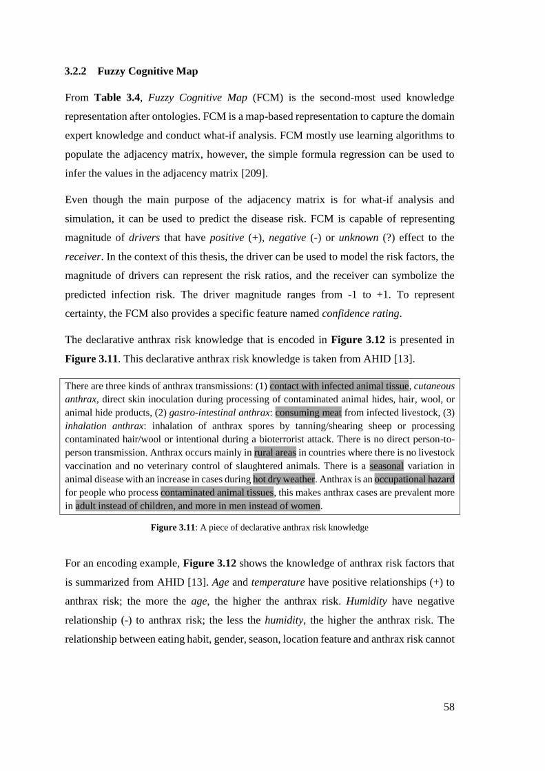
58
3.2.2 Fuzzy Cognitive Map
From Table 3.4, Fuzzy Cognitive Map (FCM) is the second-most used knowledge
representation after ontologies. FCM is a map-based representation to capture the domain
expert knowledge and conduct what-if analysis. FCM mostly use learning algorithms to
populate the adjacency matrix, however, the simple formula regression can be used to
infer the values in the adjacency matrix [209].
Even though the main purpose of the adjacency matrix is for what-if analysis and
simulation, it can be used to predict the disease risk. FCM is capable of representing
magnitude of drivers that have positive (+), negative (-) or unknown (?) effect to the
receiver. In the context of this thesis, the driver can be used to model the risk factors, the
magnitude of drivers can represent the risk ratios, and the receiver can symbolize the
predicted infection risk. The driver magnitude ranges from -1 to +1. To represent
certainty, the FCM also provides a specific feature named confidence rating.
The declarative anthrax risk knowledge that is encoded in Figure 3.12 is presented in
Figure 3.11. This declarative anthrax risk knowledge is taken from AHID [13].
There are three kinds of anthrax transmissions: (1) contact with infected animal tissue, cutaneous
anthrax, direct skin inoculation during processing of contaminated animal hides, hair, wool, or
animal hide products, (2) gastro-intestinal anthrax: consuming meat from infected livestock, (3)
inhalation anthrax: inhalation of anthrax spores by tanning/shearing sheep or processing
contaminated hair/wool or intentional during a bioterrorist attack. There is no direct person-to-
person transmission. Anthrax occurs mainly in rural areas in countries where there is no livestock
vaccination and no veterinary control of slaughtered animals. There is a seasonal variation in
animal disease with an increase in cases during hot dry weather. Anthrax is an occupational hazard
for people who process contaminated animal tissues, this makes anthrax cases are prevalent more
in adult instead of children, and more in men instead of women.
Figure 3.11: A piece of declarative anthrax risk knowledge
For an encoding example, Figure 3.12 shows the knowledge of anthrax risk factors that
is summarized from AHID [13]. Age and temperature have positive relationships (+) to
anthrax risk; the more the age, the higher the anthrax risk. Humidity have negative
relationship (-) to anthrax risk; the less the humidity, the higher the anthrax risk. The
relationship between eating habit, gender, season, location feature and anthrax risk cannot
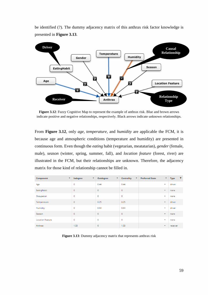
59
be identified (?). The dummy adjacency matrix of this anthrax risk factor knowledge is
presented in Figure 3.13.
Figure 3.12: Fuzzy Cognitive Map to represent the example of anthrax risk. Blue and brown arrows
indicate positive and negative relationships, respectively. Black arrows indicate unknown relationships.
From Figure 3.12, only age, temperature, and humidity are applicable the FCM, it is
because age and atmospheric conditions (temperature and humidity) are presented in
continuous form. Even though the eating habit (vegetarian, meatatarian), gender (female,
male), season (winter, spring, summer, fall), and location feature (forest, river) are
illustrated in the FCM, but their relationships are unknown. Therefore, the adjacency
matrix for those kind of relationship cannot be filled in.
Figure 3.13: Dummy adjacency matrix that represents anthrax risk
Driver
Receiver
Causal
Relationship
Relationship
Type
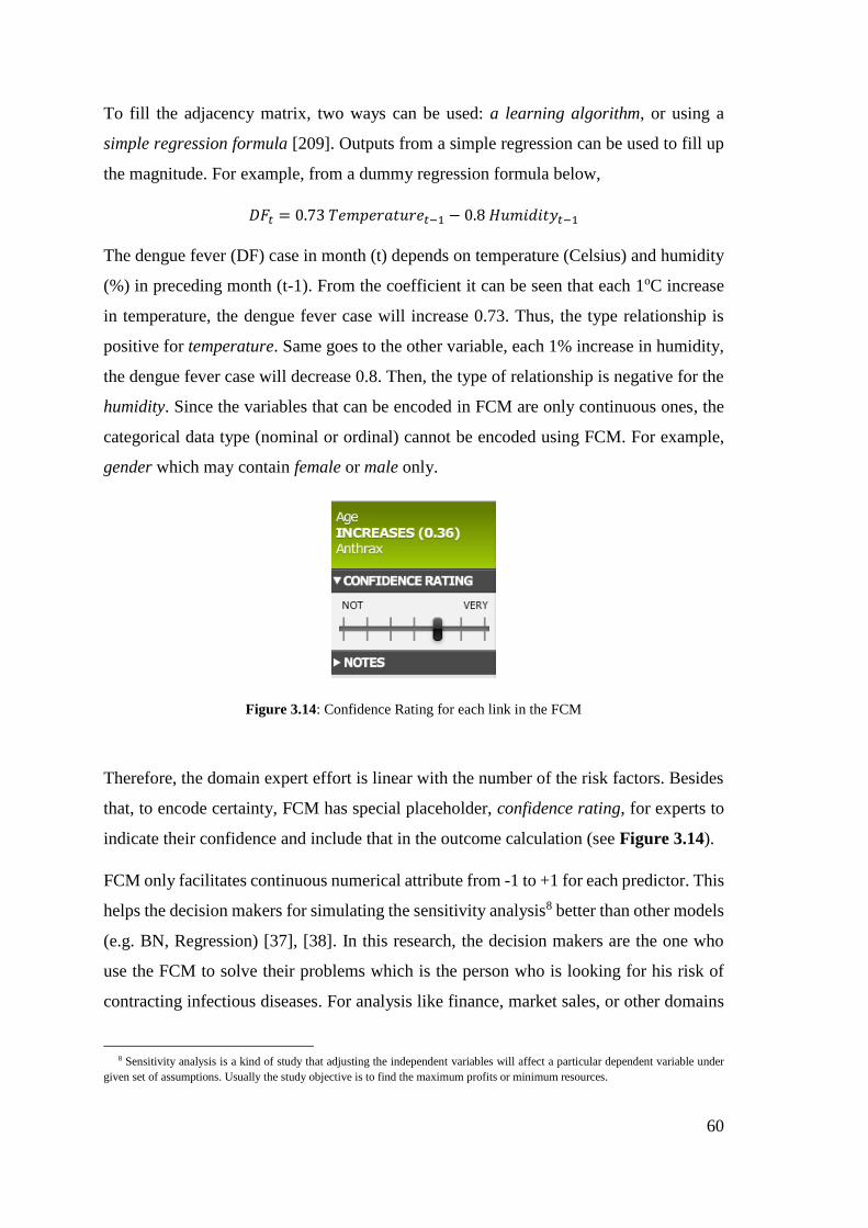
60
To fill the adjacency matrix, two ways can be used: a learning algorithm, or using a
simple regression formula [209]. Outputs from a simple regression can be used to fill up
the magnitude. For example, from a dummy regression formula below,
𝐷𝐹𝑡 = 0.73 𝑇𝑒𝑚𝑝𝑒𝑟𝑎𝑡𝑢𝑟𝑒𝑡−1 − 0.8 𝐻𝑢𝑚𝑖𝑑𝑖𝑡𝑦𝑡−1
The dengue fever (DF) case in month (t) depends on temperature (Celsius) and humidity
(%) in preceding month (t-1). From the coefficient it can be seen that each 1oC increase
in temperature, the dengue fever case will increase 0.73. Thus, the type relationship is
positive for temperature. Same goes to the other variable, each 1% increase in humidity,
the dengue fever case will decrease 0.8. Then, the type of relationship is negative for the
humidity. Since the variables that can be encoded in FCM are only continuous ones, the
categorical data type (nominal or ordinal) cannot be encoded using FCM. For example,
gender which may contain female or male only.
Figure 3.14: Confidence Rating for each link in the FCM
Therefore, the domain expert effort is linear with the number of the risk factors. Besides
that, to encode certainty, FCM has special placeholder, confidence rating, for experts to
indicate their confidence and include that in the outcome calculation (see Figure 3.14).
FCM only facilitates continuous numerical attribute from -1 to +1 for each predictor. This
helps the decision makers for simulating the sensitivity analysis8 better than other models
(e.g. BN, Regression) [37], [38]. In this research, the decision makers are the one who
use the FCM to solve their problems which is the person who is looking for his risk of
contracting infectious diseases. For analysis like finance, market sales, or other domains
8 Sensitivity analysis is a kind of study that adjusting the independent variables will affect a particular dependent variable under
given set of assumptions. Usually the study objective is to find the maximum profits or minimum resources.
61
that present their knowledge in continuous variable type and demands sensitivity analysis,
FCM address these problems well.
However, to encode infectious disease risk knowledge, with the characteristics and
quantifications presented in sections 3.1.1 and 3.1.2, respectively, two adjustments are
needed. First, the odds ratios and prevalence values need to be converted into the
acceptable range for the adjacency matrix. Second, the categorical risk factors (binary,
nominal, ordinal) need to be mapped into continuous numerical form.
3.2.3 Bayesian Network
The prediction model that is needed by this research is one that (1) represents causal
relationship, (2) encodes the infectious disease risk factors, and (3) yields risk prediction.
From section 3.1, it becomes apparent that the infectious disease risk factors can be
continuous, binary, nominal, or ordinal. The previous section, section 3.2.2, shows that
the FCM fits knowledge modelling for continuous risk factors (e.g. humidity,
temperature). Whereas, the Bayesian Network is more flexible to model (mixed)
categorical risk factors and (recent development of Bayesian also allows continuous
variable incorporation). This section elaborates the Bayesian network in relation to
disease risk prediction.
There are two types of dependency in Bayesian Network: conditionally independent and
conditionally dependent. The conditionally dependent, depicted by a blue square in
Figure 3.15, means that the result of D (Disease) depends on the k evidences (E1…Ek),
but the relationship between evidence is independent. This blue square usually depicts
the relationship between risk factors and the probability of contracting a disease.
Whereas, the yellow square represents conditional independence; this means that the
values of symptoms (S1…Sk) depends on whether a person has contracted disease D.
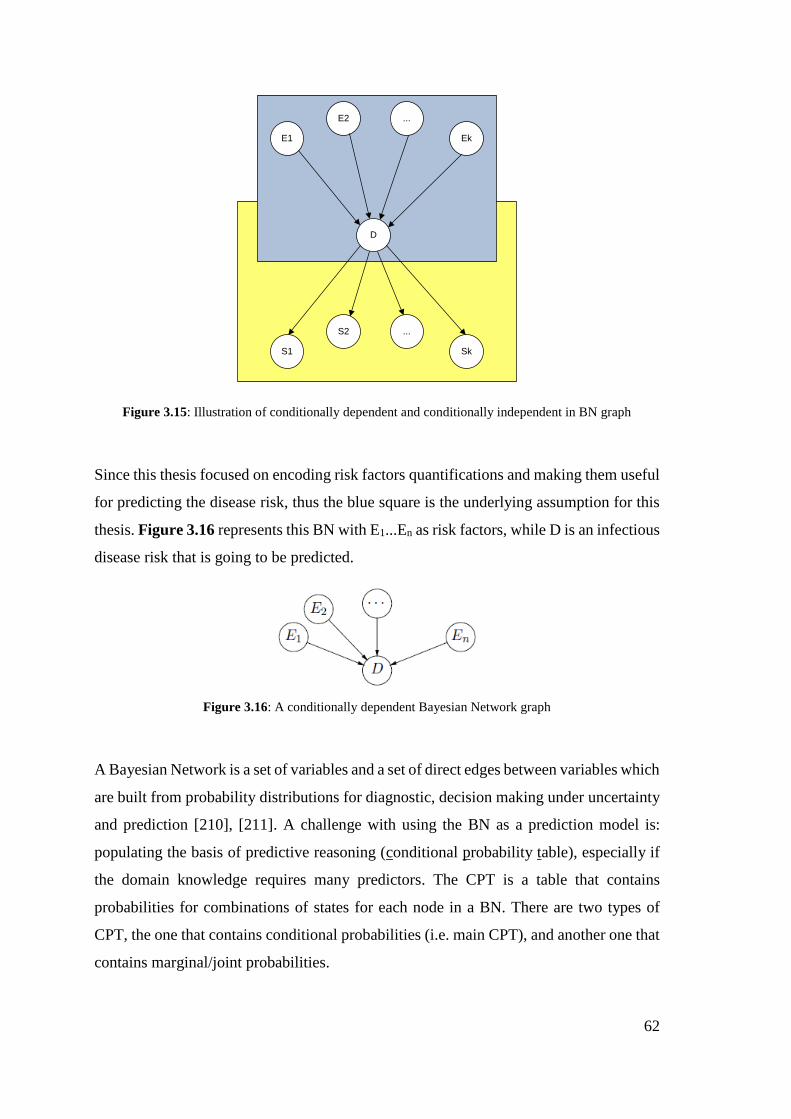
62
E1 Ek
...E2
D
S1 Sk
...S2
Figure 3.15: Illustration of conditionally dependent and conditionally independent in BN graph
Since this thesis focused on encoding risk factors quantifications and making them useful
for predicting the disease risk, thus the blue square is the underlying assumption for this
thesis. Figure 3.16 represents this BN with E1...En as risk factors, while D is an infectious
disease risk that is going to be predicted.
Figure 3.16: A conditionally dependent Bayesian Network graph
A Bayesian Network is a set of variables and a set of direct edges between variables which
are built from probability distributions for diagnostic, decision making under uncertainty
and prediction [210], [211]. A challenge with using the BN as a prediction model is:
populating the basis of predictive reasoning (conditional probability table), especially if
the domain knowledge requires many predictors. The CPT is a table that contains
probabilities for combinations of states for each node in a BN. There are two types of
CPT, the one that contains conditional probabilities (i.e. main CPT), and another one that
contains marginal/joint probabilities.
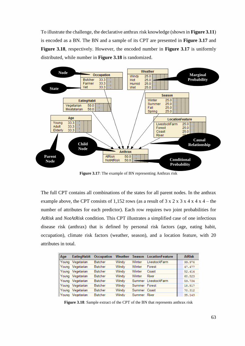
63
To illustrate the challenge, the declarative anthrax risk knowledge (shown in Figure 3.11)
is encoded as a BN. The BN and a sample of its CPT are presented in Figure 3.17 and
Figure 3.18, respectively. However, the encoded number in Figure 3.17 is uniformly
distributed, while number in Figure 3.18 is randomized.
Figure 3.17: The example of BN representing Anthrax risk
The full CPT contains all combinations of the states for all parent nodes. In the anthrax
example above, the CPT consists of 1,152 rows (as a result of 3 x 2 x 3 x 4 x 4 x 4 – the
number of attributes for each predictor). Each row requires two joint probabilities for
AtRisk and NotAtRisk condition. This CPT illustrates a simplified case of one infectious
disease risk (anthrax) that is defined by personal risk factors (age, eating habit,
occupation), climate risk factors (weather, season), and a location feature, with 20
attributes in total.
Figure 3.18: Sample extract of the CPT of the BN that represents anthrax risk
Node
State
Marginal
Probability
Conditional
Probability
Parent
Node
Child
Node
Causal
Relationship
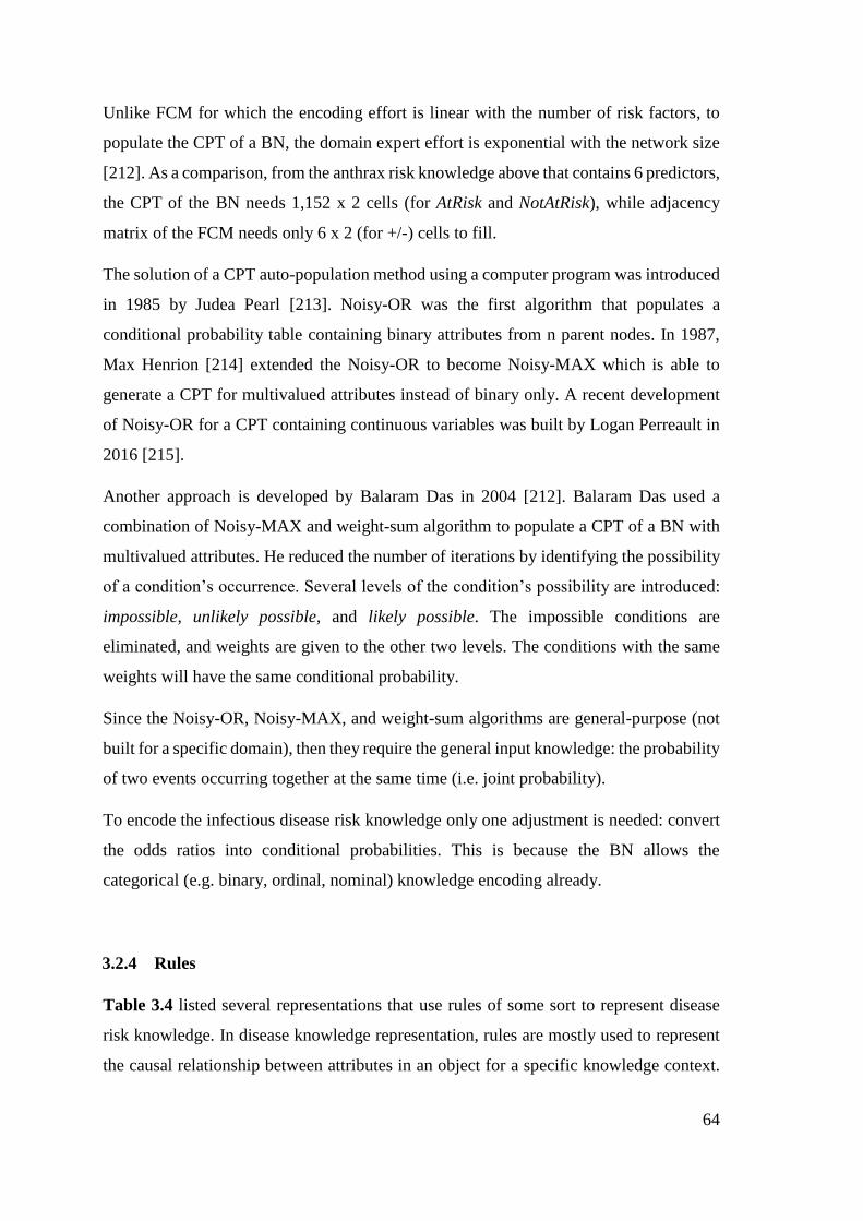
64
Unlike FCM for which the encoding effort is linear with the number of risk factors, to
populate the CPT of a BN, the domain expert effort is exponential with the network size
[212]. As a comparison, from the anthrax risk knowledge above that contains 6 predictors,
the CPT of the BN needs 1,152 x 2 cells (for AtRisk and NotAtRisk), while adjacency
matrix of the FCM needs only 6 x 2 (for +/-) cells to fill.
The solution of a CPT auto-population method using a computer program was introduced
in 1985 by Judea Pearl [213]. Noisy-OR was the first algorithm that populates a
conditional probability table containing binary attributes from n parent nodes. In 1987,
Max Henrion [214] extended the Noisy-OR to become Noisy-MAX which is able to
generate a CPT for multivalued attributes instead of binary only. A recent development
of Noisy-OR for a CPT containing continuous variables was built by Logan Perreault in
2016 [215].
Another approach is developed by Balaram Das in 2004 [212]. Balaram Das used a
combination of Noisy-MAX and weight-sum algorithm to populate a CPT of a BN with
multivalued attributes. He reduced the number of iterations by identifying the possibility
of a condition’s occurrence. Several levels of the condition’s possibility are introduced:
impossible, unlikely possible, and likely possible. The impossible conditions are
eliminated, and weights are given to the other two levels. The conditions with the same
weights will have the same conditional probability.
Since the Noisy-OR, Noisy-MAX, and weight-sum algorithms are general-purpose (not
built for a specific domain), then they require the general input knowledge: the probability
of two events occurring together at the same time (i.e. joint probability).
To encode the infectious disease risk knowledge only one adjustment is needed: convert
the odds ratios into conditional probabilities. This is because the BN allows the
categorical (e.g. binary, ordinal, nominal) knowledge encoding already.
3.2.4 Rules
Table 3.4 listed several representations that use rules of some sort to represent disease
risk knowledge. In disease knowledge representation, rules are mostly used to represent
the causal relationship between attributes in an object for a specific knowledge context.
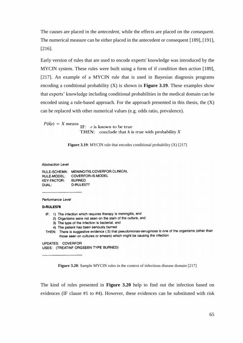
65
The causes are placed in the antecedent, while the effects are placed on the consequent.
The numerical measure can be either placed in the antecedent or consequent [189], [191],
[216].
Early version of rules that are used to encode experts' knowledge was introduced by the
MYCIN system. These rules were built using a form of if condition then action [189],
[217]. An example of a MYCIN rule that is used in Bayesian diagnosis programs
encoding a conditional probability (X) is shown in Figure 3.19. These examples show
that experts’ knowledge including conditional probabilities in the medical domain can be
encoded using a rule-based approach. For the approach presented in this thesis, the (X)
can be replaced with other numerical values (e.g. odds ratio, prevalence).
Figure 3.19: MYCIN rule that encodes conditional probability (X) [217]
Figure 3.20: Sample MYCIN rules in the context of infectious disease domain [217]
The kind of rules presented in Figure 3.20 help to find out the infection based on
evidences (IF clause #1 to #4). However, these evidences can be substituted with risk
66
factors for an infectious disease. Thus, these MYCIN rules containing risk factors become
an inspiration for designing rules in this thesis.
Though rules, semantic-web rules, and belief rule-based representations contain similar
structure (having antecedent and consequent), in this review they are discussed
separately. Semantic-web rules (encoded using Semantic-Web Rule Language – SWRL)
are only implemented together with ontology representation. Whereas, the belief rule-
based is a general rule representation that has ability to include uncertainty as in FCM or
BN representation.
SWRL can encode belief rule-based and general rules using specific notation, however,
SWRL has limitations in expressing OR and negation logical operators either in
antecedent or consequent [218]. These limitations result in numerous rules to represent
single general rule statement for which other rule approaches only need one rule.
The following examples show encoding of certainty, incorporating fuzziness and
encoding a negation operator. The SWRL notation of the general rule and belief rule-
based are presented for each example, so the differences between them can be seen.
The first example contains crisp and certain knowledge: if a person is above 10 years
old then he/she must have an adult travel card; a person aged 10 and below may have a
child travel card or none at all. The following rule encoding covers rules and SWRL
notation. Since the required knowledge is crisp and certain, the belief rule-based is not
applicable for encoding this example.
Rules: IF age > 10 years THEN travel card = adult
SWRL notation: Person(?x) ^ hasAge(?x, >10) -> ownTravelCard(adult)
Rules: IF age <= 10 years THEN travel card = child or travel card = none
SWRL notation: Person(?x) ^ hasAge(?x, <=10) -> ownTravelCard(child)
Person(?x) ^ hasAge(?x, <=10) -> ownTravelCard(none)
The second example contains crisp and uncertain knowledge: person aged 10 and below
may have a child travel card or none at all.
Belief rule-based:
67
IF age <= 10 THEN travel card {(none, 0.5), (child, 0.5), (adult, 0)}
SWRL notation: Person(?x) ^ hasAge(?x, <=10) -> ownTravelCard(child, 0.5)
Person(?x) ^ hasAge(?x, <=10) -> ownTravelCard(none, 0.5)
The next example encodes fuzzy and non-negation knowledge: if a young person lives
around a livestock farm then he is at high risk of Anthrax.
Rules: IF age = young AND liveAround = livestock farm THEN AnthraxRisk = high
SWRL notation: Person(?x) ^ hasAge(?x, young) ^ liveAround(?x, livestockFarm) ->
Anthrax(high)
The next example of uncertain and negation knowledge encoding: livestock farmers in
other than Winter season are at medium-high risk of Anthrax.
Rules: IF occupation = livestock farmer AND season != Winter THEN AnthraxRisk
= medium or high
SWRL notation: Person(?x) ^ hasOccupation(?x, livestock farmer) ^ inSeason(?x,
Summer) -> Anthrax(medium)
Person(?x) ^ hasOccupation(?x, livestock farmer) ^ inSeason(?x, Fall)
-> Anthrax(medium)
Person(?x) ^ hasOccupation(?x, livestock farmer) ^ inSeason(?x,
Spring) -> Anthrax(medium)
Person(?x) ^ hasOccupation(?x, livestock farmer) ^ inSeason(?x,
Summer) -> Anthrax(high)
Person(?x) ^ hasOccupation(?x, livestock farmer) ^ inSeason(?x, Fall)
-> Anthrax(high)
Person(?x) ^ hasOccupation(?x, livestock farmer) ^ inSeason(?x, Spring)
-> Anthrax(high)
The rules below is the encoding example of uncertain and negation using belief-rule
based: livestock farmers in other than Winter season are at medium-high risk of Anthrax.
Belief rule-based: IF occupation = livestock farmer AND season != Winter THEN AnthraxRisk
{(low, 0), (medium, 0.5), (high, 0.5)}
SWRL notation: Person(?x) ^ hasOccupation(?x, livestock farmer) ^ season(?x, Summer ->
AnthraxRisk(medium, 0.5)
Person(?x) ^ hasOccupation(?x, livestock farmer) ^ season(?x, Fall ->
AnthraxRisk(medium, 0.5)
68
Person(?x) ^ hasOccupation(?x, livestock farmer) ^ season(?x, Spring ->
AnthraxRisk(medium, 0.5)
Person(?x) ^ hasOccupation(?x, livestock farmer) ^ season(?x, Summer ->
AnthraxRisk(high, 0.5)
Person(?x) ^ hasOccupation(?x, livestock farmer) ^ season(?x, Fall ->
AnthraxRisk(high, 0.5)
Person(?x) ^ hasOccupation(?x, livestock farmer) ^ season(?x, Spring ->
AnthraxRisk(high, 0.5)
From the examples above, SWRL can be used to represent certainty of the antecedent and
consequent. However, more semantic-web rules are needed to encode one rule or belief
rule-based that contain uncertainty.
However, without any structural knowledge representation (e.g. Ontology, BN, FCM),
none of the rule encoding give the complete attributes of an object in a whole knowledge
context. This is because the rules only state the IF-Then relationship of attributes. The
attributes which are not explained by IF-Then relationship will not appear in the rules.
An example is given below,
Rules: IF age = children AND liveAround = farm THEN AnthraxRisk = high
By seeing only the rule above, the users will not know if there are 2 other attributes (adult,
elderly) or 3 other attributes (infant, adult, elderly) or even 4 other attributes (infant,
adolescent, adult, elderly) in the age object since the rule above only mention children.
Or how many location features are related to anthrax risk, that is because the rule above
only mention farm. To clarify the big picture of knowledge, the structural knowledge
representation can be implemented together with the rules.
3.2.5 Summary
This section presented knowledge representations used for disease related knowledge in
the area of computer science and medicine. To sum up, this section has three aims: (1) to
find existing representation that can be reused (partially or wholly) for encoding the
infectious disease risk knowledge which was presented in section 3.1, (2) to sense the
required efforts of the domain experts to encode their knowledge using the existing
representation, (3) to identify the needed adjustments of the existing representation to fit
the infectious disease risk knowledge.
69
The most used knowledge representation (ontology), a data-driven representation (FCM),
a knowledge-driven representation (BN), and a representation for causal relationship
(rules) were investigated based on those three aims. Ontologies are useful for encoding
the infectious disease risk knowledge since they allow sharing resources (e.g. vocabulary,
concept) and able to encode the characteristics of the infectious disease risk knowledge
and the quantifications. However, there are no existing ontologies that can be instantiated
with aim to encode the infectious disease risk factors and their risk quantifications (risk
ratios, prevalence). Therefore, some of the objects (classes and properties) of the existing
ontologies that encode concepts of disease risk factors can be reused to design the
knowledge representation.
The gathered articles show that FCM has a feature, confidence rating, that can be reused
to represent uncertainty across domain experts in a knowledge-base. The efforts of the
domain experts in encoding knowledge in FCM is linear with the size of the map (number
of the risk factors). But, from section 3.1, infectious disease risk factors are likely to
contain a mixture of nominal, binary, ordinal variables. Until the recent development of
the FCM, it can only encode the continuous variable; in fact, the continuous variable in
the infectious disease risk knowledge is very few (e.g. temperature and humidity affect
mumps risk). Thus, using FCM to encode the infectious disease risk knowledge is not
much useful.
Articles that use BN to model disease risk factors show that categorical knowledge
representation fits the characteristics of the infectious disease risk factors. However, the
required effort to encode knowledge using BN is exponential with the size of the network
(multiplication results of the number attributes for each risk factor). Some approaches to
automate these efforts are available. For these automated approaches, the risk ratios and
prevalence should be presented in a way that can be converted into conditional
probabilities.
From the reviewed articles, rules are versatile to represent crisp, fuzzy, certain, uncertain,
negation, or non-negation knowledge. Semantic-web rules are able to express causal
relationship in an ontology environment. The encoding examples of declarative
knowledge show that semantic-web rules are useful to capture uncertainty and
quantifications (e.g. odds ratios, prevalence) that may appear on the domain knowledge.
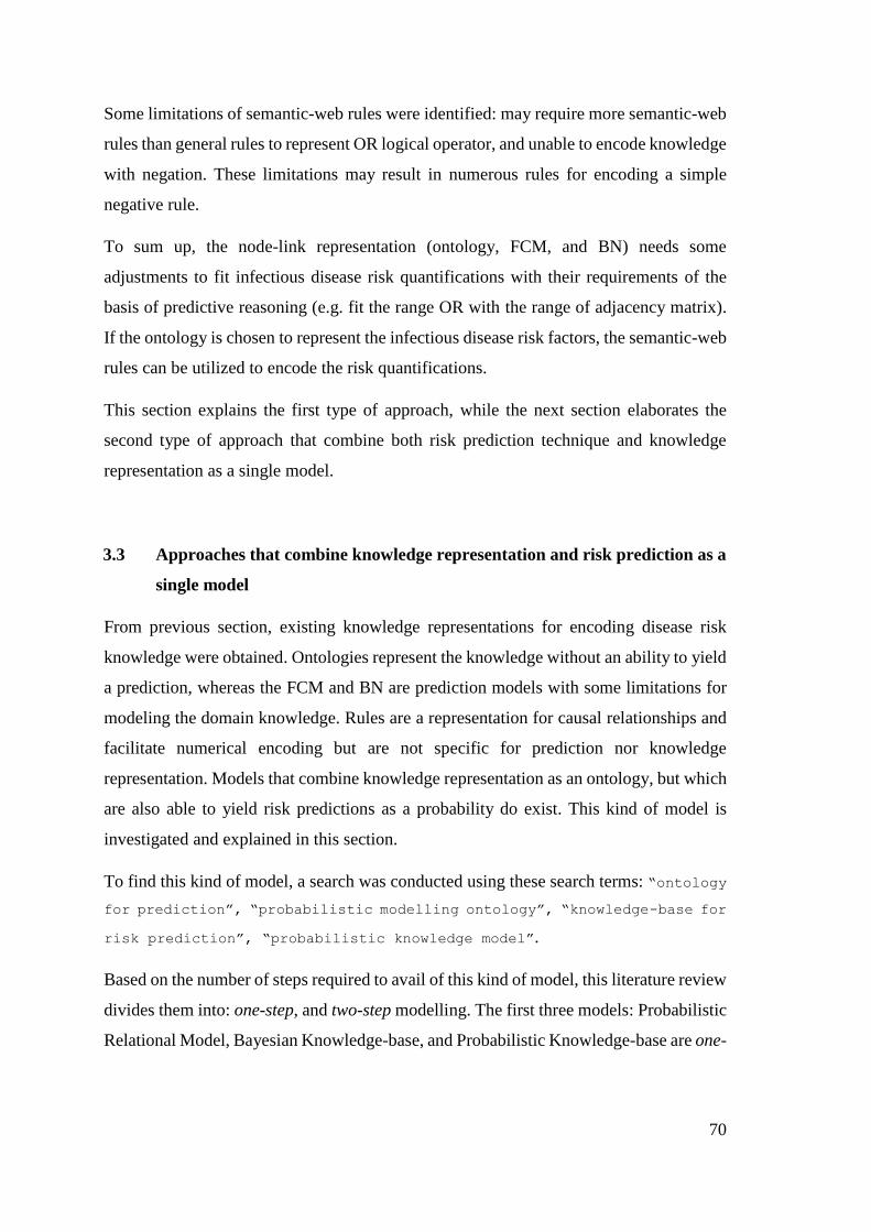
70
Some limitations of semantic-web rules were identified: may require more semantic-web
rules than general rules to represent OR logical operator, and unable to encode knowledge
with negation. These limitations may result in numerous rules for encoding a simple
negative rule.
To sum up, the node-link representation (ontology, FCM, and BN) needs some
adjustments to fit infectious disease risk quantifications with their requirements of the
basis of predictive reasoning (e.g. fit the range OR with the range of adjacency matrix).
If the ontology is chosen to represent the infectious disease risk factors, the semantic-web
rules can be utilized to encode the risk quantifications.
This section explains the first type of approach, while the next section elaborates the
second type of approach that combine both risk prediction technique and knowledge
representation as a single model.
3.3 Approaches that combine knowledge representation and risk prediction as a
single model
From previous section, existing knowledge representations for encoding disease risk
knowledge were obtained. Ontologies represent the knowledge without an ability to yield
a prediction, whereas the FCM and BN are prediction models with some limitations for
modeling the domain knowledge. Rules are a representation for causal relationships and
facilitate numerical encoding but are not specific for prediction nor knowledge
representation. Models that combine knowledge representation as an ontology, but which
are also able to yield risk predictions as a probability do exist. This kind of model is
investigated and explained in this section.
To find this kind of model, a search was conducted using these search terms: “ontology
for prediction”, “probabilistic modelling ontology”, “knowledge-base for
risk prediction”, “probabilistic knowledge model”.
Based on the number of steps required to avail of this kind of model, this literature review
divides them into: one-step, and two-step modelling. The first three models: Probabilistic
Relational Model, Bayesian Knowledge-base, and Probabilistic Knowledge-base are one-
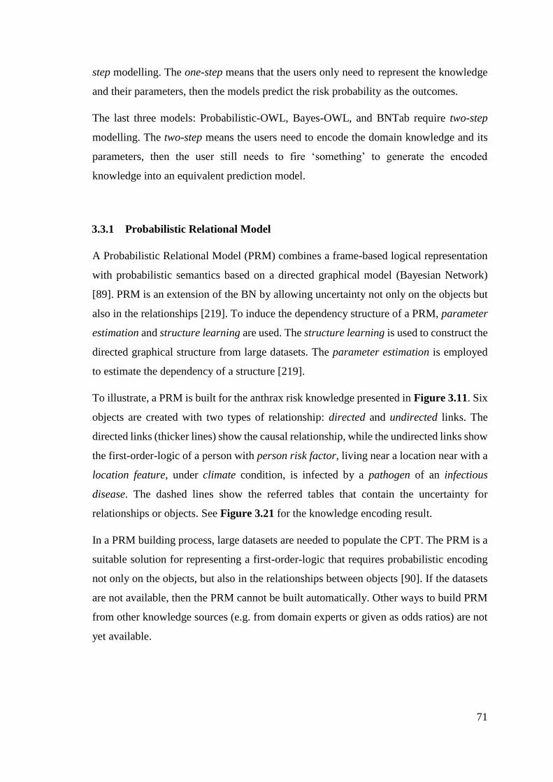
71
step modelling. The one-step means that the users only need to represent the knowledge
and their parameters, then the models predict the risk probability as the outcomes.
The last three models: Probabilistic-OWL, Bayes-OWL, and BNTab require two-step
modelling. The two-step means the users need to encode the domain knowledge and its
parameters, then the user still needs to fire ‘something’ to generate the encoded
knowledge into an equivalent prediction model.
3.3.1 Probabilistic Relational Model
A Probabilistic Relational Model (PRM) combines a frame-based logical representation
with probabilistic semantics based on a directed graphical model (Bayesian Network)
[89]. PRM is an extension of the BN by allowing uncertainty not only on the objects but
also in the relationships [219]. To induce the dependency structure of a PRM, parameter
estimation and structure learning are used. The structure learning is used to construct the
directed graphical structure from large datasets. The parameter estimation is employed
to estimate the dependency of a structure [219].
To illustrate, a PRM is built for the anthrax risk knowledge presented in Figure 3.11. Six
objects are created with two types of relationship: directed and undirected links. The
directed links (thicker lines) show the causal relationship, while the undirected links show
the first-order-logic of a person with person risk factor, living near a location near with a
location feature, under climate condition, is infected by a pathogen of an infectious
disease. The dashed lines show the referred tables that contain the uncertainty for
relationships or objects. See Figure 3.21 for the knowledge encoding result.
In a PRM building process, large datasets are needed to populate the CPT. The PRM is a
suitable solution for representing a first-order-logic that requires probabilistic encoding
not only on the objects, but also in the relationships between objects [90]. If the datasets
are not available, then the PRM cannot be built automatically. Other ways to build PRM
from other knowledge sources (e.g. from domain experts or given as odds ratios) are not
yet available.
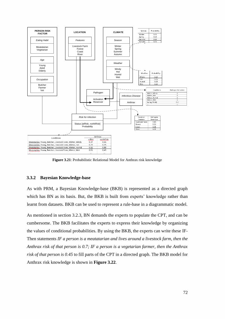
72
Eating Habit
Meatatarian
Vegetarian
Age
Young
Adult
Elderly
Occupation
Butcher
Farmer
Vet
PERSON RISK
FACTORLOCATION
Features
Livestock Farm
Forest
Coast
River
CLIMATE
Season
Winter
Spring
Summer
Autumn
Weather
Windy
Hot
Humid
Wet
Pathogen
Activation
Reservoir
Infectious Disease
Anthrax
Risk for Infection
Status [atRisk, notAtRisk]
Probability
Figure 3.21: Probabilistic Relational Model for Anthrax risk knowledge
3.3.2 Bayesian Knowledge-base
As with PRM, a Bayesian Knowledge-base (BKB) is represented as a directed graph
which has BN as its basis. But, the BKB is built from experts’ knowledge rather than
learnt from datasets. BKB can be used to represent a rule-base in a diagrammatic model.
As mentioned in section 3.2.3, BN demands the experts to populate the CPT, and can be
cumbersome. The BKB facilitates the experts to express their knowledge by organizing
the values of conditional probabilities. By using the BKB, the experts can write these IF-
Then statements IF a person is a meatatarian and lives around a livestock farm, then the
Anthrax risk of that person is 0.7; IF a person is a vegetarian farmer, then the Anthrax
risk of that person is 0.45 to fill parts of the CPT in a directed graph. The BKB model for
Anthrax risk knowledge is shown in Figure 3.22.
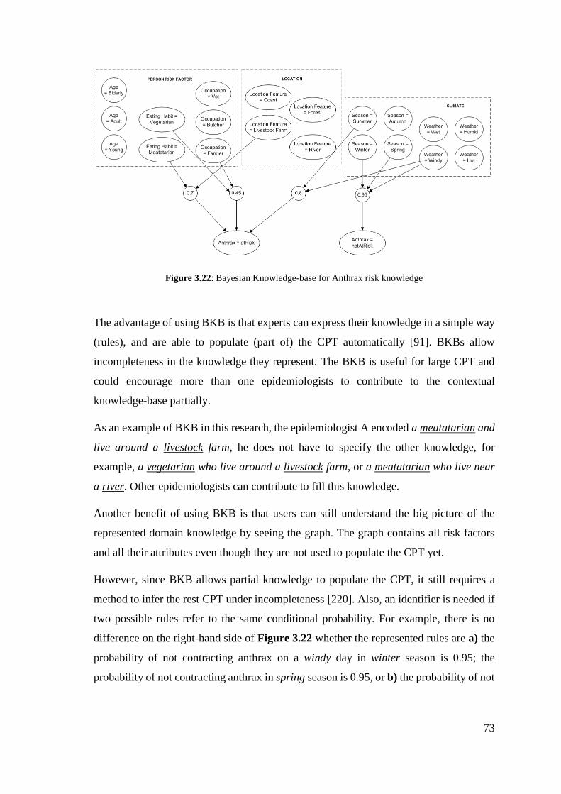
73
Figure 3.22: Bayesian Knowledge-base for Anthrax risk knowledge
The advantage of using BKB is that experts can express their knowledge in a simple way
(rules), and are able to populate (part of) the CPT automatically [91]. BKBs allow
incompleteness in the knowledge they represent. The BKB is useful for large CPT and
could encourage more than one epidemiologists to contribute to the contextual
knowledge-base partially.
As an example of BKB in this research, the epidemiologist A encoded a meatatarian and
live around a livestock farm, he does not have to specify the other knowledge, for
example, a vegetarian who live around a livestock farm, or a meatatarian who live near
a river. Other epidemiologists can contribute to fill this knowledge.
Another benefit of using BKB is that users can still understand the big picture of the
represented domain knowledge by seeing the graph. The graph contains all risk factors
and all their attributes even though they are not used to populate the CPT yet.
However, since BKB allows partial knowledge to populate the CPT, it still requires a
method to infer the rest CPT under incompleteness [220]. Also, an identifier is needed if
two possible rules refer to the same conditional probability. For example, there is no
difference on the right-hand side of Figure 3.22 whether the represented rules are a) the
probability of not contracting anthrax on a windy day in winter season is 0.95; the
probability of not contracting anthrax in spring season is 0.95, or b) the probability of not
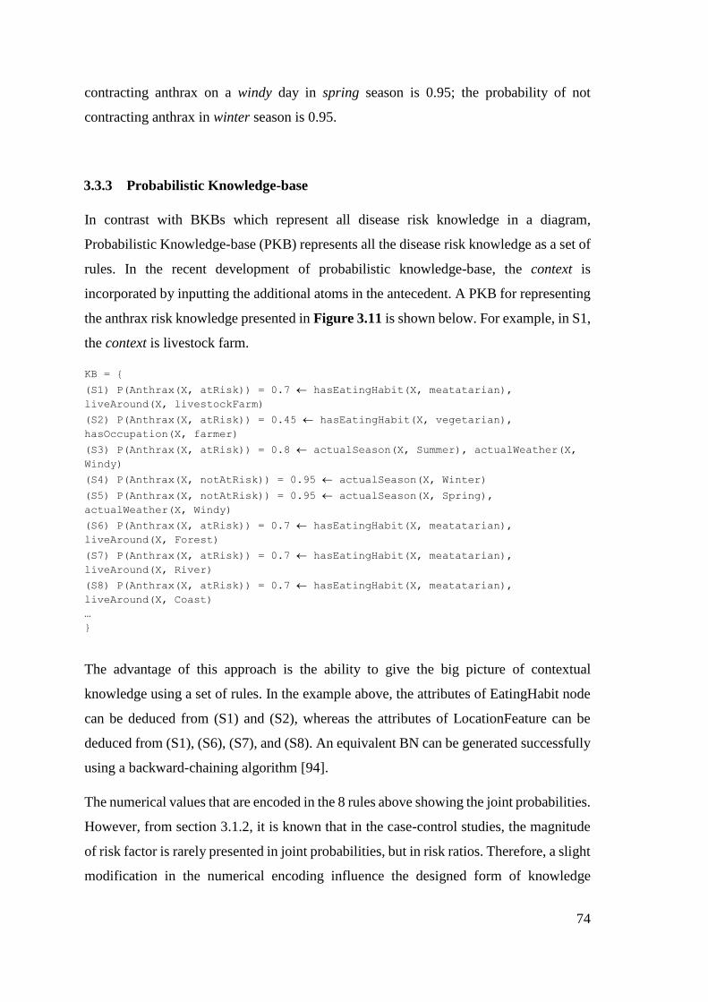
74
contracting anthrax on a windy day in spring season is 0.95; the probability of not
contracting anthrax in winter season is 0.95.
3.3.3 Probabilistic Knowledge-base
In contrast with BKBs which represent all disease risk knowledge in a diagram,
Probabilistic Knowledge-base (PKB) represents all the disease risk knowledge as a set of
rules. In the recent development of probabilistic knowledge-base, the context is
incorporated by inputting the additional atoms in the antecedent. A PKB for representing
the anthrax risk knowledge presented in Figure 3.11 is shown below. For example, in S1,
the context is livestock farm.
KB = {
(S1) P(Anthrax(X, atRisk)) = 0.7 hasEatingHabit(X, meatatarian),
liveAround(X, livestockFarm)
(S2) P(Anthrax(X, atRisk)) = 0.45 hasEatingHabit(X, vegetarian),
hasOccupation(X, farmer)
(S3) P(Anthrax(X, atRisk)) = 0.8 actualSeason(X, Summer), actualWeather(X,
Windy)
(S4) P(Anthrax(X, notAtRisk)) = 0.95 actualSeason(X, Winter)
(S5) P(Anthrax(X, notAtRisk)) = 0.95 actualSeason(X, Spring),
actualWeather(X, Windy)
(S6) P(Anthrax(X, atRisk)) = 0.7 hasEatingHabit(X, meatatarian),
liveAround(X, Forest)
(S7) P(Anthrax(X, atRisk)) = 0.7 hasEatingHabit(X, meatatarian),
liveAround(X, River)
(S8) P(Anthrax(X, atRisk)) = 0.7 hasEatingHabit(X, meatatarian),
liveAround(X, Coast)
…
}
The advantage of this approach is the ability to give the big picture of contextual
knowledge using a set of rules. In the example above, the attributes of EatingHabit node
can be deduced from (S1) and (S2), whereas the attributes of LocationFeature can be
deduced from (S1), (S6), (S7), and (S8). An equivalent BN can be generated successfully
using a backward-chaining algorithm [94].
The numerical values that are encoded in the 8 rules above showing the joint probabilities.
However, from section 3.1.2, it is known that in the case-control studies, the magnitude
of risk factor is rarely presented in joint probabilities, but in risk ratios. Therefore, a slight
modification in the numerical encoding influence the designed form of knowledge
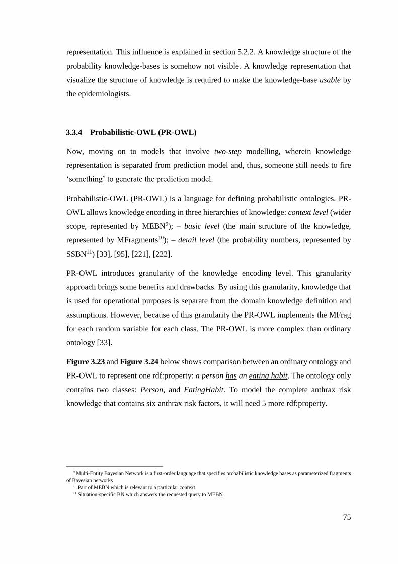
75
representation. This influence is explained in section 5.2.2. A knowledge structure of the
probability knowledge-bases is somehow not visible. A knowledge representation that
visualize the structure of knowledge is required to make the knowledge-base usable by
the epidemiologists.
3.3.4 Probabilistic-OWL (PR-OWL)
Now, moving on to models that involve two-step modelling, wherein knowledge
representation is separated from prediction model and, thus, someone still needs to fire
‘something’ to generate the prediction model.
Probabilistic-OWL (PR-OWL) is a language for defining probabilistic ontologies. PR-
OWL allows knowledge encoding in three hierarchies of knowledge: context level (wider
scope, represented by MEBN9); – basic level (the main structure of the knowledge,
represented by MFragments10); – detail level (the probability numbers, represented by
SSBN11) [33], [95], [221], [222].
PR-OWL introduces granularity of the knowledge encoding level. This granularity
approach brings some benefits and drawbacks. By using this granularity, knowledge that
is used for operational purposes is separate from the domain knowledge definition and
assumptions. However, because of this granularity the PR-OWL implements the MFrag
for each random variable for each class. The PR-OWL is more complex than ordinary
ontology [33].
Figure 3.23 and Figure 3.24 below shows comparison between an ordinary ontology and
PR-OWL to represent one rdf:property: a person has an eating habit. The ontology only
contains two classes: Person, and EatingHabit. To model the complete anthrax risk
knowledge that contains six anthrax risk factors, it will need 5 more rdf:property.
9 Multi-Entity Bayesian Network is a first-order language that specifies probabilistic knowledge bases as parameterized fragments
of Bayesian networks 10 Part of MEBN which is relevant to a particular context 11 Situation-specific BN which answers the requested query to MEBN
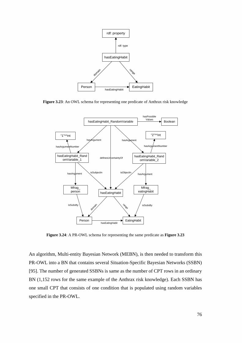
76
rdf: property
hasEatingHabit
Person EatingHabit
rdf: type
rangedo
mai
n
hasEatingHabit
Figure 3.23: An OWL schema for representing one predicate of Anthrax risk knowledge
hasEatingHabit_RandomVariable
hasEatingHabit
Person EatingHabit
definesUncertaintyOf
rangedo
main
hasEatingHabit
Boolean
hasPossible
Values
hasEatingHabit_Rand
omVariable_1hasEatingHabit_Rand
omVariable_2
Mfrag_
person
Mfrag_
eatingHabit
isSubsBy isSubsBy
“1”^^int “2”^^int
isSubjectIn isObjectIn
hasArgument hasArgument
hasArgument hasArgument
hasArgumentNumber hasArgumentNumber
Figure 3.24: A PR-OWL schema for representing the same predicate as Figure 3.23
An algorithm, Multi-entity Bayesian Network (MEBN), is then needed to transform this
PR-OWL into a BN that contains several Situation-Specific Bayesian Networks (SSBN)
[95]. The number of generated SSBNs is same as the number of CPT rows in an ordinary
BN (1,152 rows for the same example of the Anthrax risk knowledge). Each SSBN has
one small CPT that consists of one condition that is populated using random variables
specified in the PR-OWL.
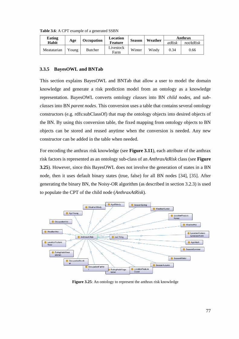
77
Table 3.6: A CPT example of a generated SSBN
Eating
Habit Age Occupation
Location
Feature Season Weather
Anthrax
atRisk notAtRisk
Meatatarian Young Butcher Livestock
Farm Winter Windy 0.34 0.66
3.3.5 BayesOWL and BNTab
This section explains BayesOWL and BNTab that allow a user to model the domain
knowledge and generate a risk prediction model from an ontology as a knowledge
representation. BayesOWL converts ontology classes into BN child nodes, and sub-
classes into BN parent nodes. This conversion uses a table that contains several ontology
constructors (e.g. rdfs:subClassOf) that map the ontology objects into desired objects of
the BN. By using this conversion table, the fixed mapping from ontology objects to BN
objects can be stored and reused anytime when the conversion is needed. Any new
constructor can be added in the table when needed.
For encoding the anthrax risk knowledge (see Figure 3.11), each attribute of the anthrax
risk factors is represented as an ontology sub-class of an AnthraxAtRisk class (see Figure
3.25). However, since this BayesOWL does not involve the generation of states in a BN
node, then it uses default binary states (true, false) for all BN nodes [34], [35]. After
generating the binary BN, the Noisy-OR algorithm (as described in section 3.2.3) is used
to populate the CPT of the child node (AnthraxAtRisk).
Figure 3.25: An ontology to represent the anthrax risk knowledge
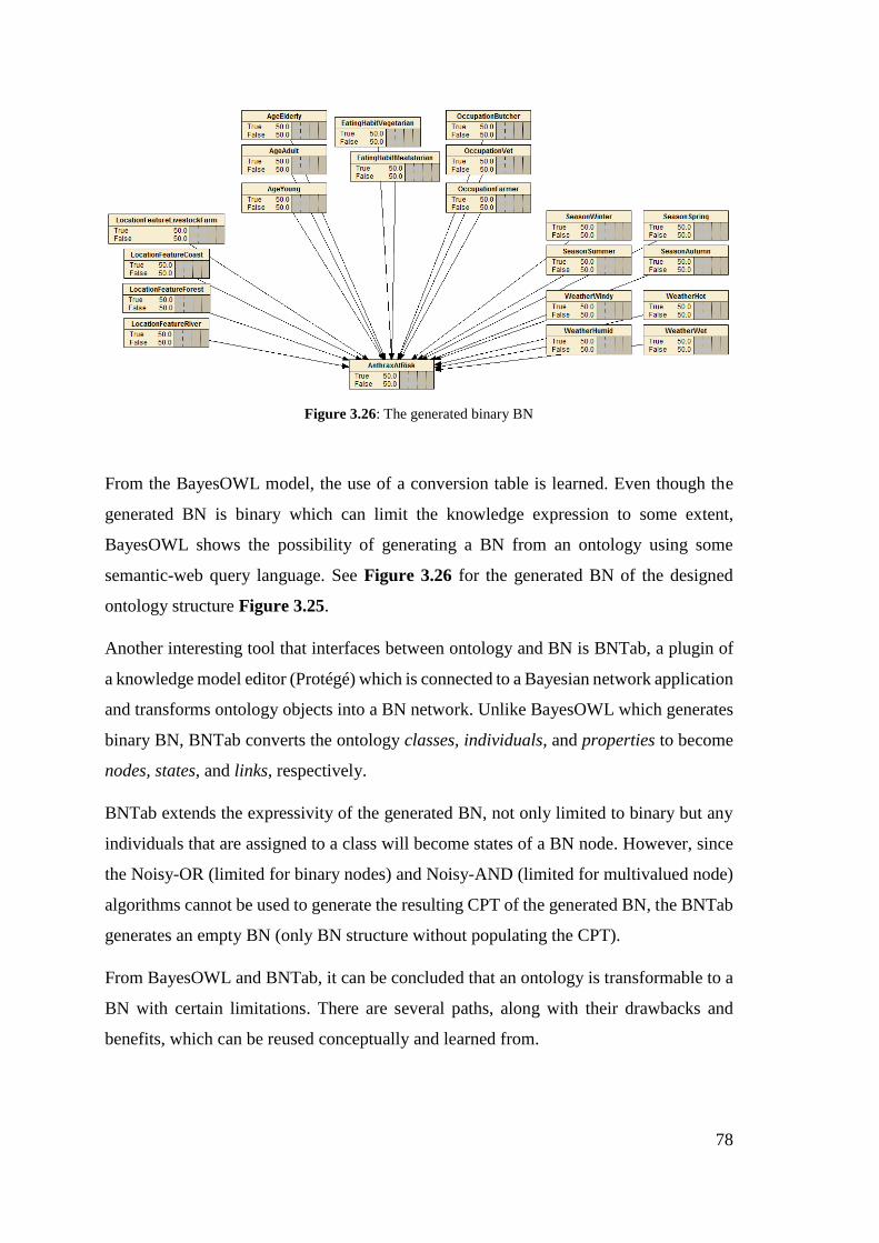
78
Figure 3.26: The generated binary BN
From the BayesOWL model, the use of a conversion table is learned. Even though the
generated BN is binary which can limit the knowledge expression to some extent,
BayesOWL shows the possibility of generating a BN from an ontology using some
semantic-web query language. See Figure 3.26 for the generated BN of the designed
ontology structure Figure 3.25.
Another interesting tool that interfaces between ontology and BN is BNTab, a plugin of
a knowledge model editor (Protégé) which is connected to a Bayesian network application
and transforms ontology objects into a BN network. Unlike BayesOWL which generates
binary BN, BNTab converts the ontology classes, individuals, and properties to become
nodes, states, and links, respectively.
BNTab extends the expressivity of the generated BN, not only limited to binary but any
individuals that are assigned to a class will become states of a BN node. However, since
the Noisy-OR (limited for binary nodes) and Noisy-AND (limited for multivalued node)
algorithms cannot be used to generate the resulting CPT of the generated BN, the BNTab
generates an empty BN (only BN structure without populating the CPT).
From BayesOWL and BNTab, it can be concluded that an ontology is transformable to a
BN with certain limitations. There are several paths, along with their drawbacks and
benefits, which can be reused conceptually and learned from.
79
3.3.6 Summary
Information about six models that combine the knowledge representation and risk
prediction in two approaches, one-step and two-step, were presented. Three one-step
models (e.g. PRM, BKB, PKB) were reviewed. Probabilistic Relational Model (PRM) is
able to encode a probabilistic table in an object or in a relationship between objects by
learning from large dataset. Bayesian Knowledge-base (BKB) can represent both rules
and the big picture of the knowledge, and also allow more than one epidemiologist to
collaborate together on one knowledge-base. Probabilistic Knowledge-base (PKB)
generates a Bayesian network from a rule-base using a backward-chaining algorithm.
Three two-step models (e.g. PR-OWL, BayesOWL, BNTab) were also included in this
review. Probabilistic-OWL (PR-OWL) provides levelling on knowledge modelling:
context – basic – detail. But from a comparison with basic OWL, PR-OWL is rather
complex even for modelling a simple triple. BayesOWL uses a conversion table to map
the ontology objects to become the Bayesian network objects; however, BayesOWL can
only generate a binary BN (true and false states). A Protégé plug-in, BNTab, is able to
model categorical knowledge and generate an isomorphic BN, but the conditional
probability table is blank.
3.4 Conclusion
Based on the collected knowledge in section 3.1, infections happen when a susceptible
host (human) is exposed to the pathogen of an infectious disease through direct or indirect
transmission. From SEIR mathematical modelling in epidemiology, a person’s risk of
contracting of infectious diseases can be deduced from the person’s susceptibility (S) and
pathogen exposure (E) level under specific atmospheric condition in a location.
The susceptibility of a person is identified from the demography, genetic, nutrition intake,
habits, and pre-existing illness (e.g. diabetes, cancer). In this thesis, these factors are
called personal risk factors. Besides the personal risk factors, climate and location are
found to have implications on the infectious disease risk, specifically on human immunity
level (e.g. wintertime-immune suppression). In this thesis, these factors are called
environmental risk factors. These factors are quantified by risk ratios (either odds ratios,
80
or relative risks). Most risk factors presented in categorical (nominal, ordinal, binary),
and very few risk factors are presented in numerical (continuous) variable type.
The infectious disease exposure can be deduced from the climate (weather and season),
and specific location features. Some climate-dependent pathogen and vector (e.g. Aedes
Aegypti) are multiply and attack hosts only under certain weather and season. Whereas
some pathogen’s reservoir is associated with some location features (e.g. cave, river), or
geographical variations (e.g. altitude). In the context of diseases, this exposure level can
be recognized through prevalence or incidence (the number of reported infection cases
divided by total population of a country). The prevalence or incidence are presented in
specific units (100,000 population or 1,000 population) depending on the diseases.
Thereafter, existing knowledge representation that fits the disease risk knowledge
characteristics were investigated. Ontologies turned out the most used representation in
the medical and computer science subject areas for the last 10 years. However, to
represent the infectious disease risk knowledge that contains causal relationship and
numerical encoding, the semantic-web rules should be used together with the ontology.
Also, since the ontology is not intended for prediction but representing knowledge,
current ontological model that can yield risk prediction were searched.
Six models were gathered, and their mechanisms were learned. All of them is able to
encode categorical knowledge for general-purpose. However, since these models are not
specific for disease related knowledge, thus, none of them that capable of encoding
infectious disease risk factors from epidemiologists and provide an automatic way to
generate their basis of predictive reasoning from risk ratios and prevalence.
To predict the personalized infectious disease risk from recent knowledge, besides an
ontology and semantic-web rules, a formula that uses risk ratios and prevalence to
populate a basis of predictive reasoning is required. Material presented in this chapter will
inform design decisions for PROSPECT-IDR, as presented in the following chapters.
81
4. DESIGN OF PROSPECT-IDR SYSTEM ARCHITECTURE AND
THE USER INTERFACES
4.1 Introduction
The introduction to this thesis outlined the need for a system that is capable of encoding,
updating, managing input knowledge about infectious disease risk, and of calculating a
person’s personalized infectious disease risk from the inputted knowledge. With such a
system, infectious disease risk knowledge can be encoded by domain experts as the
knowledge itself develops. This chapter presents the design of the PROSPECT-IDR
system, which was informed by several existing models, explained in the state-of-the-art
chapters (chapter 2 and 3). Those chapters examine the relevant use of mathematical
modelling, prediction modelling, and knowledge representation in this system context,
thus, some parts of them influence the design of this system.
This chapter begins with the taken influences from the state-of-the-art chapters (chapter
2 and 3). The influences are related to characteristics of infectious disease risk knowledge,
available and relevant data sources that can be used to personalize the resulting infectious
disease risk prediction, the reusable ontology objects (conceptually), and the mechanism
that allows a knowledge-base to yield risk prediction as probabilities. Thereafter, some
decisions related to system components will be made based on the influences.
4.2 Influences from the State of the Art
From review of the projects, apps, systems given in chapter 2, there are some existing
information that can be useful to achieve those three aims. The review about the
availability of data, prediction models, system or specific requirements is gathered in the
context of the PROSPECT-IDR.
82
4.2.1 Data Sources, Reports, APIs
This section mentions the existing data sources that can be obtained using the available
APIs or reports. This information was collected from section 2.2.
- From case-control studies, the who got what diseases can be inferred to become
magnitude of a risk factor (risk ratio) using eq. 3 or using a machine learning
approach (e.g. Logistic Regression). The risk ratios are widely available in case-
control studies published in epidemiology domain.
- There is a WHO report that exhibits number of reported cases for some notifiable
infectious diseases for some countries for a specific period. Together with the
number of total populations of each country in the world for specific year, which
provided by UNSD report, a prevalence value of an (infectious) disease in a
country for a certain period can be calculated using eq. 4.
- Several weather APIs can yield the atmospheric attributes (e.g. temperature,
humidity) based on the given city and country name (e.g. OpenWeather API).
- Several location-based APIs can yield the surrounding location features (e.g. river,
forest, market) based on a person’s geo-location (e.g. Google Place API).
4.2.2 Reused Concepts and Objects
In section 3.2.1, the disease related ontologies were collected. Since there are no existing
ontologies able to represent infectious disease risk knowledge, a knowledge
representation will be designed (explained in chapter 5). From the existing ontologies, the
containing concepts and categorizations relevant to infectious disease risk knowledge are
reused to design further knowledge representation.
From the conclusion of chapter 3, there are two types of risk factors included in this thesis,
personal risk factors that describe the relation of personal attributes with infection risks
(e.g. pre-existing illness, occupation), and environmental risk factors that explain the
relationship between climate (weather and season), location (country and location
features) and infection risks. Table 4.1 is a summary of the reusable concepts found in
the existing ontologies to be adopted as the content of personal and environmental risk
factors in the context of personalization of infectious disease risk prediction.
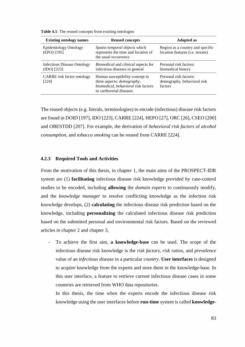
83
Table 4.1: The reused concepts from existing ontologies
Existing ontology names Reused concepts Adopted as
Epidemiology Ontology
(EPO) [195]
Spatio-temporal objects which
represents the time and location of
the usual occurrence
Region as a country and specific
location features (i.e. terrain)
Infectious Disease Ontology
(IDO) [223]
Biomedical and clinical aspects for
infectious diseases in general
Personal risk factors:
biomedical history
CARRE risk factor ontology
[224]
Human susceptibility concept in
three aspects: demography,
biomedical, behavioral risk factors
in cardiorenal diseases
Personal risk factors:
demography, behavioral risk
factors
The reused objects (e.g. literals, terminologies) to encode (infectious) disease risk factors
are found in DOID [197], IDO [223], CARRE [224], HEPO [27], ORC [26], CSEO [200]
and OBESTDD [207]. For example, the derivation of behavioral risk factors of alcohol
consumption, and tobacco smoking can be reused from CARRE [224].
4.2.3 Required Tools and Activities
From the motivation of this thesis, in chapter 1, the main aims of the PROSPECT-IDR
system are (1) facilitating infectious disease risk knowledge provided by case-control
studies to be encoded, including allowing the domain experts to continuously modify,
and the knowledge manager to resolve conflicting knowledge as the infection risk
knowledge develops, (2) calculating the infectious disease risk prediction based on the
knowledge, including personalizing the calculated infectious disease risk prediction
based on the submitted personal and environmental risk factors. Based on the reviewed
articles in chapter 2 and chapter 3,
- To achieve the first aim, a knowledge-base can be used. The scope of the
infectious disease risk knowledge is the risk factors, risk ratios, and prevalence
value of an infectious disease in a particular country. User interfaces is designed
to acquire knowledge from the experts and store them in the knowledge-base. In
this user interface, a feature to retrieve current infectious disease cases in some
countries are retrieved from WHO data repositories.
In this thesis, the time when the experts encode the infectious disease risk
knowledge using the user interfaces before run-time system is called knowledge-
84
encoding time. In this knowledge-encoding time, the knowledge engineer is also
allowed to manage the knowledge using the same user interfaces designed for
domain experts, if there are contradicting or duplicating knowledge.
- To reach the second aim, an algorithm that makes sure the recent knowledge
encoded in the knowledge-base be consistent with a predictive reasoning of a
prediction model is required. For example, the encoded knowledge is consistent
with the conditional probability table of the generated Bayesian network. The
algorithm is designed to take categorical (nominal, ordinal, binary) and numerical
(continuous) as inputs, then, it converts them into the prediction model.
To facilitate communication between the system and the users (lay people), a user
interface to submit their personal attributes is needed. The submitted personal
attributes are then used to personalize the infectious disease risk prediction. Then,
several packages might be needed to parse the given facts in order to get the
context of the given geo-position and submit them (both facts and context) to
personalize the calculated infectious disease risk prediction.
The focus of the knowledge-encoding time is inputting, modifying, and managing
knowledge in the knowledge-base. The focus of the run-time system is the collection of
personal facts (including the associated environmental contexts) and personalization the
prediction results based on the collected facts and contexts. In the run-time, the developed
algorithm ensures the encoded knowledge is consistent with the predicted infectious
disease risk. By putting the algorithm in charge every time the knowledge-base is updated,
then, this PROSPECT-IDR system is designed as a two-step approach. This means that,
in the system design, the knowledge-base is separated from the risk prediction model.
The needed components mentioned in the paragraphs above are then designed to become
a system architecture like that in Figure 4.1. The detailed explanation of the system
design and activity are given in section 4.3.
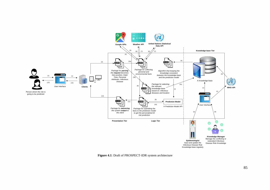
85
Package for collecting
personal and
environmental facts
A Prediction Model API
Prediction Model
Package for submitting the
facts to the prediction model
to get the personalized ID
risk prediction
Algorithm that keeping the
knowledge consistent
between the knowledge-base
and the prediction model
Clients
User Interface
Epidemiologist
Input and update the
Infectious Disease Risk
Knowledge-base regularly
Knowledge Manager
Manage the conflicting or
redundant Infectious
Disease Risk Knowledge
Package for parsing
the request becomes:
Geo-position, Date/
Time, Personal
Attributes, Infectious
Disease
Package for delivering
the system output to
the client
United Nations Statistical
Data APIWeather APIGoogle APIs
WHO API
Person whom the risk is
going to be predicted
(1)
(2) (3a)
(4)
(5)(6) (6)
(c)
(7) (7)
(d)
(8)
(9)
(10)
(11)
(12)
(13)
(a) (b)
(c)
(e)
(f)
Presentation Tier Logic Tier
Knowledge-base Tier
A Knowledge-base
Package for selecting
the relevant
knowledge-base
based on: infectious
diseases and location
(3b)(1)
(13)
User Interface
(3c)
Figure 4.1: Draft of PROSPECT-IDR system architecture
86
4.3 The PROSPECT-IDR system
In Figure 4.1, there are three tiers: presentation tier, logic tier, and knowledge-base tier.
The presentation tier and logic tier work at run-time, while the knowledge-base tier work
at knowledge-encoding time. The decision whether a separate package is needed is based
on the function; different function will be designed to have different package. The
presentation tier aims to facilitate communication between the clients and the
PROSPECT-IDR system. The presentation tier consists of two packages: one for
receiving requests from the client and parsing them to the logic tier (this package sits
between arrows number 2 and 3), and one for delivering the end result of the system to
the client (this package sits between arrows number 11 and 12).
The logic tier is the main processor of the PROSPECT-IDR system; it consists the
algorithm, the prediction model, and three packages. The algorithm keeps the knowledge
between knowledge-base and the prediction model is consistent. The prediction model
calculates the infectious disease risk prediction for all combinations of the knowledge
from knowledge-base. The first package aims to communicate with the APIs to get the
contexts of the parsed client’s request. The second package sends the facts and the
contexts (i.e. beliefs) to the prediction model as inputs of prediction. The third package
selects the relevant knowledge-base based on the submitted infectious disease and
inferred location.
The knowledge-base tier stores the infectious disease risk knowledge and the user
interfaces that facilitate communication between the knowledge-base and the
epidemiologists and the knowledge manager.
Since the prediction model depends on the knowledge encoded in the knowledge-base,
the sequence of the system started with the knowledge-encoding time, and then run-time
system. The run-time flows are denoted by numerical arrows, while the knowledge-
encoding time flows are denoted by alphabetical arrows in Figure 4.1. A dashed line
separates the run-time and knowledge-encoding time of the PROSPECT-IDR.
87
The activity flows of the knowledge-encoding time are,
a. The epidemiologist(s) input the risk knowledge for an infectious disease prevalent
in a country. For example, risk ratio for children of contracting of dengue fever in
Indonesia is twice higher than adults.
b. When there are anomalies: contradicting or duplicating rules, the knowledge
manager (in collaboration with domain expert) will resolve it by assigning
different priority for each anomaly rule. So, there is only one risk factor that has
the highest priority which will be taken by the algorithm to be included in
calculation of risk prediction.
c. When needed, the infectious disease prevalence value can be retrieved from the
WHO API. Otherwise, the epidemiologist can input the prevalence and send to
the knowledge base directly as in activity a.
d. If required, the retrieved prevalence value of the specific infectious disease in a
region is submitted to the knowledge base.
e. When the knowledge-base is updated, the algorithm that making sure that the
encoded knowledge in the knowledge-base is consistent with the prediction model
is executed.
f. This execution will renew the basis of predictive modelling of the prediction
model.
Those activities above will result in one knowledge-base that contains a set of rules for
encoding risk factors, risk ratios, prevalence values of one infectious disease. As the
dengue fever infection does not only prevalent in Indonesia, but also in other countries,
then, in knowledge-base tier could modify the prevalence value. For example, dengue
fever in Indonesia and in Malaysia have almost same risk factors and risk ratios, however,
the prevalence values of the dengue fever between those countries are different. This is
because the number of population in Malaysia and Indonesia is quite different (see eq. 4
for the prevalence formula). Therefore, a decision of whether a separate knowledge-base
is needed or not, will be explained in following section.
After the algorithm makes sure that the encoded knowledge in a particular knowledge-
base is consistent with the basis of predictive reasoning in the prediction model, then the
88
prediction model is ready to answer queries from clients at the run-time system. Based on
the numerical notation in Figure 4.1, the activity flows of the run-time system are,
1. A person is going to find prediction of his risk for an infectious disease at a time
at his current geo-position. For example, the dengue fever risk prediction for a 4-
year old female living in [-7.2759, 112.8083] at 13:55 on 4th of July 2018.
2. The person requests from an app or web as a client of the system and sends all her
personal attributes (age, gender, geo-position, request for dengue fever risk
prediction) into the system through presentation tier.
3. A package inside the tool parses the request based on the geo-position, date and
time, personal attributes, and name of infectious disease that is requested to be
predicted for the client. The parsing result is [-7.2759, 112.8083], 13:55 on
04/07/2018, female, 4, dengue fever.
4. A package for collecting the personal and environment contexts from the given
facts. First, converting the geo-position [-7.2759, 112.8083] become the city and
country names.
5. The city and country names are retrieved back for example Surabaya city in
Indonesia. (5a) A package is designed for selecting the relevant knowledge-base
(5b), based on parsed infectious disease and location (country).
6. Then, Surabaya and Indonesia are then sent to Weather API to retrieve the
weather [humidity, precipitation, temperature] for city = Surabaya, and country =
Indonesia. The detail human population of [gender = female, development stage
= children] for country = Indonesia is sent to UNSD API to get the population
context in the Indonesia. Whereas the geo-position of the user [-7.2759, 112.8083]
is sent to Google API to retrieve the location feature [altitude].
7. The package retrieves the environmental contexts from Weather API, Google
API, and UNSD API. The results from Weather API are [80%, 20mmHg, 30C];
the results from Google API are [7.234m]; the results from UNSD API are
[51.09%, 25.29%].
8. The package then pre-processes the [80%, 20mmHg, 30C], [7.234m], 04/07/2018
to become the environmental context: weather [hot, humid], season [rainy],
location feature [below 1000m].
89
9. Submitting the collected personal facts and environmental contexts: weather [hot,
humid], season [rainy], altitude [below 1000m], gender [female], development
stage [children], infectious disease [dengue fever] to a relevant prediction model.
To select which prediction model is relevant to the client request, the infectious
disease which is being predicted (dengue fever), and country name where the
client is (Indonesia) are used as selection parameters. As a result, the knowledge-
base for dengue fever in Indonesia is selected.
10. The prediction model calculates the personalized dengue fever risk based on the
given facts.
11. The prediction result for example 0.00135 (or 135 people per 100,000 population).
This result is sent back to the presentation tier using a package labelled by
‘package for delivering the system output to the client’.
12. The package inside the presentation tier delivers the result to the client.
13. Then, it is sent to the person who requested it through the client.
These activities above aim to personalize dengue fever risk prediction given the person’s
facts, and the associated environmental contexts based on the person’s geo-position.
4.4 The System Components
This section clarifies which components of the system are included in this thesis and
which are not. In chapter 3, it is concluded that there are no existing ontologies for
encoding infectious disease risk knowledge. But, there are some concepts and objects that
can be reused for designing a new form of knowledge representation. The knowledge
representation will become the main reference of the knowledge-base, therefore, it is an
essential part of the system and covered by the thesis scope. A knowledge-base that
inherits some relevant objects from the knowledge representation is then used for
evaluating the knowledge encoding process in the scope of this system. The knowledge-
base is designed to store one infectious disease risk knowledge prevalent in one projected
population. The design and evaluation of the knowledge-base, Infectious Disease Risk
(IDR), is covered in chapter 5.
90
Besides that, from the conclusion of chapter 3, there is no existing algorithm that is able
to encode categorical (mixed between binary, nominal, ordinal), and continuous risk
ratios and convert them into a basis of predictive reasoning of a prediction model.
However, there is a version of Bayes chain rule that is common in breast and lung cancer
risk prediction [42], [43]. The logic flow of Bayes chain rule is learned, however, there is
no formula which is ready to be implemented as a code program. Therefore, an equation
is written (eq. 7), and the resulting conditional probabilities are compared. The
conditional probability results from eq. 7 are exactly matched with the original Bayes
chain flow. In Appendix 3, there is a published article that showed that the rewritten BN
[42] can yield accurate predictions.
p(H|E1s1 , E2
s2 , … , Ensn) = prev(H). ∏ ORE
i
sjni=1; j=1 eq. 7
where 𝑝(𝐻|𝐸1𝑠1 , 𝐸2
𝑠1) is the risk probability for contracting an infectious disease 𝐻 given the
conditions 𝐸1𝑠1 , 𝐸2
𝑠1; 𝑝𝑟𝑒𝑣(𝐻) is the prevalence of the disease 𝐻 in a specific region during a
particular time; 𝑂𝑅𝐸𝑖
𝑠𝑗
is the risk ratio for attribute (𝐸𝑖
𝑠𝑗) of a condition (𝐸𝑖).
For example, risk of contracting anthrax for youngsters on a windy day in Indonesia is
(𝐴𝑛𝑡ℎ𝑟𝑎𝑥 − 𝐼𝑛𝑑𝑜𝑛𝑒𝑠𝑖𝑎|𝑎𝑔𝑒𝑦𝑜𝑢𝑛𝑔 , 𝑤𝑒𝑎𝑡ℎ𝑒𝑟𝑤𝑖𝑛𝑑𝑦). To obtain the conditional probability of that risk
𝑝(𝐻|𝐸1𝑠1 , 𝐸2
𝑠1), the following information is needed: first, prevalence or incidence of Anthrax
in Indonesia during a year, denoted by 𝑝𝑟𝑒𝑣(𝐴𝑛𝑡ℎ𝑟𝑎𝑥 − 𝐼𝑛𝑑𝑜𝑛𝑒𝑠𝑖𝑎); second, risk ratios for
Indonesian youngsters of contracting of Anthrax, denoted by (𝑂𝑅𝑎𝑔𝑒𝑦𝑜𝑢𝑛𝑔); on a windy day,
denoted by (𝑂𝑅𝑤𝑒𝑎𝑡ℎ𝑒𝑟𝑤𝑖𝑛𝑑𝑦).
The existence of the version of Bayes rule (given in eq. 7) leads to a decision to use
Bayesian network as the prediction model for this system. By utilizing this equation, the
conditional probability table can be populated. Furthermore, the equation is suitable for
the characteristics of the infectious disease risk factors which contain categorical risk
factors (mixed nominal, ordinal, binary) and continuous numerical risk ratio.
Besides that, the Bayesian network is chosen because it is compatible with the ontology
structure – proven by three approaches that combine knowledge representation with the
risk prediction which all use ontology as basic representation and Bayesian network as
prediction model (i.e. BKB, BayesOWL, BNTab).
91
An algorithm aims to make sure that the encoded knowledge is developed based on this
equation (eq. 6). This algorithm, BN-Builder algorithm, sits in the logic tier and converts
the chosen knowledge-base into Bayesian network. This algorithm will be the subject of
chapter 6. From the eq. 6, the decision of whether a new separate knowledge-base is
needed is whether the risk factors are same within one infectious disease. Dengue fever
in Indonesia and in Nepal have the same risk factors (e.g. weather, age), therefore, the
knowledge-base that contains dengue fever risk factors can be reused for different
countries, even if both countries have different prevalence values. In the long-term vision,
a collection of prevalence values that are retrieved from WHO regularly are stored
separately with a collection of the risk factors. By storing this separately, it allows to use
different prevalence value for the same infectious disease risk factors.
In some cases, the risk factors of an infectious disease could be different if the attacked
organ is different, for example, the tuberculosis risk knowledge. The pulmonary
tuberculosis (the attacked organ is lung) and spinal tuberculosis (the attacked organ is
spine) have different risk factors. Pulmonary tuberculosis risk factors are smoking, and
gender, but spinal tuberculosis risk factors are related to vitamin D intake (meat, egg,
milk consumption) [132], [136]. Thus, two separate knowledge-base are needed even
though the infectious disease name is same (tuberculosis): one knowledge-base for
pulmonary tuberculosis, and one knowledge-base for spinal tuberculosis. The design of
the user interfaces that facilitate communication between system and the domain experts
and knowledge engineer is also given as Appendix 2 of this thesis. Figure 4.1 shows the
arrangement of the needed components that mentioned in the previous discussions.
However, several components in Figure 4.1 but not renamed in Figure 4.2 means that
they are not included as the scope of this thesis.
Only three system components are renamed from Figure 4.1 to Figure 4.2: (1) the
algorithm that keeps the knowledge consistent between the knowledge-base and the
prediction model is relabeled as BN-Builder algorithm, (2) a prediction model is renamed
into Bayesian network; it avails of built-in functions provided by the Netica-J API, (3)
the knowledge-base is now labeled Infectious Disease Risk (IDR) Ontology and Rules.
The blue boxes in Figure 4.2 depict components contributed by this thesis: BN-Builder
algorithm, and IDR Ontology and Rules.
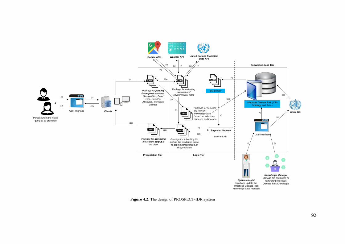
92
Package for collecting
personal and
environmental facts
Netica-J API
Bayesian Network
Package for submitting the
facts to the prediction model
to get the personalized ID
risk prediction
BN-Builder
Clients
User Interface
Epidemiologist
Input and update the
Infectious Disease Risk
Knowledge-base regularly
Knowledge Manager
Manage the conflicting or
redundant Infectious
Disease Risk Knowledge
Package for parsing
the request becomes:
Geo-position, Date/
Time, Personal
Attributes, Infectious
Disease
Package for delivering
the system output to
the client
United Nations Statistical
Data APIWeather APIGoogle APIs
WHO API
Person whom the risk is
going to be predicted
(1)
(2) (3a)
(4)
(5)(6) (6)
(c)
(7) (7)
(d)
(8)
(9)
(10)
(11)
(12)
(13)
(a) (b)
(c)
(e)
(f)
Presentation Tier Logic Tier
Knowledge-base Tier
Infectious Disease Risk (IDR)
Ontology and RulesPackage for selecting
the relevant
knowledge-base
based on: infectious
diseases and location
(3b)(1)
(13)
User Interface
(3c)
Figure 4.2: The design of PROSPECT-IDR system

93
5. DESIGN AND EVALUATION OF THE INFECTIOUS DISEASE
RISK (IDR) KNOWLEDGE-BASE (KB)
The previous chapter provided an overview of the PROSPECT-IDR system and indicated
that the essential parts of it that are the subjects of this thesis are the knowledge-base
that contains representation of infectious disease risk knowledge, and the algorithm that
keeps the encoded knowledge in the knowledge-base consistent with the Bayesian
network. Early design of the knowledge-base (ontology and rule types) was published
(the article is attached in the Appendix 4). This chapter explains the process of designing
the knowledge-base, Infectious Disease Risk (IDR), and presents several evaluations to
assess the usefulness and completeness of the IDR knowledge-base through encoding
knowledge published in several case-control studies.
5.1 Introduction
This chapter presents the design and evaluation of a knowledge representation for
encoding declarative infection risk knowledge. Section 5.2 presents the influences from
previous chapters (chapters 2, 3, and 4), on the knowledge contents to be encoded, the
frequency with which different kinds of encoding activities will occur, and how to encode
that contents. The following section, section 5.3 and 5.4, explains the design of the
knowledge representation that is fit to encode the contents. Thereafter the usefulness and
completeness of the designed representation are evaluated in section 5.5. Conclusions are
drawn in section 5.6.
5.2 Influences from the State of the Art
Chapter 3 reviewed the domain knowledge that is relevant for the IDR knowledge-base
of the PROSPECT-IDR system. This section categorizes them into what knowledge to
represent, how to represent the knowledge and yield the personalized risk prediction from
the represented knowledge.
94
5.2.1 What knowledge to represent
Based on the Bayes chain rule written specially for predicting (infectious) disease risk
(eq. 6), two types of knowledge need to be encoded in a form of representation,
- Infectious disease risk factors
The infectious disease risk factors include personal and environmental risk
factors. The personal risk factors cover demography (e.g. age, gender, occupation,
ethnicity, etc.), genetic, nutrition intake, habits (e.g. tobacco smoking, alcohol
consumption, pets), and pre-existing illness (e.g. diabetes, cancer, HIV). These
personal risk factors deduce the susceptibility of a person and getting exposed to
a pathogen through specific transmission.
The environmental risk factors include climate and location factors deduced from
a person's current geolocation and access date/time. The climate risk factors
incorporate the atmospheric attributes (e.g. temperature, humidity, precipitation),
weather condition (e.g. windy, hot), and season (e.g. winter, spring). The location
risk factors comprise of geographical attributes (e.g. altitude), land-use (e.g.
farming), or features (e.g. cave, forest).
- Infectious disease risk quantifications
Risk ratios (OR and RR) are used to describe the magnitude of a risk factor using
a numerical ratio from 0 to ~. For example, females risk of tuberculosis is twice
than males. The odds ratio for gender (male) in this knowledge is 2 compared with
gender (female). The baseline (basis of comparison) in this statement is female
and the odds ratios of the baseline is always one 12.
Morbidity frequency (prevalence and incidence) is used to quantify how common
the disease is in a region in a time period (yearly). For example, the prevalence of
tuberculosis in Indonesia in 2015 is 354 per 100,000 population.
The knowledge above need to be inputted by epidemiologists through the user interfaces
in the knowledge-base tier at knowledge-encoding time of the PROSPECT-IDR system
(see Figure 4.2). An example of risk factors and their risk ratios is presented in Figure
5.1. The illustration gives tuberculosis (TB) risk factors (smoking, gender, and HIV)
example. For each risk factor, there are several attributes that are depicted by patterned
12 Refer to the case-control studies learned using logistic regression.
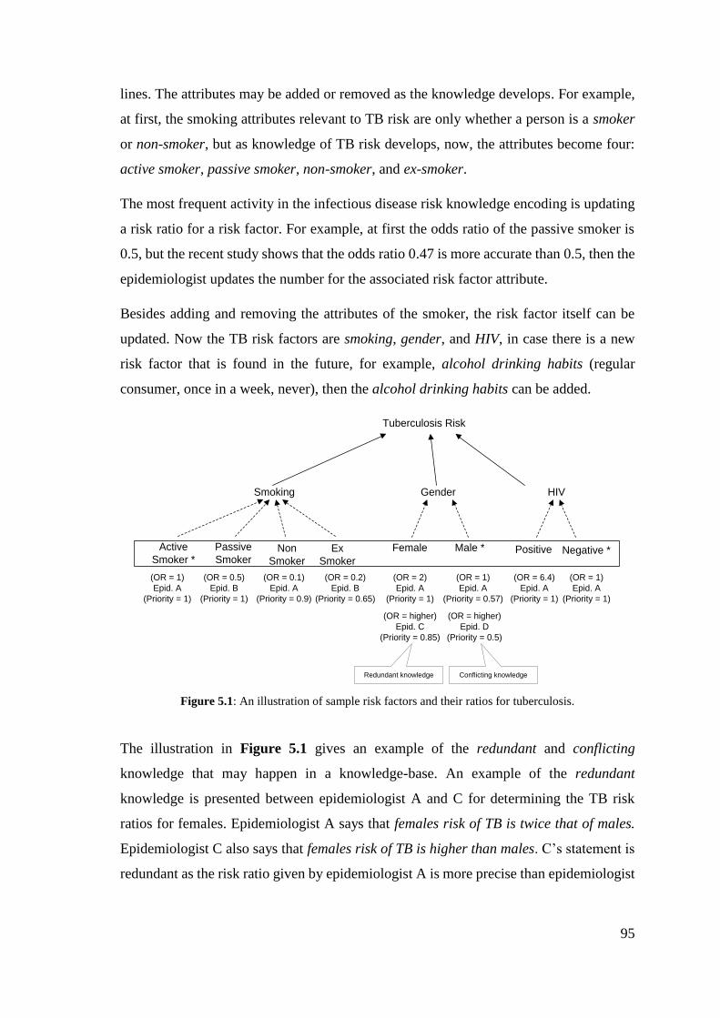
95
lines. The attributes may be added or removed as the knowledge develops. For example,
at first, the smoking attributes relevant to TB risk are only whether a person is a smoker
or non-smoker, but as knowledge of TB risk develops, now, the attributes become four:
active smoker, passive smoker, non-smoker, and ex-smoker.
The most frequent activity in the infectious disease risk knowledge encoding is updating
a risk ratio for a risk factor. For example, at first the odds ratio of the passive smoker is
0.5, but the recent study shows that the odds ratio 0.47 is more accurate than 0.5, then the
epidemiologist updates the number for the associated risk factor attribute.
Besides adding and removing the attributes of the smoker, the risk factor itself can be
updated. Now the TB risk factors are smoking, gender, and HIV, in case there is a new
risk factor that is found in the future, for example, alcohol drinking habits (regular
consumer, once in a week, never), then the alcohol drinking habits can be added.
Tuberculosis Risk
Smoking Gender
Active
Smoker *
Passive
SmokerNon
Smoker
Ex
Smoker
Female Male *
HIV
Positive Negative *
(OR = 1)
Epid. A
(Priority = 1)
(OR = 0.5)
Epid. B
(Priority = 1)
(OR = 0.1)
Epid. A
(Priority = 0.9)
(OR = 0.2)
Epid. B
(Priority = 0.65)
(OR = 2)
Epid. A
(Priority = 1)
(OR = 1)
Epid. A
(Priority = 0.57)
(OR = higher)
Epid. D
(Priority = 0.5)
(OR = higher)
Epid. C
(Priority = 0.85)
(OR = 1)
Epid. A
(Priority = 1)
(OR = 6.4)
Epid. A
(Priority = 1)
Conflicting knowledgeRedundant knowledge
Figure 5.1: An illustration of sample risk factors and their ratios for tuberculosis.
The illustration in Figure 5.1 gives an example of the redundant and conflicting
knowledge that may happen in a knowledge-base. An example of the redundant
knowledge is presented between epidemiologist A and C for determining the TB risk
ratios for females. Epidemiologist A says that females risk of TB is twice that of males.
Epidemiologist C also says that females risk of TB is higher than males. C’s statement is
redundant as the risk ratio given by epidemiologist A is more precise than epidemiologist
96
C. An example of conflicting knowledge is presented between epidemiologist A and D
for determining the TB risk ratios for male. Epidemiologist A says that females risk of TB
is twice that of males. Epidemiologist D says that males supposed to have higher risk than
females. D’s statement is conflicting, in the presence of A’s.
From this section, we conclude that the contents that need to be encoded in the knowledge
representation are the categorical risk factors, numerical risk ratios, and numerical
prevalence value. The encoding activities that the knowledge representation should
support, ordered from least to most frequent, are: modifying the risk factors, modifying
the risk factor attributes, and modifying the risk ratio for the associated attribute.
5.2.2 How to represent the knowledge and yield personalized prediction from it
From section 3.2, ontologies are the commonly used knowledge representation for
(infectious) disease risk knowledge. Further, ontologies can represent the risk factor
knowledge. To bind the risk factors with their quantifications, rules that compatible with
ontology environment are needed (i.e. semantic-web rules). Semantic-web rules are
needed to express (infectious) disease risk quantifications (risk ratios and prevalence) in
a causal relationship.
However, from section 3.2.4, it is apparent that semantic-web rules are unable to express
negation and OR logical operator. An example of encoding infectious disease risk
knowledge that contains negation operator is given, for the following rule: anthrax virus
is dormant during winter, therefore there is no anthrax risk found in winter.
To encode this kind of knowledge using semantic-web rules, instead of using the
following rule, in which “-“ denotes “NOT”:
EnvironmentRiskFactor(?all) ^ hasSeason(?all, -Winter) ->
setPathogen(Anthrax, active)
The following set of rules is needed,
EnvironmentRiskFactor(?all) ^ hasSeason(?all, Spring) ->
setPathogen(Anthrax, active)
97
EnvironmentRiskFactor(?all) ^ hasSeason(?all, Summer) ->
setPathogen(Anthrax, active)
EnvironmentRiskFactor(?all) ^ hasSeason(?all, Autumn) ->
setPathogen(Anthrax, active)
As there is no OR operator, the three non-winter seasons have to be represented as
separated rules. As can be seen form this example, the semantic-web rule-base will
contain more rules than it would if the SWRL allowed negation and OR logical operator.
Ontologies for representing disease risk factors include CARRE (ontology for cardiorenal
disease), ORC (ontology for diabetes), and OBESTTD (ontology for obesity) ontologies.
Some vocabulary from these ontologies can be used for representing infectious disease
risk factors for PROSPECT-IDR system.
Bayesian Networks are a prediction model that can work with ontology structures. This
is proven by PR-OWL, Bayesian Knowledge-base, BNTab, and BayesOWL reviewed in
section 3.3. Since the characteristics of personal or environmental infectious disease risk
factors are not only binary, then, since BNTab allows ontology classes and individuals to
encode nominal, ordinal, and binary, it is more suitable than BayesOWL for encoding
infectious disease risk knowledge.
A Probabilistic Knowledge-base allows to encode risk quantifications using rules whose
structure is the same as semantic-web rules. Fuzzy Cognitive Maps allow the uncertainty
degree encoding in using the belief rule-based; this method can be used to resolve
conflicts between rules such as the redundant and duplicate rules illustrated in Figure 5.1.
To sum up, the way the ontology encodes the risk factors (including their attributes) and
the semantic-web rules to encode the risk ratios (including prevalence value) are partially
taken from the existing approaches.
5.3 Ontology Construction
To facilitate the declarative infectious disease risk knowledge encoding, all required
knowledge is gathered. From previous section there are three levels based on the update
frequency.
98
In Figure 5.1, the tuberculosis risk factors are smoking, age, and HIV. These risk factors
can be obtained from the collation table which was constructed to help reviewing
infectious disease risk factors in section 3.1.1. The contents of the collation table are list
of all human infectious diseases and their risk factors mentioned in AHID, CDC, and
WHO, classified into person, climate, and location related. However, since there are some
differences and overlap in the infectious diseases explained in those three sources, AHID
is prioritized as the knowledge source. 107 infectious diseases are described in the AHID.
Then, 57 infectious diseases which are not covered by the AHID but mentioned in CDC
are added. Lastly, 70 infectious diseases that are notified by WHO but not explained in
both AHID and CDC are added. In total, there are 234 distinct infectious diseases as
accumulation from those three knowledge sources. The risk factors for each infectious
disease are obtained from the associated knowledge sources.
Besides risk factors, there are attributes of risk factors, such as active smoker, non-smoker,
passive smoker, and ex-smoker are attributes of smoking risk factor. Default attributes can
generally be found in the AHID, CDC, and WHO. For example, the attributes of gender
are male and female, and these apply to all infectious diseases for which gender is a risk
factor. However, some of them cannot be found in those sources. The detailed attributes,
along with the information of which attributes are treated as baseline, can be obtained
from case-control studies. This means that detailed risk factors depend on the population
characteristics of a location.
Besides the detailed risk factors’ attributes, the risk ratios for each attribute can be
retrieved from case-control studies. Sometimes, the magnitude of an attribute explained
in the associated study is not presented as numerical ratio but given either as an addition
or reduction in percentage or in ordinal value (high, medium, low) as a declarative form.
The ordinal quantifications usually appear to present the environment conditions that
trigger the activity of the pathogen or vector of a specific infection. For example, malaria
cases are high in the rainy season since the Anopheles mosquitos thrive and multiple
during hot days with high precipitation [225]. The prevalence values sometimes are
revealed in the case-control studies, and sometimes not. If it is not given through the
article text, then it can be calculated by using eq.4 (section 3.1.2) using the number of
cases (obtained from WHO) and total population for the associated country (obtained
from UNSD).
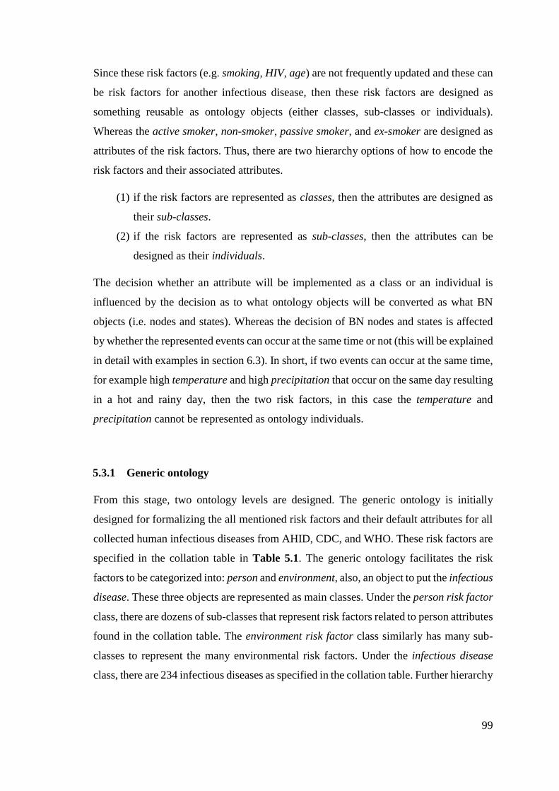
99
Since these risk factors (e.g. smoking, HIV, age) are not frequently updated and these can
be risk factors for another infectious disease, then these risk factors are designed as
something reusable as ontology objects (either classes, sub-classes or individuals).
Whereas the active smoker, non-smoker, passive smoker, and ex-smoker are designed as
attributes of the risk factors. Thus, there are two hierarchy options of how to encode the
risk factors and their associated attributes.
(1) if the risk factors are represented as classes, then the attributes are designed as
their sub-classes.
(2) if the risk factors are represented as sub-classes, then the attributes can be
designed as their individuals.
The decision whether an attribute will be implemented as a class or an individual is
influenced by the decision as to what ontology objects will be converted as what BN
objects (i.e. nodes and states). Whereas the decision of BN nodes and states is affected
by whether the represented events can occur at the same time or not (this will be explained
in detail with examples in section 6.3). In short, if two events can occur at the same time,
for example high temperature and high precipitation that occur on the same day resulting
in a hot and rainy day, then the two risk factors, in this case the temperature and
precipitation cannot be represented as ontology individuals.
5.3.1 Generic ontology
From this stage, two ontology levels are designed. The generic ontology is initially
designed for formalizing the all mentioned risk factors and their default attributes for all
collected human infectious diseases from AHID, CDC, and WHO. These risk factors are
specified in the collation table in Table 5.1. The generic ontology facilitates the risk
factors to be categorized into: person and environment, also, an object to put the infectious
disease. These three objects are represented as main classes. Under the person risk factor
class, there are dozens of sub-classes that represent risk factors related to person attributes
found in the collation table. The environment risk factor class similarly has many sub-
classes to represent the many environmental risk factors. Under the infectious disease
class, there are 234 infectious diseases as specified in the collation table. Further hierarchy
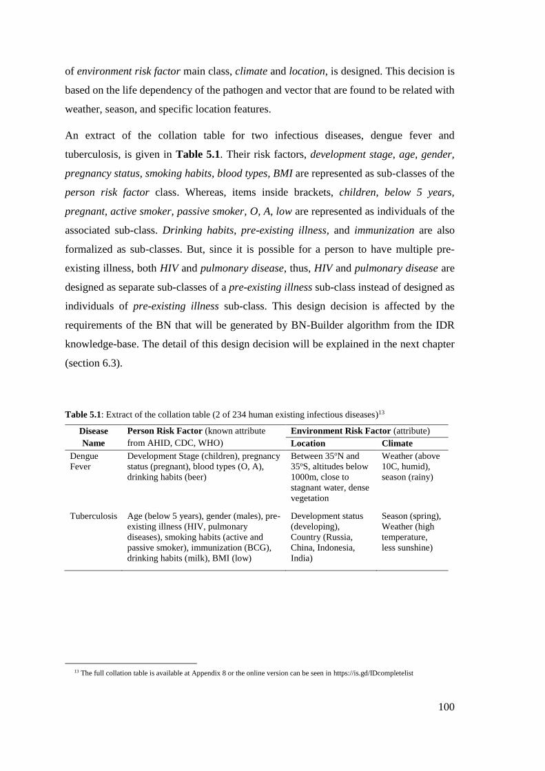
100
of environment risk factor main class, climate and location, is designed. This decision is
based on the life dependency of the pathogen and vector that are found to be related with
weather, season, and specific location features.
An extract of the collation table for two infectious diseases, dengue fever and
tuberculosis, is given in Table 5.1. Their risk factors, development stage, age, gender,
pregnancy status, smoking habits, blood types, BMI are represented as sub-classes of the
person risk factor class. Whereas, items inside brackets, children, below 5 years,
pregnant, active smoker, passive smoker, O, A, low are represented as individuals of the
associated sub-class. Drinking habits, pre-existing illness, and immunization are also
formalized as sub-classes. But, since it is possible for a person to have multiple pre-
existing illness, both HIV and pulmonary disease, thus, HIV and pulmonary disease are
designed as separate sub-classes of a pre-existing illness sub-class instead of designed as
individuals of pre-existing illness sub-class. This design decision is affected by the
requirements of the BN that will be generated by BN-Builder algorithm from the IDR
knowledge-base. The detail of this design decision will be explained in the next chapter
(section 6.3).
Table 5.1: Extract of the collation table (2 of 234 human existing infectious diseases)13
Disease
Name
Person Risk Factor (known attribute
from AHID, CDC, WHO)
Environment Risk Factor (attribute)
Location Climate
Dengue
Fever
Development Stage (children), pregnancy
status (pregnant), blood types (O, A),
drinking habits (beer)
Between 35oN and
35oS, altitudes below
1000m, close to
stagnant water, dense
vegetation
Weather (above
10C, humid),
season (rainy)
Tuberculosis Age (below 5 years), gender (males), pre-
existing illness (HIV, pulmonary
diseases), smoking habits (active and
passive smoker), immunization (BCG),
drinking habits (milk), BMI (low)
Development status
(developing),
Country (Russia,
China, Indonesia,
India)
Season (spring),
Weather (high
temperature,
less sunshine)
13 The full collation table is available at Appendix 8 or the online version can be seen in https://is.gd/IDcompletelist
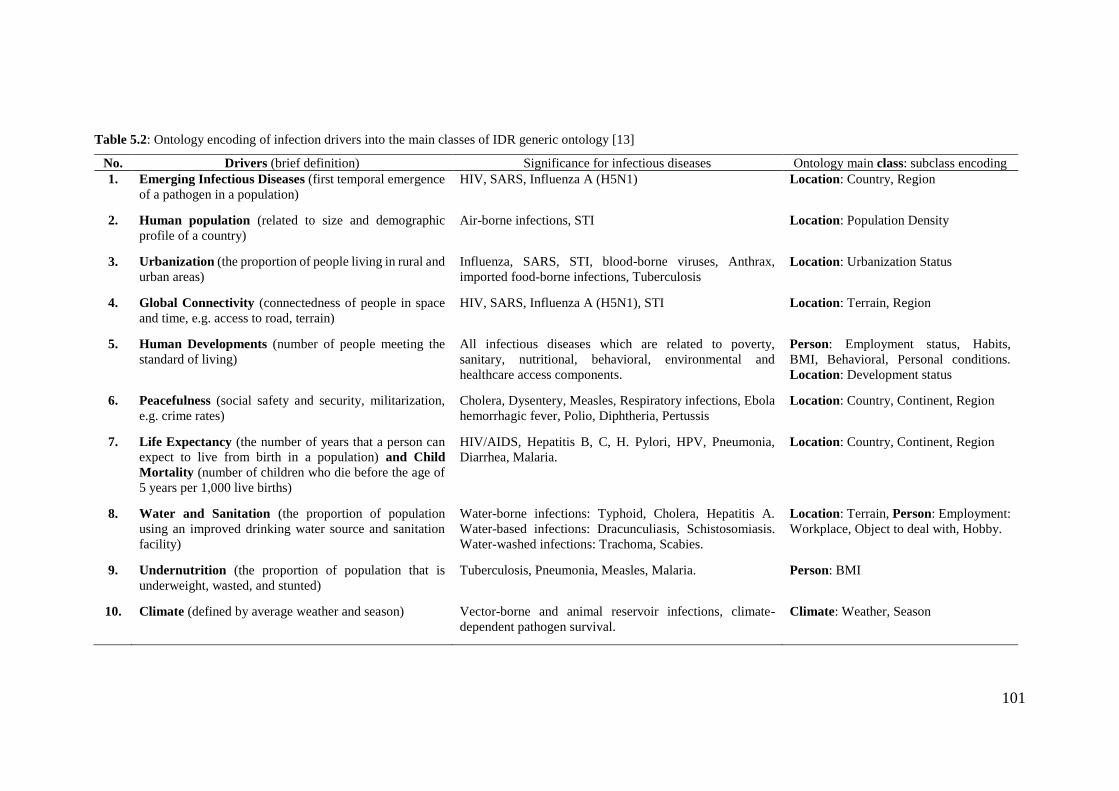
101
Table 5.2: Ontology encoding of infection drivers into the main classes of IDR generic ontology [13]
No. Drivers (brief definition) Significance for infectious diseases Ontology main class: subclass encoding
1. Emerging Infectious Diseases (first temporal emergence
of a pathogen in a population)
HIV, SARS, Influenza A (H5N1) Location: Country, Region
2. Human population (related to size and demographic
profile of a country)
Air-borne infections, STI Location: Population Density
3. Urbanization (the proportion of people living in rural and
urban areas)
Influenza, SARS, STI, blood-borne viruses, Anthrax,
imported food-borne infections, Tuberculosis
Location: Urbanization Status
4. Global Connectivity (connectedness of people in space
and time, e.g. access to road, terrain)
HIV, SARS, Influenza A (H5N1), STI Location: Terrain, Region
5. Human Developments (number of people meeting the
standard of living)
All infectious diseases which are related to poverty,
sanitary, nutritional, behavioral, environmental and
healthcare access components.
Person: Employment status, Habits,
BMI, Behavioral, Personal conditions.
Location: Development status
6. Peacefulness (social safety and security, militarization,
e.g. crime rates)
Cholera, Dysentery, Measles, Respiratory infections, Ebola
hemorrhagic fever, Polio, Diphtheria, Pertussis
Location: Country, Continent, Region
7. Life Expectancy (the number of years that a person can
expect to live from birth in a population) and Child
Mortality (number of children who die before the age of
5 years per 1,000 live births)
HIV/AIDS, Hepatitis B, C, H. Pylori, HPV, Pneumonia,
Diarrhea, Malaria.
Location: Country, Continent, Region
8. Water and Sanitation (the proportion of population
using an improved drinking water source and sanitation
facility)
Water-borne infections: Typhoid, Cholera, Hepatitis A.
Water-based infections: Dracunculiasis, Schistosomiasis.
Water-washed infections: Trachoma, Scabies.
Location: Terrain, Person: Employment:
Workplace, Object to deal with, Hobby.
9. Undernutrition (the proportion of population that is
underweight, wasted, and stunted)
Tuberculosis, Pneumonia, Measles, Malaria. Person: BMI
10. Climate (defined by average weather and season) Vector-borne and animal reservoir infections, climate-
dependent pathogen survival.
Climate: Weather, Season
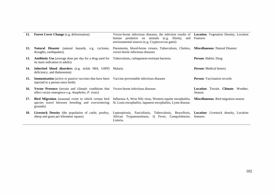
102
11. Forest Cover Change (e.g. deforestation) Vector-borne infectious diseases, the infection results of
human predation on animals (e.g. Ebola), and
environmental sources (e.g. Cryptococcus gattii)
Location: Vegetation Density, Location
Features
12. Natural Disaster (natural hazards, e.g. cyclones,
droughts, earthquakes)
Pneumonia, blood-borne viruses, Tuberculosis, Cholera,
vector-borne infectious diseases
Miscellaneous: Natural Disaster
13. Antibiotic Use (average dose per day for a drug used for
its main indication in adults)
Tuberculosis, carbapenem-resistant bacteria. Person: Habits: Drug
14. Inherited blood disorders (e.g. sickle HbS, G6PD
deficiency, and thalassemia)
Malaria Person: Medical history
15. Immunization (active or passive vaccines that have been
injected to a person since birth)
Vaccine-preventable infectious diseases Person: Vaccination records
16. Vector Presence (terrain and climatic conditions that
affect vector emergence e.g. Anopheles, P. vivax)
Vector-borne infectious diseases Location: Terrain. Climate: Weather,
Season.
17. Bird Migration (seasonal event in which certain bird
species travel between breeding and overwintering
grounds)
Influenza A, West Nile virus, Western equine encephalitis,
St. Louis encephalitis, Japanese encephalitis, Lyme disease.
Miscellaneous: Bird migration season
18. Livestock Density (the population of cattle, poultry,
sheep and goats per kilometer square)
Leptospirosis, Fascioliasis, Tuberculosis, Brucellosis,
African Trypanosomiasis, Q Fever, Campylobacter,
Listeria.
Location: Livestock density, Location
features.
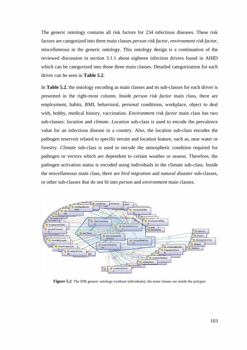
103
The generic ontology contains all risk factors for 234 infectious diseases. These risk
factors are categorized into three main classes person risk factor, environment risk factor,
miscellaneous in the generic ontology. This ontology design is a continuation of the
reviewed discussion in section 3.1.1 about eighteen infection drivers found in AHID
which can be categorized into those three main classes. Detailed categorization for each
driver can be seen in Table 5.2.
In Table 5.2, the ontology encoding as main classes and its sub-classes for each driver is
presented in the right-most column. Inside person risk factor main class, there are
employment, habits, BMI, behavioral, personal conditions, workplace, object to deal
with, hobby, medical history, vaccination. Environment risk factor main class has two
sub-classes: location and climate. Location sub-class is used to encode the prevalence
value for an infectious disease in a country. Also, the location sub-class encodes the
pathogen reservoir related to specific terrain and location feature, such as, near water or
forestry. Climate sub-class is used to encode the atmospheric condition required for
pathogen or vectors which are dependent to certain weather or season. Therefore, the
pathogen activation status is encoded using individuals in the climate sub-class. Inside
the miscellaneous main class, there are bird migration and natural disaster sub-classes,
or other sub-classes that do not fit into person and environment main classes.
Figure 5.2: The IDR generic ontology (without individuals); the main classes are inside the polygon
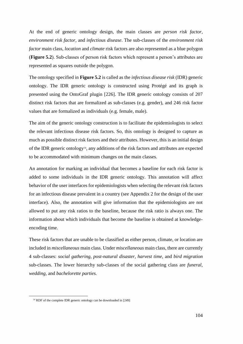
104
At the end of generic ontology design, the main classes are person risk factor,
environment risk factor, and infectious disease. The sub-classes of the environment risk
factor main class, location and climate risk factors are also represented as a blue polygon
(Figure 5.2). Sub-classes of person risk factors which represent a person’s attributes are
represented as squares outside the polygon.
The ontology specified in Figure 5.2 is called as the infectious disease risk (IDR) generic
ontology. The IDR generic ontology is constructed using Protégé and its graph is
presented using the OntoGraf plugin [226]. The IDR generic ontology consists of 207
distinct risk factors that are formalized as sub-classes (e.g. gender), and 246 risk factor
values that are formalized as individuals (e.g. female, male).
The aim of the generic ontology construction is to facilitate the epidemiologists to select
the relevant infectious disease risk factors. So, this ontology is designed to capture as
much as possible distinct risk factors and their attributes. However, this is an initial design
of the IDR generic ontology14, any additions of the risk factors and attributes are expected
to be accommodated with minimum changes on the main classes.
An annotation for marking an individual that becomes a baseline for each risk factor is
added to some individuals in the IDR generic ontology. This annotation will affect
behavior of the user interfaces for epidemiologists when selecting the relevant risk factors
for an infectious disease prevalent in a country (see Appendix 2 for the design of the user
interface). Also, the annotation will give information that the epidemiologists are not
allowed to put any risk ratios to the baseline, because the risk ratio is always one. The
information about which individuals that become the baseline is obtained at knowledge-
encoding time.
These risk factors that are unable to be classified as either person, climate, or location are
included in miscellaneous main class. Under miscellaneous main class, there are currently
4 sub-classes: social gathering, post-natural disaster, harvest time, and bird migration
sub-classes. The lower hierarchy sub-classes of the social gathering class are funeral,
wedding, and bachelorette parties.
14 RDF of the complete IDR generic ontology can be downloaded in [249]
105
Besides the classes and instances (i.e. ontology individuals), there are object properties
that connect between individuals. For example, consider “a person who has age below 5
years old is at triple risk of tuberculosis than above 5 years”. The object properties are
denoted by underlining (e.g. has age, at risk). In this example, has age is an object property
whose domain class is person risk factor and whose range class is age (below 5, above 5
years). The at triple risk is a data range of the property of the object whose range class is
infectious disease (tuberculosis) and the data range is [double].
In addition to that, the ontology formalizes different object properties that are possible
between the same individuals that appear in the AHID, CDC, and WHO. For example,
there are two possible relations between person (as domain class) and education (as range
class). The first relation is person who has education is in primary level, and the second
relation is person who has parent’s education is in primary level. Thus, two possible
object properties are included in the IDR generic ontology.
5.3.2 Disease-specific ontology
After the IDR generic ontology is constructed, the epidemiologists encode their
knowledge by (1) creating an instantiation of the generic ontology for an infectious
disease prevalent in a country (i.e. disease-specific ontology), (2) encoding the risk
quantifications using semantic-web rules, at knowledge-encoding time of the
PROSPECT-IDR system.
The disease-specific ontology is constructed by reusing some of generic ontology objects
(classes, individuals, properties) that are relevant for an infectious disease. The disease-
specific ontology is the part of the knowledge-base that is going to generate the prediction
model at the end of knowledge-encoding time (stage e and f in Figure 4.1). Thus, the
epidemiologist decision whether he/she is going to reuse an ontology object or not is
based on the availability of their quantifications in the published case-control studies or
the quantifications given by herself/himself.
106
Figure 5.3: The disease-specific ontology for cholera risk in India
Since the IDR generic ontology’s risk factors and their attributes were taken from AHID,
CDC, and WHO, while the case-control studies are mostly specific to one (infectious)
disease prevalent at a population in a location for a particular period, so, there are some
chances that during instantiation time, epidemiologists may need to encode risk factors
that are not found in the IDR generic ontology. In this case, there are two options for
adding these risk factors: (1) the needed risk factors can be added to the disease-specific
ontology which is being created at the instantiation time; this is performed by the
epidemiologists, (2) the risk factors that are constantly needed to build several disease-
specific ontologies can be added to the initial version of the IDR generic ontology; this is
performed by the knowledge manager. So, the individuals and sub-classes of the IDR
generic ontology will continue to evolve as the knowledge in case-control studies
develops.
Therefore, at the end of this chapter (section 5.5), an evaluation for assessing how many
risk factors (sub-classes), and risk factors’ attributes (individuals) found in the IDR
generic ontology will be carried out (a measure of usefulness of the generic ontology).
Also, the sub-classes and individuals that reused from the IDR generic ontology during
the instantiation process are compared with the total ontology objects per disease-specific
ontology (measuring the completeness of the generic ontology).
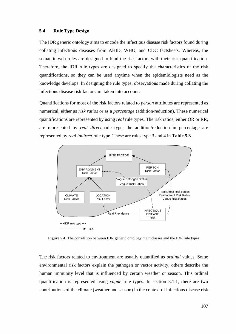
107
5.4 Rule Type Design
The IDR generic ontology aims to encode the infectious disease risk factors found during
collating infectious diseases from AHID, WHO, and CDC factsheets. Whereas, the
semantic-web rules are designed to bind the risk factors with their risk quantification.
Therefore, the IDR rule types are designed to specify the characteristics of the risk
quantifications, so they can be used anytime when the epidemiologists need as the
knowledge develops. In designing the rule types, observations made during collating the
infectious disease risk factors are taken into account.
Quantifications for most of the risk factors related to person attributes are represented as
numerical, either as risk ratios or as a percentage (addition/reduction). These numerical
quantifications are represented by using real rule types. The risk ratios, either OR or RR,
are represented by real direct rule type; the addition/reduction in percentage are
represented by real indirect rule type. These are rules type 3 and 4 in Table 5.3.
PERSON
Risk Factor
INFECTIOUS
DISEASE
Risk
ENVIRONMENT
Risk Factor
CLIMATE
Risk Factor
LOCATION
Risk Factor
RISK FACTOR
Real Direct Risk Ratios
Real Indirect Risk Ratios
Vague Risk Ratios
Real Prevalence
Vague Pathogen Status
Vague Risk Ratios
IDR rule type
is-a
Figure 5.4: The correlation between IDR generic ontology main classes and the IDR rule types
The risk factors related to environment are usually quantified as ordinal values. Some
environmental risk factors explain the pathogen or vector activity, others describe the
human immunity level that is influenced by certain weather or season. This ordinal
quantification is represented using vague rule types. In section 3.1.1, there are two
contributions of the climate (weather and season) in the context of infectious disease risk
108
knowledge: describe pathogen activation status, and human immunity level that depends
on the climate.
Quantifications that represent climate attributes to describe pathogen activity are
represented using vague pathogen status rule type. Whereas the quantifications that
explain human immunity level or other than pathogen information are represented using
vague risk ratio rule type. These are rule types 2 and 5 in Table 5.3.
In order to fulfil the Bayes chain rule to populate the conditional probability table of a
BN, the knowledge-base should contain at least one risk ratio (either person or
environment risk factor) and one prevalence value (for the contextual country). The main
classes together with the associated rule types are illustrated in Figure 5.4.
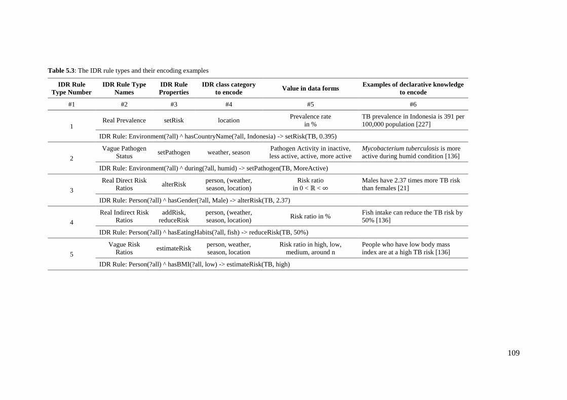
109
Table 5.3: The IDR rule types and their encoding examples
IDR Rule
Type Number
IDR Rule Type
Names
IDR Rule
Properties
IDR class category
to encode Value in data forms
Examples of declarative knowledge
to encode
#1 #2 #3 #4 #5 #6
1 Real Prevalence setRisk location
Prevalence rate
in %
TB prevalence in Indonesia is 391 per
100,000 population [227]
IDR Rule: Environment(?all) ^ hasCountryName(?all, Indonesia) -> setRisk(TB, 0.395)
2
Vague Pathogen
Status setPathogen weather, season
Pathogen Activity in inactive,
less active, active, more active
Mycobacterium tuberculosis is more
active during humid condition [136]
IDR Rule: Environment(?all) ^ during(?all, humid) -> setPathogen(TB, MoreActive)
3
Real Direct Risk
Ratios alterRisk
person, (weather,
season, location)
Risk ratio
in 0 < ℝ < ∞
Males have 2.37 times more TB risk
than females [21]
IDR Rule: Person(?all) ^ hasGender(?all, Male) -> alterRisk(TB, 2.37)
4
Real Indirect Risk
Ratios
addRisk,
reduceRisk
person, (weather,
season, location) Risk ratio in %
Fish intake can reduce the TB risk by
50% [136]
IDR Rule: Person(?all) ^ hasEatingHabits(?all, fish) -> reduceRisk(TB, 50%)
5
Vague Risk
Ratios estimateRisk
person, weather,
season, location
Risk ratio in high, low,
medium, around n
People who have low body mass
index are at a high TB risk [136]
IDR Rule: Person(?all) ^ hasBMI(?all, low) -> estimateRisk(TB, high)
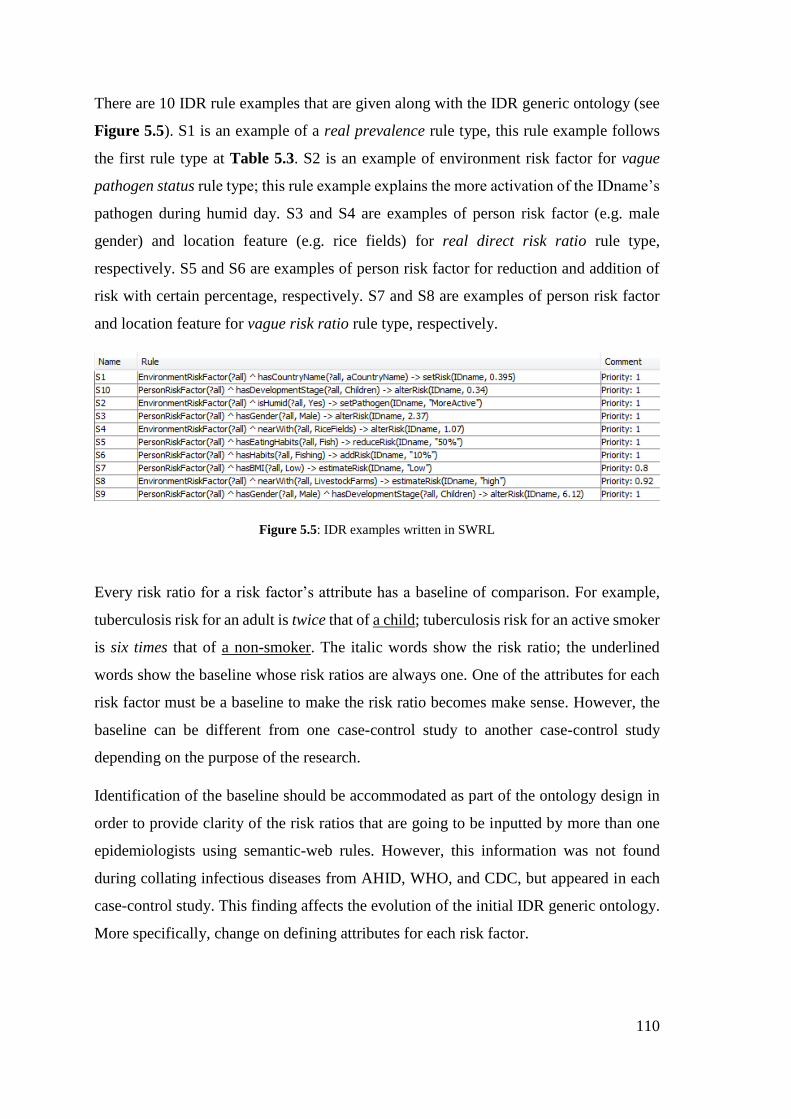
110
There are 10 IDR rule examples that are given along with the IDR generic ontology (see
Figure 5.5). S1 is an example of a real prevalence rule type, this rule example follows
the first rule type at Table 5.3. S2 is an example of environment risk factor for vague
pathogen status rule type; this rule example explains the more activation of the IDname’s
pathogen during humid day. S3 and S4 are examples of person risk factor (e.g. male
gender) and location feature (e.g. rice fields) for real direct risk ratio rule type,
respectively. S5 and S6 are examples of person risk factor for reduction and addition of
risk with certain percentage, respectively. S7 and S8 are examples of person risk factor
and location feature for vague risk ratio rule type, respectively.
Figure 5.5: IDR examples written in SWRL
Every risk ratio for a risk factor’s attribute has a baseline of comparison. For example,
tuberculosis risk for an adult is twice that of a child; tuberculosis risk for an active smoker
is six times that of a non-smoker. The italic words show the risk ratio; the underlined
words show the baseline whose risk ratios are always one. One of the attributes for each
risk factor must be a baseline to make the risk ratio becomes make sense. However, the
baseline can be different from one case-control study to another case-control study
depending on the purpose of the research.
Identification of the baseline should be accommodated as part of the ontology design in
order to provide clarity of the risk ratios that are going to be inputted by more than one
epidemiologists using semantic-web rules. However, this information was not found
during collating infectious diseases from AHID, WHO, and CDC, but appeared in each
case-control study. This finding affects the evolution of the initial IDR generic ontology.
More specifically, change on defining attributes for each risk factor.
111
Most of the risk quantification studies assume risk factors are independent. Independence
of risk factor means for example, that the risk probability for male children of contracting
of an infectious disease is the product of risk ratio for male and risk ratio for children.
However, 3 articles discover dependent risk factors [8], [21], [49], meaning that the risk
probability for male children of contracting of an infectious disease may not be equal to
the products of risk ratio for male and risk ratio for children. The instantiation examples
for the dependent rules is shown by S9 in Figure 5.5. The risk ratio in the dependent rule
S9 (for male children) shows that the value is different with the product results of the
independent rules: S3 (for male) and S10 (for children). The impact of the inclusion of
dependent risk factors to different parts of this research is to the algorithm that is going
to populate the CPT from rules that have more than one object properties. See section
6.3.4 for the design of the CPT population procedure.
To resolve the conflicts between rules, a numerical value is assigned for each rule to
indicate the priority of the containing infectious disease risk knowledge. The numeric
value (i.e. priority) is encoded in the comment column (see Figure 5.5); the range of a
priority is designed to have a value between 0 and 1. The priorities are inputted by the
epidemiologists for specifying their confidence level of their inputted knowledge via user
interfaces (see Appendix 2). By default, the real rule types have higher priorities than
vague rule types since the real rule types can be directly processed to Bayes chain rule
without using random distribution. The impact of the inclusion of the priority is to the
algorithm populates the CPT from rules that have the highest priority level. See section
6.3.4 for the design of the CPT population procedure related to the priority. However, it
is possible to have the same priority values for more than one duplicating and
contradicting IDR rule. In this case, the knowledge manager will be asked to assign
different priority values for the conflicting rules before firing the algorithm.
112
5.5 Knowledge-base Evaluation
5.5.1 Evaluation Plan
In this chapter, there are two knowledge representations proposed to encode infectious
disease risk knowledge: the IDR generic ontology, and the IDR rule types. Both are used
to instantiate an IDR knowledge-base in the knowledge-building time. To evaluate the
goodness of the IDR generic ontology and the IDR rule types, several infectious diseases
prevalent in several countries that are published in case-control studies will be selected
carefully with some criteria. Thereafter, the selected case-control studies will be encoded
to evaluate how useful and how complete the IDR generic ontology and the IDR rule types
are. Some of the evaluation presented in this section has been submitted to a journal article
which the full manuscript is given in Appendix 7.
The case-control studies are selected based on these criteria: (1) The infectious diseases
cover the known reservoir types, the known transmission modes and cover both personal
and environmental risk factors (e.g. climate and location). This criterion makes sure that
the chosen infectious diseases can represent the whole 234 human infectious diseases. So,
in order to test the usefulness and the completeness of the IDR generic ontology, it doesn’t
have to encode every infectious disease. (2) The infectious diseases are preferred to
prevalent in more than one regions. This criterion makes sure that there could be another
prevalence values to compare with. Also, to show that even though the infectious disease
is same, the risk factors and risk factor’s attributes could be different, thus, a different
knowledge-base is still needed to encode each contextual knowledge (e.g. one infectious
disease – one country).
Using the infectious disease risk encoded in the selected case-control studies based on the
criteria above, the IDR generic ontology and IDR rule types are evaluated by measuring
their completeness and usefulness to instantiate the IDR knowledge-base.
The degree of usefulness of the IDR rule types is investigated by counting how many of
the five rule types are used to bind risk factors with their risk quantifications. Whereas,
the degree of the usefulness IDR generic ontology usefulness is assessed by counting how
many ontology objects (individuals and sub-classes) are used to encode risk factors
compared with the total ontology objects for each IDR disease-specific ontology. This
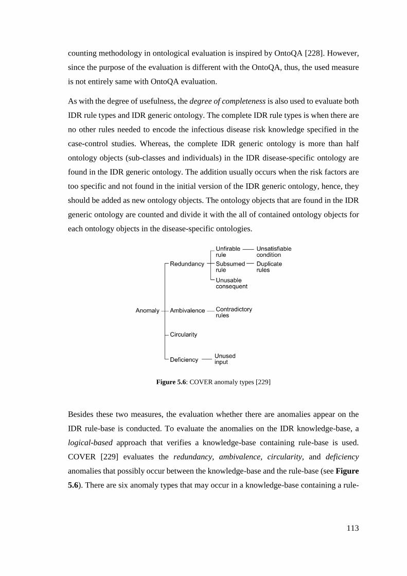
113
counting methodology in ontological evaluation is inspired by OntoQA [228]. However,
since the purpose of the evaluation is different with the OntoQA, thus, the used measure
is not entirely same with OntoQA evaluation.
As with the degree of usefulness, the degree of completeness is also used to evaluate both
IDR rule types and IDR generic ontology. The complete IDR rule types is when there are
no other rules needed to encode the infectious disease risk knowledge specified in the
case-control studies. Whereas, the complete IDR generic ontology is more than half
ontology objects (sub-classes and individuals) in the IDR disease-specific ontology are
found in the IDR generic ontology. The addition usually occurs when the risk factors are
too specific and not found in the initial version of the IDR generic ontology, hence, they
should be added as new ontology objects. The ontology objects that are found in the IDR
generic ontology are counted and divide it with the all of contained ontology objects for
each ontology objects in the disease-specific ontologies.
Figure 5.6: COVER anomaly types [229]
Besides these two measures, the evaluation whether there are anomalies appear on the
IDR rule-base is conducted. To evaluate the anomalies on the IDR knowledge-base, a
logical-based approach that verifies a knowledge-base containing rule-base is used.
COVER [229] evaluates the redundancy, ambivalence, circularity, and deficiency
anomalies that possibly occur between the knowledge-base and the rule-base (see Figure
5.6). There are six anomaly types that may occur in a knowledge-base containing a rule-
114
base: unsatisfiable condition, duplicate rules, unusable consequent, contradictory rules,
circular rules, and unused inputs.
The definition of each anomaly type is given below,
1. Unsatisfiable condition occurs if an IDR rule contains an individual (in its
antecedent) that is not match with an individual in the IDR disease-specific
ontology.
2. Duplicate rules are flagged when there are more than one rules contain the same
risk quantifications (in their consequents) for the same antecedents.
3. Unusable consequent is indicated when an IDR rule contains an individual (in its
consequent) that is not match with an individual in the IDR disease-specific
ontology.
4. Contradictory rules occur when there are more than one IDR rules contain the
different risk quantifications (in their consequents) for the same antecedents.
5. Circular rules are identified when there is a circular chain of rules referring from
consequents to antecedents.
6. Unused inputs happen if the IDR rules contain an individual that is declared in the
IDR disease-specific ontology, but it is unused.
These anomalies are screened at the knowledge-encoding time, after the epidemiologists
selecting the relevant ontology objects from the IDR generic ontology to construct the
IDR disease-specific ontology. Thereafter, the epidemiologists bind the risk factors with
their risk ratios from the case-control studies using semantic-web rules; in this stage, these
anomalies are identified.
5.5.2 IDR Evaluation Cases
From the criteria, several infectious diseases are match with the second criterion
(prevalent in several countries) based on WHO [31] are: cholera, diphtheria, anthrax,
leprosy, meningococcal (meningitis), pertussis, tetanus, tuberculosis, typhoid fever,
measles, mumps, smallpox, yellow fever, malaria. Whereas, dengue fever is chosen
because it is prevalent in Indonesia, as the country where the author lives.
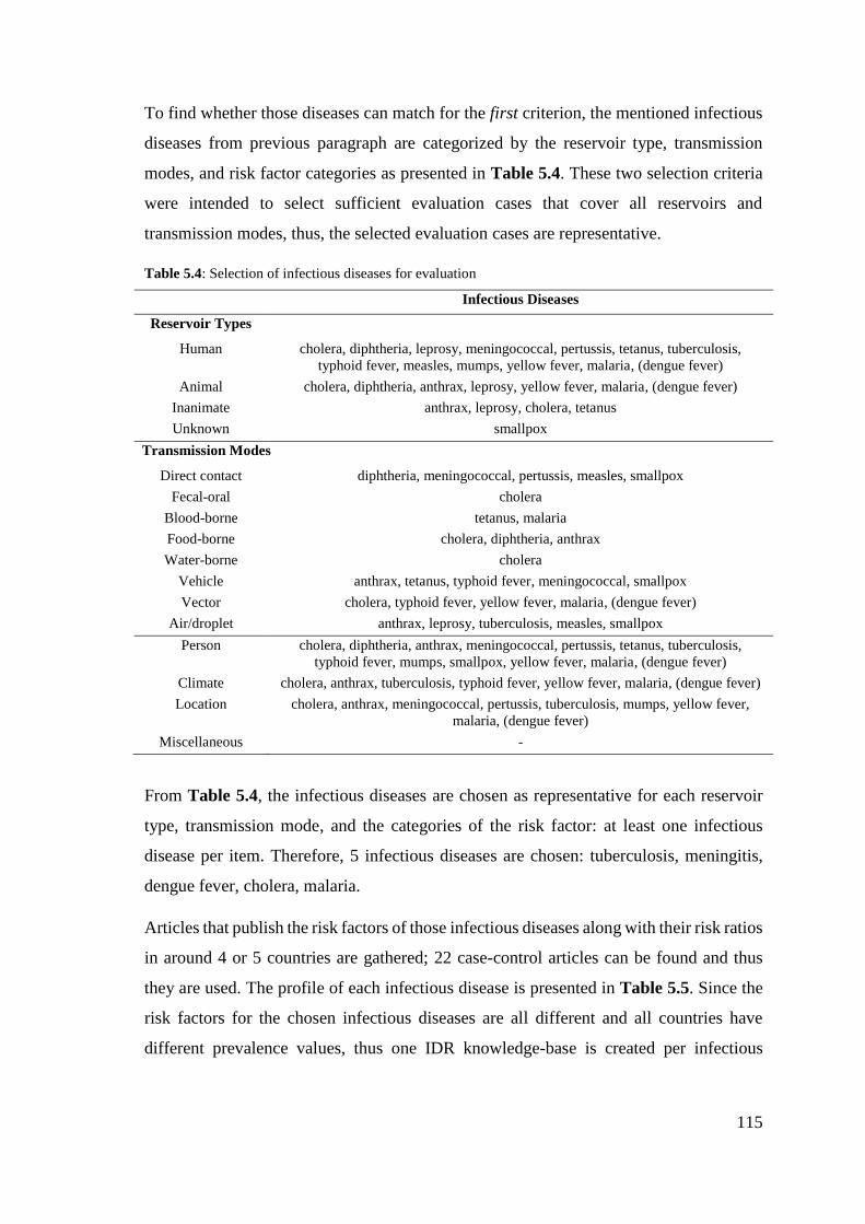
115
To find whether those diseases can match for the first criterion, the mentioned infectious
diseases from previous paragraph are categorized by the reservoir type, transmission
modes, and risk factor categories as presented in Table 5.4. These two selection criteria
were intended to select sufficient evaluation cases that cover all reservoirs and
transmission modes, thus, the selected evaluation cases are representative.
Table 5.4: Selection of infectious diseases for evaluation
Infectious Diseases
Reservoir Types
Human cholera, diphtheria, leprosy, meningococcal, pertussis, tetanus, tuberculosis,
typhoid fever, measles, mumps, yellow fever, malaria, (dengue fever)
Animal cholera, diphtheria, anthrax, leprosy, yellow fever, malaria, (dengue fever)
Inanimate anthrax, leprosy, cholera, tetanus
Unknown smallpox
Transmission Modes
Direct contact diphtheria, meningococcal, pertussis, measles, smallpox
Fecal-oral cholera
Blood-borne tetanus, malaria
Food-borne cholera, diphtheria, anthrax
Water-borne cholera
Vehicle anthrax, tetanus, typhoid fever, meningococcal, smallpox
Vector cholera, typhoid fever, yellow fever, malaria, (dengue fever)
Air/droplet anthrax, leprosy, tuberculosis, measles, smallpox
Person cholera, diphtheria, anthrax, meningococcal, pertussis, tetanus, tuberculosis,
typhoid fever, mumps, smallpox, yellow fever, malaria, (dengue fever)
Climate cholera, anthrax, tuberculosis, typhoid fever, yellow fever, malaria, (dengue fever)
Location cholera, anthrax, meningococcal, pertussis, tuberculosis, mumps, yellow fever,
malaria, (dengue fever)
Miscellaneous -
From Table 5.4, the infectious diseases are chosen as representative for each reservoir
type, transmission mode, and the categories of the risk factor: at least one infectious
disease per item. Therefore, 5 infectious diseases are chosen: tuberculosis, meningitis,
dengue fever, cholera, malaria.
Articles that publish the risk factors of those infectious diseases along with their risk ratios
in around 4 or 5 countries are gathered; 22 case-control articles can be found and thus
they are used. The profile of each infectious disease is presented in Table 5.5. Since the
risk factors for the chosen infectious diseases are all different and all countries have
different prevalence values, thus one IDR knowledge-base is created per infectious
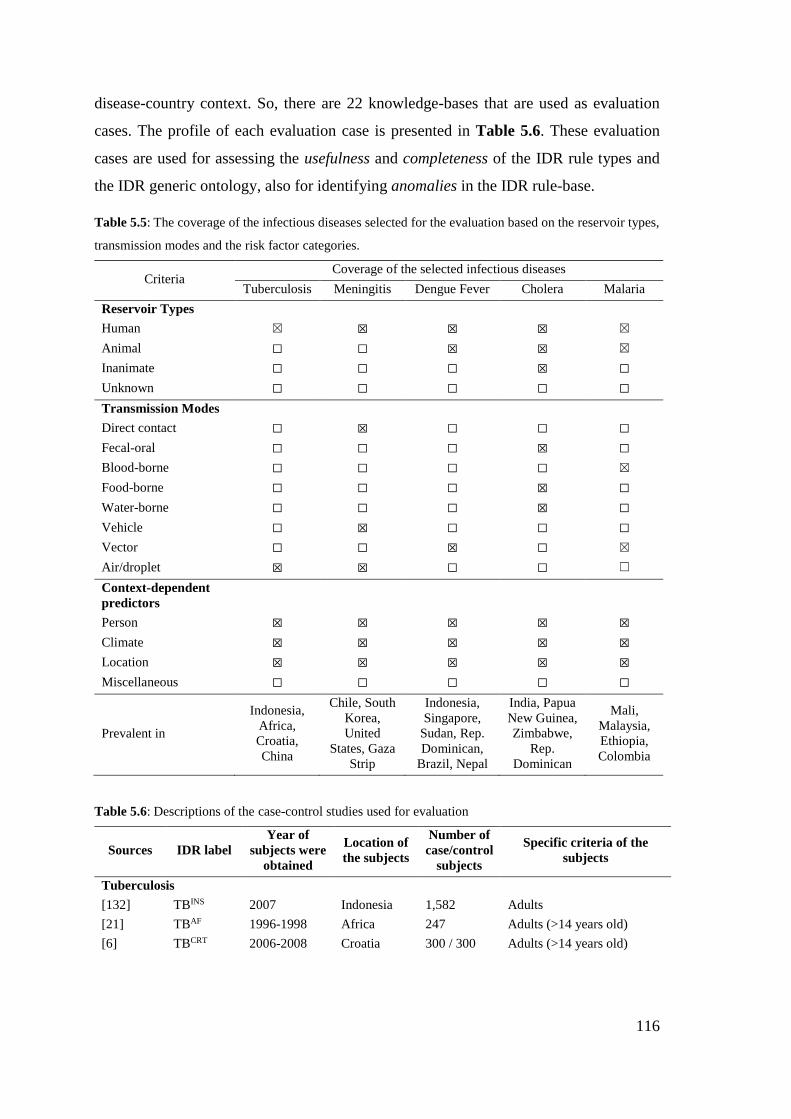
116
disease-country context. So, there are 22 knowledge-bases that are used as evaluation
cases. The profile of each evaluation case is presented in Table 5.6. These evaluation
cases are used for assessing the usefulness and completeness of the IDR rule types and
the IDR generic ontology, also for identifying anomalies in the IDR rule-base.
Table 5.5: The coverage of the infectious diseases selected for the evaluation based on the reservoir types,
transmission modes and the risk factor categories.
Criteria Coverage of the selected infectious diseases
Tuberculosis Meningitis Dengue Fever Cholera Malaria
Reservoir Types
Human ☒ ☒ ☒ ☒ ☒
Animal ☐ ☐ ☒ ☒ ☒
Inanimate ☐ ☐ ☐ ☒ ☐
Unknown ☐ ☐ ☐ ☐ ☐
Transmission Modes
Direct contact ☐ ☒ ☐ ☐ ☐
Fecal-oral ☐ ☐ ☐ ☒ ☐
Blood-borne ☐ ☐ ☐ ☐ ☒
Food-borne ☐ ☐ ☐ ☒ ☐
Water-borne ☐ ☐ ☐ ☒ ☐
Vehicle ☐ ☒ ☐ ☐ ☐
Vector ☐ ☐ ☒ ☐ ☒
Air/droplet ☒ ☒ ☐ ☐ ☐
Context-dependent
predictors
Person ☒ ☒ ☒ ☒ ☒
Climate ☒ ☒ ☒ ☒ ☒
Location ☒ ☒ ☒ ☒ ☒
Miscellaneous ☐ ☐ ☐ ☐ ☐
Prevalent in
Indonesia,
Africa,
Croatia,
China
Chile, South
Korea,
United
States, Gaza
Strip
Indonesia,
Singapore,
Sudan, Rep.
Dominican,
Brazil, Nepal
India, Papua
New Guinea,
Zimbabwe,
Rep.
Dominican
Mali,
Malaysia,
Ethiopia,
Colombia
Table 5.6: Descriptions of the case-control studies used for evaluation
Sources IDR label
Year of
subjects were
obtained
Location of
the subjects
Number of
case/control
subjects
Specific criteria of the
subjects
Tuberculosis
[132] TBINS 2007 Indonesia 1,582 Adults
[21] TBAF 1996-1998 Africa 247 Adults (>14 years old)
[6] TBCRT 2006-2008 Croatia 300 / 300 Adults (>14 years old)
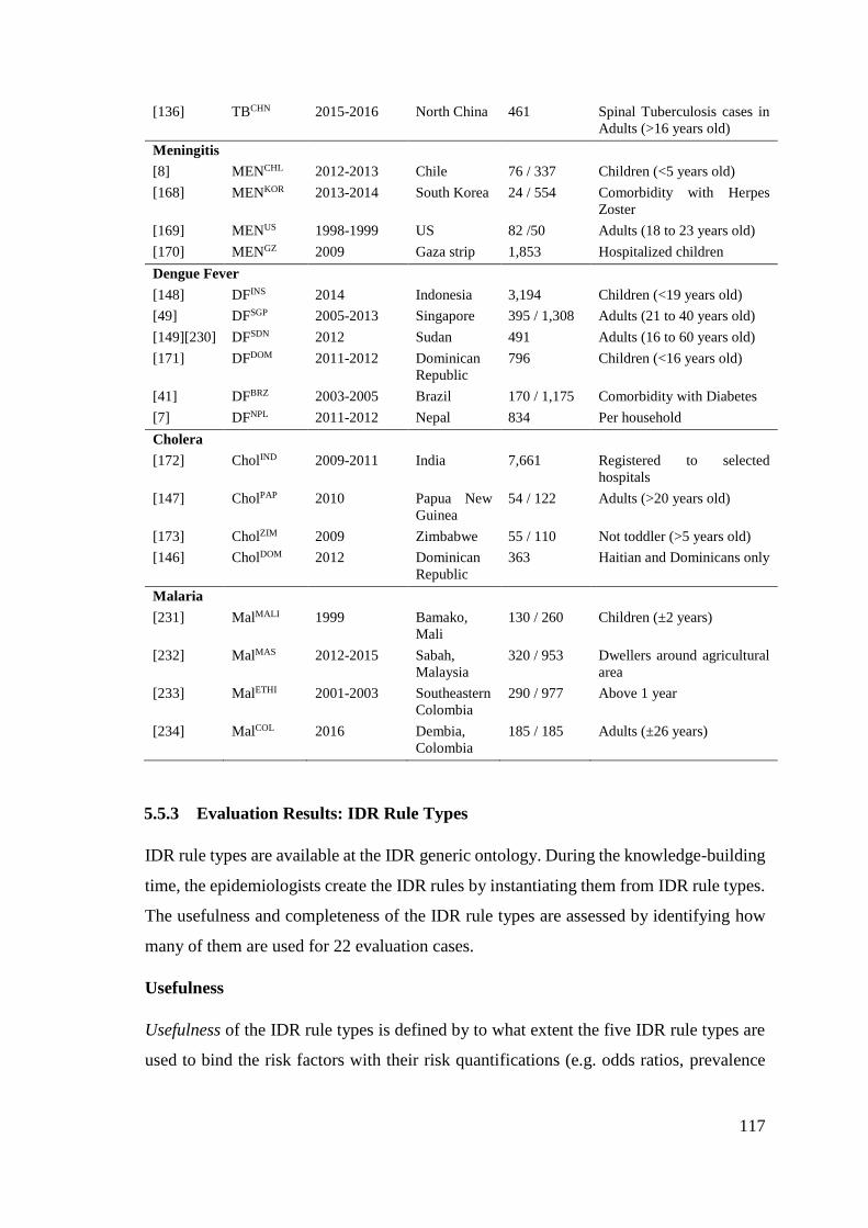
117
[136] TBCHN 2015-2016 North China 461 Spinal Tuberculosis cases in
Adults (>16 years old)
Meningitis
[8] MENCHL 2012-2013 Chile 76 / 337 Children (<5 years old)
[168] MENKOR 2013-2014 South Korea 24 / 554 Comorbidity with Herpes
Zoster
[169] MENUS 1998-1999 US 82 /50 Adults (18 to 23 years old)
[170] MENGZ 2009 Gaza strip 1,853 Hospitalized children
Dengue Fever
[148] DFINS 2014 Indonesia 3,194 Children (<19 years old)
[49] DFSGP 2005-2013 Singapore 395 / 1,308 Adults (21 to 40 years old)
[149][230] DFSDN 2012 Sudan 491 Adults (16 to 60 years old)
[171] DFDOM 2011-2012 Dominican
Republic
796 Children (<16 years old)
[41] DFBRZ 2003-2005 Brazil 170 / 1,175 Comorbidity with Diabetes
[7] DFNPL 2011-2012 Nepal 834 Per household
Cholera
[172] CholIND 2009-2011 India 7,661 Registered to selected
hospitals
[147] CholPAP 2010 Papua New
Guinea
54 / 122 Adults (>20 years old)
[173] CholZIM 2009 Zimbabwe 55 / 110 Not toddler (>5 years old)
[146] CholDOM 2012 Dominican
Republic
363 Haitian and Dominicans only
Malaria
[231] MalMALI 1999 Bamako,
Mali
130 / 260 Children (±2 years)
[232] MalMAS 2012-2015 Sabah,
Malaysia
320 / 953 Dwellers around agricultural
area
[233] MalETHI 2001-2003 Southeastern
Colombia
290 / 977 Above 1 year
[234] MalCOL 2016 Dembia,
Colombia
185 / 185 Adults (±26 years)
5.5.3 Evaluation Results: IDR Rule Types
IDR rule types are available at the IDR generic ontology. During the knowledge-building
time, the epidemiologists create the IDR rules by instantiating them from IDR rule types.
The usefulness and completeness of the IDR rule types are assessed by identifying how
many of them are used for 22 evaluation cases.
Usefulness
Usefulness of the IDR rule types is defined by to what extent the five IDR rule types are
used to bind the risk factors with their risk quantifications (e.g. odds ratios, prevalence
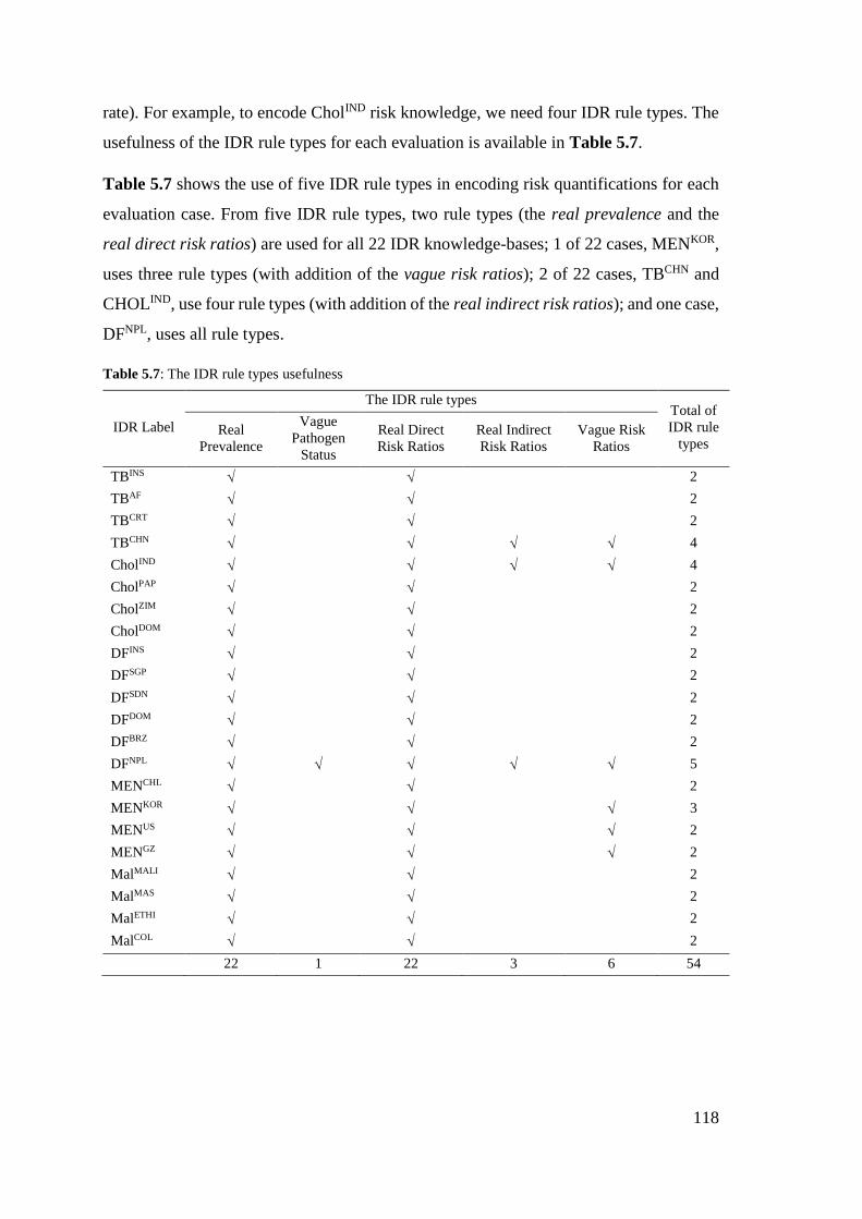
118
rate). For example, to encode CholIND risk knowledge, we need four IDR rule types. The
usefulness of the IDR rule types for each evaluation is available in Table 5.7.
Table 5.7 shows the use of five IDR rule types in encoding risk quantifications for each
evaluation case. From five IDR rule types, two rule types (the real prevalence and the
real direct risk ratios) are used for all 22 IDR knowledge-bases; 1 of 22 cases, MENKOR,
uses three rule types (with addition of the vague risk ratios); 2 of 22 cases, TBCHN and
CHOLIND, use four rule types (with addition of the real indirect risk ratios); and one case,
DFNPL, uses all rule types.
Table 5.7: The IDR rule types usefulness
IDR Label
The IDR rule types Total of
IDR rule
types Real
Prevalence
Vague
Pathogen
Status
Real Direct
Risk Ratios
Real Indirect
Risk Ratios
Vague Risk
Ratios
TBINS 2
TBAF 2
TBCRT 2
TBCHN 4
CholIND 4
CholPAP 2
CholZIM 2
CholDOM 2
DFINS 2
DFSGP 2
DFSDN 2
DFDOM 2
DFBRZ 2
DFNPL 5
MENCHL 2
MENKOR 3
MENUS 2
MENGZ 2
MalMALI 2
MalMAS 2
MalETHI 2
MalCOL 2
22 1 22 3 6 54
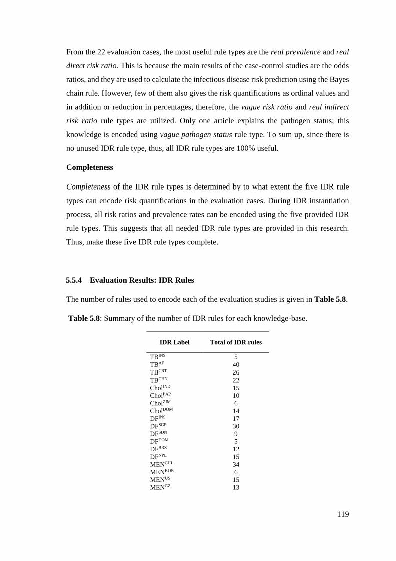
119
From the 22 evaluation cases, the most useful rule types are the real prevalence and real
direct risk ratio. This is because the main results of the case-control studies are the odds
ratios, and they are used to calculate the infectious disease risk prediction using the Bayes
chain rule. However, few of them also gives the risk quantifications as ordinal values and
in addition or reduction in percentages, therefore, the vague risk ratio and real indirect
risk ratio rule types are utilized. Only one article explains the pathogen status; this
knowledge is encoded using vague pathogen status rule type. To sum up, since there is
no unused IDR rule type, thus, all IDR rule types are 100% useful.
Completeness
Completeness of the IDR rule types is determined by to what extent the five IDR rule
types can encode risk quantifications in the evaluation cases. During IDR instantiation
process, all risk ratios and prevalence rates can be encoded using the five provided IDR
rule types. This suggests that all needed IDR rule types are provided in this research.
Thus, make these five IDR rule types complete.
5.5.4 Evaluation Results: IDR Rules
The number of rules used to encode each of the evaluation studies is given in Table 5.8.
Table 5.8: Summary of the number of IDR rules for each knowledge-base.
IDR Label Total of IDR rules
TBINS 5
TBAF 40
TBCRT 26
TBCHN 22
CholIND 15
CholPAP 10
CholZIM 6
CholDOM 14
DFINS 17
DFSGP 30
DFSDN 9
DFDOM 5
DFBRZ 12
DFNPL 15
MENCHL 34
MENKOR 6
MENUS 15
MENGZ 13
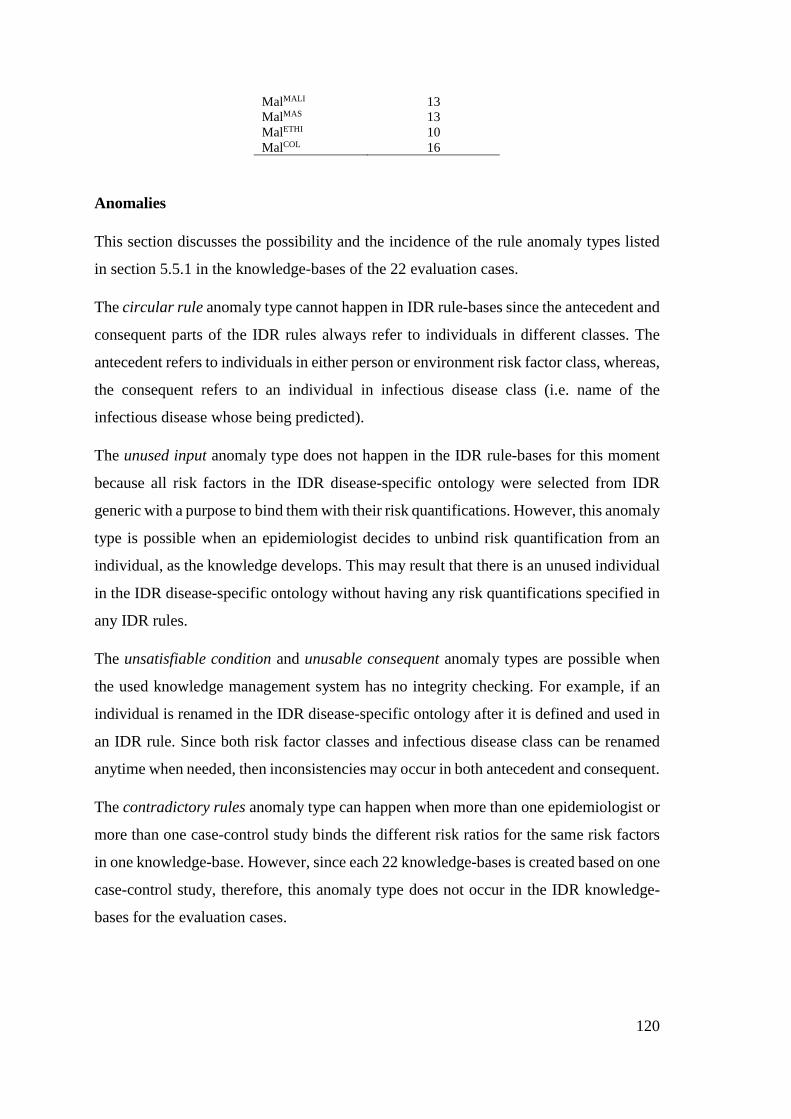
120
MalMALI 13
MalMAS 13
MalETHI 10
MalCOL 16
Anomalies
This section discusses the possibility and the incidence of the rule anomaly types listed
in section 5.5.1 in the knowledge-bases of the 22 evaluation cases.
The circular rule anomaly type cannot happen in IDR rule-bases since the antecedent and
consequent parts of the IDR rules always refer to individuals in different classes. The
antecedent refers to individuals in either person or environment risk factor class, whereas,
the consequent refers to an individual in infectious disease class (i.e. name of the
infectious disease whose being predicted).
The unused input anomaly type does not happen in the IDR rule-bases for this moment
because all risk factors in the IDR disease-specific ontology were selected from IDR
generic with a purpose to bind them with their risk quantifications. However, this anomaly
type is possible when an epidemiologist decides to unbind risk quantification from an
individual, as the knowledge develops. This may result that there is an unused individual
in the IDR disease-specific ontology without having any risk quantifications specified in
any IDR rules.
The unsatisfiable condition and unusable consequent anomaly types are possible when
the used knowledge management system has no integrity checking. For example, if an
individual is renamed in the IDR disease-specific ontology after it is defined and used in
an IDR rule. Since both risk factor classes and infectious disease class can be renamed
anytime when needed, then inconsistencies may occur in both antecedent and consequent.
The contradictory rules anomaly type can happen when more than one epidemiologist or
more than one case-control study binds the different risk ratios for the same risk factors
in one knowledge-base. However, since each 22 knowledge-bases is created based on one
case-control study, therefore, this anomaly type does not occur in the IDR knowledge-
bases for the evaluation cases.
121
One small solution has been prepared to resolve this conflict: prioritization. Before
submitting the IDR rules, epidemiologists will be asked to specify their confidence level
regarding the risk quantifications with a value between 0 and 1. Where there are two
conflicting rules with the same risk ratios, then the knowledge manager resolves the
conflict by assigning different priority to the duplicating rules, the rule with the highest
priority level is included to populate the CPT.
Duplicate rule anomaly types can occur when different rule types are used to express the
same risk ratios for the same risk factor in one knowledge-base. For example, to encode
the declarative knowledge: a person who does not consume vitamin D will have
tuberculosis risk 2.85 times higher than a person who consumes vitamin D regularly. This
knowledge can be encoded by using real indirect risk ratios rule type with 285% as the
quantification or using real direct risk ratios type with risk ratio 2.85. Even though this
case is possible, but the real indirect risk ratio is an alternative to encode risk
quantifications when they are not presented as odds ratios or relevance risks. So, if this
case ever happened, the knowledge manager should assign higher priority for the direct
risk ratio instead of the indirect one.
One preventive solution in the user interfaces for experts in the system has been prepared;
a feature is designed (as a table) to inform experts about similar pre-defined risk factors
for a knowledge-base. However, this feature is not able to diminish all the duplicate rules
perfectly, but this should eliminate duplicate rule entries. See the design of the user
interfaces at Appendix 2.
5.5.5 Evaluation Results: IDR Generic Ontology
The IDR generic ontology is designed by collating all mentioned risk factors in the AHID,
CDC, WHO factsheets because these knowledge sources cover all human infectious
diseases that exists in the world, not specific to particular infectious diseases. Therefore,
some risk factors in the IDR generic ontology might not be used in the IDR disease-
specific ontology during knowledge-encoding time for the 22 evaluation cases. However,
the aim of this thesis is to provide an IDR generic ontology that helps the epidemiologists
to encode their knowledge, so the higher the usefulness and completeness the better.
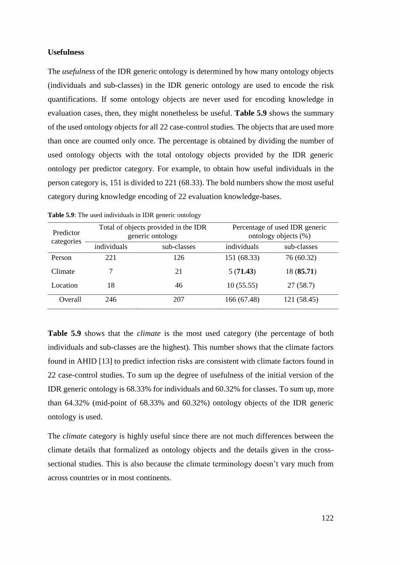
122
Usefulness
The usefulness of the IDR generic ontology is determined by how many ontology objects
(individuals and sub-classes) in the IDR generic ontology are used to encode the risk
quantifications. If some ontology objects are never used for encoding knowledge in
evaluation cases, then, they might nonetheless be useful. Table 5.9 shows the summary
of the used ontology objects for all 22 case-control studies. The objects that are used more
than once are counted only once. The percentage is obtained by dividing the number of
used ontology objects with the total ontology objects provided by the IDR generic
ontology per predictor category. For example, to obtain how useful individuals in the
person category is, 151 is divided to 221 (68.33). The bold numbers show the most useful
category during knowledge encoding of 22 evaluation knowledge-bases.
Table 5.9: The used individuals in IDR generic ontology
Predictor
categories
Total of objects provided in the IDR
generic ontology
Percentage of used IDR generic
ontology objects (%)
individuals sub-classes individuals sub-classes
Person 221 126 151 (68.33) 76 (60.32)
Climate 7 21 5 (71.43) 18 (85.71)
Location 18 46 10 (55.55) 27 (58.7)
Overall 246 207 166 (67.48) 121 (58.45)
Table 5.9 shows that the climate is the most used category (the percentage of both
individuals and sub-classes are the highest). This number shows that the climate factors
found in AHID [13] to predict infection risks are consistent with climate factors found in
22 case-control studies. To sum up the degree of usefulness of the initial version of the
IDR generic ontology is 68.33% for individuals and 60.32% for classes. To sum up, more
than 64.32% (mid-point of 68.33% and 60.32%) ontology objects of the IDR generic
ontology is used.
The climate category is highly useful since there are not much differences between the
climate details that formalized as ontology objects and the details given in the cross-
sectional studies. This is also because the climate terminology doesn’t vary much from
across countries or in most continents.
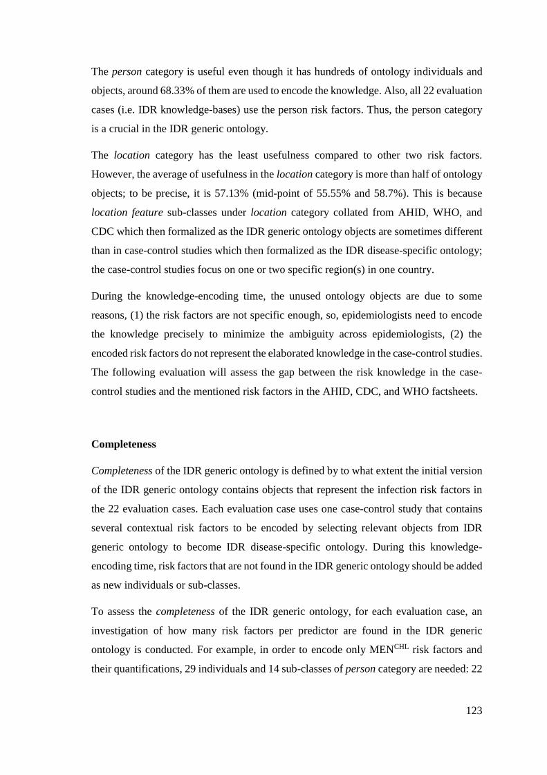
123
The person category is useful even though it has hundreds of ontology individuals and
objects, around 68.33% of them are used to encode the knowledge. Also, all 22 evaluation
cases (i.e. IDR knowledge-bases) use the person risk factors. Thus, the person category
is a crucial in the IDR generic ontology.
The location category has the least usefulness compared to other two risk factors.
However, the average of usefulness in the location category is more than half of ontology
objects; to be precise, it is 57.13% (mid-point of 55.55% and 58.7%). This is because
location feature sub-classes under location category collated from AHID, WHO, and
CDC which then formalized as the IDR generic ontology objects are sometimes different
than in case-control studies which then formalized as the IDR disease-specific ontology;
the case-control studies focus on one or two specific region(s) in one country.
During the knowledge-encoding time, the unused ontology objects are due to some
reasons, (1) the risk factors are not specific enough, so, epidemiologists need to encode
the knowledge precisely to minimize the ambiguity across epidemiologists, (2) the
encoded risk factors do not represent the elaborated knowledge in the case-control studies.
The following evaluation will assess the gap between the risk knowledge in the case-
control studies and the mentioned risk factors in the AHID, CDC, and WHO factsheets.
Completeness
Completeness of the IDR generic ontology is defined by to what extent the initial version
of the IDR generic ontology contains objects that represent the infection risk factors in
the 22 evaluation cases. Each evaluation case uses one case-control study that contains
several contextual risk factors to be encoded by selecting relevant objects from IDR
generic ontology to become IDR disease-specific ontology. During this knowledge-
encoding time, risk factors that are not found in the IDR generic ontology should be added
as new individuals or sub-classes.
To assess the completeness of the IDR generic ontology, for each evaluation case, an
investigation of how many risk factors per predictor are found in the IDR generic
ontology is conducted. For example, in order to encode only MENCHL risk factors and
their quantifications, 29 individuals and 14 sub-classes of person category are needed: 22
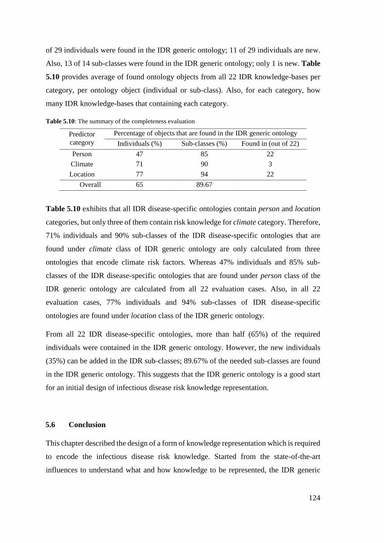
124
of 29 individuals were found in the IDR generic ontology; 11 of 29 individuals are new.
Also, 13 of 14 sub-classes were found in the IDR generic ontology; only 1 is new. Table
5.10 provides average of found ontology objects from all 22 IDR knowledge-bases per
category, per ontology object (individual or sub-class). Also, for each category, how
many IDR knowledge-bases that containing each category.
Table 5.10: The summary of the completeness evaluation
Predictor
category
Percentage of objects that are found in the IDR generic ontology
Individuals (%) Sub-classes (%) Found in (out of 22)
Person 47 85 22
Climate 71 90 3
Location 77 94 22
Overall 65 89.67
Table 5.10 exhibits that all IDR disease-specific ontologies contain person and location
categories, but only three of them contain risk knowledge for climate category. Therefore,
71% individuals and 90% sub-classes of the IDR disease-specific ontologies that are
found under climate class of IDR generic ontology are only calculated from three
ontologies that encode climate risk factors. Whereas 47% individuals and 85% sub-
classes of the IDR disease-specific ontologies that are found under person class of the
IDR generic ontology are calculated from all 22 evaluation cases. Also, in all 22
evaluation cases, 77% individuals and 94% sub-classes of IDR disease-specific
ontologies are found under location class of the IDR generic ontology.
From all 22 IDR disease-specific ontologies, more than half (65%) of the required
individuals were contained in the IDR generic ontology. However, the new individuals
(35%) can be added in the IDR sub-classes; 89.67% of the needed sub-classes are found
in the IDR generic ontology. This suggests that the IDR generic ontology is a good start
for an initial design of infectious disease risk knowledge representation.
5.6 Conclusion
This chapter described the design of a form of knowledge representation which is required
to encode the infectious disease risk knowledge. Started from the state-of-the-art
influences to understand what and how knowledge to be represented, the IDR generic
125
ontology containing three main categories (person, climate, location) and the IDR rule-
types are designed. The usefulness and completeness of the designed knowledge
representation is then evaluated.
Several infectious diseases were selected carefully with aim to choose the most
representative infectious diseases based on their reservoir types, transmission modes,
their risk factor categories, and their prevalence. So, in order to test the usefulness and
completeness of the designed knowledge representation, it is not necessary to test all of
the collated 234 infectious diseases.
Five infectious diseases prevalent in total 20 countries described in the 22 case-control
studies were encoded as 22 IDR knowledge-bases (i.e. evaluation cases). Through the
evaluation process, all rule types were found 100% useful. Minimum two IDR rule types
were used per evaluation case. For all 22 evaluation cases, there was no need to add new
IDR rule types to bind risk factors with their risk quantifications. This suggests that the
IDR rule types are 100% complete for binding risk factors with their risk quantifications,
for all evaluation cases.
An investigation of how much of the IDR generic ontology is reusable to build the
evaluation cases was carried out. Roughly more than 77% of ontology objects (mid-point
of 65% and 89.67%) of the IDR generic ontology were used to encode infection risk
factors (see Table 5.9). Completeness evaluation on the IDR generic ontology showed
that the initial version is a good start for representing infectious disease risk factors
needed in the 22 evaluation cases. To evaluate the usefulness of the IDR generic ontology,
how many individuals and sub-classes are used during knowledge encoding of the 22
evaluation cases is observed. As results, 62.97% ontology objects (mid-point of 67.48%
and 58.45%) of the IDR generic ontology are used.
To sum up, two types of ontology are created to encode knowledge about infectious
disease relevant to risk prediction. The ontologies are IDR generic ontology, and the
disease-specific ontologies as a result from instantiation of the IDR generic ontology.
Further, five IDR rule types are developed to bind the infectious disease risk factors with
their quantifications. From the evaluation, the IDR generic ontology and the rule types
are proven to be complete and useful.
126
6. DESIGN AND TEST OF THE BN-BUILDER ALGORITHM
6.1 Introduction
In chapter 4, the coverage of this thesis was outlined in the context of the personalized
infectious disease risk prediction (PROSPECT-IDR) system. The thesis covers the
knowledge representation for infectious disease risk (IDR), and the BN-Builder algorithm
that keeps knowledge consistency between the knowledge-base and prediction model.
The previous chapter has described the design and test of the IDR knowledge-base, so
this chapter explains the design and test of the BN-Builder algorithm. The BN-Builder
aims to generate a BN from the IDR disease-specific ontology structure, as well as
populate the CPT of the generated BN from the IDR semantic-web rules. The early
version of the BN-Builder algorithm had been published in an article, attached as
Appendix 5.
6.2 Influences from the State of the Art
Section 3.3 discussed the approaches that allow knowledge representation and yield a
prediction as probability from the encoded knowledge. Based on the state-of-the-art
gathered from section 3.3, this section describes what influences inspired the design of
the BN-Builder algorithm.
BayesOWL (see section 3.3.5), in its way of generating a BN structure, uses a conversion
table that specifies what inputs (ontology objects) become what outputs (BN objects). This
table is then reused every time the BayesOWL generates the BN. This table can be updated
if there is new formalization on the ontology structure that is considered to have impact
on the BN structure.
BNTab plugin (see section 3.3.5) shows how a semantic query (e.g. SPARQL) can be
used to select appropriate ontology and semantic-web rule objects to be later converted
to nodes, states, and a conditional probability table of a BN. Besides showing the way
SPARQL can be used to select the ontology and semantic-web objects, an automatic
program that converts ontology and semantic-web rules to a BN is an inspiration for this
research. However, the generated CPT is only limited to binary states only; this limitation
makes the BNTab plugin unsuitable for this thesis and thus, the features need to be
127
expanded. To be more specific, the features that fit to the characteristics of the (infectious)
disease risk knowledge.
A reduction of the iterations needed to populate the conditional probability table can be
achieved by grouping the likelihood of events occurrence. Then, a weight-sum algorithm
is used to calculate the prediction (see section 3.2.3).
6.3 The Design of BN-Builder Algorithm
The BN-Builder algorithm is designed to make sure that the encoded knowledge in the
IDR knowledge-base is consistent with the prediction results of the BN. From chapter 5,
it is known that the IDR knowledge-base consists of the IDR disease-specific ontology
and IDR semantic-web rules; each IDR knowledge-base encodes one infectious disease
prevalent in one country. The IDR disease-specific ontology represents the risk factors as
sub-classes and individuals. The IDR semantic-web rules encode the risk ratio for each
represented risk factor. To be more precise, the BN-Builder aims to generate a BN from
the IDR disease-specific ontology structure, as well as populate the CPT of the generated
BN from the IDR semantic-web rules.
The BN-Builder algorithm is needed every time the domain experts input or update the
content of the knowledge-base or the knowledge manager finish managing the conflicting
or redundant knowledge at the knowledge-encoding time. The BN-Builder algorithm
aims to produce a Bayesian network that is fully-functioning and consistent with the
encoded knowledge. Fully-functioning means that the generated BN not only contain
nodes and states, but also contains conditional probabilities for the basis of predictive
reasoning, Conditional Probability Table (CPT), as a placeholder for all combinations of
all states in the all nodes. Consistency means that the generated BN structure matches the
ontology structure and the populated CPT contains the same ratio between the encoded
risk ratios and the generated results. In order to optimize the performance of the BN-
Builder to populate the CPT, some impossible combinations are not included in the CPT
population process. For example, a <child> who works as a <nurse>.
To sum up, the BN-Builder algorithm aims to (1) construct a Bayesian network structure
based on the associated IDR knowledge-base, (2) populate the CPT correctly from
128
various categorical node attributes that appear on the infectious disease risk knowledge,
and (3) optimize the algorithm by deducing the impossibility of an event. Evaluations of
the BN-Builder algorithm are conducted based on its first and second purposes, whereas
for the third purpose, the algorithm will be evaluated whether it can recognize the
impossible events correctly or not. The evaluation results will be presented in section 6.4.
6.3.1 Translation from Ontology to Bayesian Network
A Bayesian Networks (BN) consists of a network and a Conditional Probability Table
(CPT). The network contains nodes (including states) and links. A basic network has two
types of nodes: parent and child nodes which are connected by links. In this system, the
risk factors become the parent nodes and the disease whose risk is being predicted
becomes the child node. The network links are used to define a causal relationship
between the predictors (parent nodes) and the predicted infectious disease risk (child
node). Each BN is generated from an associated IDR knowledge-base which contains an
infectious disease risk knowledge for an infectious disease prevalent in a country, thus,
the BN scope is one infectious disease-country context.
The network (nodes and links) is built from the structure of IDR disease-specific
ontology. Both ontology and BNs have the same hierarchical structure [33], [91], [221],
therefore, conversion from an ontological knowledge-base to a BN is straightforward.
Once the network is generated, a CPT has to be added. The CPT is populated from the
IDR semantic-web rules that encode risk quantifications for each risk factors. The CPT
population uses the Bayes chain rule as the basic formula for calculation of conditional
probabilities.
A BN node is a condition which contains more than one discrete attribute (i.e. state) which
can be nominal, ordinal, or binary. When using nodes to represent risk factors, the states
are the possible values for the risk factor. For example, the risk of contracting dengue
fever is determined by the gender of the person. So, gender is the node, while male and
female are the condition values (i.e. states) of the gender node.
To represent an actual condition at a time, in the prediction phase, only one state is
selectable per node [235]. Therefore, as mentioned in section 5.3, the IDR ontologies
129
(both generic and disease-specific) is designed so that mutually exclusive values are
represented as one risk factor (e.g. infant / elderly are individuals of development stage
ontology sub-class), becoming one node in the BN; whereas values that can co-occur,
such as weather conditions cloudy and cold, need to be represented in different sub-
classes, and become separate nodes in the generated BN. Then, the individuals of the
cloudy and cold can be yes or no, and low, medium, high, respectively.
To facilitate the explained situation, the BN-Builder algorithm is designed to convert
ontology sub-classes to BN nodes and ontology individuals to BN states. The network
construction procedure of the BN Builder algorithm handles the construction of the
network from the IDR ontology, addressing the first aim of the algorithm.
As mentioned in section 3.2.3, a CPT is a table that contains probabilities, either marginal
or conditional, for combinations of states in a BN. The second aim of the algorithm is to
populate the main CPT. The main CPT for the parent nodes, infectious disease risk
factors, contain states and their probabilities. An addition of one parent node causes an
addition of exponential set of conditional probabilities in the main CPT which could affect
the tractability of runtime calculation.
The other type of CPT needs marginal probability values (e.g. the probability of a person
being a child); an example of the marginal probability table can be seen in Figure 3.17.
These values can be loaded from UNSD API, but if no values are available or provided,
probabilities in parent nodes are distributed uniformly by default.
The CPT for the child node (see Figure 3.17 for the child node), predicted infectious
disease risk, consists of all parent states’ combinations and their conditional probabilities
(e.g. the conditional probability of a female infant contracting dengue fever). The contents
of this CPT are populated by CPT population procedure of the BN-Builder algorithm,
based on the risk ratios in the IDR rules.
The third aim of the BN builder algorithm is to optimize the BN-Builder algorithm by
reducing the number of iterations for impossible combinations. This function is facilitated
by a library that contains pairs of items that cannot appear together. For example, a child
who works as a nurse, the library will consist of <child> <nurse>. Thereafter, the
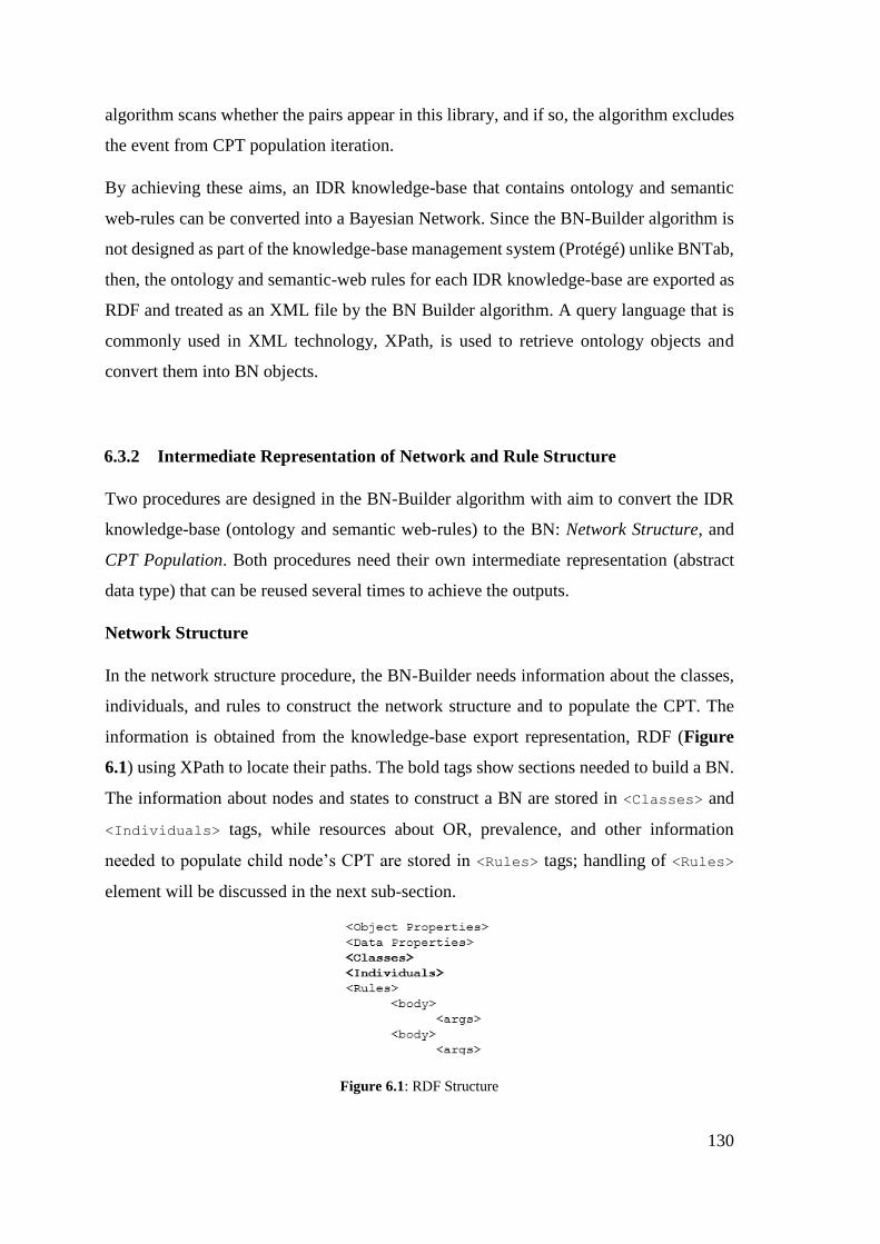
130
algorithm scans whether the pairs appear in this library, and if so, the algorithm excludes
the event from CPT population iteration.
By achieving these aims, an IDR knowledge-base that contains ontology and semantic
web-rules can be converted into a Bayesian Network. Since the BN-Builder algorithm is
not designed as part of the knowledge-base management system (Protégé) unlike BNTab,
then, the ontology and semantic-web rules for each IDR knowledge-base are exported as
RDF and treated as an XML file by the BN Builder algorithm. A query language that is
commonly used in XML technology, XPath, is used to retrieve ontology objects and
convert them into BN objects.
6.3.2 Intermediate Representation of Network and Rule Structure
Two procedures are designed in the BN-Builder algorithm with aim to convert the IDR
knowledge-base (ontology and semantic web-rules) to the BN: Network Structure, and
CPT Population. Both procedures need their own intermediate representation (abstract
data type) that can be reused several times to achieve the outputs.
Network Structure
In the network structure procedure, the BN-Builder needs information about the classes,
individuals, and rules to construct the network structure and to populate the CPT. The
information is obtained from the knowledge-base export representation, RDF (Figure
6.1) using XPath to locate their paths. The bold tags show sections needed to build a BN.
The information about nodes and states to construct a BN are stored in <Classes> and
<Individuals> tags, while resources about OR, prevalence, and other information
needed to populate child node’s CPT are stored in <Rules> tags; handling of <Rules>
element will be discussed in the next sub-section.
Figure 6.1: RDF Structure
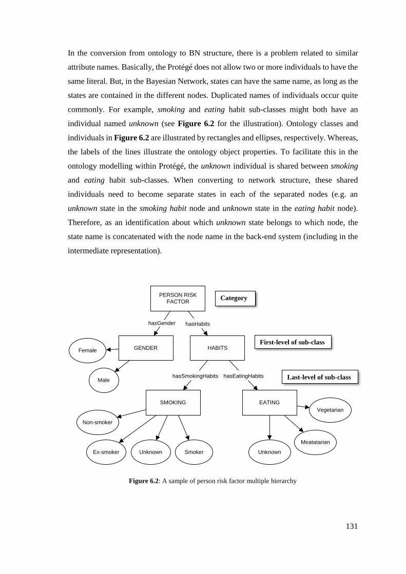
131
In the conversion from ontology to BN structure, there is a problem related to similar
attribute names. Basically, the Protégé does not allow two or more individuals to have the
same literal. But, in the Bayesian Network, states can have the same name, as long as the
states are contained in the different nodes. Duplicated names of individuals occur quite
commonly. For example, smoking and eating habit sub-classes might both have an
individual named unknown (see Figure 6.2 for the illustration). Ontology classes and
individuals in Figure 6.2 are illustrated by rectangles and ellipses, respectively. Whereas,
the labels of the lines illustrate the ontology object properties. To facilitate this in the
ontology modelling within Protégé, the unknown individual is shared between smoking
and eating habit sub-classes. When converting to network structure, these shared
individuals need to become separate states in each of the separated nodes (e.g. an
unknown state in the smoking habit node and unknown state in the eating habit node).
Therefore, as an identification about which unknown state belongs to which node, the
state name is concatenated with the node name in the back-end system (including in the
intermediate representation).
PERSON RISK
FACTOR
GENDER HABITS
SMOKING EATING
Male
Female
Smoker
Non-smoker
Ex-smoker Unknown
Vegetarian
Meatatarian
Unknown
hasHabitshasGender
hasSmokingHabits hasEatingHabits
Figure 6.2: A sample of person risk factor multiple hierarchy
First-level of sub-class
Last-level of sub-class
Category
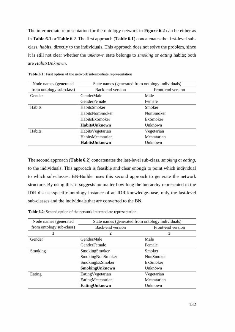
132
The intermediate representation for the ontology network in Figure 6.2 can be either as
in Table 6.1 or Table 6.2. The first approach (Table 6.1) concatenates the first-level sub-
class, habits, directly to the individuals. This approach does not solve the problem, since
it is still not clear whether the unknown state belongs to smoking or eating habits; both
are HabitsUnknown.
Table 6.1: First option of the network intermediate representation
Node names (generated
from ontology sub-class)
State names (generated from ontology individuals)
Back-end version Front-end version
Gender GenderMale Male
GenderFemale Female
Habits HabitsSmoker Smoker
HabitsNonSmoker NonSmoker
HabitsExSmoker ExSmoker
HabitsUnknown Unknown
Habits HabitsVegetarian Vegetarian
HabitsMeatatarian Meatatarian
HabitsUnknown Unknown
The second approach (Table 6.2) concatenates the last-level sub-class, smoking or eating,
to the individuals. This approach is feasible and clear enough to point which individual
to which sub-classes. BN-Builder uses this second approach to generate the network
structure. By using this, it suggests no matter how long the hierarchy represented in the
IDR disease-specific ontology instance of an IDR knowledge-base, only the last-level
sub-classes and the individuals that are converted to the BN.
Table 6.2: Second option of the network intermediate representation
Node names (generated
from ontology sub-class)
State names (generated from ontology individuals)
Back-end version Front-end version
1 2 3
Gender GenderMale Male
GenderFemale Female
Smoking SmokingSmoker Smoker
SmokingNonSmoker NonSmoker
SmokingExSmoker ExSmoker
SmokingUnknown Unknown
Eating EatingVegetarian Vegetarian
EatingMeatatarian Meatatarian
EatingUnknown Unknown
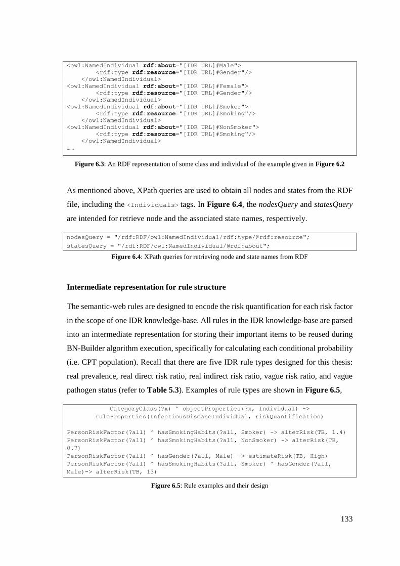
133
<owl:NamedIndividual rdf:about="[IDR URL]#Male">
<rdf:type rdf:resource="[IDR URL]#Gender"/>
</owl:NamedIndividual>
<owl:NamedIndividual rdf:about="[IDR URL]#Female">
<rdf:type rdf:resource="[IDR URL]#Gender"/>
</owl:NamedIndividual>
<owl:NamedIndividual rdf:about="[IDR URL]#Smoker">
<rdf:type rdf:resource="[IDR URL]#Smoking"/>
</owl:NamedIndividual>
<owl:NamedIndividual rdf:about="[IDR URL]#NonSmoker">
<rdf:type rdf:resource="[IDR URL]#Smoking"/>
</owl:NamedIndividual>
……
Figure 6.3: An RDF representation of some class and individual of the example given in Figure 6.2
As mentioned above, XPath queries are used to obtain all nodes and states from the RDF
file, including the <Individuals> tags. In Figure 6.4, the nodesQuery and statesQuery
are intended for retrieve node and the associated state names, respectively.
nodesQuery = "/rdf:RDF/owl:NamedIndividual/rdf:type/@rdf:resource";
statesQuery = "/rdf:RDF/owl:NamedIndividual/@rdf:about";
Figure 6.4: XPath queries for retrieving node and state names from RDF
Intermediate representation for rule structure
The semantic-web rules are designed to encode the risk quantification for each risk factor
in the scope of one IDR knowledge-base. All rules in the IDR knowledge-base are parsed
into an intermediate representation for storing their important items to be reused during
BN-Builder algorithm execution, specifically for calculating each conditional probability
(i.e. CPT population). Recall that there are five IDR rule types designed for this thesis:
real prevalence, real direct risk ratio, real indirect risk ratio, vague risk ratio, and vague
pathogen status (refer to Table 5.3). Examples of rule types are shown in Figure 6.5,
CategoryClass(?x) ^ objectProperties(?x, Individual) ->
ruleProperties(InfectiousDiseaseIndividual, riskQuantification)
PersonRiskFactor(?all) ^ hasSmokingHabits(?all, Smoker) -> alterRisk(TB, 1.4)
PersonRiskFactor(?all) ^ hasSmokingHabits(?all, NonSmoker) -> alterRisk(TB,
0.7)
PersonRiskFactor(?all) ^ hasGender(?all, Male) -> estimateRisk(TB, High)
PersonRiskFactor(?all) ^ hasSmokingHabits(?all, Smoker) ^ hasGender(?all,
Male)-> alterRisk(TB, 13)
Figure 6.5: Rule examples and their design
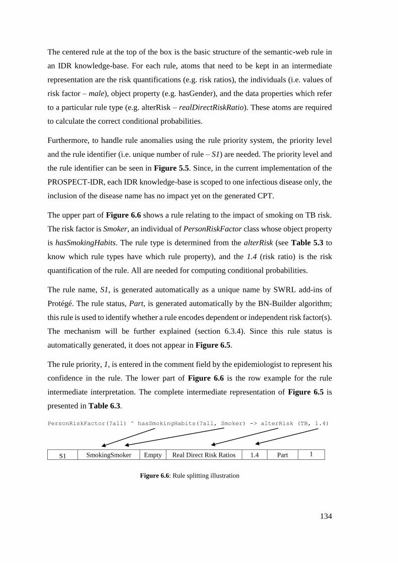
134
The centered rule at the top of the box is the basic structure of the semantic-web rule in
an IDR knowledge-base. For each rule, atoms that need to be kept in an intermediate
representation are the risk quantifications (e.g. risk ratios), the individuals (i.e. values of
risk factor – male), object property (e.g. hasGender), and the data properties which refer
to a particular rule type (e.g. alterRisk – realDirectRiskRatio). These atoms are required
to calculate the correct conditional probabilities.
Furthermore, to handle rule anomalies using the rule priority system, the priority level
and the rule identifier (i.e. unique number of rule – S1) are needed. The priority level and
the rule identifier can be seen in Figure 5.5. Since, in the current implementation of the
PROSPECT-IDR, each IDR knowledge-base is scoped to one infectious disease only, the
inclusion of the disease name has no impact yet on the generated CPT.
The upper part of Figure 6.6 shows a rule relating to the impact of smoking on TB risk.
The risk factor is Smoker, an individual of PersonRiskFactor class whose object property
is hasSmokingHabits. The rule type is determined from the alterRisk (see Table 5.3 to
know which rule types have which rule property), and the 1.4 (risk ratio) is the risk
quantification of the rule. All are needed for computing conditional probabilities.
The rule name, S1, is generated automatically as a unique name by SWRL add-ins of
Protégé. The rule status, Part, is generated automatically by the BN-Builder algorithm;
this rule is used to identify whether a rule encodes dependent or independent risk factor(s).
The mechanism will be further explained (section 6.3.4). Since this rule status is
automatically generated, it does not appear in Figure 6.5.
The rule priority, 1, is entered in the comment field by the epidemiologist to represent his
confidence in the rule. The lower part of Figure 6.6 is the row example for the rule
intermediate interpretation. The complete intermediate representation of Figure 6.5 is
presented in Table 6.3.
PersonRiskFactor(?all) ^ hasSmokingHabits(?all, Smoker) -> alterRisk (TB, 1.4)
S1 SmokingSmoker Empty Real Direct Risk Ratios 1.4 Part 1
Figure 6.6: Rule splitting illustration
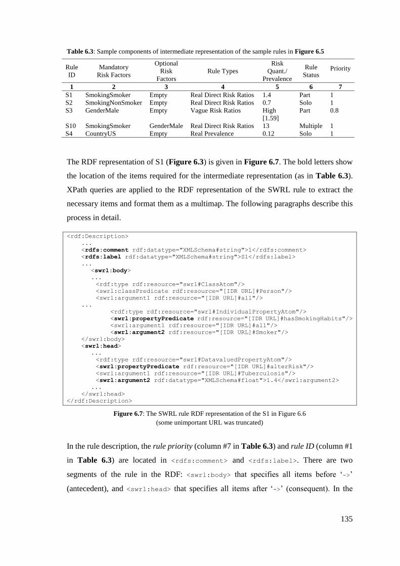
135
Table 6.3: Sample components of intermediate representation of the sample rules in Figure 6.5
Rule
ID
Mandatory
Risk Factors
Optional
Risk
Factors
Rule Types
Risk
Quant./
Prevalence
Rule
Status Priority
1 2 3 4 5 6 7
S1 SmokingSmoker Empty Real Direct Risk Ratios 1.4 Part 1
S2 SmokingNonSmoker Empty Real Direct Risk Ratios 0.7 Solo 1
S3 GenderMale Empty Vague Risk Ratios High
[1.59]
Part 0.8
S10 SmokingSmoker GenderMale Real Direct Risk Ratios 13 Multiple 1
S4 CountryUS Empty Real Prevalence 0.12 Solo 1
The RDF representation of S1 (Figure 6.3) is given in Figure 6.7. The bold letters show
the location of the items required for the intermediate representation (as in Table 6.3).
XPath queries are applied to the RDF representation of the SWRL rule to extract the
necessary items and format them as a multimap. The following paragraphs describe this
process in detail.
<rdf:Description>
...
<rdfs:comment rdf:datatype="XMLSchema#string">1</rdfs:comment>
<rdfs:label rdf:datatype="XMLSchema#string">S1</rdfs:label>
...
<swrl:body>
...
<rdf:type rdf:resource="swrl#ClassAtom"/>
<swrl:classPredicate rdf:resource="[IDR URL]#Person"/>
<swrl:argument1 rdf:resource="[IDR URL]#all"/>
...
<rdf:type rdf:resource="swrl#IndividualPropertyAtom"/>
<swrl:propertyPredicate rdf:resource="[IDR URL]#hasSmokingHabits"/>
<swrl:argument1 rdf:resource="[IDR URL]#all"/>
<swrl:argument2 rdf:resource="[IDR URL]#Smoker"/>
</swrl:body>
<swrl:head>
...
<rdf:type rdf:resource="swrl#DatavaluedPropertyAtom"/>
<swrl:propertyPredicate rdf:resource="[IDR URL]#alterRisk"/>
<swrl:argument1 rdf:resource="[IDR URL]#Tuberculosis"/>
<swrl:argument2 rdf:datatype="XMLSchema#float">1.4</swrl:argument2>
...
</swrl:head>
</rdf:Description>
Figure 6.7: The SWRL rule RDF representation of the S1 in Figure 6.6
(some unimportant URL was truncated)
In the rule description, the rule priority (column #7 in Table 6.3) and rule ID (column #1
in Table 6.3) are located in <rdfs:comment> and <rdfs:label>. There are two
segments of the rule in the RDF: <swrl:body> that specifies all items before ‘->’
(antecedent), and <swrl:head> that specifies all items after ‘->’ (consequent). In the
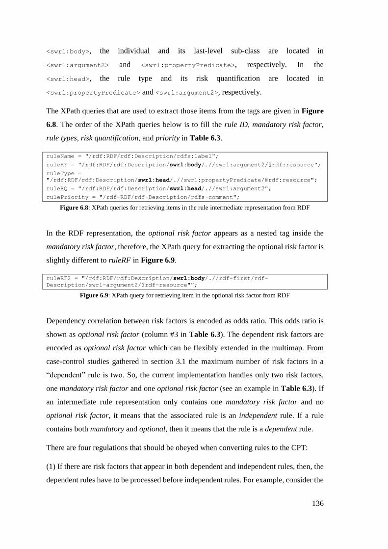
136
<swrl:body>, the individual and its last-level sub-class are located in
<swrl:argument2> and <swrl:propertyPredicate>, respectively. In the
<swrl:head>, the rule type and its risk quantification are located in
<swrl:propertyPredicate> and <swrl:argument2>, respectively.
The XPath queries that are used to extract those items from the tags are given in Figure
6.8. The order of the XPath queries below is to fill the rule ID, mandatory risk factor,
rule types, risk quantification, and priority in Table 6.3.
ruleName = "/rdf:RDF/rdf:Description/rdfs:label";
ruleRF = "/rdf:RDF/rdf:Description/swrl:body/.//swrl:argument2/@rdf:resource";
ruleType =
"/rdf:RDF/rdf:Description/swrl:head/.//swrl:propertyPredicate/@rdf:resource";
ruleRQ = "/rdf:RDF/rdf:Description/swrl:head/.//swrl:argument2";
rulePriority = "/rdf-RDF/rdf-Description/rdfs-comment";
Figure 6.8: XPath queries for retrieving items in the rule intermediate representation from RDF
In the RDF representation, the optional risk factor appears as a nested tag inside the
mandatory risk factor, therefore, the XPath query for extracting the optional risk factor is
slightly different to ruleRF in Figure 6.9.
ruleRF2 = "/rdf:RDF/rdf:Description/swrl:body/.//rdf-first/rdf-
Description/swrl-argument2/@rdf-resource"";
Figure 6.9: XPath query for retrieving item in the optional risk factor from RDF
Dependency correlation between risk factors is encoded as odds ratio. This odds ratio is
shown as optional risk factor (column #3 in Table 6.3). The dependent risk factors are
encoded as optional risk factor which can be flexibly extended in the multimap. From
case-control studies gathered in section 3.1 the maximum number of risk factors in a
“dependent” rule is two. So, the current implementation handles only two risk factors,
one mandatory risk factor and one optional risk factor (see an example in Table 6.3). If
an intermediate rule representation only contains one mandatory risk factor and no
optional risk factor, it means that the associated rule is an independent rule. If a rule
contains both mandatory and optional, then it means that the rule is a dependent rule.
There are four regulations that should be obeyed when converting rules to the CPT:
(1) If there are risk factors that appear in both dependent and independent rules, then, the
dependent rules have to be processed before independent rules. For example, consider the
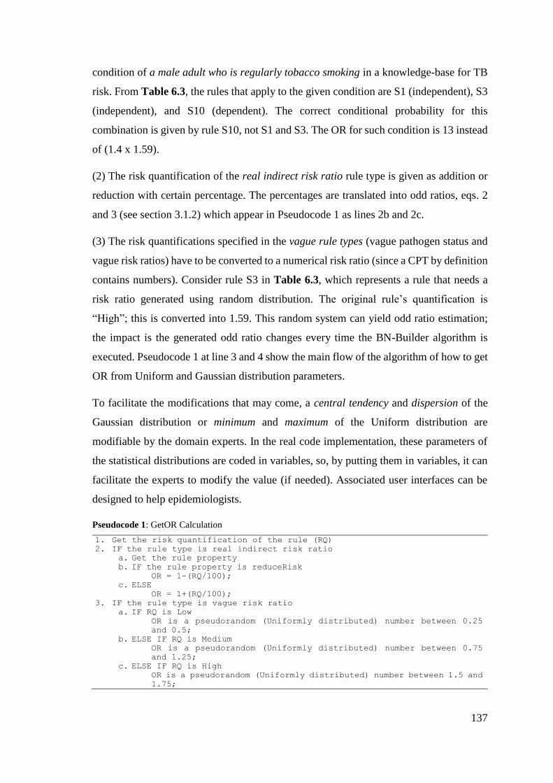
137
condition of a male adult who is regularly tobacco smoking in a knowledge-base for TB
risk. From Table 6.3, the rules that apply to the given condition are S1 (independent), S3
(independent), and S10 (dependent). The correct conditional probability for this
combination is given by rule S10, not S1 and S3. The OR for such condition is 13 instead
of (1.4 x 1.59).
(2) The risk quantification of the real indirect risk ratio rule type is given as addition or
reduction with certain percentage. The percentages are translated into odd ratios, eqs. 2
and 3 (see section 3.1.2) which appear in Pseudocode 1 as lines 2b and 2c.
(3) The risk quantifications specified in the vague rule types (vague pathogen status and
vague risk ratios) have to be converted to a numerical risk ratio (since a CPT by definition
contains numbers). Consider rule S3 in Table 6.3, which represents a rule that needs a
risk ratio generated using random distribution. The original rule’s quantification is
“High”; this is converted into 1.59. This random system can yield odd ratio estimation;
the impact is the generated odd ratio changes every time the BN-Builder algorithm is
executed. Pseudocode 1 at line 3 and 4 show the main flow of the algorithm of how to get
OR from Uniform and Gaussian distribution parameters.
To facilitate the modifications that may come, a central tendency and dispersion of the
Gaussian distribution or minimum and maximum of the Uniform distribution are
modifiable by the domain experts. In the real code implementation, these parameters of
the statistical distributions are coded in variables, so, by putting them in variables, it can
facilitate the experts to modify the value (if needed). Associated user interfaces can be
designed to help epidemiologists.
Pseudocode 1: GetOR Calculation
1. Get the risk quantification of the rule (RQ) 2. IF the rule type is real indirect risk ratio
a. Get the rule property b. IF the rule property is reduceRisk
OR = 1-(RQ/100);
c. ELSE OR = 1+(RQ/100);
3. IF the rule type is vague risk ratio a. IF RQ is Low
OR is a pseudorandom (Uniformly distributed) number between 0.25
and 0.5;
b. ELSE IF RQ is Medium OR is a pseudorandom (Uniformly distributed) number between 0.75
and 1.25;
c. ELSE IF RQ is High OR is a pseudorandom (Uniformly distributed) number between 1.5 and
1.75;
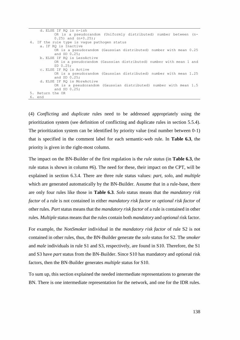
138
d. ELSE IF RQ is n-ish OR is a pseudorandom (Uniformly distributed) number between (n-
0.25) and (n+0.25);
4. IF the rule type is vague pathogen status a. IF RQ is Inactive
OR is a pseudorandom (Gaussian distributed) number with mean 0.25
and SD 0.25;
b. ELSE IF RQ is LessActive OR is a pseudorandom (Gaussian distributed) number with mean 1 and
SD 0.25;
c. ELSE IF RQ is Active OR is a pseudorandom (Gaussian distributed) number with mean 1.25
and SD 0.25;
d. ELSE IF RQ is MoreActive OR is a pseudorandom (Gaussian distributed) number with mean 1.5
and SD 0.25;
5. Return the OR 6. end
(4) Conflicting and duplicate rules need to be addressed appropriately using the
prioritization system (see definition of conflicting and duplicate rules in section 5.5.4).
The prioritization system can be identified by priority value (real number between 0-1)
that is specified in the comment label for each semantic-web rule. In Table 6.3, the
priority is given in the right-most column.
The impact on the BN-Builder of the first regulation is the rule status (in Table 6.3, the
rule status is shown in column #6). The need for these, their impact on the CPT, will be
explained in section 6.3.4. There are three rule status values: part, solo, and multiple
which are generated automatically by the BN-Builder. Assume that in a rule-base, there
are only four rules like those in Table 6.3. Solo status means that the mandatory risk
factor of a rule is not contained in either mandatory risk factor or optional risk factor of
other rules. Part status means that the mandatory risk factor of a rule is contained in other
rules. Multiple status means that the rules contain both mandatory and optional risk factor.
For example, the NonSmoker individual in the mandatory risk factor of rule S2 is not
contained in other rules, thus, the BN-Builder generate the solo status for S2. The smoker
and male individuals in rule S1 and S3, respectively, are found in S10. Therefore, the S1
and S3 have part status from the BN-Builder. Since S10 has mandatory and optional risk
factors, then the BN-Builder generates multiple status for S10.
To sum up, this section explained the needed intermediate representations to generate the
BN. There is one intermediate representation for the network, and one for the IDR rules.
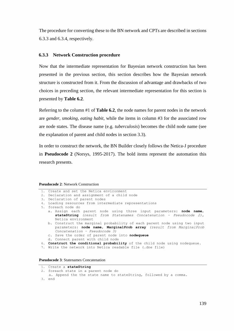
139
The procedure for converting these to the BN network and CPTs are described in sections
6.3.3 and 6.3.4, respectively.
6.3.3 Network Construction procedure
Now that the intermediate representation for Bayesian network construction has been
presented in the previous section, this section describes how the Bayesian network
structure is constructed from it. From the discussion of advantage and drawbacks of two
choices in preceding section, the relevant intermediate representation for this section is
presented by Table 6.2.
Referring to the column #1 of Table 6.2, the node names for parent nodes in the network
are gender, smoking, eating habit, while the items in column #3 for the associated row
are node states. The disease name (e.g. tuberculosis) becomes the child node name (see
the explanation of parent and child nodes in section 3.3).
In order to construct the network, the BN Builder closely follows the Netica-J procedure
in Pseudocode 2 (Norsys, 1995-2017). The bold items represent the automation this
research presents.
Pseudocode 2: Network Construction
1. Create and set the Netica environment
2. Declaration and assignment of a child node
3. Declaration of parent nodes
4. Loading resources from intermediate representations
5. foreach node do
a. Assign each parent node using three input parameters: node name,
stateString (result from Statenames Concatenation – Pseudocode 2),
Netica environment
b. Construct the marginal probability of each parent node using two input parameters: node name, MarginalProb array (result from MarginalProb
Concatenation – Pseudocode 3)
c. Save the order of parent node into nodequeue d. Connect parent with child node
6. Construct the conditional probability of the child node using nodequeue.
7. Write the network into Netica readable file (.dne file)
Pseudocode 3: Statenames Concatenation
1. Create a stateString
2. foreach state in a parent node do
a. Append the the state name to stateString, followed by a comma. 3. end
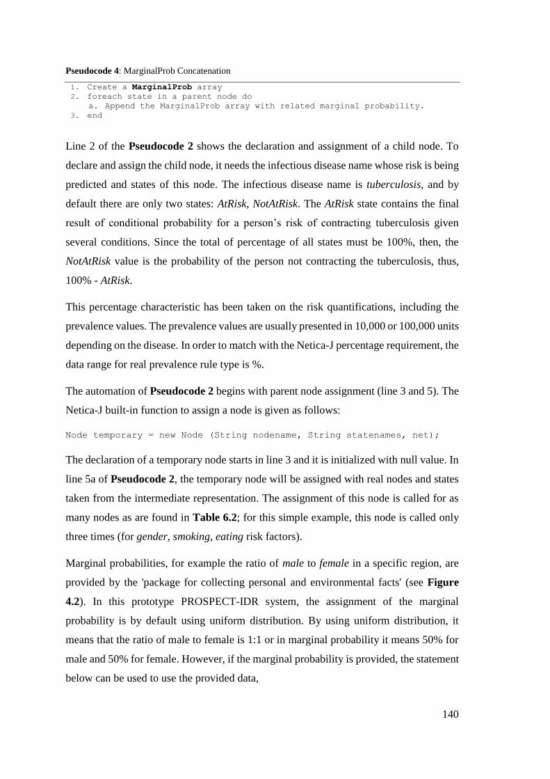
140
Pseudocode 4: MarginalProb Concatenation
1. Create a MarginalProb array
2. foreach state in a parent node do
a. Append the MarginalProb array with related marginal probability. 3. end
Line 2 of the Pseudocode 2 shows the declaration and assignment of a child node. To
declare and assign the child node, it needs the infectious disease name whose risk is being
predicted and states of this node. The infectious disease name is tuberculosis, and by
default there are only two states: AtRisk, NotAtRisk. The AtRisk state contains the final
result of conditional probability for a person’s risk of contracting tuberculosis given
several conditions. Since the total of percentage of all states must be 100%, then, the
NotAtRisk value is the probability of the person not contracting the tuberculosis, thus,
100% - AtRisk.
This percentage characteristic has been taken on the risk quantifications, including the
prevalence values. The prevalence values are usually presented in 10,000 or 100,000 units
depending on the disease. In order to match with the Netica-J percentage requirement, the
data range for real prevalence rule type is %.
The automation of Pseudocode 2 begins with parent node assignment (line 3 and 5). The
Netica-J built-in function to assign a node is given as follows:
Node temporary = new Node (String nodename, String statenames, net);
The declaration of a temporary node starts in line 3 and it is initialized with null value. In
line 5a of Pseudocode 2, the temporary node will be assigned with real nodes and states
taken from the intermediate representation. The assignment of this node is called for as
many nodes as are found in Table 6.2; for this simple example, this node is called only
three times (for gender, smoking, eating risk factors).
Marginal probabilities, for example the ratio of male to female in a specific region, are
provided by the 'package for collecting personal and environmental facts' (see Figure
4.2). In this prototype PROSPECT-IDR system, the assignment of the marginal
probability is by default using uniform distribution. By using uniform distribution, it
means that the ratio of male to female is 1:1 or in marginal probability it means 50% for
male and 50% for female. However, if the marginal probability is provided, the statement
below can be used to use the provided data,
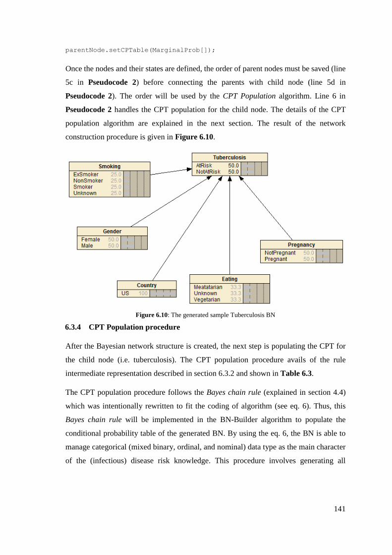
141
parentNode.setCPTable(MarginalProb[]);
Once the nodes and their states are defined, the order of parent nodes must be saved (line
5c in Pseudocode 2) before connecting the parents with child node (line 5d in
Pseudocode 2). The order will be used by the CPT Population algorithm. Line 6 in
Pseudocode 2 handles the CPT population for the child node. The details of the CPT
population algorithm are explained in the next section. The result of the network
construction procedure is given in Figure 6.10.
Figure 6.10: The generated sample Tuberculosis BN
6.3.4 CPT Population procedure
After the Bayesian network structure is created, the next step is populating the CPT for
the child node (i.e. tuberculosis). The CPT population procedure avails of the rule
intermediate representation described in section 6.3.2 and shown in Table 6.3.
The CPT population procedure follows the Bayes chain rule (explained in section 4.4)
which was intentionally rewritten to fit the coding of algorithm (see eq. 6). Thus, this
Bayes chain rule will be implemented in the BN-Builder algorithm to populate the
conditional probability table of the generated BN. By using the eq. 6, the BN is able to
manage categorical (mixed binary, ordinal, and nominal) data type as the main character
of the (infectious) disease risk knowledge. This procedure involves generating all
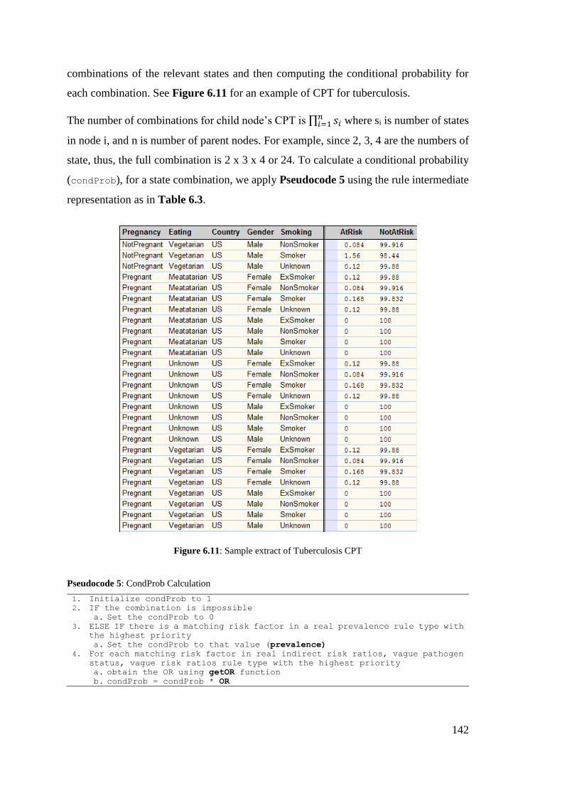
142
combinations of the relevant states and then computing the conditional probability for
each combination. See Figure 6.11 for an example of CPT for tuberculosis.
The number of combinations for child node’s CPT is ∏ 𝑠𝑖𝑛𝑖=1 where si is number of states
in node i, and n is number of parent nodes. For example, since 2, 3, 4 are the numbers of
state, thus, the full combination is 2 x 3 x 4 or 24. To calculate a conditional probability
(condProb), for a state combination, we apply Pseudocode 5 using the rule intermediate
representation as in Table 6.3.
Figure 6.11: Sample extract of Tuberculosis CPT
Pseudocode 5: CondProb Calculation
1. Initialize condProb to 1
2. IF the combination is impossible
a. Set the condProb to 0 3. ELSE IF there is a matching risk factor in a real prevalence rule type with
the highest priority
a. Set the condProb to that value (prevalence) 4. For each matching risk factor in real indirect risk ratios, vague pathogen
status, vague risk ratios rule type with the highest priority
a. obtain the OR using getOR function b. condProb = condProb * OR
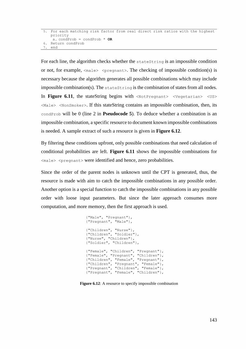
143
5. For each matching risk factor from real direct risk ratios with the highest
priority
a. condProb = condProb * OR 6. Return condProb
7. end
For each line, the algorithm checks whether the stateString is an impossible condition
or not, for example, <male> <pregnant>. The checking of impossible condition(s) is
necessary because the algorithm generates all possible combinations which may include
impossible combination(s). The stateString is the combination of states from all nodes.
In Figure 6.11, the stateString begins with <NotPregnant> <Vegetarian> <US>
<Male> <NonSmoker>. If this stateString contains an impossible combination, then, its
condProb will be 0 (line 2 in Pseudocode 5). To deduce whether a combination is an
impossible combination, a specific resource to document known impossible combinations
is needed. A sample extract of such a resource is given in Figure 6.12.
By filtering these conditions upfront, only possible combinations that need calculation of
conditional probabilities are left. Figure 6.11 shows the impossible combinations for
<male> <pregnant> were identified and hence, zero probabilities.
Since the order of the parent nodes is unknown until the CPT is generated, thus, the
resource is made with aim to catch the impossible combinations in any possible order.
Another option is a special function to catch the impossible combinations in any possible
order with loose input parameters. But since the later approach consumes more
computation, and more memory, then the first approach is used.
{"Male", "Pregnant"},
{"Pregnant", "Male"},
{"Children", "Nurse"},
{"Children", "Soldier"},
{"Nurse", "Children"},
{"Soldier", "Children"},
{"Female", "Children", "Pregnant"},
{"Female", "Pregnant", "Children"},
{"Children", "Female", "Pregnant"},
{"Children", "Pregnant", "Female"},
{"Pregnant", "Children", "Female"},
{"Pregnant", "Female", "Children"},
Figure 6.12: A resource to specify impossible combination
144
If the combination is possible, the next step is to find the prevalence value based on the
location context (e.g. country). This is performed in Line 3 of Pseudocode 5. Thereafter,
the rule types are distinguished as follows: the rule type that provides direct risk ratio (e.g.
real direct risk ratios), or the rule types that need an additional procedure to retrieve the
numerical risk ratio from an ordinal value (e.g. real indirect risk ratios, vague risk ratios,
vague pathogen status). The rule types that need additional procedure call the getOR
procedure to get the numerical OR (see Pseudocode 1 in section 6.3.2).
After the OR is obtained, for each rule type, if the attribute value is contained in the state
combination, the rule is considered “a match”. For example, the first stateString:
“Female, Vegetarian, Smoker”, only Smoker is considered as “match” with S1 rule.
Then, the conditional probability is calculated by multiplying the OR of S1 (e.g. 1.4) with
the existing condProb (line 5a). Another example for dependent rule type: “Male,
Meatatarian, Smoker”, both Male and Smoker is considered as “match” with S10 rule.
Then the conditional probability is calculated by multiplying the OR of S10 (e.g. 13) with
the existing condProb. The logic flow of the Pseudocode 5 follows the rewritten Bayes
chain rule (eq. 6) explained in section 4.4.
6.3.5 Summary
This section explains how an IDR knowledge-base which consists of the IDR disease-
specific ontology and a set of IDR rules is converted into a fully functioning and consistent
Bayesian network using the BN-Builder algorithm. The ontology subclasses and
individuals are transformed into the BN nodes and states. The rules which encode the risk
quantifications (odds ratios, percentages, prevalence value) are used to populate the CPT
of the generated BN. To convert the ontology and rules, two types of intermediate
representation (i.e. multimap) are used to facilitate the resource reusability (e.g. risk
quantifications, prevalence values) during the transformation process from an ontology
to a BN. Two procedures that make use these intermediate representations are then
designed and implemented as part of BN-Builder algorithm: network construction, and
CPT population.
145
6.4 BN-Builder Testing
This section explains the BN-Builder algorithm testing. The procedures of creating the
Bayesian network structure and populating the CPT for the child node were explained in
section 6.3.3 and 6.3.4. As explained in section 6.3, the aim of the BN-Builder algorithm
testing is to ensure that the encoded knowledge in the IDR knowledge-base is consistent
with the generated Bayesian Network. To be more detailed, the BN-Builder is expected
to be able to accommodate the variations that appear on the IDR knowledge-base. The
variation of the IDR knowledge-base here means the mixed categories of the ontology
individuals, not only one type of category (binary only, ordinal only). Since the aim of
the BN-Builder is not only creating BN structure, but also populating the CPT of the child
node, thus, the variation on the data types of each rule type described in section 5.3.3 are
also accommodated.
6.4.1 Testing Plan and Testing Cases
Test Plan
There are two procedures in the BN-Builder: network construction, and CPT population
that covered by this thesis. The network construction procedure is aimed to generate the
IDR disease-specific ontology to become a BN. To test whether the network construction
procedure is correct, the structure of the generated BN is compared to the structure of the
ontology instance. So, if all sub-classes and individuals in the ontology are all correctly
converted to BN nodes and states, the network construction procedure is correct.
The CPT population procedure calculates all combinations of the generated BN
conditions to populate the CPT. Thus, to evaluate the CPT population procedure, the
generated CPT is compared with the manual calculation of the conditional probabilities
using the Bayes chain rule. Two measurements are used to justify whether the CPT is
calculated correctly: (1) distance between the generated conditional probability and the
manually calculated conditional probability. To measure how minimum that the distance
can be accepted statistically, a chi-square test is used. (2) ratio between the observed
attributes. The first measurement is intended for checking whether the Bayes chain rule
is correctly implemented in the BN-Builder algorithm. Whereas the second measurement
146
is aimed to make sure whether the BN-Builder algorithm picks the correct IDR rules for
the correct condition and dependency. This can be observed by comparing the baseline
of the risk factor with the other risk factors.
Test Cases
To test the features of the BN-Builder algorithm, test cases (as a form of IDR knowledge-
base) need to be prepared carefully using these criteria:
For the rule-base specification, the test cases should contain (1) all five IDR rule types,
(2) risk quantifications that are covered by all rule types, (3) both dependent and
independent types, (4) conflicting and duplicate rules with different priority values.
To test whether the BN-Builder algorithm are capable of generating a fully-functioning
and consistent BN from a knowledge-base, the test cases are prepared (5) to prevalent in
two locations that have different prevalence values, (6) to have impossible combinations,
(7) to contain multi-level sub-classes, (8) to have a similar individual name for different
nodes, and (9) to have mixed categorical attributes.
Admittedly, IDR knowledge-bases that contain all these criteria might not exist.
Therefore, the closest IDR knowledge-bases are chosen from the 22 IDR knowledge-
bases used for ontology evaluation in section 5.5. Two of those, intrathoracic tuberculosis
in Indonesia (TBINS) and spinal tuberculosis in China (TBCHN), cover almost all the
criteria, and no other knowledge-base adds to the covered criteria. Therefore, dummy rules
are added to the chosen two to meet the missing criteria (the validity of the test
knowledge-bases is irrelevant for this evaluation).
The left-most column in Table 6.4 shows that all criteria are allocated either in the TBINS,
or in the TBCHN case, or both. This table makes sure that all designed functions of the BN-
Builder are implemented and tested accordingly in at least one IDR knowledge-base.
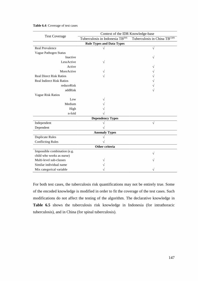
147
Table 6.4: Coverage of test cases
Test Coverage Context of the IDR Knowledge-base
Tuberculosis in Indonesia TBINS Tuberculosis in China TBCHN
Rule Types and Data Types
Real Prevalence
Vague Pathogen Status
Inactive
LessActive
Active
MoreActive
Real Direct Risk Ratios
Real Indirect Risk Ratios
reduceRisk
addRisk
Vague Risk Ratios
Low
Medium
High
n-fold
Dependency Types
Independent
Dependent
Anomaly Types
Duplicate Rules
Conflicting Rules
Other criteria
Impossible combination (e.g.
child who works as nurse)
Multi-level sub-classes
Similar individual name
Mix categorical variable
For both test cases, the tuberculosis risk quantifications may not be entirely true. Some
of the encoded knowledge is modified in order to fit the coverage of the test cases. Such
modifications do not affect the testing of the algorithm. The declarative knowledge in
Table 6.5 shows the tuberculosis risk knowledge in Indonesia (for intrathoracic
tuberculosis), and in China (for spinal tuberculosis).
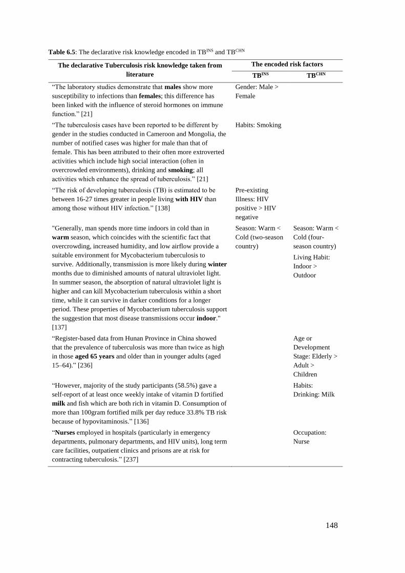
148
Table 6.5: The declarative risk knowledge encoded in TBINS and TBCHN
The declarative Tuberculosis risk knowledge taken from
literature
The encoded risk factors
TBINS TBCHN
“The laboratory studies demonstrate that males show more
susceptibility to infections than females; this difference has
been linked with the influence of steroid hormones on immune
function.” [21]
Gender: Male >
Female
“The tuberculosis cases have been reported to be different by
gender in the studies conducted in Cameroon and Mongolia, the
number of notified cases was higher for male than that of
female. This has been attributed to their often more extroverted
activities which include high social interaction (often in
overcrowded environments), drinking and smoking; all
activities which enhance the spread of tuberculosis.” [21]
Habits: Smoking
“The risk of developing tuberculosis (TB) is estimated to be
between 16-27 times greater in people living with HIV than
among those without HIV infection.” [138]
Pre-existing
Illness: HIV
positive > HIV
negative
"Generally, man spends more time indoors in cold than in
warm season, which coincides with the scientific fact that
overcrowding, increased humidity, and low airflow provide a
suitable environment for Mycobacterium tuberculosis to
survive. Additionally, transmission is more likely during winter
months due to diminished amounts of natural ultraviolet light.
In summer season, the absorption of natural ultraviolet light is
higher and can kill Mycobacterium tuberculosis within a short
time, while it can survive in darker conditions for a longer
period. These properties of Mycobacterium tuberculosis support
the suggestion that most disease transmissions occur indoor."
[137]
Season: Warm <
Cold (two-season
country)
Season: Warm <
Cold (four-
season country)
Living Habit:
Indoor >
Outdoor
“Register-based data from Hunan Province in China showed
that the prevalence of tuberculosis was more than twice as high
in those aged 65 years and older than in younger adults (aged
15–64).” [236]
Age or
Development
Stage: Elderly >
Adult >
Children
“However, majority of the study participants (58.5%) gave a
self-report of at least once weekly intake of vitamin D fortified
milk and fish which are both rich in vitamin D. Consumption of
more than 100gram fortified milk per day reduce 33.8% TB risk
because of hypovitaminosis.” [136]
Habits:
Drinking: Milk
“Nurses employed in hospitals (particularly in emergency
departments, pulmonary departments, and HIV units), long term
care facilities, outpatient clinics and prisons are at risk for
contracting tuberculosis.” [237]
Occupation:
Nurse
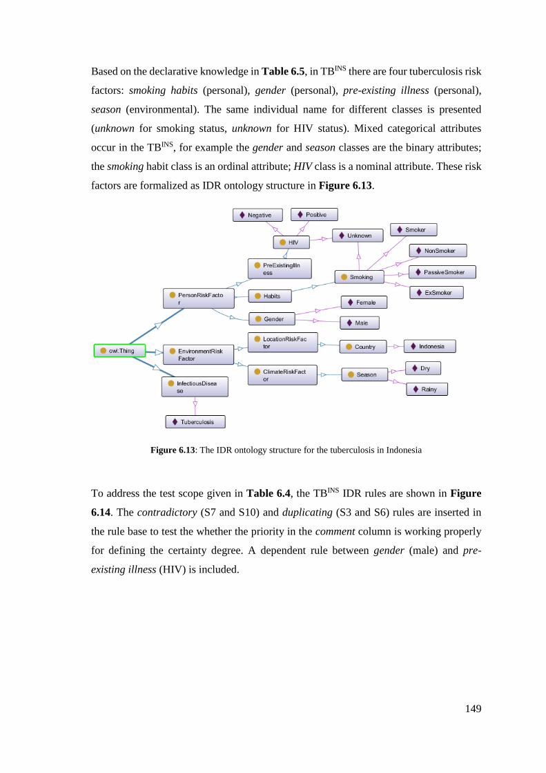
149
Based on the declarative knowledge in Table 6.5, in TBINS there are four tuberculosis risk
factors: smoking habits (personal), gender (personal), pre-existing illness (personal),
season (environmental). The same individual name for different classes is presented
(unknown for smoking status, unknown for HIV status). Mixed categorical attributes
occur in the TBINS, for example the gender and season classes are the binary attributes;
the smoking habit class is an ordinal attribute; HIV class is a nominal attribute. These risk
factors are formalized as IDR ontology structure in Figure 6.13.
Figure 6.13: The IDR ontology structure for the tuberculosis in Indonesia
To address the test scope given in Table 6.4, the TBINS IDR rules are shown in Figure
6.14. The contradictory (S7 and S10) and duplicating (S3 and S6) rules are inserted in
the rule base to test the whether the priority in the comment column is working properly
for defining the certainty degree. A dependent rule between gender (male) and pre-
existing illness (HIV) is included.
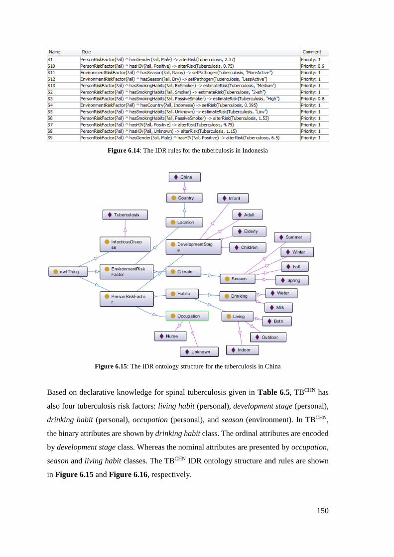
150
Figure 6.14: The IDR rules for the tuberculosis in Indonesia
Figure 6.15: The IDR ontology structure for the tuberculosis in China
Based on declarative knowledge for spinal tuberculosis given in Table 6.5, TBCHN has
also four tuberculosis risk factors: living habit (personal), development stage (personal),
drinking habit (personal), occupation (personal), and season (environment). In TBCHN,
the binary attributes are shown by drinking habit class. The ordinal attributes are encoded
by development stage class. Whereas the nominal attributes are presented by occupation,
season and living habit classes. The TBCHN IDR ontology structure and rules are shown
in Figure 6.15 and Figure 6.16, respectively.
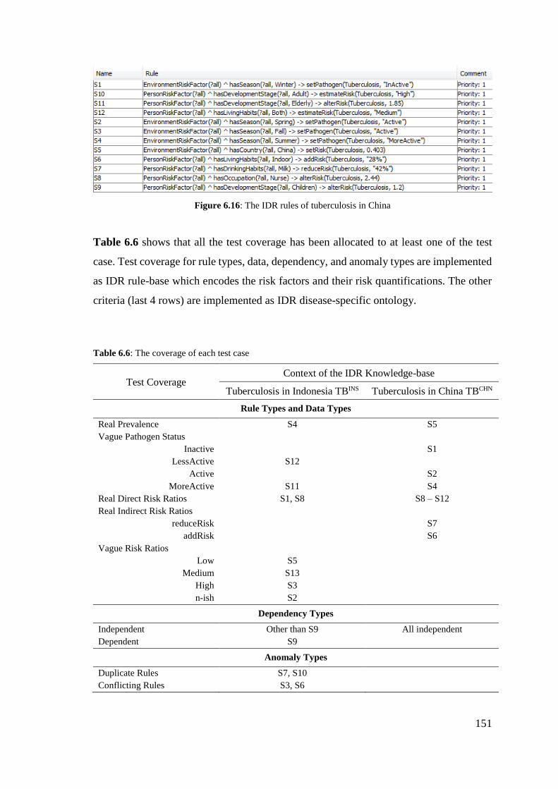
151
Figure 6.16: The IDR rules of tuberculosis in China
Table 6.6 shows that all the test coverage has been allocated to at least one of the test
case. Test coverage for rule types, data, dependency, and anomaly types are implemented
as IDR rule-base which encodes the risk factors and their risk quantifications. The other
criteria (last 4 rows) are implemented as IDR disease-specific ontology.
Table 6.6: The coverage of each test case
Test Coverage Context of the IDR Knowledge-base
Tuberculosis in Indonesia TBINS Tuberculosis in China TBCHN
Rule Types and Data Types
Real Prevalence S4 S5
Vague Pathogen Status
Inactive S1
LessActive S12
Active S2
MoreActive S11 S4
Real Direct Risk Ratios S1, S8 S8 – S12
Real Indirect Risk Ratios
reduceRisk S7
addRisk S6
Vague Risk Ratios
Low S5
Medium S13
High S3
n-ish S2
Dependency Types
Independent Other than S9 All independent
Dependent S9
Anomaly Types
Duplicate Rules S7, S10
Conflicting Rules S3, S6
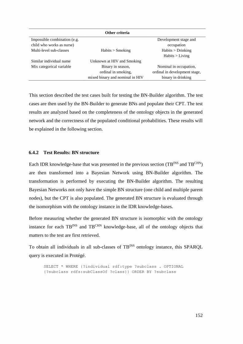
152
Other criteria
Impossible combination (e.g.
child who works as nurse)
Development stage and
occupation
Multi-level sub-classes Habits > Smoking Habits > Drinking
Habits > Living
Similar individual name Unknown at HIV and Smoking
Mix categorical variable Binary in season,
ordinal in smoking,
mixed binary and nominal in HIV
Nominal in occupation,
ordinal in development stage,
binary in drinking
This section described the test cases built for testing the BN-Builder algorithm. The test
cases are then used by the BN-Builder to generate BNs and populate their CPT. The test
results are analyzed based on the completeness of the ontology objects in the generated
network and the correctness of the populated conditional probabilities. These results will
be explained in the following section.
6.4.2 Test Results: BN structure
Each IDR knowledge-base that was presented in the previous section (TBINS and TBCHN)
are then transformed into a Bayesian Network using BN-Builder algorithm. The
transformation is performed by executing the BN-Builder algorithm. The resulting
Bayesian Networks not only have the simple BN structure (one child and multiple parent
nodes), but the CPT is also populated. The generated BN structure is evaluated through
the isomorphism with the ontology instance in the IDR knowledge-bases.
Before measuring whether the generated BN structure is isomorphic with the ontology
instance for each TBINS and TBCHN knowledge-base, all of the ontology objects that
matters to the test are first retrieved.
To obtain all individuals in all sub-classes of TBINS ontology instance, this SPARQL
query is executed in Protégé.
SELECT * WHERE {?individual rdf:type ?subclass . OPTIONAL
{?subclass rdfs:subClassOf ?class}} ORDER BY ?subclass
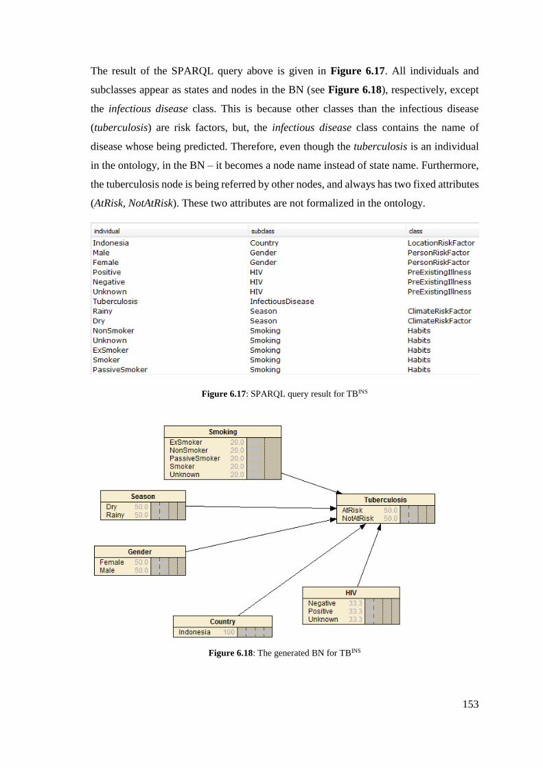
153
The result of the SPARQL query above is given in Figure 6.17. All individuals and
subclasses appear as states and nodes in the BN (see Figure 6.18), respectively, except
the infectious disease class. This is because other classes than the infectious disease
(tuberculosis) are risk factors, but, the infectious disease class contains the name of
disease whose being predicted. Therefore, even though the tuberculosis is an individual
in the ontology, in the BN – it becomes a node name instead of state name. Furthermore,
the tuberculosis node is being referred by other nodes, and always has two fixed attributes
(AtRisk, NotAtRisk). These two attributes are not formalized in the ontology.
Figure 6.17: SPARQL query result for TBINS
Figure 6.18: The generated BN for TBINS
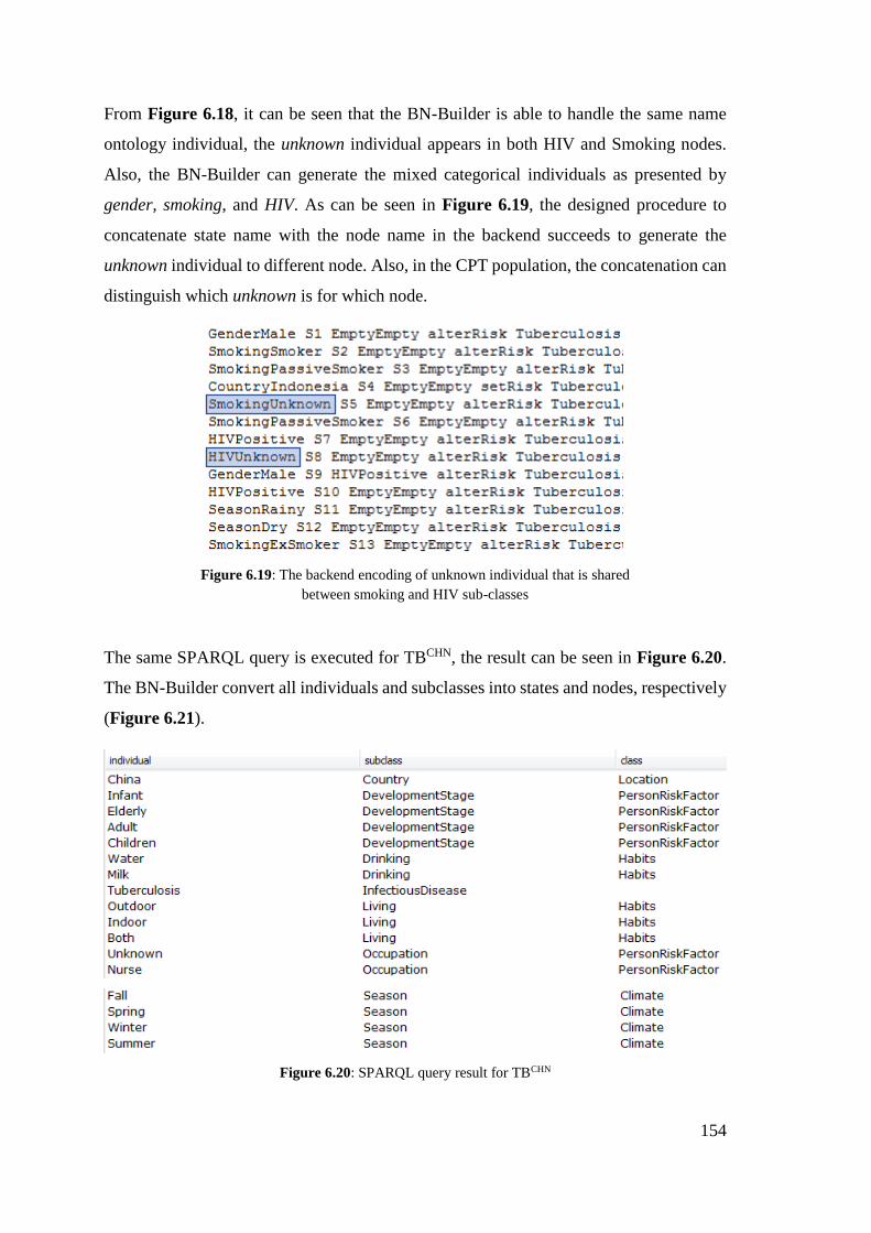
154
From Figure 6.18, it can be seen that the BN-Builder is able to handle the same name
ontology individual, the unknown individual appears in both HIV and Smoking nodes.
Also, the BN-Builder can generate the mixed categorical individuals as presented by
gender, smoking, and HIV. As can be seen in Figure 6.19, the designed procedure to
concatenate state name with the node name in the backend succeeds to generate the
unknown individual to different node. Also, in the CPT population, the concatenation can
distinguish which unknown is for which node.
Figure 6.19: The backend encoding of unknown individual that is shared
between smoking and HIV sub-classes
The same SPARQL query is executed for TBCHN, the result can be seen in Figure 6.20.
The BN-Builder convert all individuals and subclasses into states and nodes, respectively
(Figure 6.21).
Figure 6.20: SPARQL query result for TBCHN
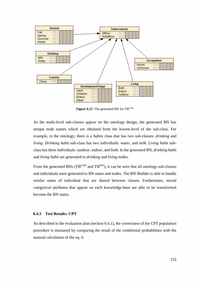
155
Figure 6.21: The generated BN for TBCHN
As the multi-level sub-classes appear on the ontology design, the generated BN has
unique node names which are obtained from the lowest-level of the sub-class. For
example, in the ontology, there is a habits class that has two sub-classes: drinking and
living. Drinking habit sub-class has two individuals: water, and milk. Living habit sub-
class has three individuals: outdoor, indoor, and both. In the generated BN, drinking habit
and living habit are generated to drinking and living nodes.
From the generated BNs (TBCHN and TBINS), it can be seen that all ontology sub-classes
and individuals were generated to BN states and nodes. The BN-Builder is able to handle
similar name of individual that are shared between classes. Furthermore, mixed
categorical attributes that appear on each knowledge-base are able to be transformed
become the BN states.
6.4.3 Test Results: CPT
As described in the evaluation plan (section 6.4.1), the correctness of the CPT population
procedure is measured by comparing the result of the conditional probabilities with the
manual calculation of the eq. 6.
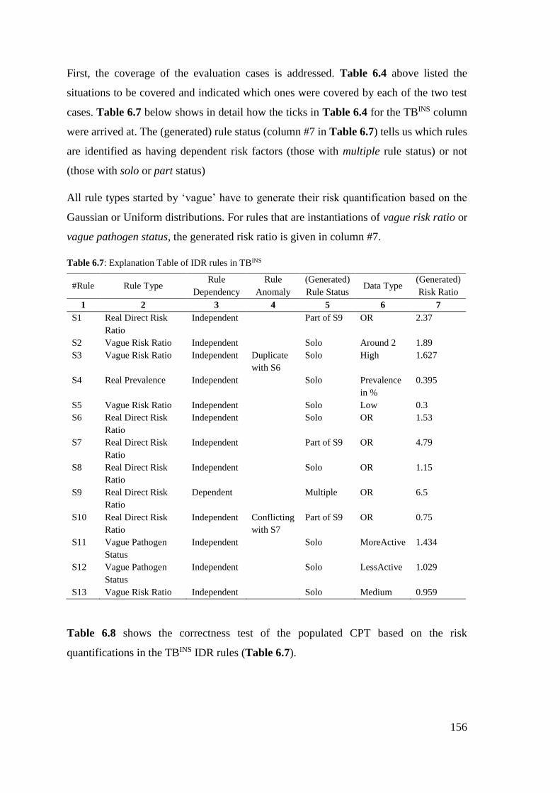
156
First, the coverage of the evaluation cases is addressed. Table 6.4 above listed the
situations to be covered and indicated which ones were covered by each of the two test
cases. Table 6.7 below shows in detail how the ticks in Table 6.4 for the TBINS column
were arrived at. The (generated) rule status (column #7 in Table 6.7) tells us which rules
are identified as having dependent risk factors (those with multiple rule status) or not
(those with solo or part status)
All rule types started by ‘vague’ have to generate their risk quantification based on the
Gaussian or Uniform distributions. For rules that are instantiations of vague risk ratio or
vague pathogen status, the generated risk ratio is given in column #7.
Table 6.7: Explanation Table of IDR rules in TBINS
#Rule Rule Type Rule
Dependency
Rule
Anomaly
(Generated)
Rule Status Data Type
(Generated)
Risk Ratio
1 2 3 4 5 6 7
S1 Real Direct Risk
Ratio
Independent Part of S9 OR 2.37
S2 Vague Risk Ratio Independent Solo Around 2 1.89
S3 Vague Risk Ratio Independent Duplicate
with S6
Solo High 1.627
S4 Real Prevalence Independent Solo Prevalence
in %
0.395
S5 Vague Risk Ratio Independent Solo Low 0.3
S6 Real Direct Risk
Ratio
Independent Solo OR 1.53
S7 Real Direct Risk
Ratio
Independent Part of S9 OR 4.79
S8 Real Direct Risk
Ratio
Independent Solo OR 1.15
S9 Real Direct Risk
Ratio
Dependent Multiple OR 6.5
S10 Real Direct Risk
Ratio
Independent Conflicting
with S7
Part of S9 OR 0.75
S11 Vague Pathogen
Status
Independent Solo MoreActive 1.434
S12 Vague Pathogen
Status
Independent Solo LessActive 1.029
S13 Vague Risk Ratio Independent Solo Medium 0.959
Table 6.8 shows the correctness test of the populated CPT based on the risk
quantifications in the TBINS IDR rules (Table 6.7).
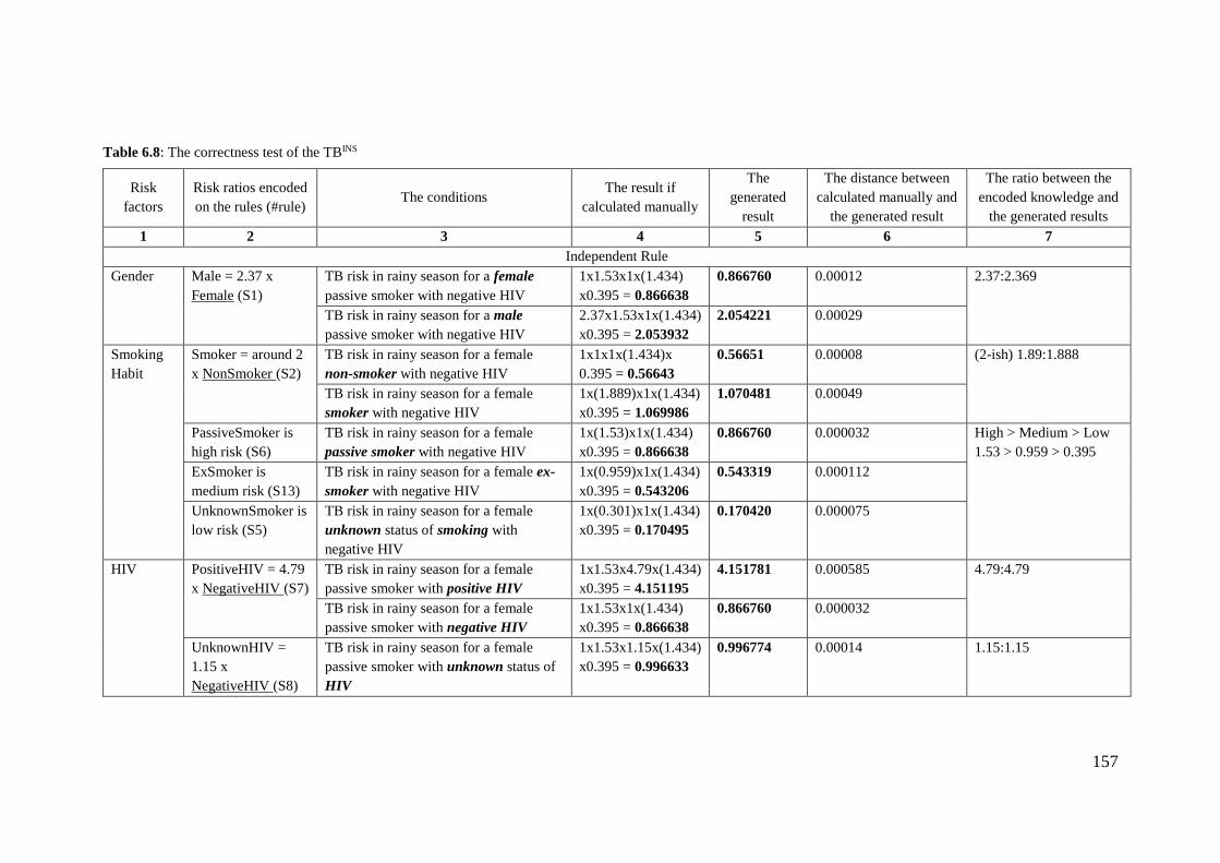
157
Table 6.8: The correctness test of the TBINS
Risk
factors
Risk ratios encoded
on the rules (#rule) The conditions
The result if
calculated manually
The
generated
result
The distance between
calculated manually and
the generated result
The ratio between the
encoded knowledge and
the generated results
1 2 3 4 5 6 7
Independent Rule
Gender Male = 2.37 x
Female (S1)
TB risk in rainy season for a female
passive smoker with negative HIV
1x1.53x1x(1.434)
x0.395 = 0.866638
0.866760 0.00012 2.37:2.369
TB risk in rainy season for a male
passive smoker with negative HIV
2.37x1.53x1x(1.434)
x0.395 = 2.053932
2.054221 0.00029
Smoking
Habit
Smoker = around 2
x NonSmoker (S2)
TB risk in rainy season for a female
non-smoker with negative HIV
1x1x1x(1.434)x
0.395 = 0.56643
0.56651 0.00008 (2-ish) 1.89:1.888
TB risk in rainy season for a female
smoker with negative HIV
1x(1.889)x1x(1.434)
x0.395 = 1.069986
1.070481 0.00049
PassiveSmoker is
high risk (S6)
TB risk in rainy season for a female
passive smoker with negative HIV
1x(1.53)x1x(1.434)
x0.395 = 0.866638
0.866760 0.000032 High > Medium > Low
1.53 > 0.959 > 0.395
ExSmoker is
medium risk (S13)
TB risk in rainy season for a female ex-
smoker with negative HIV
1x(0.959)x1x(1.434)
x0.395 = 0.543206
0.543319 0.000112
UnknownSmoker is
low risk (S5)
TB risk in rainy season for a female
unknown status of smoking with
negative HIV
1x(0.301)x1x(1.434)
x0.395 = 0.170495
0.170420 0.000075
HIV PositiveHIV = 4.79
x NegativeHIV (S7)
TB risk in rainy season for a female
passive smoker with positive HIV
1x1.53x4.79x(1.434)
x0.395 = 4.151195
4.151781 0.000585 4.79:4.79
TB risk in rainy season for a female
passive smoker with negative HIV
1x1.53x1x(1.434)
x0.395 = 0.866638
0.866760 0.000032
UnknownHIV =
1.15 x
NegativeHIV (S8)
TB risk in rainy season for a female
passive smoker with unknown status of
HIV
1x1.53x1.15x(1.434)
x0.395 = 0.996633
0.996774 0.00014 1.15:1.15
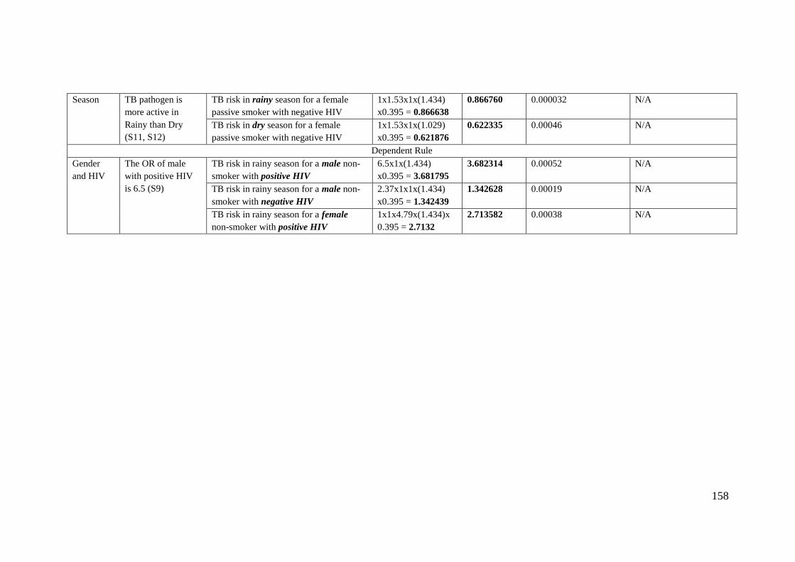
158
Season TB pathogen is
more active in
Rainy than Dry
(S11, S12)
TB risk in rainy season for a female
passive smoker with negative HIV
1x1.53x1x(1.434)
x0.395 = 0.866638
0.866760 0.000032 N/A
TB risk in dry season for a female
passive smoker with negative HIV
1x1.53x1x(1.029)
x0.395 = 0.621876
0.622335 0.00046 N/A
Dependent Rule
Gender
and HIV
The OR of male
with positive HIV
is 6.5 (S9)
TB risk in rainy season for a male non-
smoker with positive HIV
6.5x1x(1.434)
x0.395 = 3.681795
3.682314 0.00052 N/A
TB risk in rainy season for a male non-
smoker with negative HIV
2.37x1x1x(1.434)
x0.395 = 1.342439
1.342628 0.00019 N/A
TB risk in rainy season for a female
non-smoker with positive HIV
1x1x4.79x(1.434)x
0.395 = 2.7132
2.713582 0.00038 N/A
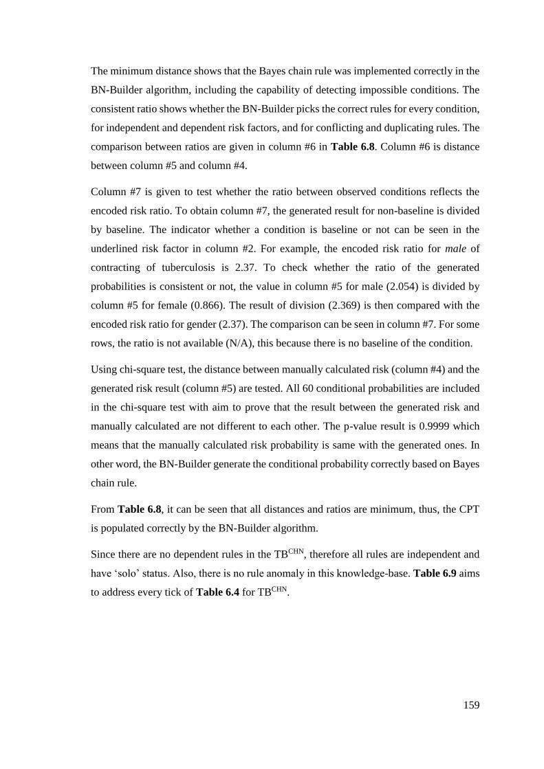
159
The minimum distance shows that the Bayes chain rule was implemented correctly in the
BN-Builder algorithm, including the capability of detecting impossible conditions. The
consistent ratio shows whether the BN-Builder picks the correct rules for every condition,
for independent and dependent risk factors, and for conflicting and duplicating rules. The
comparison between ratios are given in column #6 in Table 6.8. Column #6 is distance
between column #5 and column #4.
Column #7 is given to test whether the ratio between observed conditions reflects the
encoded risk ratio. To obtain column #7, the generated result for non-baseline is divided
by baseline. The indicator whether a condition is baseline or not can be seen in the
underlined risk factor in column #2. For example, the encoded risk ratio for male of
contracting of tuberculosis is 2.37. To check whether the ratio of the generated
probabilities is consistent or not, the value in column #5 for male (2.054) is divided by
column #5 for female (0.866). The result of division (2.369) is then compared with the
encoded risk ratio for gender (2.37). The comparison can be seen in column #7. For some
rows, the ratio is not available (N/A), this because there is no baseline of the condition.
Using chi-square test, the distance between manually calculated risk (column #4) and the
generated risk result (column #5) are tested. All 60 conditional probabilities are included
in the chi-square test with aim to prove that the result between the generated risk and
manually calculated are not different to each other. The p-value result is 0.9999 which
means that the manually calculated risk probability is same with the generated ones. In
other word, the BN-Builder generate the conditional probability correctly based on Bayes
chain rule.
From Table 6.8, it can be seen that all distances and ratios are minimum, thus, the CPT
is populated correctly by the BN-Builder algorithm.
Since there are no dependent rules in the TBCHN, therefore all rules are independent and
have ‘solo’ status. Also, there is no rule anomaly in this knowledge-base. Table 6.9 aims
to address every tick of Table 6.4 for TBCHN.
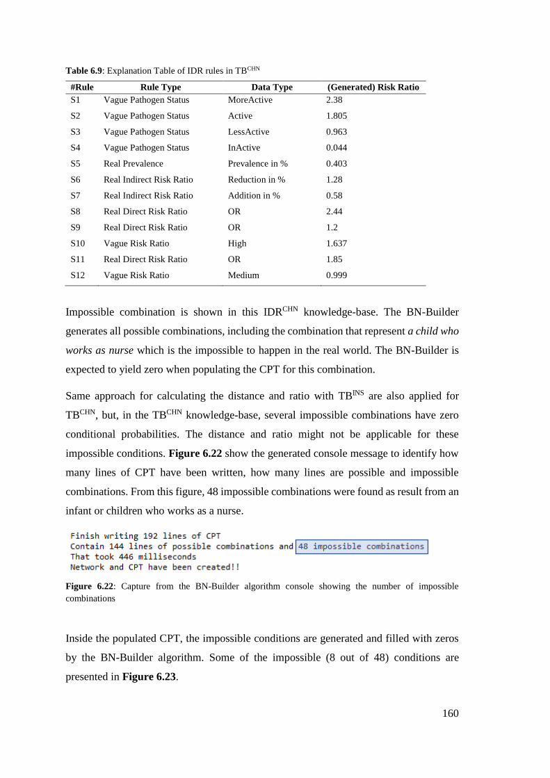
160
Table 6.9: Explanation Table of IDR rules in TBCHN
#Rule Rule Type Data Type (Generated) Risk Ratio
S1 Vague Pathogen Status MoreActive 2.38
S2 Vague Pathogen Status Active 1.805
S3 Vague Pathogen Status LessActive 0.963
S4 Vague Pathogen Status InActive 0.044
S5 Real Prevalence Prevalence in % 0.403
S6 Real Indirect Risk Ratio Reduction in % 1.28
S7 Real Indirect Risk Ratio Addition in % 0.58
S8 Real Direct Risk Ratio OR 2.44
S9 Real Direct Risk Ratio OR 1.2
S10 Vague Risk Ratio High 1.637
S11 Real Direct Risk Ratio OR 1.85
S12 Vague Risk Ratio Medium 0.999
Impossible combination is shown in this IDRCHN knowledge-base. The BN-Builder
generates all possible combinations, including the combination that represent a child who
works as nurse which is the impossible to happen in the real world. The BN-Builder is
expected to yield zero when populating the CPT for this combination.
Same approach for calculating the distance and ratio with TBINS are also applied for
TBCHN, but, in the TBCHN knowledge-base, several impossible combinations have zero
conditional probabilities. The distance and ratio might not be applicable for these
impossible conditions. Figure 6.22 show the generated console message to identify how
many lines of CPT have been written, how many lines are possible and impossible
combinations. From this figure, 48 impossible combinations were found as result from an
infant or children who works as a nurse.
Figure 6.22: Capture from the BN-Builder algorithm console showing the number of impossible
combinations
Inside the populated CPT, the impossible conditions are generated and filled with zeros
by the BN-Builder algorithm. Some of the impossible (8 out of 48) conditions are
presented in Figure 6.23.
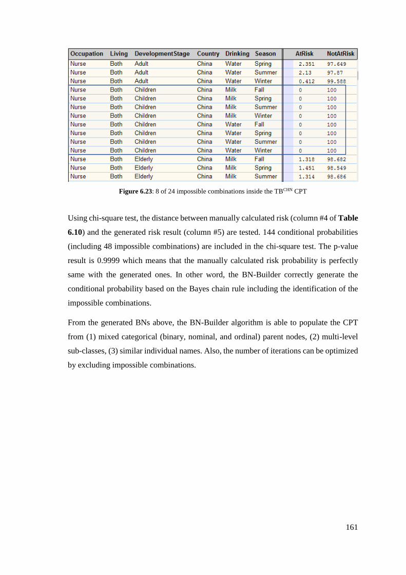
161
Figure 6.23: 8 of 24 impossible combinations inside the TBCHN CPT
Using chi-square test, the distance between manually calculated risk (column #4 of Table
6.10) and the generated risk result (column #5) are tested. 144 conditional probabilities
(including 48 impossible combinations) are included in the chi-square test. The p-value
result is 0.9999 which means that the manually calculated risk probability is perfectly
same with the generated ones. In other word, the BN-Builder correctly generate the
conditional probability based on the Bayes chain rule including the identification of the
impossible combinations.
From the generated BNs above, the BN-Builder algorithm is able to populate the CPT
from (1) mixed categorical (binary, nominal, and ordinal) parent nodes, (2) multi-level
sub-classes, (3) similar individual names. Also, the number of iterations can be optimized
by excluding impossible combinations.
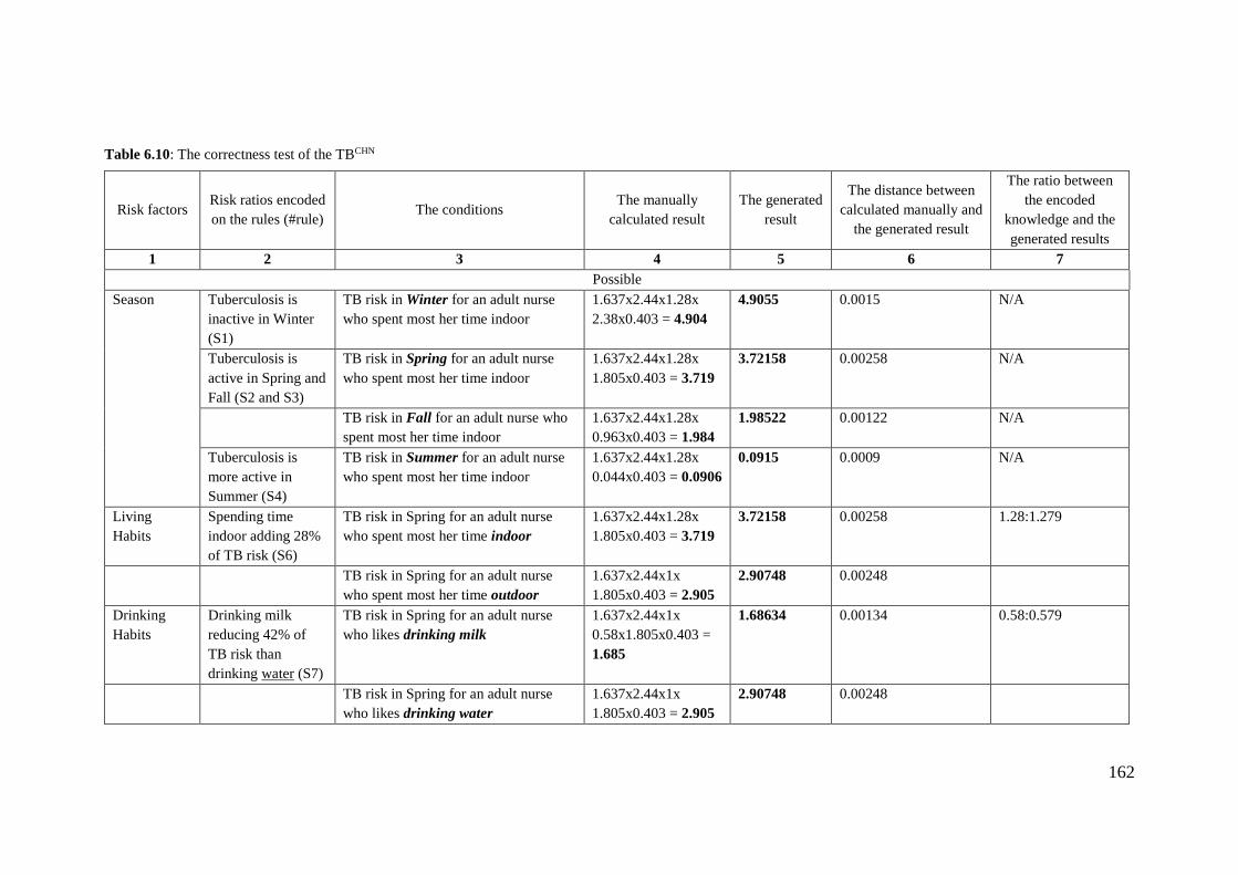
162
Table 6.10: The correctness test of the TBCHN
Risk factors Risk ratios encoded
on the rules (#rule) The conditions
The manually
calculated result
The generated
result
The distance between
calculated manually and
the generated result
The ratio between
the encoded
knowledge and the
generated results
1 2 3 4 5 6 7
Possible
Season Tuberculosis is
inactive in Winter
(S1)
TB risk in Winter for an adult nurse
who spent most her time indoor
1.637x2.44x1.28x
2.38x0.403 = 4.904
4.9055 0.0015 N/A
Tuberculosis is
active in Spring and
Fall (S2 and S3)
TB risk in Spring for an adult nurse
who spent most her time indoor
1.637x2.44x1.28x
1.805x0.403 = 3.719
3.72158 0.00258 N/A
TB risk in Fall for an adult nurse who
spent most her time indoor
1.637x2.44x1.28x
0.963x0.403 = 1.984
1.98522 0.00122 N/A
Tuberculosis is
more active in
Summer (S4)
TB risk in Summer for an adult nurse
who spent most her time indoor
1.637x2.44x1.28x
0.044x0.403 = 0.0906
0.0915 0.0009 N/A
Living
Habits
Spending time
indoor adding 28%
of TB risk (S6)
TB risk in Spring for an adult nurse
who spent most her time indoor
1.637x2.44x1.28x
1.805x0.403 = 3.719
3.72158 0.00258 1.28:1.279
TB risk in Spring for an adult nurse
who spent most her time outdoor
1.637x2.44x1x
1.805x0.403 = 2.905
2.90748 0.00248
Drinking
Habits
Drinking milk
reducing 42% of
TB risk than
drinking water (S7)
TB risk in Spring for an adult nurse
who likes drinking milk
1.637x2.44x1x
0.58x1.805x0.403 =
1.685
1.68634 0.00134 0.58:0.579
TB risk in Spring for an adult nurse
who likes drinking water 1.637x2.44x1x
1.805x0.403 = 2.905
2.90748 0.00248
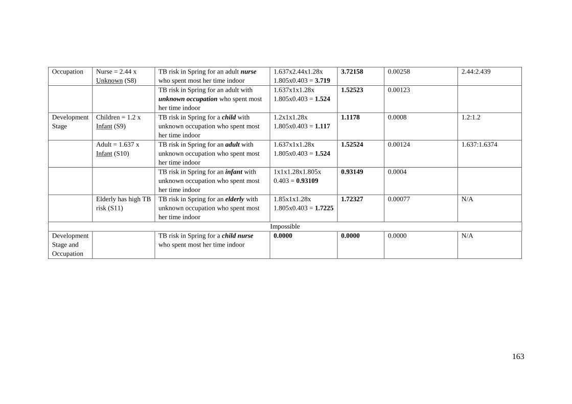
163
Occupation Nurse = 2.44 x
Unknown (S8)
TB risk in Spring for an adult nurse
who spent most her time indoor
1.637x2.44x1.28x
1.805x0.403 = 3.719
3.72158 0.00258 2.44:2.439
TB risk in Spring for an adult with
unknown occupation who spent most
her time indoor
1.637x1x1.28x
1.805x0.403 = 1.524
1.52523 0.00123
Development
Stage
Children = 1.2 x
Infant (S9)
TB risk in Spring for a child with
unknown occupation who spent most
her time indoor
1.2x1x1.28x
1.805x0.403 = 1.117
1.1178 0.0008 1.2:1.2
Adult = 1.637 x
Infant (S10)
TB risk in Spring for an adult with
unknown occupation who spent most
her time indoor
1.637x1x1.28x
1.805x0.403 = 1.524
1.52524 0.00124 1.637:1.6374
TB risk in Spring for an infant with
unknown occupation who spent most
her time indoor
1x1x1.28x1.805x
0.403 = 0.93109
0.93149 0.0004
Elderly has high TB
risk (S11)
TB risk in Spring for an elderly with
unknown occupation who spent most
her time indoor
1.85x1x1.28x
1.805x0.403 = 1.7225
1.72327 0.00077 N/A
Impossible
Development
Stage and
Occupation
TB risk in Spring for a child nurse
who spent most her time indoor
0.0000 0.0000 0.0000 N/A
164
6.5 Conclusion
The BN-Builder algorithm is designed to generate the BN structure from the ontology
structure and populate the CPT of the BN from the IDR rules. From testing results, the
BN-Builder algorithm can generate the BN structure from ontology nodes and states
correctly. By implementing the Bayes chain rule, the BN-Builder is able to populate CPT
from mixed binary, ordinal and nominal nodes. These results suggest that the BN-Builder
algorithm can surpass the existing algorithms for populating the CPT (e.g. Noisy-OR,
Noisy-AND, weight-sum) or existing approaches (e.g. BayesOWL, BNTab).
However, the Bayes chain rule is limited to (infectious) disease risk calculation only since
it makes use of risk ratios and prevalence value. For general purposes, it will require
different version of the Bayes chain rule.
The testing has shown that the BN-Builder algorithm can handle shared individual names
in the ontology correctly, as demonstrated by the unknown status for person’s smoking
habit and HIV pre-existing illness. This suggests that BN-Builder algorithm can facilitate
shared individuals in an ontology sub-class each becoming a separate state in a different
node. Besides that, the testing has also demonstrated that the BN-Builder algorithm can
manage hierarchical relationships (i.e. multi-level sub-classes). For example, a person’s
habits have specialization: smoking habit or drinking habit. The BN-Builder is able to
pick the lowest level to preserve the uniqueness of the node names.
All distances and ratios between the generated CPT and the manually calculated
probabilities are measured. Chi-square test statistics prove that there is no significant
difference between the generated and manual calculation of conditional probabilities (p
> 0.05). From this testing, it can be concluded that the BN-Builder algorithm can correctly
populate the CPT based on the Bayes chain rule.
For the ordinal risk ratios, the BN-Builder can generate a risk ratio based on the encoded
ordinal values (e.g. low, medium, high). The comparisons between the conditional
probability results and the ordinal values are consistent. Besides the ordinal risk ratios,
the conditions that involve the pathogen activation status (e.g. inactive, less active, active,
more active) that are also presented as ordinal values are correctly populated.
165
Another form of risk ratios, addition or reduction with certain percentage, is included in
the test knowledge-base (TBCHN). The results are observed and consistent with the
encoded percentage values.
Some conditions which are considered as impossible are identified by putting resources
in a library. The BN-Builder algorithm is able handle them correctly. For example, a child
who works as a nurse, as a result from auto-combination result between development
stage (infant, child, adult, elderly) and occupation (nurse, unknown). The conditional
probability for these impossible combinations are proven to be zeros.
To sum up, the BN-Builder algorithm has been designed to be able to deal with the special
characteristics of infectious disease risk knowledge which have mixed categorical, similar
individuals, and hierarchy that was encoded in the IDR knowledge-bases. It is also able
to handle the risk quantifications relevant to infectious disease risk knowledge: risk ratios
(in ratio, percentage, and ordinal), and prevalence value. From the testing, it can be
concluded that the BN-Builder algorithm can generate BN and populate the CPT
correctly, thus, it demonstrates that the generated BN is fully functioning and consistent.
166
7. CONCLUSIONS
7.1 Overview
This thesis has presented the knowledge representation (chapter 5) that is able to encode
the declarative infectious disease risk knowledge published in the Atlas of Human
Infectious Diseases (AHID), WHO, CDC factsheets, and other journals related to
epidemiology for infectious diseases. The related algorithm, the BN-Builder, which aims
to convert the instantiation of the knowledge representation (i.e. knowledge-base) into an
equivalent risk prediction model, is also presented (chapter 6). The contextual system
architecture in which these knowledge representation and algorithm will be expected to
work is also presented (chapter 4).
This chapter discusses the objectives of the thesis and how they are answered. Also, the
contribution this work has made to the state of the art of infectious disease risk knowledge
representation and in particular the BN-generation algorithm is stated.
7.2 Objectives and Achievements
The research question in this thesis was ‘can a useful knowledge representation be
designed to encode infectious disease risk knowledge and can this the encoded knowledge
be correctly availed of to yield personalized infectious disease risk prediction?’. To
answer this research question, three objectives were posed.
The first objective of the research described in this thesis was to understand the
knowledge of epidemiology for infectious disease risk in general, and how to estimate
disease risk in a person using a prediction model.
This objective was achieved through comprehending the concepts of human infection
flow, chain of infection, and all affecting environmental risk factors for human infectious
diseases from established knowledge sources. From the infection flow in a person, four
compartments that are used to estimate a person’s infectious disease risk in epidemiology
are: Susceptible (S) – Exposed (E) – Infected (I) – Recovered (R). Factors that contribute
to the S and E compartments need to be modelled and quantified in a relevant way to
calculate the personalized infectious disease risk. Most person risk factors were identified
167
from this knowledge. For example, common person attributes that are relevant to a
person’s susceptibility level are development stage, nutrition intake, habits. From the
chain of infection, pathogen life requirements, reservoirs, transmission modes, and
susceptible hosts were learned. From this knowledge, the general implication of the
person and environment attributes to the infectious disease risk were investigated. For
example, Mycobacterium Tuberculosis does not exist during Summer due to ultraviolet
light that prevents these bacteria thriving and multiplying. More detailed atmospheric
attributes of weather and season are also known to have direct contribution to infectious
disease risks.
To estimate a person's risk of contracting human infectious diseases, the obtained
personal and environmental infectious disease risk factors need to be quantified. Relevant
formulae that are used to calculate a personalized infectious disease risk from several risk
quantifications were investigated. Some limitations that appear in these formulae, such
as, binary or multivalued attributes were overcome using the Bayes chain rule for
infectious disease risk prediction.
The second objective of the research was to design a knowledge representation that is
able to encode the declarative infectious disease risk knowledge that allows automatic
generation of a prediction model.
This objective could be accomplished through utilizing an ontology for encoding the
infectious disease risk factors and availing of semantic-web rules for encoding risk
quantifications that are needed by the Bayes chain rule. The IDR generic ontology was
built to model the structure of the infectious disease risk factors. The IDR generic
ontology consists of the main classes that are always inherited by the IDR knowledge-
bases: person risk factor, environment risk factor, infectious disease. The IDR generic
ontology is expected to be representative and evolution-proof for all human infectious
diseases, including new ones. The IDR disease-specific ontology was built from using the
ontology objects (individuals, sub-classes) of the IDR generic ontology. The IDR
ontology was developed to accommodate all mentioned personal and environmental risk
factors for all human infectious diseases from AHID, WHO, and CDC factsheets.
Thereafter, all types of (infectious) disease risk quantifications were investigated and five
IDR rule types were established to accommodate all the kinds of risk quantifications. The
168
IDR generic ontology and five IDR rule types are designed to help epidemiologists to
instantiate a contextual knowledge-base that encodes an infectious disease risk
knowledge prevalent in a particular country.
An algorithm, BN-Builder, was then designed for converting the encoded infectious
disease risk prediction in the knowledge-base into the risk prediction model (Bayesian
Network). The BN-Builder converts the knowledge-base into an equivalent Bayesian
Network. Some reasoning ability is included in the BN-Builder to allow it to: manage
similar ontology individual(s) in generating the BN and populating the CPT; infer
impossible conditions; and generate numerical risk ratios from the encoded ordinal values
in the IDR rules using statistical distributions.
The third objective of the research was to evaluate the resulting knowledge representation,
and the generated prediction model. The resulting knowledge representations in this thesis
are the IDR generic ontology, IDR disease-specific ontology, and IDR rule types; the
generated prediction model is the Bayesian Network that models one infectious disease
risk knowledge prevalent in one country. For the knowledge representation, the
evaluations were performed by assessing whether kinds of changes that may occur in the
future can affect the structure of the designed generic ontology. For testing whether the
IDR ontology and IDR rule types are complete and useful enough for encoding the
declarative infectious disease risk knowledge, 22 epidemiological studies that present risk
quantifications for a particular infectious disease prevalent in a country were retrieved.
For each such study, a knowledge-base, that consists of an ontology and semantic-web
rules, was built.
To assess the completeness and usefulness of the IDR ontology and IDR rule types, the
same 22 evaluation knowledge-bases were used. Both stable and temporary infectious
disease risk knowledge were encoded in each IDR knowledge-base. Since the sources
used for IDR ontology building (AHID, WHO, CDC) are different from the evaluation
knowledge-bases, some disease risk factors mentioned in the 22 articles may not be
included in the initial version of the IDR ontology. From this deviation, the degree of
completeness is calculated. To measure how useful the IDR ontology and IDR rule types
are, the portion of the ontology objects for each IDR knowledge-base that is reused from
169
IDR ontology and IDR rule types are counted. The results are used to estimate the degree
of usefulness of the IDR ontology and IDR rule types.
Several anomaly types that are common in rule-base systems are investigated. Some
anomaly types are irrelevant to IDR rules. Two rule anomaly types are addressed. The
conflicting rule anomaly type is addressed with a facility to associate a certainty level to
rules. Users are helped to avoid duplicate rules through a user interface feature.
Moving on to evaluation of the BN-Builder algorithm, the algorithm is designed to
correctly generate the BN structure and populate the CPT. The generated BN structure
and CPT are then evaluated.
An infectious disease, tuberculosis, prevalent in two countries, Indonesia and China, is
encoded as two test cases (i.e. knowledge-bases). This aims to encode the difference of
tuberculosis prevalence in two countries, Indonesia and China, and also the differences
of the risk ratios and their quantifications. These evaluation knowledge-bases are
managed by the BN-Builder algorithm to handle similar individual names, multi-level
sub-classes, and all data types of all IDR rule types (e.g. low, medium, high).
Through the design, development, and evaluation in this system, it can be concluded that
the research meets the objectives listed in chapter 1. However, there are some limitations
to this research which will be explained in section 7.4.
7.3 Contribution to the State of the Art
As stated in section 1.5, the format of knowledge representation that allows domain
experts to encode infectious disease risk knowledge, and the BN generation algorithm
that helps to convert the knowledge representation into a risk prediction model that
predicts the personalized infectious disease risk, is the primary contribution of this thesis.
Section 3.3 reviewed the existing knowledge representation related to (infectious)
disease. From the reviews, there is no existing knowledge representation that meets the
requirements that are explained below.
170
Firstly, the IDR ontology is made with the aim to be able to encode the declarative
infectious disease risk knowledge given in the literature and to allow the domain experts
to modify or renew the knowledge. Therefore, the IDR ontology is made through the
combination of three epidemiology concepts for human infectious diseases. This is
because there is no single concept that can be used to explain the risk factors that affect a
person's risk of contracting infectious diseases. The combined concepts are (1) the
explanation of four infection stages in a person, (2) the chain for infection that describe
pathogen, reservoir, transmission modes, and hosts, and (3) the correlation between
environment (location and weather) to infectious disease risks.
Secondly, the IDR ontology encodes personal and environmental risk factors for human
infectious diseases that are not encoded yet in the existing ontologies. The established
ontologies that are related to infectious diseases and risk factors are categorized into (1)
the ontologies that encode personal risk factors for non-infectious diseases (e.g. CARRE,
OBESTTD), (2) the ontologies that describe the knowledge of infectious diseases but not
specific to their risk factors (e.g. IDO).
A minor contribution of this thesis is the design of a personalized infectious disease risk
prediction system architecture which allows (1) the PROSPECT-IDR system aims to
facilitate continuously encoding of infectious disease risk knowledge by the domain
experts (epidemiologists), (2) and to keep the knowledge consistent with the prediction
model (Bayesian Network).
The existing systems are (1) data-driven systems (i.e. machine learning) that yield the risk
quantifications from who got what diseases and when and where the disease occurred
data, (2) the SEIR mathematical model which does not allow continuously encoding of
infectious disease risk knowledge, (3) knowledge-driven systems that utilizes prediction
models (e.g. BN, FCM) but do not facilitate the domain experts to update and manage the
disease risk knowledge continuously, (4) systems that combine the knowledge
representation and the prediction models as a single method. The last type facilitates the
domain experts to continuously encode and make sure that the prediction model contains
the same information with the encoded knowledge. However, this kind of system is for
general use, not specific for disease risk prediction. Thus, the used quantification (e.g.
joint distributions) needs to be adjusted to be more relevant for disease risk quantifications
171
(e.g. risk ratios and disease prevalence). The general use of the system only allows binary
or multivalued state generation only for one BN. To generate only binary state BN and
populate its CPT, Noisy-OR algorithm and its generalizations is used. To generate only
multivalued state BN and populate its CPT, combination between Noisy-OR and weight-
sum algorithm is utilized. To model only continuous state generation, FCM is used.
Whereas, the nominal BN cannot be automatically generated using those existing
algorithms.
To encode infectious disease risk knowledge, the BN may need to contain the
combination of binary (e.g. male and female for gender), multivalued (e.g. less than one
pack/day, one pack/day, more than one pack/day for tobacco smoking), nominal (e.g.
vegetarian, meatatarian, low carbo diet for eating habit).
The designed system of this thesis utilizes an algorithm, BN-Builder, that is different from
the existing conversion algorithms (e.g. Noisy-OR, weight-sum). The BN-Builder is not
limited to binary nodes only (e.g. Noisy-OR, BayesOWL), or to multivalued nodes only
(e.g. Noisy-OR, weight-sum algorithm). Moreover, the BN-Builder is able to handle
mixed categorical nodes which none of the existing algorithms has addressed before.
However, the BN-Builder could not handle the continuous states, and this will be further
explained in the limitation section.
7.4 Limitations
There are two scopes of limitations in this thesis: limitations of the research, and
limitations of the proposed solutions (IDR generic ontology, five IDR rule types, BN-
Builder algorithm). The former is discussed in section 7.4.1, the latter in section 7.4.2.
7.4.1 Limitations of the research
This section discusses the limitation of the research, scoped from the knowledge of the
case-control studies that are encoded as knowledge-bases. The knowledge-bases were
built to evaluate the form of knowledge representation. Another limitation of this research
is also at the used technology (i.e. semantic-web rules, Bayesian networks).
172
The evaluation knowledge-bases
The knowledge-bases that were used for evaluating how much the cases covered a limited
set of conditions (i.e. 22 contextual IDR knowledge-bases). The twenty-two IDR
knowledge-bases were developed to evaluate the IDR generic ontology and five rule
types. However, they do not cover unknown reservoir type (e.g. Trichomoniasis),
sexually-transmitted infection (STI) (e.g. HIV/AIDS), unknown transmission mode (e.g.
Burkholderia), and miscellaneous predictor. This is because (1) the case-control studies
for these criteria are limited, (2) even if some infectious diseases listed in miscellaneous
predictor are common (e.g. Tuberculosis, Cholera), the existing studies do not discuss the
natural disaster that is included in miscellaneous predictor, (3) there are difficulties to
validate the metric-based evaluation results if the transmission mode or reservoir is
unknown, (4) the STI risk is affected by person category only.
The following explanations are the limitations of the solutions proposed in this thesis.
These limitations are technology for ontological encoding and for the semantic-web rules,
and in the structure of the generated BN that is used to predict the personalized infectious
disease risks.
Limitation of the SWRL
Since the semantic-web rules in this PROSPECT-IDR are implemented using SWRL in
order to be compatible with OWL ontology, thus, the limitation of SWRL are inherited:
unable to encode negation and or logical operator. Therefore, the infectious disease risk
knowledge that needs negation and or encoding will require more rules. This is because
the or logical operator is represented by different lines of semantic-web rules. Whereas
the negation logic statement can be solved by incorporating the inactive data range in the
consequent part of the IDR rule types.
The intermediate nodes
The BN-Builder developed for this thesis does not generate intermediate node(s) between
parent nodes and the child node like the Probabilistic Knowledge-base does. Even if the
user puts intermediate node(s) in the IDR ontology as multi-level sub-classes, the
generated BN only contains the lowest-level sub-class.
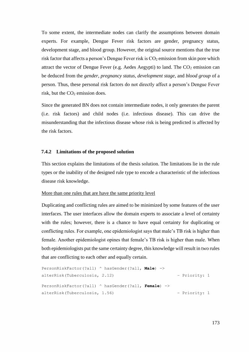
173
To some extent, the intermediate nodes can clarify the assumptions between domain
experts. For example, Dengue Fever risk factors are gender, pregnancy status,
development stage, and blood group. However, the original source mentions that the true
risk factor that affects a person’s Dengue Fever risk is CO2 emission from skin pore which
attract the vector of Dengue Fever (e.g. Aedes Aegypti) to land. The CO2 emission can
be deduced from the gender, pregnancy status, development stage, and blood group of a
person. Thus, these personal risk factors do not directly affect a person’s Dengue Fever
risk, but the CO2 emission does.
Since the generated BN does not contain intermediate nodes, it only generates the parent
(i.e. risk factors) and child nodes (i.e. infectious disease). This can drive the
misunderstanding that the infectious disease whose risk is being predicted is affected by
the risk factors.
7.4.2 Limitations of the proposed solution
This section explains the limitations of the thesis solution. The limitations lie in the rule
types or the inability of the designed rule type to encode a characteristic of the infectious
disease risk knowledge.
More than one rules that are have the same priority level
Duplicating and conflicting rules are aimed to be minimized by some features of the user
interfaces. The user interfaces allow the domain experts to associate a level of certainty
with the rules; however, there is a chance to have equal certainty for duplicating or
conflicting rules. For example, one epidemiologist says that male’s TB risk is higher than
female. Another epidemiologist opines that female’s TB risk is higher than male. When
both epidemiologists put the same certainty degree, this knowledge will result in two rules
that are conflicting to each other and equally certain.
PersonRiskFactor(?all) ^ hasGender(?all, Male) ->
alterRisk(Tuberculosis, 2.12) – Priority: 1
PersonRiskFactor(?all) ^ hasGender(?all, Female) ->
alterRisk(Tuberculosis, 1.56) – Priority: 1
174
This kind of situation is not solved yet in the conflict resolution strategy of PROSPECT-
IDR. Therefore, as mentioned above, one of the knowledge manager’s jobs is to manage
this kind of conflict.
Unable to handle continuous knowledge in the BN
In section 3.1, it was apparent that the infectious disease risk knowledge contains binary,
multivalued, nominal, and continuous knowledge. Even though the continuous risk
factors are not found in the 22 evaluation knowledge-bases, this kind of knowledge is
revealed on a source [100]. When this kind of knowledge appear, the information obtained
from regression formula could not be facilitated by the designed five rule types. The kind
of continuous knowledge is like every 1oC increase in temperature, it will cause 1%
increase in mumps case.
7.5 Discussion
This section elaborates the long-term vision of the continuation of this research. As
mentioned in motivation of chapter 1, this thesis is initial research of a vision. The
ultimate vision of this research is to support users to prevent themselves from infectious
disease risks. This thesis provides a form of knowledge representation and BN-Builder
algorithm to convert the encoded infectious disease risk knowledge into a BN that is ready
to calculate the personalized infectious disease risk.
Besides that, as the research in the pathogen detection developed, the status of pathogen
activity can be connected to this system via vague pathogen status rule type. Therefore,
the pathogen status in a region can be more precise and no longer vague. However, this
needs other studies that describe pathogen role to infectious disease risk to get the odds
ratios of risk factors related to pathogen activity. Research in air pollution can also be
plugged in to this system as API data provider. Air pollution plays a significant role in
air-borne infection transmission.
From the resulting risk prediction, the personalized actions to prevent the predicted
infectious diseases are advised. The envisaged recommendations are for example, the
precipitation level was recorded to be increasing in the last 4 weeks, the malaria case is
predicted to increase in this week (4-week lag). Since you have a sensitive skin, then, to
175
prevent mosquito bites, a mosquito repellant will not be advised for you to apply.
Alternatively, a mosquito net can reduce the malaria risk, by applying mosquito net every
day starting from today, your malaria risk will decrease by 50%.
With this kind of personalized suggestion, the users will be expected to take the
preventable actions, so, the number of incidences like presented in Table 1.2 might be
reduced. Or at least, the users are acknowledged about their infection risks based on their
personal attributes and current geo-position.
7.6 Future Work
This section describes the possible research that could be extended from this thesis for
achieving the long-term vision explained in the previous section.
Creating the case-base for personalized advice reasoning
Research into the personalization of infectious disease risk prevention is a continuation
of this research. To generate relevant advice for preventing the predicted infectious
diseases risk, person and other attributes need to be modelled. Extensive dialogs with the
epidemiologists will then be required to create cases as the basis of advice reasoning.
The cases will make use of the outputs of this thesis: meningitis risk is predicted to be
high for a particular person. The person is a female, age 20-30 years, A blood-type, living
in humid and windy region. To generate the automatic advice relevant to the person model
and the predicted meningitis risk, the actionable preventions for meningitis risk are
searched. Then, the discovered preventions are matched with the person model. If needed,
some additional information is required (e.g. allergy information). For example, a person
who is allergic to nuts will need another source of protein (e.g. egg, milk, fish) to prevent
them from the meningitis risk that is predicted to be increasing in the following weeks
because of the weather conditions. This leads to a need for research to find the relevant
advice which is based on the person model, the predicted infectious disease risks, and
environment conditions (climate and location).
176
Importing the odds ratios automatically from documents
There are two possible knowledge sources for this thesis: (1) risk factors and
quantifications from the case-control studies and (2) directly from the epidemiologists
before they are published in an article. The latter knowledge source is envisaged for the
future. In order to source knowledge automatically as it is published, a group of keywords
could be set to a journal repository to identify relevant journal articles in the public health
and infectious disease domains. Then the tabulated data in these articles, the risk factors,
odds ratios and number of case-control subjects could be captured. Then, the risk factors
and their odds ratios could be harvested using a text-mining technique. The harvesting
process could be done automatically without waiting for an expert user to encode them
into the PROSPECT-IDR system. However, the precision of the gleaned risk knowledge
should be validated by a human to make sure that they were harvested correctly.
Auto-detect the anomalies
The author envisages that the PROSPECT-IDR system will help epidemiologists all over
the world to encode their infectious disease risk knowledge in the IDR knowledge-base.
This may cause an abundance of IDR rules in an IDR knowledge-base. Besides the
abundance of rules, the knowledge manager is also expected to work with the IDR
knowledge-base continuously, as the knowledge develops. To help the work of the
knowledge manager, a computer program could be built with the aim to detect anomalies
automatically. Then this program could list the IDR rules involved in the conflicts. The
knowledge manager will observe the IDR rules from the list to decide which IDR rules
that have higher priority over the other ones.
Addition of multiple case-control studies
Multiple case-control studies which specify the same infectious disease in one location
context can be used to generate one knowledge-base. Two approaches can be used to
facilitate the case-control studies addition: (1) recalculate the odd ratios (pooled odd
ratios), and (2) machine learning. The resulting knowledge of both pooled odd ratios and
machine learning need validation from experts. Both approaches make the addition of
case-control studies less automated than current approach.
177
Data-driven approaches to deep learn Bayesian Networks
Besides encoding the risk factors and the related odds ratios, there is another way to get
the knowledge: deep learning for BNs. By deep learning the BNs, the changes of data or
pattern can be recognized quickly. Also, the resulting knowledge is up-to-date because
represents the current health data. However, this demands data which is often confidential
in nature and cannot be openly shared with researchers.
REFERENCES
[1] World Health Organization, “Disease burden and mortality estimates,” World Health
Organization, 2018.
[2] World Health Organization, “Disease incidence, prevalence and disability.”
[3] I. Albert, E. Grenier, J. Denis, and J. Rousseau, “Quantitative Risk Assessment from Farm
to Fork and Beyond : A Global Bayesian Approach Concerning Food-Borne Diseases,”
Risk Anal., vol. 28, no. 2, pp. 557–571, 2008.
[4] T.-Y. Lee, C.-B. Wang, T.-T. Chen, K. N. Kuo, M.-S. Wu, J.-T. Lin, and C.-Y. Wu, “A
Tool to Predict Risk for Gastric Cancer in Patients with Peptic Ulcer Disease, Based on a
Nationwide Cohort.,” Clin. Gastroenterol. Hepatol., vol. 13, pp. 287–293, 2015.
[5] H. Cao, L. Zhang, L. Li, and S. Lo, “Risk Factors for Acute Endophthalmitis following
Cataract Surgery : A Systematic Review and Meta- Analysis,” PLoS One, vol. 8, no. 8,
pp. 1–18, 2013.
[6] A. Jurcev-Savicevic, R. Mulic, B. Ban, K. Kozul, L. Bacun-Ivcek, J. Valic, G. Popijac-
Cesar, S. Marinovic-Dunatov, M. Gotovac, and A. Simunovic, “Risk factors for
pulmonary tuberculosis in Croatia: a matched case-control study,” BMC Public Health,
vol. 13, p. 991, 2013.
[7] M. Dhimal, I. Gautam, H. D. Joshi, R. B. O’Hara, B. Ahrens, and U. Kuch, “Risk Factors
for the Presence of Chikungunya and Dengue Vectors (Aedes aegypti and Aedes
albopictus), Their Altitudinal Distribution and Climatic Determinants of Their Abundance
in Central Nepal,” PLoS Negl. Trop. Dis., vol. 9, no. 3, pp. 1–20, 2015.
[8] A. Olea, I. Matute, C. González, I. Delgado, L. Poffald, E. Pedroni, T. Alfaro, M. Hirmas,
M. Nájera, A. Gormaz, D. López, S. Loayza, C. Ferreccio, D. Gallegos, R. Fuentes, P.
Vial, and X. Aguilera, “Case − Control Study of Risk Factors for Meningococcal Disease
in Chile,” Emerg. Infect. Dis., vol. 23, no. 7, pp. 1070–1078, 2017.
[9] D. Raja, “Artificial Intelligence in Medical Epidemiology - AIME.” .
[10] M. Woolhouse, “How to make predictions about future infectious disease risks,” Philos.
Trans. R. Soc. B Biol. Sci., vol. 366, no. 1573, pp. 2045–2054, 2011.
[11] P. R. O. Payne, “Chapter 1: Biomedical Knowledge Integration,” PLoS Comput. Biol., vol.
8, no. 12, 2012.
[12] CDC, “Principles of Epidemiology | Lesson 1 - Section 1.” .
[13] H. F. L. Wertheim, P. Horby, and J. P. Woodall, Atlas of Human Infectious Diseases.
Wiley-Blackwell, 2012.
178
[14] M. A. Al-Mozaini and M. K. Mansour, “Personalized medicine Is it time for infectious
diseases?,” www.smj.org.sa Saudi Med J, vol. 37, no. 12. 2016.
[15] S. Y. Yang and C. L. Hsu, “A location-based services and Google maps-based information
master system for tour guiding,” Comput. Electr. Eng., vol. 000, pp. 1–19, 2015.
[16] R. Chinnachodteeranun, N. D. Hung, K. Honda, A. V. M. Ines, and E. Han, “Designing
implementing weather generators as web services,” Futur. Internet, vol. 8, no. 4, 2016.
[17] R. Lowe, C. Barcellos, C. A. S. Coelho, T. C. Bailey, G. E. Coelho, R. Graham, T. Jupp,
W. M. Ramalho, M. S. Carvalho, D. B. Stephenson, and X. Rodó, “Dengue outlook for
the World Cup in Brazil: an early warning model framework driven by real-time seasonal
climate forecasts,” Lancet Infect. Dis., vol. 14, no. 7, pp. 619–626, Jul. 2014.
[18] M. Chilvers and J. Willbur, “Sporecaster: New white mold risk prediction smartphone app
now live | MSU Extension,” 2018. .
[19] United Nations, “WHO morbidity report in UN Data.” .
[20] L. K. Alexander, B. Lopes, K. Ricchetti-Masterson, and K. B. Yeatts, “Cross-sectional
Studies,” 2015.
[21] P. Gustafson, V. F. Gomes, C. S. Vieira, P. Rabna, R. Seng, P. Johansson, A. Sandström,
R. Norberg, I. Lisse, B. Samb, P. Aaby, and A. Nauclér, “Tuberculosis in Bissau :
incidence and risk factors in an urban community in sub-Saharan Africa,” Int. J.
Epidemiol., vol. 33, no. 1, pp. 163–172, 2018.
[22] L. G. Cowell and B. Smith, “Infectious disease ontology,” Infect. Dis. Informatics, pp.
373–395, 2010.
[23] Y. Lin, Z. Xiang, and Y. He, “Brucellosis Ontology ( IDOBRU ) as an extension of the
Infectious Disease Ontology,” J. Biomed. Semantics, vol. 9, no. 2, pp. 1–18, 2011.
[24] G. Camara, S. Despres, R. Djedidi, and M. Lo, “Design of Schistosomiasis Ontology (
IDOSCHISTO ) Extending the Infectious Disease,” in Medical Informatics, 2013, no. 1,
pp. 466–470.
[25] Y. Zhao, F. Parvinzamir, H. Wei, E. Liu, Z. Deng, F. Dong, A. Third, V. Marozas, E.
Kaldoudi, and G. Clapworthy, “The CARRE Project,” 2013.
[26] Ö. Kafalı, M. Sindlar, T. Van Der Weide, and K. Stathis, “ORC: an Ontology Reasoning
Component for Diabetes.”
[27] A. Khan, A. Sadia, S. Ahmed, H. Tabassum, and M. S. Khan, “HEPO: The hepatitis
ontology for abductive medical diagnostic systems,” in 2017 International Conference on
Communication, Computing and Digital Systems (C-CODE), 2017, pp. 271–275.
[28] D. Vrajitoru, “Knowledge Representation.” .
[29] S. Colton, “Knowledge Representation.” .
[30] CDC, “Infectious Diseases | 2018 National Notifiable Conditions.” .
[31] WHO, “WHO | Infectious diseases,” WHO, 2016. .
[32] M. Szumilas, “Explaining odds ratios.,” J. Can. Acad. Child Adolesc. Psychiatry, vol. 19,
no. 3, pp. 227–9, Aug. 2010.
[33] P. C. G. Da Costa, K. B. Laskey, and K. J. Laskey, “PR-OWL: A bayesian ontology
language for the Semantic Web,” Lect. Notes Comput. Sci. (including Subser. Lect. Notes
Artif. Intell. Lect. Notes Bioinformatics), vol. 5327 LNAI, pp. 88–107, 2008.
[34] Z. Ding, Y. Peng, and R. Pan, “BayesOWL : Uncertainty Modeling in Semantic Web
Ontologies,” StudFuzz, vol. 204, pp. 3–29, 2006.
[35] R. Pan, Z. Ding, Y. Yu, and Y. Peng, “A Bayesian Network Approach to Ontology
Mapping,” in International Semantic Web Conference, 2005, pp. 1–16.
[36] D. Settas, A. Cerone, and S. Fenz, “Expert Systems with Applications Enhancing
179
ontology-based antipattern detection using Bayesian networks,” Expert Syst. Appl., vol.
39, no. 10, pp. 9041–9053, 2012.
[37] P. J. Giabbanelli, T. Torsney-Weir, and V. K. Mago, “A fuzzy cognitive map of the
psychosocial determinants of obesity,” Appl. Soft Comput. J., vol. 12, no. 12, pp. 3711–
3724, 2012.
[38] N. Douali, H. Csaba, J. De Roo, E. I. Papageorgiou, and M. C. Jaulent, “Diagnosis Support
System based on clinical guidelines: Comparison between case-based fuzzy cognitive
maps and bayesian networks,” Comput. Methods Programs Biomed., vol. 113, no. 1, pp.
133–143, 2014.
[39] P. Dawson, R. Gailis, and A. Meehan, “Detecting disease outbreaks using a combined
Bayesian network and particle filter approach,” J. Theor. Biol., vol. 370, pp. 171–183,
2015.
[40] Q. Jiang, J. T. Zhou, Z. B. Jiang, and B. Xu, “Identifying risk factors of avian infectious
diseases at household level in Poyang Lake region, China,” Prev. Vet. Med., vol. 116, no.
1–2, pp. 151–160, 2014.
[41] M. A. A. Figueiredo, L. C. Rodrigues, M. L. Barreto, J. W. O. Lima, M. C. N. Costa, V.
Morato, R. Blanton, P. F. C. Vasconcelos, M. R. T. Nunes, and M. G. Teixeira, “Allergies
and diabetes as risk factors for dengue hemorrhagic fever: Results of a case control study,”
PLoS Negl. Trop. Dis., vol. 4, no. 6, 2010.
[42] C. M. Lewis, S. C. L. Whitwell, A. Forbes, J. Sanderson, and C. G. Mathew, “Estimating
risks of common complex diseases across genetic and environmental factors: the example
of Crohn disease,” pp. 689–694, 2007.
[43] A. N. Freedman, D. Seminara, M. H. Gail, P. Hartge, G. A. Colditz, R. Ballard-barbash,
and R. M. Pfeiffer, “Cancer Risk Prediction Models : A Workshop on Development,
Evaluation, and Application,” J. Natl. Cancer Inst., vol. 97, no. 10, 2005.
[44] Merriam-Webster, “Predicting | Definition of Predicting by Merriam-Webster,” 1828. .
[45] I. Ahmed, T. P. Debray, K. G. Moons, and R. D. Riley, “Developing and validating risk
prediction models in an individual participant data meta-analysis,” BMC Med. Res.
Methodol., vol. 14, no. 1, p. 3, Dec. 2014.
[46] M. Menk, L. Giebelhäuser, G. Vorderwülbecke, M. Gassner, J. A. Graw, B. Weiss, M.
Zimmermann, K.-D. Wernecke, and S. Weber-Carstens, “Nucleated red blood cells as
predictors of mortality in patients with acute respiratory distress syndrome (ARDS): an
observational study,” Ann. Intensive Care, vol. 8, no. 1, p. 42, Dec. 2018.
[47] C. Toma, A. D. Shaw, R. J. N. Allcock, A. Heath, K. D. Pierce, P. B. Mitchell, P. R.
Schofield, and J. M. Fullerton, “An examination of multiple classes of rare variants in
extended families with bipolar disorder,” Transl. Psychiatry, vol. 8, no. 1, p. 65, Dec.
2018.
[48] C. Wright and T. Dent, Quality standards in risk prediction: A summary of an expert
meeting. Cambridge: PHG Foundation, 2011.
[49] C. F. Yung, S. P. Chan, T. L. Thein, S. C. Chai, and Y. S. Leo, “Epidemiological risk
factors for adult dengue in Singapore : an 8-year nested test negative case control study,”
BMC Infect. Dis., pp. 1–9, 2016.
[50] M. J. Pencina, R. B. D. A. Sr, M. G. Larson, J. M. Massaro, and R. S. Vasan, “Predicting
the Thirty-Year Risk of Cardiovascular Disease: The Framingham Heart Study,”
Circulation, vol. 119, no. 24, pp. 3078–3084, 2009.
[51] T.-C. Li, C.-I. Li, C.-S. Liu, W.-Y. Lin, C.-H. Lin, S.-Y. Yang, J.-H. Chiang, and C.-C.
Lin, “Development and validation of prediction models for the risks of diabetes-related
hospitalization and in-hospital mortality in patients with type 2 diabetes,” Metabolism,
vol. 85, pp. 38–47, Aug. 2018.
180
[52] R. Landy, L. C. Cheung, M. Schiffman, J. C. Gage, N. Hyun, N. Wentzensen, W. K.
Kinney, P. E. Castle, B. Fetterman, N. E. Poitras, T. Lorey, P. D. Sasieni, and H. A. Katki,
“Challenges in risk estimation using routinely collected clinical data: The example of
estimating cervical cancer risks from electronic health-records,” Prev. Med. (Baltim)., vol.
111, pp. 429–435, Jun. 2018.
[53] K. Y. Clement, W. J. Wouter Botzen, R. Brouwer, and J. C. J. H. Aerts, “A global review
of the impact of basis risk on the functioning of and demand for index insurance,” Int. J.
Disaster Risk Reduct., vol. 28, pp. 845–853, Jun. 2018.
[54] C. Policiano, A. Fonseca, J. M. Mendes, N. Clode, and L. M. Graça, “Small-for-
gestational-age babies of low-risk term pregnancies: does antenatal detection matter?,” J.
Matern. Neonatal Med., vol. 31, no. 11, pp. 1426–1430, Jun. 2018.
[55] C.-H. Chan, H.-K. Wong, and P. S.-F. Yip, “Exploring the use of telephone helpline
pertaining to older adult suicide prevention: A Hong Kong experience,” J. Affect. Disord.,
vol. 236, pp. 75–79, Aug. 2018.
[56] Merriam-Webster, “Personalize | Definition of Personalize by Merriam-Webster.” .
[57] National Cancer Institute at the National Institutes of Health, “Definition of personalized
medicine - NCI Dictionary of Cancer Terms - National Cancer Institute.” .
[58] W. K. Redekop, “The Faces of Personalized Medicine: A Framework for Understanding
Its Meaning and Scope,” Value Heal., vol. 16, pp. 1–6, 2013.
[59] D. Becker, W. van Breda, B. Funk, M. Hoogendoorn, J. Ruwaard, and H. Riper,
“Predictive modeling in e-mental health: A common language framework,” Internet
Interv., vol. 12, pp. 57–67, Jun. 2018.
[60] G. Colella, F. Fazioli, M. Gallo, A. De Chiara, G. Apice, C. Ruosi, A. Cimmino, and F.
de Nigris, “Sarcoma Spheroids and Organoids—Promising Tools in the Era of
Personalized Medicine,” Int. J. Mol. Sci., vol. 19, no. 2, p. 615, Feb. 2018.
[61] P. S. Pratiwi and D. Tjondronegoro, “Towards personalisation of physical activity e-coach
using stage-matched behaviour change and motivational interviewing strategies,” in 2017
IEEE Life Sciences Conference (LSC), 2017, pp. 5–8.
[62] K. Selby, G. Bartlett-Esquilant, and J. Cornuz, “Personalized cancer screening: helping
primary care rise to the challenge.,” Public Health Rev., vol. 39, p. 4, 2018.
[63] C. Butts, S. Kamel-Reid, G. Batist, S. Chia, C. Blanke, M. Moore, M. B. Sawyer, C.
Desjardins, A. Dubois, J. Pun, K. Bonter, and F. D. Ashbury, “Benefits, issues, and
recommendations for personalized medicine in oncology in Canada.,” Curr. Oncol., vol.
20, no. 5, pp. e475-83, Oct. 2013.
[64] National Cancer Institute (NCI), “Value of Personalized Medicine.” PhRMA, 2015.
[65] C. L. Ratcliff, K. A. Kaphingst, and J. D. Jensen, “When Personal Feels Invasive:
Foreseeing Challenges in Precision Medicine Communication,” J. Health Commun., vol.
23, no. 2, pp. 144–152, Feb. 2018.
[66] S. O. Jensen and S. J. van Hal, “Personalized Medicine and Infectious Disease
Management,” Trends Microbiol., vol. 25, no. 11, pp. 875–876, Nov. 2017.
[67] CDC, “Principles of Epidemiology | Lesson 1 - Section 10,” 2012. .
[68] B. Pam and F. Gorder, “Computational Epidemiology,” Comput. Sci. Eng., 2010.
[69] CDC, “Public Health 101 Series Introduction to Public Health Informatics Instructor name
Course Topics Introduction to Public Health Informatics,” 2009.
[70] American Medical Informatics Association (AMIA), “Public Health Informatics.” .
[71] Public Health Informatics Institute (PHII), “Defining Public Health Informatics.” .
[72] D. Zeng, H. Chen, C. Lynch, and M. Eidson, “Chapter 13 INFECTIOUS DISEASE
INFORMATICS AND OUTBREAK DETECTION,” in Medical Informatics, 2005, pp.
181
359–395.
[73] M. Salathe, L. Bengtsson, T. J. Bodnar, D. D. Brewer, J. S. Brownstein, C. Buckee, E. M.
Campbell, C. Cattuto, S. Khandelwal, P. L. Mabry, and A. Vespignani, “Digital
epidemiology,” PLoS Comput. Biol., vol. 8, no. 7, pp. 1–5, 2012.
[74] Z. Huang, A. Das, Y. Qiu, and A. J. Tatem, “Web-based GIS: the vector-borne disease
airline importation risk (VBD-AIR) tool.,” Int. J. Health Geogr., vol. 11, p. 33, 2012.
[75] R. Nelson, “HealthMap: the future of infectious diseases surveillance?,” Lancet Infect.
Dis., vol. 8, no. 10, p. 596, 2008.
[76] C. C. Freifeld, K. D. Mandl, B. Y. Reis, and J. S. Brownstein, “HealthMap : Global
Infectious Disease Monitoring through,” J. Am. Med. Informatics Assoc., vol. 15, no. 2,
pp. 150–157, 2014.
[77] S. Sindi, E. Calov, J. Fokkens, T. Ngandu, H. Soininen, J. Tuomilehto, and M. Kivipelto,
“The CAIDE Dementia Risk Score App: The development of an evidence-based mobile
application to predict the risk of dementia,” Alzheimer’s Dement. Diagnosis, Assess. Dis.
Monit., vol. 1, no. 3, pp. 328–333, 2015.
[78] E. B. Postnikov and D. V Tatarenkov, “Prediction of flu epidemic activity with dynamical
model based on weather forecast,” Ecol. Complex., vol. 15, pp. 109–113, 2013.
[79] G. M. Hwang, P. J. Mahoney, J. H. James, G. C. Lin, A. D. Berro, M. A. Keybl, D. M.
Goedecke, J. J. Mathieu, and T. Wilson, “A model-based tool to predict the propagation
of infectious disease via airports,” Travel Med. Infect. Dis., vol. 10, no. 1, pp. 32–42, 2012.
[80] P. Diaz, P. Constantine, K. Kalmbach, E. Jones, and S. Pankavich, “A modified SEIR
model for the spread of Ebola in Western Africa and metrics for resource allocation,” Appl.
Math. Comput., vol. 324, pp. 141–155, May 2018.
[81] S. Side, Y. M. Rangkuti, D. G. Pane, and M. S. Sinaga, “Stability Analysis Susceptible,
Exposed, Infected, Recovered (SEIR) Model for Spread Model for Spread of Dengue
Fever in Medan,” J. Phys. Conf. Ser., vol. 954, p. 012018, Jan. 2018.
[82] T. Iskandar, N. A. Chaniago, S. Munzir, V. Halfiani, and M. Ramli, “Mathematical model
of tuberculosis epidemic with recovery time delay,” in AIP, 2017, p. 020021.
[83] X. Wang, S. Panchanathan, and G. Chowell, “A Data-Driven Mathematical Model of CA-
MRSA Transmission among Age Groups: Evaluating the Effect of Control Interventions,”
PLoS Comput. Biol., vol. 9, no. 11, 2013.
[84] B. S. Glicksberg, L. Li, M. A. Badgeley, K. Shameer, R. Kosoy, N. D. Beckmann, N. Pho,
J. Hakenberg, M. Ma, K. L. Ayers, G. E. Hoffman, S. D. Li, E. E. Schadt, C. J. Patel, R.
Chen, and J. T. Dudley, “Comparative analyses of population-scale phenomic data in
electronic medical records reveal race-specific disease networks,” Bioinformatics, vol. 32,
no. 12, pp. i101–i110, 2016.
[85] R. Villamarín, G. Cooper, M. Wagner, F. C. Tsui, and J. U. Espino, “A method for
estimating from thermometer sales the incidence of diseases that are symptomatically
similar to influenza,” J. Biomed. Inform., vol. 46, no. 3, pp. 444–457, 2013.
[86] R. G. C. Scholte, L. Gosoniu, J. B. Malone, F. Chammartin, J. Utzinger, and P. Vounatsou,
“Predictive risk mapping of schistosomiasis in brazil using bayesian geostatistical
models,” Acta Trop., vol. 132, no. 1, pp. 57–63, 2014.
[87] M. J. Vilar, S. Virtanen, R. Laukkanen-Ninios, and H. Korkeala, “Bayesian modelling to
identify the risk factors for Yersinia enterocolitica contamination of pork carcasses and
pluck sets in slaughterhouses,” Int. J. Food Microbiol., vol. 197, pp. 53–57, 2015.
[88] X. L. Zhang, X. J. Shao, J. Wang, and W. L. Guo, “Temporal characteristics of respiratory
syncytial virus infection in children and its correlation with climatic factors at a public
pediatric hospital in Suzhou,” J. Clin. Virol., vol. 58, no. 4, pp. 666–670, 2013.
[89] L. Getoor, N. Friedman, D. Koller, A. Pfeffer, and B. Taskar, “Probabilistic Relational
182
Models,” in Introduction to Statistical Relational Learning, 2007, pp. 129–174.
[90] J. Lenfestey, T. Temple, and E. Howe, “Intro to Probabilistic Relational Models.” .
[91] B. Borghetti, “Bayesian Knowledge Bases.” .
[92] E. Santos, E. S. Santos, and S. Eyal, “Implicitly preserving semantics during incremental
knowledge base acquisition under uncertainty,” Int. J. Approx. Reason., vol. 33, pp. 71–
94, 2003.
[93] L. Ngo and P. Haddawy, “Answering queries from context-sensitive probabilistic
knowledge bases,” Theor. Comput. Sci., vol. 171, no. 1–2, pp. 147–177, 1997.
[94] P. Haddawy, “Generating Bayesian Networks from Probablity Logic Knowledge Bases,”
pp. 262–269, 1994.
[95] L. L. Santos, R. N. Carvalho, M. Ladeira, and W. Li, “A New Algorithm for Generating
Situation-Specific Bayesian Networks Using Bayes-Ball Method,” Uncertain. Reason.
Semant. Web, 2016.
[96] Z. Ding, Y. Peng, and R. Pan, “BayesOWL : Uncertainty Modelling in Semantic Web
Ontologies,” Soft Comput. Ontol. Semant. Web, vol. 29, pp. 3–29, 2006.
[97] N. C. Stenseth, N. I. Samia, H. Viljugrein, K. L. Kausrud, M. Begon, S. Davis, H. Leirs,
V. M. Dubyanskiy, J. Esper, V. S. Ageyev, N. L. Klassovskiy, S. B. Pole, and K.-S. Chan,
“Plague dynamics are driven by climate variation,” Proc. Natl. Acad. Sci., vol. 103, no.
35, pp. 13110–13115, 2006.
[98] H. Khiabanian, A. B. Holmes, B. J. Kelly, M. Gururaj, G. Hripcsak, and R. Rabadan,
“Signs of the 2009 influenza pandemic in the New York-Presbyterian hospital electronic
health records,” PLoS One, vol. 5, no. 9, pp. 1–8, 2010.
[99] S. M. Upadhyayula, S. Rao Mutheneni, H. K. Nayanoori, A. Natarajan, and P. Goswami,
“Impact of weather variables on mosquitoes infected with Japanese encephalitis virus in
Kurnool district, Andhra Pradesh.,” Asian Pac. J. Trop. Med., vol. 5, no. 5, pp. 337–41,
2012.
[100] D. Onozuka and M. Hashizume, “Effect of weather variability on the incidence of mumps
in children: a time-series analysis.,” Epidemiol. Infect., vol. 139, no. 11, pp. 1692–700,
2011.
[101] C. Imai, B. Armstrong, Z. Chalabi, P. Mangtani, and M. Hashizume, “Time series
regression model for infectious disease and weather.,” Environ. Res., vol. 142, pp. 319–
327, 2015.
[102] M. Reyes, M. Eriksson, R. Bennet, K.-O. Hedlund, and A. Ehrnst, “Regular pattern of
respiratory syncytial virus and rotavirus infections and relation to weather in Stockholm,
1984-1993,” Clin. Microbiol. Infect., vol. 3, no. 6, pp. 640–646, Dec. 1997.
[103] T. S. Chang, R. E. Gangnon, C. David Page, W. R. Buckingham, A. Tandias, K. J. Cowan,
C. D. Tomasallo, B. G. Arndt, L. P. Hanrahan, and T. W. Guilbert, “Sparse modeling of
spatial environmental variables associated with asthma,” J. Biomed. Inform., vol. 53, pp.
320–329, 2015.
[104] Y. Nakamura, H. Kawanohara, and M. Kamei, “Proposition of real-time precise prediction
model of infectious disease patients from Prescription Surveillance using the National
Database of Electronic Medical Claims,” J. Infect. Chemother., vol. 21, no. 11, pp. 776–
782, 2015.
[105] R. K. Meentemeyer, M. A. Dorning, J. B. Vogler, D. Schmidt, and M. Garbelotto, “Citizen
science helps predict risk of emerging infectious disease,” 2015.
[106] R. D. Melamed, H. Khiabanian, and R. Rabadan, “Data-driven discovery of seasonally
linked diseases from an Electronic Health Records system.,” BMC Bioinformatics, vol. 15
Suppl 6, no. Suppl 6, p. S3, 2014.
183
[107] A. B. Holmes, A. Hawson, F. Liu, C. Friedman, H. Khiabanian, and R. Rabadan,
“Discovering disease associations by integrating electronic clinical data and medical
literature,” PLoS One, vol. 6, no. 6, 2011.
[108] T. W. Guilbert, B. Arndt, J. Temte, A. Adams, W. Buckingham, A. Tandias, C. Tomasallo,
H. a Anderson, and L. P. Hanrahan, “The theory and application of UW ehealth-PHINEX,
a clinical electronic health record-public health information exchange.,” Wis. Med. J., vol.
111, no. 3, pp. 124–133, 2012.
[109] H. Nesse, “SEIR Model.” .
[110] T. Jombart, A. Cori, X. Didelot, S. Cauchemez, C. Fraser, and N. Ferguson, “Bayesian
Reconstruction of Disease Outbreaks by Combining Epidemiologic and Genomic Data,”
PLoS Comput. Biol., vol. 10, no. 1, 2014.
[111] A. Huppert, O. Barnea, G. Katriel, R. Yaari, U. Roll, and L. Stone, “Modeling and
statistical analysis of the spatio-temporal patterns of seasonal influenza in Israel.,” PLoS
One, vol. 7, no. 10, p. e45107, 2012.
[112] S. Side, Irwan, U. Mulbar, and W. Sanusi, “SEIR model simulation for Hepatitis B,” 2017,
p. 020198.
[113] P. Kostkova, M. Szomszor, and C. St. Luis, “#Swineflu: The Use of Twitter as an
EarlyWarning and Risk Communication,” ACM Trans. Manag. Inf. Syst., vol. 5, no. 2, pp.
1–25, 2014.
[114] E. J. Tomayko, B. A. Weinert, L. Godfrey, A. K. Adams, and L. P. Hanrahan, “Using
Electronic Health Records to Examine Disease Risk in Small Populations: Obesity Among
American Indian Children, Wisconsin, 2007-2012.,” Prev. Chronic Dis., vol. 13, no. E29,
pp. 1–9, 2016.
[115] L. Faisandier, V. Bonneterre, R. De Gaudemaris, and D. J. Bicout, “Occupational
exposome: A network-based approach for characterizing Occupational Health Problems,”
J. Biomed. Inform., vol. 44, no. 4, pp. 545–552, 2011.
[116] Healthians, “India’s largest Blood Test & Health Test @ Home Service | Healthians.”
.
[117] P. Tiwari, A. Jaiswal, N. Vishwakarma, and P. Patel, “Smart Health Care (an Android app
to predict disease on the basis of symptoms),” Int. Res. J. Eng. Technol., pp. 2395–56,
2017.
[118] MdCalc, “Framingham Coronary Heart Disease Risk Score - MDCalc.” .
[119] “Infectious Disease Advisor App.” .
[120] J. Huan, “Smartphone app to detect risk for Ebola exposure.” .
[121] M. A. Ali, Z. Ahsan, M. Amin, S. Latif, A. Ayyaz, and M. N. Ayyaz, “ID-Viewer: a visual
analytics architecture for infectious diseases surveillance and response management in
Pakistan,” Public Health, vol. 134, pp. 72–85, 2016.
[122] H. Rahman, “Monitoring , Surveillance and Forecasting of Infectious Animal Diseases in
India,” vol. 16, pp. 177–181, 2015.
[123] I. M. Blake, P. Chenoweth, H. Okayasu, C. A. Donnelly, R. B. Aylward, and N. C. Grassly,
“Faster detection of poliomyelitis outbreaks to support polio eradication,” Emerg. Infect.
Dis., vol. 22, no. 3, pp. 449–456, 2016.
[124] W. K. Wong, a. Moore, G. Cooper, and M. Wagner, “Bayesian network anomaly pattern
detection for disease outbreaks,” Mach. Learn. Work. Then Conf., vol. 20, no. 2, p. 808,
2003.
[125] W.-K. Wong, A. Moore, G. Cooper, and M. Wagner, “WSARE: What’s Strange About
Recent Events?,” J. Urban Health, vol. 80, no. 2 Suppl 1, pp. i66-75, 2003.
[126] M. L. Barreto, M. Glo, and E. H. Carmo, “Infectious diseases epidemiology,” J.
184
Epidemiol. Community Heal., vol. 60, pp. 192–195, 2006.
[127] X. Wu, Y. Lu, S. Zhou, L. Chen, and B. Xu, “Impact of climate change on human
infectious diseases: Empirical evidence and human adaptation,” Environ. Int., vol. 86, pp.
14–23, 2016.
[128] A. Kilianski, P. Carcel, S. Yao, P. Roth, J. Schulte, G. B. Donarum, E. T. Fochler, J. M.
Hill, A. T. Liem, M. R. Wiley, J. T. Ladner, B. P. Pfeffer, O. Elliot, A. Petrosov, D. D.
Jima, T. G. Vallard, M. C. Melendrez, E. Skowronski, P. L. Quan, W. I. Lipkin, H. S.
Gibbons, D. L. Hirschberg, G. F. Palacios, and C. N. Rosenzweig, “Pathosphere.org:
Pathogen detection and characterization through a web-based, open source informatics
platform,” BMC Bioinformatics, vol. 16, no. 1, pp. 1–13, 2015.
[129] S. Altizer, A. Dobson, P. Hosseini, P. Hudson, M. Pascual, and P. Rohani, “Seasonality
and the dynamics of infectious diseases,” Ecol. Lett., vol. 9, pp. 467–484, 2006.
[130] K. Yeatts, P. Sly, S. Shore, S. Weiss, F. Martinez, A. Geller, P. Bromberg, P. Enright, H.
Koren, D. Weissman, and M. Selgrade, “A brief targeted review of susceptibility factors,
environmental exposures, asthma incidence, and recommendations for future asthma
incidence research.,” Environ. Health Perspect., vol. 114, no. 4, pp. 634–40, Apr. 2006.
[131] S. D. Gale, L. D. Erickson, A. Berrett, B. L. Brown, and D. W. Hedges, “Infectious disease
burden and cognitive function in young to middle-aged adults,” Brain. Behav. Immun.,
2015.
[132] P. F. D. Scheelbeek, A. J. G. Wirix, M. Hatta, R. Usman, and M. I. Bakker, “Risk factors
for poor tuberculosis treatment outcomes in Makassar, Indonesia,” Southeast Asian J.
Trop. Med. Public Health, vol. 45, no. 4, pp. 853–858, 2014.
[133] S. J. Chapman and A. V. S. Hill, “Human genetic susceptibility to infectious disease,” vol.
13, no. March, 2012.
[134] G. G. R. Murray, M. E. J. Woolhouse, M. Tapio, M. N. Mbole-Kariuki, T. S. Sonstegard,
S. M. Thumbi, A. E. Jennings, I. C. Van Wyk, M. Chase-Topping, H. Kiara, P. Toye, K.
Coetzer, B. M. Dec Bronsvoort, and O. Hanotte, “Genetic susceptibility to infectious
disease in East African Shorthorn Zebu: A genome-wide analysis of the effect of
heterozygosity and exotic introgression,” BMC Evol. Biol., vol. 13, no. 1, 2013.
[135] H. Yi, B. R. Devkota, J. Yu, K. Oh, J. Kim, and H.-J. Kim, “Effects of global warming on
mosquitoes & mosquito-borne diseases and the new strategies for mosquito control,”
Entomol. Res., vol. 44, no. 6, pp. 215–235, 2014.
[136] Q. Wang, Y. Liu, Y. Ma, L. Han, M. Dou, Y. Zou, L. Sun, H. Tian, T. Li, G. Jiang, B. Du,
T. Kou, and J. Song, “Severe hypovitaminosis D in active tuberculosis patients and its
predictors,” Clin. Nutr., 2017.
[137] A. Fares, “Seasonality of tuberculosis.,” J. Glob. Infect. Dis., vol. 3, no. 1, pp. 46–55, Jan.
2011.
[138] “WHO | Tuberculosis and HIV,” WHO, 2018.
[139] D. M. Pigott, R. E. Howes, A. Wiebe, K. E. Battle, N. Golding, P. W. Gething, S. F.
Dowell, T. H. Farag, A. J. Garcia, A. M. Kimball, L. K. Krause, C. H. Smith, S. J. Brooker,
H. H. Kyu, T. Vos, C. J. L. Murray, C. L. Moyes, and S. I. Hay, “Prioritising infectious
disease mapping,” PLoS Negl. Trop. Dis., vol. 9, no. 6, pp. 1–21, 2015.
[140] J. Casqueiro, J. Casqueiro, and C. Alves, “Infections in patients with diabetes mellitus : A
review of pathogenesis,” Indian J. Endocrinol. Metab., vol. 16, pp. 27–36, 2018.
[141] T. N. A. of Sciences, Critical Aspects of EPA’s IRIS Assessment of Inorganic Arsenic.
Washington, D.C.: National Academies Press, 2014.
[142] R. K. Smith and D. J. Maron, “Epidemiology, risk factors, and prevention,” Semin. Colon
Rectal Surg., vol. 27, no. 4, pp. 176–180, 2016.
[143] O. Shirai, T. Tsuda, S. Kitagawa, K. Naitoh, T. Seki, K. Kamimura, and M. Morohashi,
185
“Alcohol ingestion stimulates mosquito attraction.,” J. Am. Mosq. Control Assoc., vol. 18,
no. 2, pp. 91–6, Jun. 2002.
[144] K. Lönnroth, B. G. Williams, S. Stadlin, E. Jaramillo, and C. Dye, “Alcohol use as a risk
factor for tuberculosis - A systematic review,” BMC Public Health, vol. 8, no. May 2014,
2008.
[145] R. Mukherjee, D. Halder, S. Saha, R. Shyamali, R. Ramakrishnan, M. V Murhekar, and
Y. J. Hutin, “Five Pond-centred Outbreaks of Cholera in Villages of West Bengal , India :
Evidence for Focused Interventions,” J. Heal. Popul. Nutr., vol. 29, no. 5, pp. 421–428,
2011.
[146] A. J. Lund, H. M. Keys, S. Leventhal, J. W. Foster, and M. C. Freeman, “Prevalence of
cholera risk factors between migrant Haitians and Dominicans in the Dominican
Republic,” Pan Am. J. Public Heal., vol. 37, no. 3, pp. 125–132, 2015.
[147] A. Rosewell, B. Addy, L. Komnapi, F. Makanda, B. Ropa, E. Posanai, S. Dutta, G. Mola,
W. Y. N. Man, A. Zwi, and C. R. Macintyre, “Cholera risk factors , Papua New Guinea ,
2010,” BMC Infect. Dis., vol. 12, pp. 287–293, 2012.
[148] A. Prayitno, A. Taurel, J. Nealon, H. I. Satari, R. Karyanti, R. Sekartini, S. Soedjatmiko,
H. Gunardi, E. Medise, R. T. Sasmono, J. M. Simmerman, A. Bouckenooghe, and S. R.
Hadinegoro, “Dengue seroprevalence and force of primary infection in a representative
population of urban dwelling Indonesian children,” PLoS Negl. Trop. Dis., vol. 11, no. 6,
pp. 1–16, 2017.
[149] M. A. Soghaier, S. F. Mahmood, O. Pasha, S. I. Azam, M. M. Karsani, M. M. Elmangory,
B. A. Elmagboul, S. I. Okoued, S. M. Shareef, H. S. Khogali, and E. Eltigai, “Factors
associated with dengue fever IgG sero-prevalence in South Kordofan State , Sudan , in
2012 : Reporting prevalence ratios,” J. Infect. Public Health, vol. 7, no. 1, pp. 54–61, 2014.
[150] Centers for Disease Control and Prevention (CDC), “Cryptosporidiosis outbreak at a
summer camp--North Carolina, 2009.,” MMWR. Morb. Mortal. Wkly. Rep., vol. 60, no.
27, pp. 918–22, Jul. 2011.
[151] CDC, “Principles of Epidemiology | Lesson 3 - Section 2.” .
[152] M. Lappenschaar, A. Hommersom, P. J. F. Lucas, J. Lagro, and S. Visscher, “Multilevel
Bayesian networks for the analysis of hierarchical health care data,” Artif. Intell. Med.,
vol. 57, no. 3, pp. 171–183, 2013.
[153] M. Blangiardo, F. Finazzi, and M. Cameletti, “Two-stage Bayesian model to evaluate the
effect of air pollution on chronic respiratory diseases using drug prescriptions,” Spat.
Spatiotemporal. Epidemiol., 2016.
[154] C. Lau, P. Weinstein, and D. Slaney, “Imported cases of Ross River virus disease in New
Zealand - a travel medicine perspective.,” Travel Med. Infect. Dis., vol. 10, no. 3, pp. 129–
134, 2012.
[155] P. D. Loprinzi and A. Nooe, “Health characteristics and predicted 10-year risk for a first
atherosclerotic cardiovascular disease (ASCVD) event using the Pooled Cohort Risk
Equations among US adults who are free of cardiovascular disease,” Physiol. Behav., vol.
151, pp. 591–595, 2015.
[156] L. M. Artigao-Rodenas, J. A. Carbayo-Herencia, J. A. Divisón-Garrote, V. F. Gil-Guillén,
J. Massó-Orozco, M. Simarro-Rueda, F. Molina-Escribano, C. Sanchis, L. Carrión-Valero,
E. López de Coca, D. Caldevilla, J. López-Abril, C. Carratalá-Munuera, and A. Lopez-
Pineda, “Framingham Risk Score for Prediction of Cardiovascular Diseases: A
Population-Based Study from Southern Europe,” PLoS One, vol. 8, no. 9, pp. 1–10, 2013.
[157] S. Kalayanarooj, R. V. Gibbons, D. Vaughn, S. Green, A. Nisalak, R. G. Jarman, M. P.
Mammen, Jr., and G. Perng, “Blood Group AB Is Associated with Increased Risk for
Severe Dengue Disease in Secondary Infections,” J. Infect. Dis., vol. 195, no. 7, pp. 1014–
186
1017, 2007.
[158] A. L. Greer, S. J. Drews, and D. N. Fisman, “Why ‘Winter’ vomiting disease? seasonality,
hydrology, and norovirus epidemiology in Toronto, Canada,” Ecohealth, vol. 6, no. 2, pp.
192–199, 2009.
[159] I. Stephenson and M. Zambon, “The epidemiology of influenza,” Occup. Med. (Chic. Ill).,
vol. 52, no. 5, pp. 241–247, 2002.
[160] S. Subak, “Effects of climate on variability in Lyme disease incidence in the northeastern
United States,” Am. J. Epidemiol., vol. 157, no. 6, pp. 531–538, 2003.
[161] K. Kleinman, R. Lazarus, and R. Platt, “A generalized linear mixed models approach for
detecting incident clusters of disease in small areas, with an application to biological
terrorism,” Am. J. Epidemiol., vol. 159, no. 3, pp. 217–224, 2004.
[162] G. M. Liumbruno and M. Franchini, “Beyond immunohaematology: the role of the ABO
blood group in human diseases,” Blood Transfus, vol. 11, pp. 491–499, 2013.
[163] K. Kengkla, N. Charoensuk, M. Chaichana, S. Puangjan, T. Rattanapornsompong, J.
Choorassamee, P. Wilairat, and S. Saokaew, “Clinical risk scoring system for predicting
extended-spectrum β-lactamase-producing Escherichia coli infection in hospitalized
patients.,” J. Hosp. Infect., vol. 93, no. 1, pp. 49–56, 2016.
[164] A. Ascherio and M. A. Schwarzschild, “The epidemiology of Parkinson’s disease: risk
factors and prevention,” Lancet Neurol., vol. 15, no. 12, pp. 1257–1272, 2016.
[165] S. A. J. Schmidt, M. Vestergaard, L. M. Baggesen, L. Pedersen, H. C. Schønheyder, and
H. T. Sørensen, “Prevaccination epidemiology of herpes zoster in Denmark :
Quantification of occurrence and risk factors,” Vaccine, vol. 35, no. 42, pp. 5589–5596,
2017.
[166] H. Zhang, T. Yang, M. Wu, and F. Shen, “Intrahepatic cholangiocarcinoma:
Epidemiology, risk factors, diagnosis and surgical management,” Cancer Lett., vol. 379,
no. 2, pp. 198–205, 2016.
[167] C. A. Rostad, K. Wehrheim, J. K. Kirklin, D. Naftel, E. Pruitt, T. M. Hoffman, T.
L’Ecuyer, K. Berkowitz, W. T. Mahle, and J. N. Scheel, “Bacterial infections after
pediatric heart transplantation: Epidemiology, risk factors and outcomes,” J. Hear. Lung
Transplant., vol. 36, no. 9, pp. 996–1003, 2017.
[168] S. H. Kim, S. M. Choi, B. C. Kim, K. H. Choi, T. S. Nam, J. T. Kim, S. H. Lee, M. S.
Park, and S. J. Kim, “Risk factors for aseptic meningitis in herpes zoster patients,” Ann.
Dermatol., vol. 29, no. 3, pp. 283–287, 2017.
[169] Bruce MG; Rosenstein NE; Capparella JM; Shutt KA; Perkins B; Collins M, “Risk Factors
for Meningococcal Disease in College Students.,” J. Am. Med. Assoc., vol. 286, no. 6, pp.
688–693, 2001.
[170] A. Moat, A. Jarousha, and A. Al Afifi, “Epidemiology and Risk Factors Associated with
Developing Bac- terial Meningitis among Children in Gaza Strip,” Iran. J. Public Health,
vol. 43, no. 9, pp. 1176–1183, 2014.
[171] A. J. M. Lora, J. Fernandez, A. Morales, Y. Soto, J. Feris-iglesias, and M. O. Brito,
“Disease Severity and Mortality Caused by Dengue in a Dominican Pediatric Population,”
Am. J. Trop. Med. Hyg., vol. 90, no. 1, pp. 169–172, 2014.
[172] V. Kumar, S. Devika, S. George, and L. Jeyaseelan, “ScienceDirect Spatial mapping of
acute diarrheal disease using GIS and estimation of relative risk using empirical Bayes
approach,” Clin. Epidemiol. Glob. Heal., vol. 5, no. 2, pp. 87–96, 2017.
[173] D. Morof, S. T. Cookson, S. Laver, D. Chirundu, S. Desai, P. Mathenge, D. Shambare, L.
Charimari, S. Midzi, C. Blanton, and T. Handzel, “Community Mortality from Cholera :
Urban and Rural Districts in Zimbabwe,” Am. J. Trop. Med. Hyg., vol. 88, no. 4, pp. 645–
650, 2013.
187
[174] C. O. Schmidt and T. Kohlmann, “When to use the odds ratio or the relative risk?,” Int. J.
Public Health, vol. 53, pp. 165–167, 2008.
[175] M. S. Hossain, I. B. Habib, and K. Andersson, “A belief rule based expert system to
diagnose dengue fever under uncertainty,” in 2017 Computing Conference, 2017, pp. 179–
186.
[176] I. Ramalhosa, P. Mateus, V. Alves, H. Vicente, F. Ferraz, J. Neves, and J. Neves,
“Diagnosis of Alzheimer Disease Through an Artificial Neural Network Based System,”
Springer, Cham, 2018, pp. 162–174.
[177] M. H. F. Zarandi and M. Abdolkarimzadeh, “Fuzzy Rule Based Expert System to
Diagnose Chronic Kidney Disease,” Springer, Cham, 2018, pp. 323–328.
[178] C. Zhao, J. Jiang, Z. Xu, and Y. Guan, “A study of EMR-based medical knowledge
network and its applications,” Comput. Methods Programs Biomed., vol. 143, pp. 13–23,
May 2017.
[179] M. Krishnamurthy, P. Marcinek, K. M. Malik, and M. Afzal, “Representing Social
Network Patient Data as Evidence-Based Knowledge to Support Decision Making in
Disease Progression for Comorbidities,” IEEE Access, vol. 6, pp. 12951–12965, 2018.
[180] B. MacKellar and C. Schweikert, “Conflict Discovery and Analysis for Clinical Trials,”
in Proceedings of the 2017 International Conference on Digital Health - DH ’17, 2017,
pp. 72–76.
[181] M. A. Kadhim, M. A. Alam, and H. Kaur, “A Multi-Intelligent Agent for Knowledge
Discovery in Database (MIAKDD): Cooperative Approach with Domain Expert for Rules
Extraction,” Springer, Cham, 2014, pp. 602–614.
[182] W. Chen, A. Fang, and W. Wang, “Traditional Chinese Medicine Syndrome Knowledge
Representation Model of Gastric Precancerous Lesion and Risk Assessment Based on
Extenics,” Springer, Berlin, Heidelberg, 2011, pp. 585–590.
[183] J. Vilhena, M. Rosário Martins, H. Vicente, J. M. Grañeda, F. Caldeira, R. Gusmão, J.
Neves, and J. Neves, “An Integrated Soft Computing Approach to Hughes Syndrome Risk
Assessment,” J. Med. Syst., vol. 41, no. 3, p. 40, Mar. 2017.
[184] M. Rajabi, A. Mansourian, P. Pilesjo, F. Hedefalk, R. Groth, and A. Bazmani, “Comparing
Knowledge - Driven and Data - Driven Modeling methods for susceptibility mapping in
spatial epidemiology : a case study in Visceral Leishmaniasis,” in Proceedings of AGILE
2014 International Conference on Geographic Information Science, 2014, pp. 1–5.
[185] J. Wiens, J. Guttag, and E. Horvitz, “Patient Risk Stratification with Time-Varying
Parameters: A Multitask Learning Approach,” J. Mach. Learn. Res., vol. 17, pp. 1–23,
2016.
[186] J. F. Sowa, Knowledge representation : logical, philosophical, and computational
foundations. Brooks/Cole, 2000.
[187] M. Negnevitsky, Artificial intelligence : a guide to intelligent systems. Addison Wesley,
2002.
[188] P. Q. Rashid, “Semantic Network and Frame Knowledge Representation Formalisms in
Artificial Intelligence.”
[189] A. Onisko, P. Lucas, and M. J. Druzdzel, “Comparison of Rule-Based and Bayesian
Network Approaches in Medical Diagnostic Systems,” Artif. Intell. Med. 8th Conf. Artif.
Intell. Med. Eur. AIME 2001, Cascais, Port. July 1-4, 2001 Proc., vol. 2101, p. 283, 2001.
[190] J. Prentzas and I. Hatzilygeroudis, “Integrations of Rule-Based and Case-Based
Reasoning,” Proc. Int. Conf. Comput. Commun. Control Technol., vol. 4, pp. 81–85, 2003.
[191] P. Smets, “Jeffrey’s rule of conditioning generalized to belief functions,” Uncertain. Artif.
Intell., 1993.
188
[192] National Center for Biomedical Ontology, “Welcome to the NCBO BioPortal | NCBO
BioPortal,” 2018. .
[193] OBO, “The OBO Foundry,” 2018. .
[194] Google, “Google Code Archive - Long-term storage for Google Code Project Hosting.” .
[195] C. Pesquita, J. D. Ferreira, F. M. Couto, and M. J. Silva, “The epidemiology ontology : an
ontology for the semantic annotation of epidemiological resources,” pp. 1–7, 2014.
[196] University of Michigan Medical School, “VIOLIN: Vaccine Investigation and Online
Information Network.” .
[197] L. M. Schriml, C. Arze, S. Nadendla, Y. W. W. Chang, M. Mazaitis, V. Felix, G. Feng,
and W. A. Kibbe, “Disease ontology: A backbone for disease semantic integration,”
Nucleic Acids Res., vol. 40, no. D1, pp. 939–946, 2012.
[198] S. El-Sappagh and F. Ali, “DDO: a diabetes mellitus diagnosis ontology,” Appl.
Informatics, vol. 3, no. 1, p. 5, Dec. 2016.
[199] C. L. Gordon, S. Pouch, L. G. Cowell, M. R. Boland, H. L. Platt, A. Goldfain, and C.
Weng, “Design and evaluation of a bacterial clinical infectious diseases ontology.,” AMIA
... Annu. Symp. proceedings. AMIA Symp., vol. 2013, pp. 502–11, 2013.
[200] E. Younesi, S. Ansari, M. Guendel, S. Ahmadi, C. Coggins, J. Hoeng, M. Hofmann-
Apitius, and M. C. Peitsch, “CSEO - the Cigarette Smoke Exposure Ontology.,” J.
Biomed. Semantics, vol. 5, p. 31, 2014.
[201] W. R. Hogan, M. M. Wagner, M. Brochhausen, J. Levander, S. T. Brown, N. Millett, J.
Depasse, and J. Hanna, “The Apollo Structured Vocabulary : an OWL2 ontology of
phenomena in infectious disease epidemiology and population biology for use in epidemic
simulation,” J. Biomed. Semantics, pp. 1–12, 2016.
[202] C. X. Hong, Z. Y. Feng, C. X. Rong, L. Tian, W. Y. Wei, and M. Li, “The ontology-based
knowledge representation modeling of the traditional-Chinese-medicine symptom,” in
2017 IEEE International Conference on Bioinformatics and Biomedicine (BIBM), 2017,
pp. 1345–1349.
[203] A. Al-Rumkhani, M. Al-Razgan, and A. Al-Faris, “TibbOnto: Knowledge Representation
of Prophet Medicine (Tibb Al-Nabawi),” Procedia Comput. Sci., vol. 82, pp. 138–142,
Jan. 2016.
[204] M. Richard, X. Aimé, M.-O. Krebs, and J. Charlet, “Enrich classifications in psychiatry
with textual data: an ontology for psychiatry including social concepts.,” Stud. Health
Technol. Inform., vol. 210, pp. 221–3, 2015.
[205] A. Assawamakin, “A Development of Knowledge Representation for Thalassemia
Prevention and Control Program Ontological Knowledge Base of Southeast Asian
Thalassemia.”
[206] M. A. Elhefny, M. Elmogy, and A. A. Elfetouh, “Building OWL ontology for obesity
related cancer,” in 2014 9th International Conference on Computer Engineering &
Systems (ICCES), 2014, pp. 177–183.
[207] V. Rawte and B. Roy, “OBESTDD: Ontology Based Expert System for Thyroid Disease
Diagnosis,” in 2015 International Conference on Nascent Technologies in the Engineering
Field (ICNTE), 2015, pp. 1–6.
[208] A. Ruttenberg, “Basic Formal Ontology (BFO) | Home.” .
[209] E. I. Papageorgiou, “Learning Algorithms for Fuzzy Cognitive Maps - A Review Study,”
IEEE Trans. Syst. Man, Cybern. Part ASystems Humans, vol. 42, no. 2, pp. 150–163, 2012.
[210] R. H. Lathrop, “Bayesian Networks.”
[211] D. N. Barton, S. Kuikka, O. Varis, L. Uusitalo, H. J. Henriksen, M. Borsuk, A. D. La Hera,
R. Farmani, S. Johnson, and J. D. C. Linnell, “Bayesian networks in environmental and
189
resource management,” Integr. Environ. Assess. Manag., vol. 8, no. 3, pp. 418–429, 2012.
[212] B. Das, “Generating Conditional Probabilities for Bayesian Networks: Easing the
Knowledge Acquisition Problem,” CoRR, pp. 1–24, 2004.
[213] J. Pearl and Judea, Probabilistic reasoning in intelligent systems : networks of plausible
inference. Morgan Kaufmann Publishers, 1988.
[214] M. Henrion, Practical issues in constructing a Bayes’ belief network. Virginia: North-
Holland, 1987.
[215] L. Perreault, S. Strasser, M. Thornton, and J. W. Sheppard, “A Noisy-OR Model for
Continuous Time Bayesian Networks,” Proc. Twenty-Ninth Int. Florida Artif. Intell. Res.
Soc. Conf., pp. 668–673, 2016.
[216] G. Cheng, Q. Du, and H. Ma, “The Design and Implementation of Ontology and Rules
Based Knowledge Base for Transportation,” 2008 Int. Conf. Comput. Sci. Softw. Eng., pp.
1035–1038, 2008.
[217] Shortliffe, Computer-Based Medical Consultation. MYCIN. New York: Elsevier, 1976.
[218] M. O ’connor, “The Semantic Web Rule Language.”
[219] L. Getoor, N. Friedman, D. Koller, and A. Pfeffer, “Learning Probabilistic Relational
Models,” in Relational Data Mining, Berlin, Heidelberg: Springer Berlin Heidelberg,
2001, pp. 307–335.
[220] J. and E. S. S. Eugene. Santos, “A Framework for Building Knowledge-Base Under
Uncertainty,” J. Exp. Theor. Artif. Intell., vol. 11, no. 2, pp. 265–286, 1999.
[221] K. B. Laskey, “MEBN: A language for first-order Bayesian knowledge bases,” Artif.
Intell., vol. 172, no. 2–3, pp. 140–178, 2008.
[222] P. C. G. Costa and K. B. Laskey, “Multi-Entity Bayesian Networks Without Multi-Tears,”
pp. 1–20, 2006.
[223] L. G. Cowell, B. Smith, L. G. Cowell, and B. Smith, “Infectious Disease Ontology,” Infect.
Dis. Informatics, pp. 373–395, 2010.
[224] A. Third, E. Kaldoudi, G. Gkotsis, S. Roumeliotis, K. Pafili, J. Domingue, and M. Keynes,
“Capturing Scientific Knowledge on Medical Risk Factors,” 2010.
[225] M. C. Thomson, F. J. Doblas-Reyes, S. J. Mason, R. Hagedorn, S. J. Connor, T. Phindela,
A. P. Morse, and T. N. Palmer, “Malaria early warnings based on seasonal climate
forecasts from multi-model ensembles,” Nature, vol. 439, no. 7076, pp. 576–579, 2006.
[226] S. Falconer, “OntoGraf - Protege Wiki.” .
[227] WHO, “WHO | Disease burden and mortality estimates,” WHO, 2018. .
[228] S. Tartir, I. Arpinar, M. Moore, a Sheth, and B. Aleman-Meza, “OntoQA: Metric-Based
Ontology Quality Analysis,” IEEE Work. Knowl. Acquis. from Distrib. Auton. Semant.
Heterog. Data Knowl. Sources, pp. 45–53, 2005.
[229] A. D. Preece and R. Shinghal, “Foundation and application of knowledge base
verification,” Int. J. Intell. Syst., vol. 9, no. 8, pp. 683–701, 1994.
[230] M. A. Soghaier, S. Himatt, K. E. Osman, S. I. Okoued, O. E. Seidahmed, M. E. Beatty, K.
Elmusharaf, J. Khogali, N. H. Shingrai, and M. M. Elmangory, “Cross-sectional
community-based study of the socio-demographic factors associated with the prevalence
of dengue in the eastern part of Sudan in 2011,” BMC Public Health, pp. 1–6, 2015.
[231] I. Safeukui-Noubissi, S. Ranque, B. Poudiougou, M. Keita, A. Traoré, D. Traoré, M.
Diakité, M. B. Cissé, M. M. Keita, A. Dessein, and O. K. Doumbo, “Risk factors for severe
malaria in Bamako, Mali: A matched case-control study,” Microbes Infect., vol. 6, no. 6,
pp. 572–578, 2004.
[232] M. J. Grigg, J. Cox, T. William, J. Jelip, K. M. Fornace, P. M. Brock, L. von Seidlein, B.
E. Barber, N. M. Anstey, T. W. Yeo, and C. J. Drakeley, “Individual-level factors
190
associated with the risk of acquiring human Plasmodium knowlesi malaria in Malaysia: a
case-control study,” Lancet Planet. Heal., vol. 1, no. 3, pp. e97–e104, 2017.
[233] F. Agegnehu, A. Shimeka, F. Berihun, and M. Tamir, “Determinants of malaria infection
in Dembia district, Northwest Ethiopia: A case-control study,” BMC Public Health, vol.
18, no. 1, pp. 1–8, 2018.
[234] N. Alexander, M. Rodriguez, L. Perez, and J. Caicedo, “Case-control Study of Mosquito
Nets Against Malaria in the Amazon Region of Colombia,” Am. J. Trop. Med. Hyg., vol.
73, no. 1, pp. 140–148, 2005.
[235] Norsys Software Corp., “Norsys Software Corp. - Bayes Net Software.” .
[236] J. Negin, S. Abimbola, and B. J. Marais, “Tuberculosis among older adults – time to take
notice,” Int. J. Infect. Dis., vol. 32, pp. 135–137, Mar. 2015.
[237] Institute of Medicine (US) Committee on Enhancing Environmental Health Content in
Nursing Practice, Nursing Health, & Environment: Strengthening the Relationship
to Improve the Public’s Health. Washington (DC): National Academies Press (US), 1995.
[238] R. A. Vinarti and L. Hederman, “Introduction of a Bayesian Network Builder Algorithm
- Personalized Infectious Disease Risk Prediction,” Proc. 11th Int. Jt. Conf. Biomed. Eng.
Syst. Technol., vol. 5, no. Biostec, pp. 115–126, 2018.
[239] R. A. Vinarti and L. Hederman, “Personalization of Infectious Disease Risk Prediction:
Towards Automatic Generation of a Bayesian Network,” in Proceedings - IEEE
Symposium on Computer-Based Medical Systems, 2017, vol. 2017–June.
[240] H. M. Nemati, A. Sant’Anna, and S. Nowaczyk, “Bayesian Network representation of
meaningful patterns in electricity distribution grids,” 2016 IEEE Int. Energy Conf.
ENERGYCON 2016, 2016.
[241] E. Kaldoudi, J. Domingue, and E. Liu, “Personalized Patient Empowerment and Shared
Decision Support for Cardiorenal Disease and Comorbidities - The Carre Project,” pp. 1–
152, 2014.
[242] S. E. Keith R.Bisset, “HIGH PERFORMANCE INFORMATICS FOR PANDEMIC
PREPAREDNESS Keith,” Proc. 2012 Winter Simul. Conf., vol. 1, pp. 804–815, 2012.
[243] R. J. Hoekstra, “Ontology Representation: design patterns and ontologies that make
sense,” 2009.
[244] R. J. Brachman, On the Epistemological Status of Semantic Networks. New York:
Academic Press, 1979.
[245] R. Hartley and J. Barnden, “Semantic Networks: Visualizations of Knowledge.”
[246] T. Azuma, N. Nakada, N. Yamashita, and H. Tanaka, “Prediction, risk and control of anti-
influenza drugs in the Yodo River Basin, Japan during seasonal and pandemic influenza
using the transmission model for infectious disease,” Sci. Total Environ., vol. 521–522,
pp. 68–74, 2015.
[247] V. L. Yu and S. C. Edberg, “Global Infectious Diseases and Epidemiology Network
(GIDEON): A World Wide Web-Based Program for Diagnosis and Informatics in
Infectious Diseases,” Clin. Infect. Dis., vol. 40, no. 1, pp. 123–126, 2005.
[248] R. A. Vinarti, “Appendix (44 articles),” 2018. .
[249] R. A. Vinarti, “IDR Ontologies.” Open Science Framework, 2018.
[250] M. Horridge, M. E. Aranguren, J. Mortensen, M. Musen, and N. F. Noy, “Ontology Design
Pattern Language Expressivity Requirements.”
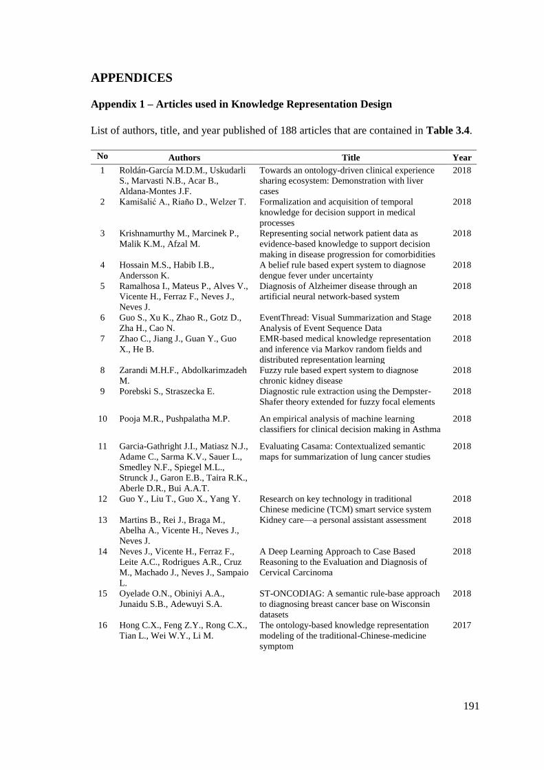
191
APPENDICES
Appendix 1 – Articles used in Knowledge Representation Design
List of authors, title, and year published of 188 articles that are contained in Table 3.4.
No Authors Title Year
1 Roldán-García M.D.M., Uskudarli
S., Marvasti N.B., Acar B.,
Aldana-Montes J.F.
Towards an ontology-driven clinical experience
sharing ecosystem: Demonstration with liver
cases
2018
2 Kamišalić A., Riaño D., Welzer T. Formalization and acquisition of temporal
knowledge for decision support in medical
processes
2018
3 Krishnamurthy M., Marcinek P.,
Malik K.M., Afzal M.
Representing social network patient data as
evidence-based knowledge to support decision
making in disease progression for comorbidities
2018
4 Hossain M.S., Habib I.B.,
Andersson K.
A belief rule based expert system to diagnose
dengue fever under uncertainty
2018
5 Ramalhosa I., Mateus P., Alves V.,
Vicente H., Ferraz F., Neves J.,
Neves J.
Diagnosis of Alzheimer disease through an
artificial neural network-based system
2018
6 Guo S., Xu K., Zhao R., Gotz D.,
Zha H., Cao N.
EventThread: Visual Summarization and Stage
Analysis of Event Sequence Data
2018
7 Zhao C., Jiang J., Guan Y., Guo
X., He B.
EMR-based medical knowledge representation
and inference via Markov random fields and
distributed representation learning
2018
8 Zarandi M.H.F., Abdolkarimzadeh
M.
Fuzzy rule based expert system to diagnose
chronic kidney disease
2018
9 Porebski S., Straszecka E. Diagnostic rule extraction using the Dempster-
Shafer theory extended for fuzzy focal elements
2018
10 Pooja M.R., Pushpalatha M.P. An empirical analysis of machine learning
classifiers for clinical decision making in Asthma
2018
11 Garcia-Gathright J.I., Matiasz N.J.,
Adame C., Sarma K.V., Sauer L.,
Smedley N.F., Spiegel M.L.,
Strunck J., Garon E.B., Taira R.K.,
Aberle D.R., Bui A.A.T.
Evaluating Casama: Contextualized semantic
maps for summarization of lung cancer studies
2018
12 Guo Y., Liu T., Guo X., Yang Y. Research on key technology in traditional
Chinese medicine (TCM) smart service system
2018
13 Martins B., Rei J., Braga M.,
Abelha A., Vicente H., Neves J.,
Neves J.
Kidney care—a personal assistant assessment 2018
14 Neves J., Vicente H., Ferraz F.,
Leite A.C., Rodrigues A.R., Cruz
M., Machado J., Neves J., Sampaio
L.
A Deep Learning Approach to Case Based
Reasoning to the Evaluation and Diagnosis of
Cervical Carcinoma
2018
15 Oyelade O.N., Obiniyi A.A.,
Junaidu S.B., Adewuyi S.A.
ST-ONCODIAG: A semantic rule-base approach
to diagnosing breast cancer base on Wisconsin
datasets
2018
16 Hong C.X., Feng Z.Y., Rong C.X.,
Tian L., Wei W.Y., Li M.
The ontology-based knowledge representation
modeling of the traditional-Chinese-medicine
symptom
2017
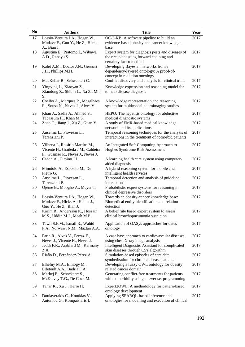
192
No Authors Title Year
17 Lossio-Ventura J.A., Hogan W.,
Modave F., Guo Y., He Z., Hicks
A., Bian J.
OC-2-KB: A software pipeline to build an
evidence-based obesity and cancer knowledge
base
2017
18 Agustina E., Pratomo I., Wibawa
A.D., Rahayu S.
Expert system for diagnosis pests and diseases of
the rice plant using forward chaining and
certainty factor method
2017
19 Kalet A.M., Doctor J.N., Gennari
J.H., Phillips M.H.
Developing Bayesian networks from a
dependency-layered ontology: A proof-of-
concept in radiation oncology
2017
20 MacKellar B., Schweikert C. Conflict discovery and analysis for clinical trials 2017
21 Yingying L., Xiaoyan Z.,
Xiaodong Z., Shibin L., Na Z., Min
S.
Knowledge expression and reasoning model for
tomato disease diagnosis
2017
22 Coelho A., Marques P., Magalhães
R., Sousa N., Neves J., Alves V.
A knowledge representation and reasoning
system for multimodal neuroimaging studies
2017
23 Khan A., Sadia A., Ahmed S.,
Tabassum H., Khan M.S.
HEPO: The hepatitis ontology for abductive
medical diagnostic systems
2017
24 Zhao C., Jiang J., Xu Z., Guan Y. A study of EMR-based medical knowledge
network and its applications
2017
25 Anselma L., Piovesan L.,
Terenziani P.
Temporal reasoning techniques for the analysis of
interactions in the treatment of comorbid patients
2017
26 Vilhena J., Rosário Martins M.,
Vicente H., Grañeda J.M., Caldeira
F., Gusmão R., Neves J., Neves J.
An Integrated Soft Computing Approach to
Hughes Syndrome Risk Assessment
2017
27 Cahan A., Cimino J.J. A learning health care system using computer-
aided diagnosis
2017
28 Minutolo A., Esposito M., De
Pietro G.
A hybrid reasoning system for mobile and
intelligent health services
2017
29 Anselma L., Piovesan L.,
Terenziani P.
Temporal detection and analysis of guideline
interactions
2017
30 Ojeme B., Mbogho A., Meyer T. Probabilistic expert systems for reasoning in
clinical depressive disorders
2017
31 Lossio-Ventura J.A., Hogan W.,
Modave F., Hicks A., Hanna J.,
Guo Y., He Z., Bian J.
Towards an obesity-cancer knowledge base:
Biomedical entity identification and relation
detection
2017
32 Karim R., Andersson K., Hossain
M.S., Uddin M.J., Meah M.P.
A belief rule based expert system to assess
clinical bronchopneumonia suspicion
2017
33 Tawil S.F.M., Ismail R., Wahid
F.A., Norwawi N.M., Mazlan A.A.
Application of OASys approaches for dates
ontology
2017
34 Faria R., Alves V., Ferraz F.,
Neves J., Vicente H., Neves J.
A case base approach to cardiovascular diseases
using chest X-ray image analysis
2017
35 Jeddi F.R., Arabfard M., Kermany
Z.A.
Intelligent Diagnostic Assistant for complicated
skin diseases through C5's algorithm
2017
36 Riaño D., Fernández-Pérez A. Simulation-based episodes of care data
synthetization for chronic disease patients
2017
37 Elhefny M.A., Elmogy M.,
Elfetouh A.A., Badria F.A.
Developing a fuzzy OWL ontology for obesity
related cancer domain
2017
38 Merhej E., Schockaert S.,
McKelvey T.G., De Cock M.
Generating conflict-free treatments for patients
with comorbidity using answer set programming
2017
39 Tahar K., Xu J., Herre H. Expert2OWL: A methodology for pattern-based
ontology development
2017
40 Doulaverakis C., Koutkias V.,
Antoniou G., Kompatsiaris I.
Applying SPARQL-based inference and
ontologies for modelling and execution of clinical
2017
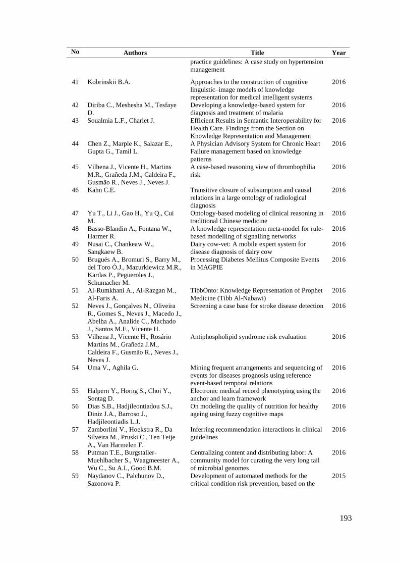
193
No Authors Title Year
practice guidelines: A case study on hypertension
management
41 Kobrinskii B.A. Approaches to the construction of cognitive
linguistic–image models of knowledge
representation for medical intelligent systems
2016
42 Diriba C., Meshesha M., Tesfaye
D.
Developing a knowledge-based system for
diagnosis and treatment of malaria
2016
43 Soualmia L.F., Charlet J. Efficient Results in Semantic Interoperability for
Health Care. Findings from the Section on
Knowledge Representation and Management
2016
44 Chen Z., Marple K., Salazar E.,
Gupta G., Tamil L.
A Physician Advisory System for Chronic Heart
Failure management based on knowledge
patterns
2016
45 Vilhena J., Vicente H., Martins
M.R., Grañeda J.M., Caldeira F.,
Gusmão R., Neves J., Neves J.
A case-based reasoning view of thrombophilia
risk
2016
46 Kahn C.E. Transitive closure of subsumption and causal
relations in a large ontology of radiological
diagnosis
2016
47 Yu T., Li J., Gao H., Yu Q., Cui
M.
Ontology-based modeling of clinical reasoning in
traditional Chinese medicine
2016
48 Basso-Blandin A., Fontana W.,
Harmer R.
A knowledge representation meta-model for rule-
based modelling of signalling networks
2016
49 Nusai C., Chankeaw W.,
Sangkaew B.
Dairy cow-vet: A mobile expert system for
disease diagnosis of dairy cow
2016
50 Brugués A., Bromuri S., Barry M.,
del Toro Ó.J., Mazurkiewicz M.R.,
Kardas P., Pegueroles J.,
Schumacher M.
Processing Diabetes Mellitus Composite Events
in MAGPIE
2016
51 Al-Rumkhani A., Al-Razgan M.,
Al-Faris A.
TibbOnto: Knowledge Representation of Prophet
Medicine (Tibb Al-Nabawi)
2016
52 Neves J., Gonçalves N., Oliveira
R., Gomes S., Neves J., Macedo J.,
Abelha A., Analide C., Machado
J., Santos M.F., Vicente H.
Screening a case base for stroke disease detection 2016
53 Vilhena J., Vicente H., Rosário
Martins M., Grañeda J.M.,
Caldeira F., Gusmão R., Neves J.,
Neves J.
Antiphospholipid syndrome risk evaluation 2016
54 Uma V., Aghila G. Mining frequent arrangements and sequencing of
events for diseases prognosis using reference
event-based temporal relations
2016
55 Halpern Y., Horng S., Choi Y.,
Sontag D.
Electronic medical record phenotyping using the
anchor and learn framework
2016
56 Dias S.B., Hadjileontiadou S.J.,
Diniz J.A., Barroso J.,
Hadjileontiadis L.J.
On modeling the quality of nutrition for healthy
ageing using fuzzy cognitive maps
2016
57 Zamborlini V., Hoekstra R., Da
Silveira M., Pruski C., Ten Teije
A., Van Harmelen F.
Inferring recommendation interactions in clinical
guidelines
2016
58 Putman T.E., Burgstaller-
Muehlbacher S., Waagmeester A.,
Wu C., Su A.I., Good B.M.
Centralizing content and distributing labor: A
community model for curating the very long tail
of microbial genomes
2016
59 Naydanov C., Palchunov D.,
Sazonova P.
Development of automated methods for the
critical condition risk prevention, based on the
2015
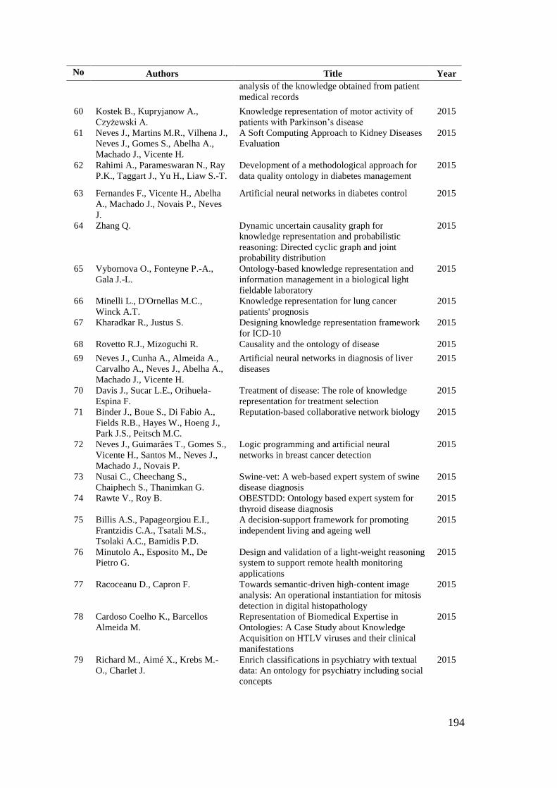
194
No Authors Title Year
analysis of the knowledge obtained from patient
medical records
60 Kostek B., Kupryjanow A.,
Czyżewski A.
Knowledge representation of motor activity of
patients with Parkinson’s disease
2015
61 Neves J., Martins M.R., Vilhena J.,
Neves J., Gomes S., Abelha A.,
Machado J., Vicente H.
A Soft Computing Approach to Kidney Diseases
Evaluation
2015
62 Rahimi A., Parameswaran N., Ray
P.K., Taggart J., Yu H., Liaw S.-T.
Development of a methodological approach for
data quality ontology in diabetes management
2015
63 Fernandes F., Vicente H., Abelha
A., Machado J., Novais P., Neves
J.
Artificial neural networks in diabetes control 2015
64 Zhang Q. Dynamic uncertain causality graph for
knowledge representation and probabilistic
reasoning: Directed cyclic graph and joint
probability distribution
2015
65 Vybornova O., Fonteyne P.-A.,
Gala J.-L.
Ontology-based knowledge representation and
information management in a biological light
fieldable laboratory
2015
66 Minelli L., D'Ornellas M.C.,
Winck A.T.
Knowledge representation for lung cancer
patients' prognosis
2015
67 Kharadkar R., Justus S. Designing knowledge representation framework
for ICD-10
2015
68 Rovetto R.J., Mizoguchi R. Causality and the ontology of disease 2015
69 Neves J., Cunha A., Almeida A.,
Carvalho A., Neves J., Abelha A.,
Machado J., Vicente H.
Artificial neural networks in diagnosis of liver
diseases
2015
70 Davis J., Sucar L.E., Orihuela-
Espina F.
Treatment of disease: The role of knowledge
representation for treatment selection
2015
71 Binder J., Boue S., Di Fabio A.,
Fields R.B., Hayes W., Hoeng J.,
Park J.S., Peitsch M.C.
Reputation-based collaborative network biology 2015
72 Neves J., Guimarães T., Gomes S.,
Vicente H., Santos M., Neves J.,
Machado J., Novais P.
Logic programming and artificial neural
networks in breast cancer detection
2015
73 Nusai C., Cheechang S.,
Chaiphech S., Thanimkan G.
Swine-vet: A web-based expert system of swine
disease diagnosis
2015
74 Rawte V., Roy B. OBESTDD: Ontology based expert system for
thyroid disease diagnosis
2015
75 Billis A.S., Papageorgiou E.I.,
Frantzidis C.A., Tsatali M.S.,
Tsolaki A.C., Bamidis P.D.
A decision-support framework for promoting
independent living and ageing well
2015
76 Minutolo A., Esposito M., De
Pietro G.
Design and validation of a light-weight reasoning
system to support remote health monitoring
applications
2015
77 Racoceanu D., Capron F. Towards semantic-driven high-content image
analysis: An operational instantiation for mitosis
detection in digital histopathology
2015
78 Cardoso Coelho K., Barcellos
Almeida M.
Representation of Biomedical Expertise in
Ontologies: A Case Study about Knowledge
Acquisition on HTLV viruses and their clinical
manifestations
2015
79 Richard M., Aimé X., Krebs M.-
O., Charlet J.
Enrich classifications in psychiatry with textual
data: An ontology for psychiatry including social
concepts
2015
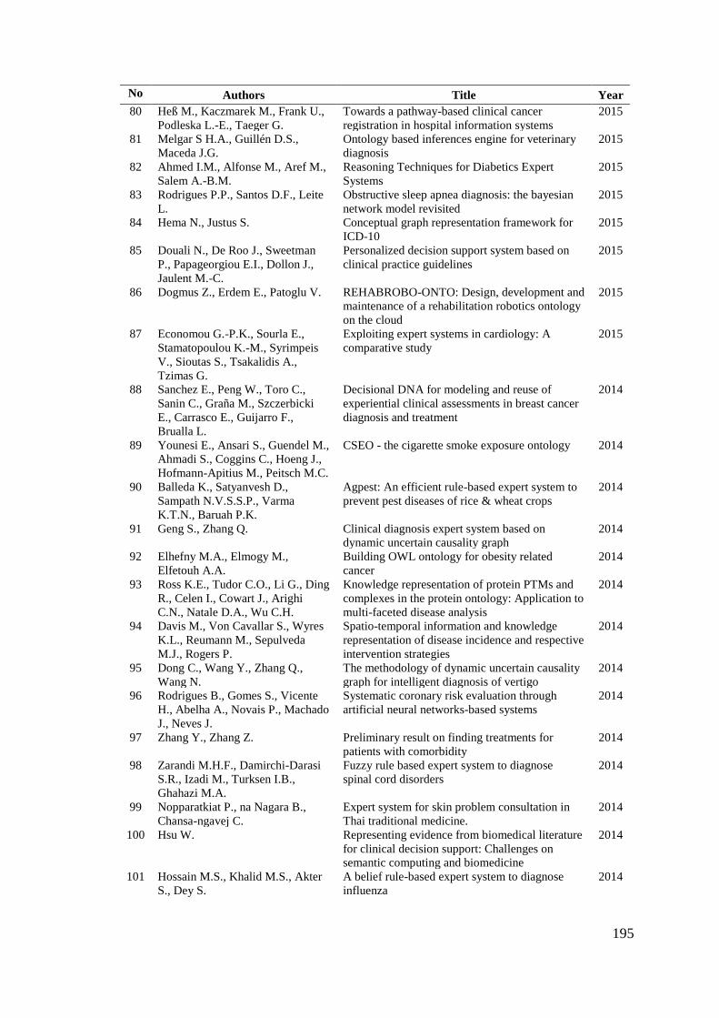
195
No Authors Title Year
80 Heß M., Kaczmarek M., Frank U.,
Podleska L.-E., Taeger G.
Towards a pathway-based clinical cancer
registration in hospital information systems
2015
81 Melgar S H.A., Guillén D.S.,
Maceda J.G.
Ontology based inferences engine for veterinary
diagnosis
2015
82 Ahmed I.M., Alfonse M., Aref M.,
Salem A.-B.M.
Reasoning Techniques for Diabetics Expert
Systems
2015
83 Rodrigues P.P., Santos D.F., Leite
L.
Obstructive sleep apnea diagnosis: the bayesian
network model revisited
2015
84 Hema N., Justus S. Conceptual graph representation framework for
ICD-10
2015
85 Douali N., De Roo J., Sweetman
P., Papageorgiou E.I., Dollon J.,
Jaulent M.-C.
Personalized decision support system based on
clinical practice guidelines
2015
86 Dogmus Z., Erdem E., Patoglu V. REHABROBO-ONTO: Design, development and
maintenance of a rehabilitation robotics ontology
on the cloud
2015
87 Economou G.-P.K., Sourla E.,
Stamatopoulou K.-M., Syrimpeis
V., Sioutas S., Tsakalidis A.,
Tzimas G.
Exploiting expert systems in cardiology: A
comparative study
2015
88 Sanchez E., Peng W., Toro C.,
Sanin C., Graña M., Szczerbicki
E., Carrasco E., Guijarro F.,
Brualla L.
Decisional DNA for modeling and reuse of
experiential clinical assessments in breast cancer
diagnosis and treatment
2014
89 Younesi E., Ansari S., Guendel M.,
Ahmadi S., Coggins C., Hoeng J.,
Hofmann-Apitius M., Peitsch M.C.
CSEO - the cigarette smoke exposure ontology 2014
90 Balleda K., Satyanvesh D.,
Sampath N.V.S.S.P., Varma
K.T.N., Baruah P.K.
Agpest: An efficient rule-based expert system to
prevent pest diseases of rice & wheat crops
2014
91 Geng S., Zhang Q. Clinical diagnosis expert system based on
dynamic uncertain causality graph
2014
92 Elhefny M.A., Elmogy M.,
Elfetouh A.A.
Building OWL ontology for obesity related
cancer
2014
93 Ross K.E., Tudor C.O., Li G., Ding
R., Celen I., Cowart J., Arighi
C.N., Natale D.A., Wu C.H.
Knowledge representation of protein PTMs and
complexes in the protein ontology: Application to
multi-faceted disease analysis
2014
94 Davis M., Von Cavallar S., Wyres
K.L., Reumann M., Sepulveda
M.J., Rogers P.
Spatio-temporal information and knowledge
representation of disease incidence and respective
intervention strategies
2014
95 Dong C., Wang Y., Zhang Q.,
Wang N.
The methodology of dynamic uncertain causality
graph for intelligent diagnosis of vertigo
2014
96 Rodrigues B., Gomes S., Vicente
H., Abelha A., Novais P., Machado
J., Neves J.
Systematic coronary risk evaluation through
artificial neural networks-based systems
2014
97 Zhang Y., Zhang Z. Preliminary result on finding treatments for
patients with comorbidity
2014
98 Zarandi M.H.F., Damirchi-Darasi
S.R., Izadi M., Turksen I.B.,
Ghahazi M.A.
Fuzzy rule based expert system to diagnose
spinal cord disorders
2014
99 Nopparatkiat P., na Nagara B.,
Chansa-ngavej C.
Expert system for skin problem consultation in
Thai traditional medicine.
2014
100 Hsu W. Representing evidence from biomedical literature
for clinical decision support: Challenges on
semantic computing and biomedicine
2014
101 Hossain M.S., Khalid M.S., Akter
S., Dey S.
A belief rule-based expert system to diagnose
influenza
2014
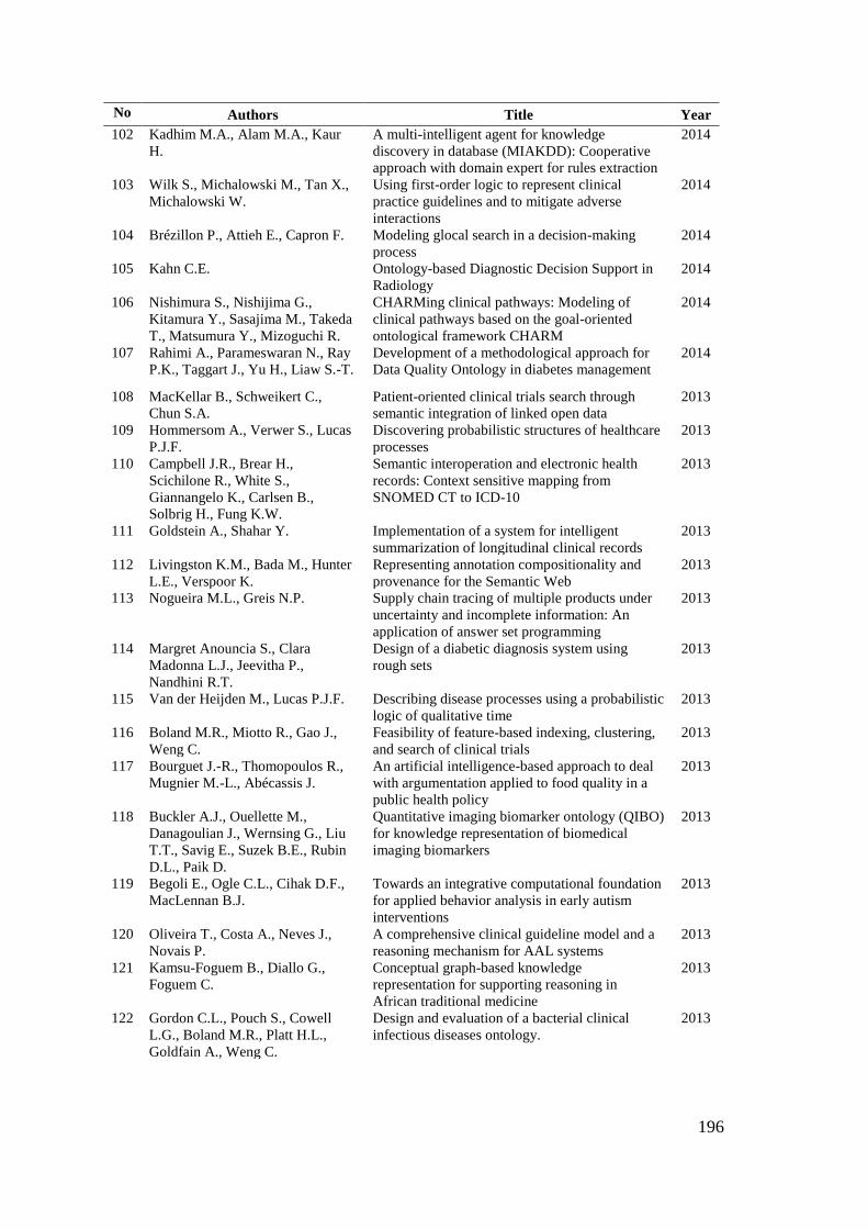
196
No Authors Title Year
102 Kadhim M.A., Alam M.A., Kaur
H.
A multi-intelligent agent for knowledge
discovery in database (MIAKDD): Cooperative
approach with domain expert for rules extraction
2014
103 Wilk S., Michalowski M., Tan X.,
Michalowski W.
Using first-order logic to represent clinical
practice guidelines and to mitigate adverse
interactions
2014
104 Brézillon P., Attieh E., Capron F. Modeling glocal search in a decision-making
process
2014
105 Kahn C.E. Ontology-based Diagnostic Decision Support in
Radiology
2014
106 Nishimura S., Nishijima G.,
Kitamura Y., Sasajima M., Takeda
T., Matsumura Y., Mizoguchi R.
CHARMing clinical pathways: Modeling of
clinical pathways based on the goal-oriented
ontological framework CHARM
2014
107 Rahimi A., Parameswaran N., Ray
P.K., Taggart J., Yu H., Liaw S.-T.
Development of a methodological approach for
Data Quality Ontology in diabetes management
2014
108 MacKellar B., Schweikert C.,
Chun S.A.
Patient-oriented clinical trials search through
semantic integration of linked open data
2013
109 Hommersom A., Verwer S., Lucas
P.J.F.
Discovering probabilistic structures of healthcare
processes
2013
110 Campbell J.R., Brear H.,
Scichilone R., White S.,
Giannangelo K., Carlsen B.,
Solbrig H., Fung K.W.
Semantic interoperation and electronic health
records: Context sensitive mapping from
SNOMED CT to ICD-10
2013
111 Goldstein A., Shahar Y. Implementation of a system for intelligent
summarization of longitudinal clinical records
2013
112 Livingston K.M., Bada M., Hunter
L.E., Verspoor K.
Representing annotation compositionality and
provenance for the Semantic Web
2013
113 Nogueira M.L., Greis N.P. Supply chain tracing of multiple products under
uncertainty and incomplete information: An
application of answer set programming
2013
114 Margret Anouncia S., Clara
Madonna L.J., Jeevitha P.,
Nandhini R.T.
Design of a diabetic diagnosis system using
rough sets
2013
115 Van der Heijden M., Lucas P.J.F. Describing disease processes using a probabilistic
logic of qualitative time
2013
116 Boland M.R., Miotto R., Gao J.,
Weng C.
Feasibility of feature-based indexing, clustering,
and search of clinical trials
2013
117 Bourguet J.-R., Thomopoulos R.,
Mugnier M.-L., Abécassis J.
An artificial intelligence-based approach to deal
with argumentation applied to food quality in a
public health policy
2013
118 Buckler A.J., Ouellette M.,
Danagoulian J., Wernsing G., Liu
T.T., Savig E., Suzek B.E., Rubin
D.L., Paik D.
Quantitative imaging biomarker ontology (QIBO)
for knowledge representation of biomedical
imaging biomarkers
2013
119 Begoli E., Ogle C.L., Cihak D.F.,
MacLennan B.J.
Towards an integrative computational foundation
for applied behavior analysis in early autism
interventions
2013
120 Oliveira T., Costa A., Neves J.,
Novais P.
A comprehensive clinical guideline model and a
reasoning mechanism for AAL systems
2013
121 Kamsu-Foguem B., Diallo G.,
Foguem C.
Conceptual graph-based knowledge
representation for supporting reasoning in
African traditional medicine
2013
122 Gordon C.L., Pouch S., Cowell
L.G., Boland M.R., Platt H.L.,
Goldfain A., Weng C.
Design and evaluation of a bacterial clinical
infectious diseases ontology.
2013
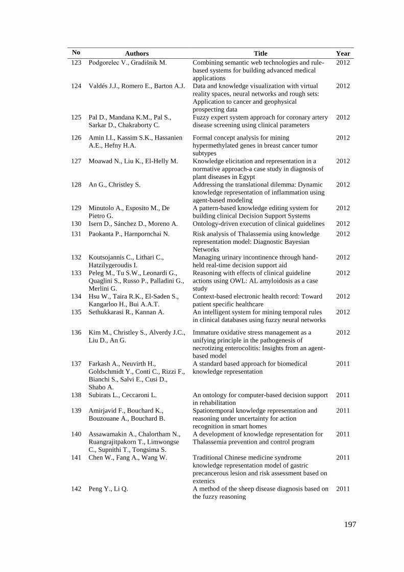
197
No Authors Title Year
123 Podgorelec V., Gradišnik M. Combining semantic web technologies and rule-
based systems for building advanced medical
applications
2012
124 Valdés J.J., Romero E., Barton A.J. Data and knowledge visualization with virtual
reality spaces, neural networks and rough sets:
Application to cancer and geophysical
prospecting data
2012
125 Pal D., Mandana K.M., Pal S.,
Sarkar D., Chakraborty C.
Fuzzy expert system approach for coronary artery
disease screening using clinical parameters
2012
126 Amin I.I., Kassim S.K., Hassanien
A.E., Hefny H.A.
Formal concept analysis for mining
hypermethylated genes in breast cancer tumor
subtypes
2012
127 Moawad N., Liu K., El-Helly M. Knowledge elicitation and representation in a
normative approach-a case study in diagnosis of
plant diseases in Egypt
2012
128 An G., Christley S. Addressing the translational dilemma: Dynamic
knowledge representation of inflammation using
agent-based modeling
2012
129 Minutolo A., Esposito M., De
Pietro G.
A pattern-based knowledge editing system for
building clinical Decision Support Systems
2012
130 Isern D., Sánchez D., Moreno A. Ontology-driven execution of clinical guidelines 2012
131 Paokanta P., Harnpornchai N. Risk analysis of Thalassemia using knowledge
representation model: Diagnostic Bayesian
Networks
2012
132 Koutsojannis C., Lithari C.,
Hatzilygeroudis I.
Managing urinary incontinence through hand-
held real-time decision support aid
2012
133 Peleg M., Tu S.W., Leonardi G.,
Quaglini S., Russo P., Palladini G.,
Merlini G.
Reasoning with effects of clinical guideline
actions using OWL: AL amyloidosis as a case
study
2012
134 Hsu W., Taira R.K., El-Saden S.,
Kangarloo H., Bui A.A.T.
Context-based electronic health record: Toward
patient specific healthcare
2012
135 Sethukkarasi R., Kannan A. An intelligent system for mining temporal rules
in clinical databases using fuzzy neural networks
2012
136 Kim M., Christley S., Alverdy J.C.,
Liu D., An G.
Immature oxidative stress management as a
unifying principle in the pathogenesis of
necrotizing enterocolitis: Insights from an agent-
based model
2012
137 Farkash A., Neuvirth H.,
Goldschmidt Y., Conti C., Rizzi F.,
Bianchi S., Salvi E., Cusi D.,
Shabo A.
A standard based approach for biomedical
knowledge representation
2011
138 Subirats L., Ceccaroni L. An ontology for computer-based decision support
in rehabilitation
2011
139 Amirjavid F., Bouchard K.,
Bouzouane A., Bouchard B.
Spatiotemporal knowledge representation and
reasoning under uncertainty for action
recognition in smart homes
2011
140 Assawamakin A., Chalortham N.,
Ruangrajitpakorn T., Limwongse
C., Supnithi T., Tongsima S.
A development of knowledge representation for
Thalassemia prevention and control program
2011
141 Chen W., Fang A., Wang W. Traditional Chinese medicine syndrome
knowledge representation model of gastric
precancerous lesion and risk assessment based on
extenics
2011
142 Peng Y., Li Q. A method of the sheep disease diagnosis based on
the fuzzy reasoning
2011
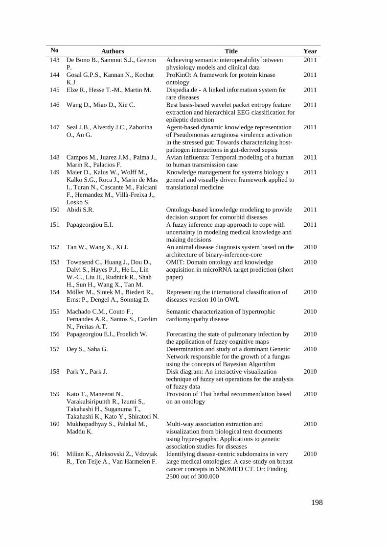
198
No Authors Title Year
143 De Bono B., Sammut S.J., Grenon
P.
Achieving semantic interoperability between
physiology models and clinical data
2011
144 Gosal G.P.S., Kannan N., Kochut
K.J.
ProKinO: A framework for protein kinase
ontology
2011
145 Elze R., Hesse T.-M., Martin M. Dispedia.de - A linked information system for
rare diseases
2011
146 Wang D., Miao D., Xie C. Best basis-based wavelet packet entropy feature
extraction and hierarchical EEG classification for
epileptic detection
2011
147 Seal J.B., Alverdy J.C., Zaborina
O., An G.
Agent-based dynamic knowledge representation
of Pseudomonas aeruginosa virulence activation
in the stressed gut: Towards characterizing host-
pathogen interactions in gut-derived sepsis
2011
148 Campos M., Juarez J.M., Palma J.,
Marin R., Palacios F.
Avian influenza: Temporal modeling of a human
to human transmission case
2011
149 Maier D., Kalus W., Wolff M.,
Kalko S.G., Roca J., Marin de Mas
I., Turan N., Cascante M., Falciani
F., Hernandez M., Villà-Freixa J.,
Losko S.
Knowledge management for systems biology a
general and visually driven framework applied to
translational medicine
2011
150 Abidi S.R. Ontology-based knowledge modeling to provide
decision support for comorbid diseases
2011
151 Papageorgiou E.I. A fuzzy inference map approach to cope with
uncertainty in modeling medical knowledge and
making decisions
2011
152 Tan W., Wang X., Xi J. An animal disease diagnosis system based on the
architecture of binary-inference-core
2010
153 Townsend C., Huang J., Dou D.,
Dalvi S., Hayes P.J., He L., Lin
W.-C., Liu H., Rudnick R., Shah
H., Sun H., Wang X., Tan M.
OMIT: Domain ontology and knowledge
acquisition in microRNA target prediction (short
paper)
2010
154 Möller M., Sintek M., Biedert R.,
Ernst P., Dengel A., Sonntag D.
Representing the international classification of
diseases version 10 in OWL
2010
155 Machado C.M., Couto F.,
Fernandes A.R., Santos S., Cardim
N., Freitas A.T.
Semantic characterization of hypertrophic
cardiomyopathy disease
2010
156 Papageorgiou E.I., Froelich W. Forecasting the state of pulmonary infection by
the application of fuzzy cognitive maps
2010
157 Dey S., Saha G. Determination and study of a dominant Genetic
Network responsible for the growth of a fungus
using the concepts of Bayesian Algorithm
2010
158 Park Y., Park J. Disk diagram: An interactive visualization
technique of fuzzy set operations for the analysis
of fuzzy data
2010
159 Kato T., Maneerat N.,
Varakulsiripunth R., Izumi S.,
Takahashi H., Suganuma T.,
Takahashi K., Kato Y., Shiratori N.
Provision of Thai herbal recommendation based
on an ontology
2010
160 Mukhopadhyay S., Palakal M.,
Maddu K.
Multi-way association extraction and
visualization from biological text documents
using hyper-graphs: Applications to genetic
association studies for diseases
2010
161 Milian K., Aleksovski Z., Vdovjak
R., Ten Teije A., Van Harmelen F.
Identifying disease-centric subdomains in very
large medical ontologies: A case-study on breast
cancer concepts in SNOMED CT. Or: Finding
2500 out of 300.000
2010
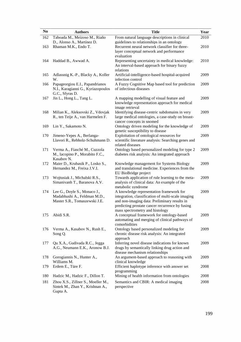
199
No Authors Title Year
162 Taboada M., Meizoso M., Riaño
D., Alonso A., Martínez D.
From natural language descriptions in clinical
guidelines to relationships in an ontology
2010
163 Rhaman M.K., Endo T. Recurrent neural network classifier for three-
layer conceptual network and performance
evaluation
2010
164 Haddad B., Awwad A. Representing uncertainty in medical knowledge:
An interval-based approach for binary fuzzy
relations
2010
165 Adlassnig K.-P., Blacky A., Koller
W.
Artificial-intelligence-based hospital-acquired
infection control
2009
166 Papageorgiou E.I., Papandrianos
N.I., Karagianni G., Kyriazopoulos
G.C., Sfyras D.
A Fuzzy Cognitive Map based tool for prediction
of infectious diseases
2009
167 Jin L., Hong L., Tang L. A mapping modelling of visual feature and
knowledge representation approach for medical
image retrieval
2009
168 Milian K., Aleksovski Z., Vdovjak
R., ten Teije A., van Harmelen F.
Identifying disease-centric subdomains in very
large medical ontologies, a case-study on breast-
cancer concepts in snomed
2009
169 Lin Y., Sakamoto N. Ontology driven modeling for the knowledge of
genetic susceptibility to disease
2009
170 Jimeno-Yepes A., Berlanga-
Llavori R., Rebholz-Schuhmann D.
Exploitation of ontological resources for
scientific literature analysis: Searching genes and
related diseases
2009
171 Verma A., Fiasché M., Cuzzola
M., Iacopino P., Morabito F.C.,
Kasabov N.
Ontology based personalized modeling for type 2
diabetes risk analysis: An integrated approach
2009
172 Maier D., Krubasik P., Losko S.,
Hernandez M., Freixa J.V.I.
Knowledge management for Systems Biology
and translational medicine. Experiences from the
EU BioBridge project
2009
173 Wojtusiak J., Michalski R.S.,
Simanivanh T., Baranova A.V.
Towards application of rule learning to the meta-
analysis of clinical data: An example of the
metabolic syndrome
2009
174 Lee G., Doyle S., Monaco J.,
Madabhushi A., Feldman M.D.,
Master S.R., Tomaszewski J.E.
A knowledge representation framework for
integration, classification of multi-scale imaging
and non-imaging data: Preliminary results in
predicting prostate cancer recurrence by fusing
mass spectrometry and histology
2009
175 Abidi S.R. A conceptual framework for ontology-based
automating and merging of clinical pathways of
comorbidities
2009
176 Verma A., Kasabov N., Rush E.,
Song Q.
Ontology based personalized modeling for
chronic disease risk analysis: An integrated
approach
2009
177 Qu X.A., Gudivada R.C., Jegga
A.G., Neumann E.K., Aronow B.J.
Inferring novel disease indications for known
drugs by semantically linking drug action and
disease mechanism relationships
2009
178 Gorogiannis N., Hunter A.,
Williams M.
An argument-based approach to reasoning with
clinical knowledge
2009
179 Erdem E., Türe F. Efficient haplotype inference with answer set
programming
2008
180 Hadzic M., Hadzic F., Dillon T. Mining of health information from ontologies 2008
181 Zhou X.S., Zillner S., Moeller M.,
Sintek M., Zhan Y., Krishnan A.,
Gupta A.
Semantics and CBIR: A medical imaging
perspective
2008
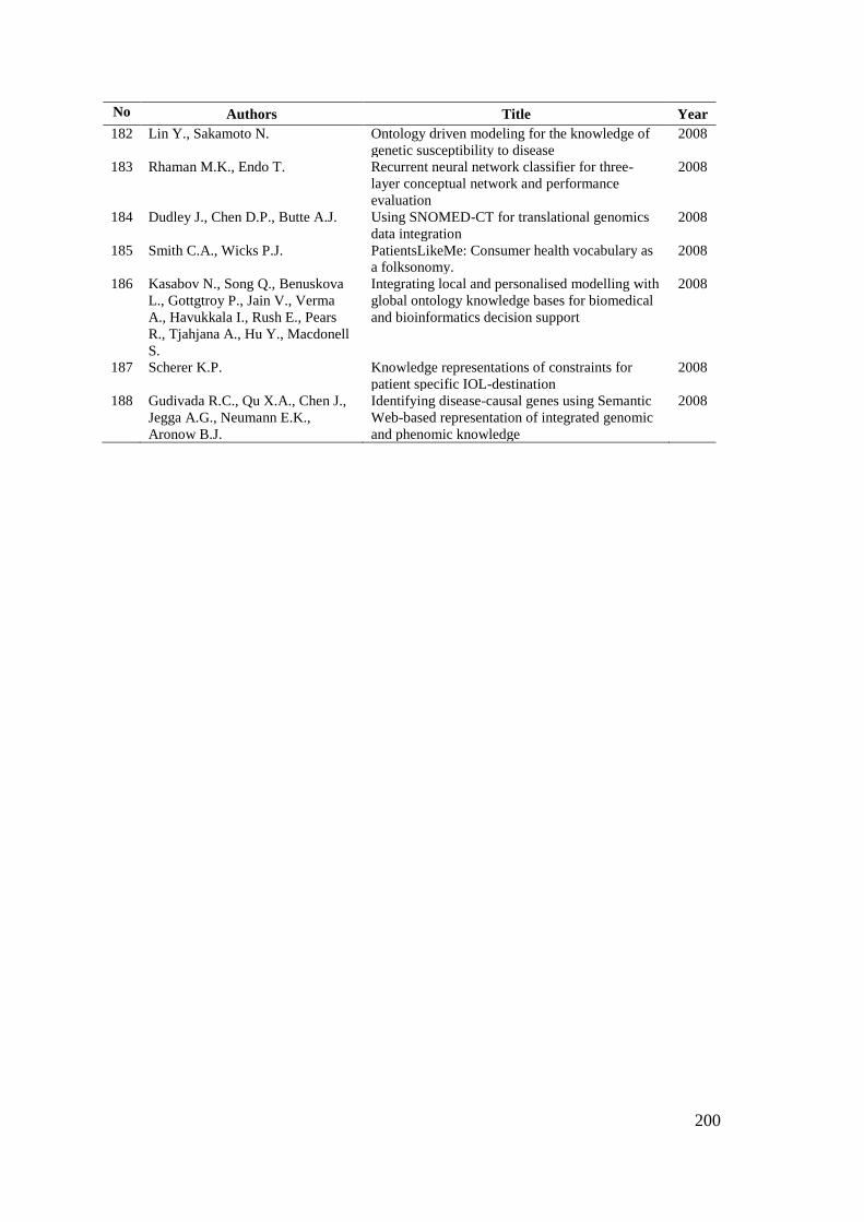
200
No Authors Title Year
182 Lin Y., Sakamoto N. Ontology driven modeling for the knowledge of
genetic susceptibility to disease
2008
183 Rhaman M.K., Endo T. Recurrent neural network classifier for three-
layer conceptual network and performance
evaluation
2008
184 Dudley J., Chen D.P., Butte A.J. Using SNOMED-CT for translational genomics
data integration
2008
185 Smith C.A., Wicks P.J. PatientsLikeMe: Consumer health vocabulary as
a folksonomy.
2008
186 Kasabov N., Song Q., Benuskova
L., Gottgtroy P., Jain V., Verma
A., Havukkala I., Rush E., Pears
R., Tjahjana A., Hu Y., Macdonell
S.
Integrating local and personalised modelling with
global ontology knowledge bases for biomedical
and bioinformatics decision support
2008
187 Scherer K.P. Knowledge representations of constraints for
patient specific IOL-destination
2008
188 Gudivada R.C., Qu X.A., Chen J.,
Jegga A.G., Neumann E.K.,
Aronow B.J.
Identifying disease-causal genes using Semantic
Web-based representation of integrated genomic
and phenomic knowledge
2008
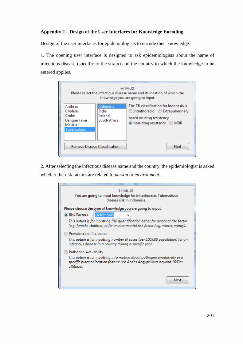
201
Appendix 2 – Design of the User Interfaces for Knowledge Encoding
Design of the user interfaces for epidemiologists to encode their knowledge.
1. The opening user interface is designed to ask epidemiologists about the name of
infectious disease (specific to the strain) and the country to which the knowledge to be
entered applies.
2. After selecting the infectious disease name and the country, the epidemiologist is asked
whether the risk factors are related to person or environment.
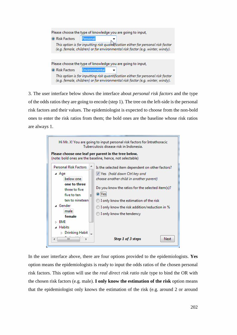
202
3. The user interface below shows the interface about personal risk factors and the type
of the odds ratios they are going to encode (step 1). The tree on the left-side is the personal
risk factors and their values. The epidemiologist is expected to choose from the non-bold
ones to enter the risk ratios from them; the bold ones are the baseline whose risk ratios
are always 1.
In the user interface above, there are four options provided to the epidemiologists. Yes
option means the epidemiologists is ready to input the odds ratios of the chosen personal
risk factors. This option will use the real direct risk ratio rule type to bind the OR with
the chosen risk factors (e.g. male). I only know the estimation of the risk option means
that the epidemiologist only knows the estimation of the risk (e.g. around 2 or around
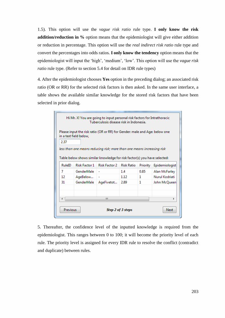
203
1.5). This option will use the vague risk ratio rule type. I only know the risk
addition/reduction in % option means that the epidemiologist will give either addition
or reduction in percentage. This option will use the real indirect risk ratio rule type and
convert the percentages into odds ratios. I only know the tendency option means that the
epidemiologist will input the ‘high’, ‘medium’, ‘low’. This option will use the vague risk
ratio rule type. (Refer to section 5.4 for detail on IDR rule types)
4. After the epidemiologist chooses Yes option in the preceding dialog; an associated risk
ratio (OR or RR) for the selected risk factors is then asked. In the same user interface, a
table shows the available similar knowledge for the stored risk factors that have been
selected in prior dialog.
5. Thereafter, the confidence level of the inputted knowledge is required from the
epidemiologist. This ranges between 0 to 100; it will become the priority level of each
rule. The priority level is assigned for every IDR rule to resolve the conflict (contradict
and duplicate) between rules.
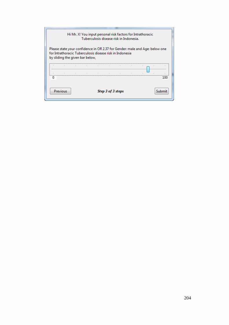
204
205
Appendix 3 – CBMS Proceeding Publication
An article published in the Proceedings of 30th IEEE Computer-based Medical Systems (CBMS)
International Conference. Thessaloniki, Greece, 22-24 June 2017. DOI: 10.1109/CBMS.2017.24
Personalization of Infectious Disease Risk Prediction: Towards automatic generation of a Bayesian Network
Retno Aulia Vinarti and Lucy Hederman
School of Computer Science and Statistics
Trinity College Dublin, The University of Dublin
Dublin, Ireland
e-mail: {retnor, hederman}@scss.tcd.ie
Abstract— Infectious diseases are a major cause of human
morbidity, but most are avoidable. An accurate and
personalized risk prediction is expected to alert people to the
risk of getting exposed to infectious diseases. However, as data
and knowledge in the epidemiology and infectious diseases
field becomes available, an updateable risk prediction model
is needed. The objectives of this article are (1) to describe the
mechanisms for generating a Bayesian Network (BN), as risk
prediction model, from a knowledge-base, and (2) to examine
the accuracy of the prediction result. The research in this
paper started by encoding declarative knowledge from the
Atlas of Human Infectious Diseases into an Infectious Disease
Risk Ontology. Automatic generation of a BN from this
knowledge uses two tools (1) a Rule Converter generates a BN
structure from the ontology (2) a Joint & Marginal
Probability Supplier tool populates the BN with probabilities.
These tools allow the BN to be recreated automatically
whenever knowledge and data changes. In a runtime phase, a
third tool, the Context Collector, captures facts given by the
client and consequent environmental context. This paper
introduces these tools and evaluates the effectiveness of the
resulting BN for a single infectious disease, Anthrax. We have
compared conditional probabilities predicted by our BN
against incidence estimated from real patient visit records.
Experiments explored the role of different context data in
prediction accuracy. The results suggest that building a BN
from an ontology is feasible. The experiments also show that
more context results in better risk prediction.
Keywords; Bayesian Network, Risk, Personalised
Prediction, Infectious diseases
I. Introduction
Infectious disease is listed as a major cause of human
morbidity [1]. However, many infectious diseases are
avoidable. There is a need for accurate prediction related to
infection risk [2] so that those at risk can take appropriate
avoidance precautions. Infectious disease risk is the result
15 Agent is a microorganism (e.g. fungus, bacteria, virus, prion, parasite
or mix) that cause illness.
of interaction between a person, pathogenic agent15 and
environment [3], The purpose of this research is to provide
people with personalised information about their risk of
being infected by a disease. The research faces several
challenges such as (1) the continuous update of knowledge
of predictors of risk, (2) the limited sources of experimental
and observational data which are costly to retrieve in full,
(3) the need for data, contexts and knowledge to describe a
complex situation that resembles the real world about risk
of getting an infectious disease, (4) establishing relevant
contextual data from a user’s details and location.
There has been extensive research in algorithms and techniques for risk prediction, such as fuzzy logic [4,5], Bayesian network [6,7], logistic regression [8-10] or combinations between them [11,12]. In general, a Bayesian network offers flexibility to incorporate dependencies between variables by defining probabilistic relationships [13], works under incomplete data [14] and its results are highly accurate compared to other prediction methods [5].
For this research, using a Bayesian Network approach, knowledge is represented as a network during the knowledge building phase. In this phase, person, season, weather and location risk factors are identified from declarative knowledge sources. Each factor is filled by a parameter value provided by a United Nations Data (UN) API. Then, predictors are transformed into BN nodes and states. After the network is created, the risk is calculated during the runtime phase. In this phase, person-related facts are given by the user. Weather and environment details are also retrieved based on user’s location from OpenWeather API and GoogleMaps API. All the retrieved facts are used to yield the personalized infectious disease risk prediction.
A recent innovation of Bayesian Networks to model relationships between variables is Dynamic Bayesian Networks (DBN) [15]. A DBN approach has been used in
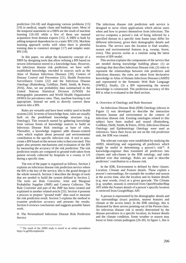
206
prediction [16-18] and diagnosing various problems [15] [19] in medical, supply chain and banking cases. Most of the temporal statements in a DBN are the result of machine learning [16-18] while a few of them use manual acquisition from domain experts [15]. A DBN is built by adding temporal dependencies to a static BN [19]. Machine learning approach works well when there is plentiful training data to construct stronger [17] and simpler static BN [18].
In this paper, we adopt the dynamicity concept of a DBN by designing tools that allow refining a BN based on newest information stored in a knowledge-base. However, for infectious disease risk prediction, we have well-established knowledge, encoded in sources such as the Atlas of Human Infectious Diseases [20], Centres of Disease Control and Prevention [21], Health Protection Surveillance Centre [22] and the Infectious Disease Ontology (Ruttenberg, Goldfain, Diehl, Smith, & Peters, 2016). Also, we use probability data summarised in the United Nations Statistical Division (UNSD) for demographic parameters and World Health Organization (WHO) for prevalence rates. Thus, machine learning is not appropriate. Instead we seek to directly convert these sources into a BN.
Rules are versatile and have been widely used in health systems [24]. In terms of knowledge-base, rules are usually built on the predefined knowledge structure (e.g. Ontology). This research started by gathering knowledge from various forms of knowledge sources to build an Infectious Disease Risk ontology as base of rules. Thereafter, a knowledge engineer adds disease-centred rules which explain about personal and environmental contribution to the specific infection risk. A tool to auto-create a BN based on the newest rules is then executed. This paper also presents mechanisms and evaluation of the BN by measuring the accuracy of the risk prediction. The risk prediction results are compared to ground truth taken from patient records collected by hospitals in a county in US during a specific time.
The rest of the paper is organized as follows. Section 2 explains an infectious disease risk prediction service where the BN is the key of the service; this is the grand design of the whole research. Section 3 describes the design of tools that are needed to build the system defined in Section 2. The tools are Rule Converter, Joint and Marginal Probability Supplier (JMP) and Context Collector. The Rule Converter and part of the JMP has been created and explained in another related-article [25]. Section 4 presents a process to prepare “ground truth” data used to measure the risk prediction result. Section 5 explains the method to examine prediction accuracy and presents the results. Section 6 reviews conclusions and suggests possible future work.
II. The Personalized Infectious Disease Risk Prediction
Service
16 The result of the AHID study is stored in an online spreadsheet
https://is.gd/IDcompletelist
The infectious disease risk prediction web service is
designed to serve client applications which advise users
when and how to protect themselves from infections. The
service computes a person’s risk of being infected by a
specified disease in a specific time frame (may differ for
different infections), given their demographic details and
location. The service uses the location to find weather,
season and environmental features (e.g. swamp, forest,
river). This process works at a runtime using the latest
version of BN model.
This section explains the components of the service that
are needed during knowledge building phase: (1) an
ontology that describes Infectious Disease risk; (2) rules to
represent the relationships between risk predictors and
infectious diseases; the rules are taken from declarative
knowledge in Atlas of Human Infectious Diseases (AHID)
and represented in the Semantic Web Rule Language
(SWRL); finally, (3) a BN representing the newest
knowledge is constructed. The prediction accuracy of this
BN is what is evaluated in the third section.
A. Overview of Ontology and Rule Structure
An Infectious Disease Risk (IDR) Ontology (shown in Figure 1) was developed to describe the interaction between human and environment in the context of infectious disease risk. Existing ontologies related to this subject have been studied and reused (Ruttenberg, Goldfain, Diehl, Smith, & Peters, 2016). Infectious Disease Ontology and Epidemiology Ontology were used as references. Since their focus are not on the risk prediction task, the IDR was created.
The relevant concepts were established by studying the AHID, identifying and organising all predictors which might be useful in determining a person’s risk16. A knowledge-engineer then translated all predictors into classes and sub-classes in the IDR ontology, and rules defined over that ontology. Rules are used to describe predictors’ contribution to a disease risk.
In the IDR, Environment is defined by three classes: Location, Climate and Feature details. These explain a person’s surroundings, for example the weather and season at the access time, also the location and its feature details (e.g. near woods, river) at a given geocode. The Climate (e.g. weather, season) is retrieved from OpenWeatherMap API while the Feature details of a person’s specific location is retrieved from GoogleMaps API.
A person is represented by his demographic details and his surroundings (exact position, nearest features and climate at the access time). In the IDR ontology, this is illustrated by three arrows pointing out of the Person class. An infectious disease risk is mostly determined by the disease prevalence in a specific location, its feature details and the climate condition. Some weather or season may boost or limit certain pathogens [26-30]. In figure 1, this is
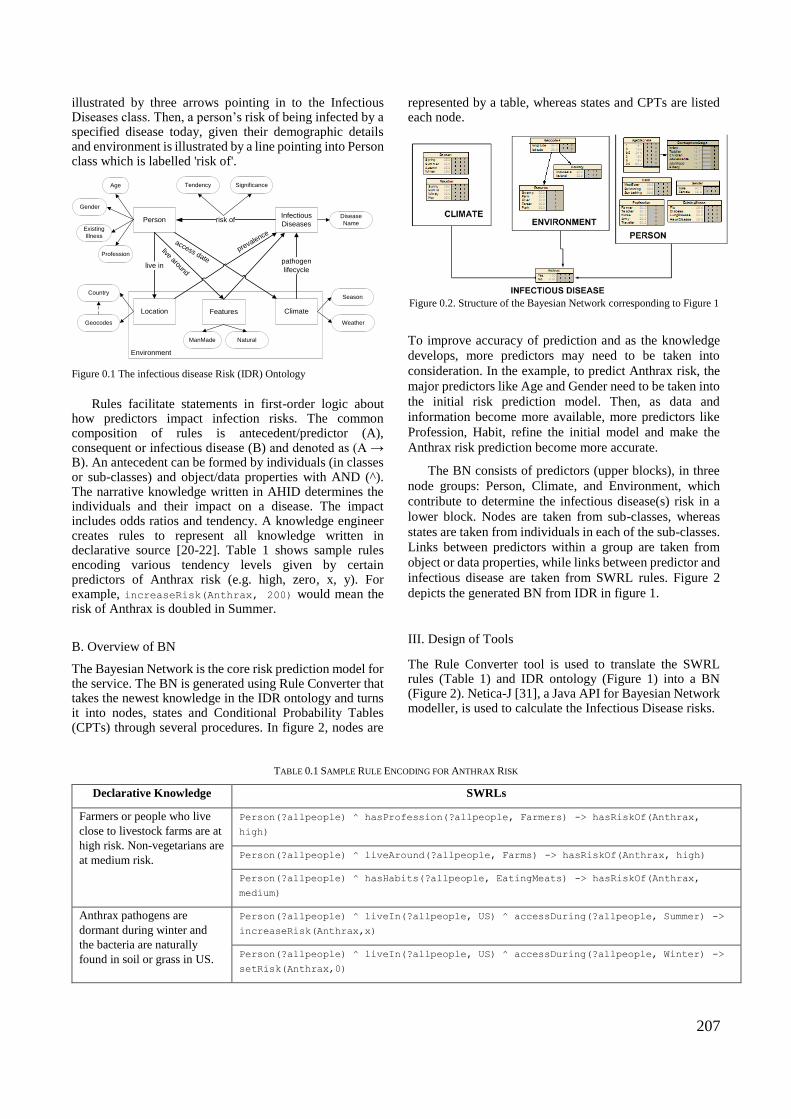
207
illustrated by three arrows pointing in to the Infectious Diseases class. Then, a person’s risk of being infected by a specified disease today, given their demographic details and environment is illustrated by a line pointing into Person class which is labelled 'risk of'.
Figure 0.1 The infectious disease Risk (IDR) Ontology
Rules facilitate statements in first-order logic about how predictors impact infection risks. The common composition of rules is antecedent/predictor (A), consequent or infectious disease (B) and denoted as (A → B). An antecedent can be formed by individuals (in classes or sub-classes) and object/data properties with AND (^). The narrative knowledge written in AHID determines the individuals and their impact on a disease. The impact includes odds ratios and tendency. A knowledge engineer creates rules to represent all knowledge written in declarative source [20-22]. Table 1 shows sample rules encoding various tendency levels given by certain predictors of Anthrax risk (e.g. high, zero, x, y). For example, increaseRisk(Anthrax, 200) would mean the risk of Anthrax is doubled in Summer.
B. Overview of BN
The Bayesian Network is the core risk prediction model for the service. The BN is generated using Rule Converter that takes the newest knowledge in the IDR ontology and turns it into nodes, states and Conditional Probability Tables (CPTs) through several procedures. In figure 2, nodes are
represented by a table, whereas states and CPTs are listed each node.
Figure 0.2. Structure of the Bayesian Network corresponding to Figure 1
To improve accuracy of prediction and as the knowledge
develops, more predictors may need to be taken into
consideration. In the example, to predict Anthrax risk, the
major predictors like Age and Gender need to be taken into
the initial risk prediction model. Then, as data and
information become more available, more predictors like
Profession, Habit, refine the initial model and make the
Anthrax risk prediction become more accurate.
The BN consists of predictors (upper blocks), in three
node groups: Person, Climate, and Environment, which
contribute to determine the infectious disease(s) risk in a
lower block. Nodes are taken from sub-classes, whereas
states are taken from individuals in each of the sub-classes.
Links between predictors within a group are taken from
object or data properties, while links between predictor and
infectious disease are taken from SWRL rules. Figure 2
depicts the generated BN from IDR in figure 1.
III. Design of Tools
The Rule Converter tool is used to translate the SWRL rules (Table 1) and IDR ontology (Figure 1) into a BN (Figure 2). Netica-J [31], a Java API for Bayesian Network modeller, is used to calculate the Infectious Disease risks.
TABLE 0.1 SAMPLE RULE ENCODING FOR ANTHRAX RISK
Declarative Knowledge SWRLs
Farmers or people who live
close to livestock farms are at
high risk. Non-vegetarians are
at medium risk.
Person(?allpeople) ^ hasProfession(?allpeople, Farmers) -> hasRiskOf(Anthrax,
high)
Person(?allpeople) ^ liveAround(?allpeople, Farms) -> hasRiskOf(Anthrax, high)
Person(?allpeople) ^ hasHabits(?allpeople, EatingMeats) -> hasRiskOf(Anthrax,
medium)
Anthrax pathogens are
dormant during winter and
the bacteria are naturally
found in soil or grass in US.
Person(?allpeople) ^ liveIn(?allpeople, US) ^ accessDuring(?allpeople, Summer) ->
increaseRisk(Anthrax,x)
Person(?allpeople) ^ liveIn(?allpeople, US) ^ accessDuring(?allpeople, Winter) ->
setRisk(Anthrax,0)
PersonInfectious
Diseases
Location Climate
risk of
live inpathogen
lifecycle
prevalence
Environment
Tendency SignificanceAge
Gender
Disease
Name
Season
Weather
Existing
Illness
Features
ManMade Natural
Country
Profession
Geocodes
live around
access date
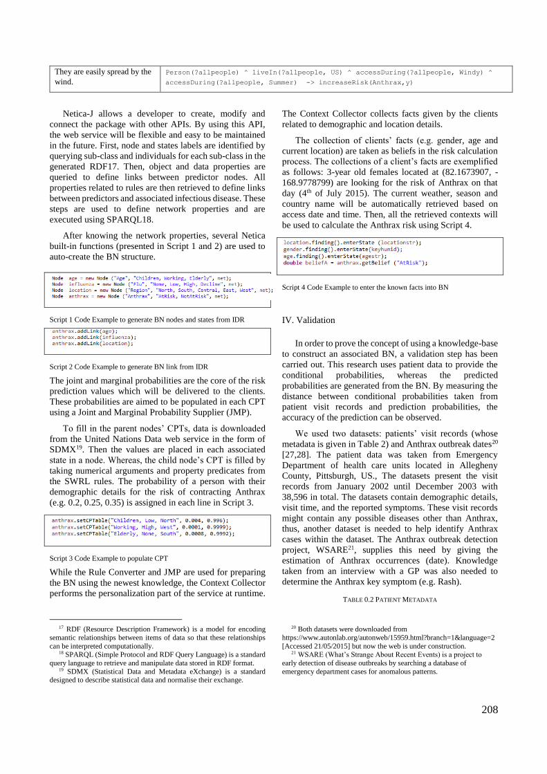
208
They are easily spread by the
wind.
Person(?allpeople) ^ liveIn(?allpeople, US) ^ accessDuring(?allpeople, Windy) ^
accessDuring(?allpeople, Summer) -> increaseRisk(Anthrax,y)
Netica-J allows a developer to create, modify and
connect the package with other APIs. By using this API,
the web service will be flexible and easy to be maintained
in the future. First, node and states labels are identified by
querying sub-class and individuals for each sub-class in the
generated RDF17. Then, object and data properties are
queried to define links between predictor nodes. All
properties related to rules are then retrieved to define links
between predictors and associated infectious disease. These
steps are used to define network properties and are
executed using SPARQL18.
After knowing the network properties, several Netica
built-in functions (presented in Script 1 and 2) are used to
auto-create the BN structure.
Script 1 Code Example to generate BN nodes and states from IDR
Script 2 Code Example to generate BN link from IDR
The joint and marginal probabilities are the core of the risk
prediction values which will be delivered to the clients.
These probabilities are aimed to be populated in each CPT
using a Joint and Marginal Probability Supplier (JMP).
To fill in the parent nodes’ CPTs, data is downloaded
from the United Nations Data web service in the form of
SDMX19. Then the values are placed in each associated
state in a node. Whereas, the child node’s CPT is filled by
taking numerical arguments and property predicates from
the SWRL rules. The probability of a person with their
demographic details for the risk of contracting Anthrax
(e.g. 0.2, 0.25, 0.35) is assigned in each line in Script 3.
Script 3 Code Example to populate CPT
While the Rule Converter and JMP are used for preparing
the BN using the newest knowledge, the Context Collector
performs the personalization part of the service at runtime.
17 RDF (Resource Description Framework) is a model for encoding
semantic relationships between items of data so that these relationships
can be interpreted computationally. 18 SPARQL (Simple Protocol and RDF Query Language) is a standard
query language to retrieve and manipulate data stored in RDF format. 19 SDMX (Statistical Data and Metadata eXchange) is a standard
designed to describe statistical data and normalise their exchange.
The Context Collector collects facts given by the clients
related to demographic and location details.
The collection of clients’ facts (e.g. gender, age and
current location) are taken as beliefs in the risk calculation
process. The collections of a client’s facts are exemplified
as follows: 3-year old females located at (82.1673907, -
168.9778799) are looking for the risk of Anthrax on that
day (4th of July 2015). The current weather, season and
country name will be automatically retrieved based on
access date and time. Then, all the retrieved contexts will
be used to calculate the Anthrax risk using Script 4.
Script 4 Code Example to enter the known facts into BN
IV. Validation
In order to prove the concept of using a knowledge-base
to construct an associated BN, a validation step has been
carried out. This research uses patient data to provide the
conditional probabilities, whereas the predicted
probabilities are generated from the BN. By measuring the
distance between conditional probabilities taken from
patient visit records and prediction probabilities, the
accuracy of the prediction can be observed.
We used two datasets: patients’ visit records (whose
metadata is given in Table 2) and Anthrax outbreak dates20
[27,28]. The patient data was taken from Emergency
Department of health care units located in Allegheny
County, Pittsburgh, US., The datasets present the visit
records from January 2002 until December 2003 with
38,596 in total. The datasets contain demographic details,
visit time, and the reported symptoms. These visit records
might contain any possible diseases other than Anthrax,
thus, another dataset is needed to help identify Anthrax
cases within the dataset. The Anthrax outbreak detection
project, WSARE21, supplies this need by giving the
estimation of Anthrax occurrences (date). Knowledge
taken from an interview with a GP was also needed to
determine the Anthrax key symptom (e.g. Rash).
TABLE 0.2 PATIENT METADATA
20 Both datasets were downloaded from
https://www.autonlab.org/autonweb/15959.html?branch=1&language=2
[Accessed 21/05/2015] but now the web is under construction. 21 WSARE (What’s Strange About Recent Events) is a project to
early detection of disease outbreaks by searching a database of
emergency department cases for anomalous patterns.
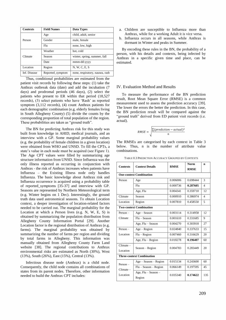
209
Contexts Field Names Data Types
Person
Age child, adult, senior
Gender male, female
Flu none, low, high
Climate
Weather hot, cold
Season winter, spring, summer, fall
Date mmm-dd-yyyy
Location Region N, W, C, E, S
Inf. Disease Reported_symptom none, respiratory, nausea, rash
Thus, conditional probabilities are estimated from the
patient visit records by following these steps: (1) take the
Anthrax outbreak data (date) and add the incubation (7
days) and prodromal periods (46 days), (2) select the
patients who present to ER within that period (18,527
records), (3) select patients who have ‘Rash’ as reported
symptom (3,112 records), (4) count Anthrax patients for
each demographic combination (e.g. elderly females living
in South Allegheny County) (5) divide the counts by the
corresponding proportion of total population of the region.
These probabilities are taken as “ground truth”.
The BN for predicting Anthrax risk for this study was
built from knowledge in AHID, medical journals, and an
interview with a GP. Some marginal probability values
(e.g. the probability of female children in a given location)
were obtained from WHO and UNSD. To fill the CPTs, a
state’s value in each node must be acquired (see Figure 1).
The Age CPT values were filled by summarizing age
structure information from UNSD. Since Influenza was the
only illness reported as occurring in conjunction with
Anthrax - the risk of Anthrax increases when patients have
Influenza – the Existing Illness node only handles
Influenza. The basic knowledge about Anthrax risk and
Influenza occurrence is acquired using a probability table
of reported_symptoms [35-37] and interview with GP.
Seasons are represented by Northern Meteorological term
(e.g. Winter begins on 1 Dec). Interestingly, the ground
truth data used astronomical seasons. To obtain Location
context, a deeper investigation of location-related factors
needed to be carried out. The marginal probability for the
Location at which a Person lives (e.g. N, W, E, S) is
obtained by summarizing the population distribution from
Allegheny County Information Portal [29]. Another
Location factor is the regional distribution of Anthrax (e.g.
farms). The marginal probability was obtained by
summarizing the number of farms per region and dividing
by total farms in Allegheny. This information was
manually obtained from Allegheny County Farm Land
website [38]. The regional contributions to Anthrax
environmental risks are estimated as North (30%), West
(13%), South (26%), East (15%), Central (13%).
Infectious disease node (Anthrax) is a child node.
Consequently, the child node contains all combinations of
states from its parent nodes. Therefore, other information
needed to build the Anthrax CPT includes:
a. Children are susceptible to Influenza more than
Anthrax, while for a working Adult it is vice versa.
b. Influenza occurs in all seasons, while Anthrax is
dormant in Winter and peaks in Summer.
By encoding these rules in the BN, the probability of a
person, with his details and contexts, being infected by
Anthrax in a specific given time and place, can be
estimated.
IV. Evaluation Method and Results
To measure the performance of the BN prediction
result, Root Mean Square Error (RMSE) is a common
measurement used to assess the prediction accuracy [39].
The lower the errors the better the prediction. In this case,
the BN prediction result will be compared against the
“ground truth” derived from ED patient visit records (i.e.
actual).
𝑅𝑀𝑆𝐸 = √∑(𝑝𝑟𝑒𝑑𝑖𝑐𝑡𝑖𝑜𝑛 − 𝑎𝑐𝑡𝑢𝑎𝑙)2
𝑛
The RMSEs are categorised by each context in Table 3
below. Thus, n is the number of attribute value
combinations.
TABLE 0.3 PREDICTION ACCURACY GROUPED BY CONTEXTS
Contexts Context Details RMSE Norm
RMSE
n
One-context Combination
Person Age 0.006006 0.698444 3
Flu 0.000736 0.287605 4
Age, Flu 0.004341 0.359710 12
Climate Season 0.000910 0.386974 4
Location Region 0.007810 0.458550 5
Two-context Combination
Person –
Climate
Age – Season 0.003114 0.314958 12
Flu – Season 0.001610 0.331685 9
Age, Flu – Season 0.004270 0.303918 27
Person –
Location
Age – Region 0.024840 0.337633 15
Flu – Region 0.007460 0.316629 20
Age, Flu – Region 0.018278 0.196407 60
Climate –
Location Season – Region 0.004783 0.283449 20
Three-context Combination
Person –
Climate –
Location
Age – Season – Region 0.015134 0.243600 60
Flu – Season – Region 0.066149 0.197595 45
Age, Flu – Season –
Region 0.035340 0.174622 135
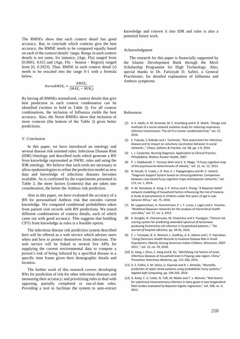
210
The RMSEs show that each context detail has good
accuracy. But, to conclude which contexts give the best
accuracy, the RMSE needs to be compared equally based
on each of the context details’ range. Range in each context
details is not same, for instance, (Age, Flu) ranged from
[0.0003, 0.01] and (Age, Flu - Season - Region) ranged
from [0, 0.2023]. Thus, RMSE in each context detail (i)
needs to be rescaled into the range 0-1 with a formula
below.
𝑁𝑜𝑟𝑚𝑅𝑀𝑆𝐸𝑖 =𝑅𝑀𝑆𝐸𝑖
(𝑀𝐴𝑋𝑖 − 𝑀𝐼𝑁𝑖)
By having all RMSEs normalized, context details that give
best prediction in each context combination can be
identified (written in bold in Table 3). For all context
combinations, the inclusion of Influenza yields the best
accuracy. Also, the Norm RMSEs show that inclusion of
more contexts (the bottom of the Table 3) gives better
predictions.
V. Conclusion
In this paper, we have introduced an ontology and
several disease risk oriented rules: Infectious Disease Risk
(IDR) Ontology and described tools which generate a BN
from knowledge represented as SWRL rules and using the
IDR ontology. We believe that such tools are necessary to
allow epidemiologists to refine the prediction model as new
data and knowledge of infectious diseases becomes
available. As is confirmed by the experiments presented in
Table 3, the more factors (contexts) that are taken into
consideration, the better the Anthrax risk prediction.
Also in this paper, we have evaluated the accuracy of a
BN for personalised Anthrax risk that encodes current
knowledge. We compared conditional probabilities taken
from patient visit records with BN predictions. We tested
different combinations of context details, each of which
came out with good accuracy. This suggests that building
CPTs from knowledge as rules is a feasible option.
The infectious disease risk prediction system described
here will be offered as a web service which advises users
when and how to protect themselves from infections. The
web service will be linked to several live APIs for
supplying the current environmental data to compute a
person’s risk of being infected by a specified disease in a
specific time frame given their demographic details and
location.
The further work of this research covers: developing
BNs for prediction of risk for other infectious diseases and
measuring their accuracy; and prioritizing rules to deal with
opposing, partially completed or out-of-date rules.
Providing a tool to facilitate the system to auto-extract
knowledge and convert it into IDR and rules is also a
potential future work.
Acknowledgment
The research for this paper is financially supported by
the Islamic Development Bank through the Merit
Scholarship Programme for High Technology. Also,
special thanks to Dr. Fariziyah D. Safitri, a General
Practitioner, for detailed explanation of Influenza and
Anthrax symptoms.
References
[1] A. E. Aiello, A. M. Simanek, M. C. Eisenberg and A. R. Walsh, "Design and methods of a social network isolation study for reducing respiratory infection transmission: The eX-FLU cluster randomized trial," vol. 15, 2016.
[2] E. Fukuda, S. Kokubo and J. Tanimoto, "Risk assessment for infectious disease and its impact on voluntary vaccination behavior in social networks.," Chaos, Solitons & Fractals, vol. 68, pp. 1-9, 2014.
[3] L. J. Carpenito, Nursing Diagnosis: Application to Clinical Practice, Philadelphia: Wolters Kluwer Health, 2007.
[4] P. J. Giabbanelli, T. Torsney-Weir and V. K. Mago, "A fuzzy cognitive map of the psychosocial determinants of obesity," vol. 12, no. 12, 2012.
[5] N. Douali, H. Csaba, J. D. Roo, E. I. Papageorgiou and M.-C. Jaulent, "Diagnosis Support System based on clinical guidelines: Comparison between case-based fuzzy cognitive maps and bayesian networks," vol. 113, no. 1, 2014.
[6] H. M. Semakula, G. Song, S. P. Achuu and S. Zhang, "A Bayesian belief network modelling of household factors influencing the risk of malaria: A study of parasitaemia in children under five years of age in sub-Saharan Africa," vol. 75, 2016.
[7] M. Lappenschaar, A. Hommersom, P. J. F. Lucas, J. Lagro and S. Visscher, "Multilevel Bayesian networks for the analysis of hierarchical health care data," vol. 57, no. 3, 2013.
[8] K. Kengkla, N. Charoensuka, M. Chaichana and S. Puangjan, "Clinical risk scoring system for predicting extended-spectrum β-lactamase-producing Escherichia coli infection in hospitalized patients.," The Journal of hospital infection, pp. 49-56, 2016.
[9] E. J. Tomayko, B. A. Weinert, L. Godfrey, A. K. Adams and L. P. Hanrahan, "Using Electronic Health Records to Examine Disease Risk in Small Populations: Obesity Among American Indian Children, Wisconsin, 2007-2012.," vol. 13, no. 29, 2016.
[10] Q. Jiang, J. Zhou, Z. Jiang and B. Xu, "Identifying risk factors of avian infectious diseases at household level in Poyang Lake region, China," Preventive Veterinary Medicine, pp. 151-160, 2014.
[11] A. S. Fialho, S. M. Vieira, U. Kaymak and R. J. Almeida, "Mortality prediction of septic shock patients using probabilistic fuzzy systems," Applied Soft Computing, pp. 194-203, 2016.
[12] G. Koop, C. A. Collar, N. Toft, M. Nielen and T. v. Werven, "Risk factors for subclinical intramammary infection in dairy goats in two longitudinal field studies evaluated by Bayesian logistic regression," vol. 108, no. 4, 2013.
211
[13] D. Beaudequin, F. Harden, A. Roiko, H. Stratton and C. Lemckert, "Beyond QMRA: Modelling microbial health risk as a complex system using Bayesian networks," vol. 80, 2015.
[14] P. A. Aguilera, A. Fernandez, R. Fernandez, R. Rumi and A. Salmeron, "Environmental Modelling & Software Bayesian networks in environmental modelling," Environmental Modelling and Software, vol. 26, no. 12, pp. 1376-1388, 2011.
[15] T. Charitos, L. C. van der Gaag, S. Visscher and K. A. M. Schurink, "A dynamic Bayesian network for diagnosing ventilator-associated pneumonia in ICU patients," Expert Systems with Applications, vol. 36, no. 2, pp. 1249-1258, 2009.
[16] P. Panayiotis, H. X. Simon, A. Denise and B. A. T. Alex, "Prediction of lung cancer incidence on the low-dose computed tomography arm of the National Lung Screening Trial: A dynamic Bayesian network," Artificial Intelligence in Medicine, vol. 72, pp. 42-55, 2016.
[17] Q. Xiao, L. Xing and G. Song, "Time series prediction using optimal theorem and dynamic," Optics, vol. 127, p. 11063–11069, 2016.
[18] J. J. Dabrowski, C. Beyers and J. P. de Villiers, "Systemic banking crisis early warning systems using dynamic Bayesian," Expert Systems with Applications, vol. 62, pp. 225-242, 2016.
[19] H.-Y. Kao, C.-H. Huang and H.-L. Li, "Supply chain diagnostics with dynamic Bayesian networks," Computers & Industrial Engineering, vol. 49, pp. 339-347, 2005.
[20] H. F. L. Wertheim, P. Horby and J. P. Woodall, Atlas of Human Infectious Diseases, Oxford: Wiley-Blackwell, 2012.
[21] CDC, "Lesson 1: Introduction to Epidemiology," 18 May 2012. [Online]. Available: http://www.cdc.gov/ophss/csels/dsepd/ss1978/lesson1/section10.html.
[22] HSPC, "Health Protection Surveillance Centre," 2016. Available: http://www.hpsc.ie/NotifiableDiseases/NotifyingInfectiousDiseases/
[23] A. Ruttenberg, A. Goldfain, A. Diehl, B. Smith and B. Peters, "Infectious Disease Ontology," The National Center for Biomedical Ontology, 5 July 2016. [Online]. Available: http://purl.obolibrary.org/obo/ido.owl.
[24] A. Onisko, P. Lucas and M. J. Druzdzel, "Comparison of Rule-Based and Bayesian Network Approaches in Medical Diagnostic Systems," in 8th Conference on Artificial Intelligence in Medicine, Portugal, 2001.
[25] R. A. Vinarti and L. M. Hederman, "A Performance Analysis of an Algorithm to Auto-create a Bayesian Network," in Database and Expert System Applications, Lyon, 2017.
[26] W. H. O. WHO, "Climate Change and Human Health - Risks and Responses Summary," World Health Organization, Geneva, 2003.
[27] X. Wu, Y. Lu, S. Zhou, L. Chen and B. Xu, "Impact of climate change on human infectious diseases: Empirical evidence and human adaptation," vol. 86, 2016.
[28] D. N. Fisman, "Seasonality of viral infections: Mechanisms and unknowns," American Journal of Preventive Medicine, vol. 18, no. 10, pp. 946-954, 2008.
[29] T. P. Monath and P. F. C. Vasconcelos, "Yellow fever," Journal of Clinical Virology, vol. 64, pp. 160-173, 2015.
[30] H. Yi, B. R. Devkota and J.-s. Yu, "Effects of global warming on mosquitoes & mosquito-borne diseases and the new strategies for mosquito control," Entomological Research, vol. 44, no. 6, pp. 215-235, 2014.
[31] Norsys, "Examples," Norsys Software Corporation, 1995-2017. [Online]. Available: https://www.norsys.com/netica-j/examples/SimulateCases.html.
[32] W.-K. Wong, A. Moore, G. Cooper and M. Wagner, "Bayesian network anomaly pattern detection for disease outbreaks," in Twentieth International Conference on Machine Learning, Washington, D.C., 2003.
[33] W.-K. Wong, A. Moore, G. Cooper and M. Wagner, "Rule-based anomaly pattern detection for detecting disease outbreaks," in Eighteenth National Conference on AI, Alberta, 2002.
[34] A. C. I. Portal, "Allegheny County Information Portal," Pittsburgh, Pennsylvania, US, [Online]. http://www.alleghenycounty.us/.
[35] F. Carrat, A. Tachet, C. Rouzioux and B. Housset, "Evaluation of clinical case definitions of Influenza: detailed investigation of patients during 1995 - 1996 epidemic in France," Clinical Infectious Diseases, vol. 28, pp. 283-290, 1999.
[36] A. S. Monto, S. Gravenstein, M. Colopy and J. Scweinle, "Clinical signs and symptoms predicting influenza infection," Arch International Medicine, vol. 160, pp. 3243-3247, 2000.
[37] D. N. Kyriacou, A. C. Stein, P. R. Yarnold and D. M. Courtney, "Clinical predictors of bioterrorism-related inhalational anthrax," The Lancet, vol. 364, pp. 449-452, 2004.
[38] A. Farmland, "Allegheny County Farmland Preservation Program," [Online]. Available: http://www.alleghenyfarmland.com/.
[39] E. W. Steyerberg, A. J. Vickers, N. R. Cook and T. Gerds, "Assessing the performance of prediction models: a framework," Epidemiology, vol. 21, no. 1, pp. 128-138, 2010.
Appendix 4 – MIE Book Section Publication
An article published in the Proceedings of the 29th Medical Informatics Europe (MIE).
Gothenburg, Sweden, 24-26 April 2018. DOI: 10.3233/978-1-61499-852-5-531
A Knowledge-base for a Personalized Infectious Disease
Risk Prediction System
Retno VINARTIa,22 and Lucy HEDERMANa a
School of Computer Science and Statistics, Trinity College Dublin,
The University of Dublin, Ireland
Abstract. We present a knowledge-base to represent collated infectious disease risk (IDR) knowledge. The knowledge is
about personal and contextual risk of contracting an infectious disease obtained from declarative sources (e.g. Atlas of Human
Infectious Diseases). Automated prediction requires encoding this knowledge in a form that can produce risk probabilities
(e.g. Bayesian Network – BN). The knowledge-base presented in this paper feeds an algorithm that can auto-generate the BN.
The knowledge from 234 infectious diseases was compiled. From this compilation, we designed an ontology and five rule
types for modelling IDR knowledge in general. The evaluation aims to assess whether the knowledge-base structure, and its
application to three disease-country contexts, meets the needs of personalized IDR prediction system. From the evaluation
results, the knowledge-base conforms to the system’s purpose: personalization of infectious disease risk.
Keywords. knowledge-base, rules, ontology, infectious disease, risk.
Introduction
We envisage a service which predicts a person’s risk of contracting an infectious disease (ID) based on their
personal attributes (age, diet) and their location (weather, geographical features). This service will supply risk
predictions to advisor applications designed to help users take risk-reducing actions (e.g. wear a mask to avoid
influenza during a windy week in autumn).
Knowledge about personal and contextual risk of contracting an ID is largely communicated in declarative form;
general, stable knowledge is documented in the Atlas of Human Infectious Diseases (AHID) and similar books
[1-3]; more specific and up to date knowledge is conveyed in epidemiology journals. Automated prediction
requires encoding this knowledge in a form that can produce risk probabilities, such as in a Bayesian Network
(BN). In previous work (Vinarti & Hederman, Personalization of Infectious Disease Risk Prediction Towards
automatic generation of a Bayesian Network, 2017) we showed that we can yield accurate predictions by
manually encoding the IDR knowledge in a BN. But this approach is not scalable to all IDs, regions and risk
factors, nor maintainable to model new knowledge.
Rather than hardcoding current general knowledge for all IDs as a BN, we seek to facilitate the ongoing encoding
by epidemiologists of up to date and region-specific ID risk. The knowledge is manually represented by experts
as ID risk rules (e.g. a rule that says smoking can double Tuberculosis (TB) risk) defined over a special purpose
ontology of ID risk. The knowledge-base (an ontology and collection of ID risk rules) is then automatically
converted to a BN, using the BN builder algorithm described in [5]. This paper describes the design and
evaluation of the knowledge-base.
Knowledge-base Design
This section describes the methodology used to design the knowledge-base. First, the ID literature was
summarized to identify risk elements and quantitative forms of risk. From this summary, the ‘backbone’ of the
22 Corresponding Author, e-mail: [email protected]. Special thanks to Dr. Fariziyah D. Safitri, and Nurul Kodriati, M.Med.Sc., (Ph.D Cand)
for feedback on the knowledge-base.
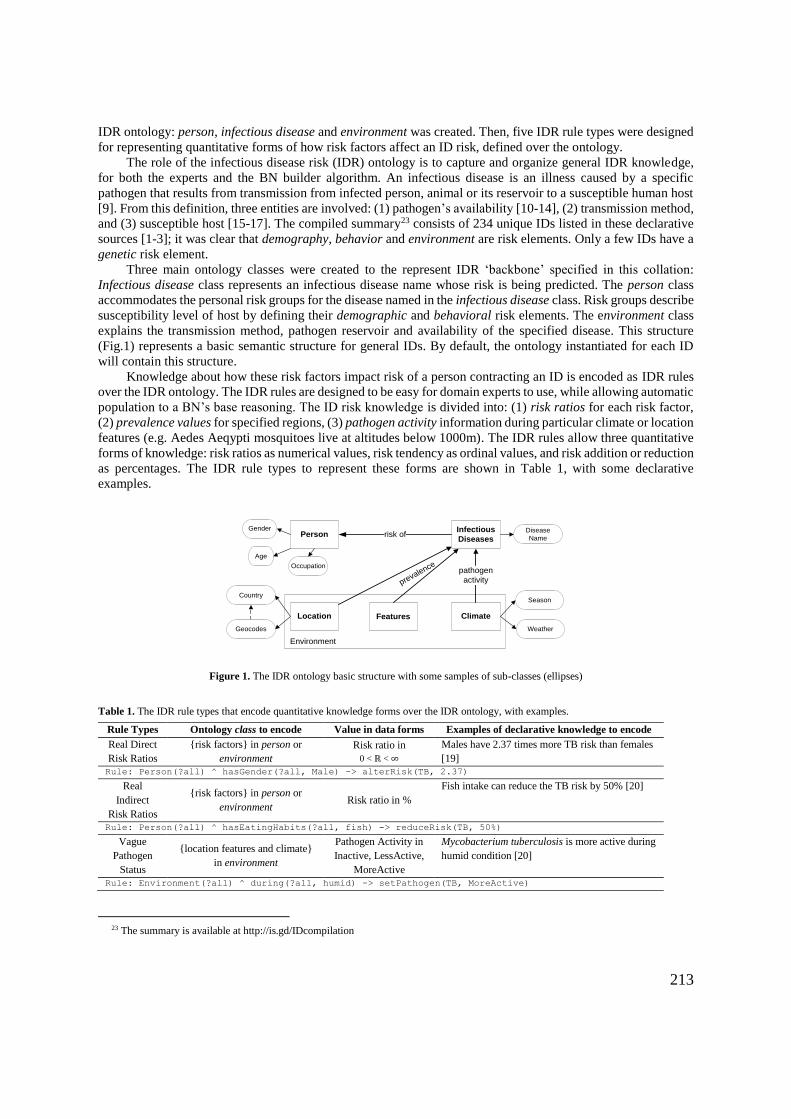
213
IDR ontology: person, infectious disease and environment was created. Then, five IDR rule types were designed
for representing quantitative forms of how risk factors affect an ID risk, defined over the ontology.
The role of the infectious disease risk (IDR) ontology is to capture and organize general IDR knowledge,
for both the experts and the BN builder algorithm. An infectious disease is an illness caused by a specific
pathogen that results from transmission from infected person, animal or its reservoir to a susceptible human host
[9]. From this definition, three entities are involved: (1) pathogen’s availability [10-14], (2) transmission method,
and (3) susceptible host [15-17]. The compiled summary23 consists of 234 unique IDs listed in these declarative
sources [1-3]; it was clear that demography, behavior and environment are risk elements. Only a few IDs have a
genetic risk element.
Three main ontology classes were created to the represent IDR ‘backbone’ specified in this collation:
Infectious disease class represents an infectious disease name whose risk is being predicted. The person class
accommodates the personal risk groups for the disease named in the infectious disease class. Risk groups describe
susceptibility level of host by defining their demographic and behavioral risk elements. The environment class
explains the transmission method, pathogen reservoir and availability of the specified disease. This structure
(Fig.1) represents a basic semantic structure for general IDs. By default, the ontology instantiated for each ID
will contain this structure.
Knowledge about how these risk factors impact risk of a person contracting an ID is encoded as IDR rules
over the IDR ontology. The IDR rules are designed to be easy for domain experts to use, while allowing automatic
population to a BN’s base reasoning. The ID risk knowledge is divided into: (1) risk ratios for each risk factor,
(2) prevalence values for specified regions, (3) pathogen activity information during particular climate or location
features (e.g. Aedes Aeqypti mosquitoes live at altitudes below 1000m). The IDR rules allow three quantitative
forms of knowledge: risk ratios as numerical values, risk tendency as ordinal values, and risk addition or reduction
as percentages. The IDR rule types to represent these forms are shown in Table 1, with some declarative
examples.
PersonInfectious
Diseases
Location Climate
risk of
pathogen
activityprevalence
Environment
Age
Gender Disease
Name
Season
Weather
Features
Country
Occupation
Geocodes
Figure 1. The IDR ontology basic structure with some samples of sub-classes (ellipses)
Table 1. The IDR rule types that encode quantitative knowledge forms over the IDR ontology, with examples.
Rule Types Ontology class to encode Value in data forms Examples of declarative knowledge to encode
Real Direct
Risk Ratios
{risk factors} in person or
environment
Risk ratio in
0 < ℝ < ∞
Males have 2.37 times more TB risk than females
[19]
Rule: Person(?all) ^ hasGender(?all, Male) -> alterRisk(TB, 2.37)
Real
Indirect
Risk Ratios
{risk factors} in person or
environment Risk ratio in %
Fish intake can reduce the TB risk by 50% [20]
Rule: Person(?all) ^ hasEatingHabits(?all, fish) -> reduceRisk(TB, 50%)
Vague
Pathogen
Status
{location features and climate}
in environment
Pathogen Activity in
Inactive, LessActive,
MoreActive
Mycobacterium tuberculosis is more active during
humid condition [20]
Rule: Environment(?all) ^ during(?all, humid) -> setPathogen(TB, MoreActive)
23 The summary is available at http://is.gd/IDcompilation
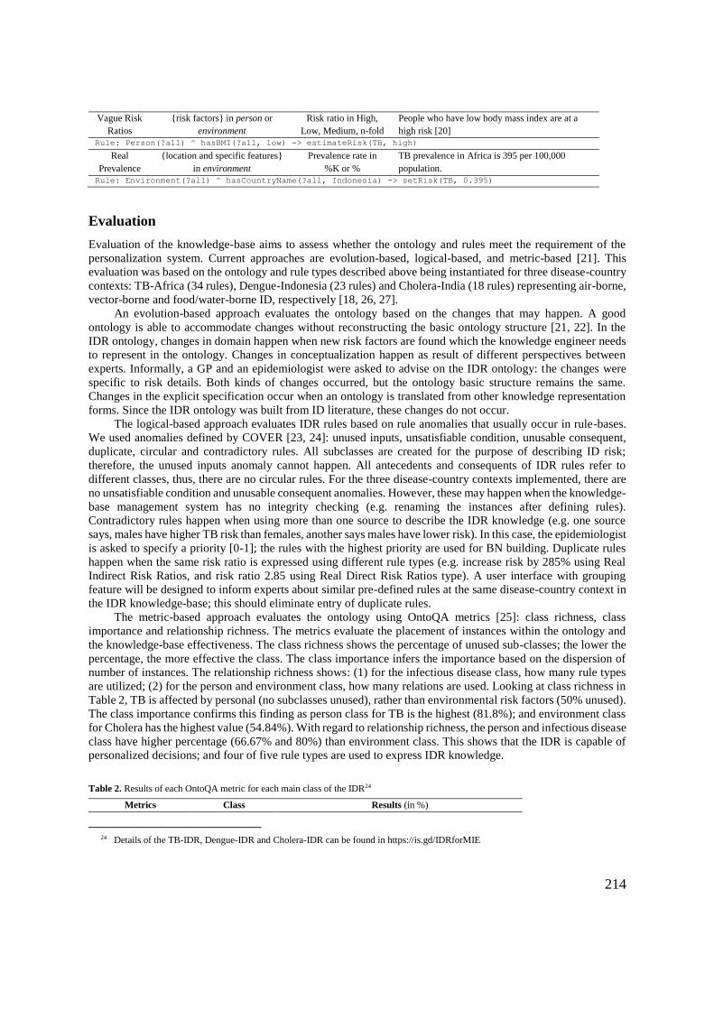
214
Vague Risk
Ratios
{risk factors} in person or
environment
Risk ratio in High,
Low, Medium, n-fold
People who have low body mass index are at a
high risk [20]
Rule: Person(?all) ^ hasBMI(?all, low) -> estimateRisk(TB, high)
Real
Prevalence
{location and specific features}
in environment
Prevalence rate in
%K or %
TB prevalence in Africa is 395 per 100,000
population.
Rule: Environment(?all) ^ hasCountryName(?all, Indonesia) -> setRisk(TB, 0.395)
Evaluation
Evaluation of the knowledge-base aims to assess whether the ontology and rules meet the requirement of the
personalization system. Current approaches are evolution-based, logical-based, and metric-based [21]. This
evaluation was based on the ontology and rule types described above being instantiated for three disease-country
contexts: TB-Africa (34 rules), Dengue-Indonesia (23 rules) and Cholera-India (18 rules) representing air-borne,
vector-borne and food/water-borne ID, respectively [18, 26, 27].
An evolution-based approach evaluates the ontology based on the changes that may happen. A good
ontology is able to accommodate changes without reconstructing the basic ontology structure [21, 22]. In the
IDR ontology, changes in domain happen when new risk factors are found which the knowledge engineer needs
to represent in the ontology. Changes in conceptualization happen as result of different perspectives between
experts. Informally, a GP and an epidemiologist were asked to advise on the IDR ontology: the changes were
specific to risk details. Both kinds of changes occurred, but the ontology basic structure remains the same.
Changes in the explicit specification occur when an ontology is translated from other knowledge representation
forms. Since the IDR ontology was built from ID literature, these changes do not occur.
The logical-based approach evaluates IDR rules based on rule anomalies that usually occur in rule-bases.
We used anomalies defined by COVER [23, 24]: unused inputs, unsatisfiable condition, unusable consequent,
duplicate, circular and contradictory rules. All subclasses are created for the purpose of describing ID risk;
therefore, the unused inputs anomaly cannot happen. All antecedents and consequents of IDR rules refer to
different classes, thus, there are no circular rules. For the three disease-country contexts implemented, there are
no unsatisfiable condition and unusable consequent anomalies. However, these may happen when the knowledge-
base management system has no integrity checking (e.g. renaming the instances after defining rules).
Contradictory rules happen when using more than one source to describe the IDR knowledge (e.g. one source
says, males have higher TB risk than females, another says males have lower risk). In this case, the epidemiologist
is asked to specify a priority [0-1]; the rules with the highest priority are used for BN building. Duplicate rules
happen when the same risk ratio is expressed using different rule types (e.g. increase risk by 285% using Real
Indirect Risk Ratios, and risk ratio 2.85 using Real Direct Risk Ratios type). A user interface with grouping
feature will be designed to inform experts about similar pre-defined rules at the same disease-country context in
the IDR knowledge-base; this should eliminate entry of duplicate rules.
The metric-based approach evaluates the ontology using OntoQA metrics [25]: class richness, class
importance and relationship richness. The metrics evaluate the placement of instances within the ontology and
the knowledge-base effectiveness. The class richness shows the percentage of unused sub-classes; the lower the
percentage, the more effective the class. The class importance infers the importance based on the dispersion of
number of instances. The relationship richness shows: (1) for the infectious disease class, how many rule types
are utilized; (2) for the person and environment class, how many relations are used. Looking at class richness in
Table 2, TB is affected by personal (no subclasses unused), rather than environmental risk factors (50% unused).
The class importance confirms this finding as person class for TB is the highest (81.8%); and environment class
for Cholera has the highest value (54.84%). With regard to relationship richness, the person and infectious disease
class have higher percentage (66.67% and 80%) than environment class. This shows that the IDR is capable of
personalized decisions; and four of five rule types are used to express IDR knowledge.
Table 2. Results of each OntoQA metric for each main class of the IDR24
Metrics Class Results (in %)
24 Details of the TB-IDR, Dengue-IDR and Cholera-IDR can be found in https://is.gd/IDRforMIE
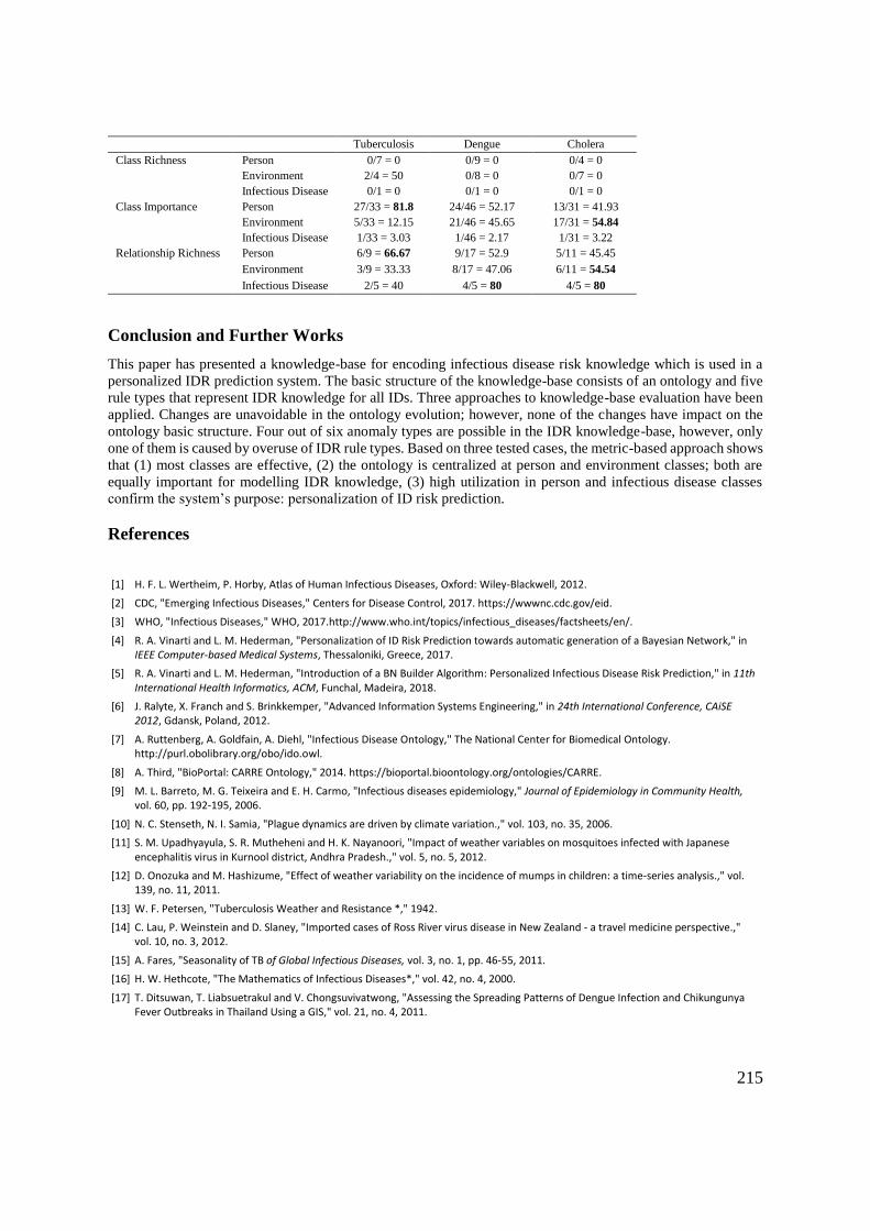
215
Tuberculosis Dengue Cholera
Class Richness Person 0/7 = 0 0/9 = 0 0/4 = 0
Environment 2/4 = 50 0/8 = 0 0/7 = 0
Infectious Disease 0/1 = 0 0/1 = 0 0/1 = 0
Class Importance Person 27/33 = 81.8 24/46 = 52.17 13/31 = 41.93
Environment 5/33 = 12.15 21/46 = 45.65 17/31 = 54.84
Infectious Disease 1/33 = 3.03 1/46 = 2.17 1/31 = 3.22
Relationship Richness Person 6/9 = 66.67 9/17 = 52.9 5/11 = 45.45
Environment 3/9 = 33.33 8/17 = 47.06 6/11 = 54.54
Infectious Disease 2/5 = 40 4/5 = 80 4/5 = 80
Conclusion and Further Works
This paper has presented a knowledge-base for encoding infectious disease risk knowledge which is used in a
personalized IDR prediction system. The basic structure of the knowledge-base consists of an ontology and five
rule types that represent IDR knowledge for all IDs. Three approaches to knowledge-base evaluation have been
applied. Changes are unavoidable in the ontology evolution; however, none of the changes have impact on the
ontology basic structure. Four out of six anomaly types are possible in the IDR knowledge-base, however, only
one of them is caused by overuse of IDR rule types. Based on three tested cases, the metric-based approach shows
that (1) most classes are effective, (2) the ontology is centralized at person and environment classes; both are
equally important for modelling IDR knowledge, (3) high utilization in person and infectious disease classes
confirm the system’s purpose: personalization of ID risk prediction.
References
[1] H. F. L. Wertheim, P. Horby, Atlas of Human Infectious Diseases, Oxford: Wiley-Blackwell, 2012.
[2] CDC, "Emerging Infectious Diseases," Centers for Disease Control, 2017. https://wwwnc.cdc.gov/eid.
[3] WHO, "Infectious Diseases," WHO, 2017.http://www.who.int/topics/infectious_diseases/factsheets/en/.
[4] R. A. Vinarti and L. M. Hederman, "Personalization of ID Risk Prediction towards automatic generation of a Bayesian Network," in IEEE Computer-based Medical Systems, Thessaloniki, Greece, 2017.
[5] R. A. Vinarti and L. M. Hederman, "Introduction of a BN Builder Algorithm: Personalized Infectious Disease Risk Prediction," in 11th International Health Informatics, ACM, Funchal, Madeira, 2018.
[6] J. Ralyte, X. Franch and S. Brinkkemper, "Advanced Information Systems Engineering," in 24th International Conference, CAiSE 2012, Gdansk, Poland, 2012.
[7] A. Ruttenberg, A. Goldfain, A. Diehl, "Infectious Disease Ontology," The National Center for Biomedical Ontology. http://purl.obolibrary.org/obo/ido.owl.
[8] A. Third, "BioPortal: CARRE Ontology," 2014. https://bioportal.bioontology.org/ontologies/CARRE.
[9] M. L. Barreto, M. G. Teixeira and E. H. Carmo, "Infectious diseases epidemiology," Journal of Epidemiology in Community Health, vol. 60, pp. 192-195, 2006.
[10] N. C. Stenseth, N. I. Samia, "Plague dynamics are driven by climate variation.," vol. 103, no. 35, 2006.
[11] S. M. Upadhyayula, S. R. Mutheheni and H. K. Nayanoori, "Impact of weather variables on mosquitoes infected with Japanese encephalitis virus in Kurnool district, Andhra Pradesh.," vol. 5, no. 5, 2012.
[12] D. Onozuka and M. Hashizume, "Effect of weather variability on the incidence of mumps in children: a time-series analysis.," vol. 139, no. 11, 2011.
[13] W. F. Petersen, "Tuberculosis Weather and Resistance *," 1942.
[14] C. Lau, P. Weinstein and D. Slaney, "Imported cases of Ross River virus disease in New Zealand - a travel medicine perspective.," vol. 10, no. 3, 2012.
[15] A. Fares, "Seasonality of TB of Global Infectious Diseases, vol. 3, no. 1, pp. 46-55, 2011.
[16] H. W. Hethcote, "The Mathematics of Infectious Diseases*," vol. 42, no. 4, 2000.
[17] T. Ditsuwan, T. Liabsuetrakul and V. Chongsuvivatwong, "Assessing the Spreading Patterns of Dengue Infection and Chikungunya Fever Outbreaks in Thailand Using a GIS," vol. 21, no. 4, 2011.
216
[18] P. Gustafson, V. F. Gomes, C. S. Vieira, "TB in Bissau: incidence and risk factors in an urban community in sub-Saharan Africa," International Journal of Epidemiology, vol. 33, pp. 163-172, 2004.
[19] D. Guwatudde, M. Nakakeeto, E. C. Jones-Lopez, "TB in Household Contacts of Infectious Cases in Kampala, Uganda," American Journal of Epidemiology, vol. 158, no. 9, pp. 887-898, 2003.
[20] Q. Wang, Y. Liu, Y. Ma and L. Han, "Severe hypovitaminosis D in active TB patients and its predictors," Clinical Nutrition, pp. 1-7, 2017.
[21] S. Tartir, I. B. Arpinar and A. P. Sheth, "Ontological Evaluation and Validation," in Theory and Applications of Ontology: Computer Applications, Dordrecht, Springer, 2010, pp. 115-130.
[22] N. F. Noy and M. A. Musen, "The PROMPT Suite: Interactive Tools For Ontology Merging And Mapping," International Journal of Human-Computer Studies, vol. 59, no. 6, pp. 983-1024, 2003.
[23] A. Preece, "Evaluating verification and validation methods in knowledge engineering," 2001.
[24] A. Preece and R. Shinghal, "Foundation and application of knowledge base verification," International Journal of Intelligent Systems, vol. 9, no. 8, pp. 683-701, 1994.
[25] S. Tartir, I. B. Arpinar, M. Moore and A. P. Sheth, "OntoQA: Metric-based Ontology Quality Analysis," in IEEE ICDM 2005 Workshop on Knowledge Acquisition. Houston, Texas, 2005.
[26] A. Prayitno, A.-F. Taurel, J. Nealon, "Dengue seroprevalence and force of primary infection in urban Indonesian children population," PLoS: Neglected Tropical Diseases, vol. 11, no. 6, pp. 1-16, 2017.
[27] V. S. Kumar, S. Devika, S. George and L. Jeyaseelan, "Spatial mapping of acute diarrheal disease using GIS and estimation of relative risk using empirical Bayes approach," vol. 5, 2017.
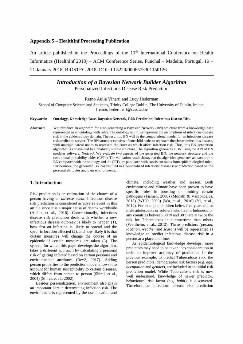
Appendix 5 – HealthInf Proceeding Publication
An article published in the Proceedings of the 11th International Conference on Health
Informatics (HealthInf 2018) – ACM Conference Series. Funchal – Madeira, Portugal, 19 –
21 January 2018, BIOSTEC 2018. DOI: 10.5220/0006573301150126
Introduction of a Bayesian Network Builder Algorithm Personalized Infectious Disease Risk Prediction
Retno Aulia Vinarti and Lucy Hederman
School of Computer Science and Statistics, Trinity College Dublin, The University of Dublin, Ireland
{retnor, hederman}@scss.tcd.ie
Keywords: Ontology, Knowledge-Base, Bayesian Network, Risk Prediction, Infectious Disease Risk.
Abstract: We introduce an algorithm for auto-generating a Bayesian Network (BN) structure from a knowledge-base
represented as an ontology with rules. The ontology and rules represent the assumptions of infectious disease
risk in the epidemiology domain. The resulting BN will be the computational model for an infectious disease
risk prediction service. The BN structure consists of one child node, to represent the chosen infectious disease,
with multiple parent nodes to represent the contexts which affect infection risk. Thus, this BN generation
algorithm is constrained to a relatively simple structure. The algorithm generates a BN using the API of BN
modeler software, Netica-J. We evaluate two aspects of the generated BN: the network structure and the
conditional probability tables (CPTs). The validation result shows that the algorithm generates an isomorphic
BN compared with the ontology and the CPTs are populated with consistent ratios from epidemiological rules.
Furthermore, the generated BN has resulted in a personalized infectious disease risk prediction based on the
personal attributes and their environments.
1. Introduction
Risk prediction is an estimation of the chance of a
person having an adverse event. Infectious disease
risk prediction is considered as adverse event in this
article since it is a major cause of deaths worldwide
(Aiello, et al., 2016). Conventionally, infectious
disease risk prediction deals with whether a new
infectious disease outbreak is likely to happen (1),
how fast an infection is likely to spread and the
specific location affected (2), and how likely it is that
certain measures will change the course of an
epidemic if certain measures are taken (3). The
system, for which this paper develops the algorithm,
takes a different approach by calculating a personal
risk of getting infected based on certain personal and
environmental attributes (Rev2, 2017). Adding
person properties to the prediction model allows it to
account for human susceptibility to certain diseases,
which differs from person to person (Shirai, et al.,
2004) (Shirai, et al., 2002).
Besides personalization, environment also plays
an important part in determining infection risk. The
environment is represented by the user location and
climate, including weather and season. Both
environment and climate have been proven to have
specific roles in boosting or limiting certain
pathogens (Fisman, 2008) (Monath & Vasconcelos,
2015) (WHO, 2003) (Wu, et al., 2016) (Yi, et al.,
2014). For example, children below five years old or
male adolescents or soldiers who live in Indonesia or
any countries between 30oN and 30oS are at twice the
risk for Tuberculosis in summertime than others
(Wertheim, et al., 2012). These predictors (person,
location, weather and season) will be represented as
knowledge to predict infectious disease risk in a
person at a place and time.
As epidemiological knowledge develops, more
predictors may need to be taken into consideration in
order to improve accuracy of prediction. In the
previous example, to predict Tuberculosis risk, the
person predictors, demographic risk factors (e.g. age,
occupation and gender), are included in an initial risk
prediction model. While Tuberculosis risk is now
well understood, knowledge of newer predictor,
behavioural risk factor (e.g. habit), is discovered.
Therefore, an infectious disease risk prediction
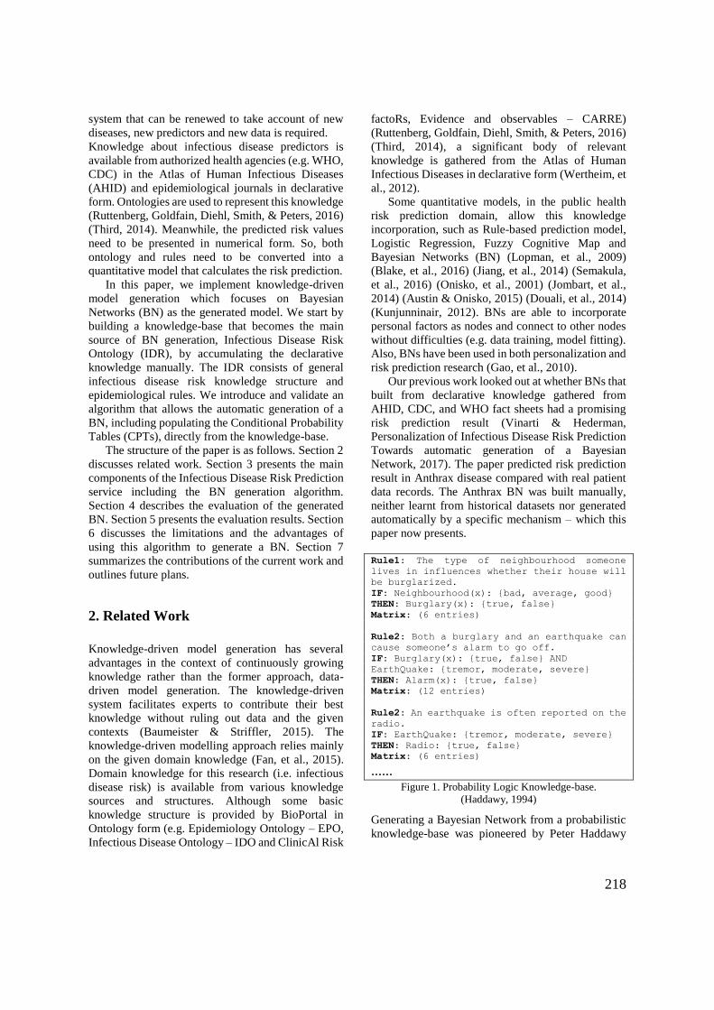
218
system that can be renewed to take account of new
diseases, new predictors and new data is required.
Knowledge about infectious disease predictors is
available from authorized health agencies (e.g. WHO,
CDC) in the Atlas of Human Infectious Diseases
(AHID) and epidemiological journals in declarative
form. Ontologies are used to represent this knowledge
(Ruttenberg, Goldfain, Diehl, Smith, & Peters, 2016)
(Third, 2014). Meanwhile, the predicted risk values
need to be presented in numerical form. So, both
ontology and rules need to be converted into a
quantitative model that calculates the risk prediction.
In this paper, we implement knowledge-driven
model generation which focuses on Bayesian
Networks (BN) as the generated model. We start by
building a knowledge-base that becomes the main
source of BN generation, Infectious Disease Risk
Ontology (IDR), by accumulating the declarative
knowledge manually. The IDR consists of general
infectious disease risk knowledge structure and
epidemiological rules. We introduce and validate an
algorithm that allows the automatic generation of a
BN, including populating the Conditional Probability
Tables (CPTs), directly from the knowledge-base.
The structure of the paper is as follows. Section 2
discusses related work. Section 3 presents the main
components of the Infectious Disease Risk Prediction
service including the BN generation algorithm.
Section 4 describes the evaluation of the generated
BN. Section 5 presents the evaluation results. Section
6 discusses the limitations and the advantages of
using this algorithm to generate a BN. Section 7
summarizes the contributions of the current work and
outlines future plans.
2. Related Work
Knowledge-driven model generation has several
advantages in the context of continuously growing
knowledge rather than the former approach, data-
driven model generation. The knowledge-driven
system facilitates experts to contribute their best
knowledge without ruling out data and the given
contexts (Baumeister & Striffler, 2015). The
knowledge-driven modelling approach relies mainly
on the given domain knowledge (Fan, et al., 2015).
Domain knowledge for this research (i.e. infectious
disease risk) is available from various knowledge
sources and structures. Although some basic
knowledge structure is provided by BioPortal in
Ontology form (e.g. Epidemiology Ontology – EPO,
Infectious Disease Ontology – IDO and ClinicAl Risk
factoRs, Evidence and observables – CARRE)
(Ruttenberg, Goldfain, Diehl, Smith, & Peters, 2016)
(Third, 2014), a significant body of relevant
knowledge is gathered from the Atlas of Human
Infectious Diseases in declarative form (Wertheim, et
al., 2012).
Some quantitative models, in the public health
risk prediction domain, allow this knowledge
incorporation, such as Rule-based prediction model,
Logistic Regression, Fuzzy Cognitive Map and
Bayesian Networks (BN) (Lopman, et al., 2009)
(Blake, et al., 2016) (Jiang, et al., 2014) (Semakula,
et al., 2016) (Onisko, et al., 2001) (Jombart, et al.,
2014) (Austin & Onisko, 2015) (Douali, et al., 2014)
(Kunjunninair, 2012). BNs are able to incorporate
personal factors as nodes and connect to other nodes
without difficulties (e.g. data training, model fitting).
Also, BNs have been used in both personalization and
risk prediction research (Gao, et al., 2010).
Our previous work looked out at whether BNs that
built from declarative knowledge gathered from
AHID, CDC, and WHO fact sheets had a promising
risk prediction result (Vinarti & Hederman,
Personalization of Infectious Disease Risk Prediction
Towards automatic generation of a Bayesian
Network, 2017). The paper predicted risk prediction
result in Anthrax disease compared with real patient
data records. The Anthrax BN was built manually,
neither learnt from historical datasets nor generated
automatically by a specific mechanism – which this
paper now presents.
Rule1: The type of neighbourhood someone
lives in influences whether their house will
be burglarized.
IF: Neighbourhood(x): {bad, average, good}
THEN: Burglary(x): {true, false}
Matrix: (6 entries)
Rule2: Both a burglary and an earthquake can
cause someone’s alarm to go off.
IF: Burglary(x): {true, false} AND
EarthQuake: {tremor, moderate, severe}
THEN: Alarm(x): {true, false}
Matrix: (12 entries)
Rule2: An earthquake is often reported on the
radio.
IF: EarthQuake: {tremor, moderate, severe}
THEN: Radio: {true, false}
Matrix: (6 entries)
...... Figure 1. Probability Logic Knowledge-base.
(Haddawy, 1994)
Generating a Bayesian Network from a probabilistic
knowledge-base was pioneered by Peter Haddawy
219
(Haddawy, 1994). He used Horn clauses to form a
probabilistic knowledge-base (Figure 1). The
knowledge-base used rules to define predictors, and
matrix to define conditional probability tables. By
using these clauses, he generated an isomorphic
Bayesian Network automatically. Whereas Haddawy
used random values in order to generate the BN, this
article seeks to populate these tables with appropriate
conditional probability values.
3. The Personalized Infectious Disease
Risk Prediction
The infectious disease risk prediction web service is
designed to serve client applications which advise
users when and how to protect themselves from
infections. The service computes a person’s risk of
being infected by a specified disease today (or this
week or season depending on the disease), given their
demographic details and location. The service uses
geocodes to find weather, season and location
features (e.g. swamp, forest, river). For example, a 3-
year old female located at (40.440625, -79.995886) is
looking for their risk of Anthrax on the day
(04/07/2017, 07:55:45).
This section explains the components of the
service that are needed for predicting infectious
disease risk: (1) an ontology and rules that describes
the main elements of infectious disease risk to
represent the relationships between risk predictors
and a disease; (2) a main engine to predict the risk, a
quantitative prediction model (BN), which represents
the newest knowledge for each infectious disease; (3)
packages that support the BN to predict accurately
(weather, location APIs, health surveillance APIs and
simple functions to accommodate inputs/outputs).
The service will contain multiple independent BNs,
one per infection.
When epidemiologists find new knowledge or
new predictors about infectious disease risk, new
objects will be added to the ontology and rules, and
the BN model needs to be renewed. The renew
process makes use of the algorithm proposed in this
article to auto-generate the BN so that the prediction
model is isomorphic with the knowledge-base that
stores newest information. In this system, the
generated BN is isomorphic if all individuals and sub-
classes in the IDR Ontology have been transformed.
The individuals become the states and their sub-
classes become their nodes in the BN.
At runtime, the Live APIs tier collects current
contexts of the environment based on user’s location
and sends the retrieved values to the Context
Collector in the Logic tier. The BN model, also in the
Logic tier, takes the person’s demographics and
values from the Context Collector as inputs (i.e.
beliefs). Thereafter, the BN uses the CPT to yield the
risk prediction which is passed to the client through
the Presentation layer. In Figure 2, the separation
between runtime (left-side) and BN build time (right-
side) is illustrated by a dashed line.
The BN used at runtime is initially generated, and
further rebuilt every time there is something new
added to the knowledge-base (ontology and rules). In
order to generate a BN, nodes and states need to be
extracted from the ontology. Also, the child node’s
CPT needs to be populated by computing numerical
values from the rules. This is the main role of the BN
Builder package. For parent nodes, marginal
probability data is retrieved from sources such as the
United Nations (UN) Data API by MarginalProb
Supplier. Then, they are loaded to form parent nodes’
CPTs.
3.1. Structure of the Knowledge Base and the
Generated Bayesian Network
An ontology is used to represent the relationship
between predictors and infectious disease risk.
Existing ontologies related to this subject and some
declarative knowledge sources have been studied and
reused to create the Infectious Disease Risk (IDR)
ontology (Figure 3). The main classes (e.g. Person,
Infectious Disease, Environment) are denoted by
rectangles. Sub-classes represent the risk factors of an
infectious disease for each class (e.g. age, gender in a
person); they are denoted by ellipses. Individuals are
the instances of the sub-classes (e.g. female and male
in gender).
Some individuals are different for each disease,
for example, age in Tuberculosis will have different
categorization with age in Anthrax. But, some other
individuals are same (e.g. female and male as
instances of gender). The individuals are not
illustrated in Figure 3. The IDR ontology is used to
support epidemiological rules in Semantic Web Rule
Language (SWRL). The SWRL rules refer to the IDR
classes, sub-classes and individuals.
Rules are used to define statements about the
factors of a person, and their environment, that affect
whether they get infected by a disease. These rules are
manually encoded from declarative knowledge
sources: Atlas of Human Infectious Disease (AHID),
Centres of Disease Control and Prevention (CDC).
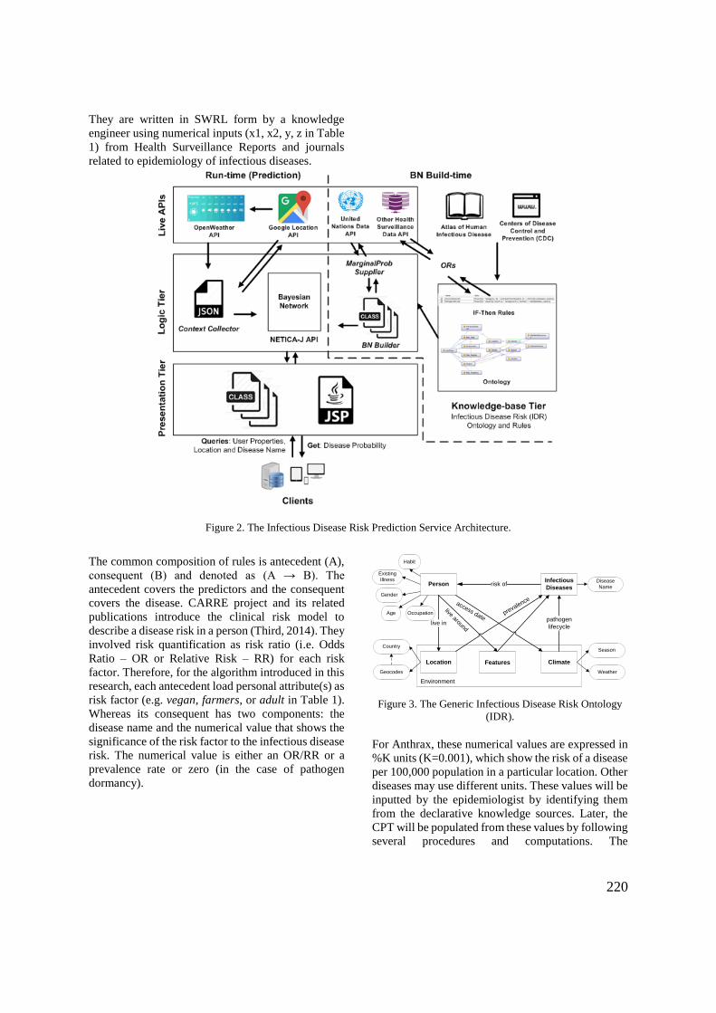
220
They are written in SWRL form by a knowledge
engineer using numerical inputs (x1, x2, y, z in Table
1) from Health Surveillance Reports and journals
related to epidemiology of infectious diseases.
Figure 2. The Infectious Disease Risk Prediction Service Architecture.
The common composition of rules is antecedent (A),
consequent (B) and denoted as (A → B). The
antecedent covers the predictors and the consequent
covers the disease. CARRE project and its related
publications introduce the clinical risk model to
describe a disease risk in a person (Third, 2014). They
involved risk quantification as risk ratio (i.e. Odds
Ratio – OR or Relative Risk – RR) for each risk
factor. Therefore, for the algorithm introduced in this
research, each antecedent load personal attribute(s) as
risk factor (e.g. vegan, farmers, or adult in Table 1).
Whereas its consequent has two components: the
disease name and the numerical value that shows the
significance of the risk factor to the infectious disease
risk. The numerical value is either an OR/RR or a
prevalence rate or zero (in the case of pathogen
dormancy).
PersonInfectious
Diseases
Location Climate
risk of
live inpathogen
lifecycle
prevalence
Environment
Age
Gender
Disease
Name
Season
Weather
Existing
Illness
Features
Country
Occupation
Geocodes
live around
access date
Habit
Figure 3. The Generic Infectious Disease Risk Ontology
(IDR).
For Anthrax, these numerical values are expressed in
%K units (K=0.001), which show the risk of a disease
per 100,000 population in a particular location. Other
diseases may use different units. These values will be
inputted by the epidemiologist by identifying them
from the declarative knowledge sources. Later, the
CPT will be populated from these values by following
several procedures and computations. The
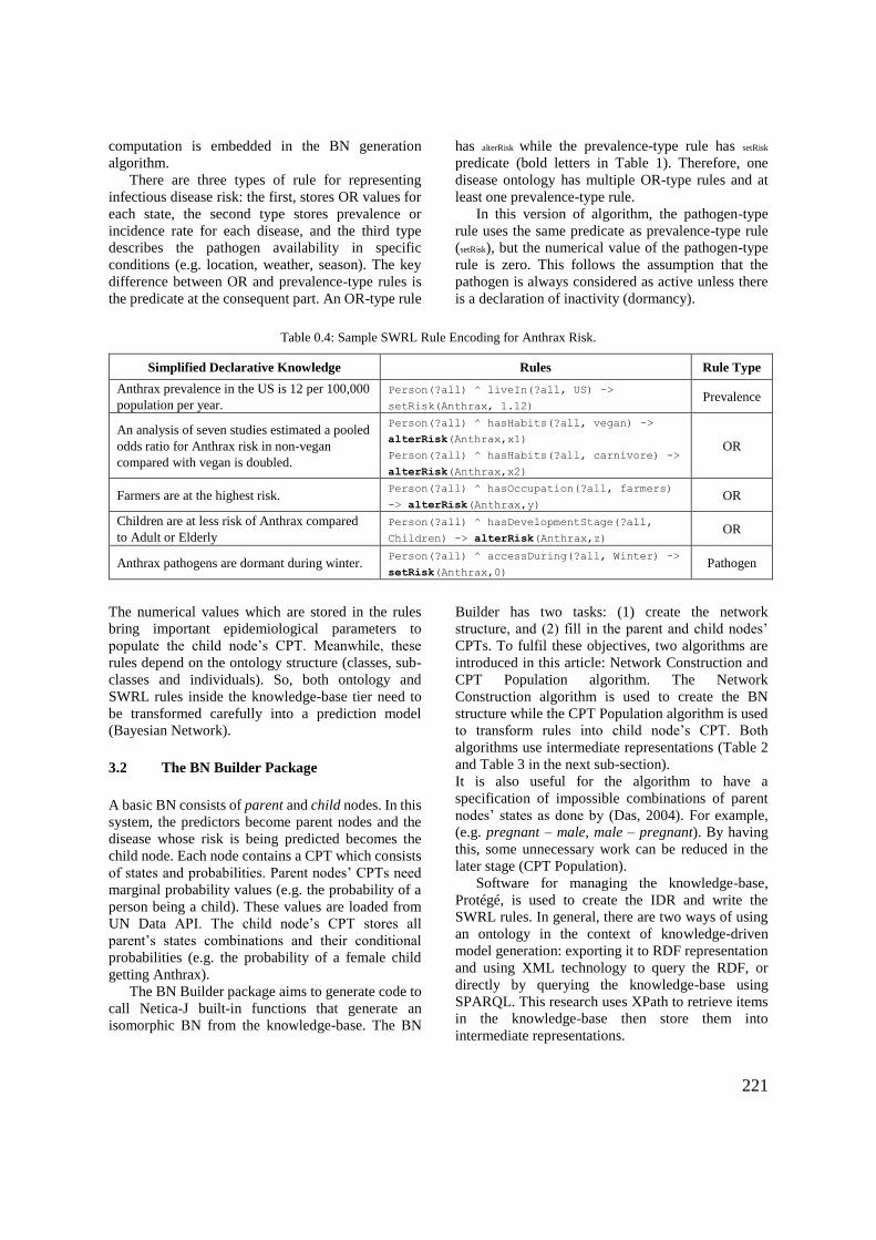
221
computation is embedded in the BN generation
algorithm.
There are three types of rule for representing
infectious disease risk: the first, stores OR values for
each state, the second type stores prevalence or
incidence rate for each disease, and the third type
describes the pathogen availability in specific
conditions (e.g. location, weather, season). The key
difference between OR and prevalence-type rules is
the predicate at the consequent part. An OR-type rule
has alterRisk while the prevalence-type rule has setRisk
predicate (bold letters in Table 1). Therefore, one
disease ontology has multiple OR-type rules and at
least one prevalence-type rule.
In this version of algorithm, the pathogen-type
rule uses the same predicate as prevalence-type rule
(setRisk), but the numerical value of the pathogen-type
rule is zero. This follows the assumption that the
pathogen is always considered as active unless there
is a declaration of inactivity (dormancy).
Table 0.4: Sample SWRL Rule Encoding for Anthrax Risk.
Simplified Declarative Knowledge Rules Rule Type
Anthrax prevalence in the US is 12 per 100,000
population per year.
Person(?all) ^ liveIn(?all, US) ->
setRisk(Anthrax, 1.12) Prevalence
An analysis of seven studies estimated a pooled
odds ratio for Anthrax risk in non-vegan
compared with vegan is doubled.
Person(?all) ^ hasHabits(?all, vegan) ->
alterRisk(Anthrax,x1)
Person(?all) ^ hasHabits(?all, carnivore) ->
alterRisk(Anthrax,x2)
OR
Farmers are at the highest risk. Person(?all) ^ hasOccupation(?all, farmers)
-> alterRisk(Anthrax,y) OR
Children are at less risk of Anthrax compared
to Adult or Elderly
Person(?all) ^ hasDevelopmentStage(?all,
Children) -> alterRisk(Anthrax,z) OR
Anthrax pathogens are dormant during winter. Person(?all) ^ accessDuring(?all, Winter) ->
setRisk(Anthrax,0) Pathogen
The numerical values which are stored in the rules
bring important epidemiological parameters to
populate the child node’s CPT. Meanwhile, these
rules depend on the ontology structure (classes, sub-
classes and individuals). So, both ontology and
SWRL rules inside the knowledge-base tier need to
be transformed carefully into a prediction model
(Bayesian Network).
3.2 The BN Builder Package
A basic BN consists of parent and child nodes. In this
system, the predictors become parent nodes and the
disease whose risk is being predicted becomes the
child node. Each node contains a CPT which consists
of states and probabilities. Parent nodes’ CPTs need
marginal probability values (e.g. the probability of a
person being a child). These values are loaded from
UN Data API. The child node’s CPT stores all
parent’s states combinations and their conditional
probabilities (e.g. the probability of a female child
getting Anthrax).
The BN Builder package aims to generate code to
call Netica-J built-in functions that generate an
isomorphic BN from the knowledge-base. The BN
Builder has two tasks: (1) create the network
structure, and (2) fill in the parent and child nodes’
CPTs. To fulfil these objectives, two algorithms are
introduced in this article: Network Construction and
CPT Population algorithm. The Network
Construction algorithm is used to create the BN
structure while the CPT Population algorithm is used
to transform rules into child node’s CPT. Both
algorithms use intermediate representations (Table 2
and Table 3 in the next sub-section).
It is also useful for the algorithm to have a
specification of impossible combinations of parent
nodes’ states as done by (Das, 2004). For example,
(e.g. pregnant – male, male – pregnant). By having
this, some unnecessary work can be reduced in the
later stage (CPT Population).
Software for managing the knowledge-base,
Protégé, is used to create the IDR and write the
SWRL rules. In general, there are two ways of using
an ontology in the context of knowledge-driven
model generation: exporting it to RDF representation
and using XML technology to query the RDF, or
directly by querying the knowledge-base using
SPARQL. This research uses XPath to retrieve items
in the knowledge-base then store them into
intermediate representations.
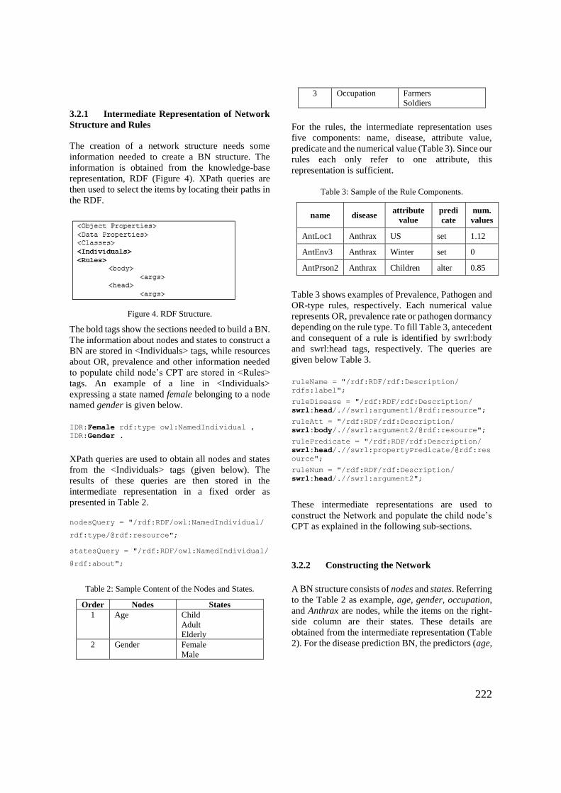
222
3.2.1 Intermediate Representation of Network
Structure and Rules
The creation of a network structure needs some
information needed to create a BN structure. The
information is obtained from the knowledge-base
representation, RDF (Figure 4). XPath queries are
then used to select the items by locating their paths in
the RDF.
Figure 4. RDF Structure.
The bold tags show the sections needed to build a BN.
The information about nodes and states to construct a
BN are stored in <Individuals> tags, while resources
about OR, prevalence and other information needed
to populate child node’s CPT are stored in <Rules>
tags. An example of a line in <Individuals>
expressing a state named female belonging to a node
named gender is given below.
IDR:Female rdf:type owl:NamedIndividual ,
IDR:Gender .
XPath queries are used to obtain all nodes and states
from the <Individuals> tags (given below). The
results of these queries are then stored in the
intermediate representation in a fixed order as
presented in Table 2.
nodesQuery = "/rdf:RDF/owl:NamedIndividual/
rdf:type/@rdf:resource";
statesQuery = "/rdf:RDF/owl:NamedIndividual/
@rdf:about";
Table 2: Sample Content of the Nodes and States.
Order Nodes States
1 Age Child
Adult
Elderly
2 Gender Female
Male
3 Occupation Farmers
Soldiers
For the rules, the intermediate representation uses
five components: name, disease, attribute value,
predicate and the numerical value (Table 3). Since our
rules each only refer to one attribute, this
representation is sufficient.
Table 3: Sample of the Rule Components.
name disease attribute
value
predi
cate
num.
values
AntLoc1 Anthrax US set 1.12
AntEnv3 Anthrax Winter set 0
AntPrson2 Anthrax Children alter 0.85
Table 3 shows examples of Prevalence, Pathogen and
OR-type rules, respectively. Each numerical value
represents OR, prevalence rate or pathogen dormancy
depending on the rule type. To fill Table 3, antecedent
and consequent of a rule is identified by swrl:body
and swrl:head tags, respectively. The queries are
given below Table 3.
ruleName = "/rdf:RDF/rdf:Description/
rdfs:label";
ruleDisease = "/rdf:RDF/rdf:Description/
swrl:head/.//swrl:argument1/@rdf:resource";
ruleAtt = "/rdf:RDF/rdf:Description/
swrl:body/.//swrl:argument2/@rdf:resource";
rulePredicate = "/rdf:RDF/rdf:Description/
swrl:head/.//swrl:propertyPredicate/@rdf:res
ource";
ruleNum = "/rdf:RDF/rdf:Description/
swrl:head/.//swrl:argument2";
These intermediate representations are used to
construct the Network and populate the child node’s
CPT as explained in the following sub-sections.
3.2.2 Constructing the Network
A BN structure consists of nodes and states. Referring
to the Table 2 as example, age, gender, occupation,
and Anthrax are nodes, while the items on the right-
side column are their states. These details are
obtained from the intermediate representation (Table
2). For the disease prediction BN, the predictors (age,
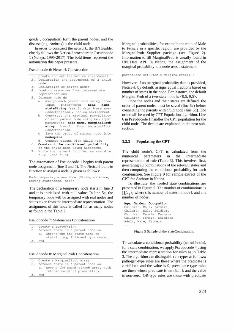
223
gender, occupation) form the parent nodes, and the
disease (e.g. Anthrax) is the child node.
In order to construct the network, the BN Builder
closely follows the Netica-J procedure in Pseudocode
1 (Norsys, 1995-2017). The bold items represent the
automation this paper presents.
Pseudocode 6: Network Construction
1. Create and set the Netica environment
2. Declaration and assignment of a child
node
3. Declaration of parent nodes
4. Loading resources from intermediate
representations
5. foreach node do
a. Assign each parent node using three
input parameters: node name,
stateString (result from Statenames
Concatenation), Netica environment
b. Construct the marginal probability
of each parent node using two input
parameters: node name, MarginalProb
array (result from MarginalProb
Concatenation)
c. Save the order of parent node into
nodequeue
d. Connect parent with child node
6. Construct the conditional probability
of the child node using nodequeue.
7. Write the network into Netica readable
file (.dne file)
The automation of Pseudocode 1 begins with parent
node assignment (line 3 and 5). The Netica-J built-in
function to assign a node is given as follows:
Node temporary = new Node (String nodename,
String statenames, net);
The declaration of a temporary node starts in line 3
and it is initialized with null value. In line 5a, the
temporary node will be assigned with real nodes and
states taken from the intermediate representation. The
assignment of this node is called for as many nodes
as found in the Table 2.
Pseudocode 7: Statenames Concatenation
1. Create a stateString
2. foreach state in a parent node do
a. Append the the state name to
stateString, followed by a comma.
3. end
Pseudocode 8: MarginalProb Concatenation
1. Create a MarginalProb array
2. foreach state in a parent node do
a. Append the MarginalProb array with
related marginal probability.
3. end
Marginal probabilities, for example the ratio of Male
to Female in a specific region, are provided by the
MarginalProb Supplier package (see Figure 2).
Information to fill MarginalProb is usually found in
UN Data API. In Netica, the assignment of the
marginal probability to a node uses a statement:
parentNode.setCPTable(MarginalProb[]);
However, if no marginal probability data is provided,
Netica-J, by default, assigns equal fractions based on
number of states in the node. For instance, the default
MarginalProb of a two-state node is <0.5, 0.5>.
Once the nodes and their states are defined, the
order of parent nodes must be saved (line 5c) before
connecting the parents with child node (line 5d). The
order will be used by CPT Population algorithm. Line
6 in Pseudocode 1 handles the CPT population for the
child node. The details are explained in the next sub-
section.
3.2.3 Populating the CPT
The child node’s CPT is calculated from the
numerical parameters in the intermediate
representation of rule (Table 3). This involves first,
generating all combinations of the relevant states and
then computing the conditional probability for each
combination. See Figure 9 for sample extract of the
CPT for Anthrax in Netica.
To illustrate, the needed state combinations are
presented in Figure 5. The number of combinations is ∏ 𝑠𝑖
𝑛𝑖=1 where si is number of states in node i, and n is
number of nodes.
Age, Gender, Occupation
Children, Male, Farmers
Children, Male, Soldiers
Children, Female, Farmers
Children, Female, Soldiers
Adult, Male, Farmers
...
Figure 5 Sample of the StateCombination.
To calculate a conditional probability (condProb),
for a state combination, we apply Pseudocode 4 using
the intermediate representation for rules as in Table
3. The algorithm can distinguish rule types as follows:
pathogen-type rules are those where the predicate is
setRisk and the value is 0; prevalence-type rules
are those whose predicate is setRisk and the value
is non-zero; OR-type rules are those with predicate
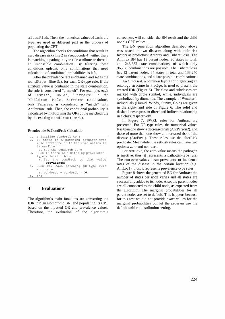
224
alterRisk. Then, the numerical values of each rule
type are used in different part in the process of
populating the CPT.
The algorithm checks for conditions that result in
zero disease risk (line 2 in Pseudocode 4): either there
is matching a pathogen-type rule attribute or there is
an impossible combination. By filtering these
conditions upfront, only combinations that need
calculation of conditional probabilities is left.
After the prevalence rate is obtained and set as the
condProb (line 3a), for each OR-type rule, if the
attribute value is contained in the state combination,
the rule is considered “a match”. For example, each
of ‘Adult’, ‘Male’, ‘Farmers’ in the
‘Children, Male, Farmers’ combinations,
only Farmers is considered as “match” with
AntPerson1 rule. Then, the conditional probability is
calculated by multiplying the ORs of the matched rule
by the existing condProb (line 4a).
Pseudocode 9: CondProb Calculation
1. Initialize condProb to 1
2. IF there is a matching pathogen-type
rule attribute or IF the combination is
impossible
a. Set the condProb to 0 3. ELSE IF there is a matching prevalence-
type rule attribute,
a. Set the condProb to that value
(Prevalence)
4. ELSE for each matching OR-type rule
attribute
a. condProb = condProb * OR 5. end
4 Evaluations
The algorithm’s main functions are converting the
IDR into an isomorphic BN, and populating its CPT
based on the inputted OR and prevalence values.
Therefore, the evaluation of the algorithm’s
correctness will consider the BN result and the child
node’s CPT values.
The BN generation algorithm described above
was tested on two diseases along with their risk
factors as predictors: Anthrax and Tuberculosis. The
Anthrax BN has 13 parent nodes, 36 states in total,
and 248,832 state combinations, of which only
96,768 combinations are possible. The Tuberculosis
has 12 parent nodes, 34 states in total and 138,240
state combinations, and all are possible combinations.
An OntoGraf, a common layout for organizing an
ontology structure in Protégé, is used to present the
created IDR (Figure 6). The class and subclasses are
marked with circle symbol, while, individuals are
symbolized by diamonds. The example of Weather’s
individuals (Humid, Windy, Sunny, Cold) are given
in the right-hand side of Figure 6. The solid and
dashed lines represent direct and indirect relationship
in a class, respectively.
In Figure 7, SWRL rules for Anthrax are
presented. For OR-type rules, the numerical values
less than one show a decreased risk (AntPerson2), and
those of more than one show an increased risk of the
disease (AntEnv1). These rules use the alterRisk
predicate. Meanwhile, the setRisk rules can have two
options: zero and non-zero.
For AntEnv3, the zero value means the pathogen
is inactive, thus, it represents a pathogen-type rule.
The non-zero values mean prevalence or incidence
rates of the disease in the certain location (e.g.
AntLoc1), thus, it represents prevalence-type rules.
Figure 8 shows the generated BN for Anthrax; the
number of states per node varies and all states are
successfully added to its node. Also, the parent nodes
are all connected to the child node, as expected from
the algorithm. The marginal probabilities for all
parent nodes are set to default. This happens because
for this test we did not provide exact values for the
marginal probabilities but let the program use the
default uniform distribution setting.
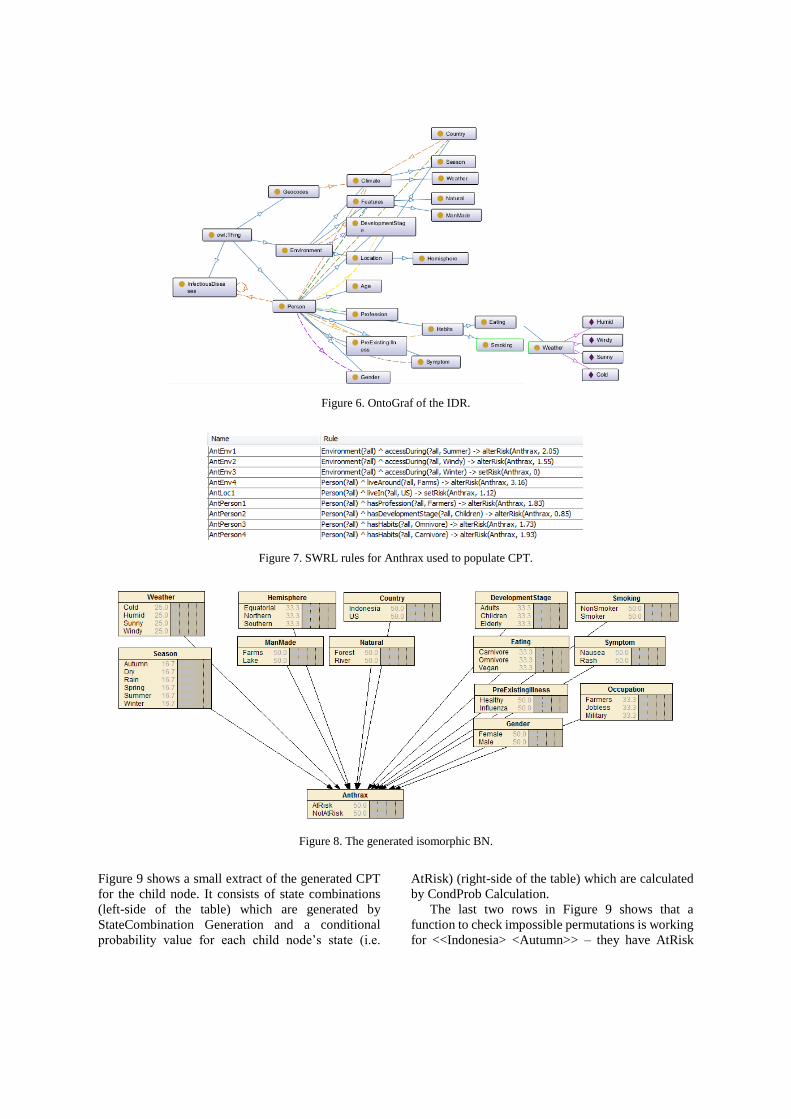
Figure 6. OntoGraf of the IDR.
Figure 7. SWRL rules for Anthrax used to populate CPT.
Figure 8. The generated isomorphic BN.
Figure 9 shows a small extract of the generated CPT
for the child node. It consists of state combinations
(left-side of the table) which are generated by
StateCombination Generation and a conditional
probability value for each child node’s state (i.e.
AtRisk) (right-side of the table) which are calculated
by CondProb Calculation.
The last two rows in Figure 9 shows that a
function to check impossible permutations is working
for <<Indonesia> <Autumn>> – they have AtRisk
226
values of 0. The middle four rows show that the
pathogen-type rule works properly on all state
combinations that contain “Winter” – they have
AtRisk values of 0.
A computer with specification Intel Core i3 CPU
1.7GHz with 4GB of memory was used to generate
the BNs and populate the CPTs. It took 17 to 19
minutes approximately. The generation of state
combinations accounts for most of the time.
5. Evaluation Results
Results of the validation will be justified by the
correctness of the algorithm. The algorithm is correct
when it generates an isomorphic BN and populates
the CPT as given odds ratios.
5.1 Evaluation on the Generated BN
Not all classes or sub-classes in the IDR will be
transformed into nodes in the BN; only classes that
have at least one individual are converted. To
compare the generated BN with the IDR, a
mechanism to retrieve all the individuals with their
corresponding classes and sub-classes directly from
the Protégé is needed. A SPARQL query is used in
the Protégé environment to execute the required
mechanism.
SELECT *
WHERE {?individual rdf:type ?type .
OPTIONAL {?type rdfs:subClassOf ?class}}
ORDER BY ?type
Thereafter, the results of this query were compared
with the generated BN (Figure 8). It can be seen from
Fig. 6 that all sub-classes are transformed into nodes
and all individuals are transformed into states.
Furthermore, the node-state arrangements in the BN
follow exactly the sub-classes and individuals’
arrangements in the ontology. Other cases have been
checked, for example, having empty sub-classes or
non-referenced data or object properties in the IDR.
Those conditions have no impact on the generated
BN. Thus, it has been shown that the generated BN is
isomorphic with the IDR.
5.2 Evaluation of the Populated CPT
To show that the algorithm correctly represents the
SWRL rules presented in Figure 7 in the child node’s
CPT, an evaluation of the CPT is carried out.
The numerical values stored in the SWRL rules
reveal the behaviour (e.g. inclination or declination)
of the disease risk. The CPT population algorithm
makes use of these numerical values to produce the
conditional probabilities. Thus, all rules are taken as
inputs and the related conditional probabilities are
taken as outputs of this evaluation.
Then, the correctness of the CPT population
algorithm is analysed by observing the outputs in two
aspects: (1) the behaviour of the conditional
probabilities has a consistent ratio with the given
numerical values in the rules, and (2) the generated
probabilities have different values for different
personal and environmental conditions.
Table 4 shows validation for all Anthrax rules
shown in Figure 7. Two countries are involved in this
evaluation: US and Indonesia. All results for
correspondent country are given for each OR-type
and pathogen-type rules. The aggregated ratio for
each state is given in the Result column. Then, to
observe the ratio of prevalence between two
countries, all ratios for OR-type rules are aggregated
and placed on the Ratio column (e.g. 1.12043 for the
AntLoc1 rule). From this process, the algorithm
populates the child node’s CPT automatically from
the SWRL rules as presented in Figure 7. Also, they
produce the comparable ratios with the given
numerical values in the SWRL rules.
Furthermore, the resulting conditional
probabilities show that these conditions result in
different prediction results as stated on the rules.
(a) different personal attributes (e.g. Age,
Gender) which are taken as different person
(b) the same person living in a country during
different season (e.g. Winter, Spring)
(c) or the same person moving to different
location features (e.g. Lake, Farms) within a
country
Thus, we see that the populated CPT yield a
personalized infectious disease risk prediction based
on the personal and environmental attributes.
6. Discussion
The algorithm describes about a mechanism to
convert a knowledge-base (ontology and rules)
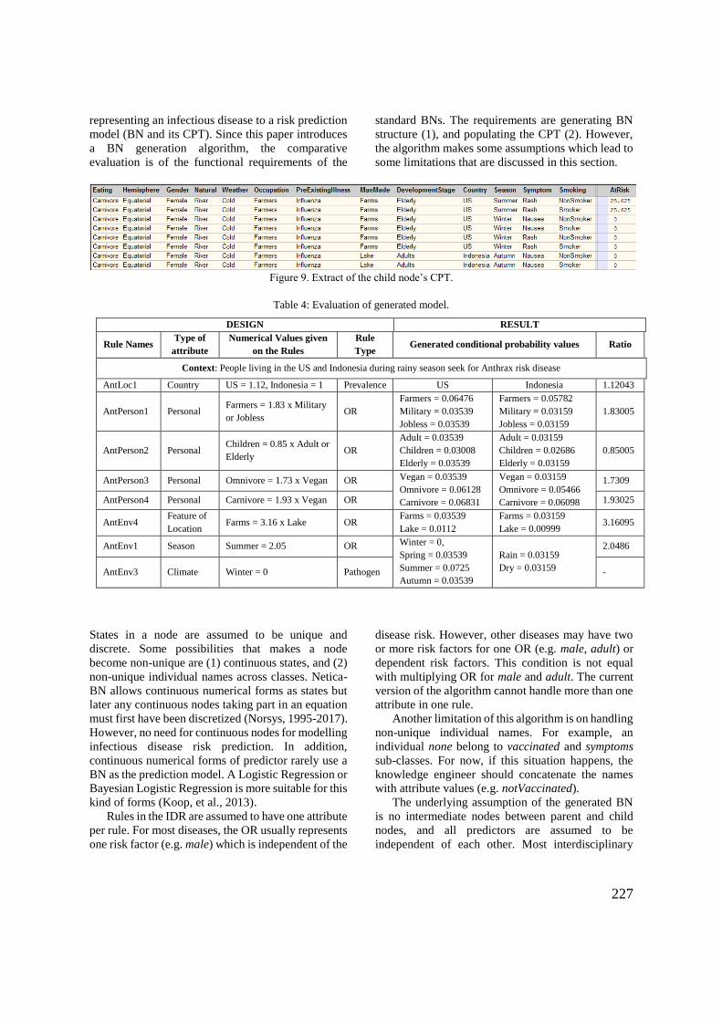
227
representing an infectious disease to a risk prediction
model (BN and its CPT). Since this paper introduces
a BN generation algorithm, the comparative
evaluation is of the functional requirements of the
standard BNs. The requirements are generating BN
structure (1), and populating the CPT (2). However,
the algorithm makes some assumptions which lead to
some limitations that are discussed in this section.
Figure 9. Extract of the child node’s CPT.
Table 4: Evaluation of generated model.
DESIGN RESULT
Rule Names Type of
attribute
Numerical Values given
on the Rules
Rule
Type Generated conditional probability values Ratio
Context: People living in the US and Indonesia during rainy season seek for Anthrax risk disease
AntLoc1 Country US = 1.12, Indonesia = 1 Prevalence US Indonesia 1.12043
AntPerson1 Personal Farmers = 1.83 x Military
or Jobless OR
Farmers = 0.06476
Military = 0.03539
Jobless = 0.03539
Farmers = 0.05782
Military = 0.03159
Jobless = 0.03159
1.83005
AntPerson2 Personal Children = 0.85 x Adult or
Elderly OR
Adult = 0.03539
Children = 0.03008
Elderly = 0.03539
Adult = 0.03159
Children = 0.02686
Elderly = 0.03159
0.85005
AntPerson3 Personal Omnivore = 1.73 x Vegan OR Vegan = 0.03539
Omnivore = 0.06128
Carnivore = 0.06831
Vegan = 0.03159
Omnivore = 0.05466
Carnivore = 0.06098
1.7309
AntPerson4 Personal Carnivore = 1.93 x Vegan OR 1.93025
AntEnv4 Feature of
Location Farms = 3.16 x Lake OR
Farms = 0.03539
Lake = 0.0112
Farms = 0.03159
Lake = 0.00999 3.16095
AntEnv1 Season Summer = 2.05 OR Winter = 0,
Spring = 0.03539
Summer = 0.0725
Autumn = 0.03539
Rain = 0.03159
Dry = 0.03159
2.0486
AntEnv3 Climate Winter = 0 Pathogen -
States in a node are assumed to be unique and
discrete. Some possibilities that makes a node
become non-unique are (1) continuous states, and (2)
non-unique individual names across classes. Netica-
BN allows continuous numerical forms as states but
later any continuous nodes taking part in an equation
must first have been discretized (Norsys, 1995-2017).
However, no need for continuous nodes for modelling
infectious disease risk prediction. In addition,
continuous numerical forms of predictor rarely use a
BN as the prediction model. A Logistic Regression or
Bayesian Logistic Regression is more suitable for this
kind of forms (Koop, et al., 2013).
Rules in the IDR are assumed to have one attribute
per rule. For most diseases, the OR usually represents
one risk factor (e.g. male) which is independent of the
disease risk. However, other diseases may have two
or more risk factors for one OR (e.g. male, adult) or
dependent risk factors. This condition is not equal
with multiplying OR for male and adult. The current
version of the algorithm cannot handle more than one
attribute in one rule.
Another limitation of this algorithm is on handling
non-unique individual names. For example, an
individual none belong to vaccinated and symptoms
sub-classes. For now, if this situation happens, the
knowledge engineer should concatenate the names
with attribute values (e.g. notVaccinated).
The underlying assumption of the generated BN
is no intermediate nodes between parent and child
nodes, and all predictors are assumed to be
independent of each other. Most interdisciplinary
228
research takes this assumption to simplify the
network and prediction model (Fenton, et al., 2016).
The current system only allows for pathogen to be
active and inactive (set risk to 0). A support for more
complex pathogen model (Kilianski, et al., 2015)
(Huang, et al., 2012) would be beneficial.
Finally, for the requirements to predict a
personalized infectious disease risk, some critical
features are already facilitated in initial version in this
paper. Further development related to detailed
specification can be accommodated without
significant changes to either the knowledge-base or
the generation algorithm.
7 Conclusions and Future Works
This paper has described an algorithm for generating
a Bayesian Network from the declarative infectious
disease knowledge stored in an Ontology and SWRL
rules. This algorithm allows additions or
modifications to the ontology and will generate an
isomorphic Bayesian Network and populate its child
node’s CPT automatically. However, the algorithm is
a preliminary result with several limitations.
This paper uses the IDR, an Infectious Disease
Risk Ontology and SWRL rules, as main reference of
BN generation. This IDR will have numerous
individuals for each disease as the knowledge
becomes available in the future. Three types of rules
have been introduced in this paper: OR, prevalence,
pathogen-type rules. In this algorithm version, the
pathogen availability is considered as always active,
unless there is a declaration of pathogen inactivity.
Another progressing work is ready to be published in
a separated article.
The algorithm introduced in this paper only
covers one possible source of OR and prevalence
values – explicitly provided by experts within rules.
There is another source that is possible to access:
WHO data sources in UN Data or Health Surveillance
API. By opting in these sources, there will be an
automated process that aims to put the numerical
values in the rule. This leads to some possibilities that
are not covered by this algorithm for now, such as
contradicting the established rules. A procedure to
manage the rules might be a substantial improvement
in the future.
Some other further works be (1) modifying the
intermediate representation and the XPath queries for
accommodating more than one dependent attribute in
one rule, (2) observing relevant time period for
predicting various infectious disease risks; this will
impact on the conditional probabilities given to a
client and thus will slightly modify the CPT
Population algorithm.
To sum up, from the evaluation section, it can be
concluded that the Network Creation algorithm has
successfully generated an isomorphic BN from the
Ontology structure. In addition, the CPT Population
algorithm has auto-populated the child node’s CPT
and the ratio of the conditional probability results are
consistent with the inputted OR. Furthermore, the BN
Builder package has resulted in a personalized
infectious disease risk prediction based on the
personal attributes and their environments.
Acknowledgements
The research for this paper is financially supported by
Islamic Development Bank (IDB) through Merit
Scholarship Programme for High Technology.
References
Aiello, A. E., Simanek, A. M., Eisenberg, M. C. & Walsh, A. R., 2016. Design and methods of a social network isolation study for reducing respiratory infection transmission. Vol. 15.
Aliferis, C. F., Tsamardinos, I., Statnikov, A. R. & Brown, L. E., 2005. A Causal Probabilistic Network Learning Toolkit for Biomedical Discovery. Las Vegas, Nevada, Mathematics and Engineering Techniques in Medicine and Biological Sciences.
Austin, R. M. & Onisko, A., 2015. Increased cervical cancer risk associated with extended screening intervals after negative human papillomavirus test results 1(1).
Baumeister, J. & Striffler, A., 2015. Knowledge-driven systems for episodic decision support. Knowledge-based systems, Volume 88, pp. 45-56.
Blake, I. M., Chenoweth, P., Okayasu, H., 2016. Detection of poliomyelitis outbreaks to support polio eradication. Emerging Infectious Diseases, 22(3), pp. 449-456.
Chang, T. S., Gangnon, R. E., Page, D., 2015. Sparse modeling of spatial environments associated with asthma. Volume 53.
Das, B., 2004. Generating Conditional Probabilities for Bayesian Networks: Easing the Knowledge Acquisition Problem. CoRR, pp. 1-24.
Douali, N. et al., 2014. Comparison between case-based fuzzy cognitive maps and bayesian networks. 113(1).
Fan, X.-R.et al., 2015. A knowledge-and-data-driven modeling approach for simulating plant growth: A
229
case study on tomato growth. Ecological Modelling, Vol 312, pp. 363-373.
Fenton, N., Neil, M. & Lagnado, D., 2016. How to model mutually exclusive events based on independent causal pathways in Bayesian network models. Volume 113.
Fisman, D. N., 2008. Seasonality of viral infections: Mechanisms and unknowns. American Journal of Preventive Medicine, 18(10), pp. 946-954.
Gao, M., Liu, K. & Wu, Z., 2010. Personalisation in web computing and informatics. Information Systems Frontiers, 12(5), pp. 607-629.
Giabbanelli, P. J., Torsney-Weir, T. & Mago, V. K., 2012. A fuzzy cognitive map of the psychosocial determinants of obesity. 12(12).
Haddawy, P., 1994. Generating Bayesian Networks from Probability Logic Knowledge Bases. Seattle, Morgan Kaufmann Publishers Inc. San Francisco, CA, USA.
Huang, Z., Das, A., Qiu, Y., 2012. The vector-borne disease airline import. risk (VBD-AIR) tool. Vol. 11.
Jiang, Q., Zhou, J. T., Jiang, Z. B. & Xu, B., 2014. Identifying risk factors of avian infectious diseases at household level in Poyang Lake region, China. Preventive Veterinary Medicine, 116(2), pp. 151-160.
Jombart, T., Aanensen, D. M., Baguelin, M., 2014. A platform for disease outbreak using the R. Vol. 7.
Kahn Jr., C. E., Roberts, L. M., Shaffer, K. A. & Haddawy, P., 1997. Construction of a BN for mammographic diagnosis of breast cancer. Computers in Biology and Medicine, 27(1), pp. 19-29.
Kilianski, A., Carcel, P., Yao, S. & Roth, P., 2015. Pathosphere.org: pathogen detection and characterization through a web-based. BMC Bioinformatics, 416(16), pp. 1-12.
Koop, G. et al., 2013. Risk factors for subclinical intramammary infection in dairy goats in two longitudinal field studies evaluated by Bayesian logistic regression. 108(4).
Kunjunninair, A. P., 2012. Clinical decision support system: risk level prediction of heart disease using weighted fuzzy rules and decision tree rules. Central European Journal of Computer Science, 2(1).
Laskey, K. B. & Mahoney, S. M., 2000. Network Engineering for Agile Belief Network Models. IEEE Transactions on Knowledge and Data Engineering, 12(4), pp. 487-499.
Lopman, B., Armstrong, B., Atchison, C., 2009. Host, weather and virological factors drive norovirus epid. PLoS One, 4(8).
Monath, T. P. & Vasconcelos, P. F. C., 2015. Yellow fever. Journal of Clin. Viro., Volume 64, pp. 160-173.
Ngo, L. & Haddawy, P., 1995. Probabilistic logic programming and Bayesian networks. Lecture Notes in Computer Science, Volume 1023, pp. 286-300.
Norsys, 1995-2017. https://www.norsys.com/netica-j/examples/SimulateCases.html.
Onisko, A., Lucas, P. & Druzdzel, M. J., 2001. Comparison of Rule-Based and Bayesian Network Approaches in Medical Diagnostic Systems. Portugal.
Rev2, 2017. HealthInformatics Conference: Reviewer comment #2. Unknown: Primoris.
Ruttenberg, A. et al., 2016. Infectious Disease Ontology. http://purl.obolibrary.org/obo/ido.owl.
Semakula, H. M., Song, G., Achuu, S. P., 2016. A Bayesian belief network modelling of household factors influencing the risk of malaria. Vol 75.
Shirai, O., Tsuda, T. & Kitagawa, S., 2002. Alcohol stimulates mosquito. Journal of the American Mosquito Control Association, 18(2), pp. 91-96.
Shirai, Y., Funada, H. & Seki, T., 2004. Landing preference of Aedes albopictus on human skin among ABO blood groups, secretors or nonsecretors. Journal of Medical Entomology, 41(4), pp. 796-799.
Third, A., 2014. BioPortal: CARRE Risk Factor Ontology. https://bioportal.bioontology.org/ontologies/CARRE.
Vinarti, R. A. & Hederman, L. M., 2017. Personalization of Infectious Disease Risk Prediction Towards automatic generation of a Bayesian Network. Thessaloniki, Greece.
Wertheim, H. F. L., Horby, P. & Woodall, J. P., 2012. Atlas of Human Infectious Diseases. Oxford: Wiley-Blackwell.
WHO, 2003. Climate Change and Human Health - Risks and Responses Summary, Geneva: WHO.
Wu, X. et al., 2016. Impact of climate change on human infectious diseases. Vol. 86.
Yi, H., Devkota, B. R. & Yu, J.-s., 2014. Effects of global warming on mosquitoes & mosquito-borne diseases and the new strategies for mosquito control. Entomological Research, 44(6), pp. 215-235.
230
Appendix 6 – ESWA Journal Submission
An article submitted to the International Journal of Expert Systems with Applications
(20th of March, 2018).
A Personalized Infectious Disease Risk Prediction System
Retno A. Vinarti a, *, and Lucy M. Hederman a
a School of Computer Science and Statistics, Trinity College Dublin, The University of Dublin, Ireland
E-mail: [email protected]*, [email protected]
Abstract
This article presents a system for predicting a human’s risk of contracting infectious diseases
based on their personal attributes and environments (region, specific location features and climate
contexts). This system is also intended to help human experts in the domain (i.e. epidemiologists)
to represent their knowledge and ease their jobs related to personalized infectious disease risk
prediction. The system consists of a knowledge representation to encode epidemiological
knowledge about infectious disease risk, and an algorithm that auto-converts the encoded
knowledge into a model that predicts the risk as a probability. The knowledge representation,
Infectious Disease Risk (IDR), consists of an ontology and rules to represent the knowledge
structure and its quantification in a way that allows auto-generation to a prediction model,
Bayesian Network (BN). The algorithm, BN-Builder, converts the IDR knowledge-base to an
infectious disease risk BN, including populating the basis of predictive reasoning from the IDR
rules. A user interface facilitates encoding of epidemiological knowledge into the IDR
knowledge-base. The system’s output, personalized infectious disease risk prediction, is validated
for three disease-country contexts: Dengue Fever and Tuberculosis in Indonesia, and Cholera in
India. The personalized infectious disease risks are reliable (p values > 0.05) for each population
parameter. The personalized infectious disease risk probability can be reliably predicted using
this system. Inclusion of more granularity on contexts in this domain will be considered in further
development of this system.
Keywords: infectious disease, risk prediction, Bayesian Network, ontology, rule.
Funding: This research of this work was supported by the Islamic Development Bank [grant
number 600026637].
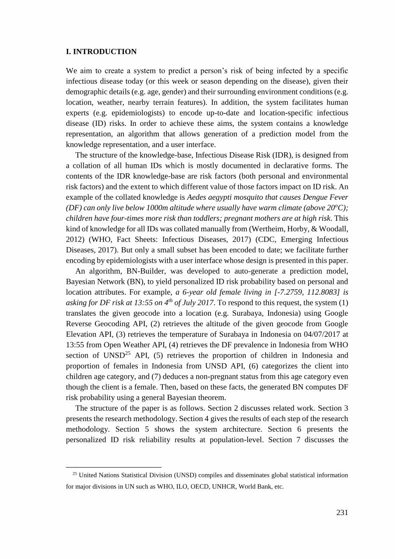
231
I. INTRODUCTION
We aim to create a system to predict a person’s risk of being infected by a specific
infectious disease today (or this week or season depending on the disease), given their
demographic details (e.g. age, gender) and their surrounding environment conditions (e.g.
location, weather, nearby terrain features). In addition, the system facilitates human
experts (e.g. epidemiologists) to encode up-to-date and location-specific infectious
disease (ID) risks. In order to achieve these aims, the system contains a knowledge
representation, an algorithm that allows generation of a prediction model from the
knowledge representation, and a user interface.
The structure of the knowledge-base, Infectious Disease Risk (IDR), is designed from
a collation of all human IDs which is mostly documented in declarative forms. The
contents of the IDR knowledge-base are risk factors (both personal and environmental
risk factors) and the extent to which different value of those factors impact on ID risk. An
example of the collated knowledge is Aedes aegypti mosquito that causes Dengue Fever
(DF) can only live below 1000m altitude where usually have warm climate (above 20oC);
children have four-times more risk than toddlers; pregnant mothers are at high risk. This
kind of knowledge for all IDs was collated manually from (Wertheim, Horby, & Woodall,
2012) (WHO, Fact Sheets: Infectious Diseases, 2017) (CDC, Emerging Infectious
Diseases, 2017). But only a small subset has been encoded to date; we facilitate further
encoding by epidemiologists with a user interface whose design is presented in this paper.
An algorithm, BN-Builder, was developed to auto-generate a prediction model,
Bayesian Network (BN), to yield personalized ID risk probability based on personal and
location attributes. For example, a 6-year old female living in [-7.2759, 112.8083] is
asking for DF risk at 13:55 on 4th of July 2017. To respond to this request, the system (1)
translates the given geocode into a location (e.g. Surabaya, Indonesia) using Google
Reverse Geocoding API, (2) retrieves the altitude of the given geocode from Google
Elevation API, (3) retrieves the temperature of Surabaya in Indonesia on 04/07/2017 at
13:55 from Open Weather API, (4) retrieves the DF prevalence in Indonesia from WHO
section of UNSD25 API, (5) retrieves the proportion of children in Indonesia and
proportion of females in Indonesia from UNSD API, (6) categorizes the client into
children age category, and (7) deduces a non-pregnant status from this age category even
though the client is a female. Then, based on these facts, the generated BN computes DF
risk probability using a general Bayesian theorem.
The structure of the paper is as follows. Section 2 discusses related work. Section 3
presents the research methodology. Section 4 gives the results of each step of the research
methodology. Section 5 shows the system architecture. Section 6 presents the
personalized ID risk reliability results at population-level. Section 7 discusses the
25 United Nations Statistical Division (UNSD) compiles and disseminates global statistical information
for major divisions in UN such as WHO, ILO, OECD, UNHCR, World Bank, etc.
232
limitations of this system. Section 8 summarizes the contributions of the current work and
outlines future plans.
II. RELATED WORK
Several projects have been published in the infectious disease and epidemiology areas.
Map-based web services (e.g. HealthMap (Nelson, 2008), VBD-AIR (Huang, Das, Qiu,
& Tatem, 2012), SickWeather (SickWeather, 2011-2017)) provide information about ID
outbreaks based on location and online case reports. Those projects use data sources from
Centers for Disease Control and Prevention (CDC), WHO, and Google APIs to visualize
their maps. However, they only present current location of ID outbreaks; they do not have
reasoners to predict the disease risk for an individual.
Other relevant health projects use an ontology as a knowledge representation:
EPidemiology Ontology (Pesquita, 2017), Infectious Disease Ontology (Cowell, 2016)
and CARdioREnal ontology (Third, 2014). EPO is designed to support semantic
annotation of epidemiology resources. In EPO, region and specific location features are
infection risk factors. IDO established eight instances per disease (e.g. HIV, Malaria) that
contains a set of biomedical and clinical aspects, such as body mass index, and
vaccination. The CARRE ontology represents a concept of human susceptibility to
cardiorenal diseases by providing personal risk factors (e.g. demographic, biomedical and
behavioral risk factors). Each factor is quantified by risk ratios.
To model the risk of a person contracting an ID, two aspects are involved: (1) the
spreading of ID in three contexts: epidemiological, individual and biological, and (2)
human immune system (Camara, Despres, Djedidi, & Lo, 2013). From IDO, we reused
standardized vocabularies of the biological aspect of ID in general, including the
pathogens, hosts, and vectors. From EPO, we reused the epidemiological aspect at
population scale, vector distributions across regions and the transmission modes of IDs
in general. From CARRE, we reused only personal risk factor types relevant to infection.
However, none of the above ontologies represent the role weather plays in both spreading
of, and immunity to, IDs, though the connection between weather and IDs is well
documented (Division, 2001).
Disease risk prediction projects have specific requirements that lead to particular
prediction models. The requirements are the ability to encode human-readable
knowledge, and to yield accurate predictions. The prediction models are suitable for these
needs: Logistic Regressions, Fuzzy Cognitive Maps, and Bayesian Networks (BN)
(Panayiotis, Simon, Denise, & Alex, 2016). BN is selected as the risk prediction model
in this system because there are general-purpose algorithms that allow BN generation
from other knowledge representations (e.g. probability logic knowledge-bases)
(Haddawy, 1994) (Zagorecki & Druzdzel, 2013) and BNs do not require training data to
build the basis of predictive reasoning. However, for disease risk purpose, the BN
generation algorithm must be redeveloped to fit the mathematical relationship between
disease risk factors and their quantifications.
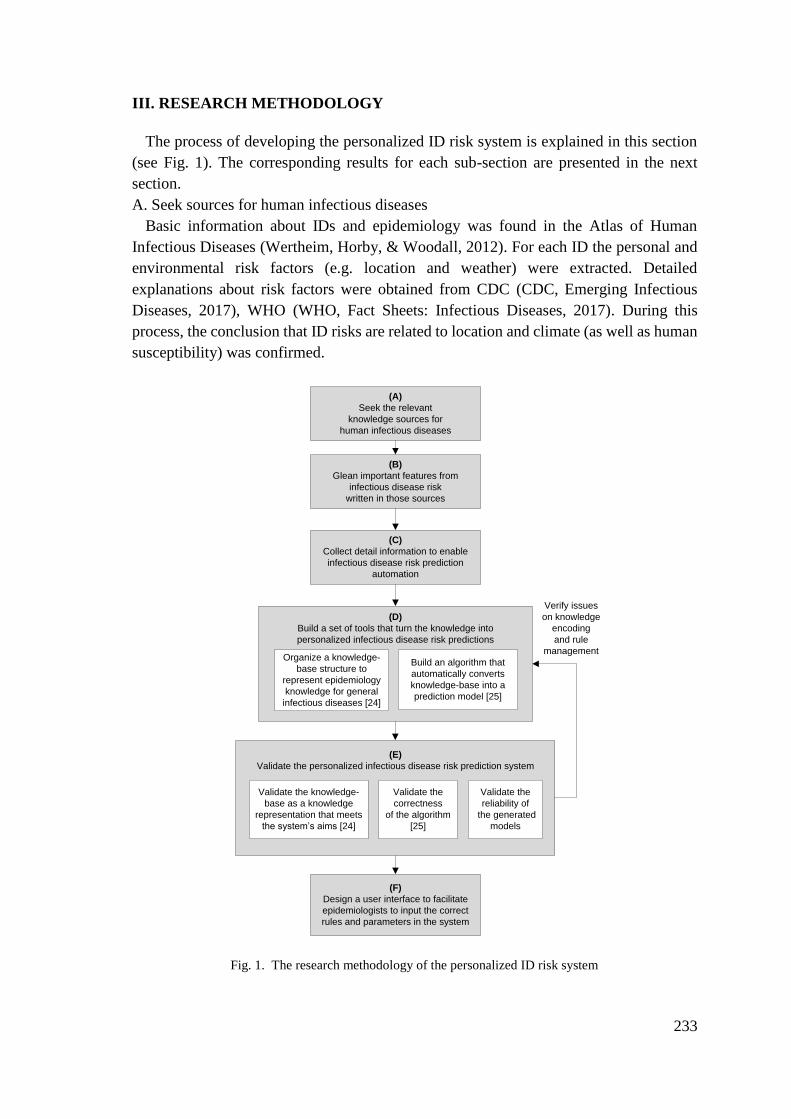
233
III. RESEARCH METHODOLOGY
The process of developing the personalized ID risk system is explained in this section
(see Fig. 1). The corresponding results for each sub-section are presented in the next
section.
A. Seek sources for human infectious diseases
Basic information about IDs and epidemiology was found in the Atlas of Human
Infectious Diseases (Wertheim, Horby, & Woodall, 2012). For each ID the personal and
environmental risk factors (e.g. location and weather) were extracted. Detailed
explanations about risk factors were obtained from CDC (CDC, Emerging Infectious
Diseases, 2017), WHO (WHO, Fact Sheets: Infectious Diseases, 2017). During this
process, the conclusion that ID risks are related to location and climate (as well as human
susceptibility) was confirmed.
(A)
Seek the relevant
knowledge sources for
human infectious diseases
(B)
Glean important features from
infectious disease risk
written in those sources
(C)
Collect detail information to enable
infectious disease risk prediction
automation
Validate the
reliability of
the generated
models
Organize a knowledge-
base structure to
represent epidemiology
knowledge for general
infectious diseases [24]
Build an algorithm that
automatically converts
knowledge-base into a
prediction model [25]
(D)
Build a set of tools that turn the knowledge into
personalized infectious disease risk predictions
Validate the
correctness
of the algorithm
[25]
(F)
Design a user interface to facilitate
epidemiologists to input the correct
rules and parameters in the system
Validate the knowledge-
base as a knowledge
representation that meets
the system’s aims [24]
(E)
Validate the personalized infectious disease risk prediction system
Verify issues
on knowledge
encoding
and rule
management
Fig. 1. The research methodology of the personalized ID risk system
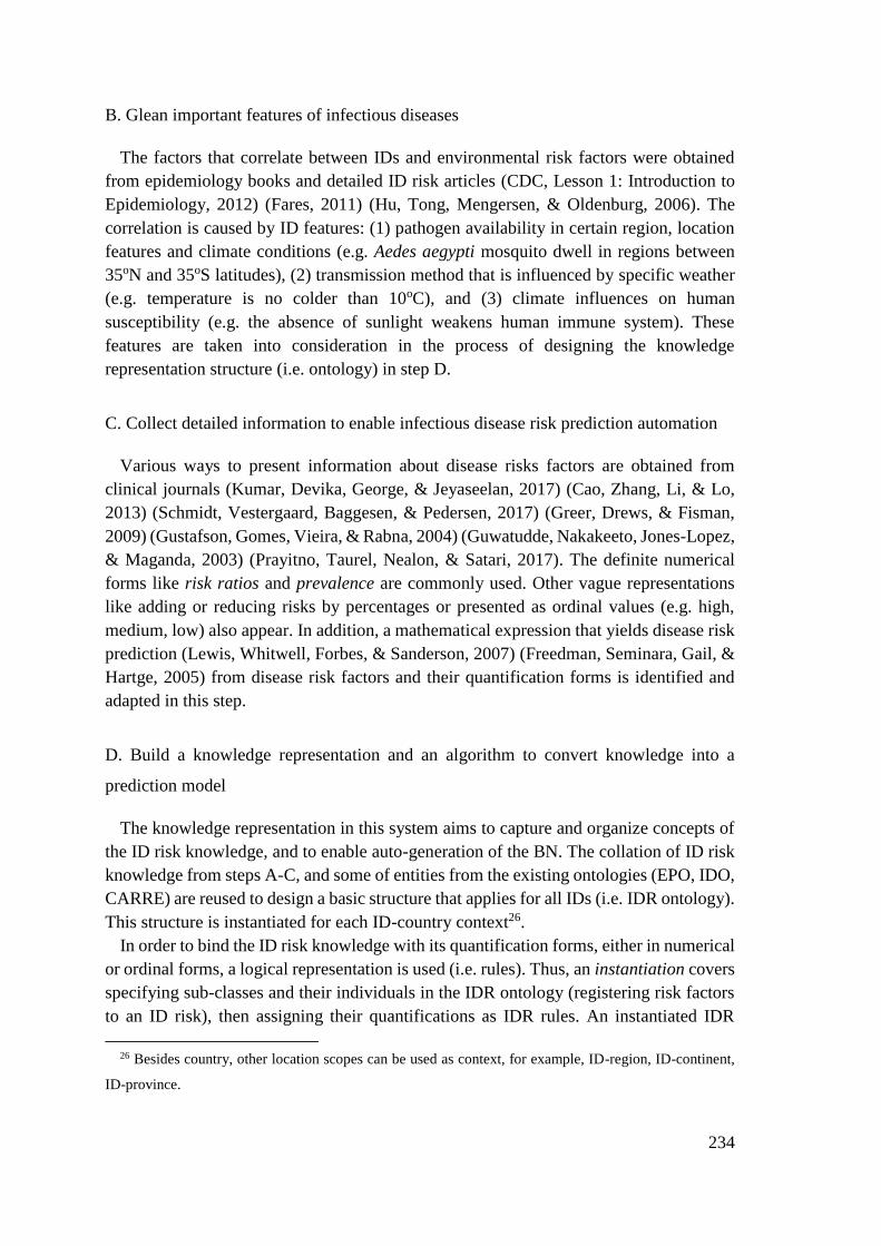
234
B. Glean important features of infectious diseases
The factors that correlate between IDs and environmental risk factors were obtained
from epidemiology books and detailed ID risk articles (CDC, Lesson 1: Introduction to
Epidemiology, 2012) (Fares, 2011) (Hu, Tong, Mengersen, & Oldenburg, 2006). The
correlation is caused by ID features: (1) pathogen availability in certain region, location
features and climate conditions (e.g. Aedes aegypti mosquito dwell in regions between
35oN and 35oS latitudes), (2) transmission method that is influenced by specific weather
(e.g. temperature is no colder than 10oC), and (3) climate influences on human
susceptibility (e.g. the absence of sunlight weakens human immune system). These
features are taken into consideration in the process of designing the knowledge
representation structure (i.e. ontology) in step D.
C. Collect detailed information to enable infectious disease risk prediction automation
Various ways to present information about disease risks factors are obtained from
clinical journals (Kumar, Devika, George, & Jeyaseelan, 2017) (Cao, Zhang, Li, & Lo,
2013) (Schmidt, Vestergaard, Baggesen, & Pedersen, 2017) (Greer, Drews, & Fisman,
2009) (Gustafson, Gomes, Vieira, & Rabna, 2004) (Guwatudde, Nakakeeto, Jones-Lopez,
& Maganda, 2003) (Prayitno, Taurel, Nealon, & Satari, 2017). The definite numerical
forms like risk ratios and prevalence are commonly used. Other vague representations
like adding or reducing risks by percentages or presented as ordinal values (e.g. high,
medium, low) also appear. In addition, a mathematical expression that yields disease risk
prediction (Lewis, Whitwell, Forbes, & Sanderson, 2007) (Freedman, Seminara, Gail, &
Hartge, 2005) from disease risk factors and their quantification forms is identified and
adapted in this step.
D. Build a knowledge representation and an algorithm to convert knowledge into a
prediction model
The knowledge representation in this system aims to capture and organize concepts of
the ID risk knowledge, and to enable auto-generation of the BN. The collation of ID risk
knowledge from steps A-C, and some of entities from the existing ontologies (EPO, IDO,
CARRE) are reused to design a basic structure that applies for all IDs (i.e. IDR ontology).
This structure is instantiated for each ID-country context26.
In order to bind the ID risk knowledge with its quantification forms, either in numerical
or ordinal forms, a logical representation is used (i.e. rules). Thus, an instantiation covers
specifying sub-classes and their individuals in the IDR ontology (registering risk factors
to an ID risk), then assigning their quantifications as IDR rules. An instantiated IDR
26 Besides country, other location scopes can be used as context, for example, ID-region, ID-continent,
ID-province.
235
knowledge-base consists of one IDR ontology and a set of IDR rules specific for one ID-
country context (e.g. Cholera-India) (Vinarti & Hederman, A knowledge-base for a
Personalized Infectious Disease Risk Prediction System, 2018).
Our BN-Builder algorithm (Vinarti & Hederman, Introduction of A Bayesian Network
Builder Algorithm: Personalized Infectious Disease Risk Prediction, 2018), is then used
to generate a BN from the IDR knowledge-base. This BN-Builder, has three aims: (1) it
generates an isomorphic BN structure, (2) it populates a correct basis of predictive
reasoning in BN (i.e. Conditional Probability Table), and (3) it deduces the personal facts
(6-year female has zero possibility to get pregnant).
E. Validate the personalized ID risk prediction system
Three key aspects of the system were evaluated, as follows:
1. Validate the IDR knowledge-base (Vinarti & Hederman, A knowledge-base for a
Personalized Infectious Disease Risk Prediction System, 2018)
The IDR knowledge-base consists of two representations: IDR ontology to represent
the structure of knowledge, and IDR rules to represent quantifications over the IDR
ontology. So, we used ontological (Tartir, Arpinar, & Sheth, 2010) and rule-based system
(Preece, 2001) approaches for evaluating the IDR ontology and the IDR rules,
respectively.
2. Validate the BN-Builder algorithm (Vinarti & Hederman, Introduction of A Bayesian
Network Builder Algorithm: Personalized Infectious Disease Risk Prediction, 2018)
The BN-Builder’s main function is generating an equivalent BN for each instantiated
knowledge-base. The equivalency was measured by (1) the isomorphisms of the
generated BN from the instantiated IDR ontology structure, (2) and the correctness of the
populated BN’s CPT. (3) Several boundary conditions of the personal facts were tested
to deduce their possibility.
3. Validate the personalized ID risk probability
Existing disease risk assessments were studied (Freedman, Seminara, Gail, & Hartge,
2005). In our previous work (Vinarti & Hederman, Personalization of Infectious Disease
Risk Prediction: Towards automatic generation of a Bayesian Network, 2017), the
accuracy was used to assess risk for Anthrax with a hand-crafted CPT. The accuracy was
measured using real hospital visit records in the US. The result is satisfying but since the
Anthrax is not a notifiable ID nor regularly reported by WHO, the risk is relatively small
and not scalable to validate the risk prediction in this system. Therefore, calibration or
reliability (Freedman, Seminara, Gail, & Hartge, 2005), at population scale, was selected
to validate the reliability of the risk probabilities.
236
B. Design a user interface
The user interface is designed with two aims, (1) to facilitate epidemiologists to encode
their knowledge in IDR knowledge-base; results from step A to C are used to design the
interface to capture typical experts’ knowledge; (2) to provide solutions for rule
anomalies that became apparent in step D (Vinarti & Hederman, A knowledge-base for a
Personalized Infectious Disease Risk Prediction System, 2018).
IV. RESULTS
This section presents the results of each step of the research methodology presented in
the previous section.
A. Seek sources for human infectious diseases
From 234 distinct infectious diseases that were gathered from (Wertheim, Horby, &
Woodall, 2012) (WHO, Fact Sheets: Infectious Diseases, 2017) (CDC, Emerging
Infectious Diseases, 2017), 215 (91.89%) have personal risk factors, 86 (36.75%) are
climate-dependent (happen during certain seasons or weather) and 175 (74.7%) are spread
only in specific locations (e.g. country, region, farms, certain altitudes). These
percentages conform that ID risks are related to weather besides personal risk factors as
explained at (Division, 2001) (Wu, Lu, Zhou, Chen, & Xu, 2016).
B. Glean important features of infectious diseases
Pathogen availability, transmission methods, and human susceptibility to diseases that
partly related to climate (CDC, Lesson 1: Introduction to Epidemiology, 2012) are
represented as entities in the existing ontologies: region and specific location features in
IDO (Cowell, 2016) and EPO (Pesquita, 2017). Also, the concepts of a person
susceptibility are captured in CARRE ontology as personal risk factors (Third, 2014).
These entities are reused in the IDR. New environmental risk factor which is confirmed
in step A, climate and its derivations, is added to IDR.
C. Collect detail information to enable infectious disease risk prediction automation
In clinical and epidemiology journals, risk ratios, represented as odds ratios (OR) or
relative risks (RR), are used to quantify risk factors. Both OR and RR have similar
meaning: OR<1 means reducing risk, OR>1 means increasing risk, OR=1 means that
more evidence is needed to correlate the risk factor with the disease risk (Szumilas, 2010).
For example, the OR for males in TB risk is 2.37; this means that males tend to have TB
risk 2.37 times more than females. OR and RR can be used interchangeably with some
considerations (Zhang & Yu, 1998). Besides using risk ratios, other representations such
as addition/reduction of risks by certain percentages, are also considered. For example,
eating one egg per day can reduce TB risk by 34%.
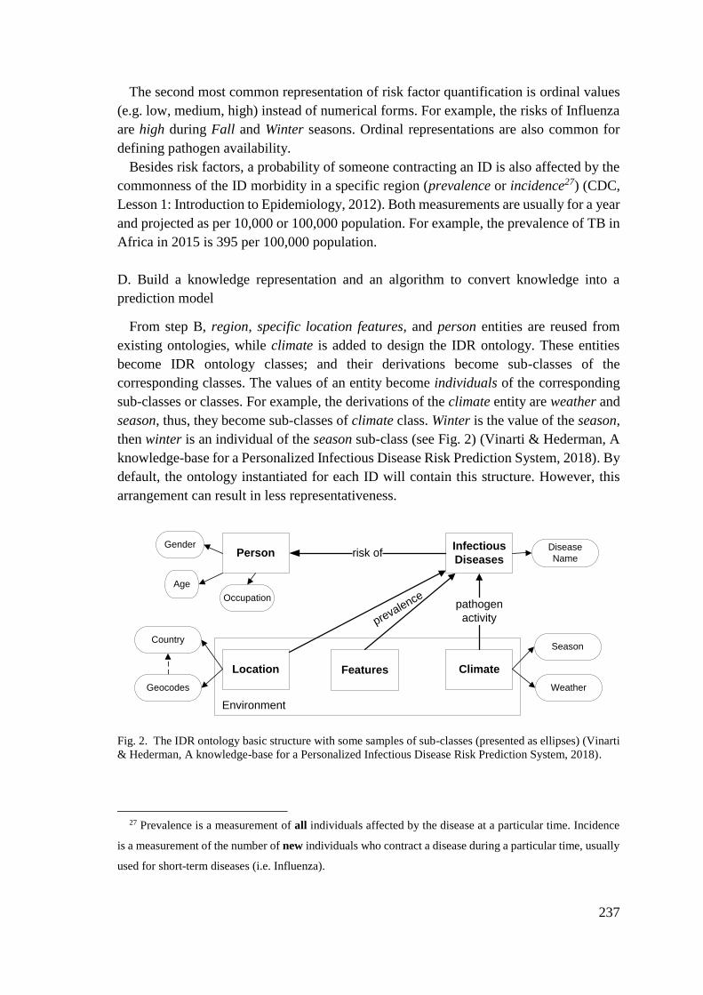
237
The second most common representation of risk factor quantification is ordinal values
(e.g. low, medium, high) instead of numerical forms. For example, the risks of Influenza
are high during Fall and Winter seasons. Ordinal representations are also common for
defining pathogen availability.
Besides risk factors, a probability of someone contracting an ID is also affected by the
commonness of the ID morbidity in a specific region (prevalence or incidence27) (CDC,
Lesson 1: Introduction to Epidemiology, 2012). Both measurements are usually for a year
and projected as per 10,000 or 100,000 population. For example, the prevalence of TB in
Africa in 2015 is 395 per 100,000 population.
D. Build a knowledge representation and an algorithm to convert knowledge into a
prediction model
From step B, region, specific location features, and person entities are reused from
existing ontologies, while climate is added to design the IDR ontology. These entities
become IDR ontology classes; and their derivations become sub-classes of the
corresponding classes. The values of an entity become individuals of the corresponding
sub-classes or classes. For example, the derivations of the climate entity are weather and
season, thus, they become sub-classes of climate class. Winter is the value of the season,
then winter is an individual of the season sub-class (see Fig. 2) (Vinarti & Hederman, A
knowledge-base for a Personalized Infectious Disease Risk Prediction System, 2018). By
default, the ontology instantiated for each ID will contain this structure. However, this
arrangement can result in less representativeness.
PersonInfectious
Diseases
Location Climate
risk of
pathogen
activityprevalence
Environment
Age
Gender Disease
Name
Season
Weather
Features
Country
Occupation
Geocodes
Fig. 2. The IDR ontology basic structure with some samples of sub-classes (presented as ellipses) (Vinarti
& Hederman, A knowledge-base for a Personalized Infectious Disease Risk Prediction System, 2018).
27 Prevalence is a measurement of all individuals affected by the disease at a particular time. Incidence
is a measurement of the number of new individuals who contract a disease during a particular time, usually
used for short-term diseases (i.e. Influenza).
238
IDR rules are used to represent risk quantifications in both numerical and ordinal forms
as explained in step C. Five rule types were designed to cover all forms of risk
quantifications. Table 1 shows all rule types with their examples. For numerical forms of
risk ratios given as OR the IDR rule type is real direct risk ratios; where risk ratios are
calculated from addition/reduction by percentages the rule type is real indirect risk ratios.
The IDR rule types that encode ordinal values for pathogen availability status, and risk
factors are named as vague pathogen status and vague risk ratios, respectively. The
ordinal values are converted into numerical values using Gaussian or Uniform
distribution by the BN-Builder algorithm. The final IDR rule type is real prevalence for
encoding prevalence or incidence value of a disease in certain region during a particular
time. The prevalence is usually provided per 10,000 or 100,000 population depending on
the disease, however, the number should be converted to percent to match the CPT units
in BN API. See the last row of Table II for an example.
The BN-Builder algorithm, first described in (Vinarti & Hederman, Introduction of A
Bayesian Network Builder Algorithm: Personalized Infectious Disease Risk Prediction,
2018), converts the IDR ontology and rules into an equivalent BN. This conversion
includes populating CPT (in the BN) with conditional probabilities which are calculated
from risk ratios and prevalence. A formula was adopted from disease risk prediction
articles (Lewis, Whitwell, Forbes, & Sanderson, 2007) (Freedman, Seminara, Gail, &
Hartge, 2005) and rewritten to become eq. (1). Essentially, the BN-Builder implements
this formula to populate the BN’s CPT (Vinarti & Hederman, Introduction of A Bayesian
Network Builder Algorithm: Personalized Infectious Disease Risk Prediction, 2018).
𝑝(𝐷|𝑦1𝑠1 , 𝑦2
𝑠2 , … , 𝑦𝑛𝑠𝑛) = 𝑝𝑟𝑒𝑣(𝐷). ∏ 𝑂𝑅𝑦
𝑖
𝑠𝑗𝑛𝑖=1; 𝑗=1 (1)
where 𝑝(𝐷|𝑦1𝑠1 , 𝑦2
𝑠1) is risk probability for disease 𝐷 given the conditions 𝑦1𝑠1 , 𝑦2
𝑠1;
𝑝𝑟𝑒𝑣(𝐷) is the prevalence of the disease 𝐷 in a specific region during a particular time;
𝑂𝑅𝑦𝑖
𝑠𝑗
is a risk ratio for an attribute (𝑦𝑖
𝑠𝑗) of a condition (yi). For example, TB risk for
females living in a sunny day in Indonesia is
(𝑇𝐵 − 𝐼𝑛𝑑𝑜𝑛𝑒𝑠𝑖𝑎|𝑔𝑒𝑛𝑑𝑒𝑟𝑓𝑒𝑚𝑎𝑙𝑒 , 𝑤𝑒𝑎𝑡ℎ𝑒𝑟𝑠𝑢𝑛𝑛𝑦). To obtain this conditional
probability, the following information is needed: (1) prevalence of TB in Indonesia during
a year 𝑝𝑟𝑒𝑣(𝑇𝐵 − 𝐼𝑛𝑑𝑜𝑛𝑒𝑠𝑖𝑎), (2) risk ratios for Indonesian female to contract TB
(𝑂𝑅𝑔𝑒𝑛𝑑𝑒𝑟𝑓𝑒𝑚𝑎𝑙𝑒), (3) risk quantification obtained from tendency of TB risk during sunny
day (𝑂𝑅𝑤𝑒𝑎𝑡ℎ𝑒𝑟𝑠𝑢𝑛𝑛𝑦).
In the context of the TB risk example, the risk probabilities result in different prediction
if (1) someone has different personal attributes (e.g. male), (2) the same person living in
the same country (Indonesia) during different weather (e.g. muggy, cloudy), or (3) the
same person moves to a different country that has different TB prevalence (e.g. Africa).
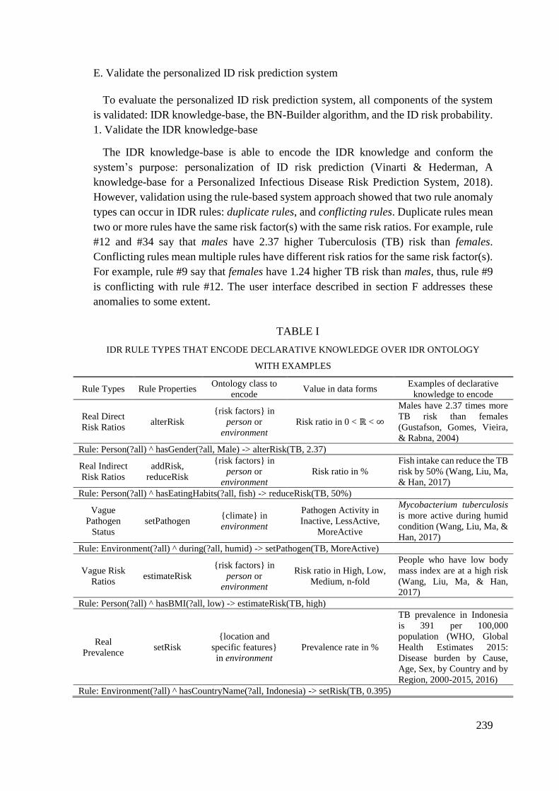
239
E. Validate the personalized ID risk prediction system
To evaluate the personalized ID risk prediction system, all components of the system
is validated: IDR knowledge-base, the BN-Builder algorithm, and the ID risk probability.
1. Validate the IDR knowledge-base
The IDR knowledge-base is able to encode the IDR knowledge and conform the
system’s purpose: personalization of ID risk prediction (Vinarti & Hederman, A
knowledge-base for a Personalized Infectious Disease Risk Prediction System, 2018).
However, validation using the rule-based system approach showed that two rule anomaly
types can occur in IDR rules: duplicate rules, and conflicting rules. Duplicate rules mean
two or more rules have the same risk factor(s) with the same risk ratios. For example, rule
#12 and #34 say that males have 2.37 higher Tuberculosis (TB) risk than females.
Conflicting rules mean multiple rules have different risk ratios for the same risk factor(s).
For example, rule #9 say that females have 1.24 higher TB risk than males, thus, rule #9
is conflicting with rule #12. The user interface described in section F addresses these
anomalies to some extent.
TABLE I
IDR RULE TYPES THAT ENCODE DECLARATIVE KNOWLEDGE OVER IDR ONTOLOGY
WITH EXAMPLES
Rule Types Rule Properties Ontology class to
encode Value in data forms
Examples of declarative
knowledge to encode
Real Direct
Risk Ratios alterRisk
{risk factors} in
person or
environment
Risk ratio in 0 < ℝ < ∞
Males have 2.37 times more
TB risk than females
(Gustafson, Gomes, Vieira,
& Rabna, 2004)
Rule: Person(?all) ^ hasGender(?all, Male) -> alterRisk(TB, 2.37)
Real Indirect
Risk Ratios
addRisk,
reduceRisk
{risk factors} in
person or
environment
Risk ratio in %
Fish intake can reduce the TB
risk by 50% (Wang, Liu, Ma,
& Han, 2017)
Rule: Person(?all) ^ hasEatingHabits(?all, fish) -> reduceRisk(TB, 50%)
Vague
Pathogen
Status
setPathogen {climate} in
environment
Pathogen Activity in
Inactive, LessActive,
MoreActive
Mycobacterium tuberculosis
is more active during humid
condition (Wang, Liu, Ma, &
Han, 2017)
Rule: Environment(?all) ^ during(?all, humid) -> setPathogen(TB, MoreActive)
Vague Risk
Ratios estimateRisk
{risk factors} in
person or
environment
Risk ratio in High, Low,
Medium, n-fold
People who have low body
mass index are at a high risk
(Wang, Liu, Ma, & Han,
2017)
Rule: Person(?all) ^ hasBMI(?all, low) -> estimateRisk(TB, high)
Real
Prevalence setRisk
{location and
specific features}
in environment
Prevalence rate in %
TB prevalence in Indonesia
is 391 per 100,000
population (WHO, Global
Health Estimates 2015:
Disease burden by Cause,
Age, Sex, by Country and by
Region, 2000-2015, 2016)
Rule: Environment(?all) ^ hasCountryName(?all, Indonesia) -> setRisk(TB, 0.395)
240
2. Validate the BN-Builder algorithm (Vinarti & Hederman, Introduction of A Bayesian
Network Builder Algorithm: Personalized Infectious Disease Risk Prediction, 2018)
To ensure the validity of the generated BN (including the CPT), this algorithm was
evaluated. The generated BN is isomorphic and its CPT is correct (Vinarti & Hederman,
Introduction of A Bayesian Network Builder Algorithm: Personalized Infectious Disease
Risk Prediction, 2018). The BN-Builder generates the equivalent BN and is able to deduce
probability of the personal facts that are unlikely to happen (Vinarti & Hederman,
Introduction of A Bayesian Network Builder Algorithm: Personalized Infectious Disease
Risk Prediction, 2018).
3. Validate the personalized ID risk probability
There are three risk assessments (calibration, discrimination and accuracy) common in
disease risk prediction research (e.g. cancer risks) (Freedman, Seminara, Gail, & Hartge,
2005). Calibration (i.e. reliability) is selected to evaluate the output of this system.
Reliability of risk predictions is measured using chi-square statistics (i.e. goodness-of-fit)
by comparing observed and expected number of events (for each generated condition in
the CPT). The expected numbers of events are gathered from country-level health
ministry for each context, while the observed number of events is the personalized ID risk
probability output of this system. The evaluation results are presented in section VI.
A. Design a user interface
The user interface retrieves a list of IDR ontology classes, sub-classes and individuals
and lets the user choose the suitable item(s) (step 1 in Fig. 3).
To provide solutions for duplicate rule anomaly, the user interface displays the existing
relevant knowledge (step 2 in Fig. 3). This feature is expected to prevent users inputting
the same value for the same risk factor(s) which may lead to duplicate rule. For the
conflicting rules anomaly, the user interface seeks the users’ confidence in the new rule
(step 3 in Fig. 3). The rules with the highest confidence are used to populate the BN’s
base reasoning by the BN-Builder algorithm. This solution, admittedly, cannot clear up
conflicting rules in the IDR rule-base but aims to minimize and keep the users aware of
the similar IDR rules.
V. THE SYSTEM ARCHITECTURE
The architecture of personalized ID risk system consists of: (1) the instantiated IDR
knowledge-base; (2) the BN-Builder algorithm to generate BN from the IDR knowledge-
base; (3) APIs that support the BN by providing the up-to-date data to predict reliable
personalized ID risks (see Fig. 4).
241
The process of building the knowledge representation is denoted BN-Build time (right).
Once the BN is generated, it is ready to process requests from clients; this phase is denoted
run-time (left). When the epidemiologists input new knowledge or new risk factors of an
ID, new objects will be added to the ontology and rules, and the BN model needs to be
renewed.
The renew process uses the BN-Builder algorithm to convert the updated knowledge-
base into an equivalent BN. Activities of the renew process are (1) retrieving population-
level parameters, such as the proportion of males and females in a country, (2) retrieving
the corresponding ID prevalence (if available from WHO API), (3) replacing the old BN
by generating a new one.
At runtime, the live APIs tier collects current facts of the environment and demography
based on users’ geocodes and sends the retrieved values to the context collector in the
logic tier. The BN, in the logic tier, takes the personal attributes (e.g. age, gender) from
the context collector as inputs (i.e. beliefs). Thereafter, the BN uses its CPT to select the
most suitable conditions that represent client's inputs. The final result is then passed to
the client through the presentation layer.
VI. RESULTS OF PREDICTION RELIABILITY EVALUATION
After the BN-Builder generates the equivalent BN, the CPT consists of all combinations
of registered risk factors (i.e. conditions and its values). The personalized ID risk
probability is calculated from the most suitable combination in the CPT.
To measure the reliability of the risk probabilities, data of the expected values for each
context are taken. For example, data about DF and TB in Indonesia are taken from
InfoDatin (Indonesian Health, 2013) and WHO (WHO, Dengue fever in Indonesia, 2017)
(WHO, Tuberculosis (TB), 2017), while data for Cholera in India is taken from WHO
(WHO, Cholera in India: an analysis of reports, 2006). We evaluate whether the
personalized ID risk prediction results (observed values) have no significant differences
with the expected values using the chi-square test.
To validate the reliability of the inputted risk quantifications, only possible
combinations are included (see Table II). Impossible combinations are deduced by the
BN-Builder. The total number of combinations is the product of number of values for all
conditions. The number of possible combinations is obtained by subtracting the number
of impossible combinations from the total combinations.
P values for chi-square test results are shown in Table II. These p values mean that
there is not enough evidence to show that there are significant differences between
predicted and real number of events in subgroup of country-level population since all p
values are >0.05. Thus, as a personalized ID risk prediction, the risk probabilities for each
context are reliable to 95% confidence level.
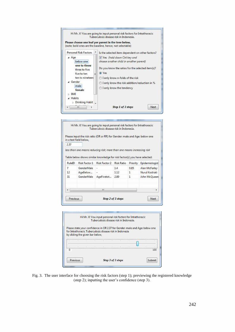
242
Fig. 3. The user interface for choosing the risk factors (step 1); previewing the registered knowledge
(step 2); inputting the user’s confidence (step 3).
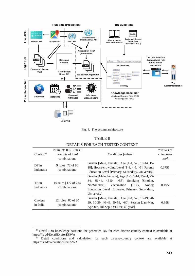
243
A Prediction
Model API
Context Collector
Tool
Ontology
Liv
e A
PIs
Lo
gic
Tie
rP
res
en
tati
on
Tie
r
BN Builder Algorithm
IF-Then Rules
Knowledge-base Tier
United Nations
Statistical Data API
Clients
Weather APIAtlas of Human
Infectious Disease
Centers of Disease
Control and
Prevention (CDC)
Bayesian
Network
Infectious Disease Risk (IDR)
Ontology and Rules
Population-level
parameters
Run-time (Prediction) BN Build-time
The User Interface
that captures risk
ratios and/or
prevalence
The
Epidemiologist(s)
Google APIs
GeocodesPersonal
Attributes
Infectious
Disease Name
WHO API
DateTime
Fig. 4. The system architecture
TABLE II
DETAILS FOR EACH TESTED CONTEXT
Context28
Num. of: IDR Rules |
possible of total
combinations
Conditions [values]
P values of
chi-square
test29
DF in
Indonesia
9 rules | 72 of 96
combinations
Gender [Male, Female]; Age [1-4, 5-9, 10-14, 15-
18]; House-crowding Level [1-3, 4-5, >5]; Parents
Education Level [Primary, Secondary, University]
0.3755
TB in
Indonesia
10 rules | 172 of 224
combinations
Gender [Male, Female]; Age [1-5, 6-14, 15-24, 25-
34, 35-44, 45-54, >55]; Smoking [Smoker,
NonSmoker]; Vaccination [BCG, None];
Education Level [Illiterate, Primary, Secondary,
University]
0.495
Cholera
in India
12 rules | 80 of 80
combinations
Gender [Male, Female]; Age [0-4, 5-9, 10-19, 20-
29, 30-39, 40-49, 50-59, >60]; Season [Jan-Mar,
Apr-Jun, Jul-Sep, Oct-Dec, all year]
0.998
28 Detail IDR knowledge-base and the generated BN for each disease-country context is available at
https://is.gd/DetailExpforESWA 29 Detail conditions and calculation for each disease-country context are available at
https://is.gd/calculationsforESWA
244
VII. DISCUSSION
This personalized ID risk prediction system consists of the IDR knowledge
representation, the BN-Builder algorithm, and the user interface to facilitate ongoing ID
risk knowledge encoding by epidemiologists. The IDR knowledge-base was validated
using ontological and rule-based system approaches; the result is the IDR knowledge-
base is generic enough to encode parameters for the disease risk prediction formula for
all IDs through time. However, some information like the number of samples and the
confidence interval for each risk ratio are not represented in the IDR knowledge-base.
Although this information is important for epidemiologists before encoding their
knowledge using the user interface, it is not used to calculate risk probabilities. Also, the
current design of the IDR ontology structure leads to a minor problem in the generated
BN. The conditions that may occur at the same time (e.g. windy and cloudy) should not
be represented as individuals but better as sub-classes. This is because BN-Builder
converts individuals in the IDR ontology to become states in the BN which can only be
selected one at a time.
In the reliability evaluation (section VI), the p-values show that the risk probabilities
for each context are reliable to 95% confidence level. However, there are some other
possibilities that contribute to the p-values: availability of data that is used to compare the
results, and number of samples for each disease-context. The more the samples, the higher
the difference tolerance which may cause the model to be overfitted (Freedman,
Seminara, Gail, & Hartge, 2005). Recalibration will be needed if one of those cases
happen. On the other hand, more samples are preferable to model variability in the real-
world cases. Trade-off between the number of samples and the expected p-value is a
common issue in the risk probability prediction research.
Admittedly, the feature for solving duplicate rule anomaly is a preventive solution. This
solution might not be strong enough to reject or clear up the duplicating rules as there
might be different confidence for the new rule and the epidemiologist wants to keep both
rules as records.
VIII. CONCLUSION AND FURTHER RESEARCH
This paper has described contributions in the context of a personalized infectious
disease risk prediction system: (1) IDR knowledge-base, (2) BN-Builder algorithm and
(3) the user interface to facilitate the ongoing IDR knowledge encoding. This paper is the
continuation of our work in (Vinarti & Hederman, A knowledge-base for a Personalized
Infectious Disease Risk Prediction System, 2018) (Vinarti & Hederman, Introduction of
A Bayesian Network Builder Algorithm: Personalized Infectious Disease Risk Prediction,
2018) (Vinarti & Hederman, Personalization of Infectious Disease Risk Prediction:
Towards automatic generation of a Bayesian Network, 2017) which explain and evaluate
245
the structure of IDR knowledge-base and BN-Builder algorithm pseudocode.
Specifically, this paper presents reliability evaluation for personalized ID risk assessment
at population-level. From the evaluation results in three disease-country contexts, the
personalized ID risk prediction is reliable.
To inform the epidemiologists about essential circumstances (e.g. specific strain of the
ID, number of samples, confidence interval of the risk ratios) before inputting a
knowledge using the designed user interface, annotations on the IDR knowledge-base
may be used and previewed in the user interface.
An IDR knowledge base guide will be written to help knowledge engineers encode new
infectious disease risk knowledge. The guide will include advice on avoiding rule
anomalies and on correctly representing overlapping conditions (such as windy and
cloudy, as described above).
VIII. REFERENCE
Camara, G., Despres, S., Djedidi, R., & Lo, M. (2013). Design of Schistosomiasis
Ontology (IDOSCHISTO) Extending the Infectious Disease. Medical
Informatics. Washington, D.C.
Cao, H., Zhang, L., Li, L., & Lo, S. (2013). Risk Factors for Acute Endophthalmitis following
Cataract Surgery: A Systematic Review and Meta-Analysis. PLoS ONE, 8(8), 1-18.
CDC. (2012, May 18). Lesson 1: Introduction to Epidemiology. Retrieved August 15, 2016,
from Centers for Disease Control and Prevention:
http://www.cdc.gov/ophss/csels/dsepd/ss1978/lesson1/section10.html
CDC. (2017). Emerging Infectious Diseases. (CDC: Centers for Disease Control and
Prevention) Retrieved October 26, 2017, from https://wwwnc.cdc.gov/eid
Cowell, L. (2016, July 5). Infectious Disease Ontology. Retrieved December 10, 2016, from
BioPortal: http://purl.obolibrary.org/obo/ido.owl
Division, N. R. (2001). Under the weather : climate, ecosystems, and infectious disease.
Washington, D. C.: National Academy Press.
Fares, A. (2011). Seasonality of Tuberculosis. Journal of Global Infectious Diseases, 3(1), 46-
55.
Freedman, A. N., Seminara, D., Gail, M. H., & Hartge, P. (2005). Cancer Risk Prediction
Models: A Workshop on Development, Evaluation, and Application. Journal of the
National Cancer Institute, 97(10), 715-723.
Greer, A. L., Drews, S. J., & Fisman, D. N. (2009). Why "Winter" vomiting disease?
seasonality, hydrology, and norovirus epidemiology in Toronto, Canada. EcoHealth,
6(2), 192-199.
Gustafson, P., Gomes, V. F., Vieira, C. S., & Rabna, P. (2004). Tuberculosis in Bissau:
incidence and risk factors in an urban community in sub-Saharan Africa. International
Journal of Epidemiology, 33, 163-172.
246
Guwatudde, D., Nakakeeto, M., Jones-Lopez, E. C., & Maganda, A. (2003). Tuberculosis in
Household Contacts of Infectious Cases in Kampala, Uganda. American Journal of
Epidemiology, 158(9), 887-898.
Haddawy, P. (1994). Generating Bayesian Networks from Probability Logic Knowledge Bases.
Seattle: Morgan Kaufmann Publishers Inc. San Francisco, CA, USA.
Hu, W., Tong, S., Mengersen, K., & Oldenburg, B. (2006). Rainfall, mosquito density and the
transmission of Ross River virus: A time-series forecasting model. 196(3-4).
Huang, Z., Das, A., Qiu, Y., & Tatem, A. J. (2012). Web-based GIS: the vector-borne disease
airline importation risk (VBD-AIR) tool. 11.
Indonesian Health, M. (2013). Kementrian Kesehatan Republik Indonesia. (KemenkesRI)
Retrieved 2017, from http://www.depkes.go.id/folder/view/01/structure-publikasi-
pusdatin-info-datin.html
Kumar, V. S., Devika, S., George, S., & Jeyaseelan, L. (2017). Spatial mapping of acute
diarrheal disease using GIS and estimation of relative risk using empirical Bayes
approach. 5.
Lewis, C. M., Whitwell, S. C., Forbes, A., & Sanderson, J. (2007). Estimating risks of common
complex diseases across genetic and environmental factors: the example of Crohn
disease. Journal of Medical Genetics, 44(11), 689-694.
Nelson, R. (2008). HealthMap: the future of infectious diseases surveillance? TheLancet, 8(10).
Panayiotis, P., Simon, H. X., Denise, A., & Alex, B. A. (2016). Prediction of lung cancer
incidence on the low-dose computed tomography arm of the National Lung Screening
Trial: A dynamic Bayesian network. Artificial Intelligence in Medicine, 72, 42-55.
Pesquita, C. (2017). Epidemiology Ontology. (The OBO Foundry) Retrieved 2017, from
https://www.ebi.ac.uk/ols/ontologies/epo
Prayitno, A., Taurel, A.-F., Nealon, J., & Satari, H. I. (2017). Dengue seroprevalence and force
of primary infection in a representative population of urban dwelling Indonesian
children. PLoS: Neglected Tropical Diseases, 11(6), 1-16.
Preece, A. (2001). Evaluating verification and validation methods in knowledge engineering.
Schmidt, S. A., Vestergaard, M., Baggesen, L. M., & Pedersen, L. (2017). Prevaccination
epidemiology of herpes zoster in Denmark: Quantification of occurrence and risk
factors. Vaccine, 1-8.
SickWeather. (2011-2017). SickWeather. (SickWeather Inc.) Retrieved December 12, 2017,
from http://www.sickweather.com/
Szumilas, M. (2010, August). Explaining Odds Ratios. Information Management for the Busy
Practitioner, pp. 227-229.
Tartir, S., Arpinar, I. B., & Sheth, A. P. (2010). Ontological Evaluation and Validation. In
Theory and Applications of Ontology: Computer Applications (pp. 115-130). Dordrecht:
Springer.
Third, A. (2014). BioPortal: CARRE Risk Factor Ontology. Retrieved October 18, 2017, from
https://bioportal.bioontology.org/ontologies/CARRE
Vinarti, R. A., & Hederman, L. M. (2017). Personalization of Infectious Disease Risk
Prediction: Towards automatic generation of a Bayesian Network. IEEE Computer-
based Medical Systems (CBMS). Thessaloniki, Greece: IEEE.
Vinarti, R. A., & Hederman, L. M. (2018). A knowledge-base for a Personalized Infectious
Disease Risk Prediction System. Medical Informatics Europe (MIE) 2018. Gothenburg,
Sweden.
247
Vinarti, R. A., & Hederman, L. M. (2018). Introduction of A Bayesian Network Builder
Algorithm: Personalized Infectious Disease Risk Prediction. 11th International Health
Informatics Conference: ACM Conference Series. Funchal, Madeira.
Wang, Q., Liu, Y., Ma, Y., & Han, L. (2017). Severe hypovitaminosis D in active TB patients
and its predictors. Clinical Nutrition, 1-7.
Wertheim, H. F., Horby, P., & Woodall, J. P. (2012). Atlas of Human Infectious Diseases.
Oxford: Wiley-Blackwell.
WHO. (2006). Cholera in India: an analysis of reports. Retrieved 2017, from
http://www.who.int/bulletin/volumes/88/3/09-073460/en/
WHO. (2016). Global Health Estimates 2015: Disease burden by Cause, Age, Sex, by Country
and by Region, 2000-2015. (Geneva, World Health Organization) Retrieved May 30,
2017, from
http://www.who.int/healthinfo/global_burden_disease/estimates/en/index2.html
WHO. (2017). Dengue fever in Indonesia. Retrieved 2017, from
http://www.who.int/csr/don/2004_05_11a/en/
WHO. (2017). Fact Sheets: Infectious Diseases. (WHO) Retrieved October 26, 2017, from
http://www.who.int/topics/infectious_diseases/factsheets/en/
WHO. (2017). Tuberculosis (TB). Retrieved 2017, from
http://www.who.int/tb/country/data/profiles/en/
Wu, X., Lu, Y., Zhou, S., Chen, L., & Xu, B. (2016). Impact of climate change on human
infectious diseases: Empirical evidence and human adaptation. 86.
Zagorecki, A., & Druzdzel, M. J. (2013). Knowledge engineering for bayesian networks: How
common are noisy-MAX distributions in practice? IEEE Transactions on Systems, Man,
and Cybernetics Part A:Systems and Humans, 43(1), 186-195.
Zhang, J., & Yu, K. F. (1998). What's the Relative Risk? A Method of Correcting the Odds
Ratio in Cohort Studies of Common Outcomes. JAMA: The Journal of the American
Medical Association, 280(19), 1690-1691.
248
Appendix 7 – BMC Journal Submission
An article submitted to the BMC – Journal of Biomedical Semantics (10th of July 2018).
Infectious Disease Risk knowledge representation for use in a
personalized IDR prediction system
Retno A. Vinarti a, *, and Lucy M. Hederman a a School of Computer Science and Statistics, Trinity College Dublin, The University of Dublin,
Ireland
*Corresponding e-mail: [email protected]
Abstract
Background: We are developing a personalized infectious disease risk (IDR) prediction system that
uses a Bayesian Network as a risk prediction model. The BN is auto-generated from a continuously
updateable knowledge-base that encodes declarative infectious disease risk knowledge and risk
quantifications that are relevant to calculate the personalized risk prediction. No existing knowledge
representations met this need. Therefore, the aim of this paper is to present a development of
knowledge-base and other representations that meet the system requirements, and help epidemiologists
in future knowledge encoding activities.
Results: We establish and evaluate three elements: an IDR core ontology, five IDR rule types, and an
IDR catalog. The IDR core ontology contains three classes to categorize relevant risk factors for human
infection (person, climate, location) and one infectious disease class. The IDR rule types are used to
bind infection risk factors with their risk quantifications (e.g. odds ratios, morbidity frequency). The
IDR catalog that inherits the IDR core structure consists of 212 classes, 246 individuals that encode all
distinct risk factors for all existing 234 human infectious diseases listed in Atlas of Human Infectious
Diseases (AHID), Centre for Disease Control and Prevention (CDC), and World Health Organization
(WHO) factsheets.
Conclusion: Through 18 cases used in the evaluation, we establish that the categorization of IDR core
ontology classes reflects the human infection risk in the epidemiology theory. All risk quantifications
to predict disease risk can be encoded by five rule types. Form the evaluation, all needed rule types are
provided to bind risk quantifications to represent the infection risk knowledge. The sub-classes and
individuals of the IDR catalog are useful (more than 60% are used) and sufficient (more than 75% of
the risk factors needed for the 18 evaluation cases), however, the epidemiologists will still need to add
some of individuals in the IDR catalog to encode the risk factors when needed. The current version of
the IDR catalog will be evolving as the infection risk knowledge develops. The current version of the
IDR catalog is freely available at http://dx.doi.org/10.17605/OSF.IO/P6QV8.
Keywords: infectious disease, risk prediction, knowledge representation, ontology, rules.
List of abbreviations: Infectious Disease Risk (IDR), Bayesian Network (BN), Atlas of Human
Infectious Diseases (AHID), World Health Organization (WHO), Center for Disease Control and
Prevention (CDC), Ontology Quality Analysis (OntoQA), Odds Ratios (OR), Relative Risks (RR),
Tuberculosis (TB), Meningitis (MEN), Dengue Fever (DF), Semantic-Web Rule Language (SWRL),
sexually-transmitted infections (STI).
249
Background
We are developing a system that aims to predict a person’s risk of contracting (specific)
infectious disease based on the personal attributes, current weather and surrounding terrain
(including land-use). This system consists of two major phases: knowledge-gleaning and run-
time. In the knowledge-gleaning phase, epidemiologists are expected to create a knowledge-
base representing epidemiology knowledge for one infectious disease prevalent in one location-
context (e.g. country). The context-specific knowledge-base is formed of two knowledge
representations: ontology and rules. After the knowledge-base is created, an algorithm,
Bayesian Network-Builder, converts it to an equivalent BN [238]. Whenever the
epidemiologists update the knowledge-base, the BN-Builder keeps the BN updated as well. In
the run-time phase, the system retrieves the current weather and surrounding terrain conditions
of the user from live APIs based on his geocodes. The retrieved facts are then processed to
calculate the personalized infectious disease risk probability using the generated BN from the
knowledge-gleaning phase. In the long-run, we will provide user interfaces to support
epidemiologists to encode their infection risk in the knowledge-base. In our pilot project, the
correctness of the risk predictions resulted from a hand-crafted BN for an infectious disease in
a country context is satisfying enough (more than 80% accurate) [239].
In the knowledge-gleaning phase, stable epidemiology knowledge about infections was
obtained from the Atlas of Human Infectious Diseases (AHID) [13], World Health
Organization (WHO) [31], Center for Disease Control and Prevention (CDC) [30], and clinical
and epidemiologic journal articles. This aims to (1) understand the chain of infection and
epidemiology knowledge for infectious diseases, and (2) capture infection risk factors and their
quantifications. The results of the first and second aims are a core ontology and collated risk
factors (i.e. catalog), respectively. The collated risk factors are represented in an ontology;
whereas their quantifications are encoded as rules.
Existing knowledge representations (ontologies) in epidemiology, infectious diseases, risk
factors domains, such as Human Disease Ontology [197], Infectious Disease Ontology [22],
Epidemiology Ontology [195], Apollo [201], Ontology for human risk factors for Cardiorenal
disease [25], have been investigated. No single ontology was intentionally built for encoding
the infection risk factors relevant to personalized infectious disease risk predictions. Although
the use of rules to support additional information for ontologies has been proven in [96], [240]–
[242], no rules in previous research were used to encode risk quantifications used for infection
risk predictions.
This paper aims to describe the development of an infectious disease risk (IDR) core ontology,
rule types and a catalog. Also, we assess the used methodology by evaluating the IDR core
ontology representativeness, and the usefulness and completeness of IDR rule types and IDR
catalog using context-specific knowledge-bases (i.e. evaluation cases). These evaluations are
inspired by metric-based ontology quality analysis (OntoQA) [228]. An instantiation process
is needed to build an IDR knowledge-base from IDR rule types and IDR catalog. An IDR
knowledge-base consists of an ontology and set of rules that was created by using relevant sub-
classes and individuals in the IDR catalog, and encoding risk quantifications using IDR rule
types, respectively. The IDR knowledge-bases will be used to generate an equivalent BN by
the BN-Builder algorithm.
The structure of the paper is as follows. Section 2 presents the outcomes: IDR core ontology,
IDR rule types and IDR catalog. Section 3 explains the evaluation results for each product.
Section 4 discusses the evaluation results, the assumptions, the limitations and the possible
future research. Section 5 outlines the conclusions made through the evaluations and
250
discussions. Section 6 describes the research methodology to develop the IDR core ontology,
IDR rule types, IDR catalog, an instantiation process to make the IDR knowledge-base, and
evaluation plans.
Results of IDR Ontology and Rule Type Design
This section presents the IDR core ontology that was constructed from the summary of
infection drivers, the IDR rule types that facilitate risk quantification encoding over the IDR
ontology, and the IDR catalog that was developed from distinct risk factors for all human
infectious diseases.
From the chain of infection risk definition [12], infectious disease is an ailment caused by a
pathogen30 which is transmitted from an infected person, animal or reservoir31 to a susceptible
human using a vector32 or vehicle33 [126]. When a pathogen enters the human, whether the
infectious disease will develop or not depends on the human immunity level. Some personal
attributes, such as age, genetics, gender, and behaviors may reduce the immunity level. Certain
terrain and atmospheric conditions may affect climate-dependent pathogen and vector. For
example, Colorado Tick Fever infection is seasonal, coinciding with the period of Ixodid wood
tick activity in early summer. Human cases can be detected from March to September in the
Rocky Mountain region. Most human cases are males, aged 20–29 years, reflecting the
frequency of outdoor activity in the mountains [13].
IDR core ontology
In this section, we construct an epistemological knowledge representation of infection risks.
The epistemological representation consists of concept types (i.e. main classes), conceptual
sub-pieces (i.e. sub-classes), inheritance and structuring relations between concepts, using a
diagrammatic form [243]–[245].
The construction of the IDR core ontology aims to (1) make the domain knowledge (risk factors
that affect a person’s risk contracting of infectious disease) explicit, and (2) support the IDR
catalog by providing the main classes and object properties; these object properties are used to
bind the risk factors with their risk quantifications using the IDR rule types.
To make the domain knowledge explicit, we categorized risk factors as person risk factors,
and environment risk factors. These categories, together with infectious disease, are
represented as main classes of the IDR core ontology. This is because personalization and
environment are the focus of the system. We define person risk factors as attributes of a person
(including habits and activities), and environment risk factors are determined by climate and
location, that affect certain pathogen or vector of an infectious disease to multiply [7], [42],
[86], [103], [129], [246]. Seventeen infection risk drivers listed in AHID [13] were summarized
into these main classes (see Appendix 1). The decision whether an object is a sub-class or an
individual of these main classes is explained in section 2.3.
30 Pathogen is an infectious agent causing an infectious disease (e.g. bacteria, virus, parasite, prion)
31 Reservoir is a habitat in which the infectious agent able to survive and multiply.
32 Vector is a living being (animal) that disseminates the agents, for example, mosquito, mice, flies.
33 Vehicle is inanimate object that transports the agent from reservoir to host
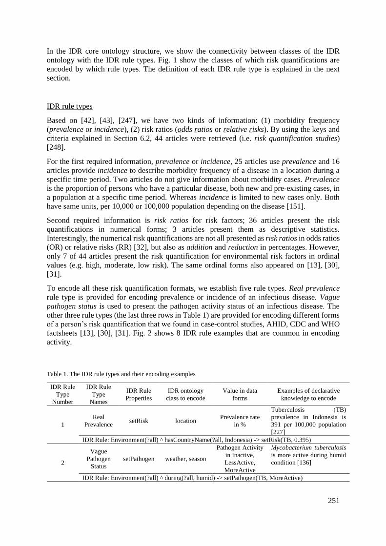
251
In the IDR core ontology structure, we show the connectivity between classes of the IDR
ontology with the IDR rule types. Fig. 1 show the classes of which risk quantifications are
encoded by which rule types. The definition of each IDR rule type is explained in the next
section.
IDR rule types
Based on [42], [43], [247], we have two kinds of information: (1) morbidity frequency
(prevalence or incidence), (2) risk ratios (odds ratios or relative risks). By using the keys and
criteria explained in Section 6.2, 44 articles were retrieved (i.e. risk quantification studies)
[248].
For the first required information, prevalence or incidence, 25 articles use prevalence and 16
articles provide incidence to describe morbidity frequency of a disease in a location during a
specific time period. Two articles do not give information about morbidity cases. Prevalence
is the proportion of persons who have a particular disease, both new and pre-existing cases, in
a population at a specific time period. Whereas incidence is limited to new cases only. Both
have same units, per 10,000 or 100,000 population depending on the disease [151].
Second required information is risk ratios for risk factors; 36 articles present the risk
quantifications in numerical forms; 3 articles present them as descriptive statistics.
Interestingly, the numerical risk quantifications are not all presented as risk ratios in odds ratios
(OR) or relative risks (RR) [32], but also as addition and reduction in percentages. However,
only 7 of 44 articles present the risk quantification for environmental risk factors in ordinal
values (e.g. high, moderate, low risk). The same ordinal forms also appeared on [13], [30],
[31].
To encode all these risk quantification formats, we establish five rule types. Real prevalence
rule type is provided for encoding prevalence or incidence of an infectious disease. Vague
pathogen status is used to present the pathogen activity status of an infectious disease. The
other three rule types (the last three rows in Table 1) are provided for encoding different forms
of a person’s risk quantification that we found in case-control studies, AHID, CDC and WHO
factsheets [13], [30], [31]. Fig. 2 shows 8 IDR rule examples that are common in encoding
activity.
Table 1. The IDR rule types and their encoding examples
IDR Rule
Type
Number
IDR Rule
Type
Names
IDR Rule
Properties
IDR ontology
class to encode
Value in data
forms
Examples of declarative
knowledge to encode
1
Real
Prevalence setRisk location
Prevalence rate
in %
Tuberculosis (TB)
prevalence in Indonesia is
391 per 100,000 population
[227]
IDR Rule: Environment(?all) ^ hasCountryName(?all, Indonesia) -> setRisk(TB, 0.395)
2
Vague
Pathogen
Status
setPathogen weather, season
Pathogen Activity
in Inactive,
LessActive,
MoreActive
Mycobacterium tuberculosis
is more active during humid
condition [136]
IDR Rule: Environment(?all) ^ during(?all, humid) -> setPathogen(TB, MoreActive)
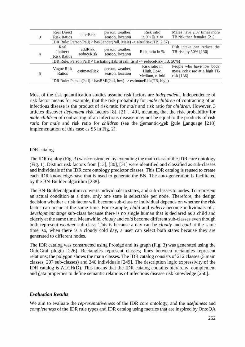
252
3
Real Direct
Risk Ratios alterRisk
person, weather,
season, location
Risk ratio
in 0 < ℝ < ∞
Males have 2.37 times more
TB risk than females [21]
IDR Rule: Person(?all) ^ hasGender(?all, Male) -> alterRisk(TB, 2.37)
4
Real
Indirect
Risk Ratios
addRisk,
reduceRisk
person, weather,
season, location Risk ratio in %
Fish intake can reduce the
TB risk by 50% [136]
IDR Rule: Person(?all) ^ hasEatingHabits(?all, fish) -> reduceRisk(TB, 50%)
5
Vague Risk
Ratios estimateRisk
person, weather,
season, location
Risk ratio in
High, Low,
Medium, n-fold
People who have low body
mass index are at a high TB
risk [136]
IDR Rule: Person(?all) ^ hasBMI(?all, low) -> estimateRisk(TB, high)
Most of the risk quantification studies assume risk factors are independent. Independence of
risk factor means for example, that the risk probability for male children of contracting of an
infectious disease is the product of risk ratio for male and risk ratio for children. However, 3
articles discover dependent risk factors [8], [21], [49], meaning that the risk probability for
male children of contracting of an infectious disease may not be equal to the products of risk
ratio for male and risk ratio for children (see the Semantic-web Rule Language [218]
implementation of this case as S5 in Fig. 2).
IDR catalog
The IDR catalog (Fig. 3) was constructed by extending the main class of the IDR core ontology
(Fig. 1). Distinct risk factors from [13], [30], [31] were identified and classified as sub-classes
and individuals of the IDR core ontology predictor classes. This IDR catalog is reused to create
each IDR knowledge-base that is used to generate the BN. The auto-generation is facilitated
by the BN-Builder algorithm [238].
The BN-Builder algorithm converts individuals to states, and sub-classes to nodes. To represent
an actual condition at a time, only one state is selectable per node. Therefore, the design
decision whether a risk factor will become sub-class or individual depends on whether the risk
factor can occur at the same time. For example, child and elderly become individuals of a
development stage sub-class because there is no single human that is declared as a child and
elderly at the same time. Meanwhile, cloudy and cold become different sub-classes even though
both represent weather sub-class. This is because a day can be cloudy and cold at the same
time, so, when there is a cloudy cold day, a user can select both states because they are
generated to different nodes.
The IDR catalog was constructed using Protégé and its graph (Fig. 3) was generated using the
OntoGraf plugin [226]. Rectangles represent classes; lines between rectangles represent
relations; the polygon shows the main classes. The IDR catalog consists of 212 classes (5 main
classes, 207 sub-classes) and 246 individuals [249]. The description logic expressivity of the
IDR catalog is ALCH(D). This means that the IDR catalog contains hierarchy, complement
and data properties to define semantic relations of infectious disease risk knowledge [250].
Evaluation Results
We aim to evaluate the representativeness of the IDR core ontology, and the usefulness and
completeness of the IDR rule types and IDR catalog using metrics that are inspired by OntoQA
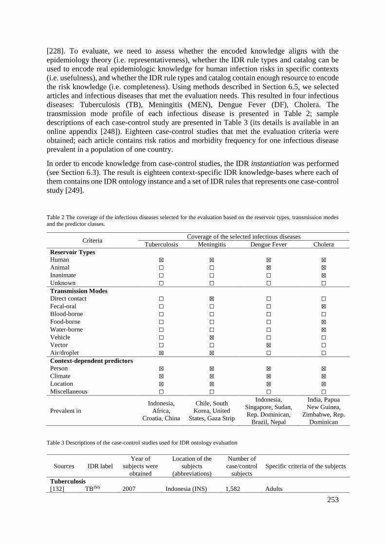
253
[228]. To evaluate, we need to assess whether the encoded knowledge aligns with the
epidemiology theory (i.e. representativeness), whether the IDR rule types and catalog can be
used to encode real epidemiologic knowledge for human infection risks in specific contexts
(i.e. usefulness), and whether the IDR rule types and catalog contain enough resource to encode
the risk knowledge (i.e. completeness). Using methods described in Section 6.5, we selected
articles and infectious diseases that met the evaluation needs. This resulted in four infectious
diseases: Tuberculosis (TB), Meningitis (MEN), Dengue Fever (DF), Cholera. The
transmission mode profile of each infectious disease is presented in Table 2; sample
descriptions of each case-control study are presented in Table 3 (its details is available in an
online appendix [248]). Eighteen case-control studies that met the evaluation criteria were
obtained; each article contains risk ratios and morbidity frequency for one infectious disease
prevalent in a population of one country.
In order to encode knowledge from case-control studies, the IDR instantiation was performed
(see Section 6.3). The result is eighteen context-specific IDR knowledge-bases where each of
them contains one IDR ontology instance and a set of IDR rules that represents one case-control
study [249].
Table 2 The coverage of the infectious diseases selected for the evaluation based on the reservoir types, transmission modes
and the predictor classes.
Criteria Coverage of the selected infectious diseases
Tuberculosis Meningitis Dengue Fever Cholera Reservoir Types
Human ☒ ☒ ☒ ☒
Animal ☐ ☐ ☒ ☒
Inanimate ☐ ☐ ☐ ☒
Unknown ☐ ☐ ☐ ☐
Transmission Modes
Direct contact ☐ ☒ ☐ ☐
Fecal-oral ☐ ☐ ☐ ☒
Blood-borne ☐ ☐ ☐ ☐
Food-borne ☐ ☐ ☐ ☒
Water-borne ☐ ☐ ☐ ☒
Vehicle ☐ ☒ ☐ ☐
Vector ☐ ☐ ☒ ☐
Air/droplet ☒ ☒ ☐ ☐
Context-dependent predictors
Person ☒ ☒ ☒ ☒
Climate ☒ ☒ ☒ ☒
Location ☒ ☒ ☒ ☒
Miscellaneous ☐ ☐ ☐ ☐
Prevalent in
Indonesia,
Africa,
Croatia, China
Chile, South
Korea, United
States, Gaza Strip
Indonesia,
Singapore, Sudan,
Rep. Dominican,
Brazil, Nepal
India, Papua
New Guinea,
Zimbabwe, Rep.
Dominican
Table 3 Descriptions of the case-control studies used for IDR ontology evaluation
Sources IDR label
Year of
subjects were
obtained
Location of the
subjects
(abbreviations)
Number of
case/control
subjects
Specific criteria of the subjects
Tuberculosis
[132] TBINS 2007 Indonesia (INS) 1,582 Adults
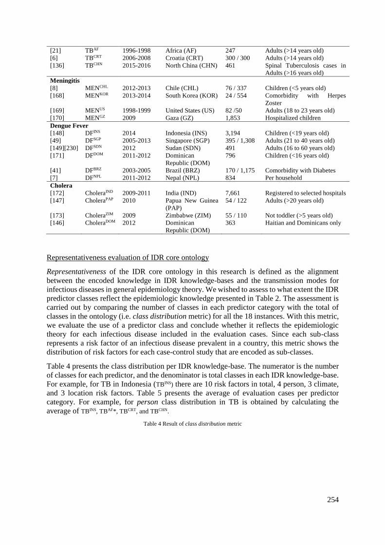
254
[21] TBAF 1996-1998 Africa (AF) 247 Adults (>14 years old)
[6] TBCRT 2006-2008 Croatia (CRT) 300 / 300 Adults (>14 years old)
[136] TBCHN 2015-2016 North China (CHN) 461 Spinal Tuberculosis cases in
Adults (>16 years old)
Meningitis
[8] MENCHL 2012-2013 Chile (CHL) 76 / 337 Children (<5 years old)
[168] MENKOR 2013-2014 South Korea (KOR) 24 / 554 Comorbidity with Herpes
Zoster
[169] MENUS 1998-1999 United States (US) 82 /50 Adults (18 to 23 years old)
[170] MENGZ 2009 Gaza (GZ) 1,853 Hospitalized children
Dengue Fever
[148] DFINS 2014 Indonesia (INS) 3,194 Children (<19 years old)
[49] DFSGP 2005-2013 Singapore (SGP) 395 / 1,308 Adults (21 to 40 years old)
[149][230] DFSDN 2012 Sudan (SDN) 491 Adults (16 to 60 years old)
[171] DFDOM 2011-2012 Dominican
Republic (DOM)
796 Children (<16 years old)
[41] DFBRZ 2003-2005 Brazil (BRZ) 170 / 1,175 Comorbidity with Diabetes
[7] DFNPL 2011-2012 Nepal (NPL) 834 Per household
Cholera
[172] CholeraIND 2009-2011 India (IND) 7,661 Registered to selected hospitals
[147] CholeraPAP 2010 Papua New Guinea
(PAP)
54 / 122 Adults (>20 years old)
[173] CholeraZIM 2009 Zimbabwe (ZIM) 55 / 110 Not toddler (>5 years old)
[146] CholeraDOM 2012 Dominican
Republic (DOM)
363 Haitian and Dominicans only
Representativeness evaluation of IDR core ontology
Representativeness of the IDR core ontology in this research is defined as the alignment
between the encoded knowledge in IDR knowledge-bases and the transmission modes for
infectious diseases in general epidemiology theory. We wished to assess to what extent the IDR
predictor classes reflect the epidemiologic knowledge presented in Table 2. The assessment is
carried out by comparing the number of classes in each predictor category with the total of
classes in the ontology (i.e. class distribution metric) for all the 18 instances. With this metric,
we evaluate the use of a predictor class and conclude whether it reflects the epidemiologic
theory for each infectious disease included in the evaluation cases. Since each sub-class
represents a risk factor of an infectious disease prevalent in a country, this metric shows the
distribution of risk factors for each case-control study that are encoded as sub-classes.
Table 4 presents the class distribution per IDR knowledge-base. The numerator is the number
of classes for each predictor, and the denominator is total classes in each IDR knowledge-base.
For example, for TB in Indonesia (TBINS) there are 10 risk factors in total, 4 person, 3 climate,
and 3 location risk factors. Table 5 presents the average of evaluation cases per predictor
category. For example, for person class distribution in TB is obtained by calculating the
average of TBINS, TBAF*, TBCRT, and TBCHN.
Table 4 Result of class distribution metric
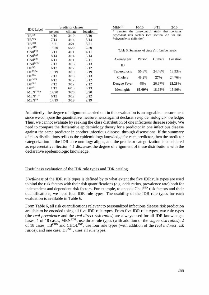
255
IDR Label predictor classes
person climate location
TBINS 4/10 3/10 3/10
TBAF* 7/14 4/14 3/14
TBCRT 15/21 3/21 3/21
TBCHN 13/20 5/20 2/20
CholIND 3/11 4/11 4/11
CholPAP 8/14 3/14 3/14
CholZIM 6/11 3/11 2/11
CholDOM 7/13 3/13 3/13
DFINS 6/12 3/12 3/12
DFSGP* 13/19 3/19 3/19
DFSDN 7/13 3/13 3/13
DFDOM 6/12 3/12 3/12
DFBRZ 7/12 3/12 2/12
DFNPL 1/13 6/13 6/13
MENCHL* 14/20 3/20 3/20
MENKOR 6/12 3/12 3/12
MENUS 14/19 3/19 2/19
MENGZ 10/15 3/15 2/15 * denotes the case-control study that contains
dependent risk factors (see section 2.2 for the
independence definition)
Table 5. Summary of class distribution metric
Average per
ID
Person Climate Location
Tuberculosis 56.6% 24.46% 18.93%
Cholera 48.2% 27% 24.76%
Dengue Fever 48% 26.67% 25.28%
Meningitis 65.09% 18.95% 15.96%
Admittedly, the degree of alignment carried out in this evaluation is an arguable measurement
since we compare the quantitative measurements against declarative epidemiologic knowledge.
Thus, we cannot evaluate by seeking the class distribution of one infectious disease solely. We
need to compare the declarative epidemiology theory for a predictor in one infectious disease
against the same predictor in another infectious disease, through discussions. If the summary
of class distributions reflects the epidemiology knowledge for each predictor, then the predictor
categorization in the IDR core ontology aligns, and the predictor categorization is considered
as representative. Section 4.1 discusses the degree of alignment of these distributions with the
declarative epidemiologic knowledge.
Usefulness evaluation of the IDR rule types and IDR catalog
Usefulness of the IDR rule types is defined by to what extent the five IDR rule types are used
to bind the risk factors with their risk quantifications (e.g. odds ratios, prevalence rate) both for
independent and dependent risk factors. For example, to encode CholIND risk factors and their
quantifications, we need four IDR rule types. The usability of the IDR rule types for each
evaluation is available in Table 6.
From Table 6, all risk quantifications relevant to personalized infectious disease risk prediction
are able to be encoded using all five IDR rule types. From five IDR rule types, two rule types
(the real prevalence and the real direct risk ratios) are always used for all IDR knowledge-
bases; 1 of 18 cases, MENKOR, use three rule types (with addition of the vague risk ratios); 2
of 18 cases, TBCHN and CHOLIND, use four rule types (with addition of the real indirect risk
ratios); and one case, DFNPL, uses all rule types.
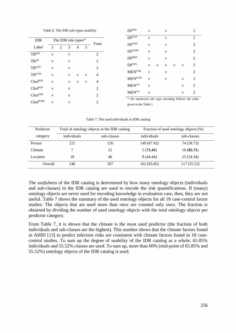
256
Table 6. The IDR rule types usability
IDR
Label
The IDR rule types* Total
1 2 3 4 5
TBINS v v 2
TBAF v v 2
TBCRT v v 2
TBCHN v v v v 4
CholIND v v v v 4
CholPAP v v 2
CholZIM v v 2
CholDOM v v 2
DFINS v v 2
DFSGP v v 2
DFSDN v v 2
DFDOM v v 2
DFBRZ v v 2
DFNPL v v v v v 5
MENCHL v v 2
MENKOR v v v 3
MENUS v v 2
MENGZ v v 2
* the numerical rule type encoding follows the order
given in the Table 1
Table 7. The used individuals in IDR catalog
Predictor
category
Total of ontology objects in the IDR catalog Fraction of used ontology objects (%)
individuals sub-classes individuals sub-classes
Person 221 126 149 (67.42) 74 (58.73)
Climate 7 21 5 (71.43) 18 (85.71)
Location 18 46 8 (44.44) 25 (54.34)
Overall 246 207 162 (65.85) 117 (55.52)
The usefulness of the IDR catalog is determined by how many ontology objects (individuals
and sub-classes) in the IDR catalog are used to encode the risk quantifications. If (many)
ontology objects are never used for encoding knowledge in evaluation case, then, they are not
useful. Table 7 shows the summary of the used ontology objects for all 18 case-control factor
studies. The objects that are used more than once are counted only once. The fraction is
obtained by dividing the number of used ontology objects with the total ontology objects per
predictor category.
From Table 7, it is shown that the climate is the most used predictor (the fraction of both
individuals and sub-classes are the highest). This number shows that the climate factors found
in AHID [13] to predict infection risks are consistent with climate factors found in 18 case-
control studies. To sum up the degree of usability of the IDR catalog as a whole, 65.85%
individuals and 55.52% classes are used. To sum up, more than 60% (mid-point of 65.85% and
55.52%) ontology objects of the IDR catalog is used.
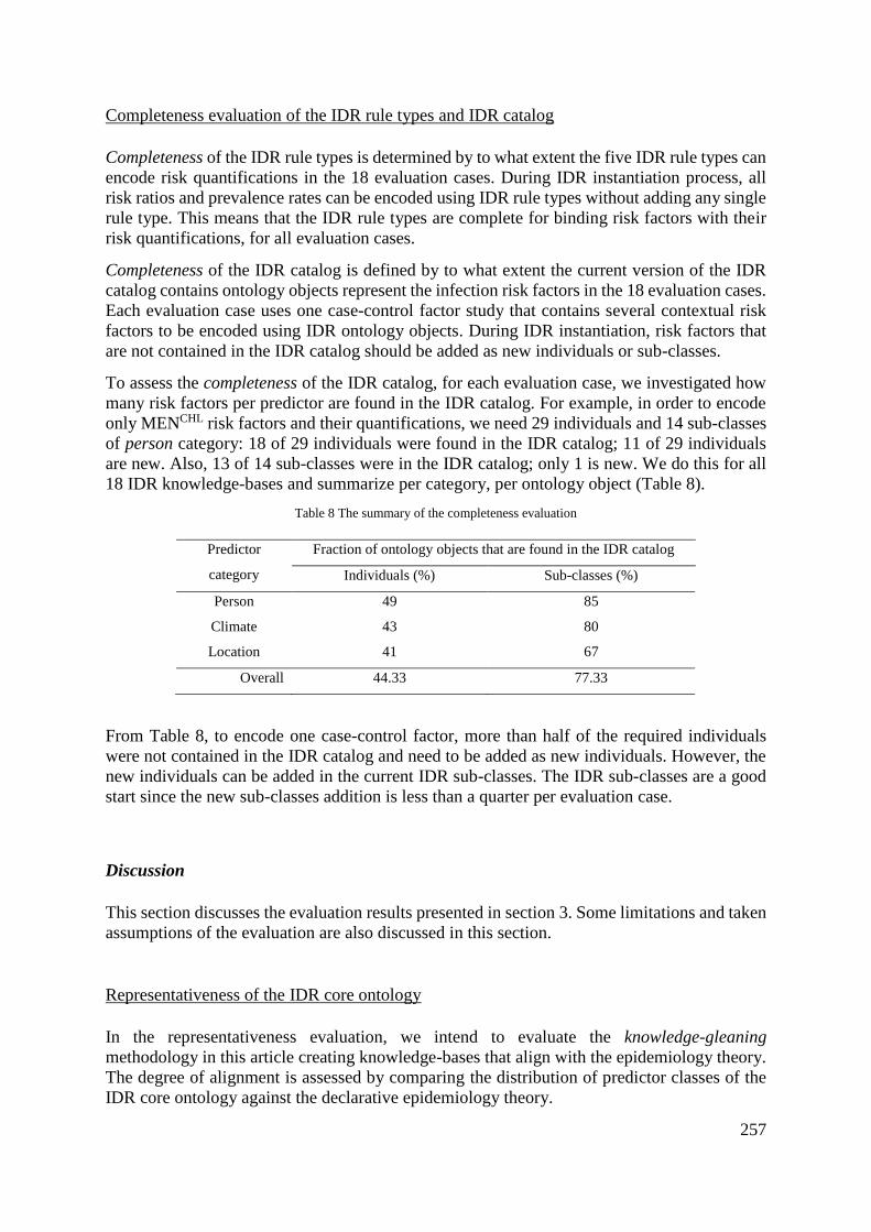
257
Completeness evaluation of the IDR rule types and IDR catalog
Completeness of the IDR rule types is determined by to what extent the five IDR rule types can
encode risk quantifications in the 18 evaluation cases. During IDR instantiation process, all
risk ratios and prevalence rates can be encoded using IDR rule types without adding any single
rule type. This means that the IDR rule types are complete for binding risk factors with their
risk quantifications, for all evaluation cases.
Completeness of the IDR catalog is defined by to what extent the current version of the IDR
catalog contains ontology objects represent the infection risk factors in the 18 evaluation cases.
Each evaluation case uses one case-control factor study that contains several contextual risk
factors to be encoded using IDR ontology objects. During IDR instantiation, risk factors that
are not contained in the IDR catalog should be added as new individuals or sub-classes.
To assess the completeness of the IDR catalog, for each evaluation case, we investigated how
many risk factors per predictor are found in the IDR catalog. For example, in order to encode
only MENCHL risk factors and their quantifications, we need 29 individuals and 14 sub-classes
of person category: 18 of 29 individuals were found in the IDR catalog; 11 of 29 individuals
are new. Also, 13 of 14 sub-classes were in the IDR catalog; only 1 is new. We do this for all
18 IDR knowledge-bases and summarize per category, per ontology object (Table 8).
Table 8 The summary of the completeness evaluation
Predictor
category
Fraction of ontology objects that are found in the IDR catalog
Individuals (%) Sub-classes (%)
Person 49 85
Climate 43 80
Location 41 67
Overall 44.33 77.33
From Table 8, to encode one case-control factor, more than half of the required individuals
were not contained in the IDR catalog and need to be added as new individuals. However, the
new individuals can be added in the current IDR sub-classes. The IDR sub-classes are a good
start since the new sub-classes addition is less than a quarter per evaluation case.
Discussion
This section discusses the evaluation results presented in section 3. Some limitations and taken
assumptions of the evaluation are also discussed in this section.
Representativeness of the IDR core ontology
In the representativeness evaluation, we intend to evaluate the knowledge-gleaning
methodology in this article creating knowledge-bases that align with the epidemiology theory.
The degree of alignment is assessed by comparing the distribution of predictor classes of the
IDR core ontology against the declarative epidemiology theory.
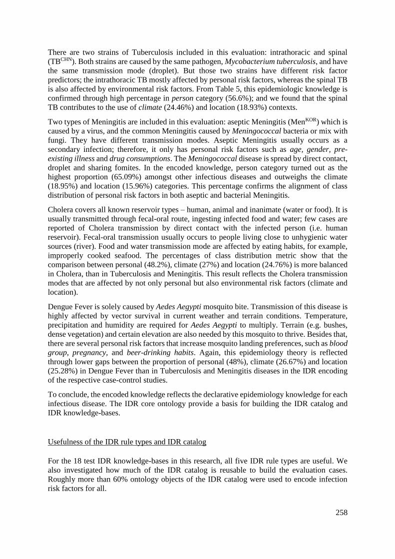
258
There are two strains of Tuberculosis included in this evaluation: intrathoracic and spinal
(TBCHN). Both strains are caused by the same pathogen, Mycobacterium tuberculosis, and have
the same transmission mode (droplet). But those two strains have different risk factor
predictors; the intrathoracic TB mostly affected by personal risk factors, whereas the spinal TB
is also affected by environmental risk factors. From Table 5, this epidemiologic knowledge is
confirmed through high percentage in person category (56.6%); and we found that the spinal
TB contributes to the use of climate (24.46%) and location (18.93%) contexts.
Two types of Meningitis are included in this evaluation: aseptic Meningitis (MenKOR) which is
caused by a virus, and the common Meningitis caused by Meningococcal bacteria or mix with
fungi. They have different transmission modes. Aseptic Meningitis usually occurs as a
secondary infection; therefore, it only has personal risk factors such as age, gender, pre-
existing illness and drug consumptions. The Meningococcal disease is spread by direct contact,
droplet and sharing fomites. In the encoded knowledge, person category turned out as the
highest proportion (65.09%) amongst other infectious diseases and outweighs the climate
(18.95%) and location (15.96%) categories. This percentage confirms the alignment of class
distribution of personal risk factors in both aseptic and bacterial Meningitis.
Cholera covers all known reservoir types – human, animal and inanimate (water or food). It is
usually transmitted through fecal-oral route, ingesting infected food and water; few cases are
reported of Cholera transmission by direct contact with the infected person (i.e. human
reservoir). Fecal-oral transmission usually occurs to people living close to unhygienic water
sources (river). Food and water transmission mode are affected by eating habits, for example,
improperly cooked seafood. The percentages of class distribution metric show that the
comparison between personal (48.2%), climate (27%) and location (24.76%) is more balanced
in Cholera, than in Tuberculosis and Meningitis. This result reflects the Cholera transmission
modes that are affected by not only personal but also environmental risk factors (climate and
location).
Dengue Fever is solely caused by Aedes Aegypti mosquito bite. Transmission of this disease is
highly affected by vector survival in current weather and terrain conditions. Temperature,
precipitation and humidity are required for Aedes Aegypti to multiply. Terrain (e.g. bushes,
dense vegetation) and certain elevation are also needed by this mosquito to thrive. Besides that,
there are several personal risk factors that increase mosquito landing preferences, such as blood
group, pregnancy, and beer-drinking habits. Again, this epidemiology theory is reflected
through lower gaps between the proportion of personal (48%), climate (26.67%) and location
(25.28%) in Dengue Fever than in Tuberculosis and Meningitis diseases in the IDR encoding
of the respective case-control studies.
To conclude, the encoded knowledge reflects the declarative epidemiology knowledge for each
infectious disease. The IDR core ontology provide a basis for building the IDR catalog and
IDR knowledge-bases.
Usefulness of the IDR rule types and IDR catalog
For the 18 test IDR knowledge-bases in this research, all five IDR rule types are useful. We
also investigated how much of the IDR catalog is reusable to build the evaluation cases.
Roughly more than 60% ontology objects of the IDR catalog were used to encode infection
risk factors for all.
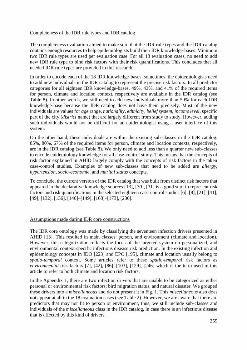
259
Completeness of the IDR rule types and IDR catalog
The completeness evaluation aimed to make sure that the IDR rule types and the IDR catalog
contains enough resources to help epidemiologists build their IDR knowledge-bases. Minimum
two IDR rule types are used per evaluation case. For all 18 evaluation cases, no need to add
new IDR rule type to bind risk factors with their risk quantifications. This concludes that all
needed IDR rule types are provided in this research.
In order to encode each of the 18 IDR knowledge-bases, sometimes, the epidemiologists need
to add new individuals in the IDR catalog to represent the precise risk factors. In all predictor
categories for all eighteen IDR knowledge-bases, 49%, 43%, and 41% of the required items
for person, climate and location context, respectively are available in the IDR catalog (see
Table 8). In other words, we still need to add new individuals more than 50% for each IDR
knowledge-base because the IDR catalog does not have them precisely. Most of the new
individuals are values for age range, nationality, ethnicity, belief system, income level, specific
part of the city (district name) that are largely different from study to study. However, adding
such individuals would not be difficult for an epidemiologist using a user interface of this
system.
On the other hand, these individuals are within the existing sub-classes in the IDR catalog.
85%, 80%, 67% of the required items for person, climate and location contexts, respectively,
are in the IDR catalog (see Table 8). We only need to add less than a quarter new sub-classes
to encode epidemiology knowledge for all case-control study. This means that the concepts of
risk factor explained in AHID largely comply with the concepts of risk factors in the taken
case-control studies. Examples of new sub-classes that need to be added are allergy,
hypertension, socio-economic, and marital status concepts.
To conclude, the current version of the IDR catalog that was built from distinct risk factors that
appeared in the declarative knowledge sources [13], [30], [31] is a good start to represent risk
factors and risk quantifications in the selected eighteen case-control studies [6]–[8], [21], [41],
[49], [132], [136], [146]–[149], [168]–[173], [230].
Assumptions made during IDR core constructions
The IDR core ontology was made by classifying the seventeen infection drivers presented in
AHID [13]. This resulted in main classes: person, and environment (climate and location).
However, this categorization reflects the focus of the targeted system on personalized, and
environmental context-specific infectious disease risk prediction. In the existing infection and
epidemiology concepts in IDO [223] and EPO [195], climate and location usually belong to
spatio-temporal context. Some articles refer to these spatio-temporal risk factors as
environmental risk factors [7], [42], [86], [103], [129], [246] which is the term used in this
article to refer to both climate and location risk factors.
In the Appendix 1, there are two infection drivers that are unable to be categorized as either
personal or environmental risk factors: bird migration status, and natural disaster. We grouped
these drivers into a miscellaneous and do not present it in Fig. 1. This miscellaneous also does
not appear at all in the 18 evaluation cases (see Table 2). However, we are aware that there are
predictors that may not fit to person or environment, thus, we still include sub-classes and
individuals of the miscellaneous class in the IDR catalog, in case there is an infectious disease
that is affected by this kind of drivers.
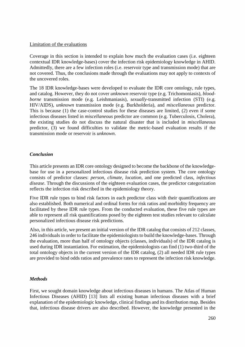
260
Limitation of the evaluations
Coverage in this section is intended to explain how much the evaluation cases (i.e. eighteen
contextual IDR knowledge-bases) cover the infection risk epidemiology knowledge in AHID.
Admittedly, there are a few infection roles (i.e. reservoir type and transmission mode) that are
not covered. Thus, the conclusions made through the evaluations may not apply to contexts of
the uncovered roles.
The 18 IDR knowledge-bases were developed to evaluate the IDR core ontology, rule types,
and catalog. However, they do not cover unknown reservoir type (e.g. Trichomoniasis), blood-
borne transmission mode (e.g. Leishmaniasis), sexually-transmitted infection (STI) (e.g.
HIV/AIDS), unknown transmission mode (e.g. Burkholderia), and miscellaneous predictor.
This is because (1) the case-control studies for these diseases are limited, (2) even if some
infectious diseases listed in miscellaneous predictor are common (e.g. Tuberculosis, Cholera),
the existing studies do not discuss the natural disaster that is included in miscellaneous
predictor, (3) we found difficulties to validate the metric-based evaluation results if the
transmission mode or reservoir is unknown.
Conclusion
This article presents an IDR core ontology designed to become the backbone of the knowledge-
base for use in a personalized infectious disease risk prediction system. The core ontology
consists of predictor classes: person, climate, location, and one predicted class, infectious
disease. Through the discussions of the eighteen evaluation cases, the predictor categorization
reflects the infection risk described in the epidemiology theory.
Five IDR rule types to bind risk factors in each predictor class with their quantifications are
also established. Both numerical and ordinal forms for risk ratios and morbidity frequency are
facilitated by these IDR rule types. From the conducted evaluation, these five rule types are
able to represent all risk quantifications posed by the eighteen test studies relevant to calculate
personalized infectious disease risk predictions.
Also, in this article, we present an initial version of the IDR catalog that consists of 212 classes,
246 individuals in order to facilitate the epidemiologists to build the knowledge-bases. Through
the evaluation, more than half of ontology objects (classes, individuals) of the IDR catalog is
used during IDR instantiation. For estimation, the epidemiologists can find (1) two-third of the
total ontology objects in the current version of the IDR catalog, (2) all needed IDR rule types
are provided to bind odds ratios and prevalence rates to represent the infection risk knowledge.
Methods
First, we sought domain knowledge about infectious diseases in humans. The Atlas of Human
Infectious Diseases (AHID) [13] lists all existing human infectious diseases with a brief
explanation of the epidemiologic knowledge, clinical findings and its distribution map. Besides
that, infectious disease drivers are also described. However, the knowledge presented in the
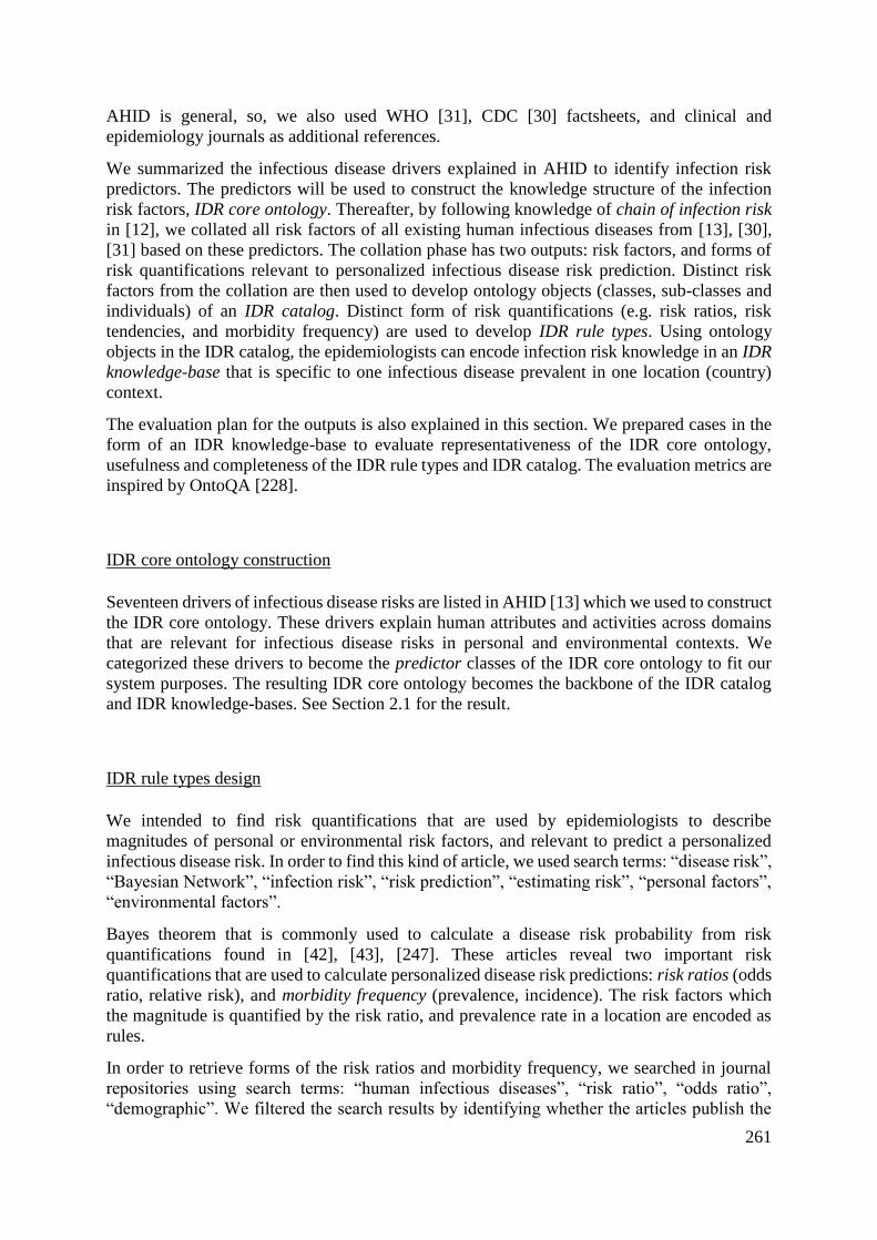
261
AHID is general, so, we also used WHO [31], CDC [30] factsheets, and clinical and
epidemiology journals as additional references.
We summarized the infectious disease drivers explained in AHID to identify infection risk
predictors. The predictors will be used to construct the knowledge structure of the infection
risk factors, IDR core ontology. Thereafter, by following knowledge of chain of infection risk
in [12], we collated all risk factors of all existing human infectious diseases from [13], [30],
[31] based on these predictors. The collation phase has two outputs: risk factors, and forms of
risk quantifications relevant to personalized infectious disease risk prediction. Distinct risk
factors from the collation are then used to develop ontology objects (classes, sub-classes and
individuals) of an IDR catalog. Distinct form of risk quantifications (e.g. risk ratios, risk
tendencies, and morbidity frequency) are used to develop IDR rule types. Using ontology
objects in the IDR catalog, the epidemiologists can encode infection risk knowledge in an IDR
knowledge-base that is specific to one infectious disease prevalent in one location (country)
context.
The evaluation plan for the outputs is also explained in this section. We prepared cases in the
form of an IDR knowledge-base to evaluate representativeness of the IDR core ontology,
usefulness and completeness of the IDR rule types and IDR catalog. The evaluation metrics are
inspired by OntoQA [228].
IDR core ontology construction
Seventeen drivers of infectious disease risks are listed in AHID [13] which we used to construct
the IDR core ontology. These drivers explain human attributes and activities across domains
that are relevant for infectious disease risks in personal and environmental contexts. We
categorized these drivers to become the predictor classes of the IDR core ontology to fit our
system purposes. The resulting IDR core ontology becomes the backbone of the IDR catalog
and IDR knowledge-bases. See Section 2.1 for the result.
IDR rule types design
We intended to find risk quantifications that are used by epidemiologists to describe
magnitudes of personal or environmental risk factors, and relevant to predict a personalized
infectious disease risk. In order to find this kind of article, we used search terms: “disease risk”,
“Bayesian Network”, “infection risk”, “risk prediction”, “estimating risk”, “personal factors”,
“environmental factors”.
Bayes theorem that is commonly used to calculate a disease risk probability from risk
quantifications found in [42], [43], [247]. These articles reveal two important risk
quantifications that are used to calculate personalized disease risk predictions: risk ratios (odds
ratio, relative risk), and morbidity frequency (prevalence, incidence). The risk factors which
the magnitude is quantified by the risk ratio, and prevalence rate in a location are encoded as
rules.
In order to retrieve forms of the risk ratios and morbidity frequency, we searched in journal
repositories using search terms: “human infectious diseases”, “risk ratio”, “odds ratio”,
“demographic”. We filtered the search results by identifying whether the articles publish the
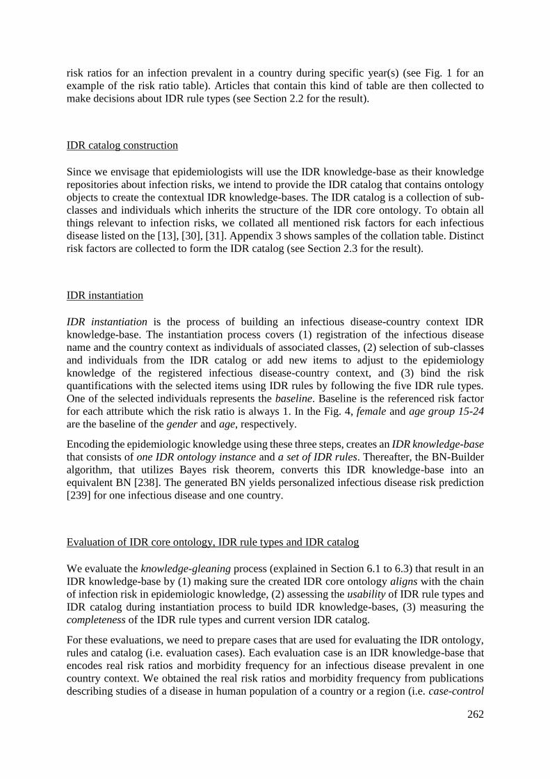
262
risk ratios for an infection prevalent in a country during specific year(s) (see Fig. 1 for an
example of the risk ratio table). Articles that contain this kind of table are then collected to
make decisions about IDR rule types (see Section 2.2 for the result).
IDR catalog construction
Since we envisage that epidemiologists will use the IDR knowledge-base as their knowledge
repositories about infection risks, we intend to provide the IDR catalog that contains ontology
objects to create the contextual IDR knowledge-bases. The IDR catalog is a collection of sub-
classes and individuals which inherits the structure of the IDR core ontology. To obtain all
things relevant to infection risks, we collated all mentioned risk factors for each infectious
disease listed on the [13], [30], [31]. Appendix 3 shows samples of the collation table. Distinct
risk factors are collected to form the IDR catalog (see Section 2.3 for the result).
IDR instantiation
IDR instantiation is the process of building an infectious disease-country context IDR
knowledge-base. The instantiation process covers (1) registration of the infectious disease
name and the country context as individuals of associated classes, (2) selection of sub-classes
and individuals from the IDR catalog or add new items to adjust to the epidemiology
knowledge of the registered infectious disease-country context, and (3) bind the risk
quantifications with the selected items using IDR rules by following the five IDR rule types.
One of the selected individuals represents the baseline. Baseline is the referenced risk factor
for each attribute which the risk ratio is always 1. In the Fig. 4, female and age group 15-24
are the baseline of the gender and age, respectively.
Encoding the epidemiologic knowledge using these three steps, creates an IDR knowledge-base
that consists of one IDR ontology instance and a set of IDR rules. Thereafter, the BN-Builder
algorithm, that utilizes Bayes risk theorem, converts this IDR knowledge-base into an
equivalent BN [238]. The generated BN yields personalized infectious disease risk prediction
[239] for one infectious disease and one country.
Evaluation of IDR core ontology, IDR rule types and IDR catalog
We evaluate the knowledge-gleaning process (explained in Section 6.1 to 6.3) that result in an
IDR knowledge-base by (1) making sure the created IDR core ontology aligns with the chain
of infection risk in epidemiologic knowledge, (2) assessing the usability of IDR rule types and
IDR catalog during instantiation process to build IDR knowledge-bases, (3) measuring the
completeness of the IDR rule types and current version IDR catalog.
For these evaluations, we need to prepare cases that are used for evaluating the IDR ontology,
rules and catalog (i.e. evaluation cases). Each evaluation case is an IDR knowledge-base that
encodes real risk ratios and morbidity frequency for an infectious disease prevalent in one
country context. We obtained the real risk ratios and morbidity frequency from publications
describing studies of a disease in human population of a country or a region (i.e. case-control

263
study). To optimize the use of IDR rule types and catalog to create an IDR knowledge-base,
the infectious diseases chosen for the evaluation cases (1) cover as much as possible infection
roles of all existing human infectious diseases, (2) have personal and environmental risk
factors, (3) and are prevalent in several countries so the classifications of their risk factors are
less subjective. The evaluation cases and the results of IDR knowledge-bases are presented in
Section 3.
We measure the degree of alignment by comparing the encoded knowledge in the IDR ontology
instance in the IDR knowledge-base with epidemiology theory. We are inspired by the OntoQA
metrics [228] to calculate the number of sub-classes for each predictor class and divide that by
the total classes (i.e. class distribution). To conclude whether the encoded knowledge aligns or
not, we compare the class distributions with the declarative epidemiologic knowledge through
discussions (see Section 4.1).
We assess the degree of usability of the IDR rule types and IDR catalog. The degree of usability
of the IDR rule types is investigated by counting how many rule types are used to bind risk
factors with their risk quantifications for all evaluation cases. Whereas, the IDR catalog
usability is assessed by counting how many ontology objects (individuals and sub-classes) of
the IDR catalog are used to encode risk factors for all evaluation cases. If more than half rule
types or ontology objects are used to encode the risk factors, then the IDR rule types and the
IDR catalog are considered as useful tools.
We determine the degree of completeness for both IDR rule types and IDR catalog. Sometimes,
during IDR instantiation process, the risk factors are too specific and not found in the current
version of the IDR catalog, hence they should be added as new ontology objects. To conclude
the degree of completeness, we count how many of the required rule types and ontology objects
are found in the IDR rule types and the IDR catalog. Then, we divide it with the total of the
required ontology objects, for all evaluation cases.
Reference List
[1] World Health Organization, “Disease burden and mortality estimates,” World Health Organization, 2018.
[2] World Health Organization, “Disease incidence, prevalence and disability.”
[3] I. Albert, E. Grenier, J. Denis, and J. Rousseau, “Quantitative Risk Assessment from Farm to Fork and Beyond : A
Global Bayesian Approach Concerning Food-Borne Diseases,” Risk Anal., vol. 28, no. 2, pp. 557–571, 2008.
[4] T.-Y. Lee, C.-B. Wang, T.-T. Chen, K. N. Kuo, M.-S. Wu, J.-T. Lin, and C.-Y. Wu, “A Tool to Predict Risk for
Gastric Cancer in Patients with Peptic Ulcer Disease, Based on a Nationwide Cohort.,” Clin. Gastroenterol. Hepatol.,
vol. 13, pp. 287–293, 2015.
[5] H. Cao, L. Zhang, L. Li, and S. Lo, “Risk Factors for Acute Endophthalmitis following Cataract Surgery : A
Systematic Review and Meta- Analysis,” PLoS One, vol. 8, no. 8, pp. 1–18, 2013.
[6] A. Jurcev-Savicevic, R. Mulic, B. Ban, K. Kozul, L. Bacun-Ivcek, J. Valic, G. Popijac-Cesar, S. Marinovic-Dunatov,
M. Gotovac, and A. Simunovic, “Risk factors for pulmonary tuberculosis in Croatia: a matched case-control study,”
BMC Public Health, vol. 13, p. 991, 2013.
[7] M. Dhimal, I. Gautam, H. D. Joshi, R. B. O’Hara, B. Ahrens, and U. Kuch, “Risk Factors for the Presence of
Chikungunya and Dengue Vectors (Aedes aegypti and Aedes albopictus), Their Altitudinal Distribution and Climatic
Determinants of Their Abundance in Central Nepal,” PLoS Negl. Trop. Dis., vol. 9, no. 3, pp. 1–20, 2015.
[8] A. Olea, I. Matute, C. González, I. Delgado, L. Poffald, E. Pedroni, T. Alfaro, M. Hirmas, M. Nájera, A. Gormaz, D.
López, S. Loayza, C. Ferreccio, D. Gallegos, R. Fuentes, P. Vial, and X. Aguilera, “Case − Control Study of Risk
Factors for Meningococcal Disease in Chile,” Emerg. Infect. Dis., vol. 23, no. 7, pp. 1070–1078, 2017.
[9] D. Raja, “Artificial Intelligence in Medical Epidemiology - AIME.” .
[10] M. Woolhouse, “How to make predictions about future infectious disease risks,” Philos. Trans. R. Soc. B Biol. Sci.,
vol. 366, no. 1573, pp. 2045–2054, 2011.
[11] P. R. O. Payne, “Chapter 1: Biomedical Knowledge Integration,” PLoS Comput. Biol., vol. 8, no. 12, 2012.
[12] CDC, “Principles of Epidemiology | Lesson 1 - Section 1.” .
[13] H. F. L. Wertheim, P. Horby, and J. P. Woodall, Atlas of Human Infectious Diseases. Wiley-Blackwell, 2012.
[14] M. A. Al-Mozaini and M. K. Mansour, “Personalized medicine Is it time for infectious diseases?,” www.smj.org.sa
264
Saudi Med J, vol. 37, no. 12. 2016.
[15] S. Y. Yang and C. L. Hsu, “A location-based services and Google maps-based information master system for tour
guiding,” Comput. Electr. Eng., vol. 000, pp. 1–19, 2015.
[16] R. Chinnachodteeranun, N. D. Hung, K. Honda, A. V. M. Ines, and E. Han, “Designing implementing weather
generators as web services,” Futur. Internet, vol. 8, no. 4, 2016.
[17] R. Lowe, C. Barcellos, C. A. S. Coelho, T. C. Bailey, G. E. Coelho, R. Graham, T. Jupp, W. M. Ramalho, M. S.
Carvalho, D. B. Stephenson, and X. Rodó, “Dengue outlook for the World Cup in Brazil: an early warning model
framework driven by real-time seasonal climate forecasts,” Lancet Infect. Dis., vol. 14, no. 7, pp. 619–626, Jul. 2014.
[18] M. Chilvers and J. Willbur, “Sporecaster: New white mold risk prediction smartphone app now live | MSU
Extension,” 2018. .
[19] United Nations, “WHO morbidity report in UN Data.” .
[20] L. K. Alexander, B. Lopes, K. Ricchetti-Masterson, and K. B. Yeatts, “Cross-sectional Studies,” 2015.
[21] P. Gustafson, V. F. Gomes, C. S. Vieira, P. Rabna, R. Seng, P. Johansson, A. Sandström, R. Norberg, I. Lisse, B.
Samb, P. Aaby, and A. Nauclér, “Tuberculosis in Bissau : incidence and risk factors in an urban community in sub-
Saharan Africa,” Int. J. Epidemiol., vol. 33, no. 1, pp. 163–172, 2018.
[22] L. G. Cowell and B. Smith, “Infectious disease ontology,” Infect. Dis. Informatics, pp. 373–395, 2010.
[23] Y. Lin, Z. Xiang, and Y. He, “Brucellosis Ontology ( IDOBRU ) as an extension of the Infectious Disease Ontology,”
J. Biomed. Semantics, vol. 9, no. 2, pp. 1–18, 2011.
[24] G. Camara, S. Despres, R. Djedidi, and M. Lo, “Design of Schistosomiasis Ontology ( IDOSCHISTO ) Extending
the Infectious Disease,” in Medical Informatics, 2013, no. 1, pp. 466–470.
[25] Y. Zhao, F. Parvinzamir, H. Wei, E. Liu, Z. Deng, F. Dong, A. Third, V. Marozas, E. Kaldoudi, and G. Clapworthy,
“The CARRE Project,” 2013.
[26] Ö. Kafalı, M. Sindlar, T. Van Der Weide, and K. Stathis, “ORC: an Ontology Reasoning Component for Diabetes.”
[27] A. Khan, A. Sadia, S. Ahmed, H. Tabassum, and M. S. Khan, “HEPO: The hepatitis ontology for abductive medical
diagnostic systems,” in 2017 International Conference on Communication, Computing and Digital Systems (C-
CODE), 2017, pp. 271–275.
[28] D. Vrajitoru, “Knowledge Representation.” .
[29] S. Colton, “Knowledge Representation.” .
[30] CDC, “Infectious Diseases | 2018 National Notifiable Conditions.” .
[31] WHO, “WHO | Infectious diseases,” WHO, 2016. .
[32] M. Szumilas, “Explaining odds ratios.,” J. Can. Acad. Child Adolesc. Psychiatry, vol. 19, no. 3, pp. 227–9, Aug.
2010.
[33] P. C. G. Da Costa, K. B. Laskey, and K. J. Laskey, “PR-OWL: A bayesian ontology language for the Semantic Web,”
Lect. Notes Comput. Sci. (including Subser. Lect. Notes Artif. Intell. Lect. Notes Bioinformatics), vol. 5327 LNAI, pp.
88–107, 2008.
[34] Z. Ding, Y. Peng, and R. Pan, “BayesOWL : Uncertainty Modeling in Semantic Web Ontologies,” StudFuzz, vol.
204, pp. 3–29, 2006.
[35] R. Pan, Z. Ding, Y. Yu, and Y. Peng, “A Bayesian Network Approach to Ontology Mapping,” in International
Semantic Web Conference, 2005, pp. 1–16.
[36] D. Settas, A. Cerone, and S. Fenz, “Expert Systems with Applications Enhancing ontology-based antipattern detection
using Bayesian networks,” Expert Syst. Appl., vol. 39, no. 10, pp. 9041–9053, 2012.
[37] P. J. Giabbanelli, T. Torsney-Weir, and V. K. Mago, “A fuzzy cognitive map of the psychosocial determinants of
obesity,” Appl. Soft Comput. J., vol. 12, no. 12, pp. 3711–3724, 2012.
[38] N. Douali, H. Csaba, J. De Roo, E. I. Papageorgiou, and M. C. Jaulent, “Diagnosis Support System based on clinical
guidelines: Comparison between case-based fuzzy cognitive maps and bayesian networks,” Comput. Methods
Programs Biomed., vol. 113, no. 1, pp. 133–143, 2014.
[39] P. Dawson, R. Gailis, and A. Meehan, “Detecting disease outbreaks using a combined Bayesian network and particle
filter approach,” J. Theor. Biol., vol. 370, pp. 171–183, 2015.
[40] Q. Jiang, J. T. Zhou, Z. B. Jiang, and B. Xu, “Identifying risk factors of avian infectious diseases at household level
in Poyang Lake region, China,” Prev. Vet. Med., vol. 116, no. 1–2, pp. 151–160, 2014.
[41] M. A. A. Figueiredo, L. C. Rodrigues, M. L. Barreto, J. W. O. Lima, M. C. N. Costa, V. Morato, R. Blanton, P. F. C.
Vasconcelos, M. R. T. Nunes, and M. G. Teixeira, “Allergies and diabetes as risk factors for dengue hemorrhagic
fever: Results of a case control study,” PLoS Negl. Trop. Dis., vol. 4, no. 6, 2010.
[42] C. M. Lewis, S. C. L. Whitwell, A. Forbes, J. Sanderson, and C. G. Mathew, “Estimating risks of common complex
diseases across genetic and environmental factors: the example of Crohn disease,” pp. 689–694, 2007.
[43] A. N. Freedman, D. Seminara, M. H. Gail, P. Hartge, G. A. Colditz, R. Ballard-barbash, and R. M. Pfeiffer, “Cancer
Risk Prediction Models : A Workshop on Development, Evaluation, and Application,” J. Natl. Cancer Inst., vol. 97,
no. 10, 2005.
[44] Merriam-Webster, “Predicting | Definition of Predicting by Merriam-Webster,” 1828. .
[45] I. Ahmed, T. P. Debray, K. G. Moons, and R. D. Riley, “Developing and validating risk prediction models in an
individual participant data meta-analysis,” BMC Med. Res. Methodol., vol. 14, no. 1, p. 3, Dec. 2014.
[46] M. Menk, L. Giebelhäuser, G. Vorderwülbecke, M. Gassner, J. A. Graw, B. Weiss, M. Zimmermann, K.-D.
Wernecke, and S. Weber-Carstens, “Nucleated red blood cells as predictors of mortality in patients with acute
respiratory distress syndrome (ARDS): an observational study,” Ann. Intensive Care, vol. 8, no. 1, p. 42, Dec. 2018.
[47] C. Toma, A. D. Shaw, R. J. N. Allcock, A. Heath, K. D. Pierce, P. B. Mitchell, P. R. Schofield, and J. M. Fullerton,
“An examination of multiple classes of rare variants in extended families with bipolar disorder,” Transl. Psychiatry,
265
vol. 8, no. 1, p. 65, Dec. 2018.
[48] C. Wright and T. Dent, Quality standards in risk prediction: A summary of an expert meeting. Cambridge: PHG
Foundation, 2011.
[49] C. F. Yung, S. P. Chan, T. L. Thein, S. C. Chai, and Y. S. Leo, “Epidemiological risk factors for adult dengue in
Singapore : an 8-year nested test negative case control study,” BMC Infect. Dis., pp. 1–9, 2016.
[50] M. J. Pencina, R. B. D. A. Sr, M. G. Larson, J. M. Massaro, and R. S. Vasan, “Predicting the Thirty-Year Risk of
Cardiovascular Disease: The Framingham Heart Study,” Circulation, vol. 119, no. 24, pp. 3078–3084, 2009.
[51] T.-C. Li, C.-I. Li, C.-S. Liu, W.-Y. Lin, C.-H. Lin, S.-Y. Yang, J.-H. Chiang, and C.-C. Lin, “Development and
validation of prediction models for the risks of diabetes-related hospitalization and in-hospital mortality in patients
with type 2 diabetes,” Metabolism, vol. 85, pp. 38–47, Aug. 2018.
[52] R. Landy, L. C. Cheung, M. Schiffman, J. C. Gage, N. Hyun, N. Wentzensen, W. K. Kinney, P. E. Castle, B.
Fetterman, N. E. Poitras, T. Lorey, P. D. Sasieni, and H. A. Katki, “Challenges in risk estimation using routinely
collected clinical data: The example of estimating cervical cancer risks from electronic health-records,” Prev. Med.
(Baltim)., vol. 111, pp. 429–435, Jun. 2018.
[53] K. Y. Clement, W. J. Wouter Botzen, R. Brouwer, and J. C. J. H. Aerts, “A global review of the impact of basis risk
on the functioning of and demand for index insurance,” Int. J. Disaster Risk Reduct., vol. 28, pp. 845–853, Jun. 2018.
[54] C. Policiano, A. Fonseca, J. M. Mendes, N. Clode, and L. M. Graça, “Small-for-gestational-age babies of low-risk
term pregnancies: does antenatal detection matter?,” J. Matern. Neonatal Med., vol. 31, no. 11, pp. 1426–1430, Jun.
2018.
[55] C.-H. Chan, H.-K. Wong, and P. S.-F. Yip, “Exploring the use of telephone helpline pertaining to older adult suicide
prevention: A Hong Kong experience,” J. Affect. Disord., vol. 236, pp. 75–79, Aug. 2018.
[56] Merriam-Webster, “Personalize | Definition of Personalize by Merriam-Webster.” .
[57] National Cancer Institute at the National Institutes of Health, “Definition of personalized medicine - NCI Dictionary
of Cancer Terms - National Cancer Institute.” .
[58] W. K. Redekop, “The Faces of Personalized Medicine: A Framework for Understanding Its Meaning and Scope,”
Value Heal., vol. 16, pp. 1–6, 2013.
[59] D. Becker, W. van Breda, B. Funk, M. Hoogendoorn, J. Ruwaard, and H. Riper, “Predictive modeling in e-mental
health: A common language framework,” Internet Interv., vol. 12, pp. 57–67, Jun. 2018.
[60] G. Colella, F. Fazioli, M. Gallo, A. De Chiara, G. Apice, C. Ruosi, A. Cimmino, and F. de Nigris, “Sarcoma Spheroids
and Organoids—Promising Tools in the Era of Personalized Medicine,” Int. J. Mol. Sci., vol. 19, no. 2, p. 615, Feb.
2018.
[61] P. S. Pratiwi and D. Tjondronegoro, “Towards personalisation of physical activity e-coach using stage-matched
behaviour change and motivational interviewing strategies,” in 2017 IEEE Life Sciences Conference (LSC), 2017, pp.
5–8.
[62] K. Selby, G. Bartlett-Esquilant, and J. Cornuz, “Personalized cancer screening: helping primary care rise to the
challenge.,” Public Health Rev., vol. 39, p. 4, 2018.
[63] C. Butts, S. Kamel-Reid, G. Batist, S. Chia, C. Blanke, M. Moore, M. B. Sawyer, C. Desjardins, A. Dubois, J. Pun,
K. Bonter, and F. D. Ashbury, “Benefits, issues, and recommendations for personalized medicine in oncology in
Canada.,” Curr. Oncol., vol. 20, no. 5, pp. e475-83, Oct. 2013.
[64] National Cancer Institute (NCI), “Value of Personalized Medicine.” PhRMA, 2015.
[65] C. L. Ratcliff, K. A. Kaphingst, and J. D. Jensen, “When Personal Feels Invasive: Foreseeing Challenges in Precision
Medicine Communication,” J. Health Commun., vol. 23, no. 2, pp. 144–152, Feb. 2018.
[66] S. O. Jensen and S. J. van Hal, “Personalized Medicine and Infectious Disease Management,” Trends Microbiol., vol.
25, no. 11, pp. 875–876, Nov. 2017.
[67] CDC, “Principles of Epidemiology | Lesson 1 - Section 10,” 2012. .
[68] B. Pam and F. Gorder, “Computational Epidemiology,” Comput. Sci. Eng., 2010.
[69] CDC, “Public Health 101 Series Introduction to Public Health Informatics Instructor name Course Topics
Introduction to Public Health Informatics,” 2009.
[70] American Medical Informatics Association (AMIA), “Public Health Informatics.” .
[71] Public Health Informatics Institute (PHII), “Defining Public Health Informatics.” .
[72] D. Zeng, H. Chen, C. Lynch, and M. Eidson, “Chapter 13 INFECTIOUS DISEASE INFORMATICS AND
OUTBREAK DETECTION,” in Medical Informatics, 2005, pp. 359–395.
[73] M. Salathe, L. Bengtsson, T. J. Bodnar, D. D. Brewer, J. S. Brownstein, C. Buckee, E. M. Campbell, C. Cattuto, S.
Khandelwal, P. L. Mabry, and A. Vespignani, “Digital epidemiology,” PLoS Comput. Biol., vol. 8, no. 7, pp. 1–5,
2012.
[74] Z. Huang, A. Das, Y. Qiu, and A. J. Tatem, “Web-based GIS: the vector-borne disease airline importation risk (VBD-
AIR) tool.,” Int. J. Health Geogr., vol. 11, p. 33, 2012.
[75] R. Nelson, “HealthMap: the future of infectious diseases surveillance?,” Lancet Infect. Dis., vol. 8, no. 10, p. 596,
2008.
[76] C. C. Freifeld, K. D. Mandl, B. Y. Reis, and J. S. Brownstein, “HealthMap : Global Infectious Disease Monitoring
through,” J. Am. Med. Informatics Assoc., vol. 15, no. 2, pp. 150–157, 2014.
[77] S. Sindi, E. Calov, J. Fokkens, T. Ngandu, H. Soininen, J. Tuomilehto, and M. Kivipelto, “The CAIDE Dementia
Risk Score App: The development of an evidence-based mobile application to predict the risk of dementia,”
Alzheimer’s Dement. Diagnosis, Assess. Dis. Monit., vol. 1, no. 3, pp. 328–333, 2015.
[78] E. B. Postnikov and D. V Tatarenkov, “Prediction of flu epidemic activity with dynamical model based on weather
forecast,” Ecol. Complex., vol. 15, pp. 109–113, 2013.
266
[79] G. M. Hwang, P. J. Mahoney, J. H. James, G. C. Lin, A. D. Berro, M. A. Keybl, D. M. Goedecke, J. J. Mathieu, and
T. Wilson, “A model-based tool to predict the propagation of infectious disease via airports,” Travel Med. Infect. Dis.,
vol. 10, no. 1, pp. 32–42, 2012.
[80] P. Diaz, P. Constantine, K. Kalmbach, E. Jones, and S. Pankavich, “A modified SEIR model for the spread of Ebola
in Western Africa and metrics for resource allocation,” Appl. Math. Comput., vol. 324, pp. 141–155, May 2018.
[81] S. Side, Y. M. Rangkuti, D. G. Pane, and M. S. Sinaga, “Stability Analysis Susceptible, Exposed, Infected, Recovered
(SEIR) Model for Spread Model for Spread of Dengue Fever in Medan,” J. Phys. Conf. Ser., vol. 954, p. 012018, Jan.
2018.
[82] T. Iskandar, N. A. Chaniago, S. Munzir, V. Halfiani, and M. Ramli, “Mathematical model of tuberculosis epidemic
with recovery time delay,” in AIP, 2017, p. 020021.
[83] X. Wang, S. Panchanathan, and G. Chowell, “A Data-Driven Mathematical Model of CA-MRSA Transmission
among Age Groups: Evaluating the Effect of Control Interventions,” PLoS Comput. Biol., vol. 9, no. 11, 2013.
[84] B. S. Glicksberg, L. Li, M. A. Badgeley, K. Shameer, R. Kosoy, N. D. Beckmann, N. Pho, J. Hakenberg, M. Ma, K.
L. Ayers, G. E. Hoffman, S. D. Li, E. E. Schadt, C. J. Patel, R. Chen, and J. T. Dudley, “Comparative analyses of
population-scale phenomic data in electronic medical records reveal race-specific disease networks,” Bioinformatics,
vol. 32, no. 12, pp. i101–i110, 2016.
[85] R. Villamarín, G. Cooper, M. Wagner, F. C. Tsui, and J. U. Espino, “A method for estimating from thermometer sales
the incidence of diseases that are symptomatically similar to influenza,” J. Biomed. Inform., vol. 46, no. 3, pp. 444–
457, 2013.
[86] R. G. C. Scholte, L. Gosoniu, J. B. Malone, F. Chammartin, J. Utzinger, and P. Vounatsou, “Predictive risk mapping
of schistosomiasis in brazil using bayesian geostatistical models,” Acta Trop., vol. 132, no. 1, pp. 57–63, 2014.
[87] M. J. Vilar, S. Virtanen, R. Laukkanen-Ninios, and H. Korkeala, “Bayesian modelling to identify the risk factors for
Yersinia enterocolitica contamination of pork carcasses and pluck sets in slaughterhouses,” Int. J. Food Microbiol.,
vol. 197, pp. 53–57, 2015.
[88] X. L. Zhang, X. J. Shao, J. Wang, and W. L. Guo, “Temporal characteristics of respiratory syncytial virus infection
in children and its correlation with climatic factors at a public pediatric hospital in Suzhou,” J. Clin. Virol., vol. 58,
no. 4, pp. 666–670, 2013.
[89] L. Getoor, N. Friedman, D. Koller, A. Pfeffer, and B. Taskar, “Probabilistic Relational Models,” in Introduction to
Statistical Relational Learning, 2007, pp. 129–174.
[90] J. Lenfestey, T. Temple, and E. Howe, “Intro to Probabilistic Relational Models.” .
[91] B. Borghetti, “Bayesian Knowledge Bases.” .
[92] E. Santos, E. S. Santos, and S. Eyal, “Implicitly preserving semantics during incremental knowledge base acquisition
under uncertainty,” Int. J. Approx. Reason., vol. 33, pp. 71–94, 2003.
[93] L. Ngo and P. Haddawy, “Answering queries from context-sensitive probabilistic knowledge bases,” Theor. Comput.
Sci., vol. 171, no. 1–2, pp. 147–177, 1997.
[94] P. Haddawy, “Generating Bayesian Networks from Probablity Logic Knowledge Bases,” pp. 262–269, 1994.
[95] L. L. Santos, R. N. Carvalho, M. Ladeira, and W. Li, “A New Algorithm for Generating Situation-Specific Bayesian
Networks Using Bayes-Ball Method,” Uncertain. Reason. Semant. Web, 2016.
[96] Z. Ding, Y. Peng, and R. Pan, “BayesOWL : Uncertainty Modelling in Semantic Web Ontologies,” Soft Comput.
Ontol. Semant. Web, vol. 29, pp. 3–29, 2006.
[97] N. C. Stenseth, N. I. Samia, H. Viljugrein, K. L. Kausrud, M. Begon, S. Davis, H. Leirs, V. M. Dubyanskiy, J. Esper,
V. S. Ageyev, N. L. Klassovskiy, S. B. Pole, and K.-S. Chan, “Plague dynamics are driven by climate variation,”
Proc. Natl. Acad. Sci., vol. 103, no. 35, pp. 13110–13115, 2006.
[98] H. Khiabanian, A. B. Holmes, B. J. Kelly, M. Gururaj, G. Hripcsak, and R. Rabadan, “Signs of the 2009 influenza
pandemic in the New York-Presbyterian hospital electronic health records,” PLoS One, vol. 5, no. 9, pp. 1–8, 2010.
[99] S. M. Upadhyayula, S. Rao Mutheneni, H. K. Nayanoori, A. Natarajan, and P. Goswami, “Impact of weather variables
on mosquitoes infected with Japanese encephalitis virus in Kurnool district, Andhra Pradesh.,” Asian Pac. J. Trop.
Med., vol. 5, no. 5, pp. 337–41, 2012.
[100] D. Onozuka and M. Hashizume, “Effect of weather variability on the incidence of mumps in children: a time-series
analysis.,” Epidemiol. Infect., vol. 139, no. 11, pp. 1692–700, 2011.
[101] C. Imai, B. Armstrong, Z. Chalabi, P. Mangtani, and M. Hashizume, “Time series regression model for infectious
disease and weather.,” Environ. Res., vol. 142, pp. 319–327, 2015.
[102] M. Reyes, M. Eriksson, R. Bennet, K.-O. Hedlund, and A. Ehrnst, “Regular pattern of respiratory syncytial virus and
rotavirus infections and relation to weather in Stockholm, 1984-1993,” Clin. Microbiol. Infect., vol. 3, no. 6, pp. 640–
646, Dec. 1997.
[103] T. S. Chang, R. E. Gangnon, C. David Page, W. R. Buckingham, A. Tandias, K. J. Cowan, C. D. Tomasallo, B. G.
Arndt, L. P. Hanrahan, and T. W. Guilbert, “Sparse modeling of spatial environmental variables associated with
asthma,” J. Biomed. Inform., vol. 53, pp. 320–329, 2015.
[104] Y. Nakamura, H. Kawanohara, and M. Kamei, “Proposition of real-time precise prediction model of infectious disease
patients from Prescription Surveillance using the National Database of Electronic Medical Claims,” J. Infect.
Chemother., vol. 21, no. 11, pp. 776–782, 2015.
[105] R. K. Meentemeyer, M. A. Dorning, J. B. Vogler, D. Schmidt, and M. Garbelotto, “Citizen science helps predict risk
of emerging infectious disease,” 2015.
[106] R. D. Melamed, H. Khiabanian, and R. Rabadan, “Data-driven discovery of seasonally linked diseases from an
Electronic Health Records system.,” BMC Bioinformatics, vol. 15 Suppl 6, no. Suppl 6, p. S3, 2014.
[107] A. B. Holmes, A. Hawson, F. Liu, C. Friedman, H. Khiabanian, and R. Rabadan, “Discovering disease associations
267
by integrating electronic clinical data and medical literature,” PLoS One, vol. 6, no. 6, 2011.
[108] T. W. Guilbert, B. Arndt, J. Temte, A. Adams, W. Buckingham, A. Tandias, C. Tomasallo, H. a Anderson, and L. P.
Hanrahan, “The theory and application of UW ehealth-PHINEX, a clinical electronic health record-public health
information exchange.,” Wis. Med. J., vol. 111, no. 3, pp. 124–133, 2012.
[109] H. Nesse, “SEIR Model.” .
[110] T. Jombart, A. Cori, X. Didelot, S. Cauchemez, C. Fraser, and N. Ferguson, “Bayesian Reconstruction of Disease
Outbreaks by Combining Epidemiologic and Genomic Data,” PLoS Comput. Biol., vol. 10, no. 1, 2014.
[111] A. Huppert, O. Barnea, G. Katriel, R. Yaari, U. Roll, and L. Stone, “Modeling and statistical analysis of the spatio-
temporal patterns of seasonal influenza in Israel.,” PLoS One, vol. 7, no. 10, p. e45107, 2012.
[112] S. Side, Irwan, U. Mulbar, and W. Sanusi, “SEIR model simulation for Hepatitis B,” 2017, p. 020198.
[113] P. Kostkova, M. Szomszor, and C. St. Luis, “#Swineflu: The Use of Twitter as an EarlyWarning and Risk
Communication,” ACM Trans. Manag. Inf. Syst., vol. 5, no. 2, pp. 1–25, 2014.
[114] E. J. Tomayko, B. A. Weinert, L. Godfrey, A. K. Adams, and L. P. Hanrahan, “Using Electronic Health Records to
Examine Disease Risk in Small Populations: Obesity Among American Indian Children, Wisconsin, 2007-2012.,”
Prev. Chronic Dis., vol. 13, no. E29, pp. 1–9, 2016.
[115] L. Faisandier, V. Bonneterre, R. De Gaudemaris, and D. J. Bicout, “Occupational exposome: A network-based
approach for characterizing Occupational Health Problems,” J. Biomed. Inform., vol. 44, no. 4, pp. 545–552, 2011.
[116] Healthians, “India’s largest Blood Test & Health Test @ Home Service | Healthians.” .
[117] P. Tiwari, A. Jaiswal, N. Vishwakarma, and P. Patel, “Smart Health Care (an Android app to predict disease on the
basis of symptoms),” Int. Res. J. Eng. Technol., pp. 2395–56, 2017.
[118] MdCalc, “Framingham Coronary Heart Disease Risk Score - MDCalc.” .
[119] “Infectious Disease Advisor App.” .
[120] J. Huan, “Smartphone app to detect risk for Ebola exposure.” .
[121] M. A. Ali, Z. Ahsan, M. Amin, S. Latif, A. Ayyaz, and M. N. Ayyaz, “ID-Viewer: a visual analytics architecture for
infectious diseases surveillance and response management in Pakistan,” Public Health, vol. 134, pp. 72–85, 2016.
[122] H. Rahman, “Monitoring , Surveillance and Forecasting of Infectious Animal Diseases in India,” vol. 16, pp. 177–
181, 2015.
[123] I. M. Blake, P. Chenoweth, H. Okayasu, C. A. Donnelly, R. B. Aylward, and N. C. Grassly, “Faster detection of
poliomyelitis outbreaks to support polio eradication,” Emerg. Infect. Dis., vol. 22, no. 3, pp. 449–456, 2016.
[124] W. K. Wong, a. Moore, G. Cooper, and M. Wagner, “Bayesian network anomaly pattern detection for disease
outbreaks,” Mach. Learn. Work. Then Conf., vol. 20, no. 2, p. 808, 2003.
[125] W.-K. Wong, A. Moore, G. Cooper, and M. Wagner, “WSARE: What’s Strange About Recent Events?,” J. Urban
Health, vol. 80, no. 2 Suppl 1, pp. i66-75, 2003.
[126] M. L. Barreto, M. Glo, and E. H. Carmo, “Infectious diseases epidemiology,” J. Epidemiol. Community Heal., vol.
60, pp. 192–195, 2006.
[127] X. Wu, Y. Lu, S. Zhou, L. Chen, and B. Xu, “Impact of climate change on human infectious diseases: Empirical
evidence and human adaptation,” Environ. Int., vol. 86, pp. 14–23, 2016.
[128] A. Kilianski, P. Carcel, S. Yao, P. Roth, J. Schulte, G. B. Donarum, E. T. Fochler, J. M. Hill, A. T. Liem, M. R.
Wiley, J. T. Ladner, B. P. Pfeffer, O. Elliot, A. Petrosov, D. D. Jima, T. G. Vallard, M. C. Melendrez, E. Skowronski,
P. L. Quan, W. I. Lipkin, H. S. Gibbons, D. L. Hirschberg, G. F. Palacios, and C. N. Rosenzweig, “Pathosphere.org:
Pathogen detection and characterization through a web-based, open source informatics platform,” BMC
Bioinformatics, vol. 16, no. 1, pp. 1–13, 2015.
[129] S. Altizer, A. Dobson, P. Hosseini, P. Hudson, M. Pascual, and P. Rohani, “Seasonality and the dynamics of infectious
diseases,” Ecol. Lett., vol. 9, pp. 467–484, 2006.
[130] K. Yeatts, P. Sly, S. Shore, S. Weiss, F. Martinez, A. Geller, P. Bromberg, P. Enright, H. Koren, D. Weissman, and
M. Selgrade, “A brief targeted review of susceptibility factors, environmental exposures, asthma incidence, and
recommendations for future asthma incidence research.,” Environ. Health Perspect., vol. 114, no. 4, pp. 634–40, Apr.
2006.
[131] S. D. Gale, L. D. Erickson, A. Berrett, B. L. Brown, and D. W. Hedges, “Infectious disease burden and cognitive
function in young to middle-aged adults,” Brain. Behav. Immun., 2015.
[132] P. F. D. Scheelbeek, A. J. G. Wirix, M. Hatta, R. Usman, and M. I. Bakker, “Risk factors for poor tuberculosis
treatment outcomes in Makassar, Indonesia,” Southeast Asian J. Trop. Med. Public Health, vol. 45, no. 4, pp. 853–
858, 2014.
[133] S. J. Chapman and A. V. S. Hill, “Human genetic susceptibility to infectious disease,” vol. 13, no. March, 2012.
[134] G. G. R. Murray, M. E. J. Woolhouse, M. Tapio, M. N. Mbole-Kariuki, T. S. Sonstegard, S. M. Thumbi, A. E.
Jennings, I. C. Van Wyk, M. Chase-Topping, H. Kiara, P. Toye, K. Coetzer, B. M. Dec Bronsvoort, and O. Hanotte,
“Genetic susceptibility to infectious disease in East African Shorthorn Zebu: A genome-wide analysis of the effect of
heterozygosity and exotic introgression,” BMC Evol. Biol., vol. 13, no. 1, 2013.
[135] H. Yi, B. R. Devkota, J. Yu, K. Oh, J. Kim, and H.-J. Kim, “Effects of global warming on mosquitoes &
mosquito-borne diseases and the new strategies for mosquito control,” Entomol. Res., vol. 44, no. 6, pp. 215–235,
2014.
[136] Q. Wang, Y. Liu, Y. Ma, L. Han, M. Dou, Y. Zou, L. Sun, H. Tian, T. Li, G. Jiang, B. Du, T. Kou, and J. Song,
“Severe hypovitaminosis D in active tuberculosis patients and its predictors,” Clin. Nutr., 2017.
[137] A. Fares, “Seasonality of tuberculosis.,” J. Glob. Infect. Dis., vol. 3, no. 1, pp. 46–55, Jan. 2011.
[138] “WHO | Tuberculosis and HIV,” WHO, 2018.
[139] D. M. Pigott, R. E. Howes, A. Wiebe, K. E. Battle, N. Golding, P. W. Gething, S. F. Dowell, T. H. Farag, A. J. Garcia,
268
A. M. Kimball, L. K. Krause, C. H. Smith, S. J. Brooker, H. H. Kyu, T. Vos, C. J. L. Murray, C. L. Moyes, and S. I.
Hay, “Prioritising infectious disease mapping,” PLoS Negl. Trop. Dis., vol. 9, no. 6, pp. 1–21, 2015.
[140] J. Casqueiro, J. Casqueiro, and C. Alves, “Infections in patients with diabetes mellitus : A review of pathogenesis,”
Indian J. Endocrinol. Metab., vol. 16, pp. 27–36, 2018.
[141] T. N. A. of Sciences, Critical Aspects of EPA’s IRIS Assessment of Inorganic Arsenic. Washington, D.C.: National
Academies Press, 2014.
[142] R. K. Smith and D. J. Maron, “Epidemiology, risk factors, and prevention,” Semin. Colon Rectal Surg., vol. 27, no.
4, pp. 176–180, 2016.
[143] O. Shirai, T. Tsuda, S. Kitagawa, K. Naitoh, T. Seki, K. Kamimura, and M. Morohashi, “Alcohol ingestion stimulates
mosquito attraction.,” J. Am. Mosq. Control Assoc., vol. 18, no. 2, pp. 91–6, Jun. 2002.
[144] K. Lönnroth, B. G. Williams, S. Stadlin, E. Jaramillo, and C. Dye, “Alcohol use as a risk factor for tuberculosis - A
systematic review,” BMC Public Health, vol. 8, no. May 2014, 2008.
[145] R. Mukherjee, D. Halder, S. Saha, R. Shyamali, R. Ramakrishnan, M. V Murhekar, and Y. J. Hutin, “Five Pond-
centred Outbreaks of Cholera in Villages of West Bengal , India : Evidence for Focused Interventions,” J. Heal.
Popul. Nutr., vol. 29, no. 5, pp. 421–428, 2011.
[146] A. J. Lund, H. M. Keys, S. Leventhal, J. W. Foster, and M. C. Freeman, “Prevalence of cholera risk factors between
migrant Haitians and Dominicans in the Dominican Republic,” Pan Am. J. Public Heal., vol. 37, no. 3, pp. 125–132,
2015.
[147] A. Rosewell, B. Addy, L. Komnapi, F. Makanda, B. Ropa, E. Posanai, S. Dutta, G. Mola, W. Y. N. Man, A. Zwi, and
C. R. Macintyre, “Cholera risk factors , Papua New Guinea , 2010,” BMC Infect. Dis., vol. 12, pp. 287–293, 2012.
[148] A. Prayitno, A. Taurel, J. Nealon, H. I. Satari, R. Karyanti, R. Sekartini, S. Soedjatmiko, H. Gunardi, E. Medise, R.
T. Sasmono, J. M. Simmerman, A. Bouckenooghe, and S. R. Hadinegoro, “Dengue seroprevalence and force of
primary infection in a representative population of urban dwelling Indonesian children,” PLoS Negl. Trop. Dis., vol.
11, no. 6, pp. 1–16, 2017.
[149] M. A. Soghaier, S. F. Mahmood, O. Pasha, S. I. Azam, M. M. Karsani, M. M. Elmangory, B. A. Elmagboul, S. I.
Okoued, S. M. Shareef, H. S. Khogali, and E. Eltigai, “Factors associated with dengue fever IgG sero-prevalence in
South Kordofan State , Sudan , in 2012 : Reporting prevalence ratios,” J. Infect. Public Health, vol. 7, no. 1, pp. 54–
61, 2014.
[150] Centers for Disease Control and Prevention (CDC), “Cryptosporidiosis outbreak at a summer camp--North Carolina,
2009.,” MMWR. Morb. Mortal. Wkly. Rep., vol. 60, no. 27, pp. 918–22, Jul. 2011.
[151] CDC, “Principles of Epidemiology | Lesson 3 - Section 2.” .
[152] M. Lappenschaar, A. Hommersom, P. J. F. Lucas, J. Lagro, and S. Visscher, “Multilevel Bayesian networks for the
analysis of hierarchical health care data,” Artif. Intell. Med., vol. 57, no. 3, pp. 171–183, 2013.
[153] M. Blangiardo, F. Finazzi, and M. Cameletti, “Two-stage Bayesian model to evaluate the effect of air pollution on
chronic respiratory diseases using drug prescriptions,” Spat. Spatiotemporal. Epidemiol., 2016.
[154] C. Lau, P. Weinstein, and D. Slaney, “Imported cases of Ross River virus disease in New Zealand - a travel medicine
perspective.,” Travel Med. Infect. Dis., vol. 10, no. 3, pp. 129–134, 2012.
[155] P. D. Loprinzi and A. Nooe, “Health characteristics and predicted 10-year risk for a first atherosclerotic cardiovascular
disease (ASCVD) event using the Pooled Cohort Risk Equations among US adults who are free of cardiovascular
disease,” Physiol. Behav., vol. 151, pp. 591–595, 2015.
[156] L. M. Artigao-Rodenas, J. A. Carbayo-Herencia, J. A. Divisón-Garrote, V. F. Gil-Guillén, J. Massó-Orozco, M.
Simarro-Rueda, F. Molina-Escribano, C. Sanchis, L. Carrión-Valero, E. López de Coca, D. Caldevilla, J. López-
Abril, C. Carratalá-Munuera, and A. Lopez-Pineda, “Framingham Risk Score for Prediction of Cardiovascular
Diseases: A Population-Based Study from Southern Europe,” PLoS One, vol. 8, no. 9, pp. 1–10, 2013.
[157] S. Kalayanarooj, R. V. Gibbons, D. Vaughn, S. Green, A. Nisalak, R. G. Jarman, M. P. Mammen, Jr., and G. Perng,
“Blood Group AB Is Associated with Increased Risk for Severe Dengue Disease in Secondary Infections,” J. Infect.
Dis., vol. 195, no. 7, pp. 1014–1017, 2007.
[158] A. L. Greer, S. J. Drews, and D. N. Fisman, “Why ‘Winter’ vomiting disease? seasonality, hydrology, and norovirus
epidemiology in Toronto, Canada,” Ecohealth, vol. 6, no. 2, pp. 192–199, 2009.
[159] I. Stephenson and M. Zambon, “The epidemiology of influenza,” Occup. Med. (Chic. Ill)., vol. 52, no. 5, pp. 241–
247, 2002.
[160] S. Subak, “Effects of climate on variability in Lyme disease incidence in the northeastern United States,” Am. J.
Epidemiol., vol. 157, no. 6, pp. 531–538, 2003.
[161] K. Kleinman, R. Lazarus, and R. Platt, “A generalized linear mixed models approach for detecting incident clusters
of disease in small areas, with an application to biological terrorism,” Am. J. Epidemiol., vol. 159, no. 3, pp. 217–
224, 2004.
[162] G. M. Liumbruno and M. Franchini, “Beyond immunohaematology: the role of the ABO blood group in human
diseases,” Blood Transfus, vol. 11, pp. 491–499, 2013.
[163] K. Kengkla, N. Charoensuk, M. Chaichana, S. Puangjan, T. Rattanapornsompong, J. Choorassamee, P. Wilairat, and
S. Saokaew, “Clinical risk scoring system for predicting extended-spectrum β-lactamase-producing Escherichia coli
infection in hospitalized patients.,” J. Hosp. Infect., vol. 93, no. 1, pp. 49–56, 2016.
[164] A. Ascherio and M. A. Schwarzschild, “The epidemiology of Parkinson’s disease: risk factors and prevention,”
Lancet Neurol., vol. 15, no. 12, pp. 1257–1272, 2016.
[165] S. A. J. Schmidt, M. Vestergaard, L. M. Baggesen, L. Pedersen, H. C. Schønheyder, and H. T. Sørensen,
“Prevaccination epidemiology of herpes zoster in Denmark : Quantification of occurrence and risk factors,” Vaccine,
vol. 35, no. 42, pp. 5589–5596, 2017.
269
[166] H. Zhang, T. Yang, M. Wu, and F. Shen, “Intrahepatic cholangiocarcinoma: Epidemiology, risk factors, diagnosis
and surgical management,” Cancer Lett., vol. 379, no. 2, pp. 198–205, 2016.
[167] C. A. Rostad, K. Wehrheim, J. K. Kirklin, D. Naftel, E. Pruitt, T. M. Hoffman, T. L’Ecuyer, K. Berkowitz, W. T.
Mahle, and J. N. Scheel, “Bacterial infections after pediatric heart transplantation: Epidemiology, risk factors and
outcomes,” J. Hear. Lung Transplant., vol. 36, no. 9, pp. 996–1003, 2017.
[168] S. H. Kim, S. M. Choi, B. C. Kim, K. H. Choi, T. S. Nam, J. T. Kim, S. H. Lee, M. S. Park, and S. J. Kim, “Risk
factors for aseptic meningitis in herpes zoster patients,” Ann. Dermatol., vol. 29, no. 3, pp. 283–287, 2017.
[169] Bruce MG; Rosenstein NE; Capparella JM; Shutt KA; Perkins B; Collins M, “Risk Factors for Meningococcal
Disease in College Students.,” J. Am. Med. Assoc., vol. 286, no. 6, pp. 688–693, 2001.
[170] A. Moat, A. Jarousha, and A. Al Afifi, “Epidemiology and Risk Factors Associated with Developing Bac- terial
Meningitis among Children in Gaza Strip,” Iran. J. Public Health, vol. 43, no. 9, pp. 1176–1183, 2014.
[171] A. J. M. Lora, J. Fernandez, A. Morales, Y. Soto, J. Feris-iglesias, and M. O. Brito, “Disease Severity and Mortality
Caused by Dengue in a Dominican Pediatric Population,” Am. J. Trop. Med. Hyg., vol. 90, no. 1, pp. 169–172, 2014.
[172] V. Kumar, S. Devika, S. George, and L. Jeyaseelan, “ScienceDirect Spatial mapping of acute diarrheal disease using
GIS and estimation of relative risk using empirical Bayes approach,” Clin. Epidemiol. Glob. Heal., vol. 5, no. 2, pp.
87–96, 2017.
[173] D. Morof, S. T. Cookson, S. Laver, D. Chirundu, S. Desai, P. Mathenge, D. Shambare, L. Charimari, S. Midzi, C.
Blanton, and T. Handzel, “Community Mortality from Cholera : Urban and Rural Districts in Zimbabwe,” Am. J.
Trop. Med. Hyg., vol. 88, no. 4, pp. 645–650, 2013.
[174] C. O. Schmidt and T. Kohlmann, “When to use the odds ratio or the relative risk?,” Int. J. Public Health, vol. 53, pp.
165–167, 2008.
[175] M. S. Hossain, I. B. Habib, and K. Andersson, “A belief rule based expert system to diagnose dengue fever under
uncertainty,” in 2017 Computing Conference, 2017, pp. 179–186.
[176] I. Ramalhosa, P. Mateus, V. Alves, H. Vicente, F. Ferraz, J. Neves, and J. Neves, “Diagnosis of Alzheimer Disease
Through an Artificial Neural Network Based System,” Springer, Cham, 2018, pp. 162–174.
[177] M. H. F. Zarandi and M. Abdolkarimzadeh, “Fuzzy Rule Based Expert System to Diagnose Chronic Kidney Disease,”
Springer, Cham, 2018, pp. 323–328.
[178] C. Zhao, J. Jiang, Z. Xu, and Y. Guan, “A study of EMR-based medical knowledge network and its applications,”
Comput. Methods Programs Biomed., vol. 143, pp. 13–23, May 2017.
[179] M. Krishnamurthy, P. Marcinek, K. M. Malik, and M. Afzal, “Representing Social Network Patient Data as Evidence-
Based Knowledge to Support Decision Making in Disease Progression for Comorbidities,” IEEE Access, vol. 6, pp.
12951–12965, 2018.
[180] B. MacKellar and C. Schweikert, “Conflict Discovery and Analysis for Clinical Trials,” in Proceedings of the 2017
International Conference on Digital Health - DH ’17, 2017, pp. 72–76.
[181] M. A. Kadhim, M. A. Alam, and H. Kaur, “A Multi-Intelligent Agent for Knowledge Discovery in Database
(MIAKDD): Cooperative Approach with Domain Expert for Rules Extraction,” Springer, Cham, 2014, pp. 602–614.
[182] W. Chen, A. Fang, and W. Wang, “Traditional Chinese Medicine Syndrome Knowledge Representation Model of
Gastric Precancerous Lesion and Risk Assessment Based on Extenics,” Springer, Berlin, Heidelberg, 2011, pp. 585–
590.
[183] J. Vilhena, M. Rosário Martins, H. Vicente, J. M. Grañeda, F. Caldeira, R. Gusmão, J. Neves, and J. Neves, “An
Integrated Soft Computing Approach to Hughes Syndrome Risk Assessment,” J. Med. Syst., vol. 41, no. 3, p. 40,
Mar. 2017.
[184] M. Rajabi, A. Mansourian, P. Pilesjo, F. Hedefalk, R. Groth, and A. Bazmani, “Comparing Knowledge - Driven and
Data - Driven Modeling methods for susceptibility mapping in spatial epidemiology : a case study in Visceral
Leishmaniasis,” in Proceedings of AGILE 2014 International Conference on Geographic Information Science, 2014,
pp. 1–5.
[185] J. Wiens, J. Guttag, and E. Horvitz, “Patient Risk Stratification with Time-Varying Parameters: A Multitask Learning
Approach,” J. Mach. Learn. Res., vol. 17, pp. 1–23, 2016.
[186] J. F. Sowa, Knowledge representation : logical, philosophical, and computational foundations. Brooks/Cole, 2000.
[187] M. Negnevitsky, Artificial intelligence : a guide to intelligent systems. Addison Wesley, 2002.
[188] P. Q. Rashid, “Semantic Network and Frame Knowledge Representation Formalisms in Artificial Intelligence.”
[189] A. Onisko, P. Lucas, and M. J. Druzdzel, “Comparison of Rule-Based and Bayesian Network Approaches in Medical
Diagnostic Systems,” Artif. Intell. Med. 8th Conf. Artif. Intell. Med. Eur. AIME 2001, Cascais, Port. July 1-4, 2001
Proc., vol. 2101, p. 283, 2001.
[190] J. Prentzas and I. Hatzilygeroudis, “Integrations of Rule-Based and Case-Based Reasoning,” Proc. Int. Conf. Comput.
Commun. Control Technol., vol. 4, pp. 81–85, 2003.
[191] P. Smets, “Jeffrey’s rule of conditioning generalized to belief functions,” Uncertain. Artif. Intell., 1993.
[192] National Center for Biomedical Ontology, “Welcome to the NCBO BioPortal | NCBO BioPortal,” 2018. .
[193] OBO, “The OBO Foundry,” 2018. .
[194] Google, “Google Code Archive - Long-term storage for Google Code Project Hosting.” .
[195] C. Pesquita, J. D. Ferreira, F. M. Couto, and M. J. Silva, “The epidemiology ontology : an ontology for the semantic
annotation of epidemiological resources,” pp. 1–7, 2014.
[196] University of Michigan Medical School, “VIOLIN: Vaccine Investigation and Online Information Network.” .
[197] L. M. Schriml, C. Arze, S. Nadendla, Y. W. W. Chang, M. Mazaitis, V. Felix, G. Feng, and W. A. Kibbe, “Disease
ontology: A backbone for disease semantic integration,” Nucleic Acids Res., vol. 40, no. D1, pp. 939–946, 2012.
[198] S. El-Sappagh and F. Ali, “DDO: a diabetes mellitus diagnosis ontology,” Appl. Informatics, vol. 3, no. 1, p. 5, Dec.
270
2016.
[199] C. L. Gordon, S. Pouch, L. G. Cowell, M. R. Boland, H. L. Platt, A. Goldfain, and C. Weng, “Design and evaluation
of a bacterial clinical infectious diseases ontology.,” AMIA ... Annu. Symp. proceedings. AMIA Symp., vol. 2013, pp.
502–11, 2013.
[200] E. Younesi, S. Ansari, M. Guendel, S. Ahmadi, C. Coggins, J. Hoeng, M. Hofmann-Apitius, and M. C. Peitsch,
“CSEO - the Cigarette Smoke Exposure Ontology.,” J. Biomed. Semantics, vol. 5, p. 31, 2014.
[201] W. R. Hogan, M. M. Wagner, M. Brochhausen, J. Levander, S. T. Brown, N. Millett, J. Depasse, and J. Hanna, “The
Apollo Structured Vocabulary : an OWL2 ontology of phenomena in infectious disease epidemiology and population
biology for use in epidemic simulation,” J. Biomed. Semantics, pp. 1–12, 2016.
[202] C. X. Hong, Z. Y. Feng, C. X. Rong, L. Tian, W. Y. Wei, and M. Li, “The ontology-based knowledge representation
modeling of the traditional-Chinese-medicine symptom,” in 2017 IEEE International Conference on Bioinformatics
and Biomedicine (BIBM), 2017, pp. 1345–1349.
[203] A. Al-Rumkhani, M. Al-Razgan, and A. Al-Faris, “TibbOnto: Knowledge Representation of Prophet Medicine (Tibb
Al-Nabawi),” Procedia Comput. Sci., vol. 82, pp. 138–142, Jan. 2016.
[204] M. Richard, X. Aimé, M.-O. Krebs, and J. Charlet, “Enrich classifications in psychiatry with textual data: an ontology
for psychiatry including social concepts.,” Stud. Health Technol. Inform., vol. 210, pp. 221–3, 2015.
[205] A. Assawamakin, “A Development of Knowledge Representation for Thalassemia Prevention and Control Program
Ontological Knowledge Base of Southeast Asian Thalassemia.”
[206] M. A. Elhefny, M. Elmogy, and A. A. Elfetouh, “Building OWL ontology for obesity related cancer,” in 2014 9th
International Conference on Computer Engineering & Systems (ICCES), 2014, pp. 177–183.
[207] V. Rawte and B. Roy, “OBESTDD: Ontology Based Expert System for Thyroid Disease Diagnosis,” in 2015
International Conference on Nascent Technologies in the Engineering Field (ICNTE), 2015, pp. 1–6.
[208] A. Ruttenberg, “Basic Formal Ontology (BFO) | Home.” .
[209] E. I. Papageorgiou, “Learning Algorithms for Fuzzy Cognitive Maps - A Review Study,” IEEE Trans. Syst. Man,
Cybern. Part ASystems Humans, vol. 42, no. 2, pp. 150–163, 2012.
[210] R. H. Lathrop, “Bayesian Networks.”
[211] D. N. Barton, S. Kuikka, O. Varis, L. Uusitalo, H. J. Henriksen, M. Borsuk, A. D. La Hera, R. Farmani, S. Johnson,
and J. D. C. Linnell, “Bayesian networks in environmental and resource management,” Integr. Environ. Assess.
Manag., vol. 8, no. 3, pp. 418–429, 2012.
[212] B. Das, “Generating Conditional Probabilities for Bayesian Networks: Easing the Knowledge Acquisition Problem,”
CoRR, pp. 1–24, 2004.
[213] J. Pearl and Judea, Probabilistic reasoning in intelligent systems : networks of plausible inference. Morgan Kaufmann
Publishers, 1988.
[214] M. Henrion, Practical issues in constructing a Bayes’ belief network. Virginia: North-Holland, 1987.
[215] L. Perreault, S. Strasser, M. Thornton, and J. W. Sheppard, “A Noisy-OR Model for Continuous Time Bayesian
Networks,” Proc. Twenty-Ninth Int. Florida Artif. Intell. Res. Soc. Conf., pp. 668–673, 2016.
[216] G. Cheng, Q. Du, and H. Ma, “The Design and Implementation of Ontology and Rules Based Knowledge Base for
Transportation,” 2008 Int. Conf. Comput. Sci. Softw. Eng., pp. 1035–1038, 2008.
[217] Shortliffe, Computer-Based Medical Consultation. MYCIN. New York: Elsevier, 1976.
[218] M. O ’connor, “The Semantic Web Rule Language.”
[219] L. Getoor, N. Friedman, D. Koller, and A. Pfeffer, “Learning Probabilistic Relational Models,” in Relational Data
Mining, Berlin, Heidelberg: Springer Berlin Heidelberg, 2001, pp. 307–335.
[220] J. and E. S. S. Eugene. Santos, “A Framework for Building Knowledge-Base Under Uncertainty,” J. Exp. Theor.
Artif. Intell., vol. 11, no. 2, pp. 265–286, 1999.
[221] K. B. Laskey, “MEBN: A language for first-order Bayesian knowledge bases,” Artif. Intell., vol. 172, no. 2–3, pp.
140–178, 2008.
[222] P. C. G. Costa and K. B. Laskey, “Multi-Entity Bayesian Networks Without Multi-Tears,” pp. 1–20, 2006.
[223] L. G. Cowell, B. Smith, L. G. Cowell, and B. Smith, “Infectious Disease Ontology,” Infect. Dis. Informatics, pp. 373–
395, 2010.
[224] A. Third, E. Kaldoudi, G. Gkotsis, S. Roumeliotis, K. Pafili, J. Domingue, and M. Keynes, “Capturing Scientific
Knowledge on Medical Risk Factors,” 2010.
[225] M. C. Thomson, F. J. Doblas-Reyes, S. J. Mason, R. Hagedorn, S. J. Connor, T. Phindela, A. P. Morse, and T. N.
Palmer, “Malaria early warnings based on seasonal climate forecasts from multi-model ensembles,” Nature, vol. 439,
no. 7076, pp. 576–579, 2006.
[226] S. Falconer, “OntoGraf - Protege Wiki.” .
[227] WHO, “WHO | Disease burden and mortality estimates,” WHO, 2018. .
[228] S. Tartir, I. Arpinar, M. Moore, a Sheth, and B. Aleman-Meza, “OntoQA: Metric-Based Ontology Quality Analysis,”
IEEE Work. Knowl. Acquis. from Distrib. Auton. Semant. Heterog. Data Knowl. Sources, pp. 45–53, 2005.
[229] A. D. Preece and R. Shinghal, “Foundation and application of knowledge base verification,” Int. J. Intell. Syst., vol.
9, no. 8, pp. 683–701, 1994.
[230] M. A. Soghaier, S. Himatt, K. E. Osman, S. I. Okoued, O. E. Seidahmed, M. E. Beatty, K. Elmusharaf, J. Khogali,
N. H. Shingrai, and M. M. Elmangory, “Cross-sectional community-based study of the socio-demographic factors
associated with the prevalence of dengue in the eastern part of Sudan in 2011,” BMC Public Health, pp. 1–6, 2015.
[231] I. Safeukui-Noubissi, S. Ranque, B. Poudiougou, M. Keita, A. Traoré, D. Traoré, M. Diakité, M. B. Cissé, M. M.
Keita, A. Dessein, and O. K. Doumbo, “Risk factors for severe malaria in Bamako, Mali: A matched case-control
study,” Microbes Infect., vol. 6, no. 6, pp. 572–578, 2004.
271
[232] M. J. Grigg, J. Cox, T. William, J. Jelip, K. M. Fornace, P. M. Brock, L. von Seidlein, B. E. Barber, N. M. Anstey,
T. W. Yeo, and C. J. Drakeley, “Individual-level factors associated with the risk of acquiring human Plasmodium
knowlesi malaria in Malaysia: a case-control study,” Lancet Planet. Heal., vol. 1, no. 3, pp. e97–e104, 2017.
[233] F. Agegnehu, A. Shimeka, F. Berihun, and M. Tamir, “Determinants of malaria infection in Dembia district,
Northwest Ethiopia: A case-control study,” BMC Public Health, vol. 18, no. 1, pp. 1–8, 2018.
[234] N. Alexander, M. Rodriguez, L. Perez, and J. Caicedo, “Case-control Study of Mosquito Nets Against Malaria in the
Amazon Region of Colombia,” Am. J. Trop. Med. Hyg., vol. 73, no. 1, pp. 140–148, 2005.
[235] Norsys Software Corp., “Norsys Software Corp. - Bayes Net Software.” .
[236] J. Negin, S. Abimbola, and B. J. Marais, “Tuberculosis among older adults – time to take notice,” Int. J. Infect. Dis.,
vol. 32, pp. 135–137, Mar. 2015.
[237] Institute of Medicine (US) Committee on Enhancing Environmental Health Content in Nursing Practice, Nursing
Health, & Environment: Strengthening the Relationship to Improve the Public’s Health. Washington (DC):
National Academies Press (US), 1995.
[238] R. A. Vinarti and L. Hederman, “Introduction of a Bayesian Network Builder Algorithm - Personalized Infectious
Disease Risk Prediction,” Proc. 11th Int. Jt. Conf. Biomed. Eng. Syst. Technol., vol. 5, no. Biostec, pp. 115–126,
2018.
[239] R. A. Vinarti and L. Hederman, “Personalization of Infectious Disease Risk Prediction: Towards Automatic
Generation of a Bayesian Network,” in Proceedings - IEEE Symposium on Computer-Based Medical Systems, 2017,
vol. 2017–June.
[240] H. M. Nemati, A. Sant’Anna, and S. Nowaczyk, “Bayesian Network representation of meaningful patterns in
electricity distribution grids,” 2016 IEEE Int. Energy Conf. ENERGYCON 2016, 2016.
[241] E. Kaldoudi, J. Domingue, and E. Liu, “Personalized Patient Empowerment and Shared Decision Support for
Cardiorenal Disease and Comorbidities - The Carre Project,” pp. 1–152, 2014.
[242] S. E. Keith R.Bisset, “HIGH PERFORMANCE INFORMATICS FOR PANDEMIC PREPAREDNESS Keith,” Proc.
2012 Winter Simul. Conf., vol. 1, pp. 804–815, 2012.
[243] R. J. Hoekstra, “Ontology Representation: design patterns and ontologies that make sense,” 2009.
[244] R. J. Brachman, On the Epistemological Status of Semantic Networks. New York: Academic Press, 1979.
[245] R. Hartley and J. Barnden, “Semantic Networks: Visualizations of Knowledge.”
[246] T. Azuma, N. Nakada, N. Yamashita, and H. Tanaka, “Prediction, risk and control of anti-influenza drugs in the Yodo
River Basin, Japan during seasonal and pandemic influenza using the transmission model for infectious disease,” Sci.
Total Environ., vol. 521–522, pp. 68–74, 2015.
[247] V. L. Yu and S. C. Edberg, “Global Infectious Diseases and Epidemiology Network (GIDEON): A World Wide Web-
Based Program for Diagnosis and Informatics in Infectious Diseases,” Clin. Infect. Dis., vol. 40, no. 1, pp. 123–126,
2005.
[248] R. A. Vinarti, “Appendix (44 articles),” 2018. .
[249] R. A. Vinarti, “IDR Ontologies.” Open Science Framework, 2018.
[250] M. Horridge, M. E. Aranguren, J. Mortensen, M. Musen, and N. F. Noy, “Ontology Design Pattern Language
Expressivity Requirements.”

272
Appendix 8 – A Collation Table


