Cold curving symmetric unstiffened I-girders

Journal of Constructional Steel Research 61 (2005) 473–492

www.elsevier.com/locate/jcsr

Cold curving symmetric unstiffened I-girders

Antoine N. Gergessa,∗, Rajan Senb

aDepartment of Civil Engineering, University of Balamand, P.O. Box 100, Tripoli, LebanonbDepartment of Civil and Environmental Engineering, University of South Florida, Tampa, FL 33620,

United States

Received 20 April 2004; accepted 26 October 2004

Abstract

Horizontally curved steel girders are usually fabricated using cut curving or heat curving. Cutcurving results in excessive waste while heat curving is a trial and error process that can be timeconsuming. In contrast, cold bending is a simple, versatile, economical procedure in which therequired curvature is directly obtained by applying loads. As most cold bending systems developedare proprietary, little published information is available and progress has been stymied. Recently,an innovative cold bending system was developed for fabricating curved steel girders used in theconstruction of the Miami Metromover. This paper presents a simplified analysis for this systemfor curving symmetrical, un-stiffened girders. A systematic practice-based curving procedure isproposed and its application illustrated by three inter-related numerical examples.© 2004 Elsevier Ltd. All rights reserved.

Keywords:Cold bending; Curving; Steel; Inelastic; Plastic; Plate; Girder; Example; Application

1. Introduction

Curved steel girders are widely used in buildings and bridges. Fabrication is usuallyperformed by cut curving or heat curving. In cut curving, the girder is fabricated fromindividual pieces cut to the required curvature. In heat curving, a fabricated straight

∗ Corresponding author.E-mail address:[email protected] (A.N. Gergess).

0143-974X/$ - see front matter © 2004 Elsevier Ltd. All rights reserved.doi:10.1016/j.jcsr.2004.10.007

http://www.elsevier.com/locate/jcsr

474 A.N. Gergess, R. Sen / Journal of Constructional Steel Research 61 (2005) 473–492

Fig. 1. View of cold bent steel girders in the Miami Metromover(Photo: Courtesy Jon Bell).

girder is curved by applying asymmetric heat in a continuous or intermittent (V-heating)manner.

Cold bending is an alternative method for curving steel sections primarily used inbuildings. A three-roller bending machine is commonly used in which a girder is bentby passing it to and fro between three rollers, two of which drive the girder while the thirdroller pinches it to form the bent. Another bending procedure (widely used for straighteningdamaged steel girders) is the application of external loads using hydraulic jacks. Bothmethods are not used for curving bridge sections because of concerns regarding potentialadverse effects on steel’s mechanical properties [1].

Cold bending is more economical than cut curving or heat curving as fabrication takesless time [2]. However, unlike heat applications (curving and straightening) [3–5], it has notbeen the subject of any detailed investigation. More importantly, as proprietary equipmentis used, little technical information is available [6].

In the early 1990’s, a new cold bending system was developed [2,7] to fabricatecurved steel girders supporting the Miami Metromover (Fig. 1). Because of severe spacelimitations in downtown Miami, the structure had to meet tight construction tolerancesthat could not be economically met by heat curving alone. The new system is versatileand can be used for straightening [8] and curving girders of different sizes. However, asno theoretical studies were carried out, the operation relies on trial and error. Nonetheless,the system is efficient; for example it took less than 2 h to curve a full-size, 13.1 m (43 ft)stiffened girder to a radius of 115 m (379 ft) [7].

This paper presents a simplified analysis that models the innovative system used in thefabrication of the Miami Metromover. The analysis is an extension of a study on coldstraightening using the same system [8]. Equations relating applied load to the resultingoffset, i.e. the perpendicular distance from load application points to the line joining thegirder’s ends, are derived and a systematic step-by-step curving procedure proposed. Theapplication of the proposed procedure is illustrated by three numerical examples. Theanalysis presented is limited to symmetric, unstiffened girders but can be readily extendedto non-symmetric, stiffened girders (common in bridges).

A.N. Gergess, R. Sen / Journal of Constructional Steel Research 61 (2005) 473–492 475

(a) Schematic plan view. (b) Side view.

Fig. 2. Layout of the U-shaped frame of the bending fixture.

Fig. 3. Illustration of the load frame for bending a single plate (Photo: Courtesy Tampa Steel Erecting Company).

2. Cold bending system

2.1. Description

The proposed cold bending system consists of a mobile, crane-supported, self-straining,U-shaped frame (Fig. 2). The ends of the two longitudinal arms of the frame haverectangular cut outs that clamp on to the top or bottom flange of the girder. Hydraulicjacks are used to apply loads. Two different-size hydraulic jacks are built into the frameto provide the capacity range needed to curve different sized flanges (the subject of futurepublications).Fig. 3 illustrates the bending of a single steel plate.

2.2. Curving procedure

The straight girder of lengthL is positioned vertically with the end supports onlyrestricting vertical movement to ensure stability under lateral loads. The supported


Fig. 4. Idealization of desired curve.

distance(nLi ) is marked off inton equal segments of lengthLi each (Fig. 4) to demarcateregions where loads are applied. Symmetric overhangs outside the end supports (length ‘a’,Fig. 4) are needed to provide space for the arms of the frame to clamp on to the flangeswhen regions near the supports are being curved. The bending loads are sequentiallyapplied from left to right at the top/bottom flange by moving the frame along the lengthof the girder starting at section 2 and ending at sectionn. As loads induce permanentdeformations, the offset (distance to the straight line joining the girder’s ends,Fig. 4) ischecked after each load application.

3. Objectives

This paper analyzes the cold bending system used in the Miami Metromover (Fig. 1).The aim is to: (1) derive solutions relating loads to offsets, (2) standardize the curvingprocedure and (3) illustrate its application by numerical examples.

4. Assumptions

The following simplifying assumptions are used in the derivations:

1. The girder is symmetric and unstiffened. Residual stresses that develop duringfabrication of the straight girder are disregarded (note that they may be released byheat treatment).

2. The restraining effect of the web on the deformation induced in the flanges is neglectedsince its stiffness is small in comparison to that of the flange.


3. Maximum strains are limited to the plastic range so that Bauschinger effects do not haveto be considered. This ensures that the yield stress in tension and compression remainsthe same.

4. The same load is applied separately to the top and bottom flange.

5. Notation

The symmetric straight girder has a web depthd, thicknesstw, and two symmetricflanges(2c wide× t f thick). Concentrated loads are sequentially applied at sections 2 ton(Fig. 4) with the load frame’s longitudinal arms (spacedSapart,Fig. 2) clamped on to thetop/bottom flange (depending on which one is being curved). Adjacent segment portions,(m− 1) and(m), Fig. 5(a), constitute a simple beam of spanSsubjected to a concentratedload P at its middle.

6. Maximum load

Inelastic loadP introduces a simple momentPS4 and a permanent deformation∆ in the

portion of the flange clamped by the longitudinal arms of the frame [9]. The relationshipbetween the loadP, the segment lengthLi and the permanent deformation∆ must first bedetermined before offset derivations can be made.

Deformations are calculated in the usual manner by integrating curvature [10]. In theelastic range,Mx

E Ixapproximates the curvature; in the inelastic region, it is obtained from

strain variation( 1R = ε

y ). The maximum loadPmax is dictated by the plastic moment of

the flange (Fig. 6(a)). Equating the externally applied momentPmaxS4 to the flange plastic

momentFyt f c2, Pmax (per flange) is given by Eq. (1) as:

Pmax = 4Fyt f c2

S. (1)

The corresponding residual deformation∆ (Fig. 5(b)) is obtained by subtracting theelastic deflection during unloading (Fig. 6(b)) from the inelastic deflection (Fig. 6(a),plastic loading) and is given by Eq. (2) [9]:

∆ = 13FyS2

216Ec. (2)

In the cold bending system, individual segments of equal lengthLi are bent. Therefore,Eq. (2) is recast in terms of∆, Li andS. As a plastic hinge forms at the load point, thisrelationship can be found from geometry since the deformed shape can be idealized bytwo straight lines,Fig. 5(b). From similar triangles, (Fig. 5(b)) δ

2Li= ∆

S (δ is the offset at

loaded sectionm with respect to adjacent sections(m − 1) and(m + 1)). Thenδ = 2∆LiS .

Settingδ ≈ l28R [4] (l is the arc length approximated as 2Li ), then 2∆Li

S = (2Li )2

8R and therelationship betweenLi , ∆, andR is given as (Fig. 5(b)):

Li = 4R∆S

. (3)


(a) Schematic plan view of bending operation (one flange).

(b) Idealization of one bending operation.

Fig. 5. Formulation.

(a) Loading. (b) Unloading. (c) Residual.

Fig. 6. Stress distributions.


Under the application of successive loads, a series of plastic hinges develops at theloaded sections, changing the overall shape of the girder. Plastic hinging allows this shapeto be idealized as a series of straight lines [11] joining the locations where permanentdeformations are induced (Fig. 7). This idealization allows the offset distance to becalculated in a simple manner, as will be demonstrated later.

7. Idealized qualitative response (Fig. 7)

The application ofPmax at section 2 induces a permanent deformation∆ causing theflange to deform overall as a triangle. This results in offsets at the loaded section 2 and atall the non-loaded sections, i.e. 3, 4, 5.

The same load is next applied at section 3 to the triangular-shaped deformed flange.The plastic hinge that now forms at section 3 changes its overall deformed shape to aquadrilateral. The load-induced deformation at section 3 is still∆, but the total offsetis increased everywhere (Fig. 7). Similarly, the application of the same load at the nextsection (section 4) changes the deformed shape of the flange from an idealized quadrilateralto a five-sided polygon, i.e. a pentagon. As before, previous offsets at all sections areincreased. Following this logic, it may be concluded that the successive application ofthe same load at sections 2 to sectionn results in the deformed shape, an idealized polygonwith (n + 1) sides. The deformation at sectionn is ∆; final offsets (sectionn loaded) aredesignated asδ2, δ3, δ4 . . . δ(n−1), δn (Fig. 7).

8. Offset equations

From the preceding discussion, it is evident that the offset at a sectioni is the sumof offsets that develop due to load applied at that section(δi i ) and due to successivelyapplied loads at the remaining sections(δi j ), i.e. from ‘ j = i + 1’ to ‘ j = n’ (Fig. 7).Derivations presented here are based on geometric relationships and are only valid if loadsare successively applied in a left-to-right sequence.

8.1. Deflection angle

As the same bending moment is induced in each segment, it induces the samedeformation∆ (Fig. 5(b)). Following the first load application at section 2, the deformedshape of the flange is idealized as triangleABC (seeTable 1) with an exterior angleα,referred to hereafter as the ‘deflection angle’. The application of the same load at the nextsection results in the superposition of the same triangular shape with the same exteriorangleα (BDC) onto the pre-existing triangle(ABC) transforming it into a quadrilateral(ABDC). The process is repeated at the next section where triangle(DEC) is added on to thepre-existing quadrilateral(ABDC). Note that the exterior angle of the triangleα is also thesame angle subtended within the spanS of the bending fixture (Fig. 5(b)). Consequently,tan(α

2 ) = ∆( S

2 ), where both∆ (Eq. (2)) and S are constants. In the plastic range, strains

are limited to around 15 to 20 times the yield strain [12]. Consequently, deformations aresmall, and tan(α

2) = α2 ; thusα (radians) may be approximated as4∆

S . Substituting∆ by


Fig. 7. Generalized bending sequence of girder to be curved.

its value from Eq. (2) leads to Eq. (4):

α = 13FyS

54Ec. (4)

8.2. Generalized equations

Generalized expressions for the offsets are derived by induction from particular cases.Brief descriptions follow. For detailed derivations refer toTable 1.

A.N

.Gerge

ss,R.S

en

/Journ

alo

fConstru

ctionalS

teelR

esearch

61

(2005)

473–492

481

Table 1Offset calculations due to geometry change

Load Deformed shape Approximation Calculations Offset

AB ≈ Li , BC ≈ (n − 1)Li ABC: sinαAC δ22 = ABsin(a′) ≈ Li a

′

= sina′BC , then ≈ (n−1)

n αLi

Section 2 AC ≈ nLi = L a′ = BCACα

(i = j = 2) = (n−1)n α

sin(a′) ≈ a′

sin(180◦ − α) ≈ α

AB = BD ≈ Li BDC: sinαBC = sinb′

DC δ23 = ABsin(a′) ≈ Li a′

= sinc1BD ≈ [(n−1)+(n−2)]

n αLi

BC ≈ (n − 1)Li b′ = DCBCα = (n−2)

(n−1)α,

c1 = BDBCα = 1

(n−1)α

DC ≈ (n − 2)Li ABC: sin(α+b′)AC = sina′

BC δ33 = CDsin(c′)= sinc2

AB ≈ (n − 2)Li × (c1 + c2)

Section 3 AC ≈ nLi = L a′ = BCAC(α + b′) ≈ 3(n−2)

n αLi

( j = 3) = [(n−1)+(n−2)]n α

sin(a′) ≈ a′, sin(b′) ≈ b′ c2 = ABAC(α + b′)

= [(n−1)+(n−2)](n−1)n α

sin(c′) ≈ c′

sin(π − α) ≈ α

sin(π − (α + b′)) ≈ (α + b′)

(continued on next page)

482A

.N.G

erge

ss,R.S

en

/Journ

alo

fConstru

ctionalS

teelR

esearch

61

(2005)

473–492

Table 1(continued)

Load Deformed Shape Approximation Calculations Offset

AB = BD = DE ≈ Li DEC: sinαDC = sind′

EC δ24 = ABsin(a′) ≈ Li × a′

= sinc1ED ≈ [(n−1)+(n−2)+(n−3)]

n αLi

BC ≈ (n − 1)Li d′ = ECDCα = (n−3)

(n−2)α,

c1 = EDDCα = 1

(n−2)α

DC ≈ (n − 2)Li BDC: sin(α+d′)BC = sinb′

DC δ34 = CDsin(c2 + c3)

= sinc2BD ≈ (n − 2)Li (c2 + c3)

Section 4 EC ≈ (n − 3)Li b′ = DCBC (α + d′) ≈ 3αLi

n [n − 2] + 2αLin [n − 3]

( j = 4) = [(n−2)+(n−3)](n−1)

α

AC ≈ nLi = L c2 = BDBC(α + d′)

= [(n−2)+(n−3)](n−1)(n−2)

α

sin(a′) ≈ a′, sin(b′) ≈ b′ ABC: sinα+b′AC = sina′

BC δ44 = ECsin(c′)= sinc3

AB ≈ (n − 3)Li (c1 + c2 + c3)

sin(c′) ≈ c′, sin(d′) ≈ d′ a′ = BCAC(α + b′) ≈ 6αLi

n [n − 3]= [(n−1)+(n−2)+(n−3)]

n α

sin(π − α) ≈ α c3 = ABAC(α + b′)

= [(n−1)+(n−2)+(n−3)](n−1)n α

sin(π − (α + b′)) ≈ (α + b′)sin(π − (α + d′)) ≈ (α + d′)


1. Offset (δ22) for load applied at section 2: The offset can be calculated from thedeformed shape (Fig. 7andTable 1) asδ22 = αLi

(n−1)n .

2. Offsets (δ23, δ33) for load applied at section 3: In quadrilateral ABDC,Fig. 7, theoffset at section 3 (δ33, the normal distance from point D to line AC) isδ33 =3αLi

(n−2)n . The new offset(δ23) at section 2 (Table 1) is now equal toαLi

(n−1)n +

αLi(n−2)

n . The first term,αLi(n−1)

n , is δ22. Consequently,δ23 = δ22 + αLi(n−2)

n .3. Offsets (δ24, δ34, δ44) for load applied at section 4: In pentagon ABDEC,Fig. 7, the

offset at section 4 (δ44, the normal distance from point E to line AC) is calculatedas δ44 = 6αLi

(n−3)n . At section 3, the offset(δ34) is re-calculated (Table 1) as

3αLi(n−2)

n + 2αLi(n−3)

n . The first term of the equation is offset(δ33). Consequently,

δ34 = δ33 + 2αLi(n−3)

n . At section 2, offset(δ24) is re-calculated as (Table 1)

αLi(n−1)

n + αLi(n−2)

n + αLi(n−3)

n . The first two terms of the equation constitute offsetδ23, leading to:

δ24 = δ23 + αLi(n − 3)

n= δ22 + αLi

[(n − 2)

n+ (n − 3)

n

].

4. Generalized offsets (δii, δij): If the load is applied at an arbitrary sectionm, the plastichinge rotation at sectionm results in a polygon of(m+1) sides (idealized as ABDEFC,Fig. 7). Following the approximations used for the particular sections (2, 3 and 4 above),the offset equations are generalized as:

δi i = αx

2n

[x

Li+ 1

][n − x

Li

](5)

δi j = δi i + αxj∑

j =i+1

[n − ( j − 1)]n

(6)

where(δi i ) is the offset at sectioni when the load is applied to sectioni , (δi j ) is theoffset due to bending loads successively applied at the remaining sections,x is thedistance from the left end support to sectioni .

In summary, Eqs. (1) and (2) determine the bending load per flange and thecorresponding residual deformation. Eq. (3) sets the length and number of segments. Thedeflection angle from Eq. (4) is then used in Eqs. (5) and (6) to determine intermediateoffsets. Note that the offsets that develop when the final load is applied at sectionn ( j = n)

must be symmetrical with respect to the offset at midlength (Fig. 4).

9. Procedure for curving

The analysis is utilized to develop a step-by-step curving procedure [2,7]. Threeillustrative numerical examples follow (also refer toTable 2for a concise summary).

Step 1 Select bending fixture spacing SS ≤ L p = 1.76rt

√EFy

(lateral bracing limit for flexural capacity governed by

plastic bending [13]). rt =√

IcAc

=√

(t f c3)/12t f c = 0.289c. ThenS < 0.51c

√EFy

=14.4c for Grade 250 and 12.2c for Grade 345 steel.


Table 2Procedure for analysis

Step Equations Illustration

Step 1 Verify:L ≤ L p,(Bending L p = 14.4c (Grade 250)fixture L p = 12.2c (Grade 345)spacingS)

Step 2 Eq. (1): Pmax = 4Fyt f c2

S

(Maximum Eq. (2): ∆ = 13FyS2

216Ecload Pmax,maximumdeflection∆)

Step 3 Eq. (3): Li = 4R∆S , n = L

Liround-down

(Li , n, a) to nearest even integer

a = (L−nLi )2

n > 10: apply load in two passes

Step 4 Eq. (4): α = 13FyS54Ec

(Generalized Eq. (5): δi j = δii + αx∑ j

j =i+1[n−( j −1)]

n

offsets,δii , δi j ) Eq. (6): δii = αx2n

[xLi

+ 1] [

n − xLi

]

Step 5 Eq. (7): y = b − R +√

R2 − X2

(Maximum b = C2 tan A

4 ≈ (nLi )2

8Roffsets) C = 2Rsin A

2

A◦ = 57.3nLiR

Step 5 Compare final offsets from(cont’d) Eqs. (5) and (6) (Step 4, load applied at

sectionn) to values fromEq. (7) (Step 5).


Step 2 Calculate maximum flange load(Pmax) and residual deflection(∆)

Use Eqs. (1) and (2) to calculate the maximum load and residual deformation:

Pmax = 4Fyt f c2

Sand ∆ = 13FyS2

216Ec.

Step 3 Establish segment length Li and number of segments n(Fig. 4)Li = 4R∆

S (Eq. (3)). n = LLi

, L is its length. Round downn to the nearest eveninteger so that the maximum offset occurs at midlength. Determine the overhangsa = (L−nLi )

2 (Fig. 4). Verify that for the first (section 2) and last (sectionn)bending operations, the fixture arms are attached to the girder, i.e.(Li + a) >

S/2. Otherwise, increasea by reducingn, until (Li + a) exceedsS/2. Pmax issequentially applied from left to right, starting at section 2 and ending at sectionn.

Note that sharp curvatures(R < 150 m (500 ft)) require small segments,e.g. large numbers of sections (n > 10 per flange). For this case, the load mustbe applied in two passes: (1) at odd sections, e.g. sections 3, 5, 7, etc. and, (2) ateven sections, e.g. sections 2, 4, 6, etc. In this case, the effect of residual stressesthat build up during the first load pass is neglected (but may be released by heattreatment).

Step 4 Calculate offsetsCalculate angleα = 13FyS

54Ec (Eq. (4)). Use Eqs. (5) and (6) to calculate the offsetsafter each load application. If the load is applied in two passes, the results for thefirst pass are determined by setting the segment length equal to 2Li . In the secondpass, the segment length isLi .

Step 5 Check maximum offsetsAISC [13] equations are convenient for calculating the required offsety for a radiusR and comparing values with offsets from Eqs. (5) and (6) when the load is appliedat last sectionn. This is given by (Table 2):

y = b − R +√

R2 − X2 (7)

whereX is the distance from midlength,b = C2 tan A

4 (maximum offset),C =2Rsin A

2 (chord length),A◦ = 57.3nLiR (angle subtended by the arc).

For small deformations(L/R < 0.5), C ≈ nLi , b ≈ (nLi )2

8R .

9.1. Comment

In the steel shop, the accuracy of the bending operation is ensured by comparingcalculated and measured offsets. Discrepancies, if any, should be rectified by applyinga corrective load using the same bending fixture. Note that Eqs. (5) and (6) assist incomparing the calculated and measured offsets in the initial stages, allowing correctionsto be made earlier, thus reducing the accumulation of errors.

10. Numerical examples

Three numerical examples illustrate the application of the proposed procedure. Thesame girder is used to make the calculations easier to follow. This is a 6 m long (19.7 ft)


W310× 158(W12× 106) section, fabricated using Grade 250(Fy = 36 ksi) steel. In thefirst example, the girder is curved to a radius of 228.6 m (750 ft) using a bending fixturespacing(S) of 2.1 m (7 ft). In the second example, the girder is curved to the same radiusbut with the fixture spacing reduced to 1.5 m (5 ft). In the third example, the girder iscurved to a tighter radius of 114.3 m (375 ft).

10.1. Parameters

c = 155 mm (6.1 in.),t f = 25.1 mm (1 in.),L = 6 m (19.7 ft).

Example 1. R = 228.6 m (750 ft),S = 2.1 m (7 ft).

Step 1 Select S:Check lateral buckling limit:L p = 14.4c (for Grade 250 steel) = 14.4 ×15.24 cm= 220 cm(7.2 ft) > S= 210 cm (7 ft) OK.

Step 2 Calculate maximum limits(Pmax, Eq. (1) and∆, Eq. (2)):

Pmax = 4Fyt f c2

S= 4 × 250 MPa× 103

104 × 2.51 cm× (15.5 cm)

210 cm

2

= 290 kN

(65 kips) ≈ 30 metric tons (32.5 tons).

∆ = 13FyS2

216Ec= 13× 250 MPa× (210 cm)2

216× 200,000 MPa× 15.5 cm= 0.214 cm(1/16 in.).

Step 3 Establish segment length Li (Eq. (3)):

Li = 4R∆S

= 4 × 228.6 m× 0.214 cm

210 cm= 0.93 m (3.1 ft).

n = 6 m/0.93 m= 6.5,

round down ton = 6, i.e. 7 sections.a = (L−nLi )2 = (6 m− 6 × 0.93 m)/2 =

0.21 m. CheckLi + a = 0.93+ 0.21= 1.14 m> S/2 = 1.05 m OK.Step 4 Calculate offsets(Fig. 8(a)):

Eq. (4): α = 13FyS54Ec = 13×250×210 cm

54×200,000×15.5 cm = 0.0041 rad.δi i andδi j from Eqs. (5)and (6) are summarized inTable 3. Symmetry in the last bending operation withrespect to the maximum offset at section 4(δ4 = 1.71 cm(11/16 in.)) is ensured:δ2 = δ6 = 0.96 cm(3/8 in.), δ3 = δ5 = 1.52 cm(5/8 in.).

Step 5 Check offsetsEq. (7): y = b − R + √

R2 − X2, R = 228.6 m (750 ft),[A◦ = 57.3nLiR ] =

57.3 × 5.6 m/228.6 m = 1.4◦. [C = 2Rsin A2 ] = 2 × 228.6 m× sin(1.4◦/2) =

nLi = 5.6 m (18.3 ft), [b = C2 tan A

4 ] = (560 cm/2) × tan(1.4◦/4) =1.71 cm(0.7 in. = 11/16 in.) = δ4 from Step 4.

At X = Li = 0.93 m, (sections 3 and 5),y = b − R + √R2 − X2 =

1.71 cm− 22860 cm+ √228602 − 932 = 1.52 cm (5/8 in.) = δ3 = δ5 from

Step 4.At X = 2Li = 1.86 m, (sections 2, 6),y = 1.71 cm− 22860 cm+√

228602 − 1862 = 0.96 cm(3/8 in.) = δ2 = δ6 in Step 4.

A.N

.Gerge

ss,R.S

en

/Journ

alo

fConstru

ctionalS

teelR

esearch

61

(2005)

473–492

487Table 3Offset calculations forExample 1

Load at section 2 Load at section 3 Load at section 4 Load at section 5 Load at section 6i = j = 2 (Step 4) j = 3 (Step 4) j = 4 (Step 4) j = 5 (Step 4) j = 6 (Step 4)

Eq. (5): i = 2: Eq. (6): i = 2, j = 3 Eq. (6): i = 2 Eq. (6): i = 2 Eq. (6): i = 2δ22 = 0.0041×93 cm

2×6 δ23 = 0.32 cm δ24 = 0.57 cm δ25 = 0.77 cm δ26 = 0.89 cm

×[1 + 1][6 − 1] + 0.0041×93 cm6 + 0.0041×93 cm

6 + 0.0041×93 cm6 + 0.0041×93 cm

6= 0.32 cm(1/8′′) ×[6 − (3 − 1)] × [6 − (4 − 1)] × [6 − (5 − 1)] × [6 − (6− 1)]= 0.57 cm(1/4′′). = 0.77 cm(5/16′′). = 0.89 cm(3/8′′). = 0.96 cm(3/8′′).Eq. (5): i = 3 Eq. (6): i = 3 Eq. (6): i = 3 Eq. (6): i = 3δ33 = 0.0041×2×93 cm

2×6 δ34 = 0.76 cm δ35 = 1.14 cm δ36 = 1.4 cm

×[2 + 1][6 − 2] + 0.0041×2×93 cm6 + 0.0041×2×93 cm

6 + 0.0041×2×93 cm6= 0.76 cm(5/16′′) ×[6 − (4 − 1)] × [6 − (5 − 1)] × [6 − (6− 1)]

= 1.14 cm(7/16′′). = 1.4 cm (9/16′′). = 1.52 cm(5/8′′).Eq. (5): i = 4 Eq. (6): i = 4 Eq. (6): i = 4δ44 = 0.0041×3×93 cm

2×6 δ45 = 1.14 cm δ46 = 1.52 cm

×[3 + 1][6 − 3] + 0.0041×3×93 cm6 + 0.0041×3×93 cm

6= 1.14 cm(7/16′′) ×[6 − (5 − 1)] × [6 − (6− 1)]= 1.52 cm(5/8′′) = 1.71 cm(11/16′′)Eq. (5): i = 5 Eq. (6): i = 5δ55 = 0.0041×4×93 cm

2×6 δ56 = 1.27 cm

×[4 + 1][6 − 4] + 0.0041×4×93 cm6= 1.27 cm(1/2′′) ×[6 − (6− 1)]

= 1.52 cm(5/8′′)Eq. (5): i = 6δ66 = 0.0041×5×93 cm

2×6×[5 + 1][6 − 5]

= 0.96 cm(3/8′′)

Eq. (3): Li = 4R∆S = 4×228.6 m×0.214 cm

210 cm = 0.93 m (3.1 ft), n = L/Li = 6 m/0.93 m = 6.5 segments, round down ton = 6; Eq. (4): α = 13FyS54Ec .

Eq. (5): δii = αx2n

[xLi

+ 1] [

n − xLi

]; Eq. (6): δi j = δii + αx

∑ jj =i+1

[n−( j −1)]n , wheren = 6, α = 0.0041 rad,Li = 0.93 m (3.1 ft).


Fig. 8. Deformed shapes.

Example 2. R = 228.6 m (750 ft),S = 1.5 m (5 ft).

In this example, the spacing of the bending fixture is reduced to 1.5 m (5 ft) so that thenumber of load applications is increased. Since the same girder is analyzed substitutionsare omitted and only results are shown:

Step 1 Select S:

S = 1.5 m (5 ft).

Step 2 Calculate the maximum load usingEq. (1):

Pmax = 394 kN (88.6 kips) ≈ 40 metric tons (45 tons) per flange.∆ = 0.111 cm(0.044 in.).


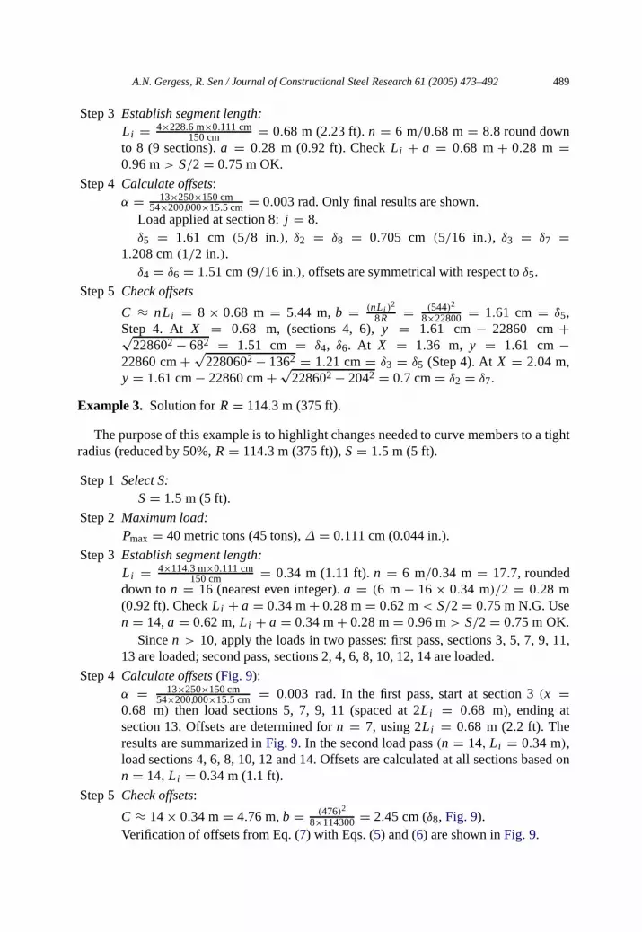
Step 3 Establish segment length:Li = 4×228.6 m×0.111 cm

150 cm = 0.68 m (2.23 ft).n = 6 m/0.68 m= 8.8 round downto 8 (9 sections).a = 0.28 m (0.92 ft). CheckLi + a = 0.68 m+ 0.28 m =0.96 m> S/2 = 0.75 m OK.

Step 4 Calculate offsets:α = 13×250×150 cm

54×200,000×15.5 cm = 0.003 rad. Only final results are shown.Load applied at section 8:j = 8.δ5 = 1.61 cm (5/8 in.), δ2 = δ8 = 0.705 cm (5/16 in.), δ3 = δ7 =

1.208 cm(1/2 in.).δ4 = δ6 = 1.51 cm(9/16 in.), offsets are symmetrical with respect toδ5.

Step 5 Check offsets

C ≈ nLi = 8 × 0.68 m = 5.44 m,b = (nLi )2

8R = (544)2

8×22800 = 1.61 cm = δ5,Step 4. At X = 0.68 m, (sections 4, 6),y = 1.61 cm − 22860 cm+√

228602 − 682 = 1.51 cm = δ4, δ6. At X = 1.36 m, y = 1.61 cm−22860 cm+ √

2280602 − 1362 = 1.21 cm= δ3 = δ5 (Step 4). AtX = 2.04 m,y = 1.61 cm− 22860 cm+ √

228602 − 2042 = 0.7 cm= δ2 = δ7.

Example 3. Solution forR = 114.3 m (375 ft).

The purpose of this example is to highlight changes needed to curve members to a tightradius (reduced by 50%,R = 114.3 m (375 ft)),S = 1.5 m (5 ft).

Step 1 Select S:S = 1.5 m (5 ft).

Step 2 Maximum load:Pmax = 40 metric tons (45 tons),∆ = 0.111 cm (0.044 in.).

Step 3 Establish segment length:Li = 4×114.3 m×0.111 cm

150 cm = 0.34 m (1.11 ft).n = 6 m/0.34 m = 17.7, roundeddown ton = 16 (nearest even integer).a = (6 m − 16× 0.34 m)/2 = 0.28 m(0.92 ft). CheckLi + a = 0.34 m+ 0.28 m= 0.62 m< S/2 = 0.75 m N.G. Usen = 14,a = 0.62 m,Li + a = 0.34 m+ 0.28 m= 0.96 m> S/2 = 0.75 m OK.

Sincen > 10, apply the loads in two passes: first pass, sections 3, 5, 7, 9, 11,13 are loaded; second pass, sections 2, 4, 6, 8, 10, 12, 14 are loaded.

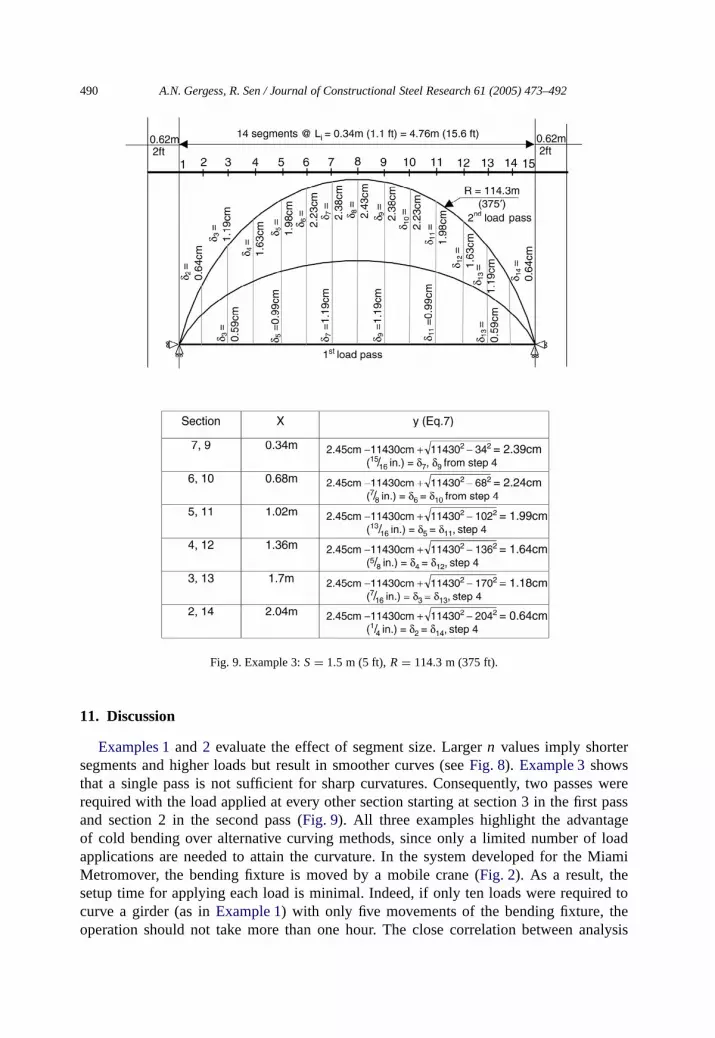
Step 4 Calculate offsets(Fig. 9):α = 13×250×150 cm

54×200,000×15.5 cm = 0.003 rad. In the first pass, start at section 3(x =0.68 m) then load sections 5, 7, 9, 11 (spaced at 2Li = 0.68 m), ending atsection 13. Offsets are determined forn = 7, using 2Li = 0.68 m (2.2 ft). Theresults are summarized inFig. 9. In the second load pass(n = 14, Li = 0.34 m),load sections 4, 6, 8, 10, 12 and 14. Offsets are calculated at all sections based onn = 14, Li = 0.34 m (1.1 ft).

Step 5 Check offsets:

C ≈ 14× 0.34 m= 4.76 m,b = (476)2

8×114300= 2.45 cm (δ8, Fig. 9).Verification of offsets from Eq. (7) with Eqs. (5) and (6) are shown inFig. 9.


Fig. 9. Example 3:S = 1.5 m (5 ft), R = 114.3 m (375 ft).

11. Discussion

Examples 1and2 evaluate the effect of segment size. Largern values imply shortersegments and higher loads but result in smoother curves (seeFig. 8). Example 3showsthat a single pass is not sufficient for sharp curvatures. Consequently, two passes wererequired with the load applied at every other section starting at section 3 in the first passand section 2 in the second pass (Fig. 9). All three examples highlight the advantageof cold bending over alternative curving methods, since only a limited number of loadapplications are needed to attain the curvature. In the system developed for the MiamiMetromover, the bending fixture is moved by a mobile crane (Fig. 2). As a result, thesetup time for applying each load is minimal. Indeed, if only ten loads were required tocurve a girder (as inExample 1) with only five movements of the bending fixture, theoperation should not take more than one hour. The close correlation between analysis


(Eqs. (5) and (6)) and exact offsets (Eq. (7)) provides confirmation of the validity andaccuracy of the analysis.

While numerical examples use nominal strengths, actual values are much higher [14],and actual not nominal values should be used in the calculations.

12. Conclusions

This paper presents a simplified analysis of cold curving for the innovative cold bendingsystem developed for the fabrication of curved steel girders in the Miami Metromover(Fig. 1). A formalized curving procedure is presented and its application illustrated bythree numerical examples.

The analysis establishes limits on the maximum applied load and the number of loadapplications needed to attain a curvature. Such limits help standardize the process andfacilitate future rigorous investigations into cracking and fracture that are preventingwidespread acceptance of cold bending at the present time. Indeed, such research has justbeen initiated by the Texas Department of Transportation [15]. In the interim period, theavailability of closed form expressions relating load and offset provide a simple methodfor monitoring fabrication accuracy and improving efficiency. This can lower fabricationcosts and improve steel’s overall competitiveness in the market place.

Acknowledgements

The authors are indebted to Mr. Robert Clark, Jr. President, Tampa Steel, Florida forfreely sharing information on his innovative cold bending system and for conducting a full-size demonstration using the proposed procedure for the benefit of the authors. They thankMs Cathy Klobuchur, Tampa Steel for her assistance. Financial support during doctoralstudies at the University of South Florida, Tampa by the Flom Graduate Fellowship isgratefully acknowledged.

References

[1] AASHTO. Standard specifications for highway bridges. 16th ed. Washington, DC; 1996. p. 517 [Section11.4.7].

[2] Klobuchur K. Cold bending, Tampa steel’s experience. AASHTO/NSBA Research & Technology Sub-Committee, Orlando, FL; 2002.

[3] Avent RR, Mukai D. What you should know about heat-straightening repair of damaged steel. AISC,Engineering Journal 2001;38(1):27–49.

[4] Brockenbrough RL. Theoretical stresses & strains from heat-curving. ASCE, Journal of Structural Division1970;96(ST7):1421–44.

[5] Sen R, Gergess A, Issa C. Finite element modeling of heat-curved I-girders. ASCE, Journal of BridgeEngineering 2003;8(3):153–61.

[6] Gover WJS. Metal bending for construction. Tipton, West Midlands (UK): The Angle Ring Company; 1996.[7] Gergess A. Cold bending and heat curving of structural steel I-girders. Ph.D. dissertation, Department of

Civil and Environmental Engineering, University of South Florida, Tampa, FL; 2001.[8] Gergess A, Sen R. Fabrication aids for cold straightening damaged steel girders. Engineering Journal, AISC

2004;41(2):69–84.


[9] Gergess A, Sen R. Inelastic response of simply supported I-girders subjected to weak axis bending. In:Zingoni A, editor. Proceedings of the international conference on structural engineering, mechanics andcomputation, vol. I. 2001. p. 243–50.

[10] Popov EV. Mechanics of materials. 2nd ed. Englewood Cliffs (NJ): Prentice-Hall Inc.; 1976. p. 135–42,377–93.

[11] Byars FE, Snyder DR. Engineering mechanics of deformable bodies. 3rd ed. Scranton (PA): InternationalTextbook Co.; 1975.

[12] Salmon CG, Johnson JE. Steel structures: design and behavior. 4th ed. New York (NY): Harper-Collins;1996. p. 51.

[13] AISC. Manual of steel construction, load and resistance factor design. 3rd ed. USA: AISC Inc.; 2001.p. 16.1–33, 17–31.

[14] Brockenbrough R. MTR survey of plate material used in structural fabrication. AISC, Engineering Journal2003;40(1):42–9.

[15] Texas DOT research project. Performance and effect of hole punching and cold bending on steel bridges.Research project conducted by University of Texas at Austin and Texas A&M University; 2003.

Documents

Cold curving symmetric unstiffened I-girders