Embed Size (px)
Citation preview

arX
iv:g
r-qc
/000
3067
v1 1
6 M
ar 2
000
Boost-rotation symmetric spacetimes – review
V. Pravda ∗, A. Pravdova †
Mathematical Institute,
Academy of Sciences,
Zitna 25, 115 67 Prague 1, Czech Republic
(February 7, 2008)
Boost-rotation symmetric spacetimes are the only locally asymptotically flat axially symmetricelectrovacuum spacetimes with a further symmetry that are radiative. They are realized by uni-formly accelerated particles of various kinds or black holes. Their general properties are summarized.Several examples of boost-rotation symmetric solutions of the Maxwell and Einstein equations arestudied: uniformly accelerated electric and magnetic multipoles, the Bonnor-Swaminarayan solu-tions, the C-metric and the spinning C-metric.
PACS: 04.20.Jb, 04.30.-w, 04.20.Ha
Contents
I Introduction 1
II Theoretical background 2
A Asymptotically flat axisymmetric spacetimes and radiation . . . . . . . . . . . . . . . . . . . . . . . 21 The Bondi method . . . . . . . . . . . . . . . . . . . . . . . . . . . . . . . . . . . . . . . . . . . 22 Symmetries of asymptotically flat axisymmetric electrovacuum spacetimes and radiation . . . . 5
B General structure of boost-rotation symmetric spacetimes . . . . . . . . . . . . . . . . . . . . . . . . 8
III Examples in electromagnetism and gravity 11
A Uniformly accelerated electromagnetic multipoles . . . . . . . . . . . . . . . . . . . . . . . . . . . . 11B The Bonnor-Swaminarayan solutions . . . . . . . . . . . . . . . . . . . . . . . . . . . . . . . . . . . 14
1 The Bonnor-Swaminarayan solution representing two pairs of freely moving CC-particles withouta nodal singularity . . . . . . . . . . . . . . . . . . . . . . . . . . . . . . . . . . . . . . . . . . . . 15
2 The Bonnor-Swaminarayan solution representing two CC-particles connected with a nodalsingularity . . . . . . . . . . . . . . . . . . . . . . . . . . . . . . . . . . . . . . . . . . . . . . . . 16
C The C-metric . . . . . . . . . . . . . . . . . . . . . . . . . . . . . . . . . . . . . . . . . . . . . . . . 171 Introduction . . . . . . . . . . . . . . . . . . . . . . . . . . . . . . . . . . . . . . . . . . . . . . . 172 Transformation of the C-metric into the Weyl form . . . . . . . . . . . . . . . . . . . . . . . . . 173 Properties of the C-metric in the original coordinates x, y and in the Weyl coordinates . . . . . 194 The C-metric in the canonical coordinates adapted to the boost-rotation symmetry . . . . . . . 215 The news function . . . . . . . . . . . . . . . . . . . . . . . . . . . . . . . . . . . . . . . . . . . . 24
D The spinning C-metric . . . . . . . . . . . . . . . . . . . . . . . . . . . . . . . . . . . . . . . . . . . 251 The SC-metric in the Weyl-Papapetrou coordinates . . . . . . . . . . . . . . . . . . . . . . . . . 262 Properties of the SC-metric in the p, q coordinates . . . . . . . . . . . . . . . . . . . . . . . . . . 263 The SC-metric in the canonical coordinates adapted to the boost-rotation symmetry . . . . . . 28
I. INTRODUCTION
There exists only one class of exact radiative solutions of the full nonlinear Einstein equations which are known inan analytical form, realized by moving objects and, in addition, are asymptotically flat (in some cases null infinity Jis even global [1]). This is the class of boost-rotation symmetric spacetimes describing uniformly accelerated particles
∗E-mail: [email protected]†E-mail: [email protected]
1

or black holes symmetrically located along the symmetry axis (see reviews [2–4]). They have two Killing vectors,the axial Killing vector with circular group orbits and the boost Killing vector which asymptotically goes over tothe generator of the Lorentz transformation along the symmetry axis in the Minkowski spacetime. The significance ofthese solutions follows from the theorem which states that among locally asymptotically flat spacetimes with the axialand an additional symmetry, boost-rotation symmetric spacetimes are the only spacetimes which are radiative. Itwas proved in [5] for vacuum spacetimes with hypersurface orthogonal Killing vectors and generalized in [6] forelectrovacuum spacetimes with Killing vectors which are not hypersurface orthogonal. These spacetimes have beenfound also useful in numerical relativity as test beds for numerical codes (approaches based on null [7,8] and spacelike[9] initial hypersurfaces).
Several boost-rotation symmetric solutions are known. The first boost-rotation symmetric solution, that has beenfound, is the C-metric [10,11], describing accelerated black holes symmetrically located on the axis of symmetrywith a nodal (conical) singularity (“cosmic string”) which causes the acceleration. Another example is a set ofBonnor-Swaminarayan solutions [12] representing a finite number of uniformly accelerated monopole “Curzon-Chazy”particles. The acceleration can be caused by nodal singularities or by mutual gravitational interaction. However,in the case with no nodal singularities, negative masses occur. The simplest case without conical singularity isrepresented by two pairs of particles, in each of which there is one particle with positive and one with negative mass(as an analogous system in the Newton mechanics, such a system is self-accelerated). A limiting procedure (similarto that in electromagnetism by which one obtains a dipole from two monopoles) leads to a special solution [13]realized by two independent, self-accelerating particles. Such a solution is asymptotically flat, admitting global nullinfinity J . Boost-rotation symmetric solutions with a cosmic string extending along the whole axis of symmetry arelocally asymptotically flat in the sense that they admit only local J . Boost-rotation symmetric solutions describinguniformly accelerated particles with a general multipole structure were also found in [13]. There exist generalizationsof the vacuum boost-rotation symmetric spacetimes containing an electromagnetic field – the charged C-metric [14],or rotating sources – the spinning C-metric [15,16]. The Killing vectors in the case of a spinning source are nothypersurface orthogonal. Also the generalized C-metric [17], generalized charged C-metric [18], and generalizedBonnor-Swaminarayan solution [13] are known that are not asymptotically flat and in which an external field ispresent to cause the acceleration.
Section II is devoted to the general theory of boost-rotation symmetric spacetimes. It is divided into two parts.In the first part II A we recall the Bondi method we further use to present the theorem about uniqueness of boost-rotation symmetric spacetimes among all locally asymptotically flat electrovacuum axially symmetric spacetimes withan additional symmetry. In the second part II B, based on [19], the definition and general features of boost-rotationsymmetric spacetimes are summarized.
Sec. III discusses several examples of boost-rotation symmetric solutions: uniformly accelerated electric and mag-netic multipoles, the Bonnor-Swaminarayan solutions, the C-metric and the spinning C-metric.
We use the signature −2 everywhere except for the last two parts concerning the standard and spinning C-metricswhere the signature +2 is used following [15,16].
II. THEORETICAL BACKGROUND
A. Asymptotically flat axisymmetric spacetimes and radiation
1. The Bondi method
If one is interested in gravitational radiation from a general bounded matter source, i.e., in the behaviour ofgravitational field far from the source, one has to turn to approximation methods, typically one expands the metric innegative powers of a suitably chosen “radial coordinate” r. This was done for axially symmetric non-rotating sourcesby Bondi et al. [20] (generalized without this assumption by Sachs [21], for charged sources by van der Burg [22] –mistakes were corrected in [6], for spacetimes with null dust by von der Gonna and Kramer [23] and for spacetimeswith polyhomogeneous J by Chrusciel et al. [24]). They introduced suitably chosen coordinates {u, r, θ, φ} in sucha way that, roughly speaking, null coordinate u, spherical angles θ and φ are constant along outgoing radial nullgeodesics – light rays – meanwhile r, the luminosity distance, varies and satisfies the condition gθθgφφ = r4 sin2 θ sothat the area of the surface u = const, r = const, φ ∈ 〈0, 2π), and θ ∈ 〈0, π〉 is 4πr2.
The Bondi method meant a breakthrough in gravitational radiation theory. It consists in prescribing initial data noton a spacelike Cauchy hypersurface and solving the Cauchy problem (which is well posed for the Einstein equations
2

[25]) but in prescribing initial data on a characteristic hypersurface of the quasilinear hyperbolic Einstein equationswhich is null, i.e., on a hypersurface u = const. Then discontinuities can arise and the Cauchy problem is ambiguous.One has to prescribe initial data not only on the initial null hypersurface but one also has to know two functions,c,u and d,u (in the vacuum case), for all u (or u in the given interval). Only then the evolution of the gravitationalfield is known, i.e., determined for all u (or in the given interval). This is why we call these two functions the news
functions of the system because they carry the whole information about changes in the system. If and only if oneof them does not vanish the total mass of the system as measured at null infinity, the Bondi mass, decreases andgravitational waves are radiated. If the u-derivative of at least one of the news functions does not vanish the Weyltensor has radiative tetrad components (proportional to r−1)
Cαβγδmαtβmγtδ = [(c + id),uu]
1
r+ O(r−2) (1)
in the standard null tetrad {kα, mα, tα, tα} introduced in [21,6]. There are exceptional cases corresponding, e.g.,to an infinite string (thus the axis of axial symmetry is not regular) with a non-zero news function and with anon-radiative Weyl tensor [26].
Hereafter we are interested in asymptotically flat electrovacuum spacetimes that are in addition axially symmetricbut a source can rotate and we thus follow the work of van der Burg [22] with the additional assumption that all metricfunctions do not depend on φ. The metric has, in the Bondi-Sachs coordinates { u, r, θ, φ } ≡ { x0, x1, x2, x3},the form
ds2 =
(
V
re2β − r2e2γU2 cosh 2δ − r2e−2γW 2 cosh 2δ − 2r2UW sinh 2δ
)
du2
+2e2βdudr + 2r2(
e2γU cosh 2δ + W sinh 2δ)
dudθ
+2r2(
e−2γW cosh 2δ + U sinh 2δ)
sin θ dudφ
−r2[
cosh 2δ(
e2γdθ2 + e−2γ sin2 θ dφ2)
+ 2 sinh 2δ sin θ dθdφ]
, (2)
where all the six metric functions U , V , W , β, γ, δ and the electromagnetic field Fµν do not depend on φ because ofthe axial symmetry. If one requires the axis of the axial symmetry (θ = 0, π) to be regular, then functions
V, β, W, γ/ sin2 θ, U/ sin θ, δ/ sin θ (3)
have to be regular for sin θ → 0.First assuming the functions γ, δ, F12 and F13 to have asymptotic expansions, the spacetime to be asymptotically
flat, and only the outgoing radiation to be asymptotically present then the expansions of these four functions at larger on an initial hypersurface u = const are of the form
γ =c
r+ (C − 1
6c3 − 3
2cd2)
1
r3+
D
r4+ O(r−5) ,
δ =d
r+ (H − 1
6d3 + 1
2c2d)
1
r3+
K
r4+ O(r−5) , (4)
F12 =e
r2+ (2E + ec + fd)
1
r3+ O(r−4) ,
F13 =
[
f
r2+ (2F + ed − fc)
1
r3+ O(r−4)
]
sin θ .
Prescribing then initial data on this null hypersurface, i.e., c, d, C, ... and M , N , P , ǫ, µ as functions of θ, allthe other metric functions are determined on the initial hypersurface by the field equations:
β = − 14(c2 + d2)
1
r2+ O(r−4) ,
U = −(c,θ +2c cot θ)1
r2+[
2N + 3(cc,θ +dd,θ ) + 4(c2 + d2) cot θ] 1
r3
+ 12
[
3(C,θ +2C cot θ) − 6(cN + dP ) − 4(2c2c,θ +cdd,θ +c,θ d2) − 8c(c2 + d2) cot θ + 2(ǫe − fµ)] 1
r4+ O(r−5) ,
W = −(d,θ +2d cot θ)1
r2+[
2P + 2(c,θ d − cd,θ )] 1
r3
3

+ 12
[
3(H,θ +2H cot θ) + 6(cP − dN) − 4(2d2d,θ +cdc,θ +c2d,θ ) − 8d(c2 + d2) cot θ + 2(µe + ǫf)] 1
r4+ O(r−5) ,
V = r − 2M −[
N,θ +N cot θ − 12(c2 + d2) − (c,θ +2c cot θ)2 − (d,θ +2d cot θ)2 − (ǫ2 + µ2)
]1
r
− 12
[
C,θθ +3C,θ cot θ − 2C + 6N(c,θ +2c cot θ) + 6P (d,θ +2d cot θ) + 4(2cc,2θ +3c,θ dd,θ −cd,2θ )
+8(2c,θ d2 + 3c2c,θ +cdd,θ ) cot θ + 16c(c2 + d2) cot2 θ + 2ǫ(e,θ +e cot θ) − 2µ(f,θ +f cot θ)] 1
r2+ O(r−3) ,
F01 = − ǫ
r2+ (e,θ +e cot θ)
1
r3+ O(r−4) , (5)
F23 =[
−µ − (f,θ +f cot θ)1
r+ O(r−2)
]
sin θ ,
F02 = X + (ǫ,θ −e,u )1
r−{
[E + 12(ec + fd)],u + 1
2(e,θ +e cot θ),θ
} 1
r2+ O(r−3) ,
F03 =
{
Y − f,ur
−[
[F + 12(ed − fc)],u
] 1
r2+ O(r−3)
}
sin θ .
Provided four news functions, two gravitational, c,u, d,u, and two electromagnetic, X , Y , are prescribed for all u,the time evolution of the system is fully determined using the Einstein-Maxwell equations (see [22] for details). Letus just mention a relation for the mass aspect M which is equal in stationary case to the total mass of the system:
M,u = −(c,2u +d,2u ) − (X2 + Y 2) + 12(c,θθ +3c,θ cot θ − 2c),u . (6)
Then the total mass at future null infinity J + at a given “retarded time” u, the Bondi mass m, defined as a meanvalue of the mass aspect of the system, M , over the sphere,1
m(u) = 12
∫ π
0
M(u, θ) sin θdθ , (7)
is decreasing if at least one of the news functions does not vanish:
m,u = − 12
π∫
0
(c,2u +d,2u +X2 + Y 2) sin θdθ ≤ 0 . (8)
The mass decrease is caused by gravitational and electromagnetic waves radiated out from the system.The rate of loss of the electromagnetic energy radiated out from the system is given by
∂
∂u
π∫
0
12(X2 + Y 2) sin θdθ , (9)
which indeed implies the loss of mass as seen from Eq. (8).There are several conserved quantities described in [22,27]. Two of them are the electric and magnetic charges of
the source
∂
∂u
π∫
0
12ǫ sin θdθ = 0 ,
∂
∂u
π∫
0
12µ sin θdθ = 0 . (10)
1If the spacetime is stationary, the Bondi mass m is the same as the mass aspect M and is equal to the total mass of the systemas measured at spatial infinity – the ADM mass.
4

2. Symmetries of asymptotically flat axisymmetric electrovacuum spacetimes and radiation
Since finding an exact radiative solution describing a general charged bounded source is a very difficult task, maybe unsolvable, it is of interest to know which isometries are compatible with asymptotic flatness and admit radiation.This question was solved in [5] for locally asymptotically flat axially symmetric vacuum spacetimes with non-rotatingsources, i.e., with hypersurface orthogonal Killing vectors, and generalized in [6] for electrovacuum spacetimes with,in general, rotating sources, i.e., with Killing vectors that are not hypersurface orthogonal. The assumption of axialsymmetry with the corresponding Killing vector field denoted by ξ = ∂/∂φ simplifies lengthy calculations.
Suppose that such an axially symmetric electrovacuum spacetime admits only a “piece” of future null infinity J +
in the sense of [1]. Then one can introduce the Bondi-Sachs coordinate system { u, r, θ, φ } ≡ { x0, x1, x2, x3} inwhich the metric has the form (2), where the metric functions and the electromagnetic field Fµν are functions of u,r, θ and have expansions (4), (5). Thanks to the existence of only local J +, we assume Eqs. (4)–(6) to be satisfiedfor all φ ∈ 〈0, 2π), however, not necessarily on the whole sphere, i.e., not for all θ ∈ 〈0, π〉 but only in some openinterval of θ and thus the Bondi mass (7) cannot be introduced. For example, the “axis of symmetry” (θ = 0, π)may contain nodal singularities and thus need not be regular and the regularity conditions on the axis (3) need notbe satisfied for any u. If the axis is singular then at least two generators of J + would be missing so that J + wouldnot be topologically S2 ×R.
Let us now assume that another Killing vector field η exists which forms together with ξ = ∂/∂φ a two-parametergroup. In Ref. [5] it is proved (see Lemma in Sec. 2) that in the case of ξ with circles as integral curves, ξ and ηdetermine an Abelian Lie algebra so that we can assume [η, ξ] = 0. Hence, the components ηα are independent of φ.
Then by solving the Killing equations Lηgαβ = 0 (explicitly given in [6,28]), the Killing vector asymptotically turnsout to be
ηα = [−ku cos θ + α(θ), kr cos θ + O(r0), −k sin θ + O(r−1), O(r−1)] , (11)
where k is a constant and α an arbitrary function of θ. This result for a locally asymptotically flat axially symmetricelectrovacuum spacetime with Killing vectors which need not be hypersurface orthogonal proved in [6] is the same asthat one for asymptotically flat axially symmetric vacuum spacetimes with hypersurface orthogonal Killing vectorsobtained in [5].
Let us analyze possibilities k = 0 and k 6= 0 separately.
1) Case k = 0
This alternative was considered in [6] and developed in detail in [29]. When k = 0, the Killing vector field η (11)generates supertranslations. However, solving Killing equations in higher orders of r−1 and assuming that the elec-tromagnetic field described by Fµν (4), (5) has the same symmetry, i.e., LηFαβ = 0, one can show that η in factgenerates translations
ηα =[
B, Bc,u +B,θ cot θ − uc,2u B
r+ O(r−2), −B,θ
1
r+ B,θ
c
r2+ O(r−3), O(r−4)
]
, (12)
where
B(θ) =sin θ
2C
[
(b0 + a0)( sin θ
cos θ + 1
)C
+ (b0 − a0)( sin θ
cos θ + 1
)−C]
, (13)
with constants a0, b0 and C ∈ (0, 1〉 in a spacetime with, in general, an infinite thin cosmic string along the symmetryaxis. The cosmic string is described by a deficit angle 2π(1 − C). The only non-vanishing news function – due tothe presence of the string – is
c,u =C2 − 1
2 sin2 θ, (14)
which depends only on θ and thus the Weyl tensor (1) does not have a radiative character. The leading metricfunctions and electromagnetic field functions have the form
c(u, θ) =u
2B(B,θθ −B,θ cot θ) = u
C2 − 1
2 sin2 θ, d(u, θ) = 0 ,
M(u, θ) = −uc,2u −a1B−3 ,
N(u, θ) = − 12B−4(2a1B,θ u + f0 sin θ) , P (u, θ) = − 1
2g0 sin θB−4 , (15)
X(u, θ) = Y (u, θ) = 0 , ǫ(u, θ) = ǫ0B−2 , µ(u, θ) = µ0B
−2 ,
e(u, θ) = −ǫ0B,θ B−3u + e1(θ) , f(u, θ) = µ0B,θ B−3u + f1(θ) ,
5

where a1, f0, g0, ǫ0, and µ0 are constants and e1, f1 are arbitrary functions of θ. The reader may find more metricand field functions in [28] and [29].
In paper [29] we proved the following statements in Theorems 1, 2. The asymptotically translational Killing vectorη, given by (12), has asymptotically the norm
‖η‖2 = (b20 − a2
0) +2a1
B
1
r+ [u2a1B
−3(B2c,u −B,2θ +BB,θ cot θ)
+ f0 sin θ B−3(−B,θ +B cot θ) + (ǫ20 + µ20)B
−2]1
r2+ O(r−3) , (16)
that may be spacelike, timelike or null. It is spacelike for a20 > b2
0. If one of the constants a1, f0 or g0 is non-vanishingthen J + is singular at θ = θ0 6= 0, π, given by the relation
cos θ0 =(a0 + b0)
2/C − (a20 − b2
0)1/C
(a0 + b0)2/C + (a20 − b2
0)1/C
, (17)
in addition to the singularity due to the presence of the cosmic string at θ = 0, π. This case corresponds to cylindricalwaves (in particular, θ0 = π/2 for b0 = 0). The Killing vector η is null if a0 = ±b0. Then J + is singular at θ = 0 orπ in addition to the string singularity if again a1 or f0 or g0 is non-vanishing. It corresponds to a wave propagatingalong the symmetry axis. The Killing vector η is timelike for a2
0 < b20 and the only singularities of J + at θ = 0, π are
due to the presence of the string.If there is no string, null infinity J + may be regular even with a non-vanishing Bondi mass m for an asymptotically
timelike translational Killing vector. However, even if the translational Killing vector is spacelike or null, J + may beregular if the spacetime is flat in its neighbourhood (i.e., constants a1, f0, g0 and thus also the mass aspect M andfunctions N , P , ... vanish).
For C = 1, without the string, we find the Killing vector field η (12) to have asymptotically the form
ηα =[
−a0 cos θ + b0, a0 cos θ + O(r−2), −a0 sin θ
r+ O(r−4), O(r−4)
]
(18)
and the mass aspect is then given by
M = − a1
(−a0 cos θ + b0)3. (19)
In the case of the timelike Killing vector (b20 > a2
0) assuming b0 > 0 and a1 < 0 we obtain the total Bondi mass to be
m = − a1b0
(b20 − a2
0)2
> 0 . (20)
The factor −a0 cos θ + b0 appearing in Eq. (19) corresponds, using the terminology of [20], to the “Doppler shift ofthe mass aspect” and the other Bondi functions. It occurs when the system is boosted with respect to the Bondiframe with the boost parameter – ν (b0 = cosh ν, a0 = sinh ν) so that its velocity is v = − tanh ν = a0/b0. Puttinga1 = −m, we get the mass aspect in Eq. (19) in the form M = m/(cosh ν − sinh ν cos θ)3, which exactly correspondsto the formula (see Eq. (72) in [20]) for the Schwarzschild mass m moving along the axis of symmetry with constantvelocity − tanh ν.
In [29] two exact solutions are studied with axial and translational Killing vectors and with an infinite cosmic stringalong the symmetry axis – the Schwarzschild solution with a string, where the Killing vector generates translationsalong the t-axis (a1 6= 0, f0 = g0 = 0) and Einstein-Rosen cylindrical waves with a string having a spacelike transla-tional Killing vector corresponding to translations along the z-axis (a1 = 0, f0 6= 0, g0 = 0).
2) Case k 6= 0
Assuming k 6= 0 in (11), it is easy to find a Bondi-Sachs coordinate system with α = 0 by performing a supertrans-lation. Hence we put α = 0 in (11) and without loss of generality we choose k = 1. Then the asymptotic form ofthe Killing vector field η is
ηα = [−u cos θ, r cos θ + O(r0), − sin θ + O(r−1), O(r−1)] . (21)
It is the boost Killing vector that generates the Lorentz transformation along the axis of axial symmetry.
6

Solving the Killing equations in higher orders of r−1 and assuming that the electromagnetic field has the samesymmetry, i.e., LηFµν = 0 is satisfied, we obtain the forms of the metric and field functions to be:
c(u, θ) = −K(w)
uw→ c,u =
K(w),wu2
, (22)
d(u, θ) = −L(w)
uw→ d,u =
L(w),wu2
, (23)
M(u, θ) =1
2 sin θ(w2K,w ),w +
λ(w)
u3w3, (24)
X(u, θ) =E(w)
u2, (25)
Y (u, θ) =B(w)
u sin θ=
B(w)
wu2=
B(w)
u2, (26)
ǫ(u, θ) =E(w)
ucot θ , (27)
µ(u, θ) =B(w)
sin θcot θ =
B(w)
ucot θ , (28)
e(u, θ) =E(w)
2+
G(w)
u2, (29)
f(u, θ) = −B(w)u
2 sin θ+
D(w)
u sin θ= −B(w)
2+
D(w)
u2, (30)
where w = sin θ/u, functions K(w), L(w), E(w) and B(w) (B(w) = B(w)/w) are arbitrary functions determining newsfunctions, and λ(w) has to satisfy the equation
λ,w = w2(K,2w +L,2w +E2 + B2) − 1
2w(w3K,ww ),w , (31)
while G(w) and D(w) (D(w) = D(w)/w) are solutions of the equations
2w2(G,w w + 2G) + (E ,w w − E) + 2wEK + 2BL = 0 , (32)
2w2(D,w w + D) − (B,w w − 2B)− 2wBK + 2w2EL = 0 . (33)
Solving Eq. (31) for λ with prescribed news functions (i.e., for given K(w),w , L(w),w , E(w) and B(w)) we find the massaspect M(u, θ) (24) and thus the total Bondi mass at J + is then given by
m(u) = 12
π∫
0
M(u, θ) sin θ dθ = 14
π∫
0
(w2K,w ),w dθ + 12
π∫
0
λ
u2w2dθ . (34)
The expansion of the boost Killing vector is as follows
ηα =[
−u cos θ , r cos θ + u cos θ + cos θ(
K,w +Kw
) 1
r+ O(r−2) ,
− sin θ − u sin θ
r+
uc sin θ
r2+ O(r−3) ,
ud
r2+ O(r−3)
]
. (35)
These results were generalized for spacetimes with in general polyhomogeneous J using Newman-Penrose formalismin [30] .
Since in boost-rotation symmetric spacetimes the news functions are in general non-vanishing functions of u andw, these spacetimes are radiative and so we may conclude with the theorem proved in [6]:
Theorem Suppose that an axially symmetric electrovacuum spacetime admits a “piece” of J + in the sense thatthe Bondi-Sachs coordinates can be introduced in which the metric takes the form (2), (4), (5) and the asymptoticform of the electromagnetic field is given by (4), (5). If this spacetime admits an additional Killing vector forming withthe axial Killing vector a two-dimensional Lie algebra (both Killing vectors need not be hypersurface orthogonal) thenthe additional Killing vector has asymptotically the form (11). For k = 0 it generates asymptotically translationsalong the z or t-axis or their combination and then the Weyl tensor does not have radiative components; it maycontain an infinite thin cosmic string along the z-axis. For k 6= 0 it is the boost Killing field and the spacetime isradiative.
7

B. General structure of boost-rotation symmetric spacetimes
The theorem mentioned in the previous section shows that boost-rotation symmetric spacetimes play a unique roleamong all locally asymptotically flat axially symmetric electrovacuum spacetimes with a further symmetry as they arethe only ones that are radiative. Moreover there is a number of boost-rotation symmetric solutions known explicitly,representing the fields of “uniformly accelerated sources” – singularities of the Curzon-Chazy type and of all the otherWeyl types or black holes.
Let us now summarize general properties and the global behaviour of boost-rotation symmetric spacetimes fromthe geometrical point of view. The reader may find the following definitions and statements in the detailed work [19](see also [2,31,32]) where the Killing vectors are assumed to be hypersurface orthogonal.
Boost-rotation symmetric spacetimes have two isometries generated by two Killing vectors – the axial Killingvector ξ and the boost Killing vector η. To gain better insight into curved boost-rotation symmetric spacetimes letus first consider the Minkowski spacetime where these two Killing vectors and their norms have the form
the axial Killing vector: ξ = x∂
∂y− y
∂
∂x, A = −ξαξα = x2 + y2 ≥ 0 ,
the boost Killing vector: η = z∂
∂t+ t
∂
∂z, B = ηαηα = z2 − t2 arbitrary . (36)
The axial Killing vector is spacelike everywhere and vanishes on the axis A = 0 containing points fixed by the rotation.The boost Killing vector is null on two hyperplanes B = 0 – the roof, spacelike “above the roof” for B < 0, where“almost all” null geodesics get in, and timelike “below the roof” for B > 0. See Fig. 1, where also the null coneof the origin A + B = 0 is plotted that is fixed under the boost-rotation group and its vertex is the fixed point ofthe group and two integral curves of the timelike boost Killing vector (hyperbolas) are indicated that may correspondto worldlines of particles uniformly accelerated in opposite directions. Notice that such particles move independentlysince their worldlines are separated by two null hypersurfaces (the roof). One obtains a similar picture for a curvedboost-rotation symmetric spacetime.
A = 0B = 0A+ B = 0B = 0
zx; yt
FIG. 1. The general structure of boost-rotation symmetric spacetimes:the axis – A = 0,the roof – B = 0,the null cone of the origin – A + B = 0.
Since we wish to examine especially the radiative properties, let us concentrate on the region above the roof (B < 0).We transform the Minkowski metric first to coordinates adapted to the boost-rotation symmetry {b, ρ, φ, χ}
x = ρ cosφ , y = ρ sin φ , z = b sinhχ , t = ± b coshχ (37)
with b ≥ 0, χ ∈ R, and further to null coordinates u, v
8

u = b − ρ , v = b + ρ . (38)
The metric then takes the form
ds2 = dudv − 14(v2 − u2)
[v − u
v + udφ2 +
v + u
v − udχ2
]
, (39)
where v = u is the axis, v = −u the roof, and the lines u, φ, χ being constant, v changing are null geodesics endingat null infinity J + for v → +∞. The Killing vectors (36) are ξ = ∂/∂φ and η = ∂/∂χ.
Inside the radiative part of the boost-rotation symmetric spacetime the boost Killing vector is spacelike. Thusone cannot distinguish between a small region of a curved boost-rotation symmetric spacetime and a small regionof a curved cylindrically symmetric spacetime (one can transform a boost-rotation symmetric metric above the rooflocally to the cylindrically symmetric Einstein-Rosen metric [33,34]). However, these two spacetimes have essentiallydifferent asymptotical properties.
The null coordinates u, v are related to canonical coordinates U , V (V = 12v2 and U = 1
2u2 sign u) that can be
used to distinguish between cylindrical and boost-rotation symmetry:
Proposition The metric of a curved spacetime admitting two spacelike, hypersurface orthogonal, commuting Killingvectors ∂/∂x and ∂/∂y, and satisfying the vacuum Einstein equations can be, in a region where W,αW ,α does notchange the sign, W being the “volume element” of the group orbits, transformed into one of the following forms:
ds2 = eΛdUdV − W [e−Ψdx2 + eΨdy2] , (40)
where Λ, Ψ are functions of U , V , and W > 0 is such that
a) W = 12(V + U) if W,α is timelike,
b) W = 12(V − U) if W,α is spacelike,
c) spacetimes with W,α null or W = const have more symmetries.
The coordinates U and V are determined uniquely up to translations.
In a boost-rotation symmetric spacetime in radiative regions, W,α is spacelike inside the null cone of the origin andtimelike outside the null cone, whereas W,α is spacelike everywhere in a cylindrically symmetric spacetime. The Killingvectors ∂/∂x and ∂/∂y are the axial and the boost Killing vector respectively.
The metric (39) can be generalized for a curved spacetime:
Definition 1 A spacetime admitting two spacelike, hypersurface orthogonal Killing vectors is called “boost-rotationsymmetric” if in canonical coordinates 1
2v2, 1
2u2 (resp. − 1
2u2 if u < 0) the metric has the form
ds2 = eλ dudv − 14(v2 − u2)
[v − u
v + ue−µ dφ2 +
v + u
v − ueµ dχ2
]
, (41)
φ ∈ 〈0, 2π), χ ∈ R, the functions λ(u, v), µ(u, v) are defined for v ∈ (0 < v0, +∞), u ∈ (u0, u1), u < v, u 6= −v,and
limv→∞
u fixed
λ(u, v) = λ0(u) , limv→∞
u fixed
µ(u, v) = κ = const . (42)
This weaker asymptotic condition is compatible with the asymptotic flatness – boost-rotation symmetric spacetimesdefined here admit a local J+. A stronger condition λ → 0, µ → 0 as v → +∞ would imply a flat spacetimeeverywhere.
The boost-rotation symmetric metric defined in Def. 1 (41) above the roof, i.e., for t2 > z2, can be extended to allvalues of “Cartesian-type” coordinates {t, x, y, z} by transformations (37) and (38):
Definition 2 The boost-rotation symmetric vacuum solutions have the metric
ds2 = −(x2 + y2)−1[eλ(xdx + ydy)2 + e−µ(xdy − ydx)2] − (z2 − t2)−1[eλ(tdt − zdz)2 − eµ(tdz − zdt)2]
= −(x2 + y2)−1[(eλx2 + e−µy2)dx2 + 2xy(eλ − e−µ)dx dy + (eλy2 + e−µx2)dy2]
−(z2 − t2)−1[(eλz2 − eµt2)dz2 − 2zt(eλ − eµ)dz dt − (eµz2 − eλt2)dt2] (43)
9

with (t, x, y, z) ∈ R4, x2 + y2 > 0, z2 − t2 6= 0, and
µ = µ(A = x2 + y2, B = z2 − t2) , λ = λ(A = x2 + y2, B = z2 − t2) . (44)
The function µ, determined up to an additive constant, is an analytic, asymptotically regular solution of the flat-spacewave equation
2µ = Aµ,AA +Bµ,BB +µ,A +µ,B = 0 (45)
except for the regions where sources uniformly accelerated with respect to the Minkowskian background and definingµ occur. The function λ, determined up to an additive constant, is the solution of the field equations
(A + B)λ,A = B(Aµ,A2 − Bµ,B
2 + 2Aµ,A µ,B ) + (A − B)µ,A −2Bµ,B , (46)
(A + B)λ,B = A(Bµ,B2 − Aµ,A
2 + 2Bµ,A µ,B ) + (A − B)µ,B +2Aµ,A (47)
and it is analytic in all regions where µ is analytic, i.e., both are analytic even on the roof and everywhere on the axisoutside the sources and nodal (conical) singularities which cause the particles to accelerate. The equation (45) is anintegrability condition for equations (46) and (47).
One can see that µ and λ (44) in canonical coordinates satisfy the boundary conditions required in Def. 1 andthe metric admits the axial and boost Killing vectors which have the same form as in the Minkowski spacetime (36).Moreover, the structure of group orbits in the curved boost-rotation symmetric spacetime outside the sources orsingularities is the same as the structure of axial and boost group orbits in the Minkowski spacetime. Thus the boostKilling vector is timelike below the roof, z2 > t2, where the spacetime is stationary and there is no radiation. It isspacelike above the roof, t2 > z2, where almost all null geodesics end and where the leading term of the Riemanntensor, proportional to r−1 (r2 = ρ2 + z2), is non-vanishing and has the same algebraic structure as in the case ofplane waves. Consequently in regular regions of J above the roof the gravitational field is radiative.
This definition of vacuum boost-rotation symmetric spacetimes is “geometrical” by virtue of an invariant geometricalmeaning of “Minkowskian” coordinates {t, x, y, z} due to their relation to the canonical coordinates.
Using polar coordinates ρ, φ instead of x, y, the metric (43) becomes
ds2 = −eλdρ2 − ρ2e−µdφ2 − 1
z2 − t2[
(eλz2 − eµt2)dz2 − 2zt(eλ − eµ)dz dt + (eλt2 − eµz2)dt2]
. (48)
Since both the functions µ and λ are determined up to an additive constant, we can make the roof regular, i.e.,
µ(A, 0) = λ(A, 0) (49)
is satisfied, by choosing the constants such that
µ(0, 0) = λ(0, 0) (50)
is fulfilled as the Einstein equations (45)–(47) then imply (49). As the sources are located on the axis, we cannotmake the whole axis regular but one can add the same constant to both µ and λ to make parts of the axis regular,i.e., to satisfy
µ(0, B) + λ(0, B) = 0 , (51)
and thus arrange the distribution of nodal (conical) singularities – “strings” – along the z-axis. One can make regulareither the spatial infinity (then the string is between symmetrically located sources on the z-axis) or the axis betweensources moving with opposite accelerations (then the string tends to infinity along the z-axis and thus propagatesalong null infinity to time infinity). Such solutions are asymptotically flat in the sense that they admit only local J(two generators are singular, or missing so that J ± 6∼= S2 ×R). See Sec. III for particular examples.
There are also solutions where no nodal singularity is necessary to cause the acceleration of the sources. Thus boththe roof and axis (except for points where particles occur) are regular and the regularity conditions of the roof (50)and axis (51) at the origin imply µ(0, 0) = λ(0, 0) = 0. Both spacelike and timelike infinities are then regular. Nullinfinity J + and J− is regular except for four points, where the worldlines of sources “start” and “end” (t = ±z,z → ±∞) – the fixed points of the boost-rotation symmetry, i.e., the solution admits global null infinity in the sense
10

of topology J± ∼= S2 × R though two generators are not complete. It can be shown that arbitrarily strong boost-rotation symmetric initial data can be prescribed on a hyperboloidal hypersurface above the roof leading to a completesmooth future null and timelike infinities. Here weak-field initial data are not necessary as in the proof of existenceof general asymptotically flat radiative solutions (the work of Friedrich [35], Cutler and Wald [36], Christodoulou andKlainerman [37]). These exceptional cases can be represented by “self-accelerating” particles due to their multipolestructure (an infinite number of these solutions is known in an explicit form [13]) or by several particles distributedsymmetrically along the z-axis where negative masses have to be introduced (for example [12]).
“Generalized” boost-rotation symmetric solutions also do not contain singularities causing the acceleration and evenno negative masses. They represent accelerated particles in external fields. The generalized C-metric was obtained bya certain procedure by Ernst [17], the generalized Bonnor-Swaminarayan solution was first constructed analogouslyand then in a more physical way as a limit of the asymptotically flat boost-rotation symmetric solution representingtwo accelerated pairs when the “outer” particle in each pair, attached to a string extending to infinity, goes to infinitywith increasing mass parameter [38]. These solutions are the best rigorous known today examples of the motionof relativistic bodies, e.g., black holes in “external fields”. However, they are not asymptotically flat and thus it isdifficult to analyze their radiative properties. In a limit of a weak external field, there are regions where radiationproperties might be investigated since spacetimes are approximately flat there. Recently Hawking and Ross [39] usedthe generalized C-metric within the framework of quantum gravity. There exists also an electromagnetic generalization[18], where the charged black hole is accelerated by an external electric field (the same solution may be achieved byinteracting electromagnetic and gravitational perturbations in a weak external limit [40]).
As was mentioned at the beginning, asymptotically flat boost-rotation symmetric spacetimes are the only non-trivial explicit exact radiative solutions representing moving objects and an analysis of their radiative properties maybe helpful to understand physically more realistic situations. These solutions are the most realistic, although theycontain nodal singularities or negative masses and their ADM mass vanishes, and thus can not serve as an exampleof a general spacetime with a positive ADM mass.
III. EXAMPLES IN ELECTROMAGNETISM AND GRAVITY
A. Uniformly accelerated electromagnetic multipoles
In this section we study boost-rotation symmetric solutions of the Maxwell equations to gain better understandingof solutions with the same symmetries in general theory of relativity. The simplest case was studied first by Born [41].It represents a field of two particles with opposite charges ±e symmetrically located and uniformly accelerated with auniform acceleration ±α−1, α > 0, along the z-axis of cylindrical coordinates {t, ρ, φ, z} in the Minkowski spacetime(see, e.g., [42]). They move independently of each other as they are separated by a null hypersurface, the roof (seeSubsec. II B). Their worldlines are hyperbolas, integral curves of the timelike boost Killing vector,
ρ = 0, z(±e) = ±√
α2 + t2 . (52)
A detailed analysis [42,43] shows that the field can be interpreted as either the purely retarded field from the charge+e in the region z + t > 0 and the purely advanced field from the charge −e in the region z + t < 0, or as 1
2(advanced
+ retarded) fields from both charges. However, the field is purely retarded in the region t > |z| and purely advancedin t < −|z|. The same interpretation may be used for a field of uniformly accelerated electric [44] and magnetic [45,46]multipoles.
The field of uniformly accelerated electric multipoles (2l−poles) ±el moving along hyperbolas (52) reads (see [44])
E(ρ)(l) = 8
el(2l − 1)!!
l!2ρz ∂(l)
α
(
α2
ζ3
)
,
E(z)(l) = −4
el(2l − 1)!!
l!2∂(l)
α
(
α2(
α2 + t2 + ρ2 − z2)
ζ3
)
, (53)
B(φ)(l) = 8
el(2l − 1)!!
l!2ρt ∂(l)
α
(
α2
ζ3
)
,
while the field corresponding to uniformly accelerated magnetic multipoles ±ml has the form (see [45,46])
11

B(ρ)(l) = 8
ml(2l − 1)!!
l!2ρz ∂(l)
α
(
α2
ζ3
)
,
B(z)(l) = −4
ml(2l − 1)!!
l!2∂(l)
α
(
α2(
α2 + t2 + ρ2 − z2)
ζ3
)
, (54)
E(φ)(l) = −8
ml(2l − 1)!!
l!2ρt ∂(l)
α
(
α2
ζ3
)
,
where
ζ =√
4ρ2α2 + (α2 + t2 − z2 − ρ2)2 . (55)
The other field components vanish. It is obvious that the field given by (54) can be obtained from that given by (53)by a simple transformation
~B → − ~E, ~E → ~B , el → ml , (56)
which is a special case of the duality symmetry.Now let us analyze these solutions from the viewpoint of radiation. The Born solution, the simplest example of
(53) representing the field of uniformly accelerated electric monopoles, was studied in some basic works by Pauli [47]and von Laue [48]. They considered the field as non-radiative as do some authors even now [49] (see also commentsin [50,51]). However, this is in a contradiction with the statement that an accelerated charge radiates energy withthe rate (2/3)e2v2. Performing a series expansion in r−1 (r2 = ρ2 + z2) with time t fixed, the asymptotic behaviour
of the Born field is ~E ∼ r−4, ~B ∼ r−5 and thus the Poynting vector ~S ∼ r−9. In Fig. 2 we see that the quantitiesdetermining the field have the character of a pulse and it is therefore understandable why the Poynting vector ~S isnon-radiative when going to spatial infinity and therefore passing through a pulse (see [43]). In the next part we will
see that ~S ∼ r−2 when travelling with the pulse with the velocity of light; then all fields (53) and (54) have a radiativecharacter.
rj ~Ej t = t1 t = t2 t = t3
FIG. 2. Pulse generated by a uniformly accelerated electric charge.
To examine the radiative properties of these solutions, we express the field components (53) and (54) in terms ofspherical coordinates (r, θ, φ) and of the retarded time of the origin u = t − r and expand them in r−1 with u, θ, φfixed (see [44–46]):
B(ρ) = mlGl sin θ cos θ1
r+ O(r−2) ,
B(z) = −mlGl sin2 θ
1
r+ O(r−2) , (57)
E(φ) = −mlGl sin θ1
r+ O(r−2) ,
where
Gl =(2l − 1)!!
l!2∂(l)
α
(
α2
(u2 + α2 sin2 θ)3/2
)
(58)
12

and similarly for electric multipoles with respect to (56). Considering a particle with an arbitrary structure of electricand magnetic multipoles, the leading term of the radial component of the Poynting vector reads
Sr =sin2 θ
4πr2
∑
l,l′
(elel′ + mlml′)GlGl′ + O(r−3) . (59)
Introducing the true retarded time u∗ of the particle by
t − u∗ = |~r − ~r ∗| , (60)
where (t, ~r) and (u∗, ~r ∗) are the coordinates of an observation and emission event, respectively, we can express
u = u∗ −√
u∗2 + α2 cos θ + O(r−1) . (61)
The radial flux emitted at u∗ = 0 thus takes the form
Sr =sin2 θ
4πr2
∑
l,l′
(2l − 1)!!(2l′ − 1)!!(elel′ + mlml′)
l!2l′!2VlVl′
αl+l′+2, (62)
where Vl can be obtained by substituting (61) and u∗ = 0 into
αl+1 ∂(l)α
(
α2
(u2 + α2 sin2 θ)3/2
)
;
thus V0 = 1, V1 = 3 cos2 θ − 1, V2 = 15 cos4 θ − 15 cos2 θ + 2, . . ..The total power radiated out, R = 2π
∫ π
0 limr→∞
(r2Sr) sin θ dθ, is then as follows
R =∑
l,l′
R(l,l′) elel′ + mlml′
αl+l′+2, (63)
where R(l,l′) are introduced by (see (24) in [44])
R(l,l′) =(2l − 1)!!(2l′ − 1)!!
2l!2l′!2
∫ π
0
VlVl′ sin3 θ dθ . (64)
This expression for the total radiated power (63) reduces to (23) in [44] when all ml = 0. As in [44] we have R(0,0) = 2/3,R(0,1) = −4/15, R(1,1) = 8/21, etc. Due to the boost symmetry, the particles radiate out energy (measured in aninertial frame in which the particle is at rest at the emission event) with a constant rate which is independent of u∗
and thus the same as at the turning point u∗ = 0. See [43] for the detailed discussion.From (5), (25), and (26) it follows that radiative components of a general boost-rotation symmetric electromagnetic
field tensor Fµν in the coordinates u, r, θ, φ are of the form
Fuθ = X =E(w)
u2,
Fuφ = Y sin θ =B(w) sin θ
u2, where w =
sin θ
u. (65)
Here X and Y correspond to the electromagnetic news functions of the system (see Subsubsec. II A 1 or [22,6]). Noticethat these radiative components are proportional to r0 rather then to r−1 due to the choice of coordinates. For auniformly accelerated electric monopole (i.e., the Born solution) we obtain
E(w) =e0α
2w
(1 + α2w2)3/2for u > 0 , E(w) = − e0α
2w
(1 + α2w2)3/2for u < 0 ,
B(w) = 0. (66)
For a uniformly accelerated electric dipole we get
13

E(w) =e1αw(2 − α2w2)
(1 + α2w2)5/2for u > 0 , E(w) = −e1αw(2 − α2w2)
(1 + α2w2)5/2for u < 0 ,
B(w) = 0 , (67)
whereas for a magnetic dipole one finds
E(w) = 0 ,
B(w) = −m1αw(2 − α2w2)
(1 + α2w2)5/2for u > 0 , B(w) =
m1αw(2 − α2w2)
(1 + α2w2)5/2for u < 0 . (68)
For a general electric 2l-pole the news functions turn out to be
E(w) = el(Glu3)w ,
B(w) = 0 , (69)
while for a magnetic 2l-pole
E(w) = 0 ,
B(w) = −ml(Glu3)w (70)
with Gl given by (58).One can check that the total electric and magnetic charges (10) for the general electric and magnetic multipoles
vanish,
π∫
0
(E cos θ/u)dθ = 0 ,
π∫
0
(B cos θ/u)dθ = 0 . (71)
B. The Bonnor-Swaminarayan solutions
In 1957 Bondi [52] proved the existence of an axially symmetric solution of the Einstein equations correspondingto two pairs of particles having equal masses but of opposite sign uniformly accelerated in opposite directions. Sevenyears later Bonnor and Swaminarayan constructed such a solution explicitly [12]. Particles in this solution – pointsingularities of Curzon-Chazy type (see [34]) – move freely and the acceleration force is caused by mutual gravitationalinteraction. They obtained also other similar metrics, some of them representing only positive masses. However,particles considered there do not move freely, line singularities of a conical type, interpreted as nodes, rods, struts orstresses, always appear.
Since Bonnor-Swaminarayan solutions (BS-solutions) are boost-rotation symmetric, their metrics have, in cylindricalcoordinates t, ρ, z, and φ, the form (48), in which the functions entering the metric read
µ = −2a1
R1− 2a2
R2+
2a1
h1+
2a2
h2+ ln k ,
λ =a1a2
(h1 − h2)2f − ρ2(z2 − t2)
(
a21
R41
+a22
R42
)
+2a1R
h1R1+
2a2R
h2R2+ ln k ,
R = 12(ρ2 + z2 − t2) , (72)
Ri =√
(R − hi)2 + 2ρ2hi , i = 1, 2 ,
f =4
R1R2[ρ2(z2 − t2) + (R − ρ2 − h1)(R − ρ2 − h2) − R1R2] ,
where a1, a2, h1 > 0, h2 > 0, k > 0 are constants.The whole class of BS-solutions describes the gravitational field of a finite number of monopole Curzon-Chazy
particles (CC-particles) uniformly accelerated in opposite directions where the acceleration force is caused by agravitational interaction among particles or by nodal singularities. Let us now study two examples separately.
14

1. The Bonnor-Swaminarayan solution representing two pairs of freely moving CC-particles without a nodal singularity
The simplest case without a nodal singularity is the BS-solution, considered first by Bondi, containing two pairsof freely falling particles: there is one particle with positive and one with negative mass in each pair. In this casethe constant parameters in (72) are given by
a1 =(h1 − h2)
2
2h2, a2 = − (h1 − h2)
2
2h1, k = 1 . (73)
To examine the radiative properties and to find the news function of this solution, we shall transform the metricat first to spherical flat-space coordinates {R, ϑ, φ} by ρ = R sinϑ, z = R cosϑ, φ = φ, and flat-space retarded timeU = t − R (see [43]) and then find a transformation to the Bondi coordinates u, r, θ, and φ, where the metric hasthe Bondi form (see (2) or [20] and (2), (4) in [43]).
For h2 = h, h1 = h + ǫ, ǫ > 0 small, k = 1 we obtain a slightly curved spacetime with the masses given bym(1) = ǫ2/[2h
√2h + 2ǫ], m(2) = −ǫ2/[(2h + 2ǫ)
√2h]. The relation between the flat coordinates {U, R, ϑ, φ} and
the Bondi coordinates {u, r, θ, φ} is then (see [43])
U = [u + O(ǫ3)] + O(r−1) , R = r + O(1) , ϑ = θ + O(r−1) , φ = φ . (74)
The only non-vanishing news function of this system in the Bondi coordinates, neglecting higher terms in ǫ, reads
c,u = ǫ33u sin2 θ
2h(u2 + 2h sin2 θ)5/2
= ǫ33w2
2h(1 + 2hw2)5/2
1
u2for u > 0 ,
= −ǫ33w2
2h(1 + 2hw2)5/2
1
u2for u < 0 , where w =
sin θ
u. (75)
One obtains the same news function (up to a constant) for another solution found in [13] as was shown in [53]. It isconstructed from the BS-solution representing two pairs of particles uniformly accelerated along the symmetry axisin opposite directions and containing one positive and one negative mass connected by a nodal singularity (this casewas not considered explicitly in [12]). A limiting procedure that brings particles in each pair together simultaneouslyincreasing their masses leads to a field representing two independent self accelerating (0,1)-pole CC-particles called“monodiperos” (the monopole and dipole parts are present in the field function). Except for places where particlesoccur, the spacetime is regular. An octupole radiation pattern was demonstrated for the BS-solution representingfreely moving CC-particles in [43] and for the field of monodiperos in [53].
Comparing (75) with the news function corresponding to a general asymptotically flat boost-rotation symmetricsolution of the Einstein equations (22), one sees that
K,w (w) = ǫ33w2
2h(1 + 2hw2)5/2for u > 0 ,
K,w (w) = −ǫ33w2
2h(1 + 2hw2)5/2for u < 0 . (76)
Then solving Eq. (31) for the function λ(w) and substituting the result into Eq. (24), we finally integrate Eq. (34) toget the total Bondi mass at J +
m =ǫ2u3(5u4 + 32u2h + 64h2)
4h7/2(u2 + 2h)7/2
√2 ×
[
− ln(u2) + ln∣
∣
∣−2
√2h√
u2 + 2h + u2 + 4h∣
∣
∣
]
+ǫ2(u2 + 4h)(15u4 + 16u2h + 32h2)
3h3u(u2 + 2h)3, ǫ =
3ǫ3
26h. (77)
In Fig. 3a we see that the Bondi mass m (77) as a function of u is everywhere decreasing and thus the system doesradiate gravitational waves. One can easily verify that the axis is regular here, i.e., c,u / sin2 θ is a regular function inthe limit sin θ → 0. Fig. 3b contains a radiation pattern of this solution at the turning point, i.e., a polar diagramof the function c,2u (θ, u∗ = 0) (see (61) for the definition of u∗) – a gravitational radiation flow to different directionsat the turning point.
15

um
FIG. 3. Two pairs of freely moving CC-particles:a) the decrease of the total Bondi mass at J+ (77) andb) the radiation pattern emitted at the turning point u∗ = 0.
2. The Bonnor-Swaminarayan solution representing two CC-particles connected with a nodal singularity
Another example of a boost-rotation symmetric solution is the BS-solution (48), (72) describing two symmetricallylocated CC-particles, uniformly accelerated in opposite directions and connected with a conical singularity of a finitelength given by the constants
ln k = −4mA , a1 =m
A, h1 =
1
2A2, a2 = h2 = 0 . (78)
As in the previous case we transform the metric first to flat-space coordinates {U, R, ϑ, φ} and then to the Bondicoordinates {u, r, θ, φ} that are connected in limits of small mass mA ≪ 1 and r → ∞ by
U = [u + O(mA)] + O(r−1) , R = r + O(1) , ϑ = θ + O(r−1) , φ = φ . (79)
Then the news function in the Bondi coordinates reads (see (28) in [54])
c,u =2mA
sin2 θ+
mu
A(u2 + sin2 θ/A2)3/2+
2mAu
sin2 θ√
u2 + sin2 θ/A2
=
[
2mA
w2+
m
A(1 + w2/A2)3/2+
2mA
w2√
1 + w2/A2
]
1
u2for u > 0 ,
=
[
2mA
w2− m
A(1 + w2/A2)3/2− 2mA
w2√
1 + w2/A2
]
1
u2for u < 0 , (80)
with w = sin θ/u and thus the function K,w (w) in (22) reads
K,w (w) =2mA
w2+
m
A(1 + w2/A2)3/2+
2mA
w2√
1 + w2/A2for u > 0 ,
K,w (w) =2mA
w2− m
A(1 + w2/A2)3/2− 2mA
w2√
1 + w2/A2for u < 0 . (81)
Following the same procedure as in the previous case, fairly long calculations lead to the total Bondi mass (it is finiteonly for u < 0 where the news function is regular)
m =1
8
m2A2 |u| ln(A |u|)(16 + 15A2u2)
(A2u2 + 1)3/2− 4m2A2 |u| ln(A |u|) + 2m2A2 |u| ln(A2u2 + 1)
− 1
16
m2A2 |u| ln(A2u2 + 2 + 2√
A2u2 + 1)(16 + 15A2u2)
(A2u2 + 1)3/2− 1
8
m2(A2u2 + 2)
(A2u2 + 1) |u| . (82)
In the regular part of the spacetime, for u < 0, the dependence of m as a function of u is qualitatively the same as inthe previous case in Fig. 3. This solution has the axis regular only for u < 0 where c,u / sin2 θ is a regular function inthe limit sin θ → 0.
16

C. The C-metric
1. Introduction
The C-metric was originally discovered in 1917 by Levi-Civita [10] and Weyl [11]. This algebraically degeneratevacuum solution of Petrov type D was called C-metric by Ehlers and Kundt [55] and its geometrical properties werestudied in [56]. Electromagnetic generalization of the C-metric was discovered in 1970 by Kinnersley and Walker[57], who also first noticed that it includes not only static regions when it is analytically continued. In the early 80’sAshtekar and Dray [58] showed that the C-metric is asymptotically flat at spatial infinity and admits smooth cross-sections of null infinity. As the original coordinate system corresponds to the special algebraic structure of the solution,it was necessary to transform the C-metric into other coordinates where physical properties can be examined (see[57,59]). In 1983 Bonnor [60] transformed the C-metric into the Weyl coordinates and further into coordinates adaptedto boost and rotation symmetries (48) where also a radiative part of the spacetime appears. Bonnor showed thatthe C-metric could be regarded as the metric of two Schwarzschild black holes with a string causing them to move witha uniform acceleration. It is necessary to perform long calculations to express metric coefficients in terms of the Weylcoordinates. In [61] Bonnor showed that the charged C-metric with m = 0 corresponds, in the weak field limit,to the electromagnetic Born solution describing uniformly accelerated charges (see Subsec. III A). In 1995 Cornishand Uttley [62] found that the C-metric in the form (83) contains four different spacetimes. Recently Yongcheng [63]derived the C-metric from the metric of two superposed Schwarzschild black holes assuming that the mass and locationof one of them approaches infinity in an appropriate way. In 1998 Tomimatsu studied power-law decay of the tails ofgravitational radiation at future null infinity for the C-metric and Wells [64] proved the black hole uniqueness theoremfor it.
The C-metric is a solution of the Einstein vacuum equations and in coordinates {x, y, p, τ} it has the form [57]
ds2 =1
A2(x + y)2(
F−1dy2 + G−1dx2 + Gdp2 − Fdτ2)
, (83)
where the functions F , G are cubic polynomials
F = −1 + y2 − 2mAy3 , (84)
G = 1 − x2 − 2mAx3 , (85)
with m and A being constant. We suppose that the condition 27m2A2 < 1 is satisfied, which implies that F , G havethree distinct real roots y1, y2, y3 and x1, x2, x3.
2. Transformation of the C-metric into the Weyl form
The metric (83) has two Killing vectors (∂/∂τ and ∂/∂p) and it can be transformed into the Weyl form in specificregions. Weyl solutions are static, axially symmetric spacetimes with the metric
ds2 = e−2U[
e2ν(dρ2 + dz2) + ρ2dφ2]
− e2Udt2 , (86)
where the functions U(ρ, z) and ν(ρ, z) are to be determined from the Einstein vacuum equations
0 =∂2U
∂ρ2+
1
ρ
∂U
∂ρ+
∂2U
∂z2,
1
ρ
∂ν
∂ρ=
(
∂U
∂ρ
)2
−(
∂U
∂z
)2
, (87)
1
ρ
∂ν
∂z= 2
∂U
∂ρ
∂U
∂z.
The first equation in (87) is the integrability condition for the other two ones. If the z-axis given by ρ = 0 is regular,then for every infinitesimal circle around it the ratio of circumference to radius is 2π and thus the Minkowski spaceexists locally. The regularity condition reads
e2ν(ρ = 0, z) = 1. (88)
17

A conical singularity appears on the z−axis if the regularity condition (88) is not satisfied.Using relations (see [60]) t = τ , ϕ = p, and
z =1 + mAxy(x − y) + xy
A2(x + y)2, (89)
ρ2 =FG
A4(x + y)4, (90)
one can transform the C-metric (83) into the Weyl form (86). It follows that the metric functions e2U and e2ν arethen given by
e2U =F
A2(x + y)2, (91)
e2ν =1
A4(x + y)4[
(
∂z∂y
)2
+(
∂ρ∂y
)2] . (92)
In order to express these functions in coordinates ρ and z, we have to invert relations (89) and (90) and substitutex = x(ρ, z) and y = y(ρ, z) into (91) and (92).
It is convenient to introduce functions Ri, i = 1, 2, 3, defined by
Ri =√
(z − zi)2 + ρ2 , (93)
where z1 < z2 < z3 are the roots of the equation
2A4zi3 − A2zi
2 + m2 = 0 . (94)
The functions Ri satisfy relations [60]
Ri2 =
(
m(Azi)−1 + A2zi(x − y) − mAxy
A2(x + y)
)2
, (95)
which, taking a square root, become
Ri = ǫi
(
m(Azi)−1 + A2zi(x − y) − mAxy
A2(x + y)
)
(96)
with ǫ1, ǫ2, ǫ3 = ±1 to be chosen in such a way that the right-hand sides of (96) are positive. Thus, all ǫi depend onx and y.
Now one can express x and y in terms of ρ, z
x =F0 + F1
2F2, (97)
y =F0 − F1
2F2, (98)
where
F0 = ǫ1ǫ2ǫ3m(z1 − z2)(z2 − z3)(z3 − z1) ,
F1 = −m [ǫ1ǫ2(z1 − z2)z3R3 + ǫ2ǫ3(z2 − z3)z1R1 + ǫ3ǫ1(z3 − z1)z2R2] , (99)
F2 =m2
2A[ǫ1ǫ2(z1 − z2)R3 + ǫ2ǫ3(z2 − z3)R1 + ǫ3ǫ1(z3 − z1)R2] .
Substituting the equations (97), (98) into (91), (92), we get the metric functions e2U and e2ν in terms of the Weylcoordinates ρ and z. Since there are eight different choices for ǫ1, ǫ2, and ǫ3, there are in principle eight different Weylspacetimes contained in (83). Four of them have signature +2 and the remaining four −2. Later we will considersome of these combinations explicitly.
18

3. Properties of the C-metric in the original coordinates x, y and in the Weyl coordinates
The metric (83) has signature +2 if G > 0 and signature −2 if G < 0. We choose signature +2 and thus weinvestigate only regions where G > 0. The Killing vector ∂/∂τ=∂/∂t is timelike (and thus spacetime is static) forF > 0. The character of various regions is illustrated in Fig. 4. Notice that Fig. 4 is only schematic in the sense thatthe squares have the same size, although the intervals between the roots (or roots and infinity) are not the same.
AAHBH BBHAHCBH DAH
curvature singularitieszero curvature�1 x1 x2 x3 1y1y2y31
FIG. 4. The character of the regions determined by roots of polynomials F and G is schematically illustrated. Static regionsare shaded, black hole horizons are denoted by BH and acceleration horizons by AH. Curvature singularities and points withzero curvature are also marked.
As was mentioned in [62], the C-metric in the x, y coordinates contains four various static regions with signature+2. These regions, denoted by A, B, C, D, have the following values of ǫi:
ǫ1 = −1, ǫ2 = −1, ǫ3 = +1 in the region A,
ǫ1 = −1, ǫ2 = +1, ǫ3 = −1 in the region B, (100)
ǫ1 = +1, ǫ2 = +1, ǫ3 = +1 in the region C,
ǫ1 = +1, ǫ2 = −1, ǫ3 = −1 in the region D,
and thus they can be transformed into different Weyl forms by the transformation (89) and (90).Now let us analyze singularities of the metric (83). For this purpose it is useful to calculate several simple invariants
of the Riemann tensor :
I1 = RαβγδRαβ
γδ = −48m2A6(x + y)6 ,
I2 = RαβγδR
γδελRελ
αβ = −96m3A9(x + y)9 , (101)
I3 = RαβγδRαελµRελβνRµν
γδ = −144m4A12(x + y)12 .
A spacetime can be flat only at those points where curvature invariants are approaching zero. Expressions (101) thusindicate that asymptotically flat regions can exist only on a line given by
x + y = 0 . (102)
Singularities of the curvature invariants (101) are located at the points x + y → ∞ and marked in Fig. 4.From (90) it follows that if F or G vanishes, then the Weyl coordinate ρ is equal to zero. Thus Eq. (90) maps
the boundaries (x = xi, ±∞) or (y = yi, ±∞) onto the z−axis of the Weyl coordinates. Note that as the Weylcoordinates describe only the static part of the spacetime there are regions of the z-axis corresponding to black holehorizons or acceleration horizons. These segments of the z-axis do not correspond to the real, smooth physical axis.
The Killing vector ∂/∂τ of the metric (83) is timelike inside the four regions A, B, C, D, but it has a zero normat the boundaries y = yi and thus the Killing horizons are located there. To distinguish between the accelerationhorizons and black hole horizons, one can calculate the area of each horizon [65]:
19

2π∫
0
xk+1∫
xk
√gϕϕ
√gxxdxdϕ =
2π
A2
xk+1∫
xk
dx
(x + yj)2=
2π
A2
xk+1 − xk
(xk + yj)(xk+1 + yj), (103)
where j = 1, . . . , 3, k = 0, 1, . . . , 4, x0 = −∞, and x4 = ∞. A horizon of a black hole has a finite area whereas anacceleration horizon has an infinite area. Locations of these horizons are indicated in Fig. 4.
Each region A, B, C, D corresponds to a different Weyl metric (see (106)–(111)). Properties of the z-axis inthe Weyl coordinates are illustrated in Fig. 5.
z1z2z3BHAH
z1z2z3BHAH
z1z2z3BH z1z2
z3AHA B C D
FIG. 5. The z-axis in the Weyl coordinates for cases A, B, C, D.
There is no horizon and curvature singularity between points z2 and z3 in the cases B, C, D, however, in general,the axis is not regular there because of a conical singularity (see Eq. (88)). The same is true for A, B, D and z < z1.
There is no acceleration horizon in the spacetime C, and so this case does not represent uniformly accelerated sources.Moreover, this spacetime is not asymptotically flat because curvature invariants (101) are everywhere non-vanishingand thus we will not study this case further.
If functions e−2U and e2ν satisfy the field equations (87), then the same do also functions
e−2U ′
= a e−2U , (104)
e2ν′
= b e2ν
for a and b being constant. This solution is for a2 6= b2 indeed a new solution and cannot be transformed intothe initial one by a coordinate transformation since a curvature invariant, which is coordinate independent, satisfies
R′αβγδR
′αβγδ=
a2
b2RαβγδR
αβγδ . (105)
Later we will use (104) to construct a solution which is regular for z < z1 or for z2 < z < z3 in the cases where thereis no curvature singularity.
Finally, let us express the functions e2U and e2ν in terms of ρ, z by substituting (97), (98) into (91), (92) (see [60]for the case B):
e2UA =
[R1 − (z − z1)] [R2 − (z − z2)]
R3 − (z − z3)in the region A, (106)
e2UB =
[R1 − (z − z1)] [R3 − (z − z3)]
R2 − (z − z2)in the region B, (107)
e2UD =
[R2 − (z − z2)] [R3 − (z − z3)]
R1 − (z − z1)in the region D, (108)
and
20

e2νA =
1
4
m2
A6(z3 − z1)2(z3 − z2)2
[
R2R3 + ρ2 + (z − z2)(z − z3)] [
R3R1 + ρ2 + (z − z3)(z − z1)]
R1R2R3 [R1R2 + ρ2 + (z − z1)(z − z2)]e2UA , (109)
e2νB =
1
4
m2
A6(z2 − z1)2(z3 − z2)2
[
R2R3 + ρ2 + (z − z2)(z − z3)] [
R1R2 + ρ2 + (z − z1)(z − z2)]
R1R2R3 [R1R3 + ρ2 + (z − z1)(z − z3)]e2UB , (110)
e2νD =
1
4
m2
A6(z1 − z2)2(z1 − z3)2
[
R1R2 + ρ2 + (z − z1)(z − z2)] [
R1R3 + ρ2 + (z − z1)(z − z3)]
R1R2R3 [R2R3 + ρ2 + (z − z2)(z − z3)]e2UD . (111)
4. The C-metric in the canonical coordinates adapted to the boost-rotation symmetry
Following Bonnor [60], we shall transform the metric from the Weyl coordinates to new coordinates in whichthe boost-rotation symmetry of the C-metric is evident. Performing an analytical continuation of the resultingmetric, two new regions of the spacetime will appear.
The metric of a general boost-rotation symmetric spacetime in polar coordinates {t, ρ, z, φ} has the form (48) andthe transformation
z − z3 = 12(t2 + ρ2 − z2) ,
ρ2 = ρ2(z2 − t2) , (112)
t = arctanh(t/z) ,
φ = φ
brings the metric (86) into this form with
eµ =e2U
z2 − t2, eλ =
e2ν
e2U(ρ2 + z2 − t2) . (113)
Applying the transformation (112), the functions R1, R2, R3 (93) turn to be
R1 =√
(R + Z1)2 − 2Z1ρ2 ,
R2 =√
(R + Z2)2 − 2Z2ρ2 , (114)
R3 = R ,
where
R = 12(z2 − t2 + ρ2) ,
Z1 = z1 − z3 , (115)
Z2 = z2 − z3 .
The functions eµ and eλ are then given by
eµA =
(R1 + R + Z1 − ρ2)(R2 + R + Z2 − ρ2)
(z2 − t2)2, (116)
eµB =
R1 + R + Z1 − ρ2
R2 + R + Z2 − ρ2, (117)
eµD =
R2 + R + Z2 − ρ2
R1 + R + Z1 − ρ2, (118)
and
eλA =
1
2
m2
A6Z12Z2
2
[
R(R2 + R + Z2) − Z2ρ2] [
R(R1 + R + Z1) − Z1ρ2]
R1R2 [R1R2 + (R + Z1)(R + Z2) − (Z1 + Z2)ρ2], (119)
eλB =
1
2
m2
A6(Z2 − Z1)2Z2
2
[
R(R2 + R + Z2) − Z2ρ2] [
R1R2 + (R + Z1)(R + Z2) − (Z1 + Z2)ρ2]
R1R2 [R(R1 + R + Z1) − Z1ρ2], (120)
eλD =
1
2
m2
A6(Z2 − Z1)2Z1
2
[
R(R1 + R + Z1) − Z1ρ2] [
R1R2 + (R + Z1)(R + Z2) − (Z1 + Z2)ρ2]
R1R2 [R(R2 + R + Z2) − Z2ρ2]. (121)
21

Let us recall the regularity condition of the metric (48) on the roof (49)
eµ = eλ for z2 = t2 , (122)
and the regularity condition of the axis (51)
limρ→0
eλeµ = 1 . (123)
There are three regions on the z-axis
region I: z2 − t2 < −2Z2 . . . between particles,
region II: −2Z2 < z2 − t2 < −2Z1 . . . particles,
region III: z2 − t2 > −2Z1 . . . outside particles.
Using the multiplicative freedom described by Eq. (104) for the metric (48) with (116), (119) in the region A, i.e.,with
eµ = αγ(R1 + R + Z1 − ρ2)(R2 + R + Z2 − ρ2)
(z2 − t2)2, (124)
eλ = βγ
[
R(R2 + R + Z2) − Z2ρ2] [
R(R1 + R + Z1) − Z1ρ2]
R1R2 [R1R2 + (R + Z1)(R + Z2) − (Z1 + Z2)ρ2], (125)
we may construct solutions which are regular on the whole roof and on a part of the z-axis (between or outsideparticles) as has been done in [66,45]. This can be arranged by appropriately chosen constants α, β, γ. The regularitycondition on the roof (122) implies
α = 2β and Z1 < 0 , Z2 < 0 . (126)
To analyze the regularity of the axis, the following limits of functions eµ and eλ for ρ → 0 will be needed:
limρ→0
eµ = 0 , limρ→0
eλ = 0 in the region I,
limρ→0
eµ = 0 , limρ→0
eλ = −2βγZ1
2 (2Z2 + B)
(2Z1 + B) (Z1 − Z2)2 in the region II,
limρ→0
eµ =αγ (2Z1 + B) (2Z2 + B)
B2, lim
ρ→0eλ = 2
B2γβ
(2 Z1 + B) (2 Z2 + B)in the region III,
where B = z2− t2 is defined in (36). Thus the only part of the axis which can be regularized is the region III (outsideblack holes) with
α = 1 , β =1
2, γ = ±1 , (127)
and then the type A solution given by (124), (125) describes two uniformly accelerated black holes connected by acurvature singularity. The rest of the axis is regular (see Fig. 6).
zt
FIG. 6. The type A solution for α = 1, β = 1/2, γ = ±1 describes two uniformly accelerated black holes connected by acurvature singularity.
22

We use the same procedure in the case B (117), (120):
eµ = αγR1 + R + Z1 − ρ2
R2 + R + Z2 − ρ2,
eλ = βγ
[
R(R2 + R + Z2) − Z2ρ2] [
R1R2 + (R + Z1)(R + Z2) − (Z1 + Z2)ρ2]
R1R2 [R(R1 + R + Z1) − Z1ρ2](128)
to determine constants α, β, and γ regularizing the roof and parts of the axis. We find that for
α = 1 , β =1
2, γ = ±1 the region III is regular, (129)
and the C-metric of the type B describes two black holes connected by a conical singularity, with the rest of the axisbeing regular (see Fig. 7a). For values
α = 1 , β =1
2, γ = ±Z1
Z2the region I is regular, (130)
and this case describes two uniformly accelerated black holes with conical singularities which are extending from blackholes to infinity. The axis is regular between the black holes (see Fig. 7b).
zt
zt
FIG. 7. The C-metric of the type B with α = 1, β = 1/2, anda) with γ = ±1 describes two uniformly accelerated black holes connected by a conical singularity;b) with γ = ±Z1/Z2 describes two uniformly accelerated black holes with conical singularities extending to infinity.
In the D-case (118), (121), i.e., for functions eµ and eλ being
eµ = αγR2 + R + Z2 − ρ2
R1 + R + Z1 − ρ2,
eλ = βγ
[
R(R1 + R + Z1) − Z1ρ2] [
R1R2 + (R + Z1)(R + Z2) − (Z1 + Z2)ρ2]
R1R2 [R(R2 + R + Z2) − Z2ρ2],
the axis is regular in the region III for values
α = 1, β =1
2, γ = ±1 . (131)
Then the C-metric of the type D describes two uniformly accelerated curvature singularities connected by a conicalsingularity. The rest of the axis is regular (see Fig. 8a). The axis is regular in the region I for values
α = 1, β =1
2, γ = ±Z2
Z1, (132)
that corresponds to two uniformly accelerated curvature singularities with conical singularities extending to infinity.The axis between curvature singularities is regular (see Fig. 8b).
23

zt
zt
FIG. 8. The C-metric of the type D with α = 1, β = 1/2, anda) with γ = ±1 corresponds to two uniformly accelerated curvature singularities connected by a conical singularity;b) with γ = ±Z2/Z1 describes two uniformly accelerated curvature singularities with conical singularities which are extendedto infinity.
5. The news function
In further we calculate the news function, c,u, which characterizes gravitational radiation radiated out to nullinfinity (see Subsubsec. II A 1), in the most realistic case of the C-metric, the type B. It is probably possible toexpress it explicitly only in a limit of small masses of the sources. Introducing flat-space spherical coordinates
ρ = R sinϑ , z = R cosϑ , t = U + R , (133)
and expanding eµ and eλ (128) in powers of R−1, with U , ϑ, φ fixed, one gets
eµ = αγ
[
1 +1
sin2 ϑ
(√
U2 − 2Z2 sin2 ϑ −√
U2 − 2Z1 sin2 ϑ
)
1
R
]
+ O(
R−2)
, (134)
eλ = βγ
[
U(U − U2) − Z2 sin2 ϑ] [
U2 − (Z1 + Z2) sin2 ϑ + U1U2
]
U1U2
[
U(U − U1) − Z1 sin2 ϑ] + O
(
R−1)
, (135)
where
U1 =
√
U2 − 2Z1 sin2 ϑ , U2 =
√
U2 − 2Z2 sin2 ϑ , (136)
and for small m
Z1 = − 1
2A2− m
A+ O(m2) , Z2 = − 1
2A2+
m
A+ O(m2) . (137)
Performing an expansion for small mass m (with A fixed), the relations (134) and (135) yield
eµ = αγ
(
1 − 2m√
A2U2 + sin2 ϑ
1
R
)
, (138)
eλ = 2γβ − 8γβmA sin2 ϑsin2 ϑ − UA
√
A2U2 + sin2 ϑ + A2U2
(
A2U2 + sin2 ϑ)
(
2U2A2 − 2UA√
A2U2 + sin2 ϑ + sin2 ϑ) . (139)
Considering a conical singularity only between particles, i.e., putting α = 1, β = 1/2, γ = 1 and following Sec. 4 in[43], we introduce functions α(U, ϑ) and B(U, ϑ) by
eµ = 1 +α
R+ O(R−2) , (140)
eλ = B + O(R−1) , (141)
where
24

α = − 2m√
A2U2 + sin2 ϑ,
B = 1 − 4mA sin2 ϑsin2 ϑ − UA
√
A2U2 + sin2 ϑ + A2U2
(
A2U2 + sin2 ϑ)
(
2U2A2 − 2UA√
A2U2 + sin2 ϑ + sin2 ϑ) . (142)
In order to analyze radiative properties of the system, we move to the Bondi coordinates u, r, θ, φ (see Subsub-sec. II A 1) connected by an asymptotic transformation (see [43])
U = π0(u, θ) + O(
r−1)
,
R = r + O(r0) ,
ϑ = θ + O(
r−1)
,
where∫
B(π0, θ)dπ0 = u, and for small m one gets π0 = u and thus U = u. To express the news function we usethe relation (26) of Ref. [43]
c,u =1 − B + α,U sin2 ϑ
2B sin2 ϑ(143)
which is valid for a general boost-rotation symmetric spacetime that is asymptotically flat, does not contain aninfinite cosmic string, and has hypersurface orthogonal Killing vectors as was shown in [53]. Then the news functionfor the B-type C-metric regularized outside the particles is, in terms of w = sin θ/u, given by [66,45]
c,u =−mA
(
A − 2√
A2 + w2)
w2
u2 (A2 + w2)3/2 (
2 A2 − 2√
A2 + w2A + w2)
for u > 0 , (144)
c,u =mA
(
A + 2√
A2 + w2)
w2
u2 (A2 + w2)3/2 (
2 A2 + 2√
A2 + w2A + w2)
for u < 0 . (145)
This is in agreement with the expression (22) obtained in [6] for a general boost rotation symmetric spacetime.The news function is regular for u < 0 and the total Bondi mass calculated there has qualitatively the same dependenceon u as in the BS-solutions (see Subsec. III B and Fig. 3a therein). The news function is singular for u > 0 at θ = 0, πdue to a conical singularity connecting the particles (recall that we assume A > 0).
D. The spinning C-metric
The spinning C-metric (SC-metric), a generalization of the C-metric with the rotation, NUT parameter, and electricand magnetic charges, was found by Plebanski and Demianski [15] in 1976 in the coordinates {τ , p, q, σ}
ds2 =E(
Q − Pq4)
Fdτ2 − EF
Qdq2 − EF
Pdp2 +
E(
Qp4 − P)
Fdσ2 − 2 E
(
Qp2 + Pq2)
Fdτdσ , (146)
where
P = γ − ε p2 + 2 mp3 − γp4 , (147)
Q = −γ + ε q2 + 2 mq3 + γq4 , (148)
E = (p + q)−2
, (149)
F = 1 + p2q2 , (150)
m, γ, ε being constant. Here we put the parameters corresponding to the NUT parameter, electric and magneticcharges, and cosmological constant, n, e, g, λ respectively, equal to zero, however, in the general form of the Plebanski-Demianski metric (Eqs. (2.1), (3.25) in [15]) they are non-vanishing. They also demonstrated that the standardC-metric (83) or the Kerr metric can be obtained from (146) by specific limiting procedures. This metric was lateranalyzed by Farhoosh and Zimmerman [59], and recently discussed by Letelier and Oliveira [65].
Hereafter we assume the polynomials P and Q to have four distinct real roots (the corresponding conditions for m,ε and γ are given in [16]).
25

The metric (146) having two Killing vectors,
∂
∂τand
∂
∂σ, (151)
was transformed into coordinates adapted to boost-rotation symmetry in [16]. However, the corresponding Killingvectors are not hypersurface orthogonal and thus the general theory summarized in Subsec. II B cannot be applied tothis case and until now no similar general theory is available for the boost-rotation symmetric spacetimes with Killingvectors which are not hypersurface orthogonal.
1. The SC-metric in the Weyl-Papapetrou coordinates
As was shown in [16] the SC-metric (146) can be converted by a transformation
dτ = κ1 dt + κ2 dφ ,
dσ = κ3 dt + κ4 dφ (152)
with constants κ1 . . . κ4 and
ρ2 = E2K2PQ , K = (κ2 κ3 − κ1 κ4) , (153)
z = K−γ − ε qp − mq2p + mqp2 + γq2p2
(p + q)2(154)
into the standard Weyl-Papapetrou form
ds2 = e−2U[
e2ν(dρ2 + dz2) + ρ2dφ2]
− e2 U(
dt + adφ)2
, (155)
where φ ∈ 〈0, 2π), ρ ∈ 〈0,∞), t, z ∈ R and functions U , ν, a depend only on ρ and z. The metric functions satisfythe vacuum Einstein equations
0 =∂2U
∂z2+
1
ρ
∂U
∂ρ+
∂2U
∂ρ2+
1
2
e4U
ρ2
[
(
∂a
∂ρ
)2
+
(
∂a
∂z
)2]
,
0 =∂
∂z
(
e4U
ρ
∂a
∂z
)
+∂
∂ρ
(
e4U
ρ
∂a
∂ρ
)
, (156)
1
ρ
∂ν
∂ρ=
(
∂U
∂ρ
)2
−(
∂U
∂z
)2
− e4U
4ρ2
[
(
∂a
∂ρ
)2
−(
∂a
∂z
)2]
,
1
ρ
∂ν
∂z= 2
∂U
∂ρ
∂U
∂z− e4U
2ρ2
∂a
∂ρ
∂a
∂z.
Notice that analogically to the non-rotating case, the z-axis of the Weyl-Papapetrou coordinates (ρ = 0) is a realsmooth geometrical (physical) axis only at points where the metric (155) satisfies the regularity conditions
limρ→∞
X,αX ,α
4X= 1 , where X = ξ(φ)αξα
(φ) , ξ(φ) =∂
∂φ. (157)
Some parts of the axis may represent either a horizon of a rotating black hole or a rotating string and thus the regularityconditions (157) are not satisfied.
2. Properties of the SC-metric in the p, q coordinates
In [16] the character of the Killing vectors (151) and their linear combinations with constant coefficients k1, k2,
η = k1∂
∂τ+ k2
∂
∂σ, (158)
26

is studied. There exists a linear combination (158) that is spacelike and another one which is timelike in regions where
PQ > 0 , (159)
and thus the spacetime is stationary there.The metric (146) has the signature −2 for P > 0, whereas P < 0 implies signature +2. Following [16] we choose
the signature +2, i.e., P < 0.The curvature invariant
I = RαβγδRαελµRελβνRµν
γδ = −144m4 (p + q)12
(1 + p2q2)6(160)
indicates that asymptotically flat regions can exist only on the line given by p + q = 0 and the curvature singularitiesare located at points [p, q] = [0,∞], [0,−∞], [−∞, 0], [∞, 0], where the invariant (160) diverges.
These results are summarized in Fig. 9, where p1 < p2 < p3 < p4 and q1 < q2 < q3 < q4 denote the roots ofthe polynomials P and Q, and the numbers 1, . . . , 5 indicate regions between individual roots or between a root andinfinity. Stationary regions with the signature +2 are shaded, the diagonal line corresponds to the asymptotically flatregions and each curvature singularity is indicated by a cross. A detailed analysis (see [16]) shows that the left edgeof the picture has to be identified with the right one and the bottom edge with the upper one as well. Notice thatlines p = pi or q = qi are mapped onto the z-axis of the Weyl coordinates due to the relation (153).12345
+1q4q3q2q1�1
1 2 3 4 5
�1 p1 p2 p3 p4 +1FIG. 9. The schematic illustration of the SC-metric in the p, q coordinates.
Further we concentrate on the square {2, 3} with p ∈ 〈p2, p3〉, q ∈ 〈q3, q4〉 as in [16]. The detailed analysis in [16]determines the location of the black hole horizon, the acceleration horizon, and the geometrical axis on the z-axis ofthe Weyl coordinates along which the string represented by a conical singularity may lay (see Fig. 10). The vorticesare marked by zi, the values of which follow from (154). The lower left vortex L has a special property: when itis approached along the left edge of the square we arrive at z → −∞, along the bottom edge at z → +∞ and byapproaching it along different lines from the interior of the square, we can achieve various values of ρ and z.�z1 �z2
�z3L +1 �z�z#�1 acceleration horizonblack hole horizon
axis axisFIG. 10. The square {2, 3} from Fig. 9.
27
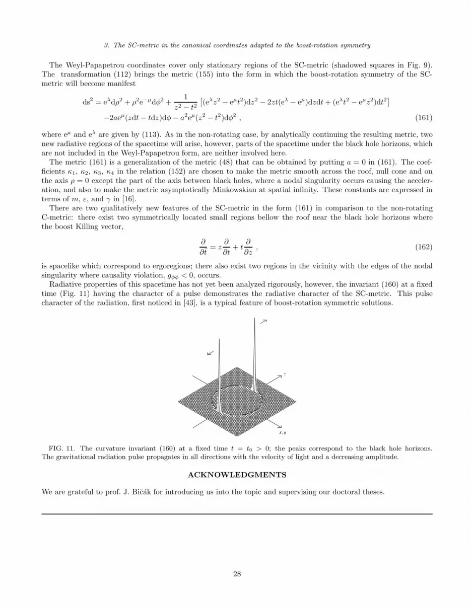
3. The SC-metric in the canonical coordinates adapted to the boost-rotation symmetry
The Weyl-Papapetrou coordinates cover only stationary regions of the SC-metric (shadowed squares in Fig. 9).The transformation (112) brings the metric (155) into the form in which the boost-rotation symmetry of the SC-metric will become manifest
ds2 = eλdρ2 + ρ2e−µdφ2 +1
z2 − t2[
(eλz2 − eµt2)dz2 − 2zt(eλ − eµ)dzdt + (eλt2 − eµz2)dt2]
−2aeµ(zdt − tdz)dφ − a2eµ(z2 − t2)dφ2 , (161)
where eµ and eλ are given by (113). As in the non-rotating case, by analytically continuing the resulting metric, twonew radiative regions of the spacetime will arise, however, parts of the spacetime under the black hole horizons, whichare not included in the Weyl-Papapetrou form, are neither involved here.
The metric (161) is a generalization of the metric (48) that can be obtained by putting a = 0 in (161). The coef-ficients κ1, κ2, κ3, κ4 in the relation (152) are chosen to make the metric smooth across the roof, null cone and onthe axis ρ = 0 except the part of the axis between black holes, where a nodal singularity occurs causing the acceler-ation, and also to make the metric asymptotically Minkowskian at spatial infinity. These constants are expressed interms of m, ε, and γ in [16].
There are two qualitatively new features of the SC-metric in the form (161) in comparison to the non-rotatingC-metric: there exist two symmetrically located small regions bellow the roof near the black hole horizons wherethe boost Killing vector,
∂
∂t= z
∂
∂t+ t
∂
∂z, (162)
is spacelike which correspond to ergoregions; there also exist two regions in the vicinity with the edges of the nodalsingularity where causality violation, gφφ < 0, occurs.
Radiative properties of this spacetime has not yet been analyzed rigorously, however, the invariant (160) at a fixedtime (Fig. 11) having the character of a pulse demonstrates the radiative character of the SC-metric. This pulsecharacter of the radiation, first noticed in [43], is a typical feature of boost-rotation symmetric solutions.
x; yz
FIG. 11. The curvature invariant (160) at a fixed time t = t0 > 0; the peaks correspond to the black hole horizons.The gravitational radiation pulse propagates in all directions with the velocity of light and a decreasing amplitude.
ACKNOWLEDGMENTS
We are grateful to prof. J. Bicak for introducing us into the topic and supervising our doctoral theses.
28

[1] A. Ashtekar and B. G. Schmidt, Null infinity and Killing fields, J. Math. Phys. 21, 862 (1980).[2] J. Bicak, Radiative spacetimes: exact approaches, in Relativistic Gravitation and Gravitational Radiation, Proceedings of
the Les Houches School of Physics, eds. J.-A. Marck and J.-P. Lasota (Cambridge University Press, Cambridge, 1995), 67(1995).
[3] J. Bicak, Selected solutions of Einstein’s field equations: their role in general relativity and astrophysics, in “Einstein’sField Equations and Their Physical Meaning”, ed. B. G. Schmidt, Springer Verlag, Berlin – New York (2000).
[4] J. Bicak, Exact radiative spacetimes, some recent developments, to appear in Ann. Phys. (Germany), (2000).[5] J. Bicak and B. G. Schmidt, Isometries compatible with gravitational radiation, J. Math. Phys. 25, 600 (1984).[6] J. Bicak and A. Pravdova, Symmetries of asymptotically flat electrovacuum space-times and radiation, J. Math. Phys. 39,
6011 (1998).[7] J. Bicak, P. Reilly, and J. Winicour, Boost-rotation symmetric gravitational null cone data, Gen. Rel. Grav. 20, 171 (1988).[8] R. Gomez, P. Papadopoulos, and J. Winicour, Null cone evolution of axisymmetric vacuum spacetimes, J. Math. Phys. 35,
4184 (1994).[9] M. Alcubierre, C. Grundlach and F. Siebel, Integration of geodesics as a testbed for comparing exact and numerically
generated spacetimes, in Abstr. 15th Int. Conf. on Gen. Rel. Grav., Pune, 83 (1997).[10] T. Levi-Civita, ds2 einsteiniani in campi newtoniani, Rend. Acc. Lincei 27, 343 (1918).[11] H. Weyl, Bemerkung uber die axisymmetrischen losungen der Einsteinschen Gravitationsgleinchungen, Ann. Phys. (Ger-
many) 59, 185 (1919).[12] W. B. Bonnor and N. S. Swaminarayan, An exact solution for uniformly accelerated particles in general relativity, Z. Phys.
177, 240 (1964); see alsoW. Israel and K. A. Khan, Collinear particles and Bondi dipoles in general relativity, Nuovo Cim. 33, 331 (1964).
[13] J. Bicak, C. Hoenselaers, and B. G. Schmidt, The solutions of the Einstein equations for uniformly accelerated particles
without nodal singularities. II. Self-accelerated particles, Proc. Roy. Soc. Lond. A 390, 411 (1983).[14] W. Kinnersley and M. Walker, Uniformly Accelerating Charged Mass in General Relativity, Phys. Rev. D 2, 1359 (1970).[15] J. F. Plebanski and M. Demianski, Rotating, charged and uniformly accelerating mass in general relativity, Ann. Phys.
(USA) 98, 98 (1976).[16] J. Bicak and V. Pravda, Spinning C-metric as a boost-rotation symmetric radiative spacetime, Phys. Rev. D 60, 044004
(1999).[17] F. J. Ernst, Generalized C-metric, J. Math. Phys. 19, 1986 (1978).[18] F. J. Ernst, Removal of the nodal singularity of the C-metric, J. Math. Phys. 17, 515 (1976).[19] J. Bicak and B. G. Schmidt, Asymptotically flat radiative space-times with boost-rotation symmetry: The general structure,
Phys. Rev. D 40, 1827 (1989).[20] H. Bondi, M. G. J. van der Burg, and A. W. K. Metzner, Gravitational waves in general relativity VII. Waves from
axi-symmetric isolated systems, Proc. Roy. Soc. Lond. A 269, 21 (1962).[21] R. K. Sachs, Gravitational waves in general relativity VIII. Waves in asymptotically flat space-time, Proc. Roy. Soc. Lond.
A 270, 103 (1962).[22] M. G. J. van der Burg, Gravitational waves in general relativity X. Asymptotic expansions for the Einstein-Maxwell field,
Proc. Roy. Soc. Lond. A 310, 221 (1969).[23] U. von der Gonna and D. Kramer, Pure and gravitational radiation, Class. Quantum Grav. 15, 215 (1998).[24] P. T. Chrusciel, M. A. H. MacCallum, and D. B. Singleton, Gravitational waves in general relativity XIV. Bondi expansions
and the ‘polyhomogeneity’ of J , Philos. Trans. R. Soc. A 350, 113 (1995).[25] R. Wald, General Relativity, The University of Chicago Press, Chicago (1984).[26] A. Ashtekar, J. Bicak, and B. G. Schmidt, Asymptotic structure of symmetry-reduced general relativity, Phys. Rev. D 55
669, (1997).[27] M. G. J. van der Burg, Gravitational waves in general relativity IX. Conserved quantities, Proc. Roy. Soc. Lond. A 294,
112 (1966).[28] A. Pravdova, Symmetries of asymptotically flat spacetimes and radiation, Ph.D. thesis, Department of Theoretical Physics,
Charles University, Prague (1999).[29] J. Bicak and A. Pravdova, Axisymmetric electrovacuum spacetimes with a translational Killing vector at null infinity,
Class. Quantum Grav. 16, 2023 (1999).[30] J. A. Valiente Kroon, On Killing vector fields and Newman-Penrose constants, J. Math. Phys. 41, 898 (2000).[31] J. Bicak, Axisymmetric asymptotically flat radiative space-times with another symmetry: the general definition and com-
ments, in “Conference on Math. Relativity”, ed. R. Bartnik, Proc. of the Centre for Mathem. Analysis, Vol. 19, AustralianNat. Univ., Canberra (1989).
[32] J. Bicak, On exact radiative solutions representing finite sources, in Galaxies, axisymmetric systems and relativity, ed. M.A. H. MacCallum, Cambridge University Press, Cambridge (1985).
[33] A. Einstein and N. J. Rosen, On gravitational waves, J. Franklin Inst. 223, 43 (1937).[34] D. Kramer, H. Stephani, E. Herlt, and M. MacCallum, Exact solutions of Einstein’s field equations, Cambridge University
Press, Cambridge (1980).[35] H. Friedrich, On the existence of n-geodesically complete or future complete solutions of Einstein’s field equations with
smooth asymptotic structure, Commun. Math. Phys. 107, 587 (1986).
29

[36] C. Cutler and R. M. Wald, Existence of radiating Eistein-Maxwell solutions which are C∞ on all of J+ and J−, Class.Quantum Grav. 6, 453 (1989).
[37] D. Christodoulou and S. Klainerman, The non linear stability of the Minkowski spacetime, Princeton University Press,Princeton (1994).
[38] J. Bicak, C. Hoenselaers, and B. G. Schmidt, The solutions of the Einstein equations for uniformly accelerated particles
without nodal singularities. I. Freely falling particles in external fields, Proc. Roy. Soc. Lond. A 390, 397 (1983).[39] S. W. Hawking, G. T. Horowitz, and S. F. Ross, Entropy, area, and black hole pairs, Phys. Rev. D 51, 4302 (1995).[40] J. Bicak, The motion of a charged black hole in an electromagnetic field, Proc. Roy. Soc. Lond. A 371, 429 (1980).[41] M. Born, Ann. Phys. (Germany) 30, 1 (1909).[42] F. Rohrlich, Classical charged particles, Addison-Wesley, Reading, Mass. (1965).[43] J. Bicak, Gravitational radiation from uniformly accelerated particles in general relativity, Proc. Roy. Soc. Lond. A 302,
201 (1968).[44] J. Bicak and R. Muschall, Electromagnetic fields and radiation patterns from multipoles in hyperbolic motion, Wiss. Z.
Univ. Jena 39, 15 (1990).[45] V. Pravda, Exact radiative spacetimes: selected problems, Ph.D. thesis, Department of Theoretical Physics, Charles Uni-
versity, Prague (1999).[46] V. Pravda and A. Pravdova, Uniformly accelerated sources in electromagnetism and gravity, in Proceedings of the week of
postgraduate students, Faculty of mathematics and physics, Charles university, Prague 1998, and gr-qc/9806114 (1998).[47] W. Pauli, Relativitatstheorie, Leipzig, Teubner (1918).[48] M. Laue, Relativitatstheorie, Braunschweig, Vieweg (1919).[49] A. K. Singal, The Equivalence principle and an electric charge in a gravitational field II. A uniformly accelerated charge
does not radiate, Gen. Rel. Grav. 29, 1371 (1997).[50] S. Parrot, Radiation from a charge uniformly accelerated for all time, Gen. Rel. Grav. 29, 1463 (1997).[51] A. Harpaz and N. Soker, Radiation from a uniformly accelerated charge, Gen. Rel. Grav. 30, 1217 (1998).[52] H. Bondi, Negative mass in general relativity, Rev. mod. Phys. 29, 423 (1957).[53] J. Bicak, Radiative properties of space-times with the axial and boost symmetries, in Gravitation and Geometry, eds. W.
Rindler and A. Trautman, Gravitation and Geometry, Bibliopolis, Naples (1987).[54] J. Bicak and B. G. Schmidt, On the asymptotic structure of axisymmetric radiative spacetimes, Class. Quantum Grav. 6,
1547 (1989).[55] J. Ehlers and W. Kundt, Exact solutions of the gravitational field equations, in: Gravitation: an introduction to current
research, ed. L. Witten, Wiley, New York, London (1962).[56] I. Robinson and A. Trautman, Some spherical gravitational waves in general relativity, Proc. Roy. Soc. Lond. A 265, 463
(1962).[57] W. Kinnersley and M. Walker, Uniformly accelerating charged mass in General Relativity, Phys. Rev. D 2, 1359 (1970).[58] A. Ashtekar and T. Dray, On the existence of solutions to Einstein’s equation with non-zero Bondi-news, Comm. Phys. 79,
581 (1981).T. Dray, On the asymptotic flatness of the C metrics at spatial infinity, Gen. Rel. Grav. 14, 109 (1982).T. Dray, The asymptotic structure of a family of Einstein-Maxwell solutions, Ph.D. Thesis, University of California,Berkeley (1981).
[59] H. Farhoosh and R. L. Zimmerman, Stationary charged C-metric, J. Math. Phys. 20, 2272 (1979).H. Farhoosh and R. L. Zimmerman, Killing horizons and dragging of the inertial frame about a uniformly accelerating
particle, Phys. Rev. D 21, 317 (1980).H. Farhoosh and R. L. Zimmerman, Surfaces of infinite red-shift around a uniformly accelerating and rotating particle,Phys. Rev. D 21, 2064 (1980).R. L. Zimmerman and H. Farhoosh, Apparent violation of the Principle of Equivalence and Killing Horizons, Gen. Rel.Grav. 12, 935 (1980).H. Farhoosh and R. L. Zimmerman, Interior C-metric, Phys. Rev. D 23, 299 (1981).
[60] W. B. Bonnor, The sources of the vacuum C-metric, Gen. Rel. Grav. 15, 535 (1983).[61] W. B. Bonnor, The C-metric with m = 0, e 6= 0, Gen. Rel. Grav. 16, 269 (1984).[62] F. H. J. Cornish and W. J. Uttley, The interpretation of the C metric. The Vacuum case, Gen. Rel. Grav. 27, 439 (1995).
F. H. J. Cornish and W. J. Uttley, The interpretation of the C metric. The charged case when e2 ≤ m2, Gen. Rel. Grav.27, 735 (1995).
[63] W. Yongcheng, Vacuum C-metric and the metric of two superposed Schwarzschild black holes, Phys. Rev. D 55, 7977(1997).
[64] C. G. Wells, Extending the black hole uniqueness theorems I. Accelerating black holes: The Ernst Solution and C-metric,gr-qc/9808044 (1998).
[65] P. S. Letelier and S. R. Oliveira, On Uniformly Accelerated Black Holes, gr-qc/9809089 (1998).[66] J. Bicak, C-metric, unpublished.
30


