Embed Size (px)
Citation preview
1
Sanco/13144/2010, version 3, 10 October 2014
Assessing Potential for Movement of
Active Substances and their Metabolites
to Ground Water in the EU
The Final Report of the Ground Water Work Group of FOCUS
(FOrum for the Co-ordination of pesticide fate models and their USe)
Contributors: J J T I Boesten, R Fischer, B Gottesbüren, K Hanze,
A Huber, T Jarvis, R L Jones, M Klein, M Pokludová,
B Remy, P Sweeney, A Tiktak, M Trevisan,
M Vanclooster, J Vanderborght
Updated by EFSA at the request of the European Commission to incorporate
pertinent aspects of the EFSA PPR panel opinions on version 1 of
13 June 2009.
2
DISCLAIMER AND IMPLEMENTATION
This document has been conceived as a working document of the Commission Services,
which was elaborated in co-operation with the Member States and examined by the
European Food Safety Authority which provided its scientific opinion on the matter. It does
not intend to produce legally binding effects and by its nature does not prejudice any
measure taken by a Member State within the implementation prerogatives under Regulation
(EC) No 1107/2009, nor any case law developed with regard to this provision. This document
also does not preclude the possibility that the European Court of Justice may give one or
another provision direct effect in Member States.
This document shall apply to applications submitted as from 1 May 2015.
FINAL COMMENTS RAISED BY MEMBER STATES
Comments from Germany on 17 September 2014
Comment to the uptake factor
FOCUS Groundwater II report May 2014, chapter 7.1, table 7-1, section 7.1.7 and FOCUS
Groundwater II Generic guidance V2.2, chapter 2.4, point 2.4.4:
We do not agree with the recommendation that the uptake factor should be estimated by
Briggs equation using the log Kow value. The Briggs equation to derive uptake factors was not
considered as state-of-the-art to predict PUF values:
As discussed also at the EU PUF workshop (2nd September 2013 in York) the study of
Briggs on TSCF values in barley is not up-to-date and is applicable to non-ionic substances
applied in barley, only.
The Briggs equation may not be applicable for all substances, crop combinations or
experimental conditions as documented in several studies due to the high variability of
uptake factors found for substances having a similar log Kow in different crops. This indicates
that the uptake factor is not only characteristic for a substance (log Kow, pKa) but also
depends on the experimental conditions (duration of exposure, temperature, pH of the pore
water and nutrient solution in the experiment, respectively) and the crop (content of lipid,
fiber, and carbohydrate of roots and shoots; root system).
3
Due to the currently existing uncertainties regarding the Briggs equation, we recommend that
the value for an uptake factor should be set at zero for all substances (active ingredient and
metabolites, ionic and non-ionic), unless appropriate experimental data are available. As it is
difficult to derive accurate values for plant uptake factors with experimental data, we suggest
to limit the plant uptake factor to 0.5 in general.
Comments from Germany on 7 October 2014
Due to the erroneous calculation of the plant uptake factor by using the log Kow there is a
danger to significantly underestimate the input of active substances into the groundwater.
We therefore propose the following changes to the FOCUS Report:
Table 7-1, line 7.1.7 Plant uptake, last column:
Please change wording to:
“Currently TSCF should be set at 0-0.5 depending on substance properties or experimental
data calculated from log Kow measurement. In future harmonised experimental data might
be an further option.”
Chapter 7.1.7 Plant uptake:
Please add the underlined sentence at the end of the chapter:
The default plant uptake factors (i.e. the transpiration stream concentration factor) can be
adjusted to measured values if substance specific uptake factors have been determined in
appropriate experiments with the crops species being assessed. In the absence of agreed
EU guidance on what the appropriate experiments to measure the transpiration stream
concentration factor should be, applicants should contact competent authorities to see what
study design (if any) they would consider appropriate. See also considerations in EFSA PPR,
2013b. However a calculation of the TSCF from logKow using the Briggs equation considers
not the state-of-the-art to predict the plant uptake and is not applicable for ground water risk
assessment.
Comments from Sweden on 26 September 2014
We have reservations regarding the recommendations made to take “Aged sorption” into
account, especially considering later publications on this topic, and the lack of an EFSA
opinion specifically addressing these recommendations.
4
Furthermore, we do not agree to consider monitoring data as the highest tier, taking
precedence over other relevant data. Monitoring data can be useful at all tiers, and should
preferably be considered together with all other available data in a weight of evidence
approach.
Finally, we would like to support DE regarding their suggestion to limit the use of plant uptake
factor to 0.5. If there is experimental data that show plant uptake than a value of 0.5 can be
used. However the actual experimental value should not be used. Regarding the use of the
Briggs equation we have no comments.
ACKNOWLEDGEMENTS
The authors would like to thank all those people outside of the work group who assisted in
this work by providing data or performing evaluations.
CITATION
Those wishing to cite this report are advised to use the following form for the citation:
European Commission (2014) “Assessing Potential for Movement of Active Substances and
their Metabolites to Ground Water in the EU” Report of the FOCUS Ground Water Work
Group, EC Document Reference Sanco/13144/2010 version 3, 613 pp.
5
FOREWORD BY THE FOCUS STEERING COMMITTEE (updated by
EFSA)
Since its beginning in 1993, FOCUS (FOrum for the Co-ordination of pesticide fate models
and their USe) has established a number of work groups to develop procedures for
estimating concentrations of plant protection products and their metabolites in various
environmental compartments (ground water, surface water, soil, sediment, and air) and for
performing kinetic analyses. The procedures for assessing potential movement to ground
water became effective in December 2000 and have been used since then as part of the EU
registration process. A few years after the release of the scenarios, scientific progress in the
field of leaching models as well as experience with the use of the scenarios resulted in
questions being raised regarding changes to the scenarios, harmonisation of the different
leaching models, the role of more advanced assessment approaches (for example, graphical
information systems and non-equilibrium sorption), how to use the results of simulations and
experimental studies (lysimeter and field studies) in the assessment, and the coverage of
new EU member states by the FOCUS scenarios. Therefore FOCUS established a work
group of experts from regulatory authorities, research institutes, and industry to develop
revised scenarios and an overall framework for assessing leaching potential. This FOCUS
group met as a whole 16 times between February 2004 and June 2008 and also many times
in various subgroups. This report is the result of extensive deliberation on the numerous
issues that arose after conducting a survey of the opinions of the member states. The output
of the work group also includes a completely revised set of models, input and output shells,
and scenarios which became available at the FOCUS web site in April 2011. The EFSA Plant
Protection Products and their Residues (PPR) panel published opinions on version 1 of this
report in 2013. This version 2 of the report has incorporated the observations and
recommendations of the EFSA PPR panel opinions. References to the legislation have also
been updated as necessary.
The version control process does not allow access to the models for regulatory use prior to
their official release date. Therefore, the FOCUS Steering Committee recommended the
revised models could be used for leaching assessments immediately after release, but that
registrants may use the models released in 2000 for submissions up to one year following
the release of these models on the FOCUS web site, i.e. April 2012.
One of the specific details in the remit of the work group was that the revision of the
scenarios would include harmonisation of the models (dispersion length, water balance, etc.).

6
This effort was largely successful and the Steering Committee recommended that the ground
water assessments could be performed with any of the models (PEARL, PELMO, and
PRZM) and there was no need to perform the assessments with more than one model.
However the EFSA PPR panel opinion identified that particularly for non irrigated crops
PEARL and PELMO provide very different results at the Sevilla scenario. Therefore in line
with EFSA PPR (2013a), applicants and rapporteurs are advised that they should again
provide simulations with PEARL and PELMO or PRZM. Where a crop of interest is defined
for Châteaudun, MACRO simulations need to be run (EFSA PPR, 2013a).
7
Table of Contents
Executive Summary 13
1 Introduction 29 1.1 References .............................................................................................................. 30
2 Glossary 32
3 Introduction to Assessment Schemes for PEC in Ground Water 39 3.1 Objectives of the risk assessment for ground water contamination at EU and
national levels .......................................................................................................... 39 3.1.1 European level ............................................................................................. 39 3.1.2 National level................................................................................................ 40
3.2 Review of existing guidance on EU and national level ............................................. 41 3.2.1 Guidance given in EU and FOCUS documents ............................................ 41
3.2.1.1 Binding requirements in directives ................................................. 41 3.2.1.2 EU guidance documents ............................................................... 42 3.2.1.3 FOCUS guidance documents ........................................................ 44
3.2.2 Review of existing national approaches for leaching assessments ............... 45 3.2.2.1 The structure of and type of questions in the questionnaire ........... 45 3.2.2.2 Summary of questions and answers divided into the main topics. . 46
3.2.2.2.1 General questions ......................................................... 46 3.2.2.2.2 Regulatory questions .................................................... 47 3.2.2.2.3 Specific questions on scenarios .................................... 48 3.2.2.2.4 Model used ................................................................... 50 3.2.2.2.5 Parameterisation ........................................................... 50 3.2.2.2.6 Additional experimental data ......................................... 52 3.2.2.2.7 Interrelationship between models and higher tier
experiments .................................................................. 53 3.2.2.2.8 Handling of metabolites ................................................. 53
3.3 References .............................................................................................................. 53
4 Generic Assessment Scheme for PEC in Ground Water (General Overview) 55 4.1 Assessment of the representativeness, scope and limitations and usability of different
study types .............................................................................................................. 55 4.1.1 Relevance of experimental and modeling studies ......................................... 55 4.1.2 Study types for leaching assessment ........................................................... 56
4.2 General principles of a generic assessment scheme for PEC in ground water on EU and national level ............................................................................................... 57
4.3 Proposal for a generic tiered approach .................................................................... 59 4.3.1 Tier 1 at EU and National Level .................................................................... 60 4.3.2 Tier 2 approaches (Tiers 2a and 2b) at EU and National level ...................... 61
4.3.2.1 Modelling with refined parameters (Tier 2a) .................................. 61 4.3.2.2 Modelling using refined scenarios (Tier 2b) ................................... 62
4.3.3 Tier 3 leaching assessment .......................................................................... 63 4.3.3.1 Tier 3a: Combination of modelling with refined parameters and
refined scenarios ........................................................................... 63 4.3.3.2 Tier 3b: Advanced spatial modelling .............................................. 63 4.3.3.3 Tier 3c: Higher tier leaching experiments set into context by
modelling ....................................................................................... 64 4.3.3.4 Tier 3d: Other modelling approaches ............................................ 65
4.3.4 Tier 4 (Monitoring) ........................................................................................ 66 4.4 References .............................................................................................................. 66
5 Interactions between Assessment Schemes on EU and on National Level 69 5.1 General interactions between the assessment schemes .......................................... 69
8
5.2 Preferential flow in EU and national assessment schemes ...................................... 70
6 Consideration of Risk Mitigation and Management on EU and on National Level 73 6.1 Important aspects affecting or used in risk mitigation ............................................... 73
6.1.1 The GAP in the EU evaluation of active substances relative to the GAP on a national level ............................................................................................. 73
6.1.2 Dose related risk mitigation .......................................................................... 74 6.1.3 Using more effective application methods .................................................... 74 6.1.4 Pesticide properties correlated to soil properties .......................................... 75 6.1.5 Hydrogeological properties ........................................................................... 75 6.1.6 Mitigation related to timing............................................................................ 76
6.2 Examples of risk mitigation measures ...................................................................... 76 6.3 Conclusion ............................................................................................................... 77
7 Approaches for Tier 2 Assessment 78 7.1 Pesticide parameter refinement (Tier 2a) ................................................................. 78
7.1.1 Soil specific sorption and degradation .......................................................... 80 7.1.1.1 Degradation parameters and soil properties .................................. 81 7.1.1.2 Sorption parameters and soil properties ........................................ 81
7.1.1.2.1 MACRO .................................................................... 81 7.1.1.2.2 PEARL .................................................................... 81 7.1.1.2.3 PELMO .................................................................... 81 7.1.1.2.4 PRZM .................................................................... 82
7.1.2 Photolytic degradation .................................................................................. 82 7.1.3 Soil specific anaerobic degradation .............................................................. 83 7.1.4 Use of field dissipation degradation rates in leaching models ....................... 84 7.1.5 Degradation kinetics that deviate from first order .......................................... 85 7.1.6 Non-equilibrium sorption .............................................................................. 85
7.1.6.1 Models for describing non-equilibrium sorption .............................. 86 7.1.6.1.1 PEARL .................................................................... 86 7.1.6.1.2 The model of Streck ...................................................... 88 7.1.6.1.3 MACRO .................................................................... 89 7.1.6.1.4 PRZM and PELMO ....................................................... 90
7.1.6.2 Experimental procedures for measuring long-term sorption kinetics and procedures for estimating the model parameters ....... 90
7.1.6.3 Overview of available measurements of long-term sorption parameters .................................................................................... 93
7.1.6.4 Recommended default values for long-term sorption parameters in risk assessment ......................................................................... 96
7.1.6.5 Fitting of aged sorption measurements to long-term kinetic sorption parameters ...................................................................... 96
7.1.6.6 Consequence of using non-equilibrium sorption for the degradation rate to be used in simulation models .......................... 98
7.1.7 Plant uptake ............................................................................................... 102 7.1.8 Volatilisation ............................................................................................... 102
7.2 Scenario refinement (Tier 2b) ................................................................................ 102 7.2.1 Modification of crop parameters ................................................................. 103 7.2.2 Introduction of realistic crop rotations ......................................................... 104 7.2.3 Introduction of new crops ........................................................................... 104 7.2.4 Specific use conditions (e.g. greenhouse scenario) .................................... 104 7.2.5 Defining use specific scenarios (e.g. use of GIS) ....................................... 105
7.2.5.1 Steps in applying use-specific scenarios ..................................... 106 7.2.5.1.1 Data compilation, check for suitability and data quality 106 7.2.5.1.2 Vulnerability mapping using a simplified leaching
concept .................................................................. 107 7.2.5.1.3 Scenario selection ....................................................... 108
9
7.2.5.1.4 Scenario parameterisation .......................................... 108 7.2.5.1.5 Simulation with a FOCUS leaching model ................... 108 7.2.5.1.6 Precautionary remark .................................................. 108
7.2.5.2 Detailed guidance ....................................................................... 109 7.2.5.2.1 Data compilation and quality check ............................. 109 7.2.5.2.2 Vulnerability mapping using a simplified leaching
concept .................................................................. 109 7.2.5.2.3 Scenario selection ....................................................... 112 7.2.5.2.4 Scenario parameterisation .......................................... 112
7.2.5.2.4.1 Meteorological time-series 113 7.2.5.2.4.2 Cropping parameters 113 7.2.5.2.4.3 Irrigation 113 7.2.5.2.4.4 Lower boundary conditions 114 7.2.5.2.4.5 Hydraulic balance 114 7.2.5.2.4.6 Soil parameters 115
7.2.5.2.5 Simulation with a FOCUS leaching model ................... 117 7.3 References ............................................................................................................ 117
8 Approaches for Tier 3 Assessment 125 8.1 Procedures for combining modelling based on refined parameters and scenarios
(Tier 3a) ................................................................................................................. 125 8.2 Procedures for building a spatially-distributed FOCUS leaching model (Tier 3b) .... 125
8.2.1 Justification for spatially-distributed modelling ............................................ 126 8.2.2 Development of a spatially distributed FOCUS leaching model .................. 128
8.2.2.1 Selection of an appropriate leaching model ................................. 128 8.2.2.2 Review of existing databases ...................................................... 128 8.2.2.3 Development of a spatial schematisation .................................... 129 8.2.2.4 Model parameterisation ............................................................... 132
8.2.2.4.1 Meteorological time-series .......................................... 132 8.2.2.4.2 Cropping parameters .................................................. 134 8.2.2.4.3 Irrigation .................................................................. 134 8.2.2.4.4 Lower boundary conditions and runoff......................... 135 8.2.2.4.5 Soil parameters ........................................................... 135
8.2.2.4.5.1 Selection of a soil profile 135 8.2.2.4.5.2 Parameterisation of basic soil data 137 8.2.2.4.5.3 Parameterisation of derived soil data using
pedotransfer rules 137 8.2.2.4.6 Pesticide properties and application scheme............... 138
8.2.2.5 Running the FOCUS leaching model and plotting the results in a map .......................................................................................... 138
8.2.2.6 Calculation of the target quantity ................................................. 139 8.2.3 Stochastic assessments ............................................................................. 140
8.3 Higher tier leaching experiments set into context by modelling (Tier 3c) ................ 141 8.3.1 Study types and their applicability for different agroclimatic conditions ....... 142
8.3.1.1 Lysimeters ................................................................................... 142 8.3.1.2 Field leaching experiments .......................................................... 144
8.3.2 Current status of higher tier leaching experiments in national regulation and appropriate guidelines ......................................................................... 145
8.3.3 Suitability for exposure assessment within FOCUS framework – “pre-processing” aspects ................................................................................... 147 8.3.3.1 Determining adequate vulnerability – through study design ......... 147
8.3.3.1.1 Lysimeters .................................................................. 147 8.3.3.1.1.1 Soil type 148 8.3.3.1.1.2 Duration 151 8.3.3.1.1.3 Replication 153 8.3.3.1.1.4 Scale and uncertainty 154
10
8.3.3.1.2 Field Leaching Studies ................................................ 155 8.3.3.2 Determining adequate vulnerability – through location selection . 155
8.3.4 Post processing approaches for higher tier experimental leaching data ..... 155 8.3.4.1 Introduction ................................................................................. 155 8.3.4.2 Proposed inverse modelling procedure for lysimeter studies ....... 158 8.3.4.3 Further use of inversely modelled lysimeter DegT50 values in
the leaching assessment ............................................................. 161 8.3.4.4 Further use of inversely modelled lysimeter Kom / Koc values in
the leaching assessment ............................................................. 163 8.4 Other modelling approaches (Tier 3d) .................................................................... 164
8.4.1 Alternative models for transport of active substances in the top soil ........... 165 8.4.2 Modelling fate and transport of active substances in the partially saturated
subsoil .................................................................................................... 167 8.4.3 Modelling fate and transport of active substances in the soil and ground
water continuum ......................................................................................... 168 8.4.4 Statistical modelling of monitoring data ...................................................... 169
8.5 References ............................................................................................................ 169
9 Approaches for the Use of Ground Water Monitoring Data at Tier 4 179 9.1 Sources of ground water monitoring data............................................................... 180 9.2 Existing national guidance ..................................................................................... 181 9.3 FOCUS guidance for EU level ............................................................................... 182 9.4 FOCUS guidance for national level ........................................................................ 184 9.5 Quality criteria ........................................................................................................ 184 9.6 References ............................................................................................................ 185
10 Guidelines for Reporting of Higher Tier Leaching Assessments 187 10.1 Description of assessment ..................................................................................... 187 10.2 Data and input parameters .................................................................................... 187 10.3 Components of a higher tier assessment ............................................................... 188 10.4 References ............................................................................................................ 189
11 Review and Changes to Existing FOCUS Ground Water Scenarios and Calculation Procedures 190 11.1 Proposal of a vulnerability concept for FOCUS scenarios ...................................... 190 11.2 Determining the 80th percentile weather concentration ........................................... 192 11.3 Review of the Porto and Piacenza FOCUS ground water scenarios ...................... 192 11.4 Harmonisation of dispersion lengths ...................................................................... 192 11.5 Harmonisation of the water balance ....................................................................... 194
11.5.1 Calculation procedure for evapotranspiration ............................................. 194 11.5.1.1 Comparison of MARS and FAO reference evapotranspiration ..... 194 11.5.1.2 Estimated crop kc factors ............................................................ 194 11.5.1.3 Evaporation from bare soil........................................................... 195 11.5.1.4 Adjustment of the rooting depths of some crops .......................... 197
11.5.2 Review of procedure to estimate runoff ...................................................... 197 11.5.3 Review of estimation of the irrigated amounts of water ............................... 199
11.6 Soil pH values in FOCUS scenarios ....................................................................... 200 11.7 Review of procedure for estimating interception of pesticide by plants ................... 201 11.8 References ............................................................................................................ 201
12 Comparison of Current and Revised Scenarios 204 12.1 Results of comparison simulations ......................................................................... 204 12.2 Conclusion ............................................................................................................. 218 12.3 References ............................................................................................................ 219
13 Applicability of FOCUS Ground Water Scenarios To the New Member States 220 13.1 Introduction ............................................................................................................ 220
13.1.1 Objective of this study ................................................................................ 220 13.1.2 Limitations .................................................................................................. 220
11
13.2 Materials and methods ........................................................................................... 221 13.2.1 Data sources .............................................................................................. 221
13.2.1.1 Climate data ................................................................................ 221 13.2.1.2 Soil texture .................................................................................. 223 13.2.1.3 Organic carbon content in topsoil ................................................ 224 13.2.1.4 Land use .................................................................................... 224
13.2.2 Original classification of agricultural zones by FOCUS (2000) .................... 225 13.2.2.1 Climate .................................................................................... 225 13.2.2.2 Soil properties ............................................................................. 228 13.2.2.3 Crops .................................................................................... 230
13.2.3 Criteria used for the assessment of scenarios ............................................ 232 13.3 Results and discussion .......................................................................................... 234
13.3.1 Coverage of Accession countries by existing FOCUS scenarios ................ 236 13.3.1.1 Estonia .................................................................................... 236 13.3.1.2 Latvia .................................................................................... 236 13.3.1.3 Lithuania .................................................................................... 236 13.3.1.4 Poland .................................................................................... 237 13.3.1.5 Czech Republic ........................................................................... 237 13.3.1.6 Slovakia .................................................................................... 237 13.3.1.7 Hungary .................................................................................... 237 13.3.1.8 Slovenia .................................................................................... 237 13.3.1.9 Malta .................................................................................... 243 13.3.1.10 Cyprus .................................................................................... 243
13.3.2 Conclusions on the applicability of FOCUS scenarios to new member states .................................................................................................... 243
13.3.3 Areas for which further analysis is needed ................................................. 243 13.4 Conclusions ........................................................................................................... 246 13.5 References ............................................................................................................ 246
Appendix 1. Questionnaire Sent to Member States 248
Appendix 2. Reponses to the Questionnaire 261
Appendix 3. FOCUS Ground Water Study Information Tables 302
Appendix 4: A Method to Derive Crop-Specific Leaching Scenarios 310
Appendix 5. A Tiered Approach to Spatially Distributed Modelling 334
Appendix 6. Example Application of Non-equilibrium Sorption 381
Appendix 7. Example Calculation of DegT50eq from a Laboratory Degradation Rate Study Based on Default Values of the Non-equilibrium Sorption Parameters 406
Appendix 8. Fact Sheets for Regional Data 413
Appendix 9. Comparison of the MetaPEARL and Index Method for Higher Tier Spatial Modelling 440
Appendix 10. The Principles of Inverse Modelling 453
Appendix 11. Example of Parameter Adjustment by Inverse Modelling 460
Appendix 12. Theoretical Basis for a Vulnerability Concept 470
Appendix 13. Review of Procedure for Selecting the 80th Percentile Concentration from a Time Series of Concentrations 474
Appendix 14. Averaging of Simulations without Annual Applications 477
Appendix 15. Review of the Porto and Piacenza FOCUS Ground Water Scenarios 479
Appendix 16. Literature Review of Dispersivity Values 486
Appendix 17. Dispersivity in the FOCUS Models 526
Appendix 18. Comparison of MARS and FAO Potential Reference Evapotranspiration 542
Appendix 19. Procedures for Estimating Crop Evaopotranspiration Factors 547

12
Appendix 20. Definition of the FOCUS Scenarios 549
Appendix 21. Calibration of Evapotranspiration at Piacenza, Sevilla, and Thiva 569
Appendix 22. Irrigation Data 572
Appendix 23. Results of Simulations Comparing the Current and the Proposed Scenarios 576
Appendix 24. Review of Procedure for Estimating Interception of Pesticide by Plants 597
Appendix 25. Comparison of Different Object Functions for the Evaluation of Kinetic Sorption Experiments 603

13
EXECUTIVE SUMMARY
Why is the work of the FOCUS Ground Water Work Group important?
The EU approval and national authorisation processes under Regulation (EC) 1107/2009
require the assessment of the potential of an active ingredient and its metabolites to move to
ground water. An earlier FOCUS work group developed a series of ground water leaching
scenarios, which were the basis for the first tier of the EU assessment procedure beginning
in 2000. Since that time a number of questions had arisen concerning these scenarios. Also
this earlier work group did not provide overall guidance for higher tiers of the entire
assessment scheme (field and monitoring studies, lysimeter studies and higher tier modelling
approaches).
The current work group has developed a tiered approach for conducting these assessments,
which includes the relative roles of modelling, field experiments, and monitoring and
incorporates higher tier modelling approaches such as geographical information systems
(GIS) and non-equilibrium sorption.
The work group also has carefully assessed the original scenarios and made changes to
harmonise differences between models and to make processes as realistic as possible. For
example, soil parameters have been adjusted for two of the original locations, crop kc factors
changed for all scenarios, runoff eliminated in all scenarios, and new irrigation schedules
generated for all irrigated crops.
Finally the EU has significantly grown in size since the original scenarios were issued in
2000. Therefore, whether new scenarios were required to cover the agricultural areas in the
new member states needed to be assessed.
To which registration processes are the recommendations directed?
The remit of the work group included developing guidelines for assessing potential
movement to ground water under both the EU and member state registration processes. The
revised scenarios are directly applicable to EU registration. Some of member states also use
these scenarios in their national registration process or may do so in the future.

14
What are the objectives of the EU and national ground water assessments?
The assessment objectives are different for EU registration of the active ingredient (EU level
approval) and product authorisations (registrations) in the member states. Although there is
no official ground water decision scheme for EU level approval, the current practice is to
consider the number of scenarios (usually standard FOCUS definitions) demonstrating safe
use on a representative crop in a significant area of Europe, noting that a single standard
FOCUS definition scenario can be considered to represent / cover conditions in a significant
area. For national assessments, all crops and the entire potential use area must be
considered. If the compound cannot be used safely throughout the country, then the
registration may be limited by national competent authorities to the subset of conditions
under which the compound can be used safely.
What are the desired characteristics of the ground water assessment scheme?
The FOCUS work group objective was to develop a scheme in which the initial (or earlier)
tiers are quick, simple, and cheap to undertake and allow the compounds that clearly do not
cause any concern to be passed. Conceptually earlier tiers are more conservative than later
tiers, which is ensured by the choice of validated models (default assumptions) and choice of
parameters (often laboratory derived) and conservative nature of the scenarios in earlier
tiers. The later (or higher) tiers are more complex and expensive but should provide a more
realistic (less conservative) result. Therefore, results of higher tier assessments supersede
results from lower tier assessments.
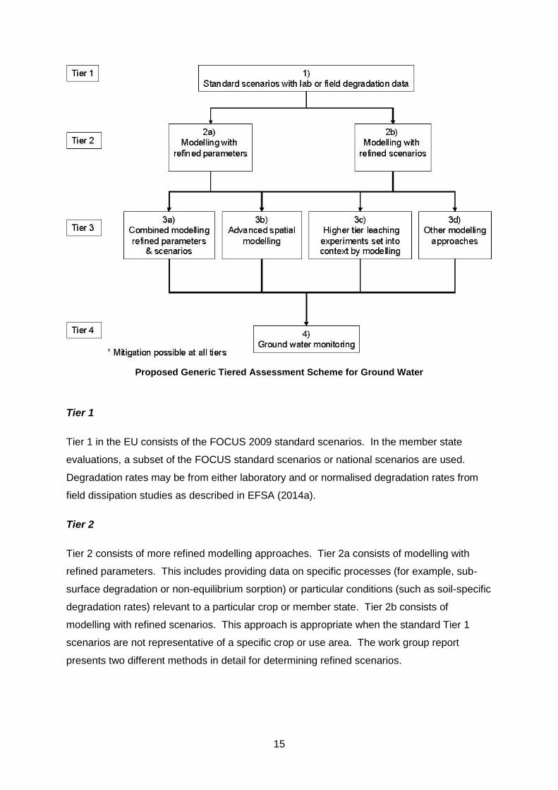
What is the work group proposing as a ground water assessment scheme?
The work group proposes the following basic scheme with four tiers. This tiered approach is
applicable to both EU and member state evaluations, even though the objectives are
different.
Where there are a number of options for a given tier, undertaking all options is not
necessary. Any single option is sufficient. However, any approaches should be justified
using all appropriate data available.
15
Proposed Generic Tiered Assessment Scheme for Ground Water
Tier 1
Tier 1 in the EU consists of the FOCUS 2009 standard scenarios. In the member state
evaluations, a subset of the FOCUS standard scenarios or national scenarios are used.
Degradation rates may be from either laboratory and or normalised degradation rates from
field dissipation studies as described in EFSA (2014a).
Tier 2
Tier 2 consists of more refined modelling approaches. Tier 2a consists of modelling with
refined parameters. This includes providing data on specific processes (for example, sub-
surface degradation or non-equilibrium sorption) or particular conditions (such as soil-specific
degradation rates) relevant to a particular crop or member state. Tier 2b consists of
modelling with refined scenarios. This approach is appropriate when the standard Tier 1
scenarios are not representative of a specific crop or use area. The work group report
presents two different methods in detail for determining refined scenarios.
16
Tier 3
Tier 3 consists of four options consisting of different modelling approaches and modelling
combined with experiments. When relevant to the proposed use pattern, Tier 3a combines
the refinements detailed in Tiers 2a and 2b to provide an assessment based on both
approaches. In Tier 3b spatially-distributed leaching models provide the user with maps of
the predicted leaching concentrations in the intended use area or in a climatic zone.
Frequency distributions and percentiles of the leaching concentration can be directly inferred
from these maps. The quality of such assessments is very much dependent on the quality
and coverage of the underlying soil profile and climatic information. Currently the uncertainty
of the soil profile information on a European scale is too high for detailed EU-wide
assessments. However, in some countries high quality data are available. Any of the
FOCUS models could be incorporated into a spatially distributed modelling framework. Note
that the PPR panel of EFSA indicated that they considered that Tier 3b modelling should be
considered a higher tier than Tiers 3a and 3c, sitting between Tiers 3a / 3c and Tier 4 (EFSA
PPR, 2013b). Tier 3c combines information from experimental studies such as lysimeter
experiments and field leaching studies. While field study measurements do not have the
limitation of the assumptions used in leaching models, the results may only be directly
relevant to the climatic, pedological and agronomic (crop, timing, application rate etc)
conditions in which the studies were conducted. The work group recommends that lysimeter
studies be incorporated into the assessment scheme by using inverse modelling to develop
estimates of input parameters such as degradation rates and sorption constants. The
parameters are then combined with measurements from other sources (for example, for
degradation rates the lysimeter results are averaged with a weight that needs to be justified
by the assessor (EFSA PPR, 2013b), (a weight of 3 was originally suggested by the FOCUS
workgroup), with the results of field dissipation studies). Then the standard scenarios are re-
run with the revised parameter. Tier 3d includes other modelling approaches (for example,
stochastic and 3-D modelling). At this time the view of the FOCUS work group is that other
modelling approaches are not sufficiently developed for regulatory use at a high tier of the
risk assessment scheme. However the work group expects that the science will develop in
the future and that current research applications may, in time be usable for regulatory
purposes.
Tier 4
Tier 4 consists of ground water monitoring data. Ground water monitoring data are seen as
the highest tier of assessment since the actual concentrations in ground water are directly
17
measured rather than being estimated by modelling approaches or approximated from small
scale lysimeter or field studies. For existing pesticides, monitoring data can be useful at both
the EU level and the national level. For instance, representative data from one member
state, if extensive, reliable and representative enough, could demonstrate a “safe use” for the
EU evaluation. For new active substances historical monitoring data are clearly not
available, but post-registration monitoring programs may be possible. Monitoring data can
include the results of dedicated analyses of ground water by notifiers or other agencies (i.e.
water companies, environment agencies etc) where there needs to be a detailed initial
assessment of the relevance of the monitoring points (for example, by knowledge of historical
compound usage in the area and characteristics of the aquifer) and when minimum quality
criteria in relation to these aspects have been demonstrated. Note the EFSA PPR panel
opinion expressed reservations whether current knowledge on groundwater hydrology at the
EU level, would be sufficient to use monitoring data to ever conclude that “safe use” might
cover an extensive area for the EU evaluation, in relation to representative EU uses (EFSA
PPR, 2013b).
Mitigation
At any tier of the assessment process, mitigation (measures taken to adjust or restrict the
use of a pesticide to reduce the risk of leaching to an acceptable level) is possible. Mitigation
measures often relate to the Good Agricultural Practice (GAP), and include crops to which a
compound can be applied, the timing/crop stage for uses on each specific crop, the
application rate, the number of applications, and the timing between applications. Other
potential mitigation measures include preventing applications on soils with certain properties
(through soil or geographical restrictions), restricting applications in hydrogeologically
vulnerable areas, and limiting applications to certain times of the year.
How have the Tier 1 scenarios been revised?
The revisions to the scenarios consisted of:
Changes to the soil profiles in Porto and Piacenza
A new procedure for calculating the leaching concentration (PECgw)
Source of potential reference evaporation data for five locations
Adding irrigation to some crops grown in Porto.
Harmonisation between models
o Harmonisation of the dispersion length
o Limiting the maximum rooting depth to 1 m
18
o Implementation of common crop kc factors for different crop periods
o Standardising the prediction of evaporation from bare soil
o Harmonising runoff by eliminating runoff in Tier 1 scenarios
o Generating crop specific irrigation schedules with PEARL and PELMO
What was the basis for the changes to the soils properties for Porto and Piacenza?
At the time that the FOCUS 2000 scenarios were established, there was a lack of high quality
and harmonised EU-wide data bases. For this reason, the original scenarios were selected
by a combination of approaches including expert judgement, locations in major agricultural
areas, and distribution of sites to cover all European climatic zones. Research conducted
after the issuing of the original scenarios indicated that scenarios at Piacenza and Porto may
not have met the desired vulnerability criteria for leaching. To revise the scenarios, the
current work group had to decide the precise vulnerability criteria for revision of these
scenarios. The criterion selected was the 80th percentile soil and 80th percentile weather for
the climatic zone represented by the respective locations. The climatic zone was defined on
the basis of the EU area with 15 member states so that the addition of member states did not
require the whole set of scenarios to be revised. In addition, the basic spatial unit for
leaching was defined as the soil mapping unit and the basic temporal unit was an annual
average for annual applications.
What were the changes to the soil properties for Porto and Piacenza?
A spatial analysis of the climatic zones represented by the Porto and Piacenza locations
indicated that a change in the organic matter was appropriate to make them fit the
vulnerability concept. The organic matter in the surface soil at Porto was decreased from 6.6
to 2.45 percent, resulting in changes to the bulk density, hydraulic properties, and the organic
matter in the deeper soil layers. The organic matter in the surface soil at Piacenza was
increased from 1.72 to 2.17 percent, along with changes to the organic matter in the deeper
soil layers.
How is the weather percentile for PECgw determined?
The previous FOCUS work group decided that the PECgw corresponding to a reasonable
worst case for leaching assessments would be approximated by an 80th percentile soil and
an 80th percentile weather. The current work group also reviewed several approaches for
determining specific percentile values and decided that the 80th percentile weather is
represented by the average of the 16th and 17th of the 20 ranked values from the simulation.
In the previous Tier 1 scenarios, the 17th ranked value was used. For applications made
19
every second or third year, FOCUS 2000 calculated the flux weighted averages for each of
the 20 two or three year periods and then selected the 80th percentile of these 20 values.
The current work group investigated taking the 80th percentile of the 40 or 60 yearly values.
Because the two methods gave similar results, the work group recommended continuing with
calculating the 80th percentile of the 20 flux weighted averages.
Why was harmonisation of the dispersion length important and how was this done?
In simulations conducted according to the procedures in the previous FOCUS work group
PEARL and MACRO used a dispersion length of 5 cm and the effective dispersion length
(set by compartment size) in PRZM and PELMO was 2.5 cm. Later work showed that the
difference in dispersion lengths was a major source of the difference between predictions of
PEARL and PELMO or PRZM. Work group members undertook several activities associated
with dispersion. First, a data base of dispersion lengths reported in the literature was
derived. This review demonstrated that dispersion increases with depth. Second, changes
in how the dispersion process is modelled in a soil profile with depth dependent sorption and
decay factors resulted in different predictions of pesticide concentrations at the bottom of the
soil profile, even when the different models predicted the same breakthrough of an inert
tracer. The pesticide fate models use a one-dimensional convection dispersion equation to
describe transport and two options to parameterise this model were discussed. The first
option assumes a constant dispersion in the entire soil profile, thereby overestimating the
leaching through the upper soil layer where most decay takes place. The second option
divided the upper meter in three layers (corresponding to the three different default
degradation factors) with increasing dispersion lengths as a function of depth, but the validity
of the process description in this approach was questioned. The work group could not come
to a consensus over which of the two approaches was preferable. However, because of the
need for harmonisation, the constant CDE approach with a dispersion length of 5 cm will be
used in the revised scenarios produced by the work group. The constant CDE approach is
the more conservative of the two approaches, at least for parent compounds.
What changes were made to harmonise the water balance predicted by the models?
Examination of these differences led to the identification of work in six areas:
the most appropriate source of reference evapotranspiration data
the importance of time varying crop kc values
adjustment of rooting depths
calculating evaporation from bare soil
20
determining appropriate amounts of runoff for each location/crop location and how to
achieve this with the different models
and developing appropriate irrigation files for each location/crop location in the
locations where irrigation is a common agricultural practice
Source of reference evapotranspiration data
FOCUS 2000 scenarios used reference evapotranspiration calculated from the MARS data
base and FAO crop coefficients. The work group examined whether FAO or MARS
referenced evapotranspiration was most appropriate. The work group decided to use FAO
reference evapotranspiration for Porto, Piacenza, Châteaudun, Thiva, and Sevilla for
consistency between the crop coefficients and evapotranspiration values. The MARS
approach to calculating reference evapotranspiration was retained for Okehampton,
Kremsmünster, Hamburg and Jokoinen because there was little difference between the two
approaches for these climatic conditions and the long wave radiation parameterisation
procedure proposed by the FAO sometimes leads to negative reference evapotranspiration
rates in northern European conditions.
Crop kc factors
A comparison of the annual potential evapotranspiration for crop and soil showed that the
different procedures within the models for implementing crop kc factors were contributing
significantly to the variability of the overall water balance. Therefore the work group decided
to harmonise the procedures by implementing a common procedure in which the year was
divided into four periods (harvest to emergence, emergence to maturity, maturity to
senescence, and senescence to harvest) and a constant kc factor was assigned to each of
the four periods. Changes have been made to the models and shells to implement this
procedure.
Adjustment of rooting depths
Because transpiration in PEARL is reduced when a substantial fraction of the roots are
located below the water table and because of the inconsistency of evaluating ground water
concentrations at a depth shallower than the root zone, the work group decided that the
maximum rooting depth would not exceed 1 m for all location/crop combinations.
Evaporation from bare soil
In the absence of a crop, evaporation from bare soil is predicted differently in the different
models. The procedure used in PEARL was used as the standard and the depth of
evaporation parameter in PELMO and PRZM has been adjusted to give approximately the
same amount of soil evaporation during the time the crop is not present.

21
Runoff
Because the work group was unable to obtain a set of crop specific European-wide data to
use as a reference for setting runoff amounts that would correspond to an agreed upon
percentile for all soils in each FOCUS climate zone, the work group decided to make the
conservative assumption of no runoff in PELMO and PRZM and to use the 24 hour storm
duration for PEARL in the Tier 1 simulations, which leads to almost no runoff in this model as
well. The work group recommends that runoff should be included in Tiers 2b and 3 in EU
evaluations and in simulations at the member state level when information on runoff amounts
is available.
22
Irrigation
The work group decided that irrigation schedules should be developed for individual crops in
Châteaudun, Piacenza, Porto, Seville, and Thiva because the current irrigation schedules
were not always consistent with the cropping season. These irrigation schedules provide
irrigation from the time of planting until senescence and are generated using irrigation
routines in PEARL and PELMO, which apply irrigation once a week on a fixed day to bring
the root zone up to field capacity. However, irrigation was applied only if the amount required
exceeded 15 mm. Because of minor differences remaining in the water balance (primarily
evapotranspiration), the irrigation routines for PEARL and PELMO predict somewhat different
amounts. However, using different irrigation routines tends to compensate for
evapotranspiration differences to provide closer estimates between the two models for the
amount of water moving below the root zone, which is the key water balance parameter
affecting leaching. The irrigation amounts generated by PELMO are used directly in PRZM.
How are these changes being implemented in MACRO?
The developers of MACRO implemented equivalent changes in the MACRO Châteaudun
scenario with the release in June 2012 of the package FOCUS MACRO 5.5.3, via FOCUS
version control.
How do predictions from the original and revised scenarios compare?
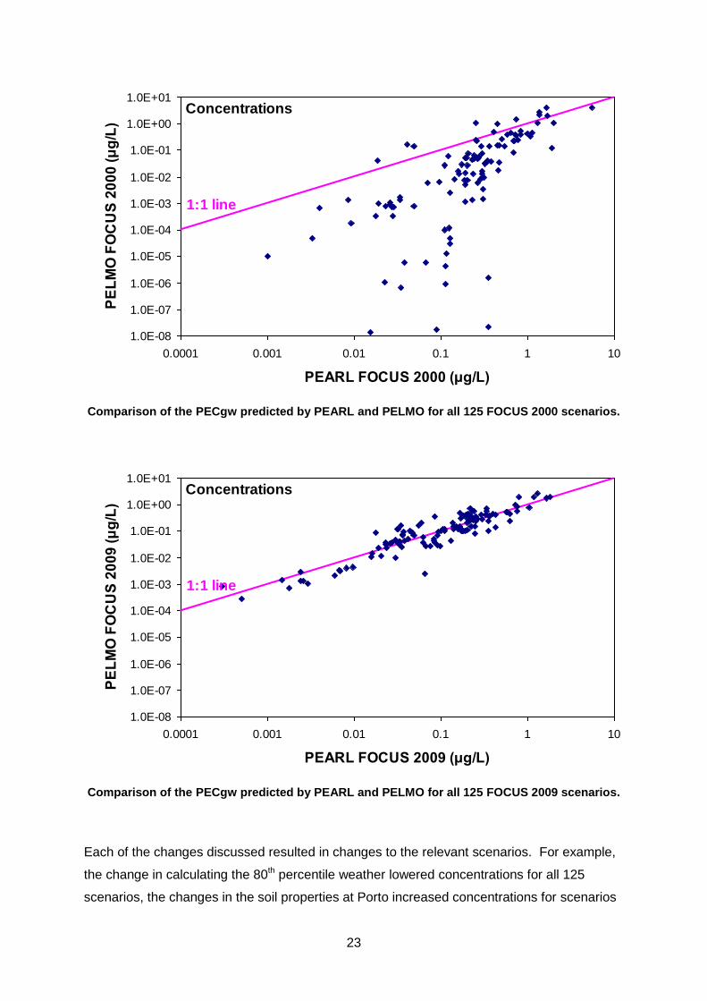
The changes to the models were successful in reducing the variability between the
predictions of the models. The following graphs show the comparison of PEARL and
PELMO results for compound D between the FOCUS 2000 scenarios and those proposed in
this report (FOCUS 2009).
23
1.0E-08
1.0E-07
1.0E-06
1.0E-05
1.0E-04
1.0E-03
1.0E-02
1.0E-01
1.0E+00
1.0E+01
0.0001 0.001 0.01 0.1 1 10
PEARL FOCUS 2000 (μg/L)
PE
LM
O F
OC
US
20
00
(μ
g/L
)
1:1 line
Concentrations
Comparison of the PECgw predicted by PEARL and PELMO for all 125 FOCUS 2000 scenarios.
1.0E-08
1.0E-07
1.0E-06
1.0E-05
1.0E-04
1.0E-03
1.0E-02
1.0E-01
1.0E+00
1.0E+01
0.0001 0.001 0.01 0.1 1 10
PEARL FOCUS 2009 (μg/L)
PE
LM
O F
OC
US
20
09
(μ
g/L
)
1:1 line
Concentrations
Comparison of the PECgw predicted by PEARL and PELMO for all 125 FOCUS 2009 scenarios.
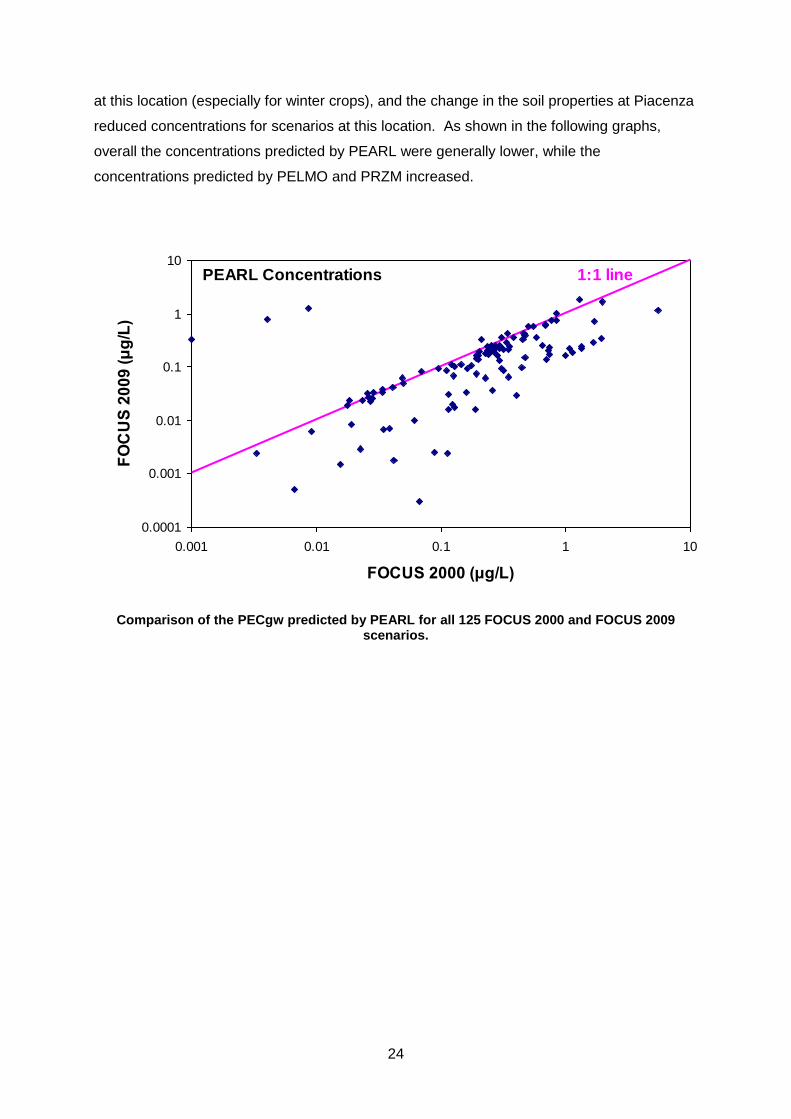
Each of the changes discussed resulted in changes to the relevant scenarios. For example,
the change in calculating the 80th percentile weather lowered concentrations for all 125
scenarios, the changes in the soil properties at Porto increased concentrations for scenarios
24
at this location (especially for winter crops), and the change in the soil properties at Piacenza
reduced concentrations for scenarios at this location. As shown in the following graphs,
overall the concentrations predicted by PEARL were generally lower, while the
concentrations predicted by PELMO and PRZM increased.
0.0001
0.001
0.01
0.1
1
10
0.001 0.01 0.1 1 10
FOCUS 2000 (μg/L)
FO
CU
S 2
00
9 (
μg
/L)
PEARL Concentrations 1:1 line
Comparison of the PECgw predicted by PEARL for all 125 FOCUS 2000 and FOCUS 2009 scenarios.
25
0.0001
0.001
0.01
0.1
1
10
1.0E-08 1.0E-07 1.0E-06 1.0E-05 1.0E-04 1.0E-03 1.0E-02 1.0E-01 1.0E+00 1.0E+01
FOCUS 2000 (μg/L)
FO
CU
S 2
00
9 (
μg
/L)
PELMO Concentrations 1:1 line
Comparison of the PECgw predicted by PELMO for the 125 FOCUS 2000 and FOCUS 2009 scenarios.
0.0001
0.001
0.01
0.1
1
10
1.0E-08 1.0E-07 1.0E-06 1.0E-05 1.0E-04 1.0E-03 1.0E-02 1.0E-01 1.0E+00 1.0E+01
FOCUS 2000 (μg/L)
FO
CU
S 2
00
9 (
μg
/L)
PRZM Concentrations 1:1 line
Comparison of the PECgw predicted by PRZM for the 125 FOCUS 2000 and FOCUS 2009 scenarios.
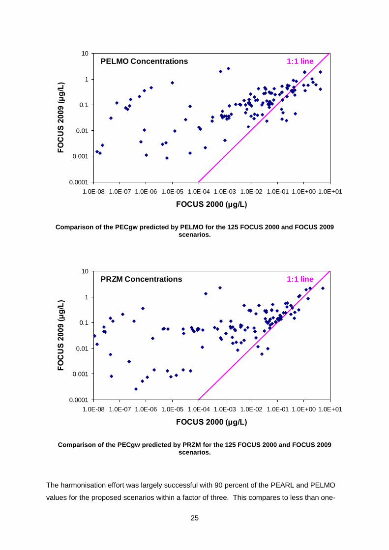
The harmonisation effort was largely successful with 90 percent of the PEARL and PELMO
values for the proposed scenarios within a factor of three. This compares to less than one-

26
fourth of the FOCUS 2000 scenarios. Given the current agreement among the models, the
work group recommends that the ground water assessments can now be performed with any
of the models (PEARL, PELMO, and PRZM) and there is no need to perform the
assessments with more than one model. However the EFSA PPR panel opinion identified
that particularly for non irrigated crops PEARL and PELMO provide very different results at
the Sevilla scenario. Therefore in line with EFSA PPR (2013a), applicants and rapporteurs
are advised that they should again provide simulations with PEARL and PELMO or PRZM.
Where a crop of interest is defined for Châteaudun, MACRO simulations need to be run
(EFSA PPR, 2013a).
Have higher tier modelling approaches been incorporated into the recommendations?
The work group report outlines the principles for spatially distributed modelling and as
mentioned earlier presents two different GIS based approaches for creating crop specific
scenarios. The work group report provides information on European-wide data sets that
could be useful in performing GIS analyses. The report also discusses several approaches,
including a detailed discussion of inverse modelling, that combine the results of both field or
lysimeter studies with modelling. The work group report also presents a detailed discussion
of non-equilibrium sorption, including recommendations for implementation in regulatory
submissions.
Have higher tier experimental data been incorporated into the recommendations?
The work group report discusses the design of lysimeter studies, field leaching studies, and
ground water monitoring studies and their role in a tiered assessment procedure.
Are the existing scenarios applicable to the new member states?
The FOCUS (2000) scenarios were developed when the European Union consisted of 15
countries. Since that time twelve additional countries have joined. Therefore the work group
assessed whether the FOCUS (2000) scenarios ‘covers’ the agricultural area of new member
states. A scenario ‘covers’ an area when it represents either the same properties or
represents a more vulnerable situation like higher rainfall amounts or lower organic carbon
contents. The spatial analysis shows that the current set of FOCUS leaching scenarios is
applicable to new member countries for the purpose of Tier 1 screening simulations. Some
smaller areas shown in the figure below, located both in the original 15 member states and in
27
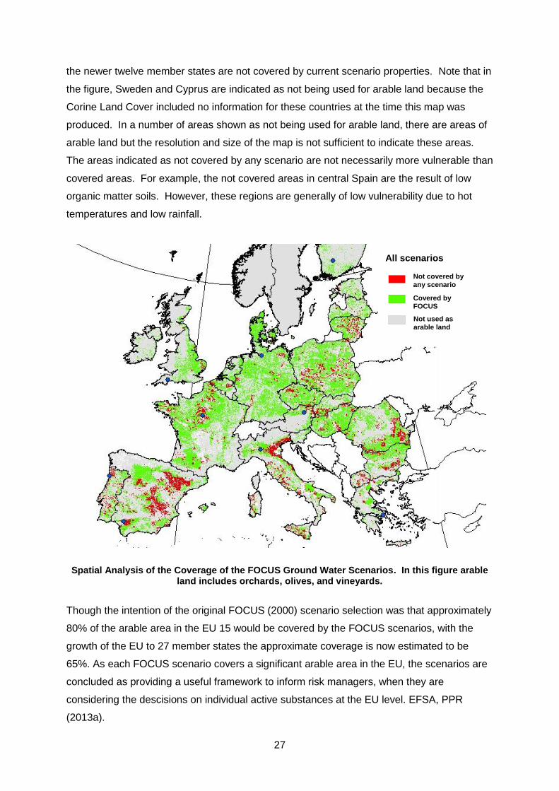
the newer twelve member states are not covered by current scenario properties. Note that in
the figure, Sweden and Cyprus are indicated as not being used for arable land because the
Corine Land Cover included no information for these countries at the time this map was
produced. In a number of areas shown as not being used for arable land, there are areas of
arable land but the resolution and size of the map is not sufficient to indicate these areas.
The areas indicated as not covered by any scenario are not necessarily more vulnerable than
covered areas. For example, the not covered areas in central Spain are the result of low
organic matter soils. However, these regions are generally of low vulnerability due to hot
temperatures and low rainfall.
Not covered by
any scenario
Covered by
FOCUS
Not used as
arable land
All scenarios
Spatial Analysis of the Coverage of the FOCUS Ground Water Scenarios. In this figure arable
land includes orchards, olives, and vineyards.
Though the intention of the original FOCUS (2000) scenario selection was that approximately
80% of the arable area in the EU 15 would be covered by the FOCUS scenarios, with the
growth of the EU to 27 member states the approximate coverage is now estimated to be
65%. As each FOCUS scenario covers a significant arable area in the EU, the scenarios are
concluded as providing a useful framework to inform risk managers, when they are
considering the descisions on individual active substances at the EU level. EFSA, PPR
(2013a).

28
29
1 INTRODUCTION
FOCUS (FOrum for the Co-ordination of pesticide fate models and their USe) was a group of
regulators, industry, and experts from government research institutes established in 1993 to
provide guidance for modelling issues in the rapidly developing EU registration process.
FOCUS has sponsored work groups to develop registration guidance in assessing pesticide
residues in ground water, soil, surface water, and air.
In the area of ground water, FOCUS sponsored two work groups prior to the work of the
current work group, which is described in this report. The first work group reviewed leaching
models available for conducting leaching assessments and provided information and
guidance on the key issues (FOCUS, 1995). Then FOCUS sponsored a work group to
develop standard scenarios for conducting leaching assessments (FOCUS, 2000).
During the years following the release of the original scenarios, a number of questions arose
concerning these FOCUS scenarios and issues regarding ground water assessments. While
FOCUS (2000) provided a procedure for conducting modelling assessments, this group did
not provide overall guidance on the respective roles for field and monitoring studies,
lysimeter studies, and modelling for the EU assessment process. In addition member states
had adopted significantly different approaches with regards to modelling and studies.
Differences between the various models, while acknowledged at the time of the release of
the scenarios, became more of an issue, especially differences in the dispersion lengths
used and the differences in the predicted water balances. An assessment by APECOP
(Vanclooster et al., 2003) challenged the appropriateness of some of the scenarios. The use
of higher tier assessment procedures including GIS techniques was becoming more
widespread due to increased availability of data and the role of such techniques in the EU
assessment process needed to be defined. Finally, the number of countries in the EU was in
the process of expanding and the question arose whether additional scenarios would be
needed.
FOCUS established a new work group to deal with the questions in the previous paragraph.
The work group’s remit covered the following four areas:
a) Develop a sequence of tiers to assess the risk for leaching to ground water in the EU,
considering results from different study types (including recommendations for national
approaches).

30
b) Provide a revised set of scenarios and leaching models. This task included the re-
evaluation of the Porto and Piacenza scenarios, and harmonisation of the dispersion
length and water balance among the models.
c) Develop guidance on the principles for higher tier leaching modelling approaches
considering GIS based approaches, the combination of modelling approaches with
experimental studies, and inclusion of relevant processes that have been ignored so
far.
d) Provide a preliminary assessment of possibilities for scenarios for new member
states.
The recommendations of the work group on the tiered assessment scheme are found in
Chapters 3-10. The revised scenarios and harmonised leaching models are provided in
Chapters 11 and 12. The guidance for higher tier approaches including the combination of
modelling approaches with experimental studies has been included in the discussion on the
tiered assessment scheme. The applicability of the current scenarios to the new member
states is presented in Chapter 13.
When the work group started the EU consisted of 25 member states. During the course of
the work, two additional states were added. The work of this work group was based on these
25 member states. However, the EU-wide maps in Chapter 13 do include information from
these two new member states.
During the time the work group was preparing this report, the EU Directive 2006/118/EC on
the protection of groundwater against pollution and deterioration (European Union, 2006)
was issued. The work in this report does not conflict with the EU directive, although in some
cases terminology and objectives may be slightly different, especially as regarding ground
water monitoring.
1.1 References
EFSA. Panel on Plant Protection Products and their Residues (PPR) 2013a; Scientific
Opinion on the report of the FOCUS groundwater working group (FOCUS, 2009):
assessment of lower tiers. EFSA Journal 2013;11(2):3114. [29 pp.]
doi:10.2903/j.efsa.2013.3114. Available online: www.efsa.europa.eu/efsajournal
EFSA Panel on Plant Protection Products and their Residues (PPR) 2013b; Scientific
Opinion on the report of the FOCUS groundwater working group (FOCUS, 2009):
31
assessment of higher tiers. EFSA Journal 2013;11(6):3291. [25 pp.]
doi:10.2903/j.efsa.2013.3291 Available online: www.efsa.europa.eu/efsajournal
EFSA 2014a European Food Safety Authority. Guidance Document for evaluating laboratory
and field dissipation studies to obtain DegT50 values of active substances of plant
protection products and transformation products of these active substances in soil. EFSA
Journal 2014;12(5):3662, 38 pp., doi:10.2903/j.efsa.2014.3662 Available online:
www.efsa.europa.eu/efsajournal
European Union. 2006. Directive 2006/118/EC of the European Parliament and of the
Council of 12 December 2006 on the protection of groundwater against pollution and
deterioration. Official Journal of the European Union, L372:10-31, 27/12/2006.
FOCUS. 1995. Leaching Models and EU registration. European Commission Document
4952/VI/95.
FOCUS. 2000. FOCUS groundwater scenarios in the EU pesticide registration process.
Report of the FOCUS Groundwater Scenarios Workgroup, EC Document Reference
Sanco/321/2000 rev 2. 202pp.
Vanclooster, M., J.D. Pineros-Garcet, J.J.T.I. Boesten , F. Van den Berg, M. Leistra, J.
Smelt, N. Jarvis, S. Roulier, P. Burauel, H. Vereecken, A. Wolters, V. Linnemann, E.
Fernandez, M. Trevisan, E. Capri, L. Padovani, M. Klein, A. Tiktak, A. Van der Linden, D.
De Nie, G. Bidoglio, F. Baouroui, A. Jones, A. Armstrong. 2003. Effective Approaches
for Assessing the Predicted Environmental Concentrations of Pesticides. Final report.
European Commission, Quality of Life and Management of Living Resources
Programme. QLK4-CT-1999-01238. Printed by the Université Catholique de Louvain,
Belgium (Available at http://www.geru.ucl.ac.be/recherche/projets/apecop-pub/).
32
2 GLOSSARY
APECOP
A European Union funded project covering a range of topics associated with modelling the
movement and degradation of pesticides in soil.
Chromatographic Flow
Flow of water and solutes through soil that follows the classical convection dispersion
equation, with no preferential flow paths bypassing portions of the water filled pore volume.
Crop kc Factors
The crop kc factor times the reference evapotranspiration for a specific day determines the
potential evapotranspiration for a specific crop. The actual evapotranspiration for the day
may be less, for example due to soil moisture constraints.
DT50, DegT50
DT50 is the time required for 50 percent of the substance to disappear from a compartment.
DegT50 is the time required for 50 percent of the substance to disappear from a
compartment due to degradation alone. DT50 values may include losses due to
volatilisation, leaching, and runoff, while DegT50 does not. In laboratory studies, the DegT50
is usually equal to the measured DT50. If degradation follows singe first order kinetics, then
the DegT50 is equal to the half life.
Equilibrium Sorption
In this report, equilibrium sorption is defined as the sorption measured after shaking a batch
system for 24 h.
Evapotranspiration
Evapotranspiration is the sum of water losses due to evaporation from the soil surface and
transpiration from plants. Evapotranspiration can be either potential (what would occur if the
soil was maintained at field capacity) or actual. Reference evapotranspiration refers to
potential losses at standard conditions (usually a grassed field for a soil maintained at field
capacity) and potential crop evapotranspiration refers to potential losses for a specific crop
with the soil maintained at field capacity.
33
Field Capacity
In the FOCUS scenarios, the field capacity is defined as the water content at a tension of 10
kPa (pF2).
Field leaching studies
Studies in which ground water and/or pore water is sampled from a small number of locations
following documented application of the pesticide of interest as part of the study. Sites are
generally subject to detailed data gathering over a period of months/years. This information
would typically include hydrological information (e.g. daily meteorological data, water
tensions at different soil depths) as well as additional pesticide information (e.g. bulk soil
concentration of pesticide at different depths).
FIFRA
Federal Insecticide, Fungicide, and Rodenticide Act, the primary law providing the legal basis
for regulation of pesticides in the United States.
GIS
Geographical Information System, the presentation and organisation of information based on
location.
GLEAMS
GLEAMS (groundwater loading effects of agricultural management systems) is a one-
dimensional leaching and runoff model developed by the U.S. Department of Agricultural.
Guideline Scenarios
Scenarios that are defined in guidelines for higher tier leaching experiments.
HYPRES
A data base of hydraulic properties of European soils.
Inverse Modelling
A modelling technique in which what is normally output information from a model data is used
to estimate what are normally input values. For example, using measurements of
concentrations as a function of time to estimate sorption constants and degradation rates.
Linear Models
A model F(x) where F is the model operator and x is a variable, is called a linear model when
F(ax+by) = aF(x)+bF(y). For example, the model relating the sorption constant, kd, and the

34
organic carbon content (OC) is a linear model: kd = koc OC whereby koc is the proportionality
factor. Another example of a linear model is a transport model of which the parameters are
not a function of the dependent variable, in this case the concentration. For instance, if the
gas-water and water-solid partitioning coefficients, and the sorption rate and decay rate
parameters are not a function of the concentration, then none of the parameters of the
transport model depends on the concentration and the transport model is a linear model. A
consequence of this linearity is that the predicted concentrations by the model scale linearly
with the applied concentration at the soil surface. Leaching estimates in PELMO, PEARL,
PRZM, and MACRO are non-linear due to the use of the Freundlich isotherm
Lysimeter
A lysimeter is a device to sample pore water in soil either at a specific depth or moving past a
specific depth. The term can be misleading since there are at least three different devices
referred to as lysimeters and all three devices can be used in experiments investigating the
movement of solutes in soil.
A soil monolith lysimeter consists of a soil block or cylinder, embedded in an inert container
(e.g. stainless or galvanised steel, fibre glass) with a bottom permeable to drainage water or
leachate (e.g. a perforated bottom, quartz sand filter bottom). See also OECD (2000).1
A zero-tension lysimeter consists of a permeable bottom plate with simulated water table at
that depth.
A soil suction lysimeter is a device that draws soil pore water from a specific point in the soil.
MACRO
MACRO is a one dimensional leaching model, which includes the process of macropore flow
that was developed at the Swedish University of Agricultural Sciences, Uppsala. MACRO is
one of four models used to evaluate potential movement to ground water in the EU
registration process.
1 OECD (2000) Guidance Document for the Performance Of Out-door Monolith Lysimeter
Studies.- OECD Environmental Health and Safety Publications; Series on Testing and Assessment; No. 22.
35
Macropore Flow
A preferential flow mechanism in which a portion of the water and dissolved solutes
bypasses the major part of the soil pore water, without mixing with it, by flowing through
cracks or channels in the soil.
Major Metabolite
A degradation product that is formed in amounts of greater a trigger level of 10 % (molar
fractions or percent applied radioactivity) of the applied amount of active ingredient at any
time evaluated during the degradation studies in the compartment (i.e. soil, water and/or
sediment) under consideration.
In the context of the guidance document on relevant metabolites in groundwater
(Sanco/221/2000 –rev.10 (25 February 2003)) degradation products must be characterised
and identified to the extent that is technically feasible and their relevance must be assessed,
if one of the following conditions applies:
a) Metabolites, which account for more than 10 % of the amount of active substance
added in soil at any time during the studies; or
b) which account for more than 5 % of the amount of active substance added in soil
in at least two sequential measurements during the studies; or
c) for which at the end of soil degradation studies the maximum of formation is not
yet reached.
Map Unit
Units with particular characteristics of which the geographical distribution is indicated on a
map.
Monitoring Studies
In this report, monitoring studies are studies in which ground water is sampled from a large
number of locations in a region or country and is subsequently analysed to determine the
concentration of the pesticide of interest. Experimentally determining the reason for the
presence or absence of the compound is not necessarily an intrinsic part of these studies,
although the weight which is placed on the findings will depend on the appropriate selection
of the sites to sample. Outside this report, the definition of monitoring studies is sometimes
expanded to include field leaching studies.

36
When used in the text, this is an abbreviation for probability density function. When this is
part of an electronic file name, this refers to a file that can be read using Adobe Acrobat.
OCTOP
A spatial data base providing information on organic carbon content in European soils.
PEARL
PEARL (Pesticide Emission Assessment at Regional and Local scales) is a one dimensional
leaching model developed by three Dutch institutes (ALTERRA, RIVM, and PBL). PEARL is
one of four models used to evaluate potential movement to ground water in the EU
registration process.
Pedologic
Relating to soil profiles or properties of soil profiles.
PELMO
PELMO (PEsticide Leaching MOdel) is a one dimensional leaching and runoff model developed by the Fraunhofer-Institut für Umweltchemie und Ökotoxikologie. PELMO is one of four models used to evaluate potential movement to ground water in the EU registration process.
Preferential Flow
Flow of water and solutes in soil that does not follow the classical convection dispersion
equation, which can result from soil inhomogeneity and channels such as cracks and worm
holes. Macropore flow, finger flow, and funnel flow are all preferential flow mechanisms.
PRZM
PRZM (Pesticide Root Zone Model) is a one dimensional leaching and runoff model
developed by the U.S. Environmental Protection Agency. PRZM is one of four models used
to evaluate potential movement to ground water in the EU registration process.
PSD
Pesticides Safety Directorate, the former government agency regulating pesticides in the
United Kingdom (now Chemicals Regulation Directorate).
Reference Scenarios
Scenarios that meet the vulnerability criteria, and define the conditions at which the
protection goal has to be met for a favourable regulatory decision. On the EU level, the
37
reference scenarios are the FOCUS scenarios. At the nation level, the reference scenarios
are either national scenarios or specific FOCUS scenarios selected by the member state
(see also scenarios).
Relevant Metabolite
In the context of ground water, the term “relevant metabolite” is used in a unique legislative
context determined according to Sanco/221/2000-rev. 10 (25 February 2003) and refers to
metabolites for which there is reason to assume that it has comparable biological activity as
the parent substance or meets certain toxicological properties.
Runoff
Runoff is a term that has been used in the scientific literature in different ways. In pesticide
risk assessment, runoff often refers to the flow of water on top of the soil, or alternately
overland flow. The most important processes leading to overland flow is infiltration excess
runoff (also called Hortonian runoff). Catchment hydrologists commonly use a broader
definition of (storm) runoff. They include all processes leading to fast stream response (i.e.
infiltration excess runoff, saturation excess runoff from partial contributing areas and
subsurface drainage through either artificial drains or naturally occurring preferential
pathways). In this report, runoff is used as a synonym for overland flow when referring to
Tier 1 scenarios, but can be used in a broader context in Tier 2 and Tier 3.
Scenarios
A representative combination of crop, soil, climate, and agronomic parameters to be used in
modelling. There are 125 scenarios in FOCUS 2000 and proposed in this report.
Society of Environmental Toxicology and Chemistry (SETAC)
A profession society dealing with exposure and effects of chemicals in the environment.
Spatially-distributed Modelling
Modelling that is based on running a large number of scenarios with input parameters
relevant to specific locations and presenting the results in a map.
STU
Soil Typological Units, which are the carriers of basic soil information, such as the FAO soil
name and the soil textural class. Soil mapping units are associations of dominant and
subdominant STU’s.
38
Study Scenarios
These scenarios consist of the soil, climatic, and agronomic conditions occurring in a specific
higher tier leaching experiment.
Subsoils
Those soil layers located below the plough layer or the surface soil. Typically such soils
begin at 0.2 to 0.3 m below the soil surface and continue until the depth of the water table. In
some cases subsoils also include layers below the water table, but this is not the case for the
usage in this report.
Tiered Assessment Procedure
A sequential assessment procedure with different levels (tiers), in which assessments at a
higher level of the procedure will replace assessments at a lower level.
UBA
Umweltbundesamt (Federal Environment Agency), the German government agency
responsible for assessing the impact of plant protection products on the environment.
Undisturbed Soil Monolith
An undisturbed soil profile that has been sampled from the field in its original layering of soil
horizons without artificial disturbance (no re-filling).
Validated Model
A model which has gone successfully through a validation process for a specified range of
validity; this implies that the number of data sets considered is sufficient for the intended use
of the model.
Validation Process
Comparison of model output with data independently derived from experiments or
observations of the environment; this implies that none of the input parameters is obtained
via calibration with the data set used for validation; note that this definition does not specify
any correspondence between model output and measured.
Wilting Point
In the FOCUS scenarios, the wilting capacity is defined as the water content at a tension of 16,000 kPa.
39
3 INTRODUCTION TO ASSESSMENT SCHEMES FOR PEC IN
GROUND WATER
3.1 Objectives of the risk assessment for ground water contamination at EU
and national levels
The objectives of the risk assessment for ground water contamination has to be considered
in the context of Commission Regulation (EU) No 546/2011 of 10 June 2011 (C 2.5.1.2):
No authorisation shall be granted if the concentration of the active substance or of relevant
metabolites, degradation or reaction products in groundwater, may be expected to exceed,
as a result of use of the plant protection product under the proposed conditions of use, the
lower of the following limit values:
(i) the maximum permissible concentration laid down by Directive 2006/118/EC of
the European Parliament and of the Council, or
(ii) the maximum concentration laid down when approving the active substance in
accordance with Regulation (EC) No 1107/2009, on the basis of appropriate data,
in particular toxicological data, or, where the concentration has not been laid
down, the concentration corresponding to one tenth of the ADI laid down when the
active substance was approved in accordance with Regulation (EC) No
1107/2009
unless it is scientifically demonstrated that under relevant field conditions the lower
concentration is not exceeded.
A definition of the relevant metabolites is given in the European guidance document
SANCO/221/2000-rev. 10 (25 February 2003).
The Directive 2006/118/EC of the European Parliament and of the Council of 12 December
2006 is on the protection of ground water against pollution and deterioration has been
published European Union (2006). The objectives for monitoring under this directive differ
from the aspects considered in this report (see Chapter 9).
3.1.1 European level
With regard to ground water contamination, currently, no official decision scheme for EU level
approval of active substances exists. The current practice is to propose EU level approval as
far as safe use is demonstrated for a relevant crop and a significant area in Europe. This can
40
be achieved by means of the official FOCUS models and the European scenarios, which
were set up to describe realistic worst-case conditions, with an overall vulnerability of the 90th
percentile, approximated by using a 80th percentile value for soil and a 80th percentile value
for weather (FOCUS, 2000). The current FOCUS group believes that a 90th percentile is
consistent with definitions used in the FOCUS 2000 report (this was agreed by the FOCUS
Steering Committee and later by the WG Pesticides Legislation). Experimental data
(lysimeter, field studies…) can also be provided as supportive information or to refine the
assessment.
3.1.2 National level
National risk assessment has to consider the whole area where a PPP is intended to be
used, as realistically as possible. The goal is to demonstrate that a compound can be used
safely for most of the relevant environmental conditions (at this level it is thought that not all
detailed conditions can be taken into consideration). If this conclusion cannot be reached,
unfavourable conditions should be identified and risk management may be considered. So, a
key point is to know if authorisation may be granted only for certain conditions (certain areas,
e.g. climatic zones, or certain factors, e.g. soil pH or clay content) or in other words if risk
management may be proposed for ground water.
A working definition of the National protection aim was considered by FOCUS to be a
prerequisite for definitions of interactions between EU and national assessment schemes.
The proposal of FOCUS is that a national protection goal upper limit should be 0.1 µg/L
annual average2 in ground water at the 90th percentile vulnerability taking into account both
spatial variability for soil and climatic conditions, and temporal variability on a multi-year
basis, in the agricultural use area of the product. The agricultural use area is defined by the
notifier by the intended use. Particular attention would have to be given to areas of higher
vulnerability within the agricultural area of the member state that can be identified (e.g. based
on defined geographical boundaries or environmental parameters). For these areas, suitable
mitigation measures would have to be taken.
2 FOCUS criteria for averaging is applied for modelling; see individual subchapters for averaging
experimental data.
41
3.2 Review of existing guidance on EU and national level
3.2.1 Guidance given in EU and FOCUS documents
At the time of drafting the workgroups report a number of publications providing both
regulatory requirements and guidance that have relevance for undertaking ground water
assessments under Directive 91/414/EEC were available. These documents refer to both
active substances and their metabolites or just to the metabolites. Those that relate to soil
degradation aspects were summarised in other FOCUS work (FOCUS, 2006). Since the
work group finalised its report important additional guidance has been provided and
implemented consequent to EFSA, PPR (2007) and EFSA (2014a). However, because the
degradation requirements are only one aspect of the ground water assessment, a useful
starting point for the current FOCUS work group is to summarise the existing information as it
relates to all aspects of ground water assessment.
There are two types of publications; EU directives which are considered to be legally binding
and Guidance documents which, though highly influential, have no mandatory basis. These
are distinguished in the following summary.
3.2.1.1 Binding requirements in directives
The Uniform principles (Directive 97/57/EC establishing the Annex VI to Directive 91/414/EC
now replaced by Commission Regulation (EU) No 546/2011 of 10 June 2011) require that
member states “estimate, using a suitable calculation model validated at the Community
level3, the concentration of the active substance and of relevant metabolites, degradation and
reaction products that could be expected in the groundwater in the area of envisaged
use…..This evaluation will also take into consideration….the specific information on the fate
and behaviour in soil and water as provided for in the Annex to Regulation (EU) No
544/2011” In practice, by analogy the specific information on the fate and behaviour in soil
and water as provided for in Regulation (EU) no 283/2013 now needs to be considered.
The decision-making section of Commission Regulation (EU) No 546/2011 of 10 June 2011
goes on to state that no authorisation shall be granted if the concentration of the active
substance or of relevant metabolites in ground water may be expected to exceed the lower
value of 0.1 µg/L4, the maximum concentration laid down by the Commission when including
3 See FOCUS (1995, 2000) for discussion of the status of validation.
4 For practical purposes FOCUS (2000) have used an operating definition of annual average
concentration at 1 m depth until it is possible to predict behaviour in ground water. Note that this definition does not have a legal basis.

42
the active substance on Annex I or one tenth of the ADI, “unless it is scientifically
demonstrated that under relevant field conditions the lower concentration is not exceeded.”
Commission Regulation (EU) No 546/2011 of 10 June 2011 and Article 4 of Regulation (EC)
No 1107/2009 of the European Parliament and the Council are the documents that set out
the regulatory decision-making criteria for product authorisation and EU level approval
respectively. The statements quoted above indicate that actual measured values under field
conditions relevant for the area of use would over-ride estimates and predictions based on
the level of understanding of the basic processes, i.e. the degradation and sorption data
required for the active substance and relevant metabolites in the data requirements for
Environmental fate.
Regulation (EU) No 283/2013 clearly states the trigger values for field soil studies for active
substances and metabolites. Reliable laboratory degradation rate endpoints (from 3 different
soils) are required for every metabolite that exceeds 10 %, 5% at two time points or 5% at
the end of a study in the available laboratory degradation studies on the active substance.
Reliable field degradation rate endpoints are required for every metabolite that exceeds the
prescribed DT triggers from laboratory degradation rate endpoints.
Regarding soil mobility aspects, Regulation (EU) No 283/2013 sets requirements for sorption
studies for the active substance and any metabolites exceeding 10 %, 5% at two time points
or 5% at the end of a study in the soil degradation studies on the active substance.
Regulation (EU) No 283/2013 indicates higher tier leaching studies (lysimeter or field
leaching experiments) may be provided taking into account the results of degradation and
other mobility studies and the predicted environmental concentrations in groundwater. The
type and conditions of the study to be performed shall be discussed with the national
competent authorities.
This is the extent of binding requirements for consideration of ground water assessments for
active substances and metabolites.
3.2.1.2 EU guidance documents
In recent years the consideration of metabolites (also encompassing degradation,
transformation and breakdown products) within the EU pesticide regulatory framework has
provoked much discussion and concern. In response to this, a specific guidance document
(Sanco/221/2000 – rev. 10) has been prepared to consider the relevance of metabolites in
ground water. This document is largely concerned with the definition of “relevant” since the

43
0.1 µg/L trigger for ground water does not apply to “non-relevant” metabolites and
“metabolites of no concern” (however the document also provides further triggers that require
additional data for non-relevant metabolites which exceed concentrations of 0.75 µg/L and
10 µg/L). These aspects of the guidance document are not directly relevant to a general
framework for leaching assessment and so are not summarised further in this document. Of
more significance is that the guidance document recommended a formal extension of the
need to consider the relevance (in ground water leaching terms) of metabolites that reach
>5% at two successive sampling times / intervals during degradation studies on the active
substance as well as those for which “the maximum of formation is not yet reached” at the
end of the study. The filosophy regarding these levels was subsequently added in the legal
data requirements in Regulation (EU) No 283/2013 in the way already outlined above. Less
controversially, the guidance document also recommends that all metabolites exceeding 0.1
µg/L annual average in the leachate in lysimeter studies should also be subject to further
assessment.
Sanco/221/2000 – rev. 10 further discusses the availability of data from experimental sources
(lysimeters and monitoring data) and this can be considered representative of current
thinking in the EU. Two particular statements are of relevance although there is no clear
attempt to define a hierarchy of other information in relation to modelling studies:
"For metabolites found in the leachate of lysimeter studies with annual average
concentrations above 0.1 µg/L an attempt should be made to assess their leaching
behaviour in other European regions with different soil and climatic conditions with the
goal to extrapolate the experimental findings to other representative regions of
European agriculture."
and
“Monitoring data from regions with well-documented use of the active substance in
question may provide a useful additional tool to supplement model calculations and
lysimeter experiments to improve the accuracy and validity of estimates of potential
groundwater contamination.”
An early draft guidance document that was never accepted for use on calculation of PEC,
including PECgw (7193/VI/99 rev 0.) has now been superseded by other guidance from
FOCUS. Therefore further consideration of this document is not necessary.
44
3.2.1.3 FOCUS guidance documents
As far back as 1995, FOCUS (1995) made some attempt to address a tiered approach to
regulatory assessments of ground water leaching potential. However, at that time
consideration of the placement of higher tier field data in the scheme was considered to be
beyond the remit of the group. A later FOCUS work group (2000) provided information on a
tiered approach to the use of available data, within the modelling context. Guidance was also
given on the derivation of input values for modelling when faced with a number of
experimental values, as generated in a standard environmental fate data package under
Directive 91/414/EEC (FOCUS, 2000, 2002).
The same work group (FOCUS, 2000, 2002) also provided recommendations for the
interpretations of the results from the relevant ground water scenarios.
“If a substance exceeds 0.1 µg/l for all relevant scenarios, then Annex 1 inclusion
would not be possible unless convincing higher tier data (e.g. studies, monitoring or
more refined modelling) was available to over-ride the modelling results.
If a substance is less than 0.1 µg/l for all relevant scenarios, then the choice of a
realistic-worst case definition for the scenarios means that there can be confidence
that the substance is safe in the great majority of situations in the EU. This does not
exclude the possibility of leaching in highly vulnerable local situations within specific
Member States, but such situations should not be widespread and can be assessed
at the Member State level when considering national authorisations.
If a substance is less than 0.1 µg/l for at least one but not for all relevant scenarios,
then in principle the substance can be included on Annex 1 with respect to leaching to
groundwater. As the scenarios represent major agricultural areas of the EU, such a
result indicates that "safe" uses have been identified, which are significant in terms of
agriculture in the EU. The scenarios which gave results less than 0.1 µg/l, along with
the results of any higher tier studies which already exist, help to indicate the extent of
the "safe" uses which exist for the substance. These higher tier studies could include
lysimeter or field leaching studies, monitoring and more refined modelling. The
results of the entire leaching assessment at the EU level could then be used to assist
local assessments of leaching at the Member State level.”

45
3.2.2 Review of existing national approaches for leaching assessments
According to the FOCUS ground water guidance document of 2000 (SANCO/321/2000
rev.2), risk assessment of the leaching of pesticides to ground water for the EU, should be
made following a tiered approach. The FOCUS guidance restricts itself to exposure
assessment on tier 1 for the EU level and there is no precise guidance on a tiered approach
for leaching assessments on a national level. Furthermore during the EU-evaluation process
a number of different methods of higher tier assessments have been used by notifiers /
rapporteur member states, which indicates that there is a need for consistency. In the review
reports, the conclusive product of the evaluation of an active substance and the basic
document for the decision, there may be included certain conditions to be taken into account
by member states at time of authorisation of products after post Annex 1 inclusion of an
active ingredient. For several active substances the following condition is included: Leaching
to groundwater: Particular attention should be given to the potential of groundwater
contamination, when the active substance is applied in regions with vulnerable soils/ or
climate conditions and risk mitigation measures should be applied where appropriate. This
implies that member states should implement a strategy to handle this condition specified
above.
The remit of the FOCUS ground water work group established in 2003 includes providing
guidance on higher tier leaching assessment and on harmonisation of risk assessment
procedures at national level. Therefore, the Work Group felt that it was vital to get
information from the member states on to what extent and how the FOCUS guideline of the
first tier assessment is currently used within member states of the European Union and how
the countries solve the ground water risk assessment on a member state level. As a first
step a questionnaire was put together with the objective of obtaining this information. The
questionnaire was sent out by the Commission to the 25 member states (including the 10
new member states). The full questionnaire is included as Appendix 1. Eighteen out of 25
member states provided responses to the questionnaire.
3.2.2.1 The structure of and type of questions in the questionnaire
The main idea with the questions has been to get an answer how member states assess risk
for ground water contamination from the use of plant protection products. The questionnaire
is divided into four main chapters and eight sub-chapters with totally 28 questions with 15
sub-questions. The aim of the work group has been to limit the number of generic questions
and, including the sub-questions, a total of about 27 questions were Yes/No questions or
where choices could be made from alternatives.
46
3.2.2.2 Summary of questions and answers divided into the main topics.
In some cases, mainly non-generic questions, member states provide very similar answers.
In other cases, such as generic questions, the answers are more diverse. As a result, the
responses have had to be presented in a simplified manner. More details are presented in
Appendix 2, which provides a synopsis of the answers by sub-topic.
3.2.2.2.1 General questions
Questions: Asking whether member states are assessing risk to ground water, if FOCUS
ground water guidance is used on a national level and if the guideline fulfils the needs.
There are also questions about what triggers a ground water assessment, and if a tiered
approach is used.
Answers: All member states, except for two that are about to implement an assessment
scheme, answer that they are assessing risk to ground water on a national level as a routine
procedure and use the FOCUS ground water guidance document. Eight countries say that
the FOCUS guidance is fully satisfactory, while the remaining nine have different reasons
why the guidance is not fully satisfying their needs. The main reason to the answer “ not
sufficient” are reasons such as the scenarios are not representing their national environment
and, in some cases that, the scenarios are not sufficiently protective (including responses
that specific models are needed for consideration of macropore flow in structured soils). One
country stated it has very shallow ground water and another country said that the scenarios
do not cover all crops.
One question only directed to “new” member states asked what method they had chosen for
their ground water assessment scheme. Some of the new member states stated that one or
several FOCUS scenarios are used for modelling as well as studies like lysimeters for higher
tier assessment. One member state answered that they used the GUS method (Gustafson,
1989). In response to an additional question to the new member states about training
possibilities, all of the countries had had some kind of training, but all wished to have more
training.
On the sub-question about the experience of technical scientific problems, five countries
recommended improvements, e.g. implementations of help/explanations in the models. One
specific example was a need for guidance in PELMO in how to treat the relationship between
degradation rates of parent, metabolites, and CO2. More scenarios with macro-pore flow
were requested and one country wanted more crops to be added. One country replied that
the FOCUS pedological and climatic conditions do not apply in their country.

47
Thirteen countries answered that the main trigger for a specific national assessment was
when the review report recommended that ground water risk should be assessed on a
member state level. However, three of these countries also said that other triggers are used
on a case by case basis. Four countries have their own triggers. Examples of other triggers
are the outcome from lysimeter and other field studies, indications of leachability (i.e.
>0.1µg/L) in FOCUS scenarios from the assessment on the EU-level, positive findings from
monitoring, experience from earlier national assessments, and divergence of the GAP from
the intended use on which the inclusion on Annex I is based.
Fourteen member states used a tiered assessment approach, while one does not currently
use a tiered approach and one is planning to use a tiered approach. The responses have
been simplified in this paragraph, but details are available in Appendix 2. Some countries
with a well defined tiered approach have identified one or more FOCUS scenarios that are
relevant for their country and perform further assessment when the prediction concentration
exceeds 0.1 µg/L in any of these scenarios. One country uses adsorption and half-life values
to trigger to simulations on a national level. Several countries include lysimeters in their
tiered approach. One country with areas where the water table is near the ground surface
also includes the behaviour in the saturated zone.
Conclusion: Each country has its own specific methods for higher tier assessment, but often
countries use similar approaches.
3.2.2.2.2 Regulatory questions
Questions: This topic asks for information on the ground water risk assessment endpoint
used by the member states (including whether a safety factor is used), whether information
other than simulation results are taken into account in making the assessment, whether there
are alternatives to full approval, and whether risk mitigation measures are considered at
national approval.
Answers: While the responses are consistent with regard to the limit value of 0.1 µg/L there
is some variation considering the procedural definition of the endpoint (e.g. depth,
percentile). Since different member states gave different sets of endpoints, there appears to
be considerable differences between countries on this topic. However, no country applies a
safety factor on the endpoint in national level assessments.

48
Two countries take decisions on simulations only, while the remaining countries said that
they do but added further comments. Some countries pointed out that field experiments (e.g.
lysimeters) are used or required before decision is made. Two countries said that their
decision is made only on model simulations when no field or lysimeters are available. One of
these countries also takes decision based on simulations if the modelling results are below
0.1 µg/L. Another country may use model results only for new active substances. Two
countries have field and lysimeter studies as a requirement within their tiered assessment
scheme. This may be the case for other countries having a tiered assessment approach in
the group of countries replying that they did not make decisions only on model simulations.
In conclusion all countries but two do not make decisions only on model simulations when
results from higher tier studies such as lysimeters are available.
Member states responded with a number of different approaches to the question regarding
different alternatives to full approval that they apply at time of the decision. See Appendix 2
for the details, but the most frequent options chosen as an alternative to full approval were to
apply special conditional registration (14 member states), followed by regional or local
approval, and special conditions (in both cases seven member states mentioned this as an
option), and finally three member states answered that special approval for farmers was an
alternative and one additional member state answered that this option is planned but not yet
implemented. Only one member state does not have a possibility for alternative approval.
See Appendix 2 for details.
Thirteen member states consider risk mitigation measures at approval on a national level.
The most frequent measures are related to changes in the GAP, i.e. dose and number of
applications, but also restricting use to only non-vulnerable areas.
Conclusions: As reflected in the answers provided by the different member states,
differences in the interpretation of the regulatory endpoint between member states are
common.
3.2.2.2.3 Specific questions on scenarios
Questions: Do member states use any of the nine FOCUS scenarios as national scenarios
or have they defined their own? If a member state uses scenarios of their own, there are
additional questions to provide more details.
Answers: Regarding the use of FOCUS scenarios to assess risk for ground water
contamination, there is a range in number of scenarios used in different countries from one to

49
six scenarios. The most frequently used scenarios are Hamburg (five member states);
Kremsmünster (four member states); Jokioinen and Piacenza (three member states);
Okehampton, Thiva, and Châteaudun (two member states); and Sevilla and Porto (one
member state). Four countries said that they have scenarios of their own. One member
stated that they use an already validated scenario based on realistic lysimeter studies, and
that the scenario is similar to the FOCUS Hamburg scenario. In two other countries, one has
two national scenarios and the other country three, all defined as representing realistic worst
case scenarios. In one of these countries the colder climate was a reason for developing
their own scenarios. The fourth country said they use scenarios that are more realistic
compared to the FOCUS scenarios. Two new member states are planning to develop a
national scenario. Yet another country, which uses the FOCUS scenarios, considers and
evaluates scenarios where national soil and weather data are used.
The three countries not using FOCUS scenarios were asked to provide information on their
national scenarios. One country uses a normal and wet regime together with realistic worst
case soil and crops according to GAP. Although described somewhat differently the other
two countries use weather representative for agricultural areas together with one worst case
soil and one realistic soil, both soils being representative for agricultural areas. In one of
these two countries, the combination of weather, soil and crops are representing major
agriculture areas.
Four countries, different from the three countries having national scenarios, have answered
the question about whether weather, soil, or crop properties are most important in defining
scenarios. One member state said that rainfall and crops are most important, while another
member state said that they consider a fluctuating ground water to be important.
The countries having national scenarios were asked whether they consider their scenarios
more conservative (vulnerable) than the FOCUS scenarios. One member state considers
their scenario similar to Hamburg but less conservative than Piacenza. Another country has
one scenario similar to Hamburg. The third country answered that macro-pore structure and
the colder climate are considered in their scenarios. For the rest of the countries this
question was not applicable, but one of them considered their scenarios to be equal to the
EU scenarios. Four of the countries having national scenarios different from the FOCUS
scenarios, consider their scenarios to be of a higher tier compared to the FOCUS scenarios.
The country having two national scenarios requires passes in both of them to grant
authorisation. The country with three scenarios uses a tiered approach in case leaching is
observed in one of the scenarios and finally an expert judgement is applied.
50
Conclusion: Different regulatory schemes in different countries are quite common. The
development of national scenarios may sometimes reflect political/historical background as
well as pedo-climatic differences.
3.2.2.2.4 Model used
Question: The member states were asked which simulation model was used in their country.
Answers: The thirteen responses are somewhat confusing, but a simplified outcome based
on responses from eleven countries is that two countries use MACRO for the simulation of
leaching through macro-pore structure. One of these countries also accepts
PELMO/Hamburg as a model/scenario. Three countries use PELMO and of these one also
accepts PRZM as both PELMO and PRZM can simulate snow melting. Four countries use
PEARL, one coupled with GeoPearl.
Conclusions: Different model recommendations are based on historical preferences and on
country specific conditions.
3.2.2.2.5 Parameterisation
Questions: The member states were asked how parameters such as degradation and
sorption were selected for use in model simulations. The questionnaire (Appendix 1)
included a long introduction providing the main recommendations on parameterisation from
the FOCUS Groundwater Scenarios Work Group. The main recommendations are that
mean values should be used and that either laboratory or field data may be used. Note that
at the time this guidance was developed, methodology for normalisation of degradation was
only applicable to laboratory data. The question was divided into first tier and higher tier
approaches.
Answers: In initial tier assessments, ten countries use laboratory data for degradation rates
while eight choose input data on a case by case basis. All of these countries normalise data
according to the FOCUS guidance. However, differences exist in calculating these values
since a majority of countries use the arithmetic mean of the available values, six use the
geometric means, three have different options based on the specific case, and one country
uses 80th percentile DegT50 input value. The dependency of degradation on pH is
considered by most countries, but in different ways (see Appendix 2). Three countries
consider pH dependency in higher tier assessments.

51
In higher tier assessments, 12 countries use degradation rates from field data. In four of
these countries, the use of laboratory data is also an alternative. Three countries require that
field studies should be relevant for their respective countries. All 12 countries normalise
degradation data and treat data in the same way as in Tier 1. Eight countries consider
degradation data from specific soils to be of higher relevancy, whereas degradation data
derived from specific study types such as lysimeters or micro-lysimeters are not necessarily
considered more relevant.
In the first tier, all countries use Koc as input parameter for adsorption. Also two countries
additionally accept time dependent adsorption, and another country additionally accepts data
from column leaching. Fifteen countries use the arithmetic mean for calculating Koc; some
use the median if a large number of data are available. One country uses the 80th percentile
worst case values. Two countries consider specific dependency on soil properties (e.g. from
soil pH).
In higher tier assessments, 13 countries use Koc and the answers of the remaining Koc
questions are similar to Tier 1. On the question whether site-specific sorption experiments
are accepted as input data, five countries say they use such data, four do not.
Few countries answered the question on use of data from soil-specific degradation and
sorption experiments. Since this question is related to an earlier question, this means that a
few countries use local input data if available while one country considers the effect of pH in
higher tier assessments. Another country uses laboratory data at the first tier and then uses
field data at the next tier.
The responses to the questions in this topic indicate that lysimeter and field study results are
seen as more important in higher tier assessments than changing the adsorption/degradation
input parameters in modelling simulations.
All countries apply quality criteria to experimental data. Some countries have pointed out
that studies not fulfilling the quality criteria are not considered in the assessment.
Conclusions:
Parameter selection in the various countries are quite harmonised (very few
exceptions), based on previous FOCUS recommendations.

52
The responses to the questions in this topic indicate that lysimeter and field study
results are seen as more important in higher tier assessments than changing the
adsorption/degradation input parameters in modelling simulations.
All countries apply quality criteria to experimental data.
3.2.2.2.6 Additional experimental data
For national assessments several member states require additional experimental data which
are not available in the EU dossier. Some of them pointed out that this is done on a case by
case basis or it is left to the applicant to show that safe use with regard to ground water
protection exists also under the relevant national conditions. Most of the member states
asking for additional experimental data require or accept lysimeter or field leaching studies.
The requirement may be triggered by modelling results exceeding 0.1 µg/L or differing
national conditions (e.g. climate), compared to those where studies, submitted with the EU
dossier, were performed. In addition, monitoring studies are taken into account by member
states for national assessments but only few examples were provided for other specific data
(experimental data for refined model input, modelling based on GIS-data), which can be
included in the assessment. Six member states indicated that no additional experimental
data is required.
Only two member states confirmed they had a national guideline for lysimeter or field
leaching studies.
The responses to the questions on the results of the experimental studies indicate that there
was probably some confusion about the information collected during a study as well as the
explicit endpoint used in the risk assessment. Most member states answering the
questionnaire use the annual average concentrations as the endpoints but there are also
member states using the highest concentrations.
Nine member states have the option to require post registration monitoring studies under
specific circumstances.
Conclusions:
There is a lack of appropriate national guidelines for the performance of higher tier
studies for national assessments.
The risk assessment endpoints determined from field studies (such as lysimeters)
varies among the member states.
53
3.2.2.2.7 Interrelationship between models and higher tier experiments
Experimental and modelling studies are both considered for the leaching risk assessment at
the member state level. Most of the member states answering the questionnaire regard
results from appropriate higher tier experiments as superior to model calculations. Only one
member state stated that model results overrode results from field studies. All countries,
except one, make a joint decision from the results of experimental data and model
simulations. The extrapolation of existing experimental data by modelling to national or
regional conditions is currently applied only in a minority of member states.
3.2.2.2.8 Handling of metabolites
Most of the member states answering the questionnaire are dealing with metabolites on the
basis of the EU Guidance document on the assessment of the relevance of metabolites in
groundwater (Sanco/221/2000 rev. 10). One of the member states said that in principle the
approach of the guidance document is followed but a few deviations and more detailed
criteria have been developed. Two member states (deviating from the guidance document)
apply the same criteria for both relevant and non-relevant metabolites. In other words, all
metabolites are regarded as relevant (except inherently non-problematic compounds such as
carbon dioxide or glucose). Several member states said that discussions on this issue are
ongoing. In accordance with the guidance, all member states treat relevant metabolites in
the same way as active substances; i.e. the limit value of 0.1 µg/L applies. For metabolites
not identified as relevant the situation is partly still unclear: Five member states said they
apply limit values as suggested by the guidance document. Eight member states said that
they do not have a trigger value for non-relevant metabolites differing from that for the active
substance, but only two of them do not distinguish between relevant and non-relevant
metabolites according to the answer on the question before.
Conclusion: Members states handle metabolites in ground water differently, based on their
acceptance and interpretation of the Guidance Document on the assessment of the
relevance of metabolites in groundwater.
3.3 References
EFSA Panel on Plant Protection Products and their Residues (PPR). 2007. European Food
Safety Authority,. Scientific Opinion of the Panel on Plant Protection Products and their
Residues on a request from EFSA related to the default Q10 value used to describe the
temperature effect on transformation rates of pesticides in soil. The EFSA Journal (2007)
622, 1-32
54
EFSA 2014a European Food Safety Authority. Guidance Document for evaluating laboratory
and field dissipation studies to obtain DegT50 values of active substances of plant
protection products and transformation products of these active substances in soil. EFSA
Journal 2014;12(5):3662, 38 pp., doi:10.2903/j.efsa.2014.3662 Available online:
www.efsa.europa.eu/efsajournal
7193/VI/99 rev. 0 (dated 09.08.99) Guidance document on the calculation of predicted
Environmental Concentration values (PEC) of Plant Protection Products for Soil, Ground
Water, Surface Water and Sediment.
FOCUS. 1995. Leaching Models and EU registration. European Commission Document
4952/VI/95.
FOCUS. 2000. FOCUS groundwater scenarios in the EU pesticide registration process.
Report of the FOCUS Groundwater Scenarios Workgroup, EC Document Reference
Sanco/321/2000 rev 2. 202pp.
FOCUS. 2002. Generic guidance for FOCUS groundwater scenarios. Version 1.1, April
2002.
FOCUS. 2006. Guidance Document on Estimating Persistence and Degradation Kinetics
from Environmental Fate Studies on Pesticides in EU Registration. Report of the FOCUS
Work Group on Degradation Kinetics, EC Document Reference Sanco/10058/2005
version 2.0, 434 pp.
Gustafson, D.I. 1989. Groundwater Ubiquity Score: a simple method for assessing pesticide
leachability. Env. Tox. Chem. Vol. 8, 339-357.
Sanco/221/2000 rev.10. 25 February 2003. Guidance document on the assessment of the
relevance of metabolites in Groundwater of substance regulated under Council Directive
91/4141/EEC

55
4 GENERIC ASSESSMENT SCHEME FOR PEC IN GROUND WATER
(GENERAL OVERVIEW)
At the time this documment was originally drafted (2009) a range of data and approaches are
used to determine the PEC in ground water5 according to Directive 91/414/EEC. FOCUS
(2000) has previously provided scenarios and guidance for predicting PECgw at the EU level
using simulation models. For practical purposes, this group decided to use an evaluation
depth of 1 m, unless simulation models are considered capable of accurately modelling the
subsoil processes down to the true ground water level and appropriate data exist. In
addition, direct experimental evidence (e.g. field leaching studies, lysimeter studies) can be
provided by applicants (see Directive 95/36/EC) and on occasion, these results have been
put into further context by the use of further modelling (e.g. inverse modelling, extrapolation
etc). Also provision is made in Directive 95/36/EC for the submission of available monitoring
data. All of these approaches may be also used by individual member states in their product
authorisation, according to national approaches.
At the EU level at least, there is no guidance regarding the relative importance of these
different approaches in decision-making. At the national level various approaches currently
exist (see review of national approaches in Section 3.2.2), but a more standard generic
approach to the process (i.e. relative importance of modelling data, field experiments,
monitoring data etc) would be helpful. The aim of this document therefore, is to develop a
generic assessment scheme that can be used at both the EU and national level in order to
provide a clearer decision-making scheme for pesticide registration.
4.1 Assessment of the representativeness, scope and limitations and usability of
different study types
4.1.1 Relevance of experimental and modelling studies
The relevance of an experiment or a modelling study to make a contribution to the
assessment of ground water vulnerability for the specific protection goal is the key factor for
balancing and defining the interactions of experimental and modelling studies.
5 “Ground water” is not defined within Directive 91/414/EEC. However the working definition used by
FOCUS is all water that is at least 1 m below the surface of the ground and in the saturated zone. This means that no water less than 1m depth is considered as ground water. This also means that below 1 m, the soil has to be saturated before the pore water is considered as ground water.

56
Before an experiment or a modelling study can be used for the assessment of a pesticide for
Annex I inclusion or national registrations with regard to possible exposure of ground water,
its relevance needs to be checked.
The relevance of each individual study depends on:
a) the reliability (i.e. the study is performed using state-of-the-art and robust
methodologies and documented adequately so results can be trusted) and
b) the usefulness, (i.e. the results or conclusions of the study deliver a contribution to the
risk assessment in question).
With regard to usefulness, the term "relevance" covers two aspects:
(i) the experimental or modelling study itself is appropriate for the use conditions
considered for Annex I inclusion or national registration
(ii) the experiment or modelling study is useful for an extrapolation to different use
conditions or environmental scenarios.
This implies that studies performed outside the EU can be used in the EU procedures if the
relevance of the study has been proven. The same criteria apply consequently also on the
national level.
4.1.2 Study types for leaching assessment
A wide range of factors determines the fate of pesticides in the environment. These include
chemical characteristics (vapour pressure, solubility, adsorptive behaviour, chemical
structure, and degradability), environmental characteristics (precipitation, temperature, wind
and soil, sediment and water characteristics), and agricultural practices (cropping practices,
application methods, timing of application, and landscape).
Leaching of a pesticide depends on both its persistence and its mobility, as well as on the
soil physical transport properties and transport processes. With regard to the substance
properties, persistence is a measure of the resistance of a pesticide to being chemically
transformed, most commonly described by the DegT50, while mobility is commonly
described by the soil-water partition coefficient, the Kd. Both are usually measured in
laboratory studies. Environmental factors as well as chemical and biological processes
affecting persistence and mobility of the pesticide fate vary in space and in time.
Consequently, when facing such complexity it is often difficult to assess fate accurately for
the purposes of risk assessment based solely upon these data. As a consequence

57
considering other methodologies is necessary to gain an understanding of fate, behaviour,
and exposure and their implications within a context of risk.
To provide guidance the FOCUS group has compiled a list of different study types (including
detailed description) useful for leaching assessment or for generating parameters for
modelling and a list of which information (data) that can be gathered from which study type.
This review of current information and experiences available within the European Union, the
USA and other countries (SETAC, OECD, FOCUS, PSD, EPA, FIFRA) is presented in
Appendix 3.
4.2 General principles of a generic assessment scheme for PEC in ground water on
EU and national level
The general concepts that have been followed in developing a tiered assessment scheme for
prediction of concentrations in ground water are:
a) simplicity (i.e. can be clearly understood)
b) foundation on scientific criteria (to be uniformly applicable)
c) consistency
(i.e. to avoid logical inconsistencies between EU level and National level or between
different Member States at the National Level).
The same regulatory principles and scientific assessment criteria should be applied at the EU
level and throughout the National authorities (uniform principles), to ensure that differences in
registrations on a national level are based on differences of environmental conditions,
management practices, and mitigation options. In other words, the criteria used for the initial
choice of pesticide properties (i.e. Tier 1 in the scheme below) should not vary in different
schemes.
These concepts are applicable to schemes for assessing ground water contamination
potential at the EU or Member State level even though the different levels have different
objectives for pesticide registration (see Section 3.1).
The broad intention of any tiered scheme is that the initial (or earlier) tiers are quick, simple
and cheap to undertake and allow the items that clearly do not cause any concern to be
passed. The later (or higher) tiers are more complex and expensive but should provide a
more realistic (less conservative) result. This philosophy is shown in Figure 4-1.
58
Figure 4-1. Schematic representation of tiered approach to issue resolution
With respect to ground water leaching schemes, the group’s aim is to have an earliest tier
(tier 1) that is always more conservative (i.e. overestimates actual exposure), while the later
tiers are more realistic (i.e. closer to actual exposure). Therefore, by definition the later tiers
should give lower estimates of exposure while concurrently being more realistic. This is
ensured by the choice of validated models (default assumptions) and choice of parameters
(laboratory) and conservative nature of the scenarios in earlier tiers (see work of APECOP,
Vanclooster et al., 2003). Validation of the tiered approach is provided by Hardy et al. (2008)
with conditions similar to the FOCUS Hamburg scenario.
However, in reality this may not always occur given the fact that the existing EU FOCUS
scenarios are only aimed to be representative of an overall 90th percentile, and that whether
this is even achieved cannot be rigorously proven. Also some of the assumptions inherent in
the existing FOCUS EU or individual Member State scenarios may not hold true for all
compounds at all times (for instance the default changes to rate of degradation with depth)
and could, in theory, lead to underestimates of the extent of leaching on isolated occasions.
Nonetheless in the overwhelming majority of cases, the existing FOCUS ground water
scenarios should provide a conservative first step for EU assessments. The work group
further considers that this approach is appropriate in the present context. Consideration of
Less
More
Early Tier
Later Tier
Less
More
Realism/Effort
59
national scenarios for simulation modelling is not within the group’s remit, but in general the
individual member states consider them to be an acceptable initial tier (according to the
questionnaire all member states use a tiered approach and those with a national scenario for
simulation modelling appear to be prepared to make favourable regulatory judgements on the
basis of the model output only, when predicted concentrations are <0.1 µg/L).
4.3 Proposal for a generic tiered approach
Following consideration of the types of data that are available for determining the PECgw,
the risk assessment approaches have been categorised into four tiers based on the
availability of information.
All PECgw modelling assessments based on data according to the minimum
requirements in Regulation (EC) 1107/2009 in combination with standard FOCUS
(2000) scenarios or the standard national ground water scenarios6, are classified as
Tier 1.
Higher tier (more refined) modelling approaches are classified as Tier 2, and
supersede assessments at Tier 17. These approaches can be categorised as:
(a) parameter refinements for modelling (e.g. non-equilibrium sorption
measurements)
(b) scenario refinements (e.g. GIS data, hydrogeological data; characterisation of
vulnerable situations or ‘risk areas’ to enable more targeted simulations for
specific crops)
Combinations of the modelling and refined parameters from Tier 2, as well as
experimental approaches set into context by modelling, or advanced spatial modelling
and in the future potentially, other modelling approaches are classified as Tier 3, and
supersede assessments at Tier 1 and 2.
Monitoring of ground water (with appropriate reality checking) is seen as the highest
tier (Tier 4) and supersedes assessments on Tier 1, Tier 2, and Tier 3.
Where there are a number of options for a given tier, undertaking all options is not
necessary. Any single option is sufficient. However, any approaches should be justified
using all appropriate data available.
6 At this time many member states do not have national ground water scenarios. Nonetheless, if
available/developed these approaches could easily be incorporated at Tier 1. 7 Options a and b in Tier 2 are used in combination with FOCUS models or national models.
60
This assessment scheme is outlined in Figure 4-2 and subsequently discussed in greater
detail.
Figure 4-2. Proposed generic tiered assessment scheme for ground water.
4.3.1 Tier 1 at EU and National Level
The first tier of the assessment scheme comprises all PECgw modelling assessments based
on data according to the requirements in Regulation (EC) 1107/2009 in combination with
standard (FOCUS, 2009) or national ground water scenarios.
Guidance on the selection of pesticide input parameters for models at the EU level is given
by FOCUS (2000, 2002) and EFSA (2014a). Further guidance on selection of appropriate
degradation kinetics as well as the averaging procedure for the representative modelling
endpoint is provided by FOCUS (2006) and EFSA (2014a). On the basis of the general
principles stated earlier, these same pesticide inputs (i.e. those selected for EU level) should
be used for national registrations at Tier 1.
61
At the EU level the current practice is to consider the number of scenarios (usually standard
FOCUS definitions) demonstrating safe use on a representative crop in a significant area of
Europe, noting that a single standard FOCUS definition scenario can be considered to
represent / cover conditions in a significant area and could in principle enable a proposal for
approval at EU level. However, as also noted in Section 9.4 this is not currently accepted by
member states. Pass criteria at the national level are currently set by individual member
states.
4.3.2 Tier 2 approaches (Tiers 2a and 2b) at EU and National level
4.3.2.1 Modelling with refined parameters (Tier 2a)
Additional information on the pesticide behaviour in soil can be used to refine the parameters
from the Tier 1 modelling step (basic parameter set as required by Regulation (EC) No
1107/2009).
This may include better data on particular processes (e.g. sub-surface degradation, non-
equilibrium term sorption) or on particular conditions (i.e. degradation rate data on additional
soils) relevant to a particular crop or member state.
This additional information could be for instance:
a higher number of Koc/DegT50 measurements that allow parameter refinement
non-equilibrium sorption parameters (long term sorption)
Koc/DegT50 from different depths in the soil profile
a correlation of Koc/DegT50 to soil properties
Koc/DegT50 in specific soils for use area
paired DegT50 / Koc values
data on plant uptake
data on volatilisation from soil surfaces
degradation kinetics other than single first order
data on soil photolysis
The refined pesticide input values are then to be used (in Tier 2a) with the modelling
scenarios from tier 1 (EU-FOCUS or the national scenarios). The results can be used e.g. to
define mitigation with regard to the use area based on soil and compound properties (if
relationship exists between e.g. Koc and/or DegT50 with specific soil properties). See Section
7.1 for more detailed information.
62
Pass criteria would be the same as for Tier 1.
4.3.2.2 Modelling using refined scenarios (Tier 2b)
GIS approaches or appropriate statistical data on cropping, soils, climate, etc may
demonstrate that existing scenarios (i.e. at Tier 1) are not appropriate or not sufficient for a
given crop or in a given member state. The refinement of scenarios with respect to soil,
crops or climate implies the development of scenario(s) that is/are tailored more specifically
for the intended use(s) of the pesticide compared to standard FOCUS or national scenarios.8
The refinement of scenarios could lead to:
scenarios tailored more specifically for intended use (compared to FOCUS/national
scenarios) with respect to soil, crops, climate
define mitigation measures with respect to use areas / use conditions
The scenario refinement must be shown to be an improvement with respect to realistic
representation of the specific soil, weather, and agronomic conditions, considering the
objective of the protection goal. The tools for scenario refinements can also be used to
define mitigation measures to ensure that uses of the pesticide do not violate the protection
goals.
Examples:
Considering realistic depths to ground water
Identifying areas with confined ground water only
Considering interactions with mitigation [see Chapter 6)]
Considering specific crops not covered by FOCUS
Considering specific conditions of use (e.g. greenhouse)
Identifying characteristic combinations of crops/soil types/ground water conditions
The refined scenarios are then to be used (in Tier 2b) with the modelling parameters from
Tier 1. For detailed approaches see Section 7.2 and Appendices 4 and 5.
8 In this circumstance the scenarios for the major crops provided by FOCUS (2000) for EU-wide
assessment are probably less likely to be open to refinement than those crops not covered (or only peripherally addressed) by FOCUS. Similarly member states with well-defined scenarios for relevant crops are less likely to be open to refinement than those in member states who do not have defined scenarios or whose scenarios do not cover the crop of interest. EFSA (2014b) provides some guidance on developing scenarios for protected crops eg. greenhouses.
63
Pass criteria are in principle the same as for Tier 1. The assumptions that lead to the revised
scenarios will define the actual approvals granted.
4.3.3 Tier 3 leaching assessment
4.3.3.1 Tier 3a: Combination of modelling with refined parameters and refined
scenarios
Where relevant to the proposed use pattern, the refinements detailed in Tiers 2a and 2b (see
above) can be combined to provide an assessment based on both approaches. This is seen
as a further refinement of the assessment and hence supersedes Tier 2. See also Section
8.1.
4.3.3.2 Tier 3b: Advanced spatial modelling
Note that the PPR panel of EFSA indicated that they considered that Tier 3b modelling
should be considered a higher tier than Tiers 3a and 3c, sitting between Tiers 3a / 3c and
Tier 4 (EFSA PPR, 2013b).
Spatially-distributed leaching models provide the user with maps of the predicted leaching
concentrations in the intended use area or in a climatic zone. Frequency distributions and
percentiles of the leaching concentration can be directly inferred from these maps. Spatially
distributed leaching models can therefore be important tools in higher tier risk assessments.
Spatial patterns of pesticide leaching can be directly simulated with process-based models,
for example one of the FOCUS leaching models. Most approaches to spatially-distributed,
process based numerical modelling come down to running a leaching model for several
(often more than 1000) scenarios and putting the results in a map.
The scenarios are usually constructed by spatially overlaying basic maps in a Geographical
Information System. With respect to pesticide leaching, maps of soil-types, climate-classes,
crop-types and ground water depth-classes are of particular interest. The disadvantage of
process based spatially distributed models is that they contain a large number of parameters,
which may be difficult to identify directly or which may not be available at larger scales.
Additionally the quality of the underlying data must be carefully considered (the reader should
be aware that pictorial representations of the data can sometimes provide false re-assurance
regarding the detail of the information on which the assessment is based).
64
If the sets of soil profile and weather data are available for the entire intended use area (and
are considered of sufficient quality), then the regulatory endpoint can be calculated directly
with a spatially distributed leaching model.
For building a set of pan-European spatially distributed pesticide leaching scenarios, soil,
climate and cropping data bases are needed. The MARS (climate) and Corine (land-use)
data bases cover the entire European Union. The Soil Profile Analytical Database of Europe,
release I (Jamagne et al., 1995), however, has serious limitations. The most serious
limitation is that only 75% of the agricultural area of the EU-15 could be assigned a soil
profile (Tiktak et al., 2004). Also, in many cases, the assigned soil profile is not an
agricultural profile. This implies that it is not yet possible to build a process based, spatially
distributed leaching model, which covers the entire EU. This also implies that it is not yet
possible to calculate the regulatory endpoint directly from a spatially distributed pesticide
leaching model.
At the national level, the situation can be different. Some countries (e.g. The Netherlands)
do have sufficient soil information available to build a full spatially distributed pesticide
leaching model and the GEOPEARL model is already in regulatory use for the Netherlands.
Further details on this can be found in Section 8.2 and details of the methodology are
presented in Appendix 5.
4.3.3.3 Tier 3c: Higher tier leaching experiments set into context by modelling
Determining the risk of ground water contamination from pesticides involving the use of
simulation models is a highly effective method. It enables the quantification of a value that
cannot be directly measured without considerable efforts (i.e. the flux weighted annual
average concentration at a specified depth) as well as the variation of the results in different
scenarios. Therefore the leaching risk of pesticides in a variety of conditions can be rapidly
and cost-effectively assessed. Simulation models predict results on the basis of a number of
assumptions that are agreed to be generally applicable. However, simulation models are
bound within the limitations of conceptual understanding of the processes actually occurring
in reality and their mathematical and technical realisation in modelling software.
Experimental data directly measuring the concentrations (instantaneous, averaged over time
etc) leached under field or lysimeter conditions constitute a different approach to addressing
potential leaching issues. However, as with any data derived under outdoor conditions they
may only be directly relevant to the climatic, pedological and agronomic (crop, timing,
65
application rate etc) conditions in which the studies were conducted. GIS approaches and
simulation modelling can be used to determine a location and conditions expected to be
relevant to the protection goal. This information can then be used to site the experimental
study at the appropriate location and hence significantly increase the likely applicability of the
experimental results (so called “pre-processing” of the experimental data). Another option to
obtain conditions relevant to the protection goal would be to collect appropriate soil monoliths
in a lysimeter station and modify the upper boundary conditions accordingly, e.g. the amount
and pattern of rainfall to obtain by additional irrigation. This may mean that various existing
aspects of currently accepted guidelines will not automatically be acceptable in the future.
Once the experimental data are available, an assessment of the results should be
undertaken to address any issues about uncertainty in a limited experimental data set.
Simulation of the experimental study conditions should be undertaken using soil-specific or
conservative inputs for DegT50 and Koc. Only when the simulation results predict leaching of
>0.1 µg/L (corrected for application rates, see Section 8.3.4 for a more detailed explanation
of this “entry criterion”) are the experimental data considered as acceptable for further
assessment.
Any lysimeter data that pass this assessment are subjected to an inverse modelling process
to derive DegT50 and Koc values. These should then be averaged with the other existing
experimental data in the regulatory package (but given a greater weighting) to derive final
DegT50 and Koc values for input into the standard FOCUS scenarios. The results of these
simulations are then the regulatory endpoints. Further detail on all these approaches is
provided in Section 8.3.4. Pass criteria would be the same as for Tier 1.
Note that the guidance for inverse modelling approach described in Section 8.3.4 is not
applicable to field leaching studies and no specific guidance has been provided at this time
for deriving appropriate DegT50 and Koc values from such studies. However the work group
believes that such approaches can be undertaken in the future based on reasonable
scientific principles by analogy to the process described for lysimeter studies.
4.3.3.4 Tier 3d: Other modelling approaches
At this time the view of the FOCUS work group is that other modelling approaches (for
example 3-D modelling) are not sufficiently developed for regulatory use at a high tier of the
risk assessment scheme. However the work group expects that the science of this will
develop in the future and hence considers that current research applications may, in time be
usable for regulatory purposes.
66
Further information on existing modelling approaches that have the potential for regulatory
use in the higher tier of the ground water risk assessment scheme is provided in Section 8.4.
4.3.4 Tier 4 (Monitoring)
Ground water monitoring data are seen as the highest tier of assessment since the actual
concentrations in ground water are directly measured rather than being estimated by
modelling approaches or approximated from small scale field studies.
For existing pesticides monitoring data if extensive, reliable and representative enough can
be useful at both the EU level and the national level. For instance, representative data from
one member state could demonstrate a “safe use” for the EU evaluation. For new active
substances historical monitoring data are clearly not available, but post-registration
monitoring programs may be possible.
Monitoring data can include the results of dedicated analyses of ground water by notifiers or
other agencies (i.e. water companies, environment agencies etc) where there needs to be a
detailed initial assessment of the relevance of the monitoring points (for example, by
knowledge of historical compound usage in the area and characteristics of the aquifer) and
when minimum quality criteria in relation to these aspects have been demonstrated. Note the
EFSA PPR panel opinion expressed reservations whether current knowledge on
groundwater hydrology at the EU level, would be sufficient to use monitoring data to ever
conclude that “safe use” might cover an extensive area for the EU evaluation, in relation to
representative EU uses (EFSA PPR, 2013b). Therefore particular attention should be made,
to it being clear that groundwater hydrology is well characterised and it has been
demonstrated that there was connectivity between the treated topsoil and each point of
sampling of the groundwater.
A detailed discussion of approaches to monitoring studies and guidance on conduct of
studies etc is provided in Chapter 9.
4.4 References
EFSA Panel on Plant Protection Products and their Residues (PPR) 2013b; Scientific
Opinion on the report of the FOCUS groundwater working group (FOCUS, 2009):
assessment of higher tiers. EFSA Journal 2013;11(6):3291. [25 pp.]
doi:10.2903/j.efsa.2013.3291 Available online: www.efsa.europa.eu/efsajournal
67
EFSA 2014a European Food Safety Authority. Guidance Document for evaluating laboratory
and field dissipation studies to obtain DegT50 values of active substances of plant
protection products and transformation products of these active substances in soil. EFSA
Journal 2014;12(5):3662, 38 pp., doi:10.2903/j.efsa.2014.3662 Available online:
www.efsa.europa.eu/efsajournal
EFSA. 2014b European Food Safety Authority. Guidance document on clustering and
ranking of emissions of plant protection products and transformation products of these
active substances from protected crops (greenhouses and crops grown under cover) to
relevant environmental compartments. EFSA Journal 2014;12(3):3615. [43 pp.]
doi:10.2903/j.efsa.2014.3615. Available online: www.efsa.europa.eu/efsajournal
FOCUS. 2000. FOCUS groundwater scenarios in the EU pesticide registration process.
Report of the FOCUS Groundwater Scenarios Workgroup, EC Document Reference
Sanco/321/2000 rev 2. 202 pp.
FOCUS. 2002. Generic Guidance for FOCUS groundwater scenarios, Version 1.1. 61 pp.
FOCUS. 2006. Guidance Document on Estimating Persistence and Degradation Kinetics
from Environmental Fate Studies on Pesticides in EU Registration. Report of the FOCUS
Work Group on Degradation Kinetics, EC Document Reference Sanco/10058/2005
version 2.0, 434 pp.
Hardy, I., B. Gottesbüren, A. Huber, B. Jene, G. Reinken, and H. Resseler. 2008.
Comparison of lysimeter results and leaching model calculations for regulatory risk
assessment. Journal für Verbraucherschutz und Lebensmittelsicherheit (Journal of
Consumer Protection and Food Safety) 4(3): 364-375.
Jamagne, M., C. Le Bas, M. Berland, and W. Eckelman. 1995. Extension of the EU
Database for the Soils of Central and Eastern Europe. p. 101-114. In D. King, R.J.A.
Jones, and A.J. Thomassen (eds.) EUR 16232 EN. Office for Official Publications of the
European Communities, Luxembourg,
Tiktak, A., D.S. de Nie, J.D. Piñeros Garcet, A. Jones, and M. Vanclooster. 2004.
Assessment of the pesticide leaching risk at the Pan-European level. The EuroPEARL
approach. J. Hydrol. 289:222-238.
Vanclooster, M., J.D. Pineros-Garcet, J.J.T.I. Boesten , F. Van den Berg, M. Leistra, J.
Smelt, N. Jarvis, S. Roulier, P. Burauel, H. Vereecken, A. Wolters, V. Linnemann, E.
Fernandez, M. Trevisan, E. Capri, L. Padovani, M. Klein, A. Tiktak, A. Van der Linden, D.
De Nie, G. Bidoglio, F. Baouroui, A. Jones, A. Armstrong. 2003. Effective Approaches
for Assessing the Predicted Environmental Concentrations of Pesticides. Final report.
European Commission, Quality of Life and Management of Living Resources
Programme. QLK4-CT-1999-01238. Printed by the Université Catholique de Louvain,
Belgium (Available at http://www.geru.ucl.ac.be/recherche/projets/apecop-pub/).

68

69
5 INTERACTIONS BETWEEN ASSESSMENT SCHEMES ON EU
AND ON NATIONAL LEVEL
5.1 General interactions between the assessment schemes
The interactions between the assessment schemes on EU and on national level are
illustrated in Figure 5-1.
The starting point will always be the EU level in which the general risk characterisation will be
undertaken. This assessment will show, in general terms, how great the possibility of the
PECgw exceeding 0.1 µg/L is likely to be and whether higher tier risk assessment is
necessary to refine the initial simulations obtained at Tier 1. These results need to be
considered when assessing the actual product authorisation at the National Level.
Generally national assessments likely will start from the level at which safe use is
demonstrated at the EU level, although there may not be a strict relationship between the
two9. If a Tier 2 assessment is needed at the EU level, the product at the same GAP on the
same crop is unlikely to pass at Tier 1 on the national level, if the conditions in the member
state are comparable to the relevant scenarios at EU level. In such a situation, starting the
national assessment immediately at the Tier 2 level may prevent the need to spend time and
effort demonstrating the expected failure at Tier 1.
Higher tier data provided for the EU assessment level are not necessarily specifically
applicable to the particular national level. For instance, a lysimeter or field leaching study
undertaken in a northern European country to demonstrate safe uses at the EU level (Tier
2.1c) may not be considered relevant for a southern European country without an additional
assessment of the relevance of the study for southern Europe. In this case, other Tier 2 data
may be required to demonstrate safety in the particular national conditions. Therefore,
progressing to a higher tier for the national scheme than was necessary for the EU
assessment could still be necessary.
Mitigation will play a role at all decision tiers at the EU and at the national level to identify if
approval can be given according to the respective protection goals.
9 Only if the national authorisation is for a product which has an inherently much lower risk than the
representative use assessed at the EU level on the basis of FOCUS scenarios, would it be sensible to start the national assessment from a lower tier than the EU assessment.
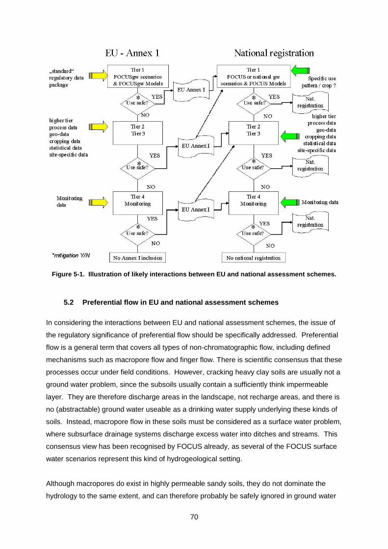
70
Figure 5-1. Illustration of likely interactions between EU and national assessment schemes.
5.2 Preferential flow in EU and national assessment schemes
In considering the interactions between EU and national assessment schemes, the issue of
the regulatory significance of preferential flow should be specifically addressed. Preferential
flow is a general term that covers all types of non-chromatographic flow, including defined
mechanisms such as macropore flow and finger flow. There is scientific consensus that these
processes occur under field conditions. However, cracking heavy clay soils are usually not a
ground water problem, since the subsoils usually contain a sufficiently think impermeable
layer. They are therefore discharge areas in the landscape, not recharge areas, and there is
no (abstractable) ground water useable as a drinking water supply underlying these kinds of
soils. Instead, macropore flow in these soils must be considered as a surface water problem,
where subsurface drainage systems discharge excess water into ditches and streams. This
consensus view has been recognised by FOCUS already, as several of the FOCUS surface
water scenarios represent this kind of hydrogeological setting.
Although macropores do exist in highly permeable sandy soils, they do not dominate the
hydrology to the same extent, and can therefore probably be safely ignored in ground water
71
leaching calculations. Finger flow can affect movement in sand soils, but there are no
models that use commonly available parameters. In less permeable sandy loams and loams,
preferential flow can significantly impact pesticide leaching in soil, and in these cases the
extent to which preferential flow is continuous to greater depths is an important question for
an assessment, especially for deeper ground water which is abstracted for drinking water.
Fissured moraine materials and fissured chalk and limestone, both overlying ground water
reserves, are examples of hydrogeological situations where preferential flow can be
important even at great depths. This has been recognised by FOCUS ground water, where
MACRO is used to calculate leaching in the Châteaudun scenario (loamy soil overlying
fractured limestone).
For risk assessment purposes, experimental studies incorporating the phenomenon of
preferential flow are extremely difficult to undertake due to the inherent spatial heterogeneity
of the soil. Simulation models are able to incorporate various types of preferential flow to
predict the effect of this process on pesticide leaching. The spatial variability of the process
still poses a significant challenge to verifying the predicted outputs of the models. However,
the effect of preferential flow must be considered where this poses a significant impact on
ground water. The best known model to address an aspect of preferential flow is MACRO,
which simulates macropore flow through consideration of soil aggregate size. Newer
versions of other models, such as PEARL, now also incorporate mathematical routines to
address various preferential flow mechanisms.
In the existing EU assessment scheme the FOCUS scenarios employ the MACRO model at
one site only (Châteaudun) to provide a comparison of results to those obtained with
chromatographic flow models (PRZM, PELMO, PEARL). To reflect the importance of
macropore flow as discussed here and reinforced further in EFSA PPR (2013a and b), it is
now recommended that MACRO Châteaudun simulations be completed for EU level
assessments where the representative use is for a crop defined for this scenario. These
results can be used directly to support decision-making on EU approval. At the national level
various member states (e.g. Denmark, Sweden, UK) use the simulation results obtained from
MACRO in decision-making for product authorisation.
For harmonisation of the assessment schemes between the EU and the Member States (and
between Member States), FOCUS has already noted (see earlier text) that differences in
between assessments at the EU and National Level should be based on differences in
environmental conditions/management practices rather than on pesticide parameters.

72
There is now scientific consensus that some preferential flows (e.g. at least macropore flow)
can result in movement to ground water and that this can be spatially significant at the spatial
scale of a confined vulnerable aquifer (EFSA PPR, 2013a and b and Jarvis N.J. et al., 2009).
As well as member states who consider that preferential flow leading to ground water
exposure is relevant for their soil types, having a justification (at the national authorisation
level) for taking these processes into account when making their assessments, it is
recommended MACRO Châteaudun simulations be completed for EU level so decision
makers have the relevant information.

73
6 CONSIDERATION OF RISK MITIGATION AND MANAGEMENT ON
EU AND ON NATIONAL LEVEL
As discussed in Chapter 3 the broad endpoints of the tiered approaches are different at
different political levels (i.e. EU evaluation, national authorisation). However, this can still be
consistent with a common framework for risk assessment at all the geographical levels.
At the EU level, the aim of risk characterisation is to identify safe uses for at least one
relevant crop and a significant area within the European Union. In contrast, at the national
level authorisation of a specific plant protection product for actual use in the relevant
agricultural, soil and climatic conditions is considered. Member states currently have
different views, or non-stated policies on what percentage of “safe use” is acceptable when
granting an authorisation. They also have different abilities to mitigate or manage a potential
risk (e.g. application restrictions to certain timings, soil types, defined areas etc).
Because both EU and national assessments will occur for each pesticide, the interactions
between the schemes should be considered. This will maintain consistency and minimise
duplication of work.
A working definition for risk mitigation with regards to the protection of ground water is:
Measures taken to adjust or restrict the use of a pesticide to obtain a favourable risk
assessment. These steps can be based either on knowledge of the behaviour of the
specific active substance, and/or on knowledge of the variability in the environment,
and/or differentiation in the use of application methods.
6.1 Important aspects affecting or used in risk mitigation
6.1.1 The GAP in the EU evaluation of active substances relative to the GAP on a national level
When an active substance is evaluated at the EU level, the aim is to identify at least one use
that is acceptable considering both possible effects on human health and the environment.
The number of uses evaluated in the EU process is usually limited to one or a few
representative crops. Therefore, the assessment of leaching to ground water on the member
state level will not usually be based on the same use pattern as the assessment during the
EU evaluation process. Therefore assessments carried out on the EU-level will not
74
necessarily be directly applicable to the authorisation procedures on the member state level.
This especially is true for the identification and implementation of risk mitigation measures.
The GAP defines the crops, dose, number of applications, recommended time between
applications, and recommended timing/crop stage for uses on each specific crop. This
information is used in the modelling simulations and other aspects of the risk assessment.
Note that only some aspects of efficacy and some of the possible application methods will
have been evaluated at the EU level, but these have to be fully evaluated at the member
state level.
6.1.2 Dose related risk mitigation
Under risk mitigation related to the dose, all measures that lead to a lower actual input of the
active substance into the soil can be considered. This lowering may be achieved by mixing
the assessed active substance with other active substance/s, resulting in the necessity for a
complete new risk assessment in all areas including efficacy studies on the relevant crops.
This approach is only considered on the member state level. Another way to lower the
amount which reaches the soil is to apply the pesticide at a later growth stage with higher
interception, though the effectiveness of this as mitigation will depend on the potential for the
substance to be washed off foliage. Since this may result in lower efficacy, this mitigation
measure can also be expected to be more country specific. Since all measures to lower the
amount reaching soil must be accompanied by efficacy data, this type of risk mitigation will in
practice only be applicable on the member state level. Lowering the number of applications
may be possible at both EU and MS level, but very likely also this adjustment has to be
based on efficacy trials. In certain cases the application may be restricted to every other
year or even longer intervals. If a particular active substance is used only on specific crops
this kind of risk mitigation may already be covered by the crop rotation according to good
agricultural practice. However, the possibility that the same active ingredient could be
applied to other crops in the rotation must be considered, so mitigation should take into
account all uses of the active substance in the crop rotation. Therefore crop rotation is a
mitigation measure usually only applicable at the member state level.
6.1.3 Using more effective application methods
Changing the method of application is likely to be more important as a risk mitigation
measure to reduce the impact on surface water rather than on ground water. A reduction of
the risk for ground water will be achieved by reducing the dose of the active substance
reaching the soil. Using band sprayers, which are used in crops growing in rows, such as
sugar beets, leeks and other vegetables, may reduce the dose significantly. This application
method is used in most European countries. Therefore, this could in principle be used as a
75
method for risk reduction both at the EU and member state level. As a prerequisite there is a
need to identify a (may be crop-specific) reduction rate from the use of this method. In this
circumstance particular attention has to be given to the definition of the application rate (i.e.
amount of active substance per area actually treated vs. amount of active substance per
whole field area). There is only a reduction in risk if the amount of active substance in the
whole field is reduced.
6.1.4 Pesticide properties correlated to soil properties
Pesticide properties are here related to both active substances and metabolites. Leaching
may be influenced by the effect of soil properties on transformation and adsorption.
For many compounds the most important factor for adsorption onto soil is the content of
organic carbon, but other soil properties (e.g. clay content) may also play a significant role.
Another important influencing factor may be the pH-dependency of transformation and
adsorption. Knowledge of these effects is mainly derived from laboratory studies. According
to the requirements of Regulation (EC) No 283/2013 and the guidance of the FOCUS
groundwater scenarios work group, the pH-dependency of the active substance and
metabolites has to be checked and considered, if appropriate. If the assessment identifies a
pH range which could result in possible leaching of the substance to ground water, the EU
recommends to the member states to consider the problem when granting authorisations.
This statement is included in the Review Report and in the Directive of inclusion of the active
substance. In this case the combined consideration of substance properties and
environmental properties (such as soil pH) may result in risk mitigation by excluding the use
in certain defined areas, where a risk for leaching is identified. This risk mitigation step can
consist of excluding use in either specific geographical areas or soil types. Geographical
exclusions allow for the easy identification of restricted areas at time of the authorisation of a
product. Soil exclusions require a well developed system of both enforcement and support
by competent local authorities and/or advisers. In addition, an appropriate post registration
monitoring programme might be required. An extensive geographical data base providing
soil properties on the EU and member state level would be helpful to identify and enforce the
options for specific cases.
6.1.5 Hydrogeological properties
Leaching may also be enhanced in areas where the hydrogeology is vulnerable to movement
to ground water. Using GIS data on the EU level (when the necessary data are available)
will give information on geographical areas with environmental properties that may lead to a
risk for ground water contamination of a specific compound. As discussed earlier, this
assessment can result in identification of vulnerable areas within EU, but also can lead to
76
identification of “safe” areas. If one safe use is identified and the area was considered to be
large enough by risk managers, an active substance can be approved at the EU level. If
there were indications from other FOCUS-scenarios of potential risk for ground water
contamination, this risk would need to be assessed by member states. These vulnerable
areas have to be identified on the member state level. As discussed previously for soil
restrictions, clearly identified areas where restrictions apply and competent local authorities
and advisers are prerequisite for successful risk mitigation.
6.1.6 Mitigation related to timing
Depending on the combination of environmental conditions and substance properties,
mitigation may also include the timing of applications. Such restrictions should be based on
the knowledge of risks identified with a set of environmental conditions such as climate and
soil properties, but also include substance properties, e.g. DegT50.
6.2 Examples of risk mitigation measures
The following risk mitigation measures are examples of possible label restrictions included in
the authorisation of certain plant protection products in some countries and may serve as an
illustration to the various aspects discussed above:
Dose related risk mitigation
The maximum load of this product containing active substance is restricted to x g (alternatively x litre) per ha and year.
The maximum application rate for active substance of x g per hectare and year must not be exceeded.
This product must not be applied before tillering. (in order to increase interception)
Products containing the active substance active substance are not to be used more than once a year on the same area
In those areas identified by the designated authority, the product must not be applied more than once a year on the same area.
Pesticide properties in correlation to soil properties
This product shall not be used on soils with less than x % organic matter. (may also be applicable to e.g. percentage of clay soil)
Not to be used on the following soil types: pure sand, slightly silty sand and slightly clayey sand.
Not to be used on the following soil types: pure sand, slightly silty sand and slightly clayey sand with an organic carbon content below x %.
Hydrogeological properties
This product is not recommended for use on karstic soils with very small top soil layer (could be a voluntary recommendation)
77
Not to be used in catchment areas of ground and spring water supply works, mineral springs and drinking water reservoirs or other sensitive ground water areas.”
Mitigation related to timing
This product must only be applied from 1st February in the year of harvest until the specified latest time of application. (in order to reduce possible ground water contamination from autumn applications.)
Not to be used between DD.MM and DD.MM.
Not to be used on drained soils between DD.MM and DD.MM.
6.3 Conclusion
On EU level only general recommendations for risk mitigation measures can be given based
on the evaluation of the properties of the active ingredient(s) and the risk assessment made
for the representative formulation in relation to the EU scenarios.
Detailed risk mitigation measures with regard to the protection of ground water against
contamination with active substances or relevant metabolites require detailed knowledge of
local environmental conditions and enforceable mitigation measures. They are therefore
mainly allocated to the authorisation procedure on the member state level. In most of the
cases risk mitigation measures will be related to restrictions imposed with the authorisation of
a certain plant protection product. Like any restriction in relation to the use of pesticides
measures aiming at the protection of ground water have to be checked with regard to their
practicable use prior to implementation. Applicators must be able to recognise the conditions
of allowed or prohibited use and (if appropriate) must have access to any necessary data.
On the other hand sound advice as well as enforcement capacities must be available from
the competent authorities.
Due to the fact that risk mitigation measures are mainly subject to MS considerations the
discussion in the context of this Guidance Document is restricted to the general aspects and
specific examples described above.
78
7 APPROACHES FOR TIER 2 ASSESSMENT
7.1 Pesticide parameter refinement (Tier 2a)
In Tier 2a parameter refinements can be made so that the pesticide-specific input for the
pesticide degradation and sorption processes can be incorporated in the assessment. The
remaining modelling parameters, i.e. the soil, crop, and climatic parameters, are considered
to be part of the scenario and are not modified. Note as the scenario selection of the FOCUS
tier 1 scenarios did not include a consideration of soil pH in vulnerability mapping, the pH
defined for each tier 1 FOCUS scenario should not be considered a part of the scenario
definition. I.e. substance properties selected should not automatically be selected base on
the scenario pH description. (EFSA, PPR 2013a and b). Also the basic modelling framework
of Tier 1 is maintained, so that pesticide flow and transport in soil is still considered to be a 1-
D chromatographic flow process. While changes in other modelling parameters and the
basic modelling framework can be made when scientifically appropriate, such modelling work
would then be classified as belonging to other tiers. Table 7-1 gives an overview of the
relevant processes which result in refinements included in Tier 2a. More details are given in
the following sections.
79
Table 7-1. Overview of the relevant processes resulting in refinements included in Tier 2a.
Section Process Parameter in Tier 1 model
Proposed Refinement
Remark
7.1.1 Soil specific sorption and degradation
Degradation rate, Kd, Kf, 1/n
Include additional degradation rates
Modify sorption and degradation in terms of known soil properties, exploiting clear relationships between soil properties and degradation and sorption.
Additional degradation rates improve the data base for parameter selection
Includes subsoil degradation
Substance specific degradation rates for changes of degradation rates with depth
Note pH dependence of Degradation rate, Kd, Kf, has to be addressed at tier 1
7.1.2 Photolytic degradation Degradation rate Include a thin soil layer with modified degradation rate on top of plough layer if evidence of photolysis is available, the degradation rate in this thin layer should not be selected to represent both microbial and photolytic rate constants, but just photolytic degradation. OR Reduce application rate by the fraction that on average will disappear by photolysis in field degradation studies, provided that photolysis is a loss process in laboratory studies and that under the actual use conditions soil will be exposed to global radiation
The production of photolysis metabolites at the soil surface when this is indicated in photolysis experiments needs to be included in exposure assessments already at tier 1. Of course this also needs to be addressd at tier 2a
7.1.3 Anaerobic degradation
Degradation rate Do not use as Tier 1 scenario definitions have bottom boundary conditions that mean that saturated soil layers for significant durations will not occur.
Note should anaerobic subsoil degradation be expected (applicable for a tier 3a assessment) novel anaerobic soil metabolites need to be addressed.
7.1.4 Field degradation rates
Degradation rate Use normalised degradation rates obtained from field studies or combine them the lab data.
see EFSA (2014a) DegT50 guidance
7.1.5 Degradation kinetics not described by first order
Degradation rate Consider non-equilibrium sorption approaches if possible. If the behaviour cannot be explained by non-equilibrium sorption an alternative bi-phasic approach may be appropriate
see Section 7.1.6 and FOCUS kinetics guidance (FOCUS, 2006)
7.1.6 Non-equilibrium sorption
Kd, Kf 1/n Introduce time dependent sorption constants
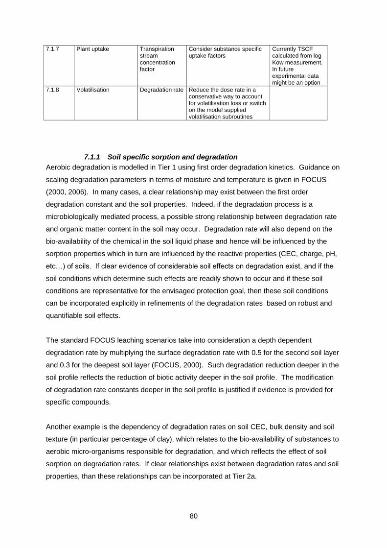
80
7.1.7 Plant uptake Transpiration stream concentration factor
Consider substance specific uptake factors
Currently TSCF calculated from log Kow measurement. In future experimental data might be an option
7.1.8 Volatilisation Degradation rate Reduce the dose rate in a conservative way to account for volatilisation loss or switch on the model supplied volatilisation subroutines
7.1.1 Soil specific sorption and degradation
Aerobic degradation is modelled in Tier 1 using first order degradation kinetics. Guidance on
scaling degradation parameters in terms of moisture and temperature is given in FOCUS
(2000, 2006). In many cases, a clear relationship may exist between the first order
degradation constant and the soil properties. Indeed, if the degradation process is a
microbiologically mediated process, a possible strong relationship between degradation rate
and organic matter content in the soil may occur. Degradation rate will also depend on the
bio-availability of the chemical in the soil liquid phase and hence will be influenced by the
sorption properties which in turn are influenced by the reactive properties (CEC, charge, pH,
etc…) of soils. If clear evidence of considerable soil effects on degradation exist, and if the
soil conditions which determine such effects are readily shown to occur and if these soil
conditions are representative for the envisaged protection goal, then these soil conditions
can be incorporated explicitly in refinements of the degradation rates based on robust and
quantifiable soil effects.
The standard FOCUS leaching scenarios take into consideration a depth dependent
degradation rate by multiplying the surface degradation rate with 0.5 for the second soil layer
and 0.3 for the deepest soil layer (FOCUS, 2000). Such degradation reduction deeper in the
soil profile reflects the reduction of biotic activity deeper in the soil profile. The modification
of degradation rate constants deeper in the soil profile is justified if evidence is provided for
specific compounds.
Another example is the dependency of degradation rates on soil CEC, bulk density and soil
texture (in particular percentage of clay), which relates to the bio-availability of substances to
aerobic micro-organisms responsible for degradation, and which reflects the effect of soil
sorption on degradation rates. If clear relationships exist between degradation rates and soil
properties, than these relationships can be incorporated at Tier 2a.
81
The various models have different options for defining sorption and degradation that can vary
with soil properties.
7.1.1.1 Degradation parameters and soil properties
In each of the FOCUS ground water models (PEARL, PELMO, PRZM, and MACRO), first
order kinetics is used to describe degradation. The user supplies rate constants for the first
soil horizon and then the programs calculate the degradation rate in each soil horizon. The
user also has the option of specifying the rate constants for each soil layer. The degradation
rate in a specific soil horizon is constant for a run, but unless specified to the contrary is
adjusted for soil moisture and temperature.
7.1.1.2 Sorption parameters and soil properties
7.1.1.2.1 MACRO
The user specifies the Koc at reference conditions and Freundlich exponent and the program
calculates the Kf values for each layer. The Freundlich exponent is a single value for the
whole profile. MACRO 5 can model non-equilibrium sorption kinetics with a two-site model.
Kinetic parameters are assumed to be constant for the whole soil profile.
7.1.1.2.2 PEARL
PEARL has the following three options:
1. pH-independent. Sorption described only with Kom. 2. pH-dependent. Sorption described by pH, Kom,base and Kom,acid according to equation
7-1 below 3. user defined. The user has to supply the Kf for each layer
PEARL contains a description of the sorption of weak acids, which is pH dependent:
H-Ka-pH
ac
H-Ka-H
ac
,,aceq,.
101
10
ppba
pppbabaeqomom
omF,eq
M
M
M
MKK
mK
(7-1)
where omm is the organic matter content, Kom,eq,ac (m3 kg-1) is the coefficient for sorption on
organic matter under acidic conditions, Kom,eq,ba (m3 kg-1) is the coefficient for sorption on
organic matter under basic conditions, M (g mol-1) is molar mass, pKa is the
-10log(KA) where KA is the dissociation constant, and ΔpH is a pH correction factor.
See Leistra et al. (2001) for the derivation of Equation 7-1.
7.1.1.2.3 PELMO
82
PELMO has the following four options:
1. pH-independent. Sorption in soil described based on Koc only. 2. pH-dependent mode 1 (Koc is known at a single pH). PELMO considers pH-
dependency of sorption for weak acids. Equilibrium conditions between the non-ionic and the ionic form are calculated based on the pKa value. PELMO assumes that the sorption of the compound can be expressed by the weighted mean of the two species according to Equation 7-2: Koc = fH-A * Koc,H-A + (1-fH-A) * Koc,A- (7-2) Koc: sorption constant of the compound (L/kg) fH-A: fraction of the non-ionic form in soil (pH-dependent) Koc,H-A: sorption constant of the non-ionic form of the compound (L/kg) Koc,A-: sorption constant of the ionic form of the compound (L/kg) In mode 1 a constant Koc ratio of 1000:1 between non-ionic and ionic form of the compound is assumed. In mode 1 PELMO is extrapolating pH-dependent sorption constants.
3. pH-dependent mode 2 (Koc is known at two different pH values). The same assumptions are assumed for the distribution of non-ionic and ionic form of the molecule. However, the ratio of the sorption coefficients between ionic form and non-ionic form is calculated compound specific based on two Koc-values given by the user. In contrast to mode 1 PELMO is therefore usually interpolating pH-dependent Koc for the range given by the user.
4. user defined. The user has to enter the sorption constant (Koc) for each layer.
7.1.1.2.4 PRZM
PRZM has the following two options:
1. pH-independent. Sorption described only with Koc at reference conditions and Freundlich exponent. The exponent is constant throughout the soil profile. The program calculates the Kf values for each layer.
2. user defined. The user has to supply the Kf values for each layer and the Freundlich exponent. The exponent is constant throughout the soil profile.
Note at tier 2a the models should not be used to model pH dependent adsorption based on the FOCUS scenario defined soil pH in the soil column, as the vulnerability of the FOCUS standard scenarios with respect to leaching is determined by the organic matter content and texture only, thus using soil properties other than organic matter and texture may significantly change the target vulnerability of the scenario. pH dependence of adsorption matched to scenario parameters belongs to tier 3a. (EFSA, PPR 2013a and b).
7.1.2 Photolytic degradation
If photolysis is significant then, as suggested by FOCUS (2006), degradation kinetics could
be simulated by using the photolysis degradation rate in the soil near the surface (i.e. the first
compartment of the soil model or for the first millimetre) and the non-photolytic degradation
rate in deeper layers. Usually, the photolysis process is significant only in the time between
application and the first rain (or irrigation) event after the application because the pesticide
will be transported to deeper soil layers where it will not be affected by sunlight any more.
83
Another practical option to consider the loss by soil photolysis would be to determine the
fraction that on average will disappear by photolysis in the field degradation studies (e.g. as a
fast phase of a biphasic decline line), provided that photolysis was is proven as a loss
process in laboratory studies and under the actual conditions the soil will be exposed to
global radiation. Note the leaching behaviour of any photolysis metabolites that might be
formed at the soil surface need to be assessed at both tier 1 and tier 2a. (EFSA, PPR
2013b).
7.1.3 Soil specific anaerobic degradation
Anaerobic degradation is not currently explicitly addressed in the FOCUS models. The
aerobic degradation term that is used as input is internally adjusted by the model depending
on the calculated soil moisture within the profile (using the “Walker” equation; see FOCUS,
2002) but this does not extend to anaerobic conditions. The PEARL and MACRO models
have a cut-off which prevents the moisture correction fraction from exceeding 1 (i.e. in the
case that the calculated soil moisture in the soil profile exceeds the reference value of pF2)
and the hydrology modules in PELMO and PRZM do not permit soil moisture to exceed the
reference value of pF2). Flooding (anaerobic conditions) in topsoil are generally not
anticipated to last for significant periods and even these periods would be during the winter
months when only limited pesticide application or residual pesticide activity is expected.
Therefore, in the overwhelming majority of cases, the incorporation of a specific anaerobic
degradation term for the topsoil is not necessary and is incompatible tier 1 FOCUS scenario
definitions.
For sub-surface degradation (to a depth of 1m), the FOCUS models contain default factors
relating the degradation rate to that in the topsoil (see Generic guidance for FOCUS
groundwater scenarios, version 1.1, April 2002). If experimental anaerobic degradation data
suggest specific mechanisms occur for a particular pesticide, for instance if degradation is
chemically mediated and/or catalysed by the presence of Fe2+ oxides (Smelt et al., 1995),
this may form a basis of a justification for amending these default values. This is in
accordance with the existing FOCUS guidance (see FOCUS, 2002). Otherwise, the use of a
specific anaerobic degradation term for the 30-100 cm soil profile is not considered
necessary. If microbially mediated anaerobic degradation is demonstrated to be important for
transformation (compared to aerobic conditions), anaerobic topsoil, transformation rates
should not be applied to deeper soil layers where microbial activity will be lower.
Evidence also exists that degradation may occur beyond 1 m in saturated zones. Leistra and
Smelt (2001), for example, have shown that the presence of fossil organic carbon may
84
sustain degradation in the subsoil. If degradation is chemically mediated and catalysed by
the presence of Fe2+ oxides e.g., then the degradation may increase in reduced ground
water where Fe2+ oxides are present (Smelt et al., 1995). Reductive dechlorination and
methanogenic dechlorination have also been shown to be the transformation pathways for
chlorinated substances in other anaerobic systems (Boesten et al., 1992; Van der Pas et al.,
1998). Compound-specific anaerobic degradation data may be useful in predicting the
degradation of a compound below 1 m (the default assumption in the FOCUS process is that
no degradation occurs below 1 m). Note should anaerobic subsoil degradation be expected
(applicable for a tier 3a assessment) novel anaerobic soil metabolites need to be addressed.
7.1.4 Use of field dissipation degradation rates in leaching models
Field dissipation trials have been conducted for a number of compounds as a requirement
under Regulation (EC) 1107/2009 or pertinent U.S. EPA or Canadian guidelines.
A clear advantage of field over laboratory results is that they are determined under conditions
specific for the intended use of a pesticide in an agricultural field (i.e. unsieved soil,
fluctuating soil temperature and moisture conditions, and sometimes the presence of crops)
and thus may closely match the situation which is to be modelled. Field DegT50 and
DegT90 values also reflect the variation in degradation due to seasonal changes in climatic
conditions. As a consequence degradation rates for parent and metabolites derived under
field conditions where the influence of surface processes have been minimised may be used
in FOCUS pesticide fate modelling. This general recommendation implies that the design of
the sampling regime excluded any significant route of dissipation other than degradation
within the soil matrix (for example, leaching, runoff, volatilisation, plant uptake and soil
surface photolysis; see EFSA 2014a).
In a strict sense, field dissipation degradation rates reflect primarily the degradation of a
compound under site-specific soil and climate conditions. As a consequence averaging field
degradation rates from different climate zones is not appropriate. To overcome this limitation
FOCUS (2006) proposed two methods to normalise the results of field dissipation trials to a
reference temperature of 20°C and a reference soil moisture of 100 % FC. One of these
normalisation methods (time step normalisation) is recommended in the more recent EFSA
DegT50 guidance EFSA (2014a). After the normalisation to reference conditions field
dissipation data where there is confidence that dissipation processes at the soil surface have
been minimised can be used in simulation models which account for the effects of
temperature and soil moisture on degradation rates (see EFSA DegT50 guidance EFSA
2014a). Furthermore averaging normalised field dissipation half-lives from various climate
85
zones (e.g. Northern and Southern Europe) as done with laboratory half-lives, is also
appropriate. This principle may also apply to field dissipation trials from the U.S. , Canada or
other temperate zones if these trials were conducted in regions that have conditions found in
Europe. When using non-European field data, a short justification must be provided as to
why the respective region is deemed representative for Europe. Some areas, like the sub-
tropical southeastern states of the U.S.A, may not be representative for Europe. Further
guidance on this subject is included in EFSA DegT50 guidance EFSA (2014a).
Note that normalised half-lives should be exclusively used as input parameters in models,
which are able to simulate daily variations of temperature and soil moisture. The normalised
field half-life represents a half-life at 20 °C and 100 % FC (which is assumed to be reached at
10 kPa) whereas the uncorrected half-life reflects local temperature and soil moisture
conditions.
EFSA DegT50 guidance (EFSA 2014a) provides detailed guidance on how to treat the
laboratory soil incubations and field soil studies to derived the normalised DegT50matrix
values to be input into FOCUS models.
7.1.5 Degradation kinetics that deviate from first order
Degradation of compound in soil may not be suitably described in all cases with single first
order kinetics models. In these cases non-equilibrium sorption approaches in FOCUS
models with linked sorption and degradation routines (see Section 7.1.6) should be checked
to see if they are capable of describing the behaviour of the compound and therefore suitable
for use in predicting leaching to ground water. Information on this subject is also given in
FOCUS (2006) (see especially Section 7.1.2.2.1 and Appendix 4).
7.1.6 Non-equilibrium sorption
Another option for pesticide parameter refinement is to include non-equilibrium sorption.
Long term sorption kinetics has been observed in many pesticide sorption experiments and
has a significant impact on pesticide fate and transport. Wauchope et al. (2002) in their
review on sorption distinguish three time scales for sorption kinetics of pesticides in soil: (i)
minutes, (ii) hours (until a day or two), (iii) weeks to years. The process at a time scale of
weeks to years is probably caused by slow diffusion of dissolved chemicals towards the
sorption sites within soil pores or organic matter polymers (pore diffusion and intraorganic
matter diffusion; see Pignatello, 2000).
86
7.1.6.1 Models for describing non-equilibrium sorption
A popular model for dealing with sorption kinetics is the two-site/two-region model (Van
Genuchten and Wagenet, 1989; Streck et al., 1995), which separates the soil sorption sites
in equilibrium and non-equilibrium sites. The basis for this simplification is that sorption sites
reacting at time scales ranging from minutes to a day or two are close enough to equilibrium
when assessing pesticide leaching to ground water. A two-site model is available in FOCUS
PEARL (Leistra et al., 2001) and in MACRO 5.0 (Larsbo and Jarvis, 2003).
To describe non-equilibrium sorption, two types of additional parameters are necessary: the
parameters describing the sorption isotherm of the non-equilibrium sites and a parameter
describing the adsorption/desorption rate of these sites. The most relevant models for
describing long-term sorption kinetics in the context of pesticide registration are described
below.
7.1.6.1.1 PEARL
The submodel used in PEARL for sorption and degradation can be described as follows
(Leistra et al., 2001):
)(* ,, PEARLNEPEARLEQL SScc (7-3)
N
RL
LRLEQFPEARLEQ
c
ccKS
,
,,, (7-4)
)( ,
,
,,,
,
PEARLNE
N
RL
LRLNEFPEARLd
PEARLNES
c
ccKk
dt
dS
(7-5)
EQFPEARLNENEF KfK ,,, (7-6)
)( ,PEARLEQLtt SckR (7-7)
where
c* = total concentration (mg/L)
cL = concentration in the liquid phase (mg/L)
cL,R = reference concentration in the liquid phase (mg/L)
= volume fraction of water (-)
= dry bulk density (kg/L)
SEQ,PEARL = content sorbed at equilibrium sites (mg/kg)
87
SNE,PEARL = content sorbed at non-equilibrium sites (mg/kg)
KF,EQ = equilibrium Freundlich sorption coefficient (L/kg)
KF,NE = non-equilibrium Freundlich sorption coefficient (L/kg)
N = Freundlich exponent (-) (elsewhere in this report 1/n was used)
kd,PEARL = desorption rate coefficient (d-1)
fNE,PEARL = factor for describing the ratio between the non-equilibrium and equilibrium
Freundlich coefficients in PEARL (-)
Rt = rate of degradation in soil (mg L-1 d-1)
kt = degradation rate coefficient (d-1)
So the total Freundlich sorption coefficient KF,tot is defined in PEARL as follows
EQFPEARLNENEFEQFtotF KfKKK ,,,,, 1 (7-8)
As follows from Equation 7-3, the total content sorbed in the PEARL model, SPEARL , is
defined as:
PEARLNEPEARLEQPEARL SSS ,, (7-9)
Equation 7-7 implies that pesticide sorbed at the non-equilibrium sorption site is not subject
to degradation. As will be demonstrated below, mathematical analysis shows that including
transformation at this site makes no difference for the description of long-term sorption
kinetics (and thus makes also no difference for the leaching endpoint of the risk assessment).
For that purpose a model is considered (based on Equation 7-5) in which additionally first-
order transformation occurs at the non-equilibrium site:
PEARLNENEtPEARLNE
N
RL
LRLNEFPEARLd
PEARLNE SkSc
ccKk
dt
dS,,,
,
,,,
,
(7-10)
where
kt,NE = rate coefficient for transformation at non-equilibrium sorption site (d-1).
Equation 7-10 can be rewritten as:
PEARLNE
N
RL
LRLNEF
NEtPEARLd
PEARLd
NEtPEARLd
PEARLNE Sc
ccK
kk
kkk
dt
dS,
,
,,
,,
,
,,
, )( (7-11)
Effective values of kd,PEARL and KF,NE are now defined as follows (Boesten, 1986, p. 161):
88
NEtPEARLd
eff
PEARLd kkk ,,, (7-12)
NEF
NEtPEARLd
PEARLdeff
NEF Kkk
kK ,
,,
,
,
(7-13)
Thus Equation 7-11 can be rewritten as:
PEARLNE
N
RL
LRL
eff
NEF
eff
PEARLd
PEARLNE Sc
ccKk
dt
dS,
,
,,,
, (7-14)
Equation 7-14 is mathematically identical to Equation 7-5. So if first-order transformation
occurs at the non-equilibrium site and Equation 7-5 is used for fitting, this process has
already been included in the fitted kd,PEARL and KF,NE values. So this analysis shows indeed
that including transformation at the non-equilibrium site makes no difference. Note that
transformation at the non-equilibrium site leads to higher apparent kd,PEARL values and lower
apparent KF,NE values.
7.1.6.1.2 The model of Streck
The model of Streck et al. (1995) defines the total concentration sorbed, SSTRECK,as follows:
STRECKNESTRECKSTRECKEQSTRECKEQSTRECK SfSfS ,,, )1( (7-15)
where
fEQ,STRECK = the fraction equilibrium sites (-).
In this model the equilibrium content sorbed is defined as
N
RL
LRLtotFSTRECKEQ
c
ccKS
,
,,, (7-16)
with KF,tot as defined by Equation 7-8. The sorption rate equation for the non-equilibrium sites
is as follows:
)()1( ,,
,
, STRECKNESTRECKEQSTRECK
STRECKNE
STRECKEQ SSdt
dSf (7-17)
where
STRECK = sorption rate coefficient (d-1).
Comparison of Equation 7-15 with Equation 7-9 shows the following relationships:
89
STRECKEQSTRECKEQPEARLEQ SfS ,,, (7-18)
STRECKNESTRECKEQPEARLNE SfS ,,, )1( (7-19)
Using Equations 7-18 and 7-19, SEQ,STRECK and SNE,STRECK can be eliminated from Equation 7-
17 Comparison of the resulting equation with Equation 7-5 leads to the following
relationships between the parameters in the model used by Streck et al. (1995) and the
parameters used in the PEARL model:
STRECKEQ
STRECKPEARLd
fk
,
,1
(7-20)
STRECKEQ
STRECKEQ
PEARLNEf
ff
,
,
,
1 (7-21)
Note that Equations 7-20 and 7-21 are based on the theory and the model descriptions by
Streck et al. (1995) and Leistra et al. (2001). Therefore, these equations are only valid in
practice if the same operational definition of “equilibrium” is used (see Section 7.1.6.2 on
experimental procedures).
7.1.6.1.3 MACRO
The submodel used in MACRO 5.0 (Larsbo and Jarvis, 2003) is based on the model of
Streck but it uses a slightly different formulation of the rate equation:
MACRONE
N
RL
LRLtotF
MACRONE
MACROMACRONES
c
ccK
fdt
dS,
,
,,
,
, (7-22)
where
SNE,MACRO = content sorbed at non-equilibrium sites in MACRO (mg/kg)
MACRO = desorption rate coefficient (d-1) used in MACRO.
fNE,MACRO = fraction of the non-equilibrium sorption sites in MACRO (-)
αSTRECK is identical to αMACRO and it can also be shown that:
STRECKEQMACRONE ff ,, 1 (7-23)
The relationships between the PEARL and MACRO parameters can be shown to be as
follows:
90
PEARLNE
PEARLNE
MACRONEf
ff
,
,
,1
(7-24)
or
MACRONE
MACRONE
PEARLNEf
ff
,
,
,1
(7-25)
and
PEARLNE
PEARLNE
PEARLdMACROf
fk
,
,
,1
(7-26)
or
MACRONE
MACROPEARLd
fk
,
,
(7-27)
In MACRO 5.0, the total sorption coefficient KF,tot is denoted as ZKD.
The above analysis shows that all three models are mathematically identical, and that
parameters derived using one of the models can be translated into parameters of the other
two models.
7.1.6.1.4 PRZM and PELMO
In the versions of PRZM and PELMO released with the new scenarios, non-equilibrium
sorption is implemented as well. In both models the approach of PEARL as shown in
7.1.6.1.1 is used. However, in PELMO the parameters can also be inserted according to the
Streck-model as shown in 7.1.6.1.3. The values are then internally converted according to
Equations 7-20 and 7-21.
7.1.6.2 Experimental procedures for measuring long-term sorption kinetics and
procedures for estimating the model parameters
The most straightforward procedure would be to measure long-term kinetics as part of the
standard degradation rate studies. Measurements of long-term sorption kinetics have to be
based on the total content of pesticide in soil because there is usually some degradation on a
time scale of weeks. As a consequence the same or similar organic-solvent extraction
procedures have to be used for measuring (i) the degradation rate and (ii) long-term kinetic
parameters. This can be illustrated with the following example. Mild extraction procedures
(e.g. single extraction with ethyl acetate or acetone) will lead to shorter half-lives than strong
extraction procedures. Strong extraction procedures (e.g. soxhlet extraction or repeated
91
extractions with different types of solvents) will lead to higher contents sorbed at the non-
equilibrium site.
The parameters for the equilibrium site should be derived from the standard adsorption
experiments. These experiments have an equilibration time of typically 24 h which
corresponds well with the time scales of the first two types of site as defined by Wauchope et
al. (2002). We use the symbol KF,ads,batch-1day for a Freundlich sorption coefficient measured in
an adsorption batch experiment of about one day (OECD, 2000). An additional advantage is
that these are also the parameters used in previous lower tiers. The parameters for the non-
equilibrium site should be derived from incubations of moist soil because this is closest to
field conditions. We will call such studies hereafter ‘aged sorption studies’. Those studies
are very similar to laboratory soil degradation studies according to OECD guideline 307
(OECD, 2002). One may expect that batch sorption experiments on time scale of weeks
lead to an overestimate of the kd,PEARL (i.e. the rate coefficient of the non-equilibrium sites)
because of the shaking procedures in such experiments.
Leistra et al. (2001) recommend to measure the equilibrium sorption coefficient in PEARL
(KF,EQ ) via a standard batch experiment (so KF,EQ = KF,ads,batch-1day). So if the true total
Freundlich coefficient KF,tot is available, fNE,PEARL can be estimated as:
11,,
,
1,,
1,,,
,
daybatchadsF
totF
daybatchadsF
daybatchadsFtotF
PEARLNEK
K
K
KKf (7-28)
As described before, Equations 7-19 and 7-20 are based on the theory and the model
descriptions by Streck et al. (1995) and Leistra et al. (2001). However, these publications
recommend different operational definitions for measuring the equilibrium and the rate of
exchange of the non-equilibrium sorption sites. Although Equations 7-19 and 7-20 are
mathematically correct, they are of little use when these different operational definitions are
used. Streck et al. (1995) propose to measure the rate coefficient αSTRECK by shaking a soil
suspension over a period of about a week. This implies that the equilibrium sites in the Streck
model equilibrate within a time period in the order of 1 h. However, Leistra et al. (2001)
propose to measure kd,PEARL in aged sorption studies that may last a few months.
Furthermore, the operational definition for the equilibrium sites of Leistra et al. (2001) is
shaking for about 1 day in a batch study. Thus if the recommendations of Streck et al. (1995)
and Leistra et al. (2001) are followed, a consistent operational value for fNE,PEARL from results
obtained by the Streck approach, can be obtained from Equation 7-28 where KF,tot is derived
from fits based on the Streck approach.
92
Measurement of long-term kinetics in moist soil requires a time series of:
(i) the total content of pesticide in soil.
(ii) the concentration of pesticide in the soil pore water.
The concentration in the pore water can be measured by collecting liquid phase (e.g.
centrifuge a soil sample over a filter). This will not work for all soil types. An acceptable
alternative is to perform a 24-h desorption experiment and to assume that (i) the equilibrium
sorption site is at equilibrium after these 24 h and (ii) the change in content sorbed at the
non-equilibrium site is negligibly small over these 24 h shaking time. The concentration in
the pore water can then be back calculated using the difference between the solid-liquid
ratios of the moist soil and the batch desorption systems or can be directly fitted if the model
is able to calculate the concentration in the suspension solution with a given soil:water ratio.
A useful resource for more up to date considerations of the most appropriate experimental
designs and methods for estimating / fitting time dependent adsorption parameters in
laboratory experiments can also be found in draft UK guidance (Beulke S and Van Beinum,
2012).
Alternatively, non-equilibrium sorption parameters can also be obtained from controlled
(steady) pesticide column leaching experiments. Analytical solutions for the two site-two
region models have been developed by Toride et al. (1993), and have been readily
implemented in the CXTFIT model identification tool (1995). Yet, inverse modelling of
pesticide breakthrough for identifying sorption kinetic parameters may be inappropriate or
subjected to a lot of uncertainty (Vanderborght et al., 1997). The parameters for the
equilibrium sorption site also in this case should be based on independent batch experiments
with a shaking time of 1 day. If breakthrough curves were inversely modelled and residual
concentrations in the soil column at the end of the column study have been measured, it is
preferable to include these results in the inverse modelling procedure. More details on
inverse modelling are given in Chapter 8.
Estimating non-equilibrium sorption parameters from lysimeter leachate concentrations may
also be possible. However, probably this is only possible in exceptional cases because other
system properties may have an effect on the pesticide breakthrough that is similar to the
effect of non-equilibrium sorption parameters.
93
Another option would be to estimate non-equilibrium sorption parameters from field
experiments that include desorption studies from soil samples from the top centimetres. So
far little experience is available with this procedure. More experience with such procedures
should be gained before using them in risk assessments.
Theoretically, non-equilibrium sorption parameters may be derived from analysis of
adsorption-desorption hysteresis as performed by Streck et al 1995 and Altfelder 2000 using
the FITHYST fitting tool (Streck 1997). Using this approach the total sorption KF,tot can be
estimated; using Equation 7-28 fNE,PEARL can then be estimated if an independently measured
value of KF,ads,batch-1day is available. Although the relevance of the estimated parameters were
tested by comparing the so-derived parameters with other experimental data (Streck, 1995,
Streck, 1999, Altfelder, 2001, Jene, 2007), more information is necessary to derive non-
equilibrium sorption parameters using this method.
Finally, sorption kinetic parameters may also be estimated from analysing bi-phasic
degradation kinetics. Indeed, the occurrence of bi-phasic degradation kinetics may be the
macroscopic expression of the microscopic non-equilibrium sorption. Guidelines for
estimating long term sorption parameters for PEARL from bi-phasic kinetic degradation
experiments are given by FOCUS (2006). However, this procedure is expected to work only
in cases in which the degradation rate of the first phase is very fast (half-lives in the order of
5 days).
7.1.6.3 Overview of available measurements of long-term sorption parameters
There are many studies demonstrating the significance of the long-term sorption process
(e.g. see data for Hawaiian soils cited by Hamaker & Thompson, 1972, and for a UK soil
measured by Walker, 1987). However few experiments have been analysed with the
submodels used by PEARL or MACRO. Boesten et al. (1989) found fNE,PEARL values ranging
from 0.3 to 0.4 and kd,PEARL values ranging from 0.01-0.02 d-1 for cyanazine and metribuzin in
a sandy soil. They showed that the assumption of non-equilibrium sorption was necessary to
explain the movement of the substances in a field experiment. Boesten and Gottesbüren
(2000) found a fNE,PEARL value of 0.55 and a kd,PEARL value of 0.015 d-1 for bentazone in a
sandy soil. Using the same bentazone data, Tiktak et al. (2000) found fNE,PEARL =0.73 and
kd,PEARL =0.019 d-1. Boesten (personal communication, 1996) found a fNE,PEARL value of 0.75
and a kd,PEARL value of 0.005 d-1 for both metamitron and hydroxychlorothalonil in a sandy soil.
Based on this information Leistra et al. (2001) recommend to use a default fNE value of 0.5
and/or a default kd value of 0.01 d-1. Gurney and Hayes (2007) analysed a herbicide where
aged sorption studies were carried out in three soils yielding fNE,PEARL values of 0.42, 0.48 and
94
0.75. They did not estimate the sorption rate coefficient kd,PEARL but fixed it to the default
value of 0.01 d-1. Jene (2006) reported an average fNE,PEARL value of 2.7 for a pesticide based
on aged sorption studies with two soils. So this fNE,PEARL value is much larger than the other
values that have been reported. However field degradation studies with the same compound
at seven sites showed extreme bi-phasic behaviour which could be well explained by
applying the non-equilibrium sorption concept using the high fNE,PEARL values from the
laboratory study.
There is also indirect evidence for the long-term sorption process. Streck et al. (1995)
showed that the leaching of simazine in a field lysimeter transport experiment could be
explained if non-equilibrium sorption estimated from sorption hysteresis data of a laboratory
batch sorption study was considered in the modelling. In Streck and Richter (1999) the depth
concentration profile of chlortoluron in a field leaching study could only be reproduced by
modelling if the kinetic parameters derived from the sorption batch experiment where used.
Finally, Altfelder et al. (2001) showed the compatibility of the results from laboratory batch
adsorption and column experiments with regard to the non-equilibrium sorption behaviour of
dimethylphtalate.
Indirect evidence can also be derived from the hysteresis phenomenon. Hysteresis in
adsorption/desorption isotherms measured in batch systems has been reported in many
publications. Altfelder et al. (2000) demonstrated for a few studies that the observed
hysteresis could be explained by long-term adsorption kinetics using the FITHYST software
package (Streck, 1997) which is based on the model of Streck et al. (1995). In one example
the 24-h adsorption isotherm had a value that was only 50% of the ‘true’ equilibrium
isotherm, so fNE,PEARL was about 1.0. Studies by Pignatello and co-workers have shown that
part of the observed hysteresis is not related to long-term sorption kinetics but to a ‘true’
change in the sorption equilibrium caused by an irreversible deformation of the organic
matter (e.g. Sander et al., 2005).
Reichenberger et al. (2002) analysed adsorption-desorption isotherms of 8 pesticides (in
total 67 studies) with the FITHYST software package and found a median ratio of the
quotient KF,tot / KF,ads,batch-1day of 1.79 which implies a median fNE,PEARL of 0.79 (See Equation 7-
28). The poster-version of their paper showed a very large scatter in this quotient.
Reichenberger et al. (2002) did not provide the source of the 67 studies but probably all data
sets comprised at least two desorption steps and a study of adsorption kinetics following
procedures described in OECD guideline 106. Reichenberger and Laabs (2003) analysed
adsorption-desorption isotherms for nine pesticides and two tropical soils. They derived KF,tot
95
values from experiments on adsorption kinetics on a time scale up to 4 days and from
experiments with five sequential desorption steps that lasted in total 7 days. They found a
median value of the quotient KF,tot / KF,ads,batch-2days of 1.6 and 2.4 for the two soils (so KF,EQ was
defined by 48 h shaking). The range of the quotients was considerable (from 0.7 to 12) and
the average value was 3.0 and 3.6 for the two soils. The median values correspond with fNE
values of 0.6 and 1.4 for the two soils. However, no standard deviations were provided for
estimated KF,tot values. It cannot be excluded that these values have a large uncertainty; e.g.
a value of the quotient KF,tot / KF,ads,batch-2days of 12 implies that the KF,tot based on experiments
that lasted at most 7 days is 12 times higher than the adsorption coefficient measured after 2
d shaking. Such an increase is very unlikely.
Reichenberger and Laabs (2003) found a median value of the rate coefficient STRECK of 0.05
d-1 for both soils and median fSTRECK values of 0.4-0.5. This means that they found kd,PEARL
values in the order of 0.1 d-1, which is an order of magnitude higher than the kd,PEARL values
found in moist soil by Boesten et al. (1989), Boesten and Gottesbüren (2000) and Tiktak et
al. (2000). This difference is probably caused by the shaking procedure used in batch
adsorption-desorption measurements which leads to faster equilibration than would occur in
field soils.
Jene (personal communication, 2004) analysed adsorption-desorption measurements in soil
suspension for one pesticide and seven soils and found ratios of the quotient KF,tot /
KF,ads,batch-1day of 3.1 to 6.6 (so fNE,PEARL values of 2.1 to 5.6). ). For one of those values
(fNE,PEARL of 2.2), which was derived from a lysimeter soil, Jene (2007) could show that almost
the same value was estimated when fitting the outflow behaviour of this pesticide from three
replicated outdoor lysimeters.
The fNE,PEARL values found in adsorption-desorption batch experiments by Altfelder et al.
(2000), Reichenberger et al. (2002), Reichenberger & Laabs (2003) and Jene (personal
communication, 2004) tend to be higher than those found in aged sorption studies. However,
no studies are available where fNE,PEARL is measured both via adsorption-desorption isotherms
and via aged sorption studies for the same pesticide-soil combination. Given the limited
number of fNE,PEARL values that are available, no conclusion is yet possible on the relationship
between fNE,PEARL values measured with both methods. The possibility cannot be excluded
that fNE,PEARL values obtained from adsorption-desorption isotherms are systematically higher
than those obtained from aged sorption. This may lead to overestimation of KF,NE if fNE,PEARL
values derived from FITHYST estimates are used in combination with KF,NE values based on
measurements of KF,ads,batch-1day.
96
Other indirect evidence is the frequently observed phenomenon that aged pesticides
residues are more difficult to extract than fresh pesticide residues (see e.g. Smith, 1981). To
the best of our knowledge there is no evidence in the opposite direction (i.e. demonstrating
that long-term kinetics did not occur when carefully studied for pesticides with significant
adsorption).
7.1.6.4 Recommended default values for long-term sorption parameters in risk
assessment
In conclusion, the considerable amount of direct and indirect evidence for a long-term kinetic
sorption process makes defensible the use a default kd,PEARL value of 0.01 d-1 and a default
fNE,PEARL value of 0.3 (and the equivalent values fNE,MACRO = 0.231 and αMACRO = 0.00231 d-1).
The kd,PEARL of 0.01 d-1 is the ‘best guess’ for the rate coefficient based on available
measurements in aged sorption studies and the fNE,PEARL of 0.3 is a realistic worst-case
estimate based on the lowest value found in an aged sorption study. The lowest value is
chosen because of the limited amount of data available and because it includes implicitly
also all variation in organic solvent extraction procedures for degradation rate studies in the
laboratory and field.
The recommended default values should only be overruled by compound-specific values
measured in aged sorption studies (either incubation studies or column leaching studies as
described above) because batch experiments may give fNE,PEARL values that are
systematically higher than those found in aged sorption studies. This recommendation might
change when more information becomes available on the comparison between long-term
sorption parameters measured in aged sorption studies and in adsorption-desorption batch
experiments.
To overrule these default values, aged sorption studies with at least two soils are needed.
The kd,PEARL and fNE,PEARL values found for the different soils should be averaged to obtain the
arithmetic mean. If data for only one soil are available, the default fNE,PEARL value of 0.3
should be used in the averaging procedure for the other soil.
7.1.6.5 Fitting of aged sorption measurements to long-term kinetic sorption parameters
When fitting of results of aged sorption studies, the equilibrium Freundlich sorption
coefficient, KF,EQ , should be taken from batch experiments with the same soil using OECD-
106 if available. In a number of cases, batch adsorption isotherms will not be available for the
soils considered in the aged sorption studies. In such cases, the kinetic model should be
used to fit the parameter KF,EQ (i.e. KF, ads, batch-1day ). In practice this means that this parameter
97
value is mainly based on the desorption point measured after 0 or 1 day equilibration. The
alternative would be to fix this parameter using the average KOM from the available batch
adsorption isotherm studies. However, then the kinetic model cannot describe accurately the
course of time of the concentration in the liquid phase in the first days of the aged sorption
study which will give less reliable values of the long-term kinetic parameters.
An example how to derive non-equilibrium sorption parameters by using different available
tools is given in Appendix 6. Fitting non-equilibrium sorption parameters is more or less a
new field of science in which so far there is limited experience. Often expert judgement will
be needed with respect to the interpretation of the data. As a minimum quality requirement,
the 95% confidence intervals of fitted parameters should be within the range from 0 to 200%
of the fitted value to be acceptable.
The kinetic sorption model itself is already a unique description of the dynamics applied.
However it can be expressed in several ways using different variables to be used as target or
object function by an optimisation algorithm (i.e. fitting tool). The basic measurements in a
typical (laboratory) aged sorption study are the concentration in the supernatant after
desorption and centrifugation and the amount extracted by organic solvents, the sum of
which is the total extractable mass. Both measurements contain a mixture of the phases as
defined in the kinetic sorption model above. The concentration in the supernatant includes
the dissolved and a part of the equilibrium sorbed mass before the desorption (because the
desorption step led to desorption of part of the adsorbed substance). The mass extracted by
organic solvents contains the non-equilibrium sorbed mass and residues of the other phases.
Thus there are two alternative possibilities to set up the target function. The first is to let the
model fit directly the measured quantities, i.e. the concentration in the supernatant as
dissolved concentration (cL ) and the total mass. The second approach is to start with
calculating back the concentrations (cL, SEQ, SNE) in the sample before the desorption from
the measurements and performing the fit on these concentrations. Both approaches should
in principle give the same results.
Weighting of data is a complicated issue because there are two types of measurements that
have to be fitted: total mass (or total content) in soil and concentration in the liquid phase. If
for instance the absolute values of the total content are several times higher than the liquid
phase concentrations, the fit will be dominated by the total mass values and only marginally
influenced by the liquid phase concentrations, although the liquid phase concentrations may
equally important for the non-equilibrium sorption.
98
FOCUS (2006) provided guidance for fitting of degradation rates. The report states on p. 71:
“Unweighted fitting to data often results in a better overall fit of SFO kinetics due to lower
sensitivity to deviations of calculated from observed data in the later stages of dissipation. In
laboratory experiments, these deviations may be due to the influence of increasing sorption
and/or decreasing microbial activity.” Moreover FOCUS (2006) states: “Logarithmic
transformation may be justified if there is experimental evidence that smaller concentrations
can be determined with greater precision than larger values. Otherwise, unweighted fitting to
untransformed data is recommended.“ This cannot be interpreted as support for using
unweighted fitting for aged sorption studies because the aim of the optimisation process for
aged sorption studies differs from the aim for fitting SFO degradation rates. The most
important difficulty for aged sorption studies is that fitted values for the kd,PEARL and fNE,PEARL
parameters are regularly very unreliable (e.g. 95% confidence intervals exceeding 100% of
the estimated value). Thus considerations to achieve a more reliable fit of kd,PEARL and
fNE,PEARL may overrule considerations to achieve the best fit of the DegT50. Given the limited
knowledge in this field a case-by-case approach is recommended with testing of different
weighting options and a justification of the selected option.
For an appropriate interpretation of the quality of the fit, the following graphs have to be
included in any report determining non-equilibrium sorption parameters:
comparison of measured and fitted total concentration of pesticide in soil as a function
of time
comparison of measured and fitted concentration of pesticide in soil pore water or in
soil suspension (depending of what was measured) as a function of time
comparison of (i) measured concentration of pesticide in soil pore water or in soil
suspension (depending of what was measured) as a function of time and (ii)
calculated concentration in soil pore water or soil suspension assuming SFO and the
equilibrium sorption parameters.
7.1.6.6 Consequence of using non-equilibrium sorption for the degradation rate to be
used in simulation models
Both in PEARL and well as in MACRO, PRZM, and PELMO (optionally), degradation is
restricted to the equilibrium sorption phase. So if non-equilibrium sorption is included in
model calculations, the consequence is that all degradation rate studies have to be re-
evaluated as well, assuming the same set of long-term kinetic parameters for all degradation
rate studies (so kd,PEARL = 0.01 d-1 and fNE,PEARL =0.3 when using the default values). The re-
calculation procedure depends on the kind of studies (laboratory or field degradation studies)
and the kind of the substance (parent or metabolite).
99
The symbol DegT50tot is used for the conventional DegT50 that is based on a rate
considering the total pesticide content in soil and the symbol DegT50eq is used for the
DegT50 that is based on only pesticide present in the equilibrium phase in soil (as described
by Equation 7-7). Figure 7-1 illustrates the difference in definition between DegT50tot and
DegT50eq. DegT50eq is linked only to the liquid phase and the equilibrium sorption sites,
whereas DegT50tot applies to the whole soil, including the long-term sorption sites. If no
non-equilibrium sorption is defined (as in default in Tier 1 calculations), DegT50tot is equal to
DegT50eq.
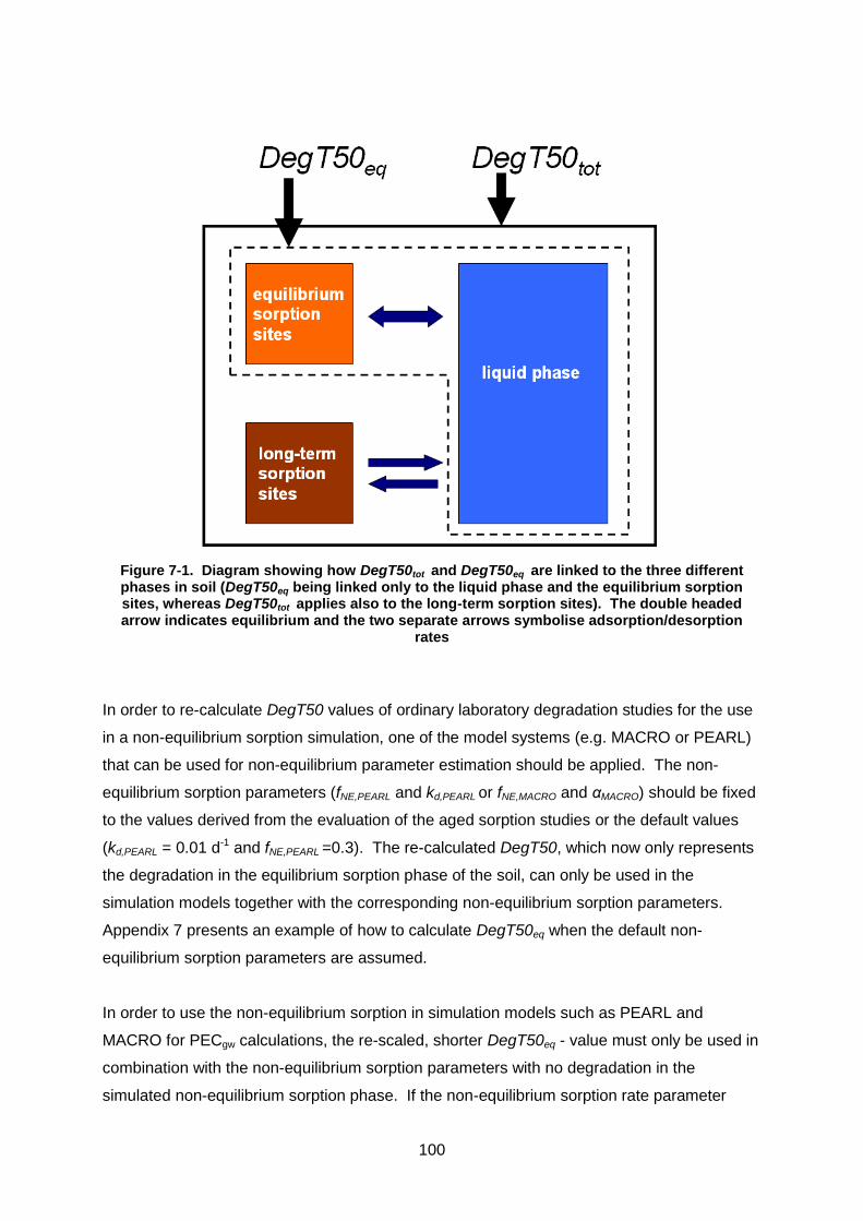
100
Figure 7-1. Diagram showing how DegT50tot and DegT50eq are linked to the three different phases in soil (DegT50eq being linked only to the liquid phase and the equilibrium sorption sites, whereas DegT50tot applies also to the long-term sorption sites). The double headed arrow indicates equilibrium and the two separate arrows symbolise adsorption/desorption
rates
In order to re-calculate DegT50 values of ordinary laboratory degradation studies for the use
in a non-equilibrium sorption simulation, one of the model systems (e.g. MACRO or PEARL)
that can be used for non-equilibrium parameter estimation should be applied. The non-
equilibrium sorption parameters (fNE,PEARL and kd,PEARL or fNE,MACRO and αMACRO) should be fixed
to the values derived from the evaluation of the aged sorption studies or the default values
(kd,PEARL = 0.01 d-1 and fNE,PEARL =0.3). The re-calculated DegT50, which now only represents
the degradation in the equilibrium sorption phase of the soil, can only be used in the
simulation models together with the corresponding non-equilibrium sorption parameters.
Appendix 7 presents an example of how to calculate DegT50eq when the default non-
equilibrium sorption parameters are assumed.
In order to use the non-equilibrium sorption in simulation models such as PEARL and
MACRO for PECgw calculations, the re-scaled, shorter DegT50eq - value must only be used in
combination with the non-equilibrium sorption parameters with no degradation in the
simulated non-equilibrium sorption phase. If the non-equilibrium sorption rate parameter
101
kd,PEARL or MACRO is zero or the parameter describing the fraction of the non-equilibrium
sorption phase fNE,PEARL or fNE,MACRO is set to zero, non-equilibrium sorption is not considered
in the model and the DegT50tot (so not the shorter DegT50eq) must be used.
For metabolites that were tested in parent studies (laboratory or field) a pragmatic approach
could be to follow the procedure used in Boesten and Van der Linden (2001). This means
that the degradation of a metabolite would be simulated according to the estimated rate
derived from the parent study (where non-equilibrium sorption was not considered). Then
the simulated total concentrations were fitted with a non-equilibrium sorption model where
the non-equilibrium sorption parameters as well as the sorption equilibrium parameter were
fixed and only the degradation rate in the equilibrium sorption phase was fitted. Equations 7-
29 to 7-31are given here only for obtaining a first guess of the magnitude of the difference
between DegT50tot and DegT50eq. They should not be used in risk assessment procedures.
Boesten and van der Linden (2001) derived an approximation for the scaling factor fdeg_NE
which can be used to obtain a first guess for the magnitude of the difference between
DegT50tot and DegT50eq). The scaling factor is defined as:
tot
eq
NEDegT
DegTf
50
50deg, (7-29)
or
totNEeq DegTfDegT 5050 deg, (7-30)
The approximation assumes a linear sorption isotherm and assumes that the degradation
rate coefficient is slow compared to kd, PEARL . The approximation can be written as:
EQFPEARLNE
EQF
NEKfw
Kwf
,,
,
deg,)1(
(7-31)
where w is the gravimetric water content of the incubation system defined as volume of water
divided by mass of dry soil (L/kg). Using e.g. w = 0.2 L/kg, KF,EQ = 1 L/kg and fNE,PEARL = 0.5,
gives fdeg_NE = 0.7, so the effect on the estimated DegT50 value may be considerable.
A useful resource for more up to date considerations of the most appropriate experimental
designs and methods for estimating / fitting time dependent adsorption parameters in
laboratory experiments can also be found in draft UK guidance (Beulke S and Van Beinum,
2012).
102
7.1.7 Plant uptake
The default plant uptake factors (i.e. the transpiration stream concentration factor) can be
adjusted to measured values if substance specific uptake factors have been determined in
appropriate experiments with the crops species being assessed. In the absence of agreed
EU guidance on what the appropriate experiments to measure the transpiration stream
concentration factor should be, applicants should contact competent authorities to see what
study design (if any) they would consider appropriate. See also considerations in EFSA PPR,
2013b.
7.1.8 Volatilisation
If volatilisation is significant then, the dose may be corrected conservatively (eg. estimate a
minimum amount of measured volatilised substanceover the first 24 hours in a relevant
experiment), or to switch on the model-supplied volatilisation subroutines in a thin soil layer
and use the standard "in-soil" degradation rate approach in deeper layers.
7.2 Scenario refinement (Tier 2b)
In Tier 2b scenario refinements are suggested to improve the initial Tier 1 simulations. In
principle, all model input parameters except product specific parameters (for example, Koc,
DegT50) or application patterns could be considered within this tier.
The overall purpose of Tier 2b is to allow modifications of the existing Tier 1 scenarios in
order to define “product specific” scenarios based on the specific use pattern of the pesticide.
Table 7-2 gives an overview of relevant aspects that can be considered for the proposed
scenario refinements. Some more details are given in the following sections.
103
Table 7-2. Overview of refinements included in Tier 2b.
Section Aspect Related Parameters
Proposed Refinement
Remarks
7.2.1 Specific crop conditions
Crop parameters
Modification of crop parameters in terms of known soil and climate properties
Considering alternative methods to define more accurate dates for emergence, maturation or harvest (note rooting depth should not exceed 1m in order to avoid conflicts with other parameterisations of the scenarios if FOCUS type soil column descriptions are maintained)
7.2.2 Specific crop conditions
Crop rotation
Definition of realistic crop rotations instead of permanent crops
Especially for pesticides that are not used on an annual basis
7.2.3 Specific crops
Crop type
Definition of additional crops not covered by FOCUS tier 1
Improvement of simulations for pesticides that are used mainly in special crops with minor importance (“niche products”)
7.2.4 Specific use pattern
Crop, climate
Definition of scenarios for greenhouse applications
The current focus scenario do not cover greenhouse applications though considerations relating to this are available in EFSA (2014b) guidance
7.2.5 General definition of “product-specific”-scenarios based on GIS. Tier 2.2a because the FOCUS scenario is replaced completely
All scenario parameters could be affected
Exclusion of areas that are not relevant with respect to the use pattern of pesticides
Identification of characteristic combinations of
crops
climate conditions
soil types
ground water conditions
hydro-geological information
7.2.6 Specific irrigation scenario
Climate parameters
Modify irrigation rates to consider implementation of more efficient drip irrigation
7.2.1 Modification of crop parameters
In Tier 1 the crop parameters (not only root depth, emergence, maturation and harvest dates,
but also runoff related parameters) are constant for each scenario. However, especially the
crop development parameters vary within the major agricultural areas due to the influence of
climate and also to some extent soil parameters. Additional information on the location of the
cropping areas and special crop parameters could be used to refine the Tier 1 simulations;
104
resulting in more realistic simulations for specific crops and excluding climate/soil/crop-
combinations that do not occur in reality.
7.2.2 Introduction of realistic crop rotations
Whether pesticides are applied annually or at other frequencies, crop rotations are never
considered within Tier 1 simulations. Instead, all crops are assumed to be cultivated as
“permanent crops”. A refinement can be considered by introducing location dependent crop
rotations in Tier 2b. If, for example, a certain pesticide is used every third year only in
potatoes only, additional crops could be defined for the years without any application. Since
the selection of crops has an important influence on the water regime, as a consequence the
fate of pesticide residues in the soil also will be affected by these refinements.
The original FOCUS input files cannot be used for these simulations. The user must always
create specific input files for this refinement, and the process for running these input files
depends on the simulation model selected. When combining different crops within
simulations, the user should start with the official FOCUS crop development dates
(emergence, maturation, harvest) rather than defining completely new figures. The warming
up period of 6 years was defined for annual, biennial and triannial application patterns only,
but the 6 years warming up period should also be maintained for other rotations.
7.2.3 Introduction of new crops
Tier 1 covers only the major European crops. If pesticides are modelled that are primarily
used for minor crops (e.g. special fruits or vegetables) the user has to select a similar major
crop. However, at Tier 2b a more realistic solution would be to develop a scenario for this
minor crop.
A cautionary remark should be made for rice cropping, which cannot be considered a minor
crop. Agricultural practice for rice cropping is completely different than for other classical
agriculture crops. The work group believes that current standard FOCUS pesticide leaching
models and scenarios can not be used for assessing risk in rice cultivated crops. For rice
cropping, interested readers are referred to the MED-Rice (2003) report.
7.2.4 Specific use conditions (e.g. greenhouse scenario)
Tier 1 scenarios are only designed to assess pesticide leaching in arable land subjected to
traditional pesticide management (e.g. spraying of chemicals using traditional spraying
equipment). Specific pesticide uses can be considered e.g. for greenhouses which may
justify the modification of the climate and soil parameters, the introduction of specific
“greenhouse” crop parameters and the modification of the timing and rate of pesticide
105
applications. EFSA guidance, EFSA (2014b) addresses assessment of emissions from
protected cropping systems including potential for groundwater exposure.
7.2.5 Defining use specific scenarios (e.g. use of GIS)
The FOCUS Tier I scenarios apply to large climatic zones (Chapter 11). In many cases,
plant protection products will only be applied in part of these climatic zones, particularly in the
case of minor crops that are grown in only a confined area. If the FOCUS scenarios are not
specific enough for the intended use, the notifier may wish to develop a scenario that is
specific for the intended use, i.e. for the relevant combination of crops, soil types, climate and
ground water conditions. The development of these so-called ‘use specific scenarios’ is the
subject of this section. The procedures in this section result in completely new scenarios,
which may complement existing FOCUS scenarios for specific uses in higher-tier
calculations.
GIS approaches play an important role in the development of new scenarios. Soil
information is combined with other spatial environmental and agricultural data (climate
patterns, crop, distribution, hydrogeological data) by spatially overlaying basic maps using
Geographic Information Systems (GIS). Such an overlay results in a large number of
possible scenarios (in many cases more than 1000), all which need to be parameterised. If
spatial information is available with sufficient detail, a spatially distributed model can be
created. The PECgw can be selected directly from the cumulative frequency distribution of
the calculated concentrations.
In many cases sufficient soil information for running spatially-distributed models is not
available. Therefore, a simplified leaching concept is required in cases where insufficient soil
and climate data is available. In these cases, the simplified leaching model is applied to the
intended use area instead of the spatially-distributed model itself (see Appendix 5 for more
details). If parameterised in an appropriate way, this simplified leaching model results in a
leaching vulnerability map that shows a strong correspondence to the leaching map obtained
with the spatially distributed model itself. This offers the opportunity to select the target
scenario directly from the frequency distribution of the calculated concentrations obtained
with the simple model. This single scenario is assigned parameter values (horizon
designations, organic matter content, texture, hydraulic properties etcetera) and a FOCUS
leaching model is run for this single scenario to generate the intended leaching
concentration.
In summary:

106
Spatially-distributed modelling comes down to running a large number of scenarios
with a FOCUS leaching model and presenting the results in a map and a cumulative
spatial leaching distribution (Tier 3b).
Modelling with use specific scenarios comes down to run a simplified leaching model,
identify the 80th percentile vulnerable location from the map and calculate the
regulatory endpoint for this single scenario (Tier 2b).
In those cases where sufficient soil and climate information is available to parameterise a
process-based spatially distributed model, this is the preferred method. In all other cases
use-specific scenarios would be the better choice although they are the second best
alternative. For this reason, spatially-distributed modelling is put at a higher tier (Tier 3) than
modelling with use-specific scenarios, which is a Tier 2 approach.
7.2.5.1 Steps in applying use-specific scenarios
The development and application of use specific scenarios at Tier 2b can be structured in
five major steps, i.e.
1. data compilation, check for suitability and data quality;
2. ground water vulnerability mapping using a simplified leaching concept
3. scenario selection;
4. scenario parameterisation;
5. simulation with a FOCUS leaching model.
The leaching in Tier 2b is assessed twice: first with the simplified leaching model to identify
areas which comply with the preset vulnerability criterion (i.e. step 2), and secondly to assess
the regulatory end point (step 5). This process is illustrated in Figure 7-2. The individual
steps are shortly described below; a more detailed guidance and examples are given later in
this section.
7.2.5.1.1 Data compilation, check for suitability and data quality
Appendix 8 gives an overview of pan-European spatial data bases and spatial data bases on
a member state level that can be used for the development of new scenarios for EU-
registration. For national registration, the use of national data bases is preferred, if they have
a higher resolution and are of better quality than EU data bases. For those cases where
national data bases are missing or of insufficient quality, the data bases referred to in
Appendix 8 can be used for the development of Tier 2 scenarios as well.
107
Figure 7-2. Illustration of the process to develop use specific scenarios at Tier 2b. Crop data refers to the distribution of crops.
7.2.5.1.2 Vulnerability mapping using a simplified leaching concept
In this step, a simplified leaching model is run to get a ground water vulnerability map. The
modelling should be done for the area of intended use. A large number of simple leaching
concepts is available in the literature (Aller et al., 1987; Jury et al., 1983; 1987; Jury and
Roth, 1990; Loague et al., 1989, 1996; Loague and Corwin, 1996; Rao et al., 1985; Douven,
1996; Vanclooster et al., 2003; Stewart and Loague, 2003; 2004; Piñeros Garcet et al., 2006;
Hollis and Sweeney, 2006; Stenemo et al., 2006; Tiktak et al., 2006). The work group
describes two different approaches in detail (Appendices 4 and 5); other approaches were
not explicitly excluded but have not been evaluated in detail by the work group.
108
7.2.5.1.3 Scenario selection
During this step, grid cells are selected that meet the target vulnerability. For EU-registration,
the target vulnerability is about the 80th percentile in space and 80th percentile in time.
Individual member states may, however, use different target vulnerabilities. The
Netherlands, for example, use the 90th percentile in space and the 50th percentile in time.
Both approaches are approximations of the overall 90th percentile vulnerability. The
selection of grid cells can be done directly from the cumulative frequency distribution of the
generated maps. The target vulnerability should apply to the intended use area only.
7.2.5.1.4 Scenario parameterisation
Once a use-specific scenario location is selected, an appropriate parameterisation of soil and
climate is needed. If runoff is important in the use area, runoff should also be included. Also
during this phase, several choices have to be made. First, soil profile data need to be
assigned on the basis of the selected soil mapping unit. This is not a trivial step, because
detailed soil information is not always available. Once a soil profile is found, derived data
such as the bulk density and the hydraulic characteristics of the soil profile must be
parameterised as well. These data are usually not available in soil profile data bases, but
must be derived by so-called pedotransfer functions. With respect to hydraulic properties,
several pedotransfer functions are available (Wösten et al., 1994; Schaap et al., 1998;
Wösten et al., 1999). A complete review of the pedotransfer functions was beyond the scope
of this work group. Runoff can be calculated using mechanistic approaches, as done in, for
example, PESERA (Kirby et al., 2004). The current FOCUS ground water models, however,
lack an appropriate description of some of the important processes relevant to the generation
of overland-flow, particularly surface crusting. Therefore, the work group recommends the
use of the more empirical NRCS curve number method, but care should be taken not to
include runoff originating from sources that are less relevant to pesticide leaching such as
saturation excess runoff originating from partial contributing areas (Richards and Brenner,
2004; Garen and Moore, 2005). One pragmatic way to deal with this is to assign an adjusted
USDA hydrological group through HOST (Hydrology Of Soil Types) attributes.
7.2.5.1.5 Simulation with a FOCUS leaching model
During this step, PECs are calculated with a standard FOCUS leaching model (i.e. MACRO,
PEARL, PELMO or PRZM).
7.2.5.1.6 Precautionary remark
As shown before, the development of new scenarios requires a large number of choices to
be made. All these choices result in uncertainty and subjectivity. First, a leaching model

109
must be chosen and parameterised for scenario selection. This may result in different
locations of the selected scenario. Also during the scenario parameterisation phase, choices
have to be made. Therefore, all steps must be reported in a transparent way so that they
can be reviewed by the national registration authorities. This requires that all data that are
used for scenario generation are available to all stakeholders free-of-charge or for
administrative costs only. Finally, the consistency of the selected scenario within the tiered
assessment scheme should be checked as well. If this is not possible directly, then the
method used to develop the scenario should be evaluated in a reference area, where
sufficient data is available to parameterise a process based numerical model.
7.2.5.2 Detailed guidance
7.2.5.2.1 Data compilation and quality check
Appendix 8 gives an overview of pan-European spatial data bases that can be used for the
development of new scenarios for EU-registration. Appendix 8 also provides procedures to
improve the quality of the spatial data bases. For new national scenarios, the use of national
data bases should be considered, because they may have a higher resolution and better
quality. For those cases where national data bases are missing or of insufficient quality, the
pan-European data bases referred to in Appendix 8 can be used for the development of
national scenarios as well. References of spatial data bases used (with their main
characteristics, including scale and spatial resolution) must be described with the selection of
the scenario.
7.2.5.2.2 Vulnerability mapping using a simplified leaching concept
In this step, a simplified leaching model is run to generate a ground water vulnerability map.
The work group agreed that methods to derive the ground water vulnerability map should:
reflect the vulnerability criterion as being a concentration with a spatial distribution;
be consistent amongst the tiers (later tiers must be more realistic and earlier tiers
must be more conservative than later tiers);
cover ideally the entire area of the EU, so that they are applicable for both national
and European procedures (harmonisation, more efficient registration).
The leaching models differ in their data needs and in the way how the data are processed. In
accordance to what has been found in the literature, the following four types of models can
be distinguished:
Process based numerical models: Leaching concentrations or loads are calculated
using process oriented leaching concepts. Numerical models solve the differential
110
equations describing pesticide fate and transport for transient boundary conditions
and complex initial conditions. All FOCUS leaching models (PEARL, PELMO, PRZM
and MACRO) fall into this category. Most approaches to spatially-distributed, process
based numerical modelling come down to running a leaching model for several (often
more than 1000) scenarios and putting the results in a map. This kind of process
based numerical leaching models can be parameterised for the catchment scale
(Petach et al., 1991; Leterme et al., 2007a), the regional scale (Capri et al. 2000), the
national scale (Tiktak et al., 1996; 2002) and the European scale (Tiktak et al., 2004).
Notice that only few attempts to model the transport of pesticides into the deeper
ground water have been reported in the literature (Tiktak et al., 2005).
Analytical, process based models: Analytical models are analytical solutions of the
differential equations, describing pesticide fate and transport in soil subjected to
simple initial and boundary conditions. The best known models of this type are the
attenuation factor (Loague et al., 1989; 1996; Loague and Corwin, 1996) and the
transfer function (Jury and Roth, 1990; Stewart and Loague, 2003; 2004). Analytical
models that are not calibrated to results from numerical models (see below) can only
be used as screening tools (Loague and Corwin, 1996; Stewart and Loague, 2004;
Tiktak et al. 2006).
Meta-models of process-based models: Meta-models reduce the complexity of
process based numerical models, but maintain the essential behaviour of the complex
model by considering the sensitivity of the different attributes in the spatial
assessment. Regression analysis can be used to construct a meta-model (Figure 7-
3). The regression model can itself be a purely statistical model (Vanclooster et al.,
2003; Stenemo et al., 2006; Piñeros Garcet et al., 2006) or a combination of a
simplified process based model and a regression model (Van der Zee and Boesten,
1991; Stewart and Loague, 2004; Tiktak et al., 2006).
Index rules: Attribute data that control leaching are combined in a simple logical rule
and corresponding arithmetic rules (mostly linear combination of attributes or
parameters) to yield a vulnerability index. Weights can be assigned to different
attributes in terms of the sensitivities of individual parameters to leaching. The
DRASTIC model (Aller et al., 1987; Lobo-Ferreira and Oliveira, 1997) assigns weights
based on expert judgement. Weights can also be based on the sensitivity of a
process-based model. In this way, process information is implicitly incorporated in the
index and the index-rule becomes a metamodel of a process-oriented model.
Appendix 4 gives an example of such an approach.
111
Figure 7-3. Metamodels are proxies of complex models
The work group concluded that metamodels and index rules are the best choice for scenario
development in Tier 2b, because these approaches are compatible with data in pan-
European data bases. Two examples of these approaches are described in detail. Appendix
4 describes an index rule, based on organic matter, precipitation and temperature. Appendix
5 describes a process based metamodel of the recently developed pan-European pesticide
leaching model EuroPEARL (Tiktak et al., 2004; 2006). Process based spatially distributed
models are considered less suitable for Tier 2b assessments, because so far they cannot be
parameterised for the entire area of the EU (Tiktak et al., 2004). They may, however, be the
best choice in certain situations, particularly if a high quality national data base is available
(Tiktak et al., 2002). In those cases, the regulatory endpoint can be selected directly from
the frequency distribution of the generated leaching maps, so that the development of use
specific scenarios is not necessary. Spatially-distributed modelling is therefore
recommended for Tier 3.
Spatially-distributed models can also be seen as the reference for simple leaching models,
because the spatially distributed models use the FOCUS leaching model directly. A
benchmark of the simple leaching concept against a process based model should be carried
out as part of the scenario development (or reference should be made to earlier attempts to
benchmark the simple leaching concept). An important element of this benchmark should be
the correlation between the maps generated with the process based model and the simple
model. The benchmark should preferably be carried out against a spatially distributed model
based on a FOCUS leaching model, such as GeoPEARL (Tiktak et al., 2002). This type of
benchmark can only be carried out in regions where sufficient soil and climatic information is
available. The two methods described by the work group meet this requirement, because
they were both benchmarked against GeoPEARL for the Netherlands (see Appendix 9).
112
Appendix 9 also contains an analysis of strengths, weaknesses, and opportunities of the two
approaches.
7.2.5.2.3 Scenario selection
The result of either of the two approaches is a map showing the leaching potential in a
normalised way (i.e. the grid cell with the highest leaching potential scores 100% and the grid
cell with the lowest leaching potential scores 0%). The target scenario can be selected
directly from this map and corresponds to 80th percentile vulnerable location (for national
registration, the target percentile may be different). Because the crop area is considered as
an approximation of potential pesticide use, the crop area could be used as a weighting
factor. See the documentation of GeoPEARL (Tiktak et al., 2003) for an example how the
crop area can be included.
The two approaches described by the work group may result in different target scenarios.
For this reason, the work group proposes to select a number of grid cells in the 85-95
percentile vulnerability range to deliver the candidate scenarios. An appropriate number of
candidate scenarios must be selected and parameterised for the selected FOCUS leaching
model. The FOCUS leaching model should be run with the selected scenarios and all PEC’s
should be reported. All scenarios should meet the trigger values to achieve a registration
without further mitigation restrictions.
7.2.5.2.4 Scenario parameterisation
The GIS analyses described in Appendices 4 and 5 both yield areas for candidate scenarios.
Since the regulatory endpoint is eventually calculated by a standard FOCUS leaching model,
a soil and climate scenario must be developed for the selected location. The following
section provides a generic but rough guidance on the parameterisation of soil and climate
scenarios in the context of a FOCUS leaching assessment. The FOCUS leaching models
contain a large number of model inputs. Guidance on the parameterisation of the FOCUS
leaching models is given in the user manuals of the individual models (PEARL, PRZM,
MACRO and PELMO), the latest versions of these manuals and parameterisation documents
are accessible through the FOCUS website.
In principle, all model inputs could be affected when building use-specific scenarios. The
work group recommends, however, staying as close as possible to the parameterisation of
the FOCUS scenario for the corresponding climatic zone (see FOCUS, 2000, and Chapter 12
for a description of these climatic zones). Particularly generic parameters that are
considered independent of the FOCUS Tier 1 scenarios should not be changed.
113
7.2.5.2.4.1 Meteorological time-series
The MARS climate data base provides daily weather data for the entire EU in a 50 x 50 km2
grid. Therefore, extracting weather files for the selected location from the appropriate grid
cell is straightforward. The MARS data base contains all parameters that are required for
simulation runs with current FOCUS models such as minimum and maximum temperature,
rainfall, potential evapotranspiration, and global radiation. All weather files for Tier-1 FOCUS
leaching scenarios were derived from this data base; therefore MARS should be used as the
primary source for weather information in Tier 1. If possible, the weather data provided by
MARS should be converted to a 66-years time-series using the rules described in FOCUS
(2000). As discussed in Section 11.5.1, MARS reference evapotranspiration should be
converted to FAO reference evapotranspiration in southern locations for consistency with the
FAO crop kc factors.
The use of data from local weather stations may be considered in specific cases when
notifiers attempt to simulate a very specific local weather situation or when sufficient
evidence exist that MARS data for the considered region is biased. In view of the large
geographic extent of most soil units in the EU soil data base, station data do not necessarily
improve the spatial accuracy compared to weather data that was specifically derived for such
larger scale assessments.
7.2.5.2.4.2 Cropping parameters
As a first approximation, most crop parameters (e.g. date of emergence, date of harvest,
crop development stages, etc.) should be taken from the Tier 1 scenario of the corresponding
climatic zone. See FOCUS (2000) or Chapter 13 in this report for a definition of these
climatic zones. In some cases more detailed information on cropping dates exist, in
particular when crops are grown in confined areas with characteristic climate conditions. In
such cases modifying cropping dates or other parameters may be appropriate. When
changing cropping parameters, a rationale for each change must be provided in order to
ensure a high degree of transparency in the assessment. If scenarios are developed for
minor crops, then a completely new cropping parameterisation may be required.
7.2.5.2.4.3 Irrigation
If irrigation is a relevant practice in the intended use area, the scenario has to be set up
accordingly and typical irrigation amounts need to be assigned. If reported irrigation data are
available, the data may be used directly in the parameterisation of the scenario. In most
cases, such data are not available and irrigation amounts will have to be estimated. The
compatibility of the irrigation data with the other climate data should be checked.
114
Typical crop water requirements during the vegetation period can be calculated on the basis
of FAO methods and MARS data (Allen et al, 1998). The difference between crop water
consumption and precipitation is then determining the irrigation demand. Note that the water
storage capacity of soils is not considered when calculating crop water requirements on the
basis of climate parameters. In these cases the calculated irrigation amounts might be
higher than those applied in reality. This problem does not occur when calculating the
irrigation demand with the soil water module within a FOCUS leaching model (for example
SWAP in PEARL) so this approach is preferable. Section 11.5.3 describes how the FOCUS
models were used to generate the irrigation schedules.
7.2.5.2.4.4 Lower boundary conditions
If detailed information on the local ground water regime is available, this information can be
used to parameterise the lower boundary condition. If no information is available, then the
parameterisation of the FOCUS Tier I scenario in the corresponding climatic zone (FOCUS,
2000) could be used.
7.2.5.2.4.5 Hydraulic balance
The hydrological subroutines of the models should be parameterised in order to mimic the
hydraulic balances for the scenarios as realistic as possible for the intended simulation
areas. In other words, estimates of recharge at target depth should neither be significantly
underestimated nor overestimated. For example, if runoff is thought to be a major process in
the area of interest, runoff should be included. Runoff can be calculated using mechanistic
approaches, as done in, for example, PESERA (Kirkby et al., 2004) The current FOCUS
ground water models, however, lack an appropriate description of some of the important
processes relevant to the generation of overland flow, particularly surface crusting.
Therefore, the work group recommends using the NRCS curve number method, but care
should be taken not to include runoff originating from sources that are less relevant to
pesticide leaching such as saturation excess runoff originating from partial contributing areas
(Richards and Brenner, 2004; Garen and Moore, 2005). One pragmatic way to deal with this
is to assign an adjusted USDA hydrological group through HOST (Hydrology Of Soil Types)
attributes. HOST uses pedotransfer rules to relate major flow pathways to generally available
pedological information (Boorman et al., 1995). HOST was originally developed and validated
in the UK, but is currently applied to the entire EU within the EU FOOTPRINT project (Dubus
et. al., 2007). However, results of this project will not become available before the end of
2008, so the work group could not evaluate this approach.
115
7.2.5.2.4.6 Soil parameters
The parameterisation of the soil properties consists of three steps: (a) selection of a soil
profile from a soil profile data base, (b) parameterisation of basic soil information, which is
directly available in these data bases (usually horizon designations, organic matter, texture
and sometimes also pH), and (c) parameterisation of derived soil properties that are not
available in the soil profile data base (soil hydraulic functions, bulk density of the soil, etc.).
Step A: Selection of a soil profile. Soil profile data bases usually contain information on the
soil mapping unit from which the soil profile originates. The link between the soil map and
the soil profile data base is then a trivial step, because there is a 1:1 link. At the European
level, however, this link is not straightforward. The problem is that the Soil Mapping Units
(SMU’s) at the EU-soil map are associations of dominant and subdominant Soil Typological
Units (STU’s). The STU’s and not the SMU’s are the carriers of basic soil information, such
as the FAO soil name and the soil textural class. For this reason, the link between the soil
map and the profile data base needs to be done in two steps. A possible approach could be
to determine the dominant STU, and then assign a soil profile to this dominant STU. Notice
that during this step information on subdominant soil profiles will be lost, leading to a possible
bias during the assessment (Vanclooster et al., 2003). An additional problem is that the Soil
Profile Analytical Database of Europe (SPADE, Madsen-Breuning and Jones, 1995) usually
does not contain explicit information on the associated soil typological unit. Finally, many
STU’s at the EU-soil map do not have an associated soil profile. To overcome these
problems, two approaches can be followed:
The link can be made at a relatively low spatial resolution (for example the resolution
of the MARS grid cells, which is 50x50 km2). Such a large grid cell usually contains
multiple soil mapping units, so that the chance of finding an STU with an associated
soil profile increases. Notice that in this procedure, the selection of the dominant STU
is not carried out at the level of soil mapping units, but at the level of these large grid
cells. An example of this approach is worked out in Appendix 4.
The second approach operates on the level of Soil Mapping Units and uses general
pedological rules to establish the link (‘class matching’). This method has often been
used in pedological research (for example Van Orshoven et al., 1993; Leterme et al.,
2007b). The method used here is based on the work done within the APECOP
project and forms the basis of the EuroPEARL model (Tiktak et al., 2004). In this
approach, a profile is assigned on the basis of the full FAO soil name, the textural
class and the country code. Including the country code in the query assures that soil
profiles from a given country could only be matched to Soil Mapping Units within that
116
country. In those situations where a link could not be established, the query was
repeated with the full FAO soil name and the country code only. Finally, a query was
carried out using the major soil type and the country code only (e.g. Cambisol instead
of Eutric Cambisol). In a recent development, Hollis and Sweeney (2006) merged the
soil typological units further, by assuming that a specific class of soil typological units
can be used to represent the characteristic of that group anywhere in the EU. In
other words, they did not use the country in their query. See Appendix 5 for more
details.
The most important difference between the two procedures is that the first merges multiple
soil mapping units and uses a relatively low spatial resolution, while the second approach
merges soil types and uses a lower ‘pedological’ resolution. The advantage of the first
method is its relatively simplicity. A disadvantage is, however, that this procedure operates
on a lower resolution than the soil mapping unit, which is the target unit for assessing the
ground water vulnerability (cf. Section 10.1). Vanclooster et al. (2003) showed that the use
of dominant values across large spatial blocks may cause bias in the leaching assessment.
Both methods result in the selection of a soil profile. When building the scenario, the
suitability of the selected soil profile for the target crop should be evaluated. In particular,
depth to parent material, pH, and texture give important indications whether the soil profile is
likely to sustain a viable growth of the target crop. If the selected STU is outside the range of
‘suitable soils’, a soil typological unit with a lower coverage should be selected instead.
Step B: Parameterisation of basic soil data. The Soil Profile Analytical Database contains
information on horizon designations (thickness of soil profiles), organic matter, textural
distribution and pH. The data in SPADE is not necessarily based on measurements, but are
estimated profiles, meaning that national soil scientists have given a best possible
description of typical soil profiles in their country. For this reason, the organic matter content
in the upper 30 cm should be scaled to the organic matter content derived at the recently
developed pan-European organic matter content map as published by the Joint Research
Centre (Jones et al., 2004, 2005). In contrast to SPADE, this map has been validated
against measured soil data in some reference areas.
SPADE-1 has some data gaps that need to be filled. In some cases, the properties of the
subsoil are not given. A very critical parameter is the organic matter content. In those cases
where organic matter content is not available, several approaches could be followed.
Leterme et al. (2007a) suggest using the following empirical relationship:
117
)exp()()( kzOMOMOMzOM bob
where z is the depth (cm); OMo and OMb are the organic matter contents in the top horizon
and at the bottom of the soil profile, respectively; and k is a constant. If no information is
available, OMb should be set zero (conservative approach). Parameter k could be obtained
from data in corresponding soil profiles.
Step C: Parameterisation of derived soil data using pedotransfer rules. Bulk density and
hydraulic properties are not available in SPADE. These parameters must therefore be
derived by so-called pedotransfer functions. PEARL has a built-in function, which relates
organic matter content to bulk density (Tiktak et al., 2000). Alternatively, Carsel et al. (1998)
use the textural distribution to predict the bulk density. Parameter values for the Mualem-van
Genuchten functions (van Genuchten, 1980) can be derived from the HYPRES data base
(Wösten et al., 1999), but alternative approaches where the hydraulic function is estimated
on the basis of advanced statistical procedures are available as well (Schaap et al., 1998).
The water content at field capacity (required by PRZM and PELMO) can be directly derived
from the above hydraulic functions.
7.2.5.2.5 Simulation with a FOCUS leaching model
Once the scenarios have been parameterised, the calculation of the endpoint can be done
with a standard FOCUS leaching model.
7.3 References
Allen, R.l.G., Pereira, L.S., D. Raes, and M. Smith. 1998. Crop evapotranspiration:
Guidelines for computing crop water requirements. FAO Irrigation and Drainage paper,
vol. 56. FAO, Rome, Italy.
Aller, L., T. Bennet, J.H. Lehr, and R.J. Petty. 1987. DRASTIC: a standardized system for
evaluating groundwater pollution potential using hydrogeologic settings, U.S. EPA Report
600/2-85/018.
Altfelder S., Streck T. and Richter J. 2000. Nonsingular sorption of organic compounds in
soil: the role of slow kinetics. Journal of Environmental Quality 29:917-925.
Altfelder, S.; Streck, T.; Maraqa, M.A. and T.C. Voice. 2001. Nonequilibrium sorption of
dimethylphtalate - compatibility of batch and column techniques. Soil Sci. Soc. Am. J.
65:102-111.
Beulke S. and Van Beinum W. 2012. Guidance on how aged sorption studies for pesticdes
should be conducted, analysed and used in regulatory assessments. Available online:

118
www.pesticides.gov.uk/resources/CRD/Migrated-
Resources/Documents/E/EnvFate_Aged_sorption_guidance_final_30_07_2012.pdf
Boesten, J.J.T.I. 1986. Behaviour of herbicides in soil: simulation and experimental
assessment. Ph.D. Thesis, Wageningen University, Wageningen, The Netherlands, 263
pp.
Boesten, J.J.T.I. & B. Gottesbueren. 2000. Testing PESTLA using two modellers to simulate
bentazone and ethoprophos behaviour in a sandy soil. Agric. Water Management
44:283-305.
Boesten JJTI, AMA van der Linden. 2001. Effect of long-term sorption kinetics on leaching
as calculated with the PEARL model for FOCUS scenarios. 2001 BCPC Symposium
Proceedings No 78: Pesticide behaviour in soils and water, p. 27-32.
Boesten J.J.T.I., Van der Pas L.T.J. and Smelt J.H. 1989. Field test of a mathematical
model for non-equilibrium transport of pesticides in soil. Pesticide Science 25:187-203.
Boesten J.T.T.I., Van der Pas, L., Leistra, M., Smelt, J., and Houx, N. 1992. Transformation
of 14C labeled, 1,2 dichloropropane in water saturated subsoil materials. Chemosphere
24:993-1011.
Boorman, D.B., Hollis, J.M and Lilly, A. 1995. Hydrology of soil types: a hydrologically-based
classification of the soils of the United Kingdom. Institute of Hydrology Report No.126.
Institute of Hydrology, Wallingford.
Capri, E., L. Padovani, and M. Trevisan. 2000. La previsione della contaminazione della
acque sotterranee da prodotti fitosanitari. Quaderni di techniche di protezione
ambientale. Pitagora, Bologna, Italy.
Carsel R.F., Imhoff J.C., Hummel P.R., Cheplick J.M. and A.S. Donigian. 1998. PRZM-3, A
model for predicting pesticide and nitrogen fate in the crop root and unsaturated soil
zones: Users Manual for release 3.0. National Exposure Research Laboratory, U.S.
Environmental Protection Agency. Athens. U.S.A.
Douven, W.J.A.M. 1996. Improving the accessibility of spatial information for environmental
management. An application to pesticide leaching risk assessment. PhD. thesis, Free
University, Amsterdam, the Netherlands, p. 203.
EFSA. Panel on Plant Protection Products and their Residues (PPR) 2013a; Scientific
Opinion on the report of the FOCUS groundwater working group (FOCUS, 2009):
assessment of lower tiers. EFSA Journal 2013;11(2):3114. [29 pp.]
doi:10.2903/j.efsa.2013.3114. Available online: www.efsa.europa.eu/efsajournal
EFSA. Panel on Plant Protection Products and their Residues (PPR) 2013b; Scientific
Opinion on the report of the FOCUS groundwater working group (FOCUS, 2009):
assessment of higher tiers. EFSA Journal 2013;11(6):3291. [25 pp.]
doi:10.2903/j.efsa.2013.3291. Available online: www.efsa.europa.eu/efsajournal
119
EFSA 2014a European Food Safety Authority. Guidance Document for evaluating laboratory
and field dissipation studies to obtain DegT50 values of active substances of plant
protection products and transformation products of these active substances in soil. EFSA
Journal 2014;12(5):3662, 38 pp., doi:10.2903/j.efsa.2014.3662 Available online:
www.efsa.europa.eu/efsajournal
EFSA. 2014b European Food Safety Authority. Guidance document on clustering and
ranking of emissions of plant protection products and transformation products of these
active substances from protected crops (greenhouses and crops grown under cover) to
relevant environmental compartments. EFSA Journal 2014;12(3):3615. [43 pp.]
doi:10.2903/j.efsa.2014.3615. Available online: www.efsa.europa.eu/efsajournal
FOCUS. 2000. FOCUS groundwater scenarios in the EU pesticide registration process.
Report of the FOCUS Groundwater Scenarios Workgroup, EC Document Reference
Sanco/321/2000 rev 2. 202pp. Available at http://arno.ei.jrc.it/focus.htm (verified 14 Feb.
2006).
FOCUS. 2002. Generic Guidance for FOCUS groundwater scenarios, Version 1.1. 61 pp.
FOCUS. 2006. Guidance Document on Estimating Persistence and Degradation Kinetics
from Environmental Fate Studies on Pesticides in EU Registration. Report of the FOCUS
Work Group on Degradation Kinetics, EC Document Reference Sanco/10058/2005
version 2.0, 434 pp.
Garen, D.C., Moore, D.S. 2005. Curve number hydrology in water quality modeling: uses,
abuses and future directions. J. American Water Resources Association, April 2005, 377-
388.
Gurney AJR and Hayes S.E. 2007. Non-equilibrium sorption and degradation of pesticides
in soil: analysis of laboratory aged sorption data using ModelMaker. In: A.A.M. Del Re, E.
Capri, G. Gragoulis, and M. Trevisan, eds. Environmental Fate and Ecological Effects of
Pesticides (Proceedings of the XIII Symposium Pesticide Chemistry). La Goliardica
Pavese, Pavia Italy, ISBN 978-88-7830-473-4, pp. 245-253.
Hamaker J.W. and Thompson J.M. 1972. Adsorption. In: Organic chemicals in the soil
environment, Goring C.A.I. & Hamaker J.W. (Eds). p. 49-143. Marcel Dekker. New York.
Hollis, J. and Sweeney, P. 2006. Use of GIS datasets to derive generic soil and climate
leaching scenarios for higher tier modelling at the European level. In: Pesticide
Behaviour in Soils, Water and Air. University of Warwick, UK, pp. B30.
Jarvis N.J., Moeys J., Hollis J.M., Reichenberger S., Lindahl, A.M.L., and Dubus, I.G. (2009)
A conceptual model of Soil Susceptibility to Macropore Flow. Vadose Zone Journal 8: pp.
902-910
120
Jene, B. 2006. Kinetic (aged) sorption in the groundwater exposure assessment of
pesticides. Book of abstracts of Symposium ‘Pesticide Behaviour in Soil, Air and Water’,
Warwick 2006, poster A31.
Jene, B. 2007. Comparison of non-equilibrium sorption parameters of a pesticide from
adsorption-desorption batch and outdoor leaching experiments. In: A.A.M. Del Re, E.
Capri, G. Gragoulis, and M. Trevisan, eds. Environmental Fate and Ecological Effects of
Pesticides (Proceedings of the XIII Symposium Pesticide Chemistry). La Goliardica
Pavese, Pavia Italy, ISBN 978-88-7830-473-4, pp. 195-202.
Jones, R. J. A., R. Hiederer, E. Rusco, and L. Montanarella. 2005. Estimating organic
carbon in the soils of Europe for policy support. European Journal of Soil Science,
56(5):655-671.
Jones, R.J.A., R. Hiederer, E. Rusco, P. J. Loveland, and L. Montanarella. 2004. The map
of organic carbon in topsoils in Europe, Version 1.2, September 2003: Explanation of
Special Publication Ispra 2004 No.72 (S.P.I.04.72). European Soil Bureau Research
Report No.17, EUR 21209 EN, 26pp. and 1 map in ISO B1 format. Office for Official
Publications of the European Communities, Luxembourg.
Jury, W.A., D.D. Focht, and. W.J. Farmer. 1987. Evaluation of pesticide groundwater
pollution potential from standard indices of soil-chemical adsorption and biodegradation.
J. Environ. Qual. 16:422-428.
Jury, W.A., and K. Roth. 1990. Transfer functions and solute movement through soil.
Theory and applications. Birkhauser, Basel.
Jury, W.A., W.F. Spencer, and W.J. Farmer. 1983. Behavior assessment model for trace
organics in soil. I. Model description. J. Environ. Qual. 12:558-564.
Kirkby, M.J., Jones, R.J.A., Irvine, B., Gobin, A, Govers, G., Cerdan, O., Van Rompaey,
A.J.J., Le Bissonnais, Y., Daroussin, J., King, D., Montanarella, L., Grimm, M.,
Vieillefont, V., Puigdefabregas, J., Boer, M., Kosmas, C., Yassoglou, N., Tsara, M.,
Mantel, S., Van Lynden, G.J. and Huting, J. 2004. Pan-European Soil Erosion Risk
Assessment: The PESERA Map, Version 1, October 2003. Explanation of Special
Publication Ispra 2004 No.73 (S.P.I.04.73). European Soil Bureau Research Report
No.16, EUR 21176, 18pp. and 1 map in ISO B1 format. Office for Official Publications of
the European Communities, Luxembourg.
Kuntze H., Roeschmann G. and G. Schwerdtfeger. 1988. Bodenkunde. Ulmer Verlag.
Stuttgart. 568 p.
Larsbo M. and Jarvis N. 2003. MACRO 5.0. A model of water flow and solute transport in
macroporous soil. Technical description. Report. Department of Soil Science. Swedish
University of Agricultural Sciences. 49 pp.
121
Leistra, M. and Smelt, J.H. 2001. An appraisal of methods for measurement of pesticide
transformation in the groundwater zone. Pesticide Management Science 57:333-340.
Leistra, M., A.M.A. Van der Linden, J.J.T.I. Boesten, A. Tiktak and F. Van den Berg. 2001.
PEARL model for pesticide behaviour and emissions in soil-plant systems. Description of
processes. Alterra report 013, Alterra, Wageningen, RIVM report 711401009, Bilthoven,
the Netherlands. Available at http://www.pearl.pesticidemodels.eu
Leterme B., M. Vanclooster, A.M.A. van der Linder, A. Tiktak and M. Rounsevell. 2007a.
The consequences of interpolating or calculating first on the simulation of pesticide
leaching at the regional scale. Geoderma 137:414-425.
Leterme, B., M. Vanclooster, A.M.A. van der Linden, A. Tiktak and M.D.A. Rounsevell.
2007b. Including spatial variability in Monte Carlo simulation of pesticide leaching.
Environ. Sci. Technol. (41):7444-7450.
Loague, K. and D.L. Corwin. 1996. Uncertainty in Regional-scale Assessments of non-point
source pollutants. In D.L. Corwin and K. Loague (eds.). Application of GIS to the
modeling of non-point source pollutants in the vadose zone. SSSA Special Publication
No. 48, SSSA, Madison, WI. p. 131-152.
Loague, K., R.S. Yost, R.E. Green, and T.C. Liang. 1989. Uncertainty in a pesticide
leaching assessment for Hawaii. J. Contam. Hydrol. 4:139-161.
Loague, K., R.L. Bernknopf, R.E. Green, and. T.W. Giambelluca. 1996. Uncertainty of
groundwater vulnerability assessments for agricultural regions in Hawaii: Review. J.
Environ. Qual. 25:475-490.
Lobo-Ferreira, J.P., and M.M. Oliveira. 1997. DRASTIC groundwater vulnerability mapping
in Portugal. In: Groundwater: An endangered resource, Proceedings of Theme C (pp.
132-137) of the 27th Congress of the International Association for Hydraulic Research,
San Fransisco, USA. Available at
http://www.dha.lnec.pt/nas/textos/novidades/drastic_e.html.
Madsen-Breuning, H., and R.J.A. Jones. 1995. The establishment of a soil profile analytical
database for the European Union. p. 55-63. In D. King, R.J.A. Jones, and A.J.
Thomassen (eds.). EUR 16232 EN. Office for Official Publications of the European
Communities, Luxembourg.
MED-Rice. 2003. Guidance document for Environmental Risk assessments of Active
Substances used on Rice in the EU for Annex I inclusion. Document Prepared by
Working Group on MED-rice, EU Document Reference SANCO/1090/2000 - rev.1,
Brussels, June 2003, 108 pp. Available at:
http://ec.europa.eu/food/plant/protection/resources/med_rice_2003_en.pdf
OECD. 2002. Guideline for the testing of chemicals No. 307. Aerobic and anaerobic
transformation in soil. OECD, Paris. 17 pp.
122
OECD. 2000. OECD guideline for the testing of chemicals No. 106. Adsorption-desorption
using a batch equilibrium method. OECD, Paris.
Petach, M.C., R.J. Wagenet, and S.D. De Gloria. 1991. Regional water flow and pesticide
leaching using simulations with spatially distributed data. Geoderma 48:245-269.
Pignatello, J.J. 2000. The measurement and interpretation of sorption and desorption rates
for organic compounds in soil media. Advances in Agronomy 69:1-73.
Piñeros-Garcet, J.D., A. Ordonnez, J. Roosen, and M. Vanclooster. 2006. Metamodelling:
Theory, concepts and applications to nitrate leaching modelling. Ecological Modelling
193:629-644.
Rao, P.S.C., A.G. Hornsby, and R.E. Jessup. 1985. Indices for ranking the potential for
pesticide contamination of groundwater. Soil Crop Sci. Soc. Fla. Proc. 44:1-8.
Reichenberger S. and Laabs V. 2003. Kinetic evaluation of pesticide sorption in two
contrasting tropical soils. Proceedings of the XII Symposium Pesticide Chemistry,
Piacenza 2003, p. 309-318.
Reichenberger, S. Jene B and Feyerabend M. 2002. Evaluation of standard
adsorption/desorption studies with a kinetic sorption model. Proceedings IUPAC
Conference Basel 2002, p. 142.
Richards, P.L. and Brenner, A.J. 2004. Delineating Source Areas for Runoff in Depressional
Landscapes: Implications for hydrological modeling. J. Great Lakes Res. 30:9-21.
Sander, M., Fu Y. and Pignatello J.J. 2005. A thermodynamically based method to quantify
true hysteresis. J. Environ. Qual. 34:1063-1072.
Schaap, M.G., Leij, F.J. and van Genuchten, M.T. 1998. Neural network analysis for
hierarchical prediction of soil hydraulic properties. Soil Sci.Soc.Am.J. 62:847-855.
Smelt J., A., van de Peppel-Groen, A.E., and Leistra, M. 1995. Transformation of aldicarb
sulfoxide and aldicarb sulfone in four water saturated sandy subsoils. Pesticide Science
44:323-334.
Smith, A.E. 1981. Comparison of solvent systems for the extraction of atrazine, bezoylprop,
flamprop, and trifluralin from weathered field soil. Journal of Agricultural and Food
Chemistry 29:111-115.
Stenemo, F., A. Lindahl, and N. Jarvis. 2006. Neural network meta-modeling of the
pesticide fate model MACRO for groundwater vulnerability assessments. In: Pesticide
Behaviour in Soils, Water and Air. University of Warwick, UK, pp. B2.
Stewart, I.T., and K. Loague. 2003. Development of type transfer functions for regional-
scale non-point source groundwater vulnerability assessments. Water Resour. Res.
39(12):1359.
123
Stewart, I.T., and K. Loague. 2004. Assessing ground water vulnerability with the type
transfer function model in the San Joaquin Valley, California. J. Environ. Qual. 33:1487-
1498.
Streck, T. 1997. FITHYST 3: Parameter estimation program for hysteretic sorption
isotherms. Dept. of Geoecology, Technical University of Braunschweig, Germany
Streck, T. and J. Richter. 1999. Field-scale study of chlortoluron movement in a sandy soil
over winter: II. Modelling. J. Environ. Qual. 28:1824-1831.
Streck, T., Poletika N.N., Jury, W.A., Farmer,W.J. 1995. Description of simazine transport
with rate-limited, two-stage, linear and nonlinear sorption. Water Resources Research
31:811-822.
Tiktak, A., A.M.A. van der Linden, and I. Leine. 1996. Application of GIS to the modeling of
pesticide leaching on a regional scale in the Netherlands. p. 259-281. In D.L. Corwin and
K. Loague (eds.) Application of GIS to the modeling of non-point source pollutants in the
vadose zone. SSSA Special Publication No. 48, SSSA, Madison, WI.
Tiktak, A., F. Van den Berg, J.J.T.I. Boesten, M. Leistra, A.M.A. Van der Linden and D. Van
Kraalingen. 2000. Pesticide Emission Assessment at Regional and Local Scales: User
Manual of FOCUS Pearl version 1.1.1. RIVM Report 711401008, Alterra Report 28,
RIVM, Bilthoven, 142 pp. Available at http://www.pearl.pesticidemodels.eu
Tiktak, A., D.S. de Nie, A.M.A. van der Linden, and R. Kruijne. 2002. Modelling the leaching
and drainage of pesticides in the Netherlands: the GeoPEARL model. Agronomie
22:373-387.
Tiktak, A., A.M.A. van der Linden, and J.J.T.I. Boesten. 2003. The GeoPEARL model.
Model description, applications and manual. RIVM report 716601007/2003. RIVM,
Bilthoven, the Netherlands.
Tiktak, A., D.S. de Nie, J.D. Piñeros Garcet, A. Jones, and M. Vanclooster. 2004.
Assessment of the pesticide leaching risk at the Pan-European level. The EuroPEARL
approach. J. Hydrol. 289:222-238.
Tiktak, A., A.M.A. van der Linden, and G. Uffink. 2005. Pesticide transport in the
groundwater at the national scale: coupling an unsaturated zone model with a
groundwater flow model. In N.R. Thomson (ed.) Bringing groundwater quality research to
the watershed scale. IAHS Publ. 297, IAHS Press, Wallingford, UK. p. 441-448.
TIktak, A., J.J.T.I. Boesten, A.M.A. van der Linden, and M. Vanclooster. 2006. Mapping
Groundwater Vulnerability to Pesticide Leaching with a process-based Metamodel of
EuroPEARL. J. Environ. Qual. 35:1213-1226.
Toride, N., Leij, F. J., and van Genuchten, M. Th. 1993. A comprehensive set of analytical
solutions for nonequilibrium solute transport with first-order decay and zero-order
production. Water-Resources-Research 29(7):2167-2182.
124
Van Genuchten, M.Th. 1980. A closed form for predicting the hydraulic conductivity of
unsaturated soils. Soil Sci. Soc. Am. J. 44:892-898.
van Genuchten, M.Th. and Wagenet, R.J. 1989. Two-site/two-region models for pesticide
transport and degradation: theoretical development and analytical solution. Soil Science
Society of America Journal 53:1303-1310.
Van Orshoven, J., and D. VandenBroucke. 1993. Guide de l’utilisateur de AARDEWERK.
Base de données de profils pédologiques. IRSIA-COBIS – Instituut voor Land- en
Waterbeheer, Katholieke Universiteit Leuven, Leuven, Belgium.
Van der Pas, L., Leistra, M., and Boesten, J.J.T.I. 1998. Rate of transformation of atrazine
and bentazone in water saturated sandy subsoils. Pesticide Science 53:223-232.
Van der Zee, S.E.A.T.M., and J.J.T.I. Boesten. 1991. Effects of soil heterogeneity on
pesticide leaching to groundwater. Water Resour. Res. 27:3051-3063.
Vanclooster, M., J.D. Pineros-Garcet, J.J.T.I. Boesten , F. Van den Berg, M. Leistra, J.
Smelt, N. Jarvis, S. Roulier, P. Burauel, H. Vereecken, A. Wolters, V. Linnemann, E.
Fernandez, M. Trevisan, E. Capri, L. Padovani, M. Klein, A. Tiktak, A. Van der Linden, D.
De Nie, G. Bidoglio, F. Baouroui, A. Jones, A. Armstrong. 2003. Effective Approaches
for Assessing the Predicted Environmental Concentrations of Pesticides. Final report.
European Commission, Quality of Life and Management of Living Resources
Programme. QLK4-CT-1999-01238. Printed by the Université Catholique de Louvain,
Belgium (Available at http://www.geru.ucl.ac.be/recherche/projets/apecop-pub/).
Vanderborght, J., Mallants, D., Vanclooster, M., and Feyen, J. 1997. Parameter uncertainty
in the mobile-immobile solute transport model. Journal of Hydrology 190[1-2], 75-101.
Walker A. 1987. Evaluation of a simulation model for prediction of herbicide movement and
persistence in soil. Weed Research 27:143-152.
Wauchope, D., Yeh, S., Linders, J., Kloskowski, R., Tanaka, K., Rubin, B., Katayama, A.,
Kördl, W., Gerstl., Z., Lane, M., and Unsworth, J.B. 2002. Pesticide sorption parameters:
theory, measurements, uses, limitations and reliability. Pesticide Management Science
58:419-445.
Wösten, J.H.M., G.J. Veerman, and J. Stolte. 1994. Water retention characteristics of
topsoils and subsoils in the Netherlands. The Winand Staring Soil Series. Renewed
Release 1994. SC-DLO Tech. Doc. 18. Alterra, Wageningen, the Netherlands.
Wösten, J.H.M., A. Nemes, A. Lilly, C. Le Bas. 1999. Development and use of a database
of hydraulic properties of European soils. Geoderma 90:169-18.

125
8 APPROACHES FOR TIER 3 ASSESSMENT
For Tier 3, four alternatives exist: First, a combination of strategies proposed in Tier 2;
second, advanced spatial modelling approaches; third, higher tier leaching studies placed
into context; and fourth, other modelling approaches.
Note that the PPR panel of EFSA indicated that they considered that Tier 3b modelling
should be considered a higher tier than Tiers 3a and 3c, sitting between Tiers 3a / 3c and
Tier 4 (EFSA PPR, 2013b).
8.1 Procedures for combining modelling based on refined parameters and scenarios (Tier 3a)
Where relevant to the proposed use pattern, the refinements detailed in Tiers 2a and 2b (see
above) can be combined to provide an assessment based on both approaches.
The relationship of the compound’s behaviour to certain soil properties or more realistic
degradation or sorption parameters in combination with environmental scenarios more
specifically adapted to the intended use pattern will provide a more realistic assessment of
the leaching behaviour than if only a single option is used. This is seen as a further
refinement of the assessment and hence supersedes Tier 2.
Only a general short description of combining modelling based on refined parameters and
scenarios is given here due to the multitude of possible options of combined Tier 2a and Tier
2b approaches. The options at Tier 3a are likely to be used quite frequently at Tier 3 at EU
and at national level.
8.2 Procedures for building a spatially-distributed FOCUS leaching model (Tier 3b)
This report describes two methods to introduce spatially-distributed data in the leaching
assessment:
In the first method, a simplified leaching model is applied to the intended use area.
This model is used to generate a ground water vulnerability map. A single scenario
representing the 80th percentile vulnerable location is selected from the so-obtained
map. This scenario is than parameterised, and the FOCUS target is obtained with a
standard FOCUS leaching model. This approach is called ‘modelling with use-
specific scenarios and is described in Section 7.2.5.
In the second method, a spatially distributed version of a FOCUS leaching model is
directly applied to the intended use area, and the regulatory endpoint can be
126
calculated directly from the frequency distribution of the so-obtained leaching map.
This can only be done in those cases where the soil and climate data cover the
intended use area (and are of sufficient quality). This method is described in this
section (Section 8.2).
In those cases where spatially-distributed modelling is considered appropriate, this is the
preferred method (see Section 8.2.1). In all other cases, use-specific scenarios would be the
better choice although they are the second best alternative. For this reason, spatially
distributed modelling is put at a higher tier (Tier 3) than modelling with use-specific scenarios,
which is a Tier 2 approach.
8.2.1 Justification for spatially-distributed modelling
The agricultural and environmental parameters that affect pesticide fate and transport are
variable in time and space. The resulting leaching event which charges ground water can
therefore be considered as a stochastic variable, characterised by its probability density
function (pdf). The elementary leaching event is thereby defined in space at the scale of the
soil mapping unit and in time at the scale of a year. The leaching event pdf measures the
variation of the elementary leaching event in a larger space area (corresponding in FOCUS
to a climatic zone in Europe) and longer time period (corresponding in FOCUS to the
simulation period of respectively 20, 40 or 60 years, not including the six year warm-up
period). With the adopted vulnerability concept, the 90th percentile of the leaching event pdf
is selected as end point for regulation. In Tier 1, the pdf of the leaching event is not explicitly
reconstructed but the appropriate percentile is inferred from the pdf of the temporal varying
leaching event, given a percentile soil. However, this pragmatic lower tier approach may give
a biased estimate of the 90th percentile:
Only one specific percentile soil is selected for a given climate area based on
qualitative information of the soil variability and expert knowledge, without explicitly
characterising the variability of soil parameters contributing to the leaching event
variability.
The leaching event percentile is calculated from the temporal variable leaching event
pdf, which is considered to be normally distributed. Extreme percentile estimates
(e.g. 90th percentile) assuming normal distributions for variables which effectively are
nonnormally distributed may be extremely biased. The shape of the leaching event
joint pdf in space and time is a-priori not known and may be skewed and exhibit high
kurtosis.
The leaching event correlation in space and time is ignored, given that the joint pdf in
space and time is not explicitly reconstructed. Some underlying properties defining
127
the leaching event pdf will be correlated in time. An example may be the activation of
macro porous flow in macroporous soils, triggered by extreme rainfall events.
In the higher tier, this bias may be reduced by introducing explicitly spatial variation of the
leaching event. Two different approaches may be distinguished:
In a first approach the spatial variation of the underlying properties (soil, crop, climate,
agricultural) driving the leaching event is considered as a basis for the selection of a
more appropriate scenario. This scenario is next combined with a leaching model to
assess the percentile of the leaching event. This is the approach proposed in Tier 2.
As compared to Tier 1, this procedure results in a explicit characterisation of the
underlying properties and therefore an improved scientific basis for scenario
selection. Examples of such a procedure have been given in Appendices 4 and 5.
In a second approach, the spatial variation of the underlying properties driving the
leaching event is also considered. Yet, in this approach the leaching event is
calculated for each realisation of the underlying variable. Examples of such
approaches are given in Tiktak et al., (2002; 2004a). Given the availability of spatially
distributed leaching events, a percentile value can be selected a posteriori. This is
the approach proposed in Tier 3, and is described further in this section.
The problem of the calculation of percentile values of a space-time variable is equivalent to
problem of the aggregating and upscaling of point values to a larger support volume
(Heuvelink and Pebesma, 1999). Given X, the set of space-time variables contributing to the
leaching event; L(X), the space-time variable leaching event; and p() the procedure of
selecting a percentile value; then it can be shown L(p(X)) = p(L(X)) is only applicable in
limited cases (namely X is uniformly distributed and L is a linear model in X). In general, the
calculated leaching event is considered to be a non-linear function of soil properties and
therefore the above mentioned equality is not trivial. For instance Heuvelink and Pebesma
(1999), showed that the calculation of a linear process model after the interpolation of
underlying variables resulted in smaller errors as compared to the situation where the
process model was calculated first. For a non-linear process models (such as the leaching
models used in FOCUS), Leterme et al. (2007a) showed that opposite results may be
obtained. The conclusions depend however on the resolution of the underlying data, the
scale at which a prediction needs to be made, and the correlation of the underlying variables
(in case of the FOCUS scenarios, the correlation between the soil, climate and crop
parameters).

128
8.2.2 Development of a spatially distributed FOCUS leaching model
The most important steps in the development of a process-based spatially distributed
FOCUS leaching model are described below. This discussion relies on the use of the
PEARL and GeoPEARL models, but other FOCUS leaching models could have been used
as well:
1. Selection of an appropriate leaching model
2. Review of existing databases
3. Development of a spatial schematisation (i.e. derivation of the unique combinations
by overlaying in a GIS basic maps)
4. Model parameterisation
5. Running the FOCUS leaching model and plotting the results in a map
6. Calculation of the target percentile
Each individual step is shortly described below. A more comprehensive description of the
various steps and background information is given in Tiktak et al. (2002, 2003, 2004b).
8.2.2.1 Selection of an appropriate leaching model
In the context of the harmonised European pesticide registration procedure, four leaching
models are currently being used, i.e. PRZM-3 (Carsel et al., 1998), PELMO (Klein, 1995),
PEARL (Tiktak et al., 2000) and MACRO (Jarvis et al., 1991). All models are one-
dimensional, dynamic, multi-layer models of the fate of a pesticide and relevant
transformation products in the soil system. PELMO, PRZM-3 and PEARL are
chromatographic flow models, while MACRO contains modules for calculating preferential
flow. Basic soil information for preferential flow models such as quantitative soil structure
information (Rawls et al., 1996) is not yet available in pan-European or national soil data
bases. Despite recent developments in this area (Jarvis and Dubus, 2006), whether this
information will become available soon is questionable. Preferential flow models are
therefore not considered in this section.
8.2.2.2 Review of existing databases
Appendix 8 gives an overview of pan-European spatial data bases that can be used for
building a spatially distributed pesticide leaching model. For national registration, the use of
national databases is preferred, if they have a higher resolution and better quality. If national
databases are missing, pan-European databases could be used as the second best
alternative.
For building a set of pan-European spatially distributed pesticide leaching scenarios, soil,
climate and cropping databases are needed. The MARS (climate) and Corine (land-use)
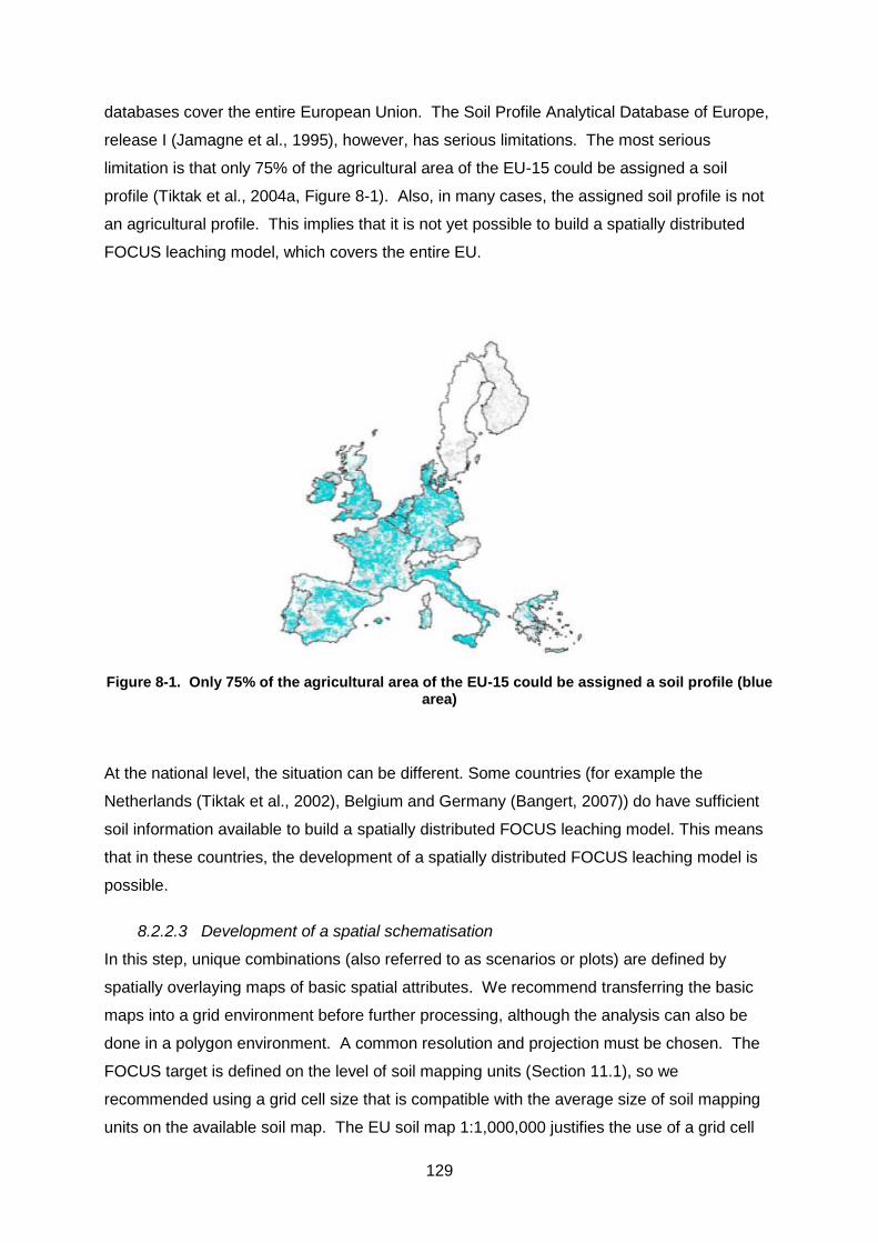
129
databases cover the entire European Union. The Soil Profile Analytical Database of Europe,
release I (Jamagne et al., 1995), however, has serious limitations. The most serious
limitation is that only 75% of the agricultural area of the EU-15 could be assigned a soil
profile (Tiktak et al., 2004a, Figure 8-1). Also, in many cases, the assigned soil profile is not
an agricultural profile. This implies that it is not yet possible to build a spatially distributed
FOCUS leaching model, which covers the entire EU.
Figure 8-1. Only 75% of the agricultural area of the EU-15 could be assigned a soil profile (blue area)
At the national level, the situation can be different. Some countries (for example the
Netherlands (Tiktak et al., 2002), Belgium and Germany (Bangert, 2007)) do have sufficient
soil information available to build a spatially distributed FOCUS leaching model. This means
that in these countries, the development of a spatially distributed FOCUS leaching model is
possible.
8.2.2.3 Development of a spatial schematisation
In this step, unique combinations (also referred to as scenarios or plots) are defined by
spatially overlaying maps of basic spatial attributes. We recommend transferring the basic
maps into a grid environment before further processing, although the analysis can also be
done in a polygon environment. A common resolution and projection must be chosen. The
FOCUS target is defined on the level of soil mapping units (Section 11.1), so we
recommended using a grid cell size that is compatible with the average size of soil mapping
units on the available soil map. The EU soil map 1:1,000,000 justifies the use of a grid cell
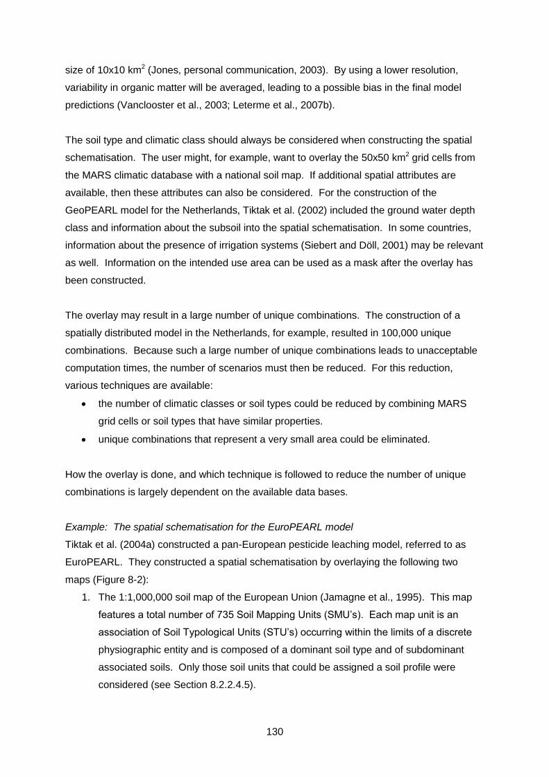
130
size of 10x10 km2 (Jones, personal communication, 2003). By using a lower resolution,
variability in organic matter will be averaged, leading to a possible bias in the final model
predictions (Vanclooster et al., 2003; Leterme et al., 2007b).
The soil type and climatic class should always be considered when constructing the spatial
schematisation. The user might, for example, want to overlay the 50x50 km2 grid cells from
the MARS climatic database with a national soil map. If additional spatial attributes are
available, then these attributes can also be considered. For the construction of the
GeoPEARL model for the Netherlands, Tiktak et al. (2002) included the ground water depth
class and information about the subsoil into the spatial schematisation. In some countries,
information about the presence of irrigation systems (Siebert and Döll, 2001) may be relevant
as well. Information on the intended use area can be used as a mask after the overlay has
been constructed.
The overlay may result in a large number of unique combinations. The construction of a
spatially distributed model in the Netherlands, for example, resulted in 100,000 unique
combinations. Because such a large number of unique combinations leads to unacceptable
computation times, the number of scenarios must then be reduced. For this reduction,
various techniques are available:
the number of climatic classes or soil types could be reduced by combining MARS
grid cells or soil types that have similar properties.
unique combinations that represent a very small area could be eliminated.
How the overlay is done, and which technique is followed to reduce the number of unique
combinations is largely dependent on the available data bases.
Example: The spatial schematisation for the EuroPEARL model
Tiktak et al. (2004a) constructed a pan-European pesticide leaching model, referred to as
EuroPEARL. They constructed a spatial schematisation by overlaying the following two
maps (Figure 8-2):
1. The 1:1,000,000 soil map of the European Union (Jamagne et al., 1995). This map
features a total number of 735 Soil Mapping Units (SMU’s). Each map unit is an
association of Soil Typological Units (STU’s) occurring within the limits of a discrete
physiographic entity and is composed of a dominant soil type and of subdominant
associated soils. Only those soil units that could be assigned a soil profile were
considered (see Section 8.2.2.4.5).
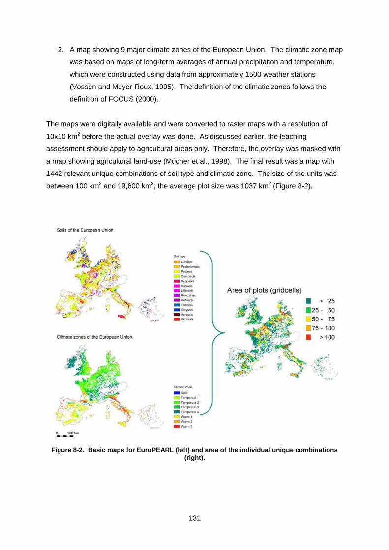
131
2. A map showing 9 major climate zones of the European Union. The climatic zone map
was based on maps of long-term averages of annual precipitation and temperature,
which were constructed using data from approximately 1500 weather stations
(Vossen and Meyer-Roux, 1995). The definition of the climatic zones follows the
definition of FOCUS (2000).
The maps were digitally available and were converted to raster maps with a resolution of
10x10 km2 before the actual overlay was done. As discussed earlier, the leaching
assessment should apply to agricultural areas only. Therefore, the overlay was masked with
a map showing agricultural land-use (Mücher et al., 1998). The final result was a map with
1442 relevant unique combinations of soil type and climatic zone. The size of the units was
between 100 km2 and 19,600 km2; the average plot size was 1037 km2 (Figure 8-2).
Figure 8-2. Basic maps for EuroPEARL (left) and area of the individual unique combinations (right).
132
Notice that the spatial schematisation for EuroPEARL was constructed with only 9 climatic
classes. This was, however, not the final resolution for the climatic data, because during the
parameterisation phase, more detailed climatic information was assigned to each individual
unique combination (see Section 8.2.2.4.1).
8.2.2.4 Model parameterisation
During the model parameterisation phase, the unique combinations must be assigned
parameter values. Each unique combination can be seen as a higher tier scenario (Section
7.2.5), for which the leaching is calculated with a standard FOCUS leaching model (PEARL,
PRZM-3 or PELMO). The reader is therefore referred to the user manual of the individual
models. The latest versions of these models and parameterisation documents are
accessible through the FOCUS website.
All FOCUS leaching models contain a large number of model inputs. To avoid data
redundancy and to assure that the data can be managed in an easy way, we recommend
organising the data in a relational data base. As an example, we show the data base that
was developed for the EuroPEARL model (Figure 8-3). This database has a hierarchy. At
the highest level, a distinction can be made between spatially constant and spatially
distributed parameters. Within the EuroPEARL context, simulations were carried out for one
single pesticide and one single crop (in other words: a single crop, for example maize, was
assumed to be grown throughout the entire intended use area). The substance and crop
code were therefore stored at the highest hierarchical level. The ‘plot’ (or unique
combination) is the central entry for all spatially distributed model inputs. As shown in Figure
8-3, a plot was created by overlaying a soil map and a climatic map. The data base structure
depends on how the unique combinations are defined. In our example, the third hierarchical
level consists of the climatic zone and the soil profile. All other properties are linked to these
two entities. Notice that in the EuroPEARL database, crop properties like emergence data
and harvest date are related to climatic zones.
8.2.2.4.1 Meteorological time-series
A meteorological time series should be attached to each individual unique combination.
Each meteorological time-series must have a length of 66-years and must be created
according to the rules given in FOCUS (2000). The MARS database, which gives data at a
resolution of 50x50 km2, could be used for this purpose, but national databases are preferred
if available at sufficient resolution. The storage of all meteorological data takes a lot of disk
space, particularly if the number of unique combinations is large. Although disk space is not
a problem as such, it makes the model less easy to transfer to other people. For this reason,
133
one time-series per climatic zone in combination with a simple scaling procedure could be
used to calculate the time-series for each unique combination. This scaling procedure uses
the long-term average annual precipitation and temperature (which can be inferred for
example from the MARS grid):
stationaplotastationdplotd
stationa
plota
stationdplotd TTTTP
PPP ,,,,
,
,
,, and (8-1)
where P is precipitation, T is temperature, and the suffixes a and d refer to daily and annual,
respectively. The central assumption in this approach is that data from one location can be
used to correctly describe the seasonal dynamics of weather conditions within the entire
climatic zone.
Run
Control;
Substance;
Crop;
Plot.
Substance
Substance properties, such as
the half-live, the
partitioning coefficient and
application type.
Plot
Climate zone;
Soil profile;
Long-term average
weather conditions.
Control
Start and end date;
Other control parameters.
Climate zone
Daily weather series;
Emergence and
harvest date of crops;
Phenological
development stages;
Application date of
pesticides.
Soil profile
Soil horizon;
Groundwater level;
Irrigation switch.
Soil horizon
Soil physical unit;
Layer thickness;
Texture;
Organic matter;
pH.
Crop properties
Critical pressure heads for drought stress and irrigation;
Extinction coefficient for solar radiation.
Development stage
LAI;
Crop factor;
Rooting depth.
Soil physical unit
Parameters of the
Mualem-
van Genuchten
functions;
Dispersion length
Spatially distributed variables
Daily weather
Temperature;
Rainfall;
Wind speed;
Humidity;
Radiation.
Figure 8-3. Structure of the EuroPEARL data base (source: Tiktak et al., 2004a)
The MARS climatic database contains all parameters that are required for simulation runs
with current FOCUS models such as minimum and maximum temperature, rainfall, reference
evapotranspiration, and global radiation. The MARS climatic database can therefore be used
to extract the daily weather data for European leaching assessments. The MARS database
134
contains weather data spatially interpolated on 50x50 km2 grids. The original weather
observations dataset originate from 1500 meteorological stations across Europe, and are
based on daily data from the period 1971 to date. It was compiled from data purchased from
various national meteorological services. Some of the data were obtained from the national
meteorological services under special copyright and agreements for MARS internal use only,
so that data at station level are not available, only interpolated daily meteorological data are
available.
The use of data from local weather stations may be considered if sufficient weather data is
available. In GeoPEARL for the Netherlands, for example, data from the Royal Netherlands
Meteorological Institute was used. In countries with large altitude differences, the link
between station data and unique combinations may not be an easy task. The variability in
climatic conditions may be large across short differences. These differences must be taken
into account when developing an appropriate geostatistical interpolation technique.
8.2.2.4.2 Cropping parameters
If leaching assessments are carried out across different climatic zones, then dynamic crop
properties (crop development stage, harvest date, and emergence date) should be related to
climatic zones (Figure 8-3). GeoPEARL has an option to make the crop development
dependent on the temperature sum since emergence, which should be used if leaching
assessments are carried out across different climatic zones.
Most crop parameters (e.g. date of emergence, date of harvest, crop development stages,
etc.) can be taken from the Tier 1 scenario of the corresponding FOCUS climatic zone. See
FOCUS (2000) and Chapter 13 for a definition of these climatic zones. In some cases more
detailed information on cropping dates exist, in particular when crops are grown in confined
areas with characteristic climate conditions. In such cases modifying cropping dates or other
parameters may be appropriate. When changing cropping parameters, a rationale for each
change must be provided in order to ensure a high degree of transparency in the
assessment. If scenarios are developed for minor crops, then a completely new cropping
parameterisation may be required.
8.2.2.4.3 Irrigation
Siebert and Döll (2001) presented a map showing the fraction of land equipped for irrigation.
This map may be used to identify areas where irrigation is a common practice. In those
areas and for certain crops, irrigation amounts must be assigned. A procedure that
considers the water storage capacity of soils should be used. If the water capacity is not
135
considered, calculated irrigation amounts might be higher than those applied in reality,
resulting in unrealistic run-off amounts. Most FOCUS leaching models have multiple options
to calculate irrigation amounts – see the manuals of the corresponding models for further
information (parameterisation procedures for the scenarios are discussed in Section 11.5.3.
8.2.2.4.4 Lower boundary conditions and runoff
The Darcy-type of models (PEARL and MACRO) needs information about the lower
boundary condition (for example depth to ground water). If information on the local ground
water regime is available, this information can be used to parameterise the lower boundary
condition. PEARL has several options for the lower boundary condition – which of these
options is most appropriate depends on the available data. Refer to the GeoPEARL and
PEARL manuals for further detail. The lower boundary condition of GeoPEARL for the
Netherlands was parameterised through a link between a regional ground water flow model,
a simplified surface water concept and the soil water flow model (Wolf et al., 2003; Tiktak et
al., 2002). This approach made possible distinguishing between the pesticide flux that
reaches the deep ground water and the pesticide flux that reaches the surface water (through
lateral drainage). Such detailed information, however, is usually not available for large scale
pesticide leaching assessments.
In those cases where no information on the ground water level is available, the ground water
depth should be set well below the target depth of 1 m. Tiktak et al. (2004a), used a depth of
2 m depth for their pan-European leaching assessments. They found that the predicted
concentration at 1 m depth was hardly affected by the lower boundary condition if the ground
water depth is situated well below the target depth.
If runoff is an important process in the area to be simulated, runoff should be simulated as
well. See Section 7.2.5.1.4 for details on runoff parameterisation.
8.2.2.4.5 Soil parameters
The parameterisation of the soil parameters consists of three steps: (a) selection of a soil
profile from a soil profile data base, (b) parameterisation of basic soil information, which is
directly available in these data bases (usually horizon designations, organic matter, texture
and sometimes also pH), and (c) parameterisation of derived soil properties that are not
available in the soil profile database (soil hydraulic functions, bulk density of the soil, etc.).
8.2.2.4.5.1 Selection of a soil profile
136
Soil profile descriptions usually contain information on the soil mapping unit from which the
soil profile originates. The link between the soil map and the soil profile data base is then a
trivial step, because there is a 1:1 link.
At the European level, however, this link is not straightforward. The problem is that the Soil
Mapping Units (SMU’s) at the EU-soil map are association of dominant and subdominant Soil
Typological Units (STU’s). The STU’s and not the SMU’s are the carriers of basic soil
information, such as the FAO soil name and the soil textural class. For this reason, the link
between the soil map and the profile data base needs to be done in two steps. A possible
approach could be to determine the dominant STU, and then assign a soil profile to this
dominant STU. Notice that during this step information on subdominant soil profiles will be
lost, leading to a possible bias during the assessment (Vanclooster et al., 2003). An
additional problem is that the Soil Profile Analytical Database of Europe (SPADE, Madsen-
Breuning and Jones, 1995) usually does not contain explicit information on the associated
soil typological unit. Finally, many STU’s at the EU-soil map do not have an associated soil
profile. To overcome these problems, Tiktak et al. (2004a) developed a two-step approach
for the parameterisation of EuroPEARL (Figure 8-4). In a first step, the dominant STU within
each SMU was determined. Then, a soil profile was assigned to the dominant STU. This
second link was made at different confidence levels. The most reliable link could be obtained
if the author of a profile has explicitly stated the corresponding STU. If the STU was not
specified, a profile was assigned on the basis of the full FAO soil name, the textural class
and the country code. By including the country code in the query, soil profiles from the soil
profile data base of a given country could only be matched to Soil Mapping Units within that
country. In those situations where assigning a soil profile was still not possible, the query
was repeated with the full FAO soil name and the country code only. Finally, a query was
carried out using the major soil type only (e.g. Cambisol instead of Eutric Cambisol). Using
this procedure, 1062 Unique Combinations could be assigned a soil profile, representing
approximately 75% of the total agricultural area of the European Union. Unfortunately,
Austria, Sweden and Finland had to be left-out, because there was insufficient soil profile
information available for these countries.
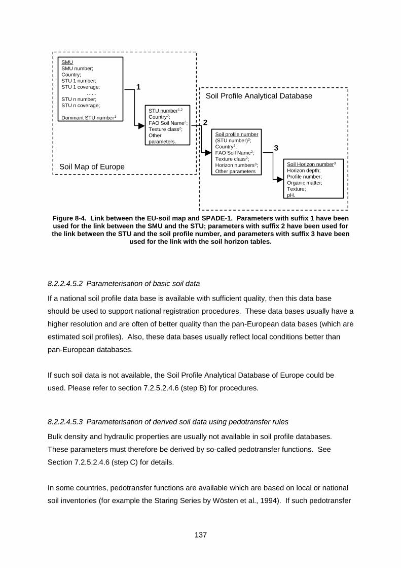
137
Soil Map of Europe
Soil Profile Analytical Database
SMU
SMU number;
Country;
STU 1 number;
STU 1 coverage;
…...
STU n number;
STU n coverage;
Dominant STU number1
STU number1,2
Country2;
FAO Soil Name2;
Texture class2;
Other
parameters.
Soil profile number
(STU number)2;
Country2;
FAO Soil Name2;
Texture class2;
Horizon numbers3;
Other parameters
Soil Horizon number3
Horizon depth;
Profile number;
Organic matter;
Texture;
pH.
1
2
3
Figure 8-4. Link between the EU-soil map and SPADE-1. Parameters with suffix 1 have been used for the link between the SMU and the STU; parameters with suffix 2 have been used for the link between the STU and the soil profile number, and parameters with suffix 3 have been
used for the link with the soil horizon tables.
8.2.2.4.5.2 Parameterisation of basic soil data
If a national soil profile data base is available with sufficient quality, then this data base
should be used to support national registration procedures. These data bases usually have a
higher resolution and are often of better quality than the pan-European data bases (which are
estimated soil profiles). Also, these data bases usually reflect local conditions better than
pan-European databases.
If such soil data is not available, the Soil Profile Analytical Database of Europe could be
used. Please refer to section 7.2.5.2.4.6 (step B) for procedures.
8.2.2.4.5.3 Parameterisation of derived soil data using pedotransfer rules
Bulk density and hydraulic properties are usually not available in soil profile databases.
These parameters must therefore be derived by so-called pedotransfer functions. See
Section 7.2.5.2.4.6 (step C) for details.
In some countries, pedotransfer functions are available which are based on local or national
soil inventories (for example the Staring Series by Wösten et al., 1994). If such pedotransfer
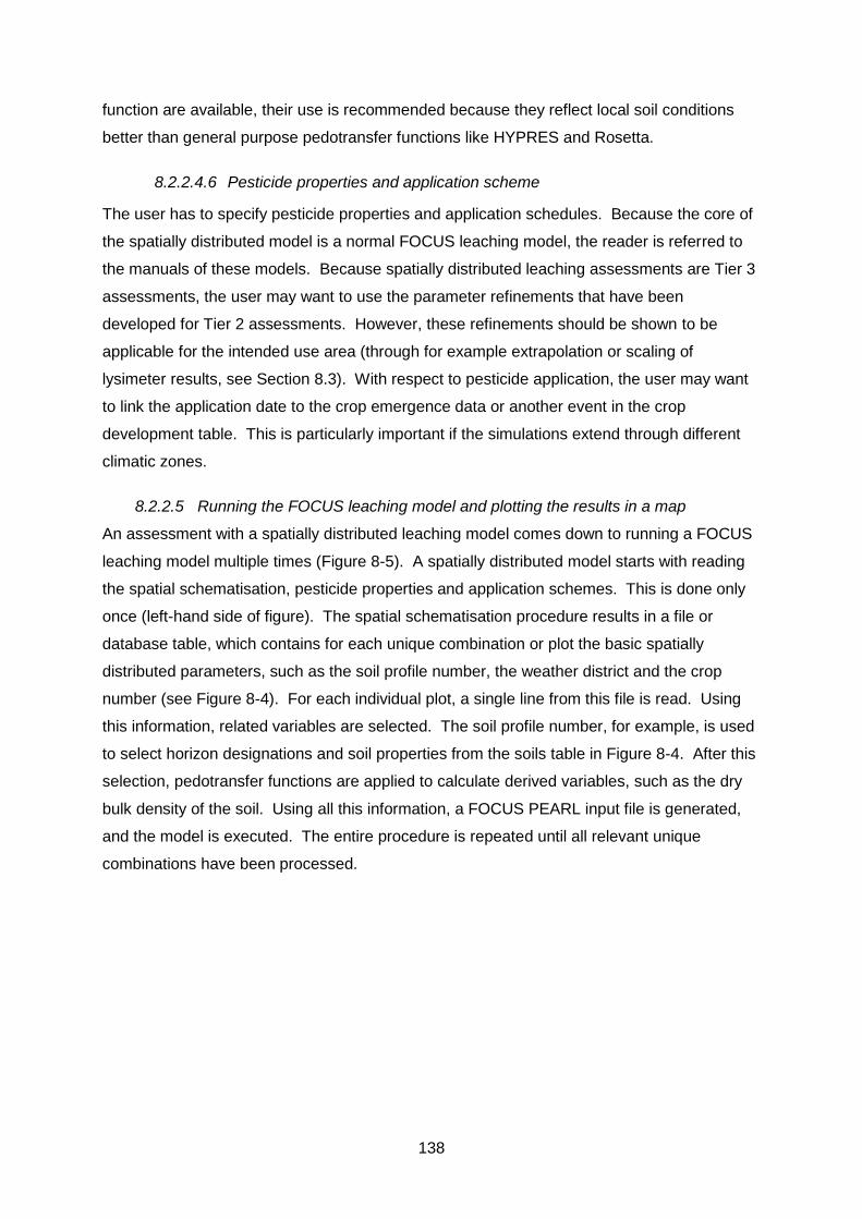
138
function are available, their use is recommended because they reflect local soil conditions
better than general purpose pedotransfer functions like HYPRES and Rosetta.
8.2.2.4.6 Pesticide properties and application scheme
The user has to specify pesticide properties and application schedules. Because the core of
the spatially distributed model is a normal FOCUS leaching model, the reader is referred to
the manuals of these models. Because spatially distributed leaching assessments are Tier 3
assessments, the user may want to use the parameter refinements that have been
developed for Tier 2 assessments. However, these refinements should be shown to be
applicable for the intended use area (through for example extrapolation or scaling of
lysimeter results, see Section 8.3). With respect to pesticide application, the user may want
to link the application date to the crop emergence data or another event in the crop
development table. This is particularly important if the simulations extend through different
climatic zones.
8.2.2.5 Running the FOCUS leaching model and plotting the results in a map
An assessment with a spatially distributed leaching model comes down to running a FOCUS
leaching model multiple times (Figure 8-5). A spatially distributed model starts with reading
the spatial schematisation, pesticide properties and application schemes. This is done only
once (left-hand side of figure). The spatial schematisation procedure results in a file or
database table, which contains for each unique combination or plot the basic spatially
distributed parameters, such as the soil profile number, the weather district and the crop
number (see Figure 8-4). For each individual plot, a single line from this file is read. Using
this information, related variables are selected. The soil profile number, for example, is used
to select horizon designations and soil properties from the soils table in Figure 8-4. After this
selection, pedotransfer functions are applied to calculate derived variables, such as the dry
bulk density of the soil. Using all this information, a FOCUS PEARL input file is generated,
and the model is executed. The entire procedure is repeated until all relevant unique
combinations have been processed.
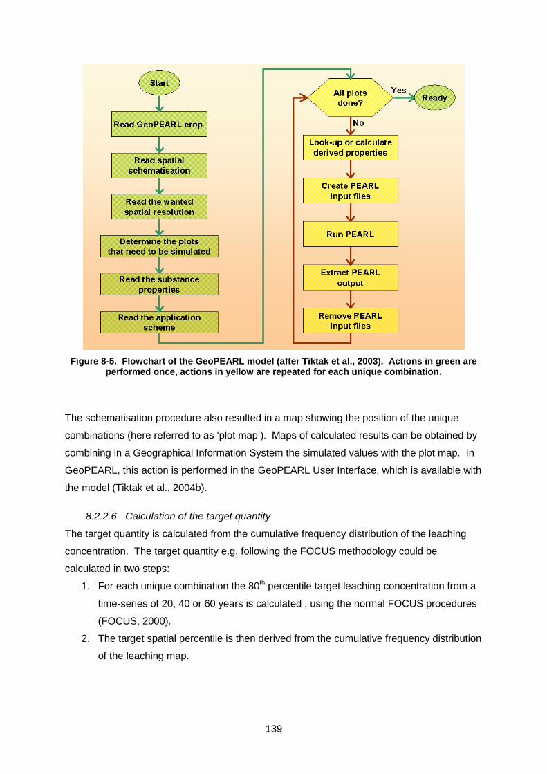
139
Figure 8-5. Flowchart of the GeoPEARL model (after Tiktak et al., 2003). Actions in green are performed once, actions in yellow are repeated for each unique combination.
The schematisation procedure also resulted in a map showing the position of the unique
combinations (here referred to as ‘plot map’). Maps of calculated results can be obtained by
combining in a Geographical Information System the simulated values with the plot map. In
GeoPEARL, this action is performed in the GeoPEARL User Interface, which is available with
the model (Tiktak et al., 2004b).
8.2.2.6 Calculation of the target quantity
The target quantity is calculated from the cumulative frequency distribution of the leaching
concentration. The target quantity e.g. following the FOCUS methodology could be
calculated in two steps:
1. For each unique combination the 80th percentile target leaching concentration from a
time-series of 20, 40 or 60 years is calculated , using the normal FOCUS procedures
(FOCUS, 2000).
2. The target spatial percentile is then derived from the cumulative frequency distribution
of the leaching map.
140
When calculating the cumulative frequency distribution, the spatial distribution of the target
crop should be used as a weighing factor. Not considering the intended use area may result
in unrealistic frequency distributions as shown in Figure 8-6 for an example at the national
level of the Netherlands.
Figure 8-6. Effect of considering the intended use area on the calculated frequency distribution of the leaching concentration (using the Netherlands as an example for a political entity).
The spatial distribution of crops can be obtained from maps based on satellite images.
These satellite images have an extremely high spatial resolution (up to 25x25 m2), but the
number of crops distinguished is limited (only major crops are mapped). To obtain the spatial
distribution of other crops, the satellite images can be combined with census data, which in
many countries are available at the level of municipalities. See further Kruijne et al. (2004).
8.2.3 Stochastic assessments
The proposed procedure for spatial schematisation relies on the soil map as a carrier of
information relevant to solute transport. Indeed, variation between soil types has been
shown to be usually larger than within-soil variation (for example Bergström and Jarvis, 1993;
Brown et al., 2000). Nevertheless, no soil-classification scheme can fully capture the
141
complexity of soil variation, and therefore the inherent stochastic variation remaining within
each class should be assessed (Jarvis and Dubus, 2006). Leterme et al. (2007b) performed
such a probabilistic assessment for atrazine leaching in a Belgian catchment, using Monte
Carlo simulations. They showed that the spatial pattern of pesticide leaching was not
strongly affected, but the simulated concentrations increased by an order of magnitude when
looking at the 80th percentile, as done in current FOCUS procedures. The increase of the
80th percentile was to be expected, as the incorporation of within-soil type variability is likely
to introduce more extreme scenarios. Another limitation of deterministic models like
GeoPEARL is that pesticide properties are taken spatially constant. In reality, however,
these properties exhibit spatial variability (e.g. Walker and Brown, 1983; Charnay et al.,
2005). The introduction of spatial variability of pesticide properties in stochastic simulations
also increases the leaching concentration, as shown by Leterme et al. (2007b).
Despite the fact that scientists now believe that stochastic assessments should be an integral
part of the decision making process (EUFRAM, 2005), the current working group chooses to
limit tier 3 simulations to deterministic simulations. One of the reasons is that standardisation
procedures for stochastic assessments are currently not available, and that the effect of user
subjectivity in performing stochastic assessments is still too large. Leterme et al. (2007b), for
example, showed that the effect of truncation of distributions of soil and pesticide properties
has a large effect on the predicted leaching percentiles. Also, the outcome of deterministic
assessments is in line with the operational definition of the protection goal as given in Section
3.1, although note that the definition of soil mapping units is scale dependent. Further
research and progress in the area of stochastic assessment may lead to a revision of the
recommendation.
8.3 Higher tier leaching experiments set into context by modelling (Tier 3c)
The broad potential for using higher tier leaching experiments in the assessment of the risk to
ground water has been covered in Chapter 4. This current section considers the practical
possibilities, limitations and concerns about the use of such studies, and their placement into
context by simulation modelling. Note that since these are higher-tier approaches, the lower
tiers usually will have indicated potential risks. These assessments (i.e. the studies and the
associated modelling) must then deliver sufficient evidence to prove the potential risks are
unlikely to exist in reality.
Generally, the appropriate context for the experimental studies can be provided in a so-called
“pre-processing” manner (i.e. explicitly designing the experiment with the intent to cover the
142
location and agroclimatic conditions that address the required protection goal for the
particular compound and use). A so-called “post-processing” manner (i.e. the field and
lysimeter observations are used to refine model parameters or model calculations) is then
required to demonstrate whether the intent of the pre-processing phase was achieved. Pre-
processing approaches alone will not lead to the experimental result being directly suitable
for regulatory decision-making (e.g. the rainfall at the chosen location over the experimental
duration may be significantly less than the target). Poorly designed studies (i.e. of short
duration with no understanding of the movement of chemical through the soil profile) cannot
necessarily become relevant for regulatory decision-making by post-processing
extrapolations. Therefore, while post-processing is essential, a combination of both
approaches usually will give the most robust results for regulatory decision-making.
Sections 8.3.1 and 8.3.2 concentrate on the advantages/disadvantages and regulatory status
of the experimental studies, followed by Section 8.3.3 on appropriate pre-processing issues
to consider. Section 8.3.4 then consider particular post-processing approaches in detail, i.e.
scaling of model parameters based on inverse modelling and scaling of the leaching
assessments based on observed differences between simulated and observed field/
lysimeter leaching.
8.3.1 Study types and their applicability for different agroclimatic conditions
8.3.1.1 Lysimeters
Regulatory lysimeter studies utilise an undisturbed soil monolith (typically 1 m deep and 1 m2
surface area) to grow a crop and follow the breakthrough of radiolabelled pesticide and
metabolites over time (See Fuhr and Hance, 1992; and Fuhr, 1998 for general reviews). This
experimental design confers the advantage that a flux-weighted concentration at 1 m depth
can be measured without necessarily completely understanding the mechanistic nature of the
actual degradation and sorption processes of the pesticide in this soil.
Due to the inherent experimental design of the lysimeters that were usually used for
regulatory submissions (i.e., this is not a function of particular study guidelines), the water
flow at the bottom boundary does not exactly replicate the real field situation, being free
draining rather than hydraulically connected to deeper soil depths. This is acknowledged as
a potential weakness in the design but is unavoidable if the flux-weighted annual
concentration of pesticide is to be obtained as the endpoint. Early assessments by Hance
and Fuhr (1992) have suggested that lysimeter and field studies result in similar amounts of
pesticide remaining in the soil profile. Studies by Jene (1998) concluded that free-draining
143
sandy soil lysimeters (0.8 m2 surface area) and suction cup instrumented field plots (2.7 m2
surface area) of the same soil type showed no system-related differences in water and solute
(including pesticide) transport. Although (i) the outflow water volumes of the field were about
60% of those in the lysimeter and (ii) the average flux concentration of benazolin in the field
was about two times higher than in the lysimeter, the sites were 20 km apart so differing
evapotranspiration (ET) amounts at the two locations were considered by Jene (1998) to
account for the difference. Extensive studies in a very similar experimental set-up, but with
the lysimeters placed at the field site (both being silty soils), showed water percolation in the
field trial (water collected via suction plates) was 67% of that in the lysimeter study.
Comparisons of the leaching of two pesticides (ethidimuron and methabenzthiazuron) give
3.3 and 0.7 µg/L annual average leachate concentrations of ethidimuron in the lysimeter and
field, respectively, and 2.8 and 0.05 µg/L annual average leachate concentrations of
methabenzthiazuron in the lysimeter and field respectively (but with large variations amongst
replicates). In both systems this leaching was considered to be the result of preferential flow
(Dressel, 2003). Further analysis of these results by Kasteel et al (2007) suggested that
methodological issues regarding the suction plates could have led to underestimation of the
water flux. The mass recovery of bromide tracer was identical despite these water volume
differences but the spreading (dispersivity) was stated to be greater in the lysimeters, leading
to lower peak concentrations. Subsequently the authors attempted to simulate the field
results to account for the effect of the suction plate and concluded that the “true”
dispersivities were similar in the field and lysimeter. (note that for non-conserved solute this
behaviour would be likely to lead to higher concentrations leached due to more compound
moving out of the zone of optimum degradation). The complexities of the experimental
system mean that broad conclusions about comparative amounts of leachate from lysimeters
and field systems should not be drawn from this single experiment.
Computer simulations (Boesten, 2007) have indicated that predicted pesticide concentrations
were always lower with the lysimeter bottom boundary type than with the field bottom
boundary type (hydraulically connected to ground water).
Significant infrastructure is required to maintain lysimeter cores during an experiment and
hence the cores can only be subjected to a limited range of meteorological conditions (i.e.
particular locations in northern Europe that have lysimeter facilities). There are also
agronomic restrictions due the relatively small surface area of the lysimeter. Therefore
experiments with tree and other permanent crops are often impractical and ridged cropping
systems (e.g. potatoes) may be difficult to maintain.
144
The use of tracers in lysimeters is a useful approach and should be considered in future to
determine the hydraulic properties of the soil cores.
Research lysimeter facilities may additionally include packed cores, longer lysimeter cores
(>> 1m) with increased residence times, or devices to apply suction to the bottom of the
lysimeter core to overcome the capillary fringe. They are often used to follow water or solute
movement. Further current information on these can be found on the internet at the following
website: www.lysimeter.com
8.3.1.2 Field leaching experiments
Field leaching experiments have the advantage that they are undertaken in actual agronomic
situations (i.e. any field) and require no particular facilities. Therefore they can be used in a
wider range of climatic situations and locations than typically occur for lysimeter studies (e.g.
also in southern Europe). Leaching can be assessed for agricultural practices that are
impractical for lysimeters e.g. ridged systems for potatoes, permanent crops etc. However a
disadvantage is that radiolabelled compounds cannot be used so compounds of interest
must be determined prior to the study (and analytical methods be available) and mass
balances cannot be obtained. Water is drawn out of the soil profile or taken directly from
ground water at different depths and analysed for the presence of the compounds of interest.
Therefore the annual average concentration cannot be directly determined, only the
concentration at a given depth at a particular time. Water balances are also not directly
obtained, although approximations of the ground water recharge can be used to estimate an
annual average from these data. In addition there can be methodological issues about the
method by which the water is drawn out of the soil profile (e.g. using suction cups, see Carter
and Fogg, 1995; Weihermüller et al, 2005, 2006; and Ferrari et al, 2007, for discussion on
appropriate methodologies). Using 'equilibrium tension plate lysimeters' 10, drainage rates
and leaching concentrations can be measured continuously and more accurately. These
systems consist of large ceramic plates which are connected to a vacuum to apply suction to
the soil water. In order to minimise the disturbance of the water flow by the suction plates,
the applied suction is controlled so that tensiometer measurements in the soil just above the
suction plate match with tensiometer measurements at the same depth in the soil profile
where water flow is not influenced by the suction plates (Byre et al., 1999; Kosugi and
Katsuyama, 2004; Mertens et al., 2005).
10 Note that the name implies that this methodology could also be a “lysimeter” study. Nonetheless it
has been designated as a field leaching study in this document because it has more in common with field leaching type approaches than with the standard regulatory type “lysimeter” study.

145
Regarding regulatory use of field leaching study, the same principles apply as for lysimeter
studies. Therefore, a field leaching study would need to be set into context by modelling
before it can be used for regulatory decision making.
Further useful information on leaching potential may be obtained from analysis of soil cores
at differing depths. Note that certain leaching study designs could be considered very similar
to monitoring studies (for which guidance is provided in Chapter 9).
8.3.2 Current status of higher tier leaching experiments in national regulation and appropriate guidelines
Within the EU there is national guidance for undertaking lysimeter studies in Germany (BBA,
1990) and in the Netherlands (CTB, 1999). In Germany, if the conditions of the guideline are
met, the results are considered directly acceptable for national regulatory decision-making. A
recent comparison of BBA guideline-compliant experimental data and national scenario
simulation studies (see Figure 8-7) suggested a high degree of agreement between the two
approaches in evaluating whether the regulatory endpoint of 0.1 µg/L is exceeded. This
figure effectively demonstrates the consistency of the German national tiered approach as
outlined by Michalski et al. (2004) and highlights the infrequency of disagreement between
lysimeter and simulation results.
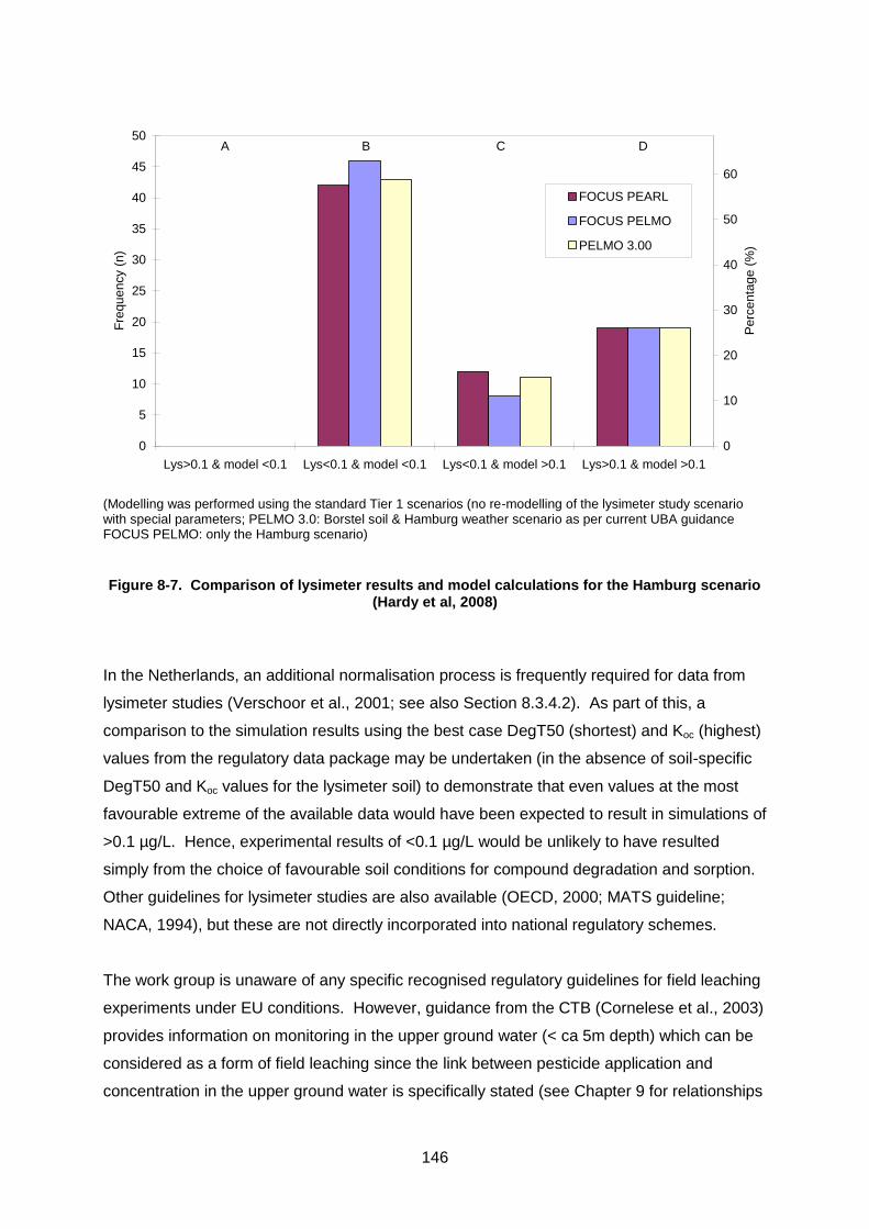
146
Lysimeter vs Model Comparison
0
5
10
15
20
25
30
35
40
45
50
Lys>0.1 & model <0.1 Lys<0.1 & model <0.1 Lys<0.1 & model >0.1 Lys>0.1 & model >0.1
Fre
quency (
n)
0
10
20
30
40
50
60
Perc
enta
ge (
%)
FOCUS PEARL
FOCUS PELMO
PELMO 3.00
A CB D
(Modelling was performed using the standard Tier 1 scenarios (no re-modelling of the lysimeter study scenario with special parameters; PELMO 3.0: Borstel soil & Hamburg weather scenario as per current UBA guidance FOCUS PELMO: only the Hamburg scenario)
Figure 8-7. Comparison of lysimeter results and model calculations for the Hamburg scenario (Hardy et al, 2008)
In the Netherlands, an additional normalisation process is frequently required for data from
lysimeter studies (Verschoor et al., 2001; see also Section 8.3.4.2). As part of this, a
comparison to the simulation results using the best case DegT50 (shortest) and Koc (highest)
values from the regulatory data package may be undertaken (in the absence of soil-specific
DegT50 and Koc values for the lysimeter soil) to demonstrate that even values at the most
favourable extreme of the available data would have been expected to result in simulations of
>0.1 µg/L. Hence, experimental results of <0.1 µg/L would be unlikely to have resulted
simply from the choice of favourable soil conditions for compound degradation and sorption.
Other guidelines for lysimeter studies are also available (OECD, 2000; MATS guideline;
NACA, 1994), but these are not directly incorporated into national regulatory schemes.
The work group is unaware of any specific recognised regulatory guidelines for field leaching
experiments under EU conditions. However, guidance from the CTB (Cornelese et al., 2003)
provides information on monitoring in the upper ground water (< ca 5m depth) which can be
considered as a form of field leaching since the link between pesticide application and
concentration in the upper ground water is specifically stated (see Chapter 9 for relationships

147
between monitoring and field leaching studies). The broad requirements for this type of
study are stated to be: 8-10 fields with 12-20 sample locations/field and 3 time points (before,
during and after the simulated peak concentration). Guidance similarly exists for prospective
ground water studies conducted in the U.S. (US EPA, 2008), which are also considered as a
variation of a field leaching study. A possible outline protocol for a regulatory field leaching
experiment is currently in preparation in Italy (Ferrari et al., 2007), although note that this is
only directed at studies abstracting shallow ground water (and not soil pore water).
8.3.3 Suitability for exposure assessment within FOCUS framework – “pre-processing” aspects
The critical point in the use of higher tier leaching studies (both lysimeter and field leaching)
in the FOCUS framework is the demonstration of adequate vulnerability. The Tier 1
simulation scenarios have been developed with the intention that they cover the 90th
percentile overall vulnerability. For experimental field data to fit logically into the FOCUS
framework they must cover a similar vulnerability. This section concentrates on addressing
vulnerability via “pre-processing” approaches. As noted elsewhere “post-processing”
approaches to putting the experimental data into context may allow greater flexibility in the
nature of the initial experimental data.
This question of study vulnerability can be separated into two main components;
1. Is the inherent study design sufficiently conservative to address the leaching process?
2. Is the experiment located in a sufficiently vulnerable location with regard to soil type,
agronomy and meteorological conditions?
8.3.3.1 Determining adequate vulnerability – through study design
8.3.3.1.1 Lysimeters
The most often raised concerns regarding lysimeter studies relate to the translation of the
concept into recognised methodologies that are applicable for regulatory decision-making,
primarily BBA guideline 4-3 (BBA, 1990); since other guidelines are largely derivative of this.
Typically the experiment is undertaken for a period of three years only (with a second
application in the second year), uses a sandy soil type only, and has very limited replication
(typically two cores but even one core is conceivable, although this does not comply with the
OECD guideline). These limitations are all valid scientific concerns and are considered
individually in the following sections.
Within the FOCUS framework, lysimeter (and field leaching) studies are clearly a higher tier
within the decision-making scheme, so logically such studies are likely to be triggered for
148
fewer compounds. Possibly such compounds will be those with different behaviour as
defined in Section 11.1. In such cases the use of a “standard” guideline (e.g. BBA guideline
4-3) may not be appropriate (for pre-processing approaches) and a greater emphasis on
compound-specific study design should be considered. In particular for many active
substances and their metabolites the “standard” study duration is often too short for a steady
state of residues to have been achieved in the soil monolith. See 8.3.3.1.1.2 for a more
detailed discussion.
8.3.3.1.1.1 Soil type
The standard BBA regulatory guideline study requires a sandy soil of low organic carbon
content (<1.5%) since this is generally considered to be the worst case for chromatographic
flow movement of a pesticide. Evidence to support this view comes from a study
(Gottesbüren, personal communication, 2008) in which the leaching of bromide has been
measured in parallel running lysimeters with two different soil types (sand and loam).
Results are shown in Figure 8-8. Bromide breakthrough started earlier and reached higher
cumulative outflow in the sandy soils, whereas in the loamy soils the cumulative
breakthrough was considerably lower and reached a maximum range of 4 – 14 % of the
applied dose by the end of the study. Gottesbüren (personal communication, 2008)
attributes the removal of the remaining bromide from the soil to plant uptake. The faster
chromatographic flow processes in the sandy soils observed for bromide in this study would
also have more quickly transported potentially leaching pesticides into deeper soil zones, in
which the degradation rate would be lower.
149
0
20
40
60
80
100
14.01.2004 23.04.2004 01.08.2004 09.11.2004 17.02.2005 28.05.2005 05.09.2005
date
cum
ula
tive B
r outflo
w [%
of applie
d]
Sand (Pos11) Sand (Pos12) Sand (Pos14) Sand (Pos15) Sand (Pos22)
Loam (Pos25) Loam (Pos34) Loam (Pos35) Loam (Pos36) Loam (Pos37)
SAND
LOAM
Figure 8-8. Bromide breakthrough in replicate sand and loam lysimeters running in parallel at the same facility (Gottesbüren, personal communication, 2008).
pH characteristics are not specified in the BBA guideline and, in practice, the pH will vary
depending on liming before the cores were taken or the study started. pH characteristics can
influence both the sorption and degradation of a pesticide and its metabolites and so a worst
case situation could only be considered on a case by case basis.
Whether for most pesticides these conditions of acidic pH and sandy soil, which prevail in
most regulatory lysimeter studies, will also be the worst case for degradation is uncertain.
That low organic carbon contents lead to reduced microbial activity and slower biological
degradation rates for pesticides is widely believed, although there appear to be no data
reviews to demonstrate that this belief is defensible. In fact an earlier review (Walker and
Allen, 1984) suggested that degradation was faster in sandy soils than more clayey soils for
the herbicides simazine and metamitron. However, the same review points out that other
factors also influenced degradation rates and that overall the difference in degradation rate
among a number of soils with differing characteristics was relatively small.
Overall the worst case for leaching will be a combination of the factors discussed above.
Therefore consideration of the actual amounts leached from various soil types under identical
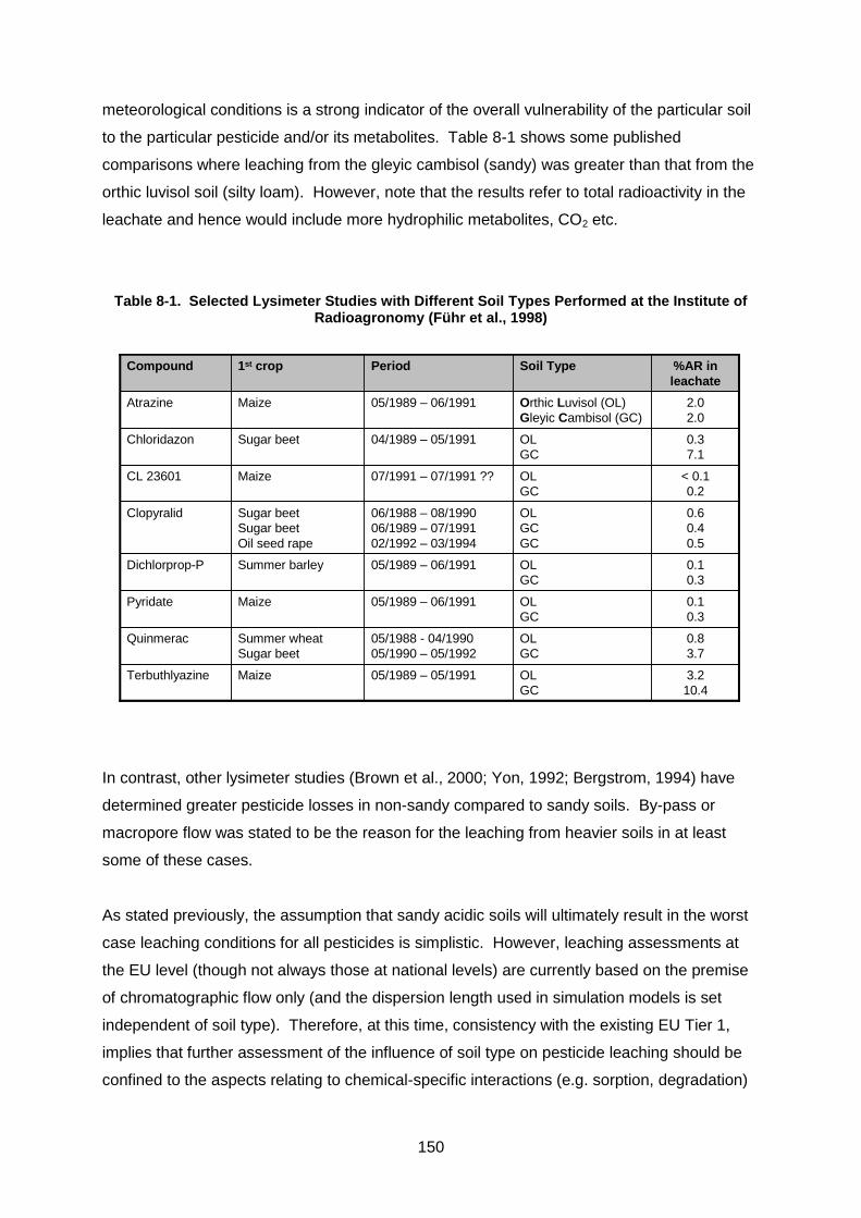
150
meteorological conditions is a strong indicator of the overall vulnerability of the particular soil
to the particular pesticide and/or its metabolites. Table 8-1 shows some published
comparisons where leaching from the gleyic cambisol (sandy) was greater than that from the
orthic luvisol soil (silty loam). However, note that the results refer to total radioactivity in the
leachate and hence would include more hydrophilic metabolites, CO2 etc.
Table 8-1. Selected Lysimeter Studies with Different Soil Types Performed at the Institute of Radioagronomy (Führ et al., 1998)
0.6
0.4
0.5
OL
GC
GC
06/1988 – 08/1990
06/1989 – 07/1991
02/1992 – 03/1994
Sugar beet
Sugar beet
Oil seed rape
Clopyralid
0.1
0.3
OL
GC
05/1989 – 06/1991Summer barleyDichlorprop-P
0.1
0.3
OL
GC
05/1989 – 06/1991MaizePyridate
0.8
3.7
OL
GC
05/1988 - 04/1990
05/1990 – 05/1992
Summer wheat
Sugar beet
Quinmerac
< 0.1
0.2
OL
GC
07/1991 – 07/1991 ?? MaizeCL 23601
3.2
10.4
OL
GC
05/1989 – 05/1991MaizeTerbuthlyazine
0.3
7.1
OL
GC
04/1989 – 05/1991Sugar beetChloridazon
2.0
2.0
Orthic Luvisol (OL)
Gleyic Cambisol (GC)
05/1989 – 06/1991MaizeAtrazine
%AR in
leachate
Soil TypePeriod1st cropCompound
In contrast, other lysimeter studies (Brown et al., 2000; Yon, 1992; Bergstrom, 1994) have
determined greater pesticide losses in non-sandy compared to sandy soils. By-pass or
macropore flow was stated to be the reason for the leaching from heavier soils in at least
some of these cases.
As stated previously, the assumption that sandy acidic soils will ultimately result in the worst
case leaching conditions for all pesticides is simplistic. However, leaching assessments at
the EU level (though not always those at national levels) are currently based on the premise
of chromatographic flow only (and the dispersion length used in simulation models is set
independent of soil type). Therefore, at this time, consistency with the existing EU Tier 1,
implies that further assessment of the influence of soil type on pesticide leaching should be
confined to the aspects relating to chemical-specific interactions (e.g. sorption, degradation)
151
and not macroporous flow. Data on degradation and sorption of the parent compound in at
least four soils (at least three soils for metabolites) is available from the standard regulatory
package and this can be examined to assess influences of soil type on sorption and
degradation. This is a relatively small data-set on which to assess particular influences of
soil characteristics and subtle effects would be difficult to observe. However, this data set is
the same that is used for the Tier 1 input parameters and seems a reasonable basis on
which to investigate whether the assumptions incorporated into the simulations at Tier 1, hold
true for the same soil types under outdoor conditions at Tier 2. In the absence of any clear
effects of soil type on compound behaviour, the current BBA guideline standard soil type (low
organic carbon, sandy soil), which is highly likely to be a worst case with respect to the
sorption coefficient, can be used for lysimeter studies as a default. However, a more detailed
consideration of the potential usage area to determine an 80th percentile worst case soil (see
Section 8.3.3.2) would be preferable.
8.3.3.1.1.2 Duration
The duration of all regulatory lysimeter experiments is significantly shorter than would be
necessary for maximum compound breakthrough of most compounds according to simulation
studies (Boesten, 2007). The requirement for the duration of lysimeter experiments is
assumed to be a pragmatic decision to enable data to be collected over a realistic timescale
for regulatory use, but no documented information has been found on this point. Some data
collected from regulatory studies has suggested that over the standard three year duration of
the BBA guideline study (Hardy et al. 2008) peak concentrations were obtained during the
study. In 34 lysimeter studies with the total sum of 63 substances the maximum annual
average concentrations (AA) were mostly reached in year 1 or in year 2 of the study (Table
8-2). The duration of the majority of the 34 studies was 3 years (N= 21; 62%), whereas 11
studies lasted 2 years (32 %), in 1 study the duration was 4 years and in 1 study only 1
year11.
11 The development of the compound in this study (7) was stopped after the 1
st year due to unacceptable leaching
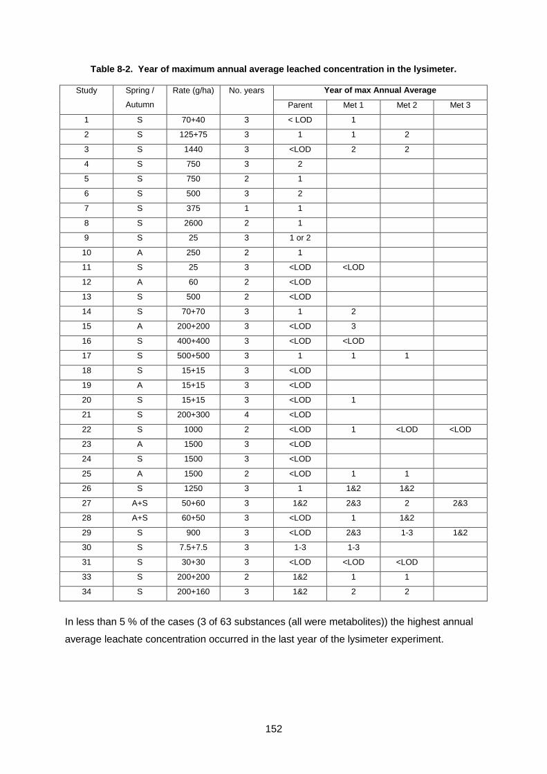
152
Table 8-2. Year of maximum annual average leached concentration in the lysimeter.
Study Spring /
Autumn
Rate (g/ha) No. years Year of max Annual Average
Parent Met 1 Met 2 Met 3
1 S 70+40 3 < LOD 1
2 S 125+75 3 1 1 2
3 S 1440 3 <LOD 2 2
4 S 750 3 2
5 S 750 2 1
6 S 500 3 2
7 S 375 1 1
8 S 2600 2 1
9 S 25 3 1 or 2
10 A 250 2 1
11 S 25 3 <LOD <LOD
12 A 60 2 <LOD
13 S 500 2 <LOD
14 S 70+70 3 1 2
15 A 200+200 3 <LOD 3
16 S 400+400 3 <LOD <LOD
17 S 500+500 3 1 1 1
18 S 15+15 3 <LOD
19 A 15+15 3 <LOD
20 S 15+15 3 <LOD 1
21 S 200+300 4 <LOD
22 S 1000 2 <LOD 1 <LOD <LOD
23 A 1500 3 <LOD
24 S 1500 3 <LOD
25 A 1500 2 <LOD 1 1
26 S 1250 3 1 1&2 1&2
27 A+S 50+60 3 1&2 2&3 2 2&3
28 A+S 60+50 3 <LOD 1 1&2
29 S 900 3 <LOD 2&3 1-3 1&2
30 S 7.5+7.5 3 1-3 1-3
31 S 30+30 3 <LOD <LOD <LOD
33 S 200+200 2 1&2 1 1
34 S 200+160 3 1&2 2 2
In less than 5 % of the cases (3 of 63 substances (all were metabolites)) the highest annual
average leachate concentration occurred in the last year of the lysimeter experiment.
153
The median annual leachate volume measured in the 34 lysimeter studies were shown to be
308 mm (Hardy et al., 2008). A considerable fraction (median: 36%) of the precipitation and
irrigation percolates through the lysimeter cores.
This provides some support for the duration of lysimeter studies according to the BBA
guideline. However, the strength of the evidence provided by this table is conditional upon
the behaviour being totally chromatographic in all cases (i.e. no subsequent annual increase
in compound leaching after an annual decline). Note that work by Dressel (2003) concluded
that loses of methabenzthiazuron and ethidimuron from lysimeters with an orthic luvisol were
by preferential flow mechanisms.
Broadly speaking the void volume of a 1 m depth soil core is approximately 250 mm
(approximately 1 year of recharge for BBA guideline conditions – although a particular
minimum recharge is not a requirement of this guideline). A more detailed examination of the
expected breakthrough of the target compound (parent or metabolite) at the bottom of the
lysimeter should be provided as part of the study design for both lysimeter and field leaching
experiments and studies should be continued at least until this time is reached. This is likely
to increase the timescale of the study in comparison to existing guidelines but, for pragmatic
reasons, five years may be the realistic limit of regulatory usefulness. In addition destructive
sampling of the core at the conclusion of the experiment as required by the BBA (BBA, 1990)
and OECD (OECD, 2000) guidelines should be undertaken to obtain more information on
compounds still in the core (this may also be particularly helpful if inverse modelling is used
as a post-processing approach). Application should occur in each year, unless there are
particularly strong reasons from the GAP that this is not appropriate (in which case a further
justification on why the results can be considered to demonstrate appropriate vulnerability,
would be required). In addition, the recharge in each year should be typical of the conditions
that are being investigated (i.e. for 800 mm rainfall under BBA lysimeter guidelines, the
recharge should be about 250 mm rather than, for example, 80 mm).
8.3.3.1.1.3 Replication
Replication is a significant issue, which was discussed as far back as 1992 (Fuhr and Hance,
1992). It is always of greater importance in field experiments where there are a larger
number of variables and uncertainties compared to laboratory studies. For undisturbed soil
monoliths 1 m2 is a relatively small surface area and hence even the variation of soil
hydraulic properties over a field are unlikely to be fully reflected in the sample size (soil
heterogeneity is also an aspect to be considered for laboratory studies but in these cases at
least maintenance of soil structure is not necessary).
154
Given the variability of leachate results between cores in lysimeters (see for example, Jene,
1998), a single replicate is clearly insufficient to obtain scientifically valid results. On the
other hand too large a number of cores would make the studies prohibitively expensive. The
use of triplicate soil cores for lysimeter studies would seem to be a reasonable compromise.
8.3.3.1.1.4 Scale and uncertainty
In absolute terms the uncertainty (this is defined as the uncertainty of the result covering the
90th percentile worst case, or equivalent regulatory endpoint, and will account for the
variability in the individual factors that contribute to the overall leaching) surrounding the
result of a lysimeter experiment is very difficult to quantify since multiple data sets covering
many different cores and soil types are not realistically available. The variability can be sub-
divided into a number of possible factors (e.g. possible variation in DegT50 in soil, Kd etc.),
but precisely how these interact to give the range of the experimental endpoint is never
certain. In addition to inter-field variation in the degradation rate and sorption of pesticides,
intra-field variation is also well-known (e.g. Beck et al., 1996; Walker et al., 2002; Rasmussen
et al., 2005). This has often been attributed to differing population of micro-organisms in
different parts of the field (e.g. Rasmussen et al., 2005; Walker et al., 2002) and variations of
DegT50 within a field have been stated as 6.5-30 days (Walker et al., 2002) and 31-483 days
(Beck et al., 1996).
Attempting to consider these aspects relative to the uncertainties and variability in the Tier 1
data is perhaps simpler, although this also brings some difficulties as the sources of the
uncertainty are not directly comparable. In a tiered assessment scheme, higher tiers should
provide equal or greater re-assurance on these aspects than the lower tiers. Standard
laboratory degradation and sorption studies generally use very small soil masses (typically
50-100 g) in duplicate samples. However, four contrasting soil types (from widely differing
fields) are investigated in regulatory submissions (whether each soil is systematically
sampled to fully account for intra-field variation is not certain). Lysimeter experiments
typically investigate only one soil type but use a much larger mass of topsoil. Therefore
based on the relative masses more of the intra-field variability would be expected to be
reflected in a field study than a laboratory study. However, when considering current
regulatory approaches, more inter-field variability in sorption and degradation parameters is
addressed by laboratory studies.

155
8.3.3.1.2 Field Leaching Studies
As mentioned previously, there are very few recognised guidelines for these studies. In
general, when designing a study some of the same factors need to be considered as for the
lysimeter study i.e. replication and duration while other factors that need consideration are
unique to this study type (e.g. method of water sampling, depth of sampling).
8.3.3.2 Determining adequate vulnerability – through location selection
There are two broadly acceptable approaches to determine adequate vulnerability of the
location of lysimeter and field leaching studies (to be undertaken prior to conducting the
study):
(1) Conduct a GIS analysis to obtain the intended regulatory vulnerability (90th percentile
based on rainfall and soil characteristics at the EU level, or that specified at the
particular national level).
(2) Conduct a limited analysis to compare the experimental location to the Tier 1
reference scenarios.
The first option can be considered using soil and climatic data as discussed in Section 7.2.5.
The second option can be considered through comparison of the climatic data and soil
characteristics of the Tier 1 scenario with the climatic data and soil characteristics of the
lysimeter/field leaching study. Note that irrigation can be used as a substitute for higher
rainfall.
In either situation, quantitative post-processing methods will still be necessary at the
conclusion of the study to ensure that the anticipated climatic conditions etc had actually
been met, as well as to incorporate the study design elements (such as duration).
8.3.4 Post processing approaches for higher tier experimental leaching data
8.3.4.1 Introduction
The guidance described below applies only to lysimeter studies. The work group is currently
unaware of any accepted methods at the EU level for putting field leaching studies into a
regulatory context. However the work group believes that such approaches can be
undertaken in the future based on reasonable scientific principles by analogy to the process
described below for lysimeter studies.
To address any issues about uncertainty in a limited experimental data set, all experimental
data should first be checked to assess the expected vulnerability of the data. The approach
156
described below should be used. Soil specific DegT50 and Koc values from the experimental
data should be used (or in the absence of these data, the most favourable (highest) Kom and
(lowest) DegT50 values from the experimental data set should be used) together with local
meteorological data. The measured annual percolated amounts of water must be simulated
reasonably well; otherwise the water flow should be calibrated (see work of Durner et al.,
2008). If the predicted output with these parameters is >0.1 μg/L, then the lysimeter/field
leaching result can be accepted for further assessment. If not the results of the lysimeter
study are ignored because the conditions in the lysimeter study did not reflect adequately
vulnerable conditions. If the proposed application rate is different from the application rate in
the lysimeter, the 0.1 μg/L criterion is adjusted by multiplying by the application rate of the
proposed use divided by the application rate in the lysimeter.
Example
A lysimeter study has been performed with application rates for parent P1 (2 x 0.2 to 2 x 0.25
kg as/ha in the lysimeter study) on winter cereals in climatic conditions of northern Germany.
Experimental results of the lysimeter study with measured concentrations of metabolite M1
are given in Table 8-3. The simulated concentrations of M1 in the lysimeter soil and climate
are stated in Table 8-4. The standard FOCUS ground water Tier 1 PECgw value for this
GAP in the Hamburg scenario was 0.4 µg/L. In this case the lysimeter shows leaching <0.1
µg/L in conditions where simulations would have predicted >0.1 µg/L. Thus the lysimeter
results could not have been predicted and can be accepted as valid for subsequent use in
further assessment.
157
Table 8-3. Application rates of parent P1 and concentrations of M1 (CLYSIMETER) in the lysimeter leachate.
lysimeter A lysimeter B lysimeter C
Application rates of P1
Application
1st year
2 x 0.25 kg as/ha 2 x 0.25 kg as/ha 2 x 0.25 kg as/ha
Application
2nd year
2 x 0.20 kg as/ha
M1 in leachate (CLYSIMETER) [µg/L
mean 1st year 0.03 0.04 0.04
mean 2nd year 0.02 0.04 0.09
Mean 3rd year - n.d. 0.01
Table 8-4. Predicted concentrations of M1 (CSIMULATION) when the experimental conditions are input into a model.
lysimeter A lysimeter B lysimeter C
M1 in leachate (CSIMULATION) [µg/L
Mean 1st year 0.06 0.06 0.08
Mean 2nd year 0.11 0.11 0.15
Mean 3rd year 0.01 0.01 0.04
In the next stage an inverse modelling (see Appendix 10 for the detailed theory of inverse
modelling) of the leaching data set is conducted to derive important pesticide parameters of
sorption and degradation (see Figure 8-9 for a general flow chart describing the inverse
modelling procedure, although it should be noted that the particular process recommended in
this report does not involve the use of a calibration step). These parameters are then used
together with the existing data set to calculate refined input values for use in standard
FOCUS scenarios. Inverse modelling has been introduced in pesticide fate modelling as a
way to remedy to the pitfalls of classical parameter identification techniques (Casey and
Simunek, 2001; Gottesbüren et al., 2001; Altman Dieses et al., 2002; Roulier and Jarives,
2003ab; Heistermann et al., 2003; Dubus et al., 2004; Larsbo and Jarvis, 2005). The
availability of new advanced modelling techniques for the soil-crop system, together with the
158
availability of fast forward simulation models and optimisation algorithms, allow now the use
of inverse modelling on a more regular basis. The choice of initial values, formulation of goal
functions, target data, may have an effect on the inferred parameters and care has to be
taken to describe the approaches and decisions as transparently as possible in order to
make it reproducible.
Figure 8-9. Flow charts describing the inverse modelling procedure (Dubus et al., 2000).
Inverse modelling cannot be based on a single soil core; as a minimum, measurements using
duplicate soil cores taken from the same field are needed. In the following sections, the term
‘lysimeter study’ refers to a study with at least two soil cores taken from the same field.
8.3.4.2 Proposed inverse modelling procedure for lysimeter studies
The first part of the inverse modelling is a calibration step to adequately describe the soil
hydrology of the leaching study, in terms of both temporal and total fluxes. In order to be
able to evaluate pesticide behaviour, the water balance in the soil must firstly be correctly
simulated. This should include a correct description of percolate volumes over the course of

159
time. If a conservative tracer was applied to the study, it must also be evaluated during the
calibration phase.
Another prerequisite is that an inverse modelling technique has been applied that allows
assessment of the uncertainty of the fitted parameters (see e.g. Mertens et al., 2009). This
could also include information on response surfaces or probability density functions of the
assessed parameters.
Inverse modelling studies with pesticide leaching from lysimeters have shown that there may
be strong dependencies between e.g. the fitted Freundlich exponent and the fitted Kom or Koc
(e.g. Mertens et al., 2009). Similar strong dependencies can be expected between the fitted
DegT50 on the one side and parameters describing effect of temperature, moisture and soil
depth on degradation on the other side. Since the fitting is based on measured pesticide
leaching at the bottom of a 1-m column, these parameters may have similar effects on the
simulated leaching concentrations. Usually the soil residues of parent and metabolites that
are measured in the soil cores of the lysimeter study at the end of the study after destructive
sampling with very sensitive analytical methods (usually 14C labelled compounds) could give
valuable additional information. Measurements of residue distribution in the soil plough layer
during the lysimeter study would also be helpful.
Mertens et al. (2009) could obtain narrow probability density functions for DegT50 and Kom
when they kept all other substance parameters constant. To ensure consistency in the risk
assessment, all substance parameters that are not fitted, should be set to the same pesticide
values used in the lower tier leaching calculation. These parameters include those
describing the moisture, temperature and depth dependencies of degradation, the Freundlich
exponent, long-term sorption parameters etc. The dispersion length should also be set to the
5 cm used in the lower tier leaching calculations (unless e.g. leaching of a tracer was
measured as well in the lysimeter study, allowing the dispersion in the individual soil core to
be estimated).
The above recommendation to use the same parameters as used in the lower tier
calculations does not apply to soil properties of the lysimeter system that were measured at
the end of the study (organic matter, texture and pH of the different horizons). For such
properties and e.g. hydraulic properties derived from them, the measurements from the
lysimeter should be used.
160
In the inverse modelling procedure, attention should be paid to the uncertainty resulting from
initial loss processes at the soil and plant surfaces. For example, consider the case where
pesticide is sprayed onto a crop and 50% of the dose is quickly photodegraded. If the
inverse modelling procedure assumed that 100% of the dose penetrated into the soil, this
would lead to a systematic underestimation of the DegT50 in soil which is undesirable. The
group proposes that a best estimate of photodegradation, volatilisation (based on the
scientific information provided as part of the regulatory dossier) and interception (based on
FOCUS, 2002 recommendations and consistent with the first tier approach) should be used
to estimate the soil loading.
A resulting DegT50 or Kom / Koc value is acceptable for further use in the risk assessment if
the lower limit of its 95% confidence interval is larger than 50% of the expected value from
the inverse modelling procedure and if the upper limit is less than 200% of the expected
value (so between a factor two lower and a factor two higher). When this criterion is not met,
then the 75th percentile (more vulnerable) value should be used.
If the concentration in the leachate of the lysimeter remained always below the LOD or LOQ
(usually in the order of 0.01 g/L ), then it is impossible to derive from the inverse modelling
distributions with expected values for the DegT50 or Kom parameters. Instead the inverse
modelling will result in a DegT50 - Kom line that divides the DegT50 - Kom plane into two
subplanes: one subplane gives the possible DegT50 - Kom combinations and the other the
impossible DegT50 - Kom combinations (see line A in Figure 8-10). In this case, the Kom
used in the lower tier assessment and the corresponding DegT50 from the DegT50 - Kom line
should be used in the further assessment. This preference for estimating the DegT50 from
the lysimeter study rather than the Kom is based on the complications with respect to an
inversely modelled Kom as described in Section 8.3.4.4.
161
Figure 8-10. Kom – DegT50 diagram illustrating the restrictions resulting from an inverse modelling study based on a lysimeter study (A) with all concentrations in the leachate below
the detection limit, and (B) with all concentrations in soil extracted at the end of the study below the detection limit. The shaded area shows the combined effect of the restrictions A and
B.
If at the end of the study, all total concentrations in the soil profile (extracted with organic
solvent) are below the detection limit (usually in the order of 1 g/kg), then the inverse
modelling procedure probably will result in an upper limit of the DegT50 (see line B in Figure
8-10). In such a case this DegT50 should be used in the further assessment.
Note that DegT50 or Kom / Koc values obtained by the above procedure are of a different
nature compared to lower tier DegT50 or Kom / Koc values: values obtained from a lysimeter
study are effective values for leaching at 1 m depth, based on the behaviour in the top 1 m of
soil.
8.3.4.3 Further use of inversely modelled lysimeter DegT50 values in the leaching
assessment
The only risk assessment cases considered in this section are where lower tier simulation
indicated a risk for ground water. Cases where lysimeters play only a confirmatory role, are
not considered. All DegT50 values from laboratory, field persistence or lysimeter studies are
assumed to reflect degradation rates within the soil (so no photochemical degradation at the
soil surface) and that they have been normalised to 20oC and field capacity. All DegT50
values are also assumed to be based on the same description of degradation (so if non-
equilibrium sorption is included all DegT50 values refer to the equilibrium part of the soil).
162
The procedure recommended below for the use of lysimeter DegT50 values in the leaching
assessment has no thorough scientific basis. However, the problem is that a choice has to
be made between alternatives. The work group considers these recommendations a
reasoned compromise between (a) ignoring single lysimeter studies because they represent
only one field, (b) giving a single lysimeter study infinite weight by letting its DegT50 overrule
all previous DegT50’s.
One case is where only DegT50 values from laboratory studies (e.g. four) are available
together with one DegT50 from a lysimeter study. In this case, averaging to obtain an overall
average DegT50 (lab and lysimeter) is inappropriate, because the procedure would be too
uncertain to conclude on the risk of leaching to ground water. Therefore, in this case the
results of the lysimeter study are ignored and the leaching assessment is based on lab
studies.
Another case is where besides DegT50 values from laboratory studies and one DegT50
value from a lysimeter study, also DegT50 values from a number of field dissipation studies
(e.g. four) are available. In this case field studies only are used when the procedures as
outlined in EFSA DegT50 guidance (EFSA, 2014a) indicate that the laboratory data come
from a different population so are discarded. The DegT50 from the lysimeter could be given
three times the weight of the other DegT50 values. An argument for this is that DegT50
values from field persistence studies reflect the degradation rate in the top 0 - 20 (or 30) cm
whereas a DegT50 value from a lysimeter study reflects the effective degradation rate in the
top 100 cm. Moreover, the FOCUS ground water scenarios consider three layers in the top
100 cm for describing the depth dependency of the transformation rate. However what
weighting should be applied should be justified and considered on a case by case basis
considering the available dataset. So using a weighting procedure that would need to be
justified on the basis of the available data, the geometric mean DegT50 should be calculated
and used in subsequent calculations.
The above recommendation has no thorough scientific basis, leaves room for scientific
judgement so is unlikely to result in harmonisation between different assessors. However, as
stated before the problem is that choices have to be made between alternatives. The EFSA
PPR panel work group considered the recommendation to apply expert judgement on a case
by case basis a compromise between (a) ignoring single lysimeter studies because they
represent only one field and (b) giving a single lysimeter study infinite weight by letting its
DegT50 overrule all other DegT50’s in a dataset.
163
8.3.4.4 Further use of inversely modelled lysimeter Kom / Koc values in the leaching
assessment
The use of Kom / Koc values obtained from lysimeters is not straightforward. For example, let
us consider a case where batch adsorption studies with four soils resulted in Kom values
ranging from 20 to 35 L/kg. Furthermore inverse modelling of a lysimeter study (assuming
only equilibrium sorption) generated a median Kom of 50 L/kg with a 95% confidence interval
of 40 to 60 L/kg. The interpretation of such a discrepancy could be that the long-term
sorption process in the lysimeter caused the higher “effective” Kom derived from the lysimeter.
In such a case to applying some averaging procedure to the Kom assuming equilibrium
sorption does not seem meaningful.
Given the above complication and given the very limited experience with Kom values obtained
by inverse modelling from lysimeters in an adequate way, only a first proposal for guidance
can be made here.
One approach could be to use Kom derived from lysimeter studies only if both in the lower tier
and in the lysimeter tier long-term sorption kinetics were included. In such a case the same
procedure could be justifiable as for the DegT50: of giving the value from the lysimeter study
a weight on a case by case basis using expert judgement regarding the available dataset,
that might where sorption data are available for 4 different soils in addition to the lysimeter,
be three times the weight of the lower tier measurement with the same reasoning: the Kom
from the lysimeter reflects the sorption behaviour of a 1-m thick soil layer whereas the lab
studies only reflect the sorption in the top soil layer.
Since Section 7.1.6.4 recommends lower limits of the non-equilibrium sorption coefficient,
including long-term sorption kinetics is advisable when estimating parameters from lysimeter
studies by inverse modelling.
Figure 8-11 provides a summary of the inverse modelling procedure process for lysimeter
studies. An example case illustrating this process is given in Appendix 11.
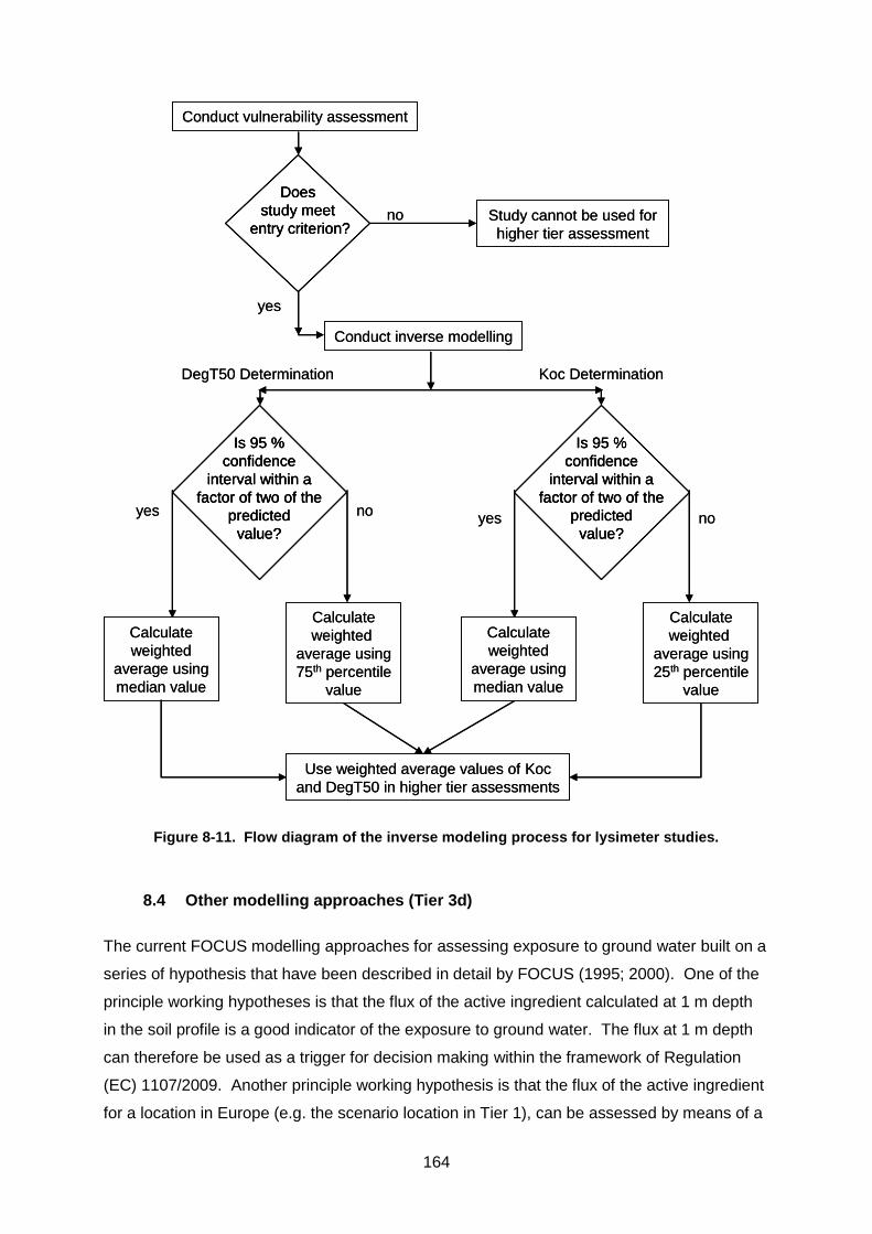
164
Conduct vulnerability assessment
Does
study meet
entry criterion?Study cannot be used for
higher tier assessment
Conduct inverse modelling
Koc DeterminationDegT50 Determination
Is 95 %
confidence
interval within a
factor of two of the
predicted
value?
Calculate
weighted
average using
median value
Use weighted average values of Koc
and DegT50 in higher tier assessments
Calculate
weighted
average using
75th percentile
value
yes
no
Is 95 %
confidence
interval within a
factor of two of the
predicted
value?
Calculate
weighted
average using
median value
Calculate
weighted
average using
25th percentile
value
yesyes
nono
Conduct vulnerability assessment
Does
study meet
entry criterion?
Does
study meet
entry criterion?Study cannot be used for
higher tier assessment
Conduct inverse modelling
Koc DeterminationDegT50 Determination
Is 95 %
confidence
interval within a
factor of two of the
predicted
value?
Is 95 %
confidence
interval within a
factor of two of the
predicted
value?
Calculate
weighted
average using
median value
Use weighted average values of Koc
and DegT50 in higher tier assessments
Calculate
weighted
average using
75th percentile
value
yes
no
Is 95 %
confidence
interval within a
factor of two of the
predicted
value?
Is 95 %
confidence
interval within a
factor of two of the
predicted
value?
Calculate
weighted
average using
median value
Calculate
weighted
average using
25th percentile
value
yesyes
nono
Figure 8-11. Flow diagram of the inverse modeling process for lysimeter studies.
8.4 Other modelling approaches (Tier 3d)
The current FOCUS modelling approaches for assessing exposure to ground water built on a
series of hypothesis that have been described in detail by FOCUS (1995; 2000). One of the
principle working hypotheses is that the flux of the active ingredient calculated at 1 m depth
in the soil profile is a good indicator of the exposure to ground water. The flux at 1 m depth
can therefore be used as a trigger for decision making within the framework of Regulation
(EC) 1107/2009. Another principle working hypothesis is that the flux of the active ingredient
for a location in Europe (e.g. the scenario location in Tier 1), can be assessed by means of a
165
1-D fate and transport model for the soil, whereby the transport of the active ingredient in the
soil is mainly considered as a chromatographic transport process. An exception to this
working hypothesis is made when the preferential flow module in MACRO is activated (e.g.
Châteaudun scenario calculations at Tier 1). The concept of homogeneous 1-D fate and
transport in the soil is maintained when moving to the higher tiers. In Tier 2a improved
parameterisation schemes of the 1-D FOCUS models are suggested. In Tier 2b and 3, the
simulations are repeated with the 1-D models to cover in a more realistic way the variability
of the soil-crop and climate properties at the larger scale.
Yet, the FOCUS models that are used in all aforementioned tiers suffer from a series of
drawbacks that are related to conceptual modelling problems and problems of parameter and
input estimation. The 1-D FOCUS models have been the subject of a set of experimental
validation studies (see Chapter 6 of FOCUS; 2000 for references on recent validation
studies) which should reduce the risk of conceptual bias. However, most of the validation
studies so far pertained to the local scale (i.e. the lysimeter scale or the small field scale) and
only few approaches have been reported to validate the predictions of the large scale
exposure (Sulmon et al., 2006). The conceptual and parameter estimation problem (at the
local and the larger scale) generate uncertainties in the final ground water exposure
assessments. Uncertainties issues were already addressed in FOCUS (2000). The
additional conceptual problem of applying local scale 1-D models to assess large scale
exposure will not reduce this uncertainty.
In spite of these weaknesses, the work group estimates that the modelling approaches
presented in previous chapters remain suitable for assessing movement of active substances
to ground water within the framework of Regulation (EC) 1107/2009. Note however that new
process knowledge on subsoil fate and transport is continuously generated, which may be
introduced to improve ground water exposure assessment in the future. The following
sections give an outlook of alternative approaches that could be considered in future ground
water exposure assessment procedures
8.4.1 Alternative models for transport of active substances in the top soil
Validation studies have elucidated the problems of the chromatographic flow concept to
model heterogeneous flow of active substances in the top soil (Vanclooster et al., 2000;
Trevisan et al., 2003). Scientific evidence exists that heterogeneous flow (e.g. preferential
flow) should be considered as the rule, rather than the exception (Jury and Fluhler, 1992;
Flury et al., 1995). Given the limitations of chromatographic flow concept to describe
heterogeneous flow, alternative transport models have been proposed for describing
166
chemical transport in soils (Vanclooster et al., 2005). These alternative models consider the
variability of the fate and transport process due to structural variation in the flow domain (e.g.
fast flow in large pores versus slow flow in small pores). The models can be ranked
depending on the degree of explicitness with which the structural variability is considered in
the model.
In a first class of models, the structural variability is embedded in a completely implicit way in
the transport model. In this class, two asymptotic transport models, which cover the end-
points of mixing in the soil, i.e. the complete mixing versus no mixing model, can be grouped
(Flühler et al., 1996). The complete mixing model implicitly assumes that the mixing scale is
much smaller than the scale of the transport process. Active substances applied at the soil
surface will move as a homogeneous front through the soil profile. On top of this
homogeneous movement, fast and slow displacements will occur which will smear out the
chemical front and which will be determined by the hydrodynamic dispersivity of the soil. The
current FOCUS models, except MACRO, belong to this class of models, and the
harmonisation of the hydrodynamic dispersion should result in consistent predictions of the
leaching percentiles with this class of models.
In contrast to these so-called full mixing models, models have been developed which assume
that the mixing scale is much larger than the transport scale. In this case, active substances
in the soil will move through a set of isolated stream tubes and no mixing of the active
substances between the stream tubes will occur (see early studies of Dagan and Bresler,
1983).
In the second class of models, the multi-domain models, the structure of the flow field is
embedded in the model by dividing the porous medium in two (e.g. van Genuchten and
Wagenet, 1989; Larsbo and Jarvis, 2003; Gerke and van Genuchten, 1993) or more
(Steenhuis et al., 1990; Skopp and Gardner, 1992; Durner and Fluhler, 1996; Durner et al.,
1999) sub-domains in which active ingredients move at different velocities. Between the sub-
domains chemicals are exchanged by diffusion and/or advection. The exchange rate is a
fitting parameter, which can be related to some extent to the structure and spatial scale of the
different flow domains. The MACRO model is an example of such a multi-domain model,
and could be applied to model heterogeneous flow if parameterisation issues are resolved.
In the third class of models, the structure of the porous medium is characterised in a geo-
statistical sense. By solving the stochastic-continuum flow and transport equations, the
lateral solute mixing and the mixing time are derived from the spatial distribution of
167
macroscopic hydraulic properties. In all previous classes, effective vertical 1-D transport is
considered to occur in the soil.
In the fourth class of models, the structure of the porous medium is explicitly considered and
2 or 3-D flow and transport processes, either at the pore or the macroscopic scale, are
solved in a medium with known structure. When the structure of the medium is identified, the
flow and transport processes may be predicted without any fitting of flow and transport
parameters (Vogel and Roth, 2003). Different numerical solvers for the 2 and 3-D
unsaturated flow and transport problem are readily available (see e.g. Simunek et al., 1995).
8.4.2 Modelling fate and transport of active substances in the partially saturated subsoil
The FOCUS modelling approach considers the exposure at 1 m soil depth as a conservative
estimate of the exposure to ground water. Yet, in many cases, vulnerable ground water
systems are situated deeper in the subsoil and active ingredients passes through a partially
saturated vadose zone before the ground water body is reached. In this case, additional
dispersion, sorption and degradation will determine the real exposure to the ground water
system.
As a first approximation, the existing FOCUS models are suggested to be used to consider
processes in the subsoil by extending the modelled soil profile. Roulier et al. (2006) for
instance studied atrazine transport through a fractured deep limestone covered by a luvisol
and calcisol in France by means of the MACRO model. They suggested that the thickness
and properties (e.g. matrix versus fissure flow) of the limestone will only have a small effect
on the long term atrazine leaching, since atrazine is a rather mobile substance and
degradation is low in the limestone.
As an alternative to the existing FOCUS models, the more advanced approaches presented
in the previous section could also be used to model the subsoil fate and transport. In most
cases however, little information, if any, on the transport, sorption and degradation properties
of the deeper subsoil is available. Therefore, 1D modelling approaches or even simplified
and empirical models are mostly adopted to model transfer of active substances from the
bottom of the soil to the top of the ground water body. Spurlock et al. (2006) coupled the
PRZM model for the top soil with a semi-empirical transfer model to predict ground water
loading in the San Joaquin valley, California. For the same ground water body, Stewart and
Loague, (1999) used simplified linear transfer function theory (Jury and Roth, 1990) to model
transport through soil and sub-soil.
168
8.4.3 Modelling fate and transport of active substances in the soil and ground water continuum
Adopting a holistic view, substance fate and transport can be modelled through the soil and
ground water continuum. The explicit introduction of the ground water body in the modelling
system changes its dimensionality, since flow and transport in ground water bodies is merely
horizontal rather than vertical. It also allows the consideration of specific ground water
processes on the final exposure to specific targets. Hoiberg et al., (2005) for instance
modelled transport and fate of three herbicides in an aerobic aquifer with variable pH. They
showed that a pH dependent degradation rate in the ground water body was needed to
explain the observed concentrations during a controlled pesticide tracer experiment.
Two approaches can be distinguished for modelling substance fate and transport in the soil-
ground water continuum: loosely coupled approaches and fully integrated approaches. In the
loosely coupled approach, the 1-D soil – subsoil model is used to define the upper boundary
condition of a ground water flow and transport model. Tiktak et al. (2005) for instance
coupled the FOCUS PEARL model to a regional ground water model to assess substance
transport in Dutch ground water bodies. Stenemo et al. (2005) coupled the FOCUS MACRO
model with a ground water model for fractured till. In this case, the linking procedure (macro
pore versus fracture) had a significant effect on the modelled substance behaviour in the
ground water body itself. They also showed that considerable differences are obtained
between steady- state and transient flow simulations. For assessing exposure of local point
pollution, Aivalioti and Karatzas (2006) illustrated the linking between a spatially distributed
version of the FOCUS PRZM model with a 3D ground water flow and contaminant transport
model.
In the fully integrated approach, the same flow and transport equations are solved as well for
the saturated (i.e. the ground water body) as for the partially saturated (the soil and subsoil)
system using numerical solvers. Mouvet et al. (2004) compared loosely and fully coupled
approaches to assess substance fate and transport in different aquifers in Europe. They
concluded that the fully coupled models were more appropriate than the loosely coupled 1-D
model to assess ground water exposure. Boivin et al. (2006) applied a fully coupled model to
assess the transport of bentazone in a tile drained field in France. They showed that outflow
(drainage and deep percolation) in this system could only be modelled by considering the 2D
flow and transport process in the field. They also showed that a reasonable matching of the
drain outflow could only be obtained when preferential flow was considered in the 2D model
and when local parameters were fitted. Even if the drain flow is merely of concern for surface
water emissions, the simulated deep percolation and hence the emission to ground water
169
was affected by this parameterisation strategy. At the regional scale, Herbst et al. (2005)
modelled isoproturon behaviour by means of the fully coupled TRACE/3DLEWASTE model.
The modelling results were consistent with the observations found in monitoring wells and
allowed in particular to elucidate the specific role of the vadose zone in calculating ground
water loadings.
8.4.4 Statistical modelling of monitoring data
The highest tier proposed in this report considers monitoring data as a trigger for decision
making. As mentioned in Chapter 9, monitoring data are unlikely to be available for new
active substances prior to a decision on suitability for positive listing. Therefore, monitoring
data will only will be available for consideration at the Annex I level for existing active
substances.
If monitoring data are available that comply with the required quality standards (see Chapter
9), than statistical modelling techniques can be used to predict pesticide in ground water
bodies at the large scale based on local scale monitoring data. Sahoo et al. (2005) used
substance data collected from 124 domestic wells to predict substance concentration in the
ground water body using artificial neural network models. They considered land use and
sampling well indicators as model predictors. By means of cross validation techniques, they
obtained modelling efficiencies which were larger than 85 %. They also illustrated that the
depth of the wells were an important predictor in the model. Geo-statistical techniques offer
another alternative for making space-time predictions of pesticide concentrations for large
ground water bodies. Yet, the available monitoring networks are in generally very coarse,
which may result in large nugget effects and small correlation lengths, and therefore large
uncertainties in the spatial predictions with geostatistical techniques like kriging (Leterme et
al., 2007a).
8.5 References
Aivalioti, M.V. and Karatzas, G.P. 2006. Modeling the flow and leachate transport in the
vadose and saturated zones of a municipal landfill. Environmental monitoring and
assessment, 11:81-87.
Allen, R.G., Pereira, L.S., D. Raes, and M. Smith. 1998. Crop evapotranspiration: Guidelines
for computing crop water requirements. FAO Irrigation and Drainage paper, vol. 56. FAO,
Rome, Italy.
170
Altman Dieses, A.E., Schloder, J.P., Bock, H.G., and Richter, O.S.O. 2002. Optimal
experimental design for parameter estimation in column outflow experiments. Water
Resources Research 38(10):46-56.
Bangert. J., Erzgraeber B., Hauck T., Horn A., Jene B. 2007. GEOPEARL_DE – SPATIAL
MODELLING OF PESTICIDE LEACHING BEHAVIOUR IN GERMANY. - In:
Environmental fate and ecological effects of pesticides (Eds. A.A.M. Del Re, E. Capri, G.
Fragoulis & M. Trevisan), Univ. Cattolica del Sacro Cuore, Piacenza, Italy, 489-496.
BBA (1990) Guidelines for the testing of Agrochemicals. Part IV 4 -3. Lysimeter tests to
establish the mobility of Agrochemicals in the subsoil (Including amendment regarding
repeated application)
Beck, A., Harris, G., Howse, K., Johnston, A. and Jones, K. 1996. Spatial and temporal
variation of isoproturon residues and associated sorption/desorption parameters at the
field scale. Chemosphere 33:1283-1295
Bergström, L.F. and N.J. Jarvis. 1993. Leaching of dichlorprop, bentazon, and 36Cl in
undisturbed field lysimeters of different agricultural soils. Weed Science 41:251-261.
Bergström, L., N. Jarvis, and J. Stenström. 1994. Pesticide leaching data to validate
simulation models for registration purposes. J. Environ. Sci. Health A29:1073-1104.
Boesten, JJTI. 2007. Simulation of pesticide leaching in the field and in zero-tension
lysimeters. Vadose Zone Journal 6:793-804.
Boivin, A., Simunek, J., Schiavon, M., and van Genuchten, M.Th. 2006. Comparison of
pesticide transport processes in three tile drained field soils using HYDRUS-2D. Vadose
Zone Journal 5:838-849.
Brown, C.D., J.M. Hollis, R.J. Bettinson, and A. Walker. 2000. Leaching of pesticides and a
bromide tracer through lysimeters from five contrasting soils. Pesticide Management
Science 56:83-93.
Brye, K.R.,Norman JM, Bundy LG, Gower ST. 1999. An equilibrium tension lysimeter for
measuring drainage through soil. Soil Science Society of America Journal 63:536-543.
Carsel, R.F., J.C. Immhoff, P.R. Hummel, J.M. Cheplick, A.S. Donigian. 1998. A model for
Predicting Pesticide and Nitrogen Fate in the Crop Root and Unsaturated Soil Zones.
Users Manual for Release 3.0.
Carter, A. D. and Fogg, P. 1995. A critical evaluation of field monitoring techniques used to
describe the leaching and run-off behaviour of pesticides. IN “Pesticide movement to
Water, BCPC Monograph No 62. Eds. Walker, A., Allen, A., Bailey, S., Blair, A., Brown,
C., Gunther, P., Leake, C., and Nicholls, P. BCPC, Farnham, Surrey.
Casey, F.X.M. and Simunek, J. 2001. Inverse analysis of transport of chlorinated
hydrocarbons subject to sequential transformation reactions. Journal of Environmental
Quality 30(4):1354-1360.
171
Charnay, M.-P., S. Tuis, Y. Coquet, and E. Barriuso. 2005. Spatial variability in 14C-herbicide
degradation in surface and subsurface soils. Pest. Management Science 61:845-855.
Cornelese, A.A.., Boesten, J.J.T.I., Leistra, M., van der Linden, A.M.A., Linders, J.B.H.J., Pol,
W.J.J and Verschoor, A.J. 2003. Monitoring Data in Pesticide Registration. RIVM report
601450015/2003.
CTB. 1999. General protocol for the execution of lysimeter studies. From “The Registration
form and guidelines for the submission of applications for the registration of pesticides”.
Appendix G.1.3.a.
Dagan, G. and Bresler, E., 1983. Unsaturated flow in spatially variable fields 1. Derivation of
models of infiltration and redistribution. Water Resources Research 19:413-420.
Dressel, J. 2003. The transport of ethidimuron, methabenzthiazuron and watertracers in a
Luvisol. PhD dissertation, Agrosphäre Forschungszentrum Jülich GmbH.
Dubus, I.G., G. Azimonti, M. Bach, E. Barriuso, G. Bidoglio, F. Bouraoui, W. Fialkiewicz, H.J.
Fowler, O. François, A. Højberg, J.M. Hollis, N.J. Jarvis, I. Kajewski, J. Kjær, K. Lewis, F.
Lobnik, P. Lolos, B.T. Nolan, B. Réal, S. Reichenberger, F. Stenemo, M. Suhadolc, N.
Surdyk, and E. Vavoulidou-Theodorou. 2007. Developing Tools for Pesticide Risk
Assessment and Management at Three Different Scales in Europe: The FOOTPRINT
Project. In: A.A.M. Del Re, E. Capri, G. Fragoulis, and M. Trevisan, eds. Environmental
Fate and Ecological Effects of Pesticides. ISBN 978-88-7830-473-4. La Goliardica
Pavese, Pavia, Italy. pp. 966-973.
Dubus, I.; Beulke, S.; Brown, C. D.; Gottesbüren, B., and Dieses, A. 2004. Inverse modeling
for estimating sorption and degradation parameters of pesticides. Pesticide Management
Science 60:859-874. Notes: In press
Dubus, I.G., S. Beulke & C.D. Brown. 2000. A briefing document on the application of
inverse modelling techniques to pesticide leaching models used for pesticide
registration.- MAFF project PL0528, SSLRC project JF3735E, pp 47
Durner, W. and Fluhler, H. 1996. Multi-domain model for pore-size dependent transport of
solutes in soils. Geoderma 70:281-297.
Durner W., Schultze, B., and Zurmuhl, T. 1999. State-of-the-art in inverse modeling of
inflow/outflow experiments. Leij, F. J. and van Genuchten, M. Th. Proceedings of the
international workshop on characterization and measurement of the hydraulic properties
of unsaturated porous media. University of California.
Durner, W., U. Jansen, and S.C. Iden. 2008. Effective Hydraulic Properties of Layered Soils
at the Lysimeter Scale Determined by Inverse Modelling, European Journal of Soil
Science 59:114-124. doi: 10.1111/j.1365-2389.2007.00972.x
172
EUFRAM. 2005. Introducing probabilistic methods into the ecological risk assessment of
pesticides. EUFRAM report vol. 1, version 6, 11 May 2005. Available at
http://www.eufram.com.
Ferrari F., Fait G., Balderacchi M., Ferrari T., Capri E., Trevisan M. 2007. Field leaching
study for maize herbicides and their metabolites. In Environmental fate and ecological
effects of pesticide (Del Re A.A.M., Capri E., Fragoulis G. & Trevisan M. eds.), ISBN 978-
88-7830-473-4, La Goliardica Pavese, Peschiera Borromeo (MI), Italy, pp. 754-762.
Flühler, H., Dürner, W., and Flury, M. 1996. Lateral solute mixing processes - A key for
understanding field-scale transport of water and solutes. Geoderma 70:165-183.
Flury, M., Leuenberger, J., Studer, B., and Flühler, H. 1995. Transport of anions and
herbicides in a loamy and a sandy field soil. Water Resources Research 31:823-835.
FOCUS. 1995. Leaching models and EU Registration. Report of the FOCUS Regulatory
Modelling Workgroup. DOC. 4952/VI/95. 124 pp.
FOCUS. 2000. FOCUS groundwater scenarios in the EU-review of active substances.
Report of the FOCUS groundwater scenarios workgroup, EC Document, Sanco/321/2000
rev. 2. 202pp. Available at http://arno.ei.jrc.it/focus.htm (verified 14 Feb. 2006).
Fuhr, F. 1998. The Lysimeter Concept : Environmental Behavior of Pesticides. American
Chemical Society Division of Agrochemicals, Calif.) American Chemical Society Meeting
1997 San Francisco, F. Fuhr (Editor), R.J. Hance (Editor), J.O. Nelson (Editor), Plimmer
Jr. (Editor).
Fuhr, F. and Hance, R. 1992. Lysimeter studies of the fate of pesticides in the soil. BCPC
Monograph No.: 53. BCPC, Farnham, Surrey.
Gerke, H.H. and van Genuchten, M.Th. 1993. A dual porosity model for simulating the
preferential movement of water and solutes in structured porous media. Water
Resources Research 29:305-319.
Gottesbüren, B., Platz, K., van de Veen, J., Dubus, I., and Beulke, S. 2001. Estimation of
pesticide parameters from static and dynamic experiments by two independent modeling
groups. BCPC Symposium proceedings 78:89-94.
Hance, R and Fuhr, F. 1992. The present situation. In Lysimeter studies of the fate of
pesticides in the soil. P181-189 BCPC Monograph No.: 53. BCPC, Farnham, Surrey.
Hardy, I., B. Gottesbüren, A. Huber, B. Jene, G. Reinken, and H. Resseler. 2008.
Comparison of lysimeter results and leaching model calculations for regulatory risk
assessment. Journal für Verbraucherschutz und Lebensmittelsicherheit (Journal of
Consumer Protection and Food Safety) 4(3): 364-375.
Herbst, M., Hardelauf, H., Harms, R., Vanderborght, J., and Vereecken, H. 2005. Pesticide
fate at the regional scale: development of an integrated model approach and application.
Physics and chemistry of the earth 30:542-549.
173
Heistermann, M., Jene, B., Fent , G., Feyerabend, M., Seppelt, R., Richter, O., and Kubiak,
R. 2003. Modelling approaches to compare sorption and degradation of metsulfuron-
methyl in laboratory micro-lysimeter and batch experiments. Pesticide Management
Science 59:1276-1290.
Heuvelink, GBM and Pebesma EJ. 1999. Spatial aggregation and soil process modelling.
Geoderma 89:47-65.
Hoiberg, A.L., Engesgaard, P., and Bjerg, P.L. 2005. Pesticide transport in an aerobic
aquifer with variable pH - Modeling of a field scale injection experiment. Journal of
Contaminant Hydrology 78:231-255.
Hopmans, J.W., Simůnek, J., Romano, N., and Durner, W. 2002. Inverse methods. In:
Dane, J.A. and Topp, G.C. (eds), Soil Sci. of Am. Book Series 5, Madison, Wisconsin,
USA.
Jamagne, M., C. Le Bas, M. Berland, and W. Eckelman. 1995. Extension of the EU
Database for the Soils of Central and Eastern Europe. p. 101-114. In D. King, R.J.A.
Jones, and A.J. Thomassen (eds.) EUR 16232 EN. Office for Official Publications of the
European Communities, Luxembourg,
Jarvis, N.J., L. Bergström and P.E. Dik. 1991. Modelling water and solute movement in
macroporous soil. II. Chloride leaching under non-steady flow. Journal of Soil Science
42:71-81.
Jarvis, N.J., and I.G. Dubus. 2006. State-of-the-art review on preferential flow. Report DL#6
of the FP6 EU-funded FOOTPRINT project (www.eu-footprint.org), 60p.
Jene B. 1998. Transport of Bromide and Benazolin in lysimeters and a field plot with suction
grid bases in a sandy soil. SLFA department of Ecology, Neustadt.
Jury, W.A. and Fluhler, H. 1992. Transport of Chemicals Through Soil - Mechanisms,
Models, and Field Applications. Advances in Agronomy 47:141-201.
Jury, W.A. and Roth, K. 1990. Transfer functions and solute movement through soil: Theory
and applications. Birkhäuser, Basel, Switzerland.
Kasteel, R., T. Pütz, H. Vereecken. 2007. An experimental and numerical study on flow and
transport in a field soil using zero-tension lysimeters and suction plates. European
Journal of Soil Science 58(3): 632-645.
Kosugi K, Katsuyama M. 2004. Controlled-suction period lysimeter for measuring vertical
water flux and convective chemical fluxes. Soil Science Society of America Journal
68:371-382.
Klein, M. 1995. PELMO: Pesticide Leaching Model, User manual version 2.01. Fraunhofer-
Institut für Umweltchemie und Ökotoxikogie, D57392.
174
Kruijne, R., A. Tiktak, D. van Kraalingen, J.J.T.I. Boesten, and A.M.A. van der Linden. 2004.
Pesticide leaching to the groundwater in drinking water abstraction areas. Analysis with
the GeoPEARL model. Alterra-report 1041, Wageningen, the Netherlands.
Lambot S., Hupet, F., Javaux, M., and Vanclooster, M. 2004. Inverse modelling techniques
to characterize soil transport processes. In: Alvarez-Benedi, I. and Munoz-Carpena, R.
(eds), CRC press.
Larsbo, M. 2005. An improved dual-permeability model of solute transport in structured
soils: model development and parameter identification in laboratory and field
experiments. 2005. Uppsala . ISSN 1652-6880, ISBN 91-576-6950-3.
Larsbo, M. and Jarvis, N. 2003. MACRO5.0: a model of water flow and solute transport in
macroporous soil. Technical description. Uppsala, Sweden, SLU, Department of soil
sciences.
Larsbo, M. and Jarvis, N. 2005. Simulating solute transport in a structured field soil:
Uncertainty in parameter identification and predictions. Journal of Environmental Quality.
34:621-634.
Leterme B., M. Vanclooster, A.M.A. van der Linden, A. Tiktak and M. Rounsevell. 2007a.
The consequences of interpolating or calculating first on the simulation of pesticide
leaching at the regional scale. Geoderma 137:414-425.
Leterme B; Vanclooster M; Linden AMA van der; Tiktak A; Rounsevell MDA. 2007. Including
spatial variability in Monte Carlo simulations of pesticide leaching. Environ Sci. Technol.
41:7444-7450. DOI:10.1021/es0714639
Madsen-Breuning, H., and R.J.A. Jones. 1995. The establishment of a soil profile analytical
database for the European Union. p. 55-63. In D. King, R.J.A. Jones, and A.J.
Thomassen (eds.). EUR 16232 EN. Office for Official Publications of the European
Communities, Luxembourg.
MATS Guideline Test 01. undated. Leaching of Agrochemicals, a method to test mobility of
chemicals in soil. L Bergstrom.
Mertens J, Barkle GF, Stenger R. 2005. Numerical analysis to investigate the effects of the
design and installation of equilibrium tension plate lysimeters on leachate volume.
Vadose Zone Journal 4:488-499.
Mertens, J.; Kahl, G.; Gottesbüren, B.; Vanderborght, J. 2009. Inverse modeling of pesticide
leaching in lysimeters: local versus global and sequential single-objective versus multi-
objective approaches.- Vadose zone journal (accepted).
Michalski, B., H. Resseler, K. Aden, F. Dechet, M. Dust, R. Fischer, B. Gottesbüren, G.
Holdt, A. Huber, B. Jene, W. Koch, G. Reinken, and R. Stein. 2004. Recommendations
for Simulation Calculations of Predicted Environmental Concentrations in Ground Water
175
(PECgw) in the National Authorisation Procedure. Nachrichtenbl. Deut. Pflanzenschutzd.
56(9):193-201.
Mouvet, C., Albrechtsen, H.J., Baran, N., Chen, T., Clausen, L., Darsy, C., Desbionne, S.,
Douguet, N., Dubus, I., Esposito, A., Fialkiewicz, W., Gutierrez, A., Haverkamp, R.,
Herbst, M., Howles, D., Jarvis, N., Jørgensen, P.R., Larsbo, M., Meiwirth, K., Mermoud,
A., Morvan, X., Normand, B., O’Connor, M., Ritsema, C., Roessle, C., Roulier, S.,
Soutter, M., Stenemo, F., Thiéry, D., Trevisan, M., Vachaud, G., Vereecken, H., and
Vischetti, C. 2004. Pesticides in European Groundwaters: detailed study of
representative Aquifers and Simulation of possible Evolution scenarios. PEGASE. RP-
52897-FR, BRGM, France, Orleans.
Mücher, C.A., K. Steinnocher, J.L. Champeaux, S. Griguolo, K. Wester and P. Loudjani.
1998. Land cover characterisation for environmental monitoring of pan-Europe. In: Proc.
18th EARSEL Symp. on Operational Remote Sensing for Sustainable development, ITC,
Enschede, 11-13th May 1998, pp 107-113.
NACA. 1994. Use of Lysimeter to evaluate the leaching of pesticides in Soil. National
Agricultural Chemicals Association, Washington, USA
OECD. 2000. OECD series on Testing and Assessment Number 22. Guidance Document
for the performance of Outdoor Lysimeter studies.
Rasmussen, J, Aamand, J., Rosenberg. P., Jacobsen, O. and Sorenson, S. 2005. Spatial
variability in the mineralization of the phenylurea herbicide linuron within a Danish
agricultural field: multivariate correlation to simple soil parameters. Pest Management
Science 61:829-837.
Rawls, W.J., D.L. Brakensiek, and S.D. Logsdon, 1996. Estimation of macropore properties
for non-till soils. Trans. ASAE 39:91-95.
Roulier, S. and Jarvis, N. 2003a. Analysis of inverse procedures for estimating parameters
controlling macropore flow and solute transport in the dual-permeability model MACRO.
Vadose Zone Journal 2:349-357.
Roulier, S. and Jarvis, N. 2003b. Modeling macropore flow effects on pesticide leaching:
Inverse parameter estimation using microlysimeters. Journal of Environmental Quality
32(6):2341-2353.
Roulier, S., Baran, N., Mouvet, C., Stenemo, F., Morvan, X., Albrechtsen, H.J., and Clausen,
L.J.N. 2006. Controls on atrazine leaching through a soil unsaturated fractured
limestone sequence et Brevilles, France. Journal of Contaminant Hydrology 84:81-105.
Sahoo, G.B., Ray, C., and Wade, H.F. 2005. Pesticide prediction in ground water in North
Carolina domestic wells using artificial neural networks. Ecological modelling 183:29-46.
176
Siebert, S. and P. Döll. 2001. A Digital Global Map of Irrigated Areas – An update for Latin
America and Europe. Report A0102, Centre for Environmental Systems Research,
University of Kassel, Germany.
Simunek, J., Huang, K., and Van Genuchten, M.Th. 1995. The SWMS_3D code for
simulating water flow and solute transport in three-dimensional variably-saturated media.
Version 1.0. Research Report n°139. U. S. Salinity Laboratory. Agricultural Research
Service. U.S. Department of Agriculture, Riverside, California.
Skopp, J. and Gardner, W.R. 1992. Miscible displacement: an interacting flow region model.
Soil Science Society of America Journal 56:1680-1686.
Spurlock, F., Clayton, M., and Das, S. 2006. Modeling herbicide movement to groundwater
in irrigated sandy soil of the San Joaquin Valley, California. Water Air and Soil Pollution.
Steenhuis, T.S., Parlange, J.-Y., and Andreini, M.S. 1990. A numerical model for
preferential solute movement in structured soils. Geoderma 46:193-208.
Stenemo, F., Jorgensen, P.R., and Jarvis, N. 2005. Linking a one-dimensional pesticide
fate model to a three-dimensional groundwater model to simulate pollution risks of
shallow and deep groundwater underlying fractured till. Journal of Contaminant
Hydrology 79:89-106.
Stewart, I.T. and Loague, K. 1999. Identification of 'type' transfer functions fore regional-
scale assessment of non-point source groundwater contamination in Fresno County,
California. Journal of Environmental Quality 28:378-387.
Sulmon, R.P., Leterme, B., Pinte, D., Vanclooster, M., and Bogaert, P. 2006. Can
groundwater vulnerability models be validated? In: Laftouhi, N.(ed.). Gestion intégrée
des ressources en eau et défi au développement durable (GIRE3D). Marrakech,
Morocco.
Tiktak, A., F. van den Berg, J.J.T.I. Boesten, M. Leistra, A.M.A. van der Linden, and D. van
Kraalingen. 2000. Pesticide emission assessment for regional and local scales: User
manual of FOCUS PEARL 1.1.1. RIVM report 711401008, RIVM, Bilthoven, the
Netherlands. Available at http://www.pearl.pesticidemodels.nl (verified 14 Feb. 2006).
Tiktak, A., D.S. de Nie, A.M.A. van der Linden, and R. Kruijne. 2002. Modelling the leaching
and drainage of pesticides in the Netherlands: the GeoPEARL model. Agronomie 22:373-
387.
Tiktak, A., A.M.A. van der Linden, and J.J.T.I. Boesten. 2003. The GeoPEARL model. Model
description, applications and manual. RIVM report 716601007/2003. RIVM, Bilthoven, the
Netherlands.
Tiktak, A., De Nie, D.S., Pineros-Garcet, J.D., Jones, A., and Vanclooster, M. 2004a.
Assessing the pesticide leaching risk at the pan European level: the EuroPEARL
approach. Journal of Hydrology 289:22-238.
177
Tiktak, A., A.M.A. van der Linden, J.J.T.I. Boesten, R. Kruijne, and D. van Kraalingen. 2004b.
The GeoPEARL model. Part II. User guide and model description update. RIVM report
716601008/2004. RIVM, Bilthoven, the Netherlands.
Tiktak, A., Van der Linden, A.M.A., and Uffink, G. 2005. Pesticide Transport in the
Groundwater at the National Scale: Coupling an Unsaturated Zone Model with a
Groundwater Flow Model. In: Thomson, N. R. (ed.) Bringing groundwater quality
research to the watershed scale. IAHS publication 297, IAHS Press, Wallingford, UK..
p. 441-448.
Trevisan, M. , Padovani, L., Jarvis, N., Roulier, S., Bouraoui, F., Klein, M., and Boesten,
J.J.T.I. 2003. Validation status of the present PEC groundwater models. In: A.A. Del
Re, M. Trevisan, and E. Capri (ed.), XII Pesticide chemistry symposium. Pesticide in air,
plant soil and water system. Piacenza, Italy.
USEPA. 2008. OPPTS 835.7100 Guidance for prospective groundwater monitoring studies.
Office of the Prevention, Pesticides and Toxic Substance (7101) US. Environmental
Protection Agency. EPA 712-B-10-001, August 25, 2008.
http://www.regulations.gov/#!documentDetail;D=EPA-HQ-OPPT-2009-0152-0044
van Genuchten, M.Th. and Wagenet, R.J. 1989. Two-site/two-region models for pesticide
transport and degradation: theoretical development and analytical solution. Soil Science
Society of America Journal 53:1303-1310.
Vanclooster, M., Boesten, J., Trevisan, M., Brown, C., Capri, E., Eklo, O.M., Gottesbüren, B.,
Gouy, V., and van der Linden, A.M.A. 2000. A European test of pesticide-leaching
models: methodology and major recommendations. Agricultural Water Management
44:1-21.
Vanclooster, M., J.D. Pineros-Garcet, J.J.T.I. Boesten , F. Van den Berg, M. Leistra, J.
Smelt, N. Jarvis, S. Roulier, P. Burauel, H. Vereecken, A. Wolters, V. Linnemann, E.
Fernandez, M. Trevisan, E. Capri, L. Padovani, M. Klein, A. Tiktak, A. Van der Linden, D.
De Nie, G. Bidoglio, F. Baouroui, A. Jones, A. Armstrong. 2003. Effective Approaches
for Assessing the Predicted Environmental Concentrations of Pesticides. Final report.
European Commission, Quality of Life and Management of Living Resources
Programme. QLK4-CT-1999-01238. Printed by the Université Catholique de Louvain,
Belgium (Available at http://www.geru.ucl.ac.be/recherche/projets/apecop-pub/).
Vanclooster, M., Javaux, M., and Vanderborght, J. 2005. Solute transport in soils.
Encyclopaedia of Hydrological Sciences. John Wiley & Sons, pp. 1041-1055.
Verschoor, A.J., J.J.T.I. Boesten, M. Leistra, A.M.A. van der Linden, J.B.H.J. Linders, , and
J.W.W. Pol. 2001. Evaluation of pesticide leaching in lysimeter and field studies.
Bilthoven, the Netherlands, RIVM. Parent substances. RIVM report 601506007/2001.
178
Vogel, H.J. and Roth, K. 2003. Moving Through Scales of Flow and Transport in Soil.
Journal of Hydrology 272:95-106.
Vossen, P., and J. Meyer-Roux. 1995. Crop monitoring and yield forecasting activities of the
MARS project. p. 11-30. In D. King, R.J.A. Jones, and A.J. Thomassen (Eds.). European
land information systems for agro-environmental monitoring, EUR EN 16232, Office for
the official publications of the European Communities, Luxembourg.
Walker, A., and Brown, P. 1983. Spatial variability in herbicide degradation rates and
residues in soil. Crop Protection 2(1):17-25.
Walker, A. and Allen, R. 1984. Influence of soil and environmental factors on pesticide
persistence. BCPC monograph No. 27. Symposium on Soils and Crop Protection
Chemicals.
Walker, A. Jurado-Exposito, M. and Smith, V. 2002. Spatial variability in the degradation
rate of isoproturon in soil. Environmental Pollution 111:07-415.
Weihermüller, L., R. Kasteel, and H. Vereecken. 2006. Soil heterogeneity effects on solute
breakthrough sampled with suction cups: numerical simulations. Vadose Zone Journal.
5:886-893.
Weihermüller, L., R. Kasteel, J. Vanderborght, T. Pütz, and H. Vereecken. 2005. Soil water
extraction with a suction cup: Results of numerical simulations. Vadose Zone Journal.
4:899-907
Wolf, J., A.H.W. Beusen, P. Groenendijk, T. Kroon, R. Rötter, and H. van Zeijts. 2003. The
integrated modelling system STONE for calculating nutrient emissions from agriculture in
the Netherlands. Environ. Modelling & Software 19:397-617.
Wösten, J.H.M., G.J. Veerman, and J. Stolte. 1994. Water retention characteristics of
topsoils and subsoils in the Netherlands. The Winand Staring Soil Series. Renewed
Release 1994. SC-DLO Tech. Doc. 18. Alterra, Wageningen, the Netherlands. 1994.
Yon, D.A. 1992. The use of lysimeters to study the fate of an experimental pesticide
following autumn and spring application to winter cereals. In: F. Führ and R.J. Hance,
eds. Lysimeter studies of the fate of pesticides in the soil. BCPC Monograph 53.
Britichs Crop Protection Council, Farnham, UK, p. 145-151.

179
9 APPROACHES FOR THE USE OF GROUND WATER
MONITORING DATA AT TIER 4
The phrase “monitoring study” is frequently used and can cover a variety of methodologies.
At the outset it is appropriate to clarify what the principle approaches are and Lee (1996) has
determined three types of study that are used in the USA:
(a) Large scale retrospective studies: The objective of these studies is to characterise the extent of occurrence of pesticides in wells over a large area. These surveys typically involve sampling of more than 100 wells.
(b) Small-scale retrospective studies: These studies are carried out in a field in which a pesticide(s) has been used over a period of time and are used to determine whether the pesticide(s) in question has leached to groundwater in certain fields and to characterise the leaching pattern in the soil profile at a given point in time. The minimum number of well sites is about four for each study site.
(c) Small-scale prospective studies: These studies are usually associated with the pesticide use registration process and their primary objective is to characterise the subsurface fate of a particular pesticide i.e. controlled study.
Within the scope of the current document however, the small scale prospective studies are
considered as a variation of a field leaching study. This is because they are controlled
experiments in which the pesticide application can be directly linked with residues moving to
the ground water. They also concentrate on obtaining detailed experimental process data on
a relatively small number of sites (typically 2-3) rather than at a larger scale. For those
interested in the conduct of these studies, guidance has been provided by the US EPA
(2008). Further, the distinction between large scale and small scale retrospective studies is
not helpful in an EU context.
Therefore, within the context of this document monitoring studies are defined as:
Studies in which ground water is sampled from a large number of locations in a region
or country and is subsequently analysed to determine the concentration of the
pesticide or metabolite of interest. Experimentally determining the reason for the
presence or absence of the compound is not necessarily an intrinsic part of these
studies, although the weight which is placed on the findings will depend on the
appropriate selection of the sites to sample
Concerns about the potential of an active substance to reach ground water at concentrations
in excess of 0.1 µg/L may be raised during the lower tiers of risk assessment in a regulatory

180
evaluation of a new or existing substance (either at the EU approval decision making stage
or the national product authorisation under Regulation (EC) 1107/2009). However,
monitoring of ground water in the EU is routinely undertaken by water companies and
government bodies (often to comply with other EU legislation) and this may also lead to a
concern that particular existing pesticides and/or metabolites have been detected in ground
water in excess of 0.1 µg/L.
The intention of this chapter is to provide some guidance on how best to use existing
monitoring data and how to most effectively generate new monitoring data in cases where
the leaching risk is considered not to have been sufficiently clarified by the simpler (lower
tier) stages of the assessment.
9.1 Sources of ground water monitoring data
Broadly speaking ground water monitoring data can be differentiated into three sources:
1. Dedicated monitoring studies conducted by the notifier in response to a specific regulatory request (generally following detailed discussions with the relevant regulatory authority)
2. Proactive targeted monitoring studies conducted by the notifier 3. Monitoring data conducted by third party organisations for purposes other than
authorisation under Regulation (EC) 1107/2009 (e.g. by environmental agencies concerned with water quality). This information may be collated and submitted by a notifier together with a justification of the results obtained. However, ground water monitoring data can also be directly submitted by a third party or the regulators may become aware of data via other sources than the notifier (e.g. from publications, presentations etc).
In each case, the focus of the work is subtly different and hence the applicability for
regulatory decision-making may not be equal in all cases. For instance source 1 relies
heavily on the prior discussion with the relevant regulatory authority, with an expectation that
the remit of the work and methodology have been specifically agreed and the decision-
making criteria are clearly understood prior to the initiation of the data collection. Source 2
would result in the notifier conducting their own studies, presumably using a dedicated
analytical method for the compound of interest. The notifier would control which sites are
sampled and would have the opportunity to construct a coherent strategy of timing and
location within the context of Regulation (EC) 1107/2209 that they can scientifically justify to
the regulator. For many existing pesticides, source 3 will be the largest available source of
information on actual concentrations in ground water and hence has the potential to
contribute significantly to the scientific decision-making process. However, as the data are
181
not generated specifically for the requirements of Regulation (EC) 1107/2009, they are likely
to be rather less focused to that legislation. Data may be multi-residue analyses with less
attention given to false negatives or false positives, they may be from less relevant areas
(e.g. where the pesticide is not used in agriculture) or they may be targeted to known spills or
point-source contamination. Therefore, the quality and relevance of these data must be
assessed before regulatory decision-making. Some potential issues are highlighted by
Leterme et al. (2006) and Schmidt et al (2005). The emphasis of the regulation is rightly on
the notifier to demonstrate that safe use of the pesticide can occur. Therefore, logically the
notifier should be initially tasked with this assessment of relevance, once the data has been
made available to them.
9.2 Existing national guidance
Certain member states such as the UK (Mackay et al., 2004), the Netherlands (Cornelese et
al., 2003), and Germany (Aden et al., 2002) have already published guidance on the use of
monitoring data in pesticide registration. At this time the work group is aware of no other
publications of national approaches.
The UK guidance notes the potential of monitoring studies to determine the actual leaching to
ground water, but focuses mostly on the difficulties of obtaining high quality data from such
analyses.
The German national guidance makes a clear distinction between addressing adverse
findings from other sources of ground water monitoring data (i.e. source 3; in the case of
existing pesticides) and the possible need for the authorisation holder to undertake dedicated
post-registration monitoring studies (i.e. source 1, for both new and existing active
substances) in the case that the available data are insufficient to determine the real exposure
of ground water during evaluation. When adverse monitoring data from source 3 (e.g. water
companies, etc.) are obtained, there is an obligation for the authorisation holder to further
investigate each of the positive detections and determine (if possible) the cause (e.g.
analytical error, cross contamination of sample, contamination of borehole, misuse of
pesticide, use of pesticide within GAP etc). Where the regulatory authority requires post
registration monitoring, the guideline requires that studies should be undertaken at a number
of sites with sampling at least monthly over at least 4 years. No clear criteria are given for
subsequent decision-making on the basis of these results.
182
In the Netherlands two separate forms of ground water monitoring are recognised; those in
upper ground water (< ca 5 m depth) and those in deeper ground water (ca 10 m depth).
Consistent with the terminology of this chapter, studies in the upper ground water might be
considered as somewhere between a field leaching study and a monitoring study since the
link between pesticide application and concentration in the upper ground water is specifically
stated in the Dutch guidance, though a known application is not made in a controlled way as
happens in typical field leaching study designs. The broad requirements for this type of study
are stated to be: 8-10 fields with 12-20 sample locations/field and 3 time points (before,
during and after the simulated peak concentration).
The existing Dutch guidance for the deeper ground water monitoring proposes single
samples from ≥100 permanent wells. The applicant must provide these data although some
or all of these data points could be provided from source 3 (see sources of ground water
monitoring data), if the stated detailed quality criteria are met. General guidance is provided
on selection of appropriate locations/wells and subsequent exclusion of false negative and
positives. The hypothesis to be tested is that the 90th percentile in space of the long-term
average concentration in ground water at 10 m depth exceeds 0.1 µg/L. Since the ground
water tested will have been formed in a number of different years (due to the range of hydro-
geological conditions), the approach considers that the “variability in long term climatic
conditions will be accounted for in the sample population”. In turn this means that a
monitoring program does not need to be undertaken over any significant length of time.
However, once the data are obtained, the implication is that a statistician still would be
required to determine whether the hypothesis is met or not.
9.3 FOCUS guidance for EU level
At the EU level (active substance approval) monitoring data is unlikely to be available for new
active substances prior to a decision on suitability for positive listing. Therefore, monitoring
data will only be available for consideration at renewal of approval for existing active
substances.
The FOCUS proposal (as stated in Chapter 4) is that where such data are available, whether
generated by the notifier or other organisations, if extensive, reliable and representative
enough they can be used for decision-making subject to quality checks to confirm these
aspects.
183
The groundwater criterion for a positive proposal for EU level approval to be presented by the
Commission for discussion and decision making by the Standing Committee of Member
State representatives is that “a safe use” has been demonstrated to exist within the EU,
covering a significant area in the context of one or more of the representative uses assessed,
noting that a single standard FOCUS definition scenario can be considered to represent /
cover conditions in a significant area. Sufficient data of acceptable quality must be available
to determine that safe use exists. This is likely to take the form of absence of positive
detections of pesticide or relevant metabolites, despite their having been analysed for, with
an appropriate (in relation to parametric legal limits) limit of quantification. The FOCUS
ground water scenarios aim to be at the 90th percentile vulnerability and FOCUS (2000) have
considered that passing any one of these nine crop/location combinations could be
considered to constitute a “safe use”. To maintain a degree of scientific consistency in the
risk assessment process, FOCUS therefore recommend that available monitoring data would
need to be from significant agricultural regions (similar to the terminology of FOCUS, 2000)
where there is good documentary evidence the active substance has a history of appropriate
use, either in line with the representative uses being assessed or from more challenging use
patterns. Further, the work group proposes that 90% of analyses, obtained from at least 50
locations (a location is defined as a single well or group of wells at the same site) would need
to be <0.1 µg/L12 in order for the Commission to consider a proposal for EU level approval (if
the data come from source 3 and are unfocused). A smaller number of locations (ca 20)
would be acceptable if they are specifically targeted to the pesticide of interest from source 1
or 2. The work group recognises that there is no statistical basis for these numbers of
locations. However they are broadly consistent with the existing Dutch (and US) national
guidance and are considered to provide a proportionate data burden for this final risk
assessment step in comparison to the earlier steps. In common with the Dutch national
guidance, the work group believes that sampling does not need to be carried out over an
extended period of time. However, the design strategy based on a single sample is not
appropriate if the ground water is greatly influenced by surface water, as when large wells
are located near streams.
When considering the appropriateness of each location, several agronomic, climate,
pedologic and hydrogeological aspects need to be examined. These include: history of
compound use, vulnerability of soil type, depth of sampling point, and aquifer type
vulnerability and representativeness. The locations should be distributed throughout the
region. Comparing results to simulation modelling may also be helpful when considering the
12 or any lower level that might be appropriate subject to the provisions of the uniform principles
184
relevance of the location. In summary, the quality and the representativeness of the
monitoring must be appropriate for the intended use under consideration
Note the EFSA PPR panel opinion expressed reservations whether current knowledge on
groundwater hydrology at the EU level, would be sufficient to use monitoring data to ever
conclude that “safe use” might cover an extensive area for the EU evaluation, in relation to
representative EU uses (EFSA PPR, 2013b). Therefore when checking that 50 / 20 suitable
locations have been monitored, particular attention should be made, to it being clear that
groundwater hydrology is well characterised and it has been demonstrated that there was
connectivity between the treated topsoil and the point of sampling of the groundwater. In
addition assesssors need the information necessary to be satisfied that the evidence of
history of use demonstrates that relevant products have been used for a sufficient number of
years in relation to the expected solute travel time to each aquifer (the estimation of which
needs to be robustly supported), such that there is confidence that lack of detection is not a
false negative. (see also section 9.5)
9.4 FOCUS guidance for national level
At the national level considering the protection goal and how to scientifically determine
whether the goal is achieved is equally important.
FOCUS considers that designing a monitoring program to scientifically and statistically test
the hypothesis provided by the protection goal is necessary at the national level. Therefore,
although monitoring data from source 3 (see sources of ground water monitoring data) may
still be acceptable on grounds of quality criteria, it is necessary to check if sufficient sites are
appropriately situated in order to test the specific hypothesis of the national protection goal
chosen solely on the basis of these data.
Note post-approval monitoring is not currently acceptable within the regulatory framework in
some countries (i.e. UK). This could therefore cause difficulty for assessment of new active
substances in these Member States.
9.5 Quality criteria
FOCUS proposes that appropriate quality criteria for data are as follows. These are partially
based on those provided by Cornelese et al. (2003) as well as on internal discussion, some
modification was also made to address issues identified in EFSA, PPR (2013b):
(Commission Regulation (EU) No 546/2011 C.2.2.5.1.2 (ii))
185
1. Data are from areas where the active substance has been used for a long period of time, the use pattern employed at least in general terms is known and documented and evidence is provided how it is still being used during the sampling period
2. Soils in study areas should be proven to be hydrologically connected to the ground water, the construction of robust estimates of solute travel times from the soil plough layer to the sampled aquifer depth for each site should be possible.
3. Sampling analysis and documentation techniques must correspond to the current state of technology (i.e. excluding possibility of contamination during analysis and using analysis methodology that is sufficiently specific for the compound). e.g. to exclude false positives and false negatives
4. Direct contamination of the borehole must be excluded. There should be proper rinsing and purging prior to sample collection
5. Removal of ground water should not be of too high a quantity to avoid withdrawal of water from other than the desired depths
6. Limit of quantification should be below 0.1 µg/L or any lower level that might be appropriate subject to the provisions of the uniform principles (Commission Regulation (EU) No 546/2011 C.2.2.5.1.2 (ii))
Monitoring data from source 3 (see sources of ground water monitoring data) will generally
be less targeted to the requirements of regulation than that from dedicated studies by the
applicant. However, this is considered acceptable as long as the data conform to the
minimum criteria given above and have been subject to critical scrutiny.
Dedicated monitoring studies for Regulation (EC) 1107/2209 (i.e. sources 1 and 2; see
sources of ground water monitoring data) are expected to conform to usual regulatory
standards including compliance with GLP, extensive documentation of: sampling
methodologies, analysis technique and evidence for the pattern of pesticide use.
9.6 References
Aden, K., Binner, R., Fischer, R., Gottschild, D., Klowskowski, R., Schnikel, K and Michalski,
B. 2002. Protection of groundwater from entry of Plant protection products: Guidance on
how to clarify findings and implement post-registration monitoring studies (Official English
translation). Nachrichtenbl. Deut. Pflanzenschutzd 54 (5) 125-129).
Cornelese, A.A.., Boesten, J.J.T.I., Leistra, M., van der Linden, A.M.A., Linders, J.B.H.J., Pol,
W.J.J and Verschoor, A.J. 2003. Monitoring Data in Pesticide Registration. RIVM report
601450015/2003.
EFSA Panel on Plant Protection Products and their Residues (PPR) 2013b; Scientific
Opinion on the report of the FOCUS groundwater working group (FOCUS, 2009):
assessment of higher tiers. EFSA Journal 2013;11(6):3291. [25 pp.]
doi:10.2903/j.efsa.2013.3291 Available online: www.efsa.europa.eu/efsajournal
186
EFSA 2014a European Food Safety Authority. Guidance Document for evaluating laboratory
and field dissipation studies to obtain DegT50 values of active substances of plant
protection products and transformation products of these active substances in soil. EFSA
Journal 2014;12(5):3662, 38 pp., doi:10.2903/j.efsa.2014.3662 Available online:
www.efsa.europa.eu/efsajournal
FOCUS. 2000. FOCUS groundwater scenarios in the EU pesticide registration process.
Report of the FOCUS Groundwater Scenarios Workgroup, EC Document Reference
Sanco/321/2000 rev 2. 202pp.
Lee, S. 1996. Pesticides in Groundwater. http://www.vadose.net/pesground.html#HDR5-2.
Link is no longer functional.
Leterme, B., Vanclooster, M., Rounsevell, M and Bogaert, P. 2006. Discriminating between
point and non-point sources of atrazine contamination of a sandy aquifer. Science of the
Total Environment 362:124-142.
Mackay, N., Terry, A., Arnold, D., Price, O. and Mason, P. 2004. Approaches and Tools for
higher Tier assessment of Environmental Fate. DEFRA contract PL0546 & PS2202.
http://www.pesticides.gov.uk/uploadedfiles/Web_Assets/PSD/Approaches%20and%20To
ols%20for%20Higher%20Tier%20Assessment%20of%20Environmental%20Fate_v2.pdf.
Schmidt, B., Neuffer, T., Häfner, M., Dechet, F., Kuchler, T., Peters, B., Resseler, H and van
Gotz, N. (2005) Evaluation of plant protection product findings in groundwater in
Germany. Nachrichtenblatt des Deutschen Pflanzenschutzdienstes 57(11):213-223.
USEPA. 2008. OPPTS 835.7100 Guidance for prospective groundwater monitoring studies.
Office of the Prevention, Pesticides and Toxic Substance (7101) US. Environmental
Protection Agency. EPA 712-B-10-001, August 25, 2008.
http://www.regulations.gov/#!documentDetail;D=EPA-HQ-OPPT-2009-0152-0044

187
10 GUIDELINES FOR REPORTING OF HIGHER TIER LEACHING
ASSESSMENTS
The intent of this chapter is not to prescribe how a higher tier leaching assessment should be
inserted into a registration dossier, but only to indicate what needs to be reported in such an
assessment, whether part of another report or as its own separate report. The nature of the
report as well as the background information that needs to be included will depend on the
study and the specific assessment.
The sections of a higher tier assessment report dealing with modelling should follow the
fundamental principle of good modelling practice that enough information should be provided
to allow independent replication of the results. Good modelling practices have been
discussed in more detail by FOCUS (1995) based on the information in Estes and Coody
(1993) and Görlitz et al. (1993).
10.1 Description of assessment
A report describing a higher tier assessment should always include introductory material
clearly stating why the higher tier assessment is being performed and which tier the reported
assessment addresses. When user developed scenarios are substituted for standard EU
Tier 1 or national scenarios, this should be clear to the reader and the reason for the
substitution justified. When using advanced and/or not commonly used assessment
techniques, the assessment report must provide transparent descriptions of the method that
can be understand by reviewers of the document. There is a special need to make
transparent descriptions of the method in such a way that you do not need to be an expert
within that specific field. Assumptions made in the performance of the assessment should be
listed and justified, although the report does not have to provide and justify routine
assumptions, such as those associated with the standard FOCUS models.
10.2 Data and input parameters
All values of input parameters not included as part of a standard scenario need to be
provided in the report. This includes but is not limited to pesticide parameters, soil
properties, and crop information. The selection of key parameters such as pesticide
degradation rates and sorption constants should be described with appropriate references to
the study reports. If the study reports are not available elsewhere in the dossier, then the

188
relevant material must be made available to the reviewer, perhaps as an appendix to the
study report. If data from field dissipation or leaching studies are normalised to standard
conditions, this procedure must be described either in the study report, a separate report, or
the higher tier assessment report. The relevance of all laboratory and field studies used in a
higher tier assessment should be assessed
Listing of multiple years of weather data or data layers used in GIS procedures is usually
impractical. For commonly available data bases, a reference to the data base is usually
sufficient. Any treatment of original data needs to be described and justified. For weather
data not part of standard packages, providing location coordinates and an appropriate
summary may be helpful to the reviewer. Also some provision may need to be made to
provide information to the reviewer in a format such as a CD when needed to permit the
reviewer to replicate the assessment.
10.3 Components of a higher tier assessment
The report should address the following aspects of the assessment:
1. Explain the need for the higher tier assessment and justify the approach taken.
2. Provide a transparent description of the methodology used. If the procedures used
are not standard methodology, the descriptions need to be detailed and should
include references to any work performed to demonstrate the validity of the
approach.
3. Provide the name and exact version of all models and software packages used. If
models used have not been included in FOCUS (2000, 2006), detailed descriptions
need to be provided along with references to work performed to demonstrate the
validity of the model.
4. Describe for which agricultural areas the higher tier assessment is relevant.
5. Provide in the report a summary section, which describes the assessment step by
step in a way that is understandable by evaluators having a scientific skill but not
necessarily having the expert skill within the fields of higher tier leaching
assessments.
All kinetic evaluations performed as part of a higher tier assessment should be conducted
and reported as outlined by FOCUS (2006).
189
10.4 References
Estes TL and Coody, PN. 1993. Toward the development of good modelling practice in
chemical fate modelling. Paper given at SETAC-US, Houston , November 1993. Written
version reproduced in FIFRA Environmental Model Validation task Force, Final Report,
April 27, 2001, US EPA MIRD number 45433201.
FOCUS. 1995. Leaching Models and EU registration. European Commission Document
4952/VI/95.
FOCUS. 2000. FOCUS groundwater scenarios in the EU pesticide registration process.
Report of the FOCUS Groundwater Scenarios Workgroup, EC Document Reference
Sanco/321/2000 rev 2. 202pp.
FOCUS. 2006. Guidance Document on Estimating Persistence and Degradation Kinetics
from Environmental Fate Studies on Pesticides in EU Registration. Report of the FOCUS
Work Group on Degradation Kinetics, EC Document Reference Sanco/10058/2005
version 2.0, 434 pp.
Görlitz, G. (ed.). 1993. Rules for the correct performance and evaluation of model
calculations for simulation of the environmental behaviour of pesticides. Prepared by
BBA, Frauenhofer Institute, IVA and UBA, 9 pp.
190
11 REVIEW AND CHANGES TO EXISTING FOCUS GROUND WATER
SCENARIOS AND CALCULATION PROCEDURES
As mentioned in Chapter 1, the remit for the work group included a providing a revised set of
scenarios and leaching models. This task included the re-evaluation of the Porto and
Piacenza scenarios, and harmonisation of the dispersion length and water balance among
the models. This chapter deals with changes to PEARL, PELMO, and PRZM. Changes in
MACRO have been completed via the FOCUS version control procedure. Relevant
documentation in relation to MACRO can be obtained from the FOCUS website.
The activities of the work group in revising the scenarios can be grouped into four areas.
First a vulnerability concept had to be defined since there was a difference between the
concepts used in FOCUS (2000) and APECOP (Vanclooster, 2004). This is described in
Section 11.1. During this discussion the methods for calculation of the 80th weather
percentile concentration were reviewed. The procedure recommended by the work group is
described in Section 11.2. Using the vulnerability concept, modifications in the soil properties
were proposed for the Piacenza and Porto locations (Section 11.3). The harmonisation of
the dispersion lengths was an issue that was not resolved by the FOCUS (2000). As stated
in the remit, PEARL calculates leaching concentrations that are at least one order of
magnitude higher than PRZM/PELMO if concentrations are close to 0.1 g/L and dosages
are in the order of 1 kg/ha. Determining the appropriate dispersion length was a difficult task
for this work group and the results of this discussion are presented in Section 11.4. The
harmonisation of the water balances (described in Section 11.5) was also a difficult task
because of the different descriptions used in the models for the various processes, such as
runoff and evapotranspiration. The work group also reviewed the crop interception routines
and decided not to make any changes (Section 11.6)
11.1 Proposal of a vulnerability concept for FOCUS scenarios
Each Tier 1 FOCUS GW scenario is intended to be a reasonable worst-case for leaching
within the climatic zone that it represents and is a physical site known to exist, i.e. the
combination of crop, soil, climate and agronomic conditions are realistic. FOCUS (2000)
defined the reasonable worst-case for leaching as the 90th percentile, which in turn was
defined as the combination of 80th percentile soil and 80th percentile weather. The leaching
vulnerability was therefore defined by the characteristics of the scenario (intrinsic
vulnerability) rather than by the combination of scenario characteristics, substance properties
191
and cropping etc (overall vulnerability)13. The vulnerability concept used by FOCUS (2000)
for the Tier 1 scenarios is intended to approximately identify the 90th percentile leaching
within a climatic zone for a broad range of substances, such as substances A- D in FOCUS
2000, but there may be exceptions for substances having different behaviour14.
Under FOCUS (2000) 125 ground water leaching scenarios at nine locations have become
established. A study designed to check vulnerability of the soil and weather associated with
the nine locations using a regionalised modelling approach (Vanclooster et al., 2003) showed
that the Porto and Piacenza locations did not represent the 80th percentile soil and weather
for the relevant climatic zone. The parameters associated with these locations therefore
need to be re-evaluated. For the purposes of this re-evaluation, we propose to consider the
90th percentile leaching vulnerability for the climatic zone represented by the Porto and
Piacenza locations. In addition, we define the basic spatial unit for leaching as the soil
mapping unit (defined by available data) and the basic temporal unit as an annual average
for annual applications. Once this re-evaluation has been done, the weather and soil
properties associated with the nine locations will represent a set of 80th percentile soil and
weather values, one for each of the climatic zones established by the original FOCUS
groundwater group (FOCUS, 2000). This implies that, within the context of this vulnerability
definition, the climatic zones are defined on the basis of the EU of the 15 Member States so
that the addition of new member states does not require the whole set of scenarios to be
revised.
The purpose of the Tier 1 FOCUS scenarios is to establish whether a safe use exists within
Europe. There has been considerable experience of using these scenarios for European
registration, and some member states have adopted scenarios in their Tier 1 national
evaluations for ground water. Given the legacy of decision-making with these sets of soil and
weather data (7 out of 9 are unchanged), and in order to maintain continuity in the decision-
making process, the work group strongly recommends that changes to this set of scenarios
be only made in the light of compelling evidence that decisions on leaching risk are no longer
credible. In particular, the addition of new member states should not require the whole set of
scenarios to be revised. Instead, the applicability of the original scenarios to conditions
within the new member states should first be established on the basis of the above concept,
13 See Appendix 12 for a discussion on how a theoretical vulnerability criterion could be constructed from a basis of perfect knowledge of leaching 14 For example FOCUS (2000) assumed implicitly that the sorption of all substances is correlated to the organic matter or organic carbon content. Therefore substances whose sorption is correlated to other soil properties (e.g. pH, sesqui-oxides or clay minerals) may need evaluation outside of the Tier 1 scenarios.
192
and sets of soil and weather data for additional locations defined only if significant agricultural
areas are not covered by the existing scenarios (for example see Section 11.2.1 on
scenarios for new member states).
11.2 Determining the 80th percentile weather concentration
After reviewing several approaches (as described in Appendix 13), the work group decided
that the 80th percentile weather concentration would be the average of the 16th and 17th
ranked values from the simulation. In the previous simulations, the 17th ranked value was
used.
For applications made every second or third year, FOCUS (2000) recommended calculating
flux weighted averages for each of the 20 two or three year periods and then selecting the
80th percentile of these 20 values. The work group investigated taking the 80th percentile of
the 40 or 60 yearly values. Because the two methods gave similar values (see Appendix 14),
the work group recommended continuing with the calculating the 80th percentile of the 20 flux
weighted averages.
11.3 Review of the Porto and Piacenza FOCUS ground water scenarios
A review of the Porto and Piacenza scenarios (Appendix 15) indicated that a change in the
organic matter was appropriate to make them fit the vulnerability concept described in
Section 11.1. The organic matter in the surface soil at Porto was decreased from 6.6 to 2.45
percent, resulting in changes to the bulk density, hydraulic properties, and the organic matter
in the lower soil layers. The organic matter in the surface soil at Piacenza was increased
from 1.72 to 2.17 percent, along with changes to the organic matter in lower soil layers. A
comparison of current and proposed soil properties for each soil layer are provided in
Appendix 15.
11.4 Harmonisation of dispersion lengths
One of the remits of the work group was to harmonise the dispersion lengths in the four
models when used to assess concentrations in ground water for Tier 1 in the EU registration
process. In simulations conducted according to the procedures in the previous work group
193
(FOCUS, 2000) PEARL and MACRO used a dispersion length of 5 cm and the effective
dispersion length (set by compartment size) in PRZM and PELMO was 2.5 cm. Later work by
Boesten (2004) showed that the difference in dispersion lengths was a major source of the
difference between predictions of PEARL and PELMO or PRZM.
Dispersion classically is used to describe the width of the peak in chromatographic flow with
the higher the dispersion the broader the peak. However, since flow in soils is not perfectly
chromatographic, currently dispersion is used as a pragmatic approach to lumping the field
variability of all processes that affect solute transport.
The vulnerability concept presented in Section 11.1 states that the 80th percentile soils in the
region are desired. In the selection of the soil meeting the 80th percentile, the dispersion
associated with each soil under the range of agricultural practices must be considered. The
only exception is for heavier soils with impermeable subsoils (typically drained), which are
not considered because the water in the soil profile is usually discharged to surface water
rather than ground water. The main transport process associated with these soils is
macropore flow.
Work group members undertook several activities associated with dispersion. This included
a literature review of dispersion lengths associated with experiments conducted with inert
tracers in soils (presented in Appendix 16). Using this information, two different approaches
were developed. One approach, described in Appendix 16, approximated the dispersion
predicted by two-dimensional simulations assuming heterogeneous water flow using a
constant value for dispersion length with the convection-dispersion equation (CDE) for
evaluating leaching at 1 m depth. The other approach divided the upper meter into three
layers (corresponding to the different default degradation factors) with increasing dispersion
lengths as a function of depth (Appendix 17). Both models were calibrated to provide the
same breakthrough curve of an inert tracer at a depth of 1 m.
The work group discussed both approaches and could not come to a consensus. However,
because of the need for harmonisation, the constant CDE approach with a dispersion length
of 5 cm will be used in the revised scenarios produced by the work group. The constant CDE
approach is the more conservative of the two approaches, at least for parent compounds.
Advocates of the constant CDE approach cited the better match to the predictions of the two-
dimensional transport model and the more conservative approach for parent compounds.
194
Advocates of the layered CDE approach noted the better match in the upper 30 cm where
the degradation rates were the highest and questioned the need for additional conservatism.
11.5 Harmonisation of the water balance
One of the objectives of the work group was to harmonise the discrepancies in the water
balances obtained with the various models. Examination of these differences led to
discussions in several areas: the most appropriate source of potential evaporation data, the
importance of time varying crop Kc values, calculating evaporation from bare soil,
determining appropriate amounts of runoff for each location/crop location and how to achieve
this with the different models, and developing appropriate irrigation files for each
location/crop location in the four locations where irrigation is a common agricultural practice.
In addition to harmonise evapotranspiration the maximum rooting depths of some crops in
certain locations needed to be changed.
11.5.1 Calculation procedure for evapotranspiration
Because of differences between potential crop and soil evapotranspiration predicted for
certain location/crop locations between the FOCUS models, the work group reviewed the
procedures used to calculate evapotranspiration. This included the appropriate source of
reference evapotranspiration data, harmonising the use of crop kc factors within the models,
and how best to harmonise the calculation of soil evaporation losses when no crop is
present.
11.5.1.1 Comparison of MARS and FAO reference evapotranspiration
FOCUS (2000) used reference evapotranspiration calculated from the MARS data base and
FAO crop coefficients. The work group examined whether FAO or MARS reference
evapotranspiration was most appropriate (Appendix 18). The work group decided to use
FAO reference evapotranspiration for Porto, Piacenza, Châteaudun, Thiva, and Sevilla for
consistency between the crop coefficients and reference evapotranspiration values. The
MARS approach to calculating reference evapotranspiration was retained for Okehampton,
Kremsmünster, Hamburg and Jokioinen because there was little difference between the two
approaches for these climatic conditions and the long wave radiation parameterisation
procedure proposed by the FAO sometimes leads to negative reference evapotranspiration
rates in northern European conditions.
11.5.1.2 Estimated crop kc factors
A comparison of the actual evapotranspiration showed that the different procedures within
the models for implementing crop kc factors were contributing significantly to the variability of
195
the overall water balance. Therefore the work group decided to harmonise the procedures
by implementing a common procedure in which the year was divided into four periods, and a
constant kc factor assumed for each period. The procedures used in determining the crop kc
factors are described in Appendix 19. For winter crops in the six locations (Châteaudun,
Hamburg, Jokioinen, Kremsmünster, Okehampton, and Piacenza), a spring point (the date in
the early spring or late winter when crop growth begins increasing at a more rapid rate due to
the warming of the soil) was also assigned for use in PEARL to avoid excessive plant growth
in the winter. For all of the crop/location combinations with a spring point, between
emergence and the spring point, the LAI increases from 0 to 0.1 and the rooting depth
increased from 0 to 0.2 m. Between the spring point and the time of maximum LAI, the LAI
increases from 0.1 to its maximum value and the rooting depth increases from 0.2 to its
maximum value. The resulting kc factors and time intervals and spring points are provided in
Appendix 20, which defines the crop and soil parameters associated with each of the
scenarios.
11.5.1.3 Evaporation from bare soil
A review of the amounts of actual evapotranspiration indicated that the amount predicted by
PEARL was systematically lower than that predicted by PELMO and PRZM at three locations
(Piacenza, Sevilla, and Thiva). Because the largest difference was observed with Thiva
cabbage, this scenario was investigated in more detail. The period chosen for investigation
was a dry period following a period of rainfall sufficient to bring the soil up to field capacity.
The cumulative evapotranspiration from the three models is shown in Figure 11-1. PRZM
(30) and PELMO (30) show very similar evapotranspiration losses while PEARL shows lower
evapotranspiration beginning on April 26 (three days after the last rainfall). These
differences are the results of the different models used to estimate soil evaporation.
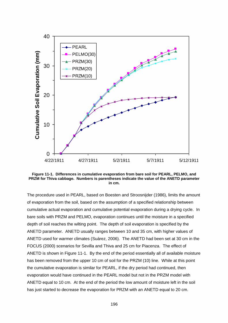
196
0
10
20
30
40
4/22/1911 4/27/1911 5/2/1911 5/7/1911 5/12/1911
Cu
mu
lati
ve
So
il E
va
po
rati
on
(m
m)
PEARL
PELMO(30)
PRZM(30)
PRZM(20)
PRZM(10)
Figure 11-1. Differences in cumulative evaporation from bare soil for PEARL, PELMO, and PRZM for Thiva cabbage. Numbers is parentheses indicate the value of the ANETD parameter
in cm.
The procedure used in PEARL, based on Boesten and Stroosnijder (1986), limits the amount
of evaporation from the soil, based on the assumption of a specified relationship between
cumulative actual evaporation and cumulative potential evaporation during a drying cycle. In
bare soils with PRZM and PELMO, evaporation continues until the moisture in a specified
depth of soil reaches the wilting point. The depth of soil evaporation is specified by the
ANETD parameter. ANETD usually ranges between 10 and 35 cm, with higher values of
ANETD used for warmer climates (Suárez, 2006). The ANETD had been set at 30 cm in the
FOCUS (2000) scenarios for Sevilla and Thiva and 25 cm for Piacenza. The effect of
ANETD is shown in Figure 11-1. By the end of the period essentially all of available moisture
has been removed from the upper 10 cm of soil for the PRZM (10) line. While at this point
the cumulative evaporation is similar for PEARL, if the dry period had continued, then
evaporation would have continued in the PEARL model but not in the PRZM model with
ANETD equal to 10 cm. At the end of the period the low amount of moisture left in the soil
has just started to decrease the evaporation for PRZM with an ANETD equal to 20 cm.
197
The work group decided after reviewing the work of Torres et al. (2006) that in the absence
of a crop, the routines in PEARL will be used as the standard for estimated evaporation from
bare soil and the ANETD parameter in PELMO and PRZM will be adjusted to give
approximately the same amount of soil evaporation during the time the crop is not present.
Based on the results of this calibration procedure (presented in Appendix 21), the work group
decided to use ANETD values of 15 cm for Piacenza and Sevilla and 20 cm for Thiva.
When a crop is present the different model routines still have the possibility to cause
differences in the amount of evapotranspiration. PELMO and PRZM extract the potential
crop evapotranspiration from the root zone, until the available water is exhausted. PEARL
divides the potential evapotranspiration into soil evaporation and plant transpiration and the
soil evaporation losses are described by the same routines as when there is no crop present.
However, differences between the models when a crop is present appear to be much less
than for bare soil.
11.5.1.4 Adjustment of the rooting depths of some crops
Because transpiration in PEARL is reduced when a substantial fraction of the roots are
located below the water table, the maximum rooting depths were set at 1 m for crop/location
combinations where this occurred in FOCUS (2000) or was likely to occur. These were vines
at Hamburg; apples at Jokioinen; apples sugar beets, winter cereals, maize, vines, and
oilseed rape at Kremsmünster, apples, citrus, and vines at Piacenza, and apples, citrus, and
vines at Porto. Because of the inconsistency of evaluating ground water concentrations at a
depth shallower than the root zone, the work group decided that the maximum rooting depth
would not exceed 1 m for all remaining location/crop combinations.
11.5.2 Review of procedure to estimate runoff
One of the major differences in the water balance between the PEARL and the PELMO and
PRZM models in the original scenarios is the amount of runoff predicted. Part of this
difference was the result of runoff from irrigation (which had been originally input into PRZM
and PELMO as additional rainfall). Both PRZM and PELMO will be modified so that irrigation
is provided as a separate input parameter from rainfall. However, this change is still not
enough to adequately harmonise the water balance between the two models (as shown in
Table 11-1). In another set of simulations, different storm lengths were evaluated in PEARL
to see if runoff values could be harmonised using a storm length other than 24 hours in
PEARL. While the numbers in PEARL and PRZM become closer (Table 11-1), there is no
reliable source of European data to determine which of the predictions is closer to reality.
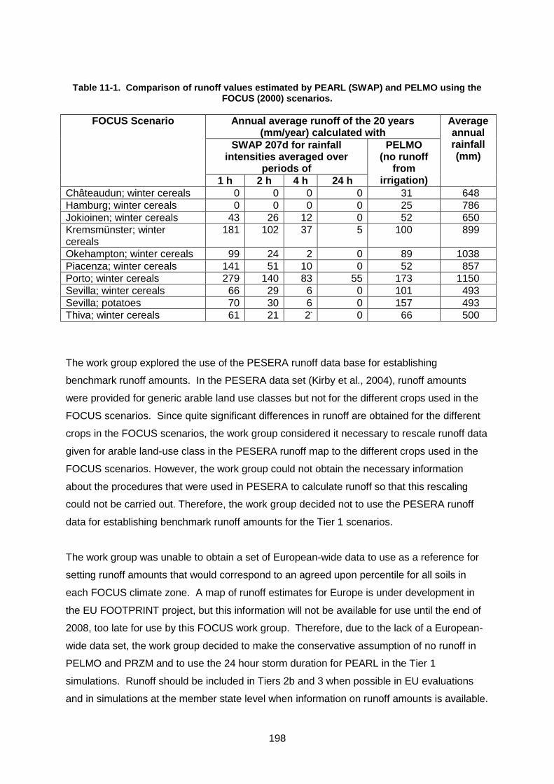
198
Table 11-1. Comparison of runoff values estimated by PEARL (SWAP) and PELMO using the FOCUS (2000) scenarios.
FOCUS Scenario Annual average runoff of the 20 years (mm/year) calculated with
Average annual rainfall (mm)
SWAP 207d for rainfall intensities averaged over
periods of
PELMO (no runoff
from irrigation) 1 h 2 h 4 h 24 h
Châteaudun; winter cereals 0 0 0 0 31 648
Hamburg; winter cereals 0 0 0 0 25 786
Jokioinen; winter cereals 43 26 12 0 52 650
Kremsmünster; winter cereals
181 102 37 5 100 899
Okehampton; winter cereals 99 24 2 0 89 1038
Piacenza; winter cereals 141 51 10 0 52 857
Porto; winter cereals 279 140 83 55 173 1150
Sevilla; winter cereals 66 29 6 0 101 493
Sevilla; potatoes 70 30 6 0 157 493
Thiva; winter cereals 61 21 2* 0 66 500
The work group explored the use of the PESERA runoff data base for establishing
benchmark runoff amounts. In the PESERA data set (Kirby et al., 2004), runoff amounts
were provided for generic arable land use classes but not for the different crops used in the
FOCUS scenarios. Since quite significant differences in runoff are obtained for the different
crops in the FOCUS scenarios, the work group considered it necessary to rescale runoff data
given for arable land-use class in the PESERA runoff map to the different crops used in the
FOCUS scenarios. However, the work group could not obtain the necessary information
about the procedures that were used in PESERA to calculate runoff so that this rescaling
could not be carried out. Therefore, the work group decided not to use the PESERA runoff
data for establishing benchmark runoff amounts for the Tier 1 scenarios.
The work group was unable to obtain a set of European-wide data to use as a reference for
setting runoff amounts that would correspond to an agreed upon percentile for all soils in
each FOCUS climate zone. A map of runoff estimates for Europe is under development in
the EU FOOTPRINT project, but this information will not be available for use until the end of
2008, too late for use by this FOCUS work group. Therefore, due to the lack of a European-
wide data set, the work group decided to make the conservative assumption of no runoff in
PELMO and PRZM and to use the 24 hour storm duration for PEARL in the Tier 1
simulations. Runoff should be included in Tiers 2b and 3 when possible in EU evaluations
and in simulations at the member state level when information on runoff amounts is available.
199
When the runoff information from the FOOTPRINT project is available, a detailed review of
the data may lead to the conclusion that this could serve as a suitable data base for
determining appropriate amounts of runoff in the Tier 1 scenarios. However, such a review is
beyond the scope of this work group.
The work group felt that the 20th percentile runoff value in a FOCUS climate zone was an
appropriate benchmark for runoff in the current and proposed FOCUS scenarios. However,
when new scenarios are developed in the future or higher tier modelling is performed,
properties determining runoff potential (such as soil hydrologic group) should be considered
in a similar manner as other important soil properties such as organic matter and soil
hydraulic properties in order to obtain an 80th percentile soil.
11.5.3 Review of estimation of the irrigated amounts of water
In the FOCUS (2000) scenarios irrigation schedules were developed for groups of crops
rather than individual crops. A review of the irrigation schedules for the FOCUS (2000)
scenarios showed that the irrigation and the cropping periods did not always match. Also in
some cases the amounts appeared to be higher than were actually applied, based on local
information. During the work on harmonising the water balance, the work group also
discovered that water stress occurred to some crops in the FOCUS (2000) Porto scenarios,
which does not assume irrigation; whereas irrigation is usually applied. The irrigation
information collected by the work group is summarised in Appendix 22.
The work group decided that irrigation schedules should be developed for individual crops in
Châteaudun, Piacenza, Porto, Seville, and Thiva. These irrigation schedules provide
irrigation from the time of planting until start of senescence and are generated using irrigation
routines in PEARL and PELMO, which apply irrigation once a week on a fixed day to bring
the root zone up to field capacity. However, irrigation was applied only if the amount required
exceeded 15 mm. Because of the minor differences remaining in the water balance
(primarily evapotranspiration), the irrigation routines for PEARL and PELMO predict
somewhat different amounts. However, using different irrigation routines tends to
compensate for evapotranspiration differences to provide closer estimates between the two
models for the amount of water moving below the root zone, which is the key water balance
parameter affecting leaching. The irrigation amounts generated by PELMO are used directly
in PRZM. While allowing PRZM to generate irrigation amounts is also possible, the work
group decided that this added a level of complexity that was not needed, given the similarity
of PELMO and PRZM.
200
The amounts of irrigation for each of the location/crop combinations are presented in the
examples shown in Chapter 12 and Appendix 23.
11.6 Soil pH values in FOCUS scenarios
The soil pH values at various depths for the FOCUS ground water scenarios were available
in the FOCUS ground water documentation but were not made available electronically for
use with models. This meant that substances showing a correlation between adsorption and
soil pH had to be modelled using an experimental adsorption value appropriate to the soil pH
of each relevant FOCUS scenario.
This FOCUS ground water group have decided to make the pH-H2O values of the FOCUS
groundwater scenarios available electronically because most of the values provided for the
soil profiles were pH-H2O values (FOCUS, 2000). Models may now be used to describe the
sorption of substances showing pH dependent sorption, however the modelling report should
demonstrate that the adsorption values predicted by the model fit the experimental data.
When introducing a measured Koc-pH relationship into the FOCUS leaching models, the pH-
H2O measuring method must be consistent with that used for analysing the sorption
measurements. If the pH-H2O is not available for the soils from the adsorption studies, it can
be calculated as follows (A.M.A. van der Linden, personal communication, 2008):
pH-H2O = 0.820 pH-KCl + 1.69
pH-H2O = 0.953 pH-CaCl2 + 0.85
where pH-KCl is the pH measured in an aqueous solution of 1 mol/L of KCl and where pH-
CaCl2 is the pH measured in an aqueous solution of 0.01 mol/L of CaCl2.
However as stated in Section 11.1, and EFSA, PPR (2013a and b) using the pH defined for
the soil columns of each FOCUS scenario would mean that these scenarios could not be
considered to possess the FOCUS-defined vulnerability regarding pH effects. Using an
experimental adsorption value appropriate for the soil pH of the relevant FOCUS scenario as
was done in the past, is no longer considered an acceptable method of including pH
dependent sorption into the FOCUS scenarios. Therefore Tier 1 simulations for
consideration of EU approval should select adsorption values, chosen to represent a realistic
worst case considering the pH of the soils in the EU that are used for the production of the
pertinent crop. Normally this pH would be selected to minimise sorption; however, there are
201
certain compounds for which lower sorption results in faster degradation. In addition to
choosing adsorption values that represent a realistic worst case applicants might also
provide simulations for all scenarios selecting a contrasting adsorption value associated for a
more best case, considering the pH of the soils in the EU that are used for the production of
the pertinent crop. Decision makers would then get a view on the range of recharge
concentrations that can result depending on the average pH of the soils overlying a confined
aquifer in a particular region. As an example ,for a compound with a single ionisable
functional group that follows a typical S shaped relationship for adsorption with pH, such as a
weak acid, two contrasting pH values for which best and worst case adsorption estimates
could be selected would be associated with a pH of 5.0 and 7.5 respectively if the crop could
grow in this range of soil pH. If the pH relationship was more ∩ or U shaped, adsorption
associated with an intermediate pH as the best or worst case respectively could be justified.
Using correct pH maps and using soil column pH descriptions to parameterise scenarios in
case of pH dependent substance properties at higher tiers is an approach that may be
followed for EU level and national assessment, though this was considered more important in
assessments at the national level rather than the EU level by the EFSA PPR panel (EFSA,
PPR 2013a).
11.7 Review of procedure for estimating interception of pesticide by plants
When FOCUS (2000) decided to estimate interception of pesticide application by the plant
canopy using experimental measurements available in the literature, not all of the FOCUS
models contained a routine for estimating crop interception. Since all the models
recommended by FOCUS for estimating ground water concentrations can now estimate
interception; the work group reviewed whether the Tier I recommendations be changed to
allow them to do so (Appendix 24). At this time the work group decided not to change this
recommendation. Note that additional literature regarding crop interception has been
reviewed on behalf of EFSA and the FOCUS crop interception tables have been updated to
incorporate the new information found (see EFSA 2014a, van Beinum & Beulke (2010) and
Olesen & Jensen (2013) and also Generic Guidance for Tier 1 FOCUS groundwater
assessments version 2.2 (available from the FOCUS website))
11.8 References
Boesten, J.J.T.I. 2004. Influence of dispersion length on leaching calculated with PEARL,
PELMO and PRZM for FOCUS groundwater scenarios. Pest Manag Sci 60:971-980.
202
Boesten, J.J.T.I., Stroosnijder, L. 1986. Simple model for daily evaporation from fallow tilled
soil under spring conditions in a temperate climate. Netherlands Journal of Agricultural
Science 34:75-90.
EFSA. Panel on Plant Protection Products and their Residues (PPR) 2013a; Scientific
Opinion on the report of the FOCUS groundwater working group (FOCUS, 2009):
assessment of lower tiers. EFSA Journal 2013;11(2):3114. [29 pp.]
doi:10.2903/j.efsa.2013.3114. Available online: www.efsa.europa.eu/efsajournal
EFSA. Panel on Plant Protection Products and their Residues (PPR) 2013b; Scientific
Opinion on the report of the FOCUS groundwater working group (FOCUS, 2009):
assessment of higher tiers. EFSA Journal 2013;11(6):3291. [25 pp.]
doi:10.2903/j.efsa.2013.3291. Available online: www.efsa.europa.eu/efsajournal
EFSA 2014a European Food Safety Authority. Guidance Document for evaluating laboratory
and field dissipation studies to obtain DegT50 values of active substances of plant
protection products and transformation products of these active substances in soil. EFSA
Journal 2014;12(5):3662, 38 pp., doi:10.2903/j.efsa.2014.3662 Available online:
www.efsa.europa.eu/efsajournal
FOCUS. 2000. FOCUS groundwater scenarios in the EU review of active substances.
Report of the FOCUS Groundwater Scenarios Workgroup, EC Document Reference
Sanco/321/2000 rev.2, 202pp.
Kirkby, M.J., Jones, R.J.A., Irvine, B., Gobin, A, Govers, G., Cerdan, O., Van Rompaey,
A.J.J., Le Bissonnais, Y., Daroussin, J., King, D., Montanarella, L., Grimm, M.,
Vieillefont, V., Puigdefabregas, J., Boer, M., Kosmas, C., Yassoglou, N., Tsara, M.,
Mantel, S., Van Lynden, G.J. and Huting, J. 2004. Pan-European Soil Erosion Risk
Assessment: The PESERA Map, Version 1, October 2003. Explanation of Special
Publication Ispra 2004 No.73 (S.P.I.04.73). European Soil Bureau Research Report
No.16, EUR 21176, 18pp. and 1 map in ISO B1 format. Office for Official Publications of
the European Communities, Luxembourg.
Olesen, M. H. Jensen P. K. 2013. Collection and evaluation of relevant information on crop
interception. Report by the Aarhus University,. Denmark, 67 pp. Available online:
www.efsa.europa.eu/en/supporting/pub/438e.htm
Suárez, L. A. 2006. PRZM-3, A Model for Predicting Pesticide and Nitrogen Fate in the
Crop Root and Unsaturated Soil Zones: Users Manual for Release 3.12.2. EPA/600/R-
05/111. National Exposure Research Laboratory, U.S. Environmental Protection Agency
Athens, GA.
Torres E.A, Rubio E, Calera A, Cuesta A. 2006. Evaluation of FAO-56 model for bare soil
evaporation in a semi-arid region using experimental data, Geophysical Research
abstracts, Vol 8.
203
van Beinum, W. Beulke, S. 2010. Collection and evaluation of relevant information on crop
interception for the revision of the Guidance Document on Persistence in Soil. Report
FERA, Sand Hutton, UK, 41 pp. Available online:
www.efsa.europa.eu/en/supporting/pub/73e.htm
Vanclooster, M., J.D. Pineros-Garcet, J.J.T.I. Boesten , F. Van den Berg, M. Leistra, J.
Smelt, N. Jarvis, S. Roulier, P. Burauel, H. Vereecken, A. Wolters, V. Linnemann, E.
Fernandez, M. Trevisan, E. Capri, L. Padovani, M. Klein, A. Tiktak, A. Van der Linden, D.
De Nie, G. Bidoglio, F. Baouroui, A. Jones, A. Armstrong. 2003. Effective Approaches
for Assessing the Predicted Environmental Concentrations of Pesticides. Final report.
European Commission, Quality of Life and Management of Living Resources
Programme. QLK4-CT-1999-01238. Printed by the Université Catholique de Louvain,
Belgium (Available at http://www.geru.ucl.ac.be/recherche/projets/apecop-pub/).
204
12 COMPARISON OF CURRENT AND REVISED SCENARIOS
One of the objectives of the revisions described in Chapter 11 was to standardise the
assumptions used by the FOCUS models to reduce the variability of predictions among
models. This objective was largely addressed by the harmonisation of dispersion length and
the water balance. Other revisions resulted in changes not directed towards harmonisation
of model predictions. This included the change in the 80th percentile weather concentration
to the average of the 16 and 17th ranked values (reducing concentrations for all scenarios at
least slightly), the change in the Porto soil profile (increasing concentrations for all crops
grown in Porto), and the change in the Piacenza soil profile (lowering concentrations for all
crops grown in Piacenza). This chapter compares the proposed ground water scenarios with
the current ground water scenarios of FOCUS (2000) as amended by the actions of the
FOCUS Version Control Work Group to date. This chapter does not consider the effects of
the various individual changes, but only the changes as a whole.
12.1 Results of comparison simulations
A comparison of the changes was performed by conducting simulations with pesticide D (as
defined by FOCUS, 2000) for all 125 location/crop combinations and for the proposed
revision of these 125 location/crop combinations as described in this report. A single
application at 1 kg ai/ha was assumed to occur the day before plant emergence. For those
location/crop combinations with two cropping periods, single applications of 1 kg ai/ha were
made during each of the cropping periods. For apples, citrus, grass, and vines, the
applications was assumed to occur on May 1. As outlined by FOCUS (2000), simulations for
each location/crop combination were performed for a 26 year period (6 year warm-up period
followed by 20 year simulation period). Water balance components were calculated as the
average of the 20 year annual values and PECgw was calculated for the current scenarios as
outlined by FOCUS (2000) and for the proposed scenarios as outlined in Section 11.2. This
chapter focuses on the changes occurring with PEARL and PELMO, since the predictions of
PRZM are similar to PELMO. However, detailed information on the results of these
simulations is presented for all models in Appendix 23 (Information on MACRO will be
included as soon as it is available). The work group also intends to make the information in
Appendix 23 available in a spreadsheet to be posted on the FOCUS web site, once the
report has been approved, to facilitate comparisons.
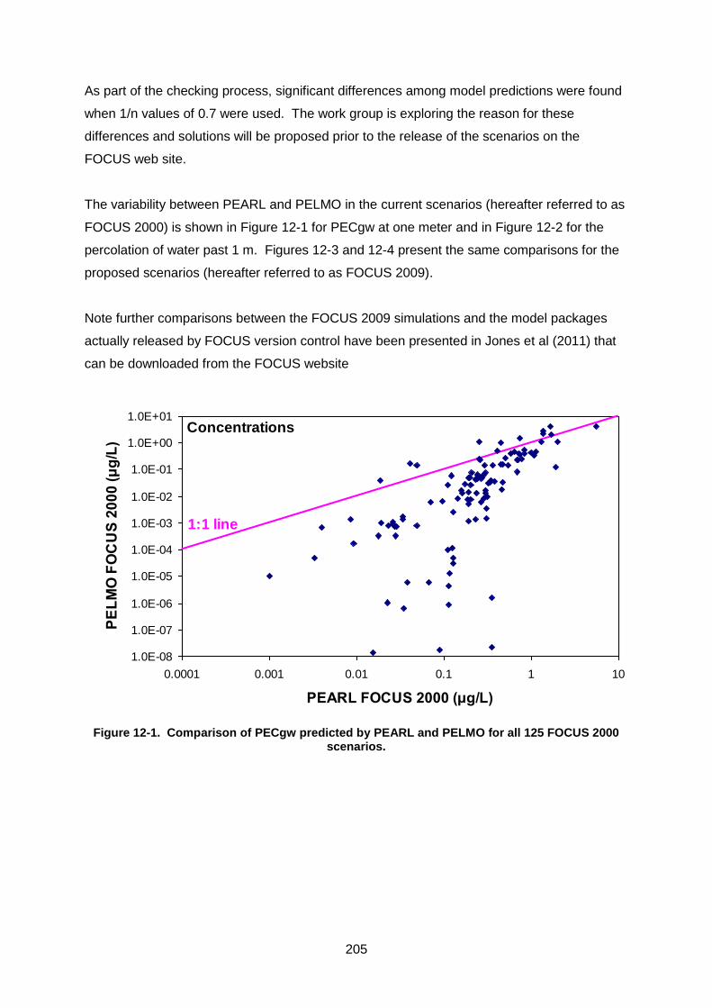
205
As part of the checking process, significant differences among model predictions were found
when 1/n values of 0.7 were used. The work group is exploring the reason for these
differences and solutions will be proposed prior to the release of the scenarios on the
FOCUS web site.
The variability between PEARL and PELMO in the current scenarios (hereafter referred to as
FOCUS 2000) is shown in Figure 12-1 for PECgw at one meter and in Figure 12-2 for the
percolation of water past 1 m. Figures 12-3 and 12-4 present the same comparisons for the
proposed scenarios (hereafter referred to as FOCUS 2009).
Note further comparisons between the FOCUS 2009 simulations and the model packages
actually released by FOCUS version control have been presented in Jones et al (2011) that
can be downloaded from the FOCUS website
1.0E-08
1.0E-07
1.0E-06
1.0E-05
1.0E-04
1.0E-03
1.0E-02
1.0E-01
1.0E+00
1.0E+01
0.0001 0.001 0.01 0.1 1 10
PEARL FOCUS 2000 (μg/L)
PE
LM
O F
OC
US
20
00
(μ
g/L
)
1:1 line
Concentrations
Figure 12-1. Comparison of PECgw predicted by PEARL and PELMO for all 125 FOCUS 2000
scenarios.
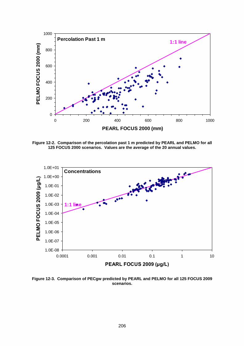
206
0
200
400
600
800
1000
0 200 400 600 800 1000
PEARL FOCUS 2000 (mm)
PE
LM
O F
OC
US
20
00
(m
m) 1:1 line
Percolation Past 1 m
Figure 12-2. Comparison of the percolation past 1 m predicted by PEARL and PELMO for all 125 FOCUS 2000 scenarios. Values are the average of the 20 annual values.
1.0E-08
1.0E-07
1.0E-06
1.0E-05
1.0E-04
1.0E-03
1.0E-02
1.0E-01
1.0E+00
1.0E+01
0.0001 0.001 0.01 0.1 1 10
PEARL FOCUS 2009 (μg/L)
PE
LM
O F
OC
US
20
09
(μ
g/L
)
1:1 line
Concentrations
Figure 12-3. Comparison of PECgw predicted by PEARL and PELMO for all 125 FOCUS 2009 scenarios.
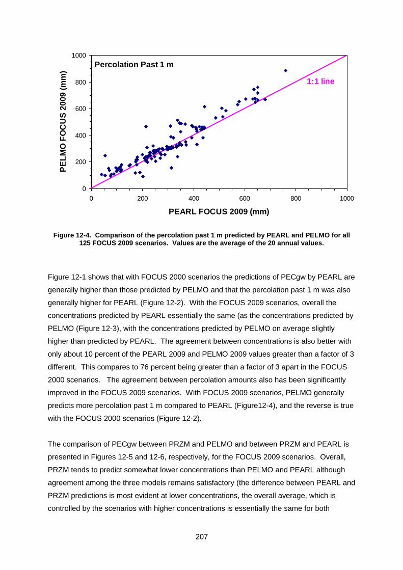
207
0
200
400
600
800
1000
0 200 400 600 800 1000
PEARL FOCUS 2009 (mm)
PE
LM
O F
OC
US
20
09
(m
m)
1:1 line
Percolation Past 1 m
Figure 12-4. Comparison of the percolation past 1 m predicted by PEARL and PELMO for all 125 FOCUS 2009 scenarios. Values are the average of the 20 annual values.
Figure 12-1 shows that with FOCUS 2000 scenarios the predictions of PECgw by PEARL are
generally higher than those predicted by PELMO and that the percolation past 1 m was also
generally higher for PEARL (Figure 12-2). With the FOCUS 2009 scenarios, overall the
concentrations predicted by PEARL essentially the same (as the concentrations predicted by
PELMO (Figure 12-3), with the concentrations predicted by PELMO on average slightly
higher than predicted by PEARL. The agreement between concentrations is also better with
only about 10 percent of the PEARL 2009 and PELMO 2009 values greater than a factor of 3
different. This compares to 76 percent being greater than a factor of 3 apart in the FOCUS
2000 scenarios. The agreement between percolation amounts also has been significantly
improved in the FOCUS 2009 scenarios. With FOCUS 2009 scenarios, PELMO generally
predicts more percolation past 1 m compared to PEARL (Figure12-4), and the reverse is true
with the FOCUS 2000 scenarios (Figure 12-2).
The comparison of PECgw between PRZM and PELMO and between PRZM and PEARL is
presented in Figures 12-5 and 12-6, respectively, for the FOCUS 2009 scenarios. Overall,
PRZM tends to predict somewhat lower concentrations than PELMO and PEARL although
agreement among the three models remains satisfactory (the difference between PEARL and
PRZM predictions is most evident at lower concentrations, the overall average, which is
controlled by the scenarios with higher concentrations is essentially the same for both
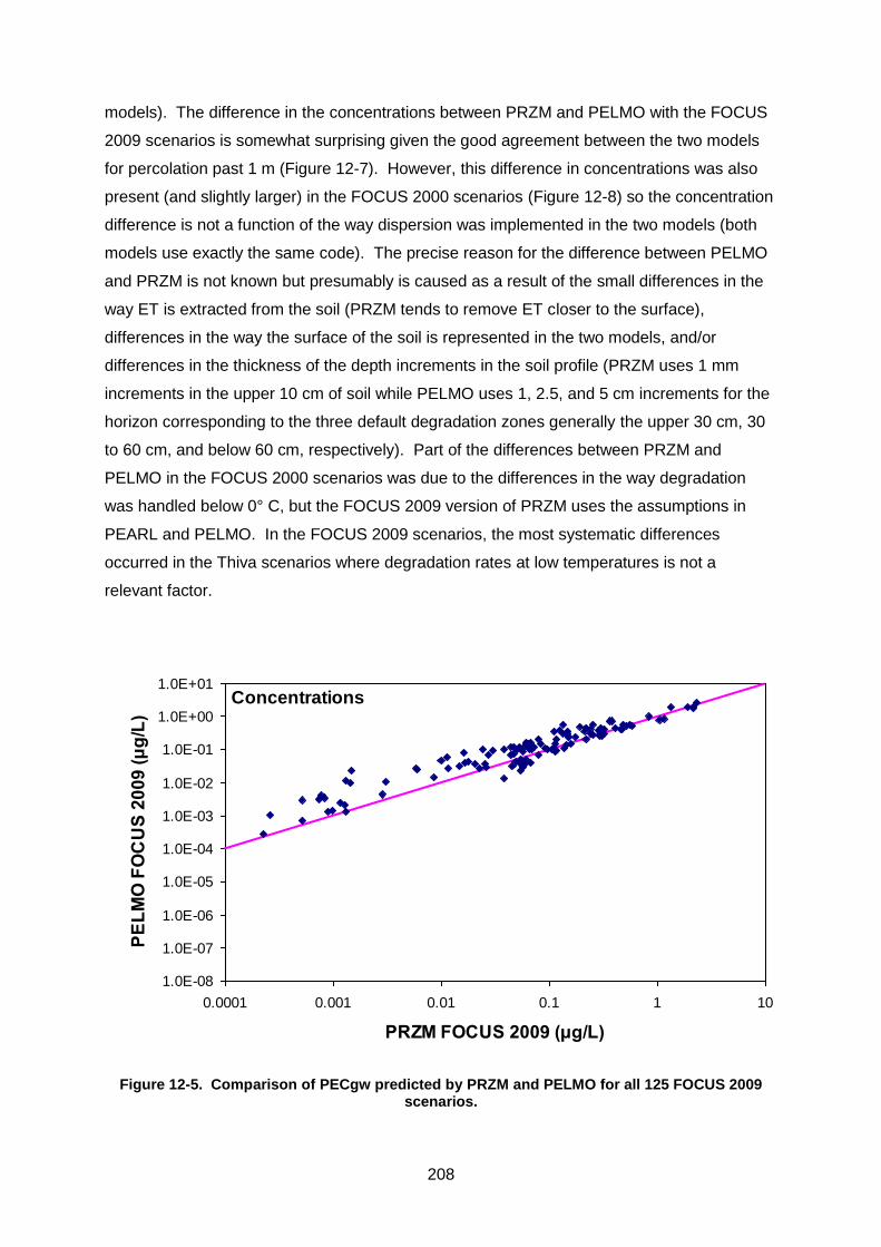
208
models). The difference in the concentrations between PRZM and PELMO with the FOCUS
2009 scenarios is somewhat surprising given the good agreement between the two models
for percolation past 1 m (Figure 12-7). However, this difference in concentrations was also
present (and slightly larger) in the FOCUS 2000 scenarios (Figure 12-8) so the concentration
difference is not a function of the way dispersion was implemented in the two models (both
models use exactly the same code). The precise reason for the difference between PELMO
and PRZM is not known but presumably is caused as a result of the small differences in the
way ET is extracted from the soil (PRZM tends to remove ET closer to the surface),
differences in the way the surface of the soil is represented in the two models, and/or
differences in the thickness of the depth increments in the soil profile (PRZM uses 1 mm
increments in the upper 10 cm of soil while PELMO uses 1, 2.5, and 5 cm increments for the
horizon corresponding to the three default degradation zones generally the upper 30 cm, 30
to 60 cm, and below 60 cm, respectively). Part of the differences between PRZM and
PELMO in the FOCUS 2000 scenarios was due to the differences in the way degradation
was handled below 0° C, but the FOCUS 2009 version of PRZM uses the assumptions in
PEARL and PELMO. In the FOCUS 2009 scenarios, the most systematic differences
occurred in the Thiva scenarios where degradation rates at low temperatures is not a
relevant factor.
1.0E-08
1.0E-07
1.0E-06
1.0E-05
1.0E-04
1.0E-03
1.0E-02
1.0E-01
1.0E+00
1.0E+01
0.0001 0.001 0.01 0.1 1 10
PRZM FOCUS 2009 (μg/L)
PE
LM
O F
OC
US
20
09
(μ
g/L
)
Concentrations
Figure 12-5. Comparison of PECgw predicted by PRZM and PELMO for all 125 FOCUS 2009 scenarios.
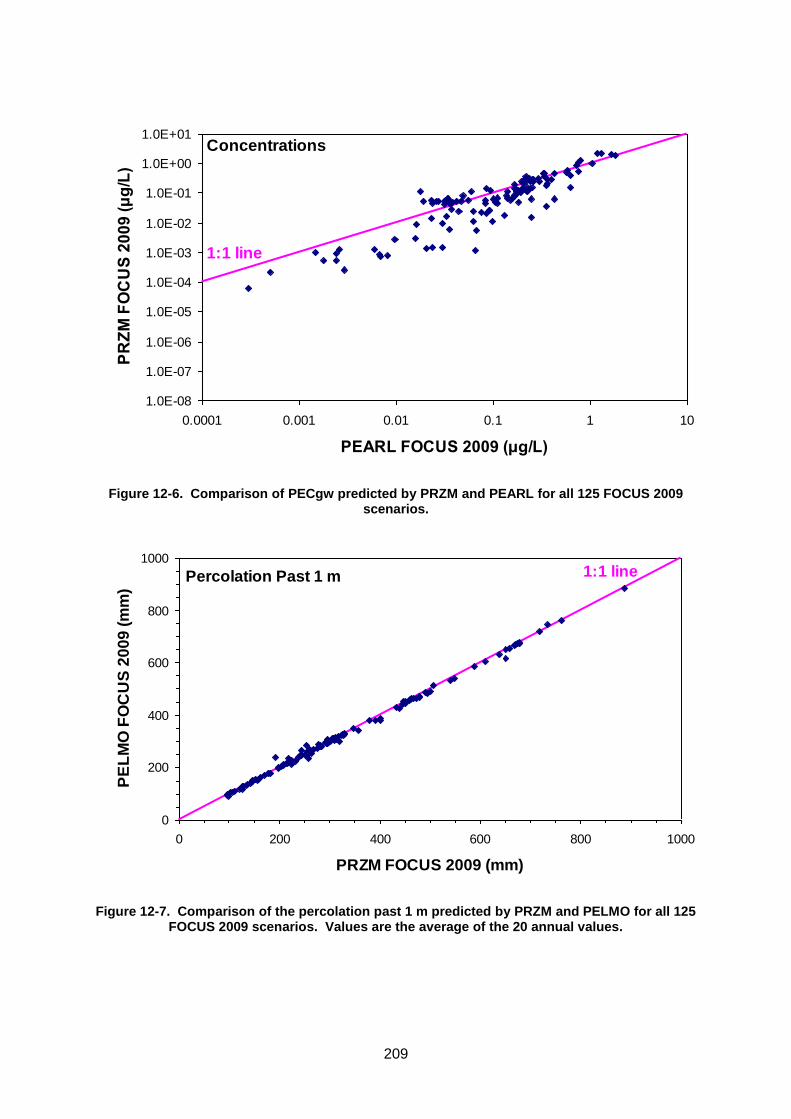
209
1.0E-08
1.0E-07
1.0E-06
1.0E-05
1.0E-04
1.0E-03
1.0E-02
1.0E-01
1.0E+00
1.0E+01
0.0001 0.001 0.01 0.1 1 10
PEARL FOCUS 2009 (μg/L)
PR
ZM
FO
CU
S 2
00
9 (
μg
/L)
Concentrations
1:1 line
Figure 12-6. Comparison of PECgw predicted by PRZM and PEARL for all 125 FOCUS 2009 scenarios.
0
200
400
600
800
1000
0 200 400 600 800 1000
PRZM FOCUS 2009 (mm)
PE
LM
O F
OC
US
20
09
(m
m)
1:1 linePercolation Past 1 m
Figure 12-7. Comparison of the percolation past 1 m predicted by PRZM and PELMO for all 125 FOCUS 2009 scenarios. Values are the average of the 20 annual values.
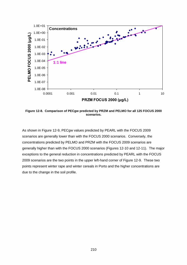
210
1.0E-08
1.0E-07
1.0E-06
1.0E-05
1.0E-04
1.0E-03
1.0E-02
1.0E-01
1.0E+00
1.0E+01
0.0001 0.001 0.01 0.1 1 10
PRZM FOCUS 2000 (μg/L)
PE
LM
O F
OC
US
20
00
(μ
g/L
)Concentrations
1:1 line
Figure 12-8. Comparison of PECgw predicted by PRZM and PELMO for all 125 FOCUS 2000 scenarios.
As shown in Figure 12-9, PECgw values predicted by PEARL with the FOCUS 2009
scenarios are generally lower than with the FOCUS 2000 scenarios. Conversely, the
concentrations predicted by PELMO and PRZM with the FOCUS 2009 scenarios are
generally higher than with the FOCUS 2000 scenarios (Figures 12-10 and 12-11). The major
exceptions to the general reduction in concentrations predicted by PEARL with the FOCUS
2009 scenarios are the two points in the upper left-hand corner of Figure 12-9. These two
points represent winter rape and winter cereals in Porto and the higher concentrations are
due to the change in the soil profile.
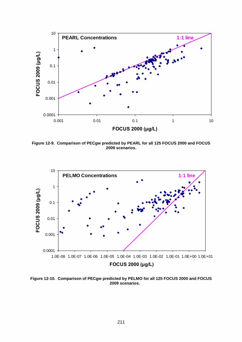
211
0.0001
0.001
0.01
0.1
1
10
0.001 0.01 0.1 1 10
FOCUS 2000 (μg/L)
FO
CU
S 2
00
9 (
μg
/L)
PEARL Concentrations 1:1 line
Figure 12-9. Comparison of PECgw predicted by PEARL for all 125 FOCUS 2000 and FOCUS 2009 scenarios.
0.0001
0.001
0.01
0.1
1
10
1.0E-08 1.0E-07 1.0E-06 1.0E-05 1.0E-04 1.0E-03 1.0E-02 1.0E-01 1.0E+00 1.0E+01
FOCUS 2000 (μg/L)
FO
CU
S 2
00
9 (
μg
/L)
PELMO Concentrations 1:1 line
Figure 12-10. Comparison of PECgw predicted by PELMO for all 125 FOCUS 2000 and FOCUS 2009 scenarios.
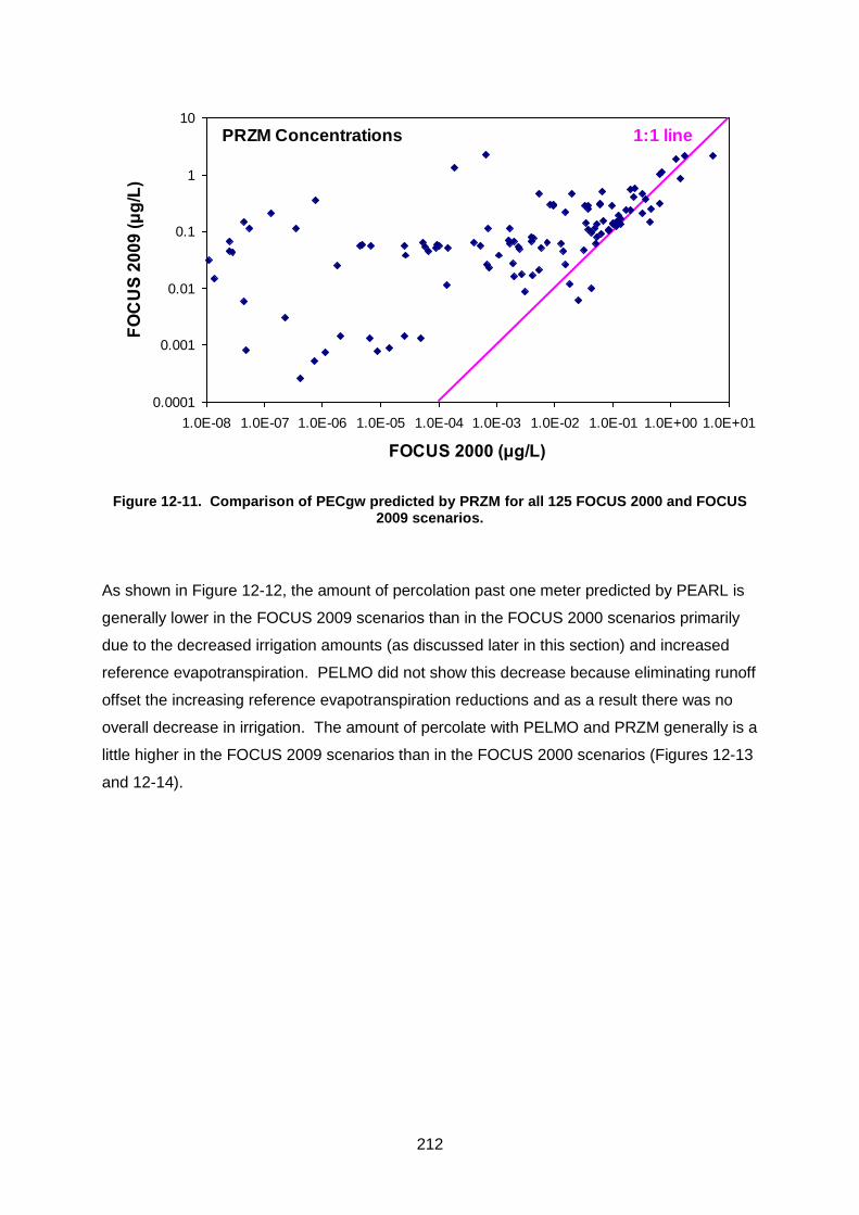
212
0.0001
0.001
0.01
0.1
1
10
1.0E-08 1.0E-07 1.0E-06 1.0E-05 1.0E-04 1.0E-03 1.0E-02 1.0E-01 1.0E+00 1.0E+01
FOCUS 2000 (μg/L)
FO
CU
S 2
00
9 (
μg
/L)
PRZM Concentrations 1:1 line
Figure 12-11. Comparison of PECgw predicted by PRZM for all 125 FOCUS 2000 and FOCUS 2009 scenarios.
As shown in Figure 12-12, the amount of percolation past one meter predicted by PEARL is
generally lower in the FOCUS 2009 scenarios than in the FOCUS 2000 scenarios primarily
due to the decreased irrigation amounts (as discussed later in this section) and increased
reference evapotranspiration. PELMO did not show this decrease because eliminating runoff
offset the increasing reference evapotranspiration reductions and as a result there was no
overall decrease in irrigation. The amount of percolate with PELMO and PRZM generally is a
little higher in the FOCUS 2009 scenarios than in the FOCUS 2000 scenarios (Figures 12-13
and 12-14).
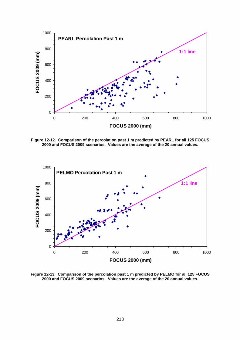
213
0
200
400
600
800
1000
0 200 400 600 800 1000
FOCUS 2000 (mm)
FO
CU
S 2
00
9 (
mm
)PEARL Percolation Past 1 m
1:1 line
Figure 12-12. Comparison of the percolation past 1 m predicted by PEARL for all 125 FOCUS 2000 and FOCUS 2009 scenarios. Values are the average of the 20 annual values.
0
200
400
600
800
1000
0 200 400 600 800 1000
FOCUS 2000 (mm)
FO
CU
S 2
00
9 (
mm
)
PELMO Percolation Past 1 m
1:1 line
Figure 12-13. Comparison of the percolation past 1 m predicted by PELMO for all 125 FOCUS 2000 and FOCUS 2009 scenarios. Values are the average of the 20 annual values.
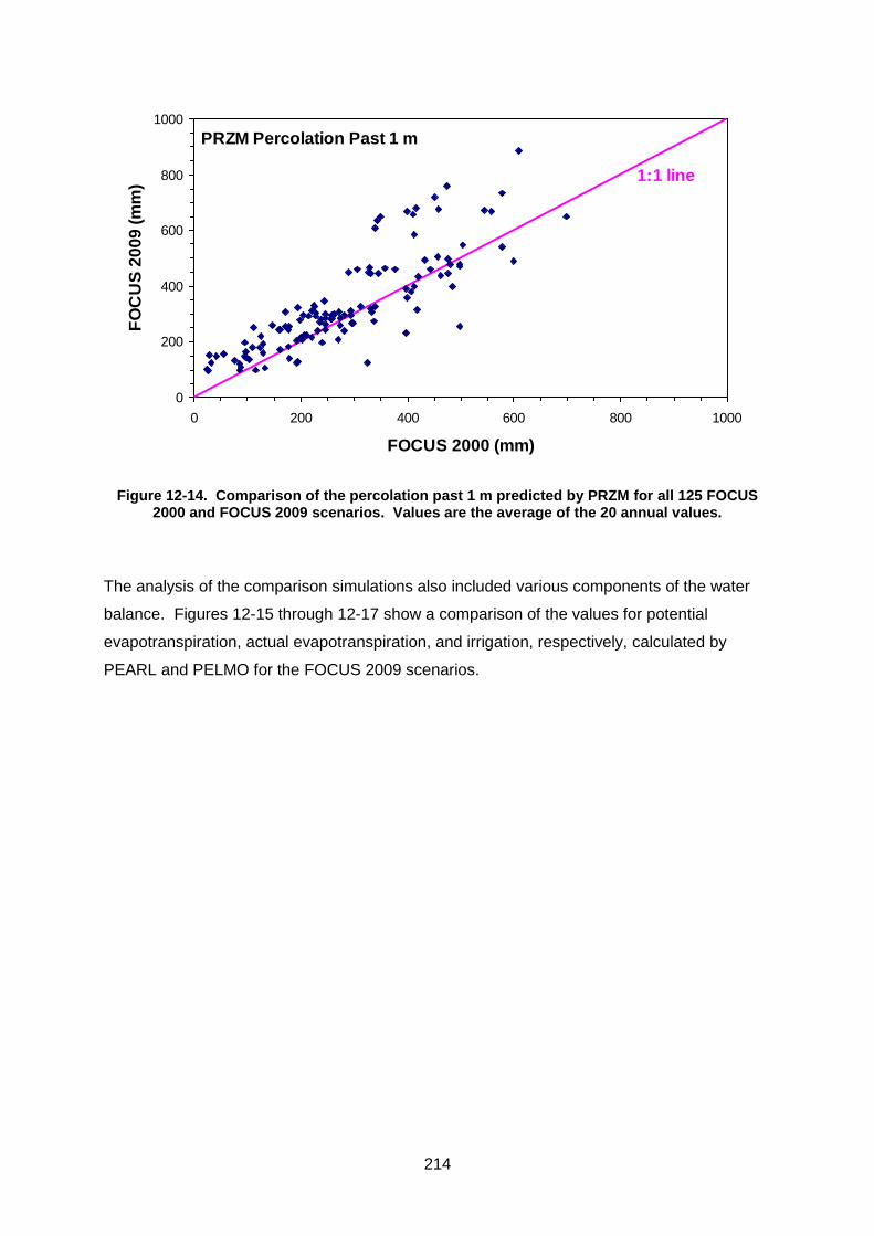
214
0
200
400
600
800
1000
0 200 400 600 800 1000
FOCUS 2000 (mm)
FO
CU
S 2
00
9 (
mm
)PRZM Percolation Past 1 m
1:1 line
Figure 12-14. Comparison of the percolation past 1 m predicted by PRZM for all 125 FOCUS 2000 and FOCUS 2009 scenarios. Values are the average of the 20 annual values.
The analysis of the comparison simulations also included various components of the water
balance. Figures 12-15 through 12-17 show a comparison of the values for potential
evapotranspiration, actual evapotranspiration, and irrigation, respectively, calculated by
PEARL and PELMO for the FOCUS 2009 scenarios.
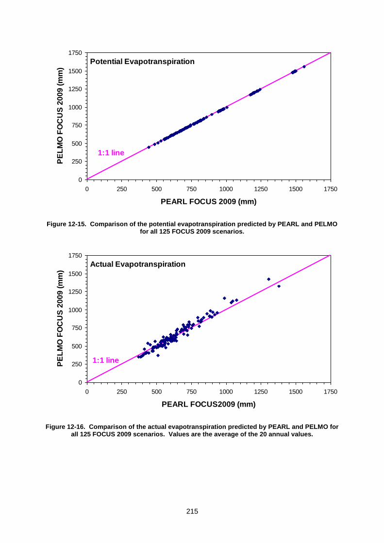
215
0
250
500
750
1000
1250
1500
1750
0 250 500 750 1000 1250 1500 1750
PEARL FOCUS 2009 (mm)
PE
LM
O F
OC
US
20
09
(m
m)
1:1 line
Potential Evapotranspiration
Figure 12-15. Comparison of the potential evapotranspiration predicted by PEARL and PELMO for all 125 FOCUS 2009 scenarios.
0
250
500
750
1000
1250
1500
1750
0 250 500 750 1000 1250 1500 1750
PEARL FOCUS2009 (mm)
PE
LM
O F
OC
US
20
09
(m
m)
1:1 line
Actual Evapotranspiration
Figure 12-16. Comparison of the actual evapotranspiration predicted by PEARL and PELMO for all 125 FOCUS 2009 scenarios. Values are the average of the 20 annual values.
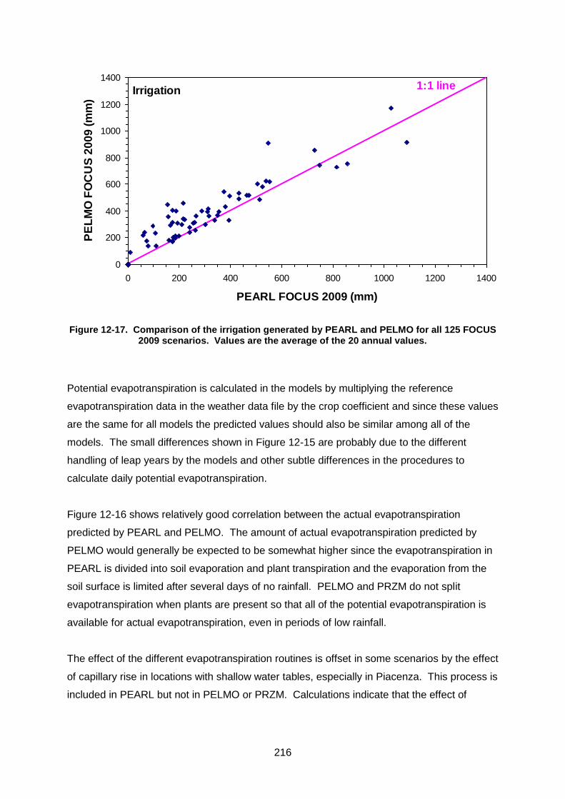
216
0
200
400
600
800
1000
1200
1400
0 200 400 600 800 1000 1200 1400
PEARL FOCUS 2009 (mm)
PE
LM
O F
OC
US
20
09
(m
m)
1:1 lineIrrigation
Figure 12-17. Comparison of the irrigation generated by PEARL and PELMO for all 125 FOCUS 2009 scenarios. Values are the average of the 20 annual values.
Potential evapotranspiration is calculated in the models by multiplying the reference
evapotranspiration data in the weather data file by the crop coefficient and since these values
are the same for all models the predicted values should also be similar among all of the
models. The small differences shown in Figure 12-15 are probably due to the different
handling of leap years by the models and other subtle differences in the procedures to
calculate daily potential evapotranspiration.
Figure 12-16 shows relatively good correlation between the actual evapotranspiration
predicted by PEARL and PELMO. The amount of actual evapotranspiration predicted by
PELMO would generally be expected to be somewhat higher since the evapotranspiration in
PEARL is divided into soil evaporation and plant transpiration and the evaporation from the
soil surface is limited after several days of no rainfall. PELMO and PRZM do not split
evapotranspiration when plants are present so that all of the potential evapotranspiration is
available for actual evapotranspiration, even in periods of low rainfall.
The effect of the different evapotranspiration routines is offset in some scenarios by the effect
of capillary rise in locations with shallow water tables, especially in Piacenza. This process is
included in PEARL but not in PELMO or PRZM. Calculations indicate that the effect of
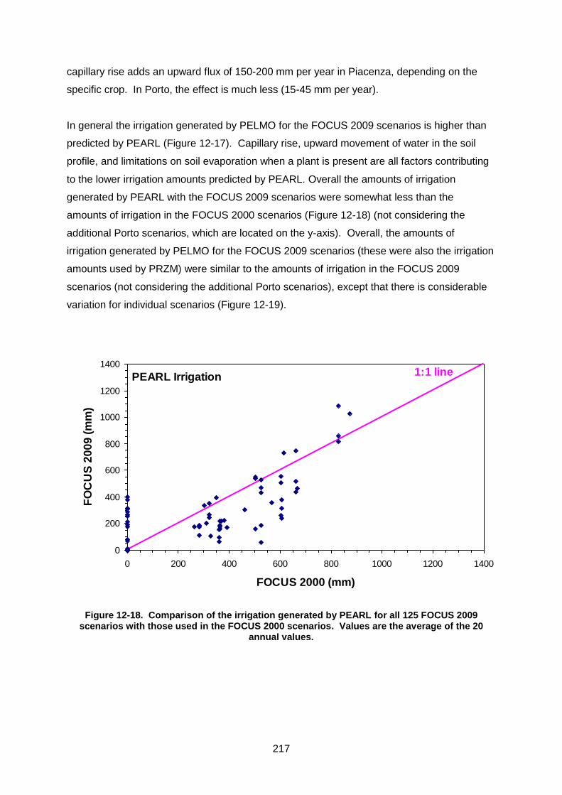
217
capillary rise adds an upward flux of 150-200 mm per year in Piacenza, depending on the
specific crop. In Porto, the effect is much less (15-45 mm per year).
In general the irrigation generated by PELMO for the FOCUS 2009 scenarios is higher than
predicted by PEARL (Figure 12-17). Capillary rise, upward movement of water in the soil
profile, and limitations on soil evaporation when a plant is present are all factors contributing
to the lower irrigation amounts predicted by PEARL. Overall the amounts of irrigation
generated by PEARL with the FOCUS 2009 scenarios were somewhat less than the
amounts of irrigation in the FOCUS 2000 scenarios (Figure 12-18) (not considering the
additional Porto scenarios, which are located on the y-axis). Overall, the amounts of
irrigation generated by PELMO for the FOCUS 2009 scenarios (these were also the irrigation
amounts used by PRZM) were similar to the amounts of irrigation in the FOCUS 2009
scenarios (not considering the additional Porto scenarios), except that there is considerable
variation for individual scenarios (Figure 12-19).
0
200
400
600
800
1000
1200
1400
0 200 400 600 800 1000 1200 1400
FOCUS 2000 (mm)
FO
CU
S 2
00
9 (
mm
)
1:1 linePEARL Irrigation
Figure 12-18. Comparison of the irrigation generated by PEARL for all 125 FOCUS 2009 scenarios with those used in the FOCUS 2000 scenarios. Values are the average of the 20
annual values.
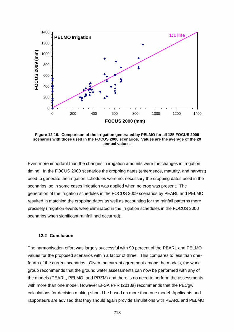
218
0
200
400
600
800
1000
1200
1400
0 200 400 600 800 1000 1200 1400
FOCUS 2000 (mm)
FO
CU
S 2
00
9 (
mm
)1:1 linePELMO Irrigation
Figure 12-19. Comparison of the irrigation generated by PELMO for all 125 FOCUS 2009 scenarios with those used in the FOCUS 2000 scenarios. Values are the average of the 20
annual values.
Even more important than the changes in irrigation amounts were the changes in irrigation
timing. In the FOCUS 2000 scenarios the cropping dates (emergence, maturity, and harvest)
used to generate the irrigation schedules were not necessary the cropping dates used in the
scenarios, so in some cases irrigation was applied when no crop was present. The
generation of the irrigation schedules in the FOCUS 2009 scenarios by PEARL and PELMO
resulted in matching the cropping dates as well as accounting for the rainfall patterns more
precisely (irrigation events were eliminated in the irrigation schedules in the FOCUS 2000
scenarios when significant rainfall had occurred).
12.2 Conclusion
The harmonisation effort was largely successful with 90 percent of the PEARL and PELMO
values for the proposed scenarios within a factor of three. This compares to less than one-
fourth of the current scenarios. Given the current agreement among the models, the work
group recommends that the ground water assessments can now be performed with any of
the models (PEARL, PELMO, and PRZM) and there is no need to perform the assessments
with more than one model. However EFSA PPR (2013a) recommends that the PECgw
calculations for decision making should be based on more than one model. Applicants and
rapporteurs are advised that they should again provide simulations with PEARL and PELMO
219
or PRZM. Where a crop of interest is defined for Châteaudun, MACRO simulations need to
be run. (EFSA PPR, 2013a).
12.3 References
EFSA Panel on Plant Protection Products and their Residues (PPR) 2013a; Scientific
Opinion on the report of the FOCUS groundwater working group (FOCUS, 2009):
assessment of lower tiers. EFSA Journal 2013;11(2):3114. [29 pp.]
doi:10.2903/j.efsa.2013.3114. Available online: www.efsa.europa.eu/efsajournal
FOCUS. 2000. FOCUS groundwater scenarios in the EU review of active substances.
Report of the FOCUS Groundwater Scenarios Workgroup, EC Document Reference
Sanco/321/2000 rev.2, 202pp.
Jones, R.L., Boesten, J.J.T.I., Klein, M. and van den Berg, E. (2011) Performance of the
FOCUS 2010 Software packages for performing Tier 1 Ground Water Assessments in the
EU, 26 pp.
220
13 APPLICABILITY OF FOCUS GROUND WATER SCENARIOS TO
THE NEW MEMBER STATES
13.1 Introduction
13.1.1 Objective of this study
In 2000 the first FOCUS groundwater group defined a set of 125 leaching scenarios that
represent collectively major agricultural areas in the EU before May 1, 2004. The general
approach for establishing the scenarios was to select locations in major agricultural areas
that covered the diversity of EU agriculture (FOCUS, 2000). With the accession of ten in
additional countries in 2004 (and more recently two additional countries) the applicability of
present FOCUS leaching scenarios to the extended agricultural area of the EU after 2004
must be assessed.
This chapter aims to provide a first assessment of the applicability of existing FOCUS
scenarios to New Member Countries (NMC). After the selection of appropriate data layers a
first classification of Europe according to the definition of FOCUS (2000) is given. Due to
several limitations of this rather general classification scheme a more detailed analysis based
on climate and soil properties of the existing nine locations is deemed appropriate before
drawing a final conclusion about the applicability of current scenario to NMCs. This refined
assessment consists of three steps:
1) Identification of spatial indicators to express the applicability of a scenario 2) Visualisation of the spatial extent of each scenario 3) Identification of missing areas
13.1.2 Limitations
The FOCUS leaching scenarios represent collectively major agricultural areas and a broad
range of crops. As a consequence the scenarios do not represent a specified worst-case
percentile for a particular country or pesticide. For that reason the approach presented in
this chapter differs from other approaches that are outlined in Section 7.2.5 and Appendices
4 and 5 in this report.
This chapter assesses whether the existing set of FOCUS scenarios ‘covers’ the agricultural
area of new member countries. A scenario ‘covers’ an area when it represents either the
same properties or represents a more vulnerable situation like higher rainfall amounts or
lower organic carbon contents. This chapter does not attempt to quantify the exact percentile
221
of vulnerability in new member states that is covered by each scenario since such a target
requires crop- and compound-specific GIS methods.
13.2 Materials and methods
13.2.1 Data sources
13.2.1.1 Climate data
The result of any spatial analysis with regional climate data is affected by the nature of the
underlying data. For that reason two data sets were tested with regard to their applicability in
this study. Both data bases cover the area of interest to a sufficient extent and allow for
conclusions on the general weather pattern. Details of the data bases are given in Appendix
8.
(A) Global climate data 1960 – 1990, Intergovernmental Panel on Climate Change, United
Nations Environment Program (= IPCC, 2004)
(B) Interpolated Meteorological Data 1992 – 2002, JRC MARS Database – EU Commission,
JRC (= MARS, 2004)
The MARS weather data base contains more recent weather data from approximately
1500 weather stations. Point data were interpolated to a 50 x 50 km grid and covers
most of the area of the EU. All weather parameters are reported as daily values and
originate exclusively from weather stations that are located in agricultural areas. Note
that a small number of grid cells in Scandinavia and Estonia do not contain data for the
entire period of 11 years.
Note that both data sets contain interpolated data from selected weather stations; in this
way both data bases are subject to errors. Nevertheless, conclusions can be drawn about
the applicability of each data base for the purpose of this assessment. The differences
between both data bases and its implications for leaching assessments is summarised in
Table 13-1.
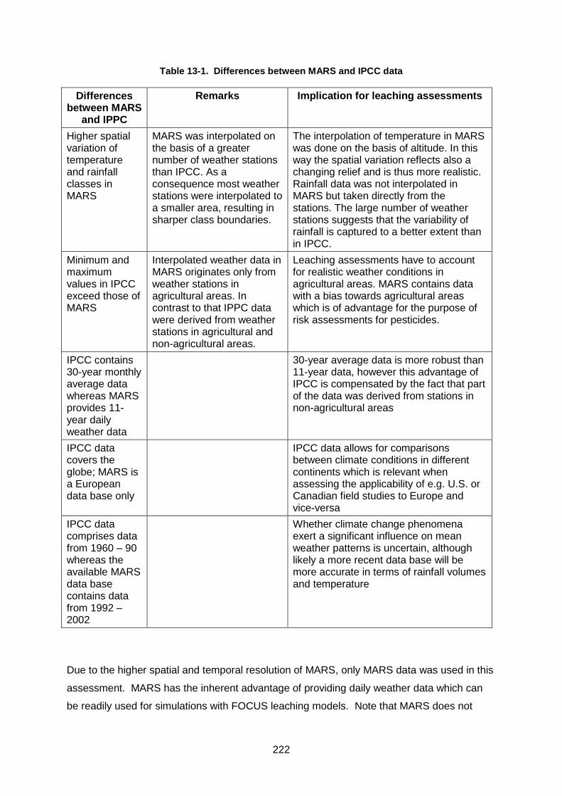
222
Table 13-1. Differences between MARS and IPCC data
Differences between MARS
and IPPC
Remarks Implication for leaching assessments
Higher spatial variation of temperature and rainfall classes in MARS
MARS was interpolated on the basis of a greater number of weather stations than IPCC. As a consequence most weather stations were interpolated to a smaller area, resulting in sharper class boundaries.
The interpolation of temperature in MARS was done on the basis of altitude. In this way the spatial variation reflects also a changing relief and is thus more realistic. Rainfall data was not interpolated in MARS but taken directly from the stations. The large number of weather stations suggests that the variability of rainfall is captured to a better extent than in IPCC.
Minimum and maximum values in IPCC exceed those of MARS
Interpolated weather data in MARS originates only from weather stations in agricultural areas. In contrast to that IPPC data were derived from weather stations in agricultural and non-agricultural areas.
Leaching assessments have to account for realistic weather conditions in agricultural areas. MARS contains data with a bias towards agricultural areas which is of advantage for the purpose of risk assessments for pesticides.
IPCC contains 30-year monthly average data whereas MARS provides 11-year daily weather data
30-year average data is more robust than 11-year data, however this advantage of IPCC is compensated by the fact that part of the data was derived from stations in non-agricultural areas
IPCC data covers the globe; MARS is a European data base only
IPCC data allows for comparisons between climate conditions in different continents which is relevant when assessing the applicability of e.g. U.S. or Canadian field studies to Europe and vice-versa
IPCC data comprises data from 1960 – 90 whereas the available MARS data base contains data from 1992 – 2002
Whether climate change phenomena exert a significant influence on mean weather patterns is uncertain, although likely a more recent data base will be more accurate in terms of rainfall volumes and temperature
Due to the higher spatial and temporal resolution of MARS, only MARS data was used in this
assessment. MARS has the inherent advantage of providing daily weather data which can
be readily used for simulations with FOCUS leaching models. Note that MARS does not
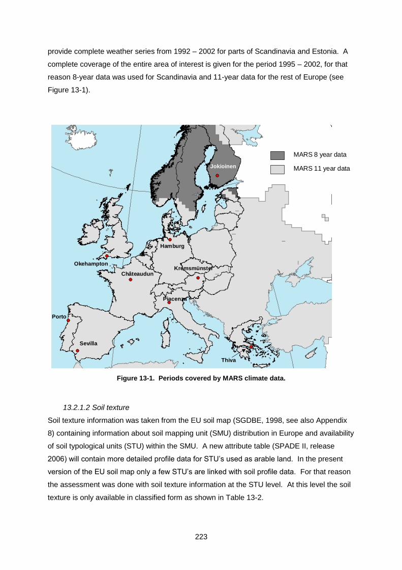
223
provide complete weather series from 1992 – 2002 for parts of Scandinavia and Estonia. A
complete coverage of the entire area of interest is given for the period 1995 – 2002, for that
reason 8-year data was used for Scandinavia and 11-year data for the rest of Europe (see
Figure 13-1).
MARS 8 year data
MARS 11 year dataJokioinen
Kremsmünster
Hamburg
Thiva
Piacenza
Châteaudun
Okehampton
Porto
Sevilla
Figure 13-1. Periods covered by MARS climate data.
13.2.1.2 Soil texture
Soil texture information was taken from the EU soil map (SGDBE, 1998, see also Appendix
8) containing information about soil mapping unit (SMU) distribution in Europe and availability
of soil typological units (STU) within the SMU. A new attribute table (SPADE II, release
2006) will contain more detailed profile data for STU’s used as arable land. In the present
version of the EU soil map only a few STU’s are linked with soil profile data. For that reason
the assessment was done with soil texture information at the STU level. At this level the soil
texture is only available in classified form as shown in Table 13-2.
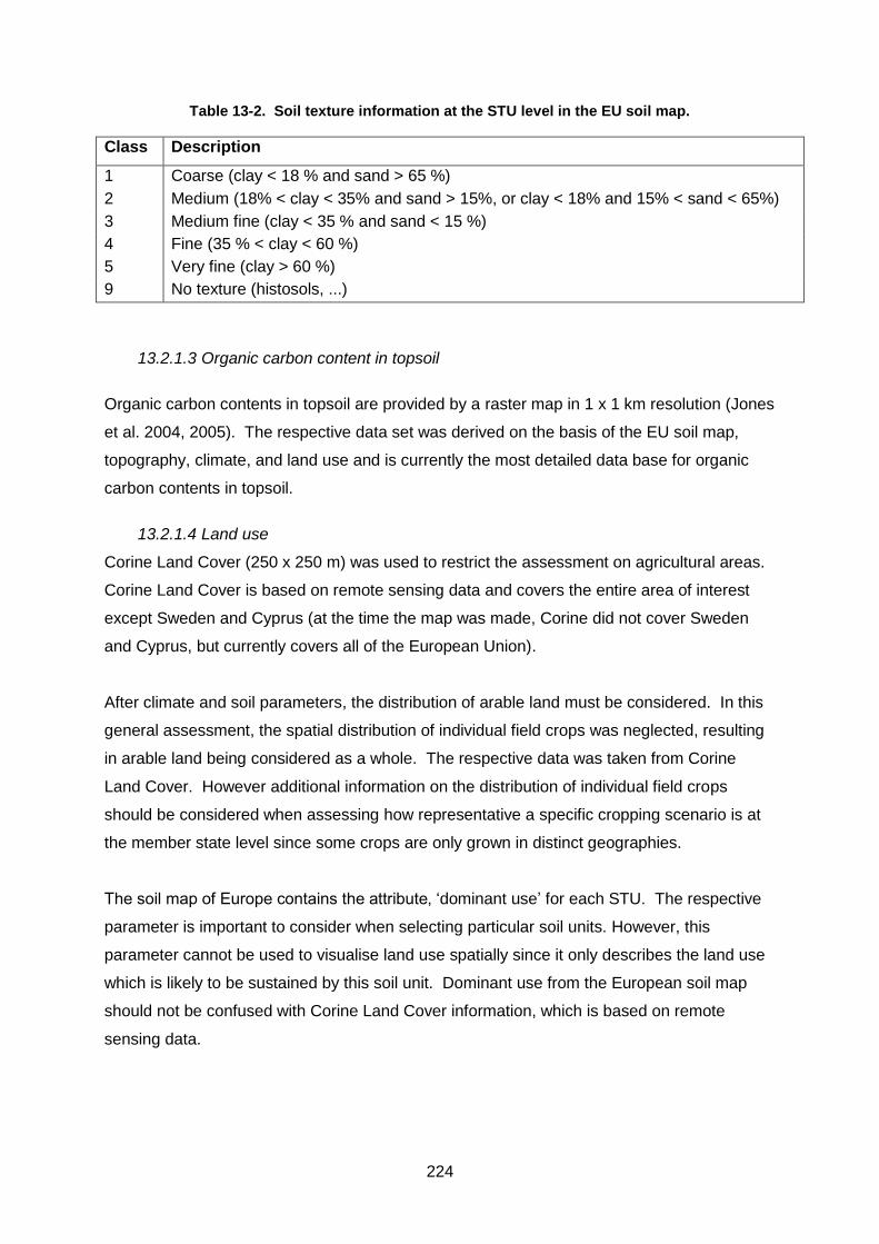
224
Table 13-2. Soil texture information at the STU level in the EU soil map.
Class Description
1 Coarse (clay < 18 % and sand > 65 %)
2 Medium (18% < clay < 35% and sand > 15%, or clay < 18% and 15% < sand < 65%)
3 Medium fine (clay < 35 % and sand < 15 %)
4 Fine (35 % < clay < 60 %)
5 Very fine (clay > 60 %)
9 No texture (histosols, ...)
13.2.1.3 Organic carbon content in topsoil
Organic carbon contents in topsoil are provided by a raster map in 1 x 1 km resolution (Jones
et al. 2004, 2005). The respective data set was derived on the basis of the EU soil map,
topography, climate, and land use and is currently the most detailed data base for organic
carbon contents in topsoil.
13.2.1.4 Land use
Corine Land Cover (250 x 250 m) was used to restrict the assessment on agricultural areas.
Corine Land Cover is based on remote sensing data and covers the entire area of interest
except Sweden and Cyprus (at the time the map was made, Corine did not cover Sweden
and Cyprus, but currently covers all of the European Union).
After climate and soil parameters, the distribution of arable land must be considered. In this
general assessment, the spatial distribution of individual field crops was neglected, resulting
in arable land being considered as a whole. The respective data was taken from Corine
Land Cover. However additional information on the distribution of individual field crops
should be considered when assessing how representative a specific cropping scenario is at
the member state level since some crops are only grown in distinct geographies.
The soil map of Europe contains the attribute‚ ‘dominant use’ for each STU. The respective
parameter is important to consider when selecting particular soil units. However, this
parameter cannot be used to visualise land use spatially since it only describes the land use
which is likely to be sustained by this soil unit. Dominant use from the European soil map
should not be confused with Corine Land Cover information, which is based on remote
sensing data.
225
13.2.2 Original classification of agricultural zones by FOCUS (2000)
13.2.2.1 Climate
The FOCUS groundwater group defined nine climate regions, which represent the majority of
arable land in the EU. Note that the selected scenario locations are ‘virtual’ scenarios. As a
part of the process for defining scenarios, target values for mean annual rainfall and
temperature were set by the FOCUS group. To achieve these target values some weather
scenarios were scaled up to reach the desired target volume for rainfall in the defined
agricultural region. For the same reason a lower rainfall volume was assigned to other
scenarios. The practical implication of this pragmatic procedure was that original MARS
rainfall data did not match the assigned target rainfall volume at the scenario location; in
other words, some scenarios represent a climate which is not found at the scenario location
but in other major agricultural areas.
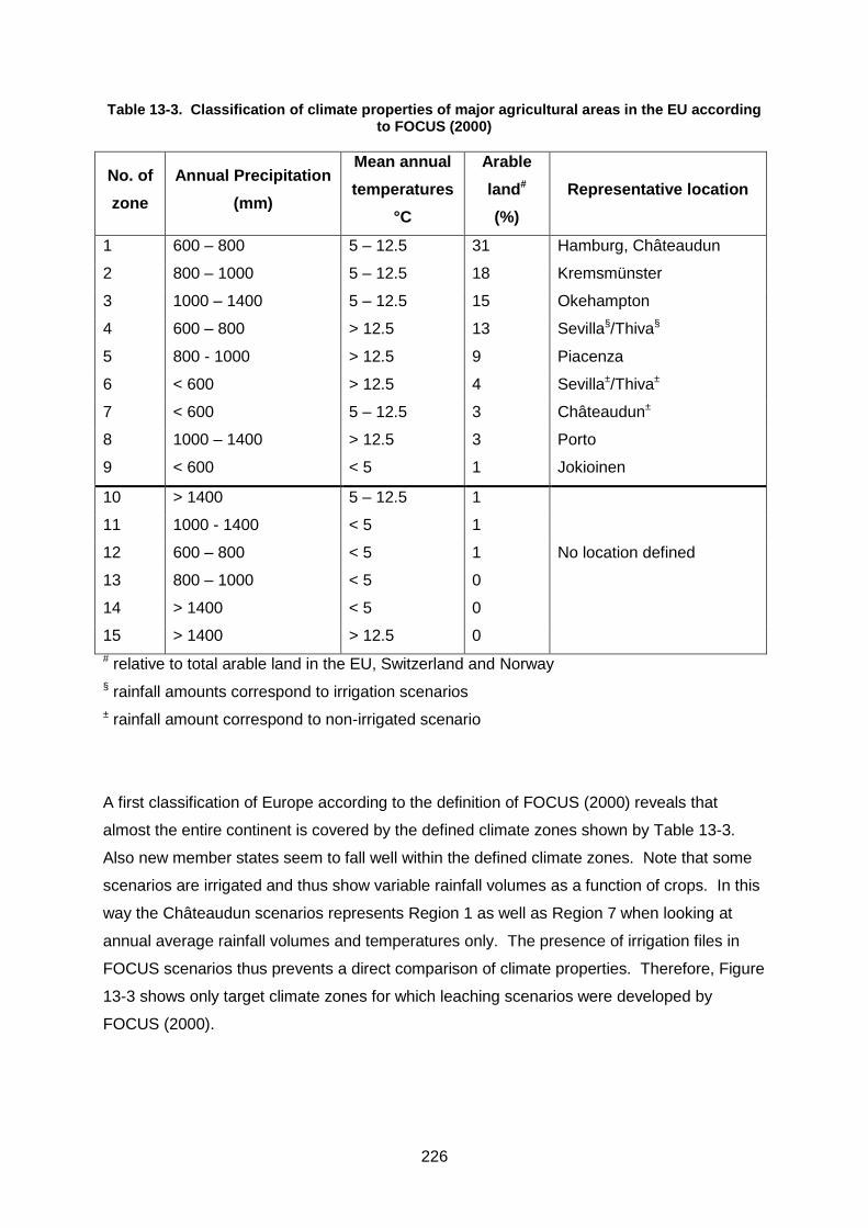
226
Table 13-3. Classification of climate properties of major agricultural areas in the EU according to FOCUS (2000)
No. of
zone
Annual Precipitation
(mm)
Mean annual
temperatures
°C
Arable
land#
(%)
Representative location
1 600 – 800 5 – 12.5 31 Hamburg, Châteaudun
2 800 – 1000 5 – 12.5 18 Kremsmünster
3 1000 – 1400 5 – 12.5 15 Okehampton
4 600 – 800 > 12.5 13 Sevilla§/Thiva§
5 800 - 1000 > 12.5 9 Piacenza
6 < 600 > 12.5 4 Sevilla±/Thiva±
7 < 600 5 – 12.5 3 Châteaudun±
8 1000 – 1400 > 12.5 3 Porto
9 < 600 < 5 1 Jokioinen
10 > 1400 5 – 12.5 1
11 1000 - 1400 < 5 1
12 600 – 800 < 5 1 No location defined
13 800 – 1000 < 5 0
14 > 1400 < 5 0
15 > 1400 > 12.5 0
# relative to total arable land in the EU, Switzerland and Norway
§ rainfall amounts correspond to irrigation scenarios
± rainfall amount correspond to non-irrigated scenario
A first classification of Europe according to the definition of FOCUS (2000) reveals that
almost the entire continent is covered by the defined climate zones shown by Table 13-3.
Also new member states seem to fall well within the defined climate zones. Note that some
scenarios are irrigated and thus show variable rainfall volumes as a function of crops. In this
way the Châteaudun scenarios represents Region 1 as well as Region 7 when looking at
annual average rainfall volumes and temperatures only. The presence of irrigation files in
FOCUS scenarios thus prevents a direct comparison of climate properties. Therefore, Figure
13-3 shows only target climate zones for which leaching scenarios were developed by
FOCUS (2000).
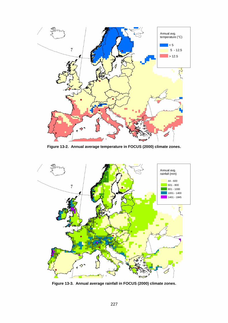
227
Annual avg.temperature (°C)
< 5
5 - 12.5
> 12.5
Figure 13-2. Annual average temperature in FOCUS (2000) climate zones.
Annual avg.rainfall (mm)
44 - 600
601 - 800
801 - 1000
1001 - 1400
1401 - 1845
Figure 13-3. Annual average rainfall in FOCUS (2000) climate zones.
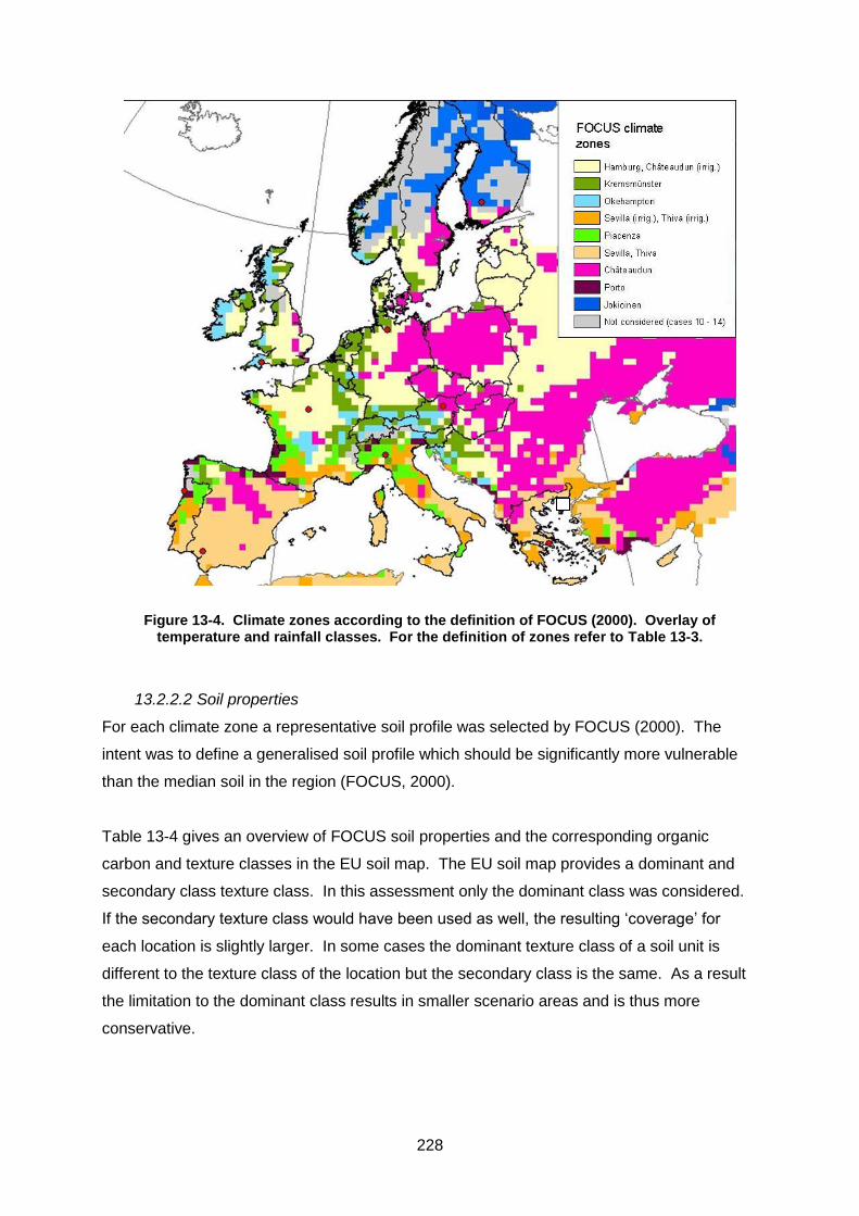
228
Figure 13-4. Climate zones according to the definition of FOCUS (2000). Overlay of
temperature and rainfall classes. For the definition of zones refer to Table 13-3.
13.2.2.2 Soil properties
For each climate zone a representative soil profile was selected by FOCUS (2000). The
intent was to define a generalised soil profile which should be significantly more vulnerable
than the median soil in the region (FOCUS, 2000).
Table 13-4 gives an overview of FOCUS soil properties and the corresponding organic
carbon and texture classes in the EU soil map. The EU soil map provides a dominant and
secondary class texture class. In this assessment only the dominant class was considered.
If the secondary texture class would have been used as well, the resulting ‘coverage’ for
each location is slightly larger. In some cases the dominant texture class of a soil unit is
different to the texture class of the location but the secondary class is the same. As a result
the limitation to the dominant class results in smaller scenario areas and is thus more
conservative.
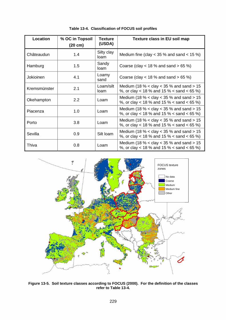
229
Table 13-4. Classification of FOCUS soil profiles
Location % OC in Topsoil
(20 cm)
Texture (USDA)
Texture class in EU soil map
Châteaudun 1.4 Silty clay loam
Medium fine (clay < 35 % and sand < 15 %)
Hamburg 1.5 Sandy loam
Coarse (clay < 18 % and sand > 65 %)
Jokioinen 4.1 Loamy sand
Coarse (clay < 18 % and sand > 65 %)
Kremsmünster 2.1 Loam/silt loam
Medium (18 % < clay < 35 % and sand > 15 %, or clay < 18 % and 15 % < sand < 65 %)
Okehampton 2.2 Loam Medium (18 % < clay < 35 % and sand > 15 %, or clay < 18 % and 15 % < sand < 65 %)
Piacenza 1.0 Loam Medium (18 % < clay < 35 % and sand > 15 %, or clay < 18 % and 15 % < sand < 65 %)
Porto 3.8 Loam Medium (18 % < clay < 35 % and sand > 15 %, or clay < 18 % and 15 % < sand < 65 %)
Sevilla 0.9 Silt loam Medium (18 % < clay < 35 % and sand > 15 %, or clay < 18 % and 15 % < sand < 65 %)
Thiva 0.8 Loam Medium (18 % < clay < 35 % and sand > 15 %, or clay < 18 % and 15 % < sand < 65 %)
FOCUS texture
zones
No data
Coarse
Medium
Medium fine
Other
FOCUS texture
zones
No data
Coarse
Medium
Medium fine
Other
Figure 13-5. Soil texture classes according to FOCUS (2000). For the definition of the classes
refer to Table 13-4.
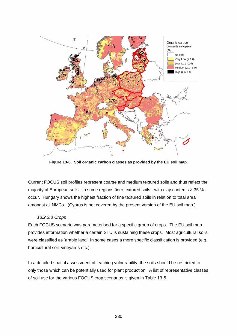
230
Organic carboncontents in topsoil
(%)
No data
Very Low (< 1.0)
Low (1.1 - 2.0)
Medium (2.1 - 6.0)
High (> 6.0 %
Figure 13-6. Soil organic carbon classes as provided by the EU soil map.
Current FOCUS soil profiles represent coarse and medium textured soils and thus reflect the
majority of European soils. In some regions finer textured soils - with clay contents > 35 % -
occur. Hungary shows the highest fraction of fine textured soils in relation to total area
amongst all NMCs. (Cyprus is not covered by the present version of the EU soil map.)
13.2.2.3 Crops
Each FOCUS scenario was parameterised for a specific group of crops. The EU soil map
provides information whether a certain STU is sustaining these crops. Most agricultural soils
were classified as ‘arable land’. In some cases a more specific classification is provided (e.g.
horticultural soil, vineyards etc.).
In a detailed spatial assessment of leaching vulnerability, the soils should be restricted to
only those which can be potentially used for plant production. A list of representative classes
of soil use for the various FOCUS crop scenarios is given in Table 13-5.
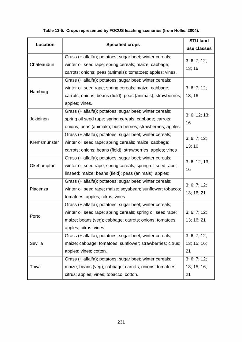
231
Table 13-5. Crops represented by FOCUS leaching scenarios (from Hollis, 2004).
Location Specified crops STU land
use classes
Châteaudun
Grass (+ alfalfa); potatoes; sugar beet; winter cereals;
winter oil seed rape; spring cereals; maize; cabbage;
carrots; onions; peas (animals); tomatoes; apples; vines.
3; 6; 7; 12;
13; 16
Hamburg
Grass (+ alfalfa); potatoes; sugar beet; winter cereals;
winter oil seed rape; spring cereals; maize; cabbage;
carrots; onions; beans (field); peas (animals); strawberries;
apples; vines.
3; 6; 7; 12;
13; 16
Jokioinen
Grass (+ alfalfa); potatoes; sugar beet; winter cereals;
spring oil seed rape; spring cereals; cabbage; carrots;
onions; peas (animals); bush berries; strawberries; apples.
3; 6; 12; 13;
16
Kremsmünster
Grass (+ alfalfa); potatoes; sugar beet; winter cereals;
winter oil seed rape; spring cereals; maize; cabbage;
carrots; onions; beans (field); strawberries; apples; vines
3; 6; 7; 12;
13; 16
Okehampton
Grass (+ alfalfa); potatoes; sugar beet; winter cereals;
winter oil seed rape; spring cereals; spring oil seed rape;
linseed; maize; beans (field); peas (animals); apples;
3; 6; 12; 13;
16
Piacenza
Grass (+ alfalfa); potatoes; sugar beet; winter cereals;
winter oil seed rape; maize; soyabean; sunflower; tobacco;
tomatoes; apples; citrus; vines
3; 6; 7; 12;
13; 16; 21
Porto
Grass (+ alfalfa); potatoes; sugar beet; winter cereals;
winter oil seed rape; spring cereals; spring oil seed rape;
maize; beans (veg); cabbage; carrots; onions; tomatoes;
apples; citrus; vines
3; 6; 7; 12;
13; 16; 21
Sevilla
Grass (+ alfalfa); potatoes; sugar beet; winter cereals;
maize; cabbage; tomatoes; sunflower; strawberries; citrus;
apples; vines; cotton.
3; 6; 7; 12;
13; 15; 16;
21
Thiva
Grass (+ alfalfa); potatoes; sugar beet; winter cereals;
maize; beans (veg); cabbage; carrots; onions; tomatoes;
citrus; apples; vines; tobacco; cotton.
3; 6; 7; 12;
13; 15; 16;
21
232
13.2.3 Criteria used for the assessment of scenarios
In a strict sense each crop would require a separate assessment of worst-case weather
properties under which it can potentially be grown. The methods presented in this paper
nevertheless neglect the spatial distribution of individual crops in an attempt to provide a
generic assessment of climate and soil properties in NMCs with respect to current FOCUS
leaching scenarios.
The assessment was carried out on the basis of 20-year weather series that were compiled
for existing FOCUS leaching scenarios. From these weather series a ‘worst-case’ and a
‘best case’ weather year can be extracted by means of the following criteria:
The year in which the highest rainfall volume coincides with the lowest temperature is
defined as the worst-case weather year. The respective combination of rainfall and
temperature sets the upper boundary of climate vulnerability that is represented by
the scenario.
The year in which the lowest rainfall volume coincides with the highest temperature is
defined as the best-case weather year. The respective combination of rainfall and
temperature sets the lower boundary of climate vulnerability that is represented by the
scenario.
Note that only existing combinations of temperature and rainfall were assessed. This method
avoids the use the global maximum rainfall and global minimum temperature when this
combination did not occur during the same year.
Upper and lower boundaries of climate vulnerability were subsequently used to visualise
cropping areas which fall into the same climate zone. The spatial query identifies all cells
where the combination of average temperatures and rainfall sums is between the upper and
lower boundaries for the given scenario. The respective boundary values are given in Table
13-6.
As a refinement of the original definition of FOCUS only rainfall volumes between October
and March where considered. This approach is based on the following rationale:
Ground water recharge is most likely occurring outside the vegetation period when
evapotranspiration is low and soil moisture is close to saturation. Northern European
soils are typically saturated after autumn rainfalls and again at the end of winter
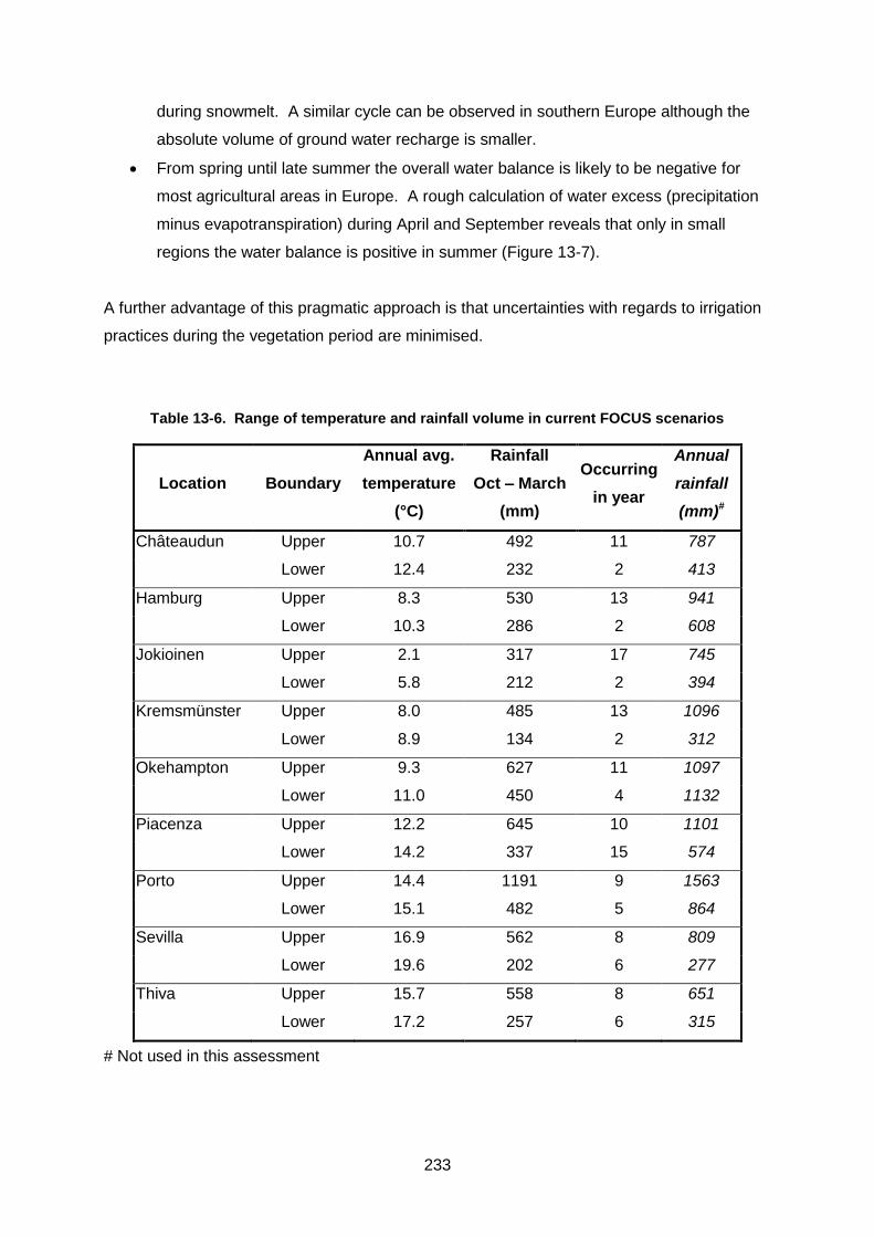
233
during snowmelt. A similar cycle can be observed in southern Europe although the
absolute volume of ground water recharge is smaller.
From spring until late summer the overall water balance is likely to be negative for
most agricultural areas in Europe. A rough calculation of water excess (precipitation
minus evapotranspiration) during April and September reveals that only in small
regions the water balance is positive in summer (Figure 13-7).
A further advantage of this pragmatic approach is that uncertainties with regards to irrigation
practices during the vegetation period are minimised.
Table 13-6. Range of temperature and rainfall volume in current FOCUS scenarios
Location Boundary
Annual avg.
temperature
(°C)
Rainfall
Oct – March
(mm)
Occurring
in year
Annual
rainfall
(mm)#
Châteaudun Upper 10.7 492 11 787
Lower 12.4 232 2 413
Hamburg Upper 8.3 530 13 941
Lower 10.3 286 2 608
Jokioinen Upper 2.1 317 17 745
Lower 5.8 212 2 394
Kremsmünster Upper 8.0 485 13 1096
Lower 8.9 134 2 312
Okehampton Upper 9.3 627 11 1097
Lower 11.0 450 4 1132
Piacenza Upper 12.2 645 10 1101
Lower 14.2 337 15 574
Porto Upper 14.4 1191 9 1563
Lower 15.1 482 5 864
Sevilla Upper 16.9 562 8 809
Lower 19.6 202 6 277
Thiva Upper 15.7 558 8 651
Lower 17.2 257 6 315
# Not used in this assessment
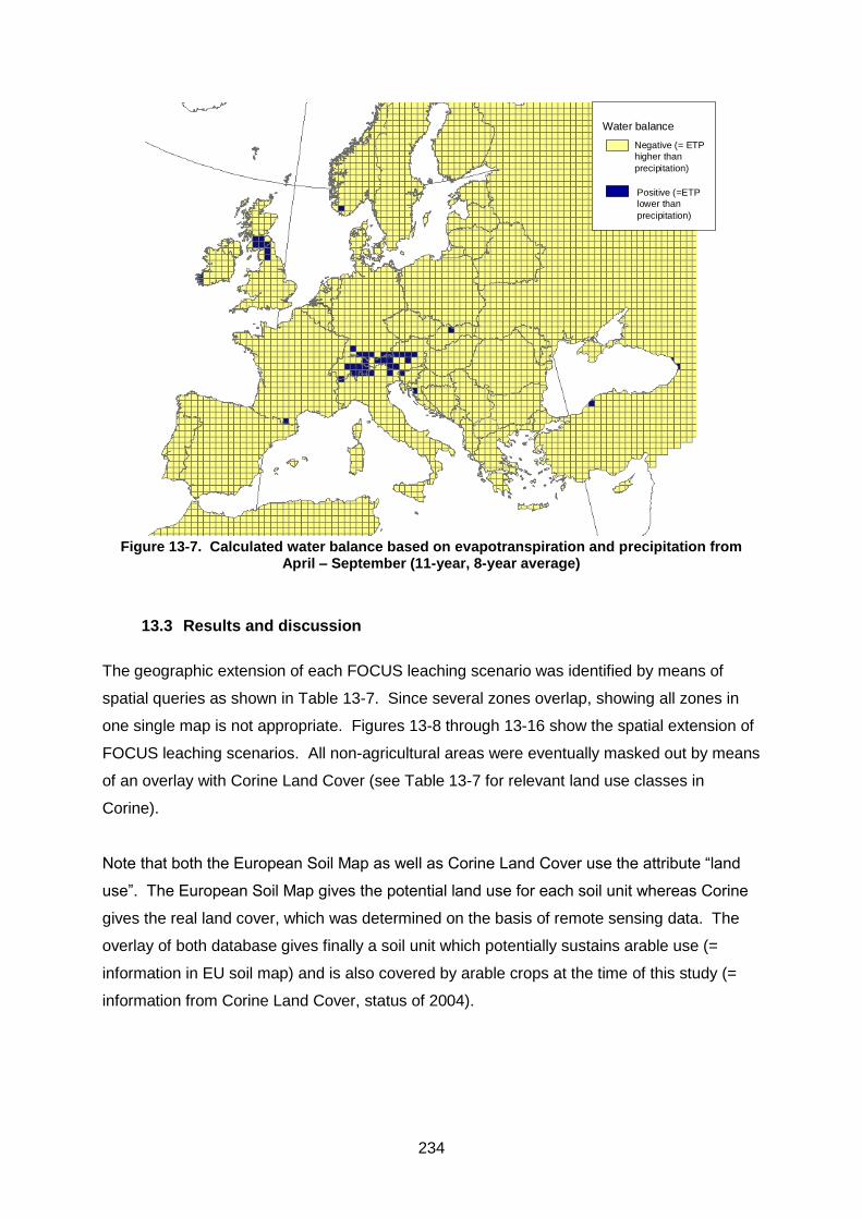
234
Water balance
Negative (= ETP
higher than
precipitation)
Positive (=ETP
lower than
precipitation)
Figure 13-7. Calculated water balance based on evapotranspiration and precipitation from
April – September (11-year, 8-year average)
13.3 Results and discussion
The geographic extension of each FOCUS leaching scenario was identified by means of
spatial queries as shown in Table 13-7. Since several zones overlap, showing all zones in
one single map is not appropriate. Figures 13-8 through 13-16 show the spatial extension of
FOCUS leaching scenarios. All non-agricultural areas were eventually masked out by means
of an overlay with Corine Land Cover (see Table 13-7 for relevant land use classes in
Corine).
Note that both the European Soil Map as well as Corine Land Cover use the attribute “land
use”. The European Soil Map gives the potential land use for each soil unit whereas Corine
gives the real land cover, which was determined on the basis of remote sensing data. The
overlay of both database gives finally a soil unit which potentially sustains arable use (=
information in EU soil map) and is also covered by arable crops at the time of this study (=
information from Corine Land Cover, status of 2004).
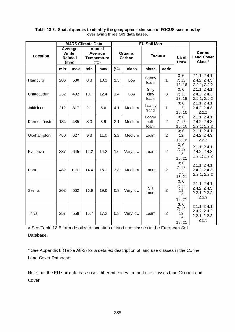
235
Table 13-7. Spatial queries to identify the geographic extension of FOCUS scenarios by overlaying three GIS data bases.
Location
MARS Climate Data EU Soil Map
Corine Land Cover
Class*
Average Winter Rainfall
(mm)
Annual Average
Temperature (°C)
Organic Carbon
Texture Land Use#
min max min max (%) class class code
Hamburg 286 530 8.3 10.3 1.5 Low Sandy loam
1 3; 6;
7; 12; 13; 16
2.1.1; 2.4.1; 2.4.2; 2.4.3; 2.2.1; 2.2.2
Châteaudun 232 492 10.7 12.4 1.4 Low Silty clay loam
3 3; 6;
7; 12; 13; 16
2.1.1; 2.4.1; 2.4.2; 2.4.3; 2.2.1; 2.2.2
Jokioinen 212 317 2.1 5.8 4.1 Medium Loamy sand
1 3; 6; 12;
13; 16
2.1.1; 2.4.1; 2.4.2; 2.4.3;
2.2.2
Kremsmünster 134 485 8.0 8.9 2.1 Medium Loam/
silt loam
2 3; 6;
7; 12; 13; 16
2.1.1; 2.4.1; 2.4.2; 2.4.3; 2.2.1; 2.2.2
Okehampton 450 627 9.3 11.0 2.2 Medium Loam 2 3; 6; 12;
13; 16
2.1.1; 2.4.1; 2.4.2; 2.4.3;
2.2.2
Piacenza 337 645 12.2 14.2 1.0 Very low Loam 2
3; 6; 7; 12;
13; 16; 21
2.1.1; 2.4.1; 2.4.2; 2.4.3; 2.2.1; 2.2.2
Porto 482 1191 14.4 15.1 3.8 Medium Loam 2
3; 6; 7; 12;
13; 16; 21
2.1.1; 2.4.1; 2.4.2; 2.4.3; 2.2.1; 2.2.2
Sevilla 202 562 16.9 19.6 0.9 Very low Silt
Loam 2
3; 6; 7; 12;
13; 15;
16; 21
2.1.1; 2.4.1; 2.4.2; 2.4.3; 2.2.1; 2.2.2;
2.2.3
Thiva 257 558 15.7 17.2 0.8 Very low Loam 2
3; 6; 7; 12;
13; 15;
16; 21
2.1.1; 2.4.1; 2.4.2; 2.4.3; 2.2.1; 2.2.2;
2.2.3
# See Table 13-5 for a detailed description of land use classes in the European Soil
Database.
* See Appendix 8 (Table A8-2) for a detailed description of land use classes in the Corine
Land Cover Database.
Note that the EU soil data base uses different codes for land use classes than Corine Land
Cover.
236
The spatial queries are illustrated in the example for Châteaudun. This location ‘covers’ all
areas in new member countries that comply with the following criteria:
Average rainfall amounts and temperatures are between the worst and best weather
year in Châteaudun. The best-case year had 232 mm winter rainfall and a
temperature of 12.4 °C, the worst-case year had 492 mm winter rainfall and 10.7 °C
temperature. All areas where such conditions occurred between 1992 and 2002 (the
time series available in MARS) are classified as ‘climate zone Châteaudun’.
The content of organic carbon is 1.4 % or higher and soil texture class is 3 or higher
(finer textured). All areas that comply with these criteria are classified as ‘soil region
Châteaudun’. Note that only soils with agricultural land use were considered.
Any area where the climate zone and soil region Châteaudun co-occur is classified as
‘scenario area Châteaudun’
13.3.1 Coverage of Accession countries by existing FOCUS scenarios
13.3.1.1 Estonia
The Jokioinen location represents well Estonian climate conditions. Prevailing low
temperatures sustain high organic carbon contents in topsoils, which are reflected in a similar
way by the Jokioinen scenarios.
13.3.1.2 Latvia
A similar conclusion as for Estonia applies to Latvia. Soils with very high contents in organic
matter are frequent although cover a slightly smaller fraction of arable land than in Estonia.
For that reason more soil units appear to be similar rather than less vulnerable than
Jokioinen.
13.3.1.3 Lithuania
The climate of northern Lithuania is still similar to Jokioinen and most soils have either similar
or less vulnerable soil properties. The larger part of the country is however warmer and
therefore better represented by Hamburg and Kremsmünster climate. The more humid
Hamburg climate is most representative for regions close to the Baltic Sea. Some areas
which are influenced by more continental climate conditions are dryer than ‘Hamburg’ but
show coarser textured soils or lower organic carbon contents than e.g. the ‘Kremsmünster’
scenarios. For that reason the ‘Hamburg’ scenarios should be assessed to determine
whether they are sufficiently conservative to cover also those areas which have a different
rainfall regime but a similar coarse texture.

237
13.3.1.4 Poland
Coarse textured soils are primarily found in the northern part of the country. This area shows
also very similar climate properties to Hamburg suggesting that this location represents
northern Poland to a sufficient extent. Large parts of Poland fall within the Kremsmünster
climate zone. Some areas are neither represented by Hamburg nor Kremsmünster, in most
cases because the prevailing soil types are coarser than ‘Kremsmünster’ soil or have a lower
organic carbon content.
13.3.1.5 Czech Republic
The majority of soils belong to a similar texture class like Kremsmünster. Also organic
carbon contents are in most cases similar to these scenarios. A few coarse textured soils
with less OC are well represented by the Hamburg scenarios. A small region in central
Bohemia and around Prague seems to have different soil characteristics than those of
Kremsmünster although its climate properties are closer to Kremsmünster than Hamburg.
13.3.1.6 Slovakia
The largest part of Slovakia is represented by Kremsmünster climate whereas Hamburg is
only representative for smaller areas. Similar conclusions as to Czech Republic apply to
Slovakia in terms of representativeness of Kremsmünster soil properties for some parts of
Slovak agriculture.
The southernmost part around Bratislava and along the Danube River belongs to a climate
zone represented by the Châteaudun. Also soil properties seem to be similar or less
vulnerable than this location.
13.3.1.7 Hungary
The EU soil map shows a high density of fine textured soils in Hungary. Organic carbon
contents are typically higher than 1.5 – 2 %. For that reason large parts of the country are
well represented by the soil in the Châteaudun scenarios. Also climate properties are very
similar to Châteaudun. None of the other locations seem to better represent Hungarian soil
and climate conditions.
13.3.1.8 Slovenia
Slovenia is located in a transitional climate which is closer to northern than southern
European weather conditions, although overall temperatures are at the upper boundary of
those found in northern Europe. Rainfall amounts in winter are close to amounts reflected by
the Okehampton, Hamburg, Kremsmünster, Châteaudun, and Piacenza scenarios. Annual
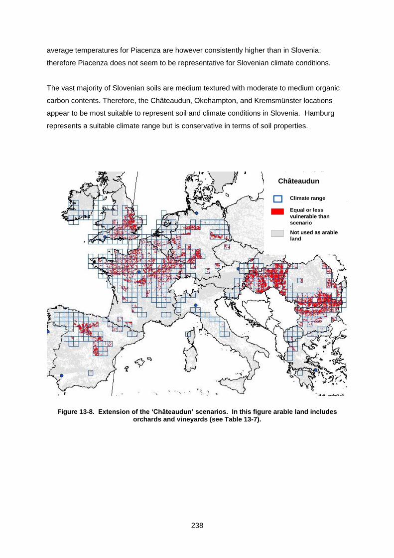
238
average temperatures for Piacenza are however consistently higher than in Slovenia;
therefore Piacenza does not seem to be representative for Slovenian climate conditions.
The vast majority of Slovenian soils are medium textured with moderate to medium organic
carbon contents. Therefore, the Châteaudun, Okehampton, and Kremsmünster locations
appear to be most suitable to represent soil and climate conditions in Slovenia. Hamburg
represents a suitable climate range but is conservative in terms of soil properties.
Châteaudun
Climate range
Equal or less
vulnerable than
scenario
Not used as arable
land
Figure 13-8. Extension of the ‘Châteaudun’ scenarios. In this figure arable land includes
orchards and vineyards (see Table 13-7).
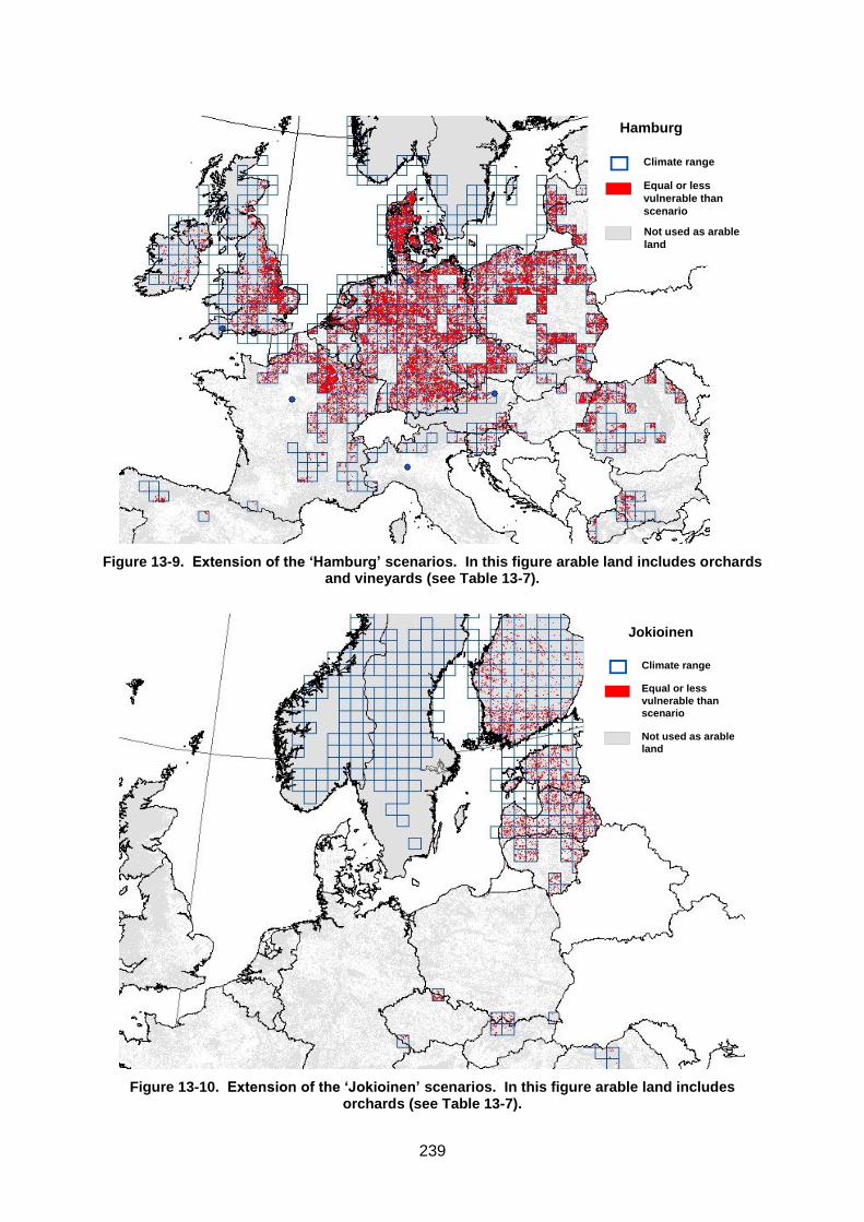
239
Hamburg
Climate range
Equal or less
vulnerable than
scenario
Not used as arable
land
Figure 13-9. Extension of the ‘Hamburg’ scenarios. In this figure arable land includes orchards and vineyards (see Table 13-7).
Climate range
Jokioinen
Equal or less
vulnerable than
scenario
Not used as arable
land
Figure 13-10. Extension of the ‘Jokioinen’ scenarios. In this figure arable land includes orchards (see Table 13-7).
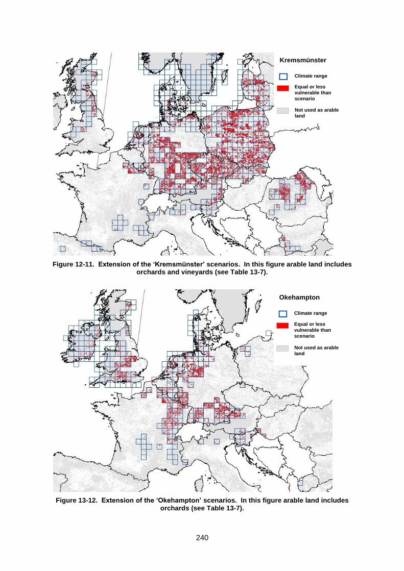
240
Climate range
Kremsmünster
Equal or less
vulnerable than
scenario
Not used as arable
land
Figure 12-11. Extension of the ‘Kremsmünster’ scenarios. In this figure arable land includes orchards and vineyards (see Table 13-7).
Climate range
Okehampton
Equal or less
vulnerable than
scenario
Not used as arable
land
Figure 13-12. Extension of the ‘Okehampton’ scenarios. In this figure arable land includes orchards (see Table 13-7).
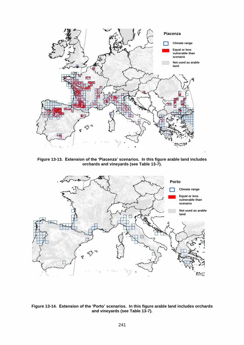
241
Climate range
Piacenza
Equal or less
vulnerable than
scenario
Not used as arable
land
Figure 13-13. Extension of the ‘Piacenza’ scenarios. In this figure arable land includes orchards and vineyards (see Table 13-7).
Climate range
Porto
Equal or less
vulnerable than
scenario
Not used as arable
land
Figure 13-14. Extension of the ‘Porto’ scenarios. In this figure arable land includes orchards and vineyards (see Table 13-7).
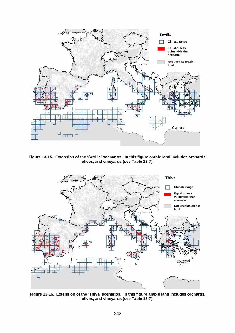
242
Climate range
Sevilla
Equal or less
vulnerable than
scenario
Not used as arable
land
Cyprus
Figure 13-15. Extension of the ‘Sevilla’ scenarios. In this figure arable land includes orchards, olives, and vineyards (see Table 13-7).
Climate range
Thiva
Equal or less
vulnerable than
scenario
Not used as arable
land
Figure 13-16. Extension of the ‘Thiva’ scenarios. In this figure arable land includes orchards, olives, and vineyards (see Table 13-7).
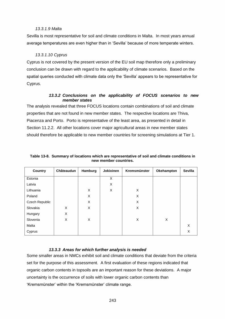
243
13.3.1.9 Malta
Sevilla is most representative for soil and climate conditions in Malta. In most years annual
average temperatures are even higher than in ‘Sevilla’ because of more temperate winters.
13.3.1.10 Cyprus
Cyprus is not covered by the present version of the EU soil map therefore only a preliminary
conclusion can be drawn with regard to the applicability of climate scenarios. Based on the
spatial queries conducted with climate data only the ‘Sevilla’ appears to be representative for
Cyprus.
13.3.2 Conclusions on the applicability of FOCUS scenarios to new member states
The analysis revealed that three FOCUS locations contain combinations of soil and climate
properties that are not found in new member states. The respective locations are Thiva,
Piacenza and Porto. Porto is representative of the least area, as presented in detail in
Section 11.2.2. All other locations cover major agricultural areas in new member states
should therefore be applicable to new member countries for screening simulations at Tier 1.
Table 13-8. Summary of locations which are representative of soil and climate conditions in new member countries.
Country Châteaudun Hamburg Jokioinen Kremsmünster Okehampton Sevilla
Estonia X
Latvia X
Lithuania X X X
Poland X X
Czech Republic X X
Slovakia X X X
Hungary X
Slovenia X X X X
Malta X
Cyprus X
13.3.3 Areas for which further analysis is needed
Some smaller areas in NMCs exhibit soil and climate conditions that deviate from the criteria
set for the purpose of this assessment. A first evaluation of these regions indicated that
organic carbon contents in topsoils are an important reason for these deviations. A major
uncertainty is the occurrence of soils with lower organic carbon contents than
‘Kremsmünster’ within the ‘Kremsmünster’ climate range.
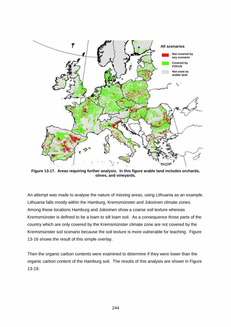
244
Not covered by
any scenario
Covered by
FOCUS
Not used as
arable land
All scenarios
Figure 13-17. Areas requiring further analysis. In this figure arable land includes orchards, olives, and vineyards.
An attempt was made to analyse the nature of missing areas, using Lithuania as an example.
Lithuania falls mostly within the Hamburg, Kremsmünster and Jokioinen climate zones.
Among these locations Hamburg and Jokioinen show a coarse soil texture whereas
Kremsmünster is defined to be a loam to silt loam soil. As a consequence those parts of the
country which are only covered by the Kremsmünster climate zone are not covered by the
Kremsmünster soil scenario because the soil texture is more vulnerable for leaching. Figure
13-16 shows the result of this simple overlay.
Then the organic carbon contents were examined to determine if they were lower than the
organic carbon content of the Hamburg soil. The results of this analysis are shown in Figure
13-19.
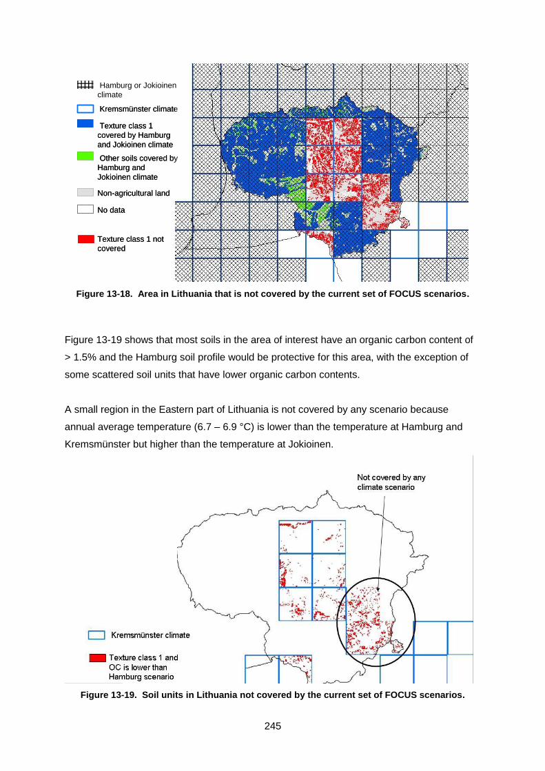
245
Kremsmünster climate
Hamburg or Jokioinen
climate
Texture class 1
covered by Hamburg
and Jokioinen climate
Other soils covered by
Hamburg and
Jokioinen climate
Non-agricultural land
No data
Texture class 1 not
covered
Kremsmünster climate
Hamburg or Jokioinen
climate
Texture class 1
covered by Hamburg
and Jokioinen climate
Other soils covered by
Hamburg and
Jokioinen climate
Non-agricultural land
No data
Texture class 1 not
covered
Figure 13-18. Area in Lithuania that is not covered by the current set of FOCUS scenarios.
Figure 13-19 shows that most soils in the area of interest have an organic carbon content of
> 1.5% and the Hamburg soil profile would be protective for this area, with the exception of
some scattered soil units that have lower organic carbon contents.
A small region in the Eastern part of Lithuania is not covered by any scenario because
annual average temperature (6.7 – 6.9 °C) is lower than the temperature at Hamburg and
Kremsmünster but higher than the temperature at Jokioinen.
Figure 13-19. Soil units in Lithuania not covered by the current set of FOCUS scenarios.
246
13.4 Conclusions
The spatial analysis shows that the current set of FOCUS leaching scenarios is applicable to
new member countries for the purpose of Tier 1 screening simulations. Some smaller areas
are not covered by current scenario properties and an example is presented of how the
missing area might be characterised. Note that the spatial analysis was completed with the
original FOCUS (2000) scenario definitions for Porto and Piacenza. The area covered by
these scenarios is expected to be significantly different consequent to their redefinitions
following the work described in chapter 11.3. Though the intention of the original FOCUS
(2000) scenario selection was that approximately 80% of the arable area in the EU 15 would
be covered by the FOCUS scenarios, with the growth of the EU to 27 member states the
approximate coverage is now estimated to be 65%. EFSA, PPR (2013a)
13.5 References
Corine. 2000. Corine Land Cover. European Topic Center on Land Cover (ETC/LC)
distributed by Environmental Satellite Data Center.
(http://dataservice.eea.eu.int/dataservice/).
EFSA Panel on Plant Protection Products and their Residues (PPR) 2013a; Scientific
Opinion on the report of the FOCUS groundwater working group (FOCUS, 2009):
assessment of lower tiers. EFSA Journal 2013;11(2):3114. [29 pp.]
doi:10.2903/j.efsa.2013.3114. Available online: www.efsa.europa.eu/efsajournal
FOCUS. 2000. FOCUS groundwater scenarios in the EU review of active substances.
Report of the FOCUS Groundwater Scenarios Workgroup, EC Document Reference
Sanco/321/2000 rev.2, 202pp.
FOCUS. 2003. FOCUS surface water scenarios in the EU plant protection product review
process. Report of the FOCUS Surface Water Scenarios Working Group, EC Document
Reference Sanco/4802/2001 rev 1.
Hollis, J.M., H.L. Smith, and C. D. Brown. 2001. Relevance of the European Union FOCUS
Groundwater Scenarios to UK Agriculture. A contribution to MAFF Project No. PL0528,
SSLRC Contract No. JA3750E. Soil Survey and Land Research Centre. Silsoe.
IPCC. 2004. Intergovernmental Panel on Climate Change – Data Distribution Center World
Meteorological Organisation (WMO) and United Nations Environment Programme
(UNEP) (2004)..
http://ipcc-ddc.cru.uea.ac.uk/asres/baseline/climate_baseline.html (29 Mar 2004).
247
Jones, R. J. A., R. Hiederer, E. Rusco, and L. Montanarella. 2005. Estimating organic
carbon in the soils of Europe for policy support. European Journal of Soil Science,
56(5):655-671.
Jones, R.J.A., R. Hiederer, E. Rusco, P. J. Loveland, and L. Montanarella. 2004. The map
of organic carbon in topsoils in Europe, Version 1.2, September 2003: Explanation of
Special Publication Ispra 2004 No.72 (S.P.I.04.72). European Soil Bureau Research
Report No.17, EUR 21209 EN, 26pp. and 1 map in ISO B1 format. Office for Official
Publications of the European Communities, Luxembourg.
MARS. 2004. Interpolated meteorological data, JRC MARS database - EU Commission -
Joint Research Centre, Ispra
SGDBE. 1998. Soil Geographical Database of Europe. Version 3.28. Space Applications
Institute, Joint Research Centre, Ispra.

248
APPENDIX 1. QUESTIONNAIRE SENT TO MEMBER STATES
Questionnaire to be answered by Member States
Regarding routines in national ground water risk assessment of plant protection products on a Member State Level
Aim of the questionnaire
The FOCUS groundwater group has been set up by the Commission in order to improve the current leaching assessment of PPPs at the EU level. As a first step in this activity, a questionnaire is being sent out to all member states to get feedback on the opinion of the current EU scheme and to have an inventory of methods used to assess the risk to groundwater at a member state level. It is hoped that by collecting this information the current method of assessment can be expanded and improved, potentially leading to greater harmonisation of leaching assessment in Europe. Most of the questions will be possible to answer by choosing among proposed alternatives, while some questions need an explanatory answer. The questionnaire will be divided in general questions and detailed questions. Prior to each section the current EU approach is summarised for ease of reference. Please indicate questions where there is a choice by overwriting the choice by yellow. In the other cases answer as briefly as possible. If you have any questions regarding this questionnaire, please, send them to on of the following FOCUS members: Bernhard Gottesbüren Karin Hanze Ralf Fischer To be able to get back to the individual Member State for further clarifications, please give name and e-mail address to a contact person who is concerned with ground water risk assessment: This answer comes from: Member State …………………………………………………….. Contact person, Name: ………………………………….. E-mail: ………………………………….. When you have answered the questionnaire, please, send it back to: Thank you for cooperation. Date of answer: ……………………………………………………
249
1. General questions
EU Approach
In the framework of the evaluation of active substances with regard to their inclusion in Annex I to Directive 91/414/EEC, the assessment of risk to groundwater is carried out according to GAP (intended use proposed and supported by the notifier) and to FOCUS GW guideline. No trigger is used before assessment, but expert judgement.
At EU level a tiered approach is recommended but not yet specified.
Q No. Question National Approach
1 Does your country assess risk to groundwater as a routine before approval of a PPP in your country?
Yes Planned but not yet implemented No
2 Is the EU GW assessment as defined in the FOCUS GW guideline sufficient for the risk assessment in the authorisation procedure of PPP in your country? If your answer is No, go to Q No. 2.1
Yes No
2.1 State shortly the main reason/s why the FOCUS GW guideline is not sufficient See also questions 13, 16 and 17.

250
Q No. Question National Approach
2.1.1 new member states only
Which GW assessment schemes do you use for national risk assessment
2.1.2. new member states only
Do you have any training for the risk assessment to groundwater in any MS? Which of MS do you have training with?
Yes No
2.2
In order to improve the existing Tier I FOCUS groundwater scheme, have you had any technical scientific difficulties (i.e. excluding software problems) with using the existing FOCUS groundwater scenarios? Examples might be, incorrect planting dates for scenarios, or non-inclusion of specific crops in scenarios etc. If yes, please provide a detailed documentation of the difficulties. Problems that have been solved already via new versions of the software packages, do not need to be reported
2.3 new member states only
Do you have any needs for training in Focus modelling?
Yes No

251
Q No. Question National Approach
3 What is the trigger for national assessment of risk for groundwater contamination? If other trigger than Review Report, such as a national judgement, please, answer Q No. 3.1
According to the Review Report (RR) for the active substance Other trigger:
3.1 If the trigger is according to national criteria You can give more than one answer here
Assessment in EU re-registration process did not result in recommendations in the RR, but “national” criteria” raise concerns that have to be addressed on MS level Give the criteria Give justification Earlier national assessment prior to the EU re-registration Positive findings from groundwater monitoring data Other
4 Do you assess along a tiered approach? If you answer Yes, go to Q No. 4.1
Yes No
4.1 Briefly describe the tiered approach you apply
Specify here
252
2 Regulatory questions
EU Approach Endpoint according to Annex VI: 0.1 µg a.s./l in groundwater Tier 1: 0.1 µg a.s./l, defined as the 80th percentile concentration derived by FOCUS modelling in the leaching water at 1 meter depth averaged over the simulation period (1 year for an annual application, 2 and 3 years for the application every 2nd and 3rd year) Higher tiers: still to be defined
Q No. Question National Approach
5 How do you define the endpoint value for approval? a) Tier 1
b) At higher tiers
a) Tier 1 at depth
b) Higher tiers
at depth/s
6 Do you apply a safety factor on the endpoint a) For parent b) For metabolites
a) Yes, which? No
b) Yes, which? No
7 Do you take decisions using model simulations only?
Yes No If No, please, specify under (20-21.2, 23-26), how other data e.g. lysimeter, field leaching studies, monitoring data are used.

253
8 Are the following possible alternatives to non-full-approval?
a) Conditional approval? b) Regional or local approval? c) Special approval for farmers? d) Special indications?
a) Yes No
b) Yes No
c) Yes No
d)
9 Are risk mitigation measures considered at approval on your national level?
No Yes If Yes, please describe
3 Specific questions on Scenarios
EU Approach Reference to the guideline - FOCUS groundwater Scenarios in the EU review of active substances within the directive 91/414/EEC (SANCO/321/2000 rev. 2)
Q No. Question National Approach
10 Do you use any of the nine FOCUS groundwater scenarios as your national scenario? If your answer is No, go to Q No. 10.1
Yes Which? No
10.1 If you have scenario/s different from the FOCUS GW scenarios, please, state shortly the reason to that? Please, briefly state the reason.
254
11 Do you have more than one national scenario?
Yes
How many? No
12 Which criteria are used for the choice of national scenarios? a) 12.1 a. weather (rainfall) b) 12.1 b. weather (temperature) c) 12.2 soil type d) 12.3 crops
In defining a scenarios is any of a) to d) more important than the other?
a) - Average rainfall - Worst case rainfall - Weather typical for major agricultural area/s b) - Average temperature - Worst case temperature - Weather typical for major agricultural area/s c) - Average soil - Worst case soil - Soil/s typical for major agricultural area/s - Crops in general Crops typical for major agricultural area/s Importance
13 Do you consider your scenario/s more or less conservative than the 9 FOCUS scenarios?
More Less
14 Do you consider your national scenarios as higher tier compared to FOCUS Tier 1?
Yes Please, give a short reason No
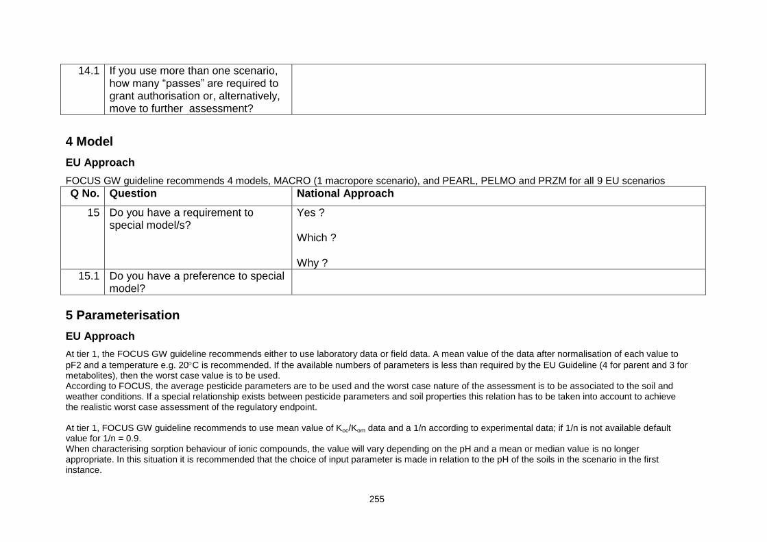
255
14.1 If you use more than one scenario, how many “passes” are required to grant authorisation or, alternatively, move to further assessment?
4 Model
EU Approach
FOCUS GW guideline recommends 4 models, MACRO (1 macropore scenario), and PEARL, PELMO and PRZM for all 9 EU scenarios
Q No. Question National Approach
15 Do you have a requirement to special model/s?
Yes ? Which ? Why ?
15.1 Do you have a preference to special model?
5 Parameterisation
EU Approach
At tier 1, the FOCUS GW guideline recommends either to use laboratory data or field data. A mean value of the data after normalisation of each value to
pF2 and a temperature e.g. 20C is recommended. If the available numbers of parameters is less than required by the EU Guideline (4 for parent and 3 for metabolites), then the worst case value is to be used. According to FOCUS, the average pesticide parameters are to be used and the worst case nature of the assessment is to be associated to the soil and weather conditions. If a special relationship exists between pesticide parameters and soil properties this relation has to be taken into account to achieve the realistic worst case assessment of the regulatory endpoint. At tier 1, FOCUS GW guideline recommends to use mean value of Koc/Kom data and a 1/n according to experimental data; if 1/n is not available default value for 1/n = 0.9. When characterising sorption behaviour of ionic compounds, the value will vary depending on the pH and a mean or median value is no longer appropriate. In this situation it is recommended that the choice of input parameter is made in relation to the pH of the soils in the scenario in the first instance.
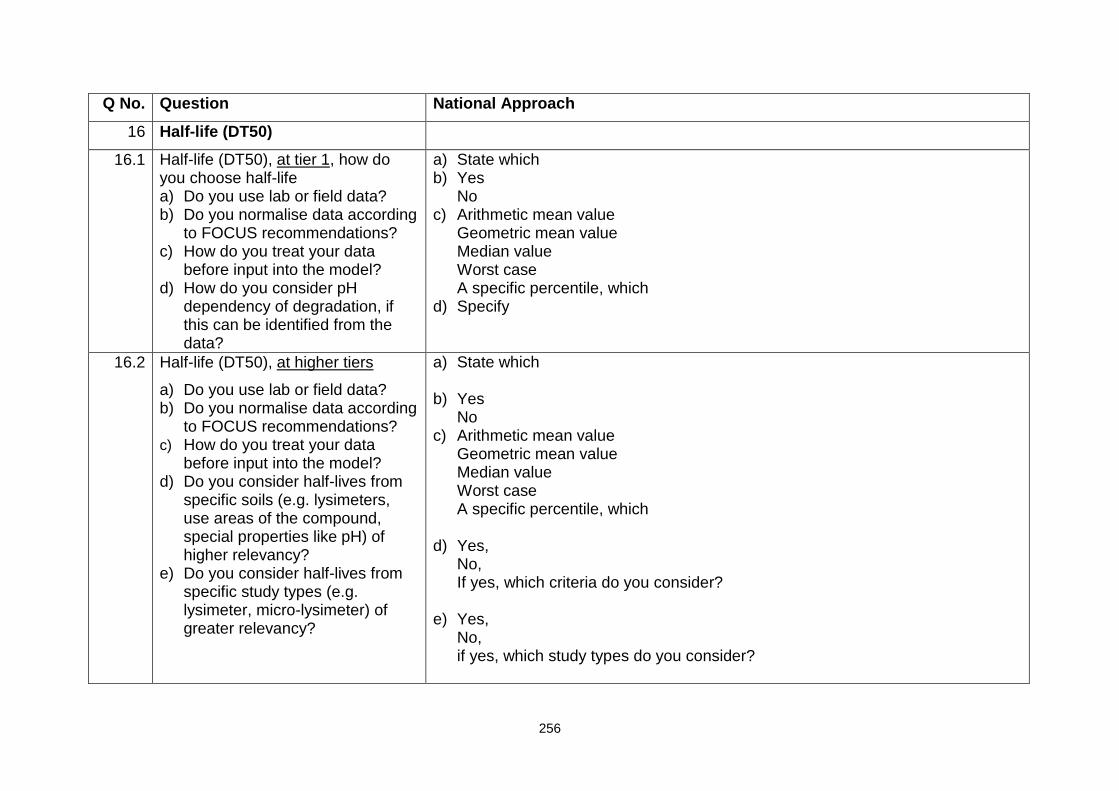
256
Q No. Question National Approach
16 Half-life (DT50)
16.1 Half-life (DT50), at tier 1, how do you choose half-life a) Do you use lab or field data? b) Do you normalise data according
to FOCUS recommendations? c) How do you treat your data
before input into the model? d) How do you consider pH
dependency of degradation, if this can be identified from the data?
a) State which b) Yes
No c) Arithmetic mean value
Geometric mean value Median value Worst case A specific percentile, which
d) Specify
16.2 Half-life (DT50), at higher tiers
a) Do you use lab or field data? b) Do you normalise data according
to FOCUS recommendations? c) How do you treat your data
before input into the model?
d) Do you consider half-lives from specific soils (e.g. lysimeters, use areas of the compound, special properties like pH) of higher relevancy?
e) Do you consider half-lives from specific study types (e.g. lysimeter, micro-lysimeter) of greater relevancy?
a) State which
b) Yes No
c) Arithmetic mean value Geometric mean value Median value Worst case A specific percentile, which
d) Yes, No, If yes, which criteria do you consider?
e) Yes, No, if yes, which study types do you consider?
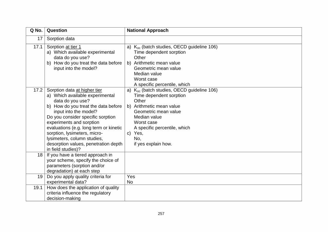
257
Q No. Question National Approach
17 Sorption data
17.1 Sorption at tier 1 a) Which available experimental
data do you use? b) How do you treat the data before
input into the model?
a) Koc (batch studies, OECD guideline 106) Time dependent sorption Other
b) Arithmetic mean value Geometric mean value Median value Worst case A specific percentile, which
17.2 Sorption data at higher tier a) Which available experimental
data do you use? b) How do you treat the data before
input into the model? Do you consider specific sorption experiments and sorption evaluations (e.g. long term or kinetic sorption, lysimeters, micro-lysimeters, column studies, desorption values, penetration depth in field studies)?
a) Koc (batch studies, OECD guideline 106) Time dependent sorption Other
b) Arithmetic mean value Geometric mean value Median value Worst case A specific percentile, which
c) Yes, No, if yes explain how.
18 If you have a tiered approach in your scheme, specify the choice of parameters (sorption and/or degradation) at each step
19 Do you apply quality criteria for experimental data?
Yes No
19.1 How does the application of quality criteria influence the regulatory decision-making
258
6 Additional Experimental data
Q No. Question National Approach
20 Do you request further experimental data for the national assessment than is available in the EU dossier? If Yes, go to Q No. 20.1
Yes No
20.1 Which additional data do you request and what triggers the request? a) Lysimeter data
b) Field leaching c) Monitoring data
d) Other
a) Lysimeter Triggers: No EU lysimeter available Nat conditions differ from EU lysimeter Other reasons
b) Field leaching Triggers: No EU lysimeter available Nat conditions differ from EU lysimeter Other reasons
c) Monitoring data d) Other
21 Lysimeter /field leaching data
21.1 Do you have national guidelines for lysimeter/field leaching studies?
Yes No
21.2 a) Which information do you take from lysimeter/field leaching data?
b) Which endpoint do you use for parent, metabolites, not identified radioactivity?
a)
b) Highest concentration (µg/l) Monthly mean Yearly mean An all over mean

259
22 Do you request or have an option for a post-registration monitoring?
Yes No If yes, please describe what may trigger it and what are the requirements/guidelines
7 Interrelationship Models – Higher tier experiments
Q No. Question National Approach
23 Do model results override results from field studies i.e. models are considered weighted higher than e.g. lysimeters?
Yes No
24 Do results from field studies override model results i.e. lysimeters are considered weighted higher than models ?
Yes No
25 Do you jointly consider models and e.g. lysimeters/field leaching studies and take a decision based on quality of the two cases?
Yes No
26 Do you apply model calculations to extrapolate experiments to national or regional assessment?
Yes No
260
8 Handling of metabolites
EU Approach
In the EU metabolite guidance document (Sanco/221/2000 –rev.10), there is a tiered scheme how to identify metabolites, which
are biological active or which are toxic. Metabolites defined as relevant are judged to be equivalent with active substances. For
relevant metabolites the trigger value in groundwater is 0.1 µg/L.
Q No. Question National Approach
27 Do you define metabolites according to the EU guidance document on relevant metabolites (rev 10)?
Yes No If no, please define the criteria to classify a metabolite as relevant describe where your exposure or relevancy triggers differ from the EU approach
28 Have you set a trigger value different from parent for metabolites, relevant or non-relevant, If Yes, at what concentration?
Relevant metabolites: Yes No At concentration: Non-relevant metabolites Yes No At concentration:
261
APPENDIX 2. REPONSES TO THE QUESTIONNAIRE
The responses to the questionnaire are tabulated below. Entries are provided only when a
response was made.
1 Does your country assess risk to groundwater as a routine before
approval of a PPP in your country?
Denmark Y
Germany Y
France Y
Ireland Y
Italy Y
Austria Y
Netherlands Y
Portugal Y
Finland Y
Sweden Y
United Kingdom Y
Czech Rep. Y
Slovakia Planned but not yet implemented
Slovenia Y
Estonia Y
Lithuania Y
Poland Planned but not yet implemented
Latvia Y
2 Is the EU GW assessment as defined in the FOCUS GW guideline
sufficient for the risk assessment in the authorisation procedure of
PPP in your country?
Denmark N
Germany N
France N
Ireland Y
Italy N
Austria Y
Netherlands N
Portugal Y
262
Finland N
Sweden Y, the methodology is sufficient. Regarding the scenarios see question 10.
United Kingdom N
Czech Rep. Y
Slovakia Y – under study
Slovenia Y
Estonia Y
Lithuania Y
Poland N
Latvia Y
2.1 State shortly the main reason/s why the FOCUS GW guideline is not
sufficient.
Denmark The FOCUS guideline is not considered to be sufficiently protective and
the scenarios not fully representative for Danish conditions
Germany For model calculations a certain national scenario is specified. The
national scenario is evaluated on the basis of lysimeter and field studies.
Valid results from higher tier experimental studies (lysimeter or
comparable field studies) override the modelling results in the
assessment.- FOCUS input parameter guidance is not sufficient- the “one
safe use” concept currently followed by the EU is not satisfying.
France Representativity of EU FOCUS GW scenarios is not established for the
French environmental conditions. EU GW assessment considered as
sufficient only if all FOCUS GW scenarios are acceptable.
Italy The nine FOCUS scenarios do not cover all the Italian territory. Moreover,
major crops of Italy are not totally represented
Netherlands Specific aquifer conditions, high ground water tables and vulnerable soils,
no higher tier guidance available in the guideline
Finland The guidelines are mainly sufficient but more detailed advice could be
given for instance how many different models should be used.
United Kingdom In the main the EU GW assessment is sufficient as defined in the FOCUS
GW guideline, however for more strongly adsorbed compounds MACRO /
Château dun must be used for UK national assessments, this is only an
option in FOCUS GW guidelines, whilst it is a requirement for the UK.
Poland Existing scenarios do not fully cover the whole country in terms of soil and
climate conditions
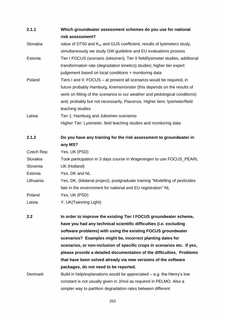
263
2.1.1 Which groundwater assessment schemes do you use for national
risk assessment?
Slovakia value of DT50 and Koc and GUS coefficient, results of lysimeters study,
simultaneously we study GW guideline and EU evaluations process
Estonia Tier I FOCUS (scenario Jokioinen); Tier II field/lysimeter studies, additional
transformation rate (degradation kinetics) studies; higher tier expert
judgement based on local conditions + monitoring data
Poland Tiers I and II: FOCUS – at present all scenarios would be required, in
future probably Hamburg, Kremsmünster (this depends on the results of
work on fitting of the scenarios to our weather and pedological conditions)
and, probably but not necessarily, Piacenza. Higher tiers: lysimeter/field
leaching studies
Latvia Tier 1: Hamburg and Jokioinen scenarios
Higher Tier: Lysimeter, field leaching studies and monitoring data
2.1.2 Do you have any training for the risk assessment to groundwater in
any MS?
Czech Rep. Yes, UK (PSD)
Slovakia Took participation in 3 days course in Wageningen to use FOCUS_PEARL
Slovenia UK (Holland)
Estonia Yes, DK and NL
Lithuania Yes, DK, (bilateral project), postgraduate training "Modelling of pesticides
fate in the environment for national and EU registration" NL
Poland Yes, UK (PSD)
Latvia Y. UK(Twinning Light)
2.2 In order to improve the existing Tier I FOCUS groundwater scheme,
have you had any technical scientific difficulties (i.e. excluding
software problems) with using the existing FOCUS groundwater
scenarios? Examples might be, incorrect planting dates for
scenarios, or non-inclusion of specific crops in scenarios etc. If yes,
please provide a detailed documentation of the difficulties. Problems
that have been solved already via new versions of the software
packages, do not need to be reported.
Denmark Build in help/explanations would be appreciated – e.g. the Henry’s low
constant is not usually given in J/mol as required in PELMO. Also a
simpler way to partition degradation rates between different
264
metabolites/CO2 in PELMO would be helpful. In general we find it
important that more scenarios that include preferential flow are developed.
Germany No problems
Ireland N
Italy non-inclusion of specific crops in scenario: for example soybean is not
considered in the Thiva scenario, relevant for Italy while like dry legumes
are not included in Piacenza scenario
Netherlands Scenarios for amenity use and glasshouses. Specific crop: ornamentals
Portugal Until now we haven’t used frequently the FOCUS models, we check the
data presented by the notifier; input and output data.
Finland There has been some technical problems in giving the user defined
application scheme to PEARL (and thus in running the model). A possible
solution is already given by FOCUS helpdesk.
Sweden We have only limited experience with the EU scenarios and so far we have
not had any difficulties
United Kingdom N
Czech Rep. N
Slovenia no, while we are making evaluation for 1st year
Estonia N
Lithuania The experts have limited experience in modelling. The partition rate,
metabolites and CO2 in PELMO is not clearly described in the guidance
document and is rather difficult. Sometimes local experts have different
opinion on selection of input parameters in comparison with input
parameters chosen by company experts.
Poland Right now we check the data and calculations submitted by the notifier.
The main problem in the nearest future will be the not full compatibility of
the existing scenarios with our pedological and climatic conditions.
Latvia No
2.3 Do you have needs for training in FOCUS modelling?
Czech Rep. Y
Slovakia Y
Slovenia Y
Estonia Y
Lithuania Y
Poland Y
Latvia Yes (additional training with MACRO could be useful)

265
3 What is the trigger for national assessment of risk for groundwater
contamination? If other trigger than Review Report, such as a
national judgement, please, answer Q No. 3.1.
Denmark RR and other trigger
Germany If DT50 > 21 d or Koc < 500, risk to ground water has to be assessed for
every application using the special national scenario (cf. Q 1).
France Other trigger: At least one relevant EU FOCUS GW scenario not
acceptable (PECgw > 0.1 µg/L).
Ireland RR
Italy RR
Austria RR
Netherlands Always national judgement according to the Dutch pesticide act
Portugal RR
Finland The ground water assessments included in RR and DAR are used
nationally but the risks are reassessed if the use amounts or intended
uses differ from those in RR and DAR or if the Jokioinen scenario is
missing.
Sweden If risk for ground water contamination is pointed out in the RR, simulation
with national scenarios is always carried out. In other cases simulations
are performed with a case by case approach
United Kingdom Other trigger
Czech Rep. According to the Review Report (RR) for the active substance
Slovakia According to the Review Report (RR) for the active substance
Slovenia According to the Review Report (RR) for the active substance
Estonia According to the Review Report (RR) for the active substance
Lithuania According to the Review Report (RR) for the active substance
Poland According to the Review Report (RR) for the active substance
Latvia According to the Review Report (RR) for the active substance
3.1 If the trigger is according to national criteria?
Denmark Assessment in EU re-registration process did not result in
recommendations in the RR, but “national” criteria” raise concerns that
have to be addressed on MS level: Borderline assessments in the EU
process and potential issues with metabolites that have not been
considered relevant in the EU process. justification: We perform a stricter
national assessment and consider more metabolites to be “relevant”.
266
Earlier national assessment prior to the EU re-registration. Positive
findings from ground water monitoring data
Germany PELMO 3.0 calculation ifDT50 > 21 d or Koc < 500; lysimeter study if
PELMO 3.0 results in concentrations > 0.1 µg/L; justification: Substances
with properties indicating a certain mobility and persistence in soil are
subject to a more detailed assessment. Field studies are higher tier
studies and overwrite calculations. Positive findings from ground water
monitoring data: Further information about the findings is required and
further studies might be triggered.
France Assessment in EU re-registration process did not result in
recommendations in the RR, but “national” criteria” raise concerns that
have to be addressed on MS level; criteria See 3; justification See 2.1
Netherlands Always national judgement; justification: NL specific conditions as listed at
question 2.1; Earlier national assessment prior to the EU re-registration
Yes can be a reason as well; Positive findings from ground water
monitoring data Always a reason for extra secure judgement on a national
level
Portugal Y
Finland Y
Sweden We have no specific criteria - case-by-case decision based on the results
from the simulations with the EU-scenarios.
United Kingdom 1. GAP from UK proposed use (proposed label use pattern) must be
assessed, if this is different to that assessed by the rapporteur. 2.
Preferential flow must be assessed using MACRO Châteaudun for some
compounds (Koc >100ml/g). 1. The actual requested UK use pattern has
to be assessed if it differs in any way from the ‘intended supported safe
use’ identified as supporting the annex 1 listing decision. . More
structured soils where preferential flow can be of concern that are
associated with relatively vulnerable ground water aquifers are relatively
common in the UK. Therefore this needs assessing.
Estonia Assessment in EU re-registration process did not result in
recommendations in the RR, but “national” criteria” raise concerns that
have to be addressed on MS level. If EU re-registration process will result
in FOCUS Tier I for scenario Jokioinen in leaching > 0.1 μg/L, we will
apply the national RA according to our conditions. Plus positive finings
from monitoring data in Nordic countries

267
4 Do you assess along a tiered approach?
Denmark Y
Germany Y
France Y
Ireland Y
Italy Y
Austria Y
Netherlands Y
Portugal Y
Finland N
Sweden Y
United Kingdom Y
Czech Rep. N
Slovakia N
Slovenia No, so far
Estonia Y
Lithuania Y
Poland Y, such approach is planned.
Latvia Yes
4.1 Briefly describe the tiered approach you apply
Denmark First tier is based on standardised input values, second tier refines the
input values and takes into account more specific issues if justified.
Germany Consideration of the active substance’s properties with regard to soil
sorption and degradation. Model calculation with a national specific
scenario. Higher tier experimental study (Lysimeter or comparable field
studies) if modelling results indicate contamination above 0.1 µg/L
France 1- All relevant FOCUS GW scenarios acceptable. 2- If not, national
approach : simulations of national scenarios with one FOCUS model
(lysimeter study also taken into consideration).
Ireland Results from the Okehampton and Kremsmünster scenarios are used in
the first tier. If PEC values for active substance or relevant metabolite(s)
exceed 0.1 μg/L for either of these scenarios, then a higher tier leaching
assessment is required, involving, for example, a lysimeter or field
leaching study conducted under vulnerable conditions appropriate for
Ireland. Site-specific modelling using Irish data and Irish ground water
monitoring data, if available, could also be used in higher tier national
268
leaching assessments. The exact nature of the higher tier assessment is
determined on a case-by-case basis.
Italy Refined modelling; Use of document of relevancy of metabolites
Austria Lysimeter studies are considered as higher tier studies
Netherlands Tier 1: FOCUS Kremsmünster; Tier 2: GeoPEARL, field/lysimeter studies,
extra (more relevant) lab studies, monitoring uppermost ground water.
Tier 3: behaviour in the saturated zone, monitoring deeper ground water;
The Dutch decision tree and the underlying steps are described in the
following reports
Portugal We follow the FOCUS Guidance document
Sweden 1) Simulations with normalised laboratory half-lives, 2) Simulations with
normalised field half-lives if available, 3) Look at available EU field
lysimeters and decide whether they are relevant for Swedish conditions.
4) Request of field lysimeter under Swedish climatic conditions if
unacceptable leakage has been simulated and the EU field lysimeters are
not considered relevant. In cases with metabolites an assessment of the
relevance of the metabolite, 5) Overall assessment based on all available
data.
United Kingdom See attachment; and
http://www.pesticides.gov.uk/applicant/registration_guides/data_reqs_han
dbook/env_fate.pdf
Estonia Tier I FOCUS (scenario Jokioinen)
expert judgement based on local conditions + monitoring data
Lithuania First Tier modelling is based on worse case standard input values (e.g.
DT50 only from lab studies), the refinement is done taking into account for
refined input parameters. The results of field lysimeter studies (if studies
done are relevant for local conditions) are considered higher tier
Poland Generally: Step 1: Focus modelling using more conservative lab.
degradation kinetics values, Step 2: Focus modelling using more realistic
degradation kinetics values from field studies (whenever available)/opt.
lysimeter or field leaching studies, Step 3: Lysimeter/field leaching studies.
Latvia 1) The use of Hamburg and Jokioinen scenarios (Jokioinen is considered
as worst case). 2) Lysimeter/field studies, monitoring data from Northern
parts of Europe.
269
5a How do you define the endpoint value for approval? a) Tier 1
Denmark 0.1 µg./l, defined as the 95th percentile concentration derived by FOCUS
PELMO Hamburg or the Danish MACRO scenarios averaged over each
year, for as and metabolites; at depth 1 m
Germany 0.1 µg/L, maximum annual average concentration at depth 1 m
France Same criteria as EU approach (with FOCUS GW as well as with national
scenarios).
Ireland 80th percentile annual average concentration (or 2- or 3-year average, as
appropriate) at 1 m depth must not exceed 0.1 μg/L
Italy depth 1 m
Austria depth 1 m
Netherlands <0.1 µg/L at depth 1 meter
Portugal 1 meter
Finland depth 1 m, 80th percentile annual average concentration
Sweden below root depth, 1.3-1.6 m
United Kingdom 1 m
Czech Rep. at I m depth
Slovakia at I m depth
Slovenia at I m depth
Estonia endpoint value < 0.1 µg/L for parent and for metabolites according to
FOCUS Tier I GW modelling using scenario Jokioinen and DT50 lab value
Lithuania 80%-ile annual concentration at 1 m depth >0.1 µg/L (derived from
FOCUS PELMO Hamburg and Jokioinen scenarios) for both AS and
metabolites.
Poland <0.1 µg/L at 1 m depth
Latvia <0.1 µg/L at 1 m depth
5b b) At higher tiers
Denmark as tier 1
Germany 0.1 µg/L, maximum annual average concentration at depth 1 m
Ireland If it can be demonstrated that depth to ground water in areas of use is >1
m, then annual average concentration impacting on top of the ground
water body must not exceed 0.1 μg/L.
Netherlands 90th percentile <0.1 µg/L at depth/s 1-10 m
Portugal to be defined
Sweden see Tier 1
270
United Kingdom The depth of simulation is to that which is technically feasible. However
applicants need to justify the use of the depth for which results are
presented and their relationship to UK vulnerable ground water depths as
associated with the intended cropping. Information on where ground water
is shallow, cropping patterns and where soils are vulnerable to ground
water contamination can be extracted from the latest version of the
SEISMIC data base that covers England and Wales.
Estonia endpoint value should be still < 0.1 µg/L for parent and for metabolites,
using for modelling the extrapolation of data from lysimeter/field studies
and considering monitoring data; if the endpoint for metabolites is > 0.1
µg/L, the toxicological relevance of metabolites is considered
Lithuania Same as in 5a
Poland <0.1 µg/L at 1 m depth
Latvia <0.1 µg/L at 1 m depth
6a Do you apply a safety factor on the endpoint a) For parent
Denmark N
Germany N
France N
Ireland N
Italy N
Austria N
Netherlands N
Portugal N
Finland N
Sweden Y, in the case of triggering a higher tier assessment
United Kingdom N
Czech Rep. N
Slovenia N
Estonia N
Lithuania N
Poland N
Latvia N
6b b) For metabolites
Denmark N
Germany N

271
France N
Ireland N
Italy N
Austria N
Netherlands N
Portugal N
Finland N
Sweden Y, in the case of triggering a higher tier assessment
United Kingdom N
Czech Rep. N
Slovenia N
Estonia N
Lithuania N
Poland N
Latvia N
7 Do you take decisions using model simulations only?
Denmark No usually not, but we might for new substances, see below
Germany Yes, if field studies are not required according to the tiered approach. No,
in all other cases
France N; Lysimeter also considered when available.
Ireland N, (See reply to Q.4.1)
Italy N
Austria N
Netherlands N, See references mentioned at 4.1
Portugal N
Finland N
Sweden N
United Kingdom Y
Czech Rep. N
Slovakia N
Slovenia Y
Estonia N
Lithuania Yes (Positive or negative), If modelling demonstrate leaching < 0,1µg/L ,
the positive decisions are based only on modelling, . If modelling
demonstrates leaching > 0,1 µg/L and field lysimeter data are not

272
available, the negative decisions are also based only on modelling results.
If field lysimeter data are available- they are considered.
Poland N
Latvia N
8a Are the following possible alternatives to non-full-approval? a)
Conditional approval?
Denmark Yes in the sense that uses are restricted e.g. max dose, max # appl., only
spring/summer use etc.
Germany Y
France Yes, Under discussion
Ireland Y
Italy Y
Austria Y
Netherlands Yes with a demand for post registration monitoring of the uppermost
ground water
Portugal Y
Finland Y
Sweden Y
United Kingdom N
Czech Rep. Y
Slovenia Y
Estonia N
Lithuania Y
Poland Y
Latvia N
8b b) Regional or local approval?
Denmark N
Germany N
France Yes, Under discussion
Ireland Y (This is possible but would not be common.)
Italy Y
Austria N
Netherlands Y
Portugal Y
Finland N

273
Sweden N
United Kingdom N
Czech Rep. N
Slovenia Y
Estonia N
Lithuania N
Poland N
Latvia N
8c c) Special approval for farmers?
Denmark N
Germany N
France Yes, Under discussion
Ireland Y (This is possible but in such a situation we would use the term
“professional users” instead of “farmers”.)
Austria N
Netherlands N
Portugal Y
Finland N
Sweden N
United Kingdom N
Czech Rep. N
Estonia N
Lithuania N
Poland Planned but not implemented.
Latvia N
8d d) Special indications?
Denmark Dispensations can be granted prior to Annex 1 inclusion if the need is
considered valid and the risks acceptable
Germany in reasonable special cases approval in combination with post-
authorisation monitoring is possible
France Under discussion
Austria Time of application
Netherlands Ground water protection areas
Portugal Approval conditions to type of soil/crop/agronomic conditions
Finland N
274
Poland Ground water protection areas (mainly drinking water sources)
Latvia N
9 Are risk mitigation measures considered at approval on your national
level?
Denmark No Not for gw - unless you consider the above mentioned (8) restrictions
to be risk mitigations
Germany Y. E.g. restriction with regard to the soil type (no application on heavy clay
soils or sand soils), restriction with regard to the maximum amount of a
certain active substance to be applied to the same field in the course of
one season (possibly from different plant protection products), restrictions
with regard to the use on drained areas
France Yes, Under discussion
Ireland Y Possibility of using a reduced rate of application and/or reducing the
frequency of application can be considered.
Italy N
Austria Y, Time of application, Reduction of application rates/number of
applications per season
Netherlands Y, Label restrictions e.g. use restricted to artificial soil (glasshouses), no
autumn use.
Portugal Y, Ex. If a compound may leach we restrict there use in sandy soils or
soil of low o.m. content.
Finland Y. Products having risks to leach in ground water (for instance model
simulations > 0.1 µg/L) are not allowed to use in classified ground water
areas.
Sweden N
United Kingdom N, not routinely. However if an applicant had a demonstrably robust
mitigation that was practical to implement, then subject to its approval by
the UK Advisory Committee on Pesticides and Ministerial agreement an
authorisation would be possible. (Note as yet there are no practical
examples where this has occurred).
Czech Rep. Yes, if reductions in dose or number of applications are accepted by the
applicant
Slovakia If the application of formulation or dose is changed
Slovenia Y
Estonia Yes, Restrictions of applications on vulnerable soils or areas, restrictions
of applications on consecutive years, reduction of dose rate etc.
275
Lithuania Y
Poland N
Latvia Just in terms of application timing
10 Do you use any of the nine FOCUS groundwater scenarios as your
national scenario?
Denmark Y, PELMO Hamburg
Germany N
France N
Ireland Y Okehampton and Kremsmünster
Italy Y, All, but Thiva, Piacenza and Châteaudun seems to the most
representative
Austria Y, Hamburg, Kremsmünster, Piacenza
Netherlands Y, Kremsmünster
Portugal Y, Sevilla, Porto, Thiva , Piacenza
Finland Y. Jokioinen scenario is used as a national scenario because our national
scenario is not yet finalised.
Sweden N
United Kingdom Y, Hamburg, Châteaudun, Okehampton, Kremsmünster
Czech Rep. N
Slovakia Yes – is planned
Slovenia Y
Estonia Y, Jokioinen but only for Tier 1 and 2
Lithuania Y
Poland Y, planned. At present we would recommend all nine scenarios, in future
probably Hamburg, Kremsmünster and, possibly, Piacenza.
Latvia Y, Hamburg and Jokioinen
10.1 If you have scenario/s different from the FOCUS GW scenarios,
please, state shortly the reason to that?
Denmark We have two national MACRO scenarios (Karup and Langvad) that
represent a sandy and a clay soil type. The scenarios represent realistic
worst case representative Danish conditions and include preferential flow.
Germany The national scenario is validated based on realistic lysimeter and field
studies. No averaging over several years. - Soil scenario is very similar to
FOCUS “Hamburg” but includes more realistic degradation factors for

276
deeper soil layers than the commonly attributed factors in all of the
FOCUS scenarios
France To take account of more realistic conditions.
Austria The three FOCUS scenarios mentioned above are considered as a
compromise. If a company submits model calculations with specific
Austrian soil and weather conditions we evaluate them and prefer them to
the above mentioned FOCUS scenarios. In most cases the three FOCUS
scenarios can be seen as a worst case.
Sweden Yes. Swedish scenarios cover a colder climate in combination with
relevant soil types and crops. Macro pore flow is included in the Swedish
scenarios.
Slovenia We are going into the process of establishing our own scenarios
Estonia Jokioinen, but only Tier I and II
Poland N
Latvia N
11 Do you have more than one national scenario?
Denmark Y, 2
Germany N
France Y. Pending standard national scenarios, notifier is asked to propose
scenarios covering the major conditions of use.
Italy N
Netherlands N
Portugal N
Finland N
Sweden Y, 3
United Kingdom Yes we use the 4 FOCUS scenarios as listed in section 10 above +
sometimes a MACRO simulation at Châteaudun is also required (see reply
to question 4.1).
Czech Rep. N
Slovakia N
Slovenia N
Estonia N
Lithuania N
Poland N, none at present (but planned in future)
Latvia We use two Focus scenarios
277
12a Which criteria are used for the choice of national scenarios? a.
weather (rainfall)
Denmark Weather typical for major agricultural area/s
Germany Average rainfall more or less (alternation of “Hamburg wet” 1961 and
“Hamburg normal” 1978
France Under discussion
Finland Weather typical for major agricultural area/s
Sweden Weather typical for major agricultural area
Slovenia Typical for agriculture areas
Estonia Average rainfall
Latvia Average rainfall
12b b. weather (temperature)
Denmark Weather typical for major agricultural area/s
Germany Average temperature more or less (alternation of “Hamburg wet” 1961 and
“Hamburg normal” 1978)
France Under discussion
Finland Weather typical for major agricultural area/s
Sweden Weather typical for major agricultural area
Slovenia Typical for agriculture areas
Estonia Average temperature
Latvia Average temperature
12c soil type
Denmark Worst case soil + realistic and representative
Germany realistic worst case soil
France Under discussion
Finland Worst case soil
Sweden Soil/s typical for major agricultural area
Slovenia Typical for agriculture areas
Estonia Typical for major agricultural areas
Latvia Soils typical of major agricultural area/s
12d crops
Denmark Crops in general
Germany Crops according to the GAP for which authorisation is sought
France Under discussion
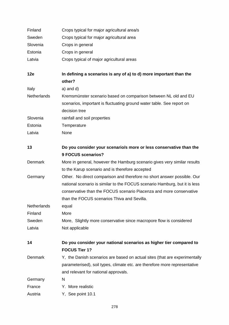
278
Finland Crops typical for major agricultural area/s
Sweden Crops typical for major agricultural area
Slovenia Crops in general
Estonia Crops in general
Latvia Crops typical of major agricultural areas
12e In defining a scenarios is any of a) to d) more important than the
other?
Italy a) and d)
Netherlands Kremsmünster scenario based on comparison between NL old and EU
scenarios, important is fluctuating ground water table. See report on
decision tree
Slovenia rainfall and soil properties
Estonia Temperature
Latvia None
13 Do you consider your scenario/s more or less conservative than the
9 FOCUS scenarios?
Denmark More in general, however the Hamburg scenario gives very similar results
to the Karup scenario and is therefore accepted
Germany Other. No direct comparison and therefore no short answer possible. Our
national scenario is similar to the FOCUS scenario Hamburg, but it is less
conservative than the FOCUS scenario Piacenza and more conservative
than the FOCUS scenarios Thiva and Sevilla.
Netherlands equal
Finland More
Sweden More, Slightly more conservative since macropore flow is considered
Latvia Not applicable
14 Do you consider your national scenarios as higher tier compared to
FOCUS Tier 1?
Denmark Y, the Danish scenarios are based on actual sites (that are experimentally
parameterised), soil types, climate etc. are therefore more representative
and relevant for national approvals.
Germany N
France Y. More realistic
Austria Y, See point 10.1

279
Netherlands No, equal at Tier 1
Finland N
Sweden Y, More representative for Swedish conditions
Estonia Yes, the extrapolation of data from lysimeter/field studies is used, expert
judgement according to local conditions and considering vulnerable areas
and soils
15 Do you have a requirement to special model/s?
Denmark Yes ? In principle, but other models are accepted in some cases (e.g.
PELMO for the Hamburg scenario)
Germany Y, PELMO 3.0, Using the national scenario, a conservative estimation of
possible leaching to ground water is obtained, which was evidenced by
comparison with the results of lysimeter and field leaching studies.
France Yes ? One of the 4 FOCUS GW models
Ireland N
Netherlands No, but same circumstances as PEARL (dispersion length!)
Portugal Y, PELMO (PEARL)
Finland No
Sweden Y, Swedish scenarios use MACRO in FOCUS. Need of model that can
handle macro pore flow
United Kingdom No except for compounds with Koc >100ml/g, MACRO must be run for
Châteaudun
Slovenia N
Estonia Yes, Recommended FOCUS GW models; According to national legislation
Poland No, however if calculations using PRZM are submitted the Notifier would
be asked to recalculate the PEC values using PELMO or/and PEARL.
Latvia N
15.1 Do you have a preference to special model?
Denmark MACRO, In order to include preferential flow + see attachment on
modelling for details
Germany see answer to question 15
France N
Ireland N
Austria PELMO
Netherlands PEARL! Coupled with GeoPEARL
Portugal Y, PELMO (PEARL)
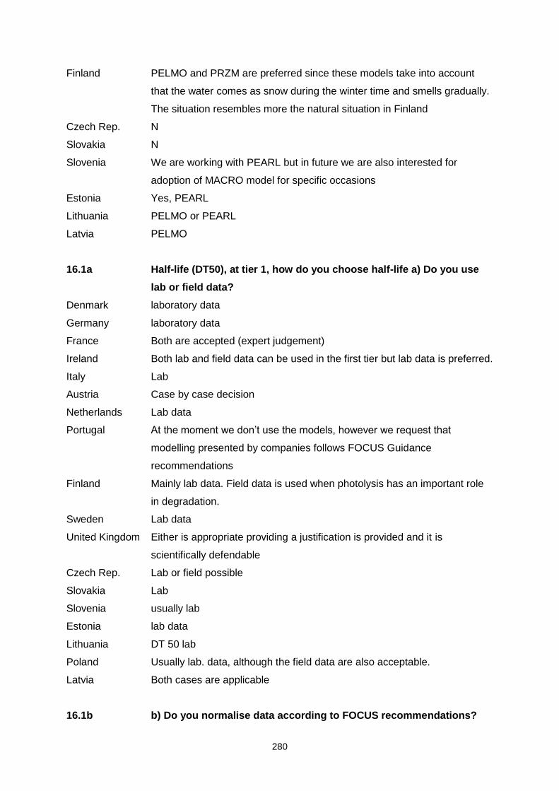
280
Finland PELMO and PRZM are preferred since these models take into account
that the water comes as snow during the winter time and smells gradually.
The situation resembles more the natural situation in Finland
Czech Rep. N
Slovakia N
Slovenia We are working with PEARL but in future we are also interested for
adoption of MACRO model for specific occasions
Estonia Yes, PEARL
Lithuania PELMO or PEARL
Latvia PELMO
16.1a Half-life (DT50), at tier 1, how do you choose half-life a) Do you use
lab or field data?
Denmark laboratory data
Germany laboratory data
France Both are accepted (expert judgement)
Ireland Both lab and field data can be used in the first tier but lab data is preferred.
Italy Lab
Austria Case by case decision
Netherlands Lab data
Portugal At the moment we don’t use the models, however we request that
modelling presented by companies follows FOCUS Guidance
recommendations
Finland Mainly lab data. Field data is used when photolysis has an important role
in degradation.
Sweden Lab data
United Kingdom Either is appropriate providing a justification is provided and it is
scientifically defendable
Czech Rep. Lab or field possible
Slovakia Lab
Slovenia usually lab
Estonia lab data
Lithuania DT 50 lab
Poland Usually lab. data, although the field data are also acceptable.
Latvia Both cases are applicable
16.1b b) Do you normalise data according to FOCUS recommendations?
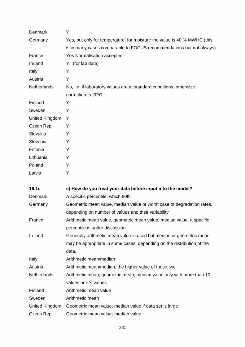
281
Denmark Y
Germany Yes, but only for temperature; for moisture the value is 40 % MWHC (this
is in many cases comparable to FOCUS recommendations but not always)
France Yes Normalisation accepted
Ireland Y (for lab data)
Italy Y
Austria Y
Netherlands No, i.e. if laboratory values are at standard conditions, otherwise
correction to 20ºC
Finland Y
Sweden Y
United Kingdom Y
Czech Rep. Y
Slovakia Y
Slovenia Y
Estonia Y
Lithuania Y
Poland Y
Latvia Y
16.1c c) How do you treat your data before input into the model?
Denmark A specific percentile, which 80th
Germany Geometric mean value, median value or worst case of degradation rates,
depending on number of values and their variability
France Arithmetic mean value, geometric mean value, median value, a specific
percentile is under discussion
Ireland Generally arithmetic mean value is used but median or geometric mean
may be appropriate in some cases, depending on the distribution of the
data.
Italy Arithmetic mean/median
Austria Arithmetic mean/median, the higher value of these two
Netherlands Arithmetic mean; geometric mean; median value only with more than 10
values or >/< values
Finland Arithmetic mean value
Sweden Arithmetic mean
United Kingdom Geometric mean value; median value if data set is large
Czech Rep. Geometric mean value; median value
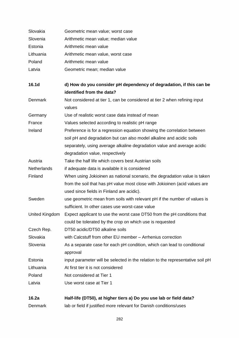
282
Slovakia Geometric mean value; worst case
Slovenia Arithmetic mean value; median value
Estonia Arithmetic mean value
Lithuania Arithmetic mean value, worst case
Poland Arithmetic mean value
Latvia Geometric mean; median value
16.1d d) How do you consider pH dependency of degradation, if this can be
identified from the data?
Denmark Not considered at tier 1, can be considered at tier 2 when refining input
values
Germany Use of realistic worst case data instead of mean
France Values selected according to realistic pH range
Ireland Preference is for a regression equation showing the correlation between
soil pH and degradation but can also model alkaline and acidic soils
separately, using average alkaline degradation value and average acidic
degradation value, respectively
Austria Take the half life which covers best Austrian soils
Netherlands if adequate data is available it is considered
Finland When using Jokioinen as national scenario, the degradation value is taken
from the soil that has pH value most close with Jokioinen (acid values are
used since fields in Finland are acidic).
Sweden use geometric mean from soils with relevant pH if the number of values is
sufficient. In other cases use worst-case value
United Kingdom Expect applicant to use the worst case DT50 from the pH conditions that
could be tolerated by the crop on which use is requested
Czech Rep. DT50 acidic/DT50 alkaline soils
Slovakia with Calcstuff from other EU member – Arrhenius correction
Slovenia As a separate case for each pH condition, which can lead to conditional
approval
Estonia input parameter will be selected in the relation to the representative soil pH
Lithuania At first tier it is not considered
Poland Not considered at Tier 1
Latvia Use worst case at Tier 1
16.2a Half-life (DT50), at higher tiers a) Do you use lab or field data?
Denmark lab or field if justified more relevant for Danish conditions/uses
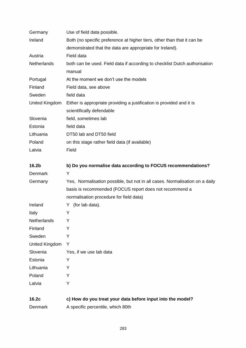
283
Germany Use of field data possible.
Ireland Both (no specific preference at higher tiers, other than that it can be
demonstrated that the data are appropriate for Ireland).
Austria Field data
Netherlands both can be used. Field data if according to checklist Dutch authorisation
manual
Portugal At the moment we don’t use the models
Finland Field data, see above
Sweden field data
United Kingdom Either is appropriate providing a justification is provided and it is
scientifically defendable
Slovenia field, sometimes lab
Estonia field data
Lithuania DT50 lab and DT50 field
Poland on this stage rather field data (if available)
Latvia Field
16.2b b) Do you normalise data according to FOCUS recommendations?
Denmark Y
Germany Yes, Normalisation possible, but not in all cases. Normalisation on a daily
basis is recommended (FOCUS report does not recommend a
normalisation procedure for field data)
Ireland Y (for lab data).
Italy Y
Netherlands Y
Finland Y
Sweden Y
United Kingdom Y
Slovenia Yes, if we use lab data
Estonia Y
Lithuania Y
Poland Y
Latvia Y
16.2c c) How do you treat your data before input into the model?
Denmark A specific percentile, which 80th
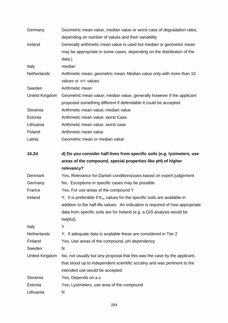
284
Germany Geometric mean value, median value or worst case of degradation rates,
depending on number of values and their variability
Ireland Generally arithmetic mean value is used but median or geometric mean
may be appropriate in some cases, depending on the distribution of the
data.)
Italy median
Netherlands Arithmetic mean; geometric mean; Median value only with more than 10
values or >/< values
Sweden Arithmetic mean
United Kingdom Geometric mean value; median value, generally however if the applicant
proposed something different if defendable it could be accepted
Slovenia Arithmetic mean value; median value
Estonia Arithmetic mean value; worst Case
Lithuania Arithmetic mean value, worst case
Poland Arithmetic mean value
Latvia Geometric mean or median value
16.2d d) Do you consider half-lives from specific soils (e.g. lysimeters, use
areas of the compound, special properties like pH) of higher
relevancy?
Denmark Yes, Relevance for Danish conditions/uses based on expert judgement
Germany No, Exceptions in specific cases may be possible
France Yes, For use areas of the compound Y
Ireland Y, It is preferable if Koc values for the specific soils are available in
addition to the half-life values. An indication is required of how appropriate
data from specific soils are for Ireland (e.g. a GIS analysis would be
helpful).
Italy Y
Netherlands Y, If adequate data is available these are considered in Tier 2
Finland Yes, Use areas of the compound, pH dependency
Sweden N
United Kingdom No, not usually but any proposal that this was the case by the applicant,
that stood up to independent scientific scrutiny and was pertinent to the
intended use would be accepted
Slovenia Yes, Depends on a.s
Estonia Yes; Lysimeters, use area of the compound
Lithuania N

285
Poland N
Latvia N
16.2e e) Do you consider half-lives from specific study types (e.g.
lysimeter, micro-lysimeter) of greater relevancy?
Denmark No, only if these are more relevant for Danish conditions/uses
Germany N
France N
Ireland Y, Lysimeter, field leaching and saturated zone studies can all be
considered, particularly if their relevancy to Irish conditions is
demonstrated
Italy Y, lysimeter
Netherlands N
Sweden N
United Kingdom No, we have no preference for particular study types, however we would
consider data from other study types as long as the applicant had a valid
justification for why they were more pertinent. Particular scrutiny would be
made of the way the data from novel study designs was used as input to
the modelling to ensure that simulations would remain valid and that
processes were not being double counted.
Slovenia NY
Estonia Yes, Lysimeters
Lithuania N
Poland N
Latvia N
17.1a Sorption at tier 1 a) Which available experimental data do you use?
Denmark Koc (batch studies, OECD guideline 106), Time dependent sorption
Germany Koc
France Koc (batch studies, OECD guideline 106)
Ireland Koc
Italy Koc
Austria Koc
Netherlands Koc, column leaching OECD 312 (low Koc and/or fast degradation)
Portugal Koc
Finland Koc (batch studies, OECD guideline 106
Sweden Koc
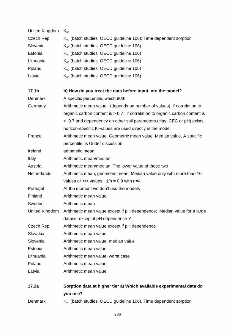
286
United Kingdom Koc
Czech Rep. Koc (batch studies, OECD guideline 106); Time dependent sorption
Slovenia Koc (batch studies, OECD guideline 106)
Estonia Koc (batch studies, OECD guideline 106)
Lithuania Koc (batch studies, OECD guideline 106)
Poland Koc (batch studies, OECD guideline 106)
Latvia Koc (batch studies, OECD guideline 106)
17.1b b) How do you treat the data before input into the model?
Denmark A specific percentile, which 80th
Germany Arithmetic mean value, (depends on number of values) if correlation to
organic carbon content is > 0.7 ; if correlation to organic carbon content is
< 0.7 and dependency on other soil parameters (clay, CEC or pH) exists,
horizon-specific Kf-values are used directly in the model
France Arithmetic mean value, Geometric mean value, Median value, A specific
percentile, is Under discussion
Ireland arithmetic mean
Italy Arithmetic mean/median
Austria Arithmetic mean/median, The lower value of these two
Netherlands Arithmetic mean; geometric mean; Median value only with more than 10
values or >/< values; 1/n = 0.9 with n=4
Portugal At the moment we don’t use the models
Finland Arithmetic mean value
Sweden Arithmetic mean
United Kingdom Arithmetic mean value except if pH dependence; Median value for a large
dataset except if pH dependence Y
Czech Rep. Arithmetic mean value except if pH dependence
Slovakia Arithmetic mean value
Slovenia Arithmetic mean value; median value
Estonia Arithmetic mean value
Lithuania Arithmetic mean value, worst case
Poland Arithmetic mean value
Latvia Arithmetic mean value
17.2a Sorption data at higher tier a) Which available experimental data do
you use?
Denmark Koc (batch studies, OECD guideline 106), Time dependent sorption
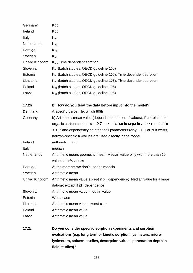
287
Germany Koc
Ireland Koc
Italy Koc
Netherlands Koc
Portugal Koc
Sweden Koc
United Kingdom Koc, Time dependent sorption
Slovenia Koc (batch studies, OECD guideline 106)
Estonia Koc (batch studies, OECD guideline 106), Time dependent sorption
Lithuania Koc (batch studies, OECD guideline 106), Time dependent sorption
Poland Koc (batch studies, OECD guideline 106)
Latvia Koc (batch studies, OECD guideline 106)
17.2b b) How do you treat the data before input into the model?
Denmark A specific percentile, which 80th
Germany b) Arithmetic mean value (depends on number of values), if correlation to
organic carbon content is
< 0.7 and dependency on other soil parameters (clay, CEC or pH) exists,
horizon-specific Kf-values are used directly in the model
Ireland arithmetic mean
Italy median
Netherlands Arithmetic mean; geometric mean; Median value only with more than 10
values or >/< values
Portugal At the moment we don’t use the models
Sweden Arithmetic mean
United Kingdom Arithmetic mean value except if pH dependence; Median value for a large
dataset except if pH dependence
Slovenia Arithmetic mean value; median value
Estonia Worst case
Lithuania Arithmetic mean value , worst case
Poland Arithmetic mean value
Latvia Arithmetic mean value
17.2c Do you consider specific sorption experiments and sorption
evaluations (e.g. long term or kinetic sorption, lysimeters, micro-
lysimeters, column studies, desorption values, penetration depth in
field studies)?

288
Denmark Yes, in principle; Not much practical experience, based on expert
judgement
Germany Y, Lysimeter study is triggered, if modelling result indicates concentration
above 0.1 µg/L.
France N
Ireland Y, Can be considered on a case-by-case basis.
Netherlands Y, Column studies, kinetic sorption. For 1/n mean of data is taken if more
than the standard 4 values are available.
Portugal N
Sweden N
United Kingdom Y, we will critically assess and scientifically scrutinise whatever the
applicant proposes / supplies to support the assessment
Slovenia Yes, As a factors in overall assessment
Estonia Yes, Desorption values will be taken into account
Lithuania N
Poland N
Latvia N
18 If you have a tiered approach in your scheme, specify the choice of
parameters (sorption and/or degradation) at each step
Denmark See above
France Same approach for FOCUS GW and national scenarios
Netherlands Tier 1 avg values for sorption and degradation, Tier 2 refinement possible
upon request and available data that demonstrate necessity
Portugal We don’t have a specific tiered approach
United Kingdom he UK tiered approach is not prescribed in this much detail. Applicants are
left to make judgement on how many parameters higher tier information is
required to demonstrate use is acceptable. If PSD consider the approach
taken by the applicant is inappropriate or unclear it will be challenged. The
applicant will be expected to justify why they consider what they have
done is appropriate. Of course PSD may choose not to accept the
justification provided if they consider it does not stand up to scientific
scrutiny.
Lithuania 1 tier : DT50 lab, sorption not time dependent; 2 tier: DT50 lab and field,
in some cases- time dependent sorption
Poland The system is still under the development, it requires some refinements,
thus it is difficult right now to fully describe it.
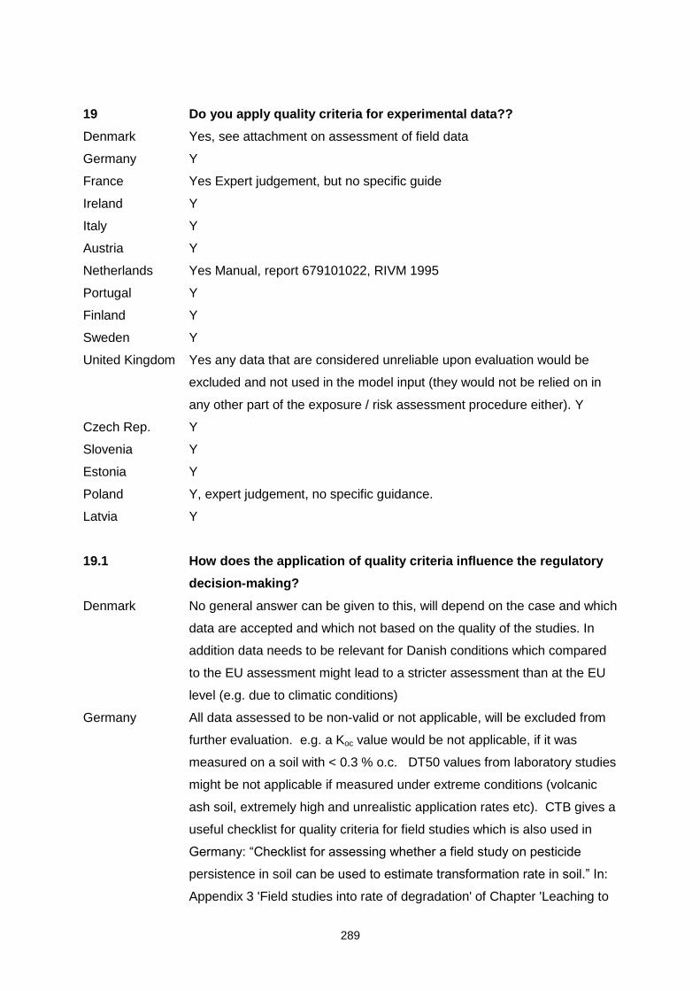
289
19 Do you apply quality criteria for experimental data??
Denmark Yes, see attachment on assessment of field data
Germany Y
France Yes Expert judgement, but no specific guide
Ireland Y
Italy Y
Austria Y
Netherlands Yes Manual, report 679101022, RIVM 1995
Portugal Y
Finland Y
Sweden Y
United Kingdom Yes any data that are considered unreliable upon evaluation would be
excluded and not used in the model input (they would not be relied on in
any other part of the exposure / risk assessment procedure either). Y
Czech Rep. Y
Slovenia Y
Estonia Y
Poland Y, expert judgement, no specific guidance.
Latvia Y
19.1 How does the application of quality criteria influence the regulatory
decision-making?
Denmark No general answer can be given to this, will depend on the case and which
data are accepted and which not based on the quality of the studies. In
addition data needs to be relevant for Danish conditions which compared
to the EU assessment might lead to a stricter assessment than at the EU
level (e.g. due to climatic conditions)
Germany All data assessed to be non-valid or not applicable, will be excluded from
further evaluation. e.g. a Koc value would be not applicable, if it was
measured on a soil with < 0.3 % o.c. DT50 values from laboratory studies
might be not applicable if measured under extreme conditions (volcanic
ash soil, extremely high and unrealistic application rates etc). CTB gives a
useful checklist for quality criteria for field studies which is also used in
Germany: “Checklist for assessing whether a field study on pesticide
persistence in soil can be used to estimate transformation rate in soil.” In:
Appendix 3 'Field studies into rate of degradation' of Chapter 'Leaching to

290
groundwater' of Authorisation manual Plant Protection Products (HTB 0.2).
Document at www.ctb-wageningen.nl
Ireland Experimental data should be obtained in a GLP-compliant facility using an
appropriate guideline. Non-guideline, non-GLP studies may be accepted
in some cases if it can be demonstrated that they are scientifically valid.
Italy Rejection of data and request of new ones
Austria Bad quality data are not considered. New data have to be submitted. In a
case by case decision a time limited authorisation can be granted.
Netherlands Studies of minor quality are excluded
Portugal We chose preferably studies with GLP and conducted according to OECD
or EU Guidelines
Finland If the experimental data is not considered properly obtained (studies not
performed according to guidelines or otherwise do not fulfil scientific
validity criteria) the results are not used in decision making
Sweden The assessment should be transparent and based on studies of
acceptable quality.
United Kingdom Yes, if excluding unreliable data means data requirements for number of
studies is not fulfilled then authorisation would probably not be possible.
Decision making would also be impacted if excluding data considered
unreliable meant the predicted concentrations fell on a different side of the
regulatory trigger/s.
Czech Rep. If excluding unreliable data means data requirements for number of
studies is not fulfilled then authorisation would probably not be possible.
Decision making would also be impacted if excluding data considered
unreliable meant the predicted concentrations fell on a different side of the
regulatory trigger/s.
Slovenia When the results of studies without GLP varies a lot from average of other
studies than we exclude the results from overall assessment
Estonia Decision-making is based only on experimental data obtained from studies
corresponding to quality criteria
Latvia Data of poor quality or not relevant climatic conditions are excluded from
further assessment.
20 Do you request further experimental data for the national assessment
than is available in the EU dossier?
Denmark Y and N - If a safe use for Danish conditions/uses can not be identified
based on the EU data approval is not granted. Thus we do not request

291
specific data, but leave it to the applicant to submit further data to show
safe use.
Germany Y
France Usually not, but case by case requirement possible.
Ireland Y (if a substance fails either the Okehampton scenario or the
Kremsmünster scenario).
Italy Y
Austria Y
Netherlands No If tier 1 value >0.1 μg/L different options are available see 20.1
Portugal Y, it depends on the assessment made in the EU dossier
Finland N
Sweden Y
United Kingdom Yes not routinely but we can. Further experimental data would only be
requested if the information in the EU dossier did not encompass UK uses
and or geoclimatic conditions
Czech Rep. N
Slovakia N
Slovenia N, so far
Estonia Y
Lithuania Further data are not routinely requested unless there were
recommendations in EU dossier
Poland Y
Latvia N
20.1a Which additional data do you request and what triggers the request?
a) Lysimeter data
Denmark Y, See attachment on field studies assessment
Germany Y, if Modelling result with the national scenario indicates contamination
above 0.1 µg/L
France Case by case (a-b-c-d)
Ireland Y - if no EU lysimeter available or national conditions differ from EU
lysimeter
Austria Y, If model calculations for Hamburg, Kremsmünster or Piacenza are
shown not to be safe.
Netherlands Y
Portugal Y, if the concentration in ground water is > 0.1 µg/L
Sweden Y, No EU lysimeter available, National conditions differ from EU lysimeter

292
Estonia Y, national conditions differ from EU lysimeter
Poland Y
20.1b b) Field leaching
Denmark Y, See attachment on field studies assessment
Germany Y (may be performed instead of a lysimeter study, if quality and conditions
of the study are adequate), if Modelling result with the national scenario
indicates contamination above 0.1 µg/L
France Case by case (a-b-c-d)
Ireland Y (Generally not requested but if a relevant field leaching study was
available it would be considered.)
Italy Y
Netherlands Y
Portugal Y, if the concentration in ground water is > 0.1 µg/L, National conditions
differ from EU lysimeter
Estonia Y, national conditions differ from EU lysimeter
Poland Y
20.1c c) Monitoring data
Denmark Y, See attachment on field studies assessment
Germany results from routine controls are used as supplementary information; a
tailored monitoring might be required on a case by case basis
France Case by case (a-b-c-d)
Ireland Y (if available)
Italy Y
Netherlands Y
Portugal Y
Poland Y
20.1d d) Other
Denmark Experimental data for metabolites or a.s. that can be used to refine input
values for model calculations.
France Case by case (a-b-c-d)
Netherlands GeoPEARL in combination with specific data, saturated zone
United Kingdom If the first tier modelling shows there is a concern then it is up to the
applicant to provide higher tier data to demonstrate uses are acceptable.
They can choose to do this by referring to an available EU lysimeter or

293
providing additional field data. To provide reassurance for the UK, the
notifier needs to demonstrate that the conditions of the study/ies
encompass UK geoclimatic conditions, cropping practice and requested
uses.
21.1 Do you have national guidelines for lysimeter/field leaching studies?
Denmark N
Germany Y
France N
Ireland N
Italy N
Austria N
Netherlands Y
Portugal N
Finland N
Sweden N
United Kingdom N
Czech Rep. N
Slovakia N
Slovenia N
Estonia N
Lithuania N
Poland N
Latvia N
21.2a a) Which information do you take from lysimeter/field leaching data?
Denmark All relevant info – see also attachment on field studies
Germany Entry of active substance or metabolites into ground water (defined by the
concentration in the leachates).
France Concentrations of compounds in drainage water and soil residues at
termination in lysimeter study.
Ireland Characterisation of leachate radioactivity, leachate concentrations,
distribution and characterisation of radioactivity in the soil profile, leachate
volumes.
Italy Metabolites and concentration
Austria Concentrations of parent and metabolites in leachates. Are the same
metabolites found in the lysimeter study as in the soil metabolism and
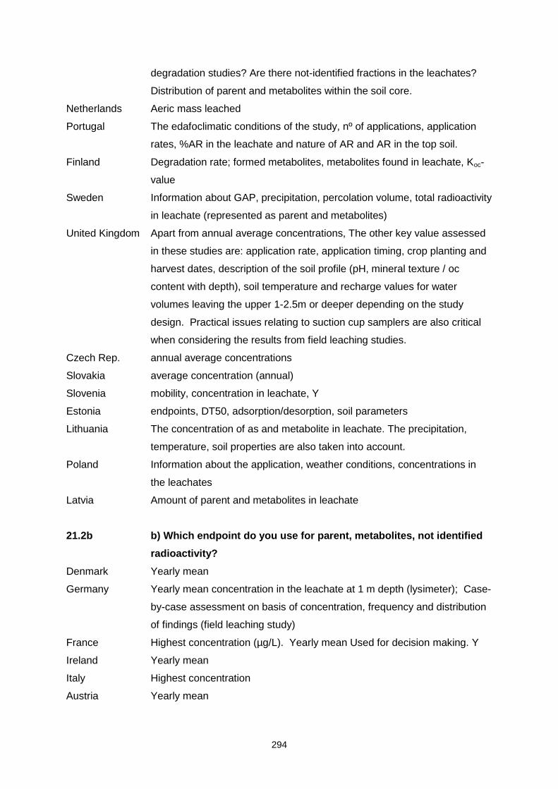
294
degradation studies? Are there not-identified fractions in the leachates?
Distribution of parent and metabolites within the soil core.
Netherlands Aeric mass leached
Portugal The edafoclimatic conditions of the study, nº of applications, application
rates, %AR in the leachate and nature of AR and AR in the top soil.
Finland Degradation rate; formed metabolites, metabolites found in leachate, Koc-
value
Sweden Information about GAP, precipitation, percolation volume, total radioactivity
in leachate (represented as parent and metabolites)
United Kingdom Apart from annual average concentrations, The other key value assessed
in these studies are: application rate, application timing, crop planting and
harvest dates, description of the soil profile (pH, mineral texture / oc
content with depth), soil temperature and recharge values for water
volumes leaving the upper 1-2.5m or deeper depending on the study
design. Practical issues relating to suction cup samplers are also critical
when considering the results from field leaching studies.
Czech Rep. annual average concentrations
Slovakia average concentration (annual)
Slovenia mobility, concentration in leachate, Y
Estonia endpoints, DT50, adsorption/desorption, soil parameters
Lithuania The concentration of as and metabolite in leachate. The precipitation,
temperature, soil properties are also taken into account.
Poland Information about the application, weather conditions, concentrations in
the leachates
Latvia Amount of parent and metabolites in leachate
21.2b b) Which endpoint do you use for parent, metabolites, not identified
radioactivity?
Denmark Yearly mean
Germany Yearly mean concentration in the leachate at 1 m depth (lysimeter); Case-
by-case assessment on basis of concentration, frequency and distribution
of findings (field leaching study)
France Highest concentration (µg/L). Yearly mean Used for decision making. Y
Ireland Yearly mean
Italy Highest concentration
Austria Yearly mean
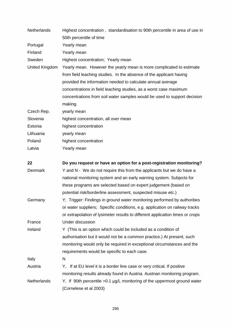
295
Netherlands Highest concentration , standardisation to 90th percentile in area of use in
50th percentile of time
Portugal Yearly mean
Finland Yearly mean
Sweden Highest concentration; Yearly mean
United Kingdom Yearly mean. However the yearly mean is more complicated to estimate
from field leaching studies. In the absence of the applicant having
provided the information needed to calculate annual average
concentrations in field leaching studies, as a worst case maximum
concentrations from soil water samples would be used to support decision
making.
Czech Rep. yearly mean
Slovenia highest concentration, all over mean
Estonia highest concentration
Lithuania yearly mean
Poland highest concentration
Latvia Yearly mean
22 Do you request or have an option for a post-registration monitoring?
Denmark Y and N - We do not require this from the applicants but we do have a
national monitoring system and an early warning system. Subjects for
these programs are selected based on expert judgement (based on
potential risk/borderline assessment, suspected misuse etc.)
Germany Y; Trigger: Findings in ground water monitoring performed by authorities
or water suppliers; Specific conditions, e.g. application on railway tracks
or extrapolation of lysimeter results to different application times or crops
France Under discussion
Ireland Y (This is an option which could be included as a condition of
authorisation but it would not be a common practice.) At present, such
monitoring would only be required in exceptional circumstances and the
requirements would be specific to each case.
Italy N
Austria Y, If at EU level it is a border line case or very critical. If positive
monitoring results already found in Austria. Austrian monitoring program.
Netherlands Y, If 90th percentile >0.1 μg/L monitoring of the uppermost ground water
(Cornelese et al 2003)

296
Portugal Y, We ask for monitoring data from areas were the PP will be used. In
cases were there is an identified potential for leaching
Finland N
Sweden No, but we are planning to introduce this. In cases with contradicting
results there is a need to follow up the decision.
United Kingdom Yes, although in recent years few examples of it being used.
Requirements and study protocols are agreed between the notifier and
PSD, and would differ depending on the exact nature of the issue that
required addressing.
Czech Rep. N
Slovenia Y, guideline is in the process of final definition
Estonia N
Lithuania Y, but in especially rare cases. Y
Poland N
Latvia N
23 Do model results override results from field studies i.e. models are
considered weighted higher than e.g. lysimeters?
Denmark N
Germany N
France N
Ireland N (If model results are satisfactory, field studies are not required.)
Italy Y
Austria N
Netherlands N, in general but equal in Tier 2
Portugal Regarding this question we don’t have sufficient data to answer Yes or No
Finland N
Sweden No all available information is considered
United Kingdom No not automatically but depending on the situation they could
Czech Rep. N
Slovenia N, if the field or lysimeter studies meet appropriate requirements
Estonia N
Lithuania N, but it depends on studies (relevance to local conditions). If studies are
done in non relevant conditions, the model results might be considered as
more relevant.
Poland N
Latvia N

297
24 Do results from field studies override model results i.e. lysimeters
are considered weighted higher than models ?
Denmark N
Germany Y
France N
Ireland Y
Italy N
Austria Y
Netherlands Y, in general but equal in Tier 2
Portugal Regarding this question we don’t have sufficient data to answer Yes or No
Finland Y
Sweden Yes a Swedish lysimeter is considered as a higher tier
United Kingdom No not automatically but depending on the situation they could
Czech Rep. Y, not automatically but in cases where the application was under realistic
and recommended conditions
Slovenia Y, if the field or lysimeter studies meet appropriate requirements
Estonia Y
Lithuania Y, if conditions are relevant.
Poland Y
Latvia Y, but not always
25 Do you jointly consider models and e.g. lysimeters/field leaching
studies and take a decision based on quality of the two cases?
Denmark Yes Quality and how representative the cases are. Y
Germany N, (of course, the quality of the studies has to be assessed)
France Y
Ireland Y (Comparability of modelling and field study results is assessed.)
Italy Y
Austria Y
Netherlands Y
Portugal Y
Finland Y
Sweden Y
United Kingdom Yes, the key criteria that would affect which of the two, greater reliance
would be placed would be the comparability of the approaches used to UK
cropping practice and geoclimatic conditions. Modelling calibrated against

298
a field study, then extrapolated to the pertinent UK conditions through
further modelling has been used to support UK authorisations, when the
approach used best experimental and modelling practice, was adequately
documented and stood up to independent scrutiny.
Czech Rep. Y
Slovenia Y
Estonia Y
Lithuania Y
Poland Y
Latvia Y
26 Do you apply model calculations to extrapolate experiments to
national or regional assessment?
Denmark Y
Germany N
France Usually no, but could be considered case by case.
Ireland N (If model results are satisfactory, field studies are not required.)
Italy Y
Austria N
Netherlands Y
Portugal N
Finland N
Sweden N
United Kingdom No, PSD doesn’t but we would accept this approach if proposed by an
applicant and the approach they had used followed best experimental and
modelling practice, was adequately documented and stood up to
independent scrutiny.
Czech Rep. N
Slovenia N, not yet
Estonia Y
Lithuania N
Poland N
Latvia N
27 Do you define metabolites according to the EU guidance document
on relevant metabolites (rev 10)?
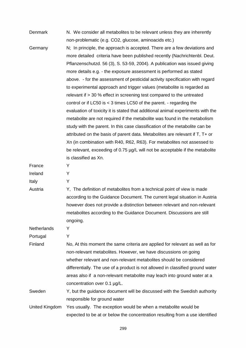
299
Denmark N. We consider all metabolites to be relevant unless they are inherently
non-problematic (e.g. CO2, glucose, aminoacids etc.)
Germany N; In principle, the approach is accepted. There are a few deviations and
more detailed criteria have been published recently (Nachrichtenbl. Deut.
Pflanzenschutzd. 56 (3), S. 53-59, 2004). A publication was issued giving
more details e.g. - the exposure assessment is performed as stated
above. - for the assessment of pesticidal activity specification with regard
to experimental approach and trigger values (metabolite is regarded as
relevant if > 30 % effect in screening test compared to the untreated
control or if LC50 is < 3 times LC50 of the parent. - regarding the
evaluation of toxicity it is stated that additional animal experiments with the
metabolite are not required if the metabolite was found in the metabolism
study with the parent. In this case classification of the metabolite can be
attributed on the basis of parent data. Metabolites are relevant if T, T+ or
Xn (in combination with R40, R62, R63). For metabolites not assessed to
be relevant, exceeding of 0.75 µg/L will not be acceptable if the metabolite
is classified as Xn.
France Y
Ireland Y
Italy Y
Austria Y, The definition of metabolites from a technical point of view is made
according to the Guidance Document. The current legal situation in Austria
however does not provide a distinction between relevant and non-relevant
metabolites according to the Guidance Document. Discussions are still
ongoing.
Netherlands Y
Portugal Y
Finland No, At this moment the same criteria are applied for relevant as well as for
non-relevant metabolites. However, we have discussions on going
whether relevant and non-relevant metabolites should be considered
differentially. The use of a product is not allowed in classified ground water
areas also if a non-relevant metabolite may leach into ground water at a
concentration over 0.1 µg/L.
Sweden Y, but the guidance document will be discussed with the Swedish authority
responsible for ground water
United Kingdom Yes usually. The exception would be when a metabolite would be
expected to be at or below the concentration resulting from a use identified
300
as a safe use for annex 1 listing, and the annex 1 listing concluded the
metabolite was not relevant, but the criteria used to agree non relevance
by member states for that active substance, predated the rev 10 guidance
document.
Czech Rep. Y
Slovenia Y
Estonia Y
Lithuania Y
Poland Y
Latvia Y
28a Have you set a trigger value different from parent for relevant
metabolites? If Yes, at what concentration?
Denmark N
Germany N
France N
Ireland N
Italy N
Austria N
Netherlands N
Portugal N
Finland N
Sweden N
United Kingdom N
Czech Rep. N
Slovenia Y, 0.1 µg/L (=N)
Estonia N
Lithuania N
Poland N
Latvia N
28b Non-relevant metabolites
Denmark N
Germany Y, Similar to the EU guidance document: 0.75 µg/L (“threshold of concern”
approach), general upper limit of 10 µg/L
France N; Non-relevant metabolites (Assessed according to the EU guidance
document)

301
Ireland Y (0.1 μg/L threshold limit does not apply to non-relevant metabolites. A
human health risk assessment should be performed to demonstrate that
there are no adverse effects arising from the predicted level of exposure.)
Italy At concentration: as suggested by the guidance on metabolite
Austria N
Netherlands For higher Tier studies there is no guidance for metabolites. Guidance
required!
Finland N
Sweden N, but might change after discussion with the ground water authority
United Kingdom Y, For parent and relevant metabolites the trigger value is 0.1μg/L. As in
the rev10 guidance document for non relevant metabolites (as defined by
the guidance document) concentrations up to 10μg/L would be considered
acceptable. Concentrations above this might be considered acceptable,
but UK Government Ministers would probably want the advice of the UK
Advisory Committee on Pesticides and consultation across a wide range of
UK Government Departments before uses where this occurred were
authorised. There are currently no practical examples where
reassessment following annex 1 listing has indicated a non relevant
metabolite with a concentration of >10μg/L.
Czech Rep. Y, according to rev. 10 guidance, up to 10 µg/L
Slovenia N
Lithuania N; The relevance of metabolites and 1-3 stages hazard assessment are
done according to guidance document on relevance of metabolites
(Sanco/221/2000-rev. 10).
Poland N
Latvia According to guidance doc. On the assessment of the relevance of
metabolites in gw. (SANCO/221/2000-rev.10)

302
APPENDIX 3. FOCUS GROUND WATER STUDY INFORMATION TABLES
Study, Directive
OECD Number
Description Useful information
Aerobic soil degradation (Laboratory) Route and rate II 7.1.1. and 7.2.1-7.2.3
Investigations are conducted under controlled laboratory conditions to evaluate both route and rate of degradation in soil for a period up to 120 day. Guidelines: Current EU guideline study is OECD307. However, older studies may have been conducted to SETAC 1995 (or US EPA) guidelines. OECD 307 – study conducted at 20
oC and 40-60%MWHC.
SETAC – study conducted at 20
oC and 40-50%MWHC.
EPA studies conducted at 25oC
and 75% of 0.33bar soil moisture and are usually drier than the studies conducted according to OECD or SETAC. Criteria for US studies are different and are considered on a case by case basis.
DegT50 (lab) of active substance under controlled temperature and soil moisture content. DegT50 should be normalised to 20
oC and
pF2 moisture content for use in FOCUS ground water assessment.
Identity and formation percentage of metabolites and metabolic pathway. CO2 mineralisation and bound residue formation.
DegT50 (lab) of metabolites by kinetic modelling [FOCUS Kinetics].
Correlation of degradation rates with soil properties – pH, CEC, clay content, OM etc.
Biphasic degradation can be indicative of kinetic sorption processes – degradation data can be analysed to derive Tier-1 kinetic sorption input parameters for ground water models (e.g. PEARL) [FOCUS Kinetics].
Aerobic degradation studies on sterile soils can indicate that abiotic degradation processes are important and allow default depth dependant degradation parameters to be adjusted.
Degradation studies on subsoils can give useful information such as identifying that other degradation processes are important and allow default depth dependant degradation parameters to be adjusted.
Soil photolysis (Laboratory) Route and rate II 7.1.3
Investigations are conducted under controlled laboratory conditions to evaluate the effect of photolysis on both the route and rate of degradation. Guidelines: Current EU guideline study is SETAC 1995.
Identifies if photolysis could be an important dissipation process (aqueous photolysis can also be an indicator).
FOCUS models do not directly account for photolysis. If this is an important dissipation route then higher-tier parameterisation of the models is required for degradation.
Anaerobic soil degradation II 7.1.2 and 7.2.4-7.2.5
Degradation in soil is investigated under anaerobic (reducing) conditions. Guidelines: Current EU guideline study is SETAC 1995.
Anaerobic soil studies can indicate that degradation will continue in anaerobic soil layers.
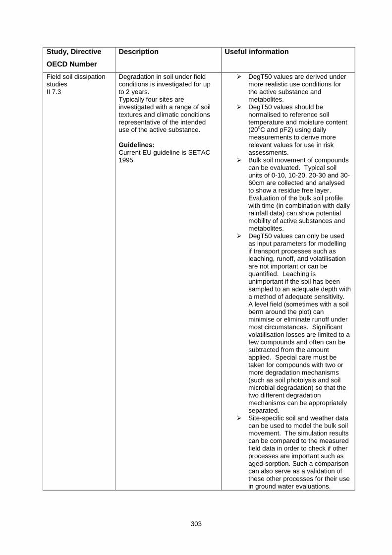
303
Study, Directive
OECD Number
Description Useful information
Field soil dissipation studies II 7.3
Degradation in soil under field conditions is investigated for up to 2 years. Typically four sites are investigated with a range of soil textures and climatic conditions representative of the intended use of the active substance. Guidelines: Current EU guideline is SETAC 1995
DegT50 values are derived under more realistic use conditions for the active substance and metabolites.
DegT50 values should be normalised to reference soil temperature and moisture content (20
oC and pF2) using daily
measurements to derive more relevant values for use in risk assessments.
Bulk soil movement of compounds can be evaluated. Typical soil units of 0-10, 10-20, 20-30 and 30-60cm are collected and analysed to show a residue free layer. Evaluation of the bulk soil profile with time (in combination with daily rainfall data) can show potential mobility of active substances and metabolites.
DegT50 values can only be used as input parameters for modelling if transport processes such as leaching, runoff, and volatilisation are not important or can be quantified. Leaching is unimportant if the soil has been sampled to an adequate depth with a method of adequate sensitivity. A level field (sometimes with a soil berm around the plot) can minimise or eliminate runoff under most circumstances. Significant volatilisation losses are limited to a few compounds and often can be subtracted from the amount applied. Special care must be taken for compounds with two or more degradation mechanisms (such as soil photolysis and soil microbial degradation) so that the two different degradation mechanisms can be appropriately separated.
Site-specific soil and weather data can be used to model the bulk soil movement. The simulation results can be compared to the measured field data in order to check if other processes are important such as aged-sorption. Such a comparison can also serve as a validation of these other processes for their use in ground water evaluations.

304
Study, Directive
OECD Number
Description Useful information
Adsorption desorption studies II 7.4.1-7.4.2
Sorption to soil is investigated under laboratory conditions according to OECD 106. Guidelines: Current EU guideline study is OECD106.
The adsorption coefficients Kd, Kf, Koc or Kom are determined for a range of soils. In addition, the Freundlich parameter (1/n) is also derived from studies conducted at multiple concentrations.
Dependence of sorption on soil properties (pH, clay content, CEC, iron ferro-oxides etc) can be investigated.
Sorption studies on subsoils can be useful for the evaluation of field studies.
Desorption hysteresis can show if kinetic (aged) sorption with time is important.
Streck kinetic sorption parameters for use in tier-1 ground water evaluations can be derived from the analysis of batch equilibrium adsorption desorption studies conducted according to OECD106.
Aged desorption studies
Increased sorption with time is determined from desorption experiments. The test compound is applied to soil and incubated under aerobic conditions (as per aerobic soil degradation study OECD 307). At various time points the soil sample is partitioned with CaCl2 (as per batch equilibrium adsorption desorption study OECD 106) to allow Kd or Kf values to be derived. Guidelines: No test guideline currently exists, but the soil incubation is conducted according to OECD 307 and the batch equilibrium according to OECD 106.
Kinetic sorption and degradation parameters can be derived from the evaluation of the data and used directly in higher-tier ground water evaluations.
The increase in Kd with time throughout the study can be determined.
Kinetic sorption data determined for soils collected from field dissipation studies can be used to validate higher-tier ground water evaluations.
Octanol water partition coefficient II 2.8.1
The octanol water coefficient (Log Kow, Log P) is determined under laboratory conditions. Shake flask or HPLC method (Koc). Guidelines: Partition coefficient octanol/water: Shake flask method OECD 107 (adopted 27 July 1995); Partition coefficient octanol/water: HPLC method, OECD 117 (adopted 13 April 2004)
Useful for estimating plant uptake and also adsorption for minor metabolites.
Kom can be estimated from Log Kow using a number of empirical routines.
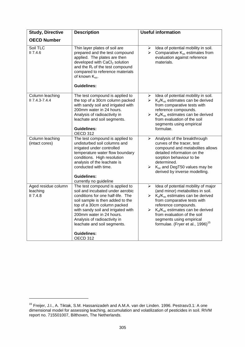
305
Study, Directive
OECD Number
Description Useful information
Soil TLC II 7.4.6
Thin layer plates of soil are prepared and the test compound applied. The plates are then developed with CaCl2 solution and the Rf of the test compound compared to reference materials of known Koc. Guidelines:
Idea of potential mobility in soil. Comparative Koc estimates from
evaluation against reference materials.
Column leaching II 7.4.3-7.4.4
The test compound is applied to the top of a 30cm column packed with sandy soil and irrigated with 200mm water in 24 hours. Analysis of radioactivity in leachate and soil segments. Guidelines: OECD 312
Idea of potential mobility in soil. Kd/Koc estimates can be derived
from comparative tests with reference compounds.
Kd/Koc estimates can be derived from evaluation of the soil segments using empirical formulae.
Column leaching (intact cores)
The test compound is applied to undisturbed soil columns and irrigated under controlled temperature water flow boundary conditions. High resolution analysis of the leachate is conducted with time. Guidelines: currently no guideline
Analysis of the breakthrough curves of the tracer, test compound and metabolites allows detailed information on the sorption behaviour to be determined.
Koc and DegT50 values may be derived by inverse modelling.
Aged residue column leaching II 7.4.8
The test compound is applied to soil and incubated under aerobic conditions for one half-life. The soil sample is then added to the top of a 30cm column packed with sandy soil and irrigated with 200mm water in 24 hours. Analysis of radioactivity in leachate and soil segments. Guidelines: OECD 312
Idea of potential mobility of major (and minor) metabolites in soil.
Kd/Koc estimates can be derived from comparative tests with reference compounds.
Kd/Koc estimates can be derived from evaluation of the soil segments using empirical formulae. (Fryer et al., 1996)
15
15 Freijer, J.I., A. Tiktak, S.M. Hassanizadeh and A.M.A. van der Linden. 1996. Pestrasv3.1: A one
dimensional model for assessing leaching, accumulation and volatilization of pesticides in soil. RIVM report no. 715501007, Bilthoven, The Netherlands.

306
Study, Directive
OECD Number
Description Useful information
Lysimeter studies II 7.4.7
Soil usually with a coarse (sandy) texture Rather high rainfall, supplemented by irrigation if not high enough For example BBA requirements often followed : % OC < 1.5 % rainfall (+ irrigation) >800 mm Maximum application rate and maximum number of applications expected, application timing at the period where leaching is expected to be maximised, but in line with the recommended GAP. Crop in agreement with the intended use or bare soil (considered as less favourable due to lower evapotranspiration) Study duration : often two lysimeters, one with single or multiple applications the first year and two-year leachate sampling, the other with single or multiple applications the first two years and three-year leachate sampling Radiolabelled material usually used Guidelines: BBA IV, 4-3 and Modification of the lysimeter guideline (Nachrichtenbl. Dt. PflSchD. 43, 1991). Guidance Document: OECD Series on Testing and Assessment, No. 22.
Active substance and metabolites contents in the leachate (possibility of detection of metabolites that were not identified in the soil metabolism)
Active substance and metabolites contents in the soil profile at the end of the study
May allow parameter refinement for modelling (only if detailed soil and weather data are available).
Limitations : No information about intermediate depths before the end of the study Hydrological specificities of a closed device.
Mass flow of leaching compounds, however, measured to be higher compared to field plots (Jene et al., 1998).
Agroclimatic and soil conditions typical of a small percentage of arable land in several countries, even if they are considered to be a worst-case for a variety of conditions (mostly close to FOCUS Hamburg scenarios)

307
Study, Directive
OECD Number
Description Useful information
Field leaching studies II 7.4.8
a) suction cups
Information about field soil hydrology (tensiometers…) Suction cups for water sampling (by application of a negative pressure) in the unsaturated and/or saturated zone or wells screened into the shallow ground water table. The material of the suction cups or wells must minimise adsorption. The installation of the suction cups must ensure a good contact between soil and cups (silica flour can be used to aid the hydraulic contact) and it is essential to prevent preferential flow along the tubes (bentonite is typically used to seal to within about 10cm of the suction cup). The cups and their pipes should not be installed in contaminated soil when measuring concentrations around 0.1 ppb because this is prone to give false postitives (better: installations from the side) It is also necessary to be careful of the possible effect of an artificial hydraulic gradient due to the pressure applied for sampling (samples should therefore only be collected when freely draining water is available i.e. when tensiometers show a positive pore water pressure / matrix potential). The depth of the water table must be specified.
Concentrations in soil and water at different depths and different sampling dates in realistic field conditions
Preferential flow can be investigated
May allow parameter refinement for modelling (only if detailed soil and weather data are available).
Limitations : No radiolabelling No balance for the active substance Concentration in water at different depths in the soil profile not necessarily reliable due to use of suction cups Spatial and temporal variations can make the interpretation of results rather complex

308
Study, Directive
OECD Number
Description Useful information
Field leaching studies II 7.4.8
b) ground water wells
Test fields are chosen that represent typical or worst case climatic, soil and ground water conditions for the use to be tested, depending on the objective of the study. The test field is extensively characterised with regard to soil and hydrological conditions. It should be large enough to be maintained with common agricultural equipment and practice. The field is equipped with a suitable number of ground water sampling wells, depending on the size of the field and the local ground water conditions. The wells must be in cluster (minimum 2 wells at 5 meters of distance) of at least three and will be placed in the field take into account the hydrology. The field is cropped with the target crop and is treated with the test substance according to the label. Samples of ground water are taken regularly (e.g. monthly) from the uppermost ground water and are analysed for the test substance or its derivatives. Additional sampling may include soil samples or water samples extracted from the unsaturated zone using e.g. suction cups. Additional data gathering that facilitates the interpretation of the results may include local weather data, soil moisture/water tension data, recording of the ground water level etc. The possibility to irrigate the field allows for additional options in the design of the study. The use of a conservative tracer may increase the acceptance of the study.
Concentration in the target compartment (ground water = actual subject of protection) at different sampling dates under real practice conditions
Total ground water load includes contribution of preferential flow
Significant local point source entries (e.g. by preferential flow) are detectable by using a sufficient number of wells
May allow for parameter refinement for modelling
Hydrolysis II 2.9.1 and II 7.5
The hydrolytic degradation of the test compound is studied under sterile conditions at various pH’s (typical [4] 5, 7 and 9) Guidelines: OECD 111
Can identify if abiotic hydrolytic degradation processes are significant for the test compound.
If the test compound readily hydrolyses at environmentally relevant pHs then the default depth dependant degradation factors can be adjusted for a higher-tier evaluation.
The effect of varying soil pH for each FOCUS scenario has to be considered.

309
Study, Directive
OECD Number
Description Useful information
Monitoring II 7.12
Information about quality of the wells, geology, aquifers (depth and characteristics like water infiltration rate), land use, list of compounds analysed, limit of detection and limit of quantification for each compound. It is possible to distinguish between general monitoring (for example national or regional programs of water quality control) and specific monitoring programs (in shallow or deeper aquifers) for one active substance and relevant metabolites decided by agrochemical companies and regulators.
Comparison / validation of predicted concentrations
Information on real concentrations in the aquifers and on long term tendencies
Regional or local differences can provide information about more vulnerable areas, allowing for regional or local risk management.
Limitations : Monitoring not possible before authorisation of a substance, however post-registration monitoring programs possible Spatial and temporal variability difficult to interpret Aquifer recharge area not always well known Abstraction of water can modify the surrounding hydrology
310
APPENDIX 4: A METHOD TO DERIVE CROP-SPECIFIC LEACHING SCENARIOS
Introduction
The aim of the FOCUS ground water group was to develop a limited number of “realistic
worst-case” leaching scenarios, which were broadly representative of agriculture in major
agricultural production areas of the EU. In order to limit the number of simulation runs to a
manageable size, the leaching scenarios are used to simulate pesticide applications to 25
crops, which were defined for each site according to the probability of occurrence in the
respective agricultural region. For that reason FOCUS leaching scenarios represent a
screening tool that reflect collectively realistic and vulnerable use conditions in relevant
climate zones and agricultural areas in Europe. As a result of this regulatory framework, the
following two characteristics of FOCUS scenarios should be considered:
1. FOCUS leaching scenarios were not designed to reflect the worst-case for the
country from where weather files were obtained but reflect vulnerable situations that
are representative for agricultural zones across various member states.
2. Each FOCUS scenario was parameterised with data for a range of crops. As a
consequence the relative leaching vulnerability for a specific crop-location scenario
varies with the crops for a given location. For major crops (e.g. cereals, maize) the
scenario might reflect a realistic worst-case whereas for other crops the scenarios
might be not representative at all (e.g. Hamburg/vines, Piacenza/citrus).
If simulations with FOCUS scenarios suggest that a more detailed analysis of leaching risk is
required at the member state level, defining crop-specific worst-case scenarios on the basis
of the actual cropping areas is appropriate. This appendix describes a method that can be
used to identify candidate locations for new crop-specific scenarios. Specific guidance on
the parameterisation of the new soil scenario files is given in Section 7.2.5. This section also
recommends the context in which new cropping scenarios should be used within the FOCUS
ground water framework for this purpose.
The proposed method intends to identify new, crop-specific leaching scenarios that can be
calculated with the same FOCUS leaching models used in Tier-1. These higher tier
scenarios are selected on the basis of the co-occurrence of climate, soil and crop properties,
which are considered vulnerable for pesticide leaching. By overlaying the respective data
layers in a GIS, the overall percentile of leaching vulnerability can be quantified in order to
put the new scenarios in the context of the overall assessment of leaching risk. More realism
311
is thus introduced into the assessment since the overall percentile is specifically derived for
the intended use area of a compound. The PECgw in Tier 2 is eventually calculated with a
standard FOCUS leaching model which was parameterised with the new crop, climate and
soil parameters and with country specific application data if appropriate. Except for the new
scenario definition, the PECgw calculation follows the guidance for simulation runs in Tier-1.
The intention of this appendix is to provide guidance for harmonised higher-tier assessments
at the EU and national level. For maximum harmonisation, the proposed method should be
applicable to every member state in the EU. For that reason GIS data sets covering the
entire EU are preferred (see fact sheets in Appendix 8). National soil data sets sometimes
contain more detailed information and might be considered superior to European data for
local assessments.
Identification of suitable indicators for leaching risk
Soil parameters
A number of soil properties influence the leaching behaviour of compounds, but due to
limited availability of soil data restricting the vulnerability assessment to a few parameters is
inevitable. The basic requirement is that the parameter should cause a pronounced
sensitivity in leaching calculations with FOCUS models AND the spatial variation of this
parameter should be available in the same resolution and quality for ALL member states in
the EU.
Van den Berg et al. (2008) provide a sensitivity analysis for the GeoPearl model. Dubus et al
(2000, 2003) conducted a sensitivity analysis for FOCUS leaching models and found that
organic carbon content, bulk density and water content at field capacity are the most
influential parameters in leaching calculations. The latter parameter is used in capacitance
models for the simulation of soil water fluxes down the soil profile and is not present in
models that solve the Richards equation. For that reason the sensitivity is dependent on the
model. Bulk density is provided across the EU only in classified form, which prevents the use
of this parameter in quantitative assessments. In view of these limitations the organic carbon
content in topsoil was used as the primary indicator for leaching vulnerability. This decision
was based on the following rationale:
Calculated organic carbon contents are available as continuous data points (1 x 1 km)
across the European Union (Jones et al. 2004, 2005).
312
The organic carbon content is one of the most sensitive soil parameters in PRZM,
PELMO, and PEARL. In this way the sensitivity is independent of the leaching model
that is used in the assessment.
Special case: Interactions between soil and pesticide parameters
In cases where compounds degrade mainly via abiotic processes, the soil pH can also be an
important indicator for site-specific degradation rates. Soil pH should be used as an
additional indicator for leaching risk if pH-dependence of leaching risk is expected. In case of
a clear relationship between soil pH and degradation rates the soil pH can be used as an
additional indicator. The impact of soil pH on the sorption behaviour is sometimes of binary
nature, which means that sorption changes abruptly once a specific pH level is passed.
Such phenomena need to be considered on a case-by-case basis if appropriate.
Currently there is no reliable coverage of pH values in European soils. The best
approximation of pH is provided by Batjes et al. (1995) who assigned average pH values to
soil units based on the FAO names. The respective estimates for pH can be visualised by
means of the EU soil map.
If the Kf of an active ingredient does not correlate with the organic carbon content in soils
alternative indicators or multiple correlations with soil properties should be used. Beside pH
such indicators could be textural parameters like clay content. As a general rule, the choice
of spatial indicators should be based on existing knowledge about the factors that determine
the mobility of the test substance. Sufficient evidence that a factor is exerting a significant
influence on the mobility is either a high correlation of Kf or DegT50 with a specific soil
parameter or, in exceptional cases, a more complex sensitivity analysis.
Climate parameters
In contrast to chemical leaching, Dubus et al. (2003) found that modelled percolation
volumes were only slightly affected by variations of soil parameters, suggesting that
meteorological variables will be the main drivers of water balance predictions. Therefore, for
the majority of compounds the average sum of precipitation during the period of ground water
recharge (October – March) and the mean annual temperature are the primary climate
indicators for leaching vulnerability.
313
As a refinement of the original definition of FOCUS only rainfall volumes between October
and March are considered if the compound is likely to be present in soil at the onset of the
recharge period. This approach is based on the following rationale:
Ground water recharge is most likely occurring outside the vegetation period when
evapotranspiration is low and soil moisture is close to saturation. Northern European
soils are typically saturated after autumn rainfalls and again at the end of winter
during snowmelt. A similar cycle can be observed in southern Europe although the
absolute volume of ground water recharge is smaller.
From spring until late summer the overall water balance is likely to be negative for
most agricultural areas in Europe. A rough calculation of water excess in the MARS
data base (= precipitation minus evapotranspiration) during April and September
reveals that only in small regions the water balance is positive in summer (see
Chapter 13).
A further advantage of this pragmatic approach is that uncertainties with regards to irrigation
practices during the vegetation period are minimised.
The current resolution of the European climate database MARS is 50 x 50 km, which is a
rather coarse resolution when performing the analysis for small cropping areas. In cases
where higher-resolution climate data are available, the resulting smaller grid-size would be
preferable because it is closer to the scale of the soil information.
Temperature is an important discriminator as this parameter influences both the calculated
volumes of leachate as well as the degradation of chemicals.
Special Case: Interactions between climate and pesticide parameters
Van der Linden et al. (2004) suggest that the leaching behaviour of compounds with a
DegT50 of less than 10 d and a Kom below 10 L kg-1 (Koc of 17 L kg-1) is highly influenced by
seasonal climate patterns. In the case of short-lived compounds with very low sorption
capacity in soils, the 3-month period after application is most appropriate. If the same
compound is applied in autumn, winter rainfall should be used.
Rainfall volumes and temperatures within the cropping area can be extracted from the MARS
(2004) weather data base, which contains daily weather data from 1992 – 2003 in 50 x 50 km
314
grid cells. MARS was also the source of FOCUS climate files and is therefore the most
appropriate data base to perform an analysis of spatial leaching risk in a Tier-II assessment.
Identifying locations for crop-specific worst-case scenarios
The area of interest
In a first step, the cropping area is identified to ensure that calculated leaching vulnerabilities
reflect only the cropping area. Some perennial crops like olives or vineyards are included as
separate classes in Corine Land Cover (Corine, 2000) and thus their regional occurrence can
be visualised with a high spatial accuracy. Individual fruit and field crops have to be
visualised by means of agricultural census data since Corine Land Cover does not
differentiate between crops on arable land or orchards.
In order to give a practical example of the application of the method, a virtual use in French
sugar beets was chosen in this section. In France the best source of statistical data is the
agricultural census of 200 at the level of cantons (Nuts 4), which is available through the
National Office of Statistics (SCEES, 2000). The area of interest was subsequently defined
as “any canton where sugar beets are grown on at least 100 ha”. The threshold of 100 ha
was chosen in this particular example because it is likely areas < 100 ha are not shown in
Nuts-4 data because of data protection regulations. If Nuts-3 data are used (i.e.
Départments in France) a higher threshold value is appropriate and needs to be justified
based on the simulated crop.
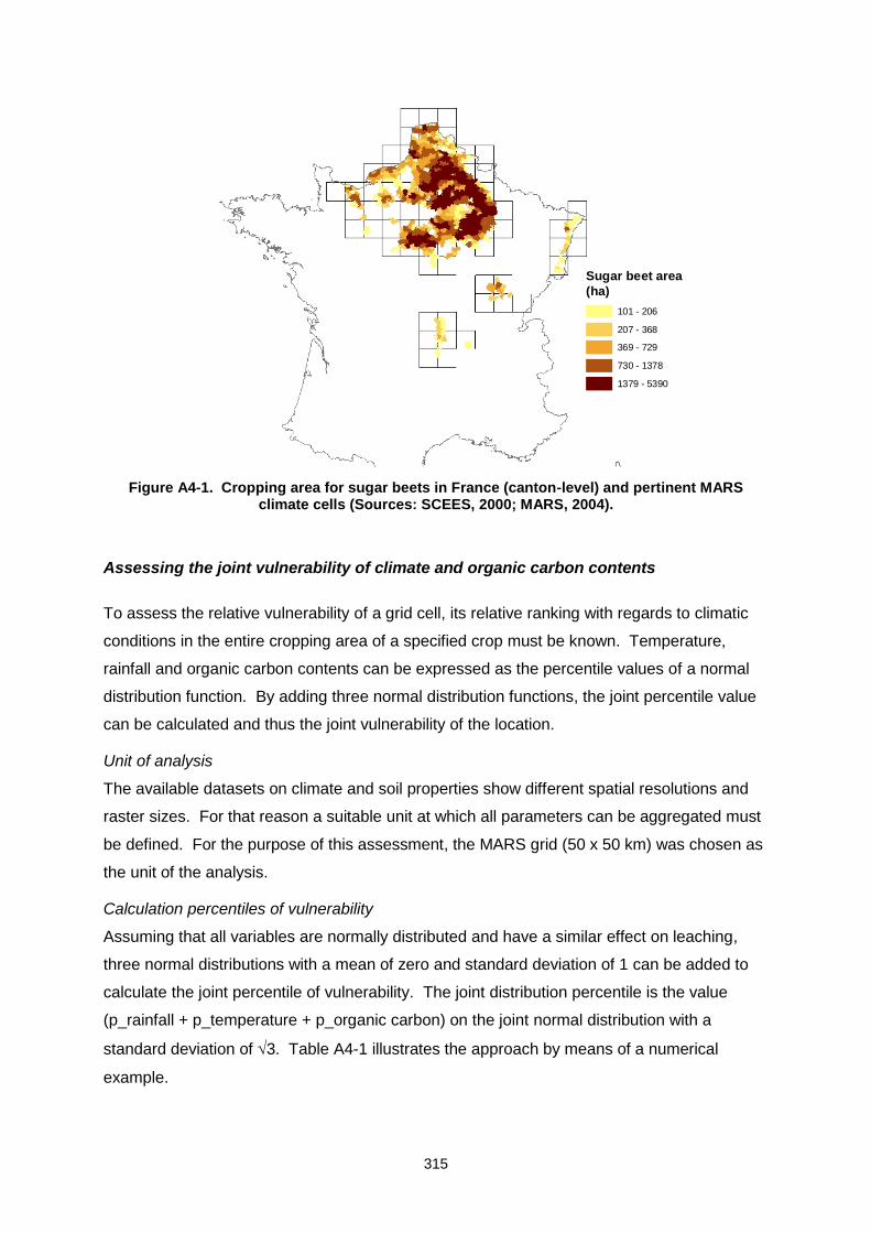
315
Sugar beet area
(ha)
101 - 206
207 - 368
369 - 729
730 - 1378
1379 - 5390
Figure A4-1. Cropping area for sugar beets in France (canton-level) and pertinent MARS climate cells (Sources: SCEES, 2000; MARS, 2004).
Assessing the joint vulnerability of climate and organic carbon contents
To assess the relative vulnerability of a grid cell, its relative ranking with regards to climatic
conditions in the entire cropping area of a specified crop must be known. Temperature,
rainfall and organic carbon contents can be expressed as the percentile values of a normal
distribution function. By adding three normal distribution functions, the joint percentile value
can be calculated and thus the joint vulnerability of the location.
Unit of analysis
The available datasets on climate and soil properties show different spatial resolutions and
raster sizes. For that reason a suitable unit at which all parameters can be aggregated must
be defined. For the purpose of this assessment, the MARS grid (50 x 50 km) was chosen as
the unit of the analysis.
Calculation percentiles of vulnerability
Assuming that all variables are normally distributed and have a similar effect on leaching,
three normal distributions with a mean of zero and standard deviation of 1 can be added to
calculate the joint percentile of vulnerability. The joint distribution percentile is the value
(p_rainfall + p_temperature + p_organic carbon) on the joint normal distribution with a
standard deviation of 3. Table A4-1 illustrates the approach by means of a numerical
example.
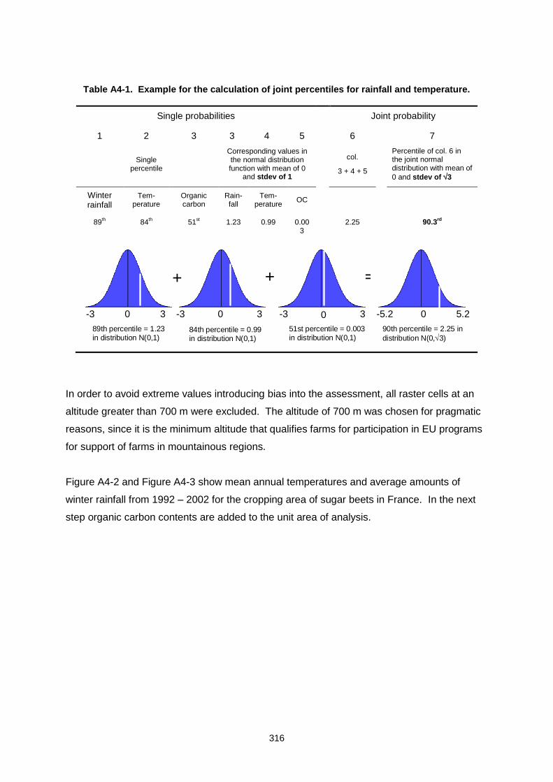
316
Table A4-1. Example for the calculation of joint percentiles for rainfall and temperature.
Single probabilities Joint probability
1 2 3 3 4 5 6 7
Single
percentile
Corresponding values in the normal distribution function with mean of 0
and stdev of 1
col.
3 + 4 + 5
Percentile of col. 6 in the joint normal distribution with mean of
0 and stdev of 3
Winter rainfall
Tem-perature
Organic carbon
Rain-fall
Tem-perature
OC
89th 84
th 51
st 1.23 0.99 0.00
3 2.25 90.3
rd
+ + =
-3 3 -3 3 -3 3 -5.2 5.20 0 0 0
89th percentile = 1.23in distribution N(0,1)
84th percentile = 0.99in distribution N(0,1)
51st percentile = 0.003in distribution N(0,1)
90th percentile = 2.25 in
distribution N(0,3)
In order to avoid extreme values introducing bias into the assessment, all raster cells at an
altitude greater than 700 m were excluded. The altitude of 700 m was chosen for pragmatic
reasons, since it is the minimum altitude that qualifies farms for participation in EU programs
for support of farms in mountainous regions.
Figure A4-2 and Figure A4-3 show mean annual temperatures and average amounts of
winter rainfall from 1992 – 2002 for the cropping area of sugar beets in France. In the next
step organic carbon contents are added to the unit area of analysis.
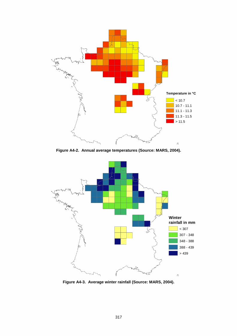
317
Temperature in °C
< 10.7
10.7 - 11.1
11.1 - 11.3
11.3 - 11.5
> 11.5
Figure A4-2. Annual average temperatures (Source: MARS, 2004).
Winter
rainfall in mm
< 307
307 - 348
348 - 388
388 - 439
> 439
Figure A4-3. Average winter rainfall (Source: MARS, 2004).
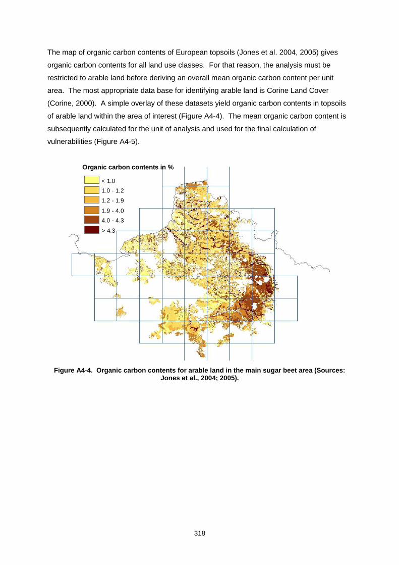
318
The map of organic carbon contents of European topsoils (Jones et al. 2004, 2005) gives
organic carbon contents for all land use classes. For that reason, the analysis must be
restricted to arable land before deriving an overall mean organic carbon content per unit
area. The most appropriate data base for identifying arable land is Corine Land Cover
(Corine, 2000). A simple overlay of these datasets yield organic carbon contents in topsoils
of arable land within the area of interest (Figure A4-4). The mean organic carbon content is
subsequently calculated for the unit of analysis and used for the final calculation of
vulnerabilities (Figure A4-5).
Organic carbon contents in %
< 1.0
1.0 - 1.2
1.2 - 1.9
1.9 - 4.0
4.0 - 4.3
> 4.3
Figure A4-4. Organic carbon contents for arable land in the main sugar beet area (Sources: Jones et al., 2004; 2005).
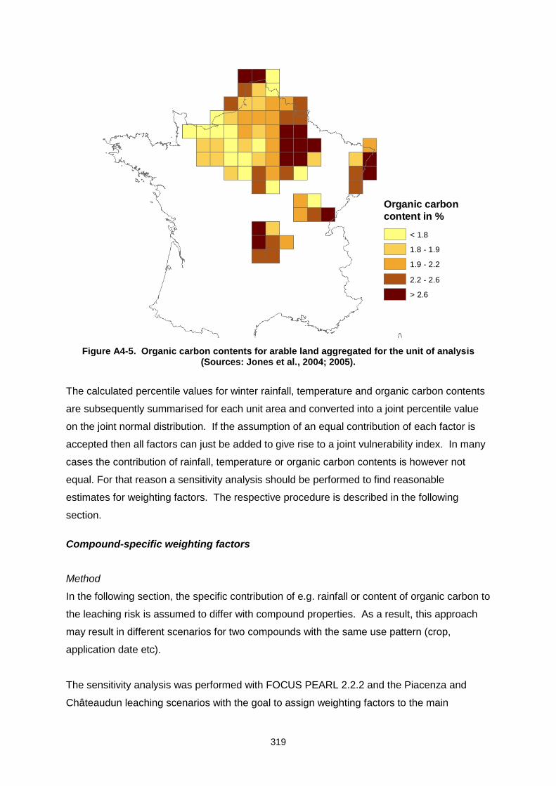
319
Organic carbon
content in %
< 1.8
1.8 - 1.9
1.9 - 2.2
2.2 - 2.6
> 2.6
Figure A4-5. Organic carbon contents for arable land aggregated for the unit of analysis (Sources: Jones et al., 2004; 2005).
The calculated percentile values for winter rainfall, temperature and organic carbon contents
are subsequently summarised for each unit area and converted into a joint percentile value
on the joint normal distribution. If the assumption of an equal contribution of each factor is
accepted then all factors can just be added to give rise to a joint vulnerability index. In many
cases the contribution of rainfall, temperature or organic carbon contents is however not
equal. For that reason a sensitivity analysis should be performed to find reasonable
estimates for weighting factors. The respective procedure is described in the following
section.
Compound-specific weighting factors
Method
In the following section, the specific contribution of e.g. rainfall or content of organic carbon to
the leaching risk is assumed to differ with compound properties. As a result, this approach
may result in different scenarios for two compounds with the same use pattern (crop,
application date etc).
The sensitivity analysis was performed with FOCUS PEARL 2.2.2 and the Piacenza and
Châteaudun leaching scenarios with the goal to assign weighting factors to the main
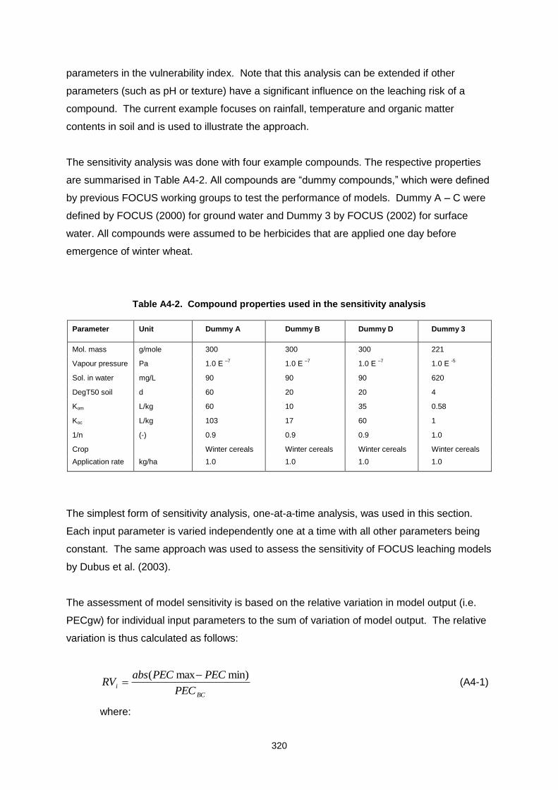
320
parameters in the vulnerability index. Note that this analysis can be extended if other
parameters (such as pH or texture) have a significant influence on the leaching risk of a
compound. The current example focuses on rainfall, temperature and organic matter
contents in soil and is used to illustrate the approach.
The sensitivity analysis was done with four example compounds. The respective properties
are summarised in Table A4-2. All compounds are “dummy compounds,” which were defined
by previous FOCUS working groups to test the performance of models. Dummy A – C were
defined by FOCUS (2000) for ground water and Dummy 3 by FOCUS (2002) for surface
water. All compounds were assumed to be herbicides that are applied one day before
emergence of winter wheat.
Table A4-2. Compound properties used in the sensitivity analysis
Parameter Unit Dummy A Dummy B Dummy D Dummy 3
Mol. mass g/mole 300 300 300 221
Vapour pressure Pa 1.0 E –7
1.0 E –7
1.0 E –7
1.0 E -5
Sol. in water mg/L 90 90 90 620
DegT50 soil d 60 20 20 4
Kom L/kg 60 10 35 0.58
Koc L/kg 103 17 60 1
1/n (-) 0.9 0.9 0.9 1.0
Crop Winter cereals Winter cereals Winter cereals Winter cereals
Application rate kg/ha 1.0 1.0 1.0 1.0
The simplest form of sensitivity analysis, one-at-a-time analysis, was used in this section.
Each input parameter is varied independently one at a time with all other parameters being
constant. The same approach was used to assess the sensitivity of FOCUS leaching models
by Dubus et al. (2003).
The assessment of model sensitivity is based on the relative variation in model output (i.e.
PECgw) for individual input parameters to the sum of variation of model output. The relative
variation is thus calculated as follows:
BC
iPEC
PECPECabsRV
min)max( (A4-1)
where:
321
RVi = ratio of variation for the landscape parameter i
PECmax = maximum PEC in sensitivity analysis for the landscape parameter i
PECmin = minimum PEC in sensitivity analysis for the landscape parameter i
PECBC = PEC value in base case scenario
The weighting factor for landscape parameter i is subsequently calculated by dividing the
ratio of variation of the single factor by the sum of the variation of all landscape factors:
i
i
iRV
RVf (A4-2)
Example sensitivity analysis
The Piacenza and Châteaudun winter cereals scenario in FOCUS PEARL 2.2.2 were used
as the base case in this study to ensure that the selection of a particular FOCUS Tier 1
scenario does not impact the results.
Selection of upper and lower boundaries for the sensitivity analysis. Depending on the
landscape one parameter may show a larger variation than another. For that reason, the
regional variation of rainfall, temperature and organic carbon should be analyzed first. The
simplest indicator for the comparison of the variability of landscape factors is the coefficient
of variation. In the sugar beet area in France organic carbon contents vary most, followed by
winter rainfall and temperature.
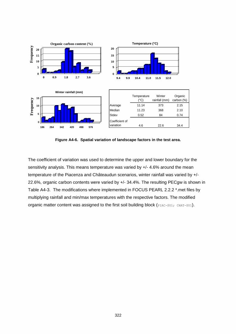
322
0 0.9 1.8 2.7 3.6
Organic carbon content (%)
0
5
10
15
20
Fre
qu
ency
Temperature (°C)
9.4 9.9 10.4 11.0 12.0
0
20
11.5
15
10
5
186 264 342 420 576
Winter rainfall (mm)
0
5
10
15
498
Fre
qu
ency
Temperature
(°C)
Winter
rainfall (mm)
Organic
carbon (%)
Average 11.14 373 2.15
Median 11.23 368 2.10
Stdev 0.52 84 0.74
Coefficient of
variation 4.6 22.6 34.4
Figure A4-6. Spatial variation of landscape factors in the test area.
The coefficient of variation was used to determine the upper and lower boundary for the
sensitivity analysis. This means temperature was varied by +/- 4.6% around the mean
temperature of the Piacenza and Châteaudun scenarios, winter rainfall was varied by +/-
22.6%, organic carbon contents were varied by +/- 34.4%. The resulting PECgw is shown in
Table A4-3. The modifications where implemented in FOCUS PEARL 2.2.2 *.met files by
multiplying rainfall and min/max temperatures with the respective factors. The modified
organic matter content was assigned to the first soil building block (PIAC-SU1; CHAT-SU1).
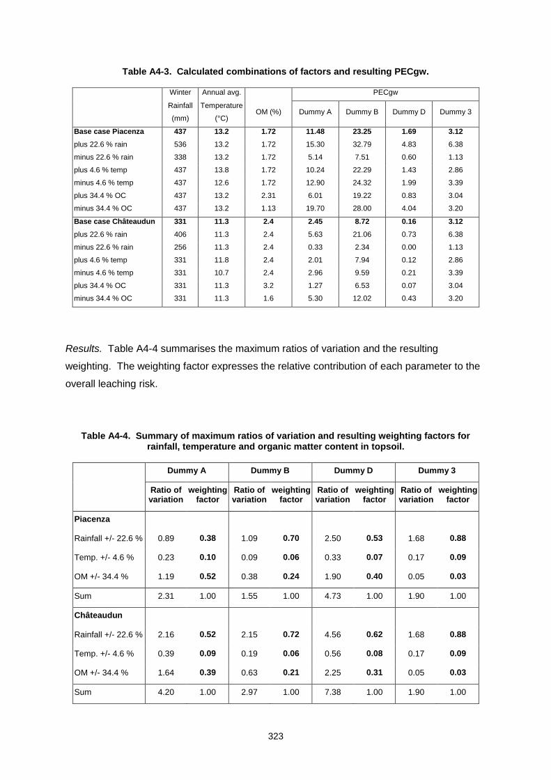
323
Table A4-3. Calculated combinations of factors and resulting PECgw.
Winter Annual avg. PECgw
Rainfall
(mm)
Temperature
(°C) OM (%) Dummy A Dummy B Dummy D Dummy 3
Base case Piacenza 437 13.2 1.72 11.48 23.25 1.69 3.12
plus 22.6 % rain 536 13.2 1.72 15.30 32.79 4.83 6.38
minus 22.6 % rain 338 13.2 1.72 5.14 7.51 0.60 1.13
plus 4.6 % temp 437 13.8 1.72 10.24 22.29 1.43 2.86
minus 4.6 % temp 437 12.6 1.72 12.90 24.32 1.99 3.39
plus 34.4 % OC 437 13.2 2.31 6.01 19.22 0.83 3.04
minus 34.4 % OC 437 13.2 1.13 19.70 28.00 4.04 3.20
Base case Châteaudun 331 11.3 2.4 2.45 8.72 0.16 3.12
plus 22.6 % rain 406 11.3 2.4 5.63 21.06 0.73 6.38
minus 22.6 % rain 256 11.3 2.4 0.33 2.34 0.00 1.13
plus 4.6 % temp 331 11.8 2.4 2.01 7.94 0.12 2.86
minus 4.6 % temp 331 10.7 2.4 2.96 9.59 0.21 3.39
plus 34.4 % OC 331 11.3 3.2 1.27 6.53 0.07 3.04
minus 34.4 % OC 331 11.3 1.6 5.30 12.02 0.43 3.20
Results. Table A4-4 summarises the maximum ratios of variation and the resulting
weighting. The weighting factor expresses the relative contribution of each parameter to the
overall leaching risk.
Table A4-4. Summary of maximum ratios of variation and resulting weighting factors for rainfall, temperature and organic matter content in topsoil.
Dummy A Dummy B Dummy D Dummy 3
Ratio of variation
weighting factor
Ratio of variation
weighting factor
Ratio of variation
weighting factor
Ratio of variation
weighting factor
Piacenza
Rainfall +/- 22.6 % 0.89 0.38 1.09 0.70 2.50 0.53 1.68 0.88
Temp. +/- 4.6 % 0.23 0.10 0.09 0.06 0.33 0.07 0.17 0.09
OM +/- 34.4 % 1.19 0.52 0.38 0.24 1.90 0.40 0.05 0.03
Sum 2.31 1.00 1.55 1.00 4.73 1.00 1.90 1.00
Châteaudun
Rainfall +/- 22.6 % 2.16 0.52 2.15 0.72 4.56 0.62 1.68 0.88
Temp. +/- 4.6 % 0.39 0.09 0.19 0.06 0.56 0.08 0.17 0.09
OM +/- 34.4 % 1.64 0.39 0.63 0.21 2.25 0.31 0.05 0.03
Sum 4.20 1.00 2.97 1.00 7.38 1.00 1.90 1.00
324
The proposed method allows for a quick assessment of the relative contribution of three
environmental parameters that are assumed to influence the leaching behaviour of
compounds. Due to its simplicity, the method can be applied routinely before deriving a
vulnerability index by means of GIS methods. Note that the relative contribution of organic
matter content, rainfall and temperature varies to a greater extent with decreasing sorption
capacity. Dummy 3 has a Koc of 1; therefore the content of organic carbon is almost
irrelevant for the explanation of the leaching behaviour of the compound. In this case other
parameters should be checked to determine whether they are a better descriptor to
differentiate regional leaching vulnerability (e.g. pH or texture). If this is not the case then the
assessment should be restricted to climate properties only.
The sensitivity analysis for four FOCUS dummy compounds revealed that the selected base-
case has only a minimal effect on the resulting weighting factors. For the sake of practicality,
the work group suggests to use only those FOCUS scenarios as base cases in which 0.1
µg/L were exceeded in Tier 1. The resulting weighting factors would then be the average
factors found in these runs.
Figure A4-7 shows a comparison between the relative leaching risk of Dummy A and Dummy
3 for the sugar beet area using the average weighting factors. The compounds show different
weighting factors and thus illustrate the impact of compound properties in the method..
The resulting overall vulnerabilities for Dummy A are shown in Figure A4-7.
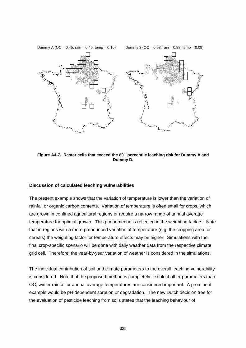
325
Dummy A (OC = 0.45, rain = 0.45, temp = 0.10)
Dummy 3 (OC = 0.03, rain = 0.88, temp = 0.09)
Figure A4-7. Raster cells that exceed the 80th
percentile leaching risk for Dummy A and Dummy D.
Discussion of calculated leaching vulnerabilities
The present example shows that the variation of temperature is lower than the variation of
rainfall or organic carbon contents. Variation of temperature is often small for crops, which
are grown in confined agricultural regions or require a narrow range of annual average
temperature for optimal growth. This phenomenon is reflected in the weighting factors. Note
that in regions with a more pronounced variation of temperature (e.g. the cropping area for
cereals) the weighting factor for temperature effects may be higher. Simulations with the
final crop-specific scenario will be done with daily weather data from the respective climate
grid cell. Therefore, the year-by-year variation of weather is considered in the simulations.
The individual contribution of soil and climate parameters to the overall leaching vulnerability
is considered. Note that the proposed method is completely flexible if other parameters than
OC, winter rainfall or annual average temperatures are considered important. A prominent
example would be pH-dependent sorption or degradation. The new Dutch decision tree for
the evaluation of pesticide leaching from soils states that the leaching behaviour of
326
compounds with a DegT50 < 10 d and a Kom < 10 L/kg would be more influenced by
seasonal rainfall and temperature like the first 2-3 months after application.
Another assumption relates to the hypothesis of a normal distribution of winter rainfall,
temperature and organic contents. Figure A4-6 shows the frequency distributions of all
landscape factors. Even though the distributions did not follow exactly a normal distribution
curve, a normal distribution was nevertheless considered to be the most practical solution for
the ranking the leaching risk within grid cells.
Selection of candidate scenarios
General considerations
In accordance with the proposed vulnerability concept the target, vulnerability is the 90th
percentile worst-case situation. In addition, a range of PECgw values should be provided to
account for temporal variations of weather patterns that are not well captured when using
mean values. For that reason the following four scenarios should be considered:
The location closest to the overall 90th percentile of rainfall, temperature and organic
carbon content
The location that reflects the 90th percentile winter rainfall without exceeding the
overall 90th percentile
The location that reflects the 90th percentile annual average temperature without
exceeding the overall 90th percentile
The location that reflects the 90th percentile worst-case organic carbon content
without exceeding the overall 90th percentile
PECgw (80th percentile) values below 0.1 µg/L at all locations would imply that the product is
safe under realistic worst-case conditions in the cropping area for which the assessment was
conducted.
The modeller must ensure that all scenarios reflect realistic conditions for the target crop
when extracting the required scenario data from MARS and the EU soil map.
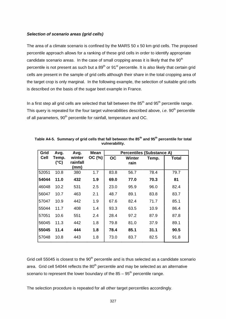
327
Selection of scenario areas (grid cells)
The area of a climate scenario is confined by the MARS 50 x 50 km grid cells. The proposed
percentile approach allows for a ranking of these grid cells in order to identify appropriate
candidate scenario areas. In the case of small cropping areas it is likely that the 90th
percentile is not present as such but a 89th or 91st percentile. It is also likely that certain grid
cells are present in the sample of grid cells although their share in the total cropping area of
the target crop is only marginal. In the following example, the selection of suitable grid cells
is described on the basis of the sugar beet example in France.
In a first step all grid cells are selected that fall between the 85th and 95th percentile range.
This query is repeated for the four target vulnerabilities described above, i.e. 90th percentile
of all parameters, 90th percentile for rainfall, temperature and OC.
Table A4-5. Summary of grid cells that fall between the 85th
and 95th
percentile for total vulnerability.
Grid Cell
Avg. Temp.
(°C)
Avg. winter rainfall (mm)
Mean OC (%)
Percentiles (Substance A)
OC Winter rain
Temp. Total
52051 10.8 380 1.7 83.8 56.7 78.4 79.7
54044 11.0 432 1.9 69.0 77.0 70.3 81
46048 10.2 531 2.5 23.0 95.9 96.0 82.4
56047 10.7 463 2.1 48.7 89.1 83.8 83.7
57047 10.9 442 1.9 67.6 82.4 71.7 85.1
55044 11.7 408 1.4 93.3 63.5 10.9 86.4
57051 10.6 551 2.4 28.4 97.2 87.9 87.8
56045 11.3 442 1.8 79.8 81.0 37.9 89.1
55045 11.4 444 1.8 78.4 85.1 31.1 90.5
57048 10.8 443 1.8 73.0 83.7 82.5 91.8
Grid cell 55045 is closest to the 90th percentile and is thus selected as a candidate scenario
area. Grid cell 54044 reflects the 80th percentile and may be selected as an alternative
scenario to represent the lower boundary of the 85 – 95th percentile range.
The selection procedure is repeated for all other target percentiles accordingly.
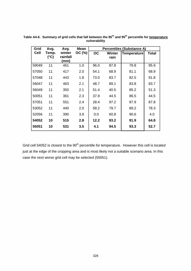
328
Table A4-6. Summary of grid cells that fall between the 85th
and 95th
percentile for temperature vulnerability
Grid Cell
Avg. Temp.
(°C)
Avg. winter rainfall (mm)
Mean OC (%)
Percentiles (Substance A)
OC Winter rain
Temperature Total
59049 11 461 1.0 96.0 87.8 79.8 95.9
57050 11 417 2.0 54.1 68.9 81.1 68.9
57048 11 443 1.8 73.0 83.7 82.5 91.8
56047 11 463 2.1 48.7 89.1 83.8 83.7
56049 11 350 2.1 51.4 40.5 85.2 51.3
50051 11 361 2.3 37.9 44.5 86.5 44.5
57051 11 551 2.4 28.4 97.2 87.9 87.8
53052 11 440 2.0 58.2 79.7 89.2 78.3
52056 11 390 3.9 0.0 60.8 90.6 4.0
54052 10 515 2.8 12.2 93.2 91.9 64.8
55051 10 531 3.5 4.1 94.5 93.3 52.7
Grid cell 54052 is closest to the 90th percentile for temperature. However this cell is located
just at the edge of the cropping area and is most likely not a suitable scenario area. In this
case the next worse grid cell may be selected (55051).
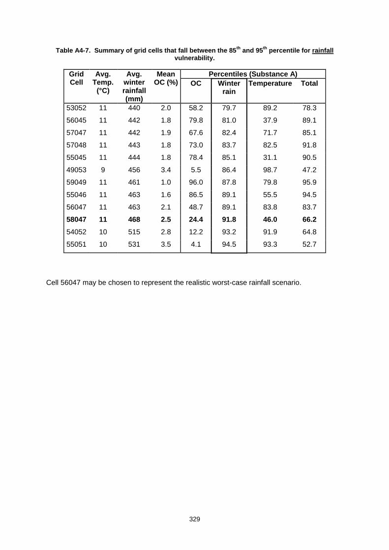
329
Table A4-7. Summary of grid cells that fall between the 85th
and 95th
percentile for rainfall vulnerability.
Grid Cell
Avg. Temp.
(°C)
Avg. winter rainfall (mm)
Mean OC (%)
Percentiles (Substance A)
OC Winter rain
Temperature Total
53052 11 440 2.0 58.2 79.7 89.2 78.3
56045 11 442 1.8 79.8 81.0 37.9 89.1
57047 11 442 1.9 67.6 82.4 71.7 85.1
57048 11 443 1.8 73.0 83.7 82.5 91.8
55045 11 444 1.8 78.4 85.1 31.1 90.5
49053 9 456 3.4 5.5 86.4 98.7 47.2
59049 11 461 1.0 96.0 87.8 79.8 95.9
55046 11 463 1.6 86.5 89.1 55.5 94.5
56047 11 463 2.1 48.7 89.1 83.8 83.7
58047 11 468 2.5 24.4 91.8 46.0 66.2
54052 10 515 2.8 12.2 93.2 91.9 64.8
55051 10 531 3.5 4.1 94.5 93.3 52.7
Cell 56047 may be chosen to represent the realistic worst-case rainfall scenario.
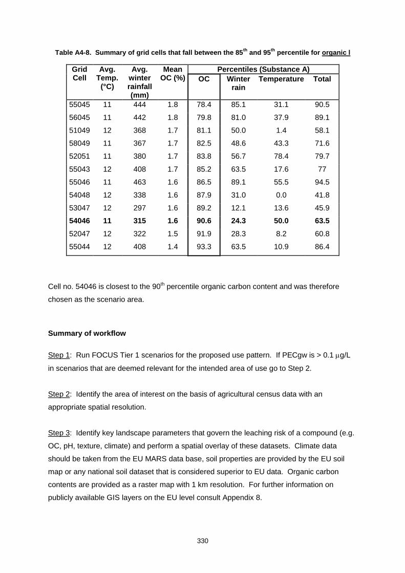
330
Table A4-8. Summary of grid cells that fall between the 85th
and 95th
percentile for organic l
Grid Cell
Avg. Temp.
(°C)
Avg. winter rainfall (mm)
Mean OC (%)
Percentiles (Substance A)
OC Winter rain
Temperature Total
55045 11 444 1.8 78.4 85.1 31.1 90.5
56045 11 442 1.8 79.8 81.0 37.9 89.1
51049 12 368 1.7 81.1 50.0 1.4 58.1
58049 11 367 1.7 82.5 48.6 43.3 71.6
52051 11 380 1.7 83.8 56.7 78.4 79.7
55043 12 408 1.7 85.2 63.5 17.6 77
55046 11 463 1.6 86.5 89.1 55.5 94.5
54048 12 338 1.6 87.9 31.0 0.0 41.8
53047 12 297 1.6 89.2 12.1 13.6 45.9
54046 11 315 1.6 90.6 24.3 50.0 63.5
52047 12 322 1.5 91.9 28.3 8.2 60.8
55044 12 408 1.4 93.3 63.5 10.9 86.4
Cell no. 54046 is closest to the 90th percentile organic carbon content and was therefore
chosen as the scenario area.
Summary of workflow
Step 1: Run FOCUS Tier 1 scenarios for the proposed use pattern. If PECgw is > 0.1 g/L
in scenarios that are deemed relevant for the intended area of use go to Step 2.
Step 2: Identify the area of interest on the basis of agricultural census data with an
appropriate spatial resolution.
Step 3: Identify key landscape parameters that govern the leaching risk of a compound (e.g.
OC, pH, texture, climate) and perform a spatial overlay of these datasets. Climate data
should be taken from the EU MARS data base, soil properties are provided by the EU soil
map or any national soil dataset that is considered superior to EU data. Organic carbon
contents are provided as a raster map with 1 km resolution. For further information on
publicly available GIS layers on the EU level consult Appendix 8.
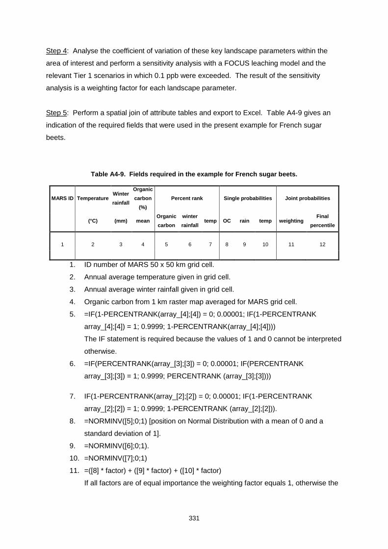
331
Step 4: Analyse the coefficient of variation of these key landscape parameters within the
area of interest and perform a sensitivity analysis with a FOCUS leaching model and the
relevant Tier 1 scenarios in which 0.1 ppb were exceeded. The result of the sensitivity
analysis is a weighting factor for each landscape parameter.
Step 5: Perform a spatial join of attribute tables and export to Excel. Table A4-9 gives an
indication of the required fields that were used in the present example for French sugar
beets.
Table A4-9. Fields required in the example for French sugar beets.
MARS ID Temperature Winter
rainfall
Organic
carbon
(%)
Percent rank Single probabilities Joint probabilities
(°C) (mm) mean Organic
carbon
winter
rainfall temp OC rain temp weighting
Final
percentile
1 2 3 4 5 6 7 8 9 10 11 12
1. ID number of MARS 50 x 50 km grid cell.
2. Annual average temperature given in grid cell.
3. Annual average winter rainfall given in grid cell.
4. Organic carbon from 1 km raster map averaged for MARS grid cell.
5. =IF(1-PERCENTRANK(array_[4];[4]) = 0; 0.00001; IF(1-PERCENTRANK
array_[4];[4]) = 1; 0.9999; 1-PERCENTRANK(array_[4];[4])))
The IF statement is required because the values of 1 and 0 cannot be interpreted
otherwise.
6. =IF(PERCENTRANK(array_[3];[3]) = 0; 0.00001; IF(PERCENTRANK
array_[3];[3]) = 1; 0.9999; PERCENTRANK (array_[3];[3])))
7. IF(1-PERCENTRANK(array_[2];[2]) = 0; 0.00001; IF(1-PERCENTRANK
array_[2];[2]) = 1; 0.9999; 1-PERCENTRANK (array_[2];[2])).
8. =NORMINV([5];0;1) [position on Normal Distribution with a mean of 0 and a
standard deviation of 1].
9. =NORMINV([6];0;1).
10. =NORMINV([7];0;1)
11. =([8] * factor) + ([9] * factor) + ([10] * factor)
If all factors are of equal importance the weighting factor equals 1, otherwise the
332
weighting factors are calculated in the present example as
factor = 3 * weighting factor from sensitivity analysis
12. NORMDIST([11];0;(SQRT(3));1)
Joint distribution with a mean of 0 and a standard deviation of √3.
Step 6: Join Excel calculations in GIS with attribute table of MARS grid cells and identify
cells close to the target percentile for vulnerability.
Step 7: Identify appropriate soil units within the selected grid cells. Soil profile data are
extracted from SPADE data base of EU soil map. Average organic carbon contents in topsoil
for the MARS grid are taken from the 1 km raster map. Daily weather data are extracted
from MARS grid data base.
Step 8: If appropriate add irrigation volumes to weather file.
References
Allen R.G., Pereira L.S., Raes D. and M. Smith. 1998. Crop evapotranspiration. Guidelines
for computing crop water requirements. FAO irrigation and drainage paper No. 56. Food
and Agriculture Organisation of the United Nations. Rome. 300 p.
Batjes N.H. 1995. A global data set of soil pH properties. Tech. Pap. 27, ISRIC,
Wageningen.
Corine. 2000. Corine Land Cover update I&CLC2000 project Technical Guidelines. Final
version August 2002. European Environment Agency. European Topic Centre Terrestrial
Environment.
Dubus I.G., Brown C.D. and S. Beulke. 2000. Sensitivity analyses for leaching models used
for pesticide registration in Europe. Final report of MAFF project PL0532. Soil Survey
and Land Research Centre. Silsoe.
Dubus I.G., Brown C.D. and S. Beulke. 2003. Sensitivity analyses for four pesticide leaching
models. Pest. Manag. Sci 59:962-982.
Jones, R. J. A., R. Hiederer, E. Rusco, and L. Montanarella. 2005. Estimating organic
carbon in the soils of Europe for policy support. European Journal of Soil Science,
56(5):655-671.
Jones, R.J.A., R. Hiederer, E. Rusco, P. J. Loveland, and L. Montanarella. 2004. The map
of organic carbon in topsoils in Europe, Version 1.2, September 2003: Explanation of
333
Special Publication Ispra 2004 No.72 (S.P.I.04.72). European Soil Bureau Research
Report No.17, EUR 21209 EN, 26pp. and 1 map in ISO B1 format. Office for Official
Publications of the European Communities, Luxembourg.
MARS. 2004. Interpolated meteorological data – JRC/MARS Database – European
Commission – JRC. Ispra.
SCEES. 2000. Recensement Agricole 2000. L’inventaire France métropolitaine. Service
central des enquêtes et etudes statistiques. Paris.
Van den Berg, F., D.J. Brus, S.L.G.E. Burgers, G.B.M Heuvelink, J.G. Kroes, J. Stolte, A.
Tiktak, and F. de Vries. 2008. Uncertainty and sensitivity of GeoPEARL. Alterra report
1330, PBL-rapport 500123001, Alterra, Wageningen, 114 pp.
Van der Linden A.M.A., Boesten J.J.T.I., Cornelese A.A., Kruijne R., Leistra M., Linders
J.B.H.J., Pol J.W., Tiktak A. and A.J. Verschoor. 2004. The new decision tree for the
evaluation of pesticide leaching from soils. RIVM report 601450019/2004. Bilthoven.
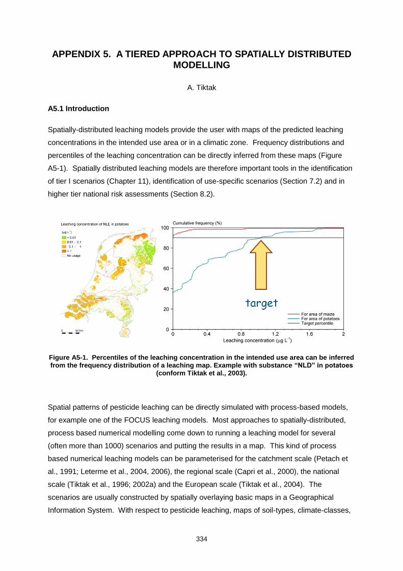
334
APPENDIX 5. A TIERED APPROACH TO SPATIALLY DISTRIBUTED MODELLING
A. Tiktak
A5.1 Introduction
Spatially-distributed leaching models provide the user with maps of the predicted leaching
concentrations in the intended use area or in a climatic zone. Frequency distributions and
percentiles of the leaching concentration can be directly inferred from these maps (Figure
A5-1). Spatially distributed leaching models are therefore important tools in the identification
of tier I scenarios (Chapter 11), identification of use-specific scenarios (Section 7.2) and in
higher tier national risk assessments (Section 8.2).
Figure A5-1. Percentiles of the leaching concentration in the intended use area can be inferred from the frequency distribution of a leaching map. Example with substance “NLD” in potatoes
(conform Tiktak et al., 2003).
Spatial patterns of pesticide leaching can be directly simulated with process-based models,
for example one of the FOCUS leaching models. Most approaches to spatially-distributed,
process based numerical modelling come down to running a leaching model for several
(often more than 1000) scenarios and putting the results in a map. This kind of process
based numerical leaching models can be parameterised for the catchment scale (Petach et
al., 1991; Leterme et al., 2004, 2006), the regional scale (Capri et al., 2000), the national
scale (Tiktak et al., 1996; 2002a) and the European scale (Tiktak et al., 2004). The
scenarios are usually constructed by spatially overlaying basic maps in a Geographical
Information System. With respect to pesticide leaching, maps of soil-types, climate-classes,
335
crop-types and ground water-depth-classes are of particular interest. The disadvantage of
process based spatially distributed models is that they contain a large number of parameters,
which may be difficult to identify directly or which may not be available at larger scales.
To mitigate the above mentioned problems, simpler leaching models could be used to assess
the leaching pattern. Many authors have used process-based, analytical or impulse
response models for this purpose. The best known models of this type are the attenuation
factor (Loague et al., 1989; 1996, Loague and Corwin, 1996) and the transfer function (Jury
and Roth, 1990; Stewart and Loague, 2003; 2004). Analytical models do not account for
vertical heterogeneity and assume steady-state conditions, so that they may not be
compatible with results from numerical models. An alternative to the direct use of simpler
models and a way to maintain the dominant behaviour of the more complex process-based
model is to reduce the complex leaching model into the mathematical form of the simple
model in a modelling step referred to as metamodelling. In metamodelling, the model
reduction is obtained by considering only those processes and parameters for which the
considered simulation output is sensitive or for which input data are available. As such, a
simpler model can be obtained which encompasses the behaviour of the complex model and
which is more compatible with available data bases. Regression analysis can be used to
construct a metamodel (Figure A5-2).
Figure A5-2. Metamodels are proxies of complex models.
The regression model can itself be a purely statistical model (Vanclooster et al., 2003;
Stenemo et al., 2006; Piñeros Garcet et al., 2006) or a combination of a simplified process
based model and a regression model (Van der Zee and Boesten, 1991; Stewart and Loague,
2004; Tiktak et al., 2006). The simplification of the model structure in a metamodel improves
also the transparency of the model and is, therefore, easier to use within the communication
process with non-technical stakeholders, in particular if a process-based metamodel is

336
proposed. Metamodelling theory and applications to emission modelling have recently been
reviewed by Piñeros Garcet et al. (2006).
This appendix describes a tiered-approach to spatially-distributed modelling. In those cases
where sufficient information for running a process based spatially distributed model is
available, this model is used to derive spatial patterns of the leaching concentration directly
(Figure A5-1). In other cases, metamodels are used to extend the simulations towards the
entire intended use area. A single scenario is selected from the cumulative frequency
distribution of the leaching map obtained with the metamodel. A FOCUS leaching model is
run for this single scenario to get the regulatory endpoint.
This appendix is based on work reported in peer-reviewed scientific articles (Tiktak et al.,
1996; 2002b; 2004; 2006). The backbone of the approach is spatially distributed versions of
the FOCUS PEARL model, referred to as GeoPEARL and EuroPEARL. GeoPEARL and
EuroPEARL results were used to calibrate a process-based metamodel (Van der Zee and
Boesten, 1991). This metamodel was based on an analytical solution for piston flow. We use
the metamodel of Van der Zee and Boesten (1991) in such a way that it describes
concentrations instead of leached fractions and show how this metamodel can be used to
assess the leaching risk at the national or at the European level.
The appendix starts with a general overview of the tiered approach (A5.2). Section A5.3
describes how to develop a spatially distributed leaching model, based on an existing
FOCUS leaching model. Section A5.4 then shows how a metamodel of this spatially
distributed model can be developed. In Section A5.5, both the metamodel and the numerical
model are applied to the Netherlands. On the basis of this example, we will show that the
metamodel gives comparable results as the original GeoPEARL model and that the results fit
into the tiered assessment scheme. Section A5.6 provides the sensitivity of the metamodel
to some basic model inputs. Section A5.7 reviews some of the uncertainties associated with
the approach. General conclusions are given in Section A5.7.
A5.2 Overview of the method
A general overview of the proposed tiered-approach to spatially distributed modelling and
calculating the regulatory endpoint is given in Figure A5-3.
337
Figure A5-3. A tiered approach to spatially distributed modelling. The numbers refer to the pathways described in the text.
The diagram shows that there are in principle three pathways possible, depending on the
availability of data:
1. If the soil profile and weather data cover the entire intended use area (and are
considered of sufficient quality), then the regulatory endpoint can be calculated
directly with a spatially distributed leaching model (Figure A5-1). An example of this
approach is given by Tiktak et al. (2002b, 2003).
2. If the soil profile and weather data do not cover the entire intended use area, then a
metamodel could be used to extend the simulations to the entire intended use area.
A process based spatially distributed model is build, which does not cover the entire
area. The model should be using local or national data bases, if possible. Then, a
metamodel is build, using results from this model as a calibration dataset. The
metamodel is then used to extend the simulations to the entire intended use area. An
example of such an approach is given by Tiktak et al. (2006). A single scenario is
selected from the cumulative frequency distribution of the leaching map generated by
the metamodel, thereby accounting for the area of the intended use. A FOCUS
leaching model is run for this single scenario to get the regulatory endpoint.
3. If there is no soil profile and weather data available from local or national inventories,
then the EU-metamodel developed by Tiktak et al. (2006) can be used. This
metamodel is applicable to the entire area of the EU and uses pan-European data
bases. The reason is that the EU-metamodel is anticipated to perform also
338
reasonably well for national applications (see Section A5.5). The regulatory endpoint
is calculated in the same way as in pathway 2.
If sufficient data are available, then pathway 1 (spatially distributed modelling) is likely to
deliver the most realistic estimate of pesticide leaching in the intended use area. The efforts
involved in developing and using a spatially distributed model are, however, also
considerable. Pathway 3 is relatively easy to use – as shown later it comes down to the
application of a single equation. Metamodelling, however, introduces an error in top of the
original model, so the results may be less reliable than results obtained with the original
model. For this reason, pathway 1 is the preferred option in those cases where sufficient
data is available, and pathways 2 and 3 are the preferred options in all other cases. In view
of this, the work group considers pathway 1 as a Tier 3 approach (Chapter 8) and pathway 2
and 3 as Tier 2b approaches (Section 7.2.5).
The most important elements of this tiered assessment scheme will be briefly described
below. The appendix relies on the use of the PEARL and GeoPEARL models, but other
FOCUS leaching models could have been used as well.
A5.3 Development of a spatially distributed pesticide leaching model
The development of a spatially distributed pesticide leaching model is described in Section
8.2.
A5.4 Metamodel development
A process-based metamodel (see pathway 2 of Figure A5-3) can be used to extrapolate
simulations from a spatially-distributed model to the entire intended use area. The
development of a metamodel consists of the following steps:
1. Selection of an appropriate metamodel
2. Derivation of the calibration dataset
3. Metamodel calibration (including an iterative step for optimising the metamodel)
4. Metamodel validation
5. Application of the metamodel to the intended use area
6. Selection of the target scenario
339
Step 1 Selection of an appropriate metamodel
Metamodelling concerns the approximation of a complex numerical model by a simple and
faster model (see also the introduction of this appendix and Figure A5-2). Metamodels can
roughly be grouped into two major categories (Janssen et al., 2005), i.e.
1. Purely statistical metamodels. The original model is executed several times and
regression techniques are used to describe the relation between model inputs and
model outputs. Statistical metamodels are black-boxes – no physical knowledge of
the system is included. An overview of regression techniques that can be used is
listed in Chambers and Hastie et al. (1991) and Janssen et al. (2005). They differ
from simple multiple (linear or polynomial) regression models to advanced statistical
techniques like kriging and artificial neural networks. Rather good approximations of
pesticide leaching models have recently be obtained with artificial neural networks
(Vanclooster et al., 2003; Stenemo et al., 2006), because they outperform other
regression methods in terms of flexibility and versatility. The disadvantages of
artificial neural networks are, however, that a large number of model runs is required
(usually more than 100,000), that artificial neural networks can easily be over
parameterised leading to non-uniqueness.
2. Process based metamodels. This kind of models tries to describe the most important
processes in a simple, but process oriented way. Many authors have used analytical
models or impulse response functions for this purpose. The best known models of
this type are the attenuation factor (Loague et al., 1989; 1996, Loague and Corwin,
1996) and the transfer function (Jury and Roth, 1990; Stewart and Loague, 2003,
2004). Analytical models do not account for vertical heterogeneity and assume
steady-state conditions, so that they may not be compatible with results from
numerical models. This problem can be overcome by introducing effective model
parameters (Van der Zee and Boesten, 1991), which need to be calibrated against
results form a numerical model. Van der Zee and Boesten (1991) fitted results from
one scenario only, so that the obtained effective model parameters might not be
applicable to the entire intended use area. Tiktak et al. (2006) build upon this
approach by fitting a large number of scenarios simultaneously. In this way, a
process-based metamodel of GeoPEARL resulted.
As shown in the literature, good model approximations can be obtained with either of the two
model types. However, due to the non-linear character of pesticide leaching models,
advanced statistical techniques like artificial neural networks are required if a purely
statistical model is used (Vanclooster et al., 2003; Stenemo et al., 2006; Piñeros Garcet et
al., 2006). For this reason, we recommend the use of process-based metamodels. In
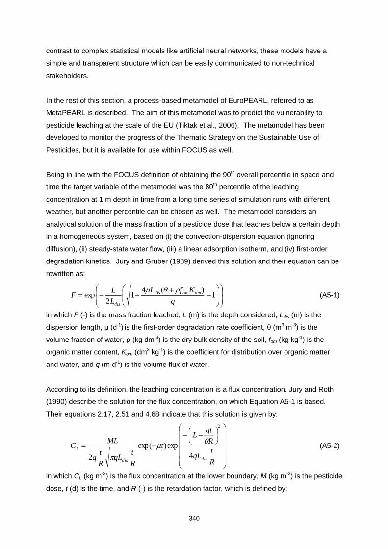
340
contrast to complex statistical models like artificial neural networks, these models have a
simple and transparent structure which can be easily communicated to non-technical
stakeholders.
In the rest of this section, a process-based metamodel of EuroPEARL, referred to as
MetaPEARL is described. The aim of this metamodel was to predict the vulnerability to
pesticide leaching at the scale of the EU (Tiktak et al., 2006). The metamodel has been
developed to monitor the progress of the Thematic Strategy on the Sustainable Use of
Pesticides, but it is available for use within FOCUS as well.
Being in line with the FOCUS definition of obtaining the 90th overall percentile in space and
time the target variable of the metamodel was the 80th percentile of the leaching
concentration at 1 m depth in time from a long time series of simulation runs with different
weather, but another percentile can be chosen as well. The metamodel considers an
analytical solution of the mass fraction of a pesticide dose that leaches below a certain depth
in a homogeneous system, based on (i) the convection-dispersion equation (ignoring
diffusion), (ii) steady-state water flow, (iii) a linear adsorption isotherm, and (iv) first-order
degradation kinetics. Jury and Gruber (1989) derived this solution and their equation can be
rewritten as:
1
)(41
2exp
q
KfL
L
LF omomdis
dis
(A5-1)
in which F (-) is the mass fraction leached, L (m) is the depth considered, Ldis (m) is the
dispersion length, μ (d-1) is the first-order degradation rate coefficient, θ (m3 m-3) is the
volume fraction of water, ρ (kg dm-3) is the dry bulk density of the soil, fom (kg kg-1) is the
organic matter content, Kom (dm3 kg-1) is the coefficient for distribution over organic matter
and water, and q (m d-1) is the volume flux of water.
According to its definition, the leaching concentration is a flux concentration. Jury and Roth
(1990) describe the solution for the flux concentration, on which Equation A5-1 is based.
Their equations 2.17, 2.51 and 4.68 indicate that this solution is given by:
R
tqL
R
qtL
t
R
tqL
R
tq
MLC
disdis
L
4
exp)exp(
2
2
(A5-2)
in which CL (kg m-3) is the flux concentration at the lower boundary, M (kg m-2) is the pesticide
dose, t (d) is the time, and R (-) is the retardation factor, which is defined by:
341
omomKfR
1 (A5-3)
For pesticide leaching, one may expect that the flux concentration evaluated at a certain
depth in soil is more or less proportional to the fraction of the dose that leaches beyond that
depth: low fractions leached can only be achieved by low leaching concentrations and
similarly high fractions leached can only be achieved by high leaching concentrations. We
made Monte Carlo simulations with Equation A5-1 and assumed uniform distributions for θ,
R, q, and the half-life of the pesticide. The range of θ was 0.1-0.3 m3 m-3; the range of R was
1-100; the range of q was 0.25-2.5 mm d-1, and the range of the half-life was 20-100 d. The
pesticide dose was 1 kg ha-1, the depth in soil was 1 m, and the dispersion length was
0.05 m. For each combination of the stochastic variables the maximum in time of the
concentration was calculated and compared with the fraction leached from Equation A5-1.
Figure A5-3 shows that the maximum concentration is indeed more or less directly
proportional to the fraction leached. This suggests that the metamodel for the 80th percentile
concentration can be based on the simpler equation for the fraction leached.
Van der Zee and Boesten (1991) adapted Equation A5-1 slightly to include also pesticide
uptake by plant roots:
1
4)(41
2exp
q
gSLKfL
L
LF disomomdis
dis
(A5-4)
where g (-) is the transpiration stream concentration factor and S (d-1) is the water uptake by
plant roots. Van der Zee and Boesten (1991) made calculations with a model similar to
PEARL for a single Dutch soil (Ldis = 0.05 m), but for a range of degradation half-lives and
Kom-values. They fitted the fraction leached to Equation A5-4 with θ, S, and q as regression
parameters. They found that Equation A5-4 was a suitable metamodel to describe the output
of the simulation model. Moreover, they found that the fitted values of θ, S and q were
physically realistic.
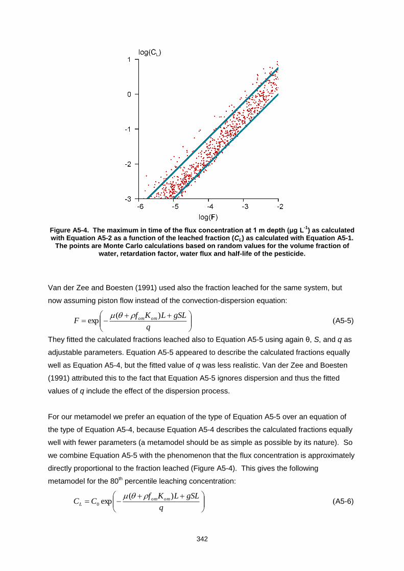
342
Figure A5-4. The maximum in time of the flux concentration at 1 m depth (μg L-1
) as calculated with Equation A5-2 as a function of the leached fraction (CL) as calculated with Equation A5-1.
The points are Monte Carlo calculations based on random values for the volume fraction of water, retardation factor, water flux and half-life of the pesticide.
Van der Zee and Boesten (1991) used also the fraction leached for the same system, but
now assuming piston flow instead of the convection-dispersion equation:
q
gSLLKfF omom )(
exp
(A5-5)
They fitted the calculated fractions leached also to Equation A5-5 using again θ, S, and q as
adjustable parameters. Equation A5-5 appeared to describe the calculated fractions equally
well as Equation A5-4, but the fitted value of q was less realistic. Van der Zee and Boesten
(1991) attributed this to the fact that Equation A5-5 ignores dispersion and thus the fitted
values of q include the effect of the dispersion process.
For our metamodel we prefer an equation of the type of Equation A5-5 over an equation of
the type of Equation A5-4, because Equation A5-4 describes the calculated fractions equally
well with fewer parameters (a metamodel should be as simple as possible by its nature). So
we combine Equation A5-5 with the phenomenon that the flux concentration is approximately
directly proportional to the fraction leached (Figure A5-4). This gives the following
metamodel for the 80th percentile leaching concentration:
q
gSLLKfCC omom
L
)(exp0
(A5-6)
343
where C0 (kg m-3) is the concentration at the upper boundary of the column.
One cannot expect that Equation A5-6 gives as accurate predictions of leaching
concentrations as a model such as GeoPEARL, which accounts for vertical heterogeneity of
soil physical and chemical properties, non-linearity in sorption, daily variations of water
fluxes, etcetera. Therefore, we rewrote Equation A5-6 as a multiple linear regression model
and fitted the leaching concentration to the leaching concentration obtained by GeoPEARL:
3322110ln XXXCL (A5-7)
in which α0, α1, α2, and α3 are the regression coefficients and where X1 (-), X2 (-), and X3 (-) are
independent regression variables, which are defined as follows:
q
LX
1 (A5-8)
q
LKfX omom
2 (A5-9)
q
gSLX 3 (A5-10)
Rewritten in this way, a process-based metamodel of GeoPEARL results.
Step 2. Derivation of the calibration dataset
Data are needed for metamodel calibration and for metamodel application. The following
general guidelines can be given:
Parameters for the calibration data set must be inferred from the same data base as
the data base used for the process-based model. As mentioned in Section A5.3, full
spatial coverage is not required, but the spatially distributed model must be
sufficiently representative for the intended use area.
Parameters for metamodel application must cover the entire intended use area.
Otherwise, the calculation of spatial percentiles would be impossible. Parameters can
be derived from different data bases.
Below follows a description how the calibration data set for a pan-European metamodel
based on EuroPEARL was developed. This description can be seen as an example; the
derivation of a calibration dataset based on local or national data bases should be done in a
corresponding way. The derivation of a data set for metamodel application is described in
step 4.
The EuroPEARL data base is sufficiently representative for conditions in Europe (Section
A5.3), so this model can be used to parameterise a metamodel for the entire EU. To assure
344
that the metamodel also covers a wide range of substances, EuroPEARL runs have to be
done for a wide range of substances. Tiktak et al. (2006) constructed a set of 56 example
pesticides from a grid in the DegT50/Kom-parameter plane. The calculations were made
assuming a single application of 1 kg/ha to two different crops (maize and winter cereals)
grown in monoculture. The pesticides were annually applied to the soil surface, one day
after crop emergence. The degradation half-life (DegT50) ranged from 10 to 200 days and
the organic matter-water partition coefficient (Kom) was between 0 and 200 dm3 kg-1. The 56
combinations of DegT50 and Kom cover the full range of relevant pesticides as described by
Boesten and van der Linden (1991). Because the number of unique combinations in
EuroPEARL amounts to 1062, the number of PEARL runs amounted to 59,808 (1062x56).
EuroPEARL is rather demanding with respect to computer resources, so we used a computer
cluster consisting of 256 loosely coupled CPU’s to perform the simulations. This assured
that the simulations could be done within 2 days.
For each PEARL run, the independent regression variables X1..X3 in Equations A5-8, A5-9,
and A5-10 must be calculated as well. These equations contain two substance parameters
(μ and Kom), two soil parameters (ρ and fom), three dynamic soil parameters (θ, S and q), and
two constants (L and g). As mentioned above, the parameters must be inferred from the
same data base as used for the parameterisation of the spatially distributed model, which in
this case is the EuroPEARL data base. In the case of dynamic properties, 20-years
averages should be taken (the simulation length excluding the warm-up years). In the case
of depth-dependent soil properties, averages for the top 1 m (the target depth) should be
calculated, using the horizon thickness as a weighing factor. The degradation rate
coefficient, μ, is not directly available in the EuroPEARL data base, because it is temperature
dependent. The Arrhenius equation should be applied to account for this effect:
50
11 )2ln(exp
DegTTT
R
Er
a
(A5-11)
where DegT50 (d) is the degradation half-life at reference temperature, Ea (J mol-1) is the
molar activation energy, R (J mol-1 K-1) is the molar gas constant, T (K) is the 20-years
average air temperature and Tr (K) is the temperature at reference conditions, which was set
to 20 oC. The molar activation energy should be fixed to the same value as used for the
PEARL calculations.
The organic matter content, fom, must be averaged over the top 1 m, using the horizon
thickness as a weighing factor. The bulk density of the soil must be calculated in exactly the
same way as done in the original model. EuroPEARL uses a continuous pedotransfer
approach to relate the bulk density, ρ (kg dm-3), to the organic matter content, so this

345
approach should be used when building a metamodel based on EuroPEARL simulations
(Tiktak et al., 1996):
)91.0(91.224.180.1ρ 2 Rff omom (A5-12)
Figure A5-5 shows the basic maps that were available for the EuroPEARL model.
Dynamic properties (θ and S) should also be taken from the output files of the spatially
distributed model. These parameters should first be averaged over the top 1 m of the soil
and then averaged over the 20-years simulation period. The water flux, q, can be
represented by the excess rainfall over evapotranspiration and run-off.
The time of application has an important effect on the spatial patterns of pesticide leaching.
Therefore different metamodels should be constructed for spring applied and for autumn
applied pesticides. In practice, this implies that the entire exercise needs to be done two
times.
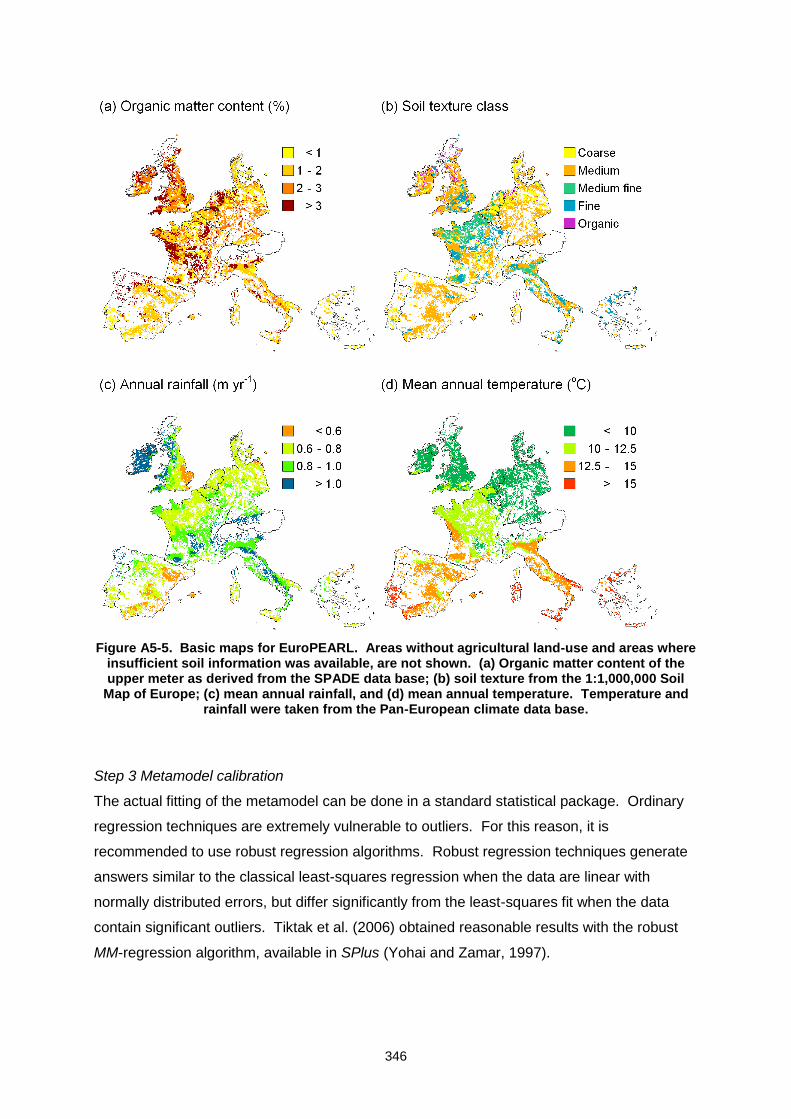
346
Figure A5-5. Basic maps for EuroPEARL. Areas without agricultural land-use and areas where insufficient soil information was available, are not shown. (a) Organic matter content of the upper meter as derived from the SPADE data base; (b) soil texture from the 1:1,000,000 Soil
Map of Europe; (c) mean annual rainfall, and (d) mean annual temperature. Temperature and rainfall were taken from the Pan-European climate data base.
Step 3 Metamodel calibration
The actual fitting of the metamodel can be done in a standard statistical package. Ordinary
regression techniques are extremely vulnerable to outliers. For this reason, it is
recommended to use robust regression algorithms. Robust regression techniques generate
answers similar to the classical least-squares regression when the data are linear with
normally distributed errors, but differ significantly from the least-squares fit when the data
contain significant outliers. Tiktak et al. (2006) obtained reasonable results with the robust
MM-regression algorithm, available in SPlus (Yohai and Zamar, 1997).
347
In the remainder of this section, the metamodel calibration done by Tiktak et al. (2006) is
summarised. They fitted two metamodels, i.e. one for a spring-applied pesticide (‘leaching
set spring’) and one for an autumn applied pesticide (‘leaching set autumn’). Based on this
example, the following general recommendations can be given for metamodel calibration:
the third term of Equation A5-7 (the plant-uptake term) should not be used, because
this yielded physically unrealistic values.
if the metamodel is intended to be used throughout different major climatic zones,
different metamodels parameterisations should be used for each individual climatic
zone (i.e. the calibration dataset should be split based on these zones). For pan-
European leaching assessments, four climatic zones were sufficient (Table A5-1).
Table A5-1. Major climate zones of the European Union, based on mean annual rainfall and mean annual temperature. Zones are a reclassification of the zones described in FOCUS
(2000).
Zone ID Mean annual rainfall (m yr-1) Mean annual temperature (oC)
Temperate, dry (TD) < 0.8 < 12.5
Temperate, wet (TW) > 0.8 < 12.5
Warm, dry (WD) < 0.8 > 12.5
Warm, wet (WW) > 0.8 > 12.5
Tiktak et al. (2006) optimised the metamodel in different calibration steps (called Model I, II
and III) and obtained a recommended version (Model III) (see Table A5-2)
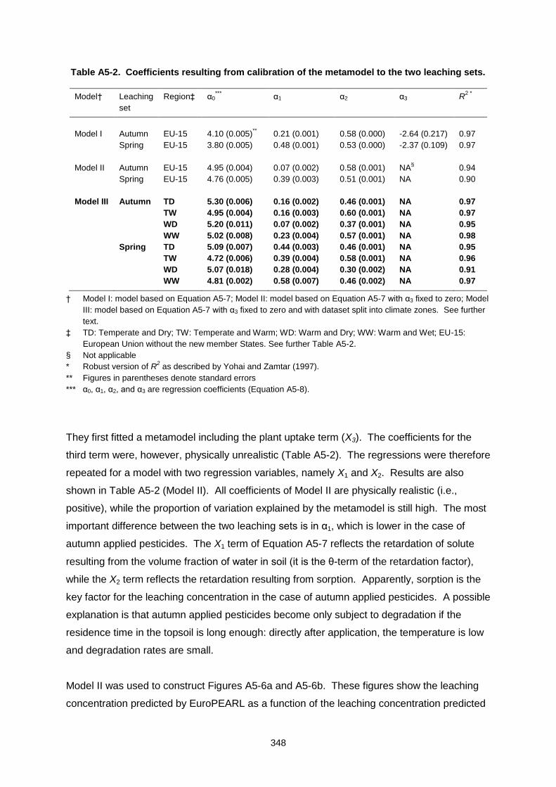
348
Table A5-2. Coefficients resulting from calibration of the metamodel to the two leaching sets.
Model† Leaching
set
Region‡ α0***
α1 α2 α3 R2 *
Model I Autumn EU-15 4.10 (0.005)** 0.21 (0.001) 0.58 (0.000) -2.64 (0.217) 0.97
Spring EU-15 3.80 (0.005) 0.48 (0.001) 0.53 (0.000) -2.37 (0.109) 0.97
Model II Autumn EU-15 4.95 (0.004) 0.07 (0.002) 0.58 (0.001) NA§ 0.94
Spring EU-15 4.76 (0.005) 0.39 (0.003) 0.51 (0.001) NA 0.90
Model III Autumn TD 5.30 (0.006) 0.16 (0.002) 0.46 (0.001) NA 0.97
TW 4.95 (0.004) 0.16 (0.003) 0.60 (0.001) NA 0.97
WD 5.20 (0.011) 0.07 (0.002) 0.37 (0.001) NA 0.95
WW 5.02 (0.008) 0.23 (0.004) 0.57 (0.001) NA 0.98
Spring TD 5.09 (0.007) 0.44 (0.003) 0.46 (0.001) NA 0.95
TW 4.72 (0.006) 0.39 (0.004) 0.58 (0.001) NA 0.96
WD 5.07 (0.018) 0.28 (0.004) 0.30 (0.002) NA 0.91
WW 4.81 (0.002) 0.58 (0.007) 0.46 (0.002) NA 0.97
† Model I: model based on Equation A5-7; Model II: model based on Equation A5-7 with α3 fixed to zero; Model
III: model based on Equation A5-7 with α3 fixed to zero and with dataset split into climate zones. See further
text.
‡ TD: Temperate and Dry; TW: Temperate and Warm; WD: Warm and Dry; WW: Warm and Wet; EU-15:
European Union without the new member States. See further Table A5-2.
§ Not applicable
* Robust version of R2 as described by Yohai and Zamtar (1997).
** Figures in parentheses denote standard errors
*** α0, α1, α2, and α3 are regression coefficients (Equation A5-8).
They first fitted a metamodel including the plant uptake term (X3). The coefficients for the
third term were, however, physically unrealistic (Table A5-2). The regressions were therefore
repeated for a model with two regression variables, namely X1 and X2. Results are also
shown in Table A5-2 (Model II). All coefficients of Model II are physically realistic (i.e.,
positive), while the proportion of variation explained by the metamodel is still high. The most
important difference between the two leaching sets is in α1, which is lower in the case of
autumn applied pesticides. The X1 term of Equation A5-7 reflects the retardation of solute
resulting from the volume fraction of water in soil (it is the θ-term of the retardation factor),
while the X2 term reflects the retardation resulting from sorption. Apparently, sorption is the
key factor for the leaching concentration in the case of autumn applied pesticides. A possible
explanation is that autumn applied pesticides become only subject to degradation if the
residence time in the topsoil is long enough: directly after application, the temperature is low
and degradation rates are small.
Model II was used to construct Figures A5-6a and A5-6b. These figures show the leaching
concentration predicted by EuroPEARL as a function of the leaching concentration predicted
349
by the metamodel. The number of leaching points in each figure equals 59,808. The
concentrations were plotted on a log10-scale and the lines represent the fit. The figure
shows that, despite the high proportion of variation explained by the metamodel (Table A5-2),
there is large scatter around the 1:1 line. Further inspection of the leaching sets suggests
that the deviation from the 1:1 line is related to the annual precipitation: under dry conditions,
the metamodel tends to underestimate the leaching concentration, whereas the leaching
concentration is overestimated in those cases where the mean annual precipitation is high.
To reduce the systematic differences due to climate, the leaching sets were split in four
subsets, namely one for each climate zone in Table A5-2. The underlying assumption is that
the climate zones are more homogeneous with respect to seasonal dynamics of weather
than Europe as a whole. Figures A5-9c and A5-6d show that the systematic errors are
indeed reduced. The regression coefficients as shown in Table A5-2 (Model III) are generally
low in dry climate zones and high in wet climate zones: α1 increases in the order WD < TD ≈
TW < WW, while coefficient α2 increases in the order WD < TD < TW ≈ WW. This suggests
that in the case of dry climates, the effective model parameters deviate more from realistic
values than in the case of wet climates. Averaging causes bias in the results of the analytical
model, which is reflected in the coefficients of the metamodel. The effect of averaging is
expected to be more pronounced in the case of dry climates, because the seasonal variability
of the water flow pattern is generally higher in those climates. Van der Zee and Boesten
(1991) found that the bias between realistic and effective model parameters appears most in
the water flow velocity. They attributed this to the fact that Equation A5-5 ignores dispersion
and thus the fitted values of q include the effect of the dispersion process. Using their
findings, one can make an estimation of the ratio between the true water flow velocity and the
apparent water flow velocity for the four climate zones by substituting α1 and α2 into
Equations A5-7 to A5-9. The calculated ratios (approximately two for wet climates and four
for dry climates) confirm that the effect of averaging is most pronounced in the dry climate
zones. Notice that the above exercise yields only a crude estimate of the apparent flow
velocity, because the averaging of the degradation rate (μ) and the non-linearity of the
sorption process affects the leaching as well.
Summarising, one can state that the time of application mainly affects the ratio between α1
and α2, while the absolute values are affected mainly by the seasonal dynamics of water flow
(represented here by the climate zone). We can conclude that Model III explains a high
proportion of variation of the original model, while also adequately describing the
dependency of the leaching concentration on the main processes, i.e., retardation,
350
degradation, and hydrology. Hence, we can use Model III to map the leaching concentration
at the European level.
Step 4 Metamodel validation
The aim of the metamodel is to find a scenario that represents the target vulnerability.
Therefore the spatial patterns of ground water vulnerability predicted by the metamodel must
show a good correspondence to the ground water vulnerability predicted by the numerical
model. Comparison of the spatial patterns predicted by the metamodel with the spatial
pattern predicted by the numerical model is therefore an essential part of the validation of the
metamodel. The following general guidelines can be given for metamodel validation:
To avoid possible biases due to the use of different data sets, the metamodel should
be validated using the same data set as the original model (otherwise comparison of
spatial patterns is impossible). If the original model does not cover the entire
intended use area, this implies that the metamodel validation is limited to the area for
which data are available in the original model (see example below).
Both visual and quantitative techniques should be used for metamodel validation.
Notice that the validation is limited to comparing the spatial patterns of ground water
vulnerability. The final aim of a Tier 2b assessment is to calculate the leaching concentration
with a FOCUS ground water model for a single use-specific scenario (see Sections 7.2.5 and
A5-2). The validation of these use-specific scenarios requires that also the procedures for
selecting these scenarios must be validated. See further Section A5.5.
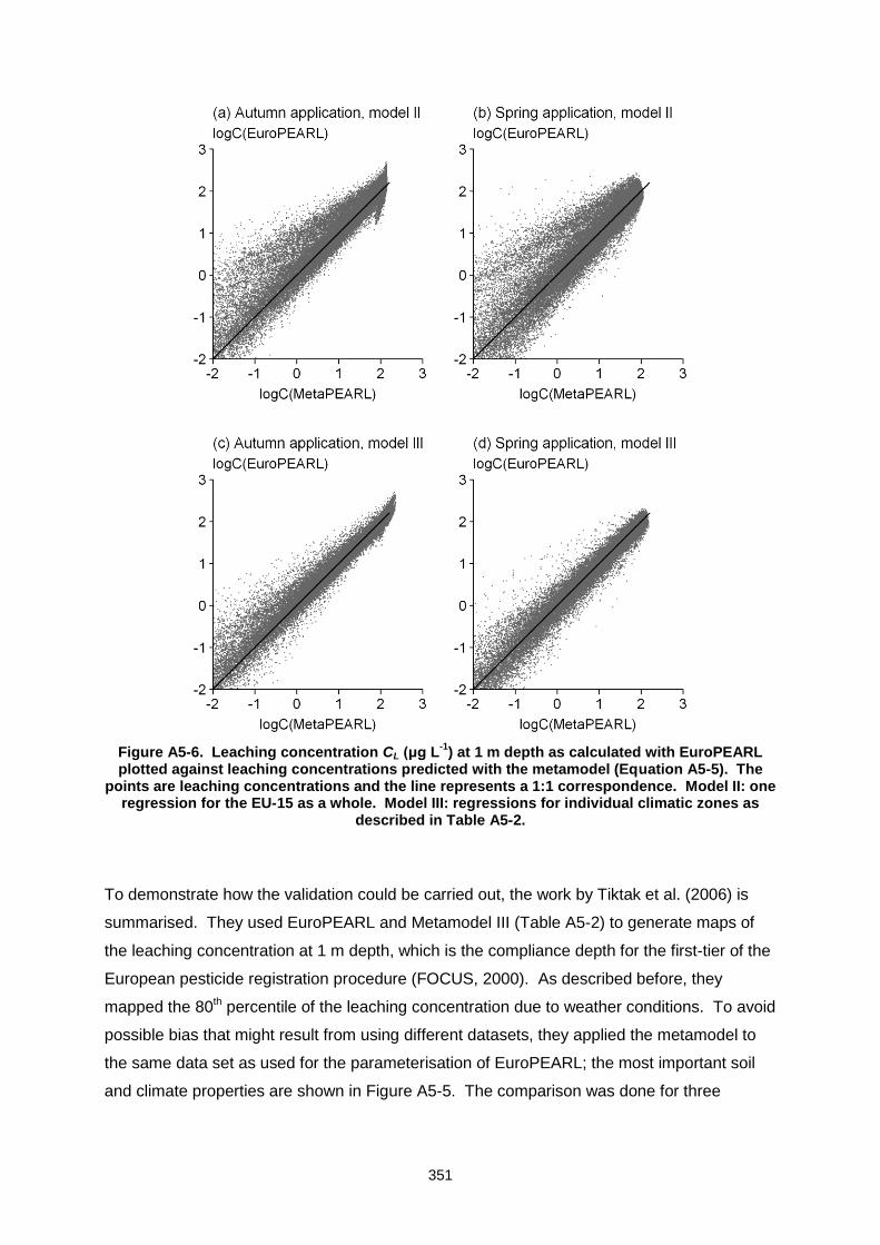
351
Figure A5-6. Leaching concentration CL (μg L-1
) at 1 m depth as calculated with EuroPEARL plotted against leaching concentrations predicted with the metamodel (Equation A5-5). The
points are leaching concentrations and the line represents a 1:1 correspondence. Model II: one regression for the EU-15 as a whole. Model III: regressions for individual climatic zones as
described in Table A5-2.
To demonstrate how the validation could be carried out, the work by Tiktak et al. (2006) is
summarised. They used EuroPEARL and Metamodel III (Table A5-2) to generate maps of
the leaching concentration at 1 m depth, which is the compliance depth for the first-tier of the
European pesticide registration procedure (FOCUS, 2000). As described before, they
mapped the 80th percentile of the leaching concentration due to weather conditions. To avoid
possible bias that might result from using different datasets, they applied the metamodel to
the same data set as used for the parameterisation of EuroPEARL; the most important soil
and climate properties are shown in Figure A5-5. The comparison was done for three
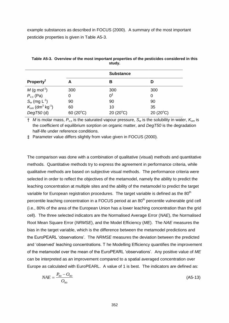
352
example substances as described in FOCUS (2000). A summary of the most important
pesticide properties is given in Table A5-3.
Table A5-3. Overview of the most important properties of the pesticides considered in this study.
Substance
Property† A B D
M (g mol-1) 300 300 300
Pv,s (Pa) 0 0‡ 0
Sw (mg L-1) 90 90 90
Kom (dm3 kg-1) 60 10 35
DegT50 (d) 60 (20oC) 20 (20oC) 20 (20oC)
† M is molar mass, Pv,s is the saturated vapour pressure, Sw is the solubility in water, Kom is
the coefficient of equilibrium sorption on organic matter, and DegT50 is the degradation
half-life under reference conditions.
‡ Parameter value differs slightly from value given in FOCUS (2000).
The comparison was done with a combination of qualitative (visual) methods and quantitative
methods. Quantitative methods try to express the agreement in performance criteria, while
qualitative methods are based on subjective visual methods. The performance criteria were
selected in order to reflect the objectives of the metamodel, namely the ability to predict the
leaching concentration at multiple sites and the ability of the metamodel to predict the target
variable for European registration procedures. The target variable is defined as the 80th
percentile leaching concentration in a FOCUS period at an 80th percentile vulnerable grid cell
(i.e., 80% of the area of the European Union has a lower leaching concentration than the grid
cell). The three selected indicators are the Normalised Average Error (NAE), the Normalised
Root Mean Square Error (NRMSE), and the Model Efficiency (ME). The NAE measures the
bias in the target variable, which is the difference between the metamodel predictions and
the EuroPEARL ‘observations’. The NRMSE measures the deviation between the predicted
and ‘observed’ leaching concentrations. T he Modelling Efficiency quantifies the improvement
of the metamodel over the mean of the EuroPEARL ‘observations’. Any positive value of ME
can be interpreted as an improvement compared to a spatial averaged concentration over
Europe as calculated with EuroPEARL. A value of 1 is best. The indicators are defined as:
80
8080
O
OPNAE
(A5-13)
353
O
OPN
NRMSE
N
i
ii
1
2)(1
(A5-14)
N
i
i
N
i
N
i
iii
OO
OPOO
ME
1
2
1 1
22
)(
)()(
(A5-15)
where Pi and Oi denote the predicted and observed value in grid cell i, respectively,
O andP are the mean values, P80 and O80 are the 80th percentiles of the leaching
concentrations in the maps, and N is the number of grid cells.
Maps of the predicted leaching concentration are shown in Figure A5-7 (autumn applications)
and Figure A5-8 (spring applications). The maps generated by EuroPEARL and the maps
generated by Metamodel III show a striking similarity. Both models simulate in a consistent
way higher leaching concentrations in response to autumn applications, which was expected.
Differences between autumn applications and spring applications are also generally higher in
southern Europe, where there is a distinct dry and hot season (see explanation in the
previous section). The two models also consistently predict that the leaching concentration
increases in the order Substance D < Substance A < Substance B. Despite the similarity
between the maps, there are also regions where there are significant differences. In
Denmark and north eastern Germany, for example, the metamodel predicts lower leaching
concentrations than EuroPEARL, while the opposite is true for the Netherlands. Analysis of
the SPADE data base showed that the soil profiles in Denmark and Germany are more
heterogeneous with respect to the vertical distribution of organic matter than the average
profile, while the opposite is true for the Netherlands. The phenomenon that the leaching
concentration is underestimated when vertical heterogeneity is underestimated is line with
earlier findings reported by Tiktak et al. (2002a).

354
Figure A5-7. Predicted leaching concentration in response to annual applications in autumn, as calculated with EuroPEARL (left) and the metamodel (right). Areas without agricultural land-
use and areas where EuroPEARL could not be parameterised are not shown.
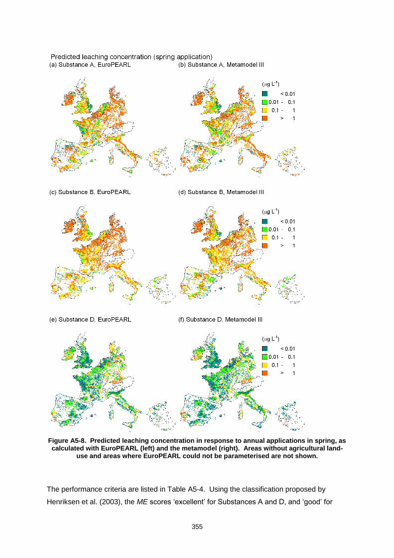
355
Figure A5-8. Predicted leaching concentration in response to annual applications in spring, as calculated with EuroPEARL (left) and the metamodel (right). Areas without agricultural land-
use and areas where EuroPEARL could not be parameterised are not shown.
The performance criteria are listed in Table A5-4. Using the classification proposed by
Henriksen et al. (2003), the ME scores ‘excellent’ for Substances A and D, and ‘good’ for
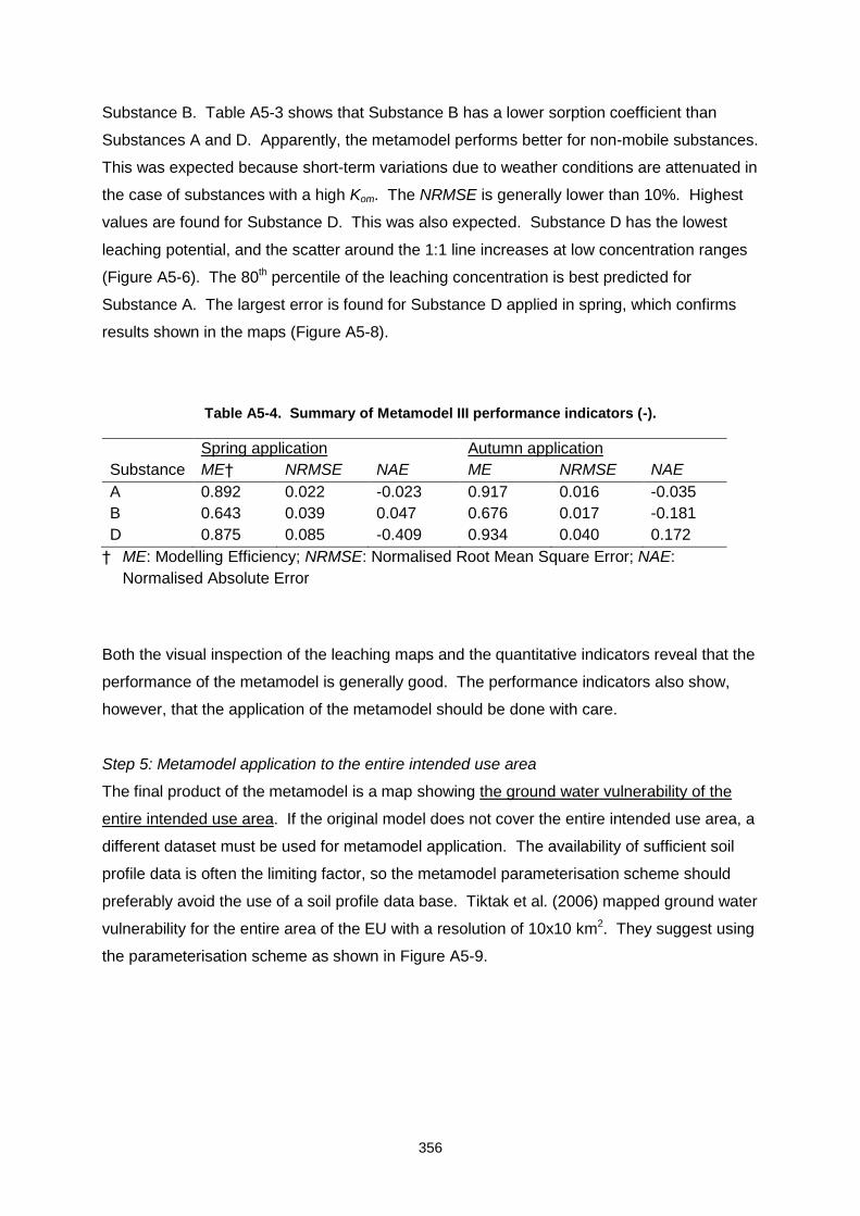
356
Substance B. Table A5-3 shows that Substance B has a lower sorption coefficient than
Substances A and D. Apparently, the metamodel performs better for non-mobile substances.
This was expected because short-term variations due to weather conditions are attenuated in
the case of substances with a high Kom. The NRMSE is generally lower than 10%. Highest
values are found for Substance D. This was also expected. Substance D has the lowest
leaching potential, and the scatter around the 1:1 line increases at low concentration ranges
(Figure A5-6). The 80th percentile of the leaching concentration is best predicted for
Substance A. The largest error is found for Substance D applied in spring, which confirms
results shown in the maps (Figure A5-8).
Table A5-4. Summary of Metamodel III performance indicators (-).
Spring application Autumn application
Substance ME† NRMSE NAE ME NRMSE NAE
A 0.892 0.022 -0.023 0.917 0.016 -0.035
B 0.643 0.039 0.047 0.676 0.017 -0.181
D 0.875 0.085 -0.409 0.934 0.040 0.172
† ME: Modelling Efficiency; NRMSE: Normalised Root Mean Square Error; NAE:
Normalised Absolute Error
Both the visual inspection of the leaching maps and the quantitative indicators reveal that the
performance of the metamodel is generally good. The performance indicators also show,
however, that the application of the metamodel should be done with care.
Step 5: Metamodel application to the entire intended use area
The final product of the metamodel is a map showing the ground water vulnerability of the
entire intended use area. If the original model does not cover the entire intended use area, a
different dataset must be used for metamodel application. The availability of sufficient soil
profile data is often the limiting factor, so the metamodel parameterisation scheme should
preferably avoid the use of a soil profile data base. Tiktak et al. (2006) mapped ground water
vulnerability for the entire area of the EU with a resolution of 10x10 km2. They suggest using
the parameterisation scheme as shown in Figure A5-9.

357
Figure A5-9. Parameterisation scheme for MetaPEARL. The final metamodel uses only four independent spatially distributed model inputs.
The following spatially distributed model input parameters are required for MetaPEARL:
The transformation rate coefficient, μ, should be calculated with Equation A5-11. The
temperature is taken from the MARS data base, which contains a map of the long-
term average temperature based on data from 1500 weather stations (Vossen and
Meyer-Roux, 1995).
The flux at 100 cm depth, q100, can be calculated from the mean annual precipitation
using the regression in Figure A5-10a. The regression was carried out on data in the
EuroPEARL output files. There appeared to be a strong correlation between mean
annual precipitation and the flux at 100-cm depth. This strong correlation was
expected, because mean actual evapotranspiration rates show limited variability
throughout Europe (Roberts, 1983). The mean annual precipitation is taken from the
MARS data base (see above).
The long-term average soil water content can be approximated by the water content
at field capacity (fc), which is obtained from soil texture using pedotransfer rules
(Jamagne et al., 1995). Analysis of the EuroPEARL output files revealed that the
long-term average soil water content was generally within 5% of the water content at
field capacity, so this is a realistic approximation (Figure A5-10b).
The organic matter content should be taken from the European organic matter map
(Jones et al., 2004; 2005).
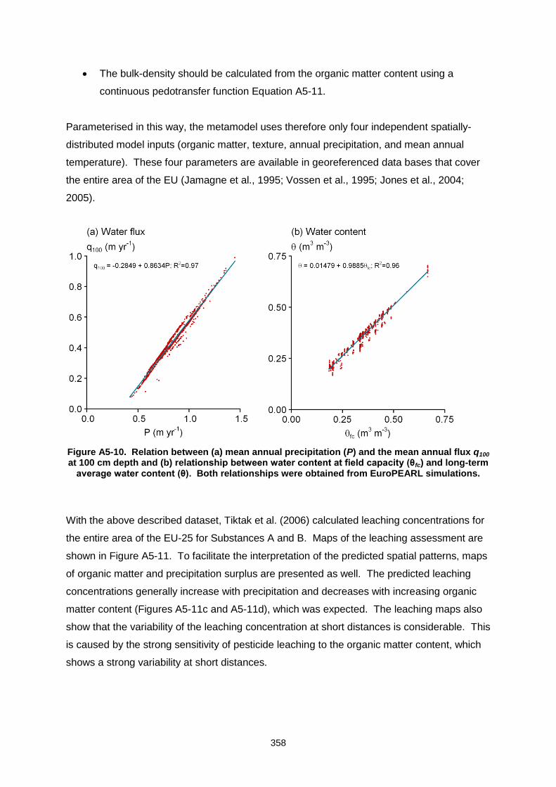
358
The bulk-density should be calculated from the organic matter content using a
continuous pedotransfer function Equation A5-11.
Parameterised in this way, the metamodel uses therefore only four independent spatially-
distributed model inputs (organic matter, texture, annual precipitation, and mean annual
temperature). These four parameters are available in georeferenced data bases that cover
the entire area of the EU (Jamagne et al., 1995; Vossen et al., 1995; Jones et al., 2004;
2005).
Figure A5-10. Relation between (a) mean annual precipitation (P) and the mean annual flux q100 at 100 cm depth and (b) relationship between water content at field capacity (θfc) and long-term
average water content (θ). Both relationships were obtained from EuroPEARL simulations.
With the above described dataset, Tiktak et al. (2006) calculated leaching concentrations for
the entire area of the EU-25 for Substances A and B. Maps of the leaching assessment are
shown in Figure A5-11. To facilitate the interpretation of the predicted spatial patterns, maps
of organic matter and precipitation surplus are presented as well. The predicted leaching
concentrations generally increase with precipitation and decreases with increasing organic
matter content (Figures A5-11c and A5-11d), which was expected. The leaching maps also
show that the variability of the leaching concentration at short distances is considerable. This
is caused by the strong sensitivity of pesticide leaching to the organic matter content, which
shows a strong variability at short distances.
359
Figure A5-11. Results of the metamodel application at the entire EU-25. Leaching set autumn application was used. (a) Organic matter content of the upper meter of the soil profile; (b)
annual mean precipitation surplus; (c) predicted leaching concentration for Substance A, (d) predicted leaching concentration for substance B; (e) normalised vulnerability score for
Substance A; (f) normalised vulnerability score for Substance B.
The leaching maps also show that the predicted leaching concentrations in certain areas of
southern Europe are relatively high. An explanation is found in the extremely low organic
360
matter contents in Mediterranean countries, which can be lower than 1% (Figure A5-11a).
Also, in some regions in southern Europe (for example Galicia), precipitation is high.
The final product of the metamodel application is the ground water vulnerability map. In such
a map, the leaching concentration is normalised: the grid-cell with the highest leaching
scores 100%, while the grid-cell with the lowest leaching scores 0% (the normalised
vulnerability score). As expected, the vulnerability score is generally high where precipitation
surplus is high and organic matter is low (Figure A5-11ef). There are, however, important
differences between the two substances. The vulnerability score of the very mobile
Substance B shows much more resemblance with the precipitation surplus map than the
vulnerability score of Substance A. The vulnerability score of Substance A is strongly
correlated with the organic matter content map. These differences are in line with results
obtained with the original model (Section A5.3), which suggests that the metamodel captures
the main features with respect to the dependency of the leaching concentration on the
various processes. This analysis further shows that pesticide properties must be included in
ground water vulnerability assessments, particularly if the metamodel is used to derive use-
specific scenarios (Section 7.2.5).
pH-dependent sorption and transformation
Van der Linden et al. (2001) developed a methodology to account for pH-dependent sorption
and transformation. These procedures are included in the GeoPEARL model (Tiktak et al.,
2003, Section 4.2). pH-dependent sorption and/or transformation can be easily incorporated
into the metamodel. Equation A5-9 describes the X2-term for ordinary behaving substances.
When applying the metamodel, this equation should be replaced by the following expression
for pH-dependent substances:
q
L
M
M
M
MKomK
f
X
pHpKapH
ac
ba
pHpKapH
ac
ba
baacom
om
101
10,
2
(A5-17)
where Kom,ac (m3 kg-1) is the coefficient for sorption on organic matter under acidic conditions,
Kom,ba (m3 kg-1) is the coefficient for sorption on organic matter under basic conditions, M
(kg mol-1) is molar mass, pKa is the negative logarithm of the dissociation constant, and ΔpH
is a pH correction factor. See further the GeoPEARL manual (Tiktak et al., 2003) for details,
particularly on using the pH-shift in an appropriate way.
361
Step 6: Selection of the target grid cell
The target grid cell(s) can be directly inferred from the normalised ground water vulnerability
map. The following procedures should be followed:
Frequency distributions should be created for the intended use area, using the crop
area as a weighing factor (see the manual of GeoPEARL for procedures).
All grid cells that meet the target vulnerability in the 80-85th vulnerability range should
be selected as candidate scenarios. Notice that the use of a range is advocated
instead of the exact 80th percentile, acknowledging that MetaPEARL is not a perfect
metamodel of GeoPEARL.
From the 80-85 percentile range, the grid cells with the highest crop area should be
chosen as the final scenario (the dominant combination). This assures that
representative unique combinations are chosen.
A5-5 Validation of the entire approach
As described in Sections 7.2.5 and A5.2, spatially-distributed models play an important role
in the tiered assessment scheme. In Tier 2, simple spatially distributed models are used to
derive use-specific scenarios (Section 7.2.5). The regulatory endpoint is calculated for this
single scenario with a FOCUS leaching model. In Tier 3, spatially distributed are used to
calculate the regulatory endpoint directly (Chapter 8).
As mentioned in Section 7.2.5, spatially-distributed models can be seen as the reference for
simple leaching models, because the spatially distributed model uses the FOCUS leaching
model directly. In this section, MetaPEARL is evaluated for using in developing scenarios for
use in Tier 2b assessments. For this reason, MetaPEARL (model III) is applied to the
Netherlands. This country was chosen, because a high quality soil, climate and crop data
base is available, which covers the entire country. This makes it possible to calculate the
FOCUS target percentile with both the original model (Tier 3 approach) and with use specific
scenarios (Tier 2b approach). The validation consisted of the following elements:
what is the correlation between the ground water vulnerability maps generated by the
two methods?
how do the results from a Tier 2b assessment compare to results of a Tier 3
assessment?
The validation was done for three pesticides (Table A5-3) and for 26 different use-specific
scenarios. A secondary aim of the validation was to test if the general EU-metamodel
parameterisation could be transferred to different data sets. This step is necessary in those
362
countries where insufficient soil information is available to build a local metamodel (see
Section A5.2).
Comparison of the EU-Metamodel with a local metamodel
A metamodel of GeoPEARL for the Netherlands was built using the procedure described in
Section A5.4. This metamodel parameterisation was compared to the metamodel
parameterisation of the final EU-metamodel (model III). Because the Netherlands are in
climatic zone TD (Table A5-2), this climatic zone was used for the final comparison. Results
presented in Table A5-5 show that there are minor differences between the two metamodel
parameterisations. The variance predicted by the Dutch metamodel (based on
GeoPEARL_NL), however, is lower than the variance predicted by the EU-metamodel (based
on EuroPEARL). In contrast to SPADE, the Dutch soil data base contains real soil profile
descriptions (not estimated soil profiles). As a consequence, the data bases contain more
extreme soil profiles than SPADE. Particularly clay on peat profiles cause additional scatter
(see later text).
Table A5-5. Coefficients resulting from calibration of the metamodel to the two leaching sets.
Model† Leaching
set
Region‡ α0*** α1 α2 α3 R2 *
Model
III
Autumn TD 5.30 (0.006) 0.16 (0.002) 0.46 (0.001) NA 0.97
NL 5.10 (0.014) 0.15 (0.003) 0.58 (0.001) NA 0.89
Model
III
Spring TD 5.09 (0.007) 0.44 (0.003) 0.46 (0.001) NA 0.95
NL 4.85 (0.016) 0.43 (0.005) 0.38 (0.001) NA 0.88
The rather good correspondence between the two metamodel parameterisations is confirmed
when the two metamodels are used to predict ground water vulnerability in the Netherlands.
If the EU-metamodel predictions are plotted as a function of the NL-metamodel predictions, a
straight line with a 1:1 slope and few scatter results (Figure A5-12). The rather good
correspondence between both metamodel parameterisation was a surprising result, because
the two data sets were collected completely independent of each other (different soil and
climate data bases were used to construct EuroPEARL and GeoPEARL). This exercise
demonstrates that the EU-metamodel can be used to map ground water vulnerability in the
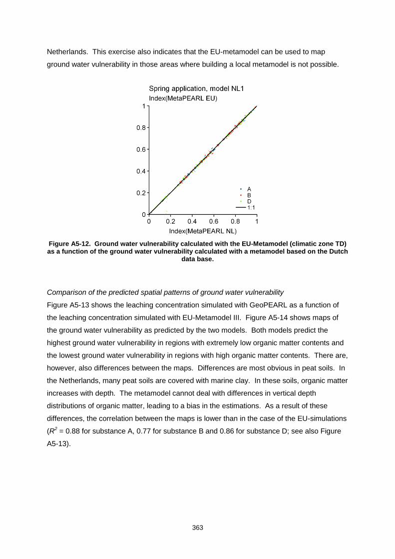
363
Netherlands. This exercise also indicates that the EU-metamodel can be used to map
ground water vulnerability in those areas where building a local metamodel is not possible.
Figure A5-12. Ground water vulnerability calculated with the EU-Metamodel (climatic zone TD) as a function of the ground water vulnerability calculated with a metamodel based on the Dutch
data base.
Comparison of the predicted spatial patterns of ground water vulnerability
Figure A5-13 shows the leaching concentration simulated with GeoPEARL as a function of
the leaching concentration simulated with EU-Metamodel III. Figure A5-14 shows maps of
the ground water vulnerability as predicted by the two models. Both models predict the
highest ground water vulnerability in regions with extremely low organic matter contents and
the lowest ground water vulnerability in regions with high organic matter contents. There are,
however, also differences between the maps. Differences are most obvious in peat soils. In
the Netherlands, many peat soils are covered with marine clay. In these soils, organic matter
increases with depth. The metamodel cannot deal with differences in vertical depth
distributions of organic matter, leading to a bias in the estimations. As a result of these
differences, the correlation between the maps is lower than in the case of the EU-simulations
(R2 = 0.88 for substance A, 0.77 for substance B and 0.86 for substance D; see also Figure
A5-13).
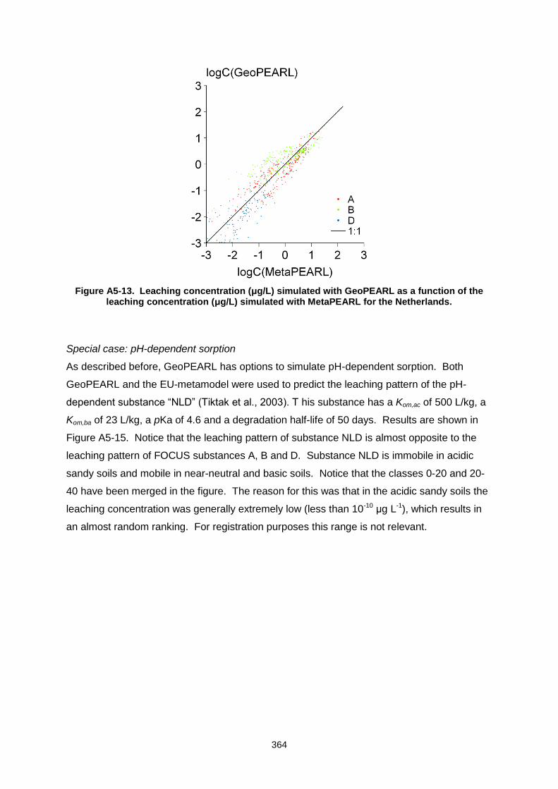
364
Figure A5-13. Leaching concentration (μg/L) simulated with GeoPEARL as a function of the leaching concentration (μg/L) simulated with MetaPEARL for the Netherlands.
Special case: pH-dependent sorption
As described before, GeoPEARL has options to simulate pH-dependent sorption. Both
GeoPEARL and the EU-metamodel were used to predict the leaching pattern of the pH-
dependent substance “NLD” (Tiktak et al., 2003). T his substance has a Kom,ac of 500 L/kg, a
Kom,ba of 23 L/kg, a pKa of 4.6 and a degradation half-life of 50 days. Results are shown in
Figure A5-15. Notice that the leaching pattern of substance NLD is almost opposite to the
leaching pattern of FOCUS substances A, B and D. Substance NLD is immobile in acidic
sandy soils and mobile in near-neutral and basic soils. Notice that the classes 0-20 and 20-
40 have been merged in the figure. The reason for this was that in the acidic sandy soils the
leaching concentration was generally extremely low (less than 10-10 μg L-1), which results in
an almost random ranking. For registration purposes this range is not relevant.
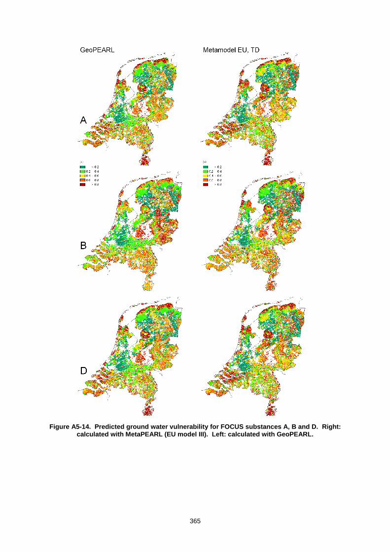
365
Figure A5-14. Predicted ground water vulnerability for FOCUS substances A, B and D. Right: calculated with MetaPEARL (EU model III). Left: calculated with GeoPEARL.
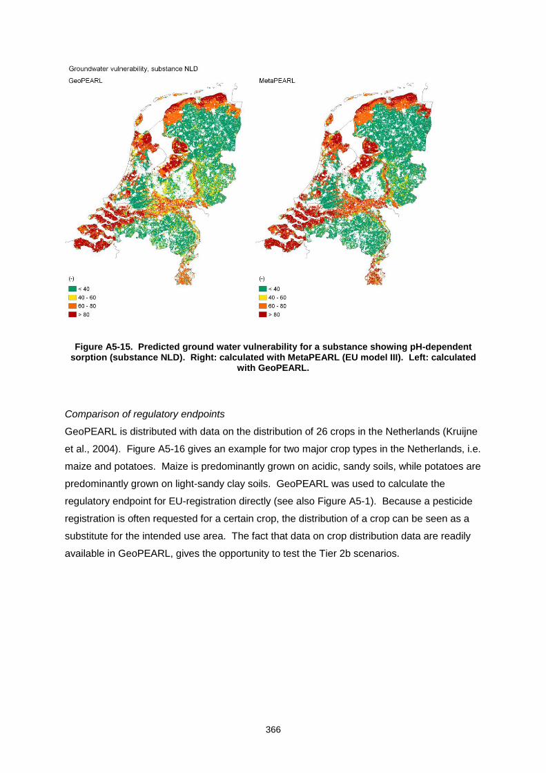
366
Figure A5-15. Predicted ground water vulnerability for a substance showing pH-dependent sorption (substance NLD). Right: calculated with MetaPEARL (EU model III). Left: calculated
with GeoPEARL.
Comparison of regulatory endpoints
GeoPEARL is distributed with data on the distribution of 26 crops in the Netherlands (Kruijne
et al., 2004). Figure A5-16 gives an example for two major crop types in the Netherlands, i.e.
maize and potatoes. Maize is predominantly grown on acidic, sandy soils, while potatoes are
predominantly grown on light-sandy clay soils. GeoPEARL was used to calculate the
regulatory endpoint for EU-registration directly (see also Figure A5-1). Because a pesticide
registration is often requested for a certain crop, the distribution of a crop can be seen as a
substitute for the intended use area. The fact that data on crop distribution data are readily
available in GeoPEARL, gives the opportunity to test the Tier 2b scenarios.
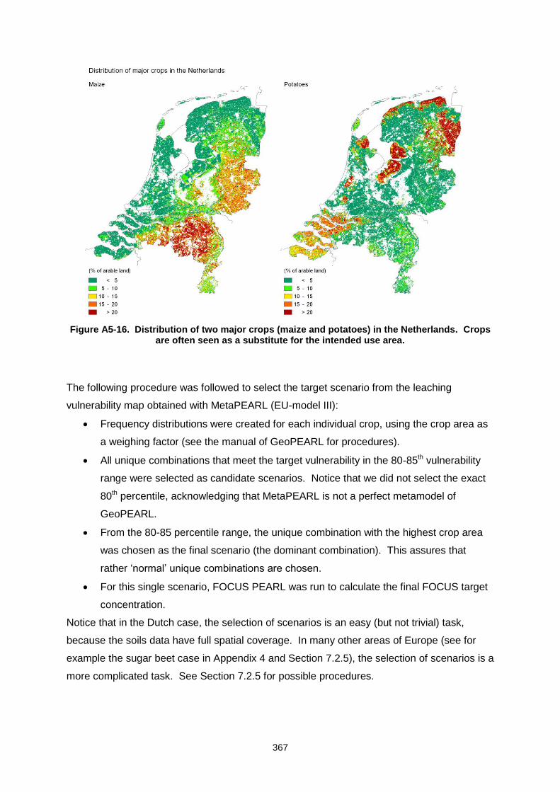
367
Figure A5-16. Distribution of two major crops (maize and potatoes) in the Netherlands. Crops are often seen as a substitute for the intended use area.
The following procedure was followed to select the target scenario from the leaching
vulnerability map obtained with MetaPEARL (EU-model III):
Frequency distributions were created for each individual crop, using the crop area as
a weighing factor (see the manual of GeoPEARL for procedures).
All unique combinations that meet the target vulnerability in the 80-85th vulnerability
range were selected as candidate scenarios. Notice that we did not select the exact
80th percentile, acknowledging that MetaPEARL is not a perfect metamodel of
GeoPEARL.
From the 80-85 percentile range, the unique combination with the highest crop area
was chosen as the final scenario (the dominant combination). This assures that
rather ‘normal’ unique combinations are chosen.
For this single scenario, FOCUS PEARL was run to calculate the final FOCUS target
concentration.
Notice that in the Dutch case, the selection of scenarios is an easy (but not trivial) task,
because the soils data have full spatial coverage. In many other areas of Europe (see for
example the sugar beet case in Appendix 4 and Section 7.2.5), the selection of scenarios is a
more complicated task. See Section 7.2.5 for possible procedures.
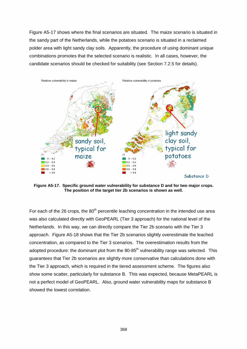
368
Figure A5-17 shows where the final scenarios are situated. The maize scenario is situated in
the sandy part of the Netherlands, while the potatoes scenario is situated in a reclaimed
polder area with light sandy clay soils. Apparently, the procedure of using dominant unique
combinations promotes that the selected scenario is realistic. In all cases, however, the
candidate scenarios should be checked for suitability (see Section 7.2.5 for details).
Figure A5-17. Specific ground water vulnerability for substance D and for two major crops. The position of the target tier 2b scenarios is shown as well.
For each of the 26 crops, the 80th percentile leaching concentration in the intended use area
was also calculated directly with GeoPEARL (Tier 3 approach) for the national level of the
Netherlands. In this way, we can directly compare the Tier 2b scenario with the Tier 3
approach. Figure A5-18 shows that the Tier 2b scenarios slightly overestimate the leached
concentration, as compared to the Tier 3 scenarios. The overestimation results from the
adopted procedure: the dominant plot from the 80-85th vulnerability range was selected. This
guarantees that Tier 2b scenarios are slightly more conservative than calculations done with
the Tier 3 approach, which is required in the tiered assessment scheme. The figures also
show some scatter, particularly for substance B. This was expected, because MetaPEARL is
not a perfect model of GeoPEARL. Also, ground water vulnerability maps for substance B
showed the lowest correlation.
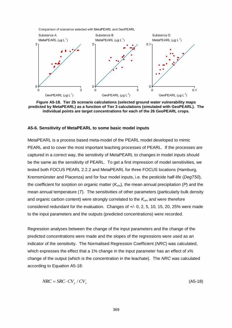
369
Figure A5-18. Tier 2b scenario calculations (selected ground water vulnerability maps predicted by MetaPEARL) as a function of Tier 3 calculations (simulated with GeoPEARL). The
individual points are target concentrations for each of the 26 GeoPEARL crops.
A5-6. Sensitivity of MetaPEARL to some basic model inputs
MetaPEARL is a process based meta-model of the PEARL model developed to mimic
PEARL and to cover the most important leaching processes of PEARL. If the processes are
captured in a correct way, the sensitivity of MetaPEARL to changes in model inputs should
be the same as the sensitivity of PEARL. To get a first impression of model sensitivities, we
tested both FOCUS PEARL 2.2.2 and MetaPEARL for three FOCUS locations (Hamburg,
Kremsmünster and Piacenza) and for four model inputs, i.e. the pesticide half-life (DegT50),
the coefficient for sorption on organic matter (Kom), the mean annual precipitation (P) and the
mean annual temperature (T). The sensitivities of other parameters (particularly bulk density
and organic carbon content) were strongly correlated to the Kom and were therefore
considered redundant for the evaluation. Changes of +/- 0, 2, 5, 10, 15, 20, 25% were made
to the input parameters and the outputs (predicted concentrations) were recorded.
Regression analyses between the change of the input parameters and the change of the
predicted concentrations were made and the slopes of the regressions were used as an
indicator of the sensitivity. The Normalised Regression Coefficient (NRC) was calculated,
which expresses the effect that a 1% change in the input parameter has an effect of x%
change of the output (which is the concentration in the leachate). The NRC was calculated
according to Equation A5-18:
xy CVCVSRCNRC / (A5-18)
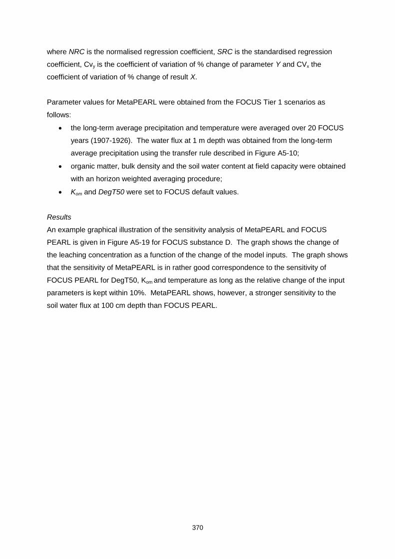
370
where NRC is the normalised regression coefficient, SRC is the standardised regression
coefficient, Cvy is the coefficient of variation of % change of parameter Y and CVx the
coefficient of variation of % change of result X.
Parameter values for MetaPEARL were obtained from the FOCUS Tier 1 scenarios as
follows:
the long-term average precipitation and temperature were averaged over 20 FOCUS
years (1907-1926). The water flux at 1 m depth was obtained from the long-term
average precipitation using the transfer rule described in Figure A5-10;
organic matter, bulk density and the soil water content at field capacity were obtained
with an horizon weighted averaging procedure;
Kom and DegT50 were set to FOCUS default values.
Results
An example graphical illustration of the sensitivity analysis of MetaPEARL and FOCUS
PEARL is given in Figure A5-19 for FOCUS substance D. The graph shows the change of
the leaching concentration as a function of the change of the model inputs. The graph shows
that the sensitivity of MetaPEARL is in rather good correspondence to the sensitivity of
FOCUS PEARL for DegT50, Kom and temperature as long as the relative change of the input
parameters is kept within 10%. MetaPEARL shows, however, a stronger sensitivity to the
soil water flux at 100 cm depth than FOCUS PEARL.
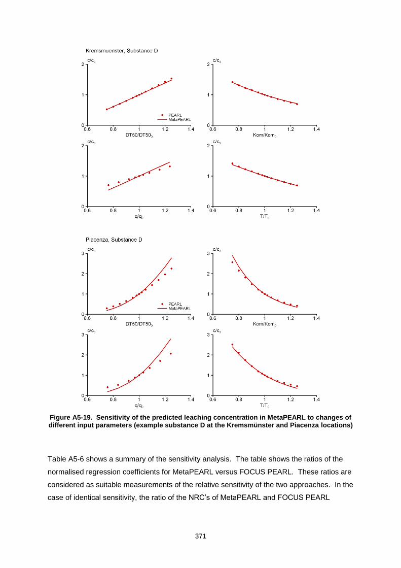
371
Figure A5-19. Sensitivity of the predicted leaching concentration in MetaPEARL to changes of different input parameters (example substance D at the Kremsmünster and Piacenza locations)
Table A5-6 shows a summary of the sensitivity analysis. The table shows the ratios of the
normalised regression coefficients for MetaPEARL versus FOCUS PEARL. These ratios are
considered as suitable measurements of the relative sensitivity of the two approaches. In the
case of identical sensitivity, the ratio of the NRC’s of MetaPEARL and FOCUS PEARL
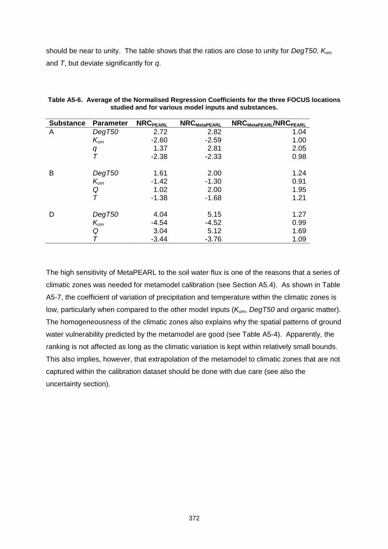
372
should be near to unity. The table shows that the ratios are close to unity for DegT50, Kom
and T, but deviate significantly for q.
Table A5-6. Average of the Normalised Regression Coefficients for the three FOCUS locations studied and for various model inputs and substances.
Substance Parameter NRCPEARL NRCMetaPEARL NRCMetaPEARL/NRCPEARL
A DegT50 2.72 2.82 1.04 Kom -2.60 -2.59 1.00 q 1.37 2.81 2.05 T -2.38 -2.33 0.98 B DegT50 1.61 2.00 1.24 Kom -1.42 -1.30 0.91 Q 1.02 2.00 1.95 T -1.38 -1.68 1.21 D DegT50 4.04 5.15 1.27 Kom -4.54 -4.52 0.99 Q 3.04 5.12 1.69 T -3.44 -3.76 1.09
The high sensitivity of MetaPEARL to the soil water flux is one of the reasons that a series of
climatic zones was needed for metamodel calibration (see Section A5.4). As shown in Table
A5-7, the coefficient of variation of precipitation and temperature within the climatic zones is
low, particularly when compared to the other model inputs (Kom, DegT50 and organic matter).
The homogeneousness of the climatic zones also explains why the spatial patterns of ground
water vulnerability predicted by the metamodel are good (see Table A5-4). Apparently, the
ranking is not affected as long as the climatic variation is kept within relatively small bounds.
This also implies, however, that extrapolation of the metamodel to climatic zones that are not
captured within the calibration dataset should be done with due care (see also the
uncertainty section).
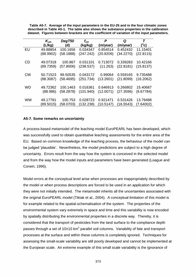
373
Table A5-7. Average of the input parameters in the EU-25 and in the four climatic zones described in Table A5-1. The table also shows the substance properties in the calibration dataset. Figures between brackets are the coefficient of variation of the input parameters.
Kom DegT50 fom P Q T (L/kg) (d) (kg/kg) (m/year) (m/year) (oc)
EU 49.88854 100.1656 0.034347 0.854514 0.452432 11.15401 (88.9902) (58.1888) (247.242) (20.8209) (34.2270) (22.8115) CD 49.07318 100.867 0.031101 0.713072 0.339283 10.42166 (89.7359) (57.8006) (238.537) (11.263) (22.8181) (15.8137) CW 50.71523 99.50535 0.043172 0.99064 0.559165 9.735488 (88.3087) (58.4695) (251.734) (13.2601) (21.8099) (16.2062) WD 49.72362 100.1463 0.016361 0.646913 0.266802 15.40687 (88.986) (58.2878) (101.940) (12.0071) (27.3596) (9.67784) WW 49.17781 100.753 0.028723 0.921471 0.531426 13.79488 (89.5015) (58.0703) (132.238) (10.5147) (16.5543) (7.64002)
A5-7. Some remarks on uncertainty
A process-based metamodel of the leaching model EuroPEARL has been developed, which
was successfully used to obtain quantitative leaching assessments for the entire area of the
EU. Based on common knowledge of the leaching process, the behaviour of the model can
be judged ‘plausible’. Nevertheless, the model predictions are subject to a high degree of
uncertainty. Errors result from the way how the system is conceived in the selected model
and from the way how the model inputs and parameters have been generated (Loague and
Corwin, 1996).
Model errors at the conceptual level arise when processes are inappropriately described by
the model or when process descriptions are forced to be used in an application for which
they were not initially intended. The metamodel inherits all the uncertainties associated with
the original EuroPEARL model (Tiktak et al., 2004). A conceptual limitation of this model is
for example related to the spatial-schematisation of the system. The properties of the
environmental system vary extremely in space and time and this variability is now encoded
by spatially distributing the environmental properties in a discrete way. Thereby, it is
considered that the transport of pesticides from the land surface to the compliance depth
passes through a set of 10X10 km2 parallel soil columns. Variability of fate and transport
processes at the surface and within these columns is completely ignored. Techniques for
assessing the small-scale variability are still poorly developed and cannot be implemented at
the European scale. An extreme example of this small scale variability is the ignorance of
374
preferential flow, a process for which consensus exists that is extremely important for
correctly describing pesticide transport in soils (Flühler et al., 2001). Basic soil information
for preferential flow models such as quantitative soil structure information (Rawls et al., 1996)
is not yet available at the European scale, so whether a regional-scale version of preferential
flow models will become available shortly remains questionable.
Input and parameter generation errors depend on the quality of the underlying data bases
and the quality of the parameter generation techniques, such as the quality of the applied
pedotransfer functions (Tiktak et al., 1999). For characterising the spatial patterns of soil
properties throughout Europe, the European Soil Map at the scale 1:1,000,000 was used in
combination with the Soil Profile Analytical Database of Europe (Jamagne et al., 1995). The
Soil Profile Database has serious limitations. The most serious limitations are that soil profile
data is available for only 75% of the agricultural area of the EU-15, and that the soil profiles
are not uniformly distributed across the continent. Jamagne et al. (1995) showed, however,
that all major soil types are included. The metamodel was used to extend the simulations
towards the entire EU. This can be done, as long as the metamodel is not applied beyond
the range of values in the original data base. Analysis of the EuroPEARL data base revealed
that only 6% of the total agricultural area of the EU-25 was outside the range of model inputs
of the original model. The missing area is mainly in cold climates, where the mean annual
temperature is below 5oC. The effect of important processes for these regions, like snow
accumulation and the effect of frost on water flow, may therefore be underestimated.
Predictions for the Nordic and Baltic countries should, therefore, be treated with extra care.
Another reason for being careful with metamodel extrapolation is the high sensitivity of the
metamodel to the mean annual rainfall as compared to FOCUS PEARL (see Section A5.7).
The metamodel validation in this study pertains only to the comparison of the metamodel with
the original model; no comparison with field-observations was made in this study. So far,
leaching models have primarily been validated at the field-scale (e.g., Vanclooster et al.,
2000; Trevisan et al., 2003) and very few studies, if any, have looked at the validity of the
spatial leaching patterns simulated by spatially distributed leaching models. Analyzing the
validity of the predicted spatial patterns needs detailed information on the occurrence of
pesticides within ground water bodies. Unfortunately, high quality regional data sets that
allow such an assessment are only available for some limited cases (e.g., Leterme et al.,
2004; 2006; Tiktak et al., 2005). The EU-Groundwater Directive is expected to call for
monitoring data on pesticide concentrations in the ground water, yet how data of such
monitoring programs could be used to assess the validity of spatial predictions of pesticide
leaching should be analysed.
375
When applying the metamodel, an additional error is added on top of the model error of the
original model. Recently, a study started to quantify the error propagation in the chain
EuroPEARL-metamodel (Van der Linden et al., 2006).
A5-8. General conclusions
A tiered assessment scheme to spatially distributed modelling has been developed, which
can be used to support both national and EU-registration. In those cases where sufficient
information is available, a process based, numerical leaching model can be used to calculate
the regulatory endpoint directly. This is seen as a Tier 3 approach (Chapter 8). It can also be
seen as a reference to other approaches, because it uses the original FOCUS leaching
model directly. In those cases where data is insufficient, metamodels have been used to
extend the simulations towards the entire intended use area. A single use-specific scenario
is selected from the ground water vulnerability map obtained with this metamodel, and a
FOCUS leaching model is run for this single scenario to get the regulatory endpoint (Tier 2b
approach, Section 7.2.5). The approach can also be used to improve existing Tier 1
scenarios or to develop new Tier 1 scenarios (for national or EU-registration).
Metamodels form the backbone of the approach reported in this appendix, because they
guarantee consistency within the tiered assessment scheme. We used a process-based
metamodel of the recently developed European leaching model EuroPEARL. In contrast to
earlier approaches, the metamodel is based on a large number of substances (56) and
scenarios (1056). The metamodel explains more than 90% of the variation of the original
model using only four independent spatially distributed parameters that are available from
general soil and climate data bases. The calibrated metamodel was applied to generate
maps of the leaching concentration in the European Union. Maps generated with the
metamodel showed a striking similarity to maps obtained with EuroPEARL. The predicted
leaching concentration generally increases with precipitation and decreases with increasing
organic matter content. The short-distance variability of the leaching concentration due to
organic matter overruled the north-south gradient caused by climatic differences, a leaching
pattern that is also simulated by the original model. Quantitative performance indicators
confirmed that the metamodel gives results comparable to the original model.
The entire approach was tested in the Netherlands, where sufficient soil data is available to
parameterise a spatially distributed model with full coverage. The EU-Metamodel could be
successfully applied to the Netherlands. This is an important result, because the data set for
376
the Netherlands was derived independently from the EU-data set. This is an indication that
the metamodel can be used in countries where insufficient soil data is available to develop a
spatially distributed leaching model, so that the approach is applicable to the entire EU.
Results from Tier 2b scenarios with results from GeoPEARL (Tier 3 approach) showed a
striking correspondence, indicating that the entire approach gives consistent predictions.
The Tier 2b scenarios were slightly more conservative than Tier 3 predictions, which
indicates that the approach suites the general FOCUS tiered-assessment scheme (earlier
tiers must be more conservative than later tiers).
A5-9. Acknowledgements
EuroPEARL was developed within the framework of the EU-funded APECOP project (project
number QLRT-CT1998-01238). MetaPEARL was developed to support the Thematic
Strategy on Pesticides. The work was done within the project ‘HArmonized environmental
Indicators for pesticide Risk (HAIR)’, which was supported by the European Commission
under the 6th framework program (project number SSPE-CT-2003-501997).
A5-10. References
Boesten, J.J.T.I., and A.M.A. van der Linden. 1991. Modeling the influence of sorption and
transformation on pesticide leaching and persistence. J. Environ. Qual. 20:425-435.
Capri, E., L. Padovani, and M. Trevisan. La previsione della contaminazione della acque
sotterranee da prodotti fitosanitari. Quaderni di techniche di protezione ambientale.
Pitagora, Bologna, Italy.
Chambers, J. and Hastie, T. 1992. Statistical models. Chapman and Hall. ISBN 0-412-
05301-2.
Flühler, H., N. Ursino, M. Bundt, U. Zimmerman and C. Stamm. 2001. The preferential flow
syndrome – a buzzword or a scientific problem? In D.C. Flanagan and J.C. Ascough
(eds.). Soil erosion research for the 21st century symposium and 2nd international
symposium on preferential flow. ASAE Publication 706P0006/7CD, ASAE, St. Joseph,
MI.
FOCUS. 2000. FOCUS groundwater scenarios in the EU-review of active substances.
Report of the FOCUS groundwater scenarios workgroup, EC Document, Sanco/321/2000
rev. 2. Available at http://arno.ei.jrc.it/focus.htm (verified 14 Feb. 2006).
Henriksen, H.J., L. Troldborg, P. Nyegaard, T.O. Sonnenborg, J.C. Refsgaard, and B.
Madsen. 2003. Methodology for construction, calibration and validation of a national
hydrological model for Denmark. J. Hydrol. 280:52-71.
377
Jamagne, M., C. Le Bas, M. Berland, and W. Eckelman. 1995. Extension of the EU
Database for the Soils of Central and Eastern Europe. In D. King, R.J.A. Jones, and A.J.
Thomassen (eds.) EUR 16232 EN. Office for Official Publications of the European
Communities, Luxembourg, p. 101-114.
Janssen, P.H.M., P.S.C. Heuberger, and A. Tiktak. 2005. Metamodelleren bij het MNP-
RIVM. Naar praktische toepassingen. MNP Rapport 500013001, MNP, Bilthoven. the
Netherlands (in Dutch).
Jones, R. J. A., R. Hiederer, E. Rusco, and L. Montanarella. 2005. Estimating organic
carbon in the soils of Europe for policy support. European Journal of Soil Science,
56(5):655-671.
Jones, R.J.A., R. Hiederer, E. Rusco, P. J. Loveland, and L. Montanarella. 2004. The map
of organic carbon in topsoils in Europe, Version 1.2, September 2003: Explanation of
Special Publication Ispra 2004 No.72 (S.P.I.04.72). European Soil Bureau Research
Report No.17, EUR 21209 EN, 26pp. and 1 map in ISO B1 format. Office for Official
Publications of the European Communities, Luxembourg.
Jury, W.A., and J. Gruber. 1989. A stochastic analysis of the influence of soil and climatic
variability on the estimate of pesticide groundwater pollution potential. Water Resour.
Res. 25:2465-2474.
Jury, W.A., and K. Roth. 1990. Transfer functions and solute movement through soil.
Theory and applications. Birkhauser, Basel.
Klein, M. 1995. PELMO: Pesticide Leaching Model, User manual version 2.01. Fraunhofer-
Institut für Umweltchemie und Ökotoxikogie, D57392.
Kruijne, R., A. Tiktak, D. van Kraalingen, J.J.T.I. Boesten, and A.M.A. van der Linden. 2004.
Pesticide leaching to the groundwater in drinking water abstraction areas. Analysis with
the GeoPEARL model. Alterra-report 1041, Wageningen, the Netherlands.
Leterme, B., M. Rounsevell, D. Pinte, J. Piñeros-Garcet, and M. Vanclooster. 2004.
Development of a probabilistic data assimilation methodology for the assessment of
groundwater contamination by pesticides at the catchment scale. In A.J. Witkowski, J.
Vrba, and A. Kowalczyk (eds.). Groundwater Vulnerability Assessment and Mapping,
Conference Abstracts, University of Silesia, Katowice, Poland. p. 83-84.
Leterme, B., M. Vanclooster, A. Tiktak, A.M.A. van der Linden, and M.D.A. Rounsevell.
2006. The consequences of interpolating or calculating first on the simulation of pesticide
leaching at the regional scale. In: Pesticide Behaviour in Soils, Water and Air. University
of Warwick, UK, pp. B12. Full paper submitted to J. Environ Qual.
Loague, K. and D.L. Corwin. 1996. Uncertainty in Regional-scale Assessments of non-point
source pollutants. In D.L. Corwin and K. Loague (eds.). Application of GIS to the
378
modeling of non-point source pollutants in the vadose zone. SSSA Special Publication
No. 48, SSSA, Madison, WI. p. 131-152.
Loague, K., R.S. Yost, R.E. Green, and T.C. Liang. 1989. Uncertainty in a pesticide
leaching assessment for Hawaii. J. Contam. Hydrol. 4:139-161.
Loague, K., R.L. Bernknopf, R.E. Green, and. T.W. Giambelluca. 1996. Uncertainty of
groundwater vulnerability assessments for agricultural regions in Hawaii: Review. J.
Environ. Qual. 25:475-490.
Petach, M.C., R.J. Wagenet, and S.D. De Gloria. 1991. Regional water flow and pesticide
leaching using simulations with spatially distributed data. Geoderma (48):245-269.
Piñeros-Garcet, J.D., A. Ordonnez, J. Roosen, and M. Vanclooster. 2006. Metamodelling:
Theory, concepts and applications to nitrate leaching modelling. Ecological Modelling. In
press. Available online at http://dx.doi.org/10.1016/j.ecolmodel.2005.08.045 (verified 14
Feb. 2006).
Rawls, W.J., D.L. Brakensiek, and S.D. Logsdon. 1996. Estimation of macropore properties
for non-till soils. Trans. ASAE 39:91-95.
Roberts, J. 1983. Forest transpiration: A conservative hydrological process? J.
Hydrol. 66:13-141.
Stenemo, F., A. Lindahl, and N. Jarvis. 2006. Neural network meta-modeling of the
pesticide fate model MACRO for groundwater vulnerability assessments. In: Pesticide
Behaviour in Soils, Water and Air. University of Warwick, UK, pp. B2.
Stewart, I.T., and K. Loague. 2003. Development of type transfer functions for regional-
scale non-point source groundwater vulnerability assessments. Water Resour. Res.
39(12):1359.
Stewart, I.T., and K. Loague. 2004. Assessing ground water vulnerability with the type
transfer function model in the San Joaguin Valley, California. J. Environ. Qual. 33:1487-
1498.
Tiktak, A., A. Leijnse, and H.A. Vissenberg. 1999. Uncertainty in a regional-scale
assessment of cadmium accumulation in the Netherlands. J. Environ. Qual. 28:461-470.
Tiktak, A., J.J.T.I. Boesten, and A.M.A. van der Linden. 2002a. Nationwide assessments of
non-point source pollution with field-scale developed models: The pesticide case. In G.J.
Hunter and K. Lowell (eds.) Proceedings of the 5th international symposium on spatial
accuracy assessment (Accuracy 2002), July 2002. Melbourne, Australia. University of
Melbourne, Melbourne, Australia. p. 17-30.
Tiktak, A., D.S. de Nie, A.M.A. van der Linden, and R. Kruijne. 2002b. Modelling the
leaching and drainage of pesticides in the Netherlands: the GeoPEARL model.
Agronomie 22:373-387.
379
Tiktak, A., A.M.A. van der Linden, and J.J.T.I. Boesten. 2003. The GeoPEARL model.
Model description, applications and manual. RIVM report 716601007/2003. RIVM,
Bilthoven, the Netherlands.
Tiktak, A., D.S. de Nie, J.D. Piñeros Garcet, A. Jones, and M. Vanclooster. 2004a.
Assessment of the pesticide leaching risk at the Pan-European level. The EuroPEARL
approach. J. Hydrol. 289:222-238.
Tiktak, A., A.M.A. van der Linden, J.J.T.I. Boesten, R. Kruijne, and D. van Kraalingen.
2004b. The GeoPEARL model. Part II. User guide and model description update. RIVM
report 716601008/2004. RIVM, Bilthoven, the Netherlands.
Tiktak, A., A.M.A. van der Linden, and G. Uffink. 2005. Pesticide transport in the
groundwater at the national scale: coupling an unsaturated zone model with a
groundwater flow model. In N.R. Thomson (ed.) Bringing groundwater quality research to
the watershed scale. IAHS Publ. 297, IAHS Press, Wallingford, UK. p. 441-448.
TIktak, A., J.J.T.I. Boesten, A.M.A. van der Linden, and M. Vanclooster. 2006. Mapping
Groundwater Vulnerability to Pesticide Leaching with a process-based Metamodel of
EuroPEARL. J. Environ. Qual. 35:1213-1226.
Trevisan, M., L. Padovani, N. Jarvis, S. Roulier, F. Bouraoui, M. Klein and J.J.T.I. Boesten.
2003. Validation status of the present PEC groundwater models. In A.A.M. Del Re, E.
Capri, L. Padovani, and M. Trevisan (eds.) Pesticide in air, plant, soil and water system.
Proceedings of the XII Symposium Pesticide Chemistry, June 2003, Piacenza, University
of Piacenza, Piacenza, Italy. p.933-940.
Vanclooster, M., J.J.T.I. Boesten, M. Trevisan, C.D. Brown, E. Capri, O.M. Eklo,
B. Gottesbüren, V. Gouy, and A.M.A. van der Linden. 2000. A European test of
pesticide-leaching models: methodology and major recommendations. Agric. Water
Manage. 44:1-19.
Vanclooster, M., J.D. Pineros-Garcet, J.J.T.I. Boesten , F. Van den Berg, M. Leistra, J. Smelt,
N. Jarvis, S. Roulier, P. Burauel, H. Vereecken, A. Wolters, V. Linnemann, E. Fernandez,
M. Trevisan, E. Capri, L. Padovani, M. Klein, A. Tiktak, A. Van der Linden, D. De Nie, G.
Bidoglio, F. Baouroui, A. Jones, A. Armstrong. 2003. Effective Approaches for
Assessing the Predicted Environmental Concentrations of Pesticides. Final report.
European Commission, Quality of Life and Management of Living Resources
Programme. QLK4-CT-1999-01238. Printed by the Université Catholique de Louvain,
Belgium (Available at http://www.geru.ucl.ac.be/recherche/projets/apecop-pub/).
Van der Linden, A.M.A., A. Tiktak and M. Leistra. 2001. Incorporation of soil-pH dependent
behaviour in pesticide leaching assessment. In: A. Walker. Pesticide Behaviour in Soils
and Water. BCPC Symposium Proceedings No. 78, MCPC, Farnham, UK, p. 45-50.
380
Van der Linden, A.M.A., Tiktak, A., Heuvelink, G.B.M., and A. Leijnse. 2006. Spatial
uncertainty analysis of pesticide leaching using a metamodel of GeoPEARL. In: Mário
Caetano and Marco Painho (eds). Proceedings of Accuracy 2006, 7th International
Symposium on Spatial Accuracy Assessment in Natural Resources and Environmental
Sciences, p 359 - 366. Instituto Geográfico Português, Lisboa, Portugal. ISBN 972-8867-
27-1.
Van der Zee, S.E.A.T.M., and J.J.T.I. Boesten. 1991. Effects of soil heterogeneity on
pesticide leaching to groundwater. Water Resour. Res. 27:3051-3063.
Vossen, P., and J. Meyer-Roux. 1995. Crop monitoring and yield forecasting activities of the
MARS project. p. 11-30. In D. King, R.J.A. Jones, and A.J. Thomassen (Eds.). European
land information systems for agro-environmental monitoring, EUR EN 16232, Office for
the official publications of the European Communities, Luxembourg.
Yohai, V.J., and R.H. Zamar. 1997. Optimal locally robust M-estimates of regression. J.
Statist. Inference and Planning 64:309-323.
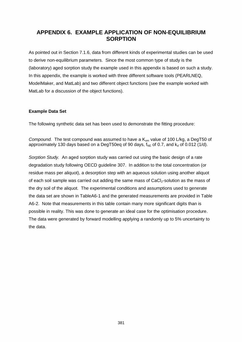
381
APPENDIX 6. EXAMPLE APPLICATION OF NON-EQUILIBRIUM SORPTION
As pointed out in Section 7.1.6, data from different kinds of experimental studies can be used
to derive non-equilibrium parameters. Since the most common type of study is the
(laboratory) aged sorption study the example used in this appendix is based on such a study.
In this appendix, the example is worked with three different software tools (PEARLNEQ,
ModelMaker, and MatLab) and two different object functions (see the example worked with
MatLab for a discussion of the object functions).
Example Data Set
The following synthetic data set has been used to demonstrate the fitting procedure:
Compound. The test compound was assumed to have a Kom value of 100 L/kg, a DegT50 of approximately 130 days based on a DegT50eq of 90 days, fNE of 0.7, and kd of 0.012 (1/d).
Sorption Study. An aged sorption study was carried out using the basic design of a rate
degradation study following OECD guideline 307. In addition to the total concentration (or
residue mass per aliquot), a desorption step with an aqueous solution using another aliquot
of each soil sample was carried out adding the same mass of CaCl2-solution as the mass of
the dry soil of the aliquot. The experimental conditions and assumptions used to generate
the data set are shown in TableA6-1 and the generated measurements are provided in Table
A6-2. Note that measurements in this table contain many more significant digits than is
possible in reality. This was done to generate an ideal case for the optimisation procedure.
The data were generated by forward modelling applying a randomly up to 5% uncertainty to
the data.
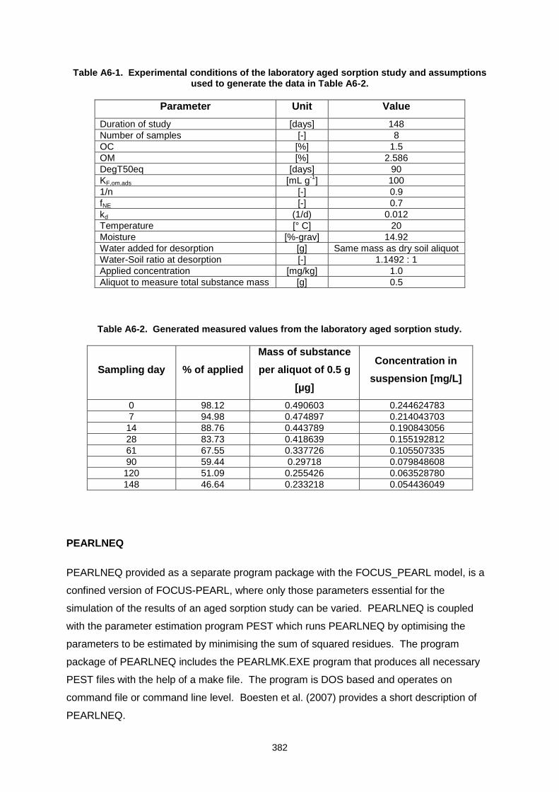
382
Table A6-1. Experimental conditions of the laboratory aged sorption study and assumptions used to generate the data in Table A6-2.
Parameter Unit Value
Duration of study [days] 148
Number of samples [-] 8
OC [%] 1.5
OM [%] 2.586
DegT50eq [days] 90
KF,om,ads [mL g-1
] 100
1/n [-] 0.9
fNE [-] 0.7
kd (1/d) 0.012
Temperature [° C] 20
Moisture [%-grav] 14.92
Water added for desorption [g] Same mass as dry soil aliquot
Water-Soil ratio at desorption [-] 1.1492 : 1
Applied concentration [mg/kg] 1.0
Aliquot to measure total substance mass [g] 0.5
Table A6-2. Generated measured values from the laboratory aged sorption study.
Sampling day % of applied
Mass of substance
per aliquot of 0.5 g
[µg]
Concentration in
suspension [mg/L]
0 98.12 0.490603 0.244624783
7 94.98 0.474897 0.214043703
14 88.76 0.443789 0.190843056
28 83.73 0.418639 0.155192812
61 67.55 0.337726 0.105507335
90 59.44 0.29718 0.079848608
120 51.09 0.255426 0.063528780
148 46.64 0.233218 0.054436049
PEARLNEQ
PEARLNEQ provided as a separate program package with the FOCUS_PEARL model, is a
confined version of FOCUS-PEARL, where only those parameters essential for the
simulation of the results of an aged sorption study can be varied. PEARLNEQ is coupled
with the parameter estimation program PEST which runs PEARLNEQ by optimising the
parameters to be estimated by minimising the sum of squared residues. The program
package of PEARLNEQ includes the PEARLMK.EXE program that produces all necessary
PEST files with the help of a make file. The program is DOS based and operates on
command file or command line level. Boesten et al. (2007) provides a short description of
PEARLNEQ.
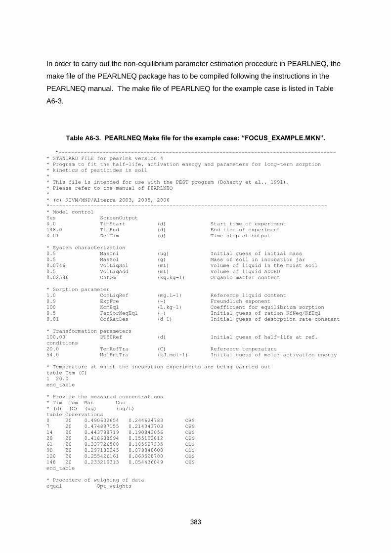
383
In order to carry out the non-equilibrium parameter estimation procedure in PEARLNEQ, the
make file of the PEARLNEQ package has to be compiled following the instructions in the
PEARLNEQ manual. The make file of PEARLNEQ for the example case is listed in Table
A6-3.
Table A6-3. PEARLNEQ Make file for the example case: “FOCUS_EXAMPLE.MKN”.
*----------------------------------------------------------------------------------------
* STANDARD FILE for pearlmk version 4
* Program to fit the half-life, activation energy and parameters for long-term sorption
* kinetics of pesticides in soil
*
* This file is intended for use with the PEST program (Doherty et al., 1991).
* Please refer to the manual of PEARLNEQ
*
* (c) RIVM/MNP/Alterra 2003, 2005, 2006
*----------------------------------------------------------------------------------------
* Model control
Yes ScreenOutput
0.0 TimStart (d) Start time of experiment
148.0 TimEnd (d) End time of experiment
0.01 DelTim (d) Time step of output
* System characterization
0.5 MasIni (ug) Initial guess of initial mass
0.5 MasSol (g) Mass of soil in incubation jar
0.0746 VolLiqSol (mL) Volume of liquid in the moist soil
0.5 VolLiqAdd (mL) Volume of liquid ADDED
0.02586 CntOm (kg.kg-1) Organic matter content
* Sorption parameter
1.0 ConLiqRef (mg.L-1) Reference liquid content
0.9 ExpFre (-) Freundlich exponent
100 KomEql (L.kg-1) Coefficient for equilibrium sorption
0.5 FacSorNeqEql (-) Initial guess of ration KfNeq/KfEql
0.01 CofRatDes (d-1) Initial guess of desorption rate constant
* Transformation parameters
100.00 DT50Ref (d) Initial guess of half-life at ref.
conditions
20.0 TemRefTra (C) Reference temperature
54.0 MolEntTra (kJ.mol-1) Initial guess of molar activation energy
* Temperature at which the incubation experiments are being carried out
table Tem (C)
1 20.0
end_table
* Provide the measured concentrations
* Tim Tem Mas Con
* (d) (C) (ug) (ug/L)
table Observations
0 20 0.490602654 0.244624783 OBS
7 20 0.474897155 0.214043703 OBS
14 20 0.443788719 0.190843056 OBS
28 20 0.418638994 0.155192812 OBS
61 20 0.337726508 0.105507335 OBS
90 20 0.297180245 0.079848608 OBS
120 20 0.255426161 0.063528780 OBS
148 20 0.233219313 0.054436049 OBS
end_table
* Procedure of weighing of data
equal Opt_weights
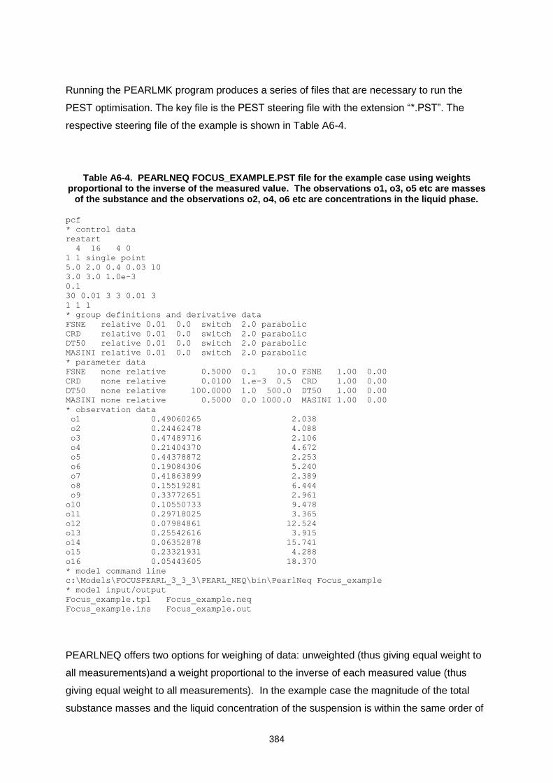
384
Running the PEARLMK program produces a series of files that are necessary to run the
PEST optimisation. The key file is the PEST steering file with the extension “*.PST”. The
respective steering file of the example is shown in Table A6-4.
Table A6-4. PEARLNEQ FOCUS_EXAMPLE.PST file for the example case using weights proportional to the inverse of the measured value. The observations o1, o3, o5 etc are masses
of the substance and the observations o2, o4, o6 etc are concentrations in the liquid phase.
pcf
* control data
restart
4 16 4 0
1 1 single point
5.0 2.0 0.4 0.03 10
3.0 3.0 1.0e-3
0.1
30 0.01 3 3 0.01 3
1 1 1
* group definitions and derivative data
FSNE relative 0.01 0.0 switch 2.0 parabolic
CRD relative 0.01 0.0 switch 2.0 parabolic
DT50 relative 0.01 0.0 switch 2.0 parabolic
MASINI relative 0.01 0.0 switch 2.0 parabolic
* parameter data
FSNE none relative 0.5000 0.1 10.0 FSNE 1.00 0.00
CRD none relative 0.0100 1.e-3 0.5 CRD 1.00 0.00
DT50 none relative 100.0000 1.0 500.0 DT50 1.00 0.00
MASINI none relative 0.5000 0.0 1000.0 MASINI 1.00 0.00
* observation data
o1 0.49060265 2.038
o2 0.24462478 4.088
o3 0.47489716 2.106
o4 0.21404370 4.672
o5 0.44378872 2.253
o6 0.19084306 5.240
o7 0.41863899 2.389
o8 0.15519281 6.444
o9 0.33772651 2.961
o10 0.10550733 9.478
o11 0.29718025 3.365
o12 0.07984861 12.524
o13 0.25542616 3.915
o14 0.06352878 15.741
o15 0.23321931 4.288
o16 0.05443605 18.370
* model command line
c:\Models\FOCUSPEARL_3_3_3\PEARL_NEQ\bin\PearlNeq Focus_example
* model input/output
Focus_example.tpl Focus_example.neq
Focus_example.ins Focus_example.out
PEARLNEQ offers two options for weighing of data: unweighted (thus giving equal weight to
all measurements)and a weight proportional to the inverse of each measured value (thus
giving equal weight to all measurements). In the example case the magnitude of the total
substance masses and the liquid concentration of the suspension is within the same order of
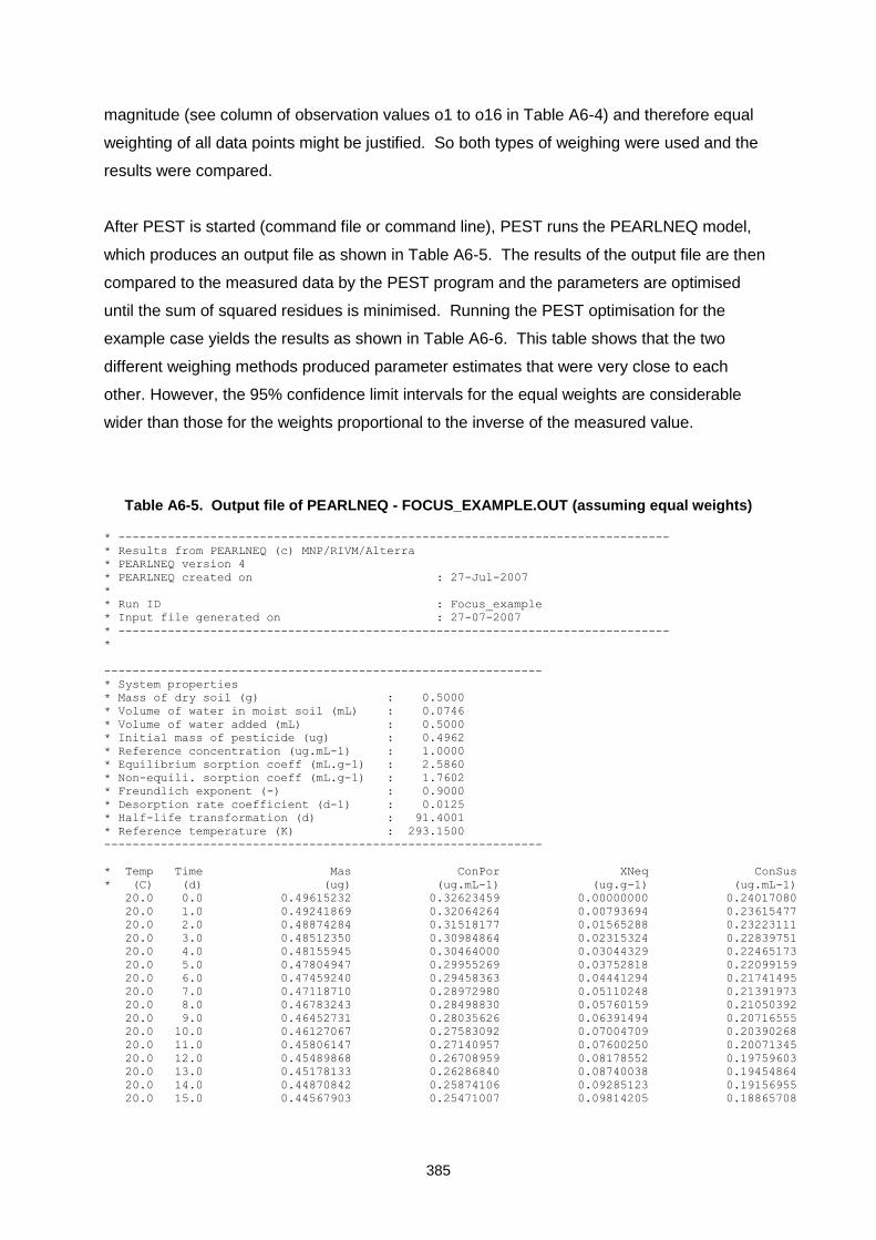
385
magnitude (see column of observation values o1 to o16 in Table A6-4) and therefore equal
weighting of all data points might be justified. So both types of weighing were used and the
results were compared.
After PEST is started (command file or command line), PEST runs the PEARLNEQ model,
which produces an output file as shown in Table A6-5. The results of the output file are then
compared to the measured data by the PEST program and the parameters are optimised
until the sum of squared residues is minimised. Running the PEST optimisation for the
example case yields the results as shown in Table A6-6. This table shows that the two
different weighing methods produced parameter estimates that were very close to each
other. However, the 95% confidence limit intervals for the equal weights are considerable
wider than those for the weights proportional to the inverse of the measured value.
Table A6-5. Output file of PEARLNEQ - FOCUS_EXAMPLE.OUT (assuming equal weights)
* ------------------------------------------------------------------------------
* Results from PEARLNEQ (c) MNP/RIVM/Alterra
* PEARLNEQ version 4
* PEARLNEQ created on : 27-Jul-2007
*
* Run ID : Focus_example
* Input file generated on : 27-07-2007
* ------------------------------------------------------------------------------
*
--------------------------------------------------------------
* System properties
* Mass of dry soil (g) : 0.5000
* Volume of water in moist soil (mL) : 0.0746
* Volume of water added (mL) : 0.5000
* Initial mass of pesticide (ug) : 0.4962
* Reference concentration (ug.mL-1) : 1.0000
* Equilibrium sorption coeff (mL.g-1) : 2.5860
* Non-equili. sorption coeff (mL.g-1) : 1.7602
* Freundlich exponent (-) : 0.9000
* Desorption rate coefficient (d-1) : 0.0125
* Half-life transformation (d) : 91.4001
* Reference temperature (K) : 293.1500
--------------------------------------------------------------
* Temp Time Mas ConPor XNeq ConSus
* (C) (d) (ug) (ug.mL-1) (ug.g-1) (ug.mL-1)
20.0 0.0 0.49615232 0.32623459 0.00000000 0.24017080
20.0 1.0 0.49241869 0.32064264 0.00793694 0.23615477
20.0 2.0 0.48874284 0.31518177 0.01565288 0.23223111
20.0 3.0 0.48512350 0.30984864 0.02315324 0.22839751
20.0 4.0 0.48155945 0.30464000 0.03044329 0.22465173
20.0 5.0 0.47804947 0.29955269 0.03752818 0.22099159
20.0 6.0 0.47459240 0.29458363 0.04441294 0.21741495
20.0 7.0 0.47118710 0.28972980 0.05110248 0.21391973
20.0 8.0 0.46783243 0.28498830 0.05760159 0.21050392
20.0 9.0 0.46452731 0.28035626 0.06391494 0.20716555
20.0 10.0 0.46127067 0.27583092 0.07004709 0.20390268
20.0 11.0 0.45806147 0.27140957 0.07600250 0.20071345
20.0 12.0 0.45489868 0.26708959 0.08178552 0.19759603
20.0 13.0 0.45178133 0.26286840 0.08740038 0.19454864
20.0 14.0 0.44870842 0.25874106 0.09285123 0.19156955
20.0 15.0 0.44567903 0.25471007 0.09814205 0.18865708
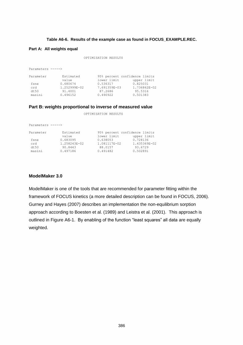
386
Table A6-6. Results of the example case as found in FOCUS_EXAMPLE.REC.
Part A: All weights equal OPTIMISATION RESULTS
Parameters ----->
Parameter Estimated 95% percent confidence limits
value lower limit upper limit
fsne 0.680674 0.536317 0.825031
crd 1.252999E-02 7.691359E-03 1.736862E-02
dt50 91.4001 87.2686 95.5316
masini 0.496152 0.490922 0.501383
Part B: weights proportional to inverse of measured value
OPTIMISATION RESULTS
Parameters ----->
Parameter Estimated 95% percent confidence limits
value lower limit upper limit
fsne 0.683095 0.638053 0.728136
crd 1.258243E-02 1.081117E-02 1.435369E-02
dt50 90.8443 88.0157 93.6729
masini 0.497186 0.491482 0.502891
ModelMaker 3.0
ModelMaker is one of the tools that are recommended for parameter fitting within the
framework of FOCUS kinetics (a more detailed description can be found in FOCUS, 2006).
Gurney and Hayes (2007) describes an implementation the non-equilibrium sorption
approach according to Boesten et al. (1989) and Leistra et al. (2001). This approach is
outlined in Figure A6-1. By enabling of the function “least squares” all data are equally
weighted.
387
Figure A6-1. Implementation of non-equilibrium sorption in ModelMaker 3.0.
The implementation of the non-equilibrium sorption in ModelMaker according to Gurney and
Hayes (2007) uses the same or similar nomenclature as in PEARLNEQ. The two data sets
for the example, the total mass in [µg] and the liquid concentration in the suspension in
[µg/mL], are shown in Figure A6-2.
Figure A6-2. Model data for the fit of the example case with ModelMaker.
388
Figure A6-3 provides the values of the initial and the fixed parameters and Figures A6-4 and
A6-5 show the optimisation configuration.
Figure A6-3. Initial or fixed set of parameters for the ModelMaker 3.0 fit of the example case.
389
Figure A6-4. Setup of the optimisation configuration definition in ModelMaker 3.0 fit for the
example
390
Figure A6-5. Setup of the advanced optimisation configuration in ModelMaker 3.0 fit for the
example
The resulting estimates for the non-equilibrium sorption parameters as well as their standard
deviations using the optimisation approach of ModelMaker 3.0 are shown in Figure A6-6.
Graphical representations are shown in Figures A6-7 and A6-8.
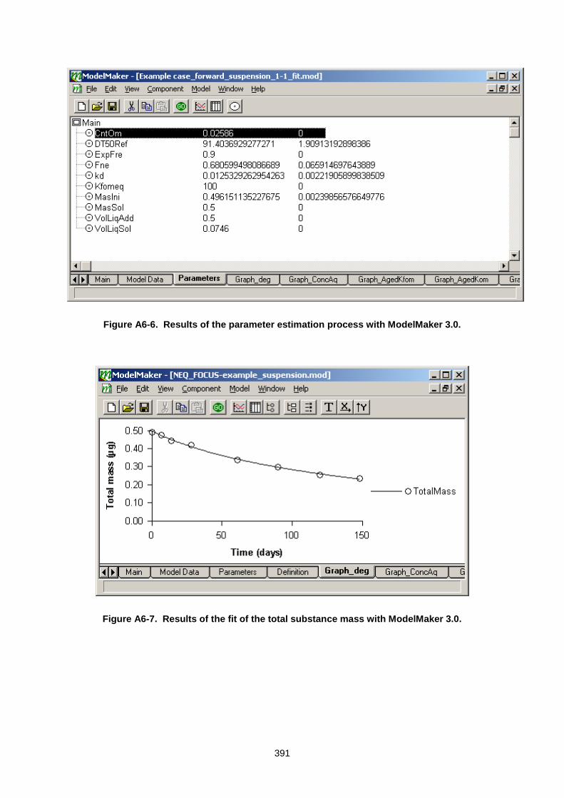
391
Figure A6-6. Results of the parameter estimation process with ModelMaker 3.0.
Figure A6-7. Results of the fit of the total substance mass with ModelMaker 3.0.
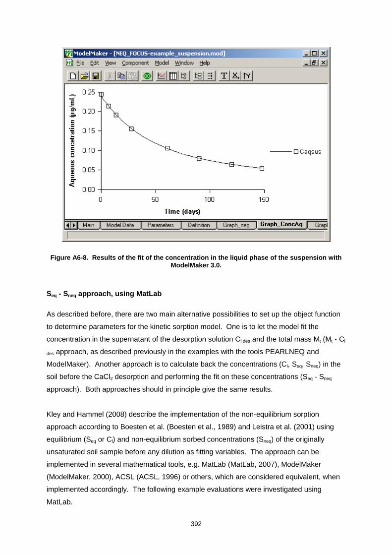
392
Figure A6-8. Results of the fit of the concentration in the liquid phase of the suspension with
ModelMaker 3.0.
Seq - Sneq approach, using MatLab
As described before, there are two main alternative possibilities to set up the object function
to determine parameters for the kinetic sorption model. One is to let the model fit the
concentration in the supernatant of the desorption solution Cl des and the total mass Mt (Mt - Cl
des approach, as described previously in the examples with the tools PEARLNEQ and
ModelMaker). Another approach is to calculate back the concentrations (Cl, Seq, Sneq) in the
soil before the CaCl2 desorption and performing the fit on these concentrations (Seq - Sneq
approach). Both approaches should in principle give the same results.
Kley and Hammel (2008) describe the implementation of the non-equilibrium sorption
approach according to Boesten et al. (Boesten et al., 1989) and Leistra et al. (2001) using
equilibrium (Seq or Cl) and non-equilibrium sorbed concentrations (Sneq) of the originally
unsaturated soil sample before any dilution as fitting variables. The approach can be
implemented in several mathematical tools, e.g. MatLab (MatLab, 2007), ModelMaker
(ModelMaker, 2000), ACSL (ACSL, 1996) or others, which are considered equivalent, when
implemented accordingly. The following example evaluations were investigated using
MatLab.
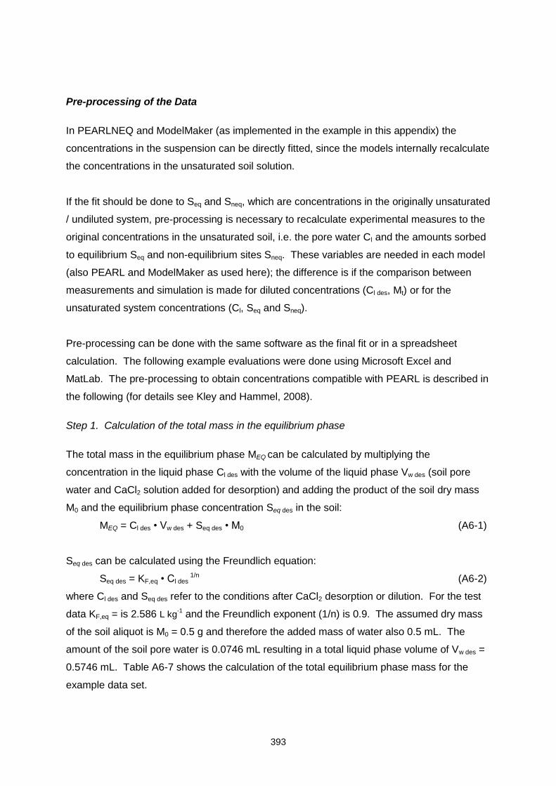
393
Pre-processing of the Data
In PEARLNEQ and ModelMaker (as implemented in the example in this appendix) the
concentrations in the suspension can be directly fitted, since the models internally recalculate
the concentrations in the unsaturated soil solution.
If the fit should be done to Seq and Sneq, which are concentrations in the originally unsaturated
/ undiluted system, pre-processing is necessary to recalculate experimental measures to the
original concentrations in the unsaturated soil, i.e. the pore water Cl and the amounts sorbed
to equilibrium Seq and non-equilibrium sites Sneq. These variables are needed in each model
(also PEARL and ModelMaker as used here); the difference is if the comparison between
measurements and simulation is made for diluted concentrations (Cl des, Mt) or for the
unsaturated system concentrations (Cl, Seq and Sneq).
Pre-processing can be done with the same software as the final fit or in a spreadsheet
calculation. The following example evaluations were done using Microsoft Excel and
MatLab. The pre-processing to obtain concentrations compatible with PEARL is described in
the following (for details see Kley and Hammel, 2008).
Step 1. Calculation of the total mass in the equilibrium phase
The total mass in the equilibrium phase MEQ can be calculated by multiplying the
concentration in the liquid phase Cl des with the volume of the liquid phase Vw des (soil pore
water and CaCl2 solution added for desorption) and adding the product of the soil dry mass
M0 and the equilibrium phase concentration Seq des in the soil:
MEQ = Cl des • Vw des + Seq des • M0 (A6-1)
Seq des can be calculated using the Freundlich equation:
Seq des = KF,eq • Cl des 1/n (A6-2)
where Cl des and Seq des refer to the conditions after CaCl2 desorption or dilution. For the test
data KF,eq = is 2.586 L kg-1 and the Freundlich exponent (1/n) is 0.9. The assumed dry mass
of the soil aliquot is M0 = 0.5 g and therefore the added mass of water also 0.5 mL. The
amount of the soil pore water is 0.0746 mL resulting in a total liquid phase volume of Vw des =
0.5746 mL. Table A6-7 shows the calculation of the total equilibrium phase mass for the
example data set.
394
Table A6-7. Calculation of total mass in the equilibrium phase of the suspension/supernatant solution system.
Sampling
day
Measured
concentration in
liquid phase
Cl des
[mg/L]
Concentration in
equilibrium soil
phase
Seq des
[mg/kg]
Mass in
liquid phase
Cl des • Vw des
[µg]
Mass in
equilibrium soil
phase
Seq des • M0
[µg]
Total mass in
equilibrium
phase
MEQ
[µg]
0 0.24462 0.72825 0.14056 0.36412 0.50469
7 0.21404 0.64577 0.12299 0.32289 0.44588
14 0.19084 0.58242 0.10966 0.29121 0.40087
28 0.15519 0.48352 0.08917 0.24176 0.33093
61 0.10551 0.34165 0.06062 0.17083 0.23145
90 0.07985 0.26587 0.04588 0.13293 0.17882
120 0.06353 0.21642 0.03650 0.10821 0.14471
148 0.05444 0.18833 0.03128 0.09417 0.12545
Step 2. Calculation of the equilibrium phase components of unsaturated soil
Now the total mass in the equilibrium sorption phase has to be distributed to the liquid and
solid phase of the original moist or unsaturated soil, before the CaCl2 desorption. For this
purpose, the total equilibrium phase mass immediately before and after CaCl2 desorption can
be assumed to be equal, because the transfer from or to the non-equilibrium sites takes time.
Before desorption the liquid phase is represented by the pore water Vw , which is 0.0746 mL
per aliquot M0 of 0.5 g dry soil. Thus the total mass in equilibrium phase can also be written
as:
MEQ = Cl • Vw + Seq • M0 (A6-3)
Seq can be calculated again using the Freundlich equation:
Seq = KF,eq • Cl1/n (A6-4)
leading to:
MEQ = Cl • Vw + KF,eq • Cl1/n • M0 (A6-5)
where all variables are known except Cl. Due to the non-linearity of the Freundlich equation
Cl cannot be calculated directly but has to be solved numerically using for example EXCEL
spreadsheets in combination with SOLVER or GOAL-SEEK function, which is described in
Table A6-8. In the first line of Table A6-8 the column numbers are given, in the second the
corresponding inputs for the EXCEL cells which are either numbers (e.g. column (6)) or
functions. The SOLVER algorithm requires basically three inputs: i) the cells to be changed
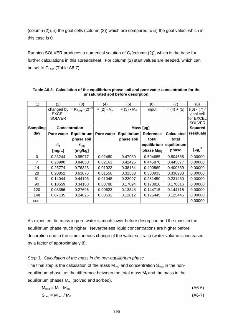
395
(column (2)), ii) the goal cells (column (8)) which are compared to iii) the goal value, which in
this case is 0.
Running SOLVER produces a numerical solution of Cl (column (2)), which is the base for
further calculations in this spreadsheet. For column (2) start values are needed, which can
be set to Cl des (Table A6-7).
Table A6-8. Calculation of the equilibrium phase soil and pore water concentration for the unsaturated soil before desorption.
(1) (2) (3) (4) (5) (6) (7) (8)
changed by EXCEL
SOLVER
= KF,eq • (2)1/n
= (2) • Vw = (3) • M0 input = (4) + (5) ((6) - (7))2
goal cell for EXCEL SOLVER
Sampling
day
Concentration Mass [µg] Squared
residuals
[µg]2
Pore water
Cl
[mg/L]
Equilibrium
phase soil
Seq
[mg/kg]
Pore water Equilibrium
phase soil
Reference
total
equilibrium
phase MEQ
Calculated
total
equilibrium
phase
0 0.33244 0.95977 0.02480 0.47989 0.504685 0.504685 0.00000
7 0.28990 0.84850 0.02163 0.42425 0.445876 0.445877 0.00000
14 0.25774 0.76328 0.01923 0.38164 0.400869 0.400869 0.00000
28 0.20852 0.63075 0.01556 0.31538 0.330933 0.330933 0.00000
61 0.14044 0.44195 0.01048 0.22097 0.231450 0.231450 0.00000
90 0.10559 0.34188 0.00788 0.17094 0.178816 0.178816 0.00000
120 0.08356 0.27696 0.00623 0.13848 0.144715 0.144715 0.00000
148 0.07135 0.24025 0.00532 0.12012 0.125445 0.125445 0.00000
sum 0.00000
As expected the mass in pore water is much lower before desorption and the mass in the
equilibrium phase much higher. Nevertheless liquid concentrations are higher before
desorption due to the simultaneous change of the water:soil ratio (water volume is increased
by a factor of approximately 8).
Step 3. Calculation of the mass in the non-equilibrium phase
The final step is the calculation of the mass Mneq and concentration Sneq in the non-
equilibrium phase, as the difference between the total mass Mt and the mass in the
equilibrium phases Meq (solved and sorbed).
Mneq = Mt - Meq (A6-6)
Sneq = Mneq / M0 (A6-7)
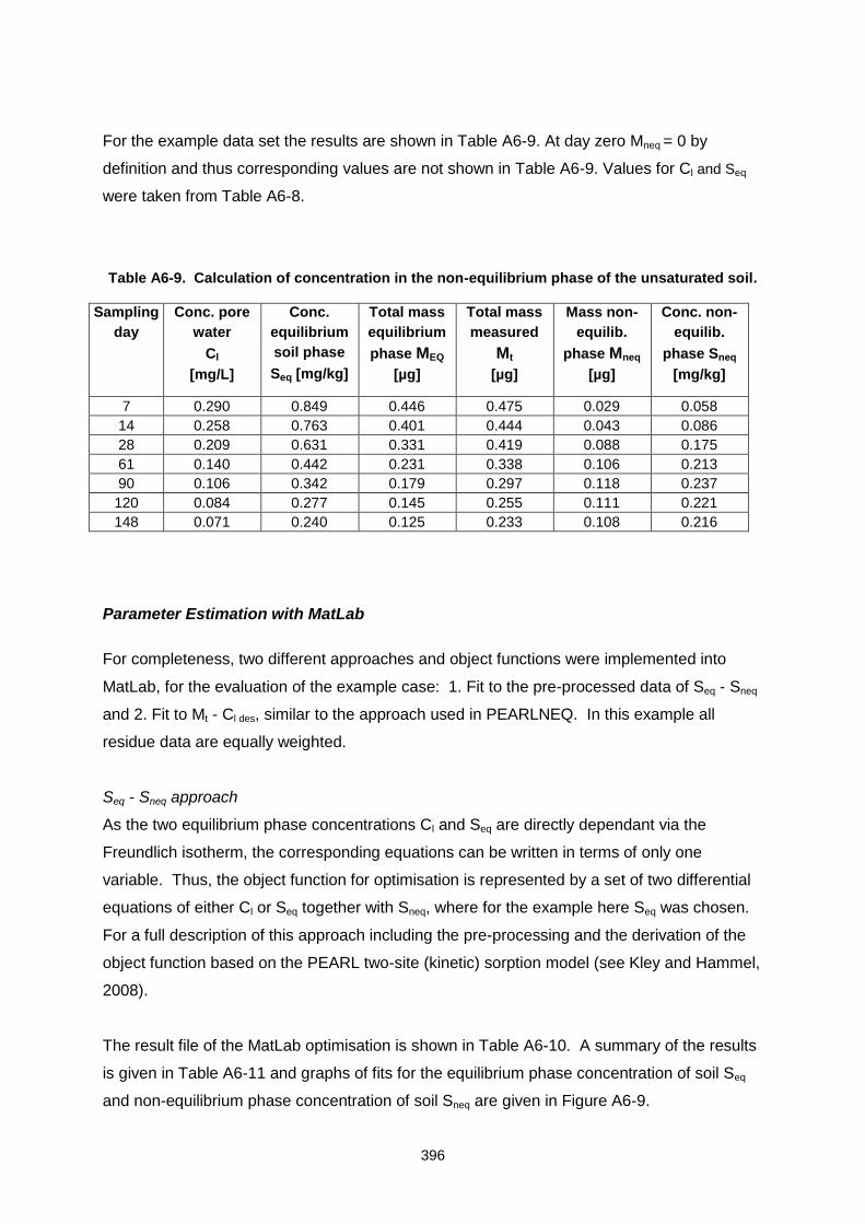
396
For the example data set the results are shown in Table A6-9. At day zero Mneq = 0 by
definition and thus corresponding values are not shown in Table A6-9. Values for Cl and Seq
were taken from Table A6-8.
Table A6-9. Calculation of concentration in the non-equilibrium phase of the unsaturated soil.
Sampling
day
Conc. pore
water
Cl
[mg/L]
Conc.
equilibrium
soil phase
Seq [mg/kg]
Total mass
equilibrium
phase MEQ
[µg]
Total mass
measured
Mt
[µg]
Mass non-
equilib.
phase Mneq
[µg]
Conc. non-
equilib.
phase Sneq
[mg/kg]
7 0.290 0.849 0.446 0.475 0.029 0.058
14 0.258 0.763 0.401 0.444 0.043 0.086
28 0.209 0.631 0.331 0.419 0.088 0.175
61 0.140 0.442 0.231 0.338 0.106 0.213
90 0.106 0.342 0.179 0.297 0.118 0.237
120 0.084 0.277 0.145 0.255 0.111 0.221
148 0.071 0.240 0.125 0.233 0.108 0.216
Parameter Estimation with MatLab
For completeness, two different approaches and object functions were implemented into
MatLab, for the evaluation of the example case: 1. Fit to the pre-processed data of Seq - Sneq
and 2. Fit to Mt - Cl des, similar to the approach used in PEARLNEQ. In this example all
residue data are equally weighted.
Seq - Sneq approach
As the two equilibrium phase concentrations Cl and Seq are directly dependant via the
Freundlich isotherm, the corresponding equations can be written in terms of only one
variable. Thus, the object function for optimisation is represented by a set of two differential
equations of either Cl or Seq together with Sneq, where for the example here Seq was chosen.
For a full description of this approach including the pre-processing and the derivation of the
object function based on the PEARL two-site (kinetic) sorption model (see Kley and Hammel,
2008).
The result file of the MatLab optimisation is shown in Table A6-10. A summary of the results
is given in Table A6-11 and graphs of fits for the equilibrium phase concentration of soil Seq
and non-equilibrium phase concentration of soil Sneq are given in Figure A6-9.
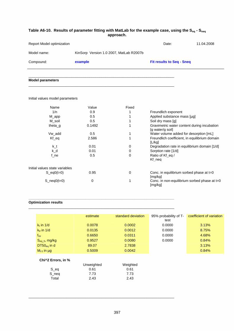
397
Table A6-10. Results of parameter fitting with MatLab for the example case, using the Seq - Sneq approach.
Report Model optimization Date: 11.04.2008
Model name: KinSorp Version 1.0 2007, MatLab R2007b
Compound: example Fit results to Seq - Sneq
__________________________________________________________________________
Model parameters
__________________________________________________________________________
Initial values model parameters
Name Value Fixed
1/n 0.9 1 Freundlich exponent
M_app 0.5 1 Applied substance mass [µg]
M_soil 0.5 1 Soil dry mass [g]
theta_g 0.1492 1 Gravimetric water content during incubation [g water/g soil]
Vw_add 0.5 1 Water volume added for desorption [mL]
Kf_eq 2.586 1 Freundlich coefficient, in equilibrium domain [L/kg]
k_t 0.01 0 Degradation rate in equilibrium domain [1/d]
k_d 0.01 0 Sorption rate [1/d]
f_ne 0.5 0 Ratio of Kf_eq / Kf_neq
Initial values state variables
S_eq0(t=0) 0.95 0 Conc. in equilibrium sorbed phase at t=0 [mg/kg]
S_neq0(t=0) 0 1 Conc. in non-equilibrium sorbed phase at t=0 [mg/kg]
__________________________________________________________________________
Optimization results
__________________________________________________________________________
estimate standard deviation 95% probability of T-test
coefficient of variation
kt in 1/d 0.0078 0.0002 0.0000 3.13%
kd in 1/d 0.0135 0.0012 0.0000 8.75%
fne 0.6650 0.0311 0.0000 4.68%
Seq_0, mg/kg 0.9527 0.0080 0.0000 0.84%
DT50eq in d 89.07 2.7838 3.13%
Mt 0 in µg 0.5009 0.0042 0.84%
Chi^2 Errors, in %
Unweighted Weighted
S_eq 0.61 0.61
S_neq 7.73 7.73
Total 2.43 2.43
__________________________________________________________________________
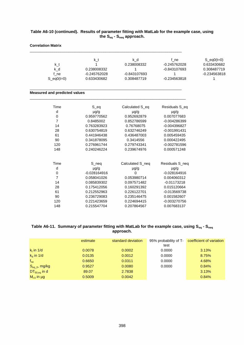
398
Table A6-10 (continued). Results of parameter fitting with MatLab for the example case, using the Seq - Sneq approach.
Correlation Matrix
__________________________________________________________________________
k_t k_d f_ne S_eq0(t=0)
k_t 1 0.238008332 -0.245762028 0.633430682
k_d 0.238008332 1 -0.843107693 0.308487719
f_ne -0.245762028 -0.843107693 1 -0.234563818
S_eq0(t=0) 0.633430682 0.308487719 -0.234563818 1
__________________________________________________________________________
Measured and predicted values
____________________________________________________________________________
Time S_eq Calculated S_eq Residuals S_eq
d µg/g µg/g µg/g
0 0.959770562 0.952692879 0.007077683
7 0.8485002 0.852786599 -0.004286399
14 0.763283923 0.76768075 -0.004396827
28 0.630754819 0.632746249 -0.001991431
61 0.441946438 0.436487003 0.005459435
90 0.341878095 0.3414556 0.000422495
120 0.276961744 0.279743341 -0.002781596
148 0.240246224 0.239674976 0.000571248
Time S_neq Calculated S_neq Residuals S_neq
d µg/g µg/g µg/g
0 -0.028164916 0 -0.028164916
7 0.058041026 0.053980714 0.004060312
14 0.085839302 0.097571482 -0.01173218
28 0.175412056 0.160291392 0.015120664
61 0.212552963 0.226122701 -0.013569738
90 0.236729083 0.235146475 0.001582607
120 0.221423659 0.224694415 -0.003270756
148 0.215547704 0.207864567 0.007683137
Table A6-11. Summary of parameter fitting with MatLab for the example case, using Seq - Sneq approach.
estimate standard deviation 95% probability of T-
test
coefficient of variation
kt in 1/d 0.0078 0.0002 0.0000 3.13%
kd in 1/d 0.0135 0.0012 0.0000 8.75%
fne 0.6650 0.0311 0.0000 4.68%
Seq_0, mg/kg 0.9527 0.0080 0.0000 0.84%
DT50,eq in d 89.07 2.7838 3.13%
Mt 0 in µg 0.5009 0.0042 0.84%
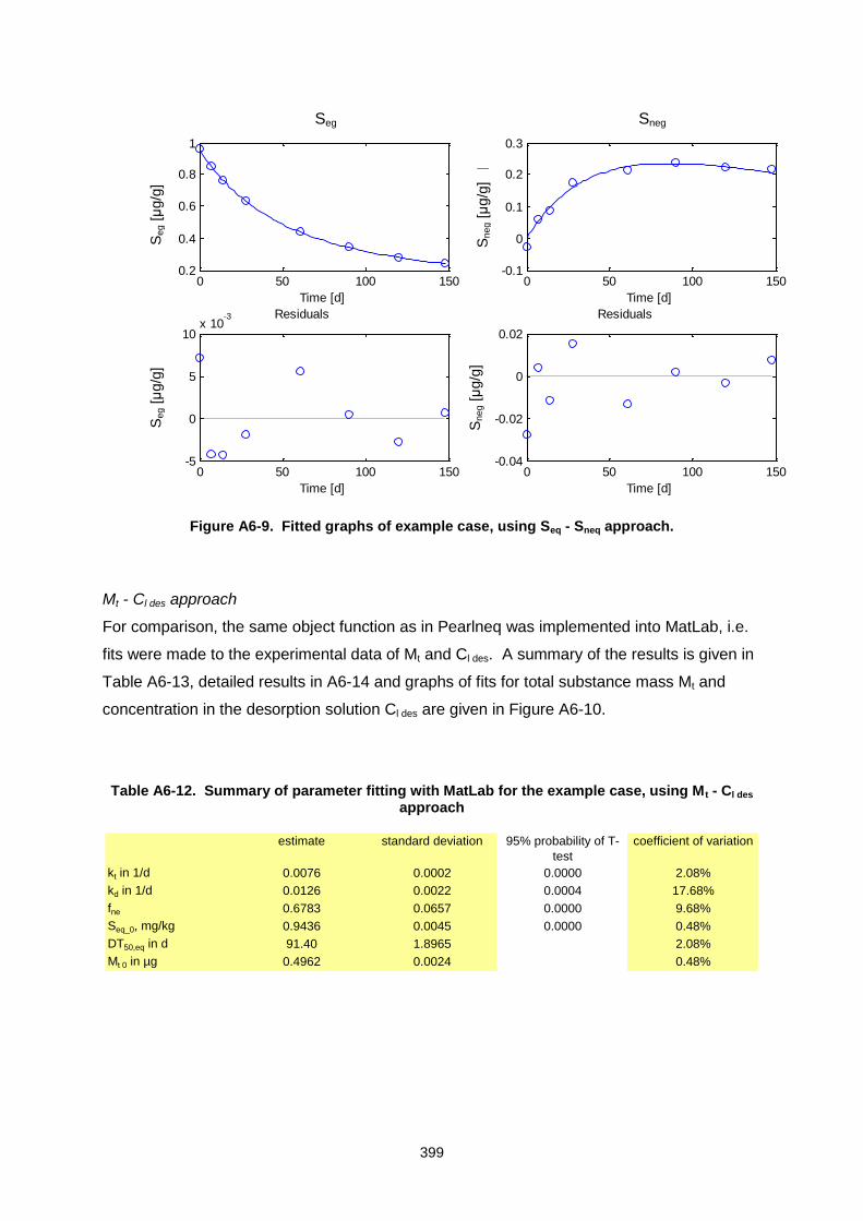
399
0 50 100 1500.2
0.4
0.6
0.8
1
Csoil
eq
Time [d]
Csoil e
q [
µg/g
]
0 50 100 150-5
0
5
10x 10
-3 Residuals Csoil
eq
Time [d]
Csoil e
q [
µg/g
]
0 50 100 150-0.1
0
0.1
0.2
0.3
Csoil
neq
Time [d]
Csoi
l neq
[µ
g/g
]0 50 100 150
-0.04
-0.02
0
0.02
Residuals Csoil
neq
Time [d]C
soil n
eq
[µg/g
]
Figure A6-9. Fitted graphs of example case, using Seq - Sneq approach.
Mt - Cl des approach
For comparison, the same object function as in Pearlneq was implemented into MatLab, i.e.
fits were made to the experimental data of Mt and Cl des. A summary of the results is given in
Table A6-13, detailed results in A6-14 and graphs of fits for total substance mass Mt and
concentration in the desorption solution Cl des are given in Figure A6-10.
Table A6-12. Summary of parameter fitting with MatLab for the example case, using M t - Cl des approach
estimate standard deviation 95% probability of T-
test
coefficient of variation
kt in 1/d 0.0076 0.0002 0.0000 2.08%
kd in 1/d 0.0126 0.0022 0.0004 17.68%
fne 0.6783 0.0657 0.0000 9.68%
Seq_0, mg/kg 0.9436 0.0045 0.0000 0.48%
DT50,eq in d 91.40 1.8965 2.08%
Mt 0 in µg 0.4962 0.0024 0.48%
Seg Sneg
Sneg [μ
g/g
] S
neg [μ
g/g
]
Seg [μ
g/g
] S
eg [μ
g/g
]
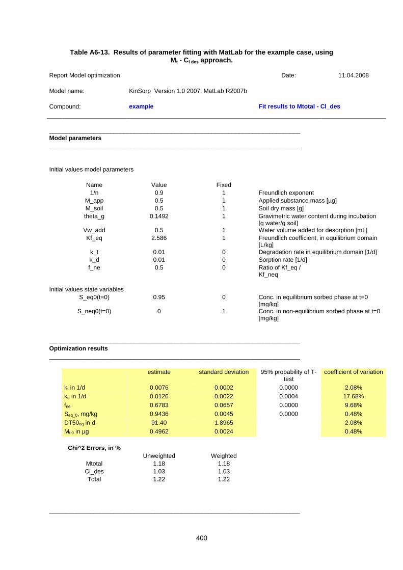
400
Table A6-13. Results of parameter fitting with MatLab for the example case, using Mt - Cl des approach.
Report Model optimization Date: 11.04.2008
Model name: KinSorp Version 1.0 2007, MatLab R2007b
Compound: example Fit results to Mtotal - Cl_des
__________________________________________________________________________
Model parameters
__________________________________________________________________________
Initial values model parameters
Name Value Fixed
1/n 0.9 1 Freundlich exponent
M_app 0.5 1 Applied substance mass [µg]
M_soil 0.5 1 Soil dry mass [g]
theta_g 0.1492 1 Gravimetric water content during incubation [g water/g soil]
Vw_add 0.5 1 Water volume added for desorption [mL]
Kf_eq 2.586 1 Freundlich coefficient, in equilibrium domain [L/kg]
k_t 0.01 0 Degradation rate in equilibrium domain [1/d]
k_d 0.01 0 Sorption rate [1/d]
f_ne 0.5 0 Ratio of Kf_eq / Kf_neq
Initial values state variables
S_eq0(t=0) 0.95 0 Conc. in equilibrium sorbed phase at t=0 [mg/kg]
S_neq0(t=0) 0 1 Conc. in non-equilibrium sorbed phase at t=0 [mg/kg]
__________________________________________________________________________
Optimization results
__________________________________________________________________________
estimate standard deviation 95% probability of T-test
coefficient of variation
kt in 1/d 0.0076 0.0002 0.0000 2.08%
kd in 1/d 0.0126 0.0022 0.0004 17.68%
fne 0.6783 0.0657 0.0000 9.68%
Seq_0, mg/kg 0.9436 0.0045 0.0000 0.48%
DT50eq in d 91.40 1.8965 2.08%
Mt 0 in µg 0.4962 0.0024 0.48%
Chi^2 Errors, in %
Unweighted Weighted
Mtotal 1.18 1.18
Cl_des 1.03 1.03
Total 1.22 1.22
__________________________________________________________________________
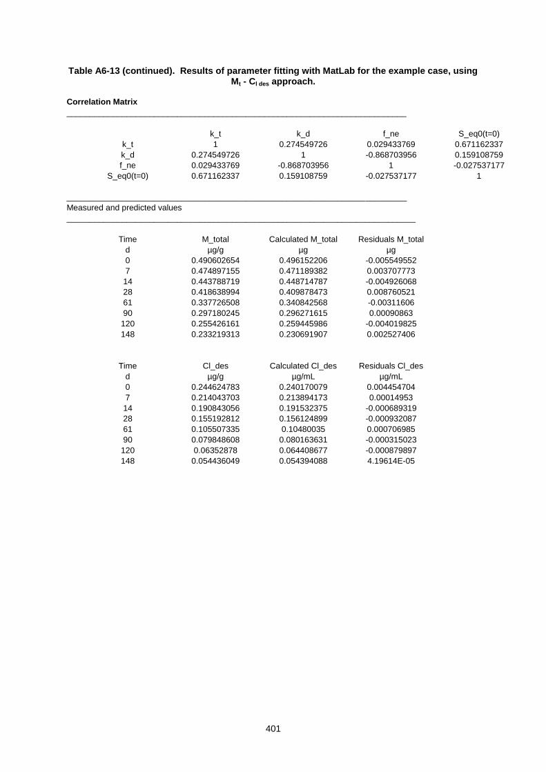
401
Table A6-13 (continued). Results of parameter fitting with MatLab for the example case, using Mt - Cl des approach.
Correlation Matrix
__________________________________________________________________________
k_t k_d f_ne S_eq0(t=0)
k_t 1 0.274549726 0.029433769 0.671162337
k_d 0.274549726 1 -0.868703956 0.159108759
f_ne 0.029433769 -0.868703956 1 -0.027537177
S_eq0(t=0) 0.671162337 0.159108759 -0.027537177 1
__________________________________________________________________________
Measured and predicted values
____________________________________________________________________________
Time M_total Calculated M_total Residuals M_total
d µg/g µg µg
0 0.490602654 0.496152206 -0.005549552
7 0.474897155 0.471189382 0.003707773
14 0.443788719 0.448714787 -0.004926068
28 0.418638994 0.409878473 0.008760521
61 0.337726508 0.340842568 -0.00311606
90 0.297180245 0.296271615 0.00090863
120 0.255426161 0.259445986 -0.004019825
148 0.233219313 0.230691907 0.002527406
Time Cl_des Calculated Cl_des Residuals Cl_des
d µg/g µg/mL µg/mL
0 0.244624783 0.240170079 0.004454704
7 0.214043703 0.213894173 0.00014953
14 0.190843056 0.191532375 -0.000689319
28 0.155192812 0.156124899 -0.000932087
61 0.105507335 0.10480035 0.000706985
90 0.079848608 0.080163631 -0.000315023
120 0.06352878 0.064408677 -0.000879897
148 0.054436049 0.054394088 4.19614E-05
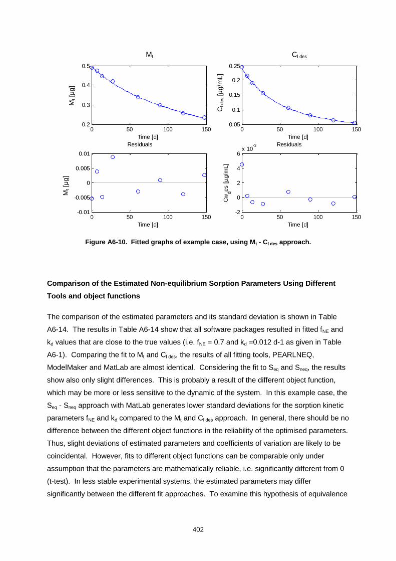
402
0 50 100 1500.2
0.3
0.4
0.5
Mtotal
Time [d]
Mto
tal [µ
g]
0 50 100 150-0.01
-0.005
0
0.005
0.01
Residuals Mtotal
Time [d]
Mto
tal [µ
g]
0 50 100 1500.05
0.1
0.15
0.2
0.25
Cwdes
Time [d]
Cw
des
[µ
g/m
L]
0 50 100 150-2
0
2
4
6x 10
-3 Residuals Cwdes
Time [d]C
wdes [
µg/m
L]
Figure A6-10. Fitted graphs of example case, using Mt - Cl des approach.
Comparison of the Estimated Non-equilibrium Sorption Parameters Using Different
Tools and object functions
The comparison of the estimated parameters and its standard deviation is shown in Table
A6-14. The results in Table A6-14 show that all software packages resulted in fitted fNE and
kd values that are close to the true values (i.e. fNE = 0.7 and kd =0.012 d-1 as given in Table
A6-1). Comparing the fit to Mt and Cl des, the results of all fitting tools, PEARLNEQ,
ModelMaker and MatLab are almost identical. Considering the fit to Seq and Sneq, the results
show also only slight differences. This is probably a result of the different object function,
which may be more or less sensitive to the dynamic of the system. In this example case, the
Seq - Sneq approach with MatLab generates lower standard deviations for the sorption kinetic
parameters fNE and kd compared to the Mt and Cl des approach. In general, there should be no
difference between the different object functions in the reliability of the optimised parameters.
Thus, slight deviations of estimated parameters and coefficients of variation are likely to be
coincidental. However, fits to different object functions can be comparable only under
assumption that the parameters are mathematically reliable, i.e. significantly different from 0
(t-test). In less stable experimental systems, the estimated parameters may differ
significantly between the different fit approaches. To examine this hypothesis of equivalence
Mt [
μg]
Cl des Mt
Mt [
μg]
Cl d
es [μ
g/m
L]
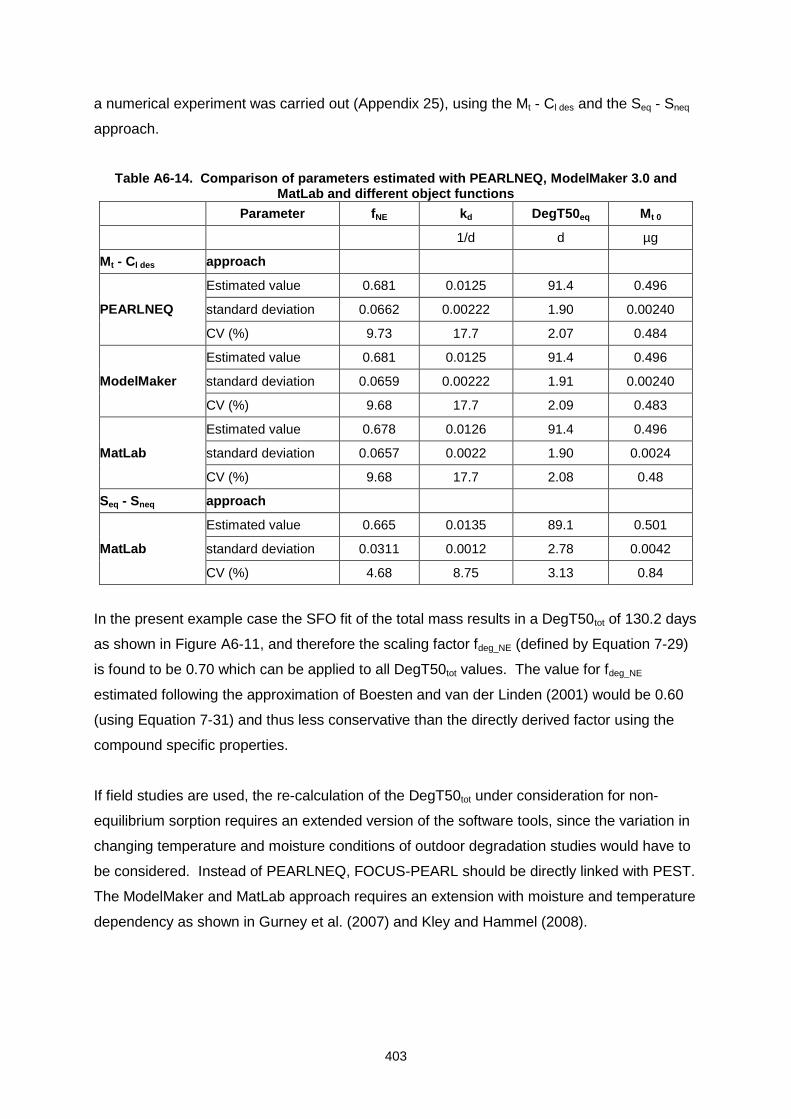
403
a numerical experiment was carried out (Appendix 25), using the Mt - Cl des and the Seq - Sneq
approach.
Table A6-14. Comparison of parameters estimated with PEARLNEQ, ModelMaker 3.0 and MatLab and different object functions
Parameter fNE kd DegT50eq Mt 0
1/d d µg
Mt - Cl des approach
PEARLNEQ
Estimated value 0.681 0.0125 91.4 0.496
standard deviation 0.0662 0.00222 1.90 0.00240
CV (%) 9.73 17.7 2.07 0.484
ModelMaker
Estimated value 0.681 0.0125 91.4 0.496
standard deviation 0.0659 0.00222 1.91 0.00240
CV (%) 9.68 17.7 2.09 0.483
MatLab
Estimated value 0.678 0.0126 91.4 0.496
standard deviation 0.0657 0.0022 1.90 0.0024
CV (%) 9.68 17.7 2.08 0.48
Seq - Sneq approach
MatLab
Estimated value 0.665 0.0135 89.1 0.501
standard deviation 0.0311 0.0012 2.78 0.0042
CV (%) 4.68 8.75 3.13 0.84
In the present example case the SFO fit of the total mass results in a DegT50tot of 130.2 days
as shown in Figure A6-11, and therefore the scaling factor fdeg_NE (defined by Equation 7-29)
is found to be 0.70 which can be applied to all DegT50tot values. The value for fdeg_NE
estimated following the approximation of Boesten and van der Linden (2001) would be 0.60
(using Equation 7-31) and thus less conservative than the directly derived factor using the
compound specific properties.
If field studies are used, the re-calculation of the DegT50tot under consideration for non-
equilibrium sorption requires an extended version of the software tools, since the variation in
changing temperature and moisture conditions of outdoor degradation studies would have to
be considered. Instead of PEARLNEQ, FOCUS-PEARL should be directly linked with PEST.
The ModelMaker and MatLab approach requires an extension with moisture and temperature
dependency as shown in Gurney et al. (2007) and Kley and Hammel (2008).
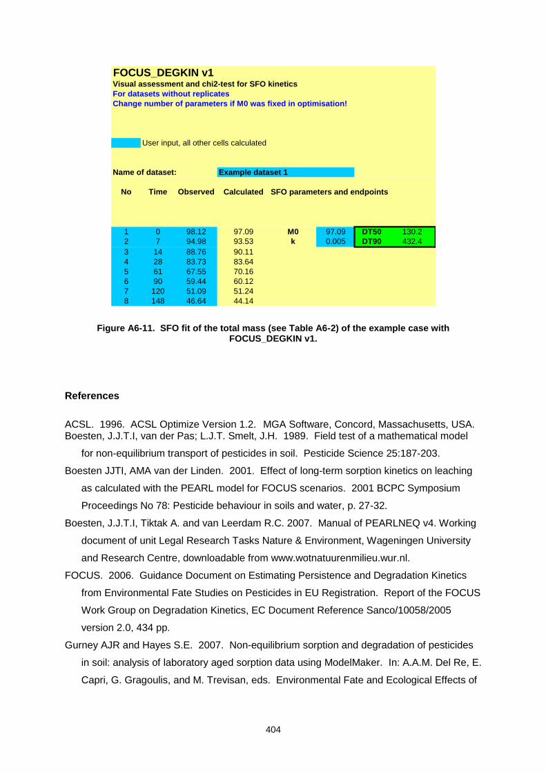
404
FOCUS_DEGKIN v1Visual assessment and chi2-test for SFO kinetics
For datasets without replicates
Change number of parameters if M0 was fixed in optimisation!
User input, all other cells calculated
Name of dataset: Example dataset 1
No Time Observed Calculated SFO parameters and endpoints
1 0 98.12 97.09 M0 97.09 DT50 130.2
2 7 94.98 93.53 k 0.005 DT90 432.4
3 14 88.76 90.11
4 28 83.73 83.64
5 61 67.55 70.16
6 90 59.44 60.12
7 120 51.09 51.24
8 148 46.64 44.14
Figure A6-11. SFO fit of the total mass (see Table A6-2) of the example case with
FOCUS_DEGKIN v1.
References
ACSL. 1996. ACSL Optimize Version 1.2. MGA Software, Concord, Massachusetts, USA. Boesten, J.J.T.I, van der Pas; L.J.T. Smelt, J.H. 1989. Field test of a mathematical model
for non-equilibrium transport of pesticides in soil. Pesticide Science 25:187-203.
Boesten JJTI, AMA van der Linden. 2001. Effect of long-term sorption kinetics on leaching
as calculated with the PEARL model for FOCUS scenarios. 2001 BCPC Symposium
Proceedings No 78: Pesticide behaviour in soils and water, p. 27-32.
Boesten, J.J.T.I, Tiktak A. and van Leerdam R.C. 2007. Manual of PEARLNEQ v4. Working
document of unit Legal Research Tasks Nature & Environment, Wageningen University
and Research Centre, downloadable from www.wotnatuurenmilieu.wur.nl.
FOCUS. 2006. Guidance Document on Estimating Persistence and Degradation Kinetics
from Environmental Fate Studies on Pesticides in EU Registration. Report of the FOCUS
Work Group on Degradation Kinetics, EC Document Reference Sanco/10058/2005
version 2.0, 434 pp.
Gurney AJR and Hayes S.E. 2007. Non-equilibrium sorption and degradation of pesticides
in soil: analysis of laboratory aged sorption data using ModelMaker. In: A.A.M. Del Re, E.
Capri, G. Gragoulis, and M. Trevisan, eds. Environmental Fate and Ecological Effects of
405
Pesticides (Proceedings of the XIII Symposium Pesticide Chemistry). La Goliardica
Pavese, Pavia Italy, ISBN 978-88-7830-473-4, pp. 245-253.
Gurney AJR, Jensen IM, Geisler G and Adam DM. 2007. Non-equilibrium sorption and
degradation of pesticides in soil: re-evaluation of normalised field half-lives using
ModelMaker. In: A.A.M. Del Re, E. Capri, G. Gragoulis, and M. Trevisan, eds.
Environmental Fate and Ecological Effects of Pesticides (Proceedings of the XIII
Symposium Pesticide Chemistry). La Goliardica Pavese, Pavia Italy, ISBN 978-88-7830-
473-4, pp. 254-261.
Kley, C., Hammel, K., 2008. Evaluation of Time-dependent Sorption Parameters Based on
Concentrations in Unsaturated Soil. Bayer CropScience AG, Metabolism and
Environmental Fate, Monheim am Rhein, Germany. Report No. MEF-07/429, internal
report available upon request.
Leistra, M, A.M.A van der Linden, J.J.T.I. Boesten, A .Tiktak and F. van den Berg. 2001.
PEARL model for pesticide behaviour and emissions in soil-plant systems: description of
the processes in FOCUS PEARL version 1.1.1. Alterra-rapport 013, Alterra, Wageningen.
RIVM Report 711401009; RIVM Bilthoven.
MatLab. 2007. MatLab Version 7.4.0.287 (R2007a), Optimisation Toolbox, Statistics
Toolbox, MatLab Compiler. The MathWorks Inc., USA. www.mathworks.com
ModelMaker. 2000. Reference and user documentation for ModelMaker version 4.0.
Cherwell Scientific, Oxford, UK.
406
APPENDIX 7. EXAMPLE CALCULATION OF DegT50eq FROM A LABORATORY DEGRADATION RATE STUDY BASED ON DEFAULT
VALUES OF THE NON-EQUILIBRIUM SORPTION PARAMETERS
J. Boesten and C. Kley
Section 7.1.6 recommends the recalculation of the DegT50 if default values of parameters
describing long-term sorption kinetics (so kd,PEARL = 0.01 d-1 , fNE,PEARL = 0.3) are included in
the leaching assessment. This appendix provides an example of such a calculation.
The data for the laboratory study were “generated” by calculations with the system of
Equations 7-3 to 7-7 using the following parameter values: KF,EQ = 1.0 L/kg, = 0.2
(volumetric), = 1 kg/L, cL,R = 1 mg/L, N = 0.9, kd,PEARL = 0.01 d-1, fNE,PEARL = 0.5,
DegT50eq = 30 d, which corresponds to kt = ln(2)/30 = 0.023 d-1. The calculation procedure
was as described by Boesten et al. (2007). Nine data points for the times 0, 10, 20, .., 70
and 80 d were calculated. Two series of calculations were made: in the first it was assumed
that the data points were free of errors, and in the second it was assumed that the
concentration in total soil was normally distributed with a coefficient of variation of 3 % (see
Table A7-1 for values). The value of fNE,PEARL was set to 0.5 for generation of the data points
because this is considered a “best guess” value (Leistra et al., 2001). Only results of the
concentration in total soil were used (and no pore water concentrations) because pore water
concentrations are not available in a case where default values of the parameters for long-
term sorption kinetics are used. Therefore, the case considered here is a soil incubation
study where the decline of the concentration in total soil was measured but with no
measurements of pore water concentrations. The example was based on hypothetical data
because this has the advantage that the true parameter values of the system are known.
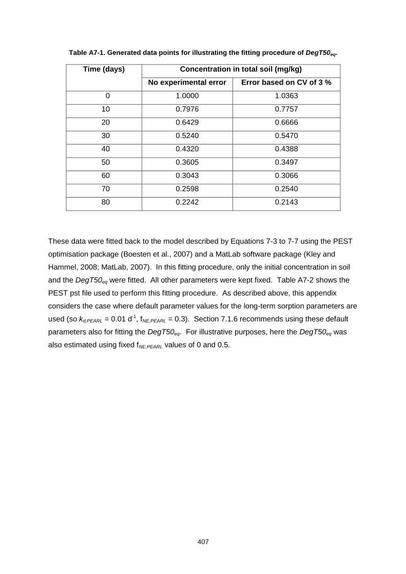
407
Table A7-1. Generated data points for illustrating the fitting procedure of DegT50eq.
Time (days) Concentration in total soil (mg/kg)
No experimental error Error based on CV of 3 %
0 1.0000 1.0363
10 0.7976 0.7757
20 0.6429 0.6666
30 0.5240 0.5470
40 0.4320 0.4388
50 0.3605 0.3497
60 0.3043 0.3066
70 0.2598 0.2540
80 0.2242 0.2143
These data were fitted back to the model described by Equations 7-3 to 7-7 using the PEST
optimisation package (Boesten et al., 2007) and a MatLab software package (Kley and
Hammel, 2008; MatLab, 2007). In this fitting procedure, only the initial concentration in soil
and the DegT50eq were fitted. All other parameters were kept fixed. Table A7-2 shows the
PEST pst file used to perform this fitting procedure. As described above, this appendix
considers the case where default parameter values for the long-term sorption parameters are
used (so kd,PEARL = 0.01 d-1, fNE,PEARL = 0.3). Section 7.1.6 recommends using these default
parameters also for fitting the DegT50eq. For illustrative purposes, here the DegT50eq was
also estimated using fixed fNE,PEARL values of 0 and 0.5.
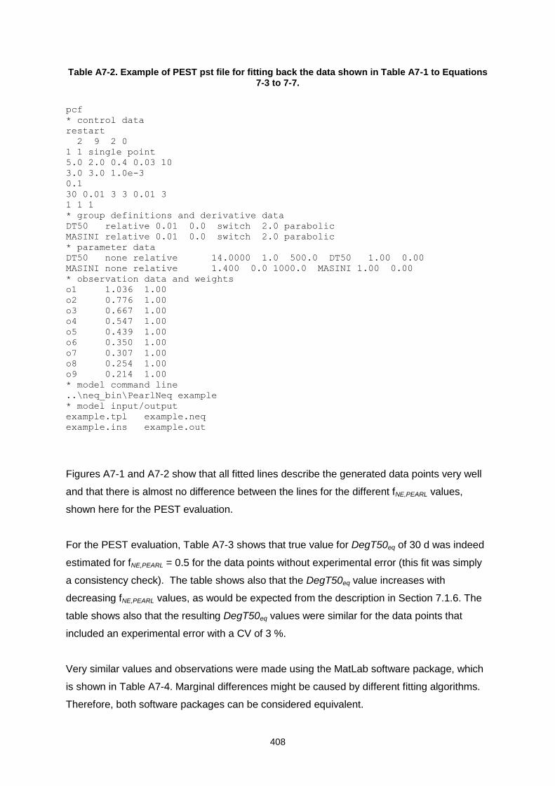
408
Table A7-2. Example of PEST pst file for fitting back the data shown in Table A7-1 to Equations 7-3 to 7-7.
pcf
* control data
restart
2 9 2 0
1 1 single point
5.0 2.0 0.4 0.03 10
3.0 3.0 1.0e-3
0.1
30 0.01 3 3 0.01 3
1 1 1
* group definitions and derivative data
DT50 relative 0.01 0.0 switch 2.0 parabolic
MASINI relative 0.01 0.0 switch 2.0 parabolic
* parameter data
DT50 none relative 14.0000 1.0 500.0 DT50 1.00 0.00
MASINI none relative 1.400 0.0 1000.0 MASINI 1.00 0.00
* observation data and weights
o1 1.036 1.00
o2 0.776 1.00
o3 0.667 1.00
o4 0.547 1.00
o5 0.439 1.00
o6 0.350 1.00
o7 0.307 1.00
o8 0.254 1.00
o9 0.214 1.00
* model command line
..\neq_bin\PearlNeq example
* model input/output
example.tpl example.neq
example.ins example.out
Figures A7-1 and A7-2 show that all fitted lines describe the generated data points very well
and that there is almost no difference between the lines for the different fNE,PEARL values,
shown here for the PEST evaluation.
For the PEST evaluation, Table A7-3 shows that true value for DegT50eq of 30 d was indeed
estimated for fNE,PEARL = 0.5 for the data points without experimental error (this fit was simply
a consistency check). The table shows also that the DegT50eq value increases with
decreasing fNE,PEARL values, as would be expected from the description in Section 7.1.6. The
table shows also that the resulting DegT50eq values were similar for the data points that
included an experimental error with a CV of 3 %.
Very similar values and observations were made using the MatLab software package, which
is shown in Table A7-4. Marginal differences might be caused by different fitting algorithms.
Therefore, both software packages can be considered equivalent.
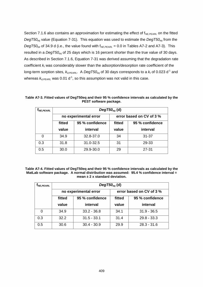
409
Section 7.1.6 also contains an approximation for estimating the effect of fNE,PEARL on the fitted
DegT50eq value (Equation 7-31). This equation was used to estimate the DegT50eq from the
DegT50tot of 34.9 d (i.e., the value found with fNE,PEARL = 0.0 in Tables A7-2 and A7-3). This
resulted in a DegT50eq of 25 days which is 16 percent shorter than the true value of 30 days.
As described in Section 7.1.6, Equation 7-31 was derived assuming that the degradation rate
coefficient kt was considerably slower than the adsorption/desorption rate coefficient of the
long-term sorption sites, kd,PEARL. A DegT50eq of 30 days corresponds to a kt of 0.023 d-1 and
whereas kd,PEARL was 0.01 d-1, so this assumption was not valid in this case.
Table A7-3. Fitted values of DegT50eq and their 95 % confidence intervals as calculated by the PEST software package.
fNE,PEARL DegT50eq (d)
no experimental error error based on CV of 3 %
fitted
value
95 % confidence
interval
fitted
value
95 % confidence
interval
0 34.9 32.8-37.0 34 31-37
0.3 31.8 31.0-32.5 31 29-33
0.5 30.0 29.9-30.0 29 27-31
Table A7-4. Fitted values of DegT50eq and their 95 % confidence intervals as calculated by the MatLab software package. A normal distribution was assumed: 95.4 % confidence interval =
mean ± 2 x standard deviation.
fNE,PEARL DegT50eq (d)
no experimental error error based on CV of 3 %
fitted
value
95 % confidence
interval
fitted
value
95 % confidence
interval
0 34.9 33.2 - 36.8 34.1 31.9 - 36.5
0.3 32.2 31.5 - 33.1 31.4 29.8 - 33.3
0.5 30.6 30.4 - 30.9 29.9 28.3 - 31.6
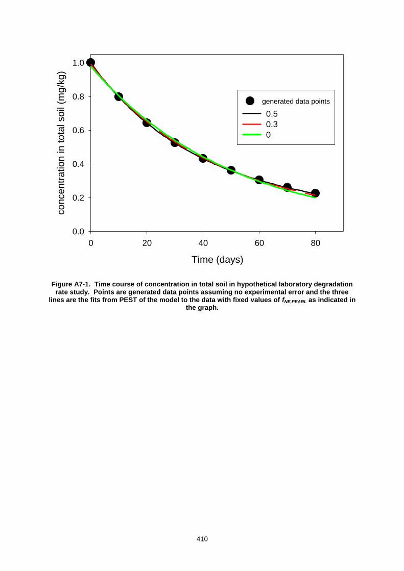
410
Figure A7-1. Time course of concentration in total soil in hypothetical laboratory degradation rate study. Points are generated data points assuming no experimental error and the three
lines are the fits from PEST of the model to the data with fixed values of fNE,PEARL as indicated in the graph.
Time (days)
0 20 40 60 80
co
nce
ntr
atio
n in
to
tal soil
(mg
/kg
)
0.0
0.2
0.4
0.6
0.8
1.0
generated data points
0.5
0.3
0
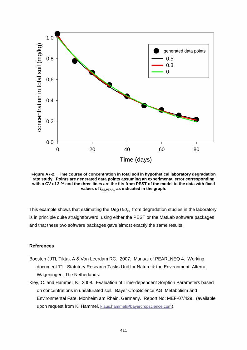
411
Figure A7-2. Time course of concentration in total soil in hypothetical laboratory degradation rate study. Points are generated data points assuming an experimental error corresponding with a CV of 3 % and the three lines are the fits from PEST of the model to the data with fixed
values of fNE,PEARL as indicated in the graph.
This example shows that estimating the DegT50eq from degradation studies in the laboratory
is in principle quite straightforward, using either the PEST or the MatLab software packages
and that these two software packages gave almost exactly the same results.
References
Boesten JJTI, Tiktak A & Van Leerdam RC. 2007. Manual of PEARLNEQ 4. Working
document 71. Statutory Research Tasks Unit for Nature & the Environment. Alterra,
Wageningen, The Netherlands.
Kley, C. and Hammel, K. 2008. Evaluation of Time-dependent Sorption Parameters based
on concentrations in unsaturated soil. Bayer CropScience AG, Metabolism and
Environmental Fate, Monheim am Rhein, Germany. Report No: MEF-07/429. (available
upon request from K. Hammel, [email protected]).
Time (days)
0 20 40 60 80
concentr
ation in tota
l soil
(mg/k
g)
0.0
0.2
0.4
0.6
0.8
1.0
generated data points
0.5
0.3
0

412
Leistra M, van der Linden AMA, Boesten JJTI, Tiktak A, van den Berg F. 2001. PEARL
model for pesticide behaviour and emissions in soil-plant systems; descriptions of the
processes in FOCUS PEARL v 1.1.1. Alterra Report 13, Alterra, Wageningen, the
Netherlands.
MatLab. 2007. MatLab Version 7.4.0.287 (R2007a), Optimisation Toolbox, Statistics
Toolbox, MatLab Compiler. The MathWorks Inc., USA. www.mathworks.com
413
APPENDIX 8. FACT SHEETS FOR REGIONAL DATA
This appendix includes information on the following data bases or maps:
CORINE Land Cover
European Soil Map
European Groundwater Map
IPCC Global Climate Data
Digital Elevation Model
Administrative Boundaries (AD)
European Zonal Map
European Census Data (AD)
MARS Climate Data Base
Irrigation Data Base
The Map of Organic Carbon in Topsoils in Europe
CORINE Land Cover
Description
The CORINE land cover data set was developed by the European Environment Agency as
part of the CORINE Program (Coordination of Information on the Environment) to provide a
consistent land cover data set at a reasonable resolution across the European Union. The
first version of Corine Land Cover – CLC1990 – reflected land use in Europe between 1986
and 1995, depending on the production date of the underlying satellite images. In the
meantime a new version – CLC2000 – is being prepared for release. The updated version
shows land use in Europe in 2000 (+/- 1 year). Table A8-1 and Figure A8-1 give an overview
about the progress of the CLC 2000 project as of May 2004. Currently Corine covers all of
the European Union.
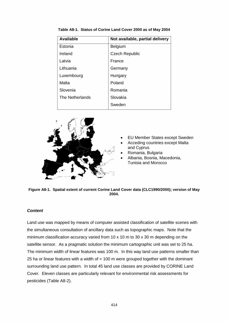
414
Table A8-1. Status of Corine Land Cover 2000 as of May 2004
Available Not available, partial delivery
Estonia Belgium
Ireland Czech Republic
Latvia France
Lithuania Germany
Luxembourg Hungary
Malta Poland
Slovenia Romania
The Netherlands Slovakia
Sweden
EU Member States except Sweden
Acceding countries except Malta and Cyprus
Romania, Bulgaria
Albania, Bosnia, Macedonia, Tunisia and Morocco
Figure A8-1. Spatial extent of current Corine Land Cover data (CLC1990/2000); version of May
2004.
Content
Land use was mapped by means of computer assisted classification of satellite scenes with
the simultaneous consultation of ancillary data such as topographic maps. Note that the
minimum classification accuracy varied from 10 x 10 m to 30 x 30 m depending on the
satellite sensor. As a pragmatic solution the minimum cartographic unit was set to 25 ha.
The minimum width of linear features was 100 m. In this way land use patterns smaller than
25 ha or linear features with a width of < 100 m were grouped together with the dominant
surrounding land use pattern. In total 45 land use classes are provided by CORINE Land
Cover. Eleven classes are particularly relevant for environmental risk assessments for
pesticides (Table A8-2).
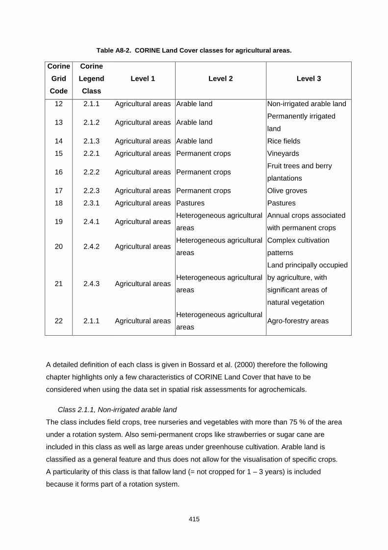
415
Table A8-2. CORINE Land Cover classes for agricultural areas.
Corine
Grid
Code
Corine
Legend
Class
Level 1 Level 2 Level 3
12 2.1.1 Agricultural areas Arable land Non-irrigated arable land
13 2.1.2 Agricultural areas Arable land Permanently irrigated
land
14 2.1.3 Agricultural areas Arable land Rice fields
15 2.2.1 Agricultural areas Permanent crops Vineyards
16 2.2.2 Agricultural areas Permanent crops Fruit trees and berry
plantations
17 2.2.3 Agricultural areas Permanent crops Olive groves
18 2.3.1 Agricultural areas Pastures Pastures
19 2.4.1 Agricultural areas Heterogeneous agricultural
areas
Annual crops associated
with permanent crops
20 2.4.2 Agricultural areas Heterogeneous agricultural
areas
Complex cultivation
patterns
21 2.4.3 Agricultural areas Heterogeneous agricultural
areas
Land principally occupied
by agriculture, with
significant areas of
natural vegetation
22 2.1.1 Agricultural areas Heterogeneous agricultural
areas Agro-forestry areas
A detailed definition of each class is given in Bossard et al. (2000) therefore the following
chapter highlights only a few characteristics of CORINE Land Cover that have to be
considered when using the data set in spatial risk assessments for agrochemicals.
Class 2.1.1, Non-irrigated arable land
The class includes field crops, tree nurseries and vegetables with more than 75 % of the area
under a rotation system. Also semi-permanent crops like strawberries or sugar cane are
included in this class as well as large areas under greenhouse cultivation. Arable land is
classified as a general feature and thus does not allow for the visualisation of specific crops.
A particularity of this class is that fallow land (= not cropped for 1 – 3 years) is included
because it forms part of a rotation system.

416
Class 2.1.2, Permanently irrigated land
Crops, which are permanently, irrigated using a permanent infrastructure (irrigation channels,
drainage network). The class excludes sporadically irrigated land as well as rice fields and
greenhouses
Class 2.1.3, Rice fields
Land prepared for rice cultivation and adjacent irrigation channels
Class 2.2.1, Vineyards
Areas planted with vines for wine, consumer grapes and raisin production. The class includes
all complex cultivation patterns were vineyard parcels cover at least 50 % of the area.
Class 2.2.2, Fruit trees and berry plantations
Parcels planted with fruit trees or shrubs. This class includes also hops and other permanent
crops like permanent horticultural plantations. In case of equal occurrence with vineyards and
olive groves priority was given to these crops.
Class 2.2.3, Olive groves
Areas planted with olive trees including mixed occurrence with vines on the same parcel.
Class 2.3.1, Pastures
This class includes also abandoned arable land, which is not part of a rotation system (> 3
years fallow). Patches of arable land that cover less than 25 % of a minimum mapping area
of 25 ha and is surrounded by pastures is classified as ‘pasture’.
Class 2.4.1, Annual crops associated with permanent crops
All complex cultivation patterns where non-permanent crops occupy more than 50 % of area.
Class 2.4.2, Complex cultivation patterns
Juxtaposition of small parcels of diverse annual crops, pasture and/or permanent crops. This
class includes also scattered houses and roads that cover < 30 % of the patchwork structure.
Class 2.4.3, Land principally occupied by agriculture with significant areas of natural
vegetation
This class includes parcels of arable land, orchards and vineyards < 25 ha which were not
grouped under one of the previous classes.
Class 2.4.4, Agro-forestry areas
Annual crops or grazing land under the wooded cover of forestry species.
417
General considerations for environmental risk assessments of pesticides
In some regions the majority of arable land is found in complex cultivation systems with
natural vegetation, permanent crops and pastures. Due to a minimum mapping unit of 25 ha
deriving e.g. the acreage of arable land from Corine Land Cover is not possible because of
generalisation errors. Nevertheless Corine Land Cover represents currently the most
accurate data source on land use in the EU. Corine Land Cover should be used for the
identification of agricultural areas vulnerable to pesticide leaching since a satellite based land
use map excludes non-agricultural areas with a sufficient degree of accuracy.
Data distribution
A 250-m grid can be acquired free of charge from the European Environment Agency
(http://dataservice.eea.eu.int/dataservice/). The data layer is available in commonly used
GIS-formats (e.g. ArcInfo Export file, Imagine Raster format).
Higher resolution versions of CORINE Land Cover (e.g. 100-m) can be obtained on request
from European Topic Center on Land Cover (ETC/LC) distributed by Environmental Satellite
Data Center (MDC Environmental Satellite Data Center, Miljodatacentrum I Kiruna AB, PO
Box 806, SE-981 28 Kiruna, Sweden, Tel: +46 0980-671 70, Fax: 0980-671 80, Email:
[email protected], Internet: www.mdc.kiruna.se).
Documentation
The most comprehensive documentation about the current version of Corine Land Cover is
provided on the website of the European Topic Center on Terrestrial Environment of the
European Environment Agency (http://terrestrial.eionet.eu.int/CLC2000).
Corine Land Cover update I&CLC2000 project Technical Guidelines. Final version
August 2002. European Environment Agency. European Topic Center Terrestrial
Environment.
Bossard M., Feranec J. and J. Otahel. 2000. Corine Land Cover technical guide –
Addendum 2000. Technical Report No. 40. European Environment Agency.
Technical and methodological guide for updating the Corine Land Cover Data Base.
Joint Research Center, EU Commission, European Environment Agency. Report No.
EUR 17288 EN.
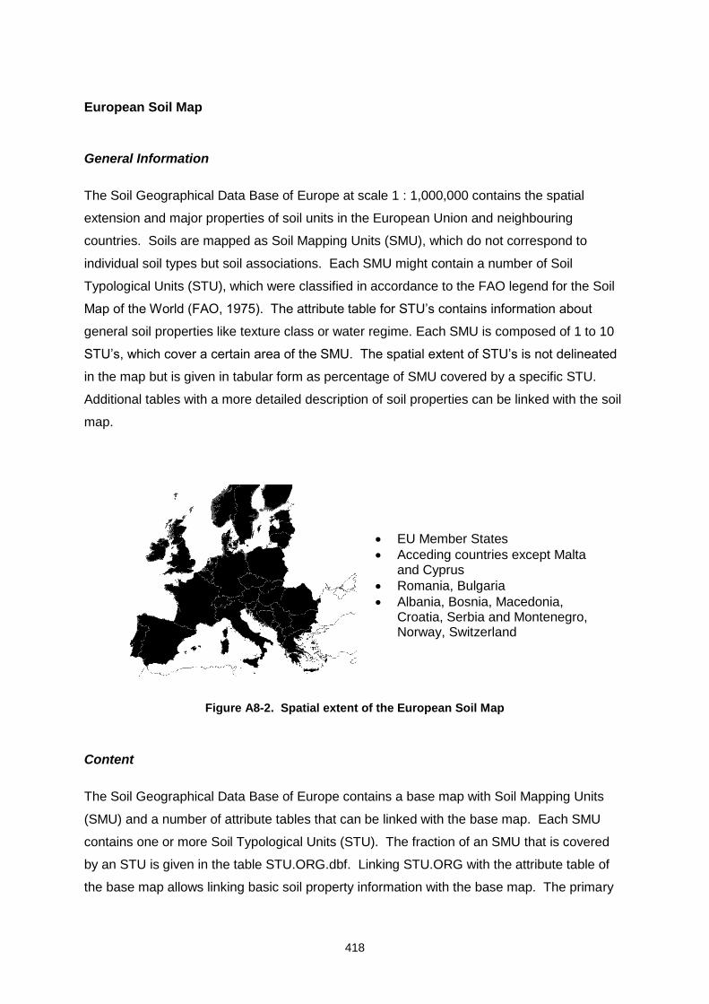
418
European Soil Map
General Information
The Soil Geographical Data Base of Europe at scale 1 : 1,000,000 contains the spatial
extension and major properties of soil units in the European Union and neighbouring
countries. Soils are mapped as Soil Mapping Units (SMU), which do not correspond to
individual soil types but soil associations. Each SMU might contain a number of Soil
Typological Units (STU), which were classified in accordance to the FAO legend for the Soil
Map of the World (FAO, 1975). The attribute table for STU’s contains information about
general soil properties like texture class or water regime. Each SMU is composed of 1 to 10
STU’s, which cover a certain area of the SMU. The spatial extent of STU’s is not delineated
in the map but is given in tabular form as percentage of SMU covered by a specific STU.
Additional tables with a more detailed description of soil properties can be linked with the soil
map.
EU Member States
Acceding countries except Malta and Cyprus
Romania, Bulgaria
Albania, Bosnia, Macedonia, Croatia, Serbia and Montenegro, Norway, Switzerland
Figure A8-2. Spatial extent of the European Soil Map
Content
The Soil Geographical Data Base of Europe contains a base map with Soil Mapping Units
(SMU) and a number of attribute tables that can be linked with the base map. Each SMU
contains one or more Soil Typological Units (STU). The fraction of an SMU that is covered
by an STU is given in the table STU.ORG.dbf. Linking STU.ORG with the attribute table of
the base map allows linking basic soil property information with the base map. The primary
419
identification code of all attribute tables is always the STU-code. The following sections
briefly describe the attribute tables of the main data bases:
Soil Geographical Data Base
STU.ORG.dbf: This table is the link between the base map and any of the following
attribute tables. STU.ORG assigns STU’s to each SMU along with the percentage of
area (PCAREA) that is covered by the STU within a SMU.
STU.dbf: STU.dbf is the primary attribute table and contains the FAO soil name,
information about parent material, soil depth and some general soil properties, which
are provided as class values. In this way most of the crucial soil properties that are
required for leaching simulations are not given as absolute numbers and cannot be
used directly as input parameters in environmental fate models.
Pedotransfer Rule Data Base
STU.dbf: The pedotransfer rule data base provides additional information that was derived
on the basis of existing information stored in the Soil Geographical Data Base. The
most relevant parameters for the assessment of leaching risk are organic carbon
contents in topsoil, available water capacity and depth to impermeable layers. Again
most parameters are given in qualitative form or as class-values.
Soil Profile Analytical Data Base (SPADE-1)
Est_prof2stu.lnk.dbf: This table stores the required links between STU’s and the
information stored in the Soil Profile Analytical Data Base.
Est_prof.dbf: The estimated profile table contains more detailed information like depth to
ground water and parent material for selected soil units. A link is provided to STU’s
by using est_prof2stu.lnk.dbf.
Est_hor.dbf: The estimated horizon table gives estimated soil properties for each horizon
of soils shown in Est_prof.dbf. This table contains absolute values for crucial soil
properties and is thus the primary source for input parameters that are required
for leaching simulations. The total number of estimated soil profiles varies
significantly between countries. Some countries (e.g. Austria) are not represented at
all by an estimated soil profile, whereas others provide only a very limited number of
profiles. An important attribute is the dominant land use (LU) of the estimated soil
profile. The current version of Est_hor.dbf contains only a limited number of soil
420
profiles with ‘arable land’ or ‘perennial crop’ as dominant land use. In leaching
modelling studies profile data from agricultural soils must be used in order to avoid
the co-occurrence of unrealistic combinations of factors.
The SPADE-1 data base, which is delivered with the current version of the European
soil map, contains 447 estimated soil profiles among which 240 are linked to STU`s (8
% of the total number of STU`s. The total number of STU`s in the 15 EU member
states before 2004 is 3164, among those 1206 STU`s have a designated dominant
land use of “arable land”. In total only 78 STU`s (6%) representing arable land are
actually linked to SPADE-1.
In the light of these deficiencies the European Crop Protection Association, supported
by the European Soil Bureau of the European Commission’s Joint Research Centre,
sponsored the compilation of a second version (SPADE-2) of the profile data base for
use with the Soil Geographical Database of Europe. SPADE-2 contains additional
soil profiles for Belgium, Luxemburg, Denmark, Italy, the Netherlands, Portugal and
Scotland. Other member states either declined to supply data or could not provide
the requested data within the project time-frame. The new data base contains 1897
complete profiles which are directly linked to 1077 STU`s.
The SPADE-2 database will be distributed in the future as part of the European Soil
Database version 3.0. The SPADE.dbf and SPADE_2_raw.xls containing the original
national data are included for circulation on a CD available with the final report of the
project (Hollis et al. 2006). The report and the CD Rom are available through the
Office for Official Publications of the European Communities in Luxembourg.
Note that all examples for higher-tier GIS work in this report were conducted with
SPADE-1 since SPADE-2 was not available to the FOCUS work group at the time
when this report was written.
Meas_prof: The Soil Analytical Data Base contains also measured soil profile data from
various countries with a varying degree of completeness. There is no direct link
between measured soil profiles and any other attribute table therefore this data base
should not be used as source for input parameters in leaching simulations.
421
HYPRES Data Base of Hydraulic Properties of European Soils
PARAM.doc: The HYPRES data base consists of a small number of pedotransfer functions
and parameters that are stored in a word document. The hydraulic parameters were
derived on the basis of European soils and were adapted to the existing parameter
structure of in the European Soil Map. The data are provided in two different ways.
Class pedotransfer functions can be used in combination with STU.dbf to visualise
hydraulic properties for whole Europe. Continuous pedotransfer functions are finally
used to derive hydraulic parameters for soil horizons as required for leaching
modelling studies.
General considerations for environmental risk assessments of pesticides
A number of soil properties are available as class values for almost all STU’s (except
developed land and some mountainous areas). European-wide maps can be derived
showing soils that e.g. belong to a certain texture class or a class of organic carbon contents
in topsoil.
Only a limited number of STU’s have data that describe soil horizons and are required for
leaching simulations. The attribute table Est_hor.dbf contains soil properties for selected
STU’s and for different soil horizons. For that reason Est_hor.dbf is recommended to be the
primary data source for soil parameters that are used in leaching simulations.
Although a number of hydrologic pedotransfer functions exist, HYPRES pedotransfer
functions were however explicitly tailored to the data structure and texture classification in the
European Soil Map. Therefore preference should be given to HYPRES when deriving
hydrological parameters.
Data distribution
The European Soil Map is available in Arc/Info format and is distributed by the European Soil
Bureau:
Dr. Luca Montanarella
European Soil Bureau
Space Applications Institute
Joint Research Centre
422
Ispra Establishment, TP 262, 21020 Ispra (VA), ITALY
Tel: 00 39 0332 785349
Fax: 00 39 0332 789936
E-mail: [email protected]
For information on SPADE-2 contact:
Office for Official Publications of the European Communities
2, rue Mercier
L-2985 Luxembourg
Tel: (352) 2929-1
Email:[email protected]
http://publications.europa.eu/
Documentation
FAO. 1975. Soil map of the World at 1 : 5,000,000. Volume I Europe. UNESCO. Paris. 62p.
Hollis J.M., Jones R.J.A., Marshall C.J, Holden A., Van de Veen J.R. and Montanarella L.
2006. SPADE-2: The soil profile analytical database for Europe, Version 1.0. European Soil
Bureau Research Report No. 19, EUR 22127 EN, 38 pp. Office for Official Publications of the
European Communities, Luxembourg.
European Soil Data Base. 1999. Soil Geographical Data Base of Europe 1 : 1,000,000 vers.
1.0, 21/7/1999. Including tables and documentation. European Soil Bureau, Joint Research
Centre. Ispra.
Wösten J.H.M., Lilly A., Nemes A. and C. Les Bas. 1999. Development and use of a
database of hydraulic properties of European Soils. Geoderma 90:169-185.
Nemes A., Wösten J.H.M., Lilly A., and J. H. Oude Voshaar. 1999. Evaluation of different
procedures to interpolate particle-size distributions to achieve compatibility within soil
databases. Geoderma 90:187-202.
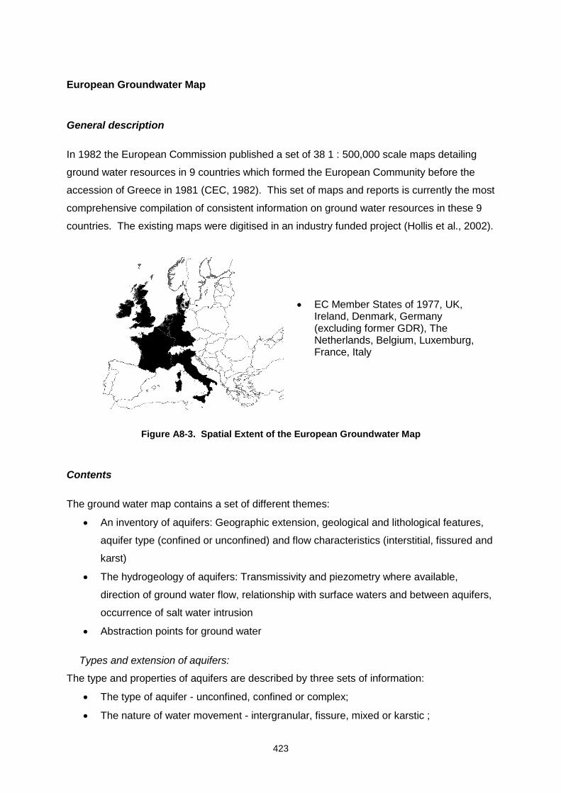
423
European Groundwater Map
General description
In 1982 the European Commission published a set of 38 1 : 500,000 scale maps detailing
ground water resources in 9 countries which formed the European Community before the
accession of Greece in 1981 (CEC, 1982). This set of maps and reports is currently the most
comprehensive compilation of consistent information on ground water resources in these 9
countries. The existing maps were digitised in an industry funded project (Hollis et al., 2002).
EC Member States of 1977, UK, Ireland, Denmark, Germany (excluding former GDR), The Netherlands, Belgium, Luxemburg, France, Italy
Figure A8-3. Spatial Extent of the European Groundwater Map
Contents
The ground water map contains a set of different themes:
An inventory of aquifers: Geographic extension, geological and lithological features,
aquifer type (confined or unconfined) and flow characteristics (interstitial, fissured and
karst)
The hydrogeology of aquifers: Transmissivity and piezometry where available,
direction of ground water flow, relationship with surface waters and between aquifers,
occurrence of salt water intrusion
Abstraction points for ground water
Types and extension of aquifers:
The type and properties of aquifers are described by three sets of information:
The type of aquifer - unconfined, confined or complex;
The nature of water movement - intergranular, fissure, mixed or karstic ;
424
Special cases like alluvial aquifers
Relevance of types of aquifers to pesticide fate assessment:
An unconfined aquifer can potentially receive recharge over the whole of its area,
while a confined aquifer will tend to have a proportionally smaller recharge area,
which will itself be unconfined; Unconfined aquifers may be vulnerable to pesticide
leaching, dependent upon the nature of overlying deposits and the thickness of the
unsaturated zone;
Confined aquifers are afforded significant protection by the overlying confining bed
(which is not depicted on the map).
complex aquifers- studies in these areas would benefit from more detailed geological
mapping in order to more accurately ascertain the extent and lithological
heterogeneity of such aquifers.
Relevance of nature of water movement to pesticide fate assessment:
Intergranular flow- water moves along tortuous flow paths, which provides both time
and the potential for significant interaction with the aquifer matrix;
Fissure flow- fractures and fissures allow for fast flow rates with limited contact with
aquifer media. The aquifer matrix may be calcareous or non-calcareous. Localised
karst flow may occur in some portions of the aquifer;
Mixed- the combination of the characteristics of both intergranular and fissure flow
allows for fast flow rates together with a large intergranular storage, into which
pollutants may diffuse from the fissures. While flow will be dominantly through the
fissures, the ground water resource comes mainly from ground water released from
intergranular storage by falling ground water levels.
Karst flow- the large solution channels associated with karstic terrain allow for very
fast flow rates (of the order of kilometres per day) with limited contact with aquifer
media, but probably in a high pH environment.
Karst flow- rates can be high enough to generate turbulent flow, allowing the
movement of particulate and colloidal material through the ground water system.
Normal unconfined karstic aquifers are often associated with a karst terrain,
characterised by solution channels, closed depressions, sinkholes and caves. These
allow very rapid movement of surface water and recharge in to the ground water
system. Karst aquifers can be very vulnerable to pollutants entering from the surface
water system.

425
The relevance of special cases like alluvial aquifers to pesticide fate assessments:
Alluvial aquifers are disproportionately important for water supply purposes; and are
potentially vulnerable to contamination from the induced infiltration of contaminated
surface water
Ground water hydrogeology data
Information on ground water flow is only partly provided in the map. Risks assessments of
regional ground water exposure to pesticides would benefit from more detailed information
on flow directions. The respective data could be used to assess (1) contaminant flow from
potential vulnerable areas from where pesticide entries might occur and (2) potential
exposure of vulnerable receptors like wetlands or springs. The current data set however
does not allow for such detailed assessments on the whole study area.
Also contour lines are given only for parts of the European Groundwater Map. More detailed
information on the topography of aquifers and a high resolution digital elevation model would
allow for the estimation of depths of ground water tables which is an important input
parameter in leaching models. Currently this information cannot be derived with the required
accuracy based on the existing map.
Areas of saltwater intrusion indicate aquifers that are unlikely to be used as source for
drinking water.
Ground water abstraction data
The size of abstraction from wells or springs provides information about the likely size of its
source area and the importance for local water supply. Mine drainage is a special case of
ground water abstraction, indicating a significant human alteration of ground water flow.
General considerations for environmental risk assessments of pesticides
The European Groundwater Map is currently the most comprehensive data set on ground
water resources in Europe. Pesticide risk assessments on a regional scale would benefit
from further work in the area of hydrogeology and in particular of an extension of the ground
water map to additional member states. This probably will be achieved soon within the
framework of the implementation of the water framework directive. At present the most
important use of the European Groundwater Map is the identification of aquifer locations and
the potential exclusion of areas without any significant ground water resources from leaching
assessments. In turn regional leaching assessments could be targeted to areas of concern
based on the presence of vulnerable aquifers that are significant sources for drinking water.
426
Data distribution
The digitised version of the Groundwater Resources Map of Europe is available in
ArcView 3.2 (shape file) format. The distribution of the data will be through the Office for
Official Publications of the European Communities in Luxembourg.
Documentation
CEC. 1982. Groundwater resources of the European Community: Synthetical Report.
Commission of the European Communities, Directorate-General for the environment,
consumer protection and nuclear safety. Th. Schäfer GmbH, Hannover. 75 pp.
Jones R.J.A., Hollis J.M. L. Montanarella and S.K. Selvaradjou (2004): Groundwater
Resources of Europe. Maps at 1 : 500,00 scale & GIS database [CD-ROM]. EUR 7940 EN. 4
September 2004.
Further information on these maps can be obtained through:
Dr Luca Montanarella / Dr. SELVARADJOU Senthil-Kumar / Dr. Bob Jones
European Soil Bureau, Institute for Environment & Sustainability
Joint Research Centre of the European Commission
TP-280 Ispra (VA) 21020 ITALY
Tel: +39 0332 785 349
Fax: +39 0332 789 936
E-mail: [email protected];[email protected] [email protected];
IPCC Global Climate Data
General description
The Intergovernmental Panel on Climate Change (IPCC) has been established by the United
Nations Environment Program (UNEP) and the Word Meteorological Organisation to assess
global climate change phenomena. The IPCC distributes global climate data as monthly
series from 1960 to 1990.
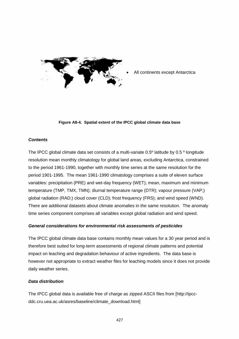
427
All continents except Antarctica
Figure A8-4. Spatial extent of the IPCC global climate data base
Contents
The IPCC global climate data set consists of a multi-variate 0.5º latitude by 0.5 º longitude
resolution mean monthly climatology for global land areas, excluding Antarctica, constrained
to the period 1961-1990, together with monthly time series at the same resolution for the
period 1901-1995. The mean 1961-1990 climatology comprises a suite of eleven surface
variables: precipitation (PRE) and wet-day frequency (WET); mean, maximum and minimum
temperature (TMP, TMX, TMN); diurnal temperature range (DTR); vapour pressure (VAP;)
global radiation (RAD;) cloud cover (CLD); frost frequency (FRS); and wind speed (WND).
There are additional datasets about climate anomalies in the same resolution. The anomaly
time series component comprises all variables except global radiation and wind speed.
General considerations for environmental risk assessments of pesticides
The IPCC global climate data base contains monthly mean values for a 30 year period and is
therefore best suited for long-term assessments of regional climate patterns and potential
impact on leaching and degradation behaviour of active ingredients. The data base is
however not appropriate to extract weather files for leaching models since it does not provide
daily weather series.
Data distribution
The IPCC global data is available free of charge as zipped ASCII files from [http://ipcc-
ddc.cru.uea.ac.uk/asres/baseline/climate_download.html]
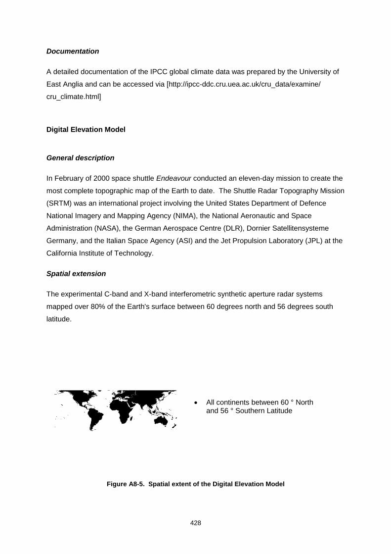
428
Documentation
A detailed documentation of the IPCC global climate data was prepared by the University of
East Anglia and can be accessed via [http://ipcc-ddc.cru.uea.ac.uk/cru_data/examine/
cru_climate.html]
Digital Elevation Model
General description
In February of 2000 space shuttle Endeavour conducted an eleven-day mission to create the
most complete topographic map of the Earth to date. The Shuttle Radar Topography Mission
(SRTM) was an international project involving the United States Department of Defence
National Imagery and Mapping Agency (NIMA), the National Aeronautic and Space
Administration (NASA), the German Aerospace Centre (DLR), Dornier Satellitensysteme
Germany, and the Italian Space Agency (ASI) and the Jet Propulsion Laboratory (JPL) at the
California Institute of Technology.
Spatial extension
The experimental C-band and X-band interferometric synthetic aperture radar systems
mapped over 80% of the Earth's surface between 60 degrees north and 56 degrees south
latitude.
All continents between 60 ° North and 56 ° Southern Latitude
Figure A8-5. Spatial extent of the Digital Elevation Model
429
Contents
NIMA will produce two public data sets, DTED-1 with worldwide coverage and DTED-2 for
the US. Digital Terrain Elevation Data (DTED) sets consist of a uniform grid of latitude,
longitude, and elevation data. DTED-1 grid posts are spaced at three arc second intervals
(approx. 100m) and DTED-2 grid posts are spaced at one arc second intervals (approx.
30m). A third reduced resolution data set, DTED-0, was also produced for the globe having
grid post spacing of 30 arc seconds (approx. 1km).
General considerations for environmental risk assessments of pesticides
In general digital elevation models have only a limited range of applications in leaching
modelling studies. Nevertheless the data is of use for a more detailed assessment of
landscape factors on a local or regional scale such as occurrence of slopes with limited
potential of showing chromatographic vertical solute fluxes. Digital elevation models can also
be used to assess the occurrence of certain soil types. Currently the delineation of certain
soil polygons in the EU soil map is corrected on the basis of SRTM data since in some cases
the boundaries of e.g. Fluvisols does not match the boundaries of floodplains.
Data distribution
SRTM data can be obtained from the United States Geological Survey (USGS) Data Center
[http://srtm.usgs.gov/]. This server stores areas of up to 30° square (1.6 gigabyte/100
megabyte files) as downloadable data sets at no charge and areas of greater than or less
than 30 degrees square on CDs at a cost of $32 per CD (approximately 600 megabyte each)
plus a $45 processing and a $5 shipping charge. Available formats include ArcGrid, BIL, and
TIFF
Documentation
A detailed documentation on SRTM data is available from National Aeronautic and Space
Administration (NASA) and European Space Agency (ESA) websites:
http://www2.jpl.nasa.gov/srtm/
http://www.spaceflight.esa.int/file.cfm?filename=sts99obj
430
Administrative Boundaries (AD)
Description
NUTS version 7 (1999)
Boundaries of 1 328 NUTS regions (Nomenclature of Territorial Units for Statistics)
4 hierarchical levels
Resolution Scale: 1/1 000 000 (1000 €)
1/3 000 000 (700 €)
Spatial extent
National boundaries of all European countries are included
(EU-15, EFTA-4, AC-12)
Content
The Nomenclature of Territorial Units for Statistics (NUTS) was established by Eurostat more
than 25 years ago in order to provide a single uniform breakdown of territorial units for the
production of regional statistics for the European Union.
Since this is a hierarchical classification, the NUTS subdivides each member state into a
whole number of NUTS 1 regions, each of which is in turn subdivided into a whole number of
NUTS 2 regions and so on.
At the regional level (without taking the municipalities into account), the administrative
structure of the member states generally comprises two main regional levels (Länder and
Kreise in Germany, régions and départements in France, Comunidades autonomas and
provincias in Spain, regioni and provincie in Italy, etc.).
The grouping together of comparable units at each NUTS level involves establishing, for
each member state, an additional regional level to the two main levels referred to above.
This additional level therefore corresponds to a less important or even non-existent
administrative structure, and its classification level varies within the first 3 levels of the NUTS,
depending entirely on the Member State: NUTS 1 for France, Italy, Greece, and Spain,
NUTS 2 for Germany, NUTS 3 for Belgium, etc.
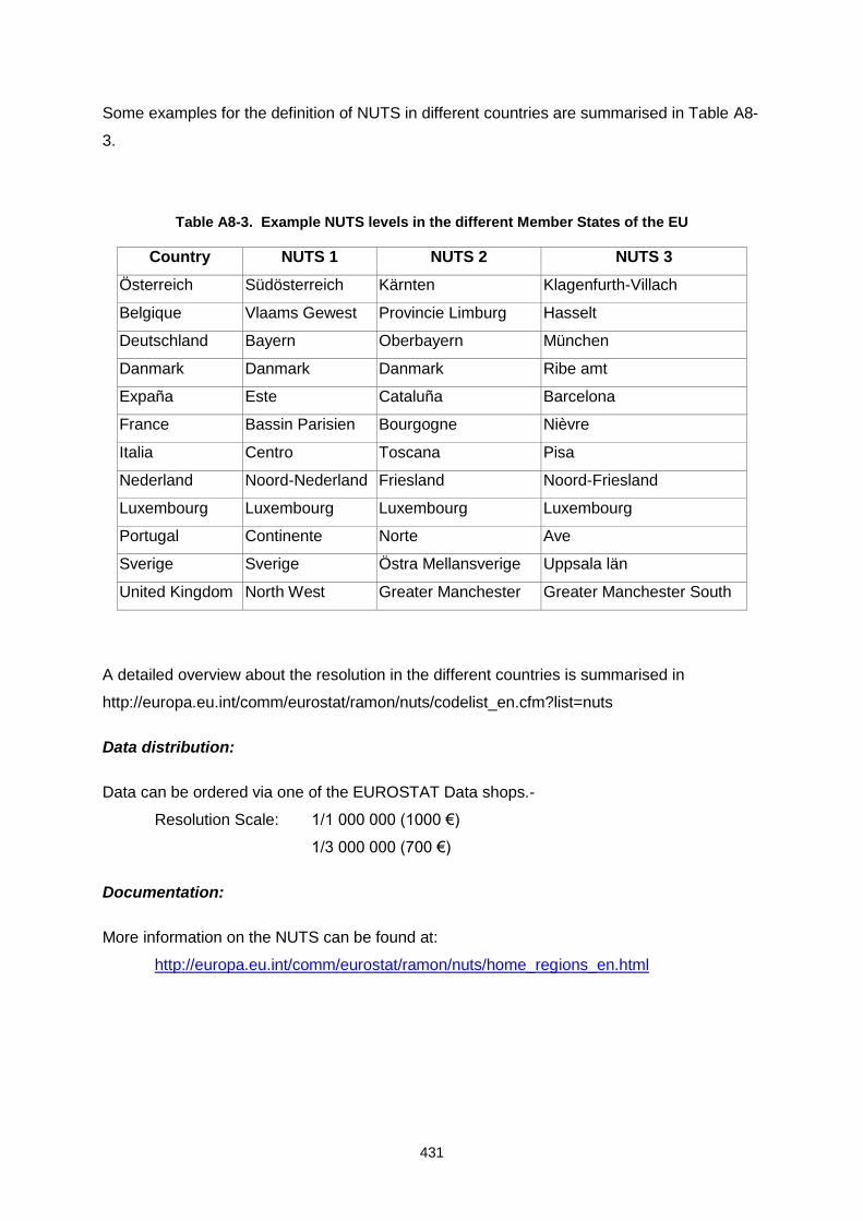
431
Some examples for the definition of NUTS in different countries are summarised in Table A8-
3.
Table A8-3. Example NUTS levels in the different Member States of the EU
Country NUTS 1 NUTS 2 NUTS 3
Österreich Südösterreich Kärnten Klagenfurth-Villach
Belgique Vlaams Gewest Provincie Limburg Hasselt
Deutschland Bayern Oberbayern München
Danmark Danmark Danmark Ribe amt
Expaña Este Cataluña Barcelona
France Bassin Parisien Bourgogne Nièvre
Italia Centro Toscana Pisa
Nederland Noord-Nederland Friesland Noord-Friesland
Luxembourg Luxembourg Luxembourg Luxembourg
Portugal Continente Norte Ave
Sverige Sverige Östra Mellansverige Uppsala län
United Kingdom North West Greater Manchester Greater Manchester South
A detailed overview about the resolution in the different countries is summarised in
http://europa.eu.int/comm/eurostat/ramon/nuts/codelist_en.cfm?list=nuts
Data distribution:
Data can be ordered via one of the EUROSTAT Data shops.-
Resolution Scale: 1/1 000 000 (1000 €)
1/3 000 000 (700 €)
Documentation:
More information on the NUTS can be found at:
http://europa.eu.int/comm/eurostat/ramon/nuts/home_regions_en.html
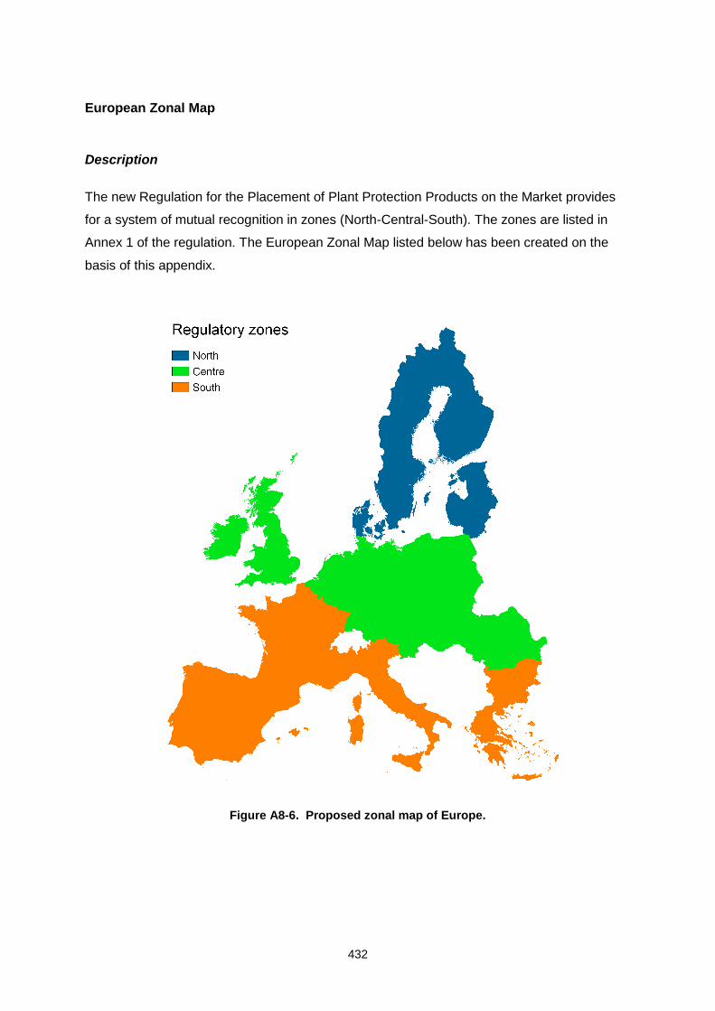
432
European Zonal Map
Description
The new Regulation for the Placement of Plant Protection Products on the Market provides
for a system of mutual recognition in zones (North-Central-South). The zones are listed in
Annex 1 of the regulation. The European Zonal Map listed below has been created on the
basis of this appendix.
Figure A8-6. Proposed zonal map of Europe.
433
European Census Data (AD)
Description
New CRONOS: long-term series data (monthly, quarterly, yearly) on the nine themes of the
official European statistics. A demo CD-ROM is available.
Spatial extent
National boundaries of all European member states are included.
Content
Data are available for in total 9 categories (general statistics, economy and finance,
population and social conditions, industry, trade and services, agriculture and fisheries,
external trade, transport, environment and energy, science and technology). The data are
provided in extended tables based on a hierarchical structure (categories, domains,
collections, tables).
In the category “Agricultural and Fisheries” in total 11 domains are considered. Most
interesting for FOCUS will be the collection PROD_VEG (“crop products”) in the domain
ZPA1 (Agricultural Products). The collection contains two data fields (“Fruits and vegetables”
and “Crops products (excluding fruits and vegetables)“. The data are provided with an
annual resolution. Data are available for more than 200 crops.
This high resolution of crops is provided only on the member state level, when this data is
purchased from the Eurostat-data-shops. Data on the regional level (NUTS 1 and 2) is
available but only for a following crops:
cereals (including rice)
cereals (without rice)
common wheat and spelt
durum wheat
winter wheat
rye
barley
grain maize
rice
potatoes
legumes
sugar beets
oilseeds
rape - turnip rape
434
sunflower seed
soybean
oil flax
cotton
tobacco
orchards
olives
There are data gaps for some combinations of crops and member states.
Data distribution:
Data can be ordered via one of the EUROSTAT Data shops. Resolution Scale: resolution 21
crops listed, regional level (NUTS 1, 2, 3): costs about 130 Euro (for one year)
Documentation:
More information on the CRONOS Data base can be found at:
http://www.eu-datashop.de/datenba/EN/allgem/infoda_1.htm
MARS Climate Data Base
Description
Joint Research Centre (JRC) at Ispra, Italy, holds long-term weather data compiled as part of
the Monitoring Agriculture by Remote Sensing (MARS) project. The data were derived using
a method developed at the former Staring Centre (now Alterra). The MARS data base
contains daily meteorological data spatially interpolated on 50 x 50 km2 grid cells. The
original weather data originate from approximately 1500 weather stations across Europe,
Maghreb countries, and Turkey, and are based on daily data for the period 1971 to date,
which was purchased from various national weather services. Some of the data were
obtained from the national meteorological services under special copyright and agreements
for MARS internal use only, so that data at station level are not available, only interpolated
daily weather data are available.
In the MARS data base, the basis for the interpolation is the selection of the suitable
combination of weather stations for the determination of the representative meteorological
conditions for a grid cell. The selection procedure relies on the similarity of the station and
the grid centre. This similarity is expressed as the results of a scoring algorithm that takes
the following characteristics into account:
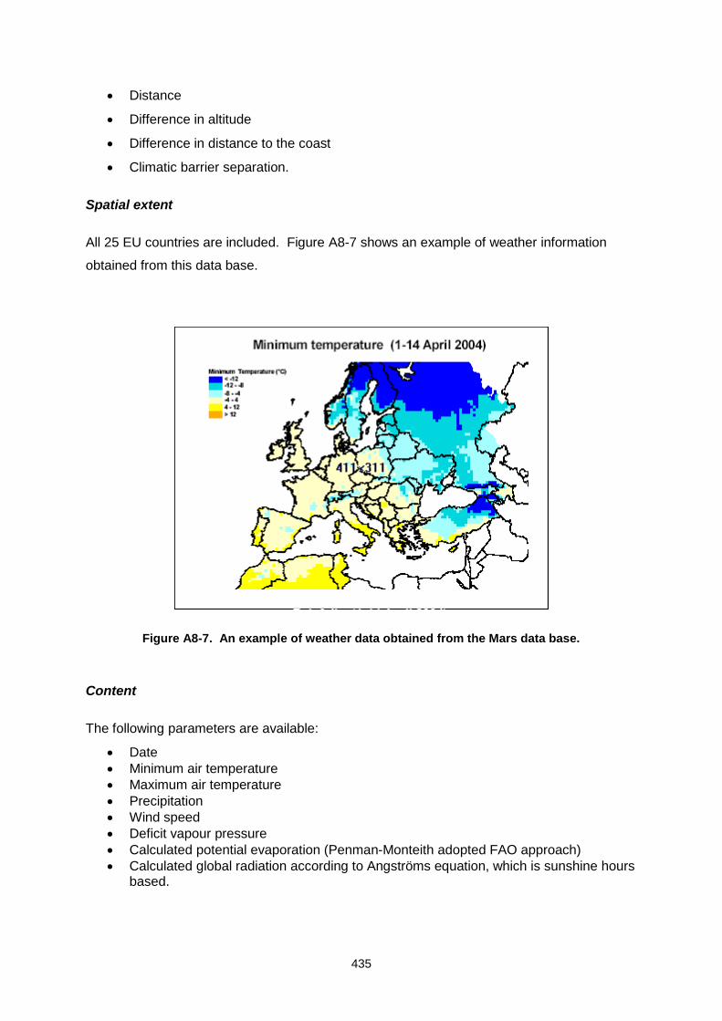
435
Distance
Difference in altitude
Difference in distance to the coast
Climatic barrier separation.
Spatial extent
All 25 EU countries are included. Figure A8-7 shows an example of weather information
obtained from this data base.
Figure A8-7. An example of weather data obtained from the Mars data base.
Content
The following parameters are available:
Date
Minimum air temperature
Maximum air temperature
Precipitation
Wind speed
Deficit vapour pressure
Calculated potential evaporation (Penman-Monteith adopted FAO approach)
Calculated global radiation according to Angströms equation, which is sunshine hours based.
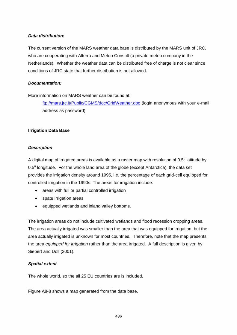
436
Data distribution:
The current version of the MARS weather data base is distributed by the MARS unit of JRC,
who are cooperating with Alterra and Meteo Consult (a private meteo company in the
Netherlands). Whether the weather data can be distributed free of charge is not clear since
conditions of JRC state that further distribution is not allowed.
Documentation:
More information on MARS weather can be found at:
ftp://mars.jrc.it/Public/CGMS/doc/GridWeather.doc (login anonymous with your e-mail
address as password)
Irrigation Data Base
Description
A digital map of irrigated areas is available as a raster map with resolution of 0.5o latitude by
0.5o longitude. For the whole land area of the globe (except Antarctica), the data set
provides the irrigation density around 1995, i.e. the percentage of each grid-cell equipped for
controlled irrigation in the 1990s. The areas for irrigation include:
areas with full or partial controlled irrigation
spate irrigation areas
equipped wetlands and inland valley bottoms.
The irrigation areas do not include cultivated wetlands and flood recession cropping areas.
The area actually irrigated was smaller than the area that was equipped for irrigation, but the
area actually irrigated is unknown for most countries. Therefore, note that the map presents
the area equipped for irrigation rather than the area irrigated. A full description is given by
Siebert and Döll (2001).
Spatial extent
The whole world, so the all 25 EU countries are is included.
Figure A8-8 shows a map generated from the data base.
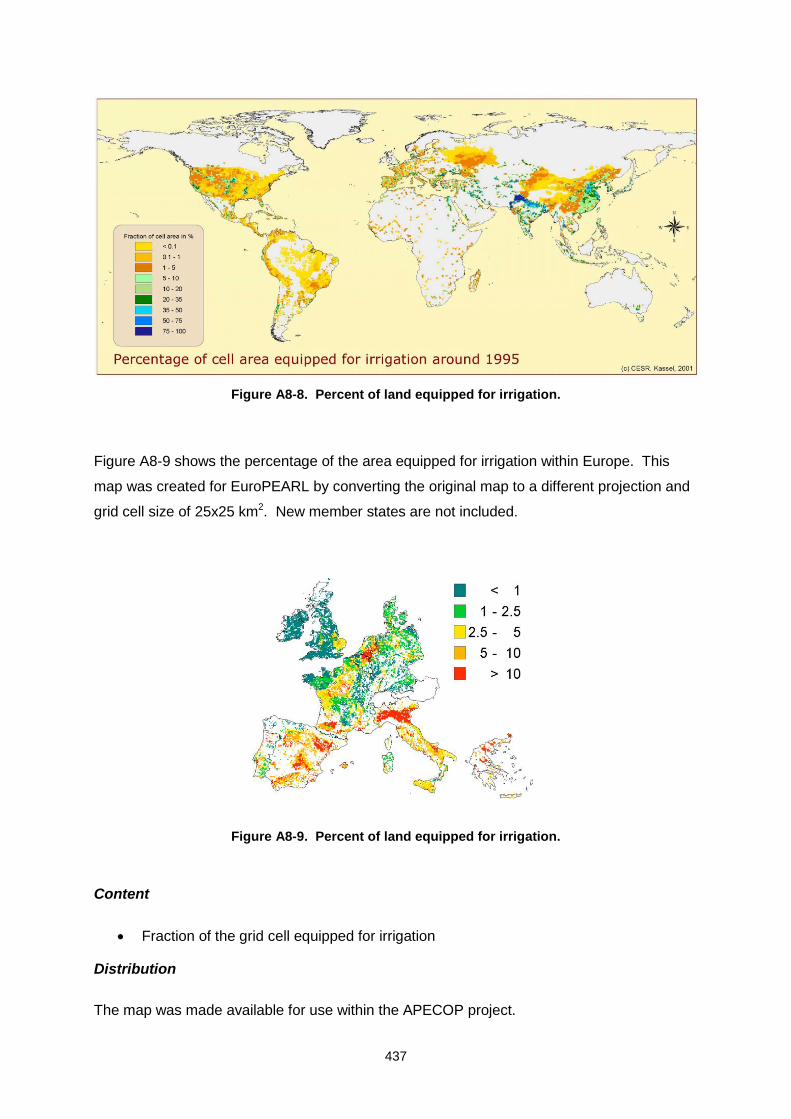
437
Figure A8-8. Percent of land equipped for irrigation.
Figure A8-9 shows the percentage of the area equipped for irrigation within Europe. This
map was created for EuroPEARL by converting the original map to a different projection and
grid cell size of 25x25 km2. New member states are not included.
Figure A8-9. Percent of land equipped for irrigation.
Content
Fraction of the grid cell equipped for irrigation
Distribution
The map was made available for use within the APECOP project.
438
Documentation
Siebert, S. and P. Döll. 2001. A Digital Global Map of Irrigated Areas – An update for Latin
America and Europe. Report A0102, Centre for Environmental Systems Research,
University of Kassel, Germany.
The Map of Organic Carbon in Topsoils in Europe
General Information
In 2004 the European Soil Bureau published a digital map (1 x 1 km raster) of organic carbon
contents in topsoils. The map was compiled by means of transfer functions that considered
soil properties as represented by the European Soil Map, information on land use as given by
CORINE Land Cover and temperature data. A detailed description of the methodology is
given in Jones et al. (2004, 2005). The authors did not consider the moisture status of soils
when compiling the map because the influence of moisture is implicitly taken into account
with the inclusion of the soil type (parameter SOIL) in the soil mapping unit (Jones et al,
2004, 2005). The influence of temperature on organic carbon contents was taken into
account in accordance with the principle that organic matter contents increase when annual
average temperatures are decreasing.
Calculated contents of organic carbon were compared with measured data from soil surveys
in the U.K (5500 data points) and Italy (6800 data points). The comparison of calculated OC
and measured OC revealed a statistically significant match between measured and simulated
data in both sampling regions.
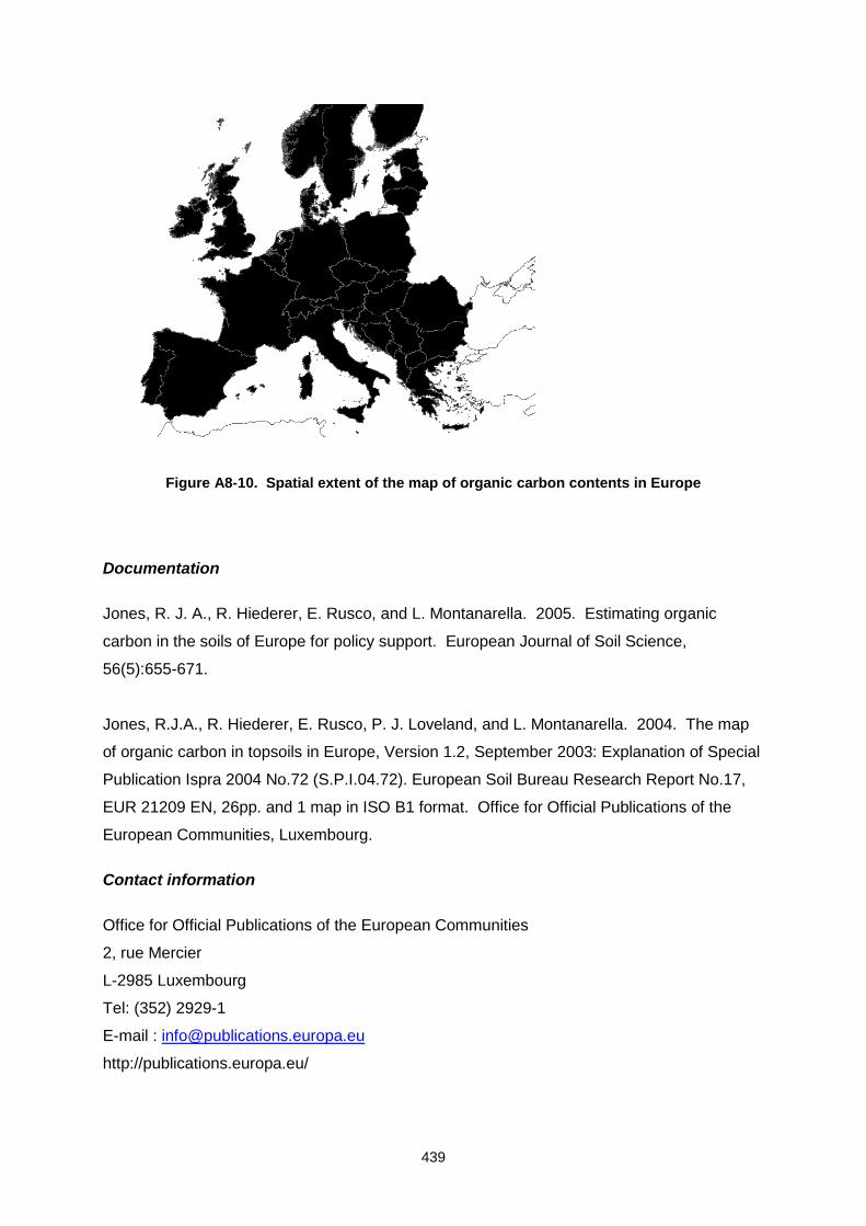
439
Figure A8-10. Spatial extent of the map of organic carbon contents in Europe
Documentation
Jones, R. J. A., R. Hiederer, E. Rusco, and L. Montanarella. 2005. Estimating organic
carbon in the soils of Europe for policy support. European Journal of Soil Science,
56(5):655-671.
Jones, R.J.A., R. Hiederer, E. Rusco, P. J. Loveland, and L. Montanarella. 2004. The map
of organic carbon in topsoils in Europe, Version 1.2, September 2003: Explanation of Special
Publication Ispra 2004 No.72 (S.P.I.04.72). European Soil Bureau Research Report No.17,
EUR 21209 EN, 26pp. and 1 map in ISO B1 format. Office for Official Publications of the
European Communities, Luxembourg.
Contact information
Office for Official Publications of the European Communities
2, rue Mercier
L-2985 Luxembourg
Tel: (352) 2929-1
E-mail : [email protected]
http://publications.europa.eu/
440
APPENDIX 9. COMPARISON OF THE METAPEARL AND INDEX METHOD FOR HIGHER TIER SPATIAL MODELLING
As described in Section 7.2.5, the work group refers to two methods for calculating ground
water vulnerability. In the first method (Appendix 4), referred to as the index method,
attribute data are combined in simple arithmetic rules to yield a vulnerability index. Weights
are assigned to the attributes in terms of the sensitivities of individual parameters to leaching.
The second method is based on a metamodel of EuroPEARL (Appendix 5). The method is
referred to as the MetaPEARL approach. Both methods generate spatial maps of candidate
scenarios meeting the predefined vulnerability concept. Candidate scenarios are
subsequently parameterised before higher tier leaching assessments are made using the
standardised FOCUS models.
Both approaches may yield different spatial maps of candidate scenarios, which
subsequently may impact the ground water assessments. Considering the strategy to
develop harmonised procedures, elucidating and documenting potential differences is
necessary. The objectives of this section are therefore:
i) to compare assessments made by the two present approaches for two contrasting
case studies (a data rich and a data poor environment)
ii) to analyse the strengths and weaknesses of both methods
Comparison of two spatial methods to define candidate scenarios
Materials and methods
The comparison is done using two data sets:
A regional assessment in a data poor environment. The case study is implemented
for assessing a sugar beet cropping scenario in northern France. See Appendix 4 for
more details.
A national assessment in a data rich environment. For this case study, a reference
model (GeoPEARL) is available. The case study is implemented for the Netherlands.
The data set is described in the GeoPEARL manual and available with the model and
some details are given in Appendix 5.
The most important difference between the two data sets is that in the first case there are not
sufficient data available to parameterise a fully spatially-distributed model like GeoPEARL. In
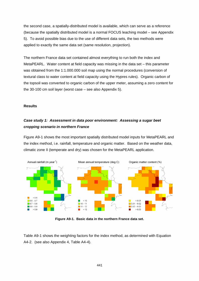
441
the second case, a spatially-distributed model is available, which can serve as a reference
(because the spatially distributed model is a normal FOCUS leaching model – see Appendix
5). To avoid possible bias due to the use of different data sets, the two methods were
applied to exactly the same data set (same resolution, projection).
The northern France data set contained almost everything to run both the index and
MetaPEARL. Water content at field capacity was missing in the data set – this parameter
was obtained from the 1:1.000.000 soil map using the normal procedures (conversion of
textural class to water content at field capacity using the Hypres rules). Organic carbon of
the topsoil was converted to organic carbon of the upper meter, assuming a zero content for
the 30-100 cm soil layer (worst case – see also Appendix 5).
Results
Case study 1: Assessment in data poor environment: Assessing a sugar beet
cropping scenario in northern France
Figure A9-1 shows the most important spatially distributed model inputs for MetaPEARL and
the index method, i.e. rainfall, temperature and organic matter. Based on the weather data,
climatic zone II (temperate and dry) was chosen for the MetaPEARL application.
Figure A9-1. Basic data in the northern France data set.
Table A9-1 shows the weighting factors for the index method, as determined with Equation
A4-2. (see also Appendix 4, Table A4-4).
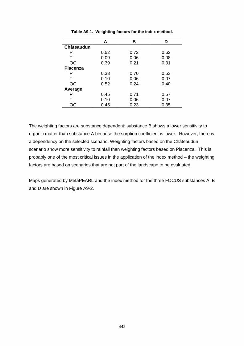
442
Table A9-1. Weighting factors for the index method.
A B D
Châteaudun P 0.52 0.72 0.62 T 0.09 0.06 0.08 OC 0.39 0.21 0.31
Piacenza P 0.38 0.70 0.53 T 0.10 0.06 0.07 OC 0.52 0.24 0.40
Average P 0.45 0.71 0.57 T 0.10 0.06 0.07 OC 0.45 0.23 0.35
The weighting factors are substance dependent: substance B shows a lower sensitivity to
organic matter than substance A because the sorption coefficient is lower. However, there is
a dependency on the selected scenario. Weighting factors based on the Châteaudun
scenario show more sensitivity to rainfall than weighting factors based on Piacenza. This is
probably one of the most critical issues in the application of the index method – the weighting
factors are based on scenarios that are not part of the landscape to be evaluated.
Maps generated by MetaPEARL and the index method for the three FOCUS substances A, B
and D are shown in Figure A9-2.
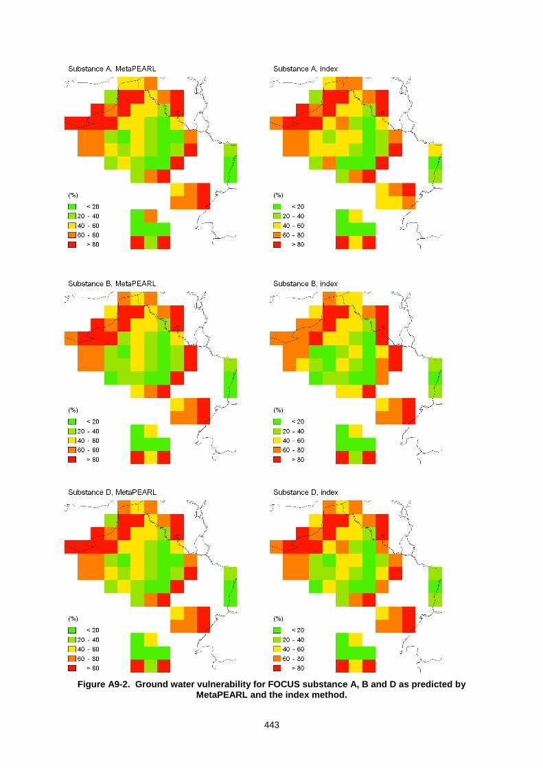
443
Figure A9-2. Ground water vulnerability for FOCUS substance A, B and D as predicted by MetaPEARL and the index method.
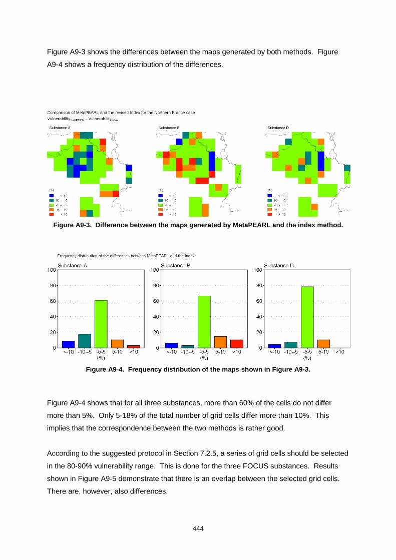
444
Figure A9-3 shows the differences between the maps generated by both methods. Figure
A9-4 shows a frequency distribution of the differences.
Figure A9-3. Difference between the maps generated by MetaPEARL and the index method.
Figure A9-4. Frequency distribution of the maps shown in Figure A9-3.
Figure A9-4 shows that for all three substances, more than 60% of the cells do not differ
more than 5%. Only 5-18% of the total number of grid cells differ more than 10%. This
implies that the correspondence between the two methods is rather good.
According to the suggested protocol in Section 7.2.5, a series of grid cells should be selected
in the 80-90% vulnerability range. This is done for the three FOCUS substances. Results
shown in Figure A9-5 demonstrate that there is an overlap between the selected grid cells.
There are, however, also differences.
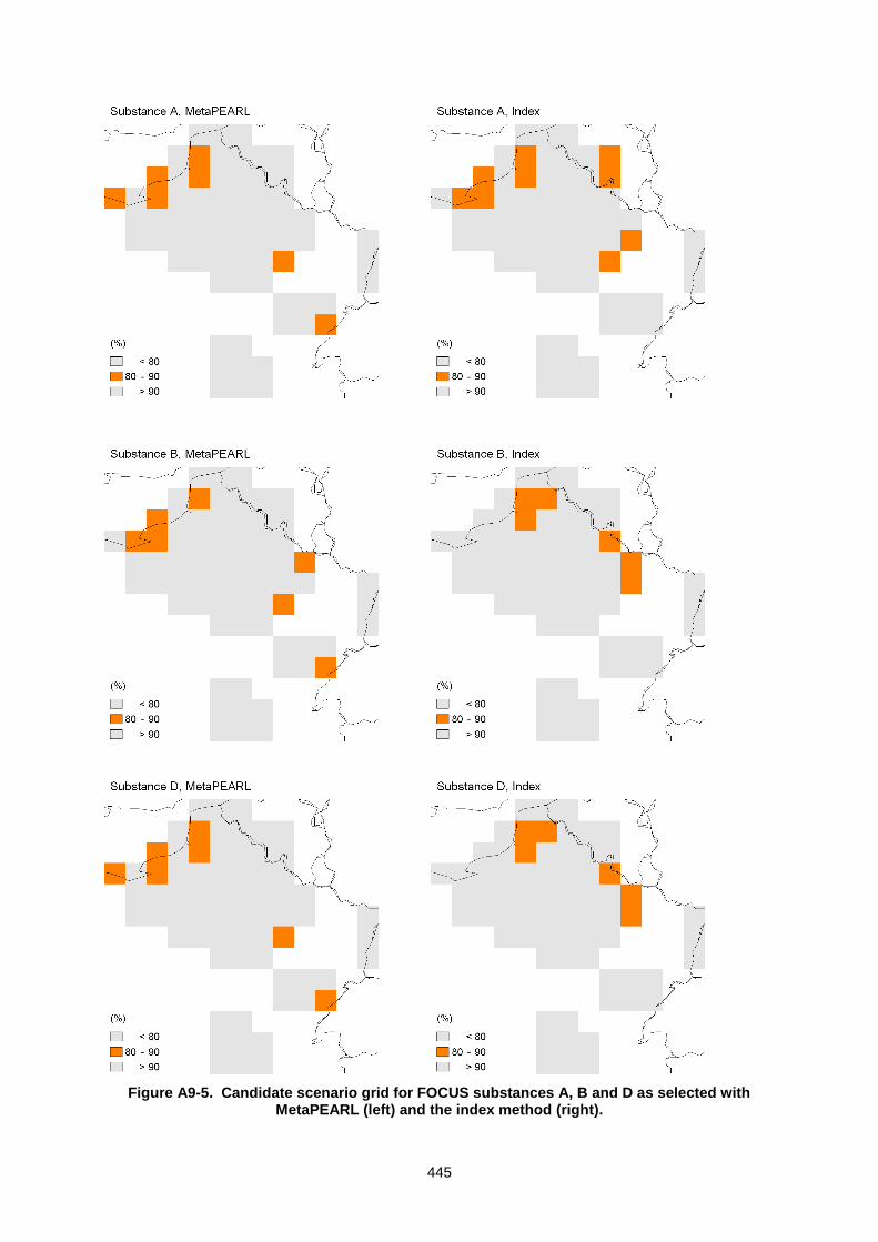
445
Figure A9-5. Candidate scenario grid for FOCUS substances A, B and D as selected with MetaPEARL (left) and the index method (right).
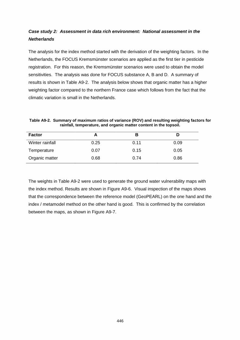
446
Case study 2: Assessment in data rich environment: National assessment in the
Netherlands
The analysis for the index method started with the derivation of the weighting factors. In the
Netherlands, the FOCUS Kremsmünster scenarios are applied as the first tier in pesticide
registration. For this reason, the Kremsmünster scenarios were used to obtain the model
sensitivities. The analysis was done for FOCUS substance A, B and D. A summary of
results is shown in Table A9-2. The analysis below shows that organic matter has a higher
weighting factor compared to the northern France case which follows from the fact that the
climatic variation is small in the Netherlands.
Table A9-2. Summary of maximum ratios of variance (ROV) and resulting weighting factors for rainfall, temperature, and organic matter content in the topsoil.
Factor A B D
Winter rainfall 0.25 0.11 0.09
Temperature 0.07 0.15 0.05
Organic matter 0.68 0.74 0.86
The weights in Table A9-2 were used to generate the ground water vulnerability maps with
the index method. Results are shown in Figure A9-6. Visual inspection of the maps shows
that the correspondence between the reference model (GeoPEARL) on the one hand and the
index / metamodel method on the other hand is good. This is confirmed by the correlation
between the maps, as shown in Figure A9-7.
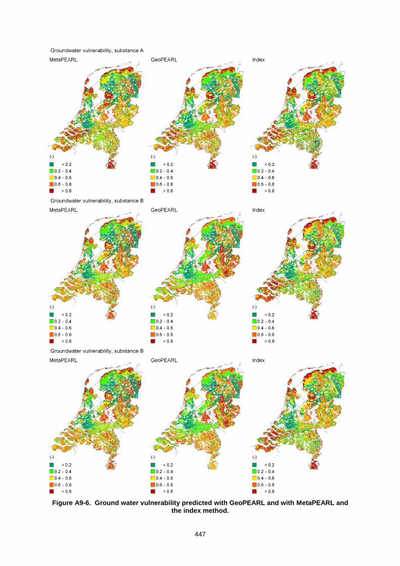
447
Figure A9-6. Ground water vulnerability predicted with GeoPEARL and with MetaPEARL and the index method.
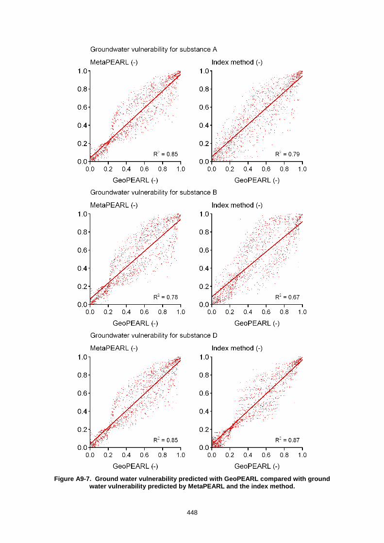
448
Figure A9-7. Ground water vulnerability predicted with GeoPEARL compared with ground water vulnerability predicted by MetaPEARL and the index method.
449
The three methods were used to select 26 use specific Tier 2b scenarios. The crops varied
from major crops (maize and potatoes) to minor crop (legumes and cannabis). First, all plots
in the 80-90th percentile vulnerability range were selected as candidate scenarios. Then the
dominant plots were selected as the final Tier 2b scenario (see Appendix 5 for details).
Results are shown in Figure A9-8. The figure shows that MetaPEARL method generally
performs better than the index method (MetaPEARL is generally slightly above the 1:1 line,
which was intended because Tier 2b scenarios must be more conservative than
GeoPEARL). For substance A and substance B this can be explained from the correlation
between the various vulnerability maps, as shown in Figure A9-7. For substance D, the
lower performance of the index model is hard to explain since the correlation between the
index model and GeoPEARL is almost the same as the correlation between the MetaPEARL
method and GeoPEARL (Figure A9-7).
Figure A9-8. Tier 2b scenario calculations (selected ground water vulnerability maps predicted
by MetaPEARL or the index method) as a function of Tier 3 calculations (simulated with GeoPEARL). The individual points are target concentrations for each of the 26 GeoPEARL
crops.
Conclusions of the comparison, based on the two case studies
The work group refers to the index method (Appendix 4) and metamodel method (Appendix
5) for deriving Tier 2b scenarios. Both methods can be applied in data rich and data poor
environments and therefore the application of either method to the intended use is feasible.
The spatial pattern of ground water vulnerability predicted by the two methods shows a
strong correspondence.
450
In the data rich environment where a benchmark against a full spatially distributed model is
possible, the spatial patterns of ground water vulnerability also compared well to the spatial
pattern predicted by a benchmark model (i.e. GeoPEARL). The correlation is generally above
80% (with an exception for the index model and substance B).
For the case study in data poor environment (the French case), there was an overlap in the
selected candidate scenarios (i.e. the grid cells in the 80-90th percentile range). There were
also, however, different grid cells.
In the data rich environment case study (the Dutch case), 26 use specific scenarios were
selected from the predicted ground water vulnerability maps. The method described in
Appendix 5 was used for this purpose, i.e. the dominant scenario within the 80-90th percentile
range was selected. Despite the fact that the dominant scenario was chosen, both methods
yielded different scenarios in virtually all cases. The regulatory endpoint obtained with tier 2b
scenarios based on MetaPEARL fit the tiered assessment scheme (i.e. they are slightly more
conservative than the predictions by GeoPEARL). In the case of the index, there is more
scatter – some scenarios underestimate the leaching while others overestimate the leaching.
Analysis of strengths and weaknesses of the index and metamodel method
The following criteria should be considered when selecting an appropriate spatially
distributed method in higher tiers:
The method should be effective, i.e. it should meet the preset objective (in this case, it should lead to a conservative estimate of the 80th percentile in space, considering the soil map unit and the rotation time as the support scale for defining the leaching event and this conservatism has to be proven.
The method should be efficient, i.e. it should use available data in an elegant way and lead to a fast, conservative estimate of the percentile in space and should therefore be easy to use.
The method should be transparent and documented.
A summary of the major strengths and weaknesses of both methods is given in the section
below.
The work group could not reach a consensus on a single method to be used in Tier2b.
Maintaining both methods to assess spatial leaching patterns reflects to some extent the
conceptual uncertainty in current understanding of large scale leaching process. The
disadvantage of maintaining both methods is less harmonisation and additional uncertainty.
451
The additional uncertainty is by definition an additional burden in the regulatory decision
making process.
The MetaPearl method
Strengths
Logical rules for selecting vulnerable areas are based on known fate and transport processes since the conceptual FOCUS leaching model is underlying MetaPEARL. Hence the modelling approach is consistent with the modelling approach used at higher tiers and therefore based on current knowledge of the behaviour of system.
The approach is compatible with data in pan-European data bases, and can therefore directly be implemented at the pan European scale.
Application of the European MetaPEARL on the Dutch case study (Appendix 5) showed that the model performance may be scale invariant. It therefore could be used to extrapolate, at least within homogeneous climatic regions.
The logical rule to combine spatially distributed soil-climate data into vulnerability is based on a large set of reference simulations, covering substantially the soil-climate data space in Europe.
The method is fast and easy to implement.
The sensitivities of the MetaPEARL to variation in pesticide (Kom, DegT50) and soil-climate (mean discharge, mean temperature) properties are similar to the sensitivities of the original model FOCUS PEARL model.
The selection of scenarios based on the methodology was, for an illustrated case study in the Netherlands, more conservative than scenarios build on the spatially distributed mechanistic model. This fits perfectly within a tiered assessment scheme.
Weaknesses
Validity cannot be demonstrated.
MetaPEARL inherits all weaknesses of the reference model on which MetaPEARL is based.
MetaPEARL needs calibration with a reference model. Calibration can be space variant and a new version of MetaPEARL may be needed for each cropping area.
The calibration introduces additional uncertainty on the prediction. This uncertainty may however in some cases be very small, but substantially at low concentration levels. Particular problems have been identified in dry climates, characterised by large variability of hydrological fluxes. In such case, spatial patterns generated by the steady state meta-model deviates substantially from the dynamic model simulations. MetaPEARL should not be used to simulate the regulatory end-point.
The calibration results may be biased if the spread of the data points along the regression line is not uniform or if outliers exist. The use of robust regression techniques however should minimise such a bias.
MetaPEARL deviates substantially from the reference model if organic matter profiles are substantially different from the normal profiles found in arable soils (e.g. peat soils covered by marine clay in the Netherlands).
The index method
Strengths
The approach is directly compatible with data in pan-European data base, and can therefore directly be implemented at the pan European scale.
452
The method is fast and easy to implement.
Winter rainfall, organic carbon and mean temperature are considered as major drivers of leaching; other factors which may drive vulnerability (soil moisture which depends also on soil texture, summer rainfall, bulk density, irrigation, time of application (spring or autumn) can be incorporated if appropriate. The method is completely flexible to incorporate landscape factors since it only ranks the occurrence probabilities.
Different factors can be weighted in the logical rule. The weighting factors can be attributed based on expert judgement or sensitivity analysis.
Weaknesses
Validity cannot be demonstrated.
Identification of vulnerability due to soil, climate and crop is based on simplified leaching concept which simplifies the pesticide fate and transport processes, i.e. the vulnerability is expressed as a spatial query in an environmental data base, combining spatial attributes which contribute to possible leaching by means of a simplified logical rule. This logical rule may not reflect the processes such as they are considered in the FOCUS Tier 1 models. Hence, inconsistency with a spatial distributed benchmark model may appear.
The method becomes less objective if expert judgment is used for attributing weighing factors in the logical rules.
The sensitivity analysis is region specific, probably application or product specific and likely scale specific. The weighting factors will therefore be case specific. For the French and Dutch case study, the weighting factors were significantly different.
As a corollary, the weighting factors have been obtained only from a limited range of simulations.
Contributing factors are considered to be normally distributed. This hypothesis may be violated, in particular for organic matter. This assumption may have strong impacts, because the vulnerability assessment is based on the “tail” of the distributions (i.e. 80-percentile in space). These tails are affected strongly by the distribution, particularly in non-linear systems.
In both of the example cases (northern France and the Netherlands) the normality hypothesis was violated. In the Dutch data set, the mean value for organic matter, for example, is 0.12 while the median value is only 0.02, suggesting an extremely skewed distribution (caused by peat soils).
453
APPENDIX 10. THE PRINCIPLES OF INVERSE MODELLING
M. Vanclooster
Components of an inverse model
The forward model
The forward model is the model which calculates system response in terms of output values.
In this case, these are the standard FOCUS leaching models, which calculate time series of
soil moisture, soil temperature, soil pesticide concentrations, soil moisture fluxes, soil heat
fluxes, and soil pesticide fluxes for the boundary conditions corresponding to those of the
experiment.
The objective function
The objective (or merit or goal) function is a measure of the agreement between the data and
a model with a particular parameter set p (e.g. the DegT50 value that has been used).
During an inversion, this objective function will be optimised (i.e. maximised or minimised,
depending on the definition of the objective function).
The criterion usually used is the weighted least squares error function (WLSE) defined as:
N
i
ii xyy1
2*
2,
1pp
or in matrix notation
*1*yyVyyp T
where yi is the ith element of the measured dataset y (e.g. the pesticide concentrations in the
leachate of a lysimeter) at xi (e.g. the different time steps) for i=1,…, N; y*(xi,p) is the ith
modelled answer of the vector y* for xi and parameter set p, ² is the variance and V the
covariance matrix of the measurement errors. In inverse modelling, the WLSE is minimised.
The WLSE can be extended to cases for which each data point (xi,yi) has a different known
standard deviation i (heteroscedasticity):
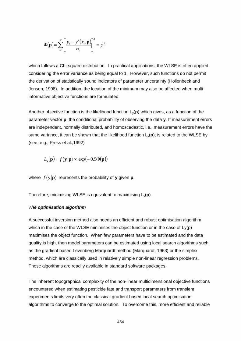
454
2
1
2
,
N
i i
ii xyy pp
which follows a Chi-square distribution. In practical applications, the WLSE is often applied
considering the error variance as being equal to 1. However, such functions do not permit
the derivation of statistically sound indicators of parameter uncertainty (Hollenbeck and
Jensen, 1998). In addition, the location of the minimum may also be affected when multi-
informative objective functions are formulated.
Another objective function is the likelihood function Ly(p) which gives, as a function of the
parameter vector p, the conditional probability of observing the data y. If measurement errors
are independent, normally distributed, and homoscedastic, i.e., measurement errors have the
same variance, it can be shown that the likelihood function Ly(p), is related to the WLSE by
(see, e.g., Press et al.,1992)
ppypy 5.0expfL
where pyf represents the probability of y given p.
Therefore, minimising WLSE is equivalent to maximising Ly(p).
The optimisation algorithm
A successful inversion method also needs an efficient and robust optimisation algorithm,
which in the case of the WLSE minimises the object function or in the case of Ly(p)
maximises the object function. When few parameters have to be estimated and the data
quality is high, then model parameters can be estimated using local search algorithms such
as the gradient based Levenberg Marquardt method (Marquardt, 1963) or the simplex
method, which are classically used in relatively simple non-linear regression problems.
These algorithms are readily available in standard software packages.
The inherent topographical complexity of the non-linear multidimensional objective functions
encountered when estimating pesticide fate and transport parameters from transient
experiments limits very often the classical gradient based local search optimisation
algorithms to converge to the optimal solution. To overcome this, more efficient and reliable
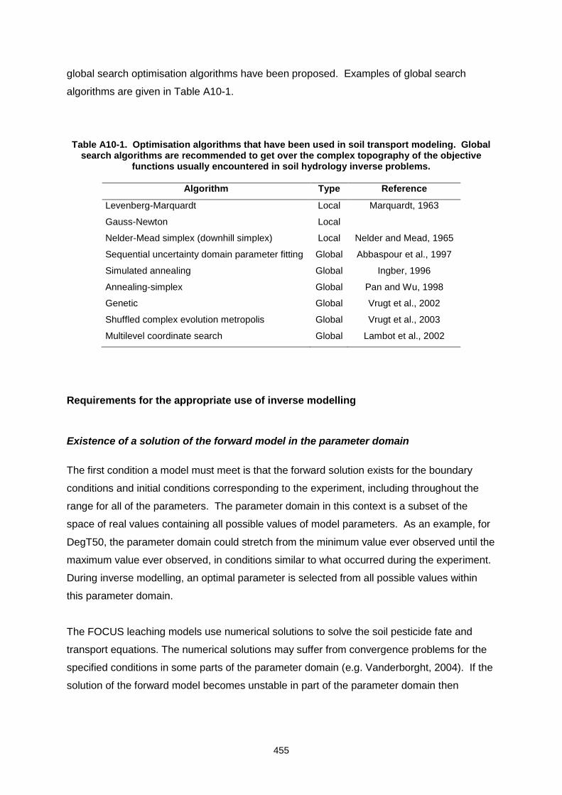
455
global search optimisation algorithms have been proposed. Examples of global search
algorithms are given in Table A10-1.
Table A10-1. Optimisation algorithms that have been used in soil transport modeling. Global search algorithms are recommended to get over the complex topography of the objective
functions usually encountered in soil hydrology inverse problems.
Algorithm Type Reference
Levenberg-Marquardt Local Marquardt, 1963
Gauss-Newton Local
Nelder-Mead simplex (downhill simplex) Local Nelder and Mead, 1965
Sequential uncertainty domain parameter fitting Global Abbaspour et al., 1997
Simulated annealing Global Ingber, 1996
Annealing-simplex Global Pan and Wu, 1998
Genetic Global Vrugt et al., 2002
Shuffled complex evolution metropolis Global Vrugt et al., 2003
Multilevel coordinate search Global Lambot et al., 2002
Requirements for the appropriate use of inverse modelling
Existence of a solution of the forward model in the parameter domain
The first condition a model must meet is that the forward solution exists for the boundary
conditions and initial conditions corresponding to the experiment, including throughout the
range for all of the parameters. The parameter domain in this context is a subset of the
space of real values containing all possible values of model parameters. As an example, for
DegT50, the parameter domain could stretch from the minimum value ever observed until the
maximum value ever observed, in conditions similar to what occurred during the experiment.
During inverse modelling, an optimal parameter is selected from all possible values within
this parameter domain.
The FOCUS leaching models use numerical solutions to solve the soil pesticide fate and
transport equations. The numerical solutions may suffer from convergence problems for the
specified conditions in some parts of the parameter domain (e.g. Vanderborght, 2004). If the
solution of the forward model becomes unstable in part of the parameter domain then
456
difficulties will occur with the inverse model if the optimal parameter is found in this part of the
parameter domain.
Adequacy of the forward model for describing the experiment
Obviously the forward model needs to be adequate for describing the experiment, which
means that the leaching model must be reasonably validated for the conditions of the
experiment. FOCUS leaching models have been subjected to a series of model validation
studies in the past (e.g. Vanclooster et al., 2000; Trevisan et al., 2003) and have often
proven to be well validated for experimental conditions in the validation experiments. Yet,
the conditions of the inverse modelling experiment may differ significantly from the validation
experiments. In such cases, inverse modelling may be inappropriate.
FOCUS leaching models view the transport of pesticide as a one-dimensional vertical
transport process through a vertical heterogeneous soil profile. Hence, for inverse modelling,
only leaching experiments which comply with this hypothesis can be considered. Inverse
modelling is not appropriate when reasonable evidence exists that processes which are not
considered in the leaching model influence the leaching event in the experiment. A typical
example is the occurrence of preferential flow in a cracking clay soil. If a field or lysimeter
experiment is conducted on a cracking clay soil, then this experiment will be of little use for
estimating the fate and transport parameters of a chromatographic flow model. Another
example is the use of a field experiment along a hill slope, where reasonable evidence exists
for horizontal flow in the subsurface (e.g. interflow).
Uniqueness of the forward and the inverse model
Different parameter sets must lead to different solutions of the forward model, if not
parameters are unidentifiable and the inverse modelling is inappropriate. Problems can
therefore occur when more than one solution of the forward model exists. To clarify,
consider the following example. Suppose total leaching has been measured during a crop
season on a one-dimensional lysimeter experiment. The initial model simulation with a given
DegT50 and Kd overestimates the total leaching. In this case, a better simulation could be
obtained if DegT50 is decreased or Kd increased, or both. Hence, for a given DegT50,
different results of total leaching can be obtained by modifying Kd. In this case, the modelling
of total leaching during the crop season in terms of DegT50 is not unique and DegT50 values
cannot be correctly identified from total leaching alone, unless additional information is
available such as the time course of the leaching event within the crop season. In addition, a
457
reliable estimate of individual parameters cannot be obtained when different parameter
combinations lead to the same solution.
Sensitivity of the model
Sensitivity means that the model should depend on the parameters, i.e., the derivative of the
model response to the parameters should be different from zero somewhere in the parameter
domain. A lack of sensitivity results usually in not being able to estimate the parameters.
Since the object function is expressed in terms of the forward model, a lack of sensitivity of
the forward model will result in a lack of sensitivity of the inverse model. Consider the
example where the fraction of water filled macropores for a macropore model needs to be
estimated from a field experiment where only soil volumetric moisture data have been
measured. The activation of macropores in this case will hardly be visible when observing
only volumetric soil moisture content since macropores contribute only to a very small
fraction of the total water filled porosity. Hence, macroporous flow is not sensitive to
volumetric soil moisture data and therefore soil moisture data alone does not allow estimation
of macropore parameters by inverse modelling.
Robustness or stability of the inversion
The solution will be stable if it depends continuously on the measured system response so
that it is not very sensitive to measurement and modelling errors, i.e., small measurement
and modelling errors do not result in large changes of the optimised parameters.
Assessing the validity of inverse modelling results
Uncertainty analysis
Uncertainties in the optimised parameter set originate from either experimental errors (or
measurement errors) or model errors (including errors in the numerical resolution, amongst
others). Both may have a systematic and a random component. However, only the
statistical or random error can be assessed statistically. Formulating the objective function
as a maximum likelihood estimator enables the evaluation of the adequacy of a model for
some given observations (Press et al., 1992; Hollenbeck and Jensen, 1998). At the global
minimum, the objective function follows a Chi-square distribution, and the probability of
model adequacy is then expressed as:
458
PNQpadeq ),(min1 p
where PNQ ),(min p is the Chi-square cumulative density function, N is the number of
observations, and P is the number of optimised parameters. The definition of the threshold
probability for an adequate model is subjective, but usually criterion padeq>0.5 is used. If the
measurement errors are normally distributed and if the model is linear in its parameters or
the sample size is large enough such that the uncertainties in the fitted parameters do not
extend outside a region in which the model could be replaced by a suitable linear model, then
an approximate confidence interval can be defined analytically (Press et al., 1992).
Response surface analysis
Response surface analysis allows documentation of the problems related to non-uniqueness,
model sensitivity, and parameter dependency in an objective and transparent way.
Response surfaces are two-dimensional contour plots representing the objective function as
a function of two parameters, while all the other parameters are held constant at their true
value. Therefore they represent only cross sections of the full M-dimensional parameter
space.
References
Abbaspour, K.C., van Genuchten, M.T., Schulin, R., and Schlappi, E. 1997. A Sequential
Uncertainty Domain Inverse Procedure for Estimating Subsurface Flow and Transport
Parameters. Water Resources Research 33(8):1879-1892.
Hollenbeck, K.J. and Jensen, K.H. 1998. Maximum-likelihood estimation of unsaturated
hydraulic parameters. Journal of Hydrology 210:192-205.
Ingber, L. 1996. Adaptive simulated annealing (ASA): Lessons learned. Control
Cybernetics 25:33-54.
Lambot, S., Javaux, M., Hupet, F., and Vanclooster, M. 2002. A global multilevel coordinate
search procedure for estimating the unsaturated soil hydraulic properties. Water
Resources Research 38(11):1224.
Marquardt, D.W. 1963. An algorithm for least-squares estimation of nonlinear parameters.
J. Soc. Indust. Appl. Math. 11:431-441.
Nelder, J.A. and R. Mead. 1965. A simplex method for function minimisation. Comp. J.
7:308-313.
459
Pan, L.H. and Wu, L.S. 1998. A Hybrid Global Optimisation Method for Inverse Estimation
of Hydraulic Parameters: Annealing-Simplex Method. Water Resources Research
34:(9):2261-2269.
Press, W. H. Teukolsky S. A. Vetterling W. T. Flannery B. P. 1992. Numerical Recipes in
FORTRAN: The Art of Scientific Computing, 2nd ed. Cambridge University Press; New
York.
Trevisan, M. , Padovani, L., Jarvis, N., Roulier, S., Bouraoui, F., Klein, M., and Boesten,
J.J.T.I. 2003. Validation status of the present PEC groundwater models. In: A.A. Del
Re, M. Trevisan, and E. Capri (ed.), XII Pesticide chemistry symposium. Pesticide in air,
plant soil and water system. Piacenza, Italy.
Vanclooster, M., Boesten, J., Trevisan, M., Brown, C., Capri, E., Eklo, O.M., Gottesbüren, B.,
Gouy, V., and van der Linden, A.M.A. 2000. A European test of pesticide-leaching
models: methodology and major recommendations. Agricultural Water Management
44:1-21.
Vanderborght J., R. Kasteel, M. Herbst, M. Javaux, D. Thiery, M. Vanclooster, C. Mouvet and
H. Vereecken. 2004. A test of numerical models for simulating for simulating flow and
transport in soil using analytical solutions. Vadose Zone Journal 4:206-221.
Vrugt, J.A., Bouten, W., Gupta, H.V., and Sorooshian, S. 2002. Toward improved
identifiability of hydrologic model parameters: The information content of experimental
data. Water Resources Research 38: article no. 1312.
Vrugt, J.A., Gupta, H.V., Bouten, W., and Sorooshian, S. 2003. A shuffled complex
evolution metropolis algorithm for optimisation and uncertainty assessment of hydrologic
model parameters. Water Resources Research 39: Doi1201 10.1029/2002WR001642.
460
APPENDIX 11. EXAMPLE OF PARAMETER ADJUSTMENT BY INVERSE MODELLING
This appendix provides an example of the procedure described in Section 8.3.3.4 and is
taken from Kahl et al., 2009).
For a substance Y the DegT50 values from laboratory studies ranged from 18 to 60 days with
an average (geomean) of 47 days. Average values for Kf,OC and 1/n values were 23 dm³/kg
and 0.92, respectively. Calculations with the laboratory parameters at Tier 1 of the FOCUS
ground water assessment scheme indicated a leaching potential.
A lysimeter study was performed over 3 years according to the German lysimeter guideline
(soil = sandy loam A). One lysimeter (A) received applications in year 1 and 2, whereas two
replicate lysimeters (B and C) were applied in the first year only. Annual average
concentrations in the leachate from individual lysimeters were below 0.1 μg/L (< 0.001 to
0.04 μg/L). Kom and DegT50 at reference conditions had been measured in the lysimeter
topsoil were (Kom =18 dm³/kg; DegT50 = 55 days.
The data from one field lysimeters (column A) were used to estimate the substance
parameters DegT50 [day] and the Freundlich sorption coefficient Kom [L/kg] by inverse
modelling together with the uncertainties of the optimised parameter values. The model
PEARL (Tiktak et al., 2000) was used for these calculations.
Three different algorithms for inverse parameter optimisation were considered by Kahl et al.
(2009) . The first algorithm (PEST) is a Levenberg-Marquardt (LM) procedure which is
relatively fast, but may get caught in local optima. The second algorithm (PDMS2) starts
multiple PEST runs with different starting values, which gives a higher probability of obtaining
the global optimum. The third algorithm is SCEM (shuffled complex evolution metropolis),
which has the highest probability of finding the global optimum, but is also the most
demanding in computation time.
The Levenberg Marquardt-method (LM) uses a Jacobian approach and approximates the
objective function based on a linearisation of the model around the optimised parameter set.
This linearisation may result in unrealistic estimates of the parameter uncertainty when the
range of the parameters in the uncertainty intervals is far beyond the range in which the
linear approximation of the model is valid.
461
In an extension of the work of Mertens et al (2009), the pesticide parameters are optimised
for the different soil horizons with respect to adsorption and for the soil layers with an
assumed decrease of degradation with depth according to FOCUS (2000). The target
substance parameters are the adsorption coefficient Kom and the normalised DegT50 (at
reference conditions of 20 °C and pF 2) for the top soil layer.
Calibration
In a first step the water balance was adjusted by optimising the crop factors with the data of
the cumulative outflow from the lysimeter. Four crops with each four crop factors led to a
large number of adjustable parameters. Optimisation of these parameters is difficult due to
the relatively few observations. Best results are achieved by PDMS2, while SCEM
performed worst, by extremely long run times. This is a hint that the default values given in
PEARL are a very good starting point. The optimised values of the crop factors obtained by
PDMS2 are used in further calculations.
In a second step the parameters hydraulic conductivity (ks [cm/day]) and saturated water
content (θs [-]) of each soil horizon were adjusted. For the four horizons this gives a total
eight adjustable parameters. As starting values the van Genuchten parameters as calculated
by HYPRES were chosen. All algorithms lead to results with both unrealistically high and low
parameter values. Further PEST indicated that correlation between horizons is relatively
high. Since the calculation with the initial values yielded similarly good modelling results, the
initial parameter values from HYPRES were used in further calculations.
The simulated versus measured hydrology of the lysimeter used for the inverse modelling of
the substance parameters DegT50 and Kom is shown in Figure A11-1.
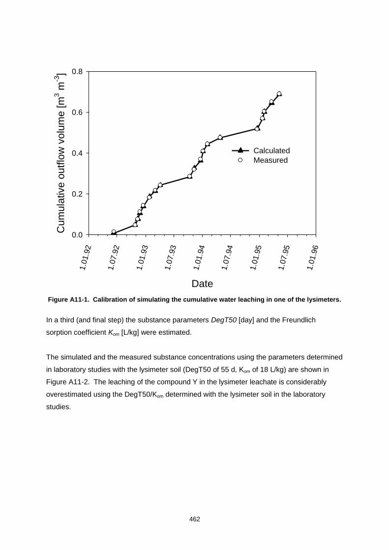
462
Date
1.0
1.9
2
1.0
7.9
2
1.0
1.9
3
1.0
7.9
3
1.0
1.9
4
1.0
7.9
4
1.0
1.9
5
1.0
7.9
5
1.0
1.9
6
Cum
ula
tive o
utflo
w v
olu
me [m
3 m
-3]
0.0
0.2
0.4
0.6
0.8
Calculated
Measured
Figure A11-1. Calibration of simulating the cumulative water leaching in one of the lysimeters.
In a third (and final step) the substance parameters DegT50 [day] and the Freundlich
sorption coefficient Kom [L/kg] were estimated.
The simulated and the measured substance concentrations using the parameters determined
in laboratory studies with the lysimeter soil (DegT50 of 55 d, Kom of 18 L/kg) are shown in
Figure A11-2. The leaching of the compound Y in the lysimeter leachate is considerably
overestimated using the DegT50/Kom determined with the lysimeter soil in the laboratory
studies.
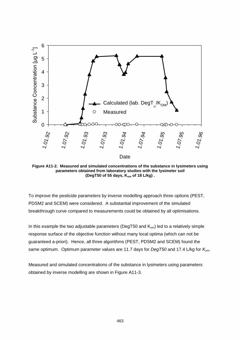
463
Date
1.0
1.9
2
1.0
7.9
2
1.0
1.9
3
1.0
7.9
3
1.0
1.9
4
1.0
7.9
4
1.0
1.9
5
1.0
7.9
5
1.0
1.9
6
Substa
nce C
oncentr
ation [µ
g L
-1]
0
1
2
3
4
5
6
Calculated (lab. DegT50
/KOM
)
Measured
Figure A11-2. Measured and simulated concentrations of the substance in lysimeters using parameters obtained from laboratory studies with the lysimeter soil
(DegT50 of 55 days, Kom of 18 L/kg) .
To improve the pesticide parameters by inverse modelling approach three options (PEST,
PDSM2 and SCEM) were considered. A substantial improvement of the simulated
breakthrough curve compared to measurements could be obtained by all optimisations.
In this example the two adjustable parameters (DegT50 and Kom) led to a relatively simple
response surface of the objective function without many local optima (which can not be
guaranteed a-priori). Hence, all three algorithms (PEST, PDSM2 and SCEM) found the
same optimum. Optimum parameter values are 11.7 days for DegT50 and 17.4 L/kg for Kom.
Measured and simulated concentrations of the substance in lysimeters using parameters
obtained by inverse modelling are shown in Figure A11-3.
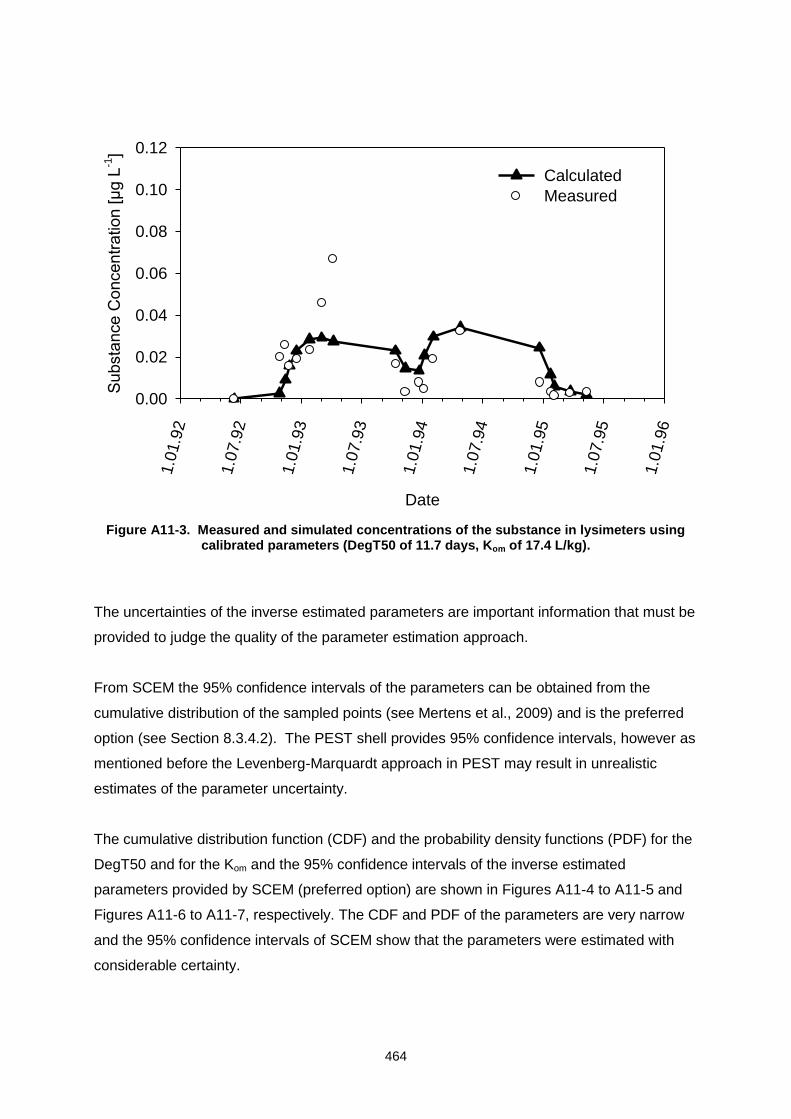
464
Date
1.0
1.9
2
1.0
7.9
2
1.0
1.9
3
1.0
7.9
3
1.0
1.9
4
1.0
7.9
4
1.0
1.9
5
1.0
7.9
5
1.0
1.9
6
Su
bsta
nce
Co
nce
ntr
atio
n [µ
g L
-1]
0.00
0.02
0.04
0.06
0.08
0.10
0.12
Calculated
Measured
Figure A11-3. Measured and simulated concentrations of the substance in lysimeters using calibrated parameters (DegT50 of 11.7 days, Kom of 17.4 L/kg).
The uncertainties of the inverse estimated parameters are important information that must be
provided to judge the quality of the parameter estimation approach.
From SCEM the 95% confidence intervals of the parameters can be obtained from the
cumulative distribution of the sampled points (see Mertens et al., 2009) and is the preferred
option (see Section 8.3.4.2). The PEST shell provides 95% confidence intervals, however as
mentioned before the Levenberg-Marquardt approach in PEST may result in unrealistic
estimates of the parameter uncertainty.
The cumulative distribution function (CDF) and the probability density functions (PDF) for the
DegT50 and for the Kom and the 95% confidence intervals of the inverse estimated
parameters provided by SCEM (preferred option) are shown in Figures A11-4 to A11-5 and
Figures A11-6 to A11-7, respectively. The CDF and PDF of the parameters are very narrow
and the 95% confidence intervals of SCEM show that the parameters were estimated with
considerable certainty.
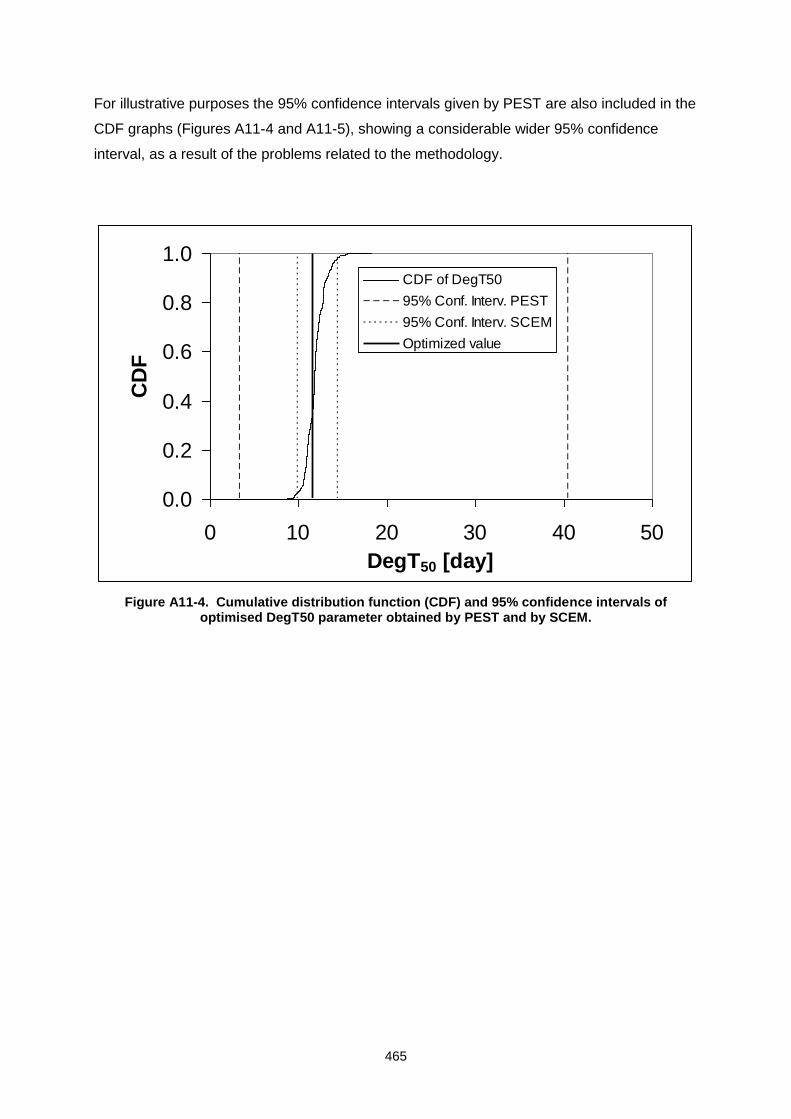
465
For illustrative purposes the 95% confidence intervals given by PEST are also included in the
CDF graphs (Figures A11-4 and A11-5), showing a considerable wider 95% confidence
interval, as a result of the problems related to the methodology.
0.0
0.2
0.4
0.6
0.8
1.0
0 10 20 30 40 50
DegT50 [day]
CD
F
CDF of DegT50
95% Conf. Interv. PEST
95% Conf. Interv. SCEM
Optimized value
Figure A11-4. Cumulative distribution function (CDF) and 95% confidence intervals of optimised DegT50 parameter obtained by PEST and by SCEM.
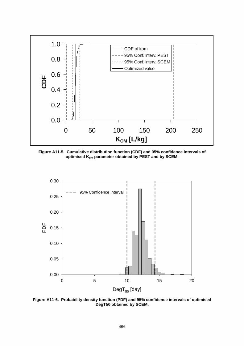
466
0.0
0.2
0.4
0.6
0.8
1.0
0 50 100 150 200 250
KOM [L/kg]
CD
FCDF of kom
95% Conf. Interv. PEST
95% Conf. Interv. SCEM
Optimized value
Figure A11-5. Cumulative distribution function (CDF) and 95% confidence intervals of optimised Kom parameter obtained by PEST and by SCEM.
DegT50
[day]
0 5 10 15 20
PD
F
0.00
0.05
0.10
0.15
0.20
0.25
0.30
95% Confidence Interval
Figure A11-6. Probability density function (PDF) and 95% confidence intervals of optimised DegT50 obtained by SCEM.
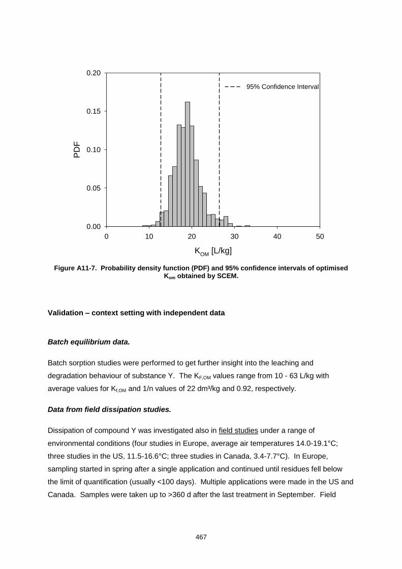
467
KOM
[L/kg]
0 10 20 30 40 50
PD
F
0.00
0.05
0.10
0.15
0.20
95% Confidence Interval
Figure A11-7. Probability density function (PDF) and 95% confidence intervals of optimised Kom obtained by SCEM.
Validation – context setting with independent data
Batch equilibrium data.
Batch sorption studies were performed to get further insight into the leaching and
degradation behaviour of substance Y. The KF,OM values range from 10 - 63 L/kg with
average values for Kf,OM and 1/n values of 22 dm³/kg and 0.92, respectively.
Data from field dissipation studies.
Dissipation of compound Y was investigated also in field studies under a range of
environmental conditions (four studies in Europe, average air temperatures 14.0-19.1°C;
three studies in the US, 11.5-16.6°C; three studies in Canada, 3.4-7.7°C). In Europe,
sampling started in spring after a single application and continued until residues fell below
the limit of quantification (usually <100 days). Multiple applications were made in the US and
Canada. Samples were taken up to >360 d after the last treatment in September. Field
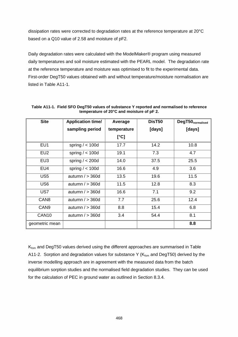
468
dissipation rates were corrected to degradation rates at the reference temperature at 20°C
based on a Q10 value of 2.58 and moisture of pF2.
Daily degradation rates were calculated with the ModelMaker® program using measured
daily temperatures and soil moisture estimated with the PEARL model. The degradation rate
at the reference temperature and moisture was optimised to fit to the experimental data.
First-order DegT50 values obtained with and without temperature/moisture normalisation are
listed in Table A11-1.
Table A11-1. Field SFO DegT50 values of substance Y reported and normalised to reference temperature of 20°C and moisture of pF 2.
Site Application time/
sampling period
Average
temperature
[°C]
DisT50
[days]
DegT50normalised
[days]
EU1 spring / < 100d 17.7 14.2 10.8
EU2 spring / < 100d 19.1 7.3 4.7
EU3 spring / < 200d 14.0 37.5 25.5
EU4 spring / < 100d 16.6 4.9 3.6
US5 autumn / > 360d 13.5 19.6 11.5
US6 autumn / > 360d 11.5 12.8 8.3
US7 autumn / > 360d 16.6 7.1 9.2
CAN8 autumn / > 360d 7.7 25.6 12.4
CAN9 autumn / > 360d 8.8 15.4 6.8
CAN10 autumn / > 360d 3.4 54.4 8.1
geometric mean 8.8
Kfom and DegT50 values derived using the different approaches are summarised in Table
A11-2. Sorption and degradation values for substance Y (Kfom and DegT50) derived by the
inverse modelling approach are in agreement with the measured data from the batch
equilibrium sorption studies and the normalised field degradation studies. They can be used
for the calculation of PEC in ground water as outlined in Section 8.3.4.
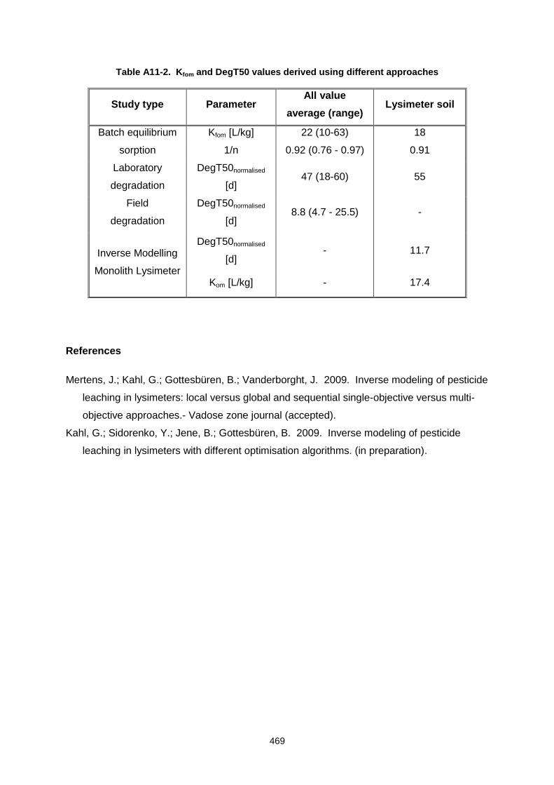
469
Table A11-2. Kfom and DegT50 values derived using different approaches
Study type Parameter All value
average (range) Lysimeter soil
Batch equilibrium
sorption
Kfom [L/kg] 22 (10-63) 18
1/n 0.92 (0.76 - 0.97) 0.91
Laboratory
degradation
DegT50normalised
[d] 47 (18-60) 55
Field
degradation
DegT50normalised
[d] 8.8 (4.7 - 25.5) -
Inverse Modelling
Monolith Lysimeter
DegT50normalised
[d] - 11.7
Kom [L/kg] - 17.4
References
Mertens, J.; Kahl, G.; Gottesbüren, B.; Vanderborght, J. 2009. Inverse modeling of pesticide
leaching in lysimeters: local versus global and sequential single-objective versus multi-
objective approaches.- Vadose zone journal (accepted).
Kahl, G.; Sidorenko, Y.; Jene, B.; Gottesbüren, B. 2009. Inverse modeling of pesticide
leaching in lysimeters with different optimisation algorithms. (in preparation).
470
APPENDIX 12. THEORETICAL BASIS FOR A VULNERABILITY CONCEPT
J. Vanderborght
The purpose of the FOCUS ground water scenarios is to identify whether conditions, which
are relevant for the intended use of the product, exist that guarantee a safe use. A ‘safe use’
guarantees that the overall protection goal, i.e. the concentration of a pesticide in the ground
water should not exceed 0.1 g/L is met. The main problem is to define what is meant by
‘relevant for the intended use’ and the criteria for determining ‘safe’.
Since guaranteeing that under all conditions the protection goal is reached is impossible, the
FOCUS ground water scenarios use a 90 % vulnerability concept (as opposed to a 100 %
vulnerability concept which guarantees that the protection goal is met for all possible
conditions). Different scenarios approximating this 90 % vulnerability concept have been
developed to produce ‘reasonable worst case’ scenarios representing ‘major agricultural
regions’ in Europe with different climatic and pedologic conditions. When applications to a
specific crop for one of these scenarios were shown not to exceed 0.1g/L, this use was
considered to be ‘safe’ and ‘relevant for the intended use’ of the product in the European
Union. However, since these ‘major agricultural regions’ have not been geographically
delineated, they are rather virtual and the relevance of the scenarios cannot be checked.
What is actually meant by ’90 % vulnerability’ and ‘areas relevant for intended use’ is not
defined in a clear cut manner and the lack of this definition is the basis for numerous
discussions.
The purpose of this appendix is to try and define 90 % vulnerability for areas which are
relevant for the intended use and which are geographically delineated if the pesticide
leaching towards the ground water were known at every location in this area. This
vulnerability concept for a hypothetical perfect knowledge of pesticide leaching may form the
basis for a concept that is based on incomplete and uncertain knowledge. This appendix is
not intended to delineate and geographically define ‘areas relevant of intended use’ that are
represented by a certain scenario.
Since pesticide concentrations in the water that recharges the ground water vary both in
space and time, both the temporal and spatial variability are considered in the vulnerability
concept. Based on two extreme mixing concepts, two extreme vulnerability concepts can be
considered: the 100 % and 50 % vulnerability. The first concept (termed here 100 %
471
vulnerability) neglects all mixing process that may dilute concentrations with time and in
space in the ground water. According to this concept, the concentration must be smaller
than 0.1 g/L at every time, t, and at each location, xa where the substance is applied to
satisfy the ground water protection limit:
C(xa;t) < 0.1 g/L for all xa and t. (A12-1)
The second concept (termed here 50 % vulnerability) assumes that all water recharging the
ground water is instantaneously mixed with the entire ground water reservoir or body of the
region. In this concept, the protection limit is achieved when the flux weighted temporally
and spatially averaged concentration is smaller than 0.1 g/L:
11.0
;
;;
gL
dtdtJ
dtdtCtJ
tot t
w
t
w
A
A
aaa
xx
xxx
a (A12-2)
where Jw is the vertical water flux or the recharge rate, Aa is the region where the substance
is applied and Atot the entire region. In the 100% vulnerability concept, no ground water is
exceeding the ground water limit at any time whereas in the 50% concept, the overall
concentration in the entire ground water body is on average below the ground water limit.
Although these concepts can be exactly defined and unequivocally interpreted, they are
irrelevant in practice. High concentrations exceeding the ground water limit can occur
sporadically in the percolating water. But, the amount of water carrying these high
concentrations may only be a minimal fraction of the directly receiving ground water body
and of the total amount of water percolating through the soil over a longer time period so that
the high concentrations may be effectively diluted. On the other hand, the lateral extent of
ground water bodies is much larger than their vertical extent so that the mixing of ground
water in the lateral direction may be considerably limited. This implies that recharge in
subregions where the pesticide is not applied may not or only very limited dilute the recharge
under fields where the substance is actually applied, or the ground water in ‘vulnerable’ areas
where the ground water limit is exceeded cannot mix with ground water in less ‘vulnerable’
areas where the limit is not exceeded.
The definition of an applicable vulnerability concept comes down to identifying the size of an
elementary area, Aa, and elementary time interval, t, over which the pesticide and water
fluxes are averaged and to identifying the proportion of the time intervals and averaging
472
areas to the overall considered time period and application area in which exceeding the
ground water limit is tolerated:
11.0
;
;;
gL
dtdtJ
dtdtCtJ
t
w
t
w
a
a
A
A
aaa
xx
xxx
for x% of all A and t (A12-3)
These spatio-temporal averaging intervals should be based on the size or volume of an
elementary completely mixed ground water volume, V that needs to be protected:
a
A
a xx
a
dtdtJVt
w
; (A12-4)
A problem with the vulnerability concept in Equation A12-3 is to divide the probability over the
spatial and temporal elementary intervals. By defining an elementary completely mixed
ground water volume as the protection goal, the temporal and spatial variability of the
pesticide leaching can be effectively integrated in the vulnerability concept since a ground
water volume represents the integrated vertical water flux or ground water recharge over time
that is in turn integrated over a certain area.
11.0
;
;;
gL
dtdtJ
dtdtCtJ
t
w
t
w
a
a
A
A
aaa
xx
xxx
for x% of all V (A12-5)
In the 100 % vulnerability concept, an infinitesimal ground water body is protected whereas in
the 50 % concept, the totally mixed entire ground water body is protected. The elementary
mixed ground water body can be directly interpreted in practical terms. For instance, for a
drinking water production well, it may be interpreted as the ground water volume in the
capture zone of the well. The capture zone of the well corresponds with the elementary area
over which the ground water recharge and pesticide fluxes are averaged and the time
interval corresponds with the time that is needed to refresh the entire ground water body by
ground water recharge in the well capture zone. A 90 % vulnerability concept could be
defined so that at any time, 90 % of the potential wells in the area where the substance is
applied would produce water with pesticide concentrations below the drinking water limit. If
the time needed to refresh the ground water volume is much larger than the time scale in
473
which most variability of the recharge occurs, e.g. more than 10 years, then the temporal
variability of temporally averaged pesticide fluxes over the elementary time interval at a
certain location can be neglected compared with the spatial variability of the temporally
averaged pesticide fluxes. In that case, only the spatial component plays a role in the
vulnerability concept whereas the temporal fluctuations are averaged out. Since the yearly
ground water recharge is mostly only a small fraction of the total ground water body, the
assumption that temporal fluctuations of yearly flux weighted averaged pesticide
concentrations are important or should be considered in the vulnerability assessment is not
reasonable in view of a vulnerability concept that is based on a practical definition of an
elementary mixed ground water volume. In that perspective, the 80 % spatial percentile of
the 80 % percentile of the yearly averaged concentrations at a certain location, which is
considered as an ‘overall 90 % percentile’, can hardly be linked to a concrete protection goal.
In view of the previous discussion, using the 90 % spatial percentile of the long term
averaged flux weighted averaged concentrations may be a more relevant approach for a
’90 % vulnerability concept’. Note that not only spatial variability of soil properties but also the
spatial variability of climatic conditions needs to be considered.
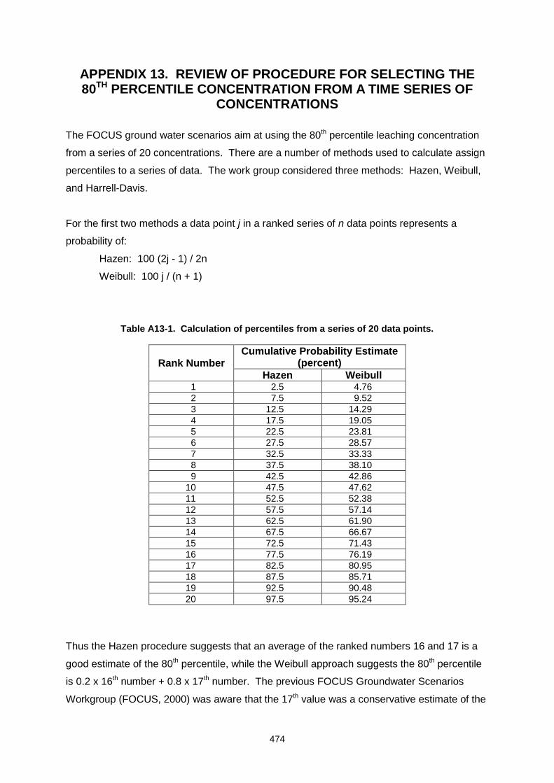
474
APPENDIX 13. REVIEW OF PROCEDURE FOR SELECTING THE 80TH PERCENTILE CONCENTRATION FROM A TIME SERIES OF
CONCENTRATIONS
The FOCUS ground water scenarios aim at using the 80th percentile leaching concentration
from a series of 20 concentrations. There are a number of methods used to calculate assign
percentiles to a series of data. The work group considered three methods: Hazen, Weibull,
and Harrell-Davis.
For the first two methods a data point j in a ranked series of n data points represents a
probability of:
Hazen: 100 (2j - 1) / 2n
Weibull: 100 j / (n + 1)
Table A13-1. Calculation of percentiles from a series of 20 data points.
Rank Number Cumulative Probability Estimate
(percent)
Hazen Weibull 1 2.5 4.76
2 7.5 9.52
3 12.5 14.29
4 17.5 19.05
5 22.5 23.81
6 27.5 28.57
7 32.5 33.33
8 37.5 38.10
9 42.5 42.86
10 47.5 47.62
11 52.5 52.38
12 57.5 57.14
13 62.5 61.90
14 67.5 66.67
15 72.5 71.43
16 77.5 76.19
17 82.5 80.95
18 87.5 85.71
19 92.5 90.48
20 97.5 95.24
Thus the Hazen procedure suggests that an average of the ranked numbers 16 and 17 is a
good estimate of the 80th percentile, while the Weibull approach suggests the 80th percentile
is 0.2 x 16th number + 0.8 x 17th number. The previous FOCUS Groundwater Scenarios
Workgroup (FOCUS, 2000) was aware that the 17th value was a conservative estimate of the
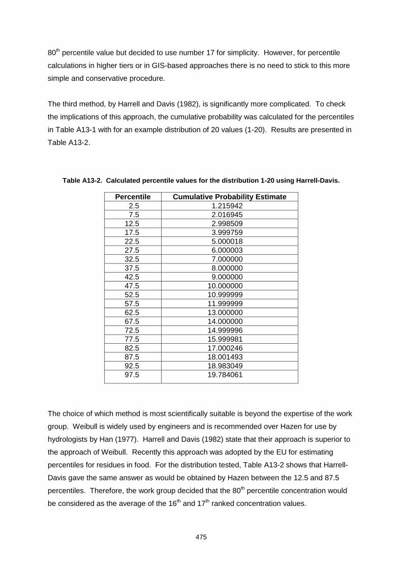
475
80th percentile value but decided to use number 17 for simplicity. However, for percentile
calculations in higher tiers or in GIS-based approaches there is no need to stick to this more
simple and conservative procedure.
The third method, by Harrell and Davis (1982), is significantly more complicated. To check
the implications of this approach, the cumulative probability was calculated for the percentiles
in Table A13-1 with for an example distribution of 20 values (1-20). Results are presented in
Table A13-2.
Table A13-2. Calculated percentile values for the distribution 1-20 using Harrell-Davis.
Percentile Cumulative Probability Estimate
2.5 1.215942
7.5 2.016945
12.5 2.998509
17.5 3.999759
22.5 5.000018
27.5 6.000003
32.5 7.000000
37.5 8.000000
42.5 9.000000
47.5 10.000000
52.5 10.999999
57.5 11.999999
62.5 13.000000
67.5 14.000000
72.5 14.999996
77.5 15.999981
82.5 17.000246
87.5 18.001493
92.5 18.983049
97.5 19.784061
The choice of which method is most scientifically suitable is beyond the expertise of the work
group. Weibull is widely used by engineers and is recommended over Hazen for use by
hydrologists by Han (1977). Harrell and Davis (1982) state that their approach is superior to
the approach of Weibull. Recently this approach was adopted by the EU for estimating
percentiles for residues in food. For the distribution tested, Table A13-2 shows that Harrell-
Davis gave the same answer as would be obtained by Hazen between the 12.5 and 87.5
percentiles. Therefore, the work group decided that the 80th percentile concentration would
be considered as the average of the 16th and 17th ranked concentration values.

476
References
FOCUS. 2000. FOCUS groundwater scenarios in the EU review of active substances.
Report of the FOCUS Groundwater Scenarios Workgroup, EC Document Reference
Sanco/321/2000 rev.2, 202pp.
Han, C. T. 1977. Statistical Methods in Hydrology. Iowa State University Press, Ames IA,
Harrell, F. E., Davis, C. E. 1982. A New Distribution-Free Quantile Estimator. Biometrika
69:635-640.
477
APPENDIX 14. AVERAGING OF SIMULATIONS WITHOUT ANNUAL APPLICATIONS
The vulnerability concept leaves open the option of how to deal with averaging in those
cases where a product is applied every second or third year. The work group considered two
approaches. One was the approach recommended by FOCUS (2000) in which flux-weighted
averages were calculated for each of the 20 two or three year periods, then ranked, and the
80th percentile value chosen. The other was taking the 80th percentile of the 40 or 60 yearly
values. Potentially the approaches could have quite different results. For example, if
essentially all of the movement to ground water occurred in one year of the two or three year
period, the first approach would end up being the concentration for 80th percentile year
divided by two or three while the second approach would be the 40th or 27th percentile year of
the 20 years with residues (but not divided by two or three as in the first case). To determine
the differences between the two approaches, a test case was evaluated using FOCUS PRZM
consisting of compound D from FOCUS (2000) applied to summer potatoes every third year
at an application rate of 1 kg ai/ha. The ratio of annual concentrations approach to the three-
year average approach ranged from 0.02 to 1.12 (Table A16-1). In general both approaches
gave about the same answer with a couple of cases being substantially lower using annual
concentrations. Since there was not much difference between the methods and the reasons
to choose one approach over another are not particularly compelling, the work group decided
not to change the averaging of simulations from the approach of ranking 20 multi-year values
as recommended by FOCUS (2000). Note that this exercise was performed with the
determination of the 80th percentile as recommended by FOCUS (2000). The change in the
calculation of 80th percentile proposed in this report should have minimal effect on the
conclusion from this example.
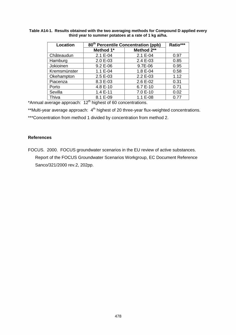
478
Table A14-1. Results obtained with the two averaging methods for Compound D applied every third year to summer potatoes at a rate of 1 kg ai/ha.
Location 80th Percentile Concentration (ppb) Ratio***
Method 1* Method 2**
Châteaudun 2.1 E-04 2.1 E-04 0.97
Hamburg 2.0 E-03 2.4 E-03 0.85
Jokioinen 9.2 E-06 9.7E-06 0.95
Kremsmünster 1.1 E-04 1.8 E-04 0.58
Okehampton 2.5 E-03 2.2 E-03 1.12
Piacenza 8.3 E-03 2.6 E-02 0.31
Porto 4.8 E-10 6.7 E-10 0.71
Sevilla 1.4 E-11 7.0 E-10 0.02
Thiva 8.1 E-09 1.1 E-08 0.77
*Annual average approach: 12th highest of 60 concentrations.
**Multi-year average approach: 4th highest of 20 three-year flux-weighted concentrations.
***Concentration from method 1 divided by concentration from method 2.
References
FOCUS. 2000. FOCUS groundwater scenarios in the EU review of active substances.
Report of the FOCUS Groundwater Scenarios Workgroup, EC Document Reference
Sanco/321/2000 rev.2, 202pp.
479
APPENDIX 15. REVIEW OF THE PORTO AND PIACENZA FOCUS GROUND WATER SCENARIOS
The remit of the FOCUS Ground Water Work Group included reviewing the relative
vulnerability of the Piacenza and Porto scenarios considering the work of the APECOP
project (Vanclooster et al., 2003). If needed new scenarios should be developed, but
changes should be kept to a minimum. This section describes a quantitative re-analysis of
the soil leaching vulnerabilities for the Piacenza and Porto scenarios and makes
recommendations for modifying the scenarios in order to achieve the target 80th percentile
soil vulnerability.
Background
The FOCUS Groundwater Scenarios Workgroup defined Tier 1 ground water modelling
scenarios at nine locations. These scenarios were designed to describe an overall
vulnerability approximating the 90th percentile of all possible situations, in order to collectively
represent realistic worst-case combinations of soil and climatic conditions for leaching in the
EU (FOCUS, 2000). Since the Tier 1 standard scenarios are intended to be used for a wide
range of compounds and crops, a generalised and pragmatic approach to scenario selection
was required, in contrast to the higher-tier crop- and compound-specific methodologies
discussed elsewhere in this document. The scenarios do not mimic specific fields, and nor
are they necessarily representative of the agriculture at the location after which they are
named or in the member states where they are located.
The exact percentile for the soil properties and weather which provide an overall vulnerability
of the 90th percentile cannot be determined precisely without extensive simulations of the
various combinations present in a specific region, and will anyway vary depending on the
compound properties and crop that are simulated. After exploratory statistical analysis, the
work group decided that the overall 90th percentile at the generic Tier 1 level could be best
approximated by using an 80th percentile vulnerability for weather and an 80th percentile
vulnerability for soil. The 80th percentile vulnerability for weather was determined by
performing simulations using multi-year weather data and selecting the 17th highest annual
concentration from 20 years of results, while the 80th percentile vulnerability for soil was
selected by expert judgement.
The FOCUS Groundwater Scenarios Workgroup acknowledged that reviewing the selection
procedure at a future date in light of new findings and better data availability may be
480
appropriate. Subsequently, the APECOP project conducted research aimed at validating the
selection of realistic worst case ground water modelling scenarios, by comparing PECGW for
each FOCUS scenario against the 90th percentile value found within the respective agro-
climatic zone using a spatial modelling approach (Table A15-1). The results of the APECOP
project indicate that the Piacenza scenarios generally represent an extreme, i.e. unrealistic
worst-case within the respective agro-climatic zone. By contrast, the results indicate that the
Porto scenarios generally do not represent a sufficiently worst-case situation within the
respective agro-climatic zone in relation to the target 90th percentile.
Table A15-1. Extent of the FOCUS agro-climatic zones. Source: Table 2.1 from FOCUS (2000).
Precipitation (mm)
Mean Annual Temperature
(C)
Arable land * (%)
Total Area * (%)
Representative Locations
601 to 800 5 to 12.5 31 19 Hamburg/Châteaudun
801 to 1000 5 to 12.5 18 13 Kremsmünster
1001 to 1400 5 to 12.5 15 12 Okehampton
601 to 800 > 12.5 13 11 Sevilla/Thiva **
801 to 1000 > 12.5 9 8 Piacenza
< 600 > 12.5 4 4 Sevilla/Thiva
< 600 5 to 12.5 3 2 Châteaudun ***
1001 to 1400 > 12.5 3 3 Porto
< 600 < 5 1 11 Jokioinen
Other combinations 3 17 -
* Relative to the area of the EU-15 plus Norway and Switzerland.
** Although these locations have less than 600 mm of precipitation, irrigation typically used at
these two locations brings the total amount of water to greater than 600 mm.
*** Most areas in this climatic zone will be irrigated, raising the total amount of water to
greater than 600 mm. Therefore, Châteaudun can be considered representative of
agriculture in this climatic zone.
Methodology
The selection of representative (80th percentile) soil properties in the original definitions of the
FOCUS ground water Tier 1 scenarios was based on expert judgement due to the lack of
comprehensive soil data bases at that time. A quantitative re-analysis of the soil leaching
vulnerabilities of the Piacenza and Porto scenarios was performed in order to identify suitable
modifications to the scenarios to achieve the target vulnerability. Since soil organic carbon

481
content has been found to be the most sensitive soil property in determining the leaching of
pesticides (e.g. Piñeros-Garcet et al., 2003, as cited by Vanclooster et al., 2003; Schlosser &
McCray, 2002), and lends itself to quantitative analysis using state-of-the-art European soil
data bases, in this analysis topsoil organic carbon content was assumed to provide a good
indicator of soil vulnerability to pesticide leaching.
The original FOCUS analysis of climatic zones was based on 5 km raster data from the EU
project by Knoche et al. (1998), as described in FOCUS (2000, Section 2.1.3). These data
were obtained from the Fraunhofer Institute in order to extend the analysis to the quantitative
assessment of soil vulnerability for the Piacenza and Porto climatic zones, using pan-
European ‘OCTOP’ topsoil organic carbon content data that have recently been made
available (Jones et al., 2004; 2005). The data layers used in the analysis were as follows:
Climatic zones from the Fraunhofer data (reconstructed from the long-term average
temperature and precipitation data according to the values given in Table A15-1
Arable areas from the Fraunhofer data (reconstructed from the original 0 – 255 land
use classification and the aggregated land use codes provided by M. Klein)
OCTOP data from the European Commission Joint Research Centre
Since the OCTOP data base is at 1 km resolution whereas the climatic and land use data
were only available at 5 km resolution, the OCTOP data were first aggregated to 5 km
resolution using average values in each cell. Values from the original data layer in the range
0 – 0.1% OC were excluded from the analysis, i.e. reclassified as ‘no data’.
The cells with arable land use for the Piacenza and Porto climatic zones were extracted from
the 5 km OCTOP layer using GIS analysis. The values were ranked and the cumulative
percentages were plotted in order to determine the 20th percentile topsoil organic carbon
content for each of these climatic zones, taken as equivalent to the 80th percentile soil
vulnerability.
Results of the analysis
The 20th percentile OC content in the Piacenza and Porto climatic zones was calculated to be
1.26% and 1.42%, respectively. The distributions of organic carbon within the FOCUS
Piacenza and Porto climatic zones are shown in Figure A15-1.
The current topsoil organic carbon content of 1% in the Piacenza soil profile is too low in
comparison to the target value of 1.26%, leading to a leaching vulnerability that is too high.
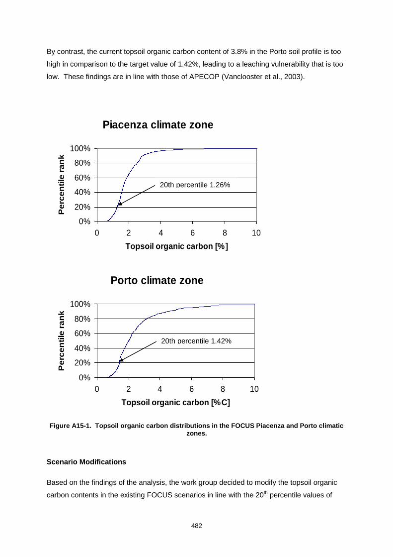
482
By contrast, the current topsoil organic carbon content of 3.8% in the Porto soil profile is too
high in comparison to the target value of 1.42%, leading to a leaching vulnerability that is too
low. These findings are in line with those of APECOP (Vanclooster et al., 2003).
Piacenza climate zone
0%
20%
40%
60%
80%
100%
0 2 4 6 8 10
Topsoil organic carbon [%]
Pe
rce
nti
le r
an
k
Porto climate zone
0%
20%
40%
60%
80%
100%
0 2 4 6 8 10
Topsoil organic carbon [%C]
Pe
rce
nti
le r
an
k
Figure A15-1. Topsoil organic carbon distributions in the FOCUS Piacenza and Porto climatic zones.
Scenario Modifications
Based on the findings of the analysis, the work group decided to modify the topsoil organic
carbon contents in the existing FOCUS scenarios in line with the 20th percentile values of
20th percentile 1.42%
20th percentile 1.26%
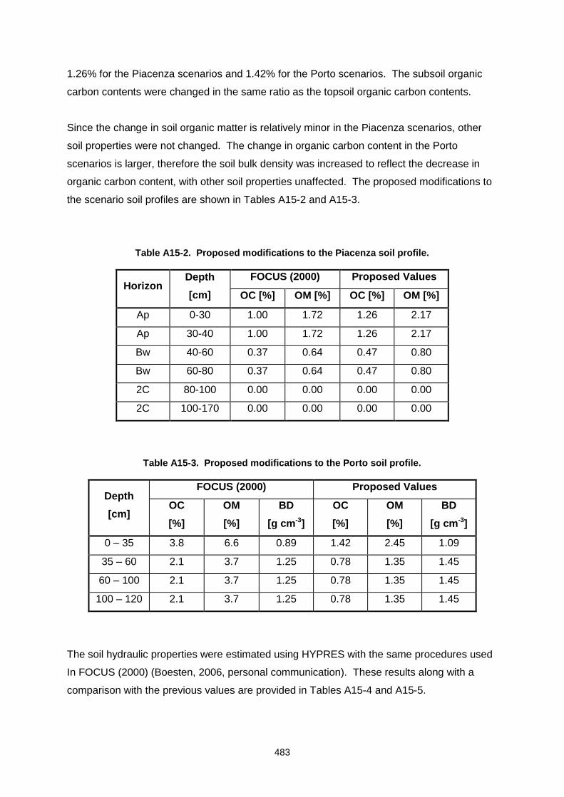
483
1.26% for the Piacenza scenarios and 1.42% for the Porto scenarios. The subsoil organic
carbon contents were changed in the same ratio as the topsoil organic carbon contents.
Since the change in soil organic matter is relatively minor in the Piacenza scenarios, other
soil properties were not changed. The change in organic carbon content in the Porto
scenarios is larger, therefore the soil bulk density was increased to reflect the decrease in
organic carbon content, with other soil properties unaffected. The proposed modifications to
the scenario soil profiles are shown in Tables A15-2 and A15-3.
Table A15-2. Proposed modifications to the Piacenza soil profile.
Horizon Depth
[cm]
FOCUS (2000) Proposed Values
OC [%] OM [%] OC [%] OM [%]
Ap 0-30 1.00 1.72 1.26 2.17
Ap 30-40 1.00 1.72 1.26 2.17
Bw 40-60 0.37 0.64 0.47 0.80
Bw 60-80 0.37 0.64 0.47 0.80
2C 80-100 0.00 0.00 0.00 0.00
2C 100-170 0.00 0.00 0.00 0.00
Table A15-3. Proposed modifications to the Porto soil profile.
Depth
[cm]
FOCUS (2000) Proposed Values
OC
[%]
OM
[%]
BD
[g cm-3]
OC
[%]
OM
[%]
BD
[g cm-3]
0 – 35 3.8 6.6 0.89 1.42 2.45 1.09
35 – 60 2.1 3.7 1.25 0.78 1.35 1.45
60 – 100 2.1 3.7 1.25 0.78 1.35 1.45
100 – 120 2.1 3.7 1.25 0.78 1.35 1.45
The soil hydraulic properties were estimated using HYPRES with the same procedures used
In FOCUS (2000) (Boesten, 2006, personal communication). These results along with a
comparison with the previous values are provided in Tables A15-4 and A15-5.
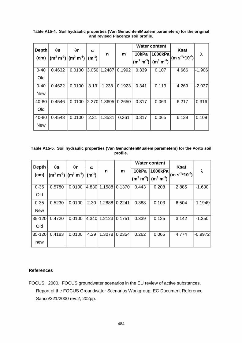
484
Table A15-4. Soil hydraulic properties (Van Genuchten/Mualem parameters) for the original and revised Piacenza soil profile.
Depth
(cm)
s
(m3 m-3)
r
(m3 m-3)
(m-1) n m
Water content Ksat
(m s-1*10-6) 10kPa
(m3 m-3)
1600kPa
(m3 m-3)
0-40
Old
0.4632 0.0100 3.050 1.2487 0.1992 0.339 0.107 4.666 -1.906
0-40
New
0.4622 0.0100 3.13 1.238 0.1923 0.341 0.113 4.269 -2.037
40-80
Old
0.4546 0.0100 2.270 1.3605 0.2650 0.317 0.063 6.217 0.316
40-80
New
0.4543 0.0100 2.31 1.3531 0.261 0.317 0.065 6.138 0.109
Table A15-5. Soil hydraulic properties (Van Genuchten/Mualem parameters) for the Porto soil profile.
Depth
(cm)
s
(m3 m-3)
r
(m3 m-3)
(m-1) n m
Water content Ksat
(m s-1*10-6) 10kPa
(m3 m-3)
1600kPa
(m3 m-3)
0-35
Old
0.5780 0.0100 4.830 1.1588 0.1370 0.443 0.208 2.885 -1.630
0-35
New
0.5230 0.0100 2.30 1.2888 0.2241 0.388 0.103 6.504 -1.1949
35-120
Old
0.4720 0.0100 4.340 1.2123 0.1751 0.339 0.125 3.142 -1.350
35-120
new
0.4183 0.0100 4.29 1.3078 0.2354 0.262 0.065 4.774 -0.9972
References
FOCUS. 2000. FOCUS groundwater scenarios in the EU review of active substances.
Report of the FOCUS Groundwater Scenarios Workgroup, EC Document Reference
Sanco/321/2000 rev.2, 202pp.
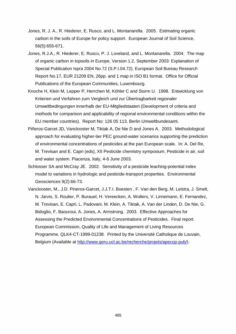
485
Jones, R. J. A., R. Hiederer, E. Rusco, and L. Montanarella. 2005. Estimating organic
carbon in the soils of Europe for policy support. European Journal of Soil Science,
56(5):655-671.
Jones, R.J.A., R. Hiederer, E. Rusco, P. J. Loveland, and L. Montanarella. 2004. The map
of organic carbon in topsoils in Europe, Version 1.2, September 2003: Explanation of
Special Publication Ispra 2004 No.72 (S.P.I.04.72). European Soil Bureau Research
Report No.17, EUR 21209 EN, 26pp. and 1 map in ISO B1 format. Office for Official
Publications of the European Communities, Luxembourg.
Knoche H, Klein M, Lepper P, Herrchen M, Köhler C and Storm U. 1998. Entwicklung von
Kriterien und Verfahren zum Vergleich und zur Übertragbarkeit regionaler
Umweltbedingungen innerhalb der EU-Mitgliedstaaten (Development of criteria and
methods for comparison and applicability of regional environmental conditions within the
EU member countries). Report No: 126 05 113, Berlin Umweltbundesamt.
Piñeros-Garcet JD, Vanclooster M, Tiktak A, De Nie D and Jones A. 2003. Methodological
approach for evaluating higher-tier PEC ground-water scenarios supporting the prediction
of environmental concentrations of pesticides at the pan European scale. In: A. Del Re,
M. Trevisan and E. Capri (eds), XII Pesticide chemistry symposium, Pesticide in air, soil
and water system. Piacenza, Italy, 4-6 June 2003.
Schlosser SA and McCray JE. 2002. Sensitivity of a pesticide leaching-potential index
model to variations in hydrologic and pesticide-transport properties. Environmental
Geosciences 9(2):66-73.
Vanclooster, M., J.D. Pineros-Garcet, J.J.T.I. Boesten , F. Van den Berg, M. Leistra, J. Smelt,
N. Jarvis, S. Roulier, P. Burauel, H. Vereecken, A. Wolters, V. Linnemann, E. Fernandez,
M. Trevisan, E. Capri, L. Padovani, M. Klein, A. Tiktak, A. Van der Linden, D. De Nie, G.
Bidoglio, F. Baouroui, A. Jones, A. Armstrong. 2003. Effective Approaches for
Assessing the Predicted Environmental Concentrations of Pesticides. Final report.
European Commission, Quality of Life and Management of Living Resources
Programme. QLK4-CT-1999-01238. Printed by the Université Catholique de Louvain,
Belgium (Available at http://www.geru.ucl.ac.be/recherche/projets/apecop-pub/).
486
APPENDIX 16. LITERATURE REVIEW OF DISPERSIVITY VALUES
J. Vanderborght
Introduction and Background
In all of the FOCUS ground water scenarios, except for the Châteaudun scenarios when
parameterised for use with MACRO, the convection dispersion equation is used to describe
the leaching of pesticides:
SCz
CD
zz
Cv
t
S
t
Cbb
(A16-1)
where is the volumetric water content, C the concentration in the soil water, b the soil bulk
density, S the concentration of the sorbed phase, v the pore water velocity, D the
hydrodynamic dispersion coefficient, and a first order decay constant.
The hydrodynamic dispersion coefficient D is defined as:
0DvD (A16-2)
where (L) is the dispersivity, v (L T-1) is the transport velocity, a tortuosity coefficient
which depends on the volumetric soil water content, , and D0 (L² T-1) the molecular diffusion
coefficient.
A study by Boesten (2004) showed that a different parameterisation of the dispersivity
explained to a large extent the differences between pesticide leaching calculated by the
PRZM and PELMO models (using a of 2.5 cm) and by the PEARL model (using a of 5
cm). A harmonisation of the dispersivity parameterisation in the different models is therefore
expected to harmonise the calculated pesticide concentrations by the different models.
A data set of dispersivity values was compiled by reviewing leaching experiments that were
reported in the literature. In leaching experiments, depth profiles or time series of an inert
tracer are measured. From these profiles or time series, the hydrodynamic dispersion
coefficient, D, and the pore water velocity v are derived. This is generally done assuming
that the transport velocity v and dispersion coefficient D are constant in the soil profile and do
not change with depth, i.e. a hydrodynamically homogeneous soil profile. For an effective
molecular diffusion coefficient (() D0) of 0.5 cm² d-1, the contribution of the diffusion to the
hydrodynamic dispersion D observed in the leaching experiments was on average 5%.
Therefore, the dispersivity, , was simply derived from the ratio D/v assuming that the
molecular diffusion can be neglected.
487
Contents of dispersivity data base
The data base contains 635 entries derived from 57 publications in scientific journals. Since
soil structure has an important impact on solute transport, only experiments in undisturbed
soils were considered and experiments in repacked or refilled soil cores or columns were
excluded. Besides dispersivities, also experimental factors were included in the data base so
that relations between experimental factors and dispersivities can be inferred. The
experimental factors form the basis for selection or exclusion of certain leaching studies
which are considered to be in agreement or disagreement with the climatic and pedologic
conditions that are represented by the FOCUS scenarios.
The following variables were included:
transport distance z (cm),i.e. the vertical distance that the applied tracer travelled
the dispersivity (cm)
the transport velocity v (cm d-1) derived from the tracer breakthrough or concentration
depth profiles
the pore water velocity vp (cm d-1) derived from the flow rate divided by the volumetric
water content
the ratio of v/vp which is a measure for preferential solute transport (v/vp > 1) or solute
retardation (v/vp < 1)
the average flow rate Jw (cm d-1) which is the net infiltrated water depth during the
leaching experiment divided by the duration of the experiment
the effective flow rate Jweff (cm d-1) which is a measure for the flow rate intensity in the
soil during the experiment (for a definition see Vanderborght et al., 2000)
the experiment number (The same experiment number was given to dispersivities that
were derived from a leaching experiment that was carried in the same soil column or
field plot, at the same flow rate, and that was monitored using the same measurement
technique)
the name of the field site where experiments were carried out or from where soil
samples were taken
USDA soil texture class
scale of the leaching experiments [Three classes were considered: core-scale (soil
cores with a length < 30 cm), column scale (undisturbed soil monoliths with a length >
30 cm), and field scale]
type of concentration that was measured: volume averaged or resident versus flux
averaged concentrations

488
measurement type: direct (in the effluent from soil columns or cores), coring (analysis
of soil samples), samplers (extraction of soil solution in the soil profile using suction
samplers or suction plates), TDR (concentrations derived from bulk soil electrical
conductivity measured with TDR), tile drains, dye tracers (image analysis of
photographic recordings of dye stained patterns on excavated soil surfaces),
calculated (average concentrations calculated from the average of local concentration
measurements)
flow type: steady (steady unsaturated flow), ponding (steady flow under saturated flow
conditions), intermittent (periodic flow under unsaturated conditions), interpond
(periodic ponding of the soil surface), climatic (natural rainfall and soil evaporation),
interclim (natural rainfall and soil evaporation with intermittent additional water
application)
Author
Year of publication
A complete list is appended to the end of this appendix.
Effect of experimental factors on dispersivity
Scale of the study, flow boundary condition type, and soil texture are considered to be the
most important experimental factors. Figures A16-1 to A16-3 show the number of data
entries as a function of these factors. These figures also provide the mean dispersivity
observed and the mean values of the flow rate and transport distance in the experiments.
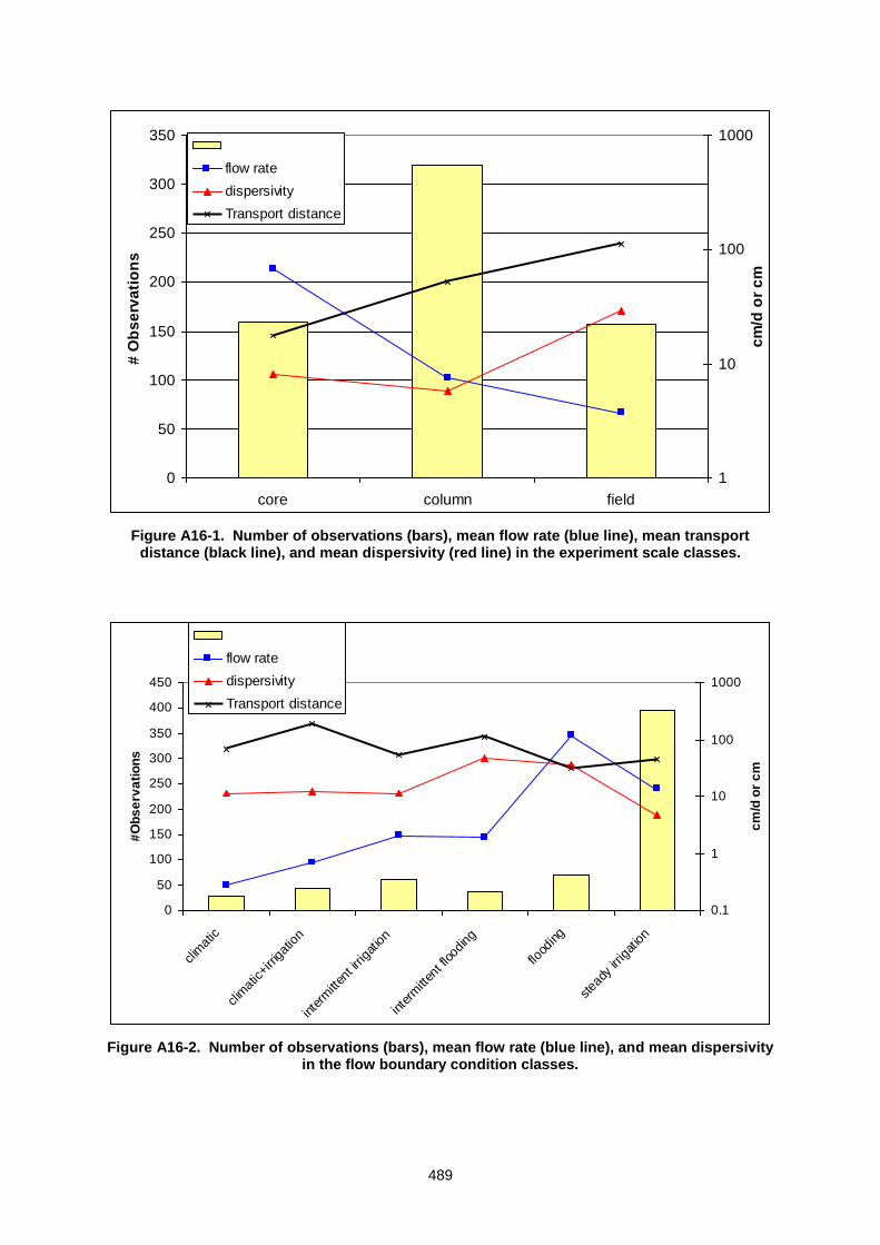
489
0
50
100
150
200
250
300
350
core column field
# O
bs
erv
ati
on
s
1
10
100
1000
cm
/d o
r c
m
flow rate
dispersivity
Transport distance
Figure A16-1. Number of observations (bars), mean flow rate (blue line), mean transport distance (black line), and mean dispersivity (red line) in the experiment scale classes.
0
50
100
150
200
250
300
350
400
450
clim
atic
clim
atic+i
rrigat
ion
inte
rmitt
ent irrig
ation
inte
rmitt
ent f
lood
ing
flood
ing
stea
dy ir
rigat
ion
#O
bs
erv
ati
on
s
0.1
1
10
100
1000
cm
/d o
r c
m
flow rate
dispersivity
Transport distance
Figure A16-2. Number of observations (bars), mean flow rate (blue line), and mean dispersivity in the flow boundary condition classes.
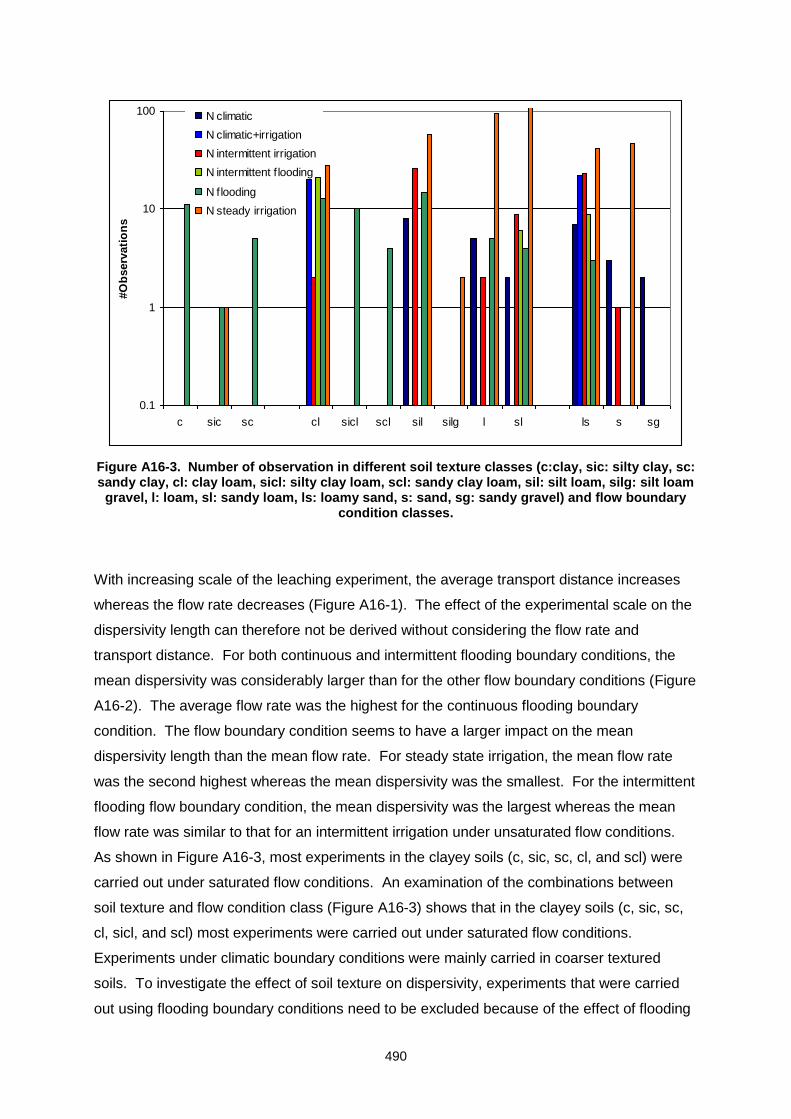
490
0.1
1
10
100
c sic sc cl sicl scl sil silg l sl ls s sg
#O
bserv
ati
on
sN climatic
N climatic+irrigation
N intermittent irrigation
N intermittent f looding
N flooding
N steady irrigation
Figure A16-3. Number of observation in different soil texture classes (c:clay, sic: silty clay, sc: sandy clay, cl: clay loam, sicl: silty clay loam, scl: sandy clay loam, sil: silt loam, silg: silt loam
gravel, l: loam, sl: sandy loam, ls: loamy sand, s: sand, sg: sandy gravel) and flow boundary condition classes.
With increasing scale of the leaching experiment, the average transport distance increases
whereas the flow rate decreases (Figure A16-1). The effect of the experimental scale on the
dispersivity length can therefore not be derived without considering the flow rate and
transport distance. For both continuous and intermittent flooding boundary conditions, the
mean dispersivity was considerably larger than for the other flow boundary conditions (Figure
A16-2). The average flow rate was the highest for the continuous flooding boundary
condition. The flow boundary condition seems to have a larger impact on the mean
dispersivity length than the mean flow rate. For steady state irrigation, the mean flow rate
was the second highest whereas the mean dispersivity was the smallest. For the intermittent
flooding flow boundary condition, the mean dispersivity was the largest whereas the mean
flow rate was similar to that for an intermittent irrigation under unsaturated flow conditions.
As shown in Figure A16-3, most experiments in the clayey soils (c, sic, sc, cl, and scl) were
carried out under saturated flow conditions. An examination of the combinations between
soil texture and flow condition class (Figure A16-3) shows that in the clayey soils (c, sic, sc,
cl, sicl, and scl) most experiments were carried out under saturated flow conditions.
Experiments under climatic boundary conditions were mainly carried in coarser textured
soils. To investigate the effect of soil texture on dispersivity, experiments that were carried
out using flooding boundary conditions need to be excluded because of the effect of flooding
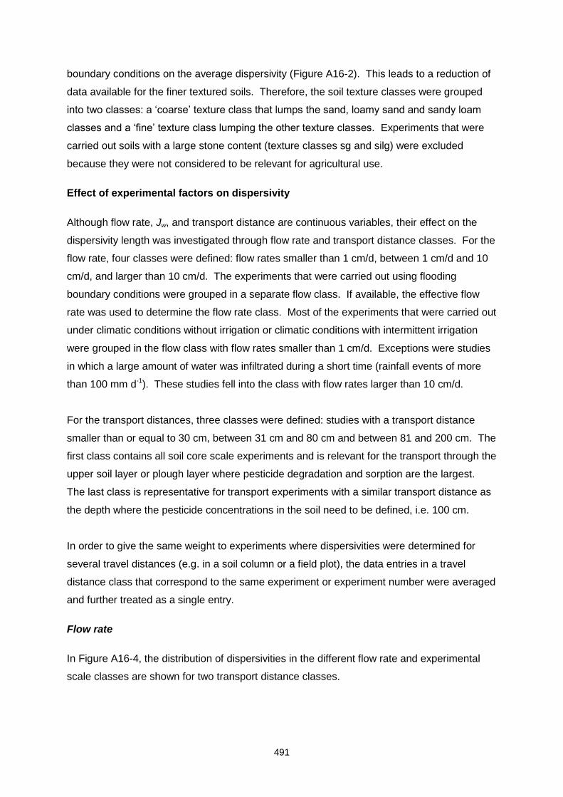
491
boundary conditions on the average dispersivity (Figure A16-2). This leads to a reduction of
data available for the finer textured soils. Therefore, the soil texture classes were grouped
into two classes: a ‘coarse’ texture class that lumps the sand, loamy sand and sandy loam
classes and a ‘fine’ texture class lumping the other texture classes. Experiments that were
carried out soils with a large stone content (texture classes sg and silg) were excluded
because they were not considered to be relevant for agricultural use.
Effect of experimental factors on dispersivity
Although flow rate, Jw, and transport distance are continuous variables, their effect on the
dispersivity length was investigated through flow rate and transport distance classes. For the
flow rate, four classes were defined: flow rates smaller than 1 cm/d, between 1 cm/d and 10
cm/d, and larger than 10 cm/d. The experiments that were carried out using flooding
boundary conditions were grouped in a separate flow class. If available, the effective flow
rate was used to determine the flow rate class. Most of the experiments that were carried out
under climatic conditions without irrigation or climatic conditions with intermittent irrigation
were grouped in the flow class with flow rates smaller than 1 cm/d. Exceptions were studies
in which a large amount of water was infiltrated during a short time (rainfall events of more
than 100 mm d-1). These studies fell into the class with flow rates larger than 10 cm/d.
For the transport distances, three classes were defined: studies with a transport distance
smaller than or equal to 30 cm, between 31 cm and 80 cm and between 81 and 200 cm. The
first class contains all soil core scale experiments and is relevant for the transport through the
upper soil layer or plough layer where pesticide degradation and sorption are the largest.
The last class is representative for transport experiments with a similar transport distance as
the depth where the pesticide concentrations in the soil need to be defined, i.e. 100 cm.
In order to give the same weight to experiments where dispersivities were determined for
several travel distances (e.g. in a soil column or a field plot), the data entries in a travel
distance class that correspond to the same experiment or experiment number were averaged
and further treated as a single entry.
Flow rate
In Figure A16-4, the distribution of dispersivities in the different flow rate and experimental
scale classes are shown for two transport distance classes.
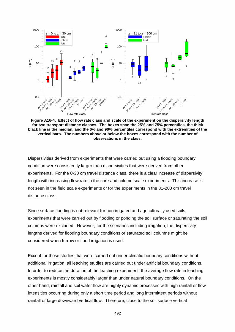
492
Jw <
1 cm
/d
1< Jw <
10
cm/d
Jw >
10
cm/d
pond
ed
Jw <
1 cm
/d
1< Jw <
10
cm/d
Jw >
10
cm/d
pond
ed
Jw <
1 cm
/d
1< Jw <
10
cm/d
Jw >
10
cm/d
pond
ed
Flow rate class
0.1
1
10
100
1000
(cm
)
16
1948
41
3
8 6
26
9
1
4z = 0 to z = 30 cm
core
column
field
Jw <
1 cm
/d
1< Jw <
10
cm/d
Jw >
10
cm/d
Jw <
1 cm
/d
1< Jw <
10
cm/d
Jw >
10
cm/d
pond
ed
Flow rate class
0.1
1
10
100
1000
(
cm
)
6
14
7
5
9
3
7
z = 81 to z = 200 cmcolumn
field
Figure A16-4. Effect of flow rate class and scale of the experiment on the dispersivity length for two transport distance classes. The boxes span the 25% and 75% percentiles, the thick
black line is the median, and the 0% and 90% percentiles correspond with the extremities of the vertical bars. The numbers above or below the boxes correspond with the number of
observations in the class.
Dispersivities derived from experiments that were carried out using a flooding boundary
condition were consistently larger than dispersivities that were derived from other
experiments. For the 0-30 cm travel distance class, there is a clear increase of dispersivity
length with increasing flow rate in the core and column scale experiments. This increase is
not seen in the field scale experiments or for the experiments in the 81-200 cm travel
distance class.
Since surface flooding is not relevant for non irrigated and agriculturally used soils,
experiments that were carried out by flooding or ponding the soil surface or saturating the soil
columns were excluded. However, for the scenarios including irrigation, the dispersivity
lengths derived for flooding boundary conditions or saturated soil columns might be
considered when furrow or flood irrigation is used.
Except for those studies that were carried out under climatic boundary conditions without
additional irrigation, all leaching studies are carried out under artificial boundary conditions.
In order to reduce the duration of the leaching experiment, the average flow rate in leaching
experiments is mostly considerably larger than under natural boundary conditions. On the
other hand, rainfall and soil water flow are highly dynamic processes with high rainfall or flow
intensities occurring during only a short time period and long intermittent periods without
rainfall or large downward vertical flow. Therefore, close to the soil surface vertical
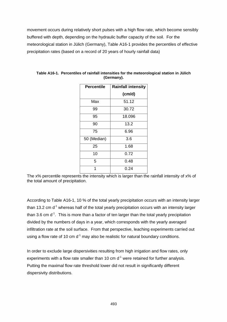
493
movement occurs during relatively short pulses with a high flow rate, which become sensibly
buffered with depth, depending on the hydraulic buffer capacity of the soil. For the
meteorological station in Jülich (Germany), Table A16-1 provides the percentiles of effective
precipitation rates (based on a record of 20 years of hourly rainfall data)
Table A16-1. Percentiles of rainfall intensities for the meteorological station in Jülich (Germany).
Percentile Rainfall intensity
(cm/d)
Max 51.12
99 30.72
95 18.096
90 13.2
75 6.96
50 (Median) 3.6
25 1.68
10 0.72
5 0.48
1 0.24
The x% percentile represents the intensity which is larger than the rainfall intensity of x% of the total amount of precipitation.
According to Table A16-1, 10 % of the total yearly precipitation occurs with an intensity larger
than 13.2 cm d-1 whereas half of the total yearly precipitation occurs with an intensity larger
than 3.6 cm d-1. This is more than a factor of ten larger than the total yearly precipitation
divided by the numbers of days in a year, which corresponds with the yearly averaged
infiltration rate at the soil surface. From that perspective, leaching experiments carried out
using a flow rate of 10 cm d-1 may also be realistic for natural boundary conditions.
In order to exclude large dispersivities resulting from high irrigation and flow rates, only
experiments with a flow rate smaller than 10 cm d-1 were retained for further analysis.
Putting the maximal flow rate threshold lower did not result in significantly different
dispersivity distributions.
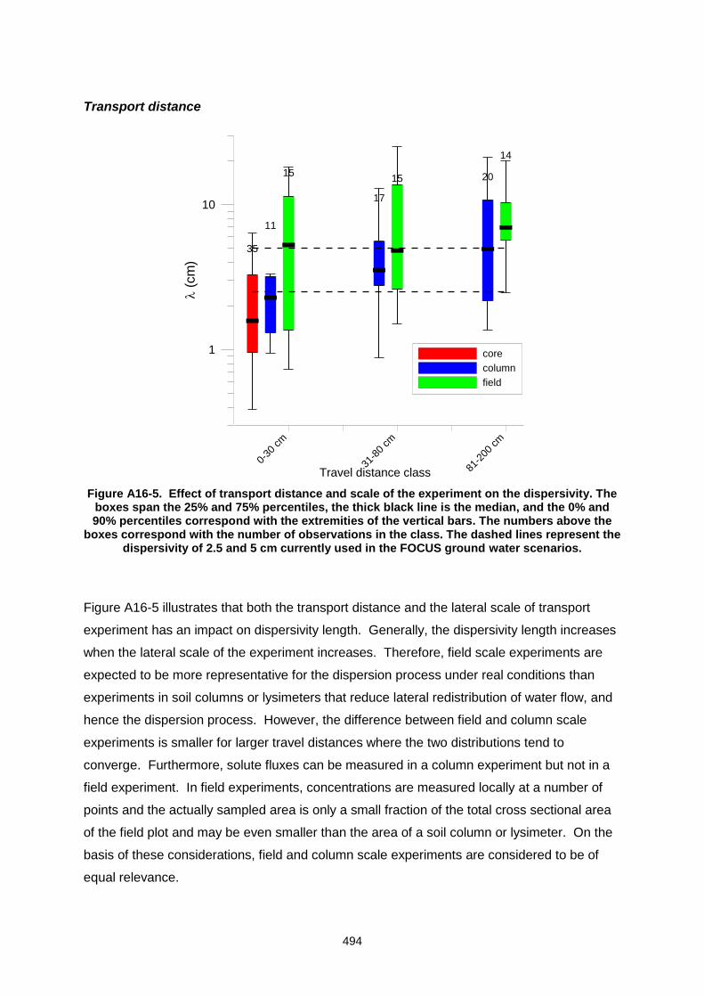
494
Transport distance
0-30
cm
31-8
0 cm
81-2
00 cm
Travel distance class
1
10
(
cm
)
35
11
15
17
15 20
14
core
column
field
Figure A16-5. Effect of transport distance and scale of the experiment on the dispersivity. The boxes span the 25% and 75% percentiles, the thick black line is the median, and the 0% and 90% percentiles correspond with the extremities of the vertical bars. The numbers above the
boxes correspond with the number of observations in the class. The dashed lines represent the dispersivity of 2.5 and 5 cm currently used in the FOCUS ground water scenarios.
Figure A16-5 illustrates that both the transport distance and the lateral scale of transport
experiment has an impact on dispersivity length. Generally, the dispersivity length increases
when the lateral scale of the experiment increases. Therefore, field scale experiments are
expected to be more representative for the dispersion process under real conditions than
experiments in soil columns or lysimeters that reduce lateral redistribution of water flow, and
hence the dispersion process. However, the difference between field and column scale
experiments is smaller for larger travel distances where the two distributions tend to
converge. Furthermore, solute fluxes can be measured in a column experiment but not in a
field experiment. In field experiments, concentrations are measured locally at a number of
points and the actually sampled area is only a small fraction of the total cross sectional area
of the field plot and may be even smaller than the area of a soil column or lysimeter. On the
basis of these considerations, field and column scale experiments are considered to be of
equal relevance.
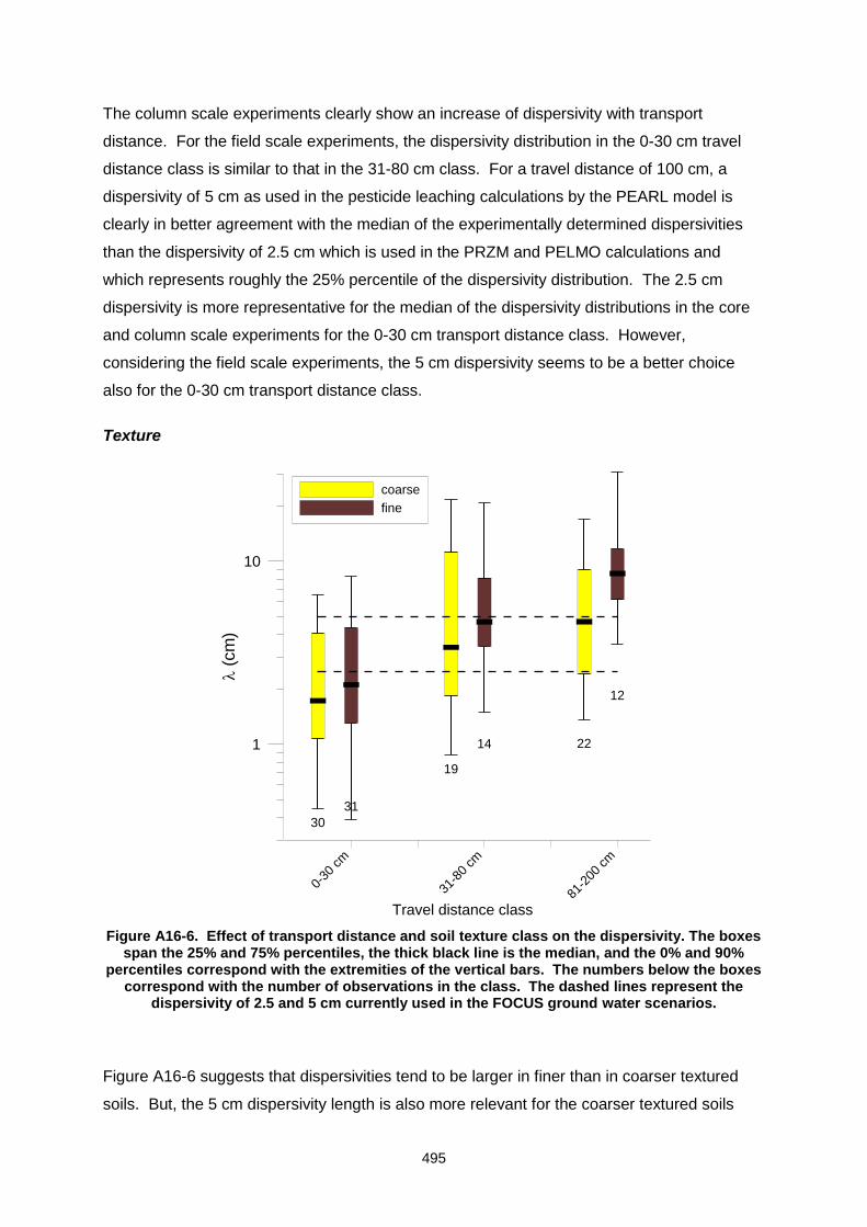
495
The column scale experiments clearly show an increase of dispersivity with transport
distance. For the field scale experiments, the dispersivity distribution in the 0-30 cm travel
distance class is similar to that in the 31-80 cm class. For a travel distance of 100 cm, a
dispersivity of 5 cm as used in the pesticide leaching calculations by the PEARL model is
clearly in better agreement with the median of the experimentally determined dispersivities
than the dispersivity of 2.5 cm which is used in the PRZM and PELMO calculations and
which represents roughly the 25% percentile of the dispersivity distribution. The 2.5 cm
dispersivity is more representative for the median of the dispersivity distributions in the core
and column scale experiments for the 0-30 cm transport distance class. However,
considering the field scale experiments, the 5 cm dispersivity seems to be a better choice
also for the 0-30 cm transport distance class.
Texture
0-30
cm
31-8
0 cm
81-2
00 cm
Travel distance class
1
10
(
cm
)
30
31
19
14 22
12
coarse
fine
Figure A16-6. Effect of transport distance and soil texture class on the dispersivity. The boxes span the 25% and 75% percentiles, the thick black line is the median, and the 0% and 90%
percentiles correspond with the extremities of the vertical bars. The numbers below the boxes correspond with the number of observations in the class. The dashed lines represent the
dispersivity of 2.5 and 5 cm currently used in the FOCUS ground water scenarios.
Figure A16-6 suggests that dispersivities tend to be larger in finer than in coarser textured
soils. But, the 5 cm dispersivity length is also more relevant for the coarser textured soils
496
and the 81-200 cm distance class. The fact that pesticide leaching is sensitive to the
dispersivity, which tends to be larger in finer textured soils, raises the question whether
coarser textured soils represent a worst case.
Variability of dispersivity values
The box plots in Figures A16-4 to A16-6 clearly illustrate that there is a large variability of the
experimentally determined dispersivity values that is not explained by experimental factors.
The dispersivity distributions are positively skewed and a logarithmic scale was used for the
vertical axis of the plots. For positively skewed distributions, the arithmetic average is
considerably larger than the median value or 50 % percentile and cannot be related directly
to a percentile of the distribution. As discussed above, the 5 cm dispersivity used in the
PEARL simulations corresponds with the median of the dispersivity distributions for the 31-80
cm and 81-200 cm travel distance classes whereas the 2.5 cm dispersivity corresponds with
the median of the 0-30 cm travel distance class. However, can a median value be used in a
scenario which is intended to represent a worst-case condition? If the 75% percentile is
considered to be relevant for a worst case condition, then based on the distribution of
experimentally determined dispersivities, a dispersivity of 10 cm should be used.
Implications of an increase of dispersivity with transport distance for the prediction of
pesticide fate in soils with vertically varying sorption and degradation parameters.
The dispersivity for a certain transport distance was derived by fitting the solution of a 1-D
convection dispersion model in a ‘hydrodynamically’ homogeneous soil profile, i.e. assuming
a constant water content and constant dispersivity with depth, to a breakthrough curve or a
concentration depth profile. The transport distance corresponds with the observation depth
of the breakthrough curve or the location of the centre of mass of the concentration profile.
The assumed ‘hydrodynamically’ homogeneous soil profile with depth independent
parameters must therefore be interpreted as an equivalent model of the real soil profile in
which the breakthrough of an inert tracer at the transport distance corresponds with that in
the real soil profile. But, since depends on the transport distance (Figure A16-5),
concentrations that are predicted in the equivalent ‘hydrodynamically’ homogeneous soil
profile at other depths than the transport distance deviate from the concentrations in the real
soil profile. These deviations introduce errors when depth dependent processes are
introduced in the equivalent ‘hydrodynamically’ homogeneous soil profile. In the FOCUS
scenarios, different decay rates and sorption coefficients are assumed in different soil layers.
For the decay rate, three soil layers are considered: the 0-0.3m, 0.3-0.6 m and 0.6-1.0 soil
layers. The decay rate in the deeper soil layers is a factor of the decay rate in the top layer:
497
0.5 for the 0.3-0.6 m and 0.3 for the 0.6-1.0 m layer. The sorption coefficient in the different
soil layers is related to the organic carbon content.
The error on the leached mass fraction resulting from assuming a hydrodynamically
homogeneous soil profile is assessed by comparing predictions in a hydrodynamically
homogeneous soil profile with those in a profile with increasing dispersivity with travel
distance. Two different models that represent a soil profile in which the dispersivity increases
with depth are considered.
The first is a ‘layered convection dispersion model’. In this model, the soil is divided into
several layers and for each layer a different dispersivity is defined. For substances that
undergo linear reactions (i.e. linear sorption isotherms and first-order decay rates) the
transport in this hydrodynamically layered soil can be predicted using transfer functions. The
breakthrough at the bottom of the nth layer is predicted by a convolution of the input
concentrations at the top of that soil layer, Cin(zn-1;t), with a transfer function, f(zn,t):
dzftzCtzC nn
t
inn ,;, 1
0
(A16-3)
where zn is the depth of the bottom of the nth soil layer, zn is the thickness of the layer, and
f(zn,t) is the transfer function in the nth layer.
For a convection dispersion equation with linear sorption and a first-order decay f(zn,t) is
given by:
nnn
n
n
n
nn
n
nnRtv
R
tvz
R
tv
zttzf
/4exp
2
exp,
2
3 (A16-4)
where n (T-1) is the first-order decay rate, vn (L T-1) is the pore water velocity, Rn the
retardation coefficient, and n (L) the dispersivity of the nth layer.
The retardation coefficient Rn is defined as:
nocbn
OCKR 1 (A16-5)
where b is the soil bulk density, Koc the pesticide-organic carbon partitioning coefficient, OCn
the organic carbon weight fraction in the nth soil layer and the volumetric soil water content.
498
The dispersivity of the nth layer is derived from the dispersivities in the overlaying layers, i,
and the dispersivity that was derived for a travel distance zn assuming a ‘hydrodynamically’
homogeneous soil profile, (zn). This is done by matching the variances of particle travel
times to depth zn, var(t;zn) that are predicted in the layered and in the ‘hydrodynamically’
homogeneous soil profiles. For the layered soil profile, var(t;zn) is related to the variance of
travel times through the soil layers, var(t;zi) as:
n
i
in ztzt1
);var(;var (A16-6)
Using the relation between the dispersivity in a ‘hydrodynamically’ homogeneous soil and
var(t;z):
2
2;var
v
zzt
(A16-7)
the dispersivity of soil layer n, n, is derived from the dispersivities in the overlaying soil
layers and the dispersivity in a ‘hydrodynamically’ homogeneous soil profile for a travel
distance zn, (zn), as:
1
1
)( n
i n
ii
n
nn
nz
z
z
zz (A16-8)
The layered convection dispersion model postulates that there is no correlation of the travel
times of given particle through different layers so that the variance of particle arrival times at
the bottom of a certain layer can be written as the sum of the travel time variances through
the overlaying layers (Equation A16-6). The fact that the dispersivity increases with travel
distance is however contradictory to this assumption since it is an indication that velocities
along the trajectory of a single particle are correlated, which implies that the travel time of a
particle through a certain layer is correlated with its travel time through another layer.
The second model, the ‘stream tube model’ with vertically varying sorption and degradation
parameters, assumes that a solute particle keeps a constant velocity along its trajectory
through the soil. Due to this correlation of particle velocities, the travel time variance
increases quadratically with travel distance. This corresponds to a linear increase of the
dispersivity length with travel distance. Using a stream tube model, the mass faction, M(z) of
a substance that leaches at a certain depth is given as:
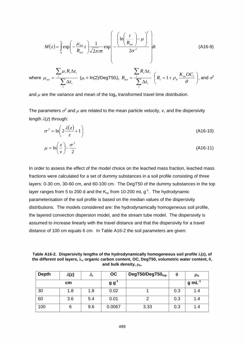
499
dtR
t
tt
RzM
tot
tot
tot
2
2
02
ln
exp2
1exp
(A16-9)
where
i
i
i
iii
totz
zR
(i = ln(2)/DegT50i),
i
i
i
ii
totz
zR
R
ioc
bi
OCKR 1 , and 2
and are the variance and mean of the loge transformed travel time distribution.
The parameters 2 and are related to the mean particle velocity, v, and the dispersivity
length (z) through:
12ln2
z
z (A16-10)
2ln
2
v
z (A16-11)
In order to assess the effect of the model choice on the leached mass fraction, leached mass
fractions were calculated for a set of dummy substances in a soil profile consisting of three
layers: 0-30 cm, 30-60 cm, and 60-100 cm. The DegT50 of the dummy substances in the top
layer ranges from 5 to 200 d and the Koc from 10-200 mL g-1. The hydrodynamic
parameterisation of the soil profile is based on the median values of the dispersivity
distributions. The models considered are: the hydrodynamically homogeneous soil profile,
the layered convection dispersion model, and the stream tube model. The dispersivity is
assumed to increase linearly with the travel distance and that the dispersivity for a travel
distance of 100 cm equals 6 cm. In Table A16-2 the soil parameters are given:
Table A16-2. Dispersivity lengths of the hydrodynamically homogeneous soil profile (z), of
the different soil layers, i, organic carbon content, OC, DegT50, volumetric water content, ,
and bulk density, b.
Depth (z) i OC DegT50/DegT50top b
cm g g-1 g mL-1
30 1.8 1.8 0.02 1 0.3 1.4
60 3.6 5.4 0.01 2 0.3 1.4
100 6 9.6 0.0067 3.33 0.3 1.4
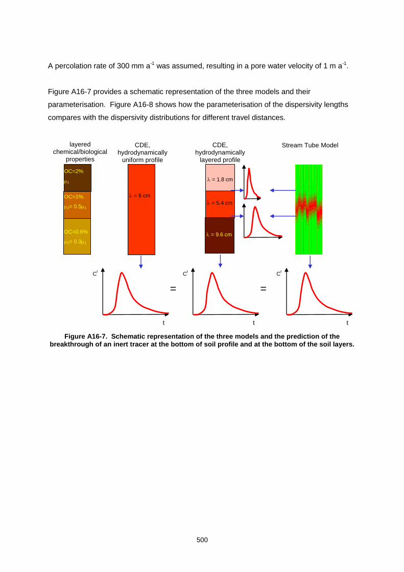
500
A percolation rate of 300 mm a-1 was assumed, resulting in a pore water velocity of 1 m a-1.
Figure A16-7 provides a schematic representation of the three models and their
parameterisation. Figure A16-8 shows how the parameterisation of the dispersivity lengths
compares with the dispersivity distributions for different travel distances.
Figure A16-7. Schematic representation of the three models and the prediction of the breakthrough of an inert tracer at the bottom of soil profile and at the bottom of the soil layers.
-2 .0
-1 .5
-1 .0
-0 .5
De
pth
(m
)
C o n c e n tra tio n p ro file a fte r 1 2 .5 d a y sS te a d y w a te r f lu x o f 2 .8 c m /d a y
0 .0 2
0 .0 6
0 .1 0
0 .1 4
0 .1 8
C
layered chemical/biological
properties
CDE, hydrodynamically
uniform profile
CDE, hydrodynamically
layered profile
Stream Tube Model
OC=2%
1
OC=1%
2= 0.51
OC=0.6%
3= 0.31
= 6 cm
= 1.8 cm
= 5.4 cm
= 9.6 cm
Cf
t
Cf
t
Cf
t
= =
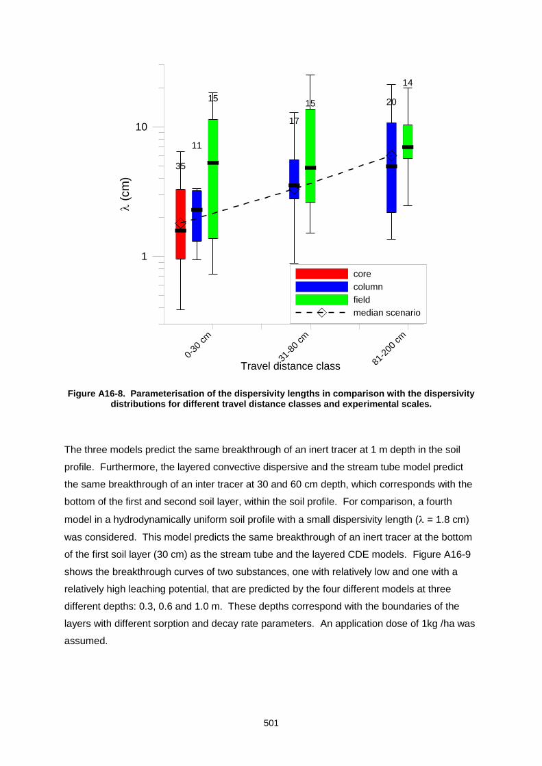
501
0-30
cm
31-8
0 cm
81-2
00 cm
Travel distance class
1
10
(cm
)
35
11
15
17
15 20
14
core
column
field
median scenario
Figure A16-8. Parameterisation of the dispersivity lengths in comparison with the dispersivity
distributions for different travel distance classes and experimental scales.
The three models predict the same breakthrough of an inert tracer at 1 m depth in the soil
profile. Furthermore, the layered convective dispersive and the stream tube model predict
the same breakthrough of an inter tracer at 30 and 60 cm depth, which corresponds with the
bottom of the first and second soil layer, within the soil profile. For comparison, a fourth
model in a hydrodynamically uniform soil profile with a small dispersivity length ( = 1.8 cm)
was considered. This model predicts the same breakthrough of an inert tracer at the bottom
of the first soil layer (30 cm) as the stream tube and the layered CDE models. Figure A16-9
shows the breakthrough curves of two substances, one with relatively low and one with a
relatively high leaching potential, that are predicted by the four different models at three
different depths: 0.3, 0.6 and 1.0 m. These depths correspond with the boundaries of the
layers with different sorption and decay rate parameters. An application dose of 1kg /ha was
assumed.
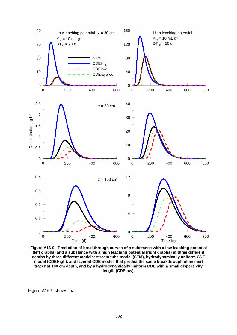
502
0 200 400 6000
10
20
30
40
0 200 400 6000
0.5
1
1.5
2
2.5
Con
ce
ntr
atio
n
g L
-3
0 200 400 600Time (d)
0
0.1
0.2
0.3
0.4
0 200 400 600 8000
40
80
120
160
STM
CDEHigh
CDElow
CDElayered
0 200 400 600 8000
10
20
30
40
0 200 400 600 800Time (d)
0
4
8
12
z = 30 cm
z = 60 cm
z = 100 cm
Low leaching potential High leaching potential
Koc = 10 mL g-1
DT50 = 20 d
Koc = 10 mL g-1
DT50 = 50 d
Figure A16-9. Prediction of breakthrough curves of a substance with a low leaching potential (left graphs) and a substance with a high leaching potential (right graphs) at three different depths by three different models: stream tube model (STM), hydrodynamically uniform CDE model (CDEHigh), and layered CDE model, that predict the same breakthrough of an inert tracer at 100 cm depth, and by a hydrodynamically uniform CDE with a small dispersivity
length (CDElow).
Figure A16-9 shows that:
503
1. The highest peak concentrations are predicted by the hydrodynamically uniform CDE
with the high dispersivity.
2. The three models that predict the same breakthrough of an inert tracer at 100 cm (i.e.
the hydrodynamically uniform CDE with high dispersivity, the stream tube model, and
the layered CDE model) do not predict the same breakthrough of a reactive tracer at
100 cm depth. The differences are in relative terms (note the different scales of the y-
axes) much larger for the substance with the low leaching potential.
3. The models that predict the same breakthrough of an inert tracer at 30 cm depth (i.e.
the CDE with a low dispersivity, the layered CDE and the STM) also predict the same
BTC of the reactive substances at 30 cm depth.
4. The two models that predict the same breakthrough of an inert tracer at the layer
boundaries within the profile (i.e. the layered CDE and the STM) do not predict the
same breakthrough of the reactive substances at 60 and 100 m depth.
Point 1 is counter intuitive since a high dispersivity implies high dispersive fluxes that smooth
out or decrease concentration peaks. A higher dispersive flux also implies that a larger
fraction of the surface applied mass can be rapidly transferred through the soil column. The
fraction that is rapidly transferred has less time or opportunity to decay. The ratio of the
mass of a decaying substance compared with that of a non decaying tracer that reaches a
certain depth is close to 1 for small transfer times but decreases with increasing transfer time.
This is illustrated in Figure A16-10 where breakthrough curves of decaying and non-decaying
substances at 100 cm depth are plotted on a logarithmic scale. When decay is relatively fast,
i.e. the ratio between the decaying and non-decaying substance concentrations decreases
rapidly in the time period between the first significant breakthrough of the non-reactive
substance and the breakthrough of the concentration peak, higher peak concentrations of the
decaying substance may be predicted for larger dispersivities. However, when decay is
relatively slow and the ratio between decaying and non-decaying substance concentrations
decreases slower between the first significant breakthrough and the arrival of the peak
concentration, smaller peak concentrations of a decaying may be predicted for a higher
dispersivity than for a lower dispersivity. This explains why the layered CDE predicts a
smaller peak concentration at 100 cm of the substance with the high leaching potential than
the CDE model with a small dispersivity.
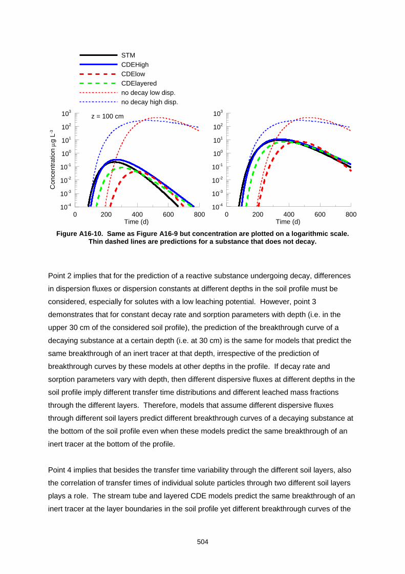
504
0 200 400 600 800Time (d)
10-4
10-3
10-2
10-1
100
101
102
103
Con
ce
ntr
atio
n
g L
-3
0 200 400 600 800Time (d)
10-4
10-3
10-2
10-1
100
101
102
103
STM
CDEHigh
CDElow
CDElayered
no decay low disp.
no decay high disp.
z = 100 cm
Figure A16-10. Same as Figure A16-9 but concentration are plotted on a logarithmic scale. Thin dashed lines are predictions for a substance that does not decay.
Point 2 implies that for the prediction of a reactive substance undergoing decay, differences
in dispersion fluxes or dispersion constants at different depths in the soil profile must be
considered, especially for solutes with a low leaching potential. However, point 3
demonstrates that for constant decay rate and sorption parameters with depth (i.e. in the
upper 30 cm of the considered soil profile), the prediction of the breakthrough curve of a
decaying substance at a certain depth (i.e. at 30 cm) is the same for models that predict the
same breakthrough of an inert tracer at that depth, irrespective of the prediction of
breakthrough curves by these models at other depths in the profile. If decay rate and
sorption parameters vary with depth, then different dispersive fluxes at different depths in the
soil profile imply different transfer time distributions and different leached mass fractions
through the different layers. Therefore, models that assume different dispersive fluxes
through different soil layers predict different breakthrough curves of a decaying substance at
the bottom of the soil profile even when these models predict the same breakthrough of an
inert tracer at the bottom of the profile.
Point 4 implies that besides the transfer time variability through the different soil layers, also
the correlation of transfer times of individual solute particles through two different soil layers
plays a role. The stream tube and layered CDE models predict the same breakthrough of an
inert tracer at the layer boundaries in the soil profile yet different breakthrough curves of the

505
reactive substances. In the stream tube model, the variance of travel times through soil
layers is the same for layers with the same thickness and the model assumes that transfer
times of a particle in two different layers are perfectly correlated. In the layered CDE model,
the transfer times of a particle in two different layers are not correlated and the loss of travel
time correlation is compensated by a higher transit time variance or higher dispersivity in the
deeper soil layer. However, this compensation is based on transit time variances of an inert
tracer. For a substance that is undergoing decay, only the fraction of the applied mass that is
rapidly transferred through the first layer reaches the surface of the second layer. In the
stream tube model, this fraction is also rapidly transferred through the second layer since a
perfect correlation of transfer times is assumed. In the layered CDE model, the transfer time
of this fraction through the second layer is not correlated to its transfer time through the first
layer so that it is transferred with an average velocity through the second layer. Therefore,
the residence time and the opportunity for decay in the second layer of the fraction of the
applied mass that leaches through the first layer and reaches the second layer are smaller
for the STM than for the layered CDE model. This explains why the stream tube model
predicts more leaching at the bottom of the second and third soil layers than the layered CDE
model.
Figure A16-11 shows the predicted leached mass fractions at 1 m depth plotted versus the
predicted leached mass fraction by the stream tube model. Despite the same inert tracer
breakthrough is predicted at 1 m depth by the three models, the predicted leached mass
fractions of a substance that undergoes sorption and decay is quite different and the relative
differences between the model predictions increase with decreasing leaching potential of the
substances.
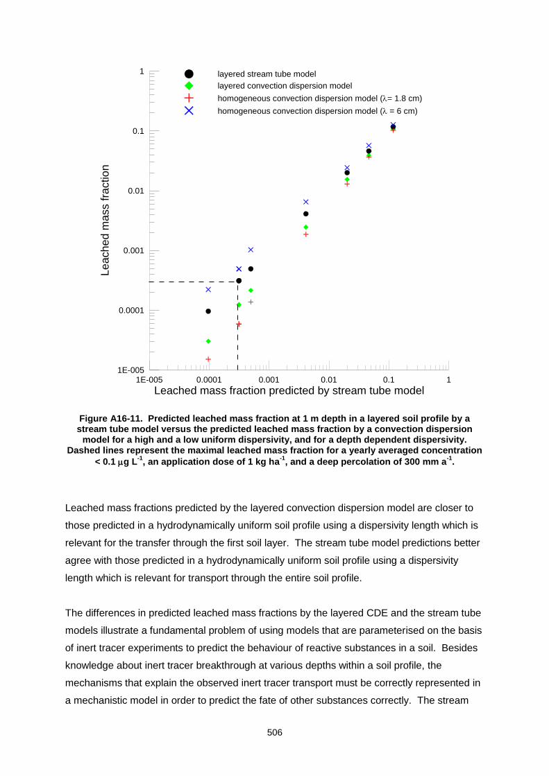
506
1E-005 0.0001 0.001 0.01 0.1 1
Leached mass fraction predicted by stream tube model
1E-005
0.0001
0.001
0.01
0.1
1
Leach
ed m
ass fra
ctio
n
layered stream tube model
layered convection dispersion model
homogeneous convection dispersion model (= 1.8 cm)
homogeneous convection dispersion model ( = 6 cm)
Figure A16-11. Predicted leached mass fraction at 1 m depth in a layered soil profile by a stream tube model versus the predicted leached mass fraction by a convection dispersion
model for a high and a low uniform dispersivity, and for a depth dependent dispersivity. Dashed lines represent the maximal leached mass fraction for a yearly averaged concentration
< 0.1 g L-1
, an application dose of 1 kg ha-1
, and a deep percolation of 300 mm a-1
.
Leached mass fractions predicted by the layered convection dispersion model are closer to
those predicted in a hydrodynamically uniform soil profile using a dispersivity length which is
relevant for the transfer through the first soil layer. The stream tube model predictions better
agree with those predicted in a hydrodynamically uniform soil profile using a dispersivity
length which is relevant for transport through the entire soil profile.
The differences in predicted leached mass fractions by the layered CDE and the stream tube
models illustrate a fundamental problem of using models that are parameterised on the basis
of inert tracer experiments to predict the behaviour of reactive substances in a soil. Besides
knowledge about inert tracer breakthrough at various depths within a soil profile, the
mechanisms that explain the observed inert tracer transport must be correctly represented in
a mechanistic model in order to predict the fate of other substances correctly. The stream
507
tube model provides a mechanistic explanation of the observed increase of dispersivity with
travel distance by postulating a correlation of velocities along the trajectories of individual
particles. Therefore, a correlation of particle velocities across layer boundaries may be
assumed to better represent the transport mechanisms than a convection dispersion model
which postulates no correlation. On the other hand, the lower dispersivity in the upper soil
layer may be explained by soil homogenisation due to tillage and the higher dispersivity in
the deep soil layer may reflect the larger heterogeneity of the natural soil. Whether this soil
homogenisation reduces the correlation between particle transit times through the top and
the subsoil layers and whether a layered CDE better describes the transport process for this
situation requires further investigation
If a convective dispersive model is to be used for predictions of pesticide fate and leaching,
then a parameterisation of the convective dispersive model assuming a hydrodynamically
homogeneous soil profile and using a dispersivity length which is relevant for the transfer
through the entire soil profile seems to be a conservative choice. However, note that the
degree of conservatism depends on the vertical layering of the decay and sorption constants.
The divergence of the predicted leached mass fraction by the different models in Figure A16-
11 depends on the profile of the normalised decay and sorption parameters (normalised with
respect to the decay and sorption parameters at the soil surface). If the sorption and decay
constants do not change with depth, then predictions by the stream tube model, the
hydrodynamically homogeneous CDE model with high dispersivity length and the layered
CDE model converge whereas the hydrodynamically homogeneous CDE model with a low
dispersivity length underestimates the leached mass fraction. If there is no decay below the
first soil layer (i.e. below 30-cm), then the layered CDE model and the homogeneous CDE
model with a low dispersivity length predict the same leached mass fraction as the stream
tube model whereas the high dispersivity CDE model overestimates the leached mass
fraction.
Note also that the above discussion applies only to substances of which the sorption
isotherm is linear. For non-linearly sorbing substances, the convective dispersive model is
less conservative than a stream tube model in soil profiles with vertically constant decay and
sorption parameters. This is a result of the lower dilution of local concentrations that are
predicted by a stream tube model. Due to the non-linearity of the sorption isotherm, higher
local concentrations in individual stream tubes propagate faster through the soil than the
horizontally lumped concentrations, which are lower, that are predicted by the convection
dispersion model.

508
Plausibility checks for layered CDE and stream tube models. Numerical simulations of
solute transport in heterogeneous flow fields
In the previous section, significant differences between the predictions of the leached mass
fractions of a reactive substance by a stream tube model and a by a layered CDE model
were observed. Both models reproduce the observed increase of dispersivity length with
travel distance (Figure A16-5), but make different assumptions about the correlation of solute
particle velocities across the layer boundaries. Since both models predict the same
breakthrough of an inert tracer at the soil layer boundaries, information about inert tracer
transport (on the basis of which the data base of dispersivity lengths was set up) cannot be
used to discriminate which of both models best predicts the transport of decaying
substances.
In order to validate both models, experimental data sets of breakthrough curves of inert and
decaying tracers at various depths in combination with data on the change of decay and
sorption rate parameters with depth would be required. Since such data sets are not
available, we must rely on other representations of reality.
An argument in favour of the layered CDE model is that the top soil is homogenised by
tillage. Therefore, a hypothesis might be that transport in the top soil is more homogeneous
and characterised by a lower dispersivity length that transport in the subsoil. This hypothesis
can be checked by looking at dispersivities observed in soil cores taken from different soil
layers (Figure A16-12).
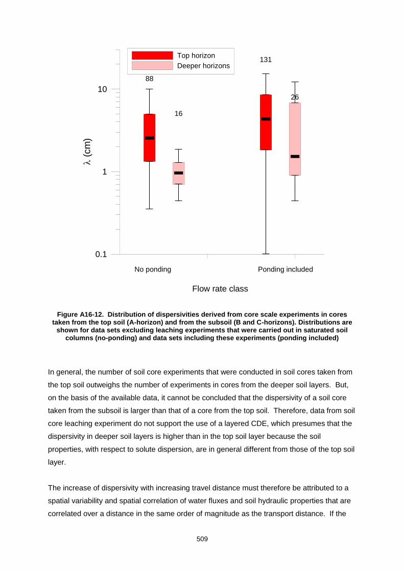
509
Flow rate class
0.1
1
10
(cm
)88
16
131
26
Top horizon
Deeper horizons
No ponding Ponding included
Figure A16-12. Distribution of dispersivities derived from core scale experiments in cores taken from the top soil (A-horizon) and from the subsoil (B and C-horizons). Distributions are
shown for data sets excluding leaching experiments that were carried out in saturated soil columns (no-ponding) and data sets including these experiments (ponding included)
In general, the number of soil core experiments that were conducted in soil cores taken from
the top soil outweighs the number of experiments in cores from the deeper soil layers. But,
on the basis of the available data, it cannot be concluded that the dispersivity of a soil core
taken from the subsoil is larger than that of a core from the top soil. Therefore, data from soil
core leaching experiment do not support the use of a layered CDE, which presumes that the
dispersivity in deeper soil layers is higher than in the top soil layer because the soil
properties, with respect to solute dispersion, are in general different from those of the top soil
layer.
The increase of dispersivity with increasing travel distance must therefore be attributed to a
spatial variability and spatial correlation of water fluxes and soil hydraulic properties that are
correlated over a distance in the same order of magnitude as the transport distance. If the
510
spatial correlation were not of the same order of magnitude as the transport distance, the
dispersivity in soil cores taken from deeper soil cores should be much larger than the one
from soil cores of the top soil to explain the increase of dispersivity with increasing travel
distance.
Both the layered CDE and the STM make extreme assumptions about the spatial correlation
of water fluxes in the soil profile. The assumption of no correlation in the layered CDE can
not be maintained when considering dispersivities of soil cores taken from different soil
layers. On the other hand, a perfect correlation of water fluxes through the soil profile would
imply a linear increase of the dispersivity length with increasing travel distance. Figure A16-8
demonstrates that the increase of dispersivity with increasing travel distance tends to level off
with increasing travel distance, which is a sign of an imperfect correlation of particle velocities
along their trajectory through the entire soil profile. To investigate further which of both
models can be used to predict transport in case of imperfectly correlated particle velocities,
numerical experiments were carried out. In one-dimensional models, the spatial variability
and correlation of water fluxes is not explicitly considered, but its effect on solute transport is
lumped into the dispersion length. Therefore, numerical simulations that explicitly account for
the spatial variability of hydraulic properties and water fluxes were used as surrogates for
real experimental data. The spatial variability of the local water fluxes is in turn determined
by the spatial variability of soil hydraulic properties, which can be characterised in a
geostatistical framework by defining the mean value, the variance, and the correlation
between values at different locations as a function of the separation between the two
locations. In order to further investigate transport of a decaying substance in a layered soil
profile (in terms of decay rate and sorption parameters), flow and transport were simulated in
heterogeneous hydraulic conductivity fields. Since the correlation of particle velocities in
layers with different decay and sorption parameters was shown to have an impact on the
predicted leached mass fraction, two contrasting models of hydraulic conductivity fields were
considered. The geostatistical parameters for both models were chosen so that dispersivities
derived from simulated inert tracer transport were similar to the median values of the
dispersivity distributions. The first model assumes a stationary distribution of the hydraulic
conductivity, i.e. the geostatistical parameters, i.e. mean, variance and spatial correlation
function, are constant in the soil profile. This assumption means that there is no soil layering
with respect to the hydraulic properties and that soil hydraulic properties are correlated
across the boundaries of soil layers with different sorption and decay parameters. But the
spatial correlation of the hydraulic properties in the main flow direction was chosen to be 10
cm, which is a factor 10 smaller than the transport distance. Therefore, this model does not
perfectly match with a stream tube model, which would presume a spatial correlation that is
511
much larger than the transport distance. In the second case, the soil profile is assumed to be
made of two layers with different geostatistical parameters, with the top layer (0-30 cm)
representing a plough layer and the deeper layer (30-100 cm) representing the subsoil. The
spatial distributions of hydraulic properties in the two layers are assumed to be independent
of each other, i.e. there is no correlation between the hydraulic properties across the layer
boundary. In order to limit the complexity of the relations between the spatial variability of
hydraulic soil properties and the dispersivity length, a water saturated soil profile was
assumed. The geostatistical parameters of the hydraulic properties can be directly
determined so that the dispersivity lengths and their dependence on the travel distance
match the constraints. Fields of hydraulic properties that lead to similar flow fields and
dispersivity lengths could also be defined for unsaturated flow conditions. But, since soil
water pressure heads must be continuous across soil layer boundaries and since the
unsaturated hydraulic conductivity depends in a strongly non-linear way on the soil water
pressure, unsaturated hydraulic conductivities will be partly correlated across the soil layer
boundaries through the water pressures, even when the hydraulic parameters are not
correlated. Therefore, flow simulations under saturated conditions can be considered as an
extreme case to investigate the effect of the correlation of hydraulic properties across layer
boundaries on transport of a decaying substance and evaluate the opposing assumptions
made in the stream tube and layered CDE model about the correlation of particle travel times
in different soil layers.
In order to limit the numerical effort, simulations were carried out in 2-D conductivity fields.
The 2-D approximation leads to quantitatively different relations between the geostatistical
parameters of the hydraulic conductivity and the dispersivity then in the 3-D case. However,
the effect of heterogeneity on transport is qualitatively the same in 2-D and 3-D flow fields.
The geostatistical parameters of the hydraulic conductivity distributions in models are given
in Table A16-3.
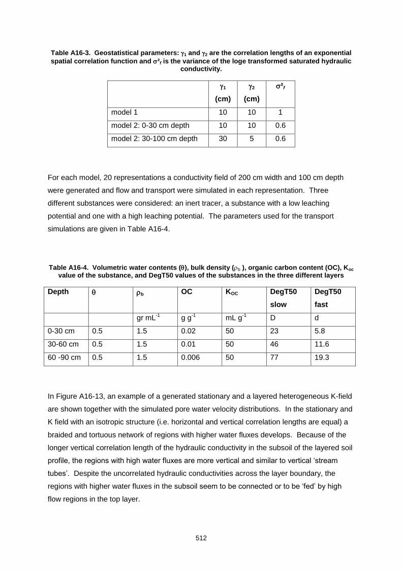
512
Table A16-3. Geostatistical parameters: 1 and 2 are the correlation lengths of an exponential
spatial correlation function and ²f is the variance of the loge transformed saturated hydraulic conductivity.
1
(cm)
2
(cm)
²f
model 1 10 10 1
model 2: 0-30 cm depth 10 10 0.6
model 2: 30-100 cm depth 30 5 0.6
For each model, 20 representations a conductivity field of 200 cm width and 100 cm depth
were generated and flow and transport were simulated in each representation. Three
different substances were considered: an inert tracer, a substance with a low leaching
potential and one with a high leaching potential. The parameters used for the transport
simulations are given in Table A16-4.
Table A16-4. Volumetric water contents (), bulk density (b ), organic carbon content (OC), Koc value of the substance, and DegT50 values of the substances in the three different layers
Depth b OC KOC DegT50
slow
DegT50
fast
gr mL-1 g g-1 mL g-1 D d
0-30 cm 0.5 1.5 0.02 50 23 5.8
30-60 cm 0.5 1.5 0.01 50 46 11.6
60 -90 cm 0.5 1.5 0.006 50 77 19.3
In Figure A16-13, an example of a generated stationary and a layered heterogeneous K-field
are shown together with the simulated pore water velocity distributions. In the stationary and
K field with an isotropic structure (i.e. horizontal and vertical correlation lengths are equal) a
braided and tortuous network of regions with higher water fluxes develops. Because of the
longer vertical correlation length of the hydraulic conductivity in the subsoil of the layered soil
profile, the regions with high water fluxes are more vertical and similar to vertical ‘stream
tubes’. Despite the uncorrelated hydraulic conductivities across the layer boundary, the
regions with higher water fluxes in the subsoil seem to be connected or to be ‘fed’ by high
flow regions in the top layer.
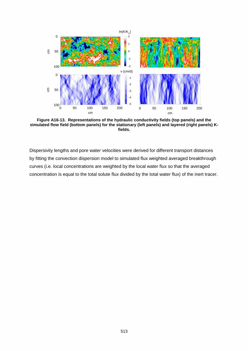
513
Figure A16-13. Representations of the hydraulic conductivity fields (top panels) and the simulated flow field (bottom panels) for the stationary (left panels) and layered (right panels) K-
fields.
Dispersivity lengths and pore water velocities were derived for different transport distances
by fitting the convection dispersion model to simulated flux weighted averaged breakthrough
curves (i.e. local concentrations are weighted by the local water flux so that the averaged
concentration is equal to the total solute flux divided by the total water flux) of the inert tracer.
0 50 100 150 200 250 300 350
cm
0 50 100 150 200 250 300 350 400
cm
-2
-1
0
1
2
-5
-4
-3
-2
-1
0 50 100 150 200
cm
ln(K/KG)
v (cm/d)0
50
100
0
50
100
0 50 100 150 200
cm
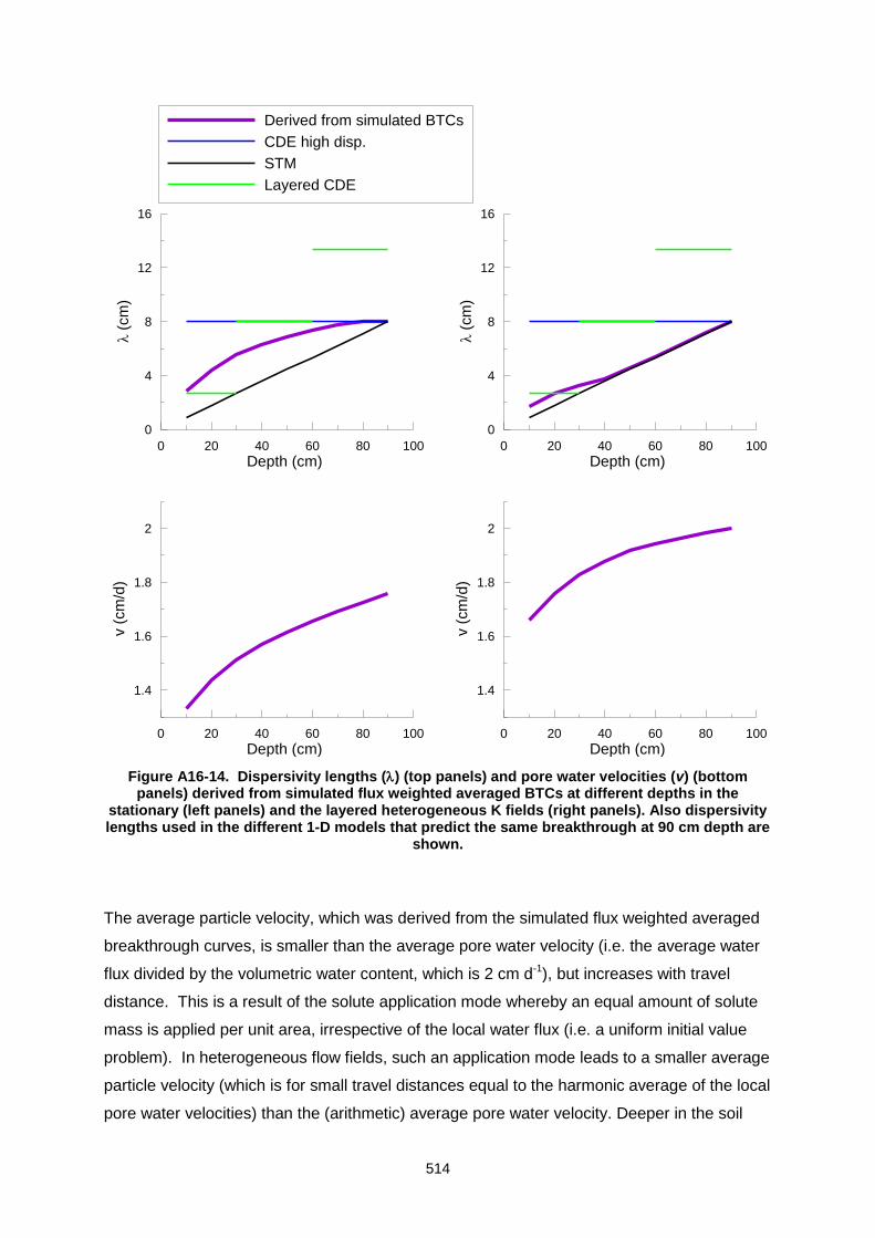
514
0 20 40 60 80 100
Depth (cm)
0
4
8
12
16
(
cm
)Derived from simulated BTCs
CDE high disp.
STM
Layered CDE
0 20 40 60 80 100
Depth (cm)
0
4
8
12
16
(
cm
)
0 20 40 60 80 100
Depth (cm)
1.4
1.6
1.8
2
v (
cm
/d)
0 20 40 60 80 100
Depth (cm)
1.4
1.6
1.8
2
v (
cm
/d)
Figure A16-14. Dispersivity lengths () (top panels) and pore water velocities (v) (bottom panels) derived from simulated flux weighted averaged BTCs at different depths in the
stationary (left panels) and the layered heterogeneous K fields (right panels). Also dispersivity lengths used in the different 1-D models that predict the same breakthrough at 90 cm depth are
shown.
The average particle velocity, which was derived from the simulated flux weighted averaged
breakthrough curves, is smaller than the average pore water velocity (i.e. the average water
flux divided by the volumetric water content, which is 2 cm d-1), but increases with travel
distance. This is a result of the solute application mode whereby an equal amount of solute
mass is applied per unit area, irrespective of the local water flux (i.e. a uniform initial value
problem). In heterogeneous flow fields, such an application mode leads to a smaller average
particle velocity (which is for small travel distances equal to the harmonic average of the local
pore water velocities) than the (arithmetic) average pore water velocity. Deeper in the soil
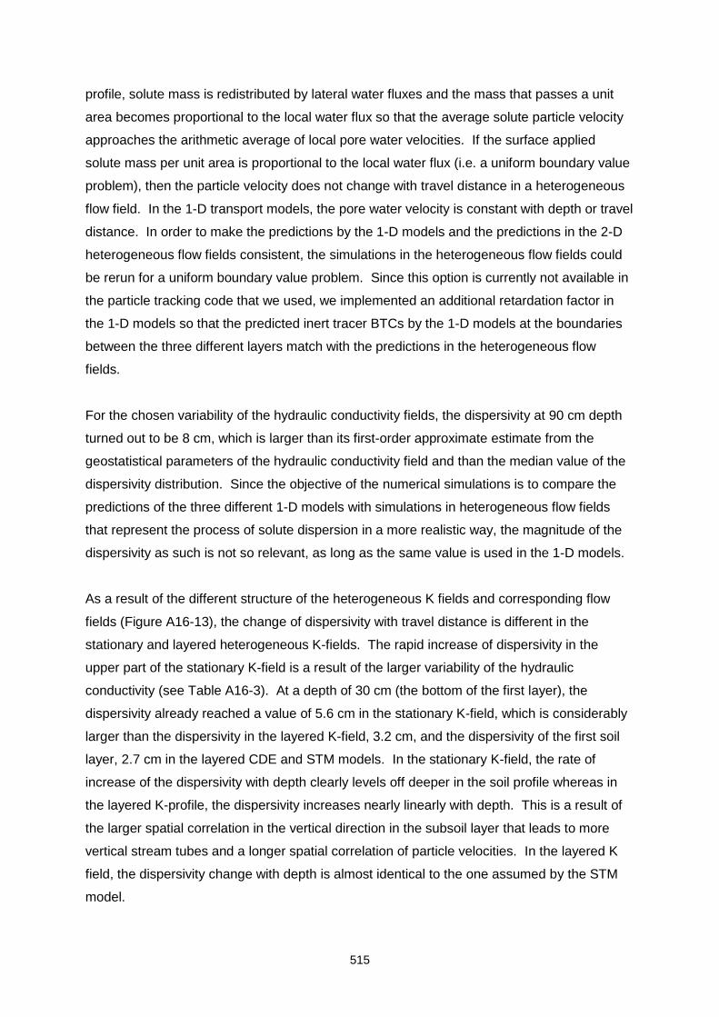
515
profile, solute mass is redistributed by lateral water fluxes and the mass that passes a unit
area becomes proportional to the local water flux so that the average solute particle velocity
approaches the arithmetic average of local pore water velocities. If the surface applied
solute mass per unit area is proportional to the local water flux (i.e. a uniform boundary value
problem), then the particle velocity does not change with travel distance in a heterogeneous
flow field. In the 1-D transport models, the pore water velocity is constant with depth or travel
distance. In order to make the predictions by the 1-D models and the predictions in the 2-D
heterogeneous flow fields consistent, the simulations in the heterogeneous flow fields could
be rerun for a uniform boundary value problem. Since this option is currently not available in
the particle tracking code that we used, we implemented an additional retardation factor in
the 1-D models so that the predicted inert tracer BTCs by the 1-D models at the boundaries
between the three different layers match with the predictions in the heterogeneous flow
fields.
For the chosen variability of the hydraulic conductivity fields, the dispersivity at 90 cm depth
turned out to be 8 cm, which is larger than its first-order approximate estimate from the
geostatistical parameters of the hydraulic conductivity field and than the median value of the
dispersivity distribution. Since the objective of the numerical simulations is to compare the
predictions of the three different 1-D models with simulations in heterogeneous flow fields
that represent the process of solute dispersion in a more realistic way, the magnitude of the
dispersivity as such is not so relevant, as long as the same value is used in the 1-D models.
As a result of the different structure of the heterogeneous K fields and corresponding flow
fields (Figure A16-13), the change of dispersivity with travel distance is different in the
stationary and layered heterogeneous K-fields. The rapid increase of dispersivity in the
upper part of the stationary K-field is a result of the larger variability of the hydraulic
conductivity (see Table A16-3). At a depth of 30 cm (the bottom of the first layer), the
dispersivity already reached a value of 5.6 cm in the stationary K-field, which is considerably
larger than the dispersivity in the layered K-field, 3.2 cm, and the dispersivity of the first soil
layer, 2.7 cm in the layered CDE and STM models. In the stationary K-field, the rate of
increase of the dispersivity with depth clearly levels off deeper in the soil profile whereas in
the layered K-profile, the dispersivity increases nearly linearly with depth. This is a result of
the larger spatial correlation in the vertical direction in the subsoil layer that leads to more
vertical stream tubes and a longer spatial correlation of particle velocities. In the layered K
field, the dispersivity change with depth is almost identical to the one assumed by the STM
model.
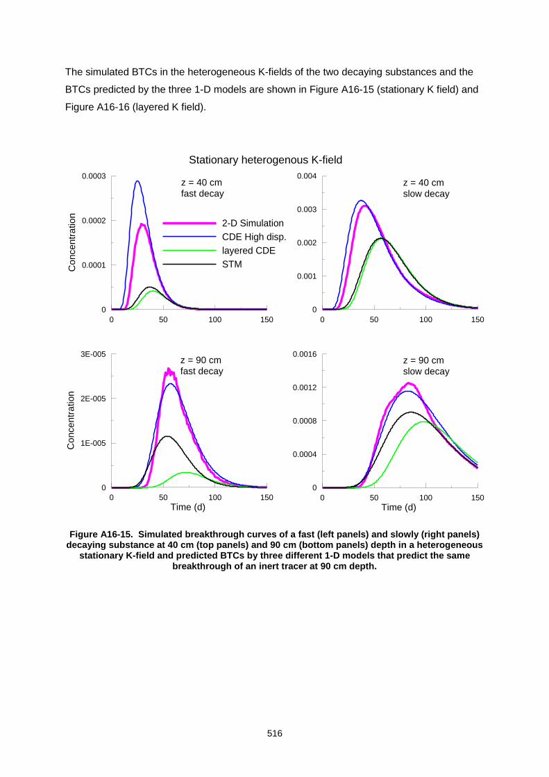
516
The simulated BTCs in the heterogeneous K-fields of the two decaying substances and the
BTCs predicted by the three 1-D models are shown in Figure A16-15 (stationary K field) and
Figure A16-16 (layered K field).
0 50 100 150
0
0.0001
0.0002
0.0003
Co
nce
ntr
atio
n
2-D Simulation
CDE High disp.
layered CDE
STM
0 50 100 150
0
0.001
0.002
0.003
0.004
0 50 100 150
Time (d)
0
1E-005
2E-005
3E-005
Co
ncen
tra
tio
n
0 50 100 150
Time (d)
0
0.0004
0.0008
0.0012
0.0016
z = 40 cmfast decay
z = 90 cmfast decay
z = 40 cmslow decay
z = 90 cmslow decay
Stationary heterogenous K-field
Figure A16-15. Simulated breakthrough curves of a fast (left panels) and slowly (right panels)
decaying substance at 40 cm (top panels) and 90 cm (bottom panels) depth in a heterogeneous stationary K-field and predicted BTCs by three different 1-D models that predict the same
breakthrough of an inert tracer at 90 cm depth.
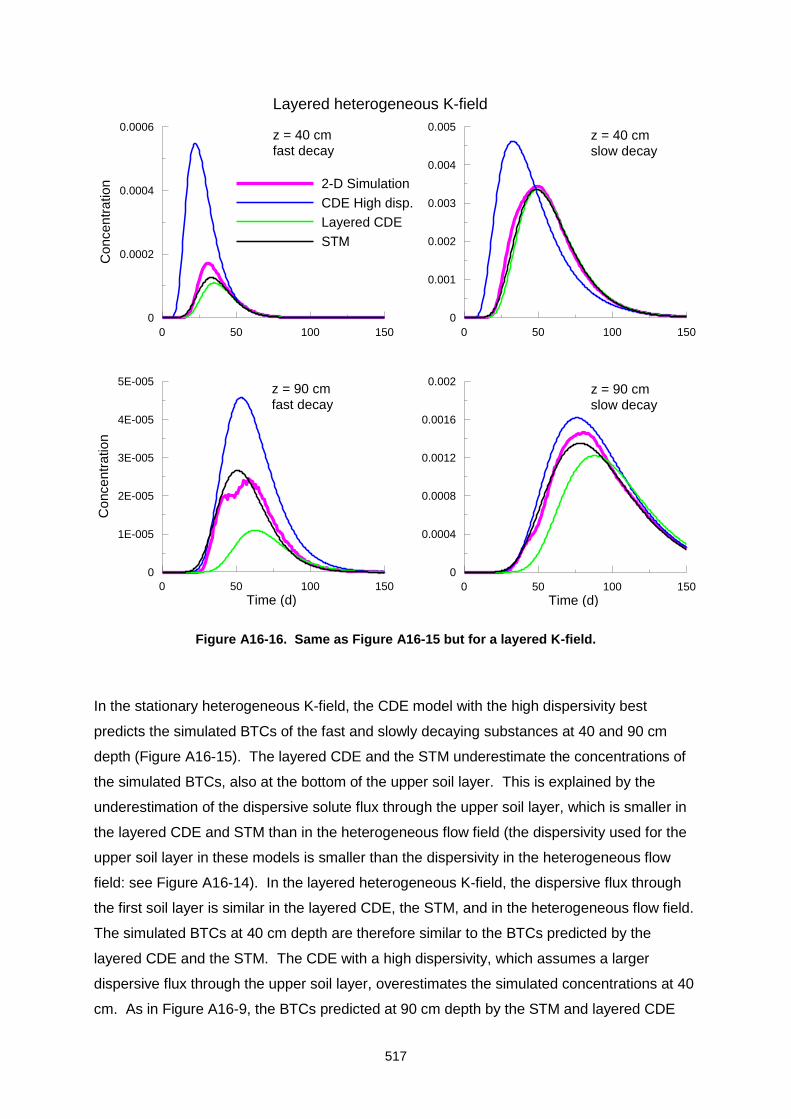
517
0 50 100 150
0
0.0002
0.0004
0.0006
Co
ncen
tra
tio
n 2-D Simulation
CDE High disp.
Layered CDE
STM
0 50 100 150
0
0.001
0.002
0.003
0.004
0.005
0 50 100 150
Time (d)
0
1E-005
2E-005
3E-005
4E-005
5E-005
Co
ncen
tra
tion
0 50 100 150
Time (d)
0
0.0004
0.0008
0.0012
0.0016
0.002
z = 40 cm
fast decay
z = 90 cm
fast decay
z = 40 cmslow decay
z = 90 cmslow decay
Layered heterogeneous K-field
Figure A16-16. Same as Figure A16-15 but for a layered K-field.
In the stationary heterogeneous K-field, the CDE model with the high dispersivity best
predicts the simulated BTCs of the fast and slowly decaying substances at 40 and 90 cm
depth (Figure A16-15). The layered CDE and the STM underestimate the concentrations of
the simulated BTCs, also at the bottom of the upper soil layer. This is explained by the
underestimation of the dispersive solute flux through the upper soil layer, which is smaller in
the layered CDE and STM than in the heterogeneous flow field (the dispersivity used for the
upper soil layer in these models is smaller than the dispersivity in the heterogeneous flow
field: see Figure A16-14). In the layered heterogeneous K-field, the dispersive flux through
the first soil layer is similar in the layered CDE, the STM, and in the heterogeneous flow field.
The simulated BTCs at 40 cm depth are therefore similar to the BTCs predicted by the
layered CDE and the STM. The CDE with a high dispersivity, which assumes a larger
dispersive flux through the upper soil layer, overestimates the simulated concentrations at 40
cm. As in Figure A16-9, the BTCs predicted at 90 cm depth by the STM and layered CDE
518
deviate despite similar predictions by both models at 40 cm depth. The simulated BTCs at
90 cm depth are best predicted by the STM whereas the layered CDE underestimates the
simulated concentrations and leached mass fraction at 90 cm depth. This shows that in
heterogeneous flow fields, particle velocities through different soil are correlated even when
the hydraulic conductivity is not correlated across the layer boundaries. Therefore, the
numerical simulations suggest that a layered CDE model that presumes uncorrelated particle
velocities in different soil layers is not a realistic representation of transport in heterogeneous
flow fields or soils in which the dispersivity length scales with travel distance. The CDE with
a high dispersivity overestimates the simulated concentrations at 90 cm depth but to a lesser
extend than the simulated concentrations at 40 cm depth.
Dispersivities of the layered CDE in the previous examples were calibrated so that the
layered CDE and STM predict the same breakthrough of an inert tracer at the layer
boundaries (i.e. at 30, 60 and 90 cm depth). An alternative way to calibrate the dispersivities
of the layered CDE is to use the simulated inert tracer BTCs in heterogeneous flow fields
(Figure A16-17).
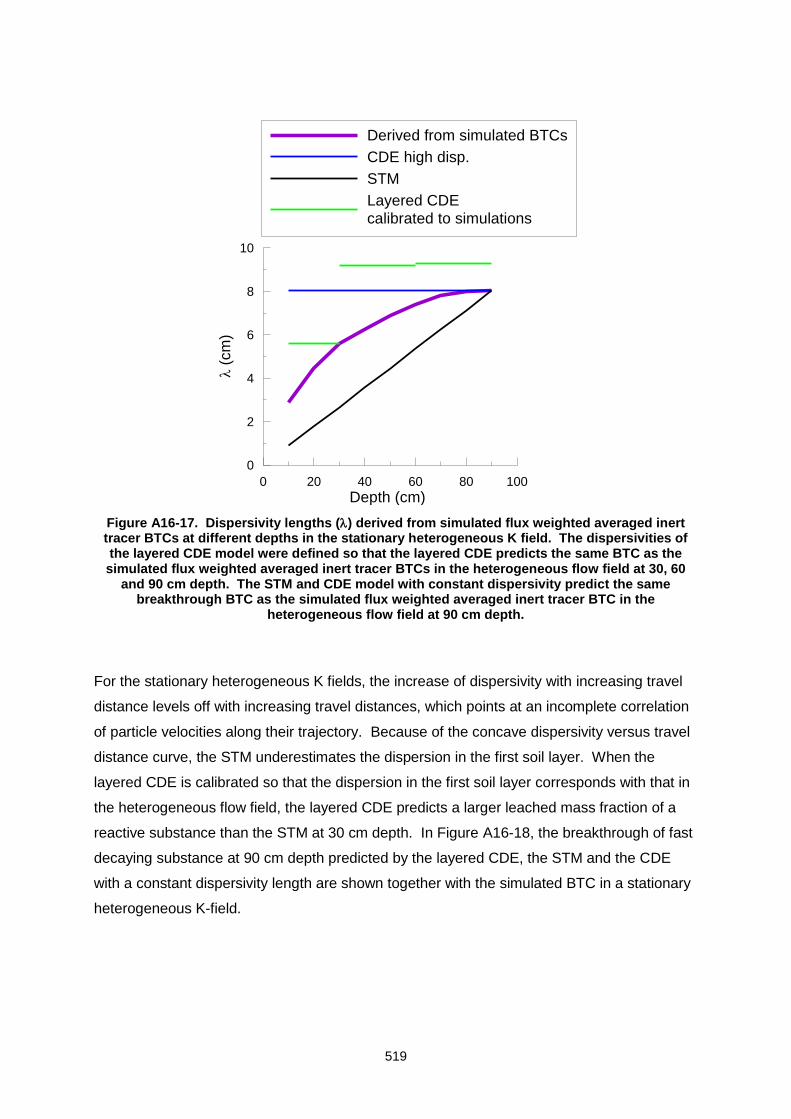
519
0 20 40 60 80 100
Depth (cm)
0
2
4
6
8
10
(
cm
)
Derived from simulated BTCs
CDE high disp.
STM
Layered CDEcalibrated to simulations
Figure A16-17. Dispersivity lengths () derived from simulated flux weighted averaged inert tracer BTCs at different depths in the stationary heterogeneous K field. The dispersivities of the layered CDE model were defined so that the layered CDE predicts the same BTC as the simulated flux weighted averaged inert tracer BTCs in the heterogeneous flow field at 30, 60
and 90 cm depth. The STM and CDE model with constant dispersivity predict the same breakthrough BTC as the simulated flux weighted averaged inert tracer BTC in the
heterogeneous flow field at 90 cm depth.
For the stationary heterogeneous K fields, the increase of dispersivity with increasing travel
distance levels off with increasing travel distances, which points at an incomplete correlation
of particle velocities along their trajectory. Because of the concave dispersivity versus travel
distance curve, the STM underestimates the dispersion in the first soil layer. When the
layered CDE is calibrated so that the dispersion in the first soil layer corresponds with that in
the heterogeneous flow field, the layered CDE predicts a larger leached mass fraction of a
reactive substance than the STM at 30 cm depth. In Figure A16-18, the breakthrough of fast
decaying substance at 90 cm depth predicted by the layered CDE, the STM and the CDE
with a constant dispersivity length are shown together with the simulated BTC in a stationary
heterogeneous K-field.
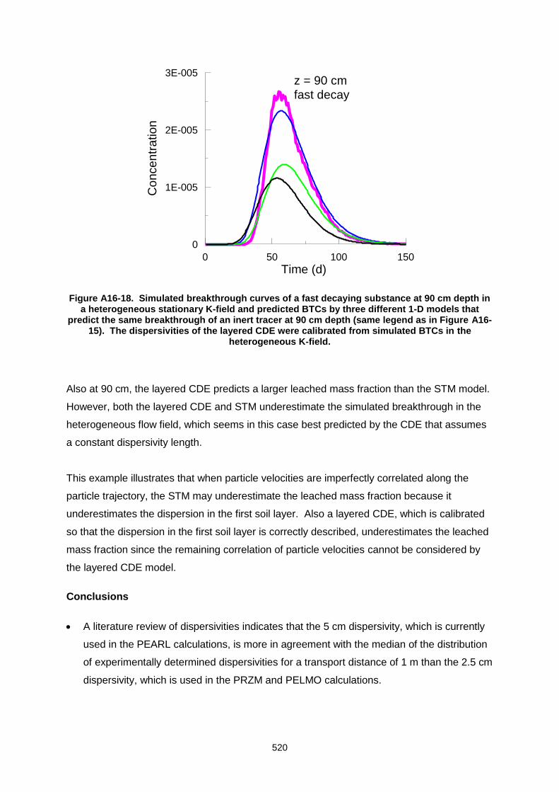
520
0 50 100 150
Time (d)
0
1E-005
2E-005
3E-005
Co
ncen
tra
tio
n
z = 90 cmfast decay
Figure A16-18. Simulated breakthrough curves of a fast decaying substance at 90 cm depth in
a heterogeneous stationary K-field and predicted BTCs by three different 1-D models that predict the same breakthrough of an inert tracer at 90 cm depth (same legend as in Figure A16-
15). The dispersivities of the layered CDE were calibrated from simulated BTCs in the heterogeneous K-field.
Also at 90 cm, the layered CDE predicts a larger leached mass fraction than the STM model.
However, both the layered CDE and STM underestimate the simulated breakthrough in the
heterogeneous flow field, which seems in this case best predicted by the CDE that assumes
a constant dispersivity length.
This example illustrates that when particle velocities are imperfectly correlated along the
particle trajectory, the STM may underestimate the leached mass fraction because it
underestimates the dispersion in the first soil layer. Also a layered CDE, which is calibrated
so that the dispersion in the first soil layer is correctly described, underestimates the leached
mass fraction since the remaining correlation of particle velocities cannot be considered by
the layered CDE model.
Conclusions
A literature review of dispersivities indicates that the 5 cm dispersivity, which is currently
used in the PEARL calculations, is more in agreement with the median of the distribution
of experimentally determined dispersivities for a transport distance of 1 m than the 2.5 cm
dispersivity, which is used in the PRZM and PELMO calculations.
521
Dispersivities in finer textured soils were found to be larger than those in coarser textured
soils but also for coarser textured soils, the 5 cm dispersivity corresponds better with the
median value of the distribution than the 2.5 cm dispersivity.
Dispersivity lengths were found to increase with travel distance indicating a general
correlation of particle velocities along the trajectories of solute particles.
In soil profiles with vertically varying decay and sorption constant, transport mechanisms
within the soil profile must be correctly described in order to predict the leached mass
fraction of a reactive substance. Different models which predict the same breakthrough
of an inert tracer at the bottom of the soil profile but which use a different
conceptualisation of the transport within the profile lead to different predictions of leached
mass fractions.
To assess which model better represents the dispersion process in soils, numerical
simulations of 2-D transport in heterogeneous hydraulic conductivity fields were carried
out. Even in a layered heterogeneous conductivity field without a correlation of the
hydraulic conductivity across soil layer boundaries, the layered CDE model, which
presumes that particle velocities are not correlated across soil layer boundaries,
underestimates the simulated breakthrough curves at the bottom of the soil profile. This
study demonstrated that the STM, which assumes a correlation of particle velocities in
different soil layers, better predicts transport, whereas the layered CDE underestimates
and the uniform CDE overestimates the leached mass fraction. When the dispersivity
versus travel distance curve is concave, which indicates an imperfect correlation of
particle velocities, a layered CDE, which is calibrated so that the dispersion in the first
layer is correctly predicted, may predict larger leached mass fractions than a STM, which
underestimates the dispersion in the first soil layer, but still underestimates the leached
mass fraction deeper in the soil profile because the correlation of particle velocities
across layer boundaries cannot be accounted for by a layered CDE model. With
decreasing particle velocity correlation (i.e. when the dispersivity versus travel distance
curve becomes more concave), the simulated leached mass fractions in a heterogeneous
flow field seems to converge more and more towards the predicted leached mass fraction
by the homogeneous CDE model.
Comparisons of the leached mass fractions predicted by a stream tube model (which is
assumed to best represent the mechanism of transport in the soil) with those predicted by
a convection dispersion model show that a convection dispersion model which assumes
a hydrodynamically uniform soil profile and is parameterised with a dispersivity length that
predicts the breakthrough of an inert tracer at the bottom of the soil profile provides a
conservative estimation of the leached mass fraction. This conclusion can at present not
522
be extrapolated to substances with non linear sorption behaviour. For substances which
do not sorb linearly, a stream tube model predicts an earlier breakthrough than a
convection dispersion model. That means that a convective dispersion model cannot be
considered as a conservative model for transport predictions of non-linearly sorbing
substances. The degree of conservatism further depends on the vertical gradients of the
decay and sorption constants, which are both assumed to decrease with increasing
depth.
The conservatism of the convection dispersion model, which is parameterised using the
median value of the dispersivity distribution, must be put in context of the variation of the
dispersivity distribution and the objective of a FOCUS scenario to represent a worst case
condition. A further investigation of the conservatism of the convection dispersion model
and its parameterisation seems therefore desirable.
References
Buchter, B., C. Hinz, M. Flury, and H. Flühler. 1995. Heterogeneous flow and solute
transport in an unsaturated stony soil monolith. Soil. Sci. soc. Am. J. 59:14-21.
Butters, G.L., and W.A. Jury. 1989. Field scale transport of bromide in an unsaturated soil.
2. Dispersion modeling. Water Resour. Res. 25:1583-1589.
Cassel, D.K., T.H. Krueger, F.W. Schroer, and E.B. Norum. 1974. Solute movement through
disturbed and undisturbed soil cores. Soil Sci. Soc. Am. Proc. 38:36-40.
Deurer M., W.H.M. Duijnisveld, and J. Böttcher, and G. Klump. 2001. Heterogeneous solute
flow in a sandy soil under a pine forest: evaluation of a modeling concept. J. Plant Nutr.
Soil Sci. 164:601-610.
Ellsworth, T.R., and W.A. Jury. 1991. A three-dimensional field study of solute transport
through unsaturated, layered, porous media. 2. Characterisation of vertical dispersion.
Water Resour. Res. 27:967-981.
Ellsworth, T.R., P.J. Shouse, T.H. Skaggs, J.A. Jobes, and J. Fargerlund. 1996. Solute
transport in unsaturated soil: experimental design, parameter estimation, and model
discrimination. Soil Sci. Soc. Am. J. 60:397-407.
Fleming, J.B., and G.L. Butters. 1995. Bromide transport detection in tilled and nontilled soil:
Solution samplers vs. soil cores. Soil Sci. Soc. Am. J. 59:1207-1216.
Forrer, I., R. Kasteel, M. Flury, and H. Flühler. 1999. Longitudinal and lateral dispersion in
an unsaturated field soil. Water Resour. Res. 35:3049-3060.
Hammel K., J. Gross, G. Wessolek, and K. Roth. 1999. Two-dimensional simulation of
bromide transport in a heterogeneous field soil with transient unsaturated flow. Eur. J.
Soil Sci. 50:633-647.
523
Jacobson, O.H., F.J. Leij, and M.Th. van Genuchten. 1992. Parameter determination for
chloride and tritium transport in undisturbed lysimeters during steady flow. Nordic
Hydrology 23:89-104.
Jacques, D., J. Simunek, A. Timmerman, and J. Feyen. 2002. Calibration of Richards’ and
convection-dispersion equations to field-scale water flow and solute transport under
rainfall conditions. J. Hydrol. 259:15-31.
Jacques D., D.J. Kim, J. Diels, J. Vanderborght, H. Vereecken, and J. Feyen. 1998.
Analysis of steady state chloride transport through two heterogeneous field soils. Water
Resour. Res. 34:2539-2550.
Jaynes, D.B., and R.C. Rice. 1993. Transport of solutes as affected by irrigation method.
Soil Sci. Soc. Am. J. 57:1348-1353.
Jury, W.A., and G. Sposito. 1985. Field calibration and validation of solute transport models
for the unsaturated zone. Soil Sci. Soc. Am. J. 49:1331-1341.
Persson, M., and R. Berndtsson. 2002. Transect scale solute transport measured by time
domain reflectometry. Nordic Hydrology 33:145-164.
Roth, K., W.A. Jury, H. Flühler, and W. Attinger. 1992. Transport of chloride through an
unsaturated field soil. Water Resour. Res. 27:2533-2541.
Salzmann, T., and J. Richter. 1995. Field scale vertical transport from horizontally variable
local scale transport parameters. Water Resour. Res. 31:2453-2459.
Seuntjens, P., D. Mallants, N. Toride, C. Cornelis, and P. Geuzens. 2001. Grid lysimeter
study of steady state chloride transport in two Spodosol types using TDR and wick
samplers. J. Contam. Hydrol. 51:13-39.
van de Pol, R.M., P.J. Wierenga, and D.R. Nielsen. 1977. Solute movement in a field soil.
Soil Sci. Soc. Am. J. 41:10-14.
van Ommen, H.C., M.Th. van Genuchten, W.H. van der Molen, R. Dijksma, and J. Hulshof.
1989. J. Hydrol. 105:225-251.
Vanderborght J., C. Gonzalez, M. Vanclooster, D. Mallants, and J. Feyen. 1997. Effects of
soil type and water flux on solute transport. Soil Sci. Soc. Am. J. 61:372-389.
Vanderborght, J., A. Timmerman, and J. Feyen. 2000. Solute transport for steady-state and
transient flow in soils with and without macropores. Soil Sci. Soc. Am. J. 64:1305-1317.
Vanderborght, J., M. Vanclooster, A. Timmerman, P. Seuntjens, D. Mallants, D.-J. Kim, D.
Jacques, L. Hubrechts, C. Gonzalez, J. Feyen, J. Diels, and J. Deckers. Overview of
inert tracer experiments in key Belgian soil types: Relation between transport and soil
morphological and hydraulic properties. Water Resour. Res. 37:2873-2888.
Ward, A.L., R.G. Kachanoski, A.P. von Bertoldi, and D.E. Elrick. 1995. Field and
undisturbed-column measurements for predicting transport in unsaturated layered soil.
Soil Sci. Soc. Am. J. 59:52-59.
524
depth Disp V Vp V_Vp Jw Jweff experiment_number Experimental_field texture Scale concentration_type measurement_technique Type_of_flow Source year
cm cm cm/d cm/d cm/d cm/d
105 10.85 8.14 8.19 0.99 2.85 2.85 1 Bekkevoort l column flux direct steady Vanderborght 2000
105 11.36 8.17 8.07 1.01 2.80 2.80 1 Bekkevoort l column flux direct steady Vanderborght 2000
105 17.99 19.37 19.02 1.02 6.80 6.80 2 Bekkevoort l column flux direct steady Vanderborght 2000
105 14.26 21.42 20.55 1.04 7.40 7.40 2 Bekkevoort l column flux direct steady Vanderborght 2000
105 3.66 3.79 3.82 0.99 1.30 1.30 3 Bekkevoort l column flux direct steady Vanderborght 2000
105 4.15 3.91 3.75 1.04 1.30 1.30 3 Bekkevoort l column flux direct steady Vanderborght 2000
70 3.77 7.37 8.00 0.92 2.84 2.84 4 Bekkevoort l field resident TDR steady Jacques 1998
90 6.23 7.13 8.00 0.89 2.84 2.84 4 Bekkevoort l field resident TDR steady Jacques 1998
105 26.80 6.70 8.20 0.82 2.80 17.60 5 Bekkevoort l column flux direct intermittent Vanderborght 2000
105 123.80 17.80 24.30 0.73 8.20 56.90 6 Bekkevoort l column flux direct intermittent Vanderborght 2000
55 19.96 0.28 7 Bekkevoort l field resident TDR climatic Jacques 2002
75 15.84 0.28 7 Bekkevoort l field resident TDR climatic Jacques 2002
95 21.72 0.28 7 Bekkevoort l field resident TDR climatic Jacques 2002
70 7.47 2.62 3.53 0.74 1.50 1.50 8 Krauthause sil field resident TDR steady Jacques 1998
90 6.59 2.62 3.52 0.74 1.50 1.50 8 Krauthause sil field resident TDR steady Jacques 1998
90 47.00 2.62 1.00 2.60 9 Bertem sil column flux calculated intermittent Vanderborght 1997
90 9.00 1.34 0.50 0.98 10 Bertem sil column flux calculated intermittent Vanderborght 1997
100 3.00 35.05 37.34 0.94 13.00 13.00 12 Geel sl column flux direct steady Vanderborght 2000
100 4.15 34.90 33.64 1.04 13.00 13.00 12 Geel sl column flux direct steady Vanderborght 2000
100 1.78 16.37 16.14 1.01 5.40 5.40 13 Geel sl column flux direct steady Vanderborght 2000
100 3.29 16.85 15.31 1.10 5.70 5.70 13 Geel sl column flux direct steady Vanderborght 2000
90 1.80 3.05 3.05 1.00 1.00 3.50 15 Geel sl column flux calculated intermittent Vanderborght 1997
100 1.40 7.26 7.55 0.96 2.50 5.80 18 Geel sl column flux direct intermittent Vanderborght 2000
100 4.30 6.45 6.61 0.98 2.30 10.30 18 Geel sl column flux direct intermittent Vanderborght 2000
100 4.40 4.52 4.43 1.02 1.00 1.00 19 Lommel s column flux direct steady Seuntjens 2001
90 39.00 2.98 1.00 2.50 20 Meer ls column flux calculated steady Vanderborght 2001
90 24.00 1.54 0.50 0.90 21 Meer ls column flux calculated steady Vanderborght 2001
150 1.87 8.40 7.78 1.08 1.40 22 Etiwanda sl field resident coring interclim Ellsworth 1991
169 10.83 7.54 7.78 0.97 1.40 22 Etiwanda sl field resident coring interclim Ellsworth 1991
198 9.05 8.40 7.78 1.08 1.40 22 Etiwanda sl field resident coring interclim Ellsworth 1991
60 13.70 1.77 3.24 0.55 0.55 23 Etiwanda sl field flux samplers interclim Butters 1989
90 23.90 1.90 3.67 0.52 0.55 23 Etiwanda sl field flux samplers interclim Butters 1989
120 15.70 2.12 3.93 0.54 0.55 23 Etiwanda sl field flux samplers interclim Butters 1989
180 20.20 2.29 3.67 0.63 0.55 23 Etiwanda sl field flux samplers interclim Butters 1989
60 25.71 2.80 4.00 0.70 0.60 24 Etiwanda sl field flux samplers climatic Jury 1985
90 15.14 3.70 4.00 0.93 0.60 24 Etiwanda sl field flux samplers climatic Jury 1985
120 19.83 3.60 4.00 0.90 0.60 24 Etiwanda sl field flux samplers climatic Jury 1985
180 15.74 4.30 4.00 1.08 0.60 24 Etiwanda sl field flux samplers climatic Jury 1985
61 25.14 0.83 0.58 1.42 0.18 25 Windsor cl field resident coring interclim Fleming 1995
80 7.49 1.02 0.58 1.75 0.18 25 Windsor cl field resident coring interclim Fleming 1995
80 14.54 0.75 0.58 1.28 0.18 25 Windsor cl field flux samplers interclim Fleming 1995
80 23.04 1.09 0.58 1.88 0.18 25 Windsor cl field flux samplers interclim Fleming 1995
120 9.78 0.68 0.58 1.16 0.18 25 Windsor cl field flux samplers interclim Fleming 1995
120 15.51 1.11 0.58 1.92 0.18 25 Windsor cl field flux samplers interclim Fleming 1995
158 5.44 0.69 0.58 1.18 0.18 25 Windsor cl field resident coring interclim Fleming 1995
160 9.70 0.73 0.58 1.26 0.18 25 Windsor cl field flux samplers interclim Fleming 1995
160 11.24 1.05 0.58 1.81 0.18 25 Windsor cl field flux samplers interclim Fleming 1995
62 1.50 0.40 0.40 27 Andelfinge l field resident dye steady Forrer 1999
100 9.05 0.92 0.92 32 Tinglev s column flux direct steady Jacobsen 1992
100 4.08 1.03 1.03 33 Tinglev s column flux direct steady Jacobsen 1992
100 1.89 1.18 1.18 34 Tinglev s column flux direct steady Jacobsen 1992
100 5.80 1.59 1.59 35 Tinglev s column flux direct steady Jacobsen 1992
100 3.86 1.63 1.63 36 Tinglev s column flux direct steady Jacobsen 1992
525
depth Disp V Vp V_Vp Jw Jweff experiment_number Experimental_field texture Scale concentration_type measurement_technique Type_of_flow Source year
cm cm cm/d cm/d cm/d cm/d
75 8.10 81.59 69.60 1.17 6.61 6.61 37 Basel silg column flux direct steady Buchter 1995
75 5.90 79.28 70.80 1.12 6.73 6.73 37 Basel silg column flux direct steady Buchter 1995
65 1.80 3.84 3.53 1.09 1.06 1.06 78 Riverside sl field flux samplers steady Ellsworth 1996
78 1.68 4.30 3.53 1.22 1.06 1.06 79 Riverside sl field resident coring steady Ellsworth 1996
115 2.46 4.42 3.53 1.25 1.06 1.06 79 Riverside sl field resident coring steady Ellsworth 1996
60 13.47 14.60 13.52 1.08 4.84 4.84 85 Phoenix cl field resident samplers steady Jaynes 1993
100 13.50 17.37 13.57 1.28 4.84 4.84 85 Phoenix cl field resident samplers steady Jaynes 1993
140 6.73 13.48 13.61 0.99 4.84 4.84 85 Phoenix cl field resident samplers steady Jaynes 1993
180 7.49 16.24 13.77 1.18 4.84 4.84 85 Phoenix cl field resident samplers steady Jaynes 1993
80 5.31 8.56 7.40 1.16 1.25 1.25 91 Delhi(ON) ls field flux samplers steady Ward 1995
85 8.22 25.74 25.00 1.03 4.00 4.00 92 Delhi(ON) ls field resident coring steady Ward 1995
66 2.41 1.94 0.26 96 Nienwohlde ls field resident coring climatic Salzmann 1995
70 28.30 0.40 0.14 97 Fuhrberger s field flux samplers climatic Deurer 2001
110 12.10 1.15 0.14 97 Fuhrberger s field flux samplers climatic Deurer 2001
84 29.00 0.38 0.56 14.40 175 Bulach l field flux samplers interclim Roth 1991
70 6.20 0.73 0.23 186 Hupsel ls field resident coring climatic van Ommen 1989
70 19.80 0.69 0.23 186 Hupsel ls field resident coring climatic van Ommen 1989
100 12.29 5.38 4.27 1.26 0.99 0.99 188 Lommel s column flux direct steady Seuntjens 2001
70 6.52 25.64 18.25 1.40 4.00 189 Loddekopin ls field resident TDR intermittent Persson 2002
90 5.28 27.18 19.90 1.37 4.00 189 Loddekopin ls field resident TDR intermittent Persson 2002
70 19.99 15.37 8.53 1.80 1.87 190 Loddekopin ls field resident TDR intermittent Persson 2002
90 6.66 16.52 9.31 1.78 1.87 190 Loddekopin ls field resident TDR intermittent Persson 2002
150 40.94 3.90 4.66 0.84 2.00 2.00 193 New Mexico sic field resident samplers steady van de Pol 1977
80 3.45 1.12 1.12 1.00 0.36 194 Beotia cl column flux direct intermittent Cassel 1974
80 4.51 1.05 1.05 1.00 0.36 195 Aberdeen cl column flux direct intermittent Cassel 1974
120 9.20 0.29 0.29 1.02 0.11 200 Merzenhaus sil column flux direct climatic Kasteel 2004
120 5.70 0.23 0.29 0.80 0.11 201 Merzenhaus sil field flux samplers climatic Kasteel 2004
122 2.90 0.74 0.12 205 Blumberg sl field resident coring climatic Hammel 1999
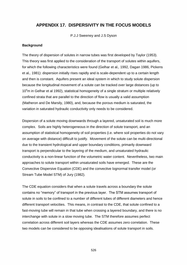
526
APPENDIX 17. DISPERSIVITY IN THE FOCUS MODELS
P.J.J Sweeney and J.S Dyson
Background
The theory of dispersion of solutes in narrow tubes was first developed by Taylor (1953).
This theory was first applied to the consideration of the transport of solutes within aquifers,
for which the following characteristics were found (Gelhar et al., 1992, Dagan 1986, Pickens
et al., 1981): dispersion initially rises rapidly and is scale-dependent up to a certain length
and then is constant. Aquifers present an ideal system in which to study solute dispersion
because the longitudinal movement of a solute can be tracked over large distances (up to
104m in Gelhar et al 1992), statistical homogeneity of a single stratum or multiple relatively
confined strata that are parallel to the direction of flow is usually a valid assumption
(Matheron and De Marsily, 1980), and, because the porous medium is saturated, the
variation in saturated hydraulic conductivity only needs to be considered.
Dispersion of a solute moving downwards through a layered, unsaturated soil is much more
complex. Soils are highly heterogeneous in the direction of solute transport, and an
assumption of statistical homogeneity of soil properties (i.e. where soil properties do not vary
on average with distance) difficult to justify. Movement of the solute can be multi-directional
due to the transient hydrological and upper boundary conditions, primarily downward
transport is perpendicular to the layering of the medium, and unsaturated hydraulic
conductivity is a non-linear function of the volumetric water content. Nevertheless, two main
approaches to solute transport within unsaturated soils have emerged. These are the
Convective Dispersive Equation (CDE) and the convective lognormal transfer model (or
Stream Tube Model STM) of Jury (1982).
The CDE equation considers that when a solute travels across a boundary the solute
contains no “memory” of transport in the previous layer. The STM assumes transport of
solute in soils to be confined to a number of different tubes of different diameters and hence
different transport velocities. This means, in contrast to the CDE, that solute confined to a
fast-moving tube will remain in that tube when crossing a layered boundary, and there is no
interchange with solute in a slow moving tube. The STM therefore assumes perfect
correlation across different soil layers whereas the CDE assumes zero correlation. These
two models can be considered to be opposing idealisations of solute transport in soils.
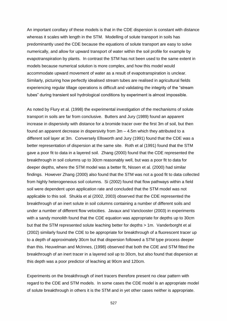
527
An important corollary of these models is that in the CDE dispersion is constant with distance
whereas it scales with length in the STM. Modelling of solute transport in soils has
predominantly used the CDE because the equations of solute transport are easy to solve
numerically, and allow for upward transport of water within the soil profile for example by
evapotranspiration by plants. In contrast the STM has not been used to the same extent in
models because numerical solution is more complex, and how this model would
accommodate upward movement of water as a result of evapotranspiration is unclear.
Similarly, picturing how perfectly idealised stream tubes are realised in agricultural fields
experiencing regular tillage operations is difficult and validating the integrity of the “stream
tubes” during transient soil hydrological conditions by experiment is almost impossible.
As noted by Flury et al. (1998) the experimental investigation of the mechanisms of solute
transport in soils are far from conclusive. Butters and Jury (1989) found an apparent
increase in dispersivity with distance for a bromide tracer over the first 3m of soil, but then
found an apparent decrease in dispersivity from 3m – 4.5m which they attributed to a
different soil layer at 3m. Conversely Ellsworth and Jury (1991) found that the CDE was a
better representation of dispersion at the same site. Roth et al (1991) found that the STM
gave a poor fit to data in a layered soil. Zhang (2000) found that the CDE represented the
breakthrough in soil columns up to 30cm reasonably well, but was a poor fit to data for
deeper depths, where the STM model was a better fit, Nissen et al. (2000) had similar
findings. However Zhang (2000) also found that the STM was not a good fit to data collected
from highly heterogeneous soil columns. Si (2002) found that flow pathways within a field
soil were dependent upon application rate and concluded that the STM model was not
applicable to this soil. Shukla et al (2002, 2003) observed that the CDE represented the
breakthrough of an inert solute in soil columns containing a number of different soils and
under a number of different flow velocities. Javaux and Vanclooster (2003) in experiments
with a sandy monolith found that the CDE equation was appropriate for depths up to 30cm
but that the STM represented solute leaching better for depths > 1m. Vanderborght et al
(2002) similarly found the CDE to be appropriate for breakthrough of a fluorescent tracer up
to a depth of approximately 30cm but that dispersion followed a STM type process deeper
than this. Heuvelman and McInnes, (1998) observed that both the CDE and STM fitted the
breakthrough of an inert tracer in a layered soil up to 30cm, but also found that dispersion at
this depth was a poor predictor of leaching at 90cm and 120cm.
Experiments on the breakthrough of inert tracers therefore present no clear pattern with
regard to the CDE and STM models. In some cases the CDE model is an appropriate model
of solute breakthrough in others it is the STM and in yet other cases neither is appropriate.
528
These findings emphasise the complexities involved in determining the dispersion of a
substance in a highly heterogeneous medium such as soil. Flury et al (1998), in a review,
suggested that the CDE might be the more appropriate model to use where there is
pronounced layering in soil and that the STM model may be more appropriate for more
homogeneous soils, and therefore that the dispersion was likely to be site specific. Jury and
Scotter (1994) also concluded that the STM was less likely to be applicable where there was
distinct layering in soils, because layering would be expected to enhance lateral mixing that
is characteristic of CDE type behaviour.
Experiments designed to measure dispersion length show a wide scatter. For example data
collected by Flury et al. (1998) showed that dispersion length measured at 1 m varied
between about 1 and 100cm. Figure A17-1 shows the values of dispersion length collected
from the literature by this FOCUS group for 30cm, 60cm and 100cm depths. These data,
which were selected to be relevant to agricultural conditions, show a variation of at least an
order of magnitude for dispersion length.
0-30
cm
31-8
0 cm
81-2
00 cm
Travel distance class
1
10
(
cm
)
35
11
15
17
15 20
14
core
column
field
Figure A17-1. Data collected on dispersion length measurements by FOCUS GW II
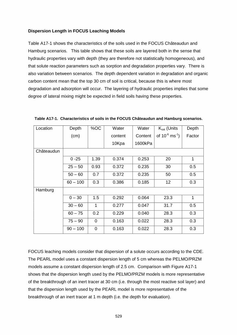
529
Dispersion Length in FOCUS Leaching Models
Table A17-1 shows the characteristics of the soils used in the FOCUS Châteaudun and
Hamburg scenarios. This table shows that these soils are layered both in the sense that
hydraulic properties vary with depth (they are therefore not statistically homogeneous), and
that solute reaction parameters such as sorption and degradation properties vary. There is
also variation between scenarios. The depth dependent variation in degradation and organic
carbon content mean that the top 30 cm of soil is critical, because this is where most
degradation and adsorption will occur. The layering of hydraulic properties implies that some
degree of lateral mixing might be expected in field soils having these properties.
Table A17-1. Characteristics of soils in the FOCUS Châteaudun and Hamburg scenarios.
Location Depth
(cm)
%OC Water
content
10Kpa
Water
Content
1600kPa
Ksat (Units
of 10-6 ms-1)
Depth
Factor
Châteaudun
0 -25 1.39 0.374 0.253 20 1
25 – 50 0.93 0.372 0.235 30 0.5
50 – 60 0.7 0.372 0.235 50 0.5
60 – 100 0.3 0.386 0.185 12 0.3
Hamburg
0 – 30 1.5 0.292 0.064 23.3 1
30 – 60 1 0.277 0.047 31.7 0.5
60 – 75 0.2 0.229 0.040 28.3 0.3
75 – 90 0 0.163 0.022 28.3 0.3
90 – 100 0 0.163 0.022 28.3 0.3
FOCUS leaching models consider that dispersion of a solute occurs according to the CDE.
The PEARL model uses a constant dispersion length of 5 cm whereas the PELMO/PRZM
models assume a constant dispersion length of 2.5 cm. Comparison with Figure A17-1
shows that the dispersion length used by the PELMO/PRZM models is more representative
of the breakthrough of an inert tracer at 30 cm (i.e. through the most reactive soil layer) and
that the dispersion length used by the PEARL model is more representative of the
breakthrough of an inert tracer at 1 m depth (i.e. the depth for evaluation).

530
The problem with harmonising dispersion length in the FOCUS models arises because the
experimental data on dispersion length are very variable and because the experimental
measurement of dispersion is likely to vary between locations as a result of variations in
hydraulic properties, which means that it may be difficult to distinguish between a dispersion
length of 2.5 cm and 5 cm with a high degree of accuracy. Note that the majority of data on
dispersion are for non-reactive solutes, and data on dispersion of reactive solutes moving
through layered systems where there are differing rates of adsorption and degradation are
sparse. Clearly, if one soil layer is much more reactive than others then the dispersion in this
layer is critical, because it will control the mass of solute entering into other layers. However
the dispersion in deeper soil layers is also important as it will influence the mass leaching to
1 m. It should also be borne in mind that the leached mass fractions that result in a leachate
concentration of 0.1 µg/L in soil pore water are extremely small (approximately 0.1% of a 1
kg/ha application) which demands a high degree of precision from model predictions, one
which is difficult to extract from the available data on dispersion length.
Different assumptions on the mechanism of solute spreading, i.e. the STM or CDE in layered
soils, give different leached mass fractions at 1m for reactive solutes. The STM
parameterised to give a dispersion length of 6 cm at 1m gave a much greater leached mass
fraction at 1 m depth than the CDE with a constant dispersion length of 1.8 cm (value of
dispersion according to the STM at 30 cm) but the agreement was closer with a constant
dispersion length of 5 cm – although it should be noted that the leached mass fractions for
the 5 cm dispersion length exceeded the STM model predictions in all cases.
The difficulty with the application of the STM is that, as noted above, there is no conclusive
evidence from the literature that it applies in all situations and, as noted by Jury and Scotter
(1994), it is less likely to be valid in situations where there is layering of the soil. It can
therefore be regarded as an extreme model of solute transport which requires perfect
correlation and soils to be statistically homogeneous (i.e. mean properties do not change with
distance). Note also that the STM calculation assumes that water movement is always
downwards and it is not known how upward movement of water resulting from
evapotranspiration by plants can affect dispersion.
The soils in the FOCUS scenarios are layered in terms of their reactivity and their hydraulic
properties (i.e. they are not statistically homogeneous), some lateral mixing can therefore be
expected. Therefore, predictions using the STM represent an upper bound. This would
imply that the CDE using a 5 cm dispersion length gives leached mass fractions that are too
531
high, conversely the CDE using a dispersion length of 1.8 cm is too low, because the
dispersion at 30 cm is used to estimate dispersion through the whole soil profile.
Hydrological modelling using K-fields has not been used to evaluate the FOCUS models
before. The key factor with regard to these models lies with the correlation length in the
vertical and horizontal directions chosen for the various soil properties. Figure A17-1 shows
K-field modelling performed for a field site by Rockhold and Rossi (1996). This Figure shows
that using a correlation length of 440 cm in the horizontal direction and 45 cm in the vertical
direction, resulted in horizontal flow field features, which would be more likely to show lateral
mixing and hence CDE type behaviour. Similarly, Russo and Bouton (1992) used a
horizontal correlation length of 83cm for Log Ksat in the horizontal direction and 19cm in the
vertical direction, which again resulted in more layered than stream tube like structures.
Also, Roth and Hammel (1996) have shown that the transition between short term stream
tube behaviour and long-term CDE type behaviour is dependent upon the assumptions made
regarding underlying soil heterogeneity. In summary therefore there are no generally
accepted values in the literature for the vertical and horizontal correlations for critical soil
parameters and the choice of these parameters has a critical impact on whether structures
are layered or “tube like”. Therefore likely either “stream tube like” or “layered type” behaviour
can be shown by suitable choice of parameters and which values are generally appropriate is
not clear. Similarly how the upward movement of water as a result of evapotranspiration
would affect the results of the modelling is unclear.
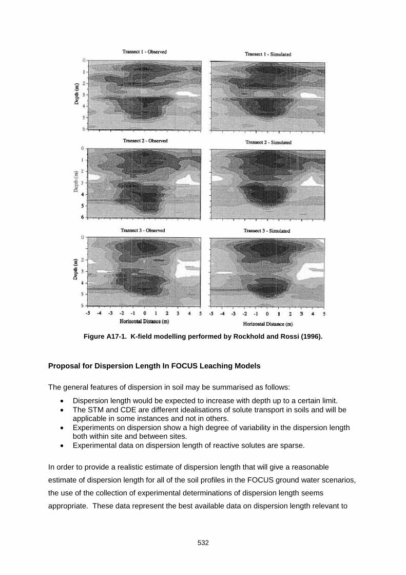
532
Figure A17-1. K-field modelling performed by Rockhold and Rossi (1996).
Proposal for Dispersion Length In FOCUS Leaching Models
The general features of dispersion in soil may be summarised as follows:
Dispersion length would be expected to increase with depth up to a certain limit.
The STM and CDE are different idealisations of solute transport in soils and will be applicable in some instances and not in others.
Experiments on dispersion show a high degree of variability in the dispersion length both within site and between sites.
Experimental data on dispersion length of reactive solutes are sparse.
In order to provide a realistic estimate of dispersion length that will give a reasonable
estimate of dispersion length for all of the soil profiles in the FOCUS ground water scenarios,
the use of the collection of experimental determinations of dispersion length seems
appropriate. These data represent the best available data on dispersion length relevant to
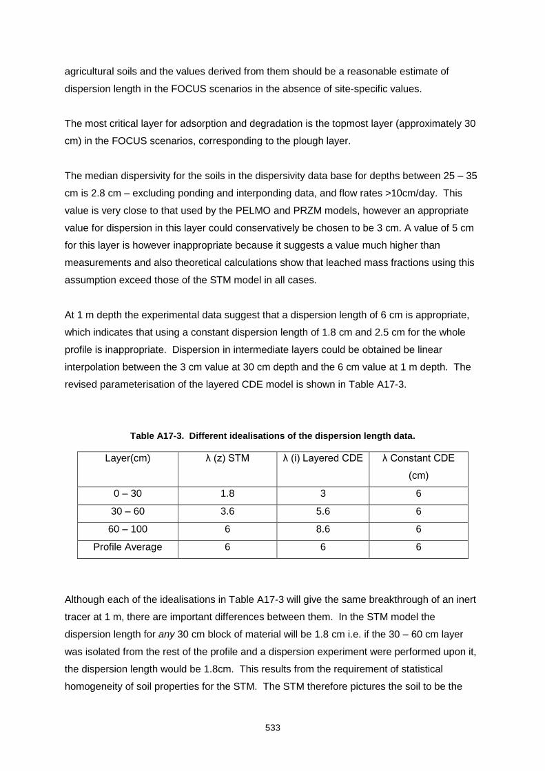
533
agricultural soils and the values derived from them should be a reasonable estimate of
dispersion length in the FOCUS scenarios in the absence of site-specific values.
The most critical layer for adsorption and degradation is the topmost layer (approximately 30
cm) in the FOCUS scenarios, corresponding to the plough layer.
The median dispersivity for the soils in the dispersivity data base for depths between 25 – 35
cm is 2.8 cm – excluding ponding and interponding data, and flow rates >10cm/day. This
value is very close to that used by the PELMO and PRZM models, however an appropriate
value for dispersion in this layer could conservatively be chosen to be 3 cm. A value of 5 cm
for this layer is however inappropriate because it suggests a value much higher than
measurements and also theoretical calculations show that leached mass fractions using this
assumption exceed those of the STM model in all cases.
At 1 m depth the experimental data suggest that a dispersion length of 6 cm is appropriate,
which indicates that using a constant dispersion length of 1.8 cm and 2.5 cm for the whole
profile is inappropriate. Dispersion in intermediate layers could be obtained be linear
interpolation between the 3 cm value at 30 cm depth and the 6 cm value at 1 m depth. The
revised parameterisation of the layered CDE model is shown in Table A17-3.
Table A17-3. Different idealisations of the dispersion length data.
Layer(cm) λ (z) STM λ (i) Layered CDE λ Constant CDE
(cm)
0 – 30 1.8 3 6
30 – 60 3.6 5.6 6
60 – 100 6 8.6 6
Profile Average 6 6 6
Although each of the idealisations in Table A17-3 will give the same breakthrough of an inert
tracer at 1 m, there are important differences between them. In the STM model the
dispersion length for any 30 cm block of material will be 1.8 cm i.e. if the 30 – 60 cm layer
was isolated from the rest of the profile and a dispersion experiment were performed upon it,
the dispersion length would be 1.8cm. This results from the requirement of statistical
homogeneity of soil properties for the STM. The STM therefore pictures the soil to be the

534
same throughout the top 1m. In contrast the layered CDE assumes that the different layers
of material behave differently, i.e. if a dispersion experiment was performed on the 30 – 60
cm block of material it would result in a value of dispersion on 5.6cm. For the constant CDE
model a dispersion experiment performed on any portion of any layer, or combination of
layers will yield a dispersion length of 6cm.
In reality, transport of solutes in soil is likely to be somewhere in-between the CDE and STM.
On the one hand, regions of fast flow are likely to be correlated to some extent across a
layered boundary, on the other some lateral mixing at a layered boundary is likely as well so
that the assumption of perfect correlation across a boundary is a theoretical extreme. The
layered CDE represents a compromise between the two models of solute dispersion.
Dispersion length increases with depth in the soil profile, and the parameterisation in Table
A17-3 will give the same breakthrough of an inert tracer at 1m as the STM. Unlike the STM
however, each soil layer behaves differently, as if it were different material. This is consistent
with the picture of soil having different structure in the plough layer through regular tillage
operations and then graduating to a more blocky structure with depth. The layered CDE is
similar to the constant CDE because each of the layers has a constant dispersivity.
In order to test this parameterisation of the layered CDE model, simulations were carried out
with the models in Table A17-3 for reactive solutes having a number of different substance
properties likely to result in leachate concentrations close to 0.1 µg/L. For these simulations
a soil having a bulk density of 1.4 g/mL and a volumetric water content of 0.3 was assumed,
as was a constant percolation rate resulting in a cumulative percolation of 300 mm/year.
Standard FOCUS assumptions for solute reactivity in the 0 – 30, 30 – 60 and 60 – 100 mm
layers was also assumed. The results of this modelling are shown in Table A17-4,
concentration profiles predicted by the various models for a substance having a Koc of 30 and
a half-life of 40 days are shown in Figure A17-2.
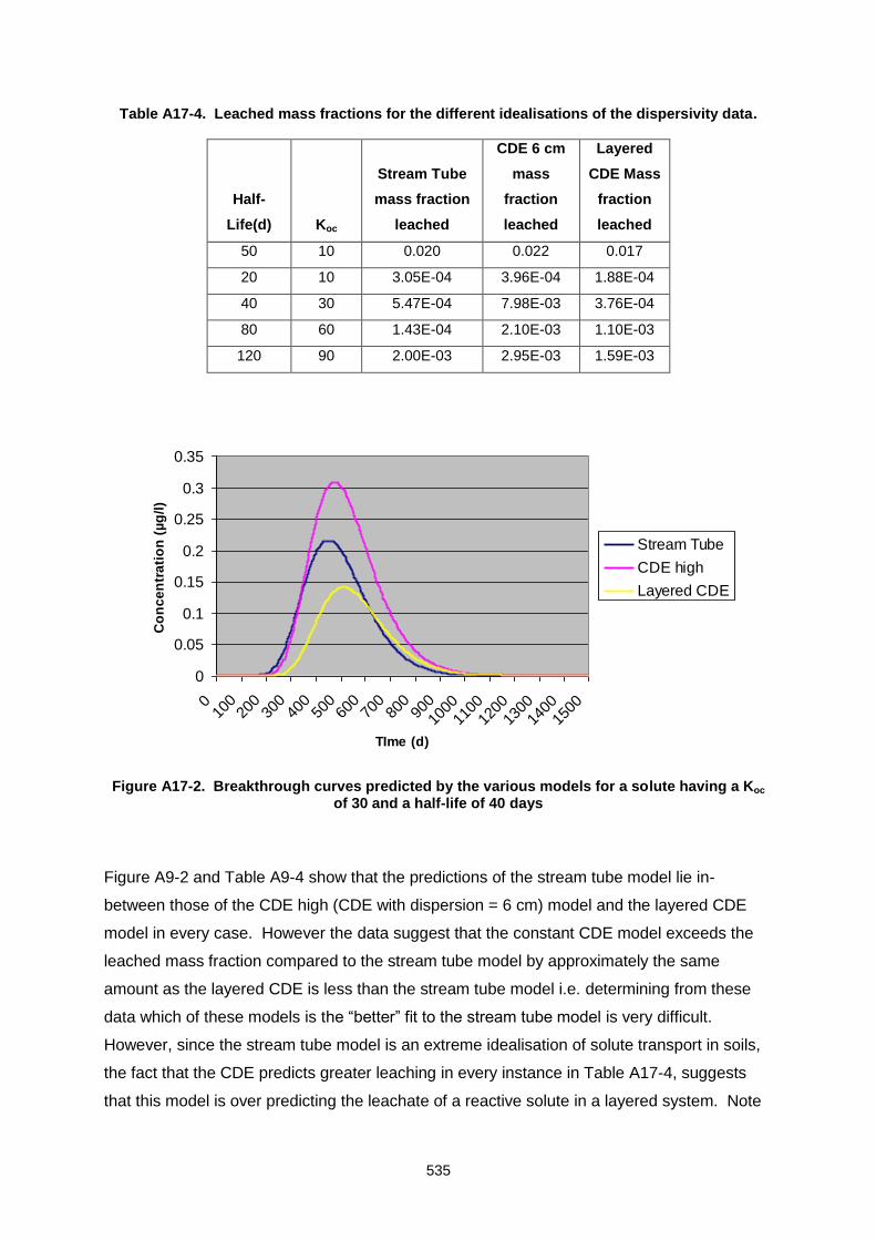
535
Table A17-4. Leached mass fractions for the different idealisations of the dispersivity data.
Half-
Life(d) Koc
Stream Tube
mass fraction
leached
CDE 6 cm
mass
fraction
leached
Layered
CDE Mass
fraction
leached
50 10 0.020 0.022 0.017
20 10 3.05E-04 3.96E-04 1.88E-04
40 30 5.47E-04 7.98E-03 3.76E-04
80 60 1.43E-04 2.10E-03 1.10E-03
120 90 2.00E-03 2.95E-03 1.59E-03
0
0.05
0.1
0.15
0.2
0.25
0.3
0.35
010
020
030
040
050
060
070
080
090
0
1000
1100
1200
1300
1400
1500
TIme (d)
Co
nc
en
tra
tio
n (
µg
/l)
Stream Tube
CDE high
Layered CDE
Figure A17-2. Breakthrough curves predicted by the various models for a solute having a Koc of 30 and a half-life of 40 days
Figure A9-2 and Table A9-4 show that the predictions of the stream tube model lie in-
between those of the CDE high (CDE with dispersion = 6 cm) model and the layered CDE
model in every case. However the data suggest that the constant CDE model exceeds the
leached mass fraction compared to the stream tube model by approximately the same
amount as the layered CDE is less than the stream tube model i.e. determining from these
data which of these models is the “better” fit to the stream tube model is very difficult.
However, since the stream tube model is an extreme idealisation of solute transport in soils,
the fact that the CDE predicts greater leaching in every instance in Table A17-4, suggests
that this model is over predicting the leachate of a reactive solute in a layered system. Note
536
that in terms of the FOCUS models the most relevant quantity to consider is the leached
mass fraction i.e. the area under each curve in Figure A9-1, because this quantity is more
similar to the output in assessments.
A key consideration in the construction of the layered CDE model was of zero correlation of
particle velocities across a layered boundary. A method by which transport across
boundaries may be correlated using the CDE model is provided at the end of this appendix.
Although this results in slightly changed values for dispersion in the various layers, the
general results outlined above are effectively unchanged.
Conclusions
The available data on dispersion of solutes in soil are far from clear; the data show a
wide degree of scatter and are based upon dispersion of inert tracers rather than
reactive substances. In addition there is no conclusive evidence from the literature
that solute transport should be stream tube or CDE and likely transport is site specific
and each model will apply in some circumstances and not in others.
How appropriate vertical and horizontal correlation distances should be chosen for
soil transport properties in K-field modelling is not clear from the literature. These
correlation lengths have a critical impact upon whether transport is likely to be stream-
tube like or like the CDE. Also how upward movement of water as a result of
evapotranspiration and the use of unsaturated water contents would affect results of
this modelling is not clear. Therefore whether highly complex K-field modelling can
be regarded as definitive is open to question.
The data on dispersion collected by this FOCUS group show that in general
dispersion increases with depth, that a value for dispersion of 3 cm is appropriate for
the top 30 cm of soil (which is the most reactive), and that a value of 6 cm is
appropriate for dispersion at 1 m. Any parameterisation of FOCUS models, which are
based upon the convection dispersion equation, to these data will require some form
of approximation and whatever approximation is used will affect concentrations at 1m
in a layered system. Given the requirement for models to predict concentrations of
substances to a precision of approximately 0.1% of an application, and the high
degree of variability of the dispersion measurements, again whether it is possible to
accurately distinguish between a dispersion of 2.5 cm and 5 cm with a high degree of
statistical certainty is open to question. Nevertheless, parameterising models to
537
represent the general features found in experiment while concentrating on the most
reactive layer i.e. 30 cm seems appropriate.
The layered CDE is an appropriate choice for dispersion in the FOCUS models
because:
o It uses a value of dispersion (3 cm) more appropriate to dispersion in the
critical, most reactive topmost layer of soil and one which is in better
agreement with the values in the dispersivity data base than the 6 cm value.
o Gives predictions for the breakthrough of an inert tracer at 1 m that are
consistent with the data from the dispersivity data base.
o Gives predictions for leached mass fractions of reactive solutes that are in as
good agreement with the values of the stream tube model as the constant
CDE model. However, since the stream tube model is an extreme of solute
transport requiring perfect correlation between layers and transport
parameters that do not change, on average, with depth, the fact that constant
CDE model exceeds the leached mass fractions predicted by the stream tube
model for a reactive solute indicate that it predicts a leached mass fraction that
are too high for reactive solutes.
o Is a suitable compromise that fits the observed features of the measured data
on dispersion (i.e. increases with depth) and is consistent with the generalised
picture of agricultural soils being well-tilled and homogeneous in the plough
layer and more blocky and structured with depth.
References
Butters G.L., and Jury W.A. 1989. Field Scale Transport of Bromide in an Unsaturated Soil,
Water resources Research 25:1583-1589.
Dagan G. 1986. Statistical Theory of Groundwater Flow and Transport: Pore to Lab, Lab to
Formation, and Formation to Regional Scale. Water Resources Research 22:120S-
134S.
Ellsworth T.R., and Jury W. A. 1991. A Three-Dimensional Filed Study for Solute Transport
through Unsaturated, Layered, Porous Media. Water Resources Research 27:967-981.
Flury M., Jury W.A, and Kladivko. 1998. Field-Scale Solute Transport in the Vadose Zone:
Experimental Observations and Interpretation. Chapter 13 in Physical Nonequilibrium in
Soils: Modelling and Application, Ann Arbor Press, Chelsea, MI.
538
Gelhar L. 1986. Stochastic Subsurface Hydrology from Theory to Applications. Water
Resources Research 22:135S-145S.
Janvaux M., and Vanclooster M. 2003. Robust Estimation of the Generalized Solute
Transfer Function Parameters. Soil Science America Journal 67:81-91.
Heuvelman H.J, and McInnes K. 1999. Solute Travel Time Distributions in Soil: A Field
Survey. Soil Science vol 164, no 1.
Jury W.A. 1982. Simulation of Solute Transport Using a Transfer Function Model. Water
Resources Research 18:363-368.
Jury W.A, and Scotter D.R. 1994. A Unified Approach to Stochastic-Convective Transport
Problems. Soil Science America Journal 58:1327-1336.
Matheron G, and De Marsily G. 1980. Is Transport in Porous Media always Diffusive? A
Counterexample. Water Resources Research 16(5):901-917.
Nissen H.H., Moldrup P., Kachanoski R.G. 2000. Time Domain Reflectormetry
Measurement of Solute Transport across a Layered Soil Boundary. Soil Science America
Journal 64:62-74.
Pickens, J F, and Grisak, G E. 1981. Scale-Dependent Dispersion in a Stratified Granular
Aquifer. Water Resources Research 17:1191-1211.
Rockhold, M. L. and R .E. Rossi. 1996. Application of similar media scaling and conditional
simulation for modeling water flow and tritium transport at the Las Cruces Trench Site.
Water Resources Research 32:595-609.
Roth, K. and K. Hammel. 1996. Transport of conservative chemical through an unsaturated
two-dimensional Miller-similar medium with steady state flow. Water Resources
Research 32:1653-1663.
Russo, D and M. Bouton. 1992. Statistical analysis of spatial variability in unsaturated flow
parameters. Water Resources Research 28:1911-1925
Shukla M.K., Kastanek F.J., Nielsen D.R. 2002. Inspectional Analysis of Convective-
Dispersive Equation and Application on Measured Breakthrough Curves. Soil Science
America Journal 66(4):1087-1094.
Shukla M.K., Ellsworth T.R., Hudson R.J., Nielson D.R. 2003. Effect of Water Flux on Solute
Velocity and Dispersion. Soil Science America Journal 67:449-457.
Si Bing Cheng. 2002. Spatial and Statistical Similarities of Local Soil Water Fluxes. Soil
Science America Journal 66:753-759.
Taylor, G. 1953. Dispersion of Soluble Matter in Solvent Flowing Slowly through a Tube.
Vanderborght J., Gahwiller P., Fluhler H. 2002. Identification of Transport Processes in Soil
Cores Using Fluorescent Tracers. Soil Science America Journal 66:774-787.
Zhang R. 2000. Generalized Transfer Function Model for Solute Transport in
Heterogeneous Soils. Soil Science America Journal 64:1595-1602.
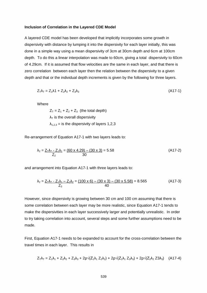
539
Inclusion of Correlation in the Layered CDE Model
A layered CDE model has been developed that implicitly incorporates some growth in
dispersivity with distance by lumping it into the dispersivity for each layer initially, this was
done in a simple way using a mean dispersivity of 3cm at 30cm depth and 6cm at 100cm
depth. To do this a linear interpolation was made to 60cm, giving a total dispersivity to 60cm
of 4.29cm. If it is assumed that flow velocities are the same in each layer, and that there is
zero correlation between each layer then the relation between the dispersivity to a given
depth and that or the individual depth increments is given by the following for three layers.
ZTλT = Z1λ1 + Z2λ2 + Z3λ3 (A17-1)
Where
ZT = Z1 + Z2 + Z3 (the total depth)
λT is the overall dispersivity
λ1,2,3 = is the dispersivity of layers 1,2,3
Re-arrangement of Equation A17-1 with two layers leads to:
λ2 = ZTλT - Z1λ1 = (60 x 4.29) – (30 x 3) = 5.58 (A17-2) Z2 30
and arrangement into Equation A17-1 with three layers leads to:
λ2 = ZTλT - Z1λ1 – Z2λ2 = (100 x 6) – (30 x 3) – (30 x 5.58) = 8.565 (A17-3) Z3 40
However, since dispersivity is growing between 30 cm and 100 cm assuming that there is
some correlation between each layer may be more realistic, since Equation A17-1 tends to
make the dispersivities in each layer successively larger and potentially unrealistic. In order
to try taking correlation into account, several steps and some further assumptions need to be
made.
First, Equation A17-1 needs to be expanded to account for the cross-correlation between the
travel times in each layer. This results in
ZTλT = Z1λ1 + Z2λ2 + Z3λ3 + 2ρ√(Z1λ1 Z2λ2) + 2ρ√(Z1λ1 Z3λ3) + 2ρ√(Z2λ2 Z3λ3) (A17-4)
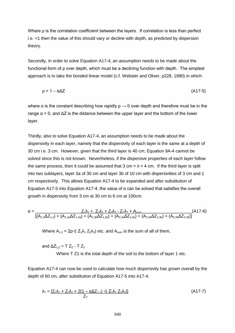
540
Where ρ is the correlation coefficient between the layers. If correlation is less than perfect
i.e. <1 then the value of this should vary or decline with depth, as predicted by dispersion
theory.
Secondly, in order to solve Equation A17-4, an assumption needs to be made about the
functional form of ρ over depth, which must be a declining function with depth. The simplest
approach is to take the bonded linear model (c.f. Webster and Oliver, p228, 1990) in which
ρ = 1 – αΔZ (A17-5)
where α is the constant describing how rapidly ρ → 0 over depth and therefore must be in the
range α > 0, and ΔZ is the distance between the upper layer and the bottom of the lower
layer.
Thirdly, also to solve Equation A17-4, an assumption needs to be made about the
dispersivity in each layer, namely that the dispersivity of each layer is the same at a depth of
30 cm i.e. 3 cm. However, given that the third layer is 40 cm, Equation 9A-4 cannot be
solved since this is not known. Nevertheless, if the dispersive properties of each layer follow
the same process, then it could be assumed that 3 cm < λ < 4 cm. If the third layer is split
into two sublayers, layer 3a of 30 cm and layer 3b of 10 cm with dispersivities of 3 cm and 1
cm respectively. This allows Equation A17-4 to be expanded and after substitution of
Equation A17-5 into Equation A17-4, the value of α can be solved that satisfies the overall
growth in dispersivity from 3 cm at 30 cm to 6 cm at 100cm.
α = Z1λ1 + Z2λ2 + Z3λ3 - ZTλT + Asum (A17-6) [(A1,2ΔZ1,2) + (A1,3aΔZ1,3a) + (A1,3bΔZ1,3b) + (A2,3aΔZ2,3a) + (A2,3bΔZ2,3b) + (A2,3bΔZ2,3b)]
Where A1,2 = 2ρ√( Z1λ1 Z2λ2) etc. and Asum is the sum of all of them,
and ΔZ1,2 = T Z2 - T Z1
Where T Z1 is the total depth of the soil to the bottom of layer 1 etc.
Equation A17-4 can now be used to calculate how much dispersivity has grown overall by the
depth of 60 cm, after substitution of Equation A17-5 into A17-4.
λT = [Z1λ1 + Z2λ2 + 2(1 – αΔZ1,2) √( Z1λ1 Z2λ2)] (A17-7) ZT
541
The results give a value for α of 0.0139 and the value of λT of 4.75 cm at 60 cm (somewhat
higher than the value of 4.29 given by linear interpolation).
Finally to determine the dispersivity values for each layer if the layered CDE is used to
implicitly incorporate the growth of the dispersivity, then Equations A17-2 and A17-3 can be
used to lump this growth giving:
λ2 = (60 x 4.75) – (30 x 3) = 6.5cm 30
λ3 = (100 x 6) – (30 x 3) – (30 x 6.5) = 7.9cm 40
542
APPENDIX 18. COMPARISON OF MARS AND FAO POTENTIAL REFERENCE EVAPOTRANSPIRATION
The reference evapotranspiration data used in the FOCUS ground water scenarios were
inferred from the MARS data base. The potential crop evapotranspiration data were
obtained by multiplying these reference evaporation data (abbreviated as ET0_MARS) with
crop coefficients (kc coefficients). However, the crop coefficients used in the FOCUS ground
water scenarios were based on the data reported by the FAO, in particular the FAO crop
water requirement calculation procedures (e.g. Allen et al., 1998). The FAO kc procedure,
however, is based on the ET0 procedures proposed by FAO, which will be referred to as
ET0_FAO. In principle the kc factors may only be combined with ET_FAO since kc factors
have been obtained by dividing the measurement of the potential evapotranspiration in field
and lysimeter studies with ET0_FAO. Although both ET0_MARS and ET0_FAO are based
on the Penman Monteith equation, the ET0_FAO and ET_MARS will not necessarily be the
same since different parameterisation schemes are used for the surface and aerodynamic
resistance terms in the Penman Monteith equation. Therefore inconsistencies may appear
when combining FAO based kc factors with ET0_MARS.
Procedure for calculating ET0_FAO from the MARS data base
All calculations were based on the FAO recommendations as described by Allen et al.,
(1998). The basic formula was (Allen et al., 1998, Equation 6 ):
)34.01(
273
900)(408.0
2
2
u
eeuT
GR
ETasn
o
(A18-1)
with
ETo , reference evapotranspiration (mm day-1) ;
, slope of vapour pressure curve (kPa K-1)
Rn, net radiation at the crop surface (MJ m-2 day-1) ;
G, soil heat flux density (MJ m-2 day-1) ;
T, air temperature at 2 m height (°C) ;
es, saturation vapour pressure (kPa) ;
ea, actual vapour pressure (kPa) ;
u2, wind speed at 2 m height (m s-1) ;
, the psychometric constraint (kPa K-1) ;
where G was set equal to 0.
543
The following subparameterisation was used for the saturation vapour pressure (Equations
11 and 12 from Allen et al., 1998)
2
)()( min
0
max
0 TeTees
(A18-2)
with
3.237
27.17exp6108.0)(0
T
TTe (A18-3)
with
e0(T), saturation vapour pressure at the air temperature T (kPa) ;
T, air temperature (°C) ;
Tmax, maximum daily air temperature (°C) ;
Tmin, minimum daily air temperature (°C) .
The slope of the vapour pressure curve was estimated from (Equation 13 of Allen et al.,
1998) :
23.237
3.237
27.17exp6108.04096
T
T
T
(A18-4)
The psychrometric constant was estimated from Equation 8 of Allen et al. (1998):
P310.665.0 (A18-5)
with
P, the atmospheric pressure (kPa).
This atmospheric pressure was estimated from the elevation above sea level using Equation
7 of Allen et al. (1998).
The wind speed at 2 m was estimated from the wind speed at 10 m (i.e. the measurement
height in the MARS database) using Equation 47 of Allen et al. (1998). This implies that the
wind speed at 2 m is 0.75 times the wind speed at 10 m.
The net radiation Rn was calculated as the difference between the net shortwave radiation
Rns and the outgoing net longwave radiation Rnl (Equation 40 of Allen et al., 1998).
35.035.114.034.0
2
4
min,
4
max,
so
sa
KK
nlR
Re
TTR (A18-6)
with
544
Rnl, net outgoing longwave radiation (MJ m-2 day-1)
, Stephan-Boltzman constant (4.903 10-9 MJ K-4 m-2 day-1)
Tmax,K , maximum absolute temperature during the 24 hours day (K)
Tmin,K , maximum absolute temperature during the 24 hours day (K)
Rs, measured incoming solar radiation (MJ m-2 day-1)
Rso, calculated clear sky radiation (MJ m-2 day-1)
The last term of this equation (1.35 Rs/Rso - 0.35) expresses the effect of cloudiness. Allen et
al. (1998) prescribe that Rs/Rso has to be less than or equal to 1.0. The clear sky radiation
Rso is estimated from the elevation above sea level and the extraterrestrial radiation, Ra,
using Equation 37 of Allen et al. (1998). This extraterrestrial radiation is estimated from the
day-month-year combination and the latitude of the location (provided in Table A20-37) using
Equations 21, 22, 23, 24 and 25 of Allen et al. (1998).
The net shortwave radiation was calculated as:
sns RR 1 (A18-7)
where the albedo (-) was set to 0.23 (Equation 38 of Allen et al., 1998).
The elevation above sea level of all nine locations was assumed to be 100 m above sea
level. Further input for the calculations were daily values of Tmax , Tmin , incoming solar
radiation Rs , wind speed at 10 m, and actual vapour pressure, ea.
Selection of ET0 approach
Table A18-1 illustrates the differences between the two methods.
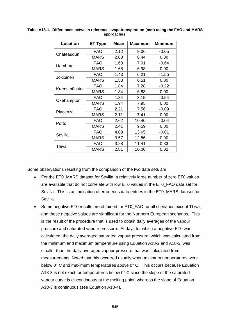
545
Table A18-1. Differences between reference evapotranspiration (mm) using the FAO and MARS approaches.
Location ET Type Mean Maximum Minimum
Châteaudun FAO 2.12 9.06 -0.05
MARS 2.03 8.44 0.00
Hamburg FAO 1.68 7.01 -0.64
MARS 1.68 6.98 0.00
Jokioinen FAO 1.43 6.21 -1.55
MARS 1.53 6.51 0.00
Kremsmünster FAO 1.84 7.28 -0.22
MARS 1.84 6.83 0.00
Okehampton FAO 1.84 8.15 -0.54
MARS 1.94 7.95 0.00
Piacenza FAO 2.21 7.56 -0.09
MARS 2.11 7.41 0.00
Porto FAO 2.62 10.40 -0.04
MARS 2.41 9.59 0.00
Sevilla FAO 4.09 13.65 -0.01
MARS 3.57 12.86 0.00
Thiva FAO 3.28 11.41 0.33
MARS 2.81 10.00 0.02
Some observations resulting from the comparison of the two data sets are:
For the ET0_MARS dataset for Sevilla, a relatively large number of zero ET0 values
are available that do not correlate with low ET0 values in the ET0_FAO data set for
Sevilla. This is an indication of erroneous data entries in the ET0_MARS dataset for
Sevilla.
Some negative ET0 results are obtained for ET0_FAO for all scenarios except Thiva,
and these negative values are significant for the Northern European scenarios. This
is the result of the procedure that is used to obtain daily averages of the vapour
pressure and saturated vapour pressure. At days for which a negative ET0 was
calculated, the daily averaged saturated vapour pressure, which was calculated from
the minimum and maximum temperature using Equation A18-2 and A18-3, was
smaller than the daily averaged vapour pressure that was calculated from
measurements. Noted that this occurred usually when minimum temperatures were
below 0° C and maximum temperatures above 0° C. This occurs because Equation
A18-3 is not exact for temperatures below 0° C since the slope of the saturated
vapour curve is discontinuous at the melting point, whereas the slope of Equation
A18-3 is continuous (see Equation A18-4).
546
The ET0_FAO is usually higher than ET0_Mars. In two stations, Thiva and Sevilla,
the mean ETO is about 15 percent of the mean ET0_Mars. In three stations, Porto,
Piacenza, and Châteaudun, this difference is between 4 and 10 percent of the mean
ET0_Mars. In the four ‘northern’ European stations, Okehampton, Kremsmünster,
Hamburg and Jokioinen, the mean ET0_Mars is equal to or smaller than the mean
ET0 (for Jokioinen even 7 percent smaller).
The ET0_FAO parameterisation is considered to be more reliable for southern
European conditions since it was developed to support irrigation water management.
For semi-arid conditions, which prevail in Thiva and Sevilla, the ET0_FAO
parameterisation even tends to underestimate the reference evapotranspiration (Dirk
Raes, K.U. Leuven, Belgium, personal communication). Therefore, the ET0_Mars is
considered to underestimate the actual reference evapotranspiration in southern
European countries.
Based on the information in this section the work group decided to use the FAO procedures
for calculating reference evapotranspiration for Porto, Piacenza, Châteaudun, Thiva, and
Sevilla. The MARS approach to calculating reference evapotranspiration will be retained for
the other four northern European locations (Okehampton, Kremsmünster, Hamburg and
Jokioinen) because there was little difference between the two approaches for these climatic
conditions and the parameterisation procedure proposed by the FAO sometimes leads to
negative reference evapotranspiration rates in northern European conditions.
As described before, the FAO procedure resulted sometimes in small negative values for
Porto, Piacenza, Châteaudun, and Sevilla (see Table A18-1). These were set to zero in the
meteorological input files of the leaching models because negative values are not considered
realistic and because these leaching models do not accept negative reference
evapotranspiration values.
References
Allen RG, Pereira LS, Raes D and Smith M. 1998. Crop evapotranspiration - Guidelines for
computing crop water requirements. FAO Irrigation and drainage paper 56. FAO, Rome.
Available at www.fao.org/docrep/X0490E/x0490e00.htm#Contents.

547
APPENDIX 19. PROCEDURES FOR ESTIMATING CROP EVAOPOTRANSPIRATION FACTORS
A comparison of the evapotranspiration showed that the different procedures within the
models for implementing crop kc factors were contributing significantly to the variability of the
overall water balance. Therefore the work group decided to harmonise the procedures by
implementing a common procedure in which the year was divided into four periods. The
cropping data from FOCUS (2000) as well as the length of the senescence period from
(Doorenbos and Pruitt, 1977; and Raes et al. 1988) was used to define these periods. The
kc values were based on information from Doorenbos and Pruitt (1977) and Raes et al.
(1988). The resulting time periods and kc factors are included in the tables in Appendix 20.
The following paragraphs describe the derivation of the kc factors.
Four each of the four periods the kc was assigned in the following manner:
Harvest to the day before emergence. The soil surface is bare soil and the kc factor was
assumed to be 1.0 as in FOCUS (2000).
Emergence to the day before maximum LAI (leaf area index). The kc for this period was
the average of the kc at the time of emergence (value of 1) and the kc at maximum LAI.
Maximum LAI to day before start of senescence. The kc for this period was the kc at
maximum LAI.
Start of senescence to the day before harvest. The kc for this period was the average of
the kc at maximum LAI and the kc at senescence.
Special Cases:
Apples. Emergence was considered to be leaf emergence and harvest was considered
to be the time of leaf drop.
Bush berries. The kc factors provided for vines were used.
Citrus. A year-round kc value of 0.60 was assumed.
Grass and alfalfa. A year-round kc value of 1 was assumed.
548
Strawberries. A kc value of 1 was assumed based on expert judgement and some
informal information found on the internet.
Senescence date before maximum LAI date. When the start of senescence, calculated
by subtracting the length of the senescence period from the harvest date, was prior to
day of maximum LAI provided by local experts, senescence was considered to start on
the day of maximum LAI and the period starting at maximum LAI until the day before the
start of senescence was eliminated.
Emergence data of March 1. Emergence dates of March 1 were changed to March 2 to
avoid that the day before emergence varied between February 28 and 29.
References
FOCUS. 2000. FOCUS groundwater scenarios in the EU review of active substances.
Report of the FOCUS Groundwater Scenarios Workgroup, EC Document Reference
Sanco/321/2000 rev.2, 202pp.
Doorenbos and Pruitt. 1997. Crop water requirements. FAO, Irrigation and drainage paper
24, Rome, 144 pp.
Raes D, H. Lemmens, P. Van Aelst, M. Vanden Bulcke and M. Smith. 1988. IRSIS,
Irrigation scheduling information system. V1, Manual. Lab. of land management, KU
Leuven.
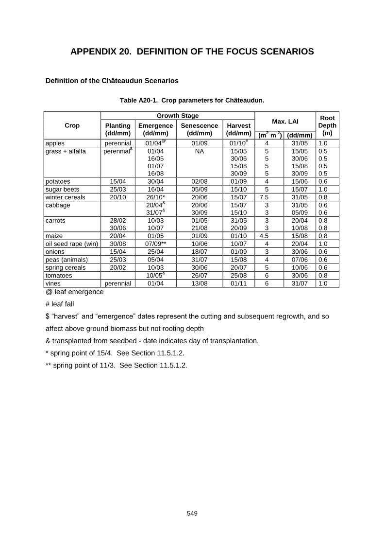
549
APPENDIX 20. DEFINITION OF THE FOCUS SCENARIOS
Definition of the Châteaudun Scenarios
Table A20-1. Crop parameters for Châteaudun.
Crop
Growth Stage Max. LAI
Root Depth
(m) Planting (dd/mm)
Emergence (dd/mm)
Senescence (dd/mm)
Harvest (dd/mm) (m
2 m
-2) (dd/mm)
apples perennial 01/04@
01/09 01/10# 4 31/05 1.0
grass + alfalfa perennial$ 01/04
16/05 01/07 16/08
NA 15/05 30/06 15/08 30/09
5 5 5 5
15/05 30/06 15/08 30/09
0.5 0.5 0.5 0.5
potatoes 15/04 30/04 02/08 01/09 4 15/06 0.6
sugar beets 25/03 16/04 05/09 15/10 5 15/07 1.0
winter cereals 20/10 26/10* 20/06 15/07 7.5 31/05 0.8
cabbage 20/04&
31/07&
20/06 30/09
15/07 15/10
3 3
31/05 05/09
0.6 0.6
carrots 28/02 30/06
10/03 10/07
01/05 21/08
31/05 20/09
3 3
20/04 10/08
0.8 0.8
maize 20/04 01/05 01/09 01/10 4.5 15/08 0.8
oil seed rape (win) 30/08 07/09** 10/06 10/07 4 20/04 1.0
onions 15/04 25/04 18/07 01/09 3 30/06 0.6
peas (animals) 25/03 05/04 31/07 15/08 4 07/06 0.6
spring cereals 20/02 10/03 30/06 20/07 5 10/06 0.6
tomatoes 10/05& 26/07 25/08 6 30/06 0.8
vines perennial 01/04 13/08 01/11 6 31/07 1.0
@ leaf emergence
# leaf fall
$ “harvest” and “emergence” dates represent the cutting and subsequent regrowth, and so
affect above ground biomass but not rooting depth
& transplanted from seedbed - date indicates day of transplantation.
* spring point of 15/4. See Section 11.5.1.2.
** spring point of 11/3. See Section 11.5.1.2.
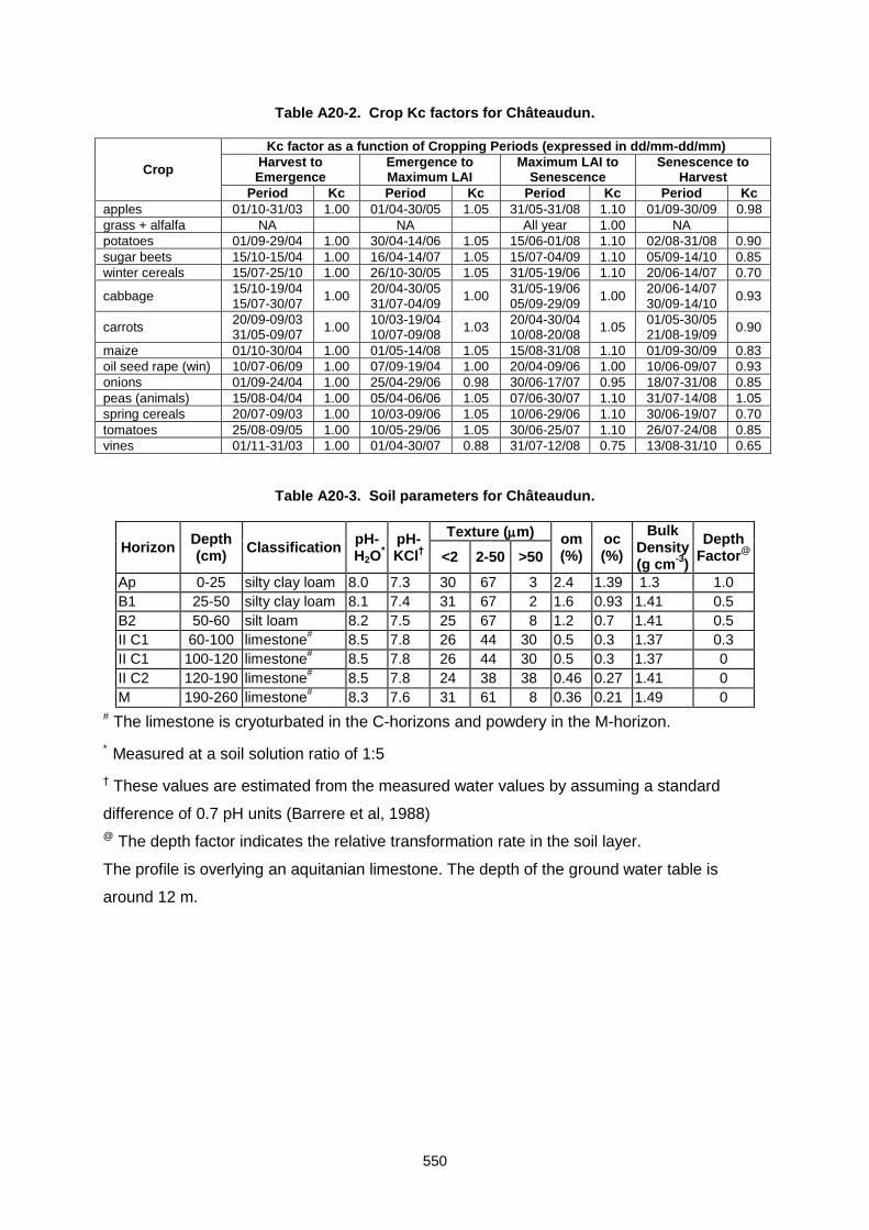
550
Table A20-2. Crop Kc factors for Châteaudun.
Crop
Kc factor as a function of Cropping Periods (expressed in dd/mm-dd/mm)
Harvest to Emergence
Emergence to Maximum LAI
Maximum LAI to Senescence
Senescence to Harvest
Period Kc Period Kc Period Kc Period Kc
apples 01/10-31/03 1.00 01/04-30/05 1.05 31/05-31/08 1.10 01/09-30/09 0.98
grass + alfalfa NA NA All year 1.00 NA
potatoes 01/09-29/04 1.00 30/04-14/06 1.05 15/06-01/08 1.10 02/08-31/08 0.90
sugar beets 15/10-15/04 1.00 16/04-14/07 1.05 15/07-04/09 1.10 05/09-14/10 0.85
winter cereals 15/07-25/10 1.00 26/10-30/05 1.05 31/05-19/06 1.10 20/06-14/07 0.70
cabbage 15/10-19/04 15/07-30/07
1.00 20/04-30/05 31/07-04/09
1.00 31/05-19/06 05/09-29/09
1.00 20/06-14/07 30/09-14/10
0.93
carrots 20/09-09/03 31/05-09/07
1.00 10/03-19/04 10/07-09/08
1.03 20/04-30/04 10/08-20/08
1.05 01/05-30/05 21/08-19/09
0.90
maize 01/10-30/04 1.00 01/05-14/08 1.05 15/08-31/08 1.10 01/09-30/09 0.83
oil seed rape (win) 10/07-06/09 1.00 07/09-19/04 1.00 20/04-09/06 1.00 10/06-09/07 0.93
onions 01/09-24/04 1.00 25/04-29/06 0.98 30/06-17/07 0.95 18/07-31/08 0.85
peas (animals) 15/08-04/04 1.00 05/04-06/06 1.05 07/06-30/07 1.10 31/07-14/08 1.05
spring cereals 20/07-09/03 1.00 10/03-09/06 1.05 10/06-29/06 1.10 30/06-19/07 0.70
tomatoes 25/08-09/05 1.00 10/05-29/06 1.05 30/06-25/07 1.10 26/07-24/08 0.85
vines 01/11-31/03 1.00 01/04-30/07 0.88 31/07-12/08 0.75 13/08-31/10 0.65
Table A20-3. Soil parameters for Châteaudun.
Horizon Depth (cm)
Classification pH-H2O
*
pH-KCl
†
Texture (m) om
(%) oc (%)
Bulk Density (g cm
-3)
Depth Factor
@ <2 2-50 >50
Ap 0-25 silty clay loam 8.0 7.3 30 67 3 2.4 1.39 1.3 1.0
B1 25-50 silty clay loam 8.1 7.4 31 67 2 1.6 0.93 1.41 0.5
B2 50-60 silt loam 8.2 7.5 25 67 8 1.2 0.7 1.41 0.5
II C1 60-100 limestone# 8.5 7.8 26 44 30 0.5 0.3 1.37 0.3
II C1 100-120 limestone# 8.5 7.8 26 44 30 0.5 0.3 1.37 0
II C2 120-190 limestone# 8.5 7.8 24 38 38 0.46 0.27 1.41 0
M 190-260 limestone# 8.3 7.6 31 61 8 0.36 0.21 1.49 0
# The limestone is cryoturbated in the C-horizons and powdery in the M-horizon.
* Measured at a soil solution ratio of 1:5
† These values are estimated from the measured water values by assuming a standard
difference of 0.7 pH units (Barrere et al, 1988)
@ The depth factor indicates the relative transformation rate in the soil layer.
The profile is overlying an aquitanian limestone. The depth of the ground water table is
around 12 m.
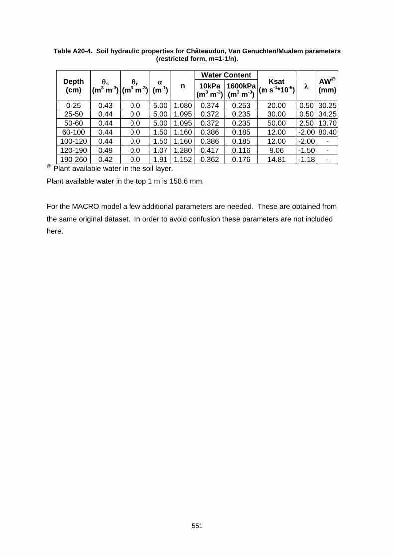
551
Table A20-4. Soil hydraulic properties for Châteaudun, Van Genuchten/Mualem parameters (restricted form, m=1-1/n).
Depth (cm)
s (m3 m-3)
r (m3 m-3)
(m-1)
n
Water Content Ksat
(m s-1*10-6)
AW@ (mm)
10kPa (m3 m-3)
1600kPa (m3 m-3)
0-25 0.43 0.0 5.00 1.080 0.374 0.253 20.00 0.50 30.25
25-50 0.44 0.0 5.00 1.095 0.372 0.235 30.00 0.50 34.25
50-60 0.44 0.0 5.00 1.095 0.372 0.235 50.00 2.50 13.70
60-100 0.44 0.0 1.50 1.160 0.386 0.185 12.00 -2.00 80.40
100-120 0.44 0.0 1.50 1.160 0.386 0.185 12.00 -2.00 -
120-190 0.49 0.0 1.07 1.280 0.417 0.116 9.06 -1.50 -
190-260 0.42 0.0 1.91 1.152 0.362 0.176 14.81 -1.18 - @ Plant available water in the soil layer.
Plant available water in the top 1 m is 158.6 mm.
For the MACRO model a few additional parameters are needed. These are obtained from
the same original dataset. In order to avoid confusion these parameters are not included
here.
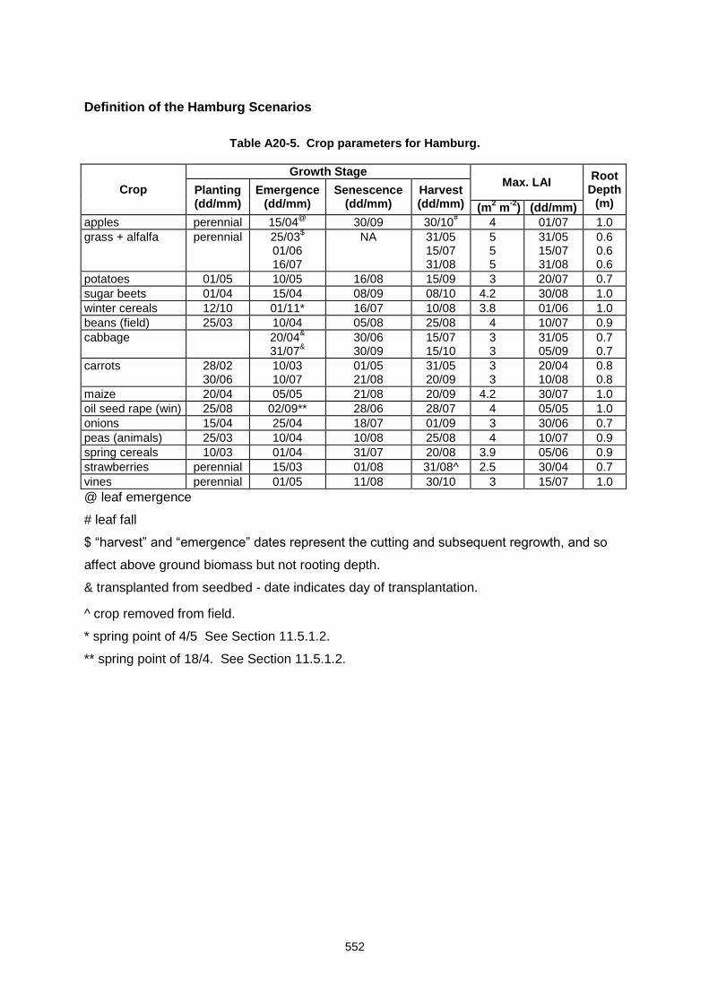
552
Definition of the Hamburg Scenarios
Table A20-5. Crop parameters for Hamburg.
Crop
Growth Stage Max. LAI
Root Depth
(m) Planting (dd/mm)
Emergence (dd/mm)
Senescence (dd/mm)
Harvest (dd/mm) (m
2 m
-2) (dd/mm)
apples perennial 15/04@
30/09 30/10# 4 01/07 1.0
grass + alfalfa perennial 25/03$
01/06 16/07
NA 31/05 15/07 31/08
5 5 5
31/05 15/07 31/08
0.6 0.6 0.6
potatoes 01/05 10/05 16/08 15/09 3 20/07 0.7
sugar beets 01/04 15/04 08/09 08/10 4.2 30/08 1.0
winter cereals 12/10 01/11* 16/07 10/08 3.8 01/06 1.0
beans (field) 25/03 10/04 05/08 25/08 4 10/07 0.9
cabbage 20/04&
31/07&
30/06 30/09
15/07 15/10
3 3
31/05 05/09
0.7 0.7
carrots 28/02 30/06
10/03 10/07
01/05 21/08
31/05 20/09
3 3
20/04 10/08
0.8 0.8
maize 20/04 05/05 21/08 20/09 4.2 30/07 1.0
oil seed rape (win) 25/08 02/09** 28/06 28/07 4 05/05 1.0
onions 15/04 25/04 18/07 01/09 3 30/06 0.7
peas (animals) 25/03 10/04 10/08 25/08 4 10/07 0.9
spring cereals 10/03 01/04 31/07 20/08 3.9 05/06 0.9
strawberries perennial 15/03 01/08 31/08^ 2.5 30/04 0.7
vines perennial 01/05 11/08 30/10 3 15/07 1.0
@ leaf emergence
# leaf fall
$ “harvest” and “emergence” dates represent the cutting and subsequent regrowth, and so
affect above ground biomass but not rooting depth.
& transplanted from seedbed - date indicates day of transplantation.
^ crop removed from field.
* spring point of 4/5 See Section 11.5.1.2.
** spring point of 18/4. See Section 11.5.1.2.
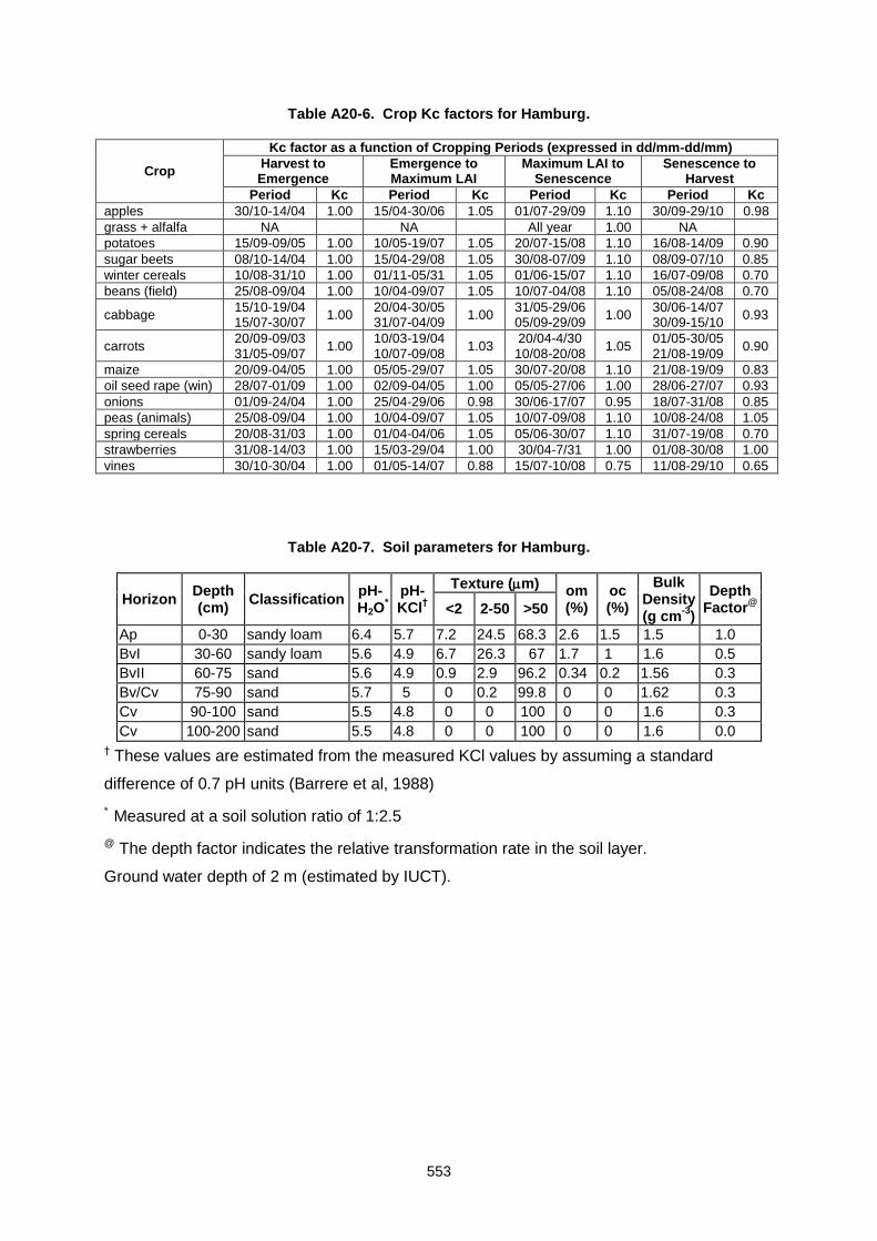
553
Table A20-6. Crop Kc factors for Hamburg.
Crop
Kc factor as a function of Cropping Periods (expressed in dd/mm-dd/mm)
Harvest to Emergence
Emergence to Maximum LAI
Maximum LAI to Senescence
Senescence to Harvest
Period Kc Period Kc Period Kc Period Kc
apples 30/10-14/04 1.00 15/04-30/06 1.05 01/07-29/09 1.10 30/09-29/10 0.98
grass + alfalfa NA NA All year 1.00 NA
potatoes 15/09-09/05 1.00 10/05-19/07 1.05 20/07-15/08 1.10 16/08-14/09 0.90
sugar beets 08/10-14/04 1.00 15/04-29/08 1.05 30/08-07/09 1.10 08/09-07/10 0.85
winter cereals 10/08-31/10 1.00 01/11-05/31 1.05 01/06-15/07 1.10 16/07-09/08 0.70
beans (field) 25/08-09/04 1.00 10/04-09/07 1.05 10/07-04/08 1.10 05/08-24/08 0.70
cabbage 15/10-19/04 15/07-30/07
1.00 20/04-30/05 31/07-04/09
1.00 31/05-29/06 05/09-29/09
1.00 30/06-14/07 30/09-15/10
0.93
carrots 20/09-09/03 31/05-09/07
1.00 10/03-19/04 10/07-09/08
1.03 20/04-4/30 10/08-20/08
1.05 01/05-30/05 21/08-19/09
0.90
maize 20/09-04/05 1.00 05/05-29/07 1.05 30/07-20/08 1.10 21/08-19/09 0.83
oil seed rape (win) 28/07-01/09 1.00 02/09-04/05 1.00 05/05-27/06 1.00 28/06-27/07 0.93
onions 01/09-24/04 1.00 25/04-29/06 0.98 30/06-17/07 0.95 18/07-31/08 0.85
peas (animals) 25/08-09/04 1.00 10/04-09/07 1.05 10/07-09/08 1.10 10/08-24/08 1.05
spring cereals 20/08-31/03 1.00 01/04-04/06 1.05 05/06-30/07 1.10 31/07-19/08 0.70
strawberries 31/08-14/03 1.00 15/03-29/04 1.00 30/04-7/31 1.00 01/08-30/08 1.00
vines 30/10-30/04 1.00 01/05-14/07 0.88 15/07-10/08 0.75 11/08-29/10 0.65
Table A20-7. Soil parameters for Hamburg.
Horizon Depth (cm)
Classification pH-H2O
*
pH-KCl
†
Texture (m) om
(%) oc (%)
Bulk Density (g cm
-3)
Depth Factor
@ <2 2-50 >50
Ap 0-30 sandy loam 6.4 5.7 7.2 24.5 68.3 2.6 1.5 1.5 1.0
BvI 30-60 sandy loam 5.6 4.9 6.7 26.3 67 1.7 1 1.6 0.5
BvII 60-75 sand 5.6 4.9 0.9 2.9 96.2 0.34 0.2 1.56 0.3
Bv/Cv 75-90 sand 5.7 5 0 0.2 99.8 0 0 1.62 0.3
Cv 90-100 sand 5.5 4.8 0 0 100 0 0 1.6 0.3
Cv 100-200 sand 5.5 4.8 0 0 100 0 0 1.6 0.0
† These values are estimated from the measured KCl values by assuming a standard
difference of 0.7 pH units (Barrere et al, 1988)
* Measured at a soil solution ratio of 1:2.5
@ The depth factor indicates the relative transformation rate in the soil layer.
Ground water depth of 2 m (estimated by IUCT).
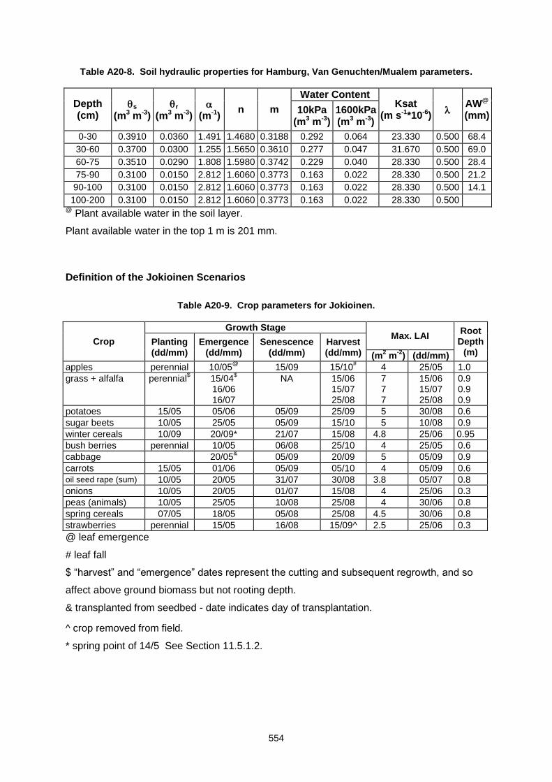
554
Table A20-8. Soil hydraulic properties for Hamburg, Van Genuchten/Mualem parameters.
Depth (cm)
s (m3 m-3)
r (m3 m-3)
(m-1)
n m
Water Content Ksat
(m s-1*10-6)
AW@ (mm)
10kPa (m3 m-3)
1600kPa (m3 m-3)
0-30 0.3910 0.0360 1.491 1.4680 0.3188 0.292 0.064 23.330 0.500 68.4
30-60 0.3700 0.0300 1.255 1.5650 0.3610 0.277 0.047 31.670 0.500 69.0
60-75 0.3510 0.0290 1.808 1.5980 0.3742 0.229 0.040 28.330 0.500 28.4
75-90 0.3100 0.0150 2.812 1.6060 0.3773 0.163 0.022 28.330 0.500 21.2
90-100 0.3100 0.0150 2.812 1.6060 0.3773 0.163 0.022 28.330 0.500 14.1
100-200 0.3100 0.0150 2.812 1.6060 0.3773 0.163 0.022 28.330 0.500 @ Plant available water in the soil layer.
Plant available water in the top 1 m is 201 mm.
Definition of the Jokioinen Scenarios
Table A20-9. Crop parameters for Jokioinen.
Crop
Growth Stage Max. LAI
Root Depth
(m) Planting (dd/mm)
Emergence (dd/mm)
Senescence (dd/mm)
Harvest (dd/mm) (m
2 m
-2) (dd/mm)
apples perennial 10/05@
15/09 15/10# 4 25/05 1.0
grass + alfalfa perennial$ 15/04
$
16/06 16/07
NA 15/06 15/07 25/08
7 7 7
15/06 15/07 25/08
0.9 0.9 0.9
potatoes 15/05 05/06 05/09 25/09 5 30/08 0.6
sugar beets 10/05 25/05 05/09 15/10 5 10/08 0.9
winter cereals 10/09 20/09* 21/07 15/08 4.8 25/06 0.95
bush berries perennial 10/05 06/08 25/10 4 25/05 0.6
cabbage 20/05& 05/09 20/09 5 05/09 0.9
carrots 15/05 01/06 05/09 05/10 4 05/09 0.6
oil seed rape (sum) 10/05 20/05 31/07 30/08 3.8 05/07 0.8
onions 10/05 20/05 01/07 15/08 4 25/06 0.3
peas (animals) 10/05 25/05 10/08 25/08 4 30/06 0.8
spring cereals 07/05 18/05 05/08 25/08 4.5 30/06 0.8
strawberries perennial 15/05 16/08 15/09^ 2.5 25/06 0.3
@ leaf emergence
# leaf fall
$ “harvest” and “emergence” dates represent the cutting and subsequent regrowth, and so
affect above ground biomass but not rooting depth.
& transplanted from seedbed - date indicates day of transplantation.
^ crop removed from field.
* spring point of 14/5 See Section 11.5.1.2.
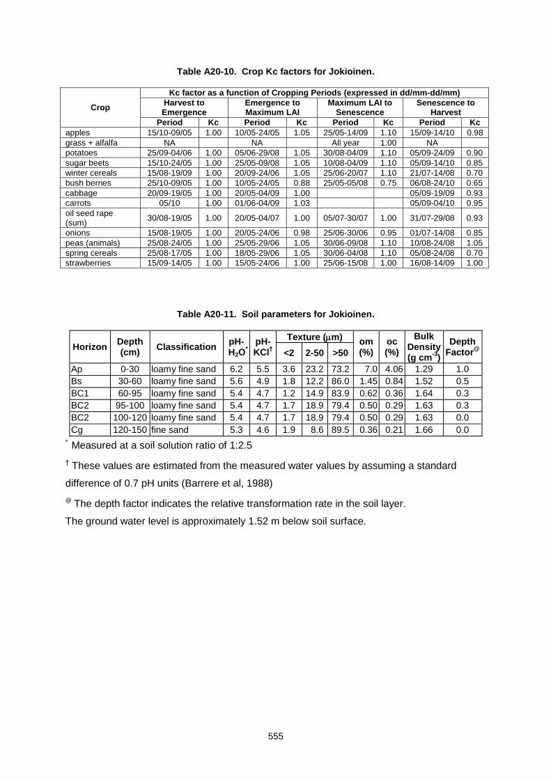
555
Table A20-10. Crop Kc factors for Jokioinen.
Crop
Kc factor as a function of Cropping Periods (expressed in dd/mm-dd/mm)
Harvest to Emergence
Emergence to Maximum LAI
Maximum LAI to Senescence
Senescence to Harvest
Period Kc Period Kc Period Kc Period Kc
apples 15/10-09/05 1.00 10/05-24/05 1.05 25/05-14/09 1.10 15/09-14/10 0.98
grass + alfalfa NA NA All year 1.00 NA
potatoes 25/09-04/06 1.00 05/06-29/08 1.05 30/08-04/09 1.10 05/09-24/09 0.90
sugar beets 15/10-24/05 1.00 25/05-09/08 1.05 10/08-04/09 1.10 05/09-14/10 0.85
winter cereals 15/08-19/09 1.00 20/09-24/06 1.05 25/06-20/07 1.10 21/07-14/08 0.70
bush berries 25/10-09/05 1.00 10/05-24/05 0.88 25/05-05/08 0.75 06/08-24/10 0.65
cabbage 20/09-19/05 1.00 20/05-04/09 1.00 05/09-19/09 0.93
carrots 05/10 1.00 01/06-04/09 1.03 05/09-04/10 0.95
oil seed rape (sum)
30/08-19/05 1.00 20/05-04/07 1.00 05/07-30/07 1.00 31/07-29/08 0.93
onions 15/08-19/05 1.00 20/05-24/06 0.98 25/06-30/06 0.95 01/07-14/08 0.85
peas (animals) 25/08-24/05 1.00 25/05-29/06 1.05 30/06-09/08 1.10 10/08-24/08 1.05
spring cereals 25/08-17/05 1.00 18/05-29/06 1.05 30/06-04/08 1.10 05/08-24/08 0.70
strawberries 15/09-14/05 1.00 15/05-24/06 1.00 25/06-15/08 1.00 16/08-14/09 1.00
Table A20-11. Soil parameters for Jokioinen.
Horizon Depth (cm)
Classification pH-H2O
*
pH-KCl
†
Texture (m) om
(%) oc (%)
Bulk Density (g cm
-3)
Depth Factor
@ <2 2-50 >50
Ap 0-30 loamy fine sand 6.2 5.5 3.6 23.2 73.2 7.0 4.06 1.29 1.0
Bs 30-60 loamy fine sand 5.6 4.9 1.8 12.2 86.0 1.45 0.84 1.52 0.5
BC1 60-95 loamy fine sand 5.4 4.7 1.2 14.9 83.9 0.62 0.36 1.64 0.3
BC2 95-100 loamy fine sand 5.4 4.7 1.7 18.9 79.4 0.50 0.29 1.63 0.3
BC2 100-120 loamy fine sand 5.4 4.7 1.7 18.9 79.4 0.50 0.29 1.63 0.0
Cg 120-150 fine sand 5.3 4.6 1.9 8.6 89.5 0.36 0.21 1.66 0.0
* Measured at a soil solution ratio of 1:2.5
† These values are estimated from the measured water values by assuming a standard
difference of 0.7 pH units (Barrere et al, 1988)
@ The depth factor indicates the relative transformation rate in the soil layer.
The ground water level is approximately 1.52 m below soil surface.
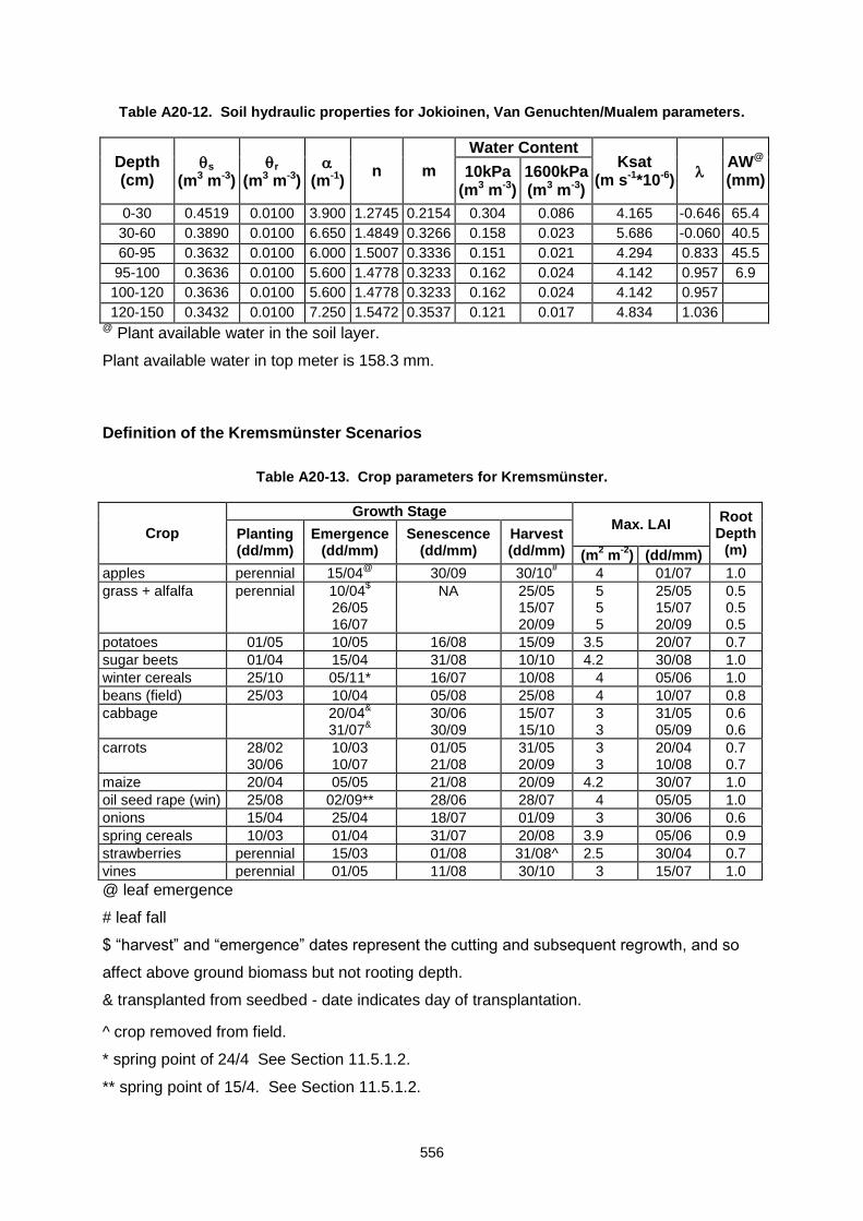
556
Table A20-12. Soil hydraulic properties for Jokioinen, Van Genuchten/Mualem parameters.
Depth (cm)
s (m3 m-3)
r (m3 m-3)
(m-1)
n m
Water Content Ksat
(m s-1*10-6)
AW@ (mm)
10kPa (m3 m-3)
1600kPa (m3 m-3)
0-30 0.4519 0.0100 3.900 1.2745 0.2154 0.304 0.086 4.165 -0.646 65.4
30-60 0.3890 0.0100 6.650 1.4849 0.3266 0.158 0.023 5.686 -0.060 40.5
60-95 0.3632 0.0100 6.000 1.5007 0.3336 0.151 0.021 4.294 0.833 45.5
95-100 0.3636 0.0100 5.600 1.4778 0.3233 0.162 0.024 4.142 0.957 6.9
100-120 0.3636 0.0100 5.600 1.4778 0.3233 0.162 0.024 4.142 0.957
120-150 0.3432 0.0100 7.250 1.5472 0.3537 0.121 0.017 4.834 1.036 @ Plant available water in the soil layer.
Plant available water in top meter is 158.3 mm.
Definition of the Kremsmünster Scenarios
Table A20-13. Crop parameters for Kremsmünster.
Crop
Growth Stage Max. LAI
Root Depth
(m) Planting (dd/mm)
Emergence (dd/mm)
Senescence (dd/mm)
Harvest (dd/mm) (m
2 m
-2) (dd/mm)
apples perennial 15/04@
30/09 30/10# 4 01/07 1.0
grass + alfalfa perennial 10/04$
26/05 16/07
NA 25/05 15/07 20/09
5 5 5
25/05 15/07 20/09
0.5 0.5 0.5
potatoes 01/05 10/05 16/08 15/09 3.5 20/07 0.7
sugar beets 01/04 15/04 31/08 10/10 4.2 30/08 1.0
winter cereals 25/10 05/11* 16/07 10/08 4 05/06 1.0
beans (field) 25/03 10/04 05/08 25/08 4 10/07 0.8
cabbage 20/04&
31/07&
30/06 30/09
15/07 15/10
3 3
31/05 05/09
0.6 0.6
carrots 28/02 30/06
10/03 10/07
01/05 21/08
31/05 20/09
3 3
20/04 10/08
0.7 0.7
maize 20/04 05/05 21/08 20/09 4.2 30/07 1.0
oil seed rape (win) 25/08 02/09** 28/06 28/07 4 05/05 1.0
onions 15/04 25/04 18/07 01/09 3 30/06 0.6
spring cereals 10/03 01/04 31/07 20/08 3.9 05/06 0.9
strawberries perennial 15/03 01/08 31/08^ 2.5 30/04 0.7
vines perennial 01/05 11/08 30/10 3 15/07 1.0
@ leaf emergence
# leaf fall
$ “harvest” and “emergence” dates represent the cutting and subsequent regrowth, and so
affect above ground biomass but not rooting depth.
& transplanted from seedbed - date indicates day of transplantation.
^ crop removed from field.
* spring point of 24/4 See Section 11.5.1.2.
** spring point of 15/4. See Section 11.5.1.2.
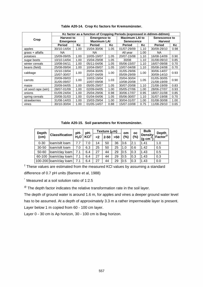
557
Table A20-14. Crop Kc factors for Kremsmünster.
Crop
Kc factor as a function of Cropping Periods (expressed in dd/mm-dd/mm)
Harvest to Emergence
Emergence to Maximum LAI
Maximum LAI to Senescence
Senescence to Harvest
Period Kc Period Kc Period Kc Period Kc
apples 30/10-14/04 1.00 15/04-30/06 1.05 01/07-29/09 1.10 30/09-29/10 0.98
grass + alfalfa NA NA All year 1.00 NA
potatoes 15/09-09/05 1.00 10/05-19/07 1.05 20/07-15/08 1.10 16/08-14/09 0.90
sugar beets 10/10-14/04 1.00 15/04-29/08 1.05 30/08 1.10 31/08-09/10 0.85
winter cereals 10/08-04/11 1.00 05/11-04/06 1.05 05/06-15/07 1.10 16/07-09/08 0.70
beans (field) 25/08-09/04 1.00 10/04-09/07 1.05 10/07-04/08 1.10 05/08-24/08 0.70
cabbage 15/10-19/04 15/07-30/07
1.00 20/04-30/05 31/07-04/09
1.00 31/05-29/06 05/09-29/09
1.00 30/06-14/07 30/09-14/10
0.93
carrots 20/09-09/03 31/05-09/07
1.00 10/03-19/04 10/07-09/08
1.03 20/04-30/04 10/08-20/08
1.05 01/05-30/05 21/08-19/09
0.90
maize 20/09-04/05 1.00 05/05-29/07 1.05 30/07-20/08 1.10 21/08-19/09 0.83
oil seed rape (win) 28/07-01/09 1.00 02/09-04/05 1.00 05/05-27/06 1.00 28/06-27/07 0.93
onions 01/09-24/04 1.00 25/04-29/06 0.98 30/06-17/07 0.95 18/07-31/08 0.85
spring cereals 20/08-31/03 1.00 01/04-04/06 1.05 05/06-30/07 1.10 31/07-19/08 0.70
strawberries 31/08-14/03 1.00 15/03-29/04 1.00 30/04-31/07 1.00 01/08-30/08 1.00
vines 30/10-30/04 1.00 01/05-14/07 0.88 15/07-10/08 0.75 11/08-29/10 0.65
Table A20-15. Soil parameters for Kremsmünster.
Depth (cm)
Classification pH-H2O
*
pH-KCl
†
Texture (m) om
(%) oc (%)
Bulk Density (g cm
-3)
Depth Factor
@ <2 2-50 >50
0-30 loam/silt loam 7.7 7.0 14 50 36 3.6 2.1 1.41 1.0
30-50 loam/silt loam 7.0 6.3 25 50 25 1.0 0.6 1.42 0.5
50-60 loam/clay loam 7.1 6.4 27 44 29 0.5 0.3 1.43 0.5
60-100 loam/clay loam 7.1 6.4 27 44 29 0.5 0.3 1.43 0.3
100-200 loam/clay loam 7.1 6.4 27 44 29 0.5 0.3 1.43 0.0
† These values are estimated from the measured KCl values by assuming a standard
difference of 0.7 pH units (Barrere et al, 1988)
* Measured at a soil solution ratio of 1:2.5
@ The depth factor indicates the relative transformation rate in the soil layer.
The depth of ground water is around 1.6 m, for apples and vines a deeper ground water level
has to be assumed. At a depth of approximately 3.3 m a rather impermeable layer is present.
Layer below 1 m copied from 60 - 100 cm layer.
Layer 0 - 30 cm is Ap horizon, 30 - 100 cm is Bwg horizon.
558
Table A20-16. Soil hydraulic properties for Kremsmünster, Van Genuchten/Mualem parameters.
Depth (cm)
s (m3 m-3)
r (m3 m-3)
(m-1) n m
Water Content Ksat
(m s-1*10-6) AW@ (mm)
10kPa (m3 m-3)
1600kPa (m3 m-3)
0-30 0.4246 0.0100 2.440 1.2186 0.1794 0.334 0.123 1.769 -2.080 63.3
30-50 0.4446 0.0100 2.700 1.1659 0.1423 0.365 0.169 2.780 -2.404 39.2
50-60 0.4430 0.0100 3.080 1.1578 0.1363 0.361 0.173 2.459 -2.065 18.8
60-100 0.4430 0.0100 3.080 1.1578 0.1363 0.361 0.173 2.459 -2.065 75.2
100-200 0.4430 0.0100 3.080 1.1578 0.1363 0.361 0.173 2.459 -2.065
@ Plant available water in soil layer.
Plant available water in top meter is 196.5 mm.
Layer 100 - 200 cm copied from layer 60 - 100 cm because of lacking information.
Definition of the Okehampton Scenarios
Table A20-17. Crop parameters for Okehampton.
Crop
Growth Stage Max. LAI
Root Depth
(m) Planting (dd/mm)
Emergence (dd/mm)
Senescence (dd/mm)
Harvest (dd/mm) (m
2 m
-2) (dd/mm)
apples perennial 25/03@
16/08 15/09# 2.5 15/06 1.0
grass + alfalfa perennial 10/02$
16/05 16/07
NA 15/05 15/07 15/09
4.5 4.5 4.5
15/05 15/07 15/09
0.45 0.45 0.45
potatoes 15/04 30/04 02/08 01/09 4 15/07 0.6
sugar beets 10/04 25/04 15/09 25/10 3 30/08 0.8
winter cereals 07/10 17/10* 07/07 01/08 7.5 15/05 0.8
beans (field) 01/03 15/03 26/08 15/09 4 07/06 0.45
linseed 25/03 30/03 18/08 25/09 3 25/06 0.6
maize 07/05 25/05 18/08 07/10 7 15/07 0.8
oil seed rape (sum) 25/03 30/03 21/07 20/08 3 15/05 0.6
oil seed rape (win) 07/08 14/08** 21/06 21/07 4.5 30/04 0.85
peas (animals) 25/03 05/04 31/07 15/08 4.0 07/06 0.45
spring cereals 25/03 01/04 31/07 20/08 4.5 22/05 0.6
@ leaf emergence
# leaf fall
$ “harvest” and “emergence” dates represent the cutting and subsequent regrowth, and so
affect above ground biomass but not rooting depth.
* spring point of 21/4 See Section 11.5.1.2.
** spring point of 9/4. See Section 11.5.1.2.
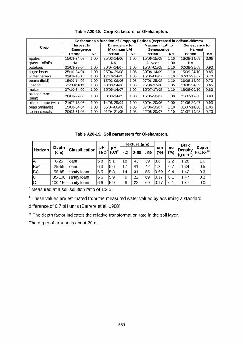
559
Table A20-18. Crop Kc factors for Okehampton.
Crop
Kc factor as a function of Cropping Periods (expressed in dd/mm-dd/mm)
Harvest to Emergence
Emergence to Maximum LAI
Maximum LAI to Senescence
Senescence to Harvest
Period Kc Period Kc Period Kc Period Kc
apples 15/09-24/03 1.00 25/03-14/06 1.05 15/06-15/08 1.10 16/08-14/09 0.98
grass + alfalfa NA NA All year 1.00 NA
potatoes 01/09-29/04 1.00 30/04-14/07 1.05 15/07-01/08 1.10 02/08-31/08 0.90
sugar beets 25/10-24/04 1.00 25/04-29/08 1.05 30/08-14/09 1.10 15/09-24/10 0.85
winter cereals 01/08-16/10 1.00 17/10-14/05 1.05 15/05-06/07 1.10 07/07-31/07 0.70
beans (field) 15/09-14/03 1.00 15/03-06/06 1.05 07/06-25/08 1.10 26/08-14/09 0.70
linseed 25/0929/03 1.00 30/03-24/06 1.03 25/06-17/08 1.05 18/08-24/09 0.65
maize 07/10-24/05 1.00 25/05-14/07 1.05 15/07-17/08 1.10 18/08-06/10 0.83
oil seed rape (sum)
20/08-29/03 1.00 30/03-14/05 1.00 15/05-20/07 1.00 21/07-19/08 0.93
oil seed rape (win) 21/07-13/08 1.00 14/08-29/04 1.00 30/04-20/06 1.00 21/06-20/07 0.93
peas (animals) 15/08-04/04 1.00 05/04-06/06 1.05 07/06-30/07 1.10 31/07-14/08 1.05
spring cereals 20/08-31/03 1.00 01/04-21/05 1.05 22/05-30/07 1.10 31/07-19/08 0.70
Table A20-19. Soil parameters for Okehampton.
Horizon Depth (cm)
Classification pH-H2O
*
pH-KCl
†
Texture (m) om
(%) oc (%)
Bulk Density (g cm
-3)
Depth Factor
@ <2 2-50 >50
A 0-25 loam 5.8 5.1 18 43 39 3.8 2.2 1.28 1.0
Bw1 25-55 loam 6.3 5.6 17 41 42 1.2 0.7 1.34 0.5
BC 55-85 sandy loam 6.5 5.8 14 31 55 0.69 0.4 1.42 0.3
C 85-100 sandy loam 6.6 5.9 9 22 69 0.17 0.1 1.47 0.3
C 100-150 sandy loam 6.6 5.9 9 22 69 0.17 0.1 1.47 0.0
* Measured at a soil solution ratio of 1:2.5
† These values are estimated from the measured water values by assuming a standard
difference of 0.7 pH units (Barrere et al, 1988)
@ The depth factor indicates the relative transformation rate in the soil layer.
The depth of ground is about 20 m.
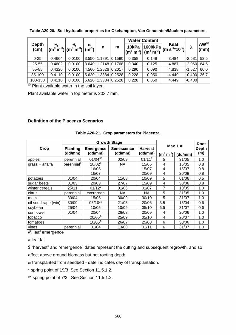
560
Table A20-20. Soil hydraulic properties for Okehampton, Van Genuchten/Mualem parameters.
Depth (cm)
s (m3 m-3)
r (m3 m-3)
(m-1)
n m
Water Content Ksat
(m s-1*10-6)
AW@ (mm)
10kPa (m3 m-3)
1600kPa (m3 m-3)
0-25 0.4664 0.0100 3.550 1.1891 0.1590 0.358 0.148 3.484 -2.581 52.5
25-55 0.4602 0.0100 3.640 1.2148 0.1768 0.340 0.125 4.887 -2.060 64.5
55-85 0.4320 0.0100 4.560 1.2526 0.2017 0.290 0.090 4.838 -1.527 60.0
85-100 0.4110 0.0100 5.620 1.3384 0.2528 0.228 0.050 4.449 -0.400 26.7
100-150 0.4110 0.0100 5.620 1.3384 0.2528 0.228 0.050 4.449 -0.400 @ Plant available water in the soil layer.
Plant available water in top meter is 203.7 mm.
Definition of the Piacenza Scenarios
Table A20-21. Crop parameters for Piacenza.
Crop
Growth Stage Max. LAI
Root Depth
(m) Planting (dd/mm)
Emergence (dd/mm)
Senescence (dd/mm)
Harvest (dd/mm) (m
2 m
-2) (dd/mm)
apples perennial 01/04@
02/09 01/11# 5 31/05 1.0
grass + alfalfa perennial$ 28/02
$
16/05 16/07
NA 15/05 15/07 20/09
4 4 4
15/05 15/07 20/09
0.8 0.8 0.8
potatoes 01/04 20/04 11/08 10/09 5 01/06 0.5
sugar beets 01/03 20/03 27/07 15/09 4 30/06 0.8
winter cereals 25/11 01/12* 01/06 01/07 7 10/05 1.0
citrus perennial evergreen NA NA 5 31/05 1.0
maize 30/04 15/05 30/09 30/10 5 31/07 1.0
oil seed rape (win) 30/09 05/10** 21/05 20/06 3.5 15/04 0.6
soybean 25/04 10/05 10/09 05/10 6.5 31/07 0.6
sunflower 01/04 20/04 26/08 20/09 4 20/06 1.0
tobacco 20/05& 25/09 05/10 4 20/07 1.0
tomatoes 10/05& 26/07 25/08 6 30/06 1.0
vines perennial 01/04 13/08 01/11 6 31/07 1.0
@ leaf emergence
# leaf fall
$ “harvest” and “emergence” dates represent the cutting and subsequent regrowth, and so
affect above ground biomass but not rooting depth.
& transplanted from seedbed - date indicates day of transplantation.
* spring point of 19/3 See Section 11.5.1.2.
** spring point of 7/3. See Section 11.5.1.2.
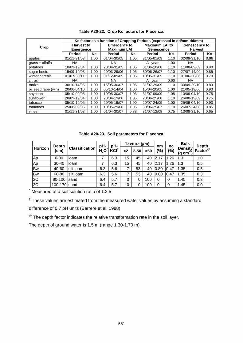
561
Table A20-22. Crop Kc factors for Piacenza.
Crop
Kc factor as a function of Cropping Periods (expressed in dd/mm-dd/mm)
Harvest to Emergence
Emergence to Maximum LAI
Maximum LAI to Senescence
Senescence to Harvest
Period Kc Period Kc Period Kc Period Kc
apples 01/11-31/03 1.00 01/04-30/05 1.05 31/05-01/09 1.10 02/09-31/10 0.98
grass + alfalfa NA NA All year 1.00 NA
potatoes 10/09-19/04 1.00 20/04-31/05 1.05 01/06-10/08 1.10 11/08-09/09 0.90
sugar beets 15/09-19/03 1.00 20/03-29/06 1.05 30/06-26/07 1.10 27/07-14/09 0.85
winter cereals 01/07-30/11 1.00 01/12-09/05 1.05 10/05-31/05 1.10 01/06-30/06 0.70
citrus NA NA All year 0.60 NA
maize 30/10-14/05 1.00 15/05-30/07 1.05 31/07-29/09 1.10 30/09-29/10 0.83
oil seed rape (win) 20/06-04/10 1.00 05/10-14/04 1.00 15/04-20/05 1.00 21/05-19/06 0.93
soybean 05/10-09/05 1.00 10/05-30/07 1.03 31/07-09/09 1.05 10/09-04/10 0.75
sunflower 20/09-19/04 1.00 20/04-19/06 1.05 20/06-25/08 1.10 26/08-19/09 0.75
tobacco 05/10-19/05 1.00 20/05-19/07 1.00 20/07-24/09 1.00 25/09-04/10 0.93
tomatoes 25/08-09/05 1.00 10/05-29/06 1.05 30/06-25/07 1.10 26/07-24/08 0.85
vines 01/11-31/03 1.00 01/04-30/07 0.88 31/07-12/08 0.75 13/08-31/10 0.65
Table A20-23. Soil parameters for Piacenza.
Horizon Depth (cm)
Classification pH-H2O
*
pH-KCl
†
Texture (m) om
(%) oc (%)
Bulk Density (g cm
-3)
Depth Factor
@ <2 2-50 >50
Ap 0-30 loam 7 6.3 15 45 40 2.17 1.26 1.3 1.0
Ap 30-40 loam 7 6.3 15 45 40 2.17 1.26 1.3 0.5
Bw 40-60 silt loam 6.3 5.6 7 53 40 0.80 0.47 1.35 0.5
Bw 60-80 silt loam 6.3 5.6 7 53 40 0.80 0.47 1.35 0.3
2C 80-100 sand 6.4 5.7 0 0 100 0 0 1.45 0.3
2C 100-170 sand 6.4 5.7 0 0 100 0 0 1.45 0.0
* Measured at a soil solution ratio of 1:2.5
† These values are estimated from the measured water values by assuming a standard
difference of 0.7 pH units (Barrere et al, 1988)
@ The depth factor indicates the relative transformation rate in the soil layer.
The depth of ground water is 1.5 m (range 1.30-1.70 m).
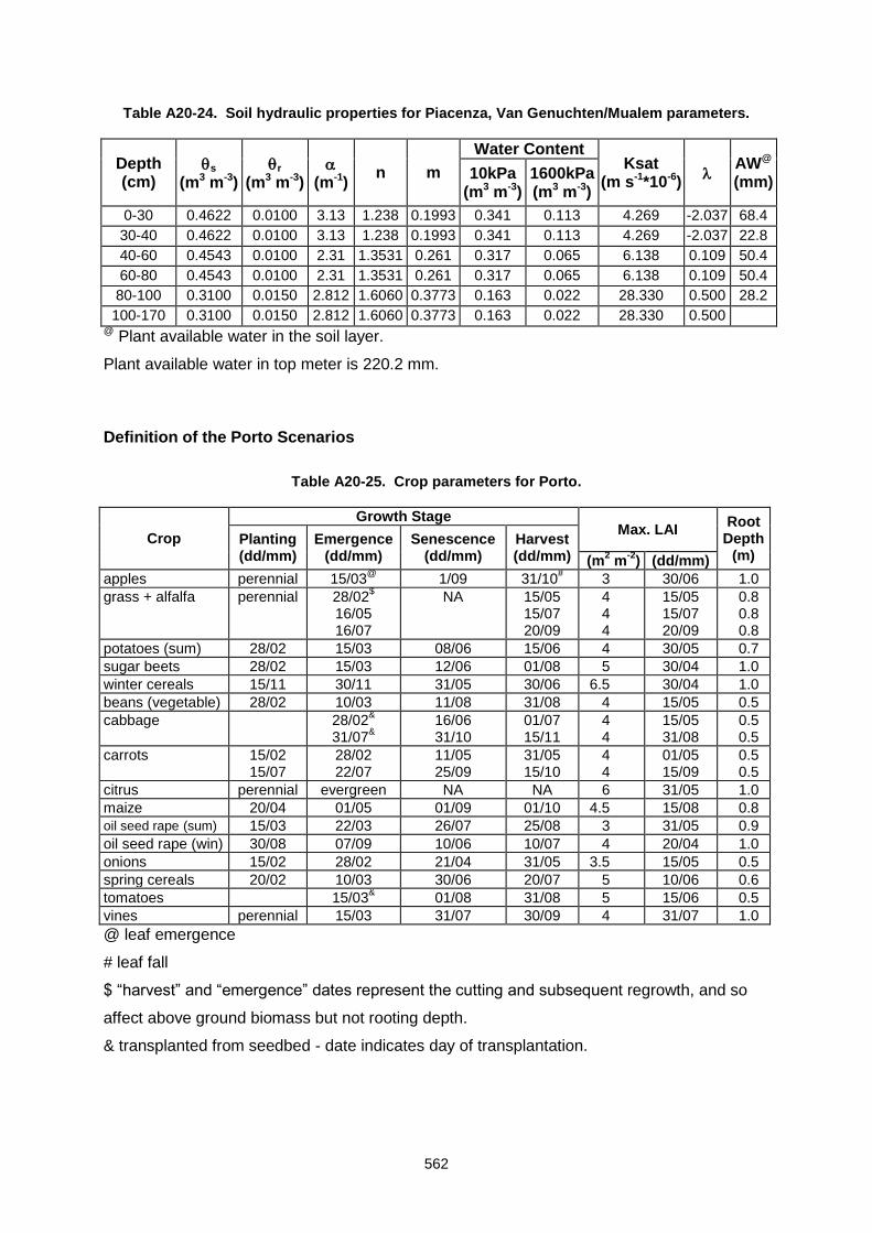
562
Table A20-24. Soil hydraulic properties for Piacenza, Van Genuchten/Mualem parameters.
Depth (cm)
s (m3 m-3)
r (m3 m-3)
(m-1)
n m
Water Content Ksat
(m s-1*10-6)
AW@ (mm)
10kPa (m3 m-3)
1600kPa (m3 m-3)
0-30 0.4622 0.0100 3.13 1.238 0.1993 0.341 0.113 4.269 -2.037 68.4
30-40 0.4622 0.0100 3.13 1.238 0.1993 0.341 0.113 4.269 -2.037 22.8
40-60 0.4543 0.0100 2.31 1.3531 0.261 0.317 0.065 6.138 0.109 50.4
60-80 0.4543 0.0100 2.31 1.3531 0.261 0.317 0.065 6.138 0.109 50.4
80-100 0.3100 0.0150 2.812 1.6060 0.3773 0.163 0.022 28.330 0.500 28.2
100-170 0.3100 0.0150 2.812 1.6060 0.3773 0.163 0.022 28.330 0.500 @ Plant available water in the soil layer.
Plant available water in top meter is 220.2 mm.
Definition of the Porto Scenarios
Table A20-25. Crop parameters for Porto.
Crop
Growth Stage Max. LAI
Root Depth
(m) Planting (dd/mm)
Emergence (dd/mm)
Senescence (dd/mm)
Harvest (dd/mm) (m
2 m
-2) (dd/mm)
apples perennial 15/03@
1/09 31/10# 3 30/06 1.0
grass + alfalfa perennial 28/02$
16/05 16/07
NA 15/05 15/07 20/09
4 4 4
15/05 15/07 20/09
0.8 0.8 0.8
potatoes (sum) 28/02 15/03 08/06 15/06 4 30/05 0.7
sugar beets 28/02 15/03 12/06 01/08 5 30/04 1.0
winter cereals 15/11 30/11 31/05 30/06 6.5 30/04 1.0
beans (vegetable) 28/02 10/03 11/08 31/08 4 15/05 0.5
cabbage 28/02&
31/07&
16/06 31/10
01/07 15/11
4 4
15/05 31/08
0.5 0.5
carrots 15/02 15/07
28/02 22/07
11/05 25/09
31/05 15/10
4 4
01/05 15/09
0.5 0.5
citrus perennial evergreen NA NA 6 31/05 1.0
maize 20/04 01/05 01/09 01/10 4.5 15/08 0.8
oil seed rape (sum) 15/03 22/03 26/07 25/08 3 31/05 0.9
oil seed rape (win) 30/08 07/09 10/06 10/07 4 20/04 1.0
onions 15/02 28/02 21/04 31/05 3.5 15/05 0.5
spring cereals 20/02 10/03 30/06 20/07 5 10/06 0.6
tomatoes 15/03& 01/08 31/08 5 15/06 0.5
vines perennial 15/03 31/07 30/09 4 31/07 1.0
@ leaf emergence
# leaf fall
$ “harvest” and “emergence” dates represent the cutting and subsequent regrowth, and so
affect above ground biomass but not rooting depth.
& transplanted from seedbed - date indicates day of transplantation.
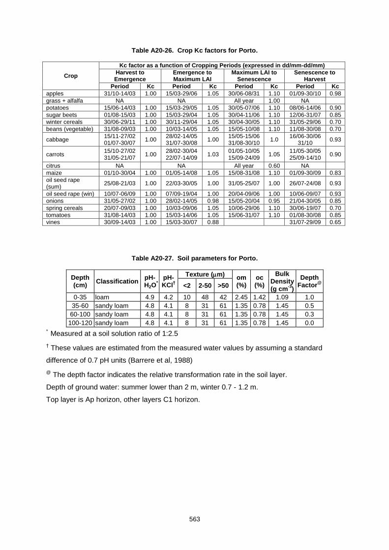
563
Table A20-26. Crop Kc factors for Porto.
Crop
Kc factor as a function of Cropping Periods (expressed in dd/mm-dd/mm)
Harvest to Emergence
Emergence to Maximum LAI
Maximum LAI to Senescence
Senescence to Harvest
Period Kc Period Kc Period Kc Period Kc
apples 31/10-14/03 1.00 15/03-29/06 1.05 30/06-08/31 1.10 01/09-30/10 0.98
grass + alfalfa NA NA All year 1.00 NA
potatoes 15/06-14/03 1.00 15/03-29/05 1.05 30/05-07/06 1.10 08/06-14/06 0.90
sugar beets 01/08-15/03 1.00 15/03-29/04 1.05 30/04-11/06 1.10 12/06-31/07 0.85
winter cereals 30/06-29/11 1.00 30/11-29/04 1.05 30/04-30/05 1.10 31/05-29/06 0.70
beans (vegetable) 31/08-09/03 1.00 10/03-14/05 1.05 15/05-10/08 1.10 11/08-30/08 0.70
cabbage 15/11-27/02 01/07-30/07
1.00 28/02-14/05 31/07-30/08
1.00 15/05-15/06 31/08-30/10
1.0 16/06-30/06
31/10 0.93
carrots 15/10-27/02 31/05-21/07
1.00 28/02-30/04 22/07-14/09
1.03 01/05-10/05 15/09-24/09
1.05 11/05-30/05 25/09-14/10
0.90
citrus NA NA All year 0.60 NA
maize 01/10-30/04 1.00 01/05-14/08 1.05 15/08-31/08 1.10 01/09-30/09 0.83
oil seed rape (sum)
25/08-21/03 1.00 22/03-30/05 1.00 31/05-25/07 1.00 26/07-24/08 0.93
oil seed rape (win) 10/07-06/09 1.00 07/09-19/04 1.00 20/04-09/06 1.00 10/06-09/07 0.93
onions 31/05-27/02 1.00 28/02-14/05 0.98 15/05-20/04 0.95 21/04-30/05 0.85
spring cereals 20/07-09/03 1.00 10/03-09/06 1.05 10/06-29/06 1.10 30/06-19/07 0.70
tomatoes 31/08-14/03 1.00 15/03-14/06 1.05 15/06-31/07 1.10 01/08-30/08 0.85
vines 30/09-14/03 1.00 15/03-30/07 0.88 31/07-29/09 0.65
Table A20-27. Soil parameters for Porto.
Depth (cm)
Classification pH-H2O
*
pH-KCl
†
Texture (m) om
(%) oc (%)
Bulk Density (g cm
-3)
Depth Factor
@ <2 2-50 >50
0-35 loam 4.9 4.2 10 48 42 2.45 1.42 1.09 1.0
35-60 sandy loam 4.8 4.1 8 31 61 1.35 0.78 1.45 0.5
60-100 sandy loam 4.8 4.1 8 31 61 1.35 0.78 1.45 0.3
100-120 sandy loam 4.8 4.1 8 31 61 1.35 0.78 1.45 0.0 * Measured at a soil solution ratio of 1:2.5
† These values are estimated from the measured water values by assuming a standard
difference of 0.7 pH units (Barrere et al, 1988)
@ The depth factor indicates the relative transformation rate in the soil layer.
Depth of ground water: summer lower than 2 m, winter 0.7 - 1.2 m.
Top layer is Ap horizon, other layers C1 horizon.
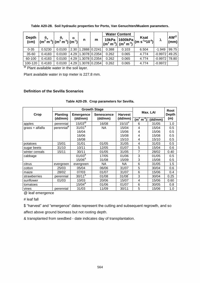
564
Table A20-28. Soil hydraulic properties for Porto, Van Genuchten/Mualem parameters.
Depth (cm)
s (m3 m-3)
r (m3 m-3)
(m-1)
n m
Water Content Ksat
(m s-1*10-6)
AW@ (mm)
10kPa (m3 m-3)
1600kPa (m3 m-3)
0-35 0.5230 0.0100 2.30 1.2888 0.2241 0.388 0.103 6.504 -1.949 99.75
35-60 0.4183 0.0100 4.29 1.3078 0.2354 0.262 0.065 4.774 -0.9972 49.25
60-100 0.4183 0.0100 4.29 1.3078 0.2354 0.262 0.065 4.774 -0.9972 78.80
100-120 0.4183 0.0100 4.29 1.3078 0.2354 0.262 0.065 4.774 -0.9972 @ Plant available water in the soil layer.
Plant available water in top meter is 227.8 mm.
Definition of the Sevilla Scenarios
Table A20-29. Crop parameters for Sevilla.
Crop
Growth Stage Max. LAI
Root Depth
(m) Planting (dd/mm)
Emergence (dd/mm)
Senescence (dd/mm)
Harvest (dd/mm) (m
2 m
-2) (dd/mm)
apples perennial 15/03@
16/08 15/10# 6 31/05 1.0
grass + alfalfa perennial$ 31/01
$
16/04 16/06 16/08
NA 15/04 15/06 15/08 15/10
4 4 4 4
15/04 15/06 15/08 15/10
0.5 0.5 0.5 0.5
potatoes 15/01 31/01 01/05 31/05 4 31/03 0.5
sugar beets 31/10 10/11 12/05 01/07 5 15/04 0.6
winter cereals 15/11 30/11 01/05 31/05 7 28/02 0.40
cabbage 01/03&
15/06&
17/05 31/08
01/06 15/09
3 3
01/05 15/08
0.5 0.5
citrus evergreen evergreen NA NA 6 31/05 1.5
cotton 25/03 05/04 06/06 31/07 5 30/04 0.6
maize 28/02 07/03 01/07 31/07 6 15/06 0.4
strawberries perennial 30/11& 01/08 31/08
* 3 30/04 0.25
sunflower 01/03 10/03 20/06 15/07 4 15/06 0.60
tomatoes 15/04& 01/06 01/07 6 30/05 0.8
vines perennial 31/03 11/09 30/11 5 15/06 1.0
@ leaf emergence
# leaf fall
$ “harvest” and “emergence” dates represent the cutting and subsequent regrowth, and so
affect above ground biomass but not rooting depth.
& transplanted from seedbed - date indicates day of transplantation.
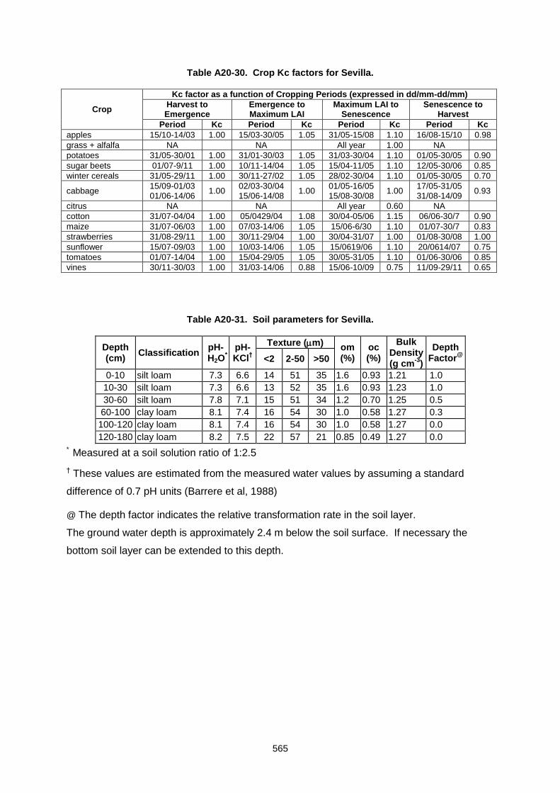
565
Table A20-30. Crop Kc factors for Sevilla.
Crop
Kc factor as a function of Cropping Periods (expressed in dd/mm-dd/mm)
Harvest to Emergence
Emergence to Maximum LAI
Maximum LAI to Senescence
Senescence to Harvest
Period Kc Period Kc Period Kc Period Kc
apples 15/10-14/03 1.00 15/03-30/05 1.05 31/05-15/08 1.10 16/08-15/10 0.98
grass + alfalfa NA NA All year 1.00 NA
potatoes 31/05-30/01 1.00 31/01-30/03 1.05 31/03-30/04 1.10 01/05-30/05 0.90
sugar beets 01/07-9/11 1.00 10/11-14/04 1.05 15/04-11/05 1.10 12/05-30/06 0.85
winter cereals 31/05-29/11 1.00 30/11-27/02 1.05 28/02-30/04 1.10 01/05-30/05 0.70
cabbage 15/09-01/03 01/06-14/06
1.00 02/03-30/04 15/06-14/08
1.00 01/05-16/05 15/08-30/08
1.00 17/05-31/05 31/08-14/09
0.93
citrus NA NA All year 0.60 NA
cotton 31/07-04/04 1.00 05/0429/04 1.08 30/04-05/06 1.15 06/06-30/7 0.90
maize 31/07-06/03 1.00 07/03-14/06 1.05 15/06-6/30 1.10 01/07-30/7 0.83
strawberries 31/08-29/11 1.00 30/11-29/04 1.00 30/04-31/07 1.00 01/08-30/08 1.00
sunflower 15/07-09/03 1.00 10/03-14/06 1.05 15/0619/06 1.10 20/0614/07 0.75
tomatoes 01/07-14/04 1.00 15/04-29/05 1.05 30/05-31/05 1.10 01/06-30/06 0.85
vines 30/11-30/03 1.00 31/03-14/06 0.88 15/06-10/09 0.75 11/09-29/11 0.65
Table A20-31. Soil parameters for Sevilla.
Depth (cm)
Classification pH-H2O
*
pH-KCl
†
Texture (m) om
(%) oc (%)
Bulk Density (g cm
-3)
Depth Factor
@ <2 2-50 >50
0-10 silt loam 7.3 6.6 14 51 35 1.6 0.93 1.21 1.0
10-30 silt loam 7.3 6.6 13 52 35 1.6 0.93 1.23 1.0
30-60 silt loam 7.8 7.1 15 51 34 1.2 0.70 1.25 0.5
60-100 clay loam 8.1 7.4 16 54 30 1.0 0.58 1.27 0.3
100-120 clay loam 8.1 7.4 16 54 30 1.0 0.58 1.27 0.0
120-180 clay loam 8.2 7.5 22 57 21 0.85 0.49 1.27 0.0
* Measured at a soil solution ratio of 1:2.5
† These values are estimated from the measured water values by assuming a standard
difference of 0.7 pH units (Barrere et al, 1988)
@ The depth factor indicates the relative transformation rate in the soil layer.
The ground water depth is approximately 2.4 m below the soil surface. If necessary the
bottom soil layer can be extended to this depth.
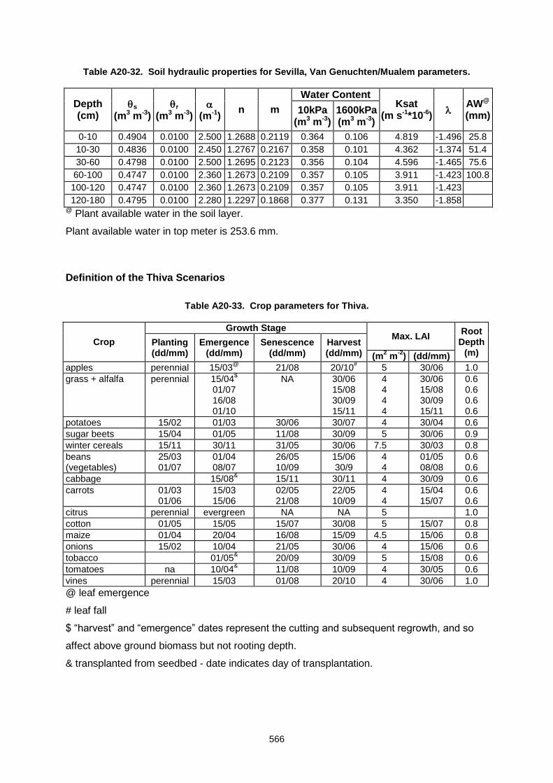
566
Table A20-32. Soil hydraulic properties for Sevilla, Van Genuchten/Mualem parameters.
Depth (cm)
s (m3 m-3)
r (m3 m-3)
(m-1)
n m
Water Content Ksat
(m s-1*10-6)
AW@ (mm)
10kPa (m3 m-3)
1600kPa (m3 m-3)
0-10 0.4904 0.0100 2.500 1.2688 0.2119 0.364 0.106 4.819 -1.496 25.8
10-30 0.4836 0.0100 2.450 1.2767 0.2167 0.358 0.101 4.362 -1.374 51.4
30-60 0.4798 0.0100 2.500 1.2695 0.2123 0.356 0.104 4.596 -1.465 75.6
60-100 0.4747 0.0100 2.360 1.2673 0.2109 0.357 0.105 3.911 -1.423 100.8
100-120 0.4747 0.0100 2.360 1.2673 0.2109 0.357 0.105 3.911 -1.423
120-180 0.4795 0.0100 2.280 1.2297 0.1868 0.377 0.131 3.350 -1.858 @ Plant available water in the soil layer.
Plant available water in top meter is 253.6 mm.
Definition of the Thiva Scenarios
Table A20-33. Crop parameters for Thiva.
Crop
Growth Stage Max. LAI
Root Depth
(m) Planting (dd/mm)
Emergence (dd/mm)
Senescence (dd/mm)
Harvest (dd/mm) (m
2 m
-2) (dd/mm)
apples perennial 15/03@
21/08 20/10# 5 30/06 1.0
grass + alfalfa perennial 15/04$
01/07 16/08 01/10
NA 30/06 15/08 30/09 15/11
4 4 4 4
30/06 15/08 30/09 15/11
0.6 0.6 0.6 0.6
potatoes 15/02 01/03 30/06 30/07 4 30/04 0.6
sugar beets 15/04 01/05 11/08 30/09 5 30/06 0.9
winter cereals 15/11 30/11 31/05 30/06 7.5 30/03 0.8
beans (vegetables)
25/03 01/07
01/04 08/07
26/05 10/09
15/06 30/9
4 4
01/05 08/08
0.6 0.6
cabbage 15/08& 15/11 30/11 4 30/09 0.6
carrots 01/03 01/06
15/03 15/06
02/05 21/08
22/05 10/09
4 4
15/04 15/07
0.6 0.6
citrus perennial evergreen NA NA 5 1.0
cotton 01/05 15/05 15/07 30/08 5 15/07 0.8
maize 01/04 20/04 16/08 15/09 4.5 15/06 0.8
onions 15/02 10/04 21/05 30/06 4 15/06 0.6
tobacco 01/05& 20/09 30/09 5 15/08 0.6
tomatoes na 10/04& 11/08 10/09 4 30/05 0.6
vines perennial 15/03 01/08 20/10 4 30/06 1.0
@ leaf emergence
# leaf fall
$ “harvest” and “emergence” dates represent the cutting and subsequent regrowth, and so
affect above ground biomass but not rooting depth.
& transplanted from seedbed - date indicates day of transplantation.
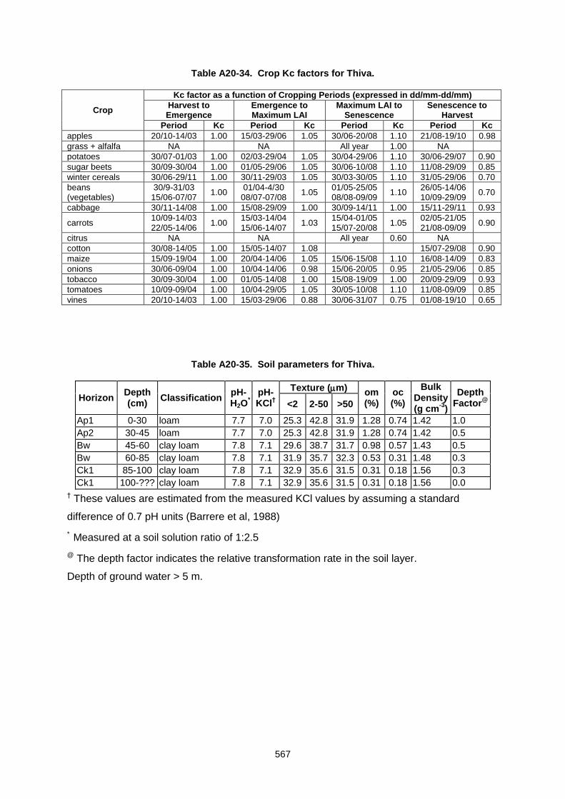
567
Table A20-34. Crop Kc factors for Thiva.
Crop
Kc factor as a function of Cropping Periods (expressed in dd/mm-dd/mm)
Harvest to Emergence
Emergence to Maximum LAI
Maximum LAI to Senescence
Senescence to Harvest
Period Kc Period Kc Period Kc Period Kc
apples 20/10-14/03 1.00 15/03-29/06 1.05 30/06-20/08 1.10 21/08-19/10 0.98
grass + alfalfa NA NA All year 1.00 NA
potatoes 30/07-01/03 1.00 02/03-29/04 1.05 30/04-29/06 1.10 30/06-29/07 0.90
sugar beets 30/09-30/04 1.00 01/05-29/06 1.05 30/06-10/08 1.10 11/08-29/09 0.85
winter cereals 30/06-29/11 1.00 30/11-29/03 1.05 30/03-30/05 1.10 31/05-29/06 0.70
beans (vegetables)
30/9-31/03 15/06-07/07
1.00 01/04-4/30
08/07-07/08 1.05
01/05-25/05 08/08-09/09
1.10 26/05-14/06 10/09-29/09
0.70
cabbage 30/11-14/08 1.00 15/08-29/09 1.00 30/09-14/11 1.00 15/11-29/11 0.93
carrots 10/09-14/03 22/05-14/06
1.00 15/03-14/04 15/06-14/07
1.03 15/04-01/05 15/07-20/08
1.05 02/05-21/05 21/08-09/09
0.90
citrus NA NA All year 0.60 NA
cotton 30/08-14/05 1.00 15/05-14/07 1.08 15/07-29/08 0.90
maize 15/09-19/04 1.00 20/04-14/06 1.05 15/06-15/08 1.10 16/08-14/09 0.83
onions 30/06-09/04 1.00 10/04-14/06 0.98 15/06-20/05 0.95 21/05-29/06 0.85
tobacco 30/09-30/04 1.00 01/05-14/08 1.00 15/08-19/09 1.00 20/09-29/09 0.93
tomatoes 10/09-09/04 1.00 10/04-29/05 1.05 30/05-10/08 1.10 11/08-09/09 0.85
vines 20/10-14/03 1.00 15/03-29/06 0.88 30/06-31/07 0.75 01/08-19/10 0.65
Table A20-35. Soil parameters for Thiva.
Horizon Depth (cm)
Classification pH-H2O
*
pH-KCl
†
Texture (m) om
(%) oc (%)
Bulk Density (g cm
-3)
Depth Factor
@ <2 2-50 >50
Ap1 0-30 loam 7.7 7.0 25.3 42.8 31.9 1.28 0.74 1.42 1.0
Ap2 30-45 loam 7.7 7.0 25.3 42.8 31.9 1.28 0.74 1.42 0.5
Bw 45-60 clay loam 7.8 7.1 29.6 38.7 31.7 0.98 0.57 1.43 0.5
Bw 60-85 clay loam 7.8 7.1 31.9 35.7 32.3 0.53 0.31 1.48 0.3
Ck1 85-100 clay loam 7.8 7.1 32.9 35.6 31.5 0.31 0.18 1.56 0.3
Ck1 100-??? clay loam 7.8 7.1 32.9 35.6 31.5 0.31 0.18 1.56 0.0
† These values are estimated from the measured KCl values by assuming a standard
difference of 0.7 pH units (Barrere et al, 1988)
* Measured at a soil solution ratio of 1:2.5
@ The depth factor indicates the relative transformation rate in the soil layer.
Depth of ground water > 5 m.
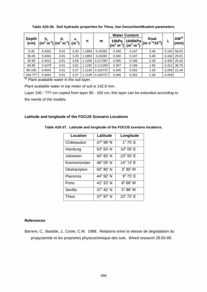
568
Table A20-36. Soil hydraulic properties for Thiva, Van Genuchten/Mualem parameters.
Depth (cm)
s (m3 m-3)
r (m3 m-3)
(m-1)
n m
Water Content Ksat
(m s-1*10-6)
AW@ (mm)
10kPa (m3 m-3)
1600kPa (m3 m-3)
0-30 0.4341 0.01 3.33 1.1804 0.15283 0.340 0.147 3.48 -3.162 58.02
30-45 0.4341 0.01 3.33 1.1804 0.15283 0.340 0.147 3.48 -3.162 29.01
45-60 0.4412 0.01 3.58 1.1330 0.117387 0.365 0.196 2.28 -3.402 25.43
60-85 0.4279 0.01 3.62 1.1252 0.111269 0.357 0.199 1.83 -3.312 39.70
85-100 0.4041 0.01 3.37 1.1145 0.102737 0.345 0.202 1.26 -3.259 21.44
100-??? 0.4041 0.01 3.37 1.1145 0.102737 0.345 0.202 1.26 -3.259 @ Plant available water in the soil layer.
Plant available water in top meter of soil is 142.9 mm.
Layer 100 - ??? cm copied from layer 85 - 100 cm; this layer can be extended according to
the needs of the models.
Latitude and longitude of the FOCUS Scenario Locations
Table A20-37. Latitude and longitude of the FOCUS scenario locations.
Location Latitude Longitude
Châteaudun 47o 98’ N 1o 75’ E
Hamburg 53o 63’ N 10o 00’ E
Jokioinen 60o 82’ N 23o 50’ E
Kremsmünster 48o 05’ N 14o 13’ E
Okehampton 50o 80’ N 3o 80’ W
Piacenza 44o 92’ N 9o 73’ E
Porto 41o 23’ N 8o 68’ W
Sevilla 37o 42’ N 5o 88’ W
Thiva 37o 97’ N 23o 72’ E
References
Barrere, C., Bastide, J., Coste, C.M. 1988. Relations entre la vitesse de degradation du
propyzamide et les proprietes physicochimique des sols. Weed research 28:93-99.
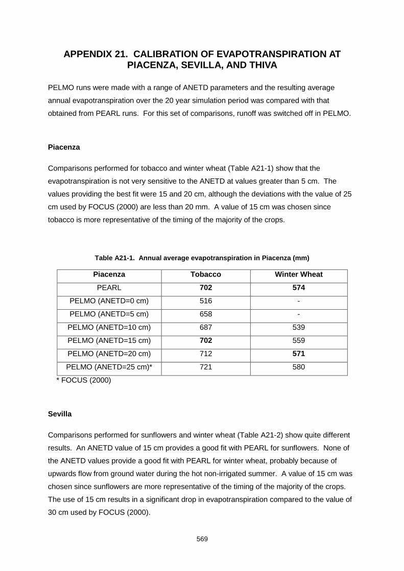
569
APPENDIX 21. CALIBRATION OF EVAPOTRANSPIRATION AT PIACENZA, SEVILLA, AND THIVA
PELMO runs were made with a range of ANETD parameters and the resulting average
annual evapotranspiration over the 20 year simulation period was compared with that
obtained from PEARL runs. For this set of comparisons, runoff was switched off in PELMO.
Piacenza
Comparisons performed for tobacco and winter wheat (Table A21-1) show that the
evapotranspiration is not very sensitive to the ANETD at values greater than 5 cm. The
values providing the best fit were 15 and 20 cm, although the deviations with the value of 25
cm used by FOCUS (2000) are less than 20 mm. A value of 15 cm was chosen since
tobacco is more representative of the timing of the majority of the crops.
Table A21-1. Annual average evapotranspiration in Piacenza (mm)
Piacenza Tobacco Winter Wheat
PEARL 702 574
PELMO (ANETD=0 cm) 516 -
PELMO (ANETD=5 cm) 658 -
PELMO (ANETD=10 cm) 687 539
PELMO (ANETD=15 cm) 702 559
PELMO (ANETD=20 cm) 712 571
PELMO (ANETD=25 cm)* 721 580
* FOCUS (2000)
Sevilla
Comparisons performed for sunflowers and winter wheat (Table A21-2) show quite different
results. An ANETD value of 15 cm provides a good fit with PEARL for sunflowers. None of
the ANETD values provide a good fit with PEARL for winter wheat, probably because of
upwards flow from ground water during the hot non-irrigated summer. A value of 15 cm was
chosen since sunflowers are more representative of the timing of the majority of the crops.
The use of 15 cm results in a significant drop in evapotranspiration compared to the value of
30 cm used by FOCUS (2000).
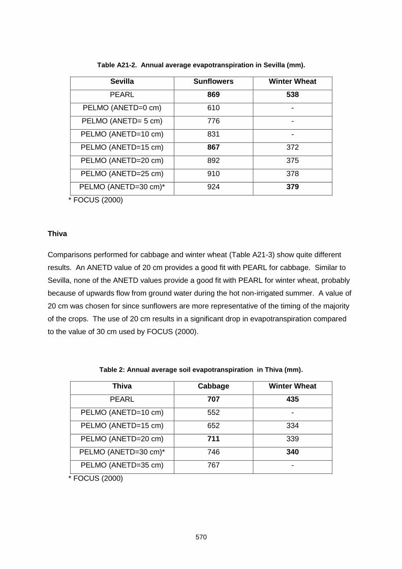
570
Table A21-2. Annual average evapotranspiration in Sevilla (mm).
Sevilla Sunflowers Winter Wheat
PEARL 869 538
PELMO (ANETD=0 cm) 610 -
PELMO (ANETD= 5 cm) 776 -
PELMO (ANETD=10 cm) 831 -
PELMO (ANETD=15 cm) 867 372
PELMO (ANETD=20 cm) 892 375
PELMO (ANETD=25 cm) 910 378
PELMO (ANETD=30 cm)* 924 379
* FOCUS (2000)
Thiva
Comparisons performed for cabbage and winter wheat (Table A21-3) show quite different
results. An ANETD value of 20 cm provides a good fit with PEARL for cabbage. Similar to
Sevilla, none of the ANETD values provide a good fit with PEARL for winter wheat, probably
because of upwards flow from ground water during the hot non-irrigated summer. A value of
20 cm was chosen for since sunflowers are more representative of the timing of the majority
of the crops. The use of 20 cm results in a significant drop in evapotranspiration compared
to the value of 30 cm used by FOCUS (2000).
Table 2: Annual average soil evapotranspiration in Thiva (mm).
Thiva Cabbage Winter Wheat
PEARL 707 435
PELMO (ANETD=10 cm) 552 -
PELMO (ANETD=15 cm) 652 334
PELMO (ANETD=20 cm) 711 339
PELMO (ANETD=30 cm)* 746 340
PELMO (ANETD=35 cm) 767 -
* FOCUS (2000)

571
References
FOCUS. 2000. FOCUS groundwater scenarios in the EU review of active substances.
Report of the FOCUS Groundwater Scenarios Workgroup, EC Document Reference
Sanco/321/2000 rev.2, 202pp.
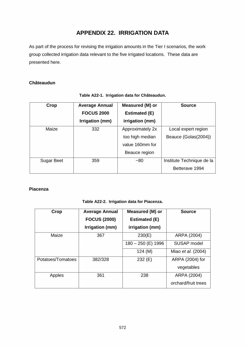
572
APPENDIX 22. IRRIGATION DATA
As part of the process for revising the irrigation amounts in the Tier I scenarios, the work
group collected irrigation data relevant to the five irrigated locations. These data are
presented here.
Châteaudun
Table A22-1. Irrigation data for Châteaudun.
Crop Average Annual
FOCUS 2000
Irrigation (mm)
Measured (M) or
Estimated (E)
irrigation (mm)
Source
Maize 332 Approximately 2x
too high median
value 160mm for
Beauce region
Local expert region
Beauce (Golas(2004))
Sugar Beet 359 ~80 Institute Technique de la
Betterave 1994
Piacenza
Table A22-2. Irrigation data for Piacenza.
Crop Average Annual
FOCUS (2000)
Irrigation (mm)
Measured (M) or
Estimated (E)
irrigation (mm)
Source
Maize 367 230(E) ARPA (2004)
180 – 250 (E) 1996 SUSAP model
124 (M) Miao et al. (2004)
Potatoes/Tomatoes 382/328 232 (E) ARPA (2004) for
vegetables
Apples 361 238 ARPA (2004)
orchard/fruit trees
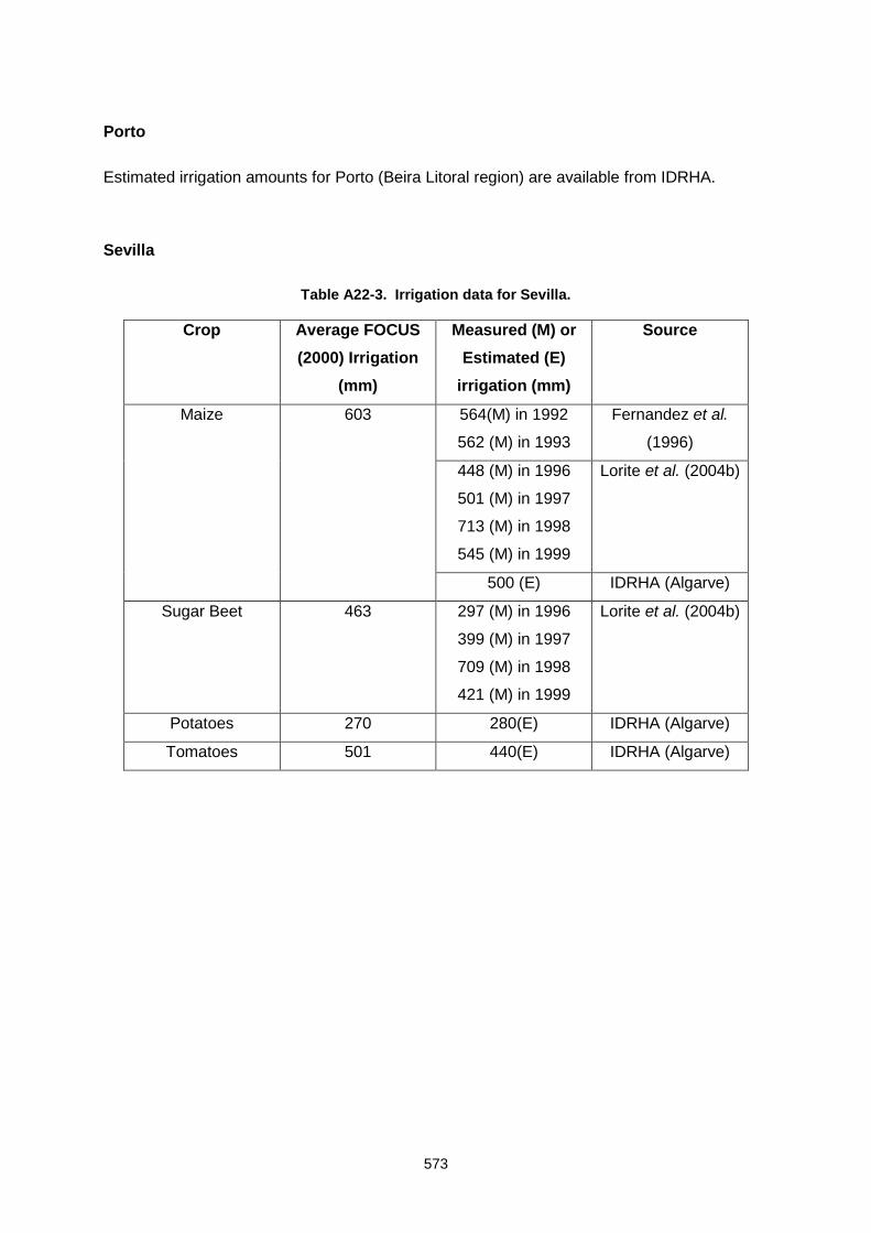
573
Porto
Estimated irrigation amounts for Porto (Beira Litoral region) are available from IDRHA.
Sevilla
Table A22-3. Irrigation data for Sevilla.
Crop Average FOCUS
(2000) Irrigation
(mm)
Measured (M) or
Estimated (E)
irrigation (mm)
Source
Maize 603 564(M) in 1992
562 (M) in 1993
Fernandez et al.
(1996)
448 (M) in 1996
501 (M) in 1997
713 (M) in 1998
545 (M) in 1999
Lorite et al. (2004b)
500 (E) IDRHA (Algarve)
Sugar Beet 463 297 (M) in 1996
399 (M) in 1997
709 (M) in 1998
421 (M) in 1999
Lorite et al. (2004b)
Potatoes 270 280(E) IDRHA (Algarve)
Tomatoes 501 440(E) IDRHA (Algarve)
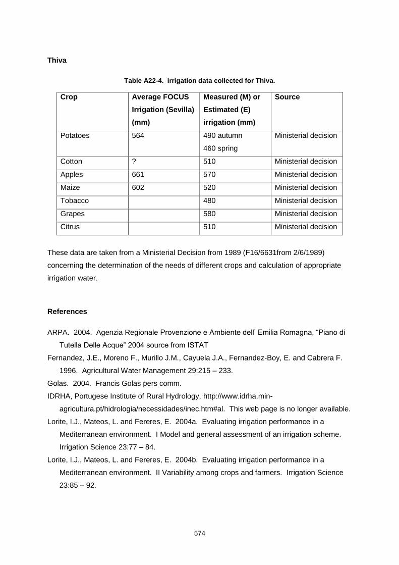
574
Thiva
Table A22-4. irrigation data collected for Thiva.
Crop Average FOCUS
Irrigation (Sevilla)
(mm)
Measured (M) or
Estimated (E)
irrigation (mm)
Source
Potatoes 564 490 autumn
460 spring
Ministerial decision
Cotton ? 510 Ministerial decision
Apples 661 570 Ministerial decision
Maize 602 520 Ministerial decision
Tobacco 480 Ministerial decision
Grapes 580 Ministerial decision
Citrus 510 Ministerial decision
These data are taken from a Ministerial Decision from 1989 (F16/6631from 2/6/1989)
concerning the determination of the needs of different crops and calculation of appropriate
irrigation water.
References
ARPA. 2004. Agenzia Regionale Provenzione e Ambiente dell’ Emilia Romagna, “Piano di
Tutella Delle Acque” 2004 source from ISTAT
Fernandez, J.E., Moreno F., Murillo J.M., Cayuela J.A., Fernandez-Boy, E. and Cabrera F.
1996. Agricultural Water Management 29:215 – 233.
Golas. 2004. Francis Golas pers comm.
IDRHA, Portugese Institute of Rural Hydrology, http://www.idrha.min-
agricultura.pt/hidrologia/necessidades/inec.htm#al. This web page is no longer available.
Lorite, I.J., Mateos, L. and Fereres, E. 2004a. Evaluating irrigation performance in a
Mediterranean environment. I Model and general assessment of an irrigation scheme.
Irrigation Science 23:77 – 84.
Lorite, I.J., Mateos, L. and Fereres, E. 2004b. Evaluating irrigation performance in a
Mediterranean environment. II Variability among crops and farmers. Irrigation Science
23:85 – 92.

575
Miao Z, Vicari A, Capri E, Ventura F, Padovani L and Trevisan M. 2004. Modeling the
Effects of Tillage Management Practices on Herbicide Runoff in Northern Italy. J. Env.
Qual. 33:1720 – 1732.
Moreno F., Cayuela J.A., Fernandez, J.E., Fernandez-Boy, E., Murillo J.M., and Cabrera F.
1996. Water balance and nitrate leaching in an irrigated maize crop in SW Spain.
Agricultural Water Management 32:71 – 83.
576
APPENDIX 23. RESULTS OF SIMULATIONS COMPARING THE CURRENT AND THE PROPOSED SCENARIOS
Table A23-1. PECgw for Pesticide D at 1 m.
Location Crop
PECgw (μg/L) for Pesticide D at 1 m
FOCUS 2009 FOCUS 2000
PEARL PELMO PRZM MACRO PEARL PELMO PRZM MACRO
Châteaudun apples 0.3618 0.3580 0.1971 - 0.5763 0.3870 0.3199 -
Châteaudun cabbage 0.1598 0.1182 0.0662 - 0.2855 0.0084 0.0039 -
Châteaudun carrots 0.1843 0.1027 0.0450 - 0.2664 0.0060 0.0024 -
Châteaudun cereals (spring) 0.0060 0.0021 0.0012 - 0.0092 0.0002 0.0000 -
Châteaudun cereals (winter) 0.0921 0.0302 0.0236 - 0.1618 0.0132 0.0156 -
Châteaudun grass 0.0906 0.0678 0.0255 - 0.0962 0.0067 0.0019 -
Châteaudun maize 0.0751 0.0280 0.0233 - 0.1911 0.0012 0.0007 -
Châteaudun onions 0.0163 0.0143 0.0079 - 0.1888 0.0078 0.0030 -
Châteaudun peas 0.0024 0.0013 0.0009 - 0.0033 0.0000 0.0000 -
Châteaudun potatoes 0.0622 0.0369 0.0247 - 0.2258 0.0014 0.0007 -
Châteaudun rape (winter) 0.0833 0.0424 0.0471 - 0.1102 0.0270 0.0318 -
Châteaudun sugar beets 0.4275 0.1436 0.0586 - 0.3393 0.0393 0.0131 -
Châteaudun tomatoes 0.0848 0.0363 0.0200 - 0.3141 0.0101 0.0052 -
Châteaudun vines 0.2532 0.2473 0.1349 - 0.6473 0.4510 0.4294 -
Hamburg apples 0.3488 0.2486 0.1522 - 1.9109 0.1210 0.1383 -
Hamburg beans (field) 0.1786 0.1022 0.0966 - 0.2358 0.0462 0.0493 -
Hamburg cabbage 0.7519 0.5922 0.4861 - 0.7704 0.2430 0.2053 -
Hamburg carrot 0.6296 0.4643 0.3616 - 0.6890 0.2310 0.2248 -
Hamburg cereals (spring) 0.2025 0.1162 0.1190 - 0.2632 0.0467 0.0528 -
Hamburg cereals (winter) 1.8052 1.8610 1.5940 - 1.2972 1.0600 1.2260 -
Hamburg grass 0.1915 0.1018 0.0927 - 0.2010 0.0261 0.0871 -
Hamburg maize 0.2209 0.1531 0.1355 - 0.2939 0.0731 0.0690 -
Hamburg onions 0.1735 0.1038 0.0842 - 0.1941 0.0505 0.0425 -
Hamburg peas 0.1763 0.1049 0.0913 - 0.2258 0.0446 0.0385 -
Hamburg potato 0.1665 0.1378 0.1234 - 0.1980 0.0518 0.0351 -
Hamburg rape (winter) 1.0476 0.8316 0.8686 - 0.8392 0.5220 0.6456 -
Hamburg strawberries 0.6198 0.2516 0.1262 - 0.6833 0.0813 0.1140 -
Hamburg sugar beets 0.1716 0.1104 0.0793 - 0.2405 0.0630 0.0635 -
Hamburg vines 0.2553 0.3188 0.2075 - 0.2927 0.1470 0.1670 -
Jokioinen apples 0.0490 0.0678 0.0602 - 0.0492 0.1410 0.0042 -
Jokioinen bush berries 0.0824 0.0504 0.0457 - 0.0693 0.0060 0.0017 -
Jokioinen cabbage 0.0239 0.0326 0.0327 - 0.0233 0.0008 0.0001 -
Jokioinen carrots 0.0231 0.0362 0.0426 - 0.0274 0.0007 0.0001 -
Jokioinen cereals (spring) 0.0317 0.0375 0.0392 - 0.0258 0.0010 0.0001 -
Jokioinen cereals (winter) 0.3272 0.4230 0.3431 - 0.2091 0.0758 0.0053 -
Jokioinen grass 0.0420 0.0492 0.0411 - 0.0414 0.1600 0.0023 -
Jokioinen onions 0.0190 0.0239 0.0391 - 0.0176 0.0003 0.0001 -
Jokioinen peas 0.0343 0.0409 0.0479 - 0.0288 0.0007 0.0001 -
Jokioinen potatoes 0.0261 0.0343 0.0414 - 0.0283 0.0003 0.0000 -
Jokioinen rape (summer) 0.0273 0.0369 0.0405 - 0.0262 0.0011 0.0001 -
577
Table A23-1 (continued). PECgw for Pesticide D at 1 m.
Location Crop
PECgw (μg/L) for Pesticide D at 1 m
FOCUS 2009 FOCUS 2000
PEARL PELMO PRZM MACRO PEARL PELMO PRZM MACRO
Jokioinen strawberries 0.0343 0.0305 0.0426 - 0.0338 0.0014 0.0005 -
Jokioinen sugar beets 0.0387 0.0435 0.0380 - 0.0342 0.0017 0.0001 -
Kremsmünster apples 0.2382 0.3012 0.1195 - 0.3578 0.1420 0.1024 -
Kremsmünster beans (field) 0.1395 0.1213 0.0596 - 0.2000 0.0078 0.0016 -
Kremsmünster cabbage 0.3612 0.4019 0.2434 - 0.3791 0.0365 0.0096 -
Kremsmünster carrots 0.3947 0.4653 0.2459 - 0.4663 0.0334 0.0084 -
Kremsmünster cereals (spring) 0.1654 0.1505 0.0678 - 0.1919 0.0147 0.0040 -
Kremsmünster cereals (winter) 0.5745 0.5397 0.4074 - 0.5478 0.1470 0.0661 -
Kremsmünster grass 0.1111 0.1166 0.0385 - 0.1208 0.0576 0.0144 -
Kremsmünster maize 0.1402 0.1481 0.0959 - 0.1908 0.0052 0.0017 -
Kremsmünster onions 0.1102 0.1063 0.0549 - 0.1440 0.0086 0.0019 -
Kremsmünster potatoes 0.1004 0.1056 0.0557 - 0.1281 0.0026 0.0004 -
Kremsmünster rape (winter) 0.5842 0.5617 0.4921 - 0.5014 0.2720 0.2376 -
Kremsmünster strawberries 0.2446 0.1551 0.0518 - 0.2978 0.0173 0.0074 -
Kremsmünster sugar beets 0.1058 0.1181 0.0430 - 0.1743 0.0283 0.0058 -
Kremsmünster vines 0.1965 0.4361 0.1909 - 0.2512 0.2370 0.2022 -
Okehampton apples 0.3338 0.5915 0.3718 - 0.4485 0.9870 0.3248 -
Okehampton beans (field) 0.2151 0.2749 0.2413 - 0.3174 0.0310 0.0337 -
Okehampton cereals (spring) 0.2936 0.2907 0.2020 - 0.3328 0.0346 0.0377 -
Okehampton cereals (winter) 1.6406 1.8038 1.7650 - 1.9732 1.0900 1.7070 -
Okehampton grass 0.2530 0.3662 0.2266 - 0.2515 1.1100 0.0984 -
Okehampton linseed 0.2190 0.2859 0.2365 - 0.2531 0.0537 0.0597 -
Okehampton maize 0.4298 0.4214 0.3694 - 0.4623 0.0189 0.0196 -
Okehampton peas 0.2007 0.2063 0.1781 - 0.2332 0.0134 0.0153 -
Okehampton potatoes 0.2332 0.2634 0.2381 - 0.2997 0.0094 0.0096 -
Okehampton rape (summer) 0.2571 0.2939 0.2290 - 0.2745 0.0597 0.0375 -
Okehampton rape (winter) 0.7564 0.8906 0.9572 - 0.8349 0.4090 0.6886 -
Okehampton sugar beets 0.2151 0.3161 0.2509 - 0.2667 0.0496 0.0609 -
Piacenza apples 0.2173 0.7635 0.3270 - 1.3552 2.2600 0.3663 -
Piacenza cereals (winter) 0.7159 1.0247 0.7932 - 1.6928 2.0800 1.4320 -
Piacenza citrus 0.2886 0.4138 0.2622 - 1.6609 4.2400 0.6345 -
Piacenza grass 0.2293 0.5785 0.1091 - 0.7350 1.4800 0.1024 -
Piacenza maize 0.2022 0.3117 0.1160 - 0.7182 0.3910 0.1347 -
Piacenza potatoes 0.1383 0.2145 0.0747 - 0.7016 0.2330 0.0531 -
Piacenza rape (winter) 1.1720 1.8819 2.0180 - 5.5158 4.2100 5.1590 -
Piacenza soybeans 0.1527 0.1543 0.0531 - 0.4719 0.1590 0.0522 -
Piacenza sugar beets 0.2202 0.3613 0.0994 - 1.0647 0.3440 0.0863 -
Piacenza sunflowers 0.1650 0.4885 0.1641 - 0.9875 0.4190 0.1262 -
Piacenza tobacco 0.1705 0.3219 0.1326 - 0.7428 0.3740 0.1318 -
Piacenza tomatoes 0.1844 0.3805 0.1069 - 1.1246 0.4650 0.1145 -
Piacenza vines 0.2371 0.5985 0.2025 - 1.3510 2.8800 0.4505 -
Porto apples 0.0550 0.1663 0.0525 - 0.0000 0.0085 0.0000 -
Porto beans (veg) 0.0365 0.0774 0.0378 - 0.0000 0.0000 0.0000 -
578
Table A23-1 (continued). PECgw for Pesticide D at 1 m.
Location Crop
PECgw (μg/L) for Pesticide D at 1 m
FOCUS 2009 FOCUS 2000
PEARL PELMO PRZM MACRO PEARL PELMO PRZM MACRO
Porto cabbage 0.3323 0.7211 0.2603 - 0.0010 0.0000 0.0000 -
Porto carrots 0.2080 0.4630 0.1716 - 0.3507 0.0000 0.0000 -
Porto cereals (spring) 0.0351 0.1628 0.0549 - 0.0000 0.0000 0.0000 -
Porto cereals (winter) 1.2923 2.5956 2.0680 - 0.0087 0.0013 0.0006 -
Porto citrus 0.0466 0.0908 0.0462 - 0.0000 0.0104 0.0000 -
Porto grass 0.0441 0.1009 0.0203 - 0.0000 0.0038 0.0000 -
Porto maize 0.0229 0.0313 0.0125 - 0.0000 0.0000 0.0000 -
Porto onions 0.0376 0.0937 0.0284 - 0.0000 0.0000 0.0000 -
Porto potatoes 0.0315 0.1179 0.0408 - 0.0000 0.0000 0.0000 -
Porto rape (summer) 0.0592 0.2092 0.1024 - 0.0000 0.0000 0.0000 -
Porto rape (winter) 0.7993 1.9727 1.2380 - 0.0040 0.0007 0.0002 -
Porto sugar beets 0.0856 0.3522 0.1248 - 0.0000 0.0000 0.0000 -
Porto tomatoes 0.0367 0.0672 0.0407 - 0.0000 0.0000 0.0000 -
Porto vines 0.0322 0.1185 0.0500 - 0.0000 0.0086 0.0000 -
Sevilla apples 0.3553 0.1040 0.0397 - 0.3059 0.0036 0.0011 -
Sevilla cabbage 0.0656 0.0026 0.0012 - 0.3507 0.0000 0.0000 -
Sevilla cereals (winter) 0.0000 0.0136 0.0347 - 0.1107 0.0001 0.0000 -
Sevilla citrus 0.0980 0.0281 0.0105 - 0.4434 0.1500 0.0181 -
Sevilla cotton 0.0098 0.0046 0.0031 - 0.0611 0.0000 0.0000 -
Sevilla grass 0.0082 0.0041 0.0008 - 0.0190 0.0010 0.0000 -
Sevilla maize 0.0005 0.0003 0.0003 - 0.0067 0.0000 0.0000 -
Sevilla potatoes 0.0015 0.0015 0.0009 - 0.0155 0.0000 0.0000 -
Sevilla strawberries 0.0176 0.0903 0.1007 - 0.1278 0.0000 0.0000 -
Sevilla sugar beets 0.0932 0.0941 0.1122 - 0.3054 0.0014 0.0007 -
Sevilla sunflowers 0.0018 0.0007 0.0006 - 0.0421 0.0000 0.0000 -
Sevilla tomatoes 0.0026 0.0013 0.0014 - 0.0885 0.0000 0.0000 -
Sevilla vines 0.1324 0.0433 0.0172 - 0.2943 0.0134 0.0026 -
Thiva apples 0.2425 0.0807 0.0200 - 0.2368 0.0487 0.0020 -
Thiva beans (veg) 0.0666 0.0274 0.0080 - 0.1266 0.0000 0.0000 -
Thiva cabbage 0.0620 0.0579 0.0169 - 0.0488 0.0008 0.0001 -
Thiva carrots 0.0303 0.0095 0.0021 - 0.1161 0.0000 0.0000 -
Thiva cereals (winter) 0.0331 0.0403 0.0204 - 0.1592 0.0174 0.0040 -
Thiva citrus 0.0301 0.0461 0.0099 - 0.4053 0.4830 0.0432 -
Thiva cotton 0.0024 0.0030 0.0009 - 0.1128 0.0000 0.0000 -
Thiva grass 0.0239 0.0235 0.0018 - 0.0184 0.0393 0.0000 -
Thiva maize 0.0159 0.0105 0.0042 - 0.1142 0.0000 0.0000 -
Thiva onions 0.0003 0.0009 0.0001 - 0.0673 0.0000 0.0000 -
Thiva potatoes 0.0067 0.0036 0.0012 - 0.0348 0.0000 0.0000 -
Thiva sugar beets 0.0204 0.0111 0.0020 - 0.1252 0.0001 0.0000 -
Thiva tobacco 0.0029 0.0011 0.0004 - 0.0225 0.0000 0.0000 -
Thiva tomatoes 0.0069 0.0033 0.0012 - 0.0385 0.0000 0.0000 -
Thiva vines 0.0361 0.0253 0.0071 - 0.2601 0.2240 0.0260 -
579
Table A23-2. Annual averages of rainfall and irrigation.
Location Crop
Rainfall (mm) Irrigation (mm)
FOCUS 2000
and 2009 FOCUS 2009
FOCUS
2000
All Models PEARL
PELMO
and
PRZM
MACRO All Models
Châteaudun apples 648 350 369 - 323
Châteaudun cabbage 648 185 198 - 284
Châteaudun carrots 648 175 171 - 284
Châteaudun cereals (spring) 648 0 0 - 0
Châteaudun cereals (winter) 648 0 0 - 0
Châteaudun grass 648 338 331 - 303
Châteaudun maize 648 264 255 - 323
Châteaudun onions 648 112 139 - 284
Châteaudun peas 648 0 0 - 0
Châteaudun potatoes 648 200 211 - 311
Châteaudun rape (winter) 648 0 0 - 0
Châteaudun sugar beets 648 395 328 - 349
Châteaudun tomatoes 648 176 177 - 284
Châteaudun vines 648 243 237 - 323
Hamburg all crops 786 0 0 - 0
Jokioinen all crops 650 0 0 - 0
Kremsmünster all crops 899 0 0 - 0
Okehampton all crops 1038 0 0 - 0
Piacenza apples 857 156 448 - 361
Piacenza cereals (winter) 857 0 0 - 0
Piacenza citrus 857 63 241 - 361
Piacenza grass 857 217 457 - 369
Piacenza maize 857 188 399 - 365
Piacenza potatoes 857 221 335 - 381
Piacenza rape (winter) 857 0 0 - 0
Piacenza soybeans 857 218 341 - 365
Piacenza sugar beets 857 168 294 - 392
Piacenza sunflowers 857 176 403 - 365
Piacenza tobacco 857 159 358 - 365
Piacenza tomatoes 857 107 234 - 328
Piacenza vines 857 97 290 - 361
Porto apples 1150 398 509 - 0
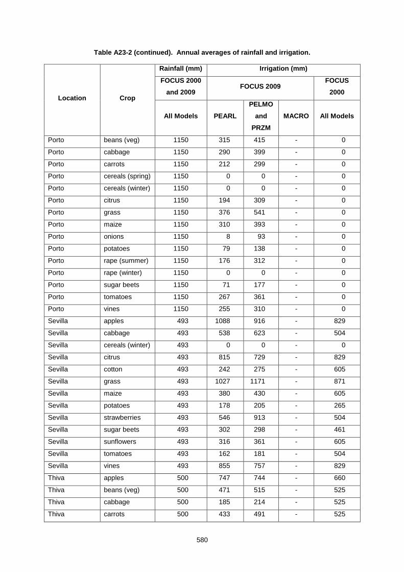
580
Table A23-2 (continued). Annual averages of rainfall and irrigation.
Location Crop
Rainfall (mm) Irrigation (mm)
FOCUS 2000
and 2009 FOCUS 2009
FOCUS
2000
All Models PEARL
PELMO
and
PRZM
MACRO All Models
Porto beans (veg) 1150 315 415 - 0
Porto cabbage 1150 290 399 - 0
Porto carrots 1150 212 299 - 0
Porto cereals (spring) 1150 0 0 - 0
Porto cereals (winter) 1150 0 0 - 0
Porto citrus 1150 194 309 - 0
Porto grass 1150 376 541 - 0
Porto maize 1150 310 393 - 0
Porto onions 1150 8 93 - 0
Porto potatoes 1150 79 138 - 0
Porto rape (summer) 1150 176 312 - 0
Porto rape (winter) 1150 0 0 - 0
Porto sugar beets 1150 71 177 - 0
Porto tomatoes 1150 267 361 - 0
Porto vines 1150 255 310 - 0
Sevilla apples 493 1088 916 - 829
Sevilla cabbage 493 538 623 - 504
Sevilla cereals (winter) 493 0 0 - 0
Sevilla citrus 493 815 729 - 829
Sevilla cotton 493 242 275 - 605
Sevilla grass 493 1027 1171 - 871
Sevilla maize 493 380 430 - 605
Sevilla potatoes 493 178 205 - 265
Sevilla strawberries 493 546 913 - 504
Sevilla sugar beets 493 302 298 - 461
Sevilla sunflowers 493 316 361 - 605
Sevilla tomatoes 493 162 181 - 504
Sevilla vines 493 855 757 - 829
Thiva apples 500 747 744 - 660
Thiva beans (veg) 500 471 515 - 525
Thiva cabbage 500 185 214 - 525
Thiva carrots 500 433 491 - 525
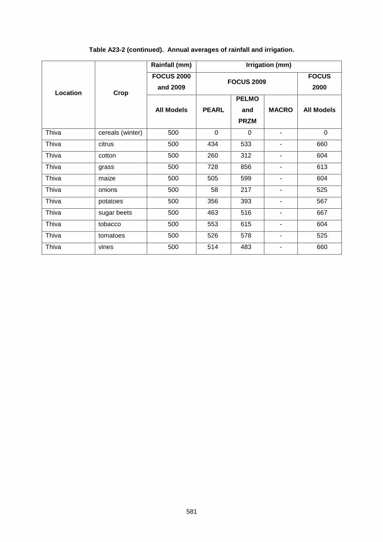
581
Table A23-2 (continued). Annual averages of rainfall and irrigation.
Location Crop
Rainfall (mm) Irrigation (mm)
FOCUS 2000
and 2009 FOCUS 2009
FOCUS
2000
All Models PEARL
PELMO
and
PRZM
MACRO All Models
Thiva cereals (winter) 500 0 0 - 0
Thiva citrus 500 434 533 - 660
Thiva cotton 500 260 312 - 604
Thiva grass 500 728 856 - 613
Thiva maize 500 505 599 - 604
Thiva onions 500 58 217 - 525
Thiva potatoes 500 356 393 - 567
Thiva sugar beets 500 463 516 - 667
Thiva tobacco 500 553 615 - 604
Thiva tomatoes 500 526 578 - 525
Thiva vines 500 514 483 - 660
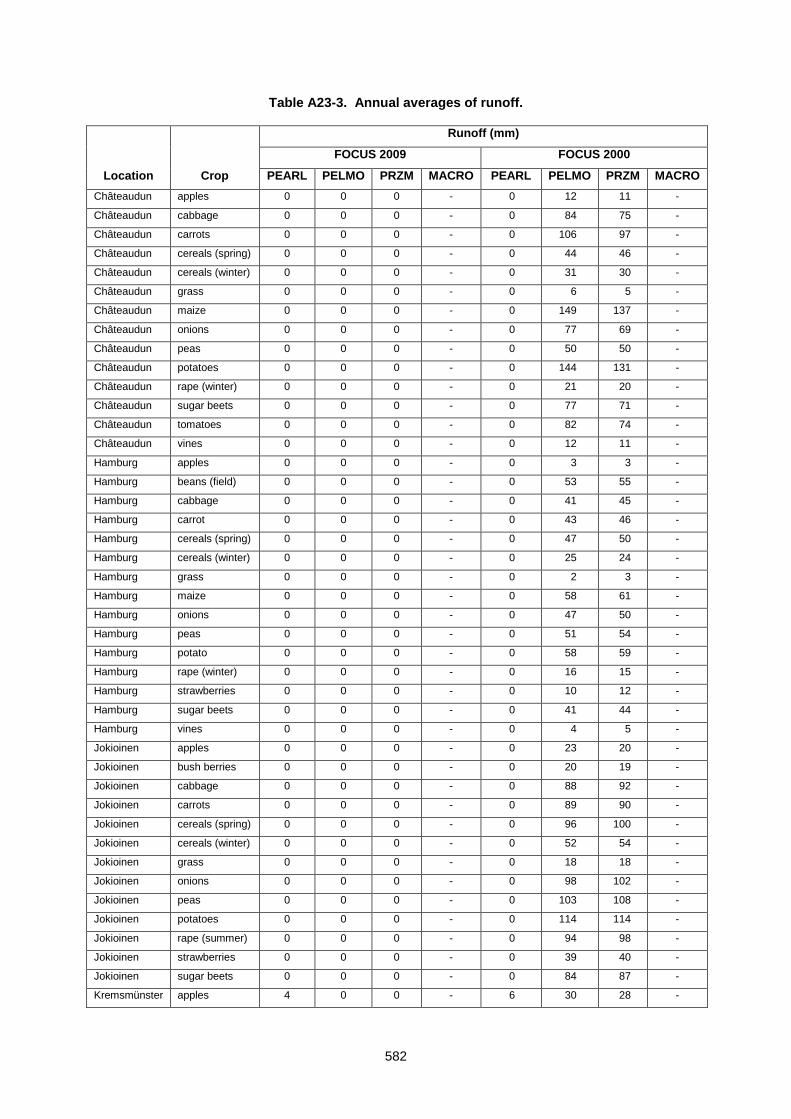
582
Table A23-3. Annual averages of runoff.
Location Crop
Runoff (mm)
FOCUS 2009 FOCUS 2000
PEARL PELMO PRZM MACRO PEARL PELMO PRZM MACRO
Châteaudun apples 0 0 0 - 0 12 11 -
Châteaudun cabbage 0 0 0 - 0 84 75 -
Châteaudun carrots 0 0 0 - 0 106 97 -
Châteaudun cereals (spring) 0 0 0 - 0 44 46 -
Châteaudun cereals (winter) 0 0 0 - 0 31 30 -
Châteaudun grass 0 0 0 - 0 6 5 -
Châteaudun maize 0 0 0 - 0 149 137 -
Châteaudun onions 0 0 0 - 0 77 69 -
Châteaudun peas 0 0 0 - 0 50 50 -
Châteaudun potatoes 0 0 0 - 0 144 131 -
Châteaudun rape (winter) 0 0 0 - 0 21 20 -
Châteaudun sugar beets 0 0 0 - 0 77 71 -
Châteaudun tomatoes 0 0 0 - 0 82 74 -
Châteaudun vines 0 0 0 - 0 12 11 -
Hamburg apples 0 0 0 - 0 3 3 -
Hamburg beans (field) 0 0 0 - 0 53 55 -
Hamburg cabbage 0 0 0 - 0 41 45 -
Hamburg carrot 0 0 0 - 0 43 46 -
Hamburg cereals (spring) 0 0 0 - 0 47 50 -
Hamburg cereals (winter) 0 0 0 - 0 25 24 -
Hamburg grass 0 0 0 - 0 2 3 -
Hamburg maize 0 0 0 - 0 58 61 -
Hamburg onions 0 0 0 - 0 47 50 -
Hamburg peas 0 0 0 - 0 51 54 -
Hamburg potato 0 0 0 - 0 58 59 -
Hamburg rape (winter) 0 0 0 - 0 16 15 -
Hamburg strawberries 0 0 0 - 0 10 12 -
Hamburg sugar beets 0 0 0 - 0 41 44 -
Hamburg vines 0 0 0 - 0 4 5 -
Jokioinen apples 0 0 0 - 0 23 20 -
Jokioinen bush berries 0 0 0 - 0 20 19 -
Jokioinen cabbage 0 0 0 - 0 88 92 -
Jokioinen carrots 0 0 0 - 0 89 90 -
Jokioinen cereals (spring) 0 0 0 - 0 96 100 -
Jokioinen cereals (winter) 0 0 0 - 0 52 54 -
Jokioinen grass 0 0 0 - 0 18 18 -
Jokioinen onions 0 0 0 - 0 98 102 -
Jokioinen peas 0 0 0 - 0 103 108 -
Jokioinen potatoes 0 0 0 - 0 114 114 -
Jokioinen rape (summer) 0 0 0 - 0 94 98 -
Jokioinen strawberries 0 0 0 - 0 39 40 -
Jokioinen sugar beets 0 0 0 - 0 84 87 -
Kremsmünster apples 4 0 0 - 6 30 28 -
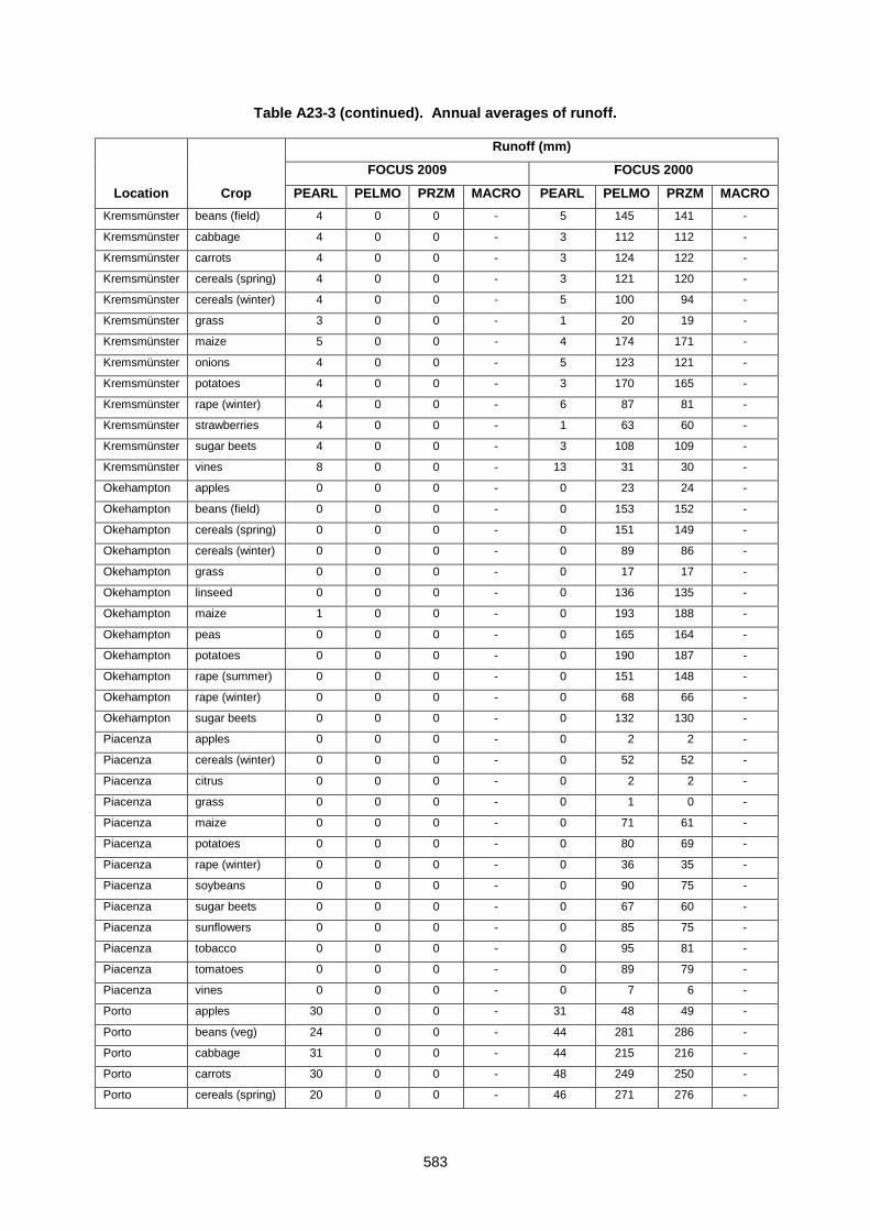
583
Table A23-3 (continued). Annual averages of runoff.
Location Crop
Runoff (mm)
FOCUS 2009 FOCUS 2000
PEARL PELMO PRZM MACRO PEARL PELMO PRZM MACRO
Kremsmünster beans (field) 4 0 0 - 5 145 141 -
Kremsmünster cabbage 4 0 0 - 3 112 112 -
Kremsmünster carrots 4 0 0 - 3 124 122 -
Kremsmünster cereals (spring) 4 0 0 - 3 121 120 -
Kremsmünster cereals (winter) 4 0 0 - 5 100 94 -
Kremsmünster grass 3 0 0 - 1 20 19 -
Kremsmünster maize 5 0 0 - 4 174 171 -
Kremsmünster onions 4 0 0 - 5 123 121 -
Kremsmünster potatoes 4 0 0 - 3 170 165 -
Kremsmünster rape (winter) 4 0 0 - 6 87 81 -
Kremsmünster strawberries 4 0 0 - 1 63 60 -
Kremsmünster sugar beets 4 0 0 - 3 108 109 -
Kremsmünster vines 8 0 0 - 13 31 30 -
Okehampton apples 0 0 0 - 0 23 24 -
Okehampton beans (field) 0 0 0 - 0 153 152 -
Okehampton cereals (spring) 0 0 0 - 0 151 149 -
Okehampton cereals (winter) 0 0 0 - 0 89 86 -
Okehampton grass 0 0 0 - 0 17 17 -
Okehampton linseed 0 0 0 - 0 136 135 -
Okehampton maize 1 0 0 - 0 193 188 -
Okehampton peas 0 0 0 - 0 165 164 -
Okehampton potatoes 0 0 0 - 0 190 187 -
Okehampton rape (summer) 0 0 0 - 0 151 148 -
Okehampton rape (winter) 0 0 0 - 0 68 66 -
Okehampton sugar beets 0 0 0 - 0 132 130 -
Piacenza apples 0 0 0 - 0 2 2 -
Piacenza cereals (winter) 0 0 0 - 0 52 52 -
Piacenza citrus 0 0 0 - 0 2 2 -
Piacenza grass 0 0 0 - 0 1 0 -
Piacenza maize 0 0 0 - 0 71 61 -
Piacenza potatoes 0 0 0 - 0 80 69 -
Piacenza rape (winter) 0 0 0 - 0 36 35 -
Piacenza soybeans 0 0 0 - 0 90 75 -
Piacenza sugar beets 0 0 0 - 0 67 60 -
Piacenza sunflowers 0 0 0 - 0 85 75 -
Piacenza tobacco 0 0 0 - 0 95 81 -
Piacenza tomatoes 0 0 0 - 0 89 79 -
Piacenza vines 0 0 0 - 0 7 6 -
Porto apples 30 0 0 - 31 48 49 -
Porto beans (veg) 24 0 0 - 44 281 286 -
Porto cabbage 31 0 0 - 44 215 216 -
Porto carrots 30 0 0 - 48 249 250 -
Porto cereals (spring) 20 0 0 - 46 271 276 -
584
Table A23-3 (continued). Annual averages of runoff.
Location Crop
Runoff (mm)
FOCUS 2009 FOCUS 2000
PEARL PELMO PRZM MACRO PEARL PELMO PRZM MACRO
Porto cereals (winter) 25 0 0 - 55 173 177 -
Porto citrus 48 0 0 - 43 50 51 -
Porto grass 32 0 0 - 37 39 41 -
Porto maize 25 0 0 - 39 306 308 -
Porto onions 29 0 0 - 57 275 277 -
Porto potatoes 30 0 0 - 54 303 307 -
Porto rape (summer) 20 0 0 - 38 273 278 -
Porto rape (winter) 23 0 0 - 54 109 111 -
Porto sugar beets 19 0 0 - 39 275 280 -
Porto tomatoes 20 0 0 - 42 272 276 -
Porto vines 33 0 0 - 36 49 50 -
Sevilla apples 0 0 0 - 0 173 132 -
Sevilla cabbage 0 0 0 - 0 262 218 -
Sevilla cereals (winter) 0 0 0 - 0 101 96 -
Sevilla citrus 0 0 0 - 0 193 166 -
Sevilla cotton 0 0 0 - 0 354 283 -
Sevilla grass 0 0 0 - 0 106 59 -
Sevilla maize 0 0 0 - 0 391 320 -
Sevilla potatoes 0 0 0 - 0 236 209 -
Sevilla strawberries 0 0 0 - 0 164 123 -
Sevilla sugar beets 0 0 0 - 0 196 157 -
Sevilla sunflowers 0 0 0 - 0 420 349 -
Sevilla tomatoes 0 0 0 - 0 300 252 -
Sevilla vines 0 0 0 - 0 178 145 -
Thiva apples 2 0 0 - 0 69 49 -
Thiva beans (veg) 1 0 0 - 0 275 281 -
Thiva cabbage 2 0 0 - 0 287 269 -
Thiva carrots 1 0 0 - 0 228 195 -
Thiva cereals (winter) 0 0 0 - 0 66 69 -
Thiva citrus 2 0 0 - 0 78 66 -
Thiva cotton 0 0 0 - 0 279 241 -
Thiva grass 2 0 0 - 0 40 23 -
Thiva maize 1 0 0 - 0 342 307 -
Thiva onions 1 0 0 - 0 281 249 -
Thiva potatoes 1 0 0 - 0 311 278 -
Thiva sugar beets 1 0 0 - 0 251 210 -
Thiva tobacco 1 0 0 - 0 253 221 -
Thiva tomatoes 1 0 0 - 0 215 176 -
Thiva vines 2 0 0 - 0 75 64 -
585
Table A23-4. Annual Averages of potential evapotranspiration (not reported by PRZM).
Location Crop
Potential Evapotranspiration (mm)
FOCUS 2009 FOCUS 2000
PEARL PELMO MACRO PEARL PELMO MACRO
Châteaudun apples 817 817 - 730 733 -
Châteaudun cabbage 765 765 - 692 719 -
Châteaudun carrots 766 765 - 687 711 -
Châteaudun cereals (spring) 770 768 - 680 682 -
Châteaudun cereals (winter) 767 767 - 675 622 -
Châteaudun grass 774 774 - 741 741 -
Châteaudun maize 788 787 - 694 696 -
Châteaudun onions 740 739 - 652 674 -
Châteaudun peas 808 808 - 699 711 -
Châteaudun potatoes 790 790 - 675 696 -
Châteaudun rape (winter) 765 766 - 655 578 -
Châteaudun sugar beets 798 796 - 684 689 -
Châteaudun tomatoes 777 776 - 702 719 -
Châteaudun vines 650 646 - 647 659 -
Hamburg apples 646 647 - 602 604 -
Hamburg beans (field) 617 615 - 527 543 -
Hamburg cabbage 604 605 - 567 592 -
Hamburg carrot 602 601 - 564 586 -
Hamburg cereals (spring) 620 619 - 537 561 -
Hamburg cereals (winter) 612 612 - 535 512 -
Hamburg grass 609 610 - 610 610 -
Hamburg maize 622 621 - 570 573 -
Hamburg onions 582 580 - 533 555 -
Hamburg peas 637 637 - 577 586 -
Hamburg potato 625 624 - 561 573 -
Hamburg rape (winter) 602 602 - 529 476 -
Hamburg strawberries 610 610 - 610 610 -
Hamburg sugar beets 627 627 - 572 567 -
Hamburg vines 512 509 - 535 543 -
Jokioinen apples 596 596 - 551 553 -
Jokioinen bush berries 446 445 - 559 559 -
Jokioinen cabbage 557 557 - 536 542 -
Jokioinen carrots 567 563 - 532 536 -
Jokioinen cereals (spring) 565 564 - 506 514 -
Jokioinen cereals (winter) 562 561 - 493 469 -
Jokioinen grass 559 559 - 559 559 -
Jokioinen onions 532 531 - 499 508 -
Jokioinen peas 582 582 - 531 536 -
Jokioinen potatoes 572 572 - 530 525 -
Jokioinen rape (summer) 554 553 - 520 520 -
Jokioinen strawberries 559 559 - 559 559 -
Jokioinen sugar beets 574 573 - 528 520 -
Kremsmünster apples 710 710 - 661 664 -
586
Table A23-4 (continued). Annual Averages of potential evapotranspiration (not reported by PRZM).
Location Crop
Potential Evapotranspiration (mm)
FOCUS 2009 FOCUS 2000
PEARL PELMO MACRO PEARL PELMO MACRO
Kremsmünster beans (field) 678 665 - 582 597 -
Kremsmünster cabbage 665 661 - 625 650 -
Kremsmünster carrots 663 680 - 621 644 -
Kremsmünster cereals (spring) 681 671 - 594 617 -
Kremsmünster cereals (winter) 673 670 - 589 563 -
Kremsmünster grass 670 681 - 670 670 -
Kremsmünster maize 682 639 - 628 630 -
Kremsmünster onions 640 685 - 589 610 -
Kremsmünster potatoes 686 667 - 619 630 -
Kremsmünster rape (winter) 663 670 - 585 523 -
Kremsmünster strawberries 670 683 - 671 670 -
Kremsmünster sugar beets 683 560 - 630 623 -
Kremsmünster vines 563 752 - 589 597 -
Okehampton apples 743 734 - 701 702 -
Okehampton beans (field) 734 721 - 585 631 -
Okehampton cereals (spring) 722 713 - 630 653 -
Okehampton cereals (winter) 714 710 - 628 596 -
Okehampton grass 709 693 - 710 710 -
Okehampton linseed 695 712 - 575 596 -
Okehampton maize 712 741 - 663 667 -
Okehampton peas 742 720 - 670 681 -
Okehampton potatoes 720 702 - 659 667 -
Okehampton rape (summer) 702 702 - 648 660 -
Okehampton rape (winter) 701 726 - 628 553 -
Okehampton sugar beets 727 856 - 669 660 -
Piacenza apples 857 788 - 757 762 -
Piacenza cereals (winter) 790 485 - 696 646 -
Piacenza citrus 485 809 - 561 562 -
Piacenza grass 809 839 - 769 769 -
Piacenza maize 839 837 - 713 723 -
Piacenza potatoes 838 800 - 683 723 -
Piacenza rape (winter) 800 812 - 699 600 -
Piacenza soybeans 814 811 - 694 708 -
Piacenza sugar beets 812 832 - 703 716 -
Piacenza sunflowers 833 807 - 621 662 -
Piacenza tobacco 808 812 - 745 754 -
Piacenza tomatoes 813 674 - 725 746 -
Piacenza vines 678 1001 - 667 685 -
Porto apples 1002 980 - 865 868 -
Porto beans (veg) 984 952 - 724 780 -
Porto cabbage 955 959 - 810 851 -
Porto carrots 963 953 - 823 842 -
Porto cereals (spring) 955 665 - 809 807 -
587
Table A23-4 (continued). Annual Averages of potential evapotranspiration (not reported by PRZM).
Location Crop
Potential Evapotranspiration (mm)
FOCUS 2009 FOCUS 2000
PEARL PELMO MACRO PEARL PELMO MACRO
Porto cereals (winter) 944 942 - 779 737 -
Porto citrus 574 575 - 640 640 -
Porto grass 958 958 - 876 877 -
Porto maize 973 970 - 822 824 -
Porto onions 942 940 - 837 798 -
Porto potatoes 972 969 - 844 824 -
Porto rape (summer) 950 948 - 801 815 -
Porto rape (winter) 949 948 - 754 684 -
Porto sugar beets 946 945 - 818 815 -
Porto tomatoes 976 975 - 816 851 -
Porto vines 820 815 - 771 780 -
Sevilla apples 1559 1559 - 1289 1295 -
Sevilla cabbage 1483 1482 - 1226 1269 -
Sevilla cereals (winter) 1479 1478 - 1202 1099 -
Sevilla citrus 896 896 - 955 955 -
Sevilla cotton 1492 1491 - 1230 1243 -
Sevilla grass 1494 1494 - 1308 1308 -
Sevilla maize 1489 1488 - 1231 1230 -
Sevilla potatoes 1499 1499 - 1251 1230 -
Sevilla strawberries 1493 1494 - 1308 1308 -
Sevilla sugar beets 1479 1478 - 1234 1217 -
Sevilla sunflowers 1475 1474 - 1179 1125 -
Sevilla tomatoes 1477 1476 - 1272 1269 -
Sevilla vines 1206 1202 - 1106 1164 -
Thiva apples 1244 1245 - 1010 1013 -
Thiva beans (veg) 1187 1184 - 880 911 -
Thiva cabbage 1196 1196 - 1001 993 -
Thiva carrots 1202 1200 - 944 982 -
Thiva cereals (winter) 1182 1180 - 906 860 -
Thiva citrus 718 718 - 747 747 -
Thiva cotton 1199 1196 - 973 972 -
Thiva grass 1197 1197 - 1024 1023 -
Thiva maize 1223 1222 - 942 962 -
Thiva onions 1173 1170 - 969 931 -
Thiva potatoes 1219 1218 - 935 962 -
Thiva sugar beets 1204 1202 - 949 952 -
Thiva tobacco 1195 1196 - 997 1003 -
Thiva tomatoes 1228 1226 - 950 993 -
Thiva vines 979 975 - 876 911 -
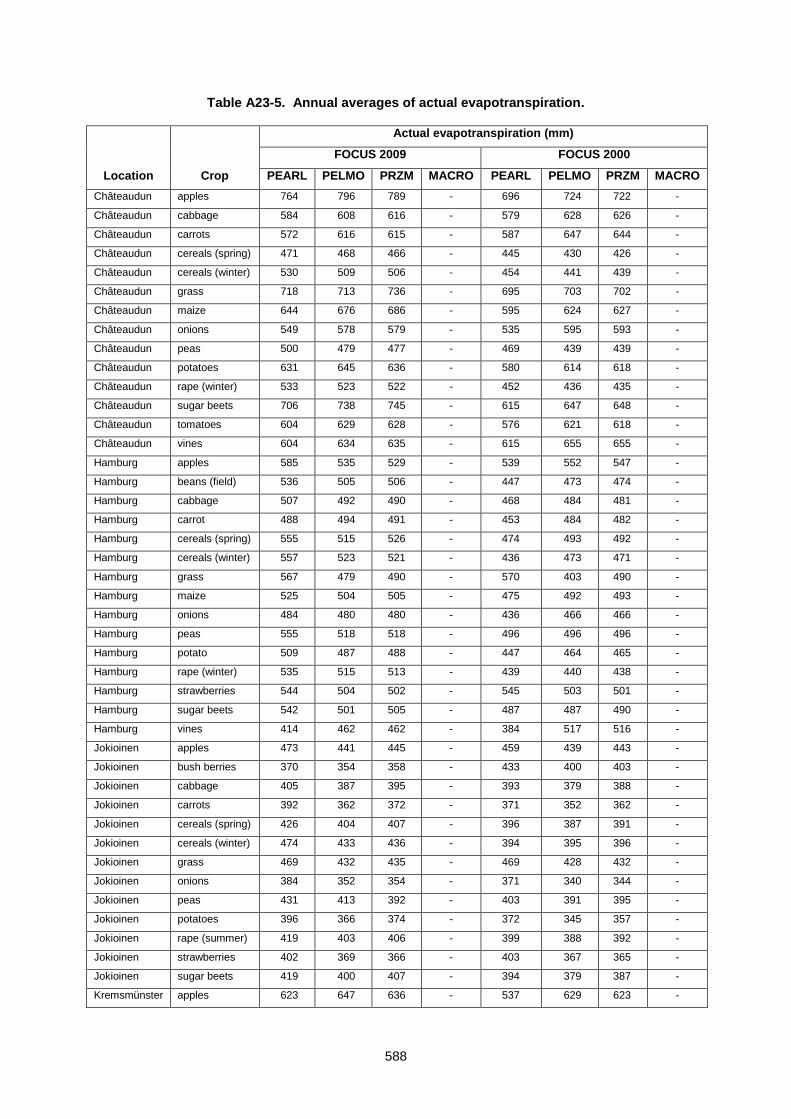
588
Table A23-5. Annual averages of actual evapotranspiration.
Location Crop
Actual evapotranspiration (mm)
FOCUS 2009 FOCUS 2000
PEARL PELMO PRZM MACRO PEARL PELMO PRZM MACRO
Châteaudun apples 764 796 789 - 696 724 722 -
Châteaudun cabbage 584 608 616 - 579 628 626 -
Châteaudun carrots 572 616 615 - 587 647 644 -
Châteaudun cereals (spring) 471 468 466 - 445 430 426 -
Châteaudun cereals (winter) 530 509 506 - 454 441 439 -
Châteaudun grass 718 713 736 - 695 703 702 -
Châteaudun maize 644 676 686 - 595 624 627 -
Châteaudun onions 549 578 579 - 535 595 593 -
Châteaudun peas 500 479 477 - 469 439 439 -
Châteaudun potatoes 631 645 636 - 580 614 618 -
Châteaudun rape (winter) 533 523 522 - 452 436 435 -
Châteaudun sugar beets 706 738 745 - 615 647 648 -
Châteaudun tomatoes 604 629 628 - 576 621 618 -
Châteaudun vines 604 634 635 - 615 655 655 -
Hamburg apples 585 535 529 - 539 552 547 -
Hamburg beans (field) 536 505 506 - 447 473 474 -
Hamburg cabbage 507 492 490 - 468 484 481 -
Hamburg carrot 488 494 491 - 453 484 482 -
Hamburg cereals (spring) 555 515 526 - 474 493 492 -
Hamburg cereals (winter) 557 523 521 - 436 473 471 -
Hamburg grass 567 479 490 - 570 403 490 -
Hamburg maize 525 504 505 - 475 492 493 -
Hamburg onions 484 480 480 - 436 466 466 -
Hamburg peas 555 518 518 - 496 496 496 -
Hamburg potato 509 487 488 - 447 464 465 -
Hamburg rape (winter) 535 515 513 - 439 440 438 -
Hamburg strawberries 544 504 502 - 545 503 501 -
Hamburg sugar beets 542 501 505 - 487 487 490 -
Hamburg vines 414 462 462 - 384 517 516 -
Jokioinen apples 473 441 445 - 459 439 443 -
Jokioinen bush berries 370 354 358 - 433 400 403 -
Jokioinen cabbage 405 387 395 - 393 379 388 -
Jokioinen carrots 392 362 372 - 371 352 362 -
Jokioinen cereals (spring) 426 404 407 - 396 387 391 -
Jokioinen cereals (winter) 474 433 436 - 394 395 396 -
Jokioinen grass 469 432 435 - 469 428 432 -
Jokioinen onions 384 352 354 - 371 340 344 -
Jokioinen peas 431 413 392 - 403 391 395 -
Jokioinen potatoes 396 366 374 - 372 345 357 -
Jokioinen rape (summer) 419 403 406 - 399 388 392 -
Jokioinen strawberries 402 369 366 - 403 367 365 -
Jokioinen sugar beets 419 400 407 - 394 379 387 -
Kremsmünster apples 623 647 636 - 537 629 623 -
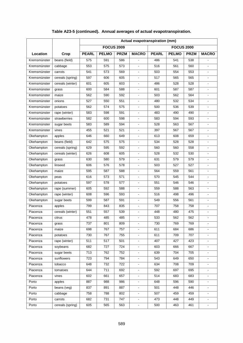
589
Table A23-5 (continued). Annual averages of actual evapotranspiration.
Location Crop
Actual evapotranspiration (mm)
FOCUS 2009 FOCUS 2000
PEARL PELMO PRZM MACRO PEARL PELMO PRZM MACRO
Kremsmünster beans (field) 575 591 586 - 486 541 538 -
Kremsmünster cabbage 553 575 573 - 516 561 560 -
Kremsmünster carrots 541 573 569 - 503 554 553 -
Kremsmünster cereals (spring) 597 606 605 - 517 565 565 -
Kremsmünster cereals (winter) 601 605 603 - 486 528 528 -
Kremsmünster grass 600 584 588 - 601 587 587 -
Kremsmünster maize 562 590 592 - 503 562 564 -
Kremsmünster onions 527 550 551 - 480 532 534 -
Kremsmünster potatoes 562 574 575 - 500 536 539 -
Kremsmünster rape (winter) 583 598 591 - 483 490 490 -
Kremsmünster strawberries 582 600 598 - 583 594 593 -
Kremsmünster sugar beets 583 589 594 - 528 563 567 -
Kremsmünster vines 455 521 521 - 397 567 567 -
Okehampton apples 646 660 649 - 613 608 659 -
Okehampton beans (field) 642 575 575 - 534 528 528 -
Okehampton cereals (spring) 629 595 592 - 560 560 558 -
Okehampton cereals (winter) 626 608 605 - 528 532 530 -
Okehampton grass 630 580 579 - 631 579 579 -
Okehampton linseed 606 576 578 - 503 527 527 -
Okehampton maize 595 587 588 - 564 559 561 -
Okehampton peas 616 573 571 - 570 545 544 -
Okehampton potatoes 597 578 577 - 551 546 546 -
Okehampton rape (summer) 605 592 588 - 559 588 563 -
Okehampton rape (winter) 608 596 593 - 516 498 496 -
Okehampton sugar beets 599 587 591 - 549 556 561 -
Piacenza apples 799 843 835 - 707 758 758 -
Piacenza cereals (winter) 551 557 539 - 448 480 475 -
Piacenza citrus 478 485 485 - 533 562 562 -
Piacenza grass 737 801 809 - 730 769 769 -
Piacenza maize 698 767 757 - 611 684 686 -
Piacenza potatoes 730 767 755 - 611 709 707 -
Piacenza rape (winter) 511 517 501 - 407 427 423 -
Piacenza soybeans 682 727 724 - 603 666 667 -
Piacenza sugar beets 713 762 752 - 639 704 705 -
Piacenza sunflowers 723 794 784 - 543 649 650 -
Piacenza tobacco 648 732 722 - 634 708 709 -
Piacenza tomatoes 644 711 692 - 592 697 695 -
Piacenza vines 602 661 657 - 514 683 683 -
Porto apples 887 988 986 - 648 596 590 -
Porto beans (veg) 837 891 887 - 501 448 446 -
Porto cabbage 758 788 802 - 507 459 459 -
Porto carrots 682 731 747 - 473 448 449 -
Porto cereals (spring) 605 565 563 - 500 463 461 -
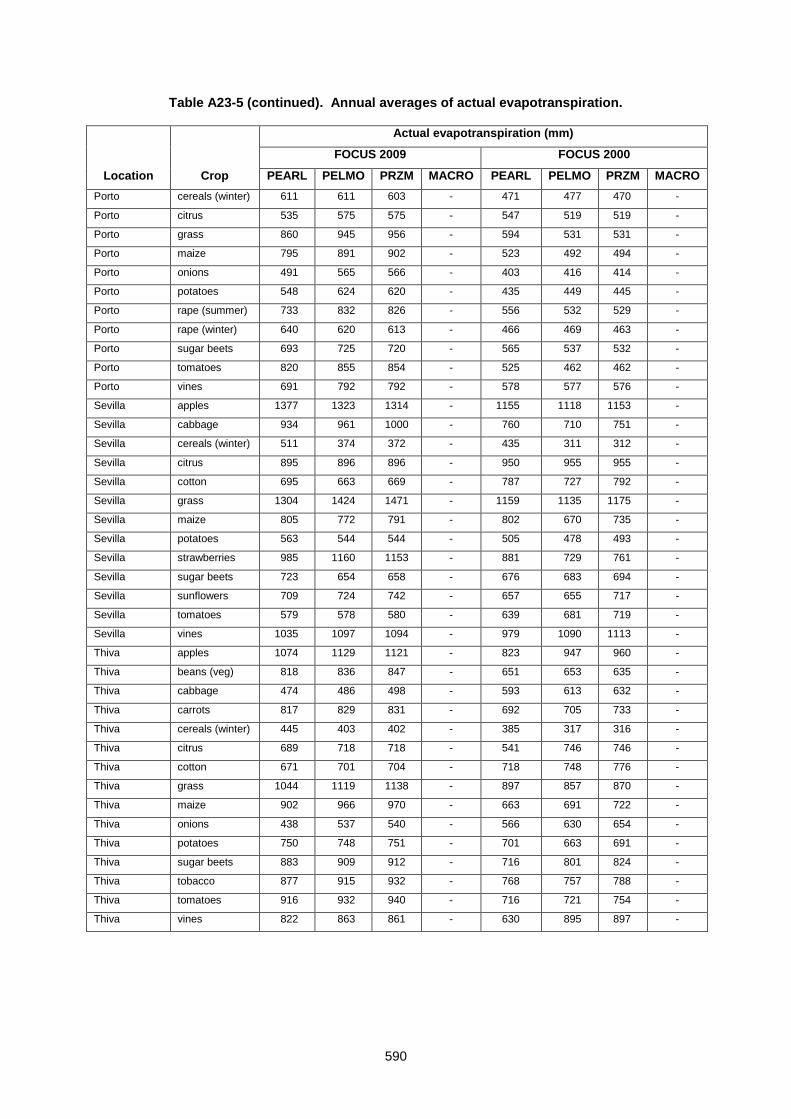
590
Table A23-5 (continued). Annual averages of actual evapotranspiration.
Location Crop
Actual evapotranspiration (mm)
FOCUS 2009 FOCUS 2000
PEARL PELMO PRZM MACRO PEARL PELMO PRZM MACRO
Porto cereals (winter) 611 611 603 - 471 477 470 -
Porto citrus 535 575 575 - 547 519 519 -
Porto grass 860 945 956 - 594 531 531 -
Porto maize 795 891 902 - 523 492 494 -
Porto onions 491 565 566 - 403 416 414 -
Porto potatoes 548 624 620 - 435 449 445 -
Porto rape (summer) 733 832 826 - 556 532 529 -
Porto rape (winter) 640 620 613 - 466 469 463 -
Porto sugar beets 693 725 720 - 565 537 532 -
Porto tomatoes 820 855 854 - 525 462 462 -
Porto vines 691 792 792 - 578 577 576 -
Sevilla apples 1377 1323 1314 - 1155 1118 1153 -
Sevilla cabbage 934 961 1000 - 760 710 751 -
Sevilla cereals (winter) 511 374 372 - 435 311 312 -
Sevilla citrus 895 896 896 - 950 955 955 -
Sevilla cotton 695 663 669 - 787 727 792 -
Sevilla grass 1304 1424 1471 - 1159 1135 1175 -
Sevilla maize 805 772 791 - 802 670 735 -
Sevilla potatoes 563 544 544 - 505 478 493 -
Sevilla strawberries 985 1160 1153 - 881 729 761 -
Sevilla sugar beets 723 654 658 - 676 683 694 -
Sevilla sunflowers 709 724 742 - 657 655 717 -
Sevilla tomatoes 579 578 580 - 639 681 719 -
Sevilla vines 1035 1097 1094 - 979 1090 1113 -
Thiva apples 1074 1129 1121 - 823 947 960 -
Thiva beans (veg) 818 836 847 - 651 653 635 -
Thiva cabbage 474 486 498 - 593 613 632 -
Thiva carrots 817 829 831 - 692 705 733 -
Thiva cereals (winter) 445 403 402 - 385 317 316 -
Thiva citrus 689 718 718 - 541 746 746 -
Thiva cotton 671 701 704 - 718 748 776 -
Thiva grass 1044 1119 1138 - 897 857 870 -
Thiva maize 902 966 970 - 663 691 722 -
Thiva onions 438 537 540 - 566 630 654 -
Thiva potatoes 750 748 751 - 701 663 691 -
Thiva sugar beets 883 909 912 - 716 801 824 -
Thiva tobacco 877 915 932 - 768 757 788 -
Thiva tomatoes 916 932 940 - 716 721 754 -
Thiva vines 822 863 861 - 630 895 897 -
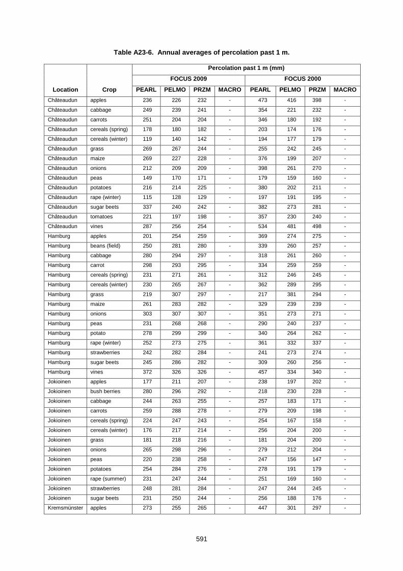
591
Table A23-6. Annual averages of percolation past 1 m.
Location Crop
Percolation past 1 m (mm)
FOCUS 2009 FOCUS 2000
PEARL PELMO PRZM MACRO PEARL PELMO PRZM MACRO
Châteaudun apples 236 226 232 - 473 416 398 -
Châteaudun cabbage 249 239 241 - 354 221 232 -
Châteaudun carrots 251 204 204 - 346 180 192 -
Châteaudun cereals (spring) 178 180 182 - 203 174 176 -
Châteaudun cereals (winter) 119 140 142 - 194 177 179 -
Châteaudun grass 269 267 244 - 255 242 245 -
Châteaudun maize 269 227 228 - 376 199 207 -
Châteaudun onions 212 209 209 - 398 261 270 -
Châteaudun peas 149 170 171 - 179 159 160 -
Châteaudun potatoes 216 214 225 - 380 202 211 -
Châteaudun rape (winter) 115 128 129 - 197 191 195 -
Châteaudun sugar beets 337 240 242 - 382 273 281 -
Châteaudun tomatoes 221 197 198 - 357 230 240 -
Châteaudun vines 287 256 254 - 534 481 498 -
Hamburg apples 201 254 259 - 369 274 275 -
Hamburg beans (field) 250 281 280 - 339 260 257 -
Hamburg cabbage 280 294 297 - 318 261 260 -
Hamburg carrot 298 293 295 - 334 259 259 -
Hamburg cereals (spring) 231 271 261 - 312 246 245 -
Hamburg cereals (winter) 230 265 267 - 362 289 295 -
Hamburg grass 219 307 297 - 217 381 294 -
Hamburg maize 261 283 282 - 329 239 239 -
Hamburg onions 303 307 307 - 351 273 271 -
Hamburg peas 231 268 268 - 290 240 237 -
Hamburg potato 278 299 299 - 340 264 262 -
Hamburg rape (winter) 252 273 275 - 361 332 337 -
Hamburg strawberries 242 282 284 - 241 273 274 -
Hamburg sugar beets 245 286 282 - 309 260 256 -
Hamburg vines 372 326 326 - 457 334 340 -
Jokioinen apples 177 211 207 - 238 197 202 -
Jokioinen bush berries 280 296 292 - 218 230 228 -
Jokioinen cabbage 244 263 255 - 257 183 171 -
Jokioinen carrots 259 288 278 - 279 209 198 -
Jokioinen cereals (spring) 224 247 243 - 254 167 158 -
Jokioinen cereals (winter) 176 217 214 - 256 204 200 -
Jokioinen grass 181 218 216 - 181 204 200 -
Jokioinen onions 265 298 296 - 279 212 204 -
Jokioinen peas 220 238 258 - 247 156 147 -
Jokioinen potatoes 254 284 276 - 278 191 179 -
Jokioinen rape (summer) 231 247 244 - 251 169 160 -
Jokioinen strawberries 248 281 284 - 247 244 245 -
Jokioinen sugar beets 231 250 244 - 256 188 176 -
Kremsmünster apples 273 255 265 - 447 301 297 -

592
Table A23-6 (continued). Annual averages of percolation past 1 m.
Location Crop
Percolation past 1 m (mm)
FOCUS 2009 FOCUS 2000
PEARL PELMO PRZM MACRO PEARL PELMO PRZM MACRO
Kremsmünster beans (field) 320 308 313 - 409 214 220 -
Kremsmünster cabbage 342 325 327 - 381 226 227 -
Kremsmünster carrots 354 327 330 - 393 222 224 -
Kremsmünster cereals (spring) 299 294 294 - 379 213 214 -
Kremsmünster cereals (winter) 295 296 297 - 419 272 282 -
Kremsmünster grass 295 316 312 - 298 293 293 -
Kremsmünster maize 333 310 308 - 406 168 172 -
Kremsmünster onions 369 350 348 - 415 244 243 -
Kremsmünster potatoes 333 325 324 - 396 193 194 -
Kremsmünster rape (winter) 313 303 309 - 423 324 333 -
Kremsmünster strawberries 313 299 301 - 316 243 246 -
Kremsmünster sugar beets 313 311 306 - 378 230 228 -
Kremsmünster vines 436 381 379 - 518 398 407 -
Okehampton apples 392 380 390 - 516 407 397 -
Okehampton beans (field) 396 463 463 - 504 357 358 -
Okehampton cereals (spring) 410 443 446 - 478 327 331 -
Okehampton cereals (winter) 412 430 433 - 510 417 422 -
Okehampton grass 408 458 459 - 407 442 442 -
Okehampton linseed 432 462 460 - 535 376 376 -
Okehampton maize 442 451 450 - 475 287 289 -
Okehampton peas 422 465 467 - 468 328 330 -
Okehampton potatoes 440 460 461 - 487 301 305 -
Okehampton rape (summer) 433 446 449 - 478 298 327 -
Okehampton rape (winter) 429 442 445 - 521 472 476 -
Okehampton sugar beets 439 451 446 - 489 350 346 -
Piacenza apples 214 464 472 - 672 498 499 -
Piacenza cereals (winter) 307 301 319 - 410 325 331 -
Piacenza citrus 442 614 651 - 809 690 698 -
Piacenza grass 337 514 506 - 496 456 457 -
Piacenza maize 346 490 501 - 611 468 476 -
Piacenza potatoes 349 425 441 - 627 450 462 -
Piacenza rape (winter) 346 341 357 - 450 394 399 -
Piacenza soybeans 393 471 482 - 620 465 481 -
Piacenza sugar beets 312 389 401 - 610 478 484 -
Piacenza sunflowers 310 467 482 - 679 488 498 -
Piacenza tobacco 368 484 497 - 589 420 433 -
Piacenza tomatoes 321 381 402 - 593 400 412 -
Piacenza vines 352 488 491 - 801 591 600 -
Porto apples 631 674 674 - 541 525 543 -
Porto beans (veg) 604 674 681 - 604 421 417 -
Porto cabbage 651 761 760 - 598 476 475 -
Porto carrots 650 719 718 - 628 453 451 -
Porto cereals (spring) 525 585 587 - 604 417 413 -
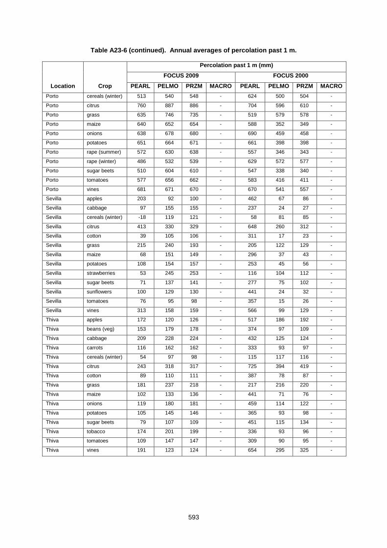
593
Table A23-6 (continued). Annual averages of percolation past 1 m.
Location Crop
Percolation past 1 m (mm)
FOCUS 2009 FOCUS 2000
PEARL PELMO PRZM MACRO PEARL PELMO PRZM MACRO
Porto cereals (winter) 513 540 548 - 624 500 504 -
Porto citrus 760 887 886 - 704 596 610 -
Porto grass 635 746 735 - 519 579 578 -
Porto maize 640 652 654 - 588 352 349 -
Porto onions 638 678 680 - 690 459 458 -
Porto potatoes 651 664 671 - 661 398 398 -
Porto rape (summer) 572 630 638 - 557 346 343 -
Porto rape (winter) 486 532 539 - 629 572 577 -
Porto sugar beets 510 604 610 - 547 338 340 -
Porto tomatoes 577 656 662 - 583 416 411 -
Porto vines 681 671 670 - 670 541 557 -
Sevilla apples 203 92 100 - 462 67 86 -
Sevilla cabbage 97 155 155 - 237 24 27 -
Sevilla cereals (winter) -18 119 121 - 58 81 85 -
Sevilla citrus 413 330 329 - 648 260 312 -
Sevilla cotton 39 105 106 - 311 17 23 -
Sevilla grass 215 240 193 - 205 122 129 -
Sevilla maize 68 151 149 - 296 37 43 -
Sevilla potatoes 108 154 157 - 253 45 56 -
Sevilla strawberries 53 245 253 - 116 104 112 -
Sevilla sugar beets 71 137 141 - 277 75 102 -
Sevilla sunflowers 100 129 130 - 441 24 32 -
Sevilla tomatoes 76 95 98 - 357 15 26 -
Sevilla vines 313 158 159 - 566 99 129 -
Thiva apples 172 120 126 - 517 186 192 -
Thiva beans (veg) 153 179 178 - 374 97 109 -
Thiva cabbage 209 228 224 - 432 125 124 -
Thiva carrots 116 162 162 - 333 93 97 -
Thiva cereals (winter) 54 97 98 - 115 117 116 -
Thiva citrus 243 318 317 - 725 394 419 -
Thiva cotton 89 110 111 - 387 78 87 -
Thiva grass 181 237 218 - 217 216 220 -
Thiva maize 102 133 136 - 441 71 76 -
Thiva onions 119 180 181 - 459 114 122 -
Thiva potatoes 105 145 146 - 365 93 98 -
Thiva sugar beets 79 107 109 - 451 115 134 -
Thiva tobacco 174 201 199 - 336 93 96 -
Thiva tomatoes 109 147 147 - 309 90 95 -
Thiva vines 191 123 124 - 654 295 325 -
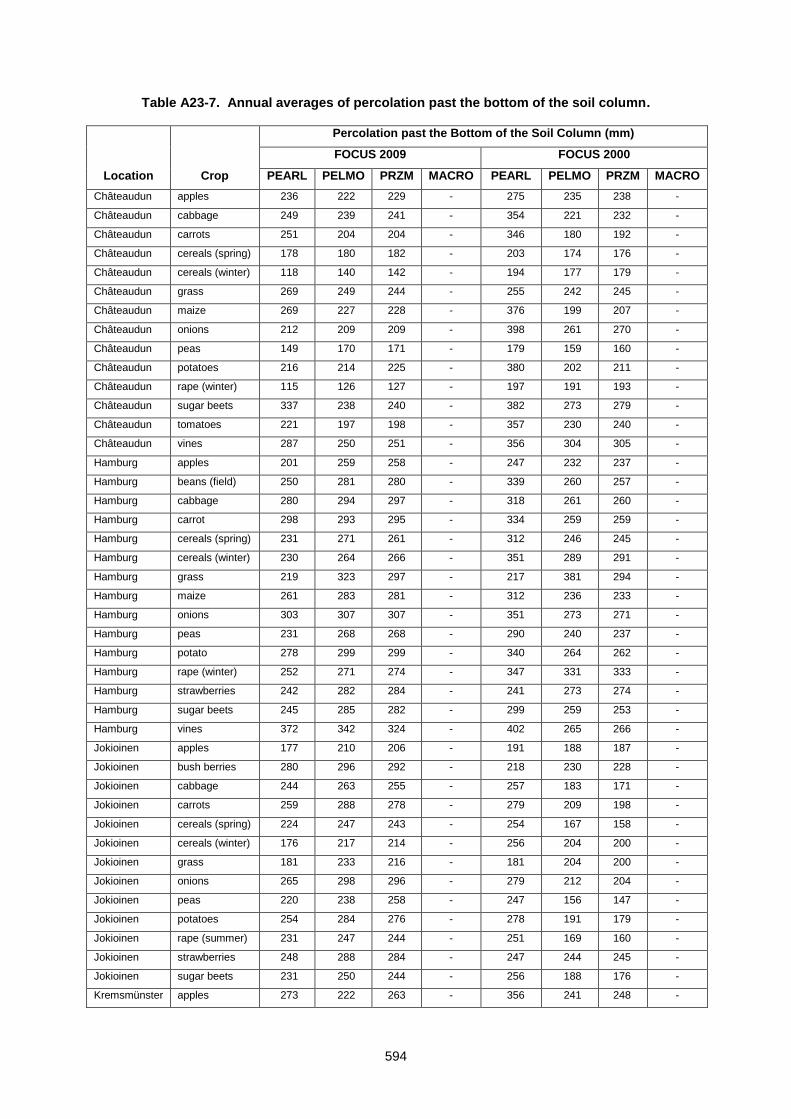
594
Table A23-7. Annual averages of percolation past the bottom of the soil column.
Location Crop
Percolation past the Bottom of the Soil Column (mm)
FOCUS 2009 FOCUS 2000
PEARL PELMO PRZM MACRO PEARL PELMO PRZM MACRO
Châteaudun apples 236 222 229 - 275 235 238 -
Châteaudun cabbage 249 239 241 - 354 221 232 -
Châteaudun carrots 251 204 204 - 346 180 192 -
Châteaudun cereals (spring) 178 180 182 - 203 174 176 -
Châteaudun cereals (winter) 118 140 142 - 194 177 179 -
Châteaudun grass 269 249 244 - 255 242 245 -
Châteaudun maize 269 227 228 - 376 199 207 -
Châteaudun onions 212 209 209 - 398 261 270 -
Châteaudun peas 149 170 171 - 179 159 160 -
Châteaudun potatoes 216 214 225 - 380 202 211 -
Châteaudun rape (winter) 115 126 127 - 197 191 193 -
Châteaudun sugar beets 337 238 240 - 382 273 279 -
Châteaudun tomatoes 221 197 198 - 357 230 240 -
Châteaudun vines 287 250 251 - 356 304 305 -
Hamburg apples 201 259 258 - 247 232 237 -
Hamburg beans (field) 250 281 280 - 339 260 257 -
Hamburg cabbage 280 294 297 - 318 261 260 -
Hamburg carrot 298 293 295 - 334 259 259 -
Hamburg cereals (spring) 231 271 261 - 312 246 245 -
Hamburg cereals (winter) 230 264 266 - 351 289 291 -
Hamburg grass 219 323 297 - 217 381 294 -
Hamburg maize 261 283 281 - 312 236 233 -
Hamburg onions 303 307 307 - 351 273 271 -
Hamburg peas 231 268 268 - 290 240 237 -
Hamburg potato 278 299 299 - 340 264 262 -
Hamburg rape (winter) 252 271 274 - 347 331 333 -
Hamburg strawberries 242 282 284 - 241 273 274 -
Hamburg sugar beets 245 285 282 - 299 259 253 -
Hamburg vines 372 342 324 - 402 265 266 -
Jokioinen apples 177 210 206 - 191 188 187 -
Jokioinen bush berries 280 296 292 - 218 230 228 -
Jokioinen cabbage 244 263 255 - 257 183 171 -
Jokioinen carrots 259 288 278 - 279 209 198 -
Jokioinen cereals (spring) 224 247 243 - 254 167 158 -
Jokioinen cereals (winter) 176 217 214 - 256 204 200 -
Jokioinen grass 181 233 216 - 181 204 200 -
Jokioinen onions 265 298 296 - 279 212 204 -
Jokioinen peas 220 238 258 - 247 156 147 -
Jokioinen potatoes 254 284 276 - 278 191 179 -
Jokioinen rape (summer) 231 247 244 - 251 169 160 -
Jokioinen strawberries 248 288 284 - 247 244 245 -
Jokioinen sugar beets 231 250 244 - 256 188 176 -
Kremsmünster apples 273 222 263 - 356 241 248 -
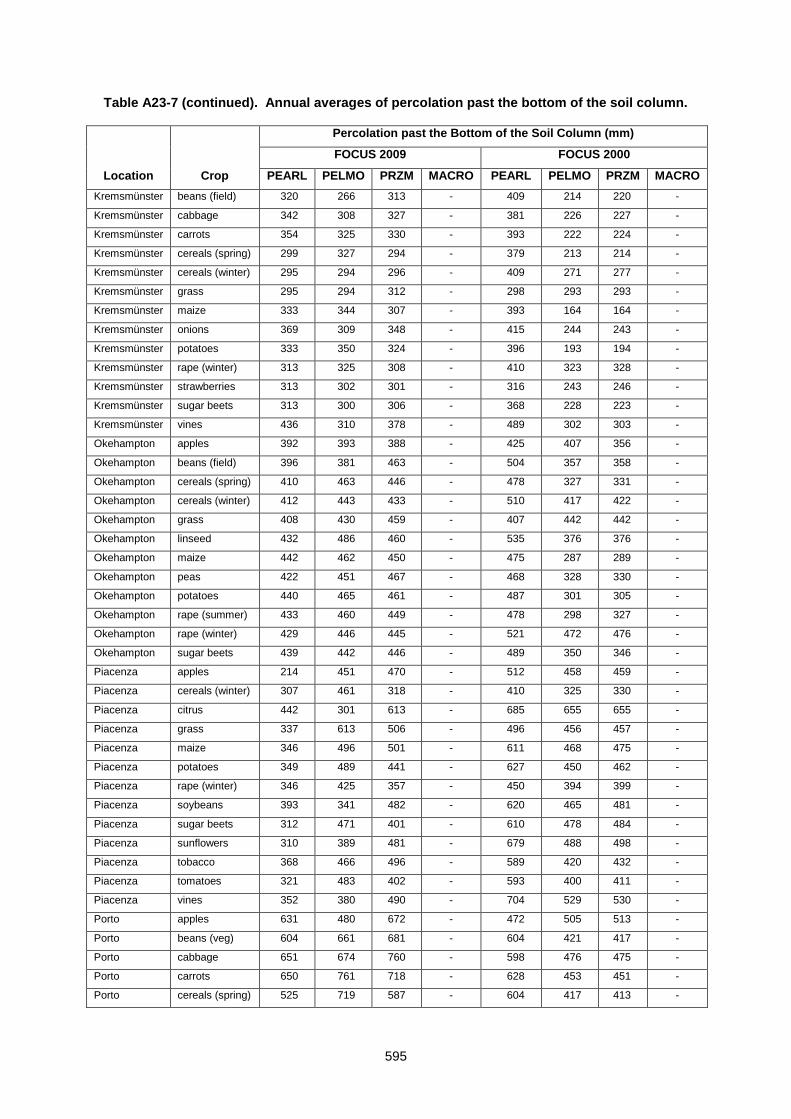
595
Table A23-7 (continued). Annual averages of percolation past the bottom of the soil column.
Location Crop
Percolation past the Bottom of the Soil Column (mm)
FOCUS 2009 FOCUS 2000
PEARL PELMO PRZM MACRO PEARL PELMO PRZM MACRO
Kremsmünster beans (field) 320 266 313 - 409 214 220 -
Kremsmünster cabbage 342 308 327 - 381 226 227 -
Kremsmünster carrots 354 325 330 - 393 222 224 -
Kremsmünster cereals (spring) 299 327 294 - 379 213 214 -
Kremsmünster cereals (winter) 295 294 296 - 409 271 277 -
Kremsmünster grass 295 294 312 - 298 293 293 -
Kremsmünster maize 333 344 307 - 393 164 164 -
Kremsmünster onions 369 309 348 - 415 244 243 -
Kremsmünster potatoes 333 350 324 - 396 193 194 -
Kremsmünster rape (winter) 313 325 308 - 410 323 328 -
Kremsmünster strawberries 313 302 301 - 316 243 246 -
Kremsmünster sugar beets 313 300 306 - 368 228 223 -
Kremsmünster vines 436 310 378 - 489 302 303 -
Okehampton apples 392 393 388 - 425 407 356 -
Okehampton beans (field) 396 381 463 - 504 357 358 -
Okehampton cereals (spring) 410 463 446 - 478 327 331 -
Okehampton cereals (winter) 412 443 433 - 510 417 422 -
Okehampton grass 408 430 459 - 407 442 442 -
Okehampton linseed 432 486 460 - 535 376 376 -
Okehampton maize 442 462 450 - 475 287 289 -
Okehampton peas 422 451 467 - 468 328 330 -
Okehampton potatoes 440 465 461 - 487 301 305 -
Okehampton rape (summer) 433 460 449 - 478 298 327 -
Okehampton rape (winter) 429 446 445 - 521 472 476 -
Okehampton sugar beets 439 442 446 - 489 350 346 -
Piacenza apples 214 451 470 - 512 458 459 -
Piacenza cereals (winter) 307 461 318 - 410 325 330 -
Piacenza citrus 442 301 613 - 685 655 655 -
Piacenza grass 337 613 506 - 496 456 457 -
Piacenza maize 346 496 501 - 611 468 475 -
Piacenza potatoes 349 489 441 - 627 450 462 -
Piacenza rape (winter) 346 425 357 - 450 394 399 -
Piacenza soybeans 393 341 482 - 620 465 481 -
Piacenza sugar beets 312 471 401 - 610 478 484 -
Piacenza sunflowers 310 389 481 - 679 488 498 -
Piacenza tobacco 368 466 496 - 589 420 432 -
Piacenza tomatoes 321 483 402 - 593 400 411 -
Piacenza vines 352 380 490 - 704 529 530 -
Porto apples 631 480 672 - 472 505 513 -
Porto beans (veg) 604 661 681 - 604 421 417 -
Porto cabbage 651 674 760 - 598 476 475 -
Porto carrots 650 761 718 - 628 453 451 -
Porto cereals (spring) 525 719 587 - 604 417 413 -
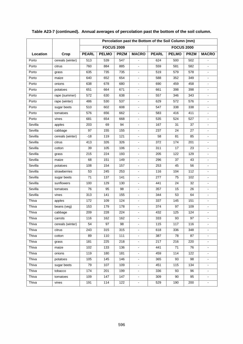
596
Table A23-7 (continued). Annual averages of percolation past the bottom of the soil column.
Location Crop
Percolation past the Bottom of the Soil Column (mm)
FOCUS 2009 FOCUS 2000
PEARL PELMO PRZM MACRO PEARL PELMO PRZM MACRO
Porto cereals (winter) 513 539 547 - 624 500 502 -
Porto citrus 760 884 885 - 559 581 582 -
Porto grass 635 735 735 - 519 579 578 -
Porto maize 640 652 654 - 588 352 349 -
Porto onions 638 678 680 - 690 459 458 -
Porto potatoes 651 664 671 - 661 398 398 -
Porto rape (summer) 572 630 638 - 557 346 343 -
Porto rape (winter) 486 530 537 - 629 572 576 -
Porto sugar beets 510 602 608 - 547 338 338 -
Porto tomatoes 576 656 662 - 583 416 411 -
Porto vines 681 654 668 - 535 524 527 -
Sevilla apples 203 69 94 - 167 31 37 -
Sevilla cabbage 97 155 155 - 237 24 27 -
Sevilla cereals (winter) -18 119 121 - 58 81 85 -
Sevilla citrus 413 326 326 - 372 174 201 -
Sevilla cotton 39 105 106 - 311 17 23 -
Sevilla grass 215 224 193 - 205 122 129 -
Sevilla maize 68 151 149 - 296 37 43 -
Sevilla potatoes 108 154 157 - 253 45 56 -
Sevilla strawberries 53 245 253 - 116 104 112 -
Sevilla sugar beets 71 137 141 - 277 75 102 -
Sevilla sunflowers 100 129 130 - 441 24 32 -
Sevilla tomatoes 76 95 98 - 357 15 26 -
Sevilla vines 313 141 155 - 344 53 64 -
Thiva apples 172 109 124 - 337 145 151 -
Thiva beans (veg) 153 179 178 - 374 97 109 -
Thiva cabbage 209 228 224 - 432 125 124 -
Thiva carrots 116 162 162 - 333 93 97 -
Thiva cereals (winter) 54 97 98 - 115 117 116 -
Thiva citrus 243 315 315 - 618 336 348 -
Thiva cotton 89 110 111 - 387 78 87 -
Thiva grass 181 225 218 - 217 216 220 -
Thiva maize 102 133 136 - 441 71 76 -
Thiva onions 119 180 181 - 459 114 122 -
Thiva potatoes 105 145 146 - 365 93 98 -
Thiva sugar beets 79 107 109 - 451 115 134 -
Thiva tobacco 174 201 199 - 336 93 96 -
Thiva tomatoes 109 147 147 - 309 90 95 -
Thiva vines 191 114 122 - 529 190 200 -
597
APPENDIX 24. REVIEW OF PROCEDURE FOR ESTIMATING INTERCEPTION OF PESTICIDE BY PLANTS
FOCUS (2000) decided to estimate interception of pesticide application by the plant canopy
using experimental measurements available in the literature. At that time the PESTLA model
(recommended for use by FOCUS 2000) did not contain a routine for estimating crop
interception. The PEARL model has superseded PESTLA and can estimate interception
automatically. All the models recommended by FOCUS for estimating ground water
concentrations can now estimate interception; so the work group reviewed whether the Tier I
recommendations should be changed to allow them to do so.
Current Method of Estimating Interception.
Look up tables are used to estimate the amount of interception of pesticide by the crop
canopy during application. These tables give percentage interception for various growth
stages of major crops. The appropriate growth stage during application is selected, and the
amount of pesticide reaching the soil surface during application is calculated by:
(1 - %interception/100)*application rate.
The data in the lookup tables were derived from experimental measurements. Crops for
which there were no data had interception estimated by the GLEAMS model on the basis of
Leaf Area Index (LAI). The FOCUS Groundwater Scenarios Workgroup used conservative
estimates of interception, i.e. using values for earlier growth stages where a range was
specified and using values towards the lower end of the measured range. Interception was
never allowed to exceed 90%.
Estimation of Interception by FOCUS Models.
All of the FOCUS models (MACRO, PEARL, PELMO, PRZM) can estimate crop growth by
assuming that growth is linear between certain crop growth stages. PELMO and PRZM
assume that interception is zero at emergence, maximum at maturity and varies linearly in-
between. Interception stays at the maximum value between maturity and harvest,
interception is expressed as a percentage interception of applied spray.
MACRO and PEARL have more detailed crop growth models. Both models calculate
interception on the basis of leaf area index (LAI) rather than percentage interception of the
application. MACRO requires the input of the LAI at emergence (generally a very low
598
number), at maximum LAI and at harvest; a day number for each event is also required. The
LAI on any particular day D between emergence and maximum LAI is given by:
x
DD
DDLAILAILAILAI
minmax
min
minmaxmin
where x is an exponent specified by the user. The above equation shows that LAI varies
according to the interval between maximum and minimum LAI in a similar way to how
interception is calculated between emergence and maturity in PELMO, except the exponent
is rarely 1.0 (for spring cereals in the Châteaudun scenario it is 2.0) meaning that LAI does
not vary linearly with time. MACRO uses a similar routine to calculate the decrease in LAI
between maturity and harvest due to senescence.
PEARL calculates LAI on the basis of development stage. Development can be simulated in
two ways: either input directly by the user as a function of time (with linear interpolation
between time points) or dependent upon a temperature sum. The fraction of interception of
pesticide is dependent upon the LAI, interception is assumed to be LAI/3 with a maximum of
100%.
Within FOCUS, models have been harmonised for emergence, maturity (max LAI) and
harvest dates for all crops in all scenarios. Figure A24-1 shows how FOCUS-PELMO and
FOCUS-PEARL would calculate crop growth stage for spring cereals in Germany. The
length of the growing season was taken from the FOCUS Hamburg scenario, growth stage
BBCH 9 was assumed to represent emergence, growth stage 90 to represent harvest. The
model estimates of growth stage are compared to typical values for oats and spring barley
measured over the period 1962-1996 at the Berlin-Dahlem experimental station
(Chemielewski, 2003).
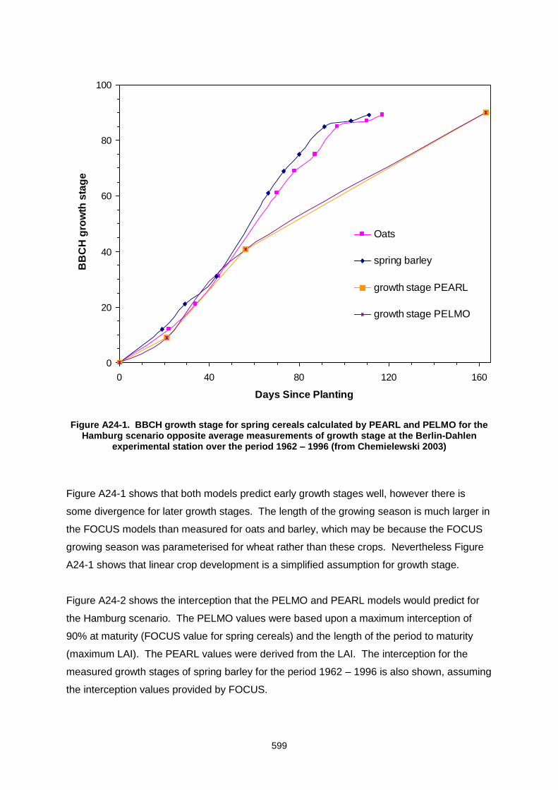
599
0
20
40
60
80
100
0 40 80 120 160
Days Since Planting
BB
CH
gro
wth
sta
ge
Oats
spring barley
growth stage PEARL
growth stage PELMO
Figure A24-1. BBCH growth stage for spring cereals calculated by PEARL and PELMO for the Hamburg scenario opposite average measurements of growth stage at the Berlin-Dahlen
experimental station over the period 1962 – 1996 (from Chemielewski 2003)
Figure A24-1 shows that both models predict early growth stages well, however there is
some divergence for later growth stages. The length of the growing season is much larger in
the FOCUS models than measured for oats and barley, which may be because the FOCUS
growing season was parameterised for wheat rather than these crops. Nevertheless Figure
A24-1 shows that linear crop development is a simplified assumption for growth stage.
Figure A24-2 shows the interception that the PELMO and PEARL models would predict for
the Hamburg scenario. The PELMO values were based upon a maximum interception of
90% at maturity (FOCUS value for spring cereals) and the length of the period to maturity
(maximum LAI). The PEARL values were derived from the LAI. The interception for the
measured growth stages of spring barley for the period 1962 – 1996 is also shown, assuming
the interception values provided by FOCUS.
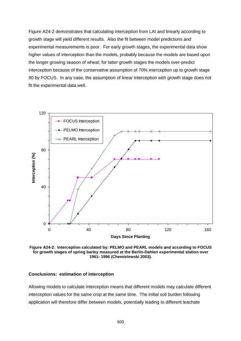
600
Figure A24-2 demonstrates that calculating interception from LAI and linearly according to
growth stage will yield different results. Also the fit between model predictions and
experimental measurements is poor. For early growth stages, the experimental data show
higher values of interception than the models, probably because the models are based upon
the longer growing season of wheat; for latter growth stages the models over-predict
interception because of the conservative assumption of 70% interception up to growth stage
90 by FOCUS. In any case, the assumption of linear interception with growth stage does not
fit the experimental data well.
0
40
80
120
0 40 80 120 160
Days Since Planting
Inte
rce
pti
on
(%
)
FOCUS Interception
PELMO Interception
PEARL Interception
Figure A24-2. Interception calculated by: PELMO and PEARL models and according to FOCUS for growth stages of spring barley measured at the Berlin-Dahlen experimental station over
1961- 1996 (Chemielewski 2003).
Conclusions: estimation of interception
Allowing models to calculate interception means that different models may calculate different
interception values for the same crop at the same time. The initial soil burden following
application will therefore differ between models, potentially leading to different leachate
601
concentrations. Note that in this comparison between PEARL and PELMO the same
maturity dates were used, and linear crop development was assumed for both models.
The models calculate interception in different ways: PEARL uses a time-dependent
specification based upon LAI; PELMO assumes that interception is linear with time according
to growth stage; MACRO uses a function to calculate interception based upon LAI that may
vary from crop to crop. Considerable effort would therefore be required to harmonise
interception in these models for all crops and for all scenarios.
The models did not reproduce the interception derived from experimental data well. This was
in part because they assume they use the length of the growing season from a different crop
and in part because of conservative assumptions used by FOCUS. The length of the
growing season will differ between different crops within the same general group (e.g. such
as cereals), so a large amount of extra work would be required to adequately model
interception with all of the FOCUS models.
The FOCUS Groundwater Scenarios Workgroup spent considerable effort determining crop
interception from experimental measurements available in the literature, and were
conservative in their assumptions. Basing interception according to growth stage from
experimental measurements is a simple way of harmonising the initial burden to the soil and
is independent of the length of the growing season. Models can only approximate these
measurements by using simplified assumptions or by inputting the experimental data directly.
Allowing models to calculate interception therefore presents no benefits either in terms of
accuracy or consistency. As stated in FOCUS (2000): “For reasons of consistency, simplicity
and accuracy, FOCUS recommend that the internal interception routines in all models are
disabled and the application rate is manually corrected for interception”.
Therefore, the work group proposed that no changes be made to the current method of
estimating interception.

602
References
Chemielewski F.M. 2003. Phenology and Agriculture, Agrarmeteorologishe Schriften, Heft
12, Landwirtsschaftlich-Gärtnerische Fakultät, Insitut für Pfanzenbauwissenschaften,
Humboldt-Universität zu Berlin.
FOCUS. 2000. FOCUS groundwater scenarios in the EU review of active substances.
Report of the FOCUS Groundwater Scenarios Workgroup, EC Document Reference
Sanco/321/2000 rev.2, 202pp.
603
APPENDIX 25. COMPARISON OF DIFFERENT OBJECT FUNCTIONS FOR THE EVALUATION OF KINETIC SORPTION EXPERIMENTS
C. Kley and K. Hammel
In general, four variables are available from time-dependant sorption studies, which can be
fitted to evaluate kinetic sorption parameters: Mt, Cl des, Seq, Sneq.
This leads to five meaningful combinations which could be used as an object function:
Mt - Cl des, Mt - Seq, Mt - Sneq, Cl des - Sneq, Seq - Sneq
There should be no difference between the fits to the different object functions with respect to
reliability and uncertainty of parameters. Thus, slight deviations of estimated parameters and
coefficients of variation should be coincidental.
However, fits to different object functions can be comparable only under the assumption that
the parameters are mathematically reliable, i.e. significantly different from 0 (t-test). In less
stable experimental systems, with low χ2 errors and low significance, the estimated
parameters may differ significantly between the different fit approaches.
To examine this hypothesis of equivalence, a numerical experiment was carried out, to
compare the results of the main approaches used to date, the Mtotal - Cl des and the Seq - Sneq
object functions.
A kinetic parameter set was chosen corresponding to the example case in Appendix 6 to
represent the “true” time curves of Seq, Sneq, Mtotal and Cl des. To introduce statistical error into
these variables, the kinetic parameters were defined as random variables with a known
distribution. For this purpose fne was defined as normal distributed random variable, with
mean = 0.6 and standard deviation = 0.06. 13 data sets were created randomly from 104
Latin Hypercube samples (8 time points per curve) of the fne distribution, using MatLab
(2007). Thus every data set of eight Seq, Sneq, Mtotal and Cl des values was generated with eight
different fne . For simplicity the remaining parameters have been fixed at their mean value.
These 13 data sets are presented in Table A25-1.
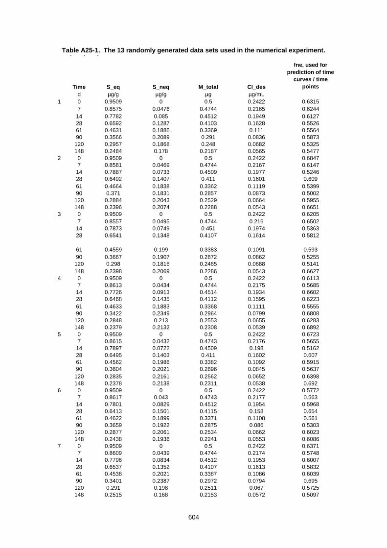
604
Table A25-1. The 13 randomly generated data sets used in the numerical experiment. created random data sets
Time S_eq S_neq M_total Cl_des
fne, used for
prediction of time
curves / time
points
d µg/g µg/g µg µg/mL
1 0 0.9509 0 0.5 0.2422 0.6315
7 0.8575 0.0476 0.4744 0.2165 0.6244
14 0.7782 0.085 0.4512 0.1949 0.6127
28 0.6592 0.1287 0.4103 0.1628 0.5526
61 0.4631 0.1886 0.3369 0.111 0.5564
90 0.3566 0.2089 0.291 0.0836 0.5873
120 0.2957 0.1868 0.248 0.0682 0.5325
148 0.2484 0.178 0.2187 0.0565 0.5477
2 0 0.9509 0 0.5 0.2422 0.6847
7 0.8581 0.0469 0.4744 0.2167 0.6147
14 0.7887 0.0733 0.4509 0.1977 0.5246
28 0.6492 0.1407 0.411 0.1601 0.609
61 0.4664 0.1838 0.3362 0.1119 0.5399
90 0.371 0.1831 0.2857 0.0873 0.5002
120 0.2884 0.2043 0.2529 0.0664 0.5955
148 0.2396 0.2074 0.2288 0.0543 0.6651
3 0 0.9509 0 0.5 0.2422 0.6205
7 0.8557 0.0495 0.4744 0.216 0.6502
14 0.7873 0.0749 0.451 0.1974 0.5363
28 0.6541 0.1348 0.4107 0.1614 0.5812
61 0.4559 0.199 0.3383 0.1091 0.593
90 0.3667 0.1907 0.2872 0.0862 0.5255
120 0.298 0.1816 0.2465 0.0688 0.5141
148 0.2398 0.2069 0.2286 0.0543 0.6627
4 0 0.9509 0 0.5 0.2422 0.6113
7 0.8613 0.0434 0.4744 0.2175 0.5685
14 0.7726 0.0913 0.4514 0.1934 0.6602
28 0.6468 0.1435 0.4112 0.1595 0.6223
61 0.4633 0.1883 0.3368 0.1111 0.5555
90 0.3422 0.2349 0.2964 0.0799 0.6808
120 0.2848 0.213 0.2553 0.0655 0.6283
148 0.2379 0.2132 0.2308 0.0539 0.6892
5 0 0.9509 0 0.5 0.2422 0.6723
7 0.8615 0.0432 0.4743 0.2176 0.5655
14 0.7897 0.0722 0.4509 0.198 0.5162
28 0.6495 0.1403 0.411 0.1602 0.607
61 0.4562 0.1986 0.3382 0.1092 0.5915
90 0.3604 0.2021 0.2896 0.0845 0.5637
120 0.2835 0.2161 0.2562 0.0652 0.6398
148 0.2378 0.2138 0.2311 0.0538 0.692
6 0 0.9509 0 0.5 0.2422 0.5772
7 0.8617 0.043 0.4743 0.2177 0.563
14 0.7801 0.0829 0.4512 0.1954 0.5968
28 0.6413 0.1501 0.4115 0.158 0.654
61 0.4622 0.1899 0.3371 0.1108 0.561
90 0.3659 0.1922 0.2875 0.086 0.5303
120 0.2877 0.2061 0.2534 0.0662 0.6023
148 0.2438 0.1936 0.2241 0.0553 0.6086
7 0 0.9509 0 0.5 0.2422 0.6371
7 0.8609 0.0439 0.4744 0.2174 0.5748
14 0.7796 0.0834 0.4512 0.1953 0.6007
28 0.6537 0.1352 0.4107 0.1613 0.5832
61 0.4538 0.2021 0.3387 0.1086 0.6039
90 0.3401 0.2387 0.2972 0.0794 0.695
120 0.291 0.198 0.2511 0.067 0.5725
148 0.2515 0.168 0.2153 0.0572 0.5097
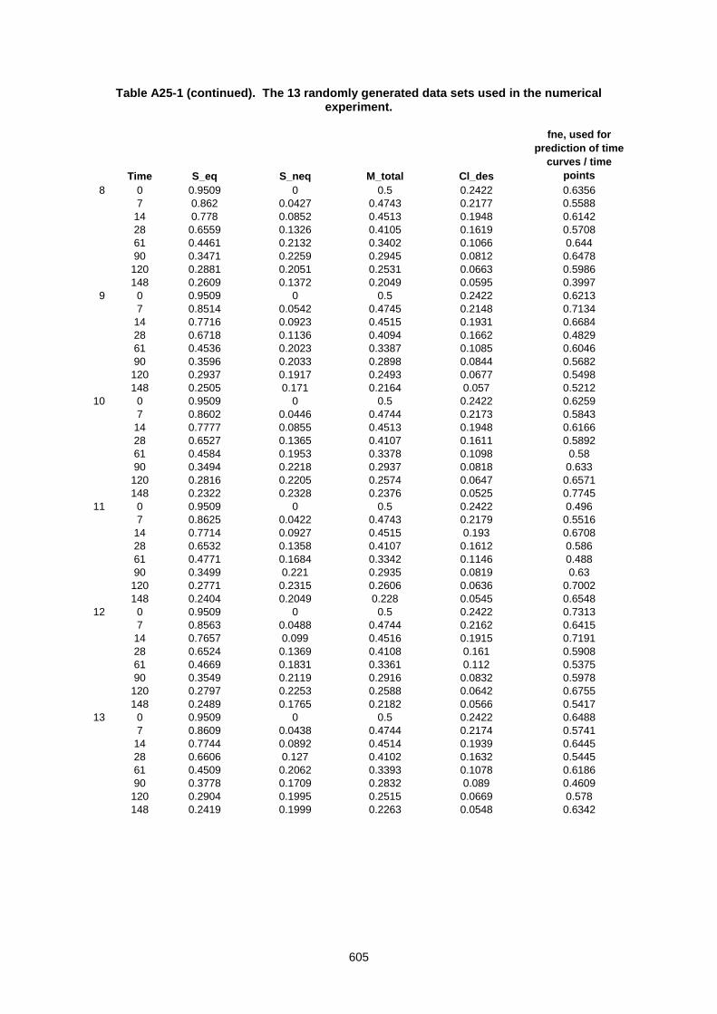
605
Table A25-1 (continued). The 13 randomly generated data sets used in the numerical experiment.
created random data sets
Time S_eq S_neq M_total Cl_des
fne, used for
prediction of time
curves / time
points
8 0 0.9509 0 0.5 0.2422 0.6356
7 0.862 0.0427 0.4743 0.2177 0.5588
14 0.778 0.0852 0.4513 0.1948 0.6142
28 0.6559 0.1326 0.4105 0.1619 0.5708
61 0.4461 0.2132 0.3402 0.1066 0.644
90 0.3471 0.2259 0.2945 0.0812 0.6478
120 0.2881 0.2051 0.2531 0.0663 0.5986
148 0.2609 0.1372 0.2049 0.0595 0.3997
9 0 0.9509 0 0.5 0.2422 0.6213
7 0.8514 0.0542 0.4745 0.2148 0.7134
14 0.7716 0.0923 0.4515 0.1931 0.6684
28 0.6718 0.1136 0.4094 0.1662 0.4829
61 0.4536 0.2023 0.3387 0.1085 0.6046
90 0.3596 0.2033 0.2898 0.0844 0.5682
120 0.2937 0.1917 0.2493 0.0677 0.5498
148 0.2505 0.171 0.2164 0.057 0.5212
10 0 0.9509 0 0.5 0.2422 0.6259
7 0.8602 0.0446 0.4744 0.2173 0.5843
14 0.7777 0.0855 0.4513 0.1948 0.6166
28 0.6527 0.1365 0.4107 0.1611 0.5892
61 0.4584 0.1953 0.3378 0.1098 0.58
90 0.3494 0.2218 0.2937 0.0818 0.633
120 0.2816 0.2205 0.2574 0.0647 0.6571
148 0.2322 0.2328 0.2376 0.0525 0.7745
11 0 0.9509 0 0.5 0.2422 0.496
7 0.8625 0.0422 0.4743 0.2179 0.5516
14 0.7714 0.0927 0.4515 0.193 0.6708
28 0.6532 0.1358 0.4107 0.1612 0.586
61 0.4771 0.1684 0.3342 0.1146 0.488
90 0.3499 0.221 0.2935 0.0819 0.63
120 0.2771 0.2315 0.2606 0.0636 0.7002
148 0.2404 0.2049 0.228 0.0545 0.6548
12 0 0.9509 0 0.5 0.2422 0.7313
7 0.8563 0.0488 0.4744 0.2162 0.6415
14 0.7657 0.099 0.4516 0.1915 0.7191
28 0.6524 0.1369 0.4108 0.161 0.5908
61 0.4669 0.1831 0.3361 0.112 0.5375
90 0.3549 0.2119 0.2916 0.0832 0.5978
120 0.2797 0.2253 0.2588 0.0642 0.6755
148 0.2489 0.1765 0.2182 0.0566 0.5417
13 0 0.9509 0 0.5 0.2422 0.6488
7 0.8609 0.0438 0.4744 0.2174 0.5741
14 0.7744 0.0892 0.4514 0.1939 0.6445
28 0.6606 0.127 0.4102 0.1632 0.5445
61 0.4509 0.2062 0.3393 0.1078 0.6186
90 0.3778 0.1709 0.2832 0.089 0.4609
120 0.2904 0.1995 0.2515 0.0669 0.578
148 0.2419 0.1999 0.2263 0.0548 0.6342
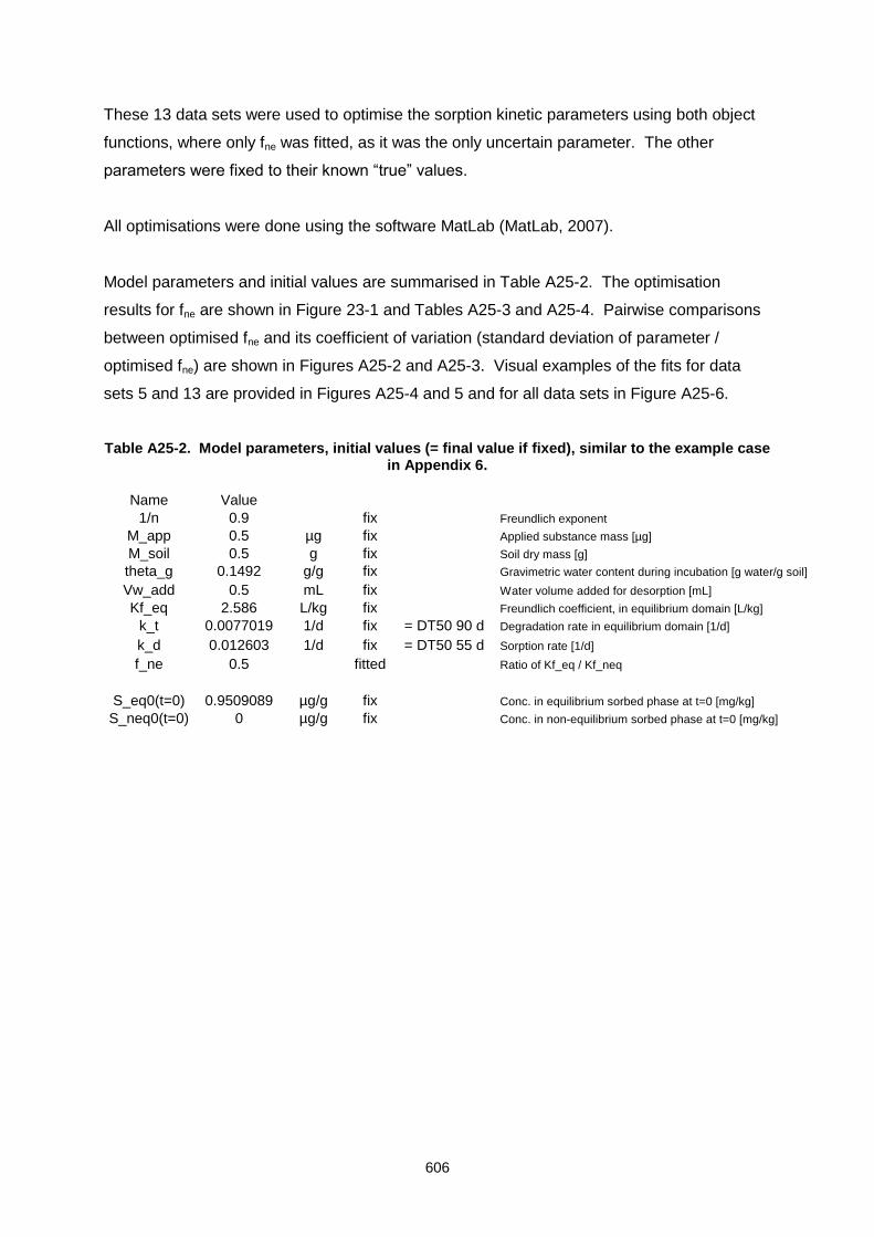
606
These 13 data sets were used to optimise the sorption kinetic parameters using both object
functions, where only fne was fitted, as it was the only uncertain parameter. The other
parameters were fixed to their known “true” values.
All optimisations were done using the software MatLab (MatLab, 2007).
Model parameters and initial values are summarised in Table A25-2. The optimisation
results for fne are shown in Figure 23-1 and Tables A25-3 and A25-4. Pairwise comparisons
between optimised fne and its coefficient of variation (standard deviation of parameter /
optimised fne) are shown in Figures A25-2 and A25-3. Visual examples of the fits for data
sets 5 and 13 are provided in Figures A25-4 and 5 and for all data sets in Figure A25-6.
Table A25-2. Model parameters, initial values (= final value if fixed), similar to the example case in Appendix 6.
Name Value
1/n 0.9 fix Freundlich exponent
M_app 0.5 µg fix Applied substance mass [µg]
M_soil 0.5 g fix Soil dry mass [g]
theta_g 0.1492 g/g fix Gravimetric water content during incubation [g water/g soil]
Vw_add 0.5 mL fix Water volume added for desorption [mL]
Kf_eq 2.586 L/kg fix Freundlich coefficient, in equilibrium domain [L/kg]
k_t 0.0077019 1/d fix = DT50 90 d Degradation rate in equilibrium domain [1/d]
k_d 0.012603 1/d fix = DT50 55 d Sorption rate [1/d]
f_ne 0.5 fitted Ratio of Kf_eq / Kf_neq
S_eq0(t=0) 0.9509089 µg/g fix Conc. in equilibrium sorbed phase at t=0 [mg/kg]
S_neq0(t=0) 0 µg/g fix Conc. in non-equilibrium sorbed phase at t=0 [mg/kg]
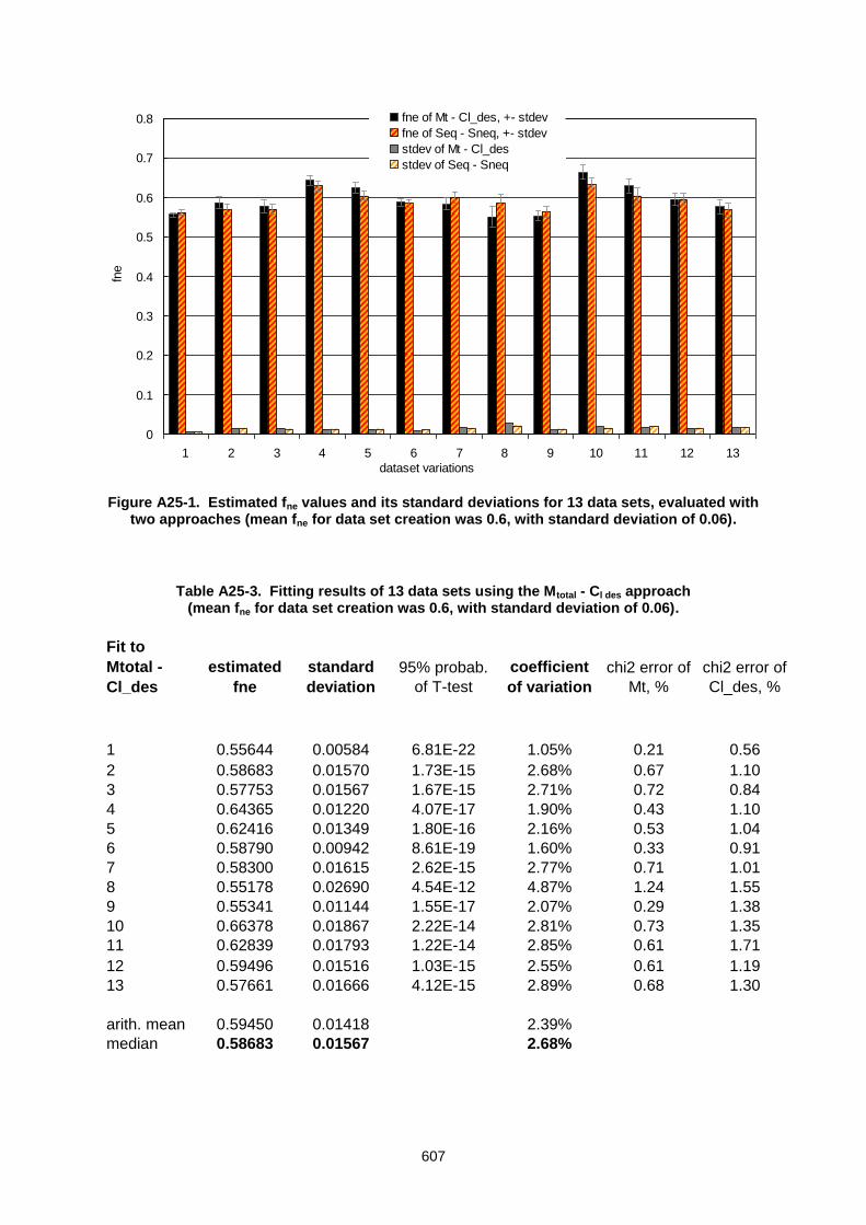
607
0
0.1
0.2
0.3
0.4
0.5
0.6
0.7
0.8
1 2 3 4 5 6 7 8 9 10 11 12 13
dataset variations
fne
fne of Mt - Cl_des, +- stdev
fne of Seq - Sneq, +- stdev
stdev of Mt - Cl_des
stdev of Seq - Sneq
Figure A25-1. Estimated fne values and its standard deviations for 13 data sets, evaluated with two approaches (mean fne for data set creation was 0.6, with standard deviation of 0.06).
Table A25-3. Fitting results of 13 data sets using the Mtotal - Cl des approach (mean fne for data set creation was 0.6, with standard deviation of 0.06).
Fit to
Mtotal -
Cl_des
estimated
fne
standard
deviation
95% probab.
of T-test
coefficient
of variation
chi2 error of
Mt, %
chi2 error of
Cl_des, %
1 0.55644 0.00584 6.81E-22 1.05% 0.21 0.56
2 0.58683 0.01570 1.73E-15 2.68% 0.67 1.10
3 0.57753 0.01567 1.67E-15 2.71% 0.72 0.84
4 0.64365 0.01220 4.07E-17 1.90% 0.43 1.10
5 0.62416 0.01349 1.80E-16 2.16% 0.53 1.04
6 0.58790 0.00942 8.61E-19 1.60% 0.33 0.91
7 0.58300 0.01615 2.62E-15 2.77% 0.71 1.01
8 0.55178 0.02690 4.54E-12 4.87% 1.24 1.55
9 0.55341 0.01144 1.55E-17 2.07% 0.29 1.38
10 0.66378 0.01867 2.22E-14 2.81% 0.73 1.35
11 0.62839 0.01793 1.22E-14 2.85% 0.61 1.71
12 0.59496 0.01516 1.03E-15 2.55% 0.61 1.19
13 0.57661 0.01666 4.12E-15 2.89% 0.68 1.30
arith. mean 0.59450 0.01418 2.39%
median 0.58683 0.01567 2.68%
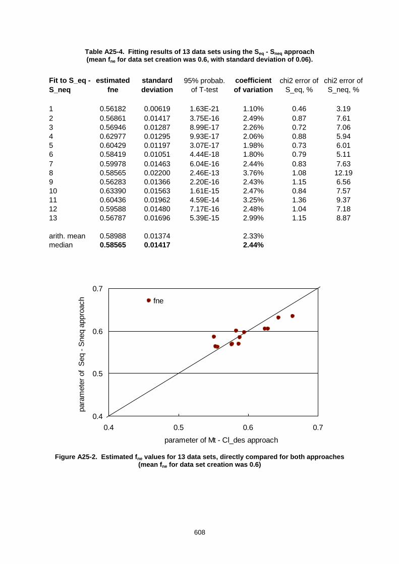
608
Table A25-4. Fitting results of 13 data sets using the Seq - Sneq approach (mean fne for data set creation was 0.6, with standard deviation of 0.06).
Fit to S_eq -
S_neq
estimated
fne
standard
deviation
95% probab.
of T-test
coefficient
of variation
chi2 error of
S_eq, %
chi2 error of
S_neq, %
1 0.56182 0.00619 1.63E-21 1.10% 0.46 3.19
2 0.56861 0.01417 3.75E-16 2.49% 0.87 7.61
3 0.56946 0.01287 8.99E-17 2.26% 0.72 7.06
4 0.62977 0.01295 9.93E-17 2.06% 0.88 5.94
5 0.60429 0.01197 3.07E-17 1.98% 0.73 6.01
6 0.58419 0.01051 4.44E-18 1.80% 0.79 5.11
7 0.59978 0.01463 6.04E-16 2.44% 0.83 7.63
8 0.58565 0.02200 2.46E-13 3.76% 1.08 12.19
9 0.56283 0.01366 2.20E-16 2.43% 1.15 6.56
10 0.63390 0.01563 1.61E-15 2.47% 0.84 7.57
11 0.60436 0.01962 4.59E-14 3.25% 1.36 9.37
12 0.59588 0.01480 7.17E-16 2.48% 1.04 7.18
13 0.56787 0.01696 5.39E-15 2.99% 1.15 8.87
arith. mean 0.58988 0.01374 2.33%
median 0.58565 0.01417 2.44%
0.4
0.5
0.6
0.7
0.4 0.5 0.6 0.7
parameter of Mt - Cl_des approach
para
mete
r of S
eq -
Sneq a
ppro
ach fne
Figure A25-2. Estimated fne values for 13 data sets, directly compared for both approaches (mean fne for data set creation was 0.6)
609
0
0.02
0.04
0.06
0.08
0.1
0 0.02 0.04 0.06 0.08 0.1
parameter of Mt - Cl_des approach
para
mete
r of S
eq -
Sneq a
ppro
ach
coeff. of variation of fne
Figure A25-3. Coefficients of variation of estimated fne values for 13 data sets, directly compared for both approaches (mean fne for data set creation was 0.6).
610
0 50 100 1500.2
0.3
0.4
0.5
Mtotal
Time [d]
Mto
tal [µ
g]
0 50 100 150-5
0
5
10x 10
-3 Residuals Mtotal
Time [d]
Mto
tal [µ
g]
0 50 100 1500.05
0.1
0.15
0.2
0.25
Cwdes
Time [d]
Cw
des
[µ
g/m
L]
0 50 100 150-2
0
2
4x 10
-3 Residuals Cwdes
Time [d]C
wdes [
µg/m
L]
0 50 100 1500.2
0.4
0.6
0.8
1
Csoil
eq
Time [d]
Csoil e
q [
µg/g
]
0 50 100 150-0.01
0
0.01
0.02
Residuals Csoil
eq
Time [d]
Csoil e
q [
µg/g
]
0 50 100 1500
0.1
0.2
0.3
0.4
Csoil
neq
Time [d]
Csoil n
eq [
µg/g
]
0 50 100 150-0.02
0
0.02
0.04
Residuals Csoil
neq
Time [d]
Csoil n
eq
[µg/g
]
Figure A25-4. Visual fits of both approaches for data set 5.
Mt Cl des
Cl d
es [
μg
/mL
]
Mt [
μg
/mL
]
Mt [
μg
/mL
]
Cl d
es [
μg
/mL
] C
l d
es [
μg
/mL
]
Seq Sneq
Se
q [
μg
/g]
Se
q [
μg
/g]
Sn
eq [
μg
/g]
Sn
eq [
μg
/g]
611
0 50 100 1500.2
0.3
0.4
0.5
Mtotal
Time [d]
Mto
tal [µ
g]
0 50 100 150-0.01
-0.005
0
0.005
0.01
Residuals Mtotal
Time [d]
Mto
tal [µ
g]
0 50 100 1500.05
0.1
0.15
0.2
0.25
Cwdes
Time [d]
Cw
des
[µ
g/m
L]
0 50 100 150-5
0
5x 10
-3 Residuals Cwdes
Time [d]C
wdes [
µg/m
L]
0 50 100 1500.2
0.4
0.6
0.8
1
Csoil
eq
Time [d]
Csoil e
q [
µg/g
]
0 50 100 150-0.01
0
0.01
0.02
Residuals Csoil
eq
Time [d]
Csoil e
q [
µg/g
]
0 50 100 1500
0.1
0.2
0.3
0.4
Csoil
neq
Time [d]
Csoil n
eq [
µg/g
]
0 50 100 150-0.04
-0.02
0
0.02
Residuals Csoil
neq
Time [d]
Csoil n
eq
[µg/g
]
Figure A25-5. Visual fits of both approaches for data set 13.
Mt Mt Mt Cl des
Cl d
es [
μg
/mL
] C
l d
es [
μg
/mL
]
Mt [
μg
/mL
]
Mt [
μg
/mL
]
Sneq Seq
Sn
eq [
μg
/g]
Sn
eq [
μg
/g]
Se
q [
μg
/g]
Se
q [
μg
/g]
612
0 50 100 1500.2
0.3
0.4
0.5
Mtotal
Time [d]
Mto
tal [µ
g]
0 50 100 150-0.02
-0.01
0
0.01
0.02
Residuals Mtotal
Time [d]
Mto
tal [µ
g]
0 50 100 1500.05
0.1
0.15
0.2
0.25
Cwdes
Time [d]
Cw
des
[µ
g/m
L]
0 50 100 150-5
0
5
10x 10
-3 Residuals Cwdes
Time [d]C
wdes [
µg/m
L]
0 50 100 1500.2
0.4
0.6
0.8
1
Csoil
eq
Time [d]
Csoil e
q [
µg/g
]
0 50 100 150-0.02
0
0.02
0.04
Residuals Csoil
eq
Time [d]
Csoil e
q [
µg/g
]
0 50 100 1500
0.1
0.2
0.3
0.4
Csoil
neq
Time [d]
Csoil n
eq [
µg/g
]
0 50 100 150-0.1
-0.05
0
0.05
0.1
Residuals Csoil
neq
Time [d]
Csoi
l neq
[µ
g/g
]
Figure A25-6. Visual fits of both approaches for all data sets.
Mt Mt Cl des
Se
q [
μg
/g]
Cl d
es [
μg
/mL
] C
l d
es [
μg
/mL
]
Mt [
μg
/mL
] M
t [μ
g/m
L]
Seq Sneq
Sn
eq [
μg
/g]
Se
q [
μg
/g]
Sn
eq [
μg
/g]
613
The compilation of the results provided in Tables A25-3 and A25-4 includes measures of the
goodness of fit (χ2 error). Obviously, the fit of Sneq results in higher χ2 errors than the fits to
the other variables, e.g. Seq. This can be explained as a combined, systematic effect of the
higher model error due to the higher sensitivity d Sneq /d fne compared to d Seq /d fne and the
lower mean Sneq compared to the mean Seq. Note, that χ2 is defined as the ratio between
model error and the mean observed.
Conclusions
Both object functions, Mtotal - Cl des and Seq - Sneq, produce on average the same parameter
estimates of 0.595 and 0.590, respectively which are very close to the “true value” of 0.6. No
systematic differences were observed, either for the estimated value of the parameter or for
its standard deviation. Thus the estimates of both approaches can be considered
independent. As a result both object functions are fully equivalent.
References
MatLab. 2007. MatLab Version 7.4.0.287 (R2007a), Optimisation Toolbox, Statistics
Toolbox, MatLab Compiler. The MathWorks Inc., USA. www.mathworks.com