Analyzing Producer Preferences for Counter-Cyclical Government Payments∗∗∗∗

J. Corey Miller

Barry J. Barnett Keith H. Coble∗∗∗∗∗∗∗∗

Selected Paper

2001 American Agricultural Economics Association Annual Meeting Chicago, Illinois August 5-8, 2001

Abstract: A dynamic-stochastic model is developed to evaluate preferences among alternative

counter-cyclical payment programs for representative farms producing corn and soybeans in Iowa and cotton and soybeans in Mississippi. These programs are found to not

necessarily be preferred to existing government programs.

Copyright © 2001 by J. Corey Miller, Barry J. Barnett, and Keith H. Coble. Readers may make verbatim copies of this document for non-commercial purposes by any means, provided that this

copyright notice appears on all such copies.

∗ The authors gratefully acknowledge helpful comments from David Orden, Department of Agricultural and Applied Economics, Virginia Tech. ∗∗ J. Corey Miller is a graduate research assistant in the Department of Agricultural and Applied Economics at Virginia Tech and a former graduate research assistant in the Department of Agricultural Economics at Mississippi State University. Barry J. Barnett is an associate professor in the Department of Agricultural and Applied Economics at the University of Georgia (effective 6/2001), and Keith H. Coble is an associate professor in the Department of Agricultural Economics at Mississippi State University. Contact author: Corey Miller, Department of Agricultural and Applied Economics, Virginia Tech, Blacksburg, VA 24061. E-mail: jamille5@vt.edu.

2

Analyzing Producer Preferences for Counter-Cyclical Government Payments

The Federal Agriculture Improvement and Reform (FAIR) Act of 1996 became law at a

time when farm commodity prices were at their highest level in twenty years. The decades old

system of price supports and deficiency payments was replaced with fixed production flexibility

contract (PFC) payments scheduled through 2002. These decoupled PFC payments were

designed to decline over the six-year life of the FAIR Act as a prelude to lower government

payment levels. Within two years, however, the high prices—which most observers believe

were a key to the passage of the FAIR Act—fell sharply, eventually plunging to levels not

anticipated by many advocates of the current farm law. Congress responded to the decline in

prices by approving four ad hoc emergency assistance packages between October 1998 and

October 2000, each providing billions of dollars in supplemental assistance.

Although the FAIR Act retains a substantial counter-cyclical component in the form of

the marketing loan program, which provides producers with loan deficiency payments (LDPs)

when national market prices fall below loan rates, the FAIR Act’s detractors contend that a

counter-cyclical alternative to PFC payments would be more desirable. These critics view the

inability of the fixed PFC payments to respond to changes in the farm economy as one of the

foremost weaknesses of the FAIR Act.

Most proposed counter-cyclical alternatives base outlays on a measure of shortfalls in

farm revenue. Rep. Charles Stenholm (D-Texas), the ranking member of the House Agriculture

Committee, introduced one of the first such programs in Congress in August of 1999. Known as

Supplemental Income Payments for Producers (SIPP), this program would have provided

producers with payments when the per-acre national gross revenue of an eligible crop is less than

95 percent of its previous five-year average (U.S. Congress, House 1999, H7884). SIPP defines

3

national gross revenue as the product of the total United States production for a commodity and

the higher of its season average price or loan rate. The total per-acre payment to producers for a

particular commodity would be equal to the positive difference between 95 percent of the

previous five-year moving average of national gross revenue per acre and the current crop year’s

national gross revenue per acre.

SIPP intended to provide producers with program payments during periods of low

market revenue. Although SIPP failed to win approval in Congress, similar counter-cyclical

payment programs are being discussed as potential components of the next farm bill scheduled

for 2002. Advocates of SIPP and other subsequent counter-cyclical proposals implicitly assume

producers prefer payments based on income variability to the fixed PFC payments of the FAIR

Act.

This paper provides an empirical evaluation of whether producers have a preference for

payments from a SIPP-type program relative to PFC payments. Our approach involves a

nonparametric bootstrapping model that simulates market-based farm revenue for representative

farms in Iowa and Mississippi over a five-year program period, 2000-2004. PFC payments,

LDPs, and possible SIPP-type payments are added to market revenue to determine income,

ending wealth, and producer welfare. Most studies that have modeled government payments

have ignored price-yield correlations and implicitly assumed risk neutrality on the part of

producers. Yet, Glauber and Miranda (1996) find that the varying results across numerous

studies about the effects of price stabilization programs on individual farm-level revenue

variability are due to the omission of production variability and/or correlation between yield and

price. Because systemic factors often cause crop losses to be widespread, many individual yields

tend to be positively correlated with aggregate yields and thereby negatively correlated with

4

price. This correlation creates a “natural hedge” that can provide a producer with protection

from changes in yield, as low (high) aggregate yields will be offset by high (low) prices. Price-

yield correlations are incorporated into the analysis reported herein, and provide a basis for

examining regional differences in policy preferences. Furthermore, producers in this study are

assumed to be slightly risk averse. The assumption of risk aversion is consistent with producers’

behavior reflected in the widespread purchase and use of instruments such as unsubsidized crop-

hail insurance, forward contracting, and futures and options.

The remainder of this paper consists of three sections. In the next section we outline our

dynamic-stochastic simulation model. We then present the results of this model for a

representative Iowa farm producing corn or soybeans and a representative Mississippi farm

producing cotton or soybeans. The results indicate that whether a producer benefits more from

the PFC payment program or a SIPP-type payment program depends on location, what crop or

crops are produced, the level at which fixed payments or counter-cyclical payment triggers are

set, and whether the current marketing loan program remains in place. We state our conclusions

in a final section of the paper, emphasizing the influence of price-yield correlations on our

results.

Model

The model developed to assess policy preferences builds on the models of Atwood,

Baquet, and Watts (1997) and Coble et al. (1999) that simulate revenue for the purposes of rating

an insurance contract. Atwood, Baquet, and Watts design a rating procedure for the Income

Protection (IP) product (a single-crop revenue insurance product), while the rating procedure

proposed by Coble et al. is for a revenue insurance product for multiple crops. In both cases,

rates are assessed using non-parametric bootstrapping procedures. Although the non-parametric

5

approach is less efficient if the underlying data distribution is known, it avoids making

distributional assumptions that could lead to biased and inconsistent estimates when distributions

are unknown. Coble et al. conclude the non-parametric approach is “a more robust estimator

capable of addressing a variety of empirical data.” In particular, a non-parametric distribution is

useful in combining multiple random variables, as for a farm facing multiple sources of risk.

Simulated Market Revenue

We assume farm-level market revenue variability is determined by two location-specific

random components: county yield and farm deviations from the county yield. Farm-level

market revenue variability is also dependent on the random component of national market prices,

which in turn is dependent on variability in national yields and other stochastic factors. Under

LDPs and counter-cyclical payment programs, national yields may also affect government

payment levels.

To estimate the random components of national and county yields, data from 1974

through 1999 from the National Agricultural Statistics Service (NASS) of the United States

Department of Agriculture (USDA) were used to fit a linear trend regression

(1) Yitiiit tY εαα ++= 10

where t is year, i is crop, and itY is national )( itit NY ≡ or county yield )( itj

it CY ≡ for a specific

location j. For each national or county regression, a matrix of residuals, Yε , with t rows and i

columns, is captured with the residuals expressed as a percentage of the predicted value. The

residuals are used to bootstrap around the predicted yield, itY . In each iteration of the model, the

simulated yields, itY~ , are calculated as

(2) ( ) jYtitit CNYtiYY ,,,1ˆ~ =∀+= ε .

6

Residuals are expressed in percentage terms to correct for any potential heteroskedasticity that

may be present in the raw yield data. To account for common events affecting yields, the

residuals for each crop are drawn for the same year by randomly selecting the kth row from the

matrix of residuals.

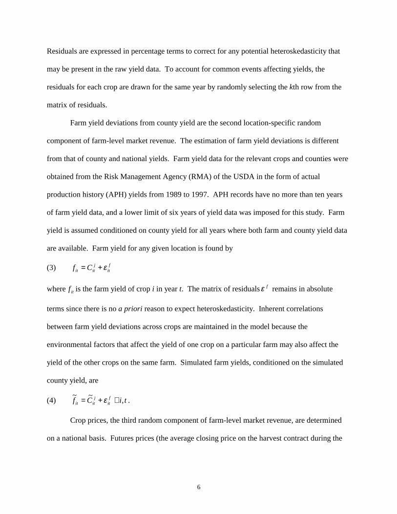
Farm yield deviations from county yield are the second location-specific random

component of farm-level market revenue. The estimation of farm yield deviations is different

from that of county and national yields. Farm yield data for the relevant crops and counties were

obtained from the Risk Management Agency (RMA) of the USDA in the form of actual

production history (APH) yields from 1989 to 1997. APH records have no more than ten years

of farm yield data, and a lower limit of six years of yield data was imposed for this study. Farm

yield is assumed conditioned on county yield for all years where both farm and county yield data

are available. Farm yield for any given location is found by

(3) fit

jitit Cf ε+=

where itf is the farm yield of crop i in year t. The matrix of residuals fε remains in absolute

terms since there is no a priori reason to expect heteroskedasticity. Inherent correlations

between farm yield deviations across crops are maintained in the model because the

environmental factors that affect the yield of one crop on a particular farm may also affect the

yield of the other crops on the same farm. Simulated farm yields, conditioned on the simulated

county yield, are

(4) tiCf fit

jitit ,~~ ∀+= ε .

Crop prices, the third random component of farm-level market revenue, are determined

on a national basis. Futures prices (the average closing price on the harvest contract during the

7

month prior to expiration) are used to approximate the market price that a producer would

receive at harvest.

Price determination in the simulation proceeds as follows. First, the prior year’s harvest

price becomes the predicted value for the current year’s futures price at planting:

(5) 01

1,0 P

ittiit PP ε+= −

where 0itP is the futures price at planting for crop i in year t, and 1

1, −tiP is the futures price of crop i

at harvest in t-1. The matrix of residuals0Pε consists of t rows and i columns with the residuals

expressed in percentage terms. By bootstrapping from0Pε the futures price at planting is

simulated as a random walk around 11, −tiP

(6) ( ) tiPP Pittiit ,1~ 01

1,0 ∀+= − ε .

These residuals are also drawn together so that each crop has residuals drawn from the same time

period. Futures prices at planting are estimated as the average closing price of the harvest

contract during the month of April. The harvest contracts for corn and cotton are based on the

month of December while the harvest contract for soybeans is based on November.

The price at harvest is assumed to be a function of the futures price at planting

conditioned on the ratio of simulated national yield to predicted national yield (Coble et al.,

Atwood, Baquet, and Watts). This price relationship is expressed by the equation

(7) Pit

it

itii

it

it

NN

PP εγγ +

+= ˆ

~100

1

where the residuals are captured in the t by i matrix Pitε . The predicted harvest price, conditioned

on the ratio of simulated national yield to predicted national yield, is

8

(8)

+=

it

itiiitit N

NPP ˆ

~ˆ

1001 γγ .

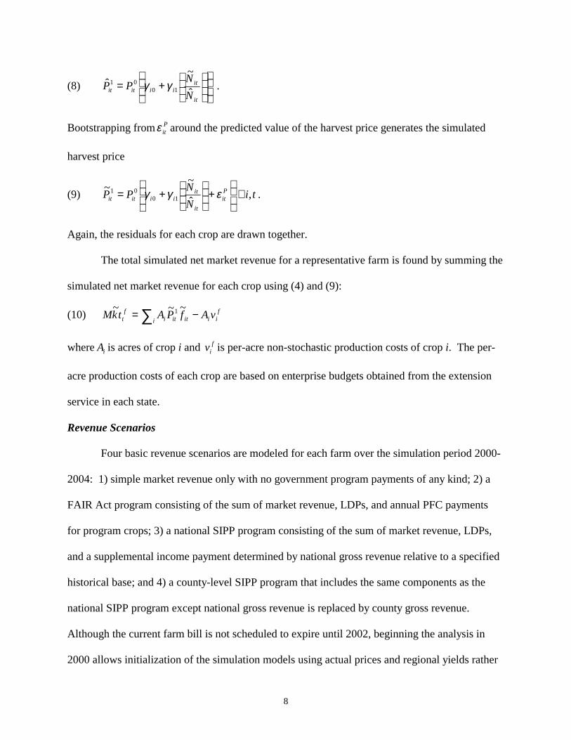
Bootstrapping from Pitε around the predicted value of the harvest price generates the simulated

harvest price

(9) tiNNPP P

itit

itiiitit ,ˆ

~~10

01 ∀

+

+= εγγ .

Again, the residuals for each crop are drawn together.

The total simulated net market revenue for a representative farm is found by summing the

simulated net market revenue for each crop using (4) and (9):

(10) fiiititi i

ft vAfPAtkM −= ∑ ~~~ 1

where iA is acres of crop i and fiv is per-acre non-stochastic production costs of crop i. The per-

acre production costs of each crop are based on enterprise budgets obtained from the extension

service in each state.

Revenue Scenarios

Four basic revenue scenarios are modeled for each farm over the simulation period 2000-

2004: 1) simple market revenue only with no government program payments of any kind; 2) a

FAIR Act program consisting of the sum of market revenue, LDPs, and annual PFC payments

for program crops; 3) a national SIPP program consisting of the sum of market revenue, LDPs,

and a supplemental income payment determined by national gross revenue relative to a specified

historical base; and 4) a county-level SIPP program that includes the same components as the

national SIPP program except national gross revenue is replaced by county gross revenue.

Although the current farm bill is not scheduled to expire until 2002, beginning the analysis in

2000 allows initialization of the simulation models using actual prices and regional yields rather

9

than estimates of these variables. Because LDPs provide some counter-cyclical protection under

the FAIR Act, and complement the counter-cyclical payments of SIPP-type programs, we also

consider scenarios in which the marketing loan program is eliminated while PFC and SIPP

payments are retained. We evaluate the impact of the alternative payment programs under two

fixed payment rates and two trigger levels for counter-cyclical payments.

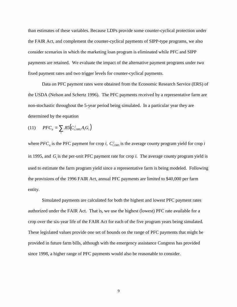
Data on PFC payment rates were obtained from the Economic Research Service (ERS) of

the USDA (Nelson and Schertz 1996). The PFC payments received by a representative farm are

non-stochastic throughout the 5-year period being simulated. In a particular year they are

determined by the equation

(11) ( )∑=i

iij

iit GACPFC 1995,85.

where itPFC is the PFC payment for crop i, jiC 1995, is the average county program yield for crop i

in 1995, and iG is the per-unit PFC payment rate for crop i. The average county program yield is

used to estimate the farm program yield since a representative farm is being modeled. Following

the provisions of the 1996 FAIR Act, annual PFC payments are limited to $40,000 per farm

entity.

Simulated payments are calculated for both the highest and lowest PFC payment rates

authorized under the FAIR Act. That is, we use the highest (lowest) PFC rate available for a

crop over the six-year life of the FAIR Act for each of the five program years being simulated.

These legislated values provide one set of bounds on the range of PFC payments that might be

provided in future farm bills, although with the emergency assistance Congress has provided

since 1998, a higher range of PFC payments would also be reasonable to consider.

10

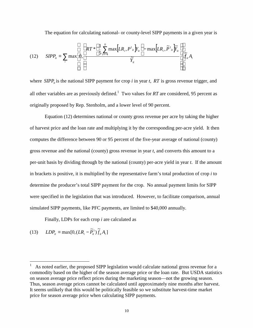
The equation for calculating national- or county-level SIPP payments in a given year is

(12) [ ] [ ]

iiti it

ititit

ititi

it AfY

YPLRYPLRRTSIPP ~

~

~~,max,max51*

,0max

10

4

1

∑∑

−

= −=

where itSIPP is the national SIPP payment for crop i in year t, RT is gross revenue trigger, and

all other variables are as previously defined.1 Two values for RT are considered, 95 percent as

originally proposed by Rep. Stenholm, and a lower level of 90 percent.

Equation (12) determines national or county gross revenue per acre by taking the higher

of harvest price and the loan rate and multiplying it by the corresponding per-acre yield. It then

computes the difference between 90 or 95 percent of the five-year average of national (county)

gross revenue and the national (county) gross revenue in year t, and converts this amount to a

per-unit basis by dividing through by the national (county) per-acre yield in year t. If the amount

in brackets is positive, it is multiplied by the representative farm’s total production of crop i to

determine the producer’s total SIPP payment for the crop. No annual payment limits for SIPP

were specified in the legislation that was introduced. However, to facilitate comparison, annual

simulated SIPP payments, like PFC payments, are limited to $40,000 annually.

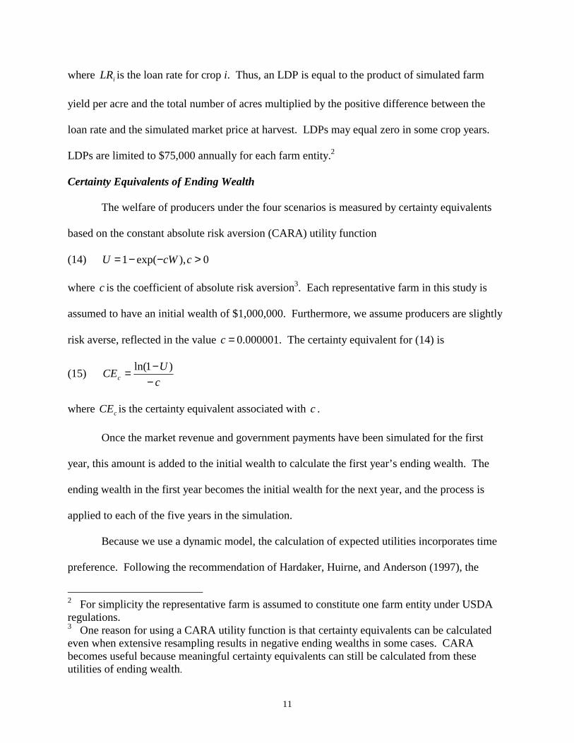
Finally, LDPs for each crop i are calculated as

(13) ]~)~(,0max[ 1iititiit AfPLRLDP −=

1 As noted earlier, the proposed SIPP legislation would calculate national gross revenue for a commodity based on the higher of the season average price or the loan rate. But USDA statistics on season average price reflect prices during the marketing season—not the growing season. Thus, season average prices cannot be calculated until approximately nine months after harvest. It seems unlikely that this would be politically feasible so we substitute harvest-time market price for season average price when calculating SIPP payments.

11

where iLR is the loan rate for crop i. Thus, an LDP is equal to the product of simulated farm

yield per acre and the total number of acres multiplied by the positive difference between the

loan rate and the simulated market price at harvest. LDPs may equal zero in some crop years.

LDPs are limited to $75,000 annually for each farm entity.2

Certainty Equivalents of Ending Wealth

The welfare of producers under the four scenarios is measured by certainty equivalents

based on the constant absolute risk aversion (CARA) utility function

(14) 0),exp(1 >−−= ccWU

where c is the coefficient of absolute risk aversion3. Each representative farm in this study is

assumed to have an initial wealth of $1,000,000. Furthermore, we assume producers are slightly

risk averse, reflected in the value =c 0.000001. The certainty equivalent for (14) is

(15) cUCEc −

−= )1ln(

where cCE is the certainty equivalent associated with c .

Once the market revenue and government payments have been simulated for the first

year, this amount is added to the initial wealth to calculate the first year’s ending wealth. The

ending wealth in the first year becomes the initial wealth for the next year, and the process is

applied to each of the five years in the simulation.

Because we use a dynamic model, the calculation of expected utilities incorporates time

preference. Following the recommendation of Hardaker, Huirne, and Anderson (1997), the

2 For simplicity the representative farm is assumed to constitute one farm entity under USDA regulations. 3 One reason for using a CARA utility function is that certainty equivalents can be calculated even when extensive resampling results in negative ending wealths in some cases. CARA becomes useful because meaningful certainty equivalents can still be calculated from these utilities of ending wealth.

12

expected present value of the utilities from individual period income flows is discounted using a

constant time preference factor. Producers are assumed to establish program preferences based

on the certainty equivalent of the present value of expected utility of ending wealth over the five-

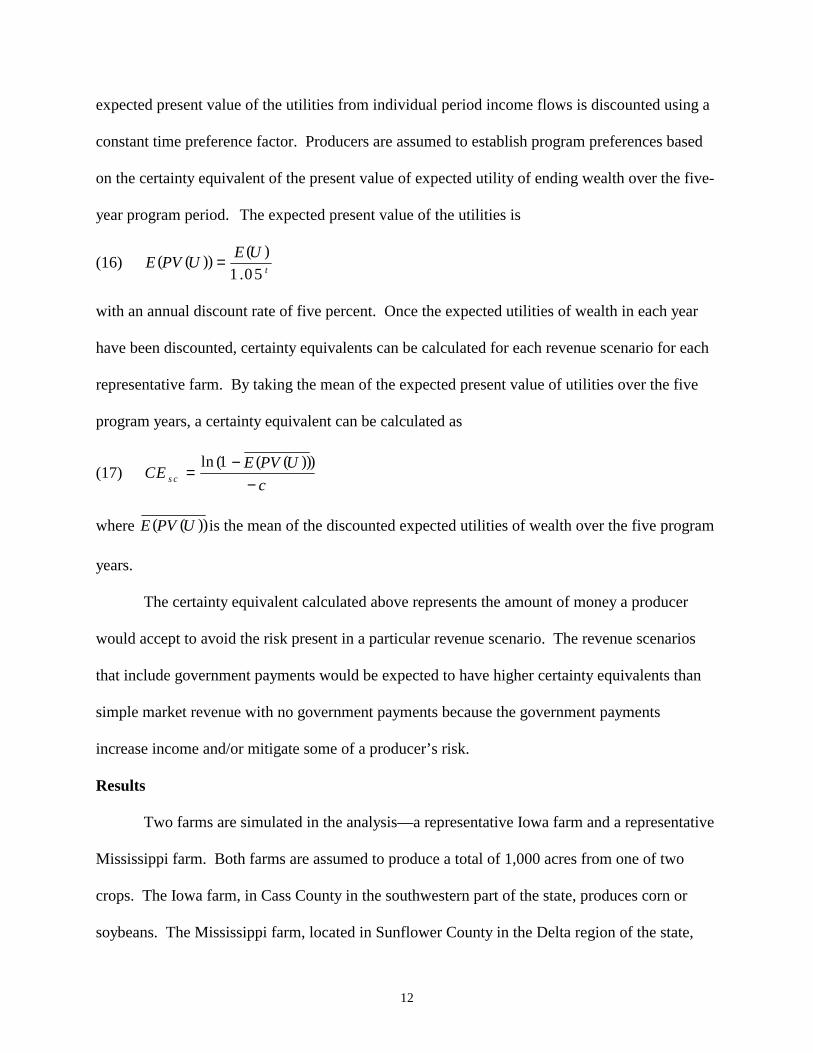
year program period. The expected present value of the utilities is

(16) t

UEUPVE05.1

)())(( =

with an annual discount rate of five percent. Once the expected utilities of wealth in each year

have been discounted, certainty equivalents can be calculated for each revenue scenario for each

representative farm. By taking the mean of the expected present value of utilities over the five

program years, a certainty equivalent can be calculated as

(17) c

UPVECEsc −−=

)))((1ln(

where ))(( UPVE is the mean of the discounted expected utilities of wealth over the five program

years.

The certainty equivalent calculated above represents the amount of money a producer

would accept to avoid the risk present in a particular revenue scenario. The revenue scenarios

that include government payments would be expected to have higher certainty equivalents than

simple market revenue with no government payments because the government payments

increase income and/or mitigate some of a producer’s risk.

Results

Two farms are simulated in the analysis—a representative Iowa farm and a representative

Mississippi farm. Both farms are assumed to produce a total of 1,000 acres from one of two

crops. The Iowa farm, in Cass County in the southwestern part of the state, produces corn or

soybeans. The Mississippi farm, located in Sunflower County in the Delta region of the state,

13

produces cotton or soybeans. The county program yield for use in the calculation of PFC

payments made for the cotton and corn crops grown on each respective farm was obtained for

Sunflower County, Mississippi, from the Farm Service Agency (FSA) field office and for Cass

County, Iowa, from the county extension office.

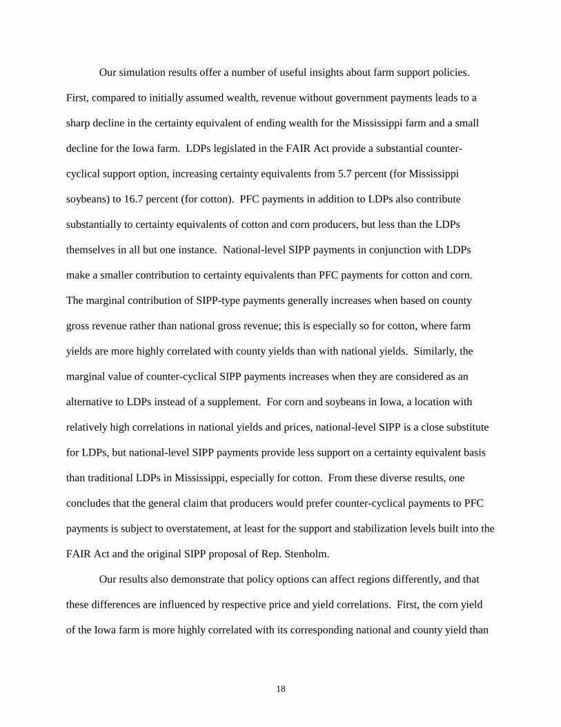
Table 1 presents correlations between the yield of each crop of each representative farm

and the respective county yields, national yields, and harvest price. Farm-level yields are more

highly correlated with county yields than national yields for each crop in both locations. Iowa

corn yields are negatively correlated with harvest prices, while Mississippi cotton yields are

essentially independent of harvest prices. Soybean yields in both locations have similar negative

correlations with harvest prices. The farm-level yield for corn in Iowa is more highly correlated

with the national and particularly the county yield than is cotton in Mississippi. This relationship

indicates that producers growing corn in Cass County, Iowa, are subject to greater systemic risk

than producers of cotton in Sunflower County, Mississippi. Thus, the farm-level risk for the

representative farm growing cotton in Mississippi should be greater than that of the

representative farm growing corn in Iowa. This conclusion follows the relationship between

aggregate and disaggregate revenues suggested by Glauber and Miranda (1996).

Based on Table 1, if the payments have the same expected monetary value, a risk averse

producer would be expected to prefer SIPP payments more than PFC payments because of the

reduction in the variability of returns. However, the expected monetary values of the two

payment programs are likely to differ.

Certainty Equivalents Under FAIR and SIPP

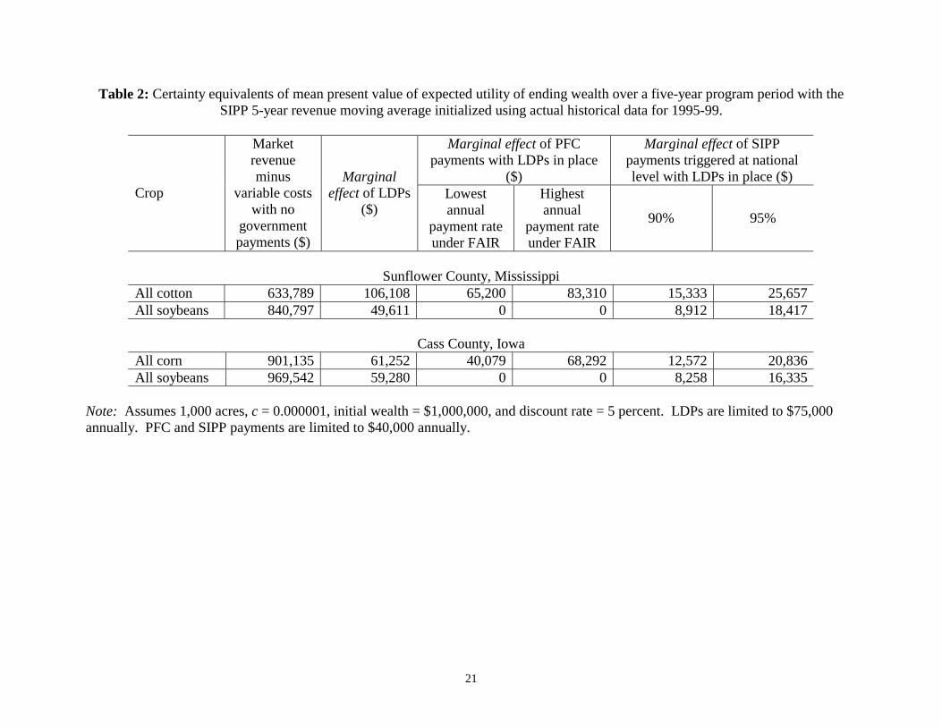
Table 2 presents certainty equivalents for the mean present value of the expected utility

of ending wealth derived from market revenue and the marginal contributions to these certainty

14

equivalents from LDPs, PFC payments, and national-level SIPP payments. There are substantial

additions to certainty equivalents under the government programs: producers are better off under

any government program than facing the market alone. The welfare of the representative

Mississippi cotton producer is generally improved more from government payments than is the

welfare of the representative Iowa corn producer. The LDPs for soybeans benefit the

representative Iowa farm somewhat more, which is likely due to the higher expected yield for

Iowa soybeans relative to Mississippi soybeans. Relative to market revenue only, LDPs for

cotton increase the certainty equivalent for the Mississippi farm by 16.7 percent. The analogous

comparison for corn shows an increase in the certainty equivalent for the Iowa farm of 6.8

percent. LDPs raise certainty equivalents for soybeans by 5.7 and 6.1 percent in Mississippi and

Iowa, respectively.

PFC payments for cotton made at the lowest annual payment rate under the FAIR Act

increase the certainty equivalent for the Mississippi farm by 8.8 percent at the margin, when

added to the increase from LDPs. PFC payments for corn at the lowest rate marginally increase

the certainty equivalent for the Iowa farm by 4.2 percent. Corresponding increases to certainty

equivalents from PFC payments at the highest rate are 11.3 percent for cotton and 7.1 percent for

corn. National-level SIPP payments received in addition to LDPs increase the certainty

equivalent for cotton by 2.1 and 3.5 percent at the 90 and 95 percent trigger levels, respectively.

Increases to the certainty equivalent for corn from national level SIPP payments are 1.3 and 2.2

percent at the respective triggers. In contrast to LDPs, the marginal effect of SIPP payments on

certainty equivalents for soybeans benefits the Mississippi farm slightly more than the Iowa farm

in both absolute and relative terms. Except for the highest PFC payments for corn, the marginal

effects of PFC and SIPP payments in all cases are smaller than the effects of LDPs.

15

Producers on both farms prefer PFC payments to SIPP payments if only program crops

are grown with LDPs in place4. If only soybeans are produced, SIPP is preferred because

soybeans are not a program crop receiving PFC payments. Comparing the lowest PFC payment

rate to national-level SIPP payments at the 90 percent trigger level, the Mississippi farm

producing cotton has a slightly stronger preference for the PFC payment than does the Iowa farm

producing corn, but this difference does not exist at the highest PFC payment rate and national-

level SIPP payments at the 95 percent trigger level.

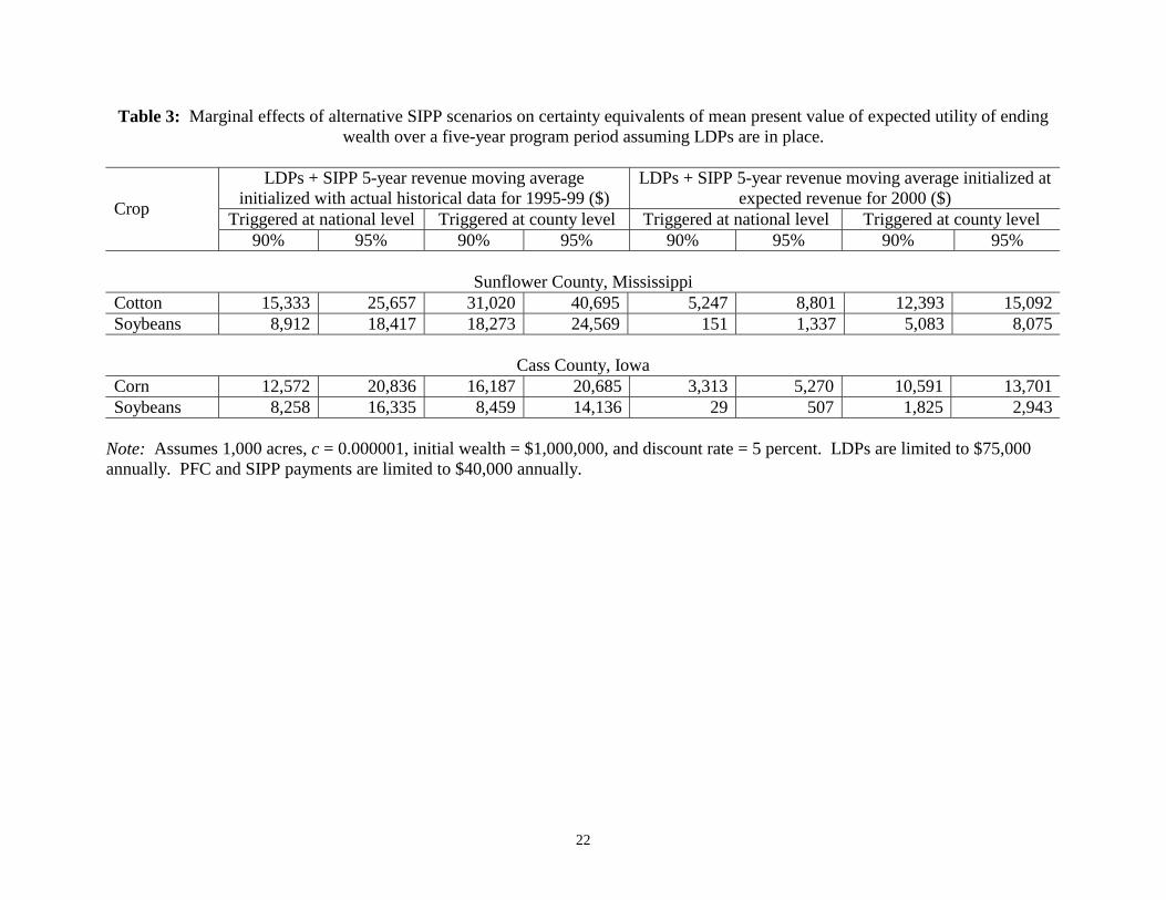
SIPP payments are triggered by shortfalls in the current year’s national gross revenue

compared to its moving average for the previous five years. SIPP payments are sensitive to this

choice of baseline as well as to the trigger level, as demonstrated in Table 3. When the five-year

moving average of revenue from 1995-99 is replaced by expected revenue for 2000, it reduces

the marginal effect of SIPP payments. For soybeans, national-level SIPP payments at the 90

percent trigger level have essentially no effect on certainty equivalents above LDPs.

Table 3 also includes SIPP payments based on county gross revenue instead of national

gross revenue. For a given trigger level, county-level SIPP payments produce substantially

higher marginal effects than national-level SIPP payments for Mississippi crops in all cases.

These higher marginal effects are due to the differences in correlations between farm yields and

county yields and farm yields and national yields. Farm yields are more highly correlated with

county yields, so that shortfalls in county gross revenue are more likely to be associated with

shortfalls in farm revenue leading to greater marginal effects for county-level SIPP payments.

While the marginal effects of county-level SIPP payments for Iowa crops increase when the

4 This study does not model the ad hoc emergency assistance payments made by Congress in the latter years of the FAIR Act, which if included would increase the value of the program to producers.

16

baseline is initialized using expected revenue for 2000, these marginal effects are smaller than

those of the county-level SIPP payments for Mississippi crops. The smaller marginal effects are

due to the relative magnitude of the difference between the respective correlations of farm yield

and national yield and farm yield and county yield. For the representative Iowa farm this

difference is 0.15 for corn and 0.21 for soybeans, and for the representative Mississippi farm it is

0.38 for cotton and 0.32 for soybeans. Thus, the Mississippi farm benefits more than the Iowa

farm from county-level SIPP payments. Indeed, because of an anomaly present in the actual

historical data, the dominance of the marginal effects of county-level SIPP payments is absent

for Iowa crops when the 1995-1999 baseline is utilized. Such an anomaly is more likely to occur

when the difference between the correlation of farm and regional revenue and the correlation

between farm and national revenue is small (as it is for Iowa soybeans).

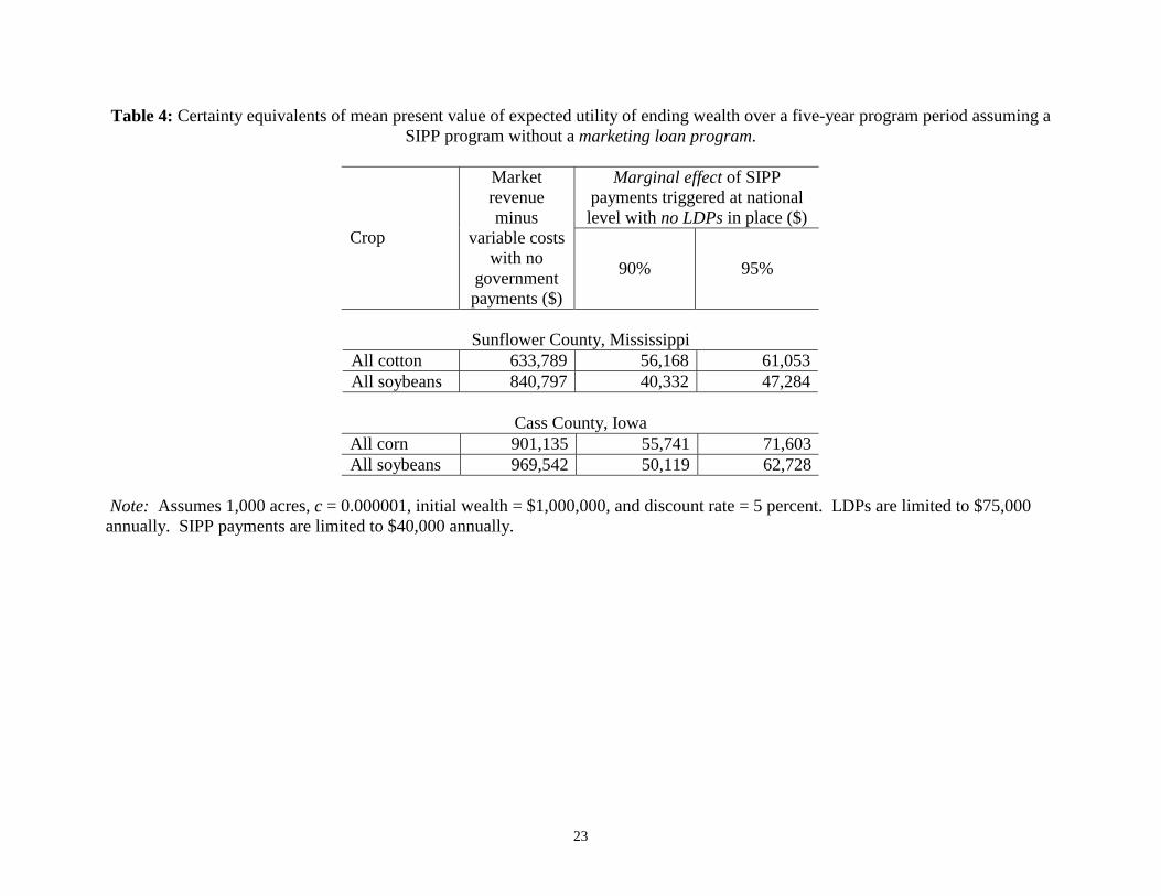
Table 4 presents the marginal effects of national-level SIPP payments without LDPs,

which can be compared to the results in Table 2. In each case, the marginal effects of SIPP

payments increase considerably. Given a choice between LDPs and SIPP, the Mississippi farm

would prefer to receive LDPs for cotton and soybeans to national-level SIPP payments at either

trigger level. The Iowa farm would prefer national-level SIPP payments at a 95 percent trigger

level to LDPs, but not at a 90 percent trigger level. This relationship indicates that, due to the

correlation issues, SIPP functions better in Iowa than in Mississippi.

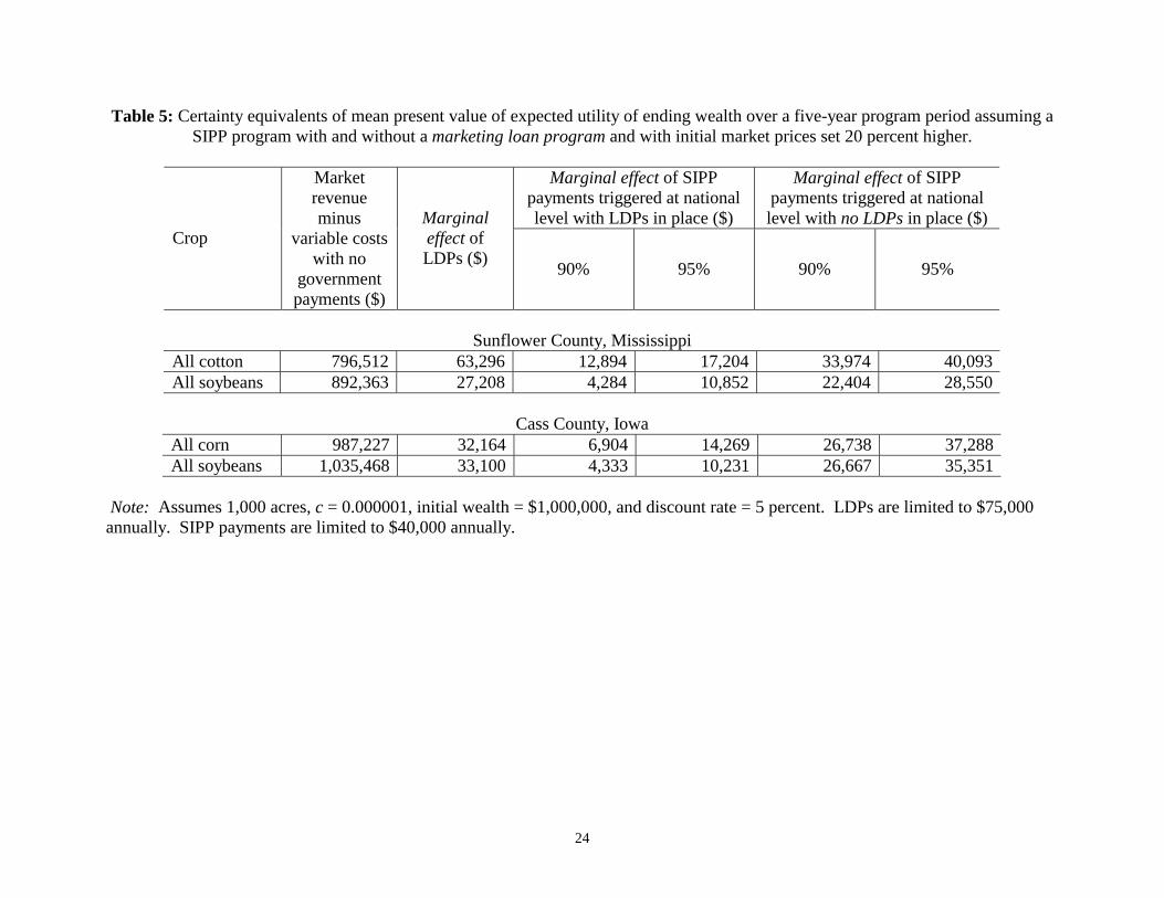
In the models above, prices are initialized at the very low levels present at the end of

1999. Table 5 presents the marginal effects of government payments with market prices initially

set 20 percent higher. Clearly, higher market prices increase market revenues and decrease

LDPs and SIPP payments. Given a choice between LDPs and SIPP, the Iowa farm prefers LDPs

to national-level SIPP payments at the 90 percent trigger, but not at the 95 percent trigger. The

17

Mississippi farm facing the same decision would prefer LDPs to SIPP payments for cotton at

both triggers and soybeans at the 90 percent trigger, but not the 95 percent trigger. The higher

prices make the national-level SIPP more attractive relative to LDPs.

Higher market prices affect the extent to which LDPs substitute for SIPP payments. The

ratio of the marginal effects of SIPP payments to those of LDPs is higher when the market prices

are higher. Therefore, higher market prices make SIPP a better substitute for LDPs. Intuitively,

this result is expected—LDPs are counter-cyclical with prices, while SIPP payments are counter-

cyclical with revenue. Higher prices would reduce the likelihood of receiving LDPs relative to

SIPP payments.

Conclusions

Design of government support programs remains a challenge in farm policy. This paper

has presented the results of a nonparametric dynamic simulation model to evaluate preferences

among alternative government payment programs for representative farms producing corn and

soybeans in Iowa and cotton and soybeans in Mississippi. Loan rates were parameterized at the

levels legislated in the 1996 FAIR Act and PFC payments were considered at both the highest

and lowest annual rates provided by this legislation. Supporters of counter-cyclical SIPP

payments based on shortfalls in annual gross revenue contend this support would be preferable to

fixed PFC payments. We consider counter-cyclical payments based on both national-level and

county-level revenue and with payment triggers of 95 percent of the previous five-year moving

average of gross revenue (as proposed by the first SIPP program in 1999) and 90 percent. Our

simulation model incorporates yield price correlations often neglected in analysis of farm

program effects and assumes slight risk aversion on the part of producers. The analysis provides

a basis for evaluating commodity and regional differences in preferences among policy options.

18

Our simulation results offer a number of useful insights about farm support policies.

First, compared to initially assumed wealth, revenue without government payments leads to a

sharp decline in the certainty equivalent of ending wealth for the Mississippi farm and a small

decline for the Iowa farm. LDPs legislated in the FAIR Act provide a substantial counter-

cyclical support option, increasing certainty equivalents from 5.7 percent (for Mississippi

soybeans) to 16.7 percent (for cotton). PFC payments in addition to LDPs also contribute

substantially to certainty equivalents of cotton and corn producers, but less than the LDPs

themselves in all but one instance. National-level SIPP payments in conjunction with LDPs

make a smaller contribution to certainty equivalents than PFC payments for cotton and corn.

The marginal contribution of SIPP-type payments generally increases when based on county

gross revenue rather than national gross revenue; this is especially so for cotton, where farm

yields are more highly correlated with county yields than with national yields. Similarly, the

marginal value of counter-cyclical SIPP payments increases when they are considered as an

alternative to LDPs instead of a supplement. For corn and soybeans in Iowa, a location with

relatively high correlations in national yields and prices, national-level SIPP is a close substitute

for LDPs, but national-level SIPP payments provide less support on a certainty equivalent basis

than traditional LDPs in Mississippi, especially for cotton. From these diverse results, one

concludes that the general claim that producers would prefer counter-cyclical payments to PFC

payments is subject to overstatement, at least for the support and stabilization levels built into the

FAIR Act and the original SIPP proposal of Rep. Stenholm.

Our results also demonstrate that policy options can affect regions differently, and that

these differences are influenced by respective price and yield correlations. First, the corn yield

of the Iowa farm is more highly correlated with its corresponding national and county yield than

19

is the cotton yield of the Mississippi farm. Second, the corn yield of the Iowa farm is also

negatively correlated with harvest price while the cotton yield of the Mississippi farm is basically

independent of the harvest price. These correlations imply that the Iowa farm’s revenue from

corn is more highly correlated with the national and county revenue than is the Mississippi

farm’s revenue from cotton, and explain why the Mississippi farm has a stronger preference for

PFC payments than does the Iowa farm. Since the Mississippi farm’s cotton revenue is relatively

less correlated with respective national and county revenue than is the Iowa farm’s corn revenue,

it is less likely to receive cotton SIPP payments than the Iowa farm corn SIPP payments. For

soybeans, a crop produced on both farms, the differences between the correlations of each farm

are smaller, which explains why there is less difference in the extent of the preference for SIPP

payments for soybeans.

Correlations also explain the relative differences between national- and county-level SIPP

payments on both farms. The Mississippi farm prefers SIPP based on county gross revenue to

SIPP based on national gross revenue relatively more than does the Iowa farm. The greater

relative difference between the farm yield-national yield correlation and the farm yield-county

yield correlation on the respective farms accounts for this difference in preferences.

The dynamic-stochastic model developed herein endogenizes these price-yield

correlations across different levels of aggregation as well as cross-crop yield correlations and

price correlations. The results of this study demonstrate the fundamental importance of

including yield and price correlations when analyzing individual preferences for different farm

programs and the effect of regional differences on these preferences. Farm-level analysis of

developing 2002 farm bill alternatives like SIPP requires more than static models to suitably

integrate these essential factors.

20

Table 1: Implicit correlation between farm-level yields and other stochastic variables

Crop Correlation

with county yield

Correlation with national

yield

Correlation with harvest

price

Mississippi Cotton 0.78 0.40 -0.01

Soybeans 0.73 0.41 -0.20

Iowa Corn 0.86 0.71 -0.41

Soybeans 0.69 0.48 -0.24

21

Table 2: Certainty equivalents of mean present value of expected utility of ending wealth over a five-year program period with the SIPP 5-year revenue moving average initialized using actual historical data for 1995-99.

Marginal effect of PFC

payments with LDPs in place ($)

Marginal effect of SIPP payments triggered at national level with LDPs in place ($)

Crop

Market revenue minus

variable costs with no

government payments ($)

Marginal effect of LDPs

($) Lowest annual

payment rate under FAIR

Highest annual

payment rate under FAIR

90% 95%

Sunflower County, Mississippi

All cotton 633,789 106,108 65,200 83,310 15,333 25,657 All soybeans 840,797 49,611 0 0 8,912 18,417

Cass County, Iowa

All corn 901,135 61,252 40,079 68,292 12,572 20,836 All soybeans 969,542 59,280 0 0 8,258 16,335

Note: Assumes 1,000 acres, c = 0.000001, initial wealth = $1,000,000, and discount rate = 5 percent. LDPs are limited to $75,000 annually. PFC and SIPP payments are limited to $40,000 annually.

22

Table 3: Marginal effects of alternative SIPP scenarios on certainty equivalents of mean present value of expected utility of ending wealth over a five-year program period assuming LDPs are in place.

LDPs + SIPP 5-year revenue moving average

initialized with actual historical data for 1995-99 ($) LDPs + SIPP 5-year revenue moving average initialized at

expected revenue for 2000 ($) Triggered at national level Triggered at county level Triggered at national level Triggered at county level Crop

90% 95% 90% 95% 90% 95% 90% 95%

Sunflower County, Mississippi Cotton 15,333 25,657 31,020 40,695 5,247 8,801 12,393 15,092 Soybeans 8,912 18,417 18,273 24,569 151 1,337 5,083 8,075

Cass County, Iowa

Corn 12,572 20,836 16,187 20,685 3,313 5,270 10,591 13,701 Soybeans 8,258 16,335 8,459 14,136 29 507 1,825 2,943

Note: Assumes 1,000 acres, c = 0.000001, initial wealth = $1,000,000, and discount rate = 5 percent. LDPs are limited to $75,000 annually. PFC and SIPP payments are limited to $40,000 annually.

23

Table 4: Certainty equivalents of mean present value of expected utility of ending wealth over a five-year program period assuming a SIPP program without a marketing loan program.

Marginal effect of SIPP

payments triggered at national level with no LDPs in place ($)

Crop

Market revenue minus

variable costs with no

government payments ($)

90% 95%

Sunflower County, Mississippi

All cotton 633,789 56,168 61,053 All soybeans 840,797 40,332 47,284

Cass County, Iowa

All corn 901,135 55,741 71,603 All soybeans 969,542 50,119 62,728

Note: Assumes 1,000 acres, c = 0.000001, initial wealth = $1,000,000, and discount rate = 5 percent. LDPs are limited to $75,000 annually. SIPP payments are limited to $40,000 annually.

24

Table 5: Certainty equivalents of mean present value of expected utility of ending wealth over a five-year program period assuming a SIPP program with and without a marketing loan program and with initial market prices set 20 percent higher.

Marginal effect of SIPP

payments triggered at national level with LDPs in place ($)

Marginal effect of SIPP payments triggered at national level with no LDPs in place ($)

Crop

Market revenue minus

variable costs with no

government payments ($)

Marginal effect of LDPs ($) 90% 95% 90% 95%

Sunflower County, Mississippi

All cotton 796,512 63,296 12,894 17,204 33,974 40,093 All soybeans 892,363 27,208 4,284 10,852 22,404 28,550

Cass County, Iowa

All corn 987,227 32,164 6,904 14,269 26,738 37,288 All soybeans 1,035,468 33,100 4,333 10,231 26,667 35,351

Note: Assumes 1,000 acres, c = 0.000001, initial wealth = $1,000,000, and discount rate = 5 percent. LDPs are limited to $75,000 annually. SIPP payments are limited to $40,000 annually.

25

REFERENCES

Atwood, Joseph A., Alan E. Baquet, and Myles J. Watts. 1997. Income protection. Department of Agricultural Economics and Economics Staff Paper 97-9. Montana State University: Bozeman, Montana.

Coble, Keith H., James C. Miller, Barry J. Barnett, and Thomas O. Knight. 1999. A proposed

method to rate a multi-crop revenue insurance product. Washington, D.C.: United States Department of Agriculture, Risk Management Agency. 29 November.

Duffy, Mike and Darnell Smith. 2000. Estimated costs of crop production in Iowa—2000. Iowa State University Extension Farm Management Publication FM-1712. Paper on-line. Available from http://www.exnet.iastate.edu/Publications/FM1712.pdf.

Economic Research Service. 1989. State-level wheat statistics. Washington, D.C.: United States Department of Agriculture. Diskette on-line. Available from http://usda.mannlib.cornell.edu/ data-sets/crops/89016/README.DOC.

Farm Service Agency. 1999. Fact sheet, upland cotton, summary of 1998 commodity loan and payment program. Washington, D.C.: United States Department of Agriculture. Bulletin on-line. Available from http://www.fsa.usda.gov/pas/publications/facts/ uplandcotton99.pdf.

Glauber, Joseph W. and Mario J. Miranda. 1996. Price stabilization, revenue stabilization and the natural hedge. Columbus, Ohio: The Ohio State University, Department of Agricultural, Environmental, and Development Economics. Photocopied.

Hardaker, J. Brian, Ruud B. M. Huirne, and Jock R. Anderson. 1997. Coping with risk in agriculture. Wallingford, Oxon, UK: CAB International.

Mississippi State University. 1999. Delta 2000 planning budgets. Agricultural Economics Report No. 110, December.

Nelson, Frederick J., and Lyle P. Schertz, eds. 1996. Provisions of the Federal Agricultural Improvement and Reform Act of 1996. Agriculture Information Bulletin No. 729. Washington, D.C.: United States Department of Agriculture, Economic Research Service, Commercial Agriculture Division. Bulletin on-line. Available from http://www.ers.usda.gov/epubs/pdf/aib729/.

Stinson, Thomas F., Jay S. Coggins, and Cyrus A. Ramezani. 1998. Was FAIR fair to U.S. corn growers? Paper presented at the annual meeting of the American Agricultural Economics Association, Salt Lake City, Utah, 1-5 August. Paper on- line. Available from http://agecon.lib.umn.edu/aaea98/spstin01.pdf.

26

Tirupattur, Viswanath, Robert J. Hauser, and Phelim P. Boyle. 1997. Theory and measurement of exotic options in U.S. agricultural support programs. American Journal of Agricultural Economics 79 (November) : 1127-1139.

U.S. Congress. House. 1999. Supplemental Income Payments for Farmers Act. 106th Cong., 1st sess., H.R. 2792. Congressional Record. 145, no. 114, daily ed. (5 August): H7251- H7887.