A behavioral model of cyclical dieting

A Behavioral Model of Cyclical Dieting

by

Steven M. Suranovic* Robert S. Goldfarb*

June 2005

Abstract This paper presents a behavioral economics model with bounded rationality to describe an individual’s food consumption choices that lead to weight gain and dieting. Using a physiological relationship determining calories needed to maintain weight, we simulate the food consumption choices of a representative female over a 30 year period. Results show that a diet will reduce weight only temporarily. Recurrence of weight gain leads to cyclical dieting, which reduces the trend rate of weight increase. Dieting frequency is shown to depend on decision period length, dieting costs, and habit persistence. JEL Codes: Keywords: _____________________________________________________ * Department of Economics, The George Washington University, Corresponding Author: Steven Suranovic, Department of Economics, The George Washington University, 1957 E St N.W., Room 501M, Washington, D.C. 20052. Ph: (202) 994-6150, FAX: (202) 994-6147, E-mail: [email protected]

1

1. Introduction

In recent years the problem of increasing obesity in the US has sparked research

interest across a variety of disciplines. Fully 35 percent of Americans are overweight, and

an additional 20 percent are obese (Mokdad et al 2001).1 Excess body weight has been

characterized as the second-leading cause of preventable death and disease in the US;

300,000 Americans die annually from obesity-related diseases (McGinnis and Foege

1993; Must et al 1999).2 The Centers for Disease Control (CDC) now refer to excess

weight and obesity as an “epidemic.”

One branch of the recent economics literature on this topic attempts to empirically

identify the causes of the observed rise in obesity over time (see, for example, Chou et al

2004, Lakdawalla and Philipson 2002, Cawley et al 2003, Cutler et al 2003). Another

branch has developed behavioral models to explain food consumption choices leading to

excess weight and dieting. (see, for example, Dockner and Feichtinger 1993, Levy 2002,

Goldfarb, Leonard and Suranovic, [GLS forthcoming]).

This paper contributes to this second branch by developing a behavioral model of

food consumption choices that illuminates observed patterns of dieting. There are both

1 Excess weight and obesity refer to the ratio of body fat to lean body mass. The body mass index (BMI) proxies for this ratio, where BMI = weight (kgs)/height (meters)2 or BMI = (705)weight (lbs)/height (inches)2. You are deemed overweight if your BMI is 25 or greater but less than 30, and you are obese with a BMI of 30 or more. 2 “An excess body weight of 30% is associated with an increase of 25% to 42% in mortality, and mortality increases with increasing body weight.” (Mitchell, 1997, citing Kushner 1993). This may be why even small amounts of weight loss can lower the risk of obesity-related illnesses. (Mitchell, 1997 p. 363, citing Goldstein 1992). “Much of the morbidity [disease] associated with obesity is due to an increase in the occurrence of hypertension... and [type 2] diabetes mellitus, all of which contribute to an increased risk of cardiovascular disease (Sjostrom, 1992...)” (Mitchell, 1997, p. 359; see also Wilmore and Costill, 1999,pp.671-72). The external costs of eating too much and exercising too little may exceed those from smoking (Manning et al. 1991). Sturm and Lakdawalla (2004, p. 25) assert that obesity “is linked to very high rates of chronic illness—higher than living in poverty and much higher than smoking or drinking.”

2

practical and analytical reasons for paying particular attention to dieting behavior. On the

practical side, dieting efforts appear to be extensive, and involve significant expenditures

of effort and money.3 On the analytical side, dieting behavior presents a number of

conceptual challenges for rational choice models of human behavior. In particular,

“cyclical” or “yo-yo” dieting --diet, lose weight, stop dieting, gain weight, diet again, etc

etc—seems to some observers to be arguably inconsistent with rational behavior.4 Also,

to the extent that the problems of obesity inspire public policy changes, a model that can

capture the behavioral dynamics of overeating and weight gain will be very useful.

Our model departs slightly from the standard approach in behavioral economics.

Much of the previous behavioral economics literature dealing with consumption of

potentially harmful products [e.g., cigarettes, illegal drugs, and overconsumption of food]

is based on the traditional model of rational intertemporal choice over time. It views

individuals as choosing a lifetime consumption path for a product at an initial decision

date. If an individual’s consumption decision about how much to smoke or eat today

affects his future utility, it seems to follow that the “rational” way to make choices is to

plan over one’s lifetime.5

In our view, this rational choice approach makes for a reasonable prescription

about how to make individual choices. However, that approach does not mimic the way a 3 A Wall Street Journal article in 2003 claimed that “at any time, 29% of men and 44% of women are on a diet.” (Parker-Pope, 2003, p. R-1). While these particular estimates may appear unrealistically high, the basic point that a sizable chunk of the population is often on diets seems unassailable. It also seems indisputable that the dieting industry (Weight Watchers, Jenny Craig, medical facilities that oversee weight loss efforts, etc) involves significant expenditures by dieters and significant use of resources. 4 For example, Dockner and Feichtinger (1993) note that, “much of empirically-observable consumption behavior seems to contradict rational-choice theory. Here we refer to heavy eating followed by strict dieting…” 5 This approach is derived from an age-old question in economics about how to allocate current production between consumption and investment goods. Since this choice affects not only current utility but also future utility, the only reasonable way to make today’s decision is to plan for all future allocations today.

3

typical individual actually makes consumption decisions. As a consequence this approach

has found it difficult to convincingly explain certain features of individual choice

including time inconsistency, and regret, among others.6

A viable alternative is to consider a “boundedly rational” choice model, following

Suranovic, Goldfarb, and Leonards’ (1999) model of cigarette consumption. In that

analysis, excessive computational costs constrain decisions to be made only for the

current consumption period. The individual does consider the future health effects of

today’s smoking, but does not consider how today’s smoking will affect tomorrow’s

smoking decisions or how tomorrow’s decisions will affect today’s choice.7

There are several reasons to adopt this approach. First, individuals are not super-

human calculators, projecting all the implications of each decision far into the future.

The mental and computational cost of solving an intertemporal decision process is very

large for the economic modeler, let alone the typical person. Second, recent

psychological research by Nobel Laureate Daniel Kahneman and others suggests that

individuals are very poor at projecting the future utility from even seemingly simple

choices.8 This makes it extremely dubious that individuals would be capable of a much

6 Recent attempts to solve these issues have led to the introduction of hyperbolic discounting [see O’Donohue and Rabin (1999) and Gruber and Koszegi (2001)] and random cue-conditioning [Bernheim and Rangel (2002)]. 7 The term “bounded rationality” is used in several different ways. Gigerenzer and Selten (2001) apply this term only if behavior is described using a heuristic device or rule-of-thumb and does not involve optimizing behavior. In our model we assume an individual does optimize, but has a constrained information set due to excessive computational costs. In either case behavioral assumptions are made that step back from the standard intertemporal choice problem. 8 In his Nobel Prize address, Kahneman points out that “Failures of hedonic prediction are even common in the short term. The participants in a study reported by Kahneman and Snell (1992) showed little ability to anticipate how their enjoyment of a piece of music or a helping of their favorite ice cream would change over a period of eight daily episodes of consumption” (Kahneman, 2003, p. 165).The more general finding Kahneman reports is that “people generally underestimate the extent of hedonic adaptation to new states.” In support he cites a review of the literature by Loewenstein and Schkade (1999), and gives an example from a study by Gilbert and Wilson (2000), indicating that assistant professors “greatly overestimate the effects of a tenure decision on their happiness a year later.” (Kahneman,2003, p. 165).

4

more complex decision process. Finally, the boundedly rational decision process has

been able to explain some choice phenomena (such as regret and cold-turkey quitting of

smoking) that are more difficult and less intuitive to explain with the intertemporal

approach.

In this paper, we extend this boundedly rational choice process to an individual’s

food consumption and dieting decisions. We develop a model that generates results

consistent with important stylized facts about dieting behavior, including the choice of

multiple, or yo-yo diets. An important outcome of the model is a behavioral rationale for

the phenomenon that more frequent dieting attempts tend to result in higher overall

weight gain. Moreover, our modeling framework allows us to identify particular

conceptual parameters that affect the patterns of weight change and dieting.

We begin by describing the basic structure of the model including the physiology

of weight change. We then turn to specifying specific functional forms for a hypothetical

individual who we call Sara. We next solve for Sara’s optimal consumption in an initial

period. Based on her choice, we update her weight and other parameters in successive

periods and thus simulate Sara’s optimal consumption path over an extended period of

time. Later we adjust key parameters to show their impact on Sara’s food consumption

and dieting behavior.

2. The Conceptual Behavioral Choice Model

We assume food consumption has three types of effects on an individual’s utility:

a standard benefit effect, a weight-utility effect, and a dieting cost effect. An individual

maximizes utility each period, choosing both food and a composite good, considering

5

these three effects of food on utility. A decisionmaking period will initially be assumed

to be one month, however parameters can be adjusted to consider alternative time frames.

The standard benefit effect is the utility gained from the consumption of food,

analogous to the utility that arises from consumption of any good. We assume utility

rises at a decreasing rate and there is a satiation point (i.e., too much food ingested in any

one day makes the individual sick).

The weight-utility effect connects food consumption to weight. We assume that

an individual has an exogenous ideal weight. If food consumption maintains that ideal

weight, then there is no weight-utility effect. However, if food consumption leads either

to overweight or underweight, then there is a weight-associated disutility effect. We’ll

assume that the weight disutility effect rises with deviations from the ideal weight. Thus,

an additional kilo of weight for a person 10 kilos overweight will have greater disutility

than if the person were only 5 kilos overweight.

In GLS [forthcoming], these two effects combine to induce an individual to

choose a food consumption level that results in a weight that is greater than ideal. The

reason is that small increases in food consumption above one’s weight maintenance level

do not have a large weight disutility effect. Thus, the normal marginal benefit of greater

food consumption will exceed the small weight disutility effect and lead to optimal

overweightedness.

GLS also explore several motivations for diets. However, the basic intuition in all

cases is that if weight rises, the disutility effect of food consumption on weight rises at an

increasing rate. Eventually, the marginal benefit of food consumption will be less than

the weight disutility effect and this inspires a reduction in food consumption, i.e., a diet.

6

The GLS analysis, however, does not incorporate the costs or disutility associated with

dieting.

The third effect of food consumption is this cost of dieting. In particular, we

assume sudden reductions in food consumption have strong negative psychological, and

perhaps physical, effects. Typically, individuals choose food consumption levels that are

relatively constant over time. We’ll refer to that constant level as a habitual level. If

consumption is chosen below that habitual level, there is a disutility effect, which

increases the greater the reduction. We’ll imagine there is no “cost” associated with

excessive consumption.

The presence of dieting costs means that an additional cost, above the rising

disutility of overweight, must be overcome before a diet occurs. Whether a diet occurs

will depend on the size of the dieting costs. If they are large, a diet may never occur. But

if a diet is chosen, it may not occur until the disutility of overweight is quite high.

In order to track the effects of food consumption decisions on weight and the

subsequent effects of weight on food consumption choices, we must discuss the

physiology of weight change. Incorporating the physiology into our utility model of

weight change, will enable us to simulate period-by-period consumption choices and

track the effects of these choices on an individual’s weight path over time.

3. The Physiology of Weight Change

The nutrition literature models weight determination and change by analyzing the

balance of energy intake and energy expenditure. Weight rises (falls) if energy intake

7

exceeds (falls short of) energy expenditure.9 Physiologists typically disaggregate energy

expenditure into three components: resting or basal metabolism, food digestion, and

muscular physical activity. Basal metabolic function accounts for 60 to 75 percent of

energy expenditure in most individuals; another ten percent is burned eating and

absorbing food. Muscular activity accounts for the remaining 15 to 30 percent in a

moderately active individual (McArdle et al 1996: 151). A continuing excess of energy

intake over energy expenditure results in weight gain.

A continuing view in the physiology literature is that basal metabolic energy

requirements or basal metabolic rate (BMR) can be viewed as a function of age, weight,

height and sex. Long-standing empirical estimates widely used in the nutrition literature

are provided by the venerable Harris-Benedict equations.10 Energy expenditure on

physical activity (and the thermic effect of food) can then be incorporated by applying a

multiplier to the basal metabolism estimates.11

9 See, for example, Willett 1990 pp. 245-46; Melby et al 1998, p.6, Forbes 1999 p. 801, and Wilmore and Costill, 1999, pp.667-68.

10 The Harris Benedict equations indicate for men, that BMR = 66 + 13.7 W + 5H - 6.8 A. For women, BMR = 655 + 9.6W + 1.8H - 4.7A , whereBMR = basal metabolic rate, H = height in cm, W = weight in kg, and A = age in years. While numerous other equations are available, “many researchers use the Harris-Benedict method to determine BMR.” (Whitney, Cataldo and Rolfes, 1998, p.267).A literature exists that compares various BMR estimating equations, and examines how well they seem to work for more narrowly defined populations. (See, for example, Cunningham,1980, Vaughan et al 1991, Taaffe et al 1995, Liu et al 1995, Wong et al 1996).These articles typically obtain direct laboratory measures of BMR for a sample of individuals (for a discussion of the laboratory techniques used to measure BMR, see McArdle et al, 1996, pp.139-141). They then compare the actual BMR laboratory measures to the predicted measures of BMR from the various available predicting equations. The Harris-Benedict equations seem to have survived these explorations. 11 McArdle, et. al., (1996) defines the following categories: Sedentary= BMR X 1.2 (little or no exercise, desk job);Lightly active= BMR X 1.375 (light exercise/sports 1-3 days/wk); Moderately active= BMR X 1.55 (moderate exercise/sports 3-5 days/wk);Very active= BMR X 1.725 (hard exercise/sports 6-7 days/wk); Extremely active= BMR X 1.9 (hard daily exercise/sports & physical job) Note that this specific sedentary multiplier gives a calorie usage that is 20% higher than one’s BMR. This includes the 10% thermic effect of food absorption plus some additional amount for low levels of physical activity.

8

These long-standing empirical estimates suggest what is well documented

elsewhere in the physiology/nutrition literature: that basal metabolism slows with age

(see the cites in McArdle et al 1996, p.152. See also Vaughan et al 1991). There is also

evidence, if less extensive, that energy expenditure on physical activity declines later in

life.12

These facts of physiology generate several important implications about patterns

of weight change. First, even with constant calorie intake, age insidiously increases

weight, and does so at a faster rate if exercise levels also fall as one ages. Second, these

facts by themselves suggest a rationale for dieting. An aging person will, ceteris paribus,

gain excess weight, and must diet (or exercise more) to avoid weight gain.

4. Simulation Model

To analyze a series of choices over time we simulate the decisions of a

hypothetical female we’ll call Sara. We posit plausible functional forms for each of the

three utility effects and calculate Sara’s optimal consumption choice for the initial period.

Once the optimum is calculated, the functions are updated with a new age, weight level,

and age-specific activity (exercise) level. Based on this updated data, Sara’s optimal

choice is recalculated for this second period. By repeating this process period by period

we can describe Sara’s time path of food consumption choices and resulting weight path

over time.

12 McArdle et al, 1996 p. 159, assert that the energy use associated with a specific exercise activity decreases from middle age on because of “the general ‘aging effect’ on aerobic capacity.” See also Rising et al, 1994, a study based on a sample of Pima Indians.

9

We next specify specific functional forms for our three utility effects: the food

benefit function, the weight loss function, and the dieting cost function.

4.1 The Food Benefit Function

The main effect of food consumption is the utility or benefits it provides. Treating

food as a normal good, the food benefit function has the following characteristics.

Benefits rise at a decreasing rate as daily consumption increases up to a satiation level,

given by the parameter M. Beyond that satiation level, benefits fall with increasing

consumption. Sara’s food consumption benefits are described by the benefit function

B(C):

2

22

M]M)(Ck[MdB(C) −−

= (1)

where C represents the daily calorie consumption level, the parameter “d” represents the

number of days over which the consumption decision is made, and “k” is a scale

parameter that determines the peak daily utility attained at the satiation consumption

level.

4.2 Weight Loss Function

Consumption greater than (less than) necessary to maintain one’s weight will

cause weight gain (loss). We imagine that an individual chooses an ideal weight, WI,

based on health considerations, social appearance norms, or a combination of the two.

The choice of WI is exogenous to the model.

10

The following function describes the effects of weight on utility. Utility losses,

L(C, W) due to over- or under-weight, are assumed to depend on the current level of daily

consumption C, and current weight W plus several other exogenous parameters such as

ideal weight WI.

2

I

I

W7700

H)]A,W,BMR(AF(CdWWmW)L(C,

⎥⎥⎥

⎦

⎤

⎢⎢⎢

⎣

⎡ −+−

=

•

(2)

Here m is a scale parameter. Current consumption affects losses because under- or over-

consumption will cause weight loss or gain. The right side of the numerator incorporates

this effect. BMR(W,A,H) represents the basal metabolic rate and is a function of current

weight (W), age (A) and height (H). As noted previously, the BMR formula for an adult

female like Sara is given by the Harris-Benedict equation:

A4.7H1.8W9.6655H)A,BMR(W, −++= (3)

where W is Sara’s weight in kilos, H is her height in centimeters, and A is age in years.

The BMR gives the number of calories needed to maintain the current weight level of a

person of given weight, height and age assuming no additional energy is expended on

activity/exercise. To obtain the full caloric intake needed for an active individual, the

BMR must be multiplied by an activity factor, AF. AF is generally about 1.35 for a

sedentary lifestyle and can rise as high as 1.8 for a very active, vigorous lifestyle. Thus

AF * BMR(W,A,H) gives the number of calories needed to maintain a weight of W. The

BMR equation indicates that the calorie intake necessary to maintain the same weight

11

will fall as a person gets older. This reflects a shift in body composition from muscle to

fat with aging.13 As indicated above,14 it is also quite common for a person to become

less active as he or she becomes older, suggesting a falling activity factor AF with age.

The expression 7700

H)A,W,BMR(AFC •− in the weight loss function above

represents the addition (or subtraction) from weight as a result of one’s current daily

consumption choice. If C exceeds AF * BMR, then one is consuming more calories than

needed to maintain current weight, and weight will rise. The physiology literature

indicates that 7700 calories are equivalent to one kilogram in weight. Thus, if C exceeds

AF * BMR by 7700 calories over some period, the person will gain one kilo. This

expression is multiplied by the time frame parameter (d for number of days) to represent

the total weight effect over the choice period.

If C = AF * BMR then the weight loss function above reduces to

2

I

I

W)W(Wm ⎥⎦

⎤⎢⎣

⎡ − , where WI is one’s perceived ideal weight and m is a scale parameter.

This simple quadratic function indicates that the farther one’s actual weight is from ideal

weight, in either direction, the greater the perceived utility losses.

Since current consumption can change current weight, the deviation in weight

from ideal weight must include the weight change effect 7700

H)]A,BMR(W,AF[C •− .

13 “Changes in body composition,either the decrease in fat-free mass and/or increase in body fat during adulthood, largely explain the…decrease in BMR usually observed through adulthood..” (McCardle et al 1996, p.152). 14 See footnote 12 above

12

Note, because of the quadratic form, an additional kilo in weight will have a larger utility

loss the farther one is from ideal weight.

4.3 Dieting Costs

People regulate their food consumption primarily by using their own body’s

hunger signals, eating when hungry and stopping when full. The actual calorie intake

level is rarely known with any accuracy. Nonetheless, since people must eat to prevent

hunger pangs, food consumption occurs at regular intervals, normally breakfast, lunch,

dinner and perhaps snacks. The types of food consumed, the quantities consumed and the

pattern of eating typically become extremely regular in form and content. In other words,

most people’s eating patterns are habitual.

Dieting, on the other hand, requires reduced calorie consumption and may force a

change in types and quantities of food consumed, and perhaps even the pattern of

consumption. These changes are very hard to undertake because they require breaking

one’s long established habits. These difficulties in adjusting one’s food consumption

habits constitute dieting, or adjustment, costs. They are not necessarily monetary

expenditures, although they certainly can be if one joins a diet center or pays to

participate in a weight-loss program. These dieting costs reflect the disutility that arises

from attempts to curtail food consumption and to change one’s habits.

The function representing dieting costs is given by AC(C) below.

13

[ ]

⎢⎢⎢

⎣

⎡ <−−−=

otherwise0

0avgcCifC(avgcgdAC(C)

1/222

(4)

where g is a scale parameter and d is the number of days in a decision period. We

imagine that adjustment costs occur only for consumption levels below one’s average

consumption level, avgc. In other words, eating too much one day is not difficult, but

eating too little causes a utility loss.

The period of time over which consumption is averaged represents habit

persistence. For example, if avgc is averaged over 6 months, then it will take 6 full

months of lower consumption for a lower calorie intake to be viewed as the new habitual

level.

The function AC is chosen so that small reductions in consumption, below one’s

habitual or average level avgc, result in a large decrease in utility. This implies it is very

difficult to make small changes in consumption levels. However, as food consumption is

reduced further, disutility continues to rise but at a decreasing rate.15

4.4 Total Utility and The Choice Problem

The consumer obtains utility from consumption of food and an additional

composite commodity Y, according to the following additively separable function.

dYAC(C)L(C)B(C)Y) UT(C, +−−= (5) 15 Clearly the choice of functional forms is ad hoc. However, these forms are chosen to duplicate the nature of the relationships that we contend exist for a typical person. The parameter values, especially the scale variables, are chosen to generate plausible consumption choices.

14

The choice problem for the consumer is to maximize total utility UT(C, Y) with respect

to C and Y, subject to the budget constraint,

Pc d C + d Y = I (6)

where we normalize the price of the composite good to one, Pc is the price of food per

calorie and d represents the number of days in the evaluation period. I represents the

consumer’s income over the period.

Solving the budget constraint for dY and substituting in to the utility function

yields,

dCPIAC(C)L(C)B(C)UT(C) C−+−−= (7)

Maximizing UT(C) with respect to C yields the first-order condition,

B’(C) - L’(C) - AC’(C) - dPC = 0 (8)

where B’(C), L’(C) and AC’(C) correspond to the first derivatives with respect to C.

More explicitly this condition can be written,

15

C22

2I

I

2

dP)C(avgc

Cdg

W7700

H)]A,W,BMR(AF(CdWW

7700md2

MC)][(Mkd2

=−

+

⎥⎥⎥

⎦

⎤

⎢⎢⎢

⎣

⎡ −+−

−−

•

(9)

whenever (avgc – C) > 0. If C exceeds avgc, the habitual level, we assume there are

no adjustment costs, thus the third term on the left-hand-side of the equation drops out in

this circumstance.

5. Simulations

5.1 Base Case

Suppose Sara is a 20-year old woman, 170cm tall (5'6") and has an ideal weight

of 60kg (132 lbs.). Assume Sara is moderately active with an activity factor AF=1.55. If

she initially weighs 60kg, we can multiply her initial BMR (1443 from equation 3) by

her activity factor to obtain her Total Daily Energy Expenditure (TDEE), measured in

calories. Thus, given her energy demands, Sara at age 20 requires 2237 daily calories to

maintain her weight. We will assume Sara’s satiation consumption level (M) is 2800

calories per day.

Figure 1 displays Sara’s benefit B(C), weight loss – L(C) and dieting, or

adjustment cost functions –AC(C). The function UF(C) represents total utility from food

consumption after accounting for the weight losses and the adjustment costs of dieting.

Insert Figure 1 in Diagrams for Diet Dynamics Paper

16

Note the food benefit function rises from zero to a peak at 2800 calories. The losses due

to weight concerns increase as consumption rises or falls from the level needed to

maintain weight, which for Sara is 2237 calories per day.16 Finally the

dieting/adjustment costs of changing calorie intake becomes larger at a decreasing weight

as calorie consumption falls below 2237, but do not arise if consumption is greater than

2237. This feature generates two key features of the food utility function, UF. First,

since adjustment costs are assumed only to arise in the downward direction, there is a

kink in UF at the weight maintaining calorie level. Second, because adjustment costs rise

at a decreasing rate as calories fall below 2237, the total food utility function falls at an

increasing, then decreasing rate for reductions in calories. These two features will

motivate the incentive to diet.

5.2 Dynamics

We’ll assume Sara makes a decision once per month about how much to optimally

consume. At the end of each month, three things can change. First, if she does not

consume precisely the number of calories needed to maintain weight, her weight will

change. Second, Sara will become one month older. Both weight change and aging will

affect her BMR. Finally, we’ll assume her activity factor falls at a gradual linear rate.

Our assumption will make Sara more sedentary by the time she is 50 years old.17 All

three changes will affect the number of calories needed to maintain Sara’s weight, and are

16 This effect is difficult to see in Figure 1 due to the small scale of the effects when Sara is at her ideal weight level. 17 The explicit function used is AF(a) = 1.55 – 0.0096(a - 20) where a is Sara’s age in years. By age 50 Sara’s activity factor will fall to 1.26 reflecting a more sedentary lifestyle as discussed in FN 11.

17

updated monthly in Sara’s decision process. We also assume that Sara’s habits persist for

6 months. This means that she would need to reduce calorie intake for 6 months in a row

to reduce her habitual consumption level to that new lower level.

We’ll assume that Sara has a constant annual income of $25,000, approximately

equal to average per capita disposable income in the US. The price of food is set at .003

dollars per calorie. At these values, Sara’s daily expenditures on food will be between 5

and 10% of her disposable income, which approximates average US consumption

patterns. Finally, by optimizing each month and updating based on her choice, we can

simulate Sara’s time path of food consumption and her weight pattern over time.

In Figure 2 we display the timepath of optimal consumption choices made by


Sara. Notice that Sara chooses to maintain consumption at her habitual level, 2237

calories per day, until approximately the age of 30. At that point she decides optimally to

reduce calorie intake to about 1300 calories for one month. In other words, she chooses

to diet. Just prior to her decision to diet, Sara’s benefit, weight, and adjustment cost

functions are as shown in Figure 3.


The key difference between the functions for Sara at age 30 compared to age 20 is

that the utility cost of higher weight has grown. This is reflected in the downward shift in

the loss function L(C), which in turn has rotated the total utility schedule downward. To

see the comparison, Figure 4 shows the total food utility curves (UF) for Sara at age 20

18

and age 30. Also drawn are two lines, labeled Pr20 and Pr30, with slopes equal to the

food price. The tangency between the Pr lines and the food utility functions satisfy the

first-order conditions given in equation (9). In the top curve at age 20, Sara would

clearly choose her habitual level of consumption on the kinked part of the food utility

function at 2237 calories per day. However, by age 30 the food utility curve has shifted

and rotated downward until Sara’s optimal choice jumps from the habitual level to a level

of about 1300 calories per day. This is shown in the lower set of curves where it appears

Sara would be indifferent between consuming 2237 or 1300.

Insert Figure 4 in Diagrams for Diet Dynamics Paper Dieting arises in this model because habitual consumption leads to weight gain

and as weight rises there is increasing disutility in consumption from each unit of weight.

When the disutility of rising weight becomes larger than the cost of dieting, Sara chooses

to cut consumption significantly. That is, she begins a diet.

Since Sara’s diet is maintained for a 30 day period, Sara’s weight will fall. With a

reduced weight, the marginal losses due to weight in her utility function will also fall and

the total utility function will rotate upwards. For this reason, in subsequent periods she

will revert back to nearly her original habitual level.18

Immediately after the diet, Sara’s new calorie intake will remain below the level

needed to maintain her new weight. Thus she will continue to lose weight after she stops

dieting, albeit at a much slower rate. However, eventually a rising age, a falling activity

18 Consumption will not return quite to the original level since one month of dieting will lower the average consumption level and reset the habitual calorie level to a slightly lower level. How far this can fall will depend on the persistence of habits. In this simulation, we assume habits persist for 6 months.

19

level and the difficulty of changing one’s habitual consumption level, will again, within

several years, result in a rising weight trajectory. Sara’s weight trajectory over a 30 year

period to age 50 is shown in Figure 5.19


Notice that Sara will again choose to diet two more times before age 50. This

shows the model is capable of explaining cyclical dieting. Sara’s modest success in her

first diet does not eliminate the insidious pattern of weight gain since she has not

sufficiently reduced her consumption to keep up with her falling caloric needs. Note also

(Figure 5) that the second diet occurs at a higher weight level than it did previously.

Here’s why.

When weight rises back up to the level attained at age 30, the marginal effect of

weight on utility will be the same as before. However, because the previous diet has

reduced the habitual consumption level, the marginal benefits of consumption will be

higher. (In other words, the allure of food is greater the less one consumes each day).

This implies that weight will need to rise even higher before the losses from weight gain

exceed the marginal benefits from consumption. This effect implies that despite several

attempts at dieting, Sara’s long-term weight trend is rising over her lifetime.

19 Note that our simulations do account for the fact that rising weight raises the individual’s BMR and thus also raises the number of calories needed to maintain weight. However, the aging effect dominates the weight effect so calories needed to maintain weight falls with age.

20

5.3 Effects of Lower Dieting Costs

The timing of Sara’s diet is affected by several factors including the cost of

dieting. Clearly different diet regimens have different costs associated with them. It is

likely that these costs are idiosyncratic; some people may find diet A easier, others may

face lower costs with diet B. Using the model, we can simulate the variability of dieting

costs and assess how more effective diet programs would influence the dieting plans of a

representative individual and that person’s lifetime weight profile.

In Figure 6, we compare Sara’s calorie choices over a 30-year period in the base

case to a situation in which diet costs are reduced by half. In other words we ask what if

Sara found dieting to be easier in the sense that it caused half as much disutility. This

investigates the dieting and consumption outcomes for an individual with a more

effective dieting program available.


During the 30-year period shown, Sara would make six diet attempts as opposed

to three attempts when her dieting costs were higher. In addition, the severity of the diet,

measured by the percentage reduction in calorie intake, is lower with lower dieting costs.

Recall that Sara’s food utility curve (refer to either one shown in Figure 4) is convex to

the left of her habitual level (where the kink occurs). However, as calorie intake falls the

curve has an inflection point whereupon it becomes concave to the origin below that

point. The convex portion of the graph is deeper with larger dieting costs. Furthermore

the inflection between the convex segment and the concave segment is pushed lower as

21

dieting costs rise. Thus, as dieting costs are reduced, the inflection point increases, and

that causes an increase in the calorie level chosen during a diet.

Sara’s weight path with lower diet costs is compared to the base case in Figure 7.


The pattern is the same in both cases. Weight rises until a one period diet is chosen. The

diet reduces weight and the habitual consumption level so that weight falls for several

periods until it begins its incessant rise again. In the case of lower dieting costs, however,

the earlier timing of the first diet and more frequent diets leads to a weight path that is

everywhere below the higher dieting cost case. The trend in weight is still upwards but

weight rises at a slower rate.

This result demonstrates the importance of dieting costs in the timing, frequency

and severity of a diet. If weight reduction programs can be made easier to implement,

this would lower weight for most individuals over their lifetime. However, marginally

lower diet costs will not eliminate the incessant increase in weight caused by aging and

falling activity levels. Instead, it will merely lower the rate at which an individual’s

weight rises. Thus, more effective diet programs may not be sufficient to help people

lose weight and keep it off.

5.4 Diet Decision Period

A second parameter that can affect the timing of diets is the choice of diet length.

In the model, the length of the diet is given exogenously. However, we can alter the

22

length of time Sara chooses for her diets. In the base case we assumed Sara made a

monthly decision for calorie intake and then maintains her chosen consumption level for

the entire month. This also means that any diet chosen by Sara must, at a minimum, be

one month in length. One month of dieting has a significant effect upon Sara’s weight

path. Her weight falls in the first month due to the diet, and then continues to fall further

for several periods due to a modest reduction in her post-diet average calorie intake. Her

weight path does eventually trend upward again, but it takes Sara another 9 years before

she attempts another diet in the base case.

In this next case we assume that Sara makes a decision every week. Because the

frequency of the dieting decision rises, we should expect that the incidence of diets

should rise as well. Also, a one week diet will have a much smaller effect upon Sara’s

weight, but should reduce weight sufficiently to cause her to drop off the diet after one

period nonetheless. However, since weight will not have fallen as far as with the one

month diet, Sara’s weight will reach the critical level much sooner thereafter.

In Figure 8 we plot Sara’s calorie consumption decisions between age 28 and 37.


This shows that the incidence of diets rises substantially. In this case Sara chooses to diet

5 times in about 7 years between ages 28 and 37. In the base case she had only dieted

once in that same period. Thus, we see that as the consumption decision period is

shortened, the number of diet episodes rises.

In Figure 9 we show Sara’s weight path over the period. Notice that her weight

continues the upward trend as in the base case. However, there are more interruptions

23

given her more frequent dieting. Also shown in the Figure is Sara’s weight path in the

base case. Notice that Sara’s weight is consistently higher when she diets more

frequently.


By age 36, Sara’s weight given the five diet episodes previously, is about 74 kg. Her

weight at age 36 in the base case, in which she had only one lengthier diet, was 71.2 kg.

This suggests that smaller more frequent diets may result in a higher weight

compared with less frequent, though lengthier diets. The model provides a clear

behavioral mechanism that generates this result. In the more frequent diet case, Sara’s

weight is higher because her more frequent but shorter dieting does not significantly

lower her habitual consumption level. One week of dieting simply is not enough to

significantly change Sara’s food consumption habit. With a one-month diet, on the other

hand, and a 6-month period to completely change habit levels, there is sufficient

reduction in habitual consumption to lower Sara’s long-term weight profile. In the base

case, after a diet occurs, weight continues to fall for several periods before returning to its

upward trend. This is because Sara’s habit consumption falls from 2237 calories per day

to 2086 (6.8%) after her first diet. In the weekly diet scenario, Sara’s first diet lowers her

habitual consumption only to 2206 (1.4%). Thus, over the years, Sara’s shorter, more

frequent diets do not lower average consumption as much as longer, less frequent diets.

24

5.5 Habit Persistence

Another factor that can affect the incidence of diets in the model is habit

persistence. Habit persistence refers to the period of time necessary for old habits to

whither away. We incorporate habits into the model by assuming that the level of

consumption, below which dieting costs arise, is based on a moving average over a fixed

period of time in the past. In the base case we set that period equal to 180 days, or six

months. This means that it would take 6 straight months of changed consumption to

completely eliminate all influence of past consumption on current diet costs.

To examine this effect we consider habit persistence of 90 days and 360 days and

compare Sara’s consumption and weight patterns to the base case of 180-day habit

persistence. Since the choice period for consumption is 30 days, this means that habits

persist for three or twelve decision periods respectively, rather than six in the base case.

In Figure 10, we show Sara’s daily calorie choices with 90 day and 360-day

habits. Relative to the base case (not shown), the change in habit persistence does not

change consumption decisions in the early periods. Also, the first diet occurs with the

same intensity and at approximately the same time. However, after the first diet,

consumption falls to different new levels depending on habit persistence. Daily

consumption falls much further with 90-day habits than it does with 360-day habits. The

diet lowers the habitual consumption level to the moving average of the pre-diet

consumption and the dieting consumption level. However, a 30-day diet with 90-day

habits changes 1/3 of the moving average, while a 30-day diet with 360-day habits only

25

changes 1/12 of the moving average. Hence post-diet consumption falls further with

shorter habits.


In the 90-day habit case the post-diet consumption is lower than the level needed

to maintain weight. Thus after the diet, Sara would continue to lose weight, albeit at a

slower rate. However, in the 360-day habit case, post-diet consumption is not below the

level needed to maintain weight. Thus once Sara stops the diet, her weight will begin to

rise immediately again.

The weight paths for different levels of habit persistence is shown in Figure 11

and compared to the base case. The uppermost path is the base case when habit

persistence is 360 days. The next two lower weight paths are the cases with 180 days and

90 days of habit persistence, respectively. Notice that as persistence falls, the number of

diet episodes fall and the ability to achieve a lower weight through dieting is enhanced.

In the case of the 90-day habit persistence we see that the first diet effectively brings

\Sara’s weight back to her ideal at 60 kg. However, within a number of years her weight

will be above the level when she began her first diet. Eventually she diets again.

However, she only diets twice in the 30 year period.


With 180 day habits, Sara diets 3 times, while with 360 day habits she diets 5

times in 30 years. Increasing diet frequency thus depends in part on habit persistence.

The greater is an individual’s habit persistence the less effective a diet is in reducing

26

average calorie intake, especially in the post diet periods. Thus weight remains higher

throughout her lifetime sparking more frequent dieting attempts.

6. Summary & Conclusion

This paper presents an economic behavioral model to describe food consumption

choices that lead to weight gain and dieting. We assume that food consumption has three

possible effects on individual utility; a positive benefit from food consumption, a

negative utility effect resulting from weight gain and a negative effect caused by dieting.

An individual maximizes utility in each period rather than projecting the long-term

impact of food on weight and future utility. In this sense, our individual has bounded

rationality.

Using the Harris-Benedict relationship from the physiology literature that relates

age, weight, height and activity levels to daily calorie requirements for maintaining

weight, we simulate a typical female consumption and weight path over a 30-year period.

The model shows that a diet will reduce weight but lasts only one period. As

weight falls the disutility of weight also falls: in the next period, the allure of food (the

marginal benefit in consumption) and the desire to avoid further dieting costs causes a

return to a higher consumption level. However, the dieting causes habitual consumption

to fall somewhat, which implies that weight will continue to fall modestly for several

periods following the diet.

After the diet, aging and falling activity continue to reduce average calories

needed to maintain weight, so that before long weight begins to rise again. Eventually,

27

after weight disutility rises sufficiently, the individual attempts a second diet. Thus the

model displays a cyclical dieting pattern. The second diet, and later diets too, each begin

at a higher weight than the previous diet. This occurs because changes in habits reduce

daily consumption, which in turn raises the marginal benefits of normal consumption. In

other words, when daily consumption falls in the aftermath of a diet, food becomes more

alluring. Thus, it will take greater disutility from weight gain to overcome the extra food

allure. The ultimate trend in weight, therefore, is upward despite periodic diets.

Nonetheless, periodic diets will reduce the rate of weight increase over a lifetime.

If the decision period is reduced, so that the individual sticks to a daily calorie

count for a week instead of a month, then the first diet occurs earlier and diets become

more frequent. Thus, diet cycling increases. However, since a shorter decision period

also results in shorter diets, the habitual consumption level is less affected by a diet. This

implies that weight will remain at higher levels for most periods when compared to the

case with a longer decision period. This result provides a behavioral explanation for the

common perception that yo-yo dieting can lead to higher overall weight gain.

Finally, we assess the impacts on dieting frequency and weight gain from

reductions in dieting costs and changes in habit persistence. We show that dieting

frequency rises as dieting costs are reduced and as habit persistence increases. Lower

diet costs also result in earlier dieting since weight does not have to rise as much to

exceed the cost of adjustment. This suggests that more effective diet programs, which

make it easier to diet and also make it easier to change habits to a lower average calorie

level, will help to reduce weight over a lifetime. However, the model also shows that

28

despite more frequent diets weight gain is likely to continue its insidious upward trend as

aging and reduced activity continue to reduce caloric needs.

The model is most useful in providing an intuitive behavioral explanation for the

choices individuals make concerning food consumption and dieting. Especially important

is that it provides a rationale for cyclical dieting. Of course the model does not

incorporate many realistic features of the dieting decision including uncertainty.

Individuals may be unaware of the costs of dieting, especially before the first diet takes

place. Also, different diets may present different costs, which may require a search

process and a trial period to allow an individual to learn which diet is least costly to

implement.

The model can be used to address many additional questions. For example, the

model could be used to assess the causes of rising obesity and overweight. In particular,

one could simulate the degree to which rising incomes, falling food prices and falling

activity levels affect an individual’s lifetime weight path. Additionally the model could

be used to assess the likely impact of diet programs and exercise programs that vary in

difficulty and cost for individuals with different incomes. Finally, since the BMR

formula for men is different from women, the model could be used to compare the dieting

experiences of men and women.

29

References

Bernheim, Douglas and Antonio Rangel (2002), "Addiction and Cue-Conditioned Cognitive

Processes,” NBER Working Paper #8973, (May) .

Chou,S., H. Saffer, and M. Grossman, 2004, “An Economic Analysis of Adult Obesity:

Resul;ts from the Behavioral Risk Factor Surveillance System,” Journal of Health

Economics 23:3 (May) pp.566-588

Cawley, J. Markowitz, S. and Tauras, J. 2003. “Lighting Up and Slimming Down: The

Effects of Body Weight and Cigarette Prices on Adolescent Smoking Initiation,”

NBER Working Paper 9561 (March)

Cunningham, John. 1980. “A Reanalysis of the Factors Influencing Basal Metabolic Rate

in Normal Adults,” American Journal of Clinical Nutrition 33 (November)

pp.2372-2374.

Cutler, David, Edward Glaeser and Jesse Shapiro. 2003. “Why Have Americans Become

More Obese?” Journal of Economic Perspectives, (Summer) 17:3. pp.93-118.

Dockner, Engelbert and Feichtinger,Gustav 1993. “Cyclical Consumption Patterns and

Rational Addiction,” American Economic Review, 83:1 (March) pp. 256-63.

Forbes, Albert. 1999. “Body Composition:Influence of Nutrition, Physical Activity,

Growth and Aging, “ in Maurice Shils et al editors, Modern Nutrition in Health

and Disease, 9th edition. Baltimore: Williams and Wilkins, pp.789-807.

Gigerenzer, Gerd and Reinhard Selten. 2001. “Rethinking Rationality” in Bounded

Rationality: The Adaptive Toolbox. Gigerenzer and Selten, eds. MIT Press,

Cambridge, MA.

30

Gilbert, Daniel and Timothy Wilson. 2000. “Miswanting: Some Problems in the

Forecasting of Future Affective States,” in J. Forgas, ed., Feeling and Thinking:

The Role of Affect in Social Cognition. NY: Cambridge U Press, pp. 178-97.

Goldfarb, Robert, Leonard, Thomas C. and Steven Suranovic, [forthcoming]

“Alternative Motivations for Dieting,” Eastern Economic Journal..

Goldstein, D.J. 1992. “Beneficial Effects of Modest Weight Loss,” International Journal

of Obesity, 16:397

Gruber, Jonathan and Botan Koszeg. 2001., “Is Addiction ‘Rational’: Theory and Evidence”,

The Quarterly Journal of Economics, Vol. 116, (November ), pp. 1261-1303.

Harris, J. Arthur and Francis Benedict. 1919. A Biometric Study of Basal Metabolism in

Man. Washington, D.C.: The Carnegie Institution

Kahneman, Daniel. 2003. “A Psychological Perspective on Economics,”American

Economic Review 93:2 (May) pp. 162-168.

Kahneman,Daniel and Jackie Snell. 1992. “Predicting a Changing Taste,” Journal of

Behavioral Decision-Making, 5:3 (July) pp. 187-200

Kahneman, Daniel. 2003. “Maps of Bounded Rationality: Psychology for Behavioral

Economics,” American Economic Review, (December),93:5, pp. 1449-1475.

Kushner,R.F. 1993. “Body Weight and Mortality,” Nutrition Review 51:127.

Lakdawalla, D and T. Philipson 2002. “The Growth of Obesity and Technical Change: A

Theoretical and Empirical Examination,” NBER Working Paper 8946.

Levy, Amnon. 2002. “Rational Eating: Can it Lead to Overweightedness or

Underweightedness?” Journal of Health Economics, 21 pp.887-899.

31

Liu, H.Y., Y.F. Lu and W.J. Chen. 1995. “Predictive Equations for Basal Metabolic Rate

in Chinese Adults: a Cross-Valdation Study,” Journal of the American Diet

Association, 95:12 (December) pp.1401-8.

Lowenstein, George and Daniel Adler. 1995. “A Bias in the Prediction of Tastes,”

Economic Journal, 105: 43 July, pp.85-105.

Loewenstein, George and David Schade. 1999. “Wouldn’t It Be Nice: Predicting Future

Feelings,” in D Kahneman, E. Diener and N. Schwartz,eds, The Foundations of

Hedonic Psychology, NY: Russall Sage Foundation, pp. 85-105.

Manning, Willard, Emmett Keeler, Joseph Newhouse, Elizabeth Sloss, and Jeffrey

Wasserman. 1991. The Costs of Poor Health Habits, A RAND Study. Cambridge:

Harvard University Press.

McArdle, William, Frank Katch, and Victor Katch. 1996. Exercise Physiology. 4th

Edition. Baltimore: Williams and Watkins.

McGinnis,J.M. and W.H. Foege. 1993. “Actual Causes of Deaths in the United States,”

JAMA,(Nov 10) 270:18 2207-12

Melby , Christopher, S. Renee Commerford, and James Hill.1998. “Exercise,

Macronutrient Balance, and Weight Control,” in David Lamb and Robert Murray,

Editors, Exercise Nutrition and Weight Control. Perspectives in Exercise Science

and Sports Medicine,Vol 11, Carmel,Indiana: Cooper Publishing, pp.1-55.

Mitchell, Mary Kay. 1997. Nutrition Across the Life Span. Philadelphia: Harcourt Brace.

Mokdad, AH, BA Bowman, ES Ford et al. “The Continuing Epidemics of Obesity and

Diabetes in the United States,” JAMA, (September 12) 286:10 , pp. 1195-1200.

32

Must, Aviva, Jennifer Spadano, Eugene Coakley, Alison Field, Graham Colditz, William

Dietz. 1999. “The Disease Burden Associated with Overweight and Obesity,”

JAMA. 282, pp. 1530-1538.

O’Donoghue, Ted and Matthew Rabin (1999), “Doing It Now or Later”, The American

Economic Review, Vol. 89, No. 1. (March ), pp. 103-124.

Parker-Pope, T. 2003. “The Diet that Works,” The Wall Street Journal, April 22, p. R1.

Rising,Russell, Ingeborg Harper, Anne Fontevielle,Robert Ferraro, Maximillian Spraul and Eric Ravussin. 1994. “Determinants of Total Energy Expenditure: Variability in Physical Activity,” American Journal of Clinical Nutrition 59:4 (April) pp.800-4.

Sturm, Richard and Darius Lakdawalla. 2004. “Swollen Waistlines, Swollen Costs,”

Rand Review, 28:1 (Spring), pp.24-29.

Suranovic, Steven, Robert Goldfarb and Thomas Leonard. 1999.”An Economic Theory of

Cigarette Addiction,” Journal of Health Economics, 18, pp.1-29.

Taaffe,D.R, J. Thompson, G.. Butterfield, and R. Marcus. 1995. “Accuracy of Equations

to Predict Basal Metabolic Rate in Older Women,” Journal of the American Diet

Association 95:12 (Dec) pp.1387-92.

Vaughan, Linda, Francesco Zurlo, and Eric Ravussin.1991. “Aging and Energy

Expenditure,” American Journal of Clinical Nutrition, 53:4 (April), pp.821-5.

Whitney, Eleanor, Corinne Cataldo and Sharon Rolfes. 1998. Understanding Normal and

Clinical Nutrition. 5th Edition. Belmont,Ca: West Wadsworth.

Willett, Walter.1990. Nutritional Epidemiology. Oxford: Oxford University Press.

Wilmore, Jack and David Costill, 1999. Physiology of Sports and Exercise. 2nd Edition.

Champaign, Ill: Human Kinetics

33

Wong , William, Nancy Butte, Albert Hergenroeder, Rebecca Hill, Janice Stuff and E.

O’brian Smith.1996. “Are Basal Metabolic Rate Prediction Equations Appropriate

for Female Children and Adolescents?”Journal of Applied Physiology 81:6

(December) pp.2407-14.

34

Figures

Figure 1Sara's age 20 Utility Functions

-150-100

-500

50

100150200

250300

0 500 1000 1500 2000 2500 3000

Daily Calories

Util

ity

B(C)

UF(C)

L(C)

AC(C)

Figure 2Sara's Consumption Choices over time

0

500

1000

1500

2000

2500

20 22 24 26 28 30 32 34 36 38 41 43 45 47 49

Age (years)

Dai

ly C

alor

ies

Base Case

35

Figure 3Age 30 Utility Functions

-150-100-50

050

100150200250300

025

050

075

010

0012

5015

0017

5020

0022

5025

0027

5030

00

Daily Calories

Util

ity

B(C)

UF(C)

AC(C)

L(C)

Figure 4Food Utility: Age 20 vs Age 30

-50

0

50

100

150

200

250

300

0 500 1000 1500 2000 2500 3000

Daily Calories

Food

Util

ity Pr20UF20

Pr30UF30

36

Figure 5Sara's Weight over time

50556065707580

20 22 23 25 27 28 30 32 33 35 36 38 40 41 43 45 46 48 50

Age (years)

Wei

ght (

kg)

Base Case

Figure 6Consumption with High and Low Diet Costs

10001200140016001800200022002400

20 22 25 27 30 32 35 37 40 42 45 47 50

Age (years)

Dai

ly C

alor

ies

Lower Diet Costs Base Case

Base Case

Lower Diet Costs

37

Figure 7Weight Path with High and Low Diet Costs

60

65

70

75

80

20 22 25 27 30 32 35 37 40 42 45 47 50

Age (years

Wei

ght (

kg)

Lower Diet Costs Base Case

Base Case

Lower Diet Costs

Figure 8Consumption with Weekly Decision

0

500

1000

1500

2000

2500

28 29 31 32 33 35 36

Age (years)

Dai

ly C

alor

ies

Weekly Decision

38

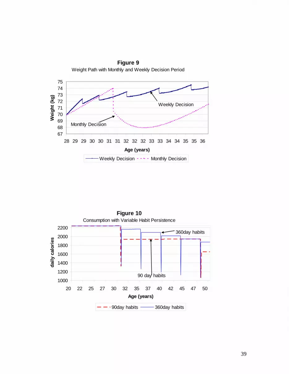
Figure 9Weight Path with Monthly and Weekly Decision Period

676869707172737475

28 29 29 30 30 31 31 32 32 32 33 33 34 34 35 35 36

Age (years)

Wei

ght (

kg)

Weekly Decision Monthly Decision

Weekly Decision

Monthly Decision

Figure 10Consumption with Variable Habit Persistence

1000

1200

1400

1600

1800

2000

2200

20 22 25 27 30 32 35 37 40 42 45 47 50Age (years)

daily

cal

orie

s

90day habits 360day habits

360day habits

90 day habits

39

Figure 11Weight Path with Variable Habit Persistence

55

60

65

70

75

80

20 22 25 27 30 32 35 37 40 42 45 47 50

Age (years)

daily

cal

orie

s

90day habits 180day habits 360day habits

360day habits

90day habits180day habits

40

Documents

A behavioral model of cyclical dieting