Capital-Labor Substitution, Equilibrium Indeterminacy, andthe Cyclical Behavior of Labor Income�

Jang-Ting GuoUniversity of California, Riversidey

Kevin J. LansingFederal Reserve Bank of San Franciscoz

April 3, 2008

Abstract

This paper examines the quantitative relationship between the elasticity of capital-laborsubstitution and the conditions needed for equilibrium indeterminacy (and belief-driven�uctuations) in a one-sector growth model. Our analysis employs a �normalized�version ofthe CES production function so that all steady-state allocations and factor income sharesare held constant as the elasticity of substitution is varied. We demonstrate numericallythat higher elasticities cause the threshold degree of increasing returns for indeterminacy todecline monotonically, albeit very gradually. When the elasticity of substitution is unity(the Cobb-Douglas case), our model requires increasing returns to scale of around 1.08for indeterminacy. When the elasticity of substitution is raised to 5, which far exceedsany empirical estimate, the threshold degree of increasing returns reduces to around 1.05.We also demonstrate analytically that labor�s share of income becomes pro-cyclical as theelasticity of substitution increases above unity, whereas labor�s share in postwar U.S. datais countercyclical. This observation, together with other empirical evidence, indicates thatthe elasticity of capital-labor substitution in the U.S. economy is actually below unity.

Keywords: Capital-Labor Substitution, Equilibrium Indeterminacy, Capital Utilization,Real Business Cycles, Labor Income.

JEL Classi�cation: E30, E32.

�For helpful comments and suggestions, we thank Russell Cooper, John Fernald, David Stockman andparticipants at the 2008 Annual Symposium of the Society for Nonlinear Dynamics and Econometrics. Part ofthis research was conducted while Guo was a visiting research fellow of economics at Academia Sinica, Taipei,Taiwan, whose hospitality is greatly appreciated. Of course, all remaining errors are our own.

y Corresponding author. Department of Economics, 4128 Sproul Hall, University of California, Riverside,CA, 92521-0427, U.S.A., Phone: (951) 827-1588, Fax: (951) 827-5685, E-mail: guojt@ucr.edu

zResearch Department, Federal Reserve Bank of San Francisco, P.O. Box 7702, San Francisco, CA 94120-7702, U.S.A., Phone: (415) 974-2393, Fax: (415) 977-4031, E-mail: kevin.j.lansing@sf.frb.org

1 Introduction

It is well-known that the elasticity of substitution between capital and labor in production can

have an important in�uence on transition dynamics in the standard one-sector growth model.1

One would therefore expect this elasticity to also a¤ect the characteristics of �uctuations near

the model�s steady state. Speci�cally, rational belief-driven business cycles or �sunspots�can

arise when the steady state of the model is locally indeterminate, i.e., a sink.2 With a few

exceptions, the indeterminacy literature has mostly restricted attention to a Cobb-Douglas

production technology that exhibits a unitary elasticity of substitution between capital and

labor. A Cobb-Douglas speci�cation also implies that factor income shares are constant over

the business cycle. In contrast, labor�s share of income in U.S. postwar data is countercyclical

while capital�s share is procyclical.

This paper examines two closely-related issues. First, we examine the quantitative relation-

ship between the elasticity of capital-labor substitution and the threshold degree of increasing

returns for local indeterminacy (and belief-driven �uctuations) within a one-sector growth

model. Second, we examine the link between the elasticity of capital-labor substitution and

the cyclical properties of the factor income shares. Following Klump and de La Grandville

(2000) and Klump and Preissler (2000), we employ a �normalized� version of the standard

CES production function so that all steady-state allocations and factor income shares are held

constant as the elasticity of capital-labor substitution is changed. The normalization procedure

identi�es a family of constant-elasticity-of-substitution (CES) production functions that are

distinguished only by the elasticity parameter, and not by the steady-state allocations which

are used to approximate the model�s local dynamics. In practical terms, the normalization

procedure amounts to recalibrating the model to �match the facts� each time the elasticity

parameter is varied. Klump and Saam (2006) emphasize that normalization is necessary to

avoid �arbitrary and inconsistent results.�

The framework for our analysis is an extended version of the one-sector real business cycle

model of Guo and Lansing (2007) that includes variable capital utilization and endogenous

maintenance expenditures. In the present paper, we demonstrate numerically that higher

elasticities of substitution cause the threshold degree of increasing returns for equilibrium

indeterminacy to decline monotonically, albeit very gradually. When the elasticity of sub-

stitution is unity (the Cobb-Douglas case considered by Guo and Lansing, 2007), the model

requires increasing returns-to-scale of around 1.08 for equilibrium indeterminacy. When the

1See, for example, Barro and Sala-i-Martin (1995, p. 45), Klump and de La Grandville (2000), Klump andPreissler (2000), Turnovsky (2002), and Smetters (2003), among others.

2See Benhabib and Farmer (1999) for a survey of this literature.

1

elasticity of substitution is raised to 5, which far exceeds any empirical estimate, the threshold

degree of increasing returns reduces to around 1.05. Intuitively, a higher elasticity of capital-

labor substitution makes indeterminacy easier to obtain because it allows equilibrium labor

hours to respond more freely to belief shocks, rather than being tightly coupled to utilized

capital which responds more sluggishly.

Our results are qualitatively consistent with those of Pintus (2006) who also shows that

higher elasticities of substitution can reduce the minimum degree of increasing returns needed

for local indeterminacy in a one-sector growth model. Our results are quantitatively di¤erent

because: (1) we allow for variable capital utilization along the lines of Wen (1998), and (2)

unlike Pintus (2006), we require the curvature of the agent�s separable utility function to be

consistent with balanced long-run growth.3 Both features are known to be important for

in�uencing the threshold degree of increasing returns in this class of models. The details of

the numerical computations are important, in our view, for assessing the quantitative impact

of capital-labor substitution in a particular model, in order to gauge whether the threshold

degree of increasing returns for indeterminacy lies within the range of empirical plausibility

(see Basu and Fernald, 1997).

We demonstrate analytically that one can infer useful information about the elasticity of

capital-labor substitution by examining the cyclical properties of the factor income shares. In

our model, movements in the labor income share over the business cycle are linked directly

to movements in the ratio of labor hours to utilized capital. Labor hours in the model are

more volatile than utilized capital in response to shocks. A positive belief shock will therefore

raise the ratio of labor hours to utilized capital while output increases. When the elasticity

of substitution exceeds unity, a higher ratio of labor hours to utilized capital causes labor�s

share to become pro-cyclical, whereas labor�s share in U.S. data is countercyclical. It follows

that in order to match the cyclical behavior of labor�s share in the data, the model requires

the elasticity of substitution to be below unity.

Direct empirical estimates also indicate that the elasticity of capital-labor substitution in

the U.S. economy is below unity. Using time series data for the period 1953 to 1998, Klump,

McAdam, and Willman (2007) �nd that the elasticity of substitution is signi�cantly below

unity, with a point estimate of 0.5 to 0.6. A panel data study by Chirinko, Fazzari, and

Meyer (2004) yields a precisely-estimated elasticity of approximately 0.4. In our model, an

elasticity of 0.4 would push up the threshold degree of increasing returns only slightly� to a

3The numerical examples in Pintus (2006) employ a utility function that is close to risk-neutral in consump-tion, with coe¢ cients of relative risk aversion that range from 0.04 to 0.15. In our model, the coe¢ cient ofrelative risk aversion for consumption is 1.0, corresponding to the logarithmic case.

2

value around 1.09.

Finally, we note that other types of growth models can become more susceptible to local or

global indeterminacy when the elasticity of capital-labor substitution is below unity, as appears

to be the case for the U.S. economy. Examples include the �nance-constrained (capitalist-

worker) model of Grandmont, Pintus, and de Vilder (1998), and the multisector growth model

of Nishimura and Venditti (2004). Another recent example is the one-sector growth model of

Wong and Yip (2007) where the elasticity of substitution is not a parameter, but rather is

assumed to be a decreasing linear function of the economy�s aggregate capital-labor ratio.

The remainder of the paper is organized as follows. Section 2 describes the model. Section

3 examines the model�s local dynamics and presents some quantitative analyses. Section 4

studies the cyclical behavior of labor income. Section 5 concludes.

2 The Model

We adopt the basic setup of Guo and Lansing (2007) that allows for: (1) variable capital

utilization along the lines of Wen (1998), and (2) endogenous maintenance activity along the

lines of McGrattan and Schmitz (1999). We depart from the usual assumption of a Cobb-

Douglas production function by introducing a �normalized�version of the standard constant-

elasticity-of-substitution (CES) production function.

2.1 Households

The economy is populated by a unit measure of identical in�nitely-lived households, each

endowed with one unit of time. The representative household maximizes

1Xt=0

�t

"log (ct)�

An1+ t

1 +

#; A > 0; (1)

subject to the budget constraint

ct = wtnt + dt; (2)

where � 2 (0; 1) is the subjective time discount factor, ct is consumption, nt is hours worked, � 0 is the inverse of the intertemporal elasticity of substitution in labor supply, wt is the

real wage, and dt is dividends paid out by the �rm which the household takes as given. The

household�s period utility function in (1) is consistent with balanced long-run growth, a feature

that is commonly maintained in the modern business cycle literature.

The �rst-order condition for the household�s optimization problem is given by

Actn t = wt; (3)

3

which equates the marginal rate of substitution between consumption and leisure to the real

wage.

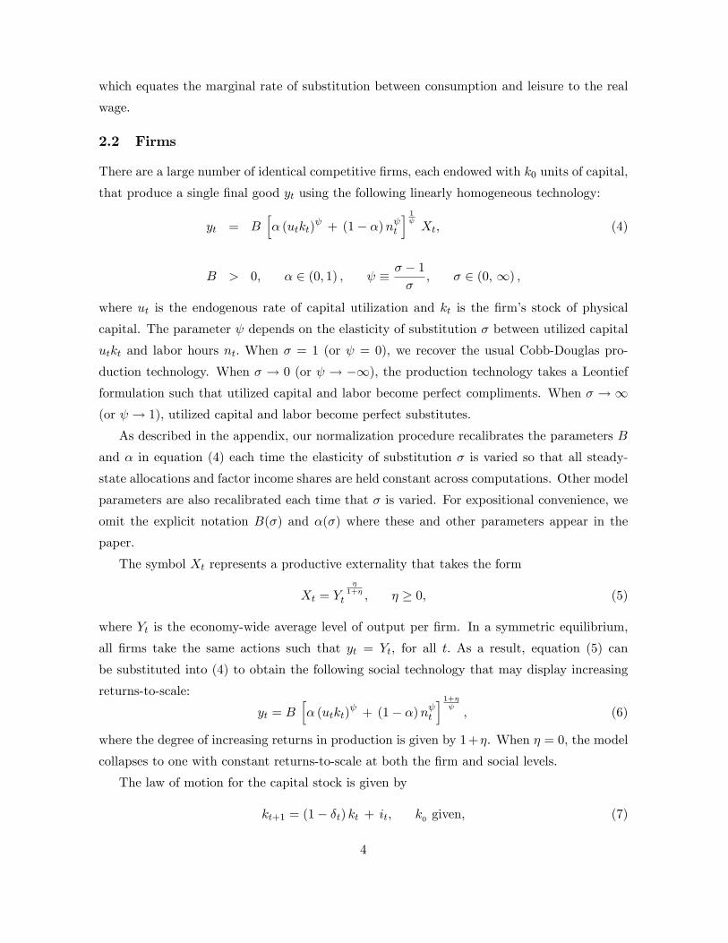
2.2 Firms

There are a large number of identical competitive �rms, each endowed with k0 units of capital,

that produce a single �nal good yt using the following linearly homogeneous technology:

yt = Bh� (utkt)

+ (1� �)n ti 1 Xt; (4)

B > 0; � 2 (0; 1) ; � � � 1�

; � 2 (0; 1) ;

where ut is the endogenous rate of capital utilization and kt is the �rm�s stock of physical

capital. The parameter depends on the elasticity of substitution � between utilized capital

utkt and labor hours nt: When � = 1 (or = 0), we recover the usual Cobb-Douglas pro-

duction technology. When � ! 0 (or ! �1), the production technology takes a Leontiefformulation such that utilized capital and labor become perfect compliments. When � ! 1(or ! 1), utilized capital and labor become perfect substitutes.

As described in the appendix, our normalization procedure recalibrates the parameters B

and � in equation (4) each time the elasticity of substitution � is varied so that all steady-

state allocations and factor income shares are held constant across computations. Other model

parameters are also recalibrated each time that � is varied. For expositional convenience, we

omit the explicit notation B(�) and �(�) where these and other parameters appear in the

paper.

The symbol Xt represents a productive externality that takes the form

Xt = Y�

1+�

t ; � � 0; (5)

where Yt is the economy-wide average level of output per �rm. In a symmetric equilibrium,

all �rms take the same actions such that yt = Yt, for all t: As a result, equation (5) can

be substituted into (4) to obtain the following social technology that may display increasing

returns-to-scale:

yt = Bh� (utkt)

+ (1� �)n ti 1+�

; (6)

where the degree of increasing returns in production is given by 1+�. When � = 0, the model

collapses to one with constant returns-to-scale at both the �rm and social levels.

The law of motion for the capital stock is given by

kt+1 = (1� �t) kt + it; k0 given, (7)

4

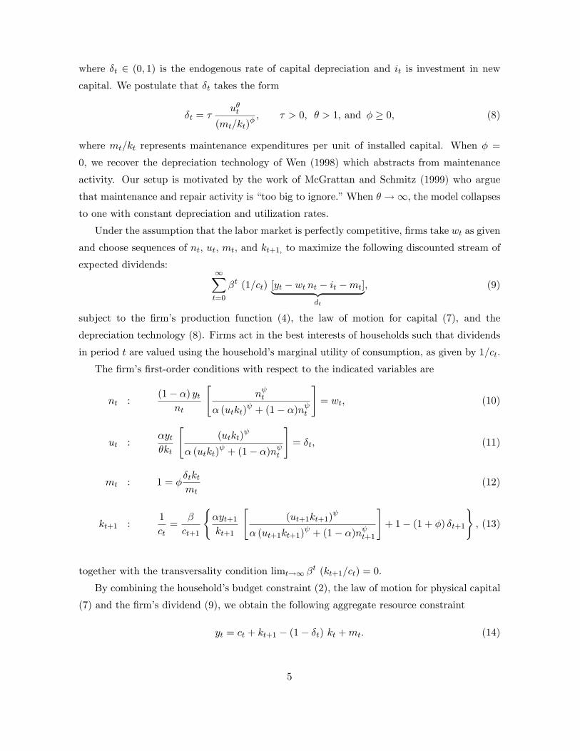
where �t 2 (0; 1) is the endogenous rate of capital depreciation and it is investment in newcapital. We postulate that �t takes the form

�t = �u�t

(mt=kt)�; � > 0; � > 1; and � � 0; (8)

where mt=kt represents maintenance expenditures per unit of installed capital. When � =

0, we recover the depreciation technology of Wen (1998) which abstracts from maintenance

activity. Our setup is motivated by the work of McGrattan and Schmitz (1999) who argue

that maintenance and repair activity is �too big to ignore.�When � !1; the model collapsesto one with constant depreciation and utilization rates.

Under the assumption that the labor market is perfectly competitive, �rms take wt as given

and choose sequences of nt; ut; mt; and kt+1; to maximize the following discounted stream of

expected dividends:1Xt=0

�t (1=ct) [yt � wt nt � it �mt]| {z }dt

; (9)

subject to the �rm�s production function (4), the law of motion for capital (7), and the

depreciation technology (8). Firms act in the best interests of households such that dividends

in period t are valued using the household�s marginal utility of consumption, as given by 1=ct:

The �rm�s �rst-order conditions with respect to the indicated variables are

nt :(1� �) yt

nt

"n t

� (utkt) + (1� �)n t

#= wt; (10)

ut :�yt�kt

"(utkt)

� (utkt) + (1� �)n t

#= �t; (11)

mt : 1 = ��tktmt

(12)

kt+1 :1

ct=

�

ct+1

(�yt+1kt+1

"(ut+1kt+1)

� (ut+1kt+1) + (1� �)n t+1

#+ 1� (1 + �) �t+1

); (13)

together with the transversality condition limt!1 �t (kt+1=ct) = 0.

By combining the household�s budget constraint (2), the law of motion for physical capital

(7) and the �rm�s dividend (9), we obtain the following aggregate resource constraint

yt = ct + kt+1 � (1� �t) kt +mt: (14)

5

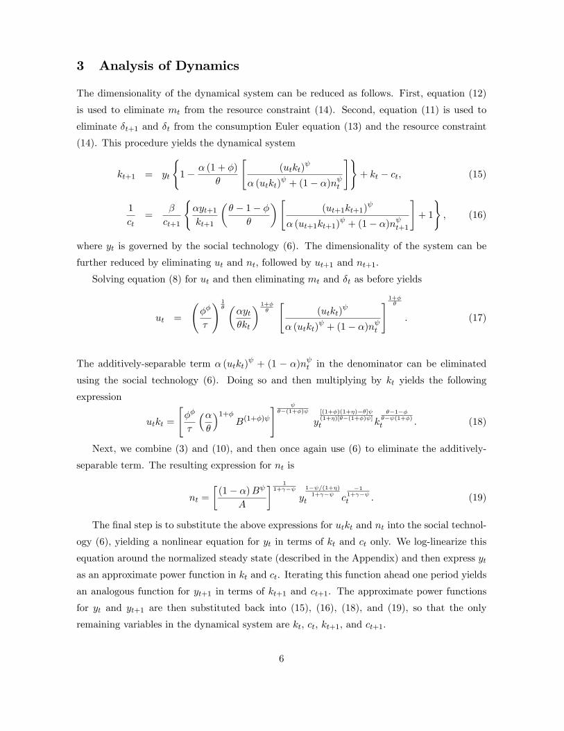
3 Analysis of Dynamics

The dimensionality of the dynamical system can be reduced as follows. First, equation (12)

is used to eliminate mt from the resource constraint (14). Second, equation (11) is used to

eliminate �t+1 and �t from the consumption Euler equation (13) and the resource constraint

(14). This procedure yields the dynamical system

kt+1 = yt

(1� � (1 + �)

�

"(utkt)

� (utkt) + (1� �)n t

#)+ kt � ct; (15)

1

ct=

�

ct+1

(�yt+1kt+1

�� � 1� �

�

�"(ut+1kt+1)

� (ut+1kt+1) + (1� �)n t+1

#+ 1

); (16)

where yt is governed by the social technology (6). The dimensionality of the system can be

further reduced by eliminating ut and nt, followed by ut+1 and nt+1:

Solving equation (8) for ut and then eliminating mt and �t as before yields

ut =

��

�

! 1� ��yt

�kt

� 1+��

"(utkt)

� (utkt) + (1� �)n t

# 1+��: (17)

The additively-separable term � (utkt) + (1 � �)n t in the denominator can be eliminated

using the social technology (6). Doing so and then multiplying by kt yields the following

expression

utkt =

"��

�

���

�1+�B(1+�)

# ��(1+�)

y[(1+�)(1+�)��] (1+�)[��(1+�) ]t k

��1���� (1+�)t : (18)

Next, we combine (3) and (10), and then once again use (6) to eliminate the additively-

separable term. The resulting expression for nt is

nt =

�(1� �)B

A

� 11+ �

y1� =(1+�)1+ �

t c�1

1+ � t : (19)

The �nal step is to substitute the above expressions for utkt and nt into the social technol-

ogy (6), yielding a nonlinear equation for yt in terms of kt and ct only. We log-linearize this

equation around the normalized steady state (described in the Appendix) and then express yt

as an approximate power function in kt and ct. Iterating this function ahead one period yields

an analogous function for yt+1 in terms of kt+1 and ct+1. The approximate power functions

for yt and yt+1 are then substituted back into (15), (16), (18), and (19), so that the only

remaining variables in the dynamical system are kt; ct; kt+1, and ct+1:

6

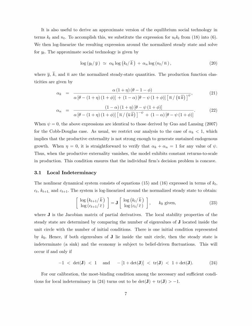
It is also useful to derive an approximate version of the equilibrium social technology in

terms kt and nt. To accomplish this, we substitute the expression for utkt from (18) into (6).

We then log-linearize the resulting expression around the normalized steady state and solve

for yt: The approximate social technology is given by

log (yt= y ) ' �k log�kt= k

�+ �n log (nt= n ) ; (20)

where y; k; and n are the normalized steady-state quantities. The production function elas-

ticities are given by

�k =� (1 + �) (� � 1� �)

� [� � (1 + �) (1 + �)] + (1� �) [� � (1 + �)]�n =�u k� � ; (21)

�n =(1� �) (1 + �) [� � (1 + �)]

� [� � (1 + �) (1 + �)]�n =�u k� ��

+ (1� �) [� � (1 + �)]: (22)

When = 0; the above expressions are identical to those derived by Guo and Lansing (2007)

for the Cobb-Douglas case. As usual, we restrict our analysis to the case of �k < 1; which

implies that the productive externality is not strong enough to generate sustained endogenous

growth. When � = 0; it is straightforward to verify that �k + �n = 1 for any value of :

Thus, when the productive externality vanishes, the model exhibits constant returns-to-scale

in production. This condition ensures that the individual �rm�s decision problem is concave.

3.1 Local Indeterminacy

The nonlinear dynamical system consists of equations (15) and (16) expressed in terms of kt;

ct; kt+1; and ct+1: The system is log-linearized around the normalized steady state to obtain:�log�kt+1= k

�log (ct+1= c )

�= J

�log�kt= k

�log (ct= c )

�; k0 given, (23)

where J is the Jacobian matrix of partial derivatives. The local stability properties of the

steady state are determined by comparing the number of eigenvalues of J located inside the

unit circle with the number of initial conditions. There is one initial condition represented

by k0: Hence, if both eigenvalues of J lie inside the unit circle, then the steady state is

indeterminate (a sink) and the economy is subject to belief-driven �uctuations. This will

occur if and only if

�1 < det(J) < 1 and � [1 + det(J)] < tr(J) < 1 + det(J). (24)

For our calibration, the most-binding condition among the necessary and su¢ cient condi-

tions for local indeterminacy in (24) turns out to be det(J) + tr(J) > �1:

7

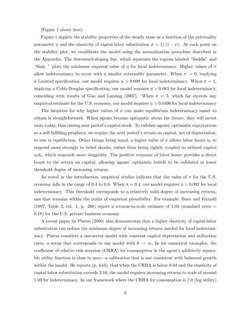
[Figure 1 about here].

Figure 1 depicts the stability properties of the steady state as a function of the externality

parameter � and the elasticity of captal-labor substitution � = 1= (1� ) : At each point onthe stability plot, we recalibrate the model using the normalization procedure described in

the Appendix. The downward-sloping line, which separates the regions labeled �Saddle�and

�Sink, � plots the minimum required value of � for local indeterminacy. Higher values of �

allow indeterminacy to occur with a smaller externality parameter. When � ! 0; implying

a Leontief speci�cation, our model requires � > 0:099 for local indeterminacy. When � = 1;

implying a Cobb-Douglas speci�cation, our model requires � > 0:083 for local indeterminacy,

coinciding with results of Guo and Lansing (2007). When � = 5; which far exceeds any

empirical estimate for the U.S. economy, our model requires � > 0:0496 for local indeterminacy

The intuition for why higher values of � can make equilibrium indeterminacy easier to

obtain is straightforward. When agents become optimistic about the future, they will invest

more today, thus raising next period�s capital stock. To validate agents�optimistic expectations

as a self-ful�lling prophecy, we require the next period�s return on capital, net of depreciation,

to rise in equilibrium. Other things being equal, a higher value of � allows labor hours nt to

respond more strongly to belief shocks, rather than being tightly coupled to utilized capital

utkt; which responds more sluggishly. The positive response of labor hours provides a direct

boost to the return on capital, allowing agents� optimistic beliefs to be validated at lower

threshold degree of increasing returns.

As noted in the introduction, empirical studies indicate that the value of � for the U.S.

economy falls in the range of 0.4 to 0.6. When � = 0:4; our model requires � > 0:092 for local

indeterminacy. This threshold corresponds to a relatively mild degree of increasing returns,

one that remains within the realm of empirical plausibility. For example, Basu and Fernald

(1997, Table 3, col. 1, p. 268) report a returns-to-scale estimate of 1.03 (standard error =

0.18) for the U.S. private business economy.

A recent paper by Pintus (2006) also demonstrates that a higher elasticity of captal-labor

substitution can reduce the minimum degree of increasing returns needed for local indetermi-

nacy. Pintus considers a one-sector model with constant capital depreciation and utilization

rates, a setup that corresponds to our model with � ! 1: In his numerical examples, thecoe¢ cient of relative risk aversion (CRRA) for consumption in the agent�s additively separa-

ble utility function is close to zero� a calibration that is not consistent with balanced growth

within the model. He reports (p. 643), that when the CRRA is below 0.04 and the elasticity of

captal-labor substitution exceeds 2.16, the model requires increasing returns to scale of around

1.03 for indeterminacy. In our framework where the CRRA for consumption is 1.0 (log utility)

8

and � = 2:16; the threshold degree of increasing returns for indeterminacy is around 1.07.

Given that our model has variable capital utilization (which, all else equal, makes it easier

to obtain indeterminacy) while Pintus�model does not, the lower threshold for indeterminacy

in Pintus�numerical examples can be traced to the assumption of very low curvature in the

utility of consumption. The near-zero risk coe¢ cient implies a very low welfare loss from

belief-driven cycles, making these cycles more likely to occur in an optimizing framework. For

any given level of risk aversion, a higher elasticity of capital-labor substitution reduces the

curvature of the �rm�s isoquants, which also makes belief-driven cycles more likely to occur.

Our results are thus qualitatively consistent with those of Pintus (2006).

4 Cyclical Behavior of Labor�s Share of Income

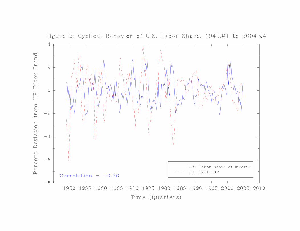
Figure 2 plots the cyclical component of labor�s share of income in U.S. data together with

the cyclical component of real GDP for the period 1949.Q1 to 2004.Q4.4 The correlation

coe¢ cient between the two series is �0:26, indicating that labor�s share of income movescountercyclically.

[Figure 2 about here]

In the model, labor�s share of income is given by

wtntyt

=(1� �)

� [nt = (utkt)]� + (1� �)

; (25)

which is obtained by rearranging the �rm�s �rst-order condition (10). The above expression

shows that movements in labor�s share over the business cycle are linked directly to movements

in the ratio nt= (utkt) :

For our calibration with indivisible labor ( = 0) ; labor hours nt are more volatile than

utilized capital utkt in response to shocks. A positive belief shock will therefore raise the ratio

nt= (utkt) while output yt increases. When � > 1; we have > 0 such that labor�s share

moves in the same direction as the ratio nt= (utkt) and hence is pro-cyclical. A countercyclical

labor share requires wtnt=yt to move in the opposite direction as the ratio nt= (utkt) : This

condition is achieved when � < 1 such that < 0: Intuitively, an elasticity of capital-labor

substitution below unity ties labor more closely to utilized capital, thus hindering labor hours

from responding as freely to positive shocks in order to generate more income.

Gomme and Greenwood (1995) and Boldrin and Horvath (1995) also document the coun-

tercyclical movement of labor�s share of income in U.S. data. Both papers develop models4Data on Labor�s share of income is from http://www.bls.gov/data, using series ID PRS85006173. Data on

real GDP is from http://research.stlouisfed.org/fred2/series/GDPC96. The cyclical components are obtainedby detrending each series with the Hodrick-Prescott �lter, using a smoothing parameter of 1600.

9

where labor contracts between workers and �rms can break the direct link between the real

wage and the marginal product of labor. The labor contracts can generate a countercyclical

labor share even when the elasticity of capital-labor substitution is unity (the Cobb-Douglas

case).

5 Conclusion

This paper highlights the quantitative link between the elasticity of capital-labor substitu-

tion and the required conditions for equilibrium indeterminacy in a one-sector growth model

developed by Guo and Lansing (2007). Under the maintained assumption of balanced long-

run growth, we show that higher elasticities cause the minimum degree of increasing returns

needed for indeterminacy and sunspots to decline monotonically, albeit very gradually. More-

over, we show that when the elasticity of substitution exceeds unity, the model�s labor share of

national income becomes procyclical, which is inconsistent with the postwar U.S. data. This

observation, together with other empirical evidence, indicates that the elasticity of capital-

labor substitution in the U.S. economy is actually below unity. In our model, a below-unity

value for the elasticity of capital-labor substitution pushes up the threshold degree of increas-

ing returns for indeterminacy only slightly relative to the Cobb-Douglas case, such that the

threshold remains empirically plausibile.

10

A Appendix: Normalization Procedure

The normalized steady state quantities are denoted by n; �; k; y; c; u; and m: As the elasticity

of capital-labor substitution � is varied, the normalized quantities are held constant by the

appropriate choice of parameters. The reference point that de�nes the normalized quantities

is the Cobb-Douglas case with � = 1 (or = 0) and B = 1. Following Guo and Lansing

(2007), straightforward computations yield:

n =

�1� �

A�A� (1 + �) =�

� 11+

; (A.1)

� =�

� � 1� �; (A.2)

k =�b �n�n =

�� ��� 1

1��k ; (A.3)

y = b k�k n�n ; (A.4)

c = [1� � (1 + �) =�] y; (A.5)

u =

"�� �

1+�

�

# 1�

; (A.6)

m =

���

�

�y; (A.7)

where � � 1=��1 is the rate of time preference, and � = 0:3 such that labor�s share of income1� �� is 0.70 for the Cobb-Douglas case. In addition, we de�ne the following combinations ofparameters for the Cobb-Douglas case:

b �"��

�

��

�

�1+� # _�(1+�)

��_�(1+�)(1+�)

; (A.8)

�k � � (1 + �) (� � 1� �)� � � (1 + �) (1 + �) ; (A.9)

�n � (1� �) (1 + �) �� � � (1 + �) (1 + �) : (A.10)

11

Given a value for the externality parameter �; the elasticity of substitution � is varied

over a wide range of values. For all computations, we set � = 0:99 to obtain a quarterly real

interest rate of 1 percent and = 0 to re�ect �indivisible labor�. The constant � a¤ects no

result, so we set � = 1:

As � takes on di¤erent values, the parameters �; �; and A are set to maintain the following

calibration targets used by Guo and Lansing (2007): m=y = 0:061; � = 0:025; and n = 0:3:

The remaining parameters for the general CES speci�cation are � and B: As � is varied,

the parameter � is set to maintain the steady-state labor�s income share at 0:7; while the

parameter B is set to maintain the steady-state output level equal to the Cobb-Douglas value

y: In this way, all steady state quantities are maintained at the corresponding Cobb-Douglas

values.

The normalization procedure can be summarized by the following calibration formulas

� = m=�� k�; (A.11)

� = 1 + �+ �= �; (A.12)

� =�

�+ (1� �)�uk=n

� (A.13)

B =y

11+��

��uk� + (1� �) n

� 1

(A.14)

A =(1� �)B y

� 1+�

�1�m=y � � k = y

��1n 1+ �

; (A.15)

where = (� � 1) =�; � = 0:3; and m; �; k; n; and y; are the steady-state quantities from the

Cobb-Douglas case.

12

References[1] Barro, R.J. and X. Sala-i-Martin (1995) Economic Growth. New York: McGraw Hill.

[2] Basu, S., and J. G. Fernald (1997), �Returns to scale in U.S. production: Estimates andimplications,�Journal of Political Economy 105, 249-283.

[3] Benhabib, J. and R.E.A. Farmer (1999), �Indeterminacy and sunspots in macroeco-nomics,�Handbook of Macroeconomics. J. Taylor and M. Woodford, eds. North Holland:Amsterdam, 387-448.

[4] Boldrin, M. and M. Horvath. (1995) �Labor contracts and business cycles,� Journal ofPolitical Economy, 103, 972-1004.

[5] Chirinko, R.S., S.M. Fazzari, and A.P. Meyer (2004) �That elusive elasticity: A long-panel approach to estimating the capital-labor substitution elasticity,�CESifo WorkingPaper No. 1240.

[6] Gomme, P. and J. Greenwood. (1995) �On the cyclical allocation of risk,� Journal ofEconomic Dynamics and Control, 19, 91-124.

[7] Grandmont, J.-M., P.A. Pintus, and R. de Vilder (1998) �Capital-labor substitution andcompetitive nonlinear endogenous business cycles.�Journal of Economic Theory 80, 14-59.

[8] Guo, J.-T. and K. J. Lansing (2007) �Maintenance expenditures and indeterminacy underincreasing returns to scale,�International Journal of Economic Theory 3, 147-158.

[9] Klump, R. and O. de La Grandville (2000) �Economic growth and the elasticity of substi-tution: Two theorems and some suggestions,�American Economic Review 90, 282-291.

[10] Klump, R. and H. Preissler (2000) �CES production functions and economic growth,�Scandinavian Journal of Economics 102, 41-56.

[11] Klump, R. and M. Saam (2006) �Calibration of normalized CES production functions indynamic models,�Centre for European Economic Research, Discussion Paper No. 06-078.

[12] Klump, R., P. McAdam, and A. Willman (2007) �Factor substitution and factor-augmenting technical progress in the United States: a normalized supply-side systemapproach,�Review of Economics and Statistics, 89, 183-192.

[13] McGrattan, E. R., and J. A. Schmitz, Jr. (1999), �Maintenance and repair: Too big toignore,�Federal Reserve Bank of Minneapolis Quarterly Review 23 (4), 2-13.

[14] Nishimura, K. and A. Venditti (2004) �Indeterminacy and the role of factor substitutabil-ity,�Macroeconomic Dynamics, 8, 438-465.

[15] Pintus, P.A. �Indeterminacy with almost constant returns to scale: capital-labor subti-tution matters,�Economic Theory, 28, 633-649.

[16] Smetters, K. (2003) �The (interesting) dynamic properties of the neoclassical growthmodel with CES production,�Review of Economic Dynamics, 6, 697-707.

[17] Turnovsky, S.J. (2002) �Intertemporal and intratemporal substitution, and the speedof convergence in the neoclassical growth model,� Journal of Economic Dynamics andControl, 26, 1765-1785.

[18] Wen, Y. (1998), �Capacity Utilization under Increasing Returns to Scale,� Journal ofEconomic Theory 81, 7-36.

13

[19] Wong, T.-N. amd C.K. Yip. (2007) �Indeterminacy and the elasticity of subsitutition inone-sector models,�Working Paper.

14