The lucky country? Life satisfaction in Australia 2001-2010

Christopher L. Ambrey and Christopher M. Fleming

No. 2012-09

Series Editor: Associate Professor Fabrizio Carmignani

Copyright © 2012 by the author(s). No part of this paper may be reproduced in any form, or stored in a retrieval system, without prior permission of the author(s).

2

The lucky country? Life satisfaction in Australia 2001-2010

Christopher L. Ambrey and Christopher M. Fleming1

Department of Accounting, Finance and Economics, Griffith Business School

Abstract Employing data from the Household, Income and Labour Dynamics in Australia (HILDA) survey, this paper examines the level, determinants and distribution of self-reported life satisfaction, as well as the prevalence and severity of dissatisfaction in Australia over the period 2001-2010. Against most objective measures, Australia’s economic performance during this period was exemplary. Yet our results indicate an overall downward trend in life satisfaction, as well as a diminishing gap between the life satisfaction of males and females. Geographic heterogeneity in the distribution of life satisfaction is apparent, and a number of socio-economic and demographic factors are found to serve an important role in determining an individual’s level of life satisfaction. Results also suggest that inequality in life satisfaction has generally declined. Measures of the extent of dissatisfaction reveal an encouraging downward trend and provide policy makers with an alternative perspective from which to assess societal welfare.

Keywords: Happiness; Household, Income and Labour Dynamics in Australia

(HILDA); Inequality; Life Satisfaction

JEL Codes: C23; D63; I31

This paper uses unit record data from the Household, Income and Labour Dynamics in Australia

(HILDA) survey. The HILDA project was initiated and is funded by the Australian Government

Department of Families, Housing, Community Services and Indigenous Affairs (FaHCSIA) and is

managed by the Melbourne Institute of Applied Economic and Social Research (Melbourne Institute).

The findings and views reported in this paper, however, are those of the authors and should not be

attributed to either FaHCSIA or the Melbourne Institute.

.

1 Corresponding Author: Department of Accounting, Finance and Economics, Nathan Campus, Griffith Business School, QLD 4111, Australia. Email: chris.fleming@griffith.edu.au.

3

“Australia is a lucky country, run mainly by second-rate people who share its luck”

Donald Horne (1964)

1. Introduction Against most objective measures, Australia’s economic performance in the first decade of the twenty-first century was exemplary. For the period 2001 to 2010 the following can be observed: per capita Gross National Income grew by 38.03%, compared to growth of 34.06% in the Euro area, 30.15% in North America and 35.17% for all OECD member states; household final consumption expenditure grew by 35.67%, compared to growth in the Euro area, North America and the OECD of 9.84%, 19.11% and 16.35% respectively; unemployment fell from 6.80% to 5.20%, whereas the Euro area, North America and the OECD experienced increasing unemployment; central government debt fell from 27.31% to 24.09% of Gross Domestic Product (GDP), whereas in the Euro area, North America and the OECD central government debt as a proportion of GDP increased (The World Bank, 2012).2 Furthermore, Australia’s Human Development Index (HDI) score (measured on a scale of 0 to 1) rose from 0.915 in 2001 to 0.937 in 2010, ranking Australia second only to Norway (United Nations Development Programme, 2010).

There remains, however, the question of how well Australia has performed against subjective measures of performance, such as those provided by self-reports of life satisfaction or happiness. These measures have been the focus of much research effort in economics in recent years. Broad reviews are provided by Frey (2008), Frey and Stutzer (2002b), Frey and Stutzer (2002a), and MacKerron (2012).

At a microeconomic level, interest in the economics of happiness is motivated, at least in part, by Richard Easterlin’s (1974, 1995) finding that real income growth in Western countries in the latter half of the twentieth century had not led to corresponding increases in happiness (the ‘Easterlin Paradox’). Consequently, the microeconomic literature devotes a great deal of effort to better understanding the socio-economic and demographic drivers of life satisfaction. Important contributions are provided by Blanchflower and Oswald (2004), Clark et al. (2008), Ferrer-i-Carbonell (2005), Oswald (1997) and van Praag et al. (2003). At a macroeconomic level, interest is drawn from a recognition that traditional (i.e. objective) means of measuring economic performance, such as Gross National Income or GDP, are deficient and that alternative measures should be sought; measures that focus on the well-being of current and future generations (Easterlin, 2010; Stiglitz et al., 2009). The literature provides evidence that conventional indicators such as national income, inflation, unemployment, and income inequality often, but not always, influence a 2 Gross National Income growth rates are calculated from figures converted to international dollars using purchasing power parity rates. Household final consumption expenditure is measured in constant 2000 USD. For further information see http://data.worldbank.org/?display=default.

4

nation’s average level of life satisfaction. Important contributions are provided by Alesina et al. (2004), Di Tella et al. (2001), Di Tella et al. (2003) and Welsch (2007).

Inequality in the distribution of life satisfaction has received some attention. Veenhoven (2005) reports that higher levels of life satisfaction are typically associated with less inequality in life satisfaction. Evidence on the effect of income inequality on inequality in life satisfaction is mixed; Delhey and Kohler (2011) find that higher income inequality leads to greater inequality in life satisfaction, whereas Stevenson and Wolfers (2008) show that, in the United States at least, inequality in happiness is falling as income inequality increases.

The issue of whether Australia’s strong performance against objective measures translates into comparably high levels of happiness has been raised before. Employing data from the 2002 International Social Survey Programme (ISSP), Blanchflower and Oswald (2005) compare Australia’s third placed ranking in the 2004 HDI against average responses to questions about general life satisfaction, satisfaction with family life, job satisfaction and tiredness. The authors conclude that Australia represents a paradox, performing only respectably in four categories of ‘happiness’ and poorly in one (job satisfaction). This conclusion is challenged by Leigh and Wolfers (2006) who, utilising a combination of ISSP and World Values Survey data, find that Australia appears happier, not sadder, than its HDI score would predict.

This paper takes an alternative approach. Rather than using cross-sectional data to make an international comparison, longitudinal data is used to present evidence on self-reported life satisfaction in Australia over time. The paper is relatively unique in that attention is paid to the level, determinants and distribution of life satisfaction, as well as the prevalence and severity of dissatisfaction. The paper proceeds as follows. Data is described in Section 2. Section 3 presents analyses and results. Section 4 discusses and concludes.

2. Data The measure of self-reported life satisfaction and various socio-economic, geographic and demographic characteristics of respondents are obtained from Waves 1-10 of the Household, Income and Labour Dynamics in Australia (HILDA) survey. First conducted in 2001, by international standards the HILDA survey is a relatively new nationally representative sample and owes much to other household panel studies conducted elsewhere in the world; particularly the German Socio-Economic Panel and the British Household Panel Survey.

The HILDA survey was conceived by the Australian Government Department of Families, Housing, Community Services and Indigenous Affairs (FaHCSIA) and was developed with the aim of supporting research and policy questions within the areas of family and household dynamics, income and welfare dynamics, and labour market dynamics. The survey takes as its sampling unit Australian households occupying

5

private dwellings and is undertaken annually through a combination of face-to-face interviews and self-completion questionnaires with individuals over 15 years of age (Watson and Wooden, 2002). As with all panel datasets, the HILDA dataset is faced with limitations including non-response, on which HILDA compares favourably to the British Household Panel Survey (Watson and Wooden, 2004a) and attrition, for which it is difficult to avoid the conclusion that the potential for bias exists (Watson and Wooden, 2004b). Watson and Wooden (2010) provide a review of progress and future developments of the HILDA survey.

The life satisfaction variable is obtained from individuals’ responses to the question: ‘All things considered, how satisfied are you with your life?’ The life satisfaction variable is ordinal, the individual choosing a number between 0 (totally dissatisfied with life) and 10 (totally satisfied with life). Presenting data from the most recent (2010) wave only, Figure 1 illustrates the distribution of responses.

Figure 1: Life satisfaction scores (2010)

Source: Derived from HILDA

Figure 2 illustrates geographical disparity in the distribution of life satisfaction. Using data from the 2010 wave and disaggregating by statistical division,3 mean life satisfaction scores range from 7.4520 for South Eastern, a region in the eastern part of the State of Western Australia, to 8.4530 for Wimmera, a region in the western part of the State of Victoria. Consistent with previous findings in Australia and elsewhere (cf.

3 A statistical division is an Australian Standard Geographical Classification defined area. Statistical divisions represent relatively homogenous regions characterised by identifiable social and economic links between the inhabitants and between the economic units with the region, under the unifying influence of one or more major town or city. Statistical divisions cover, in aggregate, the whole of Australia without gaps or overlaps. They do not cross State or Territory boundaries. Australian Bureau of Statistics, 2011a. Glossary of Statistical Geography Terminology, 2011, Catalogue No. 1217.0.55.001. Available http://www.abs.gov.au/ausstats/abs@.nsf/mf/1217.0.55.001, accessed: 12 April 2012.

010

0020

0030

0040

0050

00Fr

eque

ncy

0 1 2 3 4 5 6 7 8 9 10Life satisfaction

6

Brereton et al., 2008; Shields et al., 2009) residents of capital cities report, on average, lower levels of life satisfaction than those who live outside of capital cities (Adjusted Wald Test Pr > 0.0000). For example, residents of Sydney and Melbourne (Australia’s two largest cities) report mean life satisfaction scores of 7.7738 and 7.7257 respectively (compared to a nation-wide mean of 7.8486). Employing the Australian Bureau of Statistics’ Accessibility/Remoteness Index of Australia, which measures the remoteness of a point based on the physical road distance to the nearest urban centre, we find statistically significant differences (Pr > 0.0000) in absolute levels of life satisfaction between major cities (7.7866), inner regional Australia (7.9588), outer regional Australia (8.0155) and remote or very remote Australia (8.0311).

Figure 2: Mean life satisfaction by statistical division (2010)

Source: Derived from HILDA

As shown in Figure 3, the mean level of self-reported life satisfaction in Australia has declined since 2001. While the absolute change over the period is small (0.0907 on an 11 point scale), it is statistically significant (Pr > 0.0002) and the overall downward

7

trend is clear. This trend, albeit only over a 10-year timeframe, provides yet another example of the Easterlin Paradox (1974, 1995). Figure 3 also reveals that males, on average, have reported lower absolute levels of life satisfaction than females. However, due to female life satisfaction declining at a faster rate than the rate of decline for males, this difference (which remains statistically significant at the five percent level until wave 8 (2008)) disappears in wave 10 (2010).

Figure 3: Mean life satisfaction (2001-2010)

Source: Derived from HILDA

3. Analysis This section presents analyses and results for three key facets of life satisfaction in Australia over the period 2001 to 2010. These are: the socio-economic, geographic and demographic determinants of life satisfaction; the level of inequality in the distribution of life satisfaction; and the prevalence and severity of dissatisfaction.

3.1 Determinants of life satisfaction

The determinants of life satisfaction are identified through the estimation of a life satisfaction function, which takes the form of an indirect utility function for individual i, in location k, at time t, as follows:

Where is a vector of socio-economic, geographic and demographic characteristics, is an individual-specific effect, location effects, and time or year effects. In the micro-econometric life satisfaction function, an individual’s true utility is unobservable; hence self-reported life satisfaction is used as a proxy. Table 1 provides a description of all explanatory variables.

7.8

7.85

7.9

7.95

8M

ean

life

satis

fact

ion

2001 2002 2003 2004 2005 2006 2007 2008 2009 2010Year

Life satisfaction (All) Life satisfaction (Female)Life satisfaction (Male)

8

Table 1: Model variables

Variable name Definition Mean (std. dev.)

% value 1 (DV)

Age Age of respondent in years 44.4277 (17.9426)

Male Respondent is male 46.5% ATSI Respondent is of Aboriginal and/or Torres

Strait Islander origin 1.8%

Immigrant English

Respondent is born in a Main English Speaking country (Main English Speaking countries are: United Kingdom; New Zealand; Canada; USA; Ireland; and South Africa)

10.2%

Immigrant non-English

Respondent is not born in Australia or a Main English Speaking country

10.6%

Poor English Respondent speaks English either not well or not at all

0.8%

Married Respondent is legally married 51.9% De-facto Respondent is in a de-facto relationship 11.8% Separated Respondent is separated 2.8% Divorced Respondent is divorced 6.1% Widow Respondent is a widow 4.9% Number of children

Number of respondent’s own resident children in respondent’s household at least 50% of the time and number of own children who usually live in a non-private dwelling but spend the rest of the time mainly with the respondent

0.7293 (1.1033)

Lone parent Respondent is a lone parent 1.6% Mild health condition

Respondent has a long-term health condition, that is a condition that has lasted or is likely to last for more than six months, and this condition does not limit the type or amount of work the respondent can do

8.1%

Moderate health condition

Respondent has a long-term health condition limiting the amount or type of work that the respondent can do

17.3%

Severe health condition

Respondent has a long-term health condition and cannot work

0.6%

Year 12 Respondent’s highest level of education is Year 12

3.4%

Certificate or Respondent’s highest level of education is 29.8%

9

diploma a certificate or diploma Bachelors degree or higher

Respondent’s highest level of education is a Bachelors degree or higher

21.2%

Employed part-time

Respondent is employed and works less than 35 hours per week

21.3%

Unemployed Respondent is not employed but is looking for work

3.2%

Non-participant Respondent is a non-participant in the labour force, including retirees, those performing home duties, non-working students and individuals less than 15 years old at the end of the last financial year

32.5%

Self employed Respondent is self employed 6.9% Disposable income (ln)

Natural log of household disposable household income

10.8017 (1.1020)

Extraversion Degree of extraversion (scale 1 to 7) 4.4348 (1.0695)

Agreeableness Degree of agreeableness (scale 1 to 7) 5.3735 (0.9332)

Conscientiousness Degree of conscientiousness (scale 1 to 7) 5.0858 (1.0354)

Emotional stability

Degree of emotional stability (scale 1 to 7)

5.1868 (1.0869)

Openness to experience

Degree of openness to experience (scale 1 to 7)

4.2115 (1.0629)

Years at current address

Number of years the respondent has lived at their current address

10.1417 (11.5165)

Others present Someone was present during the interview

37.0%

Inner Respondent resides in inner regional Australia

25.2%

Outer Respondent resides in outer regional Australia

11.4%

Remote Respondent resides in remote Australia, very remote Australia or is migratory

2.0%

Several estimation techniques are employed to provide comparability with existing studies, to enable simple interpretation of marginal effects and to facilitate the investigation of time-invariant factors. The paper employs, pooled ordinary least squares (OLS), pooled individual ordered logit, random and fixed effects estimators, and an individual mean coded conditional logit estimator.

A Breusch and Pagan (1979) Lagrangian multiplier test for random effects suggests that, due to the presence of individual-specific effects, it is not appropriate to pool the

10

observations. Further, a Hausman test4 finds strong statistical evidence against the use of the random effects estimator, even after controlling for time-invariant personality traits (cf. Cobb-Clark and Schurer, 2012); that is, is correlated with suggesting a degree of endogeneity. As the error term is capturing measurement errors as well as unobserved time-invariant individual specific characteristics the validity of results could be questioned. To circumvent these otherwise confounding influences, we employ a fixed effects estimator (Ferrer-i-Carbonell and Frijters, 2004).

It is also important to consider whether life satisfaction self-reports are assumed to be ordinal or cardinal. If assumed to be ordinal, then the coefficients obtained via OLS are biased and inconsistent, and an estimation technique that appreciates the ordinal nature of the data is more appropriate (Hill et al., 2008). In short, for both technical (consistency and efficiency) and theoretical (preserving the ordinal nature of the dependent variable) reasons, the individual mean coded conditional logit model is most appropriate (Geishecker and Riedl, 2010).

In the individual mean coded conditional logit model, the dependent variable is dichotomised into a binary variable related to (self-reported) life satisfaction

; taking the value one if the score of the response variable is greater than the individual specific mean (average for the individual over time) and zero otherwise, as shown below:

In order to examine the life satisfaction effects of these time-invariant variables, we complement the individual mean coded conditional logit results with discussion of results from the pooled ordered logit model. Within the pooled model we include direct controls for Saucier’s (1994) ‘Big Five’ personality traits (extraversion, agreeableness, conscientiousness, emotional stability, and openness to experience). Results for both models are presented in Table 2. Additional model results are provided as an Appendix.

4 We take advantage of Mark Schaffer and Steven Stillman’s Stata user written command xtoverid. This is downloadable from the Statistical Software Components Archive using the Stata command "ssc install xtoverid".

11

Table 2: Model results

Variable name Individual Mean Coded

Conditional Logit estimate (standard error)

Pooled Ordered Logit estimate (standard error)

Age -0.0702*** (0.0048)

Age squared 0.0004*** (0.0001)

0.0008*** (0.0001)

Male 0.1117*** (0.0242)

ATSI 0.3193*** (0.1319)

Immigrant English 0.0544 (0.0418)

Immigrant non-English

-0.1491*** (0.0462)

Poor English -0.3616*** (0.0121)

-0.5253*** (0.1173)

Married 0.4321*** (0.0659)

0.5042*** (0.0469)

De-facto 0.3701*** (0.0549)

0.3020*** (0.0439)

Separated -0.4083*** (0.0922)

-0.5623*** (0.0773)

Divorced -0.1009 (0.0906)

-0.1293** (0.0649)

Widow -0.1512 (0.1113)

0.1675** (0.0808)

Number of children -0.1219*** (0.0195)

-0.0889*** (0.0138)

Lone parent -0.0594 (0.0753)

-0.0747 (0.0717)

Mild health condition -0.0997*** (0.0309)

-0.2058*** (0.0279)

Moderate health condition

-0.4573*** (0.0322)

-0.8903*** (0.0327)

Severe health condition

-0.6343*** (0.0980)

-1.3139*** (0.1099)

Year 12 0.2367 (0.1543)

0.0322 (0.0618)

Certificate or diploma -0.0557 (0.0631)

-0.1137*** (0.0268)

Bachelors degree or 0.1149 -0.1700***

12

higher (0.0874) (0.0336) Employed part-time 0.1987***

(0.0306) 0.2369***

(0.0255) Unemployed -0.0751

(0.0524) -0.1305** (0.0570)

Non-participant 0.2202*** (0.0373)

0.3153*** (0.0329)

Self employed -0.0375 (0.0475)

-0.0422 (0.0384)

Disposable income (ln) 0.0474*** (0.0090)

0.0806*** (0.0111)

Extraversion 0.1484*** (0.0116)

Agreeableness 0.2391*** (0.0159)

Conscientiousness 0.0976*** (0.0128)

Emotional stability 0.2542*** (0.0141)

Openness to experience

-0.0776*** (0.0146)

Others present 0.0694*** (0.0184)

0.1295*** (0.0180)

Years at current address

-0.0098*** (0.0021)

0.0058*** (0.0013)

Inner 0.1924*** (0.0565)

0.1654*** (0.0344)

Outer 0.0143* (0.0789)

0.3290*** (0.0445)

Remote 0.2052 (0.1755)

0.3745*** (0.0922)

Summary statistics Number of individuals 12428 13412 Number of observations

102463 106013

Likelihood ratio -46958.4320

-170660.4800

Pseudo R2 0.0134 0.0515

*** significant at the 1% level; ** significant at the 5% level; * significant at the 10% level.

Omitted cases are: Female; Not of indigenous origin; Country of birth Australia; Speaks English well or very well; Never married and not defacto; Not a lone parent; Does not have a long-term health condition; Year 11 or below; Not self employed; Employed working 35 hours or more per week; No others present during the interview or don’t know – telephone interview; Major city.

All estimations include wave and State/Territory dummy variables and make use of unbalanced panels. Standard errors adjusted for clustering at the primary sampling unit to account for complex survey design.

13

In regards to the influence of socio-economic and demographic characteristics, our results largely support a priori expectations as well as the existing literature (cf. Blanchflower and Oswald, 2004; Shields et al., 2009). For example, having poor English speaking skills reduces life satisfaction, being married or in a de-facto relationship is found to enhance life satisfaction, whereas being separated is found to have a pronounced negative effect. Dependent children living in a household detracts from an individual’s life satisfaction.

Having a long-term health condition is associated with lower levels of life satisfaction, with the greatest impact felt by those with a severe health condition. In the conditional logit model, no statistically significant relationship is found between level of education and life satisfaction; whereas in the pooled estimation, higher levels of education reduce life satisfaction. We suggest the absence of a statistically significant result in the fixed effects estimation reflects the fact that an individual’s highest level of educational attainment is unlikely to vary greatly over a 10-year period.

Part-time employment or being a non-participant in the labour force (including retirees, those performing home duties and non-working students) is associated with higher levels of life satisfaction than working full-time. Being unemployed (at least in the conditional logit model) has no statistically significant effect on life satisfaction; this may reflect an underrepresentation of the unemployed in the sample (Watson and Wooden, 2004b).

Higher levels of household income are found to be associated with higher levels of life satisfaction, although the income coefficient is likely to be biased downwards due to relative income effects (it is well recognised that people make comparisons with their past income as well as with the income of other people (Clark et al., 2008)). We find evidence of social desirability bias, with others being present during the interview being associated with higher levels of self-reported life satisfaction.

The number of years a respondent has spent at their current address has a negative effect on life satisfaction. The conditional logit model suggests that those living in inner and outer regional areas are more satisfied with their lives than residents of major cities. These results may underestimate the effects, however, as there is far less within-variation than there is between-variation for these variables, particularly for the more remote areas. When looking at the pooled model estimates, the positive effect of living outside of a major city is greater and includes a statistically significant positive effect for living in a remote area.

In regards to the time-invariant variables, pooled estimates suggest that: life satisfaction is U-shaped in age, reaching a minimum at the age of 45; males are more satisfied with their lives than females (in the absence of personality trait controls, the reverse is true); respondents of Aboriginal and/or Torres Strait Islander origin are more satisfied with their lives than the non-indigenous population; and immigrants

14

from non-English speaking countries are less satisfied than the native born, even after controlling for English speaking ability. All personality trait controls take the expected signs (cf. DeNeve and Cooper, 1998) and are statistically significant at the one percent level.

3.2 Inequality in life satisfaction

There is considerable debate in the literature on how best to measure inequality in life satisfaction. Kalmijn and Veenhoven (2005) consider nine measures of inequality and find four (standard deviation, mean absolute difference, mean pair difference, and inter-quartile range) to be suitable. The authors conclude that, as all four measures perform equally well, there is no reason to discontinue using standard deviation (the most common measure employed in the literature at that time).

This position is questioned by Delhey and Kohler (2011), who find fault with the use of ‘raw’ standard deviation and instead advocate the use of an instrument-effect-corrected standard deviation. This measure removes a perceived limitation of raw standard deviation, namely its dependence on the mean level of life satisfaction. Kalmijn (2012) and Veenhoven (2012), however, disagree. Specifically, they reject Delhey and Kohler’s (2011) assumption that life satisfaction is normally distributed and assert that when using life satisfaction data measured on a 10 or 11 point scale (as opposed to on a scale of seven or fewer points) dependency of the standard deviation on the mean only occurs at extreme levels that do not exist in reality. In response, Delhey and Kohler (2012) use an expanded dataset to address Kalmijn (2012) and Veenhoven’s (2012) criticisms, including empirically proving that life satisfaction is normally distributed and demonstrating that dependency on the mean remains a problem, no matter the scale of measurement.

Recognising the unresolved nature of the debate, we employ both measures. The first, the standard deviation , is calculated as follows:

Where is the individual’s self-reported life satisfaction, is the expected value or mean level of life satisfaction, and is the number of individual’s in the sample. The second measure, the instrument-effect-corrected standard deviation, is derived as follows:

Where is the standard deviation of life satisfaction and is an instrument effect (the percent maximum standard deviation) that captures structural dependency.

15

The assumption is made that life satisfaction is measured using limited ratings and is also limited in an unobserved sense, that is, there is a maximum and minimum level of life satisfaction. Consequently, standard deviation of life satisfaction will be limited between 0 and , as shown in Equation 5.

Where and represent the upper and lower bounds of life satisfaction and its mean. The suggested approach to remove the structural dependency is to define as:5

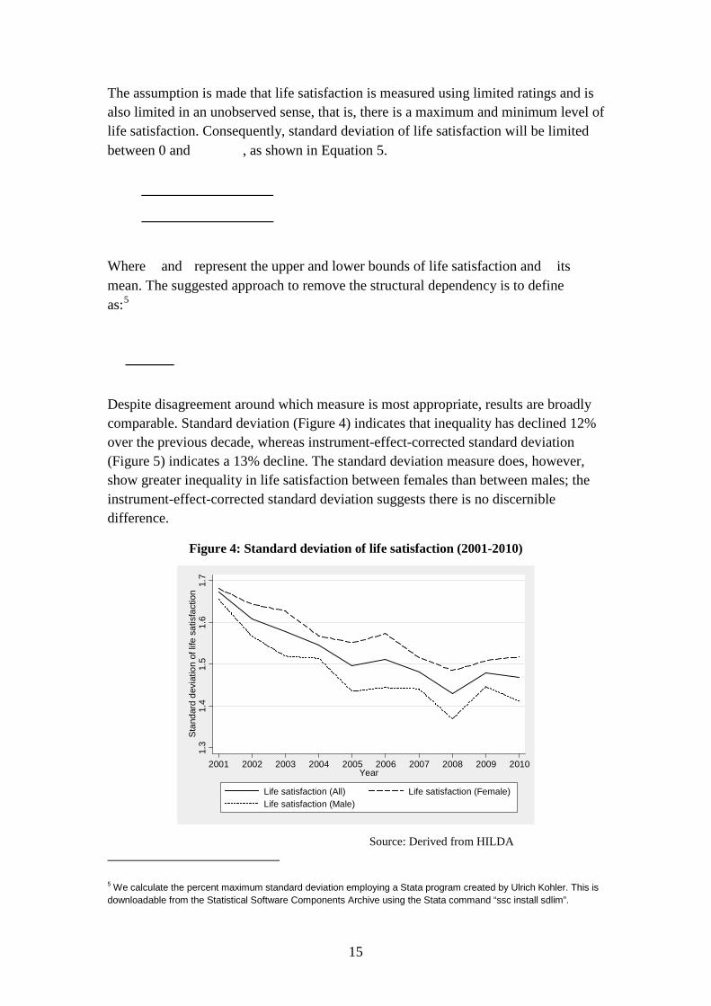
Despite disagreement around which measure is most appropriate, results are broadly comparable. Standard deviation (Figure 4) indicates that inequality has declined 12% over the previous decade, whereas instrument-effect-corrected standard deviation (Figure 5) indicates a 13% decline. The standard deviation measure does, however, show greater inequality in life satisfaction between females than between males; the instrument-effect-corrected standard deviation suggests there is no discernible difference.

Figure 4: Standard deviation of life satisfaction (2001-2010)

Source: Derived from HILDA

5 We calculate the percent maximum standard deviation employing a Stata program created by Ulrich Kohler. This is downloadable from the Statistical Software Components Archive using the Stata command “ssc install sdlim”.

1.3

1.4

1.5

1.6

1.7

Stan

dard

dev

iatio

n of

life

sat

isfa

ctio

n

2001 2002 2003 2004 2005 2006 2007 2008 2009 2010Year

Life satisfaction (All) Life satisfaction (Female)Life satisfaction (Male)

16

Figure 5: Instrument-effect-corrected standard deviation of life satisfaction (2001-2010)

Source: Derived from HILDA

Between 2001 and 2010 income inequality increased by approximately six percent (Australian Bureau of Statistics, 2011b). These results, therefore, support Stevenson and Wolfers’ (2008), and Gandelman and Porzecanski’s (2011) conclusion that non-pecuniary factors perform an integral role in determining inequalities in life satisfaction. That is not to say income plays no role. As shown in Figure 6, the decline in mean life satisfaction over the past decade has been marginally higher for individuals with middle to high incomes. Specifically, and commenting only on statistically significant results, the mean life satisfaction scores of the third quartile have fallen by almost 25% more than the mean life satisfaction scores of the first quartile.6

6 The first quartile has fallen from 7.8486 in 2001 to 7.7401 in 2010 (Pr < 0.0604), whereas the third quartile has fallen from 7.9881 in 2001 to 7.8518 in 2010 (Pr < 0.0000).

1.4

1.5

1.6

1.7

Inst

rum

ent-e

ffect

-cor

rect

ed s

tand

ard

devi

atio

n of

life

sat

isfa

ctio

n

2001 2002 2003 2004 2005 2006 2007 2008 2009 2010Year

Life satisfaction (All) Life satisfaction (Female)Life satisfaction (Male)

17

Figure 6: Mean life satisfaction by household income quartiles (2001-2010)

Source: Derived from HILDA

3.3 The prevalence and severity of dissatisfaction

There is increasing empirical evidence in the economic and psychological literature that positive and negative well-being are more than opposite ends of the same phenomenon, and that factors which increase satisfaction may not necessarily decrease dissatisfaction (Boes and Winkelmann, 2010). Therefore, in this section, we explore the severity and prevalence of dissatisfaction in Australia. This area of investigation owes something to the conventional interpretation of Rawls’ Theory of Justice (1971), where improvements in societal welfare can only be obtained from enhancements in the position of the least well-off member. It also has some of the appeal of Kahneman and Krueger’s (2006) U-index (a measure of the proportion of time an individual spends in an unpleasant state) and the idea that policy makers may be more comfortable with attempting to minimise a specific measure of ill-being, rather than maximise the more nebulous concept of happiness.

Prevalence of dissatisfaction is measured by the proportion of the sample deemed to be ‘totally dissatisfied’ (life satisfaction score equals zero) with their lives. To measure the severity of dissatisfaction, we adopt a method used in the portfolio management literature to measure downside risk, downside variance, or semi-deviation (cf. Sortino, 2010). In portfolio management this method measures the risk of achieving a rate of return below some exogenously pre-specified target rate. Adapting the method to our application, we substitute the pre-specified target rate of return with a target level of life satisfaction; the more intense a person’s dissatisfaction, the greater the deviation from this target. A Rawlsian inspired social welfare function would suggest that the larger the downside deviation from this target level, the lower societal welfare must be, as there is a greater risk of a randomly drawn individual being dissatisfied with their life.

7.6

7.7

7.8

7.9

88.

1M

ean

life

satis

fact

ion

2001 2002 2003 2004 2005 2006 2007 2008 2009 2010Year

1st Quartile 2nd Quartile3rd Quartile 4th Quartile

18

The measure of downside risk , is derived as follows:

Where an individual’s self-reported life satisfaction is and the target life satisfaction score is (in this case a score of six). is 1 for all and 0 otherwise, again is the sample size.

Figure 7 illustrates the prevalence of those individuals who report a life satisfaction score of zero (totally dissatisfied with their lives). The proportions are relatively low, ranging from 0.0415% to 0.2885% and it is encouraging to see a statistically significant overall downward trend (although in 2010, for the first time in the history of the survey, females have made a statistically significant (Pr < 0.0462) divergence from this trend). It should be noted that estimates for this measure are likely to be biased downwards, as respondents with relatively low levels of life satisfaction are more likely to leave the sample (Watson and Wooden, 2004b).

Figure 7: Proportion of individuals who report a life satisfaction score of zero (2001-2010)

Source: Derived from HILDA

Finally, Figure 8 illustrates the measure of negative life satisfaction derived from Equation 7. It can be seen that between 2001 and 2010 negative deviations in life satisfaction have generally trended downwards. That is, the severity of dissatisfaction, on average, appears to have reduced over the last 10 years by over 18%.

0.0

01.0

02.0

03Pr

opor

tion

of p

eopl

e to

tally

dis

satis

fied

with

life

2001 2002 2003 2004 2005 2006 2007 2008 2009 2010Year

Life satisfaction (All) Life satisfaction (Female)Life satisfaction (Male)

19

Figure 8: Negative deviation of life satisfaction (2001-2010)

Source: Derived from HILDA

4. Discussion This paper set out to examine the level, determinants and distribution of life satisfaction, as well as the prevalence and severity of dissatisfaction in Australia over the period 2001 to 2010. Our results indicate an overall downward trend in life satisfaction as well as a diminishing gap between males and females, largely due to the declining life satisfaction of females. On a more positive note, we find evidence indicating that inequality in life satisfaction has generally declined in Australia, as has the prevalence of dissatisfaction.

While a definitive explanation of these findings requires substantial further research, we offer the following suggestions. To begin with, we observe that the Australian Bureau of Statistics’ Measures of Australia’s Progress seeks to measure headline indicators across three dimensions (society, economy and environment). In the most recent (2011) release, three of the six societal indicators (health; education and training; and work) are judged to have improved over the previous 10 years, whereas three have gone unmeasured (crime; family, community and social cohesion; and democracy, governance and citizenship). In the economic dimension, three of the five indicators (national income; national wealth; and household economic well-being) are judged to have improved, one indicator (housing) is judged to have undergone no significant movement, and one indicator (productivity) has declined. In the environment dimension, two of the six indicators have declined (biodiversity; and atmosphere), whereas four have gone unmeasured (land; inland waters; oceans and estuaries; and waste) (Australian Bureau of Statistics, 2011c).

It may be these declining or unmeasured indicators that help explain the overall decline in life satisfaction in Australia between 2001 and 2010. Looking first at the

.5.5

5.6

.65

.7N

egat

ive

devi

atio

ns in

life

sat

isfa

ctio

n

2001 2002 2003 2004 2005 2006 2007 2008 2009 2010Year

Life satisfaction (All) Life satisfaction (Female)Life satisfaction (Male)

20

‘society’ dimension, international evidence (cf. Kroll, 2011; Winkelmann, 2009) shows that social capital plays an integral role in supporting life satisfaction and there is reason to believe that Australia’s social capital is in decline. For example, membership of major Australian organisations (including Scouts, Guides, Rotary, Lions and the Australian Conservation Foundation) has declined, as has membership of political parties and unions. Australians are also less likely to attend church or participate in sport (Leigh, 2010). In regards to the ‘environment’ dimension, on which the measured indicators suggest Australia has performed poorly, there is strong evidence that environmental quality and life satisfaction are positively related (cf. Ambrey and Fleming, 2011; Brereton et al., 2008; Smyth et al., 2011).

The declining life satisfaction of females accords with results from the United States, where declines in female happiness have eroded a gender gap in happiness to the point where a new gender gap has emerged with higher happiness for men (Stevenson and Wolfers, 2009). In the HILDA survey data, this decline in life satisfaction is accompanied, in the most recent wave, by an upward swing in the proportion of females reporting to be totally dissatisfied with their lives; against a general downward trend over the decade for this statistic. In Australia there is evidence to indicate that the trend towards more liberal attitudes about gender has stalled and, in some instances, reversed; which may go some way to explaining these findings. Specifically, while women have made great gains in obtaining access to paid employment, this movement into paid employment has been accepted largely because it has not challenged traditional divisions of labour and has continued to be supported only insofar as it does not alter gendered divisions of labour in the home. Women may be increasingly frustrated by attempts to transgress traditional divisions, undertake paid work and concurrently care for young children; raising the question of whether there are sufficient State and Commonwealth labour market policies to support a reasonable work-life balance (van Egmond et al., 2010).

With regards to geographical heterogeneity, we find that life satisfaction is not equalised across location and that living in more remote areas is associated with higher levels of life satisfaction than living in more urbanised areas. We also find that respondents residing at the same address for a longer period of time are less satisfied with their lives. We suggest this reflects a systematically perceived impediment to individuals’ location choices. That is, due to perceived transaction costs, people are unable to relocate and re-optimise their utility. This indicates that, contrary to the notion that people ‘vote with their feet’ (Tiebout, 1956), utility is not reflected in a spatial equilibrium in private markets; residual life satisfaction effects persist.

In terms of socio-economic and demographic determinants of life satisfaction, some results stand out. For example, contrary to evidence offered by objective measures of well-being (cf. Australian Bureau of Statistics, 2012), we find that individuals of Aboriginal and/or Torres Strait Islander origin report to be more satisfied with their lives than the non-indigenous population. While this result is consistent with previous studies (cf. Ambrey and Fleming, 2011; Shields et al., 2009), it remains a surprising

21

result and is an area worthy of further research. A possible explanation is that this reflects a bias in the sample; indigenous respondents tend to be lost to attrition and those who do not attrit may have specific (unobserved) characteristics, such as a strong attachment to traditional culture. Dockery (2010) finds that this attachment is statistically associated with better outcomes across a broad range of dimensions of social and economic well-being.

Another result that is consistent with the literature (cf. Shields et al., 2009), yet deserves discussion, is that dependent children in a household appears to reduce the life satisfaction of adult household members. Using data from the World Values Survey, Margolis and Myrskylä (2011) suggest that the relationship between number of dependent children and life satisfaction evolves from negative to neutral to positive as the individual ages, and this evolution is strongest amongst those most likely to benefit from upward intergenerational transfers. The authors support this conclusion by providing evidence that the negative life satisfaction affect for younger adults is weakest in countries with high public support for families, and the positive association for older adults is strongest in countries where support for the aged depends largely on family members.

Finding a negative relationship between higher educational attainment and life satisfaction, in developed countries at least, is not unusual (cf. Shields et al., 2009). Nonetheless, some explanation seems necessary. Veenhoven (1996) suggests that reduced life satisfaction among the highly educated in developed countries could be explained by a lack of employment opportunities requiring high-level skills or possibly due to the fading of earlier advantages in the process of social equalising. Helliwell (2003) demonstrates that the benefits of education flow less through a direct impact on life satisfaction than through its positive effects on the creation and maintenance of human and social capital. Making the distinction between experienced utility and decision utility, Ferrante (2009) provides evidence for Italy that education is a main driver of perceived opportunities and aspirations. The author argues that better perceived opportunities may decrease life satisfaction if they raise aspirations above real life chances. We offer an alternative explanation, and suggest that this finding reflects the ‘slavery of the talented’ (Dworkin, 1981) and a perceived ‘middle class squeeze’ (Hamilton et al., 2008). That is, for the middle class, the social equalising of opportunities comes at an indirect non-income cost and is reflected in terms of reduced life satisfaction. Individuals exercise what they perceive to be their dominant strategy, which involves regularly updating skills and education in order to remain competitive in the labour market and to attain (or maintain) social status. The Nash Equilibrium being lower life satisfaction for all individuals competing. This reasoning is supported by Schwartz et al.’s (2002) finding that ‘maximisers’ are less satisfied with their lives than ‘satisficers’ and our finding that medium to high income earners (those in the third quartile of the income distribution) have experienced a disproportionate decline in life satisfaction compared to individuals in other income quartiles.

22

Reduced inequality in the distribution of life satisfaction, whether measured by standard deviation or instrument-effect-corrected standard deviation, is unable to be attributed to an increase in average life satisfaction or a decline in income inequality. Declining inequality in life satisfaction is a global trend, which Veenhoven (2005) attributes to a more equal distribution of opportunities as a result of modernisation providing a more liveable environment and improved personal capabilities. This may also help explain the observed decline in the prevalence and severity of dissatisfaction. While outside the scope of this paper, if evidence continues to suggest that positive and negative well-being are more than opposite ends of the same phenomenon, the determinants of dissatisfaction may be an area of research worth pursuing.

We end this paper by echoing many of the conclusions drawn by Stiglitz et al. (2009). Namely, that both objective and subjective dimensions of well-being are important, should be measured, and should be regarded as complements rather than substitutes. Further, indicators such as those provided by self-reports of life satisfaction or happiness provide an opportunity to enrich policy discussion, promote public debate about the direction a society is taking, and provide a useful counter-balance to pervasive, narrowly defined, measures of progress such as Gross National Income or GDP. Measurement of inequality in the distribution of well-being, as well as the extent of dissatisfaction or ill-being, also has a role to play; in particular, when it comes to ensuring that the benefits of progress are dispersed broadly and equitably. Looking forward, as noted by Schubert (2012), increased research effort is required to translate insights from indicators of well-being into practical policy advice.

23

Acknowledgements The authors thank Griffith University for the Griffith University Postgraduate Research Scholarship and the Griffith Business School for the Griffith University Business School Top-up Scholarship Funding, which was instrumental in facilitating this research. This research would not have been possible without data provided by the Australian Government Department of Families, Housing, Community Services and Indigenous Affairs (FaHCSIA).

24

References Alesina, A., di Tella, R., MacCulloch, R., 2004. Inequality and happiness: Are Europeans and Americans different? Journal of Public Economics 88, 2009-2042. Ambrey, C., Fleming, C., 2011. Valuing scenic amenity using life satisfaction data. Ecological Economics 72, 106-115. Australian Bureau of Statistics, 2011a. Glossary of Statistical Geography Terminology, 2011, Catalogue No. 1217.0.55.001. Available http://www.abs.gov.au/ausstats/abs@.nsf/mf/1217.0.55.001, accessed: 12 April 2012. Australian Bureau of Statistics, 2011b. Household Income and Income Distribution, Catalogue No. 6523.0. Available http://www.abs.gov.au/ausstats/abs@.nsf/mf/6523.0, accessed: 1 March 2012. Australian Bureau of Statistics, 2011c. Measures of Australia's Progress: Summary Indicators 2011, Catalogue No. 1370.0.55.001. Available http://www.abs.gov.au/AUSSTATS/abs@.nsf/mf/1370.0.55.001, accessed: 17 July 2012. Australian Bureau of Statistics, 2012. 2011 Census of Population and Housing: Aboriginal and Torres Strait Islander Peoples (Indigenous) Profile, Catalogue No. 2002.0. Available http://www.censusdata.abs.gov.au/census_services/getproduct/census/2011/communityprofile/0, accessed: 9 August 2012. Blanchflower, D., Oswald, A., 2004. Well-being over time in Britain and the USA. Journal of Public Economics 88, 1359-1386. Blanchflower, D., Oswald, A., 2005. Happiness and the Human Development Index: The paradox of Australia. The Australian Economic Review 38, 307-318. Boes, S., Winkelmann, R., 2010. The effect of income on general life satisfaction and dissatisfaction. Social Indicators Research 95, 111-128. Brereton, F., Clinch, J.P., Ferreira, S., 2008. Happiness, geography and the environment. Ecological Economics 65, 386-396. Breusch, T., Pagan, A., 1979. A simple test for heteroscedasticity and random coefficient variation. Econometrica 47, 1287-1294. Clark, A., Frijters, P., Shields, M., 2008. Relative income, happiness, and utility: An explanation for the Easterlin paradox and other puzzles. Journal of Economic Literature 46, 95-144. Cobb-Clark, D., Schurer, S., 2012. The stability of big-five personality traits. Economic Letters 115, 11-15.

25

Delhey, J., Kohler, U., 2011. Is happiness inequality immune to income inequality? New evidence through instrument-effect-corrected standard deviations. Social Science Research 40, 742-756. Delhey, J., Kohler, U., 2012. Happiness inequality: Adding meaning to numbers - A reply to Veenhoven and Kalmijn. Social Science Research 41, 731-734. DeNeve, K., Cooper, H., 1998. The happy personality: A meta-analysis of 137 personality traits and subjective well-being. Psychological Bulletin 124, 197-229. Di Tella, R., MacCulloch, R., Oswald, A., 2001. Preferences over inflation and unemployment: Evidence from surveys of happiness. American Economic Review 91, 335-341. Di Tella, R., MacCulloch, R., Oswald, A., 2003. The macroeconomics of happiness. The Review of Economics and Statistics 85, 809-827. Dockery, A., 2010. Culture and wellbeing: The case of Indigenous Australians. Social Indicators Research 99, 315-332. Dworkin, R., 1981. What is equality? Part 2: Equality of resources. Philosophy and Public Affairs 10, 283-345. Easterlin, R., 1974. Does economic growth improve the human lot? Some empirical evidence, in: David, P., Redler, M. (Eds.), Nations and Households in Economic Growth: Essays in Honor of Moses Abramovitz. Academic Press: 89-125, New York, pp. 89-125. Easterlin, R., 1995. Will raising the incomes of all increase the happiness of all? Journal of Economic Behavior and Organization 27, 35-47. Easterlin, R., 2010. Well-being, front and center: A note on the Sarkozy report. Population and Development Review 36, 119-124. Ferrante, F., 2009. Education, aspirations and life satisfaction. Kyklos 62, 542-562. Ferrer-i-Carbonell, A., 2005. Income and well-being: An empirical analysis of the comparison income effect. Journal of Public Economics 89, 997-1019. Ferrer-i-Carbonell, A., Frijters, P., 2004. How important is methodology for the estimates of the determinants of happiness? Economic Journal 114, 641-659. Frey, B., 2008. Happiness: A Revolution in Economics (Munich Lectures in Economics). MIT Press, Cambridge, MA. Frey, B., Stutzer, A., 2002a. Happiness and Economics: How the Economy and Institutions Affect Human Well-Being. Princeton University Press, Princeton. Frey, B., Stutzer, A., 2002b. What can economists learn from happiness research? Journal of Economic Literature 40, 402-435.

26

Gandelman, N., Porzecanski, R., 2011. Happiness inequality: How much is reasonable? Social Indicators Research, Article in press, doi:10.1007/s11205-011-9929-z. Geishecker, I., Riedl, M., 2010. Ordered response models and non-random personalty traits: Monte Carlo simulations and a practical guide. Germany, Centre for European Governance and Economic Development Research. Hamilton, C., Downie, C., Lu, Y.-H., 2008. The state of the Australian middle class. Australasian Accounting Business and Finance Journal 2, 1-25. Helliwell, J., 2003. How's life? Combining individual and national variables to explain subjective well-being. Economic Modelling 20, 331-360. Hill, R.C., Griffiths, W., Lim, G., 2008. Principles of Econometrics, third ed. John Wiley & Sons, New Jersey. Horne, D., 1964. The Lucky Country: Australia in the Sixties. Penguin, Melbourne. Kahneman, D., Krueger, A., 2006. Developments in the measurement of subjective well-being. Journal of Economic Perspectives 20, 3-24. Kalmijn, W., 2012. Happiness is not normally distributed: A comment to Delhey and Kohler. Social Science Research 41, 199-202. Kalmijn, W., Veenhoven, R., 2005. Measuring inequality of happiness in nations: In search for proper statistics. Journal of Happiness Studies 6, 357-396. Kroll, C., 2011. Different things make different people happy: Examining social capital and subjective well-being by gender and parental status. Social Indicators Research 104, 157-177. Leigh, A., 2010. Disconnected. University of New South Wales Press, Sydney. Leigh, A., Wolfers, J., 2006. Happiness and the Human Development Index: Australia is not a paradox. The Australian Economic Review 39, 176-184. MacKerron, G., 2012. Happiness economics from 35 000 feet. Journal of Economic Surveys 26, 705-735. Margolis, R., Myrskylä, M., 2011. A global perspective on happiness and fertility. Population and Development Review 37, 29-56. Oswald, A., 1997. Happiness and economic performance. Economic Journal 107, 1815-1831. Rawls, J., 1971. A Theory of Justice. Oxford University Press, Cambridge, MA.

27

Saucier, G., 1994. Mini-markers: A brief version of Goldberg's unipolar Big-Five markers. Journal of Personality Assessment 63, 506-516. Schubert, C., 2012. Pursuing happiness. Kyklos 65, 245-261. Schwartz, B., Ward, A., Monterosso, J., Lyubomirsky, S., White, K., Lehman, D., 2002. Maximizing versus satisficing: Happiness is a matter of choice. Journal of Personality and Social Psychology 83, 1178-1197. Shields, M., Price, S., Wooden, M., 2009. Life satisfaction and the economic and social characteristics of neighbourhoods. Journal of Population Economics 22, 421-443. Smyth, R., Nielsen, I., Zhai, Q., Liu, T., Liu, Y., Tang, C., Wang, Z., Wang, Z., Zhang, J., 2011. A study of the impact of environmental surroundings on personal well-being in urban China using a multi-item well-being indicator. Population and Environment 32, 353-375. Sortino, F., 2010. The Sortino Framework for Constructing Portfolios: Focusing on Desired Target Return to Optimize Upside Potential Relative to Downside Risk. Elsevier, Boston. Stevenson, B., Wolfers, J., 2008. Happiness inequality in the United States. Journal of Legal Studies 37, s33-s79. Stevenson, B., Wolfers, J., 2009. The paradox of declining female happiness. American Economic Journal: Economic Policy 1, 190-225. Stiglitz, J., Sen, A., Fitoussi, J.-P., 2009. Report by the Commission on the Measurement of Economic Performance and Social Progress, Paris. The World Bank, 2012. Data. Available: http://data.worldbank.org/?display=default. Available http://data.worldbank.org/?display=default, accessed: 2 August 2012. Tiebout, C., 1956. A pure theory of local expenditures. Journal of Political Economy 64, 416-424. United Nations Development Programme, 2010. Human Development Report 2010: The Real Wealth of Nations (Pathways to Human Development), New York. van Egmond, M., Baxter, J., Buchler, S., Western, M., 2010. A stalled revolution? Gender role attitudes in Australia, 1986-2005. Journal of Population Research 27, 147-168. van Praag, B., Frijters, P., Ferrer-i-Carbonell, A., 2003. The anatomy of subjective well-being. Journal of Economic Behavior and Organization 51, 29-49. Veenhoven, R., 1996. Developments in satisfaction research. Social Indicators Research 37, 1-46.

28

Veenhoven, R., 2005. Return of inequality in modern society? Test by dispersion of life-satisfaction across time and nations. Journal of Happiness Studies 6, 457-487. Veenhoven, R., 2012. The medicine is worse than the disease: Comment on Delhey and Kohler's proposal to measure inequality in happiness using 'instrument-effect-corrected' standard deviation. Social Science Research 41, 203-205. Watson, N., Wooden, M., 2002. The Household, Income and Labour Dynamics in Australia (HILDA) survey: Wave 1 survey methodology, HILDA Project Technical Paper Series No. 1/02. Melbourne Institute of Applied Economic and Social Research, Melbourne. Watson, N., Wooden, M., 2004a. Assessing the quality of the HILDA survey wave 2 data, HILDA Project Technical Paper Series No. 5/04. Melbourne Institute of Applied Economic and Social Research, Melbourne. Watson, N., Wooden, M., 2004b. Sample attrition in the HILDA survey. Australian Journal of Labour Economics 7, 293-308. Watson, N., Wooden, M., 2010. The HILDA survey: Progress and future developments. The Australian Economic Review 43, 326-336. Welsch, H., 2007. Macroeconomics and life satisfaction: Revisiting the "Misery Index". Journal of Applied Economics 10, 237-251. Winkelmann, R., 2009. Unemployment, social capital, and subjective well-being. Journal of Happiness Studies 10, 421-430.

29

Appendix: Additional results

Variable name Pooled OLS estimate

(standard error)

Random Effects estimate

(standard error)

Fixed Effects estimate

(standard error) Age -0.0505***

(0.0033) -0.0480*** (0.0033)

Age squared 0.0006*** (0.0000)

0.0005*** (0.0000)

0.0003*** (0.0001)

Male 0.0647*** (0.0179)

0.0558*** (0.0171)

ATSI 0.1881** (0.0881)

0.1345 (0.084)

Immigrant English 0.0357 (0.0293)

0.0043 (0.0296)

Immigrant non-English -0.1198*** (0.0346)

-0.1299*** (0.0341)

Poor English -0.3545*** (0.0906)

-0.2373*** (0.0718)

-0.1713* (0.0893)

Married 0.3655*** (0.0341)

0.3201*** (0.0280)

0.2354*** (0.0369)

De-facto 0.2216*** (0.0322)

0.2442*** (0.0476)

0.2305*** (0.0298)

Separated -0.5066*** (0.0642)

-0.4275*** (0.0488)

-0.4183*** (0.0575)

Divorced -0.1547*** (0.0528)

-0.1615*** (0.0420)

-0.1415* (0.0559)

Widow 0.0884 (0.0564)

-0.0904* (0.0521)

-0.2522*** (0.0756)

Number of children -0.0644*** (0.0104)

-0.0533*** (0.0084)

-0.0437 (0.0115)

Lone parent -0.0671 (0.0560)

-0.0294 (0.0420)

-0.0098 (0.0441)

Mild health condition -0.1648*** (0.0197)

-0.0984*** (0.0146)

-0.0580*** (0.0152)

Moderate health condition -0.7150*** (0.0261)

-0.4232*** (0.0180)

-0.2999*** (0.0193)

Severe health condition -1.0155*** (0.0894)

-0.5933*** (0.0680)

-0.4220*** (0.0693)

Year 12 0.0269 (0.0466)

0.0445 (0.0393)

0.0990 (0.0623)

Certificate or diploma -0.0599*** (0.0196)

-0.0639 (0.0190)

-0.0323 (0.0352)

30

Bachelors degree or higher -0.0972*** (0.0249)

-0.0688*** (0.0230)

0.0187 (0.0430)

Employed part-time 0.1545*** (0.0183)

0.0872*** (0.0143)

0.0720*** (0.0159)

Unemployed -0.1799*** (0.0431)

-0.1605*** (0.0313)

-0.1501*** (0.0320)

Non-participant 0.1425*** (0.0236)

0.0495*** (0.0173)

0.0343* (0.0194)

Self employed -0.0365 (0.0274)

-0.0098 (0.0220)

0.0016 (0.0253)

Disposable income (ln) 0.0585*** (0.0079)

0.0340*** (0.0046)

0.0279*** (0.0045)

Extraversion 0.1019*** (0.0085)

0.1093*** (0.0088)

Agreeableness 0.1519*** (0.0117)

0.1531*** (0.0116)

Conscientiousness 0.0684*** (0.0096)

0.0713*** (0.0097)

Emotional stability 0.1964*** (0.0106)

0.1942*** (0.0103)

Openness to experience -0.0517*** (0.0104)

-0.0656*** (0.0100)

Others present 0.0890*** (0.0133)

0.0522*** (0.0009)

0.0446*** (0.0091)

Years at current address 0.0045*** (0.0009)

0.0007 (0.0009)

-0.0052*** (0.0012)

Inner 0.1201*** (0.0245)

0.1083*** (0.0220)

0.1071*** (0.0327)

Outer 0.2347*** (0.0306)

0.1329*** (0.0282)

0.0455 (0.0475)

Remote 0.2690*** (0.0614)

0.1997*** (0.0567)

0.1022 (0.0737)

Constant 5.7592*** (0.1346)

6.0420*** (0.1141)

7.1917*** (0.1384)

Summary statistics Number of individuals 13412 13412 13412 Number of observations 106013 106013 106013 Adjusted R2 0.1546

0.42238 0.5512 R2 within 0.01800 0.0200 R2 between 0.23400 0.0361 R2 overall 0.14790 0.0409

31

*** significant at the 1% level; ** significant at the 5% level; * significant at the 10% level.

Omitted cases are: Female; Not of indigenous origin; Country of birth Australia; Speaks English well or very well; Never married and not defacto; Not a lone parent; Does not have a long-term health condition; Year 11 or below; Not self employed; Employed working 35 hours or more per week; No others present during the interview or don’t know – telephone interview; Major city.

All estimations include wave and State/Territory dummy variables and make use of unbalanced panels. Standard errors adjusted for clustering at the primary sampling unit to account for complex survey design.